Equity-credit modeling under affinejump-diffusion models with jump-to-default

Tsz Kin Chung

Department of Mathematics, Hong Kong University of Science and Technology

E-mail: tkchung@ust.hk

Yue Kuen Kwok

Department of Mathematics, Hong Kong University of Science and Technology

E-mail: maykwok@ust.hk

1

EQUITY-CREDIT MODELING UNDER AFFINE

JUMP-DIFFUSION MODELS WITH

JUMP-TO-DEFAULT

ABSTRACT

This article reviews the stochastic models for pricing credit-sensitive financial derivatives using

the joint equity-credit modeling approach. The modeling of credit risk is embedded into a

stochastic asset dynamics model by adding the jump-to-default feature. We discuss the class

of stochastic affine jump-diffusion models with jump-to-default and apply the models to price

defaultable European options and credit default swaps. Numerical implementation of the

equity-credit models is also considered. The impact on the pricing behavior of derivative

products with the added jump-to-default feature is examined.

1 Introduction

The affine jump-diffusion (AJD) models have been widely used in continuous time modeling

of stochastic evolution of asset prices, bond yields and credit spreads. Some of the well known

examples include the stochastic volatility (SV) model of Heston (1993), stochastic volatility

jump-diffusion models (SVJ) of Bates (1996) and Bakshi et al. (1997), and stochastic volatility

coherent jump model (SVCJ) of Duffie et al. (2000). The AJD models possess flexibility to

capture the dynamics of market prices in various asset classes, while also admit nice analytical

tractability. The affine term structure models, which fall into the family of AJD models, have

been frequently used to study the dynamics of bond yields and credit spreads (Duffie and

Singleton, 1999).

A number of studies have addressed the importance of including jump dynamics to valuation

and hedging of derivatives. In the modeling of equity derivatives, Bakshi et al. (1997) illustrate

that the stochastic volatility model augmented with the jump-diffusion feature produces a

parsimonious fit to stock option prices for both short-term and long-term maturities. Empirical

2

studies reported by Bates (1996), Pan (2002) and Erakar (2004) show that the inclusion of

jumps in the modeling of stock price is necessary to reconcile the time series behavior of

the underlying with the cross-sectional pattern of option prices. In particular, Erakar (2004)

concludes from his empirical studies that simultaneous jumps in stock price and return variance

are important in catering for different volatility regimes.

While the AJD models have been successfully applied in valuation of both equity and credit

derivatives, the joint modeling of equity and credit derivatives have not been fully addressed

in the literature. Recently, a growing literature has highlighted such an interaction between

equity risk (stock return and its variance) and credit risk (firm default risk). While the risk

neutral distribution of stock return is fully conveyed by traded option prices of different strikes

and maturities, the information of the arrival rate of default can be extracted from the bond

yield spreads or credit default swap spreads. With the growing liquidity of the credit default

swap (CDS) markets, the CDS spreads provide more reliable and updated information about

the credit risk of firms. Achyara and Johnson (2007) find that the CDS market contains forward

looking information on equity return, in particular during times of negative credit outlooks.

For equity options, Cremers et al. (2008), Zhang et al. (2009) and Cao et al. (2010) show that

the out-of-the-money put options, which depict the negative tail of the underlying risk neutral

distribution, are closely linked to yield spreads and CDS spreads of the reference firm.

Several innovative equity-credit models have been proposed in the literature. Carr and

Linetsky (2006) propose an equity-credit hybrid model in which the stock price is sent to a

cemetery state upon the arrival of default of the reference company. Carr and Wu (2009)

introduce another equity-credit hybrid model which incorporates jump-to-default in which the

equity price drops to zero given the default arrival. Carr and Madan (2010) consider a local

volatility model enhanced by jump-to-default. Mendoza-Arriaga et al. (2010) and Bayraktar

and Yang (2011), respectively, propose a flexible modeling framework to unify the valuation of

equity and credit derivatives using the time-changed Markov process and multiscale stochastic

volatility. Cheridito andWugalter (2011) propose a general framework under affine models with

possibility of default for the simultaneous modeling of equity, government bonds, corporate

bonds and derivatives.

In this article, we propose an equity-credit model under the general affine jump-diffusion

framework in the presence of jump-to-default (JtD-AJD model). We illustrate how to use the

proposed JtD-AJD model for pricing defaultable European options and credit default swaps.

The article is organized as follows. In the next section, we present the mathematical framework

of the affine jump-diffusion with jump-to-default. The reduced form approach is adopted, where

the default process is modeled as a Cox process with stochastic intensity. We illustrate how to

apply the Fourier transform technique to derive the joint characteristic function of the stock

price distribution in the JtD-AJD model. In Section 3, we consider pricing of defaultable

3

European contingent claims and credit defaults swaps using the JtD-AJD model. We manage

to obtain closed form pricing formulas of these two credit-sensitive derivative products, a

demonstration for nice analytical tractability of the proposed equity-credit model. In Section

4, we discuss the practical implementation of the jump-to-default feature to several popular

option pricing models. We also consider numerical valuation of defaultable European options

using various numerical approaches, like the Fast Fourier transform (FFT) techniques and

Monte Carlo simulation. The impact of various jump parameters on the pricing behavior

of defaultable European options is examined. Conclusive remarks are presented in the last

section.

2 Affine jump diffusion with jump-to-default

This section summarizes the mathematical framework of the AJD model (Duffie et al., 2000).

Consider the filtered probability space (Ω,G, Gt , Q), the AJD process of the vector stochastic

state variable Xt is defined in some state space D ⊂ Rn as follows:

dXt = µ (Xt) dt+ σ (Xt) dWt + dZt, (1a)

where Q is some appropriate equivalent martingale measure adopted for pricing contingent

claims, Gt = σ Xs| s < t is the natural filtration generated by the vector state variable Xt,

Wt is an Gt-standard Brownian motion in Rn, µ : D → Rn is the drift vector, σ : D → Rn×n

is the diffusion matrix, and Zt is a pure jump process whose jumps have a fixed probability

distribution ν on Rn and arrive with intensity λ (Xt) : t ≥ 0 , λ : D → [0,∞) . The interest

rate process is specified as r (Xt) : t ≥ 0 , r : D → [0,∞) . Under the AJD model, the

parameter functions µ (Xt) , σ (Xt), λ (Xt) and the risk-free interest rate r (Xt) are specified

as follows:

µ (X) = K0 +K1 ·X, for K0 ∈ Rn and K1 ∈ Rn×n;σ (X)σ (X)T

ij= H0ij + H1ij ·X, for H0 ∈ Rn×n and H1 ∈ Rn×n×n;

λ (X) = l0 + l1 ·X, for l0 ∈ R and l1 ∈ Rn;

r (X) = r0 + r1 ·X, for r0 ∈ R and r1 ∈ Rn.

Without loss of generality, we let the first component of Xt be the logarithm of the stock price

St. Under the AJD framework, stochastic interest rate and stochastic volatility (expressed

as some linear combination of the vector state variable Xt) can be incorporated. Also, the

correlation structures between the different factors can be introduced by specifying the diffusion

matrix σ (Xt) . It is worth noting that the drift vector µ (Xt) is determined by requiring the

4

stock price process to be a martingale under the equivalent martingale measure Q.

Specification of the default process

Next, we extend the AJD framework by incoporating the jump-to-default feature of the stock

price process. Upon the arrival of default, the stock price jumps to some constant level called

the cemetery state (Carr and Linetsky, 2006). In principle, the state can be a prior known level

or a level that is arbitrarily close to zero. Following the reduced form framework, we assume

the default process to be generated by a Cox process that is defined in the same state space

D. Formally, we define the first jump time

τd = inf

t ≥ 0 :

t∫0

h (Xs) ds ≥ e

as the random time of default arrival. Here, e is the standard exponential random variable

and the intensity process of default arrival (hazard rate) is assumed to be a function of the

state variable as represented by h (Xt) : t ≥ 0, h : D → [0,∞) , and adapted to Gt. The

filtration Ht = σ(1τd<s

∣∣ s ≤ t)contains the information of whether there has been a default

by time t. We define Ft = Ht∨ Gt to be the information set that contains the knowledge of

the evolution of the vector state variable Xt and history of default by time t. In order to have

the risk adjusted interest rate to be affine, the hazard rate process h (Xt) is specified as

h (X) = h0 + h1 ·X, for h0 ∈ R and h1 ∈ Rn. (1b)

The above specification falls into the affine term structure framework commonly used in the

modeling of interest rate and credit derivatives (Lando, 1998; Duffie and Singleton, 1999).

2.1 Transform analysis

The discounted expectation of a contingent claim that pays F (XT ) when there is no default

prior expiration is given by

EQ

[exp

(−∫ T

t

r (Xs) ds

)F (XT )1τd>T

∣∣∣∣Ft

]= 1τd>tE

Q

[exp

(−∫ T

t

R (Xs) ds

)F (XT )

∣∣∣∣Gt

],

where R (Xs) = r (Xs) + h (Xs) is the risk adjusted discount rate at time s and the payoff

F (XT ) is GT -measurable requiring no knowledge of the default process. The price function of

5

the contingent claim conditional on Xt = X at time t is defined by

V (X, t) = EQ

[exp

(−∫ T

t

R (Xs) ds

)F (XT )

]. (2)

By the Feynman-Kac representation formula, we deduce that V (X, t) satisfies the following

partial integro-differential equation (PIDE):

∂V (X, t)

∂t+ LV (X, t) = 0. (3a)

Here, L is the infinitesimal generator as defined by

LV (X, t) = µ (X)VX (X, t) +1

2tr[σ (X)σ (X)T VXX (X, t)

]+ λ (X)

∫Rn

[V (X + z, t)− V (X, t)] dν (z)−R (X)V (X, t) . (3b)

The solution to the above PIDE subject to an exponentially affine form of the terminal condi-

tion is stated in Theorem 1.

Theorem 1. When the terminal payoff function is exponentially affine, where

F (XT ) = exp (u ·XT ) ,

for u ∈ Cn, the conditional expectation

F0 (u,Xt, t;T ) = EQ

[exp

(−∫ T

t

R (Xs) ds

)eu·XT

∣∣∣∣Gt

](4)

has the solution of the form

F0 (u,Xt, t;T ) = exp (α (τ) + β (τ) ·Xt) , τ = T − t,

where α (τ) and β (τ) satisfy the following system of complex-valued ordinary differential equa-

tions (ODEs):

α′ (τ) = −R0 +K0β (τ) +1

2β (τ)T H0β (τ) + l0 [Λ (β (τ))− 1] , τ > 0

β′ (τ) = −R1 +KT1 β (τ) +

1

2β (τ)T H1β (τ) + l1 [Λ (β (τ))− 1] , τ > 0, (5)

with the initial conditions: α (0) = 0, β (0) = u. Here, β (τ)T H1β (τ) is a vector whose kth

component is given by∑i

∑j

βi H1ijk βj and Λ(c) is the jump transform as defined by

6

Λ(c) =

∫Rn

exp (c · z) dν (z) for some c ∈ Cn.

The proof of Theorem 1 can be found in Duffie et al. (2000).

Defaultable bond with fixed recovery

We consider a defaultable zero-coupon bond which pays one dollar when there is no default

prior to maturity, otherwise a recovery payment Rp is paid at maturity. Hence, the terminal

payoff can be formulated as 1τd>T + Rp × 1τd<T. The non-default component of the zero-

coupon bond is given by

B0 (t, T ;Xt) = EQ

[exp

(−∫ T

t

r (Xs) ds

)1τd>T

∣∣∣∣Ft

]= 1τd>tE

Q

[exp

(−∫ T

t

R (Xs) ds

)∣∣∣∣Gt

]= 1τd>t exp (α (T − t) + β (T − t) ·Xt) , (6)

by virtue of the transform analysis stated in Theorem 1. Here, α (τ) and β (τ) satisfy the same

system of ODEs as depicted in eq. (5), with the corresponding initial conditions specified

as α (0) = 0, β (0) = (0, 0, ..., 0)T . Similarly, the risk neutral discounted expectation of the

recovery payment Rp contingent upon default is given by

BR (t, T ;Xt) = Rp EQ

[exp

(−∫ T

t

r (Xs) ds

)1τd<T

∣∣∣∣Ft

]= Rp

EQ

[exp

(−∫ T

t

r (Xs) ds

)∣∣∣∣Gt

]− 1τd>tE

Q

[exp

(−∫ T

t

R (Xs) ds

)∣∣∣∣Gt

]. (7a)

The first term can be visualized as the risk-free discount factor as defined by

Bf (t, T ;Xt) = EQ

[exp

(−∫ T

t

r (Xs) ds

)∣∣∣∣Gt

]= exp

(α (T − t) + β (T − t) ·Xt

), (7b)

where α (τ) and β (τ) satisfy a similar system of ODEs as depicted in eq. (5), except that

the risk-free rate (r0, r1) replace the role of the risk adjusted discount rate (R0, R1). The

corresponding initial conditions are specified as: α (0) = 0, β (0) = (0, 0, ..., 0)T . Adding the

7

two components yields the defaultable bond price with fixed recovery as follows:

B (t, T ;Xt) = B0 (t, T ;Xt) +BR (t, T ;Xt)

= 1τd>t (1−Rp) exp [α (T − t) + β (T − t) ·Xt]

+ Rp exp[α (T − t) + β (T − t) ·Xt

]. (8)

2.2 Joint characteristic function

The pre-default discounted characteristic function, which provides information on the evolution

of the stock price dynamics prior to default, is defined by the following conditional expectation:

Ψ (ω, T ;Xt, t) = EQ

[exp

(−∫ T

t

r (Xs) ds

)exp (iω ·XT )1τd>T

∣∣∣∣Ft

]= 1τd>tE

Q

[exp

(−∫ T

t

R (Xs) ds

)exp (iω ·XT )

∣∣∣∣Gt

]= 1τd>t exp (α (T − t) + β (T − t) ·Xt]), (9)

where ω = (ω1, ω2, ..., ωn)T ∈ Rn. Again, α (τ) and β (τ) satisfy the same system of ODEs

as depicted on eq. (5), while the corresponding initial conditions are specified as α (0) =

0, β (0) = (iω1, iω2, ..., iωn)T . The marginal characteristic function of the first component of

Xt, which is the logarithm of the stock price, can be obtained by setting ω = (ω, 0, ..., 0)T . For

notational convenience, we write the first component of Xt as xt in our subsequent discussion.

3 Pricing of defaultable European options and credit de-

fault swaps

In this section, we illustrate the pricing of defaultable European contingent claims and credit

default swaps under the JtD-AJD model. Provided that analytic solution to the associated

system of ODEs is available, we are able to obtain closed form pricing formulas of these credit-

sensitive derivatives. Fortunately, nice analytic tractability of the Ricatti system of ODEs

is feasible for a wide range of stochastic stock price dynamics models, which include the SV

model (Heston, 1993), SVJ model (Bates, 1996; Bakshi et al., 1997), SVCJ model (Duffie et al.,

2000; Erakar, 2004), and Carr-Wu’s model (Carr and Wu, 2009). Moreover, the exponential

affine structure is preserved in the characteristic function of the stock price distribution, which

proves to be useful in the computation of risk sensitivity of derivatives.

8

3.1 Defaultable European contingent claims

Consider a defaultable European contingent claim which pays P (XT ) when no default occurs

before maturity and zero payoff upon default (zero recovery). Given that the payoff depends

only on the terminal stock price St = exp (xt) , the time-t value of the contingent claim is given

by

P (Xt, t) = EQ

[exp

(−∫ T

t

r (Xs) ds

)P (xT )1τd>T

∣∣∣∣Ft

]= 1τd>tE

Q

[exp

(−∫ T

t

R (Xs) ds

)P (xT )

∣∣∣∣Gt

], (10)

where R (Xs) = r (Xs) + h (Xs) is the risk-adjusted discount rate at time s. Let P (ω) denote

the Fourier transform of the terminal payoff with respect to xT , where

P (ω) =

∫ ∞

−∞eiωxTP (xT ) dxT ,

the terminal payoff can be expressed in the following representation as a generalized Fourier

transform integral:

P (xT ) =1

2π

∫ iε+∞

iε−∞e−iωxT P (ω) dω.

Here, the parameter ε = Im ω denotes the imaginary part of ω which falls into some regularity

strip, ε ∈ (a, b) , such that the generalized Fourier transform exists (Lord and Kahl, 2007). By

virtue of Fubini’s theorem, we obtain the following integral representation of the time-t value

of the contingent claim

P (Xt, t) =1

2π

∫ iε+∞

iε−∞Ψ(−ω) P (ω, T ) dω, (11)

where

Ψ (ω) = 1τd>tEQ

[exp

(−∫ T

t

R (Xs) ds

)exp (iωxT )

∣∣∣∣Gt

].

This is precisely the pre-default discounted first-component marginal characteristic function

[see eq. (9)]. If there is a fixed recovery payment Rp to be paid on the maturity date upon

earlier default, the present value of this recovery payment is given by

PR (Xt, t) = Rp

EQ

[exp

(−∫ T

t

r (Xs) ds

)∣∣∣∣Gt

]− 1τd>tE

Q

[exp

(−∫ T

t

R (Xs) ds

)∣∣∣∣Gt

]. (12)

9

Recall that the jump transform is defined by

Λ(c) =

∫Rn

exp(c · z) dν(z) for some c ∈ Cn.

It is worth noting that different terminal payoff functions may impose different restrictions on

the regularity strip ε ∈ (a, b), inside which the generalized Fourier transform exists. Indeed,

one has to choose a particular regularity strip such that both the jump transform and the

Fourier transform of the terminal payoff exist. Taking the double exponential jump model as

an example, the jump transform exists for −η1 < Im ω < η2, where η1 > 1 and η2 > 0 are the

parameters defining the sizes of the upward and downward jumps. Usually, there exist certain

restrictions on the regularity strip with respect to some standard option payoffs. In case when

the regularity strip does not conform with the transformed option terminal payoff function, one

may use the put-call parity relation or other relation derived from an appropriate replication

portfolio to compute the desired option price.

European call option

Consider a call option which pays (ST −K)+ at maturity when there is no default prior to the

maturity date T and zero otherwise, so the terminal payoff function is given by

(ST −K)+ 1τd>T = (exT −K)+ 1τd>T,

where xT = lnST . The Fourier transformed of the above terminal payoff function is

C (ω) =

∫ ∞

−∞eiωxT (exT −K)+ dxT = −Keiω lnK

ω2 − iω,

for ε = Im ω ∈ (1, εmax) . The upper bound of ε, as denoted by εmax, can be determined by the

non-explosive moment condition Ψ (−iε) < ∞ (Carr and Madan, 1999). The call option price

has the following Fourier integral representation

C (Xt, t) =1

2π

∫ iε+∞

iε−∞Ψ(−ω)

[−Keiω lnK

ω2 − iω

]dω

=K

π

∫ ∞

0

Re

ei(ζ+iε) lnKΨ(− (ζ + iε))

i (ζ + iε)− (ζ + iε)2

dζ, ω = ζ + iε. (13a)

It is worth noting that along the contour ω = a+ ib for b ∈ (1, εmax), there is no singularity in

the integrand and one can perform numerical integration without much difficulty.

10

It can be shown by replacing k = lnK, ζ = −v and ε = α + 1 that the expression in eq.

(13a) is equivalent to the pricing formulation in Carr and Madan (1999), where

C (Xt, t) =e−αk

π

∫ ∞

0

Re

e−ivkΨ(v − i (α+ 1))

− (v − iα) [v − i (α+ 1)]

dv. (13b)

In other words, one would obtain the same analytic expression of the Fourier integral represen-

tation no matter one considers the transform with respect to the log-stock price or log-strike

price.

Lord and Kahl (2007) propose two approaches to compute the above Fourier integral. The

first approach is the direct numerical integration using an adaptive numerical quadrature, such

as the Gauss-Kronrod quadrature (for example, the “quadgk” subroutine in Matlab). The

adaptive quadrature can achieve high order of accuracy by choosing appropriately different

optimal damping factors α for options at different strikes. The second approach is to employ

the Fast Fourier transform (FFT) technique to invert the Fourier integral to obtain option

prices on a uniform grid of log-strikes. Since option prices at discrete strikes are obtained on a

uniform grid of log-strikes, one needs to perform interpolation to obtain the option price at an

arbitrary strike price (Carr and Madan, 1999). For short-maturity options, the interpolation

errors can be quite substantial.

European put option

Suppose a put option pays at maturity the following payoff: (K − ST )+ 1τd>T = (K − exT )+ 1τd>T

when there is no default prior to maturity, and a recovery payment RP1τd<T to be paid at

maturity when default occurs during the contractual period. The transformed payoff of the

non-default component of the put option is given by

P0 (ω) =

∫ ∞

−∞eiωxT (K − exT )+ dxT = −Keiω lnK

ω2 − iω,

for ε = Im ω ∈ (−εmax, 0) . Inside the regularity strip where the above Fourier transform is

well defined, the non-default component has the following integral representation

P0 (Xt, t) =1

2π

∫ iε+∞

iε−∞Ψ(−ω)

(−K0e

iω lnK

ω2 − iω

)dω

=K

π

∫ ∞

0

Re

ei(ζ+iε) lnKΨ(− (ζ + iε))

i (ζ + iε)− (ζ + iε)2

dζ, ω = ζ + iε. (14)

It is interesting to find that the Fourier transform of the terminal payoff function for the put

option and the call option counterpart both have the same integral representation, though

subject to different constraints on the regularity strip. Note that Im ω ∈ (1, εmax) for the call

11

option and Im ω ∈ (−εmax, 0) for the put option.

As shown earlier, the recovery payment can be obtained similar to PR (Xt, t) in eq. (12).

The defaultable European put option price is then given by

P (Xt, t) = P0 (Xt, t) + PR (Xt, t) . (15)

Remark

For the Merton jump-diffusion model, there is no additional restriction on the regularity strip.

For the Kou double exponential jump model, the jump transform exists only for Im ω ∈(−η1, η2), where η1 > 1 and η2 > 0. In this case, it is more convenient to implement the put

option formula [which requires ε = Im ω ∈ (−∞, 0)] and obtain the call option price using the

put-call parity relation (to be discussed next).

Put-call parity relation under jump-to-default

In the presence of jump-to-default, a porfolio of a long call and a short put has the terminal

payoff

(ST −K)+ 1τd>T −[(K − ST )

+ 1τd>T +K1τd<T]

= (ST −K)1τd>T −K1τd<T.

Hence, the difference of defaultable European call and put prices is given by

C (Xt, t)− P (Xt, t) = 1τd>tEQ

[exp

(−∫ T

t

R (Xs) ds

)(S −K)

∣∣∣∣Gt

]− EQ

[K exp

(−∫ T

t

r (Xs) ds

)∣∣∣∣Gt

]+ 1τd>tE

Q

[K exp

(−∫ T

t

R (Xs) ds

)∣∣∣∣Gt

]= 1τd>tSt −KBf (t, T ) , (16)

where Bf (t, T ) is defined in eq. (7b). The put-call parity relation in the presence of jump-to-

default is seen to be the same as the standard relation. This is consistent with the model-free

property of the put-call parity relation.

3.2 Credit default swap

A credit default swap (CDS) is an over-the-counter (OTC) credit protection contract in which

a protection buyer pays a stream of fixed premium (CDS spread) to a protection seller and in

12

return entitles the protection buyer to receive a contingent payment upon the occurrence of

a pre-defined credit event. The CDS spread is set at initiation of the contract in such a way

that the expected present value of the premium leg received by protection seller equals that of

the protection leg received by the protection buyer. We would like to determine the fair CDS

spread, assuming a fixed and known recovery rate of the underlying risky bond. In practice,

the recovery rate is commonly set to be 30− 40% for corporate bonds in the US and Japanese

markets.

Based on the proposed JtD-AJD model, the hazard rate of default arrival is assumed to be

affine [see eqs. (1a,b)], where

h (Xt) = h0 + h1 ·X, for h0 ∈ R and h1 ∈ Rn;

dXt = µ (Xt) dt+ σ (Xt) dWt + dZt.

For simplicity, we assume the hazard rate to be independent of the interest rate process so

that the survival probability is given by

S (t, T ) = EQ

[exp

(−∫ T

t

h (Xu) du

)∣∣∣∣Gt

].

Hence, the price of a defaultable zero-coupon bond with zero recovery is given by

D (t, T ) = EQ

[exp

(−∫ T

t

r (Xu) + h (Xu) du

)∣∣∣∣Gt

]= Bf (t, T )S (t, T ) .

Both S(t, T ) and D(t, T ) can be readily obtained using the transform analysis.

We now consider the determination of the fair CDS spread c. Consider a CDS contract

with unit notional to be initiated at time t and expire at time T , the present value of the

premium leg LP (t, T ) can be formulated as

LP (t, T ) = EQ

[∫ T

t

c exp

(−∫ s

t

r (Xu) + h (Xu) du

)ds

∣∣∣∣Gt

].

On the other hand, the corresponding present value of the protection leg LR (t, T ) is given by

LR (t, T ) = (1− w) EQ

[∫ T

t

h (Xs) exp

(−∫ s

t

r (Xu) + h (Xu) du

)ds

∣∣∣∣Gt

],

where w is the loss given default of the risky bond (assumed to be fixed and known). Equating

13

the two payment legs yields the CDS spread as follows:

c = (1− w)

EQ

[∫ T

t

h (Xs) exp

(−∫ s

t

r (Xu) + h (Xu) du

)ds

∣∣∣∣Gt

]EQ

[∫ T

t

exp

(−∫ s

t

r (Xu) + h (Xu) du

)ds

∣∣∣∣Gt

] . (17)

When the default intensity assumes the constant value λ, we recover the obvious while sim-

ple result: c = (1− w)λ. By interchanging the order of taking expectation and performing

integration, the denominator and numerator in eq. (17) can be simplified as

EQ

[∫ T

t

exp

(−∫ s

t

r (Xu) + h (Xu) du

)ds

∣∣∣∣Gt

]=

∫ T

t

D (t, s) ds,

and

EQ

[∫ T

t

h (Xs) exp

(−∫ s

t

r (Xu) + h (Xu) du

)ds

∣∣∣∣Gt

]=

∫ T

t

Bf (t, s)

[−∂S

∂s(t, s)

]ds,

respectively. Hence, the CDS spread can be expressed as

c = (1− w)

[∫ T

t

D (t, s) ds

]−1 ∫ T

t

Bf (t, s)

[−∂S

∂s(t, s)

]ds, (18)

which can be computed directly from the risk adjusted discount factor and survival probability.

4 Numerical valuation of defaultable options and impact

of jump-to-default feature

In the last two sections, we presented the general mathematical formulation of equity-credit

modeling under affine-diffusion models with the jump-to-default feature and demonstrated the

pricing of defaultable European options and credit default swaps using the proposed equity-

credit formulation. In this section, we discuss the practical implementation of the jump-to-

default feature to several popular option pricing models. Our choices of the stochastic stock

price dynamics models include Heston’s stochastic volatility model (Heston, 1993), Merton’s

jump-diffusion model (Merton, 1976), and Kou’s double exponential jump model (Kou, 2002).

First, we briefly review the mathematical formulation of each of these popular stock price dy-

namics models and show that they are all nested under the stochastic volatility jump-diffusion

model (SVJ). We then demonstrate how to find the closed form formula of the characteristic

function of the SVJ model with a specified set of parameter functions. Next, we report the

numerical experiments that were performed on valuation of the prices of defaultable European

14

options using various numerical approaches, namely,

(i) direct numerical integration of the Fourier integral representation of the price function;

(ii) Fast Fourier transform algorithm of inverting the Fourier transform;

(iii) Monte Carlo simulation of the terminal stock price and computation of the sampled aver-

-aged discounted expectation of the terminal payoff.

Besides comparing option prices with varying moneyness (ratio of strike price to stock price)

and maturities under different stock price dynamics models, it is also instructive to compare

the implied volatility values and examine the nature of implied volatility smile patterns under

various moneyness conditions.

4.1 Stochastic dynamics of stochastic volatility and jump-diffusion

models with jump-to-default

We present the stochastic differential equations that govern the stock price dynamics under

Heston’s stochastic volatility model. Also, we derive the moment generating functions of

Merton’s Gaussian jump-diffusion model and Kou’s exponential jump-diffusion model. The

stochastic volatility (with no price jumps) and jump-diffusion models (with non-stochastic

volatility) are actually nested by the SVJ models since they can be recovered from the SVJ

model by switching off the jump component and stochastic volatility component, respectively.

We now derive the closed form representation of the characteristic function of the SVJ model

with jump-to-default.

Heston’s stochastic volatility model

Let x(t) = lnS(t) be the logarithm of the stock price S(t). The pre-default dynamics of

Heston’s stochastic volatility model is specified by

dx (t) =

[r(t)− 1

2ν (t) + h (t)

]dt+

√ν (t) dWs,

dν (t) = κ [θ − ν (t)] dt+ σν

√ν (t) dWν , (19)

where the instantaneous variance ν (t) is assumed to follow a square-root process with a mean-

reversion level θ, mean-reversion speed κ, and volatility of volatility σν . The correlation between

the price process and instantaneous variance is given by ρ, where E[dWsdWν ] = ρ dt. The nice

analytical tractability of the stochastic volatility model with jump-to-default prevails provided

that the generalization of the hazard rate h (t) is state dependent on the instantaneous variance

ν (t).

15

As a remark, we consider the degenerate case where the variance ν (t) is taken to be

constant. This reduces to the standard Black-Scholes formulation, except with the inclusion

of jump-to-default. Let σ be the constant volatility, h be the constant hazard rate and r be

the constant interest rate. The pre-default dynamics of the stock price is given by

dx (t) =

(r − σ2

2+ h

)dt+ σ dWs. (20)

The call price formula can be obtained as follows:

c (S, τ) = SN (d1)−Ke−(r+h)τN (d2) , τ = T − t, (21)

where K is the strike price, and

d1 =ln S

K+(r + h+ σ2

2

)τ

σ√τ

, d2 = d1 − σ√τ .

This call price formula is simply the standard Black-Scholes option price formula with the

replacement of the riskfree interest rate r by the default risk adjusted discount rate r + h.

Stochastic stock price models with jumps

To incorporate the stock price jumps prior the arrival of jump-to-default, we may modify the

stock price dynamics as

dx (t) =

[r(t)− 1

2ν (t)− λm+ h(t)

]dt+

√ν (t) dWs + q dN (t) , (22)

where the jump in stock price is modeled by the counting process dN (t) with intensity λ and

jump size q. Here, the compensator m = EQ [exp (q)− 1] is the expected jump size which

renders the discounted stock price process to be a martingale under the equivalent martingale

measure Q. The two popular distribution specifications of the jump size q are the Gaussian

distribution (Merton model) and the double exponential distribution (Kou model).

Gaussian jump distribution (Merton model)

The Gaussian jump distribution is a normal distribution with mean µj and volatility σj so that

q ∼ N (µj, σj). The moment generating function of the Gaussian jump distribution is given by

MM (ζ) = EQ[eζq]= exp

(µjζ +

σ2j

2ζ2). (23)

16

The corresponding jump compensator is given by

m = exp

(µj +

σ2j

2

)− 1.

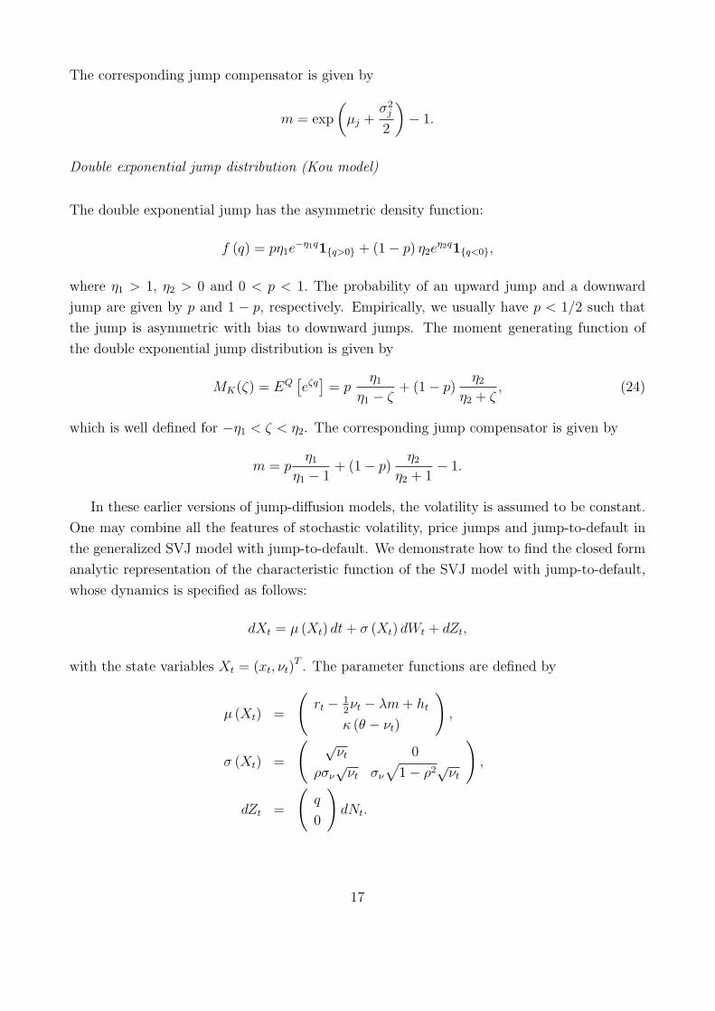
Double exponential jump distribution (Kou model)

The double exponential jump has the asymmetric density function:

f (q) = pη1e−η1q1q>0 + (1− p) η2e

η2q1q<0,

where η1 > 1, η2 > 0 and 0 < p < 1. The probability of an upward jump and a downward

jump are given by p and 1 − p, respectively. Empirically, we usually have p < 1/2 such that

the jump is asymmetric with bias to downward jumps. The moment generating function of

the double exponential jump distribution is given by

MK(ζ) = EQ[eζq]= p

η1η1 − ζ

+ (1− p)η2

η2 + ζ, (24)

which is well defined for −η1 < ζ < η2. The corresponding jump compensator is given by

m = pη1

η1 − 1+ (1− p)

η2η2 + 1

− 1.

In these earlier versions of jump-diffusion models, the volatility is assumed to be constant.

One may combine all the features of stochastic volatility, price jumps and jump-to-default in

the generalized SVJ model with jump-to-default. We demonstrate how to find the closed form

analytic representation of the characteristic function of the SVJ model with jump-to-default,

whose dynamics is specified as follows:

dXt = µ (Xt) dt+ σ (Xt) dWt + dZt,

with the state variables Xt = (xt, νt)T . The parameter functions are defined by

µ (Xt) =

(rt − 1

2νt − λm+ ht

κ (θ − νt)

),

σ (Xt) =

( √νt 0

ρσν√νt σν

√1− ρ2

√νt

),

dZt =

(q

0

)dNt.

17

4.2 Characteristic functions

We would like to demonstrate how to derive the closed form representation of the characteristic

function of the SVJ model with jump-to-default. According to the governing equation of the

AJD process as depicted in eqs. 1(a,b), we set the coefficient functions to be

µ (X) =

(r − λm+ h

κθ

)+

(0 −1

2

0 −κ

)X

σ (X)σ (X)T =

(ν ρσνν

ρσνν σ2νν

).

Taking the interest rate r and hazard rate h to be constant, the characteristic function with

u = (u0, u1, u2)T is given by

Ψ (u,Xt, t;T ) = EQ

[exp

(−∫ T

t

R (Xs) ds

)eu·XT

∣∣∣∣Gt

]= exp [α (τ) + β1 (τ) xt + β2 (τ) νt] , τ = T − t. (25)

The time dependent coefficient functions, α (τ) and β (τ) = (β1 (τ) , β2 (τ))T , are obtained by

solving the following system of ODEs

dα (τ)

dτ= (r − λm+ h) β1 (τ) + κθβ2 (τ) + λ [Λ (β (τ))− 1]− h− r,

dβ1 (τ)

dτ= 0, (26)

dβ2 (τ)

dτ=

1

2σ2νβ

22 (τ) + ρσνβ1 (τ) β2 (τ)− κβ2 (τ) +

1

2β21 (τ)−

1

2β1 (τ) ,

with initial conditions: α (0) = u0 and β (0) = (u1, u2)T . Since there are only jumps in stock

price, the jump transform

Λ (β (τ)) =

∫Rn

exp (β (τ) · z) dν (z) =∫

f (q) exp (β1 (τ) q) dq

can be explicitly computed as:

(i) Λ (β (τ)) = MM(β1 (τ)) under the Gaussian jump-diffusion model;

(ii) Λ (β (τ)) = MK(β1 (τ)) under the double exponential jump model.

It is seen that β1 (τ) admits a trivial solution of β1 (τ) = u1. As a result, the ODE governing

β2 (τ) can be recasted as a Riccati equation

dβ2 (τ)

dτ= b0 + b1β2 (τ) + b2β

22 (τ) ,

18

where

b0 =1

2u1 (u1 − 1) , b1 = ρσνu1 − κ, b2 =

1

2σ2ν ,

with initial condition: β2 (0) = u2. The system of ODEs has the following explicit solution:

α (τ) = u0 + (r − λm+ h)u1 + λ [Λ (u1)− 1]− h− r τ

+ κθ

[r−τ − 1

b2ln

(1− g exp (−τd)

1− g

)],

β1 (τ) = u1, β2 (τ) = r−1− g exp (−τd)

1− g exp (−τd), (27)

where

r± =1

2b2(−b1 ± d) , g =

r− − u2

r+ − u2

, g =r+r−

g, d =√b21 − 4b0b2.

Remark

When the ODEs governing α (τ) and βj (τ), j = 1, 2, have coupled or non-linear terms, we

may not have closed form solution. One then has to resort to numerical method such as the

fourth-order Runga-Kutta method to solve the system of ODEs. Nevertheless, the charac-

teristic function perserves the simple exponential expression with argument which is a linear

combination of the solution of the system of ODEs.

4.3 Numerical valuation of defaultable European options

First, we present numerical calculations on pricing of defaultable European options under the

JtD-AJD model using different approaches of evaluating the Fourier integral of the option

price function. We also examine the impact of the jump-to-default feature on the values of the

defaultable European options and the corresponding implied volatility smile patterns. In our

numerical calculations, the model parameters are specified as: ρ = −0.3, κ = 5, θ = 0.12, σν =

0.2, ν0 = 0.09, λ = 0.5, h = 0.02. The model parameters are chosen based on the following

assumptions. The stochastic volatility has a mean-reversion speed with a half-life of 0.2 year

under a moderately upward sloping term structure. The hazard rate of 0.02 implies an CDS

spread of around 100− 150 bps. For the stock price jump, we assume the arrival intensity to

be 0.5 and the jump sizes are assumed to be either the Merton jump or double exponential

jump. The values of the jump parameters are taken to be:

Merton jump: µj = −0.12, σj = 0.15;

Double exponential jump: p = 0.25, η1 = 8 and η2 = 6.

The above parameter values are chosen to be similar to those in Broadie and Kaya (2006).

Also, we assume constant interest rate to be 2% and the spot stock price to be 100 (unless

19

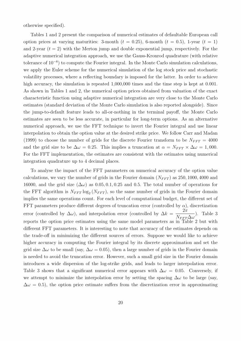
otherwise specified).

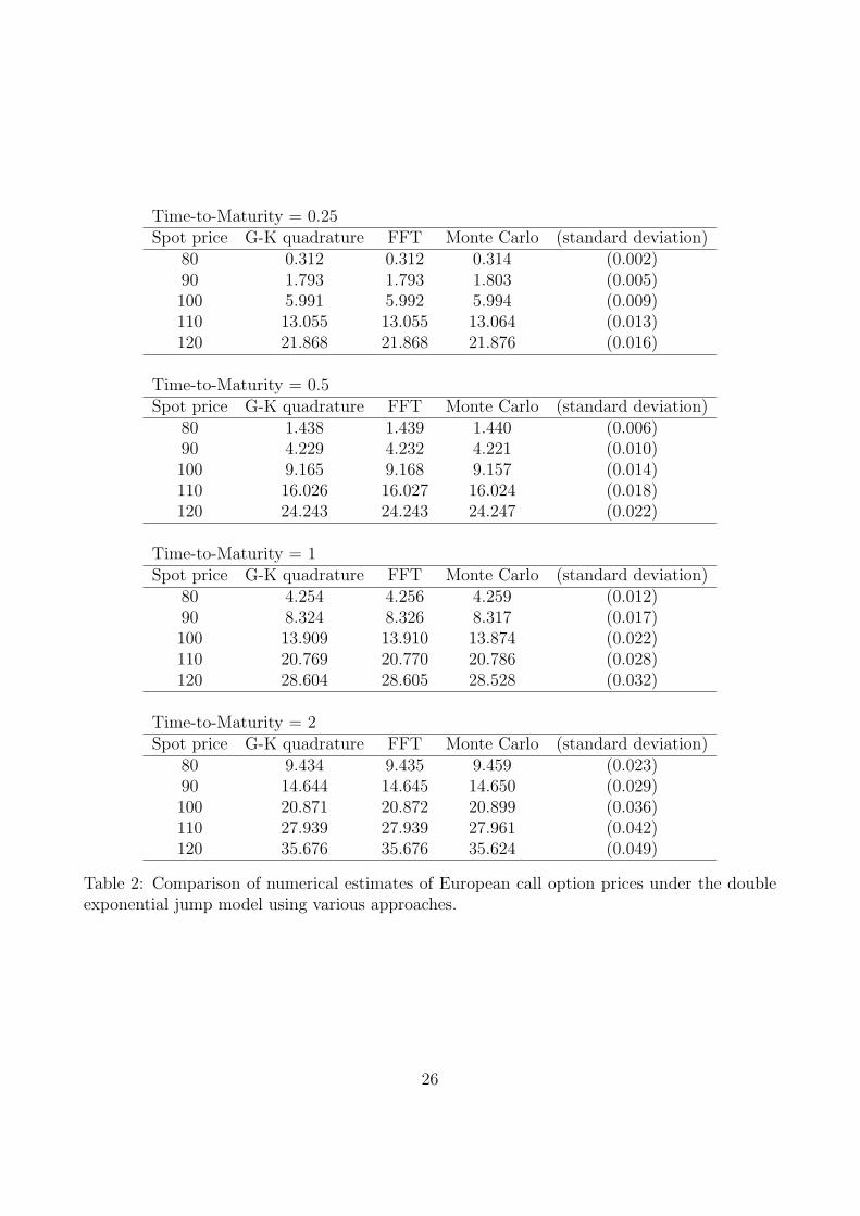
Tables 1 and 2 present the comparison of numerical estimates of defaultable European call

option prices at varying maturities: 3-month (t = 0.25), 6-month (t = 0.5), 1-year (t = 1)

and 2-year (t = 2) with the Merton jump and double exponential jump, respectively. For the

adaptive numerical integration approach, we use the Gauss-Kronrod quadrature (with relative

tolerance of 10−8) to compute the Fourier integral. In the Monte Carlo simulation calculations,

we apply the Euler scheme for the numerical simulation of the log stock price and stochastic

volatility processes, where a reflecting boundary is imposed for the latter. In order to achieve

high accuracy, the simulation is repeated 1,000,000 times and the time step is kept at 0.001.

As shown in Tables 1 and 2, the numerical option prices obtained from valuation of the exact

characteristic function using adaptive numerical integration are very close to the Monte Carlo

estimates (standard deviation of the Monte Carlo simulation is also reported alongside). Since

the jump-to-default feature leads to all-or-nothing in the terminal payoff, the Monte Carlo

estimates are seen to be less accurate, in particular for long-term options. As an alternative

numerical approach, we use the FFT technique to invert the Fourier integral and use linear

interpolation to obtain the option value at the desired strike price. We follow Carr and Madan

(1999) to choose the number of grids for the discrete Fourier transform to be NFFT = 4000

and the grid size to be ∆ω = 0.25. This implies a truncation at α = NFFT × ∆ω = 1, 000.

For the FFT implementation, the estimates are consistent with the estimates using numerical

integration quadrature up to 4 decimal places.

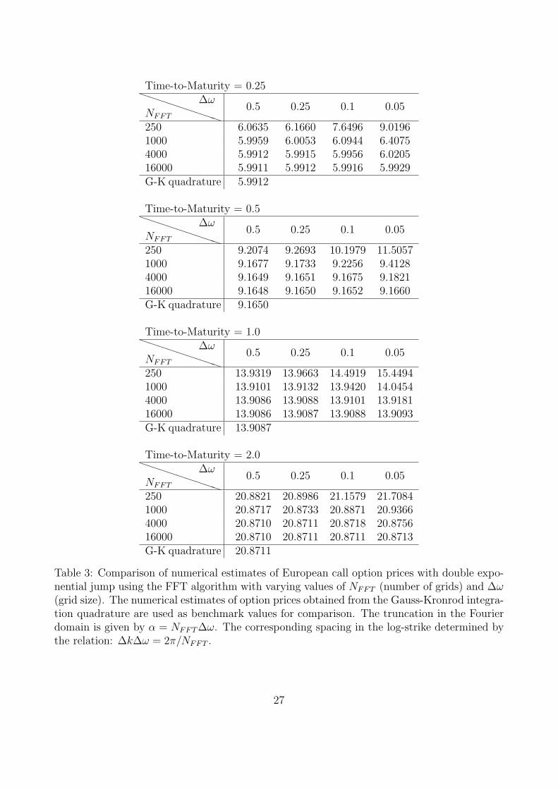
To analyse the impact of the FFT parameters on numerical accuracy of the option value

calculations, we vary the number of grids in the Fourier domain (NFFT ) as 250, 1000, 4000 and

16000, and the grid size (∆ω) as 0.05, 0.1, 0.25 and 0.5. The total number of operations for

the FFT algorithm is NFFT log2 (NFFT ), so the same number of grids in the Fourier domain

implies the same operations count. For each level of computational budget, the different set of

FFT parameters produce different degrees of truncation error (controlled by α), discretization

error (controlled by ∆ω), and interpolation error (controlled by ∆k =2π

NFFT∆ω). Table 3

reports the option price estimates using the same model parameters as in Table 2 but with

different FFT parameters. It is interesting to note that accuracy of the estimates depends on

the trade-off in minimizing the different sources of errors. Suppose we would like to achieve

higher accuracy in computing the Fourier integral by its discrete approximation and set the

grid size ∆ω to be small (say, ∆ω = 0.05), then a large number of grids in the Fourier domain

is needed to avoid the truncation error. However, such a small grid size in the Fourier domain

introduces a wide dispersion of the log-strike grids, and leads to larger interpolation error.

Table 3 shows that a significant numerical error appears with ∆ω = 0.05. Conversely, if

we attempt to minimize the interpolation error by setting the spacing ∆ω to be large (say,

∆ω = 0.5), the option price estimate suffers from the discretization error in approximating

20

the Fourier integral. Fortunately, one can use better numerical integration scheme to minimize

the impact of discretization error. Indeed, when a higher order integration scheme is employed

(say, Simpson’s rule), the discretization is negligible even when the spacing is set at 0.5 or

higher. Our results are consistent with the observation in Carr and Madan (1999). As a

conclusion, it is desirable to have a coarse grid size in the Fourier domain in order to minimize

the truncation and interpolation errors, and adopt a higher order quadrature to approximate

the Fourier integral.

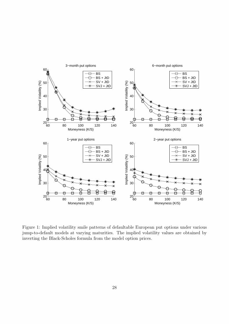
Implied volatility smile patterns with jump-to-default

It is more convenient to use put options to examine the impact of jump-to-default. Empirical

evidence shows that the out-of-the-money (OTM) put options are more closely linked to the

yield spreads and CDS spreads of the underlying firm. Also, the corresponding skew in the

implied volatility smile is strongly correlated with the default risk of the firm. Figure 1 shows

the implied volatility smile patterns of defaultable European put options under different jump-

to-default (JtD) models at varying maturities of 3 months, 6 months, 1 year and 2 years.

We consider the following jump-to-default models: (i) Black-Scholes model with JtD (BS-JtD

model); (ii) Heston model with JtD (SV-JtD model); and (iii) SVJ model with JtD (SVJ-JtD)

model. We also show the flat Black-Scholes implied volatility as benchmark for the implied

volatility smile generated by these models.

A higher implied volatility indicates a higher put option price, so a higher premium to

buy the downside protection. It can be seen that the presence of jump-to-default significantly

increases the implied volatility of the deep OTM put options and produces a strongly skewed

implied volatility smile. The jump-to-default feature adds to the implied volatility smile with

magnitude varying from 10 to 30 volatility points as the moneyness moves from 0.8 and 0.6.

This is consistent with the empirical evidence that the implied volatility of a deep OTM put

option is strongly correlated with the default risk of the underlying firm. In particular, it is

important to note that for short-term options, the implied volatility generated by different JtD

models converge as the moneyness goes deep out-of-the-money, except for the SVJ-JtD model

which produces a slightly different pattern. With the possibility of jump-to-default, the price

of a short-term deep OTM option is primarily determined by default risk while the diffusion

stock price dynamics is of less importance.

Given the possibility of jump-to-default, the skew in the implied volatility is more persis-

tence for long-term options, a feature that cannot be produced by pure stochastic volatility

models as their asymptotic implied volatility smile becomes flat as time-to-maturity increases

since the variance reverts to its long-run mean. It is also worth to note that the jump-to-default

feature introduces a notable shift in the implied volatility smile for the long-term options (by

10 to 15 volatility points for the BS-JtD model). This suggests that the volatility risk premium

21

(net amount that the implied volatility value exceeds the historical volatility value) embedded

in the long-term options is largely attributed to the default risk of the underlying firm.

5 Conclusion

The joint modeling of equity risk and credit exposure is important in any state-of-the-art op-

tion pricing models of credit-sensitive equity derivatives. Our proposed equity-credit models

attempt to perform pricing of equity and credit derivatives under a unified framework. We

have demonstrated the robustness of adding the jump-to-default feature in the popular affine

jump-diffusion models for pricing defaultable European claims and credit default swaps. By as-

suming the hazard rate to be affine, analytic tractability in typical affine jump-diffusion models

is maintained even with the inclusion of the jump-to-default feature. Once the analytic formula

is available for the characteristic function of the joint equity-credit price dynamics, numerical

valuation of the derivative prices can be performed easily using a standard numerical integra-

tion quadrature or Fast Fourier transform algorithm. Our numerical experiments showed that

accuracy of the Fast Fourier transform algorithm may deteriorate for short-maturity options.

Also, volatility skew effects may be significant for short-maturity deep-out-of-the-money puts

under the joint modeling of equity and credit risks. This may be attributed to the observation

that the price of a short-term deep-out-of-the-money put may be more sensitive to default risk.

As future research works, one may consider pricing of credit-sensitive exotic equity derivatives,

like variance swap products with default cap feature.

ACKNOWLEDGEMENT

This work was supported by the Hong Kong Research Grants Council under Project 642110

of the General Research Funds.

REFERENCES

Acharya, V.V. and Johnson, T.C. Insider Trading in Credit Derivatives. Journal of Finance

Economics 84 (2007): 110-141.

Bakshi, G., Cao, C. and Chen, Z. Empirical Performance of Alternative Option Pricing Models.

Journal of Finance 52(5) (1997): 2003-2049.

22

Bates, D.S. Jumps and Stochastic Volatility: Exchange Rate Processes Implicit in Deutsche

Mark Options. Review of Financial Studies 9(1) (1996): 69-107.

Broadie, M. and Kaya, O. Exact Simulation of Stochastic Volatility and Other Affine Jump

Diffusion Processes. Operations Research 54(2), (2006): 217-231.

Bayraktar, E. and Yang, B.A. Unified Framework for Pricing Credit and Equity Derivatives.

To appear in Mathematical Finance (2011).

Cao, C., Yu, F. and Zhong, Z. The Information Content of Option-Implied Volatility for Credit

Default Swap Valuation. Journal of Financial Markets 13(3) (2010): 321-343.

Carr, P. and Linetsky, V. A Jump to Default extended CEV models: An application of Bessel

Processes. Finance and Stochastics 10 (2006): 303-330.

Carr, P. and Wu, L. Stock Options and Credit Default Swaps: A Joint Framework for Valuation

and Estimation. Journal of Financial Econometrics (2009): 1-41.

Carr, P. and Madan, D.B. Option Valuation using the Fast Fourier Transform. Journal of

Computational Finance 2(4) (1999): 61-73.

Carr, P. and Madan, D.B. Local Volatility Enhanced by a Jump to Default. SIAM Journal of

Financial Mathematics 1 (2010): 2-15.

Cheridito, P. and Wugalter, A. Pricing and Hedging in Affine Models with Possibility of De-

fault. Working paper of Princeton University (2011).

Cremers, M., Driessen, J., Maenhout, P. and Weinbaum, D. Individual Stock-Option Prices

and Credit Spreads. Journal of Banking and Finance 32 (2008): 2706-2715.

Duffie, D. and Singleton, K. Modeling Term Structures of Defaultable Bonds. Review of

Financial Studies 12 (1999): 687-720.

Duffie, D., Pan, J. and Singleton, K. Transform Analysis and Asset Pricing for Affine Jump-

Diffusions. Econometrica 68(6) (2000): 1343-1376.

Erakar, B. Do Stock Prices and Volatility Jump? Reconciling Evidence from Spot and Option

Prices. Journal of Finance 59 (3) (2004): 1367-1403.

Heston, S.A. Closed-form Solution for Options with Stochastic Volatility with Application to

Bond and Currency Options. Review of Financial Studies 6(2) (1993): 327-343.

Kou, S.G. A Jump-Diffusion Model for Option Pricing. Management Science (48) (2002):

1086-1101.

Lando, D. On Cox Processes and Credit Risky Securities. Review of Derivatives Research 2

(1998): 99-120.

23

Lord, R. and Kahl, C. Optimal Fourier Inversion in Semi-analytical Option Pricing. Journal

of Computational Finance 10(4) (2007): 1-30.

Merton, R.C. Option Pricing when Underlying Stock Returns are Discontinuous. Journal of

Financial Economics 3 (1976): 125-144.

Mendoza-Arriaga, R., Carr, P. and Linetsky, V. Time-changed Markov Processes in Unified

Credit-Equity Modeling. Mathematical Finance 20(4) (2010): 527-569.

Pan, J. The Jump-Risk Premia Implicit in Options: Evidence from an Integrated Time-Series

Study. Journal of Financial Economics 63 (2002): 3-50.

Zhang, B.Y., Zhou, H. and Zhu, H. Explaining Credit Default Swap Spreads with the Equity

Volatility and Jump Risks of Individual Firms. Review of Financial Studies 22(12)

(2009): 5099-5131.

24

Time-to-Maturity = 0.25Spot price G-K quadrature FFT Monte Carlo (standard deviation)

80 0.246 0.246 0.245 (0.002)90 1.730 1.730 1.729 (0.005)100 5.961 5.961 5.966 (0.009)110 13.032 13.032 13.032 (0.012)120 21.821 21.821 21.821 (0.015)

Time-to-Maturity = 0.5Spot price G-K quadrature FFT Monte Carlo (standard deviation)

80 1.338 1.338 1.334 (0.005)90 4.133 4.133 4.134 (0.009)100 9.080 9.080 9.080 (0.014)110 15.937 15.937 15.930 (0.018)120 24.138 24.138 24.139 (0.022)

Time-to-Maturity = 1Spot price G-K quadrature FFT Monte Carlo (standard deviation)

80 4.097 4.097 4.094 (0.011)90 8.151 8.151 8.158 (0.016)100 13.724 13.724 13.695 (0.021)110 20.574 20.574 20.563 (0.027)120 28.401 28.401 28.398 (0.032)

Time-to-Maturity = 2Spot price G-K quadrature FFT Monte Carlo (standard deviation)

80 9.163 9.163 9.164 (0.022)90 14.341 14.341 14.356 (0.028)100 20.547 20.547 20.581 (0.035)110 27.602 27.602 27.615 (0.041)120 35.336 35.336 35.366 (0.047)

Table 1: Comparison of numerical estimates of European call option prices under the Mertonjump model using various numerical approaches.

25

Time-to-Maturity = 0.25Spot price G-K quadrature FFT Monte Carlo (standard deviation)

80 0.312 0.312 0.314 (0.002)90 1.793 1.793 1.803 (0.005)100 5.991 5.992 5.994 (0.009)110 13.055 13.055 13.064 (0.013)120 21.868 21.868 21.876 (0.016)

Time-to-Maturity = 0.5Spot price G-K quadrature FFT Monte Carlo (standard deviation)

80 1.438 1.439 1.440 (0.006)90 4.229 4.232 4.221 (0.010)100 9.165 9.168 9.157 (0.014)110 16.026 16.027 16.024 (0.018)120 24.243 24.243 24.247 (0.022)

Time-to-Maturity = 1Spot price G-K quadrature FFT Monte Carlo (standard deviation)

80 4.254 4.256 4.259 (0.012)90 8.324 8.326 8.317 (0.017)100 13.909 13.910 13.874 (0.022)110 20.769 20.770 20.786 (0.028)120 28.604 28.605 28.528 (0.032)

Time-to-Maturity = 2Spot price G-K quadrature FFT Monte Carlo (standard deviation)

80 9.434 9.435 9.459 (0.023)90 14.644 14.645 14.650 (0.029)100 20.871 20.872 20.899 (0.036)110 27.939 27.939 27.961 (0.042)120 35.676 35.676 35.624 (0.049)

Table 2: Comparison of numerical estimates of European call option prices under the doubleexponential jump model using various approaches.

26

Time-to-Maturity = 0.25PPPPPPPPPNFFT

∆ω0.5 0.25 0.1 0.05

250 6.0635 6.1660 7.6496 9.01961000 5.9959 6.0053 6.0944 6.40754000 5.9912 5.9915 5.9956 6.020516000 5.9911 5.9912 5.9916 5.9929G-K quadrature 5.9912

Time-to-Maturity = 0.5PPPPPPPPPNFFT

∆ω0.5 0.25 0.1 0.05

250 9.2074 9.2693 10.1979 11.50571000 9.1677 9.1733 9.2256 9.41284000 9.1649 9.1651 9.1675 9.182116000 9.1648 9.1650 9.1652 9.1660G-K quadrature 9.1650

Time-to-Maturity = 1.0PPPPPPPPPNFFT

∆ω0.5 0.25 0.1 0.05

250 13.9319 13.9663 14.4919 15.44941000 13.9101 13.9132 13.9420 14.04544000 13.9086 13.9088 13.9101 13.918116000 13.9086 13.9087 13.9088 13.9093G-K quadrature 13.9087

Time-to-Maturity = 2.0PPPPPPPPPNFFT

∆ω0.5 0.25 0.1 0.05

250 20.8821 20.8986 21.1579 21.70841000 20.8717 20.8733 20.8871 20.93664000 20.8710 20.8711 20.8718 20.875616000 20.8710 20.8711 20.8711 20.8713G-K quadrature 20.8711

Table 3: Comparison of numerical estimates of European call option prices with double expo-nential jump using the FFT algorithm with varying values of NFFT (number of grids) and ∆ω(grid size). The numerical estimates of option prices obtained from the Gauss-Kronrod integra-tion quadrature are used as benchmark values for comparison. The truncation in the Fourierdomain is given by α = NFFT∆ω. The corresponding spacing in the log-strike determined bythe relation: ∆k∆ω = 2π/NFFT .

27

60 80 100 120 14020

30

40

50

603−month put options

Moneyness (K/S)

Impl

ied

Vol

atili

ty (

%)

BSBS + JtDSV + JtDSVJ + JtD

60 80 100 120 14020

30

40

50

606−month put options

Moneyness (K/S)Im

plie

d V

olat

ility

(%

)

BSBS + JtDSV + JtDSVJ + JtD

60 80 100 120 14020

30

40

50

601−year put options

Moneyness (K/S)

Impl

ied

Vol

atili

ty (

%)

BSBS + JtDSV + JtDSVJ + JtD

60 80 100 120 14020

30

40

50

602−year put options

Moneyness (K/S)

Impl

ied

Vol

atili

ty (

%)

BSBS + JtDSV + JtDSVJ + JtD

Figure 1: Implied volatility smile patterns of defaultable European put options under variousjump-to-default models at varying maturities. The implied volatility values are obtained byinverting the Black-Scholes formula from the model option prices.

28