Option Pricing Under a Double ExponentialJump Diffusion Model∗

S. G. Kou and Hui Wang

This version May 27, 2003

Abstract

Analytical tractability is one of the challenges faced by many alternative models thattry to generalize the Black-Scholes option pricing model to incorporate more empiricalfeatures. The aim of this paper is to extend the analytical tractability of the Black-Scholes model to alternative models with jumps. We demonstrate a double exponentialjump diffusion model can lead to an analytic approximation for Þnite horizon Americanoptions (by extending the Barone-Adesi and Whaley method) and analytical solutionsfor popular path-dependent options (such as lookback, barrier, and perpetual Americanoptions). Numerical examples indicate that the formulae are easy to be implementedand accurate.

Keywords: contingent claims, high peak, heavy tails, volatility smile, overshoot.

1 Introduction

Many researches have been conducted to modify the Black-Scholes model based on Brownian

motion and normal distribution in order to incorporate two empirical features: (1) The

asymmetric leptokurtic features. In other words, the return distribution is skewed to the

left, and has a higher peak and two heavier tails than those of the normal distribution. (2)

The volatility smile. More precisely, if the Black-Scholes model is correct, then the implied

volatility should be constant; but it is widely recognized that the implied volatility curve

resembles a �smile,� meaning it is a convex curve of the strike price.

∗ S. G. Kou, 312 Mudd Building, Department of IEOR, Columbia University, New York, NY 10027, e-mail:sk75@columbia.edu; Hui Wang, Division of Applied Mathematics, Brown University, Box F, Providence, RI02912, e-mail: huiwang@cfm.brown.edu

1

To incorporate the asymmetric leptokurtic features in asset pricing, a variety of models

have been proposed, including, among others: (a) chaos theory, fractal Brownian motion,

and stable processes; (b) generalized hyperbolic models, including log t model and log hy-

perbolic model; (c) time changed Brownian motions, including log variance gamma model.

In a parallel development, different models are also proposed to incorporate the �volatility

smile� in option pricing. Popular ones are: (a) stochastic volatility1 and GARCH models;

(b) constant elasticity model (CEV model); (c) normal jump diffusion models; (d) affine

stochastic volatility and affine jump diffusion models; (e) models based on Levy processes.

For the background of these alternative models, see, for example, Hull (2000).

Unlike the original Black-Scholes model, although many alternative models can lead to

analytic solutions for European call and put options, it is difficult to do so for path-dependent

options, such as American options, lookback options, and barrier options. Even numerical

methods for these derivatives are not easy. For example, the convergence rates of binomial

trees and Monte Carlo simulation for path-dependent options are typically much slower than

those for call and put options; for a survey, see, for example, Boyle, Broadie, and Glasserman

(1997).

This paper attempts to extend the analytical tractability of Black-Scholes analysis for

the classical geometric Brownian motion to alternative models with jumps. In particular,

we demonstrate that a double exponential jump diffusion model (Kou, 2002) can lead to

analytic approximation for Þnite horizon American options (by extending the approximation

in Barone-Adesi and Whaley, 1987, for the classical geometric Brownian motion model), and

analytical solutions for lookback, barrier, and perpetual American options.

The paper is organized as follows. Section 2 gives basic setting of the double exponential

jump diffusion model, and presents intuition on why the analytical solutions are possible.

An analytical approximation of Þnite time American options is given in Section 3, and the

analysis of other path-dependent options is conducted in Section 4. The concluding remarks

1One empirical phenomenon worth mentioning is that the daily return distribution tends to have morekurtosis than the distribution of monthly returns. As Das and Foresi (1996) point out, this is consistentwith models with jumps, but inconsistent with stochastic volatility models or other pure diffusion models.

2

in given in Section 5. All the proofs are given in the appendices.

2 Background and Intuition

2.1 The Double Exponential Jump Diffusion Model

Under the double exponential jump diffusion model, the dynamics of the asset price S(t) is

given by

dS(t)

S(t−) = µdt+ σ dW (t) + dN(t)X

i=1

(Vi − 1) ,

where W (t) is a standard Brownian motion, N(t) a Poisson process with rate λ, and {Vi}a sequence of independent identically distributed (i.i.d.) nonnegative random variables such

that Y = log(V ) has an asymmetric double exponential distribution with the density

fY (y) = p · η1e−η1y1{y≥0} + q · η2eη2y1{y<0}, η1 > 1, η2 > 0,

where p, q ≥ 0, p + q = 1. Here the condition η1 > 1 is imposed to ensure that the stock

price S(t) has Þnite expectation. Note that the means of the two exponential distributions

are 1/η1 and 1/η2 respectively. In the model, all sources of randomness, N(t), W (t), and

Y �s, are assumed to be independent.

Because of the jumps, the risk-neutral probability measure is not unique. Following

Lucas (1978), Naik and Lee (1990), it can be shown (see, e.g., Kou 2002) that, by using the

rational expectations argument with a HARA type utility function for the representative

agent, one can choose a particular risk-neutral measure2 P∗ so that the equilibrium price

of an option is given by the expectation under this risk neutral measure of the discounted

option payoff. Under this risk neutral probability measure, the asset price S(t) still follows

a double exponential jump diffusion process3:

dS(t)

S(t−) = (r − λ∗ζ∗) dt+ σ dW ∗(t) + d

N∗(t)Xi=1

(V ∗i − 1) , (1)

2The measure P∗ is called risk-neutral because that E∗(e−rtS(t)) = S(0).3For option pricing, the case of the underlying asset having a continuous dividend yield δ can be easily

treated by changing r to r − δ in (1).

3

with the return process X(t) = log(S(t)/S(0)) given by

X(t) = (r − 12σ2 − λ∗ζ∗) t+ σW ∗(t) +

N∗(t)Xi=1

Y ∗i , X(0) = 0. (2)

Here W ∗(t) is a standard Brownian motion under P∗, {N∗(t); t ≥ 0} is a Poisson processwith intensity λ∗, V ∗ = eY

∗. The log jump sizes {Y ∗1 , Y ∗2 , · · · } still form a sequence of

independent identically distributed (i.i.d.) random variables with a new double exponential

density fY ∗(y) ∼ p∗ ·η∗1e−η∗1y1{y≥0}+ q∗ ·η∗2eyη∗21{y<0}. The constants p∗, q∗ ≥ 0, p∗+ q∗ = 1,λ∗ > 0, η∗1 > 1, η

∗2 > 0, and

ζ∗ := E∗[V ∗]− 1 = p∗η∗1η∗1 − 1

+q∗η∗2η∗2 + 1

− 1 (3)

all depend on the utility function of the representative agent. All sources of randomness,

N∗(t), W ∗(t), and Y ∗�s, are still independent under P∗.

Since we focus on option pricing in this paper, to simplify the notation (without causing

much confusion), we shall drop the superscript ∗ in the parameters, i.e. using p, q, η1, η2rather than p∗, q∗, η∗1, η

∗2. The understanding is that all the processes and parameters below

are under the risk-neutral probability measure P∗.

2.2 Intuition of the Pricing Formulae

Without the jump part, the model simply becomes the classical geometric Brownian motion

model. Pricing formulae for American options, barrier options, and lookback options are all

well known under the geometric Brownian motion model4. With the jump part, however, it

becomes very difficult to derive analytical solutions for these options.

The reason for that is as follows. To price American options, barrier options, and lookback

options for general jump diffusion processes, it is crucial to study the Þrst passage times that

the process crosses a ßat boundary with a level b. Without loss of generality, assume b > 0.

When a jump diffusion process crosses the boundary, sometimes it hits the boundary exactly

4Davydov and Linetsky (2001, 2003) provide analytical solutions for various path-dependent optionsunder the CEV diffusion model.

4

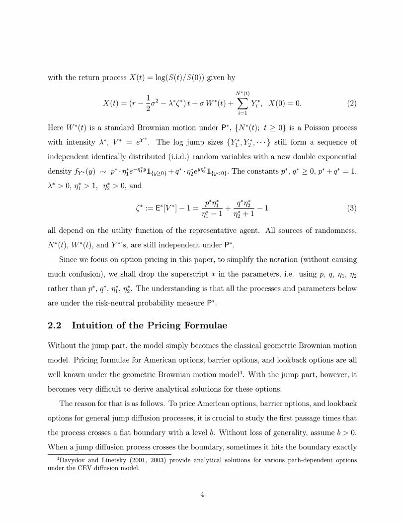
and sometimes it incurs an �overshoot�, X(τb)− b, over the boundary, where τb is the Þrsttime that the process X(t) crosses the boundary. See Fig. 1 for an illustration.

Figure 1: A Simulated Sample Path with the Overshoot Problem

The overshoot presents several problems, if one wants to compute the distribution of the

Þrst passage times analytically. First, one needs the exact distribution of the overshoot,

X(τb) − b; particularly, P[X(τb) − b = 0] and P[X(τb) − b > x], x > 0. Secondly, one needsto know the dependence structure between the overshoot, X(τb) − b, and the Þrst passagetime τb. Both difficulties can be resolved under the assumption that the jump size Y has an

exponential type distribution; see Kou and Wang (2003). Finally, if one wants to use the

reßection principle to study the Þrst passage times, the dependence structure between the

overshoot and the terminal value X(t) is also needed afterwards. This is not known to the

best of our knowledge, even for the double exponential jump diffusion process.

Consequently, we can get analytic approximations for Þnite horizon American options,

closed form solutions for the Laplace transforms of lookback and barrier options, and closed

form solutions for the perpetual American options5, under the double exponential jump

diffusion model, yet cannot give more explicit calculations beyond that, as the correlation

5Essentially, to compute the values of perpetual American options, one only needs to know the Laplacetransforms (there is no need to invert the transforms). Hence, we can get closed form solutions for perpetualAmerican options.

5

between the terminal state X(t) and the overshoot X(τb)− b is not available6.It is worth mentioning that the double exponential jump diffusion process is a special case

of Levy process with two-sided jumps, whose characteristic exponent admits the (unique)

representation

φ(θ) = E£eiθX1

¤= exp

½iγθ − 1

2Aθ2 +

Z ∞

−∞(eiθy − 1− iθy1{|y|≤1})Π(dy)

¾,

where the generating triplet (γ, A,Π) is given by

A = σ2, γ = µ+ λp

µ1− e−η1η1

− e−η1¶− λq

µ1− e−η2η2

− e−η2¶,

Π(dy) = λ · fY (y)dy = λpη1e−η1y1{y≥0}dy + λqη2eη2y1{y<0}dy.If the jump size distribution is one-sided, one can solve the overshoot problems7 by ei-

ther using renewal equations or ßuctuation identities for Levy processes; see, e.g., Avram,

Chan, and Usabel (2001), Rogers (2000). However, for two-sided jumps, because of the

ladder-variable problems, generally speaking the renewal equations are not available and

the ßuctuation identities becomes too complicated for explicit computation; see, e.g., the

discussion in Siegmund (1985) and Rogers (2000).

2.3 Some Notations

The moment generating function of X(t) is given by E∗[eθX(t)] = exp{G(θ)t}, where thefunction G(·) is deÞned as

G(x) := x(r − 12σ2 − λζ) + 1

2x2σ2 + λ

µpη1η1 − x +

qη2η2 + x

− 1¶.

Lemma 3.1 in Kou and Wang (2003) shows that the equation G(x) = α, ∀α > 0, has exactlyfour roots: β1,α, β2,α, −β3,α, −β4,α, where

0 < β1,α < η1 < β2,α <∞, 0 < β3,α < η2 < β4,α <∞. (4)

6See, for example, Siegmund (1985), Boyarchenko and Levendorskiùi (2002b), and Kyprianou and Pistorius(2003) for some representations (though not explicit calculations) related to the overshoot problems forgeneral Levy processes.

7For a jump diffusion process with one-sided jumps, the overshoot problem may not occur if the boundarylevel is on the opposite direction of the jumps; e.g., the jump sizes are negative and the boundary level b > 0.Under this circumstance, explicit solution may be possible (at least for perpetual American options) even ifthe distribution of jump size take a general form; see e.g. Mordecki (1999).

6

To use the It�o formula for jump processes, we also need the inÞnitesimal generator of X(t):

(LV )(x) := 1

2σ2V 00(x) + (r − 1

2σ2 − λζ)V 0(x) + λ

Z ∞

−∞[V (x+ y)− V (x)]fY (y)dy. (5)

3 Pricing Finite Time Horizon American Options

Most of call and put options traded in the exchanges in both U.S. and Europe are American

type options. Therefore, it is of great interest to calculate the prices of American options

accurately and quickly. The price of a Þnite horizon American option is the solution of a

Þnite horizon free boundary problem. Even within the classical geometric Brownian motion

model, except in the case of the American call option with no dividend, there is no analytical

solution available8.

To price American options under general jump diffusion models, one may consider nu-

merically solving the free boundary problems via lattice or differential equation methods;

see, e.g., Amin (1993), Zhang (1997), d�Halluin, Forsyth, and Vetzal (2003). Extending the

Barone-Adesi and Whaley (1987) approximation for the classical geometric Brownian motion

model, we shall consider an alternative approach that takes into consideration of the special

structure of the double exponential jump diffusions. One motivation for such an extension is

its simplicity, as it yields an analytic approximation that only involves the price of a Euro-

pean option. Our numerical results in Tables 1 and 2 suggest that the approximation error

is typically less than 2%, which is less than the typical bid-ask spread (about 5% to 10%)

for American options in exchanges. Therefore, the approximation can serve as an easy way

to get a quick estimate that is perhaps accurate enough for many practical situations.

The extension of Barone-Adesi and Whaley�s method works nicely for double exponential

jump diffusion models mainly because explicit solutions are available to a class of relevant

integro-differential free boundary problems; see (15) and (16). We want to point out that

8For recent developments of numerical solution and analytic approximation of Þnite horizon Americanoptions within the classical geometric Brownian motion model, see, for example, Broadie and Detemple(1996), Carr (1998), Ju (1998), Geske and Johnson (1984), McMillan (1986), Tilley (1993), Tsitsiklis andvan Roy (1999), Sullivan (2000), Broadie and Glasserman (1997), Carriere (1996), Longstaff and Schwartz(2001), Rogers (2002), Haugh and Kogan (2002) and references therein.

7

there exist other more elaborate but more accurate approximations (such as Broadie and De-

temple 1996, Carr 1998, and Ju 1998) for geometric Brownian motion models, and whether

these algorithms can be effectively extended to jump diffusion models invites further inves-

tigation.

To simplify notation, we shall focus only on the Þnite horizon American put option

without dividends, as the methodology is also valid for the Þnite horizon American call

option with dividends. The analytic approximation involves two quantities, EuP(v, t) which

denotes the price of the European put option with initial stock price v and maturity t, and

Pv[S(t) ≤ K] which is the probability that the stock price at t is below K with initial stock

price v. Both EuP(v, t) and Pv[S(t) ≤ K] can be computed fast by using either the closedform solutions in Kou (2002) or the Laplace transforms in Petrella, Kou, and Wang (2003).

We need some notations. Let z = 1 − e−rt, β3 ≡ β3, rz, β4 ≡ β4, r

z, Cβ = β3β4(1 + η2),

Dβ = η2(1 + β3)(1 + β4), in the notation of equation (4). DeÞne v0 ≡ v0(t) ∈ (0, K) as theunique solution 9 to the equation

CβK −Dβ [v0 + EuP(v0, t)] = (Cβ −Dβ)Ke−rt · Pv0 [S(t) ≤ K]. (6)

Note that the left hand side of (6) is a strictly decreasing function of v0 (because v0 +

EuP(v0, t) = e−rtE∗ [max(S(t), K)|S(0) = v0]), and the right hand side of (6) is a strictlyincreasing function of v0 (because Cβ −Dβ = β3β4− η2(1 + β3+ β4) < 0). Therefore, v0 canbe obtained easily by using, for example, the bisection method.

Approximation: The price of a Þnite horizon American put option with maturity t and

strike K can be approximated by ψ(S(0), t), where the value function ψ is given by

ψ(v, t) =

½EuP(v, t) +Av−β3 +Bv−β4 ; if v ≥ v0K − v; if v ≤ v0 , (7)

with v0 being the unique root of the equation (6) and the two constants A and B given by

A =vβ30

β4 − β3©β4K − (1 + β4)[v0 + EuP(v0, t)] +Ke−rtPv0 [S(t) ≤ K]

ª> 0. (8)

9In Appendix A, we give a better upper bound in (18) for v0, that is K > v0 + EuP(v0, t).

8

B =vβ40

β3 − β4©β3K − (1 + β3)[v0 + EuP(v0, t)] +Ke−rtPv0 [S(t) ≤ K]

ª> 0. (9)

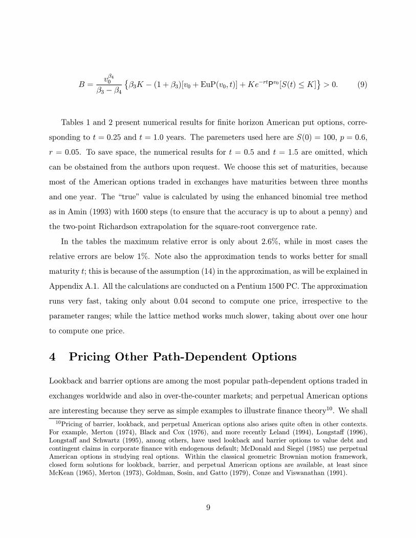
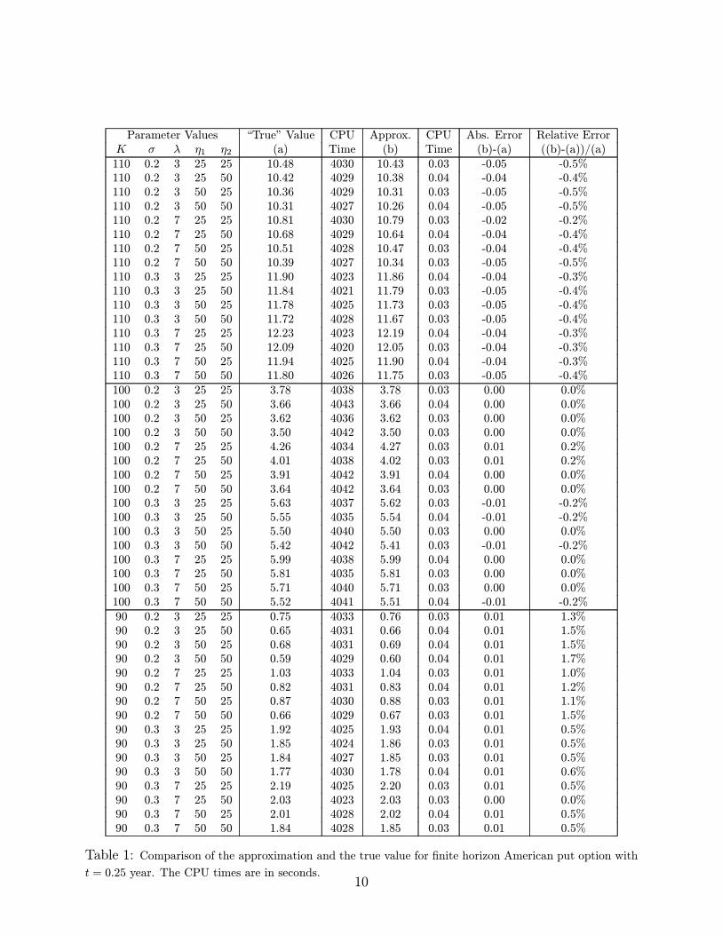
Tables 1 and 2 present numerical results for Þnite horizon American put options, corre-

sponding to t = 0.25 and t = 1.0 years. The paremeters used here are S(0) = 100, p = 0.6,

r = 0.05. To save space, the numerical results for t = 0.5 and t = 1.5 are omitted, which

can be obstained from the authors upon request. We choose this set of maturities, because

most of the American options traded in exchanges have maturities between three months

and one year. The �true� value is calculated by using the enhanced binomial tree method

as in Amin (1993) with 1600 steps (to ensure that the accuracy is up to about a penny) and

the two-point Richardson extrapolation for the square-root convergence rate.

In the tables the maximum relative error is only about 2.6%, while in most cases the

relative errors are below 1%. Note also the approximation tends to works better for small

maturity t; this is because of the assumption (14) in the approximation, as will be explained in

Appendix A.1. All the calculations are conducted on a Pentium 1500 PC. The approximation

runs very fast, taking only about 0.04 second to compute one price, irrespective to the

parameter ranges; while the lattice method works much slower, taking about over one hour

to compute one price.

4 Pricing Other Path-Dependent Options

Lookback and barrier options are among the most popular path-dependent options traded in

exchanges worldwide and also in over-the-counter markets; and perpetual American options

are interesting because they serve as simple examples to illustrate Þnance theory10. We shall

10Pricing of barrier, lookback, and perpetual American options also arises quite often in other contexts.For example, Merton (1974), Black and Cox (1976), and more recently Leland (1994), Longstaff (1996),Longstaff and Schwartz (1995), among others, have used lookback and barrier options to value debt andcontingent claims in corporate Þnance with endogenous default; McDonald and Siegel (1985) use perpetualAmerican options in studying real options. Within the classical geometric Brownian motion framework,closed form solutions for lookback, barrier, and perpetual American options are available, at least sinceMcKean (1965), Merton (1973), Goldman, Sosin, and Gatto (1979), Conze and Viswanathan (1991).

9

Parameter Values �True� Value CPU Approx. CPU Abs. Error Relative ErrorK σ λ η1 η2 (a) Time (b) Time (b)-(a) ((b)-(a))/(a)110 0.2 3 25 25 10.48 4030 10.43 0.03 -0.05 -0.5%110 0.2 3 25 50 10.42 4029 10.38 0.04 -0.04 -0.4%110 0.2 3 50 25 10.36 4029 10.31 0.03 -0.05 -0.5%110 0.2 3 50 50 10.31 4027 10.26 0.04 -0.05 -0.5%110 0.2 7 25 25 10.81 4030 10.79 0.03 -0.02 -0.2%110 0.2 7 25 50 10.68 4029 10.64 0.04 -0.04 -0.4%110 0.2 7 50 25 10.51 4028 10.47 0.03 -0.04 -0.4%110 0.2 7 50 50 10.39 4027 10.34 0.03 -0.05 -0.5%110 0.3 3 25 25 11.90 4023 11.86 0.04 -0.04 -0.3%110 0.3 3 25 50 11.84 4021 11.79 0.03 -0.05 -0.4%110 0.3 3 50 25 11.78 4025 11.73 0.03 -0.05 -0.4%110 0.3 3 50 50 11.72 4028 11.67 0.03 -0.05 -0.4%110 0.3 7 25 25 12.23 4023 12.19 0.04 -0.04 -0.3%110 0.3 7 25 50 12.09 4020 12.05 0.03 -0.04 -0.3%110 0.3 7 50 25 11.94 4025 11.90 0.04 -0.04 -0.3%110 0.3 7 50 50 11.80 4026 11.75 0.03 -0.05 -0.4%100 0.2 3 25 25 3.78 4038 3.78 0.03 0.00 0.0%100 0.2 3 25 50 3.66 4043 3.66 0.04 0.00 0.0%100 0.2 3 50 25 3.62 4036 3.62 0.03 0.00 0.0%100 0.2 3 50 50 3.50 4042 3.50 0.03 0.00 0.0%100 0.2 7 25 25 4.26 4034 4.27 0.03 0.01 0.2%100 0.2 7 25 50 4.01 4038 4.02 0.03 0.01 0.2%100 0.2 7 50 25 3.91 4042 3.91 0.04 0.00 0.0%100 0.2 7 50 50 3.64 4042 3.64 0.03 0.00 0.0%100 0.3 3 25 25 5.63 4037 5.62 0.03 -0.01 -0.2%100 0.3 3 25 50 5.55 4035 5.54 0.04 -0.01 -0.2%100 0.3 3 50 25 5.50 4040 5.50 0.03 0.00 0.0%100 0.3 3 50 50 5.42 4042 5.41 0.03 -0.01 -0.2%100 0.3 7 25 25 5.99 4038 5.99 0.04 0.00 0.0%100 0.3 7 25 50 5.81 4035 5.81 0.03 0.00 0.0%100 0.3 7 50 25 5.71 4040 5.71 0.03 0.00 0.0%100 0.3 7 50 50 5.52 4041 5.51 0.04 -0.01 -0.2%90 0.2 3 25 25 0.75 4033 0.76 0.03 0.01 1.3%90 0.2 3 25 50 0.65 4031 0.66 0.04 0.01 1.5%90 0.2 3 50 25 0.68 4031 0.69 0.04 0.01 1.5%90 0.2 3 50 50 0.59 4029 0.60 0.04 0.01 1.7%90 0.2 7 25 25 1.03 4033 1.04 0.03 0.01 1.0%90 0.2 7 25 50 0.82 4031 0.83 0.04 0.01 1.2%90 0.2 7 50 25 0.87 4030 0.88 0.03 0.01 1.1%90 0.2 7 50 50 0.66 4029 0.67 0.03 0.01 1.5%90 0.3 3 25 25 1.92 4025 1.93 0.04 0.01 0.5%90 0.3 3 25 50 1.85 4024 1.86 0.03 0.01 0.5%90 0.3 3 50 25 1.84 4027 1.85 0.03 0.01 0.5%90 0.3 3 50 50 1.77 4030 1.78 0.04 0.01 0.6%90 0.3 7 25 25 2.19 4025 2.20 0.03 0.01 0.5%90 0.3 7 25 50 2.03 4023 2.03 0.03 0.00 0.0%90 0.3 7 50 25 2.01 4028 2.02 0.04 0.01 0.5%90 0.3 7 50 50 1.84 4028 1.85 0.03 0.01 0.5%

Table 1: Comparison of the approximation and the true value for Þnite horizon American put option witht = 0.25 year. The CPU times are in seconds.

10

Parameter Values �True� Value CPU Approx. CPU Abs. Error Relative ErrorK σ λ η1 η2 (a) Time (b) Time (b)-(a) ((b)-(a))/(a)110 0.2 3 25 25 12.37 4026 12.32 0.04 -0.05 -0.4%110 0.2 3 25 50 12.17 4026 12.11 0.03 -0.06 -0.5%110 0.2 3 50 25 12.04 4025 12.00 0.04 -0.04 -0.3%110 0.2 3 50 50 11.84 4025 11.78 0.03 -0.06 -0.5%110 0.2 7 25 25 13.29 4026 13.27 0.03 -0.02 -0.2%110 0.2 7 25 50 12.85 4026 12.79 0.04 -0.06 -0.5%110 0.2 7 50 25 12.54 4024 12.54 0.03 0.00 0.0%110 0.2 7 50 50 12.08 4024 12.03 0.03 -0.05 -0.4%110 0.3 3 25 25 15.79 4025 15.76 0.04 -0.03 -0.2%110 0.3 3 25 50 15.63 4027 15.59 0.04 -0.04 -0.3%110 0.3 3 50 25 15.51 4028 15.49 0.03 -0.02 -0.1%110 0.3 3 50 50 15.36 4028 15.32 0.03 -0.04 -0.3%110 0.3 7 25 25 16.51 4025 16.51 0.04 0.00 0.0%110 0.3 7 25 50 16.17 4028 16.14 0.03 -0.03 -0.2%110 0.3 7 50 25 15.89 4028 15.91 0.03 0.02 0.1%110 0.3 7 50 50 15.53 4028 15.52 0.04 -0.01 -0.1%100 0.2 3 25 25 6.60 4027 6.62 0.03 0.02 0.3%100 0.2 3 25 50 6.36 4025 6.37 0.03 0.01 0.2%100 0.2 3 50 25 6.26 4025 6.29 0.04 0.03 0.5%100 0.2 3 50 50 6.01 4025 6.03 0.03 0.02 0.3%100 0.2 7 25 25 7.57 4026 7.62 0.03 0.05 0.7%100 0.2 7 25 50 7.07 4026 7.09 0.04 0.02 0.3%100 0.2 7 50 25 6.83 4024 6.88 0.03 0.05 0.7%100 0.2 7 50 50 6.28 4025 6.31 0.04 0.03 0.5%100 0.3 3 25 25 10.10 4025 10.13 0.03 0.03 0.3%100 0.3 3 25 50 9.94 4027 9.96 0.03 0.02 0.2%100 0.3 3 50 25 9.83 4028 9.87 0.04 0.04 0.4%100 0.3 3 50 50 9.67 4029 9.70 0.03 0.03 0.3%100 0.3 7 25 25 10.81 4025 10.86 0.03 0.05 0.5%100 0.3 7 25 50 10.46 4026 10.49 0.03 0.03 0.3%100 0.3 7 50 25 10.22 4036 10.29 0.04 0.07 0.7%100 0.3 7 50 50 9.85 4028 9.89 0.02 0.04 0.4%90 0.2 3 25 25 2.91 4025 2.96 0.04 0.05 1.7%90 0.2 3 25 50 2.70 4025 2.75 0.03 0.05 1.9%90 0.2 3 50 25 2.66 4025 2.72 0.04 0.06 2.3%90 0.2 3 50 50 2.46 4025 2.51 0.03 0.05 2.0%90 0.2 7 25 25 3.68 4026 3.75 0.03 0.07 1.9%90 0.2 7 25 50 3.24 4025 3.29 0.04 0.05 1.5%90 0.2 7 50 25 3.12 4024 3.20 0.03 0.08 2.6%90 0.2 7 50 50 2.66 4025 2.72 0.03 0.06 2.3%90 0.3 3 25 25 5.79 4024 5.85 0.04 0.06 1.0%90 0.3 3 25 50 5.65 4025 5.70 0.03 0.05 0.9%90 0.3 3 50 25 5.58 4028 5.64 0.04 0.06 1.1%90 0.3 3 50 50 5.43 4029 5.49 0.03 0.06 1.1%90 0.3 7 25 25 6.42 4027 6.49 0.04 0.07 1.1%90 0.3 7 25 50 6.09 4026 6.15 0.03 0.06 1.0%90 0.3 7 50 25 5.92 4029 6.00 0.03 0.08 1.4%90 0.3 7 50 50 5.59 4031 5.65 0.04 0.06 1.1%

Table 2: Comparison of the approximation and the true value for Þnite horizon American put option witht = 1 year.

11

demonstrate in this section that in the double exponential jump diffusion model the closed

form solutions for these options can still be obtained.

4.1 Lookback Options

As the calculation for the lookback call option follows just by symmetry, we will only provide

the result for the lookback put option, whose price is given by

LP(T ) = E∗∙e−rT

µmax{M, max

0≤t≤TS(t)}− S(T )

¶¸= E∗

∙e−rT

µmax{M, max

0≤t≤TS(t)}

¶¸− S(0),

where M ≥ S(0) is a Þxed constant representing the preÞxed maximum at time 0.

Theorem 4.1. Using the notation β1,α+r and β2,α+r as in (4), the Laplace transform of

the lookback put is given byZ ∞

0

e−αTLP(T )dT =S(0)AαCα

µS(0)

M

¶β1,α+r−1+S(0)BαCα

µS(0)

M

¶β2,α+r−1+

M

α+ r− S(0)

α

for all α > 0; here

Aα =(η1 − β1,α+r)β2,α+r

β1,α+r − 1 , Bα =(β2,α+r − η1)β1,α+r

β2,α+r − 1 , Cα = (α+ r)η1(β2,α+r − β1,α+r).

The proof of Theorem 4.1 will be given in Appendix B.1. Essentially, the proof explores

a link between the Laplace transform of the lookback option and the Laplace transform of

the Þrst passage times of the double exponential jump diffusion process as solved explicitly

in Kou and Wang (2003).

4.2 Barrier Options

There are eight types of (one dimensional, single) barrier options, namely up (down)-and-in

(out) call (put) options. For example, the price of a down-and-out put (DOP) option is

given by DOP = E∗£e−rT (K − S(T ))+1{min0≤t≤T S(t)≥H}

¤, where H < S(0) is the barrier

level. Since all the eight types barrier options can be solved in similar ways, we shall only

illustrate with the up-and-in call (UIC) option, whose price is given by

UIC = E∗£e−rT (S(T )−K)+1{max0≤t≤T S(t)≥H}

¤,

12

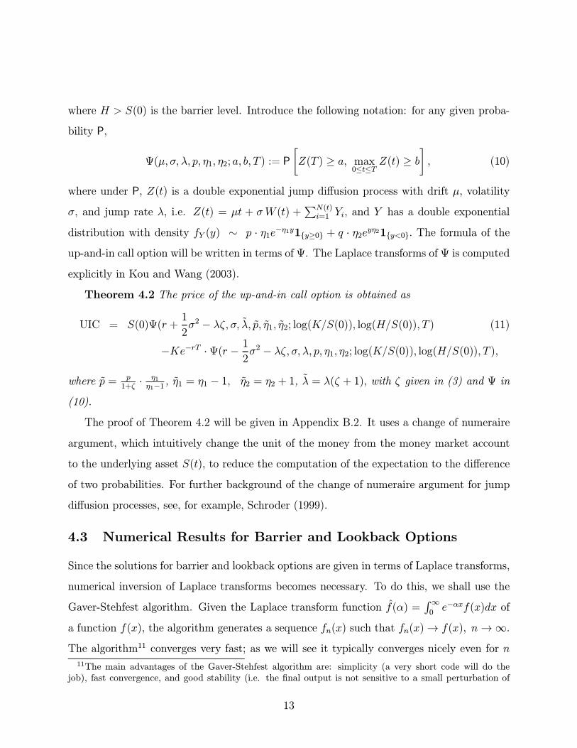
where H > S(0) is the barrier level. Introduce the following notation: for any given proba-

bility P,

Ψ(µ,σ,λ, p, η1, η2; a, b, T ) := P

∙Z(T ) ≥ a, max

0≤t≤TZ(t) ≥ b

¸, (10)

where under P, Z(t) is a double exponential jump diffusion process with drift µ, volatility

σ, and jump rate λ, i.e. Z(t) = µt + σW (t) +PN(t)

i=1 Yi, and Y has a double exponential

distribution with density fY (y) ∼ p · η1e−η1y1{y≥0} + q · η2eyη21{y<0}. The formula of theup-and-in call option will be written in terms of Ψ. The Laplace transforms of Ψ is computed

explicitly in Kou and Wang (2003).

Theorem 4.2 The price of the up-and-in call option is obtained as

UIC = S(0)Ψ(r +1

2σ2 − λζ, σ, �λ, �p, �η1, �η2; log(K/S(0)), log(H/S(0)), T ) (11)

−Ke−rT ·Ψ(r − 12σ2 − λζ, σ,λ, p, η1, η2; log(K/S(0)), log(H/S(0)), T ),

where �p = p1+ζ

· η1η1−1 , �η1 = η1 − 1, �η2 = η2 + 1, �λ = λ(ζ + 1), with ζ given in (3) and Ψ in

(10).

The proof of Theorem 4.2 will be given in Appendix B.2. It uses a change of numeraire

argument, which intuitively change the unit of the money from the money market account

to the underlying asset S(t), to reduce the computation of the expectation to the difference

of two probabilities. For further background of the change of numeraire argument for jump

diffusion processes, see, for example, Schroder (1999).

4.3 Numerical Results for Barrier and Lookback Options

Since the solutions for barrier and lookback options are given in terms of Laplace transforms,

numerical inversion of Laplace transforms becomes necessary. To do this, we shall use the

Gaver-Stehfest algorithm. Given the Laplace transform function �f(α) =R∞0e−αxf(x)dx of

a function f(x), the algorithm generates a sequence fn(x) such that fn(x)→ f(x), n→∞.The algorithm11 converges very fast; as we will see it typically converges nicely even for n11The main advantages of the Gaver-Stehfest algorithm are: simplicity (a very short code will do the

job), fast convergence, and good stability (i.e. the Þnal output is not sensitive to a small perturbation of

13

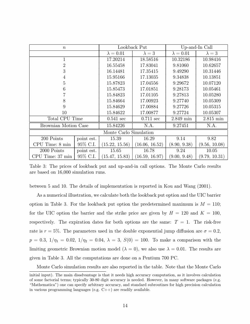
n Lookback Put Up-and-In Callλ = 0.01 λ = 3 λ = 0.01 λ = 3

1 17.20214 18.58516 10.32186 10.984162 16.55458 17.83041 9.81060 10.626573 16.14481 17.35415 9.49290 10.314464 15.95166 17.13035 9.34838 10.138515 15.87823 17.04556 9.29672 10.071206 15.85473 17.01851 9.28173 10.054617 15.84823 17.01105 9.27813 10.052808 15.84664 17.00923 9.27740 10.053099 15.84629 17.00884 9.27726 10.0531510 15.84622 17.00877 9.27724 10.05307

Total CPU Time 0.541 sec 0.711 sec 2.849 min 2.815 min

Brownian Motion Case 15.84226 N.A. 9.27451 N.A.

Monte Carlo Simulation200 Points point est. 15.39 16.29 9.14 9.82

CPU Time: 8 min 95% C.I. (15.22, 15.56) (16.06, 16.52) (8.90, 9.38) (9.56, 10.08)2000 Points point est. 15.65 16.78 9.24 10.05

CPU Time: 37 min 95% C.I. (15.47, 15.83) (16.59, 16.97) (9.00, 9.48) (9.79, 10.31)

Table 3: The prices of lookback put and up-and-in call options. The Monte Carlo resultsare based on 16,000 simulation runs.

between 5 and 10. The details of implementation is reported in Kou and Wang (2001).

As a numerical illustration, we calculate both the lookback put option and the UIC barrier

option in Table 3. For the lookback put option the predetermined maximum is M = 110;

for the UIC option the barrier and the strike price are given by H = 120 and K = 100,

respectively. The expiration dates for both options are the same: T = 1. The risk-free

rate is r = 5%. The parameters used in the double exponential jump diffusion are σ = 0.2,

p = 0.3, 1/η1 = 0.02, 1/η2 = 0.04, λ = 3, S(0) = 100. To make a comparison with the

limiting geometric Brownian motion model (λ = 0), we also use λ = 0.01. The results are

given in Table 3. All the computations are done on a Pentium 700 PC.

Monte Carlo simulation results are also reported in the table. Note that the Monte Carlo

initial input). The main disadvantage is that it needs high accuracy computation, as it involves calculationof some factorial terms; typically 30-80 digit accuracy is needed. However, in many software packages (e.g.�Mathematica�) one can specify arbitrary accuracy, and standard subroutines for high precision calculationin various programming languages (e.g. C++) are readily available.

14

simulation has two sources of errors: the random sampling error and systematic discretiza-

tion bias. It is quite possible to signiÞcantly reduce the random sampling error here (thus

the width of the conÞdence intervals) by using some variance reduction techniques, such as

control variates and importance sampling. However, the systematic discretization bias, re-

sulting from approximating the maximum of a continuous time process by the maximum of a

discrete time process in simulation, is very difficult to be reduced. For both the lookback put

and the UIC, it makes the calculation from the simulation biased low. Even in the Brownian

motion case, because of the presence of boundary, this type of discretization bias is very sig-

niÞcant, resulting in a surprisingly slow rate of convergence12 in simulating the Þrst passage

time, both theoretically and numerically. In the presence of jumps, the discretization bias

could be even more serious, especially for large T or large jump parameters.

4.4 Perpetual American Options

To simplify the derivation, we shall only focus on the perpetual American put option, as

the methodology is valid for the perpetual American call option with dividends as well.

Under the jump diffusion model, the price of an American put option is given by ψ(S(0)) =

supτ E∗ [e−rτ (K − S(τ ))+] = supτ E∗

he−rτ

¡K − S(0)eX(τ)¢+i , where the supremum is taken

over all stopping times τ taking values in [0,∞].Theorem 4.3. Using13 the notation β3,r and β4,r as in (4), the value

14 of the perpetual

American-put option is given by ψ(S(0)) = V (S(0)), where the value function V is given by

V (v) =

½K − v ; if v < v0

Av−β3,r +Bv−β4,r ; if v ≥ v0 , (12)

12Asmussen, Glynn, and Pitman (1995) showed that theoretically the discretization error has an order1/2, which is much slower than the order 1 convergence for simulation without the boundary; 16,000 pointsare suggested in the paper for a Brownian motion with drift −1 and volatility σ = 1 and time T = 8.13Actually, β1,r = 1.14Gerber and Shiu (1998) and Mordecki (1999) study the same optimal stopping problem with one-sided

jumps (can only jump up or down); this may not have the overshoot problem if the process always jumps awayfrom (not jump towards) the boundary. Also r = 0 in Mordecki (1999). Here we focus on the (two-sided)double exponential jump diffusion processes with r ≥ 0.

15

where

v0 = Kη2 + 1

η2· β3,r1 + β3,r

· β4,r1 + β4,r

,

A = vβ3,r0

1 + β4,rβ4,r − β3,r

∙β4,r

1 + β4,rK − v0

¸> 0, B = v

β4,r0

1 + β3,rβ4,r − β3,r

∙v0 − β3,r

1 + β3,rK

¸> 0.

Furthermore, the optimal stopping time is given by τ ∗ = inf{t ≥ 0 : S(t) ≤ v0}.The proof15 will be given in Appendix B.3. Note that the solution given in (12) satisÞes

the smooth-Þt principle (i.e., the value function is continuous and continuously differentiable

across the free boundary v0)16.

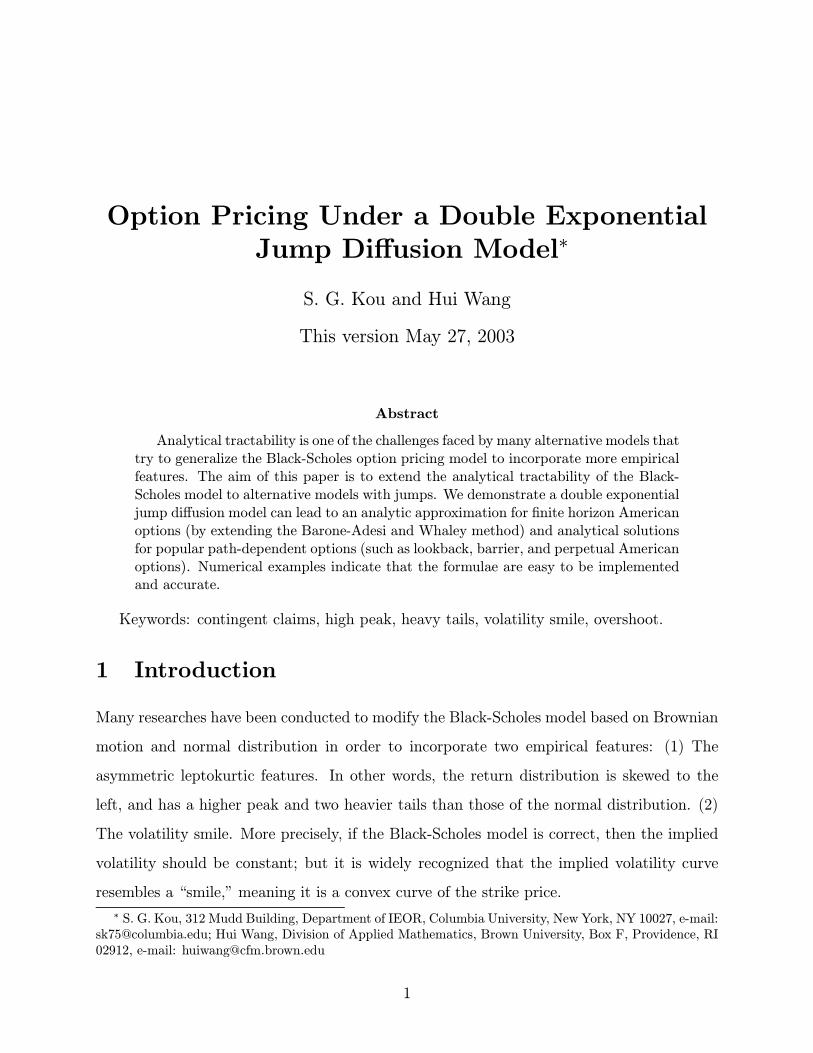
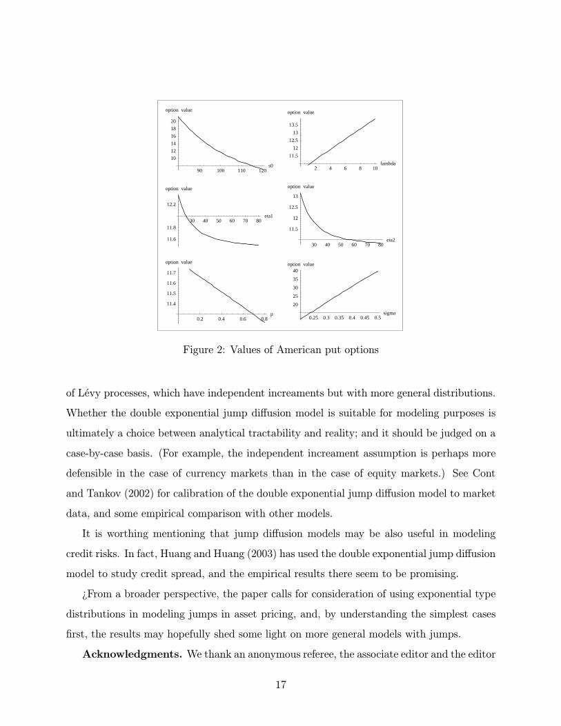
Figure 2 graphs of the value of a perpetual American put option versus its parameters,

S(0), η1, η2, p, λ. The defaulting parameters are r = 0.06, σ = 0.20, K = 100, S(0) = 100,

λ = 3, p = 0.3, 1/η1 = 0.02, and 1/η2 = 0.03. It only takes less than one second to generate

all the pictures in Figure 2 on a Pentium 700 PC. Not surprisingly, Figure 2 indicates that

the option value is a decreasing function of S(0), p, and is an increasing function of λ, 1/η2,

and σ, as it is a put option. What is interesting is that the option value is an increasing

function of 1/η1, which is the mean of the positive jumps. The reason is that the risk neutral

drift also depends on η1; a similar phenomenon was also pointed out in Merton (1976).

5 Concluding Remarks

Both the normal jump diffusion model and the double exponential jump diffusion model

are special cases of the affine jump diffusion models (Duffie, Pan, and Singleton 2000, and

Chacko and Das 2002), which include stochastic volatility and jumps in the volatility, and15A result similar to (12) is also independently obtained by Mordecki (2002). However, there are two

key differences. First, our proof not only covers the case of the perpetual American options, but alsosolves another inÞnite horizon free boundary problem (with a more complicated boundary condition) of (15)and (16), arising in approximating the Þnite horizon American options; see Appendix A.1. Secondly, theproof in Mordecki (2002) shows the results indirectly, as it Þrst derives some general representations forLevy processes, and then shows that the representations can be computed explicitly if the jump sizes areexponentially distributed. Here we prove and calculate the result directly by using martingale and PDEmethods, without appealing to more general results from Levy processes.16The smooth-Þt principle may not hold for general Levy processes; see Pham (1997), Boyarchenkov and

Levendorskiùi (2002a), where sufficient conditions for the smooth-Þt principle are given.

16

0.2 0.4 0.6 0.8p

11.4

11.5

11.6

11.7

option value

0.25 0.3 0.35 0.4 0.45 0.5sigma

20

25

30

35

40option value

30 40 50 60 70 80eta1

11.6

11.8

12.2

option value

30 40 50 60 70 80eta2

11.5

12

12.5

13

option value

90 100 110 120s0

10

12

14

16

18

20

option value

2 4 6 8 10lambda

11.5

12

12.5

13

13.5

option value

Figure 2: Values of American put options

of Levy processes, which have independent increaments but with more general distributions.

Whether the double exponential jump diffusion model is suitable for modeling purposes is

ultimately a choice between analytical tractability and reality; and it should be judged on a

case-by-case basis. (For example, the independent increament assumption is perhaps more

defensible in the case of currency markets than in the case of equity markets.) See Cont

and Tankov (2002) for calibration of the double exponential jump diffusion model to market

data, and some empirical comparison with other models.

It is worthing mentioning that jump diffusion models may be also useful in modeling

credit risks. In fact, Huang and Huang (2003) has used the double exponential jump diffusion

model to study credit spread, and the empirical results there seem to be promising.

¿From a broader perspective, the paper calls for consideration of using exponential type

distributions in modeling jumps in asset pricing, and, by understanding the simplest cases

Þrst, the results may hopefully shed some light on more general models with jumps.

Acknowledgments. We thank an anonymous referee, the associate editor and the editor

17

for many helpful comments. We are also grateful to many people who offered insights into

this work including seminar participants at various universities, and conference participants

at Risk Annual Boston Meeting 2000, UCLA Mathematical Finance Conference 2001, Taipei

International Quantitative Finance Conference 2001, Fifth SIAM Conference on Control and

Its Applications 2001, American Finance Association Annual Meeting 2001, and the 11th

Derivatives Conference in New York City 2003. We would like to thank Giovanni Petrella

for his assistance in computing the numerical values of American options. All errors are ours

alone.

A Appendix: Derivation of the Approximation (7)

A.1 Outline of the Main Steps in the Derivation

Let t be the remaining time to maturity. Suppose the optimal exercise boundary is v0(t); in

other words, it is optimal to exercise the option whenever the stock price falls below v0(t).

Letting x0(t) = log(v0(t)), x = log(v), and using the generator L in (5), the value functionV (x, t) = ψ(ex, t) and the optimal exercise boundary v0(t) must satisfy the free boundary

problem: −Vt − rV + LV = 0, for x > x0(t); and V (x, t) = K − ex, for x ≤ x0(t). DeÞnethe early exercise premium as ε(x, t) := V (x, t) − EuP(ex, t). Since the European put pricesatisÞes the equation −EuPt− rEuP+LEuP = 0, for all x, it follows that the early exercisepremium satisÞes the equation

−εt − rε+ Lε = 0, ∀ x > x0(t); ε(x, t) = K − ex − EuP(ex, t), ∀ x ≤ x0(t). (13)

Introduce the change of variable z = 1− e−rt, g(x, z) = ε(x, t)/z. It is easy to see thatzt = re

−rt, εx = zgx, εxx = zgxx, εt = ztg + zgzzt. Plugging this back into (13), and dividing

z on both sides, we have

−r(1− z)gz −³rz+ λ

´g +

1

2σ2gxx + (r − 1

2σ2 − λξ)gx + λ

Z ∞

−∞g(x+ y, z) fY (y) dy = 0

for all x > x0(t) and g(x, z) =1z(K − ex − EuP(ex, t)), ∀ x ≤ x0(t). Following Barone-Adesi

18

and Whaley (1987), the approximation will set

(1− z)gz ≈ 0. (14)

This is a reasonable assumption especially for very big or very small t. Indeed, as t → 0,

1 − z → 0, while as t → ∞, gz → 0, because g(x, z) converges to the price of a perpetual

American put option. This also explains why in the numerical tables the error tends to be

larger when t = 1.

With the approximation (14), the function g satisÞes the following equations:

−(rz+ λ)g +

1

2σ2gxx + (r − 1

2σ2 − λζ)gx + λ

Z ∞

−∞g(x+ y, z) fY (y) dy = 0, ∀ x > x0(t)

(15)

and

g(x, z) =1

z(K − ex − EuP(ex, t)), ∀ x ≤ x0(t). (16)

If we regard t, and hence z and x0(t), to be Þxed, the above equation becomes an ordinary

integral-differential equation with free-boundary x0(t). Note that the boundary condition in

(16) involves the European put option price EuP(ex, t), which makes solving the free boundary

problem more difficult than that for perpetual American options. Under the assumption of

exponential jump size distribution, however, the above free boundary problem can be solved

explicitly as in Appendix A.2, resulting in the approximation in (7).

A.2 Solving the Free Boundary Problem (15) and (16)

Lemma A.1. DeÞne

�V (x) =

½K − ex − h(x) , if x < x0Ae−xβ3 +Be−xβ4 , if x ≥ x0 ;

here β3, β4 > 0, x0 ∈ (−∞,∞) are arbitrary constants, and h(x) arbitrary continuous func-tion. Then for any constant b, we have for all x > x0,

(−b�V + L �V )(x) = Ae−xβ3 �f(β3) +Be−xβ4 �f(β4)+ λqη2e

(x0−x)η2∙K

η2− ex0

1 + η2− Ae

−x0β3

η2 − β3 −Be−x0β4

η2 − β4 −Z 0

−∞h(x0 + y)e

yη2dy

¸,

19

where �f(x) := G(−x)− b.Proof. First, we want to compute

R∞−∞

�V (x+ y) dF (y), which is essential to compute the

generator (L �V )(x). For x > x0, we haveZ ∞

−∞�V (x+ y) dF (y)

=

Z x0−x

−∞(K − ey+x − h(x+ y))qη2eyη2 dy +

Z 0

x0−x(Ae−β3(y+x) +Be−β4(y+x))qη2eyη2 dy

+

Z ∞

0

(Ae−β3(y+x) +Be−β4(y+x))pη1e−yη1 dy

= qe(x0−x)η2∙K − η2e

x0

1 + η2

¸+

qη2A

η2 − β3£e−β3x − e−β3x0 · e(x0−x)η2¤− Z x0−x

−∞h(x+ y)qη2e

yη2dy

+qη2B

η2 − β4£e−β4x − e−β4x0 · e(x0−x)η2¤+ ∙Apη1e−β3x

η1 + β3+B

pη1e−β4x

η1 + β4

¸.

Next, for x > x0, we have

(−b �V + L �V )(x)=

1

2σ2(Aβ23e

−xβ3 +Bβ24e−xβ4) + (r − 1

2σ2 − λζ)(−Aβ3e−xβ3 −Bβ4e−xβ4)

−b(Ae−xβ3 +Be−xβ4)− λ(Ae−xβ3 +Be−xβ4) + λ½qe(x0−x)η2

∙K − η2e

x0

1 + η2

¸+qη2A

η2 − β3£e−β3x − e−β3x0 · e(x0−x)η2¤− qη2e(x0−x)η2 Z 0

−∞h(x0 + y)e

yη2dy

+qη2B

η2 − β4£e−β4x − e−β4x0 · e(x0−x)η2¤+ ∙Apη1e−β3x

η1 + β3+B

pη1e−β4x

η1 + β4

¸¾= Ae−xβ3 �f(β3) +Be−xβ4 �f(β4)

+λqe(x0−x)η2∙K − η2e

x0

1 + η2− η2Ae

−x0β3

η2 − β3 − η2Be−x0β4

η2 − β4 − η2Z 0

−∞h(x0 + y)e

yη2dy

¸,

from which the proof is terminated. 2

Lemma A.2. For every x0, we have

∂

∂xEuP(ex, t)

¯x=x0

= EuP(ex0 , t)−Ke−rtP∗(S(t) ≤ K|S(0) = ex0),Z 0

−∞EuP(ex0+y, t)eη2y dy =

1

η2 + 1EuP(ex0 , t) +

Ke−rt

η2(η2 + 1)P∗(S(t) ≤ K|S(0) = ex0)

+Ke−rt

η2(η2 + 1)· E∗ £(S(t)/K)−η21{S(t)>K}|S(0) = ex0¤ .

20

Proof. We have

EuP(ex, t) = E∗£e−rt(K − exeX(t))+¤ = E∗ Z K−exeX(t)

−∞e−rt1{y≥0} dy

= E∗Z ∞

exe−rteX(t)1{K−zeX(t)≥0} dz =

Z ∞

exE∗£e−rteX(t)1{K−zeX(t)≥0}

¤dz.

Hence

∂

∂xEuP(ex, t)

¯x=x0

= −ex0 · E∗ ©e−rteX(t)1{K−ex0eX(t)≥0}ª ,from which the Þrst equation follows readily. As for the second equation, we haveZ 0

−∞EuP(ex0+y, t)eη2y dy = E∗

Z 0

−∞e−rt(K − ex0+yeX(t))+ · eη2y dy

= e−rtE∗Z 0

−∞1{K−ex0eX(t)≥0}e

η2y(K − ex0+yeX(t)) dy

+e−rtE∗Z log

³K

eX(t)

´−x0

−∞1{K−ex0eX(t)<0}e

η2y(K − ex0+yeX(t)) dy

= e−rtE∗∙µK

η2− S(t)

η2 + 1

¶1{K−S(t)≥0}

¸+

Kη2+1

η2(η2 + 1)· e−rtE∗ £(S(t))−η21{K−S(t)<0}¤ ,

from which the conclusion follows. 2

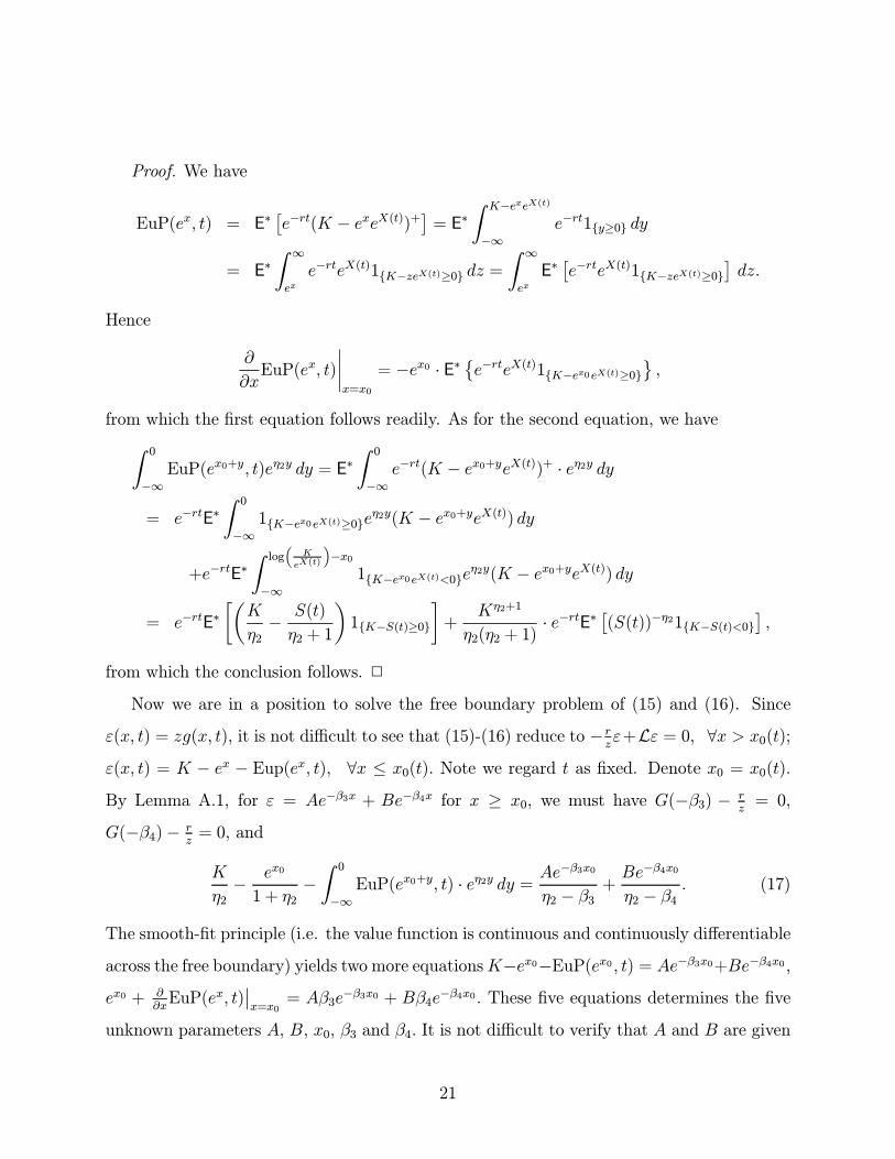
Now we are in a position to solve the free boundary problem of (15) and (16). Since

ε(x, t) = zg(x, t), it is not difficult to see that (15)-(16) reduce to − rzε+Lε = 0, ∀x > x0(t);

ε(x, t) = K − ex − Eup(ex, t), ∀x ≤ x0(t). Note we regard t as Þxed. Denote x0 = x0(t).

By Lemma A.1, for ε = Ae−β3x + Be−β4x for x ≥ x0, we must have G(−β3) − rz= 0,

G(−β4)− rz= 0, and

K

η2− ex0

1 + η2−Z 0

−∞EuP(ex0+y, t) · eη2y dy = Ae−β3x0

η2 − β3 +Be−β4x0

η2 − β4 . (17)

The smooth-Þt principle (i.e. the value function is continuous and continuously differentiable

across the free boundary) yields two more equationsK−ex0−EuP(ex0 , t) = Ae−β3x0+Be−β4x0 ,ex0 + ∂

∂xEuP(ex, t)

¯x=x0

= Aβ3e−β3x0 + Bβ4e−β4x0. These Þve equations determines the Þve

unknown parameters A, B, x0, β3 and β4. It is not difficult to verify that A and B are given

21

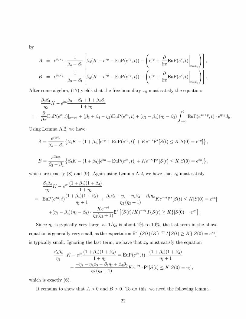
by

A = eβ3x0 · 1

β4 − β3

"β4(K − ex0 − EuP(ex0, t))−

Ãex0 +

∂

∂xEuP(ex, t)

¯x=x0

!#,

B = eβ4x0 · 1

β3 − β4

"β3(K − ex0 − EuP(ex0, t))−

Ãex0 +

∂

∂xEuP(ex, t)

¯x=x0

!#.

After some algebra, (17) yields that the free boundary x0 must satisfy the equation:

β3β4η2K − ex0 β3 + β4 + 1 + β4β3

1 + η2

=∂

∂xEuP(ex, t)|x=x0 + (β3 + β4 − η2)EuP(ex0 , t) + (η2 − β4)(η2 − β3)

Z 0

−∞EuP(ex0+y, t) · eη2ydy.

Using Lemma A.2, we have

A =eβ3x0

β4 − β3©β4K − (1 + β4)[ex0 + EuP(ex0, t)] +Ke−rtP∗[S(t) ≤ K|S(0) = ex0 ]

ª,

B =eβ4x0

β3 − β4©β3K − (1 + β3)[ex0 + EuP(ex0, t)] +Ke−rtP∗[S(t) ≤ K|S(0) = ex0 ]

ª,

which are exactly (8) and (9). Again using Lemma A.2, we have that x0 must satisfy

β3β4η2K − ex0 (1 + β3)(1 + β4)

1 + η2

= EuP(ex0 , t)(1 + β4)(1 + β3)

η2 + 1+β4β3 − η2 − η2β3 − β4η2

η2 (η2 + 1)Ke−rtP∗[S(t) ≤ K|S(0) = ex0 ]

+(η2 − β4)(η2 − β3) · Ke−rt

η2(η2 + 1)E∗£(S(t)/K)−η2 I{S(t) ≥ K}|S(0) = ex0¤ .

Since η2 is typically very large, as 1/η2 is about 2% to 10%, the last term in the above

equation is generally very small, as the expectation E∗£(S(t)/K)−η2 I{S(t) ≥ K}|S(0) = ex0¤

is typically small. Ignoring the last term, we have that x0 must satisfy the equation

β3β4η2

K − ex0 (1 + β3)(1 + β4)1 + η2

= EuP(ex0, t) · (1 + β4)(1 + β3)η2 + 1

+−η2 − η2β3 − β4η2 + β4β3

η2 (η2 + 1)Ke−rt · P∗[S(t) ≤ K|S(0) = v0],

which is exactly (6).

It remains to show that A > 0 and B > 0. To do this, we need the following lemma.

22

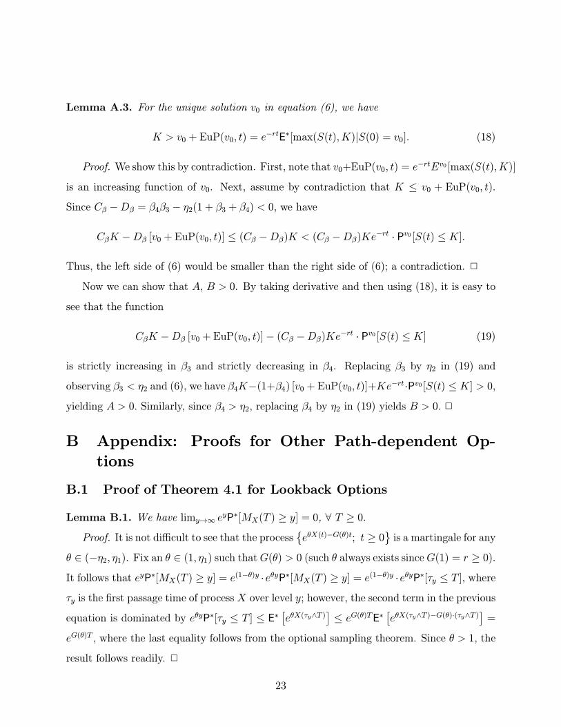
Lemma A.3. For the unique solution v0 in equation (6), we have

K > v0 + EuP(v0, t) = e−rtE∗[max(S(t), K)|S(0) = v0]. (18)

Proof. We show this by contradiction. First, note that v0+EuP(v0, t) = e−rtEv0 [max(S(t), K)]

is an increasing function of v0. Next, assume by contradiction that K ≤ v0 + EuP(v0, t).

Since Cβ −Dβ = β4β3 − η2(1 + β3 + β4) < 0, we have

CβK −Dβ [v0 + EuP(v0, t)] ≤ (Cβ −Dβ)K < (Cβ −Dβ)Ke−rt · Pv0 [S(t) ≤ K].

Thus, the left side of (6) would be smaller than the right side of (6); a contradiction. 2

Now we can show that A, B > 0. By taking derivative and then using (18), it is easy to

see that the function

CβK −Dβ [v0 + EuP(v0, t)]− (Cβ −Dβ)Ke−rt · Pv0 [S(t) ≤ K] (19)

is strictly increasing in β3 and strictly decreasing in β4. Replacing β3 by η2 in (19) and

observing β3 < η2 and (6), we have β4K−(1+β4) [v0 + EuP(v0, t)]+Ke−rt·Pv0 [S(t) ≤ K] > 0,yielding A > 0. Similarly, since β4 > η2, replacing β4 by η2 in (19) yields B > 0. 2

B Appendix: Proofs for Other Path-dependent Op-

tions

B.1 Proof of Theorem 4.1 for Lookback Options

Lemma B.1. We have limy→∞ eyP∗[MX(T ) ≥ y] = 0, ∀ T ≥ 0.Proof. It is not difficult to see that the process

©eθX(t)−G(θ)t; t ≥ 0ª is a martingale for any

θ ∈ (−η2, η1). Fix an θ ∈ (1, η1) such thatG(θ) > 0 (such θ always exists sinceG(1) = r ≥ 0).It follows that eyP∗[MX(T ) ≥ y] = e(1−θ)y ·eθyP∗[MX(T ) ≥ y] = e(1−θ)y ·eθyP∗[τy ≤ T ], whereτy is the Þrst passage time of process X over level y; however, the second term in the previous

equation is dominated by eθyP∗[τy ≤ T ] ≤ E∗£eθX(τy∧T )

¤ ≤ eG(θ)TE∗ £eθX(τy∧T )−G(θ)·(τy∧T )¤ =eG(θ)T , where the last equality follows from the optional sampling theorem. Since θ > 1, the

result follows readily. 2

23

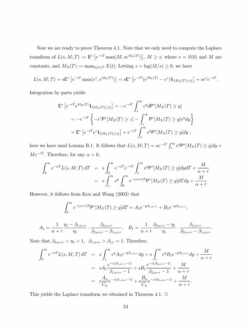
Now we are ready to prove Theorem 4.1. Note that we only need to compute the Laplace

transform of L(s,M ;T ) := E∗£e−rT max(M, seMX(T ))

¤, M ≥ s, where s = S(0) and M are

constants, and MX(T ) := max0≤t≤T X(t). Letting z = log(M/s) ≥ 0, we have

L(s,M ;T ) = sE∗£e−rT max(ez, eMX(T ))

¤= sE∗

£e−rT (eMX(T ) − ez)1{MX(T )≥z}

¤+ seze−rT .

Integration by parts yields

E∗£e−rT eMX(T )1{MX(T )≥z}

¤= −e−rT

Z ∞

z

eydP∗[MX(T ) ≥ y]

= −e−rT½−ezP∗[MX(T ) ≥ z]−

Z ∞

z

P∗[MX(T ) ≥ y]eydy¾

= E∗£e−rT ez1{MX(T )≥z}

¤+ e−rT

Z ∞

z

eyP∗[MX(T ) ≥ y]dy ;

here we have used Lemma B.1. It follows that L(s,M ;T ) = se−rTR∞zeyP∗[MX(T ) ≥ y]dy+

Me−rT . Therefore, for any α > 0,Z ∞

0

e−αTL(s,M ;T ) dT = s

Z ∞

0

e−αT e−rTZ ∞

z

eyP∗[MX(T ) ≥ y]dydT + M

α+ r

= s

Z ∞

z

eyZ ∞

0

e−(α+r)TP∗[MX(T ) ≥ y]dTdy + M

α+ r

However, it follows from Kou and Wang (2003) thatZ ∞

0

e−(α+r)TP∗[MX(T ) ≥ y]dT = A1e−yβ1,α+r +B1e−yβ2,α+r ,

A1 =1

α+ r

η1 − β1,α+rη1

· β2,α+rβ2,α+r − β1,α+r , B1 =

1

α+ r

β2,α+r − η1η1

· β1,α+rβ2,α+r − β1,α+r .

Note that β2,α+r > η1 > 1, β1,α+r > β1,r = 1. Therefore,Z ∞

0

e−αTL(s,M ;T ) dT = s

Z ∞

z

eyA1e−yβ1,α+rdy + s

Z ∞

z

eyB1e−yβ2,α+rdy +

M

α+ r

= sA1e−z(β1,α+r−1)

β1,α+r − 1 + sB1e−z(β2,α+r−1)

β2,α+r − 1 +M

α+ r

= sAαCαe−z(β1,α+r−1) + s

BαCαe−z(β2,α+r−1) +

M

α+ r.

This yields the Laplace transform we obtained in Theorem 4.1. 2

24

B.2 Proof of Theorem 4.2 for Barrier Options

We can write UIC as

UIC = E∗£e−rT (S(T )−K)+1{max0≤t≤T S(t)≥H}

¤= E∗

£e−rTS(T )1{S(T )≥K, max0≤t≤T S(t)≥H}

¤−Ke−rTP∗ ∙S(T ) ≥ K, max0≤t≤T

S(t) ≥ H¸

= I −Ke−rT · II (say).

It is easy to compute the second term, as

II = Ψ(r − 12σ2 − λζ ,σ,λ, p, η1, η2; log(K/S(0)), log(H/S(0)), T ).

For the Þrst term, we can use a change of numeraire argument. More precisely, introduce

a new probability �P deÞned as

d�P

dP∗

¯¯t=T

= e−rTS(T )

S(0)= e−rT eX(T ) = exp

(−12σ2 − λζ)T + σW (T ) +N(T )Xi=1

Yi

.Note that this is a well deÞned probability as E∗

ne−rt S(t)

S(0)

o= 1. We have, by the Girsanov

theorem for jump processes, �W (t) :=W (t)−σt is a new Brownian motion under �P, and theoriginal process

X(t) = (r − 12σ2 − λζ) t+ σW (t) +

N(t)Xi=1

Yi = (r +1

2σ2 − λζ) t+ σ �W (t) +

N(t)Xi=1

Yi

is a new double exponential jump diffusion process with the Poisson process N(t) having a

new rate �λ = λE∗(eY ) = λ(1 + ζ). and the jump sizes Y �s are i.i.d. with a new density given

by

1

E∗(eY )eyfY (y) =

1

E∗(eY )eypη1e

−η1y1{y≥0} +1

E∗(eY )eyqη2e

η2y1{y<0}

= p1

E∗(eY )· η1η1 − 1(η1 − 1)e

−(η1−1)y1{y≥0} + q1

E∗(eY )· η2η2 + 1

(η2 + 1)e(η2+1)y1{y<0}.

Thus, it is still a double exponential density with �η1 = η1 − 1, �η2 = η2 + 1,

�p = p

½pη1η1 − 1 +

qη2η2 + 1

¾−1η1

η1 − 1 , �q = q

½pη1η1 − 1 +

qη2η2 + 1

¾−1η2

η2 + 1.

25

In summary, we have

I = S(0)E∗∙e−rT

S(T )

S(0)· 1{S(T )≥K, max0≤t≤T S(t)≥H}

¸= S(0)�P[S(T ) ≥ K, min

0≤t≤TS(t) ≤ H]

= S(0)Ψ(r +1

2σ2 − λζ, σ, �λ, �p, �η1, �η2; log(K/S(0)), log(H/S(0)), T ),

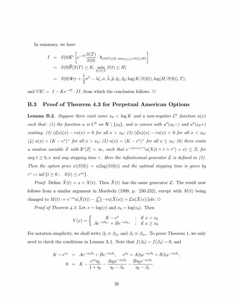
and UIC = I −Ke−rT · II, from which the conclusion follows. 2

B.3 Proof of Theorem 4.3 for Perpetual American Options

Lemma B.2. Suppose there exist some x0 < logK and a non-negative C1 function u(x)such that: (1) the function u is C2 on R \ {x0}, and is convex with u00(x0−) and u00(x0+)existing; (2) (Lu)(x) − ru(x) = 0 for all x > x0; (3) (Lu)(x) − ru(x) < 0 for all x < x0;

(4) u(x) > (K − ex)+ for all x > x0; (5) u(x) = (K − ex)+ for all x ≤ x0; (6) there existsa random variable Z with E∗[Z] < ∞, such that e−r(t∧τ∧τ∗)u(X(t ∧ τ ∧ τ ∗) + x) ≤ Z, for

any t ≥ 0, x and any stopping time τ . Here the inÞnitesimal generator L is deÞned in (5).Then the option price ψ(S(0)) = u(log(S(0))) and the optimal stopping time is given by

τ∗ := inf {t ≥ 0 : S(t) ≤ ex0} .Proof: DeÞne �X(t) = x +X(t). Then �X(t) has the same generator L. The result now

follows from a similar argument in Mordecki (1999, p. 230-232), except with M(t) being

changed to M(t) := e−rtu( �X(t))− R t0{−ru( �X(s)) + Lu( �X(s))}ds. 2

Proof of Theorem 4.3. Let x = log(v) and x0 = log(v0). Then

V (x) =

½K − ex ; if x < x0

Ae−xβ3,r +Be−xβ4,r ; if x ≥ x0For notation simplicity, we shall write β3 ≡ β3,r and β4 ≡ β4,r. To prove Theorem 1, we onlyneed to check the conditions in Lemma A.1. Note that f(β3) = f(β4) = 0, and

K − ex0 = Ae−x0β3 +Be−x0β4 , ex0 = Aβ3e−x0β3 +Bβ4e−x0β4 ,

0 = K − ex0η21 + η2

− Aη2e−x0β3

η2 − β3 − Bη2e−x0β4

η2 − β4 .

26

Therefore, Condition 2 follows from Lemma A.1 with h = 0. Conditions 1, 4, 5, and 6 are

trivial by noting that V (x0+) = V (x0−) and 0 ≤ V (x) ≤ K.As to Condition 3, note that for x < x0, we haveZ ∞

−∞V (x+ y)a dF (y) =

Z 0

−∞(K − ey+x)qη2eyη2 dy +

Z x0−x

0

(K − ey+x)pη1e−yη1 dy

+

Z ∞

x0−x(Ae−β3(y+x) +Be−β4(y+x))pη1e−yη1 dy

= K − ex∙qη2η2 + 1

+pη1η1 − 1

¸− pe−η1(x0−x)

∙K − η1e

x0

η1 − 1 −Aη1e

−x0β3

η1 + β3−B η1e

−x0β4

η1 + β4

¸.

Therefore, for x < x0,

(−rV + LV )(x) = −12σ2ex + (r − 1

2σ2 − λζ)(−ex)− r(K − ex)− λ(K − ex)

+ λ

½K − ex

∙qη2η2 + 1

+pη1η1 − 1

¸− pe−η1(x0−x)

∙K − η1e

x0

η1 − 1 − Aη1e

−β3x0

η1 + β3−B η1e

−β4x0

η1 + β4

¸¾.

Rearranging terms and using (3) we have for x < x0,

(−rV + LV )(x) = −rK − λe−η1(x0−x)p∙K − η1e

x0

η1 − 1 −Aη1e

−β3x0

η1 + β3−B η1e

−β4x0

η1 + β4

¸.

The right hand side can be further simpliÞed as

K − η1ex0

η1 − 1 −η1Ae

−β3x0

η1 + β3− η1Be

−β4x0

η1 + β4

= K − η1v0η1 − 1 −

η1η1 + β3

1 + β4β4 − β3

∙β4

1 + β4K − v0

¸− η1η1 + β4

1 + β3β4 − β3

∙v0 − β3

1 + β3K

¸= K

β3β4(η1 + β3)(η1 + β4)

− v0η1 (1 + β3)(1 + β4)

(η1 − 1)(η1 + β3)(η1 + β4)= −K β3β4

(η1 + β3)(η1 + β4)

η2 + η1η2(η1 − 1) .

In summary we have for x < x0,

(−rV + LV )(x) = −rK + pλe−η1(x0−x)K β3β4(η2 + η1)

(η1 + β3)(η1 + β4)η2(η1 − 1) ,

from which it is easy to see that (−rV + LV )(x) is an increasing function, thanks to theassumption η1 > 1. Thus, to show Condition 3 it suffices to show that (−rV +LV )(x0−) ≤ 0.

27

However, since V (x) is bounded and continuous, it follows from the Dominated Convergence

Theorem that

(LV )(x0−)−(LV )(x0+) = 1

2(V 00(x0−)− V 00(x0+)) = −1

2

¡ex0 + β23Ae

−β3x0 + β24Be−β2x0¢ ≤ 0.

But (−rV + LV )(x0+) = 0, which completes the proof. 2

References

[1] Amin, K. (1993). Jump diffusion option valuation in discrete time. J. Finance 48 1833-

1863.

[2] Asmussen, S., P. Glynn, and J. Pitman. 1995. Discretization error in simulation of

one-dimensional Brownian motion. Ann. Appl. Probab. 5 875-896.

[3] Avram, F., T. Chan, and M. Usabel. 2001. Pricing American options under spectrally

negative exponential Levy models. Working paper, Heriot-Watt University, Edinburgh.

[4] Barone-Adesi, G., R. E. Whaley. 1987. Efficient analytic approximations of American

option values. J. of Finance 42 301-320.

[5] Black, F. , J. Cox. 1976. Valuing corporate debt: some effects of bond indenture provi-

sions. J. Finance 31 351-367.

[6] Boyle, Ph., M. Broadie, P. Glasserman. 1997. Simulation methods for security pricing.

J. Econom. Dynam. Control 21 1267-1321.

[7] Boyarchenko, S., S. Levendorskiùi. 2002a. Perpetual American options under Levy

processes. SIAM J. Control and Optimization 40 1663-1696.

[8] Boyarchenko, S., S. Levendorskiùi. 2002b. Barrier options and touch-and-out options

under regular Levy processes of exponential type. Ann. of Appl. Probab. 12 1261-1298.

[9] Broadie, M., J. Detemple. 1996. American option valuation: new bounds and approxi-

mations. Rev. Financial Stud. 9 1211-1250.

28

[10] Broadie, M., P. Glasserman. 1997. Pricing American-style securities using simulation.

J. Econom. Dynam. Control 21 1323-1352.

[11] Carr, P. 1998. Randomization and the American put. Rev. Financial Stud. 11 597-626.

[12] Carriere, J. 1996. Valuation of early-exercise price of options using simulations and

nonparametric regressions. Insurance: Math. and Econom. 19 19-30.

[13] Chacko, G., S. R. Das. 2002. Pricing interest rate derivatives: a general approach. Rev.

of Financial Stud., 15 195-241.

[14] Conze, A., R. Viswanathan. 1991. Path dependent options: the case of lookback options.

J. Finance 46 1893-1907.

[15] Cont, R., P. Tankov. 2002. Calibration of jump-diffusion option pricing models: a robust

non-parametric approach. Working paper, Ecole Polytechnique, Paris.

[16] Das, S. R., S. Foresi. 1996. Exact solutions for bond and option prices with systematic

jump risk. Rev. of Derivatives Research 1 7-24.

[17] Davydov, D., V. Linetsky. 2001. The valuation and hedging of path-dependent options

under the CEV process. Management Sci. 47 949-965.

[18] Davydov, D., V. Linetsky. 2003. Pricing options on scalar diffusions: an eigenfunction

expansion approach. To appear in Operations Research.

[19] Duffie, D., J. Pan, K. Singleton. 2000. Transform analysis and option pricing for affine

jump-diffusions. Econometrica. 68 1343-1376.

[20] Gerber, H. U., E. Shiu. 1998. Pricing perpetual options for jump processes. North Amer-

ican Acturial Journal 2 101-112.

[21] Geske, R., E. Johnson. 1984. The American put option valued analytically. J. Finance

39 1511-1524.

29

[22] Goldman, M.B., H. B. Sosin, M. A. Gatto. 1979. Path-Dependent Options: Buy at the

Low, Sell at the High. J. Finance 34 1111-1127.

[23] d�Halluin, J., P. Forsyth, K. Vetzal. 2003. Rubust numerical methods for contingent

claims under jump diffusion processes. Working paper, Univ. of Waterloo.

[24] Haugh, M., L. Kogan. 2002. Pricing American Options: A Duality Approach. To appear

in Operations Research.

[25] Huang, J., M. Huang. 2003. How much of the corporate-treasury yield spread is due to

credit risk? Working paper, New York University and Stanford University.

[26] Hull, J. 2000. Options, Futures, and Other Derivative Securities. 4th edition, Prentice

Hall, New Jersey.

[27] Ju, N. 1998. Pricing by American option by approximating its early exercise boundary

as a multipiece exponential function. Rev. Financial Stud. 11 627-646.

[28] Kou, S. G. 2002. A jump diffusion model for option pricing. Management Sci. 48 1086-

1101.

[29] Kou, S. G., H. Wang. 2003. First passage times for a jump diffusion process. Adv.

Applied Probab. 35 504-531.

[30] Kyprianou, A., M. Pistorius. 2003. Perpetual options and canadization through ßuctu-

ation theory. To appear in Ann. Applied Prob.

[31] Leland, H. E. 1994. Corporate Debt Value, Bond Covenants, and Optimal Capital

Structure. J. Finance 49 1213-1252.

[32] Longstaff, F. A. 1995. How Much Can Marketability Affect Security Values? J. Finance

50 1767-1774.

[33] Longstaff, F. A., E. S. Schwartz. 1995. A Simple Approach to Valuing Risky Fixed and

Floating Rate Debt. J. Finance 50 789-819.

30

[34] Longstaff, F. A., E. S. Schwartz. 2001. Valuing American options by simulation: a

simple least-squares approach. Rev. Financial Stud. 14 113-147.

[35] Lucas, R. E. 1978. Asset prices in an exchange economy. Econometrica 46 1429-1445.

[36] McDonald, R., D. Siegel. 1986. The value of waiting to invest. Quarterly J. of Economics

101 707-727.

[37] McKean, H. P. 1965. A free boundary problem for the heat equation arising from a

problem in mathematical economics. Industrial Management Review 6 33-39.

[38] McMillan, L. 1986. Analytic approximation for the American put option. Advances in

Futures and Options Research. 1 119-140.

[39] Merton, R. C. 1973. The theory of rational option pricing. Bell J. of Econom. and

Management Sci. 4 141-183.

[40] Merton, R. C. 1974. On the pricing of corporate debt: the risk structure of interest

rates. J. Finance 29 449�469.

[41] Merton, R. C. 1976. Option pricing when underlying stock returns are discontinuous.

J. Financial Econom. 3 125-144.

[42] Mordecki, E. 1999. Optimal stopping for a diffusion with jumps. Finance and Stochastics

3 227-236.

[43] Mordecki, E. 2002. Optimal stopping and perpetual options for Levy processes. Finance

and Stochastics 6 273-293.

[44] Naik, V., M. Lee. 1990. General equilibrium pricing of options on the market portfolio

with discontinuous returns. Rev. Financial Stud. 3 493-521.

[45] Petrella, G., S. G. Kou, H. Wang. 2003. Some Laplace transforms in option pricing.

Working paper, Columbia University and Brown University.

31

[46] Pham, H. 1997. Optimal stopping, free boundary and American option in a jump-

diffusion model. Appl. Math. and Optimization 35 145-164.

[47] Rogers, L. C. G. 2000. Evaluating Þrst-passage probabilites for spectrally one-sided Levy

processes. J. Appl. Probab. 37 1173-1180.

[48] Rogers, L. C. G. 2002. Monte Carlo valuation of American options. Math. Finance 12

271-286.

[49] Schroder, M. 1999. Change of numeraire for pricing futures, forwards, and options. Rev.

Financial Stud. 12 1143-1163.

[50] Siegmund, D. 1985. Sequential Analysis. Springer, New York.

[51] Sullivan, M. A. 2000. Valuing American put options using Gaussian quadrature. Rev.

Financial Stud. 13 75-94.

[52] Tilley, J. A. 1993. Valuing American options in a path simulation model. Transactions

of the Society of Acturaries 45 83-104.

[53] Tsitsiklis, J., B. van Roy. 1999. Optimal stopping of Markov processes: Hilbert space

theory, approximation of algorithms, and an application to pricing high-dimensional

Þnancial derivatives. IEEE Transactions on Automatic Control 44 1840-1851.

[54] Zhang, X. L. 1997. Numerical analysis of American option pricing in a jump diffusion

model. Math. of Operations Research 22 668-690.

32