Equilibrium Assumptions and Efficiency Agreements: Macroeconomic Effects of Climate

Policies for UK Road Transport, 2000-2010

Jonathan Rubin, University of Maine

Terry Barker, University of Cambridge

Comparing North American and European Approaches to Climate Change

Viessmann European Research Centre, Wilfrid Laurier University, Canada

September 28, 2007

Outline• Results • Intro: macroeconomic models of energy

efficiency improvements – CGE v. Sectoral models– Integration of top-down, bottom-up

modelling

• Modelling the macroeconomic rebound effect using MDM-E3

• Application to transport sector• Findings and conclusions

Results

• Voluntary efficiency agreement– Positive macroeconomic impacts

• GDP, employment, inflation

– Reductions in energy demand & CO2

• Equivalent fuel taxes (in terms of CO2)– Without revenue recycling

• Lower GDP & employment– With revenue recycling that reduces income taxes

• Eliminates negative macroeconomic impacts• Equity/distributional issues remain

• Inflation neutral scenario, VA & fuel duties

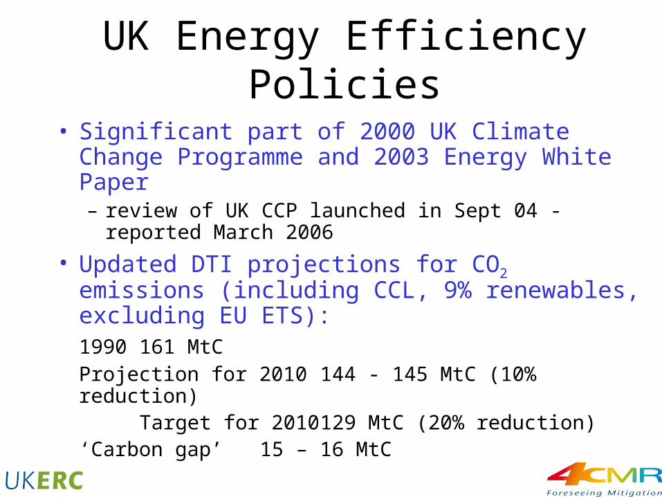
UK Energy Efficiency Policies

• Significant part of 2000 UK Climate Change Programme and 2003 Energy White Paper– review of UK CCP launched in Sept 04 - reported

March 2006

• Updated DTI projections for CO2 emissions (including CCL, 9% renewables, excluding EU ETS):1990 161 MtCProjection for 2010 144 - 145 MtC (10% reduction)

Target for 2010 129 MtC (20% reduction)‘Carbon gap’ 15 – 16 MtC

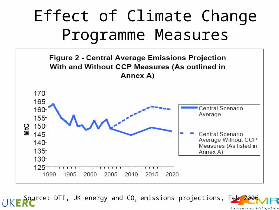
Effect of Climate Change Programme Measures

Source: DTI, UK energy and CO2 emissions projections, Feb 2006

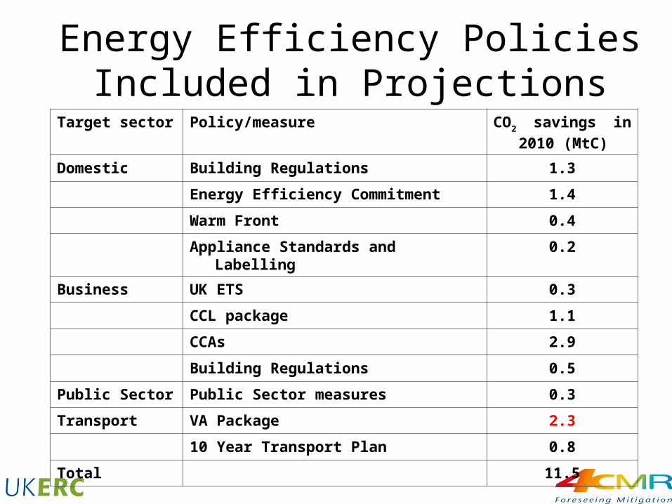
Energy Efficiency Policies Included in Projections

Target sector Policy/measure CO2 savings in 2010

(MtC)

Domestic Building Regulations 1.3

Energy Efficiency Commitment 1.4

Warm Front 0.4

Appliance Standards and Labelling 0.2

Business UK ETS 0.3

CCL package 1.1

CCAs 2.9

Building Regulations 0.5

Public Sector Public Sector measures 0.3

Transport VA Package 2.3

10 Year Transport Plan 0.8

Total 11.5

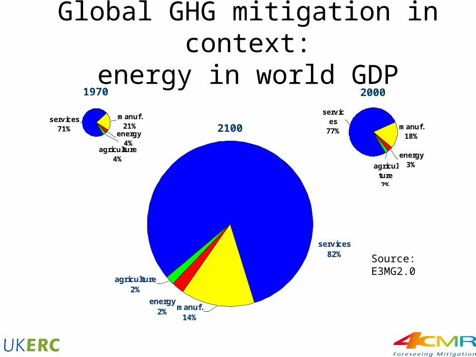
energy2%

agriculture2%

services82%

manuf.14%

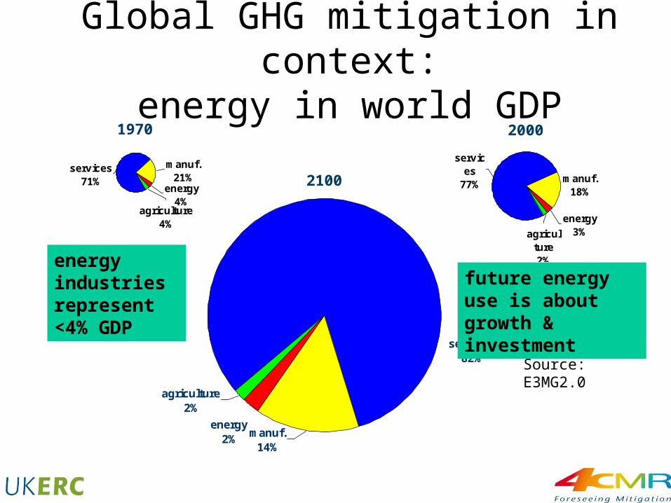
Global GHG mitigation in context:energy in world GDP

energy4%

manuf.21%

services71%

agriculture4% energy

3%

manuf.18%

services

77%

agriculture2%

1970 2000

2100

Source: E3MG2.0

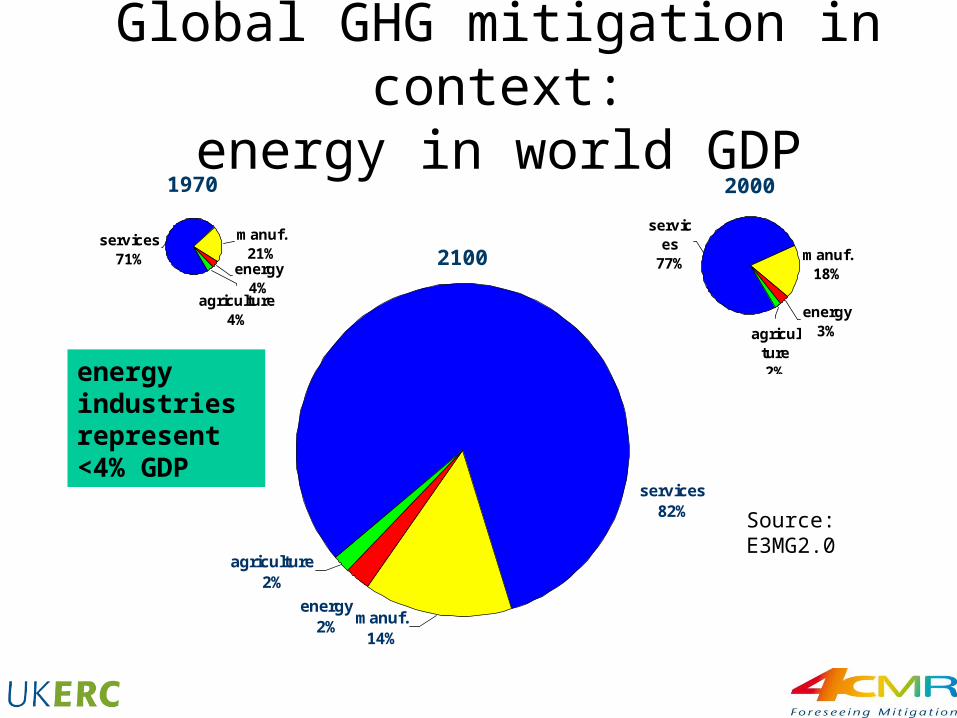
energy2%

agriculture2%

services82%

manuf.14%

Global GHG mitigation in context:energy in world GDP

energy4%

manuf.21%

services71%

agriculture4% energy

3%

manuf.18%

services

77%

agriculture2%

1970 2000

2100

Source: E3MG2.0

energy industries represent <4% GDP

energy2%

agriculture2%

services82%

manuf.14%

Global GHG mitigation in context:energy in world GDP

energy4%

manuf.21%

services71%

agriculture4% energy

3%

manuf.18%

services

77%

agriculture2%

1970 2000

2100

Source: E3MG2.0

energy industries represent <4% GDP

future energy use is about growth & investment

Macroeconomic Modeling of Energy

• CGE models– treatment of energy as factor of production in

a production function with labor and capital

• Econometric models– traditional approach with energy demand

equations– Literature on income and price elasticities

Macroeconomic Costs of Mitigation

• Costs not directly observable from market prices– outcome of complex energy-environment-economy (E3) system– involve changes in environment that have no market valuations– hypothetical: comparison of 2 states of the E3 system over future

years

• Macroeconomic costs usually measured in terms of future loss of GDP, comparing one hypothetical state of the world with another

• Debate: are such costs to be offset by ancillary benefits and benefits from use of tax or emission permit revenues? – taxes/auctioned permits may incur high “political” costs– free allocation of emission permits (as in phase I EU emissions

trading scheme (ETS)) yields no revenues to recycle

Treatment of Technological Change in Cost Modelling

• Usual assumption in IPCC literature is of autonomous growth in energy efficiency, constant across all economies: therefore no effect on efficiency from stabilisation policies

• However there is good evidence that – higher real prices of energy increase efficiencies (e.g. Popp, 2002; Jaffe,

Newell and Stavins, 2003)– costs of renewable power fall as markets develop (e.g. McDonald and

Schrattenholzer, 2001)

• New research: – modelling of endogenous technological change (bottom-up and top-

down) and implications for policy action– low-carbon paths as low-cost, even beneficial, global options

Induced Technological Change in Global Climate Models

• Method: introduce R&D and/or learning-by-doing into costs of energy technologies, so that higher real carbon prices induce change

• CGE models face special problems– whole-economy increasing returns are incompatible with a

general solution– increased substitution possibilities (e.g. to renewable power or

carbon-capture) are typically introduced in the only one sector (energy)

– economic growth remains largely given by assumption, with general technological change unaffected by the energy sector technologies

• An open question: can increased technological change lead to higher economic growth?

Question: Full Employment of Labor and “Efficient” Economy?

• Economy-wide studies that assume full efficiency report that the regulatory policies incur costs– Parry and Williams (1999) - CGE compare 8 policy instruments

to reduce CO2• Find: High costs of the energy efficiency regulations,

exacerbated by tax interaction effects– Smulders and Nooij (2003) - CGE analyse energy conservation

on technology and economic growth• Find: Policies that reduce the level of energy use

unambiguously depress output levels – Pizer et al. (2006) - CGE calibrated to sectoral models of the US

• Find: CAFE standards to be significantly more expensive than broad carbon taxes.

Alternative Approach

• A main alternative approach: detailed sectoral studies that feed into a CGE macroeconomic model– Roland-Holst (2006) uses a CGE model for

California to assess energy efficiency policies for CO2 reductions

• Find: CO2-efficiency policies can reduce transportation CO2 emissions by nearly 6% and increase Gross State Output by over 2%

The Approach of MDM-E3 (Multisectoral Dynamic Model – w/ Energy-

Environment-Economy system)

• MDM is a multisectoral regional econometric model of the UK economy developed in the 1990s

• Equilibrium & constant returns to scale are not assumed • The solutions are dynamic, integrated and consistent

across the model and submodels• Energy demand is derived from demand for heat & power

from demand for final products– No explicit production function– 2-level hierarchy: aggregate energy demand equations and fuel

share equations – Aggregate demand affected by industrial output of user

industry, household spending in total, relative prices, temperature, technical progress indicator, trends, efficiency policies

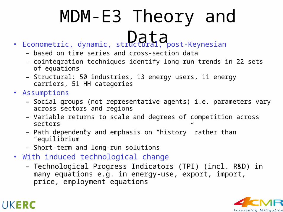
MDM-E3 Theory and Data• Econometric, dynamic, structural, post-Keynesian

– based on time series and cross-section data– cointegration techniques identify long-run trends in 22 sets of equations– Structural: 50 industries, 13 energy users, 11 energy carriers, 51 HH

categories

• Assumptions– Social groups (not representative agents) i.e. parameters vary across

sectors and regions– Variable returns to scale and degrees of competition across sectors– Path dependency and emphasis on “history” rather than “equilibrium” – Short-term and long-run solutions

• With induced technological change – Technological Progress Indicators (TPI) (incl. R&D) in many

equations e.g. in energy-use, export, import, price, employment equations

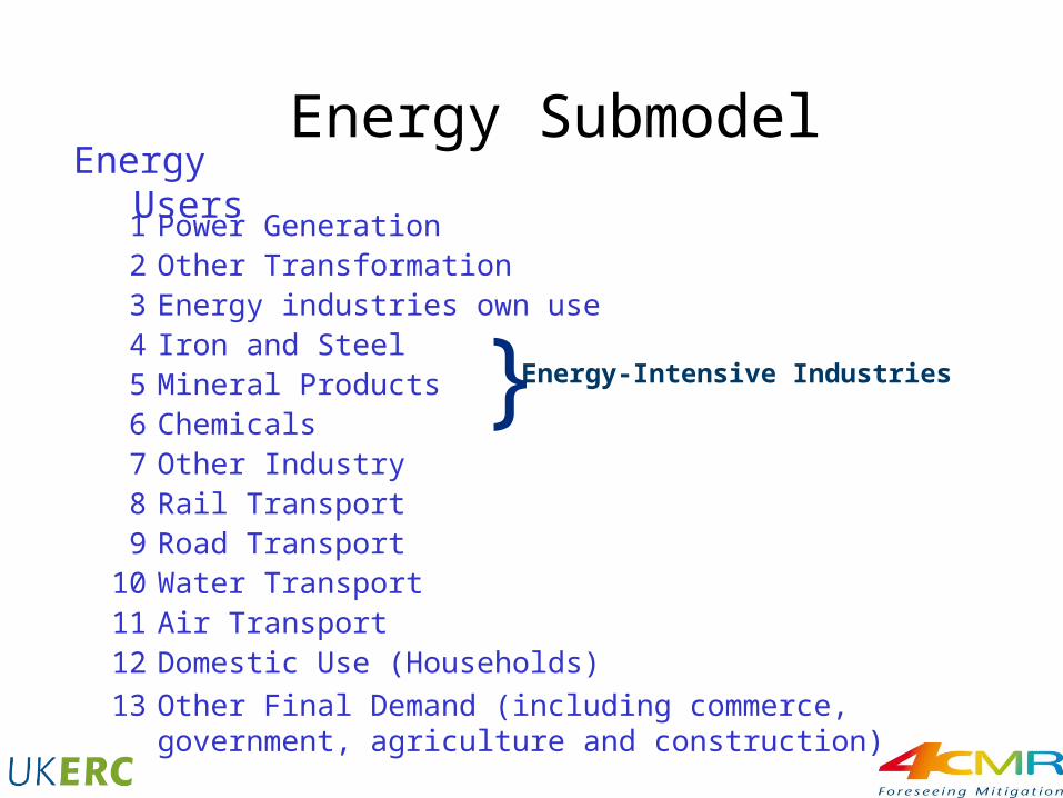
Energy Submodel

1 Power Generation2 Other Transformation3 Energy industries own use4 Iron and Steel5 Mineral Products6 Chemicals7 Other Industry8 Rail Transport9 Road Transport

10 Water Transport11 Air Transport12

13

Domestic Use (Households)

Other Final Demand (including commerce,government, agriculture and construction)

} Energy-Intensive Industries

Energy Users

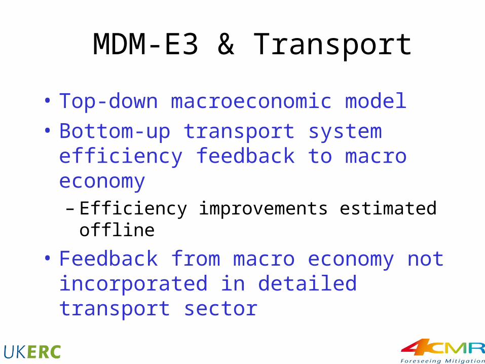
MDM-E3 & Transport

• Top-down macroeconomic model

• Bottom-up transport system efficiency feedback to macro economy– Efficiency improvements estimated offline

• Feedback from macro economy not incorporated in detailed transport sector

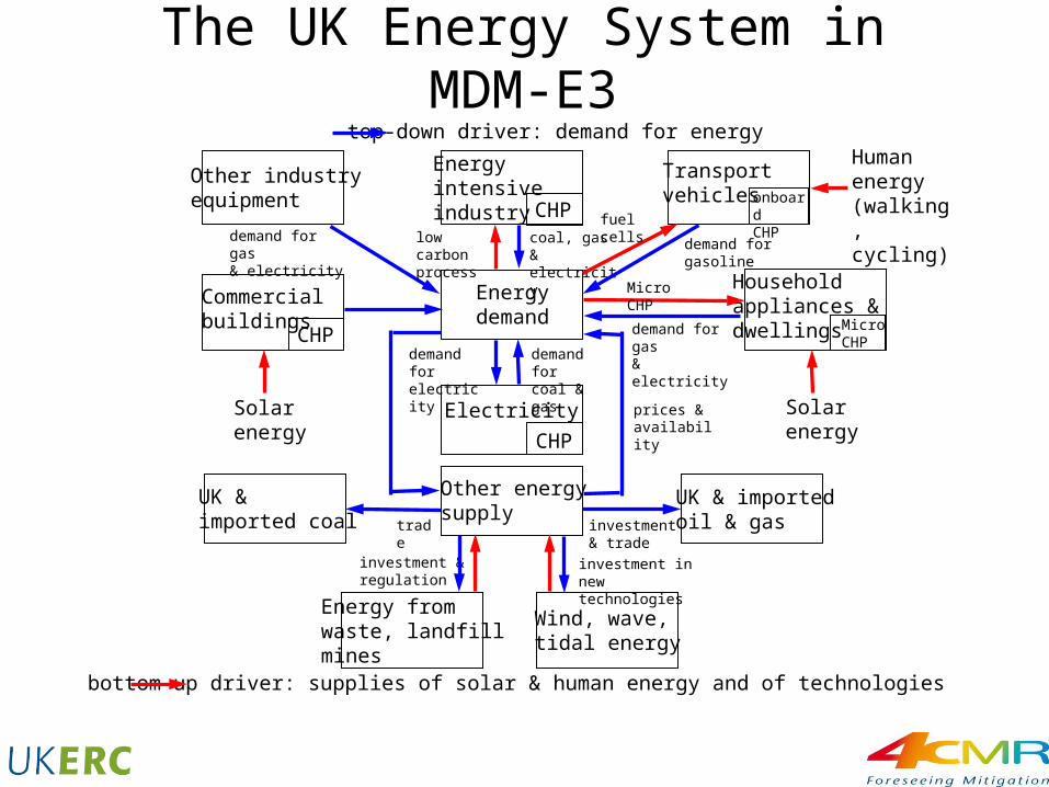
bottom-up driver: supplies of solar & human energy and of technologies

Humanenergy(walking,cycling)

top-down driver: demand for energy

Other industryequipment

Energyintensiveindustry CHP

Transportvehicles

Commercialbuildings

Energydemand

Householdappliances &dwellings Micro

CHPCHP

Electricity

Other energysupply

CHP

UK & importedoil & gas

UK &imported coal

Energy fromwaste, landfillmines

Wind, wave,tidal energy

Solarenergy

demand for gas& electricity

low carbonprocess

coal, gas &electricity

demand for gasoline

fuel cells

Micro CHP

demand for gas& electricity

Solarenergy

trade investment & trade

investment innew technologies

investment &regulation

prices &availability

demand forcoal & gas

demand forelectricity

The UK Energy System in MDM-E3

onboardCHP

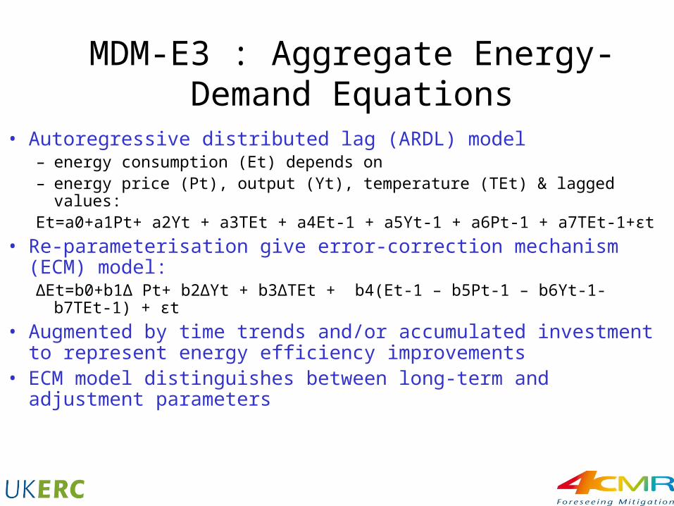
MDM-E3 : Aggregate Energy-Demand Equations

• Autoregressive distributed lag (ARDL) model– energy consumption (Et) depends on– energy price (Pt), output (Yt), temperature (TEt) & lagged values:Et=a0+a1Pt+ a2Yt + a3TEt + a4Et-1 + a5Yt-1 + a6Pt-1 + a7TEt-1+εt

• Re-parameterisation give error-correction mechanism (ECM) model:ΔEt=b0+b1Δ Pt+ b2ΔYt + b3ΔTEt + b4(Et-1 – b5Pt-1 – b6Yt-1- b7TEt-1) +

εt

• Augmented by time trends and/or accumulated investment to represent energy efficiency improvements

• ECM model distinguishes between long-term and adjustment parameters

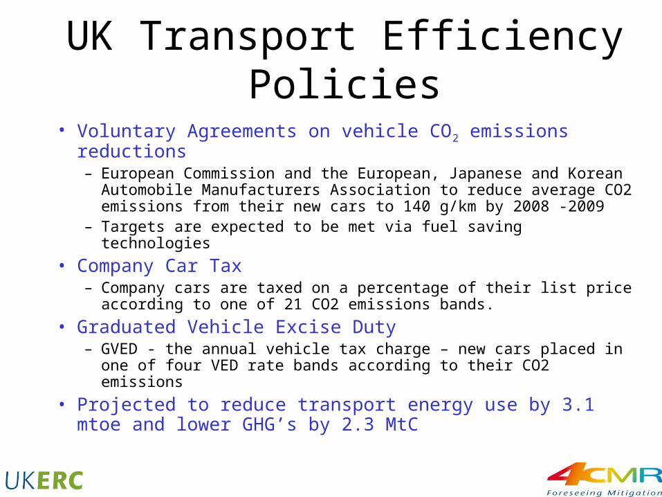
UK Transport Efficiency Policies

• Voluntary Agreements on vehicle CO2 emissions reductions– European Commission and the European, Japanese and Korean

Automobile Manufacturers Association to reduce average CO2 emissions from their new cars to 140 g/km by 2008 -2009

– Targets are expected to be met via fuel saving technologies

• Company Car Tax– Company cars are taxed on a percentage of their list price

according to one of 21 CO2 emissions bands.

• Graduated Vehicle Excise Duty– GVED - the annual vehicle tax charge – new cars placed in one of

four VED rate bands according to their CO2 emissions

• Projected to reduce transport energy use by 3.1 mtoe and lower GHG’s by 2.3 MtC

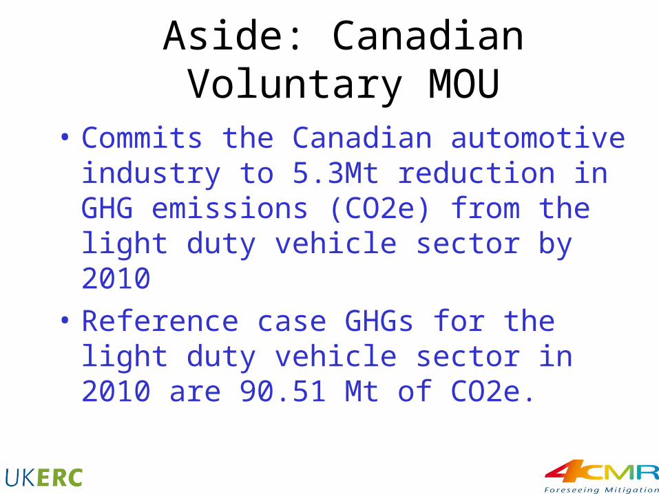
Aside: Canadian Voluntary MOU

• Commits the Canadian automotive industry to 5.3Mt reduction in GHG emissions (CO2e) from the light duty vehicle sector by 2010

• Reference case GHGs for the light duty vehicle sector in 2010 are 90.51 Mt of CO2e.

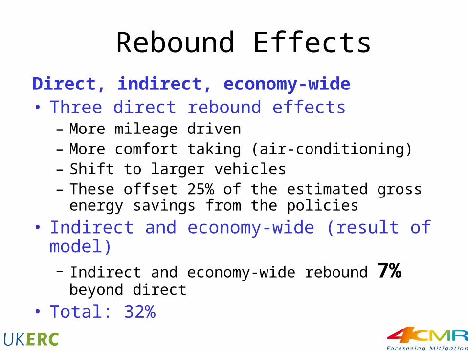
Rebound EffectsDirect, indirect, economy-wide• Three direct rebound effects

– More mileage driven– More comfort taking (air-conditioning)– Shift to larger vehicles– These offset 25% of the estimated gross energy

savings from the policies

• Indirect and economy-wide (result of model)– Indirect and economy-wide rebound 7% beyond

direct

• Total: 32%

Impacts of VAs on Key Macroeconomic Variables

Sector 2000 2005 2010

Final Energy Demand (mtoe, level)-0.29 -1.86 -2.89

Final Energy Demand (% level)-0.18 -1.20 -1.81

CO2 Emissions (mtC, level)-0.26 -1.61 -2.42

CO2 Emissions (%, level)-0.17 -1.11 -1.80

GDP (%, level)0.05 0.43 0.48

GDP Deflator (%, level)-0.05 -0.77 -1.28

Employment (%, level)0.00 0.19 0.28

Public Sector Borrowing (%GDP, level)0.00 0.15 0.22

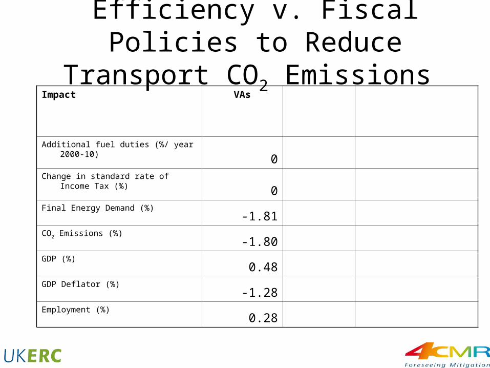
Efficiency v. Fiscal Policies to Reduce Transport CO2 Emissions

Impact VAs

Additional fuel duties (%/ year 2000-10)

0Change in standard rate of Income Tax (%)

0Final Energy Demand (%)

-1.81CO2 Emissions (%)

-1.80GDP (%)

0.48GDP Deflator (%)

-1.28Employment (%)

0.28

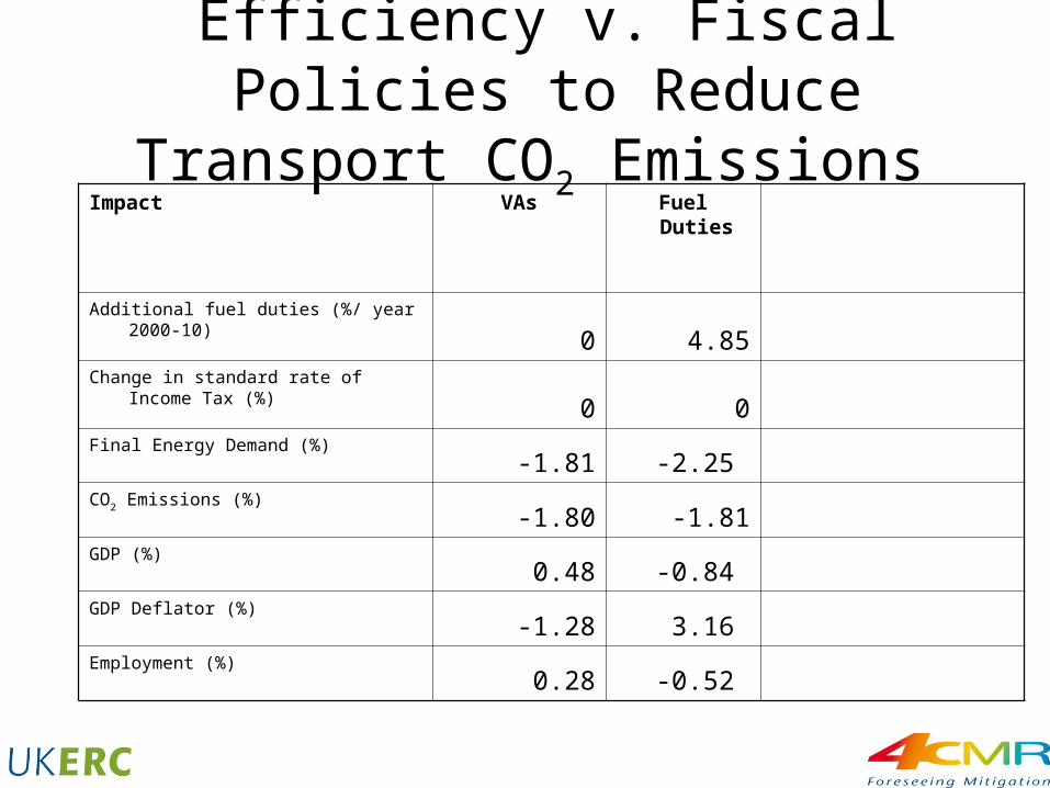
Efficiency v. Fiscal Policies to Reduce Transport CO2 Emissions

Impact VAs Fuel Duties

Additional fuel duties (%/ year 2000-10)

0 4.85Change in standard rate of Income Tax (%)

0 0Final Energy Demand (%)

-1.81 -2.25 CO2 Emissions (%)

-1.80 -1.81GDP (%)

0.48 -0.84 GDP Deflator (%)

-1.28 3.16 Employment (%)

0.28 -0.52

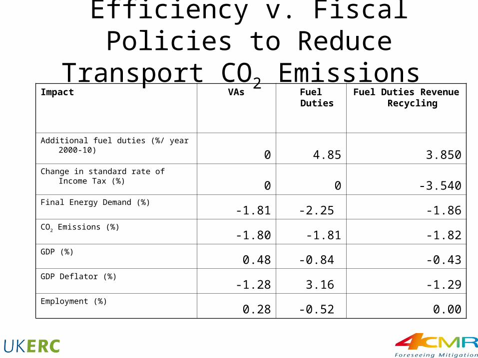
Efficiency v. Fiscal Policies to Reduce Transport CO2 Emissions

Impact VAs Fuel Duties Fuel Duties Revenue Recycling

Additional fuel duties (%/ year 2000-10)

0 4.85 3.850Change in standard rate of Income Tax (%)

0 0 -3.540Final Energy Demand (%)

-1.81 -2.25 -1.86CO2 Emissions (%)

-1.80 -1.81 -1.82GDP (%)

0.48 -0.84 -0.43GDP Deflator (%)

-1.28 3.16 -1.29Employment (%)

0.28 -0.52 0.00

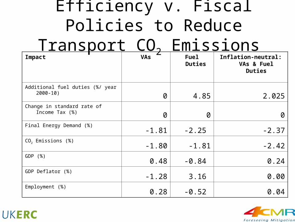
Efficiency v. Fiscal Policies to Reduce Transport CO2 Emissions

Impact VAs Fuel Duties Inflation-neutral: VAs & Fuel Duties

Additional fuel duties (%/ year 2000-10)

0 4.85 2.025Change in standard rate of Income Tax (%)

0 0 0Final Energy Demand (%)

-1.81 -2.25 -2.37CO2 Emissions (%)

-1.80 -1.81 -2.42GDP (%)

0.48 -0.84 0.24GDP Deflator (%)

-1.28 3.16 0.00Employment (%)

0.28 -0.52 0.04

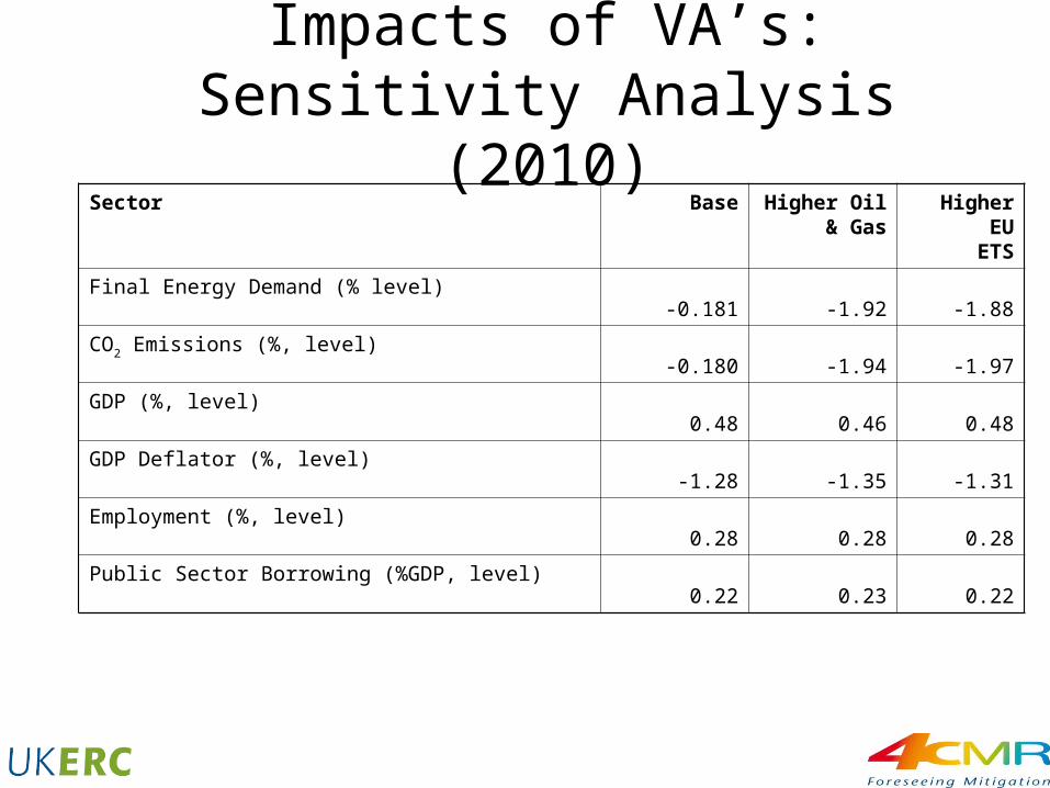
Impacts of VA’s: Sensitivity Analysis (2010)

Sector Base Higher Oil & Gas

Higher EU ETS

Final Energy Demand (% level)-0.181 -1.92 -1.88

CO2 Emissions (%, level)-0.180 -1.94 -1.97

GDP (%, level)0.48 0.46 0.48

GDP Deflator (%, level)-1.28 -1.35 -1.31

Employment (%, level)0.28 0.28 0.28

Public Sector Borrowing (%GDP, level)0.22 0.23 0.22

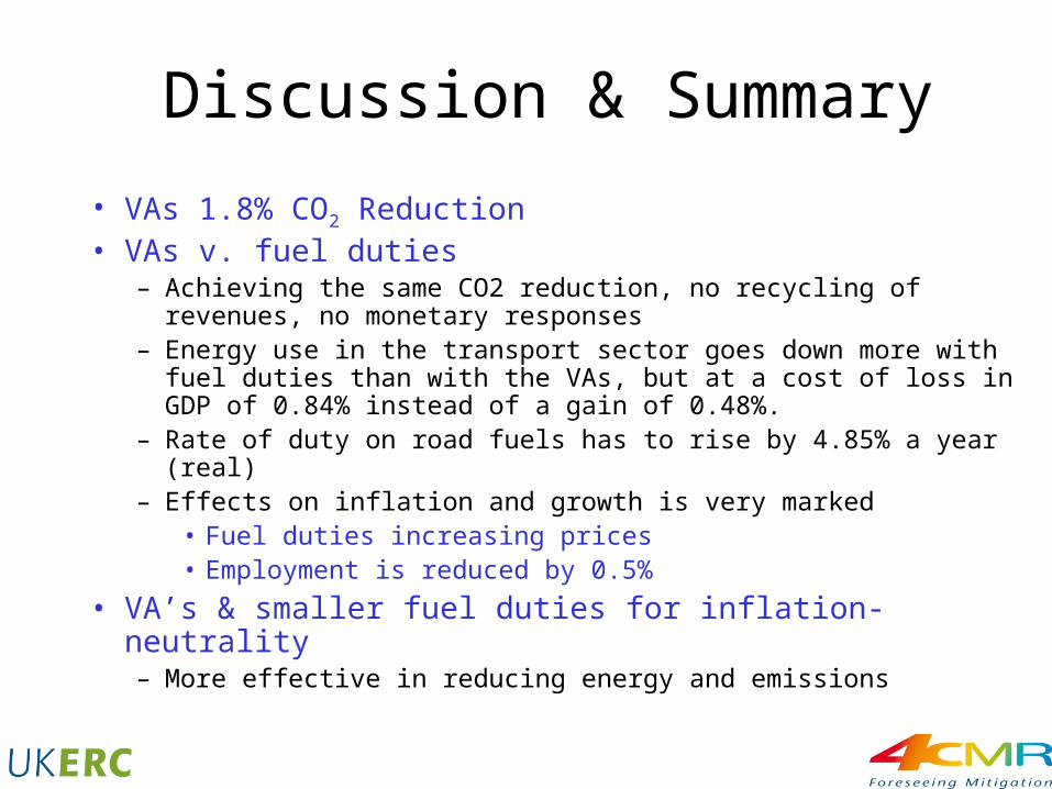
Discussion & Summary

• VAs 1.8% CO2 Reduction • VAs v. fuel duties

– Achieving the same CO2 reduction, no recycling of revenues, no monetary responses

– Energy use in the transport sector goes down more with fuel duties than with the VAs, but at a cost of loss in GDP of 0.84% instead of a gain of 0.48%.

– Rate of duty on road fuels has to rise by 4.85% a year (real) – Effects on inflation and growth is very marked

• Fuel duties increasing prices• Employment is reduced by 0.5%

• VA’s & smaller fuel duties for inflation-neutrality– More effective in reducing energy and emissions

Discussion & Summary

• Our approach enables a partial integration of top-down macroeconomic aspects and bottom-up energy systems– We do not assume that resources are used at full economic

efficiency

• Limitations– Bottom-up energy savings and direct rebound effects had to be

imposed on the model– These are below the level of disaggregation currently in the

model– No feedbacks incorporated from the wider macroeconomic

effects to the bottom-up energy savings

• Currently working to develop greater sectoral detail for better integration with the macro model