ELSEWIER Annals of Pure and Applied Logic 70 (1994) 17-49

ANNALS OF PURE AND APPLIED LOGIC

Equational derivation vs. computation*

W.G. Handley **, S.S. Wainer

School of Mathematics. University of Leeds. Leeds, United Kingdom LS2 9JT

Communicated by J.-Y. Girard; received 19 December 1992; revised 23 October 1993

Abstract

Subrecursive hierarchy classifications are used to compare the complexities of recursive functions according to (i) their derivations in a version of Kleene’s equation calculus, and (ii) their computations by term-rewriting. In each case ordinal bounds are assigned, and it turns out that the respective complexity measures are given by (i) a version of the Fast Growing Hierarchy, and (ii) the Slow Growing Hierarchy. Known comparisons between the two hierarchies then provide ordinal trade-offs between (i) derivation and (ii) computation. Charac- teristics of some well-known subrecursive classes are also read off.

1. Introduction

Just as ordinal assignments are a fundamental tool in proof-theoretic analysis, so

should they also be expected to play a basic r61e in the related but simpler analysis of

recursive definitions. After all, verification of the total correctness of a recursive

program involves proof of a I7:-statement:

Vinput. 3output. Spec(input, output)

and it would be strange indeed if there were not some deep connection between the

(logical) complexity of the proof and the (computational) complexity of the program.

Much has been written about this.

Our interest here lies in the development and preliminary investigation of “natural”

ordinal assignments to Herbrand-GGdel-Kleene-style recursive definitions [ 13, $541,

such that ordinal-“structure” usefully reflects inherent program-“uniformity” and

-“complexity”. In this context it is not surprising therefore that ordinals are to be

viewed intensionally. not merely as set-theoretic objects but rather as presentations of

* This research was partly supported by the Science and Engineering GR\G\27126.

** Corresponding author.

0168-0072/94/$07.00 0 1996Elsevier Science B.V. All rights reserved

SSDI 0168-0072(93)EOOSO-8

Research Council under Grant

18 W.G. Handley, S.S. Wainer 1 Annals of Pure and Applied Logic 70 11994) 17-49

well-orderings with distinguished choices of fundamental sequences to limits. The

concept of a “natural” well-ordering still remains vague (see [2] for discussion) and

maybe it always will, but suffice it to say here that the fundamental sequence f(n),

n = 0, 42, . . . to the first limit ordinal, should be considered far more natural if f were

the identity or successor function, than if f were some wildly-increasing or diffi-

cult-to-compute function.

The “derivation” of f( ‘ni 1,. . . , ‘nkl) = rml in Kleene’s Equation Calculus allows

the rule of substitution or “call-by-value”, thus if for example f is defined from g and

h by the equation

f(x I,..., 'Qc) = g(Xl,...,xk,h(x1,...,xk))

then f(rn,l,. . . , rnkl) = rrnl is derived immediately, in one step, from the two

sub-derivations:

h(‘ql,..., ‘nk’) = ‘nk+ 1’ and g(‘+l, . ..) ‘nk’, rnk+ 1’) = rml.

Viewed proof-theoretically this rule is nothing other than the Cut-Rule at the level of

terms.

On the other hand, the “computation” of f(n, , . . . , nk) = m from a given (finite) set

of defining equations would normally be thought of in terms of rewriting only - each

defining equation being regarded as a possible left-to-right rewrite. Thus in the above

example,

f(‘nil,..., ‘nk’) -, g(‘ni’,..., mkl, h(‘nll ,..., ‘tlkl)) + ... +

+ g(rnll,...,r!t,l, ‘nk+l’) -+ ... + rmT.

Inputs and outputs are restricted to terms of an acceptable form (e.g. unary

numerals as in the classical equation calculus) and all we require at the outset is

a normalization assumption that there is a unique acceptable normal form for each

acceptable input.

In this paper we set out to compare “derivation” with “computation” via a method

of ordinal assignment due originally to Buchholz [l], but somewhat modified and

simplified since. We set up systems n : N k; f(n) = m, n : N b: f(n) = m correspond-

ing respectively to derivation, computation from a set E of defining equations, with

ordinal bound LX If c( is a uniform bound over all inputs n then we should expect there

to be canonical ways of reading off hierarchies of complexity-bounding functions B,:

N -+ N, G,: N --) N corresponding to derivation, computation respectively.

It turns out that B,, G, are just (versions of) the Fast- and Slow-Growing Hierar-

chies respectively. Known connections between these hierarchies due to Girard [9],

Wainer [lS] and others then give immediate access to proof-theoretic characteriza-

tions of the functions computed below a given bound c(, and to the extraction of

natural termination-orderings for their rewrite-systems, relating to work of Der-

showitz and Okada [6], Cichon [3], Gallier [S], and Weiermann [16]. The work in

addition gives clear demonstration of the usefulness of the Fast- and Slow-Growing

W.G. Handle)>, S.S. Waker/Annals of Pure and Applied Logic 70 (1994) 17-49 19

Hierarchies in providing fundamental scales against which various computational

notions may be measured and compared.

The paper is divided into sections as follows: Section 2 introduces some elementary

facts about rewriting; Section 3 introduces the structured tree ordinals (which repres-

ent a more convenient way of considering assignments of fundamental sequences to

the usual, “set-theoretic” ordinals) and states some known properties; Section 4 intro-

duces slow- and fast-growing bounding functions indexed by these tree ordinals (the

reader may care to note that the B-functions are built up in the same way as

Grzegorczyk’s original hierarchy functions [lo]); Section 5 shows how the structure

of derivations and computations can be associated with structured tree ordinals;

Section 6 uses this to give bounds on computations unwound from derivations;

Section 7 relates ordinal complexity to conventional computational complexity;

Section 8 connects this work with previously known results based on “natural” fixed

fundamental sequences.

The authors thank the referees for their thoroughness and insight. We have striven

to remedy the defects which they have pointed out.

2. Preliminaries

Rewrite systems

2.1. Notation. ii stands for the tuple (nl ,..., Q).

2.2. Definition. We define rml to be the numeral s(s( ... s(O)...)) representing m.

2.3. Definitions. (i) A rewrite rule is a pair (I, r) of terms such that Vurs(r) E Vurs( I)

(see Definition 2.5 below). We write I--) r.

(ii) A rewrite system is a finite collection of rewrite rules.

(iii) Given a rewrite system E, a term t rewrites to term u iff there is some rule l--f r in

E and some substitution r~ such that la is a subterm of t and u results from

replacing that subterm by rcr. We write t aE u.

(iv) +* is the relaxive, transitive closure of =+. If t S-E* u, we say that t reduces to v.

2.4. Definition. For a given rewrite system E, function letter f and function

cp: Nk + N, f E-represents q iff for all iz~ Nk, f(%l) *$ ‘~(6)~.

Numbers of leaves and extensions to rewrite systems

2.5. Definition. For a term t, Vurs(t) is defined to be the set of variables occurring in t.

2.6. Definition. For a term t, Leaves(t) is defined to be the number of occurrences of

0-ary symbols (i.e. variables or constants) in c.

20 W.G. Handley, S.S. Wainer 1 Annals of Pure and Applied Logic 70 (1994) 17-49

2.7. Note. Since all terms have at least one leaf, Leaves(t) 2 1 for all terms t.

2.8. Definition. For a rewrite-system E, we define

&:= max(Leaves(r): (I-+ Y)EE}.

2.9. Note. Since all terms have at least one leaf, 2s > 1 for all E.

2.10. Proposition. For any rewrite system E,

t *E w implies Leaves(w) < Leaves(t)-&.

Proof. Relatively easy. Observe first that, by definition of a rewrite system, (I + r) E E

implies that

Vurs(r) E Vars(l).

We show, by induction on the construction oft, that if Vars(t) E Vars(l) then, for all

substitutions (T,

Leaves(to) Q Leaves( lo) - Leaves(t).

If t has just a single variable then to is a subterm of la and so

Leaves(W) < Leaves(b) < Leaves(b)* Leaves(t).

On the other hand if t is a single constant, then

Leaves( to) = 1 < Leaves( lo) * Leaves(t).

Now if t Ef(tl,..., tk), then

Leaves( to) = 1 LeUVeS( ti0)

but also

Leaves(t) = 2 LeUVf?S(ti).

Therefore, using the I.H.,

Leaves(W) < C [ Leaves( lo) * LeUVt?S(ti)] = Leaves( lo) * Leaves(t).

The proposition as stated follows straightforwardly. 0

3. Structured tree ordinals

3.1. Definition. Sz, a subclass of the countable sets, is defined inductively as follows:

(Z) O=OEQ;

(S) srEs2 implies (c( + 1) = txu (a}EQ;

(L) If VnEN. c(,EQ then a~s2 where CC N + Sz and is defined by n-a,.

W.G. Handley, S.S. Wainer/ Annals of Pure and Applied Logic 70 (1994) 17-49 21

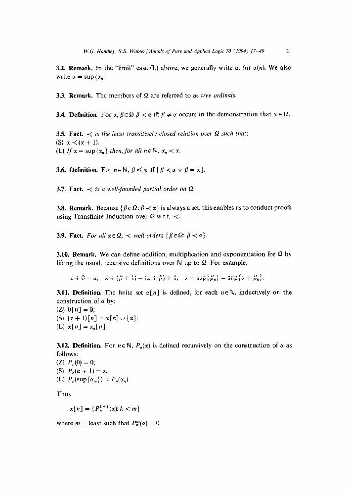
3.2. Remark. In the “limit” case (L) above, we generally write c(, for a(n). We also

write c( = sup{cc,}.

3.3. Remark. The members of 52 are referred to as tree ordinals.

3.4. Definition. For ~1, /?EQ /I < CI iff /? # tl occurs in the demonstration that a E 52.

3.5. Fact. < is the least transitively closed relation over 52 such that:

(S) a < (a + 1). (L) 1f~ = sup{a,} then,for all HEN, a,, < a.

3.6. Definition. For no N, /I < c( iff [/I < a v j3 = CC].

3.7. Fact. < is a well-founded partial order on 52.

3.8. Remark. Because {p E 52: /I 4 M} is always a set, this enables us to conduct proofs

using Transfinite Induction over Sz w.r.t. <.

3.9. Fact. For all a E Q, < well-orders { fi E L?: p < a}.

3.10. Remark. We can define addition, multiplication and exponentiation for Q by

lifting the usual, recursive definitions over N up to 52. For example,

a + 0 = a, a + (/3 + 1) = (a + P) + I, a + sup(A) = sup@ + Pn3.

3.11. Definition. The finite set a[n] is defined, for each n E N, inductively on the

construction of a by:

(Z) OCnl = (b; (9 (a + 1)Cnl = aCn1 u {a}; (L) aCn1 = a,Cnl.

3.12. Definition. For n E N, P,(a) is defined recursively on the construction of a as

follows:

(Z) P”(O) = 0; (S) P,(a + 1) = a;

(L) P,(sup{a,)) = PAad

Thus

a[n] = (Pf:+‘(a): k < m)

where m = least such that P:(a) = 0.

22 W.G. Handley. S.S. Wainer / Annals of Pure and Applied Logic 70 (1994) 17-49

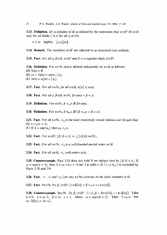
3.13. Definition. Q”, a subclass of Q, is defined by the restriction that CI E P iff c( E 52

and, for all limits < =$ CC, for all n, rnE N,

n < m implies inE[[m].

3.14. Remark. The members of 52” are referred to as structured tree ordinals.

3.15. Fact. For all a, BEC?, c(ECJ~ and /? < CI together imply /?EL?“.

3.16. Definition. For nE N, a(n) is defined inductively on ~1 EQ as follows:

(Z) O(n) = 0.

(S) (c( + l)(n) = cc(n) u {LX}.

(L) u(n) = a,(n) u (~1.

3.17. Fact. For all n E N,for all a~0, a[n] E a(n).

3.18. Fact. For all a,j?~Q, nEN, /3~cr(n)+p<or.

3.19. Definition. For nE N, B <. M iff pea(n).

3.20. Definition. For nE N, /? 4na iff [fl <,,c( v j3 = cr].

3.21. Fact. For all n E N, <, is the least transitively closed relation over C2 such that:

(S) f.x <,(E + 1). (L) Zf a = sup{a,) then cx,, <, CL

3.22. Fact. For CIESZ~, {p: /? < a} = u {rx[n]: nE N ).

3.23. Fact. For all nE N, <” is a well-founded partial order on 52.

3.24. Fact. For all a~0, <. well-orders a(n).

3.25. Counterexample. Fact 3.24 does not hold if we replace cc(n) by {B: p 4 tl

o = sup{n + l), then 2 < o <(o + 1) but 2 $ o(O) = (0, 1). o so 2 is excludec

Facts 3.18 and 3.9.

>. If

1 by

3.26. Fact. < , < and <,, (for any nE N) coincide on the jinite elements of Q.

3.27. Fact. VneN. VGI,~, YEW. [ye/?[n] A j? <“a--+ YEa[n]].

3.28. Counterexample. 3nE N. ~GI, P, YE@. Cy <,P A BEECnl A Y tf a[nll. Take n = 0, c~~w.2, fi=w, y=l, where w=sup{m+l}. Then 1<0w but

(w*2)[n] = {O,w}.

W.G. Handley. S.S. Waker/Annals cf Pure and Applied Logic 70 (1994) 17-49 23

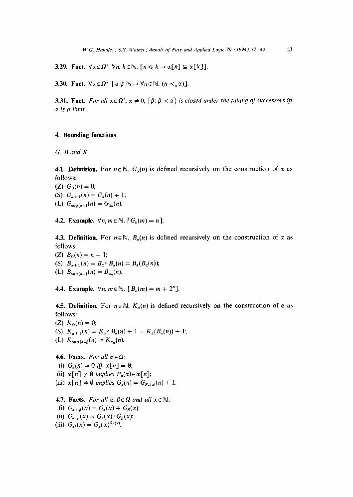
3.29. Fact. Vcr~0”. Vn, kEN. [n d k+ cx[n] E ark]].

3.30. Fact. VMEP. [M $ N -+ Vne N. (n 4. @)I.

3.31. Fact. For all CI E P, a # 0, {/I: /I < CX} is closed under the taking of successors ifs

c1 is a limit.

4. Bounding functions

G. B and K

4.1. Definition. For nE N, G,(n) is defined recursively on the construction of c( as

follows:

(Z) G,(n) = 0;

(S) G,+l(n) = G,(n) + 1;

(L) Gsup(a,) (n) = G,,,(n).

4.2. Example. Vn, me N. [G,,(m) = n].

4.3. Definition. For n E N, B,(n) is defined recursively on the construction of TV as

follows:

(Z) B,,(n) = n + 1;

6) &+ I (HI= B, a B,(n) = &P&(n));

(L) Bsupta,) (n) = 4(n).

4.4. Example. Vn, rnE N. [B,(m) = m + 2”].

4.5. Definition. For n E N, K,(n) is defined recursively on the construction of CI as

follows:

(Z) K,(n) = 0;

(S) K,+ I(n) = K, o B,(n) + 1 = U&(n)) + 1;

(L) K sUp~or,)(n) = K,,(n).

4.6. Facts. For all x E 52:

(i) G,(n) = 0 ijf a[n] = 8;

(ii) ~[n] # 0 implies P,(cr)Eu[n];

(iii) u[n] # 0 implies G,(n) = GP&n) + 1.

4.7. Facts. For all ~1, p~s2 and all XE N:

(i) G,+&) = G,(x) + G&); (ii) G,.,(x) = G,(x) - G@(x);

(iii) G,,(x) = G,(x)~@(~).

24 W.G. Hand&, S.S. Wainer / Annals of Pure and Applied Logic 70 (1994) 17-49

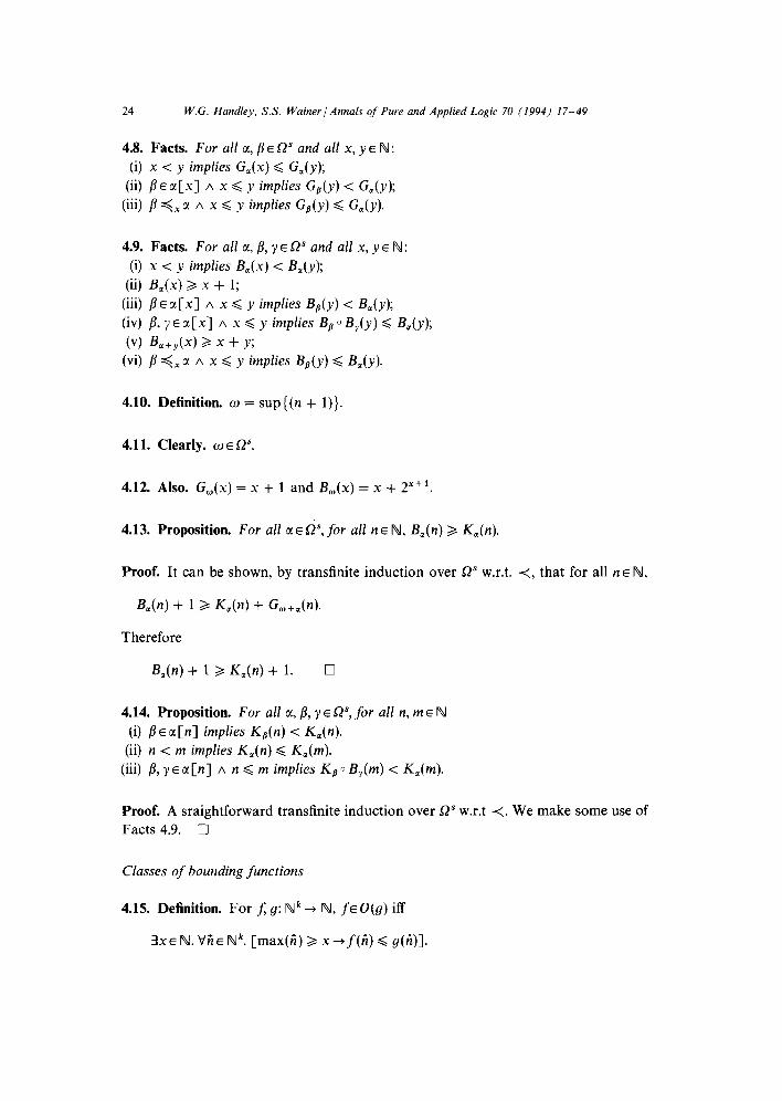
4.8. Facts. For all a, /I E 52” and all x, y E N: (i) x < y implies G,(x) d G,(y);

(ii) /?ea[x] A x 6 y implies Go(y) < G,(y); (iii) fi <Xcr A x d y implies G,(y) < G,(y).

4.9. Facts. For all ~1, /?, y E 52” and all x, YE N:

(i) x < y implies B,(x) < B,(y); (ii) B,(x) 3 x + 1;

(iii) /?Ec~[x] A x d y implies BP(y) < B,(y);

(iv) fl, y E cr[x] A x d y implies BP 0 B,(y) d B,(y);

(4 K+,(x) 2 x + y;

(vi) /? <, cI A x < y implies BP(y) Q B,(y).

4.10. Definition. o = sup{ (n + 1)).

4.11. Clearly. cc) E 52”.

4.12. Also. G,(x) = x + 1 and B,(x) = x + 2”+‘.

4.13. Proposition. For all CIEW,~OY all DIE N, B,(n) B f&(n).

Proof. It can be shown, by transfinite induction over Q” w.r.t. i, that for all no N,

B,(n) + 1 2 K,(n) + G,+,(n).

Therefore

B,(n) + 1 2 K,(n) + 1. 0

4.14. Proposition. For all 01, /?, PER”, for all n, me N (i) Pe~([n] implies Kg(n) < K,(n).

(ii) n < m implies K,(n) d K,(m). (iii) p, y~cl[n] A n < m implies K,o B,(m) < K,(m).

Proof. A sraightforward transfinite induction over CL?” w.r.t <. We make some use of Facts 4.9. 0

Classes of bounding functions

4.15. Definition. For f, g: Nk + N, f~ O(g) iff

3x~ N. V’jl~ Nk. [max(C) 2 x-f(h) 6 g(i)].

W.G. Handley, S.S. Wainer 1 Annals of Pure and Applied Logic 70 (1994) 17-49 25

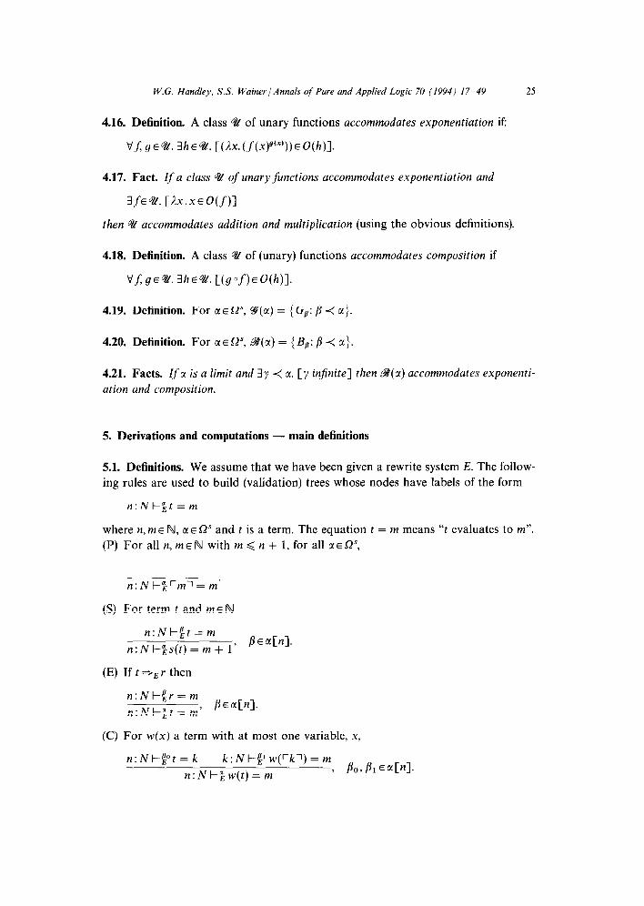
4.16. Definition. A class 42 of unary functions accommodates exponentiation if:

Vf; ge42. 3hEQ. [(Ax.(j-(x)“‘“‘))EO(h)].

4.17. Fact. If a class % of unary functions accommodates exponentiation and

3fG92. [AX.XEO(f)]

then f& accommodates addition and multiplication (using the obvious definitions).

4.18. Definition. A class 42 of (unary) functions accommodates composition if

VfT gE%.Z!he@. [(gof)EO(h)].

4.19. Definition. For ME@, 9(cr) = {CD: b < a}.

4.20. Definition. For CI E Q”, B(r) = { Bg: j3 < a}.

4.21. Facts. If GI is a limit and 3y < c(. [y infinite] then @(cc) accommodates exponenti-

ation and composition.

5. Derivations and computations - main definitions

5.1. Definitions. We assume that we have been given a rewrite system E. The follow-

ing rules are used to build (validation) trees whose nodes have labels of the form

n:Nt-Et = m

where n, me N, c~ECP and t is a term. The equation t = m means “t evaluates to m”.

(P) For all n, me N with m < n + 1, for all tl~!X,

n:Nt-%rml=m’

(S) For term t and rnE N

n:Nl-it = m

n: N l-Es(t) = m + 1’ BE@nl.

(E) If t =z-E I then

~r~~%~ I z, BEaCnl.

(C) For w(x) a term with at most one variable, x,

n:Nt-pt=k k:N!--gw(rkl)=m

n:NF”,w(t)=m > DO, PI EaCnl.

26 W.G. Handley, S.S. Wainer / Annals of Pure and Applied Logic 70 (1994) 17-49

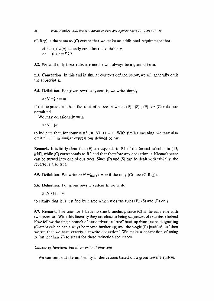
(C-Reg) is the same as (C) except that we make an additional requirement that

either (i) w(x) actually contains the variable x,

or (ii) t E rkl.

5.2. Note. If only these rules are used, t will always be a ground term.

5.3. Convention. In this and in similar contexts defined below, we will generally omit

the subscript E.

5.4. Definition. For given rewrite system E, we write simply

n:NE$t=m

if this expression labels the root of a tree in which (P)-, (S)-, (E)- or (C)-rules are

permitted.

We may occasionally write

n:Nt-“,t

to indicate that, for some m E N, n : N F$ t = m. With similar meaning, we may also

omit “ = m” in similar expressions defined below.

Remark. It is fairly clear that (E) corresponds to Rl of the formal calculus in [13,

$541, while (C) corresponds to R2 and that therefore any deduction in Kleene’s sense

can be turned into one of our trees. Since (P) and (S) can be dealt with trivially, the

reverse is also true.

5.5. Definition. We write n: N Fi&g,E t = m if the only (C)s are (C-Reg)s.

5.6. Definition. For given rewrite system E, we write

n:NI;t =m

to signify that it is justified by a tree which uses the rules (P), (S) and (E) only.

5.7. Remark. The trees for 1 have no true branching, since (C) is the only rule with

two premises. With this linearity they are close to being sequences of rewrites. (Indeed

if we follow the single branch of our derivation “tree” back up from the root, ignoring

(S)-steps (which can always be moved further up) and the single (P)-justified leaf then

we see that we have exactly a rewrite deduction.) We make a convention of using

D (rather than T) to stand for these reduction sequences.

Classes of functions based on ordinal indexing

We can seek out the uniformity in derivations based on a given rewrite system.

W.G. Handley, S.S. Wainer/ Annals qf Pure and Applied Logic 70 (1994) 17-49 27

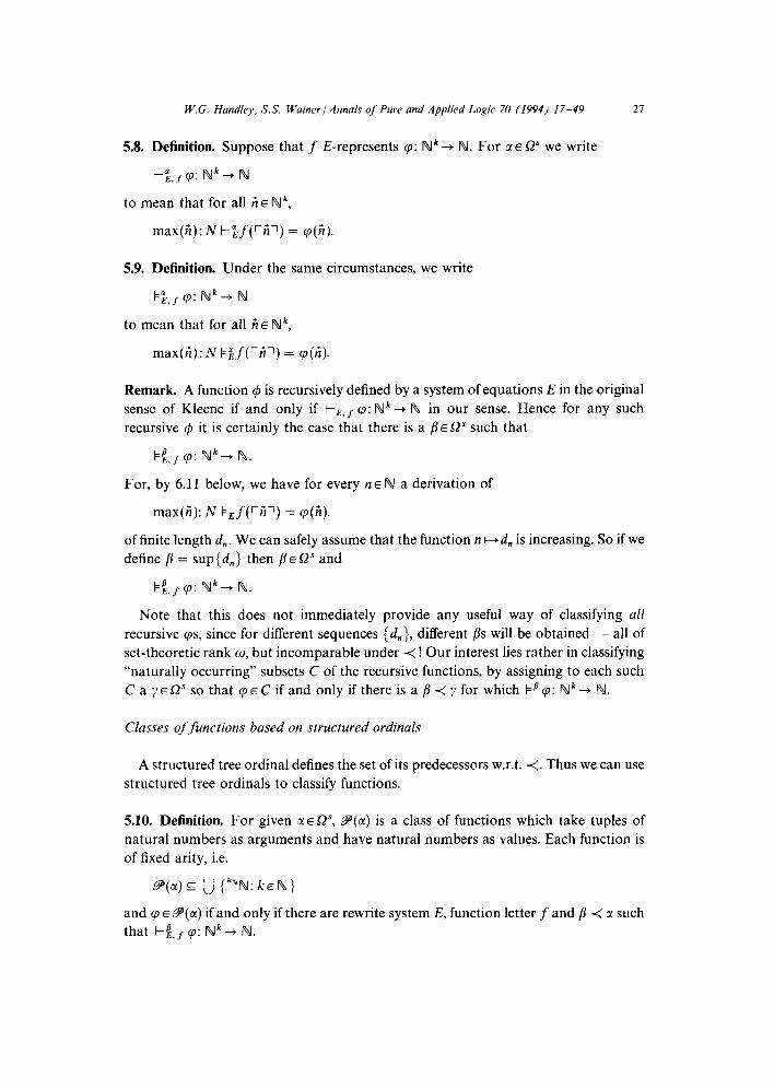
5.8. Definition. Suppose that f E-represents cp: N k -+ N. For CI E 0’ we write

t-&f cp: Nk+fV

to mean that for all 6 E Nk,

max(2): N kif(‘;ll) = cp(;l).

5.9. Definition. Under the same circumstances, we write

to mean that for all fi E RJ k,

max(fi): N b;f(rGl) = cp(fi).

Remark, A function 4 is recursively defined by a system of equations E in the original

sense of Kleene if and only if l---E,S cp: N k + N in our sense. Hence for any such

recursive $I it is certainly the case that there is a fi~s2” such that

@r cp: Nk-+ N.

For, by 6.11 below, we have for every n E N a derivation of

max(fi): N +Ef(rG1) = cp(;l).

of finite length d,. We can safely assume that the function n H d, is increasing. So if we

define j3 = sup { d,} then fi E s2” and

Note that this does not immediately provide any useful way of classifying all

recursive cps, since for different sequences {d,}, different /?s will be obtained - all of

set-theoretic rank w, but incomparable under < ! Our interest lies rather in classifying

“naturally occurring” subsets C of the recursive functions, by assigning to each such

CayEPsothatcpECifandonlyifthereisafi<yforwhich kpq:fIk+N.

Classes of functions based on structured ordinals

A structured tree ordinal defines the set of its predecessors w.r.t. i. Thus we can use

structured tree ordinals to classify functions.

5.10. Definition. For given CI E Q”, P(a) is a class of functions which take tuples of

natural numbers as arguments and have natural numbers as values. Each function is

of fixed arity, i.e.

and cp Ed if and only if there are rewrite system E, function letter f and j3 < c1 such

that k{,s cp: fV k+RJ.

28 W.G. Handley, S.S. Wainer 1 Annals qf Pure and Applied Logic 70 (1994) 17-49

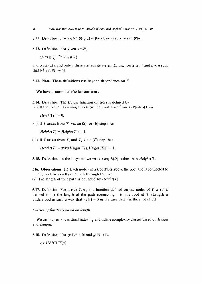
5.11. Definition. For a~fi~, Y&(a) is the obvious subclass of P(U).

5.12. Definition. For given c(ES~~,

9(a) E u {““N: kEN)

and cp E 9(cr) if and only if there are rewrite system E, function letter f and p 4 tl such

that k{,fcp: N k-+ N.

5.13. Note. These definitions rise beyond dependence on E.

We have a notion of size for our trees.

5.14. Definition. The Height function on trees is defined by

(i) If the tree T has a single node (which must arise from a (P)-step) then

Height(T) = 0.

(ii) If T arises from T’ via an (S)- or (E)-step then

Height(T) = Height( T’) + 1.

(iii) If T arises from Tl and T2 via a (C) step then

Height(T) = max(Height(T,), Height( T,)) + 1.

5.15. Definition. In the l=-system we write Length(D) rather than Height(D).

516. Observations. (1) Each node v in a tree T lies above the root and is connected to

the root by exactly one path through the tree.

(2) The length of that path is bounded by Height(T).

5.17. Definition. For a tree T, rc3 is a function defined on the nodes of T. z~(v) is

defined to be the length of the path connecting v to the root of T. (Length is

understood in such a way that rcr(v) = 0 in the case that v is the root of T.)

Classes qf,functions based on length

We can bypass the ordinal indexing and define complexity classes based on Height and Length.

5.18. Definition. For cp: N“ -+ N and g: N -+ N,

cp E HEIGHT(g)

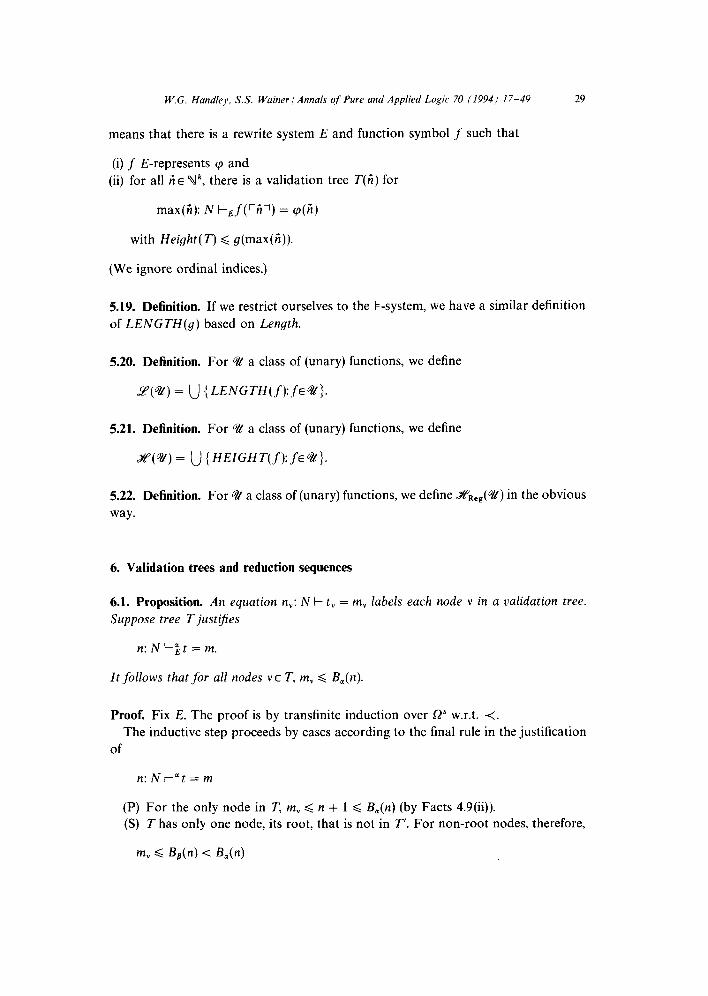
W.G. Handley, S.S. Wainer / Annals qf Pure and Applied Logic 70 (1994) 17-49 29

means that there is a rewrite system E and function symbol f such that

(i) f E-represents cp and

(ii) for all G E Nk, there is a validation tree T(C) for

max(2): N tJ(‘Gl) = q(i)

with Height(r) < g(max(;l)).

(We ignore ordinal indices.)

5.19. Definition. If we restrict ourselves to the k-system, we have a similar definition

of LENGTH(g) based on Length.

5.20. Definition. For % a class of (unary) functions, we define

5.21. Definition. For %! a class of (unary) functions, we define

z(e)= U {HEzc~~(f):f~a').

5.22. Definition. For % a class of (unary) functions, we define ~%~,,(a) in the obvious

way.

6. Validation trees and reduction sequences

6.1. Proposition. An equation n,: N k t, = m, labels each node v in a validation tree. Suppose tree T justijies

n:Nk--“,t=m.

It follows that for all nodes VE T, m, d B,(n).

Proof. Fix E. The proof is by transfinite induction over Q2” w.r.t. 4.

The inductive step proceeds by cases according to the final rule in the justification

of

n:Nk--“t=m

(P) For the only node in T, m, ,< n + 1 < B,(n) (by Facts 4.9(ii)).

(S) T has only one node, its root, that is not in T’. For non-root nodes, therefore,

m, G B,(n) < B,(n)

30 W.G. Handley, S.S. Wainer 1 Annals of Pure and Applied Logic 70 (1994) 17-49

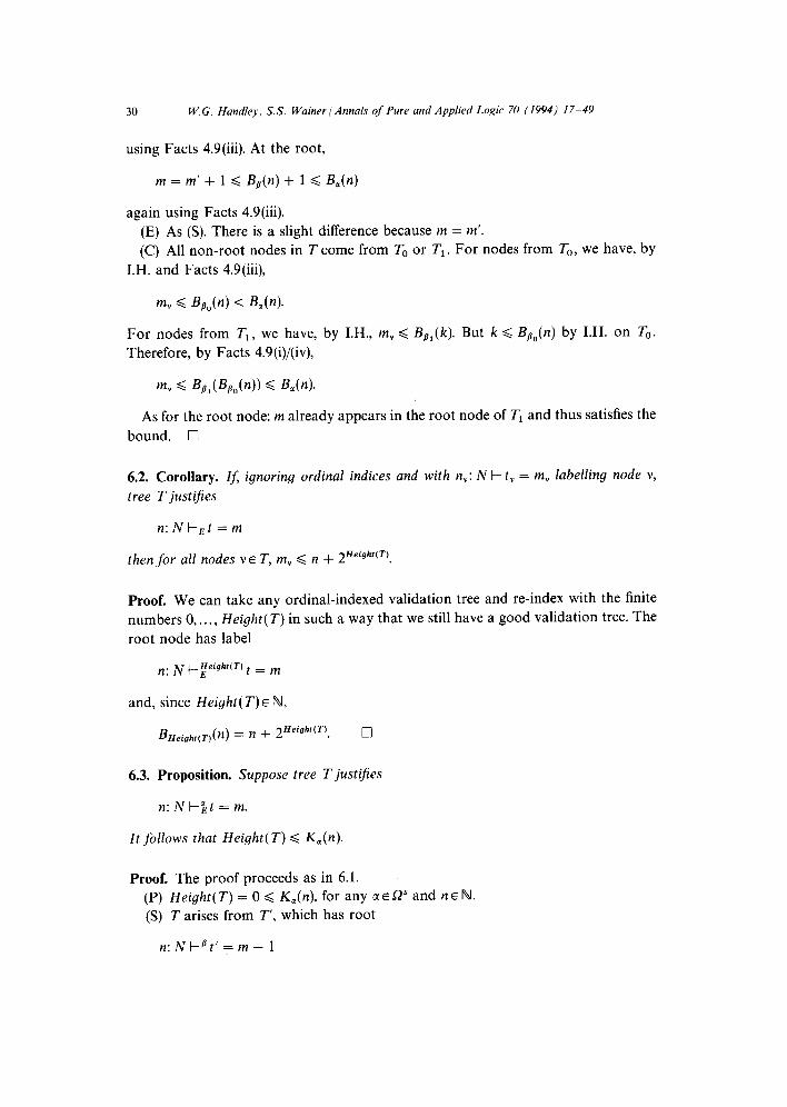
using Facts 4.9(iii). At the root,

m = m’ + 1 < B,(n) + 1 < B,(n)

again using Facts 4.9(iii).

(E) As (S). There is a slight difference because m = m’. (C) All non-root nodes in T come from To or T,. For nodes from T,, we have, by

I.H. and Facts 4.9(iii),

m, d BP,(~) < B,(n).

For nodes from T,, we have,

Therefore, by Facts 4.9(i)/(iv),

m, G Bfi,(&(n)) d B&r).

by I.H., m, d BP,(k). But k d BP,(n) by I.H. on To.

As for the root node: m already appears in the root node of T, and thus satisfies the

bound. Cl

6.2. Corollary. If, ignoring ordinal indices and with n,: N F t, = m, labelling node v,

tree T justijes

n:NI-Et=m

then for all nodes VE T, m, < n + 2Heighr(T’.

Proof. We can take any ordinal-indexed validation tree and re-index with the finite

numbers 0,. . . , Height(T) in such a way that we still have a good validation tree. The

root node has label

n. N +Eeight(T) t = m

and, since Z-Zeight( T) E N,

BHeight(T) (n) = n + ZHeight(T). 0

6.3. Proposition. Suppose tree T justijies

n:NFit=m.

It follows that Height(T) < K,(n).

Proof. The proof proceeds as in 6.1.

(P) Height(T) = 0 < K,(n), for any CIEQ’ and nE /I. (S) T arises from T’, which has root

n:NEPt’=m- 1

W.G. Handlq, S.S. Wainer / Annals of Pure and Applied Logic 70 (1994) 17-49 31

where t = s(t’) and /IEcx[~]. Then

Height(T) = Height(T) + 1 < Kp(n) + 1 < K,(n)

by Proposition 4.14(i).

(E) As (9. (C) T arises from TO and T,, whose roots are labelled

n:NI-gt’=k and k:Nl-pw(‘kl)=m

respectively, where PO, /?i ~a[n] and w(x) is such that w(t’) = t.

Height(T) = max(Height( TO), Height( T,)) + 1

d max(&,(n), I&(k)) + 1 (by I.H.)

Now KB,(n) < K,(n) by Proposition 4.14(i). On the other hand, by Proposition 6.1,

k d BP,(n) and this implies, by Proposition 4.14(ii), that

&l(k) d &,(&o(n)).

But applying Proposition 4.14(iii), we then have KPI(k) < K,(n). Thus

Height(T) < K,(n). 0

6.4. Corollary.

Proof. 6.3 + 4.13. 0

6.5. Proposition. For all rewrite systems E, for all a E ~2” and n E h4, for all terms t and

me:N:

n: N I-” t = m implies n: N t-i,, rml = m.

Proof. Easy. Cl

6.6. Proposition. For all rewrite systems E, for all a E QS and n E N, for all terms t and

rnEN:

n: Nk”t = m implies n: NE$,,t = m.

Proof. Fix E. The proof is by transfinite induction over 0” w.r.t. <, and proceeds by

cases according to the final step in the demonstration of

n:Nk”t=m.

(P/S/E) All these are trivial.

32 W.G. Handley, S.S. Waker/ Annals qf Pure and Applied Logic 70 (1994) 17-49

(C) There are /I,,, pi E 01 [n], t’ and w(x) such that

t = w[t’], n: Nt-pot’ = k and k: N l-@l w(‘kl) = m.

Since /&,, /I1 < OZ, the I.H. tells us that

n: N kk, t’ = k and k: N I-&, w(‘kl) = tn.

We need to consider two subcases:

(1) If the (C)-step is a (C-Reg)-step then the case is just as direct as the (S) and (E) cases above.

(2) If the (C)-step is not a (C-Reg)-step then

w(x) 3 w[‘kl] SE w[t’] = t

because the variable x does not actually appear in w(x). But, applying Proposition 6.5, we have

n: N k&rkl = k

and, applying a (C-Reg)-step, we find

n:Nl-f&t=m. q

6.7. Corollary. For all GIEW, 9(a) = P&(u).

6.8. Corollary. Zf T justi$es n: NE t = m, then there is a tree T’ justifying

n: N kReg t = m

with Height( T’) = Height(T).

Proof. We use Proposition 6.6 observing, as in Corollary 6.2, that

6.9. Corollary. For any class %! of(unary)finctions, X(e) = XReg(42).

6.10. Proposition. Let T be a validation tree for

n: N k Reg t = m.

(Ignore ordinal indices,) For all nodes v E T, if v has label

n,: N k t, = m,

then

Leaues(f,) < Leaves(t) * A~eight(T’.

W.G. Handley. S.S. Wainer / Annals of Pure and Applied Logic 70 (1994) 17-49 33

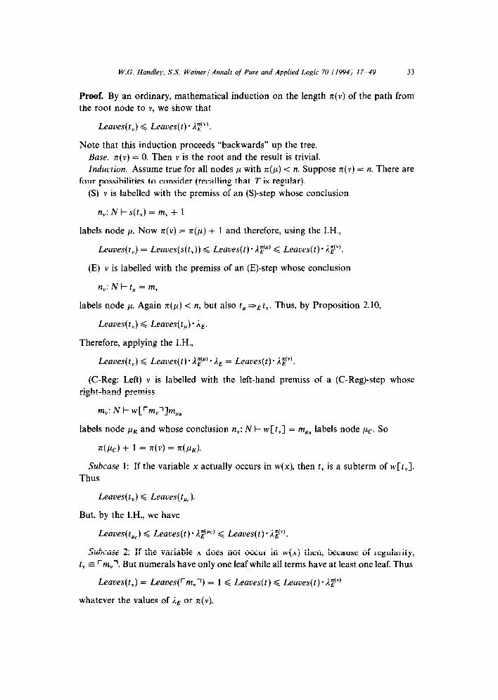
Proof. By an ordinary, mathematical induction on the length x(v) of the path from the root node to v, we show that

Leaves( t,) < Leaves(t) - AZ”).

Note that this induction proceeds “backwards” up the tree. Base. x(v) = 0. Then v is the root and the result is trivial. Induction. Assume true for all nodes ,U with ~(11) < n. Suppose x(v) = n. There are

four possibilities to consider (recalling that T is regular). (S) v is labelled with the premiss of an (S)-step whose conclusion

n,: N F s(t,) = m, + 1

labels node p. Now x(v) = 7c(p) + 1 and therefore, using the I.H.,

Leaoes(t,) = Leuues(s(t,)) d Leuves(t)-I$fl’ < Leuues(t)*;1$“‘.

(E) v is labelled with the premiss of an (E)-step whose conclusion

n,:Nk-~t, = m,

labels node p. Again x(p) < n, but also t, =sE t,. Thus, by Proposition 2.10,

Leuues(t,) < Leuues(t,). IzE.

Therefore, applying the I.H.,

Leaves(&) d Leuues(t)-A$p’*l, = Leuues(t)- A$“.

(C-Reg: Left) v is labelled with the left-hand premiss of a (C-Reg)-step whose right-hand premiss

m,: N F w[rm,l]m,,

labels node pR and whose conclusion n,: N k w[tY] = mPn labels node ccc. So

n(j.fc) + 1 = Jr(V) = n(/&).

Subcuse 1: If the variable x actually occurs in w(x), then t, is a subterm of w[tY].

Thus

Leuues( t,) < Leuues(t,,).

But, by the I.H., we have

Leuues(t,,) < Leaves(t) * A$“C) < Leaves(t) * A$“).

Subcuse 2: If the variable x does not occur in w(x) then, because of regularity, t, z rmv’. But numerals have only one leaf while all terms have at least one leaf. Thus

Leuues(t,) = Leuues(fm,l) = 1 < Leuues(t) < Leaves(t)-22’)

whatever the values of & or n(v).

34 W.G. Handle?, S.S. Wainer/ Annals qf Pure and Applied Logic 70 (1994) 17-49

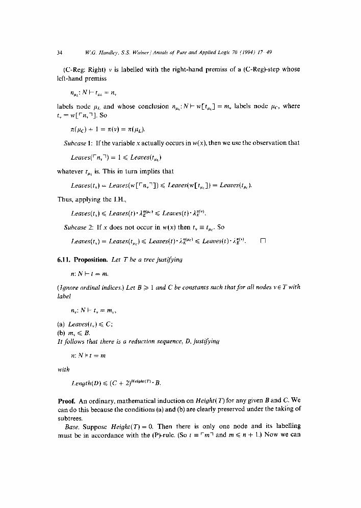
(C-Reg: Right) v is labelled with the right-hand premiss of a (C-Reg)-step whose

left-hand premiss

npL: N I- t,,. = n,

labels node pL and whose conclusion nrL. . N l-- w [ t,J = m, labels node ,uc, where

t, = w[‘n,l]. so

4%) + 1 = n(v) = 4PJ.

Subcase 1: If the variable x actually occurs in w(x), then we use the observation that

Leaues(‘n,l) = 1 < Leaues(t,,)

whatever t,, is. This in turn implies that

Leuves(t,) = Leaves(w[rnyl]) < Leuves(w[t,,]) = Leuves(t,,).

Thus, applying the I.H.,

Leuves(t,) < Leuues(t) * A$pC) < Leaves(t) * A$“).

Subcuse 2: If x does not occur in w(x) then t, E t,,. So

Leaves(&) = Leuues(t,,) d Leaves(t)* 22°C’ d Leuues(t)*i$“. 0

6.11. Proposition. Let T be a tree justifying

n:Nkt=m.

(Ignore ordinal indices.) Let B > 1 and C be constants such that for all nodes v E T with

label

n,: N I-- t, = m,,

(a) Leuues(t,) d C;

(b) m, d B. It follows that there is a reduction sequence, D, justifying

n:Nl=t=m

with

Length(D) < (C + 2)Heighr(T)* B.

Proof. An ordinary, mathematical induction on Height(T) for any given B and C. We

can do this because the conditions (a) and (b) are clearly preserved under the taking of

subtrees.

Base. Suppose Height(T) = 0. Then there is only one node and its labelling

must be in accordance with the (P)-rule. (So t = rml and m < n + 1.) Now we can

W.G. Handley. S.S. Wainer / Annals qf Pure and Applied L‘ogic 70 (1994) 17-49 35

apply the (P)-rule with equal ease to produce a reduction sequence, D, with one

element, namely

n:NIrml=m.

And now

Length(D) = 0 < (C + 2)‘. B.

Induction. Assume true for all trees with Height strictly less than Height(T). There

are three possibilities for the final step in constructing T:

(S) T arises from T’ by an (S)-step. Thus the root of T’ is labelled

n:NI-t’=m-1

where t E s(f). Since

a reduction sequence,

n:Nbt’=m- 1

and such that

Height(T) = Height(T’) + 1 we can apply the I.H. to obtain

D’, with endequation

Length(D’) < (C + 2)Heighz(T’)* B.

Extending D’ by an (S)-step, we obtain a sequence D with endequation n: N 1 t = m

and such that

Length(D) d [(C + 2)Height(T’) * B] + 1 < (C + 2)Height(T) - B.

This last inequality

(E) If T arises by

case (S).

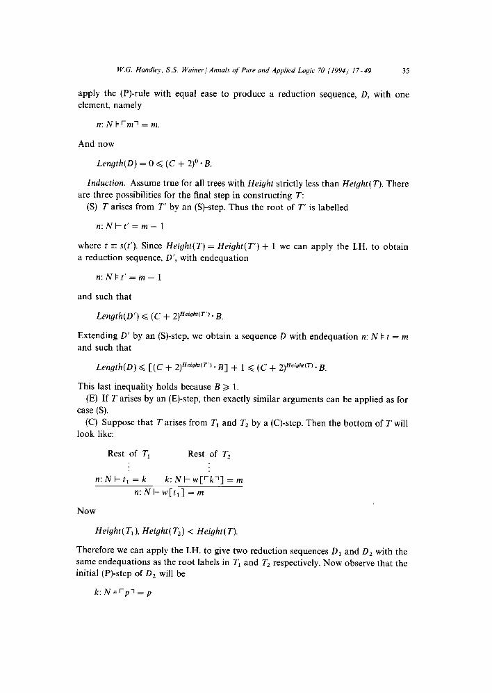
(C) Suppose that

look like:

holds because B 2 1.

an (E)-step, then exactly similar arguments can be applied as for

T arises from TI and Tz by a (C)-step. Then the bottom of Twill

Rest of T, Rest of T,

n: N F tI = k k: N I- w[rkl] = m

n:Nl--w[t,]=m

Now

Height( T,), Height( T2) < Height(T)

Therefore we can apply the I.H. to give two reduction sequences D1 and D, with the

same endequations as the root labels in T, and Tz respectively. Now observe that the

initial (P)-step of D, will be

k:N+‘pl=p

36 W.G. Handley, S.S. Wainer / Annals C$ Pure and Applied Logic 70 (1994) 17-49

for some p d m. Now, using at most p successor steps, we will always (no matter what

our chosen rewrite system E may be) have a sequence

n:Nt=‘pl=p

where I E {0, 1). The number of steps here is at most p and p d m < B (using condi-

tion (b)).

Observe next that the only rule that pays heed to the ‘declaration’ “-: N” is (P). Also

a given sequence, e.g. D,, contains only one (P)-step, which gives the first element. All

other steps in the sequence remain valid no matter what the ‘declaration’. This means

that

n:Nb’pl=p

n: N t= w(‘kl) = m

is valid. Furthermore its Length is at most

B + Length(D*).

Now consider Dr. It can be shown that the steps in Di may be rearranged so that

the initial (P)-step is followed by a block of (S)-steps, which is followed by a block of

(E)-steps at the end. The proof of this is relatively easy. It relies on the fact that if

a sequence contains an (E)-step immediately followed by an (S)-step, then the two can

be swapped round. This is because v +E w implies s(u) aE s(w).

The (E)-tail of D 1,

n:Nb’kl=k

n: N b tl = k

uses only (E)-steps and, furthermore, not more than Length(I),) of them. (This tail is

not valid on its own; its first element need not accord with the (P)-rule).

Now, as we have already observed, the validity of (E)-steps in unaffected by the

‘declaration’ n: N, or indeed by the value of k, provided both remain unchanged by the

step. Furthermore rewriting, by its nature, can be extended to superterms. Thus

essentially the same (E)-steps will give us a subsequence

n: N b ...rkl . . . = m

n: N I= . . . tl . . . = m.

W.G. Handley. S.S. Wainer/ Annals of Pure and Applied Logic 70 (1994) 17-49 37

Now, to get from

n: N 1 w[‘kl] = m to IZ: N b w[tr] = m,

we must repeat this for every occurrence of x in w(x). But there can be no more

occurrences of x in w(x) than there are leaves in w [rkl] (variables and numerals have

the same number of leaves, namely one). Therefore, using (a) of the hypothesis, we

need at most C * Length(Di) (E)-steps to give the subsequence

n: N b w[rkl] = m

n:Nkw[tI]=m.

And now putting everything together, we have a reduction sequence

n: N 1 rll = 1

n:Nbrpl=p

n: N b w(rkl) = m

n: N b w[tl] = m

This sequence D has endequation corresponding to the root-label of T. Also

Length(D) Q B + Length(D1) + C*Length(Di).

So relying on the I.H.,

Length(D) < B + (C + 2)Height(T2) * B + C * (C + 2)Heighr(T1) - B

< (c + 2)HeigWTz). B + (c + 2)HeigWTz). B + C. (C + 2)HeWCTz). B

d (C + 2) Height(T). B. 0

6.12. Proposition. For all rewrite systems E, for all u~s2, for all n, rnE N and for all

terms t,

n:NI”,t=m (9

ifand only if there is a reduction sequence, D, for n: N bE t = m (ignoring ordinal indices) with

Length(D) d G,(n). (ii)

Proof. (i) implies (ii). This implication is easy using Facts 4.8(ii).

(ii) implies (i). Fix E and n. Th e proof is by transfinite induction on Q’ w.r.t <, the

inductive step breaking up into (P), (S) and (E) cases according to the last step in the

justification of

n: N kE t = m.

38 W.G. Handley, S.S. Waker 1 Annals of Pure and Applied Logic 70 (1994) 17-49

(P) IZ: N b; t = m holds trivially.

(S) D arises by an (S)-step from D’ with endequation

n:Nk,t’=(m- 1)

where t = s(t’). Length(D) > 0 implies G,(n) # 0, i.e. c( [n] # 8. From this we know

(4.6) that

P,(cr)~c~[n] and that G,“(a)(n) = G,(n) - 1.

But

Length(D’) < Length(D) and so Length(D’) < G,“{,,(n).

Now we apply the I.H. to obtain

n: N 1;%’ = (m - l),

from which we infer n: N 1 it = m.

(E) Is similar to (S). 0

6.13. Theorem. For all CXESZ~, _Y(Q(cc)) = 9(z).

Proof. This is a simple corollary to Proposition 6.12. 0

6.14. Lemma. Suppose CIEQ~ is such that:

(i) cx is a limit.

(ii) There is an injinite y such that y < a. (So u does not arise immediately as the limit of

a sequence of elements of IV.)

Then 5?( LA?(U)) s 9R._,(a).

Proof. Supose q: R_J k + N and cp E Y( a(z)). Then there is a rewrite system E, function

letter f and r] < CI such that for all fi E Nk, there is a reduction sequence D(6) justifying

max(fi): Nbf(rnIl,...,rnkl) = cp(fi)

with

Length(D(6)) < B,(max(G)).

W.1.o.g. yl is infinite, since by Example 4.4 and Facts 4.9(v), B,(n) < B(,+,,,(n) for all

m, n E k!. (Then use Fact 3.31.) By Facts 3.30 and 4.8(iii), 9 infinite implies

n = G,(n) < G,,(n) for all nE N.

In particular

Vfi E Nk. [&,(max(ji)) < G,(B,(max(fi)))].

W.G. Hand&y, S.S. Wainer / Annals of Pure and Applied Logic 70 (1994) 17-49 39

Since for any ‘1, B,,(n) 2 n, we can transform D into D’ with endequation

B,(max(h)): N +f(rnll,...,nkl) = cp(ir)

and

Length(D’) = Length(D) d B,(max(fi)) d G,(B,(max(~))).

Applying Proposition 6.12,

B,(max(&)): N bqf(rnll,...,rnkl) = cp(ir).

But then

B,(max(fi)): N t-_X,,f(rnll,...,rnkl) = cp(fi) (i)

since all the rules allowed in I-justifications are allowed in t--,,,-justifications. It is also

quite easy to establish that, whatever E may be, we can always justify

max(fi): N Ea,,rB,(max(fi))l = /?,(max(fi)). (ii)

Take w ~f(~nil,..., ‘~1) (thus not actually containing the variable x) and apply

(C-Reg) with (ii) and (i) as premises to obtain

max(6): N ~~~~‘)f(rnll,...,rnkl) = ~(2).

Since 4 < M and c( is a limit, we have (yl + 1) < CI. Therefore cp E&,(U). 0

6.15. Theorem. Suppose 4% is a class of(unary)functions such that:

(i) %! accommodates exponentiation.

(ii) 4!/ contains afunctionfsuch that (Ax.x)~O(f).

It follows that XReg( 42) = Y( 49).

Proof. (In the following we use the abbreviation n:= max(fi).)

It is trivial that _Y(@) & XReg(%).

Let cp E Y&J%). Let g be the bounding function for cp. For given ii E fVk, let tree

T( fi) justify

n: N tRegf(rnll,...,rnkl) = ‘cp(fi)l

with Height( T(2)) < g(n).

We observe that, for all ielYk, Height(T(iz)) 2 1 since f(rnll,...,rnkl) is not

a numeral and therefore cannot be reached in a single (P)-step.

For all nodes v E T, if v has label

n,: N FE t, = m,

40 W.G. Handley. S.S. Wainer / Annals of Pure and Applied Logic 70 (1994) 17-49

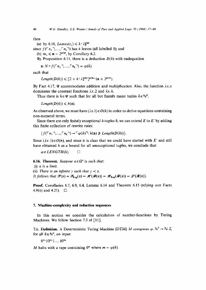
then (a) by 6.10, Leaves(&) < k-;l~(“’

since f(‘nll,..., ‘nkl) has k leaves (all labelled 0); and (b) m, < n + 29(n), by Corollary 6.2. By Proposition 6.11, there is a deduction D(G) with endequation

n: N kf(‘nll,...,‘nkl) = cp(fi)

such that

Length(D(A)) < [2 + k ; A@‘)]g(n)-(n + 2g(“‘).

By Fact 4.17, Q accommodates addition and multiplication, Also, the function 2x.x dominates the constant functions 1x.2 and Ix. k.

Thus there is hi% such that for all but finitely many tuples i’i~ Nk,

Length(D(ti)) < h(n).

As observed above, we must have (nx.1) E O(h) in order to derive equations containing non-numeral terms.

Since there are only finitely exceptional k-tuples ii, we can extend E to E’ by adding this finite collection of rewrite rules:

{jYn11,..., ‘nkl) + ‘cp(i?)l: h(n) 3 Length(D(ii))}.

Since (Ax. l)~O(h), and since it is clear that we could have started with E’ and still have obtained h as a bound for all unexceptional tuples, we conclude that

cp E LENGTH(h). 0

6.16. Theorem. Suppose CIEP is such that:

(i) CI is a limit. (ii) There is an infinite y such that y < a.

Itfollows that P(a) = &(a) = %(93(a)) = %&(99(a)) = 9(99(a)).

Proof. Corollaries 6.7, 6.9, 6.4, Lemma 6.14 and Theorem 6.15 (relying oon Facts

4.9(ii) and 4.21). 0

7. Machine-complexity and reduction sequences

In this section we consider the calculation of number-functions by Turing Machines. We follow Section 7.3 of [ll].

7.1. Definition. A Deterministic Turing Machine (DTM) M computes cp: Nk + N if, for all ii E Nk, on input

0”’ 10”’ 1 . . . 10””

M halts with a tape containing 0” where m = q(6).

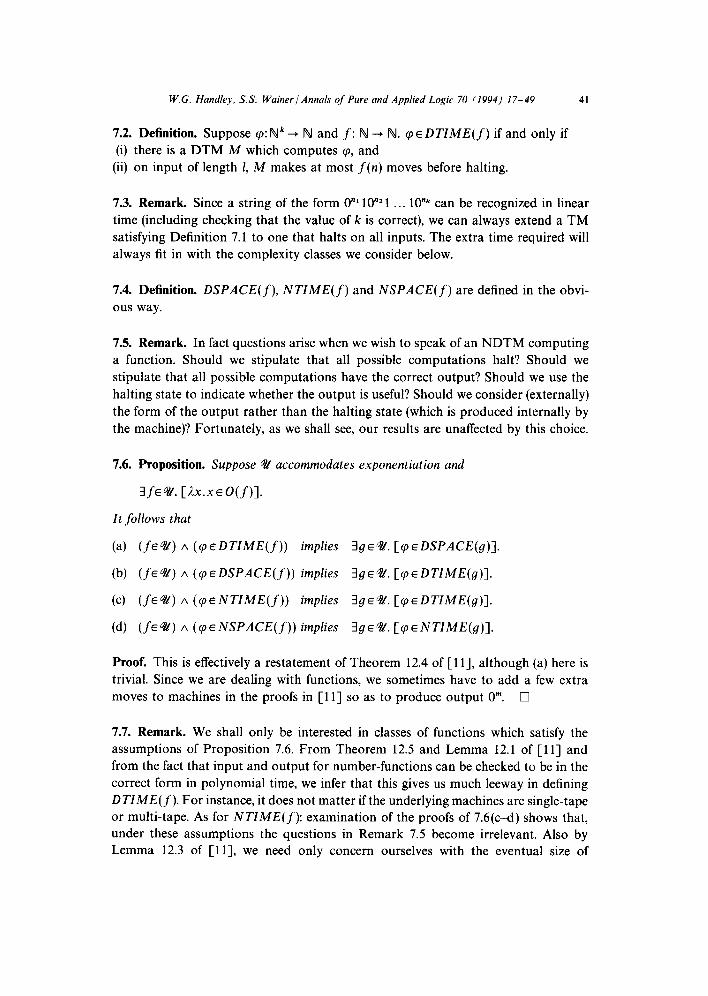
W.G. Handley, S.S. Wainer / Annals qf Pure and Applied Logic 70 (1994) 17-49 41

7.2. Definition. Suppose cp: Nk + N and f: lV + N. cp E DTZME(f) if and only if

(i) there is a DTM M which computes cp, and

(ii) on input of length 1, M makes at most f(n) moves before halting.

7.3. Remark. Since a string of the form 0”’ 10”’ 1 . . . lo”* can be recognized in linear

time (including checking that the value of k is correct), we can always extend a TM

satisfying Definition 7.1 to one that halts on all inputs. The extra time required will

always fit in with the complexity classes we consider below.

7.4. Definition. DSPACE(f), NTZME(f) and NSPACE(f) are defined in the obvi-

ous way.

7.5. Remark. In fact questions arise when we wish to speak of an NDTM computing

a function. Should we stipulate that all possible computations halt? Should we

stipulate that all possible computations have the correct output? Should we use the

halting state to indicate whether the output is useful? Should we consider (externally)

the form of the output rather than the halting state (which is produced internally by

the machine)? Fortunately, as we shall see, our results are unaffected by this choice.

7.6. Proposition. Suppose 42 accommodates exponentiation and

3fE42. [AX.X~O(f)].

It follows that

(a) (fee) A (~EDTZME(~)) implies 3ge%!. [qEDSPACE(g)].

(b) (f~4Y) A (~JEDSPACE(~)) implies 3gE44!. [qEDTZME(g)].

(c) (fe42) A (qeNTZME(j)) implies 3ge42. [qEDTZME(g)].

(d) (fee’) A (~~ENSPACE(~)) implies 3ge4. [qENTZME(g)].

Proof. This is effectively a restatement of Theorem 12.4 of [l 11, although (a) here is

trivial. Since we are dealing with functions, we sometimes have to add a few extra

moves to machines in the proofs in [l l] so as to produce output 0”. 0

7.7. Remark. We shall only be interested in classes of functions which satisfy the

assumptions of Proposition 7.6. From Theorem 12.5 and Lemma 12.1 of [ll] and

from the fact that input and output for number-functions can be checked to be in the

correct form in polynomial time, we infer that this gives us much leeway in defining

DTZME(f). For instance, it does not matter if the underlying machines are single-tape

or multi-tape. As for NTZME(f): examination of the proofs of 7.6(c-d) shows that,

under these assumptions the questions in Remark 7.5 become irrelevant. Also by

Lemma 12.3 of [ll], we need only concern ourselves with the eventual size of

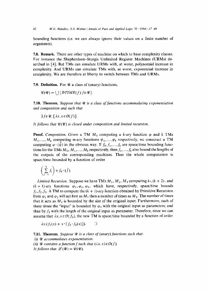
42 W.G. Handley. S.S. Wainer 1 Annals of Pure and Applied Logic 70 (1994) 17-49

bounding functions (i.e. we can always ignore their values on a finite number of

arguments).

7.8. Remark. There are other types of machine on which to base complexity classes.

For instance the Shepherdson-Sturgis Unlimited Register Machines (URMs) de-

scribed in [4]. But TMs can simulate URMs with, at worst, polynomial increase in

complexity. And URMs can simulate TMs with, at worst, exponential increase in

complexity. We are therefore at liberty to switch between TMs and URMs.

7.9. Definition. For ‘32 a class of (unary) functions,

%?(%) = u {DTzME(f):fE%}.

7.10. Theorem. Suppose that S is a class offinctions accommodating exponentiation

and composition and such that

3fE& [AX.XEO(f)].

It follows that %(a) is closed under composition and limited recursion.

Proof. Composition. Given a TM M,, computing a k-ary function cp and k TMs

M I,..., Mk computing m-ary functions $r, . . . . $k respectively, we construct a TM

computing cp 0 ($) in the obvious way. If fO,fi,. . . ,fk are space/time bounding func-

tions for the TMs M,, M 1,. . . , Mk respectively, then fi ,. . . ,fk also bound the lengths of

the outputs of the corresponding machines. Thus the whole computation is

space/time-bounded by a function of order

Limited Recursion. Suppose we have TMs MI, M2, M3 computing k-, (k + 2)-, and

(k + 1)-ary functions cpl, cpZ, (p3, which have, respectively, space/time bounds

fi ,fi ,f3. A TM to compute the (k + 1)-ary function obtained by Primitive Recursion

from (pr and (p2 will act first as MI then a number of times as Mz. The number of times

that it acts as M2 is bounded by the size of the original input. Furthermore, each of

these times the “input” is bounded by (p3 with the original input as parameters; and

thus by f3 with the length of the original input as parameter. Therefore, since we can

assume that %x.x E 0( f3), the new TM is space/time bounded by a function of order

7.11. Theorem. Suppose 4V is a class of (unary)functions such that:

(i) @ accommodates exponentiation.

(ii) % contains afunctionfsuch that (Ax.x)~O(f). It follows that Y(e) = %?(a).

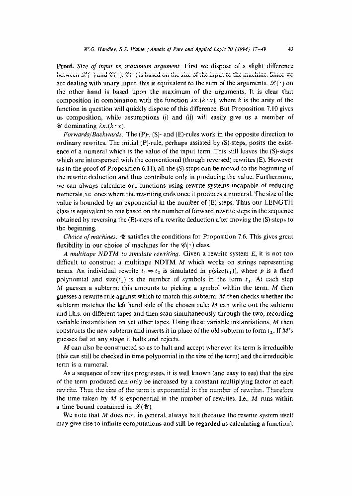
W.G. Handle?, S.S. Wainer / Annals of Pure and Applied Logic 70 (1994) 17-49 43

Proof. Size of input vs. maximum argument. First we dispose of a slight difference

between _Y( *) and U(a). %?( *) is based on the size of the input to the machine. Since we

are dealing with unary input, this is equivalent to the sum of the arguments. .Y( *) on

the other hand is based upon the maximum of the arguments. It is clear that

composition in combination with the function Jx.(k*x), where k is the arity of the

function in question will quickly dispose of this difference. But Proposition 7.10 gives

us composition, while assumptions (i) and (ii) will easily give us a member of

$2 dominating Ax.(k *x). Forwards/Backwards. The (P)-, (S)- and (E)-rules work in the opposite direction to

ordinary rewrites. The initial (P)-rule, perhaps assisted by (S)-steps, posits the exist-

ence of a numeral which is the value of the input term. This still leaves the (S)-steps

which are interspersed with the conventional (though reversed) rewrites (E). However

(as in the proof of Proposition 6.1 l), all the (S)-steps can be moved to the beginning of

the rewrite deduction and thus contribute only in producing the value. Furthermore,

we can always calculate our functions using rewrite systems incapable of reducing

numerals, i.e. ones where the rewriting ends once it produces a numeral. The size of the

value is bounded by an exponential in the number of (E)-steps. Thus our LENGTH

class is equivalent to one based on the number of forward rewrite steps in the sequence

obtained by reversing the (E)-steps of a rewrite deduction after moving the (S)-steps to

the beginning.

Choice of machines. 42 satisfies the conditions for Proposition 7.6. This gives great

flexibility in our choice of machines for the V( *) class.

A multitape NDTM to simulate rewriting. Given a rewrite system E, it is not too

difficult to construct a multitape NDTM M which works on strings representing

terms. An individual rewrite t1 =z= t2 is simulated in p(size(tl)), where p is a fixed

polynomial and size(t,) is the number of symbols in the term t,. At each step

M guesses a subterm: this amounts to picking a symbol within the term. M then

guesses a rewrite rule against which to match this subterm. M then checks whether the

subterm matches the left hand side of the chosen rule: M can write out the subterm

and 1.h.s. on different tapes and then scan simultaneously through the two, recording

variable instantiation on yet other tapes. Using these variable instantiations, M then

constructs the new subterm and inserts it in place of the old subterm to form t2. If M’s

guesses fail at any stage it halts and rejects.

M can also be constructed so as to halt and accept whenever its term is irreducible

(this can still be checked in time polynomial in the size of the term) and the irreducible

term is a numeral.

As a sequence of rewrites progresses, it is well known (and easy to see) that the size

of the term produced can only be increased by a constant multiplying factor at each

rewrite. Thus the size of the term is exponential in the number of rewrites. Therefore

the time taken by M is exponential in the number of rewrites. I.e., M runs within

a time bound contained in Y(e).

We note that M does not, in general, always halt (because the rewrite system itself

may give rise to infinite computations and still be regarded as calculating a function).

44 W.G. Handley, S.S. Wainer / Annals qf Pure and Applied Logic 70 (1994) 17-49

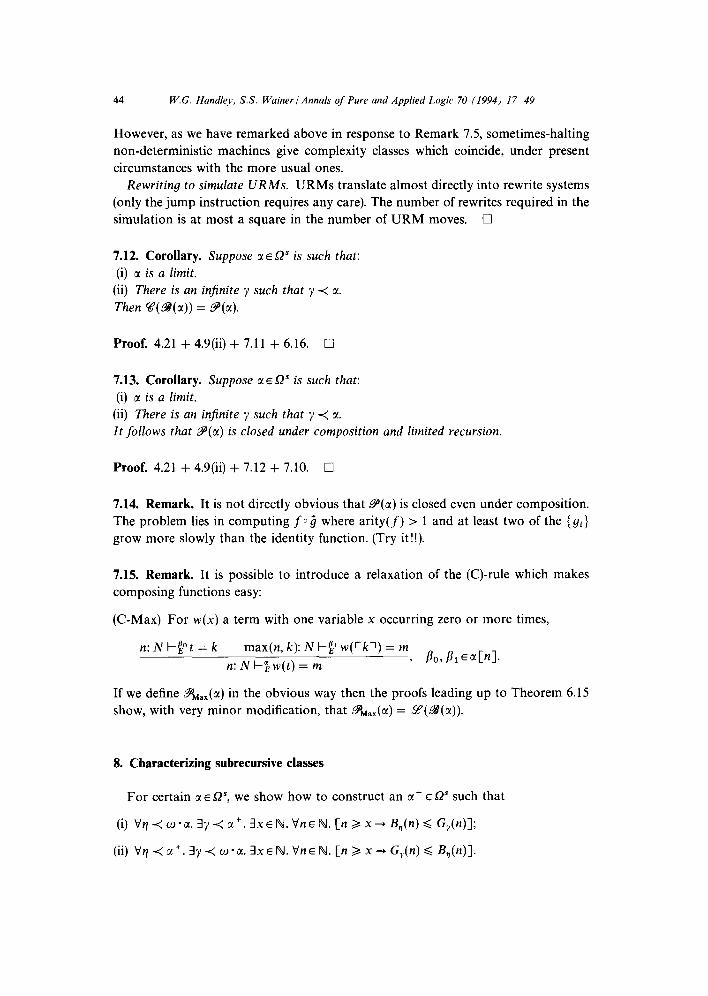
However, as we have remarked above in response to Remark 7.5, sometimes-halting

non-deterministic machines give complexity classes which coincide, under present

circumstances with the more usual ones.

Rewriting to simulate URMs. URMs translate almost directly into rewrite systems

(only the jump instruction requires any care). The number of rewrites required in the

simulation is at most a square in the number of URM moves. 0

7.12. Corollary. Suppose OIE 0” is such that:

(i) tl is a limit. (ii) There is an injinite y such that y < CL

Then %?(B(rx)) = Y(U).

Proof. 4.21 + 4.9(ii) + 7.11 + 6.16. Cl

7.13. Corollary. Suppose IXEW is such that:

(i) c( is a limit. (ii) There is an injinite y such that y < CI. It follows that P’(U) is closed under composition and limited recursion.

Proof. 4.21 + 4.9(ii) + 7.12 + 7.10. 0

7.14. Remark. It is not directly obvious that B(cc) is closed even under composition.

The problem lies in computing fog where arity(f) > 1 and at least two of the {gi}

grow more slowly than the identity function. (Try it!!).

7.15. Remark. It is possible to introduce a relaxation of the (C)-rule which makes

composing functions easy:

(C-Max) For w(x) a term with one variable x occurring zero or more times,

n:NFgt=k max(n, k): N I-$’ w(‘kl) = m

n: Nb-“,w(t) = m 3 SO? PI EaCnl.

If we define gMa,(or) in the obvious way then the proofs leading up to Theorem 6.15

show, with very minor modification, that YMax(~) = _Y(g(cr)).

8. Characterizing subrecursive classes

For certain CIEW, we show how to construct an IX+ ~52” such that

(i) Vq <w*cr. 3yi c1+. !IxEF~~.V~E~J(. [n 2 x+ B,(n) 6 G,(n)];

(ii) t/q < LX+. 3y < W-CL 3x~N. VnEFA. [n > x-+ G,(n) < B,,(n)].

W.G. Handley. S.S. Waker/Annals qf Pure and Applied Logic 70 (1994) 17-49 45

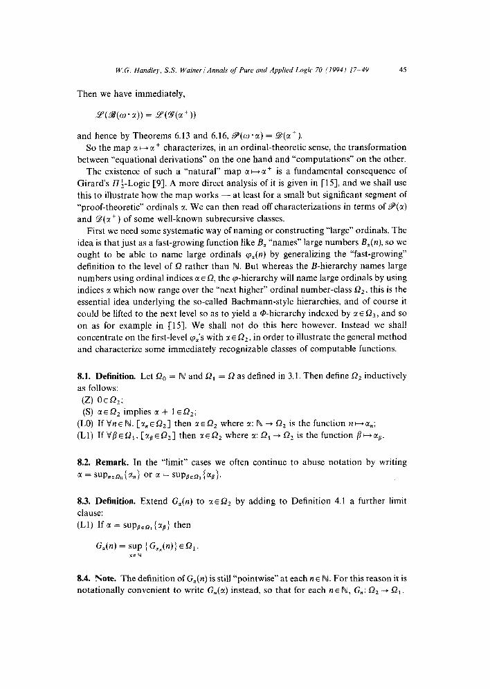
Then we have immediately,

LqLB(o-a)) = 8(9(a+))

and hence by Theorems 6.13 and 6.16, P(w*a) = Q(c1+).

So the map a H c1+ characterizes, in an ordinal-theoretic sense, the transformation

between “equational derivations” on the one hand and “computations” on the other.

The existence of such a “natural” map CI H CI + is a fundamental consequence of

Girard’s fl$Logic [9]. A more direct analysis of it is given in [15], and we shall use

this to illustrate how the map works - at least for a small but significant segment of

“proof-theoretic” ordinals CI. We can then read off characterizations in terms of P(c()

and g(a ‘) of some well-known subrecursive classes.

First we need some systematic way of naming or constructing “large” ordinals. The

idea is that just as a fast-growing function like B, “names” large numbers B,(n), so we

ought to be able to name large ordinals q,(n) by generalizing the “fast-growing”

definition to the level of 0 rather than N. But whereas the B-hierarchy names large

numbers using ordinal indices c( E Q, the q-hierarchy will name large ordinals by using

indices CI which now range over the “next higher” ordinal number-class Q2, this is the

essential idea underlying the so-called Bachmann-style hierarchies, and of course it

could be lifted to the next level so as to yield a @-hierarchy indexed by c( E Qsr and so

on as for example in [15]. We shall not do this here however. Instead we shall

concentrate on the first-level (pa’s with SI E fi2, in order to illustrate the general method

and characterize some immediately recognizable classes of computable functions.

8.1. Definition. Let C& = N and Szi = s2 as defined in 3.1. Then define Q2 inductively

as follows:

(Z) OeQ,; (S) aEQ2 implies tx + le52,;

(LO) If Vn E IV. [ol,, E Q,] then u E a2 where CI: N -+ 52, is the function n H cc,;

(Ll) If Vfl E Q,. [aB E Cl,] then CI E Q2 where CC: !Z?i + fi2, is the function p H CQ.

8.2. Remark. In the “limit” cases we often continue to abuse notation by writing

c( = su~~~~~(~) or a = su~p~~~(~).

8.3. Definition. Extend G,(n) to cres2, by adding to Definition 4.1 a further limit

clause:

(Ll) If CI = suppeR, {Q} then

G,(n) = sup { G&n)) E a,. X-EN

8.4. Note. The definition of G,(n) is still “pointwise” at each n E N. For this reason it is

notationally convenient to write G,(U) instead, so that for each IZE N, G,: Q2 -+ Q1.

46 W.G. Handle-v, S.S. Wainer/ Annals qf Pure and Applied Logic 70 (19943 17-49

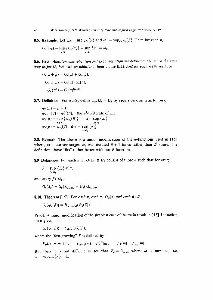
8.5. Example. Let w. = supxEN { } x an d oi = supBEn { j?}. Then for each ~1,

G,(w,) = sup {G,(x)} = sup {x} = WO. XSN xeN

8.6. Fact. Addition, multiplication and exponentiation are dejined on Q, in just the same

way as for Q1 but with an additional limit clause (Ll). And for each n E N we have

G,(~ + /3) = G,(a) + G,(Bk

G,(~*B) = G,(a)*G,(B)>

G, { crs) = G,(cx)~“‘~‘.

8.7. Definition. For CCEQ, define cpol: s2i + Sz, by recursion over CL as follows:

cpo(B) = P + 1; cp,+i(/?) = cp,Z”(/?), the 2s-th iterate of qa;

CPM = ~9: {cp.,(P)> ifE = sup k>; xeN

CPU) = S,(B) if@ = sup {MC). CERl

8.8. Remark. The above is a minor modification of the q-functions used in [15]

where, at successor stages, qa was iterated /I + 1 times rather than 28 times. The

definition above “fits” rather better with our B-functions.

8.9 Definition. For each n let O,(n) s R, consist of those c( such that for every

1 = sup {A,} 5 c1, <ERl

and every fi~s2,,

G,(&) = G,(kuq) = W~)W,.

8.10. Theorem [lS]. For each n, each cle02(n) and each ~EQ~.

G,(cp,(B)) = B,.cncol,(Gn(B)).

Proof. A minor modification of the simplest case of the main result in [15]. Induction

on CI gives

G,((P~(P)) = F,,w(G,(P))

where the “fast-growing” F is defined by

Fe(m) = m + 1, F,+ 1 Cm) = Fi”(m), Fl(m) = F~,,,W

But then it is not difficult to see that F, = B,.,, where o is now WO, i.e.

w = SUp,,N{X}. q

W.G. Handlep, S.S. Waker 1 Annals qf Pure and Applied Logic 70 (1994) 17-49 41

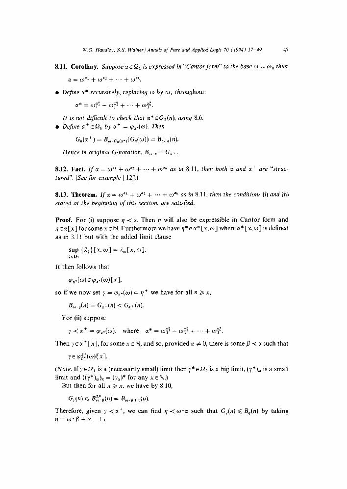
8.11. Corollary. Suppose CI E Q, is expressed in “Cantor form” to the base o = coo thus:

a = gal + (Jp + . . . + (g*

Dejine c1* recursively, replacing o by co, throughout:

m* = W”l’ + m”i’ + . . . + my’:.

It is not dij’icult to check that actor, using 8.6.

Dejine a+ ESZ, by u+ = q,*(w). Then

G,(a’) = &.w*)(G,(~J)) = L,(n).

Hence in original G-notation, B,., = G,+ .

8.12. Fact. Zf CI = d1 + d2 + ... + wak as in 8.11, then both z and a + are “struc-

tured”. (See for example [ 123.)

8.13. Theorem. If c1 = wal + waz + . . . + UP as in 8.11, then the conditions (i) and (ii)

stated at the beginning of this section, are satisjied.

Proof. For (i) suppose v] < cc Then r] will also be expressible in Cantor form and

q E a [x] for some x E N. Furthermore we have ye* E c(* [x, o] where c(* [x, w] is defined

as in 3.11 but with the added limit clause

sup {n&x, 01 = &Cx, 01. CEO1

It then follows that

so if we now set y = q,,.(w) = q+ we have for all n > x,

B,.,(n) = G,,+(n) < G,+(n).

For (ii) suppose

y<cr+ = q..(o). where c(* = (& + a”;’ + . . . + &“.

Then y E c1+ [xl, for some x E N, and so, provided a # 0, there is some /? < a such that

Y E cpp2W [xl.

(Note. If y E Q1 is a (necessarily small) limit then y* E Q2 is a big limit, (Y*)~ is a small

limit and ((y*),), = (yX)* for any x E N.)

But then for all n > x, we have by 8.10,

G,(n) < Bgfl(n) = B,.B+,(n).

Therefore, given y < a+, we can find q i w * LY. such that G,(n) < B,(n) by taking

yI=o’fl+x. 0

48 W.G. Hand1e.t.. S.S. Wainer 1 Annals qf Pure and Applied Logic 70 (1994) 17-49

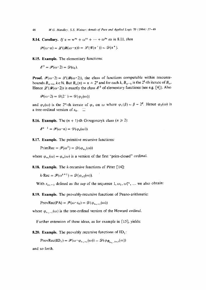
8.14. Corollary. 1f a = w”l + wZ2 + ... + wuk as in 8.11, then

Y(O’c() = Z(L?.3(o*cc)) = Y(S(x’)) = Q(a+).

8.15. Example. The elementary functions:

B3 = $70’2) = 9(&g).

Proof. Y(o - 2) = _Y(g(w - 2)), the class of functions computable within resource-

bounds Bofk, kc N. But B,(n) = n + 2” and for each k, B,+, is the 2k-th iterate of B,.

Hence LZ’( S?( o - 2)) is exactly the class g3 of elementary functions (see e.g. [4]). Also

9(W’2) = c@(2+) = ~((p~(O))

and (~~(0) is the 2”-th iterate of cpi on w where cp,(fl) = /3 + 2p. Hence (p*(o) is

a tree-ordinal version of aO. 0

8.16. Example. The (n + 1)-th Grzegorczyk class (n 2 2):

d “+I = 9(w*n) = 9(cp”(O)).

8.17. Example. The primitive recursive functions:

PrimRec = 9(02) = S(cp,,(w))

where cp,,(w) = cpw(w) is a version of the first “prim-closed” ordinal.

8.18. Example. The k-recursive functions of Peter [14]:

k-Ret = 9(gk+i) = 9(cpw:(o)).

With s,,+i defined as the sup of the sequence 1, w,, Q$‘, . . . we also obtain:

8.19. Example. The provably-recursive functions of Peano-arithmetic:

ProvRec(PA) = B(o-se) = 9(cp,,.,,+,(o))

where (Pi,,, + 1 (w) is the tree-ordinal version of the Howard ordinal.

Further extension of these ideas, as for example in [lS], yields:

8.20. Example. The provably recursive functions of IDi:

ProvRecUDi) = y(a * CP,,.,,+~(W)) = ~(c~~,,~**,,,,,,,(w))

and so forth.

W.G. Handley, S.S. Waker/Annals of Pure and Applied Logic 70 (1994) X7-49 49

References

[l] W. Buchholz, An independence result for l7:-CA + BI, Ann. Pure Appl. Logic 33 (1987) 131-155.

[Z] J.N. Crossley and J. Bridge Kister, Natural well-orderings, Arch. Math. Logik 26 (19867) 57776.

[3] E.A. Cichon, Termination orderings and complexity characterizations, in: P. Aczel, H. Simmons and

S. Wainer, eds., Proof Theory (Cambridge University Press, 1992) 171-193.

[4] N.J. Cutland, Computability: An Introduction to Recursive Function Theory (Cambridge University

Press, 1980).

[S] E.A. Cichon and S.S. Wainer, The slow-growing and the Grzegorczyk hierarchies, J. Symbolic Logic

48 (1983) 399-408.

[6] N. Dershowitz and M. Okada, Proof-theoretic techniques for term rewriting theory, in: Proceedings

of the Third Annual Symposium on Logic in Computer Science (Computer Society Press, Washing-

ton, DC, 1988), 104-l Il.

[7] E.C. Dennis-Jones and S.S. Wainer, Subrecursive hierarchies via direct limits, in: Computation and

Proof Theory, Proceedings, Logic Colloquium Aachen 1983, Part 11 (Springer, Berlin 1983) 399-408.

[8] J. Gallier, What’s so special about Kruskal’s theorem and the ordinal r,? A survey of some results in

proof theory, Ann. Pure Appl. Logic 53 (1991) 199-260.

[9] J.-Y. Girard, II:-Logic, Part 1: dilators, Ann. Math. Logic 21 (1981) 75-219.

[lo] A. Grzegorczyk, Some classes of recursive functions, Rozprawy Matematyczne 4 (1953).

[I I] J.E. Hopcroft and J.D. Ullman, Introduction to Automata Theory, Languages and Computation

(Addison-Wesley, Reading, MA, 1979).

[12] Kadota, Ph.D. Thesis, Hiroshima University, 1991.

[13] S.C. Kleene, Introduction to Metamathematics, sixth reprint (Walters-Noordhoff/North-Holland, Groningen/Amsterdam, 1971).

[14] R. Peter, Rekursive Funktionen (Verlag der Ungarischen Akademie der Wissenschaften, Budapest,

1957). English translation: Academic Press, New York, 1967.

[15] S.S. Wainer, Slow growing versus fast growing, J. Symbolic Logic 54 (1989) 6088614.

[16] A. Weiermann, Proving termination for term-rewriting systems, in: E. Biirger, G. Jlger, H. Kleine

Burring and M. Richter, eds., Computer Science Logic, Lecture Notes in Computer Science 626 (Springer, Berlin, 1991) 419-428.