Embed Size (px)
Citation preview
Filipe Miguel Cristo Sena
Bachelor of Computer Science and Engineering
Epistemic Game Master:A referee for GDL-III Games
Dissertation submitted in partial fulfillmentof the requirements for the degree of
Master of Science inComputer Science and Engineering
Co-advisers: João Leite,Associate Professor, NOVA University LisbonMichael Thielscher,Professor, University of New South Wales, Sydney
March, 2018

Epistemic Game Master:A referee for GDL-III Games
Copyright © Filipe Miguel Cristo Sena, Faculty of Sciences and Technology, NOVA Uni-
versity of Lisbon.
The Faculty of Sciences and Technology and the NOVA University of Lisbon have the
right, perpetual and without geographical boundaries, to file and publish this disserta-
tion through printed copies reproduced on paper or on digital form, or by any other
means known or that may be invented, and to disseminate through scientific reposito-
ries and admit its copying and distribution for non-commercial, educational or research
purposes, as long as credit is given to the author and editor.
This document was created unsing the (pdf)LATEX processor, based in the “unlthesis” template[1], developed at the Dep.Informática of FCT-NOVA [2]. [1] https://github.com/joaomlourenco/unlthesis [2] http://www.di.fct.unl.pt


To everyone that helped me in my jorney...One Master to rule them all.
Source: [One]


Acknowledgements
I would like to express my gratitude to everyone that supported me during the devel-
opment of this work. Firstly, to co-advisers: João Leite and Michael Thielscher, for all
the support, and for allowing me the opportunity to do this project. It was an absolute
pleasure to work under their guidance. I would also like to thank both FCT-UNL and
UNSW for allowing this project to be developed.
To my family that supported me day in and day out, keeping me on track to fulfill my
goals. To Gulbahar Bozan, my life, that supported me inconditionally and made sure I
had all the motivation necessary whenever I was lacking it.
To all my friends, specially: Francisco Pinto; Guilherme Rito; Nuno Martins; Bernardo
Albergaria and Tomás Rogeiro. To Armin Chitizadeh and Farhad Amouzgar, friends in
the other side of the world, from Michael’s research group which supported me with all
my nagging and brainstorming.
This thesis was partially funded by the ICM Erasmus + Project and NOVA.id.FCT.
vii

Abstract
General Game Playing is the field of Artificial Intelligence that designs agents that
are able to understand game rules written in Game Description Language and use them
to play those games effectively. A General Game Playing system uses a Game Master, or
referee, to control games and players. With the introduction of the latest extension of
GDL, the GDL-III enabled to describe epistemic games. However, the complexity of the
state space of these new games became in such way large that is impossible for both the
players and the manager to reason precisely about GDL-III games. One way to approach
this problem is to use an approximative approach, such as model-sampling.
This dissertation shows a Game Master that is able to understand and control games
in GDL-III and its players, by using model-sampling to sample possible game states. With
the development of this Game Master, players can be developed to be able to play GDL-III
games without human intervention.
Throughout this dissertation, we present details of our developed solution, how we
manage to make the Game Master understand a GDL-III game and how we implemented
model sampling. Furthermore, we show that our solution, however approximative, has
the same capabilities of an non approximative approach while given enough resources.
We show how the Game Master timely scales with increasingly bigger epistemic games.
Keywords: GGP; GDL; GDL-II; GDL-III; EGGP; Epistemic Logic; Model-sampling.
ix

Resumo
General Game Playing é o ramo da Inteligência Artificial que desenha agentes que
são capazes de perceber regras de um jogo, escritas na Game Description Language e
usam-nas para jogar esses jogos efectivamente. Um sistema de General Game Playing usa
um Game Master, ou árbitro para controlar os jogos e os jogadores. Com a introdução
da última extensão de GDL, o GDL-III deixa permite a descrição de jogos epistémicos.
No entanto, o tamanho necessário para manter esses estados todos ficou de certa forma
grande, que torna impossível para os jogadores e o árbitro raciocinarem com jogos em
GDL-III. Uma forma de contornar este problema é utilizando uma aproximação desse
espaço de estados como model-sampling.
Esta dissertação apresenta um Game Master que consegue entender e controlar um
jogo em GDL-III e os seus jogadores, usando model-sampling para testar possiveis estados
do jogo. Com o desenvolvimento deste Game Master, podem ser desenvolvidos jogadores
para jogar jogos em GDL-III sem intervenção humana.
Ao longo desta dissertação, apresentamos detalhes da nossa solução desenvolvida,
como conseguimos que o Game Master consiga compreender um jogo em GDL-III e como
implementamos o nosso model-sampling. Também, mostramos que a nossa solução de
ser aproximada, possui as mesmas capacidades que uma solução que considera todos os
estados do jogo, dados recursos suficientes. Mostramos também como este Game Master
escala com jogos epistémicos cada vez maiores.
Palavras-chave: GGP; GDL; GDL-II; GDL-III; EGGP; Epistemic Logic; Model-sampling.
xi

Contents
List of Figures xvii
1 Introduction 1
1.1 Structure . . . . . . . . . . . . . . . . . . . . . . . . . . . . . . . . . . . . . 4
2 Related Work 7
2.1 Game Theory . . . . . . . . . . . . . . . . . . . . . . . . . . . . . . . . . . . 7
2.1.1 Normal-Form . . . . . . . . . . . . . . . . . . . . . . . . . . . . . . 7
2.1.2 Perfect-Information Extensive Form . . . . . . . . . . . . . . . . . 10
2.1.3 Imperfect-Information Extensive Form . . . . . . . . . . . . . . . . 12
2.2 General Game Playing for Perfect Information . . . . . . . . . . . . . . . . 13
2.2.1 GDL . . . . . . . . . . . . . . . . . . . . . . . . . . . . . . . . . . . 14
2.2.2 General Game Master . . . . . . . . . . . . . . . . . . . . . . . . . . 16
2.2.3 Game Protocol . . . . . . . . . . . . . . . . . . . . . . . . . . . . . . 16
2.2.4 Strategy . . . . . . . . . . . . . . . . . . . . . . . . . . . . . . . . . . 17
2.3 General Game Playing for Imperfect Information . . . . . . . . . . . . . . 20
2.3.1 GDL-II . . . . . . . . . . . . . . . . . . . . . . . . . . . . . . . . . . 20
2.3.2 Game Protocol . . . . . . . . . . . . . . . . . . . . . . . . . . . . . . 21
2.3.3 Strategy . . . . . . . . . . . . . . . . . . . . . . . . . . . . . . . . . . 21
2.4 Epistemic General Game Playing . . . . . . . . . . . . . . . . . . . . . . . 26
2.4.1 GDL-III . . . . . . . . . . . . . . . . . . . . . . . . . . . . . . . . . . 27
2.4.2 Syntax . . . . . . . . . . . . . . . . . . . . . . . . . . . . . . . . . . 27
2.4.3 Semantics . . . . . . . . . . . . . . . . . . . . . . . . . . . . . . . . 27
2.5 Epistemic Logic . . . . . . . . . . . . . . . . . . . . . . . . . . . . . . . . . 29
2.5.1 Syntax . . . . . . . . . . . . . . . . . . . . . . . . . . . . . . . . . . 29
2.5.2 Semantics . . . . . . . . . . . . . . . . . . . . . . . . . . . . . . . . 29
2.6 Answer Set Programing . . . . . . . . . . . . . . . . . . . . . . . . . . . . . 31
3 An Epistemic Game Master 35
3.1 Problem Description . . . . . . . . . . . . . . . . . . . . . . . . . . . . . . 35
3.1.1 Requirements . . . . . . . . . . . . . . . . . . . . . . . . . . . . . . 36
3.2 Solution . . . . . . . . . . . . . . . . . . . . . . . . . . . . . . . . . . . . . . 36
3.3 Evolving to an Epistemic Architecture . . . . . . . . . . . . . . . . . . . . 40
xiii
CONTENTS
3.4 Server . . . . . . . . . . . . . . . . . . . . . . . . . . . . . . . . . . . . . . . 41
3.5 Knowledge . . . . . . . . . . . . . . . . . . . . . . . . . . . . . . . . . . . . 45
3.5.1 Indistinguishable Play Sequences . . . . . . . . . . . . . . . . . . . 45
3.5.2 Consistency . . . . . . . . . . . . . . . . . . . . . . . . . . . . . . . 46
3.5.3 Semantics . . . . . . . . . . . . . . . . . . . . . . . . . . . . . . . . 46
3.6 Sampling . . . . . . . . . . . . . . . . . . . . . . . . . . . . . . . . . . . . . 47
3.6.1 Random . . . . . . . . . . . . . . . . . . . . . . . . . . . . . . . . . 48
3.6.2 Perspective Shifting . . . . . . . . . . . . . . . . . . . . . . . . . . . 48
3.7 Plausibility . . . . . . . . . . . . . . . . . . . . . . . . . . . . . . . . . . . . 49
3.8 A Dynamic Epistemic Resample . . . . . . . . . . . . . . . . . . . . . . . . 51
3.9 Information Stealing . . . . . . . . . . . . . . . . . . . . . . . . . . . . . . 51
4 Analysis 53
4.1 Correction . . . . . . . . . . . . . . . . . . . . . . . . . . . . . . . . . . . . 53
4.1.1 Knowledge . . . . . . . . . . . . . . . . . . . . . . . . . . . . . . . . 53
4.1.2 Random Sampler . . . . . . . . . . . . . . . . . . . . . . . . . . . . 55
4.1.3 Perspective Sampler . . . . . . . . . . . . . . . . . . . . . . . . . . . 58
4.2 Scalability . . . . . . . . . . . . . . . . . . . . . . . . . . . . . . . . . . . . 60
4.2.1 Number Guessing Epistemic . . . . . . . . . . . . . . . . . . . . . . 60
4.2.2 Muddy Children . . . . . . . . . . . . . . . . . . . . . . . . . . . . . 62
4.2.3 Russian Cards Games . . . . . . . . . . . . . . . . . . . . . . . . . . 63
5 Conclusion 67
5.1 Future Work . . . . . . . . . . . . . . . . . . . . . . . . . . . . . . . . . . . 68
Bibliography 71
Webography 75
A Class Diagrams 77
A.1 Overview . . . . . . . . . . . . . . . . . . . . . . . . . . . . . . . . . . . . . 77
A.2 Terms Processor . . . . . . . . . . . . . . . . . . . . . . . . . . . . . . . . . 77
A.3 Dynamic Epistemic Sampler . . . . . . . . . . . . . . . . . . . . . . . . . . 78
A.4 Accessibility Relation Manager . . . . . . . . . . . . . . . . . . . . . . . . 78
A.5 Knowledge Verifier . . . . . . . . . . . . . . . . . . . . . . . . . . . . . . . 79
A.6 Dynamic Epistemic Knowledge Machine . . . . . . . . . . . . . . . . . . . 79
B Games used for Analysis 85
B.1 Number Guessing Epistemic . . . . . . . . . . . . . . . . . . . . . . . . . . 85
B.2 Muddy Children . . . . . . . . . . . . . . . . . . . . . . . . . . . . . . . . . 87
B.3 Russian Cards Games . . . . . . . . . . . . . . . . . . . . . . . . . . . . . . 89
C Hats Puzzle 97
xiv
CONTENTS
D Tested Problems 101
D.1 Player Knowledge uncertainty without percepts . . . . . . . . . . . . . . . 101
D.2 Player Knowledge without percepts . . . . . . . . . . . . . . . . . . . . . . 103
D.3 Steal the Ruby . . . . . . . . . . . . . . . . . . . . . . . . . . . . . . . . . . 105
D.4 Conjunction . . . . . . . . . . . . . . . . . . . . . . . . . . . . . . . . . . . 107
E Run the Game Master 111
xv

List of Figures
2.1 Matching Pennies . . . . . . . . . . . . . . . . . . . . . . . . . . . . . . . . . . 8
2.2 Battle of the Sexes . . . . . . . . . . . . . . . . . . . . . . . . . . . . . . . . . . 9
2.3 Subgame-perfect-equilibria . . . . . . . . . . . . . . . . . . . . . . . . . . . . 11
2.4 Imperfect-information extensive-form . . . . . . . . . . . . . . . . . . . . . . 12
2.5 Simple GGP sytem . . . . . . . . . . . . . . . . . . . . . . . . . . . . . . . . . 13
2.6 Game Manager for GDL-I . . . . . . . . . . . . . . . . . . . . . . . . . . . . . . 17
2.7 Monte Carlo Search . . . . . . . . . . . . . . . . . . . . . . . . . . . . . . . . . 18
2.8 Monte Carlo Tree Search Cycle . . . . . . . . . . . . . . . . . . . . . . . . . . . 19
2.9 Incomplete Mastermind Information Set . . . . . . . . . . . . . . . . . . . . . 22
2.10 Incomplete Mastermind Information Set Filtered . . . . . . . . . . . . . . . . 22
2.11 Epistemic Model M . . . . . . . . . . . . . . . . . . . . . . . . . . . . . . . . . 31
3.1 Sampling Approach . . . . . . . . . . . . . . . . . . . . . . . . . . . . . . . . . 37
3.2 Two Stage Semantics Approach . . . . . . . . . . . . . . . . . . . . . . . . . . 39
3.3 An Abstract Game and two game instances . . . . . . . . . . . . . . . . . . . 39
3.4 Epistemic Game Manager Modules . . . . . . . . . . . . . . . . . . . . . . . . 41
3.5 Plausibility . . . . . . . . . . . . . . . . . . . . . . . . . . . . . . . . . . . . . . 50
4.1 Number Guessing . . . . . . . . . . . . . . . . . . . . . . . . . . . . . . . . . . 61
4.2 Muddy Children 3 . . . . . . . . . . . . . . . . . . . . . . . . . . . . . . . . . . 62
4.3 Role Scalability . . . . . . . . . . . . . . . . . . . . . . . . . . . . . . . . . . . 63
4.4 Russian Cards Games . . . . . . . . . . . . . . . . . . . . . . . . . . . . . . . . 64
A.1 Overview . . . . . . . . . . . . . . . . . . . . . . . . . . . . . . . . . . . . . . . 81
A.2 Rules Processor . . . . . . . . . . . . . . . . . . . . . . . . . . . . . . . . . . . 82
A.3 Sampler . . . . . . . . . . . . . . . . . . . . . . . . . . . . . . . . . . . . . . . . 82
A.4 Accessibility Relation Manager . . . . . . . . . . . . . . . . . . . . . . . . . . 83
A.5 Knowledge Verifier . . . . . . . . . . . . . . . . . . . . . . . . . . . . . . . . . 83
A.6 Dynamic Epistemic Knowledge Machine . . . . . . . . . . . . . . . . . . . . . 84
xvii

Chapter
1Introduction
Artificial Inteligence (AI) — the field of computer science that studies intelligent agents,
has become essential to the modern world. From medical diagnosis where agents help
rendering an image of a tumour, self-driving cars to targeting online advertisements,
where an agent tries to evaluate the user preferences to present them with adverts that
they might be interested. Everything, in the modern world, uses some AI.
However, modern AI have been focused on solving specific problems that the devel-
oped agents lack the ability to perform those tasks under different circumstances. How
can an online advertisement agent differ from a Portuguese user preference from a Brazil-
ian? Since they share the same language, but would their tastes be the same? How can a
self-driving car adapt to rain, snow or fog? In all of the situations, the best solution might
be to reduce speed. However, snow might require different tires.
The fact that these agents perceive their environment and take actions that maximise
their success often leads to situations where if we change their environment, even just a
little, they will fail. The reason — problem — is that no matter the conditions they are in,
they lack the adaptability of a human being. They lack the ability to reason like a human.
There is a field within AI that addresses this problem. This field is called Artificial
General Inteligence (AGI). Agents are tested in different sets of environments and are
expected behave well on all of them. Notwithstanding, building an agent to test in a
real-world scenario can be very expensive, again like self-driving cars, or self-landing
rockets. These costly experiments are why a good solution is to develop agents to play
games.
Since the Bronze Age, where generals would test and learn new strategic skills by play-
ing Chess, that games where found useful to model different situations. Moreover, games
are used as real-life metaphors. E.g. Monopoly, however silly, is a financial metaphor of
the real world economics; Battleships, like Chess as a war metaphor.
1
CHAPTER 1. INTRODUCTION
Indeed, games are so famous for their properties, that since 1713 they have been
theoretically studied. Being later formalised as a mathematical discipline called Game
Theory (GT), where not only games are studied, but also interactions between agents. GT
is nowadays, the centre of the knowledge about games and interactions. It is so essential
that more than its scope being economics, where it was born from, it also affects political
sciences, psychology, as well as computer science [Mye97].
Despite studying games theoretically, it is necessary to develop agents that apply the
theory. General Game Playing for Perfect Information (GGP-I) is the domain, within
computer science, that develops agents to play games. The agents, general game players
(here merely players), play against each other in a full human free setting. They only
realise the game that they are going to play just minutes before it starts. Which means
that they are inserted on a new, different environment every time they play a different
game. Thus, needing to adapt to any game and without human intervention.
However, to have a human free game it is necessary to have not only players but also a
referee that controls the game. In GGP-I, this agent is often called a Game Manager (GM).
Without one it would be impossible to have a GGP-I system.
Albeit all, one question remains. How can players understand which the game they
are playing? For that was created the Game Description Language (GDL) [GT14]. This
language, as the name says, has the objective to describe any game. To specify a game
one has to identify and define the set of rules that characterise it. To understand which
kind of rules we are referring to, consider a game like the Tic-Tac-Toe. Such game has two
players, X and O. An initial state that is the board 3× 3 empty. Actions that one can do,
i.e. mark the board with the player’s particular mark. Middle states that which can be
achieved by making a move, e.g. after marking a X the X should always be characterised
in that board position. Terminal states and their payoffs, e.g. one draws if the board is
filled with X’s and O’s; or win for the player that completes its’ line. These game rules are
what is necessary to describe using GDL to define the Tic-Tac-Toe game. Notice that, even
though we use a game like the last, GDL allows the description of any perfect-information1
game, e.g. Chess, Checkers.
There are many strategies to play GDL games. The most basic is to assume a pes-
simistic approach. Since one does not know who is one is playing against, one cannot
expect that the adversary will behave rationally. This strategy is called the Minimax. A
player tries to maximise their payoff while assuming that others will try anything to min-
imise it. This game strategy is one of many that work by exploring all possible states of a
game to find the best move. So, for a simple case like Tic-Tac-Toe, that has a small number
of states, this strategy suffices since it can be computed. However, would it be able to be
computed in a game of Go? In this game, the set of possible states is so large2 that search-
ing the entire game space is impossible. Because of games like this, that have so many
1Game theory term that refers to games were each agent, when choosing an action, is perfectly informedof all the events that have occurred previously, and the initial state of the game
2A board of Chess has 8×8 and leads to 1030 possible states. A board of Go has 19×19 intersecting lines
2
possible states, those other strategies were developed. One that is worth mentioning is
the Monte Carlo strategy. This strategy consists of, instead of searching all possibilities
like the Minimax, probing to explore which is the best move.
A problem with GDL is that even though players do not know who are they playing
against, they can see the moves that they make. However, much like a human, an agent
is expected to conclude what is its best outcome even on tasks where uncertainty is
associated. Several games serve as an abstraction to such case. For example, a game of
Poker like Texas Hold’em. At the beginning of this game, each player does not see the card
of their opponents. A game like this is called imperfect-information3 game and cannot be
described using GDL. For that purpose was created an extension, the Game Description
Language for games with Imperfect Information (GDL-II) [Thi11a]. We can find many
games that belong to this category, e.g. Mastermind (see section 2.3.1), Battle Ships, Blind
Tic-Tac-Toe, Blind Chess, as well as most4 card games.
Under this imperfect information environment, even though previous methods can
still work, they are not necessarily good. Because the setting in which players are pre-
sented to play in changes. One approach is useful in imperfect-information is the use of
an Information Set. This approach comes from the definition of an imperfect information
game in GT. More precisely, players consider every possible state where they could be at
some time in the game and filter them whenever they obtain new information5. Most of
the strategies used on GDL-II have as the basis of using an information set. The problem
with this is that maintaining the set of all the possible states that a player could be that
at some point, might be too large and will just not work. Remember the previous note: a
game of Chess has 1030 possible states. What about Blind Chess? The set of possible states
is even larger. Because of that, it was developed a solution called HyperPlay (HP) [ST15]
(see section 2.3.3.1), that involves keeping only a subset of incomplete states6 instead of
the all possible incomplete states of information set. This solution uses a technique called
model-sampling, which as the name implies, involves completing the incomplete states
and testing them.
However, much like we said before regarding GDL, GDL-II also has a limitation. It
does not support the specification of games where the rules depend on the epistemic state
of players — the description of an epistemic game. An epistemic state is defined by what
the player know at that state, i.e. imagine that we were given a bag that does not show
what is inside. This bag contains a ball that can either be red or blue. Unfortunately,
while is inside the bag all that we know is that it is a ball. Hence, our epistemic state is
defined by that we know that inside the bag is a ball. However, the property of the colour
is not part of our epistemic state since we cannot distinguish if it is red or blue, while it
is inside the bag.
3Game theory term that refers to games where each player, even though they know the initial state ofthe game, they do not know accurately in which state they are in
4Requires at least one: shuffling or not showing the cards to an opponent5Imperfect-information does not mean any information at all6Since, one does not know in which state he is in, it is safe to conclude that one is in an incomplete state
3
CHAPTER 1. INTRODUCTION
This new extension, the Game Description Language for games with Imperfect In-
formation and Introspection (GDL-III) [Thi16] forces players to reason with their and
the opponents’ epistemic state. Forces them to be rational. Remember the last example
of Blind Chess? Where the state space already enormous? What if we had the players’
epistemic state to the mixture? One game state7 can have many epistemic states. Which
means that there is an unmeasurable amount states8 in the game.
A simple example of an epistemic game is the Russian Cards Problems[Cor+13]. It
states that, from a deck of seven distinct cards, Alice and Bob are each dealt three cards,
and Cathy is dealt the remaining card. None of the players knows any of the cards of the
other players. Using a series of truthful public announcements, Alice and Bob should
exchange information about the hands they hold without Cathy being able to deduce the
owner of any card other than her own.
This example shows that players will always need to calculate what they know, and
their opponents’ know. One way to do it is with an Epistemic Logic principle called
indistinguishability. This principle says that a player knows something, if and only if it
can see that, in all the states in its information set. Some reasoners allow us to reason
with epistemic logic, such as Answer Set Programming (ASP). However, such solutions
consider all possible states, which as we already stated is impossible to maintain, because
the state space is unmeasurable large.
A GM for both GDL and GDL-II only have one state to update — the game instance
being played. However, by players having to reason about their knowledge, it is necessary
for the GM to be able to deduce if players know something. This means that the GM
needs to consider the same game space as the players. Therefore, unlike the previous GM,
a referee for GDL-III raises some issues.
The primary objective of this dissertation is to present a new GM for Epistemic Gen-
eral Game Playing (EGGP), which allows players to play games in GDL-III. This GM
implements the semantics of GDL-III. We present a GM that samples the game states,
since keeping track of all of them is impossible.
The primary beneficiaries of this dissertation are the EGGP community since it allows
the community to be able to develop new players to play epistemic games. Players can
use parts of our developed solution to be able to play a GDL-III game. Even more, AGI
also benefits from this dissertation since it belongs to their scope.
1.1 Structure
The remainder of this document is structured as follows:
• Chapter 2 presents the related work, with GT; GGP-I; General Game Playing for Im-
perfect Information (GGP-II); EGGP; Epistemic Logic and ASP, already mentioned7For simplicity, let’s make a distinction between the state in the game for a player and his epistemic
states, even though they are all different states of the game8From now on, we consider that every time the epistemic state changes, it is a new state of the game
4
1.1. STRUCTURE
in this chapter;
• Chapter 3 describes our implementation of the GM, from a broader perspective into
a more detailed one;
• Chapter 4 shows the analysis of our solution;
• Chapter 5 presents our conclusions to this dissertation, as well as, it suggests a set
of improvements, that can be developed towards the future.
5

Chapter
2Related Work
In this chapter we explore the state of the art concerning the basics of the technologies
that relate to our intended work. We start by describing the very basics of game theory
necessary for the understanding of our work, like the normal-form, perfect-information
extensive-form and imperfect-information extensive-for, as well as, the equilibrium. We
then, explore each version of general game playing, going in each version to GDL, the
game protocol and strategies used by the players. Moreover we present epistemic logic
and a special reasoner for epistemic logic: ASP.
2.1 Game Theory
GT is the mathematical study of interaction among independent self-interested agents [LS08].
It is mainly studied by mathematicians, economists and computer scientists, but is acquir-
ing more interest in other disciplines like political science or sociology. On this subsection
we will present the basics of GT necessary for a better understanding of our work.
2.1.1 Normal-Form
The normal-form is the simplest form used to represent a game in GT. On this form,
games are assumed to have only one turn and players have to play their actions at the
same time. This form is defined as [LS08]:
Definition 1. A finite n-person normal-form game is a tuple (N,A,u) where:
N is the finite set of n players, indexed by i;
A = A1 × ... × An where Ai is a finite set of available actions to player i, and every a =
(a1, ..., an) ∈ A is called an action profile;
u = (u1, ...,un) where ui : A→R is the payoff function for player i.
7
CHAPTER 2. RELATED WORK
Because of the characteristics of the games that this form describes, the games repre-
sentation usually acquires the image of a matrix. Moreover, any game can be described
using this form. No matter the kind of game that it is. For a better understanding con-
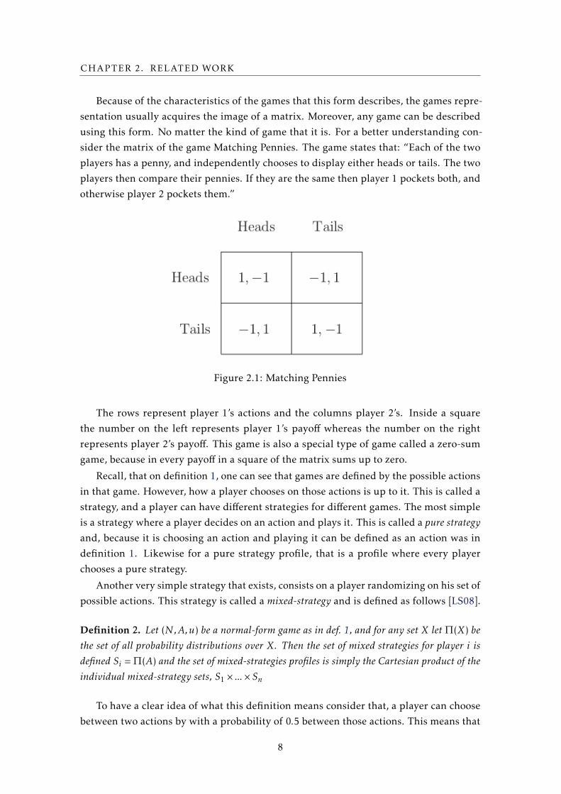
sider the matrix of the game Matching Pennies. The game states that: “Each of the two
players has a penny, and independently chooses to display either heads or tails. The two
players then compare their pennies. If they are the same then player 1 pockets both, and
otherwise player 2 pockets them.”
Figure 2.1: Matching Pennies
The rows represent player 1’s actions and the columns player 2’s. Inside a square
the number on the left represents player 1’s payoff whereas the number on the right
represents player 2’s payoff. This game is also a special type of game called a zero-sum
game, because in every payoff in a square of the matrix sums up to zero.
Recall, that on definition 1, one can see that games are defined by the possible actions
in that game. However, how a player chooses on those actions is up to it. This is called a
strategy, and a player can have different strategies for different games. The most simple
is a strategy where a player decides on an action and plays it. This is called a pure strategyand, because it is choosing an action and playing it can be defined as an action was in
definition 1. Likewise for a pure strategy profile, that is a profile where every player
chooses a pure strategy.
Another very simple strategy that exists, consists on a player randomizing on his set of
possible actions. This strategy is called a mixed-strategy and is defined as follows [LS08].
Definition 2. Let (N,A,u) be a normal-form game as in def. 1, and for any set X let Π(X) bethe set of all probability distributions over X. Then the set of mixed strategies for player i isdefined Si = Π(A) and the set of mixed-strategies profiles is simply the Cartesian product of theindividual mixed-strategy sets, S1 × ...× Sn
To have a clear idea of what this definition means consider that, a player can choose
between two actions by with a probability of 0.5 between those actions. This means that
8
2.1. GAME THEORY
half of the time he will play an action, the other half he will play the other. This is mixed
strategy.
The objective of a player is to always maximize his payoff. Unfortunately, on a multi-
player game, one’s payoffs depend of the move of other players, who are also trying to
maximize their payoffs. So it is safe to reason that one’s best strategy depends on the
choices made by others. For the same reason one can simplify the problem. That is,
if our best payoff depends on the other player play, then let us assume that he already
played. Hence, our player would only have to select the move that maximizes his utility
according to what the other player did. In other words it is his best response to that play.
The definition goes like this [LS08] (Adapted):
Definition 3. Let s¬i = (s1, ..., si−1, si+1, ..., sn) be a strategy profile without i’s strategy, thusbeing able to define s = (si , s¬i). Then, player i’s best response to the strategy profile s¬i is amixed strategy s∗i ∈ Si such that ui(s∗i , s¬i) ≥ ui(si , s¬i) for all strategies si ∈ Si
A best response doesn’t have to be unique. And they can be pure strategies or even
mixed-strategies.
The definition 3 helps defining the most basic principle in GT for non cooperative
games and more specifically zero-sum games, the Nash Equilibrium [LS08].
Definition 4. A strategy profile s = (s1, ..., sn) is a Nash Equilibrium if, for all agents i, si is abest response to s¬i .
This states that, a strategy profile is a Nash Equilibrium if no player wants to change
his action regarding what the other player do. Hence, we can call it a stable strategy
profile, since everybody is happy with their decision.
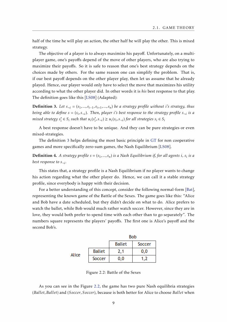
For a better understanding of this concept, consider the following normal-form [Bat],
representing the known game of the Battle of the Sexes. The game goes like this: “Alice
and Bob have a date scheduled, but they didn’t decide on what to do. Alice prefers to
watch the ballet, while Bob would much rather watch soccer. However, since they are in
love, they would both prefer to spend time with each other than to go separately”. The
numbers square represents the players’ payoffs. The first one is Alice’s payoff and the
second Bob’s.
Figure 2.2: Battle of the Sexes
As you can see in the Figure 2.2, the game has two pure Nash equilibria strategies
(Ballet,Ballet) and (Soccer,Soccer), because is both better for Alice to choose Ballet when
9
CHAPTER 2. RELATED WORK
Bob chooses Ballet, since she would receive a payoff of zero instead of two. By the same
reasoning Bob should do the same when Alice chooses Ballet. The other Nash equilibrium
can be justified using the same reasoning for Soccer.
There’s also mixed Nash equilibria, since Bob could play (Ballet,Soccer) with a prob-
ability of 13 for Ballet and 2
3 for Soccer. The probability changes when we look to Alice’s
side 23 for Ballet and 1
3 for Soccer.
Even though, agents can assume something about the opponent strategies, they don’t
known effectively what’s that the opponent are going to do. So sometimes the best strategy
is the one that maximizes the worst-case scenario. That strategy is called the Maxminstrategy [LS08].
Definition 5. The maxmin strategy for player i is argmaxi min¬i ui(si , s¬i) and the maxminvalue for player i is maxi min¬i ui(si , s¬i)
This strategy can be understood as player i makes the first move and then the other
players will try to minimize it. Even if the other players play arbitrarily, i will receive at
least his maxmin value.
The interesting part is that, according with the Minimax theorem [VN27], in a finite
two player zero-sum game each player receives a payoff that is equal to both his maxmin-
value and his minimax-value. And they are in fact a nash equilibrium [LS08].
2.1.2 Perfect-Information Extensive Form
The perfect information extensive form is a representation that doesn’t assume that play-
ers have to play at the same time. A perfect information game can be interpreted a tree
where each node represents a choice of one of the players, an edge represents a possi-
ble action, and each leaf represents the terminal node where each player has his payofffunction. The formal definition of the perfect information extensive form is [LS08]:
Definition 6. A perfect-information game in the extensive-form is a tupleG = (N,A,H,Z,χ,ρ,σ ,u)
where:N is the set of players;A is the single set of actions;H is the set of nonterminal choice nodes;Z is the set of terminal nodes (disjoint from H);χ :H → 2A is the action function that assings to each choice node a set of possible actions;ρ :H →N is the player function, which assigns each nonterminal node a player i ∈N who
chooses an action in that node;σ :H ×A→H ∪Z is the successor function, which maps a choice node and an action to a
new choice or a terminal node such that for all h1,h2 ∈H and a1, a2 ∈ A if σ (h1, a1) = η(h2, a2),then h1 = h2 and a1 = a2; and
u = (u1, ...,un) where ui : Z→R is the payoff function for player i on the terminal nodes Z.
10
2.1. GAME THEORY
It is an extensive form, so every game on this form can be changed into a game in
the normal-form described in Definition 1, but not without having redundancy. This
representation is much smaller than the normal-form, and can be more natural to reason
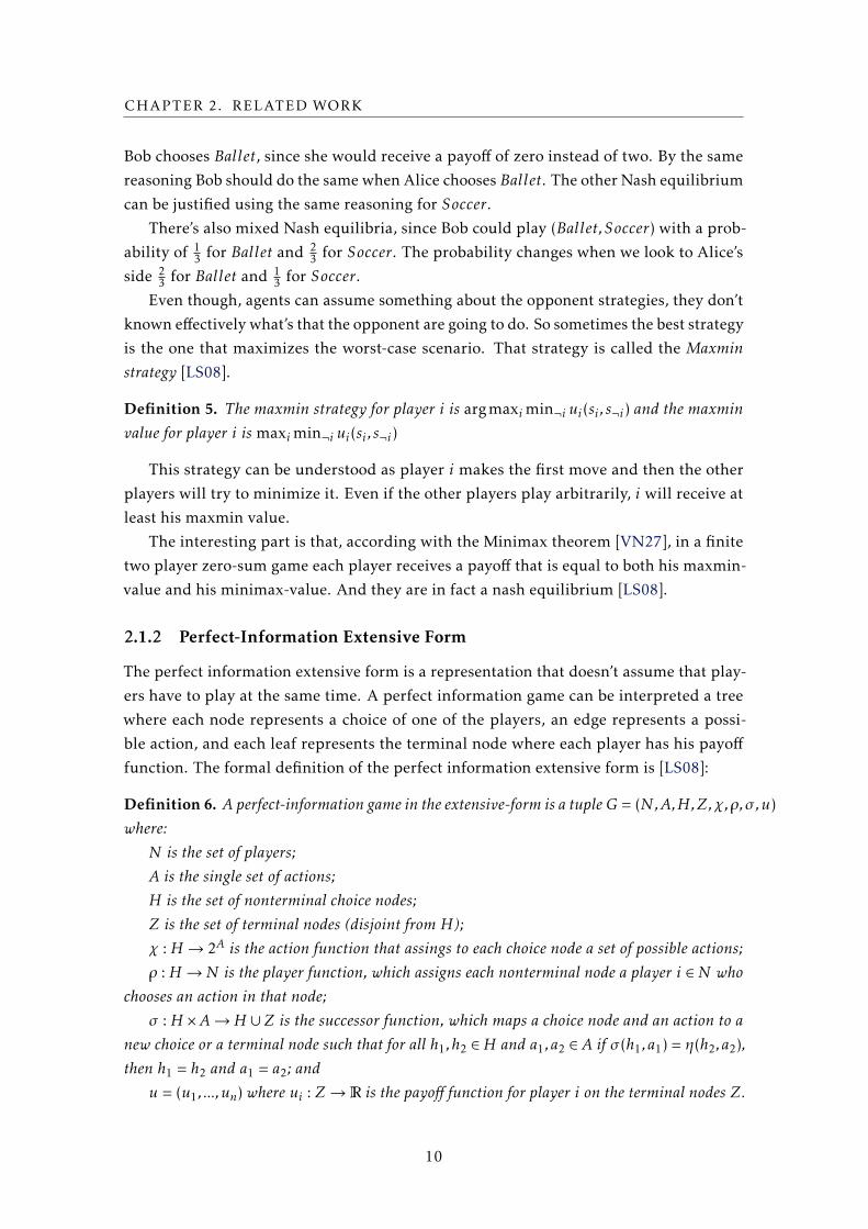
with. Consider the Figure 2.3. The game is interpreted as player 1 chooses one move
between: A,B and the player 2 chooses one move for each node: Y ,Z.
Figure 2.3: Subgame-perfect-equilibria
All the strategies considered in the normal-form work in this new form, but one
thing needs to be consistent. That’s the equilibria. However, there can be more nash
equilibria in this extensive-form, that might not be an optimal strategy profile. Consider
the previous Figure shown. It has two nash equilibria: A, (Z,Z) and B(Z,Y ). But notice,
the A, (Z,Z). Is it really possible that player 2, on his right most node will choose option Z,
when Y gives him a better payoff? The answer is no. This is why is necessary to introduce
a notion of subgame-perfect equilibrium. The equilibria needs to be consistent with the
subgame or subtree after each action. Before defining a subgame-perfect equilibria, one
needs to formally define a subgame [LS08]:
Definition 7. Given a perfect-information extensive-form game G as in def. 6, the subgameof G rooted at node h is a restriction of G to the descendants of h. The set of subgames of Gconsists of all of subgames of G rooted at some node of G
Simply speaking, a subgame is the game considered as in begining of the node that the
last action took us to. Then one can finally define a subgame-perfect equilibrium [LS08]:
Definition 8. The subgame-perfect equilibria (SP E) of a gameG as in def. 6 are all the strategyprofiles s such that for any subgame G
′of G, the restriction of s to G
′is a Nash equilibrium of
G′.
11
CHAPTER 2. RELATED WORK
Intuitively speaking, for a strategy profile be a SP E it must be a nash equilibria in ev-
ery subgame from: the root of the game, passing through all the decision nodes consistent
with the strategy profile.
A SP E is normally deduced by backward induction from the various outcomes of
the game. It eliminates branches which would involve any player making a move that
is not viable (because it is not optimal) from that node. A game in which the backward
induction solution is well known is Tic-Tac-Toe.
2.1.3 Imperfect-Information Extensive Form
In the previous section, games where in an environment of perfect-information, but there
are some situations where players need act with partial or no knowledge of what other
players did. This new extensive-form is an extension of the perfect-information extensive
form where nodes are splited into information sets. So if, two nodes belong on the same
set of the same player, then that player cannot see any difference between them. The
imperfect-information extensive-form is defined as follows [LS08]:
Definition 9. An imperfect-information game in the extensive-form is a tupleG = (N,A,H,Z,χ,ρ,σ ,u, I)
where:
G = (N,A,H,Z,χ,ρ,σ ,u) is a perfect-information extensive-form game; and
I = (I1, ..., In), where Ii = (Ii,1, ..., Ii,ki ) is and equivalence relation (i.e. partition of){h ∈H : ρ(h) = i
}with the property that χ(h) = χ(h
′) and ρ(h) = ρ(h
′) whenever it exists an j for which h ∈ Ii,j
and h′ ∈ Ii,j
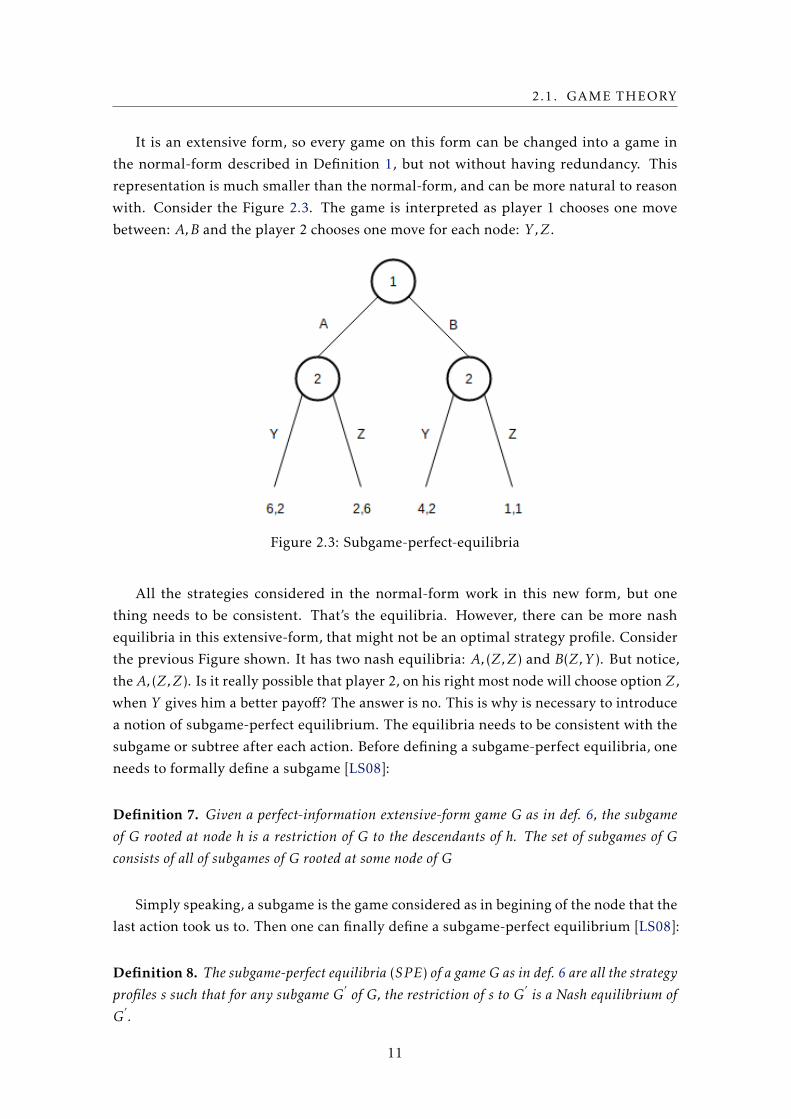
As an example of a game in this form, consider the following Figure 2.4, representing
a game in the imperfect-information extensive-form:
Figure 2.4: Imperfect-information extensive-form
12
2.2. GENERAL GAME PLAYING FOR PERFECT INFORMATION
The difference between this form and the last is that the two nodes of player two are
in his information set. This means that now he cannot see any difference between them.
As we can see, both this form and the last form are very similar, so one might think that
SP E would still work. That is not the case anymore. Because, the SP E was a constriction
of the possible equilibrias in a game of perfect-information. However, since players don’t
know where they are, they not only have a game to consider, but several games as well.
In other words we have a set of subgames. So, it is necessary to do a relaxation of these
possible equilibria. This is called a Sequential Equilibrium. It can be defined as [LS08]:
Definition 10. A strategy profile S is a sequential equilibrium of an extensive-form game Gas in def. 9, if there exists probability distribution µ(h) for each information set h in G, suchthat the following two conditions hold:
(S,µ) = limn→∞(Sn,µn) for some sequence (S1,µ1), (S2,µ2), ... where Sn is fully mixed, andµn is consistent with Sn (in fact, since Sn is fully mixed, µn is uniquely determined by Sn); and
For any information set h belonging to agent i, and any alternative strategy S′
i of i, we havethat
ui(S |h,µ(h)) ≥ ui((S′,S¬i)|h,µ(h)).
We can think about this equilibrium like this: the first condition consists in the mod-
ulation of the players’ beliefs about where they are in the tree for every information set;
the second condition can be interpreted as: the modulation of the players beliefs’ is not
contradicted by the actual play of the game and so, the players always best respond to
their beliefs.
2.2 General Game Playing for Perfect Information
As said in the Chapter 1, a GGP-I is a system that receives a game description at runtime.
This player has to interpret it and play accordingly. But, in order to be able to play a
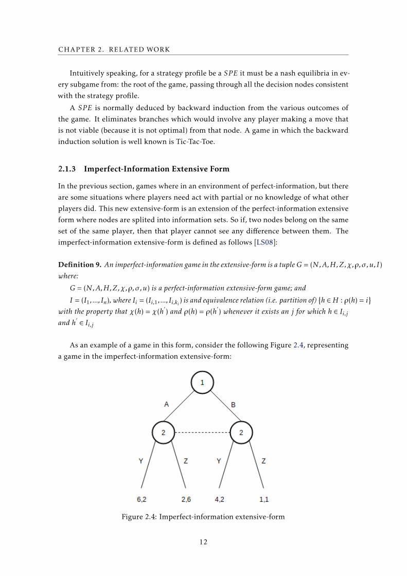
game, more elements are necessary. Specifically a GM and a Game Protocol (GP).
Figure 2.5: Simple GGP sytem
A GGP-I system can be viewed in the Figure 2.5. The GM is the entity that regulates
the game, according to the game description. This system conserves the actual state of
13
CHAPTER 2. RELATED WORK
the game, decides if the players moves are legal and if not selects one at random. The
communication with players is through HTTP connections using the GP. In the Figure,
we are only showing one player, but this player represents any player.
2.2.1 GDL
GDL is a language that allows the description of any perfect-information extensive form
from GT. It is a pure declarative language that allows: constants, variables, functions and
relations. Variables have to begin with an uppercase letter, while constants, functions
and relations must start with a lowercase1.
A GDL description is formed with a set of logical sentences that must be true in every
state of the game[Lov+08].
2.2.1.1 Syntax
GDL is an open language in the sense that, the vocabulary can be extended. However, the
meaning of these basic vocabulary items is fixed for all games. Those words are:
• role (R) — R is a player;
• init (P) — P is true in the initial state;
• true (P) — P is true in the current state;
• legal (R, A) — player R can do action A in the current state;
• does (R, A) — player R does action A
• next (P) — P is true in the next state;
• distinct (P1, P2) — P1 is be different of P2;
• terminal — current state is terminal;
• goal (R, V) — player R has a payoff V.
GDL also allows the use of 101 numbers. They go from 0 to 100 in decimal base. The
0 is considered the lowest and 100 the highest. These numbers are used to describe payoffV on goal rules and usually a step counter representing a turn.
Notice that, in GGP-I every player has to make an action every round, unlike a perfect-
information game in GT, which is turn base. However, GDL allows the description of
rules where the meaning of the rule is that the players is skipping turn. This rule is often
called no-operation, or noop.
Recall in the Chapter 1, where we debated about the set of rules that was necessary
to describe the Tic-Tac-Toe game. The following is the presentation of a possible game
description of those rules, available in [Lov+08]:1For a better understanding of the game rules we will use infix GDL instead of prefix GDL
14
2.2. GENERAL GAME PLAYING FOR PERFECT INFORMATION
1 % t h e r o l e s2 role ( xplayer )
3 role ( oplayer )
4
5 % i n i t i a l s t a t e s6 i n i t ( c e l l ( 1 , 1 , b ) )
7 i n i t ( c e l l ( 1 , 2 , b ) )
8 i n i t ( c e l l ( 1 , 3 , b ) )
9 i n i t ( c e l l ( 2 , 1 , b ) )
10 i n i t ( c e l l ( 2 , 2 , b ) )
11 i n i t ( c e l l ( 2 , 3 , b ) )
12 i n i t ( c e l l ( 3 , 1 , b ) )
13 i n i t ( c e l l ( 3 , 2 , b ) )
14 i n i t ( c e l l ( 3 , 3 , b ) )
15 i n i t ( c o n t r o l ( xplayer ) )
16
17 % l e g a l moves f o r each p l a y e r i f t h e board i s empty18 l e g a l (W, mark (X, Y ) ) :− true ( c e l l (X , Y , b ) ) & true ( c o n t r o l (W) )
19
20 % l e g a l moves o f t h e p l a y e r i f i s t h e o t h e r p l a y i n g21 l e g a l ( xplayer , noop ) :− true ( c o n t r o l ( oplayer ) )
22 l e g a l ( oplayer , noop ) :− true ( c o n t r o l ( xplayer ) )
23
24 % next s t a t e t h e c e l l has a mark i f t h e p l a y e r marked a c e l l and25 % t h a t c e l l was b lank26 next ( c e l l (M, N, x ) ) :− does ( xplayer , mark (M, N) ) & true ( c e l l (M, N, b ) )
27 next ( c e l l (M, N, o ) ) :− does ( oplayer , mark (M, N) ) & true ( c e l l (M, N, b ) )
28
29 % i n e r t i a − a l l t h e c e l l s c o n s e r v e t h e i r mark f o r t h e next s t a t e30 next ( c e l l (M, N, W) ) :− true ( c e l l (M, N, W) ) & d i s t i n c t (W, b )
31 next ( c e l l (M, N, b ) ) :− does (W, mark ( J , K) ) & true ( c e l l (M, N, b ) ) & d i s t i n c t (M, J )
32 next ( c e l l (M, N, b ) ) :− does (W, mark ( J , K) ) & true ( c e l l (M, N, b ) ) & d i s t i n c t (N, K)
33
34 % p l a y e r s turn s w i t c h e v e r y round35 next ( c o n t r o l ( xplayer ) ) :− true ( c o n t r o l ( oplayer ) )
36 next ( c o n t r o l ( oplayer ) ) :− true ( c o n t r o l ( xplayer ) )
37
38 % t e r m i n a l s t a t e s39 terminal :− l i n e (W)
40 terminal :− ~open
41
42 % g o a l s43 goal ( xplayer , 100) :− l i n e ( x ) & ~ l i n e ( o )
44 goal ( xplayer , 50) :− ~ l i n e ( x ) & ~ l i n e ( o )
45 goal ( xplayer , 0) :− ~ l i n e ( x ) & l i n e ( o )
46 goal ( oplayer , 100) :− ~ l i n e ( x ) & l i n e ( o )
47 goal ( oplayer , 50) :− ~ l i n e ( x ) & ~ l i n e ( o )
48 goal ( oplayer , 0) :− l i n e ( x ) & ~ l i n e ( o )
49
15
CHAPTER 2. RELATED WORK
50 % a u x i l i a r p r e d i c a t e s51 % a row52 row (M, Z) :− true ( c e l l (M, 1 , Z ) ) & true ( c e l l (M, 2 , Z ) ) & true ( c e l l (M, 3 , Z ) )
53
54 % column55 column (N, Z) :− true ( c e l l ( 1 , N, Z ) ) & true ( c e l l ( 2 , N, Z ) ) & true ( c e l l ( 3 , N, Z ) )
56
57 % d i a g o n a l58 diagonal (Z) :− true ( c e l l ( 1 , 1 , Z ) ) & true ( c e l l ( 2 , 2 , Z ) ) & true ( c e l l ( 3 , 3 , Z ) )
59 diagonal (Z) :− true ( c e l l ( 1 , 3 , Z ) ) & true ( c e l l ( 2 , 2 , Z ) ) & true ( c e l l ( 3 , 1 , Z ) )
60
61 % l i n e i f f one makes a row , a column or a d i a g o n a l62 l i n e (Z) :− row (M, Z)
63 l i n e (Z) :− column (M, Z)
64 l i n e (Z) :− diagonal (Z)
65
66 % game i s open i f f t h e r e i s s t i l l a c e l l b lank67 open :− true ( c e l l (M, N, b ) )
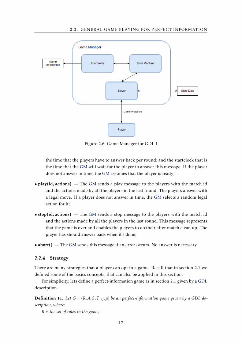
2.2.2 General Game Master
In this section we describe the GM available from the GGP-Base package [Ggp]. Figure 2.6
shows it’s main components, where arrows represent interactions. For example, the
Interpreter interacts with the Game Description, in the sense that, interprets it according
to GDL semantics. The State Machine is the module that, as the name suggests, handles
games states regarding the Game Description. For instance, to check if a state is terminal
is necessary to call the function in the State Machine with the desired state as an argument.
This function converts the contents of a state — recall that in GDL the state content is
represented with what is with the true keyword — and calls the Interpreter to prove the
terminal rule. The Server is the module that communicates with the players and controls
the state of the game.
The GGP-Base package also provides the implementation for the random player be-
cause of games in perfect information games that require a die to be played, e.g. Backgam-
mon.
2.2.3 Game Protocol
The GM and each player communicate through a protocol that has 5 types of messages:
• info() — The GM checks if the player is running. To whom the player answers that he
is either available or busy;
• start(id, role, description, startclock, playclock) — The GM starts a match. He sends
a message to the player with the match id; the role that the player will have in the
game; the description of the game that is going to be played; the playclock, which is
16
2.2. GENERAL GAME PLAYING FOR PERFECT INFORMATION
Figure 2.6: Game Manager for GDL-I
the time that the players have to answer back per round; and the startclock that is
the time that the GM will wait for the player to answer this message. If the player
does not answer in time, the GM assumes that the player is ready;
• play(id, actions) — The GM sends a play message to the players with the match id
and the actions made by all the players in the last round. The players answer with
a legal move. If a player does not answer in time, the GM selects a random legal
action for it;
• stop(id, actions) — The GM sends a stop message to the players with the match id
and the actions made by all the players in the last round. This message represents
that the game is over and enables the players to do their after match clean up. The
player has should answer back when it’s done;
• abort() — The GM sends this message if an error occurs. No answer is necessary.
2.2.4 Strategy
There are many strategies that a player can opt in a game. Recall that in section 2.1 we
defined some of the basics concepts, that can also be applied in this section.
For simplicity, lets define a perfect-information game as in section 2.1 given by a GDL
description.
Definition 11. Let G = (R,A,S,T ,η,µ) be an perfect-information game given by a GDL de-scription, where:
R is the set of roles in the game;
17
CHAPTER 2. RELATED WORK
S is the set of all states in the game;A is the set of actions in the game; and L(r, s) ⊆ A is the set of legal moves of role r ∈ R in
state s ∈ S;T ⊆ S is the set of terminal states;µ : T ×R→R is the payoff function;η : S ×A|R|→ T is the successor function;
Remember that, the backwards induction works by identifying the equilibria at the
bottom subgame trees, and assuming those equilibria will be played as one backs up and
considers increasingly larger trees. The problem is that when one is in a game with a
large state space he doesn’t enough time to search the equilibria. And in games like Go
players can’t evaluate every branch of the tree in the playclock they have to play.
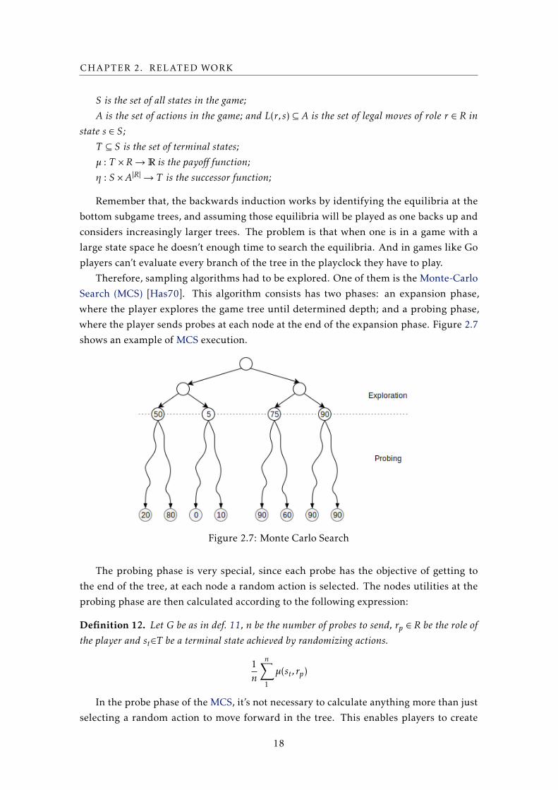
Therefore, sampling algorithms had to be explored. One of them is the Monte-Carlo
Search (MCS) [Has70]. This algorithm consists has two phases: an expansion phase,
where the player explores the game tree until determined depth; and a probing phase,
where the player sends probes at each node at the end of the expansion phase. Figure 2.7
shows an example of MCS execution.
Figure 2.7: Monte Carlo Search
The probing phase is very special, since each probe has the objective of getting to
the end of the tree, at each node a random action is selected. The nodes utilities at the
probing phase are then calculated according to the following expression:
Definition 12. Let G be as in def. 11, n be the number of probes to send, rp ∈ R be the role ofthe player and st∈T be a terminal state achieved by randomizing actions.
1n
n∑1
µ(st , rp)
In the probe phase of the MCS, it’s not necessary to calculate anything more than just
selecting a random action to move forward in the tree. This enables players to create
18
2.2. GENERAL GAME PLAYING FOR PERFECT INFORMATION
lots of probes to search each node. Furthermore, this algorithm has been proven that it’s
solution tends to the subgame-perfect equilibria.
However, with MCS the game tree is equally searched, even when it’s clear that it isn’t
necessary. That leads to an unnecessary search on the sides of the tree that will take us
nowhere, when we could be using that time to search the nodes that are promising. The
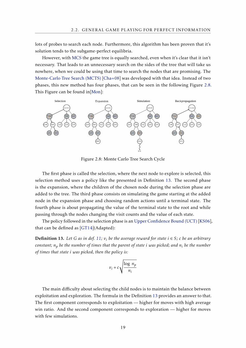
Monte-Carlo Tree Search (MCTS) [Cha+08] was developed with that idea. Instead of two
phases, this new method has four phases, that can be seen in the following Figure 2.8.
This Figure can be found in[Mon]:
Figure 2.8: Monte Carlo Tree Search Cycle
The first phase is called the selection, where the next node to explore is selected, this
selection method uses a policy like the presented in Definition 13. The second phase
is the expansion, where the children of the chosen node during the selection phase are
added to the tree. The third phase consists on simulating the game starting at the added
node in the expansion phase and choosing random actions until a terminal state. The
fourth phase is about propagating the value of the terminal state to the root and while
passing through the nodes changing the visit counts and the value of each state.
The policy followed in the selection phase is an Upper Confidence Bound (UCT) [KS06],
that can be defined as [GT14](Adapted):
Definition 13. Let G as in def. 11; vi be the average reward for state i ∈ S; c be an arbitraryconstant; np be the number of times that the parent of state i was picked; and ni be the numberof times that state i was picked, then the policy is:
vi + c
√log npni
The main difficulty about selecting the child nodes is to maintain the balance between
exploitation and exploration. The formula in the Definition 13 provides an answer to that.
The first component corresponds to exploitation — higher for moves with high average
win ratio. And the second component corresponds to exploration — higher for moves
with few simulations.
19
CHAPTER 2. RELATED WORK
Using the MCTS allows the game tree to grow asymmetrically because the method
focus on the most promising subtrees. Thus, achieving better results than classical algo-
rithms in games with a higher branching factor.
Moreover, the MCTS can be interrupted at any time and the player can at that moment
choose the most promising move. Unlike using a Minimax algorithm, for example.
2.3 General Game Playing for Imperfect Information
GGP-II is the General Game Playing concerned with games for imperfect-information,
e.g. Battle Ships, or Poker. The General Game Playing system as in Figure 2.5 remains
the same. However, there are some changes regarding the GDL and the protocol, in order
to ensure that the players act under imperfect-information.
2.3.1 GDL-II
GDL-II [Thi11a] was introduced due to the impossibility of describing games like the
Mastermind, or Poker. In this games it is impossible to describe, for instance, the act of a
random event. Moreover, using GDL-II, players are not able to see what other players do.
Only information that their’ actions might trigger.
2.3.1.1 Syntax
GDL-II extends the syntax of GDL, and the set of keywords is extended:
• sees R P — player R sees proposition P in the next state;
• random — represents randomness;
The first rule allows the players to see that they successfully triggered an event. Using
the description, a player can then see what caused it and use it for his gain. This keyword
can also be used to allow communication in a game between players, either public or
private. GDL-II is an extension of GDL, which means that any game in GDL can also
be described in GDL-II. That’s very simple to accomplish, one just needs to add a game
rule where a player can always see the moves made by other players, and the game, even
though is described in GDL-II it would be a perfect-information game. The keyword
random, on the other hand, must be added as a role. This is a game independent role
that represents a way to choose legal moves with a uniform probability. For a better
understanding of how those keywords can be used, consider the following example — a
snapshot of the Mastermind game:
1 % t h e r o l e s2 role ( random )
3 role ( player )
4
5 % The random p l a y e r s e t s up t h e c o l o r s in t h e f i r s t s t e p .
20
2.3. GENERAL GAME PLAYING FOR IMPERFECT INFORMATION
6 l e g a l ( random , s e t (C1 , C2 , C3 , C4 ) ) :− true ( guess ( setup ) ) & c o l o r (C1)
7 & c o l o r (C2) & c o l o r (C3) & c o l o r (C4)
8
9 % The p l a y e r i s in formed o f a l l c o l o r s c o r r e c t l y g u e s s e d .10 sees ( player , s e t ( 1 , C1 ) ) :− does ( player ( guessColors (C1 , C2 , C3 , C4 ) )
11 & true ( s e t ( 1 , C1 ) )
12 sees ( player , s e t ( 2 , C2 ) ) :− does ( player ( guessColors (C1 , C2 , C3 , C4 ) )
13 & true ( s e t ( 2 , C2 ) )
14 sees ( player , s e t ( 3 , C3 ) ) :− does ( player ( guessColors (C1 , C2 , C3 , C4 ) )
15 & true ( s e t ( 3 , C3 ) )
16 sees ( player , s e t ( 4 , C4 ) ) :− does ( player ( guessColors (C1 , C2 , C3 , C4 ) )
17 & true ( s e t ( 4 , C4 ) )
On this game, the player random selects the colours so that the player can guess it
on other steps of the game. After the player guesses, he will be notified if he correctly
guessed a color in the right position. He can use this information to correctly guess the
other remaining colours.
2.3.2 Game Protocol
As GDL-II introduces uncertainty, the GP needs the to have the necessary modifications
in order for that to happen. Though, it’s only necessary to change two methods. The other
methods remain the same:
• play(id, turn, action, percepts) — the GM sends a play message to the player with the
match id, the turn of the game, the action that the player made last turn and the
array of percepts, triggered with all the moves received from all the players, accord-
ing with the game rules. The player has to answer with a legal action. Otherwise,
the GM selects a random legal action.
• stop(id, turn, action, percepts) — the GM sends a stop message to the player with the
match id, the turn of the game, the action that the player made last turn and the
array of percepts triggered according with the game rules. The player has to clean
the data regarding the match and respond done.
Recall in the previous version of the GP all the players were notified about the adver-
sary move, according to the protocol. In the new modification, the GM sends to the player
only his last move and the array of events that were triggered. Notice that, the players
don’t communicate with each other directly, it always passes trough the GM. Then he
warns the players on their array of percepts, as accorded in the game rules.
2.3.3 Strategy
One of the hidden challenges of GDL-II is that the systems need to be able to draw
conclusions from partial observations. The most common assumption on this type of
games is the use of an Information Set. This strategy is widely utilized because the
21
CHAPTER 2. RELATED WORK
initial state is always known to the players. Using that, they can use the description to
model the next states, having in consideration, all the possible moves. They also use the
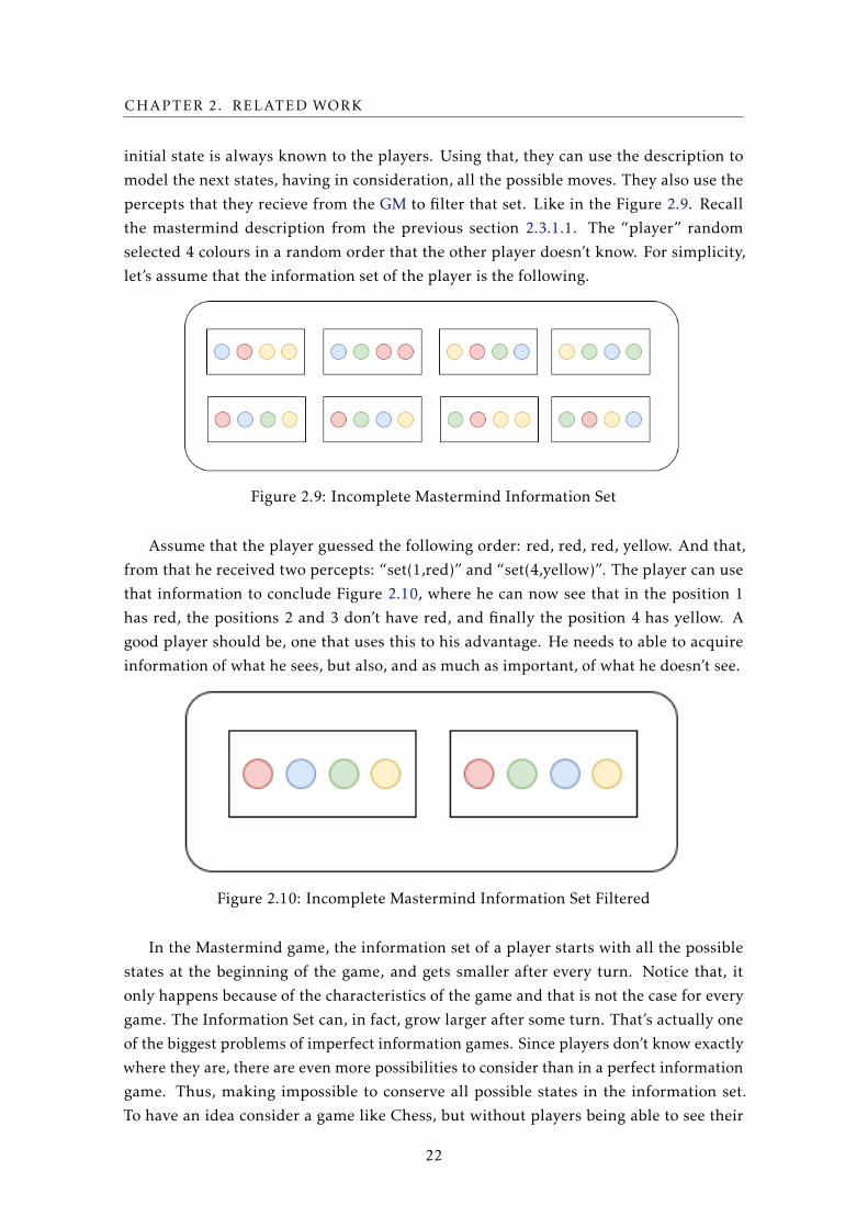
percepts that they recieve from the GM to filter that set. Like in the Figure 2.9. Recall
the mastermind description from the previous section 2.3.1.1. The “player” random
selected 4 colours in a random order that the other player doesn’t know. For simplicity,
let’s assume that the information set of the player is the following.
Figure 2.9: Incomplete Mastermind Information Set
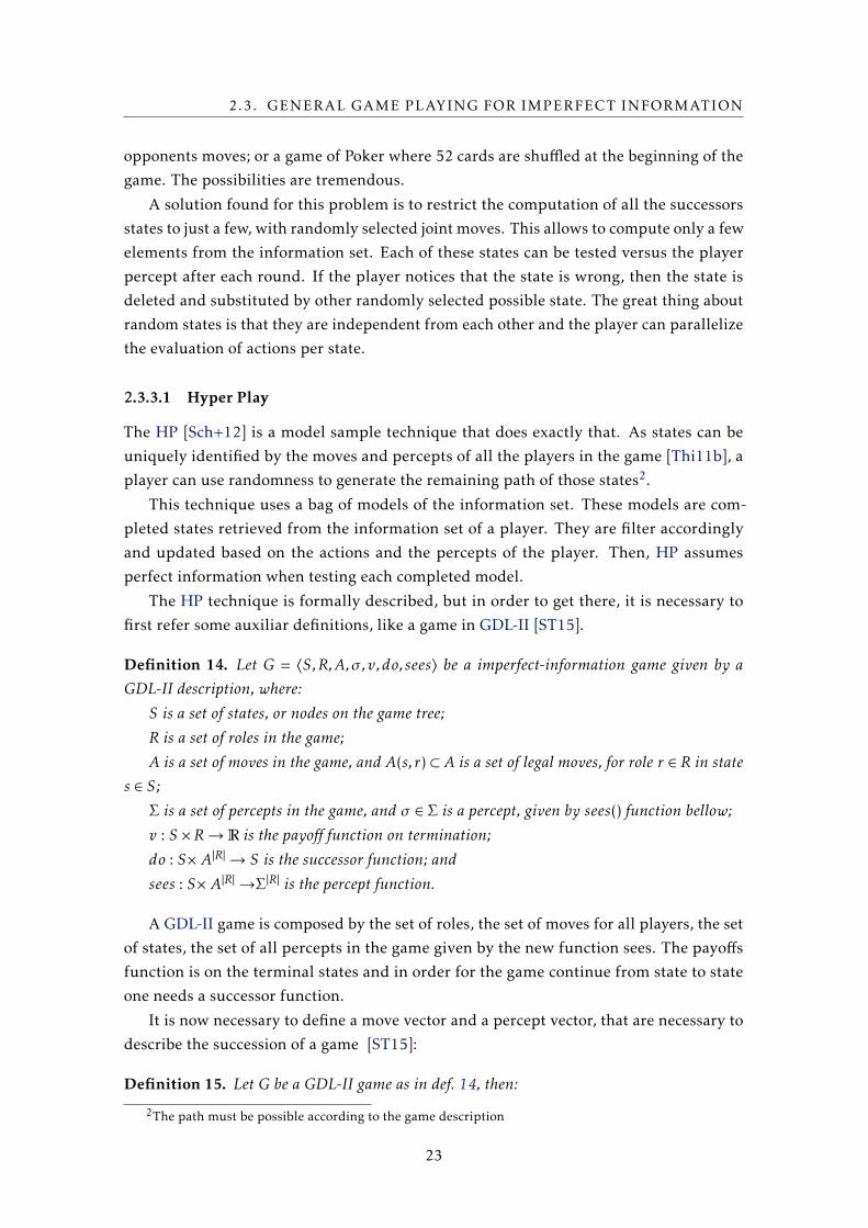
Assume that the player guessed the following order: red, red, red, yellow. And that,
from that he received two percepts: “set(1,red)” and “set(4,yellow)”. The player can use
that information to conclude Figure 2.10, where he can now see that in the position 1
has red, the positions 2 and 3 don’t have red, and finally the position 4 has yellow. A
good player should be, one that uses this to his advantage. He needs to able to acquire
information of what he sees, but also, and as much as important, of what he doesn’t see.
Figure 2.10: Incomplete Mastermind Information Set Filtered
In the Mastermind game, the information set of a player starts with all the possible
states at the beginning of the game, and gets smaller after every turn. Notice that, it
only happens because of the characteristics of the game and that is not the case for every
game. The Information Set can, in fact, grow larger after some turn. That’s actually one
of the biggest problems of imperfect information games. Since players don’t know exactly
where they are, there are even more possibilities to consider than in a perfect information
game. Thus, making impossible to conserve all possible states in the information set.
To have an idea consider a game like Chess, but without players being able to see their
22
2.3. GENERAL GAME PLAYING FOR IMPERFECT INFORMATION
opponents moves; or a game of Poker where 52 cards are shuffled at the beginning of the
game. The possibilities are tremendous.
A solution found for this problem is to restrict the computation of all the successors
states to just a few, with randomly selected joint moves. This allows to compute only a few
elements from the information set. Each of these states can be tested versus the player
percept after each round. If the player notices that the state is wrong, then the state is
deleted and substituted by other randomly selected possible state. The great thing about
random states is that they are independent from each other and the player can parallelize
the evaluation of actions per state.
2.3.3.1 Hyper Play
The HP [Sch+12] is a model sample technique that does exactly that. As states can be
uniquely identified by the moves and percepts of all the players in the game [Thi11b], a
player can use randomness to generate the remaining path of those states2.
This technique uses a bag of models of the information set. These models are com-
pleted states retrieved from the information set of a player. They are filter accordingly
and updated based on the actions and the percepts of the player. Then, HP assumes
perfect information when testing each completed model.
The HP technique is formally described, but in order to get there, it is necessary to
first refer some auxiliar definitions, like a game in GDL-II [ST15].
Definition 14. Let G = 〈S,R,A,σ ,v,do, sees〉 be a imperfect-information game given by aGDL-II description, where:
S is a set of states, or nodes on the game tree;
R is a set of roles in the game;
A is a set of moves in the game, and A(s, r) ⊂ A is a set of legal moves, for role r ∈ R in states ∈ S;
Σ is a set of percepts in the game, and σ ∈ Σ is a percept, given by sees() function bellow;
v : S ×R→R is the payoff function on termination;
do : S× A|R|→ S is the successor function; and
sees : S× A|R|→Σ|R| is the percept function.
A GDL-II game is composed by the set of roles, the set of moves for all players, the set
of states, the set of all percepts in the game given by the new function sees. The payoffs
function is on the terminal states and in order for the game continue from state to state
one needs a successor function.
It is now necessary to define a move vector and a percept vector, that are necessary to
describe the succession of a game [ST15]:
Definition 15. Let G be a GDL-II game as in def. 14, then:
2The path must be possible according to the game description
23
CHAPTER 2. RELATED WORK
ar ∈ A(d,r) is a move for role r ∈ R in state d ∈ D, where D = S \ T is the set of decisionstates and T is the set of termination states;
~a = 〈ar , a¬r〉 is a move vector, one for each role;
〈a¬r , ar〉 =⟨a1...ar ...a|R|
⟩is a move vector containing a specific move ar for role r ∈ R
σ ∈ Σ given by sees(d,~a) is a percept for actions ~a in state d ∈D;
~σ =⟨σ1...σ|R|
⟩is a percept vector; and
s = do(d,~a) and ~σ = sees(d,~a) is the natural progression of the game.
On this definition it is stated that a move vector is composed by an action of each
player in the game. There are special move vectors where a specific action must be made
for a player. The percept vector is given by the function sees and it is composed by all the
percepts of all the players.
For a game to be played until one reaches the final state it is necessary to define how
can one define a move selection policy, or strategy [ST15].
Definition 16. Let G be a GDL-II game as in def 14, then:
Π : D ×R→ φ(A) be a move selection policy expressed as a probability distribution overthe set A;
~π =⟨~π1, ..., ~πR
⟩is a tuple of move selection policies; and
play : S ×Π|R|→ φ(T ) is the playout of a game to termination according to the given moveselection policies.
This above definition refers that a move selection policy is described by a decision
state (recall that it’s the set of all the decision states minus the terminal states). A tuple of
move selection policies is given by a policy chosen by each player and a playout function
is the function that plays the game to a terminal state given a state and a move selection
policies tuple.
In order to be able to evaluate the utility of a state it is necessary a evaluation function
that uses the play function already defined [ST15].
Definition 17. Let G be a GDL-II game as in def. 14, then:
φ(s) is the a priori probability that s = st;
eval : S ×Π|R| ×R×N→R is an evaluation function, where
eval(s, ~π,r,n) = 1n
∑n1φ(s) × v(play(s, ~π)) evaluates the node s ∈ S using the policies in ~π,
and sample size n.
By applying the evaluation function to a move vector⟨~a¬r , ari
⟩one gets eval(do(d,
⟨~a¬r , ari
⟩), ~π,r,n);
and
argmaxari[eval(do(d,
⟨~a¬r , ari
⟩), ~π,r,n)
]is a selection process for making a move choice.
On this definition, one can understand better the process of evaluation. The first thing
to consider, is that by having uncertainty a player doesn’t know the state where he is in,
though, he must have beliefs of where he is — where is he more to likely to be. Then
the eval function has four arguments, where it receives a state, a playout policy vector,
24
2.3. GENERAL GAME PLAYING FOR IMPERFECT INFORMATION
a role and the number of probes to send from that state for the mentioned role. Finally
notice that by the eval function to a move vector we get the evaluation of that state and
the selection process is therefore the maximization of the utilities.
Before a player can start evaluating the models, it is necessary to identify a state. This
consists on a list of play messages, that represent the moves and percepts of all the players
in the game. This is defined as follows [ST15]:
Definition 18. Let G be a GDL-II game as in def. 14, then:p ∈ P is a play message from the set of all play messages in the game G;pr = 〈ar ,σr〉 is a play message for role r ∈ R;~p =
⟨p1, ...,p|R|
⟩is a play message vector;
ξ : S→ P ∗ is a function that extracts the path;ξ(s) =
⟨~p0, ..., ~pn
⟩is an ordered list of play messages from s0 ∈ S (the initial state) to s called
the path; andξr(s) =
⟨~pr1, ..., ~prn
⟩is an ordered list of play messages received by role r ∈ R
Definition 18 shows a play message for a specific player, that consists on his action
and his percepts; a play message vector is a play message for each role. Since we want
to identify a state, then we have the necessary tools to define a function that extracts a
path of a state. That function returns an ordered list with the complete path of the state,
from the initial state until the considered state. Then we can finally define a function that
extracts the incomplete path of the state for a role.
The HP technique then constructs the models by grounding the unknown values. This
is defined as following [ST15].
Definition 19. Let G be the GDL-II game as in def. 14, then:hp : P n→ 2P
nis the Hyperplay function that completes the path in game G; and
hr ∈ Hr = hp(ξr(st)) where st is the true state of the game and Hr is the information set ofr ∈ R.
The HP function, as aforementioned, returns a completed state or model. Note that,
the new path might not be the same as the true path (it only needs to be a legal path).
Finally, move selection policy is the one that maximizes the expected utility of actions for
the completed states. It is defined as follows [ST15]:
Definition 20. Let G be a GDL-II game as in def. 14, then:
argmaxari
[∑|Hr |j=1 eval(do(hrj ,
⟨~a¬r , ari
⟩), ~mc,r,n)
]is the move selection policy πhp where ~mc
is random.
2.3.3.2 HyperPlay-II
The problem with the predecessor technique is that it doesn’t have in consideration the
moves where it’s clearly better one can gain more information, since it assumes that it’s in
a perfect-information environment after completing the states. To solve this problem, the
25
CHAPTER 2. RELATED WORK
HyperPlay for Imperfect-Information (HP-II) was developed. This new technique, extends
the last one in the sense that it also completes the incomplete path of a state. Moreover,
it includes a Incomplete Information Simulation (ISS) to reason with the incomplete
information, by exploring the consequences of each action and uses that outcome to
make a decision [ST15].
The HP-II can be defined using the definitions of the last subsubsection [ST15]:
Definition 21. Let G be a GDL-II game as in def.??, then:
replay : S × P n ×Π→ S |R| is the replay of the game consistent with the path of a state;
replay(s0,ξi(hr), ~π) is the replay of a game, as if hr = st, and generates information for allroles, such that, hp(ξi(hr ))→Hi where r is our role and i is any role;
ISS : S ×Π×R×N→R is the incomplete information simulation; where
ISS(hr , ~πhp, r,n) is an evaluation using an incomplete information simulation, and is de-fined as eval(replay(s0,ξi(hr ), ~πhp), ~πhp, r,n).
This technique works by completing the path of a state in the information set of the
player, then breaking that path into two different paths and complete those paths again.
This makes that from one incomplete state path, we get two complete states paths even
though they might not even be in the player’s information set. Then the playout is done
from the beginning of the game to the new path, having in account that path.
The HP-II technique can finally be defined as [ST15]:
Definition 22. Let G be a GDL-II game as in def. ?? above, then:
ari ∈ A(hr , r) is a move to be evaluated by role r;⟨~a¬r , ari
⟩, is the move vector containing the move ari ;
ISS(do(hr ,⟨~a¬r , ari
⟩), ~πhp, r,n) is an evaluation; and
argmaxari
[∑|Hr |j=1 ISS(do(hrj ,
⟨~a¬r , ari
⟩), ~πhp, r,n)
]is the move selection policy ~πhpii .
Notice the use of the HP policy on this new policy. This makes the HP-II a nested
player. And, because it utilises a nested playout for evaluating move choices, it causes a
significant increase in the number of states visited during the analysis [ST16]. However,
since we are working with imperfect-information it is necessary to generate paths across
other information sets (not only our player), so that one can evaluate what the other play-
ers might know. The use of this extended domain and the incomplete information reason-
ing makes the HP-II more suitable than HP to play in games with imperfect-information.
2.4 Epistemic General Game Playing
EGGP is the category concerned with systems that in human free environments that are
able to play epistemic games. This category was created with the introduction of GDL-III.
26
2.4. EPISTEMIC GENERAL GAME PLAYING
2.4.1 GDL-III
The GDL-III [Thi17] has the same assumptions as his predecessor, all the described games
are in imperfect-information. Though, the difference is that rules depend on the player’s
knowledge.
2.4.2 Syntax
In order to the players to understand that they need to know something a new keyword
was added. This keyword comes in two different forms: [Gdl]
• knows (R, P) — player R knows the proposition P in the current state;
• knows (P) — proposition P is common knowledge;
This keyword can only be used in the body of the GDL-III rules since players must be
able to reason about their own knowledge. The knowledge cannot be defined itself in the
rules. There is also other restrictions, such as: there must be a total ordering on all the
predicates symbols P so that circular definitions are not allowed.
2.4.3 Semantics
The semantics of GDL-III are characterized by the semantics of GDL-II as pre semantics,
followed by the semantics of the knowledge rules. Formally, the semantics of GDL-III
are presented in Definition 23, which is an adaptation from [Thi17]. Specifically, the
derivable (role r) instances represent the players; the state s0 is represented by the in-
stances (init f ). All the other keywords use a state (S,K), which S is encoded by us-
ing the keyword true, and K the keyword knows — the defined in Definition 23. Let
S = {f1, . . . , fn} be a finite set of ground terms over the signature of G. Moreover, let Strue =
{(true f1) . . . (true fn)} be an extension of G by the n facts. The legal moves m of player r in
position S,K are defined by all instances of (legal r m) that follow from G∪Strue∪K . Like-
wise for the terminal and (goal r m) clauses, that define the terminal states and the goal
values relative to the given state S,K . Finally, let M denote a joint move, where players
r1, . . . , rk make movesm1, . . . ,mk and useMdoes = {(does r1 m1) . . . (does rk mk)}. The update
position is defined by all instances of (next f ) that follow from G∪Mdoes ∪Strue ∪K , and
the percepts that the players receive after joint move M, in a given position S,K are all
the derivable instances of (sees r p).
Definition 23. The semantics of a valid GDL-III game description G is given by
• R = {r : G |= (role r)}
• s0 = {f : G |= (init f )}
• t ={(S,K) : G∪ Strue ∪K |= terminal
}27
CHAPTER 2. RELATED WORK
• l ={(r,m,S,K) : G∪ Strue ∪K |= (legal r m)
}• u(M,S,K) =
{f : G∪Mdoes ∪ Strue ∪K |= (next f )
}• I =
{(r,M,S,K,p) : G∪Mdoes ∪ Strue ∪K |= (sees r p)
}• g =
{(r,v,S,K) : G∪ Strue ∪K |= (goal r v)
}Definition 32, copied from [Thi17], shows how the knowledge set K is defined by
using indistinguishable legal play sequences, notion that comes from GDL-II. But first,
a legal play sequence is a sequence of joint moves M1, . . .Mn, where Mi(r) is a move —
one for each role — at step i, such that there are states s0, s1, . . . , sn with: (r,Mi(r), si−1) ∈ l,for all r ∈ R; and, si = u(Mi , si−1). We can see at this point how the GDL-II acts as pre
semantics of GDL-III, since si−1 represents just the state without the knowledge setK , also
valid in a GDL-II description. Moreover, two legal play sequences δ,δ′ are indistinguish-
able (δ ∼r δ′) for role r ∈ R if for all i ∈ {1, . . . ,n}: Mi(r) = M ′i (r) and {p : (r,Mi , si−1,p)} =
{p′ : (r,Mi , si−1,p′)}. For common knowledge, is defined using a notion of reflexive tran-
sitive closure ∼+ of a given family of indistinguishable relations ∼r (one for every role
r ∈ R). Formally [Thi17], ∼+ is the smallest relation such that for all δ,δ′ ,δ′′:
• δ ∼+ δ′
• if δ ∼+ δ′ and δ′ ∼r δ′′ for some r ∈ R then δ ∼+ δ′′.
Definition 24. Let G be a game description along with all the sets and relations it describesaccording to Definition 23.
• The play sequence of length 0, denoted by ε, is legal and satisfies ε ∼r ε, for all r ∈ R. Itresults in state s0 and knowledge state Kε as the smallest set that satisfies
Kε ={(knows r p) : r ∈ R,G∪ strue0 ∪Kε |= p
}∪
{(knows p) : G∪ strue0 ∪Kε |= p
}• For the inductive definition, let δ be a legal play sequence of length n ≥ 0 resulting in
(sn,Kn).
Sequence δ followed by M, written δM, is a legal play sequence of length n + 1 if(M(r), sn,Kn) ∈ l for all r ∈ R. It results in the state sδM = u(M,sn,Kn) and, as theknowledge state, the smallest KδM that satisfies:
KδM ={(knows r p) : G∪ strueδ′M ′ ∪KδM |= p f or all δ
′M ′ ∼r δM}
∪{(knows p) : G∪ strueδ′M ′ ∪KδM |= p f or all δ
′M ′ ∼+ δM}
Definition 32 can be understood as follows: relations δM ∼r δ′M ′ holds if for role r ∈ R:
δ ∼r δ′ the legal play sequences are indistinguishable, and after applying the same move
M(r) = M ′(r), it gets the same percepts {p : (r,M,sn,Kn,p) ∈ I} = {p′ : (r,M,s′n,K′n,p′) ∈ I}.
28
2.5. EPISTEMIC LOGIC
Then the (knows r p) is defined by using this relation to find all the states that are indis-
tinguishable to player r and in all of them p needs to be derived. For common knowledge
(knows p) applies the same logic, but with the transitive closure relation ∼+ to find the
states.
2.5 Epistemic Logic
Epistemic logic is the logic that reasons about knowledge and belief. It recognizes ex-
pressions like knows that P or believes that P to have properties that are susceptible to
formal study. Is exclusively concerned about propositional knowledge. In other words,
in knowing that something is true. The semantics of Epistemic logic is very similar to the
semantics of GDL-III. Therefore, problems already defined and solved using in Epistemic
Logic can be defined in as GDL-III game, such as the Russian Cards Problems, and Muddy
Children.
The applications of Epistemic Logic range from computer science e.g. robotics or
network security to economics in the study of interactions on different environments.
2.5.1 Syntax
The Epistemic Logic language is presented in the form BNF[VD+07](Adapted):
Definition 25. Let P be the set of propositions, and p ∈ P be a proposition, A be the set of allagents, a ∈ A be an agent and G ⊆ A be a group of agents, then:
ε ::= p | ¬ε | (ε∧ ε) | Kaε | CGε
A formula can be build using propositions; formulas with negation; conjunction with
other formulas; the knowledge operator for an agent and the group knowledge operator.
Finally another operator can be defined using the previous already defined: K̂aε := ¬Ka¬εthat simbolizes that agent a still thinks that ε is possible.
2.5.2 Semantics
The semantics of Epistemic Logic uses a special case of Kripke models. There are two
important notions: The notion of state and the indistinguishability. The following is the
definition of a Kripke model [VD+07].
Definition 26. Let P be the set of propositions, and p ∈ P be a proposition, A be the finiteset of all agents, a ∈ A be an agent and G ⊆ A be a group of agents, then a Kripke model is astructure M =
⟨S,RA,V P
⟩, where:
S is an non-empty set of states;
RA is a function yielding an accessibility relation Ra ⊆ S×S for every a;
V P : P → ρ(S). V(p) is the subset of the domain where p is true.
29
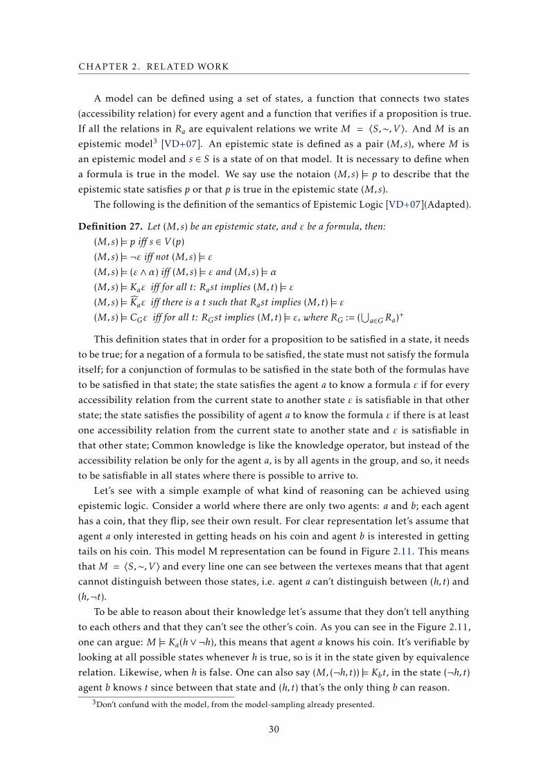
CHAPTER 2. RELATED WORK
A model can be defined using a set of states, a function that connects two states
(accessibility relation) for every agent and a function that verifies if a proposition is true.
If all the relations in Ra are equivalent relations we write M = 〈S,∼,V 〉. And M is an
epistemic model3 [VD+07]. An epistemic state is defined as a pair (M,s), where M is
an epistemic model and s ∈ S is a state of on that model. It is necessary to define when
a formula is true in the model. We say use the notaion (M,s) |= p to describe that the
epistemic state satisfies p or that p is true in the epistemic state (M,s).
The following is the definition of the semantics of Epistemic Logic [VD+07](Adapted).
Definition 27. Let (M,s) be an epistemic state, and ε be a formula, then:(M,s) |= p iff s ∈ V (p)
(M,s) |= ¬ε iff not (M,s) |= ε(M,s) |= (ε∧α) iff (M,s) |= ε and (M,s) |= α(M,s) |= Kaε iff for all t: Rast implies (M,t) |= ε(M,s) |= K̂aε iff there is a t such that Rast implies (M,t) |= ε(M,s) |= CGε iff for all t: RGst implies (M,t) |= ε, where RG := (
⋃a∈GRa)
+
This definition states that in order for a proposition to be satisfied in a state, it needs
to be true; for a negation of a formula to be satisfied, the state must not satisfy the formula
itself; for a conjunction of formulas to be satisfied in the state both of the formulas have
to be satisfied in that state; the state satisfies the agent a to know a formula ε if for every
accessibility relation from the current state to another state ε is satisfiable in that other
state; the state satisfies the possibility of agent a to know the formula ε if there is at least
one accessibility relation from the current state to another state and ε is satisfiable in
that other state; Common knowledge is like the knowledge operator, but instead of the
accessibility relation be only for the agent a, is by all agents in the group, and so, it needs
to be satisfiable in all states where there is possible to arrive to.
Let’s see with a simple example of what kind of reasoning can be achieved using
epistemic logic. Consider a world where there are only two agents: a and b; each agent
has a coin, that they flip, see their own result. For clear representation let’s assume that
agent a only interested in getting heads on his coin and agent b is interested in getting
tails on his coin. This model M representation can be found in Figure 2.11. This means
that M = 〈S,∼,V 〉 and every line one can see between the vertexes means that that agent
cannot distinguish between those states, i.e. agent a can’t distinguish between (h, t) and
(h,¬t).To be able to reason about their knowledge let’s assume that they don’t tell anything
to each others and that they can’t see the other’s coin. As you can see in the Figure 2.11,
one can argue: M |= Ka(h∨¬h), this means that agent a knows his coin. It’s verifiable by
looking at all possible states whenever h is true, so is it in the state given by equivalence
relation. Likewise, when h is false. One can also say (M, (¬h, t)) |= Kbt, in the state (¬h, t)agent b knows t since between that state and (h, t) that’s the only thing b can reason.
3Don’t confund with the model, from the model-sampling already presented.
30

2.6. ANSWER SET PROGRAMING
Figure 2.11: Epistemic Model M
Moreover, it is possible to reason about nested knowledge, e.g. (M, (h,¬t)) |= KaKbt.
At (h,¬t) one can go to (h,¬t) through the indistinguishability relation of a and in that
state is true that the agent b knows t, so KaKbt.
Finally, common knowledge it must be achievable in all the states of the model i.e.
M |= Cab(Kah∨Ka¬h). It is common knowledge that agent a knows his card. This can be
verified by starting at the state (h, t) and verifying that Kah holds, then proceed to state
(¬h, t) through the accessibility relation of b and verifying that Ka¬h holds and then to
(¬h,¬t) with the ∼a, where Ka¬h holds, and finally to (h,¬t) with ∼b and verifying that
Kah holds. As a remark we can say that common knowledge also be interpreted as ‘any
fool knows p’. And that it must be true in all the states that we can arrive at by at path of
links belonging to the agents considered. Hence, defined by the transitive closure.
The principle of indistinguishability important to the way the knowledge is verified,
since it is necessary to verify that on all accessible states.
2.6 Answer Set Programing
ASP is a form of declarative programming oriented towards difficult search problems [Geb+12].
Problems are described as a collection of logic clauses like GDL, and solved by finding
the minimal model for the specification. To demonstrate a problem written in ASP we
present the following example, that can be found in [Gra]:
1 % D e f a u l t2 # const n = 3 .
3
4 % Generate nodes5 node ( 1 . . 6 ) .
6
7 % Generate ( D i r e c t e d ) Edges8 edge ( 1 , ( 2 ; 3 ; 4 ) ) . edge ( 2 , ( 4 ; 5 ; 6 ) ) . edge ( 3 , ( 1 ; 4 ; 5 ) ) .
9 edge ( 4 , ( 1 ; 2 ) ) . edge ( 5 , ( 3 ; 4 ; 6 ) ) . edge ( 6 , ( 2 ; 3 ; 5 ) ) .
10
11 % Generate C o l o r s − one f o r each node .12 { c o l o r (X , 1 . . n ) } = 1 :− node (X ) .
31
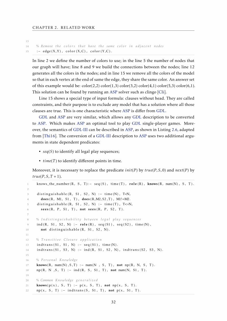
CHAPTER 2. RELATED WORK
13
14 % Remove t h e c o l o r s t h a t have t h e same c o l o r in a d j a c e n t nodes15 :− edge (X, Y) , c o l o r (X,C) , c o l o r (Y ,C ) .
In line 2 we define the number of colors to use; in the line 5 the number of nodes that
our graph will have; line 8 and 9 we build the connections between the nodes; line 12
generates all the colors in the nodes; and in line 15 we remove all the colors of the model
so that in each vertex at the end of same the edge, they share the same color. An answer set
of this example would be: color(2,2) color(1,3) color(3,2) color(4,1) color(5,3) color(6,1).
This solution can be found by running an ASP solver such as clingo [Cli].
Line 15 shows a special type of input formula: clauses without head. They are called
constraints, and their purpose is to exclude any model that has a solution where all those
clauses are true. This is one characteristic where ASP is differ from GDL.
GDL and ASP are very similar, which allows any GDL description to be converted
to ASP. Which makes ASP an optimal tool to play GDL single-player games. More-
over, the semantics of GDL-III can be described in ASP, as shown in Listing 2.6, adapted
from [Thi16]. The conversion of a GDL-III description to ASP uses two additional argu-
ments in state dependent predicates:
• seq(S) to identify all legal play sequences;
• time(T ) to identify different points in time.
Moreover, it is necessary to replace the predicate init(P ) by true(P ,S,0) and next(P ) by
true(P ,S,T + 1).
1 knows_the_number (R , S , T) : − seq ( S ) , time (T ) , role (R) , knows (R , num(N) , S , T ) .
2
3 d i s t i n g u i s h a b l e (R , S1 , S2 , N) :− time (N) , T<N,
4 does (R , M1, S1 , T ) , does (R ,M2, S2 , T ) , M1!=M2.
5 d i s t i n g u i s h a b l e (R , S1 , S2 , N) :− time (T ) , T<=N,
6 sees (R , P , S1 , T ) , not sees (R , P , S2 , T ) .
7
8 % I n d i s t i n g u i s h a b i l i t y between l e g a l p lay s e q u e n c e s9 ind (R , S1 , S2 , N) :− role (R) , seq ( S1 ) , seq ( S2 ) , time (N) ,
10 not d i s t i n g u i s h a b l e (R , S1 , S2 , N) .
11
12 % T r a n s i t i v e Clo sure a p p l i c a t i o n13 indtrans ( S1 , S1 , N) :− seq ( S1 ) , time (N) .
14 indtrans ( S1 , S3 , N) :− ind (R , S1 , S2 , N) , indtrans ( S2 , S3 , N) .
15
16 % P e r s o n a l Knowledge17 knows (R , num(N) , S , T) :− num(N , S , T ) , not np (R, N, S , T ) .
18 np (R, N , S , T) :− ind (R , S , S1 , T ) , not num(N, S1 , T ) .
19
20 % Common Knowledge g e n e r a l i z e d21 knows ( p ( x ) , S , T) :− p ( x , S , T ) , not np ( x , S , T ) .
22 np ( x , S , T) :− indtrans ( S , S1 , T ) , not p ( x , S1 , T ) .
32
2.6. ANSWER SET PROGRAMING
Listing 2.6 is a snapshot of the Epistemic Number Guessing, where the remainder
of the GDL-III description can be found in Appendix B. Line 1 is the extension of the
knowledge predicate used in the goal definition by the sequences and time; Line 3-6
represent the distinguishability between legal play sequences in different time points.
We can see that two sequences are distinguishable for player R is he doesn’t make the
same move, or he sees different percepts at some point in time; Line 9-10 show the
definition of indistinguishable legal play sequences; Line 13-14 represent the definition
of the transitive closure; Line 17-18 show the semantics of personal knowledge for the
Epistemic Number Guessing game. We would have that R knows the num(N ) if sequence
S is the actual play sequence at time T , num(N ) holds and predicate np does not, meaning
that is not the case that there is another sequence S1 that R cannot distinguish from S
where num(N ) does not hold; and, finally, Line 21-22 represent a generalized common
knowledge rule — since this game does not have a common knowledge rule, because it is
a single player game— uses the same logic, using instead the transitive closure predicate
to find other legal play sequences S1.
This solution, however, as explained in [Thi17], it is very inefficient, since it explicitly
requires maintaining the set of relevant legal play sequences. Which is practically viable
for short epistemic games or puzzles. But it does not scale for bigger games. In this aspect,
a model-sampling is better since it does not require to maintain the set of relevant legal
play sequences.
33


Chapter
3An Epistemic Game Master
This chapter showcases some of the implementation details of the developed GM for
GDL-III. We provide the source code available at: https://gitlab.com/Demofrager/
GDL-III_GameMaster. Throughout the chapter, we reaffirm our problem; we explain
generally our implemented solution; and then, we detail how the main modules of our
GM were implemented and the advantages of our approach over alternatives—as well
as some of their limitations. In particular, we briefly introduce the architecture of our
implementation; we expose our server implementation that controls the state of the game;
we detail how players’ knowledge is verified; explain the samplers that were developed;
we also introduce a new concept used in this dissertation;
3.1 Problem Description
The introduction of GDL-III raises two problems. This new version extends an general
game playing system to allow players to play epistemic games — EGGP. Therefore, the
previous iteration of the GM does not have this ability. And secondly, the language forces
players to have to reason about what they know. According to GDL-III defined semantics,
in order to calculate what a certain player knows, one needs to evaluate all the other
states that that player cannot distinguish between.
The GM in all GDL-III extensions always acts under perfect-information, since the
initial state is known and receives the players moves at every round. However, by forcing
players to reason about their own knowledge, it also forces the master to reason about
their knowledge as well. Therefore it is also necessary to consider the state space of the
game, in order to be able to consider the states that players cannot distinguish between
thus calculating what each one of them knows. Our objective is to make sure that players
can play the game e.g. by making sure players can only make certain moves if they know
35
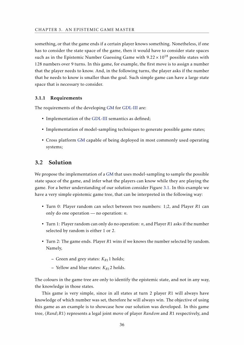
CHAPTER 3. AN EPISTEMIC GAME MASTER
something, or that the game ends if a certain player knows something. Nonetheless, if one
has to consider the state space of the game, then it would have to consider state spaces
such as in the Epistemic Number Guessing Game with 9.22 × 10¹⁸ possible states with
128 numbers over 9 turns. In this game, for example, the first move is to assign a number
that the player needs to know. And, in the following turns, the player asks if the number
that he needs to know is smaller than the goal. Such simple game can have a large state
space that is necessary to consider.
3.1.1 Requirements
The requirements of the developing GM for GDL-III are:
• Implementation of the GDL-III semantics as defined;
• Implementation of model-sampling techniques to generate possible game states;
• Cross platform GM capable of being deployed in most commonly used operating
systems;
3.2 Solution
We propose the implementation of a GM that uses model-sampling to sample the possible
state space of the game, and infer what the players can know while they are playing the
game. For a better understanding of our solution consider Figure 3.1. In this example we
have a very simple epistemic game tree, that can be interpreted in the following way:
• Turn 0: Player random can select between two numbers: 1;2, and Player R1 can
only do one operation — no operation: n.
• Turn 1: Player random can only do no operation: n, and PlayerR1 asks if the number
selected by random is either 1 or 2.
• Turn 2: The game ends. Player R1 wins if we knows the number selected by random.
Namely,
– Green and grey states: KR11 holds;
– Yellow and blue states: KR12 holds.
The colours in the game tree are only to identify the epistemic state, and not in any way,
the knowledge in those states.
This game is very simple, since in all states at turn 2 player R1 will always have
knowledge of which number was set, therefore he will always win. The objective of using
this game as an example is to showcase how our solution was developed. In this game
tree, 〈Rand;R1〉 represents a legal joint move of player Random and R1 respectively, and
36
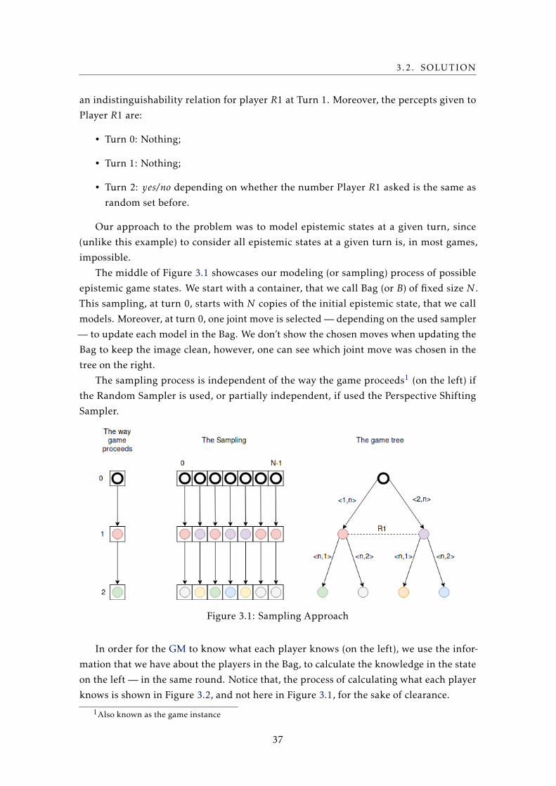
3.2. SOLUTION
an indistinguishability relation for player R1 at Turn 1. Moreover, the percepts given to
Player R1 are:
• Turn 0: Nothing;
• Turn 1: Nothing;
• Turn 2: yes/no depending on whether the number Player R1 asked is the same as
random set before.
Our approach to the problem was to model epistemic states at a given turn, since
(unlike this example) to consider all epistemic states at a given turn is, in most games,
impossible.
The middle of Figure 3.1 showcases our modeling (or sampling) process of possible
epistemic game states. We start with a container, that we call Bag (or B) of fixed size N .
This sampling, at turn 0, starts with N copies of the initial epistemic state, that we call
models. Moreover, at turn 0, one joint move is selected — depending on the used sampler
— to update each model in the Bag. We don’t show the chosen moves when updating the
Bag to keep the image clean, however, one can see which joint move was chosen in the
tree on the right.
The sampling process is independent of the way the game proceeds1 (on the left) if
the Random Sampler is used, or partially independent, if used the Perspective Shifting
Sampler.
Figure 3.1: Sampling Approach
In order for the GM to know what each player knows (on the left), we use the infor-
mation that we have about the players in the Bag, to calculate the knowledge in the state
on the left — in the same round. Notice that, the process of calculating what each player
knows is shown in Figure 3.2, and not here in Figure 3.1, for the sake of clearance.
1Also known as the game instance
37
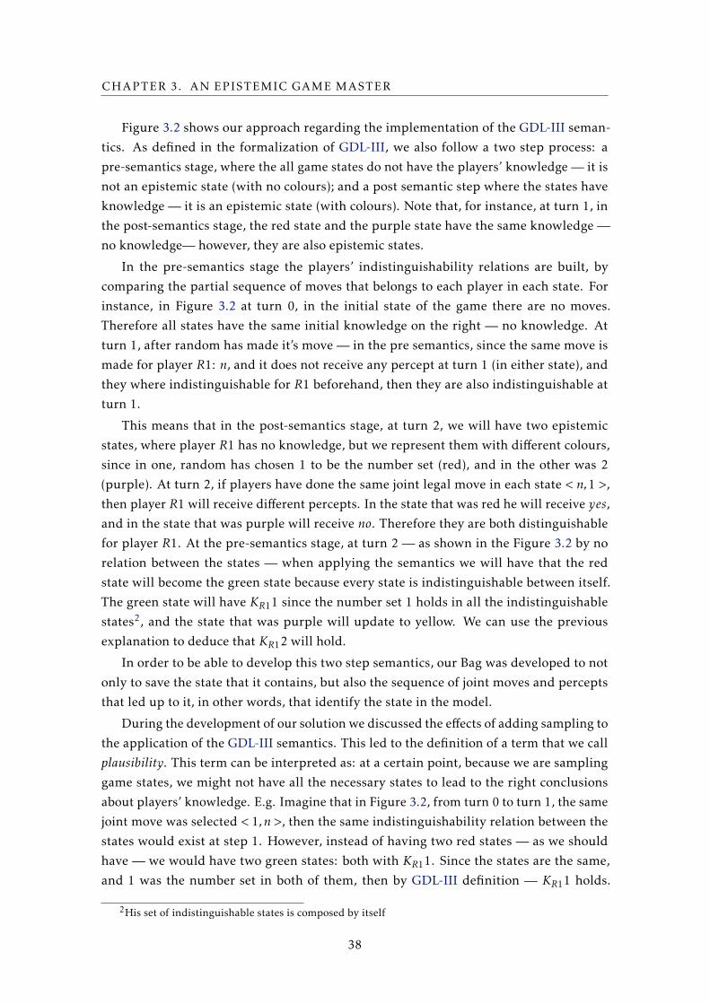
CHAPTER 3. AN EPISTEMIC GAME MASTER
Figure 3.2 shows our approach regarding the implementation of the GDL-III seman-
tics. As defined in the formalization of GDL-III, we also follow a two step process: a
pre-semantics stage, where the all game states do not have the players’ knowledge — it is
not an epistemic state (with no colours); and a post semantic step where the states have
knowledge — it is an epistemic state (with colours). Note that, for instance, at turn 1, in
the post-semantics stage, the red state and the purple state have the same knowledge —
no knowledge— however, they are also epistemic states.
In the pre-semantics stage the players’ indistinguishability relations are built, by
comparing the partial sequence of moves that belongs to each player in each state. For
instance, in Figure 3.2 at turn 0, in the initial state of the game there are no moves.
Therefore all states have the same initial knowledge on the right — no knowledge. At
turn 1, after random has made it’s move — in the pre semantics, since the same move is
made for player R1: n, and it does not receive any percept at turn 1 (in either state), and
they where indistinguishable for R1 beforehand, then they are also indistinguishable at
turn 1.
This means that in the post-semantics stage, at turn 2, we will have two epistemic
states, where player R1 has no knowledge, but we represent them with different colours,
since in one, random has chosen 1 to be the number set (red), and in the other was 2
(purple). At turn 2, if players have done the same joint legal move in each state < n,1 >,
then player R1 will receive different percepts. In the state that was red he will receive yes,
and in the state that was purple will receive no. Therefore they are both distinguishable
for player R1. At the pre-semantics stage, at turn 2 — as shown in the Figure 3.2 by no
relation between the states — when applying the semantics we will have that the red
state will become the green state because every state is indistinguishable between itself.
The green state will have KR11 since the number set 1 holds in all the indistinguishable
states2, and the state that was purple will update to yellow. We can use the previous
explanation to deduce that KR12 will hold.
In order to be able to develop this two step semantics, our Bag was developed to not
only to save the state that it contains, but also the sequence of joint moves and percepts
that led up to it, in other words, that identify the state in the model.
During the development of our solution we discussed the effects of adding sampling to
the application of the GDL-III semantics. This led to the definition of a term that we call
plausibility. This term can be interpreted as: at a certain point, because we are sampling
game states, we might not have all the necessary states to lead to the right conclusions
about players’ knowledge. E.g. Imagine that in Figure 3.2, from turn 0 to turn 1, the same
joint move was selected < 1,n >, then the same indistinguishability relation between the
states would exist at step 1. However, instead of having two red states — as we should
have — we would have two green states: both with KR11. Since the states are the same,
and 1 was the number set in both of them, then by GDL-III definition — KR11 holds.
2His set of indistinguishable states is composed by itself
38
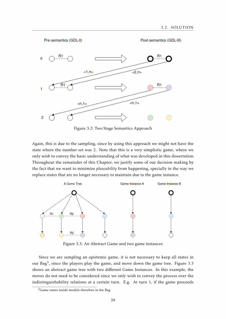
3.2. SOLUTION
Figure 3.2: Two Stage Semantics Approach
Again, this is due to the sampling, since by using this approach we might not have the
state where the number set was 2. Note that this is a very simplistic game, where we
only wish to convey the basic understanding of what was developed in this dissertation.
Throughout the remainder of this Chapter, we justify some of our decision making by
the fact that we want to minimize plausability from happening, specially in the way we
replace states that are no longer necessary to maintain due to the game instance.
Figure 3.3: An Abstract Game and two game instances
Since we are sampling an epistemic game, it is not necessary to keep all states in
our Bag3, since the players play the game, and move down the game tree. Figure 3.3
shows an abstract game tree with two different Game Instances. In this example, the
moves do not need to be considered since we only wish to convey the process over the
indistinguishability relations at a certain turn. E.g. At turn 1, if the game proceeds
3Game states inside models therefore in the Bag
39
CHAPTER 3. AN EPISTEMIC GAME MASTER
according to the Game Instance A, which states would be useful to consider having in the
Bag? Would epistemic state blue be useful for knowledge calculation at turn 1? Similarly,
if the Game Instance were B, at turn 1, would we need to consider the red, green or
grey states? The answer is no because every player can distinguish between those states,
according to the game instance, respectively.
Moreover, if at turn 1 in the game instance A, would it be better to have in the Bag
both states green and grey, since common knowledge can be interpreted as jumping from
a state to another if there is a indistinguishability relation for some player — within the
game instance, i.e. would it be useful in game instance A, to consider the blue state and
any other state eventually connected to it? The answer is also no.
However, still in game instance A at turn 2, is it really necessary to consider the
orange state presented in the game tree? The answer is: it depends. Games where legal
moves and percepts depend on knowledge, or dynamic epistemic games, it is necessary
to consider them in our sampler, though not for knowledge calculation. We detail this
further in section 3.7.
3.3 Evolving to an Epistemic Architecture
From the starting point we had either GM for GDL-II with the source code written in
Prolog, or another for GDL in Java. Both of them were good starting points. However,
since we have more experience with Java, and that by extending from GDL to GDL-II
before extending to GDL-III would provide us with detailed knowledge of the starting
solution. We chose to continue with the GM in Java.
The function of the GM is to allow players to play a GDL-III game ensuring that they
have enough information to deduct their knowledge correctly. Since the state space is too
large to be considered, we chose to implement an approximative solution to sample it.
Figure 3.4 shows the modules of our developed solution. As in Figure 2.6 in Chapter 2
arrows represent interactions, and the State Machine and Interpreter are implicit in the
Server. Our developed GM is composed by two new modules:
Sampler - where possible states of the game are modeled;
Knowledge - where GDL-III semantics are implemented as in [Thi17];
By looking at Figure 3.4 we can verify that both new modules interact with each other.
This happens because we are sampling an epistemic game, where game state models
need be updated with knowledge. And we also need those models to calculate the thatknowledge. We go into a detailed explanation about how we managed to accomplish it in
the following sections.
Notice that since we started the development of the new GM with the starting solution
for GGP-I, before developing a solution for EGGP, it was necessary to implement the
remaining GGP-II features. This means we created sees function in the State Machine
40
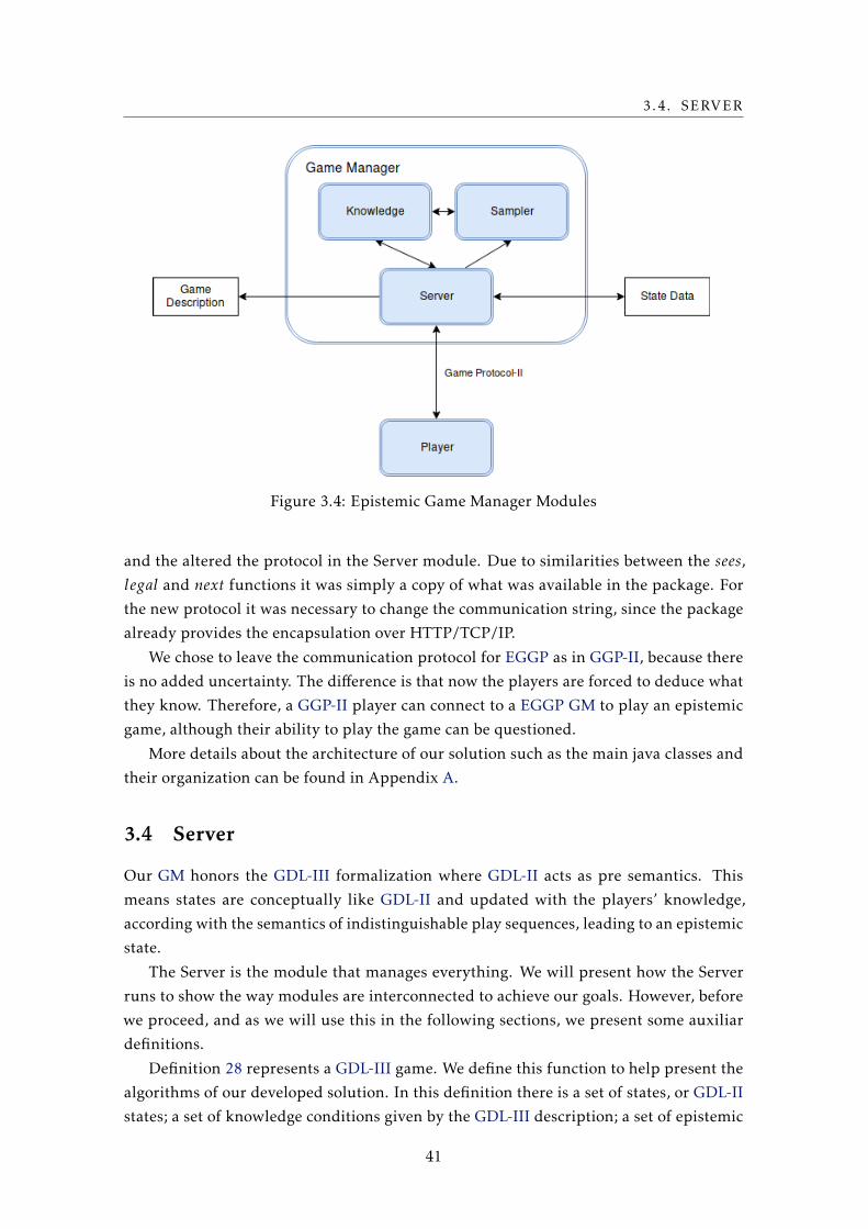
3.4. SERVER
Figure 3.4: Epistemic Game Manager Modules
and the altered the protocol in the Server module. Due to similarities between the sees,
legal and next functions it was simply a copy of what was available in the package. For
the new protocol it was necessary to change the communication string, since the package
already provides the encapsulation over HTTP/TCP/IP.
We chose to leave the communication protocol for EGGP as in GGP-II, because there
is no added uncertainty. The difference is that now the players are forced to deduce what
they know. Therefore, a GGP-II player can connect to a EGGP GM to play an epistemic
game, although their ability to play the game can be questioned.
More details about the architecture of our solution such as the main java classes and
their organization can be found in Appendix A.
3.4 Server
Our GM honors the GDL-III formalization where GDL-II acts as pre semantics. This
means states are conceptually like GDL-II and updated with the players’ knowledge,
according with the semantics of indistinguishable play sequences, leading to an epistemic
state.
The Server is the module that manages everything. We will present how the Server
runs to show the way modules are interconnected to achieve our goals. However, before
we proceed, and as we will use this in the following sections, we present some auxiliar
definitions.
Definition 28 represents a GDL-III game. We define this function to help present the
algorithms of our developed solution. In this definition there is a set of states, or GDL-II
states; a set of knowledge conditions given by the GDL-III description; a set of epistemic
41
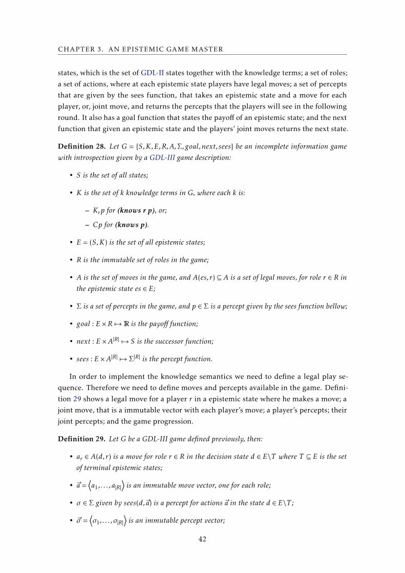
CHAPTER 3. AN EPISTEMIC GAME MASTER
states, which is the set of GDL-II states together with the knowledge terms; a set of roles;
a set of actions, where at each epistemic state players have legal moves; a set of percepts
that are given by the sees function, that takes an epistemic state and a move for each
player, or, joint move, and returns the percepts that the players will see in the following
round. It also has a goal function that states the payoff of an epistemic state; and the next
function that given an epistemic state and the players’ joint moves returns the next state.
Definition 28. Let G = {S,K,E,R,A,Σ, goal,next, sees} be an incomplete information gamewith introspection given by a GDL-III game description:
• S is the set of all states;
• K is the set of k knowledge terms in G, where each k is:
– Krp for (knows r p), or;
– Cp for (knows p).
• E = (S,K) is the set of all epistemic states;
• R is the immutable set of roles in the game;
• A is the set of moves in the game, and A(es, r) ⊆ A is a set of legal moves, for role r ∈ R inthe epistemic state es ∈ E;
• Σ is a set of percepts in the game, and p ∈ Σ is a percept given by the sees function bellow;
• goal : E ×R 7→R is the payoff function;
• next : E ×A|R| 7→ S is the successor function;
• sees : E ×A|R| 7→ Σ|R| is the percept function.
In order to implement the knowledge semantics we need to define a legal play se-
quence. Therefore we need to define moves and percepts available in the game. Defini-
tion 29 shows a legal move for a player r in a epistemic state where he makes a move; a
joint move, that is a immutable vector with each player’s move; a player’s percepts; their
joint percepts; and the game progression.
Definition 29. Let G be a GDL-III game defined previously, then:
• ar ∈ A(d,r) is a move for role r ∈ R in the decision state d ∈ E\T where T ⊆ E is the setof terminal epistemic states;
• ~a =⟨a1, . . . , a|R|
⟩is an immutable move vector, one for each role;
• σ ∈ Σ given by sees(d,~a) is a percept for actions ~a in the state d ∈ E\T ;
• ~σ =⟨σ1, . . . ,σ|R|
⟩is an immutable percept vector;
42
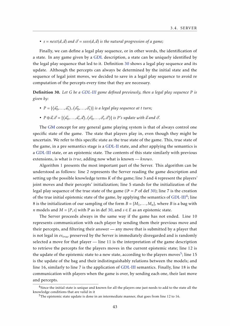
3.4. SERVER
• s = next(d,~a) and ~σ = sees(d,~a) is the natural progression of a game;
Finally, we can define a legal play sequence, or in other words, the identification of
a state. In any game given by a GDL description, a state can be uniquely identified by
the legal play sequence that led to it. Definition 30 shows a legal play sequence and its
update. Although the percepts can always be determined by the initial state and the
sequence of legal joint moves, we decided to save in a legal play sequence to avoid re
computation of the percepts every time that they are necessary.
Definition 30. Let G be a GDL-III game defined previously, then a legal play sequence P isgiven by:
• P ={⟨~a0, . . . , ~at
⟩,⟨~σ0, . . . , ~σt
⟩}is a legal play sequence at t turn;
• P ⊕ ~a, ~σ ={⟨~a0, . . . , ~at ,~a
⟩,⟨~σ0, . . . , ~σt , ~σ
⟩}is P ’s update with ~a and ~σ .
The GM concept for any general game playing system is that of always control one
specific state of the game. The state that players play in, even though they might be
uncertain. We refer to this specific state as the true state of the game. This, true state of
the game, in a pre semantics stage is a GDL-II state, and after applying the semantics is
a GDL-III state, or an epistemic state. The contents of this state similarly with previous
extensions, is what is true, adding now what is known — knows.
Algorithm 1 presents the most important part of the Server. This algorithm can be
understood as follows: line 2 represents the Server reading the game description and
setting up the possible knowledge terms K of the game; line 3 and 4 represent the players’
joint moves and their percepts’ initialization; line 5 stands for the initialization of the
legal play sequence of the true state of the game (P= P of def 30); line 7 is the creation
of the true initial epistemic state of the game, by applying the semantics of GDL-III4; line
8 is the initialization of our sampling of the form B = {M1, . . . ,Mn}, where B is a bag with
n models and M = {P ,s} with P as in def 30, and s ∈ E as an epistemic state.
The Server proceeds always in the same way if the game has not ended. Line 10
represents communication with each player by sending them their previous move and
their percepts, and filtering their answer — any move that is submitted by a player that
is not legal in estrue preserved by the Server is immediately disregarded and is randomly
selected a move for that player — line 11 is the interpretation of the game description
to retrieve the percepts for the players moves in the current epistemic state; line 12 is
the update of the epistemic state to a new state, according to the players moves5; line 15
is the update of the bag and their indistinguishably relations between the models; and
line 16, similarly to line 7 is the application of GDL-III semantics. Finally, line 18 is the
communication with players when the game is over, by sending each one, their last move
and percepts.4Since the initial state is unique and known for all the players one just needs to add to the state all the
knowledge conditions that are valid in it5The epistemic state update is done in an intermediate manner, that goes from line 12 to 16.
43
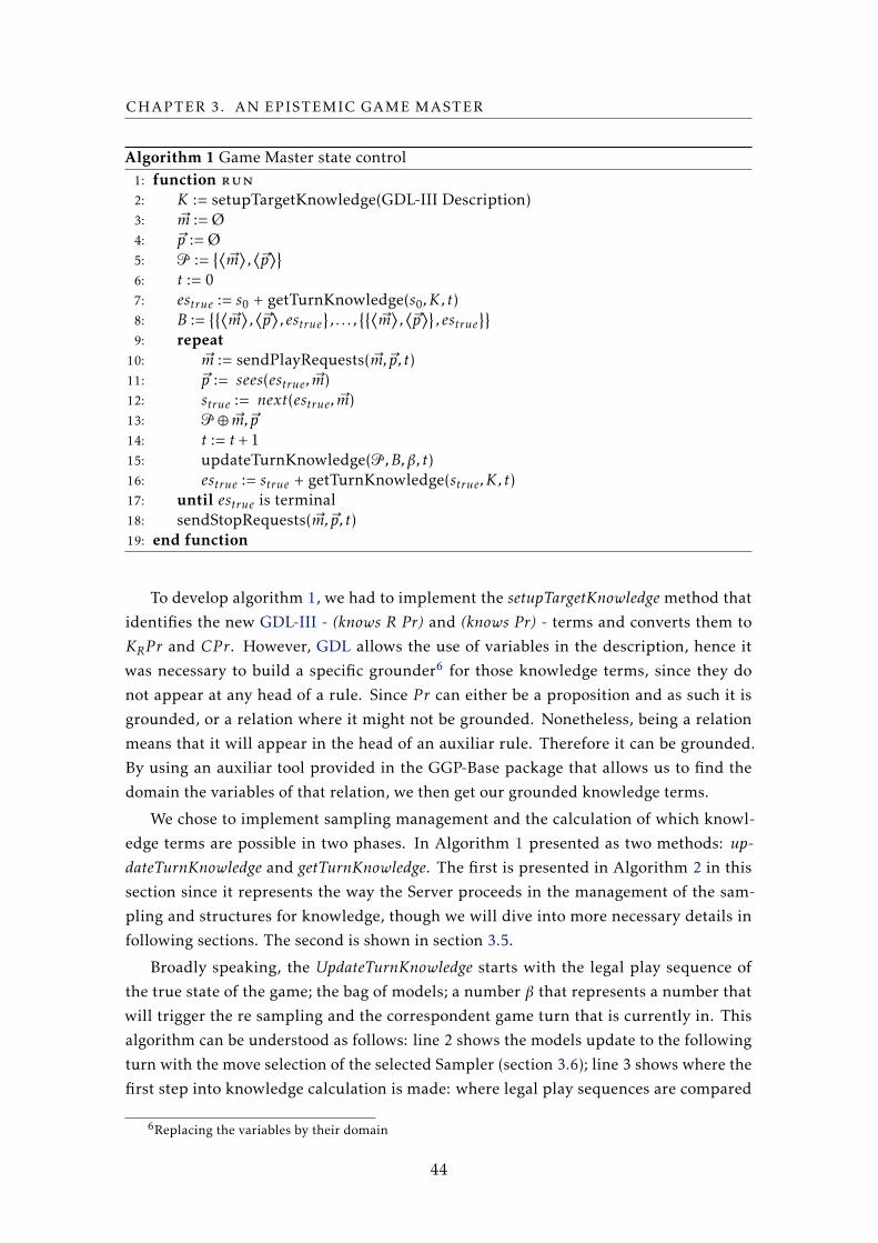
CHAPTER 3. AN EPISTEMIC GAME MASTER
Algorithm 1 Game Master state control1: function run
2: K := setupTargetKnowledge(GDL-III Description)3: ~m := Ø4: ~p := Ø5: P :=
{⟨~m⟩,⟨~p⟩}
6: t := 07: estrue := s0 + getTurnKnowledge(s0,K, t)8: B :=
{{⟨~m⟩,⟨~p⟩, estrue
}, . . . ,
{{⟨~m⟩,⟨~p⟩}, estrue
}}9: repeat
10: ~m := sendPlayRequests( ~m,~p, t)11: ~p := sees(estrue, ~m)12: strue := next(estrue, ~m)13: P⊕ ~m,~p14: t := t + 115: updateTurnKnowledge(P,B,β, t)16: estrue := strue + getTurnKnowledge(strue,K, t)17: until estrue is terminal18: sendStopRequests( ~m,~p, t)19: end function
To develop algorithm 1, we had to implement the setupTargetKnowledge method that
identifies the new GDL-III - (knows R Pr) and (knows Pr) - terms and converts them to
KRP r and CP r. However, GDL allows the use of variables in the description, hence it
was necessary to build a specific grounder6 for those knowledge terms, since they do
not appear at any head of a rule. Since P r can either be a proposition and as such it is
grounded, or a relation where it might not be grounded. Nonetheless, being a relation
means that it will appear in the head of an auxiliar rule. Therefore it can be grounded.
By using an auxiliar tool provided in the GGP-Base package that allows us to find the
domain the variables of that relation, we then get our grounded knowledge terms.
We chose to implement sampling management and the calculation of which knowl-
edge terms are possible in two phases. In Algorithm 1 presented as two methods: up-dateTurnKnowledge and getTurnKnowledge. The first is presented in Algorithm 2 in this
section since it represents the way the Server proceeds in the management of the sam-
pling and structures for knowledge, though we will dive into more necessary details in
following sections. The second is shown in section 3.5.
Broadly speaking, the UpdateTurnKnowledge starts with the legal play sequence of
the true state of the game; the bag of models; a number β that represents a number that
will trigger the re sampling and the correspondent game turn that is currently in. This
algorithm can be understood as follows: line 2 shows the models update to the following
turn with the move selection of the selected Sampler (section 3.6); line 3 shows where the
first step into knowledge calculation is made: where legal play sequences are compared
6Replacing the variables by their domain
44
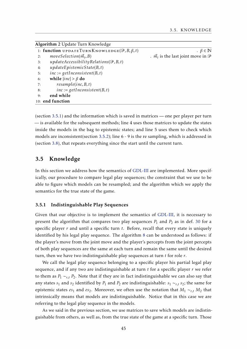
3.5. KNOWLEDGE
Algorithm 2 Update Turn Knowledge1: function updateTurnKnowledge(P,B,β, t) . β ∈N2: moveSelection( ~mt ,B) . ~mt is the last joint move in P
3: updateAccessibilityRelations(P,B, t)4: updateEpistemicState(B,t)5: inc := getInconsistent(B,t)6: while |inc| > β do7: resample(inc,B, t)8: inc := getInconsistent(B,t)9: end while
10: end function
(section 3.5.1) and the information which is saved in matrices — one per player per turn
— is available for the subsequent methods; line 4 uses those matrices to update the states
inside the models in the bag to epistemic states; and line 5 uses them to check which
models are inconsistent(section 3.5.2); line 6 - 9 is the re sampling, which is addressed in
(section 3.8), that repeats everything since the start until the current turn.
3.5 Knowledge
In this section we address how the semantics of GDL-III are implemented. More specif-
ically, our procedure to compare legal play sequences; the constraint that we use to be
able to figure which models can be resampled; and the algorithm which we apply the
semantics for the true state of the game.
3.5.1 Indistinguishable Play Sequences
Given that our objective is to implement the semantics of GDL-III, it is necessary to
present the algorithm that compares two play sequences P1 and P2 as in def. 30 for a
specific player r and until a specific turn t. Before, recall that every state is uniquely
identified by his legal play sequence. The algorithm 8 can be understood as follows: if
the player’s move from the joint move and the player’s percepts from the joint percepts
of both play sequences are the same at each turn and remain the same until the desired
turn, then we have two indistinguishable play sequences at turn t for role r.
We call the legal play sequence belonging to a specific player his partial legal play
sequence, and if any two are indistinguishable at turn t for a specific player r we refer
to them as P1 ∼r,t P2. Note that if they are in fact indistinguishable we can also say that
any states s1 and s2 identified by P1 and P2 are indistinguishable: s1 ∼r,t s2; the same for
epistemic states es1 and es2. Moreover, we often use the notation that M1 ∼r,t M2 that
intrinsically means that models are indistinguishable. Notice that in this case we are
referring to the legal play sequence in the models.
As we said in the previous section, we use matrices to save which models are indistin-
guishable from others, as well as, from the true state of the game at a specific turn. Those
45
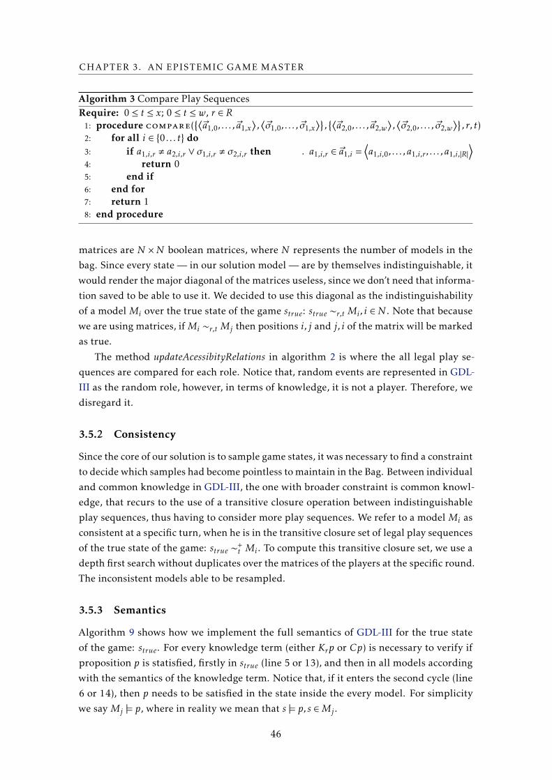
CHAPTER 3. AN EPISTEMIC GAME MASTER
Algorithm 3 Compare Play SequencesRequire: 0 ≤ t ≤ x; 0 ≤ t ≤ w, r ∈ R
1: procedure compare({⟨~a1,0, . . . ,~a1,x
⟩,⟨~σ1,0, . . . , ~σ1,x
⟩},{⟨~a2,0, . . . ,~a2,w
⟩,⟨~σ2,0, . . . , ~σ2,w
⟩}, r, t)
2: for all i ∈ {0 . . . t} do3: if a1,i,r , a2,i,r ∨ σ1,i,r , σ2,i,r then . a1,i,r ∈ ~a1,i =
⟨a1,i,0, . . . , a1,i,r , . . . , a1,i,|R|
⟩4: return 05: end if6: end for7: return 18: end procedure
matrices are N ×N boolean matrices, where N represents the number of models in the
bag. Since every state — in our solution model — are by themselves indistinguishable, it
would render the major diagonal of the matrices useless, since we don’t need that informa-
tion saved to be able to use it. We decided to use this diagonal as the indistinguishability
of a model Mi over the true state of the game strue: strue ∼r,t Mi , i ∈N . Note that because
we are using matrices, ifMi ∼r,t Mj then positions i, j and j, i of the matrix will be marked
as true.
The method updateAcessibityRelations in algorithm 2 is where the all legal play se-
quences are compared for each role. Notice that, random events are represented in GDL-
III as the random role, however, in terms of knowledge, it is not a player. Therefore, we
disregard it.
3.5.2 Consistency
Since the core of our solution is to sample game states, it was necessary to find a constraint
to decide which samples had become pointless to maintain in the Bag. Between individual
and common knowledge in GDL-III, the one with broader constraint is common knowl-
edge, that recurs to the use of a transitive closure operation between indistinguishable
play sequences, thus having to consider more play sequences. We refer to a model Mi as
consistent at a specific turn, when he is in the transitive closure set of legal play sequences
of the true state of the game: strue ∼+t Mi . To compute this transitive closure set, we use a
depth first search without duplicates over the matrices of the players at the specific round.
The inconsistent models able to be resampled.
3.5.3 Semantics
Algorithm 9 shows how we implement the full semantics of GDL-III for the true state
of the game: strue. For every knowledge term (either Krp or Cp) is necessary to verify if
proposition p is statisfied, firstly in strue (line 5 or 13), and then in all models according
with the semantics of the knowledge term. Notice that, if it enters the second cycle (line
6 or 14), then p needs to be satisfied in the state inside the every model. For simplicity
we say Mj |= p, where in reality we mean that s |= p,s ∈Mj .
46
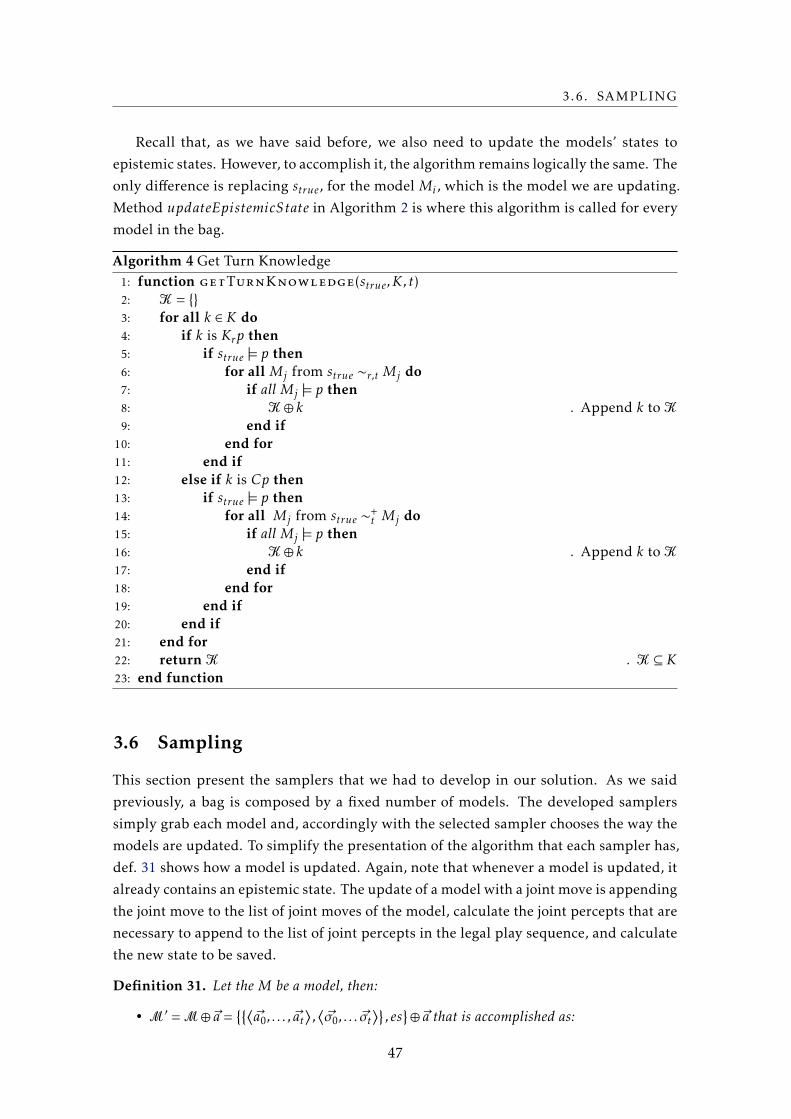
3.6. SAMPLING
Recall that, as we have said before, we also need to update the models’ states to
epistemic states. However, to accomplish it, the algorithm remains logically the same. The
only difference is replacing strue, for the model Mi , which is the model we are updating.
Method updateEpistemicState in Algorithm 2 is where this algorithm is called for every
model in the bag.
Algorithm 4 Get Turn Knowledge1: function getTurnKnowledge(strue,K, t)2: K= {}3: for all k ∈ K do4: if k is Krp then5: if strue |= p then6: for all Mj from strue ∼r,t Mj do7: if all Mj |= p then8: K⊕ k . Append k to K
9: end if10: end for11: end if12: else if k is Cp then13: if strue |= p then14: for all Mj from strue ∼+
t Mj do15: if all Mj |= p then16: K⊕ k . Append k to K
17: end if18: end for19: end if20: end if21: end for22: return K .K⊆ K23: end function
3.6 Sampling
This section present the samplers that we had to develop in our solution. As we said
previously, a bag is composed by a fixed number of models. The developed samplers
simply grab each model and, accordingly with the selected sampler chooses the way the
models are updated. To simplify the presentation of the algorithm that each sampler has,
def. 31 shows how a model is updated. Again, note that whenever a model is updated, it
already contains an epistemic state. The update of a model with a joint move is appending
the joint move to the list of joint moves of the model, calculate the joint percepts that are
necessary to append to the list of joint percepts in the legal play sequence, and calculate
the new state to be saved.
Definition 31. Let the M be a model, then:
• M′ = M⊕ ~a ={{⟨~a0, . . . , ~at
⟩,⟨~σ0, . . . ~σt
⟩}, es
}⊕ ~a that is accomplished as:
47
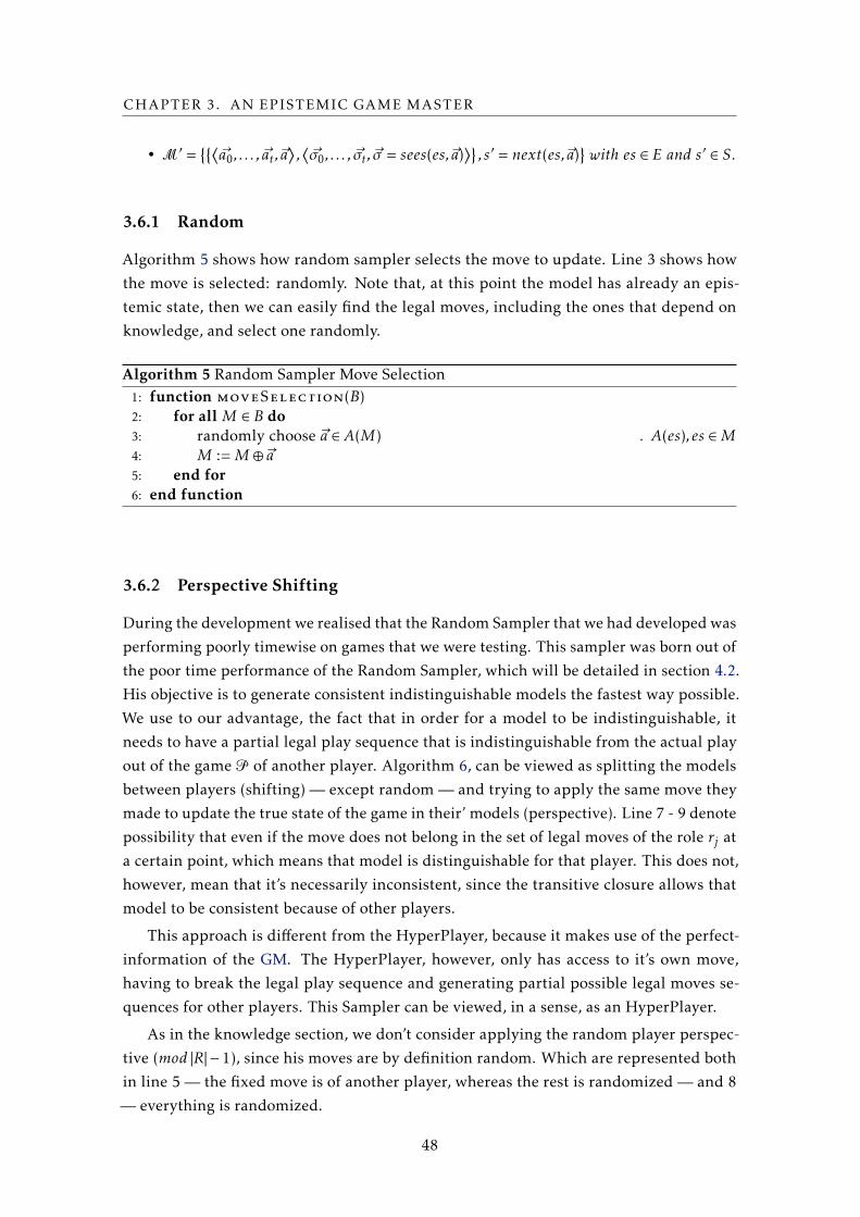
CHAPTER 3. AN EPISTEMIC GAME MASTER
• M′ ={{⟨~a0, . . . , ~at ,~a
⟩,⟨~σ0, . . . , ~σt , ~σ = sees(es,~a)
⟩}, s′ = next(es,~a)
}with es ∈ E and s′ ∈ S.
3.6.1 Random
Algorithm 5 shows how random sampler selects the move to update. Line 3 shows how
the move is selected: randomly. Note that, at this point the model has already an epis-
temic state, then we can easily find the legal moves, including the ones that depend on
knowledge, and select one randomly.
Algorithm 5 Random Sampler Move Selection1: function moveSelection(B)2: for all M ∈ B do3: randomly choose ~a ∈ A(M) . A(es), es ∈M4: M :=M ⊕ ~a5: end for6: end function
3.6.2 Perspective Shifting
During the development we realised that the Random Sampler that we had developed was
performing poorly timewise on games that we were testing. This sampler was born out of
the poor time performance of the Random Sampler, which will be detailed in section 4.2.
His objective is to generate consistent indistinguishable models the fastest way possible.
We use to our advantage, the fact that in order for a model to be indistinguishable, it
needs to have a partial legal play sequence that is indistinguishable from the actual play
out of the game P of another player. Algorithm 6, can be viewed as splitting the models
between players (shifting) — except random — and trying to apply the same move they
made to update the true state of the game in their’ models (perspective). Line 7 - 9 denote
possibility that even if the move does not belong in the set of legal moves of the role rj at
a certain point, which means that model is distinguishable for that player. This does not,
however, mean that it’s necessarily inconsistent, since the transitive closure allows that
model to be consistent because of other players.
This approach is different from the HyperPlayer, because it makes use of the perfect-
information of the GM. The HyperPlayer, however, only has access to it’s own move,
having to break the legal play sequence and generating partial possible legal moves se-
quences for other players. This Sampler can be viewed, in a sense, as an HyperPlayer.
As in the knowledge section, we don’t consider applying the random player perspec-
tive (mod |R| − 1), since his moves are by definition random. Which are represented both
in line 5 — the fixed move is of another player, whereas the rest is randomized — and 8
— everything is randomized.
48
3.7. PLAUSIBILITY
Algorithm 6 Perspective Shifting Sampler Move Selection1: function moveSelection( ~m,B) . ~m ∈P2: for all Mi ∈ B do3: j := i mod (|R| − 1)4: if mrj ∈ A(Mi , rj ) then . estrue ∼rj Mi
5: randomly choose ~a ∈ A(Mi), where arj =mrj6: Mi :=Mi ⊕ ~a7: else . Consider estrue ∼+ Mi
8: randomly choose ~a ∈ A(Mi)9: M :=Mi ⊕ ~a
10: end if11: end for12: end function
3.7 Plausibility
In this section we need to address the fact that our solution is by definition approximative.
It is necessary to define a new concept, that of plausibility. To explain it, we will use an
example. Unlike we have been using throughout this chapter, in this section we only
consider epistemic states. Notice that, by applying the semantics of GDL-III leads to an
epistemic game tree with epistemic states.
Having that said, as you can see in the Figure 3.5, there are two joint game trees of
Muddy Children Game with two children (A and B). On the left a complete game tree
with all epistemic states, on the right an incomplete tree. In this game children know that
at least one of them is muddy, and the objective is for them to know that themselves are
muddy. For simplicity, we assume that the children’ percepts are received right after a
move is made; and that the game finishes after a child says yes. A child can say yes if and
only if she knows that she has mud.
As one can see on the tree in the left, in round 0 the random player chooses between
the configurations to setup the muddy children. The possibilities are 01 and B is muddy,
11 both A and B are muddy, 10 and A is muddy. The children do nothing, represented
as n. Depending on the configuration if is either 01, or 10, at round 1, the child that has
mud says yes (y) because she can see the other doesn’t have, but if they both have mud,
they do no operation — also denoted by n — , symbolizing that they don’t know if they
have mud. Therefore, at round 2, if they both said no, then both know that they have
mud, because they can distinguish between all the possible epistemic states of the game.
This is what happens when you can consider all the possible states at a certain turn.
However, since our solution is approximative, such case as in the right tree can happen.
Imagine that one doesn’t have enough space in the bag for all the possible epistemic states
at round 1. Or better, in every game sample, since it is random, the chosen settings were
always 11 and 01. One can see that player A can not distinguish between the states 01,
and 11, because in both cases he can see that B has mud, but he is still not sure about
49
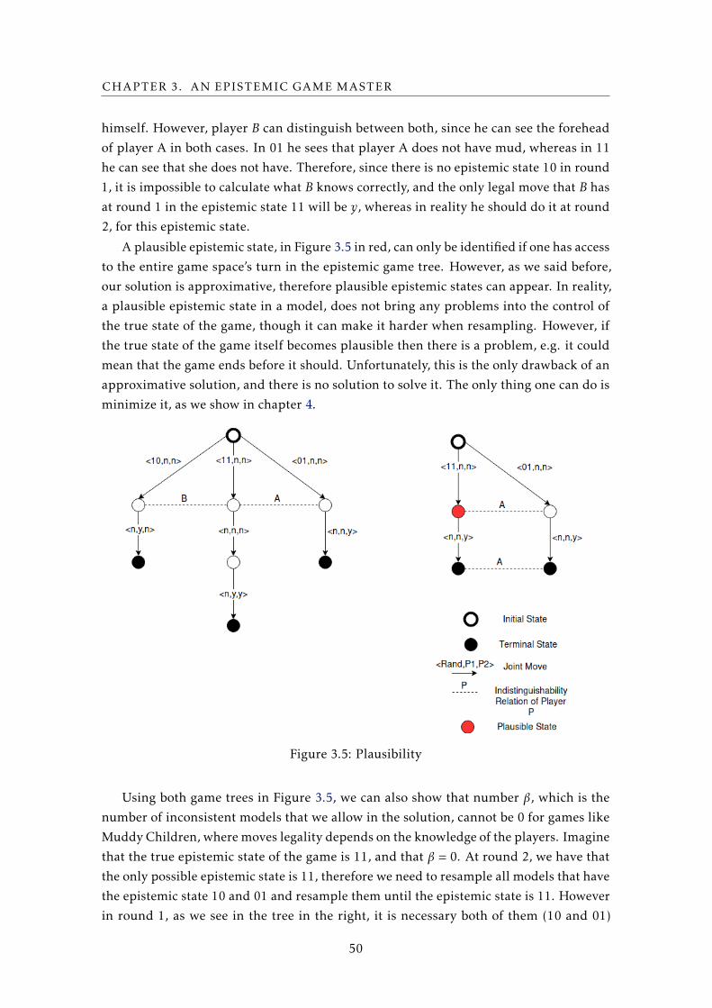
CHAPTER 3. AN EPISTEMIC GAME MASTER
himself. However, player B can distinguish between both, since he can see the forehead
of player A in both cases. In 01 he sees that player A does not have mud, whereas in 11
he can see that she does not have. Therefore, since there is no epistemic state 10 in round
1, it is impossible to calculate what B knows correctly, and the only legal move that B has
at round 1 in the epistemic state 11 will be y, whereas in reality he should do it at round
2, for this epistemic state.
A plausible epistemic state, in Figure 3.5 in red, can only be identified if one has access
to the entire game space’s turn in the epistemic game tree. However, as we said before,
our solution is approximative, therefore plausible epistemic states can appear. In reality,
a plausible epistemic state in a model, does not bring any problems into the control of
the true state of the game, though it can make it harder when resampling. However, if
the true state of the game itself becomes plausible then there is a problem, e.g. it could
mean that the game ends before it should. Unfortunately, this is the only drawback of an
approximative solution, and there is no solution to solve it. The only thing one can do is
minimize it, as we show in chapter 4.
Figure 3.5: Plausibility
Using both game trees in Figure 3.5, we can also show that number β, which is the
number of inconsistent models that we allow in the solution, cannot be 0 for games like
Muddy Children, where moves legality depends on the knowledge of the players. Imagine
that the true epistemic state of the game is 11, and that β = 0. At round 2, we have that
the only possible epistemic state is 11, therefore we need to resample all models that have
the epistemic state 10 and 01 and resample them until the epistemic state is 11. However
in round 1, as we see in the tree in the right, it is necessary both of them (10 and 01)
50
3.8. A DYNAMIC EPISTEMIC RESAMPLE
so that epistemic state 11 does not become plausible, as well. Then, it is necessary to
keep some inconsistent models (β , 0) in these types of dynamic epistemic games. These
models, do not introduce problems in the knowledge verification, since they are already
inconsistent at round 2. This avoids infinite re sampling, since the plausible epistemic
state 11 at round 2 (marked in red in the right tree) would also be inconsistent.
3.8 A Dynamic Epistemic Resample
Whenever models are not in the transitive closure set of the true state of the game, they
are able to be removed and replaced by other models with consistent epistemic states. On
our re sample approach we considered two options:
• Redo the model from the initial state until the current turn;
• Going back to previous turn and generate a new joint move.
Both approaches could work. However, since our goal with re sampling was to mini-
mize plausibility, we chose the first approach. Our option is due to the fact that the con-
tent of an epistemic state is usually determined by the random player’s move at round 0.
Algorithm 7 presents our resampling. This algorithm can be viewed as follows: it
receives the identification number of the inconsistent models, which is the model position
in the bag; the bag of models; and the current turn; line 2-4 shows the replacement of
the epistemic state inside the inconsistent model with the true initial epistemic state
of the game, and the replacement of it’s legal play sequence as empty; After this part is
concluded, it starts doing the same thing round by round, until one reaches the given turn
t. This means that at every turn it is necessary to apply a joint move with the designated
sampler (line 6-8). Followed by a comparison the new legal play sequences until the
current turn i with all the other models, and the legal play sequence of the true state
of the game (line 9-11). When we have the matrices of the players updated with this
new information about their indistinguishability, it is necessary to apply the semantics
of GDL-III only to the models’ states being resampled (12-14), the others aren’t changed.
Another decision we had to consider was the checking of inconsistent models. The
options were that, either at each turn i that we complete, or just when we would reach
the turn t. In our point of view, both ways would lead to the same end result. But since
evaluating the consistency of the bag turn by turn could increase even more time sent on
re sampling, so chose the later.
3.9 Information Stealing
A EGGP setting always assumes that the players are truthful about themselves. This
means that players should not lie. However, since players’ moves can be described by
knowledge terms two things can happen. Either a player can submit a move were he
51
CHAPTER 3. AN EPISTEMIC GAME MASTER
Algorithm 7 Re Sampling1: function resample(inc = 〈0, . . . ,N 〉 ,B, t)2: for all j ∈ inc do3: replace(Mj , es0)4: end for5: for i ∈ {0, . . . , t} do6: for all j ∈ inc do7: moveSelection(Mj ∈ B)8: end for9: for all j ∈ inc do
10: updateAccessibilityRelations(P,Mj ∈ B, i)11: end for12: for all j ∈ inc do13: updateEpistemicState(Mj ∈ B)14: end for15: end for16: end function
thinks he knows something when in fact he does not; or he could use the fact that the GM
as access to information of all the players and intentionally submit a move that he is still
not sure, just so that the GM answer whether that move was legal or not. Notice that in
both cases the player submits a move but, that in the first case the player is being truthful,
and in the second it is not. If the situation becomes problematic such as in competitive
settings, a game designer should consider the following Listing to ensure that a player
thinks twice before submitting these types of moves. The GM does not have the ability to
differentiate the situations. He will only make sure players obey the game description.
1 % t h e move in q u e s t i o n2 (<= ( l e g a l ? r ?m) ( knows ? r p ) )
3
4 % copy o f t h e r e l a t i o n s i n c e t h e l e g a l keyword shouldn ’ t appear in t h e r u l e s ’ body5 (<= ( i s L e g a l ? r ?m) ( knows ? r p ) )
6
7 % s a v i n g f o r l a t e r punish i f p l a y e r ? r ’ s move i s not l e g a l8 (<= ( next ( punish ? r ) ) ( does ? r ?m) ( not ( i s L e g a l ? r ?m) ) )
9 (<= ( next ( punish ? r ) ) ( true ( punish ? r ) ) )
10
11 (<= ( goal ? r 100) ( true ( someProposition ) ) )
12 % punish ing13 (<= ( goal ? r 0) ( true ( someProposition ) ) ( true ( punish ? r ) ) )
52
Chapter
4Analysis
In this chapter, we study the correction of the knowledge semantics implementation,
which is based, as aforementioned in the semantics described in [Thi17]. We study the
correction of the developed samplers and show that they act as a solution that considers
the hole state space, given enough resources. Furthermore, we test the scalability of our
developed GM regarding the complexity of games, versus time by turn that it takes to
execute to make a consistent bag of models for that turn and calculate the knowledge of
players.
4.1 Correction
In this section we show that our developed solution behaves according to what is expected
given enough resources.
4.1.1 Knowledge
We now show that our knowledge algorithms are not what induces errors when calculat-
ing the knowledge for a specific state. Algorithms 8 and 9 presented in Section 3.5 were
copied here in order to be able to make comparisons with Definition 32 which is also
copied from Section 2.4.3.
Algorithm 8 shows how two legal play sequences are compared for a specific player.
It showcases that for two legal play sequences to be indistinguishable for a player, his
partial legal play sequence has to be the same from the initial state until the current state
at time t. By starting from the initial turn until the current turn, if at any turn i in the
between, if his move or percepts are different then it returns: 0. Otherwise, if it goes out
from line 5 and returns: 1 since they are equal. This algorithm is therefore correct in the
way it compares any two legal play sequences for a given player at a given turn.
53
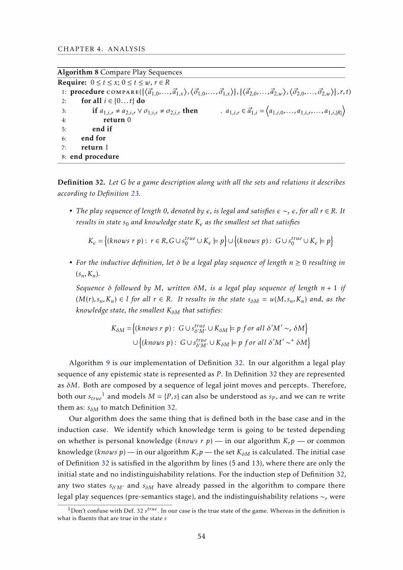
CHAPTER 4. ANALYSIS
Algorithm 8 Compare Play SequencesRequire: 0 ≤ t ≤ x; 0 ≤ t ≤ w, r ∈ R
1: procedure compare({⟨~a1,0, . . . ,~a1,x
⟩,⟨~σ1,0, . . . , ~σ1,x
⟩},{⟨~a2,0, . . . ,~a2,w
⟩,⟨~σ2,0, . . . , ~σ2,w
⟩}, r, t)
2: for all i ∈ {0 . . . t} do3: if a1,i,r , a2,i,r ∨ σ1,i,r , σ2,i,r then . a1,i,r ∈ ~a1,i =
⟨a1,i,0, . . . , a1,i,r , . . . , a1,i,|R|
⟩4: return 05: end if6: end for7: return 18: end procedure
Definition 32. Let G be a game description along with all the sets and relations it describesaccording to Definition 23.
• The play sequence of length 0, denoted by ε, is legal and satisfies ε ∼r ε, for all r ∈ R. Itresults in state s0 and knowledge state Kε as the smallest set that satisfies
Kε ={(knows r p) : r ∈ R,G∪ strue0 ∪Kε |= p
}∪
{(knows p) : G∪ strue0 ∪Kε |= p
}• For the inductive definition, let δ be a legal play sequence of length n ≥ 0 resulting in
(sn,Kn).
Sequence δ followed by M, written δM, is a legal play sequence of length n + 1 if(M(r), sn,Kn) ∈ l for all r ∈ R. It results in the state sδM = u(M,sn,Kn) and, as theknowledge state, the smallest KδM that satisfies:
KδM ={(knows r p) : G∪ strueδ′M ′ ∪KδM |= p f or all δ
′M ′ ∼r δM}
∪{(knows p) : G∪ strueδ′M ′ ∪KδM |= p f or all δ
′M ′ ∼+ δM}
Algorithm 9 is our implementation of Definition 32. In our algorithm a legal play
sequence of any epistemic state is represented as P . In Definition 32 they are represented
as δM. Both are composed by a sequence of legal joint moves and percepts. Therefore,
both our strue1 and models M = {P ,s} can also be understood as sP , and we can re write
them as: sδM to match Definition 32.
Our algorithm does the same thing that is defined both in the base case and in the
induction case. We identify which knowledge term is going to be tested depending
on whether is personal knowledge (knows r p) — in our algorithm Krp — or common
knowledge (knows p) — in our algorithm Krp — the set KδM is calculated. The initial case
of Definition 32 is satisfied in the algorithm by lines (5 and 13), where there are only the
initial state and no indistinguishability relations. For the induction step of Definition 32,
any two states sδ′M ′ and sδM have already passed in the algorithm to compare there
legal play sequences (pre-semantics stage), and the indistinguishability relations ∼r were
1Don’t confuse with Def. 32 strue. In our case is the true state of the game. Whereas in the definition iswhat is fluents that are true in the state s
54
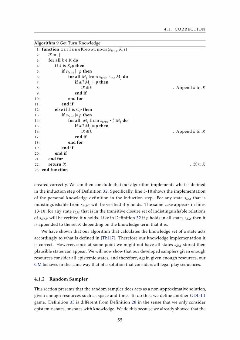
4.1. CORRECTION
Algorithm 9 Get Turn Knowledge1: function getTurnKnowledge(strue,K, t)2: K= {}3: for all k ∈ K do4: if k is Krp then5: if strue |= p then6: for all Mj from strue ∼r,t Mj do7: if all Mj |= p then8: K⊕ k . Append k to K
9: end if10: end for11: end if12: else if k is Cp then13: if strue |= p then14: for all Mj from strue ∼+
t Mj do15: if all Mj |= p then16: K⊕ k . Append k to K
17: end if18: end for19: end if20: end if21: end for22: return K .K⊆ K23: end function
created correctly. We can then conclude that our algorithm implements what is defined
in the induction step of Definition 32. Specifically, line 5-10 shows the implementation
of the personal knowledge definition in the induction step. For any state sδM that is
indistinguishable from sδ′M ′ will be verified if p holds. The same case appears in lines
13-18, for any state sδM that is in the transitive closure set of indistinguishable relations
of sδ′M ′ will be verified if p holds. Like in Definition 32 if p holds in all states sδM then it
is appended to the set K depending on the knowledge term that it is.
We have shown that our algorithm that calculates the knowledge set of a state acts
accordingly to what is defined in [Thi17]. Therefore our knowledge implementation it
is correct. However, since at some point we might not have all states sδM stored then
plausible states can appear. We will now show that our developed samplers given enough
resources consider all epistemic states, and therefore, again given enough resources, our
GM behaves in the same way that of a solution that considers all legal play sequences.
4.1.2 Random Sampler
This section presents that the random sampler does acts as a non-approximative solution,
given enough resources such as space and time. To do this, we define another GDL-III
game. Definition 33 is different from Definition 28 in the sense that we only consider
epistemic states, or states with knowledge. We do this because we already showed that the
55
CHAPTER 4. ANALYSIS
algorithm that implements GDL-III semantics acts accordingly to its definition. Therefore
it is not necessary to split between a pre-semantics stage and a post-semantics, and we
can only consider the post-semantics that lead to the epistemic game tree.
Definition 33. Let G = {S,R,A,Σ, goal,next, sees} be an incomplete information game withintrospection given by a GDL-III game description:
• S is the set of all epistemic states on the game tree;
• R is the set of roles in the game;
• A is the set of moves in the game, and A(s, r) ⊆ A is a set of legal moves, for role r ∈ R inthe epistemic state s ∈ S;
• Σ is a set of percepts in the game, and p ∈ Σ is a percept given by the sees function bellow;
• goal : S ×R 7→R is the payoff function;
• next : S ×A|R| 7→ S is the successor function;
• sees : S ×A|R| 7→ Σ|R| is the percept function.
Moreover, let:
• s0 be the initial epistemic state;
• Si ⊆ S denote the epistemic state space of G at turn i ∈ N0, such that S0 = {s0} andSi+1 =
{si+1 : si+1 = next(si ,~a) for all si ,~a ∈ A(si , r1)× ...×A(si , r|R|)
};
Definition 33 defines an epistemic game, that has the set of all epistemic states in
the game; the set of roles in the game; the set of actions; the set of percepts; the payofffunction; the state update function; and the percept function. Si denotes a specific state
space at turn i.
Definition 34. Let G be an epistemic game as defined in def. 33, and:
• Choose : S 7→ A|R| be a stochastic function, and ~a = Choose(s) is the chosen joint movewith uniform probability from the set A(s, r1)× ...×A(s, r|R|), with s ∈ S;
• Bi is a set of ordered pairs of size N ∈N at turn i ∈N0, such that:
– B0 = {(s0, j) : s0 ∈ S0, j ∈ {1, . . . ,N } } and,
– Bi+1 = {(si+1, j) : (si , j) ∈ Bi ∧ si+1 = next(si ,Choose(si))}.
Definition 34 defines the Random Sampler. Throughout the rest of this thesis, we
denote by si,j pairs (si , j) ∈ Bi , where j represents the position of state si in the bag of
models represented by Bi . As one can deduce from the definition above, the position
associated with each state never changes, even after applying the function next. The only
56
4.1. CORRECTION
thing that changes is si to si+1. We have that function Choose uses a uniform probability
over the domain of the joint legal moves of the players. The set B is defined using an
inductive definition where at turn 0, B0 has copies of the initial state of the game. One
for each pair in the set. The following turns are accomplished by applying the Choose
function to each state in the set B of the previous turn.
We use this Definition 34 to define set Bi in the Lemma 4.1.1, that represents the
set of all possible sets Bi at turn i, to be able to mathematically show that our samplers
behave as a solution that considers all states given enough resources. Lemma 4.1.1 proves
that the random sampler behaves accordingly. By defining the function that chooses
randomly an action to update a state, we can show that if set B’s size is infinite, then it
will always have all the epistemic states belonging to a game at that round.
Lemma 4.1.1. Let G be as in def. 33, Bi as in def. 34 and:
• Bi denote the set of all possible Bi at turn i.
Then,∀s∈Si ,Bi∈Bi
limN→+∞
P (s ∈ Bi) = 1.
Proof Skecth. By induction on the turn i of game G.
• Base case (i = 0): Let s ∈ S0 be an epistemic state, and B0 ∈B0 be a possible set as
described previously. With i = 0, we have that S0 = {s0}, therefore s = s0. Since, by
definition, B0 contains N ordered pairs (s0, j) (for j ∈ {0, . . . ,N }, corresponding to the
N copies of the initial state s0), it follows:
P (s ∈ B0) = 1.
• Induction step (i > 0): Let si ∈ Si be an epistemic state at turn i, where si,j ∈ Bimeans that si is at position j of Bi . And, si+1 ∈ Si+1 be a state that follows from
unequivocally choosing ~a from A(si,j , r1)× ...×A(si,j , r|R|) and applying the function
si+1 = next(si ,~a) as defined in def. 33.
Then, let: Ej be the event of choosing an action ~a for the state si,j , and Ej+1 be the
event of choosing an action ~a for the state si,j+1. Therefore, since by definition Ejand Ej+1 are chosen with a uniform probability. And, furthermore, both Ej and Ej+1
are independent events, since there is no correlation between choosing ~a for state
si,j or si,j+1. Then, we can say that:
∞∑j=1
P (Ej ) =∞
Using the Second Borel-Cantelli Lemma we have that the probability of a non null
independent event to happen when the number of times the same event occurs is
infinite is:
limj→∞
P (Ej ) = 1.
57
CHAPTER 4. ANALYSIS
Then we can conclude since the probability of the event Ej , when j → ∞ is one,
then for sure ~a will be selected, which will follow that si+1,j = next(si,j ,~a), we can
conclude that:
P (si+1 ∈ Bi+1) = 1.
Note that if our solution would have infinite space, then we do not need to resample
models since the probability of having all the epistemic states of the game at any round
in the bag is one. Moreover, we can also conclude that if we have enough space for all
states, then there are no plausible states since they only happen if we do not consider all
the necessary states.
4.1.3 Perspective Sampler
As in the previous section, we will show why this sampler is correct, in the sense that
considers all possible epistemic states.
Definition 35. Let G be as in Definition 33, and:
• strue,i ∈ Si - the true state of the game at turn i;
• ar is a specific move for role r ∈ R in joint move ~a ∈ A|R|;
• ~m is the real joint move that updated strue,i+1 = next(strue,i , ~m), with ~m ∈ A(strue,i , r1)×...×A(strue,i , r|R|).
Definition 35 shows the definition of the true state of the game, which the state that
is being updated by the players. Likewise, the real joint move is the move that updates
the true state of the game. Definition 36 shows the definition of the Perspective Sampler.
Definition 36. Let G be as in def. 33 and m as in def. 35, then:
Bi is a set of ordered pairs of size N ∈N at turn i ∈N0, such that:
• B0 = {(s0, j) : s0 ∈ S0, j ∈ {1, . . . ,N } } and,
• Bi+1 ={(si+1, j) : (si , j) ∈ Bi ∧ si+1 = next(si ,Choose(si , j, ~m))
}, where:
– Choose : S ×N×A|R| 7→ A|R| is a stochastic function chooses with a uniform proba-bility from the set M ⊆ A|R|, such that ~a = Choose(si , j, ~m):M = A(si , r1)× · · · ×
{mrz
}× · · · ×A(si , r|R|), if mrz ∈ A(si , rz)
M = A(si , r1)× ...×A(si , r|R|), otherwise,
where z = j mod (|R| − 1).
58
4.1. CORRECTION
Like our previous sampler we have that set B at turn 0, or B0, starts with N copies
of the initial state of the game. The update of the set is also like the previous sampler.
However, Choose function in this sampler takes an extra argument, a joint move ~m. We
use the position of the state in the set Bi to determine a role rz. Then we calculate a new
domain for the legal joint moves of rz. This new domain is built from the given role,
where the specific move of that role is fixed, if the role rz can make that move in that state,
or in other words, mrz ∈ A(si,j , rz). Otherwise, the domain of legal moves of rz remains the
same. All the sets of legal joint moves for the other players continue the same.
We will now present the conjecture that this sampler is correct and therefore considers
all epistemic states of a game G at a particular turn for games where |R| > 1. Notice that
also that if |R| = 1 then there is only one player, which is either random (which is pointless
to describe an epistemic game with only the nature). Or that, there is only a player, but
there is no uncertainty since the player is the only one in the game2.
Conjecture 4.1.1. Let G be as in Definition 33 for |R| > 1 and Bi as defined in Definition 36:
• Bi denote the set of all possible Bi at turn i.
Then:
∀s∈Si ,Bi∈Bilim
N→+∞P (s ∈ Bi) = 1.
We argue why we believe this sampler considers all the possible states at turn i. At turn
0 we have that B0 starts with N copies of s0, therefore we can say that, since S0 = {s0} then
P (s0 ∈ B0) = 1. As for the following turns, we have ~a ∈M, where ~a is chosen with a uniform
probability over the setM. M is determined by two conditions: the "otherwise" condition,
where M is as in the previous sampler, which it is proven as correct in Lemma 4.1.1 proof
sketch. Or the first condition, where move mrz is fixed. It will always enter this condition
if player rz is uncertain about that state. However, if it’s certain that it is not in that state,
it will always go to the "otherwise" condition. The probability of rz being certain about
that state will be one at a certain turn since the objective of an uncertain game reduce
the number of uncertain states for each player. Therefore it will always jump onto the
"otherwise" condition.
Another reason why we believe that the conjecture is true is that since a move is fixed
at a state si,j in the set Bi — because of j — and that if the size of Bi tends to infinity, then
there will be infinite si ,∞, were will be fixed each player move infinite times. With the
fact that the random player’s move is always random and that this is represented by its
set of legal moves always remains untouched. We can say that even though rz is fixed in
si,j , it will not be fixed in si,j+1, because even though is the same state, the fixed move
will be of another player, except if it is a single player game (note that a single-player
game is a game with 2 roles: random and the player). In a single-player game to explore
the other moves of the player are unnecessary since both the personal knowledge set and
2Single-player epistemic games should be described using two players: the player and random
59
CHAPTER 4. ANALYSIS
the common knowledge set are the same. For the other cases, we can say that the union
of the update the function Chooses infinite times also gives all states, using the Second
Borel-Cantelli Lemma, since choosing over the set M is always independent and with a
probability different than 0.
4.2 Scalability
In this section shows how our solution scales timely by increasing the size of the game.
We measure the time it takes into updating models, making sure these are consistent
and calculating knowledge in between turns. In some plots, we use a logarithmic scale
in order to be able show all the information on it. We also present the results in a
table so that the reader can understand them clearly. Each line in a plot is represented
as⟨Sampler;N ;β;K ;R
⟩, where N means the total number os models; β the number of
inconsistent models allowed; K the number of rules that the game has; and R the number
of roles in the game. Results are presented turn by turn, by the time it took execute do line
15 and 16 of algorithm 1. All the tests were executed 20 times in a localhost environment
between the GM and the players, in an Intel® Core™ i7-3537U CPU @ 2.00GHz and 4
GB of RAM machine. Tries where the game instance became plausible were disregarded.
Games used to analyse the scalability can be found in Appendix B. We have developed
more games, such as the hats puzzle problem that is presented in Appendix C, but because
this game is similar to the Muddy Children we do not analyse the GM scalability with
it. Furthermore, we also build games, that are presented in Appendix D, however these
games were developed to test if the GM would act accordingly to what it should, and not
to measure scalability.
4.2.1 Number Guessing Epistemic
This game is a variation of a GDL-II game, where a player wants to know the secret
number. This secret number is set by the nature by the first move. After that, nature
does always no operation, whereas the player can always ask if the secret number is less
than another. This game has a branching factor of the numbers of the game. The tests
procedure were: nature selected always the same number, and the selected move was
always the same at the same round. It was applied in order to divide the set consistent
epistemic states of the player by half. The game has a branching factor of the possible
numbers in the game. The game was intentionally designed to end when the player knows
the number. That is the reason why a game with 4 numbers has only measured 3 turns. At
turn 3, player knows the number set by random. Therefore for games with more numbers:
8, 16 and 256, games end at turn 4, 5 and 9, respectively.
Figure 4.1 shows the time scalability by using the different samplers. Recall that
each line in the plot represents a different setting and that the horizontal scale is in
60
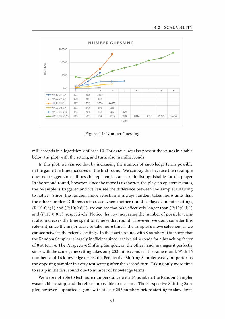
4.2. SCALABILITY
Figure 4.1: Number Guessing
milliseconds in a logarithmic of base 10. For details, we also present the values in a table
below the plot, with the setting and turn, also in milliseconds.
In this plot, we can see that by increasing the number of knowledge terms possible
in the game the time increases in the first round. We can say this because the re sample
does not trigger since all possible epistemic states are indistinguishable for the player.
In the second round, however, since the move is to shorten the player’s epistemic states,
the resample is triggered and we can see the difference between the samplers starting
to notice. Since, the random move selection is always random takes more time than
the other sampler. Differences increase when another round is played. In both settings,
〈R;10;0;4;1〉 and 〈R;10;0;8;1〉, we can see that take effectively longer than 〈P ;10;0;4;1〉and 〈P ;10;0;8;1〉, respectively. Notice that, by increasing the number of possible terms
it also increases the time spent to achieve that round. However, we don’t consider this
relevant, since the major cause to take more time is the sampler’s move selection, as we
can see between the referred settings. In the fourth round, with 8 numbers it is shown that
the Random Sampler is largely inefficient since it takes 44 seconds for a branching factor
of 8 at turn 4. The Perspective Shifting Sampler, on the other hand, manages it perfectly
since with the same game setting takes only 233 milliseconds in the same round. With 16
numbers and 16 knowledge terms, the Perspective Shifting Sampler vastly outperforms
the opposing sampler in every test setting after the second turn. Taking only more time
to setup in the first round due to number of knowledge terms.
We were not able to test more numbers since with 16 numbers the Random Sampler
wasn’t able to stop, and therefore impossible to measure. The Perspective Shifting Sam-
pler, however, supported a game with at least 256 numbers before starting to slow down
61
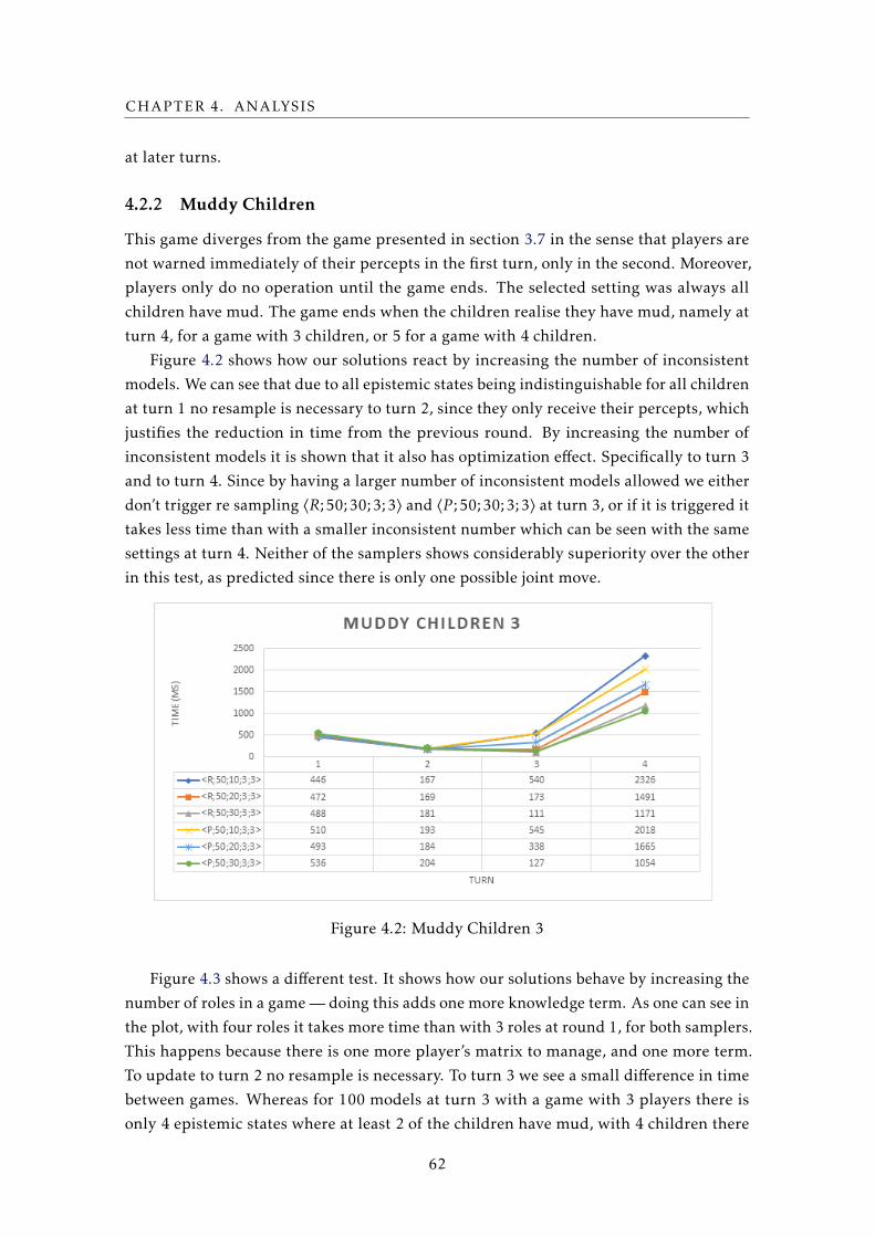
CHAPTER 4. ANALYSIS
at later turns.
4.2.2 Muddy Children
This game diverges from the game presented in section 3.7 in the sense that players are
not warned immediately of their percepts in the first turn, only in the second. Moreover,
players only do no operation until the game ends. The selected setting was always all
children have mud. The game ends when the children realise they have mud, namely at
turn 4, for a game with 3 children, or 5 for a game with 4 children.
Figure 4.2 shows how our solutions react by increasing the number of inconsistent
models. We can see that due to all epistemic states being indistinguishable for all children
at turn 1 no resample is necessary to turn 2, since they only receive their percepts, which
justifies the reduction in time from the previous round. By increasing the number of
inconsistent models it is shown that it also has optimization effect. Specifically to turn 3
and to turn 4. Since by having a larger number of inconsistent models allowed we either
don’t trigger re sampling 〈R;50;30;3;3〉 and 〈P ;50;30;3;3〉 at turn 3, or if it is triggered it
takes less time than with a smaller inconsistent number which can be seen with the same
settings at turn 4. Neither of the samplers shows considerably superiority over the other
in this test, as predicted since there is only one possible joint move.
Figure 4.2: Muddy Children 3
Figure 4.3 shows a different test. It shows how our solutions behave by increasing the
number of roles in a game — doing this adds one more knowledge term. As one can see in
the plot, with four roles it takes more time than with 3 roles at round 1, for both samplers.
This happens because there is one more player’s matrix to manage, and one more term.
To update to turn 2 no resample is necessary. To turn 3 we see a small difference in time
between games. Whereas for 100 models at turn 3 with a game with 3 players there is
only 4 epistemic states where at least 2 of the children have mud, with 4 children there
62
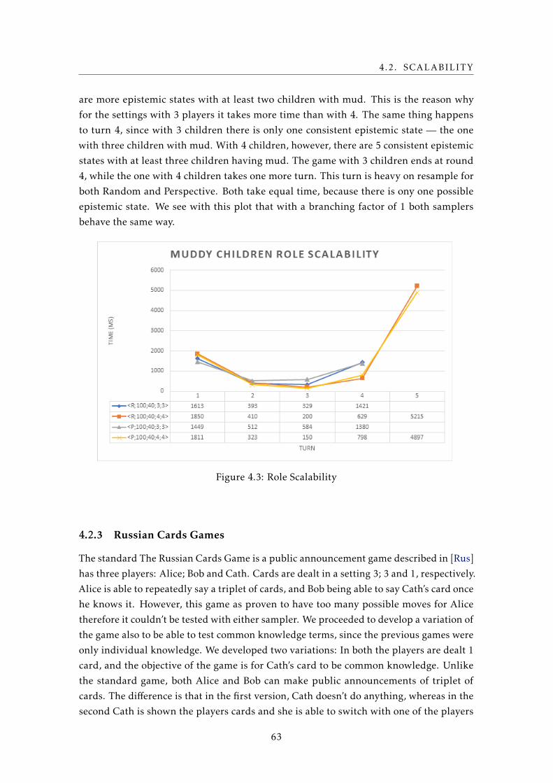
4.2. SCALABILITY
are more epistemic states with at least two children with mud. This is the reason why
for the settings with 3 players it takes more time than with 4. The same thing happens
to turn 4, since with 3 children there is only one consistent epistemic state — the one
with three children with mud. With 4 children, however, there are 5 consistent epistemic
states with at least three children having mud. The game with 3 children ends at round
4, while the one with 4 children takes one more turn. This turn is heavy on resample for
both Random and Perspective. Both take equal time, because there is ony one possible
epistemic state. We see with this plot that with a branching factor of 1 both samplers
behave the same way.
Figure 4.3: Role Scalability
4.2.3 Russian Cards Games
The standard The Russian Cards Game is a public announcement game described in [Rus]
has three players: Alice; Bob and Cath. Cards are dealt in a setting 3; 3 and 1, respectively.
Alice is able to repeatedly say a triplet of cards, and Bob being able to say Cath’s card once
he knows it. However, this game as proven to have too many possible moves for Alice
therefore it couldn’t be tested with either sampler. We proceeded to develop a variation of
the game also to be able to test common knowledge terms, since the previous games were
only individual knowledge. We developed two variations: In both the players are dealt 1
card, and the objective of the game is for Cath’s card to be common knowledge. Unlike
the standard game, both Alice and Bob can make public announcements of triplet of
cards. The difference is that in the first version, Cath doesn’t do anything, whereas in the
second Cath is shown the players cards and she is able to switch with one of the players
63
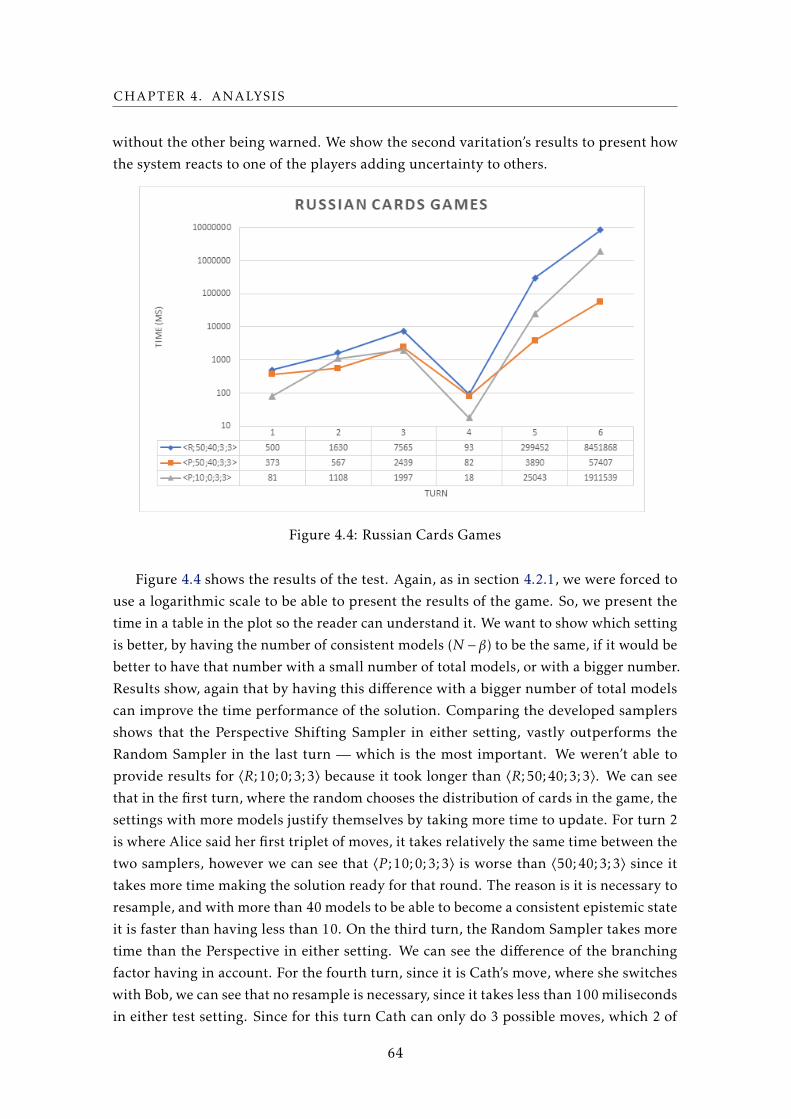
CHAPTER 4. ANALYSIS
without the other being warned. We show the second varitation’s results to present how
the system reacts to one of the players adding uncertainty to others.
Figure 4.4: Russian Cards Games
Figure 4.4 shows the results of the test. Again, as in section 4.2.1, we were forced to
use a logarithmic scale to be able to present the results of the game. So, we present the
time in a table in the plot so the reader can understand it. We want to show which setting
is better, by having the number of consistent models (N −β) to be the same, if it would be
better to have that number with a small number of total models, or with a bigger number.
Results show, again that by having this difference with a bigger number of total models
can improve the time performance of the solution. Comparing the developed samplers
shows that the Perspective Shifting Sampler in either setting, vastly outperforms the
Random Sampler in the last turn — which is the most important. We weren’t able to
provide results for 〈R;10;0;3;3〉 because it took longer than 〈R;50;40;3;3〉. We can see
that in the first turn, where the random chooses the distribution of cards in the game, the
settings with more models justify themselves by taking more time to update. For turn 2
is where Alice said her first triplet of moves, it takes relatively the same time between the
two samplers, however we can see that 〈P ;10;0;3;3〉 is worse than 〈50;40;3;3〉 since it
takes more time making the solution ready for that round. The reason is it is necessary to
resample, and with more than 40 models to be able to become a consistent epistemic state
it is faster than having less than 10. On the third turn, the Random Sampler takes more
time than the Perspective in either setting. We can see the difference of the branching
factor having in account. For the fourth turn, since it is Cath’s move, where she switches
with Bob, we can see that no resample is necessary, since it takes less than 100 miliseconds
in either test setting. Since for this turn Cath can only do 3 possible moves, which 2 of
64
4.2. SCALABILITY
them will continue to make the models consistent, no resample is necessary. Therefore
the test settings which takes more time are the ones with more models. Althouh the
difference is barely noticeble. We start to see meaningful differences after the uncertainty,
when Alice and Bob start to do their own move to restrict the number of consistent models.
For the fifth turn, Alice has made her move, we can see that the resample is triggered.
Again more inconsistent models acts as an optimization. Notice, that at this point only
one of the samplers with a specific setting is acceptable: 〈P ;50;40;3;3〉, since it takes
around 4 seconds. On others settings, the Perspective Shifting with 10 total models is
inefficient, since it takes 25 seconds and the Random Sampler is even worse because it
takes 300 seconds or, 5 minutes. For the last round, all the samplers take way to much
time, being the best of them the Perspective Shifting with N = 50;β = 40 which took 57
seconds. The other Perspective with N = 10,β = 0 took 1911 seconds which is essentially
31 minutes. The Random is the worst of the samplers taking 8452 seconds approximatly,
which is 140 minutes on that round. We can conclude with this test that by increasing N
and β accordingly can provide games to be able to be played. Although the more we go
deep into the joint game tree, the harder it is for the GM to be able to making sure that
the bag is consistent and calculating the knowledge of the players at that round using
either of the samplers.
65

Chapter
5Conclusion
The work done in the context of this thesis resulted in a functional Game Master for
EGGP that successfully implements the semantics of GDL-III. This GM was developed
with model sampling due to the fact that solutions that consider all possible states of a
game in GDL-III are impossible to maintain thanks to games’ state space complexity. We
have shown that, because we are not considering every state, using a sampling method
can cause errors in the way the GM controls a game.
Our work started from a disappointingly undocumented GM package that was, nev-
ertheless, very modular and easy to work with. The end result was a functional GM that
may be deployed in any Operating System thanks to the technology on which it was devel-
oped: Java Ant [Apa] (section E). We enjoyed working and developing games for GDL-III.
Our efforts to optimize the developed GM resulted in a second sampler, the Perspective
Shifting Sampler, that is able to perform its job in a less time consuming manner. Yet,
while we formally show that with the Random Sampler the GM is able to reach every
possible state, for the Perspective Shifting Sample we only provide an intuition on why it
should also consider all epistemic states.
As shown in this document, when a game has many rounds, calculating what each
player knows becomes very time consuming: this happens not because of the knowledge
that the GM has to calculate, but because of the time that it takes to resample to the
round in question (since game trees can be very large). However, we show how this may
be optimized by increasing the number of total models and the number of inconsistent
models. Moreover, we show that for dynamic epistemic games we must allow some
inconsistent models so that the resampling may finish.
In an EGGP system, while players only have fifteen seconds to decide a move, there is
no defined time limit for the GM: this is because until GDL-III the GM’s job was straight-
forward (only having to update the true state of the game and not having to consider more
67
CHAPTER 5. CONCLUSION
states than that one). Because the situation changes in GDL-III, it is necessary to calculate
what players know. With that in mind, the GM needs to consider the possible states of
the players. This significantly increases the time complexity of the GM. Whereas players
in a GGP-I system only have 15 seconds to calculate everything they need, it would only
be fair that the GM has some kind of constraint as well.
Finally, to conclude this dissertation, we recall an example brought up in Chapter 1
about automated cars. By successfully developing this GM, we allow game designers to
build GDL-III games where, for instance, in order for an agent (car) to pass another agent
(car), he must know that there is no risk in doing so. The risk can then be defined as an
auxiliar term in the game to represent conditions such as the type of the road, weather,
etc. These agents can then be tested in different games, with different risk conditions,
and find the best solution for their risks. This way, stakeholders can practice real world
problems without having to spend funds on cars: since the car would be the agent playing
the game controlled by our solution.
5.1 Future Work
The following paragraphs present some of the possible features and improvements:
Nested Knowledge Rules Support — GDL-III supports the use of nested knowledge key-
words through the use of auxiliar rules. However, the GM does not support this
functionality. Like the GDL-III nested knowledge rule is defined as:
1 ( a ( knows r2 p ) )
2 (<= ( goal r1 100) ( knows r1 a ) )
This could be achieved by creating our representation rules that follow the same
type: Kr1a and Kr2p, with Kr1a points to Kr2p. When applying the semantics of the
nested knowledge rule will start with Kr2p and then proceed to apply the outwards
rule Kr1a;
Timed Resample — Our developed resample strategy can adapt to a timely resample,
since it can be stopped whenever the re sampling turn matches the turn of the game.
We will add a time constraint so that the resample can stop even if the bag of models
it is not completely consistent;
Knowledge Terms Grounder — The developed knowledge terms grounder has a limi-
tation, were it only creates knowledge rules that have one variable. We will use
the same intuition when explained the intuition behind it. Moreover, since the
semantics of GDL-III and ASP are similar, this can also be achieved by using an ASP
Solver such as Clingo to ground the knowledge rules;
68
5.1. FUTURE WORK
Comparing Legal Play Sequences — The methods that compare the legal play sequences
may be optimized by not comparing all play sequences. Since we allow some mod-
els to be inconsistent, we can adapt the solution to not keep comparing consistent
legal play sequences with inconsistent ones;
Prespective Shifting Sampler — We can optimize this Sampler by whenever the move
we are trying to apply is not legal, to try to apply legal move of another player;
Dynamic Epistemic Sampling — A dynamic solution can be achieved by increasing, or
decreasing, the number of inconsistent models throughout the rounds of a game;
Developing Games — As GDL-III is a recent language extension, there are not many
games developed. It would be interesting to implement more games specially public
and private announcement games;
Player Implementation — By using parts of our developed prototype a player that can
reason with in epistemic games can be built. This can be achieved by using our
Knowledge module and the Random Sampler;
User Game Interface — The base package that we started our solution from allows the
description of an interface for the game to be displayed. This can be accomplished
by adapting those interface classes from the base package to allow GDL-III games
to be displayed on screen so that viewers can see the game being played out;
Optimization for Single Player Games In case of a single player game there is no motive
to use the common knowledge as the constraint to trigger resample, since in those
games it is the knowledge set is the same because there is only one player. Instead
of recurring to the transitive closure algorithm to calculate if states are inconsistent,
one can redirect it in order to only calculate the models that are indistinguishable
for that player;
Plausibility Comparison between Samplers This can be achieved by calculating the
number of expected plausible states at a certain round for both Samplers.
69

Bibliography
[Cha+08] G. Chaslot, S. Bakkes, I. Szita, and P. Spronck. “Monte-Carlo Tree Search: A
New Framework for Game AI.” In: AIIDE. 2008.
[Cor+13] A. Cordón-Franco, H. van Ditmarsch, D. F. Duque, and F. Soler-Toscano. “A
colouring protocol for the generalized Russian cards problem”. In: Theor.Comput. Sci. 495 (2013), pp. 81–95. doi: 10.1016/j.tcs.2013.05.010.
url: http://dx.doi.org/10.1016/j.tcs.2013.05.010.
[Geb+12] M. Gebser, R. Kaminski, B. Kaufmann, and T. Schaub. Answer Set Solving inPractice. Synthesis Lectures on Artificial Intelligence and Machine Learning.
Morgan & Claypool Publishers, 2012. doi: 10.2200/S00457ED1V01Y201211AIM019.
url: https://doi.org/10.2200/S00457ED1V01Y201211AIM019.
[GT14] M. R. Genesereth and M. Thielscher. General Game Playing. Synthesis Lec-
tures on Artificial Intelligence and Machine Learning. Morgan & Claypool
Publishers, 2014. doi: 10.2200/S00564ED1V01Y201311AIM024. url: http:
//dx.doi.org/10.2200/S00564ED1V01Y201311AIM024.
[Has70] W. K. Hastings. “Monte Carlo sampling methods using Markov chains and
their applications”. In: Biometrika 57.1 (1970), pp. 97–109.
[KS06] L. Kocsis and C. Szepesvári. “Bandit Based Monte-Carlo Planning”. In: Ma-chine Learning: ECML 2006, 17th European Conference on Machine Learning,Berlin, Germany, September 18-22, 2006, Proceedings. 2006, pp. 282–293. doi:
10.1007/11871842_29. url: http://dx.doi.org/10.1007/11871842_29.
[LS08] K. Leyton-Brown and Y. Shoham. Essentials of Game Theory: A ConciseMultidisciplinary Introduction. Synthesis Lectures on Artificial Intelligence
and Machine Learning. Morgan & Claypool Publishers, 2008. doi: 10 .
2200/S00108ED1V01Y200802AIM003. url: http://dx.doi.org/10.2200/
S00108ED1V01Y200802AIM003.
[Lov+08] N. Love, T. Hinrichs, D. Haley, E. Schkufza, and M. Genesereth. General gameplaying: Game description language specification. 2008.
[Mye97] R. B. Myerson. Game theory - Analysis of Conflict. Harvard University Press,
1997. isbn: 978-0-674-34116-6. url: http://www.hup.harvard.edu/
catalog/MYEGAM.html.
71
BIBLIOGRAPHY
[SHDT08] C. S. Hardin and A. D. Taylor. “An Introduction to Infinite Hat Problems”.
In: 30 (Sept. 2008), pp. 20–25.
[ST15] M. J. Schofield and M. Thielscher. “Lifting Model Sampling for General
Game Playing to Incomplete-Information Models”. In: Proceedings of theTwenty-Ninth AAAI Conference on Artificial Intelligence, January 25-30, 2015,Austin, Texas, USA. 2015, pp. 3585–3591. url: http://www.aaai.org/ocs/
index.php/AAAI/AAAI15/paper/view/10014.
[ST16] M. J. Schofield and M. Thielscher. “The Scalability of the HyperPlay Tech-
nique for Imperfect-Information Games”. In: Computer Poker and ImperfectInformation Games, Papers from the 2016 AAAI Workshop, Phoenix, Arizona,USA, February 13, 2016. 2016. url: http://www.aaai.org/ocs/index.
php/WS/AAAIW16/paper/view/12632.
[Sch+12] M. J. Schofield, T. J. Cerexhe, and M. Thielscher. “HyperPlay: A Solution
to General Game Playing with Imperfect Information”. In: Proceedings ofthe Twenty-Sixth AAAI Conference on Artificial Intelligence, July 22-26, 2012,Toronto, Ontario, Canada. 2012. url: http://www.aaai.org/ocs/index.
php/AAAI/AAAI12/paper/view/5033.
[Thi11a] M. Thielscher. “GDL-II”. In: KI 25.1 (2011), pp. 63–66. doi: 10.1007/
s13218-010-0076-5. url: http://dx.doi.org/10.1007/s13218-010-
0076-5.
[Thi11b] M. Thielscher. “The General Game Playing Description Language Is Univer-
sal”. In: IJCAI 2011, Proceedings of the 22nd International Joint Conferenceon Artificial Intelligence, Barcelona, Catalonia, Spain, July 16-22, 2011. 2011,
pp. 1107–1112. doi: 10.5591/978-1-57735-516-8/IJCAI11-189. url:
http://dx.doi.org/10.5591/978-1-57735-516-8/IJCAI11-189.
[Thi16] M. Thielscher. “GDL-III: A Proposal to Extend the Game Description Lan-
guage to General Epistemic Games”. In: ECAI 2016 - 22nd European Con-ference on Artificial Intelligence, 29 August-2 September 2016, The Hague, TheNetherlands - Including Prestigious Applications of Artificial Intelligence (PAIS2016). 2016, pp. 1630–1631. doi: 10.3233/978-1-61499-672-9-1630.
url: http://dx.doi.org/10.3233/978-1-61499-672-9-1630.
[Thi17] M. Thielscher. “GDL-III: A Description Language for Epistemic General
Game Playing”. In: Proceedings of the Twenty-Sixth International Joint Confer-ence on Artificial Intelligence, IJCAI-17. 2017, pp. 1276–1282. doi: 10.24963/
ijcai.2017/177. url: https://doi.org/10.24963/ijcai.2017/177.
[VD+07] H. Van Ditmarsch, W. van Der Hoek, and B. Kooi. Dynamic epistemic logic.
Vol. 337. Springer Science & Business Media, 2007.
72
BIBLIOGRAPHY
[VN27] J. Von Neumann. “Mathematische Begründung der Quantenmechanik”. In:
Nachrichten von der Gesellschaft der Wissenschaften zu Göttingen, Mathematisch-Physikalische Klasse 1927 (1927), pp. 1–57.
73

Webography
[Apa] Apache Ant. url: http://ant.apache.org/ (visited on 07/07/2018).
[Bat] Battle of the Sexes. url: https://www.classes.cs.uchicago.edu/archive/
2012/fall/12100-1/assignments/pa2-part1/images/bos.png (visited
on 02/02/2017).
[Cli] Clingo. url: https://potassco.org/ (visited on 03/20/2018).
[Ggp] General Game Playing Base Package. url: https://github.com/ggp-org/
ggp-base (visited on 01/04/2017).
[Gdl] General Game Playing: Game Description Language Specification. url: https:
//www.google.pt/url?sa=t&rct=j&q=&esrc=s&source=web&cd=2&cad=
rja&uact=8&ved=0ahUKEwjrwpDu3_rZAhWCOxQKHUv1AkMQFggvMAE&url=
https%3A%2F%2Fpdfs.semanticscholar.org%2F2530%2Fdb839eaa4e212c11d557f3b91800a58cf6ac.
pdf&usg=AOvVaw050kgUCH_xoBKO17k5FmzW (visited on 03/20/2018).
[Gra] graphColoring. url: http://potassco.sourceforge.net/clingo.html
(visited on 01/27/2017).
[One] LoR. url: https://vignette.wikia.nocookie.net/somtest/images/d/
d4/One_Ring_PNG.png/revision/latest?cb=20140814153842 (visited on
03/24/2018).
[Rus] Michael Thielscher. A formal description language for general epistemic games.url: https://cgi.cse.unsw.edu.au/~reports/ (visited on 02/16/2018).
[Mon] The Monte Carlo Tree Search Image. url: https://en.wikipedia.org/wiki/
Monte_Carlo_tree_search (visited on 01/18/2017).
75

Appendix
AClass Diagrams
This chapter we show the class diagrams of our developed prototype.
A.1 Overview
The class that deals with the knowledge of the players at a certain round of the game is
called Knowledge State Machine. This abstract class was developed with the intention
to implement any kind of logic semantics to calculate the knowledge of the players. We
extended this class and implement their methods to use model sampling with GDL-III
semantics. This class is called Dynamic Epistemic State Machine (It is an intermediate
class that in Chapter 3 we assume in the Server module). This class only deals with a
Machine State - the true state of the game. It uses the classes presented in the figure A.1.
Specifically, those classes are:
KnowledgeRule java representation that we said previously. It is necessary at least one
of this objects, otherwise it is not a GDL-III game;
DynamicEpistemicSampler entity that manages the models;
AccessibilityRelationManager entity that manages the structures - where we save the
information about the players (pre semantics);
KnowledgeVerifier entity that implements the semantics of the GDL-III (post-semantics).
A.2 Terms Processor
Our implementation only recognizes KnowledgeRules. Those can be one of the two
classes:
77
APPENDIX A. CLASS DIAGRAMS
• CommonKnowledge - equivalent to the GDL-III keyword: (knows P), where P is a
proposition.
• PersonalKnowledge - equivalent to the GDL-III keyword: (knows R P), where R is a
role and P is a proposition.
The Knowledge Terms Processor, which can be found in the figure A.2, is the entity
that parses the terms from a GDL-III description into Personal Knowledge or Common
Knowledge.
A.3 Dynamic Epistemic Sampler
The Dynamic Epistemic Sampler is an extension of a Sampler. The Sampler is a simple
class that saves the models of the game that we have in a Bag. As we can see the in the
figure A.3, the most important methods for Dynamic Epistemic Sampler are:
getSamplerRound Returns the round that the sampler is currently on;
sample Updates all the models into the next round by selecting a legal joint move;
updateMState Epistemic updates the mstate of all the models inside the bag, according
to what the players can’t distinguish;
updateMState Epistemic updates the mstate of a specific number of models, given by
their ID, and according to what the players can’t distinguish;
resample Resamples a specific number of models, given by their ID, in a specific round
according, or not, to their moves. Essentially, the same as the sample but for a
specific round;
setTargetKnowsRules Similar to what was described in section ??
To develop a Dynamic Epistemic Sampler it is only necessary to implement the re-
ferred abstract methods. There are two types of Dynamic Epistemic Samplers:
1. Random Sampler;
2. Perspective Shifting Sampler;
A.4 Accessibility Relation Manager
This class manages the accessibility relations necessary to the calculation of knowledge
of the players. For that effect, we use a Accessibility Relation Structure per player. This
object uses a boolean matrix that is N ×N , where N is the number of models presented
in the Sampler.
78
A.5. KNOWLEDGE VERIFIER
From the figure A.4 shows the ARS of a specific round is called a Krike structure, and
the Kripke structures of all the rounds is called a Kripke history. The methods in this
figure are:
updateCurrentAccessibilityRelation updates the current ARS. To be used after the
sample of the Sampler;
getCurrentStructures returns the Kripke structures of the current round;
getStructures returns the Kripke structure of a specific round;
updateAcessibilityRelation updates the ARS of a specific round and only for the mod-
elID passed as argument. It is used in the re sampling;
saveCurrentStructure saves the Kripke structure of the current round;
A.5 Knowledge Verifier
The knowledge verifier is the class where the semantics of the GDL-III are implemented.
Whereas the Accessibility Relation Manager as the function of updating the ARS, this
class has the objective of verify if the Knowledge Rules are true in the models’ state that
the players can’t distinguish between.
The methods of the Knowledge Verifier are show in Figure A.5. In this class, the
Knowledge Rules are verified changes from whether we are verifying a model or the
actual state of the game:
• Personal Knowledge
State Verify if the target is true in all the useful states of the player’s models;
Model Verify if the target is true in all the indistinguishable states of the player’s
models;
• Common Knowledge
State Check all the models that are transitive closure useful. Then, verify if the
target is true in all of the states of those models;
Model Verify the target in all the transitive closure set of the given model.
A.6 Dynamic Epistemic Knowledge Machine
This class implements the Knowledge State Machine. It uses all the classes described
to calculate the knowledge of the players in the state of the game at a certain round.
As we can see from the figure A.6, it is necessary a Dynamic Epistemic Sampler and an
79
APPENDIX A. CLASS DIAGRAMS
Accessibility Relations Manager. The Knowledge Verifier is used in the method getTurn-
Knowledge, since it is the one that returns which knowledge terms are satisfied in the
current round.
80
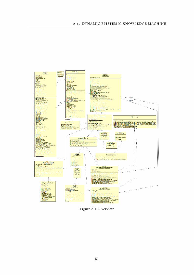
A.6. DYNAMIC EPISTEMIC KNOWLEDGE MACHINE
Figure A.1: Overview
81
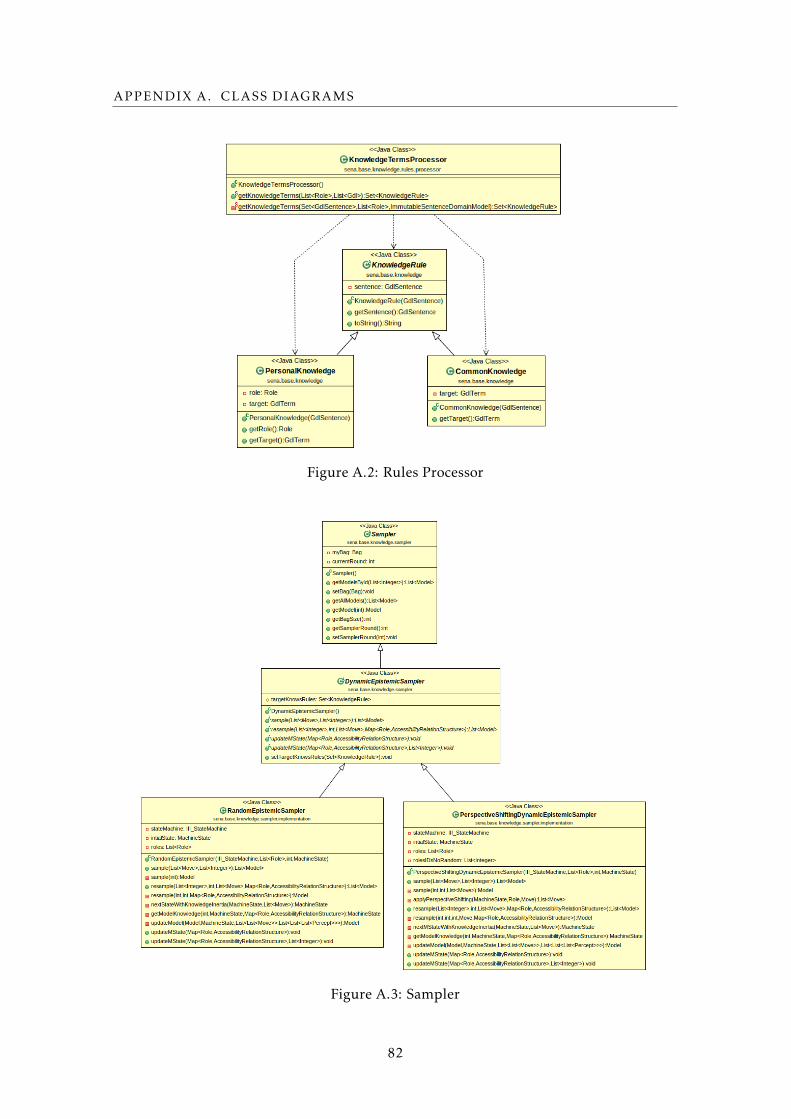
APPENDIX A. CLASS DIAGRAMS
Figure A.2: Rules Processor
Figure A.3: Sampler
82
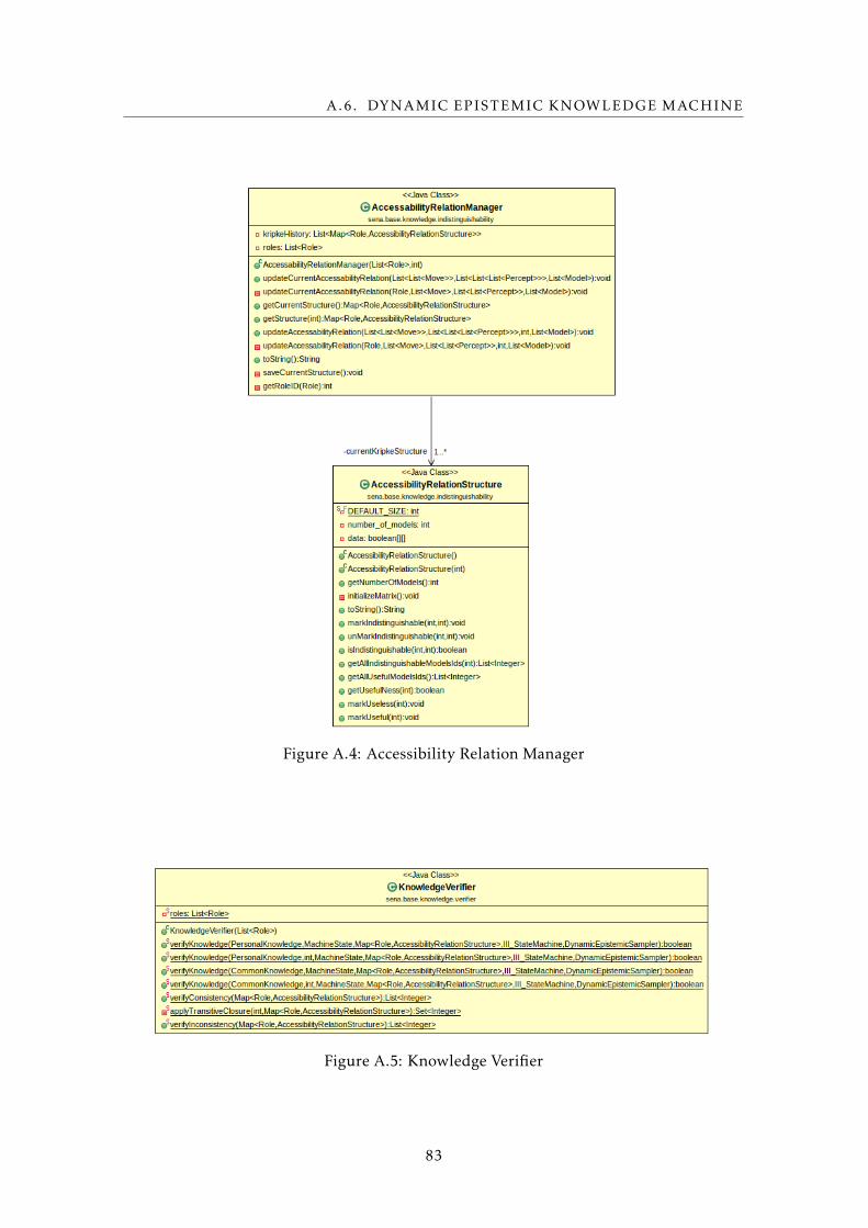
A.6. DYNAMIC EPISTEMIC KNOWLEDGE MACHINE
Figure A.4: Accessibility Relation Manager
Figure A.5: Knowledge Verifier
83
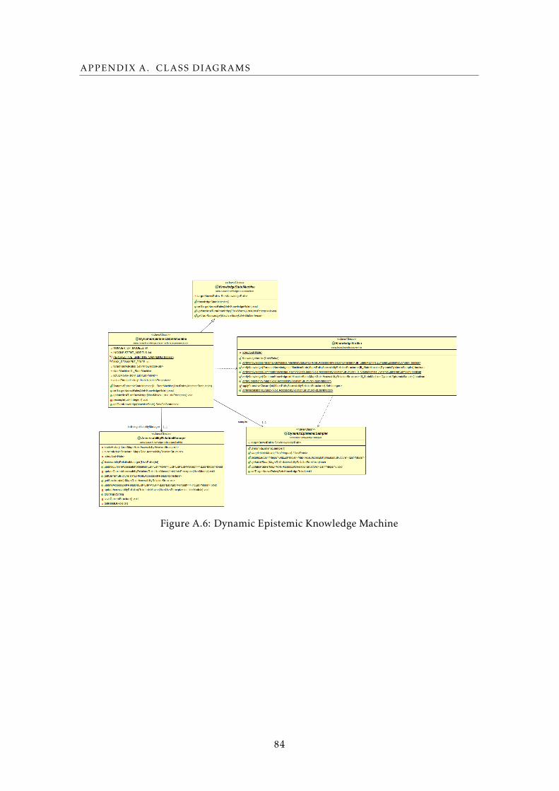
APPENDIX A. CLASS DIAGRAMS
Figure A.6: Dynamic Epistemic Knowledge Machine
84
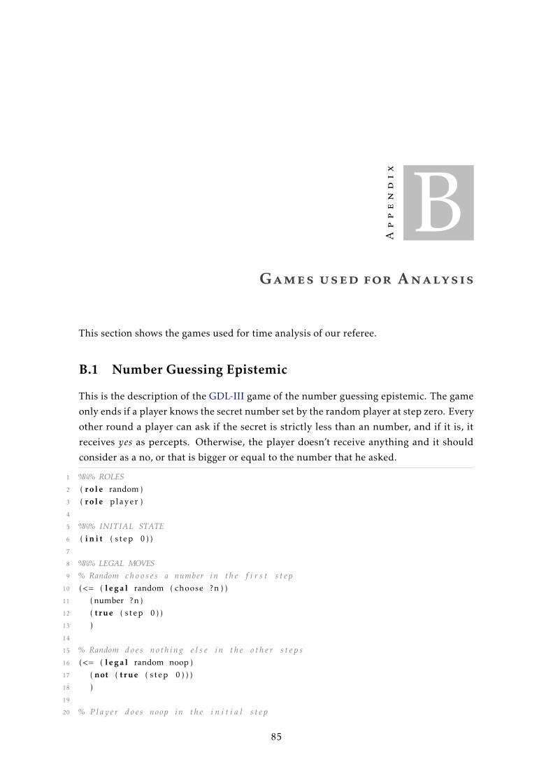
Appendix
BGames used for Analysis
This section shows the games used for time analysis of our referee.
B.1 Number Guessing Epistemic
This is the description of the GDL-III game of the number guessing epistemic. The game
only ends if a player knows the secret number set by the random player at step zero. Every
other round a player can ask if the secret is strictly less than an number, and if it is, it
receives yes as percepts. Otherwise, the player doesn’t receive anything and it should
consider as a no, or that is bigger or equal to the number that he asked.
1 %%% ROLES2 ( role random )
3 ( role player )
4
5 %%% INITIAL STATE6 ( i n i t ( s tep 0 ) )
7
8 %%% LEGAL MOVES9 % Random c h o o s e s a number in t h e f i r s t s t e p
10 (<= ( l e g a l random ( choose ?n ) )
11 ( number ?n )
12 ( true ( s tep 0 ) )
13 )
14
15 % Random does noth ing e l s e in t h e o t h e r s t e p s16 (<= ( l e g a l random noop )
17 ( not ( true ( s tep 0 ) ) )
18 )
19
20 % P l a y e r does noop in t h e i n i t i a l s t e p
85
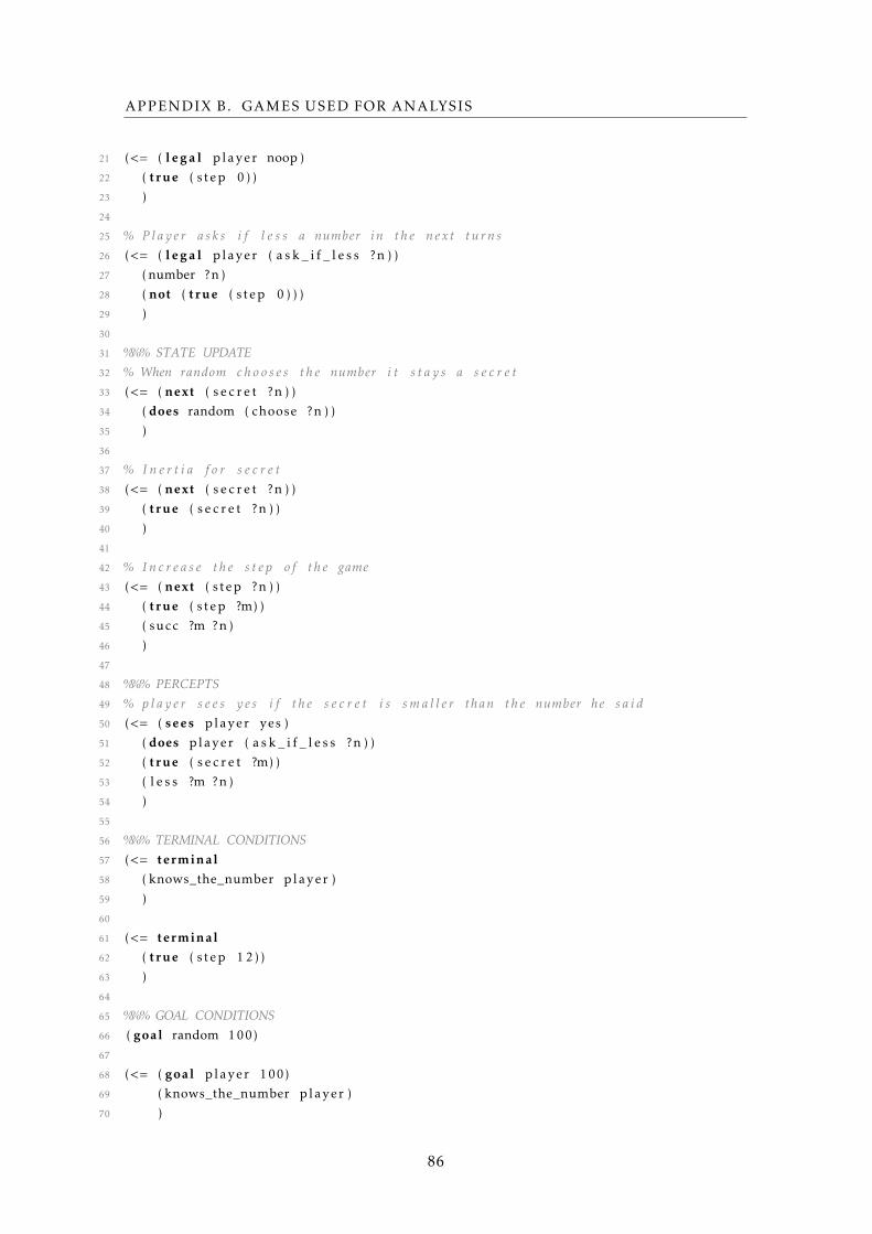
APPENDIX B. GAMES USED FOR ANALYSIS
21 (<= ( l e g a l player noop )
22 ( true ( s tep 0 ) )
23 )
24
25 % P l a y e r a s k s i f l e s s a number in t h e next turns26 (<= ( l e g a l player ( a s k _ i f _ l e s s ?n ) )
27 ( number ?n )
28 ( not ( true ( s tep 0 ) ) )
29 )
30
31 %%% STATE UPDATE32 % When random c h o o s e s t h e number i t s t a y s a s e c r e t33 (<= ( next ( s e c r e t ?n ) )
34 ( does random ( choose ?n ) )
35 )
36
37 % I n e r t i a f o r s e c r e t38 (<= ( next ( s e c r e t ?n ) )
39 ( true ( s e c r e t ?n ) )
40 )
41
42 % I n c r e a s e t h e s t e p o f t h e game43 (<= ( next ( s tep ?n ) )
44 ( true ( s tep ?m) )
45 ( succ ?m ?n )
46 )
47
48 %%% PERCEPTS49 % p l a y e r s e e s y e s i f t h e s e c r e t i s s m a l l e r than t h e number he s a i d50 (<= ( sees player yes )
51 ( does player ( a s k _ i f _ l e s s ?n ) )
52 ( true ( s e c r e t ?m) )
53 ( l e s s ?m ?n )
54 )
55
56 %%% TERMINAL CONDITIONS57 (<= terminal58 ( knows_the_number player )
59 )
60
61 (<= terminal62 ( true ( s tep 1 2 ) )
63 )
64
65 %%% GOAL CONDITIONS66 ( goal random 100)
67
68 (<= ( goal player 100)
69 ( knows_the_number player )
70 )
86
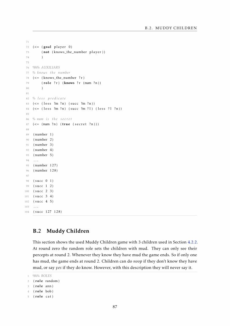
B.2. MUDDY CHILDREN
71
72 (<= ( goal player 0)
73 ( not ( knows_the_number player ) )
74 )
75
76 %%% AUXILIARS77 % knows t h e number78 (<= ( knows_the_number ? r )
79 ( role ? r ) ( knows ? r (num ?n ) )
80 )
81
82 % l e s s p r e d i c a t e83 (<= ( l e s s ?m ?n ) ( succ ?m ?n ) )
84 (<= ( l e s s ?m ?n ) ( succ ?m ? l ) ( l e s s ? l ?n ) )
85
86 % num i s t h e s e c r e t87 (<= (num ?n ) ( true ( s e c r e t ?n ) ) )
88
89 ( number 1)
90 ( number 2)
91 ( number 3)
92 ( number 4)
93 ( number 5)
94 . . .
95 ( number 127)
96 ( number 128)
97
98 ( succ 0 1)
99 ( succ 1 2)
100 ( succ 2 3)
101 ( succ 3 4)
102 ( succ 4 5)
103 . . .
104 ( succ 127 128)
B.2 Muddy Children
This section shows the used Muddy Children game with 3 children used in Section 4.2.2.
At round zero the random role sets the children with mud. They can only see their
percepts at round 2. Whenever they know they have mud the game ends. So if only one
has mud, the game ends at round 2. Children can do noop if they don’t know they have
mud, or say yes if they do know. However, with this description they will never say it.
1 %%% ROLES2 ( role random )
3 ( role ann )
4 ( role bob )
5 ( role ca t )
87
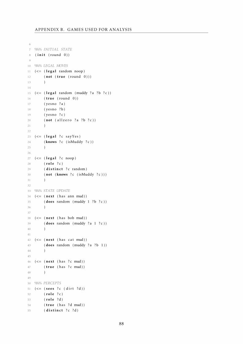
APPENDIX B. GAMES USED FOR ANALYSIS
6
7 %%% INITIAL STATE8 ( i n i t ( round 0 ) )
9
10 %%% LEGAL MOVES11 (<= ( l e g a l random noop )
12 ( not ( true ( round 0 ) ) )
13 )
14
15 (<= ( l e g a l random (muddy ? a ?b ? c ) )
16 ( true ( round 0 ) )
17 ( yesno ? a )
18 ( yesno ?b )
19 ( yesno ? c )
20 ( not ( a l l z e r o ? a ?b ? c ) )
21 )
22
23 (<= ( l e g a l ? c sayYes )
24 ( knows ? c ( isMuddy ? c ) )
25 )
26
27 (<= ( l e g a l ? c noop )
28 ( role ? c )
29 ( d i s t i n c t ? c random )
30 ( not ( knows ? c ( isMuddy ? c ) ) )
31 )
32
33 %%% STATE UPDATE34 (<= ( next ( has ann mud) )
35 ( does random (muddy 1 ?b ? c ) )
36 )
37
38 (<= ( next ( has bob mud) )
39 ( does random (muddy ? a 1 ? c ) )
40 )
41
42 (<= ( next ( has ca t mud) )
43 ( does random (muddy ? a ?b 1 ) )
44 )
45
46 (<= ( next ( has ? c mud) )
47 ( true ( has ? c mud) )
48 )
49
50 %%% PERCEPTS51 (<= ( sees ? c ( d i r t ?d ) )
52 ( role ? c )
53 ( role ?d )
54 ( true ( has ?d mud) )
55 ( d i s t i n c t ? c ?d )
88
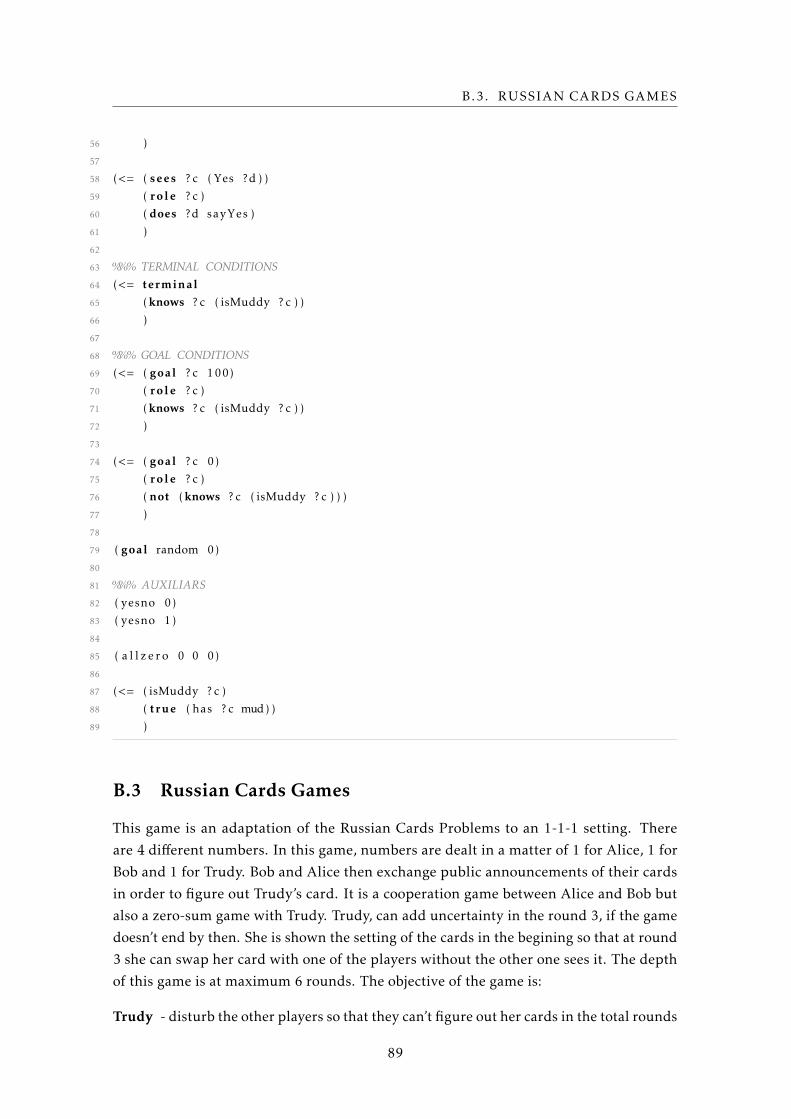
B.3. RUSSIAN CARDS GAMES
56 )
57
58 (<= ( sees ? c ( Yes ?d ) )
59 ( role ? c )
60 ( does ?d sayYes )
61 )
62
63 %%% TERMINAL CONDITIONS64 (<= terminal65 ( knows ? c ( isMuddy ? c ) )
66 )
67
68 %%% GOAL CONDITIONS69 (<= ( goal ? c 100)
70 ( role ? c )
71 ( knows ? c ( isMuddy ? c ) )
72 )
73
74 (<= ( goal ? c 0)
75 ( role ? c )
76 ( not ( knows ? c ( isMuddy ? c ) ) )
77 )
78
79 ( goal random 0)
80
81 %%% AUXILIARS82 ( yesno 0)
83 ( yesno 1)
84
85 ( a l l z e r o 0 0 0)
86
87 (<= ( isMuddy ? c )
88 ( true ( has ? c mud) )
89 )
B.3 Russian Cards Games
This game is an adaptation of the Russian Cards Problems to an 1-1-1 setting. There
are 4 different numbers. In this game, numbers are dealt in a matter of 1 for Alice, 1 for
Bob and 1 for Trudy. Bob and Alice then exchange public announcements of their cards
in order to figure out Trudy’s card. It is a cooperation game between Alice and Bob but
also a zero-sum game with Trudy. Trudy, can add uncertainty in the round 3, if the game
doesn’t end by then. She is shown the setting of the cards in the begining so that at round
3 she can swap her card with one of the players without the other one sees it. The depth
of this game is at maximum 6 rounds. The objective of the game is:
Trudy - disturb the other players so that they can’t figure out her cards in the total rounds
89
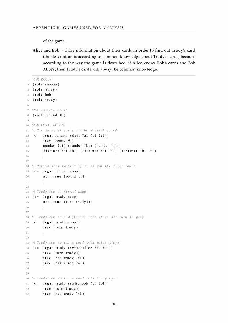
APPENDIX B. GAMES USED FOR ANALYSIS
of the game.
Alice and Bob - share information about their cards in order to find out Trudy’s card
(the description is according to common knowledge about Trudy’s cards, because
according to the way the game is described, if Alice knows Bob’s cards and Bob
Alice’s, then Trudy’s cards will always be common knowledge.
1 %%% ROLES2 ( role random )
3 ( role a l i c e )
4 ( role bob )
5 ( role trudy )
6
7 %%% INITIAL STATE8 ( i n i t ( round 0 ) )
9
10 %%% LEGAL MOVES11 % Random d e a l s c a r d s in t h e i n i t i a l round12 (<= ( l e g a l random ( deal ? a1 ? b1 ? t1 ) )
13 ( true ( round 0 ) )
14 ( number ? a1 ) ( number ? b1 ) ( number ? t1 )
15 ( d i s t i n c t ? a1 ? b1 ) ( d i s t i n c t ? a1 ? t1 ) ( d i s t i n c t ? b1 ? t1 )
16 )
17
18 % Random does noth ing i f i t i s not t h e f i r s t round19 (<= ( l e g a l random noop )
20 ( not ( true ( round 0 ) ) )
21 )
22
23 % Trudy can do normal noop24 (<= ( l e g a l trudy noop )
25 ( not ( true ( turn trudy ) ) )
26 )
27
28 % Trudy can do a d i f f e r e n t noop i f i s her turn t o p lay29 (<= ( l e g a l trudy noop1 )
30 ( true ( turn trudy ) )
31 )
32
33 % Trudy can s w i t c h a card with a l i c e p l a y e r34 (<= ( l e g a l trudy ( s w i t c h a l i c e ? t1 ? a1 ) )
35 ( true ( turn trudy ) )
36 ( true ( has trudy ? t1 ) )
37 ( true ( has a l i c e ? a1 ) )
38 )
39
40 % Trudy can s w i t c h a card with bob p l a y e r41 (<= ( l e g a l trudy ( switchbob ? t1 ? b1 ) )
42 ( true ( turn trudy ) )
43 ( true ( has trudy ? t1 ) )
90
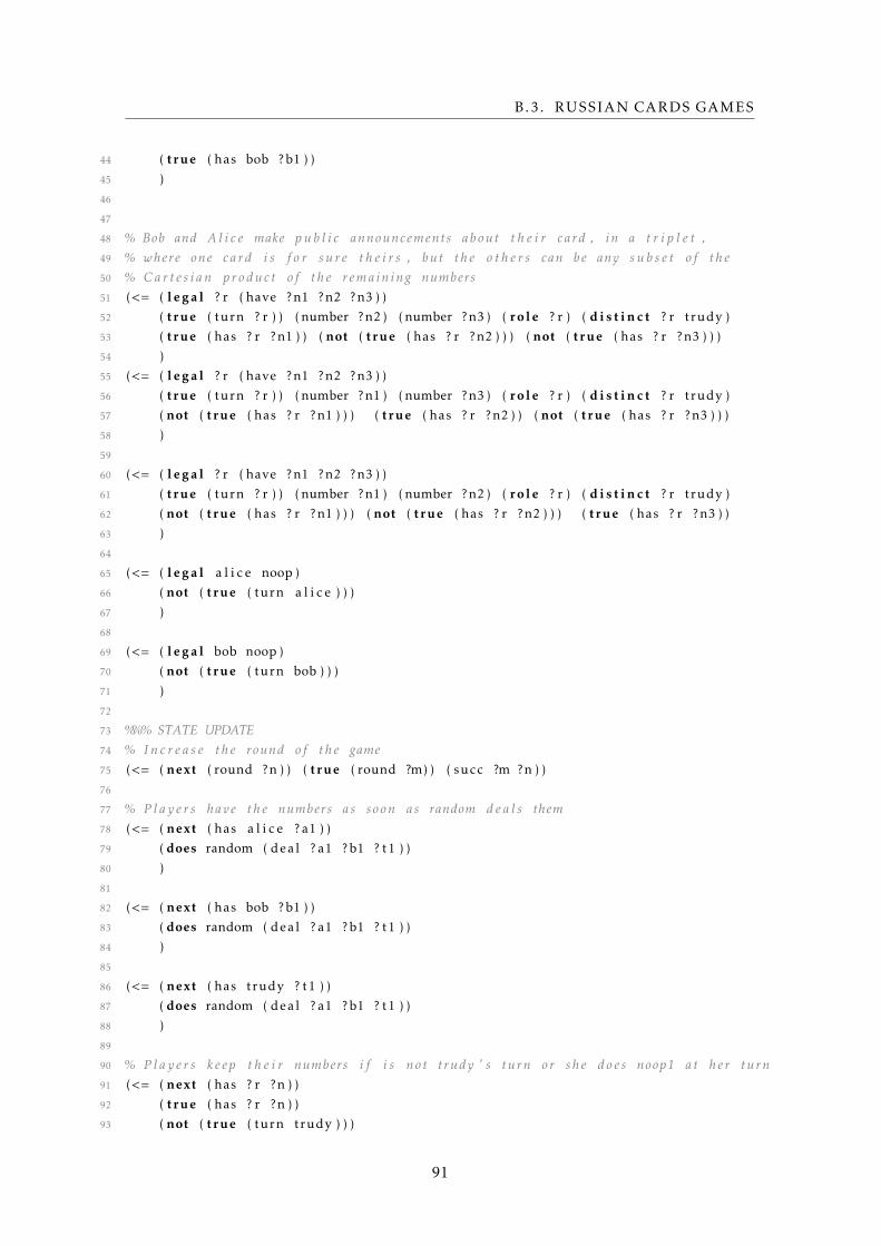
B.3. RUSSIAN CARDS GAMES
44 ( true ( has bob ? b1 ) )
45 )
46
47
48 % Bob and A l i c e make p u b l i c announcements about t h e i r card , in a t r i p l e t ,49 % where one card i s f o r s u r e t h e i r s , but t h e o t h e r s can be any s u b s e t o f t h e50 % C a r t e s i a n produc t o f t h e remaining numbers51 (<= ( l e g a l ? r ( have ?n1 ?n2 ?n3 ) )
52 ( true ( turn ? r ) ) ( number ?n2 ) ( number ?n3 ) ( role ? r ) ( d i s t i n c t ? r trudy )
53 ( true ( has ? r ?n1 ) ) ( not ( true ( has ? r ?n2 ) ) ) ( not ( true ( has ? r ?n3 ) ) )
54 )
55 (<= ( l e g a l ? r ( have ?n1 ?n2 ?n3 ) )
56 ( true ( turn ? r ) ) ( number ?n1 ) ( number ?n3 ) ( role ? r ) ( d i s t i n c t ? r trudy )
57 ( not ( true ( has ? r ?n1 ) ) ) ( true ( has ? r ?n2 ) ) ( not ( true ( has ? r ?n3 ) ) )
58 )
59
60 (<= ( l e g a l ? r ( have ?n1 ?n2 ?n3 ) )
61 ( true ( turn ? r ) ) ( number ?n1 ) ( number ?n2 ) ( role ? r ) ( d i s t i n c t ? r trudy )
62 ( not ( true ( has ? r ?n1 ) ) ) ( not ( true ( has ? r ?n2 ) ) ) ( true ( has ? r ?n3 ) )
63 )
64
65 (<= ( l e g a l a l i c e noop )
66 ( not ( true ( turn a l i c e ) ) )
67 )
68
69 (<= ( l e g a l bob noop )
70 ( not ( true ( turn bob ) ) )
71 )
72
73 %%% STATE UPDATE74 % I n c r e a s e t h e round o f t h e game75 (<= ( next ( round ?n ) ) ( true ( round ?m) ) ( succ ?m ?n ) )
76
77 % P l a y e r s have t h e numbers as soon as random d e a l s them78 (<= ( next ( has a l i c e ? a1 ) )
79 ( does random ( deal ? a1 ? b1 ? t1 ) )
80 )
81
82 (<= ( next ( has bob ? b1 ) )
83 ( does random ( deal ? a1 ? b1 ? t1 ) )
84 )
85
86 (<= ( next ( has trudy ? t1 ) )
87 ( does random ( deal ? a1 ? b1 ? t1 ) )
88 )
89
90 % P l a y e r s keep t h e i r numbers i f i s not trudy ’ s turn or she does noop1 at her turn91 (<= ( next ( has ? r ?n ) )
92 ( true ( has ? r ?n ) )
93 ( not ( true ( turn trudy ) ) )
91
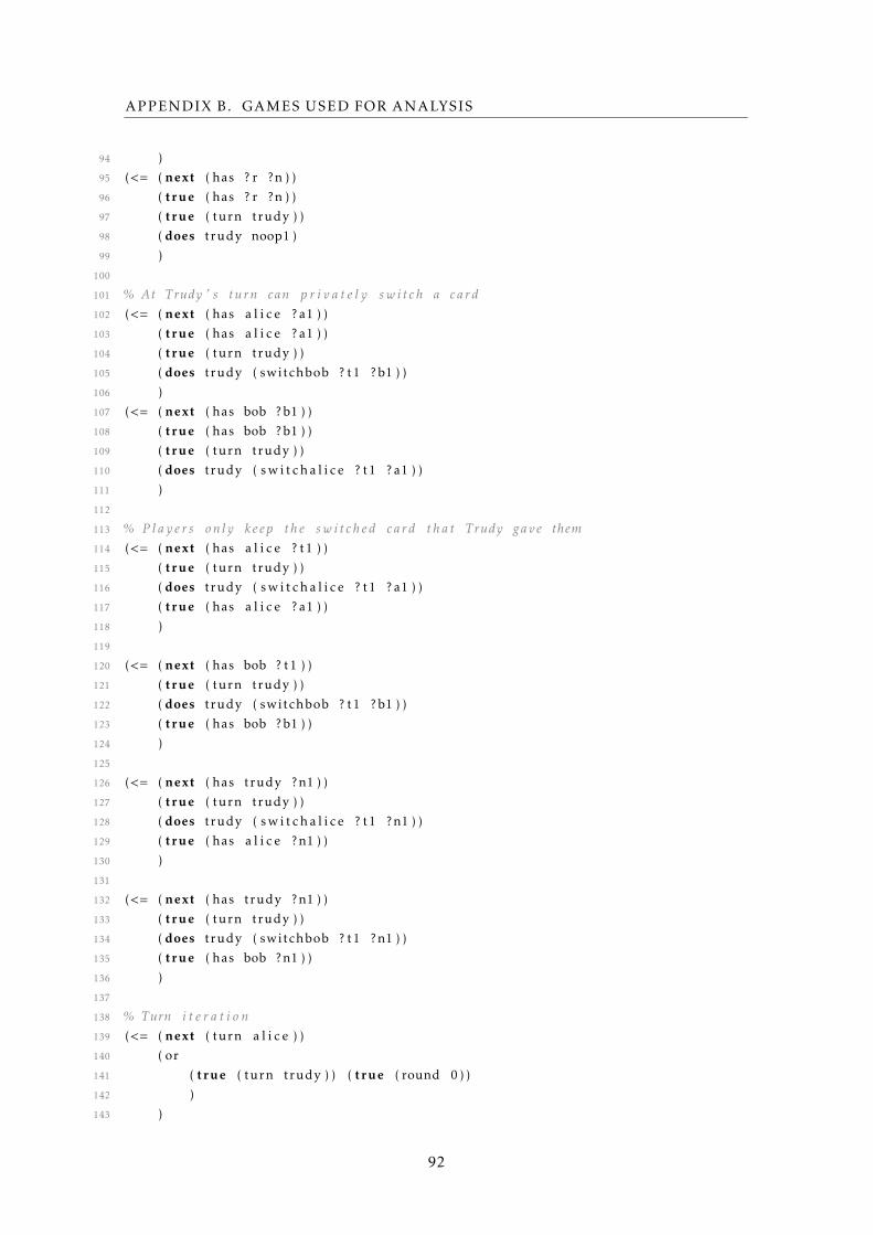
APPENDIX B. GAMES USED FOR ANALYSIS
94 )
95 (<= ( next ( has ? r ?n ) )
96 ( true ( has ? r ?n ) )
97 ( true ( turn trudy ) )
98 ( does trudy noop1 )
99 )
100
101 % At Trudy ’ s turn can p r i v a t e l y s w i t c h a card102 (<= ( next ( has a l i c e ? a1 ) )
103 ( true ( has a l i c e ? a1 ) )
104 ( true ( turn trudy ) )
105 ( does trudy ( switchbob ? t1 ? b1 ) )
106 )
107 (<= ( next ( has bob ? b1 ) )
108 ( true ( has bob ? b1 ) )
109 ( true ( turn trudy ) )
110 ( does trudy ( s w i t c h a l i c e ? t1 ? a1 ) )
111 )
112
113 % P l a y e r s only keep t h e s w i t c h e d card t h a t Trudy gave them114 (<= ( next ( has a l i c e ? t1 ) )
115 ( true ( turn trudy ) )
116 ( does trudy ( s w i t c h a l i c e ? t1 ? a1 ) )
117 ( true ( has a l i c e ? a1 ) )
118 )
119
120 (<= ( next ( has bob ? t1 ) )
121 ( true ( turn trudy ) )
122 ( does trudy ( switchbob ? t1 ? b1 ) )
123 ( true ( has bob ? b1 ) )
124 )
125
126 (<= ( next ( has trudy ?n1 ) )
127 ( true ( turn trudy ) )
128 ( does trudy ( s w i t c h a l i c e ? t1 ?n1 ) )
129 ( true ( has a l i c e ?n1 ) )
130 )
131
132 (<= ( next ( has trudy ?n1 ) )
133 ( true ( turn trudy ) )
134 ( does trudy ( switchbob ? t1 ?n1 ) )
135 ( true ( has bob ?n1 ) )
136 )
137
138 % Turn i t e r a t i o n139 (<= ( next ( turn a l i c e ) )
140 ( or
141 ( true ( turn trudy ) ) ( true ( round 0 ) )
142 )
143 )
92
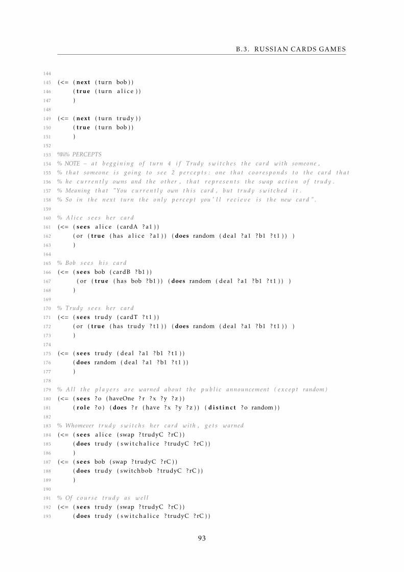
B.3. RUSSIAN CARDS GAMES
144
145 (<= ( next ( turn bob ) )
146 ( true ( turn a l i c e ) )
147 )
148
149 (<= ( next ( turn trudy ) )
150 ( true ( turn bob ) )
151 )
152
153 %%% PERCEPTS154 % NOTE − a t b e g g i n i n g o f turn 4 i f Trudy s w i t c h e s t h e card with someone ,155 % t h a t someone i s go ing t o s e e 2 p e r c e p t s : one t h a t c o o r e s p o n d s t o t h e card t h a t156 % he c u r r e n t l y owns and t h e o ther , t h a t r e p r e s e n t s t h e swap a c t i o n o f trudy .157 % Meaning t h a t "You c u r r e n t l y own t h i s card , but trudy s w i t c h e d i t .158 % So in t h e next turn t h e only p e r c e p t you ’ l l r e c i e v e i s t h e new card " .159
160 % A l i c e s e e s her card161 (<= ( sees a l i c e ( cardA ? a1 ) )
162 ( or ( true ( has a l i c e ? a1 ) ) ( does random ( deal ? a1 ? b1 ? t1 ) ) )
163 )
164
165 % Bob s e e s h i s card166 (<= ( sees bob ( cardB ? b1 ) )
167 ( or ( true ( has bob ? b1 ) ) ( does random ( deal ? a1 ? b1 ? t1 ) ) )
168 )
169
170 % Trudy s e e s her card171 (<= ( sees trudy ( cardT ? t1 ) )
172 ( or ( true ( has trudy ? t1 ) ) ( does random ( deal ? a1 ? b1 ? t1 ) ) )
173 )
174
175 (<= ( sees trudy ( deal ? a1 ? b1 ? t1 ) )
176 ( does random ( deal ? a1 ? b1 ? t1 ) )
177 )
178
179 % A l l t h e p l a y e r s a r e warned about t h e p u b l i c announcement ( e x c e p t random )180 (<= ( sees ? o ( haveOne ? r ? x ? y ? z ) )
181 ( role ? o ) ( does ? r ( have ? x ? y ? z ) ) ( d i s t i n c t ? o random ) )
182
183 % Whomever trudy s w i t c h s her card with , g e t s warned184 (<= ( sees a l i c e ( swap ? trudyC ?rC ) )
185 ( does trudy ( s w i t c h a l i c e ? trudyC ?rC ) )
186 )
187 (<= ( sees bob ( swap ? trudyC ?rC ) )
188 ( does trudy ( switchbob ? trudyC ?rC ) )
189 )
190
191 % Of c o u r s e trudy as w e l l192 (<= ( sees trudy ( swap ? trudyC ?rC ) )
193 ( does trudy ( s w i t c h a l i c e ? trudyC ?rC ) )
93
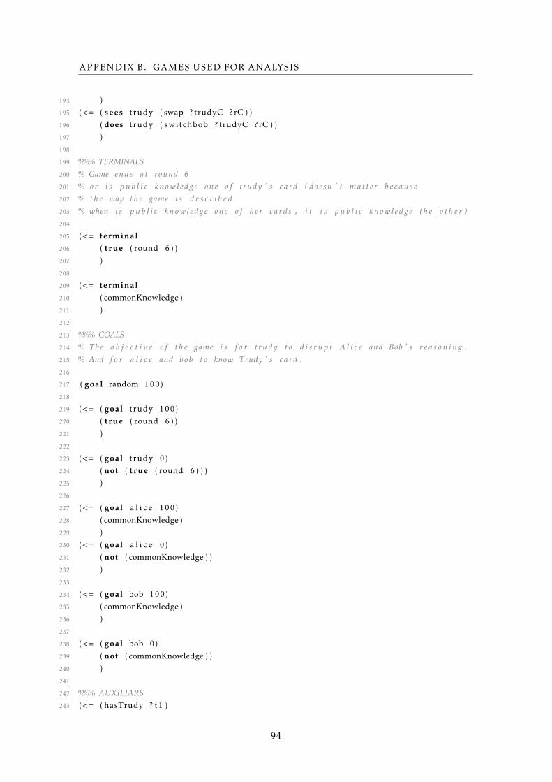
APPENDIX B. GAMES USED FOR ANALYSIS
194 )
195 (<= ( sees trudy ( swap ? trudyC ?rC ) )
196 ( does trudy ( switchbob ? trudyC ?rC ) )
197 )
198
199 %%% TERMINALS200 % Game ends a t round 6201 % or i s p u b l i c knowledge one o f trudy ’ s card ( doesn ’ t mat ter b e c a u s e202 % t h e way t h e game i s d e s c r i b e d203 % when i s p u b l i c knowledge one o f her cards , i t i s p u b l i c knowledge t h e o t h e r )204
205 (<= terminal206 ( true ( round 6 ) )
207 )
208
209 (<= terminal210 ( commonKnowledge )
211 )
212
213 %%% GOALS214 % The o b j e c t i v e o f t h e game i s f o r trudy t o d i s r u p t A l i c e and Bob ’ s r e a s o n i n g .215 % And f o r a l i c e and bob t o know Trudy ’ s card .216
217 ( goal random 100)
218
219 (<= ( goal trudy 100)
220 ( true ( round 6 ) )
221 )
222
223 (<= ( goal trudy 0)
224 ( not ( true ( round 6 ) ) )
225 )
226
227 (<= ( goal a l i c e 100)
228 ( commonKnowledge )
229 )
230 (<= ( goal a l i c e 0)
231 ( not ( commonKnowledge ) )
232 )
233
234 (<= ( goal bob 100)
235 ( commonKnowledge )
236 )
237
238 (<= ( goal bob 0)
239 ( not ( commonKnowledge ) )
240 )
241
242 %%% AUXILIARS243 (<= ( hasTrudy ? t1 )
94
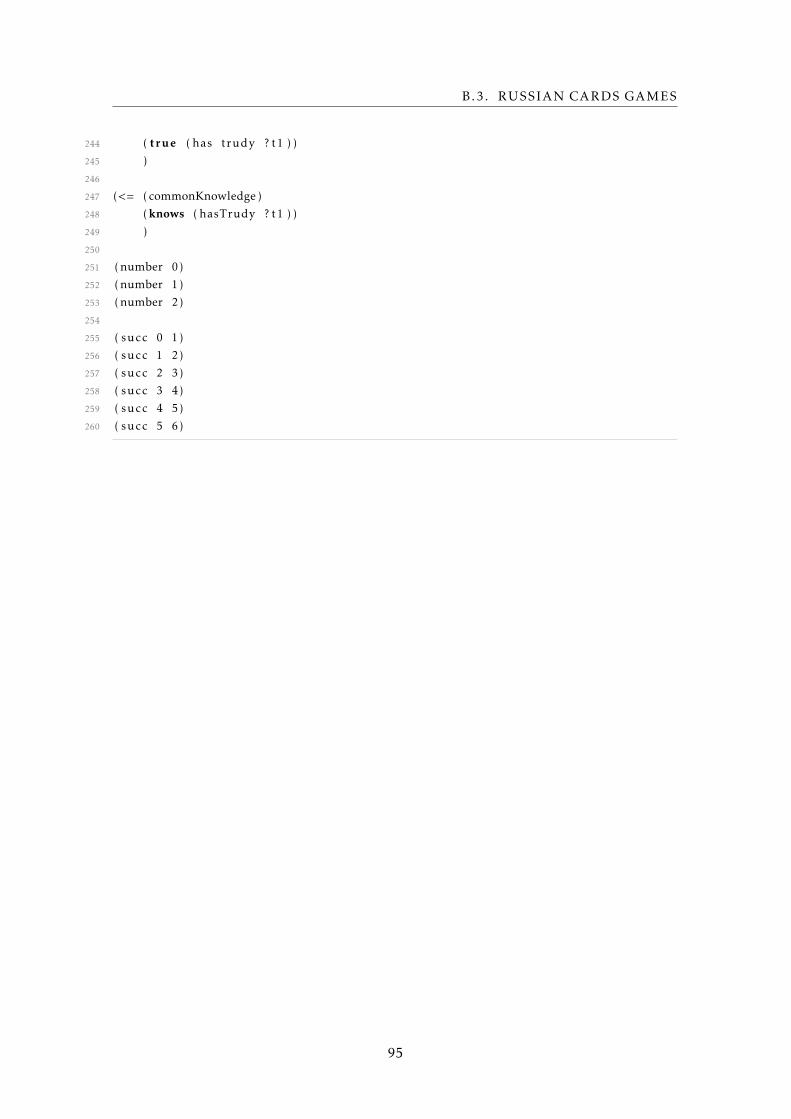
B.3. RUSSIAN CARDS GAMES
244 ( true ( has trudy ? t1 ) )
245 )
246
247 (<= ( commonKnowledge )
248 ( knows ( hasTrudy ? t1 ) )
249 )
250
251 ( number 0)
252 ( number 1)
253 ( number 2)
254
255 ( succ 0 1)
256 ( succ 1 2)
257 ( succ 2 3)
258 ( succ 3 4)
259 ( succ 4 5)
260 ( succ 5 6)
95

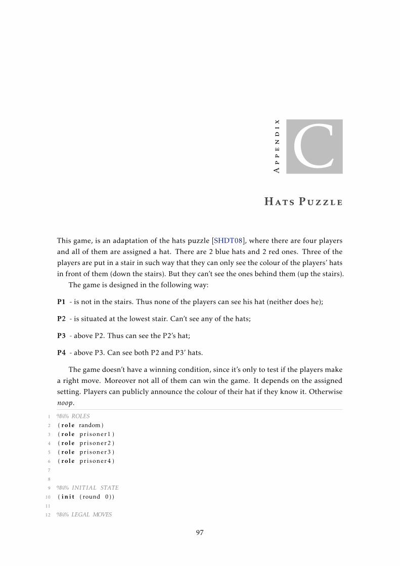
Appendix
CHats Puzzle
This game, is an adaptation of the hats puzzle [SHDT08], where there are four players
and all of them are assigned a hat. There are 2 blue hats and 2 red ones. Three of the
players are put in a stair in such way that they can only see the colour of the players’ hats
in front of them (down the stairs). But they can’t see the ones behind them (up the stairs).
The game is designed in the following way:
P1 - is not in the stairs. Thus none of the players can see his hat (neither does he);
P2 - is situated at the lowest stair. Can’t see any of the hats;
P3 - above P2. Thus can see the P2’s hat;
P4 - above P3. Can see both P2 and P3’ hats.
The game doesn’t have a winning condition, since it’s only to test if the players make
a right move. Moreover not all of them can win the game. It depends on the assigned
setting. Players can publicly announce the colour of their hat if they know it. Otherwise
noop.
1 %%% ROLES2 ( role random )
3 ( role prisoner1 )
4 ( role prisoner2 )
5 ( role prisoner3 )
6 ( role prisoner4 )
7
8
9 %%% INITIAL STATE10 ( i n i t ( round 0 ) )
11
12 %%% LEGAL MOVES
97
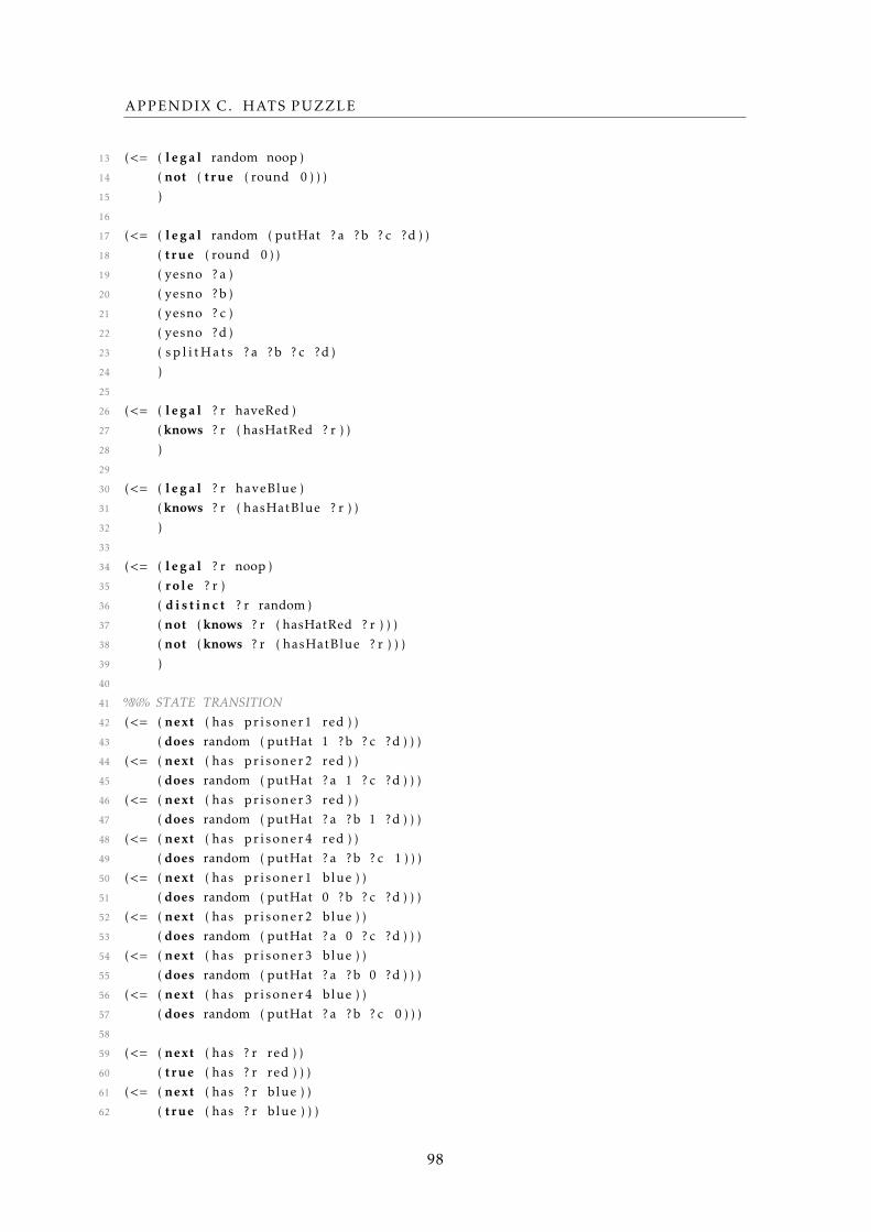
APPENDIX C. HATS PUZZLE
13 (<= ( l e g a l random noop )
14 ( not ( true ( round 0 ) ) )
15 )
16
17 (<= ( l e g a l random ( putHat ? a ?b ? c ?d ) )
18 ( true ( round 0 ) )
19 ( yesno ? a )
20 ( yesno ?b )
21 ( yesno ? c )
22 ( yesno ?d )
23 ( s p l i t H a t s ? a ?b ? c ?d )
24 )
25
26 (<= ( l e g a l ? r haveRed )
27 ( knows ? r ( hasHatRed ? r ) )
28 )
29
30 (<= ( l e g a l ? r haveBlue )
31 ( knows ? r ( hasHatBlue ? r ) )
32 )
33
34 (<= ( l e g a l ? r noop )
35 ( role ? r )
36 ( d i s t i n c t ? r random )
37 ( not ( knows ? r ( hasHatRed ? r ) ) )
38 ( not ( knows ? r ( hasHatBlue ? r ) ) )
39 )
40
41 %%% STATE TRANSITION42 (<= ( next ( has prisoner1 red ) )
43 ( does random ( putHat 1 ?b ? c ?d ) ) )
44 (<= ( next ( has prisoner2 red ) )
45 ( does random ( putHat ? a 1 ? c ?d ) ) )
46 (<= ( next ( has prisoner3 red ) )
47 ( does random ( putHat ? a ?b 1 ?d ) ) )
48 (<= ( next ( has prisoner4 red ) )
49 ( does random ( putHat ? a ?b ? c 1 ) ) )
50 (<= ( next ( has prisoner1 blue ) )
51 ( does random ( putHat 0 ?b ? c ?d ) ) )
52 (<= ( next ( has prisoner2 blue ) )
53 ( does random ( putHat ? a 0 ? c ?d ) ) )
54 (<= ( next ( has prisoner3 blue ) )
55 ( does random ( putHat ? a ?b 0 ?d ) ) )
56 (<= ( next ( has prisoner4 blue ) )
57 ( does random ( putHat ? a ?b ? c 0 ) ) )
58
59 (<= ( next ( has ? r red ) )
60 ( true ( has ? r red ) ) )
61 (<= ( next ( has ? r blue ) )
62 ( true ( has ? r blue ) ) )
98
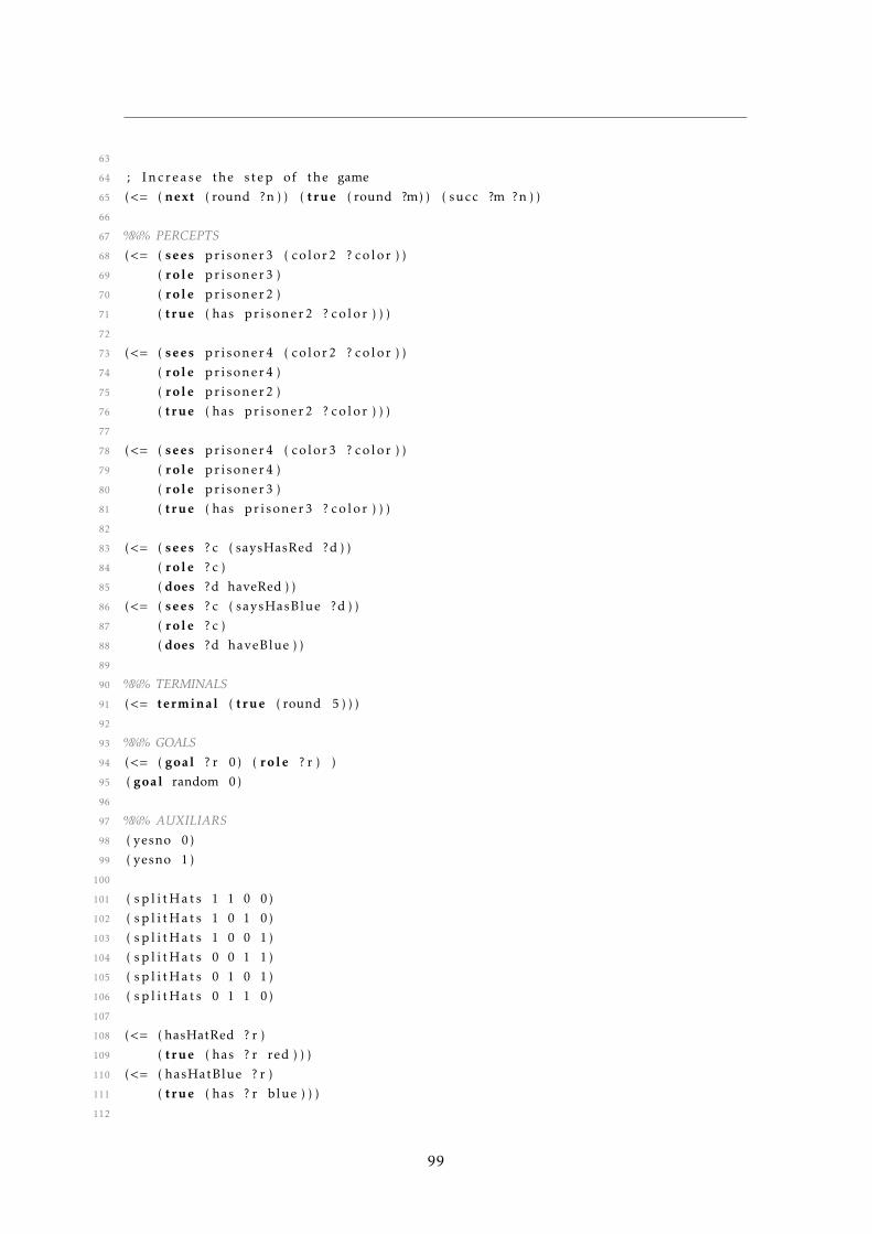
63
64 ; Increase the step of the game
65 (<= ( next ( round ?n ) ) ( true ( round ?m) ) ( succ ?m ?n ) )
66
67 %%% PERCEPTS68 (<= ( sees prisoner3 ( color2 ? c o l o r ) )
69 ( role prisoner3 )
70 ( role prisoner2 )
71 ( true ( has prisoner2 ? c o l o r ) ) )
72
73 (<= ( sees prisoner4 ( color2 ? c o l o r ) )
74 ( role prisoner4 )
75 ( role prisoner2 )
76 ( true ( has prisoner2 ? c o l o r ) ) )
77
78 (<= ( sees prisoner4 ( color3 ? c o l o r ) )
79 ( role prisoner4 )
80 ( role prisoner3 )
81 ( true ( has prisoner3 ? c o l o r ) ) )
82
83 (<= ( sees ? c ( saysHasRed ?d ) )
84 ( role ? c )
85 ( does ?d haveRed ) )
86 (<= ( sees ? c ( saysHasBlue ?d ) )
87 ( role ? c )
88 ( does ?d haveBlue ) )
89
90 %%% TERMINALS91 (<= terminal ( true ( round 5 ) ) )
92
93 %%% GOALS94 (<= ( goal ? r 0) ( role ? r ) )
95 ( goal random 0)
96
97 %%% AUXILIARS98 ( yesno 0)
99 ( yesno 1)
100
101 ( s p l i t H a t s 1 1 0 0)
102 ( s p l i t H a t s 1 0 1 0)
103 ( s p l i t H a t s 1 0 0 1)
104 ( s p l i t H a t s 0 0 1 1)
105 ( s p l i t H a t s 0 1 0 1)
106 ( s p l i t H a t s 0 1 1 0)
107
108 (<= ( hasHatRed ? r )
109 ( true ( has ? r red ) ) )
110 (<= ( hasHatBlue ? r )
111 ( true ( has ? r blue ) ) )
112
99

APPENDIX C. HATS PUZZLE
113 ( succ 0 1)
114 ( succ 1 2)
115 ( succ 2 3)
116 ( succ 3 4)
117 ( succ 4 5)
100
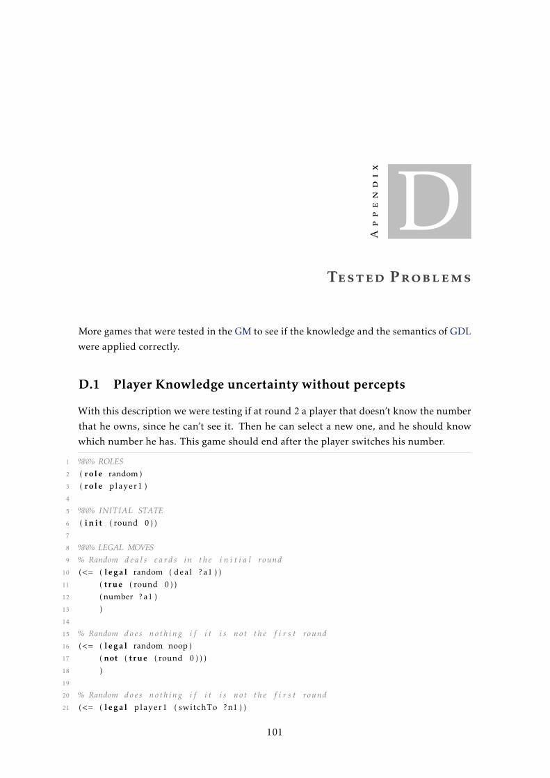
Appendix
DTested Problems
More games that were tested in the GM to see if the knowledge and the semantics of GDL
were applied correctly.
D.1 Player Knowledge uncertainty without percepts
With this description we were testing if at round 2 a player that doesn’t know the number
that he owns, since he can’t see it. Then he can select a new one, and he should know
which number he has. This game should end after the player switches his number.
1 %%% ROLES2 ( role random )
3 ( role player1 )
4
5 %%% INITIAL STATE6 ( i n i t ( round 0 ) )
7
8 %%% LEGAL MOVES9 % Random d e a l s c a r d s in t h e i n i t i a l round
10 (<= ( l e g a l random ( deal ? a1 ) )
11 ( true ( round 0 ) )
12 ( number ? a1 )
13 )
14
15 % Random does noth ing i f i t i s not t h e f i r s t round16 (<= ( l e g a l random noop )
17 ( not ( true ( round 0 ) ) )
18 )
19
20 % Random does noth ing i f i t i s not t h e f i r s t round21 (<= ( l e g a l player1 ( switchTo ?n1 ) )
101
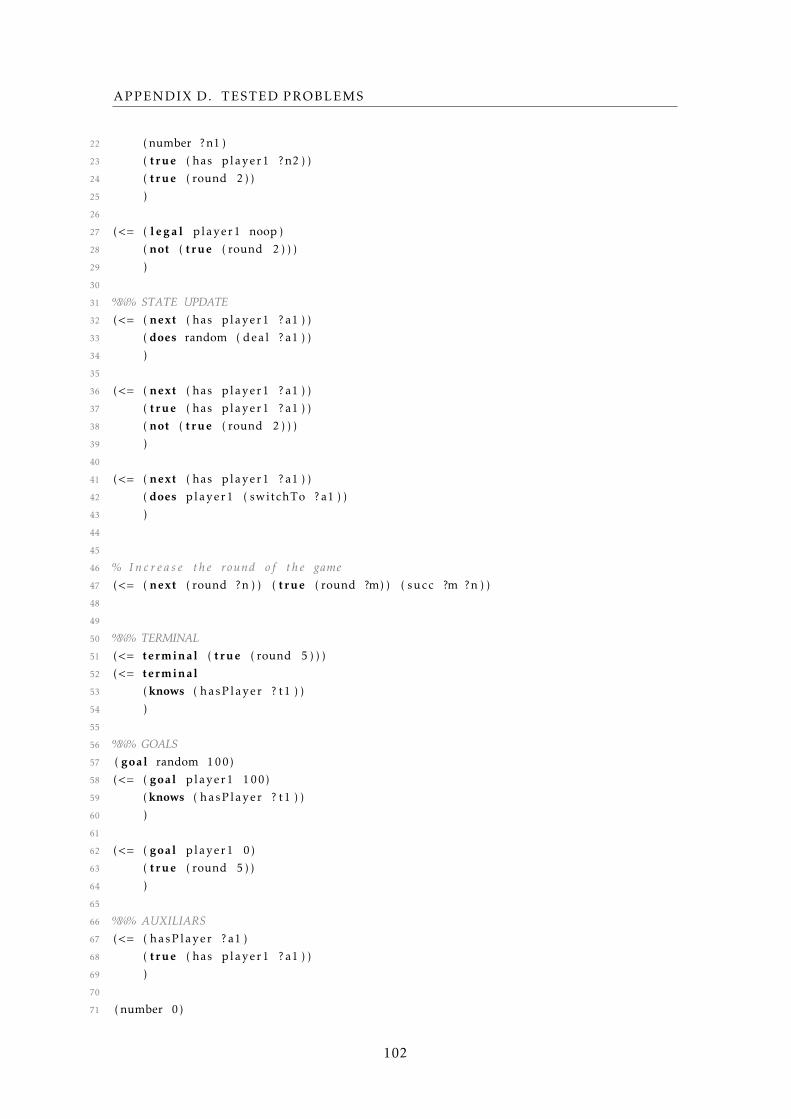
APPENDIX D. TESTED PROBLEMS
22 ( number ?n1 )
23 ( true ( has player1 ?n2 ) )
24 ( true ( round 2 ) )
25 )
26
27 (<= ( l e g a l player1 noop )
28 ( not ( true ( round 2 ) ) )
29 )
30
31 %%% STATE UPDATE32 (<= ( next ( has player1 ? a1 ) )
33 ( does random ( deal ? a1 ) )
34 )
35
36 (<= ( next ( has player1 ? a1 ) )
37 ( true ( has player1 ? a1 ) )
38 ( not ( true ( round 2 ) ) )
39 )
40
41 (<= ( next ( has player1 ? a1 ) )
42 ( does player1 ( switchTo ? a1 ) )
43 )
44
45
46 % I n c r e a s e t h e round o f t h e game47 (<= ( next ( round ?n ) ) ( true ( round ?m) ) ( succ ?m ?n ) )
48
49
50 %%% TERMINAL51 (<= terminal ( true ( round 5 ) ) )
52 (<= terminal53 ( knows ( hasPlayer ? t1 ) )
54 )
55
56 %%% GOALS57 ( goal random 100)
58 (<= ( goal player1 100)
59 ( knows ( hasPlayer ? t1 ) )
60 )
61
62 (<= ( goal player1 0)
63 ( true ( round 5 ) )
64 )
65
66 %%% AUXILIARS67 (<= ( hasPlayer ? a1 )
68 ( true ( has player1 ? a1 ) )
69 )
70
71 ( number 0)
102
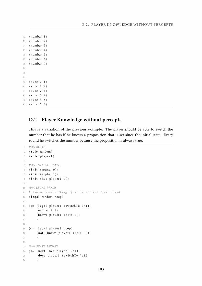
D.2. PLAYER KNOWLEDGE WITHOUT PERCEPTS
72 ( number 1)
73 ( number 2)
74 ( number 3)
75 ( number 4)
76 ( number 5)
77 ( number 6)
78 ( number 7)
79
80
81
82 ( succ 0 1)
83 ( succ 1 2)
84 ( succ 2 3)
85 ( succ 3 4)
86 ( succ 4 5)
87 ( succ 5 6)
D.2 Player Knowledge without percepts
This is a variation of the previous example. The player should be able to switch the
number that he has if he knows a proposition that is set since the initial state. Every
round he switches the number because the proposition is always true.
1 %%% ROLES2 ( role random )
3 ( role player1 )
4
5 %%% INITIAL STATE6 ( i n i t ( round 0 ) )
7 ( i n i t ( alpha 1 ) )
8 ( i n i t ( has player1 1 ) )
9
10 %%% LEGAL MOVES11 % Random does noth ing i f i t i s not t h e f i r s t round12 ( l e g a l random noop )
13
14 (<= ( l e g a l player1 ( switchTo ?n1 ) )
15 ( number ?n1 )
16 ( knows player1 ( beta 1 ) )
17 )
18
19 (<= ( l e g a l player1 noop )
20 ( not ( knows player1 ( beta 1 ) ) )
21 )
22
23 %%% STATE UPDATE24 (<= ( next ( has player1 ? a1 ) )
25 ( does player1 ( switchTo ? a1 ) )
26 )
103
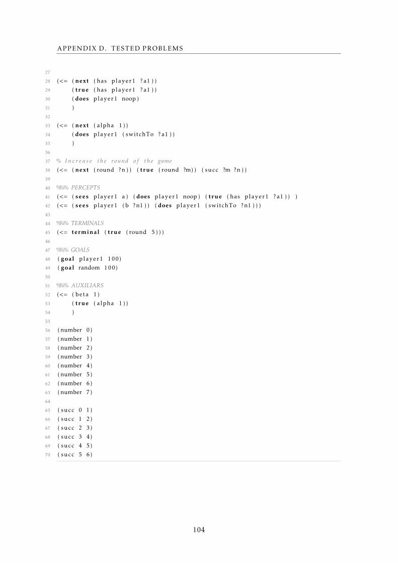
APPENDIX D. TESTED PROBLEMS
27
28 (<= ( next ( has player1 ? a1 ) )
29 ( true ( has player1 ? a1 ) )
30 ( does player1 noop )
31 )
32
33 (<= ( next ( alpha 1 ) )
34 ( does player1 ( switchTo ? a1 ) )
35 )
36
37 % I n c r e a s e t h e round o f t h e game38 (<= ( next ( round ?n ) ) ( true ( round ?m) ) ( succ ?m ?n ) )
39
40 %%% PERCEPTS41 (<= ( sees player1 a ) ( does player1 noop ) ( true ( has player1 ? a1 ) ) )
42 (<= ( sees player1 ( b ?n1 ) ) ( does player1 ( switchTo ?n1 ) ) )
43
44 %%% TERMINALS45 (<= terminal ( true ( round 5 ) ) )
46
47 %%% GOALS48 ( goal player1 100)
49 ( goal random 100)
50
51 %%% AUXILIARS52 (<= ( beta 1)
53 ( true ( alpha 1 ) )
54 )
55
56 ( number 0)
57 ( number 1)
58 ( number 2)
59 ( number 3)
60 ( number 4)
61 ( number 5)
62 ( number 6)
63 ( number 7)
64
65 ( succ 0 1)
66 ( succ 1 2)
67 ( succ 2 3)
68 ( succ 3 4)
69 ( succ 4 5)
70 ( succ 5 6)
104
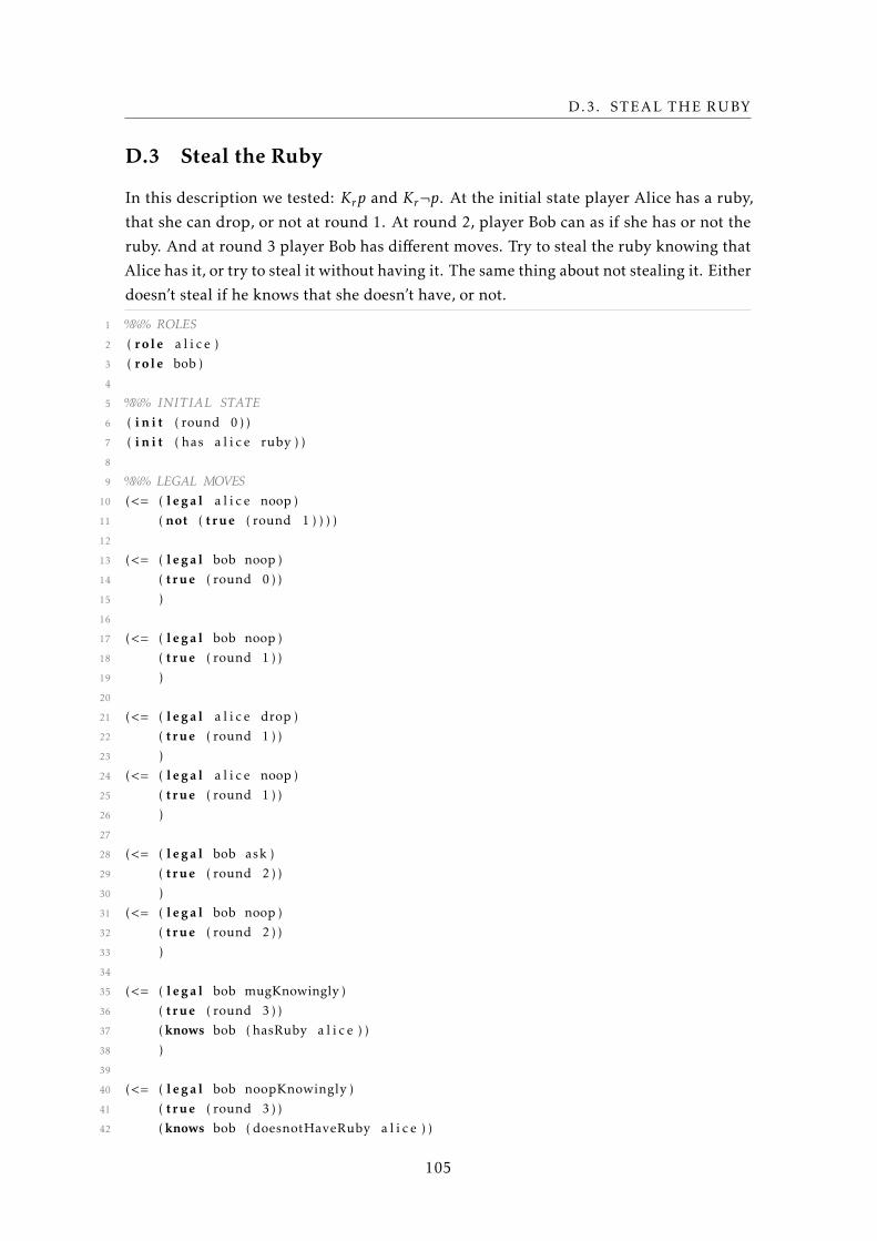
D.3. STEAL THE RUBY
D.3 Steal the Ruby
In this description we tested: Krp and Kr¬p. At the initial state player Alice has a ruby,
that she can drop, or not at round 1. At round 2, player Bob can as if she has or not the
ruby. And at round 3 player Bob has different moves. Try to steal the ruby knowing that
Alice has it, or try to steal it without having it. The same thing about not stealing it. Either
doesn’t steal if he knows that she doesn’t have, or not.
1 %%% ROLES2 ( role a l i c e )
3 ( role bob )
4
5 %%% INITIAL STATE6 ( i n i t ( round 0 ) )
7 ( i n i t ( has a l i c e ruby ) )
8
9 %%% LEGAL MOVES10 (<= ( l e g a l a l i c e noop )
11 ( not ( true ( round 1 ) ) ) )
12
13 (<= ( l e g a l bob noop )
14 ( true ( round 0 ) )
15 )
16
17 (<= ( l e g a l bob noop )
18 ( true ( round 1 ) )
19 )
20
21 (<= ( l e g a l a l i c e drop )
22 ( true ( round 1 ) )
23 )
24 (<= ( l e g a l a l i c e noop )
25 ( true ( round 1 ) )
26 )
27
28 (<= ( l e g a l bob ask )
29 ( true ( round 2 ) )
30 )
31 (<= ( l e g a l bob noop )
32 ( true ( round 2 ) )
33 )
34
35 (<= ( l e g a l bob mugKnowingly )
36 ( true ( round 3 ) )
37 ( knows bob ( hasRuby a l i c e ) )
38 )
39
40 (<= ( l e g a l bob noopKnowingly )
41 ( true ( round 3 ) )
42 ( knows bob ( doesnotHaveRuby a l i c e ) )
105
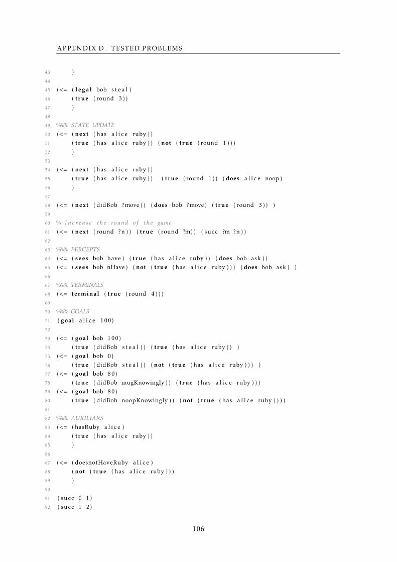
APPENDIX D. TESTED PROBLEMS
43 )
44
45 (<= ( l e g a l bob s t e a l )
46 ( true ( round 3 ) )
47 )
48
49 %%% STATE UPDATE50 (<= ( next ( has a l i c e ruby ) )
51 ( true ( has a l i c e ruby ) ) ( not ( true ( round 1 ) ) )
52 )
53
54 (<= ( next ( has a l i c e ruby ) )
55 ( true ( has a l i c e ruby ) ) ( true ( round 1 ) ) ( does a l i c e noop )
56 )
57
58 (<= ( next ( didBob ?move ) ) ( does bob ?move ) ( true ( round 3 ) ) )
59
60 % I n c r e a s e t h e round o f t h e game61 (<= ( next ( round ?n ) ) ( true ( round ?m) ) ( succ ?m ?n ) )
62
63 %%% PERCEPTS64 (<= ( sees bob have ) ( true ( has a l i c e ruby ) ) ( does bob ask ) )
65 (<= ( sees bob nHave ) ( not ( true ( has a l i c e ruby ) ) ) ( does bob ask ) )
66
67 %%% TERMINALS68 (<= terminal ( true ( round 4 ) ) )
69
70 %%% GOALS71 ( goal a l i c e 100)
72
73 (<= ( goal bob 100)
74 ( true ( didBob s t e a l ) ) ( true ( has a l i c e ruby ) ) )
75 (<= ( goal bob 0)
76 ( true ( didBob s t e a l ) ) ( not ( true ( has a l i c e ruby ) ) ) )
77 (<= ( goal bob 80)
78 ( true ( didBob mugKnowingly ) ) ( true ( has a l i c e ruby ) ) )
79 (<= ( goal bob 80)
80 ( true ( didBob noopKnowingly ) ) ( not ( true ( has a l i c e ruby ) ) ) )
81
82 %%% AUXILIARS83 (<= ( hasRuby a l i c e )
84 ( true ( has a l i c e ruby ) )
85 )
86
87 (<= ( doesnotHaveRuby a l i c e )
88 ( not ( true ( has a l i c e ruby ) ) )
89 )
90
91 ( succ 0 1)
92 ( succ 1 2)
106
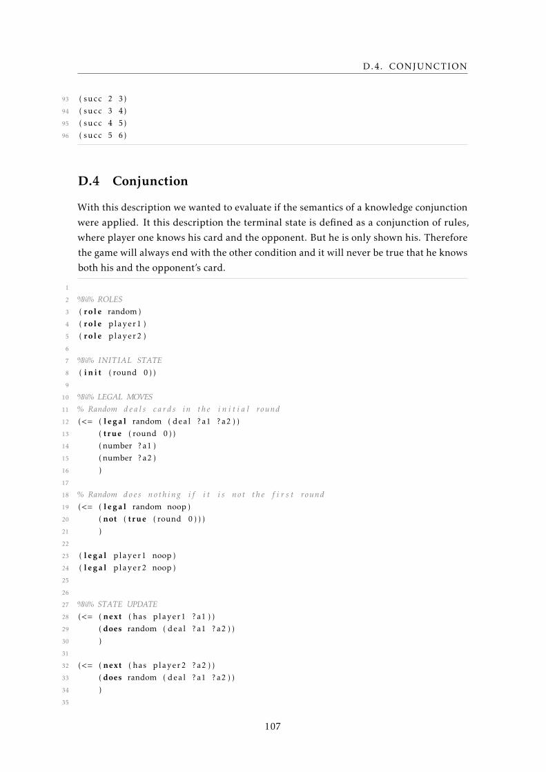
D.4. CONJUNCTION
93 ( succ 2 3)
94 ( succ 3 4)
95 ( succ 4 5)
96 ( succ 5 6)
D.4 Conjunction
With this description we wanted to evaluate if the semantics of a knowledge conjunction
were applied. It this description the terminal state is defined as a conjunction of rules,
where player one knows his card and the opponent. But he is only shown his. Therefore
the game will always end with the other condition and it will never be true that he knows
both his and the opponent’s card.
1
2 %%% ROLES3 ( role random )
4 ( role player1 )
5 ( role player2 )
6
7 %%% INITIAL STATE8 ( i n i t ( round 0 ) )
9
10 %%% LEGAL MOVES11 % Random d e a l s c a r d s in t h e i n i t i a l round12 (<= ( l e g a l random ( deal ? a1 ? a2 ) )
13 ( true ( round 0 ) )
14 ( number ? a1 )
15 ( number ? a2 )
16 )
17
18 % Random does noth ing i f i t i s not t h e f i r s t round19 (<= ( l e g a l random noop )
20 ( not ( true ( round 0 ) ) )
21 )
22
23 ( l e g a l player1 noop )
24 ( l e g a l player2 noop )
25
26
27 %%% STATE UPDATE28 (<= ( next ( has player1 ? a1 ) )
29 ( does random ( deal ? a1 ? a2 ) )
30 )
31
32 (<= ( next ( has player2 ? a2 ) )
33 ( does random ( deal ? a1 ? a2 ) )
34 )
35
107
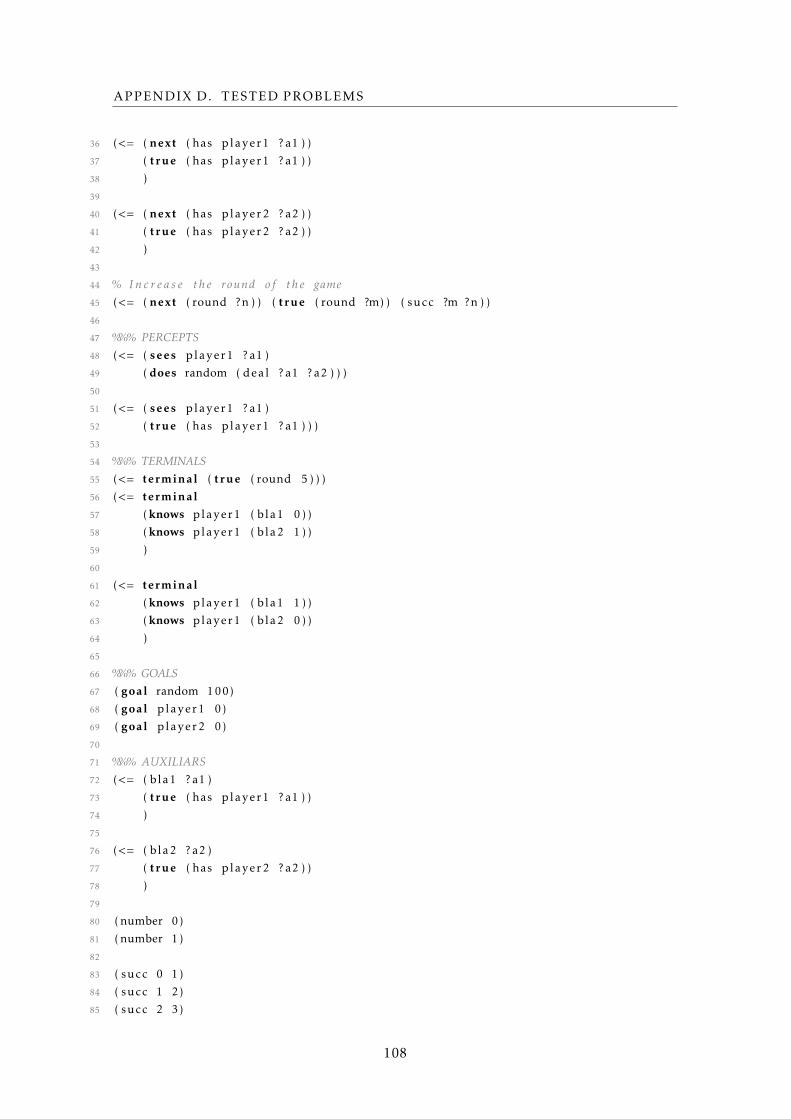
APPENDIX D. TESTED PROBLEMS
36 (<= ( next ( has player1 ? a1 ) )
37 ( true ( has player1 ? a1 ) )
38 )
39
40 (<= ( next ( has player2 ? a2 ) )
41 ( true ( has player2 ? a2 ) )
42 )
43
44 % I n c r e a s e t h e round o f t h e game45 (<= ( next ( round ?n ) ) ( true ( round ?m) ) ( succ ?m ?n ) )
46
47 %%% PERCEPTS48 (<= ( sees player1 ? a1 )
49 ( does random ( deal ? a1 ? a2 ) ) )
50
51 (<= ( sees player1 ? a1 )
52 ( true ( has player1 ? a1 ) ) )
53
54 %%% TERMINALS55 (<= terminal ( true ( round 5 ) ) )
56 (<= terminal57 ( knows player1 ( bla1 0 ) )
58 ( knows player1 ( bla2 1 ) )
59 )
60
61 (<= terminal62 ( knows player1 ( bla1 1 ) )
63 ( knows player1 ( bla2 0 ) )
64 )
65
66 %%% GOALS67 ( goal random 100)
68 ( goal player1 0)
69 ( goal player2 0)
70
71 %%% AUXILIARS72 (<= ( bla1 ? a1 )
73 ( true ( has player1 ? a1 ) )
74 )
75
76 (<= ( bla2 ? a2 )
77 ( true ( has player2 ? a2 ) )
78 )
79
80 ( number 0)
81 ( number 1)
82
83 ( succ 0 1)
84 ( succ 1 2)
85 ( succ 2 3)
108

D.4. CONJUNCTION
86 ( succ 3 4)
87 ( succ 4 5)
88 ( succ 5 6)
109

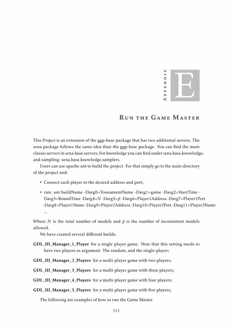
Appendix
ERun the Game Master
This Project is an extension of the ggp-base-package that has two additional servers. The
sena package follows the same idea than the ggp-base package. You can find the main
classes servers in sena.base.servers; For knowledge you can find under sena.base.knowledge;
and sampling: sena.base.knowledge.samplers.
Users can use apache-ant to build the project. For that simply go to the main directory
of the project and:
• Connect each player to the desired address and port;
• run: ant buildName -Darg0=TounamentName -Darg1=game -Darg2=StartTime -
Darg3=RoundTime -Darg4=N -Darg5=β -Darg6=Player1Address -Darg7=Player1Port
-Darg8=Player1Name -Darg9=Player2Address -Darg10=Player2Port -Darg11=Player2Name
...
Where N is the total number of models and β is the number of inconsistent models
allowed.
We have created several different builds:
GDL_III_Manager_1_Player for a single player game. Note that this setting needs to
have two players as argument. The random, and the single-player;
GDL_III_Manager_2_Players for a multi-player game with two players;
GDL_III_Manager_3_Players for a multi-player game with three players;
GDL_III_Manager_4_Players for a multi-player game with four players;
GDL_III_Manager_5_Players for a multi-player game with five players;
The following are examples of how to run the Game Master.
111
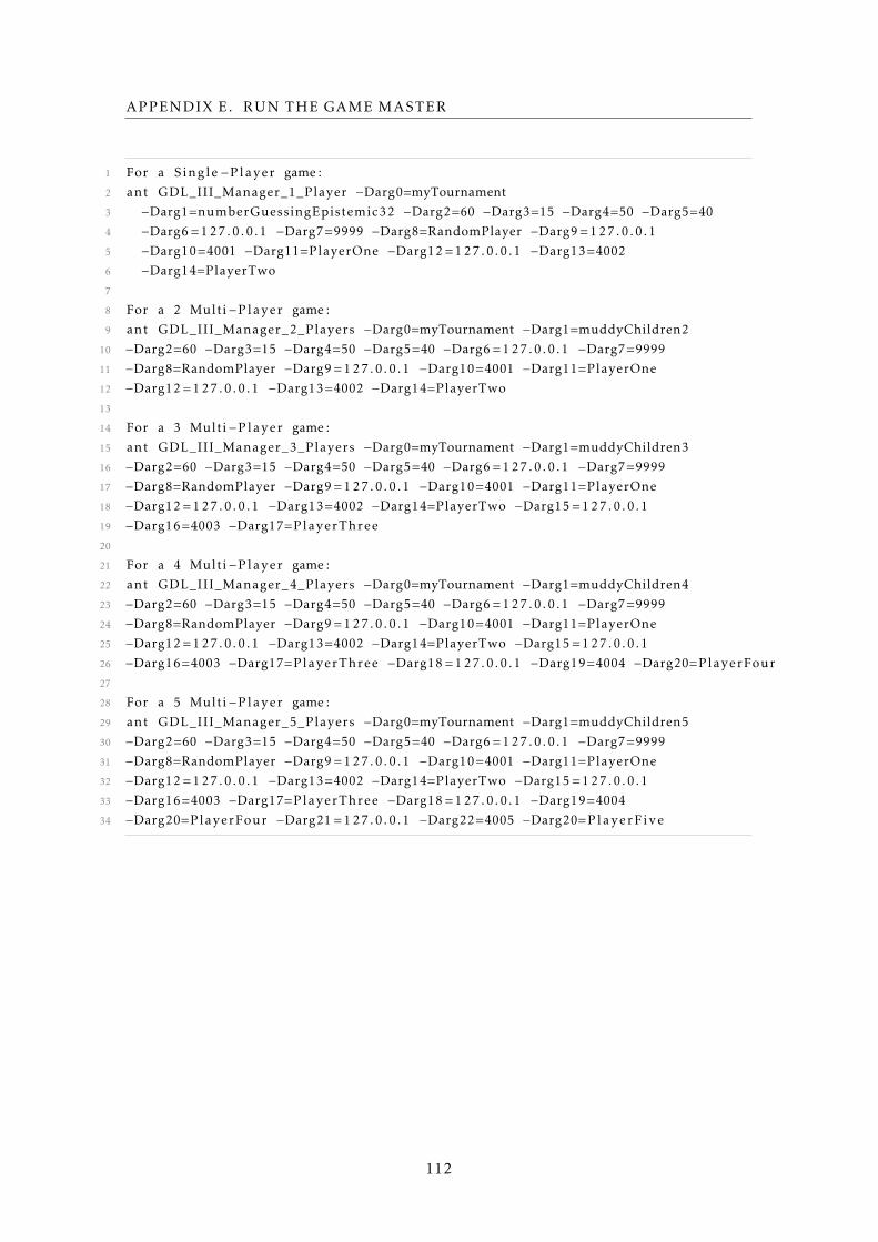
APPENDIX E. RUN THE GAME MASTER
1 For a Single −Player game :
2 ant GDL_III_Manager_1_Player −Darg0=myTournament
3 −Darg1=numberGuessingEpistemic32 −Darg2=60 −Darg3=15 −Darg4=50 −Darg5=40
4 −Darg6 =127.0 .0 .1 −Darg7=9999 −Darg8=RandomPlayer −Darg9 =127.0 .0 .1
5 −Darg10=4001 −Darg11=PlayerOne −Darg12 =127.0 .0 .1 −Darg13=4002
6 −Darg14=PlayerTwo
7
8 For a 2 Multi−Player game :
9 ant GDL_III_Manager_2_Players −Darg0=myTournament −Darg1=muddyChildren2
10 −Darg2=60 −Darg3=15 −Darg4=50 −Darg5=40 −Darg6 =127.0 .0 .1 −Darg7=9999
11 −Darg8=RandomPlayer −Darg9 =127.0 .0 .1 −Darg10=4001 −Darg11=PlayerOne
12 −Darg12 =127.0 .0 .1 −Darg13=4002 −Darg14=PlayerTwo
13
14 For a 3 Multi−Player game :
15 ant GDL_III_Manager_3_Players −Darg0=myTournament −Darg1=muddyChildren3
16 −Darg2=60 −Darg3=15 −Darg4=50 −Darg5=40 −Darg6 =127.0 .0 .1 −Darg7=9999
17 −Darg8=RandomPlayer −Darg9 =127.0 .0 .1 −Darg10=4001 −Darg11=PlayerOne
18 −Darg12 =127.0 .0 .1 −Darg13=4002 −Darg14=PlayerTwo −Darg15 =127.0 .0 .1
19 −Darg16=4003 −Darg17=PlayerThree
20
21 For a 4 Multi−Player game :
22 ant GDL_III_Manager_4_Players −Darg0=myTournament −Darg1=muddyChildren4
23 −Darg2=60 −Darg3=15 −Darg4=50 −Darg5=40 −Darg6 =127.0 .0 .1 −Darg7=9999
24 −Darg8=RandomPlayer −Darg9 =127.0 .0 .1 −Darg10=4001 −Darg11=PlayerOne
25 −Darg12 =127.0 .0 .1 −Darg13=4002 −Darg14=PlayerTwo −Darg15 =127.0 .0 .1
26 −Darg16=4003 −Darg17=PlayerThree −Darg18 =127.0 .0 .1 −Darg19=4004 −Darg20=PlayerFour
27
28 For a 5 Multi−Player game :
29 ant GDL_III_Manager_5_Players −Darg0=myTournament −Darg1=muddyChildren5
30 −Darg2=60 −Darg3=15 −Darg4=50 −Darg5=40 −Darg6 =127.0 .0 .1 −Darg7=9999
31 −Darg8=RandomPlayer −Darg9 =127.0 .0 .1 −Darg10=4001 −Darg11=PlayerOne
32 −Darg12 =127.0 .0 .1 −Darg13=4002 −Darg14=PlayerTwo −Darg15 =127.0 .0 .1
33 −Darg16=4003 −Darg17=PlayerThree −Darg18 =127.0 .0 .1 −Darg19=4004
34 −Darg20=PlayerFour −Darg21 =127.0 .0 .1 −Darg22=4005 −Darg20=PlayerFive
112