Epipolar Geometry Based On Line Similarity

Gil Ben-Artzi Tavi Halperin Michael Werman Shmuel PelegSchool of Computer Science and Engineering

The Hebrew University of Jerusalem, Israel

Abstract

It is known that epipolar geometry can be computed fromthree epipolar line correspondences but this computation israrely used in practice since there are no simple methods tofind corresponding lines. Instead, methods for finding cor-responding points are widely used. This paper proposes asimilarity measure between lines that indicates whether twolines are corresponding epipolar lines and enables findingepipolar line correspondences as needed for the computationof epipolar geometry.

A similarity measure between two lines, suitable for videosequences of a dynamic scene, has been previously described.This paper suggests a stereo matching similarity measuresuitable for images. It is based on the quality of stereo match-ing between the two lines, as corresponding epipolar linesyield a good stereo correspondence. Instead of an exhaustivesearch over all possible pairs of lines, the search space issubstantially reduced when two corresponding point pairs aregiven.

We validate the proposed method using real-world imagesand compare it to state-of-the-art methods. We found thismethod to be more accurate by a factor of five compared tothe standard method using seven corresponding points andcomparable to the 8-point algorithm.

1. Introduction

The fundamental matrix is a basic building block of mul-tiple view geometry and its computation is the first step inmany vision tasks. The computation is usually based on pairsof corresponding points. Matching points across images iserror prone and many subsets of points need to be sampleduntil a good solution is found. In this work we addressthe problem of robustly estimating the fundamental matrixfrom line correspondences, given a similarity measure betweenlines.

The best-known algorithm, adapted for the case of fun-damental matrix, is the eight point algorithm by Longuet-Higgins [8]. It was made practical by Hartley [5]. The overallmethod is based on normalization of the data, solving a setof linear equations and enforcing the rank 2 constraint [9].The requirement of eight point correspondences can be relaxedto seven. This results in a cubic equation with one or threereal solutions. The estimation from 7 points is very sensitiveto noise. These methods are often followed by a non-linearoptimization step.

The fundamental matrix can also be computed from threematching epipolar lines [6]. Given three such correspondences,the one dimensional homography between the lines can berecovered as the epipolar lines in each of the images intersectat the epipoles. The 3 degrees of freedom for the 1D homog-raphy together with the 4 degrees of freedom of the epipolesyield the required 7 degrees of freedom needed to computethe fundamental matrix.

There are a few papers using corresponding epipolar linesto compute epipolar geometry, but these are only applicableto videos of dynamic scenes [11], [1], [7]. The most relevantpaper is [7], describing a similarity between lines based onscene dynamics.

We present a new similarity measure between lines, andutilize it to robustly compute the fundamental matrix. Thissimilarity measure is based on the brightness consistency(stereo matching) that exists between corresponding epipolarlines. We can reduce the search space for correspondingepipolar lines by giving two corresponding points. This iscompared to the 7 or 8 points normally required.

Fundamental matrix computation from points correspon-dences has to take into account mistaken correspondences(outliers). Using a RANSAC approach, multiple subsets ofpoints are sampled, so that with high probability one subsetwill not include any outlier. Using only 2 points as neededin our method substantially reduces the number of samples.For example, if 50% of correspondences are correct, and werequire a probability of 99% that one subset will have nooutliers, we will need to select 1, 177 8-point subsets, 5887-point subsets, and only 17 subsets of 2-points.

2. Previous Work

2.1. Computing the Fundamental Matrix

The fundamental matrix is a 3× 3 homogeneous ranktwo matrix with seven degrees of freedom. There are variousformulations that have been considered to produce a minimalparameterization with only seven parameters [6].

The most common parameterization is from the correspon-dences of seven points and can be computed as the null spaceof a 7×9 matrix. The rank two constraint leads to a cubicequation with one or three possible solutions.

The method we will follow is based directly on the epipo-lar geometry entities. The fundamental matrix is representedby the epipoles and the epipolar line homography. Each of the

Figure 1: A motion barcode b of a line l is a vector in {0, 1}N .The value of bl(i) is ”1” when a moving object intersects the line inframe i (black entries) and ”0” otherwise (white entries).

two epipoles accounts for two parameters. The epipolar linehomography represents the 1D-line homography between theepipolar pencils and accounts for three degrees of freedom.

2.2. Finding Corresponding Epipolar Lines

Previous methods found corresponding epipolar lines fromvideos of dynamic scenes. Sinha and Pollefeys [11] used sil-houettes to find corresponding epipolar lines for calibration ofa network of cameras, assuming a single moving silhouette ina video. Ben-Artzi et al. [1] accelerated Sinha’s method usinga similarity measure for epipolar lines. The similarity measureis a generalization of Motion Barcodes [2] to lines. This linemotion barcode was also used in [7] to find correspondingepipolar lines.

2.3. Motion Barcodes of Lines

Motion Barcodes of Lines were used in the case of syn-chronized stationary cameras viewing a scene with movingobjects. Following background subtraction [3] we obtain abinary video, where ”0” represents static background and ”1”moving objects.

Given such a video of N binary frames, the MotionBarcode of a given image line l [1] is a binary vector blin {0, 1}N . bl(i) = 1 iff a silhouette of a foreground objectintersects at least one pixel of line l at the ith frame. Anexample of a Motion Barcode is shown in Fig 1.

The case of a moving object seen by two cameras isillustrated in Fig. 2. If the object intersects the epipolar planeπ at frame i, and does not intersect the plane π at frame j,both Motion Barcodes of lines l and l′ will be 1, 0 at framesi, j respectively. Corresponding epipolar lines therefore havehighly correlated Motion Barcodes.

Similarity Score Between Two Motion Barcodes. It wassuggested in [2] that a good similarity measure betweenmotion barcodes b and b′ is their normalized cross correlation.

2.4. Stereo Matching

Depth from two stereo images is traditionally computed bymatching along corresponding epipolar lines. Our hypothesisis that stereo matching will be more successful when applied tocorresponding epipolar lines, rather than to random, unrelatedlines. The success of stereo matching along two lines is ourindicator whether these two lines are corresponding epipolarlines.

Many different stereo matching methods exist (seeScharstein and Szeliski [10] for a survey). The stereo matchingmethods can be roughly divided to global and local methods.Since we are not interested in estimating an accurate per-pixel disparity, but only in line-to-line matching, we used a

Figure 2: Illustration of a scene with a moving object viewed by twovideo cameras. The lines l and l′ are corresponding epipolar lines,and π is the 3D epipolar plane that projects to l and l′. At timet = 1 the object does not intersect the plane π, and thus does notintersect l or l′ in the video. At times t = 2, 3 the object intersectsthe plane π, so the projections of this object on the cameras doesintersect the epipolar lines l and l′. The motion barcodes of both land l′ is (0, 1, 1)

a) b)

c) d)Figure 3: Matching epipolar lines using stereo matching. (a-b)Matching epipolar lines across two view. Computed epipolar linesby our method (green) are very close to the ground truth (blue). (c)The intensity profile of the two corresponding lines found by ourapproach. (d) Intensity profile after warping due to stereo correspon-dence.

dynamic programming stereo method. Dynamic programmingis the simplest and fastest global stereo algorithm, is relativelyrobust, and it gives the optimal solution for scanline matching.

3. The Stereo Matching Similarity

Two corresponding epipolar lines are projections of thescene intersected by the same epipolar plane. We assumethat the intensities along corresponding epipolar lines arerelated through stereo disparities, as is traditionally used instereo. Stereo depth is computed by matching points alongcorresponding epipolar lines. The stereo matching similaritybetween two lines, l1, l2, is therefore related to their stereomatching score as defined in Eq. 1.

As the compared lines are usually not aligned with theimages axes, they should be re-quantized to equidistant points

along them. Let xi be the 2D coordinates of equidistant pointsalong line l1, and let yi be the 2D coordinates of equidistantpoints along line l2. The similarity between the two lines isbased on their intensity differences. It is formulated by thewell known stereo matching equation [10], [12] given the twolines l1 and l2, and the disparity di for every point xi on l1:

C(d; l1, l2) =

n∑i=1

φ(di; r) +

n∑i=2

ψ(di;α, λ), (1)

where φ(di; r) is the truncated L2 intensity difference:

φ(di; r) = min{(I1(xi)− I2(yi+di))2, r}

and r = 502 [10]. The smoothness term ψ of the disparitiesdi is given by:

ψ(di;α, λ) = min(λ · (di − di−1)2, α).

where in our implementation we selected λ = 2 and α = 3.The distance between two lines is the minimal disparity, C∗:

C∗ = mind∈Zn

{C(d; l1, l2)

}, (2)

Since we find the minimal disparities in Eq. 2 usingdynamic programming, the order constraint commonly usedin stereo matching, di+1 ≥ di, is naturally obtained.

4. Fundamental Matrix from CorrespondingLines

Given candidate corresponding pairs of epipolar lines be-tween cameras A and B, our goal is to find the fundamentalmatrix F between the cameras. This will be carried outusing a RANSAC approach, as not all of our correspondencecandidates are correct. Among all possible pairs of lines,one in each image, we pick as candidate pairs those pairshaving highest stereo matching similarity. To overcome thewrong correspondences among those candidates pairs, we useRANSAC [4].

In each RANSAC trial, two pairs of candidate correspond-ing epipolar lines are selected. This gives two candidates forepipolar lines in each camera, and the epipole candidate forthis camera as the intersection of these two epipolar lines.Next, an additional pair of corresponding epipolar lines isfound from lines incident to these epipoles. The homographyH between corresponding epipolar lines is computed fromthese three pairs of epipolar lines, described in detail inSec. 4.1.

The consistency score of a proposed homography H de-pends on the number of inliers that H transforms successfullyas described in Section 4.2. Given the homography H , andthe epipole e′ in B, the fundamental matrix F is [6]:

F = [e′]xH (3)

4.1. Computing the Epipolar Line Homography

We compute the Epipolar Line Homography usingRANSAC. We sample pairs of corresponding epipolar linecandidates with a probability proportional to their stereo

matching similarity as in Eq. 2. Given 2 sampled pairs (l1, l′1)

and (l2, l′2), corresponding epipole candidates are: e = l1× l2

in Camera A, and e′ = l′1 × l′2 in Camera B. Given e and e′,a third pair of corresponding epipolar line candidates, (l3, l′3),is selected such that they pass through the correspondingepipoles.

The homography H between the epipolar pencils is cal-culated by the homography DLT algorithm [6], using the 3proposed pairs of corresponding epipolar lines.

4.2. Consistency of Proposed Homography

Given the homography H , a consistency measure withall epipolar line candidates is calculated. This is done foreach corresponding candidate pair (l, l′) by comparing thesimilarity between l′ and l̃′ = Hl. A perfect consistencyshould give l′ ∼= l̃′.

Each candidate line l in A is transformed to B using thehomography H giving l̃′ = Hl. To measure the similarity inB between l′ and l̃′ we use the image area enclosed betweenthe lines.

The candidate pair (l, l′) is considered an inlier relativeto the homography H if the area between l′ and l̃′ is smallerthan a predefined threshold. In the experiments in Sec. 6 thisthreshold was taken to be 3 pixels times the width of theimage. The consistency score of H is the number of inliersamong all candidate lines.

5. Fundamental Matrix From Two Points

The process described in Sec 4 starts by computing thestereo matching similarity between all possible pairs of linesin the two images. This is computationally expensive, andmany wrong correspondences will still have a good score. Inorder to reduce the computation time and reduce the numberof mismatches, we assume that two pairs of correspondingpoints are given. Note that it is still much lower than the 7 or8 pairs of points usually needed.

5.1. Problem Formulation

Given two images I1, I2 with two pairs of correspondingpoints (p1, p2) and (q1, q2), we want to estimate the funda-mental matrix F between the images.

We start by seeking epipolar lines for each pair of cor-responding points, using the consistency of the intensitiesalong the lines. This consistency is computed from an optimalstereo matching along these lines. Each corresponding pair ofpoints gives us an epipolar line in each images, and two pairsof corresponding points give us two epipolar lines in eachimage. Once we find the epipolar lines for the two pairs ofcorresponding points, the intersections in each image of thetwo epipolar lines gives the epipole. The third epipolar lineneeded for computing F is found from lines passing throughthe recovered epipoles.

In later subsections we introduce an iterative approachto compute the fundamental matrix using a RANSAC basedalgorithm for finding epipolar lines and epipoles.

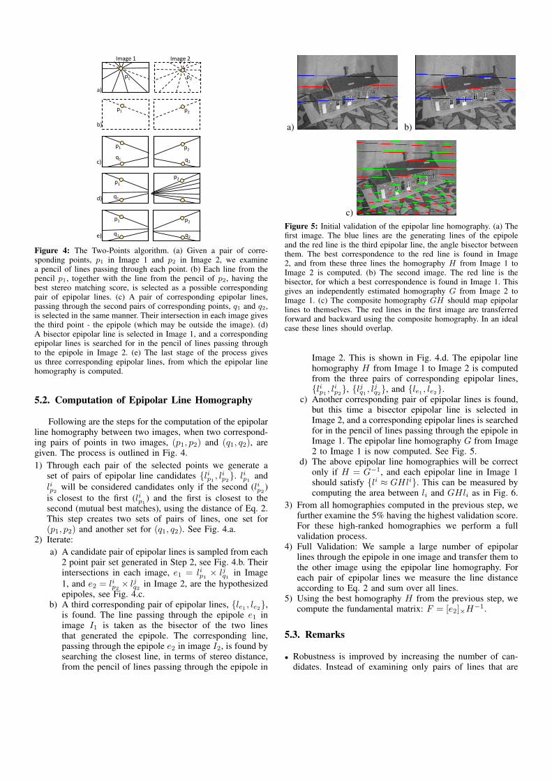
Image 1 Image 2

a)

b)

c)

d)

e)

q1

p1 p2

p1

p1

p1

p1

p2

p2

p2

p2

q1

q1

q2

q2

Figure 4: The Two-Points algorithm. (a) Given a pair of corre-sponding points, p1 in Image 1 and p2 in Image 2, we examinea pencil of lines passing through each point. (b) Each line from thepencil p1, together with the line from the pencil of p2, having thebest stereo matching score, is selected as a possible correspondingpair of epipolar lines. (c) A pair of corresponding epipolar lines,passing through the second pairs of corresponding points, q1 and q2,is selected in the same manner. Their intersection in each image givesthe third point - the epipole (which may be outside the image). (d)A bisector epipolar line is selected in Image 1, and a correspondingepipolar lines is searched for in the pencil of lines passing throughto the epipole in Image 2. (e) The last stage of the process givesus three corresponding epipolar lines, from which the epipolar linehomography is computed.

5.2. Computation of Epipolar Line Homography

Following are the steps for the computation of the epipolarline homography between two images, when two correspond-ing pairs of points in two images, (p1, p2) and (q1, q2), aregiven. The process is outlined in Fig. 4.1) Through each pair of the selected points we generate a

set of pairs of epipolar line candidates {lip1, lip2}. lip1

andlip2

will be considered candidates only if the second (lip2)

is closest to the first (lip1) and the first is closest to the

second (mutual best matches), using the distance of Eq. 2.This step creates two sets of pairs of lines, one set for(p1, p2) and another set for (q1, q2). See Fig. 4.a.

2) Iterate:a) A candidate pair of epipolar lines is sampled from each

2 point pair set generated in Step 2, see Fig. 4.b. Theirintersections in each image, e1 = lip1

× ljq1 in Image1, and e2 = lip2

× ljq2 in Image 2, are the hypothesizedepipoles, see Fig. 4.c.

b) A third corresponding pair of epipolar lines, {le1 , le2},is found. The line passing through the epipole e1 inimage I1 is taken as the bisector of the two linesthat generated the epipole. The corresponding line,passing through the epipole e2 in image I2, is found bysearching the closest line, in terms of stereo distance,from the pencil of lines passing through the epipole in

a) b)

c)Figure 5: Initial validation of the epipolar line homography. (a) Thefirst image. The blue lines are the generating lines of the epipoleand the red line is the third epipolar line, the angle bisector betweenthem. The best correspondence to the red line is found in Image2, and from these three lines the homography H from Image 1 toImage 2 is computed. (b) The second image. The red line is thebisector, for which a best correspondence is found in Image 1. Thisgives an independently estimated homography G from Image 2 toImage 1. (c) The composite homography GH should map epipolarlines to themselves. The red lines in the first image are transferredforward and backward using the composite homography. In an idealcase these lines should overlap.

Image 2. This is shown in Fig. 4.d. The epipolar linehomography H from Image 1 to Image 2 is computedfrom the three pairs of corresponding epipolar lines,{lip1

, lip2}, {ljq1 , l

jq2}, and {le1 , le2}.

c) Another corresponding pair of epipolar lines is found,but this time a bisector epipolar line is selected inImage 2, and a corresponding epipolar lines is searchedfor in the pencil of lines passing through the epipole inImage 1. The epipolar line homography G from Image2 to Image 1 is now computed. See Fig. 5.

d) The above epipolar line homographies will be correctonly if H = G−1, and each epipolar line in Image 1should satisfy {li ≈ GHli}. This can be measured bycomputing the area between li and GHli as in Fig. 6.

3) From all homographies computed in the previous step, wefurther examine the 5% having the highest validation score.For these high-ranked homographies we perform a fullvalidation process.

4) Full Validation: We sample a large number of epipolarlines through the epipole in one image and transfer them tothe other image using the epipolar line homography. Foreach pair of epipolar lines we measure the line distanceaccording to Eq. 2 and sum over all lines.

5) Using the best homography H from the previous step, wecompute the fundamental matrix: F = [e2]×H

−1.

5.3. Remarks

• Robustness is improved by increasing the number of can-didates. Instead of examining only pairs of lines that are

a) b)

c)Figure 6: The epipolar area measure. (a) The epipolar distance ofone point. (b) Considering all the point on the line and evaluatingtheir symmetric epipolar distance is the area between the two lines.(c) The total epipolar area is evaluated for several sampled epipolarlines.

mutual best matches, we only require them to be in the top2 matches of each other.

• If 3 (instead of 2) corresponding pairs of point matches aregiven, the algorithm can be significantly accelerated.

• The stereo matching is computed with an O(N) time dy-namic program.

5.3.1. Complexity Analysis. Let the image sizes be N×N .Through each point we sample O(N) lines. We compare,using stereo matching, O(N), each sampled line with theO(N) lines sampled at its corresponding point. After O(N2)comparisons we are left with O(N) candidate pairs of epipolarlines. As we are given two points in each image, each pointgenerates O(N) candidate epipolar lines, we get O(N2) pos-sible intersections of epipolar lines, each such intersection isan hypotheses for the epipoles, e1 and e2.

For the third pair of corresponding epipolar line we selectlines through the epipoles. In I1 we select the bisector of thetwo epipolar lines that generated e1. We find the best match forthis line in I2 by comparing it to O(N) lines through e2. Thisstep can be skipped if there is a third pair of correspondingpoints r1 and r2, then r1×e1 and r2×e2 is the third epipolarline pair.

Validation is carried out by taking the epipolar area mea-sure (See Fig. 6) of a fixed number of epipolar line in I1through e1, {lie1, GHlie1} with a complexity of O(1).

For two points finding the possible pairs of epipoles to-gether with finding the third line pair and validation takesO(N4) steps. When the algorithm is based on 3 pairs ofcorresponding points it requires at most O(N3) steps.

In practice, after filtering lines with little texture, a muchsmaller number of iterations is required.

6. Experiments

We evaluated our method using stereo images of the housedataset by VGG, Oxford university [14]. The house dataset

Figure 7: The house dataset from VGG is used for real dataexperiments. The dataset includes 10 images with various angles.Ground truth points and camera matrices are available.

includes 10 images, representing different angles. The imagesare presented in Figure 7. We used every consecutive pair ofimages as a stereo pair, which results in 9 pairs. The size ofthe images is 768× 576.

The quality of the computed fundamental matrices wasevaluated using the symmetric epipolar distance [6] with re-spect to the given ground truth points. The baseline method isthe 7-point algorithm. The 7-point method returns 3 possiblesolutions. In all experiments we selected for comparison thesolution with the lowest symmetric epipolar distance. We alsocompared with the 8-point algorithms, which returned high-quality solutions after data normalization. Both the 7-point and8-point algorithm were computed using the VGG toolbox[13].

For each pair of images we repeatedly executed 10 iter-ations. In each iteration we randomly sampled two pairs ofcorresponding points as input to our approach, seven pairs ofcorresponding points to use as input to the 7-point methodand eight pairs of corresponding points to use as input to the8-point method. The points were sampled so that they wereat least 30 pixels apart to ensure stability. We computed thefundamental matrix using our method, the 7-point method,and the 8-point method. The symmetric epipolar distance wascomputed for each method. The points were sampled so thatthey were at least 30 pixels apart to ensure stability.

Fig. 8 shows the resulting fundamental matrix for eachpair of images. Our method significantly outperforms thethe 7-point algorithm. In 66% of the cases the symmetricepipolar distance is less than 3 pixels. The median error inour approach is 2.54. For the 8-point algorithm the median is2.77 while the median in the 7-point algorithm is 25.8. Ourapproach depends on global intensity matching rather thanon the exact matching of the points. Pairs 7, 8 introduce achallenging stereo matching and as a result the quality ofour method is effected. The global intensities in pairs 1-6can be accurately matched and as a result the quality of theestimated fundamental matrix is high. Fig. 9 shows an exampleof rectification using our estimated fundamental matrix forpair number 1. Each horizontal line in the images is a pair ofepipolar lines. Corresponding feature points are placed on the

Image Pairs 7-point 8-point 2-point

1 27.11 3.27 2.54

2 25.80 2.11 2.91

3 27.14 2.02 2.01

4 27.11 2.5 2.04

5 25.47 2.00 2.34

6 14.67 2.77 4.12

7 18.87 3.7 5.76

8 18.97 4.22 5.66

9 26.13 5.89 2.30

Figure 8: The symmetric epipolar distance of the estimated fun-damental matrix using the 7-point/8-point algorithm, and our 2-point algorithm. The distance is with respect to ground truth points.Accuracy of our 2-point algorithm is substantially higher than the7-point algorithm and slightly better than the 8-point algorithm. Themedian error of our algorithm is 2.54. For the 8-point algorithm themedian is 2.77 while for the 7-point it is 25.8.

Figure 9: Rectification example, the images are rectified after esti-mation of the fundamental matrix using our approach from only twopairs of corresponding points. Each horizontal line in the images is apair of epipolar lines. Corresponding feature points are on the sameepipolar lines.

same epipolar lines.

7. Conclusions

We presented a method to compare lines, based on stereomatching, suitable for finding corresponding epipolar lines.This can be used to compute the fundamental matrix basedon only three such line correspondences.

Finding corresponding epipolar lines is greatly acceleratedif we have 2 matching points. In this case our algorithm isvery robust and fast with accuracy greatly outperforming the7 point method and competitive with 8 point methods.

Acknowledgment. This research was supported by Google, byIntel ICRI-CI, by DFG, and by the Israel Science Foundation.

References

[1] Gil Ben-Artzi, Yoni Kasten, Shmuel Peleg, and Michael Werman. Cam-era calibration from dynamic silhouettes using motion barcodes. InCVPR’16, 2016.

[2] Gil Ben-Artzi, Michael Werman, and Shmuel Peleg. Event retrievalusing motion barcodes. In ICIP’15, pages 2621–2625, 2015.

[3] Rita Cucchiara, Costantino Grana, Massimo Piccardi, and Andrea Prati.Detecting moving objects, ghosts, and shadows in video streams. IEEETrans. PAMI, 25(10):1337–1342, 2003.

[4] Martin. Fischler and Robert Bolles. Random sample consensus: Aparadigm for model fitting with applications to image analysis andautomated cartography. CACM, 24(6):381–395, June 1981.

[5] Richard Hartley. In defense of the eight-point algorithm. IEEE Trans.PAMI, 19(6):580–593, 1997.

[6] Richard Hartley and Andrew Zisserman. Multiple view geometry incomputer vision. Cambridge university press, 2003.

[7] Yoni Kasten, Gil Ben-Artzi, Shmuel Peleg, and Michael Werman.Epipolar geometry from moving objects using line motion barcodes.In ECCV’16, 2016.

[8] H. C. Longuet-Higgins. A computer algorithm for reconstructing a scenefrom two projections. Nature, 293:133–135, September 1981.

[9] Quan-Tuan Luong and Olivier Faugeras. The fundamental matrix:Theory, algorithms, and stability analysis. IJCV, 17(1):43–75, 1996.

[10] Daniel Scharstein and Richard Szeliski. A taxonomy and evaluation ofdense two-frame stereo correspondence algorithms. IJCV, 47(1-3):7–42,2002.

[11] Sudipta Sinha and Marc Pollefeys. Camera network calibration andsynchronization from silhouettes in archived video. IJCV, 87(3):266–283, 2010.

[12] Richard Szeliski, Ramin Zabih, Daniel Scharstein, Olga Veksler,Vladimir Kolmogorov, Aseem Agarwala, Marshall Tappen, and CarstenRother. A comparative study of energy minimization methods formarkov random fields. In ECCV’06, pages 16–29. Springer, 2006.

[13] VGG. Matlab Functions for Multiple View Geometry,http://www.robots.ox.ac.uk/˜vgg/hzbook/code/, 2010.

[14] VGG. University of Oxford Multiple View Dataset,http://www.robots.ox.ac.uk/˜vgg/data, 2010.