Epidemics in the presence of social attraction and repulsion

Evelyn Sander

Department of Mathematical Sciences

George Mason University, Fairfax, VA 22030, USA

Chad M. Topaz

Department of Mathematics, Statistics, and Computer Science

Macalester College, St. Paul, MN 55105, USA

(Dated: October 1, 2010)

Abstract

We develop a spatiotemporal epidemic model incorporating attractive-repulsive social interac-

tions similar to those of swarming biological organisms. The swarming elements of the model

describe the ability of distinct classes of individuals to sense each other over finite distances and

react accordingly. Our model builds on the non-spatial SZR model of [Munz, Hudea, Smith?,

2009] modeling a specific epidemic, namely the attack of zombies. This case is interesting from

the modeling standpoint, as zombie epidemics are particularly virile, albeit restricted to a theater

near you and certain parts of San Francisco, Washington D.C., and other major metropolitan

areas [http://www.zombiewalk.com]. Spatial effects not only enhance entertainment value (as a

cinematic portrayal of a spatially invariant zombie attack would be somewhat lacking in thrill) but

are critical to understanding the epidemic. We show that in the absence of a cure for zombiism,

the alert human population will eventually be annihilated, but at a slower rate than in the non-

spatial model. The extra time to extinction might allow the development of a cure. We also show

that without any assumption of collusion, the system self-organizes into transient traveling pulse

solutions consisting of a swarm of zombies in pursuit of a swarm of alert humans. In the presence

of a zombie cure, the traveling solutions exist persistently and stably for all time.

PACS numbers: 87.10.Ed,87.19.X-,87.23.-n

1

I. INTRODUCTION

The notion of a zombie has its roots in the African Kingdom of Kongo, from whence the

African diaspora brought it to Haiti. In Haitian voodoo, a sorcerer (or boko) could force

someone (either living or dead) to become a zombie, while the boko maintained control

of the soul. In contrast, the more modern view of zombiism is that it does not result

from a sorcerer’s control, but rather is an uncontrolled and unmodulated epidemiological

effect, spread via contact like a disease. This “viral” zombiism is depicted the classic 1968

movie The Night of the Living Dead, in Michael Jackson’s 1993 music video Thriller, in the

computer game Plants versus Zombies, and at public events such as zombie walks and the

game Humans vs. Zombies played on many college campuses.

On the scientific front, in 2009, [1] first quantified the epidemiological view of zombies.

This work (of which we later provide a detailed discussion) adapted classical epidemiological

models to predict the course and ultimate outcome of zombie attacks. This important, foun-

dational zombie modeling effort focused on the zombification of a population of healthy alert

humans, but did not consider any geographic or spatial information pertaining to zombie

attacks. Of course, spatial information is often critical for understanding how to effec-

tively treat an epidemic. For example, consider the citizens of Copenhagen in 1349, during

the bubonic plague. A year later, the epidemic arrived in the city and spread explosively.

Knowledge that the epidemic front was moving steadily northwards in an east-west band

from the south [2] would have been much more actionable for Copenhangen’s citizens than

only knowing that the epidemic was adversely effecting the total population of Europe.

In this paper, we develop an epidemiological model of zombies which addresses the need

for spatial information. Ours is not the first epidemiological model to treat spatial effects.

However, most such models have incorporated spatial effects using the concept of spatial

diffusion, via which individuals are modeled to move at random, with each interaction with

an infected individual resulting in a potential spread of the infection. In contast, random

motion is not an appropriate assumption for the case of zombies, who by nature seek out

healthy humans as prey. Thus, our modeling methods will necessarily be different.

One aspect of the standard epidemiological models that we do adopt here is the mean field

hypothesis, which says that the behavior of individuals can be understood by considering a

continuous function describing average behavior. From day-to-day observations of fluids, one

2

finds it perfectly plausible that their flow and motion can be modeled (for most applications)

by such averages, rather than by keeping track of the motion of individual molecules. One

might wonder if this is a reasonable modeling assumption to make about the macroscopic

behavior of populations of complex biological organisms. In fact, such an assumption does

prove to be quite successful in many situations, and the mean field approach in biology is

supported by a substantial literature tracing its roots (at least) back to work such as [3, 4].

As a visual example, consider the crowd phenomenon “the human wave” in a stadium.

Although each individual initiates an individual action to stand and sit, the macroscopic

effect resembles the motion of a fluid wave.

We now return to the question of how to model zombies, keeping in mind that their

motion is mostly directed, rather than purely random. Our goal is to address the observation

that zombies can behave in an organized fashion, for instance, pursuing humans in packs.

One possible explanation is that their behavior is being controlled, with the control exerted

by someone such as the a traditional Haitian boko. However, as mentioned before, such

control is not part of the modern viewpoint of zombies. In a modern zombie epidemic

there would be no external controlling force. A second possible explanation is collusion,

that is, the agreement of a master plan amongst the zombies (or perhaps as assigned by

a zombie leader). We discard this possibility as well, due to the minimal brain power

possessed by zombies. They may have the brain power of a fish or a bird, but certainly not

sufficient mental capacity to design any sophisticated strategy of directed attack. Consider

however that both birds and fish can behave in organized schools and swarms, and that

these behaviors arise without control or collusion. A body of mathematical research has

successfully modeled such swarming and flocking behavior. The key model element is that

each individual is able to sense the behavior of others within reasonably close proximity, and

to instinctively react accordingly. The result of the reaction to local behavior is that the

population spontaneously organizes itself into a structure such as a swirling school of fish, a

directed flock of birds, or a traveling wave of sitting-and-standing humans in a sports arena.

Based on the successes of the swarm modeling approach, the spatial aspects of the epi-

demiological model we will present are adapted from the swarming literature, with the

assumption that each individual zombie is attracted to populations of alert humans, and

each alert human is repelled by zombies. Our primary result is that the population self-

organizes into swarms of zombies pursuing humans. If there is no cure for zombiism, the

3

alert human population eventually dies out, but not as quickly as predicted by a non-spatial

epidemic model. However, in the presence of a cure, it is possible for a population of zombies

to stably pursue a population of alert humans for all time – a traveling wave. In addition,

we find many other types configurations of zombies in pursuit, with humans on the run.

Much can be gained by full knowledge of these different moving population configurations,

and the likelihood of successful persistence of the alert human population. Specifically, an

understanding of the types of behavior possible and how to recognize their onset is critical

for purposes planning and preparation for large scale epidemiological events.

The remainder of this introduction consists of a detailed and more technical overview

of the body of scientific literature on epidemiological models and swarming models, and a

description of how our modeling fits into this framework.

Epidemiological modeling in perspective. Though the history of epidemic model-

ing reaches back to studies of smallpox in the mid-18th century [5, 6], the incorporation of

spatial effects has roots in the last hundred years. Spatial epidemic models are reviewed,

e.g., in [7–9]. One major class of spatial models treats the population as a continuum in

space and tracks the population density in space and time (per the mean field assumption

discussed above). Within this realm of continuum models, the most basic studies of spa-

tial epidemics modify non-spatial differential equation based compartmental models, which

divide a population into different epidemiological classes such as susceptible, infected, and

recovered. The basic spatial models add simple diffusion as the macroscopic description of

the underlying random motion of individuals within a population [10–12], and focus on the

propagation of epidemic fronts from a clustered initial condition of infected individuals. A

generalization of these models is the distributed infectives model [13, 14] which incorporates

dispersal that is longer-range than that described by diffusion. Another class of models uses

spatial terms to describe not the movement of the individuals, who are now assumed to be

stationary, but rather the transmission of the disease itself. For instance, in the distributed

contacts model [15–17] the infectivity at each point in space is computed from a weighted

spatial average of the field of infected individuals over long ranges.

Most short-range spatial effects can be modeled with mathematical terms that involve

spatial derivatives, which compute rates of change of a quantity over an infinitesimal spatial

range. One intuitive example is that of chemotaxis [18]. In a simple chemotactic situation,

a biological organism such as a bacterium senses a chemical field (perhaps a nutrient field)

4

immediately surrounding it and moves in the direction of greatest increase. In contrast,

long-range effects such as those in the distributed infectives and distributed contacts models

cannot be accurately described with spatial derivatives. Instead, one typically uses so-

called nonlocal operators such as integral operators, which compute quantities over finite

(or potentially infinite) ranges.

Swarming models. We introduce a spatial model for epidemics in which nonlocal

terms capture a completely different effect from those previously examined. In particular,

we will model the directed motion of individuals due to social forces in an epidemiological

context. By social forces, we mean forces such as attraction to and repulsion from other

members of the population. These forces have received substantial attention in studies of

swarming groups such as fish schools, bird flocks, and insect plagues; see the literature

reviews in [19–21] and others. In the traditional biological swarming context, attraction and

repulsion operate simultaneously between conspecific organisms. Some fish, for example, are

evolutionarily preprogrammed with attraction, which provides safety and group cohesion,

and repulsion, which helps avoid collisions. The balance between the two forces typically

leads to a preferred separation distance between neighboring organisms in a group. Social

forces may arise directly from organisms’ sensing over finite distances via sound, sight, smell,

or touch, or indirectly via chemical or other signals.

We now turn our attention to zombie epidemics in the presence of social forces. The

recent work of [1] was the first to develop a mathematical model for zombie epidemics. It

concluded that in the absence of a cure, the only possible outcome of a zombie epidemic

is complete annihilation of the healthy, alert human population. However, as we have

mentioned, by neglecting spatial features, the original model leaves open a key question of

zombie epidemics, namely that of how a swarm of zombies self-organizes to pursue and attack

a swarm of self-organized healthy humans without any collusion on the part of either the

zombie or the alert human populations. We will probe this phenomenon by generalizing the

model of [1] to include spatial variation, and in particular by incorporating social interaction

terms. These terms account for zombies being socially attracted to healthy humans, and

healthy humans being socially repulsed from zombies.

Organization of the paper. The rest of this paper is organized as follows. In Section

II we construct our model. In Section III, we examine some of its basic properties. The

model conserves total population, but does not conserve center of mass. We then consider

5

mass balanced states and show that spatial coexistence of healthy humans and zombies

is impossible. Finally, we show that the only possible steady states are homogeneous in

space, and we compute their stability. In Section IV we perform numerical simulations

of our model, focusing on the effect that the spatial terms have vis-a-vis the non-spatial

model. Though the spatial and non-spatial models reach the same doomsday equilibrium in

which zombies extinguish healthy humans, the approach to the equilibrium can be slower

in the spatial case. Furthermore, in the spatial case, the population can self-organize into

a traveling pulse of susceptible humans that is pursued by a group of zombies. Though the

pulse is merely transient, it is possible that the added time necessary to reach the doomsday

equilibrium would afford the opportunity to develop a cure for zombiism. In Section V we

consider an extension of the model in which such a cure exists, again examining equilibria

and their stability. In Section VI, we perform numerical simulations for this case of a cure

and show that traveling solutions can persist stably. Finally, we conclude in Section VII

with some open questions for the zombie research community.

The model we will develop and the mathematical tools we will use to study it draw from

partial differential equations, dynamical systems, and analysis. However, we strive to keep

mathematical details to a minimum in the body of our paper. For the material presented

in Sections II through VI, we focus our presentation on the main ideas; the reader who is

especially mathematically-inclined will find details and derivations in the appendices.

II. MODEL CONSTRUCTION

We begin by reviewing the following spatially homogeneous SZR model of [1]:

S = ΠS − βSZ − δS, (1a)

Z = βSZ + ζR− αSZ, (1b)

R = δS + αSZ − ζR. (1c)

The total population consists of three classes of individuals: active alert humans, denoted

by S, zombies, who are deceased reanimated humans, denoted by Z, and those who are

recently deceased but not reanimated, and thus are removed from either alert human or

zombie populations, denoted by R. Each over-dot in (1) represents a time derivative. The

6

right-hand sides represent rules for the instantaneous rates of change of the number in each

different population class.

Members of the healthy human population are susceptible to becoming zombies as a

direct result of an encounter with a zombie, with a zombie bite as the usual mechanism of

transmission. The recruitment of alert humans to the zombie population occurs via mass-

action kinetics with transmission parameter β. The mass-action kinetics assumption means,

for instance, that the rate at which alert humans are bitten by zombies is proportional

to the rate of contact between the two different classes. This is in turn assumed to be

proportional to the product of the number of individuals within each class, hence giving rise

to the product SZ in (1). Though the model uses the law of mass action, in future studies

one could modify this to be the standard incidence model, which assumes that the contact

rate is not dependent on the total population size (see, e.g., [7]).

The zombification of the removed population R is independent of social interaction as the

members of this class are deceased and inanimate. It is assumed to be directly proportional

to R with proportionality constant ζ, the natural undeath rate for reanimation of recently

deceased humans. In addition to the two routes into the zombie class, it is possible for

zombies to join the removed class as a result of an altercation between a zombie and a

healthy, alert human in which the latter triumphs. Once again, this route from Z to R

occurs via mass action, with altercation rate α.

The model above incorporates the fact that independent of zombie interaction, the sus-

ceptible class has natural birth and death rates, denoted respectively by Π and δ. However,

compared to the time scale of a zombie epidemic, these effects are negligible and one can

set Π = δ = 0 as in [1]. Therefore, the total population size N = S + Z + R is fixed, and

the equations become

S = −βSZ, (2a)

Z = βSZ + ζR− αSZ, (2b)

R = αSZ − ζR. (2c)

Governing equations. The model (2) neglects the spatial structure of the zombie epi-

demic. We now construct a spatiotemporal version of this model. As discussed in Section I,

the most basic spatial models of epidemics incorporate linear diffusion, modeling the random

7

movement of individuals; see, e.g., [10–12]. However, such an assumption is insufficient to

model zombie epidemics in that it does include any directed motion. Crucial to the under-

standing of interactions between zombies and alert humans is the fact that zombies tend to

be attracted to alert humans, and alert humans seek to avoid zombies. Furthermore, the

attraction and repulsion are not local effects. As with many socially interacting populations,

both zombies and humans can sense population densities on finite (rather than infinitesi-

mal) distances. Hence, we will need to incorporate into our model swarming-type social

interaction terms such as those discussed in Section I and used commonly in the biological

swarming literature; see, e.g., [19, 20].

In mathematical models of swarms, one commonly assumes that social interactions take

place in a pairwise, linear manner, so that to compute the total social force on a given

organism, one adds the interaction force between it and each other organism. Continuum

swarming models, then, typically involve convolution-type integral terms of the form

∫K(x− y)ρ(y, t) dy ≡ K ∗ ρ, (3)

where ρ(x, t) is population density and K is a kernel in which are embedded the rules for

social interaction as it arises from sensing; that is, K gives the effect that organisms at loca-

tion y have on those at location x. Some methods of sensing, such as sound, are essentially

omnidirectional. Others, such as sight, are more unidirectional. Because many organisms

process a combination of communication signals, one often assumes that communication is

omnidirectional [21, 22]. Another common assumption is that distinct organisms exert equal

and opposite social forces on each other.

The simplest continuum swarming model assumes the total population is conserved (e.g.,

no birth or death) and neglects intertia. In this case, the population is governed by the

conservation equation

ρ+∇ · (ρv) = 0, v = K ∗ ρ. (4)

In a one-dimensional domain, the aforementioned assumptions of omnidirectional commu-

nication and equal-and-opposite forces cause the social kernel K = K to be odd. Negative

values of sgn(x)K(x) correspond to attraction and positive values to repulsion. Recently, [20]

explored the manner in which the asymptotic dynamics of (4) in a one-dimensional domain

depend on properties of K.

8

Using these ideas from biological swarming, we now modify the non-spatial zombie epi-

demic model (1). We only include spatial terms in the equations for S and Z, since the

individuals in the removed class are deceased and not animated, and are thus completely

immobile. Our model is

S +∇ · (vSS) = DS∆S − βSZ, (5a)

Z +∇ · (vZZ) = DZ∆Z + βSZ + ζR− αSZ, (5b)

R = αSZ − ζR, (5c)

where S,Z, and R are functions of x and t and are now interpreted as population densities.

The parameters DS and DZ are the diffusion constants measuring the random motion of

susceptibles and zombies. For simplicity, we restrict attention to one-dimensional spatial

domains so that ∆ ≡ ∂xx and ∇· ≡ ∂x.

Since susceptible individuals flee from zombies, we describe susceptibles’ velocity due to

social interaction as

vS = KS ∗ Z, KS = sgn(x) · FSe−|x|/`S . (6)

Here, KS is a repulsive kernel, where FS and `S describe the characteristic strength and

length scale of repulsion. We have chosen K to be a simple kernel capturing the essential

property that a susceptible’s reaction to a zombie should decay with the distance between

the two, due to the limitations of human sensing. Similarly, we model the zombies’ advective

velocity as

vZ = KZ ∗ S, KZ = −sgn(x) · FZe−|x|/`Z , (7)

so that zombies are attracted to susceptibles. Figure 1 shows an example of the velocities vS

and vZ for given population density profiles. We assume that FZ ≤ FS, so that alert humans

are more violently repelled by oncoming zombies than zombies are attracted to humans. The

opposite assumption would result in a faster velocity of zombies than susceptibles, and in

turn the speedy annihilation of the entire susceptible population. We also assume that

`Z ≤ `S, that is, zombies generally sense with less acuity than susceptibles due to their

lower level of brain function.

9

0 2 4 6 8 10

0

x

(a)

0 2 4 6 8 10

0

x

(b)

FIG. 1: Social advection velocities. Schematic of typical populations plotted with the corre-sponding nonlocally-determined advective velocities; see Equations (6) and (7). (a) Susceptiblepopulation S (solid) plotted with the rescaled zombie velocity vZ(S) (dashed). Zombies are at-tracted to susceptibles and move towards maxima of S. (b) Zombie population Z (solid) plottedwith the rescaled susceptible velocity vS(Z) (dashed). Susceptibles are repelled from zombies andmove outwards from maxima of Z. Though the population density fields have different units thanthe velocity fields, we have plotted them on the same axes for a qualitative schematic comparison.

Plugging (6) and (7) into (5), we have our full equation

S + (SKS ∗ Z)x = DSSxx − βSZ, (8a)

Z + (ZKZ ∗ S)x = DZZxx + βSZ + ζR− αSZ, (8b)

R = αSZ − ζR. (8c)

Nondimensionalization. Nondimensionalization is a standard mathematical technique

which involves making a change of variables to remove the physical dimensions (such as

length, time, and mass) from an equation in order to obtain a simpler model, possibly by

reducing the number of model parameters. This reduction is convenient for analysis and

for numerical simulation. One can always re-cast results in dimensional form simply by re-

versing the change of variables, without any loss of information. The nondimensionalization

10

procedure for our model appears in Appendix A. The dimensionless model is

S + (SKS ∗ Z)x = DSSxx − βSZ, (9a)

Z + (ZKZ ∗ S)x = DZZxx + βSZ +R− αSZ, (9b)

R = αSZ −R. (9c)

KS and KZ have been redefined as

KS = sgn(x) · e−|x|, (10a)

KZ = −sgn(x) · Fe−|x|/`. (10b)

The dimensionless parameters F ≤ 1 and ` ≤ 1 measure, respectively, the relative strength

and length scale of attraction to repulsion. The parameters DS, DZ , α, and β are dimen-

sionless versions of the corresponding parameters from the original dimensioned model.

Boundary conditions. Since the governing equations (9) are a spatial model, one must

specify a spatial domain and set appropriate boundary conditions, which dictate the behavior

of the model at the boundary of the domain. To facilitate our analysis and our computation,

we assume that the domain is a finite interval with periodic boundary conditions. To get

insight into the behavior for very large domains, one can always choose L very large and

focus on the middle of the domain where the finite-size and boundary effects are presumed

to be small. For specificity, let the domain be the interval [0, L]. Then solutions for S have

S(0) = S(L), and Sx(0) = Sx(L), with similar conditions for Z and F . In addition, the

length scale of the interaction is assumed extremely small compared to L. Thus, we modify

our kernel functions KS and KZ to be periodic and this has little effect on their values. That

is, outside a small region near their centers, KS and KZ are very close to zero.

III. BASIC MODEL PROPERTIES

We now examine some basic properties of (9), seek mass balanced states and spatially

homogeneous steady states, and calculate the linear stability of the latter. We also show

that spatially homogeneous steady states are the only possible steady states.

11

Conservation of total population. By construction, the total population size (alert

humans, the dead, and the undead all combined) should remain unchanged under the dy-

namics of (9). If we denote the population size at each point by n(x, t) and the total

population size as N(t),

n(x, t) = S + Z +R, (11)

N(t) =

∫ L

0

n(x, t) dx, (12)

then conservation of population means that N is constant, as in [1]. Appendix B derives

the conservation of population – or as we will sometimes say, conservation of mass – for the

model (9). For the remainder of this paper, we treat the population size N as an additional

parameter in the model.

Center of mass and traveling solutions. One question of interest throughout the

rest of this paper pertains to the ability of the population to migrate under the dynamics

of the model. One simple way to touch upon this question is to determine whether the

center of mass of the population can move, or whether it must be stationary. In qualitative

terms, the center of mass of the population is defined as the average of the positions of all of

the individuals within the population. A proof that the center of mass remains stationary

would mean that solutions consisting the population translating in one direction would be

impossible. We show in Appendix C that, in fact, the center of mass can migrate. This means

that traveling solutions are not a priori ruled out, although in our numerical simulations

of (9) we have only found transient traveling solutions; see Figures 2(a) and 3(a-c). In

Appendix C we calculate the center of mass to show that the center of mass can travel with

a nonzero speed.

Mass balanced solutions, steady states, and stability. We now turn our attention

to different types of equilibria of (9). Though a system such as (9) could, in theory, have

long-term behavior more complicated than an equilibrium, equilibria are some of the most

fundamental long-term behaviors one might wish to study.

We are first interested in mass balanced states. By mass balanced states, we mean states

where the number of individuals within each class is not changing in time. It is important to

note that even in such a state, the solution itself could still be changing (for instance, imagine

a group of fixed population count traveling in space). However, finding mass balanced states

12

would still provide useful information for epidemiological tallies. In Appendix D, we show

that at mass balance, R = 0, meaning there are no deceased individuals. All individuals are

alert humans or zombies. Furthermore, we show that either S = 0 or Z = 0 at every point

in space. This means that alert humans and zombies cannot co-exist at the same spatial

location.

Now consider steady-states of (9). Steady states are states for which the time derivatives

vanish, meaning that the solutions do not change in time. This is a more restricted class of

solutions than mass balanced states. That is, while every steady state is a mass balanced

state, not every mass balanced state need be a steady state.

In Appendix E we show that the only possible steady states are spatially homogeneous

ones, that is, solutions where not only is the mass balanced, and not only are the solutions

no longer changing in time, but there is no spatial variation in the profile. The steady state

solutions have population density within each class S,Z,R that is constant in space. The

two steady state solutions are the susceptible state

(S∗, Z∗, R∗) = (N/L, 0, 0), (13)

and the doomsday state

(S∗, Z∗, R∗) = (0, N/L, 0), (14)

in which all individuals have become zombies. To obtain the mass balance for each steady

state (that is, the number of individuals within each class) one must integrate over the

spatial domain. For (13) the mass balance is

∫ L

0

S∗ dx = N,

∫ L

0

Z∗ dx = 0,

∫ L

0

R∗ dx = 0, (15)

and for (14) it is

∫ L

0

S∗ dx = 0,

∫ L

0

Z∗ dx = N,

∫ L

0

R∗ dx = 0. (16)

These are the same mass balances as the steady states of the non-spatial model of [1]. We

have not established whether (9) has other attractors such as inhomogeneous steady states

and traveling waves. Our numerical investigations (described at greater length in Section IV)

13

show transient traveling solutions, but have not revealed any long-term behavior other than

the spatially homogeneous states.

We conclude this section with a study of the linear stability of the two spatially homo-

geneous steady states (13) and (14). We review the concept of linear stability of solutions

to partial differential equations with the following (nonmathematical) thought experiment.

Imagine taking an equilibrium solution for (S, Z,R) and applying a very small spatial per-

turbation to the solution profile. If all such small (in fact, infinitesimal) perturbations decay

over time so that the system again reaches the equilibrium, then we say the equilibrium is

linearly stable. If any such perturbations grow in time, then the equilibrium is unstable.

The stability properties of equilibria are crucial for us because they give hints about the

possible long-time consequences of zombie epidemics. A stable equilibrium has the hope of

being reached in the long-term if the system begins at some non-equilibrium state (though

it is not guaranteed). An unstable equilibrium can never in practice be reached (since tiny

perturbations and fluctuations will always be present in real systems).

The calculation of the linear stability of the equilibria (13) and (14) appears in Ap-

pendix F. We show that (13) is linearly unstable to generic noisy perturbations (at least, for

L sufficiently large). This means that the state in which all individuals are healthy humans

cannot be regained if any zombies are introduced into the population. On the other hand,

the doomsday state (14) is linearly stable. These stability properties are the same as for the

non-spatial model in [1].

IV. NUMERICAL SIMULATIONS AND DISSIPATING TRAVELING PULSES

In this section we present results of numerical simulations of (9). Our numerical scheme

is spectral in space, taking advantage of the periodic domain. We treat the nonlocal (con-

volution) terms via multiplication in Fourier space, and we compute the reaction terms

pseudospectrally in real space. Time integration in Fourier space uses Matlab’s built-

in timestepper ode45). For the zombie epidemiologist interested in conducing her or his

own simulations, our Matlab code is available at http://www.macalester.edu/~ctopaz/

zombieswarm.m.

Figure 2 compares the total number of individuals in each class S, Z, and R as a function

of time for three different models. Figure 2(a) corresponds to the full spatial model (9). The

14

epidemiological parameters are α = 0.005 and β = 0.0095 as in [1], and we take F = 0.01,

` = 0.02, DS = 0.1, DZ = 0.05, and L = 10. Figure 2(b) is similar, but has the social

interaction terms turned off, i.e., KS = KZ = 0. Both simulations are begun with initial

populations ∫ L

0

S dx = 500,

∫ L

0

Z dx = 3, R = 0, (17)

with S and Z distributed randomly in space. Despite the difference in the spatial effects

for these two situations, the time evolution of the total number in each compartment is

strikingly similar. Both models approach the doomsday equilibrium (14) and take equally

long to do so. This can be understood by examining linear stability results in Appendix

F. From (F12) and (F15), diffusive terms affect the linearization around the susceptible

and doomsday equilibria, but the social terms do not. Our simulations begin close to

the susceptible equilibrium and conclude at the doomsday one. This suggests that the

system spends most of its time in regimes where the linearizations are good descriptions,

and hence that social interactions are only transiently important. Despite the similarity of

Figures 2(ab), the actual solution profiles for the two cases are markedly different, and we

discuss these momentarily. Before doing so, we consider the non-spatial model of Figure 2(c).

The decay of the susceptible population is much faster. In fact, by the time the susceptible

population has been extinguished in the non-spatial model, susceptibles within the spatial

model have barely been impacted by the zombies.

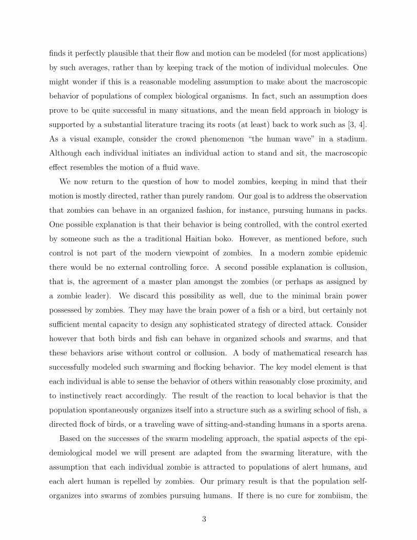
Figure 3 shows S, Z, and R profiles in space-time corresponding to the simulations of

Figures 2(ab). For the full model, shown in Figure 3(a-c), the solution shows transient

traveling pulses, which are apparent as streakiness in the picture. These pulses are absent

in the diffusion-only case, shown in Figure 3(d-f).

We conclude from our numerical explorations that persistence of the healthy human pop-

ulation is impossible within the framework of (9). In all variations of the model considered

here, the zombie population eventually overtakes the susceptible population, leading to the

doomsday state. However, the manner of approach is important. Spatial effects can slow

the decline of the healthy human population, and furthermore, social attraction and repul-

sion provide for spatial localization of susceptibles and zombies. In the event of a zombie

attack, the added time to extinction might allow the healthy, alert humans to seek a cure

for zombiism. We consider the effect of such a cure in the next section.

15

0 10 20 300

200

400

600

t

Population

(a)

0 10 20 300

200

400

600

t

Population

(b)

0 10 20 300

200

400

600

t

Population

(c)

FIG. 2: A comparison of spatial and non-spatial models. The total susceptible (solid),zombie (dashed) and removed (dot-dashed) populations plotted as a function of time. Decay tothe doomsday state (no susceptibles) is much slower for the spatial models of (a) and (b) than thenon-spatial model of (c). Though the evolution of total mass in each compartment is similar for(a) and (b), the actual solution profiles are different; see Figure 3. The epidemiological parametersare α = 0.005 and β = 0.0095 as in [1]. We begin with a total susceptible mass of 500 and a zombiemass of 3 (distributed randomly in space). (a) The full spatial model (9) with F = 0.01, ` = 0.02,DS = 0.1, DZ = 0.05, and L = 10. (b) Like (a) but with the social interaction terms turned off,i.e., KS = KZ = 0. (c) The non-spatial version of the model.

V. EPIDEMICS WITH TREATMENT

Now consider the case that there exists a treatment for zombiism. We repeat for this mod-

ified case the analytical studies presented in Section III. We perform numerical simulations

16

FIG. 3: Space-time profiles of spatial models. (a-c) S, Z, and R (respectively) for thefull spatial model simulation of (9) summarized in Figure 2(a). Darker shading corresponds tohigher population density. Note the presence of transient traveling pulses, which are apparent asstreakiness in the picture. The system approaches the doomsday equilibrium (14). (d-f) Like (a-c),but for the diffusion-only (no social interaction) model summarized in Figure 2(b). The systemapproaches the same equilibrium as in (a), but transient pulses do not occur.

in the next section.

Model construction, conservation of population, and center of mass. Assume

that the treatment for zombiism moves zombies back to the susceptible class with rate c.

17

Modifying (9) appropriately, we have

S + (SKS ∗ Z)x = DSSxx − βSZ + cZ, (18a)

Z + (ZKZ ∗ S)x = DZZxx + βSZ +R− αSZ − cZ, (18b)

R = αSZ −R. (18c)

This model is similar to that in Section 5 of [1] except that we do not include a class

of latently-infected zombies; the introduction of treatment even without latent infection

introduces new solution types into the model as we show below. Calculations identical to

those of Section III establish that (18) conserves the total population size but not the center

of mass.

Mass balance. We now seek mass balanced solutions. There are two different cases of

mass balanced solutions for (18). The calculation of these is presented in Appendix D. The

first mass balanced state is the spatially homogeneous steady state

(S∗, Z∗, R∗) = (N/L, 0, 0). (19)

The second mass balanced state is actually a family of states parameterized by the quantity

〈S,Z〉, defined as

〈S,Z〉 ≡∫ L

0

SZ dx. (20)

These states are

∫ L

0

S dx = N −(β

c+ α

)〈S,Z〉, (21a)∫ L

0

Z dx =β

c〈S,Z〉, (21b)∫ L

0

Rdx = α〈S,Z〉. (21c)

Nothing in the conditions for mass balance selects a particular member of this family. For

18

this family of solutions, the ratio of total members in the Z class to those in R is

∫ L

0

Z dx∫ L

0

Rdx

=β

αc. (22)

Homogeneous steady states and stability. Eq. (18) has two spatially homogeneous

steady states. One is (19) found above. The other is the endemic state

(S∗, Z∗, R∗) =

(c

β,Nβ − LcL(β + αc)

,αc

Lβ

Nβ − Lcβ + αc

), (23)

which exists only for

c/β < N/L. (24)

The mass balance for (19) is

∫ L

0

S∗ dx = N,

∫ L

0

Z∗ dx = 0,

∫ L

0

R∗ dx = 0, (25)

and for (23) it is

∫ L

0

S∗ dx =cL

β,

∫ L

0

Z∗ dx =Nβ − Lcβ + αc

,

∫ L

0

R∗ dx =αc

β

Nβ − Lcβ + αc

. (26)

It is crucial to make a careful comparison between these mass balances and those of the

corresponding non-spatial model. We showed in Section III that for the model without

cure (9) the mass balance of steady states is the same for the spatial model as for the non-

spatial model. This is not the case for the model with cure. The non-spatial version of the

model,

S = −βSZ + cZ, (27a)

Z = βSZ +R− αSZ − cZ, (27b)

R = αSZ −R. (27c)

has susceptible steady state

(S∗, Z∗, R∗) = (N, 0, 0) , (28)

19

which does correspond to the mass balance (25) of the susceptible state in the spatial model.

However, the non-spatial model has endemic steady state

(S∗, Z∗, R∗) =

(c

β,Nβ − cβ + αc

,αc

β

Nβ − cβ + αc

), (29)

which does not correspond to the mass balance (26) of the endemic state in the spatial

model. Thus, the introduction of spatial structure inherently shifts the mass balance of the

endemic equilibrium in a manner dependent on the size of the domain.

Focusing now on steady states of the spatial model (18), we compute the linear stability

of the susceptible steady state (19). The full calculation is given in Appendix F, where we

derive the stability condition

c/β > N/L, (30)

(which we have also verified numerically for sample parameters by measuring the evolution of

small perturbations to the steady state). This condition is complementary to the condition

(24) for existence of the endemic state.

Calculation of the linear stability of (23) is more complex. The full analysis appears in

Appendix F. A primary result is that the conditions

β > α, DS > 2Z∗F`2, and DZ > 2S∗, (31)

are sufficient (though not necessary) for the linear stability of the endemic state. Instability

of the endemic equilibrium is possible as well. For instance, the parameters

α = 1, β = 0.1, DS = 0.1, DZ = 0.05, (32)

c = 0.2, F = 0.3, ` = 0.3, N = 70, L = 10,

provide a numerical example of instability, as demonstrated in the Appendix. For this set

of parameters, note that c/β = 2 and N/L = 7. Hence, according to (30), the susceptible

equilibrium (19) is unstable as well. Thus, we expect that the system must have long-term

behavior other than a spatially homogeneous steady state. Our numerical simulations will

demonstrate such behavior (see Figures 4 and 5).

In summary, we have shown that the susceptible equilibrium (19) is stable when the cure

20

rate c is sufficiently large as determined by (30). The endemic state (23) model can also

be stable or unstable. We have demonstrated the possibility of instability via the numerical

example (32) (details in Appendix F) and have derived the conditions (31) which guarantee

stability for strong enough diffusion and transmission.

VI. NUMERICAL SIMULATIONS AND PERSISTENT TRAVELING PULSES

We now consider numerical results for three different models related to (18), namely the

full model, the model with diffusion but no social interaction, i.e., KS = KZ = 0, and the

version of the model with no spatial structure. The epidemiological parameters are α = 1,

β = 0.1, and c = 0.2, and we take F = 0.03, ` = 0.3, DS = 0.1, DZ = 0.05, and L = 10. We

take the initial condition to satisfy

∫ L

0

S dx = 50,

∫ L

0

Z dx = 50, R = 0, (33)

with the nonzero populations distributed randomly in space.

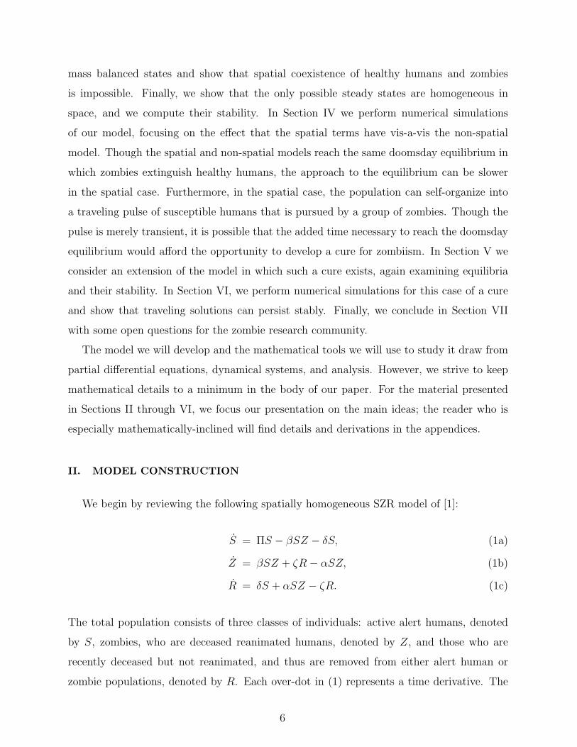
Figure 4(a) shows the total number of individuals in each class S, Z, and R for the full

spatial model (18). The system approaches neither a doomsday state nor an endemic steady

state. Rather, the total mass in S, Z, and R fluctuate around nonzero values. In contrast

to the cure-less model (9), the population of healthy humans survives. The space-time plots

of Figures 5(a-c) reveal that the susceptibles survive as persistent traveling pulses that are

pursued by groups of zombies. Due to the finite size of the domain and periodic boundary

conditions, there is a merging and splitting of pulses, and this effect is responsible for the

slight oscillation in the long-term population count in Figure 4(a).

Figures 4(b) and 5(a-c) correspond to the reduced spatial model without social interac-

tion. In this case, the system reaches the spatially homogeneous endemic equilibrium with

mass balance (26). While some healthy, alert humans survive, their total mass is less than

that contained in the traveling pulse of susceptibles discussed above. Hence, for at least

some parameters, social effects can enhance the survival of the healthy human population.

Figure 4(c) corresponds to the compartmental model (27). The system again reaches an

endemic equilibrium, albeit with different levels of S, Z, and R. As discussed above, the

mass balance (26) for the endemic equilibrium within the spatial model necessarily differs

21

0 50 100 150 2000

50

100

t

Population

(a)

0 50 100 150 2000

50

100

t

Population

(b)

0 50 100 150 2000

50

100

t

Population

(c)

FIG. 4: A comparison of spatial and non-spatial models with a zombie cure. The totalsusceptible (solid), zombie (dashed) and removed (dot-dashed) populations plotted as a function oftime for α = 1, β = 0.1, c = 0.2 and an initial condition of 50 susceptibles and 50 zombies. (a) Thefull model (18) produces a persistent susceptible population. Here, F = 0.03, ` = 0.3, DS = 0.1,DZ = 0.05, and L = 10. (b) The reduced model (18) with no social forces, i.e., KS = KZ = 0,reaches the endemic equilibrium with mass balance (26). Asymptotically, more susceptibles survivefor the case shown in (a) with social advection. (c) The compartmental model reaches an endemicequilibrium with mass balance (29), in which even fewer susceptibles survive.

from the mass balance (29) for the compartmental model.

For the full model (18), the splitting and merging pulses are not the only long-term

behavior we have observed. We have conducted simulations at different parameter values,

revealing slightly different non-steady-state solutions. To systematize our study, we fix the

22

FIG. 5: Space-time profiles of spatial models with zombie cure. (a-c) S, Z, and R (respec-tively) for the full spatial model simulation summarized in Figure 4(a). Darker shading correspondsto higher population density. Note the presence of splitting and merging traveling pulses. (d-f) Like(a-c), but for the diffusion-only (no social interaction) model summarized in Figure 4(b). Pulsesdo not occur, and the system reaches the spatially homogeneous steady state (23).

following parameters to the values in Figures 4 and 5: α = 1, β = 0.1, ` = 0.3, DS = 0.1,

DZ = 0.05, and L = 10. We concentrate on the dependence of the solutions on c and F in

the range 0 ≤ c ≤ 0.21 and 0.01 ≤ F ≤ 0.05. (This range is chosen based on preliminary

studies on a larger parameter range. For c much larger, the susceptible steady state attracts

all of the initial conditions that we tried.) We run each simulation to time t = 60 to remove

transient behavior. We then retain the data from t = 60 to 120 for study. Our findings are

23

F 0.01 0.014 0.019 0.023 0.28 0.032 0.037 0.041 0.046 0.05

c0.01 Transient Pulses0.03 2.43 2.41 2.26 2.30 2.15 2.13 −2.10 2.12 2.04 −1.970.05 2.72 −2.30 −2.75 −2.13 2.08 −2.57 1.99 1.94 1.89 1.870.08 3.13 3.07 −3.09 2.28 −2.35 2.19 −2.41 −2.08 −2.14 −2.070.10 −3.84 −2.80 2.47 2.62 3.60 −2.41 3.19 −2.72 −2.37 2.410.12 −3.23 −3.10 3.09 −2.76 −3.14 2.85 −2.71 −2.83 −2.71 HC0.14 4.76 P 3.73 HC −4.04 P 3.71 3.76 P 3.76 P −3.15 −3.21 3.380.17 −4.36 HC −4.75 4.01 −4.06 −4.05 4.04 4.39 P 4.36 P −4.250.19 5.02 P HC HC HC −4.58 PP −5.02 PP 4.48 4.82 P −4.77 P 4.19 P0.21 5.17 PP HC HC 4.92 P HC −5.80 PP 5.48 PP −5.38 PP HC HC

TABLE I: Non-steady-state attracting solutions and their velocity for the spatial modelwith zombie cure. This table summarizes the type of solutions found in simulations of (18) forvarying c and F values in the range 0 ≤ c ≤ 0.21 and 0.01 ≤ F ≤ 0.05 where we have fixedα = 1, β = 0.1, ` = 0.3, DS = 0.1, DZ = 0.05 and L = 10. The initial conditions have total massof the S and Z populations both equal to 50, distributed randomly in space. We have performedone simulation per parameter value. If the solution is a traveling pulse, its velocity is stated.Oscillatory and highly oscillatory traveling pulses are denoted with a P and a PP respectively afterthe value of the average velocity. Finally, HC denotes solutions in which pulses periodically splitand rejoin, giving a honeycomb-like appearance to the space-time diagram. A velocity no longermakes sense for such solutions.

summarized in Table I.

We find three distinct long-term behaviors that are not spatially homogeneous steady

states. For c slightly greater than zero, there are traveling pulse solutions with constant

velocity; Figure 6(a-c) shows an example. These types of solutions are indicated in the

Table by entries consisting only of a numerical entry, which is the traveling velocity of the

pulse. The speed depends on the c and F , but the simulations indicate that the direction is

dependent only on the initial conditions (which is consistent with the equations themselves

having no inherent direction preference). As c grows larger, the velocity increases. For

larger c values, the solutions still are traveling pulses, but with accompanying oscillation

in the pulse speed; Figure 6(d-f) shows an example. These solutions are indicated in the

Table by entries marked with a P or PP (to denote low or high degrees of oscillation). The

number given is the average velocity, which generally appears to be close to the speed of

non-oscillating pulses nearby in parameter space. Finally, for certain large c values, pulses

periodically join and split. We have already shown this type of solution in Figure 5(a-c) and

we give an additional example in Figure 6(g-i) for comparison with the other solution types.

24

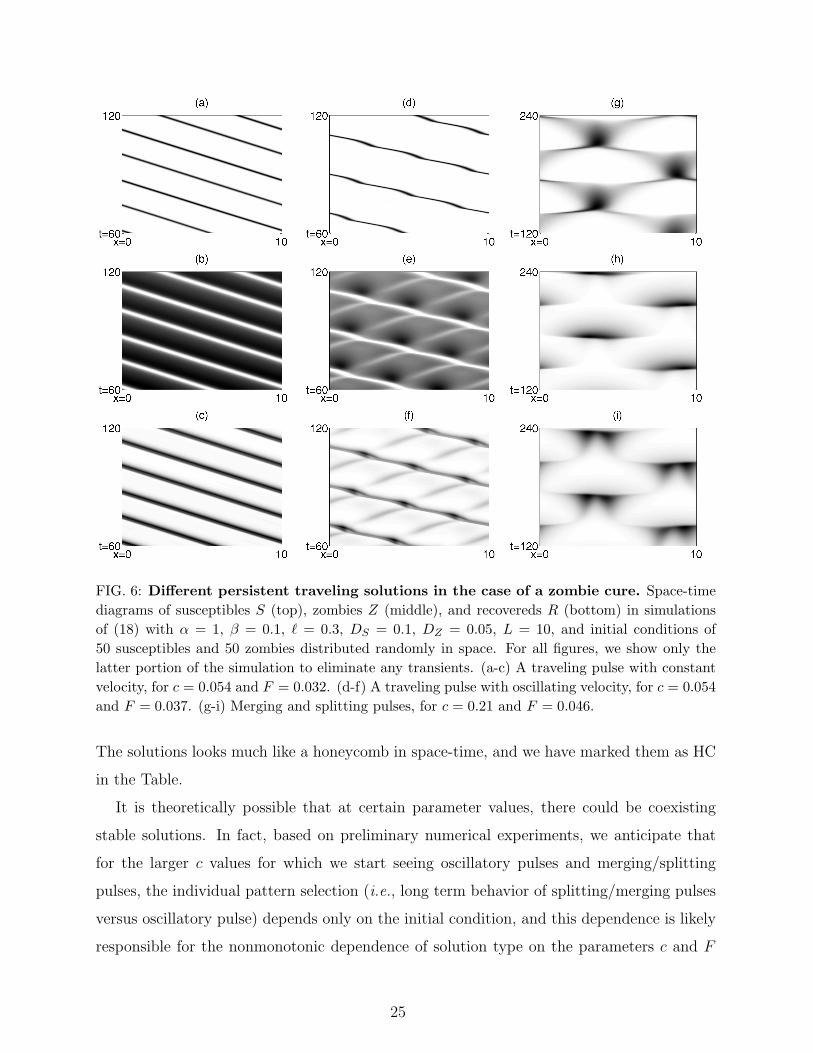
FIG. 6: Different persistent traveling solutions in the case of a zombie cure. Space-timediagrams of susceptibles S (top), zombies Z (middle), and recovereds R (bottom) in simulationsof (18) with α = 1, β = 0.1, ` = 0.3, DS = 0.1, DZ = 0.05, L = 10, and initial conditions of50 susceptibles and 50 zombies distributed randomly in space. For all figures, we show only thelatter portion of the simulation to eliminate any transients. (a-c) A traveling pulse with constantvelocity, for c = 0.054 and F = 0.032. (d-f) A traveling pulse with oscillating velocity, for c = 0.054and F = 0.037. (g-i) Merging and splitting pulses, for c = 0.21 and F = 0.046.

The solutions looks much like a honeycomb in space-time, and we have marked them as HC

in the Table.

It is theoretically possible that at certain parameter values, there could be coexisting

stable solutions. In fact, based on preliminary numerical experiments, we anticipate that

for the larger c values for which we start seeing oscillatory pulses and merging/splitting

pulses, the individual pattern selection (i.e., long term behavior of splitting/merging pulses

versus oscillatory pulse) depends only on the initial condition, and this dependence is likely

responsible for the nonmonotonic dependence of solution type on the parameters c and F

25

in the Table.

VII. CONCLUSION

In this paper, we have considered spatial models of zombie epidemics. Our model is based

on that in [1]. The spatial elements we introduce capture social forces between zombies and

alert, healthy humans. In particular, we have incorporated the tendency of healthy humans

to move away from zombies, and the tendency of zombies to move towards healthy humans.

For our spatial model (9), the main analytical results include:

• We show explicitly that the center of mass of the population may travel.

• Mass balanced solutions have no removed individuals. They have spatial separation

between zombies and susceptibles.

• The only steady possible state solutions are the spatially homogeneous susceptible and

doomsday states.

• The susceptible state is linearly unstable, and the doomsday state is linearly stable.

Numerical simulations provided further information. For the non-spatial version of the model

in [1], the only stable equilibrium is the doomsday state in which all individuals are zombies.

In the spatial model, not only is this state linearly stable, but it is also the only long-term

behavior observed in numerical simulations. However, in the spatial model, convergence to

the equilibrium can occur more slowly than in the non-spatial model, and this convergence

occurs via a self-organized cluster of susceptibles that is pursued by a group of zombies. The

additional time to the annihilation of alert humans might allow for the development of a

cure.

In this vein, we considered a modification of our spatial model to include a cure for

zombiism. Results for (18) include:

• Mass balanced solutions do not necessarily have spatial separation between zombies

and susceptibles.

• The model has two spatially homogeneous steady states. One is the susceptible state,

which has the same mass balance as the susceptible state in the non-spatial analogue

26

of the model. The other is the endemic state. The mass balance of the endemic state

differs from that of the endemic state in the non-spatial model.

• The susceptible steady state exists for all parameter values, and is linearly stable for

a sufficiently large cure rate.

• The endemic steady state exists for a sufficiently small cure rate, and is stable if

diffusion and transmission are sufficiently large.

• There exist parameter regimes in which both homogeneous steady states are unstable.

Via numerical simulations, we saw the existence of three qualitatively distinct types of so-

lutions that are not homogeneous steady states. Each consisted of self-organized pulses of

healthy, alert humans pursued by groups of zombies. In the first type, the pulse travels

at constant velocity. In the second, the pulse travels at a nonzero average velocity, but is

oscillatory. In the third type, there is a periodic splitting and rejoining of the susceptible

population. In contrast to the first model (9) in which a cure was absent, these traveling

pulses of susceptibles in (18) are all persistent, signaling hope of survival for the healthy pop-

ulation. Furthermore, in many of our example simulations, the total mass contained in the

susceptible pulse was greater than that of the susceptibles within the spatially homogeneous

endemic equilibrium.

We close with some open questions for the community of mathematicians undertaking

zombie research. We show in Appendix E that homogeneous steady states are the only steady

states of (9). However, this argument assumes continuity of the functions S and Z. A proof

of regularity of the solutions is needed to justify this assumption. On a related topic, our

numerics indicate that homogeneous steady states are not just the only steady states, but are

the only mass balanced states; however, a proof of this statement is lacking. In addition, one

could imagine attractors that are not steady states, and are not mass balanced, but perhaps

are time-periodic. Based on the variety of numerical simulations we have conducted, we

conjecture that the doomsday state is the only attractor, but a definitive proof is lacking.

Such a proof would also serve, among other things, to rule out the possibility of persistent

traveling pulses for this model.

For the model (18) with a cure we have shown analytically that depending on parameter

choices, there is a susceptible steady state and an endemic steady state in which zombies

27

and alert humans coexist. Our numerical simulations indicate that there exist attractors

other than homogeneous steady states. In fact, we observed three different types of traveling

pulses. We pose as an open problem the analytical proof for the existence of traveling pulses.

Numerical simulations also indicate that bi-stability of the different types of solutions is

possible. There is a need for more extensive numerical examination of these coexisting pulse

types, followed by the development of early detection methods to distinguish between them.

The early detection methods are of high priority, since they would allow more time for the

implementation of the distinct corresponding strategies which would be needed for surviving

a zombie epidemic.

Appendix A: Nondimensionalization

To reduce the number of parameters in the original dimensioned model (8), we nondi-

mensionalize as follows. Let

x → `Sx, (A1a)

t → 1

ζt, (A1b)

{S,Z,R} → `Sζ

FS

{S, Z, R}. (A1c)

Substituting, cleaning up, and dropping the hats, we have

S +(S{

sgn(x) · e−|x| ∗ Z})

x=

DS

`2SζSxx −

β`SFS

SZ, (A2a)

Z +(Z{−sgn(x) · FZ/FSe

−|x|`S/`Z ∗ S})

x=

DZ

`2SζZxx −

β`SFS

SZ +R− α`SFS

SZ, (A2b)

R = −α`SFS

SZ −R, (A2c)

where the overdot and the subscript x are now understood to represent derivatives with

respect to dimensionless variables. Now define

F = FZ/FS, (A3a)

` = `Z/`S. (A3b)

28

For convenience, redefine

KS = sgn(x) · e−|x|, (A4a)

KZ = −sgn(x) · Fe−|x|/`, (A4b)

and

α`SFS

→ α, (A5a)

β`SFS

→ β, (A5b)

DS

`2Sζ→ DS, (A5c)

DZ

`2Sζ→ DZ . (A5d)

Then the model reads

S + (SKS ∗ Z)x = DSSxx − βSZ, (A6a)

Z + (ZKZ ∗ S)x = DZZxx + βSZ +R− αSZ, (A6b)

R = αSZ −R, (A6c)

which is (9). Here, KS and KZ are given by (A4). The dimensionless parameters F ≤ 1 and

` ≤ 1 measure, respectively, the relative strength and length scale of attraction to repulsion.

The parametersDS, DZ , α, and β are dimensionless versions of the corresponding parameters

in the original dimensioned model.

Appendix B: Conservation of population

Here we show that the total population size remains constant under the dynamics of (9).

First we add the three equations in (9) together, rearrange, and expand spatial derivatives

to obtain∂

∂t(S + Z +R) = DSSxx +DZZxx − (SKS ∗ Z)x − (ZKZ ∗ S)x. (B1)

Now integrate over the domain [0, L] and assume that this operation commutes with time

differentiation. We recall the definitions (11) and we also define the inner product on two

29

functions a and b as

〈a, b〉 ≡∫ L

0

a · b dx. (B2)

Then (B1) is

N = DS〈Sxx, 1〉+DZ〈Zxx, 1〉 − 〈(SKS ∗ Z)x, 1〉 − 〈ZKZ ∗ S, 1〉. (B3)

Using integration by parts, and recalling that the convolution of two L-periodic functions is

L-periodic, we have

〈Sxx, 1〉 = Sx(L)− Sx(0) = 0, and (B4)

〈(SKS ∗ Z)x, 1〉 = S(L)(KS ∗ Z)(L)− S(0)(SS ∗ Z)(0) = 0. (B5)

Similar statements hold for the Z terms. Hence,

N = 0,

and the total population is conserved, as with the compartmental model from [1]. The

calculation showing conservation of mass for (18) is essentially identical.

Appendix C: Center of mass

In this appendix we show that the population center of mass is not conserved under (9),

and we derive a time-dependent upper bound on the speed at which the center of mass can

travel.

Begin with the first moment 〈n, x〉 of n(x, t) (proportional to the center of mass) by

30

taking an inner product of n with x. We obtain

〈n, x〉 = DS〈Sxx, x〉+DZ〈Zxx, x〉 (C1a)

−〈(SKS ∗ Z)x, x〉 − 〈(ZKZ ∗ S)x, x〉,

= H(t) + 〈SKS ∗ Z, 1〉+ 〈ZKZ ∗ S, 1〉, (C1b)

= H(t) + 〈S,KS ∗ Z〉+ 〈KZ ∗ S,Z〉, (C1c)

= H(t) + 〈S,KS ∗ Z〉+ 〈S,KZ ∗ Z〉, (C1d)

= H(t) + 〈S,K ∗ Z〉, (C1e)

where K = KS +KZ , and H(t) = L(DsSx(L, t) +DzZx(L, x)− (Svs(L, t) +Zvz(L, t))). The

second equation follows from integration by parts (twice for the diffusive terms and once for

the advective ones), the third follows from properties of multiplication, and the fourth follows

from the fact that convolution may be moved across the inner product. In the integration

by parts leading to the second equation, note that the boundary terms which would arise

all collapse to H(t) due to the periodic boundary conditions. Since the quantity in (C1e) is

generically nonzero, it follows that the center of mass of the solution is not conserved, which

means traveling solutions are not a priori ruled out, although in our numerical simulations

of (9) we have only found transient traveling solutions; see Figures 2(a) and 3(a-c).

Using our previous calculation, we can bound the speed at which the center of mass of

n (equivalently, the first moment divided by the total mass) is permitted to move. Define

xc(t) = 〈n, x〉/N , the center of mass of n. Let G(t) = H(t)/N . From our calculation above,

|xc| = |〈S,K ∗ Z〉|/N +G(t), (C2a)

≤ 〈S, |K| ∗ Z〉/N +G(t), (C2b)

= ‖S|K| ∗ Z‖1/N +G(t), (C2c)

≤ ‖S‖1 · ‖|K| ∗ Z‖∞/N +G(t), (C2d)

≤ ‖S‖1 · ‖K‖∞ · ‖Z‖1/N +G(t), (C2e)

≤ 1

4‖K‖∞N2/N +G(t), (C2f)

≤ 1

4‖K‖∞N +G(t), (C2g)

where the second line follows from the property of absolute value, the third from the defini-

31

tion of the L1 norm, the fourth from Holder’s inequality, the fifth from Young’s inequality

for convolutions, and the sixth from the fact that ‖S‖1 + ‖Z‖1 ≤ N and so the maximum

value of ‖S‖1 · ‖Z‖1 is N2/4. Therefore,

1

4‖K‖∞N +G(t), (C3)

is an upper bound on the speed of the center of mass of the population.

We can find ‖K‖∞ using simple calculus. From the antisymmetry of K, it suffices to

consider K on x ≥ 0, where K ≥ 0. The global maximum on this domain must either occur

at x = 0 or at the critical point where K ′ = 0. The critical point is

xcrit =` ln(`/F )

`− 1. (C4)

If F < ` then the critical point is outside of the domain. The global maximum, therefore,

is K(0) = 1− F . If F = ` then the critical point coincides with the domain boundary and

1− F is still the global maximum. On the other hand, if F ≥ `, the critical point is on the

interior of the domain, and the global maximum is K(xcrit). In summary, we have

‖K‖∞ =

1− F F ≤ `,(`

F

) `1−`

− F(`

F

) 11−`

F > `,(C5)

where in the bottom expression we have evaluated K(xcrit).

Note that as F, ` → 1, the upper bound (C3) implies that the maximum speed of a

traveling solution limits to L/N(DsSx(L, t) +DzZx(L, t)).

For the cure model (18), the demonstration that center of mass is not conserved and the

bound for the speed of the center of mass are essentially identical to what we have presented

in this appendix.

Appendix D: Mass balanced states

We seek mass balanced states of (9), that is, states where the number of individuals

within each class is not changing in time, even if the solution profiles themselves are. We

32

integrate each of (9) on the real line to obtain

〈S, 1〉+ 〈(SKS ∗ Z)x, 1〉 = 〈DSSxx, 1〉 − 〈βSZ, 1〉, (D1a)

〈Z, 1〉+ 〈(ZKZ ∗ S)x, 1〉 = 〈DZZxx, 1〉+ 〈βSZ, 1〉 (D1b)

+〈R, 1〉 − 〈αSZ, 1〉,

〈R, 1〉 = 〈αSZ, 1〉 − 〈R, 1〉. (D1c)

At mass balance, the first term of each equation will be zero by definition. Using integration

by parts shows terms involving spatial derivatives are zero. Then (D1) simplifies to

〈S,Z〉 = 0, (D2a)

(β − α)〈S,Z〉+ 〈R, 1〉 = 0, (D2b)

α〈S,Z〉 − 〈R, 1〉 = 0. (D2c)

Substituting (D2a) into (D2c) shows that R must be identically zero. Eq. (D2a) itself

implies that in a point-wise sense, either S or Z is 0. Thus, at mass balance (and therefore,

at any steady states) there is physical separation between susceptibles and zombies. They

cannot coexist at the same spatial location.

We now consider mass balanced states of (18). The conditions (D2) are modified to

−β〈S,Z〉+ c〈Z, 1〉 = 0, (D3a)

(β − α)〈S,Z〉+ 〈R, 1〉 − c〈Z, 1〉 = 0, (D3b)

α〈S,Z〉 − 〈R, 1〉 = 0. (D3c)

The solution may be written in terms of 〈S,Z〉 as

∫ L

0

S dx = N −(β

c+ α

)〈S,Z〉, (D4a)∫ L

0

Z dx =β

c〈S,Z〉, (D4b)∫ L

0

Rdx = α〈S,Z〉. (D4c)

We consider separately two cases for 〈S,Z〉. If 〈S,Z〉 = 0 then the only mass balanced state

33

is the spatially homogeneous steady state (19). If 〈S,Z〉 6= 0 then there is a family of mass

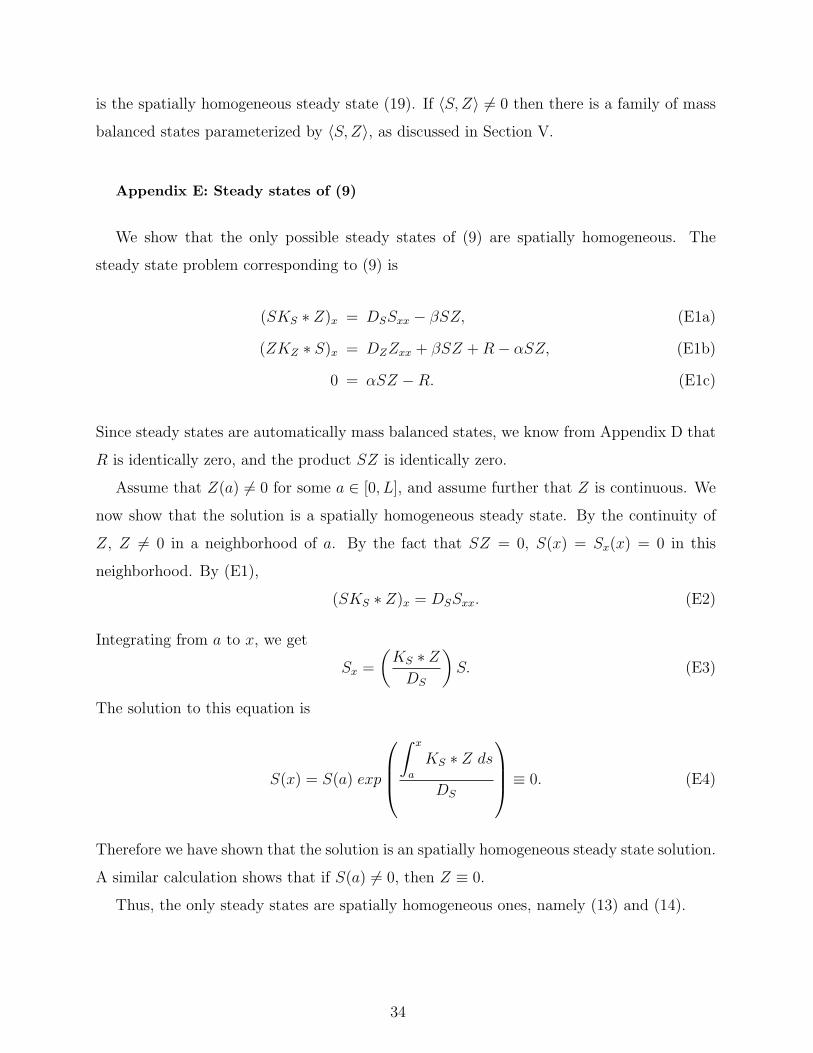
balanced states parameterized by 〈S,Z〉, as discussed in Section V.

Appendix E: Steady states of (9)

We show that the only possible steady states of (9) are spatially homogeneous. The

steady state problem corresponding to (9) is

(SKS ∗ Z)x = DSSxx − βSZ, (E1a)

(ZKZ ∗ S)x = DZZxx + βSZ +R− αSZ, (E1b)

0 = αSZ −R. (E1c)

Since steady states are automatically mass balanced states, we know from Appendix D that

R is identically zero, and the product SZ is identically zero.

Assume that Z(a) 6= 0 for some a ∈ [0, L], and assume further that Z is continuous. We

now show that the solution is a spatially homogeneous steady state. By the continuity of

Z, Z 6= 0 in a neighborhood of a. By the fact that SZ = 0, S(x) = Sx(x) = 0 in this

neighborhood. By (E1),

(SKS ∗ Z)x = DSSxx. (E2)

Integrating from a to x, we get

Sx =

(KS ∗ ZDS

)S. (E3)

The solution to this equation is

S(x) = S(a) exp

∫ x

a

KS ∗ Z ds

DS

≡ 0. (E4)

Therefore we have shown that the solution is an spatially homogeneous steady state solution.

A similar calculation shows that if S(a) 6= 0, then Z ≡ 0.

Thus, the only steady states are spatially homogeneous ones, namely (13) and (14).

34

Appendix F: Linear stability

We compute the linear stability of the steady states (13) and (14) of (9) by allowing small

perturbations, which for convenience we write in a normal mode expansion, that is,

S = S∗ +∑

k

Sk(t)eikx, Z = Z∗ +∑

k

Zk(t)eikx, R = R∗ +∑

k

Rk(t)eikx, (F1)

where the wave number k is

k =2jπ

L, j ∈ Z, (F2)

to be commensurate with the periodic domain.

In the analysis below, since the ranges of KS and KZ are small compared to the size

of the domain (i.e., L � 1), we approximate the Fourier transforms of the repulsive and

attractive kernels by their values on the infinite domain:

KS(k) ≈ − 2ik

1 + k2, (F3a)

KZ(k) ≈ 2iF `2k

1 + `2k2. (F3b)

(F3c)

Let Uk = (Sk, Zk, Rk)T . We substitute (13) and (14) into a linearized version of (9),

giving us the systemd

dtUk = LUk, (F4)

where L consists of terms arising from advection, diffusion, and the original compartmental

model of [1]:

L = Ladv + Ldiff + Lcomp. (F5)

We have

Lcomp =

−βZ∗ −βS∗ 0

(β − α)Z∗ (β − α)S∗ 1

αZ∗ αS∗ −1

, (F6)

35

and

Ldiff =

−DSk

2 0 0

0 −DZk2 0

0 0 0

. (F7)

For the linearized advection operator, we have

Ladv =

0 −ikKS(k)S∗ 0

−ikKZ(k)Z∗ 0 0

0 0 0

, (F8)

but use (F3) to write

Ladv ≈

0 − 2k2

1 + k2S∗ 0

2F`2k2

1 + `2k2Z∗ 0 0

0 0 0

. (F9)

In obtaining the expression (F8) we have used the fact that x derivatives transform as ik

and convolution with a kernel K transforms as multiplication by K.

Using this general form of the linearization, we can analyze stability for each of the steady

state solutions.

For (13), the linearization is

L =

−DSk

2 −2(N/L)k2

1 + k2− βN/L 0

0 −DZk2 + (β − α)N/L 1

0 αN/L −1

. (F10)

Linear (in)stability will depend on the eigenvalues of the matrix L. Though the eigenvalues

may be computed directly, the expressions are inconvenient to analyze. Instead, recall that

the characteristic polynomial may be written down in terms of the eigenvalues λ1,2,3 as

λ3 − τλ2 + γλ−∆ = 0, (F11)

36

where

τ = trace = λ1 + λ2 + λ3, (F12a)

γ = cross terms = λ1λ2 + λ1λ3 + λ2λ3, (F12b)

∆ = determinant = λ1λ2λ3. (F12c)

From (F4) it follows that

τ(k) = −(DS +DZ)k2 + (β − α)N/L− 1, (F13a)

γ(k) = DSDZk4 + [DS(α− β)N/L+DS +DZ ] k2 − βN/L, (F13b)

∆(k) = −DSDZk4 + (DSβN/L)k2. (F13c)

For the equilibrium to be linearly stable, the eigenvalues λ1,2,3(k) must have negative real

part for all admissible k. It follows from (F12) that necessary conditions are τ < 0, γ > 0,

∆ < 0 for all k. An examination of (F13) shows that it is impossible to satisfy these

necessary conditions. For instance, the opposing signs on the k2 and k4 terms in ∆(k) mean

that ∆ > 0 for some k, and hence the equilibrium is linearly unstable as long to generic

noisy perturbations as L is sufficiently large. This result of linear instability is the same as

for the non-spatial model in [1].

For the susceptible equilibrium (13), the linear stability matrix is

L =

−DSk

2 − βN/L 0 0

2NF`2k2

1 + `2k2+ (β − α)N/L −DZk

2 1

αN/L 0 −1

(F14)

which has eigenvalues with simple expressions that are easy to analyze. We have

λ1 = −DSk2 − βN/L, λ2 = −DZk

2, λ3 = −1. (F15)

Since λ1,2,3 < 0, we see that the population is linearly stable, as in the non-spatial model.

The only exception is for a perturbation with k = 0, in which case there is one eigenvalue

equal to zero. The corresponding eigenvector is (S0, Z0, R0) = (0, 1, 0) which tells us that a

37

perturbation that changes an all-zombie state to another all-zombie state (by changing the

total population size) is neutrally stable.

We now turn attention to the linear stability of homogeneous steady states of the cure

model (18). The calculation is similar to those presented above. Stability of the susceptible

equilibrium (19) is determined by the matrix

L =

−DSk

2 −2(N/L)k2

1 + k2− βN/L+ c 0

0 −DZk2 + (β − α)N/L− c 1

0 αN/L −1

. (F16)

One eigenvalue has a simple expression, λ1 = −DSk2 ≤ 0. It follows from above that the

remaining eigenvalues satisfy

λ2 + λ3 = −DZk2 + (β − α)N/L− 1− c, (F17a)

λ2λ3 = DZk2 − βN/L+ c. (F17b)

Necessary and sufficient conditions for the remaining two eigenvalues to have negative real

part are λ2 + λ3 ≤ 0 and λ2λ3 ≥ 0 which lead to the stability condition (30).

The linear stability of the endemic state (23) is determined by the matrix

L =

−DSk

2 − βZ∗ − 2S∗k2

1 + k20

2Z∗F`2k2

1 + `2k2+ (β − α)Z∗ −DZk

2 − αS∗ 1

αZ∗ αS∗ −1

, (F18)

where we have used the equilibrium value for S∗ to simplify parts of some entries in the

matrix in order to have convenient expressions. It is straightforward to compute eigenvalues

of (F18) numerically. We also make some analytical statements. Recall from (F12) that

necessary conditions for stability are τ < 0, γ > 0, ∆ < 0 for all k. For (F18),

τ(k) = −(DS +DZ)k2 − 1− Z∗β − αc

β< 0, (F19a)

∆(k) = −DZk2(βZ∗ +DSk

2)− 2cZ∗k2

1 + k2− 4F`2cZ∗k4

β (1 + `2k2) (1 + k2)≤ 0, (F19b)

38

with ∆(k) = 0 only for k = 0. However, the lengthy expression for γ (omitted here) is of

indeterminate sign. Negativity of γ would guarantee instability, but positivity of γ does not

guarantee stability as these are necessary conditions. The two conditions τ < 0 and ∆ < 0

from above combined with the condition ∆− τγ > 0, which results from the Routh-Hurwitz

criteria (see, e.g., Appendix B of [23]) constitute a set of necessary and sufficient conditions

for stability. Unfortunately, the Routh-Hurwitz conditions for (F18) are difficult to analyze

due to the large number of parameters and the rational dependence on k.

Elegant conditions sufficient for stability can be obtained by using the Gerschgorin Circle

Theorem [24] applied to the columns of L. Application of the theorem guarantees that the

eigenvalues of L lie in the union of three discs in the plane of complex numbers w,

∣∣w +(DSk

2 + βZ∗)∣∣ ≤ ∣∣∣∣2Z∗F`2k2

1 + `2k2+ (β − α)Z∗

∣∣∣∣+ αZ∗, (F20a)

∣∣w +(DZk

2 + αS∗)∣∣ ≤ 2S∗k2

1 + k2+ αS∗, (F20b)

|w + 1| ≤ 1. (F20c)

By forcing these discs to lie entirely in the left half-plane, we can guarantee stability. By

simple algebra, (F20a) lies in the left half-plane for all k if β > α and DS > 2Z∗F`2. The

second disc (F20b) lies in the left half plane if DZ > 2S∗. The third disc (F20c) lies in the

left half plane no matter what. Hence, the three conditions

β > α, DS > 2Z∗F`2, and DZ > 2S∗, (F21)

are sufficient for stability of the endemic state.

Instability of the endemic equilibrium is possible as well. As mentioned in Section V, the

parameters

α = 1, β = 0.1, DS = 0.1, DZ = 0.05, (F22)

c = 0.2, F = 0.3, ` = 0.3, N = 70, L = 10,

provide a numerical example of instability. One eigenvalue λ1 is negative for all k. For the

remaining eigenvalues, Re(λ2,3) are shown in Figure 7(a) and Im(λ2,3) in Figure 7(b). For an

intermediate range of k, Re(λ2,3) > 0 and Im(λ2,3) 6= 0, rendering the endemic equilibrium

39

0 2 4 6 82

1

0

k

Re(

2,3)

(a)

0 2 4 6 81

0

1

k

Im(2,3)

(b)

FIG. 7: Example instability of the endemic state. (a) Real part of two eigenvalues λ2,3 forthe linearization (F18) of the endemic steady state (23) of the model (18) with parameters (F22).As the spectrum is discrete, data are given by the filled circles; curves are plotted to guide the eyes.The first eigenvalue λ1 (not shown) is always negative. Since there exist values of the wave numberk for which Re(λ2,3) > 0, the equilibrium is unstable. (b) Like (a), but depicting Im(λ2,3). Theeigenvalues are complex for a range of k, including the subset for which Re(λ2,3) > 0, indicatingan oscillatory instability.

unstable to an oscillatory solution.

[1] P. Munz, I. Hudea, J. Imad, and R. J. Smith?, in Infectious Disease Modelling Research

Progress, edited by J. Tchuenche and C. Chiyaka (Nova Science Publishers, Inc., 2009), chap. 4,

pp. 133 – 150.

[2] T. Prentice and L. T. Reinders, Tech. Rep., World Health Organization (2007).

[3] E. F. Keller and L. A. Segel, J. Theor. Biol. 30, 225 (1971).

[4] A. Okubo, Diffusion and Ecological Problems (Springer, New York, 1980).

[5] D. Bernoulli, Mem. Math. Phy. Acad. Roy. Sci. Paris pp. 1–45 (1760).

[6] S. Blower and D. Bernoulli, Rev. Med. Virol. 14, 275 (2004).

40

[7] H. W. Hethcote, SIAM Review 42, 599 (2000).

[8] J. D. Murray, Mathematical Biology II: Spatial Models and Biomedical Applications, no. 18 in

Interdisciplinary Applied Mathematics (Springer, New York, 2002), 3rd ed.

[9] S. Ruan, in Mathematics for Life Sciences and Medicine, edited by Y. Takeuchi, K. Sato, and

Y. Iwasa (Springer-Verlag, New York, 2006), vol. 2, pp. 99–122.

[10] J. V. Noble, Nature 250, 726 (1974).

[11] A. Kallen, P. Arcuri, and J. D. Murray, J. Theor. Bio. 116, 377 (1985).

[12] J. D. Murray, E. A. Stanley, and D. L. Brown, Proc. Roy. Soc. Lon. B 229, 111 (1986).

[13] S. Fedotov, Phys. Rev. Lett. 86, 926 (2001).

[14] J. Medlock and M. Kot, Math. Biosci. 184, 201 (2003).

[15] D. G. Kendall, in Mathematics and Computer Science in Biology and Medicine (H.M. Sta-

tionery Off., London, 1965), pp. 213–225.

[16] D. Mollison, Adv. Appl. Prob. 4, 233 (1972).

[17] D. Mollison, in Proceedings of the Sixth Berkeley Symposium on Mathematical Statistics and

Probability (Univ. of Calif. Press, Berkeley, CA, 1972), vol. 3, pp. 579–614.

[18] T. Hillen and K. J. Painter, Journal of Mathematical Biology 58, 183 (2009).

[19] A. Mogilner and L. Edelstein-Keshet, J. Math. Bio. 38, 534 (1999).

[20] A. J. Leverentz, C. M. Topaz, and A. J. Bernoff, SIAM J. Appl. Dyn. Sys. 8, 880 (2009).

[21] R. Eftimie, G. de Vries, and M. A. Lewis, Proc. Natl. Acad. Sci. 104, 6974 (2007).

[22] S. R. Partan and P. Marler, Am. Nat. 166, 231 (2005).

[23] J. D. Murray, Mathematical Biology I: An Introduction, no. 17 in Interdisciplinary Applied

Mathematics (Springer, New York, 2002), 3rd ed.

[24] R. A. Brualdi and S. Mellendorf, Amer. Math. Month. 101, 975 (1994).

41