DSCOVR-SPEC-007

EPIC Level 0 to Level 1A Processing Algorithm Description Document

July 2, 2017

Goddard Space Flight Center Greenbelt, Maryland

National Aeronautics and Space Administration

DSCOVR-SPEC-007

ii

TABLE OF CONTENTS

Page 1 Introduction .................................................................................................................... 1-1

1.1 Identification ........................................................................................................ 1-11.2 L0 to L1A ProCESSOR Overview ...................................................................... 1-1

2 EPIC L0 to L1A Processing description ...................................................................... 2-22.1 Pixel-Type array ................................................................................................... 2-32.2 Read image (step 1) ............................................................................................. 2-52.3 Basic image checks (step 2) ................................................................................. 2-62.4 Load dark count correction (step 3) ..................................................................... 2-62.5 Enhanced pixel detection (step 4) ........................................................................ 2-72.6 Read wave correction (step 5) .............................................................................. 2-82.7 Offset correction (step 6) ..................................................................................... 2-82.8 Latency correction (step 7) .................................................................................. 2-92.9 Dark slope correction (step 8) .............................................................................. 2-92.10 Non-linearity correction (step 9) .......................................................................... 2-92.11 Temperature sensitivity correction (step 10) ..................................................... 2-102.12 Integration time normalization (step 11) ............................................................ 2-112.13 Flat field correction (step 12) ............................................................................. 2-112.14 Stray light correction (step 13) .......................................................................... 2-112.15 Conversion to radiances (step 14) ...................................................................... 2-12

3 summary ....................................................................................................................... 3-134 References ....................................................................................................................... 4-2Appendix A. Abbreviations and Acronyms ................................................................................1

DSCOVR-SPEC-007

iii

LIST OF FIGURES Figure Page Figure 1 – Pixel-type location classifications 2-4

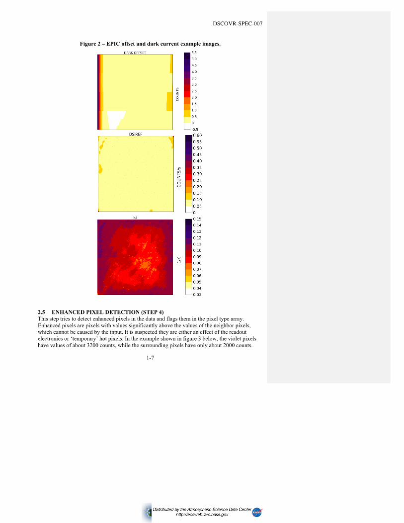
Figure 2 – EPIC offset and dark current example images. 2-7

Figure 3 – EPIC enhanced pixel detection 2-8

Figure 4 – Example read wave correction 2-8

Figure 5 – Example latency correction 2-9

Figure 6 – EPIC electronics non-linearity error and correction. 2-10

Figure 7 – EPIC temperature sensivity correction 2-10

Figure 8 – EPIC pre-launch relative flat field correction maps (arbitrary units) 2-11

Figure 9 – EPIC stray light error 2-12

DSCOVR-SPEC-007

iv

LIST OF TABLES Table Page Table 1 – Make_L1a input summary ........................................................................................ 1-2 Table 2 – Make_L1a output processing list summary .............................................................. 1-2 Table 3 – Processing steps of L1aP .......................................................................................... 2-3

Table 4 – Pixel-type array value descriptions ........................................................................... 2-5

DSCOVR-SPEC-007

1-1

1 INTRODUCTION

1.1 IDENTIFICATION This document is the Level 0 to Level 1A (L1A) Processing Algorithm Description Document for the DSCOVR EPIC instrument science data products. It describes the conversion of raw EPIC data to corrected count rates (L1A). Products are archived at the Atmospheric Science Data Center (ASDC) in Hierarchal Data Format (HDF). Information about HDF and official documentation may be found at the HDF web site (http://www.hdfgroup.org).

1.2 L0 TO L1A PROCESSOR OVERVIEW The Earth Polychromatic Imaging Camera (EPIC) instrument collects radiance data of the Earth and other sources through the Camera/Telescope Assembly. A complete description of the instrument can be found in the “EPIC Instrument Description Document”. L0 data are processed using the L1A processing software (L1aP) resident on the NASA Center for Climate Simulation (NCCS) supercomputer. The L1aP is written in Python version 2.7. Corresponding instrument meta data files are also used as inputs in order to properly convert the images to L1A format. Image pixel geo-location is an auxillary data product and is not part of the L1aP software. The L1aP consists of two files, the L0_L1a.py which includes all functions necessary for the L1aP and also for the production of stray light correction arrays. L0_L1a_wrapper.py is a wrapper program that calls the L0_L1a.py routine. The purpose of the wrapper routine is to make sure all input parameters are correct and perform any error handling related to those inputs. In general, the L1aP performs three steps. First, the wrapper imports the class ‘L1aP’ from L0_L1a.py. Second, the wrapper calls the ‘Get_CalData’ function which imports the EPIC calibration file, named EPIC_CalFile_vX.txt (X = version number). This ASCII file contains all of the information needed for the L1aP such as calibration parameter filenames and calibration parameter storage locations. These parameters are used as input into the ‘Make_L1a.py’ routine which assumes that the proper parameters were loaded and provided to it as input. In other words, it is the responsibility of the wrapper routine to load the proper EPIC calibration parameter files for the images being processed. Lastly, the wrapper calls the ‘Make_L1a’ function which returns the L1a image data and additional information obtained during the data processing. This additional information includes processing errors and warnings. This last step is performed for each L0 input image file. Table 1 summarizes the inputs accepted by the Make_L1a processing routine of L1aP.

DSCOVR-SPEC-007

1-2

Table 1 – Make_L1a input summary

Element Description InputType0 Filternumber;integer;thisis0forDark,between1and10for

singlefilters,and11foropen-open;itcanalsobe-1inwhichcasethefilternumberisdefinedbythefirstletterofthefilename

Mandatory

1 (Commanded)exposuretime[ms];positivefloat Mandatory2 Shutteropentime[ms];positivefloat Mandatory3 Binningwidth;either1(unbinned)or2(2x2-binned);integer Mandatory4 CCUMode,either3or4;integer Mandatory5 CCD-temperature[degC];float Mandatory6 Filenamesofdarkimagestobeusedforthedarkcorrection;

listofstrings;thiscanbeanemptylist,inwhichcasethedarkcountisdeterminedbythecalibrationdata.

Mandatory

O1 Monotonicallyincreasinglistofprocessingstepstoapplytothedata.Ifnolistisgiven,allprocessingstepswillbeperformed.

Optional

O2 FilenamewheretheL1adatawillbestored.Ifempty,nodatawillbestored.

Optional

O3 Listofsettingsforthestraylightcorrection. Optional The output of the Make_L1a routine contains the corrected count rates for the input L0 image and a pixel-type array containing information for each processed image pixel. The L1a image is a float64 array with the same dimensions as the input image (e.g. 2048x2048 for unbinned images or 1024x1024 for 2x2 binned images). The pixel-type array is an unsigned, 8bit integer array of the same dimension as the L1a image. See section 2.1 for more details. An additional list of processing steps that were applied to the L0 data is output. It contains the same number of elements as the processing steps applied where each step contains a list of 4 elements describing the processing (see Table 2).

Table 2 – Make_L1a output processing list summary

ListElementNumber Description0 Processingstepnumber1 Listoferror-indicesraisedintheprocessingstep2 Timeneededforthisprocessingstep3 Additionalinformationspecifictothisprocessingstep

2 EPIC L0 TO L1A PROCESSING DESCRIPTION Inordertoproducescientificallymeaningfulandaccuratedata,theL0dataareprocessedonthegroundtoLevel1a(L1a)databyapplyingasequenceofcorrectionsteps.Thesecorrectionstepsutilizeparametersthataresavedintheprocessingsoftware’sinputcalibrationfileandhavebeendeterminedfromanalysesofpre-launchEPICmeasurementsperformedinthelaboratoryandpost-launchEPICmeasurements.

DSCOVR-SPEC-007

1-3

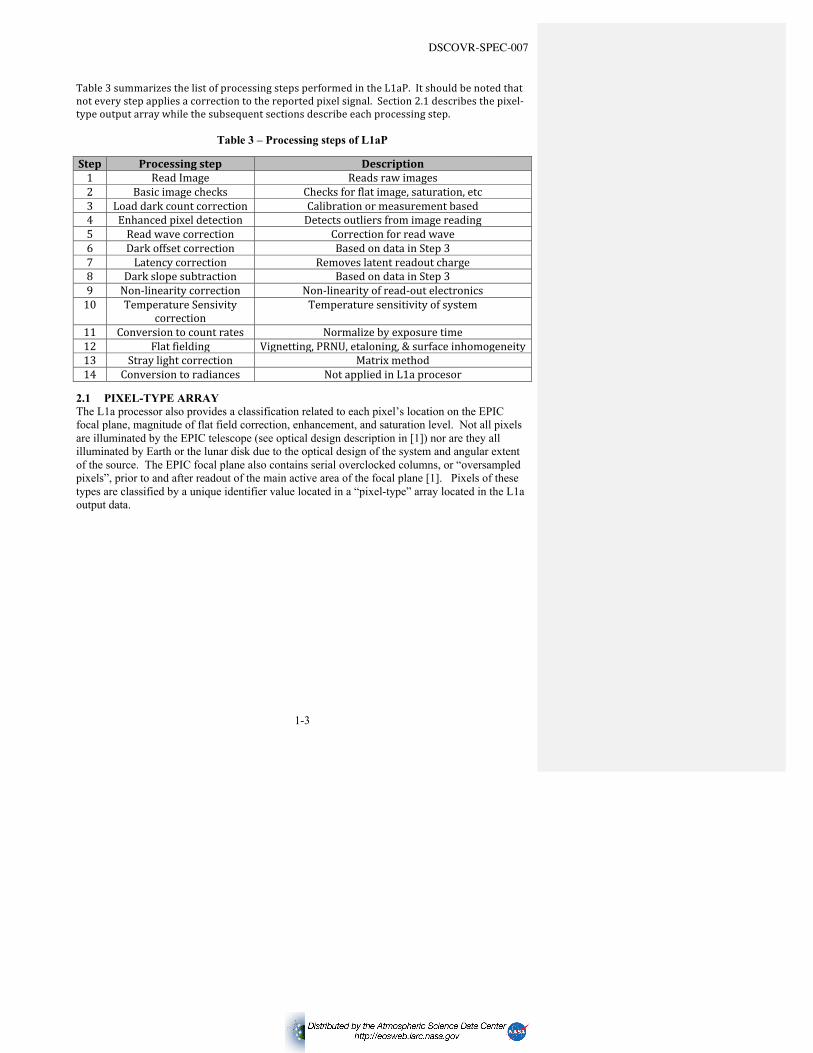
Table3summarizesthelistofprocessingstepsperformedintheL1aP.Itshouldbenotedthatnoteverystepappliesacorrectiontothereportedpixelsignal.Section2.1describesthepixel-typeoutputarraywhilethesubsequentsectionsdescribeeachprocessingstep.

Table 3 – Processing steps of L1aP

Step Processingstep Description1 ReadImage Readsrawimages2 Basicimagechecks Checksforflatimage,saturation,etc3 Loaddarkcountcorrection Calibrationormeasurementbased4 Enhancedpixeldetection Detectsoutliersfromimagereading5 Readwavecorrection Correctionforreadwave6 Darkoffsetcorrection BasedondatainStep37 Latencycorrection Removeslatentreadoutcharge8 Darkslopesubtraction BasedondatainStep39 Non-linearitycorrection Non-linearityofread-outelectronics10 TemperatureSensivity

correctionTemperaturesensitivityofsystem

11 Conversiontocountrates Normalizebyexposuretime12 Flatfielding Vignetting,PRNU,etaloning,&surfaceinhomogeneity13 Straylightcorrection Matrixmethod14 Conversiontoradiances NotappliedinL1aprocesor

2.1 PIXEL-TYPE ARRAY The L1a processor also provides a classification related to each pixel’s location on the EPIC focal plane, magnitude of flat field correction, enhancement, and saturation level. Not all pixels are illuminated by the EPIC telescope (see optical design description in [1]) nor are they all illuminated by Earth or the lunar disk due to the optical design of the system and angular extent of the source. The EPIC focal plane also contains serial overclocked columns, or “oversampled pixels”, prior to and after readout of the main active area of the focal plane [1]. Pixels of these types are classified by a unique identifier value located in a “pixel-type” array located in the L1a output data.

DSCOVR-SPEC-007

1-4

Pixels that require additional information related to the size of correction or magnitude of measured signal have their pixel-type array values modified by a discrete value pertaining to the type and level. The pixel-type array is an unsigned, 8-bit array that has the same size (2048x2048, unbinned or 1024x1024, binned) as the observation image size taken by EPIC. Table 4 summarizes the pixel-type array values related a pixel’s focal plane location classification, correction size, and signal level warning.

Figure 1 – Pixel-type location classifications

DSCOVR-SPEC-007

1-5

Table 4 – Pixel-type array value descriptions

Pixel-TypePixel-Typevalue

Description

“RegularPixels”

0 InsideFOVandilluminatedbysource(whiteinFigure1)

1InsideFOVandsurroundingtheilluminatedsourceregion;signallevellikelyinfluencedbysource(yellowinFigure1)

2 InsideFOV,notdirectlyilluminatedbysourceandsignallevelunlikelyinfluencedbysource(orangeinFigure1)

3 InsideFOV,notdirectlyilluminatedbysource;transitionregiontopixelsoutsideFOV(redinFigure1)

4 OutsideFOVwithnodirectilluminationbysource(violetinFigure1)

“OversampledPixels”

10 Fast(Type1)oversampledpixelnotinanedgecolumn(darkblueinFigure1)

11 Slow(Type2)oversampledpixel12 Doubleoversampledpixel13 Edgecolumnpixelofthefastoversampledpixels

“EdgePixels”20 Edgecolumnpixel21 2ndedgecolumnpixel22 Edgerowpixel

“CorrectionandSignalLevel”

+25 Extremeflatfieldcorrection(>50%)+50 Moderately(type1)enhancedpixel+100 Strongly(type2)enhancedpixel+150 Saturated+200 “Bad”pixel

2.2 READ IMAGE (STEP 1) This step reads the image with the input file name. Three different file extensions/formats are accepted. These are:

• epc: this is the “Lockheed binary format”. The program reads the file header (with metadata such as the CCU mode and the exposure time) and the raw image.

• j*: This is a compressed JPG file. The program calls the JPG Decompression function ‘JPG_Decomp_C’, and then reads the raw image from the binary file made by ‘JPG_Decomp_C’.

• b*: This is the raw image in a binary file without header, which is read by the program.

For .epc-data, it shifts the row and columns to go from the EPIC readout arrangement (i.e. the pixels in the order they were read) to the physical arrangement (i.e. the pixels in the order as they are on the CCD). In the other cases the images are already in the physical arrangement.

DSCOVR-SPEC-007

1-6

2.3 BASIC IMAGE CHECKS (STEP 2) This step determines whether the image is “flat”, meaning that all image pixels have the same value. It also determines which, if any, pixels are saturated and updates the pixel-type array accordingly.

2.4 LOAD DARK COUNT CORRECTION (STEP 3) This step returns the best estimation for the dark current present during the conditions of the image. In the case no dark images are given (i.e. element 5 of the metadata is empty), the dark current DCi at each pixel i is estimated from this equation:

[ ][ ] EXPREFCCDiiREF

REFCCDiREFi

iCCDCCDEXPi

tTTkDSTTkDC

DOTDBTtDC

×-××+-××

++=

)(exp)(exp*

)(),(

00

tEXP is the exposure time, TCCD the CCD temperature, TREF is the reference temperature (=-40°C), and DB the dark bias, determined from oversampled pixels. tEXP and TCCD are given in the L0 meta data. Examples of the EPIC bias, dark rate, and temperature dependence are shown in figure 2; DO (top figure) , DC*i0REF, k0i, DSiREF (center figure) and ki (bottom figure) are dark current parameters determined during instrument calibration. All figures are for CCU mode 3. k0i is 0.166/K. Also in this step a rough estimation of the target extension is made and the pixel type array is updated accordingly.

DSCOVR-SPEC-007

1-7

2.5 ENHANCED PIXEL DETECTION (STEP 4) This step tries to detect enhanced pixels in the data and flags them in the pixel type array. Enhanced pixels are pixels with values significantly above the values of the neighbor pixels, which cannot be caused by the input. It is suspected they are either an effect of the readout electronics or ‘temporary’ hot pixels. In the example shown in figure 3 below, the violet pixels have values of about 3200 counts, while the surrounding pixels have only about 2000 counts.

Figure 2 – EPIC offset and dark current example images.

DSCOVR-SPEC-007

1-8

2.6 READ WAVE CORRECTION (STEP 5) This step removes the read wave caused by the EPIC readout electronics. The read wave has a period of about 11 pixels and an amplitude between 0 and 0.6 counts (see figure 4).

Figure 4 – Example read wave correction

2.7 OFFSET CORRECTION (STEP 6) The offset correction is performed using the dark offset determined during Step 3, Loading Dark Current Correction.

Figure 3 – EPIC enhanced pixel detection

DSCOVR-SPEC-007

1-9

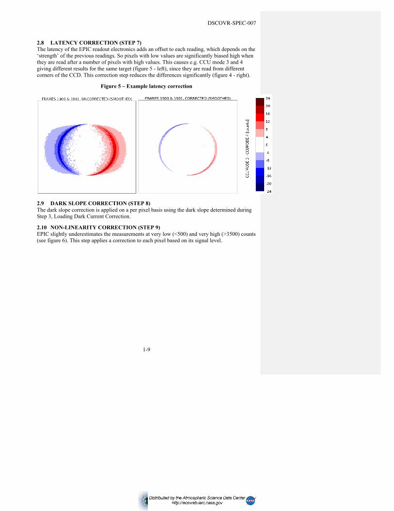
2.8 LATENCY CORRECTION (STEP 7) The latency of the EPIC readout electronics adds an offset to each reading, which depends on the ‘strength’ of the previous readings. So pixels with low values are significantly biased high when they are read after a number of pixels with high values. This causes e.g. CCU mode 3 and 4 giving different results for the same target (figure 5 - left), since they are read from different corners of the CCD. This correction step reduces the differences significantly (figure 4 - right).

Figure 5 – Example latency correction

2.9 DARK SLOPE CORRECTION (STEP 8) The dark slope correction is applied on a per pixel basis using the dark slope determined during Step 3, Loading Dark Current Correction.

2.10 NON-LINEARITY CORRECTION (STEP 9) EPIC slightly underestimates the measurements at very low (<500) and very high (>3500) counts (see figure 6). This step applies a correction to each pixel based on its signal level.

DSCOVR-SPEC-007

1-10

Figure 6 – EPIC electronics non-linearity error and correction.

2.11 TEMPERATURE SENSITIVITY CORRECTION (STEP 10) EPIC’s radiometric sensitivity increases slightly with temperature (0.01% per K, see figure). This effect has been characterized pre-launch and is shown in figure 7.

Figure 7 – EPIC temperature sensivity correction

Deleted:

DSCOVR-SPEC-007

1-11

2.12 INTEGRATION TIME NORMALIZATION (STEP 11) Image data are normalized by the exposure time (in seconds), converting the units of the data from ‘counts’ to ‘count rates’ [counts per second].

2.13 FLAT FIELD CORRECTION (STEP 12) EPIC CTA introduces instrument artifacts in the reported image data due to vignetting, pixel response non-uniformity, etaloning, and surface inhomogeneity. These effects are classified as flat fielding errors and corrected by dividing the image by the filter-specific flat field correction matrix. Filter 6 (551nm) has the ‘best’ flat field. The UV filters 1 to 5 are dominated by the surface inhomogeneity, while filters 7 to 10 (above 600nm) are dominated by etaloning. The original derivation of the flat field correction was based on pre-launch data that had many issues, including source uniformity and differences between the 2011 and 2014 calibrations. A new techinique using an average Earth image calculated for each filter was used to improve the flat field correction. This technique relies on the fact that small terrestrial features from the atmosphere and groud should average out if enough images over a long period of time were used. Over a year’s worth of non-stray light corrected data, 13 June 2015 to 8 Auguest 2016, were used in this new analysis. Additional fitting and smoothing were required to remove residual source features resulting in the flat field corrections shown in Figure 8.

2.14 STRAY LIGHT CORRECTION (STEP 13) EPIC’s stray light causes the signal of a point source to spread around the whole CCD. To correct for this effect, a stray light correction matrix is applied to the image. This matrix is stored in several files. Note that before this correction is done, bad, oversampled, and saturated pixels are replaced with average values over the surrounding pixels.

Figure 8 – EPIC pre-launch relative flat field correction maps (arbitrary units)

DSCOVR-SPEC-007

1-12

The images in figure 9 show the stray light error in percent for a sample Earth image for filters 1 to 10.

Figure 9 – EPIC stray light error

2.15 CONVERSION TO RADIANCES (STEP 14) In this step the absolute calibration factors for each filter are applied, which convert the corrected count rates [count per second] to radiances [mW/m2/nm/sr].

In this version of the calibration file, the radiance conversion factors are not applied and are still set to nominal 1-values, i.e. the L1a data are still in unit of counts per second. Any conversion to radiances will be performed after the L1aP software processing due to a lack of adequate pre-launch calibration data.

DSCOVR-SPEC-007

1-13

3 SUMMARY The L1aP applies the necessary corrections to the L0 data in order to calculate corrected count rates while the geolocation calucations occur independent of this software. The final conversions to calculate radiances are to be applied outside of this software as accurate sensitivities must be determined based on in-flight data. All processing steps related to the conversion have been described as well as the required and optional inputs into the processing software.

DSCOVR-SPEC-007

1-2

4 REFERENCES

1. “EPIC Instrument Description Document”, Tobin, J., Mobilia, J., October 2001.

DSCOVR-SPEC-007

A-1

Appendix A. Abbreviations and Acronyms

Abbreviation/

Acronym

DEFINITION ADC Analog to Digital Converter ADU Analog Digital Unit BRDF Bi-directional distribution function CCD Charge coupled device CCU CCD Control Unit CTA Camera/Telescope Assembly DC Dark current DSCOVR Deep Space Climate Observatory EPIC Earth Polychromatic Imaging Camera FOV Field of view HDF Hierarchal Data Format K degrees Kelvin L0 Level 0 L1A Level 1A L2 Level 2 NCCS NASA Center for Climate Simulation PRNU Pixel response non-uniformity UV ultraviolet