EPA0037 Future Air Quality in Victoria FINAL GSedit v10

Scientific report Future air quality in Victoria – Final report

Publication 1535 July 2013 Authorised and published by EPA Victoria, 200 Victoria Street, Carlton

Melbourne on a winter afternoon in 2012.

2

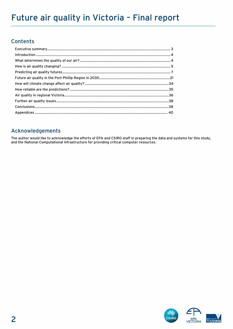
Future air quality in Victoria – Final report

Contents

Executive summary.......................................................................................................................................... 3

Introduction ....................................................................................................................................................... 4

What determines the quality of our air?...................................................................................................... 4

How is air quality changing? .......................................................................................................................... 5

Predicting air quality futures......................................................................................................................... 7

Future air quality in the Port Phillip Region in 2030...............................................................................21

How will climate change affect air quality? ..............................................................................................34

How reliable are the predictions? ...............................................................................................................35

Air quality in regional Victoria.....................................................................................................................36

Further air quality issues..............................................................................................................................38

Conclusions......................................................................................................................................................38

Appendices ..................................................................................................................................................... 40

Acknowledgements The author would like to acknowledge the efforts of EPA and CSIRO staff in preparing the data and systems for this study, and the National Computational Infrastructure for providing critical computer resources.

3


Executive summary Air pollution is always present in our cities, and often in rural areas as well. Over time, the patterns of air pollution are changing, because of changes in technology, climate, population and industry. This study seeks a scientific understanding of likely future trends in air quality in Victoria. This information will be used to develop policies and strategies to control air pollution, now and in the future.

It was found that changes in vehicle technology and population are the main factors likely to affect urban air quality impacts over the next two decades. Air pollution emissions in 2030 were estimated under three plausible future scenarios, which were then used in air quality modelling. Population change between 2006 and 2030 was examined using a population distribution model based on census data and published data on population growth.

By 2030, it is predicted that total motor vehicle exhaust emissions will have significantly reduced, despite the large growth expected in the use of cars and trucks. This is because improved technology is entering the vehicle fleet faster than the rate of growth in vehicle use. The net effect is a reduction in the impacts of exhaust-related pollutants: carbon monoxide, nitrogen dioxide and air toxics such as benzene. This prediction is supported by independent data. When long-term measurements of these pollutants in Melbourne were examined, a clear downward trend was seen.

For emissions that are linked to domestic and business activities, significant increases are expected due to the 45 per cent population growth projected for the Melbourne and Geelong areas between 2006 and 2030. Unless pollutant concentrations are zero or low enough to have no effect, population growth itself is a driver of increased impact, as the health burden for a given pollution situation is increased as more people are exposed. Our population is also predicted to age significantly. Between 2006 and 2030 we are expecting a large increase in the number of people aged 65 years or older. This is important because people in this age category are known to be more sensitive to air pollution.

Climate change may also affect our air quality in the future. Over the next two decades, climate change will not significantly affect urban air pollution. However, in the decades beyond 2030, if emissions are not kept in check, climate change is predicted to cause significant increases in summer smog (ozone). It is also possible that the frequency of droughts may increase, which would lead to an increase in particle air pollution from bushfires and wind-blown dust.

Under the most likely future scenario, the net effect of climate change, growth in domestic and small business emissions, and growth in the receiving population is an increase in population exposure to fine particles (PM2.5) and ozone (O3) between 2006 and 2030. Population exposure is a measure of the overall ‘dose’ of pollution received by a community over a period of time, factoring in both pollution levels and population levels. Given that fine particles and ozone are currently of concern in Victoria, it is clear that these two pollutants should be the primary focus of policy effort over the next 10-20 years.

The net effect for nitrogen dioxide (NO2) is a reduction in impact by 2030, under all three future scenarios. Significant reductions are also expected for carbon monoxide (CO) and air toxics (benzene, formaldehyde, toluene and xylenes). Sulfur dioxide (SO2) impacts are extremely low in Melbourne, and this is expected to remain the case despite some industrial growth.

The primary focus of this study was on air quality in the Port Phillip Region, which includes Melbourne and Geelong. Some preliminary work was done to see if statewide air quality impacts due to wind-blown dust and bushfire smoke could be predicted under future climates. Using four global climate models, dust impacts were modelled across Victoria in the year 2070. The predictions indicate a slight increase in extreme dust events and a slight decrease in moderate dust events. A feasibility study was also conducted to see if fire activity and fire emissions could be modelled under future conditions. The study found that with some further research to link fire ignition and fire spread models with smoke emission estimates, it should be possible to estimate future trends in bushfire activity and consequent smoke impacts.

There are clear signs of improvement in many of the air pollutants typically found in our cities – especially those linked to vehicle exhaust. For other pollutants such as particles and ozone, which result from many different emission sources, only gradual changes are expected. As Melbourne grows, the impacts of these pollutants are likely to increase, and in the long term, climate change is likely to increase levels further. Managing particles and ozone will need a coordinated approach to tackle the relevant pollution sources.

4


Introduction The quality of the air we breathe is important, because air pollution can affect our health. EPA Victoria is responsible for managing outdoor air quality, which can be affected by industry, transport, business and domestic activities. This project, a partnership between EPA Victoria and CSIRO, explores the likely trends in air quality between now and the year 2030. It also seeks to understand what the key drivers of air quality issues will be in the future, with a view to developing effective policies for air pollution control over the next 10-20 years.

What determines the quality of our air? Air quality refers to the nature of the air that we breathe, and how it affects us. In this study, we look at chemical pollution of the air. In particular, we examine those common air pollutants that are known to affect our health:

Particles: These come in all different shapes and sizes, and can be measured in a number of ways. The two most common measures of particles are PM10 (particles smaller than 0.010 mm) and PM2.5 (particles smaller than 0.0025 mm). Very small particles can get into our lungs, causing a range of health problems, especially for young children and those with existing lung or heart disease.

Ozone (O3): A gas like oxygen (O2), but with an extra atom making it very reactive. Ozone is not directly emitted into the air, instead it forms when other air pollutants combine together on warm summer days. Ozone is harmful to the lungs, especially for the elderly and those with asthma.

Nitrogen dioxide (NO2): This gas is produced by the burning of fuels such as natural gas, petrol or diesel. It is harmful to health, especially for children, the elderly and those with asthma.

Carbon monoxide (CO): This odourless gas, mainly from petrol exhaust, can get into the bloodstream where it displaces oxygen. It can cause heart problems, especially in the elderly.

Sulfur dioxide (SO2): This gas can irritate the lungs, and is particularly harmful for people with asthma. Most of the sulfur dioxide in our air comes from coal-fired power stations and metal smelting operations.

Air toxics: This term refers to a range of gases which exist in very small concentrations, but are potentially hazardous because of their high toxicity. This study has examined four common air toxics: benzene, toluene, xylenes and formaldehyde.

In sufficient concentrations, any of these air pollutants can be harmful to humans. Even in Australian cities where air pollution is reasonably well controlled, studies have shown that some people may be seriously affected by air pollution. A day of poor air quality can increase the number of people who attend hospital with lung and heart problems. Those with asthma and elderly people with existing health issues are most at risk.

5


How is air quality changing?

Measured trends

EPA has measured Melbourne’s air quality every day since 19791. These measurements clearly show that air quality has improved over this time. Over the last 15 years, pollutants from motor vehicle exhaust have continued to reduce, despite significant increases in the number of vehicles on our roads. This is because the improvements to exhaust emissions are occurring faster than the growth in traffic.

Some air pollutants, especially ozone and particles, are affected by a wide range of sources. These pollutants are changing more slowly, and we still experience occasional days of poor air quality in summer (due to ozone) and winter (due to particles).

Analysis of long term trend sites in Melbourne (appendix A) shows that between 1996 and 2012:

• average carbon monoxide (CO) concentrations decreased

• average nitrogen dioxide (NO2) concentrations decreased

• average sulfur dioxide (SO2) concentrations were extremely low and show no clear trend

• average PM10 concentrations show no clear trend

• average PM2.5 concentrations show no clear trend.

The focus of the trend analysis was on annual average concentrations, to give an overview of the level of pollution in the air. There were also significant improvements in peak concentrations, measured as the highest pollution level during each year. For example, peak ozone levels significantly improved during the 1980s and early 1990s, although there was no clear trend after 1996. In contrast, carbon monoxide levels show a continuing downward trend, which can be seen in Figure 1.

Figure 1: Carbon monoxide trend in Melbourne, compared with the health-based standard (red line)

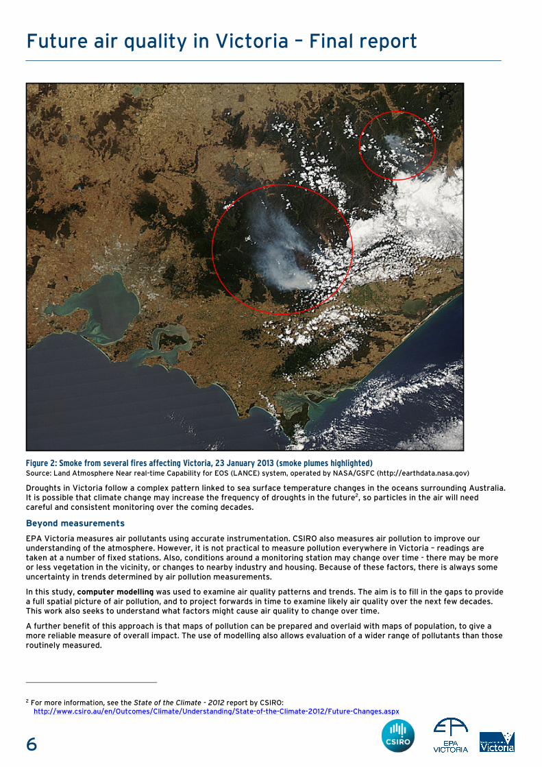
In the last 15 years there have been significant periods of drought, resulting in major bushfires and dust storms. These events can affect air quality over large areas in Victoria. Bushfires, as well as harming life and property, can result in extremely high levels of airborne particle pollution, as seen in the satellite image in Figure 2:

11 Note that there are a number of different units for describing air pollutants. These are explained in appendix A.

0.0

2.0

4.0

6.0

8.0

10.0

19

96

19

97

19

98

19

99

20

00

20

01

20

02

20

03

20

04

20

05

20

06

20

07

20

08

20

09

20

10

20

11

20

12

An

nu

al m

axim

um

8-h

ou

r a

ve

rag

e C

O [

pa

rts p

er

mill

ion]

Annual maximum 8-hour Carbon monoxide (CO) : 1996-2012 [ppm]

Air quality standard for 8-hour average CO (9 ppm)

6


Figure 2: Smoke from several fires affecting Victoria, 23 January 2013 (smoke plumes highlighted) Source: Land Atmosphere Near real-time Capability for EOS (LANCE) system, operated by NASA/GSFC (http://earthdata.nasa.gov)

Droughts in Victoria follow a complex pattern linked to sea surface temperature changes in the oceans surrounding Australia. It is possible that climate change may increase the frequency of droughts in the future2, so particles in the air will need careful and consistent monitoring over the coming decades.

Beyond measurements

EPA Victoria measures air pollutants using accurate instrumentation. CSIRO also measures air pollution to improve our understanding of the atmosphere. However, it is not practical to measure pollution everywhere in Victoria – readings are taken at a number of fixed stations. Also, conditions around a monitoring station may change over time - there may be more or less vegetation in the vicinity, or changes to nearby industry and housing. Because of these factors, there is always some uncertainty in trends determined by air pollution measurements.

In this study, computer modelling was used to examine air quality patterns and trends. The aim is to fill in the gaps to provide a full spatial picture of air pollution, and to project forwards in time to examine likely air quality over the next few decades. This work also seeks to understand what factors might cause air quality to change over time.

A further benefit of this approach is that maps of pollution can be prepared and overlaid with maps of population, to give a more reliable measure of overall impact. The use of modelling also allows evaluation of a wider range of pollutants than those routinely measured.

2 For more information, see the State of the Climate - 2012 report by CSIRO: http://www.csiro.au/en/Outcomes/Climate/Understanding/State-of-the-Climate-2012/Future-Changes.aspx

7


Predicting air quality futures

To use a computer model to predict air quality impacts in the future, three basic inputs are needed:

• Emissions - How much pollution is emitted into the air.

• Weather - Winds, temperature, sunlight, clouds etc.

• Population - How many people live in the study region.

An air quality model is used to combine these inputs to predict air pollution levels. The predictions are then assessed to determine to what extent we expect air quality to be a problem in future. This is done in two ways, firstly by checking air pollution levels against health-based standards, and secondly by undertaking an impact assessment (see Figure 3).

Figure 3: Flowchart for assessing air quality impacts

This section of the report describes each of the three inputs into the model, and the model itself. Later in the report, model results will be used to examine future air pollution levels against air quality standards, and to assess likely future impacts.

Emissions

To study trends in air quality, emissions of air pollutants were estimated for a baseline year (2006) and a future year (2030). An emissions ‘inventory’ for 2006 was prepared using a detailed study of all transport activity, major industry, small business and domestic activities. By carefully examining trends in population, industry and transport, emissions in the year 2030 have also been estimated. As with any attempt to predict the future, there are uncertainties in these estimates. To provide a realistic picture of the range of possible futures, three alternative emission scenarios have been prepared (see Appendices B and C):

E1: a low impact scenario

E2: a medium impact (most likely future) scenario

E3: a high impact scenario

For 2006 and each of the 2030 emission scenarios, a map of pollution emissions across Victoria was prepared, plus a more detailed map for the Port Phillip Region, which includes Melbourne and Geelong. Figure 4 shows an example – in this case estimated emissions of carbon monoxide for 2006 and 2030 (the most likely future scenario). Emissions from road transport, shipping and industry can be clearly seen in these maps. It can also be seen that road transport emissions are predicted to reduce in the future, due to cleaner exhausts.

Emissions Weather

Population

Air pollution

What is the impact of air pollution?

Will air quality comply with standards?

Air quality model

8


Figure 4: Maps of estimated carbon monoxide emissions in the Port Phillip Region: 2006 vs. 2030 (most likely future scenario)

2006

2030

0 - 5

5 - 50 50 - 150 150 - 200 200 - 300 300 - 400 400 - 600 600 - 800 800 - 1500 1500 - 10000

EEEEmissions of carbon monoxide

[tonnes/km

2/yr]

9


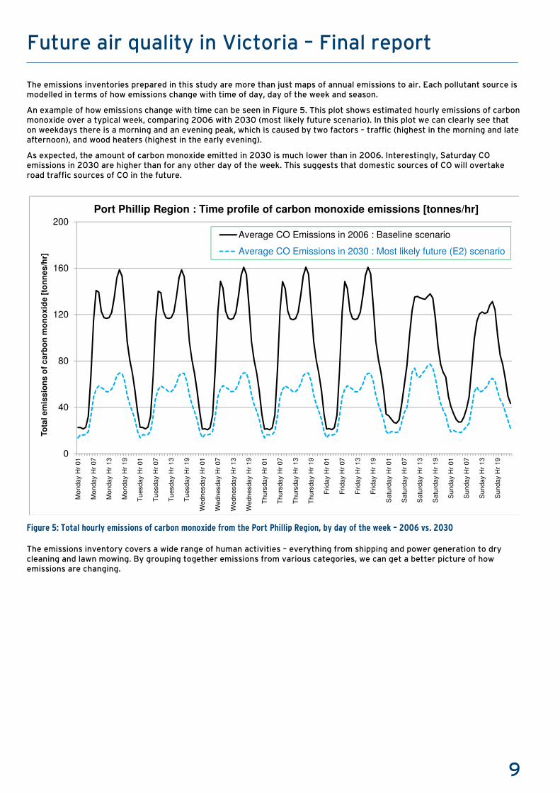
The emissions inventories prepared in this study are more than just maps of annual emissions to air. Each pollutant source is modelled in terms of how emissions change with time of day, day of the week and season.

An example of how emissions change with time can be seen in Figure 5. This plot shows estimated hourly emissions of carbon monoxide over a typical week, comparing 2006 with 2030 (most likely future scenario). In this plot we can clearly see that on weekdays there is a morning and an evening peak, which is caused by two factors – traffic (highest in the morning and late afternoon), and wood heaters (highest in the early evening).

As expected, the amount of carbon monoxide emitted in 2030 is much lower than in 2006. Interestingly, Saturday CO emissions in 2030 are higher than for any other day of the week. This suggests that domestic sources of CO will overtake road traffic sources of CO in the future.

Figure 5: Total hourly emissions of carbon monoxide from the Port Phillip Region, by day of the week – 2006 vs. 2030

The emissions inventory covers a wide range of human activities – everything from shipping and power generation to dry cleaning and lawn mowing. By grouping together emissions from various categories, we can get a better picture of how emissions are changing.

0

40

80

120

160

200

Mo

nd

ay H

r 0

1

Mo

nd

ay H

r 0

7

Mo

nd

ay H

r 1

3

Mo

nd

ay H

r 1

9

Tu

esd

ay H

r 0

1

Tu

esd

ay H

r 0

7

Tu

esd

ay H

r 1

3

Tu

esd

ay H

r 1

9

Wed

ne

sda

y H

r 0

1

Wed

ne

sda

y H

r 0

7

Wed

ne

sda

y H

r 1

3

Wed

ne

sda

y H

r 1

9

Thu

rsda

y H

r 0

1

Thu

rsda

y H

r 0

7

Thu

rsda

y H

r 1

3

Thu

rsda

y H

r 1

9

Frid

ay H

r 0

1

Frid

ay H

r 0

7

Frid

ay H

r 1

3

Frid

ay H

r 1

9

Sa

turd

ay H

r 0

1

Sa

turd

ay H

r 0

7

Sa

turd

ay H

r 1

3

Sa

turd

ay H

r 1

9

Su

nd

ay H

r 0

1

Su

nd

ay H

r 0

7

Su

nd

ay H

r 1

3

Su

nd

ay H

r 1

9

To

tal em

iss

ion

s o

f c

arb

on

mo

no

xid

e [

ton

ne

s/h

r]

Port Phillip Region : Time profile of carbon monoxide emissions [tonnes/hr]

Average CO Emissions in 2006 : Baseline scenario

Average CO Emissions in 2030 : Most likely future (E2) scenario

10


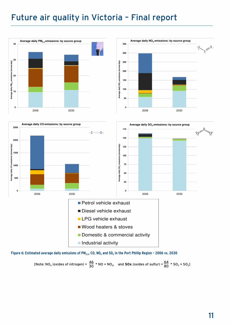
Figures 6-7 compare 2006 emissions with projected emissions for 2030 (most likely future scenario). Emissions are grouped using the following categories:

Petrol vehicle exhaust: Tailpipe emissions from road-based petrol vehicles

Diesel vehicle exhaust: Tailpipe emissions from road-based diesel vehicles

LPG vehicle exhaust: Tailpipe emissions from road-based LPG (liquefied petroleum gas) vehicles

Petrol vehicle evaporative: Leakage of fuel vapours from fuel tanks and the fuel supply system of petrol vehicles

Wood heaters & stoves: Emissions from burning of wood (for heating and cooking)

Domestic & commercial activity: Emissions from all other domestic and commercial activities

Industrial activity: Emissions from large industries

From this data we can see some trends:

• Significant reductions are expected in emissions of carbon monoxide, nitrogen oxides and benzene. • Moderate reductions are expected in emissions of toluene, xylenes and formaldehyde. • Small reductions are expected in emissions of particles and sulfur oxides.

These trends and the reasons for them are discussed in more detail below.

Particles ( PM2.5 )

Particles (top left in Figure 6) are emitted from a wide range of sources. We expect significantly reduced particle emissions from diesel engines, but this is somewhat offset by growth from domestic, commercial and industrial activities. Note that wood heaters are a significant source of particles in Melbourne, but this source is not expected to grow as the effects of population growth are likely to be offset by the reduced popularity of wood heaters in the future3.

Emissions of particles from industry are expected to grow slightly through long term economic growth. Most particles from industry are emitted from tall stacks (chimneys) or away from residential areas, however some emissions occur close to where people live. Some of these emissions are from small to medium sized industries that are too numerous to manage through EPA licences. Some particle emissions come from dust on roads (sealed and unsealed). We can see an example of both these sources in the Brooklyn industrial estate, where particles are emitted from small industries and unsealed roads4. Road dust becomes re-suspended into the air when vehicles use the road in dry weather, so these emissions are likely to increase in the future in line with traffic growth.

Nitrogen oxides ( NOX )

Emissions of nitrogen oxides (top right in Figure 6) are expected to reduce significantly through cleaner exhaust from petrol and diesel engines. Some growth is expected in industrial emissions of NOX, however this is mainly from large gas-fired power plants which have tall stacks to disperse pollutants away from where people live. Growth is also expected in domestic and commercial emissions – mainly from the combustion of natural gas for heating and cooking.

Carbon monoxide ( CO )

Emissions of carbon monoxide (bottom left in figure 6) are expected to reduce significantly through reduced emissions from petrol and LPG engines. This is confirmed by measurements in Melbourne, which show that levels of carbon monoxide are on a strong downward trend.

Sulfur oxides ( SOX )

Emissions of sulfur oxides (bottom right in Figure 6) are mainly from industry, with a small contribution from diesel engines. Very little change is expected in emissions of sulfur oxides in the future. This means that sulfur dioxide levels in Melbourne are likely to remain low.

3 ABS 2006. Australian Social Trends, 2006 - Environmental Impact of household energy use. Australian Bureau of Statistics. 4 EPA Victoria 2012. Air Monitoring in Brooklyn: Year 2: November 2010 to October 2011. EPA Publication 1444.

11


Petrol vehicle exhaust

Diesel vehicle exhaust

LPG vehicle exhaust

Wood heaters & stoves

Domestic & commercial activity

Industrial activity

Figure 6: Estimated average daily emissions of PM2.5, CO, NOX and SOX in the Port Phillip Region – 2006 vs. 2030

[Note: NOX (oxides of nitrogen) = 4630

* NO + NO2, and SOx (oxides of sulfur) = 6480

* SO3 + SO2]

0

500

1000

1500

2000

2500

2006 2030

Av

era

ge

da

ily C

O e

mis

sio

ns

(to

nn

es

/day)

Average daily CO emissions: by source group

0

50

100

150

200

250

300

350

2006 2030

Av

era

ge

da

ily N

OX

em

iss

ion

s (

ton

nes

/day)

Average daily NOX emissions: by source group

0

25

50

75

100

125

150

175

2006 2030

Av

era

ge

da

ily S

OX

em

issio

ns (

ton

ne

s/d

ay)

Average daily SOX emissions: by source group

0

10

20

30

40

2006 2030

Ave

rag

e d

ail

y P

M2.5

em

iss

ion

s (

ton

nes

/day)

Average daily PM2.5 emissions: by source group

12


Toluene ( C6H5CH3 ) and xylenes ( C6H4(CH3)2 )

Toluene and xylenes (top left and top right in Figure 7) are emitted from petrol engines, in exhaust and by evaporation of fuel. They are also emitted from a wide variety of other human activities, including the use of solvents, paints, varnishes and inks. Measurements have found that levels of toluene and xylenes in Melbourne are very low5.

Benzene ( C6H6 )

Motor vehicles are currently the major source of benzene emissions (bottom left in Figure 7). As vehicle emission controls improve, significant reductions in benzene emissions are expected. We expect some growth in emissions of benzene from domestic and commercial activities, mainly from small petrol engines used in garden equipment, boats and portable generators, in line with population growth projections.

Figure 7 also shows that large industries are not a significant source of benzene. This is because larger industries tend to be more tightly regulated by EPA Victoria, and any significant sources of benzene must be licensed and controlled under state legislation.

In contrast, smaller sources such as wood heaters, lawn mowers and motorised boats are not so well regulated. As transport emissions reduce, and as our population grows, these sources will need careful attention. There is currently a national project underway to address emissions from small petrol engines6.

Formaldehyde ( HCHO )

Formaldehyde emissions (bottom right in Figure 7) come from a wide variety of sources, including wood heaters, motor vehicles and jet aircraft exhaust. Formaldehyde is also formed in the atmosphere through chemical reactions. Measurements have found that levels of formaldehyde in Melbourne are generally very low.

5 For details of air toxics measurements in Victoria, refer to the EPA website: http://www.epa.vic.gov.au/our-work/monitoring-the-environment/monitoring-victorias-air/monitoring-results/ 6 This is called the ‘Non-road Spark Ignition Engines and Equipment’ project. For or more information, see the COAG Standing Committee for Environment & Water website: http://www.scew.gov.au/strategic-priorities/clean-air-plan/nrsiee.html

13


Petrol vehicle exhaust

Diesel vehicle exhaust

LPG vehicle exhaust

Petrol vehicle evaporative

Wood heaters & stoves

Domestic & commercial activity

Industrial activity

Figure 7: Estimated average daily emissions of air toxics in the Port Phillip Region – 2006 vs. 2030

0.0

5.0

10.0

15.0

20.0

25.0

2006 2030

Ave

rag

e d

ail

y t

olu

en

e e

mis

sio

ns

(to

nn

es/d

ay)

Average daily toluene emissions: by source group

CH3

0.0

2.0

4.0

6.0

8.0

10.0

12.0

14.0

16.0

18.0

2006 2030

Ave

rag

e d

ail

y x

yle

ne

em

iss

ion

s (

ton

nes

/da

y)

Average daily xylene emissions: by source group

CH3

CH3

CH3

CH3

CH3

CH3

0.0

1.0

2.0

3.0

4.0

5.0

6.0

7.0

8.0

9.0

2006 2030

Av

era

ge

da

ily b

en

zen

e e

mis

sio

ns

(to

nn

es/d

ay)

Average daily benzene emissions: by source group

0.0

1.0

2.0

3.0

4.0

5.0

6.0

2006 2030

Ave

rag

e d

ail

y f

orm

ald

eh

yd

e e

mis

sio

ns

(to

nn

es

/da

y)

Average daily formaldehyde emissions: by source group

14


Seasonal effects

Emissions of air pollutants can be strongly affected by weather. For example, emissions of CO, formaldehyde and PM2.5 from domestic heating are much higher during winter compared with other seasons, mainly due to increased use of wood heaters. The seasonal variation in emissions of these pollutants is likely to become more noticeable in the future as motor vehicle emissions reduce. Figure 8 shows the estimated seasonal breakdown of formaldehyde emissions in 2030.

Figure 8: Estimated average daily emissions of formaldehyde in 2030

In general, total emissions of most pollutants are higher in winter, however emissions from some sources can be higher in summer. For example, vapours from solvents and paints are higher in summer, and lawn mowing emissions are higher in spring and summer. During warm, calm weather in summer, emissions from solvents and paints can contribute to summer smog7.

7 NEPCSC (2009). VOCs from surface coatings - Assessment of the categorisation, VOC content and sales volumes of coating products sold

in Australia, report by ENVIRON Australia Pty Ltd to NEPC Service Corporation. Available from http://www.scew.gov.au/archive/air

Summer2.1

Autumn2.7

Winter7.4

Spring3.4

Estimated daily emissions of formaldehyde from the Port Phillip Region in 2030, by season

(units: tonnes/day)

15


Weather

Weather has a very important effect on air pollution levels. As well as affecting emissions, the weather controls how pollutants disperse and react in the atmosphere. During light winds, pollutants can build up and the air can remain smoggy for several days. Temperature, sunlight and rain also have important effects on air pollutants.

In this study, weather data have been obtained from global climate projections undertaken by CSIRO. Global weather information has been carefully downscaled to provide details for Victoria and Melbourne. This data includes synoptic-scale patterns such as troughs and cold fronts, as well as local-scale patterns such as sea breezes.

In south-east Australia it is very common for the weather to vary significantly from year to year. For this reason, 10 years of weather data have been gathered for each scenario. For the ‘baseline’ scenario (2006 emissions), climate data from 1996-2005 have been used. For future scenarios (2030 emissions), climate projections for the years 2025-2034 have been used. A limited study, looking at the effects of climate change only, was also conducted for the years 2065-2074.

Figure 9 shows an example of the kind of weather data used in this study. The white arrows refer to winds, with short arrows representing light winds and long arrows representing stronger winds. This example shows that winds can be quite different in different locations around Melbourne. A detailed understanding of weather conditions helps EPA understand how pollutants move around in the environment.

Figure 9: Example snapshot of model-generated hourly winds over the Port Phillip Region

Extreme weather is also important for air quality. When soil is dry and exposed, strong winds can lift and carry dust many hundreds of kilometres. During bushfire episodes, smoke can create severe air quality impacts. In this study, the focus was on urban-generated pollution, as the science of modelling this type of pollution is well established. Later in this report some preliminary results are presented for dust and smoke pollution during extreme weather conditions.

A further factor to consider is that during heat-waves there may be combined health effects of air pollution and high temperatures8. Calculating this effect is beyond the scope of the current study, however it is plausible that Melbourne may experience more frequent events combining air pollution and extreme heat in the future.

8 See for example, Doherty et al. 2009. ‘Current and future climate and air pollution-mediated impacts on human health’, Environmental

Health, vol 8, supplement 1:S8.

16


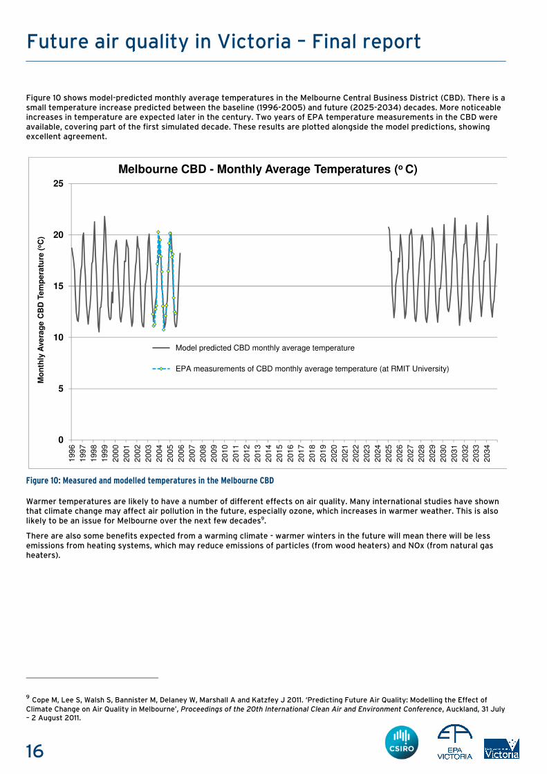
Figure 10 shows model-predicted monthly average temperatures in the Melbourne Central Business District (CBD). There is a small temperature increase predicted between the baseline (1996-2005) and future (2025-2034) decades. More noticeable increases in temperature are expected later in the century. Two years of EPA temperature measurements in the CBD were available, covering part of the first simulated decade. These results are plotted alongside the model predictions, showing excellent agreement.

Figure 10: Measured and modelled temperatures in the Melbourne CBD

Warmer temperatures are likely to have a number of different effects on air quality. Many international studies have shown that climate change may affect air pollution in the future, especially ozone, which increases in warmer weather. This is also likely to be an issue for Melbourne over the next few decades9.

There are also some benefits expected from a warming climate - warmer winters in the future will mean there will be less emissions from heating systems, which may reduce emissions of particles (from wood heaters) and NOx (from natural gas heaters).

9 Cope M, Lee S, Walsh S, Bannister M, Delaney W, Marshall A and Katzfey J 2011. ‘Predicting Future Air Quality: Modelling the Effect of

Climate Change on Air Quality in Melbourne’, Proceedings of the 20th International Clean Air and Environment Conference, Auckland, 31 July – 2 August 2011.

0

5

10

15

20

25

199

6

199

7

199

8

199

9

200

0

200

1

200

2

200

3

200

4

200

5

200

6

200

7

200

8

200

9

201

0

201

1

201

2

201

3

201

4

201

5

201

6

201

7

201

8

201

9

202

0

202

1

202

2

202

3

202

4

202

5

202

6

202

7

202

8

202

9

203

0

203

1

203

2

203

3

203

4

Mo

nth

ly A

ve

rag

e C

BD

Te

mp

era

ture

(oC

)

Melbourne CBD - Monthly Average Temperatures (o C)

Model predicted CBD monthly average temperature

EPA measurements of CBD monthly average temperature (at RMIT University)

17


Population

The Australian Bureau of Statistics10 (ABS 2008) predicts that the population of the Melbourne Statistical Division will grow by 50 per cent between 2006 and 2030, with much lower rates of growth elsewhere in Victoria. For the Port Phillip Region studied in this project, population growth is estimated to be 45 per cent over this time.

Victoria in Future 2008 projections11 provide estimates of population growth in each council region. The majority of the growth is expected to be in outer areas of Melbourne including Wyndham, Melton, Hume, Whittlesea, Casey and Cardinia. Significant growth is also expected in the City of Melbourne.

Figure 11 shows total population estimates for the Port Phillip Region, with details for three age groups. The population is not only increasing, but also ageing significantly. Population growth means an increase in emissions from some sectors, but also that more people will be exposed to air pollution. Even if pollution levels were to remain constant, an increase in population means an increase in pollution-related health costs to the community.

Many studies have shown that children and the elderly are more sensitive to air pollution. Given the expected strong growth in the 65+ age group, greater attention will need to be given to protecting the health of elderly and retired residents through transport and planning decisions.

Figure 11: Projected population growth: 2006 – 2030

10 ABS 2008. Population Projections, Australia, 2006 to 2101. ABS Publication 3222.0, September 2008. 11 DPCD 2009. Victoria in Future 2008 - Victorian State Government Population and Household Projections 2006-2036.

0

1,000,000

2,000,000

3,000,000

4,000,000

5,000,000

6,000,000

7,000,000

2006population

2030population

65+

15-64

0-14

Population in the Port Phillip Region : 2006 vs 2030

18


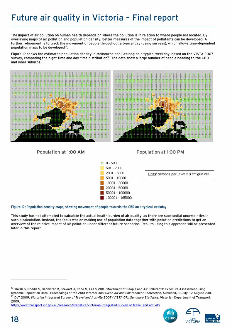
The impact of air pollution on human health depends on where the pollution is in relation to where people are located. By overlaying maps of air pollution and population density, better measures of the impact of pollutants can be developed. A further refinement is to track the movement of people throughout a typical day (using surveys), which allows time-dependent population maps to be developed12.

Figure 12 shows the estimated population density in Melbourne and Geelong on a typical weekday, based on the VISTA 2007 survey, comparing the night-time and day-time distribution13. The data show a large number of people heading to the CBD and inner suburbs.

Population at 1:00 AM Population at 1:00 PM

Figure 12: Population density maps, showing movement of people towards the CBD on a typical weekday

This study has not attempted to calculate the actual health burden of air quality, as there are substantial uncertainties in such a calculation. Instead, the focus was on making use of population data together with pollution predictions to get an overview of the relative impact of air pollution under different future scenarios. Results using this approach will be presented later in this report.

12 Walsh S, Roddis S, Bannister M, Stewart J, Cope M, Lee S 2011. ‘Movement of People and Air Pollutants: Exposure Assessment using Dynamic Population Data’. Proceedings of the 20th International Clean Air and Environment Conference, Auckland, 31 July – 2 August 2011. 13 DoT 2009. Victorian Integrated Survey of Travel and Activity 2007 (VISTA 07): Summary Statistics, Victorian Department of Transport,

2009. http://www.transport.vic.gov.au/research/statistics/victorian-integrated-survey-of-travel-and-activity

Units: persons per 3 km x 3 km grid cell

19


Air quality model

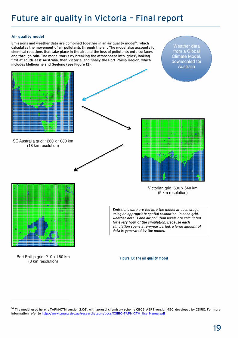
Emissions and weather data are combined together in an air quality model14, which calculates the movement of air pollutants through the air. The model also accounts for chemical reactions that take place in the air, and the loss of pollutants onto surfaces and through rain. The model works by breaking the atmosphere into ‘grids’, looking first at south-east Australia, then Victoria, and finally the Port Phillip Region, which includes Melbourne and Geelong (see Figure 13).

14 The model used here is TAPM-CTM version 2.061, with aerosol chemistry scheme CB05_AERT version 450, developed by CSIRO. For more information refer to http://www.cmar.csiro.au/research/tapm/docs/CSIRO-TAPM-CTM_UserManual.pdf

Weather data from a Global

Climate Model, downscaled for

Australia

SE Australia grid: 1260 x 1080 km (18 km resolution)

Victorian grid: 630 x 540 km (9 km resolution)

Port Phillip grid: 210 x 180 km (3 km resolution)

Emissions data are fed into the model at each stage,

using an appropriate spatial resolution. In each grid,

weather details and air pollution levels are calculated

for every hour of the simulation. Because each

simulation spans a ten-year period, a large amount of

data is generated by the model.

Figure 13: The air quality model

20


The air quality model has been tested against EPA measurements in Melbourne, and has been found to perform well15. A key feature of the chosen model is that it dynamically varies emissions from wood heaters and motor vehicles according to weather conditions. For example, on cold nights it is assumed that more wood is burnt in wood heaters, and on hot days it is assumed that there is greater leakage of fuel vapours from the fuel systems of petrol vehicles. These factors can have significant impacts on the air quality, especially in winter and summer.

The model also includes emissions of natural chemicals from vegetation, which can contribute significantly to air pollution in summer and autumn16. This requires an understanding of the patterns of land use and vegetation cover across Victoria, as each type of vegetation produces a different mix of natural chemicals17. Natural emissions are also adjusted each hour according to weather conditions – for example, more volatile gases are emitted from eucalypt trees in hot weather and direct sunshine.

By including the effect of weather changes on emissions, the model can undertake a more accurate assessment of how climate change might alter future air quality.

15 Cope M, Lee S, Walsh S, Bannister M, Delaney W, Marshall A 2011a. ‘Assessment of a Dynamical Downscaling System for Undertaking Air Quality Projections in Melbourne, Australia’, Proceedings of the 20th International Clean Air and Environment Conference, Auckland, 31 July – 2 August 2011. 16 A number of volatile gases are emitted from trees and grasses during warm, sunny weather. These natural chemicals mix with human-generated pollution to increase the formation of ozone in the air. Very small particles (‘secondary particles’) can also form in the atmosphere from these chemicals. These effects are accounted for in the air quality model. 17 Bannister M, Cope M, Lee S and Walsh S 2011. ‘Developing Biogenic Emission Sources Data for Chemical Transport Modelling.’ Proceedings

of the 20th International Clean Air and Environment Conference, Auckland, 31 July – 2 August 2011.

21


Future air quality in the Port Phillip Region in 2030

Comparison with air quality standards

Key results

Table 1 shows how predicted pollution levels compare with current air quality standards under each scenario. The numbers in the table are the predicted number of days on which air quality standards are breached in the Port Phillip Region in a 10-year period. The data show that the only pollutants likely to breach standards in 2030 are ozone (O3) and fine particles (PM2.5).

Table 1: Predicted number of days per decade on which air pollution levels are above standards in the Port Phillip Region. For air toxics, the criteria given here are Monitoring Investigation Levels. For PM2.5, the criterion is an Advisory Reporting Standard.

Air quality standard

Baseline

2006 emissions

1996-2005 weather

Future

2030 emissions

2025-2034 weather

E1 E2 E3

Short-term standards

CO (8-hr average : 9 ppm) 0 0 0 0

NO2 (1-hr average : 120 ppb) 0 0 0 0

Ozone (1-hr average : 100 ppb) 21 2 12 17

Ozone (4-hr average : 80 ppb) 39 19 32 34

SO2 (1-hr average : 200 ppb) 0 0 0 0

SO2 (24-hr average : 80 ppb) 0 0 0 0

PM2.5 (24-hr average : 25 µg/m3) 12 3 6 15

PM10 (24-hr average : 50 µg/m3) - - - -

Formaldehyde (24-hr average : 40 ppb) 0 0 0 0

Toluene (24-hr average : 1000 ppb) 0 0 0 0

Xylenes (24-hr average : 250 ppb) 0 0 0 0

Long-term standards

NO2 (annual average : 30 ppb) 0 0 0 0

SO2 (annual average : 20 ppb) 0 0 0 0

PM2.5 (annual average : 8 µg/m3) 0 0 0 1

Lead (annual average : 0.5 µg/m3) - - - -

Benzene (annual average : 3 ppb) 0 0 0 0

Toluene (annual average : 100 ppb) 0 0 0 0

Xylenes (annual average : 200 ppb) 0 0 0 0

Benzo(a)pyrene (annual average : 0.3 ng/m3) - - - -

Note that some pollutants have not been assessed in the computer modelling, either because levels are too low to be of concern (which is the case for atmospheric lead), or because the technology does not yet exist to undertake reliable simulations in urban environments (this is the case for PM10 and benzo(a)pyrene).

22


Discussion

The results show that we can generally expect fewer breaches of air quality standards in the future, under the most likely scenario. The key factor behind this expected improvement is the national motor vehicle standards. The Australian Government has committed to improve the standards for light-duty vehicles, based on the European system of standards (Euro 5 and 6)18. The most likely future (E2) scenario assumes this schedule of improvements will be fully implemented.

The compliance results also show that the E1 and E3 alternative future scenarios would result in noticeably different levels of compliance with air quality standards. For example, under the E3 scenario, the model predicts an increase in the number of breaches of the PM2.5 annual advisory standard. This highlights the importance of implementing the planned improvements to motor vehicle emissions.

We can see in the compliance results there are two short-term standards for ozone, and that the four-hour standard is likely to be breached more often. This is consistent with measurements made in Melbourne. The model predicts that on about three days each year in 2030 (32 days per decade), we can expect four-hour average ozone to be above the air quality standard.

In summary, fine particles (PM2.5) and ozone (O3) are the only pollutants expected to breach current air quality standards in 2030. Some improvement is expected in the number of days on which these pollutants breach the standards, however this depends on which emissions scenario eventuates in Victoria.

Impact assessment

Overview

Checking compliance with standards gives us some insight into air pollution levels. However, there are some significant limitations with this approach:

• It does not take into account where policy breaches occur in relation to where people live. • When a breach occurs, there is no account for how far pollution levels are in excess of the standard. • It only assesses air quality against current standards. Air quality standards are currently undergoing a national review19.

For these reasons, a number of other measures have been developed to provide further insight into air pollution levels in the future. These measures are:

� maps of predicted air pollution levels – to show what areas are most affected � time series charts - to show how pollution changes over time � number of people affected - how many people are exposed to various pollution levels � population exposure – based on overlaying population and pollution maps.

This section of the report presents the major findings of the impact assessment. It also presents a case study showing the importance of the height at which emissions are released. The focus will be on the two pollutants that are expected to breach current air quality standards – ozone (O3) and fine particles (PM2.5).

18 For more information see the Australian Government Department of Infrastructure and Transport website:

http://www.infrastructure.gov.au/roads/environment/emission/index.aspx 19 For more information see the Standing Committee for Environment and Water website: http://www.scew.gov.au/nepms/ambient-air-quality.html

23


What areas are most affected?

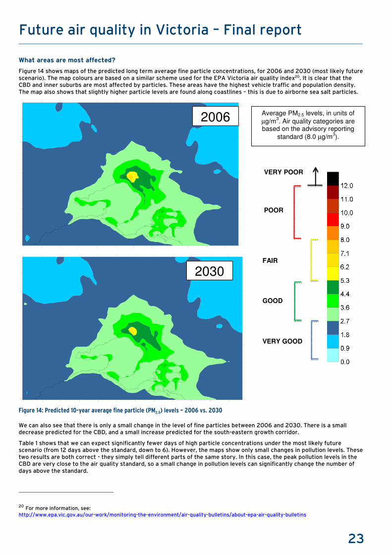
Figure 14 shows maps of the predicted long term average fine particle concentrations, for 2006 and 2030 (most likely future scenario). The map colours are based on a similar scheme used for the EPA Victoria air quality index20. It is clear that the CBD and inner suburbs are most affected by particles. These areas have the highest vehicle traffic and population density. The map also shows that slightly higher particle levels are found along coastlines – this is due to airborne sea salt particles.

Figure 14: Predicted 10-year average fine particle (PM2.5) levels – 2006 vs. 2030

We can also see that there is only a small change in the level of fine particles between 2006 and 2030. There is a small decrease predicted for the CBD, and a small increase predicted for the south-eastern growth corridor.

Table 1 shows that we can expect significantly fewer days of high particle concentrations under the most likely future scenario (from 12 days above the standard, down to 6). However, the maps show only small changes in pollution levels. These two results are both correct - they simply tell different parts of the same story. In this case, the peak pollution levels in the CBD are very close to the air quality standard, so a small change in pollution levels can significantly change the number of days above the standard.

20 For more information, see: http://www.epa.vic.gov.au/our-work/monitoring-the-environment/air-quality-bulletins/about-epa-air-quality-bulletins

VERY POOR

POOR

FAIR

GOOD

VERY GOOD

Average PM2.5 levels, in units of

µg/m3. Air quality categories are

based on the advisory reporting

standard (8.0 µg/m3).

2030

2006

24


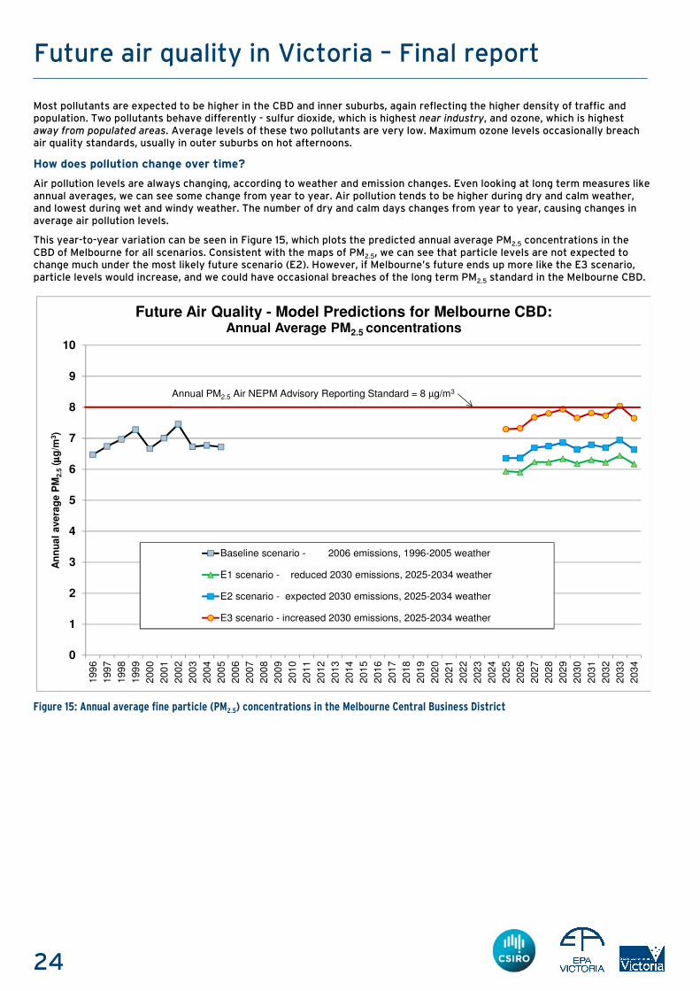
Most pollutants are expected to be higher in the CBD and inner suburbs, again reflecting the higher density of traffic and population. Two pollutants behave differently - sulfur dioxide, which is highest near industry, and ozone, which is highest away from populated areas. Average levels of these two pollutants are very low. Maximum ozone levels occasionally breach air quality standards, usually in outer suburbs on hot afternoons.

How does pollution change over time?

Air pollution levels are always changing, according to weather and emission changes. Even looking at long term measures like annual averages, we can see some change from year to year. Air pollution tends to be higher during dry and calm weather, and lowest during wet and windy weather. The number of dry and calm days changes from year to year, causing changes in average air pollution levels.

This year-to-year variation can be seen in Figure 15, which plots the predicted annual average PM2.5 concentrations in the CBD of Melbourne for all scenarios. Consistent with the maps of PM2.5, we can see that particle levels are not expected to change much under the most likely future scenario (E2). However, if Melbourne’s future ends up more like the E3 scenario, particle levels would increase, and we could have occasional breaches of the long term PM2.5 standard in the Melbourne CBD.

Figure 15: Annual average fine particle (PM2.5) concentrations in the Melbourne Central Business District

0

1

2

3

4

5

6

7

8

9

10

199

6

199

7

199

8

199

9

200

0

200

1

200

2

200

3

200

4

200

5

200

6

200

7

200

8

200

9

201

0

201

1

201

2

201

3

201

4

201

5

201

6

201

7

201

8

201

9

202

0

202

1

202

2

202

3

202

4

202

5

202

6

202

7

202

8

202

9

203

0

203

1

203

2

203

3

203

4

An

nu

al

ave

rag

e P

M2.5

( µµ µµg

/m3)

Future Air Quality - Model Predictions for Melbourne CBD:Annual Average PM2.5 concentrations

Baseline scenario - 2006 emissions, 1996-2005 weather

E1 scenario - reduced 2030 emissions, 2025-2034 weather

E2 scenario - expected 2030 emissions, 2025-2034 weather

E3 scenario - increased 2030 emissions, 2025-2034 weather

Annual PM2.5 Air NEPM Advisory Reporting Standard = 8 µg/m3

25


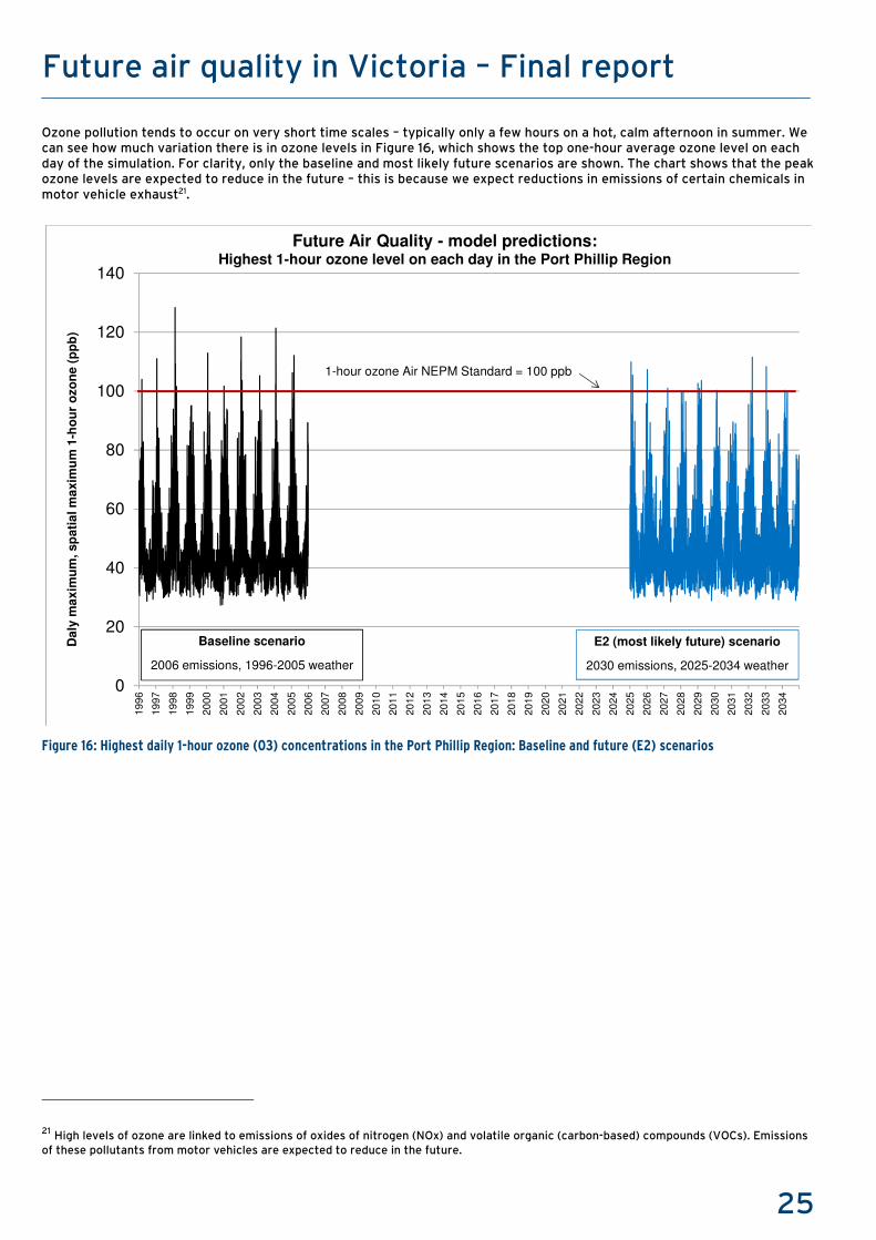
Ozone pollution tends to occur on very short time scales – typically only a few hours on a hot, calm afternoon in summer. We can see how much variation there is in ozone levels in Figure 16, which shows the top one-hour average ozone level on each day of the simulation. For clarity, only the baseline and most likely future scenarios are shown. The chart shows that the peak ozone levels are expected to reduce in the future – this is because we expect reductions in emissions of certain chemicals in motor vehicle exhaust21.

Figure 16: Highest daily 1-hour ozone (O3) concentrations in the Port Phillip Region: Baseline and future (E2) scenarios

21 High levels of ozone are linked to emissions of oxides of nitrogen (NOx) and volatile organic (carbon-based) compounds (VOCs). Emissions of these pollutants from motor vehicles are expected to reduce in the future.

0

20

40

60

80

100

120

140

19

96

19

97

19

98

19

99

20

00

20

01

20

02

20

03

20

04

20

05

20

06

20

07

20

08

20

09

20

10

20

11

20

12

20

13

20

14

20

15

20

16

20

17

20

18

20

19

20

20

20

21

20

22

20

23

20

24

20

25

20

26

20

27

20

28

20

29

20

30

20

31

20

32

20

33

20

34

Da

ly m

ax

imu

m, sp

ati

al m

axim

um

1-h

ou

r o

zo

ne

(p

pb

)

Future Air Quality - model predictions:Highest 1-hour ozone level on each day in the Port Phillip Region

1-hour ozone Air NEPM Standard = 100 ppb

Baseline scenario

2006 emissions, 1996-2005 weather

E2 (most likely future) scenario

2030 emissions, 2025-2034 weather

26


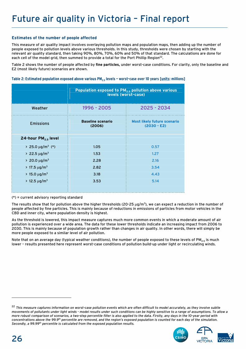
Estimates of the number of people affected

This measure of air quality impact involves overlaying pollution maps and population maps, then adding up the number of people exposed to pollution levels above various thresholds. In this study, thresholds were chosen by starting with the relevant air quality standard, then taking 90%, 80%, 70%, 60% and 50% of that standard. The calculations are done for each cell of the model grid, then summed to provide a total for the Port Phillip Region22.

Table 2 shows the number of people affected by fine particles, under worst-case conditions. For clarity, only the baseline and E2 (most likely future) scenarios are shown.

Table 2: Estimated population exposed above various PM2.5 levels – worst-case over 10 years [units: millions]

Population exposed to PM2.5 pollution above various

levels (worst-case)

Weather 1996 - 2005 2025 - 2034

Emissions Baseline scenario

(2006) Most likely future scenario

(2030 - E2)

24-hour PM2.5 level

> 25.0 µg/m3 (*) 1.05 0.57

> 22.5 µg/m3 1.53 1.27

> 20.0 µg/m3 2.28 2.16

> 17.5 µg/m3 2.82 3.54

> 15.0 µg/m3 3.18 4.43

> 12.5 µg/m3 3.53 5.14

(*) = current advisory reporting standard

The results show that for pollution above the higher thresholds (20-25 µg/m3), we can expect a reduction in the number of people affected by fine particles. This is mainly because of reductions in emissions of particles from motor vehicles in the CBD and inner city, where population density is highest.

As the threshold is lowered, this impact measure captures much more common events in which a moderate amount of air pollution is experienced over a wide area. The data for these lower thresholds indicate an increasing impact from 2006 to 2030. This is mainly because of population growth rather than changes in air quality. In other words, there will simply be more people exposed to a similar level of air pollution.

Note that on an average day (typical weather conditions), the number of people exposed to these levels of PM2.5 is much lower – results presented here represent worst-case conditions of pollution build-up under light or recirculating winds.

22 This measure captures information on worst-case pollution events which are often difficult to model accurately, as they involve subtle

movements of pollutants under light winds - model results under such conditions can be highly sensitive to a range of assumptions. To allow a

more robust comparison of scenarios, a two-step percentile filter is also applied to the data. Firstly, any days in the 10-year period with

concentrations above the 99.9th percentile are removed, and the region’s exposed population is counted for each day of the simulation.

Secondly, a 99.99th percentile is calculated from the exposed population results.

27


Table 3 shows the number of people affected by ozone (both 1-hour and 4-hour averaging times), under worst-case conditions.

Table 3: Estimated population exposed above various ozone levels – worst-case over 10 years [units: millions]

Population exposed to ozone pollution above various

levels (worst-case)

Weather 1996 - 2005 2025 - 2034

Emissions Baseline scenario

(2006) Most likely future scenario

(2030 - E2)

1-hour ozone level

> 100 ppb (*) 0.03 0.05

> 90 ppb 0.15 0.18

> 80 ppb 0.38 0.61

> 70 ppb 0.81 1.44

> 60 ppb 1.78 3.12

> 50 ppb 3.02 4.89

4-hour ozone level

> 80 ppb (*) 0.44 1.06

> 72 ppb 0.99 2.47

> 64 ppb 1.84 3.90

> 56 ppb 2.85 4.46

> 48 ppb 3.63 5.43

> 40 ppb 4.06 6.09

(*) = current national air quality standards

These results show that the number of people exposed to ozone is expected to increase for all threshold levels.

At low thresholds, most of the city is affected under worse-case pollution conditions. In this case the predicted changes from 2006 to 2030 are mainly due to population growth. Note that there is a natural background level of ozone of around 25-30 ppb, even in remote areas.

At higher thresholds, which are more of a concern in terms of human health, the increase from 2006 to 2030 is partly due to population growth and urban expansion, but also due to complex changes in the pattern of emissions and weather.

The results also show that four-hour ozone levels are generally higher in relation to the air quality standard than one-hour ozone levels, consistent with the compliance results in Table 1. A significant fraction of the population is expected to be exposed to high four-hour average ozone levels under worst-case summer smog conditions in 2030.

In summary, although the peak levels of ozone are expected to reduce (Figure 16), the impact of ozone pollution is likely to increase in the future.

28


Population exposure

This measure is also based on the overlaying of pollution and population maps. In this case the calculation involves multiplying air pollution levels by the population density in each cell of the model grid, then adding up the results over the region.

This gives a measure that is proportional to the overall community ‘dose’ of air pollution, indicating the relative change in health impacts. Note that because this measure includes the population, even if air pollution levels are kept constant, it will increase in line with population growth. This is intentional – so long as air pollution exists at levels that may cause harm, an increase in population means an increase in impact.

Figure 17 provides the population exposure results for fine particles (PM2.5).

Figure 17: Estimated population exposure to fine particles (PM2.5) in the Port Phillip Region – comparison of scenarios

The chart shows that we can expect the population exposure to fine particles to increase under all scenarios.

Compared with the most likely future, the E3 scenario results are noticeably higher. This is partly due to increased emissions, but also because the E3 scenario involves more people living in the inner suburbs, where particle pollution is highest. As expected, if Melbourne’s future follows the E1 scenario, the population exposure to fine particles would be reduced.

0

100

200

300

400

500

600

700

Baseline Scenario

(2006)

Scenario E1

Low Impact Future

(2030)

Scenario E2

Most Likely Future

(2030)

Scenario E3

High Impact Future

(2030)

Po

pu

lati

on

exp

osu

re (

10

6µµ µµ

g/m

3-p

ers

on

-ho

urs

/da

y)

-P

ort

Ph

illi

p R

eg

ion Population Exposure to PM2.5 - comparison of scenarios

29


Figure 18 provides the population exposure results for ozone (O3).

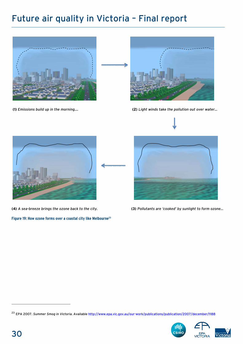
Figure 18: Estimated population exposure to 1-hour ozone in the Port Phillip Region – comparison of scenarios

The ozone results show a more complex pattern than for particles. Ozone forms in the air through a long sequence of chemical reactions involving sunlight and recirculating winds. On a typical ‘summer smog’ day, morning pollution emissions are taken away from the city by light winds, then ‘cooked’ by the sun to form ozone. The ozone cloud is then blown back over the city by a sea-breeze (see Figure 19).

As it comes back over the city, ozone reacts further with fresh afternoon NOX emissions - in fact, ozone gets destroyed in this afternoon reaction. This complicated pathway can result in some non-intuitive results. For example, ozone tends to be lowest in the CBD, where traffic emissions are highest.

Between 2006 and 2030 under the most likely future scenario, we expect a 70 per cent increase in the population exposure to ozone. This is partly because of strong population growth, but also because average levels of ozone in the CBD and inner suburbs are expected to be higher in the future. The increase in inner-city ozone is simply a result of cleaner cars – there are less fresh emissions to cause ozone to be destroyed.

Comparing the three future scenarios, we find that the normal pattern is reversed. Under the E3 scenario, the population exposure is reduced, and under the E1 scenario, it is increased. Again this is because of the expected change in emissions, mainly in the inner suburbs. For all other pollutants (apart from ozone), we expect that the pattern will follow that seen for particles; in other words, E3 impact > E2 impact > E1 impact.

0

500

1000

1500

2000

2500

3000

3500

4000

Baseline Scenario

(2006)

Scenario E1

Low Impact Future

(2030)

Scenario E2

Most Likely Future

(2030)

Scenario E3

High Impact Future

(2030)

Po

pu

lati

on

exp

osu

re (

10

6p

pb

-pe

rso

n-h

ou

rs/d

ay

) -

Po

rt P

hil

lip

Re

gio

n

Population Exposure to Ozone - comparison of scenarios

30


(1) Emissions build up in the morning…. (2) Light winds take the pollution out over water…

(4) A sea-breeze brings the ozone back to the city. (3) Pollutants are ‘cooked’ by sunlight to form ozone…

Figure 19: How ozone forms over a coastal city like Melbourne23

23 EPA 2007. Summer Smog in Victoria. Available http://www.epa.vic.gov.au/our-work/publications/publication/2007/december/1188

31


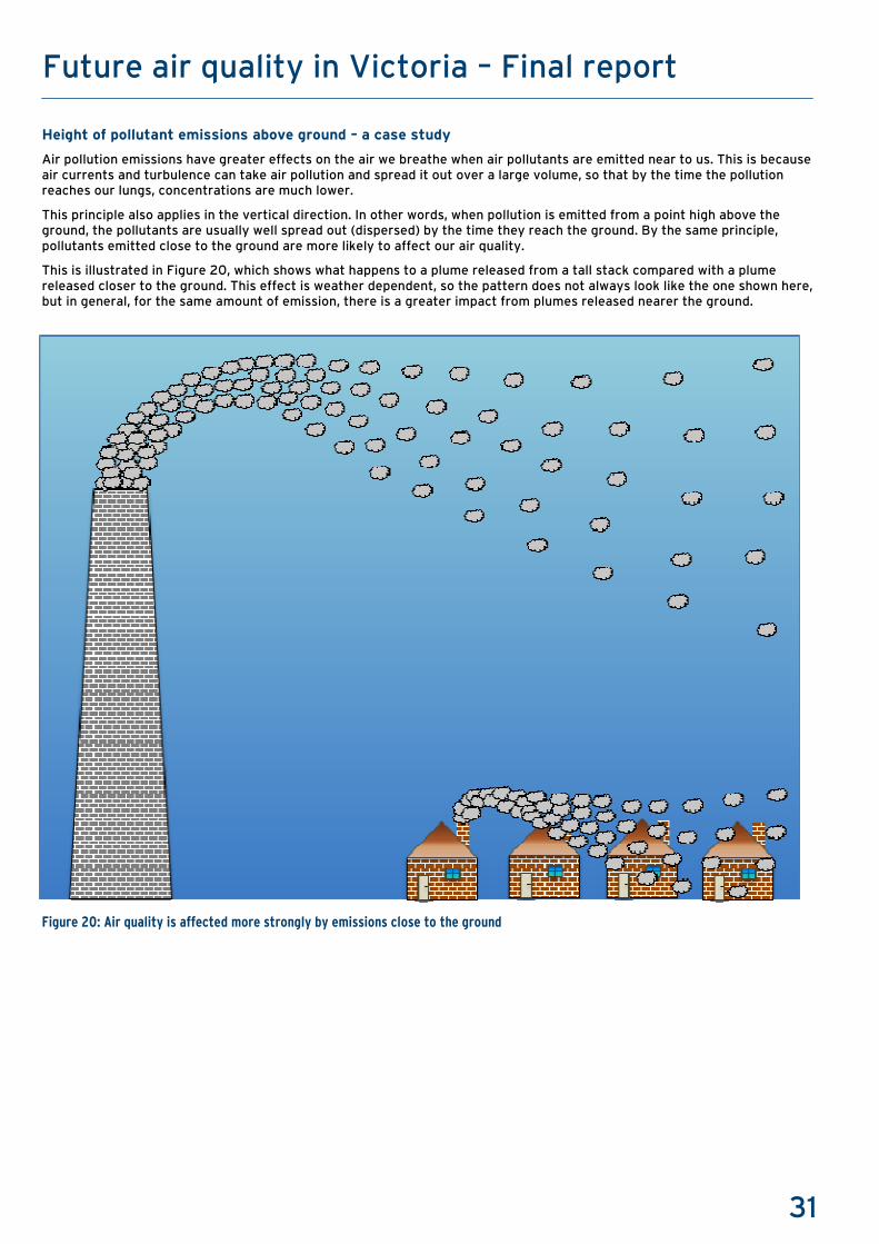
Height of pollutant emissions above ground – a case study

Air pollution emissions have greater effects on the air we breathe when air pollutants are emitted near to us. This is because air currents and turbulence can take air pollution and spread it out over a large volume, so that by the time the pollution reaches our lungs, concentrations are much lower.

This principle also applies in the vertical direction. In other words, when pollution is emitted from a point high above the ground, the pollutants are usually well spread out (dispersed) by the time they reach the ground. By the same principle, pollutants emitted close to the ground are more likely to affect our air quality.

This is illustrated in Figure 20, which shows what happens to a plume released from a tall stack compared with a plume released closer to the ground. This effect is weather dependent, so the pattern does not always look like the one shown here, but in general, for the same amount of emission, there is a greater impact from plumes released nearer the ground.

Figure 20: Air quality is affected more strongly by emissions close to the ground

32


Using the emissions inventory and the air quality model, it is possible to estimate the size of this effect for the urban area as a whole, in the year 2030. To do this, the air quality model was run firstly for the most likely future 2030 scenario, then again with a number of artificial changes made to the emissions data. The three cases studied were:

• emissions set to zero for all stacks taller than 15 m • emissions set to zero for all stacks shorter than 15 m • emissions set to zero for all domestic/commercial sources, including wood heaters (emitted at ground-level).

In each case a single year of weather data was used, and road transport emissions were left unchanged. The results are expressed in terms of the change in population exposure per kilotonne of emission reduction. This gives a measure of the relative amount of benefit gained for a given amount of emission control.

Figure 21 shows this relative benefit value for one of the key components of PM2.5, in this case elemental carbon (soot), which is commonly produced when fuels are burnt. (This pollutant indicator was chosen as it is chemically stable in the air, making it easier to study pollutant dispersion).

Figure 21: Predicted relative air quality benefit from reducing emissions at various heights (year 2030)

The results clearly indicate that controlling emissions near ground level would result in a greater benefit than would be obtained if the same emissions were reduced from industrial stacks. Also, controls on short stacks would bring more benefits than equivalent controls on tall stacks.

Air pollutants may be emitted near ground level from transport, domestic, commercial and industrial activities. Transport emissions are reducing over time, but many other near-ground sources, especially those linked to population growth, are likely to increase over time.

0.0

5.0

10.0

15.0

20.0

25.0

30.0

No emission from stacks tallerthan 15m

No emissions from stacksshorter than 15m

No emissions fromdomestic/commercial sourcesor wood heaters (near-ground)

Rati

o o

f ch

an

ge i

n e

xp

os

ure

to

ch

an

ge

in

em

iss

ion

s

[u

nits:

(10

6µ

g/m

3-p

ers

on

-hrs

/da

y) /

kilo

tonn

es ]

Relative benefit : Reduction in population exposure per kilotonne of emissions reduced.

Port Phillip Region, elemental carbon component of PM2.5.

Incre

asin

g b

en

efit

33


Impact assessment - summary

The results presented in this section show that population growth is likely to drive significant increases in the overall impact of air pollution in the future. The location of this growth is important, because for most pollutants, more development in the CBD and inner suburbs would mean higher impacts from air pollution.

Overall, peak air pollution levels are expected to reduce in the future. Small reductions are expected for particles and ozone, and more significant reductions are expected for exhaust-related pollutants like carbon monoxide. However, the impact of

particles and ozone may actually be higher in the future, because of the location and timing of air pollution events in relation to where people are, and because our population is growing.

The location and height of emissions is very important in determining impacts. Impacts are reduced when emissions are located away from residential areas, or are released well above ground level. Between now and 2030, we expect growth in emissions from some near-to-ground sources, especially from domestic, commercial and small industry sectors. A key challenge in managing air quality impacts into the future is to create a detailed understanding of these near-to-ground sources, including where and when they are emitted in relation to where people spend their time.

34


How will climate change affect air quality? Many studies have shown that climate change is likely to affect air quality in the future24,25. These studies predict that urban areas are likely to experience increases in ozone pollution under a warming climate. This has also been predicted in recent studies of Melbourne’s air quality26,27.

The current study included a simulation of how climate change might affect air pollutants in the year 2070, using ten years of predicted weather data (2065 – 2074). In this simulation, emissions from human activity were held constant at 2006 levels, but the effects of daily weather changes on emissions from wood heaters, motor vehicles and vegetation were accounted for. For example, 60 years from now we expect warmer winters, which will mean somewhat less particle emissions from wood heaters in winter, but also hotter summers, which means greater evaporation from petrol fuel systems.

Four Global Climate Models (GCMs) were used, and all models were run with IPCC scenario A2. The models are listed in Table 4.

Table 4: Global Climate Models

Model Country of origin Description

GFDL USA Geophysical Fluid Dynamics Laboratory Climate Model v 2.1

UKMO UK Hadley Centre UKMO-HadCM3

ECHAM5 Germany Max Planck Institute ECHAM5/MPI-OM

CSIRO Australia CSIRO MK3.5

The key results are presented in Table 5, which shows the relative change in population exposure to various pollutants, between baseline conditions and 2070. Population was held constant at 2006 levels for purposes of this calculation.

Table 5: Relative change in population exposure in the Port Phillip Region (1996-2005) → (2065-2074). Effects of climate change only

Summer ozone Summer NO2 Winter NO2 Summer PM2.5 Winter PM2.5

Model

GFDL + 30% - 2% + 12% + 4% + 10%

UKMO + 20% + 1% + 2% + 4% - 5%

ECHAM5 + 15% + 6% + 2% + 13% - 3%

CSIRO + 20% + 4% + 4% + 6% - 2%

From these results we can see that:

• substantial increases in ozone (O3) population exposure are predicted under all four GCMs

• small to moderate increases in summer PM2.5 population exposure are predicted under all four GCMs

• small increases in winter NO2 population exposure are predicted under all four GCMs.

The ozone results are very significant, because they show that beyond 2030, a warming climate is likely to drive significantly higher ozone impacts in Melbourne. This will create a further challenge for future air quality management.

24 Cope M et al. 2008. ‘A methodology for determining the impact of climate change on ozone levels in an urban area’. Final report to the Department of Environment, Water, Heritage and the Arts, Canberra, ACT. http://www.environment.gov.au/atmosphere/airquality/publications/climate-change.html 25 Jacob D and Winner D 2009. ‘Effect of Climate Change on Air Quality’, Atmospheric Environment, vol 43, pp 51-53. 26 Walsh S et al. 2009. ‘Urban Ventilation and Photochemical Smog in Melbourne for a Future Climate Scenario’. Proceedings of the 9th

International Conference on Southern Hemisphere Meteorology and Oceanography, Melbourne, 9-13 Feb 2009. 27 Cope M et al. 2011. ‘Predicting Future Air Quality: Modelling the Effect of Climate Change on Air Quality in Melbourne’, Proceedings of the

20th International Clean Air and Environment Conference, Auckland, 31 July – 2 August 2011.

35


How reliable are the predictions? The Future Air Quality in Victoria study involved significant research using state-of-the-art methods. However, as with any study of this kind, there remain many uncertainties, including:

• variability associated with the choice of Global Climate Model (GCM)

• uncertainty due to the choice of IPCC global greenhouse gas emission scenario

• uncertainty in the downscaling of climate projections to Victoria

• uncertainty in the scenario projections (e.g. industry growth, population growth)

• uncertainty in the emissions estimates for a given scenario

• uncertainty in the chemical transport model (physics and chemistry)

• uncertainty associated with the measurements used for verification

• uncertainty associated with population modelling.

To manage these uncertainties, scientific rigour and quality assurance was applied throughout the project. The development of the emissions and modelling system involved many years of research effort, using techniques derived from published scientific studies as well as newly developed methods. The system was extensively tested and verified against historical measurements in Melbourne28,29.

For purposes of informing decision making, the system needs to be reliable enough to:

• correctly predict the direction of any trends

• provide an indication of which pollutants will be of most concern in the future

• provide information about sources and issues of concern in the future

• describe where and when air quality impacts will occur.

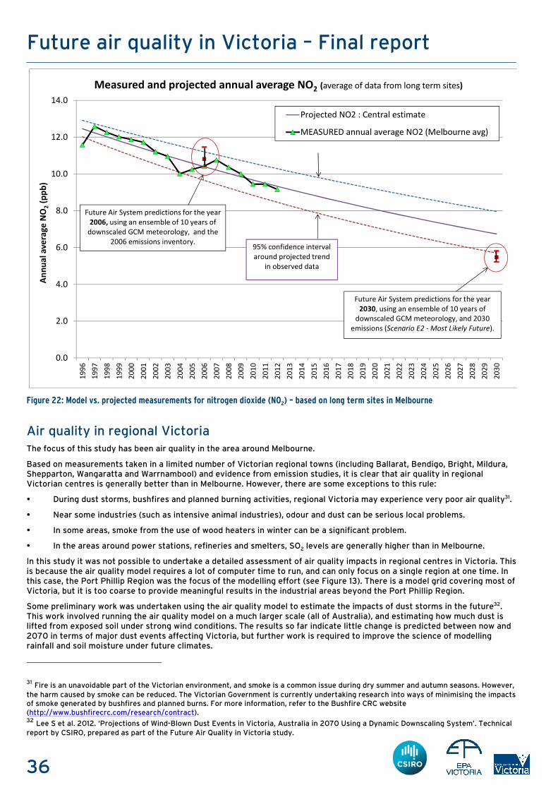
For these purposes the system is sufficiently robust, but for common air pollutants where verification against extensive measurements and trends has been possible, the system should also be capable of predicting actual concentrations with reasonable accuracy. This is confirmed in Figure 22, where model predictions of NO2 for 2006 and 2030 are found to compare well with measured concentrations and projected trends.

The model has also been found to perform well in predictions of air toxics concentrations. For example, measurements of benzene were made at Alphington in 2003, and an annual average value of 0.56 ppb was found30. Using emissions from 2006 (Baseline scenario) and ten years of weather data, the model predicts that annual average benzene levels at Alphington are between 0.42 and 0.48 ppb, indicating good agreement between modelled values and measurements.

28 Marshall A et al. 2011. ‘Techniques for verifying air emissions estimates.’ Proceedings of the 20th International Clean Air and Environment

Conference, Auckland, 31 July – 2 August 2011. 29 Cope M et al. 2011. ‘Assessment of a Dynamical Downscaling System for Undertaking Air Quality Projections in Melbourne, Australia’,

Proceedings of the 20th International Clean Air and Environment Conference, Auckland, 31 July – 2 August 2011. 30 www.epa.vic.gov.au/our-work/monitoring-the-environment/monitoring-victorias-air/monitoring-results/benzene-levels-in-victorian-air-2003-07

36


Figure 22: Model vs. projected measurements for nitrogen dioxide (NO2) – based on long term sites in Melbourne

Air quality in regional Victoria The focus of this study has been air quality in the area around Melbourne.

Based on measurements taken in a limited number of Victorian regional towns (including Ballarat, Bendigo, Bright, Mildura, Shepparton, Wangaratta and Warrnambool) and evidence from emission studies, it is clear that air quality in regional Victorian centres is generally better than in Melbourne. However, there are some exceptions to this rule:

• During dust storms, bushfires and planned burning activities, regional Victoria may experience very poor air quality31.

• Near some industries (such as intensive animal industries), odour and dust can be serious local problems.

• In some areas, smoke from the use of wood heaters in winter can be a significant problem.

• In the areas around power stations, refineries and smelters, SO2 levels are generally higher than in Melbourne.

In this study it was not possible to undertake a detailed assessment of air quality impacts in regional centres in Victoria. This is because the air quality model requires a lot of computer time to run, and can only focus on a single region at one time. In this case, the Port Phillip Region was the focus of the modelling effort (see Figure 13). There is a model grid covering most of Victoria, but it is too coarse to provide meaningful results in the industrial areas beyond the Port Phillip Region.

Some preliminary work was undertaken using the air quality model to estimate the impacts of dust storms in the future32. This work involved running the air quality model on a much larger scale (all of Australia), and estimating how much dust is lifted from exposed soil under strong wind conditions. The results so far indicate little change is predicted between now and 2070 in terms of major dust events affecting Victoria, but further work is required to improve the science of modelling rainfall and soil moisture under future climates.

31 Fire is an unavoidable part of the Victorian environment, and smoke is a common issue during dry summer and autumn seasons. However,

the harm caused by smoke can be reduced. The Victorian Government is currently undertaking research into ways of minimising the impacts of smoke generated by bushfires and planned burns. For more information, refer to the Bushfire CRC website (http://www.bushfirecrc.com/research/contract). 32 Lee S et al. 2012. ‘Projections of Wind-Blown Dust Events in Victoria, Australia in 2070 Using a Dynamic Downscaling System’. Technical report by CSIRO, prepared as part of the Future Air Quality in Victoria study.

0.0

2.0

4.0

6.0

8.0

10.0

12.0

14.0

19

96

19

97

19

98

19

99

20

00

20

01

20

02

20

03

20

04

20

05

20

06

20

07

20

08

20

09

20

10

20

11

20

12

20

13

20

14

20

15

20

16

20

17

20

18

20

19

20

20

20

21

20

22

20

23

20

24

20

25

20

26

20

27

20

28

20

29

20

30

An

nu

al

av

era

ge

NO

2(p

pb

)

Measured and projected annual average NO2 (average of data from long term sites)

Projected NO2 : Central estimate

MEASURED annual average NO2 (Melbourne avg)

Future Air System predictions for the year

2030, using an ensemble of 10 years of

downscaled GCM meteorology, and 2030

emissions (Scenario E2 - Most Likely Future).

Future Air System predictions for the year

2006, using an ensemble of 10 years of

downscaled GCM meteorology, and the

2006 emissions inventory.95% confidence interval

around projected trend

in observed data

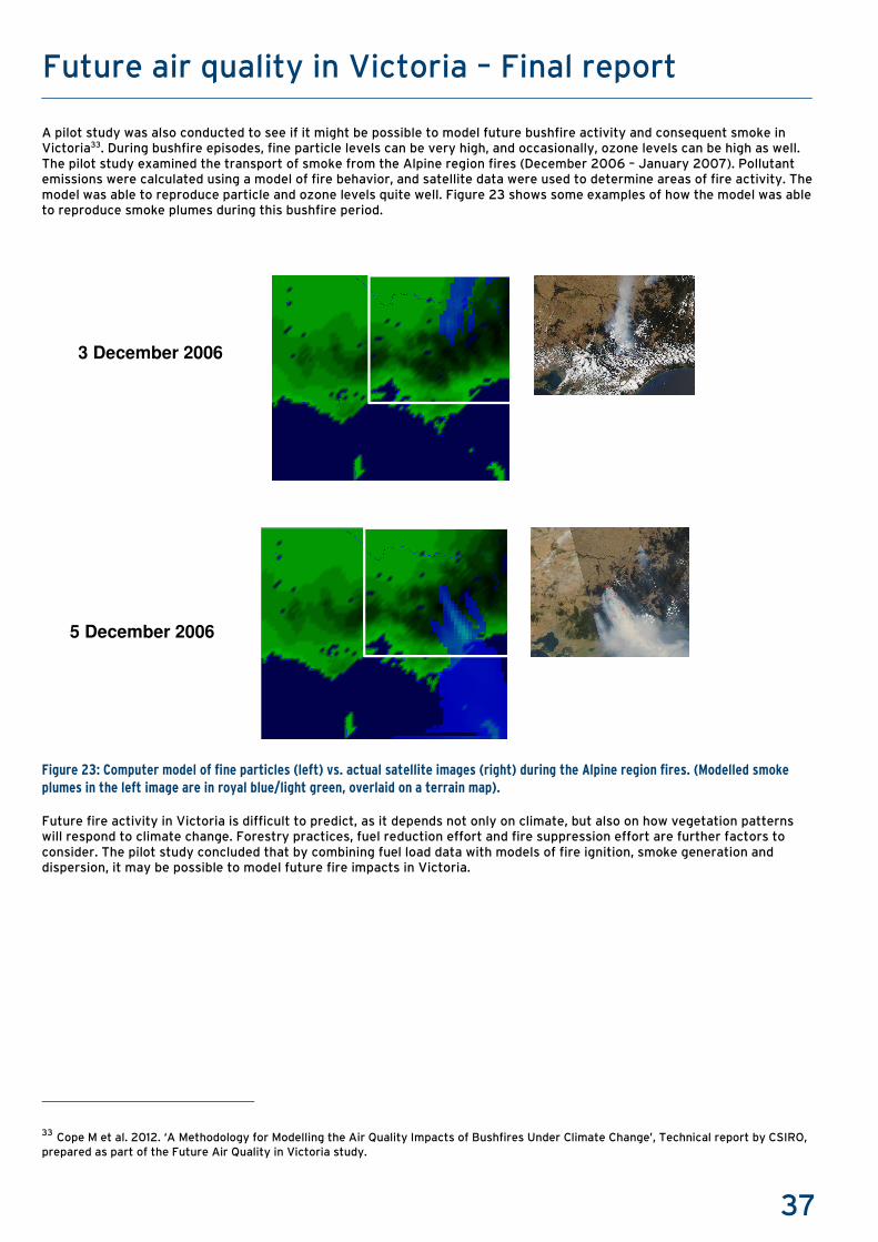
37


A pilot study was also conducted to see if it might be possible to model future bushfire activity and consequent smoke in Victoria33. During bushfire episodes, fine particle levels can be very high, and occasionally, ozone levels can be high as well. The pilot study examined the transport of smoke from the Alpine region fires (December 2006 – January 2007). Pollutant emissions were calculated using a model of fire behavior, and satellite data were used to determine areas of fire activity. The model was able to reproduce particle and ozone levels quite well. Figure 23 shows some examples of how the model was able to reproduce smoke plumes during this bushfire period.

Figure 23: Computer model of fine particles (left) vs. actual satellite images (right) during the Alpine region fires. (Modelled smoke plumes in the left image are in royal blue/light green, overlaid on a terrain map).

Future fire activity in Victoria is difficult to predict, as it depends not only on climate, but also on how vegetation patterns will respond to climate change. Forestry practices, fuel reduction effort and fire suppression effort are further factors to consider. The pilot study concluded that by combining fuel load data with models of fire ignition, smoke generation and dispersion, it may be possible to model future fire impacts in Victoria.

33 Cope M et al. 2012. ‘A Methodology for Modelling the Air Quality Impacts of Bushfires Under Climate Change’, Technical report by CSIRO, prepared as part of the Future Air Quality in Victoria study.

5 December 2006

3 December 2006

38


Further air quality issues The focus of this study was on common air pollutants in the Port Phillip Region, which are subject to air quality management through Victoria’s State Environment Protection Policies and National Environment Protection Measures. Issues such as odour and nuisance dust, whilst very important in Victoria, were beyond the scope of this study.

Also, because air quality was modelled over a large urban region, it was not possible to predict local scale effects, such as air quality very close to roads and industries.

Finally, new or emerging pollutants such as ultrafine particles were not assessed, mainly because of a lack of data describing the emissions of these pollutants.

Conclusions This study combined expertise in climate science, emissions estimation, atmospheric modelling and population projections to evaluate how Victoria’s air quality might change in the future. A state-of-the-art computer model was developed which can predict trends in a range of air pollutants in the Port Phillip Region. This model has been verified against EPA measurements and found to perform well.

The major findings are summarised below.

Impact trends

• Measurements show that the air in Melbourne is much cleaner now than when monitoring started in 1979. For many air pollutants we expect further improvements between now and 2030.

• The key pollutants of concern in the future are expected to be fine particles (PM2.5) and ozone (O3). The model predicts that these pollutants will continue to breach current air quality standards.

• Measurement and modelling studies show that nitrogen dioxide (NO2) and carbon monoxide (CO) levels are reducing in the Port Phillip Region, and will continue to reduce over the next 20 years, due to improvements in motor vehicle exhausts, which are occurring faster than the growth of traffic.

• Levels of sulfur dioxide (SO2) and air toxics (benzene, toluene, xylenes and formaldehyde) are currently very low in the Port Phillip Region, and this is expected to remain the case in the future.

• Fine particle (PM2.5) levels occasionally breach current air quality standards in Melbourne. Population exposure to PM2.5 is expected to increase significantly, mainly because of strong population growth. However, peak impacts from particles on days of poor dispersion are likely to be reduced in 2030, due to lower motor vehicle emissions in the CBD and inner suburbs where both PM2.5 levels and population density are highest.

• Ozone (O3) levels occasionally breach current air quality standards in Melbourne. Population exposure to ozone is expected to increase strongly. Maximum ozone levels are expected to reduce a little by 2030, but the number of people affected by high ozone levels is expected to increase significantly in the future, because of expected changes in the location of ozone pollution in relation to future population.

Drivers of change

• Population growth is likely to be a key driver of change between 2006 and 2030. Emissions linked to residential and business activities are projected to grow significantly, due to the 45 per cent population growth expected in the Port Phillip Region.

• Population ageing is likely to increase the impacts of air pollution in the future. The number of people aged 65 years and over is increasing rapidly, and it is known that the elderly are more sensitive to air pollution.

• Traffic growth is expected to drive increases in re-suspended road dust emissions during dry weather. • Climate change is unlikely to significantly affect urban air quality by 2030. However, beyond 2030, in the absence

of compensating emission controls, climate change is likely to drive an increase in pollution impacts, especially from ozone (and to a lesser extent, fine particles in summer). This effect will continue to increase in line with predicted increases in summer temperatures.

• Technology change, especially in the transport sector, is likely to bring about a number of benefits for air quality in the future.

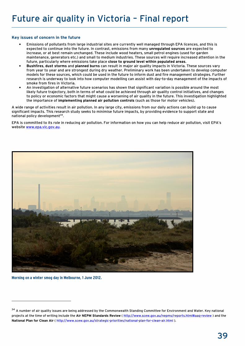
39


Key issues of concern in the future

• Emissions of pollutants from large industrial sites are currently well managed through EPA licences, and this is expected to continue into the future. In contrast, emissions from many unregulated sources are expected to increase, or at best remain unchanged. These include wood heaters, small petrol engines (used for garden maintenance, generators etc.) and small to medium industries. These sources will require increased attention in the future, particularly where emissions take place close to ground level within populated areas.

• Bushfires, dust storms and planned burns can result in major air quality impacts in Victoria. These sources vary from year to year and are strongest during dry weather. Preliminary work has been undertaken to develop computer models for these sources, which could be used in the future to inform dust and fire management strategies. Further research is underway to look into how computer modelling can assist with day-to-day management of the impacts of smoke from fires in Victoria.

• An investigation of alternative future scenarios has shown that significant variation is possible around the most likely future trajectory, both in terms of what could be achieved through air quality control initiatives, and changes to policy or economic factors that might cause a worsening of air quality in the future. This investigation highlighted the importance of implementing planned air pollution controls (such as those for motor vehicles).

A wide range of activities result in air pollution. In any large city, emissions from our daily actions can build up to cause significant impacts. This research study seeks to minimise future impacts, by providing evidence to support state and national policy development34.

EPA is committed to its role in reducing air pollution. For information on how you can help reduce air pollution, visit EPA’s website www.epa.vic.gov.au.

Morning on a winter smog day in Melbourne, 1 June 2012.

34 A number of air quality issues are being addressed by the Commonwealth Standing Committee for Environment and Water. Key national

projects at the time of writing include the Air NEPM Standards Review ( http://www.scew.gov.au/nepms/reports.html#aaq-review ) and the

National Plan for Clean Air ( http://www.scew.gov.au/strategic-priorities/national-plan-for-clean-air.html ).

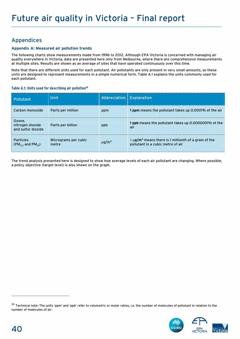
40


Appendices

Appendix A: Measured air pollution trends

The following charts show measurements made from 1996 to 2012. Although EPA Victoria is concerned with managing air quality everywhere in Victoria, data are presented here only from Melbourne, where there are comprehensive measurements at multiple sites. Results are shown as an average of sites that have operated continuously over this time.

Note that there are different units used for each pollutant. Air pollutants are only present in very small amounts, so these units are designed to represent measurements in a simple numerical form. Table A.1 explains the units commonly used for each pollutant.

Table A.1: Units used for describing air pollution35

Pollutant Unit Abbreviation Explanation

Carbon monoxide Parts per million ppm 1 ppm means the pollutant takes up 0.0001% of the air

Ozone, nitrogen dioxide and sulfur dioxide

Parts per billion ppb 1 ppb means the pollutant takes up 0.0000001% of the air

Particles (PM2.5 and PM10)

Micrograms per cubic metre

µg/m3 1 µg/m3 means there is 1 millionth of a gram of the pollutant in a cubic metre of air

The trend analysis presented here is designed to show how average levels of each air pollutant are changing. Where possible, a policy objective (target level) is also shown on the graph.

35 Technical note: The units ‘ppm’ and ‘ppb’ refer to volumetric or molar ratios, i.e. the number of molecules of pollutant in relation to the

number of molecules of air.

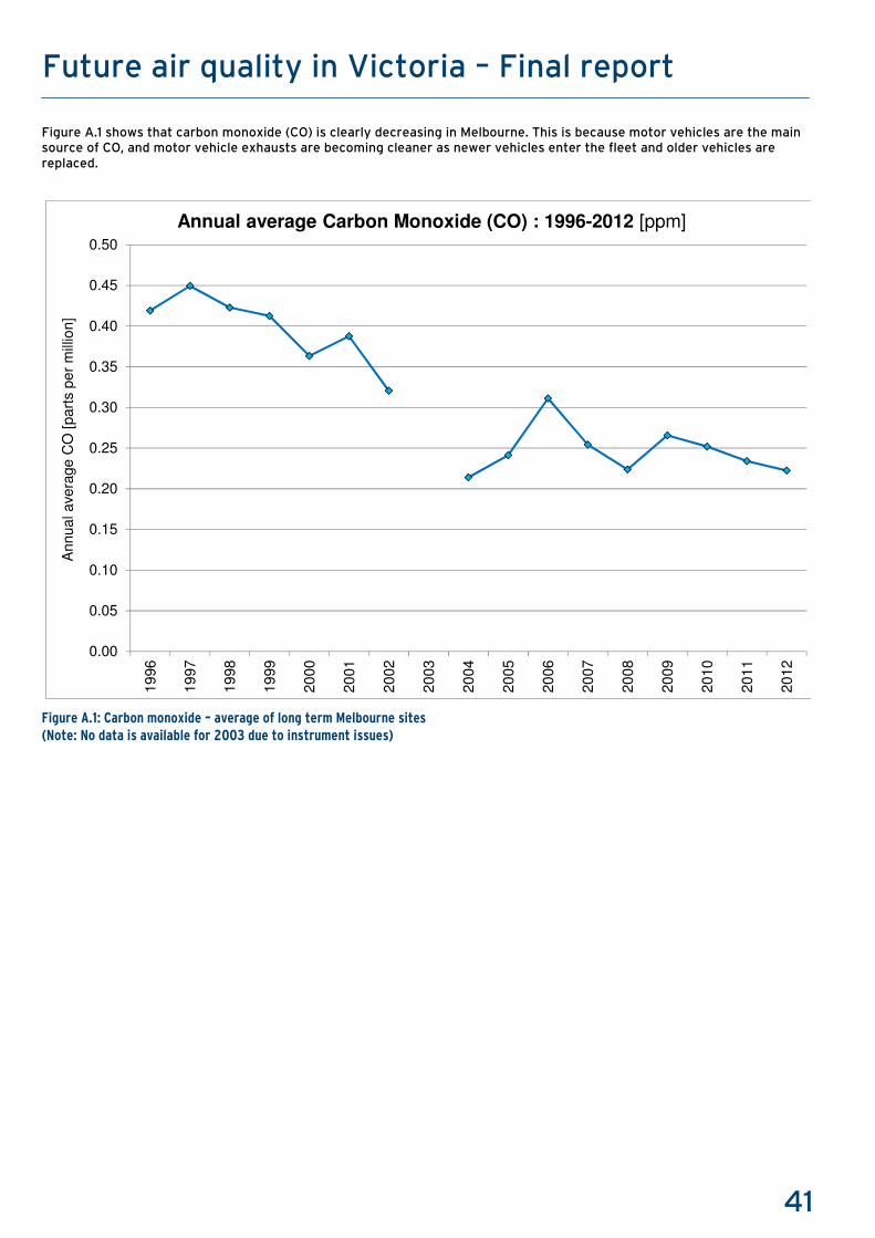
41


Figure A.1 shows that carbon monoxide (CO) is clearly decreasing in Melbourne. This is because motor vehicles are the main source of CO, and motor vehicle exhausts are becoming cleaner as newer vehicles enter the fleet and older vehicles are replaced.

Figure A.1: Carbon monoxide – average of long term Melbourne sites (Note: No data is available for 2003 due to instrument issues)

0.00

0.05

0.10

0.15

0.20

0.25

0.30

0.35

0.40

0.45

0.50

19

96

19

97

19

98

19

99

20

00

20

01

20

02

20

03

20

04

20

05

20

06

20

07

20

08

20

09

20

10

20

11

20

12

Annual avera

ge C

O [part

s p

er

mill

ion]

Annual average Carbon Monoxide (CO) : 1996-2012 [ppm]

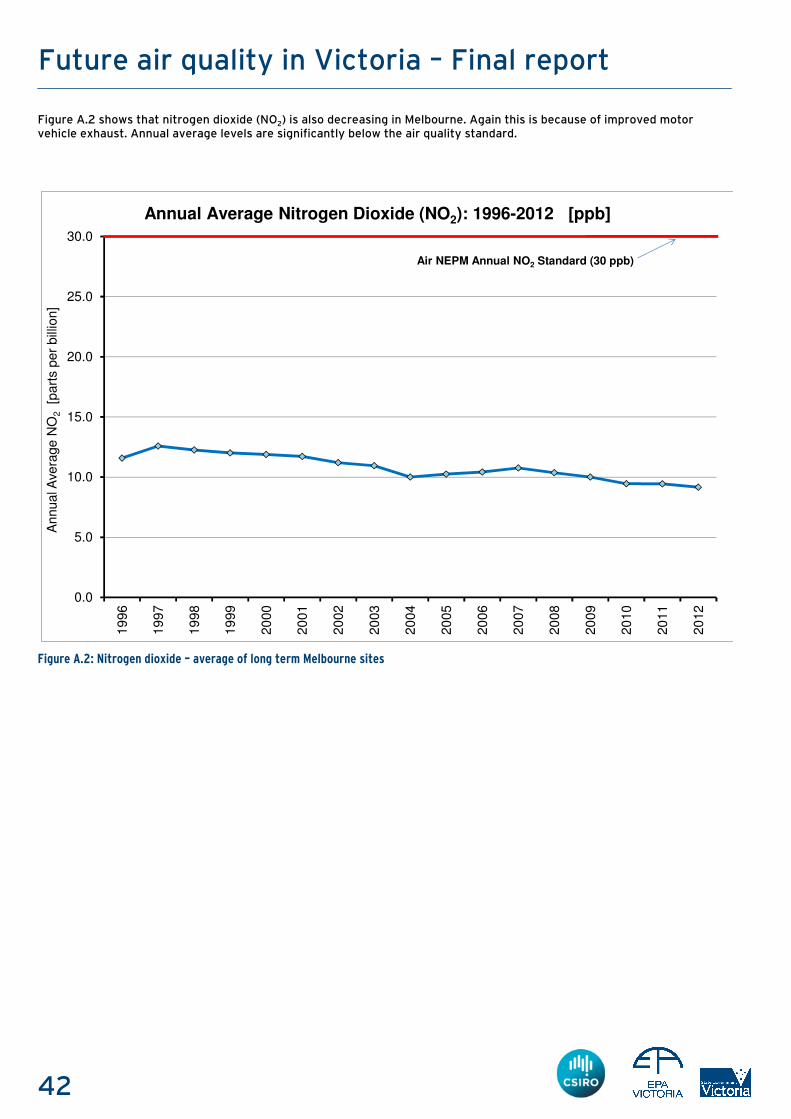
42


Figure A.2 shows that nitrogen dioxide (NO2) is also decreasing in Melbourne. Again this is because of improved motor vehicle exhaust. Annual average levels are significantly below the air quality standard.

Figure A.2: Nitrogen dioxide – average of long term Melbourne sites

0.0

5.0

10.0

15.0

20.0

25.0

30.0

19

96

19

97

19

98

19

99

20

00

20

01

20

02

20

03

20

04

20

05

20

06

20

07

20

08

20

09

20

10

20

11

20

12

Annual A

vera

ge N

O2

[part

s p

er

bill

ion]

Annual Average Nitrogen Dioxide (NO2): 1996-2012 [ppb]

Air NEPM Annual NO2 Standard (30 ppb)

43


Figure A.3 shows that sulfur dioxide (SO2) levels are very low in Melbourne, with no clear trend. These levels are low because there is very little sulfur in the fuels typically used in Melbourne for transport and heating.

The situation is different close to major industries such as refineries, smelters and power stations. However, these large industries operate under EPA licences and are carefully managed to minimise impacts.

In the chart two datasets are shown – an average of all non-industrial measurement sites across Melbourne, and for comparison, a semi-industrial area (Altona North, near a petrochemical complex). Even in the semi-industrial area, average levels of sulfur dioxide are very low compared with the Air NEPM standard.

Figure A.3: Sulfur dioxide – average of long term Melbourne sites

Note: the small negative values seen here for some years are a normal part of the scientific measurement process, and simply reflect extremely low levels of this air pollutant – so low that the instrument cannot distinguish the reading from zero.

-5

0

5

10

15

20

1996

1997

1998

1999

2000

2001

2002

2003

2004

2005

2006

2007

2008

2009

2010

2011

2012

Annual A

vera

ge S

O2

[part

s p

er

bill

ion]

Melbourne average : non-industrial sites

Altona North : semi-industrial area

Annual Average Sulfur Dioxide (SO2): 1996-2012 [ppb]

Air NEPM 1-hour SO2 Standard (20 ppb)

44


Figure A.4 shows an upward trend in annual average ozone (O3) concentrations since 1998. Average ozone concentrations in Melbourne are actually cleaner than natural background air due to the reaction of ozone with nitric oxide (NO), which is emitted along with NO2 in all combustion processes. As car exhausts improve, there is less nitric oxide available, resulting in an upward trend in typical daily ozone levels. Eventually, non-transport sources will dominate, and if these remain stable, average ozone levels will level off at a value somewhere below the natural background (about 25-30 ppb). Because these levels are below the natural background, it is unlikely that this upward trend will have any significant implications for human health.

During 2007 average levels of ozone were noticeably higher than normal. Several factors may have been responsible for this:

• Melbourne was unusually hot during 2007 (the average city temperature was 17.1 oC). More ozone is formed when temperatures are high.

• Cloud cover was low during this year, allowing more sunlight through. Sunlight acts in a number of ways to increase ozone concentrations in the air.

• There were major bushfires burning in Victoria and Tasmania during January to February 2007. The smoke from these fires contributed extra pollutants that resulted in higher than normal levels of ozone.

Figure A.4: Ozone – average of long term Melbourne sites

0

5

10

15

20

25

1996

1997

1998

1999

2000

2001

2002

2003

2004

2005

2006

2007

2008

2009

2010

2011

2012

An

nual A

ve

rage

Ozon

e [p

art

s p

er

bill

ion]

Annual Average Ozone (O3): 1996-2012 [ppb]

Southern ocean background ozone = 25 ppb (annual average).

Rural background varies from 15 ppb to 45 ppb.

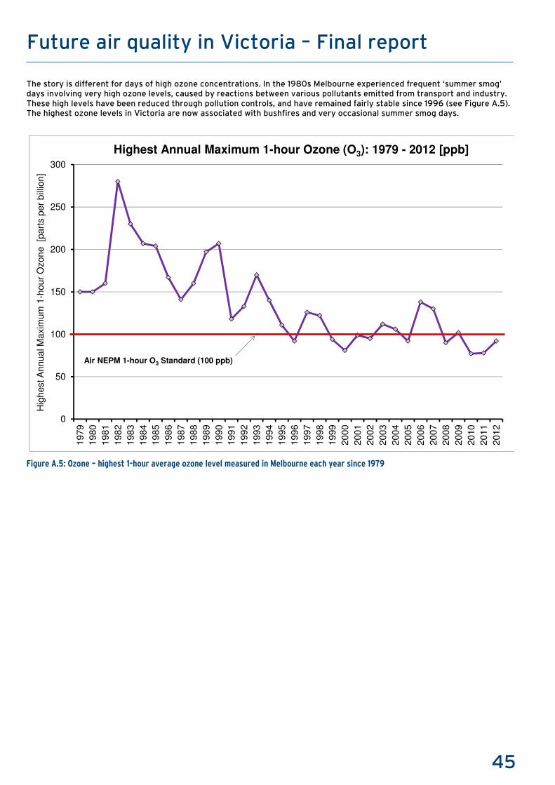
45


The story is different for days of high ozone concentrations. In the 1980s Melbourne experienced frequent ‘summer smog’ days involving very high ozone levels, caused by reactions between various pollutants emitted from transport and industry. These high levels have been reduced through pollution controls, and have remained fairly stable since 1996 (see Figure A.5). The highest ozone levels in Victoria are now associated with bushfires and very occasional summer smog days.

Figure A.5: Ozone – highest 1-hour average ozone level measured in Melbourne each year since 1979

0

50

100

150

200

250

300

1979

1980

1981

1982

1983

1984

1985

1986

1987

1988

1989

1990

1991

1992

1993

1994

1995

1996

1997

1998

1999

2000

2001

2002

2003

2004

2005

2006

2007

2008

2009

2010

2011

2012

Hig

hest A

nnua

l M

axim

um

1-h

our

Ozon

e [p

art

s p

er

bill

ion

]

Highest Annual Maximum 1-hour Ozone (O3): 1979 - 2012 [ppb]

Air NEPM 1-hour O3 Standard (100 ppb)

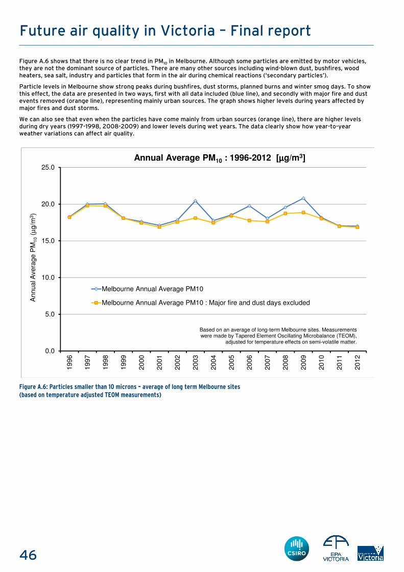
46


Figure A.6 shows that there is no clear trend in PM10 in Melbourne. Although some particles are emitted by motor vehicles, they are not the dominant source of particles. There are many other sources including wind-blown dust, bushfires, wood heaters, sea salt, industry and particles that form in the air during chemical reactions (‘secondary particles’).

Particle levels in Melbourne show strong peaks during bushfires, dust storms, planned burns and winter smog days. To show this effect, the data are presented in two ways, first with all data included (blue line), and secondly with major fire and dust events removed (orange line), representing mainly urban sources. The graph shows higher levels during years affected by major fires and dust storms.

We can also see that even when the particles have come mainly from urban sources (orange line), there are higher levels during dry years (1997-1998, 2008-2009) and lower levels during wet years. The data clearly show how year-to-year weather variations can affect air quality.

Figure A.6: Particles smaller than 10 microns – average of long term Melbourne sites (based on temperature adjusted TEOM measurements)

0.0

5.0

10.0

15.0

20.0

25.0

1996

1997

1998

1999

2000

2001

2002

2003

2004

2005

2006

2007

2008

2009

2010

2011

2012

Annual A

vera

ge P

M1

0(µ

g/m

3)

Melbourne Annual Average PM10

Melbourne Annual Average PM10 : Major fire and dust days excluded

Annual Average PM10 : 1996-2012 [µµµµg/m3]

Based on an average of long-term Melbourne sites. Measurements were made by Tapered Element Oscillating Microbalance (TEOM),

adjusted for temperature effects on semi-volatile matter.

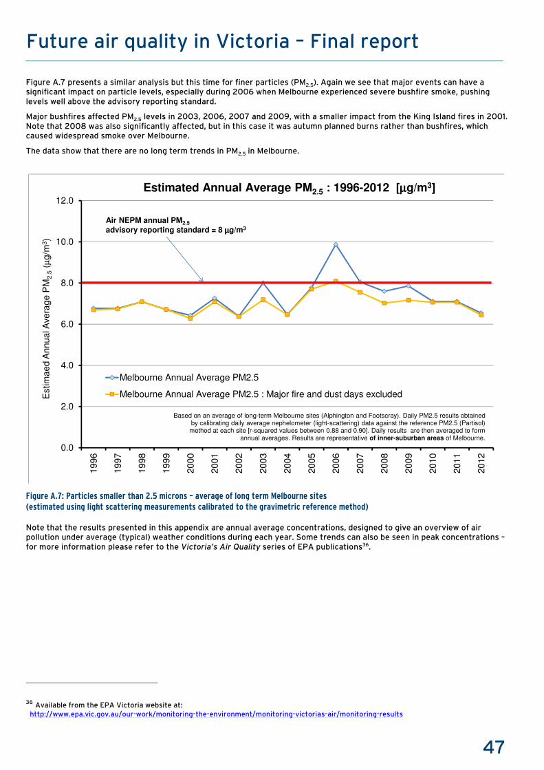
47


Figure A.7 presents a similar analysis but this time for finer particles (PM2.5). Again we see that major events can have a significant impact on particle levels, especially during 2006 when Melbourne experienced severe bushfire smoke, pushing levels well above the advisory reporting standard.

Major bushfires affected PM2.5 levels in 2003, 2006, 2007 and 2009, with a smaller impact from the King Island fires in 2001. Note that 2008 was also significantly affected, but in this case it was autumn planned burns rather than bushfires, which caused widespread smoke over Melbourne.

The data show that there are no long term trends in PM2.5 in Melbourne.

Figure A.7: Particles smaller than 2.5 microns – average of long term Melbourne sites (estimated using light scattering measurements calibrated to the gravimetric reference method)

Note that the results presented in this appendix are annual average concentrations, designed to give an overview of air pollution under average (typical) weather conditions during each year. Some trends can also be seen in peak concentrations – for more information please refer to the Victoria’s Air Quality series of EPA publications36.

36 Available from the EPA Victoria website at: http://www.epa.vic.gov.au/our-work/monitoring-the-environment/monitoring-victorias-air/monitoring-results

0.0

2.0

4.0

6.0

8.0

10.0

12.0

1996

1997

1998

1999

2000

2001

2002

2003

2004

2005

2006

2007

2008

2009

2010

2011

2012

Estim

aed

Annual A

vera

ge P

M2.5

(µg/m

3)

Melbourne Annual Average PM2.5

Melbourne Annual Average PM2.5 : Major fire and dust days excluded

Estimated Annual Average PM2.5 : 1996-2012 [µµµµg/m3]

Based on an average of long-term Melbourne sites (Alphington and Footscray). Daily PM2.5 results obtained by calibrating daily average nephelometer (light-scattering) data against the reference PM2.5 (Partisol) method at each site [r-squared values between 0.88 and 0.90]. Daily results are then averaged to form

annual averages. Results are representative of inner-suburban areas of Melbourne.

Air NEPM annual PM2.5

advisory reporting standard = 8 µµµµg/m3

48


Appendix B: The most likely future emission (E2) scenario

Overview

The first step in developing the E2 scenario involved contacting a number of state and commonwealth agencies to obtain their latest projections, and examining all known trends in population, resource and energy usage, transport technology and emission controls. The year 2030 was chosen as this was the year for which the most projected data was available. Note that although this scenario has been called the ’most likely future’, it is just one scenario out of a vast number that are possible. To ensure the scenario was realistic, all assumptions were subject to scrutiny by scientific and policy officers.

Energy consumption is expected to grow strongly in all economic sectors (Figure B.1) and much of this consumption will result in air pollution emissions. In some sectors, technology improvements or fuel switching will reduce the amount of air pollution emitted for a given amount of energy consumption. This is the case for road transport - we know that motor vehicle emissions are reducing from laboratory tests of newer vehicles compared with older vehicles (Delaney et al. 2009)37. In contrast, emissions linked with domestic and small business activities are likely to be increasing, in line with population growth. Industrial emissions in some sectors are also changing, depending on technology, the growth occurring in each sector, and general economic conditions.

Figure B.1: Energy consumption projections in Australia to 203038

The likely changes between 2006 and 2030 were reviewed carefully for each emissions sector. Intensive quality assurance was applied to estimated 2030 emissions. This included using test model runs to check predicted concentrations against expectations. The following sections of this appendix provide further detail on each emissions sector.

37 Delaney W, Cope M and Azzi M 2009. ‘Passenger Vehicle Emission Factors for Victoria Derived from CUEDEC Drive Cycle Data’.

Proceedings of the 19th International Clean Air and Environment Conference, Perth, Australia, September 2009, CASANZ. 38 ABARE 2006. Australian Energy: National and State Projections to 2029-30. Australian Bureau of Agricultural and Resource Economics.

0

1000

2000

3000

4000

5000

6000

2004-05 2010-11 2019-20 2029-30

Other Residential

Commercial & Services Transport

Manufacturing Mining

Agriculture

Energy consumption projections in Australia, by sector (in PetaJoules, i.e. 1015 Joules)source: ABARE (2006). Australian Energy: National and state projections to 2029-30

49


Domestic and commercial sources

Technological innovation to control air emissions in the domestic and small business sector tends to be slow. Therefore emissions from a number of domestic and commercial sectors will be directly affected by increased population. This includes domestic fuel consumption, use of aircraft, restaurants, surface coatings and many others. In line with population growth, the number of dwellings (housing units) is also expected to increase. This will drive increases in emissions from domestic lawn mowing and waste burning.

Domestic wood consumption (wood heaters and stoves) can be a major source of air pollutants in winter. Growth in this sector would be expected to follow growth in the number of dwellings, however the Australian Bureau of Statistics39 provides fuel use projections to 2030 which suggest a decrease in per-capita consumption of wood, as people switch to electricity and natural gas for heating. The net effect is that there will be little change from 2006 to 2030 in total wood combustion.

There is some uncertainty regarding the use of wood heaters in the future. It may be that the vast majority of new housing is built without wood heaters; conversely an increase in wood heater use may result from the implementation of a carbon pricing policy for climate change mitigation. Alternative future scenarios were used to explore the effect of this uncertainty.

Transport sources

Between 2006 and 2030 we can expect to see significant changes in vehicles, fuels and the level of transport activity, including freight as well as passenger travel. Diesel and petrol will still be widely used, along with less common fuels (natural gas and biofuels). An increasing number of hybrid and electric vehicles are expected, although these will remain a minor component of the fleet. It is assumed that ethanol blends will only be used in a small fraction of petrol vehicles in 2030. Hydrogen and biodiesel are not expected to become significant before 2050.

The emission of pollutants from individual vehicles is expected to reduce through new standards (Euro 5 and 6 for light vehicles, and Euro 5 for heavy vehicles), although the number of kilometres travelled on roads is expected to increase. Overall, the effect of the new standards is expected to outweigh the growth in travel, so total vehicle exhaust emissions should reduce by 2030. It is assumed that the fleet-turnover rate will remain constant.

An upgraded road network for 2030 has been obtained from the Victorian Department of Transport and VicRoads, and an upgraded rail network has also been included. In 2030, the Regional Rail Link should be operational, increasing regional passenger train traffic from the north and west. Across Victoria, diesel passenger train travel is expected to grow by 20 per cent.

Strong growth in shipping and rail freight is expected over the next 20 years, driven by significant population growth and increasing consumption of goods in Victoria. Activity at Victorian ports is expected to increase in line with freight projections. The sulfur content of shipping fuels has been assumed to remain constant, as it is unclear to what extent international standards for shipping fuel will be enforced for ships entering Victorian ports.

39 Australian Bureau of Statistics 2006. Australian Social Trends, 2006: Environmental Impact of Household Energy Use, ABS release 4102.0.

50


Industrial sources

All new industries reporting in the 2009 National Pollutant Inventory were included in the list of industries assumed to be operating in 2030. Industry growth rates by sector were based on industry projections to 2018, with the same growth rates assumed to be valid out to 2030.

There will be significant changes to the power generation sector by 2030. It is assumed that most electrical power will be generated using natural gas, brown coal, co-generation and tri-generation (the latter two located particularly in urban areas). Some existing large power stations are expected to be closed40,41. Smaller amounts of power will be generated using wind, black coal, hydro-electric, biomass (from landfill), liquid fuels and solar.

In Victoria, there are more than 30 sites with installed and operating co-generation facilities. Hospitals are one example where co-generation offers the benefits of improved security of electricity supply and reduced energy costs. Co-generation and tri-generation plants are assumed to be located in major hospitals, shopping centres, and in some office buildings, industrial sites, recreation centres, educational institutions and housing developments.

The location of power generation plants in the 2030 inventory is based on information publicly available in 2010. The total amount of power generation in the scenario will meet expected demand, however the total amount of generated power is below the top-down predictions from CPRS-5 modelling42. A small fraction of the total generation comes from a few industries that convert waste to energy - this is assumed to still be the case in 2030.

There will be some changes in the landfill sector. The Metropolitan Waste Management Group has indicated that sending waste to landfill is likely to decrease by 2030; some existing landfills will close and some will use landfill gas to generate energy. Data was obtained from existing licensed landfills and through discussion with Regional Waste Management Groups. Note that composting is sometimes used to divert organic material from landfill, however emissions of non-greenhouse gases from composting are likely to be very small43 and therefore have not been included in this scenario.

Wastewater generation per person is assumed to remain constant, so the amount of wastewater processed will increase with population growth. Some treatment plants will capture emissions to generate energy. The distribution and consolidation of some treatment plants may change but it is assumed current plants continue to operate.

It is expected that the number of agricultural engine/equipment units will increase, which is primarily a function of the longer life spans of agricultural engines and equipment44. It is assumed that US standards will be introduced progressively which will improve emissions. The number of heavy industrial (construction, mining) units is also expected to increase by 2030, but their overall contribution should decrease assuming US standards are introduced progressively.

40 DPI 2005. Latrobe Valley 2100 Coal Resource Project: Executive Summary. Prepared by GHD for the Department of Primary Industries,

November 2005. 41 MCA 2009. Vision 2020 Project: The Australian Minerals Industry’s Infrastructure Path to Prosperity - An assessment of industrial and

community infrastructure in major resources regions. Prepared by ACIL Tasman for the Minerals Council of Australia, May 2009. 42 Australian Government 2008. Australia’s Low Pollution Future: The Economics of Climate Change Mitigation, Commonwealth of Australia,

Barton, ACT. 43 CARB 2008. Emissions Inventory Estimates – Compost Emissions Work Group, Californian EPA Air Resources Board. 44 ENVIRON 2010. Cleaner non-road diesel engine project – Identification and recommendation of measures to support the uptake of cleaner

non-road diesel engines in Australia. Final report to NSW Department of Environment, Climate Change and Water. ENVIRON Australia, April 2010.

51


Appendix C: Two alternative future emission scenarios

Overview

In Appendix B, a ‘most likely future’ scenario for 2030 emissions was described. In any attempt to predict the future, it is important to acknowledge a range of plausible futures. A full examination of the spectrum of possible futures is beyond the scope of this study, however some useful information can be gained by considering a limited number of alternative scenarios.

For this study, two alternative future scenarios were developed - a ‘low impact’ and ‘high impact’ scenario. Together with the most likely future, this gives three emission scenarios for 2030:

E1: a low impact scenario

E2: a medium impact (most likely future) scenario

E3: a high impact scenario.

The process of developing these scenarios included running the atmospheric model to test how changes in emissions and population assumptions would translate into changes in modelled impact. This is important because not all changes in emissions result in significant on-the-ground changes.

The process also included checks by EPA policy officers to ensure that each change was plausible within the current state and national policy frameworks. Note that the changes from the most likely future in these alternative scenarios do not represent EPA policy but simply represent a preliminary exploration of the range of possible future pathways for air pollutant emissions45.

E1: A ‘low impact scenario’ for 2030

Under this scenario, there are six plausible initiatives to improve air quality:

All wood heaters compliant with AS/NZS 4013 (PM10 emissions set to 4g/(kg of dry fuel))

This initiative is in response to the projection that wood heaters are the largest source of fine particle emissions in winter in 2030 in Melbourne. Current evidence suggests that typical wood heaters emit on average 10 g of PM10 per kg of dry wood (10 g/kg) due to poor operation, incorrect fuel or use of substandard heaters. This initiative would involve enforcing the current Australian standard of 4 g/kg.

All 2-stroke lawn mowers replaced with 4-stroke mowers

This initiative is in response to the observation that lawn mowers are predicted to become a very significant source of air pollutants in spring and summer in 2030; with much of the emissions coming from 2-stroke engines.

50 per cent of passenger vehicles replaced with electric vehicles

This is intended to explore the sensitivity of air quality impacts to a dramatic change in the motor vehicle fleet. Such a change might come about if there were large increases in fuel prices either due to peak oil or carbon pricing.

30 per cent less exhaust and evaporative emissions through better maintenance of light vehicles

This initiative involves improving emissions from the existing vehicle fleet through better maintenance of vehicles. The selected value of 30 per cent is somewhat arbitrary and is intended to test the sensitivity of air quality impacts to a large improvement in vehicle maintenance.

All briquettes replaced with natural gas of equivalent energy content

This initiative is in response to the finding that briquette combustion represents a noticeable source of particle emissions in the 2030 emissions inventory. The initiative represents a phase-out of the use of briquettes in favour of natural gas.

90 per cent reduction in SO2 emissions from Anglesea power station

This initiative is in response to the finding that Anglesea power station contributes a noticeable quantity of sulfate particles to the Melbourne airshed, particularly in summer. The initiative involves the application of best-practice flue desulfurisation to reduce SO2 emissions by 90 per cent.

45 Note: These alternative scenarios do not involve any changes to greenhouse gas emissions – only emissions of common air pollutants that are directly harmful to human health (carbon monoxide, particles, etc). The greenhouse emission scenario was kept fixed (IPCC A2). Climate change effects are relatively small over the time frame of this study (1996 – 2030), and there are also significant time lags between greenhouse emissions and climatic effects. Thus, air pollution under different pollutant emission scenarios can be studied using a single greenhouse emission scenario.

52


E3: A ‘high impact scenario’ for 2030

Under this scenario, there are a range of outcomes which might result from unexpected changes to existing policies, or sudden increases in the price of fuels. This scenario also includes an alternative spatial distribution of future population growth.

All trucks as diesel, no Euro 6 (but including Euro 5)

This change considers what would happen if there is a substantial weakening of the planned improvements in heavy vehicle standards. It also removes any trucks that do not operate on a standard diesel engine (i.e. CNG, hybrid CNG and hybrid diesel) from the 2030 fleet.

Euro 5 and Euro 6 switched off for all light vehicles

This change considers what would happen if there is a substantial weakening of the planned improvements in light vehicle standards.

Additional co-generation within the Port Phillip Region

This change considers the potential for increased use of co-generation at hospitals, new precinct residential areas, leisure centres, sports/entertainment venues, shopping centres, universities and industrial sites.

Increased shipping freight at the Port of Hastings and Port of Melbourne

This change considers moderate increases in shipping freight at both Hastings and Melbourne ports.

25 per cent more wood burnt in wood heaters

This change assumes that factors such as carbon pricing will drive an increased use of wood heaters in Melbourne in 2030. The 25 per cent value has been chosen to represent a likely upper bound in the growth in wood use, having regard for constraints and trends in housing design, and access to wood.

50 per cent of outer Melbourne population growth redistributed to inner Melbourne

This change is to help explore the sensitivity of air quality impacts to the spatial location of future population growth. Greater growth in the inner areas is likely to lead to an increased intensity of emissions. Even more importantly, the higher population densities would result in higher population exposures to most pollutants.

Documents

EPA0037 Future Air Quality in Victoria FINAL GSedit v10