1

Environmental Performance andIts Determinants in China:

Spatial Econometric Approach

Katsuya Tanaka

IDEC, Hiroshima University

LBJ School of Public Affairs, University of Texas at Austin

COE Seminar

October 20, 2006

2

Presentation Outline

• Introduction of spatial econometrics– Consequences of the OLS under spatial

autocorrelation

– Spatial autocorrelation in dependent variable

– Spatial autocorrelation in residuals

• Application of spatial econometrics– Industrial SO2 emission and its determinants

3

Introduction

4

IntroductionWho cares?

– First Law of Geography (by Tobler)• Everything is related to everything else,

but near things are more related than distant things.

• Examples:– Is your income level likely to be similar to your neighbor’s?

– Are farm practices likely to be similar on neighboring farms?

– Are housing values likely to be similar in nearby developments?

– Do nearby provinces have similar economic trends?

– Spatial data tends to follow the First Law of Geography, and to include spatial autocorrelation problems

5

Spatial Autocorrelation

What is spatial autocorrelation?– There exists spatial autocorrelation when the value at any one

point in space is dependent on values at its neighbors.

– That is, the arrangement of values is not just random

Figure 1. Positive autocorrelation Figure 2. No autocorrelation

6

Gauss-Markov Theorem

• The ordinary least squares (OLS) estimates are best, linear, and unbiased estimator (BLUE) if the following assumptions are satisfied:1. Correctly specified linear model

2. X is full rank

3. Zero-mean disturbances

4. Homoscedasticity (spherical disturbances)

5. Normality

Xy β ε= +

[ ]| X 0iE ε =

' 2| X IE εε σ⎡ ⎤ =⎣ ⎦

( )2| X ~ 0,Nε σ

See Greene (2003) or Ramanathan (2002) for details

7

Spatial Autocorrelation

OK. So what’s the matter?– The OLS estimates will not be BLUE due to violation of

assumption under Gauss-Markov Theorem.

– Spatial data is likely to violate assumptions of OLS

– Depending on assumption violated, your OLS estimates are either:

• Inefficient (violation of assumption 4)

• Biased and inconsistent (violation of assumption 1)

– Consequences of the OLS depends on the types of spatial autocorrelation

1. Spatial autocorrelation in dependent variable

2. Spatial autocorrelation in residuals

8

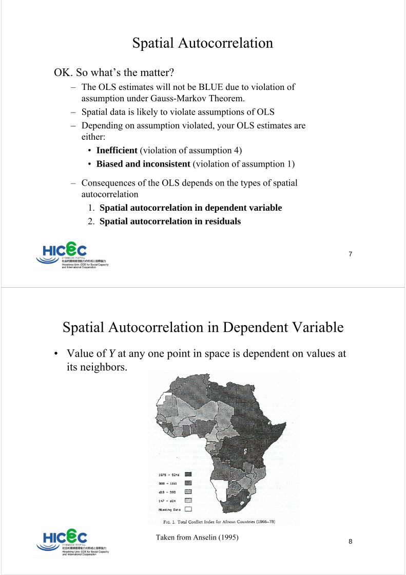
Spatial Autocorrelation in Dependent Variable

• Value of Y at any one point in space is dependent on values at its neighbors.

Taken from Anselin (1995)

9

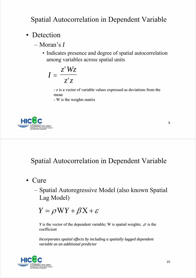
Spatial Autocorrelation in Dependent Variable

• Detection– Moran’s I

• Indicates presence and degree of spatial autocorrelation among variables across spatial units

Iz Wz

z z=

′′

-- z is a vector of variable values expressed as deviations from tz is a vector of variable values expressed as deviations from the he meanmean-- W is the weights matrixW is the weights matrix

10

Spatial Autocorrelation in Dependent Variable

• Cure– Spatial Autoregressive Model (also known Spatial

Lag Model)

W XY Yρ β ε= + +

YY is the vector of the dependent variable; W is spatial weights; is the vector of the dependent variable; W is spatial weights; ρρ is the is the coefficientcoefficient

Incorporates spatial effects by including a spatially lagged depIncorporates spatial effects by including a spatially lagged dependent endent variable as an additional predictorvariable as an additional predictor

11

Spatial Weights Matrix

• How spatial weights matrix (W) is defined– Rook contiguity

• common boundary at edge

– Queen contiguity• common boundary at both edge and point

– Distance-based

– k-nearest neighbors

12

Spatial Weights Matrix

• Example of rook contiguity

2 4

31

1 2 3 4

1 0 1 0 02 1 0 1 03 0 1 0 14 0 0 1 0

13

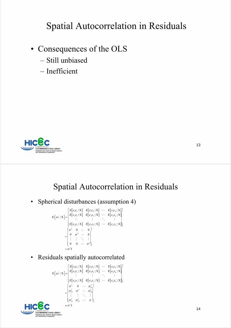
Spatial Autocorrelation in Residuals

• Consequences of the OLS– Still unbiased

– Inefficient

14

Spatial Autocorrelation in Residuals

• Spherical disturbances (assumption 4)

• Residuals spatially autocorrelated

[ ] [ ] [ ][ ] [ ] [ ]

[ ] [ ] [ ]

1 1 1 2 1

2 1 2 2 2'

1 2

2

2

2

2

| X | X | X

| X | X | X| X

| X | X | X

0 0

0 0

0 0

n

n

n n n n

E E E

E E EE

E E E

I

ε ε ε ε ε εε ε ε ε ε ε

εε

ε ε ε ε ε ε

σσ

σ

σ

⎡ ⎤⎢ ⎥⎢ ⎥⎡ ⎤ =⎣ ⎦ ⎢ ⎥⎢ ⎥⎢ ⎥⎣ ⎦⎡ ⎤⎢ ⎥⎢ ⎥=⎢ ⎥⎢ ⎥⎢ ⎥⎣ ⎦

=

L

L

M M O M

L

L

L

M M O M

L

[ ] [ ] [ ][ ] [ ] [ ]

[ ] [ ] [ ]

1 1 1 2 1

2 1 2 2 2'

1 2

2 21

2 2 221 2

2 21 2

2

| X | X | X

| X | X | X| X

| X | X | X

0

n

n

n n n n

n

n

n n

E E E

E E EE

E E E

I

ε ε ε ε ε εε ε ε ε ε ε

εε

ε ε ε ε ε ε

σ σσ σ σ

σ σ σ

σ

⎡ ⎤⎢ ⎥⎢ ⎥⎡ ⎤ =⎣ ⎦ ⎢ ⎥⎢ ⎥⎢ ⎥⎣ ⎦⎡ ⎤⎢ ⎥⎢ ⎥=⎢ ⎥⎢ ⎥⎢ ⎥⎣ ⎦

≠

L

L

M M O M

L

L

L

M M O M

L

15

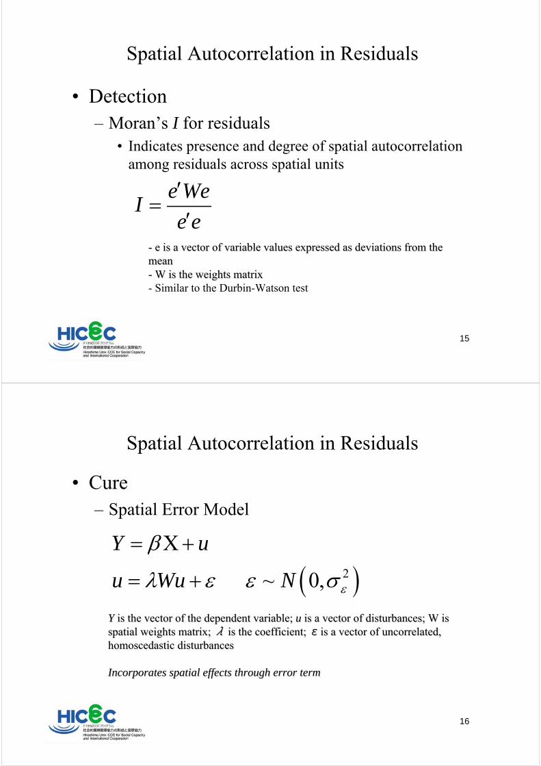
Spatial Autocorrelation in Residuals

• Detection– Moran’s I for residuals

• Indicates presence and degree of spatial autocorrelation among residuals across spatial units

e WeI

e e

′=

′-- e is a vector of variable values expressed as deviations from te is a vector of variable values expressed as deviations from the he meanmean-- W is the weights matrixW is the weights matrix- Similar to the Durbin-Watson test

16

Spatial Autocorrelation in Residuals

• Cure– Spatial Error Model

YY is the vector of the dependent variable; is the vector of the dependent variable; uu is a vector of disturbances; W is is a vector of disturbances; W is spatial weights matrix; spatial weights matrix; λλ is the coefficient; is the coefficient; εεis a vector of uncorrelated, is a vector of uncorrelated, homoscedastic disturbanceshomoscedastic disturbances

Incorporates spatial effects through error termIncorporates spatial effects through error term

( )2

X

~ 0,

Y u

u Wu N ε

β

λ ε ε σ

= +

= +

17

Available Computer Packages

• SpaceStat– Easy graphical interface

– relatively old architecture

• GeoDa– Easy graphical interface with basic estimation routines

– Good for creating weights matrix

• R– Various estimation libraries available

– Works good with GeoDa

• MatLab– Extensive support from LeSage’s Spatial Econometric Toolbox

18

Conclusions from Introduction

• Spatial data is likely to have spatial autocorrelation problems

• Spatial autocorrelation violates the OLS assumptions

• If you use spatial data for your analysis, spatial autocorrelation needs to be tested

• Spatial autoregressive and spatial error models are solutions

• Recommended computer packages:1. R + GeoDa

2. MatLab

19

Application

20

Objectives

• Empirically environmental performance and its determinants in China

• Test the Environmental Kuznets Curve (EKC) hypothesis

• Examine the role of the SCEM on environmental performance

• Environmental performance: Industrial SO2 emission

• China’s 29 provinces during 1994-2003 (10 years)

21

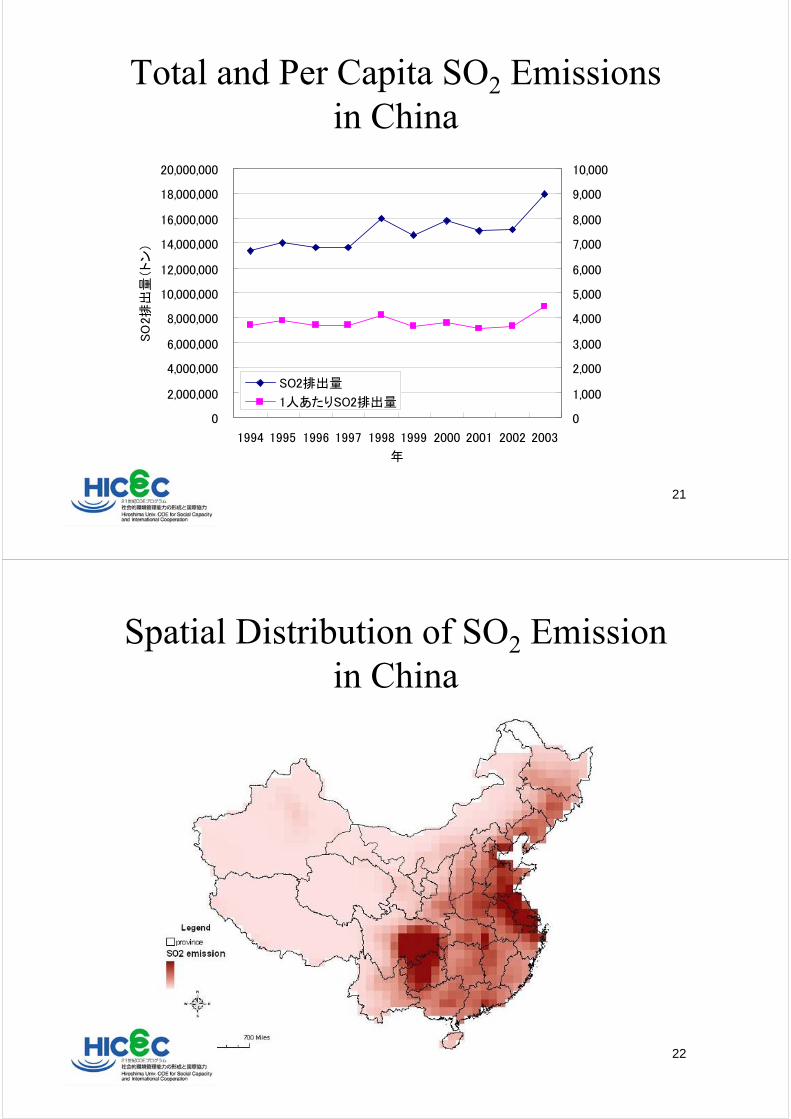
Total and Per Capita SO2 Emissionsin China

0

2,000,000

4,000,000

6,000,000

8,000,000

10,000,000

12,000,000

14,000,000

16,000,000

18,000,000

20,000,000

1994 1995 1996 1997 1998 1999 2000 2001 2002 2003

年

SO

2排

出量

（ト

ン）

0

1,000

2,000

3,000

4,000

5,000

6,000

7,000

8,000

9,000

10,000

SO2排出量

1人あたりSO2排出量

22

Spatial Distribution of SO2 Emissionin China

23

Tests for Spatial Autocorrelation

• Spatial autocorrelation in dependent variable:– Not detected by Moran’s I

• Spatial autocorrelation in residuals– Detected by Moran’s I for residuals

24

Spatial Error Model

( )2

1 2

3 4 5 6

ln ln ln

ln ln ln

Y X X

G F C TIME u

α β ββ β β β

= + +

+ + + + +

Y: SO2 emission per capita

X: GRP per capita

G: Environmental management capacity of government

(share of environmental budget in GRP)

F: Environmental management capacity of government

(SO2 removal ratio in industrial sector)

C: Environmental management capacity of government

(# of air quality complaints per population)

TIME: Time trend

25

Spatial Error Model

u: Disturbance

W: Spatial weights matrix

λ: Parameter to be estimated

ε: random component of disturbance

( )2W , ~ 0,u u N Iελ ε ε σ= +

26

The Estimated Results ofSpatial Error Model

Coefficient P-value Coefficient P-value

4.43835 *** < 2e-16 4.55480 *** < 2.2e-16

1.28135 *** 4.88e-14 1.32416 *** < 2.2e-16

0.78681 *** 3.20e-13 0.81911 *** 2.220e-16

G -0.39800 *** 1.66e-13 -0.39009 *** 4.796e-14

F -0.21989 0.11181 -0.22390 ** 0.02185

C -0.12368 *** 0.00079 -0.13785 *** 0.00016

0.02794 * 0.03291 0.02368 *** 0.00460

- - 0.27700 *** 0.00516

290

0.33

-272.59 -217.50559.18 453.00AIC

λ

n

Adjusted R 2

Log likelihood

GRP pre capita

(GRP per capita)2

SCEM

Time trend

OLS Spatial Error Model

Intercept

27

Conclusions from Application

• Spatial error dependence exists in China’s SO2

emissions among provinces

• Spatial error model significantly improves the estimation

• EKC hypothesis not met

• Significant contribution of the SCEM on SO2

emission reduction in China