Embed Size (px)
Citation preview
ENVIRONMENTAL IMPACT CALCULATORS: MYTH OR REALITY?
JOÃO GUERRA DE OLIVEIRA COSTA
Dissertação submetida para satisfação parcial dos requisitos do grau de MESTRE EM ENGENHARIA CIVIL — ESPECIALIZAÇÃO EM PLANEAMENTO
Orientador: António José Fidalgo do Couto
Co-Orientador: Professor Doctor Cathy Macharis
JULHO DE 2011
MESTRADO INTEGRADO EM ENGENHARIA CIVIL 2009/2010 DEPARTAMENTO DE ENGENHARIA CIVIL Tel. +351-22-508 1901 Fax +351-22-508 1446 ! [email protected] Editado por
FACULDADE DE ENGENHARIA DA UNIVERSIDADE DO PORTO Rua Dr. Roberto Frias 4200-465 PORTO Portugal Tel. +351-22-508 1400 Fax +351-22-508 1440 ! [email protected] ! http://www.fe.up.pt Reproduções parciais deste documento serão autorizadas na condição que seja mencionado o Autor e feita referência a Mestrado Integrado em Engenharia Civil - 2010/2011 - Departamento de Engenharia Civil, Faculdade de Engenharia da Universidade do Porto, Porto, Portugal, 2010.
As opiniões e informações incluídas neste documento representam unicamente o ponto de vista do respectivo Autor, não podendo o Editor aceitar qualquer responsabilidade legal ou outra em relação a erros ou omissões que possam existir.
Este documento foi produzido a partir de versão electrónica fornecida pelo respectivo Autor.
Environmental Impact Calculators: Myth or Reality?
i
ACKNOWLEDGEMENTS With the conclusion of this work, I feel that there are numerous people I should thank, some for conceding me opportunities, others for helping me in my work and others for just being there.
Firstly, I would like to thank my supervisor at the Universiteit Vrije Brussel, Doctor Cathy Macharis for the opportunity given to work within the MOSI-T research group guiding my work with great optimism and always pushing me forward on my research, assisting me in what way was possible. I am also very grateful for the chance given to me in attending the workshop “CO2 emissions from Inland Navigation – How to measure them? How to reduce them?” held by the Central Commission for the Navigation of the Rhine in Strasbourg. It was a big asset to my work and gave me a clearer perspective of the issues that are relevant within this subject.
Secondly, I would like to thank Tom van Lier for his availability, for helping me with the specificities inherent to this theme, for providing the material that was needed and for broadening the scope of my work to then assist me in limiting it.
Thirdly, I would like to thank Doctor Lieselot Vanhaverbeke for all the support.
Fourthly, I would like to thank Maarten Messagie for his full support and for always being available to assist me in my work. Without his insight on Life Cycle Analysis, this work would not have been possible.
I would also like to thank everyone in the MOSI-T research group for making me feel welcome amongst them.
I would like to thank Professor António Fidalgo Couto for his support and supervision, despite the distance between us during the larger part of this work.
This is also the chance to thank everyone that supported me in my first experience abroad, especially Pedro Martins, Iliona Wolfowicz and Maud Consigny. Brussels seemed so much cosier thanks to them and their friendship.
I would like to thank my family, especially my parents for providing me this opportunity to study and live abroad and my sister Catarina for the very special bond we have.
I would like to thank Sofia for always being there and for putting up with me, even though it must be very hard sometimes. Her stability was very important to mine and helped me through the physical barrier that was the distance between us during the course of my thesis.
I would like to thank all my friends for the great times we’ve shared together. I hope many will follow.
Lastly, I would like to thank David Portner, Noah Lennox, Brian Weitz and Josh Dibb for all the inspiration given. It was a dream to see you 3 times in the last 5 months.

Environmental impact calculators: myth or reality?
ii
Environmental Impact Calculators: Myth or Reality?
iii
RESUMO O objectivo principal desta dissertação é estudar o que está a ser feito em relação a calculadores de emissões de CO2 no sector dos transportes, com ênfase especial a ser dado ao transporte por via navegável.
Na primeira parte do trabalho, abordou-se o problema das externalidades no sector dos transportes juntamente com a sua definição económica. Expôs-se as principais externalidades bem como as suas principais características.
De seguida, analisou-se o que tem sido feito por parte da Comissão Europeia em relação ao problema específico da emissão de gases de efeito de estufa ligado aos transportes, seja através da encomenda de estudo ou através de directivas publicadas pela mesma, nomeadamente o seu Livro Branco em transportes. Nesse contexto foi possível avaliar o possível papel que o transporte por via navegável poderá vir a ter, sendo as principais características, pontos fracos e pontos fortes deste modo de transporte, apresentados. O que está a ser feito no transporte por via navegável é também apresentado tendo como base o workshop “Inland navigation CO2 emissions – How to measure them? How to reduce them?”, cuja organização esteve ao cabo da Central Commission for the navigation of the Rhine.
Subsequentemente, analisou-se alguns estudos e calculadores da emissão de gases de efeito de estufa derivado dos transportes. Aqui, apesar do facto de alguns dos estudos analisados serem mais específicos ao transporte por via navegável, o principal objectivo passou pela percepção da forma como os diferentes modos e os diferentes constituintes dos transportes estão a ser abordados no que se refere à sua pegada ecológica. A metodologia de avaliação do ciclo de vida (LCA) é proposta após se constatar que dificilmente se pode comparar os resultados relativos aos diferentes modos de transporte de uma forma clara e objectiva.
Foi dado a conhecer a avaliação de ciclo de vida e as fases inerentes à mesma. De seguida, enquadrou-se a avaliação de ciclo de vida com um modo de transporte, recorrendo à metodologia ecoInvent. O exemplo presente na sua metodologia referente ao transporte por via navegável foi exposto acompanhado das suas emissões de gases de efeito de estufa.
Foi então desenvolvido o caso de estudo desta dissertação, referente ao canal Leuven-Dijle, situado na região da Flandres da Bélgica, fazendo-se uma comparação com o caso estudado na metodologia ecoInvent. Seja em termos de características específicas do próprio canal ou dos parâmetros estudados em cada um deles, identificou-se as diferenças que compunham as suas avaliações de ciclo de vida.
Por fim, foram apresentados os prós e os contras do uso da avaliação de ciclo de vida na análise de um modo de transporte. Foram feitas algumas sugestões a este respeito, especialmente no que se refere ao transporte por via navegável e ao conhecimento das suas emissões.
PALAVRAS-CHAVE: transportes, calculadora de pegada ecológica, transporte por via navegável, avaliação de ciclo de vida, externalidade.

Environmental impact calculators: myth or reality?
iv
Environmental Impact Calculators: Myth or Reality?
v
ABSTRACT
The main goal of this thesis is to study what is being done on CO2 calculators in the transport sector with special attention being given to inland waterway transport.
In the first part of this work, the problem of external costs in the transport sector was approached together with its economic definition. The main external costs were looked at along with their key characteristics.
After that, the specific problem of greenhouse gas emissions related to transport was looked at with an analysis on what’s been done on behalf of the European Commission, be it through studies that were commissioned or through directives published by them, namely their White Paper on transport. In that context it was possible to evaluate a possible role that inland waterway transport can play being the main features, weak points and strengths of this transport mode displayed. Some insight is also given on what is being done on inland waterway transport as presented at the workshop “Inland navigation CO2 emissions – How to measure them? How to reduce them?” held by the Central Commission for the navigation of the Rhine.
Subsequently, some studies and calculators of greenhouse gas emissions due to transport were looked into. Here, despite the fact that some of the studies analysed were more specific to inland waterway transport, the goal was to observe how the different modes and the different components of transport are being approached when it comes to their carbon footprint. After observing that difficultly the results for the different modes in the studies can be compared in a neutral way and transparent way, the methodology of Life Cycle Assessment was proposed.
Some insight was given on Life Cycle Assessment and its different phases. After that, Life Cycle Assessment of a transport mode was looked into resorting to the ecoInvent methodology. The example referent to inland waterway transport in their methodology was presented along with its greenhouse gas emissions.
The case study of this thesis referent to the Leuven-Dijle canal, situated in the Flemish region of Belgium, was then developed and compared to that of the ecoInvent methodology. Along with that the identification of the differences between the examples studied both in terms of specific characteristics and of the parameters studied that made the carbon footprint was made.
At last, the pros and cons of using Life Cycle Assessment in the analysis of a transport mode were presented. Some suggestions were made in this respect, especially in regards to inland waterway transport and the insight of this mode of transport on their emissions.
KEYWORDS: transport, carbon footprint calculators, inland waterway transport, Life Cycle Assessment, external cost.

Environmental impact calculators: myth or reality?
vi
Environmental Impact Calculators: Myth or Reality?
vii
CONTENT ACKNOWLEDGEMENTS....................................................................................................... I!RESUMO .............................................................................................................................. III!ABSTRACT ........................................................................................................................... V!1 INTRODUCTION ................................................................................................................ 1!
1.1 WHAT ARE EXTERNAL COSTS? ........................................................................................ 1!1.1.1. IN ECONOMICS ........................................................................................................ 1!1.1.2. IN TRANSPORT ........................................................................................................ 2!
1.2 WHAT KIND OF EXTERNAL COSTS? .................................................................................. 3!1.2.1. GENERAL ............................................................................................................... 3!1.2.2. CLIMATE CHANGE ................................................................................................... 3!
1.2.2.1. General ........................................................................................................................... 3!1.2.2.2. The role of the transport sector ...................................................................................... 4!
1.2.3. AIR POLLUTION ....................................................................................................... 4!1.2.3.1. General ........................................................................................................................... 4!1.2.3.2. In transport ..................................................................................................................... 5!
1.2.4. NOISE .................................................................................................................... 5!1.2.4.1. General ........................................................................................................................... 6!1.2.4.2. In transport ..................................................................................................................... 6!
1.2.5. ACCIDENT .............................................................................................................. 6!1.2.6. CONGESTION .......................................................................................................... 7!1.2.7. OTHER EXTERNAL COSTS ........................................................................................ 8!
1.3 WHO PAYS? ................................................................................................................... 9!1.4 “IF YOU CAN’T MEASURE IT YOU CAN’T MANAGE IT!” MCKINNON, PIECYK (2010) ............. 10!
1.4.1. GENERAL ............................................................................................................. 10!1.4.2. SYSTEM BOUNDARY .............................................................................................. 10!
1.5 GOAL .......................................................................................................................... 11!2 CO2 IN THE TRANSPORT SECTOR ................................................................................ 13!
2.1 HOW HAS IT EVOLVED? (THEN AND NOW) ...................................................................... 13!2.2 HOW MUCH DOES CO2 COST? ....................................................................................... 14!
2.2.1. GENERAL ............................................................................................................. 14!2.2.2. DAMAGE-COST APPROACH .................................................................................... 14!2.2.3. AVOIDING-COST APPROACH ................................................................................... 15!2.2.4. THE POSITION OF THE EUROPEAN AUTOMOBILE MANUFACTURERS ASSOCIATION ..... 15!
2.3 INTERNALISATION OF EXTERNAL COSTS?....................................................................... 16!3 INLAND WATERWAY TRANSPORT ........................................................................................ 19!
3.1 WHERE DOES IT STAND? .............................................................................................. 19!3.2 WORKSHOP “INLAND NAVIGATION CO2 EMISSIONS – HOW TO MEASURE THEM? HOW TO REDUCE THEM? ................................................................................................................. 19!
3.2.1. GENERAL ............................................................................................................. 19!3.2.2. PARALLEL WORKSHOP 1 – METHODS TO DETERMINE THE CO2 EMISSIONS FROM INLAND NAVIGATION ........................................................................................................ 20!
3.2.2.1. Standardization of a common methodology for the calculation, declaration and reporting on energy consumption and GHG emissions of transport services (Marc Cottignies, ADEME, Valbonne) ................................................................................................................... 20!
Environmental impact calculators: myth or reality?
viii
3.2.2.2. Measuring and managing CO2 emissions of European chemical transport (Jos Verlinden, CEFIC, Brussels) ...................................................................................................... 20!3.2.2.3. Monitoring and assessment tool for CO2 emissions in inland transport (Romain Hubert, UNECE, Geneva) ...................................................................................................................... 21!3.2.2.4. Environmental performance of inland navigation in comparison with other modes (Eelco den Boer, CE Delft) ........................................................................................................ 21!3.2.2.5. Calculation of CO2 emissions for a comparison of transport modes (Frank Trosky, PLANCO Consulting, Essen) ..................................................................................................... 22!3.2.2.6. Overview of parallel workshop 1 ................................................................................... 22!
3.2.3. OVERVIEW OF THE WORKSHOP .............................................................................. 23!4 WHAT IS BEING DONE ON THE CALCULATION OF CO2 EMISSIONS DUE TO TRANSPORT ...................................................................................................................... 25!
4.1 WHAT IS BEING DONE ON CO2 CALCULATORS ................................................................ 25!4.1.1. GENERAL ............................................................................................................. 25!4.1.2. METHODS FOR CALCULATING CO2 EMISSIONS FROM FREIGHT TRANSPORT OPERATIONS ..................................................................................................................................... 25!
4.1.2.1. Energy-based approach ............................................................................................... 25!4.1.2.2. Activity-based approach ............................................................................................... 25!
4.1.3. SOME STUDIES AND CALCULATORS OF CO2 EMISSIONS RELATED TO TRANSPORT ...... 26!4.1.3.1. EcoTransIT: Ecological Transport Information Tool ..................................................... 26!4.1.3.2. Infrastructure, environmental and accident costs for Rhine container shipping (UNITE) ................................................................................................................................................... 27!4.1.3.3. Charging and pricing in the area of inland waterways – Practical guideline for realistic transport pricing, ECORYS ........................................................................................................ 28!4.1.3.4. Economic aspects of inland waterways (PIANC) ......................................................... 29!4.1.3.5. Carbon footprint of high-speed rail infrastructure (Pre-study) ...................................... 30!
5 LIFE CYCLE ASSESSMENT (LCA) ................................................................................. 31!5.1 WHAT IS LIFE CYCLE ASSESSMENT (LCA)? .................................................................. 31!5.2 OVERVIEW OF AN LCA STUDY ....................................................................................... 31!
5.2.1. GENERAL ............................................................................................................. 31!5.2.2. DEFINING THE GOAL .............................................................................................. 32!
5.2.2.1. General ......................................................................................................................... 32!5.2.3. DEFINING THE SCOPE ............................................................................................ 32!5.2.4. LIFE CYCLE INVENTORY ANALYSIS .......................................................................... 33!5.2.5. LIFE CYCLE IMPACT ASSESSMENT.......................................................................... 33!5.2.6. LIFE CYCLE INTERPRETATION ................................................................................. 34!
5.3 LIFE CYCLE INVENTORIES OF TRANSPORT SERVICES – BACKGROUND DATA FOR FREIGHT TRANSPORT: THE ECOINVENT METHODOLOGY ...................................................................... 34!
5.3.1. GENERAL ............................................................................................................. 34!5.3.2. GOAL ................................................................................................................... 34!5.3.3. SCOPE ................................................................................................................. 34!5.3.4. TRANSPORT MODEL AND TRANSPORT COMPONENTS ............................................... 35!
5.3.4.1. General ......................................................................................................................... 35!5.3.4.2. Vehicle Operation ......................................................................................................... 36!5.3.4.3. Vehicle fleet .................................................................................................................. 36!
Environmental Impact Calculators: Myth or Reality?
ix
5.3.4.4. Transport infrastructure ................................................................................................ 36!5.3.4.5. Demand factors ............................................................................................................ 36!
5.3.5. INLAND WATER TRANSPORT .................................................................................. 37!5.3.5.1. General ......................................................................................................................... 37!5.3.5.2. Vehicle Operation ......................................................................................................... 37!5.3.5.3. Vehicle Fleet ................................................................................................................. 37!5.3.5.4. Transport infrastructure ................................................................................................ 38!
6 CASE STUDY: THE LEUVEN-DIJLE CANAL .................................................................. 39!6.1 THE LEUVEN-DIJLE CANAL ........................................................................................... 39!6.2 LCA OF INLAND WATERWAY TRANSPORT IN THE LEUVEN-DIJLE CANAL .......................... 39!
6.2.1. GOAL ................................................................................................................... 39!6.2.2. SCOPE ................................................................................................................. 40!6.2.3. WHAT ARE THE RELEVANT EMISSIONS? .................................................................. 42!6.2.4. THE VEHICLE ........................................................................................................ 43!6.2.5. THE INFRASTRUCTURE .......................................................................................... 45!
6.2.5.1. General ......................................................................................................................... 45!6.2.5.2. Canal construction ........................................................................................................ 45!6.2.5.3. Infrastructure running emissions .................................................................................. 47!
6.3 CARBON FOOTPRINT OF INLAND WATERWAY TRANSPORT IN THE LEUVEN-DIJLE CANAL ... 49!6.3.1. GENERAL ............................................................................................................. 49!6.3.2. THE LEUVEN-DIJLE CANAL COMPARED WITH THE MAIN-DONAU CANAL ...................... 50!
7 CONCLUSIONS ............................................................................................................... 51!7.1 GENERAL CONCLUSIONS .............................................................................................. 51!7.2 FUTURE DEVELOPMENTS .............................................................................................. 52!
BIBLIOGRAFIA ................................................................................................................... 53!

Environmental impact calculators: myth or reality?
x
Environmental Impact Calculators: Myth or Reality?
xi
LIST OF FIGURES Figure 1- Market without external costs (adapted from (Frank & Bernanke, 2004)) ............................. 1!
Figure 2 - Market with an external cost (adapted from (Frank & Bernanke, 2004)) .............................. 2!
Figure 3 - Evolution of pollutant emissions from transport between 1990 and 2007 (1990=100) (source: (European Commission, 2011))......................................................................................... 5!
Figure 4 - The deadweight-loss of excessive traffic congestion (adapted from (Button, 1993)) ............ 8!
Figure 5 - System Boundaries around Transport Operations for Carbon Measurement (McKinnon & Piecyk, 2010) ................................................................................................................................. 11!
Figure 6 - Scope of EcoTransIT (The Institute for Energy and Environment Research (IFEU), 2008) 27!
Figure 7 - Principle model structure and transport components and their interrelationship ................. 35!
Figure 8 - Share of the different components on the global Carbon footprint of inland waterway transport as modelled in the ecoInvent methodology .................................................................... 42!
Figure 9 - Share of the different components on the Carbon footprint of barge on the Leuven-Dijle canal .............................................................................................................................................. 45!
Figure 10 - Share of the Carbon footprint of the different components of the infrastructure of the Leuven-Dijle canal ........................................................................................................................ 49!
Figure 11 - Share of the Carbon footprint of the different components of Inland Waterway Transport in the Leuven-Dijle canal .................................................................................................................. 50!

Environmental impact calculators: myth or reality?
xii
Environmental Impact Calculators: Myth or Reality?
xiii
LIST OF TABLES Table 1 - Specific fuel consumption for dry bulk barges (source: (Spielmann, Bauer, Dones, Scherrer,
& Tuchshmid, 2007)) and respective GHG emissions .................................................................. 43!
Table 2 - Materials and respective quantities used in the production of the Leuven-Dijle canal.......... 46!
Table 3 - Materials and respective quantities used in the construction of quay walls along the Leuven-Dijle canal ..................................................................................................................................... 46!
Table 4 - Materials, their quantities and respective emissions due to the construction of moveable bridges along the Leuven-Dijle canal ............................................................................................ 47!
Table 5 - Energy consumption data of the moveable bridges and locks that make up the Leuven-Dijle canal .............................................................................................................................................. 48!
Environmental impact calculators: myth or reality?
xiv
NOTATION ACEA - European Automobile Manufacturers Association
ADEME - French Environment and Energy Management Agency
CCNR - Central Commission for the Navigation of the Rhine
CE Delft - Committed to the Environment
CEFIC - The European Chemical Industry Council
CH4 - methane
CO2 - carbon dioxide
dB - decibel
dB (A) - A weighted decibel
dB (B) - B weighted decibel
EU - European Union
EU-12 – member countries that joined the European Union after 1May 2004
EU-15 - member countries in the European Union prior to the accession of ten candidate countries on 1 May 2004
EU27 – member countries that currently make part of the European Union
ForFITS - For Future Inland Transport Systems
g/tkm - grams per ton-kilometre
gCO2e/tkm - grams of carbon dixide equivalent per ton kilometre
GDP - Gross domestic product
GHG - greenhouse gas
GIS - Geographic information system
Gtkm - gross ton-kilometre
GWP - global warming potential
IFEU - The Institute for Energy and Environmental Research
ILCD - International Reference Life Cycle Data System
ISO - International Organization for Standardization
kWh - kilowatt hour
LCA - life-cycle assessment
LCI - life-cycle inventory
LCIA - life-cycle impact assessment
N2O - dinitrogen monoxide
NMVOC - non-methane volatile organic compound
Environmental Impact Calculators: Myth or Reality?
xv
NOx - nitrous oxides
OECD - Organisation for Economic Co-operation and Development
PIANC - The World Association for Waterborne Transport Infrastructure
PM - particulate matter
PM10 - particulate matter with 2,5 to 10 micrometres of diameter
SB - system boundary
SO2 - sulphur dioxide
STREAM - Study on the Transport Emissions of All Modes
t - ton
tkm - ton-kilometre
UNECE - United Nations Economic Commission for Europe
vkm - vehicle-kilometre
VOC - volatile organic compound

Environmental Impact Calculators: Myth or Reality?
1
1 INTRODUCTION
1.1 WHAT ARE EXTERNAL COSTS? 1.1.1. IN ECONOMICS
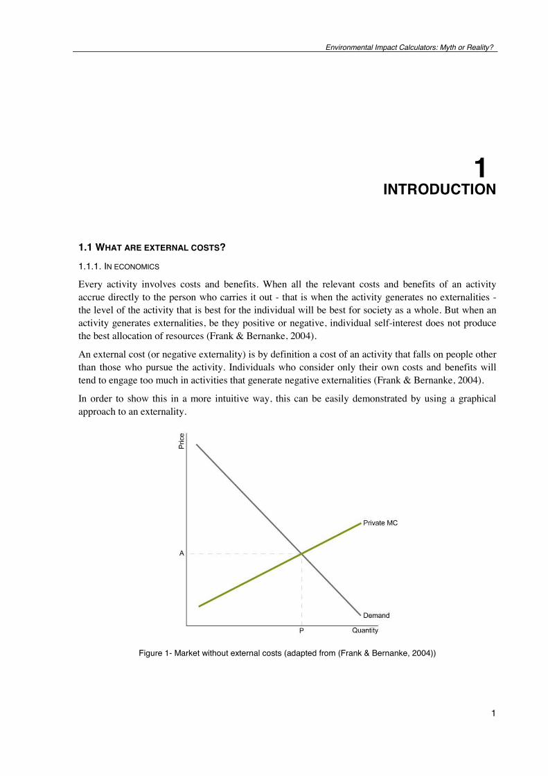
Every activity involves costs and benefits. When all the relevant costs and benefits of an activity accrue directly to the person who carries it out - that is when the activity generates no externalities - the level of the activity that is best for the individual will be best for society as a whole. But when an activity generates externalities, be they positive or negative, individual self-interest does not produce the best allocation of resources (Frank & Bernanke, 2004).
An external cost (or negative externality) is by definition a cost of an activity that falls on people other than those who pursue the activity. Individuals who consider only their own costs and benefits will tend to engage too much in activities that generate negative externalities (Frank & Bernanke, 2004).
In order to show this in a more intuitive way, this can be easily demonstrated by using a graphical approach to an externality.
Figure 1- Market without external costs (adapted from (Frank & Bernanke, 2004))
Environmental impact calculators: myth or reality?
2
In Figure 1 is shown the situation of a market without any external costs or benefits thus making the resulting equilibrium quantity and price the socially optimal one (Frank & Bernanke, 2004).
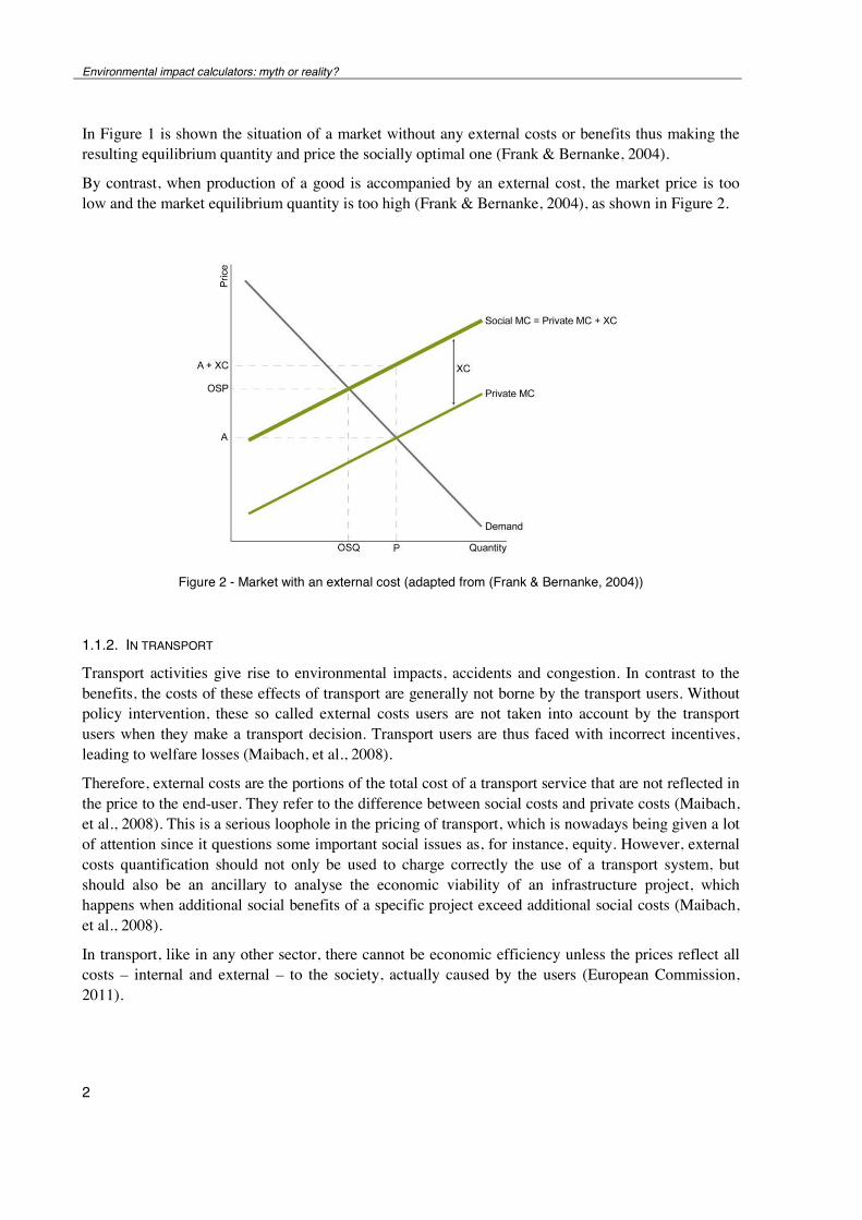
By contrast, when production of a good is accompanied by an external cost, the market price is too low and the market equilibrium quantity is too high (Frank & Bernanke, 2004), as shown in Figure 2.
Figure 2 - Market with an external cost (adapted from (Frank & Bernanke, 2004))
1.1.2. IN TRANSPORT
Transport activities give rise to environmental impacts, accidents and congestion. In contrast to the benefits, the costs of these effects of transport are generally not borne by the transport users. Without policy intervention, these so called external costs users are not taken into account by the transport users when they make a transport decision. Transport users are thus faced with incorrect incentives, leading to welfare losses (Maibach, et al., 2008).
Therefore, external costs are the portions of the total cost of a transport service that are not reflected in the price to the end-user. They refer to the difference between social costs and private costs (Maibach, et al., 2008). This is a serious loophole in the pricing of transport, which is nowadays being given a lot of attention since it questions some important social issues as, for instance, equity. However, external costs quantification should not only be used to charge correctly the use of a transport system, but should also be an ancillary to analyse the economic viability of an infrastructure project, which happens when additional social benefits of a specific project exceed additional social costs (Maibach, et al., 2008).
In transport, like in any other sector, there cannot be economic efficiency unless the prices reflect all costs – internal and external – to the society, actually caused by the users (European Commission, 2011).
Environmental Impact Calculators: Myth or Reality?
3
The internalization of external costs in the transport sector is therefore an important line of approach, since it aims to correct some private behaviour by attributing a market price to these costs, shifting them from the scope of the society to the user himself.
1.2 WHAT KIND OF EXTERNAL COSTS? 1.2.1. GENERAL
There are various types of external costs due to transport, namely accidents, noise, air pollution (health, material damage and biosphere), climate change risks, costs for nature and landscape, additional costs in urban areas, up and downstream processes and congestion (Schreyer et al., 2004). However, there are different costs for different transport modes and road transport has been the one more penalized by the different external costs assessments. The European Automobile Manufacturers Association (ACEA) contested the IMPACT study in terms of the external costs considered. They question the legitimacy of some of the costs considered with the argument that they are partly internalized by the free market and, thus, don’t need regulation. According to the ACEA, the ones that enter in this spectrum are congestion costs because they are internalized by the motorists themselves, accident costs since insurance companies play the biggest role in these costs and noise costs, partly compensated by lower rents of houses exposed to this externality. However, it is acknowledged that climate change and air pollution are external costs that are not paid for in any way (Baum et al., 2008). It is therefore possible to conclude that these two cost categories are considered external whatever the economic interest of a certain transport mode. Some insight will also be given on other external costs due to transport so as to display the problem of external costs as fully as possible.
1.2.2. CLIMATE CHANGE
1.2.2.1. General
Climate change related with greenhouse gas emissions (GHG) is an issue that is currently being given a lot of attention. There is raising awareness about this problem, due to its special characteristics when it comes to external costs as (Maibach, et al., 2008):
• Climate change is a global issue so that the impact of emissions is not dependent on the loca-tion of emissions;
• Greenhouse gases, especially CO2 have a long lifetime in the atmosphere so that present emissions contribute to impacts in the distant future;
• Especially the long-term impacts of continued emissions of greenhouse gases are difficult to predict, but potentially catastrophic.
As far as the European Commission is concerned, the goals have been set. In 2010 The European Council endorsed the European 2020 strategy for smart, sustainable and inclusive growth, setting out a vision of Europe’s new social market economy for the 21st century. Among these, the aim of the resource efficiency flagship is to support the shift towards a resource-efficient and low-carbon economy that is efficient in the way it uses all resources. The stated aim is to decouple economic growth from resource and energy use, reduce CO2 emissions, enhance competitiveness and promote greater energy security (European Commission, 2011). The goal is to obtain a reduction of GHG emissions that is consistent with the long-term requirements for limiting climate change to 2º C and
Environmental impact calculators: myth or reality?
4
with the overall target for EU of reducing emissions by 80% by 2050 compared to 1990 (European Commission, 2011).
1.2.2.2. The role of the transport sector
Climate change or global warming impacts of transport are mainly caused by emissions of the green-house gases carbon dioxide (CO2), nitrous oxide (N2O) and methane (CH4) (Maibach et al., 2008). Transport-related emissions play a very important role on global CO2 emissions. Nowadays, the sector accounts for approximately 15% of overall greenhouse gas emissions (OECD, 2010) and 29% of the greenhouse gas emissions among the EU27 (European Federation for Transport and Environment 2010). There is a natural concern with the trends of CO2 emissions due to transport, since they have grown 45% between 1990 and 2007 (OECD, 2010). This being said, it also has to be taken into account that transport is the fastest growing economic sector (Schreyer et al., 2004).
Therefore, transport is seen as one of the core sectors of intervention. The European Commission has recently published their White Paper on Transport, with the main goal being the achievement of a 60% reduction of transport-related emissions by 2050 when compared to 1990 values (European Commission, 2011). Having transport-related emissions in the EU27 grown around 24% between 1990 and 2008 (excluding international aviation and maritime, in accordance with the Kyoto Protocol) (European Environment Agency, 2010) the reduction from current emissions to the ones aimed at by 2050 comes up to around 75%, which seems a very ambitious goal. It is important to note, that this reduction goal on emissions is only on a tank-to-wheel basis (European Commission, 2011), meaning that only the direct emissions from the vehicle are accounted for. In practice, this can mean that an electric vehicle will have a 0 emissions balance. Therefore, power generation mix plays here an important role: the large scale electrification of transport not accompanied by the decarbonisation of power generation would only shift CO2 emissions from transport to the energy sector (European Commission, 2011). Tuchschmid (2009) points out that higher costs (and emissions) on infrastructure tend to reduce the emissions during the vehicle’s operation.
These facts seem to point in the way that vehicle and infrastructure should not be treated separately and that the reduction goal of transport-related emissions should be aimed at in a much larger scope, taking in account the transport mode in its whole. If such thing is not done, internalization measures could have the perverse effect of favouring a less efficient transport mode.
1.2.3. AIR POLLUTION
1.2.3.1. General
Air pollution costs are caused by the emission of air pollutants such as particulate matter (PM), nitrous oxides (NOx), sulphur dioxide (SO2) and volatile organic compound (VOC) and consist of health costs, building/material damages, crop losses and costs for further damages for the ecosystem (biosphere, soil, water) (Maibach, et al., 2008). The approach to these effects is different from that of climate change, since the location of the emission is in this case relevant, contrarily to that of greenhouse gases.
Environmental Impact Calculators: Myth or Reality?
5
1.2.3.2. In transport
When it comes to transport, transport flows and emissions are the main inputs to assess the concentration of air polluters. The consequences of these concentrations and thus, the effects on society are however dependent on geographical distribution of people and on the dominant wind directions (Maibach, et al., 2008). This is the general approach to this problem done by the Impact Pathway Approach.
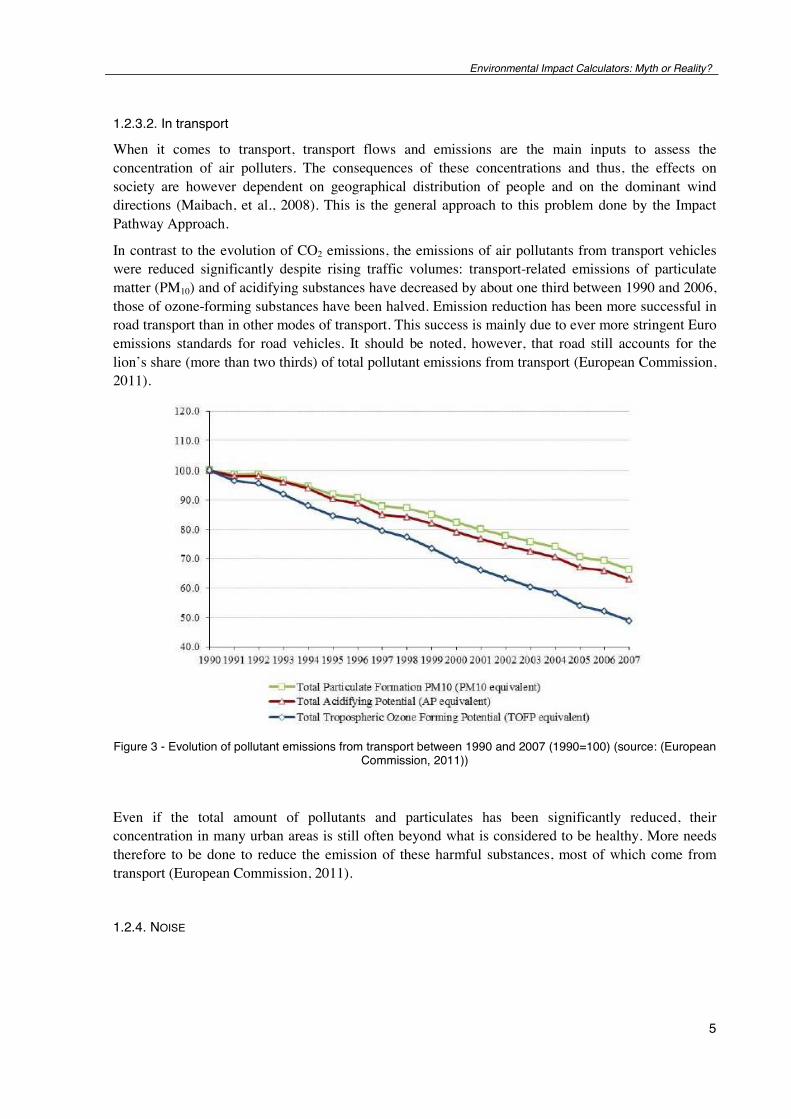
In contrast to the evolution of CO2 emissions, the emissions of air pollutants from transport vehicles were reduced significantly despite rising traffic volumes: transport-related emissions of particulate matter (PM10) and of acidifying substances have decreased by about one third between 1990 and 2006, those of ozone-forming substances have been halved. Emission reduction has been more successful in road transport than in other modes of transport. This success is mainly due to ever more stringent Euro emissions standards for road vehicles. It should be noted, however, that road still accounts for the lion’s share (more than two thirds) of total pollutant emissions from transport (European Commission, 2011).
Figure 3 - Evolution of pollutant emissions from transport between 1990 and 2007 (1990=100) (source: (European
Commission, 2011))
Even if the total amount of pollutants and particulates has been significantly reduced, their concentration in many urban areas is still often beyond what is considered to be healthy. More needs therefore to be done to reduce the emission of these harmful substances, most of which come from transport (European Commission, 2011).
1.2.4. NOISE
Environmental impact calculators: myth or reality?
6
1.2.4.1. General
Noise can be defined as the unwanted sound or sounds of duration, intensity, or other quality that causes physiological harm to humans (Maibach, et al., 2008).
Noise costs consist of costs for annoyance and health. The annoyance costs are usually economically based on preferences of individuals, whereas health costs are based on dose response figures (Maibach, et al., 2008).
1.2.4.2. In transport
In general, two types of negative impacts of transport noise can be distinguished (Maibach, et al., 2008):
• Costs of annoyance: transport noise imposes undesired social disturbances which result in so-cial and economic costs like any restrictions on enjoyment of desired leisure activities, dis-comfort or inconvenience;
• Health costs: transport noise can also cause physical health damages. Hearing damage can be caused by noise levels above 85 dB(A) while lower levels (above 60 dB(A)) may result in nervous stress reactions, such as change of heart beat frequency, increase of blood pressure and hormonal changes.
The basis measurement index for noise is the decibel (dB). This index has a logarithmic scale, reflect-ing the logarithmic manner the human ear responds to sound pressure. The logarithmic nature of noise is also reflected in the relationship between noise and traffic volume. By halving or doubling the amount of traffic the noise level will be changed by 3 dB, irrespective of the existing flow (Maibach, et al., 2008).
The fact mentioned above gives this external cost a particular characteristic, especially when the question raised is on how to price it. Marginal noise costs are extremely sensitive to existing traffic flows or more general to existing (background) noise. If the existing traffic levels are already high, adding one extra vehicle to the traffic will result in almost no increase in the existing noise level. Due to this decreasing cost function marginal noise costs can fall below average costs for medium to high traffic volumes (Maibach, et al., 2008).
1.2.5. ACCIDENT
Transport is a dangerous activity. These accidents can concern not just those involved in transport itself but also third parties (Button, 1993).
Valuing the external accident costs of transport poses a particular problem. Accident risks are partly internalized within transport in the sense that individuals can insure themselves. However, many travellers have no insurance or, where it has been taken up, it is on the basis of a misperception of the risks involved. There are also third-party risks involved in the possibility of accidents during the transport of dangerous goods or toxic waste (Button, 1993).
Besides the uncertainty behind the external cost itself, its monetary valuation is not clear.
There are many studies and conventions available on total (social) accident costs, as information for the assessment of optimal safety measures in the transport sector. Not many studies so far have however focused on (marginal) external accident costs (Maibach, et al., 2008).
Environmental Impact Calculators: Myth or Reality?
7
It is quite a complex problem since the uncertainty is quite high in respect to the cost drivers that are assumed to be responsible for these accidents. This makes it difficult to acknowledge the avoidance costs correctly. If another approach is chosen and the assessment of these costs is aimed at, it is neces-sary to put a monetary value on human life. Button (1993) raises this question to show that this cannot be done in terms of lost production (what output the economy forgoes if someone is killed in a transport related accident) since a pensioner’s death would be considered positive!
1.2.6. CONGESTION
When users of a particular facility begin to interfere with other users because the capacity of the infrastructure is limited, the congestion externalities arise (Button, 1993). This is a relevant externality for road transport because it is not access regulated.
On access regulated infrastructures this problem is of a different nature, being denominated as scarcity of infrastructure. Scarcity costs denote the opportunity costs to service providers for the non-availability of desired departure and arrival times (Maibach, et al., 2008). It may happen that these costs turn out to be internal, imposed on other users of the same company. This is the case if only one operator is present in an infrastructure (Maibach, et al., 2008).
This external cost has the particularity of not existing by itself. It is an outcome of the non-internalization of the other external costs of transport, leading to a dead weight loss due to market inefficiency.
Schreyer (2004) states that while all other cost categories considered reflect the external costs by transport on the whole of society, including inhabitants not participating in transport, congestion is a phenomenon within the transport sector. Yet, congestion does not only impose costs on the road user in terms of wasted time and fuel (the pure congestion cost) but the stopping and starting it entails can also worsen atmospheric and other forms of pollution (Button, 1993).
Congestion costs consist of internal and external components. Internal or private congestion costs are those increasing time and operating costs experienced by an operator when approaching or exceeding system capacity. External congestion costs are those costs experienced by all other system users due to the entrance of this operator into the system (Maibach, et al., 2008).
Environmental impact calculators: myth or reality?
8
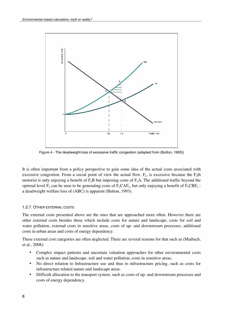
Figure 4 - The deadweight-loss of excessive traffic congestion (adapted from (Button, 1993))
It is often important from a policy perspective to gain some idea of the actual costs associated with excessive congestion. From a social point of view the actual flow, Fa, is excessive because the Fath motorist is only enjoying a benefit of FaB but imposing costs of FaA. The additional traffic beyond the optimal level Fo can be seen to be generating costs of FoCAFa, but only enjoying a benefit of FoCBFa - a deadweight welfare loss of (ABC) is apparent (Button, 1993).
1.2.7. OTHER EXTERNAL COSTS
The external costs presented above are the ones that are approached more often. However there are other external costs besides these which include costs for nature and landscape, costs for soil and water pollution, external costs in sensitive areas, costs of up- and downstream processes, additional costs in urban areas and costs of energy dependency.
These external cost categories are often neglected. There are several reasons for that such as (Maibach, et al., 2008):
• Complex impact patterns and uncertain valuation approaches for other environmental costs such as nature and landscape, soil and water pollution, costs in sensitive areas.
• No direct relation to Infrastructure use and thus to infrastructure pricing, such as costs for infrastructure related nature and landscape areas.
• Difficult allocation to the transport system, such as costs of up- and downstream processes and costs of energy dependency.
Environmental Impact Calculators: Myth or Reality?
9
While the assessment of the impacts relative to up- and downstream processes is somewhat straight forward, since they ultimately fall into the external costs categories mentioned above, the impacts on the environment are attached with much more uncertainty.
A critical aspect concerning the costs for nature and landscape as well as the costs for soil and water pollution are the very complex impact patterns of the natural ecosystems. Therefore, the knowledge about the detailed impact patterns and dose-response-relationships is less developed than for other cost categories. Often, negative impacts of transport activities on the natural environment can be proven. However, the detailed relationship between activity and impact can hardly be quantified. As a consequence, damage costs can often not be quantified and the calculation has to be done with second best approaches such as the estimation of repair cost based on specific local situations (Maibach, et al., 2008).
1.3 WHO PAYS? There are two essential ways of looking at this problem: that of Pigou and that of Coase.
Pigou tax literature – particularly the policy literature – concentrates on the presumption that the tax should equal the marginal externality, also known as the Pigou externality (Nye, 2008). This is done by assuming that a party A inflicts harm on B, raising the question: how should we restrain A?
Coase (1960) argues that this is a wrong approach and looks at this problem as one of a reciprocal nature. To avoid the harm to B would inflict harm on A. He concludes by stating that in the absence of transaction costs (idyllic), A and B will agree to achieve the efficient solution irrespective of whether A has the right to pollute or B has the right to amenity initially.
These points of view have led to great discussion among economists but are also relevant for policy-makers in the transport sector. While the EU seems to be following a polluter pays principle for their future internalization measures, the road sector (International Road Transport Union, 2008) defends that it is outdated and that Coase’s cheapest cost avoider principle should be used.
Ng (2007) criticizes Coase’s approach for not taking into account several aspects of the problem among which the under-provision of environmental quality due to its global public-good and long-term nature. This is an important aspect, since it is questionable if the environment and its finite resources can be exchanged for the “right” price. He defends the usefulness of a bilateral tax on an external cost not only in making the sufferer take account of the costs imposed on the causer in having to reduce the relevant activity, but also in ensuring that the sufferer has no incentive to exaggerate or understate the true damage.
Nye (2008) defends that even an increase on fuel taxes by substitution of the existing ones for a flat Pigou tax would only mean a small shift on fuel prices, resulting in minor changes when it comes to fuel consumption.
When it comes to externalities, specifically environmental ones, the question raised is if this is really an economic problem.
There might be a conflict between the desire to attain the optimal efficiency level and the desire to attenuate pollution, congestion or carbon emissions directly. The main concern of policy seems to be the reduction of the size of the externality itself, rather than finding an economic optimal. The relevant issue is not how much pollution/externality remains, but whether the activities causing the externality are at their optimal social level (Nye, 2008).
Environmental impact calculators: myth or reality?
10
However, the European Commission aims at a decoupling of economic growth from resource and energy use along with a reduction of CO2 emissions (European Commission, 2011), therefore aiming at a reduction of this specific externality.
1.4 “IF YOU CAN’T MEASURE IT YOU CAN’T MANAGE IT!” MCKINNON, PIECYK (2010) 1.4.1. GENERAL
If the goal is to reduce GHG emissions, the right place to start seems to be their correct measurement.
Efforts have been made internationally to standardize the measurement and reporting of these emissions in order to ensure comparability. At present there is no single agreed standard (McKinnon & Piecyk, 2010). This fact raises a problem since, accordingly with their background, the goals, the methods used, the assumptions and thus the results vary between different studies with consequences on possible comparability between them.
So the present-day question is: what is the way to measure these emissions correctly so as to be agreed upon universally?
McKinnon and Piecyk (2010) give some guidance to the individual business on the appropriate steps to be taken for the measurement and reporting of carbon emissions from their operations, approaching the most relevant aspects to measure the transport related ones.
1.4.2. SYSTEM BOUNDARY
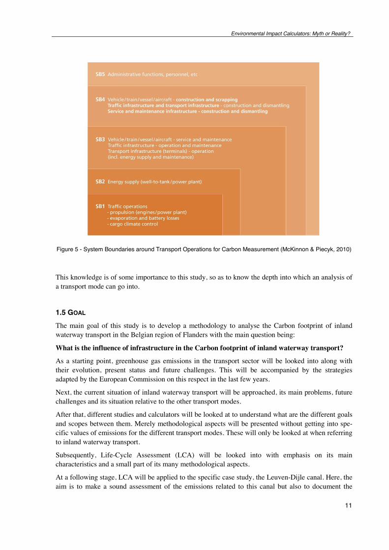
The Swedish environmental organization, NTM, has differentiated the levels of system boundary that can be drawn around a transport operation and labeled them SB1-SB5 (Figure 5). These levels are cumulative (McKinnon & Piecyk, 2010):
• SB1: confines the calculation to emissions from the actual transport operation, most of which emanate from the vehicle exhaust, though in the case of electrified rail freight operations include emissions from the electrical power source
• SB2: also takes account of the extraction, production, refining, generation and distribution of energy, taking a so called ”well-to-tank” perspective
• SB3: also includes the servicing and maintenance of vehicles and transport infrastructure • SB4: broadens the scope even further to include emissions from the manufacture of the vehi-
cles, construction of transport infrastructure and their subsequent scrappage and dismantling • SB5: also includes emissions associated with the management of transport operations, essen-
tially office functions and the activities of staff
Environmental Impact Calculators: Myth or Reality?
11
Figure 5 - System Boundaries around Transport Operations for Carbon Measurement (McKinnon & Piecyk, 2010)
This knowledge is of some importance to this study, so as to know the depth into which an analysis of a transport mode can go into.
1.5 GOAL The main goal of this study is to develop a methodology to analyse the Carbon footprint of inland waterway transport in the Belgian region of Flanders with the main question being:
What is the influence of infrastructure in the Carbon footprint of inland waterway transport?
As a starting point, greenhouse gas emissions in the transport sector will be looked into along with their evolution, present status and future challenges. This will be accompanied by the strategies adapted by the European Commission on this respect in the last few years.
Next, the current situation of inland waterway transport will be approached, its main problems, future challenges and its situation relative to the other transport modes.
After that, different studies and calculators will be looked at to understand what are the different goals and scopes between them. Merely methodological aspects will be presented without getting into spe-cific values of emissions for the different transport modes. These will only be looked at when referring to inland waterway transport.
Subsequently, Life-Cycle Assessment (LCA) will be looked into with emphasis on its main characteristics and a small part of its many methodological aspects.
At a following stage, LCA will be applied to the specific case study, the Leuven-Dijle canal. Here, the aim is to make a sound assessment of the emissions related to this canal but also to document the

Environmental impact calculators: myth or reality?
12
limitations of the methodology applied and of data provision, though these are closely related. Furthermore, some conclusions will be made about the results attained.
Environmental Impact Calculators: Myth or Reality?
13
2 CO2 IN THE TRANSPORT SECTOR
2.1 HOW HAS IT EVOLVED? (THEN AND NOW) Transport demand has shown strong growth rates in the 1990s. Rapidly rising traffic volumes resulted in high levels of congestion, noise and air pollution which were considered to be unsustainable (European Commission, 2011).
As transport growth in the 1990s had been uneven, mainly benefiting road and air, while largely neglecting cleaner and less congested modes of transport such as rail and inland waterways, another main objective in 2001 was rebalancing the modal distribution of transport, away from congested roads and airports towards other, less congested and often also more environmentally friendly modes (European Commission, 2011).
The 2001 White Paper therefore included a series of measures which were to allow the non-road modes to return by 2010 to their market shares of 1998 and prepare ground for a shift in the modal balance from then on. Shifting the balance between the modes of transport had become one of the main objectives of the White Paper. This was to be achieved by regulating the competition between the modes and by promoting intermodal transport. The objective of bringing the modal share of road by 2010 back to where it was in 1998 has not been achieved. In fact, the share of road haulage in total intra-EU freight transport has increased from close to 43% in 1998 to almost 46% in 2008 (European Commission, 2011).
The general idea was that full internalisation of external costs could solve this problem, putting an end to some nuisances that occur within the freight transport sector and paving the path to the goal of decoupling transport from GDP growth assumed by the European Commission in its White Paper of 2001.
Yet over time, it had become clear that the objective of decoupling, as it was, needed to be refined. While the renewed EU Sustainable Development Strategy of 2006 kept the operational objective of “decoupling economic growth and the demand for transport with the aim of reducing environmental impacts”, the 2006 mid-term review of the White Paper modified the original target into one of decoupling the growth of transport from its negative effects such as congestion, accidents and the emission of pollutants, CO2 and noise (European Commission, 2011).
In 2007, the Commission adopted a Freight Transport Logistics Action Plan which aimed at making freight transport in the EU more efficient and more sustainable. It contained a number of measures which were to increase the attractiveness of non-road modes, e.g. through the creation of a European maritime space without barriers, the development of a freight-oriented rail network or the definition of green corridors. Other measures looked at the whole logistics chain and tried to reduce the
Environmental impact calculators: myth or reality?
14
administrative hurdles in intermodal transport by developing a single transport document. In addition, the use of new technologies such as e-freight and intelligent transport systems in freight transport was to be promoted. The rules on vehicle dimensions and standards in road transport were also to be reviewed. Some of the measures have only recently been adopted or are still in the pipeline; it is therefore too early to assess any measurable impact from them (European Commission, 2011).
One can conclude that the European Commission’s refined goals are relatively new and that they are an adaptation to the challenges that the transport sector is faced with in the present being also an active voice on the future of the transport sector. While before the main goal was to decouple transport growth from the economic growth so as to head towards a more sustainable economy, today the stated goal is the reduction of the CO2 emissions regarding transport as economically and as socially sound as possible. This change in the order of priorities is a reflection of the urgency needed to approach this problem.
2.2 HOW MUCH DOES CO2 COST? 2.2.1. GENERAL
Climate change costs have a high level of complexity due to the fact that they are long term and global and that risk patterns are very difficult to anticipate. Various impacts of global warming causing external costs are listed below (Maibach, et al., 2008):
• Sea level rise • Energy use • Agricultural impacts • Water supply • Health impacts • Ecosystems and biodiversity • Extreme weather events • Major events
In a damage cost approach a valuation of these effects needs to be carried out. In the avoidance cost approach the costs of avoiding these effects to a desired extent are estimated (Maibach, et al., 2008).
The main cost drivers for marginal climate cost of transport are the fuel consumption and carbon content of the fuel. Therefore, marginal climate costs are preferably expressed in Euro per litre of fuel. For internalisation purposes the estimated external costs of CO2 emissions can be factored in to the price of transport fuels on the basis of their respective CO2 contents (direct emissions of burning a litre of fuel) or total well-to-wheel greenhouse gas emissions per litre of fuel used by multiplying the grams of CO2 per litre with the external costs per gram of CO2 emitted (Maibach, et al., 2008).
2.2.2. DAMAGE-COST APPROACH
The damage cost approach follows the impact pathway approach and uses detailed modelling to assess the physical impacts of climate change and combines these with estimations of the economic impacts resulting from these physical impacts (see e.g. Watkiss 2005a and 2005b). The costs of sea level rise could e.g. be expressed as the costs of land loss. Agricultural impact can be expressed as costs or benefits to producers and consumers, and changes in water runoff might be expressed in new flood damage estimates (Maibach, et al., 2008).
Environmental Impact Calculators: Myth or Reality?
15
Impact pathway assessment is a bottom-up methodology in which environmental benefits and costs are estimated by following the pathway from source emissions via quality changes of air, soil and water to physical impacts, before being expressed in monetary benefits and costs. The use of such detailed bottom-up methodology – in contrast to earlier top-down approaches – is necessary, as external costs are highly site-dependent (cf. local effects of pollutants) and as marginal (and not average) costs have to be calculated. Within the pathway approach, exposure-response models are used to derive physical impacts on the basis of these receptor data and concentration levels of air pollutants (European Commission, 2003).
Economic valuation, especially in the area of climate change, is often controversial. First of all there is a general lack of knowledge about the physical impacts caused by global warming. Some impacts are rather certain and proven by detailed modelling, while other possible impacts, such as extended flooding or hurricanes with higher energy density are often not taken into account due to lack of information on the relationship between global warming and these effects (Maibach, et al., 2008).
Available damage cost estimations of greenhouse gas emissions vary by orders of magnitude due to special theoretical valuation problems related to equity, irreversibility and uncertainty. Concerning equity both intergenerational and intragenerational equity must be considered (Maibach, et al., 2008).
2.2.3. AVOIDING-COST APPROACH
The method is based on a cost-effectiveness analysis that determines the least-cost option to achieve a required level of greenhouse gas emission reduction, e.g. related to a policy target. The target can be specified at different system levels, e.g. at a national, EU or worldwide level and may be defined for the transport sector only or for all sectors together (Maibach, et al., 2008).
According to (Watkiss, 2005b), (RECORDIT, 2000) and other studies the avoidance costs approach is not a first-best-solution from the perspective of welfare economics, but can be considered theoretically correct under the assumption that the selected reduction target represents people’s preferences appropriately. Under that assumption the marginal avoidance costs associated with the reduction target can be interpreted as a ‘willingness-to-pay’ value. For this reason the avoidance cost approach should only be used in combination with reduction targets that are laid down in existing and binding policies or legislation. For CO2 emissions this generally comes down to targets fixed in the context of the Kyoto-protocol (Maibach, et al., 2008).
2.2.4. THE POSITION OF THE EUROPEAN AUTOMOBILE MANUFACTURERS ASSOCIATION
When it comes to putting a price on CO2 the road sector is particularly critic on the IMPACT study, mainly for choosing damage-costs over avoiding-costs.
In the case of the use of damage-costs to evaluate long-term climate effects, they argue that with this approach, damages that refer to crop losses, weather fluctuations, floods, land losses, and serious health problems are to be detected. Especially for the long-term perspective, such climate damages are not assessable. It is not useful to evaluate damages which cannot be sufficiently specified in terms of extent, the time of incidence or the occurrence probability. Hence, the estimation of CO2 emission costs is afflicted with substantial uncertainties and speculative elements. These uncertainties are also evident through the fact that the fluctuation range is substantially larger for damage costs than for avoiding costs (Baum, Geibler, Schneider, & Buhne, 2008).
Environmental impact calculators: myth or reality?
16
2.3 INTERNALISATION OF EXTERNAL COSTS? Modern transport systems have given Europe a high degree of mobility with an ever increasing performance in terms of speed, comfort, safety and convenience. However, this enhanced mobility has developed over the last decades in a context of generally cheap oil, expanding infrastructure and loose environmental constraints. Now that those framework conditions have changed, the transport system is no longer able to develop along the same path without serious unintended consequences in the form of environmental, economic and social costs (European Commission, 2011).
The internalisation of external costs was seen as the ideal measure to solve the deadweight loss resultant of the congestion of a transport system, therefore making the private optimal equal to the social optimum.
In practice this meant eliminating “unnecessary” transport activities – activities that do not add any economic value or which are the result of regulatory failures. One regulatory failure was seen in the fact that transport users did not pay the full price of the external costs which their activities produce. As long as external costs were not fully borne by transport users, the demand for transport was bound to be artificially high. Appropriate pricing and infrastructure policies that applied the “user pays” principle and the “polluter pays” principle would largely remove these inefficiencies over time (European Commission, 2011).
The policy of internalizing all external costs is still far from being fully implemented. Consequently, it has so far not contributed much to the decoupling of transport and GDP growth (European Commission, 2011).
However, even if all proposed measures had been fully implemented, it is questionable whether significant progress in decoupling freight transport from economic growth could have been achieved. Freight transport is largely a commercial business in which “unnecessary” transport activities are already limited. Moreover, logistics practices like “just-in-time” delivery and growing specialisation patterns dominate in modern industries. While improving the efficiency of European industry, they tend to increase the transport intensity of the economy (European Commission, 2011).
The ACEA criticise the way the European Commission view the issue of externalities, arguing that what remain as external costs have to be set against the external benefits of the transport mode. The economic welfare theory demands that motorists are only charged the cost minus the benefits. Road transport gives rise to a multitude of external benefits. Mobility improves the division of labour, increases productivity and leads to more growth, income and employment. The external benefits of transport are entirely neglected in the IMPACT study methodology. In this respect, charging only external costs does not result in a welfare optimum (Baum, Geibler, Schneider, & Buhne, 2008).
The ACEA states that if the goal is to achieve market equilibrium between the different modes, certain aspects would have to be arranged so as to achieve this. These measures have to do with the fact that presently different modes are charged in very different ways.
In the EU, considerable subsidies are paid for the railways and urban public transport in particular. Subsidies represent costs for the general public, who are not compensated for these by the recipients of the subsidies. Subsidies must therefore be added to the external costs. This improves the relative cost position for the roads (Baum, Geibler, Schneider, & Buhne, 2008).
It is also important that taxes and charges paid already are included in the external costs. Road transport pays more in taxes and charges than is necessary to cover infrastructure costs. This excess
Environmental Impact Calculators: Myth or Reality?
17
must be included as partial compensation for the external costs. This reduces the payment charge for road transport (Baum, Geibler, Schneider, & Buhne, 2008).
The ACEA conclude by arguing that it is doubtful whether there is a need for internalisation of CO2 costs at all, since those are already charged through high petrol and diesel taxes (Baum, Geibler, Schneider, & Buhne, 2008).
So one can question, is it an economic problem? Does it demand a market-based solution?
The latest White Paper on transport seems to answer these questions in some way, clearly stating that the main objective of achieving a sustainable transport system by 2050 can be translated into more specific goals (European Commission, 2011):
• A reduction of GHG emissions that is consistent with the long term requirements for limiting climate change to 2ºC and with the overall target fir the EU of reducing emissions by 80% by 2050 compared to 1990. Transport-related emissions of CO2 should be reduced by around 60% by 2050 compared to 1990. It includes aviation, but excludes international maritime.
• A drastic decrease in the oil dependency ratio of transport-related activities by 2050 • Limit the growth of congestion
The three specific policy objectives could be broadly summarised as the prescription to “use less energy, use cleaner energy and better exploit infrastructure” (European Commission, 2011).
However, policies of this nature can sometimes have undesirable effects.
It is generally accepted that sustainable transport implies finding a proper balance between (current and future) environmental, social and economic sustainability goals. Two main trade-offs between sustainability goals can be highlighted (European Commission, 2011):
• First of all, there could be a conflict between cheap transport and GHG abatement. Fossil fuels have the great advantage of energy density. This is a valuable characteristic in mobile applications and the reason why fossil fuels are currently the cheapest option for transport. Clearly it will cost more to replace them. The trade-off is solved by setting a goal for emissions (the priority objective) and by devising a cost minimising strategy to achieve it.
• Secondly, there could be a conflict between improving accessibility and lowering congestion, which could imply additional infrastructure, and land use. This trade-off is more severe in the EU-12, where catching up with EU-15 makes certain infrastructure development a necessity. This trade-off is solved by giving priority to the upgrade of infrastructure over new construction and to “green infrastructure” but each project would have to be assessed individually on its own merits.
Therefore, it is possible to conclude that with the most recent White Paper on transport the problem is no longer economical. The goal is not to internalise external costs so as to achieve market equilibrium between transport modes and global social welfare. The goal is to reduce the external cost of CO2 emissions as responsibly as possible, socially and economically. However, if one is to achieve such ambitious goals, there will surely be a social and economic cost attached.
It is even questionable if one can use the definition of external cost to describe these emissions, since they are not confronted with the benefits attached to them and as the goal is not to achieve a market-based solution to the problem inherent to the transport sector.

Environmental impact calculators: myth or reality?
18
Environmental Impact Calculators: Myth or Reality?
19
3 INLAND WATERWAY TRANSPORT
3.1 WHERE DOES IT STAND? It is in the context presented before that inland waterway transport can have a prominent role.
Inland waterways transport has a reputation for environmentally friendly transport as it has very little impact on landscape, pollution of water is small and air emission per tonne kilometre is low compared to road transport given the current applied technologies (van Donselaar & Carmigchelt, 2001).
However, this transport mode has an important limitation that has to be taken into account which is the fact that inland waterway transport is only part of the transport chain, since it cannot generally deliver goods door-to-door and must therefore be complemented by rail or road transport at each end linked by intermodal transhipment (International Navigation Association, 2005).
Traditionally, inland shipping has a strong position in the long-distance haulage of bulk transport. In the last two decades inland shipping has also successfully entered new markets such as the hinterland transport of maritime containers, experiencing a two-digit annual growth rate. Its expansion into the transport of continental cargo and short distance traffic also unlocks the potential for new distribution solutions, responding better to modern logistics requirements (Commission of the European Communities, 2006).
However, the image of the inland navigation sector has not kept pace with the logistics and technological performance achieved. General awareness and knowledge of the real potential of the sector in terms of quality and reliability need to be improved (Commission of the European Communities, 2006).
3.2 WORKSHOP “INLAND NAVIGATION CO2 EMISSIONS – HOW TO MEASURE THEM? HOW TO REDUCE THEM? 3.2.1. GENERAL
On April 12th 2011, the Central Commission for the Navigation of the Rhine (CCNR) held a workshop intended at determining the amount of CO2 emissions due to inland water transport and also aimed at examining measures to reduce them.
An objective and well-founded depiction of greenhouse gas emissions by inland navigation is urgently needed, since current studies for freight forwarders and policy-advise use emission values that seem to ignore the greater efficiency achieved by inland navigation in recent years (CCNR 2011).
Environmental impact calculators: myth or reality?
20
It was in the above mentioned context that the workshop “Inland Navigation CO2 emissions – How to measure them? How to reduce them?” was held with its division being made into 4 parallel workshops focusing on different aspects concerning the main theme. The one that is relevant to this study and at the same time the one that the author participated in is Parallel Workshop 1 focusing on methods to determine the Carbon footprint of this transport mode. However, this workshop turned out to be a broad overlook on the assumptions that were being made when it comes to these calculators.
3.2.2. PARALLEL WORKSHOP 1 – METHODS TO DETERMINE THE CO2 EMISSIONS FROM INLAND NAVIGATION
3.2.2.1. Standardization of a common methodology for the calculation, declaration and reporting on energy consumption and GHG emissions of transport services (Marc Cottignies, ADEME, Valbonne)
This presentation was a very simple one that just described the basic assumptions behind the French Environment and Energy Management Agency (ADEME) project when it comes to CO2 calculators. They are presently working in a common methodology for the calculation and declaration on energy consumption and GHG emissions related to a transport service. This is part of the Work Group 10 of the European Committee for Standardization and its Technical Committee 320 on transport logistics and services.
The scope of their project is limited to the energy used by a vehicle of a certain mode of transport during its user-life phase, a Scope 1 approach. They also take into account a well-to-wheel approach, meaning that the upstream processes of energy provision are taken into account (Scope 2), otherwise, in an extreme case, an electric train would have a 0 emissions balance. An important and advantageous aspect is that they’re focusing on energy-based values to do this, only opting for activity-based values when no measurements are made available for a certain route. They also take into account empty trips.
Their primary goal is to make this understandable and user-friendly for companies that contract a transport service so as to make the declaration of the CO2 emissions related to transport as transparent as possible.
However, one cannot stop thinking that there are many variables that are not being taken into account. The simple fact that they are not taking into account any infrastructure costs, construction or even maintenance, can make a transport mode seem greener than it actually is. Higher costs (and emissions) on infrastructure, tend to reduce the emissions during the vehicle’s operation (Tuchschmid, 2009), so this kind of approach could lead companies to opt for a “less green” mode of transporting there goods.
Having said this, their goal is to develop this kind of thinking and consciousness on companies as soon as they can. This is because according to an article in law Grenelle II adopted in July 2010: information on CO2 emissions will become mandatory for each transport service, sent to the beneficiary by the supplier. This law is expected to be enforced around mid-2013.
Thus, their primary goal is to make this understandable and user-friendly for companies that provide a transport service.
3.2.2.2. Measuring and managing CO2 emissions of European chemical transport (Jos Verlinden, CEFIC, Brussels)
This presentation was based on the McKinnon report (2009) for CEFIC. In terms of calculation methods nothing new is approached in this report, having the values given been taken from previous
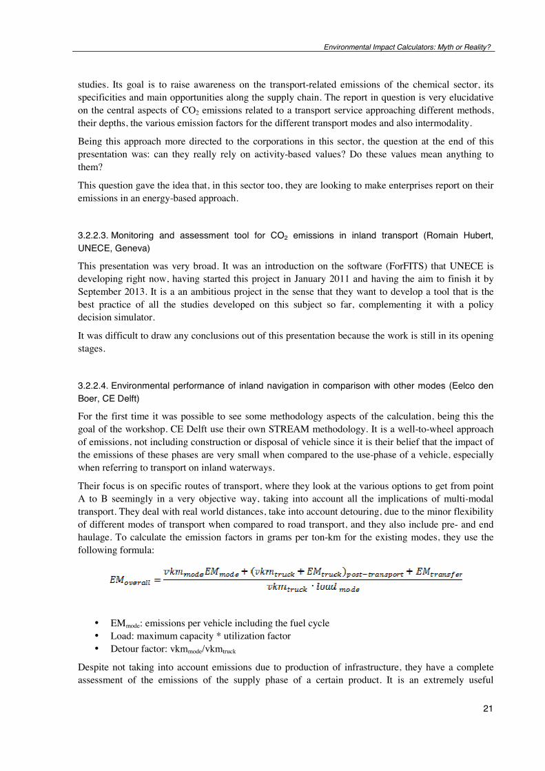
Environmental Impact Calculators: Myth or Reality?
21
studies. Its goal is to raise awareness on the transport-related emissions of the chemical sector, its specificities and main opportunities along the supply chain. The report in question is very elucidative on the central aspects of CO2 emissions related to a transport service approaching different methods, their depths, the various emission factors for the different transport modes and also intermodality.
Being this approach more directed to the corporations in this sector, the question at the end of this presentation was: can they really rely on activity-based values? Do these values mean anything to them?
This question gave the idea that, in this sector too, they are looking to make enterprises report on their emissions in an energy-based approach.
3.2.2.3. Monitoring and assessment tool for CO2 emissions in inland transport (Romain Hubert, UNECE, Geneva)
This presentation was very broad. It was an introduction on the software (ForFITS) that UNECE is developing right now, having started this project in January 2011 and having the aim to finish it by September 2013. It is a an ambitious project in the sense that they want to develop a tool that is the best practice of all the studies developed on this subject so far, complementing it with a policy decision simulator.
It was difficult to draw any conclusions out of this presentation because the work is still in its opening stages.
3.2.2.4. Environmental performance of inland navigation in comparison with other modes (Eelco den Boer, CE Delft)
For the first time it was possible to see some methodology aspects of the calculation, being this the goal of the workshop. CE Delft use their own STREAM methodology. It is a well-to-wheel approach of emissions, not including construction or disposal of vehicle since it is their belief that the impact of the emissions of these phases are very small when compared to the use-phase of a vehicle, especially when referring to transport on inland waterways.
Their focus is on specific routes of transport, where they look at the various options to get from point A to B seemingly in a very objective way, taking into account all the implications of multi-modal transport. They deal with real world distances, take into account detouring, due to the minor flexibility of different modes of transport when compared to road transport, and they also include pre- and end haulage. To calculate the emission factors in grams per ton-km for the existing modes, they use the following formula:
• EMmode: emissions per vehicle including the fuel cycle • Load: maximum capacity * utilization factor • Detour factor: vkmmode/vkmtruck
Despite not taking into account emissions due to production of infrastructure, they have a complete assessment of the emissions of the supply phase of a certain product. It is an extremely useful
Environmental impact calculators: myth or reality?
22
approach and seems to be very complete for corporations hoping to improve their supply chain in terms of efficiency. Specific routes were presented with the various emissions per transport mode and the results were very different between them, making a state that these aspects are in a sense unique to a transport route.
They conclude that there are many factors that influence emissions and that modal comparison depends heavily on vehicle capacity and utilization, stating that economies of scale are advantageous when it comes to inland freight transport and that there is still a significant reduction potential for this mode.
From this presentation one got the idea that when it comes to CO2 calculators, the idea of coming up with a universal calculator for all transport modes is a utopia. It would probably be preferable to look at the whole picture in a geographically limited area with similar characteristics for transporting goods of similar characteristics.
3.2.2.5. Calculation of CO2 emissions for a comparison of transport modes (Frank Trosky, PLANCO Consulting, Essen)
This presentation and the CE Delft one, above, were the only ones to approach specifically inland navigation and their emissions. However their results were quite different and the impression one got is that this one was more transport service-based than logistics-based, like the CE Delft one.
Firstly, in the presentation it was stated that motor trucks polluted much more than train and inland waterway transport, something that had confirmed results from 1990. While this might be true, the truth is that the trucking sector has evolved in a way that both train and vessels haven’t in the last twenty years. They argue that the studies related to train transportation (EcoTransit/Ifeu) don’t use the values for emissions of the biggest vessels which are normally smaller in terms of ton-km. Return trips are approached and some assumptions about these are made. They also take into account the depth of the water, which can limit the transport on an inland waterway. No reference is made to transhipments.
A comparison between the different transport modes on all the costs (including external costs) is done for several different selected routes and the conclusion is that inland waterways is always the most economic.
However, when looking at the study, one can observe that infrastructure costs are included but environmental costs due to infrastructure are not. Only CO2 emissions are taken into account and these are directly derived from the amount of energy consumption of a transport mode, i.e. from burning of fuel by motors of trucks, diesel locomotives and inland vessels. For electrical locomotives, emissions are caused by corresponding power generation, with these being the lowest CO2 emitters per unit of energy (PLANCO Consulting, 2007).
3.2.2.6. Overview of parallel workshop 1
The general idea that one got from this workshop is that there is not correct and standard way to calculate transport related emissions and that is especially notorious when it comes to inland water transport.
From the methodologies presented, one was logistics-based and made the comparison of different transport modes from one point to another, including detouring and operations of modal transfer when
Environmental Impact Calculators: Myth or Reality?
23
approaching intermodality; the other was service-based and made comparisons of different transport modes between different O-D pairs without making any reference to the necessary complementary actions needed for rail and waterway transport modes.
A logistics-based emission value of a whole transport operation seems like the best way to compare the different transport modes when it comes to their Carbon footprint. However, a full and specific assessment of all the emissions relative to a transport mode is necessary.
The impression one got is that there is need for the methodology to be as transparent as possible. Despite the fact that none of the presentations approached Carbon footprint with LCA, this seems to be the most transparent way to compare different transport modes. Another idea taken from this workshop is that these comparisons should be made the more site-specific as possible in a geographically limited area or for a specific O-D pair.
3.2.3. OVERVIEW OF THE WORKSHOP
At the end of the parallel workshops, the participants gathered to debate what had been discussed in the different parallel workshops. There were different technical proposals for the reduction of emissions related with inland waterway transport and there seems to be a lot of room for improvement. However, some impressive values for reduction of emissions were given and when questioned turned out to be for very extreme situations. The fact that inland vessels have a long lifespan, accentuates the difference between emissions of old and new boats which makes it necessary to be careful when handling this kind of data.

Environmental impact calculators: myth or reality?
24
Environmental Impact Calculators: Myth or Reality?
25
4 WHAT IS BEING DONE ON THE
CALCULATION OF CO2 EMISSIONS DUE TO TRANSPORT
4.1 WHAT IS BEING DONE ON CO2 CALCULATORS 4.1.1. GENERAL
Although climate change due to the transport sector is not a new found problem, only in recent years has it been approached more insistently, resulting in the production of several studies and calculators. The main goal is to estimate emission factors of the different transport modes or of the same one requested in different ways so as to compare them. The main aspect referred to in most of these studies has to do with the direct emissions of a transport mode, i.e., those that are emitted during the operation of a vehicle, with Tank-to-Wheel emissions being the main portion of these and the ones to be sanctioned in the near future according to the EU commission’s White Paper on transport.
Within the studies and calculators available there are also different target audiences. Some are directed to specific sectors and products, others to the individual businesses and others to policy-makers.
The most important studies and calculators will be briefly presented below.
4.1.2. METHODS FOR CALCULATING CO2 EMISSIONS FROM FREIGHT TRANSPORT OPERATIONS
4.1.2.1. Energy-based approach
Since almost all CO2 emissions from freight transport are energy-related, the simplest and most accu-rate way of calculating these emissions is to record energy use and employ standard emission factors to convert energy values into CO2. The unit of energy will typically be litres of fuel for trucks, diesel-hauled trains, barges and ships, and kilowatt hours (kWh) for electrified rail and pipeline (McKinnon & Piecyk, 2010).
4.1.2.2. Activity-based approach
In the absence of energy data, it is possible to make a rough estimate of the carbon footprint of a transport operation by applying a simple formula:
CO2= tonnes transported x average distance travelled x CO2 emissions factor per tonne-km. (McKinnon & Piecyk, 2010).
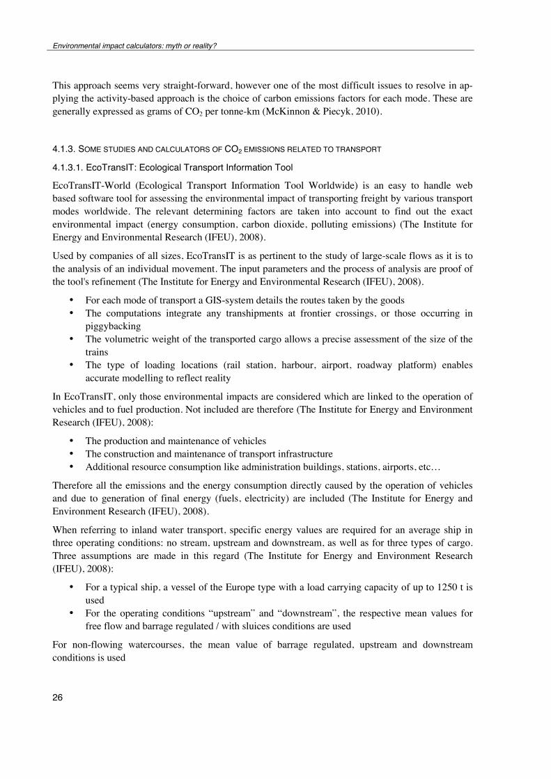
Environmental impact calculators: myth or reality?
26
This approach seems very straight-forward, however one of the most difficult issues to resolve in ap-plying the activity-based approach is the choice of carbon emissions factors for each mode. These are generally expressed as grams of CO2 per tonne-km (McKinnon & Piecyk, 2010).
4.1.3. SOME STUDIES AND CALCULATORS OF CO2 EMISSIONS RELATED TO TRANSPORT
4.1.3.1. EcoTransIT: Ecological Transport Information Tool
EcoTransIT-World (Ecological Transport Information Tool Worldwide) is an easy to handle web based software tool for assessing the environmental impact of transporting freight by various transport modes worldwide. The relevant determining factors are taken into account to find out the exact environmental impact (energy consumption, carbon dioxide, polluting emissions) (The Institute for Energy and Environmental Research (IFEU), 2008).
Used by companies of all sizes, EcoTransIT is as pertinent to the study of large-scale flows as it is to the analysis of an individual movement. The input parameters and the process of analysis are proof of the tool's refinement (The Institute for Energy and Environmental Research (IFEU), 2008).
• For each mode of transport a GIS-system details the routes taken by the goods • The computations integrate any transhipments at frontier crossings, or those occurring in
piggybacking • The volumetric weight of the transported cargo allows a precise assessment of the size of the
trains • The type of loading locations (rail station, harbour, airport, roadway platform) enables
accurate modelling to reflect reality
In EcoTransIT, only those environmental impacts are considered which are linked to the operation of vehicles and to fuel production. Not included are therefore (The Institute for Energy and Environment Research (IFEU), 2008):
• The production and maintenance of vehicles • The construction and maintenance of transport infrastructure • Additional resource consumption like administration buildings, stations, airports, etc…
Therefore all the emissions and the energy consumption directly caused by the operation of vehicles and due to generation of final energy (fuels, electricity) are included (The Institute for Energy and Environment Research (IFEU), 2008).
When referring to inland water transport, specific energy values are required for an average ship in three operating conditions: no stream, upstream and downstream, as well as for three types of cargo. Three assumptions are made in this regard (The Institute for Energy and Environment Research (IFEU), 2008):
• For a typical ship, a vessel of the Europe type with a load carrying capacity of up to 1250 t is used
• For the operating conditions “upstream” and “downstream”, the respective mean values for free flow and barrage regulated / with sluices conditions are used
For non-flowing watercourses, the mean value of barrage regulated, upstream and downstream conditions is used
Environmental Impact Calculators: Myth or Reality?
27
Return-trips were modelled as empty and it was taken into consideration that those empty trips are usually made against the course of the actual transport: an empty trip following a transport upstream will therefore be downstream. This was taken into account by assigning the assumed empty trip part of the calculation an energy consumption value according to the counter-direction (The Institute for Energy and Environment Research (IFEU), 2008).
Figure 6 - Scope of EcoTransIT (The Institute for Energy and Environment Research (IFEU), 2008)
4.1.3.2. Infrastructure, environmental and accident costs for Rhine container shipping (UNITE)
The Rhine is the most important European waterway with respect to inland shipping (van Donselaar & Carmigchelt, 2001).
The study focuses on the part of the Rhine where the biggest inland vessels can navigate, i.e. where this transport mode benefits from economies of scale. It is therefore expected for this to be the most favourable scenario for this transport mode. Marginal costs relative to the infrastructure, the environment and accident costs are approached.
In this study, the chapters that cover marginal infrastructure costs and marginal environmental costs are central to the case of the Leuven-Dijle canal. Although the waterway covered has very different characteristics from the case study, values relative to allocation matters can be taken into account and are of vital importance, since very little information about these aspects is available elsewhere.
Within the scope of marginal cost analysis are all infrastructure costs which can be identified to vary with traffic volume (van Donselaar & Carmigchelt, 2001). A number of terminals are also included in
Environmental impact calculators: myth or reality?
28
the Rhine waterway stretch, however, as the case study focuses on container transport these are by definition multi-modal. Intermodal freight terminals are not taken into account, only the costs relating to investments in quay walls and the port basin will be further researched with respect to terminal infrastructure costs (van Donselaar & Carmigchelt, 2001).
While the costs given are of a monetary nature, the ones intended for the case-study are to be given relatively to GHG emissions due to the various phases of the supplied transport mode. However, the values of this study will only be used for allocation purposes, mostly assuming that operational monetary costs are allocated in the same way as the external costs caused by GHG emissions. This would be true if operational costs were merely energy consumption dependent. However, it is thought that it is a reliable proxy to the allocation aspects relative to the GHG emissions of the transport mode. The allocation values used for infrastructure will be approached in the next chapter.
When it comes to the marginal environmental cost calculation and the CO2 emissions related with inland water transport, they are assumed to be relative to barge operation and are differentiated into 9 different ship size classes. There is also differentiation for steady and non-steady operation with the latter concerning operations such as hoteling, docking and undocking.
4.1.3.3. Charging and pricing in the area of inland waterways – Practical guideline for realistic transport pricing, ECORYS
The purpose of this study is to enable the European Commission to prepare a Community Framework for infrastructure charging based on marginal costs on the inland waterways in the European Union. The marginal (social) costs are defined as the costs generated by an additional transport unit when using the infrastructure (ECORYS Transport, 2005).
This study does not approach impacts due to GHG emissions, with the only environmental burden covered being due to local air pollution. However, some insight is given on what are the costs of operating an inland waterway and what are the main drives of these operations. On infrastructure costs, only the actual monetary costs are analysed. However, one can take into account some allocation assumptions made here and adapt them to the case-study.
Several approaches are covered with the goal to attribute a cost function to inland waterways, these being an econometric approach, an engineering approach and a cost-allocation approach. The two former approaches require a considerable amount of high-quality data (ECORYS Transport, 2005) while the need for cost information is considerably lower for the latter one.
The econometric approach starts with real occurring costs and seeks for a function to estimate the marginal costs. This means that the total expenditures, if necessary modified to reflect the equilibrium level of expenditure required, are analysed by using methods such as time series analysis or cross-section analysis (ECORYS Transport, 2005). Yet, expenditure on maintenance and renewals may be lagged many years behind the traffic that caused it, so that misleading results may be obtained if an organisation is not pursuing a “steady state” maintenance policy but running down its assets or adjusting maintenance and renewals according to the state of its finances (ECORYS Transport, 2005). Therefore, an adaptation will have to be made for postponement of infrastructure costs so as to turn into a continuous function so as to allocate these costs correctly.
Environmental Impact Calculators: Myth or Reality?
29
The engineering approach assumes specific knowledge of how specific infrastructure costs are determined and influenced. By specifying this exact relation the total costs can be determined as a function of a number of variables (ECORYS Transport, 2005).
The cost-allocation approach starts with the cost registration and tries to split up relevant costs into fixed and variable costs on a level of detail that is better (i.e. nearer to marginal cost) than simply applying average costs (ECORYS Transport, 2005).
Apart from the method adopted, the relevant costs for maintenance and management of an inland waterway were considered to be costs for (ECORYS Transport, 2005):
• Dredging • Operation of locks and bridges • River police • Maintenance and management of inland ports
4.1.3.4. Economic aspects of inland waterways (PIANC)
This study focuses on transport infrastructure and its costs proposing a cost-benefit analysis to evaluate its usefulness. It takes into account the traffic system as a whole, stating that this consists of infrastructure costs and vehicle costs (International Navigation Association, 2005) with the latter being dependent on the former.
Infrastructure running costs are approached, being divided into maintenance and operational costs.
Maintenance costs comprise the costs of regular maintenance and renewal of waterways. The principal determining factors are (International Navigation Association, 2005):
• Number and type of structures (locks, weirs, bridges, sag pipes, bank, revetments and river engineering structures)
• The fixed assets reflecting the value of structures and installations • The age of structures and the technical condition of installations • The need for navigational aids on canals • The need for maintenance dredging • Erosion protection
Contrarily to other studies mentioned, some of these factors don’t seem to be significant to GHG emissions of the whole transport mode.
The operating costs of inland waterways are primarily the costs associated with the operation of locks, bridges and weirs. The major item here is labour costs, which account for around three-quarters of total operating costs (International Navigation Association, 2005). Consequently the operating of traffic infrastructure has no significant GHG emissions in this study.
There are also some suggestions made to diminish external costs. These rely on the transport network promoting fast delivery with minimal need for storage (“just in time”) the application of the “he who pollutes” principle (International Navigation Association, 2005).
This study concludes that (International Navigation Association, 2005):
• As yet there is no official scientifically or empirically proven method for calculating what proportion of infrastructure costs should be attributed to goods transport, passenger transport and/or other functions
Environmental impact calculators: myth or reality?
30
• Existing studies on the subject deal mainly with the question of how users should be charged for their use of transport infrastructure. Since most of these studies tend to use average figures, which may lead to completely erroneous conclusions, more data is needed
• The various reports show an enormous variation in types of external cost and their valuation; the method’s theoretical foundation is weak.
This basically means that the main problems are due to matters of allocation, generalizations due to lack of data and methodological aspects. These are closely connected with the limitations of external cost assessment, namely GHG emissions.
4.1.3.5. Carbon footprint of high-speed rail infrastructure (Pre-study)
Is the transport by rail more environmentally friendly even if rail infrastructure is included? (Tuchschmid, 2009)
This question is raised in this study since the tools for the comparison of transport modes developed in the past focused merely on the operation of vehicles also including the upstream emissions from the energy supply. The carbon footprint of the infrastructure is mainly determined by the track system. The most important factor is the share of bridges and tunnels: the higher the part of bridges/tunnels, the higher the carbon footprint of the infrastructure. Other aspects to be taken into account are the electricity mix (lower carbon footprint of the electricity mix means a higher share of the total carbon footprint is taken by infrastructure) and average use of the infrastructure (higher average usage means a lower carbon footprint) (Tuchschmid, 2009).
As the scope of this report is the carbon footprint if the infrastructure of railway high-speed traffic, the following processes of rail high-speed infrastructure were considered (Tuchschmid, 2009):
• Operation: production of electricity • Track system: earth works, bridges, tunnels, rail track, telecommunication & signalization,
energy equipment, buildings • Rolling stock: production of vehicle, maintenance and cleaning, revision, disposal of vehicle
Three scenarios were built and the conclusion was that the share of the infrastructure on the carbon footprint of the transport mode is not negligible with two of the scenarios having percentages of 31% and 85% of the whole carbon footprint due to infrastructure.
Therefore, in this study the emissions that are focused on are the emissions relative to SB 3 and 4 in respect to the McKinnon approach, although maintenance of the track system has not been included. Intuitively, these seem very relevant on any electricity moved transport. This study is a complement to the EcoTransIT, since it takes into account the emissions for railway transport that are overlooked in that tool due to the fact that in that tool the scope is limited to SB 2.
Although this study has nothing to do with inland waterways, it seems to make a statement that to limit the scope of the analysis of different transport modes to the same system boundary can make a transport mode look cleaner than it actually is. This can happen because a transport system consists of vehicle and infrastructure and it is possible to shift the larger part of the emissions from one to the other depending on the investments that are made.
Environmental Impact Calculators: Myth or Reality?
31
5 LIFE CYCLE ASSESSMENT (LCA)
5.1 WHAT IS LIFE CYCLE ASSESSMENT (LCA)? Life Cycle Assessment (LCA) is a method for the analysis and assessment of potential environmental impacts along the life cycle of a good or a service. It is applicable on products, processes or firms, to document their environmental performance, to identify potentials for environmental improvements, to compare alternative options as well as to substantiate ecolabelling criteria (Frischknecht, 1998).
Life Cycle Assessment takes into account a product’s full life cycle: from the extraction of resources, through production, use and recycling, up to the disposal of remaining waste. Critically, LCA studies thereby help to avoid resolving one environmental problem while creating others: This unwanted shifting of burdens is where you reduce the environmental impact at one point in the life cycle, only to increase it another point (European Commission - Institute for Environment and Sustainability, 2010).
Therefore, LCA seems to be the right approach to analyse exactly how a transport mode behaves environmentally in the sense that it takes into account not only the emissions directly associated with the operation of a vehicle, but also with the every step that makes this operation possible.
It is also important to notice that life cycle inventories of transport modes are of extreme importance because transport occurs between nearly any two process steps of a product system and is often of major importance for a product life cycle (Spielmann & Scholz, Life Cycle Inventories of Transport Services, 2004).
Life Cycle Assessment is therefore a vital and powerful decision support tool, complementing other methods, which are equally necessary to help effectively and efficiently make consumption and production more sustainable (European Commission - Institute for Environment and Sustainability, 2010)
5.2 OVERVIEW OF AN LCA STUDY 5.2.1. GENERAL
There are four phases in an LCA study:
• The goal and scope definition phase; • The inventory analysis phase; • The impact assessment phase; • The interpretation phase (European Committee for Standardization, 2006a).
Environmental impact calculators: myth or reality?
32
The goal and scope phase were separated below though they strongly depend on each other. This was done because of the fact that LCA’s are of an iterative nature and that can sometimes imply a change of the goal, the scope or both in a future phase of the study if necessary.
The most important general aspects of these different phases in order to carry out the study here presented are approached below. These are a mere guidance so as to better understand what has been done in the subsequent chapters of this work.
5.2.2. DEFINING THE GOAL
5.2.2.1. General
According to the ISO standards, a clear initial goal definition is essential for a correct later interpretation of the results. This goal definition takes into account four aspects that should be addressed and documented in this phase:
• Intended application; • The reasons for carrying out the study; • The intended audience, i.e. to whom the results of the study are intended to be communicated; • Whether the results are intended to be used in comparative assertions intended to be disclosed
to the public (European Committee for Standardization, 2006b)
5.2.3. DEFINING THE SCOPE
During the scope definition phase the object of the LCA study is identified and defined in detail. The main part of this phase is to derive the requirements on methodology, quality, reporting and review in accordance with the goal of the study (European Commission - Institute for Environment and Sustainability, 2010). Basically, this part is where the depth of the study is defined.
In defining the scope if an LCA, the following items shall be considered and clearly described (European Committee for Standardization, 2006b):
• The product system to be studied; • The functions of the product system or, in the case of comparative systems, the systems; • The functional unit; • The system boundary; • Allocation procedures; • LCIA methodology and types of impacts; • Interpretation to be used; • Data requirements; • Assumptions; • Value choices and optional elements; • Limitations; • Data quality requirements; • Type of critical review, if any; • Type and format of the report required for the study.
Environmental Impact Calculators: Myth or Reality?
33
5.2.4. LIFE CYCLE INVENTORY ANALYSIS
During the life cycle inventory (LCI) phase the actual data collection and modelling of the system is to be done. This is to be done in line with the goal definition and meeting the requirements derived in the scope phase (European Commission - Institute for Environment and Sustainability, 2010).
Typically, the LCI phase requires the highest efforts and resources of an LCA: for data collection, acquisition, and modelling (European Commission - Institute for Environment and Sustainability, 2010).
The data quality requirements should address the following (European Committee for Standardization, 2006b):
• Time related coverage: age of data and the minimum length of time over which data should be collected;
• Geographical coverage: geographical area from which data for unit processes should be collected to satisfy the goal of the study;
• Technology coverage: specific technology or technology mix; • Precision: measure of the variability of the data values for each data expressed (e.g. variance); • Completeness: percentage of flow that is measured or estimated; • Representativeness: qualitative assessment of the degree to which the data set reflects the true
population of interest (i.e. geographical coverage, time period and technology coverage); • Consistency: qualitative assessment of whether the study methodology is applied uniformly to
the various components of the analysis; • Reproducibility: qualitative assessment of the extent to which information about the
methodology and data values would allow an independent practitioner to reproduce the results reported in the study;
• Sources of the data; • Uncertainty of the information (e.g. data, models and assumptions).
It is also stated that all the aforementioned requirements are to be approached when the study in question is of a comparative nature aimed to be disclosed to the public (European Committee for Standardization, 2006b)
The question of missing data is also addressed being the solution proposed one between three (European Committee for Standardization, 2006b):
• A “non-zero” data value that is explained, • A “zero” data value if explained, or • A calculated value based on the reported values from unit processes employing similar
technology.
5.2.5. LIFE CYCLE IMPACT ASSESSMENT
Life Cycle Impact Assessment (LCIA) is the phase in an LCA where the inputs and outputs of elementary flows that have been collected and reported in the inventory are translated into impact indicator results related to human health, natural environment, and resource depletion (European Commission - Institute for Environment and Sustainability, 2010).
The LCIA phase shall include the following mandatory elements (European Committee for Standardization, 2006b):
Environmental impact calculators: myth or reality?
34
• Selection of impact categories, category indicators and characterization models; • Assignment of LCI results to the selected impact categories (classification); • Calculation of category indicator results (characterization).
It is important to note that even if the application of the LCI/LCA study does not require to report any impact assessment results, it is still relevant to perform an impact assessment of the data set for this is the part of the study where the level of completeness and precision (cut-off criteria) of the LCI data set is to be judged (European Commission - Institute for Environment and Sustainability, 2010).
5.2.6. LIFE CYCLE INTERPRETATION
In life cycle interpretation, the results of the life cycle assessment are appraised in order to answer questions posed in the goal definition. The interpretation relates to the intended applications of the LCI/LCA study and is used to develop recommendations (European Commission - Institute for Environment and Sustainability, 2010).
If aimed at (e.g. in case of a comparative study or a weak-point analysis), the final outcome of the interpretation should be conclusions or recommendations, which are to respect the intentions and restrictions of the goal and scope definition of the LCI/LCA study (European Commission - Institute for Environment and Sustainability, 2010).
The life cycle interpretation phase of an LCA or an LCI study comprises several elements, as follows (European Committee for Standardization, 2006b):
• Identification of the significant issues based on the results of the LCI and LCIA phases of LCA;
• An evaluation that considers completeness, sensitivity and consistency checks; • Conclusions, limitations and recommendations.
5.3 LIFE CYCLE INVENTORIES OF TRANSPORT SERVICES – BACKGROUND DATA FOR FREIGHT TRANSPORT: THE ECOINVENT METHODOLOGY 5.3.1. GENERAL
The ecoInvent database is a reference work for life cycle inventory data covering the areas of energy, building materials, metals, chemicals, paper and cardboard, forestry, agriculture, detergents, transport services and waste treatment (Spielmann & Scholz, Life Cycle Inventories of Transport Services, 2004)
5.3.2. GOAL
The goal of freight transport modelling is to provide background data for transport services, which occur between nearly any two process steps of a product system (Spielmann, Bauer, Dones, Scherrer, & Tuchshmid, 2007)
5.3.3. SCOPE
Generic background data have been generated for four modes of transport (air-, rail-, road- and water transport) to account for cumulative exchanges due to the transportation occurring between two
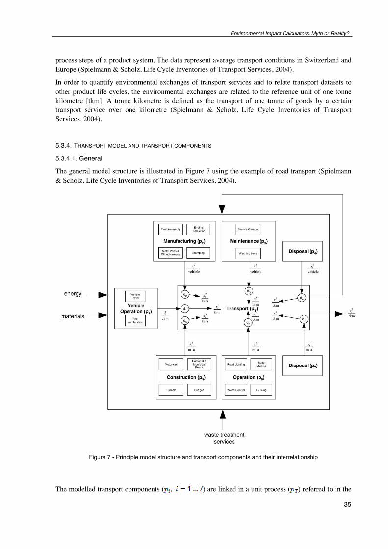
Environmental Impact Calculators: Myth or Reality?
35
process steps of a product system. The data represent average transport conditions in Switzerland and Europe (Spielmann & Scholz, Life Cycle Inventories of Transport Services, 2004).
In order to quantify environmental exchanges of transport services and to relate transport datasets to other product life cycles, the environmental exchanges are related to the reference unit of one tonne kilometre [tkm]. A tonne kilometre is defined as the transport of one tonne of goods by a certain transport service over one kilometre (Spielmann & Scholz, Life Cycle Inventories of Transport Services, 2004).
5.3.4. TRANSPORT MODEL AND TRANSPORT COMPONENTS
5.3.4.1. General
The general model structure is illustrated in Figure 7 using the example of road transport (Spielmann & Scholz, Life Cycle Inventories of Transport Services, 2004).
Figure 7 - Principle model structure and transport components and their interrelationship
The modelled transport components ( ) are linked in a unit process ( ) referred to in the
Environmental impact calculators: myth or reality?
36
database as “transport, transport service” (e.g. transport, lorry 16 t). In order to link various transport components to the reference flow of one tonne kilometre (tkm), so-called demand factors are
determined. Cumulative LCI results for a transport service, are calculated as follows:
Where denotes the number of transport components and / indicates the cumulative
environmental exchanges ( , e.g. CO2 to air) of a certain transport component (unit process )
related to its reference flow ( , e.g. manufacturing of one lorry) (Spielmann & Scholz, Life Cycle Inventories of Transport Services, 2004).
5.3.4.2. Vehicle Operation
The first component contains all processes that are directly connected with the operation of the vehicles. The only interface to other ecoInvent modules are fuel supply, or in case of rail systems, electricity supply. The reference unit for operation is tonne kilometre [tkm] and in case of road transport vehicle kilometre [vkm] (Spielmann, Bauer, Dones, Scherrer, & Tuchshmid, 2007).
5.3.4.3. Vehicle fleet
Vehicle fleet comprises three components that are connected with the vehicle life cycle (excluding the operation) such as vehicle and part manufacture, vehicle maintenance and support as well as disposal of motor vehicles and parts. The data of the referring modules represent mainly European conditions. The reference unit for unit processes of this component is one vehicle [unit] (Spielmann, Bauer, Dones, Scherrer, & Tuchshmid, 2007).
5.3.4.4. Transport infrastructure
Transport infrastructure comprises three components addressing construction, operation and maintenance and disposal of the transport infrastructure. Generated dated predominately describes Swiss conditions. Land use data is recorded in the unit process “operation and maintenance”. Due to the fact that various elements of infrastructure are characterized by a different life span all data is calculated for one year. Thus the reference unit used for infrastructure modules is [m*a] or, in case of airports and ports [m2*a] (Spielmann, Bauer, Dones, Scherrer, & Tuchshmid, 2007).
5.3.4.5. Demand factors
Demand factors for vehicle fleet components, i.e. vehicle manufacturing ( ), vehicle maintenance
( ), and vehicle disposal ( ), with , are calculated as the inverse of the vehicle’s lifetime kilometric performance. Thus, assumptions of the lifetime kilometric performance and
Environmental Impact Calculators: Myth or Reality?
37
average load factor are required (Spielmann & Scholz, Life Cycle Inventories of Transport Services, 2004).
For construction, including the renewal ( ) and disposal ( ) of infrastructure, the yearly Gross-tonne kilometer performance (Gtkm) is employed as the allocation rule so as to account for the fact that damage, and hence the resulting renewal expenditure of roads, is mainly due to vehicle weight. In
contrast, for the determination of demand factors of infrastructure operation datasets ( ), the temporal occupation of the infrastructure by different user types, irrespective of the vehicle weight, is used as the allocation principle (Spielmann & Scholz, Life Cycle Inventories of Transport Services, 2004)
5.3.5. INLAND WATER TRANSPORT
5.3.5.1. General
Despite its assumed advantages, the truth is that inland waterway transport and its impact on the environment is still a topic that is relatively unknown, especially when compared to other transport modes, namely road. The ecoInvent methodology is one that is agreed upon and that can be taken as a guide for the environmental impact of inland waterway transport.
5.3.5.2. Vehicle Operation
Exclusively use of diesel for propelling is assumed.
The average fuel consumption available from Dorland (2000) as quoted in Bickel (2001). The class specific fuel consumption is aggregated using the total carrying capacity of each class ZKR (2003) as allocation factor.
In the ecoInvent methodology, emission factors for dry bulk barges and barge tankers are given for various different carrying capacities.
Fuel consumption can differ significantly depending on several parameters such as upstream/downstream operation, vehicle size class among others. A detailed comparison of the data found in literature with the data employed for this project is beyond the scope of this project.
The final value of specific fuel consumption [g/tkm] is 8,74 for barge tanker of 1000 ton carrying capacity and 9,39 for dry bulk barges of 1200 ton carrying capacity.
5.3.5.3. Vehicle Fleet
Exchanges due to vessel manufacturing and disposal as well as maintenance are addressed. All interventions and exchanges are related to one vehicle [unit].
In order to relate these interventions to the functional unit of 1 tkm, kilometric performance and transport performance per average vehicle must be determined.
Regarding vessel manufacture, the exchanges of the barge and barge tanker manufacturing represent the current average total capacity for a barge (1000 t/vessel) and a barge tanker (1200 t/vessel) as calculated from information available in ZKR (2003).
In this project waste treatment processes for non-metal components of vessels are accounted for.
Environmental impact calculators: myth or reality?
38
When it comes to barge maintenance, this inventory includes the use of paint and emissions of the solvent of the paint as NMVOC. In this project we assume that inland waterway vessels are painted 10 times in their entire life span.
5.3.5.4. Transport infrastructure
The inventory calls processes of material production, representing the material used in the construction phase of the canal. Also lorry transport of materials to and from the construction site has been taken into account. Expenditures due to disposal are excluded. Also expenditures for the construction of bridges are excluded. Assumptions for the construction of the canal are derived from the Main-Donau canal in Germany. The canal is characterized by a width of 42 meters and an average depth of 4 metres. Life time of port is assumed to be of 118 years (ecoInvent v2.2).
The processes of the materials that are part of the construction of this canal are shown per metre and year of canal lifetime. Life span of the canal is assumed to be 118 years. Yearly transport performance on one kilometre canal is about 8’600’000 tkm/(km*a). Consequently, the specific canal demand is 1.16E-04 (m*a)/tkm (ecoInvent v2.2).
This methodology also takes into account port infrastructure, its construction and its operational emissions. However, it is discussable if this part of the infrastructure should be fully allocated to barge transport since transhipments are operations that make co-modality between modes possible, being operations of the supply chain but not of a particular mode of transport.
Environmental Impact Calculators: Myth or Reality?
39
6 CASE STUDY: THE LEUVEN-DIJLE
CANAL
6.1 THE LEUVEN-DIJLE CANAL The Leuven-Dijle canal is part of the Flemish inland waterway network. It began taking form on the 29th of January of 1750 with the issue of a patent approval for the construction of the canal between the cities of Leuven and Mechelen by the Empress Maria Theresia. The first graft is dated of February 9th of 1750 and was done in the presence of Prince Charles Alexander of Lorraine. The canal was inaugurated in 1763 with the existence of 2 sluices along the waterway. Only later, the number of locks was raised to the 5 existing today, being these presently classified as protected monuments. Not much about the canal structure has changed since its origin.
It is a small canal, with 30034 metres length managed by Waterwegen en Zeekanaal NV. It only links to the inland waterway network at one point with the other being a dead end, in the city of Leuven. It is considered a Klasse II canal, meaning that only barges with up to 600 tons of carrying capacity can navigate in these waters (Promotion Office for Inland Navigation in Flanders, 2008). Along the canal, there are 5 sluices and 10 moveable bridges.
Waterwegen en Zeekanaal NV provided the information regarding the average dimensions of the canal, stating that 28 meters is the average width and 2,7 meters the average depth.
In their annual report, it was also possible to observe that 315000 tons were transported in this water-way in the year of 2010, with the total tkm being 7119113 (Waterwegen en Zeekanaal NV, 2011).
6.2 LCA OF INLAND WATERWAY TRANSPORT IN THE LEUVEN-DIJLE CANAL 6.2.1. GOAL
The goal of this study is to assess the environmental impact in terms of greenhouse gases linked with global warming of a transport mode, namely inland waterways.
The intended application of the deliverables will be the development of the Carbon footprint of inland waterways in the region of Flanders in Belgium, but the eventual identification of weak points in this chain is also envisioned. It is important to notice that effects other than that of climate change related greenhouse gas emissions will not be approached. The canal covered is the Leuven-Dijle canal, which has very specific characteristics.
Environmental impact calculators: myth or reality?
40
The main motivation behind the study is the acquirement of knowledge of the carbon emissions of the whole life cycle of this mode of transport to enhance its competitiveness relatively to other transport modes.
The target audience of the results produced in this study is the Flemish University of Brussels and the research group in charge of developing the study in Flanders on the “Operational and infrastructural emissions of inland navigation” for Waterwegen en Zeekanaal NV.
No comparative assertions will be made being this study of an accounting character only, therefore not implying a direct decision support (European Commission - Institute for Environment and Sustaina-bility, 2010).
6.2.2. SCOPE
The system to be studied here will be inland waterway transport in the Leuven-Dijle canal. The function to be analysed will be the transport of goods by barge on the canal considered, with special attention being given to the infrastructural part of the transport mode. SB 5 emissions, which are constituted by administrative functions and personnel (McKinnon & Piecyk, 2010) are not included in this work. The functional unit of the system is gCO2e/tkm, meaning that all results are given in grams of global warming potential (GWP) of carbon per ton kilometre of transported goods. This is the functional unit normally used for greenhouse gas emissions related with freight transportation.
The parts of the infrastructure that are to be analysed are the canal itself, the locks, the bridges and the quays. In accordance with the data provided by Waterwegen en Zeekanaal, emissions regarding the construction of towpaths are not accounted for in this work, the same happening with ministry buildings and with the five hydroelectric power stations that combined have an annual energy production of approximately 1500 kWh. Inland ports are also not taken into account in this work since through informal conversations it was possible to assess that these are seldom and of very small dimensions, having almost no infrastructure other than the quays. Disposal of the canal infrastructure will not be assessed which goes in accordance with the ecoInvent methodology. Therefore, canal construction and its maintenance and operation will comprehend the infrastructural part of this study. These phases take into account all the emissions of the materials that are used, since their extraction until they are processed, forming the end-product to be used in the canal infrastructure. However, transport to the landsite is not accounted for in the modelled scenario for the Leuven-Dijle canal due to insufficient data. There is a transport value for canal infrastructure in the ecoInvent database, however, it is aggregated for all the needed materials. As different quantities of these materials are needed from those in the ecoInvent approach and because there is no apparent correlation between the needs of the canal in that model and the ones of the Leuven-Dijle canal, it is assumed that there is also no correlation for transport.
Barge emissions take into account all the emissions in its life cycle, from construction, maintenance and final disposal. Since no data was collected on the operating barges in the Leuven-Dijle canal, some assumptions were taken from the ecoInvent methodology, while others were made by the author himself. This is due to the fact that the ecoInvent database takes a 1000 ton barge as its reference while the Leuven-Dijle canal has only the capacity for a maximum of a 600 ton barge.
Canal infrastructure serves other functions besides that of freight transport namely water management, flood protection, recreational purposes by vessels and recreational facilities on embankments, also contributing to the costs (ECORYS Transport, 2005) and therefore the emissions. However, at first
Environmental Impact Calculators: Myth or Reality?
41
these have not been taken into account and all external costs were allocated to barge transport. When it comes to moveable bridges, it would be questionable if they should be fully allocated to this transport mode, being its use shared with road transport. However, construction and operation of these bridges has been fully allocated to the activity along the canal in this work, meaning that they are allocated to the vessels that use this infrastructure, being them of a recreation or of a transportation nature. This option confers a big weight to the final Carbon footprint of the transport mode.
When it comes to the impact assessment of these emissions, they were done at a mid-point level (ILCD). This means that the emissions of greenhouse gases were measured in terms of their effect on climate change whereas if it would have been done at an end-point level, the impacts would be accounted for their effects like for instance, human health or consequences on natural environment. In this case, only greenhouse gases related with climate change shall be quantified according to their GWP. In this study only the three gases that cause the most impact, were taken into account being them carbon dioxide (CO2), dinitrogen monoxide (N2O) and methane (CH4) which are thought to be responsible for 99% of the emissions related with climate change due to transport. Carbon dioxide is the reference gas, being the equivalent to 1 GWP while dinitrogen monoxide has a GWP of 296 and methane a GWP of 23 (Maibach, et al., 2008).
The interpretation of the values given is not of an easy nature due to the specifics of this canal, however, these circumstances give the idea that these are possibly the worst conditions for inland waterway transport there could be due to the small dimensions of the canal and therefore limited navigability and lack of economies of scale; the fact that the canal reaches a dead end which is logistically less sound. Due to this, a possible interpretation is that the Carbon footprint given is for a worst case scenario of inland waterway transport. Although this is not a comparative study, one can have the idea of the differences between the case study and what is considered average in Europe for inland waterways by looking at the ecoInvent methodology.
Data used in this methodology shall be specific to the case study whenever possible. Whenever this is not achievable, ecoInvent data is used. This will be the case for the upstream processes of the materials used in the infrastructure and for the mix of electricity required in the different operations along the Leuven-Dijle canal, namely operation of locks and bridges. However, the amounts of a certain material used in an infrastructure process and the needs of electricity for operations along the canal are given by Waterwegen en Zeekanaal NV. Direct emissions from barge operation, maintenance and disposal will be taken from the ecoInvent methodology complemented by some basic assumptions to make them more consistent with the case study.
Traffic demand data on the Leuven-Dijle canal is taken from the latest report on the yearly statistics provided by Waterwegen en Zeekanaal NV. It refers to the year of 2010 and gives only values for the whole year in an aggregated way. Therefore some assumptions have to be made to allocate operational emissions along the canal to freight transport. Initially, all the emissions related with canal infrastructure will be fully allocated to freight transport. After the first iteration, with the identification of the major portions of the emissions related with infrastructure, the model will be refined to try and resemble reality when it comes to the share of freight transport in these emissions. 857 barges entered this canal in the year 2010. Of these, 614 were loaded when they entered the canal. The number of loaded barges that left the canal is of 446, so it is assumed that the 203 boats that entered the canal unloaded, left it loaded and that also make their round-trip loaded. It is assumed that all the barges that come in and out of the canal have a 400 ton maximum capacity. With the average load of an incoming barge being of 259 tons and the average load of an outgoing barge being 349, these will have respectively a 65% and an 87% load. The values referent to emissions in the ecoInvent methodology refer to an average load of 71% of the carrying capacity of all barges, bulk or tanker. Freight transport
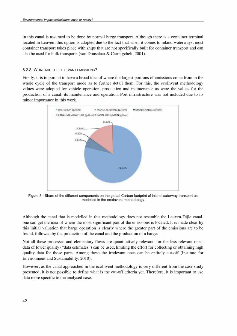
Environmental impact calculators: myth or reality?
42
in this canal is assumed to be done by normal barge transport. Although there is a container terminal located in Leuven, this option is adopted due to the fact that when it comes to inland waterways, most container transport takes place with ships that are not specifically built for container transport and can also be used for bulk transports (van Donselaar & Carmigchelt, 2001).
6.2.3. WHAT ARE THE RELEVANT EMISSIONS?
Firstly, it is important to have a broad idea of where the largest portions of emissions come from in the whole cycle of the transport mode as to further detail them. For this, the ecoInvent methodology values were adopted for vehicle operation, production and maintenance as were the values for the production of a canal, its maintenance and operation. Port infrastructure was not included due to its minor importance in this work.
Figure 8 - Share of the different components on the global Carbon footprint of inland waterway transport as
modelled in the ecoInvent methodology
Although the canal that is modelled in this methodology does not resemble the Leuven-Dijle canal, one can get the idea of where the most significant part of the emissions is located. It is made clear by this initial valuation that barge operation is clearly where the greater part of the emissions are to be found, followed by the production of the canal and the production of a barge.
Not all these processes and elementary flows are quantitatively relevant: for the less relevant ones, data of lower quality (“data estimates”) can be used, limiting the effort for collecting or obtaining high quality data for those parts. Among these the irrelevant ones can be entirely cut-off (Institute for Environment and Sustainability, 2010).
However, as the canal approached in the ecoInvent methodology is very different from the case study presented, it is not possible to define what is the cut-off criteria yet. Therefore, it is important to use data more specific to the analysed case.
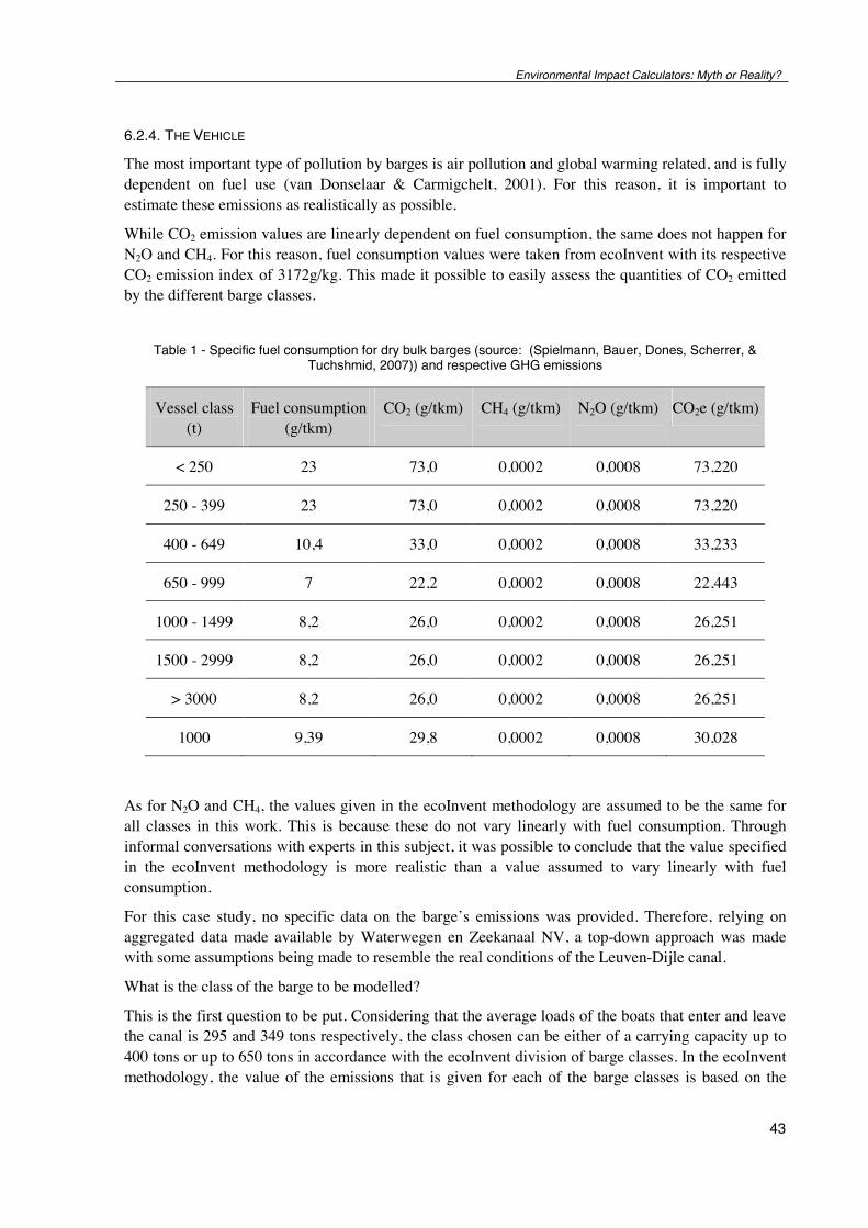
Environmental Impact Calculators: Myth or Reality?
43
6.2.4. THE VEHICLE
The most important type of pollution by barges is air pollution and global warming related, and is fully dependent on fuel use (van Donselaar & Carmigchelt, 2001). For this reason, it is important to estimate these emissions as realistically as possible.
While CO2 emission values are linearly dependent on fuel consumption, the same does not happen for N2O and CH4. For this reason, fuel consumption values were taken from ecoInvent with its respective CO2 emission index of 3172g/kg. This made it possible to easily assess the quantities of CO2 emitted by the different barge classes.
Table 1 - Specific fuel consumption for dry bulk barges (source: (Spielmann, Bauer, Dones, Scherrer, &
Tuchshmid, 2007)) and respective GHG emissions
Vessel class (t)
Fuel consumption (g/tkm)
CO2 (g/tkm) CH4 (g/tkm) N2O (g/tkm) CO2e (g/tkm)
< 250 23 73,0 0,0002 0,0008 73,220
250 - 399 23 73,0 0,0002 0,0008 73,220
400 - 649 10,4 33,0 0,0002 0,0008 33,233
650 - 999 7 22,2 0,0002 0,0008 22,443
1000 - 1499 8,2 26,0 0,0002 0,0008 26,251
1500 - 2999 8,2 26,0 0,0002 0,0008 26,251
> 3000 8,2 26,0 0,0002 0,0008 26,251
1000 9,39 29,8 0,0002 0,0008 30,028
As for N2O and CH4, the values given in the ecoInvent methodology are assumed to be the same for all classes in this work. This is because these do not vary linearly with fuel consumption. Through informal conversations with experts in this subject, it was possible to conclude that the value specified in the ecoInvent methodology is more realistic than a value assumed to vary linearly with fuel consumption.
For this case study, no specific data on the barge’s emissions was provided. Therefore, relying on aggregated data made available by Waterwegen en Zeekanaal NV, a top-down approach was made with some assumptions being made to resemble the real conditions of the Leuven-Dijle canal.
What is the class of the barge to be modelled?
This is the first question to be put. Considering that the average loads of the boats that enter and leave the canal is 295 and 349 tons respectively, the class chosen can be either of a carrying capacity up to 400 tons or up to 650 tons in accordance with the ecoInvent division of barge classes. In the ecoInvent methodology, the value of the emissions that is given for each of the barge classes is based on the
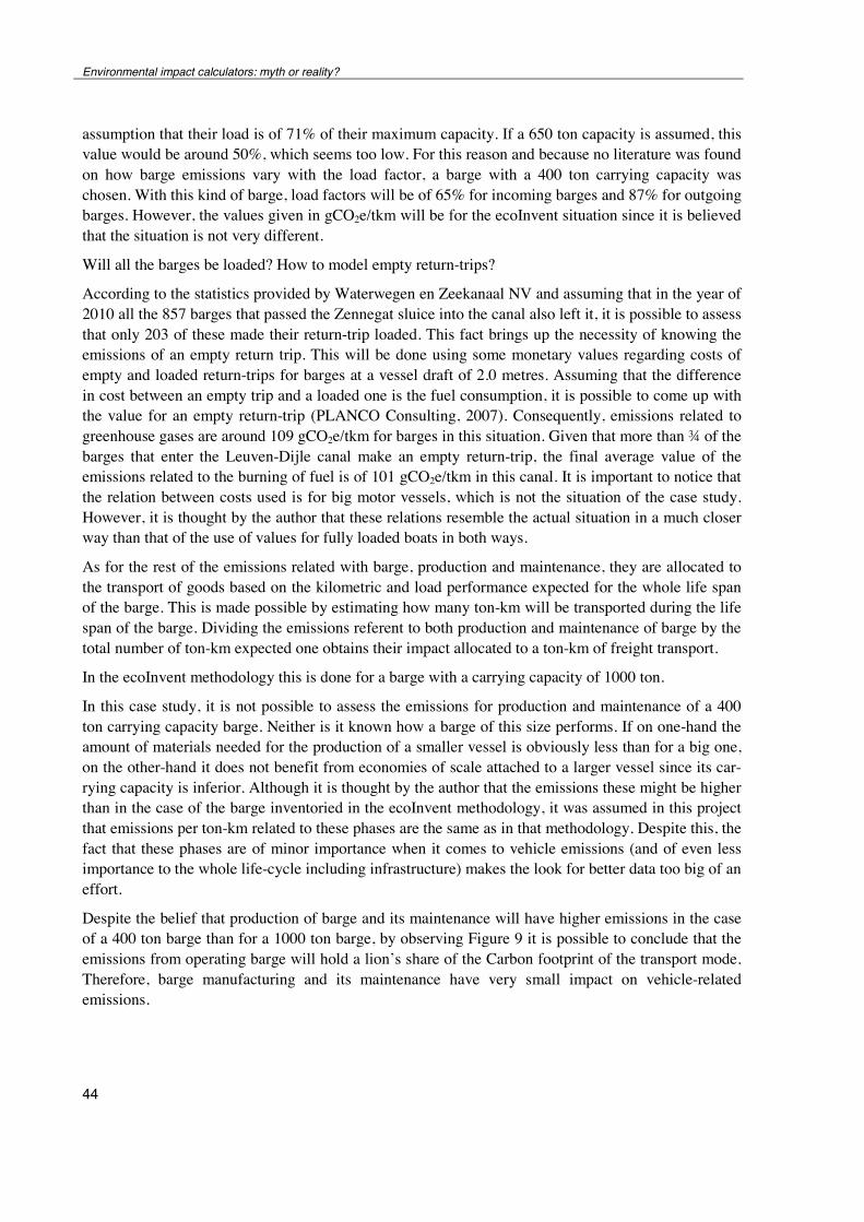
Environmental impact calculators: myth or reality?
44
assumption that their load is of 71% of their maximum capacity. If a 650 ton capacity is assumed, this value would be around 50%, which seems too low. For this reason and because no literature was found on how barge emissions vary with the load factor, a barge with a 400 ton carrying capacity was chosen. With this kind of barge, load factors will be of 65% for incoming barges and 87% for outgoing barges. However, the values given in gCO2e/tkm will be for the ecoInvent situation since it is believed that the situation is not very different.
Will all the barges be loaded? How to model empty return-trips?
According to the statistics provided by Waterwegen en Zeekanaal NV and assuming that in the year of 2010 all the 857 barges that passed the Zennegat sluice into the canal also left it, it is possible to assess that only 203 of these made their return-trip loaded. This fact brings up the necessity of knowing the emissions of an empty return trip. This will be done using some monetary values regarding costs of empty and loaded return-trips for barges at a vessel draft of 2.0 metres. Assuming that the difference in cost between an empty trip and a loaded one is the fuel consumption, it is possible to come up with the value for an empty return-trip (PLANCO Consulting, 2007). Consequently, emissions related to greenhouse gases are around 109 gCO2e/tkm for barges in this situation. Given that more than ! of the barges that enter the Leuven-Dijle canal make an empty return-trip, the final average value of the emissions related to the burning of fuel is of 101 gCO2e/tkm in this canal. It is important to notice that the relation between costs used is for big motor vessels, which is not the situation of the case study. However, it is thought by the author that these relations resemble the actual situation in a much closer way than that of the use of values for fully loaded boats in both ways.
As for the rest of the emissions related with barge, production and maintenance, they are allocated to the transport of goods based on the kilometric and load performance expected for the whole life span of the barge. This is made possible by estimating how many ton-km will be transported during the life span of the barge. Dividing the emissions referent to both production and maintenance of barge by the total number of ton-km expected one obtains their impact allocated to a ton-km of freight transport.
In the ecoInvent methodology this is done for a barge with a carrying capacity of 1000 ton.
In this case study, it is not possible to assess the emissions for production and maintenance of a 400 ton carrying capacity barge. Neither is it known how a barge of this size performs. If on one-hand the amount of materials needed for the production of a smaller vessel is obviously less than for a big one, on the other-hand it does not benefit from economies of scale attached to a larger vessel since its car-rying capacity is inferior. Although it is thought by the author that the emissions these might be higher than in the case of the barge inventoried in the ecoInvent methodology, it was assumed in this project that emissions per ton-km related to these phases are the same as in that methodology. Despite this, the fact that these phases are of minor importance when it comes to vehicle emissions (and of even less importance to the whole life-cycle including infrastructure) makes the look for better data too big of an effort.
Despite the belief that production of barge and its maintenance will have higher emissions in the case of a 400 ton barge than for a 1000 ton barge, by observing Figure 9 it is possible to conclude that the emissions from operating barge will hold a lion’s share of the Carbon footprint of the transport mode. Therefore, barge manufacturing and its maintenance have very small impact on vehicle-related emissions.
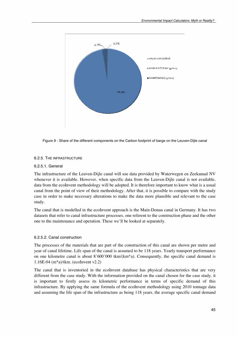
Environmental Impact Calculators: Myth or Reality?
45
Figure 9 - Share of the different components on the Carbon footprint of barge on the Leuven-Dijle canal
6.2.5. THE INFRASTRUCTURE
6.2.5.1. General
The infrastructure of the Leuven-Dijle canal will use data provided by Waterwegen en Zeekanaal NV whenever it is available. However, when specific data from the Leuven-Dijle canal is not available, data from the ecoInvent methodology will be adopted. It is therefore important to know what is a usual canal from the point of view of their methodology. After that, it is possible to compare with the study case in order to make necessary alterations to make the data more plausible and relevant to the case study.
The canal that is modelled in the ecoInvent approach is the Main-Donau canal in Germany. It has two datasets that refer to canal infrastructure processes, one referent to the construction phase and the other one to the maintenance and operation. These we’ll be looked at separately.
6.2.5.2. Canal construction
The processes of the materials that are part of the construction of this canal are shown per metre and year of canal lifetime. Life span of the canal is assumed to be 118 years. Yearly transport performance on one kilometre canal is about 8’600’000 tkm/(km*a). Consequently, the specific canal demand is 1.16E-04 (m*a)/tkm. (ecoInvent v2.2)
The canal that is inventoried in the ecoInvent database has physical characteristics that are very different from the case study. With the information provided on the canal chosen for the case study, it is important to firstly assess its kilometric performance in terms of specific demand of this infrastructure. By applying the same formula of the ecoInvent methodology using 2010 tonnage data and assuming the life span of the infrastructure as being 118 years, the average specific canal demand
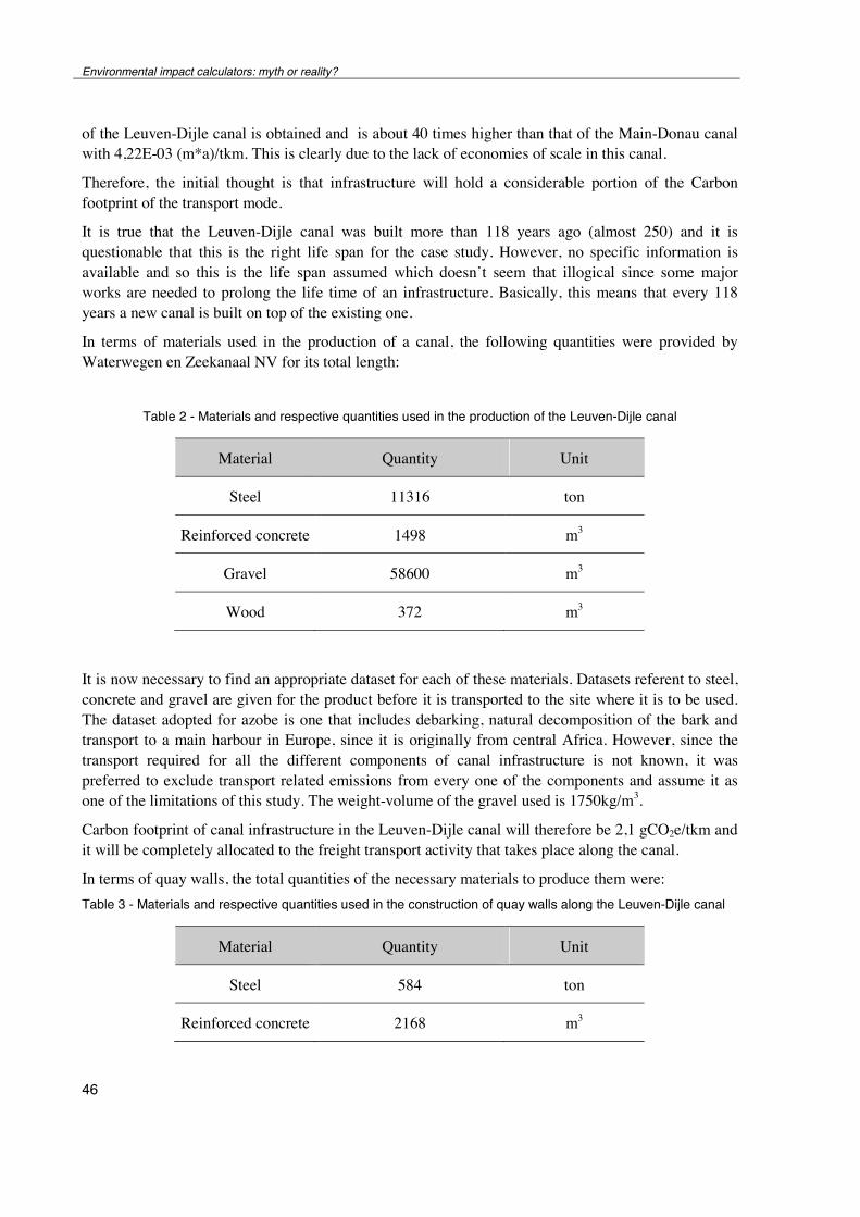
Environmental impact calculators: myth or reality?
46
of the Leuven-Dijle canal is obtained and is about 40 times higher than that of the Main-Donau canal with 4,22E-03 (m*a)/tkm. This is clearly due to the lack of economies of scale in this canal.
Therefore, the initial thought is that infrastructure will hold a considerable portion of the Carbon footprint of the transport mode.
It is true that the Leuven-Dijle canal was built more than 118 years ago (almost 250) and it is questionable that this is the right life span for the case study. However, no specific information is available and so this is the life span assumed which doesn’t seem that illogical since some major works are needed to prolong the life time of an infrastructure. Basically, this means that every 118 years a new canal is built on top of the existing one.
In terms of materials used in the production of a canal, the following quantities were provided by Waterwegen en Zeekanaal NV for its total length:
Table 2 - Materials and respective quantities used in the production of the Leuven-Dijle canal
Material Quantity Unit
Steel 11316 ton
Reinforced concrete 1498 m3
Gravel 58600 m3
Wood 372 m3
It is now necessary to find an appropriate dataset for each of these materials. Datasets referent to steel, concrete and gravel are given for the product before it is transported to the site where it is to be used. The dataset adopted for azobe is one that includes debarking, natural decomposition of the bark and transport to a main harbour in Europe, since it is originally from central Africa. However, since the transport required for all the different components of canal infrastructure is not known, it was preferred to exclude transport related emissions from every one of the components and assume it as one of the limitations of this study. The weight-volume of the gravel used is 1750kg/m3.
Carbon footprint of canal infrastructure in the Leuven-Dijle canal will therefore be 2,1 gCO2e/tkm and it will be completely allocated to the freight transport activity that takes place along the canal.
In terms of quay walls, the total quantities of the necessary materials to produce them were: Table 3 - Materials and respective quantities used in the construction of quay walls along the Leuven-Dijle canal
Material Quantity Unit
Steel 584 ton
Reinforced concrete 2168 m3
Environmental Impact Calculators: Myth or Reality?
47
The emissions due to the construction of these walls were fully allocated to barge transport and are of around 0,8 gCO2e/tkm.
Contrarily to the ecoInvent methodology, the construction of moveable bridges is taken into account in the construction of the Leuven-Dijle canal. It is true that these infrastructures are common to both inland waterway transport and to road transport, however, in this study the emissions related with the construction of this part of the infrastructure will be fully allocated to inland waterway transport and the ones related with the construction of the non-moveable bridges will not be accounted for, therefore assumed to be part of the road transport infrastructure. The emissions related with the construction of moveable bridges are the following:
Table 4 - Materials, their quantities and respective emissions due to the construction of moveable bridges along
the Leuven-Dijle canal
Material Quantity Unit gCO2e/tkm2010
Steel 1537 ton 0,00
Concrete 9923 m3 3,90
Masonry 27 m3 0,02
Masonry was assumed to be 2000 kg/m3.
It is noticeable that construction of bridges in this canal is of importance since it is the process related to the construction of infrastructure that has a higher environmental burden with a value of 3,9 gCO2e/tkm.
6.2.5.3. Infrastructure running emissions
Firstly it is important to identify the sources of these emissions. According to the (ECORYS Transport, 2005) study, relevant maintenance and management costs are derived from:
• Dredging; • Operation of locks and bridges; • River police; • Maintenance and management of inland ports.
However, in this case study not all these will be approached. Information on emissions related to dredging is not known, emissions related to patrol of the waterways are considered administrative emissions and therefore SB 5 which are not within the boundaries of the scope of this analysis and the fact that ports in this canal are almost inexistent or of very small dimension makes their impact redundant to the global Carbon footprint of the transport mode. Therefore, operation of locks and bridges will be the main focus of the emissions related to the running of the Leuven-Dijle canal infrastructure.
When it comes to maintenance related emissions, very little information is available about this canal. Some information was provided by Waterwegen en Zeekanaal NV for maintenance operations regarding locks, but there was no information regarding the time frame attached to these works,
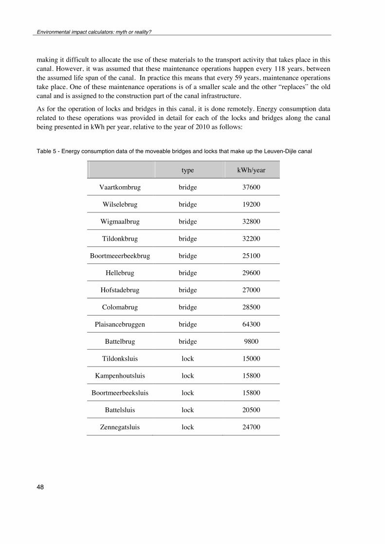
Environmental impact calculators: myth or reality?
48
making it difficult to allocate the use of these materials to the transport activity that takes place in this canal. However, it was assumed that these maintenance operations happen every 118 years, between the assumed life span of the canal. In practice this means that every 59 years, maintenance operations take place. One of these maintenance operations is of a smaller scale and the other “replaces” the old canal and is assigned to the construction part of the canal infrastructure.
As for the operation of locks and bridges in this canal, it is done remotely. Energy consumption data related to these operations was provided in detail for each of the locks and bridges along the canal being presented in kWh per year, relative to the year of 2010 as follows:
Table 5 - Energy consumption data of the moveable bridges and locks that make up the Leuven-Dijle canal
type kWh/year
Vaartkombrug bridge 37600
Wilselebrug bridge 19200
Wigmaalbrug bridge 32800
Tildonkbrug bridge 32200
Boortmeeerbeekbrug bridge 25100
Hellebrug bridge 29600
Hofstadebrug bridge 27000
Colomabrug bridge 28500
Plaisancebruggen bridge 64300
Battelbrug bridge 9800
Tildonksluis lock 15000
Kampenhoutsluis lock 15800
Boortmeerbeeksluis lock 15800
Battelsluis lock 20500
Zennegatsluis lock 24700
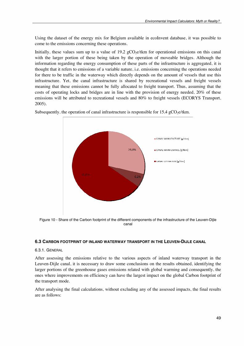
Environmental Impact Calculators: Myth or Reality?
49
Using the dataset of the energy mix for Belgium available in ecoInvent database, it was possible to come to the emissions concerning these operations.
Initially, these values sum up to a value of 19,2 gCO2e/tkm for operational emissions on this canal with the larger portion of these being taken by the operation of moveable bridges. Although the information regarding the energy consumption of these parts of the infrastructure is aggregated, it is thought that it refers to emissions of a variable nature, i.e. emissions concerning the operations needed for there to be traffic in the waterway which directly depends on the amount of vessels that use this infrastructure. Yet, the canal infrastructure is shared by recreational vessels and freight vessels meaning that these emissions cannot be fully allocated to freight transport. Thus, assuming that the costs of operating locks and bridges are in line with the provision of energy needed, 20% of these emissions will be attributed to recreational vessels and 80% to freight vessels (ECORYS Transport, 2005).
Subsequently, the operation of canal infrastructure is responsible for 15,4 gCO2e/tkm.
Figure 10 - Share of the Carbon footprint of the different components of the infrastructure of the Leuven-Dijle
canal
6.3 CARBON FOOTPRINT OF INLAND WATERWAY TRANSPORT IN THE LEUVEN-DIJLE CANAL 6.3.1. GENERAL
After assessing the emissions relative to the various aspects of inland waterway transport in the Leuven-Dijle canal, it is necessary to draw some conclusions on the results obtained, identifying the larger portions of the greenhouse gases emissions related with global warming and consequently, the ones where improvements on efficiency can have the largest impact on the global Carbon footprint of the transport mode.
After analysing the final calculations, without excluding any of the assessed impacts, the final results are as follows:
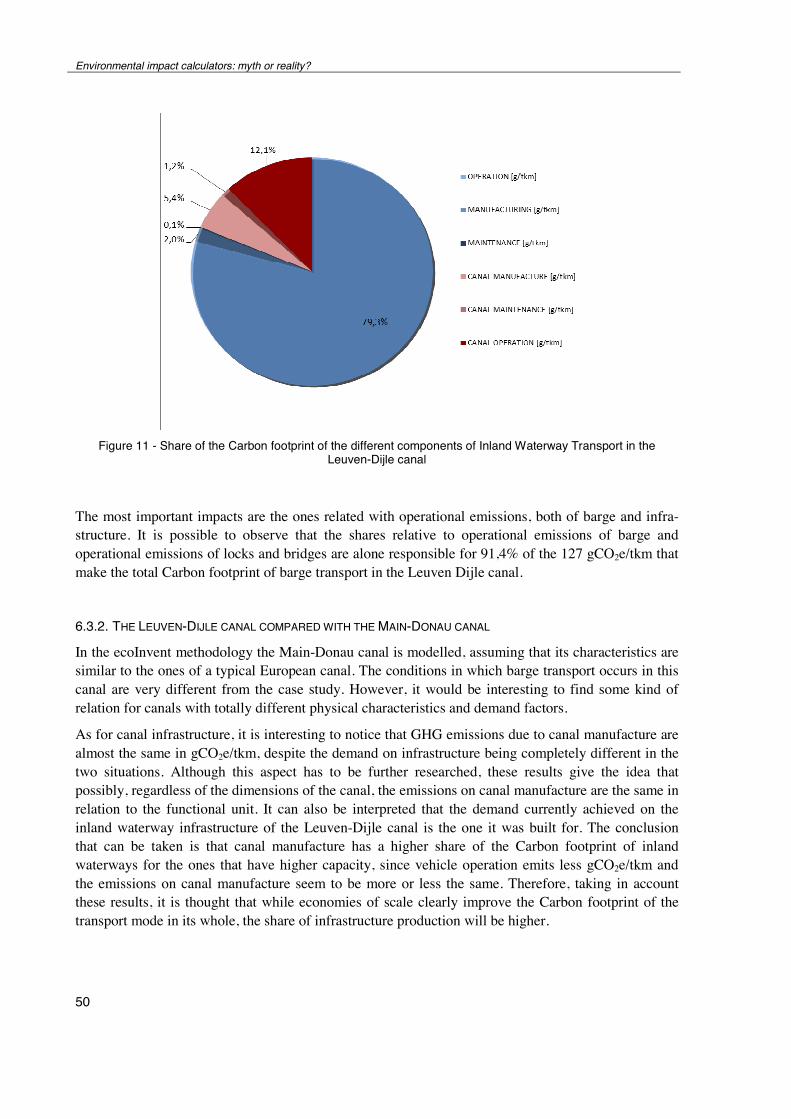
Environmental impact calculators: myth or reality?
50
Figure 11 - Share of the Carbon footprint of the different components of Inland Waterway Transport in the
Leuven-Dijle canal
The most important impacts are the ones related with operational emissions, both of barge and infra-structure. It is possible to observe that the shares relative to operational emissions of barge and operational emissions of locks and bridges are alone responsible for 91,4% of the 127 gCO2e/tkm that make the total Carbon footprint of barge transport in the Leuven Dijle canal.
6.3.2. THE LEUVEN-DIJLE CANAL COMPARED WITH THE MAIN-DONAU CANAL
In the ecoInvent methodology the Main-Donau canal is modelled, assuming that its characteristics are similar to the ones of a typical European canal. The conditions in which barge transport occurs in this canal are very different from the case study. However, it would be interesting to find some kind of relation for canals with totally different physical characteristics and demand factors.
As for canal infrastructure, it is interesting to notice that GHG emissions due to canal manufacture are almost the same in gCO2e/tkm, despite the demand on infrastructure being completely different in the two situations. Although this aspect has to be further researched, these results give the idea that possibly, regardless of the dimensions of the canal, the emissions on canal manufacture are the same in relation to the functional unit. It can also be interpreted that the demand currently achieved on the inland waterway infrastructure of the Leuven-Dijle canal is the one it was built for. The conclusion that can be taken is that canal manufacture has a higher share of the Carbon footprint of inland waterways for the ones that have higher capacity, since vehicle operation emits less gCO2e/tkm and the emissions on canal manufacture seem to be more or less the same. Therefore, taking in account these results, it is thought that while economies of scale clearly improve the Carbon footprint of the transport mode in its whole, the share of infrastructure production will be higher.
Environmental Impact Calculators: Myth or Reality?
51
7 CONCLUSIONS
7.1 GENERAL CONCLUSIONS The main goal of this thesis was to study what is being done on CO2 calculators due to transport.
The first conclusions regarding this thesis are that the external costs of transport are still to be defined properly. It seems that the definition of external cost has been distorted and attributed to every negative aspect of transport that hasn’t been solved, instead of being a manner to try and regulate the demand for transport. Some of the negative impacts are evaluated in a dubious way along with a good deal of uncertainties while the extra taxes paid by road transport and subsidies given to transport modes other than road are not accounted for. This penalises road transport severely. This is not the problem since road transport is responsible for a lot of the problems regarding transport. Yet, justifying this by stating that it has to do with the external costs it imposes on society is a fallacy, since most of the evaluations lack an economic justification and do not seem to have the goal of solving welfare losses due to transport. This issue has been partly solved with the latest White Paper on transport where the European Commission states that its main goal when it comes to transport is the reduction of GHG emissions. This means that no economic justification is needed to over-charge the transport modes that pollute more, which is a more honest approach to what is sought.
Regarding CO2 calculators, it was possible to observe there is not a correct and standard way to calculate transport related emissions. This fact highlights the need for objectivity and transparency when it comes to CO2 calculators. This was especially noticeable in the workshop “Inland navigation CO2 emissions – How to measure them? How to reduce them?” held by the Central Commission for the navigation of the Rhine where it was seen that people from different backgrounds have different goals and thus use different methods. It was here that Life Cycle Assessment came in, being it a method for the analysis and assessment of potential environmental impacts along the life cycle of a good or a service. This methodology takes into account a product’s full life cycle: from the extraction of resources, through production, use and recycling, up to the disposal of remaining waste. Therefore, all the possible impacts intrinsic to a transport mode will be accounted for when using this methodology.
As for the inland waterway transport and its emissions, information is very scarce and the one that was found relates to the same study, that of Dorland (2000). This is a study that was developed too long ago for the pace that the issue of GHG emissions related to transport has been evolving. It is therefore probable that the emissions referent to this mode of transport are not sufficiently well known, most likely giving the idea of a greater carbon footprint than the one presently existent. Information on emissions other from the ones that derive from the operation of barge was also very hard to find, giving the idea that this subject is very unexplored. The truth is that inland waterway transport has the
Environmental impact calculators: myth or reality?
52
distinction of being more ecological than other transport modes (except vehicles moved by electricity) when comparing tank-to-wheel emissions and its advantages would probably be even more enhanced if other parts of the transport mode were to be included, since they are known to have a long life span.
When it comes to the case study of the Leuven-Dijle canal, transport on this waterway takes part in conditions that are not favourable to its environmental performance. Economies of scale are not possible due to limitations on the capacity of barges that operate on this canal (600 tonnes) and the canal reaches a dead end in the city of Leuven, conditions that do not help its environmental performance. However it was possible to conclude that the emissions regarding the production of infrastructure are very similar (in reference to the functional unit of gCO2/tkm) between the case study and the large capacity canal Main-Donau, being the latter therefore responsible for a larger share of the carbon footprint of the canal with the economy of scale, since the operational emissions of barge are necessarily much lower for canals with more capacity. Operational emissions of infrastructure were, however, much higher for the Leuven-Dijle canal than for the Main-Donau canal. The main conclusions are that while the CO2 emissions of inland waterway transport are lower for a canal with a higher capacity, emissions regarding infrastructure take up a larger share of the carbon footprint of the transport mode in that same case. Therefore, emissions related to infrastructure should be assessed, since they have an impact that is not negligible on the Carbon footprint of inland waterway transport.
7.2 FUTURE DEVELOPMENTS The obvious development is the standardization of the measurement of CO2 emissions regarding transport, something that is already advancing.
As for Life Cycle Assessment, it is a methodology that offers no doubts when calculating the carbon footprint of a transport mode since it looks at all the aspects intrinsic to it. However, information regarding emissions other than the operational ones is not often known. These should be made available by carriers so as to inform clients of the least harmful option of transport, taking into every aspect that makes up the transport mode. In that way, it would be easier to opt for a more environmentally friendly way to transport goods from A to B knowing the Carbon footprint of the whole supply chain. Therefore, emissions regarding infrastructural emissions be them of production, maintenance or operation are to be further looked into.
An interesting way to present any work regarding the Carbon footprint of a transport mode would be to initially describe and highlight which parts of it would be analysed in that study, making use of the LCA figure for a transport mode (Figure 7). This would make the communication of the results of the study easier and more transparent.
Specifically regarding inland waterway transport, it would be interesting to confirm which aspects of the infrastructural emissions are more sensitive to economies of scale.
A lot of information is to be collected if inland waterway transport is to know its position on greenhouse gas emissions, namely for operations like reparation of the infrastructure and dredging. These need a time-scope attached to them, something that was very hard to find for this thesis.
Environmental Impact Calculators: Myth or Reality?
53
BIBLIOGRAFIA Baum, H., Geibler, T., Schneider, J., & Buhne, J. A. (2008). External Costs in the Transport Sector - A
Critical Review of the EC-Internalisation-Policy. Cologne: Institute for Transport Economics at the University of Cologne.
Button, K. J. (1993). Transport Economics. Cheltenham, UK / Northampton, MA, USA: Edward Elgar Publishing.
Coase, R. H. (1960). The Problem of Social Cost. Journal of Law and Economics, 1-44.
Commission of the European Communities. (2006). Communication from the Commission on the promotion of Inland Waterway Transport. Brussels: Commission of the European Communities.
ECORYS Transport. (2005). Charging and pricing in the area of inland waterways. Rotterdam: European Commission.
European Commission. (2003). External costs - Research results on socio-environmental damages due to electricity and transport. Luxembourg: Office for Official Publications of the European Communities.
European Commission - Institute for Environment and Sustainability. (2010). General guide for Life Cycle Assessment - Detailed guidance. Ispra: European Union.
European Commission. (2011). White Paper. Brussels: European Commission.
European Committee for Standardization. (2006). Environmental management - Life cycle assessment - Principles and framework (ISO 14040:2006). Brussels: European Committee for Standardization.
European Committee for Standardization. (2006). Environmental management - Life cycle assessment - Requirements and guidelines (ISO 14044:2006). Brussels: European Committee for Standardization.
European Environment Agency. (06 de 12 de 2010). Articles. Obtido em 03 de 04 de 2011, de European Environment Agency: http://www.eea.europa.eu/articles/tackling-climate-change-requires-a
Frank, R. H., & Bernanke, B. S. (2004). Principles of economics (2ª ed.). New York: McGraw-Hill.
Frischknecht, R. (1998). Life Cycle Inventory Analysis For Decision-Making. Zurich: Swiss Federal Institute of Technology Zurich.
Institute for Environment and Sustainability. (2010). ILCD Handbook: General guide for Life Cycle Assessment - Detailed guidance. Ispra: European Union.
International Navigation Association. (2005). Economic Aspects of Inland Waterways. Brussels.
International Road Transport Union. (2008). IRU Position on the Internalisation of External Costs. Geneva.
Maibach, M., Schreyer, C., Sutter, D., van Essen, H. P., Boon, B. H., Smokers, R., et al. (2008). Handbook on estimation of external costs in the transport sector. Delft: CE.
McKinnon, A., & Piecyk, M. (2010). Measuring and Managing CO2 Emissions of European Chemical Transport. Edinburgh: CEFIC.
Environmental impact calculators: myth or reality?
54
Ng, Y. K. (2007). Eternal Coase and External Costs: A Case for Bilateral Taxation and Amenity Rights. European Journal of Political Economy, 641-659.
Nye, J. (20 de August de 2008). The Pigou Problem. Regulation, 31, 32-37.
OECD. (2010). Reducing transport GHG emissions - Trends & Data. OECD/ITF.
PLANCO Consulting. (2007). Economical and Ecological Comparison of Transport Modes: Road, Railway, Inland Waterways - Summary of Findings. Essen.
Schreyer, C., Schneider, C., Maibach, M., Rothengatter, W., Doll, C., & Schmedding, D. (2004). External Costs of Transport. Zurich/Karlsruhe.
Spielmann, M., & Scholz, R. W. (2004). Life Cycle Inventories of Transport Services. Zurich: Swiss Federal Institute of Technology Zurich.
Spielmann, M., Bauer, C., Dones, R., Scherrer, P., & Tuchshmid, M. (2007). Transport Services. Villigen/Uster: Swiss Centre for Life Cycle Inventories.
The Institute for Energy and Environment Research (IFEU). (2008). EcoTransIT: Ecological Transport Information Tool - Environmental Methodology and Data. Heidelberg: The Institute for Energy and Environment Research (IFEU).
The Institute for Energy and Environmental Research. (s.d.). General Information. Obtido em 06 de April de 2011, de EcoTransIT: http://www.ecotransit.org/information.en.phtml
The Institute for Energy and Environmental Research. (s.d.). Guided Tour. Obtido em 06 de April de 2011, de EcoTransIT: http://www.ecotransit.org/example.en.phtml
Tuchschmid, M. (2009). Carbon Footprint of High-Speed railway infrastructure (Pre-Study). Zurich: The International Union of Railways (UIC).
van Donselaar, P., & Carmigchelt, H. (2001). Infrastructure, environmental and accident costs for Rhine container shipping.
Waterwegen en Zeekanaal NV. (2011). Statistiek van het vervoer op de waterwegen beheerd door Waterwegen en Zeekanaal NV 2010. Evergem: Uitgave.

Environmental Impact Calculators: Myth or Reality?
55