Embed Size (px)
Citation preview
1
Environmental effects in an integrated hub location and pricing problem
Mohaddese Mohammadi a, Hossein Karimi
b*
a MSc, Department of Industrial Engineering, University of Bojnord;
b* Corresponding author: Assistant professor, Department of Industrial Engineering, University
of Bojnord, E-mail: [email protected] , Postal Code: 94531-55111, Mobile:09112713453, Tel.:
+98 584 2284611; fax: +98 584 2410700;
Abstract
The product pricing decision is one of the important factors in the profitability of organizations,
which has a key role in their survival. Moreover, the pricing is determined based on the demand
and location of applicants. Therefore, the location of facilities and services influence the pricing.
Also, the location problem is a critical issue in the survival of the organization. Furthermore, the
hub location problem is a type of location problems, which has many applications and saves time
and money. On the other hand, location is impossible without considering transportation, and
transportation has many negative effects on environmental, such as greenhouse gas emissions, air
pollution, noise, etc. Considering this reason, it is important to consider the environmental costs
to reduce the adverse effects. In this paper, we consider integrated pricing and hub location
problem with environmental costs in the competitive market that customer choice is calculated
according to the logit model (LM). We use a genetic algorithm (GA) to solve and observe the
environmental cost, entrant profit, incumbent income, the impact of customer sensitivity and
discount between hubs on the entrant profit. As a final point, the computational experiments
demonstrate that the suggested GA is both efficient and effective.
Keywords: Pricing; Hub location; Environmental costs; Logit model; Genetic algorithm.
2
1. Introduction
Price is a measurement and criterion, and pricing is just determining the value of goods and
services. Pricing is common practice with a considerable impact on the profit and loss of an
organization. Also, the correct pricing policy is effective in survival, cost coverage, and
expanded sales, which in turn translates into a larger market share.
Evidence suggests that determining a place to build an industrial plant is one of the basic
decisions of investors that can play an essential role in directing the strategic orientation of the
factory, as it affects the profitability and survival of the organization. For example, if the initial
resources of an organization are bulky, the factory should be in the vicinity of the suppliers of
raw materials. Moreover, when products are bulky, the factory should not be far from customers.
In addition to the economic impact, the selection principle or non-principle location can affect
the cultural, social, and environmental aspects. Location is generally seen as a decision closely
related to the demand, which in turn is primarily associated with prices. The factors affecting
product pricing are generally divided into two internal and external groups. One of the external
factors is market properties with the marketplace and the number of customers serving as two
sub-branches of market properties [1]. Therefore, the price of products and services is
determined based on the demand and location of customers. In conclusion, location and pricing
can mutually interrelated. Location is a long-term decision and pricing appears to be a short-term
decision, in fact, it represents a continuous process. For this reason, the organization needs to
consider the issues of optimal location and appropriate pricing together.
The location decision aims to find the best site for facilities, factories, or companies to reduce
costs. Nonetheless, connecting all nodes could be costly and time-consuming, and reduce the
efficiency of the model. Hence, it is essential to incorporate a network design in the location
problems. To overcome this problem, the hub-and-spoke network topology is used. A key feature
of this network is that it can be applied to indirect and fewer connections between
origin/destination (O/D) pairs using hub nodes. The hub nodes are tasked with the collection,
transshipment, and distribution. Also, the connection of two hub nodes is moderated with a
discount factor, which is shown by 10 . Therefore, reducing connections and incorporating
the discount factor between hub nodes can reduce overall transportation costs.
Hub location problems (HLPs) typically involve locating hub nodes and non-hub nodes as well
as allocating non-hub nodes to hub nodes with spoke links. The goal of this problem is to
minimize costs, distance, or maximize profit. In fact, in HLPs, location and network design
decisions are combined. Hub location is important for a wide range of scientific and industrial
processes such as transportation [2], postal services [3], and telecommunications [4]. One of the
best functional examples of pricing at HLP is the airline industry. Pricing at the airport is
considered during the planning horizon. Although a daily route may have different pricing
depending on the pricing policy of the airport, its pricing over a planning horizon indicates the
average of all prices during that period. Naturally, hub airports have a greater demand compared
3
to non-hub airports. As a result, the number of flights and the need for new airplanes will be
higher, as will be the amount of required fuel. In addition to optimizing flights schedule, the
probability of increasing demand for an airport runway should be considered. Therefore,
problems such as runway pavement, resource consumption, noise, and greenhouse gas (GHGs)
emissions induced by extra flights, all of which hurt the ecosystem, should be considered.
Among these deleterious effects, GHGs emissions, especially co2 is the most concerning [5].
Also, air pollution in addition to affecting human health and ecosystem affects nations’ economic
dimensions; these effects are studied on housing prices by [6].
Since routing is an integral part of location decision, and vehicles can damage the environment
and human health, it is important to consider environmental costs through the optimal use of
vehicles by choosing the optimal path as part of the pricing decision at HLPs. The pollution
generated by a vehicle depends on its load and speed, among other factors [7].
There is a paucity of studies on the impact of environmental costs on hub location with few
studies considering pricing at hub location together with environmental costs. Hence, we
consider integrated pricing and HLP with environmental costs in this paper. The
competitive market is studied because it resembled the real world and special
discriminatory pricing policy. The price-sensitive demand is more compatible with real-life
conditions. The process of customer choice is modeled using an LM, which is mostly used
for representing a discrete choice. One of the major attributes of this model is matching
different features of options. For example, some variables in transportation include cost,
waiting time, travel time, type of car, and price. This model also has a sensitivity parameter
that is shown by . A large means that consumers are sensitive to the price and they
would concentrate on less expensive paths and vice versa. (For more studies on LMs, see
[8, 9]). Also, this paper gives an account of environmental costs and analyzes the impact of
and different discount factors 6,0.8,10.2,0.4,0. on the entrant’s profit and the
incumbent’s (i.e., existing company) income. It is assumed that the incumbent charges its
costs plus an additional percentage to their customers (i.e., mill pricing). When customers
transport the product from the firm to their warehouses or other places, the pricing strategy
is mill pricing. In this case, the full price for all customers irrespective of their locations is
equal to mill price, plus transportation cost. However, in the uniform pricing, customers
pay the same price regardless of distance, but ordinarily, the firm may refuse to transport
beyond a certain maximal range [10]. We do not consider the incumbent’s profit, as it is
4
assumed to have existed in the market for a while, and therefore its investment costs have
shrunken.
The rest of this paper proceeds as follows: section 2 presents an overview of the recent studies.
Section 3 describes the problem and model formulation. Section 4 and 5 present the statistical
analysis using the Civil Aeronautics Board (CAB) dataset and discussion, respectively. Finally,
conclusions are drawn in section 6.
2. Literature review
In this section, a review of relevant literature is provided. Goldman [11] was the first to introduce
the HLP network, but the first mathematical formulation of an HLP was presented by O'Kelly
[12]. In the classical hub location models, it is assumed that all hub nodes are completely
connected via hub links that are discounted by a constant factor. Furthermore, in the classic
models, non-hub nodes are not connected directly. A new approach to HLPs called hub arc
location was introduced by Campbell et al [13, 14]. In this approach, the assumption that all hubs
are connected is relaxed, generating some unrealistic results in real-life applications [15].
As mentioned, HLP is used in many areas. Nickel et al. [16] introduced the first mixed-integer
programming models for public transportation networks. They suggested two models: Public
Transport (PT) and Generalized Public Transport (GPT). Then, Gelareh and Nickel [17]
expanded PT into Hub Location Model for Public Transport (HLPPT) by reducing the number of
variables and constraints.
Generally, solutions can be categorized into exact and approximation methods. Some of the
exact methods include game theory [18], branch and bound [19], and dynamic programming
[20]. One of the approximation methods is metaheuristic. Different algorithms have been
proposed to be metaheuristic including tabu search algorithm [21], GA [22], and variable
neighborhood search algorithm [23].
For further studies on hub location with alternate assumptions in the transportation area see [24,
25]. The objective of most studies in the hub location is to minimize costs and travel time or
maximize profit and service level. Some researchers such as Campbell [15] have integrated both
cost and service. However, the location decision is not the only profitable component of the
company, and pricing plays a critical role in profitability. One of the most notable examples is
pricing at 27 large US airports, which helped solve the delay problem of 13 passenger-years and
1000 aircraft-hours and save 3–5 million dollars daily [26].
There are a host of studies on pricing-location and HLPs. In the following, some studies on
pricing hub locations are reviewed. Spiller [27] was one of the first to study the pricing of the
hub and spoke networks in the monopoly market at airlines. Daniel [28] modeled a congestion
pricing problem at large hub airports that accounted for the capacity of hubs and stochastic
queues. Oum et al. [29] examined marginal pricing policy over a network of hub-and-spoke
airports. Another paper on pricing at hub airports was the study undertaken by Nero and Black
5
[30]. This article differed from other relevant research in considering environmental costs.
Vowles [31] explored the determinants of airfare prices in the hub-to-hub market.
Moreover, some studies which are described in the following have been researched on the
environmental aspect of hub location. O'Kelly considered the environmental costs and benefits of
using hubs [32]. He worked on fuel burn as an indicator of environmental cost. Loo et al. worked
on the impact of the environmental aspects of hub nodes in air transportation [33]. They used
data of Greek and Hong Kong/Sanya flight information. Niakan et al. considered a multi-
objective model, in which two objectives in this model minimize fuel consumption and
greenhouse emissions costs [34]. As another research, Zhalechian et al. presented a multi-
objective model [35]. An objective of their model minimized pollution costs.
Simultaneous consideration of hub location and pricing problems was first undertaken by Lüer-
Villagra and Marianov [22]. In their model, the number of hubs, prices, and locations were
determined.
The factors affecting carrier pricing behavior were studied by Zhang et al [36]. They investigated
the effect of hub hierarchy on the airfare pricing in a competitive market. Lin and Zhung [37]
analyzed the discriminatory pricing of the airfare on the hub-and-spoke network. An analysis of
the discriminatory pricing in a hub airport, which accounted for congestion, scheduling, and
capacity investment, was conducted by Lin and Zhung [38].
However, hub networks make extra environmental costs which have been discussed in the
literature. What is not yet clear is the impact of environmental costs on pricing in the hub
location problem. Therefore, the main contribution of this paper is modeling an integrated hub
location and pricing problem with environmental costs. To increase compatibility with real-
world applications, some aspects such as single allocation, special discriminatory pricing, and
competitive market were considered and the LM was used for modeling the process of customer
choice.
3. Model formulation
One of the best examples of application-based pricing in hub location is the ground fright
services. These prices are determined by factors such as the number of competitors, the load of
frights, and the distance between the origin and destination nodes. As we know, in this service,
capacity and demand at hub nodes are higher than other nodes. As a result, the number of
transportation and the need for new vehicles is increasing at hub nodes. This issue results in
more fuel consumption. Maybe, there is also a need for a new freeway or highway and
maintenance of asphalt. Therefore, more fuel and greenhouse gases are added as a result of
added transportation. All of these have adverse effects on the ecosystem. In this application,
vehicle speed and acceleration are different in each transportation according to the characteristics
of the road. Hence, in the following, we consider a hub-and-spoke network in the competitive
market in which the first company (incumbent) operated. The second company (entrant) desired
6
to enter this market and maximizes its profit by choosing the optimum hub-and-spoke network
and prices. The incumbent used a hub network topology. The entrant’s price covered costs in
addition to a fixed profit percentage. Both entrant and incumbent could use common hub nodes,
but this led to congestion. As a result, the incumbent and entrant’s hub nodes were different from
each other.
Some of the basic assumptions of this model are as follows:
All incumbent and entrant’s hubs are interconnected.
The discount factor is considered for inter-hub connections and non-hub nodes are
forbidden.
The customer decision process is modeled by an LM.
The environmental costs depended on the speed of the vehicle.
A single allocation strategy is employed for the entrant.
The hub nodes of the incumbent are specified.
Mill pricing strategy is considered for an incumbent.
A completed hub network is considered.
In the following, first sets, indices, parameters, and variables are defined and then the model is
described.
sets:
N : set of all nodes.
P : set of incumbent hubs.
Indices:
ji, : Origin and destination nodes.
mk, : Entrant hub nodes.
Parameters:
ijq : Demand between origin i and destination j .
kF : fixed cost of opening a hub node.
: Discount factor between hub nodes.
: Discount factor between non-hub origin and hub destination.
: Discount factor between hub origin and non-hub destination.
7
ijd : Distance between i and j .
fc : Unit cost of fuel.
e : Unit cost of GHGs emitted.
a : Acceleration of the vehicle 2/ sm .
g : Gravitational constant 2/ 9.81 sm .
ij : Road angle between i and j nodes.
ijv : Speed of the vehicle between i and j nodes.
dc
rc , : Coefficients of rolling resistance and aerodynamic drag.
: Air density
3/ mKg .
ij : The arc specific constant which is calculated from Eq. (1) [7].
ijrgC
ijga
ij cossin
Nji ,
(1)
A : Frontal surface area of the vehicle 2m .
: A vehicle-specific constant, which is calculated from Eq. (2) [7].
Ad
c0.5 (2)
ijc : Variable cost per unit of the flow between nodes i and j , which is obtained from the Eq.
(3).
ijd
ije
fc
ijc
Nji ,
(3)
ijkmc : Variable cost per unit of the flow between nodes i and j that passes through one or two
hub(s) and is achieved from Eq. (4).
mjc
kmc
ikc
ijkmcc ... Nmkji ,,,
(4)
ijk : The fixed cost per unit of the flow for each arc between nodes i and j .
8
: The sensitivity parameter of the LM.
ijsndelta PnsNji ,,, : The extra percentage charged by the incumbent between origin and
destination nodes make profits. This percentage may be different for each path and it is assumed
that these values are produced uniformly at 4.0,1.0 which is inspired from [22].
ijsnp : Incumbent price, which is obtained from Eq. (5). This equation is defined according to
the mill pricing strategy which is defined as an assumption.
ijsncc
ijsndeltaijsnp .1
PnsNji ,,, (5)
ij : This parameter is obtained from Eq. (6).
Pns
ijsnij p,
exp Nji , (6)
Variables:
ijkmx : The fraction of flow between i and j that served via entrant’s hub nodes k and m .
Nmkji ,,,
ijkmp : The entrant’s price to transfer one unit of flow between i and j through hub nodes k
and m . Nmkji ,,,
1ik
h : If the entrant makes a connection between the non-hub node i and hub node k ; 0:
otherwise. Nki ,
1k
y : If the entrant creates one hub at node k ; 0: otherwise. Nk
The modeling is as follows.
(7)
Njij
yi
yij
vij
def
cik
hik
vik
d
Nki
ef
c
Nkk
yk
F
Nkiik
hik
k
Nmkjiijkm
xij
qijkm
cijkm
p
,
)()()(
,
,,,,
max
22
(8) Nmkji ,,,
ijNns
ijsnp
njh
ish
ijkmp
ijkmx
,
exp
exp
9
(9) jiNmkji ,,,, ikh
ijkmx
(10) jiNmkji ,,,, jmh
ijkmx
(11) Ni 1
Nkik
h
(12) Nki , ky
ikh
(13) kiNki ,, iy
ikh 1
(14) Nk 1,0k
y
(15) Nki , 1,0ik
h
(16) Nmkji ,,, 0ijkm
p
(17) Nmkji ,,, 0ijkm
x
The objective function (7) maximizes the entrant’s profit, which comprises of the income with
fixed and variable costs subtracted. Generally, there are four types of cost including variable
costs per unit of flow, fixed costs per unit of flow for each arc, fixed costs of opening a hub
node, and environmental costs incurred by the vehicle speed between entrant’s hubs. The last
term of cost function has inspired by [7]. Constraint (8) shows the fraction of flow or market
share served by entrant according to the LM. This market share is earned by prices that entrant
wants to consider. Constraints (9) and (10) ensure that origin i and destination j are assigned to
the hub nodes k and m , respectively, and ijkm
x can take a value. Constraints (11) represent a
single allocation strategy. Constraints (12) ensure that node i remains connected to node k
when k is a hub. Constraints (13) indicate that node i connects to node k when i is non-hub.
Finally, the last four constraints exhibit types of decision variables.
As can be seen, this model is mixed-integer non-linear programming, and incorporation of
pricing and HLP adds to the complexity of the model. An exact process for a problem of this size
would be excessively time-consuming, as four indices must be formulated for the pricing of each
path. Therefore, we used GA to resolve this problem. The reasons for choosing a genetic
algorithm are (1) No need for local search processes, as genetic operators assist the algorithm to
discover the solution space. (2) GAs have also had many successes in solving various problems
including hub location-based problems (see [39], [40]). (3) GAs have been demonstrated to show
a good and near optimization solution [41].
At each step of GA, possible solutions and arc connections are discovered for HLP. Moreover,
pricing problems and environmental costs are resolved, and the optimum flows and prices are
10
obtained. Finally, the objective value is calculated after subtracting costs from income. The
pricing problem is proved according to [22].
3.1. Genetic Algorithm
GA is the most popular metaheuristic search technique that is widely used for finding near-
optimal (and sometimes optimal) solutions in optimization problems. First, random feasible
solutions with population size (pop
n ) in the valid hub-and-spoke networks are created and saved
in a solution set S. This value in our algorithm set at 10 using trial and error method. Each
member of the population is called chromosome and each chromosome consists of several genes.
Then, the main loop of the algorithm is initiated. On each iteration of the algorithm, two
solutions (called parents) are randomly selected from S, and two solutions are generated by
applying a single-point crossover operator called offspring. Then, an offspring is mutated with
probabilitym
p . The objective function is calculated for all produced solutions. In the next step,
the previous population produces offspring of crossover, and mutation is merged and sorted
according to the objective function so that the first pop
n is chosen. One round of the loop ends
in this part and the algorithm keeps iterating until an ending condition has occurred. The
components of the GA are described in the following.
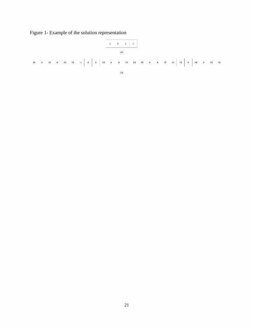
3.1.1. Solution representation
The solution representation is an important component of the GA, as it affects the performance
and runtime of the algorithm. Here, we use a binary display and the hub nodes and nodes
connections are shown as a binary string. For example, if an entrant’s potential hubs set is
4,11,14,18 and nodes 4,14,18 are chosen as the hub, the solution representation for hub nodes
and nodes assignment would be as follows. As shown in Figure 1 (a), the value of node cells
4,14,18 is equal to one. Also, in node assignment representation shown in Figure 1 (b), the
value of the first cell is 18, meaning that the first node is assigned to the hub node 18 or the
fourth hub node.
{Insert Figure 1 here}
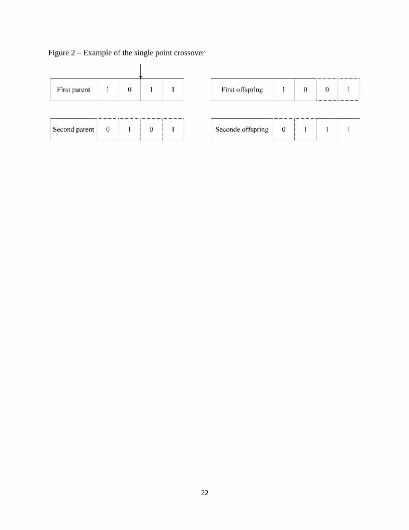
3.1.2. Crossover operator
The basic operator for producing new solutions in GA is a crossover. The crossover operator
discovers the solutions for a search space. In this paper, we used the roulette wheel to select
parents and single-point crossover. This used vertical or horizontal cut in the vector or matrix
randomly and produced two new offspring that shared some parts of both parents. If nh is the
number of the hubs, a 1-point crossover operator uses a random number 1,1 nht to cut the
parent vectors. If nodes 4,11,14,18 are entrant potential hubs, as shown in Figure 2, two parents
11
are selected and a random number and offsprings are generated as follows. Also, a random
number is generated again for infeasible offspring.
{Insert Figure 2 here}
In the first parent, nodes 4,14,18 are selected as the hub, meaning that variables 3
,1
yy and 4
y
are equal 1. In the second parent, nodes 11,18 are selected as the hub. Then 2t is chosen for
random cutting of the point and the offspring are produced. After the cutting of parents, the first
offspring would be composed of the first part of the first parent and the second part of the second
parent, meaning that nodes 4,18 become a hub and variables 1
y and 4
y will be equal 1. The
crossover rate in the suggested GA is set at 0.6.
3.1.3. Mutation operator
The mutation operator makes some changes in genes of the chromosome with low probability.
This is intended to escape from the local optimum and prevent early convergence. Also, the
mutation maintains diversity in the population. In this step, one solution is selected randomly and
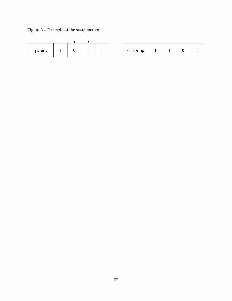
some chromosome genes are changed. We used the swap method to create a neighborhood. In
this method, two random numbers are produced and their genes are moved. An example of a
swap method is shown in Figure 3.
{Insert Figure 3 here}
As shown in Figure 3, by considering nodes 4,11,14,18 as the potential hub set, nodes 4,14,18
are chosen as the hub. Then, numbers 2 and 3 are created randomly and the offspring are
produced by moving the second and third cells. It should be noted that the mutation rate is set at
0.4 for this GA.
4. Computational experiments
For model evaluation, the Civil Aeronautics Board (CAB) dataset was used for 25 nodes [42]
and ij
k were calculated based on the following expression [43].
kmkmPHmk
ijij
ijqc
qck
/max
/10
),(
Nji , (18)
In the parameters related to environmental costs, 0.7d
c and 5A [44], 0.012r
c [45] and
7f
c , 5e , 9.81g , 1.2041p , 0.1a Also, ij
and ij were obtained from [7].
ijsndelta
was produced uniformly in 0.1,0.4 and the speed of the vehicle was uniform in 40,100 hkm/ .
Also, 6,0.8,10.2,0.4,0. , 1 and 1.55,15.397.7,9.63,13.85,5.78, were also used [22]. It
12
should be noted that for a dataset with 25 nodes to balance the parameters, the ij
k and k
F are
divided by 100. Also, the whole environmental costs are divided by 10000.
We solved this problem with Basic Open-source Nonlinear Mixed INteger programming
(BONMIN) solver and GA programmed in MATLAB 2016 for the first 5 nodes of the dataset
using a PC with a Core i5 processor of 2.5 GHz and 4 GB of RAM with 6,0.80.2,0.4,0. and
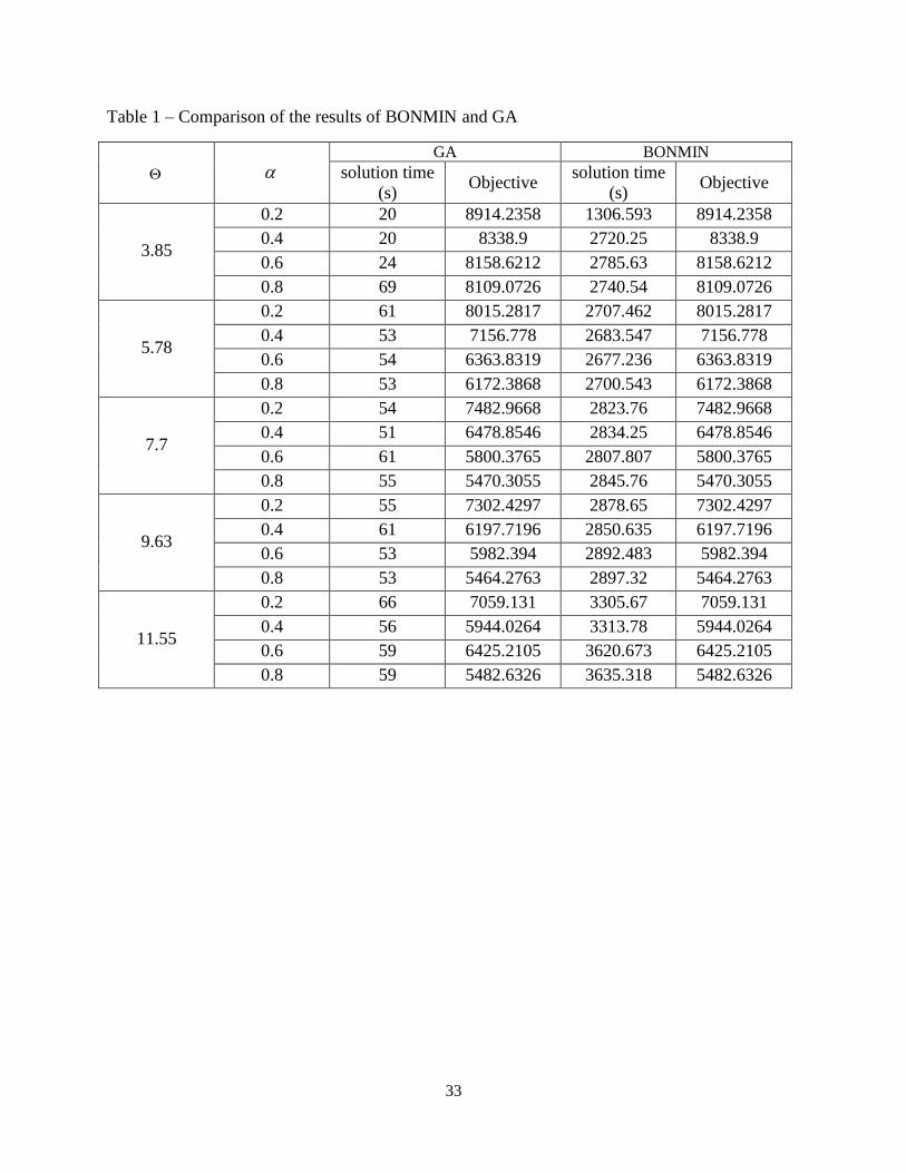
1.557.7,9.63,13.85,5.78, . The results are shown in Table 1. In this example, the incumbent’s
hubs are 2 and 4. Moreover, the potential entrant’s hubs are all five nodes.
{Insert Table 1 here}
As shown in Table 1, the objective function values obtained from BONMIN and GA are the
same, but the solution time of BONMIN and GA are significantly different. The solution time
increases by enlarging the size of the problem, and a PC with listed configurations would be
unable to solve this problem. As a result, the use of GA would yield better results.
For the analysis of data, the impact of , and the ratio of entrant number of the potential hub
nh to the incumbent hub number nhmt on the entrant profit was examined for the CAB dataset
using only GA with 10 replications. The average incumbent income (not the profit) was
considered because the incumbent was in the market for a while [22]. It is worth mentioning that
when nhmtnh , nh is considered as the entrant potential hubs, and when nhmtnh , nh acts
as entrant hubs (not potential hubs) because the number of the hub(s) selected by the entrant may
be less than nhmt in GA, which contradicts nhmtnh . In this research, when nhmtnh , nh
was 4,11,14,18 and nhmt was 7,13,17 and when nhmtnh , nh was 11,14,18 and nhmt was
4,7,13,17 . In that mode, three nodes were selected as the hub for 3.85,0.2 ,
3.85,0.6 and the eighteenth node was selected as the hub in other values of and .
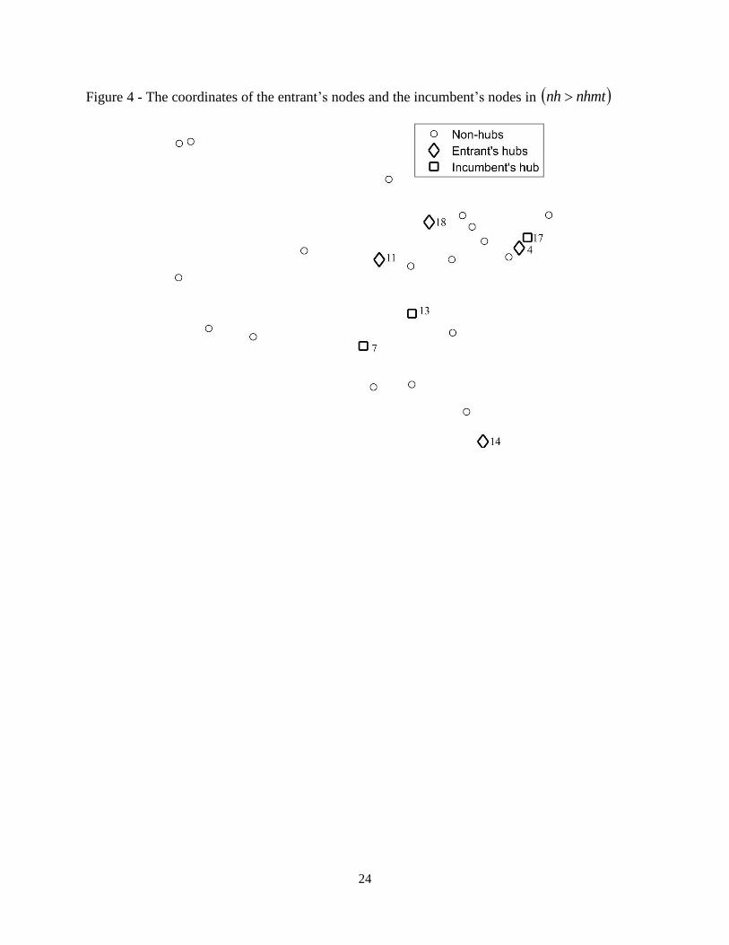
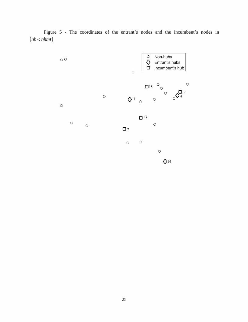
The coordinate points of applicants, nh , nhmt in the cases of nhmtnh and nhmtnh are
shown in Figures 4 and 5, respectively. The computational results included the entrant’s profit,
the incumbent’s income, and environmental costs induced by speed, which are shown in Tables 2
and 3, respectively.
{Insert Figure 4 here}
{Insert Table 2 here}
{Insert Figure 5 here}
{Insert Table 3 here}
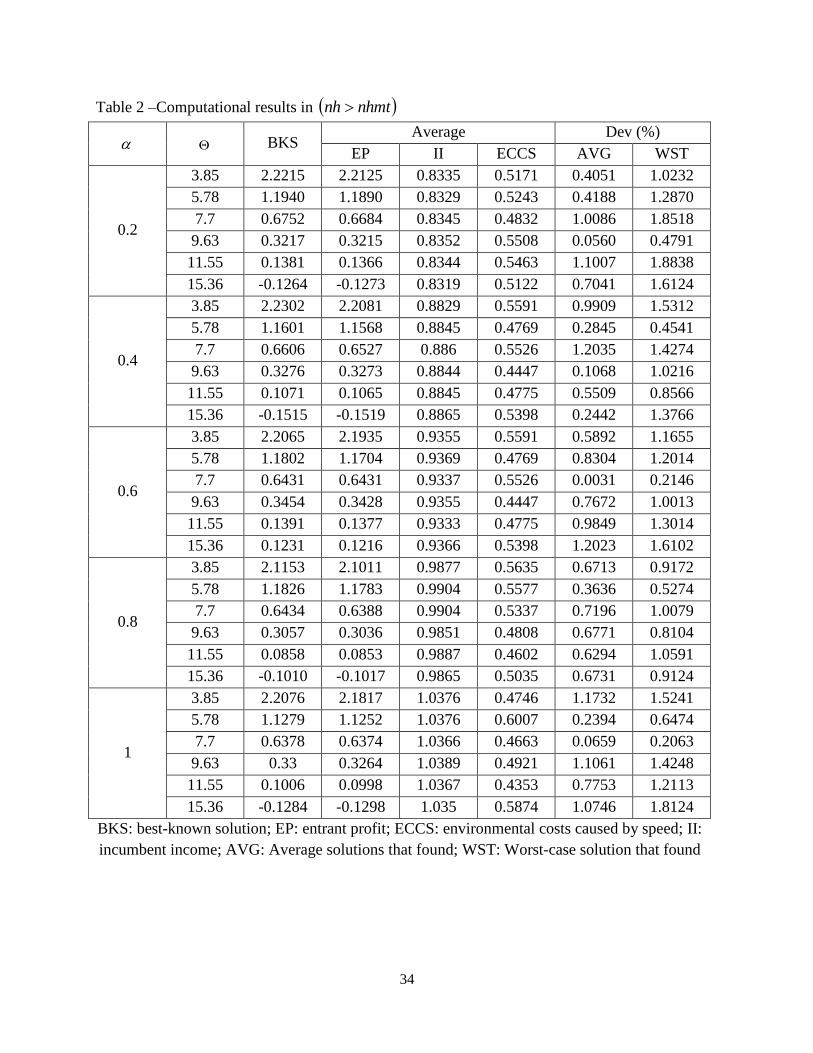
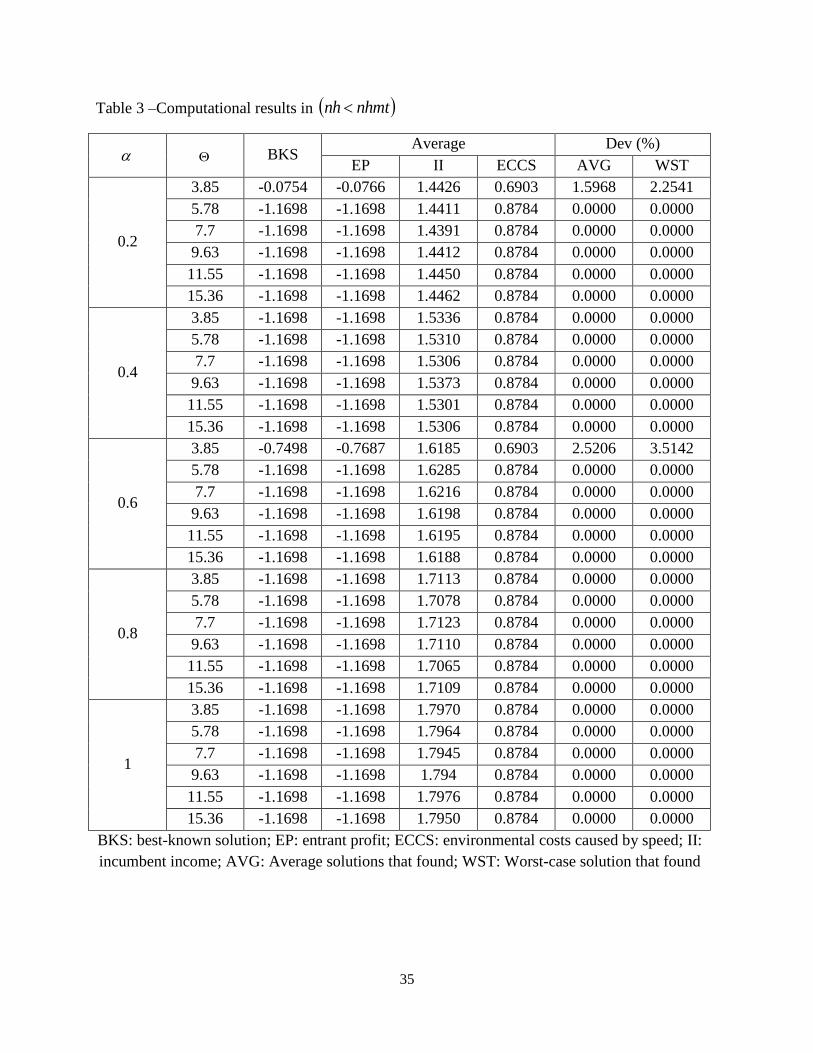
In Tables 2 and 3, the first column shows the discount factor and the second column presents the
sensitivity parameter of the LM. Moreover, the third column shows the best-known solutions
(BKS), which is obtained from the best case of GA. The fourth column shows the average
solution of GA. More data such as entrant profit (EP), which is the objective function, incumbent
13
income (II), and environmental costs caused by speed (ECCS) are presented due to depicting
their behaviors according to the average. Column Dev (%) shows the deviation between the BKS
and other solutions. In particular, the column under the heading AVG reports the deviation
between the BKS and the average solution found by GA. Also, column WST presents the
deviation between the BKS and the GA worst-case solution. It should be noted that in Table 3,
the Dev is more case is zero due to using only one hub the network, therefore, finding the
solution is easier than other cases. It seems that in these cases the GA obtained the optimal
solution.
As shown in Tables 2 and 3, in nhmtnh , the entrant’s profit drops by increasing the value of
and ; but in nhmtnh , the entrant’s profit for all values of and is -1.1698 except in
two cases. As a result, in a problem with this assumption, the number of hubs used by the entrant
must exceed that of the incumbent hubs. Also, in nhmtnh , the entrant’s profit is only greater
than the incumbent’s income in 3.85,5.78 for all values of . In other words, the entrant
can make more profits compared to the incumbent when customer sensitivity to price is low. In
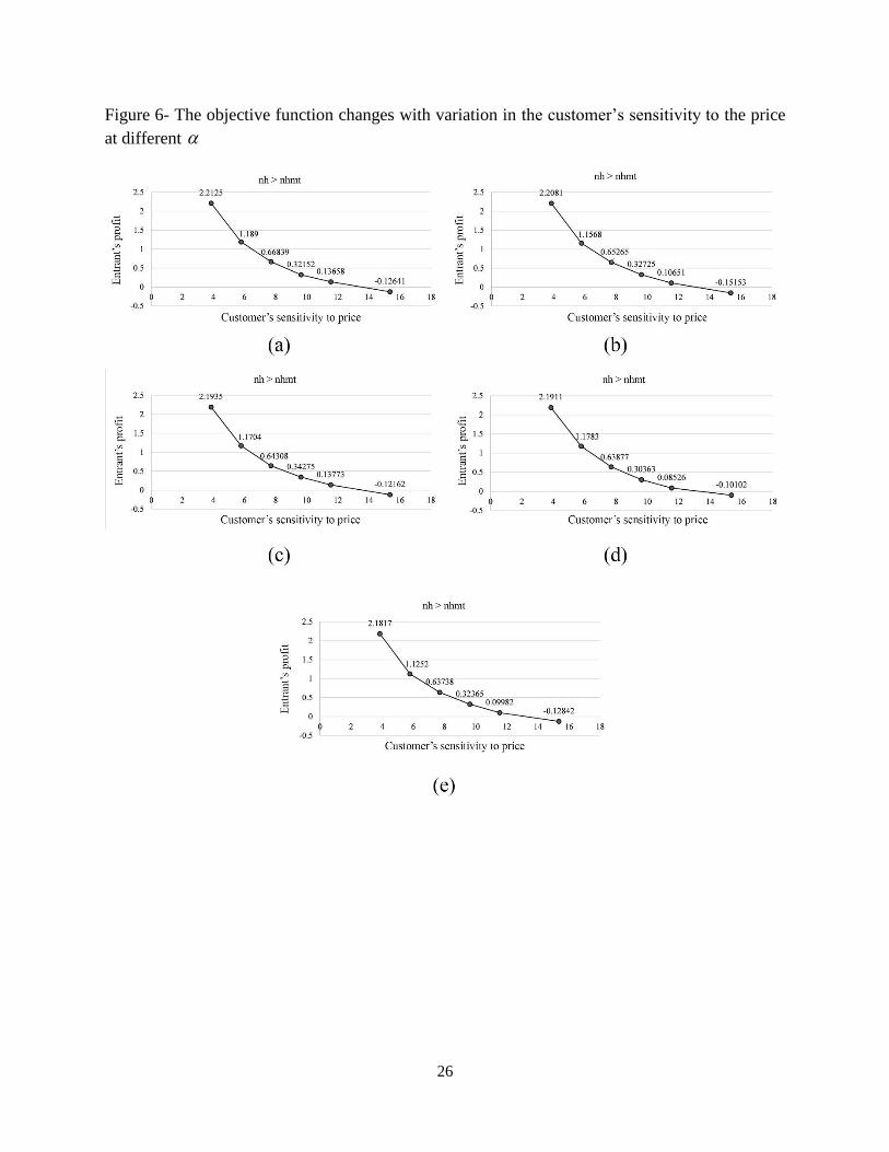
the following, a description of the results in Figure 6 is given.
{Insert Figure 6 here}
As shown in all charts of Figure 6, with a change of the objective function to in nhmtnh ,
the entrant’s profit drops by increasing the customer sensitivity to the price for all discount
values between hubs.
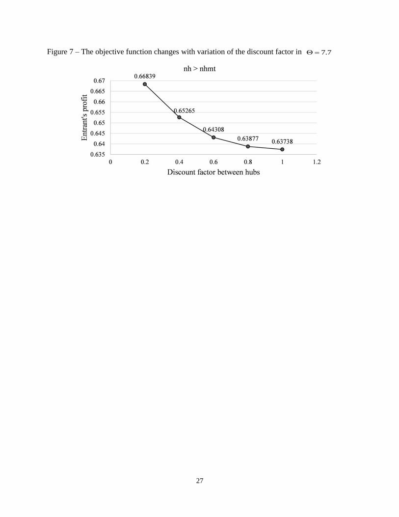
{Insert Figure 7 here}
Figure 7 demonstrates entrant profit is decreased by increasing .
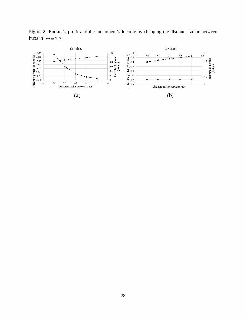
{Insert Figure 8 here}
According to Figure 8 (a), the entrant’s profit takes a declining process and the incumbent’s
income takes an incremental process when is increased nhmtnh and 7.7 . It should be
noted that in 7.7 the entrant’s profit is always lower than that of the incumbent, and as
mentioned, the entrant’s profit in 3.85,5.78 is higher than the incumbent’s income. It should
be noted that the entrant’s profit is shown in the axis on the left and the incumbent income in the
axis on the right. Also, according to Figure 8 (b), the entrant’s profit remains unchanged (-
1.1698) by increasing in nhmtnh and 7.7 , and the incumbent’s income takes an
incremental trend. In general, the entrant’s profit is less than the incumbent income’s, as shown
in Figure 8 (a).
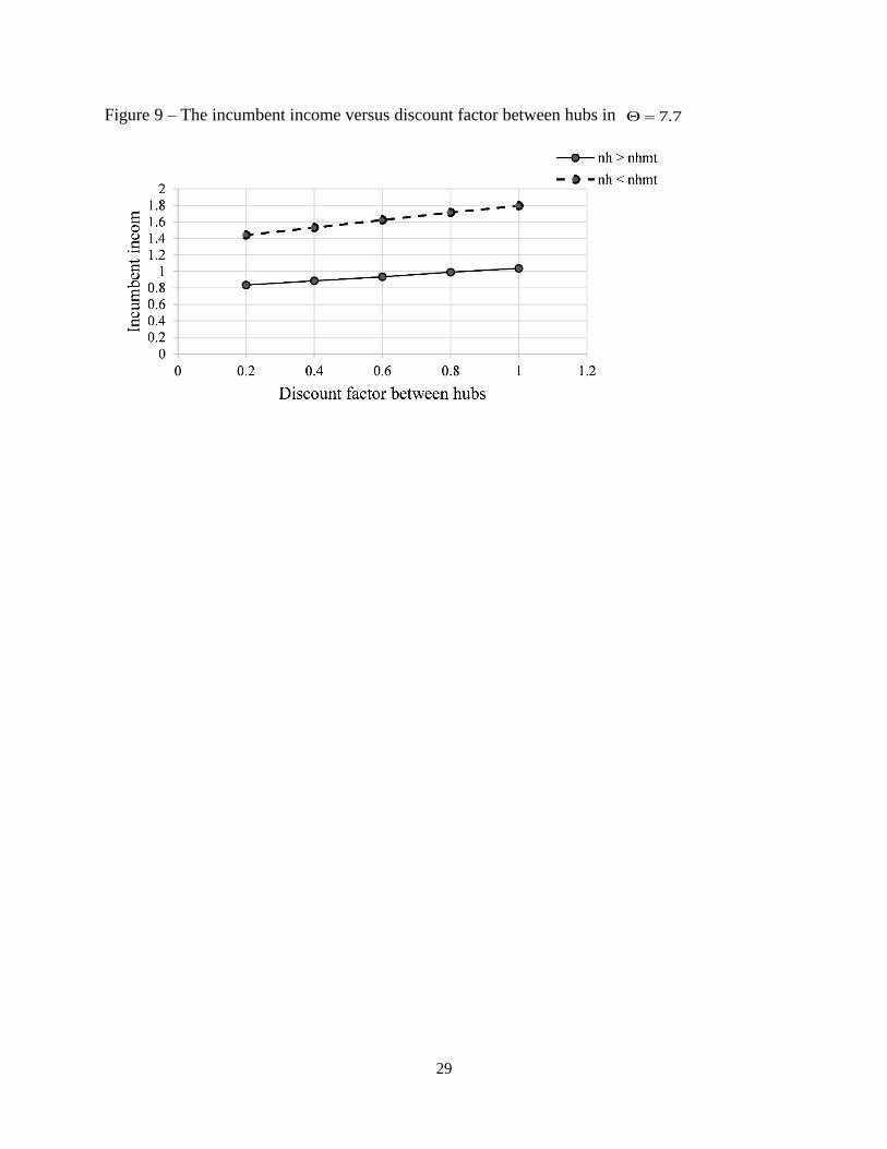
{Insert Figure 9 here}
A comparison of the incumbent’s income in two modes of nhmtnh and nhmtnh is shown in
Figure 9. As can be seen, the incumbent’s income in nhmtnh is more than the incumbent’s
14
income in nhmtnh . It is obvious because the incumbent’s ability to serve is greater than that of
the entrant in nhmtnh . As a result, the incumbent gain larger market share and generate more
revenues
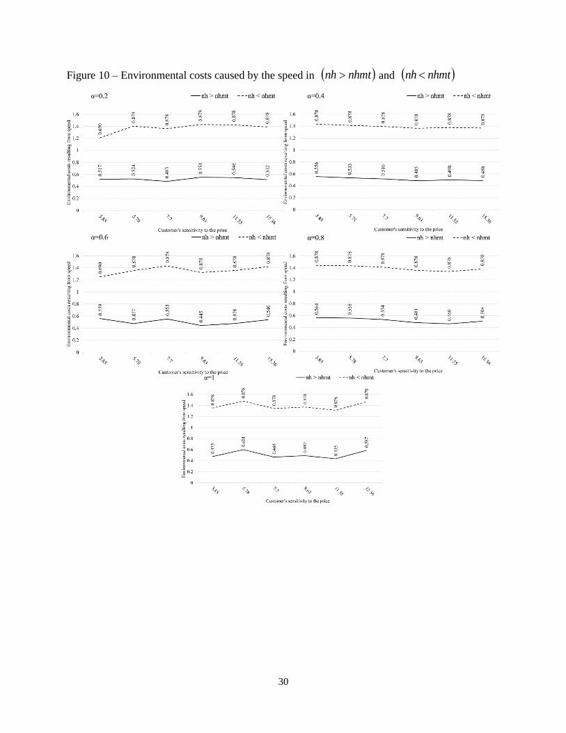
{Insert Figure 10 here}
Figure 10 shows that the environmental costs incurred from speed significantly lower in the
mode of nhmtnh as compared to the mode nhmtnh for different and . As shown in this
figure, the changes in and do not result in descending or ascending changes in
environmental costs. As expected, in nhmtnh , the number of links between non-hubs to hubs
are less than nhmtnh . Instead of these links, the network used hub links. Therefore, in the
obtained results for nhmtnh the model causes fewer environmental costs. Furthermore, the
trends in nhmtnh and nhmtnh maybe the same for each except in two cases (i.e., 2.0
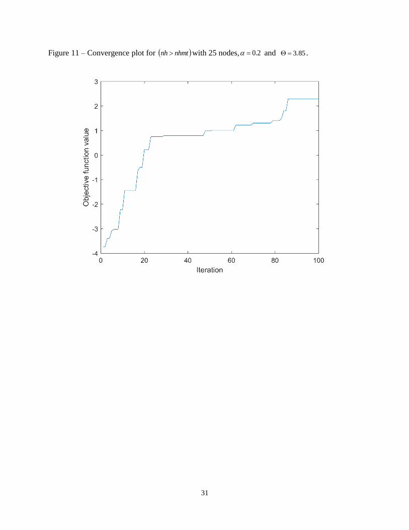
, 5.78 and 6.0 , 5.78 ). To show the solution convergence in the proposed GA, an
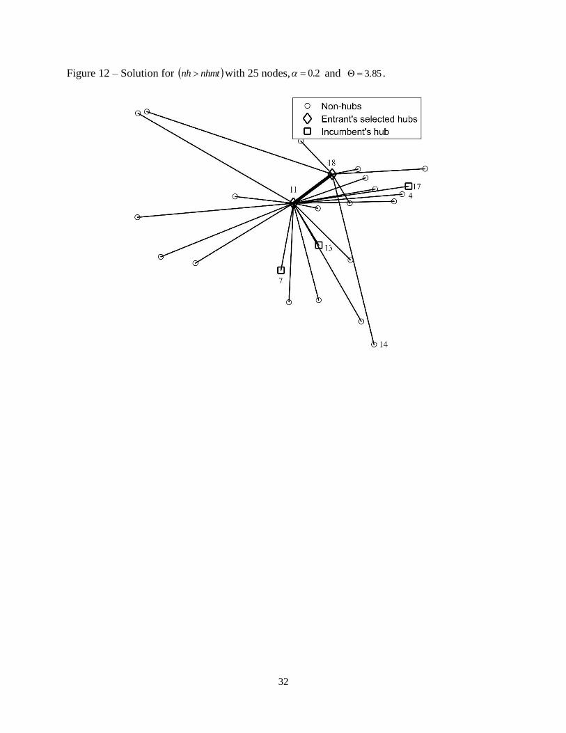
instance for nhmtnh with 25 nodes, 2.0 and 3.85 is solved. Figure 11 describes this
convergence plot and Figure 12 shows its solution.
{Insert Figure 11 here}
{Insert Figure 12 here}
5. Discussion
The design of hub networks with the price decision variable is an issue that has researched rarely
in the literature. In this research, we present a model that integrated pricing and hub location
problem with environmental costs in the competitive market. Computational experiments
demonstrate the efficiency of our model in small-sized instances. For large-sized instances, GA
is proposed to find optimal or near-optimal with reasonable computational effort. Tables 2 and 3
show the GA performance. Moreover, the proposed GA explores the hub network and finds
feasible solutions. Once a valid hub configuration is found, the pricing problem is solved for this
network, and the optimal flows and prices are found. Therefore, the performance of GA is
dependent on the obtained hub network. Moreover, a sensitivity analysis was conducted to gain a
preliminary understanding of how the entrant’s or incumbent’s profit or income are affected by
some changing of parameters such as the number of hubs.
The results show when the entrant’s hubs outnumber incumbent’s hubs nhmtnh , the entrant’s
profit drops with an increase in for all values of . In both nhmtnh and nhmtnh
modes for an exact , the incumbent’s income rises by increasing and in the second mode
nhmtnh , the incumbent earns more income in comparison to the first mode because of using
the more hubs and decreasing the transportation costs. However, the entrant’s profit is fixed in
the second state and this is due to the algorithm only selects the node 18 from the potential hub
15
nodes 11,14,18 for all values of and , as a result, the entrant’s profit does not change. The
reason that the algorithm selects just the node 18 as a hub can be the lack of capacity
constraint for hubs or hub arcs. In other words, if lower bound and upper bound were considered
for the capacity of each hub node or an upper bound was considered for all arcs, the only node
18 was not selected as a hub. Also, due to not considering the coverage limit, it is possible that
one non-hub node assigned to the hub farther away through two hubs. For example, for 0.2
and 3.85 , the distance between a non-hub node 22 and hub node 18 is more than the
distance between a non-hub node 22 and hub node 11 , but the node 22 is assigned the hub
node 18 . This issue can convert hub nodes to mini-hub and major-hub. It should also be noted
that in nhmtnh , the entrant’s profit is only in 3.85,5.78 more than the incumbent’s
income; in other words, incumbent get more market share by increasing customer’s sensitivity to
the entrant’s prices and accordingly its income increases. Finally, the environmental costs caused
by the speed of the entrant’s vehicles in nh nhmt is more than nh nhmt , that could be
because of distance and vehicle speed. Thus, the entrant requires more hubs than incumbent to
reduce environmental costs and increase its profits.
As that is existing in the literature of hub location, there is a discount factor between two hub
nodes. In the first mode nh nhmt , the total costs, time, and the number of trips are decreased,
although the fixed cost of using more hubs is added to the total costs.
Finally, in the two modes nh nhmt and nh nhmt , we select entrant’s and incumbent’s
hub nodes based on the map and the best coverage of all nodes. Also, in selecting hub nodes, we
take care that in those nodes and their around would have existed less green space for more
decreasing environmental pollution.
6. Conclusion
In this paper, we considered a pricing problem and HLP together with environmental costs,
which is a mixed-integer non-linear programming problem. We solved this problem with GA and
analyzed results from the following perspectives: (1) the impact of and on the entrant’s
profit and the incumbent’s income. (2) The ratio of the number of entrant’s hubs to the number
of incumbent’s hubs. The results show that the higher the number of potential entrant’s hubs than
the incumbent, the lower the entrant’s gain as the discount factor between hub nodes increases.
Therefore, managers should consider this important observation on their decision making. Also,
if the number of potential entrant’s hub is higher than the incumbent, for all discount factors, the
customer's profitability decreases with increasing price sensitivity. In each price sensitivity
coefficient, the incumbent’s income increases as the discount factor increases, and the incumbent
16
income is higher when the number of incumbent’s hub is more than the potential entrant’s hub.
Finally, when the number of potential entrant’s hub is more than the incumbent’s hub, the
environmental costs of the entrant are less than another case, so the entrant must use more hubs
than the incumbent to reduce environmental costs and increase profits.
Moreover, in this research, customer choice behavior was modeled based on an LM. This
behavior depends only on the price of each path. To be more compatible with the real world, this
study can be conducted using a multinomial LM. Furthermore, in this model, the customer
behavior can be affected by the transportation time or the number of stops (hubs) in addition to
the price. Also, an interesting future research direction would be to consider a capacity for hubs
and hub arc threshold. Also, further studies regarding the role of other metaheuristic algorithms
for larger size instances would be worthwhile.
References
[1]. Haron.A. “Factors Influencing Pricing Decisions”, Int J Econ & Manag Sci, 5(1), pp. 312-
315 (2016).
[2]. Gelareh.S, Monemi, R.N, Nickel, S, "Multi-period hub location problems in transportation",
Transport Res E-Log, 75(1), pp.67-94 (2015).
[3]. Karimi, H, Setak, M, "A bi-objective incomplete hub location-routing problem with flow
shipment scheduling", Appl Math Model, 57(1), pp. 406-431 (2018).
[4]. Sarkis.J, Sundarraj.R.P. “Hub location at Digital Equipment Corporation: A comprehensive
analysis of qualitative and quantitative factors”, Eur J Oper Res, 137(2), pp. 336-347 (2002).
[5]. McKinnon.A. “CO2 Emissions from freight transport in the UK”, In Transport and Climate
Change (Vol. 2). T. Reley, L. Chapman, Emerald Group Publishing Limited, New York
(2007).
[6]. Chen.S, Shiyi.H. “Pricing for the clean air: Evidence from Chinese housing market”, J
Clean Prod. 206(1), pp. 297-306 (2019).
[7]. Bektas.T, Laporte.G. (2011). “The Pollution-Routing Problem”, Transport Res B-Meth,
45(8), pp. 1232-1250 (2011).
[8]. Garrow.L.A. “Discrete Choice Modelling and Air Travel Demand: Theory and Applications
(Vol. 5)”. UK: Georgia Institute of Technology, USA (2016).
[9]. Rayfield, W.Z, Rusmevichientong, P, Topaloglu, H. "Approximation methods for pricing
problems under the nested logit model with price bounds", INFORMS J Comput, 27(2), 335-
357 (2015).
[10]. Beckmann, M. J., Thisse, J. F. The location of production activities. In Handbook of
regional and urban economics (Vol. 1, pp. 21-95). Elsevier (1987).
17
[11]. Goldman, A. “Optimal Location for Centers in a Network”. Transport Sci, 3(4), pp. 352-
360 (1969).
[12]. O'Kelly.M.E. “The Location of Interacting Hub Facilities”, Transport Sci, 20(2), pp. 92-
106 (1986).
[13]. Campbell.J.F, Ernst, A.T, Krishnamoorthy.M. “Hub Arc Location Problems: Part I—
Introduction and Results”, Manage Sci, 51(10), pp. 1540-1555 (2005).
[14]. Campbell.J.F, Ernst, A.T, Krishnamoorthy.M. “Hub arc location Problems: Part II—
formulations and optimal algorithms”, Manage Sci, 51(10), pp. 1556-1571 (2005).
[15]. Campbell.J.F. “Hub location for time-definite transportation”, Comput Oper Res, 36(12),
pp. 3107-3116 (2009).
[16]. Nickel.S, Schöbel.A, Sonneborn.T. “Hub location problems in urban traffic networks”, In
P. Niittymäki.J, Mathematics Methods and Optimization in Transportation Systems pp. 95-
107, Kluwer Academic Publishers (2001).
[17]. Gelareh.S, Nickel.S. “Hub location problems in transportation networks”, Transport Res E-
Log, 47(6), pp. 1092-1111 (2011).
[18]. Adler.N, Smilowitz.K. “Hub-and-spoke network alliances and mergers: Price-location
competition in the airline industry”, Transport Res B-Meth, 41(4), pp. 394-409 (2007).
[19]. Hansen.p, Peeters.D, Thisse.J. “Facility location under zone pricing”, J Regional Sci,
37(1), pp. 1-22 (1997).
[20]. Chu.C.Y.C, Lu.H. “The multi-store location and pricing decisions of a spatial monopoly”,
Reg Sci Urban Econ, 28(3), pp. 255-281 (1998).
[21]. Zhang, Y, "Designing a retail store network with strategic pricing in a competitive
environment", Int J Prod Econ, 159(1), pp. 265-273 (2015).
[22]. Lüer-Villagra. A & Marianov.V. “A competitive hub location and pricing problem”, Eur J
Oper Res, 231(3), pp. 734-744 (2013).
[23]. Setak.M, Sadeghi-Dastaki.M, Karimi.H. “Investigating zone pricing in a location-routing
problem using a variable neighborhood search algorithm”, Int J Eng, 28(11), pp. 1624-1633
(2015).
[24]. Karimi. H, Setak. M. “ Proprietor and customer costs in the incomplete hub location-
routing network topology”, Appl Math Model, 38(3), pp. 1011-1023 (2014).
[25]. Korani.E, Eydi. A, Nakhai. I. “Reliable Hierarchical Multimodal Hub Location Problem:
Models and Lagrangian Relaxation Algorithm”, Scientia Iranica,
DOI:10.24200/sci.2018.50797.1870.
[26]. Daniel.J, Harback.K.T. “Pricing the major US hub airport”, J Urban Econ, 66(1), pp. 33-
56 (2009).
18
[27]. Spiller.P.T. “A note on pricing of hub and spoke networks”, Econ Lett, 30(2), pp. 165-169
(1989).
[28]. Daniel.J.I. “Congestion Pricing and Capacity of Large Hub Airports : A Bottleneck
Model with Stochastic Queues”, Econometrica, 63(2), pp. 327-370 (1995).
[29]. Oum.T, zhang.A, zhang.Y. “A note on optimal airport pricing in a hub-and-spoke system”,
Transport Res B-Meth, 30(1), pp. 11-18 (1996).
[30]. Nero.G, Black.J. “Hub-and-Spoke Networks and the Inclusion of Environmental Costs on
Airport Pricing”, Transport Res D-Trans Env, 3(5), pp. 275-296 (1998).
[31]. Vowles.T.M. “Airfare pricing determinants in hub-to-hub markets”, J Transp Geogr,
14(1), pp. 15-22 (2006).
[32]. O’Kelly, M. E. “Fuel burn and environmental implications of airline hub networks”.
Transport Res D-Trans Env, 17(7), pp. 555-567 (2012).
[33]. Loo, B.P.Y, Linna L, Voula P, Ioanna P. "CO2 emissions associated with hubbing
activities in air transport: an international comparison", J Transp Geogr, 34, pp. 185-193
(2014).
[34]. Niakan, F., Vahdani, B., Mohammadi, M. “A multi-objective optimization model for hub
network design under uncertainty: An inexact rough-interval fuzzy approach” Eng Opt,
47(12), pp. 1670-1688 (2015).
[35]. Zhalechian, M., Tavakkoli-Moghaddam, R., Rahimi, Y., Jolai, F. “An interactive
possibilistic programming approach for a multi-objective hub location problem: Economic
and environmental design”. Appl. Soft. Comput, 52, pp.699-713 (2017).
[36]. Zhang.S, Derudder.B, Witlox.F. “The impact of hub hierarchy and market competition on
airfare pricing in US hub-to-hub markets”, J Air Transp Manag, 32(2),pp. 65-70 (2013).
[37]. Lin.M, Zhang.A. “Hub congestion pricing: Discriminatory passenger charges”, Econ of
Transp, 5(1), pp. 37-48 (2016).
[38]. Lin, M.H, Zhang.Y. “Hub-airport congestion pricing and capacity investment”, Transport
Res B-Meth, 101(1), pp. 89-106 (2017).
[39]. Cunha C.B, Silva. M.R, “A genetic algorithm for the problem of configuring a hub-and-spoke
network for a LTL trucking company in Brazil,” Eur. J. Oper. Res., 179(3), pp. 747-758, (2007).
[40]. Topcuoglu, H., Corut, F., Ermis., M, Yilmaz, G., “Solving the uncapacitated hub location problem
using genetic algorithms,” Comput. Oper. Res., 32(4), pp. 967-984, (2005).
[41]. Rudolph G, “Convergence analysis of canonical genetic algorithms,” IEEE Trans. Neural
Networks, 5(1), pp. 96-101, (1994).
[42]. O'kelly, M. E. “A quadratic integer program for the location of interacting hub facilities”,
Eur J Oper Res, 32(3), pp. 393-404 (1987).
19
[43]. Calik.H, Alumur.S, Kara.B, Karasan.O. “A tabu-search based heuristic for the hub
covering problem over incomplete hub networks”, Comput Oper Res, 36(12), pp. 3088-3096
(2010).
[44]. Akçelik.R, Besley.M. “Operating cost, fuel consumption, and emission models in
aaSIDRA and aaMOTION”, 25th Conference of Australian Institute of Transport research
(2013).
[45]. Genta.G. “Motor vehicle dynamics : modeling and simulation” World Scientific, Italy
(1997).
Mohaddese Mohammadi is received her bachelor’s and master’s degree in Industrial
Engineering from Babol Noshirvani University of Technology in 2014 and University of
Bojnord in 2017, respectively. Her interest researches are: facility location, optimizations,
mathematical modelling and integer programming.
Hossein Karimi is the head of Industrial Engineering department at the University of Bojnord.
He completed his bachelor’s, master’s and PhD degree at the University of Bojnord, Shahed
University and K.N.T University of Technology, respectively. He is the author of several journal
papers on hub location problem, vehicle routing problem, and multiple attribute decision making.
In addition, he wrote three academic books in Persian about location problems and integer
programming.
List of figures and tables
Figure 1- Example of the solution representation
Figure 2 – Example of the single point crossover
Figure 3 – Example of the swap method
Figure 4 - The coordinates of the entrant’s nodes and the incumbent’s nodes in nhmtnh
Figure 5 - The coordinates of the entrant’s nodes and the incumbent’s nodes in nhmtnh
Figure 6- The objective function changes with variation in the customer’s sensitivity to the price
at different
Figure 7 – The objective function changes with variation of the discount factor in 7.7
Figure 8- Entrant’s profit and the incumbent’s income by changing the discount factor between
hubs in 7.7
20
Figure 9 – The incumbent income versus discount factor between hubs in 7.7
Figure 10 – Environmental costs caused by the speed in nhmtnh and nhmtnh
Figure 11 – Convergence plot for nhmtnh with 25 nodes, 2.0 and 3.85 .
Figure 12 – Solution for nhmtnh with 25 nodes, 2.0 and 3.85 .
Table 1 – Comparison of the results of BONMIN and GA
Table 2 –Computational results in nhmtnh
Table 3 –Computational results in nhmtnh
21
Figure 1- Example of the solution representation
22
Figure 2 – Example of the single point crossover
23
Figure 3 – Example of the swap method
24
Figure 4 - The coordinates of the entrant’s nodes and the incumbent’s nodes in nhmtnh
25
Figure 5 - The coordinates of the entrant’s nodes and the incumbent’s nodes in
nhmtnh
26
Figure 6- The objective function changes with variation in the customer’s sensitivity to the price
at different
27
Figure 7 – The objective function changes with variation of the discount factor in 7.7
28
Figure 8- Entrant’s profit and the incumbent’s income by changing the discount factor between
hubs in 7.7
29
Figure 9 – The incumbent income versus discount factor between hubs in 7.7
30
Figure 10 – Environmental costs caused by the speed in nhmtnh and nhmtnh
31
Figure 11 – Convergence plot for nhmtnh with 25 nodes, 2.0 and 3.85 .
32
Figure 12 – Solution for nhmtnh with 25 nodes, 2.0 and 3.85 .
33
Table 1 – Comparison of the results of BONMIN and GA
GA BONMIN
solution time
(s) Objective
solution time
(s) Objective
3.85
0.2 20 8914.2358 1306.593 8914.2358
0.4 20 8338.9 2720.25 8338.9
0.6 24 8158.6212 2785.63 8158.6212
0.8 69 8109.0726 2740.54 8109.0726
5.78
0.2 61 8015.2817 2707.462 8015.2817
0.4 53 7156.778 2683.547 7156.778
0.6 54 6363.8319 2677.236 6363.8319
0.8 53 6172.3868 2700.543 6172.3868
7.7
0.2 54 7482.9668 2823.76 7482.9668
0.4 51 6478.8546 2834.25 6478.8546
0.6 61 5800.3765 2807.807 5800.3765
0.8 55 5470.3055 2845.76 5470.3055
9.63
0.2 55 7302.4297 2878.65 7302.4297
0.4 61 6197.7196 2850.635 6197.7196
0.6 53 5982.394 2892.483 5982.394
0.8 53 5464.2763 2897.32 5464.2763
11.55
0.2 66 7059.131 3305.67 7059.131
0.4 56 5944.0264 3313.78 5944.0264
0.6 59 6425.2105 3620.673 6425.2105
0.8 59 5482.6326 3635.318 5482.6326
34
Table 2 –Computational results in nhmtnh
BKS Average Dev (%)
EP II ECCS AVG WST
0.2
3.85 2.2215 2.2125 0.8335 0.5171 0.4051 1.0232
5.78 1.1940 1.1890 0.8329 0.5243 0.4188 1.2870
7.7 0.6752 0.6684 0.8345 0.4832 1.0086 1.8518
9.63 0.3217 0.3215 0.8352 0.5508 0.0560 0.4791
11.55 0.1381 0.1366 0.8344 0.5463 1.1007 1.8838
15.36 -0.1264 -0.1273 0.8319 0.5122 0.7041 1.6124
0.4
3.85 2.2302 2.2081 0.8829 0.5591 0.9909 1.5312
5.78 1.1601 1.1568 0.8845 0.4769 0.2845 0.4541
7.7 0.6606 0.6527 0.886 0.5526 1.2035 1.4274
9.63 0.3276 0.3273 0.8844 0.4447 0.1068 1.0216
11.55 0.1071 0.1065 0.8845 0.4775 0.5509 0.8566
15.36 -0.1515 -0.1519 0.8865 0.5398 0.2442 1.3766
0.6
3.85 2.2065 2.1935 0.9355 0.5591 0.5892 1.1655
5.78 1.1802 1.1704 0.9369 0.4769 0.8304 1.2014
7.7 0.6431 0.6431 0.9337 0.5526 0.0031 0.2146
9.63 0.3454 0.3428 0.9355 0.4447 0.7672 1.0013
11.55 0.1391 0.1377 0.9333 0.4775 0.9849 1.3014
15.36 0.1231 0.1216 0.9366 0.5398 1.2023 1.6102
0.8
3.85 2.1153 2.1011 0.9877 0.5635 0.6713 0.9172
5.78 1.1826 1.1783 0.9904 0.5577 0.3636 0.5274
7.7 0.6434 0.6388 0.9904 0.5337 0.7196 1.0079
9.63 0.3057 0.3036 0.9851 0.4808 0.6771 0.8104
11.55 0.0858 0.0853 0.9887 0.4602 0.6294 1.0591
15.36 -0.1010 -0.1017 0.9865 0.5035 0.6731 0.9124
1
3.85 2.2076 2.1817 1.0376 0.4746 1.1732 1.5241
5.78 1.1279 1.1252 1.0376 0.6007 0.2394 0.6474
7.7 0.6378 0.6374 1.0366 0.4663 0.0659 0.2063
9.63 0.33 0.3264 1.0389 0.4921 1.1061 1.4248
11.55 0.1006 0.0998 1.0367 0.4353 0.7753 1.2113
15.36 -0.1284 -0.1298 1.035 0.5874 1.0746 1.8124
BKS: best-known solution; EP: entrant profit; ECCS: environmental costs caused by speed; II:
incumbent income; AVG: Average solutions that found; WST: Worst-case solution that found
35
Table 3 –Computational results in nhmtnh
BKS Average Dev (%)
EP II ECCS AVG WST
0.2
3.85 -0.0754 -0.0766 1.4426 0.6903 1.5968 2.2541
5.78 -1.1698 -1.1698 1.4411 0.8784 0.0000 0.0000
7.7 -1.1698 -1.1698 1.4391 0.8784 0.0000 0.0000
9.63 -1.1698 -1.1698 1.4412 0.8784 0.0000 0.0000
11.55 -1.1698 -1.1698 1.4450 0.8784 0.0000 0.0000
15.36 -1.1698 -1.1698 1.4462 0.8784 0.0000 0.0000
0.4
3.85 -1.1698 -1.1698 1.5336 0.8784 0.0000 0.0000
5.78 -1.1698 -1.1698 1.5310 0.8784 0.0000 0.0000
7.7 -1.1698 -1.1698 1.5306 0.8784 0.0000 0.0000
9.63 -1.1698 -1.1698 1.5373 0.8784 0.0000 0.0000
11.55 -1.1698 -1.1698 1.5301 0.8784 0.0000 0.0000
15.36 -1.1698 -1.1698 1.5306 0.8784 0.0000 0.0000
0.6
3.85 -0.7498 -0.7687 1.6185 0.6903 2.5206 3.5142
5.78 -1.1698 -1.1698 1.6285 0.8784 0.0000 0.0000
7.7 -1.1698 -1.1698 1.6216 0.8784 0.0000 0.0000
9.63 -1.1698 -1.1698 1.6198 0.8784 0.0000 0.0000
11.55 -1.1698 -1.1698 1.6195 0.8784 0.0000 0.0000
15.36 -1.1698 -1.1698 1.6188 0.8784 0.0000 0.0000
0.8
3.85 -1.1698 -1.1698 1.7113 0.8784 0.0000 0.0000
5.78 -1.1698 -1.1698 1.7078 0.8784 0.0000 0.0000
7.7 -1.1698 -1.1698 1.7123 0.8784 0.0000 0.0000
9.63 -1.1698 -1.1698 1.7110 0.8784 0.0000 0.0000
11.55 -1.1698 -1.1698 1.7065 0.8784 0.0000 0.0000
15.36 -1.1698 -1.1698 1.7109 0.8784 0.0000 0.0000
1
3.85 -1.1698 -1.1698 1.7970 0.8784 0.0000 0.0000
5.78 -1.1698 -1.1698 1.7964 0.8784 0.0000 0.0000
7.7 -1.1698 -1.1698 1.7945 0.8784 0.0000 0.0000
9.63 -1.1698 -1.1698 1.794 0.8784 0.0000 0.0000
11.55 -1.1698 -1.1698 1.7976 0.8784 0.0000 0.0000
15.36 -1.1698 -1.1698 1.7950 0.8784 0.0000 0.0000
BKS: best-known solution; EP: entrant profit; ECCS: environmental costs caused by speed; II:
incumbent income; AVG: Average solutions that found; WST: Worst-case solution that found

36