Environmental Boundary Tracking and EstimationUsing Multiple Autonomous Vehicles

Zhipu Jin and Andrea L. Bertozzi

Abstract— In this paper, we develop a framework for envi-ronmental boundary tracking and estimation by considering theboundary as a hidden Markov model (HMM) with separatedobservations collected from multiple sensing vehicles. For eachvehicle, a tracking algorithm is developed based on Page’scumulative sum algorithm (CUSUM), a method for change-point detection, so that individual vehicles can autonomouslytrack the boundary in a density field with measurement noise.Based on the data collected from sensing vehicles and priorknowledge of the dynamic model of boundary evolvement, weestimate the boundary by solving an optimization problem, inwhich prediction and current observation are considered in thecost function. Examples and simulation results are presentedto verify the efficiency of this approach.

Index Terms— Boundary tracking and estimation, hiddenMarkov model, change-point detection, CUSUM, optimization.

I. INTRODUCTION

Monitoring environmental boundaries has been an interest-ing topic for many years due to scientific and public safetyapplications. Examples include monitoring poisonous oilspills, harmful algae blooms, wild fire spreading, temperatureand salinity distribution in the ocean, and hazardous weatherconditions such as hurricanes and tropical storms.

There are many cases in which it is difficult to getglobal images of the boundary we are interested in fromremote sensing technology. Two examples are transparentchemical spills and underwater “dead-zones” generated byalgae blooms. In recent years, a considerable amount ofwork has been reported on using mobile sensing vehiclesfor environmental monitoring. Barat and Rendas [1] usesingle autonomous underwater vehicle (AUV) with a profilersonar to detect the boundaries between distinct benthicregions. Kemp et al. [2] propose a simple algorithm formultiple AUVs surveillance that only requires concentrationmeasurements. This algorithm has been tested on Caltech’smulti-vehicle wireless testbed [3], [4]. Bertozzi et al [5]design a centralized collective motion algorithm based onthe “snake algorithm” in image processing to detect andtrack algae blooms, where each agent needs to measure theconcentration gradient.

Coordination among multiple sensing vehicles is also arelated research area. Clark and Fierro [6] try to detect and

Zhipu Jin is with the Department of Mathematics, University of Cali-fornia, Los Angeles, USA. He also holds a position as visiting scholar inthe Department of Control and Dynamical Systems, California Institute ofTechnology. zhipu@math.ucla.edu

Andrea L. Bertozzi is with the Faculty of the Department of Mathematics,University of California, Los Angeles, USA. bertozzi@math.ucla.edu

surround a dynamic perimeter using a group of nonholo-nomic robots equipped with collision avoidance controllers.Zhang and Leonard [7] use four robots to compose aformation so that the gradient at the formation center canbe measured in a density field. Susca et al. [8] proposea distributed coordination algorithm in which each vehicletracks the boundary individually and communicates with itsnearby neighbors. Vertices are generated uniformly along theboundary based on certain metric and a polygon is generatedto approximate the boundary.

In this paper, we treat those mobile vehicles as an “ob-server” in which each vehicle can autonomously track theboundary with or without coordinating with others. The out-puts of this “observer” are separated and noisy observationscollected from vehicles. Assuming that there exists certain“hidden” relationship behind those separated data, whichgoverns the dynamics of the boundary evolvement, and weneed to reveal this relationship so that the boundary canbe accurately tracked and estimated. This idea is inspiredby hidden Markov model (HMM) in [9] and interactiveBayesian filters in [10].

Our contribution includes two parts: First, we propose arevised tracking algorithm for a single vehicle based on [2],where CUSUM filters are embedded so that each vehicle cantrack the boundary even with noisy measurements. CUSUMis an efficient change-point detection method which canquickly detect small drifts in the parameters for randomprocess [11], [12], [13], [14]. Second, assuming that theboundary can be approximated with an ellipse, we formulatethe boundary estimation problem as an optimization problem.Finding the optimal ellipse parameters can be done by com-bining a priori prediction and measurements from sensingvehicles with additional noise. This is a first step towards ageneral framework using spatio-temporal nonlinear filteringfor pattern recognition in environment monitoring.

The remainder of this paper is organized as follows: InSection II, we develop a tracking algorithm for a singlevehicle by using CUSUM filters to process noisy measure-ments. CUSUM filters generate a binary signal, which isused as a navigation signal in each sensing vehicle. We thenpropose a framework to estimate the boundary based onseparated observations in Section III. Assuming the boundarycan be approximated by an ellipse and its parameters evolveaccording to Markov models, we show how to estimate thoseparameters by solving an optimization problem. Section IVis devoted to examples and simulation results that verify theefficiency of this approach. Finally, conclusions and futurework are summarized in Section V.

II. TRACKING ALGORITHM WITH SINGLE VEHICLE

Assume an environmental boundary can be described bya density field in 2-D Euclidian space. The density functionis a mapping

d(x) : R2 → R (1)

where x is the location and d(x) is the density value. Theboundary is defined by a level set

Ω = {x ∈ R2 | d(x) = B} (2)

where B is the density threshold. In order to simplify theproblem, we assume that d(x) ∈ C1 and all level sets aresmooth, i.e, Ω is continuous. Also, we assume that d(x) > Bif x is inside Ω and d(x) < B if x is outside. Suppose eachvehicle has a sensor which can measure the density field as

z(k) = d(x(k)) + v(k) (3)

where k is the time, v(k) is the sensor noise with zero mean,and z(k) is the density measurement. Moreover, we assumethat the speed of the vehicle is a constant, V , and we cancontrol its orientation, θ, by

θ(k + 1) = θ(k) + u(k). (4)

Perhaps the simplest tracking algorithm for a single vehi-cle is the one used in [2], where the vehicle keeps turning inone direction when it is inside the boundary and in anotherdirection when it is outside, i.e.,

u(k) =

⎧⎨⎩

+ω when z(k) > B0 when z(k) = B−ω when z(k) < B.

(5)

where ω > 0. It is similar to the bang-bang control strategyexcept that ω is not necessarily the maximum value forthe control law. Figure 1 shows a simple diagram of thevehicle’s trajectory between two consecutive crossing points.This algorithm works well except for a few drawbacks.

• With large crossing angle θc, the tracking becomes veryinefficient. The plot at the top of Figure 2 shows anexample.

• When the noise v(k) is large, it may turn the wrongway and fail to track the boundary.

• It may fail to cover the whole boundary when theboundary has narrow bottlenecks [2].

Boundary

Trajectory

θc

θref

Δθ

Fig. 1. Geometry analysis between two consecutive crossing points.

In this section, we propose an control strategy with non-linear filters to overcome the first two issues. The crossingangle θc may change a lot when a sensing vehicle tracksa boundary. Suppose the vehicle crosses the boundary at

time t1 and t2, consecutively. Based on the time differencet = t2 − t1, we know the angle change Δθ = tω and definethe control law at t2 to be

u(t2) ={

(t · ω − 2θref)/2 when z(k) > B−(t · ω − 2θref)/2 when z(k) < B

(6)

where θref is a pre-set reference. Figure 2 shows that theefficiency can be improved, although there are still difficul-ties where the boundary has sharp turns. Obviously, Equation(6) depends on an accurate record of crossing times. Whennoise v(k) is not negligible, false records may be taken nearthe boundary and make Equation (6) useless. Thus, we needfilters to attenuate the noise and record the crossing moments.

Start

End

Start

End

Fig. 2. Tracking a boundary. The blue curve is the boundary and the blackcurve is the trajectory of a sensing vehicle. Top: without angle correction.Bottom: with angle correction.

Assume v(k) is given by Gaussian white noise with zeromean and covariance R > 0. Thus z(k) is a random processwith the same covariance and the mean value is E[z(k)] =d(x(k)). Suppose the vehicle crosses the boundary at time t1and E[z(k)] drifts from below B to above B. The filter takesz(k) as the input and outputs a time t > t1, which is the timethat the filter believes the crossing happened. The detectiondelay is defined as Δ = t−t1. Another performance metric isthe probability of making a false record. A good filter shouldhave a small Δ while keeping the false record probabilitylow. This kind of problem is called a change-point detectionproblem in statistics analysis society. CUSUM is one of themost powerful methods for change-point detection and isespecially good for small or linear drifts [11], [13].

For each vehicle, we employ two independent CUSUMfilters to detect crossing times from outside to inside and

form inside to outside, respectively. Equation (7) describesthe main part of the first filter, called the “high-side filter”.When the mean value increases above B, U(k) quicklyincreases due to the accumulation of the measurements.When U(k) > U , an accumulation threshold we can define,the filter believes that E[z(k)] > B and outputs the time k.For discrete-time, it is still an open problem to analyticallyidentify the tradeoff between the delay and the probabilityof a false record even with a Gaussian distribution andlinear drifts. There are two parameters: “dead-zone” cu andthreshold U . Simply speaking, the value of cu determinesthe speed of the accumulation. A smaller cu means theaccumulation increases faster but false records are morelikely. The value of U affects the delay. A larger U meansfalse records are less likely but delays are larger. The sameproperty holds for the second filter, called the “low-sidefilter”, which is described in Equation (8).

U(k) ={

0 k = 0max(0, z(k) − B − cu + U(k − 1)) k > 0

(7)

L(k) ={

0 k = 0min(0, z(k) − B + cl + L(k − 1)) k > 0

(8)Combining the outputs of those two filters, we have a

record of crossing times {t1, t2, · · · } and we can easilygenerate a binary signal b(k) if a correct initial conditioncan be obtained. Let b(k) = 1 when the vehicle is inside theboundary and b(k) = 0 when the vehicle is outside. Then theconditions on z(k) in Equation (5) and (6) can be replacedby conditions on b(k).

Decision Making

DensitySensor

CUSUM

Motion Controller Vehicle Dynamics

Enviromental Density Field

Individal Vehicle

Other VehiclesHigh Level Commands

Fig. 3. Diagram for single vehicle tracking with CUSUM filters.

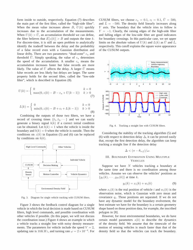
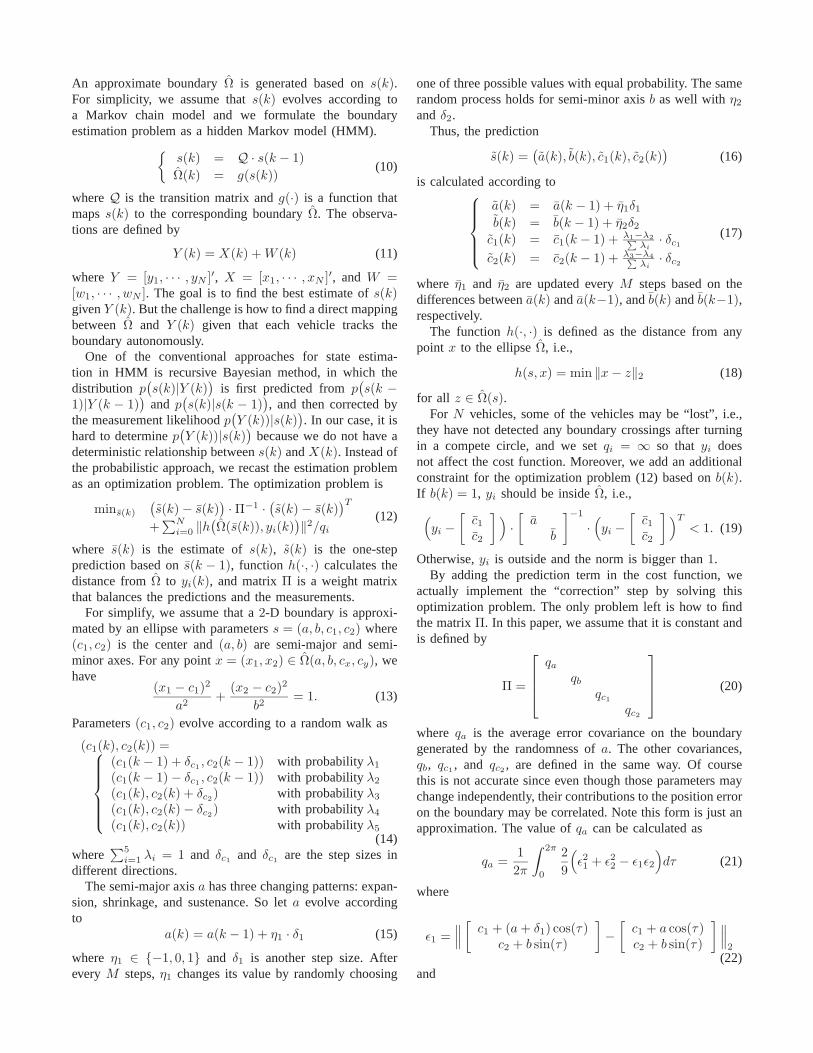
Figure 3 shows the feedback control diagram for a singlevehicle in which the local decision is made based on CUSUMfilters, high level commands, and possible coordination withother vehicles if possible. (In this paper, we will not discussthe coordination issue.) Figure 4 shows an example in whicha vehicle tracks a straight line with noisy density measure-ments. The parameters for vehicle include the speed V = 2,updating rate is 10KHz, and turning rate ω = 2×10−4. For

CUSUM filters, we choose cu = 0.1, cl = 0.1, U = 500,and L = −500. The density field linearly increases alongY axis. The boundary that the vehicle tries to follow isY = −1. Clearly, the raising edges of the high-side filterand falling edges of the low-side filter are good indicatorsfor boundary crossings. In this particular case, we set upperlimits on the absolute values of U(k) and L(k) as U and L,respectively. This cutoff explains the square wave appearanceof the CUSUM outputs.

−6 −4 −2 0 2 4 6 8 10 12

−5

0

5

X

Y

Noisy measurementsVehicle trajectoryBoundary

0 2 4 6 8 10 12−600

−400

−200

0

200

400

600

Time

Out

puts

of C

US

UM

High−sideLowe−sideCrossings

Fig. 4. Tracking a straight line with CUSUM filters.

Considering the stability of the tracking algorithm (5) and(6) with respect to detection delay Δ, it can be proved easilythat, except the first detection delay, the algorithm can keeptracking a straight line if the detection delay

Δ < (π − θref )/ω.

III. BOUNDARY ESTIMATION USING MULTIPLE

VEHICLES

Suppose we have N vehicles tracking a boundary atthe same time and there is no coordination among thosevehicles. Assume we can observe the vehicles’ positions as{y1(k), · · · , yN (k)} at time k.

yi(k) = xi(k) + wi(k) (9)

where xi(k) is the real position of vehicle i and wi(k) is theobservation noise, which is Gaussian with zero mean andcovariance qi. Those positions are separated. If we do nothave any dynamic model for the boundary evolvement, thebest estimate we have for the boundary is a certain geometryshape based on those position data, for example, the inscribedpolygon in [8].

However, for most environmental boundaries, we do havecertain model parameters s(k) to describe the dynamicsof the density field. We assume that the timescale of themotion of sensing vehicles is much faster than that of thedensity field so that the vehicles can track the boundary.

An approximate boundary Ω is generated based on s(k).For simplicity, we assume that s(k) evolves according toa Markov chain model and we formulate the boundaryestimation problem as a hidden Markov model (HMM).

{s(k) = Q · s(k − 1)Ω(k) = g(s(k))

(10)

where Q is the transition matrix and g(·) is a function thatmaps s(k) to the corresponding boundary Ω. The observa-tions are defined by

Y (k) = X(k) + W (k) (11)

where Y = [y1, · · · , yN ]′, X = [x1, · · · , xN ]′, and W =[w1, · · · , wN ]. The goal is to find the best estimate of s(k)given Y (k). But the challenge is how to find a direct mappingbetween Ω and Y (k) given that each vehicle tracks theboundary autonomously.

One of the conventional approaches for state estima-tion in HMM is recursive Bayesian method, in which thedistribution p

(s(k)|Y (k)

)is first predicted from p

(s(k −

1)|Y (k − 1))

and p(s(k)|s(k − 1)

), and then corrected by

the measurement likelihood p(Y (k))|s(k)

). In our case, it is

hard to determine p(Y (k))|s(k)

)because we do not have a

deterministic relationship between s(k) and X(k). Instead ofthe probabilistic approach, we recast the estimation problemas an optimization problem. The optimization problem is

mins(k)

(s(k) − s(k)

) · Π−1 · (s(k) − s(k))T

+∑N

i=0 ‖h(Ω(s(k)), yi(k)

)‖2/qi

(12)

where s(k) is the estimate of s(k), s(k) is the one-stepprediction based on s(k − 1), function h(·, ·) calculates thedistance from Ω to yi(k), and matrix Π is a weight matrixthat balances the predictions and the measurements.

For simplify, we assume that a 2-D boundary is approxi-mated by an ellipse with parameters s = (a, b, c1, c2) where(c1, c2) is the center and (a, b) are semi-major and semi-minor axes. For any point x = (x1, x2) ∈ Ω(a, b, cx, cy), wehave

(x1 − c1)2

a2+

(x2 − c2)2

b2= 1. (13)

Parameters (c1, c2) evolve according to a random walk as

(c1(k), c2(k)) =⎧⎪⎪⎪⎪⎨⎪⎪⎪⎪⎩

(c1(k − 1) + δc1 , c2(k − 1)) with probability λ1

(c1(k − 1) − δc1 , c2(k − 1)) with probability λ2

(c1(k), c2(k) + δc2) with probability λ3

(c1(k), c2(k) − δc2) with probability λ4

(c1(k), c2(k)) with probability λ5

(14)where

∑5i=1 λi = 1 and δc1 and δc1 are the step sizes in

different directions.The semi-major axis a has three changing patterns: expan-

sion, shrinkage, and sustenance. So let a evolve accordingto

a(k) = a(k − 1) + η1 · δ1 (15)

where η1 ∈ {−1, 0, 1} and δ1 is another step size. Afterevery M steps, η1 changes its value by randomly choosing

one of three possible values with equal probability. The samerandom process holds for semi-minor axis b as well with η2

and δ2.Thus, the prediction

s(k) =(a(k), b(k), c1(k), c2(k)

)(16)

is calculated according to⎧⎪⎪⎪⎨⎪⎪⎪⎩

a(k) = a(k − 1) + η1δ1

b(k) = b(k − 1) + η2δ2

c1(k) = c1(k − 1) + λ1−λ2∑λi

· δc1

c2(k) = c2(k − 1) + λ3−λ4∑λi

· δc2

(17)

where η1 and η2 are updated every M steps based on thedifferences between a(k) and a(k−1), and b(k) and b(k−1),respectively.

The function h(·, ·) is defined as the distance from anypoint x to the ellipse Ω, i.e.,

h(s, x) = min ‖x − z‖2 (18)

for all z ∈ Ω(s).For N vehicles, some of the vehicles may be “lost”, i.e.,

they have not detected any boundary crossings after turningin a compete circle, and we set qi = ∞ so that yi doesnot affect the cost function. Moreover, we add an additionalconstraint for the optimization problem (12) based on b(k).If b(k) = 1, yi should be inside Ω, i.e.,

(yi −

[c1

c2

] )·[

ab

]−1

·(yi −

[c1

c2

] )T

< 1. (19)

Otherwise, yi is outside and the norm is bigger than 1.By adding the prediction term in the cost function, we

actually implement the “correction” step by solving thisoptimization problem. The only problem left is how to findthe matrix Π. In this paper, we assume that it is constant andis defined by

Π =

⎡⎢⎢⎣

qa

qb

qc1

qc2

⎤⎥⎥⎦ (20)

where qa is the average error covariance on the boundarygenerated by the randomness of a. The other covariances,qb, qc1 , and qc2 , are defined in the same way. Of coursethis is not accurate since even though those parameters maychange independently, their contributions to the position erroron the boundary may be correlated. Note this form is just anapproximation. The value of qa can be calculated as

qa =12π

∫ 2π

0

29

(ε21 + ε22 − ε1ε2

)dτ (21)

where

ε1 =∥∥∥

[c1 + (a + δ1) cos(τ)

c2 + b sin(τ)

]−

[c1 + a cos(τ)c2 + b sin(τ)

] ∥∥∥2

(22)and

ε2 =∥∥∥

[c1 + (a − δ1) cos(τ)

c2 + b sin(τ)

]−

[c1 + a cos(τ)c2 + b sin(τ)

] ∥∥∥2.

(23)The value of qb can be calculated in the same way. For

qc1 and qc2 , the distributions of errors are shown in Table Iand the covariance can be calculated easily.

TABLE I

DISTRIBUTION OF ERRORS GENERATED BY c1 AND c2

Error distribution for c1

Error δc1 0 −δc1

Probability λ1 λ3 + λ4 + λ5 λ2

Error distribution for c2

Error δc2 0 −δc2

Probability λ3 λ1 + λ2 + λ5 λ4

IV. EXAMPLES AND SIMULATION RESULTS

In this section, we present some simulation results. Sup-pose we have an dynamic ellipse. Parameters c1 and c2

evolve according to Equation (14) with λ1 = λ2 = λ3 =λ4 = λ5 = 1/5 and σc1 = σc2 = 0.004. For a and b,the steps are σ1 = 0.01, σ2 = 0.015, and M = 100. Weuse five sensing vehicles to track the ellipse. The motionparameters for vehicles are V = 0.1 per step and ω = 0.4.Each vehicle starts from a random initial position outsidethe ellipse. Its initial orientation is set towards the initialcenter of the ellipse. Each vehicle runs the tracking algorithmdiscussed in Section II right after it crosses the boundary forthe first time.

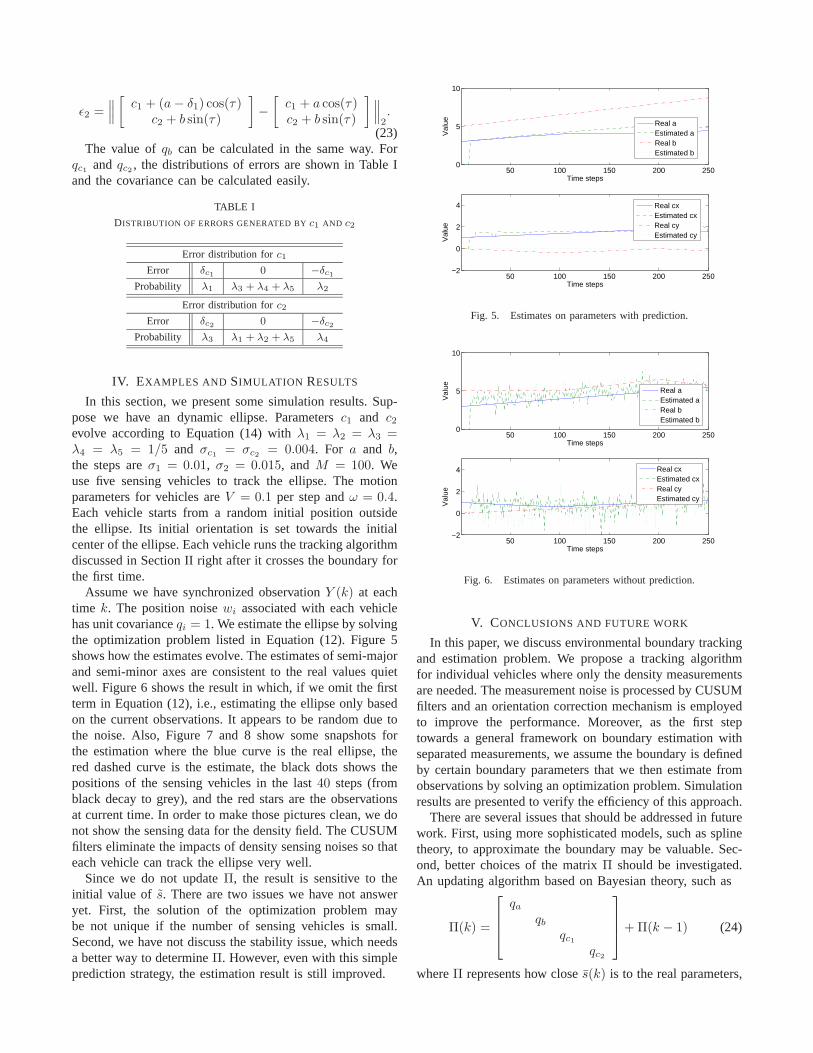
Assume we have synchronized observation Y (k) at eachtime k. The position noise wi associated with each vehiclehas unit covariance qi = 1. We estimate the ellipse by solvingthe optimization problem listed in Equation (12). Figure 5shows how the estimates evolve. The estimates of semi-majorand semi-minor axes are consistent to the real values quietwell. Figure 6 shows the result in which, if we omit the firstterm in Equation (12), i.e., estimating the ellipse only basedon the current observations. It appears to be random due tothe noise. Also, Figure 7 and 8 show some snapshots forthe estimation where the blue curve is the real ellipse, thered dashed curve is the estimate, the black dots shows thepositions of the sensing vehicles in the last 40 steps (fromblack decay to grey), and the red stars are the observationsat current time. In order to make those pictures clean, we donot show the sensing data for the density field. The CUSUMfilters eliminate the impacts of density sensing noises so thateach vehicle can track the ellipse very well.

Since we do not update Π, the result is sensitive to theinitial value of s. There are two issues we have not answeryet. First, the solution of the optimization problem maybe not unique if the number of sensing vehicles is small.Second, we have not discuss the stability issue, which needsa better way to determine Π. However, even with this simpleprediction strategy, the estimation result is still improved.

50 100 150 200 2500

5

10

Time steps

Val

ue

50 100 150 200 250−2

0

2

4

Time steps

Val

ue

Real aEstimated aReal bEstimated b

Real cxEstimated cxReal cyEstimated cy

Fig. 5. Estimates on parameters with prediction.

50 100 150 200 2500

5

10

Time stepsV

alue Real a

Estimated aReal bEstimated b

50 100 150 200 250−2

0

2

4

Time steps

Val

ue

Real cxEstimated cxReal cyEstimated cy

Fig. 6. Estimates on parameters without prediction.

V. CONCLUSIONS AND FUTURE WORK

In this paper, we discuss environmental boundary trackingand estimation problem. We propose a tracking algorithmfor individual vehicles where only the density measurementsare needed. The measurement noise is processed by CUSUMfilters and an orientation correction mechanism is employedto improve the performance. Moreover, as the first steptowards a general framework on boundary estimation withseparated measurements, we assume the boundary is definedby certain boundary parameters that we then estimate fromobservations by solving an optimization problem. Simulationresults are presented to verify the efficiency of this approach.

There are several issues that should be addressed in futurework. First, using more sophisticated models, such as splinetheory, to approximate the boundary may be valuable. Sec-ond, better choices of the matrix Π should be investigated.An updating algorithm based on Bayesian theory, such as

Π(k) =

⎡⎢⎢⎣

qa

qb

qc1

qc2

⎤⎥⎥⎦ + Π(k − 1) (24)

where Π represents how close s(k) is to the real parameters,

−10 −5 0 5 10

−10

−5

0

5

10

−10 −5 0 5 10

−10

−5

0

5

10

−10 −5 0 5 10

−10

−5

0

5

10

Fig. 7. Snapshots for estimating an ellipse with prediction.

−10 −5 0 5 10

−10

−5

0

5

10

−10 −5 0 5 10

−10

−5

0

5

10

−10 −5 0 5 10

−10

−5

0

5

10

Fig. 8. Snapshots for estimating an ellipse without prediction.

is a good target for us to work towards. Third, the dynamicsand motion patterns of individual vehicles definitely arecrucial to determining the distribution p(Y (k))|s(k)). Also,the single vehicle tracking algorithms can be improved withmore advanced interpolation and estimation methods. Last,but not least, coordination and cooperation among vehiclesshould help with boundary estimation by making the motionof vehicles more predictable.

VI. ACKNOWLEDGEMENTS

The authors would like to thank Prof. Boris Rozovsky, Dr.Alexander Tartakovsky, and Ernie Esser for discussions andcomments. This research is partly supported by ARO MURIgrant 50363-MA-MURI and ONR grant N000140610059.

REFERENCES

[1] C. Barat and M. J. Rendas, “Benthic boundary tracking using aprofiler sonar,” in Proceedings of IEEE/RSJ International Conferenceon Intelligent Robots and Systems, vol. 1, Oct. 2003, pp. 830–835.

[2] M. Kemp, A. L. Bertozzi, and D. Marthaler, “Multi-uuv perime-ter surveillance,” Proceedings of 2004 IEEE/OES Workshop on Au-tonomous Underwater Vehicles, pp. 102–107, 2004.

[3] C. H. Hsieh, Z. Jin, D. Marthaler, B. Q. Nguyen, D. J. Tung, A. L.Bertozzi, and R. M. Murray, “Experimental validation of an algorithmfor cooperative boundary tracking,” Proceedings of the AmericanControl Conference 2005, pp. 1078–1083, 2005.

[4] B. Q. Nguyen, Y.-L. Chuang, D. J. Tung, C. H. Hsieh, Z. Jin, L. Shi,D. Marthaler, A. L. Bertozzi, and R. M. Murray, “Virtual attractive-repulsive potentials for cooperative control of second order dynamicvehicles on the caltech mvwt,” Proceedings of the American ControlConference 2005, pp. 1084–1089, 2005.

[5] A. L. Bertozzi, M. Kemp, and D. Marthaler, Cooperative Control,Lecture Notes in Control and Information Systems, 2004, vol. 309,ch. Determining Environmental Boundaries: Asynchronous communi-cation and physical scales, pp. 25–42.

[6] J. Clark and R. Fierro, “Cooperative hybrid control of robotic sensorsfor perimeter detection and tracking,” Proceedings of the AmericanControl Conference 2005, pp. 3500–3505, 2005.

[7] F. Zhang and N. Leonard, “Coordinated patterns on smooth curves,”Proceedings of IEEE International Conference On Networking, Sens-ing and Control, pp. 434–440, 2006.

[8] S. Susca, S. Martinez, and F. Bullo, “Monitoring environmentalboundaries with a robotic sensor network,” IEEE Transactions onControl Systems Technology, 2007, to appear.

[9] L. Rabiner and B.-H. Juang, Fundamentals of speech recognition, ser.Prentice Hall Signal Processing Series, A. V. Oppenheim, Ed. PrenticeHall PTR, 1993.

[10] B. L. Rozovskii, A. Petrov, and R. B. Blazek, “Interactive banksof bayesian matched filters,” SPIE Proceedings: Signal and DataProcessing of Small Targets, 2000.

[11] E. S. Page, “Continuous inspection schemes,” Biometrika, vol. 41, no.1/2, pp. 100–115, Jun. 1954.

[12] L. L. Gan, “Cusum control charts under linear drift,” The Statistician,vol. 41, no. 1, pp. 71–84, 1992.

[13] M. S. Srivastava and Y. Wu, “Comparison of ewma, cusum andshiryayev-roberts procedures for detecting a shift in the mean,” TheAnnals of Statistics, vol. 21, no. 2, pp. 645–670, 1993.

[14] A. G. Tartakovsky, B. L. Rozovskii, R. B. Blazek, and H. Kim,“Detection of intrusions in information systems by sequential change-point methods,” Statistical Methodology, vol. 3, pp. 252–293, 2006.

[15] A. Savvides, J. Fang, and D. Lymberopoulos, “Using mobile sensingnodes for boundary estimation,” in in Workshop on Applications ofMobile Embedded Systems, Boston, MA, Jun. 2004.

[16] P. Bhatta, E. Fiorelli, F. Lekien, N. E. Leonard, D. A. Paley, F. Zhang,R. Bachmayer, R. E. Davis, D. M. Fratantoni, and R. Sepulchre,“Coordination of an underwater glider fleet for adaptive sampling,”Proceedings of International Workshop on Underwater Robotics, pp.61–69, 2005.

[17] S. Martinez, F. Bullo, J. Cortes, and E. Frazzoli, “On synchronousrobotic networks Part I: Models, tasks and complexity,” IEEE Trans.Automat. Contr., 2007, to appear.