Environment for Development · Environment for Development Kenya ... Any investment in the electricity sector is likely to speed up ... residential electricity prices using a Structural

Environment for Development

Discussion Paper Series Apr i l 2015 EfD DP 15-07

The Residential Demand for Electricity in Ethiopia

Fan tu Gut a , Abeb e Damte , and Tade le Fe rede

Environment for Development Centers

The Environment for Development (EfD) initiative is an environmental economics program focused on international

research collaboration, policy advice, and academic training. Financial support is provided by the Swedish

International Development Cooperation Agency (Sida). Learn more at www.efdinitiative.org or contact

[email protected].

Central America Research Program in Economics and Environment for Development in Central America Tropical Agricultural Research and Higher Education Center (CATIE) Email: [email protected]

Chile Research Nucleus on Environmental and Natural Resource Economics (NENRE) Universidad de Concepción Email: [email protected]

China Environmental Economics Program in China (EEPC) Peking University Email: [email protected]

Ethiopia Environmental Economics Policy Forum for Ethiopia (EEPFE) Ethiopian Development Research Institute (EDRI/AAU) Email: [email protected]

Kenya Environment for Development Kenya University of Nairobi with Kenya Institute for Public Policy Research and Analysis (KIPPRA) Email: [email protected]

South Africa Environmental Economics Policy Research Unit (EPRU) University of Cape Town Email: [email protected]

Sweden Environmental Economics Unit University of Gothenburg

Email: [email protected]

Tanzania Environment for Development Tanzania University of Dar es Salaam Email: [email protected]

USA (Washington, DC) Resources for the Future (RFF) Email: [email protected]

mailto:[email protected]










Discussion papers are research materials circulated by their authors for purposes of information and discussion. They have

not necessarily undergone formal peer review.


Fantu Guta, Abebe Damte, and Tadele Ferede

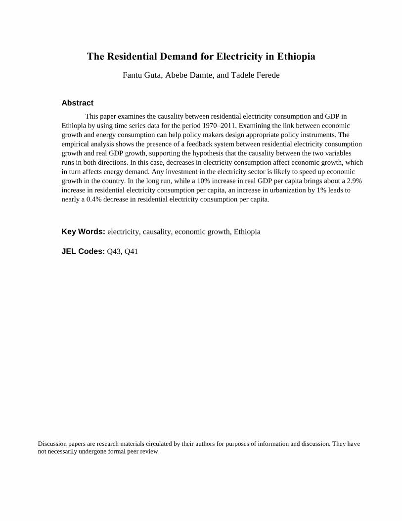
Abstract

This paper examines the causality between residential electricity consumption and GDP in

Ethiopia by using time series data for the period 1970–2011. Examining the link between economic

growth and energy consumption can help policy makers design appropriate policy instruments. The

empirical analysis shows the presence of a feedback system between residential electricity consumption

growth and real GDP growth, supporting the hypothesis that the causality between the two variables

runs in both directions. In this case, decreases in electricity consumption affect economic growth, which

in turn affects energy demand. Any investment in the electricity sector is likely to speed up economic

growth in the country. In the long run, while a 10% increase in real GDP per capita brings about a 2.9%

increase in residential electricity consumption per capita, an increase in urbanization by 1% leads to

nearly a 0.4% decrease in residential electricity consumption per capita.

Key Words: electricity, causality, economic growth, Ethiopia

JEL Codes: Q43, Q41

Contents

1. Introduction ......................................................................................................................... 1

2. Brief Review of the Literature ........................................................................................... 2

3. Methodology ........................................................................................................................ 4

3.1 Households’ Electricity Demand Model ....................................................................... 4

3.2 The Data Source and Patterns of Domestic Electricity Consumption .......................... 5

3.3 Analytical Approaches .................................................................................................. 6

4. Econometric Specification and Estimation Results ......................................................... 7

4.1 Time Series Properties of the Individual Series ............................................................ 7

4.2 The VAR System .......................................................................................................... 8

4.3 Cointegration Testing.................................................................................................. 10

4.4 The Short-run Error Correction Model ....................................................................... 12

5. Autoregressive Distrubuted Lag Model (ADL) for Residential Electricity

Consumption in Ethiopia ............................................................................................... 15

6. Conclusion and Implications ............................................................................................ 16

References .............................................................................................................................. 18

Tables and Figures ................................................................................................................ 20

Environment for Development Guta, Damte, and Ferede

1


Fantu Guta, Abebe Damte, and Tadele Ferede

1. Introduction

In Ethiopia, the lack of access to modern energy services that are clean, efficient and

environmentally sustainable is a critical limitation on economic growth and sustainable

development. Recognizing the critical role played by the energy sector in the economic growth

and development process, the Government of Ethiopia (GoE) has embarked on large scale

hydroelectricity projects, with a view to developing renewable and sustainable energy sources. It

has currently injected a huge amount of money into energy infrastructure, i.e., electricity

generation from hydro and from other renewable energy sources such as wind, solar and

geothermal. The total hydropower generation capacity country-wide increased from 714 MW in

2004/5 to 2,000 MW in 2009/10 and is expected to increase to over 10,000 MW by 2014

(MoFED 2010). Accordingly, electricity service coverage is expected to increase from 41% in

2009/10 to 75% by the end of the Growth and Transformation Plan (GTP) period, which is

2014/2015. Currently, the per-capita consumption of electricity in Ethiopia remains relatively

low at about 200 kWh per year. The national energy balance is dominated by a heavy reliance on

traditional biomass energy sources such as wood fuels, crop residues, and animal dung.

Energy is an important factor in all sectors of the economy. Because the quantitative

relationship between energy use and economic growth has been studied using various

approaches, time periods, and proxy variables, empirical evidence on the causal relationship

between energy consumption and economic growth in different countries is still mixed, both in

terms of the direction of the causality and the magnitude of the impact of consumption of energy

on economic growth (Ouedraogo 2012; Inglesi-Lotz 2013). In Africa, unlike developed

countries, there are few studies that examine the causality between residential electricity

consumption and economic growth (exceptions are Ziramba, 2008; Gabreyohannes, 2010).

Corresponding author: Abebe Damte, Environmental Economics Policy Forum for Ethiopia,

[email protected]. Fantu Guta and Tadele Ferede, Addis Ababa University. The authors acknowledge with

thanks financial support for data collection and analysis from the Swedish International Development Cooperation

Agency (Sida)through the Environment for Development (EfD) initiative and the EfD Center in Ethiopia, the

Environmental Economics Policy Forum for Ethiopia (EEPFE),based at the Ethiopian Development Research

Institute (EDRI).



2

It is important to address this issue in Ethiopia, as it has significant policy implications in

terms of the importance of energy consumption for economic growth and in the design of energy

and environmental policies. Given this importance, and the current growth of both the economy

and electricity consumption, policies and strategies should be based on empirical studies.

Therefore, it is timely to inform planners about the link between economic growth and energy

consumption in general and electricity consumption in particular. Hence, this study aims to

examine the causal relationship between residential demand for electricity and economic growth

in Ethiopia using time series data spanning four decades.

The paper is organized as follows. Section 2 briefly discusses the empirical studies on the

nexus between energy and economic growth. Section 3 provides the methodology, including a

brief theoretical framework, the data sources, and some descriptive statistics. The

macroeconometric results are presented in Sections 4 and 5. Section 6 presents conclusion and

implications of the findings.

2. Brief Review of the Literature

There is a plethora of empirical studies on the link between energy consumption and

economic growth, though we found few in Africa. A study by Ouedraogo (2012) tests the long-

run relationship between energy access and economic growth for fifteen African countries from

1980 to 2008. The results suggest that causality runs from GDP to energy consumption in the

short run, and from energy consumption to GDP in the long run. The author further argues that

this long run causality is unidirectional. A similar study by Oh and Lee (2004) in Korea indicates

a long-run bidirectional causal relationship between energy and GDP, and short-run

unidirectional causality running from energy to GDP.

A cross-country study by Wolde-Rufael (2006) indicated that economic growth Granger

causes electricity consumption in Nigeria, Cameroon, Ghana, Zimbabwe, Senegal, and Zambia,

while the opposite case was found for Benin, Congo and Tunisia. Similarly, Akinlo (2008)

examines the causality between energy consumption and economic growth for eleven sub-

Saharan African countries, using ARDL bound tests and Granger causality test within the context

of a VECM framework. The findings show that the relationship between energy consumption

and economic growth is different for different countries. For example, there is a bi-directional

relationship between energy consumption and economic growth for Gambia, Ghana and Senegal.

But the same test shows evidence of the neutrality hypothesis for Cameroon and Cote D'Ivoire,

Nigeria, Kenya and Togo. According to Akinlo (2008), each country should formulate


3

appropriate energy conservation policies based on its particular country situation. Other related

studies can be found in Kebede et al. (2010).

In addition to examining the direction of causation between economic growth and energy

or electricity consumption, a number of studies analyzed other macro determinants of energy

consumption. Ziramba (2008) examined the demand for residential electricity in South Africa.

Using a linear double-logarithmic form, he finds that income is the main determinant of

electricity demand, while electricity price is insignificant. Similarly, the residential electricity

demand for Taiwan was estimated by Holtedahl and Joutz (2004). The results show that the

income elasticity is unitary elastic in the long run, but the own-price effect is found to be

negative and inelastic. Dilaver and Hunt (2010) estimated the relationship between Turkish

residential electricity consumption, household total final consumption expenditure and

residential electricity prices using a Structural Time Series Model (STSM) approach over the

period 1960 to 2008. Their findings show that household total final consumption expenditure,

real energy prices and an underlying energy demand trend are important drivers of residential

electricity demand.

Based on the above brief review, and as argued by other authors, we can conclude that

empirical studies on the causality between energy consumption and economic growth in both

developed and developing countries give mixed results (Inglesi-Lotz 2013; Wolde-Rufael 2005).

A similar conclusion was reached by Payne (2010) in his review of the causal relationship

between electricity consumption and economic growth. The main differences identified were the

time periods examined, the econometric approaches and the variables included in the

estimations.

To our knowledge, a study by Gabreyohannes (2010) is the only one that addresses the

macro aspect of residential electricity consumption in Ethiopia. The findings of Gabreyohannes

(2010) indicate that the long-run effect of price changes significantly affects electricity

consumption. However, that study does not look at the effect of other macroeconomic variables

on the residential demand for electricity in Ethiopia.

This analysis of macroeconomic determinants of residential electricity demand will add

to the limited literature on the link between economic growth and consumption of electricity in

Ethiopia. This will also help policy makers understand the mechanism of the link between

economic growth and consumption of electricity, which will in turn help in the design of

appropriate energy policies. Unlike most other related studies, this research also conducted some

forecasting exercises to understand the future changes in the residential demand for electricity in


4

response to changes in macroeconomic variables such as growth in GDP. This is important for

both short- and long-term planning in the energy sector.

3. Methodology

3.1 Households’ Electricity Demand Model

In this section, we present a modified version of the Fisher and Kaysen (1962) energy

demand model. Following Holtedahl and Joutz (2004), household electricity consumption at time

t can be expressed, in general, as follows:

tttt XurbanXFKwh ,

(3.1)

where vector tX represents factors such as disposable income, energy prices, and the number of

customers. Hence, the modified version of the Fisher-Kaysen energy demand model canbe

specified as follows:

ttttttttttt NCPEYUrbanUrbanPEYuKuKwh ,,.,,. (3.2)

where tNC represents the number of customers.

The component u t is the utilization rate(s) of the appliance stocks. Therefore, a general

model for households’ electricity demand in Ethiopia is specified as follows:

urbanOiloficeKwhiceIncomePopultionfKwh ,Pr,/Pr,, (3.3)

where the left hand side variable, Kwh, is households’ electricity consumption; Income is real

disposable income; Price/Kwh is the real price of electricity per KWh; Price of Oil is the world

price of oil and is used as a proxy for substitutes for electricity energy; Urban is the degree of

urbanization, expressed as the percentage of people living in urban areas with 10,000+

population; and Population is a proxy for the number of customers. Weather variables for

cooling degree or heating degree days are not included in this model, as they are insignificant in

terms of energy demand in the Ethiopian context. The price of electricity, disposable income,

and urbanization are treated as exogenous variables. However, we test whether these variables


5

can be treated as weakly exogenous, as the variables could be determined jointly with the

dependent variable.

Electricity can be regarded as a normal good (service) and, thus, higher disposable

income is expected to increase consumption through greater economic activity and purchases of

electricity-using appliances in both the short- and long-run. On the other hand, a rise in

electricity prices ceteris paribus will lead to a fall in quantity demanded. Economic theory

suggests that electricity purchases will depend on the prices of its substitutes such as fuel oil. The

independent influence of alternate fuel prices is rather small because of the response by suppliers

and the constraints faced by consumers in fuel switching. However, fuel oil prices could be taken

as an alternative measure of prices.

Urbanization, which can also be considered a proxy measure of economic development

(Holtedahl and Joutz 2004), is expected to increase the consumption of electricity. The reason is

twofold. First, urbanization facilitates access to electricity for urban households, as they can

easily connect to the grid. Second, urbanization is likely to lead to the use of more appliances,

such as radios, televisions, modern cooking facilities, etc., due to better awareness of urban

households.

3.2 The Data Source and Patterns of Domestic Electricity Consumption

The dataset for this paper is based on secondary sources collected from various

institutions. Data on macroeconomic variables such as GDP was obtained from the World Bank

and data on electricity consumption was obtained from the Ethiopian Electricity Power

Corporation (EEPCo). Data on crude oil average prices per barrel is obtained from the World

Bank Commodity Price Data. A time series dataset spanning from 1972/73 to 2012/13 (about 40

years) is obtained for the purpose of the analysis. With this data, we are able to include variables

such as urban population size, average price of crude oil, and unit price of electricity. However,

we are unable to analyze two variables that have been found to be important in the empirical

analysis of energy demand. One is the price of electrical appliances, for which we do not have

information. The other is the tariff rate, which is flat and not variable among customers in

Ethiopia.

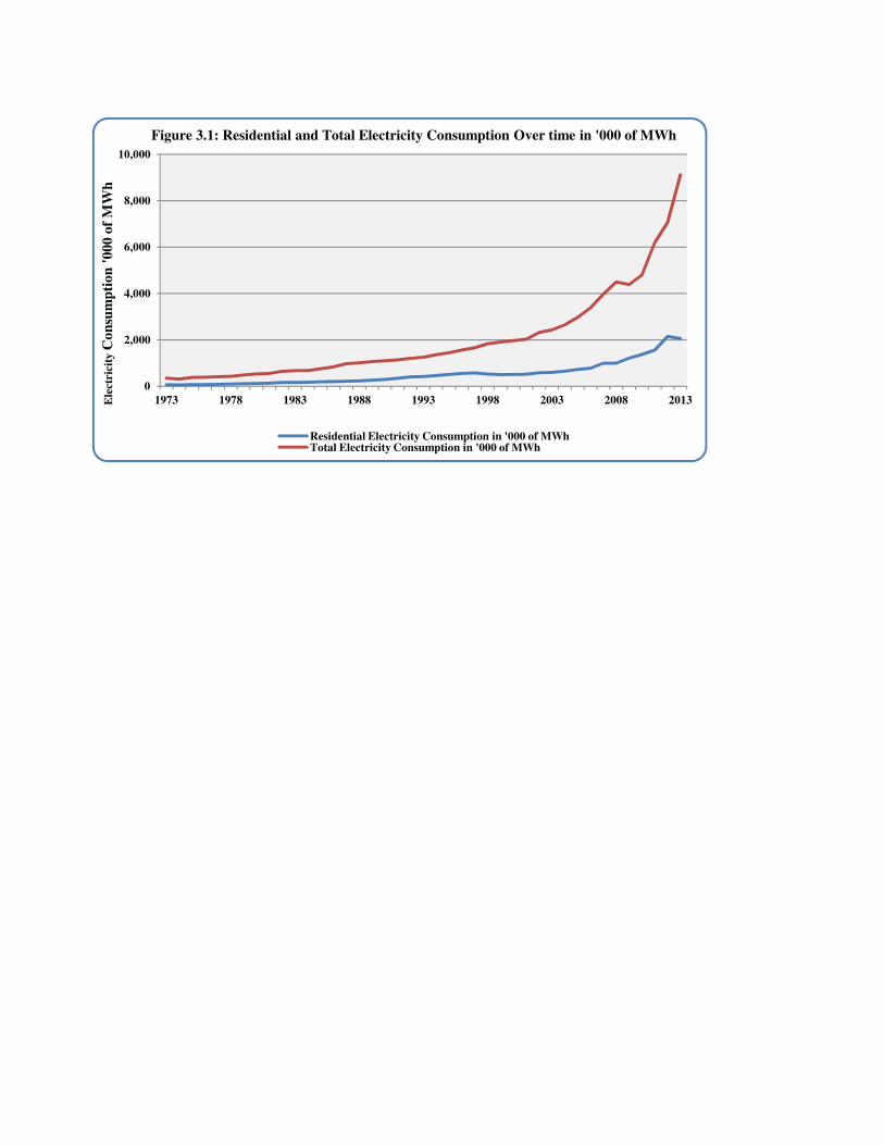
Figure 3.1 shows the trend in both residential and total electricity consumption in the

country for the last 40 years. It is clear that consumption of electricity is increasing at a faster

rate over time, especially for the past 10 years. In 1972/73, residential electricity consumption

was approximately 66 GWh; by 2012/13, it had grown over 30 fold to reach over 2,060 GWh.


6

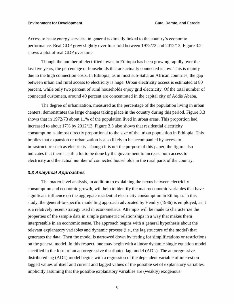
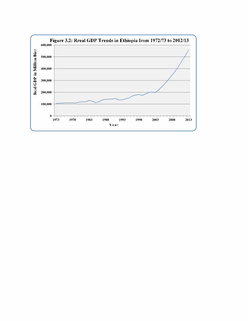
Access to basic energy services in general is directly linked to the country’s economic

performance. Real GDP grew slightly over four fold between 1972/73 and 2012/13. Figure 3.2

shows a plot of real GDP over time.

Though the number of electrified towns in Ethiopia has been growing rapidly over the

last five years, the percentage of households that are actually connected is low. This is mainly

due to the high connection costs. In Ethiopia, as in most sub-Saharan African countries, the gap

between urban and rural access to electricity is huge. Urban electricity access is estimated at 80

percent, while only two percent of rural households enjoy grid electricity. Of the total number of

connected customers, around 40 percent are concentrated in the capital city of Addis Ababa.

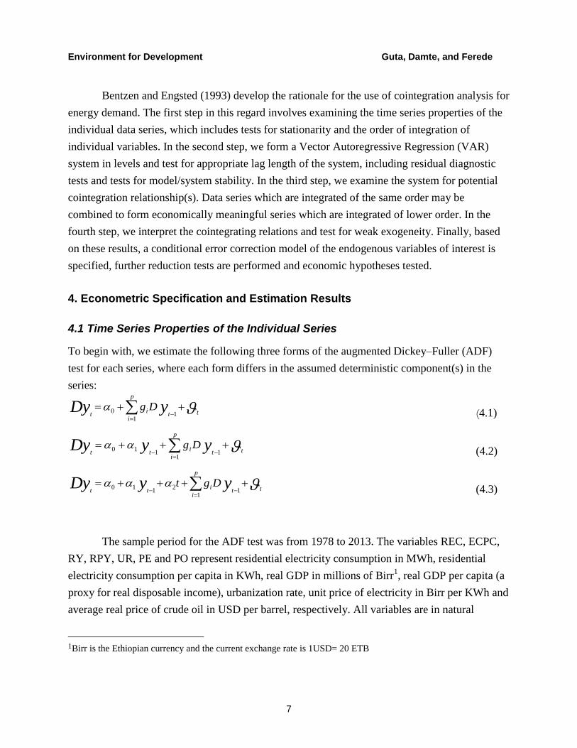
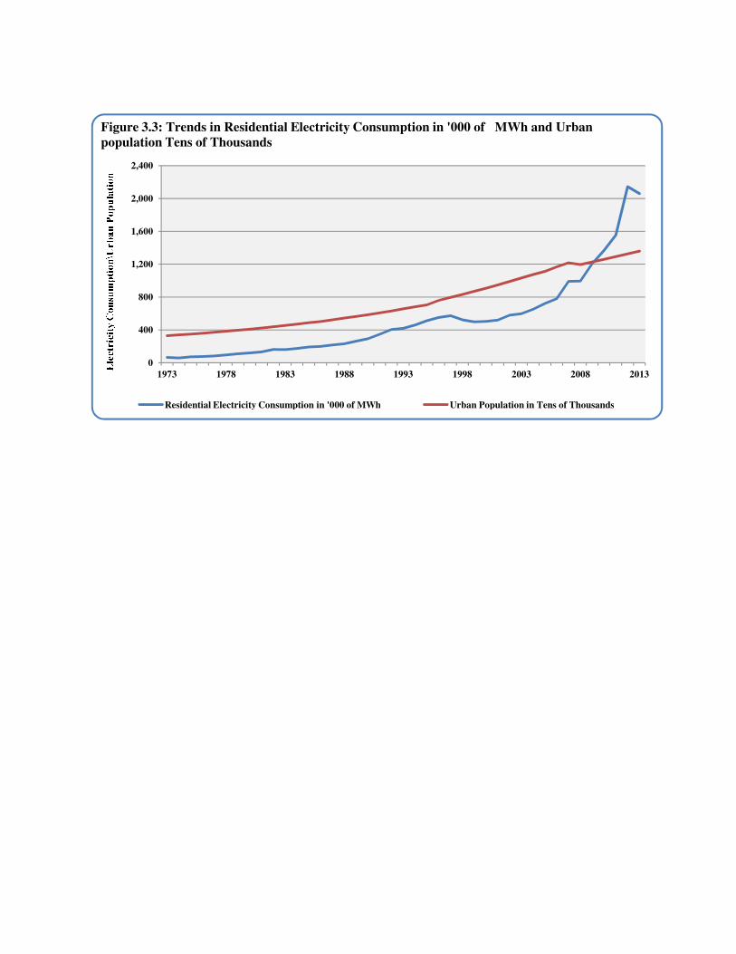
The degree of urbanization, measured as the percentage of the population living in urban

centers, demonstrates the large changes taking place in the country during this period. Figure 3.3

shows that in 1972/73 about 11% of the population lived in urban areas. This proportion had

increased to about 17% by 2012/13. Figure 3.3 also shows that residential electricity

consumption is almost directly proportional to the size of the urban population in Ethiopia. This

implies that expansion or urbanization is also likely to be accompanied by access to

infrastructure such as electricity. Though it is not the purpose of this paper, the figure also

indicates that there is still a lot to be done by the government to increase both access to

electricity and the actual number of connected households in the rural parts of the country.

3.3 Analytical Approaches

The macro level analysis, in addition to explaining the nexus between electricity

consumption and economic growth, will help to identify the macroeconomic variables that have

significant influence on the aggregate residential electricity consumption in Ethiopia. In this

study, the general-to-specific modelling approach advocated by Hendry (1986) is employed, as it

is a relatively recent strategy used in econometrics. Attempts will be made to characterize the

properties of the sample data in simple parametric relationships in a way that makes them

interpretable in an economic sense. The approach begins with a general hypothesis about the

relevant explanatory variables and dynamic process (i.e., the lag structure of the model) that

generates the data. Then the model is narrowed down by testing for simplifications or restrictions

on the general model. In this respect, one may begin with a linear dynamic single equation model

specified in the form of an autoregressive distributed lag model (ADL). The autoregressive

distributed lag (ADL) model begins with a regression of the dependent variable of interest on

lagged values of itself and current and lagged values of the possible set of explanatory variables,

implicitly assuming that the possible explanatory variables are (weakly) exogenous.


7

Bentzen and Engsted (1993) develop the rationale for the use of cointegration analysis for

energy demand. The first step in this regard involves examining the time series properties of the

individual data series, which includes tests for stationarity and the order of integration of

individual variables. In the second step, we form a Vector Autoregressive Regression (VAR)

system in levels and test for appropriate lag length of the system, including residual diagnostic

tests and tests for model/system stability. In the third step, we examine the system for potential

cointegration relationship(s). Data series which are integrated of the same order may be

combined to form economically meaningful series which are integrated of lower order. In the

fourth step, we interpret the cointegrating relations and test for weak exogeneity. Finally, based

on these results, a conditional error correction model of the endogenous variables of interest is

specified, further reduction tests are performed and economic hypotheses tested.

4. Econometric Specification and Estimation Results

4.1 Time Series Properties of the Individual Series

To begin with, we estimate the following three forms of the augmented Dickey–Fuller (ADF)

test for each series, where each form differs in the assumed deterministic component(s) in the

series:

tt

p

i

it

yDy Dg

1

1

0 (4.1)

tt

p

i

itt

yyDy Dg

11

110 (4.2)

tt

p

i

itt

yyDy Dgt

1

1

21

10 (4.3)

The sample period for the ADF test was from 1978 to 2013. The variables REC, ECPC,

RY, RPY, UR, PE and PO represent residential electricity consumption in MWh, residential

electricity consumption per capita in KWh, real GDP in millions of Birr1, real GDP per capita (a

proxy for real disposable income), urbanization rate, unit price of electricity in Birr per KWh and

average real price of crude oil in USD per barrel, respectively. All variables are in natural

1Birr is the Ethiopian currency and the current exchange rate is 1USD= 20 ETB


8

logarithms, with the exception of the urbanization rate variable. The first three rows, I(1)-i,

present the ADF t-tests corresponding to tests for unit roots in the levels of the series. The last

three rows, I(2)-i, report the ADF t-test results for testing whether the first difference has a unit

root. A rejection implies that the first difference of the series is a stationary process. The

identifier i refers to equations (4.1)–(4.3), which are ADF regressions with no constant, a

constant and a constant plus trend, respectively. The critical values for the t-tests at 5% with no

constant, a constant and a constant plus a trend are -1.95, -2.94 and -3.53, respectively, and the

corresponding critical values at 1% are -2.63, -3.62 and -4.23, respectively. Rejections at the 5%

and 1% critical values are denoted as ** and ***, respectively. The critical values for the above

table are calculated from MacKinnon (1991). A maximum of three lags was used in each test.

The appropriate lag length was chosen by examining the autocorrelation function of the

residuals.

The t is assumed to be a Gaussian white noise random error and 1, 2, , t T (the

number of observations in the sample) is a term for time trend. In Equation (4.1), there is no

constant or trend. Equation (4.2) contains a constant but no trend. Both a constant and a trend are

included in Equation (4.3). The number of lagged differences, P, is chosen to ensure that the

estimated errors are not serially correlated. The results from the unit root tests are found in Table

4.1. The first three rows test the null hypothesis that a series follows a unit root process or

random walk. This implies it is non-stationary and (possibly) integrated of order one, I(1), rather

than I(0). The second three rows test the null hypothesis that the first differences of a series

follow a unit root. If true, the researcher must difference the series twice to obtain a stationary

process. For all series in Table 4.1, we find that the null hypothesis of a unit root in the level

cannot be rejected. The tests for unit roots in the first differences are rejected, implying that the

series are I(1) and stationary in their first differences.

4.2 The VAR System

The model for electricity demand is specified to reflect the economic determinants and

process of development from a predominantly rural economy to an urban industrial one.

ePORPEeRPYAECPCtt u

tt

UR

ttt

4321

(4.4)

where ECPCt is the quantity of electricity consumption per capita in KWh, RPYtis real GDPper

capita in Birr (a proxy for real disposable income per capita), URtis the population living in

urban areas as a proportion of total population (Urbanization Rate), RPEt is unit price of


9

electricity in Birr per KWh deflated by consumer price index (a proxy for real electricity price in

Birr per KWh) and POt is average real price of crude oil in USD per barrel. TheAt term can

include deterministic elements such a strend(s) and dummy variables.

In the econometric analysis, the variables are transformed to natural logarithms, with the

exception of the urbanization variable, because it is already in percentage terms. Note that

modeling in double log form makes it possible to interpret the coefficients of real GDP as a

measure of income elasticities of electricity consumption. We specify the VAR as a five variable

system with a sample period from 1973 to 2013. The model includes a trend term and dummy

variable. Starting in 2007, there wasa sharp increase in the energy consumption and real GDP

variables. We constructed a pulse dummy variable with a value of unity for the years since 2007

and zero in all other years.

uxbyAay tit

q

iiit

p

iit

11

0 (4.5)

barrelperoilcrudeofpriceAveragex

KWhperBirrinyelectricitofpriceal

BirrincapitaperGDPal

rateonUrbanizati

KWhincapitapernconsumptioyElectricit

y

y

y

y

ywhere

t

t

t

t

t

t

Re

Re

4

3

2

1

where ut, is a vector of random disturbances assumed to be approximately normally distributed.

In the above specification, 0a is a 4 1 vector of constants, which includes a constant, a time

trend and a dummy variable for the period 2007 to 2013. While 1,2, ,Ai i p are 4 4

coefficient matrices at different lags of the endogenous variables in the system, 1,2, ,bi i q

are 4 1 coefficient vectors at different lags of the exogenous variable in the system. The

4 1 vector of disturbances, ut,, is assumed to be white noise.

Table 4.2 presents the VAR order selection criteria. All information criteria indicate that

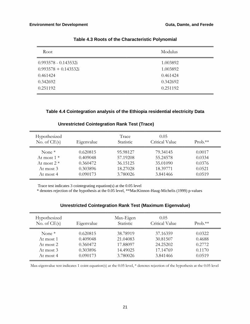
the optimal lag order is one. Table 4.3 provides the autoregressive roots of the characteristic


10

polynomial. Moduli of the characteristic roots indicate that the VAR does not satisfy the stability

condition, as the modulus of at least one root lies outside the unit circle.

4.3 Cointegration Testing

Cointegration tests are a multivariate form of integration analysis. Individual series may

be 1I , but a linear combination of the series may be 0I . The error correction model is a

generalization of the traditional partial adjustment model and permits the estimation of short-run

and long-run elasticities. Many macroeconomic and aggregate level series are shown to be well-

modeled as stochastic trends, i.e., integrated of order one, or 1I . Simple first differencing of

the data will remove the non-stationarity problem, but with a loss of generality regarding the

long-run ‘equilibrium’ relationships among the variables. Engle and Granger (1987) solve this

filtering problem with the cointegration technique. They suggest that if all, or a subset of, the

variables are 1I , there may exist a linear combination of the variables that is stationary, 0I .

The linear combination is then taken to express a long-run ‘equilibrium’ relationship. Series that

are cointegrated can always be represented in an error correction model. The error correction

model is specified in first differences, which are stationary, and represent the short-run

movements in the variables where the error correction term (one period lagged value of the

residuals from the cointegrating regression), ecm, is included in the model to account for the

long-run, or equilibrium, relations. The ecm term represents the deviation from the equilibrium

relation in the previous period. For example, the growth rate of residential electricity

consumption per capita would be a function of the growth rate in real GDP per capita, the degree

of urbanization, the growth rate of real electricity price, the growth rate of real average price of

crude oil per barrel and the error correction term. Lags of the dependent variable would be

included to capture additional short- and medium-term dynamics of residential electricity

consumption per capita.

The advantage of the first difference model is that the specification is stationary, so that

estimation and statistical inference can be performed using standard statistical methods. The

contemporaneous coefficients are interpreted as short-run elasticities. The VAR system in levels

given in equation (4.5) above, without loss of generality, can be transformed to a model in first

differences and the error correction term:


11

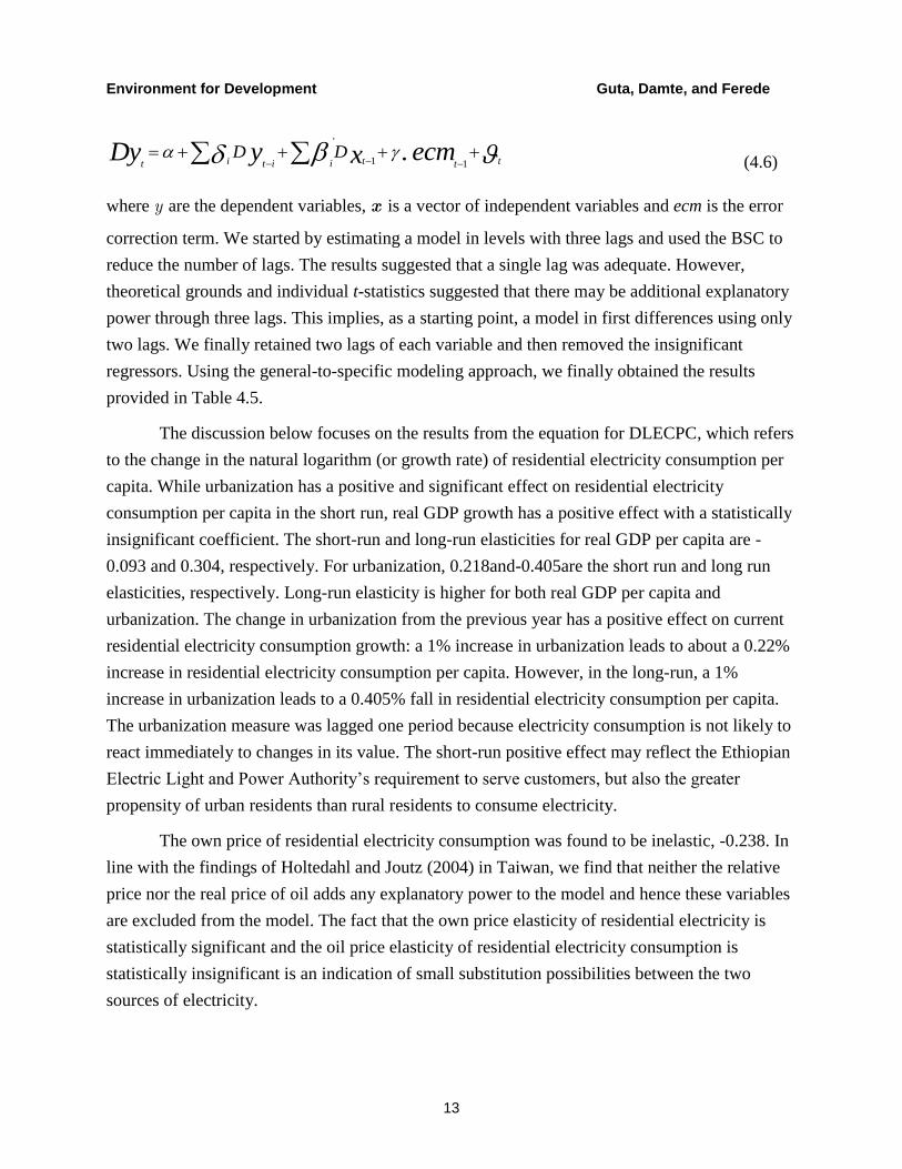
uyGyGyGyaDy tptpttttDDDP

11221110...

(4.6)

Where

AAAAG ppiiPpi

...1,...,2,1...

11

The rank of the coefficient matrix for the level terms, , is of reduced rank in the

presence of cointegrating relationships. In the presence of cointegrating relations, the coefficient

matrix can be written as , where is the k r matrix of speed of adjustment

coefficients and is the k r matrix whose r columns are cointegrating vectors or long-run

relationships. Cointegration testing and the maximum likelihood estimation of are derived

from a series of regressions and reduced rank regressions.

Table 4.4 provides the results from the cointegration analysis. The first column of the

upper part of Table 4.4 gives the null hypotheses of no cointegrating relationship among the five

I(1) variables, at most one cointegrating relationship, at most two cointegrating relationships, at

most three cointegrating relationships and at most four cointegrating relationships. When there

are no cointegrating vectors, the VAR model in first differences is appropriate.

While the result from the maximum eigenvalue statistic indicates the presence of a single

cointegrating relationship between the five 1I variables, the result from the trace statistic

indicates the presence of at most three cointegrating relationships. For small samples, the two

tests do not always agree on the number of cointegrating relationships. Given these results,

however, we can safely conclude that there exists at least one cointegrating relationship between

the variables under consideration. The implied cointegrating relationship is obtained from the

first row of the normalized cointegrating equation. We interpret it as the desired level of

residential electricity consumption per capita. It was also found that all three variables, namely,

urbanization, real gross domestic product and real price of residential electricity, are jointly weak

exogenous, as the calculated value of the 2χ with three degrees of freedom is 5.46 and a P-value

of 0.14.

LPORLRPELRYURLECPC .160.0.193.0.289.0.405.0 (4.7)

This result suggests that the income elasticity is inelastic, implying that a 10% increase in

real GDP per capita brings about a 2.9% increase in residential electricity consumption per

capita. On the other hand, an increase in urbanization by 1% leads to nearly a 0.4% decrease in

residential electricity consumption per capita. This might be due to the gap between growth in


12

urbanization and growth in electricity consumption. The available supply for electricity may not

be able to cope with the increase in urban population, though the government has put in

tremendous effort to increase the supply of electricity.

From the estimated cointegrating relationship, one can easily note that the real electricity

price and real oil price coefficients are roughly equal but of opposite signs. We test for the

relative price restriction along with the weak exogeneity of the real oil price and obtain the

following reduction in the cointegration vector.

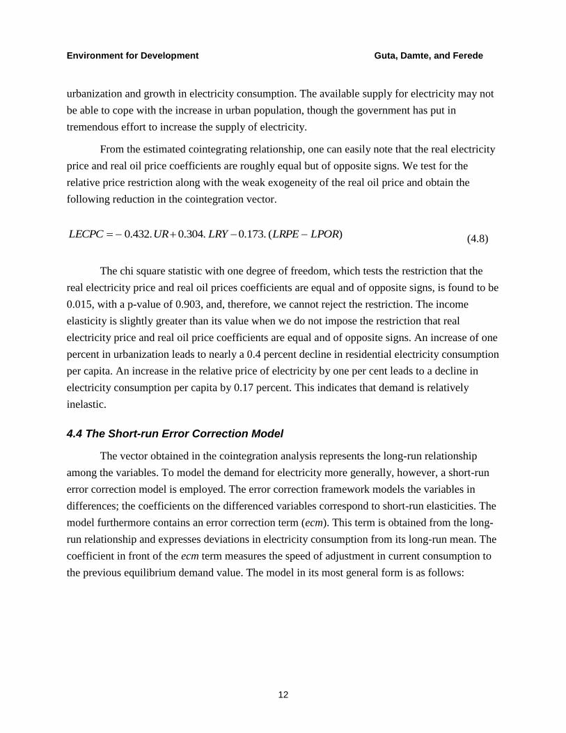
)(.173.0.304.0.432.0 LPORLRPELRYURLECPC (4.8)

The chi square statistic with one degree of freedom, which tests the restriction that the

real electricity price and real oil prices coefficients are equal and of opposite signs, is found to be

0.015, with a p-value of 0.903, and, therefore, we cannot reject the restriction. The income

elasticity is slightly greater than its value when we do not impose the restriction that real

electricity price and real oil price coefficients are equal and of opposite signs. An increase of one

percent in urbanization leads to nearly a 0.4 percent decline in residential electricity consumption

per capita. An increase in the relative price of electricity by one per cent leads to a decline in

electricity consumption per capita by 0.17 percent. This indicates that demand is relatively

inelastic.

4.4 The Short-run Error Correction Model

The vector obtained in the cointegration analysis represents the long-run relationship

among the variables. To model the demand for electricity more generally, however, a short-run

error correction model is employed. The error correction framework models the variables in

differences; the coefficients on the differenced variables correspond to short-run elasticities. The

model furthermore contains an error correction term (ecm). This term is obtained from the long-

run relationship and expresses deviations in electricity consumption from its long-run mean. The

coefficient in front of the ecm term measures the speed of adjustment in current consumption to

the previous equilibrium demand value. The model in its most general form is as follows:


13

tttiitit

ecmxyDy DD

.11

'

(4.6)

where y are the dependent variables, x is a vector of independent variables and ecm is the error

correction term. We started by estimating a model in levels with three lags and used the BSC to

reduce the number of lags. The results suggested that a single lag was adequate. However,

theoretical grounds and individual t-statistics suggested that there may be additional explanatory

power through three lags. This implies, as a starting point, a model in first differences using only

two lags. We finally retained two lags of each variable and then removed the insignificant

regressors. Using the general-to-specific modeling approach, we finally obtained the results

provided in Table 4.5.

The discussion below focuses on the results from the equation for DLECPC, which refers

to the change in the natural logarithm (or growth rate) of residential electricity consumption per

capita. While urbanization has a positive and significant effect on residential electricity

consumption per capita in the short run, real GDP growth has a positive effect with a statistically

insignificant coefficient. The short-run and long-run elasticities for real GDP per capita are -

0.093 and 0.304, respectively. For urbanization, 0.218and-0.405are the short run and long run

elasticities, respectively. Long-run elasticity is higher for both real GDP per capita and

urbanization. The change in urbanization from the previous year has a positive effect on current

residential electricity consumption growth: a 1% increase in urbanization leads to about a 0.22%

increase in residential electricity consumption per capita. However, in the long-run, a 1%

increase in urbanization leads to a 0.405% fall in residential electricity consumption per capita.

The urbanization measure was lagged one period because electricity consumption is not likely to

react immediately to changes in its value. The short-run positive effect may reflect the Ethiopian

Electric Light and Power Authority’s requirement to serve customers, but also the greater

propensity of urban residents than rural residents to consume electricity.

The own price of residential electricity consumption was found to be inelastic, -0.238. In

line with the findings of Holtedahl and Joutz (2004) in Taiwan, we find that neither the relative

price nor the real price of oil adds any explanatory power to the model and hence these variables

are excluded from the model. The fact that the own price elasticity of residential electricity is

statistically significant and the oil price elasticity of residential electricity consumption is

statistically insignificant is an indication of small substitution possibilities between the two

sources of electricity.


14

The error correction term is significant and has a coefficient of -0.548, indicating that,

when demand is above or below its equilibrium level, consumption adjusts by about 55% within

the first year. The model overall has coefficients with the expected signs and with magnitudes

that seem reasonable, with the exception of the coefficient of real GDP, which is found to be

statistically insignificant. The model also performs well statistically: more than sixty percent of

the annual variation of the change is explained. While the residual summary statistics for

autocorrelation and heteroscedasticity do not reveal any problems, the residual normality test

shows that the residuals from the urbanization equation are non-normal.

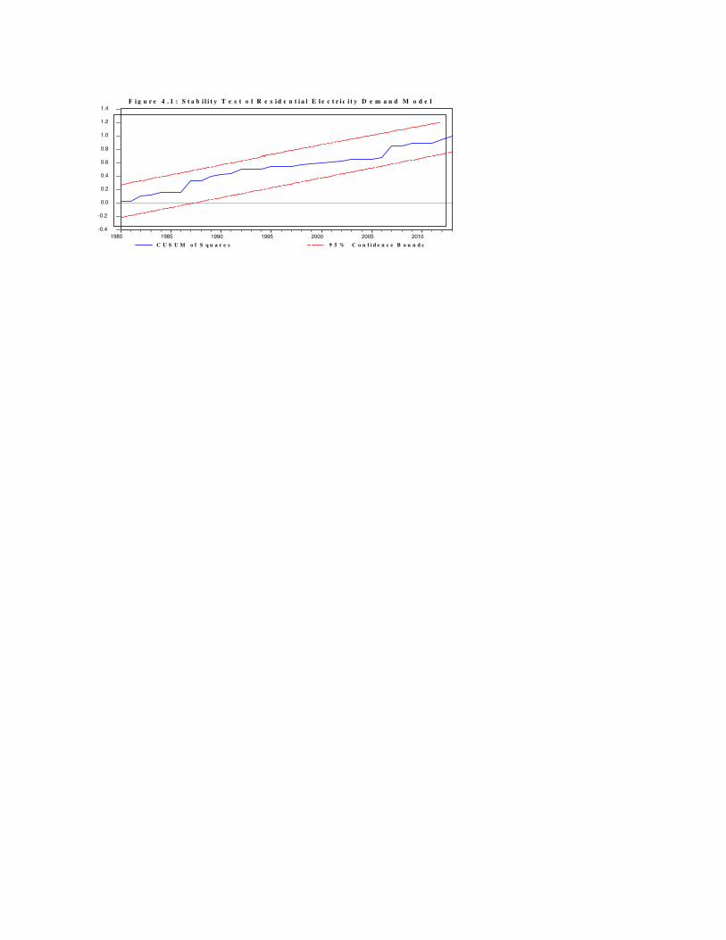
Stability of the model is tested by examining the cumulative sum of squares test and

parameter constancy through recursive estimation. Figure 4.1 provides the cumulative sum of

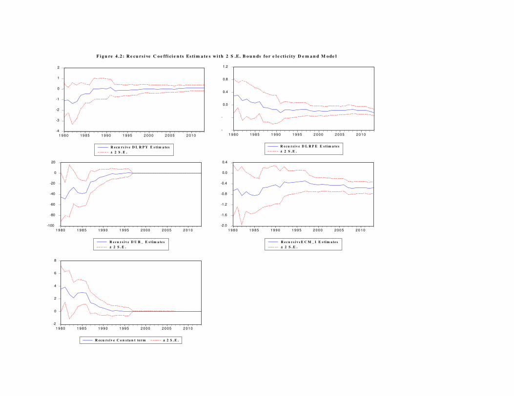
squares of recursive residuals model stability tests. Figure 4.2 provides the recursive coefficient

estimates and the associated two standard error bounds.

The recursive coefficient estimates with their plus or minus two standard error bounds are

given for the current change in real income per capita, current change in real electricity price,

change in urbanization last year, error correction and the constant terms of the model. The figure

indicates that all parameter estimates are stable.

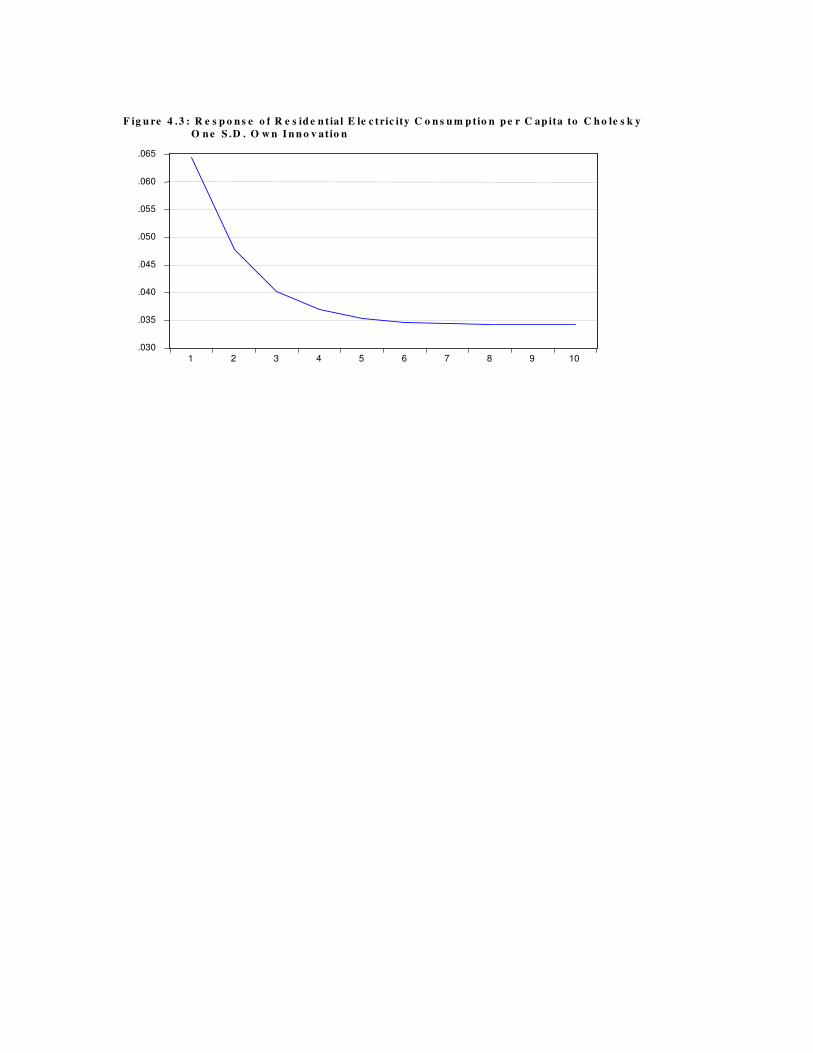
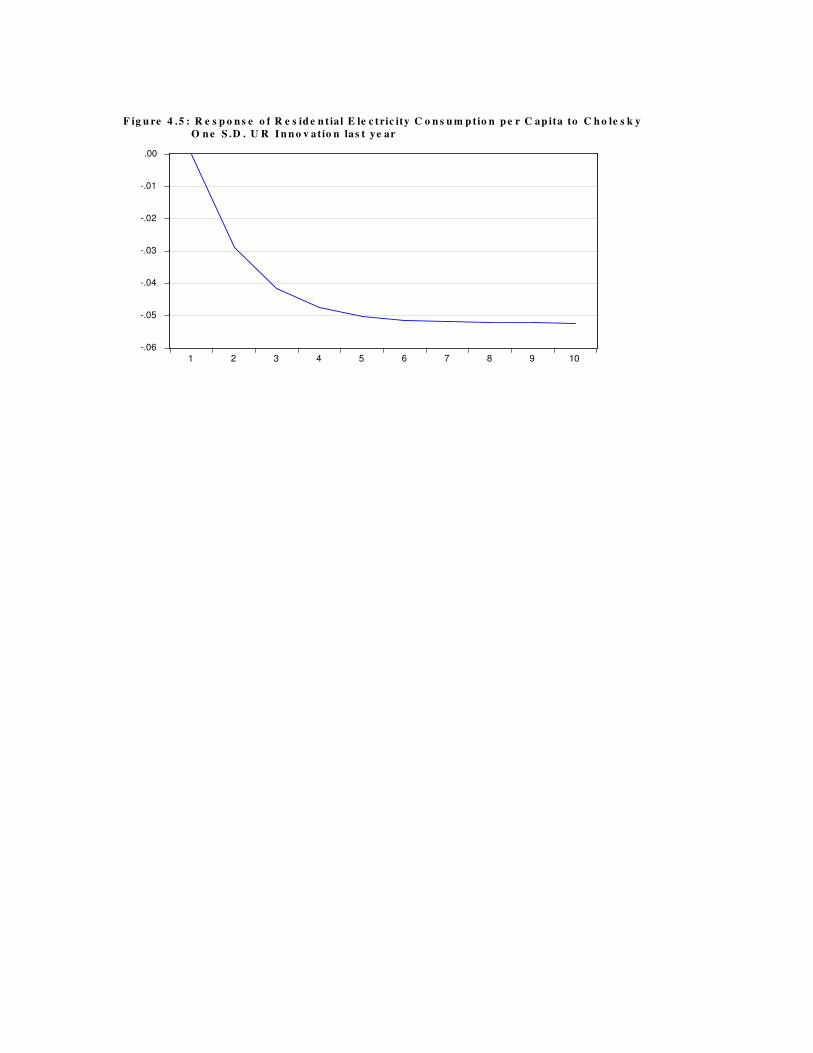
Figures 4.3, 4.4 and 4.5 show the responses of residential electricity consumption per

capita in Ethiopia to a Cholesky one standard deviation of own innovation, innovations in real

GDP per capita and urbanization rate. Figure 4.3 shows the response of residential electricity

demand to a Cholesky one standard deviation of own innovation impulse in which residential

electricity demand responded positively between periods two and three and negatively for all

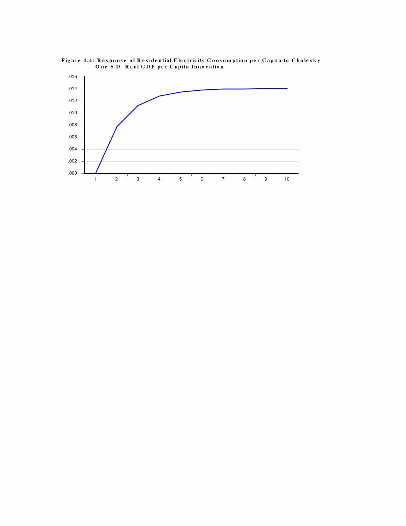
other periods. Figure 4.4 shows the response of residential electricity demand to a Cholesky one

standard deviation of real GDP innovation in which residential electricity demand responded

negatively for the first two periods and positively for all other periods to impulses of real GDP

innovations.

Figure 4.5 is the response of residential electricity demand to a Cholesky one standard

deviation of urbanization rate innovation in the last year in which residential electricity demand

responded positively for all periods but at a decreasing rate to impulses of urbanization

innovations.

Table 4.6 provides the variance decomposition of residential electricity consumption in

Ethiopia. It reveals that the bulk of the variation in residential electricity demand is accounted for

by its own innovation for the first seven periods. By the end of period seven, the urbanization

rate accounts for about 31.3% of the variation in residential electricity demand per capita,


15

whereas innovations in real GDP accounts for only about 2.3% of the variation in residential

electricity demand in the country by the end of period seven. By the end of period ten, the

urbanization rate accounts for about 33.8% of the variation in residential electricity demand per

capita, followed by own innovations and innovations in real oil price which, respectively,

account for about 26.8% and 20.4% of the variation in residential electricity demand. By end of

period ten, innovations in real GDP per capita account only for about 2.4% of the variation in

residential electricity demand in the country.

5. Autoregressive Distrubuted Lag Model (ADL) for Residential Electricity Consumption in Ethiopia

In estimating an ADL model for residential electricity consumption in Ethiopia, we begin

with a general model that includes five lags for each of the variables. Initially, we also included a

dummy variable, DUM, to capture the dramatic change in residential electricity consumption in

Ethiopia since 2007. However, this dummy variable was found to be statistically insignificant

and dropped from the final ADL model. We then reduced the model following the general to

specific modelling strategy. Finally, we arrived at the following parsimonious ADL model for

residential electricity consumption per capita in Ethiopia (Table 5.1).

The model overall has coefficients with unexpected signs, though the magnitudes of the

estimates seem reasonable. The model performs well statistically. Over 99% of the annual

variation in residential electricity consumption per capita is explained. The residual summary

statistics for serial correlation, heteroscedasticity and normality tests do not reveal any problems.

Table 5.2 provides the summary statistics for serial correlation, heteroscedasticity and normality

tests.

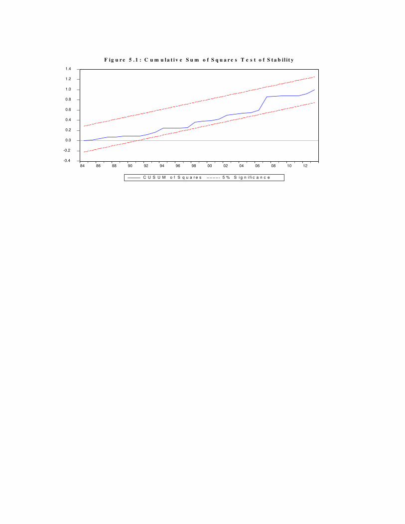
The model also passes the Ramsey RESET test of omitted variables. Figure 5.1 provides

cumulative sum of squares tests of model stability together with 95% confidence bounds. Figure

5.2 provides recursive estimates of the coefficients of the model together with their two standard

error bounds.

Unit root tests of the residuals from the model also reveal that the residuals are stationary;

together with the aforementioned diagnostic test statistics, this indicates that the model passes the

entire battery of diagnostic tests and reveals no statistical problems.

The long-run income elasticity derived from the ADL model (Table 5.1) is found to be

about -0.424, implying that a 1% increase in real GDP per capita leads to about a 0.42% decline

in residential electricity consumption per capita. However, the income elasticity derived from the


16

error correction analysis was found to be about 0.289, implying that a 1% increase in real GDP

per capita leads to about a 0.29% increase in residential electricity consumption per capita. On

the other hand, an increase in urbanization two years back has a positive effect on current

residential electricity consumption per capita: a 1% increase in urbanization two years back leads

to about a 0.2% increase in residential electricity consumption per capita in the long-run.

However, the error correction analysis revealed that, in the long run, a 1% increase in

urbanization leads to a 0.4% decline in residential electricity consumption per capita.

6. Conclusion and Implications

As a result of growing demand for electricity and recognizing the critical role played by

the energy sector in the economic growth and development process, the Government of Ethiopia

has already embarked on large scale hydroelectricity projects in view of developing renewable

and sustainable energy sources. Hence, it is necessary and timely to examine and understand the

link between economic growth and energy consumption in order to help policy makers design

appropriate policy instruments.

The macroeconometric result shows the presence of a feedback system between

residential electricity consumption growth and real GDP growth, supporting the hypothesis that

the causality between the two variables runs in both directions. In this case, decreases in

electricity consumption will affect economic growth, which will in turn affect residential

electricity demand. Alternatively, any policy measure to reduce consumption of electricity will

affect economic growth negatively. This indicates that any policy measure to increase investment

in the electricity sector is likely to stimulate economic growth in the country. In other words,

demand for residential electricity is a result of economic development, but equally lack of access

to electricity could probably hinder economic growth in the country. Therefore, the current

efforts of the country in increasing the current capacity of electricity generation and developing

alternative energy sources from renewable energy sources such as solar power, wind power and

geothermal should be encouraged because these alternative energy production methods are also

environmentally friendly. Moreover, the country has a huge potential for producing energy from

renewable energy resources.

Other variables were included in the analysis, unlike most other related studies in

residential electricity demand in most developing countries. For example, in order to take into

account the effect of economic development, we have included a measure of urbanization. The

result shows that a 1% increase in urbanization leads to about 0.22% increase in residential

electricity consumption per capita. However, urbanization is negatively related to per capita


17

electricity consumption in the long run. The findings suggest that it is necessary to understand

the dynamics of the urban centers in the country, which are currently growing at up to 3.7 % per

year (Dorosh et al. 2011)

The income elasticity of residential demand is less than unity in the long-run. The relative

price of electricity (to oil) elasticity is inelastic in the long run. As expected, an increase in the

relative price of electricity by one per cent leads to a decline in electricity consumption per capita

by 0.17 percent. This indicates that demand is relatively inelastic.

In general, the findings of this study provide empirical evidence on the link between

residential electricity consumption and economic growth which could be used by policy makers

and planners for future planning in the energy sector. It also shows the role of other variables

such as urbanization, which is an issue for countries like Ethiopia, in the demand for residential

electricity. Further studies on the determinants of electricity demand by incorporating important

variables such as the price of other substitute energy sources could enable us to understand the

relationships between different energy sources. Furthermore, examining the causality between

economic growth and other types of energy consumption could help us have a complete picture

of the nexus between economic growth and various types of energy sources.


18

References

Akinlo, A.E. 2008. Energy Consumption and Economic Growth: Evidence from 11 Sub-Sahara

African Countries. Journal of Energy Economics 30(2): 2391-2400.

Bentzen, J. and Engsted, T. 1993. Short- and Long-run Elasticities in Energy Demand: A

Cointegration Approach. Energy Economics 15(1): 9-16.

Dilaver, Z., and L.C. Hunt. 2010. Modelling and Forecasting Turkish Residential Electricity

Demand. Surrey Energy Economics Discussion Paper Series No. 131.

Dorosh, P., G. Alemu, A. de Brauw, M. Malek, V. Mueller, E. Schmidt, K. Tafere, and J.

Thurlow. 2011. The Rural-Urban Transformation in Ethiopia. Ethiopia Strategy Support

Program II (ESSP II). International Food Policy Research Institute.

Engle, R., and C.W.J. Granger. 1987. Cointegration and Error-Correction: Representation,

Estimation and Testing. Econometrica 55(2): 251-276.

Fisher, F.M., and C. Kaysen. 1962. A Study in Econometrics: The Demand for Electricity in the

United States. Amsterdam: North-Holland Publ.

Gabreyohannes, E. 2010. A Nonlinear Approach to Modelling the Residential Electricity

Consumption in Ethiopia. Energy Economics 32: 515-523.

Hendry, D.F. 1986. Econometric Modelling with Cointegrated Variables: An Overview. Oxford

Bulletin of Economics and Statistics 48(3): 201-12.

Holtedahl, P., and F.L. Joutz. 2004. Residential Electricity Demand in Taiwan. Energy

Economics 26: 201-224.

Inglesi-Lotz, R. 2013. On the Causality and Determinants of Energy and Electricity Demand in

South Africa: A Review. University of Pretoria, Department of Economics Working

Paper Series: 2013-14.

Kebede, E., J. Kagochi, M. Curtis, and C.M. Jolly. 2010. Energy Consumption and Economic

Development in Sub-Sahara Africa. Energy Economics 32: 532-537.

MacKinnon, J.G. 1991. Critical Values for Cointegration Tests. In Long-Run Economic

Relationship, edited by R.F. Engle, C.W.J. Granger. Oxford University Press.

MacKinnon, J. G., A. A. Haug, and L. Michelis .1999. Numerical Distribution Functions of

Likelihood Ratio Tests for Cointegration. Journal of Applied Econometrics 14, 563–577.


19

MoFED (Ministry of Finance and Economic Development). 2010b. The Growth and

Transformation Program (GTP) 2010-2015, Volume II: Policy Matrix. Addis Ababa:

MOFED.

Narayan, P.K., and A. Prasad. 2008. Electricity Consumption-real GDP Causality Nexus:

Evidence from a Bootstrapped Causality Test for 30 OECD Countries. Energy Policy 36:

910-918.

Oh, W., and K. Lee. 2004. Causal Relationship between Energy Consumption and GDP

Revisited: The Case of Korea 1970–1999. Energy Economics 26: 51-59.

Ouedraogo, N.S. 2012. Energy Consumption and Economic Growth: Evidence from the

Economic Community of West African States (ECOWAS). Energy Economics.

http://dx.doi.org/10.1016/j.eneco.2012.11.011.

Payne, J.E. 2010. A Survey of the Electricity Consumption-growth Literature. Applied Energy

87: 723-731.

Wolde-Rufael, Y. 2005. Energy Demand and Economic Growth: The African Experience.

Journal of Policy Modeling 27: 891-903.

Wolde-Rufael Y. 2006. Electricity Consumption and Economic Growth: A Time Series

Experience for 17 African Countries. Energy Policy 34: 1106-1114.

Ziramba, E. 2008. The Demand for Residential Electricity in South Africa. Energy Policy 36:

3460-3466.


20

Tables and Figures

Table 4.1 ADF(1) Statistic Testing for a Unit Root

Variable

Order REC ECPC RY RPY UR PE PO

I 1 1 1.70 1.34 1.87 0.96 1.87 1.27 0.43

I 1 2 -0.33 -0.44 2.47 0.22 -0.73 -0.40 -1.26

I 1 3 -2.88 -2.87 0.07 0.20 -2.10 -2.62 -2.55

I 2 1 -3.65*** -4.45*** -3.05*** -3.85*** -2.49** -6.40*** -8.19***

I 2 2 -7.13*** -6.75*** -4.13*** -4.00*** -3.86*** -6.66*** -8.09***

I 2 3 -6.94*** -6.56*** -5.28*** -5.09*** -3.79** -6.60*** -7.97***

Table 4.2 VAR Lag Order Selection Criteria

Lag LogL LR FPE AIC SC HQ

0 71.56329 NA 2.70e-08 -3.240173 -2.809230 -3.086847

1 197.7360 205.8607* 1.34e-10* -8.565051* -7.056748* -8.028408*

2 216.6419 25.87130 2.02e-10 -8.244311 -5.658649 -7.324352

3 236.9690 22.46677 3.25e-10 -7.998368 -4.335346 -6.695093

* indicates lag order selected by the criterion

LR: sequential modified LR test statistic (each test at 5% level)

FPE: Final prediction error

AIC: Akaike information criterion

SC: Schwarz information criterion

HQ: Hannan-Quinn information criterion


21

Table 4.3 Roots of the Characteristic Polynomial

Root Modulus

0.993578 - 0.143532i 1.003892

0.993578 + 0.143532i 1.003892

0.461424 0.461424

0.342692 0.342692

0.251192 0.251192

Table 4.4 Cointegration analysis of the Ethiopia residential electricity Data

Unrestricted Cointegration Rank Test (Trace)

Hypothesized Trace 0.05

No. of CE(s) Eigenvalue Statistic Critical Value Prob.** None * 0.620815 95.98127 79.34145 0.0017

At most 1 * 0.409048 57.19208 55.24578 0.0334 At most 2 * 0.360472 36.15125 35.01090 0.0376 At most 3 0.303896 18.27028 18.39771 0.0521 At most 4 0.090173 3.780026 3.841466 0.0519

Trace test indicates 3 cointegrating equation(s) at the 0.05 level

* denotes rejection of the hypothesis at the 0.05 level, **MacKinnon-Haug-Michelis (1999) p-values

Unrestricted Cointegration Rank Test (Maximum Eigenvalue)

Hypothesized Max-Eigen 0.05

No. of CE(s) Eigenvalue Statistic Critical Value Prob.** None * 0.620815 38.78919 37.16359 0.0322

At most 1 0.409048 21.04083 30.81507 0.4688 At most 2 0.360472 17.88097 24.25202 0.2772 At most 3 0.303896 14.49025 17.14769 0.1170 At most 4 0.090173 3.780026 3.841466 0.0519

Max-eigenvalue test indicates 1 coint equation(s) at the 0.05 level, * denotes rejection of the hypothesis at the 0.05 level


22

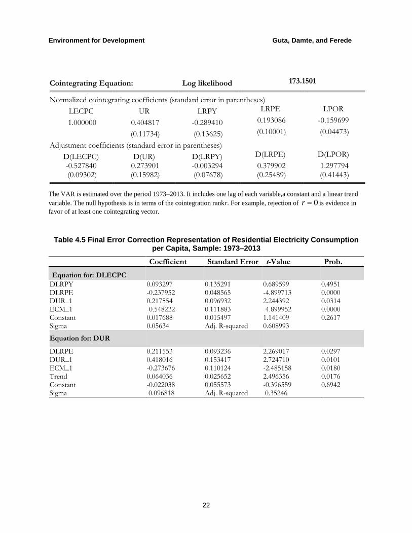
Cointegrating Equation:

Log likelihood

173.1501

Normalized cointegrating coefficients (standard error in parentheses)

LECPC UR LRPY LRPE LPOR

1.000000 0.404817 -0.289410 0.193086 -0.159699

(0.11734) (0.13625) (0.10001) (0.04473)

Adjustment coefficients (standard error in parentheses)

D(LECPC) D(UR) D(LRPY) D(LRPE) D(LPOR)

-0.527840 0.273901 -0.003294 0.379902 1.297794 (0.09302) (0.15982) (0.07678) (0.25489) (0.41443)

The VAR is estimated over the period 1973–2013. It includes one lag of each variable,a constant and a linear trend

variable. The null hypothesis is in terms of the cointegration rankr. For example, rejection of 0r is evidence in

favor of at least one cointegrating vector.

Table 4.5 Final Error Correction Representation of Residential Electricity Consumption per Capita, Sample: 1973–2013

Coefficient Standard Error t-Value Prob.

Equation for: DLECPC DLRPY 0.093297 0.135291 0.689599 0.4951 DLRPE -0.237952 0.048565 -4.899713 0.0000 DUR_1 0.217554 0.096932 2.244392 0.0314 ECM_1 -0.548222 0.111883 -4.899952 0.0000 Constant 0.017688 0.015497 1.141409 0.2617 Sigma 0.05634 Adj. R-squared 0.608993

Equation for: DUR

DLRPE 0.211553 0.093236 2.269017 0.0297 DUR_1 0.418016 0.153417 2.724710 0.0101 ECM_1 -0.273676 0.110124 -2.485158 0.0180 Trend 0.064036 0.025652 2.496356 0.0176 Constant -0.022038 0.055573 -0.396559 0.6942 Sigma 0.096818 Adj. R-squared 0.35246


23

Table 4.6 Variance Decomposition of Residential Electricity Consumption in Percent

Period S.E. LECPC UR LRPY LRPE LPOR

1 0.064380 100.0000 0.000000 0.000000 0.000000 0.000000 2 0.090660 78.18086 10.07229 0.727847 4.949962 6.069040 3 0.116674 59.12400 18.86944 1.363549 9.273265 11.36975 4 0.140974 47.35459 24.30251 1.756155 11.94331 14.64343 5 0.163036 40.12059 27.64192 1.997468 13.58444 16.65559 6 0.183028 35.43241 29.80610 2.153857 14.64802 17.95961 7 0.201285 32.21893 31.28953 2.261053 15.37704 18.85345 8 0.218120 29.90624 32.35713 2.338200 15.90170 19.49673 9 0.233789 28.17314 33.15717 2.396013 16.29488 19.97880 10 0.248489 26.83054 33.77695 2.440799 16.59946 20.35224

Table 5.1 Residential Electricity Consumption in Ethiopia: An ADL Model

Variable Coefficient Std. Error t-Statistic Prob. LECPC_4 0.186099 0.067094 2.773708 0.0094

UR_2 0.160800 0.018431 8.724268 0.0000 LRPY_4 -0.345030 0.088167 -3.913371 0.0005 LRPE -0.466071 0.042418 -10.98752 0.0000 LRPE_2 -0.215205 0.059083 -3.642413 0.0010 LPOR_4 -0.064660 0.022380 -2.889196 0.0071 Constant 1.745938 0.669182 2.609064 0.0140

R-squared 0.994465 Mean dependent variable 2.048615

Adjusted R-squared 0.993358 S.D. dependent variable 0.569840 S.E. of regression 0.046441 Akaike info criterion -3.132624 Sum squared residuals 0.064702 Schwarz criterion -2.827856 Log likelihood 64.95354 Hannan-Quinn criterion -3.025179 F-statistic 898.3595 Durbin-Watson stat 1.917227 Prob(F-statistic) 0.000000


24

Table 5.2 Serial Correlation, Heteroscedasticity and Normality Tests of Residuals

Breusch-Godfrey Serial Correlation LM Test

F-statistic 0.910025 Prob. F(5,25) 0.4904

Obs*R-squared 5.697257 Prob. Chi-Square(5) 0.3368 Breusch-Pagan-Godfrey Heteroscedasticity Tests F-statistic 0.980197 Prob. F(6,30) 0.4558

Obs*R-squared 6.064565 Prob. Chi-Square(6) 0.4160 Scaled explained SS 5.465055 Prob. Chi-Square(6) 0.4857

Normality Test of Residuals

Jarque-Bera 3.602803 Probability 0.165067

Figures: see following pages.

0

2,000

4,000

6,000

8,000

10,000

1973 1978 1983 1988 1993 1998 2003 2008 2013

Residential Electricity Consumption in '000 of MWhTotal Electricity Consumption in '000 of MWh

Figure 3.1: Residential and Total Electricity Consumption Over time in '000 of MWh

Ele

ctri

city

Co

nsu

mp

tio

n '

00

0 o

f M

Wh

0

100,000

200,000

300,000

400,000

500,000

600,000

1973 1978 1983

1988 1993 1998 2003 2008 2013

2013

0

400

800

1,200

1,600

2,000

2,400

1973 1978 1983

Residential Electricity Consumption in '000 of MWh

Figure 3.3: Trends in Residential Electricity Consumption in '000 of MWh and Urban

population Tens of Thousands

1983 1988 1993 1998 2003

Residential Electricity Consumption in '000 of MWh Urban Population in Tens of Thousands


2008 2013

Urban Population in Tens of Thousands


-0.4

-0.2

0.0

0.2

0.4

0.6

0.8

1.0

1.2

1.4

1980 1985 1990 1995 2000 2005 2010

C U S U M o f

S q u a r e s

9 5 %

C o n f i d e n c e

B o u n d s

F i g u r e 4 . 1 :

S t a b i l i t y

T e s t o f

R e s i d e n t i a l E l e c t r i c i t y

D e m a n d M o d e l

-4

-3

-2

-1

0

1

2

1 980 1 9 8 5 1 9 9 0 1 9 9 5 2 0 0 0 2 0 0 5 2 01 0

R ec u rs iv e

D L R P Y E s t i m a t es

±

2

S . E .

-

-

0.0

0.4

0.8

1.2

1 980 1 9 8 5 1 9 90 1 9 9 5 2 0 0 0 2 0 0 5 2 01 0

R ecu rs i v e D L R P E

E s ti m a t es

±

2

S . E .

-100

-80

-60

-40

-20

0

20

1 98 0 1 98 5 1 9 9 0 1 9 95 2 00 0 20 0 5 2 0 1 0

R ecu rs i v e

D U R _ E s tim a te s

±

2

S . E .

-2.0

-1.6

-1.2

-0.8

-0.4

0.0

0.4

1 9 8 0 19 85 1 9 9 0 1 9 9 5 2 0 0 0 2 0 0 5 20 10

R e cu rs iv eE C M _ 1 E s t im a te s

±

2 S . E .

-2

0

2

4

6

8

1 98 0 1 98 5 1 9 9 0 1 9 95 2 00 0 20 0 5 2 0 1 0

R ec u rs i v e C o n s t a n t

term ±

2

S . E .

F i g u re 4 .2 :

R e cu r s i v e

C o e f f i ci e n t s

Es ti m a te s

w i t h

2

S .E.

B o u n ds

f o r

e l e ct i c i t y

D e m a n d

M o d e l

.030

.035

.040

.045

.050

.055

.060

.065

1 2 3 4 5 6 7 8 9 10

F ig u re 4 .3 : R e s p o n s e o f R e s id e n t ia l E le c t ric it y C o n s u m p t io n p e r C a p ita t o C h o le s k y

O n e S .D . O w n I n n o v a t io n

.000

.002

.004

.006

.008

.010

.012

.014

.016

1 2 3 4 5 6 7 8 9 10

F ig u re 4 .4 : R e s p o n s e o f R e s id e n t ia l E le c t ric it y C o n s u m p tio n p e r C ap it a t o C h o le s k y

O n e S .D . R e a l G D P p e r C ap it a I n n o v a t io n

-.06

-.05

-.04

-.03

-.02

-.01

.00

1 2 3 4 5 6 7 8 9 10

F ig u re 4 .5 : R e s p o n s e o f R e s id e n t ia l E le c t ric it y C o n s u m p t io n p e r C a p ita t o C h o le s k y

O n e S .D . U R I n n o v a t io n la s t y e ar

-0.4

-0.2

0.0

0.2

0.4

0.6

0.8

1.0

1.2

1.4

84 86 88 90 92 94 96 98 00 02 04 06 08 10 12

C U S U M o f

S q u a r e s 5 %

S i g n i f i c a n c e

F ig u r e 5 . 1 : C u m u l a t i v e S u m o f S q u a r e s T e s t o f S t a b i l i t y

-.8

-.4

.0

.4

.8

19 8 5 1 9 9 0 1 9 95 2 000 2 00 5 2 0 1 0

Rec u rsi ve

L ECPC _ 4

Coe ffi ci e n t

Estim a te s ±

2

S .E .

-2.0

-1.5

-1.0

-0.5

0.0

0.5

1.0

1.5

1 9 85 1 9 9 0 1 995 2 00 0 2 005 2 0 1 0

R e cu rsi ve

UR_ 2

C o effic i e n t

Esti m a te s±

2

S .E .

-4

-3

-2

-1

0

1

19 8 5 1 9 9 0 1 995 2 0 0 0 2 0 0 5 2 0 1 0

Re cu r si ve

L RPY_ 4

Co e ffi c i e nt

Esti ma te s ±

2

S .E .

-1.4

-1.2

-1.0

-0.8

-0.6

-0.4

-0.2

0.0

19 8 5 1 9 9 0 1 9 95 2 000 2 0 0 5 2 0 1 0

Re c ursive

L RPE

C o e ffi ci e nt

Estima te s ±

2

S .E .

-.6

-.5

-.4

-.3

-.2

-.1

.0

1 9 8 5 1 9 9 0 1 9 95 2 0 0 0 2 005 2 0 1 0

R e c u rsive

L RPE_ 2

C o e fficen t

Esti ma te s±

2

S .E .

-.20

-.15

-.10

-.05

.00

.05

19 8 5 1 9 9 0 1 995 2 0 0 0 2 0 0 5 2 0 1 0

Re cu rsi ve

L POR_ 4

Co e ffie n c ie nt

Estima te s±

2

S .E .

Fi gure

5.. 2:

R ec ursive

Est ima t e s

of

Mod el

Pra met e rs

Documents

Environment for Development · Environment for Development Kenya ... Any investment in the electricity sector is likely to speed up ... residential electricity prices using a Structural