Embed Size (px)
Citation preview
NBER WORKING PAPER SERIES
ENTREPRENEURSHIP AND THE CITY
Edward L. Glaeser
Working Paper 13551http://www.nber.org/papers/w13551
NATIONAL BUREAU OF ECONOMIC RESEARCH1050 Massachusetts Avenue
Cambridge, MA 02138October 2007
Kristina Tobio provided superb research assistance and oversaw a team consisting of Yün-ke Chin-Lee,Elizabeth Cook, Andrew Davis, and Charles Redlick. This paper has been written for a KauffmanFoundation conference on entrepreneurship and for a related conference volume. Jason Furman providedhelpful comments. The views expressed herein are those of the author(s) and do not necessarily reflectthe views of the National Bureau of Economic Research.
© 2007 by Edward L. Glaeser. All rights reserved. Short sections of text, not to exceed two paragraphs,may be quoted without explicit permission provided that full credit, including © notice, is given tothe source.
Entrepreneurship and the CityEdward L. GlaeserNBER Working Paper No. 13551October 2007JEL No. R0
ABSTRACT
Why do levels of entrepreneurship differ across America's cities? This paper presents basic facts ontwo measures of entrepreneurship: the self-employment rate and the number of small firms. Bothof these measures are correlated with urban success, suggesting that more entrepreneurial cities aremore successful. There is considerable variation in the self-employment rate across metropolitan areas,but about one-half of this heterogeneity can be explained by demographic and industrial variation.Self-employment is particularly associated with abundant, older citizens and with the presence ofinput suppliers. Conversely, small firm size and employment growth due to unaffiliated new establishmentsis associated most strongly with the presence of input suppliers and an appropriate labor force. I alsofind support for the Chinitz (1961) hypothesis that entrepreneurship is linked to a large number ofsmall firms in supplying industries. Finally, there is a strong connection between area-level educationand entrepreneurship.
Edward L. GlaeserDepartment of Economics315A Littauer CenterHarvard UniversityCambridge, MA 02138and [email protected]
I. Introduction
In 1961, Benjamin Chinitz described Pittsburgh and New York City as “contrasts in
agglomeration.” While New York City appeared to be full of independent entrepreneurs,
Pittsburgh was dominated by a small number of large, vertically integrated firms. Thirty years
later, Annalee Saxenian described a similar contrast between the highly entrepreneurial computer
industry in Silicon Valley and its much more corporate counterpart in Boston’s Route 128.
Today, measures of entrepreneurship, like the self-employment rate, continue to show sizable
differences across metropolitan areas. One in every ten workers in the West Palm Beach
metropolitan area is self-employed; the comparable number for Dayton, Ohio, is less than one in
thirty.
Why are some cities so much more entrepreneurial than others? This paper attempts to analyze
some basic facts about entrepreneurship across urban areas. In Section II of this paper, I discuss
two widely available measures of entrepreneurship: the self-employment rate and average firm
size. Both of these measures are quite imperfect attempts to capture the number of entrepreneurs
relative to the overall amount of employment in an industry. Though it has a long history of
being used to study entrepreneurship, the self-employment rate is particularly oriented towards
the smallest entrepreneurs and makes little distinction between Michael Bloomberg and a hot
dog vendor outside of city hall (Evans and Jovanovic, 1989; Blanchflower and Oswald, 1998).
Conversely, the number of workers per firm is more likely to capture the presence of larger scale
entrepreneurs. One problem with either measure is that when entrepreneurs are successful, they
will hire more workers, and this will cause the self-employment rate in the industry to fall and
the number of firms per worker to decline. The problems with both measures push towards
using more dynamic measures, such as new establishment creation, but these measures require
the use of restricted datasets such as the Longitudinal Research Database (LRD), which I will
discuss at the end of the paper.
In Section II, I examine the patterns of entrepreneurial activity within individual industries as
well. Generally, the correlations across metropolitan areas between self-employment rates
across industry groups are fairly high, except for the self-employment rate in high-skilled
manufacturing. For instance, West Palm Beach is among the five most entrepreneurial places in
retail trade; wholesale trade and transportation; education, health and social services; low skilled
manufacturing; and other services. The correlations of self-employment rates across income
categories within a metropolitan area are also quite positive, although somewhat less strong. The
self-employment rates are also related to the firm size-based measures of entrepreneurship.
Section II concludes by looking at the correlation between these entrepreneurship measures and
city growth. Glaeser et al. (1992) and Miracky (1994) both found a connection between small
firm size and employment growth. I duplicate this result, and find that an abundance of small
firms is strongly correlated to later employment growth in a city industry. I also find that the
self-employment rate at the city level in 1970 predicts growth in population and income over the
next 30 years. While these finding are far from conclusive, they do suggest that local
entrepreneurship helps explain why some cities grow faster than others.
Section III describes four theories that explain why entrepreneurship differs so much across
space. The simplest theory holds that entrepreneurship reflects a supply of potential
entrepreneurs with plenty of either general human capital or human capital that is particularly
valuable for entrepreneurs. According to this view, cities differ in their human capital base for
historical reasons, and these initial human capital differences drive the level of entrepreneurship
today. A second theory emphasizes a local “culture of entrepreneurship”. This theory predicts
that exogenous variables that cause an increase in entrepreneurship in one sector of the economy
will also increase the level of entrepreneurship in other sectors of the economy.
A third theory emphasizes the presence of inputs to entrepreneurship such as capital, labor and
goods. A variant of this theory, following from Chinitz (1961), emphasizes the presence of
small, independent input suppliers. A fourth theory emphasizes the presence of a large customer
base.
In Section IV, I evaluate these four hypotheses using data on self-employment, firm size and
employment growth due to unaffiliated plant formation. Self-employment is strongly connected
to age, education and industry. These variables can explain roughly 50 percent of the variation in
self-employment rates across metropolitan areas, and this fact supports the view that
entrepreneurial people explain a fair amount of why some places are more entrepreneurial than
others. Using firm size data, I also find that basic demographic variables can explain about one-
third of the variation in firm sizes across metropolitan areas.
By contrast, the evidence for the “culture of entrepreneurship” hypothesis is much weaker.
Looking across metropolitan areas, there is a tendency for people who live in metropolitan areas
filled with more entrepreneurial industries to be more entrepreneurial, holding their industry
constant. This is the only positive evidence for a culture of entrepreneurship, and it could be
explained by many theories, such as the tendency of more entrepreneurial industries to locate in
places with more entrepreneurial people. When I look at industry clusters within metropolitan
areas, there is no correlation between entrepreneurial industries and individual entrepreneurship,
again holding the individual industry constant. The firm size evidence also points against the
culture of entrepreneurship theory.
Both the self-employment and firm size data show that the entrepreneurship levels are higher
when industry employment is lower. One explanation for this phenomenon is that if the number
of entrepreneurs is relatively constant over space, but the success of entrepreneurs differs, then
we should expect to see more employment in areas where entrepreneurs are more successful, and
that higher level of employment then causes the entrepreneurship rate to look lower.
The self-employment rate is correlated with the presence of input suppliers. It is not correlated
with the presence of customers, appropriate labor supply, venture capitalists or small firms that
supply inputs. The self-employment level in retail industries does rise in big cities, but this is the
only demand-side effect that is readily apparent.
Average firm size tends to decrease with the availability of inputs, and the presence of many
small input suppliers is also highly indicative of a large number of small firms, just as Chinitz
suggests. Firm size is also weakly associated with demand, but the presence of the appropriate
labor force seems to be the most important variable for explaining an abundance of small firms.
The entrepreneurs seem to be in areas where there are lots of workers, either because they are
attracted by those workers or because these workers provide the pool of potential entrepreneurs.
The regressions taken from Dumais, Ellison and Glaeser (1997) confirm the importance of labor
supply. New plant growth is associated with input suppliers and customers, but the impact of
workers is far more important. We also find that intellectual connections across industries are
important.
Section V concludes and emphasizes that these results should be seen as a tentative first step in
the task of explaining the variation in entrepreneurship across metropolitan areas. My limited
evidence suggests that local entrepreneurship depends mainly on having the right kind of people.
Older, skilled workers are more likely to be entrepreneurs, and entrepreneurship in an industry
depends strongly on the presence of workers who both provide the pool of labor for
entrepreneurs and are themselves the source of new entrepreneurship.
II. The Measurement of Entrepreneurship
In this section, I discuss the measurement of entrepreneurship across space. Perhaps the most
natural individual measure of entrepreneurship is the self-employment rate, which captures the
share of people who lead their own enterprise. Since self-employment rates are easy to measure,
they have been the standard for much of the empirical work in this area (Evans and Jovanovic,

1989; Blanchflower and Oswald, 1998). The downside of using self-employment rates is that
the raw measure is extremely coarse. There are over 8.5 million self-employed Americans in the
2000 Census, and that group includes both many of the richest and many of the poorest people in
the country. Since I am interested not only in the amount of entrepreneurial activity, but also in
the amount of successful entrepreneurial activity, I will examine both the total amount of self-
employment and the amount of self-employment in different income categories.
Income categories offer one way of dividing up self-employment rates; industry grouping
represents a second means of doing so. Since self-employment information comes from the
Census, respondents are identified by their industry group using the North American Industrial
Classification System (NAICS). This system offers finely detailed industry groupings, which I
will use in later analysis in this paper. For the purposes of this preliminary data description, I
divide the overall population into ten groups based on one and two-digit NAICS codes.
The essential division is along one-digit lines. Within the initial nine different one digit codes, I
eliminate all of the workers in agriculture, since my focus is on urban areas, and in public
administration and the military, since my focus is on the private sector. This leaves me with
seven one-digit codes. I then divide each of the three largest one-digit codes — manufacturing
(NAICS code 3), trade (NAICS code 4) and information-related services (NAICS code 5) — into
two groups. Manufacturing and information-related services are divided on the basis of the
average education level in the two-digit NAICS code, separating the self-employed in the more
educated two-digit industry codes from the self-employed in the less educated two-digit codes.
Since education is correlated with both technology and income, it provides a reasonable dividing
line. I also divide the trade related industries into a retail trade category and a wholesale trade,
transportation and warehousing category. This division is based on the fact that entrepreneurship
in retail trade is likely to be correlated with ordinary consumers in a way that is less true for the
other trade industries.

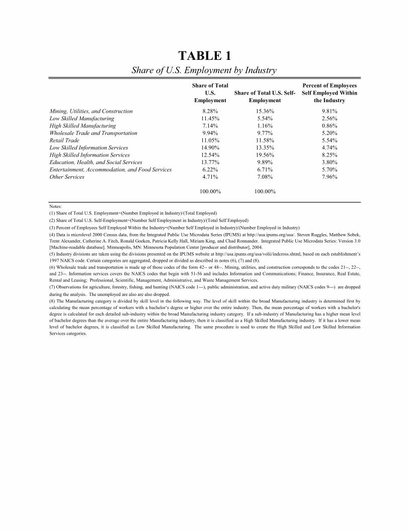
Table 1 shows the distribution of the non-agricultural, non-governmental workforce across these
ten groupings. The first column shows the overall share of employment in each one of the
industry categories. The second column shows the share of the total overall self-employment in
each of these industry categories, and the third column gives the self-employment rate within
each industry category.
The first category of mining, utilities and construction has only 8 percent of total employment in
the United States, but it accounts for more than 15 percent of the total self-employment in the
United States. The self-employment rate in this category is the highest across all industry
groupings at almost 10 percent, and this mainly reflects the high self-employment rates in
construction. The home building business is populated by thousands of independent contractors,
and is in many ways one of the most entrepreneurial sectors of the economy.
The next two rows in the table show the results for high and low skilled manufacturing. As there
tend to be large economies of scale in these industries, self-employment rates are low. High
skilled manufacturing is an area where less than one percent of its labor force is self-employed.
This fact clearly illustrates the mismatch between the number of people who are self-employed
and the importance of entrepreneurship within an industry. Certainly, some of the country’s
most important entrepreneurs are in high skilled manufacturing, but there are very few of them
relative to the overall workforce in those industries. This fact is a warning against treating the
self-employment rate as any kind of definitive measure of entrepreneurship.
Both retail trade and wholesale trade and transportation have self-employment rates of around
five percent. The share of self-employed workers in the less skilled information services is
similar. The self-employment rate in high skilled information services is over 8 percent. While
the more skilled manufacturing industries have less self-employment, the more skilled
information services have more self-employment. This reflects both the lower capital
requirements and the general entrepreneurial nature of many information services such as
accounting, management consulting and law.

The self-employment rate in education, health and social services is quite low. Non-profit firms
figure prominently in this sector and many of them are extremely large. The self-employment
rate in entertainment, accommodation and food services is over 5 percent. Given the large
number of independent food salesman, it makes sense that this number is rather high. The final
grouping is “other services,” which includes a hodgepodge of service industries ranging from
“repair and maintenance services” to “personal and laundry services” to “religious services”.
The self-employment rate in this sector is almost 8 percent, and it is the third most
entrepreneurial of these industry groupings.
Entrepreneurs differ in the industries they choose, and they also differ in the degree of their
financial success. When I turn to the cross-metropolitan statistical area data, I will be interested
in examining both the correlates of self-employment and the correlates of being prosperous and
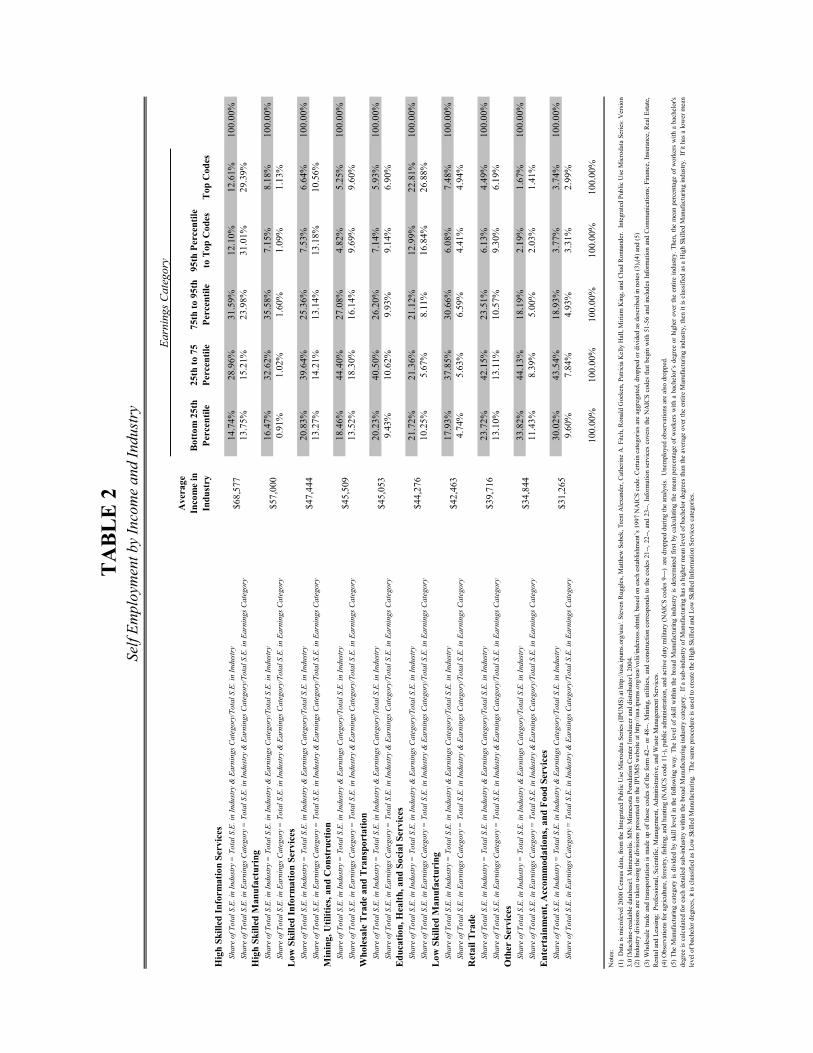
self-employed. Table 2 shows the distribution of prosperity among the self-employed across the
ten industry groups.
The columns of the table represent five different financial groupings. The lowest group includes
people earning less than 23,000 dollars, which are those people in the bottom quartile of the
income distribution. The second group includes people earning between 23,000 and 53,000
dollars, which are those people in the middle two quartiles of the income distribution. The third
group includes people earning between 53,000 and 110,000 dollars, which are those people in
the top quartile of the income distribution, but outside of the top five percent of the income
distribution. The fourth group earns between 110,000 and 175,000 dollars, which means that
they earn more than 95 percent of the employed workers in the Census, but that they are not
among the elite group of workers whose income has been top-coded. The fifth and final group
includes only those whose incomes have been top-coded.
The industry groups are ranked by mean earnings, with high skilled information services at the
top of the table and entertainment, accommodation and food services at the bottom. The average

income for that top group is more than double the average income in the bottom group. The
matrix gives two entries in every cell. The top entry refers to a ratio that is calculated as the
number of people in that particular industry group and in that particular earnings category who
are self-employed, divided by the total number of people in that particular industry group who
are self-employed. The bottom entry refers the ratio that is calculated as the number of people in
that particular industry group and particular earnings category who are self-employed, divided by
the total number of people in that particular earnings category who are self-employed. The top
numbers sum horizontally to equal one hundred percent; the bottom numbers sum vertically to
equal one hundred percent. The top figures give a sense of the income distribution of the
industry; the bottom numbers tell us what share of total self-employed people earning a certain
amount work for a particular industry group.
For example, the top row tells that 14.74 percent of the self-employed in high skilled information
services are in the bottom quartile of the income distribution while 12.61 percent of them are in
the top coded category. 29.39 percent of all self-employed people in the top coded category are
in high skilled information services. This industry group is the largest repository of highly paid
entrepreneurs. The second largest repository is in education, health and social services, which
has 26.88 percent of the top coded self-employed workers. There is much truth to the view that
doctors and lawyers provide a large share of the most successful self-employed people.
Interestingly, the education, health and social service group is particular unequal, and overall has
a relatively low average income grouping. Together, the high skilled information services and
the education, health and social services industry groups contain approximately 56 percent of the
top coded self-employed workers, and almost 50 percent of the self-employed people in the top
five percent of the income distribution.
The poorest industry groups are entertainment, accommodation and food services and “other
services”, which includes industries such as “repair and maintenance services” and “personal and
laundry services”. More than 70 percent of the self-employed people in these areas are in the
bottom three quarters of the income distribution. Of course, they are not particularly poorer than
the U.S. population is as a whole, but they are not particularly richer as a group either. Retail

trade and low skilled manufacturing are the other groups that have an income distribution that is
closest to the overall U.S. income distribution. However, these people are still vastly
overrepresented among the top-coded earners, which suggests that even in these industry groups
there is some chance of doing quite well.
The earnings distributions for low skilled information services; wholesale trade and
transportation; and mining, utilities and construction are all quite similar. Average earnings in
these sectors are clustered around 45,000 dollars, and between 5 and 7 percent of their
populations are in the top-coded category. High skilled manufacturing has average earnings that
are higher than any of these groups, and more than 8 percent of its entrepreneurs have top-coded
income levels.
One issue with comparing the earnings of self-employed workers with the U.S. population as a
whole is that the earnings of the self-employed typically include both the returns to their labor
and the returns to any capital that they have invested. The earnings of most workers do not
include any returns to capital. As a result, the high incomes earned by some self-employed
workers surely overstate their labor income.
I now turn to the heterogeneity of self-employment rates across metropolitan areas. To get a
sense of the range of self-employment rates, Table 3 presents the five metropolitan areas with the
highest and lowest self-employment rates overall and in each of the ten industry groups. The top
panel of Table 3 shows that the heterogeneity in the overall self-employment rate is significant
but not extreme. All but eight of the country’s metropolitan areas have overall self-employment
rates, across all industries, between 3.2 and 7.76 percent. This top panel shows some outliers,
like West Palm Beach and Honolulu, and these MSAs reappear in Table 3 in some of the other
panels representing our ten different industry groups. The problems with this overall measure
are well illustrated by the fact that San Jose, CA, has among the lowest self-employment rates in
the country. Despite all those Silicon Valley entrepreneurs who have changed the world, their
region has, on a per capita basis, far fewer entrepreneurs than all but four other areas.

The remaining panels give us the top and bottom five metropolitan areas ranked by the self-
employment rate within each MSA. The self-employment rate is defined as the share of workers
in that industry group who are self-employed. In these areas, the heterogeneity can be striking.
The self-employment rate in mining, utilities and construction is more than 20 percent in Fort
Wayne, Indiana, but less than 2 percent in Modesto, California. In high skilled information
services, the self-employment rate in Spokane, Washington, is 16 percent, while the self-
employment rate in Bakersfield, California is 3.13 percent.
In some cases, these differences are driven by industrial differences within the categories.
Construction has a high self-employment rate, while mining and utilities do not. As such, MSAs
that have a large portion of their labor force employed in mining will likely have low overall
self-employment rates within the aggregated mining, utilities and construction industry group,
because the very low self-employment rates in mining will offset any high self-employment rates
in construction in those areas. Thus, it is clear that controlling for very finely detailed industry
groups will be important for any further work on the local determinants of entrepreneurship.
Still, the continuing reappearance of some metropolitan areas in a wide range of different
categories makes it clear that industrial differences cannot be entirely responsible for the
variation across metropolitan areas. For example, West Palm Beach ranks in the top five for five
of the ten industry groups (low skilled manufacturing; retail trade; high skilled information
services; education; health and social services; and other services). Honolulu is in the top five
for three different industry groups, and Springfield, Massachusetts, is in the bottom five for three
different industry groups.
The heavy representation of Florida’s cities in so many of the top five lists is quite striking. This
might represent a preponderance of older citizens who have enough human capital to operate
independently and who prefer the control that comes from working on their own. Alternatively,

it might represent a response to the physical distance of Florida from the locations of many of the
larger corporations in America.
Table 4 presents an overview of the degree to which self-employment rates across these
industrial categories are correlated with the overall self-employment rate. The first column gives
the correlation of the overall self-employment rate in an MSA with the self-employment rate
within each industry group in an MSA, which is calculated as the number self-employed workers
in the industry group divided by total employment in the industry group. The third column shows
correlations of the same self-employment rates using a smaller sample of people earning over
75,000 dollars a year. The second column gives the correlation between the overall self-
employment rate in an MSA with the share of the metropolitan area’s workers that are self-
employed in each of the industry groups, which is calculated by dividing the number of self-
employed workers in an industry group by the total number of self-employed workers in all
industries in the MSA.
The correlations shown in the first column can be separated into three groups. Five of the
industries have self-employment rates that have a correlation with the overall self-employment
rate between 61 and 66 percent. These five are both information services groups; both types of
trade; and mining, utilities and construction. The second column shows that the overall self-
employment rate is also quite correlated with the share overall city’s workforce that is self-
employed in those industry groups. Figure 1 shows the correlation across MSAs between the
overall self-employment rate and the share of the workforce that is self-employed in retail trade.
The second group includes four industries with self-employment rates that have a correlation
with the overall self-employment rate ranging from 35 percent (low skilled manufacturing) to 50
percent (other services). The other two industry groups in this set are education, health and
social services and entertainment, accommodation and food services.
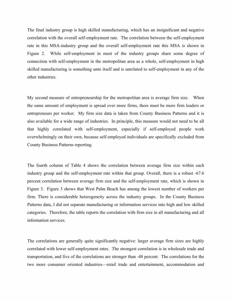
The final industry group is high skilled manufacturing, which has an insignificant and negative
correlation with the overall self-employment rate. The correlation between the self-employment
rate in this MSA-industry group and the overall self-employment rate this MSA is shown in
Figure 2. While self-employment in most of the industry groups share some degree of
connection with self-employment in the metropolitan area as a whole, self-employment in high
skilled manufacturing is something unto itself and is unrelated to self-employment in any of the
other industries.
My second measure of entrepreneurship for the metropolitan area is average firm size. When
the same amount of employment is spread over more firms, there must be more firm leaders or
entrepreneurs per worker. My firm size data is taken from County Business Patterns and it is
also available for a wide range of industries. In principle, this measure would not need to be all
that highly correlated with self-employment, especially if self-employed people work
overwhelmingly on their own, because self-employed individuals are specifically excluded from
County Business Patterns reporting.
The fourth column of Table 4 shows the correlation between average firm size within each
industry group and the self-employment rate within that group. Overall, there is a robust -67.6
percent correlation between average firm size and the self-employment rate, which is shown in
Figure 3. Figure 3 shows that West Palm Beach has among the lowest number of workers per
firm. There is considerable heterogeneity across the industry groups. In the County Business
Patterns data, I did not separate manufacturing or information services into high and low skilled
categories. Therefore, the table reports the correlation with firm size in all manufacturing and all
information services.
The correlations are generally quite significantly negative: larger average firm sizes are highly
correlated with lower self-employment rates. The strongest correlation is in wholesale trade and
transportation, and five of the correlations are stronger than -48 percent. The correlations for the
two more consumer oriented industries—retail trade and entertainment, accommodation and

food services—are close to -40 percent. The weakest correlation is in other services which is
less than -20 percent. This correlation is shown in Figure 4.
In the later empirical work, I will use both measures of entrepreneurship. The primary
advantage of the self-employment rate is that I am able to control for individual level
characteristics. With the firm size data, I will only be able to control for aggregate statistics at
the metropolitan area level and the industrial composition of the metropolitan area. Both
measures are quite imperfect, but they are convenient and surely at least correlated with some
aspects of local entrepreneurship.
Entrepreneurship and City Growth
I now turn to the correlation between the entrepreneurship measures and metropolitan growth.
Glaeser et al. (1992) found a significant correlation between average firm size and employment
growth at the city-industry level, and Miracky (1994) confirmed this result for a larger sample.
Using data from 1977 and 2000 County Business Patterns, I can relate employment growth
within each metropolitan area-industry cell to the logarithm of the average firm size in the
metropolitan area. In this case, in part because of a desire to avoid suppressed data, I use the
following, quite coarse, industry groupings: “manufacturing”, “services,” “finance, insurance and
real estate”, “retail trade”, “wholesale trade”, “construction,” “mining” and “transportation,
warehousing and utilities.”
Using these measures, I estimate the regression:
(1) ( ) DummiesIndustryandMSAEmpLogEmp
FirmsLog
EmppEm
Log ++
−=
1977)01(.
1977
1977
)04(.1977
2000 04.60.
Standard errors are in parentheses and clustered at the metropolitan area level. There are 2735
observations. A .1 log point increase in average firm size is associated with a .06 decrease in
industry employment growth over the 1977-2000 period. This effect has a t-statistic of 15 and is
quite statistically significant.
If these regressions are run independently for each of the seven broad industry groups (obviously
without metropolitan area dummies), the effect of firm size is negative and significant in each
one of the groups, and ranges from -.31 in retail trade to -.86 in wholesale trade.
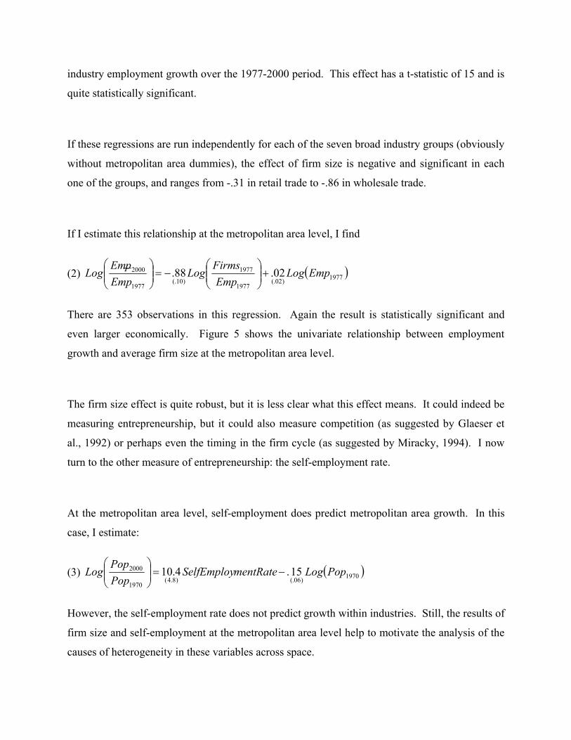
If I estimate this relationship at the metropolitan area level, I find
(2) ( )1977)02(.1977
1977
)10(.1977
2000 02.88. EmpLogEmp
FirmsLog
EmppEm
Log +
−=
There are 353 observations in this regression. Again the result is statistically significant and
even larger economically. Figure 5 shows the univariate relationship between employment
growth and average firm size at the metropolitan area level.
The firm size effect is quite robust, but it is less clear what this effect means. It could indeed be
measuring entrepreneurship, but it could also measure competition (as suggested by Glaeser et
al., 1992) or perhaps even the timing in the firm cycle (as suggested by Miracky, 1994). I now
turn to the other measure of entrepreneurship: the self-employment rate.
At the metropolitan area level, self-employment does predict metropolitan area growth. In this
case, I estimate:
(3) ( )1970)06(.)8.4(1970
2000 15.4.10 PopLogmentRateSelfEmployPopPop
Log −=
However, the self-employment rate does not predict growth within industries. Still, the results of
firm size and self-employment at the metropolitan area level help to motivate the analysis of the
causes of heterogeneity in these variables across space.
III. Why Does Entrepreneurship Differ Across Cities?
In this section, I discuss the four different theories that can explain the heterogeneity of
entrepreneurship. I will test these four theories empirically in the next section.
Hypothesis # 1: Supply of Entrepreneurs
Perhaps the simplest hypothesis about the heterogeneity of entrepreneurship across space is that
some people are inherently more entrepreneurial than others because of their education levels,
ages or industry of choice. Better educated people could easily have more skills to succeed as
entrepreneurs. Older people might have accumulated more capital or experience that might
make entrepreneurship more attractive. Finally, some industries inherently have lower capital
requirements, and this might make entrepreneurship easier.
This hypothesis suggests that controlling for individual characteristics and the industry mix of a
metropolitan area will explain a significant amount of the variation in entrepreneurship rates
across metropolitan areas. Perhaps the most intuitive means of testing this hypothesis is to look
at raw entrepreneurship rates at the metropolitan area level, and then to compare those rates with
rates that are calculated as the residuals from individual level regressions that control for
individual characteristics and industries. If this hypothesis is correct, the variance of
metropolitan area self-employment rates should decline substantially by controlling for the
industry mix in the metropolitan area. I can also test this hypothesis by looking at the extent to
which area-level demographic variables can explain the average firm size at the metropolitan
area level.
This hypothesis does not seek to explain why the education level or age characteristics differ
across metropolitan areas. Presumably these variables are themselves a function of historical

variables (like the existence of universities before 1940 as in Moretti, 2004) or temperature. If
demographics are found to be important, then future work can use more exogenous variables as
instruments for demographics.
Hypothesis # 2: A Culture of Entrepreneurship
A second hypothesis is that cities tend to have an entrepreneurial zeitgeist that then infects their
citizenry. According to this view, there are some places that are intrinsically full of new ideas
and a spirit of change. Alternatively, there are other places where tradition and old social
structures rule.
In a sense, this model argues that there are positive social spillovers from entrepreneurship that
generate high degrees of variation across space (as in Glaeser et al. 1992). If one person’s
decision to start a new firm makes it more likely that his neighbor will also become an
entrepreneur, this could create a cascade within the city and variation across cities. In some
cases, these complementarities may work through easy-to-understand economic processes. If
there are fixed costs in the provision of venture capital or inputs, then the positive spillover may
work through inducing more of these needed inputs. In other cases, the positive
complementarity may work through more ephemeral channels.
One critical issue is the extent to which this positive spillover works across industries. If we
believe that there is a general urban tendency towards entrepreneurship, then this can be tested
by looking at the impact of being around other entrepreneurial industries in the city. To measure
this, I create a predicted entrepreneurship measure by using a measure
∑≠ij USAMSA
USAjMSAj
urshipEntrepreneEmpurshipEntrepreneEmp
** ,, , where MSAjEmp , is the employment in industry j in the
MSA, MSAEmp is the total employment in the MSA, USAjurshipEntreprene , is an

entrepreneurship measure (either the self-employment rate or average firm size) for industry j
across the entire U.S. and USAurshipEntreprene is the same entrepreneurship measure across all
industries in the county.
This measure takes the average of the entrepreneurship measures weighted by the industrial
employment outside of the industry in question. In other words, it is the predicted level of
entrepreneurship based on the industry mix in the city and the entrepreneurship measure for that
industry in the country as a whole. I will use both the self-employment measure and the average
firm size measure for this input.
As there is some question about whether or not this “spirit of entrepreneurship” travels far across
industrial borders, I will calculate this measure both for the country as a whole and within
specific industry groups, i.e. 1-digit NAICS industries. I will also estimate this spirit of
entrepreneurship using both the self-employment rate and average firm size data.
Hypothesis # 3: Inputs for New Firms
A third hypothesis is that different metropolitan areas are endowed with the inputs that are
needed to produce new firms. Chinitz himself emphasized the importance of decentralized
inputs in making things easier for entrepreneurship. I will focus on three inputs that are needed
by new firms forming in particular industries.
One of the inputs into entrepreneurship that has received the most attention is venture capital.
These high risk lenders have certainly played a major role in a large number of new start-ups.
Naturally, one can question the extent to which geographic distance makes it difficult to get
financing. Venture capitalists have been known to get on airplanes. As a result, I think that
while there is no question that venture capital matters to new start-ups, there is a question about
whether local venture capital is needed for local entrepreneurship.
Unfortunately, finding exogenous variation in venture capital is far from easy. I will take the
easier step of just looking at whether measures of venture capital (at
https://www.pwcmoneytree.com/MTPublic/ns/index.jsp) correlate with self-employment and
firm size at the metropolitan area level. I will also ask whether this financing has more of an
effect for manufacturing industries with more capital requirement.
While venture capital is a particularly obvious input, firms also purchase inputs and hire labor,
and supplies of inputs and labor also differ across metropolitan areas. Dumais, Ellison and
Glaeser (1997) look at the connection between measures of input, labor supply and new firm
births. Our input measure is jiij MSA
MSAjMSAi Input
EmpEmp
Input ∑≠
= ,, where jiInput describes the share
of industry i’s inputs that are bought from industry j.
Chinitz emphasized the role of small decentralized input suppliers, rather than large centralized
firms. He argued that the overall level of entrepreneurship depended on the presence of many
small firms that can readily supply new start-ups. To capture this, I use an alternative input
measure jiij MSA
MSAjji
ij MSA
MSAj
MSAj
MSAjMSAi Input
EmpFirms
InputEmpEmp
EmpFirms
Chinitz ∑∑≠≠
== ,,
,
,, . This measure
captures the number of firms that supply this industry’s needs in this metropolitan area.
My third measure of inputs focuses on the labor supply. In this case, I start with oiShare , which
is the share of industry i’s in occupation o. I then use the distribution of occupations within the
metropolitan area to define ∑=o
ojMSA
MSAoMSAi Share
EmpEmp
MixLabor ,, , which represents the
preponderance of employment in occupation o in this particular metropolitan area.
In all cases, these measures are endogenous to the level of entrepreneurship. I believe that this
problem is less severe when looking at our entrepreneurship measure than it would be if I was
examining the overall employment in the industry. Nonetheless, if these factors do matter,
endogeneity would generally mean that the estimated coefficients may be biased upwards.
Hypothesis # 4: Customers
A final hypothesis is that entrepreneurship is driven by local customer needs. There are at least
three reasons why customers would tend to increase the overall amount of entrepreneurship.
First, the entrepreneurs may start firms to cater to this customer base. This is surely the most
natural reason for a connection between entrepreneurship and customer base. I suspect that this
is particular important for industries like health services. There are surely more doctors in West
Palm Beach because of their retiree customers.
A second reason why customers might matter for entrepreneurship is that innovators often learn
by connecting with their customer base. Porter (1990) emphasizes this connection in the
Sassuolo ceramics industry. There is also evidence that this chain of information flow operates
in the software industry as well (Saxenian, 1994). A third reason why customers might matter is
that erstwhile customers may have eventually become entrepreneurs themselves.
The most basic demand side measure is ijij MSA
MSAjMSAi Output
EmpEmp
Demand ∑≠
= ,, , where
ijOutput represents the share of output in industry i that is sold to industry j. This is the measure
used by Dumais, Ellison and Glaeser (1997) and it represents the extent to which employment in
this area is skewed towards industry where industry i generally sells its goods.
I will also consider two alternative measures of consumer demand. First, I will use an interaction
of population and retail trade to examine whether industries that sell directly to the public have
more entrepreneurship in cities that are bigger, relative to sectors that don’t sell directly to the
public. Second, I will specifically look at whether entrepreneurs that take care of the elderly
specifically locate in places with an older population.
IV. The Correlates of Entrepreneurship across Metropolitan Areas
I now turn to three empirical exercises which are meant to assess the relative importance of these
different theories in explaining the level of entrepreneurial activity across American cities. I first
look at self-employment rates using individual data from the 2000 Census. I then turn to average
firm size. Finally, I reproduce results from Dumais, Ellison and Glaeser (1997) on growth in
new establishments using the Longitudinal Research Database.
Self-Employment Evidence
Table 5 includes regressions where self-employment is regressed on individual characteristics,
including dummies for gender, eight age categories and five education categories. The data
includes only employed adults between 25 and 65. The regression also includes industry
dummies in all regressions, and the standard errors are clustered at the metropolitan area level.
The results are from a linear probability model. The coefficients are quite similar if a Probit
model is used instead; the linear probability model is used to facilitate correcting the standard
errors.
The first regression (1) includes only the industry dummies and the individual demographic
controls. Men are about 3.7 percent more likely to be self-employed than women. Self-
employment rates rise steadily with age, where 60-65 year olds are 8.1 percent more likely to be
self-employed than 25-30 year olds. The relationship with education is also monotonic. High
school dropouts are 6.9 percent less likely to be self-employed than college graduates. Education
and age are associated with both human capital and assets, both of which are useful inputs when
starting your own business.
How well can individual characteristics and industries explain the self-employment rates across
space? The overall r-squared of the regression is 7 percent, which means that these
characteristics can only explain 7 percent of the individual variation in self-employment. To
calculate the extent to which metropolitan area variation in self-employment can be explained by
individual characteristics, I compare the raw standard deviation of self-employment rates across
areas with the self-employment rates correcting for individual characteristics. I form these
corrected rates by taking the residuals the first regression and averaging them at the metropolitan
area level.
The raw standard deviation of self-employment rates is .013. The standard deviation of the
averaged residual is .009. Squaring these standard deviations to get variances, I find that the
variance of the corrected rates is slightly less than one-half of the variance of uncorrected rates.
In other words, correcting for individual characteristics and industries explains one-half of the
variation in self-employment rates across space. Nothing that I will do subsequently will have
the same ability to explain the variation in self-employment rates across space. This means that
the most important indicators of the heterogeneity in self-employment rates across space are the
industrial mix of the area and the tendency of some areas to have older people who are more
likely to be self-employed.
The second regression (2) looks at the impact of area level characteristics, including city size and
the presence of venture capital. The regression shows that the self-employment rate rises
significantly with the size of the metropolitan area, but the effect is modest. As the size of the
metropolitan area increases by 10 percent, the self-employment rate increases by .09 percentage
points. Big cities seem to be moderately friendlier to entrepreneurs. The regression finds little
connection between venture capital and the self-employment rate, perhaps because venture
capital is targeted towards a small set of industries that have high returns, but don’t account for a
large share of the total self-employed population.

This regression includes the logarithm of overall employment in one’s industry in the area. The
coefficient on this variable is -.008. This suggests that as one’s industry becomes more
prevalent, the self-employment rates declines by .08 percentage points. High self-employment
rates are more prevalent in areas where industries are poorly represented rather than in areas
where industries are more common. All subsequent regressions include this control.
This regression also presents a test of the culture of entrepreneurship hypothesis by adding the
variable ∑≠ −
−
ij USAMSA
USAjMSAj
EmploymentSelfEmpEmploymentSelfEmp
** ,, . This variable is a predicted self-employment
rate in the city, outside of an individual’s industry, based on the industrial mix of the city. In the
regression, this measure has a coefficient of .91 and a standard error of .14. People who work in
cities which have industries that are prone to be entrepreneurial are more likely to be
entrepreneurial themselves.
The magnitude of the coefficient implies that as predicted entrepreneurship outside of one’s own
industry increases by 10 percent, relative to the U.S. self-employment rate, the probability of
being self-employed increases by about 9 percent. The biggest problem in interpreting this result
is that the industrial mix of the area may not be endogenous. Areas that have attributes that
make them friendlier to self-employment may attract industries that have higher self-
employment rates. As a result, these findings may be compromised by an omitted variables bias,
where the omitted variables create a spurious correlation between the predicted self-employment
rate and the self-employment in one’s own industry.
To address this issue, regression (3) includes metropolitan area fixed effects. Since the overall
predicted self-employment rate variable does not differ significantly within the metropolitan
area, I instead use the measure calculated within an individual’s one digit industry. This
regression should be seen, therefore, as testing the hypothesis that people who are in one-digit
industries that are particularly oriented towards high self-employment rate activities are more
likely to be self-employed. In this case, the coefficient is -.45 and the standard error is .13.
People are less likely to be self-employed if the industry mix within their one-digit industry in
the city favors self-employment. When I estimate regression (3) without metropolitan area fixed
effects, the coefficient remains quite negative and significant.
Since regressions (2) and (3) give us such different results, it is hard to know how to interpret
these findings. Regression (2) certainly suggests a strong connection between areas with
industries that are oriented towards self-employment and individual self-employment.
Regression (3) shows that this does not persist with metropolitan area fixed effects. One
interpretation is that regression (2) is driven entirely by omitted area level characteristics.
Another interpretation is that the culture of entrepreneurship is not particularly localized to one’s
own industry. Further work will be needed to differentiate between these two interpretations.
Regression (4) includes our first measures of inputs to entrepreneurship: the measure of presence
of industry suppliers, jiij MSA
MSAjMSAi Input
EmpEmp
Input ∑≠
= ,, , and the interaction of venture capital with
being a capital intensive industry. The input measure has a strong and significant positive
effect. As the value of this variable increases by .05, which could signal a transfer of 20 percent
of employment from an industry that provide no inputs for industry i to an industry that provides
25 percent of industry i’s inputs, then the self-employment rate goes up by slightly over two
percent in that industry.
This regression also includes an interaction term between the venture capital measure and being
in a high skilled manufacturing industry. This interaction is testing the hypothesis that venture
capital particularly matters in that capital intensive sector. I find no evidence of this interaction.
In general, the venture capital measures have little correlation with the self-employment rate, so I
omit them from future regressions in this table.
Regression (5) includes our measure of input suppliers who are in small firms,
jiij MSA
MSAjMSAi Input
EmpFirms
Chinitz ∑≠
= ,, . In this case, there is no effect of this variable. Input
suppliers seem to increase self-employment, but the size of these suppliers is not important.
Regression (6) includes the labor mix variable ∑=o
ojMSA
MSAoMSAi Share
EmpEmp
MixLabor ,, . In this
case, more workers lead to less, not more, self-employment in the area.
Regression (7) looks at demand side variables. The basic demand variable
ijij MSA
MSAjMSAi Output
EmpEmp
Demand ∑≠
= ,, has a negative effect. I also look at whether city
population has a disproportionate impact on self-employment rates in those industries that cater
directly to the public. I find that self-employment rates rise in big cities for retail trade in this
regression with metropolitan area fixed effects. I also look at whether self-employment rates rise
in the health services industry in those cities with a greater population over the age of 65. I find
that the opposite is true and self-employment rates in the health services industry are actually
lower in the cities with a more elderly population.
Regression (8) combines all of our major explanatory variables. The significant variables that
are positively associated with self-employment are the input measure and the interaction between
city size and retail trade. Beyond that, there is little evidence for the other hypotheses. Suppliers
seem to matter, but consumers are less important apart from retail trade. There is certainly
evidence (Ellison, Glaeser and Kerr, 2007) that the location of suppliers and workers matters for
overall employment in an industry, but there is no evidence that the demand side factors increase
the rate of self-employment in the industry. I now turn to regressions on firm size.
Firm Size Correlations
Table 6 looks at the correlates of firm size across metropolitan areas. Regression (1) looks at
average firm size in the metropolitan area as a dependent variable. Regressions (2)-(5) look at
average firm size in a metropolitan area in a particular industry as a dependent variable.
In the first regression, I include the basic city demographics, the log of city population and the
log of venture capital spending as explanatory variables. To correct for the industrial mix of the
city, I include a control variable USAj
USAj
j MSA
MSAj
EmpFirms
EmpEmp
,
,,∑ , which is average firm size in the
industries in the metropolitan area, weighted by the employment share of each industry in the
area. This measure is meant to control for the industrial mix of the metropolitan area.
The first regression shows the basic correlates of firm size in the city as a whole. The industry
mix certainly does matter, but it tends to matter less than one-for-one. For every extra person per
firm predicted by this measure, the city will have only one quarter of an extra person per firm.
This result actually also tends to reject the “culture of entrepreneurship” hypothesis, which
would predict that this coefficient would be greater than one because entrepreneurship in one
industry should inspire more entrepreneurship in other industries. Under this hypothesis, this
would create a social multiplier and a coefficient greater than one.
The demographic variables do not correspond well to the individual level facts about
demographics and self-employment. Education is associated with bigger, not smaller, firms.
An abundance of people under the age of 40 predicts smaller firms. Only the coefficient on
people over the age of 60 supports the previous finding that older people are more
entrepreneurial. City size also favors bigger firms. This finding runs in the opposite direction
than the self-employment regressions. I do find that venture capital positively predicts small
firms. The overall r-squared in this regression is 35 percent. This supports the view that basic
demographics can explain a significant amount of the variation across cities.
In the second regression, I turn to industry-specific measures. Since these regressions are
performed at the MSA-industry level, I include both industry and MSA fixed effects. I also
include the logarithm of employment in the industry in the MSA. Just as the logarithm of
employment is associated with less self-employment, it is also associated with smaller average
firm sizes.
In regression (2), I also include the input measure and an interaction of the venture capital
measure with high skilled manufacturing. In this case, the interaction works as predicted, as
more venture capital is associated with smaller average firm sizes in high skilled manufacturing.
The input measure is associated with smaller average firm size, but the effect is small. As this
variable increases by .05, there are .0015 fewer workers per firm in the industry in the
metropolitan area. Still, this confirms the view that there is more entrepreneurship in places
where inputs are more readily available.
The third regression includes the Chinitz measure, which captures the firm size in industries that
supply inputs in the area. The Chinitz measure is quite significant statistically. If the number of
firms per worker increases by .1 in every industry that supplied this industry, then the expected
number of workers per firm in this industry would decrease by -.03. The presence of many
suppliers doesn’t impact self-employment, but it does increase the number of independent firms.
The fourth regression includes the labor mix variable, which has a significant negative impact on
average firm size. If this variable increases by .05, which indicates that 20 percent of all
employment moves from occupations that provide none of the workers for this industry into
occupations that provide 25 percent of the workers for this industry, then the predicted number of
workers per firm declines by -.35.
In regression (5), I include the demand-side measures. Though more demand is associated with
smaller firms, the effect of this variable is quite modest. As this variable increases by .05,

workers per firm declines by -.002. The other demand measures- the interaction between retail
trade and population and the interaction between health and the share of the population that is
older—have no impact.
In regression (6), I include all of the major explanatory variables, and their coefficients are
relatively stable, except for the Chinitz variable which switches signs. All four variables remain
statistically significant, but the labor mix variable and the Chinitz variable are the most important
measures. Overall, input measures and demand do all seem to matter, but the variables that are
particularly important for small firms are multiple input suppliers and abundant workers.
Evidence from the Longitudinal Research Database
Table 7, my final table, is taken from Dumais, Ellison and Glaeser (1997), and contains evidence
on new establishment creation in the Longitudinal Research Database. The advantage of this
data is that I am able to look at creation of new plants over time. Unfortunately, the restricted
nature of this data means that I have not been able to update these results or change the
regressions. This data includes only data from manufacturing and it represents a panel with
linked establishment level data between 1972 and 1992.
My regressions here are of the form:
(4) ControlsOtherMixLaborDemandInputEmpLog ist +++=∆+ 321)1( βββ
The variable )1( istEmpLog ∆+ reflects the increase in employment due to new establishments in
industry i, place s, and time period t. We distinguish between new firm establishments and old
firm establishments. New firm establishments are those establishments that are not part of the
same firm as any other establishment in the manufacturing database. Old firm establishments
include those establishments that are part of the same firm as other firms in the database. The
new firm employment growth is probably closer to capturing the amount of entrepreneurial
growth in the area.
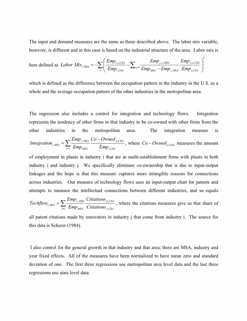
The input and demand measures are the same as those described above. The labor mix variable,
however, is different and in this case is based on the industrial structure of the area. Labor mix is
here defined as 2
,
,,
,
,,
,
,,, ∑ ∑
−−−=
≠o USAj
USAojij
MSAjMSA
MSAsj
USAi
USAoiMSAi Emp
EmpEmpEmp
EmpEmpEmp
MixLabor
which is defined as the difference between the occupation pattern in the industry in the U.S. as a
whole and the average occupation pattern of the other industries in the metropolitan area.
The regression also includes a control for integration and technology flows. Integration
represents the tendency of other firms in that industry to be co-owned with other firms from the
other industries in the metropolitan area. The integration measure is
∑≠
−=
ij USAi
USAji
MSA
MSAjMSAi Emp
OwnedCoEmpEmp
nIntegratio,
,,, , where USAjiOwnedCo ,− measures the amount
of employment in plants in industry i that are in multi-establishment firms with plants in both
industry i and industry j. We specifically eliminate co-ownership that is due to input-output
linkages and the hope is that this measure captures more intangible reasons for connections
across industries. Our measure of technology flows uses an input-output chart for patents and
attempts to measure the intellectual connections between different industries, and so equals
∑≠
=ij USAj
USAji
MSA
MSAjMSAi Citiations
CitiationsEmpEmp
Techflow,
,,, , where the citations measures give us that share of
all patent citations made by innovators in industry j that come from industry i. The source for
this data is Scherer (1984).
I also control for the general growth in that industry and that area; there are MSA, industry and
year fixed effects. All of the measures have been normalized to have mean zero and standard
deviation of one. The first three regressions use metropolitan area level data and the last three
regressions use state level data.
In the first regression, we find no positive correlations between new firm employment growth
and both input suppliers. The demand measure has a weak positive effect. A one standard
deviation increase in this variable is associated with a .02 log point increase in new firm plant
birth employment. The labor mix variable is much more powerful. A one standard deviation
increase in this variable is associated with a .18 log point increase in new firm plant birth
employment. The integration measure is the second most powerful variable in the regression,
after labor mix. A one standard deviation increase in this variable is associated with a .08 log
point increase in employment growth. The technology flow variable is insignificant.
Regression (2) tests two related hypotheses. First, labor mix will be more important in more
volatile industries. According to this hypothesis, the willingness of workers to take a chance on
a new firm depends on the presence of many other employers with whom they could potentially
work. The labor fix variable can be seen as measuring the extent of local demand for firms in
industry i. The second hypothesis suggests that integration measures something about
information spillovers across industries, and that these are more important for more skilled
workers.
Regression (2) uses the closure rate of firms in this industry as a proxy for volatility. The
importance of the labor mix variable is higher in those industries with a higher closure rate. The
integration measure is not particularly higher for those industries with more college educated
workers.
Regression (3) repeats regression (1) using employment growth due to plant birth, in cases where
plants are co-owned with other plants in the LRD. The results are broadly similar, although in
this case the presence of input suppliers becomes marginally more important. The importance of
labor mix falls somewhat, but this variable remains the most important one in the regression. A
comparison of regression (3) and (1) suggests at least that labor mix may be more important for
new plant start-ups than for existing firms starting new plants in an area.

Regressions (4)-(6) repeat regressions (1)-(3) using states rather than metropolitan areas as the
units of analysis. At the state level, the importance of labor mix rise to .43 in regression (4).
Both input and demand measures are statistically significant, but they are about one-tenth the
size of the labor mix variable. Regression (5) shows that the interactions are insignificant at the
state level. Regression (6) shows that labor mix is again far less important for old firm plant
birth and that input suppliers have become more important.
Table 7 provides us with a different view of entrepreneurship by looking exclusively within
manufacturing and looking at the amount of new employment in an area associated with new
plant births. The results do look different from the other work. The presence of firms that use
the same type of labor seems like the crucial aspect for the location of these new manufacturing
plants. Input suppliers and customers matter much less. The integration measure also has some
significance, but interpreting this measure is far from easy.
V. Conclusion
This paper has documented a series of stylized facts about entrepreneurship over space. I have
used average firm size and the self-employment rate as my measures of entrepreneurship. Both
of these measures have their problems, but I believe that they certainly capture something about
the level of entrepreneurship in an area. Moreover, both of these measures predict urban success
at the metropolitan area level. The number of workers per firm is also strongly negatively
associated with growth at the industry level within metropolitan areas.
There is a significant amount of heterogeneity in entrepreneurship over space, and this
heterogeneity appears more strongly within individual industries than across the economy as a
whole. Florida appears to be particularly entrepreneurial, while many Rust Belt metropolitan
areas are not. Across individuals, age and schooling both predict entrepreneurship. These
demographic variables, and industry sectors, together explain about one-half of the heterogeneity
in overall self-employment rates across metropolitan areas.
I find mixed evidence for the existence of a “culture of entrepreneurship” in a particular
metropolitan area. Self-employment rates are higher among individuals who live in metropolitan
areas that are filled with particularly entrepreneurial industries. However, this effect does not
hold within more narrow industrial categories. As the industry mix changes in a way that
predicts one extra worker per firm, the actual number of workers per firm only increases by .25.
As such, there is little evidence for a social multiplier where entrepreneurial industries create
abundant entrepreneurs outside of their industries.
One general fact is that these entrepreneurship figures always decline with the concentration of
an industry in an area. The number of self-employed workers and the number of firms per
worker are higher in areas where industries are less common. This fact can be explained by
many factors, including the possibility that entrepreneurs are spread relatively evenly, but in
some areas they are more successful. In that case, high levels of employment would be
associated with a lower number of entrepreneurs per employee.
The presence of an appropriate workforce is the most powerful predictor of new firm birth (a
third measure of entrepreneurship) and small firms. Workers seem to be a crucial input into new
businesses. There is no correlation between labor mix and the self-employment rate. A measure
of the presence of small firms in supplying industries, as suggested by Chinitz (1961), also
correlates strongly with the presence of small firms. The self-employment rate is most strongly
associated with input suppliers, but that variable is more weakly connected with either of the
other two measures of entrepreneurship. The presence of customers seems to be relatively
unimportant in all of the regressions.
Overall, these results are, at best, suggestive. There are no forms of exogenous variation and
there are many potential explanations for each one of the facts. However, they do point to the
paramount importance of labor supply in driving entrepreneurship. Skilled, older people are
much more likely to be entrepreneurs, and entrepreneurship increases in areas with an

appropriate labor force, presumably because these people provide both workers and
entrepreneurs. These results suggest that pro-entrepreneurship policies might focus particularly
on attracting the right type of workers.

References
Blanchflower, D.G. and A. J. Oswald (1998), “What Makes an Entrepreneur?” Journal of Labor Economics, 16 (1), 26-60.
Chinitz, B. (1961). “Contrasts in Agglomeration: New York and Pittsburg,” American Economic Review, 51 (2), 279-289.
Dumais, G., G. Ellison and E.L. Glaeser (1997), "Geographic Concentration As A Dynamic Process," NBER Working Paper #6270.
Ellison, G., E.L. Glaeser, and W. Kerr (2007), “What Causes Industry Agglomeration? Evidence from Coagglomeration Patterns,” NBER Working Paper #13068.
Evans, D.S., and B. Jovanovic (1989), “An Estimated Model of Entrepreneurial Choice Under Liquidity Constraints,” Journal of Political Economy, 97 (4), 808-827.
Glaeser, E.L., H. Kallal, J.A. Scheinkman, A. Shleifer (1992); “Growth in Cities,” The Journal of Political Economy, 100 (6), 1126-1152.
Miraky, W. (1994), “The Firm Product Cycle,” MIT mimeograph.
Moretti, E. (2004), “Estimating the Social Return to Higher Education: Evidence from Longitudinal and Repeated Cross-Sectional Data,” Journal of Econometrics, 121 (1-2), 175-212.
Porter, M.E. (1990), The Competitive Advantage of Nations, New York:Free Press.
Saxenian, A. (1994), Regional Advantage: Culture and Competition in Silicon Valley and Route 128, Cambridge, Mass.:Harvard University Press.
Scherer, F.M. (1984), “Using Linked Patent Data and R&D Data to Measure Technology Flows,” in Z. Griliches (ed), R & D, Patents and Productivity, Chicago:University of Chicago Press.
Share of Total U.S.
EmploymentShare of Total U.S. Self-
Employment
Percent of Employees Self Employed Within
the Industry
Mining, Utilities, and Construction 8.28% 15.36% 9.81%Low Skilled Manufacturing 11.45% 5.54% 2.56%High Skilled Manufacturing 7.14% 1.16% 0.86%Wholesale Trade and Transportation 9.94% 9.77% 5.20%Retail Trade 11.05% 11.58% 5.54%Low Skilled Information Services 14.90% 13.35% 4.74%High Skilled Information Services 12.54% 19.56% 8.25%Education, Health, and Social Services 13.77% 9.89% 3.80%Entertainment, Accommodation, and Food Services 6.22% 6.71% 5.70%Other Services 4.71% 7.08% 7.96%
100.00% 100.00%
Notes:
TABLE 1
(6) Wholesale trade and transportation is made up of those codes of the form 42-- or 48--. Mining, utilities, and construction corresponds to the codes 21--, 22--,and 23--. Information services covers the NAICS codes that begin with 51-56 and includes Information and Communications; Finance, Insurance, Real Estate,Rental and Leasing; Professional, Scientific, Management, Administrative, and Waste Management Services.
(5) Industry divisions are taken using the divisions presented on the IPUMS website at http://usa.ipums.org/usa/volii/indcross.shtml, based on each establishment’s1997 NAICS code. Certain categories are aggregated, dropped or divided as described in notes (6), (7) and (8).
(8) The Manufacturing category is divided by skill level in the following way. The level of skill within the broad Manufacturing industry is determined first bycalculating the mean percentage of workers with a bachelor’s degree or higher over the entire industry. Then, the mean percentage of workers with a bachelor'sdegree is calculated for each detailed sub-industry within the broad Manufacturing industry category. If a sub-industry of Manufacturing has a higher mean levelof bachelor degrees than the average over the entire Manufacturing industry, then it is classified as a High Skilled Manufacturing industry. If it has a lower meanlevel of bachelor degrees, it is classified as Low Skilled Manufacturing. The same procedure is used to create the High Skilled and Low Skilled InformationServices categories.
(7) Observations for agriculture, forestry, fishing, and hunting (NAICS code 1---), public administration, and active duty military (NAICS codes 9---) are droppedduring the analysis. The unemployed are also are also dropped.
Share of U.S. Employment by Industry
(4) Data is microlevel 2000 Census data, from the Integrated Public Use Microdata Series (IPUMS) at http://usa.ipums.org/usa/. Steven Ruggles, Matthew Sobek,Trent Alexander, Catherine A. Fitch, Ronald Goeken, Patricia Kelly Hall, Miriam King, and Chad Ronnander. Integrated Public Use Microdata Series: Version 3.0 [Machine-readable database]. Minneapolis, MN: Minnesota Population Center [producer and distributor], 2004.
(1) Share of Total U.S. Employment=(Number Employed in Industry)/(Total Employed)(2) Share of Total U.S. Self-Employment=(Number Self Employment in Industry)/(Total Self Employed)(3) Percent of Employees Self Employed Within the Industry=(Number Self Employed in Industry)/(Number Employed in Industry)
Ave
rage
In
com
e in
In
dust
ryB
otto
m 2
5th
Perc
entil
e25
th to
75
Perc
entil
e75
th to
95t
h Pe
rcen
tile
95th
Per
cent
ile
to T
op C
odes
Top
Cod
esH
igh
Skill
ed In
form
atio
n Se
rvic
es
Shar
e of
Tot
al S
.E. i
n In
dust
ry =
Tot
al S
.E. i
n In
dust
ry &
Ear
ning
s Cat
egor
y/To
tal S
.E. i
n In
dust
ry14
.74%
28.9
6%31
.59%
12.1
0%12
.61%
100.
00%
Shar
e of
Tot
al S
.E. i
n Ea
rnin
gs C
ateg
ory
= T
otal
S.E
. in
Indu
stry
& E
arni
ngs C
ateg
ory/
Tota
l S.E
. in
Earn
ings
Cat
egor
y13
.75%
15.2
1%23
.98%
31.0
1%29
.39%
Hig
h Sk
illed
Man
ufac
turi
ng
Shar
e of
Tot
al S
.E. i
n In
dust
ry =
Tot
al S
.E. i
n In
dust
ry &
Ear
ning
s Cat
egor
y/To
tal S
.E. i
n In
dust
ry16
.47%
32.6
2%35
.58%
7.15
%8.
18%
100.
00%
Shar
e of
Tot
al S
.E. i
n Ea
rnin
gs C
ateg
ory
= T
otal
S.E
. in
Indu
stry
& E
arni
ngs C
ateg
ory/
Tota
l S.E
. in
Earn
ings
Cat
egor
y0.
91%
1.02
%1.
60%
1.09
%1.
13%
Low
Ski
lled
Info
rmat
ion
Serv
ices
Sh
are
of T
otal
S.E
. in
Indu
stry
= T
otal
S.E
. in
Indu
stry
& E
arni
ngs C
ateg
ory/
Tota
l S.E
. in
Indu
stry
20.8
3%39
.64%
25.3
6%7.
53%
6.64
%10
0.00
%Sh
are
of T
otal
S.E
. in
Earn
ings
Cat
egor
y =
Tot
al S
.E. i
n In
dust
ry &
Ear
ning
s Cat
egor
y/To
tal S
.E. i
n Ea
rnin
gs C
ateg
ory
13.2
7%14
.21%
13.1
4%13
.18%
10.5
6%M
inin
g, U
tiliti
es, a
nd C
onst
ruct
ion
Shar
e of
Tot
al S
.E. i
n In
dust
ry =
Tot
al S
.E. i
n In
dust
ry &
Ear
ning
s Cat
egor
y/To
tal S
.E. i
n In
dust
ry18
.46%
44.4
0%27
.08%
4.82
%5.
25%
100.
00%
Shar
e of
Tot
al S
.E. i
n Ea
rnin
gs C
ateg
ory
= T
otal
S.E
. in
Indu
stry
& E
arni
ngs C
ateg
ory/
Tota
l S.E
. in
Earn
ings
Cat
egor
y13
.52%
18.3
0%16
.14%
9.69
%9.
60%
Who
lesa
le T
rade
and
Tra
nspo
rtat
ion
Shar
e of
Tot
al S
.E. i
n In
dust
ry =
Tot
al S
.E. i
n In
dust
ry &
Ear
ning
s Cat
egor
y/To
tal S
.E. i
n In
dust
ry20
.23%
40.5
0%26
.20%
7.14
%5.
93%
100.
00%
Shar
e of
Tot
al S
.E. i
n Ea
rnin
gs C
ateg
ory
= T
otal
S.E
. in
Indu
stry
& E
arni
ngs C
ateg
ory/
Tota
l S.E
. in
Earn
ings
Cat
egor
y9.
43%
10.6
2%9.
93%
9.14
%6.
90%
Edu
catio
n, H
ealth
, and
Soc
ial S
ervi
ces
Shar
e of
Tot
al S
.E. i
n In
dust
ry =
Tot
al S
.E. i
n In
dust
ry &
Ear
ning
s Cat
egor
y/To
tal S
.E. i
n In
dust
ry21
.72%
21.3
6%21
.12%
12.9
9%22
.81%
100.
00%
Shar
e of
Tot
al S
.E. i
n Ea
rnin
gs C
ateg
ory
= T
otal
S.E
. in
Indu
stry
& E
arni
ngs C
ateg
ory/
Tota
l S.E
. in
Earn
ings
Cat
egor
y10
.25%
5.67
%8.
11%
16.8
4%26
.88%
Low
Ski
lled
Man
ufac
turi
ng
Shar
e of
Tot
al S
.E. i
n In
dust
ry =
Tot
al S
.E. i
n In
dust
ry &
Ear
ning
s Cat
egor
y/To
tal S
.E. i
n In
dust
ry17
.93%
37.8
5%30
.66%
6.08
%7.
48%
100.
00%
Shar
e of
Tot
al S
.E. i
n Ea
rnin
gs C
ateg
ory
= T
otal
S.E
. in
Indu
stry
& E
arni
ngs C
ateg
ory/
Tota
l S.E
. in
Earn
ings
Cat
egor
y4.
74%
5.63
%6.
59%
4.41
%4.
94%
Ret
ail T
rade
Shar
e of
Tot
al S
.E. i
n In
dust
ry =
Tot
al S
.E. i
n In
dust
ry &
Ear
ning
s Cat
egor
y/To
tal S
.E. i
n In
dust
ry23
.72%
42.1
5%23
.51%
6.13
%4.
49%
100.
00%
Shar
e of
Tot
al S
.E. i
n Ea
rnin
gs C
ateg
ory
= T
otal
S.E
. in
Indu
stry
& E
arni
ngs C
ateg
ory/
Tota
l S.E
. in
Earn
ings
Cat
egor
y13
.10%
13.1
1%10
.57%
9.30
%6.
19%
Oth
er S
ervi
ces
Shar
e of
Tot
al S
.E. i
n In
dust
ry =
Tot
al S
.E. i
n In
dust
ry &
Ear
ning
s Cat
egor
y/To
tal S
.E. i
n In
dust
ry33
.82%
44.1
3%18
.19%
2.19
%1.
67%
100.
00%
Shar
e of
Tot
al S
.E. i
n Ea
rnin
gs C
ateg
ory
= T
otal
S.E
. in
Indu
stry
& E
arni
ngs C
ateg
ory/
Tota
l S.E
. in
Earn
ings
Cat
egor
y11
.43%
8.39
%5.
00%
2.03
%1.
41%
Ent
erta
inm
ent,
Acc
omm
odat
ions
, and
Foo
d Se
rvic
esSh
are
of T
otal
S.E
. in
Indu
stry
= T
otal
S.E
. in
Indu
stry
& E
arni
ngs C
ateg
ory/
Tota
l S.E
. in
Indu
stry
30.0
2%43
.54%
18.9
3%3.
77%
3.74
%10
0.00
%Sh
are
of T
otal
S.E
. in
Earn
ings
Cat
egor
y =
Tot
al S
.E. i
n In
dust
ry &
Ear
ning
s Cat
egor
y/To
tal S
.E. i
n Ea
rnin
gs C
ateg
ory
9.60
%7.
84%
4.93
%3.
31%
2.99
%
100.
00%
100.
00%
100.
00%
100.
00%
100.
00%
Self
Empl
oym
ent b
y In
com
e an
d In
dust
ry
Not
es:
(3)W
hole
sale
trade
and
trans
porta
tion
ism
ade
upof
thos
eco
des
ofth
efo
rm42
--or
48--.
Min
ing,
utili
ties,
and
cons
truct
ion
corre
spon
dsto
the
code
s21
--,22
--,an
d23
--.I
nfor
mat
ion
serv
ices
cove
rsth
eN
AIC
Sco
des
that
begi
nw
ith51
-56
and
incl
udes
Info
rmat
ion
and
Com
mun
icat
ions
;Fin
ance
,Ins
uran
ce,R
ealE
stat
e,R
enta
l and
Lea
sing
; Pr
ofes
siona
l, Sc
ient
ific,
Man
agem
ent,
Adm
inis
trativ
e, a
nd W
aste
Man
agem
ent S
ervi
ces.
(4) O
bser
vatio
ns fo
r agr
icul
ture
, for
estry
, fish
ing,
and
hun
ting
(NA
ICS
code
11-
), pu
blic
adm
inist
ratio
n, a
nd a
ctiv
e du
ty m
ilita
ry (N
AIC
S co
des
9---)
are
dro
pped
dur
ing
the
anal
ysis.
Une
mpl
oyed
obs
erva
tions
are
also
dro
pped
.(5
)The
Man
ufac
turin
gca
tego
ryis
divi
ded
bysk
illle
veli
nth
efo
llow
ing
way
.The
leve
lofs
kill
with
inth
ebr
oad
Man
ufac
turin
gin
dust
ryis
dete
rmin
edfir
stby
calc
ulat
ing
the
mea
npe
rcen
tage
ofw
orke
rsw
itha
bach
elor
’sde
gree
orhi
gher
over
the
entir
ein
dust
ry.T
hen,
the
mea
npe
rcen
tage
ofw
orke
rsw
itha
bach
elor
'sde
gree
isca
lcul
ated
fore
ach
deta
iled
sub-
indu
stry
with
inth
ebr
oad
Man
ufac
turin
gin
dust
ryca
tego
ry.
Ifa
sub-
indu
stry
ofM
anuf
actu
ring
has
ahi
gher
mea
nle
velo
fbac
helo
rdeg
rees
than
the
aver
age
over
the
entir
eM
anuf
actu
ring
indu
stry
,the
nit
iscl
assif
ied
asa
Hig
hSk
illed
Man
ufac
turin
gin
dust
ry.
Ifit
has
alo
wer
mea
nle
vel o
f bac
helo
r deg
rees
, it i
s cla
ssifi
ed a
s Low
Ski
lled
Man
ufac
turin
g. T
he sa
me
proc
edur
e is
used
to c
reat
e th
e H
igh
Skill
ed a
nd L
ow S
kille
d In
form
atio
n Se
rvic
es c
ateg
orie
s.
$45,
053
$44,
276
$42,
463
$39,
716
TA
BL
E 2
(2) I
ndus
try d
ivisi
ons
are
take
n us
ing
the
divi
sion
s pre
sent
ed o
n th
e IP
UM
S w
ebsit
e at
http
://us
a.ip
ums.
org/
usa/
volii
/indc
ross
.shtm
l, ba
sed
on e
ach
esta
blis
hmen
t’s 1
997
NA
ICS
code
. Cer
tain
cat
egor
ies
are
aggr
egat
ed, d
ropp
ed o
r div
ided
as
desc
ribed
in n
otes
(3),(
4) a
nd (5
)
$68,
577
$57,
000
$47,
444
$45,
509
Earn
ings
Cat
egor
y
$34,
844
$31,
265
(1)
Dat
ais
mic
role
vel2
000
Cen
sus
data
,fro
mth
eIn
tegr
ated
Publ
icU
seM
icro
data
Serie
s(IP
UM
S)at
http
://us
a.ip
ums.
org/
usa/
.Ste
ven
Rug
gles
,Mat
thew
Sobe
k,Tr
entA
lexa
nder
,Cat
herin
eA
.Fitc
h,R
onal
dG
oeke
n,Pa
trici
aK
elly
Hal
l,M
iriam
Kin
g,an
dC
had
Ron
nand
er.
Inte
grat
edPu
blic
Use
Mic
roda
taSe
ries:
Ver
sion
3.0
[Mac
hine
-rea
dabl
e da
taba
se].
Min
neap
olis
, MN
: Min
neso
ta P
opul
atio
n C
ente
r [pr
oduc
er a
nd d
istrib
utor
], 20
04.
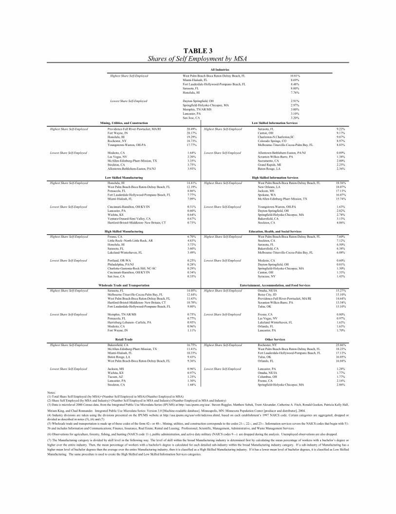
Highest Share Self-Employed West Palm Beach-Boca Raton-Delray Beach, FL 10.81%Miami-Hialeah, FL 8.69%Fort Lauderdale-Hollywood-Pompano Beach, FL 8.48%Sarasota, FL 8.00%Honolulu, HI 7.76%
Lowest Share Self-Employed Dayton-Springfield, OH 2.91%Springfield-Holyoke-Chicopee, MA 2.97%Memphis, TN/AR/MS 3.00%Lancaster, PA 3.10%San Jose, CA 3.20%
Highest Share Self-Employed Providence-Fall River-Pawtucket, MA/RI 20.49% Highest Share Self-Employed Sarasota, FL 9.22%Fort Wayne, IN 20.17% Canton, OH 9.17%Honolulu, HI 19.29% Charleston-N.Charleston,SC 9.07%Rochester, NY 18.73% Colorado Springs, CO 8.97%Youngstown-Warren, OH-PA 17.77% Melbourne-Titusville-Cocoa-Palm Bay, FL 8.83%
Lowest Share Self-Employed Modesto, CA 1.64% Lowest Share Self-Employed Allentown-Bethlehem-Easton, PA/NJ 0.89%Las Vegas, NV 2.20% Scranton-Wilkes-Barre, PA 1.38%McAllen-Edinburg-Pharr-Mission, TX 3.35% Sacramento, CA 2.00%Stockton, CA 3.75% Grand Rapids, MI 2.25%Allentown-Bethlehem-Easton, PA/NJ 3.93% Baton Rouge, LA 2.36%
Highest Share Self-Employed Honolulu, HI 14.41% Highest Share Self-Employed West Palm Beach-Boca Raton-Delray Beach, FL 18.56%West Palm Beach-Boca Raton-Delray Beach, FL 12.19% New Orleans, LA 18.07%Pensacola, FL 8.86% Jackson, MS 17.13%Fort Lauderdale-Hollywood-Pompano Beach, FL 7.77% Spokane, WA 16.07%Miami-Hialeah, FL 7.09% McAllen-Edinburg-Pharr-Mission, TX 15.74%
Lowest Share Self-Employed Cincinnati-Hamilton, OH/KY/IN 0.51% Lowest Share Self-Employed Youngstown-Warren, OH-PA 1.63%Lancaster, PA 0.60% Dayton-Springfield, OH 2.02%Wichita, KS 0.64% Springfield-Holyoke-Chicopee, MA 2.74%Ventura-Oxnard-Simi Valley, CA 0.67% Bakersfield, CA 3.13%Hartford-Bristol-Middleton- New Britain, CT 0.73% Stockton, CA 4.06%
Highest Share Self-Employed Fresno, CA 6.70% Highest Share Self-Employed West Palm Beach-Boca Raton-Delray Beach, FL 7.60%Little Rock--North Little Rock, AR 4.83% Stockton, CA 7.12%Honolulu, HI 3.72% Sarasota, FL 6.50%Sarasota, FL 3.60% Bakersfield, CA 6.38%Lakeland-Winterhaven, FL 3.49% Melbourne-Titusville-Cocoa-Palm Bay, FL 6.08%
Lowest Share Self-Employed Portland, OR-WA 0.25% Lowest Share Self-Employed Modesto, CA 0.60%Philadelphia, PA/NJ 0.28% Dayton-Springfield, OH 0.81%Charlotte-Gastonia-Rock Hill, NC-SC 0.29% Springfield-Holyoke-Chicopee, MA 1.30%Cincinnati-Hamilton, OH/KY/IN 0.34% Canton, OH 1.33%San Jose, CA 0.35% Syracuse, NY 1.43%
Highest Share Self-Employed Sarasota, FL 14.05% Highest Share Self-Employed Omaha, NE/IA 15.27%Melbourne-Titusville-Cocoa-Palm Bay, FL 12.44% Boise City, ID 15.10%West Palm Beach-Boca Raton-Delray Beach, FL 11.65% Providence-Fall River-Pawtucket, MA/RI 14.64%Hartford-Bristol-Middleton- New Britain, CT 10.70% Scranton-Wilkes-Barre, PA 13.54%Fort Lauderdale-Hollywood-Pompano Beach, FL 9.80% Tulsa, OK 13.10%
Lowest Share Self-Employed Memphis, TN/AR/MS 0.75% Lowest Share Self-Employed Fresno, CA 0.80%Pensacola, FL 0.77% Las Vegas, NV 0.97%Harrisburg-Lebanon--Carlisle, PA 0.95% Lakeland-Winterhaven, FL 1.63%Modesto, CA 0.96% Orlando, FL 1.63%Fort Wayne, IN 1.11% Lancaster, PA 1.70%
Highest Share Self-Employed Bakersfield, CA 16.75% Highest Share Self-Employed Rochester, NY 25.86%McAllen-Edinburg-Pharr-Mission, TX 11.41% West Palm Beach-Boca Raton-Delray Beach, FL 18.23%Miami-Hialeah, FL 10.23% Fort Lauderdale-Hollywood-Pompano Beach, FL 17.12%Baton Rouge, LA 9.43% Tulsa, OK 16.05%West Palm Beach-Boca Raton-Delray Beach, FL 9.36% Orlando, FL 16.04%
Lowest Share Self-Employed Jackson, MS 0.96% Lowest Share Self-Employed Lancaster, PA 1.28%Wichita, KS 0.97% Omaha, NE/IA 1.77%Tucson, AZ 1.25% Columbus, OH 1.77%Lancaster, PA 1.30% Fresno, CA 2.16%Stockton, CA 1.44% Springfield-Holyoke-Chicopee, MA 2.86%
Notes:
Retail Trade
High Skilled Manufacturing
Wholesale Trade and Transportation
TABLE 3Shares of Self Employment by MSA
Low Skilled Information Services
High Skilled Information ServicesLow Skilled Manufacturing
Mining, Utilities, and Construction
All Industries
(6) Observations for agriculture, forestry, fishing, and hunting (NAICS code 11-), public administration, and active duty military (NAICS codes 9---) are dropped during the analysis. Unemployed observations are also dropped.
(7) The Manufacturing category is divided by skill level in the following way. The level of skill within the broad Manufacturing industry is determined first by calculating the mean percentage of workers with a bachelor’s degree orhigher over the entire industry. Then, the mean percentage of workers with a bachelor's degree is calculated for each detailed sub-industry within the broad Manufacturing industry category. If a sub-industry of Manufacturing has ahigher mean level of bachelor degrees than the average over the entire Manufacturing industry, then it is classified as a High Skilled Manufacturing industry. If it has a lower mean level of bachelor degrees, it is classified as Low SkilledManufacturing. The same procedure is used to create the High Skilled and Low Skilled Information Services categories.
Education, Health, and Social Services
Entertainment, Accommodation, and Food Services
Other Services
(1) Total Share Self Employed (by MSA)=(Number Self Employed in MSA)/(Number Employed in MSA)(2) Share Self Employed (by MSA and Industry)=(Number Self Employed in MSA and Industry)/(Number Employed in MSA and Industry)(3) Data is microlevel 2000 Census data, from the Integrated Public Use Microdata Series (IPUMS) at http://usa.ipums.org/usa/. Steven Ruggles, Matthew Sobek, Trent Alexander, Catherine A. Fitch, Ronald Goeken, Patricia Kelly Hall,
Miriam King, and Chad Ronnander. Integrated Public Use Microdata Series: Version 3.0 [Machine-readable database]. Minneapolis, MN: Minnesota Population Center [producer and distributor], 2004.(4) Industry divisions are taken using the divisions presented on the IPUMS website at http://usa.ipums.org/usa/volii/indcross.shtml, based on each establishment’s 1997 NAICS code. Certain categories are aggregated, dropped ordivided as described in notes (5), (6) and (7)(5) Wholesale trade and transportation is made up of those codes of the form 42-- or 48--. Mining, utilities, and construction corresponds to the codes 21--, 22--, and 23--. Information services covers the NAICS codes that begin with 51-56 and includes Information and Communications; Finance, Insurance, Real Estate, Rental and Leasing; Professional, Scientific, Management, Administrative, and Waste Management Services.
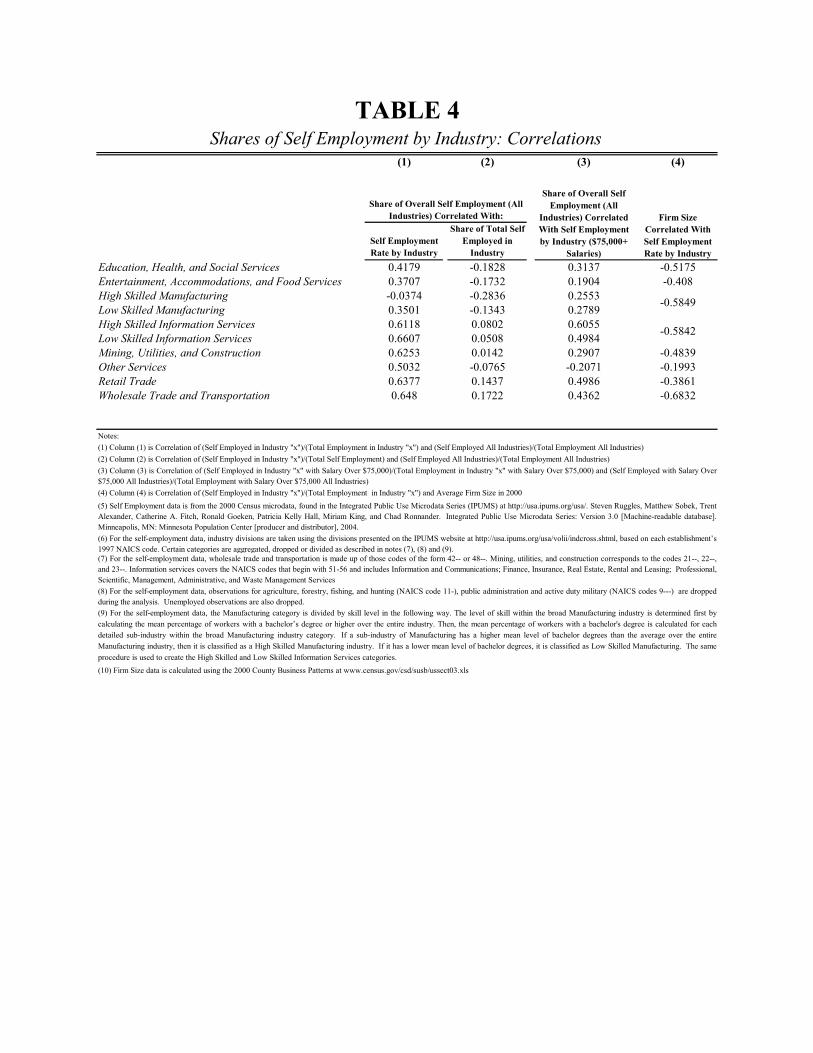
(1) (2) (3) (4)
Self Employment Rate by Industry
Share of Total Self Employed in
IndustryEducation, Health, and Social Services 0.4179 -0.1828 0.3137 -0.5175Entertainment, Accommodations, and Food Services 0.3707 -0.1732 0.1904 -0.408High Skilled Manufacturing -0.0374 -0.2836 0.2553Low Skilled Manufacturing 0.3501 -0.1343 0.2789High Skilled Information Services 0.6118 0.0802 0.6055Low Skilled Information Services 0.6607 0.0508 0.4984Mining, Utilities, and Construction 0.6253 0.0142 0.2907 -0.4839Other Services 0.5032 -0.0765 -0.2071 -0.1993Retail Trade 0.6377 0.1437 0.4986 -0.3861Wholesale Trade and Transportation 0.648 0.1722 0.4362 -0.6832
(6) For the self-employment data, industry divisions are taken using the divisions presented on the IPUMS website at http://usa.ipums.org/usa/volii/indcross.shtml, based on each establishment’s1997 NAICS code. Certain categories are aggregated, dropped or divided as described in notes (7), (8) and (9).(7) For the self-employment data, wholesale trade and transportation is made up of those codes of the form 42-- or 48--. Mining, utilities, and construction corresponds to the codes 21--, 22--,and 23--. Information services covers the NAICS codes that begin with 51-56 and includes Information and Communications; Finance, Insurance, Real Estate, Rental and Leasing; Professional,Scientific, Management, Administrative, and Waste Management Services(8) For the self-employment data, observations for agriculture, forestry, fishing, and hunting (NAICS code 11-), public administration and active duty military (NAICS codes 9---) are droppedduring the analysis. Unemployed observations are also dropped.
Share of Overall Self Employment (All
Industries) Correlated With Self Employment by Industry ($75,000+
Salaries)
Firm Size Correlated With Self Employment Rate by Industry
(4) Column (4) is Correlation of (Self Employed in Industry "x")/(Total Employment in Industry "x") and Average Firm Size in 2000(5) Self Employment data is from the 2000 Census microdata, found in the Integrated Public Use Microdata Series (IPUMS) at http://usa.ipums.org/usa/. Steven Ruggles, Matthew Sobek, TrentAlexander, Catherine A. Fitch, Ronald Goeken, Patricia Kelly Hall, Miriam King, and Chad Ronnander. Integrated Public Use Microdata Series: Version 3.0 [Machine-readable database].Minneapolis, MN: Minnesota Population Center [producer and distributor], 2004.
Notes:
(10) Firm Size data is calculated using the 2000 County Business Patterns at www.census.gov/csd/susb/ussect03.xls
Shares of Self Employment by Industry: CorrelationsTABLE 4
(3) Column (3) is Correlation of (Self Employed in Industry "x" with Salary Over $75,000)/(Total Employment in Industry "x" with Salary Over $75,000) and (Self Employed with Salary Over$75,000 All Industries)/(Total Employment with Salary Over $75,000 All Industries)
(1) Column (1) is Correlation of (Self Employed in Industry "x")/(Total Employment in Industry "x") and (Self Employed All Industries)/(Total Employment All Industries)(2) Column (2) is Correlation of (Self Employed in Industry "x")/(Total Self Employment) and (Self Employed All Industries)/(Total Employment All Industries)
-0.5849
-0.5842
(9) For the self-employment data, the Manufacturing category is divided by skill level in the following way. The level of skill within the broad Manufacturing industry is determined first bycalculating the mean percentage of workers with a bachelor’s degree or higher over the entire industry. Then, the mean percentage of workers with a bachelor's degree is calculated for eachdetailed sub-industry within the broad Manufacturing industry category. If a sub-industry of Manufacturing has a higher mean level of bachelor degrees than the average over the entireManufacturing industry, then it is classified as a High Skilled Manufacturing industry. If it has a lower mean level of bachelor degrees, it is classified as Low Skilled Manufacturing. The sameprocedure is used to create the High Skilled and Low Skilled Information Services categories.
Share of Overall Self Employment (All Industries) Correlated With:

(1) (2) (3) (4) (5) (6) (7) (8)
Predicted Self Employed - 1 0.909(0.145)
Log of Venture Capital per Capita (State Level) -0.003(0.000)
Log of Population in the MSA 0.009(0.001)
Predicted Self Employed - 2 -0.445(0.133)
Log of VC/capita Interacted with High Skilled Info Services -0.004(0.001)
Input Measure 0.422 0.470(0.054) (0.058)
Chinitz Measure (see Note) .0154 0.012(.070) (0.069)
Labor Mix Measure -0.018 -0.018(0.004) (0.004)
Demand -0.059 -0.301(0.078) (0.084)
Log of Population Interacted with Retail Trade 0.004 0.003(0.001) (0.001)
Share of Population over 65 Interacted with Health Services -0.112 -0.102(0.028) (0.028)
Log Employment in Industry in MSA -0.008 -0.008 -0.01 -0.008 -0.007 -0.008 -0.009(0.001) (0.001) (0.001) (0.001) (0.001) (0.001) (0.001)
Male 0.037 0.037 0.037 0.036 0.037 0.037 0.036 0.036(0.001) (0.001) (0.001) (0.001) (0.001) (0.001) (0.001) (0.001)
30 to 34 0.014 0.014 0.014 0.014 0.014 0.014 0.014 0.014(0.001) (0.001) (0.001) (0.001) (0.001) (0.001) (0.001) (0.001)
35 to 39 0.033 0.033 0.033 0.033 0.033 0.033 0.033 0.033(0.001) (0.001) (0.001) (0.001) (0.001) (0.001) (0.001) (0.001)
40 to 44 0.046 0.046 0.046 0.046 0.046 0.046 0.046 0.046(0.001) (0.001) (0.001) (0.001) (0.001) (0.001) (0.001) (0.001)
45 to 49 0.055 0.055 0.055 0.055 0.055 0.055 0.055 0.055(0.001) (0.001) (0.001) (0.001) (0.001) (0.001) (0.001) (0.001)
50 to 54 0.063 0.063 0.063 0.062 0.063 0.063 0.062 0.062(0.001) (0.001) (0.001) (0.001) (0.001) (0.001) (0.001) (0.001)
55 to 60 0.073 0.073 0.073 0.072 0.073 0.073 0.072 0.071(0.002) (0.002) (0.002) (0.002) (0.002) (0.002) (0.002) (0.002)
60 to 65 0.081 0.081 0.08 0.08 0.081 0.08 0.079 0.08(0.002) (0.002) (0.002) (0.002) (0.002) (0.002) (0.002) (0.002)
No High School -0.069 -0.069 -0.07 -0.068 -0.07 -0.07 -0.067 -0.043(0.002) (0.002) (0.002) (0.002) (0.002) (0.002) (0.002) (0.001)
Some High School -0.058 -0.059 -0.059 -0.056 -0.059 -0.059 -0.056 -0.068(0.002) (0.002) (0.002) (0.002) (0.002) (0.002) (0.002) (0.002)
High School Graduate -0.045 -0.045 -0.046 -0.044 -0.045 -0.046 -0.044 -0.028(0.001) (0.001) (0.001) (0.001) (0.001) (0.001) (0.001) (0.001)
Some College -0.029 -0.029 -0.029 -0.028 -0.029 -0.029 -0.028 -0.056(0.001) (0.001) (0.001) (0.001) (0.001) (0.001) (0.001) (0.002)
Constant -0.033 -0.108 0.059 0.033 0.023 0.02 0.024 0.026(0.016) (0.018) (0.021) (0.018) (0.019) (0.018) (0.018) (0.019)
Observations 369,544 369,543 369,543 361,271 364,613 369,543 361,271 356,341R-squared 0.07 0.07 0.08 0.07 0.08 0.08 0.07 0.08
Notes:
(10)The coefficient and s.e. on the Chinitz Measure was multiplied by 100 for readability.
(6) The "Chinitz Measure" variable is used to capture the number of firms that supply an industry’s needs in this metropolitan area, based on Chinitz's argument that the overall level of entrepreneurshipdepended on the presence of many small firms that can readily supply new start-ups. See text for a detailed description of how this variable was calculated.
(4) The measure of venture capital used to calculate the "Log of VC/capita Interacted with High Skilled Info Services" variable and the "Log of VC/capita Interacted with High Skilled Info Services"variable is found at https://www.pwcmoneytree.com/MTPublic/ns/index.jsp.
(7) The "Labor Mix Measure" captures the labor mix of an area. See text for a detailed description of how this variable was calculated. (8) The "Demand" variable captures the demand of other industries for a particular industry's goods. See text for a detailed description of how this variable was calculated.
(5) The "Input Measure" variable captures the share of an industry's inputs that are bought from other industries. See text for a detailed description of how this variable was calculated.
TABLE 5Self-Employment Regressions
(9) There are two measures of consumer demand, captured with the "Log of Population Interacted with Retail Trade" variable and the "Share of Population over 65 Interacted with Health Services" variable.See text for a detailed description of how these variables were calculated
Dependent Variable: Self Employment Indicator (0 or 1)
(2) Except for the venture capital measure, data is from 2000 Census microdata, found in the Integrated Public Use Microdata Series (IPUMS) at http://usa.ipums.org/usa/. Steven Ruggles, Matthew Sobek,Trent Alexander, Catherine A. Fitch, Ronald Goeken, Patricia Kelly Hall, Miriam King, and Chad Ronnander. Integrated Public Use Microdata Series: Version 3.0 [Machine-readable database].Minneapolis, MN: Minnesota Population Center [producer and distributor], 2004; the 2000 County Business Patterns; and the Bureau of Economic Analysis Input-Output tables athttp://www bea gov/industry/(3) The "Predicted Self Employed - 1" variable is test of the culture of entrepreneurship hypothesis, predicted self-employment rate in the city, outside of an individual’s industry, based on the industrial
mix of the city. The "Predicted Self Employed - 2" is a similar measure calculated within an individual’s one digit industry. See text for a detailed description of how these variables were calculated.
(1) Standard errors in parenthesis. All regressions include detailed industry fixed effects. Regressions (3)-(8) also include MSA fixed effects. Standard errors in parenthesis and are clustered at the MSAlevel.
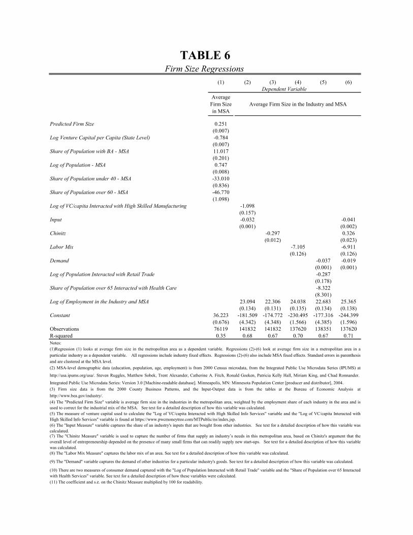
(1) (2) (3) (4) (5) (6)
Average Firm Size in MSA
Average Firm Size in the Industry and MSA
Predicted Firm Size 0.251(0.007)
Log Venture Capital per Capita (State Level) -0.784(0.007)
Share of Population with BA - MSA 11.017(0.201)
Log of Population - MSA 0.747(0.008)
Share of Population under 40 - MSA -33.010(0.836)
Share of Population over 60 - MSA -46.770(1.098)
Log of VC/capita Interacted with High Skilled Manufacturing -1.098(0.157)
Input -0.032 -0.041(0.001) (0.002)
Chinitz -0.297 0.326(0.012) (0.023)
Labor Mix -7.105 -6.911(0.126) (0.126)
Demand -0.037 -0.019(0.001) (0.001)
Log of Population Interacted with Retail Trade -0.287(0.178)
Share of Population over 65 Interacted with Health Care -8.322(8.301)
Log of Employment in the Industry and MSA 23.094 22.306 24.038 22.683 25.365(0.134) (0.131) (0.135) (0.134) (0.138)
Constant 36.223 -181.509 -174.772 -230.495 -177.316 -244.399(0.676) (4.342) (4.348) (1.566) (4.385) (1.596)
Observations 76119 141832 141832 137620 138351 137620R-squared 0.35 0.68 0.67 0.70 0.67 0.71
(11) The coefficient and s.e. on the Chinitz Measure multiplied by 100 for readability.
(1)Regression (1) looks at average firm size in the metropolitan area as a dependent variable. Regressions (2)-(6) look at average firm size in a metropolitan area in aparticular industry as a dependent variable. All regressions include industry fixed effects. Regressions (2)-(6) also include MSA fixed effects. Standard errors in parenthesisand are clustered at the MSA level.(2) MSA-level demographic data (education, population, age, employment) is from 2000 Census microdata, from the Integrated Public Use Microdata Series (IPUMS) at
http://usa.ipums.org/usa/. Steven Ruggles, Matthew Sobek, Trent Alexander, Catherine A. Fitch, Ronald Goeken, Patricia Kelly Hall, Miriam King, and Chad Ronnander.
Integrated Public Use Microdata Series: Version 3.0 [Machine-readable database]. Minneapolis, MN: Minnesota Population Center [producer and distributor], 2004.
(4) The "Predicted Firm Size" variable is average firm size in the industries in the metropolitan area, weighted by the employment share of each industry in the area and isused to correct for the industrial mix of the MSA. See text for a detailed description of how this variable was calculated.(5) The measure of venture capital used to calculate the "Log of VC/capita Interacted with High Skilled Info Services" variable and the "Log of VC/capita Interacted withHigh Skilled Info Services" variable is found at https://www.pwcmoneytree.com/MTPublic/ns/index.jsp.
(10) There are two measures of consumer demand captured with the "Log of Population Interacted with Retail Trade" variable and the "Share of Population over 65 Interactedwith Health Services" variable. See text for a detailed description of how these variables were calculated.
(8) The "Labor Mix Measure" captures the labor mix of an area. See text for a detailed description of how this variable was calculated.
(9) The "Demand" variable captures the demand of other industries for a particular industry's goods. See text for a detailed description of how this variable was calculated.
(3) Firm size data is from the 2000 County Business Patterns, and the Input-Output data is from the tables at the Bureau of Economic Analysis athttp://www.bea.gov/industry/.
TABLE 6Firm Size Regressions
(7) The "Chinitz Measure" variable is used to capture the number of firms that supply an industry’s needs in this metropolitan area, based on Chinitz's argument that theoverall level of entrepreneurship depended on the presence of many small firms that can readily supply new start-ups. See text for a detailed description of how this variablewas calculated.
(6) The "Input Measure" variable captures the share of an industry's inputs that are bought from other industries. See text for a detailed description of how this variable wascalculated.
Dependent Variable
Notes:

(1) (2) (3) (4) (5) (6)New firm
birthsNew firm
births Old firm births New firm births New firm births Old firm births-.00 -.00 .03 .04 .04 .08(0.0) (0.0) (2.8) (5.5) (5.6) (7.8).02 .02 .01 .03 .03 .01
(3.2) (3.4) (0.6) (5.1) (5.1) (1.6).18 .17 .13 .43 .43 .25
(13.4) (12.6) (9.7) (11.0) (10.6) (5.4).02 .00
(6.1) (0.0).08 .08 .10 .06 .06 .09
(5.0) (5.2) (4.9) (5.9) (5.9) (6.5).01 -.05
(1.2) (-1.5).00 .00 .04 -.01 -.01 .03
(0.3) (0.3) (4.9) (-1.5) (-1.5) (3.3)Adjusted R^2 0.56 0.56 0.32 .73 .73 .54Number of obs. 163,938 163,938 163,938 27,234 27,234 27,336Notes:
Table 7
Integration*College
Technological Flows
Input
Demand
MSA Level State Level
(7) The "Technological Flows" variable uses an input-output chart for patents and attempts to measure the intellectual connections between different industries.The source for this data is Scherer (1984). See text for a detailed description of how this variable was calculated.
Employment Growth due to Births and Closures
(4) The "Closure Rate" of firms in this industry interacted with the "Labor Mix" is used as a proxy for volatility.(5) The "Integration" variable represents the tendency of other firms in that industry to be co-owned with other firms from the other industries in the metropolitanarea. See text for a detailed description of how this variable was calculated.
Dependent variable: log(1 + ∆E^j_ist)
(6) The "College" variable is a measure of the fraction of the employment in the industry that is contained in occupations that would normally require a collegedegree. It is interacted with the "Integration" variable to create a measure of intellectual spillovers.
(8) MSA level regressions include MSA, industry, and year fixed effects. State level regressions include state, industry, and year fixed effects.
Labor Mix
Labor Mix*Closure rate
Integration
(2) The dependent variable is the increase in employment due to new establishments in industry i, place s, and time period t.
(2) Data is from the Longitudinal Research Database, and includes only data from manufacturing and it represents a panel with linked establishment level databetween 1972 and 1992.
(3) The "Input" and "Demand" variables are the same as described in the other tables. The "Labor Mix" variable is defined slightly differently. See text for adetailed description of how these variables were calculated
(1) The results presented in this table are taken from Dumais, Ellison and Glaeser (1997).
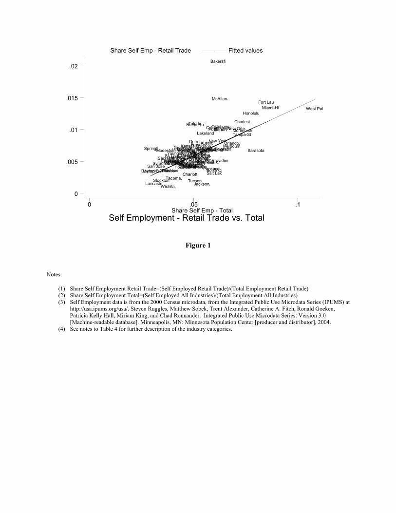
Self Employment - Retail Trade vs. TotalShare Self Emp - Total
Share Self Emp - Retail Trade Fitted values
0 .05 .1
0
.005
.01
.015
.02
Akron, OAlbany-S
Albuquer
Allentow
Atlanta,Austin,
Bakersfi
Baltimor
Baton Ro
Birmingh
Boise Ci
Boston, Buffalo-
Canton,
Charlest
Charlott
Chicago,CincinnaClevelan
Colorado
Columbia
Columbus
Dallas-F
Dayton-S
Denver-B
Detroit,
El Paso,
Fort Lau
Fort WayFresno,
Grand RaGreensbo
HarrisbuHartford
Honolulu
Houston-Indianap
Jackson,
Jacksonv
Kansas C
Knoxvill
Lakeland
Lancaste
Las Vega
Little R
Los AngeLouisvil
McAllen-
Melbourn
Memphis,
Miami-Hi
Milwauke
Minneapo
Modesto,
Monmouth
Nashvill
New Orle
New YorkNorfolk-
Oklahoma
Omaha, N
Orlando,
Pensacol
PhiladelPhoenix,
Pittsbur
Portland
Providen
Raleigh-Richmond
RiversidRochesteSacramen
Salt Lak
San AntoSan DiegSan FranSan Jose
Sarasota
ScrantonSeattle-
Spokane,Springfi
St. Loui
Stockton
Syracuse
Tacoma,
Tampa-St
Toledo,
Tucson,
Tulsa, O
Ventura-Washingt
West Pal
Wichita,
Youngsto
Figure 1
Notes:
(1) Share Self Employment Retail Trade=(Self Employed Retail Trade)/(Total Employment Retail Trade) (2) Share Self Employment Total=(Self Employed All Industries)/(Total Employment All Industries) (3) Self Employment data is from the 2000 Census microdata, from the Integrated Public Use Microdata Series (IPUMS) at
http://usa.ipums.org/usa/. Steven Ruggles, Matthew Sobek, Trent Alexander, Catherine A. Fitch, Ronald Goeken, Patricia Kelly Hall, Miriam King, and Chad Ronnander. Integrated Public Use Microdata Series: Version 3.0 [Machine-readable database]. Minneapolis, MN: Minnesota Population Center [producer and distributor], 2004.
(4) See notes to Table 4 for further description of the industry categories.

Self Employment - High Skill Mfg vs. TotalShare Self Emp - Total
Share Self Emp - High Skill Mfg Fitted values
0 .05 .1
0
.001
.002
.003
.004
Akron, O
Albuquer
Atlanta,
Austin, Baltimor
Boston, Buffalo-
Charlott
Chicago,Cincinna
Clevelan
ColumbiaDallas-FDetroit, Fort Lau
Fresno,
Grand Ra
GreensboHartfordHonolulu
Houston-
Indianap
Kansas C
Lakeland
Las Vega
Little R
Los Ange
Louisvil Miami-HiMilwauke
Minneapo
New YorkNorfolk-
Orlando,Philadel
Phoenix,
Pittsbur Portland
Providen
Raleigh-
Riversid
Sacramen
Salt Lak
San Anto
San Dieg
San Fran
San JoseSarasota
Seattle-
St. Loui
Syracuse
Tampa-St
Tucson,
Ventura-
Washingt
West Pal
Wichita,
Figure 2
Notes:
(1) Share Self Employment High Skilled Manufacturing=(Self Employed High Skilled Manufacturing)/(Total Employment High Skilled Manufacturing)
(2) Share Self Employment Total=(Self Employed All Industries)/(Total Employment All Industries) (3) Self Employment data is from the 2000 Census microdata, from the Integrated Public Use Microdata Series (IPUMS) at
http://usa.ipums.org/usa/. Steven Ruggles, Matthew Sobek, Trent Alexander, Catherine A. Fitch, Ronald Goeken, Patricia Kelly Hall, Miriam King, and Chad Ronnander. Integrated Public Use Microdata Series: Version 3.0 [Machine-readable database]. Minneapolis, MN: Minnesota Population Center [producer and distributor], 2004.
(4) See notes to Table 4 for further description of the industry categories.
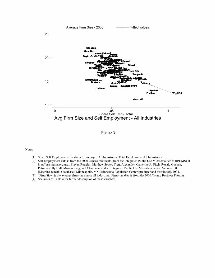
Avg Firm Size and Self Employment - All IndustriesShare Self Emp - Total
Average Firm Size - 2000 Fitted values
0 .05 .1
10
15
20
25
Akron, OAkron, OAkron, OAkron, OAkron, OAkron, OAkron, OAkron, OAlbany-SAlbany-SAlbany-SAlbany-SAlbany-SAlbany-SAlbany-SAlbany-S
AlbuquerAlbuquerAlbuquerAlbuquerAlbuquerAlbuquerAlbuquerAlbuquer
AllentowAllentowAllentowAllentowAllentowAllentowAllentowAllentow
Atlanta,Atlanta,Atlanta,Atlanta,Atlanta,Atlanta,Atlanta,Atlanta,
Austin, Austin, Austin, Austin, Austin, Austin, Austin, Austin,
BakersfiBakersfiBakersfiBakersfiBakersfiBakersfiBakersfiBakersfi
BaltimorBaltimorBaltimorBaltimorBaltimorBaltimorBaltimorBaltimor
Baton RoBaton RoBaton RoBaton RoBaton RoBaton RoBaton RoBaton Ro
BirminghBirminghBirminghBirminghBirminghBirminghBirmingh
Boise CiBoise CiBoise CiBoise CiBoise CiBoise CiBoise CiBoise Ci
Boston, Boston, Boston, Boston, Boston, Boston, Boston, Boston,
Buffalo-Buffalo-Buffalo-Buffalo-Buffalo-Buffalo-Buffalo-Buffalo-Canton, Canton, Canton, Canton, Canton, Canton, Canton, Canton,
CharlestCharlestCharlestCharlestCharlestCharlestCharlestCharlest
CharlottCharlottCharlottCharlottCharlottCharlottCharlottCharlottChicago,Chicago,Chicago,Chicago,Chicago,Chicago,Chicago,Chicago,
CincinnaCincinnaCincinnaCincinnaCincinnaCincinnaCincinnaCincinna
ClevelanClevelanClevelanClevelanClevelanClevelanClevelanClevelan
ColoradoColoradoColoradoColoradoColoradoColoradoColoradoColorado
ColumbiaColumbiaColumbiaColumbiaColumbiaColumbiaColumbiaColumbia
ColumbusColumbusColumbusColumbusColumbusColumbusColumbusColumbusDallas-FDallas-FDallas-FDallas-FDallas-FDallas-FDallas-FDallas-FDayton-SDayton-SDayton-SDayton-SDayton-SDayton-SDayton-SDayton-S
Denver-BDenver-BDenver-BDenver-BDenver-BDenver-BDenver-BDenver-B
Detroit,Detroit,Detroit,Detroit,Detroit,Detroit,Detroit,Detroit,
El Paso,El Paso,El Paso,El Paso,El Paso,El Paso,El Paso,El Paso,
Fort LauFort LauFort LauFort LauFort LauFort LauFort LauFort Lau
Fort WayFort WayFort WayFort WayFort WayFort WayFort WayFort Way
Fresno, Fresno, Fresno, Fresno, Fresno, Fresno, Fresno, Fresno,
Grand RaGrand RaGrand RaGrand RaGrand RaGrand RaGrand RaGrand Ra
GreensboGreensboGreensboGreensboGreensboGreensboGreensboGreensboHarrisbuHarrisbuHarrisbuHarrisbuHarrisbuHarrisbuHarrisbuHarrisbuHartfordHartfordHartfordHartfordHartfordHartfordHartfordHartford
HonoluluHonoluluHonoluluHonoluluHonoluluHonoluluHonoluluHonolulu
Houston-Houston-Houston-Houston-Houston-Houston-Houston-Houston-
IndianapIndianapIndianapIndianapIndianapIndianapIndianapIndianap
Jackson,Jackson,Jackson,Jackson,Jackson,Jackson,Jackson,Jackson,
JacksonvJacksonvJacksonvJacksonvJacksonvJacksonvJacksonvJacksonv
Kansas CKansas CKansas CKansas CKansas CKansas CKansas CKansas C
KnoxvillKnoxvillKnoxvillKnoxvillKnoxvillKnoxvillKnoxvillKnoxvillLakelandLakelandLakelandLakelandLakelandLakelandLakelandLakeland
LancasteLancasteLancasteLancasteLancasteLancasteLancasteLancaste
Las VegaLas VegaLas VegaLas VegaLas VegaLas VegaLas VegaLas Vega
Little RLittle RLittle RLittle RLittle RLittle RLittle RLittle RLos AngeLos AngeLos AngeLos AngeLos AngeLos AngeLos AngeLos Ange
LouisvilLouisvilLouisvilLouisvilLouisvilLouisvilLouisvilLouisvil
McAllen-McAllen-McAllen-McAllen-McAllen-McAllen-McAllen-McAllen-MelbournMelbournMelbournMelbournMelbournMelbournMelbournMelbourn
Memphis,Memphis,Memphis,Memphis,Memphis,Memphis,Memphis,Memphis,
Miami-HiMiami-HiMiami-HiMiami-HiMiami-HiMiami-HiMiami-HiMiami-Hi
MilwaukeMilwaukeMilwaukeMilwaukeMilwaukeMilwaukeMilwaukeMilwaukeMinneapoMinneapoMinneapoMinneapoMinneapoMinneapoMinneapoMinneapo
Modesto,Modesto,Modesto,Modesto,Modesto,Modesto,Modesto,Modesto,
MonmouthMonmouthMonmouthMonmouthMonmouthMonmouthMonmouthMonmouth
NashvillNashvillNashvillNashvillNashvillNashvillNashvillNashvill
New OrleNew OrleNew OrleNew OrleNew OrleNew OrleNew OrleNew Orle
New YorkNew YorkNew YorkNew YorkNew YorkNew YorkNew YorkNew York
Norfolk-Norfolk-Norfolk-Norfolk-Norfolk-Norfolk-Norfolk-Norfolk-
OklahomaOklahomaOklahomaOklahomaOklahomaOklahomaOklahomaOklahoma
Omaha, NOmaha, NOmaha, NOmaha, NOmaha, NOmaha, NOmaha, NOmaha, N
Orlando,Orlando,Orlando,Orlando,Orlando,Orlando,Orlando,Orlando,
PensacolPensacolPensacolPensacolPensacolPensacolPensacolPensacol
PhiladelPhiladelPhiladelPhiladelPhiladelPhiladelPhiladelPhiladel
Phoenix,Phoenix,Phoenix,Phoenix,Phoenix,Phoenix,Phoenix,Phoenix,
PittsburPittsburPittsburPittsburPittsburPittsburPittsburPittsbur
PortlandPortlandPortlandPortlandPortlandPortlandPortlandPortlandProvidenProvidenProvidenProvidenProvidenProvidenProvidenProviden
Raleigh-Raleigh-Raleigh-Raleigh-Raleigh-Raleigh-Raleigh-Raleigh-
RichmondRichmondRichmondRichmondRichmondRichmondRichmondRichmond
RiversidRiversidRiversidRiversidRiversidRiversidRiversidRiversid
RochesteRochesteRochesteRochesteRochesteRochesteRochesteRocheste
SacramenSacramenSacramenSacramenSacramenSacramenSacramenSacramen
Salt LakSalt LakSalt LakSalt LakSalt LakSalt LakSalt LakSalt Lak
San AntoSan AntoSan AntoSan AntoSan AntoSan AntoSan AntoSan Anto
San DiegSan DiegSan DiegSan DiegSan DiegSan DiegSan DiegSan Dieg
San FranSan FranSan FranSan FranSan FranSan FranSan FranSan Fran
San JoseSan JoseSan JoseSan JoseSan JoseSan JoseSan JoseSan Jose
SarasotaSarasotaSarasotaSarasotaSarasotaSarasotaSarasotaSarasota
ScrantonScrantonScrantonScrantonScrantonScrantonScrantonScrantonSeattle-Seattle-Seattle-Seattle-Seattle-Seattle-Seattle-Seattle-
Spokane,Spokane,Spokane,Spokane,Spokane,Spokane,Spokane,Spokane,SpringfiSpringfiSpringfiSpringfiSpringfiSpringfiSpringfiSpringfi
St. LouiSt. LouiSt. LouiSt. LouiSt. LouiSt. LouiSt. LouiSt. Loui
StocktonStocktonStocktonStocktonStocktonStocktonStocktonStockton
SyracuseSyracuseSyracuseSyracuseSyracuseSyracuseSyracuseSyracuse
Tacoma, Tacoma, Tacoma, Tacoma, Tacoma, Tacoma, Tacoma, Tacoma,
Tampa-StTampa-StTampa-StTampa-StTampa-StTampa-StTampa-StTampa-St
Toledo, Toledo, Toledo, Toledo, Toledo, Toledo, Toledo, Toledo,
Tucson, Tucson, Tucson, Tucson, Tucson, Tucson, Tucson, Tucson,
Tulsa, OTulsa, OTulsa, OTulsa, OTulsa, OTulsa, OTulsa, OTulsa, O
Ventura-Ventura-Ventura-Ventura-Ventura-Ventura-Ventura-Ventura-
WashingtWashingtWashingtWashingtWashingtWashingtWashingtWashingt
West PalWest PalWest PalWest PalWest PalWest PalWest PalWest Pal
Wichita,Wichita,Wichita,Wichita,Wichita,Wichita,Wichita,Wichita,
YoungstoYoungstoYoungstoYoungstoYoungstoYoungstoYoungstoYoungsto
Figure 3
Notes:
(1) Share Self Employment Total=(Self Employed All Industries)/(Total Employment All Industries) (2) Self Employment data is from the 2000 Census microdata, from the Integrated Public Use Microdata Series (IPUMS) at
http://usa.ipums.org/usa/. Steven Ruggles, Matthew Sobek, Trent Alexander, Catherine A. Fitch, Ronald Goeken, Patricia Kelly Hall, Miriam King, and Chad Ronnander. Integrated Public Use Microdata Series: Version 3.0 [Machine-readable database]. Minneapolis, MN: Minnesota Population Center [producer and distributor], 2004.
(3) “Firm Size” is the average firm size across all industries. Firm size data is from the 2000 County Business Patterns. (4) See notes to Table 4 for further description of these variables.
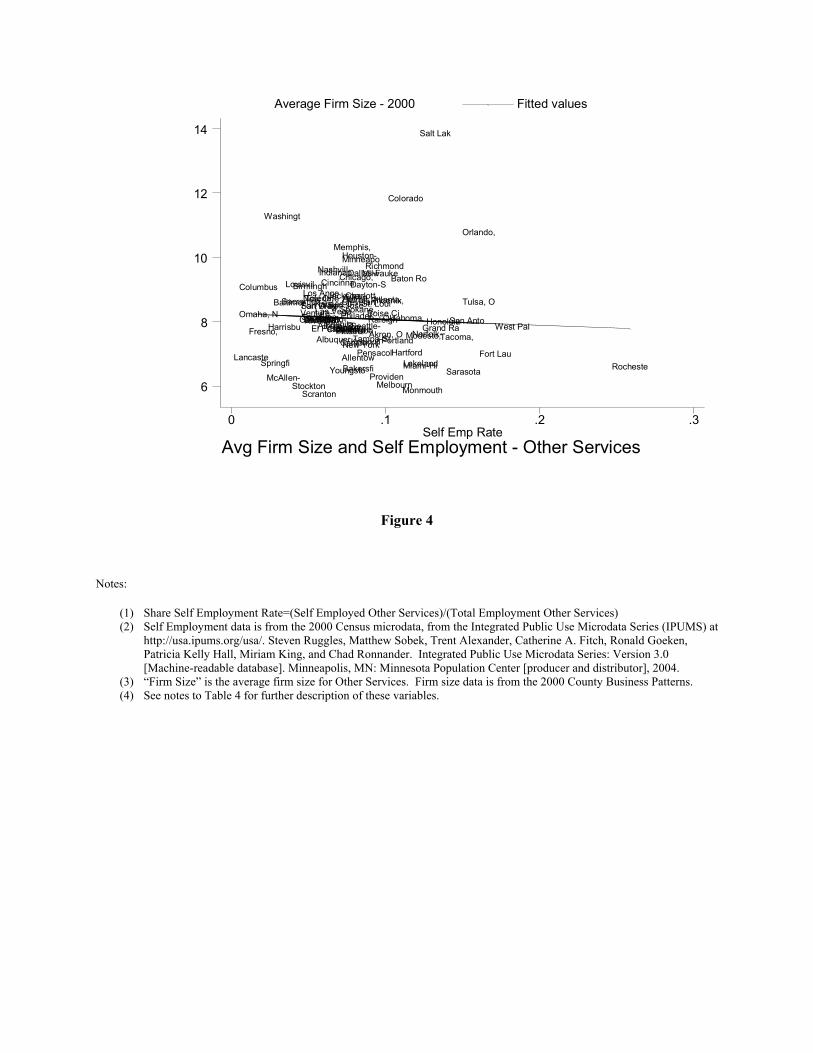
Avg Firm Size and Self Employment - Other ServicesSelf Emp Rate
Average Firm Size - 2000 Fitted values
0 .1 .2 .3
6
8
10
12
14
Akron, OAlbany-SAlbuquer
Allentow
Atlanta,Austin,
Bakersfi
Baltimor
Baton RoBirmingh
Boise Ci
Boston, Buffalo-
Canton, Charlest
Charlott
Chicago,Cincinna
Clevelan
Colorado
Columbia
ColumbusDallas-FDayton-S
Denver-B
Detroit,
El Paso,
Fort Lau
Fort Way
Fresno, Grand RaGreensboHarrisbu
Hartford
Honolulu
Houston-
Indianap
Jackson,
Jacksonv
Kansas C
Knoxvill
LakelandLancaste
Las Vega
Little R
Los AngeLouisvil
McAllen-Melbourn
Memphis,
Miami-Hi
MilwaukeMinneapo
Modesto,
Monmouth
Nashvill
New Orle
New YorkNorfolk-
OklahomaOmaha, N
Orlando,
Pensacol
Philadel
Phoenix,
PittsburPortland
Providen
Raleigh-
Richmond
Riversid
Rocheste
Sacramen
Salt Lak
San Anto
San DiegSan Fran
San Jose
Sarasota
Scranton
Seattle-
Spokane,
Springfi
St. Loui
Stockton
SyracuseTacoma, Tampa-St
Toledo,
Tucson,
Tulsa, OVentura-
Washingt
West PalWichita,
Youngsto
Figure 4
Notes:
(1) Share Self Employment Rate=(Self Employed Other Services)/(Total Employment Other Services) (2) Self Employment data is from the 2000 Census microdata, from the Integrated Public Use Microdata Series (IPUMS) at
http://usa.ipums.org/usa/. Steven Ruggles, Matthew Sobek, Trent Alexander, Catherine A. Fitch, Ronald Goeken, Patricia Kelly Hall, Miriam King, and Chad Ronnander. Integrated Public Use Microdata Series: Version 3.0 [Machine-readable database]. Minneapolis, MN: Minnesota Population Center [producer and distributor], 2004.
(3) “Firm Size” is the average firm size for Other Services. Firm size data is from the 2000 County Business Patterns. (4) See notes to Table 4 for further description of these variables.
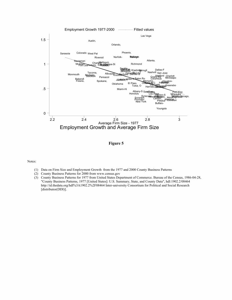
Employment Growth and Average Firm SizeAverage Firm Size - 1977
Employment Growth 1977-2000 Fitted values
2.2 2.4 2.6 2.8 3
0
.5
1
1.5
Akron, O
Albany-S
Albuquer
Allentow
Atlanta,
Austin,
Bakersfi
Baltimor
Baton Ro
Birmingh
Boise Ci
Boston,
Buffalo-
Canton,
Charlest
Charlott
Chicago,
Cincinna
Clevelan
Colorado
Columbia
Columbus
Dallas-F
Dayton-S
Denver-B
Detroit,
El Paso,
Fort Lau
Fort Way
Fresno, Grand Ra
GreensboHarrisbu
Hartford
Honolulu
Houston-IndianapJackson,
Jacksonv
Kansas C
Knoxvill
Lakeland
Lancaste
Las Vega
Little R
Los Ange
Louisvil
McAllen-Melbourn
Memphis,
Miami-Hi
Milwauke
MinneapoModesto,Monmouth
Nashvill
New Orle
New York
Norfolk-
Oklahoma Omaha, N
Orlando,
Pensacol
Philadel
Phoenix,
Pittsbur
Portland
Providen
Raleigh-
Richmond
Riversid
Rocheste
Sacramen
Salt LakSan Anto
San Dieg
San Fran
San Jose
Sarasota
Scranton
Seattle-
Spokane,
SpringfiSt. Loui
Stockton
Syracuse
Tacoma,
Tampa-St
Toledo,
Tucson,
Tulsa, O
Ventura-
Washingt
West Pal
Wichita,
Youngsto
Figure 5
Notes:
(1) Data on Firm Size and Employment Growth from the 1977 and 2000 County Business Patterns (2) County Business Patterns for 2000 from www.census.gov (3) County Business Patterns for 1977 from United States Department of Commerce. Bureau of the Census, 1986-04-28,
"County Business Patterns, 1977 [United States]: U.S. Summary, State, and County Data", hdl:1902.2/08464 http://id.thedata.org/hdl%3A1902.2%2F08464 Inter-university Consortium for Political and Social Research [distributor(DDI)].