1

Entrepreneurship and Income Inequality

Daniel Halvarsson Ratio Institute

Stockholm Sweden

E-mail: daniel.halvarsson@ratio.se

Martin Korpi Ratio Institute

Stockholm Sweden

E-mail: martin.korpi@ratio.se

Karl Wennberg **

Institute for Analytical Sociology (IAS)

&

Department of Management and Engineering

Linköping University, Sweden

and

Ratio Institute

Stockholm Sweden

E-mail: karl.wennberg@liu.se

Working paper version: 2016-02-18.

PLEASE DO NOT CITE OR QUOTE.

* We are grateful for helpful comments by Chanchal Balachandran, Frédéric Delmar, Vivek

Sundriyal, Jesper Roine and seminar participants at Copenhagen Business School. This work

was generously funded by the Swedish Research Council (DNR 340-2013-5460) and Riksbankens

Jubileumsfond (DNR M12-0301:1). Any errors remain ours alone.

** Corresponding author.

Keywords: Inequality, entrepreneurship, income decomposition

JEL-Codes: J31, J24, L26, 015

2

Abstract: Entrepreneurship research highlights individual’s entrepreneurship as a

simultaneous source of enhanced income mobility for some, but a potential source of poverty

for others. Research on inequality has furthered new types of models to decompose and

problematize various sources of income inequality in modern economies, but attention to

entrepreneurship as an increasingly prevalent occupational choice in these models remains

scant. This paper seeks to bridge these two literatures by applying regression based

decomposition of income among entrepreneurs and paid workers, distinguishing between self-

employed (SE) and incorporated self-employed (ISE). We find that the proportion of self-

employed in the workforce significantly increase income dispersion by way of widening the

bottom-end of the distribution, while incorporated self-employed has only a marginal

contribution to income dispersion in the top-end of the distribution.

1. Introduction

The latest decades have witnessed a rise in self-employment and small business ownership in

most developed economies (Blanchflower, 2000; Steinmetz & Wright, 1989). Much of public

policy has been directed towards increasing the supply of entrepreneurs, most often measured

as the number of self-employed or the numbers of businesses in an economy (Shane, 2009).

Parallel to this ‘rise of the entrepreneurial economy’ (Audretsch, 2009) scholars have noted a

trend of accelerating income inequality and increasingly stratified unemployment (Atkinson,

2003; Autor, 2014; Goldthorpe, 2010). This type of stratification is also apparent in research

on entrepreneurship which highlights self-employment as a simultaneous source of enhanced

income mobility for some, but a potential source of poverty for a large fraction of the self-

employed workforce (Åstebro, Chen, & Thompson, 2011).

This paper is motivated by these trends and addresses two orthogonal theoretical concerns in

the literatures on entrepreneurship and economic inequality. First, while entrepreneurship

constitutes a source of enhanced income mobility for some, the majority of entrepreneurs earn

incomes lower than population average (Hamilton, 2000; Åstebro et al., 2011). Work that

probes the relationship between entrepreneurship and overall workforce income inequality

however remains scant in the previous literature (Van Praag & Versloot, 2007; Wright &

Zahra, 2011). Second, recent inequality research has furthered new types of models to

decompose and problematize various sources of income inequality in modern economies (e.g.

3

Cowell & Fiorio, 2011; Creedy & Hérault, 2011; Thewissen, Wang, & Van Vliet, 2013) but

these models still lack attention to entrepreneurship as an increasingly common occupation.1

This paper seeks to bridge these literatures by developing and empirically testing a model of

the relationship between entrepreneurship and income inequality. We start by discussing the

different ways in which entrepreneurship can contribute to overall income inequality. We then

develop an econometric model that lets us decompose aggregate measures of income

dispersion into its individual micro-level sources. Our empirical analysis departs from a sub-

group decomposition analysis of income inequality using the Generalized-entropy index (GE-

index), where we distinguish between workers (W) self-employed entrepreneurs (SE), and

incorporated self-employed (ISE) (e.g. Åstebro & Tåg, 2015; Özcan, 2011). These groups are

likely to contribute to income inequality in differing ways. In tuning the GE-index to different

segments of the income distribution, we are able to study inequality at different parts of the

income distribution, and how they relate to SE and ISE. Our analysis also includes an

integrated factor-source decomposition where we consider a number of explanatory variables

to account for the inequality each of the groups respectively. This allows us to test how

different explanatory variables relate to the within-group inequality, but also the extent to

which the same group-specific explanatory variables individually relate to the total aggregate

inequality (Cowell & Fiorio, 2011; Fields, 2003).

We find that on average, SE entrepreneurs exhibit lower incomes than W and this type of

entrepreneurship consequently increases inequality by way of a widening of the bottom-end

of the distribution. ISE entrepreneurs on the other hand exhibit higher incomes than workers,

augmenting inequality from the top end of the income distribution by way of enhancing the

total number of high income earners in society. The combined contribution of

entrepreneurship on aggregate income inequality accounts for between 20 and 30% of overall

inequality, depending on the inequality measure. This finding, together with the increasing

rates of entrepreneurship as an occupational category highlighting the importance to also

consider this increasingly prevalent occupation in models of income decomposition (e.g.

Cowell & Fiorio, 2011).

1 At October 1

st 2010, the minimum equity required when forming an incorporated business was lower from

100 000 SEK to 50 000 SEK.

4

To the best of our knowledge, this paper is the first to assess the effects of entrepreneurship

for income inequality using state-of-the art decomposition techniques. It also represents a first

attempt at addressing the joint theoretical concern in the literatures on entrepreneurship and

economic inequality, namely how changes in the relative number of entrepreneurs and their

within-group income dispersion affect aggregate income dynamics in modern economies. Our

methodology leans heavily on the Cowell and Fiorio (2011), who shows how to decompose

entropy-based inequality indexes using several sub-groups, in a regression framework.

estimating inequality both between and within each sub-group. This helps explain each

group’s contribution to overall inequality, providing a clearer picture of the group dynamics

that drive inequality at the population level. Further, we are able to pinpoint the significance

of each explanatory factor and its contribution to subgroup inequality.

Our paper is structured as follows: In the next section we outline the theoretical background

and previous literature. Section 3 outlines the empirical strategy and the regression based

decomposition method used to analyse the link between entrepreneurship and income

inequality. Section 4 details the data used in the analysis, followed by the results section. The

paper concludes with a discussion about the implications for public policy.

2. Entrepreneurship, income dynamics and inequality

It has been noted in the empirical literature that much of the entrepreneurship in modern

economies does not take the form of growing productive firms, but rather increasing rates of

self-employment (Sanandaji & Leeson, 2013; Stam, 2013; Steinmetz & Wright, 1989).

However, research has been scant on the possible consequences of this in terms of income

dispersion.

A substantial number of studies have investigated income differentials between employees

and the self-employed. By and large, this literature has concluded that entrepreneurship for

the most part results in earnings lower than comparable salaried work. For example, the well-

cited papers by Blau (1987), Borjas and Bronars (1989) and Evans and Leighton (1989)

estimate earnings of the self-employed to be below those of workers, and - for the latter two

studies - that the distribution of these earnings is considerably skewed downwards (i.e.

skewed toward low-income earners). Similarly, in a paper addressing the same questions but

5

instead comparing the returns to investment in U.S. non-publicly traded equity with public

equity, Moskowitz and Vissing-Jorgensen (2002) identify a large public equity investment

premium and similarly argue that entrepreneurship has overall poor returns.

More recent studies have furthered these findings, confirming that entrepreneurial earnings

are below those of comparable salaried workers on average, but have added that the overall

distribution of entrepreneurial earnings also comes with substantial ‘fat’ upward tails. Lin,

Picot, and Yates (2000), using data from the Canadian Survey of Labor and Income Dynamics

(SLID) 1993–1994, address earnings differences at different quantiles of the earnings

distribution and the extent and cyclicality of entry and exit into and out of entrepreneurship.

Their study shows that the mean income of the self-employed is about 20% lower than among

comparable workers across the first four quantiles of the earnings distribution, but more than

double that of employed workers in the top fifth quantile. Similarly, using monthly panel data

on US male non-farm workers, 1983-1986, a well-cited study by Hamilton (2000) finds that

most entrepreneurs persist in small businesses despite the fact that they have both lower initial

earnings and lower earnings growth relative to employees. Estimating a median worker-

entrepreneur earnings differential of around 35 percent across industries, and ruling out the

possibility of entrepreneurs on average being lower-ability individuals, the study suggests

non-pecuniary benefits to be a likely explanation of both entrepreneurial entry and

persistence. However, Hamilton also finds support for the “superstar hypothesis" – that

entrepreneurial income at the very top of the earnings distribution is highly skewed upwards

because of a relatively small number very successful high-productivity individuals – and

cautions that this pattern is not captured in his estimates of median income differentials.

This outcome is also in line with results from Åstebro et al. (2011) and Levine and Rubinstein

(2013). In the first study, utilizing 1998–2004 panel data from the Korean Labor and Income

Panel Study (KLIPS) to test their model of occupational choice, Åstebro et. al find that

entrants into self-employment are drawn disproportionately from both tails of the earnings

distribution. However, in contrast to the Hamilton (2000) study, Åstebro et. al also find that

this reflects the distribution of ability in the workforce, where workers with above-average

and below-average unobserved ability are more likely to engage in entrepreneurship. Levine

and Rubinstein (2013) also provide evidence in line with this outcome. Using US data from

the Current Population Survey, 1994–2010, which separates between salaried workers, the

self-employed and incorporated entrepreneurs, they pinpoint determinants of the underlying

6

sorting into these different types of employment, the differences in cognitive and non-

cognitive traits as well as their subsequent earnings. Levine and Rubinstein argue that earlier

findings suggesting that entrepreneurs earn below the median income of salaried workers

essentially reflects the fact that incorporated entrepreneurs are much fewer than the self-

employed, and that this latter group – that indeed do earn lower incomes – tend to dominate

estimates of ‘average outcomes’ in earning equations comparing entrepreneurs to workers. In

contrast, their results suggest that incorporated entrepreneurs have earnings of around 30%

above salaried workers with comparable traits and skills, who in turn earn more than their

self-employed counterparts. Similar to Åstebro et al. (2011), they also find that these

outcomes to a significant degree reflect ability (non-cognitive traits and cognitive skills).

Where some traits were common to both types of entrepreneurs (such as having been engaged

in ‘illicit activities’ as teenagers and ‘risky behaviour’), where the self-employed incorporated

entrepreneurs on average scored higher in learning aptitude tests this did however not

characterize the self-employed. 2

Turning to studies that focus specifically of entrepreneurship and income inequality, we note

a more scarce empirical literature which has tended to focus on the association between

inequality within organizations and employees’ transition to entrepreneurship. Rather than

exploring possible links to workforce income dispersion per se, these studies have mostly

focused on the conditions in which income dispersion within firms may represent a source of

upward earnings mobility among individuals choosing to leave these firms for

entrepreneurship (Carnahan, Agarwal, & Campbell, 2012; Sørensen & Sharkey, 2014). The

few available macro oriented studies however indicate that the greater the number of small

firms in an economy, the more unequal is the earnings distribution in that economy (Davis,

2013; Fields & Yoo, 2000). In terms of explanations for this pattern, the literature has mostly

provided very broad structural patterns. For example, (Lippmann, Davis, & Aldrich, 2005),

provide cross-country evidence on the relationship between workforce income inequality and

the rate of entrepreneurship using Global Entrepreneurship Monitor (GEM) data. They find

2 These results are also in line with work specifically focusing on necessity entrepreneurship. Necessity

entrepreneurs are defined as those who have started their own firms “because they cannot find a suitable role in

the world of work, creating a new business is their best available option” (Reynolds et al., 2005, p.217). Recent

data from the Global Entrepreneurship Monitor suggest that between 3 and 30 percent of all entrepreneurs in

OECD countries fit this last category, with high fluctuations over time (Singer, Amoros, & Moska, 2014). These

necessity entrepreneurs have been shown to exhibit limited income mobility as well as low gains in individual

productivity (Block & Wagner, 2010; Poschke, 2013).

7

that entrepreneurship rates are higher in countries with significant income inequality and

discuss seven structural factors broadly associated with this pattern; level of economic

development, government policies, foreign direct investment, service sector growth,

increasing labor market flexibility, wealth transfer programs and variation in worker

unionization.

To summarize, as for the literature on earnings differentials between salaried workers and

entrepreneurs, rising levels of entrepreneurship has been suggested to potentially increase

inequality by expanding the share of either top or bottom income earners in the workforce, or

both. This possibility has however been indirectly inferred from equations of earning

differentials between entrepreneurs and workers, and we do not know how entrepreneurship

affects total inequality within the workforce taken as a whole. As for the literature using

country comparisons to address the issue, this literature also suggest entrepreneurship as

positively related to inequality, but is lacking in terms understanding of the dynamics

involved, which parts of the income distribution that might be affected or how different types

of entrepreneurship might affect the outcome.

Resolving this puzzle is vital if we are to provide any clear cut answer on the relationship

between entrepreneurship and income inequality. This question forms the basis for our overall

research question: How does entrepreneurship affect overall workforce income inequality?

3. Empirical strategy and method

To address the question of how entrepreneurship contribute to inequality, we distinguish self-

between self-employed in a private business (SE) and self-employed in an incorporated

business (ISE) to account for income both income trends observed among entrepreneurs. We

also need to settle on an appropriate inequality measure. The most common inequality

measure in the literature is the Gini coefficient (Akita, Lukman, & Yamada, 1999). Its

attractiveness comes from its simplicity and emphasis on the middle income ranges. Since our

study encompasses income levels both in the bottom and top of the income distribution, we

require a more comprehensive measure that can be used to gauge the differential contribution

of L, SE, and ISE on the overall income distribution. For this purpose we use the Generalized

Entropy index (GE-Index). It has two important advantages relative the Gini-index. One, is

8

that it can be decomposed into several sub-groups, which allows us to study inequality among

in each group separately to assess how much each group accounts for aggregate inequality.

Two, the GE-Index is defined as a function of a sensitivity parameter 𝛼 ∈ (−∞,∞), which

allows us to adjust the focus to specific parts of the income distribution. Thus, by choosing

appropriate values on 𝛼 when computing the contribution to overall inequality from each of

the sub-groups, we can discern which part of the income distribution that is mostly affected

by each group. The lower value on 𝛼, the more sensitive is the GE-index to dispersion in the

lower parts of the income distribution, and conversely, the higher the level of 𝛼 the more

sensitive it is to dispersion in the upper parts (Cowell, 2000). We use the following subset of

values of 𝛼 ∈ {−1, 0, 1,2}. Of particular interest is the relative contribution of SE and ISE to

overall inequality when 𝛼 is tuned to either the bottom or top parts of the income distribution

(i.e. ∈ {−1, 2} ), as compared to the middle parts of the income distribution ( 𝛼 ∈ {0,1} ).3

The formal definition of the GE index is as follows. Let 𝑦 = [𝑦1…𝑦𝑁] represent a vector of

incomes for a total of 𝑁 individuals that are active in the labor market. The sample analogue

of the GE-index can then be defined on the income vector 𝑦 as a function of 𝛼 by

𝐺𝐸(𝑦; 𝛼) =

1

𝛼(𝛼 − 1)𝑁∑[(

𝑦𝑖𝜇(𝑦)

)𝛼

− 1]

𝑁

𝑖=1

, 𝛼 ∈ (−∞,∞) ∩ {0,1}. (1)

The sum is taken over the 𝛼-exponent of individual incomes 𝑦𝑖 (𝑖 = 1,… , 𝑁) weighted by the

population’s mean income 𝜇(𝑦).

For 𝛼 = 2, the 𝐺𝐸(𝑦; 2) index reduces to half the squared coefficient of variation, that is

𝐺𝐸(𝑦; 2) =var(𝑦)

2𝜇(𝑦), synonymous with the Hirschman-Herfindahl concentration index

(Quintano, Castellano, & Regoli, 2005). If 𝛼 → 1 or 𝛼 → 0 in the limit, the GE-index is

identical to the Theil index and the mean log deviation (MLD).4 When 𝛼 = −1, the index

3 With the possible exception for possibly 𝛼 = −1, this also constitutes the most popular values in similar studies

that use the GE-Index, which focus on values of 𝛼 ∈ {0,1,2}. Since 𝛼 = −1 turns the focus to the bottom of the

income distribution, we include it as one of our focus values given our research purpose. 4 The corresponding formulas for MLD and Theil is found by using l’hopitals rule on the GE-index:

𝐺𝐸(𝑦; 0 ) =1

𝑁∑ln

𝜇(𝑦)

𝑦𝑖

𝑁

𝑖=1

9

𝐺𝐸(𝑦;−1) tunes even more to the bottom income ranges, as it contains the expected value of

1/𝑦.

3.1. Subgroup decomposition of the generalized entropy (GE) index

The additive property of the GE-index is crucial in evaluating the contributions from different

subgroups for overall inequality.5 Let’s consider a total number of 𝐽 subgroups (𝐽 = 3

throughout this study). The GE-index can then be divided into two parts, one between-group

part, 𝐺𝐸𝑏(𝑦; 𝛼), and one within-group part 𝐺𝐸𝑤(𝑦; 𝛼), that adds up to 𝐺𝐸(𝑦; 𝛼 ), that is

𝐺𝐸(𝑦; 𝛼) = 𝐺𝐸𝑏(𝑦; 𝛼) + 𝐺𝐸𝑤(𝑦; 𝛼).

(2)

Here 𝐺𝐸𝑤(𝑦; 𝛼) is a weighted sum of the GE-index computed for each of the 𝑗 = 1,… , 𝐽

subgroups by

𝐺𝐸𝑤(𝑦; 𝛼) =∑𝑤𝑗𝐺𝐸(𝑦𝑗; 𝛼).

𝐽

𝑗=1

(3)

The weight is defined by 𝑤𝑗 = 𝑝𝑗𝑟𝑗𝛼, with 𝑝𝑗 = 𝑁𝑗/𝑁 as a population weight and the mean-

income ratio 𝑟𝑗 = 𝜇(𝑌𝑗)/𝜇(𝑌) (Fiorio and Cowell, 2011). Substituting the components of the

weight into expression (3) and using (1) yields the following expression of total within-group

inequality:

𝐺𝐸𝑤(𝑦; 𝛼) =1

𝛼2 − 𝛼∑

𝑁𝑗

𝑁(𝜇(𝑌𝑗)

𝜇(𝑌))

𝛼1

𝑁𝑗∑[(

𝑦𝑗𝑖

𝜇 (𝑦𝑗))

𝛼

− 1]

𝑁𝑗

𝑖=1

𝐽

𝑗=1

. (4)

Expression (4) reflects the share of 𝐺𝐸(𝑦; 𝛼) that results from income dispersion within each

of the separate subgroups combined. Using the identity in eq. (2), and the expression for

𝐺𝐸𝑤(𝑦; 𝛼) in eq. (4), the between part 𝐺𝐸𝑏(𝑦; 𝛼) can easily be backed out to

𝐺𝐸(𝑦; 0 ) =1

𝑁∑ln

𝜇(𝑦)

𝑦𝑖

𝑁

𝑖=1

.

5 𝐺𝐸(𝑦; 𝛼) is strictly decomposable indices because their between-group components measure the reduction in

overall inequality when group means are equalized, keeping the within-group component constant.

10

𝐺𝐸𝑏(𝑦; 𝛼) =

1

𝛼2 − 𝛼∑

𝑁𝑗

𝑁[(𝜇(𝑌𝑗)

𝜇(𝑌))

𝛼

− 1]

𝐽

𝑗=1

. (5)

Expression (5) measures the ‘residual inequality’ once within-group inequality is accounted

for.6 It accounts for the differences in mean incomes across the sub/groups.

7 Thus while

within-part accounts for the dispersion in incomes among individuals in the group, the

between-part accounts for difference in the mean income in the group compared to the mean

income in the population. Note that sub-group decomposition in (4) and (5) allows for an

alternative decomposition by defining the contribution to 𝐺𝐸(𝑦; 𝛼) from individual group 𝑗 by

𝐺�̃�(𝑦𝑗; 𝛼),

𝐺�̃�(𝑦𝑗; 𝛼) = 𝑝𝑗(𝑟𝑗

𝛼 − 1)

𝛼2 − 𝛼+ 𝑤𝑗𝐺𝐸(𝑦𝑗; 𝛼), (6)

The first term in expression (6) reflect group 𝑗’s part for between income dispersion and the

second term its within part. By summing both sides of the expression over the 𝐽 groups we

end up with population inequality 𝐺𝐸(𝑦; 𝛼). Whenever we distinguish between a particular

group’s contribution to between and within inequality, it is this expression we rely on, if not

mentioned otherwise.

3.2. Factor source decomposition of subgroup within inequality

In this section we turn to factor-source decomposition of inequality that often accompanies an

analysis of sub-group decomposition. This enables one to assess how different income factors

contribute to inequality. Traditionally, a factor source regards the income from a particular

sources, for instance salaried income, capital income or transfer payments. We rely

6 The between part in eq. (5) is written slightly different here compared to e.g. Fiorio and Cowell (2011), where

the population weight is included within the square brackets as follows 1

𝛼2−𝛼(∑ [

𝑁𝑗

𝑁(𝜇(𝑌𝑗)

𝜇(𝑌))𝛼

] − 1𝐽𝑗=1 ). Although

the two expressions are equivalent, it is not clear in using the above expression how to calculate the contribution

to aggregate inequality from one particular group’s between part since it leave a ‘residual term’ of −1

𝛼2−𝛼 that also

needs to be distributed among the groups. Expression (5) takes care of this directly.

7 Using the expression in footnote (4), similar expressions can be reached for the MLD and Theil index. We do

not show separate derivations for these measures here. As long as 𝛼 > 0, it is apparent that for groups with

lower mean income than the population average, the between-part contributes negatively to overall inequality.

The converse is true for groups with mean income larger than the population average. For 𝛼 < 0 the relationship

becomes the opposite.

11

extensively on the work of Fields (2003) and Fiorio and Cowell (2011) who develop a

regression based framework that allows for a much wider set of possible sources that

determines an individual’s income and hence income inequality in a group or population. By

applying a regression methodology to decomposition, this also establishes a direct link to

research into the determinants of income using income regressions on the form given in eq.

(12) below.

Let income for individuals (𝑖 = 1,… ,𝑁) in subgroup 𝑗 (𝑗 = 1,… , 𝐽), be split into a sum of 𝐾

different factor sources, here components:

𝑦𝑗𝑖 = 𝑦1𝑗𝑖 + 𝑦2𝑗𝑖 +⋯+ 𝑦𝐾𝑗𝑖 .

(7)

Provided that an inequality index denoted by 𝐼(𝑦𝑗) satisfies six basic assumptions laid out by

Shorrocks (1982, see appendix 1), it can be decomposed into a sum of 𝐾 inequality

components, here denoted by 𝑆𝑘𝑗(𝑦𝑘𝑗, 𝑦𝑗) for 𝑘 = 1,… , 𝐾:

𝐼(𝑦𝑗) = 𝑆1𝑗 (𝑦1𝑗, 𝑦𝑗)+ 𝑆2𝑗 (𝑦2𝑗, 𝑦𝑗)+⋯+ 𝑆𝐾𝑗 (𝑦𝐾𝑗, 𝑦𝑗), (8)

where 𝑦𝑘𝑗 refers to the kth

income source for the jth

group. In fact, provided the assumptions

are fulfilled, this decomposition is invariant to the choice of inequality measure 𝐼(𝑦)

(Shorrocks, 1982). To see this, define the share, i.e. the proportional contribution of 𝑆𝑗𝑘 to

𝐼(𝑦𝑗) by

𝑠𝑘𝑗 ≡𝑆𝑘𝑗(𝑦𝑘𝑗, 𝑦𝑗)

𝐼 (𝑦𝑗)

. (9)

Since 𝑠1𝑗 + 𝑠2𝑗 +⋯+ 𝑠𝐾𝑗 = 1 by construction, multiplying through with 𝐼(𝑦𝑗) shows that

𝑠𝑗𝑘 becomes a “loading” of the factor 𝑘 to the inequality 𝐼(𝑦𝑗) given by,

𝐼(𝑦𝑗) = 𝑠1𝑗𝐼(𝑦𝑗)+ 𝑠2𝑗𝐼(𝑦𝑗)+⋯+ 𝑠𝐾𝑗𝐼(𝑦𝑗)

(10)

For this class of inequality measures (the GE-index among them) the function 𝑠𝑘𝑗 can be

furthermore written in terms of the covariance between the income component 𝑦𝑘𝑗 and total

income 𝑦𝑗 divided by the variance of 𝑦𝑗. Thus

𝑠𝑗𝑘 =𝜎(𝑦𝑘𝑗 , 𝑦𝑗)

𝜎2(𝑦𝑗). (11)

12

This result comes from Shorrocks (1982), and is key, first realized by Fields (2003), to

connect standard regression analysis with the a priori inequality decomposition methods.

3.2. Combining factor source decomposition with Mincer-type regression

Following Fields (2003), we consider a linear model of income for some individual 𝑖 in group

𝑗 by,

𝑦𝑗𝑖 = 𝑏0𝑗 +∑ 𝑏𝑘𝑗𝑥𝑘𝑗𝑖

𝐾−1

𝑘=1

+ 𝑢𝑗𝑖, (12)

that includes a number of (potentially endogenous) explanatory variables and an error term.

Because of the linearity of regression equation in (7), it has the same form as the expression in

equation (7), which means that a factor source decomposition of 𝑦𝑗 can be accomplished by

mapping 𝑏𝑘𝑗𝑥𝑘𝑗𝑖 to 𝑦𝑘𝑗 in eq. (7).While the result in Fields (2003) are with respect to the full

population, we keep with the sub-group indexation 𝑗 as in Fiorio and Cowell (2011). By

expanding the covariance we can see better how different parts of the regression equation

contributes to 𝐼 (𝑦𝑗),

𝑠𝑘𝑗 = 𝑏𝑘𝑗2𝜎2(𝑥𝑘𝑗)

𝜎2 (𝑦𝑗)+ 𝑏𝑘𝑗∑𝑏𝑟𝑗

𝐾−1

𝑟≠𝑘

𝜌(𝑥𝑟𝑗, 𝑥𝑘𝑗)𝜎(𝑥𝑟𝑗)𝜎(𝑥𝑘𝑗)

𝜎2 (𝑦𝑗)+ 𝑏𝑘𝑗𝜌(𝑢𝑗, 𝑥𝑘𝑗)

𝜎(𝑢𝑗)𝜎(𝑥𝑘𝑗)

𝜎2 (𝑦𝑗),

(13)

𝑠𝐾𝑗 =𝜎2(𝑢𝑗)

𝜎2 (𝑦𝑗)+ ∑ 𝑏𝑘𝑗

𝐾−1

𝑘=1

𝜌(𝑢𝑗, 𝑥𝑘𝑗)𝜎(𝑢𝑗)𝜎(𝑥𝑘𝑗)

𝜎2 (𝑦𝑗)

(14)

Starting with 𝑠𝑘𝑗, the first term gives the direct contribution of 𝑏𝑘𝑗𝑥𝑘𝑗, the second represents

the contribution should 𝑥𝑘𝑗 be correlated with 𝑥𝑟𝑗 for 𝑟 ≠ 𝑘 other explanatory variables

(multicollinearity), whereas the third term represents the variation due to endogeneity, i.e.

should the 𝑥𝑘𝑗 term be correlated with the residual term 𝑢𝑗 .

As for the 𝑠𝐾𝑗 share, which represents the contribution to inequality from the unobserved part

of equation (12) in terms of the residual’s direct contribution, and the variation resulting from

any endogenous explanatory variables.

13

Since all direct contributions are squared, a necessary condition for 𝑠𝑘 to be negative is that

𝑥𝑘 is either correlated with at least one 𝑥𝑟 (𝑟 ≠ 𝑘 and hence multicolinear) or that 𝑥𝑘 is

correlated with the error term and hence endogenous (Fiorio and Cowell, 2011). On the other

hand, if all assumptions in OLS are satisfied, 𝑠𝑘𝑗 and 𝑠𝐾𝑗 are reduced to their respective first

terms, 𝑠𝑘𝑗 = 𝑏𝑘𝑗2 𝜎2(𝑥𝑘𝑗)/𝜎

2 (𝑦𝑗) and 𝑠𝐾𝑗 = 𝜎2(𝑢𝑗)/𝜎

2 (𝑦𝑗).

To find the point estimates of 𝑠𝑘𝑗 and 𝑠𝐾𝑗, we simply run the appropriate regression on (no-

log) income and collect the estimates. These are combine with information about covariance

and correlation matrix, which is readily available, to form �̂�𝑘 and �̂�𝐾.

When it comes to the standard deviations of the estimates �̂�𝑘 and �̂�𝐾, Fiorio and Cowell

(2011) suggests a bootstrapping procedure from the difficulty of computing analytical

standard errors. Since the computation outlined in this section involves numerous separate

computations, and in our case almost 2.5 million observations, bootstrapping becomes very

time consuming. Fortunately, using a result in Bigotta, Krishnakumar, and Rani (2015, p.5,

theorem 2) we can compute asymptotic standard error for 𝑠𝑘 based on the square root of the

kth

diagonal elements in the following covariance matrix Σ̂(𝑠𝑘𝑗):

Σ̂ =1

𝑁�̂�2(𝑢)

(𝐼𝐾⨂�̂�𝑇𝑋𝑇𝑋) 𝐿(𝑋𝑇𝑋)−1𝐿𝑇 (𝐼𝐾⨂�̂�

𝑇𝑋𝑇𝑋)

(�̂�𝑇𝑋𝑇𝑋�̂� + �̂�

2(𝑢))2 . (15)

Here we dispense with the 𝑗 sub-group indexation, but Σ̂ should here be understood to

correspond to the regression of a particular sub-group. 𝐼𝐾 is a 𝐾 × 𝐾 identity matrix; ⨂, the

Kronecker product; and 𝐿, a 𝐾2 × 𝐾 selection matrix 𝐿 = [𝑙1 ⋯ 𝑙𝐾]𝑇, where 𝑙𝑘 is a 𝐾 × 𝐾

matrix of zeros and 1 on the kth

diagonal entry. To calculate the 95% confidence interval for

the kth

factor, we use the kth

diagonal element of Σ̂ to form asymptotical standard errors with

the formula:

𝑠𝑘 = [�̂�𝑘 ± 1.96√Σ̂𝑘𝑘].

3.4. Combining sub-group decomposition with factor-source decomposition

This section takes is based on Fiorio and Cowell (2011) which presents a unifying framework

including both sub-group decomposition (Section 3.2) and factor-source decomposition

14

(Section 3.3). From the fact that 𝜇(𝑦𝑗) = ∑ 𝑏𝑘𝑗𝜇(𝑥𝑘𝑗)𝐾−1𝑘=1 , the inequality contribution from

group 𝑗 given by eq. (6) can be written as

𝐺�̃�(𝑦𝑗; 𝛼) = 𝑝𝑗

𝛼2 − 𝛼([∑ 𝑏𝑘𝑗𝜇(𝑥𝑘𝑗)𝐾−1𝑘=1

∑ 𝑏𝑘𝑗𝜇(𝑥𝑘)𝐾−1𝑘=1

]

𝛼

− 1) + 𝑤𝑗∑𝐺𝐸(𝑦𝑗; 𝛼)𝑠𝑘

𝐾

𝑘=1

. (16)

The term in the nominator refers to the parameters from a regression restricted to the

individuals in sub-group 𝑗, whereas the denominator gives the parameters from a regression

on the full population. Except for the population shares that are calculated directly from the

data, all information regarding the subgroup-factor-source decomposition are provided by

regressing income on the set of explanatory variables in equation (18).

4. Data and descriptive statistics

4.1. Data

The empirical test for our model is based on microdata from Sweden for the years 2005 and

2013. The Swedish economy is traditionally characterized by one of the worlds’ lowest rates

of income inequality. However the growth in inequality between 1985 and the early 2010s

was the largest among all OECD countries, increasing by roughly one-third (OECD, 2015).

During the same period the country has been characterized by increasing rates of

entrepreneurship in the form of self-employment and newly registered firms, making Sweden

an interesting case to probe the role of entrepreneurship for income inequality.

Our paper relies on data from LISA database which includes all individuals residing in

Sweden aged 16 and older. The database is drawn from governmental registers and

maintained for research purposes by Statistics Sweden. The data contains a wealth of

demographic and income information and is generated from a number of sources, including

individual tax statements, birthplace registries, and school records. This offers information on

employment, industrial and occupational structures, and also tracks flows in the labor market.

While information on income dates back to 1990, the database does not include necessary

data on entrepreneurial income and occupational data until more recently. In our analysis we

therefore focus on two cross-sections, 2005 and 2013, the first and last years for which the

LISA database includes comprehensive data on income and occupation. These two data points

represent a full economic cycle and also allow us to include detailed data on disposable

15

income that accounts for capital losses and income from active businesses, both available

from 2005. Using the methodology described in the previous section, we can hereby account

for both the level of inequality for each of these years, but also for any increase or decrease

that occurs over the nine year period.

We sampled all individuals in the active work force between 25 and 65 years of age in the

respective years for which labor market data is available. We also exclude individuals that are

not associated with an employing organization such as sailors and seasonal workers. The

sample that enters into the analysis comprise 3,530,060 individuals in 2005 and 3,678,212

individuals in 2013, representing the active Swedish workforce in the relevant age range.

This rich data further enables us to distinguish between two types of entrepreneurs. We

differentiate between individuals that are self-employed (SE) in a private business from

individuals that are self-employed in an incorporated firm (ISE) (Blanchflower, 2000).

Consistent with government classifications, we define an entrepreneur as an individual who’s

main source of income comes from a company in which he or she has a majority ownership

stake and works full time (Folta, Delmar, & Wennberg, 2010).

To classify an individual into one of the three categories of workers, self-employed

entrepreneurs or incorporated self-employed entrepreneurs we use information from three

different sources. First, from where an individual derives the majority of her income. To

compensate for the fact that business income is lower in terms of the ours spent working

compared to workers, the reported business income is weighted by a factor of 1.6 in the

classification.

Even though an individual may earn the majority of her income as an entrepreneur, it does not

preclude that she has some alternative employment on the side. These so called “combinators”

are expunged from the category of SE and ISE to ensure that the income reported from

correspond to business related income to as large extent as possible. In deciding whether or

not to drop these combinators from the data or not, we ended up placing them in the category

of workers. Last, we also have further information from RAMS about whether the

entrepreneur consider herself as active, in the sense that she works at least 600 hours a year in

her own business. Unless she reports that she is actively doing business individuals are put

into the workers category.

16

This rather strict definition of what constitutes entrepreneurship may reduce the count of

people in the SE and ISE category, but at least we can be fairly certain that they are full time

entrepreneurs. We include two different income variables in our models: Market income

refers to the sum of gross wage income + net income from an active business + capital

income. The reason for using all three variables is that while SE entrepreneurs receive 100%

of their earnings in the form of ‘net income from an active business’, ISE entrepreneurs

receive their earnings both as ‘gross wage income’ (from their own business) and ‘capital

income’ (Alstadsæter & Jacob, 2015; Edmark & Gordon, 2013). We base all analyses on

entrepreneurs’ Market Income.

Disposable income is measured by Statistics Sweden by equalized disposable income,

awarding different members of the household with potentially different consumption weights.

For each member of a family, his or hers personal disposable income is multiplied with an

individual consumption weight, as calculated by Statistics Sweden, then divided by the

family’s total consumption weight. Disposable income contains factor incomes such as gross

wage and business related income (net deficit) and net capital profits, as well as taxable (and

non-taxable) transfers such as rehabilitation compensation, pensions, and child allowance,

(e.g. housing benefits, social security, and study allowance). We use disposable income in a

series of robustness tests (Appendix 2) to ascertain that our results are not tainted by the

potential problem of tax evasion among entrepreneurs (Engström & Holmlund, 2009).

The analysis of income inequality abstracts from the top 1 % highest income earners, which

skew the distribution of both market and disposable income. Although the recent literature has

directed a significant interest at top income earners(see e.g. Quadrini, 1999; Roine &

Waldenström, 2008), including these into the regression analysis presents a challenge since

they clearly violates the normality assumption. Since standard log-linear transformations that

are estimated in Mincer type equations only allows for the decomposition of log income and

not income in levels that we analyze in this paper, we have chosen to drop the individuals

with highest 1% in market income and disposable income in either period. In addition to the

two entrepreneurship variables, other explanatory variables included in the regression are age

and age squared, job tenure and job tenure square, job changes and years of education (e.g.

Folta et al., 2010; Yamauchi, 2001; Åstebro et al., 2011). All individuals living in Sweden

receive a personal identification number based on their date of birth. We used this information

to calculate individual’s age (in years) as well the squared term. Job tenure and job changes

17

were computed from LISA by measured by the number of years of experience at a focal

workplace and number of workplace switches since 1990.8 Years of education is the most

common operationalization of general human capital in the entrepreneurship and inequality

literatures (Arum & Müller, 2004; Cowell & Fiorio, 2011; Van Praag, van Witteloostuijn, &

van der Sluis, 2013). The variable was created from educational codes, included for all

individuals in the LISA register. The educational codes are based on the International

Standard Classification (ISCED 97) that reports the length of the highest attained education.

Further, we also control for the number of children living at home, marital status, individuals’

sex, and individuals’ occupation (1 digit-level, based on the Swedish Standard Classification

of Occupations 1996 (SSYK) comparable to the International Standard Classification of

Occupations (ISCO-88).

We also control for local labor market (75 geographical regions) and industry (at the two digit

NACE level) of the workplace where an individual works. Descriptive statistics for the

complete sample as well as our two groups of entrepreneurs are presented below in Table 1.

8 To account for the potential bias arising from the left censoring of the job tenure variable, in unreported

robustness tests we replicated the results from the factors source regression analyses in Tables 5 and 6 with an

additional dummy variable taking the value 1 for those individuals with the maximum years of job tenure

(Wennberg et al., 2010). These results – available upon request – were consistent with the ones reported here.

18

Table 1. Descriptive statistics: Total workforce, and SE and ISE sub-groups.

4.2. Descriptive statistics

4.2.1 Inequality

Table 1 shows descriptive statistics for three sub-groups of the population, namely workers

(W), self-employed entrepreneurs (SE) and the incorporated entrepreneurs (ISE) for all

variables in the years 2005 and 2013. The share of SE entrepreneurs to total workforce

decreases from 3.5 to 5.6%, whereas and the share of ISE increases from 2.18 to 2.43%,

respectively from 2005 to 2013. Most variables display fairly moderate changes across the

2005

2013

Mean Sd. Min Max

Mean Sd. Min Max

Variables: (1) (2) (3) (4) (5) (6) (7) (8)

Number of Workers (W)

Market income 2,324.541 1,176.23 0.909 7,915.223 2,682.033 1,347.201 0.812 9,275.121

Age 43.958 10.86 25 64 44.108 10.924 25 64

Age squared (demeaned) 132.852 134.611 0.033 520.699 134.77 141.971 0.001 530.632

Job tenure 6.307 5.291 0 15 7.599 7.097 0 23

Job changes 1.94 1.692 0 14 2.746 2.174 0 20

Children living at home 0.976 1.093 0 12 1.005 1.083 0 14

Gender (1=Men) 0.499 0.5 0 1 0.498 0.5 0 1

Marital status (1=Married/cohabitant) 0.486 0.5 0 1 0.466 0.499 0 1

Years of education 12.312 2.295 9 20 12.713 2.299 9 20

Obs. 3,312,618 (93.84% of the work force) 3,464,330 (94.19% of the work force)

Self-employed (SE)

Market income 1,564.278 1,265.852 0.909 7,911.586 1,702.328 1,351.855 0.812 9,270.25

Age 47.856 10.427 25 64 48.097 10.538 25 64

Age squared (demeaned) 108.723 108.631 0.033 520.699 111.043 115.558 0.001 530.632

Job tenure 6.462 5.29 0 15 8.83 6.875 0 23

Job changes 1.751 1.601 0 12 2.488 2.075 0 18

Children living at home 0.986 1.141 0 12 0.986 1.114 0 11

Gender (1=Men) 0.685 0.465 0 1 0.66 0.474 0 1

Marital status (1=Married/cohabitant) 0.557 0.497 0 1 0.519 0.5 0 1

Years of education 11.384 2.051 9 20 11.752 2.105 9 20

Obs. 140,401 (3.98% of the work force) 124,666 (3.39% of the work force)

Incorporated entrepreneurs (ISE)

Market income 2,824.959 1,413.357 0.909 7,914.313 3,330.515 1,683.662 0.812 9,275.121

Age 47.111 9.74 25 64 47.156 9.421 25 64

Age squared (demeaned) 95.358 98.171 0.033 520.699 89.529 101.375 0.001 530.632

Job tenure 8.248 5.072 0 15 8.863 7.062 0 23

Job changes 1.744 1.592 0 13 3.048 2.193 0 16

Children living at home 1.059 1.104 0 10 1.141 1.09 0 10

Gender (1=Men) 0.791 0.407 0 1 0.785 0.411 0 1

Marital status (1=Married/cohabitant) 0.613 0.487 0 1 0.578 0.494 0 1

Years of education 11.888 2.208 9 20 12.325 2.227 9 20

Obs. 77,041 (2.18% of the work force) 89,216 (2.43% of the work force)

19

two time periods, which is to be expected when working with large sample sizes. There are

however some noteworthy differences, in particular looking at the average share of

married/cohabiting individuals and the years of schooling. While the share of married and

cohabiting individuals has decreased over the period in all groups, the sample average years

of education has increased. This observations seem to hold for all groups.9

Both SE and ISE are predominately men with a higher average age of around 48 and 47

respectively compared to workers with an average age of 44. Table 1 also indicates average

years of education increased somewhat for all groups from 2005 to 2013, however the group

of SE entrepreneurs exhibit somewhat lower level of education than the worker as well as the

ISE entrepreneurs in both periods (Robinson & Sexton, 1994).

Turning our attention to descriptive statistics of aggregate inequality developments, Figure 1

shows Lorentz curves for market income inequality in 2005 and 2013, followed by Table 2

that displays a set of common inequality measures. The Lorentz curves show a slight inward

shift between the two years, indicating that the overall dispersion of market income becomes

less unequal over the period.

Figure 2. Lorentz curve for workforce market income, 2005 and 2013

9 The fact that average job tenure displays an increase from 2005 to 2013 is mainly due to the fact that the tenure

variable is left-censored in 1990, which means that the maximum tenure allowed in 2005 is 15 years compared to

23 years in 2013.

20

While the outward change in overall income inequality appears small in Figure 1, the

inequality statistics in Table 2 reveals this change to be non-negligible. The table shows

different measures of income inequality in the years 2005 and 2013 for the separate sub-

groups of workers (W), self-employed (SE), and incorporated entrepreneurs (ISE).

Specifically, we show income percentile ratios and the generalized entropy index (GE-index)

at various percentiles and parts of the income distribution, together with the Gini index.

Table 2. Income inequality statistics of market income

2005

2013

W SE ISE

W SE ISE

Inequality measure: (1) (2) (3) (4) (5) (6)

p90/p10 3.857 15.328 3.804 3.635 15.225 3.976

p90/p50 1.692 2.453 1.821 1.712 2.331 1.828

p50/ p10 2.279 6.249 2.089 2.124 6.531 2.175

p75/p25 1.741 3.728 1.811 1.697 3.6 1.917

GE(-1) 0.642 3.602 0.294 0.53 5.088 0.306

GE(0) 0.159 0.464 0.139 0.147 0.47 0.145

GE(1) 0.125 0.313 0.121 0.121 0.304 0.125

GE(2) 0.128 0.327 0.125 0.126 0.315 0.128

Gini 0.277 0.271

Note: All inequality measures are computed as raw figures for each of the subgroups, without weights that

accounts for their contribution to the aggregate income inequality. The subgroups are created such that W + SE

+ ISE = workforce (population), where the SE and ISE groups corresponds to the number of individuals

presented in Table 1, while W here corresponds to W = workforce - SE – ISE.

Table 2 also contains the equivalent measures of inequality in market income for workers (W)

in column (1) and (4), for SE entrepreneurs in columns 2 and 5 and for ISE entrepreneurs in

columns 3 and 6. Beginning with workers, we actually see a slight decrees in inequality over

the period almost across all inequality measures. The decrease may be slight, by nevertheless

present. The exception is the percentile ratio p90/p50 that displayed a slight increase of 1.2 %.

Among SE entrepreneurs, we see somewhat disparate developments across different income

distributions, with decreasing inequality registered the p90/p10, p90/p50 and p75/p25 ratios

but increasing inequality for the p50/p10. This would suggest some form of contraction of top

incomes, whereas bottom incomes became more dispersed. As for the different GE-indices,

they suggest the same development of shifting inequality from the top to the bottom. At the

extremes, GE(-1) increased by 41.26%, compared to GE(2) merely showed a decrease of

3.7%.

21

Among the ISE entrepreneurs, change in income inequality is strictly positive, across all

indices. The magnitude appears to be around 3 to 4 % for most indicators. The largest

increase, however, is found in the middle income ranges with a p75/25 of 5.9%, whereas the

smallest increase seem to occur for p90/50 of less than 1 percent.

5. RESULTS

5.1. Sub-group decomposition of the GE-index

To investigate what lies behind the increasing levels inequality presented in Table 2, we use

the decomposability of the GE-index to disaggregate the inequality 𝐺𝐸(𝑦; 𝛼) into between

and within parts for the various sub-groups (L, SE, and ISE). Instead of reporting the

contributions in terms of inequality points, we calculate the percentage contributions for each

of the terms in 𝐺�̃�(𝑦𝑗; 𝛼) (eq. 16), which facilitates interpretation. Dividing both sides of

𝐺�̃�(𝑦𝑗; 𝛼) with the aggregate inequality 𝐺𝐸(𝑦; 𝛼), we define Λ (𝑦𝑗; 𝛼) as:

Λ (𝑦𝑗; 𝛼) ≡

𝐺�̃� (𝑦𝑗; 𝛼)

𝐺𝐸(𝑦; 𝛼)=

𝑝𝑗(𝑟𝑗

𝛼 − 1)

𝐺𝐸(𝑦; 𝛼)(𝛼2 − 𝛼)⏟

Λ𝑏(𝑦𝑗;𝛼)

+𝑤𝑗𝐺𝐸 (𝑦𝑗; 𝛼)

𝐺𝐸(𝑦; 𝛼)⏟ .

Λ𝑤(𝑦𝑗;𝛼)

(17)

The term Λ𝑏(𝑦𝑗; 𝛼) here represents the contribution in percentage points to aggregate

inequality from group 𝑗’s between part and where Λ𝑤(𝑦𝑗; 𝛼) represents the group’s

contribution from its within part. The total contribution from a specific group is given by

Λ(𝑦𝑗; 𝛼). These calculations are presented for market income in Table 3 below, corresponding

to the rows Between, Within and Total. The tables show separate calculations for each of the

inequality indexes GE(-1), GE(0), GE(1), and GE(2) with index values for the different

subgroups presented in the first row. Columns (1-4) uses income data from the year 2005, and

columns (5-8) from the year 2013.

It is informative to calculate the contributions when between and within parts are summed

across the groups. By taking the sum over all 𝐽 groups, the equation takes the following

identity:

22

∑Λ(𝑦𝑗; 𝛼)

𝐽

𝑗=1

=∑[Λ𝑏 (𝑦𝑗; 𝛼) + Λ𝑤 (𝑦𝑗; 𝛼)]

𝐽

𝑗=1

= 1. (18)

By the rules of decomposition, summing all contributions amounts to 1 (100%). In table 3 this

represents the sum of the entries in the row for Total, presented in the column for Total. The

sums across the groups’ between and within contributions are calculated using the terms

∑ Λ𝑏 (𝑦𝑗; 𝛼)𝐽𝑗=1 and ∑ Λ𝑤 (𝑦𝑗; 𝛼)

𝐽𝑗=1 , presented in the column Total as they sum the

corresponding rows for Between and Within.

Table 3: Sub-group decomposition in percentage points of 𝐺𝐸(𝑦; 𝛼) for market income, 2005

and 2013

2005 2013

W SE ISE Total W SE ISE Total

(1) (2) (3) (4) (5) (6) (7) (8)

GE(-1) 0.642 3.602 0.294 0.817 0.53 5.088 0.306 0.776

Between: Λ𝑏(𝑦𝑗; 𝛼) -0.477 1.152 -0.246 0.43 -0.396 1.235 -0.313 0.527

Within: Λ𝑤(𝑦𝑗; 𝛼) 73.1 25.829 0.641 99.57 63.903 34.804 0.766 99.473

Total: Λ(𝑦𝑗; 𝛼) 72.623 26.982 0.395 100 63.507 36.039 0.454 100

GE(0) 0.159 0.464 0.139 0.174 0.147 0.47 0.145 0.161

Between: Λ𝑏(𝑦𝑗; 𝛼) -4.495 8.853 -2.547 1.811 -3.818 9.416 -3.355 2.243

Within: Λ𝑤(𝑦𝑗; 𝛼) 85.862 10.587 1.741 98.189 85.697 9.875 2.185 97.757

Total: Λ(𝑦𝑗; 𝛼) 81.367 19.44 -0.807 100 81.88 19.291 -1.17 100

GE(1) 0.125 0.313 0.121 0.133 0.121 0.304 0.125 0.128

Between: Λ𝑏(𝑦𝑗; 𝛼) 5.924 -7.852 4.08 2.152 4.836 -7.571 5.278 2.543

Within: Λ𝑤(𝑦𝑗; 𝛼) 89.093 6.328 2.426 97.848 89.368 5.129 2.96 97.457

Total: Λ(𝑦𝑗; 𝛼) 95.017 -1.523 6.506 100 94.204 -2.442 8.238 100

GE(2) 0.128 0.327 0.125 0.135 0.126 0.315 0.128 0.133

Between: Λ𝑏(𝑦𝑗; 𝛼) 5.854 -7.954 4.059 1.959 4.675 -7.565 5.144 2.254

Within: Λ𝑤(𝑦𝑗; 𝛼) 90.555 4.445 3.041 98.041 90.804 3.29 3.652 97.746

Total: Λ(𝑦𝑗; 𝛼) 96.409 -3.509 7.1 100 95.479 -4.275 8.796 100

Note: The table shows the percentage contribution (1=100%) of the between and within inequality component

from the sub-groups workers (W), self-employed (SE), and incorporated entrepreneurs (ISE). Separate

contributions are calculated for the various GE-indices with 𝛼 = {−1,0,1,2}. The inequality levels for each of

the subgroups are calculated using eq. (16) with the appropriate weights. These inequality levels differs from

those presented in Table 2 that comprise raw calculations based on equation (1) applied to the restricted sample.

Looking at GE(-1), the total contribution to inequality from W, SE and ISE in terms of

percent corresponds to 72.62%, 26.98% and 0.40%. Hence the majority of inequality when

emphasizing the bottom parts of the income distribution comes from W. But considering their

relatively small size of merely 3.98% (Table 1), the contribution is sizable. At GE(-1) it is the

within group of each group that account for almost all of inequality.

23

Turning the sensitivity parameter to higher levels of the income distribution, we see that

entrepreneurs as a group, i.e. SE and ISE, explains a decreasing share of total inequality.

Beginning at 27.4 for GE(-1), it shrinks to 18.63% with GE(0), 4.98% with GE(1), and finally

3.6% with GE(2). As we gradually increase 𝛼, there are two interesting tendencies that stands

out. The first is that the between inequality term plays a more prominent role, which leads to

the second property of a reversal between SE and ISE in terms of their total contribution to

inequality. Although, their combined effect decreases with larger 𝛼, ISE account for a larger

share than SE for GE(1) and GE(2). At these measures the SE registers a total contribution of

roughly -7.9%. whereas ISE registers a contribution with a size of 4%. The negative

contribution of SE comes from the fact that the negative contribution from between inequality

exeeds the amount of within inequality.

With one exception the same pattern is observed when we do the same decomposition for

2013, and that is the increasing share of SE when the GE(-1) index is used. This is a

substantial change, indicating that the relative contribution of entrepreneurship compared to

workers for total workforce inequality (Λ(𝑦;−1)) increased from 2005 to 2013 by almost

10% from the bottom part of the income distribution. This change is also almost completely

driven by changes in the within-inequality part and suggest a sizable shift in the low-income

part of the market income distribution from 2005 to 2013.

We can illustrate the changing income dynamics of the sub-groups by plotting the total

percentage contribution to aggregate income inequality for increasing values of 𝛼. This is

shown in Figures 2 and 3 (market income inequality, 2005 and 2013, respectively). In the

figures, workers’ contributions to overall income inequality is represented by the drawn line,

SE by the dashed line, and ISE by the dotted line. From Figures 2 and 3 it can be seen that the

downward shift for workers with GE(-1) corresponds to an upward shift for the group of SE,

while the contribution from ISE to inequality at low income levels remains largely

unchanged..

24

Figure 2. Proportional contribution to overall inequality in market income from workers, self-

employed and incorporated entrepreneurs

(i) Market income 2005 (ii) Market income 2013

5.2. Regression estimates from factor sources of income inequality

The final step in our analysis concerns estimating the income equation based on the same

sample and variables as in the decomposition analysis. Our regression model is based on

equation (12) when 𝑦𝑖𝑡 = market income. We run separate regressions for each of the three

sub-groups (𝑗 = 1,… ,3) of workers (L, 𝑗 = 1), self-employed (SE, 𝑗 = 2) , and incorporated

entrepreneurs (IES, j = 3). To shed light upon recent trends of increasing inequality, the

model is estimated for the two cross-sections, presented in column (1) to (3) in Table 5 for

2005 and in Table 6 for 2013. We use the type of OLS model specified by Fiorio and Cowell

(2011) where each table shows both individual-level coefficients and aggregate results for

each coefficient’s proportional contribution to income inequality 𝑠𝑘𝑗 in column (4) to (6), and

should not be interpreted causally. These estimates give the percentage contribution to the

inequality 𝐺𝐸(𝑦𝑗; 𝛼) of the combined “price” and “quantity” effect �̂�𝑘𝑗𝜇(𝑥𝑘𝑗), where �̂�𝑘𝑗 is

the estimated marginal effect and 𝜇(𝑥𝑘𝑗) the mean of explanatory variable 𝑥𝑘𝑗 (𝑘 = 1,… , 𝐾).

In addition to the explanatory variables outlined in Section 4, each regression is fitted with

three sets of dummy variables that capture fixed effects at the regional (75 local labor market

areas), industry (10 categories for two-digit NACE level) and individuals’ occupational types

(113 categories for ISCO-88) within the respective sub-groups. In presenting the contribution

of these fixed effects, individual contributions from the respective set are added up to yield a

singular value.

-20

0

20

40

60

80

100

-1 0 1 2

W SE ISE

-20

0

20

40

60

80

100

-1 0 1 2

W SE ISE

25

In decomposing inequality to its various components �̂�𝑘𝑗𝜇(𝑥𝑘𝑗), the regression approach is

limited by the amount of variance in income explained by the regression run for each

subgroup. Thus, for a given subgroup 𝑗, adding up the contributions of all explanatory

variables (𝑠𝑘𝑗) amounts to the R-square of each respective regression. The unexplained part of

the model(1 − 𝑅2) equals the proportional contribution of 𝑠𝐾𝑗, computed for the residual in

equation (14). These estimates are provided in the bottom row of each Table and shows how

much of the variance in income inequality that cannot be attributed to the factor sources

investigated.

Importantly, 𝑠𝑘𝑗 represents the raw contribution to inequality computed for a particular

subgroup. Since each group varies in size, this means that 𝑠𝑘𝑗 needs to be reweighted to assess

the contribution to aggregate inequality, Λ(𝑦𝑗; 𝛼).10

Focusing on the within-group inequality

component shown to account for most of aggregate inequality, 𝑠𝑘𝑗 is then scaled by:

𝑤𝑗𝐺𝐸(𝑦𝑗; 0)

𝐺𝐸(𝑦; 0),

(19)

where 𝑤𝑗 is the weight function defined in connection to expression (3). The different weight

schemes computed for 𝐺𝐸(𝑦𝑗; 𝛼) with sensitivity parameters 𝛼 = {−1,0,1,2} are presented in

Table 4.

Table 4: Inequality weights (𝑤𝑗) for the GE-index.

2005 2013

GE-index Workers SE ISE Workers SE ISE

GE(-1) 0.931 0.059 0.018 0.936 0.053 0.019

GE(0) 0.938 0.04 0.022 0.942 0.034 0.024

GE(1) 0.946 0.027 0.027 0.948 0.022 0.03

GE(2) 0.954 0.018 0.033 0.954 0.014 0.038

The aggregate inequality variance𝑠𝑘𝑗 applies to all inequality indices, not solely to the various

GE-indices, provided the basic assumptions in Shorrocks (1982) are satisfied (see Appendix

1). In order to investigate the contribution to aggregate inequality of a particular explanatory

10 In terms of percentage points, we showed in Table 3 that within-group inequality contributed 97.8% and

97.5% of aggregate inequality for all 𝛼 = 1 in 2005 respective 2013. For differences values of 𝛼 the within-share

is even higher.

26

variable in a specific subgroup, one needs to specify a given index in order to define the

scaling function.

5.1. Regression models of income inequality in 2005

Beginning with inequality the year 2005, Table 5 shows separate regression models of the

main contributors to within-group inequality for the three groups: W, SE and ISE. Columns 1-

3 display Mincer-type estimates (OLS) regressing our explanatory variables on individuals’

market income, while columns 4-6 shows the effects of the same explanatory variables for

overall income inequality in each specific group. Almost all variables are found statistically

significant in the regressions, which is not unsurprising given the large number of

observations. Regardless of subgroup, three variables stand out as the major contributors to

inequality. These are Years of education, Gender (1=Male), and Age. Years of education

shows large marginal effect in the individual-level estimates 84.810 for workers (W), which

corresponds to a 8 481 SEK(€913) higher yearly income for each additional year of education.

Among SE and ISE entrepreneurs, each additional year translates into a higher income of 3

562 SEK(€384) and 10 473 SEK(€1 129), respectively. Although ISE showed the largest

marginal effect of education, inspecting the proportional contributions of education for overall

income inequality in each groups (Columns 4-6), we observe another pattern, namely, that

Education contributes the most to inequality among workers with 4.46%, whereas for SE only

0.338% for SE entrepreneurs, and with 3.92% for the group of ISE entrepreneurs. As much

as these results inform us about the contribution to the inequality of 𝐺(𝑦𝑖, 𝛼), it remains to

compute their estimated contribution to aggregate inequality, that is to 𝐺(𝑦, 𝛼).

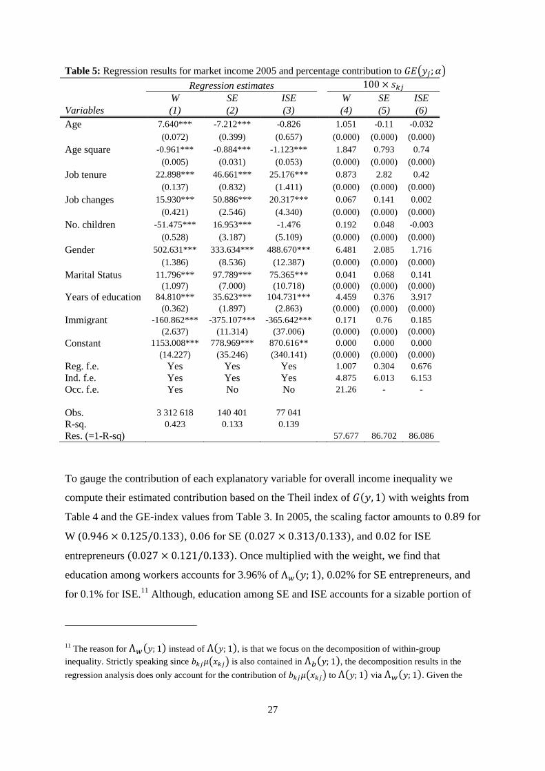
27

Table 5: Regression results for market income 2005 and percentage contribution to 𝐺𝐸(𝑦𝑗; 𝛼)

Regression estimates 100 × 𝑠𝑘𝑗

W SE ISE W SE ISE

Variables (1) (2) (3) (4) (5) (6)

Age 7.640*** -7.212*** -0.826 1.051 -0.11 -0.032

(0.072) (0.399) (0.657) (0.000) (0.000) (0.000)

Age square -0.961*** -0.884*** -1.123*** 1.847 0.793 0.74

(0.005) (0.031) (0.053) (0.000) (0.000) (0.000)

Job tenure 22.898*** 46.661*** 25.176*** 0.873 2.82 0.42

(0.137) (0.832) (1.411) (0.000) (0.000) (0.000)

Job changes 15.930*** 50.886*** 20.317*** 0.067 0.141 0.002

(0.421) (2.546) (4.340) (0.000) (0.000) (0.000)

No. children -51.475*** 16.953*** -1.476 0.192 0.048 -0.003

(0.528) (3.187) (5.109) (0.000) (0.000) (0.000)

Gender 502.631*** 333.634*** 488.670*** 6.481 2.085 1.716

(1.386) (8.536) (12.387) (0.000) (0.000) (0.000)

Marital Status 11.796*** 97.789*** 75.365*** 0.041 0.068 0.141

(1.097) (7.000) (10.718) (0.000) (0.000) (0.000)

Years of education 84.810*** 35.623*** 104.731*** 4.459 0.376 3.917

(0.362) (1.897) (2.863) (0.000) (0.000) (0.000)

Immigrant -160.862*** -375.107*** -365.642*** 0.171 0.76 0.185

(2.637) (11.314) (37.006) (0.000) (0.000) (0.000)

Constant 1153.008*** 778.969*** 870.616** 0.000 0.000 0.000

(14.227) (35.246) (340.141) (0.000) (0.000) (0.000)

Reg. f.e. Yes Yes Yes 1.007 0.304 0.676

Ind. f.e. Yes Yes Yes 4.875 6.013 6.153

Occ. f.e. Yes No No 21.26 - -

Obs. 3 312 618 140 401 77 041

R-sq. 0.423 0.133 0.139

Res. (=1-R-sq) 57.677 86.702 86.086

To gauge the contribution of each explanatory variable for overall income inequality we

compute their estimated contribution based on the Theil index of 𝐺(𝑦, 1) with weights from

Table 4 and the GE-index values from Table 3. In 2005, the scaling factor amounts to 0.89 for

W (0.946 × 0.125/0.133), 0.06 for SE (0.027 × 0.313/0.133), and 0.02 for ISE

entrepreneurs (0.027 × 0.121/0.133). Once multiplied with the weight, we find that

education among workers accounts for 3.96% of Λ𝑤(𝑦; 1), 0.02% for SE entrepreneurs, and

for 0.1% for ISE.11

Although, education among SE and ISE accounts for a sizable portion of

11 The reason for Λ𝑤(𝑦; 1) instead of Λ(𝑦; 1), is that we focus on the decomposition of within-group

inequality. Strictly speaking since 𝑏𝑘𝑗𝜇(𝑥𝑘𝑗) is also contained in Λ𝑏(𝑦; 1), the decomposition results in the

regression analysis does only account for the contribution of 𝑏𝑘𝑗𝜇(𝑥𝑘𝑗) to Λ(𝑦; 1) via Λ𝑤(𝑦; 1). Given the

28

that groups within-inequality, the contribution of differences in education level within these

groups to aggregate income inequality naturally drops because of these groups being

comparatively small compared to W. What is more, to know the total contribution of an

explanatory variable to aggregate inequality, we can simply add the weighted contributions of

that variable from all groups. For Years of education, this amounts to 4.08% (out of 100%).

Turning to the gender variable that takes the value of 1 if the individual is male and 0

otherwise, we find the largest marginal effect for all groups. Among workers it appears that

men on average earn 50 263 SEK (€ 5 028) more than the average woman.12

The gender

income difference is smaller for SE of 33 363 SEK (€ 3 595), as with ISE with a difference of

48 867 SEK (€5 266). The proportional contributions of gender to within- group inequality is

even more pronounced for workers, with 6.48% for W compared to the 2.09% for SE and

1.72% for ISE. Rescaled as contributions to aggregate within-inequality Λ𝑤(𝑦; 1), the gender

composition of each group contributes with 5.76% from W, 0.13% from SE, and 0.04%

from ISE. We can also add these last percentage-point contributions to get the total workforce

inequality contribution attributable to gender differences in income. Doing this, we find that

gender accounts for 5.93% out of total aggregate inequality.13

Table 5 also shows that while age is positively associated with incomes for both W and ISE it

is negatively associated for SE (Yamauchi, 2001). Using the scaling factor we see that the

total contribution of Age to income inequality in each group amounts to 0.94% for W,

−0.01% for SE, and −0.00% for ISE. From adding the scaled contributions we get the total

contribution from Age-squared to Λ𝑤(𝑦; 1), which amounts to 0.93%.

Before comparing the same results for the regression in the 2013 sample, it is worth

mentioning the fixed effects, and the model fit. Among the fixed effects included in we see in

columns 4-6 of Table 5 that the occupational fixed effects accounts for the highest share of

inequality in each sub-group. The variance in income across occupations accounts for 21.26%

for W and if scaled it amounts to 22.22% of Λ𝑤(𝑦; 1).

comparatively small contribution of Λ𝑏(𝑦; 1) to Λ(𝑦; 1), however, the impact from any particular 𝑏𝑘𝑗𝜇(𝑥𝑘𝑗) on

Λ𝑏(𝑦; 1) is almost negligible and therefore left out when presenting the results.

12 The large gender income gap may be partly attributed to women more often working part-time.

13 Strictly speaking, the total contribution of 4.99% from Gender refers to the aggregate within inequality of

Λ𝑤(𝑦; 1) = 98.3%, and not to the 100% that corresponds to Λ(𝑦; 1).

29

An important reason for why we find larger contributions in the group of workers can be seen

from the R2 value, which shows that the empirical model explains 42% of the variance in

income for W. High R2 values are common in mincer-type earnings equations (Robinson &

Sexton, 1994). For the SE and ISE entrepreneurs however, R2 amounts to 13.3%, and 13.9%,

partly reflecting the no inclusion of occupational fixed effects for the entrepreneurial groups.

This means that the residual contribution to within group inequality as captured by the error

term in the model, is comparatively large for entrepreneurs. One reason for this difference is

empirical in that the higher variance in market income among these groups compared to

workers leads to lower explanatory power in OLS models. Another reason may be theoretical

in that income among entrepreneurs is known to be more affected by unobserved ability than

among workers (Åstebro et al., 2011)

The contribution of the error term for overall income inequality within groups is presented in

the bottom row in columns (4) to (6), and accounts for 57.7% for the inequality within W,

which for SE amounts to 86.7%, and for ISE 86.1%. Since the residual enters the model just

as any other explanatory variable we can also compute the total contribution to aggregate

inequality Λ𝑤(𝑦; 1) from 𝑢𝑗𝑖 in expression (12), which amounts to 60%.

5.2. Changes in inequality over time, 2005 – 2013

By repeating the empirical analysis for a later period we are able to investigate changes in the

determinants of inequality between the two time periods. Table 6 presents identical models to

those of Table 5 but for the 2013 sample. To begin with, we observe that Years of education,

Gender, and Age all still play a significant role in accounting for inequality in 2013.

Continuing with the Theil index, the scaling factors for 2013 amounts to 0.90 for W (0.95 ×

0.12/0.13), 0.05 for SE (0.02 × 0.304/0.13), and 0.03 for ISE (0.03 × 0.13/0.13). Going

forward we focus on the scaled contribution to the inequality aggregate when discussing

differences in 2013 compared to 2005.

Starting with education, in W it accounts for 3,38% of aggregate inequality, compared to

Years of education among SE and ISE that contributes by 0.004% and 0,07%. As a total,

considering the effect from education across all groups it accounts for 3.38% of aggregate

inequality. Since education accounted for 4.08% in 2005, the results for 2013 suggest that

education as a means to explain the development of income inequality has declined.

30

A similar development seems to have occurred if we consider the age and gender variable,

which appears to be lesser correlates of income inequality in 2013 compared to 2005. The

percentage contribution from the gender variables 3.59% for W, 0.09% for SE, and 0.03% for

ISE, which adds up to 3.71% in total. For Age, we have 1.56 for W, -0.01% for SE and -

0.01% for ISE, which together amount to 1.54%.

One explanation to this particular development can be located at the bottom row of Table 6.

For each of the groups, we see that the part of the variance in income that is not explained by

the model has increased, which directly impacts the size of the estimates for the partial

contributions 𝑠𝑘𝑗.

Table 6. Regression results for market income 2013 and contribution to 𝐺𝐸(𝑌𝑗; 0)

Regression estimates 100 × 𝑠𝑘𝑗

W SE ISE W SE ISE

Variables (1) (2) (3) (4) (5) (6)

Age 11.660*** -11.596*** -5.932*** 1.736 -0.204 -0.223

(0.080) (0.462) (0.731) (0.000 (0.006) (0.008)

Age square -0.952*** -0.806*** -1.608*** 2.096 0.684 1.101

(0.005) (0.035) (0.058) (0.000) (0.001) (0.001)

Job tenure 20.027*** 40.156*** 35.948*** 1.157 2.686 1.384

(0.114) (0.731) (1.039) (0.000) (0.003) (0.002)

Job changes 13.271*** 44.339*** 9.633*** 0.156 0.336 0.001

(0.358) (2.115) (3.162) (0.000) (0.002) (0.002)

No. children -42.097*** 24.039*** 13.295** 0.01 0.079 0.035

(0.597) (3.728) (5.670) (0.000) (0.001) (0.002)

Gender 453.313*** 309.497*** 486.060*** 4.009 1.662 1.146

(1.506) (9.795) (14.138) (0.000) (0.003) (0.003)

Marital Status 27.663*** 83.136*** 100.675*** 0.107 0.061 0.188

(1.224) (7.889) (11.474) (0.000) (0.001) (0.002)

Years of education 86.578*** 24.837*** 92.213*** 3.686 0.074 2.451

(0.389) (2.081) (3.156) (0.000) (0.006) (0.009)

Immigrant -136.289*** -304.619*** -368.599*** 0.208 0.617 0.237

(2.301) (12.192) (29.902) (0.000) (0.000) (0.000)

Constant 1347.316*** 1277.275*** 2297.892** 0.000 0.000 0.000

(15.939) (40.870) (1097.735) (0.000) (0.000) (0.000)

Reg. f.e. Yes Yes Yes 1.116 0.598 0.845

Ind. f.e. Yes Yes Yes 5.733 4.754 6.912

Occ. f.e. Yes No No 21.392 - -

Obs. 3464330 124666 89216

R-sq. 0.414 0.113 0.141

Res. (=100-R2*100) 58.594 88.652 85.921

4. Summary and Discussion.

31

We have outlined an approach which seeks to problematize and probe the ways in which

entrepreneurship may contribute to income inequality. We develop an econometric model to

decompose aggregate changes in income dispersion based on a generalized-entropy index

distinguishing between self-employed (SE) and incorporated entrepreneurs (ISE) using

detailed microdata for Sweden in 2005 and 2013. Sweden represents a setting traditionally

characterized by low income inequality but where inequality has recently increased rapidly,

providing an interesting case to probe the role of entrepreneurship for income inequality. At

the same time, the rate of necessity entrepreneurs in Sweden remains low (Singer et al., 2014),

meaning that our results are of limited risk of being severely affected by workers being forced

into entrepreneurship due to lack of alternative employment opportunities. By tuning the GE-

index to different segments of the income distribution, we find across a range of specifications

that the self-employed entrepreneurs seem to increases workforce inequality by way of a

widening of the bottom-end of the distribution. Incorporated entrepreneurs more modestly

increases workforce inequality by increasing the total number of high income earners in

society. The aggregate effects of both types of entrepreneurship for overall workforce income

inequality are similar in magnitude to more conventional factors such as relative educational

group size, suggesting that entrepreneurship do not represent an exclusive explanation for the

rising income inequality in contemporary economies. This finding is of value for

entrepreneurship research discussing the role of entrepreneurship for economic development

(Lippmann et al., 2005; Praag & Versloot, 2007; Shane, 2009).

To the best of our knowledge, this paper is the first to assess the effects of entrepreneurship

for income inequality using state-of-the art decomposition techniques. By decomposing

entropy-based inequality indexes by several sub-groups and estimating inequality both

between and within each sub-group, our model provides a clearer picture of the group

dynamics that drive inequality at the population level. Further, we are able to pinpoint the

significance of each explanatory factor and its contribution to subgroup inequality. Self-

employed (SE) and incorporated entrepreneurs (ISE) do contribution to workforce income

inequality but in different ways, and the relative importance of entrepreneurship for overall

income inequality seems to have increased. This suggests that inequality scholars could

benefit from including entrepreneurship in their analyses of workforce inequality in various

settings.

32

Our model and results also comes with limitations that could be extended and probed by

future research efforts. Specifically, after the abolition of wealth taxation in Sweden in 2005,

the microdata do not include measures of wealth. Future research could expand on our model

by examining wealth inequality instead of income inequality, as prior studies suggest that

entrepreneurship is a key element to understand wealth concentration (Buera, 2009; Quadrini,

1999). Further, the decomposition techniques utilized do not lend themselves to causal

interpretations in that they are driven by both within-workforce shifts in occupational

categories and changes in income dispersion within those categories. Future research could

benefit from using regulatory changes or other quasi experimental settings to gauge causal

relationship between rates of entrepreneurship and levels of income inequality (Kerr &

Nanda, 2009).

33

Appendix 1: The Shorrocks’ assumption for income decomposition

Shorrock’s (1982) six assumptions for computing inequality measures has for long been

central in the literature (Bigotta et al., 2015). The six assumptions posits inequality as a

function 𝐼(𝒚) and are listed below:

ASSUMPTION 1: (i) 𝐼(𝒚) is continuous and symmetric. (ii) 𝐼(𝒚) = 0 iff 𝒚 = 𝜇𝒆, for

𝒆 = (𝟏,… , 𝟏), where 𝜇 is the mean income.

ASSUMPTION 2: (i) 𝑆𝑘(𝒚𝟏, … , 𝒚𝑲; 𝐾) is continuous in 𝒚𝒌. (ii) That 𝑆𝛑𝒌(𝒚

𝟏, … , 𝒚𝑲; 𝐾) =

𝑆𝑘(𝒀𝛑𝟏 , … , 𝒀𝛑𝑲; 𝐾), where 𝛑𝟏, … , 𝛑𝑲 is some permutation of 1,… , 𝐾.

ASSUMPTION 3: That 𝑆1(𝒚𝟏, … , 𝒚𝑲; 𝐾) = 𝑆1(𝒚

𝟏, 𝒚 − 𝒚𝟏; 2) = 𝑆(𝒚𝟏, 𝒚), which means

independence of the level of disaggregation.

ASSUMPTION 4: That decomposition is consistent, hence ∑ 𝑆𝑘(𝒚𝟏, … , 𝒚𝑲; 𝐾)𝑘 =

∑ 𝑆(𝒚𝒌, 𝒚)𝑘 = 𝐼(𝒚).

ASSUMPTION 5: (i) Of population symmetry, that 𝑷 is some 𝑛 by 𝑛 permutation matrix.

𝑆(𝒚𝒌𝑷, 𝒚𝑷) = 𝑆(𝒚𝒌, 𝒚). (ii) And normalization for equal factor distribution, which means

that 𝑆(𝜇𝒌𝒆, 𝒚) = 0, ∀ 𝜇𝑘.

ASSUMPTION 6: That for all permutation matrices, 𝑆(𝒚𝟏, 𝒚𝟏 + 𝒚𝟏𝑷) = 𝑆(𝒚𝟏𝑷, 𝒚𝟏 + 𝒚𝟏𝑷).

34

Appendix 2: Robustness tests for disposable income

In this section we present the corresponding tables, figures and results for disposable income

in place of market income.

Figure A.1. Lorentz curve for workforce disposable income, 2005 and 2013

Table A1. Descriptive statistics: Disposable income among entrepreneurs

2005

2013

Mean Sd. Min Max

Mean Sd. Min Max

Variables: (1) (2) (3) (4) (5) (6) (7) (8)

Number of Workers (W)

Market income 1493.661 672.915 0.909 4693.129 1842.711 859.643 0.812 6071.121

Obs. 3346001 3509346

Self-employed (SE)

Market income 1186.328 717.269 0.909 4693.129 1444.678 910.184 0.812 6071.121

Obs. 159966 150800

Incorporated entrepreneurs (ISE)

Market income 1789.158 836.433 5.455 4693.129 2326.387 1121.46 4.871 6071.121

Obs. 77087 89168

35

Table A2 Income inequality statistics (disposable income)

2005

2013

Pop. SE ISE

Pop. SE. ISE

Inequality measure: (1) (2) (3) (4) (5) (6)

Disposable Income

p90/p10 3.197 4.949 3.538 3.278 5.466 3.7

p90/p50 1.682 2.051 1.779 1.714 2.093 1.832

p50/ p10 1.9 2.414 1.989 1.913 2.611 2.019

p75/p25 1.86 2.285 1.909 1.884 2.383 1.984

GE(-1) 0.125 0.591 0.144 0.137 1.034 0.151

GE(0) 0.1 0.202 0.112 0.106 0.233 0.12

GE(1) 0.096 0.171 0.105 0.102 0.187 0.112

GE(2) 0.101 0.183 0.109 0.109 0.198 0.116

Gini 0.249 0.257

In Tables A3 and Figure A1 we present the same decomposition as in Table 3 and Figure 2 in

the main paper, but for disposable income instead of market income. The results are

qualitatively similar to those for market income. Workers accounts for roughly 80% of

aggregate inequality. Looking at Figure 3 (i) and (ii) we see that the inequality-group

dynamics between SE and ISE largely remains for disposable income over the period. SE

(ISE) stands for most of workers’ residual contribution when inequality is computed with

emphasis on the lower (upper) tail of the disposable income distribution

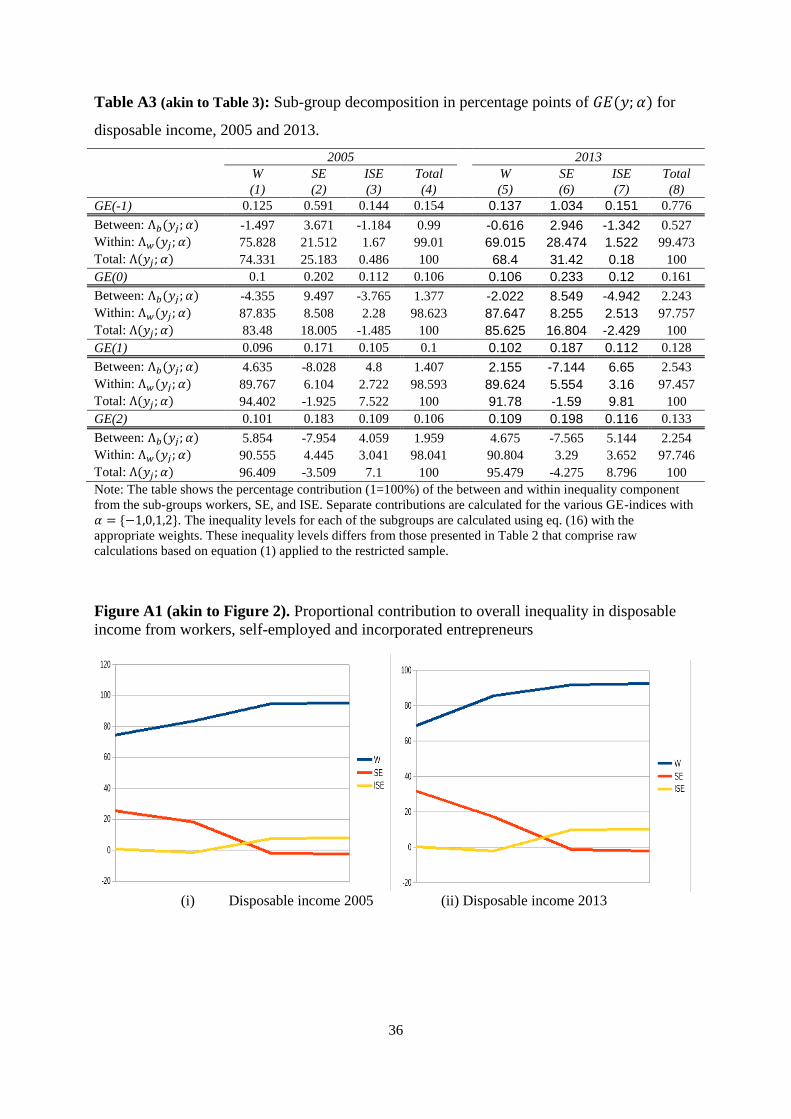
36

Table A3 (akin to Table 3): Sub-group decomposition in percentage points of 𝐺𝐸(𝑦; 𝛼) for

disposable income, 2005 and 2013.

2005 2013

W SE ISE Total W SE ISE Total

(1) (2) (3) (4) (5) (6) (7) (8)

GE(-1) 0.125 0.591 0.144 0.154 0.137 1.034 0.151 0.776

Between: Λ𝑏(𝑦𝑗; 𝛼) -1.497 3.671 -1.184 0.99 -0.616 2.946 -1.342 0.527

Within: Λ𝑤(𝑦𝑗; 𝛼) 75.828 21.512 1.67 99.01 69.015 28.474 1.522 99.473

Total: Λ(𝑦𝑗; 𝛼) 74.331 25.183 0.486 100 68.4 31.42 0.18 100

GE(0) 0.1 0.202 0.112 0.106 0.106 0.233 0.12 0.161

Between: Λ𝑏(𝑦𝑗; 𝛼) -4.355 9.497 -3.765 1.377 -2.022 8.549 -4.942 2.243

Within: Λ𝑤(𝑦𝑗; 𝛼) 87.835 8.508 2.28 98.623 87.647 8.255 2.513 97.757

Total: Λ(𝑦𝑗; 𝛼) 83.48 18.005 -1.485 100 85.625 16.804 -2.429 100

GE(1) 0.096 0.171 0.105 0.1 0.102 0.187 0.112 0.128

Between: Λ𝑏(𝑦𝑗; 𝛼) 4.635 -8.028 4.8 1.407 2.155 -7.144 6.65 2.543

Within: Λ𝑤(𝑦𝑗; 𝛼) 89.767 6.104 2.722 98.593 89.624 5.554 3.16 97.457

Total: Λ(𝑦𝑗; 𝛼) 94.402 -1.925 7.522 100 91.78 -1.59 9.81 100

GE(2) 0.101 0.183 0.109 0.106 0.109 0.198 0.116 0.133

Between: Λ𝑏(𝑦𝑗; 𝛼) 5.854 -7.954 4.059 1.959 4.675 -7.565 5.144 2.254

Within: Λ𝑤(𝑦𝑗; 𝛼) 90.555 4.445 3.041 98.041 90.804 3.29 3.652 97.746

Total: Λ(𝑦𝑗; 𝛼) 96.409 -3.509 7.1 100 95.479 -4.275 8.796 100

Note: The table shows the percentage contribution (1=100%) of the between and within inequality component

from the sub-groups workers, SE, and ISE. Separate contributions are calculated for the various GE-indices with

𝛼 = {−1,0,1,2}. The inequality levels for each of the subgroups are calculated using eq. (16) with the

appropriate weights. These inequality levels differs from those presented in Table 2 that comprise raw

calculations based on equation (1) applied to the restricted sample.

Figure A1 (akin to Figure 2). Proportional contribution to overall inequality in disposable

income from workers, self-employed and incorporated entrepreneurs

(i) Disposable income 2005 (ii) Disposable income 2013

-0,2

0,0

0,2

0,4

0,6

0,8

1,0

-1 0 1 2

GE(α)

Workers Self-emp. Inc. Ent.

-0,2

0,0

0,2

0,4

0,6

0,8

1,0

-1 0 1 2

GE(α)

Workers Self-emp. Inc. Ent

37

The next three tables replicates tables 4-6 in the main paper using disposable income instead

of market income. Again, we use the method of Fiorio and Cowell (2011) to decompose

within group inequality Λ𝑤(𝑦𝑗; 𝛼) to a number of explanatory variables (factor sources).

Table A4: Inequality weights (𝑤𝑗) for the GE-index.

Workers SE ISE Workers SE ISE

Disposable income, 2005 Disposable income, 2013

GE(-1) 0.929 0.056 0.018 0.934 0.051 0.019

GE(0) 0.934 0.045 0.022 0.936 0.04 0.024

GE(1) 0.938 0.036 0.026 0.938 0.032 0.03

GE(2) 0.943 0.028 0.031 0.941 0.025 0.038

GE(3) 0.948 0.023 0.038 0.943 0.02 0.048

Table A5: Regression results for disposable income 2005 and contribution to 𝐺𝐸(𝑌𝑗;0)

Regression estimates disp. inc. % contrib. to 𝐺𝐸(𝑦𝑗; 𝛼) (𝑠𝑘 × 100)

Variable Workers Self-emp. Inc. emp. Workers Self-emp. Inc. emp.

Age 11.901*** 12.641*** 13.694*** 4.576 4.669 4.264

(0.044) (0.212) (0.376) (0.000) (0.002) (0.005)

Age square -0.109*** 0.181*** -0.088*** 0.13 -0.016 0.003

(0.003) (0.017) (0.031) (0.000) (0.000) (0.001)

Job tenure 6.202*** 11.260*** 11.392*** 0.277 0.888 0.736

(0.081) (0.424) (0.783) (0.000) (0.001) (0.002)

Job Changes 13.958*** 31.502*** 15.766*** 0.088 0.063 -0.189

(0.236) (1.274) (2.361) (0.000) (0.000) (0.001)

Children living at home -202.706*** -85.785*** -211.268*** 12.502 2.9 8.992

(0.309) (1.544) (2.789) (0.000) (0.000) (0.001)

Gender 264.791*** 220.129*** 342.141*** 5.446 2.312 2.245

(0.787) (4.303) (7.164) (0.000) (0.001) (0.002)

Marital Status -78.738*** 97.844*** -18.195*** 0.337 0.374 0.007

(0.654) (3.602) (5.956) (0.000) (0.000) (0.001)

Years of education 31.583*** 24.226*** 47.948*** 1.6 0.479 1.946

(0.204) (0.972) (1.600) (0.000) (0.002) (0.005)

Imigrant -96.247*** -207.135*** -191.386*** 0.207 1.058 0.188

(1.430) (5.721) (20.291) (0.000) (0.000) (0.000)

Constant 920.204*** 16.917 538.702*** - - -

(8.025) (18.416) (196.975) - - -

Reg. f.e. yes yes yes 1.166 0.428 0.748

38

Ind. f.e. yes yes yes 2.624 3.961 3.459

Occ. f.e. yes yes yes 9.044 - -

Obs. 3346001 159966 77087

R-sq. 0.38 0.171 0.224

Res. (=1-R-sq)

62.003 82.884 77.601

Table A6: Regression results for disposable income 2013 and contribution to 𝐺𝐸(log 𝑌𝑗;0)

Regression estimates disp inc. % contrib. to 𝐺𝐸(𝑦𝑗; 𝛼), (𝑠𝑘 × 100)

Variable Workers Self-emp. Inc. emp. Workers Self-emp. Inc. emp.

Age 15.154*** 11.616*** 15.993*** 4.685 3.035 3.33

(0.056) (0.278) (0.480) (0.000) (0.002) (0.005)

Age square -0.094*** 0.223*** -0.293*** 0.142 -0.07 0.062

(0.004) (0.021) (0.038) (0.000) (0.000) (0.001)

Job tenure 7.311*** 15.956*** 15.904*** 0.54 1.773 1.258

(0.078) (0.438) (0.673) (0.000) (0.001) (0.001)

Job Changes 14.670*** 32.862*** 15.318*** 0.222 0.352 -0.098

(0.231) (1.239) (1.987) (0.000) (0.001) (0.001)

Nr. children -239.937*** -93.317*** -261.534*** 9.876 1.946 7.094

(0.393) (2.048) (3.527) (0.000) (0.000) (0.001)

Gender 298.296*** 225.840*** 427.118*** 4.137 1.71 1.86

(0.971) (5.599) (9.069) (0.000) (0.001) (0.002)

Marital Status -75.802*** 131.779*** -15.537** 0.191 0.352 0.01

(0.831) (4.676) (7.267) (0.000) (0.001) (0.001)

Years of education 34.685*** 20.820*** 49.692*** 1.166 0.149 1.393

(0.249) (1.225) (2.035) (0.000) (0.002) (0.005)

Imigrant -122.704*** -255.266*** -212.346*** 0.341 1.239 0.227

(1.465) (6.905) (18.421) (0.000) (0.000) (0.000)

Constant 1119.658*** 326.949*** 962.651*** - - -

(10.164) (24.326) (228.985)

Reg. f.e. yes yes yes 1.612 0.809 1.46

Ind. f.e. yes yes yes 3.316 3.1 4.325

Occ. f.e. yes yes yes 9.242 - -

Obs. 3509346 150800 89168

R-sq. 0.355 0.144 0.209

Res. (=1-R-sq)

64.53 85.605 79.077

39

References

Akita, T., Lukman, R. A., & Yamada, Y. 1999. Inequality in the distribution of household

expenditures in Indonesia: A Theil decomposition analysis. The Developing Economies,

37(2): 197-221.

Alstadsæter, A., & Jacob, M. 2015. Dividend taxes and income shifting. Scandinavian Journal of

Economics.

Arum, R., & Müller, W. 2004. The reemergence of self-employment: a comparative study of self-

employment dynamics and social inequality: Princeton Univ Pr.

Atkinson, A. B. 2003. Income inequality in OECD countries: data and explanations. CESifo

Economic Studies, 49(4): 479-513.

Audretsch, D. B. 2009. The entrepreneurial society. The Journal of Technology Transfer, 34(3): 245-

254.

Autor, D. H. 2014. Skills, education, and the rise of earnings inequality among the" other 99 percent".

Science, 344(6186): 843-851.

Bigotta, M., Krishnakumar, J., & Rani, U. 2015. Further results on the regression-based approach to

inequality decomposition with evidence from India. Empirical Economics, 48(3): 1233-1266.

Blanchflower, D. G. 2000. Self-employment in OECD countries. Labour Economics, 7(5): 471-505.

Blau, D. M. 1987. A time-series analysis of self-employment in the United States. Journal of Political

Economy, 95(3): 445-467.

Block, J. H., & Wagner, M. 2010. Necessity and opportunity entrepreneurs in Germany:

Characteristics and earnings differentials. Schmalenbach Business Review, 62: 154-174.

Borjas, G. J., & Bronars, S. G. 1989. Consumer Discrimination and Self-Employment. Journal of

Political Economy, 97(3): 581-605.

Buera, F. J. 2009. A dynamic model of entrepreneurship with borrowing constraints: theory and

evidence. Annals of finance, 5(3-4): 443-464.

Carnahan, S., Agarwal, R., & Campbell, B. A. 2012. Heterogeneity in turnover: The effect of relative

compensation dispersion of firms on the mobility and entrepreneurship of extreme performers.

Strategic Management Journal, 33(12): 1411-1430.

Cowell, F., & Fiorio, C. 2011. Inequality decompositions—a reconciliation. The Journal of

Economic Inequality, 9(4): 509-528.

Cowell, F. A. 2000. Measurement of inequality. In A. B. Atkinson, & F. Bourguignon (Eds.),

Handbook of Income Distribution Vol. 1: 87-166. North-Holland: Elsevier.

Creedy, J., & Hérault, N. 2011. Decomposing inequality and social welfare changes: the use of

alternative welfare metrics.

Davis, G. F. 2013. After the Corporation. Politics & Society, 41(2): 283-308.

Edmark, K., & Gordon, R. H. 2013. The choice of organizational form by closely-held firms in

Sweden: tax versus non-tax determinants. Industrial and Corporate Change, 22(1): 219-243.

40

Engström, P., & Holmlund, B. 2009. Tax evasion and self-employment in a high-tax country: evidence

from Sweden. Applied Economics, 41(19): 2419-2430.

Evans, D. S., & Leighton, L. S. 1989. Some Empirical Aspects Of Entrepreneurship. The American

Economic Review, 79(3): 519-535.

Fields, G. S. 2003. Accounting for income inequality and its change: A new method, with application

to the distribution of earnings in the United States, Solomon W. Polachek (ed.) Worker Well-

Being and Public Policy (Research in Labor Economics) Vol. 22: 1-38: Emerald Group.

Fields, G. S., & Yoo, G. 2000. Falling labor income inequality in Korea's economic growth: Patterns

and underlying causes. Review of Income and Wealth, 46(2): 139-159.

Folta, T. B., Delmar, F., & Wennberg, K. 2010. Hybrid Entrepreneurship. Management Science,

56(2): 253-269.

Goldthorpe, J. H. 2010. Analysing social inequality: a critique of two recent contributions from

economics and epidemiology. European Sociological Review, 26(6): 731-744.

Hamilton, B. H. 2000. Does entrepreneurship pay? An empirical analysis of the returns of self-

employment. Journal of Political Economy, 108(3): 604-631.

Kerr, W., & Nanda, R. 2009. Financing constraints and entrepreneurship: National Bureau of

Economic Research.

Levine, R., & Rubinstein, Y. 2013. Smart and illicit: Who becomes an entrepreneur and does it pay?

Available at SSRN 2314667.

Lin, Z., Picot, G., & Yates, J. 2000. The entry and exit dynamics of self-employment in Canada. Small

business economics, 15(2): 105-125.

Lippmann, S., Davis, A., & Aldrich, H. E. 2005. Entrepreneurship and inequality. Research in the

Sociology of Work, 15: 3-31.

Moskowitz, T. J., & Vissing-Jorgensen, A. 2002. The returns to entrepreneurial investment: A private

equity premium puzzle?: National Bureau of Economic Research.

Murphy, K. M., Shleifer, A., & Vishny, R. W. 1991. The Allocation of Talent: Implications for

Growth. The Quarterly Journal of Economics, 106(2): 503-531.

OECD. 2015. OECD Income inequality data update: Sweden. http://www.oecd.org/sweden/OECD-

Income-Inequality-Sweden.pdf.

Poschke, M. 2013. ‘Entrepreneurs out of necessity’: a snapshot. Applied Economics Letters, 20(7):

658-663.

Praag, C. M., & Versloot, P. 2007. What is the value of entrepreneurship? A review of recent research.

Small Business Economics, 29(4): 351-382.

Quadrini, V. 1999. The importance of entrepreneurship for wealth concentration and mobility. Review

of Income and Wealth, 45(1): 1-19.

Quintano, C., Castellano, R., & Regoli, A. 2005. The Contribution of Self-Employment to Income

Inequality. A Decomposition Analysis of Inequality Measures by Sources and Subgroups

41

for Italy, 1998–2002. Paper presented at the International Conference in Memory of Two

Eminent Social Scientists: C. Gini and M. O. Lorenz., Siena, Italy.

Reynolds, P., Bosma, N., Autio, E., Hunt, S., De Bono, N., Servais, I., Lopez-Garcia, P., & Chin, N.

2005. Global entrepreneurship monitor: Data collection design and implementation 1998–

2003. Small Business Economics, 24(3): 205-231.

Robinson, P. B., & Sexton, E. A. 1994. The effect of education and experience on self-employment

success. Journal of Business Venturing, 9(2): 141-156.

Roine, J., & Waldenström, D. 2008. The evolution of top incomes in an egalitarian society: Sweden,

1903–2004. Journal of Public Economics, 92(1): 366-387.

Sanandaji, T., & Leeson, P. T. 2013. Billionaires. Industrial and Corporate Change, 22(1): 313-337.

Shane, S. 2009. Why encouraging more people to become entrepreneurs is bad public policy. Small

Business Economics, 33(2): 141-149.

Shorrocks, A. F. 1982. Inequality decomposition by factor components. Econometrica: Journal of the

Econometric Society, 50(1): 193-211.

Singer, S., Amoros, J. E., & Moska, D. 2014. Global Entrepreneurship Monitor: 2014 Global Report.

www.gemconsortium.org/report: ISBN: 978-1-939242-05-1.

Stam, E. 2013. Knowledge and entrepreneurial employees: a country-level analysis. Small Business

Economics, 41(4): 887-898.

Steinmetz, G., & Wright, E. O. 1989. The fall and rise of the petty bourgeoisie: changing patterns of

self-employment in the postwar United States. American journal of sociology: 973-1018.

Sørensen, J. B., & Sharkey, A. J. 2014. Entrepreneurship as a Mobility Process. American

Sociological Review, 79(2): 328-349.

Thewissen, S., Wang, C., & Van Vliet, O. 2013. Sectoral Trends in Earnings Inequality and

Employment: International Trade, Skill-Biased Technological Change, or Labour Market

Institutions?

Van Praag, C. M., & Versloot, P. H. 2007. What is the value of entrepreneurship? A review of recent

research. Small business economics, 29(4): 351-382.

Van Praag, M., van Witteloostuijn, A., & van der Sluis, J. 2013. The higher returns to formal

education for entrepreneurs versus employees. Small Business Economics, 40(2): 375-396.

Wright, M., & Zahra, S. 2011. The other side of paradise: Examining the dark side of

entrepreneurship. Entrepreneurship Research Journal, 1(3).

Yamauchi, F. 2001. Does inequality of labor earnings emerge in young days or later?: Labor earnings

dynamics and learning about individual ability in heterogeneous society. Journal of

Economic Behavior & Organization, 44(4): 413-434.

Åstebro, T., Chen, J., & Thompson, P. 2011. Stars and misfits: Self-employment and labor market

frictions. Management Science, 57(11): 1999-2017.

Åstebro, T., & Tåg, J. 2015. Jobs Incorporated: Incorporation Status and Job Creation. IFN Working

paper 1059, http://papers.ssrn.com/sol3/papers.cfm?abstract_id=2576044.

42

Özcan, B. 2011. Only the lonely? The influence of the spouse on the transition to self-employment.

Small Business Economics, 37(4): 465-492.