Embed Size (px)
Citation preview

Staffordshire University
Business School
Economics
ENTREPRENEURSHIP AND ECONOMIC PERFORMANCE:
INTERNATIONAL EVIDENCE
Ermal LUBISHTANI
A thesis submitted in partial fulfilment of the requirement of Staffordshire
University for the degree of Doctor of Philosophy in Economics
November 2018
i
ABSTRACT
The thesis investigates the effect of entrepreneurship on national economic growth as well as the individual-level and institutional determinants of entrepreneurial growth aspirations. The renewed focus on entrepreneurial firms in the early twenty-first century has resulted on an increased interest of both researcher and policymakers in the study of entrepreneurship. Although, in general, the previous empirical literature reports positive association between entrepreneurship and economic performance, the evidence is still not conclusive. Given the heterogeneity of results, methodological approaches and study characteristics, this thesis aims at shedding light on factors that influence this relationship. Using Meta-Regression Analysis (MRA), the appropriate statistical method and methodological approach to synthesise the existing entrepreneurship-economic performance literature, the thesis has provided relevant insights to the study of entrepreneurship. In addition to finding that there is a general tendency to report positive effects, the results indicate that there is also a positive genuine effect of entrepreneurship on country-level economic performance.
Moreover, using the Global Entrepreneurship Monitor (GEM) data at country-level and a diversified modelling strategy, the thesis provides an original and comprehensive empirical investigation of the effect of entrepreneurship on economic growth. Benefiting from the work of Schumpeter (1934) and Baumol (1990; 1993), the focus of the thesis is on growth-oriented and innovative entrepreneurial activity (‘productive entrepreneurship’). A total of 48 developed and developing economies over the 2006-2014 period are included in the empirical analysis. The results indicate that growth aspiring and innovative entrepreneurial activities, rather than overall entrepreneurial activity, have a positive impact on short- and long-run national economic growth. The more developed economies compared to less developed economies, on average, are shown to benefit more from an increased growth-oriented entrepreneurial activity.
Given the positive effect of growth aspirations on economic growth, the thesis then explores the factors influencing entrepreneurial growth aspirations in more detail. Using individual-level data from GEM and a set of quality of institutions variables in 55 countries, entrepreneurial growth aspirations for eighteen thousand young (new) entrepreneurial ventures are assessed. The hierarchical nature of the analysis requires the use of multilevel estimation modelling. The results indicate that individual-level attributes, including human, financial and social capital determine entrepreneurial growth aspirations. Also, the quality of institutions, including the protection of property rights, the level of corruption, the size of government activity and the existence of specifically designed programmes to support high-growth firms, determine growth aspirations. In addition, the interplay between individual and institutional variables moderates the effect of the latter on entrepreneurial growth aspirations. The empirical evidence generated throughout the thesis, provides useful policy implications for countries seeking to nurture more productive entrepreneurship and sustain long-run economic growth.

ii
Abstract........................................................................................................... ...................................... i
Table of Content............................................................................................................................... ii
List of Tables...................................................................................................................................... v
List of Figures....................................................................................................................... ........... vii
List of Appendices........................................................................................................................... ix
List of Abbreviations.................................................................................................................... xiv
Acknowledgement........................................................................................................................ xvi
CHAPTER 1 INTRODUCTION 1. Chapter 1 ............................................................................................................................................................................................................... 1
THE CONCEPT OF ENTREPRENEURSHIP ......................................................................... 3
The origins of entrepreneurship ................................................................................. 5
Schumpeter’s concept of entrepreneurship ........................................................... 8
Kirzner’s concept of entrepreneurship ................................................................. 10
AIMS AND OBJECTIVES OF THE THESIS ........................................................................ 12
GEM CONCEPTUAL FRAMEWORK AND TYPES OF ENTREPRENEURIAL ACTIVITY .................................................................................................................................................... 14
GEM entrepreneurship data and the context ...................................................... 20
STRUCTURE OF THE THESIS .............................................................................................. 26
CHAPTER 2 THEORETICAL AND EMPIRICAL LITERATURE ON
ENTREPRENEURIAL ACTIVITIES AND ECONOMIC PERFORMANCE 2. Chapter 2 ............................................................................................................................................................................................................ 29
INTRODUCTION ........................................................................................................................ 30
ECONOMIC GROWTH THEORIES AND ENTREPRENEURSHIP.............................. 31
Entrepreneurship and economic growth in the neoclassical growth
model .…..………………………………………………………………………………………………………..32
Entrepreneurship and economic growth in the endogenous growth
model ……………………………………………………………………………………………………………..38
2.2.2.1 The Knowledge Spillover Theory of Entrepreneurship (KSTE) ............. 43
Schumpeterian growth theory .................................................................................. 48
REVIEW OF EMPIRICAL LITERATURE ............................................................................ 55
Evidence from studies using ‘growth’ as a measure of economic
performance ......................................................................................................................................... 57
Evidence from the studies using employment growth as a measure of
economic performance .................................................................................................................... 67
Evidence from studies using ’other’ dependent variables ............................ 76
CONCLUSIONS ........................................................................................................................... 84

iii
CHAPTER 3 ENTREPRENEURSHIP AND ECONOMIC PERFORMANCE: A
META-REGRESSION ANALYSIS 3. Chapter 3 ............................................................................................................................................................................................................ 86
INTRODUCTION ........................................................................................................................ 87
THEORETICAL CONTEXT AND CONCEPTUAL FRAMEWORK ............................... 89
METHODOLOGY AND DATA ................................................................................................ 92
Criteria for inclusion of studies ................................................................................ 93
Primary literature included in this MRA............................................................... 94
(i) Main characteristics of studies using GDP growth or growth of GDP per capita
(subsample I) .................................................................................................................................. 95
(ii) Main characteristics of studies using employment growth as dependent
variable (subsample II) .............................................................................................................. 96
(iii) Main characteristics of studies using ’other’ measures of economic
performance (subsample III) ................................................................................................... 97
Summary of the MRA database ................................................................................. 98
THE MRA METHODOLOGY ................................................................................................. 101
Effect sizes ....................................................................................................................... 101
Publication Bias: Funnel Plot ................................................................................... 103
THE BIVARIATE MRA ........................................................................................................... 106
FAT – PET – PEESE ...................................................................................................... 106
THE MULTIVARIATE MRA ................................................................................................. 115
Heterogeneity ................................................................................................................ 115
Descriptive statistics ................................................................................................... 119
Bayesian Model Averaging ....................................................................................... 122
EMPIRICAL RESULTS ........................................................................................................... 122
CONCLUSIONS ......................................................................................................................... 133
CHAPTER 4 THE IMPACT OF ENTREPRENEURIAL ACTIVITY ON ECONOMIC
GROWTH: A MULTI-COUNTRY ANALYSIS 4. Chapter 4 .......................................................................................................................................................................................................... 136
INTRODUCTION ...................................................................................................................... 137
THEORETICAL FRAMEWORK ........................................................................................... 138
Entrepreneurship and economic growth ........................................................... 139
METHODOLOGY AND DATA .............................................................................................. 141
Data .................................................................................................................................... 144
4.3.1.1 The dependent variable: economic growth .................................................. 146
4.3.1.2 Entrepreneurship measures ............................................................................... 147
4.3.1.3 Institutional quality and other control variables ....................................... 149
4.3.1.4 Descriptive statistics .............................................................................................. 156

iv
ESTIMATION STRATEGY .................................................................................................... 157
Econometric approach and model specification ............................................. 161
EMPIRICAL RESULTS ........................................................................................................... 170
Employment growth-oriented entrepreneurial activity .............................. 173
Innovation: new product and new product-market entrepreneurial
activity ……………………………………………………………………………………………………….182
The moderating impact of stages of development on entrepreneurship-
economic growth relationship ................................................................................................... 188
Robustness of estimated results ............................................................................ 196
CONCLUSIONS ......................................................................................................................... 197
CHAPTER 5 INDIVIDUAL AND INSTITUTIONAL DETERMINANTS OF ENTREPRENEURIAL GROWTH ASPIRATIONS:
A MULTI-COUNTRY ANALYSIS 5. Chapter 5 .......................................................................................................................................................................................................... 201
INTRODUCTION ...................................................................................................................... 202
THEORETICAL FRAMEWORK ........................................................................................... 203
Entrepreneurial Growth Aspirations ................................................................... 203
Growing vs non-growing firms ............................................................................... 206
5.2.2.1 Dependent variable................................................................................................. 215
5.2.2.2 Individual and young business characteristics and controls ................ 217
5.2.2.3 Institutional variables ............................................................................................ 222
5.2.2.4 Country level characteristics .............................................................................. 228
Descriptive statistics by stages of economic development ......................... 232
ESTIMATION STRATEGY AND MODEL SPECIFICATION ....................................... 235
Model specification ...................................................................................................... 241
EMPIRICAL RESULTS ........................................................................................................... 245
Results ............................................................................................................................... 245
Robustness checks ....................................................................................................... 267
CONCLUSIONS ......................................................................................................................... 268
CHAPTER 6 CONCLUSIONS AND POLICY IMPLICATIONS 6. Chapter 6 .......................................................................................................................................................................................................... 270
Introduction ............................................................................................................................. 271
Main findings ........................................................................................................................... 272
Contribution to knowledge ................................................................................................ 280
Policy implications ................................................................................................................ 284
Limitations and recommendations for future research ......................................... 287
References……………………………………………………………………………………………………... 290
v
LIST OF TABLES
Chapter 2
Table 2.1 Entrepreneurship and economic performance (GDP growth or GDP per capita
used as a measure of economic growth) ............................................................................ 58
Table 2.2 Entrepreneurship and economic performance (employment growth used as a
measure of economic growth)............................................................................................. 68
Table 2.3 Entrepreneurship and economic performance (‘other’ used as a measure of
economic growth) ................................................................................................................ 77
Chapter 3
Table 3.1 Reported estimates of the relationship between entrepreneurship and
economic performance in different groups of studies (subsamples) .............................. 91
Table 3.2 Estimates of the overall partial correlation coefficient (PCC) - unweighted and
weighted .............................................................................................................................. 102
Table 3.3 Funnel-Asymmetry Test (FAT), Precision Effect Test (PET) and Precision
Effect Estimate with SE (PEESE)a (adjusted for outliers) ............................................... 111
Table 3.4 Funnel-Asymmetry Test (FAT), Precision Effect Test (PET) and Precision
Effect Estimate with SE (PEESE)a (not adjusted to outliers) .......................................... 111
Table 3.5 Description and summary statistics of the variables used in the MRA ......... 120
Table 3.6 Multiple MRA results for the three subsamples (adjusted for outliers) ........ 124
Table 3.7 Average publication selection bias and average genuine empirical effect
derived for each subsample (results are derived from multiple MRA: Table 3.6, after
adjusting for outliers .......................................................................................................... 130
Table 3.8 Average publication selection bias and average genuine empirical effect
derived for each subsample (results are derived from multiple MRA: Appendix 3.9,
Table 3.2, unadjusted for outliers) .................................................................................... 130
Chapter 4
Table 4.1 Variable name, description, source and the expected sign ............................ 154
Table 4.2 Descriptive statistics: all countries, innovation-driven and efficiency-driven
economies ........................................................................................................................... 156
Table 4.3 Static and dynamic estimator; 'Employment growth-oriented'
Entrepreneurial Activity and economic growth .............................................................. 176
Table 4.4 Static and dynamic estimator: 'Innovative’ Entrepreneurial Activity and
economic growth ................................................................................................................ 184
Table 4.5 Dynamic estimator: The impact of stage of development in the
entrepreneurship-economic growth relationship ........................................................... 190
Chapter 5
Table 5.1 The distribution of growth aspiration among newly-established (young)
businesses ........................................................................................................................... 207
Table 5.2 Variable name, description, source and the expected sign ............................ 230
vi
Table 5.3 Descriptive statistics: all countries, innovation-driven and efficiency-driven
economies ........................................................................................................................... 234
Table 5.4 Results for entrepreneurial growth aspirations: (EGA - columns 1-5); (HJG -
columns 6-10) – All countries included ............................................................................ 247
Table 5.5 Results of Employment Growth Aspirations (EGA) aspirations according to
the stage of development ................................................................................................... 253
Table 5.6 Results of High-job Growth (HJG) aspirations according to the stages of
development ....................................................................................................................... 262

vii
LIST OF FIGURES
Chapter 1
Figure 1.1 The GEM Conceptual Framework ..................................................................... 17
Figure 1.2 The entrepreneurial process and GEM operational definition ....................... 19
Figure 1.3 Geographical distribution of Total Entrepreneurial Activity (TEA) (country
average)................................................................................................................................. 20
Figure 1.4 TEA rates in the five world regions (country averages) ................................. 21
Figure 1.5 TEA rates distributed according to the two economic development stages
(country averages) ............................................................................................................... 21
Figure 1.6 Types of entrepreneurial activity in the two stages of economic development
(country averages) ............................................................................................................... 22
Figure 1.7 The TEA and HJG entrepreneurial activity and GDP growth of innovation-
driven economies (country average) .................................................................................. 24
Figure 1.8 The TEA and HJG entrepreneurial activity and GDP growth of efficiency-
driven economies (country average) .................................................................................. 25
Chapter 3
Figure 3.1 Funnel plots for each sub-sample: (A) all lags; (B) no outliers; and (C) zero
lags ....................................................................................................................................... 104
Chapter 4
Figure 4.1 Growth and the relation to the Total Entrepreneurial activity (TEA),
(country-means) ................................................................................................................. 143
Figure 4.2 Growth and the relation to the share of Young Businesses, (country-means)
............................................................................................................................................. 143
Figure 4.3 Growth and the relation to high-job growth entrepreneurial activity,
(country-means) ................................................................................................................. 143
Figure 4.4 Growth and the relation to job growth entrepreneurial activity, (country-
means) ................................................................................................................................. 143
Figure 4.5 Growth and the relation to new product entrepreneurial. activity, (country-
means) ................................................................................................................................. 143
Figure 4.6 Growth and the relation to new product-market innovation (country-means)
............................................................................................................................................. 143
Figure 4.7 Predictive margins: High-job growth and Stage of Development – Economic
growth (growth) - All countries included ........................................................................ 193
Figure 4.8 Predictive margins: High-job growth and OECD membership – Economic growth (growth) - All countries included ........................................................................ 193
Figure 4.9 Average marginal effects: GDP per capita and High-job growth – Economic
growth (growth) - All countries included ........................................................................ 193
Figure 4.10 Predictive margins: New product and Stage of Development – Economic
growth (growth) - All countries included ........................................................................ 194
Figure 4.11 Predictive margins: New product and OECD membership – Economic
growth (growth) - All countries included ........................................................................ 194
Figure 4.12 Average marginal effects: GDP per capita and High-job growth – Economic
growth (growth) - All countries included ........................................................................ 194
viii
Chapter 5
Figure 5.1 Employment growth aspirations per country: in rank order with 95%
confidence intervals ........................................................................................................... 209
Figure 5.2 High-job Growth Aspirations (HJG) per country: in rank order with 95%
confidence intervals ........................................................................................................... 210
Figure 5.3 Young Business: Employment Growth Aspirations (EMP) ........................... 212
Figure 5.4 Young Business: High-job Growth Aspirations (HJG) and the relation to the
overall young business activity (country-means) ........................................................... 212
Figure 5.5 Young Business: High-job Growth Aspirations (HJG) and the relation to the
Employment Growth Aspirations (EGA) (country-means) ............................................. 213
Figure 5.6 Residuals of the Country_Year effects (null model) shown in rank order: GEM 2006
-2013 .................................................................................................................................... 238
Figure 5.7 Predictive margins: Government size and social contacts (capital) –
Employment Growth Aspirations (EMP) – All countries included ................................. 265
Figure 5.8 Predictive margins: Government size and social contacts (capital) –
Employment Growth Aspirations (EMP) – Efficiency-driven economies ...................... 265
Figure 5.9 Predictive margins: Corruption and household income (financial capital) –
Employment Growth Aspirations (EMP) – Efficiency-driven economies ...................... 266
Figure 5.10 Predictive margins: Government size and social contacts (capital) – High-
Job Growth Aspirations (HJG) – All countries included .................................................. 266

ix
LIST OF APPENDICES
Chapter 3
Appendix 3.1 Descriptive statistics .................................................................................................... 331
Appendix 3.1.1 Growth studies ....................................................................................................... 331
Appendix 3.1.2 Employment growth studies ............................................................................ 333
Appendix 3.1.3 ‘other’ studies ......................................................................................................... 335
Appendix 3.1.4 Descriptive statistics and variable description (without outliers) .. 338
Appendix 3.1.5 Correlation Matrix ................................................................................................ 340
Appendix 3.2 Overall PCCs – weighted and unweighted .......................................................... 348
Appendix 3.2.1 Overall PCCs – weighted and unweighted – growth studies .............. 348
Appendix 3.2.2 Overall PCCs – weighted and unweighted – employment growth studies ....................................................................................................................................................... 349
Appendix 3.2.3 Overall PCCs – weighted and unweighted – ‘other’ studies ................ 351
Appendix 3.2.4 Overall PCCs – weighted and unweighted – adjusted for outliers.... 353
Appendix 3.3 Bivariate MRA (Growth studies) ............................................................................. 353
Appendix 3.3.1 Weighted Least Square (WLS)......................................................................... 353
Appendix 3.3.2 Fixed Effect (FE) .................................................................................................... 354
Appendix 3.3.3 Fixed Effect (FE) General-to-Specific approach ....................................... 356
Appendix 3.3.4 Robust estimator .................................................................................................. 357
Appendix 3.4 Bivariate MRA (Employment growth studies) .................................................. 358
Appendix 3.4.1 Weighted Least Square (WLS)......................................................................... 358
Appendix 3.4.2 Fixed Effect (FE) .................................................................................................... 358
Appendix 3.4.3 Fixed Effect (FE) General-to-Specific approach ....................................... 360
Appendix 3.4.4 Robust estimator .................................................................................................. 361
Appendix 3.5 Bivariate MRA (‘other’ studies) ............................................................................... 361
Appendix 3.5.1 Weighted Least Square (WLS)......................................................................... 361
Appendix 3.5.2 Fixed Effect (FE) .................................................................................................... 362
Appendix 3.5.3 Fixed Effect (FE) General-to-Specific approach ....................................... 363
Appendix 3.5.4 Robust estimator .................................................................................................. 365
Appendix 3.6 Multivariate MRA (Growth studies) ...................................................................... 365
Appendix 3.6.1 Weighted Least Square (WLS) – adjusted for outliers .......................... 365
Appendix 3.6.2 Fixed Effect (FE) – adjusted for outliers ..................................................... 368
Appendix 3.6.3 Robust estimator .................................................................................................. 373
Appendix 3.6.4 Bayesian Model Averaging (BMA) ................................................................. 376
Appendix 3.7 Multivariate MRA (Employment growth studies) ........................................... 379
Appendix 3.7.1 Weighted Least Square (WLS) – adjusted for outliers .......................... 379
Appendix 3.7.2 Fixed Effect (FE) – adjusted for outliers ..................................................... 382

x
Appendix 3.7.3 Robust estimator – adjusted for outliers .................................................... 386
Appendix 3.7.4 Bayesian Model Averaging (BMA) – adjusted for outliers ................... 388
Appendix 3.8 Multivariate MRA (‘Other’ studies) ........................................................................ 391
Appendix 3.8.1 Weighted Least Square (WLS) – adjusted for outliers .......................... 391
Appendix 3.8.2 Fixed Effect (FE) – adjusted for outliers ..................................................... 394
Appendix 3.8.3 Robust estimator – adjusted for outliers .................................................... 398
Appendix 3.8.4 Bayesian Model Averaging (BMA) ................................................................. 401
Appendix 3.9 Multivariate MRA (Original dataset – no adjustment to outliers) ............ 405
Appendix 3.10 Bivariate MRA (Growth studies) – no adjustment to outliers ................. 407
Appendix 3.10.1 Weighted Least Square (WLS) – no adjustment to outliers ............. 407
Appendix 3.10.2 Fixed effect (FE) – no adjustment to outliers ......................................... 407
Appendix 3.10.3 Fixed effect – General – to – specific (FE G-S)) – no adjustment to outliers ...................................................................................................................................................... 409
Appendix 3.10.4 Robust estimator – no adjustment to outliers ....................................... 410
Appendix 3.11 Bivariate MRA (Employment growth studies) – no adjustment to outliers ........................................................................................................................................................... 410
Appendix 3.11.1 Weighted Least Square (WLS) – no adjustment to outliers ............. 410
Appendix 3.11.2 Fixed effect (FE) – no adjustment to outliers ......................................... 411
Appendix 3.11.3 Fixed effect – General – to – specific (FE G-S)) – no adjustment to outliers ...................................................................................................................................................... 412
Appendix 3.11.4 Robust estimator – no adjustment to outliers ....................................... 413
Appendix 3.12 Bivariate MRA (‘other’ studies) – no adjustment to outliers .................... 413
Appendix 3.12.1 Weighted Least Square (WLS) – no adjustment to outliers ............. 413
Appendix 3.12.2 Fixed effect (FE) – no adjustment to outliers ......................................... 414
Appendix 3.12.3 Fixed effect – General – to – specific (FE G-S)) – no adjustment to outliers ...................................................................................................................................................... 415
Appendix 3.12.4 Robust estimator – no adjustment to outliers ....................................... 416
Appendix 3.13 Reported effects according to the year of publication ................................ 417
Appendix 3.14 Box plot of the estimates reported in the primary studies ....................... 418
Appendix 3.15 Heterogeneity............................................................................................................... 419
Chapter 4
Appendix 4.1 Correlation Matrix ........................................................................................................ 421
Appendix 4.2 Diagnostics ....................................................................................................................... 422
Appendix 4.2.1 VIF command (Multicollinearity) .................................................................. 422
Appendix 4.2.2 Collin (Collinearity) ............................................................................................. 425
Appendix 4.2.3 RESET test................................................................................................................ 426
xi
Appendix 4.2.4 Normality assumption ........................................................................................ 428
Appendix 4.2.5 Modified Hausman test ...................................................................................... 429
Appendix 4.2.6 Breusch and Pagan Lagrangian multiplier test for random effects . 436
Appendix 4.2.7 Heteroscedasticity (the modified Wald test) ............................................ 437
Appendix 4.2.8 Serial correlation .................................................................................................. 438
Appendix 4.2.9 Cross Sectional Dependence ............................................................................ 439
Appendix 4.3 Model Estimation .......................................................................................................... 440
Appendix 4.3.1 Using high-job growth (teahjg) ....................................................................... 440
Appendix 4.3.2 Using job growth (teayyjg5) ............................................................................. 443
Appendix 4.3.3 Using innovative: new product (teayynwp) .............................................. 448
Appendix 4.3.4 Using innovative: new product and new market (teanpm) ................ 451
Appendix 4.3.5 The moderating impact of stages of development on
entrepreneurship-economic growth relationship – using high-job growth entrepreneurial activity ..................................................................................................................... 454
Appendix 4.3.6 The moderating impact of stages of development on entrepreneurship-economic growth relationship – using Innovative (new product) entrepreneurial activity ..................................................................................................................... 463
Appendix 4.3.7 The contrast test performed for Fig. 4.7 and 4.8 ..................................... 473
Appendix 4.3.8 The contrast test performed for Fig. 4.10 and 4.11 ................................ 474
Appendix 4.4 OLS – GMM – FE ............................................................................................................. 476
Appendix 4.5 IV – Instrumental Variable approach .................................................................... 479
Appendix 4.6 Dynamic – dropping year 2008 and year 2009 ................................................ 480
Appendix 4.6.1 Dynamic – interaction between investment to GDP ratio and dummy including only 2009-2014 ................................................................................................................. 481
Appendix 4.7 Transformations using ladder and gladder ........................................................ 483
Appendix 4.7.1 Transformation of L1teayynwp ...................................................................... 483
Appendix 4.7.2 Transformation of L1teanpm .......................................................................... 484
Appendix 4.8 Robustness checks ........................................................................................................ 485
Appendix 4.8.1 The share of new businesses (babybus) instead of overall TEA ....... 485
Appendix 4.8.2 FE-DK - A measure of innovation (lntotal_patent_appapp_origin) included in the model ......................................................................................................................... 487
Appendix 4.8.3 Dynamic specification - A measure of innovation (lntotal_patent_appapp_origin) ...................................................................................................... 487
Appendix 4.8.4 Optimal level of high-job growth entrepreneurial activity ................. 489
Appendix 4.8.5 Optimal level of job growth entrepreneurial activity ............................ 490
Appendix 4.8.6 Investmet to GDP and trade claimed as endogenous – diagnostics fail ...................................................................................................................................................................... 491
Appendix 4.8.7 An illustration when results in Chapter 4 would not have been affected if we had treated Trinidad and Tobago as efficiency-driven economy for all four years ................................................................................................................................................. 492

xii
Chapter 5
Appendix A Countries and their stage of development ............................................................. 496
Appendix 5.1 Detecting outliers for the main variable of interest - EGA ........................... 496
Appendix 5.2 Pairwise correlation ..................................................................................................... 496
Appendix 5.3 Random intercept of the null model - HJG .......................................................... 497
Appendix 5.3.1 Random intercept of the null model - EGA ................................................. 501
Appendix 5.4 Multicollinearity test ................................................................................................... 501
Appendix 5.5 Employment Growth Aspirations – All countries - results .......................... 503
Appendix 5.5.1 Model 1 – EGA – All countries.......................................................................... 503
Appendix 5.5.2 Model 2 – EGA – All countries.......................................................................... 505
Appendix 5.5.3 Model 3 – EGA – All countries.......................................................................... 508
Appendix 5.5.4 Model 4 – EGA – All countries.......................................................................... 511
Appendix 5.6 High-Job Growth (HJG) aspirations – All countries - results ....................... 515
Appendix 5.6.1 Model 1 – HJG – All countries........................................................................... 515
Appendix 5.6.2 Model 2 – HJG – All countries........................................................................... 516
Appendix 5.6.3 Model 3 – HJG – All countries........................................................................... 518
Appendix 5.6.4 Model 4 – HJG – All countries........................................................................... 519
Appendix 5.7 Employment Growth Aspirations – Innovation-driven economies- results ........................................................................................................................................................................... 521
Appendix 5.7.1 Model 0 – EGA – Innovation-driven economies ....................................... 521
Appendix 5.7.2 Model 1 – EGA – Innovation-driven economies ....................................... 522
Appendix 5.7.3 Model 2 – EGA – Innovation-driven economies ....................................... 524
Appendix 5.7.4 Model 3 – EGA – Innovation-driven economies ....................................... 529
Appendix 5.7.5 Model 4 – EGA – Innovation-driven economies ....................................... 533
Appendix 5.8 Employment Growth Aspirations – Efficiency-driven economies - results ........................................................................................................................................................................... 537
Appendix 5.8.1 Model 0 – EGA – Efficiency-driven economies ......................................... 537
Appendix 5.8.2 Model 1 – EGA – Efficiency-driven economies ......................................... 538
Appendix 5.8.3 Model 2 – EGA – Efficiency -driven economies ........................................ 540
Appendix 5.8.4 Model 3 – EGA – Efficiency -driven economies ........................................ 544
Appendix 5.8.5 Model 4 – EGA – Efficiency -driven economies ........................................ 547
Appendix 5.9 High-Job Growth (HJG) aspirations – HJG– Innovation-driven economies ........................................................................................................................................................................... 551
Appendix 5.9.1 Model 0 – HJG – Innovation-driven economies ........................................ 551
Appendix 5.9.2 Model 1 – HJG – Innovation-driven economies ........................................ 551
Appendix 5.9.3 Model 2 – HJG – Innovation-driven economies ........................................ 553
Appendix 5.9.4 Model 3 – HJG – Innovation-driven economies ........................................ 555
Appendix 5.9.5 Model 4 – HJG – Innovation-driven economies ........................................ 558
xiii
Appendix 5.10 High-Job Growth (HJG) aspirations – HJG– Efficiency-driven economies ........................................................................................................................................................................... 561
Appendix 5.10.1 Model 0 – HJG – Efficiency-driven economies ........................................ 561
Appendix 5.10.2 Model 1 – HJG – Efficiency-driven economies ........................................ 562
Appendix 5.10.3 Model 2 – HJG – Efficiency-driven economies ........................................ 563
Appendix 5.10.4 Model 3 – HJG – Efficiency-driven economies ........................................ 566
Appendix 5.10.5 Model 4 – HJG – Efficiency-driven economies ........................................ 569
Appendix 5.10.6 The contrast test performed for Fig. 5.7 and 5.8 .................................. 541
Appendix 5.11 A new dummy (emp_growth_dum2) for robustness checks – all economies ..................................................................................................................................................... 573
Appendix 5.12 Hit rate for the multilevel logistic approach ................................................... 574

xiv
LIST OF ABBREVIATIONS
AGR – Average Growth Rate
APS – Adult Population Survey
BEA – Bureau of Economic Analysis
BMA – Bayesian Model Averaging
COMPENDIA – COMParative Entrepreneurship Data for International Analysis
EGA – Employment Growth Aspirations
EGLS – Estimated Generalised Least Square
EFC – Entrepreneurial Framework Conditions
EU – European Union
EVS – European Values Studies
FGLS – Feasible Generalised Least Squares
FE – Fixed Effect
FE-DK – Fixed Effect Driscoll-Kraay
FEVD – Fixed Effect Vector Decomposition
FAT – Funnel-Asymmetry Test
GCR – Global Competitiveness Report
GDP – Gross Domestic Product
GEI – Global Entrepreneurship Index
GEM – Global Entrepreneurship Monitor
GLS – Generalised Least Squares
GMM – Generalised Method of Moments
GNIC – Gross National Income per capita
HF – Heritage Foundation
HJG – High-Job Growth
HT – Hausman-Taylor
IEF – Index of Economic Freedom
IMF – International Monetary Fund
IV – Instrumental Variable
JG – Job Growth
KSTE – Knowledge Spillover Theory of Entrepreneurship
LAC – Latin American & Caribbean
LEEM – Longitudinal Establishment and Enterprise Microdata

xv
LMA – Labour Market Approach
LSDV – Least Square Dummy Variable
MRA – Meta-Regression Analysis
NES – National Expert Survey
NUTS – Nomenclature Unités Territoriales Statistiques
OECD – Organisation for Economic Co-operation and Development
OLS – Ordinary Least Squares
OR – Odds Ratios
PCC – Partial Correlation Coefficient
PEESE – Precision Effect Estimate with Standard Error
PET – Precision Effect Test
PPP – Purchasing Power Parity
R&D – Research & Development
RE – Random Effect
RIM – Random Intercept Model
SLX – Spatial specification
TEA – Total (early-stage) Entrepreneurial Activity
TFP – Total Factor Productivity
TPB – Theory of Planned Behaviour
US MSA – US Metropolitan Statistical Areas
VEC – Vector Error Correction
WB – World Bank
WEF – World Economic Forum
WGI – Worldwide Governance Indicators
WLS – Weighted Least Squares
ZEW – Centre for European Economic Research

xvi
ACKNOWLEDGEMENT
I would like to express my sincere gratitude to my supervisors, Dr. Ian Jackson and Professor Emeritus Iraj Hashi for supporting me towards successfully completing this research project. I am very grateful to my principal supervisor, Dr. Ian Jackson, for many insightful advice and discussions and for his continuous support and encouragement. He was a major influence on my academic development since the start of my studies at Staffordshire University and I will always be indebted to him. I am also grateful to Professor Iraj Hashi who is and will remain my role model for an academic and mentor. Professor Hashi is someone who shows instant positive energy and once you meet him you will never forget him. He has given me an unparalleled guidance and confidence to undertake this research project. I will always be grateful to my supervisors for their mentorship and most importantly their friendship.
The best part of these past years is that I got to share this journey with Albulena, my best friend and wife. Writing a Ph.D. thesis is a long and frustrating process, so I appreciate having someone who helped me enjoy this experience. I feel that, during this period we both learned a lot about life and how to live life to the fullest. It has been incredible to have her by my side during our studies. It has been an exceptional experience to work on the last bits of this research project alongside my 9 months old son, Nili.
I especially thank my parents Afrim and Elmije and my brother Erblin for their support throughout my education, professional and personal life. My parents have sacrificed a lot to provide for my education. Their dedication toward family values will always accompany me. There is no doubt that my achievements are also yours.
I am also thankful to Open Society Foundation and Staffordshire University for awarding me with a Ph.D. scholarship. I am grateful to the University for Business and Technology (UBT) for supporting me during the years of my Ph.D. I am also thankful to Prof. Edmond Hajrizi, rector of UBT, who has encouraged me to work with passion and dedication in whatever project I am engaged in. I am also very grateful to CERGE-EI for their fellowship.
Many thanks go to my Ph.D. colleagues and friends at Staffordshire University for long and fruitful discussions. I was lucky to share parts of the last few years with Fisnik, Aida and Chris. I am also thankful to Jenny and Marion for their kind support and friendship throughout the years.

xvii
I dedicate this thesis to
my wonderful parents, Afrim and Elmije,
my lovely wife, Albulena
and my precious son, Nili

1
1. Chapter 1
INTRODUCTION
THE CONCEPT OF ENTREPRENEURSHIP ......................................................................... 3
The origins of entrepreneurship ................................................................................. 5
Schumpeter’s concept of entrepreneurship ........................................................... 8
Kirzner’s concept of entrepreneurship ................................................................. 10
AIMS AND OBJECTIVES OF THE THESIS ........................................................................ 12
GEM CONCEPTUAL FRAMEWORK AND TYPES OF ENTREPRENEURIAL
ACTIVITY .................................................................................................................................................... 14
GEM entrepreneurship data and the context ...................................................... 20
STRUCTURE OF THE THESIS .............................................................................................. 26

2
The thesis investigates the impact of entrepreneurship on national economic
growth as well as the individual-level attributes and institutional determinants
of entrepreneurial growth aspirations. Schumpeter’s (1934; 1942) work has
been widely accredited as the pioneering and most comprehensive development
towards an entrepreneurship theory. According to Schumpeter, entrepreneurs
are the driving force of change, innovation, economic dynamism and growth.
Since then the role of entrepreneurship has been recognised by researchers and
policymakers, however more consensus is still required.
A noteworthy development in the study of entrepreneurship was the shift from
the managed to the knowledge-based and entrepreneurial economy (Audretsch
and Thurik, 2000; 2001; 2004; Baumol, 2004; Audretsch, 2007). In the
entrepreneurial economy, the focus is on flexibility, decentralised decision-
making, new and small firms, knowledge-generation and innovation, while
managed economies relied heavily on large corporations (Karlsson et al., 2004;
Stam and Garnsey, 2006; Audretsch and Sanders, 2009). Guerrero et al. (2015)
argue that entrepreneurship has enhanced the capabilities of countries to
generate more knowledge and exploit more economic opportunities and has,
therefore, promoted the entrepreneurial economy. According to Baumol (2010),
the entrepreneurial (modern) economy is more conducive to productive
entrepreneurship, i.e., the type of entrepreneurial activity that is mostly
associated with innovation generation and economic growth.
Although the entrepreneurship literature, in general, reports a positive
relationship between entrepreneurial activity and economic growth (Acs et al.,
2018; Urbano et al., 2018), there is still no unanimity about this relationship. The
effect varies according to the country’s stage of development, the type and
measure of entrepreneurial activity, and other contextual and institutional
quality factors (Bosma et al., 2018). Desai (2016) argues that the study of
entrepreneurship and specifically the role of different types of entrepreneurial
activity on economic growth remains challenging. The multifaceted nature of
entrepreneurship and the entrepreneur has led to several definitions, measures
and data collection initiatives which, for some time, had impeded the cross-study
comparability. A consensus on the definition and the appropriate measures of
3
entrepreneurship would improve the understanding of entrepreneurship and
provide more accurate policy-relevant recommendations (Desai, 2016).
Given the inconclusiveness of the entrepreneurship-economic growth literature,
the thesis aims to contribute to the ongoing debate by providing a quantitative
synthesis of the literature by applying Meta-Regression Analysis (MRA).
Moreover, the thesis provides a direct empirical contribution by investigating the
effect of growth-oriented and innovative entrepreneurial activity on economic
growth. Furthermore, the thesis explores the impact of individual-level attributes
and country-level factors on entrepreneurial growth aspirations.
The rest of this chapter is organised as follows: Section 1.1 provides some of the
definitions of entrepreneurship and the challenges of measuring it. It also
provides a summary of some of the contributions to the concept of
entrepreneurship and the entrepreneur by classical authors. The aims and
objectives of the thesis are presented in section 1.2. In section 1.3, we discuss and
elaborate the conceptual framework and the entrepreneurial process used by the
Global Entrepreneurship Monitor (GEM) to collect data on entrepreneurship. In
the same section, we provide an overview of the entrepreneurship data used in
the thesis, while section 1.4 offers the overall structure of the thesis.
THE CONCEPT OF ENTREPRENEURSHIP
To investigate the impact of entrepreneurship on economic growth as well as be
able to identify what determines entrepreneurial growth aspirations, the concept
of entrepreneurship needs to be discussed. Over the years, the definition of
entrepreneurship and its measurement have evolved to include new concepts
and new categories. Researchers of the discipline argue that entrepreneurship is
a multifaceted phenomenon, characterised by many definitions and meanings
(Desai, 2016; Szerb et al., 2017). Perhaps, the lack of clarity in the literature
regarding the role of entrepreneurship in the economic growth process might
partly be attributed to the various definitions and measures of entrepreneurship.
The multidimensional nature of entrepreneurship has led to some studies to try
to establish some boundaries in the field of entrepreneurship which would help
4
explain “what is not entrepreneurship” (Bruyat and Julien, 2001, p.166; Busenitz
et al. 2003, p.298).
Hitt et al. (2011) and Ferreira et al. (2015) highlight the influence of other fields,
such as strategic management which makes it more difficult to set the boundaries
of the discipline of entrepreneurship. For instance, Dividsson (2016) argues that,
for some time, there has been a significant overlap between entrepreneurship
and small business. However, some influential studies (e.g., Birch 1979; 1987)
have emphasised that it is the new entrepreneurial venture entry with innovative
and growth-oriented potential and not the small firms per se that generates most
of the new jobs. Birch’s studies influenced a shift in the paradigm, from
considering that small firms are important to considering that new entry is more
relevant (Haltiwanger et al., 2013; Davidsson, 2016). Audretsch et al. (2007)
argue that parallel to this shift in the paradigm, the policy-making community
also started to focus more on entrepreneurship-related policies compared to
small business-related policies.
However, some recent studies (e.g., Corbett et al., 2013; Braunerhjeml et al.,
2018) recognise the role of entrepreneurship in corporations, i.e., a form of
intrapreneurship. According to Wiklund et al. (2011), the introduction of new
economic activity, regardless of the type of economic agent, is what defines
entrepreneurship. Finally, another significant overlap in the literature between
entrepreneurship and innovation should be mentioned. For instance, Hong et al.
(2013) link entrepreneurship to the degree of product innovation novelty -
something that will also be examined in greater detail in this thesis.
According to Davidsson (2003), the variety of entrepreneurship definition is
linked to the multi-dimensionality of the concept of entrepreneurship. Attempts
have been made to define entrepreneurship in terms of (i) dispositions – inherent
characteristics of individuals; (ii) behaviour – the process of discovery and
exploitation of a profit opportunity (Kirzner, 1983); and (iii) outcomes – success
or failure of new ventures. In addition, researchers have also defined
entrepreneurship based on the economic domain, i.e., commercial and social
entrepreneurship (e.g., Estrin et al., 2016). Also, as discussed earlier, researchers

5
have questioned whether entrepreneurship is only related to small firms or it
also happens in other organisational contexts and whether the term is linked to
the purpose, growth, innovation and success of the venture. Baumol (1968, p.48)
highlighted the difficulties of defining and measuring the impact of
entrepreneurs, asserting that: “the entrepreneur is at the same time one of the
most intriguing and one of the most elusive characters in the cast that constitutes
economic analysis”.
Casson and Wadeson (2007, p.240) identify four approaches that help
researchers arrive at a definition of entrepreneurship. In their view, the function,
which includes innovation and risk-taking capabilities, the role, which includes
being an owner, personal characteristics, including attitudes, and the behaviour,
which includes leadership skills of an individual, need to be examined to qualify
someone as an entrepreneur. The function is assumed to influence the role, as are
the personal characteristics. Then the function, the role and personal
characteristics, altogether, are associated with the distinctive behaviour of the
entrepreneur.
The definition of entrepreneurship ranges from individual-level decisions on
activities such as self-employment (e.g., Blanchflower, 2000), new firm creation
(e.g., Garnter, 1988; Reynolds et al., 2005), opportunity perception (e.g., Shane
and Venkataraman, 2000) and identification of new market opportunities (e.g.,
Kirzner, 1973). Then, the individual and firm-level ‘entrepreneurial orientation’
(e.g., Lumpkin and Dess, 1996; Davidsson, 2015), the experimenter and maker of
connections (e.g., Shackle, 1979), a specialised individual in judgemental decision
making (e.g., Casson, 2005) and an innovator (e.g., Schumpeter, 1934; Baumol,
1968). The following subsections provide a more detailed elaboration of the
concept of entrepreneurship, since the time of Cantillon, and in a more systematic
way.
The origins of entrepreneurship
The subsection provides a review of some of the classic contributions to the
theory of entrepreneurship: the thoughts of Richard Cantillon, Jean-Baptiste Say,
Alfred Marshall and Frank Knight on entrepreneurship and the entrepreneur.

6
The entrepreneurship literature recognises that the introduction of the term
‘entrepreneur’ in the economic theory and the economic meaning of the concept
of entrepreneur traces back to, at least, Richard Cantillon (1755). According to
him, an entrepreneur is an individual who specialises in taking risk and can be
viewed as a connecting point between producers and buyers by serving as an
‘arbitrager’.1 While Cantillon is credited for introducing the term ‘entrepreneur’,
it was Say (1803) who brought the concept to the attention of a wider public. Say
emphasised the role of the entrepreneur in coordinating production resources,
both at the market level as well as the firm level. More specifically, in the view of
Say (1803) entrepreneurship was considered the fourth factor of production but
with an additional task, that of coordinating the three other factors (Land, labour
and capital). Say (1803, 1971) ascribed many qualities to the entrepreneurs,
including sound judgment, determination, knowledge of the business and of the
profession as well as the ability to acquire capital (funding) and the willingness
to bear the risk of investing own funds. Say recognised that the entrepreneur is
driven by profit, arguing that the surplus between the selling price of a product
and its cost of production (including wages, interest, etc.), i.e., profit, motivated
and remained with the entrepreneur. As a result of the many qualities required
to be an entrepreneur, Say argued that the number of entrepreneurs is always
limited and therefore, the entrepreneurial wage, i.e., the profit might often be
very high (van Praag, 1999).
The neoclassical thought on entrepreneurship is mostly linked with the work of
Marshall (1919), who suggested that entrepreneurs’ task is to supply the
commodities. Marshall (1930) had also discussed the innovative (new paths in
his writings) aspect of the entrepreneur and had also highlighted the managerial
and coordinating skills of entrepreneurs in the production process. In Marshall’s
view, an essential task of the entrepreneur, at the market-level, is the
coordination of supply and demand. At the same time, but at the firm-level, the
entrepreneur is responsible for taking business risk, coordinating the production
factors and identifying new opportunities and innovations with the aim of
1 Richard Cantillon’s original writing were in French language. When translated in English by Higgs (1931), the equivalent term for the entrepreneur was ‘the undertaker’.

7
minimising costs (van Praag, 1999). Similar to Say, Marshall ascribed a rich list
of qualities and abilities that influence the success of an entrepreneur. These
ranged from family background and inherited characteristics (general abilities)
to the ability to forecast economic activity, identify opportunities and bear risks
(specialised abilities). In addition, Marshall highlighted the role of leadership, the
financial capabilities and the influence of parents with businesses on the success
of the entrepreneur. Marshall had also elaborated other relevant factors that
determine the share of entrepreneurs, including the expected entrepreneurial
profits, alternative earnings in the labour markets and the fear of failure that
might discourage entry. However, Marshall highlighted that as long as the
expected profits are higher than the wage-earning alternative, some capable
individuals will always consider entrepreneurial entry as a viable choice.2
However, as it will be further elaborated in Chapter 2 of the thesis, the
neoclassical thinkers (unlike Marshall) have almost completely ignored (at least
explicitly) the role of the entrepreneur in the growth models. The neoclassical
philosophy of perfect information, perfect credit markets and stable market
equilibrium, unless there is an exogenous shock, left no room for the
entrepreneur (Baumol; 1993; van Praag, 1999). Casson (2010, p.8) argues that
although Marshall had emphasised the role of firms and entrepreneurs, they
were omitted in the formal models of supply and demand, perhaps because of the
modelling techniques available at the time.
The theory of entrepreneurship has benefited considerably from the writings of
Knight in the early twentieth century. Knight (1921) emphasised the role of the
entrepreneur in bearing the uncertainty. He was the first writer to provide the
difference between risk and uncertainty, the former being a measurable
characteristic while the latter being uninsurable. According to Knight, the
production process and also marketing activities of a firm fall into the uncertainty
category. Knight posited that because of the willingness to bear uncertainty,
entrepreneurs are often rewarded with high-profit opportunities. More
specifically, Knight (1921, p.232) stated that: “It is this true uncertainty which
2 The Global Entrepreneurship Monitor (GEM), which is the main source of the entrepreneurship data in this thesis, collects data on some of the characteristics and factors highlighted by Marshall. More on this, later in this chapter.
8
gives the characteristic form of ‘enterprise’ to economic organisation as a whole
and accounts for the peculiar income for the entrepreneur”. Knight emphasised the
judgemental abilities of the entrepreneur to forecast and predict the estimated
value of an investment. He had also outlined the impact of entrepreneurs to
achieve economic progress at the country-level.
To encapsulate, the earlier concepts of entrepreneurship involved characteristics
and activities such as organising resources and production (Say, 1816; Marshall,
1919; 1920) to good judgemental, risk-taking and uncertainty-bearing
perspectives (Knight, 1921).
Schumpeter’s concept of entrepreneurship
Schumpeter (1934) provided one of the most compelling and most wide-ranging
concept and definition of entrepreneurship. In his view, entrepreneurship
constitutes the introduction of new products, new ways of organising production
and exploration of new markets. In his subsequent work (1942), he suggested
that by performing these roles, entrepreneurs contribute to the process of
‘creative destruction’. More precisely, Schumpeter identified five tasks (the so-
called new combinations) which distinguish entrepreneurs from others. The five
new combinations and tasks are:
“(1) The introduction of a new good – that is one which consumers are not
yet familiar – or a new quality of good; (2) The introduction of a new method
of production, that is one not yet tested by experience in the branch of
manufacture concerned, which need by no means be founded upon discovery
scientifically new, and can also exist in a new way of handling a commodity
commercially; (3) The opening of a new market, that is a market into which
the particular branch of manufacture of the country in question has not
previously entered, whether or not this market has existed before; (4) The
conquest of a new source of supply of raw materials or half-manufactured
goods, again irrespective of whether this source already exists or whether it
has first to be created; (5) The carrying out of the new organisation of any
industry, like the creation of a monopoly position (for example through
trustification) or the breaking up of a monopoly position (Schumpeter,
1934, p.66).
Schumpeter (1934, pp. 81-82) argued that the carrying out of new combinations
is a special function undertaken by entrepreneurs as a unique type of people with
a special behaviour. Unlike the Knightian entrepreneur who is willing to bear the

9
risk and uncertainty, the main task of the Schumpeterian entrepreneur is to
provide new combinations, i.e., innovate. Schumpeter had also introduced the
role of financial system in supplying the required capital for the success of the
entrepreneurial venture and was the first to distinguish between the
entrepreneur and the manager. Besides the profit motive, Schumpeter
emphasised the psychological aspects and motives influencing an individual to
engage in entrepreneurial ventures. The other, mainly psychological motives,
include: the ‘dream and the will to found (create) a private kingdom’; the ‘will to
conquer: the impulse to fight, to prove oneself superior to others, to succeed’; and
the ‘joy of creating, of getting things done’ (Schumpeter, 1934, pp.90-94).
Schumpeter (1934) emphasised the role of entrepreneurs in commercialising
entrepreneurial opportunities and inventions. In this vein, Fritsch (2017) argues
that the Schumpeterian entrepreneur impacts economic growth by transforming
inventions and ideas into commercialised innovations. In his 1934 book,
Schumpeter attributed the success of transforming ideas and knowledge into
innovations and the creation of economic activity to the small and ‘new firms’
operating in competitive markets, as opposed to large firms with market power.
This view is later recognised as Schumpeter Mark I and has been theoretically
explained and empirically examined by many researchers (e.g., Baumol, 2004;
Lazonick, 2005).3 Schumpeter (1934) or Schumpeter Mark I, asserts that the new
information flow, generated from the technological, political, regulatory or social
changes, knowledge and new innovative entry create a constant state of
disequilibrium in the market. As markets are characterised by some degree of
asymmetric information, Schumpeter argued that only a few entrepreneurs,
those who possess the new knowledge, achieve to convert it into innovations and
commercialised products (Shane and Venkataraman, 2000).4 Reflecting on these
last two assertions of Schumpeter, Lazonick, (2005) states that individual-level
3 The labels Schumpeter Mark I and Schumpeter Mark II were originally introduced by Nelson and Winter (1982) and Kamien and Schwartz (1982). These two studies provide a synthesis of the work of Schumpeter, including the theoretical models proposed by Schumpeter in the Theory of Economic Development (1934) and in Capitalism, Socialism and Democracy (1942), respectively. Schumpeter (1942) work is sometimes referred to as Schumpeter Mark II. The main premise of this work was that most of the innovation happens in resourceful large corporations. 4 Schumpeter (1934) argued that not all economic agents receive this newly generated information and especially not in the same time.
10
specific skills that some entrepreneurs possess differentiate them from other
individuals and firms in the market. The specific set of individual-level skills, i.e.,
the ability to possess and convert knowledge into innovations, is then linked to
the disequilibrium and the economic growth at the country-level (Lazonick,
2005, p.32). Similarly, Frank (1998) argues that the innovative Schumpeterian
entrepreneurs shift the production cycle, thus disturbing the static state, leading
to disequilibrium, enhanced economic activity and ultimately growth.
In the Schumpeter’s (1942) work, the role of innovative entrepreneurs in the
process of ‘creative destruction’ was highlighted. Schumpeter (1942, p.83)
described the process of creative destruction as: ‘a process that incessantly
revolutionises the economic structure from within, incessantly destroying the old
one, incessantly creating a new one’. The Schumpeterian entrepreneur distorts
the equilibrium through the process of creative destruction. Wong et al. (2005,
p.336) argue that for that equilibrium to restore, and now at a higher equilibrium
position, new entrepreneurs (also Kirznerian type) and more innovations should
take place. The Kirznerian entrepreneur, too, is driven by profit, therefore if the
entrepreneur discovers a profit opportunity, such as fulfilling an increase in
demand, deciding to exploit it, moves the market toward the new equilibrium
position.
Kirzner’s concept of entrepreneurship
Influenced by the writings of the Austrian school, Mises (1949) and Hayek (1937;
1945), Kirzner (1973; 1997; 2000) has introduced the concepts of discovery of
entrepreneurial opportunities and entrepreneurial alertness. The
entrepreneurial alertness, i.e., the process of discovering opportunities, is the
critical characteristic of the Kirznerian entrepreneur (Yu, 2001). Kirzner (1973,
p.68) considered ‘alertness’ as a specific ‘high order’ knowledge that the
entrepreneur should possess. Entrepreneurial opportunities are constantly
created in the market, mainly from the technological and regulatory external
shocks, so some alert entrepreneur will always be able to identify them. Kirzner
(1997) identified another source of entrepreneurial opportunities, which emerge
from prior entrepreneurial actions resulting in errors. Some entrepreneurial
actions and decisions are overly optimistic, while some lack the required level of

11
optimism to succeed in the market. In both situations, entrepreneurial errors
might occur mainly because of resource misallocation leading to demand and/or
supply shortages or surpluses. Kirzner (1973, p.75) identified that the
mainstream theories had ignored the role of the entrepreneur and emphasised
that the role of the entrepreneur in the market process and especially in price
theory should be re-evaluated. With regard to the profit opportunities, Kirzner
(1973) argues that entrepreneurial alertness enables the discovery and
exploitation of profit-making situations in the market, where the entrepreneur
buys at lower prices and sells at higher prices. In his view, the pure
entrepreneurial profit does not require the exchange of anything but rather, only
the difference between the two sets of prices. Thus, Kirzner (1973, p.48) states
that: ‘the discovery of a profit opportunity means the discovery of something
obtainable for nothing at all. No investment at all is required; the free ten-dollar
bill is discovered to be already within one’s grasp’. van Praag (1999) argues that
that activities such as: (i) buying (selling) at one place and selling (buying) at the
other; (ii) buying in one period and selling in the other; and/or (iii) buying inputs
and selling modified outputs are all considered as profit opportunities for the
Kirznerian entrepreneur.
Those entrepreneurs who discover and exploit such opportunities are simply
known as ‘arbitragers’ in the Kirzner’s view and the profit gained from this
activity was regarded as entrepreneurial profit (Kirzner, 2009). The pure
arbitrage model of entrepreneurship as referred by Kirzner and Sautet (2006),
includes spotting product price differentials as well as identifying new ways of
assembling resources and generating new products. In an analogy with the
Schumpeter’s ‘agent of change’ entrepreneur, Kirzner (2009, p.148) describes
the entrepreneur as the agent driving the competitive-equilibrative forces of the
market. In this vein, Kirzner (1973, p.81) states that the function of an
entrepreneur is not to shift the curves of costs and revenues but to notice that
they have shifted. In addition, Kirzner has a different view as compared to
Schumpeter on what qualifies as an entrepreneurial activity. According to
Kirzner, new market penetrations by innovative products along with the
imitations by incumbent firms should be regarded as entrepreneurial activity
12
(Wong et al., 2005). To sum up, while the Schumpeterian entrepreneur is a
creative and innovative entrepreneur, the Kirznerian entrepreneur is an alert
entrepreneur, ready to grasp any prevailing entrepreneurial opportunities.
AIMS AND OBJECTIVES OF THE THESIS
The determinants of economic growth have always been a central concern of
researchers and policymakers (Wennekers and Thurik, 1999; Hasan and Tucci,
2010). Schumpeter (1934; 1942) suggested that economic performance will be
positively affected by new entrepreneurs entering existing and new markets with
innovative products, new technologies or new organisational settings.
Schumpeter’s work has motivated numerous theoretical and empirical
investigations on the effect of entrepreneurship on economic growth (see Urbano
et al., 2018). However, a major shortcoming of the empirical literature was
highlighted by Baumol (1990) who suggested that researchers should
distinguish between ‘productive’ and ‘unproductive’ entrepreneurial activity.5
According to Baumol (1993, p.30), productive entrepreneurial activity
represents: ”any entrepreneurial activity that contributes directly or indirectly to
net output of the economy or to the capacity to produce additional output”. Baumol
(2010) argues that productive entrepreneurship also includes the type of
entrepreneurial ventures that generate economic growth through innovation,
i.e., innovative entrepreneurial ventures. Unproductive entrepreneurial activity,
on the other hand, is mostly associated with the use of the legal system for rent-
seeking activities (Baumol 1990, p.907). Although the ‘productive’
entrepreneurial activity is suggested to have a greater influence on economic
growth (Bosma et al., 2018), the number of studies investigating its effect on
economic growth or, in general, distinguishing between productive and other
types of entrepreneurship is still scarce. In addition, the entrepreneurship
literature on the determinants of entrepreneurial growth aspirations is still
insufficient (Hermans et al., 2015). The two identified gaps in the
5 Baumol (1990) refers also to ‘destructive’ entrepreneurial activity which includes categories such as organised crime behaviour.

13
entrepreneurship-economic growth and entrepreneurial growth aspirations
literature have motivated this thesis.
Additionally, the reason for the focus of the thesis on growth-oriented and
innovative entrepreneurial activity is twofold. First, in our view, growth-oriented
and innovative entrepreneurial activity better represent the Schumpeterian-type
entrepreneurs as well as the Baumol-type productive entrepreneurial activity.
Second, by focusing on growth-oriented and innovative entrepreneurial activity,
the thesis moves beyond the, perhaps overestimated debate on ‘opportunity vs
necessity’ type of entrepreneurial activity. Given the main gaps in the literature,
the first aim of the thesis is to investigate the impact of growth-oriented and
innovative entrepreneurship on economic growth from a multi-country
perspective. Furthermore, to develop the debate on ‘productive’
entrepreneurship, the second aim of the thesis is to investigate the individual-
level and institutional determinants of entrepreneurial growth aspirations. Thus,
altogether the thesis aims at exploring those factors influenced by
entrepreneurship, including the growth-oriented and innovative entrepreneurial
activity, as well as those factors that affect entrepreneurial growth aspirations.
Accordingly, the thesis has the following specific objectives:
1. To provide a critical review of the entrepreneurship-economic growth
theories;
2. To provide a comprehensive and comparative review of the empirical
literature linking entrepreneurship to economic performance. The review
focuses on the theoretical frameworks, methodologies and other study
characteristics that might have influenced the study’s findings;
3. To provide a quantitative review of the previous empirical literature on
entrepreneurship-economic performance relationship by applying Meta-
Regression Analysis (MRA). The focus is on identifying whether there is a
‘genuine’ effect and whether the entrepreneurship-economic
performance relationship is subject to publication bias;
4. To identify whether some of the study characteristics of the primary
literature can explain the heterogeneity of the empirical results;

14
5. To provide an analytical cross-country investigation of the effect of
employment growth-oriented and innovative entrepreneurial activity and
to analyse whether this effect is moderated by the stage of development;
6. To examine the role of individual-level factors as well as institutional
factors on determining entrepreneurial growth aspirations; and to
analyse whether the financial and social capital moderate the effect of
institutions on entrepreneurial growth aspirations;
7. To provide research-informed policy recommendations that are more
conducive to entrepreneurial growth aspirations and ultimately economic
growth;
GEM CONCEPTUAL FRAMEWORK AND TYPES OF
ENTREPRENEURIAL ACTIVITY
The Global Entrepreneurship Monitor (GEM) is the leading worldwide study of
entrepreneurship (Alvarez et al., 2014). GEM’s data on entrepreneurship have
greatly enhanced the understanding of the research and policymaking
community as well as the understanding of the wider public. In addition, GEM has
influenced a whole research community and publications, investigating the
benefits of entrepreneurship and the factors determining country-level
differences in entrepreneurial activity. The recent waves of data collection cover
more than a hundred countries at different stages of development. The focus of
GEM is on two key elements: (i) the entrepreneurial behaviour and attitudes of
individuals; and (ii) the national context and how that impacts
entrepreneurship.
Unlike some of the international organisations which use secondary data to
provide entrepreneurship indices, e.g., Organisation for Economic Co-operation
and Development (OECD), GEM collects primary data on entrepreneurship. The
individual-level data are collected through the Adult Population Survey (APS),
while the National Expert Survey (NES) is used to collect the data for the national-
level context. The individual-level APS provides data on the attitudes, activities
and aspirations of at least 2000 adults in each country. The country-level NES is
based on the selection of a minimum of 36 ‘experts’ per country who provide
answers to nine contextual, including institutional factors, also known as the
Entrepreneurial Framework Conditions (EFCs). An advantage of using GEM data

15
over other sources is the focus of GEM on the individual entrepreneur and not on
small firms. Moreover, GEM considers entrepreneurship as a process and
therefore, collects data on different phases, from seeing an opportunity, making
the first steps towards starting a business (nascent), nurturing a new (young)
business and scaling it up (growth-orientation). The GEM - APS uses appropriate
weighting schemes to ensure that the sample data are as close a representation
to the overall adult population of the country surveyed. GEM uses at least two
criteria, age and gender, to ensure that the adequate distribution is achieved, i.e.,
the age and gender distribution in the sample data should match the distribution
within the overall adult population of the country surveyed. Additional
distribution criteria used by GEM are the region, education level and urban/rural
stratification. For instance, in some countries the number of respondents from
urban areas might easily be higher than that of rural areas, so a specific weighting
is required to adjust for the potential overrepresentation of the urban
respondents. The data on population statistics, e.g., age, gender, urban/rural,
mostly come from specific country official sources. The data of the US Census
International Population Data are used if some countries lack some of the
statistics (GEM, 2012 report). The country-level indicators are derived from the
individual-level data.
The GEM conceptual framework, which provides an overview of the overall
entrepreneurship ecosystem, is presented in Fig. 1.1 below. It portrays how
different individual-level and country-level factors influence entrepreneurial
activity, including the growth-oriented and innovative activity, as well as how
entrepreneurial activity might influence job and economic value creation and
improve the overall economic outcome (including social wellbeing). The specific
contextual factors (social, cultural, political and economic) in Fig. 1.1, are a
combination of the World Economic Forum’s (WEF) Global Competitiveness
Report (GCR) twelve pillars of competitiveness and nine components of the GEM
National Entrepreneurial Framework Conditions (EFC). GEM has adopted the
WEF’s classification of economies, based on their stage of development (see

16
Porter et al., 2002). According to WEF, economies can be in one the three stages:
factor-driven, efficiency-driven and innovation-driven.6
The individual attributes are closely linked to the individuals’ capabilities to
identify and seize entrepreneurial opportunities. The individual traits include
several demographic factors (gender, age, education), psychological factors
(perceived capabilities, perceived opportunities) and also motivational aspects
(the main reason for starting a new venture). Similarly, the affirmative social
values toward entrepreneurship contribute to the development of an
entrepreneurial culture conducive to new entrepreneurial entry (GEM
2017/2018 report). GEM acknowledges that entrepreneurship is a multifaceted
phenomenon with many different meanings and definitions. GEM defines
entrepreneurship as: "any attempt at new business or new venture creation, such
as self-employment, a new business organisation, or the expansion of an existing
business, by an individual, a team of individuals, or an established business". Central
to the definition of entrepreneurship used by GEM is new business activity.
However, unlike other entrepreneurship data sources that rely solely on
official business registries, GEM collects primary individual-level data through
APS and is, thus, able also to include the self-employed as well as the employees
within organisations who behave entrepreneurially, i.e., intrapreneurship or
corporate entrepreneurship. The latter, however, is only part of the nascent
phase of entrepreneurial activity, i.e., the business is still in the set-up stage and
has not yet paid any wages.
6 Factor-driven economies (the least developed) are dominated mostly by agriculture sector, extractive business activities, high reliance on natural resources and an unskilled labour force. Efficiency-driven economies are concentrated in improving production efficiency, product quality and increase competitiveness. Innovation-driven economies (the most developed) are dominated by service sectors and rely heavily on knowledge-intensive sectors.
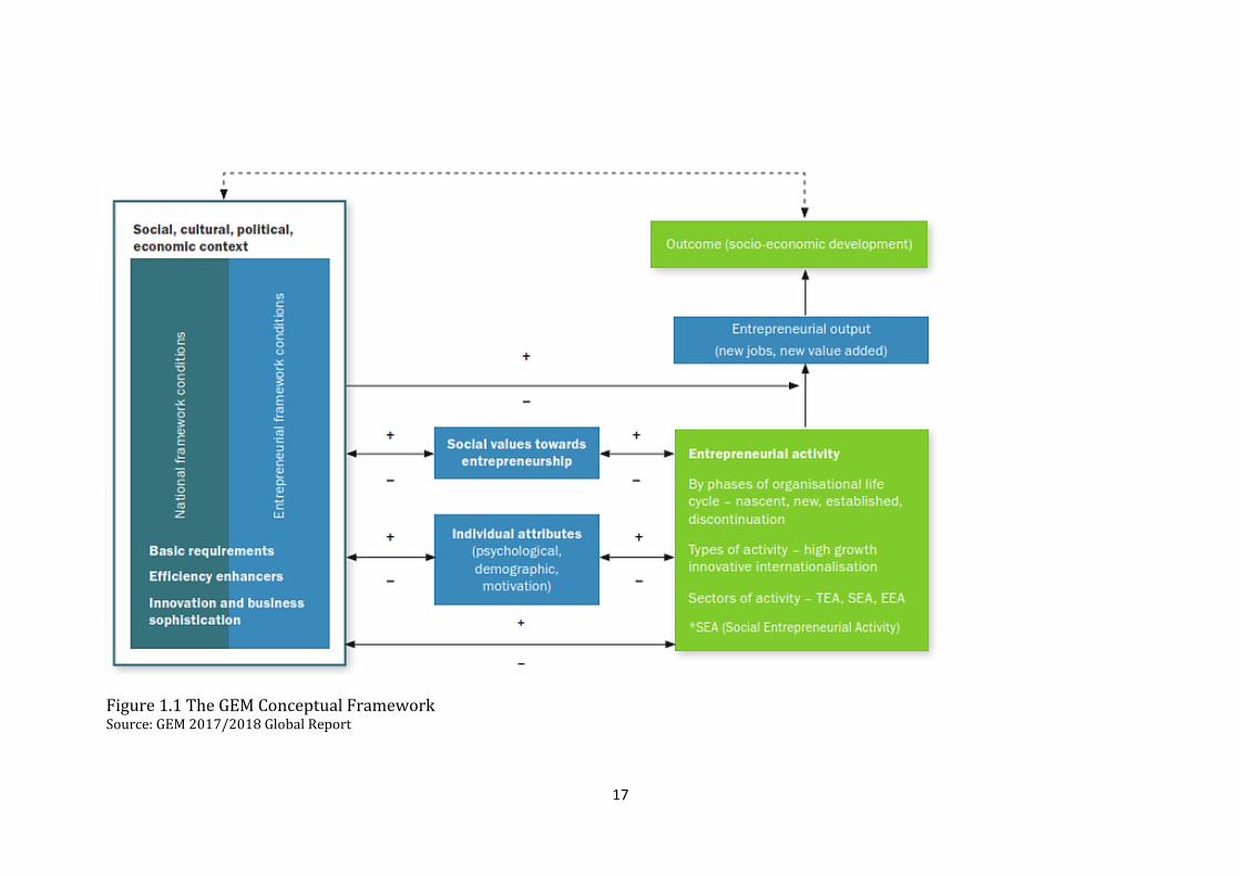
17
Figure 1.1 The GEM Conceptual Framework Source: GEM 2017/2018 Global Report
18
Fig. 1.2 presents the entrepreneurial process which represents different phases
and three important milestones, namely, conception, firm birth and persistence.
The two most relevant phases identified constitute the most widely used
indicator of GEM, the Total (early-stage) Entrepreneurial Activity (TEA). The TEA
is comprised of nascent entrepreneurship or the stage before the start of a new
firm, and the stage directly after the start of a new firm (owning-managing a new
firm younger than 3.5 years). TEA, therefore, represents the percentage of total
population (18 – 64 years) who are either nascent entrepreneur or owner-
manager of a new (younger than 3.5 years) business. The GEM – APS can also
identify individual and country-level entrepreneurial attitudes, i.e., potential
entrepreneurs as well as the category of established businesses (older than 3.5
years) and those who for different reasons discontinued their operations. Fig. 1.2
also shows some of the personal characteristics, such as age and gender that
might influence entrepreneurial attitudes and the entrepreneurial growth
aspirations of young businesses.
To conclude, the discussion in this section and also Fig 1.1 and Fig 1.2 show that
the focus of GEM toward entrepreneurship is unique in at least three ways. First,
GEM collects individual-level primary data on several personal attributes,
including the entrepreneurial aspirations, enabling a more comprehensive
approach toward the study of entrepreneurship and its impact on economic
outcomes. The rich dataset allows for investigating not only the country-level
differences in the rate of entrepreneurial activity but also the type of
entrepreneurial activity and entrepreneurial growth aspirations. Second, GEM
covers all phases of entrepreneurial activity (the entrepreneurship cycle),
including the conception stage and the more matured (established) stages of
entrepreneurial activity. Researchers can, perhaps, identify that different sets of
personal attributes and contextual factors play different roles in different phases
of the entrepreneurial cycle. Third, as GEM provides data on a global basis, it is
possible to make cross-country and also cross-regional comparisons, e.g.,
according to the stage of development, making GEM data a useful tool to
policymakers.
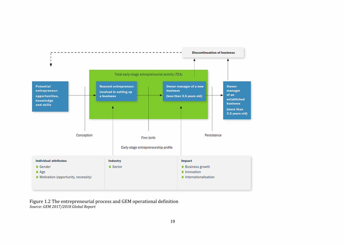
19
Figure 1.2 The entrepreneurial process and GEM operational definition Source: GEM 2017/2018 Global Report
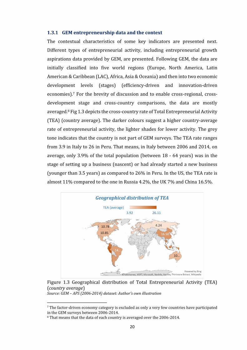
20
GEM entrepreneurship data and the context
The contextual characteristics of some key indicators are presented next.
Different types of entrepreneurial activity, including entrepreneurial growth
aspirations data provided by GEM, are presented. Following GEM, the data are
initially classified into five world regions (Europe, North America, Latin
American & Caribbean (LAC), Africa, Asia & Oceania) and then into two economic
development levels (stages) (efficiency-driven and innovation-driven
economies).7 For the brevity of discussion and to enable cross-regional, cross-
development stage and cross-country comparisons, the data are mostly
averaged.8 Fig 1.3 depicts the cross-country rate of Total Entrepreneurial Activity
(TEA) (country average). The darker colours suggest a higher country-average
rate of entrepreneurial activity, the lighter shades for lower activity. The grey
tone indicates that the country is not part of GEM surveys. The TEA rate ranges
from 3.9 in Italy to 26 in Peru. That means, in Italy between 2006 and 2014, on
average, only 3.9% of the total population (between 18 - 64 years) was in the
stage of setting up a business (nascent) or had already started a new business
(younger than 3.5 years) as compared to 26% in Peru. In the US, the TEA rate is
almost 11% compared to the one in Russia 4.2%, the UK 7% and China 16.5%.
Figure 1.3 Geographical distribution of Total Entrepreneurial Activity (TEA) (country average) Source: GEM – APS (2006-2014) dataset: Author’s own illustration
7 The factor-driven economy category is excluded as only a very few countries have participated in the GEM surveys between 2006-2014. 8 That means that the data of each country is averaged over the 2006-2014.
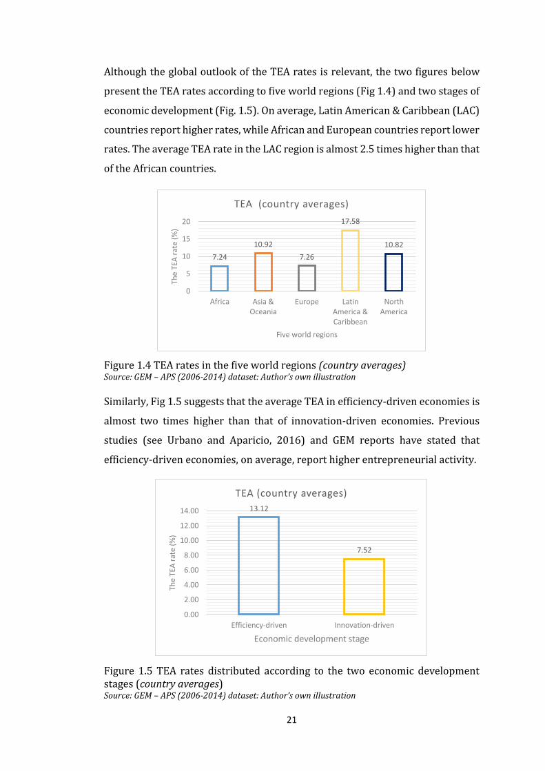
21
Although the global outlook of the TEA rates is relevant, the two figures below
present the TEA rates according to five world regions (Fig 1.4) and two stages of
economic development (Fig. 1.5). On average, Latin American & Caribbean (LAC)
countries report higher rates, while African and European countries report lower
rates. The average TEA rate in the LAC region is almost 2.5 times higher than that
of the African countries.
Figure 1.4 TEA rates in the five world regions (country averages) Source: GEM – APS (2006-2014) dataset: Author’s own illustration
Similarly, Fig 1.5 suggests that the average TEA in efficiency-driven economies is
almost two times higher than that of innovation-driven economies. Previous
studies (see Urbano and Aparicio, 2016) and GEM reports have stated that
efficiency-driven economies, on average, report higher entrepreneurial activity.
Figure 1.5 TEA rates distributed according to the two economic development stages (country averages) Source: GEM – APS (2006-2014) dataset: Author’s own illustration
7.24
10.92
7.26
17.58
10.82
0
5
10
15
20
Africa Asia &Oceania
Europe LatinAmerica &Caribbean
NorthAmerica
The
TEA
rat
e (%
)
Five world regions
TEA (country averages)
13.12
7.52
0.00
2.00
4.00
6.00
8.00
10.00
12.00
14.00
Efficiency-driven Innovation-driven
The
TEA
rat
e (%
)
Economic development stage
TEA (country averages)
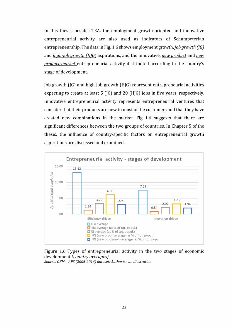
22
In this thesis, besides TEA, the employment growth-oriented and innovative
entrepreneurial activity are also used as indicators of Schumpeterian
entrepreneurship. The data in Fig. 1.6 shows employment growth, job growth (JG)
and high-job growth (HJG) aspirations, and the innovative, new product and new
product-market entrepreneurial activity distributed according to the country’s
stage of development.
Job growth (JG) and high-job growth (HJG) represent entrepreneurial activities
expecting to create at least 5 (JG) and 20 (HJG) jobs in five years, respectively.
Innovative entrepreneurial activity represents entrepreneurial ventures that
consider that their products are new to most of the customers and that they have
created new combinations in the market. Fig 1.6 suggests that there are
significant differences between the two groups of countries. In Chapter 5 of the
thesis, the influence of country-specific factors on entrepreneurial growth
aspirations are discussed and examined.
Figure 1.6 Types of entrepreneurial activity in the two stages of economic development (country averages)
Source: GEM – APS (2006-2014) dataset: Author’s own illustration
13.12
7.52
1.24 0.84
3.292.07
6.06
3.232.991.94
0.00
5.00
10.00
15.00
Efficiency-driven Innovation-driven
As
a %
of
tota
l po
pu
lati
on
Entrepreneurial activity - stages of development
TEA averageHJG average (as % of tot. popul.)JG average (as % of tot. popul.)INN (new prod.) average (as % of tot. popul.)INN (new prod&mkt) average (as % of tot. popul.)
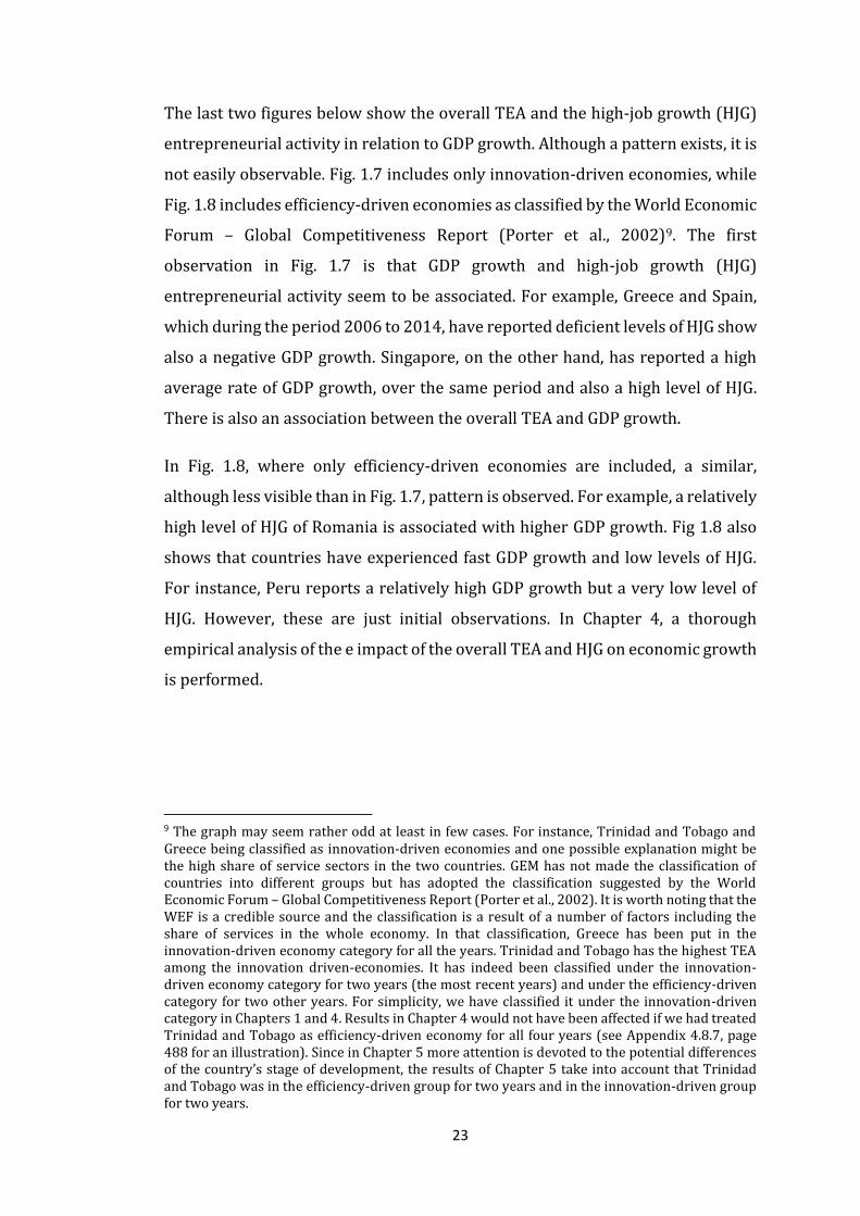
23
The last two figures below show the overall TEA and the high-job growth (HJG)
entrepreneurial activity in relation to GDP growth. Although a pattern exists, it is
not easily observable. Fig. 1.7 includes only innovation-driven economies, while
Fig. 1.8 includes efficiency-driven economies as classified by the World Economic
Forum – Global Competitiveness Report (Porter et al., 2002)9. The first
observation in Fig. 1.7 is that GDP growth and high-job growth (HJG)
entrepreneurial activity seem to be associated. For example, Greece and Spain,
which during the period 2006 to 2014, have reported deficient levels of HJG show
also a negative GDP growth. Singapore, on the other hand, has reported a high
average rate of GDP growth, over the same period and also a high level of HJG.
There is also an association between the overall TEA and GDP growth.
In Fig. 1.8, where only efficiency-driven economies are included, a similar,
although less visible than in Fig. 1.7, pattern is observed. For example, a relatively
high level of HJG of Romania is associated with higher GDP growth. Fig 1.8 also
shows that countries have experienced fast GDP growth and low levels of HJG.
For instance, Peru reports a relatively high GDP growth but a very low level of
HJG. However, these are just initial observations. In Chapter 4, a thorough
empirical analysis of the e impact of the overall TEA and HJG on economic growth
is performed.
9 The graph may seem rather odd at least in few cases. For instance, Trinidad and Tobago and Greece being classified as innovation-driven economies and one possible explanation might be the high share of service sectors in the two countries. GEM has not made the classification of countries into different groups but has adopted the classification suggested by the World Economic Forum – Global Competitiveness Report (Porter et al., 2002). It is worth noting that the WEF is a credible source and the classification is a result of a number of factors including the share of services in the whole economy. In that classification, Greece has been put in the innovation-driven economy category for all the years. Trinidad and Tobago has the highest TEA among the innovation driven-economies. It has indeed been classified under the innovation-driven economy category for two years (the most recent years) and under the efficiency-driven category for two other years. For simplicity, we have classified it under the innovation-driven category in Chapters 1 and 4. Results in Chapter 4 would not have been affected if we had treated Trinidad and Tobago as efficiency-driven economy for all four years (see Appendix 4.8.7, page 488 for an illustration). Since in Chapter 5 more attention is devoted to the potential differences of the country’s stage of development, the results of Chapter 5 take into account that Trinidad and Tobago was in the efficiency-driven group for two years and in the innovation-driven group for two years.
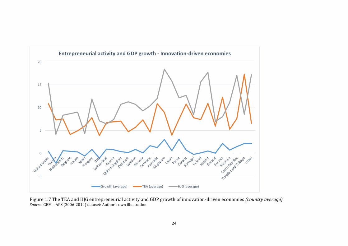
24
Figure 1.7 The TEA and HJG entrepreneurial activity and GDP growth of innovation-driven economies (country average)
Source: GEM – APS (2006-2014) dataset: Author’s own illustration
-5
0
5
10
15
20
Entrepreneurial activity and GDP growth - Innovation-driven economies
Growth (average) TEA (average) HJG (average)
25
Figure 1.8 The TEA and HJG entrepreneurial activity and GDP growth of efficiency-driven economies (country average) Source: GEM – APS (2006-2014) dataset: Author’s own illustration
-5
0
5
10
15
20
25
30
Entrepreneurial activity and GDP growth - Efficiency-driven economies
Growth (average) TEA (average) HJG (average)

STRUCTURE OF THE THESIS
This section presents the structure of the thesis, divided into six chapters. The
focus is on the methodology, research questions addressed and the expected
contributions of each chapter to the overall aims of the thesis.
The review of the literature on economic growth theories and the role of
entrepreneurship is provided in Chapter 2 of the thesis. In addition to the two
traditional growth theories, namely the neoclassical and endogenous growth
theories, Chapter 2 identifies that researchers have also framed their studies
using the Knowledge Spillover Theory of Entrepreneurship (KSTE) and the
Schumpeterian growth theory. The first objective (Objective 1) of the thesis is
addressed by this review of the relationship between entrepreneurship-
economic growth, through the lenses of economic growth theories. The review of
growth theories is followed by a comprehensive empirical review of the studies
that have investigated the impact of entrepreneurship on economic growth or
economic performance in general. Based on the choice of economic performance
measure used, the review of literature is divided into three subsamples. The first
subsample reviews studies that use GDP growth or growth of GDP per capita as
a proxy for economic performance. The second subsample consists of studies that
use employment growth as a measure of economic performance, while the third
subsection includes all ‘other’ measures of economic performance used by the
empirical studies of the field. The comprehensive review of empirical literature
addresses Objective 2 of the thesis.
Chapter 3 employs a Meta-Regression Analysis (MRA), to quantitatively review
the entrepreneurship-economic performance empirical literature. Similar to the
approach in Chapter 2, the identified primary literature (52 studies) is divided
into three subsamples, based on the choice of the measure of economic
performance. The findings (effect sizes) and the main characteristics of published
and unpublished primary literature investigating the relationship between
entrepreneurship and economic performance, over the 2000 – 2016 period, are
coded and included in the MRA database. Following the guidelines provided by
Stanley et al. (2013), the MRA uses Weighted Least Squares (WLS) and the Fixed

27
Effect (FE) estimators. In addition, robust estimator and the Bayesian Model
Averaging (BMA) methods are used to ensure the robustness of the results. By
applying MRA, Chapter 3 aims to determine: (i) the extent to which heterogeneous
samples and methodologies moderate the effect of entrepreneurship on economic
performance; (ii) the degree, if any, of publication selection bias in the literature;
and (iii) the average ‘genuine’ effect of entrepreneurship on economic performance,
beyond ‘publication bias’ and after controlling for sources of heterogeneity. Thus,
Chapter 3 addresses Objective 3 and Objective 4 of the thesis.
Following the findings of the MRA and the discussion in Chapter 2, Chapter 4
provides a cross-country empirical investigation of the effect of growth-oriented
and innovative entrepreneurial activity on economic growth. The focus on
growth-oriented and innovative entrepreneurial activity is influenced by the
work of Baumol (1990) and by the motivation to offer an investigation beyond
the exacerbated debate of opportunity vs necessity entrepreneurship. Moreover,
the chapter differs from the previous studies by employing static and dynamic
approach estimators. The use of the dynamic estimator, in particular, contributes
to the entrepreneurship-economic growth debate by distinguishing between
short and long-run effects of the entrepreneurship on economic growth and by
controlling for the potential presence of endogeneity. To the best of author’s
knowledge, this chapter is amongst the few to have used the ‘System’ GMM
approach to examine the impact of entrepreneurship on economic growth. The
data set used in this chapter is, an unbalanced panel based on GEM data for 48
countries (innovation-driven and efficiency-driven economies) over the 2006 –
2014 period. In addition to examining the effect of different measures of
entrepreneurship, including employment growth-oriented and innovative
entrepreneurial activity, Chapter 4 provides an analysis of the hypothesised
moderating effect of the countries’ stage of development. By providing an original
investigation, Chapter 4 addresses Objective 5 of the thesis.
To make the debate on growth-oriented entrepreneurial activity more
comprehensive, determinants of the individual-level entrepreneurial growth
aspirations are examined in Chapter 5. In this chapter, the individual-level
factors as well as the role of contextual factors, institutions and macroeconomic
28
environment, are used to determine the level of entrepreneurial growth
aspirations. In addition, Chapter 5 investigates the interplay between the two
groups of factors. Thus, Chapter 5 relies on multilevel modelling techniques. The
multi-stage structure (individual-level and country-level) allows investigating
the conjoint effect of individual factors (individual-level) and the institutions
(country-level) on young businesses and modelling the intra-cluster (cross-
country-year) correlation. Entrepreneurial growth aspirations of the young
businesses (up to 3.5 years) are examined using two dependent variables: (i)
employment growth aspirations (EGA), the expected increase in employment over
a five-year horizon; and (ii) high-job growth aspirations (HJG), focusing on those
young businesses that expect to create at least 20 jobs in five years time. The use
of two dependent variables with different measurement units, i.e., continuous
and dichotomous, requires applying two different estimators. The multilevel
(mixed-effects) linear estimator is used for the first dependent variable, while the
multilevel logistic estimator is used for the second. The empirical analysis is
initially performed on the full sample, 55 countries over the 2006 – 2013 period,
which is then divided into two subsamples (innovation-driven and efficiency-
driven economies). Using interaction terms, Chapter 5 investigates the
moderating effect of financial, and social capital on entrepreneurial growth
aspirations. Chapter 5 addresses Objective 6 of the thesis.
Chapter 6 provides a summary of the main findings of the thesis and highlights
its contributions to knowledge. Based on the main findings, a set of policy
recommendations are suggested (Objective 7). Chapter 6 also provides the
limitations of this thesis and the potential future work avenues.

29
2. Chapter 2
THEORETICAL AND EMPIRICAL LITERATURE ON
ENTREPRENEURIAL ACTIVITIES AND ECONOMIC
PERFORMANCE
INTRODUCTION ........................................................................................................................ 30
ECONOMIC GROWTH THEORIES AND ENTREPRENEURSHIP.............................. 31
Entrepreneurship and economic growth in the neoclassical growth
model …………………………………………………………………………………………………………32
Entrepreneurship and economic growth in the endogenous growth
model …………………………………………………………………………………………………………38
2.2.2.1 The Knowledge Spillover Theory of Entrepreneurship (KSTE) ............. 43
Schumpeterian growth theory .................................................................................. 48
REVIEW OF EMPIRICAL LITERATURE ............................................................................ 55
Evidence from studies using ‘growth’ as a measure of economic
performance ......................................................................................................................................... 57
Evidence from the studies using employment growth as a measure of
economic performance .................................................................................................................... 67
Evidence from studies using ’other’ dependent variables ............................ 76
CONCLUSIONS ........................................................................................................................... 84
30
INTRODUCTION
Chapter 1 provided an introduction to the nature, definition and measure of the
entrepreneurial activity and its potential contribution to the macroeconomic
growth. This chapter aims to provide a critical appraisal of the literature on
entrepreneurship-economic growth relationship and the underlying theories
supporting the hypothesised the relationship between the two. The
entrepreneurship-economic growth literature widely accepts the work of
Schumpeter (1934; 1942) and the process of ‘creative destruction’ as the crucial
contribution in the field (Wong et al., 2005; Aghion and Festre, 2017).
Schumpeter’s underlining argument was that increased entrepreneurial
activities, generated by the process of ‘creative destruction’ lead to increased
economic dynamism and growth (Wennekers and Thurik, 1999).
Recently, the relationship between entrepreneurship and economic growth has
becoming an increasingly attractive research topic (Urbano et al., 2018). The
work of Wennekers and Thurik (1999) which provided a conceptual framework
linking entrepreneurship to economic growth has also been regarded to have
influenced the subsequent volume of entrepreneurship-economic growth
literature. They have argued that studying the entrepreneurship-economic
growth relationship is a relevant topic to all societies as “economic growth is a key
issue both in economic policymaking and in economic research” Wennekers and
Thurik (1999, p.27). In general, entrepreneurship is viewed as an important
mechanism to achieve economic growth and development (Schumpeter, 1934;
Baumol, 1968; 1990; Carree et al., 2002; Audrestch and Keilbach 2004; 2008; van
Stel et al., 2005; Acs et al., 2008; Acs et al., 2012; Bosma, 2013; Aparicio et al.,
2016; Ferreira et al., 2017; Acs et al., 2018).
As Baumol (2010) points out, although the empirical studies have developed
significantly, especially in the last two decades, the theory of entrepreneurship
has not yet received the deserved place in the mainstream economic theory. In
an earlier study, Baumol (1968, p.66) argues that it is difficult to explain cross-
country macroeconomic growth differences without taking into account the
share and the type of entrepreneurial activity. Since then, the majority of
empirical studies investigating the impact of entrepreneurship on economic

31
growth, or economic performance, in general, find a positive and significant
association between the two (see Stam et al., 2010). Some studies, however, find
that there is a negative relationship between entrepreneurship and economic
performance (see Blanchflower, 2000), while others suggest that there is no
significant relationship between entrepreneurship and economic growth (see
Dejardin, 2001).
The rest of the chapter is organised as follows. Section 2 reviews the two most
prominent growth theories, namely neoclassical and endogenous growth,
specifically focusing on how the relationship between entrepreneurship and
economic growth is framed within these growth theories. In addition to these two
theories, the Knowledge Spillover Theory of Entrepreneurship (KSTE) and the
Schumpeterian theory of economic growth are also discussed in the second
section. Section 3 offers a comprehensive critical review of the empirical
literature on the entrepreneurship-economic performance relationship. Section
4 provides the conclusions of this chapter.
ECONOMIC GROWTH THEORIES AND ENTREPRENEURSHIP
The quest for identifying the key determinants of economic growth remains a
valid topic of interest for researchers (Levine and Renelt, 1992; Easterly and
Easterly, 2001; Helpman, 2004; Aghion and Festre, 2017). The one size-fits-all
country-level growth policy advice such as the 10-points policy
recommendations advocated by the so-called ‘Washington Consensus’, focussing
on three main areas of macroeconomic stabilisation, privatisation and market
liberalisation, (Rodrik, 2006), has not achieved the desired outcome. Hausmann
et al. (2005), opposing the idea of one policy fits all countries regardless of the
country’s stage of development, and especially of institutions, argue that
macroeconomic growth is to be analysed on a case-by-case approach.
Neoclassical growth theory is one of the first major contributions to provide a
growth model aiming to explain growth mechanics (Solow, 1956; Swan, 1956).
The work of Solow (1956), especially, has served as the origin of much of the
economics literature and to some extent as a platform for other growth models

32
(Solow, 2007).10 The key premise of the Solow’s neoclassical growth model is
that, besides of the contribution of classical factors (labour and capital), growth
can be explained by exogenously determined technological progress (Mankiw et
al., 1992; Wennekers and Thurik, 1999; Wong et al., 2005).
In the late 1980s, the endogenous growth theory (Romer, 1986; 1990; Lucas
1988; Grossman and Helpman, 1991; Aghion and Howitt, 1992) emerged. The
central premise of the endogenous growth theory is the assumption that growth
is endogenously determined by human capital and investment in knowledge (Acs
et al., 2003). Acknowledging the contribution of endogenous growth theory, in
this section, the Knowledge Spillover Theory of Entrepreneurship (KSTE) (Acs et
al., 2003; 2009) is also discussed. The main contribution of this theory to
entrepreneurship is that it considers entrepreneurs as the ‘missing link’,
converting general knowledge into economic and commercialised knowledge
and, therefore, positively affecting growth. The two traditional growth models,
the KSTE and the Schumpeterian theory of growth and how entrepreneurship is
incorporated into these models and theories are discussed in greater detail
below.
Entrepreneurship and economic growth in the neoclassical growth
model
As it is outlined earlier, the neoclassical growth model of Solow (1956) and Swan
(1956) was based on capital and labour enhancements. The Solow’s model
assumes constant returns to scale, diminishing marginal productivity of capital
and considers savings, population growth and technological advances as
exogenous. In subsequent years, the neoclassical growth model has been
augmented to also include advances in human capital (Barro, 1991; Mankiw et
al., 1992), government spending and international (trade) openness (Barro and
Sala-i-Martin, 1995; 2004). The neoclassical growth model contributed to the
debate of conditional convergence, suggesting that low per capita GDP countries
(low relative to the long-run or steady-state position) experience higher growth
10 Solow (2007) explains why the work of Swan (1956), although a similar neoclassical growth model based on the Cobb-Douglas production function, did not achieve the success and penetration to the economic literature as the work of Solow (1956).
33
rates (Barro and Sala-i-Martin, 2004).11 If economies have a different initial
condition (different per capita income) and share the same steady state
condition, the expectations are that low per capita economies grow faster than
the high per capita ones.12 In general, an economy will grow faster the further it
is from the technological frontier (steady state) (Jones and Romer, 2009).
As the basic neoclassical growth models (e.g., Solow’s (1956) growth model)
assume perfect information, the entrepreneur and especially Schumpeterian
type entrepreneurs, were explicitly absent and had no role assigned (Leibenstein,
1968; Wennekers and Thurik, 1999; Bjørnskov and Foss, 2013). The role of
entrepreneurship is, however, implicit in the neoclassical growth models as it
assumed to be in the production decisions (Urbano et al., 2018). Solow (2007,
p.11) acknowledges the developments in the entrepreneurship domain,
especially the literature on Knowledge Spillover Theory of Entrepreneurship,
and suggests that it would be a relevant augmentation to the explanatory power
of the growth theory if these ideas can be embodied in empirical growth models.
Solow’s (1957) empirical investigations suggested that a large part of US GDP
growth (87% to be more precise) is determined by exogenous technological
progress. After this study, the research community started to investigate and
finally endogenise the technological progress in the endogenous growth models
(Romer, 1986; 1990; Lucas, 1988).
The first step of the model used by Solow (1957) to explain the aggregate output
of the economy is expressed by the following production function equation:
𝑄 = 𝐹 (𝐾, 𝐿; 𝑡) (2.1)
Where, 𝑄 represents output and 𝐾 and 𝐿 represent capital and labour inputs in
"physical" units, whereas 𝑡 represents time which is included to allow for
technical change. To incorporate technical change in the equation, as a sperate
factor in addition to capital and labour, then Eq. (2.1) takes the following form.
11 According to Mankiw et al. (1992) the Solow model predicts convergence only after controlling for the determinants of the steady state, hence the term ‘conditional’. 12 Solow (1956) argues that because countries have different saving and population growth rates, they also have different steady-states.

34
𝑄 = 𝐹 (𝐾, 𝐿; 𝐴(𝑡)) (2.2)
Where, 𝐴(𝑡) measures the cumulated effect of shifts over time and allows
productivity changes over time without increasing the two “physical” factor
inputs. Eq. (2.2), is then differentiated with respect to time and divided by Q to
obtain the following equation:
�̇�
𝑄=
�̇�
𝐴+ 𝐴
𝜕𝑓
𝜕𝐾 �̇�
𝑄+ 𝐴
𝜕𝑓
𝜕𝐿
�̇�
𝑄 (2.3)
where �̇�, �̇� and �̇� represent the first order derivative of Q, K and L. Defining the
relative share of capital and labour as: 𝑤𝑘 = 𝜕𝑄
𝜕𝐾 𝐾
𝑄 and 𝑤𝐿 =
𝜕𝑄
𝜕𝐿
𝐿
𝑄 , Equation (2.3)
can be written as:
�̇�
𝑄=
�̇�
𝐴+ 𝑤𝐾
�̇�
𝐾+ 𝑤𝐿
�̇�
𝐿 (2.4)
Assuming that only two factors 𝐾 and 𝐿 explain total output, then 𝑤𝐾 and 𝑤𝐿
should always add up to one. In that case, applying Euler’s theorem, Solow arrives
at the equation below:
�̇�
𝑞=
�̇�
𝐴+ 𝑤𝑘
�̇�
𝑘 (2.5)
Thus, Eq. (2.5), which represents output per man hour, capital per man hour and
share of capital, is used to disentangle growth into the elements caused by capital
inputs and technical change, respectively (Solow, 1957, p.313; Acs et al., 2018,
p.503).
Mankiw et al. (1992), Barro and Sala-i-Martin (2004) and Romer (2011) have
extensively contributed to explaining the dynamics of Solow’s (1956; 1957)
growth model. To arrive at one of the equations, which Romer (2011) considers
to be the key equation of Solow’s growth model, let us use the same notations as
Mankiw et al. (1992) and Romer (2011), respectively. Thus, the new equation
which is a Cobb-Douglas production function including the ‘knowledge’ or
‘effectiveness of labour’ (A) takes the following form:
𝑌𝑡 = 𝐹 (𝐾𝑡, 𝐴𝑡𝐿𝑡) = 𝐾𝑡𝛼 (𝐴𝑡𝐿𝑡)1−𝛼 0 < 𝛼 < 1 (2.6)
35
Where 𝑌𝑡 denotes the output, 𝐾𝑡, represents capital and 𝐴𝑡𝐿𝑡 represents the
effective labour, t is for the time and α and 1-α denote the output elasticities of
capital and labour, respectively.13 Transforming Eq. (2.6), by dividing by the
technology-augmented labour 𝐴𝑡𝐿𝑡 , gives us the intensive form of the production
function:
𝑦𝑡 = (𝐾𝑡
𝐴𝑡𝐿𝑡)𝛼 = 𝑘𝑡
𝛼 (2.7)
Eq. (2.7) represents the situation where output per unit of effective labour 𝑦𝑡 is
a function of capital per unit of effective labour 𝑘𝑡 (Romer, 2011, p.11). To arrive
at the balanced growth path of an economy (also known as the steady state), Eq.
(2.7) needs to be augmented by the savings rate (s), a depreciation rate (δ) that
will avoid a decline in capital due to depreciation, the rate of technological
progress (g) and finally the growth rate of population (n). Now Eq. (2.7) can be
transformed into:
�̇�𝑡= sf(𝑘𝑡) – (n + g + δ) kt (2.8)
Eq. (2.8) which is also considered a key equation of Solow model, states that the
rate of change of the capital stock per unit of effective labour �̇�𝑡 is the difference
between actual investment per unit of effective labour sf(𝑘𝑡) and the so-called
break-even investment (n + g + δ) kt (Romer, 2011, p.16).14 Eq. (2.8) shows that
when actual investment per unit of effective labour is higher than the break-even
investment, the capital stock per unit of effective labour �̇�𝑡 is rising. When the
actual investment per unit of effective labour is lower than the break-even
investment, the capital stock per unit of effective labour �̇�𝑡 is falling. Finally, when
�̇�𝑡 = 0, the steady-state assumption holds, and the actual investment and break-
even investment are equal (Romer, 2011). Eq. (2.8) emphasises the role of
population growth and savings rate. Should the population grow fast, the capital
stock per unit of effective labour might decline. In the same vein, a shortage of
savings has a negative impact on the capital stock per unit of effective labour. An
13 Romer (2011, p.10) posits that technological progress that enters in this fashion is known as labour-augmenting or Harrod-neutral. If technological progress enters in the form Y = AF(K, L ), technological progress is Hicks-neutral. 14 The break-even investment represents the amount of investment required to keep k at its existing level.

36
increase in the savings, however, would have a positive impact. However, Romer
(2011) argues that changes in savings, population growth and in investment in
general impact only the short-run growth. Eq. (2.8) also shows that when the
actual investment and break-even investment are equal (the steady-state), the
long-run growth of per capita output (income) is depended on exogenously
determined factors, such as the technological progress.
The Solow’s neoclassical growth model has been subject to augmentations during
the early 1990s’. The inclusion of human capital by Mankiw et al. (1992) is one of
the most critical developments as it improves the model and came at a time when
economists were dismissing Solow's model over the endogenous growth models.
The estimates of savings and population growth had very large magnitudes in the
Solow’s growth model examples. Mankiw et al. (1992) found that when human
capital is included in the growth model, the estimates of savings and population
growth become smaller (they imply less bias) and at the same time the model’s
explanatory power increases as now it can account for up to 80% of the cross-
country variations.
Solow (1956; 1957) and Mankiw et al. (1992) growth models have been
augmented with new variables to account for the influence of government
spending (Sheehey, 1993), institutions (North, 1990; Acemoglu et al., 2005),
ideas (Romer, 1990), etc. For instance, Jones and Romer (2009), highlight the role
of human capital and argue that to be able to explain better the Solow’s residual,
a cross-country rather than a single country time-series approach should be
followed. Moreover, Jones and Romer (2009, p.20) argue that the cross-country
differences in the quality of institutions are also one of the potential sources of
varying levels of national income and Total Factor Productivity (TFP) growth
rates.
Concerning the impact of entrepreneurship on economic growth, a considerable
number of theoretical and empirical studies, use an augmented Solow (1956;
1957) model to include entrepreneurship as a determinant of growth. Iyigun and
Owen (1999), Audretsch and Keilbach (2004; 2005; 2007), Minniti and Levesque
(2010), Mateyovski et al. (2014), González-Pernía and Peña-Legazkue (2015),

37
Capello and Lenzi (2016), Prieger et al. (2016), Acs et al. (2018), are some of the
studies that use neoclassical growth model as a platform for their investigations.
For instance, Acs et al. (2018), adapting a standard Cobb-Douglas production
function, augment Eq. (2.2) to also include a measure of entrepreneurship. Hence,
the Solow-like equation (aggregate production function) used in their
investigation takes the following form:
𝑄 = 𝐹 (𝐾, 𝐿, 𝐸; 𝐴(𝑡)) (2.9)
Where, 𝐸 represents a measure of entrepreneurial activity at the country-level
and K, L, A represent the capital and labour inputs in physical units, and the
technical change, respectively. The authors argue that entrepreneurs serve a
critical function in the growth model by providing the link between inputs and
outputs by introducing new technologies and new production processes. Any
positive change in the production function is reflected in technical change and
ultimately output (Lafuente et al., 2016). For this to happen, Acs et al. (2018)
argue that a set of high quality institutions should be in place to enable an
increased level of entrepreneurial activity.
A similar approach is also followed by Capello and Lenzi (2016), where the
Solow’s model is used as a framework to include entrepreneurship measures in
the growth equation at the regional level. The following model specification is
used in their study.
𝛥𝐺𝐷𝑃_𝑝𝑐𝑟 = 𝛼𝑜 + β1GDP_pc𝑟 + β2𝛥𝑒𝑚𝑝𝑙𝑟 + β3𝛥𝐾𝑟 + β4𝐹𝐷𝐼𝑟 +
β5𝐶𝑜𝑚𝑝𝑒𝑡𝑒𝑛𝑐𝑖𝑒𝑠𝑟 + β6𝐸𝑑𝑢𝑐𝑎𝑡𝑖𝑜𝑛𝑟 + β7𝐸𝑛𝑡𝑟𝑒𝑝𝑟𝑒𝑛. 𝑐ℎ𝑎𝑟𝑎𝑐𝑡.𝑟+ ε𝑟 (2.10)
Eq. (2.10) includes the classic explanatory variables, such as the initial level of
GDP per capita, a measure of capital (based on Solow’s model), employment and
human capital (competencies and education), Foreign Direct Investment (FDI).
The dependent variable 𝛥𝐺𝐷𝑝_𝑝𝑐𝑟 denotes the changes in annual average real
GDP per capita growth rate (2006-2013). GDP_pc𝑟 on the right-hand side of the
equation represents the level of GDP per capita in 2006 (the first year of data).
All the variables are at the regional level 𝑟. Generally, the authors report a
positive relationship between entrepreneurship measures and regional growth.
The positive result is also suggested when entrepreneurship variables are

38
interacted with regional innovation dummies. The authors consider that
entrepreneurship directly and also indirectly (through the mediation of regional
innovation) impact economic growth at the regional level. This finding is a
significant contribution of the study in the indirect linkages between
entrepreneurship and growth at the regional level. In Chapter 4 and 5 of the
thesis, the importance of investigating the moderating impact of institutions and
the stages of development are highlighted through the use of various interaction
terms.
Entrepreneurship and economic growth in the endogenous growth
model
Researchers have credited the ability of endogenous growth models to explain
long-run growth within the model and not relying on exogenous technological
change or population growth (see Barro and Sala-i-Martin, 2004; Hasan and
Tucci, 2010; Aghion and Festre, 2017). Compared to the neoclassical growth
models, the endogenous growth models are characterised by the presence of
constant or increasing returns to scale (Lucas, 1988; Romer 1990; Barro; 1990;
Rebelo, 1991; Barro and Sala-i-Martin, 2004). Thus, according to the endogenous
growth theory, growth might happen for longer (even unlimited) time, as there
is no expectation that the broadly defined capital, i.e., a capital measure (K) that
includes human capital, will experience a diminishing marginal return even when
economies grow and develop (Barro and Sala-i-Martin, 2004, p.20).
The endogenous growth models (also known as idea-based or knowledge-based
models) have been extended continuously to include new factors and variables
such as R&D, knowledge, innovation (patents), and different policy measures
(Romer, 1990; Aghion and Howitt, 1992; Aghion and Festre, 2017). However, not
enough attention has been paid to directly model the impact of entrepreneurship
on economic growth (Aghion and Howitt, 1998; Friis et al., 2006; Aghion and
Festre, 2017). The endogenous growth theory, developed by Romer (1986;
1990), Lucas (1988), Grossman and Helpman (1991) and Aghion and Howitt
(1992; 1998), asserts that investment in knowledge and human capital are the
main driving forces of economic growth (Acs et al., 2003). As Audretsch and
Keilbach (2004) and Audretsch (2006) have pointed out, while physical capital

39
was considered at the heart of Solow (1956) growth model, the accumulation and
the creation of knowledge capital substituted it in the Romer’s (1986; 1990)
model. Moreover, the endogenous growth theory highlights that growth is
endogenously determined by the decisions of economic agents to seek profit-
maximising opportunities (Acs et al., 2003; Wong et al., 2005).
As noted above, the endogenous growth models have been continuously
augmented and modified. The simplest endogenous growth model which
satisfies the assumption of constant or increasing returns to capital is the AK
model (Barro and Sala-i-Martin, 2004):
𝛾𝑡 = 𝐴𝐾𝑡 (2.11)
In Eq. (2.11) technology is fixed, or changes in an exogenous manner and is
represented by 𝐴 (a positive constant) and 𝐾 denotes capital in the broad sense,
i.e., including also the human capital. Transforming Eq. (2.11) to look similar to
the Eq. (2.8) of the neoclassical growth model, leads to the following form of an
equation:
𝑌∗ = 𝑠𝐴 − (𝑛 + 𝛿) (2.12)
Note that Eq. (2.12) does not include the rate of technological progress (g) as in
Eq. (2.8). Hence, according to Barro and Sala-i-Martin (2004), the AK model of Eq.
(2.12) expressed in per capita terms, has the ability to explain the positive long-
run per capita growth even when technological progress is excluded from the
model. In other words, in a steady state, 𝑌∗ > 0 when 𝑠𝐴 > (𝑛 + 𝛿) suggesting
that in an economy described by the AK model, an increase in savings 𝑠 leads to
a higher long-run per capita growth. The same impact on the long-run growth per
capita rate is also achieved when the level of technology A increases. Both the
positive changes in technology level and the increase in savings might result from
governmental policies (Barro and Sala-i-Martin, 2004, p.64). Recalling Eq. (2.8)
of the neoclassical growth model, an increase in savings was reflected only on the
capital stock per unit of effective labour �̇�𝑡 and not on long-run per capita growth.
40
More complex endogenous growth models, also eliminating the tendency of
diminishing returns in the neoclassical models have been proposed by Romer,
(1990), Grossman and Helpman (1991) and Aghion and Howitt (1992). Eq. (2.13)
below represents a situation with two sectors, one where the output is produced,
the goods-producing sector, and one where the additions in the stock of
knowledge are generated, the R&D sector. Unlike capital, knowledge has the non-
excludability and non-rivalry feature, which means that if a piece of knowledge
is used in one place, its use in other places cannot be prevented, and that
knowledge capital does not diminish from being available to more users
(Braunerhjelm et al., 2010).15 That suggests that the full stock of knowledge is to
be used in both sectors. Following Romer (2011, p.103), Eq. (2.13), the output
producing sector, takes the following form:
𝑌(𝑡) = [(1 − 𝑎𝐾)𝐾(𝑡)]𝛼 [𝐴(𝑡)(1 − 𝑎𝐿)𝐿(𝑡)]1−𝛼, 0 < α < 1 (2.13)
Eq. (2.13) uses the standard notations, where, 𝑌 denotes output, 𝐾 denotes
capital, 𝐿 denotes labour, and 𝐴 denotes technology. The difference between Eq.
(2.13) and previous neoclassical equations is that the stock of labour (labour
force) and the stock of the capital is now divided (not necessarily equally)
between the two sectors. A part of the labour stock 𝑎𝐿 is used in the R&D sector
and the remaining part 1 − 𝑎𝐿 is used in the goods-producing sector. Likewise,
𝑎𝐾 represents the fraction of capital devoted to the R&D sector while 1 − 𝑎𝐾
represents the remaining fraction that has is used in the goods-producing
industry. The stock of capital and labour force are constant and exogenous. Eq.
(2.13) is assumed to be of a generalised Cobb-Douglas production form and
corresponds to the constant returns to capital and labour, meaning that a
duplication of inputs should lead the duplication of output, assuming that the
level of technology remains constant.
In the endogenous growth model, the generation of knowledge and ideas is
critical. Knowledge and idea generation is a function of the quantities of capital
and labour directed to R&D sector and technology enhancement. The equation
15 Note that non-excludability feature holds in situations where the absence of legal protection of knowledge and ideas exists. In other situations, e.g., the legal protection of patented ideas prohibits free use of knowledge and ideas (at least for some time).
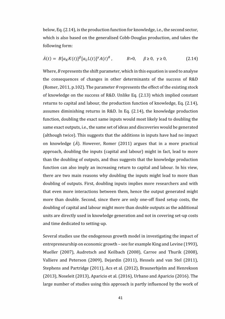
41
below, Eq. (2.14), is the production function for knowledge, i.e., the second sector,
which is also based on the generalised Cobb-Douglas production, and takes the
following form:
�̇�(𝑡) = 𝐵[𝑎𝐾𝐾(𝑡)]𝛽[𝑎𝐿𝐿(𝑡)]𝛾𝐴(𝑡)𝜃 , 𝐵>0, β ≥ 0, γ ≥ 0, (2.14)
Where, B represents the shift parameter, which in this equation is used to analyse
the consequences of changes in other determinants of the success of R&D
(Romer, 2011, p.102). The parameter θ represents the effect of the existing stock
of knowledge on the success of R&D. Unlike Eq. (2.13) which implied constant
returns to capital and labour, the production function of knowledge, Eq. (2.14),
assumes diminishing returns in R&D. In Eq. (2.14), the knowledge production
function, doubling the exact same inputs would most likely lead to doubling the
same exact outputs, i.e., the same set of ideas and discoveries would be generated
(although twice). This suggests that the additions in inputs have had no impact
on knowledge (�̇�). However, Romer (2011) argues that in a more practical
approach, doubling the inputs (capital and labour) might in fact, lead to more
than the doubling of outputs, and thus suggests that the knowledge production
function can also imply an increasing return to capital and labour. In his view,
there are two main reasons why doubling the inputs might lead to more than
doubling of outputs. First, doubling inputs implies more researchers and with
that even more interactions between them, hence the output generated might
more than double. Second, since there are only one-off fixed setup costs, the
doubling of capital and labour might more than double outputs as the additional
units are directly used in knowledge generation and not in covering set-up costs
and time dedicated to setting-up.
Several studies use the endogenous growth model in investigating the impact of
entrepreneurship on economic growth – see for example King and Levine (1993),
Mueller (2007), Audretsch and Keilbach (2008), Carree and Thurik (2008),
Valliere and Peterson (2009), Dejardin (2011), Hessels and van Stel (2011),
Stephens and Partridge (2011), Acs et al. (2012), Braunerhjelm and Henrekson
(2013), Noseleit (2013), Aparicio et al. (2016), Urbano and Aparicio (2016). The
large number of studies using this approach is partly influenced by the work of
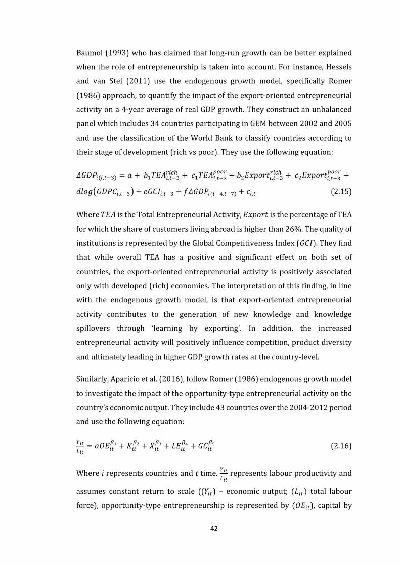
42
Baumol (1993) who has claimed that long-run growth can be better explained
when the role of entrepreneurship is taken into account. For instance, Hessels
and van Stel (2011) use the endogenous growth model, specifically Romer
(1986) approach, to quantify the impact of the export-oriented entrepreneurial
activity on a 4-year average of real GDP growth. They construct an unbalanced
panel which includes 34 countries participating in GEM between 2002 and 2005
and use the classification of the World Bank to classify countries according to
their stage of development (rich vs poor). They use the following equation:
𝛥𝐺𝐷𝑃𝑖(𝑖,𝑡−3) = 𝑎 + 𝑏1𝑇𝐸𝐴𝑖,𝑡−3𝑟𝑖𝑐ℎ + 𝑐1𝑇𝐸𝐴𝑖,𝑡−3
𝑝𝑜𝑜𝑟 + 𝑏2𝐸𝑥𝑝𝑜𝑟𝑡𝑖,𝑡−3𝑟𝑖𝑐ℎ + 𝑐2𝐸𝑥𝑝𝑜𝑟𝑡𝑖,𝑡−3
𝑝𝑜𝑜𝑟 +
𝑑𝑙𝑜𝑔(𝐺𝐷𝑃𝐶𝑖,𝑡−3) + 𝑒𝐺𝐶𝐼𝑖,𝑡−3 + 𝑓𝛥𝐺𝐷𝑃𝑖(𝑡−4,𝑡−7) + 휀𝑖,𝑡 (2.15)
Where 𝑇𝐸𝐴 is the Total Entrepreneurial Activity, 𝐸𝑥𝑝𝑜𝑟𝑡 is the percentage of TEA
for which the share of customers living abroad is higher than 26%. The quality of
institutions is represented by the Global Competitiveness Index (𝐺𝐶𝐼). They find
that while overall TEA has a positive and significant effect on both set of
countries, the export-oriented entrepreneurial activity is positively associated
only with developed (rich) economies. The interpretation of this finding, in line
with the endogenous growth model, is that export-oriented entrepreneurial
activity contributes to the generation of new knowledge and knowledge
spillovers through ‘learning by exporting’. In addition, the increased
entrepreneurial activity will positively influence competition, product diversity
and ultimately leading in higher GDP growth rates at the country-level.
Similarly, Aparicio et al. (2016), follow Romer (1986) endogenous growth model
to investigate the impact of the opportunity-type entrepreneurial activity on the
country’s economic output. They include 43 countries over the 2004-2012 period
and use the following equation:
𝑌𝑖𝑡
𝐿𝑖𝑡= 𝑎𝑂𝐸𝑖𝑡
𝛽1 + 𝐾𝑖𝑡𝛽2 + 𝑋𝑖𝑡
𝛽3 + 𝐿𝐸𝑖𝑡𝛽4 + 𝐺𝐶𝑖𝑡
𝛽5 (2.16)
Where i represents countries and t time. 𝑌𝑖𝑡
𝐿𝑖𝑡 represents labour productivity and
assumes constant return to scale ((𝑌𝑖𝑡) – economic output; (𝐿𝑖𝑡) total labour
force), opportunity-type entrepreneurship is represented by (𝑂𝐸𝑖𝑡), capital by

43
(𝐾𝑖𝑡), exports by (𝑋𝑖𝑡), life expectancy by (𝐿𝐸𝑖𝑡), and final government
consumption by (𝐺𝐶𝑖𝑡).16 They find that labour productivity is positively
influenced by opportunity entrepreneurship. They report that a 1% increase on
opportunity-type entrepreneurial activity, on average, is associated with a 0.04%
increase on labour productivity, ceteris paribus. When only Latin American
countries are included, the effect becomes much larger in magnitude (up to 0.62).
The applicability of endogenous growth models within the domain of the thesis,
has benefited significantly from the contribution of a group of authors, who have
introduced the knowledge filter and suggested the Knowledge Spillover Theory
of Entrepreneurship (KSTE) (Audretsch, 1995; Acs et al., 2003; 2009; 2013
Audretsch et al., 2005; Agarwal et al., 2007; 2010; Audretsch and Keilbach, 2008;
Braunerhjelm et al., 2010). The following subsection provides more details of this
branch of literature.
2.2.2.1 The Knowledge Spillover Theory of Entrepreneurship (KSTE)
One of the main criticisms of the knowledge-based endogenous growth models is
the assumptions that knowledge spillovers occur automatically, and that
knowledge directly translates into economic knowledge and macroeconomic
growth (Audretsch et al., 2005; Braunerhjelm et al., 2010). The Knowledge
Spillover Theory of Entrepreneurship (KSTE) claims that entrepreneurs are the
‘missing link’ in converting knowledge into economically relevant knowledge,
thereby facilitating knowledge diffusion and ultimately growth (Braunerhjelm et
al., 2010, p.105). Thus, Acs et al. (2013, p.758) claim that the KSTE provides a
framework which contributes to the understanding of microeconomic
foundations of the endogenous growth theory. Therefore, the KSTE framework
enables researchers to better explain the heterogeneity of regional and macro-
level economic growth rates (Acs et al., 2013). The original observation of
Audretsch (1995), who introduced the KSTE, was that, although new and small
firms generally have invested a negligible amount of resources (and money) in
R&D activities, they are still able to offer innovative products and services. He
attributes this outcome to the ability of entrepreneurs to exploit previously
16 Even though in the equation (2.16) of Aparicio et al. (2016), logarithms are not used, in their discussion they argue that they have used natural logarithms for institutional quality variables.

44
generated knowledge by R&D focused organisations, such as universities and
large incumbent firms’ R&D departments (Audretsch, 1995, p.179).
The logic of the KSTE framework to link entrepreneurship with growth, states
that entrepreneurs who enter the markets by using and commercialising existing
ideas and knowledge, which is previously generated by incumbent firms, serve
as a conduit for the spillover of knowledge. Further, Acs et al. (2009; 2018) argue
that by serving as a conduit (‘missing link’) for the spillover of knowledge, new
entrepreneurial entry promotes innovative activity leading to growth.
The focus of KSTE is not on the individual characteristics of the entrepreneur per
se but how a knowledge-rich context can influence an individual’s cognitive
process, especially opportunity recognition entrepreneurial abilities (Audretsch
et al., 2005; Busenitz et al., 2014). Since the work of Kirzner (1979) and Shane
and Venakataramen (2000), researchers have recognised ‘entrepreneurial
opportunities’ as a relevant entrepreneurial characteristic and sometimes even
try to define entrepreneurship by it. For instance, Krueger (2003, p.105)
considers that discovering opportunities is the core of entrepreneurship. In a
critical literature review, Davidsson (2015) identifies 210 papers that have used
the word ‘opportunity’ in their title, keywords, or abstract, suggesting that the
field of entrepreneurship pays significant attention to it.
However, what seems to have been missing in the set of studies that acknowledge
the role of ‘opportunities’, is the impact of context, e.g., the stock of knowledge
generated elsewhere and not already utilised (commercialised). As previously
stated, unlike other entrepreneurship theories which mostly rely on an
individual’s ability to identify and seize opportunities, the KSTE emphasis the
influence of context in shaping these individual-level entrepreneurial abilities. In
the view of Audretsch et al. (2005, pp.70-71), by analysing how context, and
specifically how the stock of existing uncommercialised knowledge and ideas in
the market, influence an individual’s decision-making toward entrepreneurship,
the KSTE is able to endogenise the process of entrepreneurial entry and
opportunity recognition.

45
As outlined earlier, the assumption of endogenous growth models and
specifically of Romer’s (1986; 1990) growth model, that knowledge spillovers
happen automatically, has motivated the conception of the KSTE. In the Romer’s
growth model, knowledge capital is assumed to be non-excludable and non-
exhaustive, which is consistent with Arrow (1962) work on the economics of
knowledge. However, Romer (1986) did not consider additional differences
between knowledge and the two traditional factors of production, namely
physical and human capital. According to Arrow (1962), new knowledge (new
and fresh ideas) or investment in new knowledge is characterised by a higher
degree of uncertainty, higher information asymmetry and higher transaction
costs than the two traditional factors of production (capital and labour). These
three characteristics might prevent new knowledge to automatically spillover
from one economic agent to another. Audretsch et al. (2005) argue that because
of these three conditions embedded in knowledge, some economic agents can
negatively evaluate a new potential opportunity, i.e., decide not to pursue it,
while at the same time another economic agent or team of economic agents might
think that the idea is worth pursuing and worth commercialising. If it hadn't been
for the latter economic agent or team of economic agents, that knowledge might
have remained uncommercialised, potentially with minimal impact on growth.
In an attempt to better explain this phenomenon, Acs et al. (2004) introduced the
term of ‘knowledge filter’, which represents the gap between general (new)
knowledge and what Arrow (1962) refers to as the economic or commercialised
knowledge. A large knowledge filter means that the gap between new knowledge
and economically relevant knowledge is more pronounced (Audretsch et al.,
2005). A similar approach to the knowledge filter is also proposed by
Braunerhjelm et al. (2010) who instead of ‘knowledge filter’ use the term
‘efficiency’. The ‘efficiency’ refers to the process of transforming knowledge into
economic knowledge. Braunerhjelm et al. (2010) identify two categories of
individuals in the economy that can transform knowledge, those employed in
knowledge (invention) producing sector (LR); and entrepreneurial (innovation)
sector (LE). In addition, the level of knowledge transformation efficiency (σ) (LR
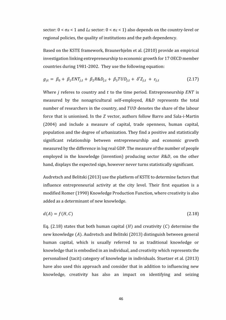
46
sector: 0 < σR < 1 and LE sector: 0 < σE < 1) also depends on the country-level or
regional policies, the quality of institutions and the path dependency.
Based on the KSTE framework, Braunerhjelm et al. (2010) provide an empirical
investigation linking entrepreneurship to economic growth for 17 OECD member
countries during 1981-2002. They use the following equation:
𝑔𝑗𝑡 = 𝛽0 + 𝛽1𝐸𝑁𝑇𝑗,𝑡 + 𝛽2𝑅&𝐷𝑗,𝑡 + 𝛽3𝑇𝑈𝐷𝑗,𝑡 + 𝛿′𝑍𝑗,𝑡 + 휀𝑗,𝑡 (2.17)
Where 𝑗 referes to country and 𝑡 to the time period. Entrepreneurship 𝐸𝑁𝑇 is
measured by the nonagricultural self-employed, 𝑅&𝐷 represents the total
number of researchers in the country, and 𝑇𝑈𝐷 denotes the share of the labour
force that is unionised. In the 𝑍 vector, authors follow Barro and Sala-i-Martin
(2004) and include a measure of capital, trade openness, human capital,
population and the degree of urbanization. They find a positive and statistically
significant relationship between entrepreneurship and economic growth
measured by the difference in log real GDP. The measure of the number of people
employed in the knowledge (invention) producing sector 𝑅&𝐷, on the other
hand, displays the expected sign, however never turns statistically significant.
Audretsch and Belitski (2013) use the platform of KSTE to determine factors that
influence entrepreneurial activity at the city level. Their first equation is a
modified Romer (1990) Knowledge Production Function, where creativity is also
added as a determinant of new knowledge.
𝑑(𝐴) = 𝑓(𝐻, 𝐶) (2.18)
Eq. (2.18) states that both human capital (𝐻) and creativity (𝐶) determine the
new knowledge (𝐴). Audretsch and Belitski (2013) distinguish between general
human capital, which is usually referred to as traditional knowledge or
knowledge that is embodied in an individual, and creativity which represents the
personalised (tacit) category of knowledge in individuals. Stuetzer et al. (2013)
have also used this approach and consider that in addition to influencing new
knowledge, creativity has also an impact on identifying and seizing

47
entrepreneurial opportunities. Audretsch and Belitski (2013) use the following
equation to determine factors that influence urban entrepreneurial activity:
𝐸𝑖 = 𝛽0 + 𝛽1𝑋𝑖 + 𝛽2𝑍𝑖 + 𝑎𝑖 + 𝑒𝑖 (2.19)
Where 𝐸𝑖 denotes urban entrepreneurial activity (1990-2010), which is
measured as the number of business registrations; self-employed and SMEs. 𝑋𝑖 is
a vector representing the creativity pillar, which distinguishes between workers
at the culture or entertainment sector and professionals in the finance, business
intermediation and management. 𝑍𝑖 is a vector of other country-level
institutional and control variables (some controls are also at the city-level). Their
main finding suggests that creativity has a positive and significant impact on city-
level entrepreneurial activity. They also find that the ‘thicknesses’ of the
knowledge filter, i.e., the efficiency with which knowledge is transformed into
economic knowledge, depends on the quality of institutions and that only a
fraction of general knowledge (human capital) and creativity achieve to be
converted into economically relevant knowledge.
The literature on Knowledge Spillover Theory of Entrepreneurship has provided
another direction of studying entrepreneurial entry. Authors of this direction
argue that there exists a spatial (geographic) dimension in the study of
knowledge spillovers. For instance, Audretsch and Lehmann (2005) and Fritsch
and Schmude (2007) argue that entrepreneurial activity tends to be spatially
localised, i.e., proximity to more intensive knowledge generation areas facilitates
entrepreneurial entry. More recently, Hundt and Sternberg (2014) find that
entrepreneurial entry in 15 European countries and regions (NUTS1/NUTS2) is
subject to both the individual level characteristics and the spatial context.
To sum up, the KSTE aims to more explicitly include entrepreneurship in the
endogenous growth theory by suggesting that entrepreneurs serve as the
missing link to transfer new knowledge into economically relevant knowledge
(facilitate the process of knowledge spillovers). Entrepreneurs identify and seize
opportunities that are made possible by new knowledge and have not been
appropriated or commercialised by incumbent firms or other economic agents.
Generally, countries rich in new knowledge tend to induce more entrepreneurial

48
activity, which will then further facilitate the process of knowledge spillover, i.e.,
the transformation of new knowledge into economic knowledge. Finally, higher
growth rates and job creation capacities are expected in contexts characterised
by higher levels of entrepreneurial activity. According to Braunerhjelm et al.
(2010, p.123), the augmentation of the endogenous growth model, with
entrepreneurship as the missing link, will narrow the gap between the model and
the real-world economy behaviour.
Schumpeterian growth theory
Aghion (2017, p.10) argues that although the Solow model has been the template
of growth models, nevertheless it fails to provide some of the understandings
which are relevant today. First, the long-run growth is dependent on
technological change, however, the model is unable to show how technological
progress is created. Second, some countries with low per capita GDP are still
unable to have faster growth rates of some countries with relatively high per
capita GDP. In addition, the idea of conditional convergence does not explain why
some countries are not converging to the per capita GDP of developed countries.
Third, the model ignores the firm perspective and, with that, the entrepreneur
from the original growth model. In the Solow model, the role of institutions and
the economic environment is also absent.
In contrast to the other growth theories, the Schumpeterian theory (Aghion and
Howitt, 1992; 1998) explicitly accounts for the impact of entrepreneurs and their
innovative behaviour through ‘creative destruction’ in macroeconomic growth
and development. Moreover, the Schumpeterian paradigm or growth theory put
entrepreneurs and firms in the heart of the growth process (Aghion and Festre
2017, pp. 28-29). Thus, the Schumpeterian (growth) theory (Aghion and Howitt,
1992; 1998; Aghion, 2017; Aghion and Festre, 2017) enables researchers to
theoretically and empirically justify the inclusion of entrepreneurship measures
in a growth model (Urabano et al., 2018).
The Schumpeterian growth theory derives from Schumpeter’s Theory of
Economic Development (1934) and Capitalism, Socialism and Democracy
(1942). Building on this literature, Aghion and Festre (2017), have provided
49
three main reasons that make the Schumpeterian paradigm a useful approach to
explain the growth process. The first reason is that innovation (Aghion, 2017
refers to innovative entrepreneurs), be it a product, process or organisational
innovation, is the source of long-run growth. Entrepreneurial efforts to bring new
products in the market, re-arrange production processes to improve productivity
and improve the efficiency of the organisational and production processes are all
part of the definition of entrepreneurship proposed by Schumpeter (1934).17
Fritsch (2017) argues that for Schumpeter, the critical function of
entrepreneurship for economic growth is the introduction and the
commercialisation of innovations and new combinations in the competitive
markets. The second reason is that profit or monopoly rents are the key
motivations that encourage firms and entrepreneurial ventures to invest in R&D
activities, new skills and to explore new market expansion opportunities. Thus,
in contexts where innovations can easily be expropriated, or when there is a lack
of appropriate institutions and specifically property right protection (see
Acemoglu and Robinson, 2002), innovative entrepreneurial entry and growth
will tend to be discouraged. The third reason is the concept of ‘creative
destruction’ (Schumpeter, 1942), whereby innovations replace or make the
existing (old) innovations obsolete. According to Aghion (2017, p.9), growth
processes involve a constant conflict between incumbents and new innovative
entrepreneurial entries, with incumbent firms trying to prevent new
entrepreneurial firms from entering markets.
The next analysis is a step by step explanation of the first attempt to integrate the
role of the entrepreneur in the growth models, i.e., the Aghion and Howitt (1992)
model of growth through creative destruction. In this growth model, Aghion and
Howitt (1992) suggest that entrepreneurs intentionally invest resources in R&D
activities to arrive at innovations, whereby old innovations are replaced, and
entrepreneurial firms earn a monopoly rent. The process of shifting resources is,
however, characterised by uncertainty as the outcome of the investment in R&D
17 Recalling the discussion in Chapter 1, Schumpeter (1934, p.66) assigned five roles to the entrepreneur: (1) The introduction of a new good; (2) The introduction of a new method of production; (3) The opening of a new market; (4) The conquest of a new source of supply of raw materials or half-manufactured goods; (5) the carrying out of the new organisation of any industry, like the creation of a monopoly position or the breaking up of a monopoly position.
50
and the potential innovation is not known ex-ante. This gives even more
importance to the function of the entrepreneur in this model.
The model of Aghion and Howitt (1992) assumes the three relevant variables in
the initial model, namely labour, an intermediate good (x) and a consumption
good (y). Labour is divided into two categories: (i) unskilled (M), used only in
producing the consumption good; (ii) skilled, used either in producing the
intermediate product or in the research sector. The amount of skilled labour used
in research is denoted by (n), and the remaining in producing the intermediate
good is indicated by (N-n). The quantity of both unskilled and the skilled labour
is fixed. The Cobb-Douglas type of production function in this situation takes the
following form:
𝑦𝑡 = 𝐴𝑡𝑥𝑡𝛼 0 < α < 1 (2.20)
Where t is the period index, and 𝐴𝑡 is the productivity parameter of the
intermediate input in period t, which is produced using the amount of skilled
labour not used in the research sector 𝑥𝑡 = 𝑁 − 𝑛𝑡 . It is assumed that
improvements in the productivity parameter, i.e., innovations arrive in random
sequence and follow a Poisson arrival rate 𝜆𝑛𝑡 (Aghion and Howitt, 1992; Howitt
and Aghion, 1998). In addition, it is assumed that innovation may arrive solely as
a result of the current flow of inputs devoted to research and that the prior
research experience and memory does not count. The period index t increases by
one unit each time an innovation arrives. It thus, represents the interval between
the old and new innovation which is assumed to arrive randomly. In other words,
the interval starts at t and ends at t+1, i.e., when new innovation arrives and has
an exponential distribution with parameter 𝜆𝑛𝑡. It is also assumed that prices
and quantities remain constant during the time intervals, i.e., constant during the
time interval between t to t+1. Aghion and Howitt (1992) introduce the creative
destruction feature here by suggesting that each innovation consists of a new
invention of the intermediate good which makes older inventions obsolete. The
new inventions are thus, assumed to increase the productivity (efficiency) of the
parameter 𝐴𝑡 by the following equation:
𝐴𝑡 = 𝐴0𝛾𝑡 γ > 1 (2.21)
51
Eq. (2.21) states the situation where innovation has arrived, is perhaps patented
and has provided monopoly rents to the successful inventor (firm or new
entrepreneurial venture). There is no time limit to the monopoly rents, however,
that is only a temporary monopoly power as it conditioned on the length of the
time interval. When the new invention arrives, at interval period t+1, the existing
innovation is assumed to become obsolete, and with that, the successful
innovator is assumed to lose the monopoly power. Except for the monopoly
power and profits, other market conditions are assumed to be perfectly
competitive. The equations below represent the situation where the innovator
tends to benefit from the temporary monopoly power by maximising its profit.
The consumption good sector chooses the amount of 𝑥𝑡, the intermediate good
sector, that maximizes 𝑦𝑡 = 𝑝𝑡 − 𝑥𝑡 . Hence, the first-order condition gives us the
following equation:
𝑝𝑡 = 𝛼𝐴𝑡𝑥𝑡𝛼−1 (2.22)
Where 𝑝𝑡 denoted the final price charged by the inventor (monopolist).
Moreover, to maximise the profit the monopolist choses (𝛼𝐴𝑡𝑥𝑡𝛼−1 − 𝜔𝑡)𝑥𝑡. The
wage of the skilled laborer is represented by 𝜔𝑡. Finally, the profit maximizing
condition is given by the following equation:
𝑝𝑡 = 𝜔𝑡
𝛼, 𝛱𝑡 = (
1−𝛼
𝛼) 𝜔𝑡𝑥𝑡 𝑎𝑛𝑑 𝑥𝑡 = (
𝜔𝑡
𝛼2 𝐴𝑡)
1/(𝛼−1)
(2.23)
Eq. (2.23) is considered to provide the notations and the key parameters that are
used for the stationary equilibrium value. In this situation, it is assumed that 𝑛𝑡 =
𝑛𝑡+1 = �̂�. Aghion and Howitt (1992) derive the following equation which shows
how the research in a stationary equilibrium �̂� is linked to the monopoly power
and how this is all related to the role of entrepreneur.
�̂� = 𝛾(1−𝛼)/𝛼
1+ 𝛾((1−𝛼)/𝛼 𝑁 −
𝑟
𝜆(1+ 𝛾((1−𝛼)/𝛼) (2.24)
Where, the constant rate of the time preference is denoted by r. Eq. (2.24) implies
that the higher the value of α, the lower is the monopolist market power.18Thus,
one of the basic ideas of Aghion and Howitt (1992) Schumpeterian growth model
18 The Lerner index is (1-α)
52
is that there should be some market power, i.e., some degree of imperfect
competition leading to monopoly rent to encourage research in the stationary
equilibrium. As it is outlined above, it is the entrepreneur who is now motivated
to invest in new knowledge generation (research) as there are monopoly rents
to be acquired. Aghion and Howitt (1992, p.366) argue that even the equation
that shows how the average growth rate (AGR) of real output, represented by
λ�̂�ln(𝛾), implies that a degree of imperfect competition is required for the growth
process.
However, the latter assumption, although not directly related to the topic of the
thesis but to the overall Schumpeterian growth theory, was after a few years
found not to hold. As outlined above, in the initial work of Aghion and Howitt
(1992), it was assumed that enhanced competition discourages investment in
R&D, as it negatively impacts monopoly power (rents). This assumption was
rejected by Blundell et al. (1995; 1999) who found, through a UK firm-level data
empirical investigation, that firms’ innovation and productivity growth is
positively correlated to competition. The findings of Blundell et al. (1995, 1999)
helped improve the initial Schumpeterian growth theory of Aghion and Howitt
(1992). In the subsequent works (Aghion et al., 1997; 2001) identified that firms’
reaction toward increased competition depends on the current position of the
firm in the market. They suggest that firms that are closer to the current
technological frontiers will be encouraged to innovate more, to escape
competition, when the increased rivalry is predicted. On the other hand, firms
that are far from the technological frontier, i.e., ‘laggard firms’ will be further
discouraged and demotivated to compete and invest in innovative activities. That
further suggests that the relationship between competition and innovation is not
linear but of an inverted U-shape, which is also confirmed by empirical
investigations (see e.g., Aghion et al., 2005; Aghion et al., 2009).19
The review of the literature identified a number of studies that have used
Schumpeterian theory when empirically investigating the relationship between
entrepreneurship and economic growth or economic development. There is also
19 The authorship in the 2009 study is shared with two of the authors of Blundell et al. (1995; 1999).
53
a significant number of theoretical studies which are mostly influenced by the
work of Schumpeter (1934; 1942) and also by the work of Aghion and Howitt
(1992; 1998). Some of the studies that use Schumpeterian theory include: Carree
et al. (2002, 2007), van Stel and Carree (2004), Sternberg and Wennekers (2005),
van Stel et al. (2005), Wong et al. (2005), Bosma (2013), van Oort and Bosma
(2013), Ferreira et al. (2017). For instance, van Oort and Bosma (2013) use data
on 111 regions across 14 European countries, between 2001 and 2006. The
equation they use has the following form:
𝑙𝑜𝑔𝑄𝑖𝑗 − 𝑙𝑜𝑔𝑁𝑖𝑗 = 𝛼𝑗 + 𝜃(𝑙𝑜𝑔𝑁𝑖𝑗 − 𝑙𝑜𝑔𝐴𝑖𝑗) + 𝜂𝐻𝑖𝑗 + 𝜌𝑆𝐷𝑖𝑗 + 𝜅𝐸𝑖𝑗 + 𝜈𝐼𝑖𝑗 + 𝜇𝐻𝑖𝑗
(2.25)
Where 𝑖 denotes regions, 𝑗 denotes countries, 𝑄 denotes value added at the
regional level, 𝑁 denotes employment density, 𝐴 denotes the acreage of the
region in square kilometres, 𝐸 denotes entrepreneurship, 𝐼 denotes invention, 𝐻
human capital, and 𝑆𝐷 denotes specialisation/diversity. They have used GEM
data to proxy for entrepreneurship. In total, four types of total entrepreneurial
activity TEA are utilised, namely (i) no growth TEA; (ii) some growth TEA; (iii)
high growth TEA; and (iv) innovation-oriented TEA. Generally, they find that
entrepreneurial activity, together with human capital and the degree of invention
are positively associated with regional output. The effect is more pronounced in
regions with large and medium-sized cities of the 14 European countries. They
conclude that entrepreneurial entry through innovations and growth-oriented
entrepreneurial activity can help explain the creative destruction mechanism.
In general, the review of the growth models and the theories of growth re-affirms
that the incorporation of entrepreneurship in the growth models is not
straightforward. The neoclassical growth models are part of the puzzle, as they
had ignored for so many years the role of entrepreneurs (Baumol, 1968; 2010).
Almost 50 years ago, Baumol (1968, p.68) had stated that in the neoclassical
growth models: “The theoretical firm is entrepreneurless – the Prince of Denmark
has been expunged from the discussion of Hamlet”. As mentioned earlier, in a
recent publication, however, Solow (2007) seems to recognise the role of
54
entrepreneurship and asserts that if entrepreneurship is in fact incorporated in
growth models, the overall explanatory power of the models may improve.
An additional complexity to the entrepreneurship-economic growth relationship
is perhaps the fact that for some time researchers were considering big firms
rather than small and entrepreneurial firms as the engine of growth (Audretsch
et al., 2002; Friis et al., 2006). The ‘managed’ economy relied on economies of
scale and scope, hence favouring large corporations (Audretsch and Thurik,
2001). Schumpeter (1942) himself had played a role in these developments, by
suggesting that most of the innovations happen in resourceful large corporations,
an approach that is later known as Schumpeter Mark II. Only when the shift from
the ‘managed’ to the ‘entrepreneurial’ economy, which emphasises the role of
knowledge and production flexibility, happened, the focus was directed to small
firms and entrepreneurial entry (Friis et al., 2006).
The shift to ‘entrepreneurial’ and ‘knowledge-based’ economy, in the early
1990s, and the emergence of endogenous growth models is recorded as a positive
development in the entrepreneurship-economic growth relationship. However,
even in the idea- and knowledge-based endogenous growth models,
entrepreneurship was still not included in the equation. As outlined earlier, even
in 2010, Baumol (2010) is still demanding that entrepreneurship receives its
deserved place in the mainstream economic theories. The Knowledge Spillover
Theory of Entrepreneurship was developed as an attempt to integrate the role of
entrepreneurship in the endogenous growth theory. Authors supporting this
approach (see Audretsch and Keilbach, 2008) claim that entrepreneurs serve as
a conduit of knowledge transfer. As it is elaborated in section 2.2.2.1, the
endogenous growth theory assumed that knowledge spillovers happen
automatically and in addition did not distinguish between general knowledge
and economically-relevant knowledge. The key contribution of the KSTE is that
entrepreneurship serves as the ‘missing link’ converting general knowledge into
economically relevant knowledge and affecting growth (Audrestsch, 1995;
Braunerhjelm et al., 2010). In this vein, Audretsch and Feldman (1996) argue that
the ability of entrepreneurs to influence the diffusion of knowledge among
economic agents can also be used to explain the significant impact of
55
entrepreneurship on economic growth, both at regional and country-level
studies.
Although the Schumpeterian theory of growth, advanced by Aghion and Howitt
(1992; 1998) is seen as the framework which supports the inclusion of
entrepreneurship in the growth models (Urbano et al., 2018), still studies tend to
find it challenging to provide theoretical justifications. Perhaps, due to the fact
that this approach is motivated by the process of ‘creative destruction’ and,
therefore, is mostly linked with innovative entry. In the view of the
Schumpeterian theory of growth, entrepreneurs are the individuals who can bear
the uncertainty of investing in R&D, even when the results are unknown, and
have the ability to identify and exploit new ideas and commercialise new
knowledge. Some studies using this theory, include both entrepreneurship and
innovation measures in one single equation (see Wong et al., 2005).
In summary, the two traditional growth theories and especially the neoclassical
growth model, provide comparatively little discussion on the direct role of
entrepreneurship on economic growth. However, researchers using the
neoclassical growth models have included entrepreneurship measures in the
growth equations, assuming that entrepreneurial decisions are to be found in the
production decisions (Urbano et al., 2018). Researchers using endogenous
growth theory, including the KSTE and the Schumpeterian approach, argue that
entrepreneurs bear the uncertainty of investment in knowledge generation
(innovations) and then help the new knowledge spillover, ultimately impacting
growth.
REVIEW OF EMPIRICAL LITERATURE
Despite the partial absence of entrepreneurship in the mainstream growth
model, the number of empirical studies considering entrepreneurship as an
essential ingredient of economic growth and economic development is
increasing (see Wong et al., 2005; Acs et al., 2008, 2012; Audretsch and Keilbach,
2008; Minniti and Lévesque, 2010; Hessels and van Stel, 2011; Bjørnskov and
Foss; 2013; Bosma, 2013; Audretsch et al., 2015; Urbano and Aparicio, 2016; Acs
et al., 2018; Urbano et al., 2018). According to the GEM reports (2015;

56
2017/2018), entrepreneurship serves as a driving force to national economic
growth, competitiveness and social well-being. Another channel highlighted in
the existing literature is that entrepreneurship contributes to economic growth
by commercialising and putting into practice new ideas and new knowledge
which if it was not for the entrepreneurs might have never seen the light (Acs and
Armington, 2006; Audretsch et al., 2006; Braunerhjelm et al., 2010; Acs et al.,
2013; Aghion and Festre, 2017). Reynolds et al. (2005) have emphasised job
creation as an outcome result of increased new venture creation and growth of
young existing firms. Similarly, Fritsch and Mueller (2004) argue that new firms
have an immediate and long-term impact on job creation. In their framework,
they argue that new entrants tend to grow themselves and improve the
competitive abilities of incumbent firms, thus resulting in increased performance
and employment opportunities at the regional or national level.
In a recent publication, Ferreira et al. (2017) argue that there are three attributes
usually assigned to entrepreneurship: (i) the creation of new economic
dynamism and activity (Schumpeterian entrepreneurship) (Schumpeter, 1934;
Davidsson et al., 2006; Aghion, 2017); (ii) identification and discovery of
entrepreneurial opportunities (Kirznerian entrepreneurship) (Shane and
Venkataraman, 2000; Bosma and Levie, 2010; Urbano and Aparicio, 2016); and
(iii) dissemination of innovation (Schumpeterian entrepreneurship) (Santarelli
and Vivarelli, 2007; Baumol, 2010, Öner and Kunday, 2016) which all lead to the
enhancement of economic performance. Nonetheless, not all the types of
entrepreneurial activity affect economic growth in the same way. As outlined
earlier Baumol (1990; 2010), argues that researchers should distinguish
between productive (innovative ventures; opportunity entrepreneurship) and
unproductive entrepreneurship (imitative and rent-seeking entrepreneurship.
The former is mostly reported to have a positive influence on economic growth
while the effect of the latter is ambiguous, if not negative. Yet, Reynolds et al.
(2005) maintain that any individual effort related to new venture creation has a
positive, at least indirect, influence on national economic activity.
The review of the literature confirms the multidimensional nature of
entrepreneurship, which has influenced the variability of measures of
57
entrepreneurship used. In addition, studies have also investigated different
economic outcomes, such as GDP growth, GDP at levels, labour productivity,
employment growth, etc as a measure of economic performance. These studies
have also used different methodological approaches and theoretical frameworks
to investigate the entrepreneurship-economic performance relationship. Thus,
given this heterogeneity in the literature, the three subsections below provide
separate reviews of: (i) studies that used GDP growth as a measure of economic
performance; (ii) studies that used employment growth as a measure of
economic performance; and (iii) studies that used GDP at levels and other
economic performance measures. The same approach is also used in the next
chapter (Chapter 3) when the MRA is performed.
Evidence from studies using ‘growth’ as a measure of economic
performance
The majority of studies investigating the impact of entrepreneurship on
economic performance use GDP growth or growth of GDP per capita as the
indicators of economic performance. With regard to the unit of analysis, the
review indicates that most of the previous studies use country rather than
regional or any other disaggregated levels. Table 2.1 below provides some of the
details of the studies that belong to this subsample. Studies are listed based on
alphabetical order of the name of the first author. Studies in Table 2.1, in general,
reported a positive association between entrepreneurship and economic growth
measures. For instance, Hessels and van Stel (2011) use two measures of GEM,
overall TEA and export-oriented new ventures, for a set of 34 countries between
2005 – 2008. They use OLS estimation and divide countries into higher-income
and lower-income to examine if countries’ stage of development influences the
impact of entrepreneurship on economic growth. They find that overall TEA has
a positive impact on economic growth of both higher- and lower-income
countries. However, the effect of export-oriented new ventures is positive and
significant only in the set of higher-income countries and positive but
insignificant in the set of lower-income countries. In their view, the positive
impact of export-oriented new ventures is linked with the knowledge spillovers
that are generated from exporting and learning processes which than have an
impact on GDP growth.
Table 2.1 Entrepreneurship and economic performance (GDP growth or GDP per capita used as a measure of economic growth)
Study Data
Study period Context (No. of obs.)
Theoretical framework
Estimation method/s
Level of analysis
Economic growth measure (dependent variable)
Entrepreneurial activity measure (source of the measure)
Main results (comments)
Acs et al. (2012)
Panel 18 developed countries 1981–1998 (110-268)
Endogenous growth & Knowledge Spillover Theory of Entrepreneurship (KSTE)
Feasible Generalised Least Squares (FGLS) &2SLS
Country The 5-year moving average of GDP per capita growth
Self-employed, as a percentage of total non-agricultural employ. (OECD - Statistical Compendium)
Mainly positive and significant results. Self-employment is found to impact GDP per capita growth positively.
Acs et al. (2018)
Panel 46 developed and developing countries 2002-2011 (414)
Neoclassical growth & Institutional approach
FE Country Real GDP growth - Logarithmic change (year to year) in real GDP at constant 2005 national prices in mil. 2005 US$
Global Entrepreneurship Index (GEI) (GEM)
The study reports a positive and significant association between GEI and real GDP growth.
Adusei (2016) Panel 12 developing countries 2004-2011 (46-70)
Endogenous growth theory
RE Country Natural logarithm of annual per capita GDP growth
Natural logarithm of the number of new businesses (IMF)
Positive and significant relationship between new businesses and the log of annual per capita GDP growth.
Beugelsdijk and Noorderhaven (2004)
Cross-section 54 EU developed regions (7 EU countries) 1950-1998 (54)
Not defined OLS Regional (54 region; NUTS)
Regional growth Entrepreneurial attitude: risk-taking propensity; and an innovative attitude (European Values Studies (EVS))
Entrepreneurial attitude has a positive and highly significant (at the 1%) impact on regional growth.
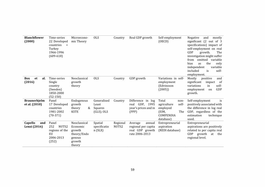
59
Blanchflower (2000)
Time-series 22 Developed countries + Turkey 1966-1996 (609-618)
Microecono-mic Theory
OLS Country Real GDP growth Self-employment (OECD)
Negative and mostly significant (2 out of 3 specifications) impact of self-employment on real GDP growth. The investigation might suffer from omitted variable bias as the only independent variable included is self-employment.
Box et al. (2016)
Time-series Single country (Sweden) 1850-2000 (52-150)
Neoclassical growth theory
OLS Country GDP growth Variations in self-employment (Edvinsson (2005))
Mostly positive and significant impact of variations in self-employment on GDP growth.
Braunerhjelm et al. (2010)
Panel 17 Developed countries 1981-2002 (70-371)
Endogenous growth theory & KSTE
Generalised Least Squares (GLS); OLS
Country Difference in log real GDP, 1995 year’s prices and in (PPP)
Total non-agriculture self-employed (EIM, The COMPENDIA database)
Self-employment is positively associated with the difference in log real GDP, regardless of the estimation technique used.
Capello and Lenzi (2016)
Panel 252 NUTS2 regions of the EU 2006-2013 (252)
Neoclassical Economic growth theory/Endogenous growth theory
Spatial specification (SLX)
Regional NUTS2
Average annual regional per capita real GDP growth rate 2006-2013
Entrepreneurial aspiration (REDI database)
Entrepreneurial aspirations are positively related to per capita real GDP growth at the regional level.
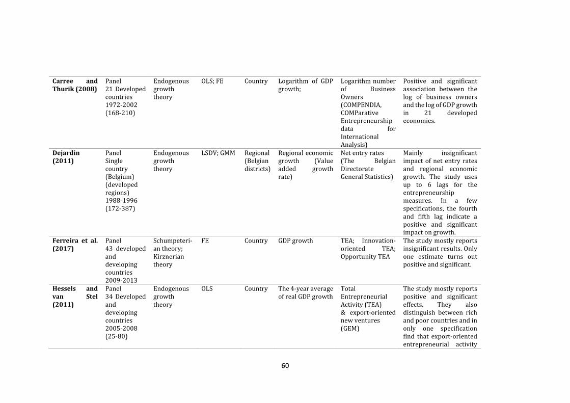
60
Carree and Thurik (2008)
Panel 21 Developed countries 1972-2002 (168-210)
Endogenous growth theory
OLS; FE Country Logarithm of GDP growth;
Logarithm number of Business Owners (COMPENDIA, COMParative Entrepreneurship data for International Analysis)
Positive and significant association between the log of business owners and the log of GDP growth in 21 developed economies.
Dejardin (2011)
Panel Single country (Belgium) (developed regions) 1988-1996 (172-387)
Endogenous growth theory
LSDV; GMM Regional (Belgian districts)
Regional economic growth (Value added growth rate)
Net entry rates (The Belgian Directorate General Statistics)
Mainly insignificant impact of net entry rates and regional economic growth. The study uses up to 6 lags for the entrepreneurship measures. In a few specifications, the fourth and fifth lag indicate a positive and significant impact on growth.
Ferreira et al. (2017)
Panel 43 developed and developing countries 2009-2013
Schumpeteri-an theory; Kirznerian theory
FE Country GDP growth TEA; Innovation-oriented TEA; Opportunity TEA
The study mostly reports insignificant results. Only one estimate turns out positive and significant.
Hessels and van Stel (2011)
Panel 34 Developed and developing countries 2005-2008 (25-80)
Endogenous growth theory
OLS Country The 4-year average of real GDP growth
Total Entrepreneurial Activity (TEA) & export-oriented new ventures (GEM)
The study mostly reports positive and significant effects. They also distinguish between rich and poor countries and in only one specification find that export-oriented entrepreneurial activity
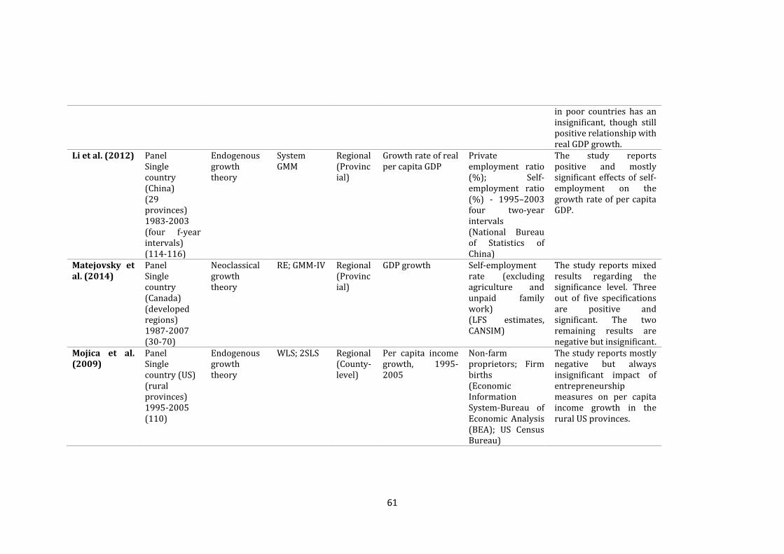
61
in poor countries has an insignificant, though still positive relationship with real GDP growth.
Li et al. (2012) Panel Single country (China) (29 provinces) 1983-2003 (four f-year intervals) (114-116)
Endogenous growth theory
System GMM
Regional (Provincial)
Growth rate of real per capita GDP
Private employment ratio (%); Self-employment ratio (%) - 1995–2003 four two-year intervals (National Bureau of Statistics of China)
The study reports positive and mostly significant effects of self-employment on the growth rate of per capita GDP.
Matejovsky et al. (2014)
Panel Single country (Canada) (developed regions) 1987-2007 (30-70)
Neoclassical growth theory
RE; GMM-IV Regional (Provincial)
GDP growth Self-employment rate (excluding agriculture and unpaid family work) (LFS estimates, CANSIM)
The study reports mixed results regarding the significance level. Three out of five specifications are positive and significant. The two remaining results are negative but insignificant.
Mojica et al. (2009)
Panel Single country (US) (rural provinces) 1995-2005 (110)
Endogenous growth theory
WLS; 2SLS Regional (County-level)
Per capita income growth, 1995-2005
Non-farm proprietors; Firm births (Economic Information System-Bureau of Economic Analysis (BEA); US Census Bureau)
The study reports mostly negative but always insignificant impact of entrepreneurship measures on per capita income growth in the rural US provinces.
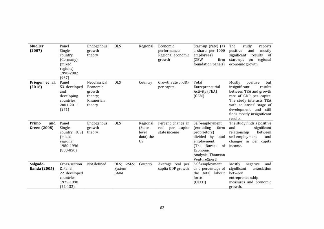
62
Mueller (2007)
Panel Single country (Germany) (mixed regions) 1990-2002 (937)
Endogenous growth theory
OLS Regional Economic performance: Regional economic growth
Start-up (rate) (as a share: per 1000 employees) (ZEW firm foundation panels)
The study reports positive and mostly significant results of start-ups on regional economic growth.
Prieger et al. (2016)
Panel 53 developed and developing countries 2001-2011 (271)
Neoclassical Economic growth theory; Kirznerian theory
OLS Country Growth rate of GDP per capita
Total Entrepreneurial Activity (TEA) (GEM)
Mostly positive but insignificant results between TEA and growth rate of GDP per capita. The study interacts TEA with countries’ stage of development and still finds mostly insignificant results.
Primo and Green (2008)
Panel Single country (US) (mixed regions) 1980-1996 (800-850)
Endogenous growth theory
OLS Regional (State-level data) the US
Percent change in real per capita state income
Self-employment (excluding farm proprietors) divided by total employment: (The Bureau of Economic Analysis; Thomson VentureXpert)
The study finds a positive and significant relationship between self-employment and changes in per capita income.
Salgado-Banda (2005)
Cross-section & Panel 22 developed countries 1975-1998 (22-132)
Not defined OLS; 2SLS; System GMM
Country Average real per capita GDP growth
Self-employment as a percentage of the total labour force (OECD)
Mostly negative and significant association between entrepreneurship measures and economic growth.
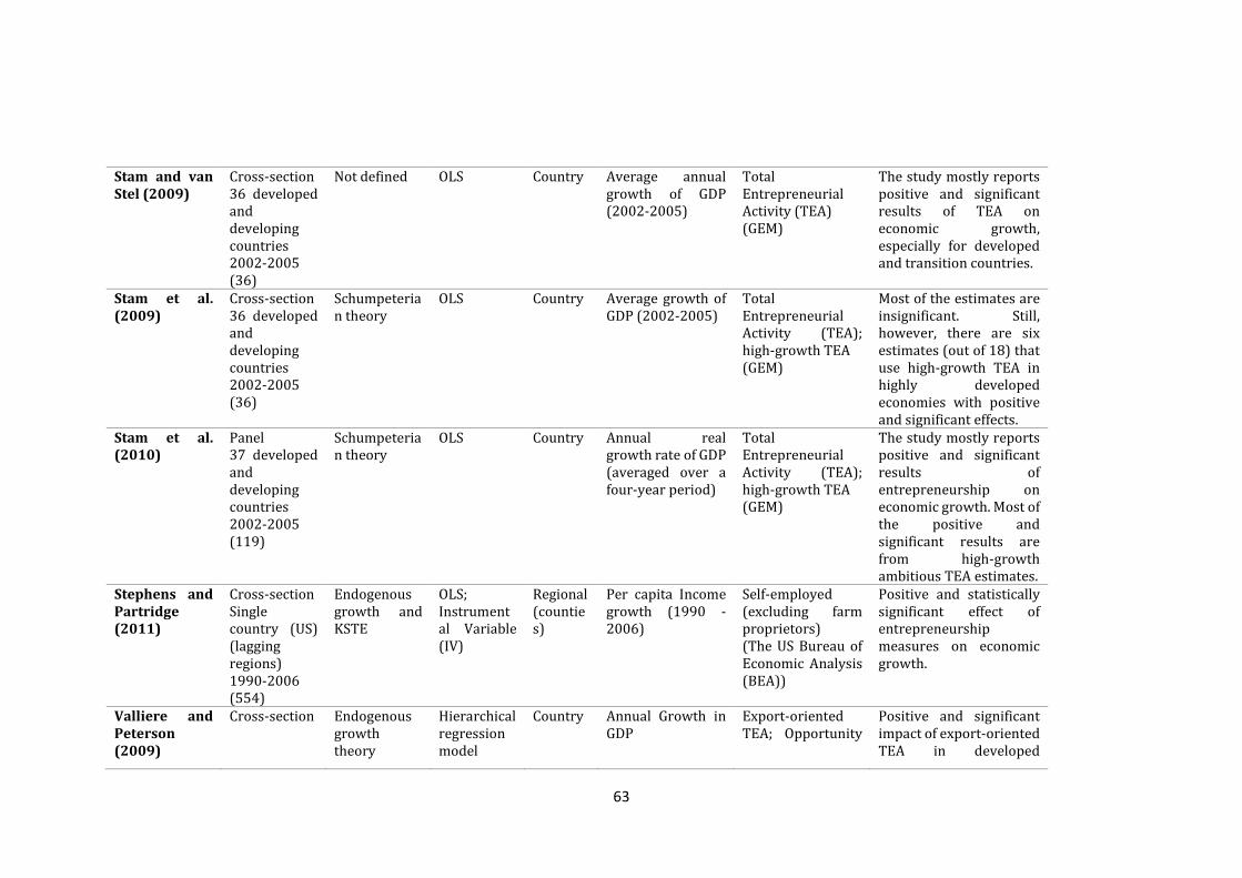
63
Stam and van Stel (2009)
Cross-section 36 developed and developing countries 2002-2005 (36)
Not defined OLS Country Average annual growth of GDP (2002-2005)
Total Entrepreneurial Activity (TEA) (GEM)
The study mostly reports positive and significant results of TEA on economic growth, especially for developed and transition countries.
Stam et al. (2009)
Cross-section 36 developed and developing countries 2002-2005 (36)
Schumpeterian theory
OLS Country Average growth of GDP (2002-2005)
Total Entrepreneurial Activity (TEA); high-growth TEA (GEM)
Most of the estimates are insignificant. Still, however, there are six estimates (out of 18) that use high-growth TEA in highly developed economies with positive and significant effects.
Stam et al. (2010)
Panel 37 developed and developing countries 2002-2005 (119)
Schumpeterian theory
OLS Country Annual real growth rate of GDP (averaged over a four-year period)
Total Entrepreneurial Activity (TEA); high-growth TEA (GEM)
The study mostly reports positive and significant results of entrepreneurship on economic growth. Most of the positive and significant results are from high-growth ambitious TEA estimates.
Stephens and Partridge (2011)
Cross-section Single country (US) (lagging regions) 1990-2006 (554)
Endogenous growth and KSTE
OLS; Instrumental Variable (IV)
Regional (counties)
Per capita Income growth (1990 - 2006)
Self-employed (excluding farm proprietors) (The US Bureau of Economic Analysis (BEA))
Positive and statistically significant effect of entrepreneurship measures on economic growth.
Valliere and Peterson (2009)
Cross-section Endogenous growth theory
Hierarchical regression model
Country Annual Growth in GDP
Export-oriented TEA; Opportunity
Positive and significant impact of export-oriented TEA in developed
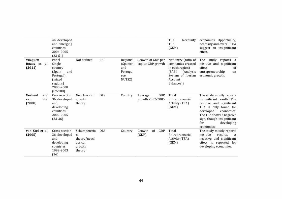
64
44 developed and emerging countries 2004-2005 (33-51)
TEA; Necessity TEA (GEM)
economies. Opportunity, necessity and overall TEA suggest an insignificant effect.
Vazquez-Rozas et al. (2011)
Panel Single country (Spain and Portugal) (mixed regions) 2000-2008 (87-188)
Not defined FE Regional (Spanish and Portuguese NUTS2)
Growth of GDP per capita; GDP growth
Net-entry (ratio of companies created in each region) (SABI (Analysis System of Iberian Account Balances))
The study reports a positive and significant effect of entrepreneurship on economic growth.
Verheul and van Stel (2008)
Cross-section 36 developed and developing countries 2002-2005 (33-36)
Neoclassical growth theory
OLS Country Average GDP growth 2002-2005
Total Entrepreneurial Activity (TEA) (GEM)
The study mostly reports insignificant results. The positive and significant TEA is only found for developed economies. The TEA shows a negative sign, though insignificant for developing economies.
van Stel et al. (2005)
Cross-section 36 developed and developing countries 1999-2003 (36)
Schumpeterian theory/neoclassical growth theory
OLS Country Growth of GDP (GDP)
Total Entrepreneurial Activity (TEA) (GEM)
The study mostly reports positive results. A negative and significant effect is reported for developing economies.
Similarly, Stam et al. (2009) use growth-oriented and ambitious
entrepreneurship for 36 developed and developing economies over 2002-2005.
They generally find that GDP growth is accelerated when there are more
ambitious entrepreneurs.20 The positive and significant effect of ambitious
entrepreneurship, utilised by employing TEA high-growth employment measure,
mostly holds for highly developed economies (see Wong et al., 2005; Stam et al.,
2010). However, in the analysis they find that transition economies benefit the
most (larger magnitude and significance level) from a higher share of ambitious
entrepreneurs, especially from the new ventures expecting to create more than
20 new jobs in 5 years. A more recent study, Prieger et al. (2016), uses a larger
sample of countries (53) and a longer period (2001-2011) confirms the findings
of the previous researchers. In addition, the authors investigate the optimal level
of entrepreneurial activity which would positively influence growth. They argue
that even though less-developed economies, usually experience higher rates of
entrepreneurial activity, still the number of entrepreneurs is not optimal for the
countries to catch on the desired economic growth rates. Most of the empirical
studies in the first subsample (11 out of 27) have sourced their entrepreneurship
data from the GEM (e.g., van Stel et al., 2005; Stam et al., 2010; Ferreira et al.,
2017; Acs et al. 2018).
Other studies have also used self-employment, which in most situations is
adjusted to exclude the agriculture sector, the number of business owners, net-
entry, etc. For instance, using the number of business owners as a measure of
entrepreneurship, Carree and Thurik (2008) found that economic growth,
measured by GDP growth, is positively affected by entrepreneurship (in most of
the specifications). The study uses OLS and fixed effect (FE) estimator and
includes 21 developed countries over the 1972 – 2002 period. Carree and Thurik
(2008) use different lag structures to identify if there exists a time-lag when the
effect of entrepreneurship on economic growth becomes more pronounced. They
find that there is an immediate and positive impact of new businesses, which is
then followed by a negative effect. According to the authors, the negative effect is
20 The term ambitious is used interchangeably with aspirations, growth-oriented and growth-expectations

66
suggested to appear as the new businesses distort the market and influence the
exit of some incumbent firms. Finally, in the last stages, the positive impact of
entrepreneurship on economic growth re-appears. The study, however, lacks a
well-specified model as it does not account for the impact of any of the traditional
explanatory variables or controls of growth equations. The situation, where
studies omit the classic variables suggested by the theory, will be accounted in
the Meta-Regression Analysis (MRA) chapter (Chapter 3).
Studies that have used self-employment report mixed results. For example, using
self-employment (self-employment as a: (i) % of total employment; (ii) % of
labour force; and (iii) % of population age 16-64), Blanchflower (2000), finds
negative and statistically significant effect on real GDP growth for 22 developed
economies and Turkey between 1966-1996. Similar to Carree and Thurik (2008),
the study might be subject to the omitted variable bias. The estimated models
include changes in the number of employees, country dummies and a lagged
dependent variable; however, do not control for other factors such as capital,
human capital, institutions or other macroeconomic country characteristics.
Failure to include such control variables might result in potentially biased
estimates. Another group of studies in Table 2.1 use the framework of the
Knowledge Spillover Theory of Entrepreneurship (KSTE) and suggest that
entrepreneurial activity serves as the mechanism facilitating the
commercialisation of knowledge, leading to more start-ups, enhanced economic
activity and economic growth (Acs et al., 2004; Audretsch and Keilbach, 2004).
Following this framework, Acs et al. (2012) report a positive association between
entrepreneurship and economic growth in 18 developed countries for the 1981
– 1998 period. This study emphasises the role of entrepreneurs serving as a
channel allowing the new knowledge to spillover and facilitate entrepreneurial
entry.
Although researchers have highlighted the benefits of cross-country over single-
country studies (e.g., Wong et al., 2005; Acs et al., 2014), still there are several
studies that have investigated the effect on a single-country structure. These
studies use regions (NUTS1-NUTS3), districts or provinces, within countries, as
the unit of analysis. Using net entry rates as a proxy for entrepreneurship,

67
Dejardin (2011) found that there is an insignificant (and mostly negative)
relationship between regional growth rates in the 43 Belgian districts
(arrondissements) and business activity. The study uses lagged values for the
measure of entrepreneurship and the only positive and significant relationship
between net entry, and regional growth is suggested between the fourth and fifth
lag, although not for all the specifications. Vazquez-Rozas et al. (2011) include
regions (NUTS2) of the two neighbouring countries, Spain and Portugal, and find
that net entry is positively associated to regional economic growth over the 2000
– 2008 period. Unlike Dejardin (2011), the study of Vazquez-Rozas et al. (2011)
seems to have followed the theoretical suggestions and has included a set of
control variables, such as capital, labour, human capital, social capital, innovation
and a measure for Foreign Direct Investment (FDI).
Primo and Green (2008) and Stephens and Partridge (2011) use self-
employment and find that growth rates of several US regions are positively
influenced by entrepreneurship. While Primo and Green (2008) include mixed
regions (mixed in terms of the stage of development), Stephens and Partridge
(2011) include only laggard regions. Primo and Green (2008) use only OLS
estimator for the analysis, whereas Stephens and Partridge (2011) use OLS and
instrumental variable (IV) approach. Some additional details for most of the
studies in Table 2.1 will be provided in Chapter 3, where the MRA is performed.
Evidence from the studies using employment growth as a measure
of economic performance
Table 2.2 below provides details of the studies that use employment growth or
changes in employment as a measure of economic performance. These studies
have mainly used start-up rates as a measure of entrepreneurial activity and the
analysis are mostly performed within a single-country context (see Mueller et al.,
2008).21
21 Some studies refer to start-up rates as ‘formation rates’, ‘firm birth rates’, etc.
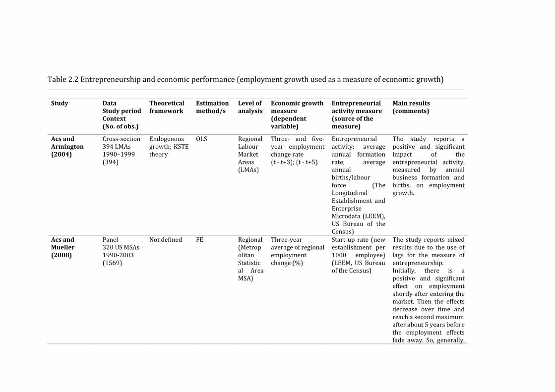
Table 2.2 Entrepreneurship and economic performance (employment growth used as a measure of economic growth)
Study Data Study period Context (No. of obs.)
Theoretical framework
Estimation method/s
Level of analysis
Economic growth measure (dependent variable)
Entrepreneurial activity measure (source of the measure)
Main results (comments)
Acs and Armington (2004)
Cross-section 394 LMAs 1990–1999 (394)
Endogenous growth; KSTE theory
OLS Regional Labour Market Areas (LMAs)
Three- and five-year employment change rate (t - t+3); (t - t+5)
Entrepreneurial activity: average annual formation rate; average annual births/labour force (The Longitudinal Establishment and Enterprise Microdata (LEEM), US Bureau of the Census)
The study reports a positive and significant impact of the entrepreneurial activity, measured by annual business formation and births, on employment growth.
Acs and Mueller (2008)
Panel 320 US MSAs 1990-2003 (1569)
Not defined FE Regional (Metropolitan Statistical Area MSA)
Three-year average of regional employment change (%)
Start-up rate (new establishment per 1000 employee) (LEEM, US Bureau of the Census)
The study reports mixed results due to the use of lags for the measure of entrepreneurship. Initially, there is a positive and significant effect on employment shortly after entering the market. Then the effects decrease over time and reach a second maximum after about 5 years before the employment effects fade away. So, generally,
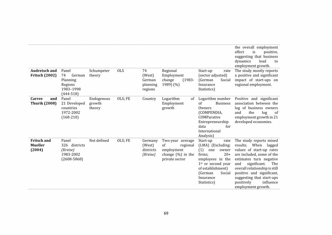
69
the overall employment effect is positive, suggesting that business dynamics lead to employment growth.
Audretsch and Fritsch (2002)
Panel 74 German Planning Regions 1983–1998 (444-518)
Schumpeter theory
OLS 74 (West) German planning regions
Regional Employment change (1983-1989) (%)
Start-up rate (sector adjusted) (German Social Insurance Statistics)
The study mostly reports a positive and significant impact of start-ups on regional employment.
Carree and Thurik (2008)
Panel 21 Developed countries 1972-2002 (168-210)
Endogenous growth theory
OLS; FE Country Logarithm of Employment growth
Logarithm number of Business Owners (COMPENDIA, COMParative Entrepreneurship data for International Analysis)
Positive and significant association between the log of business owners and the log of employment growth in 21 developed economies.
Fritsch and Mueller (2004)
Panel 326 districts
(Kreise) 1983-2002 (2608-5868)
Not defined OLS; FE Germany (West) districts (Kreise)
Two-year average of regional employment change (%) in the private sector
Start-up rate (LMA) (Excluding: (1) one owner firms; 20+ employees in the 1st or second year of establishment) (German Social Insurance Statistics)
The study reports mixed results. When lagged values of start-up rates are included, some of the estimates turn negative and significant. The overall relationship is still positive and significant, suggesting that start-ups positively influence employment growth.
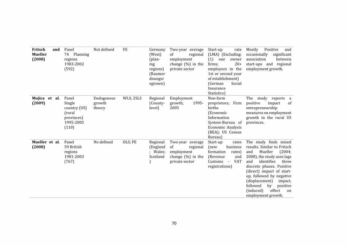
70
Fritsch and Mueller (2008)
Panel 74 Planning regions 1983-2002 (592)
Not defined FE Germany (West) (plan-ing regions) (Raumordnungsregionen)
Two-year average of regional employment change (%) in the private sector
Start-up rate (LMA) (Excluding: (1) one owner firms; 20+ employees in the 1st or second year of establishment) (German Social Insurance Statistics)
Mostly Positive and occasionally significant association between start-ups and regional employment growth.
Mojica et al. (2009)
Panel Single country (US) (rural provinces) 1995-2005 (110)
Endogenous growth theory
WLS; 2SLS Regional (County-level)
Employment growth, 1995-2005
Non-farm proprietors; Firm births (Economic Information System-Bureau of Economic Analysis (BEA); US Census Bureau)
The study reports a positive impact of entrepreneurship measures on employment growth in the rural US provinces.
Mueller et al. (2008)
Panel 59 British regions 1981-2003 (767)
No defined OLS; FE Regional (England; Wales; Scotland)
Two-year average of regional employment change (%) in the private sector
Start-up rates (new business formation rates) (Revenue and Customs – VAT registrations)
The study finds mixed results. Similar to Fritsch and Mueller (2004; 2008), the study uses lags and identifies three discrete phases. Positive (direct) impact of start-up, followed by negative (displacement) impact, followed by positive (induced) effect on employment growth.
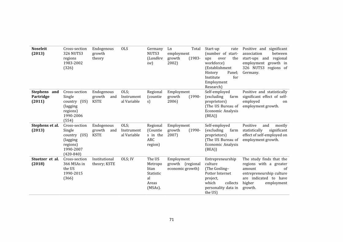
71
Noseleit (2013)
Cross-section 326 NUTS3 regions 1983-2002 (326)
Endogenous growth theory
OLS Germany NUTS3 (Landkreise)
Ln Total employment growth (1983-2002)
Start-up rate (number of start-ups over the workforce) (Establishment History Panel; Institute for Employment Research)
Positive and significant association between start-ups and regional employment growth in 326 NUTS3 regions of Germany.
Stephens and Partridge (2011)
Cross-section Single country (US) (lagging regions) 1990-2006 (554)
Endogenous growth and KSTE
OLS; Instrumental Variable
Regional (counties)
Employment growth (1990-2006)
Self-employed (excluding farm proprietors) (The US Bureau of Economic Analysis (BEA))
Positive and statistically significant effect of self-employed on employment growth.
Stephens et al. (2013)
Cross-section Single country (US) (lagging regions) 1990-2007 (420-840)
Endogenous growth and KSTE
OLS; Instrumental Variable
Regional (Counties in the ARC region)
Employment growth (1990-2007)
Self-employed (excluding farm proprietors) (The US Bureau of Economic Analysis (BEA))
Positive and mostly statistically significant effect of self-employed on employment growth.
Stuetzer et al. (2018)
Cross-section 366 MSAs in the US 1990-2015 (366)
Institutional theory; KSTE
OLS; IV The US Metropolitan Statistical Areas (MSAs).
Employment growth (regional economic growth)
Entrepreneurship culture (The Gosling–Potter Internet project, which collects personality data in the US)
The study finds that the regions with a greater amount of entrepreneurship culture are indicated to have higher employment growth.
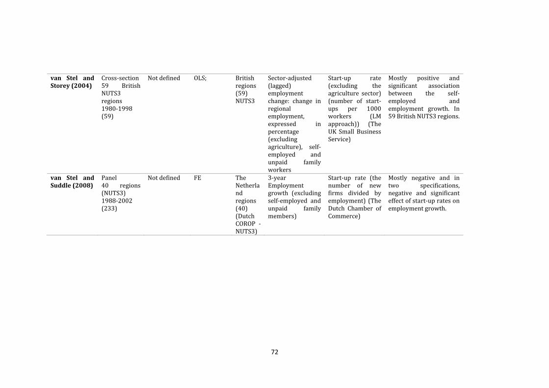
72
van Stel and Storey (2004)
Cross-section 59 British NUTS3 regions 1980-1998 (59)
Not defined OLS; British regions (59) NUTS3
Sector-adjusted (lagged) employment change: change in regional employment, expressed in percentage (excluding agriculture), self-employed and unpaid family workers
Start-up rate (excluding the agriculture sector) (number of start-ups per 1000 workers (LM approach)) (The UK Small Business Service)
Mostly positive and significant association between the self-employed and employment growth. In 59 British NUTS3 regions.
van Stel and Suddle (2008)
Panel 40 regions (NUTS3) 1988-2002 (233)
Not defined FE The Netherland regions (40) (Dutch COROP -NUTS3)
3-year Employment growth (excluding self-employed and unpaid family members)
Start-up rate (the number of new firms divided by employment) (The Dutch Chamber of Commerce)
Mostly negative and in two specifications, negative and significant effect of start-up rates on employment growth.
The use of employment growth as a measure of economic growth or economic
performance in general has been criticised by various researchers. For instance,
Acs and Armington (2004) use employment growth as a measure of economic
performance, but still, recognise that employment growth is not the best measure
of economic activity. Perhaps, a relevant difference between employment growth
and economic growth is the ability of the latter to also account for the growth of
productivity and not only the growth of the number of newly employed
individuals. Moreover, as Stuetzer et al. (2018) argue, studies at the regional level
opt for the use of employment growth as a measure of economic performance
mainly for two reasons. First, over the last two decades, employment growth has
been the most-often-used indicator of regional economic performance (see
Glaeser et al., 2015). This makes the comparison of the results across regions and
contexts easier. Second, employment growth remains one of the critical national
economic agendas of both developed and developing countries (see Moretti,
2012). In addition, studies have linked entrepreneurial activity with job creation
at both national and regional level (see Reynolds et al., 2005; Van Praag and
Versloot, 2007), thus investigation this relationship is a worthwhile research
agenda.
As Table 2.2 demonstrates, the majority of studies investigating the impact of
entrepreneurship on employment growth are at the regional (e.g., NUTS1-3),
district, county level or an equivalent unit of analysis. Moreover, in this
subsample, except for Carree and Thurik (2008) who provide an investigation at
the country-level, all the other authors provide single-country studies. Carree
and Thurik (2008) investigation cover 21 OECD countries and reports a positive
effect of the number of business owners on employment growth. Investigating
the relationship at the regional level, Audretsch and Fritsch (2002) hypothesise
that entrepreneurship, proxied by the number of start-ups, together with large
incumbent firms significantly affect regional economic development, measured
by employment change.22 The study uses data on start-ups for 74 West German
regions during 1980 and 1990. Their findings indicate a, mainly, positive (5 out
22 However, they also add that there should be tailored made growth regional strategies to address regional characteristics and those single approach strategies are not appropriate.

74
of 8 estimates are positive and statistically significant) impact of start-ups on
regional changes in employment. The study by Audretsch and Fritsch (2002) has
been influential, and their approach has been followed by many studies in this
subsample. For instance, Fritsch and Mueller (2004) have also looked at the
regional level differences in Germany between 1983-2002. More specifically, the
study investigates the effect of start-up rates on regional employment change at
the district (326 districts) level. However, unlike Audretsch and Fritsch (2002)
that reported a positive effect between the number of start-ups and employment
change, Fritsch and Mueller (2004) results are more mixed. This is due to the fact
that the latter study has used a variety of lag structures for the measure of
entrepreneurship when examining its effect on employment. Using up to 10 lags
for the measure of entrepreneurship, Fritsch and Mueller (2004) claim to have
identified a pattern which can be used to explain the impact of start-ups on
employment over years. The immediate impact (t) is suggested to be positive,
followed by a negative influence on employment for years (t-1) to (t-5). The
positive impact of start-ups on employment is suggested to re-appear between
(t-6) to (t-9) but, however, again followed by a negative impact on (t-10), which
is also the last year considered. In their view, this pattern indicates for three
phases on how start-ups impact regional employment and through that
positively impacts economic performance. The immediate effect of new start-ups
in the first year leads to additional jobs as new capacities are brought up into the
market (phase I). In the second phase (phase II), new start-ups and incumbent
firms face increased competition and as some of them fail to compete, “crowding-
out” of incumbent firms occurs leading to lay-offs. The positive effect of start-ups
re-appears again between year 6 and 10, due to the increased competitiveness
and performance capabilities of the surviving regional firms, resulting from
market selection (phase III).
Following Fritsch and Mueller (2004), Mueller et al. (2008) identify the same
pattern and phases, but for the regions of a different country (59 NUTS3 British
regions). The first and the third phase suggests the positive impact of start-ups
on employment changes, whereas in phase II, there is suggested a negative
(displacement) effect of start-ups on regional employment changes. Other
studies investigating the effect of start-ups on regional employment growth

75
include: van Stel and Storey (2004) for 59 British regions (NUTS3); van Stel and
Suddle (2008) for 40 regions in the Netherlands, Noseleit (2013) German regions
(NUTS3) and Acs and Armington (2004) and Acs and Mueller (2008) 394 US
Labour Market Ares (regions) and for 320 U.S. Metropolitan Statistical Areas
(MSA) respectively. Stephens and Partridge (2011) and Stephens et al. (2013)
use the share of non-farm proprietors in the 534 U.S. counties and report a
positive and statistically significant effect on employment growth between 1990
and 2006. In a more recent study, Stuetzer et al. (2018) investigate the effect of
entrepreneurship culture on regional economic growth in 366 US Metropolitan
Statistical Areas (MSAs) over the 1990 – 2005 period. They find that
entrepreneurship culture, measured through an individual-level data survey
following the Big Five personality approach (John et al., 2008), is positively
associated to regional economic growth, measured by employment growth.23
A relatively few studies in this subsample, investigating the relationship between
entrepreneurship and regional employment growth, use self-employment
(usually excluding the agriculture sector) as a proxy for entrepreneurship.24
However, Box et al. (2016) argue that self-employment is not an adequate
measure of entrepreneurship as it might capture only some aspects of
entrepreneurial activity. Henrekson and Sanandaji (2014) argue that self-
employment does not adequately represent an individual with business
opportunity-seeking behaviour (opportunity-type Schumpeterian
entrepreneurship), but rather an individual seeking self-employment as the only
viable alternative (necessity-type entrepreneurship). Also, self-employment fails
to account for the entrepreneurial activity that happens in already established
business ventures (Bjørnskov and Foss, 2013). Nevertheless, the broad definition
of entrepreneurship provided by early contributors of the field (Knight, 1921;
Schumpeter, 1934; Kirzner, 1973), suggests that any new profit-seeking initiative
under uncertain circumstances qualifies as entrepreneurial activity, makes self-
employment a viable proxy for entrepreneurship. Table 2.2 below provides
23 The Big Five personality approaches are: high in extraversion (E), conscientiousness (C), openness (O), and low in agreeableness (A) as well in neuroticism (N). 24 Only two studies use self-employment as a measure of entrepreneurship: Stephens and Partridge (2011) and Stephens et al. (2013).

76
further details of the literature that use employment growth or changes in
employment as a measure of economic performance.
Evidence from studies using ’other’ dependent variables
The last group of studies identified in the empirical literature review comprises
studies that used ‘other’ measures of economic growth, development or
economic performance in general. Unlike the two previous tables which included
studies using ‘growth’, Table 2.3 below includes studies that used the dependent
variable at the ‘levels’25 - GDP per capita; GDP in millions of US dollars; Labour
productivity measured as the total output over the employed population; Total
Factor Productivity (TFP) and other similar measures of economic performance.
This subsample of studies shares similarities with the first subsample, ‘growth’
studies, in terms of theoretical frameworks used, the unit of analysis (the
majority of studies are at the country level) and the choice of entrepreneurship
measures.
Wong et al. (2005) is one of the influential studies in this subsample for three
main reasons. First, it uses a rather large cross-country analysis, which included
37 developed and developing economies. Second, it uses the Schumpeterian
theory of entrepreneurship, incorporating entrepreneurship and innovation
measures along with capital in an equation. Third, in their study, Wong et al.
(2005) found that not all types of entrepreneurship affect economic performance
and that it is only high-growth potential entrepreneurial activity (GEM measure)
that has a positive and statistically significant effect on labour productivity. This
finding was seen as a confirmation of Baumol (1990; 1993; 1996) hypothesis of
productive entrepreneurship and it seems to have motivated other similar
studies in the next years. In their study, opportunity-motivated entrepreneurial
activity displays a positive sign, though insignificant, whereas necessity-
motivated and overall entrepreneurial activity, in fact, have a negative sign, still
statistically insignificant.
25 Only one study used growth of labour productivity but still it was decided to include in this subsample and not in the first subsample I, as the latter subsample includes only studies that used GDP growth or growth of GDP per capita as the dependent variable.
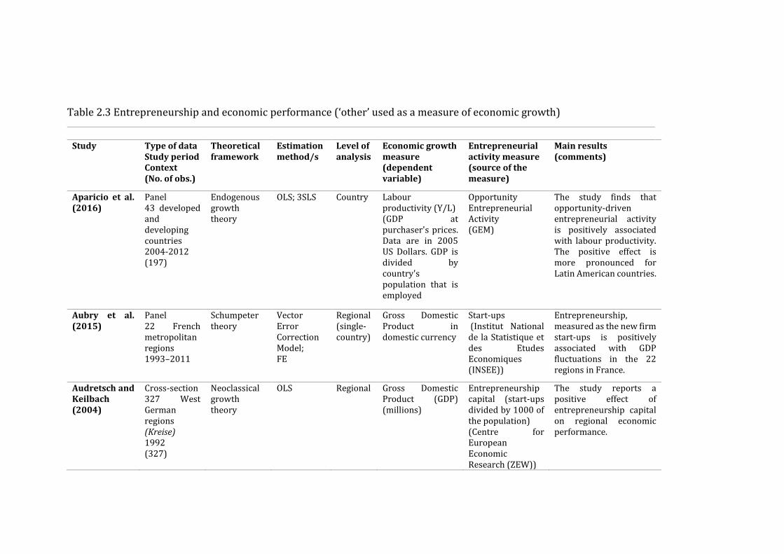
Table 2.3 Entrepreneurship and economic performance (‘other’ used as a measure of economic growth)
Study Type of data Study period Context (No. of obs.)
Theoretical framework
Estimation method/s
Level of analysis
Economic growth measure (dependent variable)
Entrepreneurial activity measure (source of the measure)
Main results (comments)
Aparicio et al. (2016)
Panel 43 developed and developing countries 2004-2012 (197)
Endogenous growth theory
OLS; 3SLS Country Labour productivity (Y/L) (GDP at purchaser's prices. Data are in 2005 US Dollars. GDP is divided by country's population that is employed
Opportunity Entrepreneurial Activity (GEM)
The study finds that opportunity-driven entrepreneurial activity is positively associated with labour productivity. The positive effect is more pronounced for Latin American countries.
Aubry et al. (2015)
Panel 22 French metropolitan regions 1993–2011
Schumpeter theory
Vector Error Correction Model; FE
Regional (single-country)
Gross Domestic Product in domestic currency
Start-ups (Institut National de la Statistique et des Etudes Economiques (INSEE))
Entrepreneurship, measured as the new firm start-ups is positively associated with GDP fluctuations in the 22 regions in France.
Audretsch and Keilbach (2004)
Cross-section 327 West German regions (Kreise) 1992 (327)
Neoclassical growth theory
OLS Regional Gross Domestic Product (GDP) (millions)
Entrepreneurship capital (start-ups divided by 1000 of the population) (Centre for European Economic Research (ZEW))
The study reports a positive effect of entrepreneurship capital on regional economic performance.
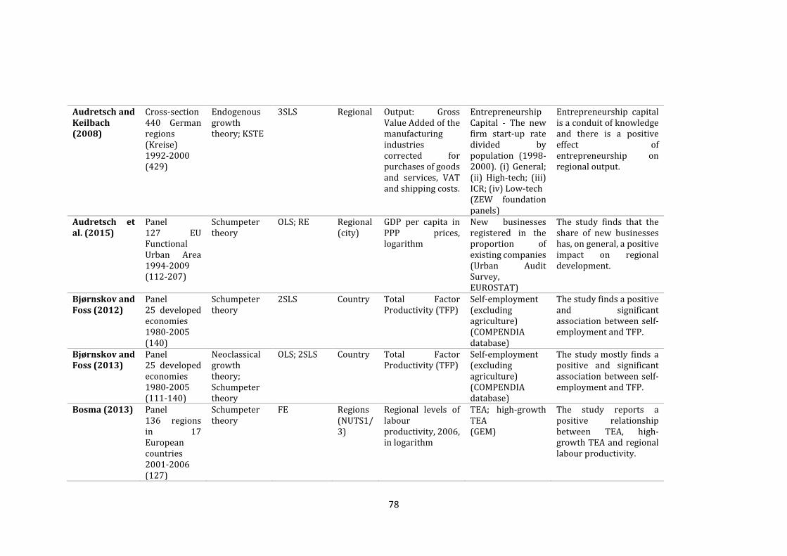
78
Audretsch and Keilbach (2008)
Cross-section 440 German regions (Kreise) 1992-2000 (429)
Endogenous growth theory; KSTE
3SLS Regional Output: Gross Value Added of the manufacturing industries corrected for purchases of goods and services, VAT and shipping costs.
Entrepreneurship Capital - The new firm start-up rate divided by population (1998-2000). (i) General; (ii) High-tech; (iii) ICR; (iv) Low-tech (ZEW foundation panels)
Entrepreneurship capital is a conduit of knowledge and there is a positive effect of entrepreneurship on regional output.
Audretsch et al. (2015)
Panel 127 EU Functional Urban Area 1994-2009 (112-207)
Schumpeter theory
OLS; RE Regional (city)
GDP per capita in PPP prices, logarithm
New businesses registered in the proportion of existing companies (Urban Audit Survey, EUROSTAT)
The study finds that the share of new businesses has, on general, a positive impact on regional development.
Bjørnskov and Foss (2012)
Panel 25 developed economies 1980-2005 (140)
Schumpeter theory
2SLS Country Total Factor Productivity (TFP)
Self-employment (excluding agriculture) (COMPENDIA database)
The study finds a positive and significant association between self-employment and TFP.
Bjørnskov and Foss (2013)
Panel 25 developed economies 1980-2005 (111-140)
Neoclassical growth theory; Schumpeter theory
OLS; 2SLS Country Total Factor Productivity (TFP)
Self-employment (excluding agriculture) (COMPENDIA database)
The study mostly finds a positive and significant association between self-employment and TFP.
Bosma (2013) Panel 136 regions in 17 European countries 2001-2006 (127)
Schumpeter theory
FE Regions (NUTS1/3)
Regional levels of labour productivity, 2006, in logarithm
TEA; high-growth TEA (GEM)
The study reports a positive relationship between TEA, high-growth TEA and regional labour productivity.
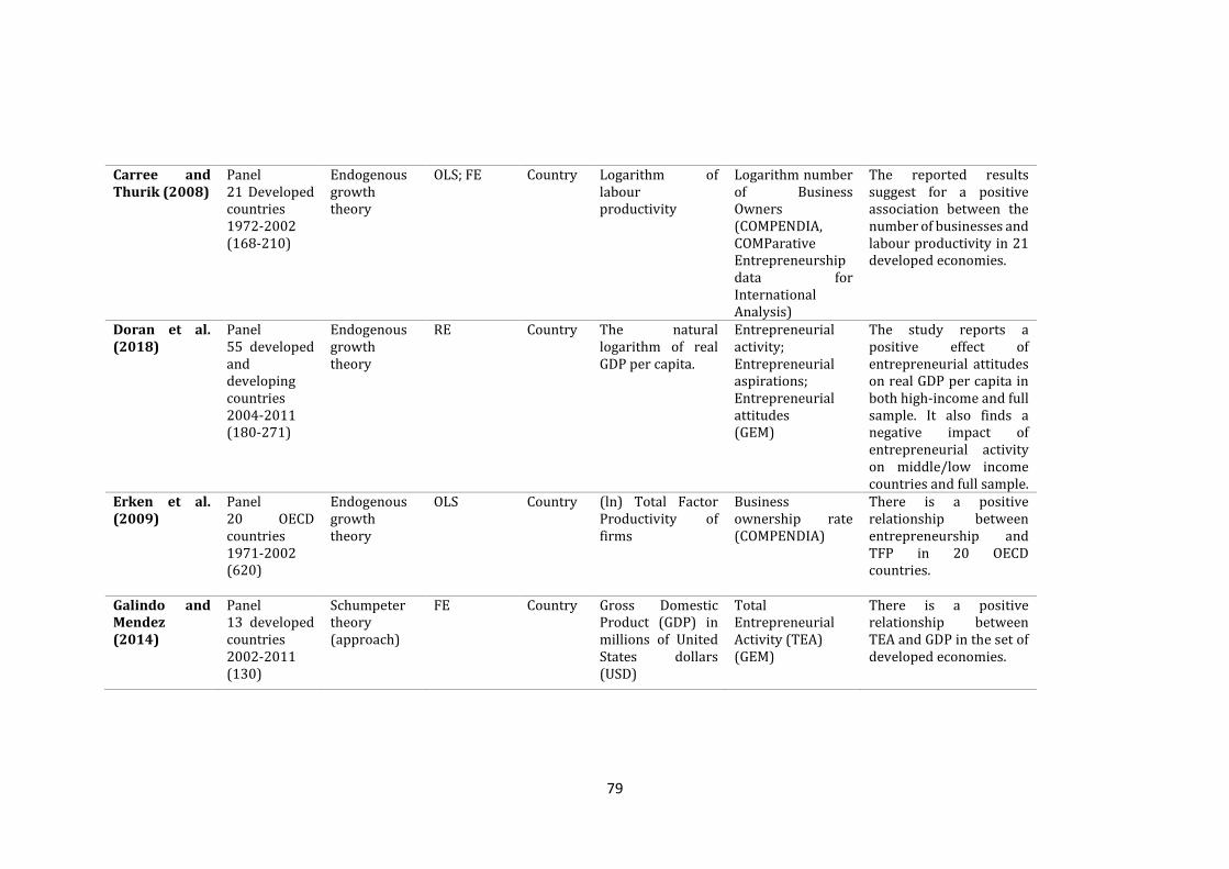
79
Carree and Thurik (2008)
Panel 21 Developed countries 1972-2002 (168-210)
Endogenous growth theory
OLS; FE Country Logarithm of labour productivity
Logarithm number of Business Owners (COMPENDIA, COMParative Entrepreneurship data for International Analysis)
The reported results suggest for a positive association between the number of businesses and labour productivity in 21 developed economies.
Doran et al. (2018)
Panel 55 developed and developing countries 2004-2011 (180-271)
Endogenous growth theory
RE Country The natural logarithm of real GDP per capita.
Entrepreneurial activity; Entrepreneurial aspirations; Entrepreneurial attitudes (GEM)
The study reports a positive effect of entrepreneurial attitudes on real GDP per capita in both high-income and full sample. It also finds a negative impact of entrepreneurial activity on middle/low income countries and full sample.
Erken et al. (2009)
Panel 20 OECD countries 1971-2002 (620)
Endogenous growth theory
OLS Country (ln) Total Factor Productivity of firms
Business ownership rate (COMPENDIA)
There is a positive relationship between entrepreneurship and TFP in 20 OECD countries.
Galindo and Mendez (2014)
Panel 13 developed countries 2002-2011 (130)
Schumpeter theory (approach)
FE Country Gross Domestic Product (GDP) in millions of United States dollars (USD)
Total Entrepreneurial Activity (TEA) (GEM)
There is a positive relationship between TEA and GDP in the set of developed economies.
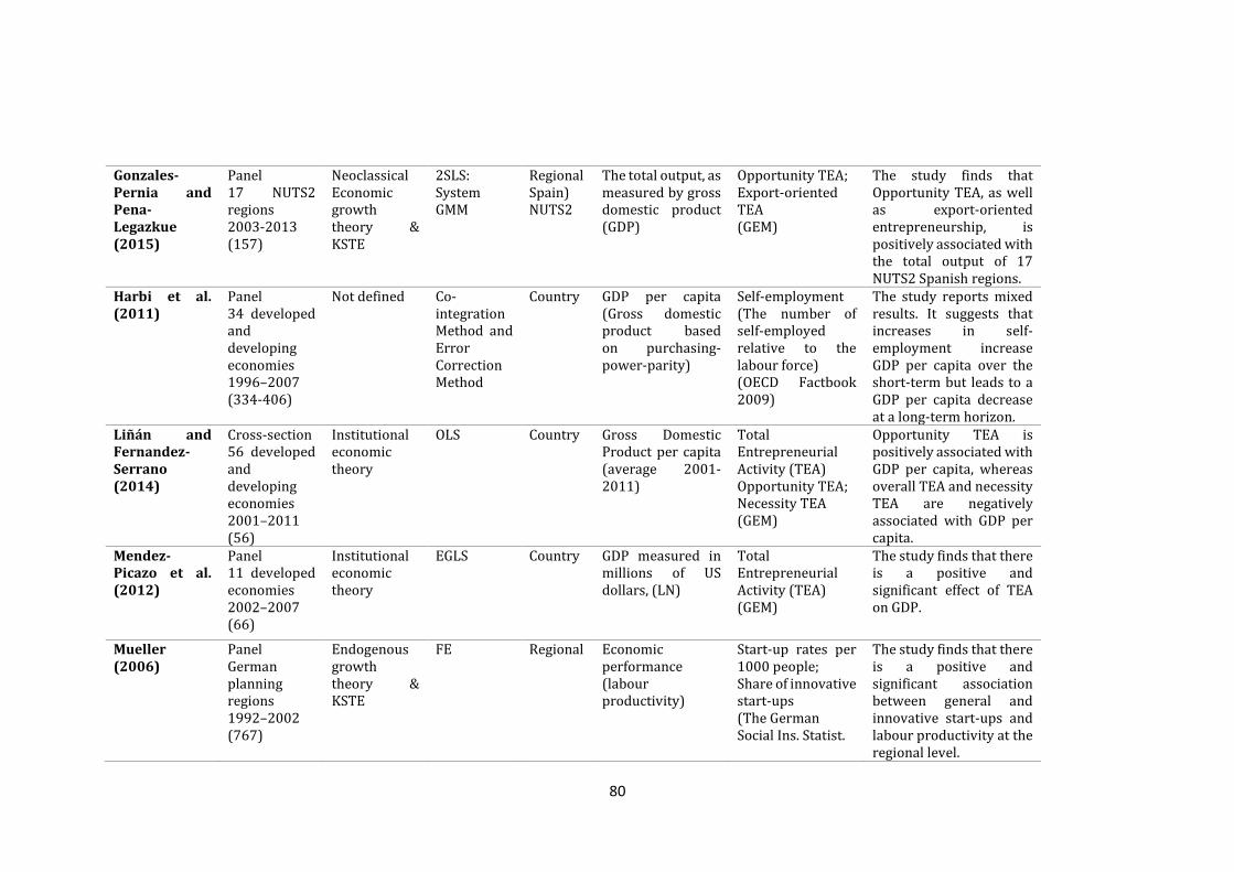
80
Gonzales-Pernia and Pena-Legazkue (2015)
Panel 17 NUTS2 regions 2003-2013 (157)
Neoclassical Economic growth theory & KSTE
2SLS: System GMM
Regional Spain) NUTS2
The total output, as measured by gross domestic product (GDP)
Opportunity TEA; Export-oriented TEA (GEM)
The study finds that Opportunity TEA, as well as export-oriented entrepreneurship, is positively associated with the total output of 17 NUTS2 Spanish regions.
Harbi et al. (2011)
Panel 34 developed and developing economies 1996–2007 (334-406)
Not defined Co-integration Method and Error Correction Method
Country GDP per capita (Gross domestic product based on purchasing-power-parity)
Self-employment (The number of self-employed relative to the labour force) (OECD Factbook 2009)
The study reports mixed results. It suggests that increases in self-employment increase GDP per capita over the short-term but leads to a GDP per capita decrease at a long-term horizon.
Liñán and Fernandez-Serrano (2014)
Cross-section 56 developed and developing economies 2001–2011 (56)
Institutional economic theory
OLS Country Gross Domestic Product per capita (average 2001-2011)
Total Entrepreneurial Activity (TEA) Opportunity TEA; Necessity TEA (GEM)
Opportunity TEA is positively associated with GDP per capita, whereas overall TEA and necessity TEA are negatively associated with GDP per capita.
Mendez-Picazo et al. (2012)
Panel 11 developed economies 2002–2007 (66)
Institutional economic theory
EGLS Country GDP measured in millions of US dollars, (LN)
Total Entrepreneurial Activity (TEA) (GEM)
The study finds that there is a positive and significant effect of TEA on GDP.
Mueller (2006)
Panel German planning regions 1992–2002 (767)
Endogenous growth theory & KSTE
FE Regional Economic performance (labour productivity)
Start-up rates per 1000 people; Share of innovative start-ups (The German Social Ins. Statist.
The study finds that there is a positive and significant association between general and innovative start-ups and labour productivity at the regional level.
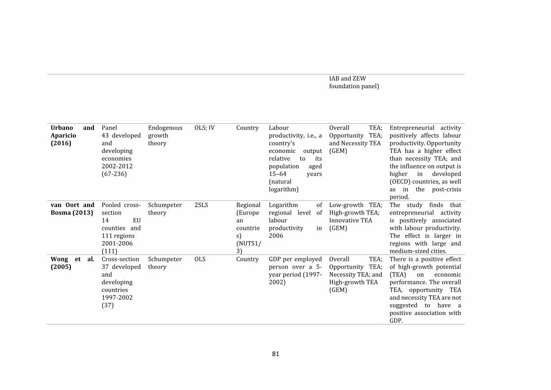
81
IAB and ZEW foundation panel)
Urbano and Aparicio (2016)
Panel 43 developed and developing economies 2002-2012 (67-236)
Endogenous growth theory
OLS; IV Country Labour productivity, i.e., a country's economic output relative to its population aged 15–64 years (natural logarithm)
Overall TEA; Opportunity TEA; and Necessity TEA (GEM)
Entrepreneurial activity positively affects labour productivity. Opportunity TEA has a higher effect than necessity TEA; and the influence on output is higher in developed (OECD) countries, as well as in the post-crisis period.
van Oort and Bosma (2013)
Pooled cross-section 14 EU counties and 111 regions 2001-2006 (111)
Schumpeter theory
2SLS Regional (European countries) (NUTS1/3)
Logarithm of regional level of labour productivity in 2006
Low-growth TEA; High-growth TEA; Innovative TEA (GEM)
The study finds that entrepreneurial activity is positively associated with labour productivity. The effect is larger in regions with large and medium-sized cities.
Wong et al. (2005)
Cross-section 37 developed and developing countries 1997-2002 (37)
Schumpeter theory
OLS Country GDP per employed person over a 5-year period (1997-2002)
Overall TEA; Opportunity TEA; Necessity TEA; and High-growth TEA (GEM)
There is a positive effect of high-growth potential (TEA) on economic performance. The overall TEA, opportunity TEA and necessity TEA are not suggested to have a positive association with GDP.
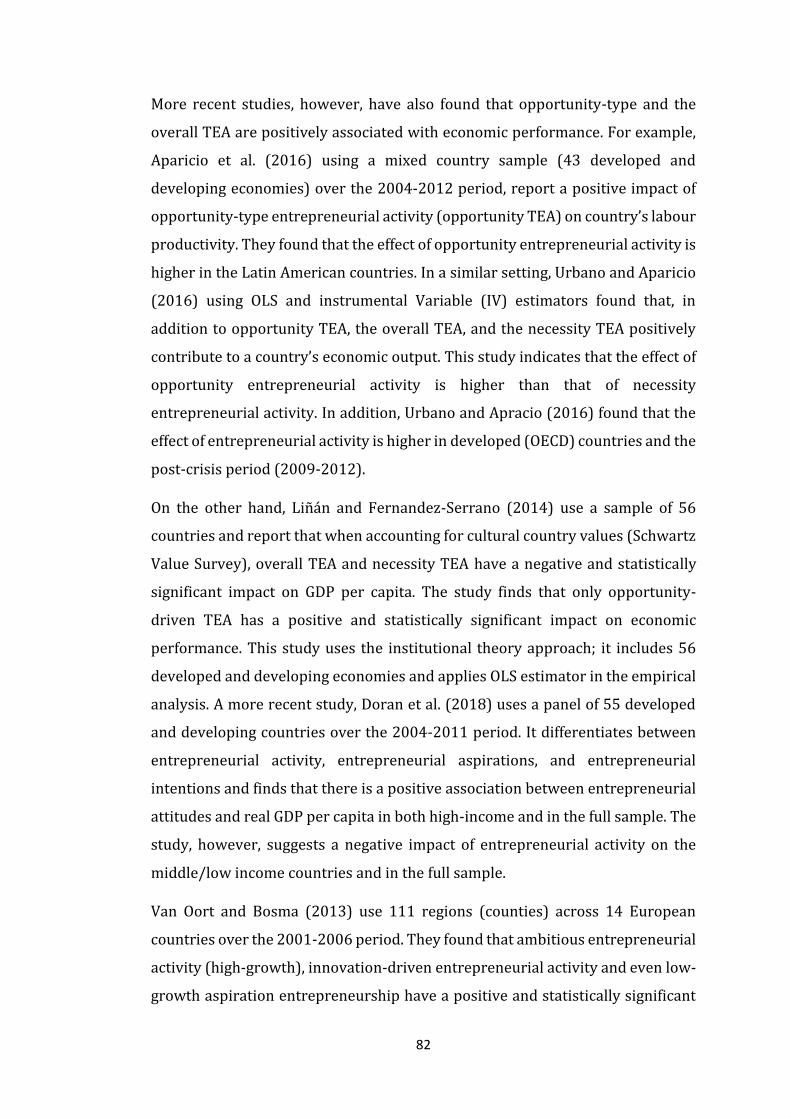
82
More recent studies, however, have also found that opportunity-type and the
overall TEA are positively associated with economic performance. For example,
Aparicio et al. (2016) using a mixed country sample (43 developed and
developing economies) over the 2004-2012 period, report a positive impact of
opportunity-type entrepreneurial activity (opportunity TEA) on country’s labour
productivity. They found that the effect of opportunity entrepreneurial activity is
higher in the Latin American countries. In a similar setting, Urbano and Aparicio
(2016) using OLS and instrumental Variable (IV) estimators found that, in
addition to opportunity TEA, the overall TEA, and the necessity TEA positively
contribute to a country’s economic output. This study indicates that the effect of
opportunity entrepreneurial activity is higher than that of necessity
entrepreneurial activity. In addition, Urbano and Apracio (2016) found that the
effect of entrepreneurial activity is higher in developed (OECD) countries and the
post-crisis period (2009-2012).
On the other hand, Liñán and Fernandez-Serrano (2014) use a sample of 56
countries and report that when accounting for cultural country values (Schwartz
Value Survey), overall TEA and necessity TEA have a negative and statistically
significant impact on GDP per capita. The study finds that only opportunity-
driven TEA has a positive and statistically significant impact on economic
performance. This study uses the institutional theory approach; it includes 56
developed and developing economies and applies OLS estimator in the empirical
analysis. A more recent study, Doran et al. (2018) uses a panel of 55 developed
and developing countries over the 2004-2011 period. It differentiates between
entrepreneurial activity, entrepreneurial aspirations, and entrepreneurial
intentions and finds that there is a positive association between entrepreneurial
attitudes and real GDP per capita in both high-income and in the full sample. The
study, however, suggests a negative impact of entrepreneurial activity on the
middle/low income countries and in the full sample.
Van Oort and Bosma (2013) use 111 regions (counties) across 14 European
countries over the 2001-2006 period. They found that ambitious entrepreneurial
activity (high-growth), innovation-driven entrepreneurial activity and even low-
growth aspiration entrepreneurship have a positive and statistically significant

83
influence on regional labour productivity of 111 European regions (NUTS1/3).
They also found that the effect of entrepreneurial activity tends to be higher in
EU counties hosting large and medium-sized cities. This study follows the
Schumpeterian theory and uses the Instrumental Variable (IV) approach. A
similar finding is also reported by Bosma (2013) for 136 regions (NUTS1/3) in
17 European countries over the 2001 – 2006 period. He finds that both the
overall TEA and high-growth TEA have a positive association with regional
labour productivity. In a single-country setting, González-Pernía and Peña-
Legazkue (2015) include 17 Spanish NUTS2 regions and report similar findings.
Specifically, they found that opportunity TEA and export-oriented TEA are
positively associated with the total regional output (GDP). Mueller (2006) is
another study at the regional level that finds a positive relationship. It uses ten-
year data from 1992-2002 and reports that entrepreneurship, measured by
general and innovative start-up rates, has a positive impact on the regional
economic performance of German planning regions. Similarly, Audrestch and
Keilbach (2008) use 440 German regions over the 1992-2000 period and find
that new firm start-up rates have a positive effect on regional output. In addition,
following the KSTE approach, they argue that their study confirms that
entrepreneurship serves as a conduit of knowledge spillover and that it facilitates
the transformation of general knowledge into economically relevant knowledge.
Bjørnskov and Foss (2012; 2013) use Total Factor Productivity (TFP) to account
for economic performance and report a positive and statistically significant
association between self-employment and TFP. The studies follow the
Schumpeterian theory and include only developed economies in the analysis.
Additional study characteristics of the other included studies in the third
subsample are presented in Table 2.3.
In summary, the studies reviewed in this chapter tend to generally report a
positive and significant effect of entrepreneurship on economic performance,
both at the country and the regional level. However, the results are not conclusive
across different studies, particularly regarding the effect of different types of
entrepreneurial activity measures on economic performance. Opportunity-
driven and high-growth potential entrepreneurial activity are the two measures
of entrepreneurship mostly suggested to have a significant impact on economic
84
growth measures. The overall TEA and necessity-driven entrepreneurial activity
are generally indicated to have a mixed effect on economic performance
measures. Mixed results are also obtained when self-employment, start-up rates
and other similar measures of entrepreneurship are used.
Furthermore, the use of a variety of measures as a proxy for entrepreneurship,
mainly due to the multi-dimensional definition of entrepreneurship and for
economic performance has led to some heterogeneity in the econometric
approaches, theoretical frameworks used, and the results obtained. Also, the use
of different lag structures has further influenced this heterogeneity. Another
critical observation, regarding the methodological approaches, is that, although
the reviewed studies tend to use one of the growth theories, still they ignore some
of the critical control variables in their model specifications, potentially suffering
from the omitted variable bias. This shortcoming, as well as the heterogeneity
outlined above, will be accounted for in the empirical chapters of the thesis.
CONCLUSIONS
This chapter has provided a review of the empirical research undertaken in the
entrepreneurship-economic growth literature. The empirical review was divided
into three subsamples based on the dependent variable used for economic
performance. The first subsample consisted of studies that used ‘growth’ (GDP or
GDP per capita). The studies of the second subsample used employment growth
as a measure of economic performance. In the third subsample, studies using
‘other’ different measures of economic performance, were reviewed. Moreover,
the entrepreneurship-economic growth relationship was analysed through the
lenses of growth theories, mainly neoclassical, endogenous and Schumpeterian
growth theories. The augmentation of the endogenous growth theory with the
Knowledge Spillover Theory of Entrepreneurship (KSTE) is also elaborated. In
addition, the chapter has provided a comprehensive discussion of the effect of
institutional context on entrepreneurial growth aspirations.
This chapter has highlighted that the literature on entrepreneurship-economic
growth relationship lacks some solid theoretical foundations. This is because the
two traditional growth theories seem to have overlooked the impact of

85
entrepreneurship on growth. Yet, most of the existing empirical studies in the
entrepreneurship-economic growth relationship, both at the country and at the
regional level, applied either explicitly or implicitly one of the economic growth
frameworks in their analysis. The contribution of the KSTE was outlined as it
provided a channel explaining how entrepreneurship affects economic growth.
The Schumpeterian growth theory has also linked entrepreneurship with
economic growth through the process of ‘creative destruction’ and as it was
discussed, many studies have used this approach.
The comprehensive review of empirical literature, at both national and regional
level, in general, indicated for a positive impact of entrepreneurship measures on
economic performance. The review suggested that growth and innovation-
oriented entrepreneurial activity (GEM measures) are mainly positively and
significantly associated with economic performance. However, there are also
studies that reported no significant relationship and some even found that
entrepreneurship is harmful to growth and economic performance. The review
also found that the effect of the overall TEA, the most widely used GEM measure
of entrepreneurship, is mixed. It was also highlighted in this chapter, that the
multidimensionality of entrepreneurship has led to the use of different proxies.
However, the use of GEM measures is becoming more common, especially at the
country-level studies.
The next chapter provides a more comprehensive review of the relationship
between entrepreneurship and economic performance by conducting a Meta-
Regression Analysis (MRA). The MRA will focus on identifying the average
‘genuine’ effect of entrepreneurship on economic performance, beyond
‘publication bias’ and after controlling for the sources of heterogeneity.

86
3. Chapter 3
ENTREPRENEURSHIP AND ECONOMIC PERFORMANCE:
A META-REGRESSION ANALYSIS
INTRODUCTION ........................................................................................................................ 87
THEORETICAL CONTEXT AND CONCEPTUAL FRAMEWORK ............................... 89
METHODOLOGY AND DATA ................................................................................................ 92
Criteria for inclusion of studies ................................................................................ 93
Primary literature included in this MRA............................................................... 94
(i) Main characteristics of studies using GDP growth or growth of GDP per capita
(subsample I) .................................................................................................................................. 95
(ii) Main characteristics of studies using employment growth as dependent
variable (subsample II) .............................................................................................................. 96
(iii) Main characteristics of studies using ’other’ measures of economic
performance (subsample III) ................................................................................................... 97
Summary of the MRA database ................................................................................. 98
THE MRA METHODOLOGY ................................................................................................. 101
Effect sizes ....................................................................................................................... 101
Publication Bias: Funnel Plot ................................................................................... 103
THE BIVARIATE MRA ........................................................................................................... 106
FAT – PET – PEESE ...................................................................................................... 106
THE MULTIVARIATE MRA ................................................................................................. 115
Heterogeneity ................................................................................................................ 115
Descriptive statistics ................................................................................................... 119
Bayesian Model Averaging ....................................................................................... 122
EMPIRICAL RESULTS ........................................................................................................... 122
CONCLUSIONS ......................................................................................................................... 133

87
INTRODUCTION
The relationship between entrepreneurship and economic performance has been
debated for a long time (Schumpeter, 1934; Baumol, 1968; 1996; Leibenstein,
1968; Wennekers and Thurik, 1999). Despite the limited theoretical guidance,
the empirical research has gained increased interest in the last few decades
(Wong et al., 2005; Carree and Thurik, 2008; Stam et al., 2009; Hessels and van
Stel, 2011; Bosma, 2013; Urbano and Aparicio, 2016; Acs et al., 2018). As
discussed in Chapter 2, in general, the empirical literature reports a positive
relationship between entrepreneurship and economic growth, both at the
country and at the regional-level (regions within a country) (see Acs et al., 2012;
Stephens et al., 2013; Aparicio et al., 2016). But, as Chapter 2 of the thesis
emphasised, that although a positive link between entrepreneurship and
economic performance has been established, the empirical evidence on the topic
is still inconclusive.
The empirical literature generally reports on the positive effects of
entrepreneurship on economic performance, especially in developed economies
(see van Stel et al., 2005; Wong et al., 2005; Carree and Thurik, 2008; Acs et al.,
2012). However, some studies find little or no relationship between the two
(Valliere and Peterson, 2009; Prieger et al., 2016) while others even report
negative effects (Linan and Fernandez-Serrano, 2014). This inconclusiveness
might be the result of studies using a wide variety of measures of
entrepreneurship and economic performance, the relatively limited number of
empirical studies, mostly using data for developed economies, e.g., OECD
countries, and of a wide range of theoretical and methodological approaches. The
heterogeneity of reported effects and the methodological approaches followed in
the primary literature motivate the Meta-Regression Analysis (MRA) presented
in this chapter.
According to Stanley et al. (2008), in addition to the integration of economic
research results, MRA provides the necessary tools to identify and quantify the
extent of publication selection bias in empirical studies. Such publication
selection bias arises from researchers trying to find significant results that are in
line with conventional economic theories. Gigerenzer (2004, p.588) posits that

88
‘the idea of getting empirical research papers published, makes researchers less
interested in statistical thinking’, leading to what Altman (2004) and Ziliak and
McCloskey (2004) refer to as the “abuse” of statistical significance in empirical
studies. Further, MRA enables the identification and quantification of the genuine
representative effect - net of publication selection bias - established in the
literature and explains to what degree the heterogeneous findings are influenced
by the heterogeneity of study characteristics, such as methodological approaches
and empirical strategies, measures, contexts, samples, etc.
As a result of these ambiguities, this chapter systematically and critically reviews
the existing literature on the relationship between entrepreneurship and
economic performance between 2000 and 2016 and applies MRA to determine:
(a) the extent to which heterogeneous samples and methodologies moderate
the effect of entrepreneurship on economic performance;
(b) the degree, if any, of publication selection bias in the literature; and
(c) the average entrepreneurship effect, beyond ‘publication bias’ and after
controlling for sources of heterogeneity.
In total, 52 published and unpublished empirical studies (primary studies, in
meta-regression terminology) investigating the relationship between
entrepreneurship and economic performance between 2000 and 2016 are
included in the MRA database. The choice of the year 2000 is intentional, it is the
year of the first wave of surveys of the Global Entrepreneurship Monitor (GEM),
the largest and most comprehensive source of data on entrepreneurship, (both
at the individual and the national level). GEM has undoubtedly had a significant
influence on the research in the field (Reynolds et al., 2005; Amoros et al., 2013;
Szerb et al., 2013; Alvarez et al., 2014; Levie et al., 2014; Urbano and Aparicio,
2016; Bosma et al., 2018). The 52 primary studies used for MRA contain 657
effects sizes,26 capturing either the contemporaneous or the previous periods’
effects of entrepreneurship on economic performance which are modelled by
lags of the main variable of interest, i.e., entrepreneurship. Due to different
26 An effect size in the terminology of meta-regression is similar to a regression coefficient (estimate), in the conventional regression terminology.
89
measures of economic performance (the dependent variable) used, pooling the
reported effects into a single database is not an appropriate approach to
statistical analysis. Accordingly, the reported effects in the primary studies were
grouped into three categories forming three coherent subsamples valid for
separate investigations. The first subsample includes effects estimated from
specifications where ‘growth of GDP or GDP per capita’ are used as the dependent
variable. The second subsample pertains to specifications using ‘employment
growth’ as the measure of economic performance whereas the third subsample
contains studies using ‘other’ measures of economic performance such as GDP in
levels.
The rest of this chapter is organised as follows: Section 3.2 provides the
theoretical context and the conceptual framework on which this MRA is based.
The methodology, criteria for the inclusion of studies, details of the MRA database
and the initial visual test of potential publication bias using funnel plots are
offered in sub-sections 3.3-3.4.2. The bivariate MRA results and an analysis using
elasticities are provided in section 3.5. The multivariate MRA moderators are
discussed in section 3.6 while the multivariate empirical results are presented
and elaborated in section 3.7. Conclusions are offered in section 3.8.
THEORETICAL CONTEXT AND CONCEPTUAL FRAMEWORK
As explained in Chapter 2, the first theory linking entrepreneurship to economic
growth and development originates from the early work of Schumpeter (1934),
who argued that entrepreneurs generate economic dynamism by new entry and
innovation processes. Schumpeter (1934) suggests that innovative
entrepreneurial activities, the so-called ‘creative destruction’ processes,
positively affect economic growth and development. However, as the neoclassical
growth theory advanced by Solow (1956) and Swan (1956) dominated the
overall economic theory of the mid-twentieth century, the role of
entrepreneurship was largely neglected. In the Solow-Swan (1956) neoclassical
growth model, growth is determined by capital and labour enhancements, and
the long-run growth is explained only by exogenously determined technological
change (Wennekers and Thurik, 1999; Wong et al., 2005). As Schumpeter (1961)

90
posited, in the neoclassical growth model, no role or function is assigned to the
entrepreneur.
The endogenous growth theory, developed by Lucas (1988), Romer (1986;
1990), Grossman and Helpman (1991) and Aghion and Howitt (1992), highlights
that human capital, knowledge and technological change (innovation) are the
main driving forces of economic growth, which is endogenously determined by
decisions of economic agents to innovate and seek profit-maximizing
opportunities (see Verspagen, 1992; Ruttan, 1997). More recent evolutionary
theories (Jovanovic, 1982; Audretsch, 1995) and empirical evidence (see e.g.,
Audretsch and Keilbach, 2004; 2008) emphasise the role of knowledge that
brings new changes in the market. These theories argue that knowledge and
information enable innovation which is a crucial factor enabling firms to enter
markets, grow and ultimately bring new positive dynamisms in the economic life.
Knowledge and information may spur new ideas which are then utilised and
commercialised by potential entrepreneurs who might even leave wage
employment for a new business opportunity. Burns (2010) argues that,
according to the evolutionary theory, the impact of entrepreneurship on
economic growth is threefold: (i) entrepreneurial activity increases competition
by increasing the number of new business ventures; (ii) entrepreneurship serves
as a mechanism for ‘knowledge spillovers’ allowing newly generated knowledge
to be transmitted to the market and be appropriated by new and potential
entrepreneurs; and (iii) entrepreneurial activity creates economic diversity and
enhanced product variety, thus influencing economic performance.
As discussed in Chapter 1 and 2, researchers argue that entrepreneurship is a
multifaceted concept and has been measured in more than one way. Some of the
measures applied by previous research use self-employment; net-entry; business
ownership; start-ups and new venture creation (Blanchflower, 2000; van Stel et
al., 2005; Carree and Thurik, 2008; Dejardin, 2011). With increased cross-
country harmonisation, recent studies tend to use one single measure, the Total
(Early-stage) Entrepreneurial Activity (TEA), provided and popularised by
Global Entrepreneurship Monitor (GEM).
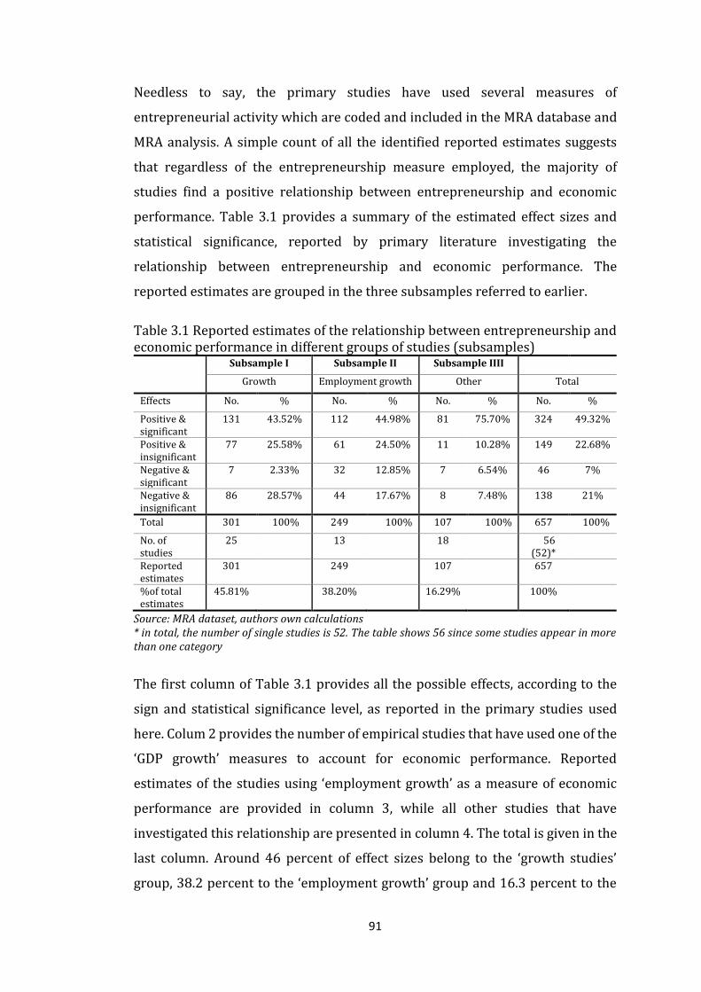
91
Needless to say, the primary studies have used several measures of
entrepreneurial activity which are coded and included in the MRA database and
MRA analysis. A simple count of all the identified reported estimates suggests
that regardless of the entrepreneurship measure employed, the majority of
studies find a positive relationship between entrepreneurship and economic
performance. Table 3.1 provides a summary of the estimated effect sizes and
statistical significance, reported by primary literature investigating the
relationship between entrepreneurship and economic performance. The
reported estimates are grouped in the three subsamples referred to earlier.
Table 3.1 Reported estimates of the relationship between entrepreneurship and economic performance in different groups of studies (subsamples)
Subsample I Subsample II Subsample IIII
Growth Employment growth Other Total
Effects No. % No. % No. % No. %
Positive & significant
131 43.52% 112 44.98% 81 75.70% 324 49.32%
Positive & insignificant
77 25.58% 61 24.50% 11 10.28% 149 22.68%
Negative & significant
7 2.33% 32 12.85% 7 6.54% 46 7%
Negative & insignificant
86 28.57% 44 17.67% 8 7.48% 138 21%
Total 301 100% 249 100% 107 100% 657 100%
No. of studies
25 13 18 56 (52)*
Reported estimates
301 249 107 657
%of total estimates
45.81% 38.20% 16.29% 100%
Source: MRA dataset, authors own calculations * in total, the number of single studies is 52. The table shows 56 since some studies appear in more than one category
The first column of Table 3.1 provides all the possible effects, according to the
sign and statistical significance level, as reported in the primary studies used
here. Colum 2 provides the number of empirical studies that have used one of the
‘GDP growth’ measures to account for economic performance. Reported
estimates of the studies using ‘employment growth’ as a measure of economic
performance are provided in column 3, while all other studies that have
investigated this relationship are presented in column 4. The total is given in the
last column. Around 46 percent of effect sizes belong to the ‘growth studies’
group, 38.2 percent to the ‘employment growth’ group and 16.3 percent to the

92
third, ‘other’ group. Table 3.1 highlights the fact that almost half of the studies
report a positive relationship between entrepreneurship and economic
performance. In all the three subsamples, the share of primary studies reporting
positive effect sizes is higher (72%) than the share of studies with negative
estimates (28%). Almost half (49%) of the reported effect sizes are positive and
statistically significant as compared to only 7% negative and significant
estimates.
METHODOLOGY AND DATA
Meta-regression analysis (MRA) provides a systematic review of existing
quantitative literature on a specific topic of interest by using statistically
designed methods to extract and aggregate the main characteristics of the
selected primary studies (Stanley et al., 2015). Compared to the conventional
narrative literature reviews, MRA attempts to identify all studies that have
investigated a selected topic by using more advanced search techniques and by
employing firmer statistical methods and approaches (Stanley and Doucouliagos,
2012). Stanley et al. (2015, p.9) state: ‘… meta-regression analysis (MRA) examines
the results of previously published studies that are based upon the use of multiple
regression models on empirical data…’. In our case, studies that investigate the
relationship between some measure of entrepreneurship and economic
performance, generally use an augmented growth model, where
entrepreneurship is explicitly included in the model:
𝐸𝑐𝑜𝑛𝑜𝑚𝑖𝑐 𝑃𝑒𝑟𝑓𝑜𝑟𝑚𝑎𝑛𝑐𝑒𝑖𝑡 = 𝛼 + 𝛽𝐸𝑁𝑇𝑖𝑡 + 𝛾𝑋𝑖𝑡 + 𝛿𝑡 + 𝜂𝑖 + 휀𝑖𝑡 (3.1)
where i and t denote country/region and time subscript; Economic Performance
represents a measure of economic performance; ENT represents a measure of
entrepreneurship; X is a vector of control variables accounting for other factors
considered important in the growth process (for example, capital; labour,
institutions, trade, macroeconomic conditions, etc.); δt captures a common time-
specific effect; ηi denotes an unobserved country-specific effect; and εit is the
error term. Although Eq. (3.1) describes a model in a general panel data setting,
some of the primary studies have used cross-section or time-series structures in

93
the investigation. In such a situation, Eq. (3.1) can collapse and represent cross-
section or time-series structures.
Criteria for inclusion of studies
This chapter follows the guidelines proposed by Stanley et al. (2013) for
conducting a meta-analysis in economics. A search for potentially relevant
studies in EconLit online database using the keywords “entrepreneurship +
economic growth”, “entrepreneurship + economic development” and
“entrepreneurship + economic performance” was performed and resulted in 241,
260 and 18 results respectively. Also, using the same keywords and the study
inclusion period criteria, Google Scholar, Research Gate and RePEc were also
used to look for other potential studies. The search for literature terminated on
the 30th of October 2016. The abstracts of the identified studies that had at least
one of the keywords in the title were read, and an initial decision on the inclusion
was made. The reference list of the most recent studies was also observed, and
the potential studies were extracted. The search was conditioned to studies
published from 2000 to 2016. Two reasons have influenced the choice of the
starting year of the investigation. First, the increased importance of
entrepreneurship in the twenty-first century; and second, the initiation of the
Global Entrepreneurship Monitor (GEM) consortium which collects data in a
uniform format, starting from 2000.27 To avoid any potential selectivity issue,
resulting from selecting only published studies, the approach of this MRA is to
include studies that have been published in (i) peer-review journals or/and as a
book chapter and (ii) published as working and/or discussion paper. For clarity,
in some sections, the latter category is referred to as the unpublished work
(literature).
As is the practice, the main criteria were the use of econometric analysis by
primary studies investigating the relationship between entrepreneurship and
economic performance and that the primary studies report some or all the key
statistics (e.g., standard errors; t-statistics; p-values). The identified papers were
examined to confirm the relevance to the MRA between entrepreneurship and
economic performance. This process resulted in excluding some of the studies
27 The first GEM data were made available to the GEM partners in 2001.

94
which did not specifically investigate the entrepreneurship and economic
performance relationship. During this screening phase, 227 papers were finally
excluded, and the remaining 92 papers were read carefully which resulted in the
exclusion of a further 40 which did not meet the pre-defined criteria.
Thus, in total only 52 studies, published between 2000 and 2016, investigating
the relationship between entrepreneurship and economic performance (growth
and/or development, employment growth, labour productivity, TFP, etc.,) are
included in the MRA database28 (these are identified by an asterisk in the list of
references). As in previous MRA (see Dimos and Pugh, 2016; Havranek et al.,
2016), each study consists of several estimations; thus, in total, 657 effects sizes
were initially coded.29 On average, primary studies report 13 effect sizes each
with the number ranging from 1 (Galindo and Mendez, 2014) to 96 (Dejardin,
2011) with an overall median of 9. To increase the number of observations and
studies included, this chapter has also considered studies that have used lags of
the main variable of interest. The extent of lags used is also noted in the funnel
plots (see funnel plots in section 3.4, Fig. 3.1). To account for this phenomenon, a
new weighting arrangement is developed which takes into account the number
of effect sizes extracted from specifications using lags.30
Primary literature included in this MRA
This chapter divides the MRA dataset into three subsamples, according to the
measure of economic performance used. The number of observations allows for
such a division and the MRA practices allow looking at different subsamples (e.g.,
separately looking at studies that have used GDP growth or growth of GDP per
capita as a measure of economic performance). Some of the main characteristics
of the primary literature in each subsample are provided here.
28 Initially 672 observations and 55 studies were coded. However, after conducting additional screening processes, 15 observations coming from 4 studies were excluded. 29 After accounting for outliers and the choice of dependent variable, a few more of the effect sizes were dropped. 30 A more detailed discussion about this ‘weight’ is provided in section 3.4.1 and 3.5.1.
95
(i) Main characteristics of studies using GDP growth or growth of GDP per capita
(subsample I)
Nine out of 25 studies in this subsample (subsample I) employ GEM measures as
a proxy of entrepreneurial activity (e.g., van Stel et al., 2005; Stam et al., 2010)
and mainly report a positive relationship between entrepreneurship and
economic growth measures. van Stel et al. (2005) use GEM data for 36 developed
and developing economies for the period 1993-2003 and find that Total
Entrepreneurial Activity (TEA)31 has a positive impact on GDP growth in highly
developed and relatively rich economies. They report a negative and significant
effect for less developed and relatively poor economies and argue that the effect
of TEA on GDP growth is subject to the country’s stage of economic
development.32
The second most commonly used measure of entrepreneurship in the first
subsample is self-employment, which usually excludes the agriculture sector
self-employment and unpaid family work. Acs et al. (2012) investigate the
relationship between entrepreneurship (self-employed as a percentage of total
nonagricultural employment) and growth of GDP per capita in 18 developed
economies for the 1981-1998 period. They report positive and significant
estimates suggesting that entrepreneurship promotes economic growth. Another
characteristic of this subsample is the presence of regional studies (sometimes
regions within the country). For instance, Dejardin (2011) investigates the link
between net entry rates in the 43 Belgian districts (arrondissements) and the
regional economic growth. Making use of extensive lags (six lags for the
entrepreneurship measure, net-entry rate), he finds mostly negative, though
statistically insignificant results. Using the same measure of entrepreneurial
activity, but for the Spanish and Portuguese regions, Vazquez-Rozas et al. (2011)
find positive and statistically significant impact on GDP growth.
31 TEA is the most commonly used measure of GEM to proxy for entrepreneurship. It is defined as the prevalence rate of individuals who are currently involved in starting up a new business, having taken concrete steps to start, (nascent), or owner of a business that is less than 42 months active and generating income. 32 The study uses Gross National Income per capita (GNIC) to distinguish between developed (relatively rich) and less developed (relatively poor, including both transformation economies and developing countries).

96
(ii) Main characteristics of studies using employment growth as dependent variable
(subsample II)
The second subsample of identified studies from the primary literature uses
employment growth as a measure of economic performance and mainly start-ups
as a measure of entrepreneurial activity. As argued in Chapter 2, although
employment growth is not equivalent to economic growth, still many studies
have relied on this measure. Critiques argue that by focusing only on employment
growth, this measure disregards the importance of productivity growth of an
economy or a region (Acs and Armington, 2004). However, as argued by Stuetzer
et al. (2018), the use of employment growth as a measure of, economic
performance, especially at the regional level, has two main advantages. First, the
comparison of results with previous studies, since employment growth has
previously been used in the studies investigating regional economic differences
and second, due to the fact that increasing employment is one of the top national
economic priorities. Hence, studies that use employment growth as a proxy for
economic performance are included in this MRA and effect sizes are derived from
these primary studies.
Most studies are conducted at the regional (e.g., NUTS1-3) or an equivalent unit
of analysis and are mostly single-country studies. Only one study (Carree and
Thurik, 2008) provides an investigation at the country level by analyzing 21
OECD countries. A distinctive characteristic of the studies in this subsample is the
use of lag structures to determine the effect of entrepreneurship measures on
employment growth. For example, Fritsch and Mueller (2004) investigated the
effect of start-ups on regional employment growth in 326 German (West)
districts, using a variety of lag structures. They argue that the largest effect of
start-ups on employment growth in German districts is found for: (i) firms in the
first year of establishment; and (ii) for firms that were established 6-7 years
earlier (i.e., start-ups (t-6) and (t-7)). A similar approach is also followed by van
Stel and Storey (2004) for 59 British regions (NUTS3) where they report that the
highest effect of business formation rates on employment growth is found for the
start-ups of year t-5, i.e., businesses that were created five years earlier, have the
highest impact on this year’s employment growth.

97
Two studies have used self-employment (usually excluding the agricultural
sector) as a proxy for entrepreneurship. As discussed in Chapter 2, this practise
has been criticised as self-employment is unable to capture all the aspects of
entrepreneurial activity at regional and country-level (see Box et al., 2016).
Researchers argue that self-employment does not explain the complex nature of
the entrepreneurial activity and should not be considered as synonymous to it
(Bjørnskov and Foss, 2013). In this vein, Sanandaji (2010) argues that self-
employment might not resemble the process of business opportunity
identification, (as discussed in Chapter 2 of the thesis, opportunity identification
is a typical characteristic of an entrepreneur) but instead it represents the single
(self) employment opportunity an individual has. Therefore, it can be argued that
self-employment does not represent growth-oriented or opportunity-driven
entrepreneurial activity. It might only represent the necessity type of
entrepreneurial activity. However, as discussed in Chapter 2, the broad definition
of entrepreneurship accomodates also measures such as self-employment,
therefore, this chapter considers self-employment as a viable proxy for
entrepreneurship and includes these studies in the present analysis. Similar to
self-employment, net-entry rates, used by studies in this subsample do not
distinguish between any types of entrepreneurial activity but rather represent
the dynamics of business creation in a specific country or region.
(iii) Main characteristics of studies using ’other’ measures of economic performance
(subsample III)
The third subsample of identified studies uses other measures of economic
performance, such as GDP per capita; GDP in millions of US dollars; Labour
productivity, Total Factor Productivity (TFP) and other similar measures. As with
the first subsample, the majority of studies use GEM indicators as proxies for
entrepreneurial activity. Using an augmented Cobb-Douglas production function
with Constant Returns to Scale, Wong et al. (2005) find that it is only high-growth
potential entrepreneurial activity (High Potential TEA) that has a positive and
statistically significant effect on GDP per employed person, i.e., labour
productivity.
98
Studies using Total Factor Productivity (TFP) to account for economic
performance, report only positive and statistically significant results (21 out 22
effect sizes show a positive and statistically significant impact). Single country
studies report mixed findings, usually influenced by the choice of
entrepreneurship measure. For instance, González-Pernía and Pena-Legazkue
(2015), using data for Spanish regions over the 2003-2013 period, report that
only opportunity-driven and export-oriented entrepreneurship have a positive
and significant effect on total output, as measured by Gross Domestic Product
(GDP).
Summary of the MRA database
This section provides a summary of the study characteristics, including the
choice of entrepreneurship and economic performance measures.
Outcome characteristics: The typical estimate of the effect of entrepreneurship on
economic growth reported in primary studies is positive (0.29 for growth
studies; 0.39 for employment growth studies; and 0.33 for ‘other’ studies) and
large reported standard error, especially for the first two sub-samples (2.76;
2.07; and 0.71). This effect size is an outcome of different proxies of
entrepreneurship, economic performance and different estimation techniques
used for analysing the effect of entrepreneurship on economic performance. Due
to this fact, the reported estimates are not easily comparable and should be
standardised. The majority of meta-regression studies use Partial Correlation
Coefficient (PCC) as a standardised measure of the effect (see Stanley and
Doucouliagos, 2012).33 The unweighted mean PCC (see Table 3.3) is still positive
and has a value of 0.092 for growth studies, 0.07 for employment studies and 0.18
for ‘other’ studies, which would be classified as a ‘moderate’ effect according to
Doucouliagos (2011) guidelines for the interpretation of partial correlations in
economics.34 The mean number of observations used in the primary literature is
194 (195 without outliers) for growth studies; 1301 (1150 without outliers) for
33 PCC is a unitless measure of the association between a dependent and independent variable while holding all other variables constant (Greene, 2008). Section 3.4 provides more details on the transformation of effect sizes to PCCs. 34 Doucouliagos (2011, p.3), provides guidelines on the magnitude of the effects. According to his approach, PCCs can be characterised as either ‘small’ (PCC < 0.07), ‘moderate’ (0.07 ≤ PCC ≤ 0.33) or ‘large’ (PCC > 0.33).

99
employment growth studies and 230 (216 without outliers) for ‘other’ studies.
The relatively large number of observations in the second subsample is the result
of studies using regional or even city level data as the unit of analysis.
Consequently, this chapter includes a moderator to account for primary studies
that have investigated the effect of entrepreneurship on economic performance
at the regional level. Primary studies have, on average, used 9 explanatory
variables (including lags) (7 and 10 for growth studies; 11 and 16 for
employment growth studies; and 7 and 9 for ‘other’ studies) and 12 time periods.
The choice of the dependent variable: The majority of the studies at the country
level employ GDP growth and growth of GDP per capita as the dependent
variables (measures of economic performance). Studies at the regional level have
investigate mainly the effect of start-ups and self-employment on employment
growth. Other primary studies have used GDP at levels, labour productivity and
Total Factor Productivity as measures of economic performance.
The choice of entrepreneurship measures: It can be argued that the choice of
dependent variable influences the choice of entrepreneurship measure. Most of
the studies that have investigated the effect of entrepreneurship on employment
growth use start-up rates and self-employment as a measure of entrepreneurial
activity. Studies that have analysed this relationship at the regional level,
specifically, have relied mostly on start-up rates. Another factor influencing the
choice of entrepreneurship measure is argued to be data availability. Since the
launch of Global Entrepreneurship Monitor (GEM), and specifically in the last ten
years, there is a tendency to use Total Entrepreneurial Activity (TEA) or other
measures in GEM to proxy for entrepreneurial activity. Only 29 effect sizes of
primary studies (three studies in total) published before 2009 come from GEM
measures, whereas between 2009 and 2016, GEM measures resulted in 113
reported effect sizes (14 studies).
Macroeconomic and institutional control variables: Primary studies that belong to
the first subsample have generally included a measure of institutional quality and
a measure of the quality of human capital. About 33 percent of effect sizes of the
first subsample come from the studies which control for the effect of initial
income levels (e.g., initial GDP per capita) which would account for the

100
convergence or catch-up effect. Studies of the second subsample have hardly
used any macroeconomic or institutional control variables, perhaps due to the
fact that most of these studies looked at regions within a single country, where
the institutional quality does not change. However, this might have led to the
alleged omitted variable bias. About half of the studies belonging to the third
subsample have used some of the conventional variables of economic growth and
development models, namely, a measure of capital (e.g., capital formation),
labour (e.g., the no. of unemployed), the quality of human capital (e.g., years of
schooling), the quality of institutions (e.g., Global Competitiveness Indicator;
Index of Economic Freedom).
Dataset structure: Most of the observations come from studies that have used
panel estimation techniques. This can be considered a positive aspect, as
according to van der Ploeg (2011), studies that rely on cross-section structures
in growth estimation regressions are likely to suffer from omitted variable bias.
Most of the selected papers seem to have considered this and applied panel
structures rather than cross-section or time-series.
Estimation method: About 38 per cent of the primary studies used Ordinary Least
Squares (OLS) in their estimations. The second most frequently used estimation
technique is the fixed effect (FE) estimator (24%). The FE estimator is especially
used for the estimations of the second subsample (55%). Generalised Method of
Moments (GMM) is used to derive more than 10 per cent of the effect sizes, while
instrumental variables (IV) estimator is used infrequently, in about 9 percent of
cases. The rest of the estimates come from other estimation methods, e.g., the
random effects (RE), etc.
Other characteristics of primary studies: More than 80 percent of the primary
studies have been published in journals. The study has also considered the
potential influence of financial providers on the results. The summary statistics
suggest that there is a risk that 15% of effect sizes might come from studies that
can potentially be associated with a conflict of interest. A typical case would be,
e.g., an agency for start-ups to finance a study that investigates the importance of
start-ups for economic growth. The primary literature has accounted for
endogeneity in almost 30 percent of the results derived.

101
THE MRA METHODOLOGY
In MRA, the well-thought-of best practice is to conduct robustness checks of the
MRA findings across different estimators (Stanley and Doucouliagos, 2012,
p.104; Stanley et al., 2013). Accordingly, it is consistent to employ Weighted Least
Squares (WLS) and fixed effect (FE) estimation (including General-to-Specific (G-
S) approach). In this MRA, in addition to WLS and FE, the robust estimator for
both bivariate and multivariate MRA is used. Furthermore, as an additional
robustness check for the multivariate MRA, also the Bayesian Model Averaging
(BMA) is used. However, before conducting any analysis, effects sizes for each of
the three subsamples need to be discussed.
Effect sizes
The coefficients extracted from the identified primary studies and coded in the
MRA database are based on three types of underlying model specifications: (i)
level-level; (ii) log-level or level-log; and (iii) log-log. In addition, primary studies
have used different proxies for entrepreneurship and economic performance,
thus making coefficients incomparable. Following Doucouliagos and Stanley
(2009) and Stanley and Doucouliagos (2012), the extracted coefficients are
transformed into Partial Correlation Coefficients (PCCs). Such a transformation
of the estimated coefficients allows the comparison of the relationship between
entrepreneurship and economic performance regardless of the type of effect,
choice of proxies or model specification. According to Dimos and Pugh (2016,
p.801): “the PCC is a unit-free measure of the magnitude and direction of the
association between two variables holding other variables constant”. However,
given that PCCs are not reported in the econometric studies, their calculation is
possible using the conventional statistics reported in primary studies. The
calculation of PCCs and the standard error of PCCs can be derived by using the
following two equations:
𝑃𝐶𝐶 = 𝑡
√(𝑡2+𝑑𝑓) (3.2)
𝑆𝐸𝑃𝐶𝐶 = √[(1−𝑃𝐶𝐶2)
𝑑𝑓] (3.3)

102
where t stands for the t-statistic for the effect of the estimated entrepreneurship
measure and df stand for the corresponding number of degrees of freedom
extracted from the respective estimate in the primary literature.
As an initial analysis, Table 3.2 reports weighted and unweighted average PCCs
for each subsample (Columns 1, 3 and 5 respectively). In Column 1, the
unweighted PCCs suggest, according to Doucouliagos (2011) guidelines on the
magnitude of the effects, a ‘moderate’ positive effect of entrepreneurship
measures on ‘growth’ (PCC=0.092) and ‘other’ studies (PCC= 0.178) and a ‘small’
effect on employment growth studies (PCC=0.067). However, when PCCs are
weighted (column 3) by the inverse variance, the magnitude of ‘growth’ studies
changes from ‘moderate’ to ‘small’. The magnitude of the two other subsamples
remains in the same range (as the unweighted).
Table 3.2 Estimates of the overall partial correlation coefficient (PCC) - unweighted and weighted
Average PCC
Subsample Unweighted
1
Unweighted TOP - 10%
2
Weighteda
3
Weighted TOP - 10%
4
Weightedb
5
Weighted TOP - 10%
6 Growth of GDP/ GDP per cap. 301 obs [25 studies]
0.092 [0.071; 0.113]
0.024 [-0.002; 0.049] 31 obs.
0.057 [0.042; 0.072]
0.027 [0.001; 0.053] 31 obs.
0.149 [0.125; 0.174]
0.037 [0.007; 0.066] 31 obs.
Employment growth 249 obs [13 studies]
0.067 [0.05; 0.083]
0.107 [0.077; 0.137] 25 obs.
0.059 [0.046; 0.073]
0.109 [0.082; 0.136] 25 obs.
0.121 [0.102; 0.139]
0.110 [0.087; 0.133] 25 obs.
Other studies 107 obs [18 studies]
0.178 [0.139; 0.218]
0.258 [0.146; 0.369] 11 obs.
0.213 [0.179; 0.247]
0.281 [0.166 - 0.397] 11 obs.
0.169 [0.133; 0.207]
0.272 [0.158; 0.386] 11 obs.
Notes: 95% Confidence Intervals are reported in brackets a - Column 3 and 4 are weighted by the precision (inverse variance) b - Column 5 and 6 are weighted by study and specification weight, which takes into account the effects of lags
This first weighting scheme (weighta)has been regarded as appropriate by
several authors (see Stanley et al., 2010; Havranek et al., 2016). However, as
discussed in section 3.3.1, this MRA uses an additional weight (weightb) (column
5) which controls for the effect of lags on the reported estimates. The results
remain the same regarding the sign, though the magnitude of the estimates
changes, however still indicating a ‘moderate’ effect. Both weights give greater
weights to more precise estimates, i.e., those located at the top of the funnel plots

103
in Fig. 3.2 (see next section). The more precise an estimate, the more it represents
the population parameter and the less it is affected by publication selection bias
(Dimos and Pugh, 2016, p. 802). It is the less precise estimates that are thought
to be derived from researchers trying different methodological approaches,
estimators, model specifications and sample sizes to achieve commonly accepted
and statistically significant results.
Stanley et al. (2010) suggest using the top 10 percent of the most precise effect
sizes as it usually performs better than the general parameter and is an additional
remedy to publication selection bias. In Table 3.2, Columns 2, 4 and 6
respectively, report the unweighted and weighted averages of this statistic (10
percent most precise PCCs of each subsample). In the first subsample, the
average of both the unweighted and weighted 10 percent most precise effect
sizes point to a smaller effect of entrepreneurship than when every estimate is
taken into account. This is an indication that this subsample might suffer from
the presence of publication selection bias. For the second and third subsample,
however, the mean PCCs increase suggesting that the most precise estimates
report a larger positive effect. Appendix 3.2.4 provides the same information
after adjusting for outliers. The positive PCCs are also visually illustrated in the
section below where funnel plots are presented and analysed for the three
subsamples separately and in Appendix 3.14, where box plots are displayed.
Publication Bias: Funnel Plot
The core of meta-regression analysis, according to Stanley (2005), is to identify
if the literature suffers from publication selection bias and then to filter out that
bias in order to be able to investigate the genuine effect. MRA practices suggest
that the initial step to the analysis of publication selection bias is generating
funnel plots to visually inspect the potential presence of the bias (Doucouliagos
and Stanley 2009). The measure of precision (inverse variance) is displayed on
the vertical axes while standardised effect sizes (PCCs), derived from the primary
studies, are shown on the horizontal axes. It is expected that the more precise
estimates, are to be located on the upper part of the funnel and closer to the
underlying effect. Less precise estimates, on the other hand, are expected to be
found in the bottom of the funnel and be much more dispersed. Theoretically, it
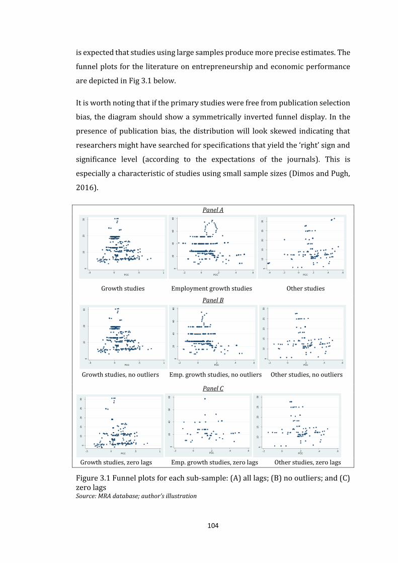
104
is expected that studies using large samples produce more precise estimates. The
funnel plots for the literature on entrepreneurship and economic performance
are depicted in Fig 3.1 below.
It is worth noting that if the primary studies were free from publication selection
bias, the diagram should show a symmetrically inverted funnel display. In the
presence of publication bias, the distribution will look skewed indicating that
researchers might have searched for specifications that yield the ‘right’ sign and
significance level (according to the expectations of the journals). This is
especially a characteristic of studies using small sample sizes (Dimos and Pugh,
2016).
Panel A
Growth studies Employment growth studies Other studies
Panel B
Growth studies, no outliers Emp. growth studies, no outliers Other studies, no outliers
Panel C
Growth studies, zero lags Emp. growth studies, zero lags Other studies, zero lags
Figure 3.1 Funnel plots for each sub-sample: (A) all lags; (B) no outliers; and (C) zero lags Source: MRA database; author’s illustration
010
20
30
INV
SE
pcc
-.5 0 .5 1PCC
020
40
60
80
INV
SE
pcc
-.2 0 .2 .4 .6PCC
510
15
20
25
30
INV
SE
pcc
-.4 -.2 0 .2 .4 .6PCC
010
20
30
INV
SE
pcc
-.5 0 .5 1PCC
020
40
60
80
INV
SE
pcc
-.2 0 .2 .4 .6PCC
510
15
20
25
30
INV
SE
pcc
-.2 0 .2 .4 .6PCC
510
15
20
25
30
INV
SE
pcc
-.5 0 .5 1PCC
020
40
60
80
INV
SE
pcc
-.2 0 .2 .4 .6PCC
51
01
52
02
53
0
INV
SE
pcc)
-.2 0 .2 .4 .6PCC

105
These funnels plot the effect sizes (PCCs) from each estimate reported in the
primary studies against its precision (inverse of the standard errors). Panel A of
Fig. 3.1 presents plots when no adjustment is made to the identified outliers or
the use of lags for the entrepreneurship measures. Panel B presents plots when
the identified outliers are excluded while Panel C represents plots when all the
lags of the entrepreneurship measures used by studies are excluded. The initial
observation of the growth literature (subsample I) seems to suggest that the
effects are symmetrically distributed around a small positive PCC, which
indicates a small average effect of entrepreneurship on economic growth.
However, the bottom part of the graph shows that PCCs are skewed to the right
(asymmetrical) suggesting that positive estimates are perhaps more preferred
for reporting and publication. Such asymmetry serves as a visual indication of
publication selection bias and suggests that it should be further investigated and
controlled for in the bivariate and multivariate analysis (Stanley, 2008; Stanley
and Doucouliagos, 2012). Similar findings are valid also for the second and the
third subsample. In both of these subsamples, the right-hand side of the funnel
plots seems to be heavier than the left side, suggesting the preference of
reviewers and the research community toward positive estimates.
An additional observation worth discussing is the relatively large number of
effects widely spread in the upper part of the funnel plots. This area of the graph
provides high levels of precision; hence such scattering of the results might not
be as a result of sampling error alone but rather of the choice of variables and
estimation techniques by the primary literature. It is, therefore, crucially
important that the subsequent sections of this chapter control for such effects
through the multivariate MRA. Although the visual inspection of funnel plots
provides an indication, it is unable to provide a definitive answer to the potential
presence of publication bias. In the subsequent sections, more accurate methods
are used to test for the presence of the publication selection bias.
Regarding the lags used, the funnel plots demonstrate that lags are used mostly
in the second subsample, employment growth studies, occasionally used in the
first subsample and barely used in the third subsample. Fig 3.1 provides another
useful information that will be considered for the subsequent analyses: funnel

106
plots suggest the potential presence of outliers which might influence the final
results if not taken into account. Thus, this chapter uses leverage plots to check
for the presence of outliers. The test (‘lv test-Letter-value displays’) reveals that,
indeed, subsample II and III suffer from the presence of a significant number of
outliers. The test suggests 27 outliers in subsample II, 12 outliers in subsample
III, and only four in subsample I.
THE BIVARIATE MRA
Following Stanley (2005; 2008) and Stanley and Doucouliagos (2012), this
section aims to identify whether the literature in investigation is contaminated
by the presence of publication selection bias and whether there is a genuine effect
– net of publication selection bias. The underlying theoretical framework is
developed by Egger et al. (1997) who argue that in order to ‘find’ significant
results and ‘as expected’ estimates, researchers with small sample sizes will
intensely ‘search’ for model specifications, data measurement, and econometrics
approaches. In so doing, the reported estimates are correlated with their
standard errors. The graphical (visual) analysis presented in the section above
indicated the presence of a positive publication selection bias. In this section, a
more advanced approach to detect the publication selection bias and the
presence (if any) of genuine effect is used. While the Funnel-Asymmetry Test
(FAT) is used to detect the presence of publication selection bias, the Precision
Effect Test (PET) and the Precision Effect Estimate with Standard Error (PEESE)
are used to detect and quantify the presence of genuine effect.
FAT – PET – PEESE
The tendency to be selective on the empirical results by reporting only
statistically significant, and according to the theoretical expectation results, leads
to biased representation and the exaggeration of genuine effects (Doucouliagos
and Stanley, 2013). In their own words: “It is as if empirical results are generated
by a stopping rule, whereby researchers cease analysing data when they have
reached what they believe to be the ‘truth’, or a sufficiently close approximation to
it. However, what a researcher believes to be the ‘truth’ is likely to be influenced by
what is consistent with prevailing theory. That is, theory defines the parameters of

107
what is ‘acceptable’ and hence what might be publishable. Contested theory widens
the set of acceptable results and thereby relaxes this stopping rule” (Doucouliagos
and Stanley, 2013, p.318). Goldfarb (1995) and Stanley (2008), use the concept
of ‘economic research cycle’ to describe the situation where researchers initially
try to find empirical results that would confirm a new theory and thereby be
published. However, after some time, finding results that contradict that theory
becomes more ‘publishable’ due to the law of the diminishing marginal utility.
The bivariate meta-regression model typically regresses the effect sizes of
interest, entrepreneurship, on an intercept and the standard error (SEi), which
represents the statistical precision. It assumes that the error term is
independently and identically distributed (i.i.d) which implies that the effect
sizes (PCCi) are independent of their standard errors (SEi), hence the following
equation:
𝑃𝐶𝐶𝑖 = 𝛽0 + 𝛽1𝑆𝐸𝑖 + 휀𝑖 (3.4)
where i = 1,…,n, the 657 individual estimates reported in the primary studies. SEi
represents the standard error of the ith effect reported in the primary literature
and εi is the conventional error term. Coefficient β1 will turn out to be statistically
significant if there is publication selection, the direction of it will be indicated by
its sign and the magnitude by the coefficient itself. Note as the SEi tends to equal
0, the effect size (PCCi) converges to β0 which provides an estimate of the
underlying effect of entrepreneurship measures on economic performance. The
so-called Funnel-Asymmetry Test (FAT) is used to test the hypothesis (H0: β1=0),
while Precision Effect Test (PET) is used to test whether there is a genuine
underlying effect beyond publication selection bias. 35 Thus, PET tests whether
H0: β0=0. Rejecting the null hypothesis (H0: β1=0) suggests the presence of
publication selection bias, likewise rejecting the null hypothesis (H0: β0=0)
indicates the presence of the genuine empirical effect beyond publication
selection bias.
35 This is called the Funnel-Asymmetry Test (FAT) due to its relation to the funnel graphs (Stanley, 2005).
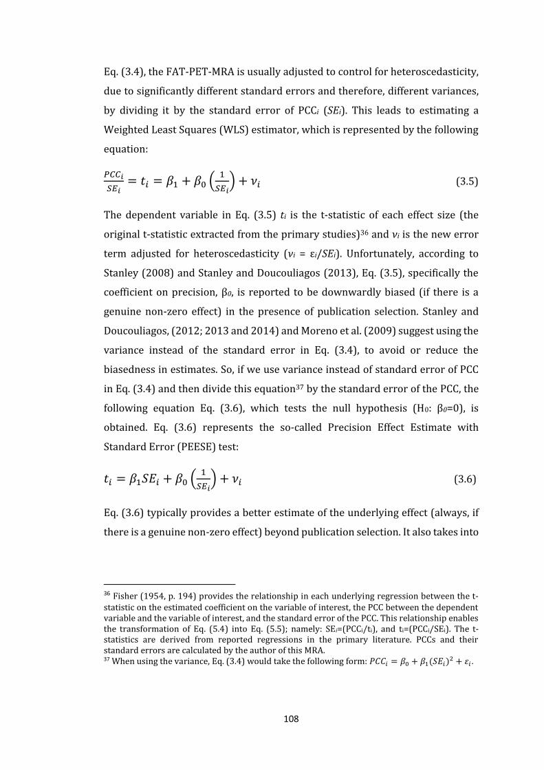
108
Eq. (3.4), the FAT-PET-MRA is usually adjusted to control for heteroscedasticity,
due to significantly different standard errors and therefore, different variances,
by dividing it by the standard error of PCCi (SEi). This leads to estimating a
Weighted Least Squares (WLS) estimator, which is represented by the following
equation:
𝑃𝐶𝐶𝑖
𝑆𝐸𝑖= 𝑡𝑖 = 𝛽1 + 𝛽0 (
1
𝑆𝐸𝑖) + 𝜈𝑖 (3.5)
The dependent variable in Eq. (3.5) ti is the t-statistic of each effect size (the
original t-statistic extracted from the primary studies)36 and νi is the new error
term adjusted for heteroscedasticity (νi = εi/SEi). Unfortunately, according to
Stanley (2008) and Stanley and Doucouliagos (2013), Eq. (3.5), specifically the
coefficient on precision, β0, is reported to be downwardly biased (if there is a
genuine non-zero effect) in the presence of publication selection. Stanley and
Doucouliagos, (2012; 2013 and 2014) and Moreno et al. (2009) suggest using the
variance instead of the standard error in Eq. (3.4), to avoid or reduce the
biasedness in estimates. So, if we use variance instead of standard error of PCC
in Eq. (3.4) and then divide this equation37 by the standard error of the PCC, the
following equation Eq. (3.6), which tests the null hypothesis (H0: β0=0), is
obtained. Eq. (3.6) represents the so-called Precision Effect Estimate with
Standard Error (PEESE) test:
𝑡𝑖 = 𝛽1𝑆𝐸𝑖 + 𝛽0 (1
𝑆𝐸𝑖) + 𝜈𝑖 (3.6)
Eq. (3.6) typically provides a better estimate of the underlying effect (always, if
there is a genuine non-zero effect) beyond publication selection. It also takes into
36 Fisher (1954, p. 194) provides the relationship in each underlying regression between the t-statistic on the estimated coefficient on the variable of interest, the PCC between the dependent variable and the variable of interest, and the standard error of the PCC. This relationship enables the transformation of Eq. (5.4) into Eq. (5.5); namely: SEi=(PCCi/ti), and ti=(PCCi/SEi). The t-statistics are derived from reported regressions in the primary literature. PCCs and their standard errors are calculated by the author of this MRA. 37 When using the variance, Eq. (3.4) would take the following form: 𝑃𝐶𝐶𝑖 = 𝛽0 + 𝛽1(𝑆𝐸𝑖)2 + 휀𝑖.
109
account the issue of heteroscedasticity (Stanley and Doucouliagos, 2012;
Doucouliagos et al., 2014; Dimos and Pugh, 2016).
As previously discussed in section 3.3, and given the common practice in
quantitative research, most of the primary studies report more than one estimate
(i.e., effect size). Due to the use of lags for the entrepreneurship measures, some
studies reported significantly different effects in one single specification (see
Fritsch and Mueller, 2004) and they were included as unique effects in the MRA
dataset. For instance, Fritsch and Mueller (2004), in one of the specifications,
report a positive and significant effect of entrepreneurship (start-up rate, (t)) on
employment growth followed by four negative and significant effects (start-up
rate (t-1) – (t-4)), and three positive and significant effects (start-up rate (t-6) –
(t-8)). To account for such a pronounced between-specification heterogeneity,
due to the prevalent use of lags, the chapter uses a specific weight designed to
give equal weights to specifications within one single study, regardless of the
number of effects reported per specification. The weight, ’study-specification
weight’, assigned to each reported effect within one study depends on the
number of reported estimates per specification. Thus, a study reporting 11
effects from two specifications, 10 effects from specification (1) and 1 effect from
specification (2) would have these corresponding weights: Both specifications
would have a weight of 0.5, suggesting that each of the 10 effects coming from
specification (1) would have a weight of 0.05 (0.5 (specification weight)/10
(reported effects)) while the one effect coming from specification (2) will have a
weight of 0.5 alone. In other words, if a study has 5 different specifications, each
would have a weight of 0.2, irrespective of how many effects are produced
through lags.38 Thus, this approach reduces the influence of the use of extensive
lags. To our knowledge, this kind of weighting is applied for the first time in the
MRA literature and is an original contribution to knowledge. In addition to the
use of lags, the variety of potential sources of within-study and between
specification heterogeneity includes: different proxies for entrepreneurship;
38 The single study will always have a weight of 1, as all specifications are subject to one set of theoretical background and empirical approach as well as the researcher’s inclinations and views. Giving more weight to a paper with several specifications would overemphasise the views of one author.
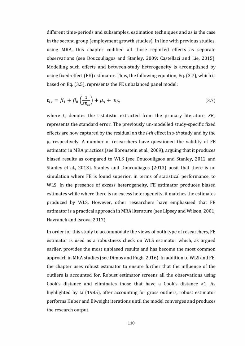
110
different time-periods and subsamples, estimation techniques and as is the case
in the second group (employment growth studies). In line with previous studies,
using MRA, this chapter codified all those reported effects as separate
observations (see Doucouliagos and Stanley, 2009; Castellaci and Lie, 2015).
Modelling such effects and between-study heterogeneity is accomplished by
using fixed-effect (FE) estimator. Thus, the following equation, Eq. (3.7), which is
based on Eq. (3.5), represents the FE unbalanced panel model:
𝑡𝑖𝑠 = 𝛽1 + 𝛽0 (1
𝑆𝐸𝑖𝑠) + 𝜇𝑠 + 𝜐𝑖𝑠 (3.7)
where tis denotes the t-statistic extracted from the primary literature, SEis
represents the standard error. The previously un-modelled study-specific fixed
effects are now captured by the residual on the i-th effect in s-th study and by the
µs respectively. A number of researchers have questioned the validity of FE
estimator in MRA practices (see Borenstein et al., 2009), arguing that it produces
biased results as compared to WLS (see Doucouligaos and Stanley, 2012 and
Stanley et al., 2013). Stanley and Doucouliagos (2013) posit that there is no
simulation where FE is found superior, in terms of statistical performance, to
WLS. In the presence of excess heterogeneity, FE estimator produces biased
estimates while where there is no excess heterogeneity, it matches the estimates
produced by WLS. However, other researchers have emphasised that FE
estimator is a practical approach in MRA literature (see Lipsey and Wilson, 2001;
Havranek and Isrova, 2017).
In order for this study to accommodate the views of both type of researchers, FE
estimator is used as a robustness check on WLS estimator which, as argued
earlier, provides the most unbiased results and has become the most common
approach in MRA studies (see Dimos and Pugh, 2016). In addition to WLS and FE,
the chapter uses robust estimator to ensure further that the influence of the
outliers is accounted for. Robust estimator screens all the observations using
Cook’s distance and eliminates those that have a Cook’s distance >1. As
highlighted by Li (1985), after accounting for gross outliers, robust estimator
performs Huber and Biweight iterations until the model converges and produces
the research output.
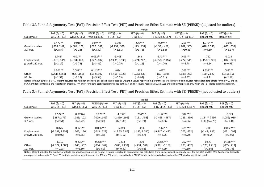
111
Table 3.3 Funnel-Asymmetry Test (FAT), Precision Effect Test (PET) and Precision Effect Estimate with SE (PEESE)a (adjusted for outliers)
Table 3.4 Funnel-Asymmetry Test (FAT), Precision Effect Test (PET) and Precision Effect Estimate with SE (PEESE)a (not adjusted to outliers)
Model
Subsample FAT (β1 = 0) WLS Eq. (3.5)
PET (β0 = 0) WLS Eq. (3.5)
PEESE (β0 = 0) WLS Eq. (3.6)
FAT (β1 = 0) FE Eq. (3.7)
PET (β0 = 0) FE Eq. (3.7)
FAT (β1 = 0) FE (G-S) Eq. (3.7)
PET (β0 = 0) FE (G-S) Eq. (3.7)
FAT (β1 = 0) Robust est.
PET (β0 = 0) Robust est.
Growth studies 297 obs.
1.477** [.278; 2.67]
(t=2.54)
0.010 [-.081; .102]
(t=0.23)
0.074** [.007; .141]
(t=2.30)
-1.196 [-2.731; .339]
(t=-1.61)
.276*** [.123; .431]
(t=3.72)
-.999*** [-1.53; -.469]
(t=-3.88)
.256*** [.207; .305]
(t=10.81)
1.079*** [.618; 1.540]
(t=4.60)
-0.023 [-.057; .010]
(t=-1.37) Employment growth 222 obs.
1.741* [-.010; 3.49]
(t=2.17)
0.0174 [-.034; .068]
(t=0.74)
0.052*** [.022; .082]
(t=3.81)
-3.408 [-13.35; 6.536]
(t=-0.75)
.343 [-.274; .961]
(t=1.21)
-5.43*** [-7.953; -2.916]
(t=-4.70)
.409*** [.277; .541]
(t=6.78)
.792 [-.158; 1.741]
(t=1.64)
0.014 [-.014; .041]
(t=0.95) Other 95 obs.
1.501** [.251; 2.751]
(t=2.53)
0.081** [.005; .156]
(t=2.26)
0.142*** [.092; .192]
(t=5.94)
-.084 [-5.491; 5.323]
(t=-0.03)
.206 [-.235; .647]
(t=0.98)
-.077 [-.853; .699]
(t=-0.21)
.205*** [.148; .263]
(t=7.57)
1.539*** [.450; 2.627]
(t=2.81)
.0832** [.010; .156]
(t=2.26) Notes: Without outliers (‘lv’ t). Weight adjusted for number of effects per specification used as weight. t-values reported in parentheses are calculated from cluster-robust standard errors for the WLS and FE. 95% Confidence Intervals are reported in brackets. *** and ** indicate statistical significance at the 1% and 5% levels, respectively. a PEESE should be interpreted only when the PET yields a significant result.
Model
Subsample FAT (β1 = 0) WLS Eq. (3.5)
PET (β0 = 0) WLS Eq. (3.5)
PEESE (β0 = 0) WLS Eq. (3.6)
FAT (β1 = 0) FE Eq. (3.7)
PET (β0 = 0) FE Eq. (3.7)
FAT (β1 = 0) FE (G-S) Eq. (3.7)
PET (β0 = 0) FE (G-S) Eq. (3.7)
FAT (β1 = 0) Robust est.
PET (β0 = 0) Robust est.
Growth studies 301 obs.
1.522** [.287; 2.76]
(t=2.54)
0.00974 [.083; .102]
(t=0.22)
0.076** [.009; .142]
(t=2.33)
-1.332* [-2.859; .195]
(t=-1.80)
.294*** [.131; .458]
(t=3.71)
-1.52*** [-2.455; -.587]
(t=-3.36)
.312*** [.225; .399]
(t=7.36) 1.13*** [.656; 1.60] (t=4.70)
-0.024 [-.059; .010]
(t=-1.40) Employment growth 249 obs.
0.876 [-1.198; 2.951]
(t=0.92)
0.071** [.005; .136]
(t=2.35)
0.086*** [.043; .129]
(t=4.33)
-6.849 [-19.55; 5.85]
(t=-1.17)
.494 [-.192; 1.180]
(t=1.57)
-5.66** [-9.847; -1.482]
(t=-2.95)
.429*** [.207; .652]
(t=4.20)
-.305 [-1.42; .813]
(t=-0.54)
0.062*** [.031; .093]
(t=3.95) Other 107 obs.
-1.319 [-4.324; 1.686]
(t=-0.93)
0.275** [.043; .507]
(t=2.50)
0.228*** [.094; .362]
(t=3.59)
-1.233 [-9.89; 7.432]
(t=-0.30)
.270 [-.431; .970]
(t=0.81)
2.266*** [-3.381; -1.152]
(t=-4.29)
.352*** [.273; .432]
(t=9.39)
0.571 [-.573; 1.715]
(t=0.99)
0.138*** [.065; .212]
(t=3.74) Notes: Weight adjusted for number of effects per specification used as weight. t-values reported in parentheses are calculated from cluster-robust standard errors for the WLS and FE. 95% Confidence Intervals are reported in brackets. *** and ** indicate statistical significance at the 1% and 5% levels, respectively. a PEESE should be interpreted only when the PET yields a significant result.

Tables 3.3 and 3.4, based on Eq. (3.5), Eq. (3.6) and Eq. (3.7) report the results of
the bivariate FAT-PET-PEESE for each subsample analysis. Eq. (3.5) is used to
obtain the WLS estimates of FAT and PET, Eq. (3.6) estimates for PEESE while Eq.
(3.7) to obtain the FAT-PET estimates using fixed-effect estimator (FE) and FE G-
S (General-to-Specific) approach. Taking a conventional approach to inference, all
the FAT-PET-PEESE reported estimates of the WLS and FE were produced using
cluster-robust standard errors, thus correcting standard errors for data
dependence among effect sizes as primary studies report multiple estimates per
study.
Table 3.3 presents results after adjusting for the presence of outliers, while Table
3.4 presents results when no agistment is made to the identified outliers and its
results will be interpreted only when significant differences with Table 3.3 are
found. The first column of Table 3.3 and Table 3.4 show the identified subsamples
in the primary literature. As discussed earlier, the three subsamples share
enough similarities, but at the same time use different economic performance
proxies, thus making it impossible to group them in a single MRA database.
Moreover, the approach of having more than one subsample is a common
practice in the MRA studies (see Efendic et al., 2011; Dimos and Pugh, 2016).
The bivariate MRA suggests the presence of ‘substantial’ (FAT=1.48) positive
publication selection bias and the absence of genuine effect in the first
subsample, when WLS is applied. As discussed in section 3.4.2 there is a tendency
and, perhaps, a preference of researchers to report positive estimates, as
observed by the visual inspection of the funnel plots. Although the plots suggest
that as the reported estimates become more precise (i.e., higher values of inverse
of PCC) they tend to be positioned around 0. On the other hand, a negative FAT (-
0.999) result is suggested when the G-S (General-to-Specific) approach to the FE
estimator is used. This approach requires dropping the least significant
moderators (in this case fixed effects) until no insignificant moderator remains
in the model. However, when the fixed effect (FE) is used, FAT indicates a
negative, though statistically insignificant publication selection bias. Also, when
robust estimator is used, FAT shows a positive and significant coefficient,
suggesting the positive publication selection bias. Similar results are obtained
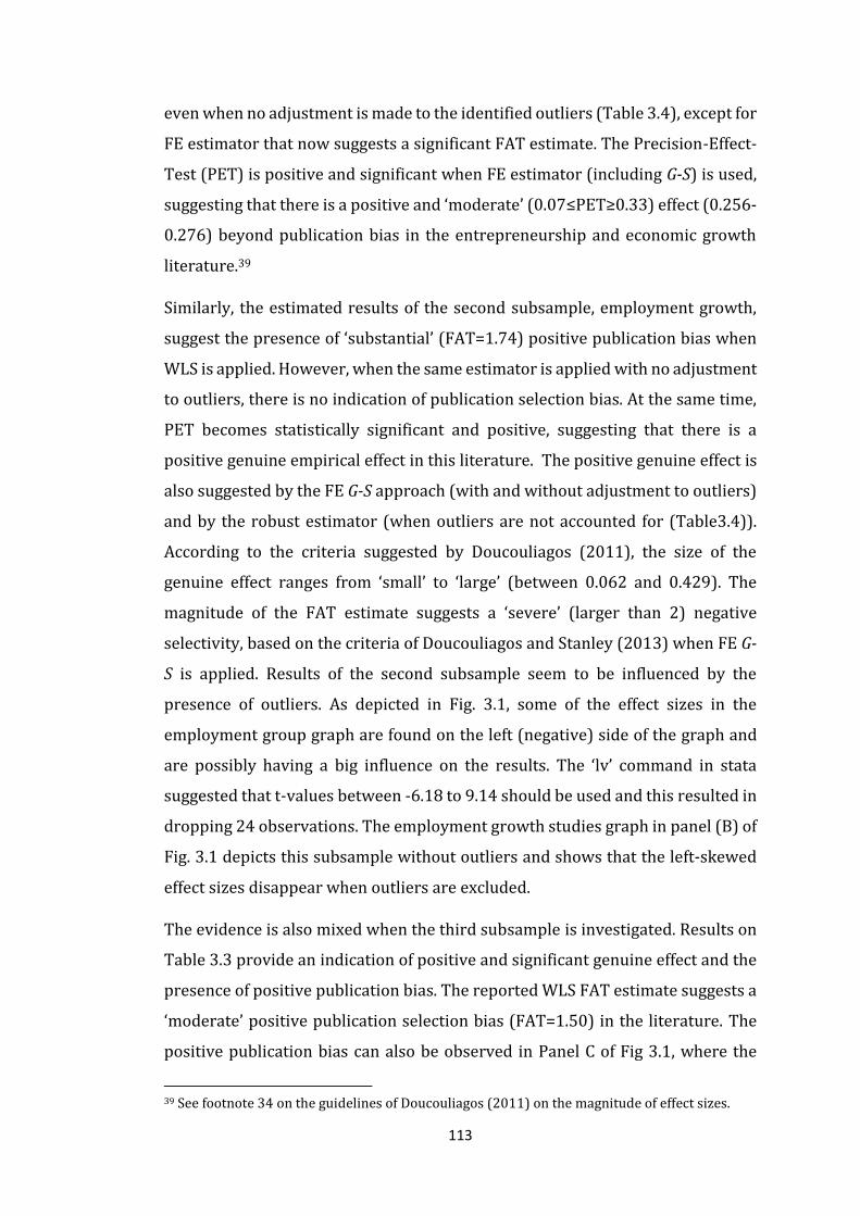
113
even when no adjustment is made to the identified outliers (Table 3.4), except for
FE estimator that now suggests a significant FAT estimate. The Precision-Effect-
Test (PET) is positive and significant when FE estimator (including G-S) is used,
suggesting that there is a positive and ‘moderate’ (0.07≤PET≥0.33) effect (0.256-
0.276) beyond publication bias in the entrepreneurship and economic growth
literature.39
Similarly, the estimated results of the second subsample, employment growth,
suggest the presence of ‘substantial’ (FAT=1.74) positive publication bias when
WLS is applied. However, when the same estimator is applied with no adjustment
to outliers, there is no indication of publication selection bias. At the same time,
PET becomes statistically significant and positive, suggesting that there is a
positive genuine empirical effect in this literature. The positive genuine effect is
also suggested by the FE G-S approach (with and without adjustment to outliers)
and by the robust estimator (when outliers are not accounted for (Table3.4)).
According to the criteria suggested by Doucouliagos (2011), the size of the
genuine effect ranges from ‘small’ to ‘large’ (between 0.062 and 0.429). The
magnitude of the FAT estimate suggests a ‘severe’ (larger than 2) negative
selectivity, based on the criteria of Doucouliagos and Stanley (2013) when FE G-
S is applied. Results of the second subsample seem to be influenced by the
presence of outliers. As depicted in Fig. 3.1, some of the effect sizes in the
employment group graph are found on the left (negative) side of the graph and
are possibly having a big influence on the results. The ‘lv’ command in stata
suggested that t-values between -6.18 to 9.14 should be used and this resulted in
dropping 24 observations. The employment growth studies graph in panel (B) of
Fig. 3.1 depicts this subsample without outliers and shows that the left-skewed
effect sizes disappear when outliers are excluded.
The evidence is also mixed when the third subsample is investigated. Results on
Table 3.3 provide an indication of positive and significant genuine effect and the
presence of positive publication bias. The reported WLS FAT estimate suggests a
‘moderate’ positive publication selection bias (FAT=1.50) in the literature. The
positive publication bias can also be observed in Panel C of Fig 3.1, where the
39 See footnote 34 on the guidelines of Doucouliagos (2011) on the magnitude of effect sizes.
114
PCCs are found to be skewed on the right-hand side of the funnel plot. The WLS
PET estimate suggests a ‘moderate’ genuine effect (PET=0.081) which is
confirmed by PEESE (0.142). The fixed effect (FE) estimator suggests neither
significant genuine effect nor publication bias. However, when the FE G-S
approach is applied, PET estimate turns positive and significant (PET=0.205).
The PET estimate remains positive and significant even when robust estimator is
used. However, when no adjustment is made to outliers, the estimated results
suggest that besides the genuine positive effect, there is no evidence of
publication selection bias, when WLS and robust estimator are applied.
Overall, the FAT-PET-PEESE procedures suggest the presence of publication
selection bias and the genuine empirical effect, especially for the third
subsample. The estimated FAT of the second subsample, suggests a ‘severe’
negative publication selection (FAT>2) when FE G-S is applied. When outliers are
not taken into account, the second subsample report PET and PEESE estimates,
which correspond to ‘moderate’ magnitude, suggesting that entrepreneurship
measures have a genuine positive impact on employment growth. In the third
subsample, when WLS and robust estimator are applied and when the estimates
are adjusted for outliers, FAT estimate is positive but smaller than 2, yet
suggesting the presence of positive publication bias. This preliminary finding is
in line with the proposition of Bosma et al. (2018) who argue that studies using
income levels or productivity, as their measure of economic performance, might
suffer from publication bias. O’Boyle et al. (2014) provided a systematic review
of 15 papers and suggest that the entrepreneurship literature is not immune to
publication bias. At the same time, the estimated PET suggests that there is a
‘moderate’ (between 0.081 to 0.205) positive genuine effect in this literature. The
deviations of the PET estimates from the reported unweighted PCC of 0.178
(Table 3.2) of the third subsample studies are consistent with the FAT findings,
i.e., they support the presence of publication bias.40
40 The unweighted PCC of the same subsample becomes even larger (0.201), after adjusting for outliers.
115
THE MULTIVARIATE MRA
Heterogeneity
This section employs multivariate MRA model to analyse the sources of effect size
heterogeneity. Following Stanley et al. (2015) and Dimos and Pugh (2016),
Cochran’s Q-statistic (Higgins et al., 2003) is used to identify the level of
heterogeneity on the reported effects by the primary literature (see Appendix
3.15 where the Cochran’s Q-statistic is reported).41 In all the subsamples,
Cochran’s Q-statistic suggests the presence of excess heterogeneity (p-
value<0.001). The expectations, a priori, are that this observed heterogeneity is
not attributed only to the differences in sample sizes but also to the choice of the
methodology employed, type of the data and other characteristics of the primary
studies. Multivariate MRA allows for the augmentation of the bivariate MRA to
include all these potential sources of heterogeneity in a single equation. These
moderators are extracted from the primary literature and provide the
information that helps explain the variation in the reported effects. In this MRA,
to enter the equation as a ‘moderator’, a study dimension must meet two criteria:
(i) be found in at least two studies in each subsample; and (ii) the frequency of
this dimension to be at least 5% of each subsample, i.e., if at least 15 effect sizes
of the first subsample have been influenced by this dimension (297 effect sizes in
total after adjusting for outliers).
The identified study dimensions in the primary literature are briefly discussed in
section 3.2.3 and 3.3.3. Table 3.5 at the end of this section provides the definitions
of all moderators, along with the descriptive statistics for each subsample. This
section elaborates the rationale for including these study characteristics and the
expected effect on reported effects (PCCs). As previously discussed (see section
3.3.2), the choice of the measure of entrepreneurial activity might have an impact
on the reported effect sizes. Thus, the study has identified all the proxies used in
41 According to Stanley and Doucouliagos, (2012, p.45), the Cochran’s Q-statistic measures the deviation of observed effect size (y) in a regression j of a study i, from an underlying overall effect size (θ), giving a weight (wi) to each study. It is calculated as the weighted sum of squared differences between individual study effects and the pooled effect across studies (Harris et al., 2008). In the MRA, this can be easily detected by the sum of squared errors of the bivariate MRA without constant term. Higgins et al. (2003) argue that the test has considerable power when the number of studies in the dataset is large.
116
the primary literature, such as Total Entrepreneurial Activity (TEA) (overalltea);
High-Growth Aspiration (ambitious) Entrepreneurial Activity (hgatea); Export-
oriented Entrepreneurial Activity (exptea); Opportunity-driven Entrepreneurial
Activity (opportunitytea); Necessity-driven Entrepreneurial Activity
(necessitytea), all measures being available in the Global Entrepreneurship
Monitor (GEM) dataset. The advantage of GEM data and specifically of using TEA
measures is the fact that GEM uses uniform definition of variables and data
collection methodologies, thus making the indices easily comparable across
countries (Acs et al., 2008; Urbano and Aparicio, 2016).
Besides the use of the GEM measures, primary studies have also used other
proxies of entrepreneurial activity, which have to be included in the multivariate
MRA as specific moderators. Thus, the study controls also for these measures of
entrepreneurial activity: start-up rates (startups); self-employment
(selfemployment); net entry (netentry); and business ownership
(businessownership). Start-up rates are usually calculated using the so-called
Labour Market Approach (LMA), which assumes that the labour market
dynamics influence the number of new firms, i.e., the number of new-firm start-
ups is divided by employment (Fritsch and Mueller 2004; van Stel and Suddle,
2008). Carree and Thurik (2008) use the natural logarithm of the number of
business owners in relation to the total labour force to proxy for entrepreneurial
activity, arguing that positive changes in the number of business owners have a
positive impact on employment growth, labour productivity and GDP growth.
Studies differ also on the choice of dependent variable i.e., the measure of
economic performance by using: GDP growth (gdpgrowth); the growth of GDP
per capita (growthofgdppercapita); GDP at levels (levelofgdp); employment
growth (employmentgrowth); GDP per capita (gdppercapita); labour
productivity (labourproductivity) and; Total Factor Productivity (TFP)
(totalfactorproductivity). The majority of studies (25 out of 52) and reported
effects (301 out of 657 or 297 out of 574 when adjusted for outliers) come from
GDP growth and growth of GDP per capita and are grouped into the first sub-
sample of the MRA database. The hypothesis states that higher entrepreneurial
activity rates lead to higher rates of GDP growth. Employment growth is the only

117
measure of economic performance used by 13 studies that comprise the second
subsample. Labour productivity, GDP per capita, GDP at levels and TFP will also
be included in the multivariate MRA as studies in the third subsample use them.
Differences in the methodological research design will also be controlled for by
including the following set of moderators in the multivariate MRA: Instrumental
Variable approach (2SLS; 3SLS) (IV), the conventional caveat in accounting for
endogeneity; Fixed-effect estimator (fe), allowing for country and regional
specific effects to be modelled; GMM estimator (GMM), allowing for modelling
the dynamics in the relationship between entrepreneurship and economic
performance; and Ordinary Least Squares (OLS) (ols) estimator.
In addition to the choice of estimation strategies, the study also controls for lags
or entrepreneurship in previous periods used to account for potential
endogeneity (lags); the type of specification of the variables of interest i.e., log-
log specification (log); study explicitly addressing the issue of endogeneity
(endogeneity); distinguishes between main and robustness checks reported
estimates (mainest); the differences in the level of development, i.e.,
distinguishing between developing and developed economies (developing;
developed); if the study uses GEM data (gem).42 Furthermore, the study controls
for: primary studies which include a measure of capital (e.g., gross capital
formation) (capital) and; primary studies which include a measure of labour
(e.g., the no. of unemployed) (labour) and institutions (e.g., GCI) (institutions).
In addition, human capital (human), investment (investment), trade (trade) are
also accounted for. It has been argued that developing countries have higher
growth rates (see Diao et al., 2017) compared to developed economies, thus the
study controls for the catch-up or convergence effect (convergence). Time
dummies are also an important research design approach, to account for year-
specific shocks (timedummy). This chapter also controls for the type of data
used, panel data (panel), allowing for country unobserved heterogeneity to be
captured by panel estimators, pooled cross-section (pooledcrsection), cross-
section data structures (crosssection), and time-series (ts). The expectation is
42 For GEM, the study controls only indirectly; studies that use one of the measures of GEM, e.g., overall TEA; high-growth aspiration TEA, etc.

118
that the type of data has a significant influence on the findings of the primary
literature.
Further, the study controls whether the primary study is published in a peer-
reviewed journal (publishedjournal); which is an indication of the quality of the
study and has received financial support, especially from any related parties that
might influence the research findings (financial_conflict). Finally, the
multivariate MRA controls for the influence of data period, i.e., the mid-year of
data of the studies in the primary literature and for the tendency of recently
published papers, i.e., the mid-year of publication. More rationale for
specifically selecting this set of moderators will also be provided when the
multivariate MRA results are interpreted in more details in the next sections.
Equation (3.5) and (3.7) of the bivariate MRA need to be augmented to allow for
including the set of moderators identified in the primary literature. Previous
studies distinguish between (i) K-variables or moderators capturing contextual
study characteristics, influencing publication selection bias and (ii) Z-variables
or moderators capturing research design, methodological approaches and
sample size, influencing the genuine empirical effect (see Doucouliagos et al.,
2014; Dimos and Pugh, 2016). This chapter follows this approach by
acknowledging the moderators influencing the genuine empirical effect and the
moderators influencing publication selection bias. Thus, the augmented versions
of Eq. (3.5) and Eq. (3.7), allowing the room for including the K and Z moderators,
take the following form:
𝑡𝑖 = 𝛽1 + ∑ 𝛾𝑚𝐾𝑚𝑖 + 𝛽0 (1
𝑆𝐸𝑖) + ∑ 𝛽𝑛 (
𝑍𝑛𝑖
𝑆𝐸𝑖) + 𝜈𝑖 (3.8)
𝑡𝑖 = 𝛽1 + ∑ 𝛾𝑚𝐾𝑚𝑖𝑠 + 𝛽0 (1
𝑆𝐸𝑖𝑠) + ∑ 𝛽𝑛 (
𝑍𝑛𝑖𝑠
𝑆𝐸𝑖𝑠) + 𝜇𝑠 + 𝜐𝑖𝑠 (3.9)
where m K-variables are represented by Kmi and Kmis and n Z-variables by Zni and
Znis all modelling the sources of potential publication selection bias and
heterogeneity of the effect sizes (PCCs), respectively. γm and βn stand as the
coefficients of K and Z-variables. In all the three subsamples, most of the
moderators included belong to the Z-variable category while ony three
moderators belong to the K-variable category. The K-moderators capture

119
contextual study characteristics that influence publication selection bias (β1) and
Z-moderators capture research design, methodological approaches and sample
size, influencing the genuine empirical effect (β0). 𝜇𝑠 in Eq. (3.9) represents the
unobserved study-specific fixed-effects, while νis is the error term. The
moderators that influence the genuine empirical effect are all interacted with the
inverse SE as it has been explained in variable names (Table 3.6 and also shown
in Appendix 3.6.1).
Descriptive statistics
Following on the discussions in sections 3.3.2 and 3.3.3, the definition and the
descriptive statistics of all moderator variables identified in this meta-regression
analysis are provided in Table 3.5.43 This table contains information and
identifies the sources of potential heterogeneity in the results of primary studies.
Table 3.5 presents the characteristics of the primary studies divided into several
categories such as the choice of dependent (economic performance) and
independent variable (entrepreneurship), methodological approaches and
estimation method used, conventional control variables used, other study
characteristics and details, etc.
Following the narrative discussion in in section 3.3.2 and 3.3.3, in Table 3.5 the
selected descriptive statistics are reported in separate columns for the three
subsamples to specifically highlight the differences in the choice of
entrepreneurship and other subsample specific moderators. As it can be
observed in Table 3.2 and as elaborated in sections above, there is a
harmonisation of variable choice in subsample I and subsample III, while the
choice of moderators in subsample II is relatively different. Appendix (3.1.4)
provides descriptive statistics of the three subsamples after adjusting for
outliers.44
43 Some of the identified moderators are not included in the multivariate analysis due to high correlation, or as they have failed to meet the two criteria set in this chapter. 44 The study elaborates how outliers were detected in section 3.4.2 and discusses differences when they appear to influence significance levels.
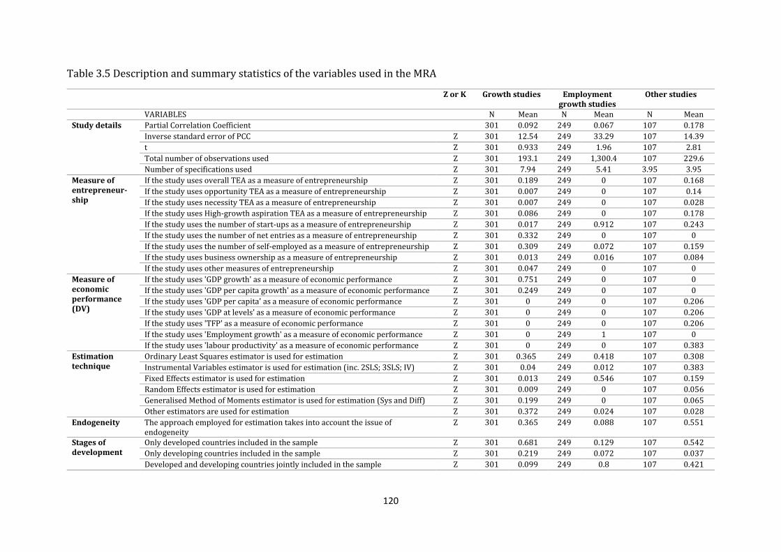
120
Table 3.5 Description and summary statistics of the variables used in the MRA
Z or K Growth studies Employment growth studies
Other studies
VARIABLES N Mean N Mean N Mean
Study details Partial Correlation Coefficient 301 0.092 249 0.067 107 0.178
Inverse standard error of PCC Z 301 12.54 249 33.29 107 14.39
t Z 301 0.933 249 1.96 107 2.81
Total number of observations used Z 301 193.1 249 1,300.4 107 229.6
Number of specifications used Z 301 7.94 249 5.41 3.95 3.95
Measure of entrepreneur-ship
If the study uses overall TEA as a measure of entrepreneurship Z 301 0.189 249 0 107 0.168
If the study uses opportunity TEA as a measure of entrepreneurship Z 301 0.007 249 0 107 0.14
If the study uses necessity TEA as a measure of entrepreneurship Z 301 0.007 249 0 107 0.028
If the study uses High-growth aspiration TEA as a measure of entrepreneurship Z 301 0.086 249 0 107 0.178
If the study uses the number of start-ups as a measure of entrepreneurship Z 301 0.017 249 0.912 107 0.243
If the study uses the number of net entries as a measure of entrepreneurship Z 301 0.332 249 0 107 0
If the study uses the number of self-employed as a measure of entrepreneurship Z 301 0.309 249 0.072 107 0.159
If the study uses business ownership as a measure of entrepreneurship Z 301 0.013 249 0.016 107 0.084
If the study uses other measures of entrepreneurship Z 301 0.047 249 0 107 0
Measure of economic performance (DV)
If the study uses 'GDP growth' as a measure of economic performance Z 301 0.751 249 0 107 0
If the study uses 'GDP per capita growth' as a measure of economic performance Z 301 0.249 249 0 107 0
If the study uses 'GDP per capita' as a measure of economic performance Z 301 0 249 0 107 0.206
If the study uses 'GDP at levels' as a measure of economic performance Z 301 0 249 0 107 0.206
If the study uses 'TFP' as a measure of economic performance Z 301 0 249 0 107 0.206
If the study uses 'Employment growth' as a measure of economic performance Z 301 0 249 1 107 0
If the study uses 'labour productivity' as a measure of economic performance Z 301 0 249 0 107 0.383
Estimation technique
Ordinary Least Squares estimator is used for estimation Z 301 0.365 249 0.418 107 0.308
Instrumental Variables estimator is used for estimation (inc. 2SLS; 3SLS; IV) Z 301 0.04 249 0.012 107 0.383
Fixed Effects estimator is used for estimation Z 301 0.013 249 0.546 107 0.159
Random Effects estimator is used for estimation Z 301 0.009 249 0 107 0.056
Generalised Method of Moments estimator is used for estimation (Sys and Diff) Z 301 0.199 249 0 107 0.065
Other estimators are used for estimation Z 301 0.372 249 0.024 107 0.028
Endogeneity The approach employed for estimation takes into account the issue of endogeneity
Z 301 0.365 249 0.088 107 0.551
Stages of development
Only developed countries included in the sample Z 301 0.681 249 0.129 107 0.542
Only developing countries included in the sample Z 301 0.219 249 0.072 107 0.037
Developed and developing countries jointly included in the sample Z 301 0.099 249 0.8 107 0.421
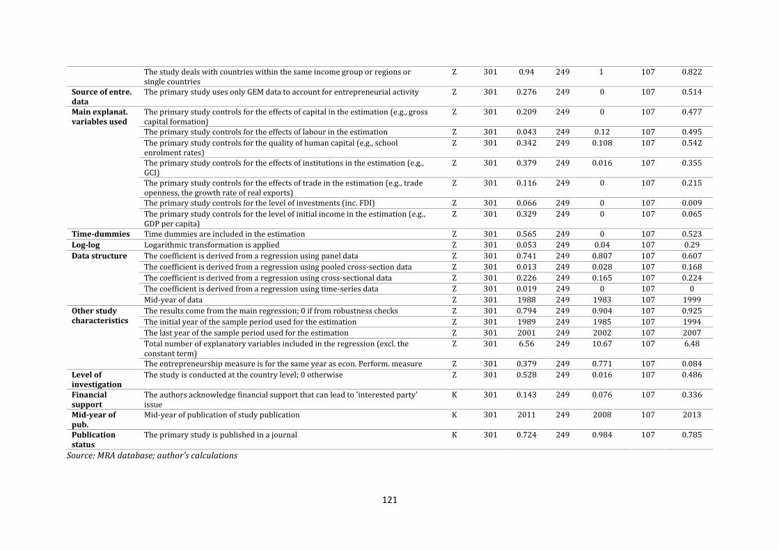
121
The study deals with countries within the same income group or regions or single countries
Z 301 0.94 249 1 107 0.822
Source of entre. data
The primary study uses only GEM data to account for entrepreneurial activity Z 301 0.276 249 0 107 0.514
Main explanat. variables used
The primary study controls for the effects of capital in the estimation (e.g., gross capital formation)
Z 301 0.209 249 0 107 0.477
The primary study controls for the effects of labour in the estimation Z 301 0.043 249 0.12 107 0.495
The primary study controls for the quality of human capital (e.g., school enrolment rates)
Z 301 0.342 249 0.108 107 0.542
The primary study controls for the effects of institutions in the estimation (e.g., GCI)
Z 301 0.379 249 0.016 107 0.355
The primary study controls for the effects of trade in the estimation (e.g., trade openness, the growth rate of real exports)
Z 301 0.116 249 0 107 0.215
The primary study controls for the level of investments (inc. FDI) Z 301 0.066 249 0 107 0.009
The primary study controls for the level of initial income in the estimation (e.g., GDP per capita)
Z 301 0.329 249 0 107 0.065
Time-dummies Time dummies are included in the estimation Z 301 0.565 249 0 107 0.523
Log-log Logarithmic transformation is applied Z 301 0.053 249 0.04 107 0.29
Data structure The coefficient is derived from a regression using panel data Z 301 0.741 249 0.807 107 0.607
The coefficient is derived from a regression using pooled cross-section data Z 301 0.013 249 0.028 107 0.168
The coefficient is derived from a regression using cross-sectional data Z 301 0.226 249 0.165 107 0.224
The coefficient is derived from a regression using time-series data Z 301 0.019 249 0 107 0
Mid-year of data Z 301 1988 249 1983 107 1999
Other study characteristics
The results come from the main regression; 0 if from robustness checks Z 301 0.794 249 0.904 107 0.925
The initial year of the sample period used for the estimation Z 301 1989 249 1985 107 1994
The last year of the sample period used for the estimation Z 301 2001 249 2002 107 2007
Total number of explanatory variables included in the regression (excl. the constant term)
Z 301 6.56 249 10.67 107 6.48
The entrepreneurship measure is for the same year as econ. Perform. measure Z 301 0.379 249 0.771 107 0.084
Level of investigation
The study is conducted at the country level; 0 otherwise Z 301 0.528 249 0.016 107 0.486
Financial support
The authors acknowledge financial support that can lead to 'interested party' issue
K 301 0.143 249 0.076 107 0.336
Mid-year of pub.
Mid-year of publication of study publication K 301 2011 249 2008 107 2013
Publication status
The primary study is published in a journal K 301 0.724 249 0.984 107 0.785
Source: MRA database; author’s calculations

122
Bayesian Model Averaging
The multivariate MRA of this chapter employs Bayesian Model Averaging (BMA),
procedure introduced by Magnus et al. (2010) as an additional tool to test (and
perhaps confirm) whether the identified set of moderators should be included in
the model specification. There is always some uncertainty about the choice of the
appropriate moderators and, consequently, the danger of the omitted variable
bias. The BMA procedure addresses this issue by considering a large number of
potential model specifications and then identifying the explanatory variables
according to their ‘importance’ across all the models (Schneider and Yaşar,
2016). The BMA uses a classical linear regression model framework and divides
explanatory variables into two groups, the focus and auxiliary variables. The
inclusion of the variables in the first group is theoretically driven, while the
second group contains all other variables, for which there is no certainty of their
relevance to the model (Magnus et al., 2010). The auxiliary variables are judged
on their posterior inclusion probabilities, i.e., the posterior probability that a
variable is included in the model (De Luca and Magnus, 2011, p. 15). A posterior
inclusion probability of 0.5 corresponds to a t-ratio of 1 (Raffrey, 1995; Masanjala
and Papageorgiou, 2008; Eicher et al., 2011). In Table 3.6, we have marked (†)
estimates with a t-ratio of 1 and higher (the posterior inclusion probability of
0.5). The estimates of BMA are obtained after all of the possible models (e.g.,
262,144 possible models for the first subsample) are considered. The number of
possible models depends on the number of auxiliary variables included and can
be expressed by I = 2k2, where k2 represents the number of auxiliary variables.
Hence, the larger the number of auxiliary variables, the higher the number of
potential models to be considered.45 BMA has been used in some previous meta-
regression analysis, for example, by Havranek and Irsova (2017).
EMPIRICAL RESULTS
The multivariate MRA results presented in Table 3.6, are derived by estimating
Eqs. (3.7) and (3.8). As elaborated in section 3.4, subsample II and III seem to
suffer from the presence of outliers. Thus the results presented in this section are
derived only after excluding the outliers. The results using the original datasets
45 In growth studies the number of auxiliary variables included equals 18, hence 218 = 262,144

123
(before adjustment for outliers) are presented in Appendix 3.9, and comparisons
will be provided when some of the moderators are discussed in more details.
Each subsample has been subject to four types of estimators, WLS, FE, robust
estimator and BMA as shown in Table 3.6. Apart from the robust estimator, all
the three other estimations use the weights computed to account for the number
of lags and/or the number of reported effect sizes per specification. The
interpretation of MRA multivariate results in Table 3.6 focuses only on the
direction of the impact that moderators (study characteristics) have on the effect
sizes. Therefore, any positive and significant coefficient is an indication that the
moderator increases the estimated effect size, while the negative and significant
coefficients typically decrease the size of the reported effects (Stanley and
Doucouliagos, 2012).
The Weighted Least Squares (WLS) and the Fixed-effect (FE) estimators use
cluster-robust standard errors, with studies serving as clusters. This approach is
not allowed in the robust estimator, nor it is in the Bayesian Model Averaging
(BMA). As this chapter uses BMA in conducting the multivariate MRA analysis,
the general-to-specific approach which requires that the model is iterated until
no statistically insignificant (at the 10% confidence interval) variables remain in
the model, is not employed. The BMA estimates of the first subsample show very
high consistency with the estimates of the three other estimators. All the
moderates, to which BMA has reported a posterior inclusion probability of higher
than 0.8 (marked) are found to be significant in at least of the three estimators.
The consistency is lower in the two other subsamples, perhaps due to the low
number of moderators (subsample II) and low number of observations
(subsample III). When the number of moderators is low, the number of potential
models is also low and that influences BMA ability to predict the posterior
inclusion probability. Similarly, De Luca and Magnus (2011, p.21) argue that
large sample sizes improve the outcome of BMA as they improve the
normalisation of model weights.
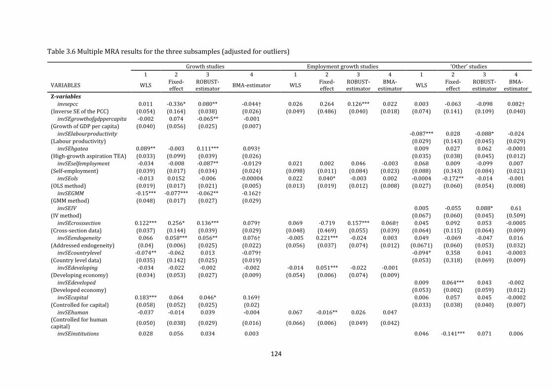
124
Table 3.6 Multiple MRA results for the three subsamples (adjusted for outliers)
Growth studies Employment growth studies ‘Other' studies
1 2 3 4 1 2 3 4 1 2 3 4
VARIABLES WLS Fixed-effect
ROBUST-estimator
BMA-estimator WLS Fixed-effect
ROBUST-estimator
BMA-estimator
WLS Fixed-effect
ROBUST-estimator
BMA-estimator
Z-variables
invsepcc 0.011 -0.336* 0.080** -0.044† 0.026 0.264 0.126*** 0.022 0.003 -0.063 -0.098 0.082†
(Inverse SE of the PCC) (0.054) (0.164) (0.038) (0.026) (0.049) (0.486) (0.040) (0.018) (0.074) (0.141) (0.109) (0.040)
invSEgrowthofgdppercapita -0.002 0.074 -0.065** -0.001 (Growth of GDP per capita) (0.040) (0.056) (0.025) (0.007) invSElabourproductivity
-0.087*** 0.028 -0.088* -0.024
(Labour productivity) (0.029) (0.143) (0.045) (0.029)
invSEhgatea 0.089** -0.003 0.111*** 0.093† 0.009 0.027 0.062 -0.0001
(High-growth aspiration TEA) (0.033) (0.099) (0.039) (0.026) (0.035) (0.038) (0.045) (0.012)
invSEselfemployment -0.034 -0.008 -0.087** -0.0129 0.021 0.002 0.046 -0.003 0.068 0.009 -0.099 0.007
(Self-employment) (0.039) (0.017) (0.034) (0.024) (0.098) (0.011) (0.084) (0.023) (0.088) (0.343) (0.084) (0.021)
invSEols -0.013 0.0152 -0.006 -0.00004 0.022 0.040* -0.003 0.002 -0.0004 -0.172** -0.014 -0.001
(OLS method) (0.019) (0.017) (0.021) (0.005) (0.013) (0.019) (0.012) (0.008) (0.027) (0.060) (0.054) (0.008)
invSEGMM -0.15*** -0.077*** -0.062** -0.162† (GMM method) (0.048) (0.017) (0.027) (0.029) invSEIV
0.005 -0.055 0.088* 0.61
(IV method) (0.067) (0.060) (0.045) (0.509)
invSEcrosssection 0.122*** 0.256* 0.136*** 0.079† 0.069 -0.719 0.157*** 0.068† 0.045 0.092 0.053 -0.0005
(Cross-section data) (0.037) (0.144) (0.039) (0.029) (0.048) (0.469) (0.055) (0.039) (0.064) (0.115) (0.064) (0.009)
invSEendogeneity 0.066 0.058*** 0.056** 0.076† -0.005 0.221*** -0.024 0.003 0.049 -0.069 -0.047 0.016
(Addressed endogeneity) (0.04) (0.006) (0.025) (0.022) (0.056) (0.037) (0.074) (0.012) (0.0671) (0.060) (0.053) (0.032)
invSEcountrylevel -0.074** -0.062 0.013 -0.079† -0.094* 0.358 0.041 -0.0003
(Country level data) (0.035) (0.142) (0.025) (0.019) (0.053) (0.318) (0.069) (0.009)
invSEdeveloping -0.034 -0.022 -0.002 -0.002 -0.014 0.051*** -0.022 -0.001 (Developing economy) (0.034) (0.053) (0.027) (0.009) (0.054) (0.006) (0.074) (0.009) invSEdeveloped 0.009 0.064*** 0.043 -0.002
(Developed economy) (0.053) (0.002) (0.059) (0.012)
invSEcapital 0.183*** 0.064 0.046* 0.169† 0.006 0.057 0.045 -0.0002
(Controlled for capital) (0.058) (0.052) (0.025) (0.02) (0.033) (0.038) (0.040) (0.007)
invSEhuman -0.037 -0.014 0.039 -0.004 0.067 -0.016** 0.026 0.047 (Controlled for human capital)
(0.050) (0.038) (0.029) (0.016) (0.066) (0.006) (0.049) (0.042)
invSEinstitutions 0.028 0.056 0.034 0.003 0.046 -0.141*** 0.071 0.006

125
(Controlled for institutions) (0.035) (0.068) (0.023) (0.011) (0.052) (0.033) (0.047) (0.017)
invSElabour -0.072
0.047***
-0.087*
-0.040
-0.008
0.006*
0.003
0.001
(Controlled for labour capital) (0.058) (0.009) (0.049) (0.028) (0.018) (0.003) (0.039) (0.009)
invSElog 0.137*** 0.770** 0.118*** 0.103† 0.133** 0.217*** 0.054 0.151† 0.128*** -0.099 0.133** 0.002
(Log-log specification) (0.045) (0.305) (0.036) (0.027) (0.051) (0.027) (0.064) (0.033) (0.042) (0.147) (0.059) (0.010)
invSElag -0.021 0.108 -0.13*** -0.002 -0.022 -0.021 -0.089*** -0.002 -0.112*** -0.148*** -0.266*** -0.002
(Primary study uses lags) (0.059) (0.073) (0.034) (0.012) (0.038) (0.049) (0.016) (0.008) (0.028) (0.008) (0.06) (0.015)
invSEconvergence 0.034 0.066*** 0.044 0.001
(Convergence-catch-up effect) (0.034) (0.002) (0.040) (0.010)
invse_start_1983_1 0.029 0.137* 0.002 0.002
(Mid-year of data) (0.018) (0.069) (0.016) (0.008)
invse_start_1988_1 -0.089* 0.044 -0.008 -0.082† (Mid-year of data) (0.046) (0.039) (0.033) (0.022) invse_start_1999_1 -0.001 -0.121 -0.161** -0.0004
(Mid-year of data) (0.085) (0.266) (0.079) (0.011)
K-variables
publishedjournal -0.373 2.714 0.119 -0.07 0.629 7.753 0.205 0.232 -0.571 -1.859* -1.220* -0.251
(Study published in a journal) (0.389) (1.844) (0.259) (0.167) (1.103) (5.265) (1.635) (0.578) (0.598) (1.039) (0.672) (0.433)
financial_conflict 0.975* 1.536 0.33 1.187† 0.872 -10.03 1.600* 0.049 -0.678 -2.255 -1.168 -0.175
(Financial conflict) (0.538) (1.753) (0.344) (0.282) (0.512) (7.192) (0.851) (0.212) (0.685) (4.929) (0.844) (0.44)
midyearofpublication_2008 -1.596*** 13.59* -1.266** -2.263†
(Mid-year of publication) (0.453) (6.281) (0.52) (0.342)
midyearofpublication_2011 1.676*** -1.291 1.917*** 1.534† (Mid-year of publication) (0.395) (1.536) (0.317) (0.211) midyearofpublication_2013 1.239*** -1.486 2.227*** 0.058
(Mid-year of publication) (0.277) (1.888) (0.68) (0.203)
Constant 0.741 -3.246** -0.849** 0.978† 0.694 -17.96** 0.019 2.059† 2.045* 4.751 3.107*** 1.484†
(0.718) (1.566) (0.347) (0.261) (1.08) (6.177) (1.608) (0.669) (1.041) (3.419) (1.021) (0.629)
Observations 297 297 297 297 222 222 222 222 95 95 95 95
R-squared 0.576 0.776 0.477 n.a. 0.427 0.537 0.365 n.a. 0.402 0.495 0.571 n.a.
Number of studies (clusters) 25 25 25 25 13 13 13 13 18 18 18 18 Ramsey RESET (p-value for H0: linear functional form)
0.01 0.00 n.a. n.a. 0.001 0.00 n.a. n.a. 0.75 0.42 n.a. n.a.
Notes: Robust standard errors in parenthesis
*** p<0.01, ** p<0.05, * p<0.1, denote statistical significance at 1%, 5% and 10% levels, respectively, n.a.- not applicable † - Statistically significant – BMA estimates only

126
The multivariate results reported in Table 3.6 suggest that the use of growth of
GDP per capita (invSEgrowthofgdppercapita) is associated with smaller effect
sizes for studies of subsample I (-0.065**). Similarly, the use of labour
productivity (invSElabourproductivity), as a measure of economic performance,
has the same effect on PCCs, i.e., decreases the size of the estimated effect of the
studies in subsample III. It is suggested that studies using growth of GDP per
capita (subsample I) report a negative and statistically significant behaviour
when robust estimator is employed, while studies that use labour productivity
(subsample III) report the same when both WLS and robust estimators are used
(see coefficient on Table 3.6 to follow the sign and significance levels). However,
when the analyses do not adjust for outliers, it is suggested that studies of the
subsample III using labour productivity tend to report larger PCCs (see Table 3.2
in Appendix 3.9).
In terms of the the measure of entrepreneurship used, results presented on Table
3.6 suggest that growth studies that use measures of high growth aspiration
entrepreneurship (invSEhgatea) tend to report larger effect sizes, except when
the FE estimator is used. This finding is in line with the previous theoretical and
empirical evidence (see Stam et al., 2009; 2010; Valliere and Peterson 2009;
Block et al., 2017; Darnihamedani et al., 2018) which reports that ambitious
entrepreneurship, rather than the overall entrepreneurial activity, is commonly
found as a determinant of growth. The same moderator is mostly positive, though
statistically insignificant, for the primary studies belonging to the third
subsample. It becomes statistically significant when no adjustment over potential
outliers is made, and only when the robust estimator is used (see Table 3.2 in
Appendix 3.9). Using self-employment (invSEselfemployment), in contrast,
seems to lead to smaller effect sizes in the first subsample when robust estimator
is applied. The same moderator has a positive sign in most of the specifications
of subsample II and III. However it is always statistically insignificant. When WLS
is used, and the analyses do not account for outliers, self-employment leads to
larger estimated effects for the studies of the third subsample (see Appendix 3.9).
Growth studies (subsample I) that employ GMM estimator, (invSEGMM) are
indicated to report smaller effect sizes, even when the analyses do not adjust for

127
outliers. This finding might suggest that more rigorous methodological
approaches do not allow the exaggeration of effects which, according to
Doucouliagos and Stanley (2013), is commonly present in the economic
literature. Alternatively, using cross-section data (invSEcrosssection) is usually
associated with larger positive effect sizes, especially for the growth studies sub-
sample. It was discussed in the previous sections that cross-section data are not
suitable for studies investigating growth (see Ploeg, 2011). Ordinary Least
Squares (OLS) (invSEols) on the other hand, provides somewhat inconclusive
findings. Employment growth studies tend to report larger PCCs when OLS is
used as their estimation technique, while ‘other’ studies seem to report smaller
PCCs when the same estimator is employed. These estimates become significant
only when the FE estimator is used in this MRA.
However, for the studies using employment growth as the measure of economic
performance, if the data for the MRA multivariate analysis is not adjusted for
outliers, OLS estimations are likely to lead to larger PCCs, regardless of the MRA
estimator (see Appendix 3.9). The analyses suggest that studies in the third sub-
sample tend to report larger effect sizes when one of the instrumental variables
(invSEIV) approaches is used. This finding turns statistically significant (at 10%)
only when robust estimator is used. When no adjustment is made for outliers,
using one of the instrumental variables leads to mixed results. MRA fixed-effect
estimator suggests that IV approaches lead to smaller PCCs, whereas robust
estimator suggests that they lead to larger PCCs. Considering that robust
estimator itself controls for outliers, the finding that studies using IV tend to
report larger effects seems to be consistent in both sets of results (with and
without adjustment to outliers).
The analysis also suggests that studies accounting for endogeneity
(invSEendogeneity) are more likely to report larger effect sizes, especially
studies of the first subsample. Some authors refer to this as a ‘good
methodological practise’ implying good quality of the research output. Similarly,
growth studies that have included more conventional moderators as explanatory
variables, such as capital (invSEcapital) tend to report larger PCCs. Employment
studies that use some measure of human capital (invSEhuman) tend to report

128
smaller effects when the fixed effect estimator is used. Similarly, using a measure
to capture the quality of institutions (invSEinstitutions), leads to smaller PCCs in
the third subsample when the FE estimator is used, while including an
explanatory variable that accounts for labour characteristics (invSElabour)
leads to larger PCCs for both employment growth studies and ‘other’ studies
when FE estimator is used and smaller PCCs for employment growth when
robust estimator is used. Using log-log specification (invSElog) is found to lead
to larger effect sizes, generally in all the three subsamples. On the other hand,
studies that have used lags (invSElag) in their specifications are indicated to
report smaller PCCs, especially studies of the third subsample. Studies that have
used data at the country level (invSEcountrylevel), in general, tend to report
smaller PCCs, this applies to the first and third subsample. The same finding is
also reported when no adjustment is made to the identified outliers (see
Appendix 3.9).
In terms of the differences in the level of economic development, results suggest
that studies that belong to the third subsample tend to report larger PCC when
the primary literature concentrated on developed economies when the FE
estimator is used. On the other side, employment growth studies tend to report
larger effects when studies use the developing economies context. Studies using
‘other’ measures of economic performance that account for convergence effect,
tend to report larger estimated effects, regardless of whether the MRA analyses
adjust for outliers or not. Finally, growth studies and studies of the third
subsample tend to report smaller effects when more recent data
(invse_midyearoofdata) are used, whereas employment growth studies tend to
report larger effects.
The interpretation is now focused on K-variable, i.e., those that have an influence
on publication selection bias. Results suggest that peer-reviewed published
studies (publishedjournal) of the third subsample usually report a smaller effect
if research is published. Estimates of the two other subsamples are indicated to
be statistically not influenced by this moderator. On the presence of potential
financial conflict (financial_conflict), growth studies are suggested to report
larger effects when WLS is used. Similarly, when robust estimator is applied

129
employment growth studies are indicated to report larger effects, which might
further influence the positive publication bias. In this study, all the acknowledged
funding bodies have been assessed for their potential material interest in the
findings of the study. However, there is still some subjectivity in making this
judgement and we acknowledge that the results for this moderator should be
taken with caution.
Results on Table 3.6 suggest that more recent publications
(midyearofpublication) of the first and third subsample tend to report larger
PCCs, whereas second subsample studies tend to report, in general, smaller
effects (see also appendix 3.13 where effects according to the year of publication
are reported). In some way, this last finding contradicts one earlier finding, which
suggested that more recent data decrease the size of the effect of the growth
studies (subsample I). The assumption is that more recent published studies use
more recent data and that their effects should be similar. In our situation, results
suggest that using more recent data tend to reduce the effect of entrepreneurship
on economic performance, but at the same time, more recent published work
tend to report larger estimates. The negative effect on reported effects of using
more recent data might be as a result of an increased harmonisation of the data
in the last few years. Early data on entrepreneurship measures did not
distinguish between different types of entrepreneurial activity (e.g.,
Schumpeterian as opposed to necessity type entrepreneur) nor did they consider
the overall entrepreneurship ecosystem when data were gathered.
Estimates of the average magnitudes of publication selection bias and genuine
empirical effect for the three subsamples are reported in Tables 3.7 and 3.8 using
all four empirical approaches. As suggested by Stanley and Doucouliagos (2012),
deriving publication selection bias and genuine effect from multiple MRA
requires the following two steps: (i) calculating the linear combination (lincom)
of the constant term (_cons) and the sum of each estimated K-moderator
weighted by the mean values; and (ii) calculating the linear combination (lincom)
of the inverse standard error of PCCs (invSEpcc) and the sum of all the Z-
moderators, weighted by their mean values.
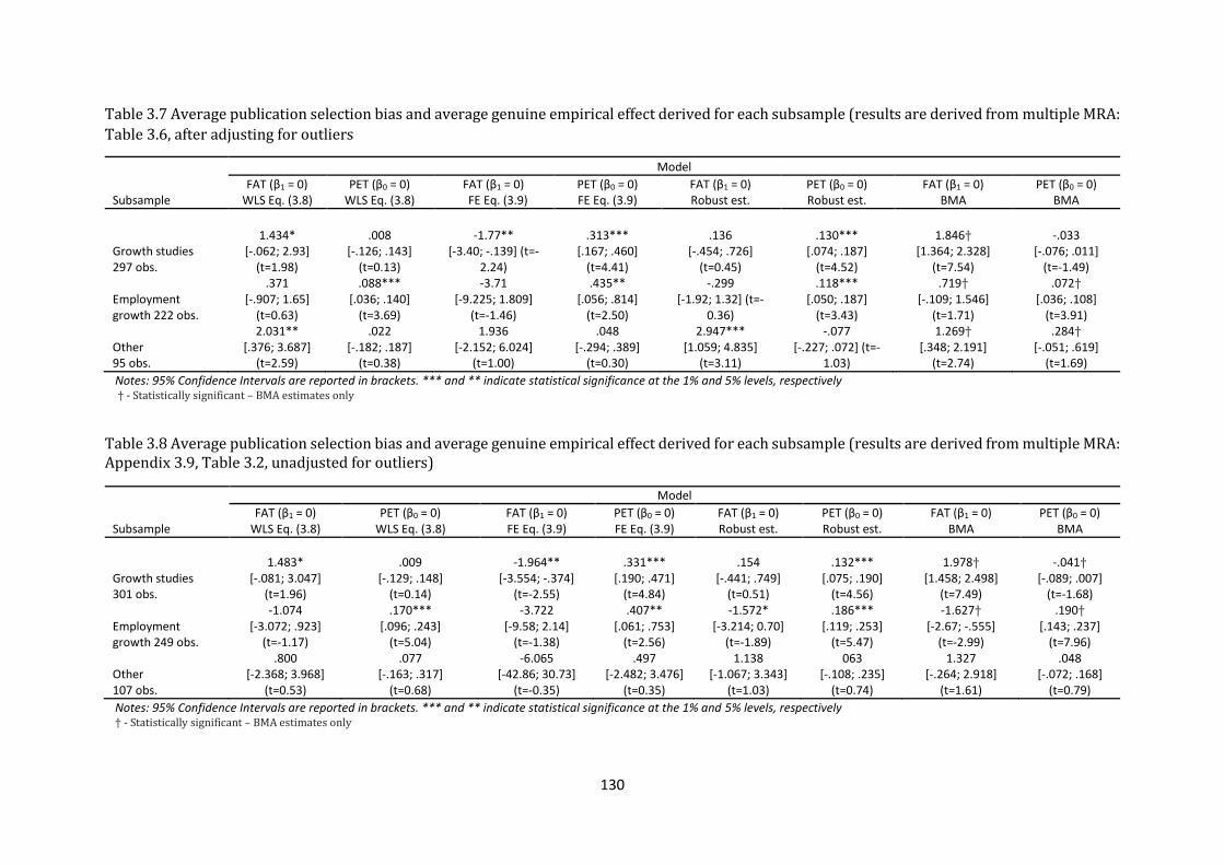
130
Table 3.7 Average publication selection bias and average genuine empirical effect derived for each subsample (results are derived from multiple MRA:
Table 3.6, after adjusting for outliers
Model
Subsample FAT (β1 = 0)
WLS Eq. (3.8) PET (β0 = 0)
WLS Eq. (3.8) FAT (β1 = 0)
FE Eq. (3.9) PET (β0 = 0) FE Eq. (3.9)
FAT (β1 = 0) Robust est.
PET (β0 = 0) Robust est.
FAT (β1 = 0) BMA
PET (β0 = 0) BMA
Growth studies 297 obs.
1.434* [-.062; 2.93]
(t=1.98)
.008 [-.126; .143]
(t=0.13)
-1.77** [-3.40; -.139] (t=-
2.24)
.313*** [.167; .460]
(t=4.41)
.136 [-.454; .726]
(t=0.45)
.130*** [.074; .187]
(t=4.52)
1.846† [1.364; 2.328]
(t=7.54)
-.033 [-.076; .011]
(t=-1.49) Employment growth 222 obs.
.371 [-.907; 1.65]
(t=0.63)
.088*** [.036; .140]
(t=3.69)
-3.71 [-9.225; 1.809]
(t=-1.46)
.435** [.056; .814]
(t=2.50)
-.299 [-1.92; 1.32] (t=-
0.36)
.118*** [.050; .187]
(t=3.43)
.719† [-.109; 1.546]
(t=1.71)
.072† [.036; .108]
(t=3.91) Other 95 obs.
2.031** [.376; 3.687]
(t=2.59)
.022 [-.182; .187]
(t=0.38)
1.936 [-2.152; 6.024]
(t=1.00)
.048 [-.294; .389]
(t=0.30)
2.947*** [1.059; 4.835]
(t=3.11)
-.077 [-.227; .072] (t=-
1.03)
1.269† [.348; 2.191]
(t=2.74)
.284† [-.051; .619]
(t=1.69)
Notes: 95% Confidence Intervals are reported in brackets. *** and ** indicate statistical significance at the 1% and 5% levels, respectively † - Statistically significant – BMA estimates only
Table 3.8 Average publication selection bias and average genuine empirical effect derived for each subsample (results are derived from multiple MRA: Appendix 3.9, Table 3.2, unadjusted for outliers)
Model
Subsample FAT (β1 = 0)
WLS Eq. (3.8) PET (β0 = 0)
WLS Eq. (3.8) FAT (β1 = 0) FE Eq. (3.9)
PET (β0 = 0) FE Eq. (3.9)
FAT (β1 = 0) Robust est.
PET (β0 = 0) Robust est.
FAT (β1 = 0) BMA
PET (β0 = 0) BMA
Growth studies 301 obs.
1.483* [-.081; 3.047]
(t=1.96)
.009 [-.129; .148]
(t=0.14)
-1.964** [-3.554; -.374]
(t=-2.55)
.331*** [.190; .471]
(t=4.84)
.154 [-.441; .749]
(t=0.51)
.132*** [.075; .190]
(t=4.56)
1.978† [1.458; 2.498]
(t=7.49)
-.041† [-.089; .007]
(t=-1.68) Employment growth 249 obs.
-1.074 [-3.072; .923]
(t=-1.17)
.170*** [.096; .243]
(t=5.04)
-3.722 [-9.58; 2.14]
(t=-1.38)
.407** [.061; .753]
(t=2.56)
-1.572* [-3.214; 0.70]
(t=-1.89)
.186*** [.119; .253]
(t=5.47)
-1.627† [-2.67; -.555]
(t=-2.99)
.190† [.143; .237]
(t=7.96) Other 107 obs.
.800 [-2.368; 3.968]
(t=0.53)
.077 [-.163; .317]
(t=0.68)
-6.065 [-42.86; 30.73]
(t=-0.35)
.497 [-2.482; 3.476]
(t=0.35)
1.138 [-1.067; 3.343]
(t=1.03)
063 [-.108; .235]
(t=0.74)
1.327 [-.264; 2.918]
(t=1.61)
.048 [-.072; .168]
(t=0.79)
Notes: 95% Confidence Intervals are reported in brackets. *** and ** indicate statistical significance at the 1% and 5% levels, respectively † - Statistically significant – BMA estimates only

131
In general, the findings reported in Table 3.7 and 3.8 are relatively consistent
with those reported in bivariate MRA in section 3.5, Table 3.4 and 3.5. According
to Doucouliagos and Stanley (2013) criteria, WLS and robust estimator bivariate
estimates suggested ‘substantial’ (1≤FAT≥2) positive publication bias in the
growth studies literature. When the FE estimator (G-S approach) was used,
results suggest that there is a negative and statistically significant “little to
modest” publication bias (FAT<1) in the same literature. Similar results are also
reported in the multivariate MRA, except for the FAT estimate using robust
estimator which now turns insignificant. The WLS estimate (1.434*) suggests
that the primary literature, of the first subsample, is likely to be contaminated by
a ‘substantial’ positive publication selection bias. The FE estimator shows the
same behaviour as in the bivariate analyses, a negative and statistically
significant effect on publication bias. Results were the same even when no
attention was paid to outliers (Table 3.8). As the WLS compared to FE is the main
estimator, it is suggested that these findings indicate that the reported estimates
by primary literature (growth studies) suffer ‘substantially’ from positive
publication selection bias. Also, the FAT estimate of BMA, which is used as an
additional robustness check, indicates a statistically significant (t=7.54)
‘substantial’ positive publication bias. The bivariate MRA suggested that
employment growth literature experiences positive and ‘substantial’ publication
bias when WLS estimator is employed, and the adjustment is made for outliers.
Such a positive publication bias is not suggested in the multivariate MRA when
WLS is used.
The FE (G-S approach) estimator applied only in the bivariate analyses suggested
that there is ‘severe’ negative publication bias in the employment literature, but
the same effect is not found when the FE estimator is used in the multivariate
MRA. When the BMA approach is used, results suggest that there is ‘little’ to
‘moderate’ positive publication bias in the employment growth literature.
However, the BMA estimates provide very weak evidence and are to be taken
with caution. In addition, the BMA estimates are not to be used as a definitive
indication of publication selection bias or genuine effect. When no adjustment to
outliers is made, robust estimator suggests that there is a ‘substantial’ negative

132
publication bias. The last finding is perhaps influenced by a few effects that were
considered highly precise (see Panel B in Fig 3.1) and reported negative
estimates. Overall, there is a weak evidence to indicate that also this literature
suffers from publication selection bias. However the findings are more
inconclusive compared to the first subsample.
Similar to ‘growth’ studies, the third subsample, ‘other’ studies, is also suggested
to have experienced positive publication bias. Two of the four estimators in the
bivariate MRA, namely the WLS and robust estimator, indicate a ‘substantial’
positive publication bias, after adjusting for outliers. The positive and statistically
significant publication bias becomes more pronounced in the multivariate MRA,
as FAT estimates obtained by using the WLS and robust estimator suggest a
‘severe’ positive bias when outliers are dropped from the analysis. Overall, like
the first subsample, this literature is also subject to ‘substantial’ to ‘severe’
positive publication bias. None of the FAT and PET estimates, however, turn
statistically significant when no adjustment is made to outliers. To conclude,
there is some evidence to suggest that entrepreneurship and economic
performance literature, in general, tends to report positive estimates. This
influence might come from the absence of competing theories on this
relationship. Doucouliagos and Stanley (2013) argue that in situations where
researchers have to conform to a single mainstream theory, the appearance of
publication selection bias is highly likely.
In addition to identifying publication selection bias and the heterogeneity of the
reported estimates, this chapter also aims at identifying the genuine empirical
effect beyond publication bias in the entrepreneurship-economic performance
literature. Once again there is some consistency between bivariate and
multivariate MRA findings in all the three subsamples. The PET estimates for
‘growth’ studies in Table 3.7 suggest a ‘moderate’ positive genuine effect in both
bivariate and multivariate MRA, when FE estimator is used, and outliers are
excluded. Similarly, the robust estimator suggests that there is ‘moderate’
positive effect in the entrepreneurship-economic growth literature. Except for
the BMA estimate, results remain largely the same also when no adjustment is
made for outliers. The multivariate MRA of the second subsample, employment

133
growth studies, suggest a ‘moderate positive genuine effect in the
entrepreneurship and economic performance literature. All the three
conventional estimators employed in the multiple MRA and also the BMA point
to this finding. The bivariate results are somehow more inconclusive, as only one
of the estimators (FE G-S) suggests a ‘moderate’ positive effect in this literature.
The WLS, (FE G-S) and the robust estimator employed in the bivariate MRA
suggested a ‘moderate’ positive genuine effect in the third subsample (‘other’
studies). However, when multivariate MRA is undertaken, the same literature
indicates a ‘moderate’ positive genuine effect only when the BMA approach is
used. As highlighted earlier, the evidence provided by BMA is, however, only to
be taken as a weak indication of the presence of a positive genuine effect in this
literature. All in all, the analysis suggests that the entrepreneurship-economic
performance literature seems to be subject to ‘substantial’ to ‘severe’ positive
publication bias. In addition, the MRA provided an indication of a ‘moderate’
positive genuine effect in this literature.
CONCLUSIONS
The literature review in Chapter 2 and section 3.3 of this Chapter suggested that
studies differ in respect to their measures of entrepreneurship, economic
performance, methodological approaches, estimation techniques, specifications,
level of analysis, contexts, and time periods covered. Therefore, a meta-
regression analysis was undertaken with the aim of quantitatively summarising
the effect of entrepreneurship on economic performance and separate the
genuine effect from the publication bias. In total, 52 primary studies with 657
reported estimates covering the period 2000-2016, were coded and included in
the MRA database for the MRA analysis. This chapter has identified and provided
explanations for the origin of heterogeneity in the literature, the existence and
potential causes of the mainly positive publication bias and the presence of a
genuine empirical effect. The bivariate MRA uses three estimators, WLS, FE
(including FE General-to-Specific approach) and robust estimator. To provide
additional robustness checks and reduce substantial model uncertainty, the
multivariate MRA employs Bayesian Model Averaging (BMA), which is suggested
to be a better alternative to the FE G-S approach (Havranek and Irsova, 2017).

134
In general, there is evidence for a positive publication bias which can be
characterised as ‘substantial’ to ‘severe’ across all the three subsamples in both
bivariate and multivariate MRA. When publication bias is filtered out, we mainly
find positive authentic effects with these tending to be stronger when ‘growth’
and employment growth studies are used as the measure of economic
performance. The results indicate that growth studies that use one of the
measures of high-growth aspiration entrepreneurship, in general, report larger
effects (PCCs). Holding other estimate and study characteristics constant, using
high-growth aspiration entrepreneurship measures implies a PCC of around 0.1,
suggesting a positive and ‘moderate’ relationship between entrepreneurship and
economic growth measures. Growth studies that use self-employment, on the
other hand, are suggested to report smaller effects (PCCs) when robust estimator
is used in the multivariate analysis. With respect to the influence of the stage of
economic development, i.e., economic context, the FE estimator suggest that
studies of the third subsample that use data of developed economies report
larger effects (PCCs), while employment growth studies that use data of
developing economies are suggested to report positive and larger effects.
We find that good research practice of controlling for reverse causation
(endogeneity) and using log-log specification tend to lead to larger estimated
effects. Moreover, growth studies that use more theoretically motivated
specifications, i.e., include conventional variables in the model, report larger
estimated effects. The primary literature on growth studies that use GMM,
country-level data, more recent data and employ lags to model the effect of
previous periods, generally report smaller effects. The multivariate results also
suggest that employment growth studies that use OLS in estimations tend to
report larger estimated effects, whereas ‘other’ studies tend to report larger
effects when the instrumental variable approach is employed. The multivariate
results also indicate that studies receiving financial support from bodies that
have an interest in the outcome of the research, in general, report larger
estimates. This finding is more pronounced in the first subsample. Finally, results
suggest that studies that belong to the third subsample, report smaller estimated
effects if they are published in a referred journal. Recently published research, in

135
general, report larger PCCs with the exception of employment growth studies,
where they report smaller effects.
To date, and to the best of our knowledge, the literature on the effect of
entrepreneurship on economic performance has not been the subject of an MRA.
This chapter has attempted to fill this gap in the literature and contribute to the
ongoing debate by providing additional unique empirical evidence which may
help to understand this further. This is of particular importance to the policy-
making community.
To further explore the relationship between entrepreneurship and economic
performance, Chapter 4 of this thesis investigates the impact of entrepreneurial
activity on GDP growth in a large cross-country context. Given the advantages of
GEM data highlighted in Chapter 1, the empirical investigation of Chapter 4 relies
only on that source while using other sources of data for other control variables.
Chapter 5 of the thesis investigates the determinants of entrepreneurial growth
aspiration using GEM data, again in an international context.
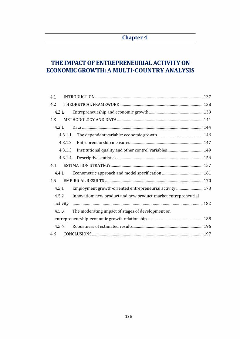
136
4. Chapter 4
THE IMPACT OF ENTREPRENEURIAL ACTIVITY ON ECONOMIC GROWTH: A MULTI-COUNTRY ANALYSIS
INTRODUCTION ...................................................................................................................... 137
THEORETICAL FRAMEWORK ........................................................................................... 138
Entrepreneurship and economic growth ........................................................... 139
METHODOLOGY AND DATA .............................................................................................. 141
Data .................................................................................................................................... 144
4.3.1.1 The dependent variable: economic growth .................................................. 146
4.3.1.2 Entrepreneurship measures ............................................................................... 147
4.3.1.3 Institutional quality and other control variables ....................................... 149
4.3.1.4 Descriptive statistics .............................................................................................. 156
ESTIMATION STRATEGY .................................................................................................... 157
Econometric approach and model specification ............................................. 161
EMPIRICAL RESULTS ........................................................................................................... 170
Employment growth-oriented entrepreneurial activity .............................. 173
Innovation: new product and new product-market entrepreneurial
activity ……………………………………………………………………………………………………….182
The moderating impact of stages of development on
entrepreneurship-economic growth relationship ............................................................. 188
Robustness of estimated results ............................................................................ 196
CONCLUSIONS ......................................................................................................................... 197

INTRODUCTION
The literature review in Chapter 2 and the Meta-regression analysis (MRA) in
Chapter 3, offered evidence on the relevance of studying the effect of
entrepreneurship on economic performance. Chapter 2 highlighted that despite
the theoretical and empirical evidence on this relationship, there is still a lack of
consensus and studies are very heterogenous on the methodologies, contexts,
data for the main variable of interest and time-span used (Bjørnskov and Foss,
2013; 2016; Aparicio, 2017; Bosma et al., 2018). The heterogeneity of both the
theoretical and empirical literature motivated the MRA in Chapter 3, while this
chapter focuses on providing an original contribution and shed more light on this
debate by empirically investigating the effect of entrepreneurship on national
economic performance. Shepherd (2011) argues that it is highly relevant to
investigate how the entrepreneurship of firms and individuals aggregates up to
growth at the country-level. The empirical part of this chapter uses an
unbalanced panel setting, which includes 48 countries for the period 2006-2014.
A number of empirical strategies are employed to address empirical issues
pertinent to the entrepreneurship – economic performance relationship. A
distinctive feature of this chapter is the use of both static and dynamic modelling
techniques in investigating the effect of entrepreneurial activity on economic
growth at the national level.
Chapter 2 emphasised the importance of distinguishing between different types
of entrepreneurial activity and investigating their potential effect on economic
growth separately. The debate is pioneered by Baumol (1990; 2010) who
distinguishes between productive and unproductive entrepreneurial activity.
According to Baumol (1993, p.30), productive entrepreneurial activity is “any
entrepreneurial activity that contributes directly or indirectly to net output of the
economy or to the capacity to produce additional output”. Moreover, Baumol
(2010) refers to productive entrepreneurship as an activity which generates
economic growth through innovation. The use of the Global Entrepreneurship
Monitor (GEM) data in this chapter, enables us to account for different types of
entrepreneurial activity, including the ones referred to by Baumol (1990; 2010).
The GEM entrepreneurship data allow for investigating the effect of
138
entrepreneurial activity on economic growth based on the motivation to start,
the expectation of job creation, innovativeness and new market development,
and international orientation.46
The analysis in this chapter does not concentrate on the potentially different
effects of opportunity vs necessity-type entrepreneurial activity (motivation to
start) as this has been extensively researched (see e.g., Minniti et al., 2006; Cullen
et al., 2014; Aparicio et al., 2016; Ferreira et al., 2017; Mrożewski and Kratzer,
2017; Rodrigues, 2018). Although the international orientation type of
entrepreneurial activity seems relevant to economic growth, the theoretical and
empirical literature has mostly emphasised the impact of job creating and
innovative entrepreneurial activity (Reynolds et al., 2005; Estrin et al., 2013;
Hermans et al., 2015; Lim et al., 2016; Terjesen et al., 2016). Accordingly, in
addition to Total (early-Stage) Entrepreneurial Activity (TEA), the focus of this
study is on: (i) ‘Employment Growth’ entrepreneurial activity, measured by: (a)
job growth and (b) high-job growth expectations and (ii) ‘Innovative’
entrepreneurial activity, measured by: (a) new product and (b) new product-
market combination. These types of entrepreneurial activities better represent
Schumpeterian-type entrepreneurs.
This rest of the chapter is organised as follows: the theoretical framework is
elaborated in the second section, with a short review of literature on
entrepreneurship-economic growth relationship. The data, descriptive statistics
and the variables included in the model are presented and elaborated in section
three. Section four discusses the estimation strategies, econometric approaches
and the models used in this empirical analysis. In section five, relevant model
diagnostic tests are discussed, followed by the interpretation of results and the
robustness checks. Conclusions are offered in section six.
THEORETICAL FRAMEWORK
The section below provides a short discussion of the main theories. The more
detailed discussion on the theories is provided in Chapter 2 of the thesis.
46 For more details, see GEM Conceptual Framework discussed in Chapter 1.

139
Entrepreneurship and economic growth
As discussed in Chapter 2 and 3, the central role of entrepreneurship in
determining economic performance of nations has been recognised since the
early work of Schumpeter (1934). Schumpeter’s proposition (1934) that
entrepreneurship represents the introduction of new combinations of
production factors in the economy (the innovative character of entrepreneur),
can be used to explain the cross-country differences in dynamism and economic
growth.47 According to Schumpeter, entrepreneurs create constant disturbances
to the economic system in equilibrium. In his view, market disturbances enable
the so-called process of ‘creative destruction’ which could then create even more
opportunities for new entrants. Hence, the ‘creative destruction’ process is
suggested to lead to increased entrepreneurial activity, which in turn manifests
itself in increased rate of economic growth (Wennekers and Thurik, 1999).
The Schumpeterian tradition has served as the basis for many investigations in
the entrepreneurship-economic growth literature. It is suggested that the
interest in the topic of entrepreneurship increased, especially, as the economies
started to increasingly be based on knowledge. The theoretical basis of the
positive relationship between entrepreneurship and economic growth was then
subjected to extensive examination by a large number of authors (see e.g.,
Leibenstein, 1968; Lumpkin and Dess, 1996; Wennekers and Thurik, 1999; Wong
et al., 2005; van Praag and Versloot, 2007; 2008; Naude, 2010; Urbano and
Aparicio, 2016; Acs et al., 2018; Bosma et al., 2018). However, despite the vast
literature in this area, there is still insufficient number of studies investigating
the relationship between entrepreneurship and economic growth at the country
level (Shane and Venkataraman, 2000; van Stel et al., 2005; Naude, 2010; Baumol,
2010; Teixeira, 2011; Aparicio et al., 2016; Terjesen et al., 2016; Bosma et al.,
2018). More specifically, there is still no conclusive empirical evidence
supporting the hypothesised positive relationship between entrepreneurial
activity and macroeconomic growth. Stam and van Stel (2011) argue that this
47 In the 1934 book: “The Theory of Economic Development: An Inquiry into Profits, Capital, Credit, Interest and the Business Cycle”, Schumpeter has all the time highlighted the embedded innovative nature of entrepreneurship and the innovative character of the entrepreneur.
140
inconclusiveness might be the result of the complexity of the relationship, the
diversity of empirical strategies (e.g., estimators; data, etc.) and the influence of
the context on the empirical results. In line with this, Bjørnskov and Foss (2016)
argue that the literature on the relationship between entrepreneurship and
economic performance is mostly associated with small sample sizes, miss-
specified empirical models (e.g., omitted variable bias, etc.) and sometimes
insufficient theoretical background to explain the links between
entrepreneurship and macro-economic growth. Moreover, as pointed out in
Chapters 2 and 3, the way some measures of entrepreneurial activity are
constructed and used by researchers has led to even more confusion. For
instance, studies have used self-employment, start-up rates, firms’ net birth rates,
etc. to proxy for entrepreneurial activity which, according to Bjørnskov and Foss
(2016), represent a narrow definition of entrepreneurship. In addition, the
number of studies that have paid attention to, and have distinguished between,
different types of entrepreneurial activity, except for opportunity- and necessity-
type entrepreneurship, is still sparse. Investigating the role of entrepreneurship,
by employing measures that do not distinguish between any type of
entrepreneurial activity, has led to further criticisms from researchers (see e.g.,
Santarelli and Vivarelli, 2007; Shane, 2009). For instance, Santarelli and Vivarelli
(2007) argue that in some empirical studies, entrepreneurship measures
employed are too broad and as such unable to detect the true relationship
between entrepreneurship and economic growth. These studies have been
unsuccessful to distinguish between more productive and unproductive
entrepreneurial activity (Baumol, 2010).
As it is elaborated in Chapter 2, the neoclassical (Solow, 1956; Swan, 1956) and
the endogenous growth theory (Romer, 1986; 1990; Lucas, 1988, Aghion and
Howitt, 1992) are the two growth theories mostly used to investigate country-
level differences in economic growth.48 The neoclassical growth model postulates
that the accumulation of capital and labour are the two prime determinants of
growth. The remaining unexplained part (the residual) is exogenous and is
attributed to technological change (Wennekers and Thurik, 1999; Acs et al., 2003;
48 See the discussion in Chapter 2, section 2.2 for a more detailed overview on growth theories.
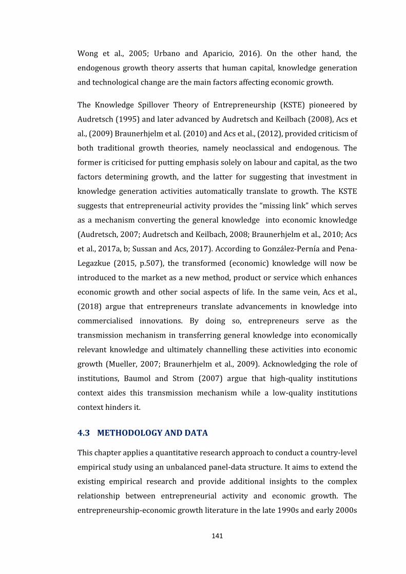
141
Wong et al., 2005; Urbano and Aparicio, 2016). On the other hand, the
endogenous growth theory asserts that human capital, knowledge generation
and technological change are the main factors affecting economic growth.
The Knowledge Spillover Theory of Entrepreneurship (KSTE) pioneered by
Audretsch (1995) and later advanced by Audretsch and Keilbach (2008), Acs et
al., (2009) Braunerhjelm et al. (2010) and Acs et al., (2012), provided criticism of
both traditional growth theories, namely neoclassical and endogenous. The
former is criticised for putting emphasis solely on labour and capital, as the two
factors determining growth, and the latter for suggesting that investment in
knowledge generation activities automatically translate to growth. The KSTE
suggests that entrepreneurial activity provides the “missing link” which serves
as a mechanism converting the general knowledge into economic knowledge
(Audretsch, 2007; Audretsch and Keilbach, 2008; Braunerhjelm et al., 2010; Acs
et al., 2017a, b; Sussan and Acs, 2017). According to González-Pernía and Pena-
Legazkue (2015, p.507), the transformed (economic) knowledge will now be
introduced to the market as a new method, product or service which enhances
economic growth and other social aspects of life. In the same vein, Acs et al.,
(2018) argue that entrepreneurs translate advancements in knowledge into
commercialised innovations. By doing so, entrepreneurs serve as the
transmission mechanism in transferring general knowledge into economically
relevant knowledge and ultimately channelling these activities into economic
growth (Mueller, 2007; Braunerhjelm et al., 2009). Acknowledging the role of
institutions, Baumol and Strom (2007) argue that high-quality institutions
context aides this transmission mechanism while a low-quality institutions
context hinders it.
METHODOLOGY AND DATA
This chapter applies a quantitative research approach to conduct a country-level
empirical study using an unbalanced panel-data structure. It aims to extend the
existing empirical research and provide additional insights to the complex
relationship between entrepreneurial activity and economic growth. The
entrepreneurship-economic growth literature in the late 1990s and early 2000s

142
was dominated by cross-sectional country analysis (see e.g., Acs et al., 2005;
Wong et al., 2005), however, as it has been indicated in the MRA chapter, the
more recent studies have mostly used panel data settings (see also: Aparicio,
2017). The use of panel data is a positive development in this literature, since
investigating growth in a cross-section structure might lead to omitted variable
bias and other econometric problems (Frees, 2004, p.7; van der Ploeg, 2011).
The data used in this chapter allows for different estimation techniques,
including the use of dynamic approaches (e.g., General Method of Moments
(GMM) estimator to control for potential endogeneity between predictors and
the outcome variable. The analyses are performed in a global setting, using a
sample of 48 countries over 2006-2014.49 The MRA revealed that some of the
previous research studies have performed their analysis even in a single-country
setting or within the same income group or region (see Dejardin, 2011). In this
chapter, the empirical analyses provide multiple-country findings and include
countries at different stages of development over a long-enough period 2006-
2014. According to Acs et al. (2008), including a large number of countries at
different stages of economic development over long periods of data, allows better
understanding of the possible differences between certain groups and time
periods. The data used to construct the panel dataset for this chapter is obtained
from different sources but mostly from: (i) the Global Entrepreneurship Monitor
- Adult Population Survey.
Fig. 4.1 to Fig. 4.6 below provide the first encounter of the data, where the
relationship between different measures of entrepreneurial activity (country-
mean) and country-mean GDP growth are presented. All the figures seem to
indicate a positive relationship between our measures of entrepreneurial activity
and economic growth. Generally, countries with high rates of ‘employment
growth’ expectations and innovative entrepreneurial activity are also reported
to have high rates of growth. For instance, countries like Turkey and Singapore
report above the average values of high-job growth entrepreneurial activity and
49 The original dataset of this chapter included 67 countries, however since 8 countries had participated in only one wave of survey, and 4 only in two waves, the number of observation they provided was considerably small and perhaps underrepresented, thus were not included in the final dataset. In addition, after deciding to use lags, adjusting for outliers and including countries with at least two years of data, only 48 countries remained in the analysis.
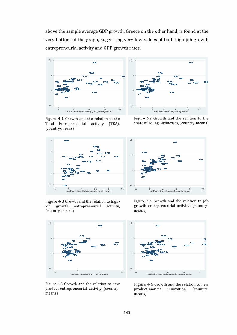
143
above the sample average GDP growth. Greece on the other hand, is found at the
very bottom of the graph, suggesting very low values of both high-job growth
entrepreneurial activity and GDP growth rates.
Figure 4.1 Growth and the relation to the
Total Entrepreneurial activity (TEA), (country-means)
Figure 4.2 Growth and the relation to the share of Young Businesses, (country-means)
Figure 4.3 Growth and the relation to high-job growth entrepreneurial activity, (country-means)
Figure 4.4 Growth and the relation to job growth entrepreneurial activity, (country-means)
Figure 4.5 Growth and the relation to new product entrepreneurial. activity, (country-means)
Figure 4.6 Growth and the relation to new product-market innovation (country-means)
USUSUSUSUSUSUSUSUS
RURURURURURURURURU
SASASASASASASASASA
GRGRGRGRGRGRGRGRGR
NTHNTHNTHNTHNTHNTHNTHNTHNTHBEBEBEBEBEBEBEBEBE FRFRFRFRFRFRFRFRFR
ESESESESESESESESES
HUHUHUHUHUHUHUHUHU
ITITITITITITITITIT
RORORORORORORORORO
SWSWSWSWSWSWSWSWSWUKUKUKUKUKUKUKUKUKDKDKDKDKDKDKDKDKDK
SWESWESWESWESWESWESWESWESWE
NONONONONONONONONO
POPOPOPOPOPOPOPOPO
DEDEDEDEDEDEDEDEDE
PEPEPEPEPEPEPEPEPE
MEXMEXMEXMEXMEXMEXMEXMEXMEX
ARGARGARGARGARGARGARGARGARGBRBRBRBRBRBRBRBRBR
CHICHICHICHICHICHICHICHICHICOCOCOCOCOCOCOCOCO
MLMLMLMLMLMLMLMLML SIGSIGSIGSIGSIGSIGSIGSIGSIG THATHATHATHATHATHATHATHATHA
JPJPJPJPJPJPJPJPJP
KOKOKOKOKOKOKOKOKO
CHCHCHCHCHCHCHCHCH
TURTURTURTURTURTURTURTURTUR
PRPRPRPRPRPRPRPRPRIRLIRLIRLIRLIRLIRLIRLIRLIRL
ICLICLICLICLICLICLICLICLICLFIFIFIFIFIFIFIFIFI
LILILILILILILILILI
LALALALALALALALALA
CROCROCROCROCROCROCROCROCROSLOSLOSLOSLOSLOSLOSLOSLOSLO
SLKSLKSLKSLKSLKSLKSLKSLKSLK
PANPANPANPANPANPANPANPANPAN
ECUECUECUECUECUECUECUECUECU
URURURURURURURURUR
DRDRDRDRDRDRDRDRDR
TTBTTBTTBTTBTTBTTBTTBTTBTTB
JAMJAMJAMJAMJAMJAMJAMJAMJAM
ISRISRISRISRISRISRISRISRISR
-50
51
0
Gro
wth
, cou
ntr
y m
ea
ns
5 10 15 20 25Total Entrepreneurial Activity (TEA), country means
USUSUSUSUSUSUSUSUS
RURURURURURURURURU
SASASASASASASASASA
GRGRGRGRGRGRGRGRGR
NTHNTHNTHNTHNTHNTHNTHNTHNTHBEBEBEBEBEBEBEBEBEFRFRFRFRFRFRFRFRFR
ESESESESESESESESES
HUHUHUHUHUHUHUHUHU
ITITITITITITITITIT
RORORORORORORORORO
SWSWSWSWSWSWSWSWSWUKUKUKUKUKUKUKUKUKDKDKDKDKDKDKDKDKDK
SWESWESWESWESWESWESWESWESWE
NONONONONONONONONO
POPOPOPOPOPOPOPOPO
DEDEDEDEDEDEDEDEDE
PEPEPEPEPEPEPEPEPE
MEXMEXMEXMEXMEXMEXMEXMEXMEX
ARGARGARGARGARGARGARGARGARGBRBRBRBRBRBRBRBRBR
CHICHICHICHICHICHICHICHICHICOCOCOCOCOCOCOCOCO
MLMLMLMLMLMLMLMLMLSIGSIGSIGSIGSIGSIGSIGSIGSIG THATHATHATHATHATHATHATHATHA
JPJPJPJPJPJPJPJPJP
KOKOKOKOKOKOKOKOKO
CHCHCHCHCHCHCHCHCH
TURTURTURTURTURTURTURTURTUR
PRPRPRPRPRPRPRPRPRIRLIRLIRLIRLIRLIRLIRLIRLIRL
ICLICLICLICLICLICLICLICLICLFIFIFIFIFIFIFIFIFI
LILILILILILILILILI
LALALALALALALALALA
CROCROCROCROCROCROCROCROCROSLOSLOSLOSLOSLOSLOSLOSLOSLO
SLKSLKSLKSLKSLKSLKSLKSLKSLK
PANPANPANPANPANPANPANPANPAN
ECUECUECUECUECUECUECUECUECU
URURURURURURURURUR
DRDRDRDRDRDRDRDRDR
TTBTTBTTBTTBTTBTTBTTBTTBTTB
JAMJAMJAMJAMJAMJAMJAMJAMJAM
ISRISRISRISRISRISRISRISRISR
-50
51
0
Gro
wth
, cou
ntr
y m
ea
ns
2 4 6 8 10 12Baby Businesses rate, country means
USUSUSUSUSUSUSUSUS
RURURURURURURURURU
SASASASASASASASASA
GRGRGRGRGRGRGRGRGR
NTHNTHNTHNTHNTHNTHNTHNTHNTHBEBEBEBEBEBEBEBEBE FRFRFRFRFRFRFRFRFR
ESESESESESESESESES
HUHUHUHUHUHUHUHUHU
ITITITITITITITITIT
RORORORORORORORORO
SWSWSWSWSWSWSWSWSW
UKUKUKUKUKUKUKUKUKDKDKDKDKDKDKDKDKDK
SWESWESWESWESWESWESWESWESWE
NONONONONONONONONO
POPOPOPOPOPOPOPOPO
DEDEDEDEDEDEDEDEDE
PEPEPEPEPEPEPEPEPE
MEXMEXMEXMEXMEXMEXMEXMEXMEX
ARGARGARGARGARGARGARGARGARGBRBRBRBRBRBRBRBRBR
CHICHICHICHICHICHICHICHICHIMLMLMLMLMLMLMLMLML SIGSIGSIGSIGSIGSIGSIGSIGSIGTHATHATHATHATHATHATHATHATHA
JPJPJPJPJPJPJPJPJP
KOKOKOKOKOKOKOKOKO
TURTURTURTURTURTURTURTURTUR
PRPRPRPRPRPRPRPRPRIRLIRLIRLIRLIRLIRLIRLIRLIRL
ICLICLICLICLICLICLICLICLICL
FIFIFIFIFIFIFIFIFI
LILILILILILILILILI
LALALALALALALALALA
CROCROCROCROCROCROCROCROCROSLOSLOSLOSLOSLOSLOSLOSLOSLO
SLKSLKSLKSLKSLKSLKSLKSLKSLK
PANPANPANPANPANPANPANPANPAN
ECUECUECUECUECUECUECUECUECU
URURURURURURURURUR
DRDRDRDRDRDRDRDRDR
TTBTTBTTBTTBTTBTTBTTBTTBTTB
JAMJAMJAMJAMJAMJAMJAMJAMJAM
ISRISRISRISRISRISRISRISRISR
-20
24
6
Gro
wth
, cou
ntr
y m
ea
ns
0 .5 1 1.5 2 2.5Job Expecations: High-job growth, country means
USUSUSUSUSUSUSUSUS
RURURURURURURURURU
SASASASASASASASASA
GRGRGRGRGRGRGRGRGR
NTHNTHNTHNTHNTHNTHNTHNTHNTHBEBEBEBEBEBEBEBEBE FRFRFRFRFRFRFRFRFR
ESESESESESESESESES
HUHUHUHUHUHUHUHUHU
ITITITITITITITITIT
RORORORORORORORORO
SWSWSWSWSWSWSWSWSWUKUKUKUKUKUKUKUKUKDKDKDKDKDKDKDKDKDK
SWESWESWESWESWESWESWESWESWE
NONONONONONONONONO
POPOPOPOPOPOPOPOPO
DEDEDEDEDEDEDEDEDE
PEPEPEPEPEPEPEPEPE
MEXMEXMEXMEXMEXMEXMEXMEXMEX
ARGARGARGARGARGARGARGARGARGBRBRBRBRBRBRBRBRBR
CHICHICHICHICHICHICHICHICHICOCOCOCOCOCOCOCOCO
MLMLMLMLMLMLMLMLML SIGSIGSIGSIGSIGSIGSIGSIGSIGTHATHATHATHATHATHATHATHATHA
JPJPJPJPJPJPJPJPJP
KOKOKOKOKOKOKOKOKO
CHCHCHCHCHCHCHCHCH
TURTURTURTURTURTURTURTURTUR
PRPRPRPRPRPRPRPRPRIRLIRLIRLIRLIRLIRLIRLIRLIRL
ICLICLICLICLICLICLICLICLICLFIFIFIFIFIFIFIFIFI
LILILILILILILILILI
LALALALALALALALALA
CROCROCROCROCROCROCROCROCROSLOSLOSLOSLOSLOSLOSLOSLOSLO
SLKSLKSLKSLKSLKSLKSLKSLKSLK
PANPANPANPANPANPANPANPANPAN
ECUECUECUECUECUECUECUECUECU
URURURURURURURURUR
DRDRDRDRDRDRDRDRDR
TTBTTBTTBTTBTTBTTBTTBTTBTTB
JAMJAMJAMJAMJAMJAMJAMJAMJAM
ISRISRISRISRISRISRISRISRISR
-50
51
0
Gro
wth
, cou
ntr
y m
ea
ns
0 2 4 6 8 10Job Expecations: Job growth, country means
USUSUSUSUSUSUSUSUS
RURURURURURURURURU
SASASASASASASASASA
GRGRGRGRGRGRGRGRGR
NTHNTHNTHNTHNTHNTHNTHNTHNTHBEBEBEBEBEBEBEBEBE FRFRFRFRFRFRFRFRFR
ESESESESESESESESES
HUHUHUHUHUHUHUHUHU
ITITITITITITITITIT
RORORORORORORORORO
SWSWSWSWSWSWSWSWSWUKUKUKUKUKUKUKUKUKDKDKDKDKDKDKDKDKDK
SWESWESWESWESWESWESWESWESWE
NONONONONONONONONO
POPOPOPOPOPOPOPOPO
DEDEDEDEDEDEDEDEDE
MEXMEXMEXMEXMEXMEXMEXMEXMEX
ARGARGARGARGARGARGARGARGARGBRBRBRBRBRBRBRBRBR
CHICHICHICHICHICHICHICHICHICOCOCOCOCOCOCOCOCO
MLMLMLMLMLMLMLMLML SIGSIGSIGSIGSIGSIGSIGSIGSIG THATHATHATHATHATHATHATHATHA
JPJPJPJPJPJPJPJPJP
KOKOKOKOKOKOKOKOKO
CHCHCHCHCHCHCHCHCH
TURTURTURTURTURTURTURTURTUR
PRPRPRPRPRPRPRPRPRIRLIRLIRLIRLIRLIRLIRLIRLIRL
ICLICLICLICLICLICLICLICLICLFIFIFIFIFIFIFIFIFI
LILILILILILILILILI
LALALALALALALALALA
CROCROCROCROCROCROCROCROCROSLOSLOSLOSLOSLOSLOSLOSLOSLO
SLKSLKSLKSLKSLKSLKSLKSLKSLK
PANPANPANPANPANPANPANPANPAN
ECUECUECUECUECUECUECUECUECU
URURURURURURURURUR
DRDRDRDRDRDRDRDRDR
TTBTTBTTBTTBTTBTTBTTBTTBTTB
JAMJAMJAMJAMJAMJAMJAMJAMJAM
ISRISRISRISRISRISRISRISRISR
-50
51
0
Gro
wth
, cou
ntr
y m
ea
ns
0 5 10 15Innovation: New prod./serv, country means
USUSUSUSUSUSUSUSUS
RURURURURURURURURU
SASASASASASASASASA
GRGRGRGRGRGRGRGRGR
NTHNTHNTHNTHNTHNTHNTHNTHNTHBEBEBEBEBEBEBEBEBE FRFRFRFRFRFRFRFRFR
ESESESESESESESESES
HUHUHUHUHUHUHUHUHU
ITITITITITITITITIT
RORORORORORORORORO
SWSWSWSWSWSWSWSWSWUKUKUKUKUKUKUKUKUKDKDKDKDKDKDKDKDKDK
SWESWESWESWESWESWESWESWESWE
NONONONONONONONONO
POPOPOPOPOPOPOPOPO
DEDEDEDEDEDEDEDEDE
PEPEPEPEPEPEPEPEPE
MEXMEXMEXMEXMEXMEXMEXMEXMEX
ARGARGARGARGARGARGARGARGARGBRBRBRBRBRBRBRBRBR
CHICHICHICHICHICHICHICHICHICOCOCOCOCOCOCOCOCO
MLMLMLMLMLMLMLMLML SIGSIGSIGSIGSIGSIGSIGSIGSIG THATHATHATHATHATHATHATHATHA
JPJPJPJPJPJPJPJPJP
KOKOKOKOKOKOKOKOKO
CHCHCHCHCHCHCHCHCH
TURTURTURTURTURTURTURTURTUR
PRPRPRPRPRPRPRPRPRIRLIRLIRLIRLIRLIRLIRLIRLIRL
ICLICLICLICLICLICLICLICLICLFIFIFIFIFIFIFIFIFI
LILILILILILILILILI
LALALALALALALALALA
CROCROCROCROCROCROCROCROCROSLOSLOSLOSLOSLOSLOSLOSLOSLO
SLKSLKSLKSLKSLKSLKSLKSLKSLK
PANPANPANPANPANPANPANPANPAN
ECUECUECUECUECUECUECUECUECU
URURURURURURURURUR
DRDRDRDRDRDRDRDRDR
TTBTTBTTBTTBTTBTTBTTBTTBTTB
JAMJAMJAMJAMJAMJAMJAMJAMJAM
ISRISRISRISRISRISRISRISRISR
-50
51
0
Gro
wth
, cou
ntr
y m
ea
ns
0 2 4 6 8Innovation: New prod & new mkt., country means
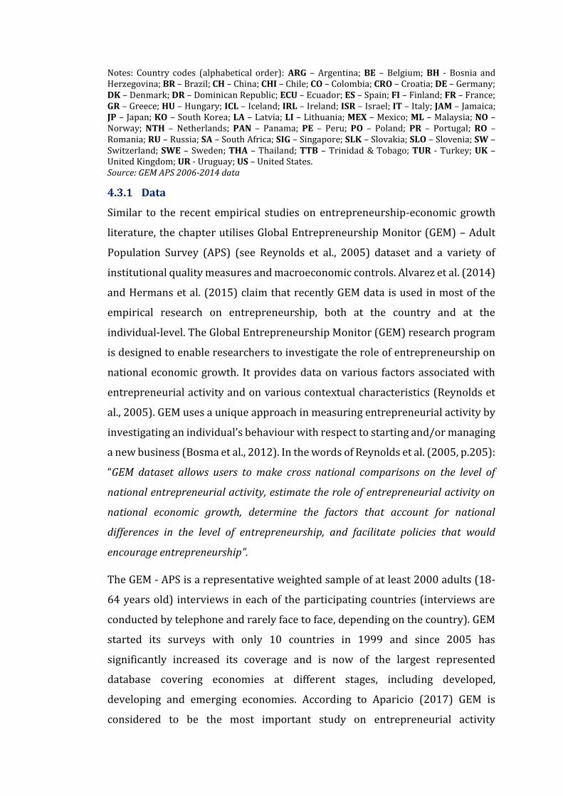
Notes: Country codes (alphabetical order): ARG – Argentina; BE – Belgium; BH - Bosnia and Herzegovina; BR – Brazil; CH – China; CHI – Chile; CO – Colombia; CRO – Croatia; DE – Germany; DK – Denmark; DR – Dominican Republic; ECU – Ecuador; ES – Spain; FI – Finland; FR – France; GR – Greece; HU – Hungary; ICL – Iceland; IRL – Ireland; ISR – Israel; IT – Italy; JAM – Jamaica; JP – Japan; KO – South Korea; LA – Latvia; LI – Lithuania; MEX – Mexico; ML – Malaysia; NO – Norway; NTH – Netherlands; PAN – Panama; PE – Peru; PO – Poland; PR – Portugal; RO – Romania; RU – Russia; SA – South Africa; SIG – Singapore; SLK – Slovakia; SLO – Slovenia; SW – Switzerland; SWE – Sweden; THA – Thailand; TTB – Trinidad & Tobago; TUR - Turkey; UK – United Kingdom; UR - Uruguay; US – United States. Source: GEM APS 2006-2014 data
Data
Similar to the recent empirical studies on entrepreneurship-economic growth
literature, the chapter utilises Global Entrepreneurship Monitor (GEM) – Adult
Population Survey (APS) (see Reynolds et al., 2005) dataset and a variety of
institutional quality measures and macroeconomic controls. Alvarez et al. (2014)
and Hermans et al. (2015) claim that recently GEM data is used in most of the
empirical research on entrepreneurship, both at the country and at the
individual-level. The Global Entrepreneurship Monitor (GEM) research program
is designed to enable researchers to investigate the role of entrepreneurship on
national economic growth. It provides data on various factors associated with
entrepreneurial activity and on various contextual characteristics (Reynolds et
al., 2005). GEM uses a unique approach in measuring entrepreneurial activity by
investigating an individual’s behaviour with respect to starting and/or managing
a new business (Bosma et al., 2012). In the words of Reynolds et al. (2005, p.205):
“GEM dataset allows users to make cross national comparisons on the level of
national entrepreneurial activity, estimate the role of entrepreneurial activity on
national economic growth, determine the factors that account for national
differences in the level of entrepreneurship, and facilitate policies that would
encourage entrepreneurship”.
The GEM - APS is a representative weighted sample of at least 2000 adults (18-
64 years old) interviews in each of the participating countries (interviews are
conducted by telephone and rarely face to face, depending on the country). GEM
started its surveys with only 10 countries in 1999 and since 2005 has
significantly increased its coverage and is now of the largest represented
database covering economies at different stages, including developed,
developing and emerging economies. According to Aparicio (2017) GEM is
considered to be the most important study on entrepreneurial activity
145
worldwide. The choice of variables included is mostly derived from the
theoretical framework, MRA and literature review presented in the previous two
chapters. The data span, 2006-2014, is however, conditioned on two main
reasons. First, GEM applies a data policy which envisages that data are made
publicly available only three years (sometime more) after data collection. This
means that 2015 data will only be available in late 2018 or most probably in
2019. Hence, the last year of our data set is 2014 which was made available in
2018. Second, the first waves of GEM questionnaires distributed between 2001
and 2005 did not include some of the main variables of interest (at least not in
the definition and measurement unit that they have now).
In addition, cross-country data descriptive statistics suggest that there was lack
of standardization and uniformity of definition or perhaps misreporting and
misinterpretation by the interviewers, the respondents or both. For instance, in
Denmark in 2004, the value of high-job growth entrepreneurial activity (teahjg)
was as high as 7800, whereas in the same year, but in Norway, the value of high-
job growth entrepreneurial activity would be as low as 46. Such large differences
are very unlikely even between countries at very different stages of development
or with significant differences in the overall entrepreneurship ecosystem. One
possible explanation of the large differences might be to the unit of measurement
of the variable. High-job growth entrepreneurial activity (teahjg) was expressed
as a percentage of TEA; a percentage of total population; or in relation to 10,000
inhabitants, which might have added complexity and might have influenced
misreporting. Hence, given the concerns in the data reporting between 2001-
2005, particularly for ‘employment growth’ expectations and innovative
entrepreneurial activity, the empirical analysis of this chapter starts only from
2006 and onwards. Nevertheless, studies (see e.g., Prieger et al., 2016) using GEM
data have provided empirical investigations even with the 2001 data, however,
their main variable of interest was overall TEA as they looked at the
entrepreneurial activity as a whole or at most distinguished between
opportunity-driven and necessity-driven entrepreneurial activity. Since 2006,
GEM questionnaires have become more uniform in terms of definition,
measurement, reporting and presentation of the collected data and in addition
have been extended to include more questions.

146
4.3.1.1 The dependent variable: economic growth
In this chapter, growth of GDP is used as a proxy for economic performance. This
is in line with the previous research in the entrepreneurship-economic
performance literature (van Stel et al., 2005; Hessels and van Stel, 2011; Acs et
al., 2012; Capello and Lenzi, 2016; Acs et al., 2018). Most of the studies reviewed
in the MRA (over 70%) and in Chapter 2 had used GDP growth and/or growth of
GDP per capita as their preferred dependent variable (measure of economic
performance). Acs et al. (2012) use 5-year moving average on GDP per capita
growth to smooth out short-run cyclical variations. Similarly, Hessels and van
Stel (2011) use real GDP growth 4-year averages as their measure of economic
performance. Some studies, however, use output level types of measures of
economic performance. For instance, Urbano and Aparicio (2016) use labour
productivity, which represents a country's economic output relative to its
population aged 15–64 years. Bjørnskov and Foss (2013) used Total Factor
Productivity (TFP), as a measure of economic performance. Another group of
scholars use employment growth to proxy for economic output (Fritsch and
Mueller 2008; Noseleit, 2013; Stephens et al., 2013; Doran et al., 2016).
The preferred economic performance measure growth of GDP (growth) utilised
in this chapter is calculated as the first difference of purchasing power parity
(PPP) adjusted real GDP per capita in logarithmic form (at constant 2011
international dollars $). An advantage of using the PPP adjusted real GDP per
capita is the adjustment that it provides, in terms of changes in exchange rates
between countries, and the impact of price changes and inflation periods in
country’s output. Initially, also the readily-available annual percentage growth
rate of GDP at market prices based on constant local currencies was used.50 In
addition, annual growth of GDP per capita sourced from the World Bank, World
Development Indicators is also considered, but finally the chosen dependent
variable is decided to be growth as it seem to be more appropriate for this study.
50 Aggregates are based on constant 2010 U.S. dollars

147
4.3.1.2 Entrepreneurship measures
As it is discussed in Chapter 2, the definition of entrepreneurship is complex
(Shepherd, 2011) and there is still lack of a universal and generally accepted
entrepreneurship definition (Shane and Venkataramann, 2000; Bosma et al.,
2009; Audretsch et al., 2015; Henrekson and Sanandaji, 2018). Davidsson (2015)
argues that entrepreneurship is a function of different contexts, portrayed in a
several varieties of forms and is a result of different motivations. The MRA in
Chapter 3 revealed that researchers use different approaches and measures at
the country-level, such as: self-employment, new firm startups, firm net birth or
the GEM sourced Total (Early-stage) Entrepreneurial Activity (TEA) rate
(Blanchflower, 2000; Carree and Thurik, 2003; Reynolds., 2005; Iversen et al.,
2008, Acs and Szerb, 2010; Erken et al., 2016). In this Chapter, we argue that
entrepreneurship represents a multifaceted phenomenon (Zahra and Wright,
2011; Szerb et al., 2013; Acs and Correa., 2015; Kuckertz et al., 2016), therefore
measuring it and estimating its effect requires a set of well-defined variables,
especially when it comes to assess its impact on economic growth (Acs et al.,
2014).
The main variables of interest are all sourced form GEM – APS. A significant
advantage of GEM measures over other measures of entrepreneurship, is the
uniformity of data collection methodologies and of the definitions of key
variables (Acs et al., 2008).51 In addition, Reynolds et al. (2005) argue that
compared to other measures of entrepreneurial activity, GEM measures capture
country-level capacities and intentions to create new ventures and influence
macroeconomic growth. Moreover, by using GEM data, the empirical results are
more likely to be comparable with other studies in the entrepreneurship-
economic growth literature (e.g., Urbano and Aparacio, 2016; Acs et al., 2018).
Besides the Total Entrepreneurial Activity (TEA), defined as ‘the prevalence rate
of individuals who are currently involved in starting up a new business, having
taken concrete steps to start, (nascent), or owner of a business that is less than
51 Although we argued earlier that high-job growth (teahjg) entrepreneurial activity was not strictly uniformly measured and reported until 2006, still the GEM methodology is the most advanced in the field of entrepreneurship.
148
42 months active and generating income’, GEM provides data portraying other
different types and nuances of entrepreneurial activity. As discussed in Chapter
2, the overall TEA is a very broad measure of entrepreneurial activity and does
not provide information on the motives to start, growth aspirations, or strategic
market orientation of new entrepreneurial ventures. Rather, it treats all new
entrepreneurial initiatives as being equally important (Bosma et al., 2018). The
two additional types of entrepreneurial activity provided by GEM data, which
represent entrepreneurial aspirations and innovation, are used in this
investigation: (i) Employment Growth and; (ii) ‘Innovative’ entrepreneurial
activity
The two types of entrepreneurial activity represent new ventures with the
potential to make a major contribution to the national economic growth (Valliere
and Peterson, 2009; Stam et al., 2012). The ‘Employment growth expectations’
type of entrepreneurial activity is measured by (i) High-Job Growth Expectations
entrepreneurial activity (teahjg) – entrepreneurial ventures expecting at least
20 jobs in five years; and (ii) Job Growth Expectations entrepreneurial activity
(teayyjg5) – entrepreneurial ventures expecting at least 5 jobs in five years. The
innovative and new market development entrepreneurial activity is measured
by: (i) Product or service innovation entrepreneurial activity (teayynwp) – new
product to at least some customers; and (ii) New product and new market
combination entrepreneurial activity (teanpm) – new product to all/most
customers and no/few competitors. It is argued that these types of
entrepreneurial activity represent better the Schumpeterian type entrepreneur
and might be able to more effectively capture the impact of entrepreneurship on
economic growth (Autio, 2011; Coad et al., 2014; Ferreira et al., 2017; Block et
al., 2017; Acs et al., 2018).52
It is worth highlighting that although the first two measures of ‘employment
growth expectations’, represent growth aspirations and ambitions, there is both
theoretical and empirical evidence to suggest that firms’ growth aspirations are
52 Recalling the discussion in Chapter 2, the creation of new economic dynamism and activity (entry with impact) and dissemination of innovation represent Schumpeterian entrepreneurship (Davidsson et al., 2006; Santarelli and Vivarelli, 2007; Baumol, 2010, Öner and Kunday, 2016).

149
positively and significantly associated to firm’s realised growth (see e.g., Wiklund
and Shepherd, 2003; Davidsson et al., 2006; Delmar and Wiklund, 2008; Terjesen
and Szerb, 2008).
4.3.1.3 Institutional quality and other control variables
The literature on economic growth has highlighted the crucial role of institutions.
North (1990), Barro (1996), Acemoglu et al. (2002), Rodrik et al. (2004), Rodrik
(2004), Acemoglu and Johnson (2005), Acemoglu and Robinson (2012), are
among the studies to have suggested a positive relationship between the quality
of institutions and economic growth. As such, neglecting the impact of
institutions on a growth model setting would bias the estimates and the
hypothesised relationship between entrepreneurial activity measures and
economic growth. Accordingly, proxies of institutional quality are used, jointly
with entrepreneurship variables, to model the impact of entrepreneurial activity
on growth.
Acemoglu and Robertson (2012) claim that besides the influence of institutions
on economic growth, they also have an impact on inequality and poverty rate by
arguing that low quality institutions (non-inclusive) will negatively affect the
lowest-income groups of population. One of the variables used to reflect the level
of institutional quality is the ‘rule of law’ index of the World Bank’s Worldwide
Governance Indicators (WGI) database. The state of ‘rule of law’ is one of the six
dimensions that define the overall quality of governance. Acknowledging the
positive effect of governance on economic outcomes, Kaufmann et al. (2009, p. 5)
define governance as “the traditions and institutions by which authority in a
country is exercised for the common good”. Besides the ‘rule of law’, governance
consists of five other dimensions, related to voice and accountability, political
stability and absence of violence, government effectiveness, regulatory quality
and control of corruption. For the purpose of this thesis, the composite ‘rule of
law’ index (rule_of_law_wgi) is considered as the closest approximation to the
quality of institutions. The ‘rule of law’ index represents: “perceptions of the
extent to which agents have confidence in and abide by the rules of society, and in
particular the quality of contract enforcement, property rights, the police, and the
courts, as well as the likelihood of crime and violence” (Kaufmann et al., 2010, p.4).

150
The index is constructed from a multisource perspective and ranges from -2.5 to
2.5, where higher values denote higher levels of the ‘rule of law’. It is expected
that a higher ‘rule of law’ index provides better institutional conditions for an
enhanced economic growth at the country-level.
Volumes of research have suggested that excessive government spending,
commonly leading to large budget deficits and public debts, has a negative impact
on economic dynamism (see e.g., Bleaney and Nishiyama 2002; Bjørnskov and
Foss, 2013; Urbano and Aparicio, 2016). Moreover, a very large public sector is
also accompanied by misallocation of key country resources and comes at the
cost of significant losses in economic efficiency (Miller et al., 2018). Government
consumption varies from country to country as it is affected by culture, political
regimes, country size, geographic conditions and the stage of economic
development. Hence, it is difficult to identify an optimal level of government
consumption. Bjørnskov and Foss (2013) find that government consumption has
a negative impact on the growth of total factor productivity of 25 OECD countries
between 1980 and 2005. Barro (1990) provides a review of three empirical
growth models and distinguishes between productive government spending and
unproductive government spending. The former is suggested to be directed to
the enforcement of property rights, while the latter leads to an increase in income
taxes, thus reducing the share of private investments and lowering the rate of
economic growth (Barro, 1990, pp.120-121)
Accordingly, the analysis includes government consumption as a share of GDP
(the size of public sector) to investigate whether growth of GDP is affected by the
size of public sector. Government consumption relative to GDP includes all
government current expenditure for purchases of goods and services (including
compensation of employees). It also includes most expenditure on national
defense and security, but excludes government military expenditure that are part
of government capital formation.
The role of human capital as a determinant of economic growth has been
emphasised in the theoretical and empirical literature (see e.g., Lucas, 1988;
Mankiw et al., 1992; Barro and Lee, 1993; Enayati, 2007; Barro and Lee, 2013).
Schooling is reported to increase employee marginal productivity, hence

151
positively impacting national income growth (Breton, 2013). Barro (1991)
suggests that per capita GDP growth rates are positively affected by initial human
capital, proxied by school enrolment rates. The study used data between 1960-
1985 for a large cross-country investigation.53 Nevertheless, finding the most
appropriate measure of human capital has always been a concern in the growth
economics (Islam, 1995).
The literature on economic growth suggests several variables that can be used as
a proxy of human capital. Most of the proxies rely on educational measures, as
education is considered one of the key dimensions of human capital. For instance,
Le et al. (2005) find that studies have used school enrolment rates – both gross
and net – at all the three levels, namely primary, secondary and tertiary, literacy
rates and test scores. The rationale behind these types of measures is that they
indicate the level of investment in education which is considered a critical
determinant of the quality of human capital (Le et al., 2005). Some of the most
recent studies (Barro and Lee, 2013; Hanushek and Woessmann 2011; Hanushek
and Woessmann, 2012a; 2012b), have used average years of schooling and the
level of students’ cognitive skills, while Bosma et al. (2018) use the Penn World’s
Table logarithm of human capital index per person, which is also based on
average years of schooling, to proxy for investment in human capital.
Following Barro and Lee (2013), this chapter uses average years of schooling
(mean-year of schooling) to proxy for human capital. The annual data are
sourced from the UNDP and reflect the number of years of education of
population aged 25 and over. The data that UNDP provides is also sourced and
therefore based on the methodology of Barro and Lee (2013; 2018) but also
complemented with data on educational attainment of UNESCO Institute for
Statistics (2013). In addition, for robustness checks, we have also used gross
enrolment rates in tertiary and secondary education, spending on education and
the human development index of UNDP which includes data on years of
schooling, life expectancy and GNI per capita.
53 In total, this study included 98 countries

152
For the rate of accumulation of physical capital, the study uses gross fixed capital
formation as a share of GDP, i.e., investment to GDP ratio (inv_gdp_grosscapfor).
Both theoretical and empirical studies, suggest that the share of physical capital
investment is a determinant of economic growth (see e.g., Mueller, 2007; Bruns
et al., 2017; Bosma et al., 2018). Solow (1956, p.91; 2007, p.8) argues that
investment in physical and human capital along with technological and
organizational innovation can explain most of the long-run growth of modern
economies. Apergis and Payne (2010) find that an increase in gross fixed capital
formation is positively associated with real GDP of 20 OECD countries over the
period 1985-2005.
Another relevant variable, as suggested by theoretical and empirical literature, is
trade openness (trade_sharegdp), measured as the share of exports of goods and
services to GDP (Frankel and Romer, 1999). Hausmann et al. (2007) find a
positive relationship between exports (of goods associated with higher
productivity) and economic growth. Similar to Hausmann et al. (2007), studies in
the international trade and economic growth literature, report that trade
(export) positively impacts economic growth (see e.g., Barro and Sala-i-Martin,
1995; 2004; Makki and Somwaru, 2004; Chang et al., 2005). Generally, increasing
international trade activity tends to also promote the accumulation of human
capital, which in turn leads to higher long-run macroeconomic growth.
Additional benefits of trading include positive spillovers, technology transfer,
improved business climate, better utilization of capacities and learning effects
(Grosmann and Helpman, 1991). Exporting is also a signal of high firm (and
country) productivity as only the most productive firms (countries) are likely to
engage in international markets i.e., export their products or services (Bernard
et al., 2007; Wagner, 2007).
Population growth is amongst the commonly used explanatory variables in the
growth literature. Annual population growth (ann_pop_growth) is measured as
the annual growth rate of midyear population expressed as a percentage. The
Classical and Solow models of growth suggest that population growth is crucial
for economic growth (Van den Berg, 2017). Romer (2011, p.106) argues that
positive population growth is essential for sustained growth of output per
153
worker. Bosma et al. (2018) use population growth as a proxy for labour growth
at the country level (Barro and Sala-i-Martin, 2004). Although contradicts exists,
in this investigation, the expectations are that economic growth will be
negatively influenced by population growth.
Following the practice in growth models, this chapter will also use country’s
initial condition to account for the catch-up and convergence effect. Barro (1991)
finds that the initial level of real per capita GDP is negatively related to the growth
rate of per capita GDP of 98 countries between 1960-1985. More recent studies
report similar findings and in line with Mankiw et al. (1992) suggestion for catch-
up effects in the growth literature. For instance, Capello and Lenzi (2016) report
evidence for the presence of convergence, i.e., low per capita GDP regions grow
at a higher rate than high per capita GDP regions, in a regional level study for the
period 2006-2013. The choice of measures to capture this effect, in this chapter,
were also subject to the estimators used. Knowing that fixed effect (FE) estimator
will not estimate time-invariant variables makes it impossible to include GDP
initial level (the start year of the dataset). Rather, the first lagged level of GDP per
capita at 2011 constant prices is included in the model when the FE estimator is
used. However, when other estimators are employed, GDP initial at the start year
of the dataset (2006) and GDP initial with three additional lags, namely GDP per
capita of year 2003 are used. Table 4.1 below presents details of the variables
included in the analysis, their definition, measurement, variable source and the
expected sign.
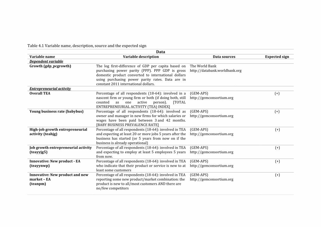
Table 4.1 Variable name, description, source and the expected sign
Data Variable name Variable description Data sources Expected sign Dependent variable Growth (gdp_pcgrowth) The log first-difference of GDP per capita based on
purchasing power parity (PPP). PPP GDP is gross domestic product converted to international dollars using purchasing power parity rates. Data are in constant 2011 international dollars.
The World Bank http://databank.worldbank.org
Entrepreneurial activity Overall TEA Percentage of all respondents (18-64): involved in a
nascent firm or young firm or both (if doing both, still counted as one active person). [TOTAL ENTREPRENEURIAL ACTIVITY (TEA) INDEX]
(GEM-APS) http://gemconsortium.org
(+)
Young business rate (babybus) Percentage of all respondents (18-64): involved as owner and manager in new firms for which salaries or wages have been paid between 3 and 42 months. [BABY BUSINESS PREVALENCE RATE]
(GEM-APS) http://gemconsortium.org
(+)
High-job growth entrepreneurial activity (teahjg)
Percentage of all respondents (18-64): involved in TEA and expecting at least 20 or more jobs 5 years after the business has started (or 5 years from now on if the business is already operational)
(GEM-APS) http://gemconsortium.org
(+)
Job growth entrepreneurial activity (teayyjg5)
Percentage of all respondents (18-64): involved in TEA and expecting to employ at least 5 employees 5 years from now.
(GEM-APS) http://gemconsortium.org
(+)
Innovative: New product - EA (teayynwp)
Percentage of all respondents (18-64): involved in TEA who indicate that their product or service is new to at least some customers
(GEM-APS) http://gemconsortium.org
(+)
Innovative: New product and new market – EA (teanpm)
Percentage of all respondents (18-64): involved in TEA reporting some new product/market combination: the product is new to all/most customers AND there are no/few competitors
(GEM-APS) http://gemconsortium.org
(+)
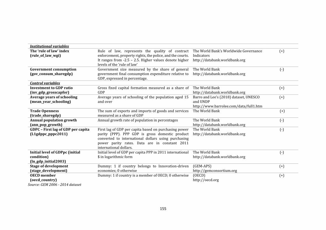
155
Source: GEM 2006 - 2014 dataset
Institutional variables The ‘rule of law’ index (rule_of_law_wgi)
Rule of law, represents the quality of contract enforcement, property rights, the police, and the courts. It ranges from -2.5 – 2.5. Higher values denote higher levels of the ‘rule of law’
The World Bank’s Worldwide Governance Indicators http://databank.worldbank.org
(+)
Government consumption (gov_consum_sharegdp)
Government size measured by the share of general government final consumption expenditure relative to GDP, expressed in percentage.
The World Bank http://databank.worldbank.org
(-)
Control variables Investment to GDP ratio (inv_gdp_grosscapfor)
Gross fixed capital formation measured as a share of GDP
The World Bank http://databank.worldbank.org
(+)
Average years of schooling (mean_year_schooling)
Average years of schooling of the population aged 15 and over
Barro and Lee’s (2018) dataset, UNESCO and UNDP http://www.barrolee.com/data/full1.htm
(+)
Trade Openness (trade_sharegdp)
The sum of exports and imports of goods and services measured as a share of GDP
The World Bank (+)
Annual population growth (ann_pop_growth)
Annual growth rate of population in percentages The World Bank http://databank.worldbank.org
(-)
GDPC – First lag of GDP per capita (L1gdppc_pppc2011)
First lag of GDP per capita based on purchasing power parity (PPP). PPP GDP is gross domestic product converted to international dollars using purchasing power parity rates. Data are in constant 2011 international dollars.
The World Bank http://databank.worldbank.org
(-)
Initial level of GDPpc (initial condition) (ln_gdp_initial2003)
Initial level of GDP per capita PPP in 2011 international $ in logarithmic form
The World Bank http://databank.worldbank.org
(-)
Stage of development (stage_development)
Dummy: 1 if country belongs to Innovation-driven economies; 0 otherwise
(GEM-APS) http://gemconsortium.org
(+)
OECD member (oecd_country)
Dummy: 1 if country is a member of OECD; 0 otherwise (OECD) http://oecd.org
(+)
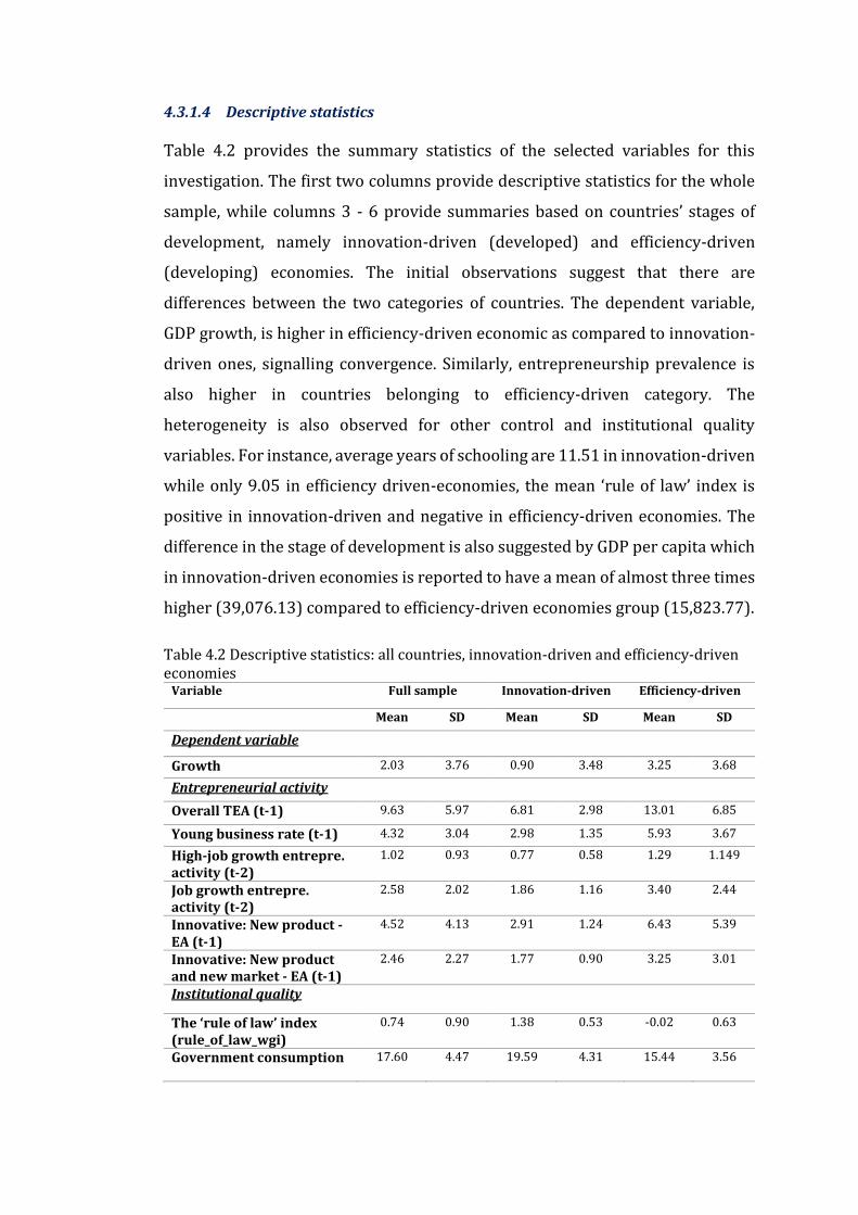
4.3.1.4 Descriptive statistics
Table 4.2 provides the summary statistics of the selected variables for this
investigation. The first two columns provide descriptive statistics for the whole
sample, while columns 3 - 6 provide summaries based on countries’ stages of
development, namely innovation-driven (developed) and efficiency-driven
(developing) economies. The initial observations suggest that there are
differences between the two categories of countries. The dependent variable,
GDP growth, is higher in efficiency-driven economic as compared to innovation-
driven ones, signalling convergence. Similarly, entrepreneurship prevalence is
also higher in countries belonging to efficiency-driven category. The
heterogeneity is also observed for other control and institutional quality
variables. For instance, average years of schooling are 11.51 in innovation-driven
while only 9.05 in efficiency driven-economies, the mean ‘rule of law’ index is
positive in innovation-driven and negative in efficiency-driven economies. The
difference in the stage of development is also suggested by GDP per capita which
in innovation-driven economies is reported to have a mean of almost three times
higher (39,076.13) compared to efficiency-driven economies group (15,823.77).
Table 4.2 Descriptive statistics: all countries, innovation-driven and efficiency-driven economies
Variable Full sample Innovation-driven Efficiency-driven
Mean SD Mean SD Mean SD
Dependent variable
Growth 2.03 3.76 0.90 3.48 3.25 3.68
Entrepreneurial activity
Overall TEA (t-1) 9.63 5.97 6.81 2.98 13.01 6.85
Young business rate (t-1) 4.32 3.04 2.98 1.35 5.93 3.67
High-job growth entrepre. activity (t-2)
1.02 0.93 0.77 0.58 1.29 1.149
Job growth entrepre. activity (t-2)
2.58 2.02 1.86 1.16 3.40 2.44
Innovative: New product - EA (t-1)
4.52 4.13 2.91 1.24 6.43 5.39
Innovative: New product and new market - EA (t-1)
2.46 2.27 1.77 0.90 3.25 3.01
Institutional quality
The ‘rule of law’ index (rule_of_law_wgi)
0.74 0.90 1.38 0.53 -0.02 0.63
Government consumption 17.60 4.47 19.59 4.31 15.44 3.56

157
Control variables
Investment to GDP ratio 22.74 5.28 21.91 4.56 23.66 5.84
Human Capital 10.33 1.92 11.51 1.27 9.05 1.68
Trade Openness 92.36 58.79 104.74 69.81 78.94 39.83
Annual population growth 0.64 0.86 0.60 0.85 0.68 0.87
GDP per capita (t-1) 27510.01 14833.1 38774.7 11704.3 15354.6 4966.6
Log of Initial level of GDPpc (initial condition)
9.89 0.64 10.41 0.33 9.34 0.35
Stage of development 0.52 0.50 1 0 1 0
OECD member 0.56 0.49 0.89 0.32 0.21 0.41
GDPpc 27917.07 14826.2 39076.13 11801.89 15823.77 5063.27
Note: The summary statistics are produced after adjusting for outliers
Source: GEM 2006-2014
ESTIMATION STRATEGY
In this chapter, the impact of different types of entrepreneurial activity on
economic growth is empirically tested using a panel data setting, covering 48
countries over a nine-year period 2006-2014. The set of countries included in
this investigation is reliant on the GEM data availability, as GEM is the source of
our main variables of interest, entrepreneurship. In the final data set 25 countries
belong to the innovation-driven economy group and 23 to the efficiency-driven
economy group as categorised by Porter’s et al. (2002) typology and endorsed by
the GEM methodology.54 The selected empirical strategy is subject to theoretical
considerations, discussed in Chapter 2, dataset structure, and the potential
econometric issues that need to be dealt with in this investigation. Specifically,
the theoretical arguments, data and econometric issues that have to be addressed
by the empirical approach, among others include:
i. The potential dynamics in the entrepreneurship-economic growth
relationship
ii. Potential endogeneity between entrepreneurship measures and
economic growth
iii. Cross-country heterogeneity; and
iv. Time invariant or slowly changing variables.
The use of panel data is the first remedy to address some the above-listed issues
in the entrepreneurship-economic growth relationship. According to Hsiao
54 The classification of economies in discussed in more details in Chapter 1 and Chapter 5.
158
(2006), Greene (2011, p.343) and Wooldridge (2013), panel data structures take
into account the cross-country heterogeneity while also allowing for modelling
the dynamics in the investigation. The potential heterogeneity within our
selected countries may influence or bias the results as it may lead to correlation
between entity’s error term and the predictor variables. Similarly, failing to
account for the presence of potential dynamics in the analysis is usually
associated with biases of the estimates (Frees, 2004). Baltagi (2005, p.6) suggests
that one of the benefits of using panel data is the ability to model the “dynamics
of adjustment”. The MRA in Chapter 3, suggests that modelling the dynamics of
the impact of entrepreneurship on economic growth literature is still sparse. It is
highly likely that the main reason for this is the lack of adequate time series data,
and the lack of a uniform definition of entrepreneurship. The latter has led to
multiple proxies used in an attempt to capture the effect of entrepreneurship and
to the absence of a longer time-series component in the entrepreneurship data.
Since this investigation uses nine-year data periods for the selected variables,
modelling the dynamics is a viable estimation approach.
However, although the original data set has nine periods, the use of lags for our
main variables of interest has impacted the sample size. It has been argued that
entrepreneurship is more likely to manifest its effect on economic growth with
time lags (see e.g., Fritsch and Mueller, 2004; van Stel and Storey, 2004; Carree
and Thurik, 2010; Stam and van Stel, 2011; Faggian et al., 2017). Moreover, the
construction of, especially, the ‘employment growth expectations’ variables
motivate the use of lags. For example, high-job growth expectations
entrepreneurial activity (teahjg) is defined as: ‘Percentage of all respondents (18-
64), involved in TEA and expecting at least 20 jobs 5 years after the business has
started’. Assuming that at the time of the GEM survey, some businesses might
have been in the market for only six months to one year, makes their
contemporaneous expected impact on growth very limited. Expecting that firms,
having these growth aspirations, influence economic growth after some lags
seems more plausible (Caree and Thurik, 2010). Thus, for ‘employment growth
expectations’ variables, we have used two lags, while we expect that the two
measures of innovative entrepreneurial activity to influence growth with one-
year period lag, as the latter represent the current firm situation and not their

159
expectations five years from now.55 Moreover, using lags for entrepreneurial
activity measures has an additional benefit, that of addressing the presence of
potential endogeneity in the entrepreneurship-economic growth relationship.56
The use of lags for the control variables is avoided mainly for practical reasons.
Having additional lags in the models specified would be at the cost of losing
additional observations.57
Prior to jumping into modelling dynamics, this chapter follows the previous
research practice which suggests that static estimators, namely fixed effect (FE)
and random effect (RE) are more commonly used in panel data analysis. The
suitability of the two alternative estimators is assessed on theoretical basis, the
relationship to be investigated, the type of the data (heterogeneity; unobserved
effects) and on the diagnostics tests (Hausman, 1978; Baltagi, 2005; 2008;
Greene, 2012; Wooldridge, 2013). Random effects (RE) estimator is preferred in
situations where the unobserved country effects are assumed to be uncorrelated
with the included regressors (Gujarati, 2004; Wooldridge, 2009). On the other
hand, the fixed effect (FE) estimator accounts for such correlation between the
unobserved heterogeneity and explanatory variables in the model, within each
cross-sectional observation, i.e., between countries (Wooldridge, 2013; Baltagi,
2005). The assumption of no correlation between country unobserved effects
and the predictor variables rarely holds (Greene, 2002). As it is also identified in
Chapter 3, the FE rather than the RE is more frequently applied in the
entrepreneurship-economic performance literature. Favouring the use of FE,
Wooldridge (2009, p. 450) claims that “in many applications, the whole reason for
using panel data is to allow the unobserved effect to be correlated with the
explanatory variables”.
Besides the above outlined arguments, the chapter relies on Hausman test to
confront the decision of which is the most appropriate estimator for this
investigation (Hausman, 1978). The Hausman test checks whether the
55 In addition, the use of lags for the main variables of interest seems to also improve diagnostics and also the model explanatory power (R2). 56 More details on the potential presence of endogeneity are offered in subsection 4.4.1 57 In some situations, adding lags to the control variables is also found to be at the risk of good diagnostics, contrary to the situation with our main variables of interest.
160
assumption of the conditional independence between the intercept and
independent variables holds (Wooldridge, 2002; Greene, 2012). The null
hypothesis states that there are no systematic differences between the two
estimators, i.e., that the RE model is valid. A rejection of the null hypothesis
suggests that the fixed effect (FE) is preferred over the random effect (RE)
(Baltagi, 2005; Wooldridge, 2009). Since the two estimators apply different error
variances, Hoechle (2007) and Cameron and Trivedi (2009) suggest that the
default version of Hausman test might produce a negative chi-square test
statistic, thus making the test invalid and failing to inform our decision-making.
Instead, the chapter performs the Hausman test as suggested by Wooldridge
(2002, p.290) by using the stata option ‘sigmamore’. According to Cemeron and
Trivedi (2009), the ‘sigmamore’ option specifies that the covariance matrices be
based on the estimated disturbance variance from the efficient estimator, i.e., the
RE estimator. The Hausman test suggest that the FE is more appropriate
estimation approach than the RE, since the H0 of no systematic differences
between the two, is strongly rejected at the 1% significance level (p<0.001).58 As
a result, the baseline regression model, the FE, to be estimated in this chapter is
the one of the form:
𝑔𝑟𝑜𝑤𝑡ℎ𝑖𝑡 = 𝛽0𝑖 + 𝛽1𝐸𝑁𝑇𝑖𝑡 + 𝛾𝑖𝜒𝑖𝑡 + 휀𝑖𝑡 (4.1)
where, 𝛽0𝑖 represents the specific intercept for each country59, 𝐸𝑁𝑇𝑖𝑡 is a vector
of entrepreneurship measures, 𝜒𝑖𝑡 is the vector of institutional quality and other
control variables, while 휀𝑖𝑡 represents the idiosyncratic error term.
However, using the FE estimator has its own shortcomings. The most important
in this investigation is the inability of the selected (FE) estimator to: (i) handle
potentially endogenous variables; (ii) produce consistent, efficient and unbiased
estimates in the presence of heteroscedasticity, autocorrelation and cross-
sectional dependency (Hoechle, 2007) and: (iii) model time-invariant or slowly-
58 See Appendix 4.2.5 for the stata output. Also, the Breusch and Pagan Lagrangian multiplier test
for random effects favours FE (see Appendix 4.2.6). 59 In the RE model, 𝛽0 is the overall intercept, fitting all the countries in one single intercept. In the FE estimator, each intercept is considered as unknown parameter to be estimated, while the slopes of the coefficients remain the same (Gujarati, 2004; Greene, 2008).

161
moving variables. The section below discusses some of the alternative estimators
to help design the most appropriate estimation strategy and specifies the models
of this chapter.
Econometric approach and model specification
The outcome of the Hausman test suggests that the FE rather than RE estimator
is more preferred. However, the diagnostic tests of the baseline FE model suggest
the presence of heteroscedasticity (the modified Wald test), serial correlation
and cross-sectional dependency (see Appendices 4.2.7 – 4.2.9).60 The FE
estimator is either inconsistent, biased or inefficient in the presence of
heteroscedasticity, non-normality, serial correlation and cross-sectional
dependency. To illustrate this, heteroscedasticity would make the estimates
inefficient and their standard errors biased. Following Baltagi (2005), to correct
for such bias in the standard errors, robust standard errors must be used. Cross-
sectional dependency might appear as some of the country characteristics are
unable to be quantified and thus represent the unobserved common factor part
of the panel (Hoechle, 2007). A typical example of such unobserved common
country characteristics might be the occurrence of shocks (financial and
economic crisis), similarly affecting groups of countries. Sarafidis et al. (2009,
p.2) argue that spatial correlation is another reason for the presence of cross-
sectional dependency. Countries sharing similar characteristics are also expected
to have similar trends in entrepreneurial activity. As observed in section 4.3.1,
countries that belong to innovation-driven economies share more similar
patterns of entrepreneurial activity compared to the countries in efficiency-
driven stage.
To address some the above empirical issues and to ensure econometric validity
and statistical inference, Hoechle (2007) suggests using Driscoll and Kraay
(1998) standard errors adjusted for unbalanced panel data. Hoechle (2007,
p.310) argues that “Driscoll-Kraay standard errors are well calibrated when the
regression residuals are cross-sectionally dependent”. According to Driscoll and
60 Due to the unbalanced structure of our data, the presence of cross-sectional dependence, using the the ‘xtcsd, pesaran abs’ stata command, was unable to produce valid tests. However, as Hoechle (2007, p.281) argues, “erroneously ignoring possible correlation of regression disturbances over time and between subjects can lead to biased statistical inference”.
162
Kraay (1998), Driscoll-Kraay standard errors are robust to most of the forms of
cross-sectional "spatial" and dependence. The second concern in the empirical
analysis is the presence of time-invariant or slowly-moving (rarely-changing)
regressors.61 The transformation applied by the FE estimator leaves any time-
constant explanatory variable out of the analysis (Wooldridge, 2013). To
overcome the issue of losing relevant information in the models, two other
estimators are included in the analysis. The two estimators share some of the
features of the FE estimator and in addition are able to handle time-constant and
slowly-moving variables. First, the Fixed Effect Vector Decomposition (FEVD)
approach developed by Plümper and Troeger (2007) is applied. Plümper and
Troeger (2011) show that the FEVD is a three-stage approach that combines fixed
effects estimation to analyze the effect of time-varying variables and pooled
ordinary least squares (OLS) estimation of both time-varying and time-invariant
or “rarely changing” variables. More specifically, the first stage of this approach,
uses a standard FE estimator only with variables that have a high within-group
variation. The predicted unit effects of the first stage are then included in the
model together with time-constant and slowly-moving variables. The third stage
is estimated by poled OLS and includes the full set of explanatory variables, high
within-group variation and time-constant or slowly-moving, and the residuals
from the second stage. The stata program (ado file) ‘xtfevd’ developed by Plümper
and Troeger (2007) executes the three stags and also corrects for degrees of
freedom.62
The FEVD estimator, however, has been subject to criticism from
econometricians, amongst them Greene (2011) and Breusch et al. (2011). Their
main critique suggests that there are no significant differences and advantages,
in terms of efficiency gains, of using FEVD over the conventional FE estimator.
For example, Greene (2011) argues that stage three of the FEVD estimator
produce very small standard errors, hence suggesting that the FEVD estimates
61 The between- and within-group variation (measured by standard deviations) for each variable in our model indicates that, according to the guidelines, four of the variables are to be considered as slowly-changing. Government spending; Rule of Law; Average years of schooling; and Trade openness have a between to within ratio of higher than 2.8. 62 Because ‘residuals’ is not a fixed realization but rather an estimated variable, xtfevd in addition to adjusting for standard errors, harmonizes the degrees of freedom too.
163
might be inconsistent. However, that same year Plümper and Troeger (2011, pp.
3 and 33) conceded the argument of ‘too small standard errors’ and in the
updated stata ado file have made sure that the FEVD “computes standard errors
which are closer to the true sampling variance”.
The next alternative estimator to handle time-invariant explanatory variables
and in addition to control for the effect of unobserved country specific effects was
proposed by Hausman and Taylor (1981) and Amemiya and MaCurdy (1986).
The Hausman-Taylor (HT) estimator fits panel-data models in which some of the
explanatory variables (time-varying and time-invariant) are correlated with the
unobserved country specific effects. The general form of an HT equation is as
follows:
𝛾𝑖𝑡 = 𝛽1𝜒′1𝑖𝑡 + 𝛽2𝜒′2𝑖𝑡 + 𝛾1𝛧1𝑖′ + 𝛾2𝛧2𝑖′ + 𝛼𝑖 + 휀𝑖𝑡 (4.2)
where 𝜒′1𝑖𝑡 represents the set of variables that are time varying and uncorrelated
with 𝛼𝑖; 𝜒′2𝑖𝑡 represents the set of variables that are time varying and correlated
with 𝛼𝑖; 𝛧1𝑖′ represents the set of variables that are time-invariant and
uncorrelated with 𝛼𝑖; 𝛧2𝑖′ represents the set of variables that are time-invariant
and correlated with 𝛼𝑖; 𝛼𝑖; represents the unobserved country specific effect, 휀𝑖𝑡
is the error term, while, 𝑖 denotes countries, and 𝑡 denotes time.
Although the distinction is not straightforward, given that the country specific
effect component is unobservable, in this investigation we argue that there are
unobserved country characteristics, such as culture, tradition, historical
background, etc. that might influence some of the regressors. First, our main
variables of interest, i.e., ambitious entrepreneurial activity (high-job growth
(teahjg); job growth (teayyjg5); new product (teayynwp) and new product new
market combination (teanpm)) are perceived to be correlated with the
unobserved country specific effect 𝛼𝑖. As it is examined in Chapter 5 of the thesis,
countries might have different attitudes toward ambitious entrepreneurship, and
tradition, norms and other country specific characteristics determine the type of
entrepreneurial activity. Similarly, countries might have unobserved
characteristics that influence government spending (gov_consum_sharegdp)
such as political regimes, inequality, stage of development, etc. Countries might

164
also exhibit different attitudes towards education (mean_year_schooling), i.e.,
some countries have higher expenditure on education. Also, countries’ openness
(trade_sharegdp) might be subject to several unobserved characteristics, some
of them being proximity, exchange rate regimes, etc. hence all these variables are
claimed as being correlated with the unobserved country effects. Finally, it is
worth noting that the FEVD and HT estimator rely on strong assumptions. Should
these assumptions fail to hold, both estimators are likely to produce inconsistent
estimates. Thus, the estimated results obtained from these two estimators, are to
be interpreted with great caution.
Recent studies in the entrepreneurship-economic growth literature have
discussed the issue of potential endogeneity (see e.g., Hessels and van Stel, 2011;
Acs et al., 2012; Acs et al., 2018; Bosma et al., 2018). Theoretically, it is argued
that the source of this potential endogeneity is suspected to arise from reverse
causality (feedback effect) between growth and entrepreneurial activity
(Stephens et al., 2013; Aparicio et al., 2016; Bjørnskov and Foss, 2016;). The link
is expected to be stronger for growth-oriented (ambitious) entrepreneurial entry
and activity, i.e., higher growth rates at the country level could indulge more
ambitious entrepreneurial activity (higher job growth expectations, higher
innovative activity and greater market expansion capabilities) (Stam et al.,
2009).63
An estimation method which accounts for such potential endogeneity is the
instrumental variable (IV) estimation approach (xtivreg2) developed by Schaffer
(2010). Although, some studies have used instrumental variable (IV) approach
and have suggested some instruments (e.g., Stephen et al., 2013; Urbano and
Aparicio, 2016), it is still argued that the existing literature has not been able to
identify suitable instruments that would correct for potential endogeneity
(Bruns et al., 2017). In situations where finding appropriate external instruments
is difficult and not error-free, the IV approach allows using internal instruments
i.e., the lagged values of the potential endogenous variables. However, even after
63 Higher growth rates are also associated with higher perceived business opportunities. In Chapter 5, it is suggested that perceived opportunities have a positive and significant impact on high-job growth entrepreneurial activity

165
giving too many attempts (using different proxies of entrepreneurial activity,
claiming different variables as endogenous, changing the number of lags used) to
find a specification that would produce acceptable diagnostics, the
‘Underidentification’ test, the ‘Hansen/Sargan’ test and the ‘endogeneity test’
would still fail.64 Going further and amend the specification with completely new
variables is perhaps not a sensible decision for three main reasons. First, the
selected variables are based on theory, on the review of literature in Chapter 2
and on the MRA in Chapter 3. Second, using different sets of variables to
investigate the same relationship might raise the issue of ‘omitted variable’ bias
and in addition make the estimated results incomparable among different
estimators. Third, IV approach is unable to provide consistent estimates in the
presence of slowly-moving or time-invariant regressors. Moreover, as discussed
above, the diagnostics tests suggested the presence of cross-sectional
dependence which, if unaccounted for, in an IV approach could lead to biased and
inconsistent estimates (De Hoyos and Sarafidis, 2006; Hoechle, 2007). Therefore,
at this stage, grounding our decision on the tests, the diagnostics of the IV
approach and the three reasons outlined above, a decision to not proceed further
with the analysis using this estimator is taken.
The potential endogeneity between entrepreneurial activity measures and
economic growth is however, accounted for by using “system GMM” (Generalized
Method of Moments). In addition, the System GMM, developed by Arellano and
Bover (1995) and Blundell and Bond (1998), accounts for the “dynamics of
adjustment”65, which according to Bond (2002) help improve the estimated
consistency of the coefficients and of the model. Consequently, Bond suggests
including the lagged dependent variable even when researchers are not
primarily concerned with its impact on the dependent variable. Moreover,
Roodman (2009b) claims that, besides accounting for endogeneity, GMM models
are also robust to heteroscedasticity and serial correlation, within the unit of
64 See Appendix 4.5 for more details. 65 Kiviet (1995) and Bruno (2005) have also proposed an estimator (LSDVC) which can model ‘dynamics’ by including the lagged dependent variable. The stata command xtlsdvc calculates bias corrected, (Nickell bias), LSDV estimators for the standard autoregressive panel data models. Although suitable for short panels, its main shortcoming is that it assumes that the explanatory variables are strictly exogenous.

166
analysis (countries), and allow relaxing the normality of error terms assumption
(Verbeek, 2004, p.152). Further, the superiority of system GMM estimator is that
it combines the equation in first differences with the equation in levels (Arellano
and Bover, 1995; Blundell and Bond, 1998).
The superiority of system GMM compared to the first-differenced GMM is further
demonstrated by Bond et al. (2001). Among other advantages, system GMM
outperforms difference GMM by providing better finite sample properties
(Blundell and Bond, 1998; Bond et al., 2001). The finite sample bias, or the bias
due to “weak instruments” (Bound et al., 1995) in this investigation, might be
further influenced by the small sample size (especially small time-series) (Bond
et al., 2001) and persistent explanatory variables (Blundell and Bond, 2000).
According to Bond et al. (2001) the two conditions are a typical characteristic of
empirical growth models. Further, the time-invariant variables, identified above,
would remain in the model only when system GMM is applied and would be
dropped in the difference GMM, thus reducing its explanatory power and casting
doubts on economic inference.
Furthermore, Roodman (2009b, p.21) suggest that in the presence of an
unbalanced dataset structure, difference GMM would magnify the gaps, whereas
system GMM would minimize data loss.66 Considering that this investigation uses
a relatively small sample size, allowing for additional data loss might risk the
instrument validity and lead to imprecise estimates. Although there is no strict
rule in terms of the ‘acceptable number’ of instrument, Roodman (2009a)
suggests that the number of instruments should not exceed the number of cross-
section units. The system GMM, applied through the user-written stata
programme (xtabond2), provides an option to reduce the number of instruments
(‘collapse’) as a remedy to the ‘too many’ instruments situation. In addition, the
investigation is parsimonious to the lag-limits used, which is another source of
instruments proliferation, making instruments invalid (Hansen’s J test statistic).
The use of xtabond2 makes available a finite-sample correction to the two-step
covariance matrix derived by Windmeijer (2005) making estimations robust to
66 Roodman (2009b) suggest the use of orthogonal deviations (stata option: ‘orthog’) in panels with gaps, i.e., unbalanced panel structures.
167
heteroscedasticity and autocorrelation. Finally, based on the suggestions of
Sarafidis et al. (2009), time dummies are included in all specifications to control
for cross-sectional dependencies. Given the fact that the sample in this
investigation includes the financial crisis period (2008-2009), the inclusion of
time-dummies is of critical importance to account for economy-wide shocks
(Posner, 2009; Solow, 2009).
For the dynamic approach, the chapter follows Bond et al. (2001) model
specification guidelines when using system GMM to empirically estimate growth
models. Accordingly, the initial Eq. (4.3) below presents a growth model which
includes the lagged dependent variable, our main variables of interest
(entrepreneurship measures) and a vector of institutional quality and other
control variables (𝜒). In addition, the equation allows the inclusion of the initial
condition level of GDP to account for convergence. Eq. (4.3) takes the following
the form:
𝑔𝑟𝑜𝑤𝑡ℎ𝑖𝑡 = 𝛽0 + 𝛽1𝑔𝑟𝑜𝑤𝑡ℎ𝑖,𝑡−1 + 𝛽2𝐸𝑁𝑇𝑖𝑡 + 𝛾𝑖𝜒𝑖𝑡 + (𝑢𝑖 + 휀𝑖𝑡) (4.3)
where, β0 is the intercept, 𝑔𝑟𝑜𝑤𝑡ℎ𝑖,𝑡−1 is the lagged dependent variable, 𝐸𝑁𝑇𝑖𝑡 is
a vector of entrepreneurship measures, 𝜒𝑖𝑡 is a vector of institutional quality and
other control variables. The time-constant composite error term, also known as
country heterogeneity, of an unobserved effect is represented by (𝑢𝑖), while (휀𝑖𝑡)
represents the idiosyncratic error term. Due to the high correlation between
some of the measures of entrepreneurial activity67, only two measures will be
included in the same specification. The first two specifications include measures
of entrepreneurial activity directed at ‘employment growth expectations’ only,
i.e., high-job growth and job growth expectations entrepreneurial activity. The
last two specifications include measures directed at both ‘job expectations (high-
job growth)’ and ‘innovative entrepreneurial activity’, i.e., new product or
services and new markets entrepreneurial activity. The main focus on the second
sets of specifications will be on the innovation-type entrepreneurial activity.
More specifically, Eq. (4.3) in this investigation, with the full set of variables, takes
67 See Appendix 4.2.1

168
the following form, when high-job growth (teahjg) entrepreneurial activity is
used as the main variable of interest:
𝑔𝑟𝑜𝑤𝑡ℎ𝑖𝑡 = 𝛽0 + 𝛽1𝑔𝑟𝑜𝑤𝑡ℎ𝑖,𝑡−1 + 𝛽2𝑡𝑒𝑎𝑖,𝑡−1 + 𝛽3𝑡𝑒𝑎ℎ𝑗𝑔𝑖,𝑡−2 +
𝛽4𝑔𝑜𝑣_𝑐𝑜𝑛𝑠𝑢𝑚_𝑠ℎ𝑎𝑟𝑒𝑔𝑑𝑝𝑖𝑡 + 𝛽5𝑖𝑛𝑣_𝑔𝑑𝑝_𝑔𝑟𝑜𝑠𝑠𝑐𝑎𝑝𝑓𝑜𝑟𝑖𝑡 +
𝛽6𝑟𝑢𝑙𝑒_𝑜𝑓_𝑙𝑎𝑤_𝑤𝑔𝑖𝑖𝑡 + 𝛽7𝑚𝑒𝑎𝑛_𝑦𝑒𝑎𝑟_𝑠𝑐ℎ𝑜𝑜𝑙𝑖𝑛𝑔𝑖𝑡 + 𝛽8𝑡𝑟𝑎𝑑𝑒_𝑠ℎ𝑎𝑟𝑒𝑔𝑑𝑝𝑖𝑡 +
𝛽9𝑎𝑛𝑛_𝑝𝑜𝑝_𝑔𝑟𝑜𝑤𝑡ℎ𝑖𝑡 + 𝛽10𝑙𝑛_𝑔𝑑𝑝_𝑖𝑛𝑖𝑡𝑖𝑎𝑙𝑖𝑡 + (𝑢𝑖 + 휀𝑖𝑡)
(4.3a)
When job growth (teayyjg5) is used as the main variable of interest:
𝑔𝑟𝑜𝑤𝑡ℎ𝑖𝑡 = 𝛽0 + 𝛽1𝑔𝑟𝑜𝑤𝑡ℎ𝑖,𝑡−1 + 𝛽2𝑡𝑒𝑎𝑖,𝑡−1 + 𝛽3𝑡𝑒𝑎𝑦𝑦𝑗𝑔5𝑖,𝑡−2 +
𝛽4𝑔𝑜𝑣_𝑐𝑜𝑛𝑠𝑢𝑚_𝑠ℎ𝑎𝑟𝑒𝑔𝑑𝑝𝑖𝑡 + 𝛽5𝑖𝑛𝑣_𝑔𝑑𝑝_𝑔𝑟𝑜𝑠𝑠𝑐𝑎𝑝𝑓𝑜𝑟𝑖𝑡 +
𝛽6𝑟𝑢𝑙𝑒_𝑜𝑓_𝑙𝑎𝑤_𝑤𝑔𝑖𝑖𝑡 + 𝛽7𝑚𝑒𝑎𝑛_𝑦𝑒𝑎𝑟_𝑠𝑐ℎ𝑜𝑜𝑙𝑖𝑛𝑔𝑖𝑡 + 𝛽8𝑡𝑟𝑎𝑑𝑒_𝑠ℎ𝑎𝑟𝑒𝑔𝑑𝑝𝑖𝑡 +
𝛽9𝑎𝑛𝑛_𝑝𝑜𝑝_𝑔𝑟𝑜𝑤𝑡ℎ𝑖𝑡 + 𝛽10𝑙𝑛_𝑔𝑑𝑝_𝑖𝑛𝑖𝑡𝑖𝑎𝑙𝑖𝑡 + (𝑢𝑖 + 휀𝑖𝑡)
(4.3b)
When new product (teayynwp) is used as a measure of entrepreneurial activity:
𝑔𝑟𝑜𝑤𝑡ℎ𝑖𝑡 = 𝛽0 + 𝛽1𝑔𝑟𝑜𝑤𝑡ℎ𝑖,𝑡−1 + 𝛽2𝑡𝑒𝑎ℎ𝑗𝑔𝑖,𝑡−2 + 𝛽3𝑙𝑛𝑡𝑒𝑎𝑦𝑦𝑛𝑤𝑝𝑖,𝑡−1 +
𝛽4𝑔𝑜𝑣_𝑐𝑜𝑛𝑠𝑢𝑚_𝑠ℎ𝑎𝑟𝑒𝑔𝑑𝑝𝑖𝑡 + 𝛽5𝑖𝑛𝑣_𝑔𝑑𝑝_𝑔𝑟𝑜𝑠𝑠𝑐𝑎𝑝𝑓𝑜𝑟𝑖𝑡 +
𝛽6𝑟𝑢𝑙𝑒_𝑜𝑓_𝑙𝑎𝑤_𝑤𝑔𝑖𝑖𝑡 + 𝛽7𝑚𝑒𝑎𝑛_𝑦𝑒𝑎𝑟_𝑠𝑐ℎ𝑜𝑜𝑙𝑖𝑛𝑔𝑖𝑡 + 𝛽8𝑡𝑟𝑎𝑑𝑒_𝑠ℎ𝑎𝑟𝑒𝑔𝑑𝑝𝑖𝑡 +
𝛽9𝑎𝑛𝑛_𝑝𝑜𝑝_𝑔𝑟𝑜𝑤𝑡ℎ𝑖𝑡 + 𝛽10𝑙𝑛_𝑔𝑑𝑝_𝑖𝑛𝑖𝑡𝑖𝑎𝑙𝑖𝑡 + (𝑢𝑖 + 휀𝑖𝑡)
(4.3c)
When new product-market combination (teanpm) is used as a measure of
entrepreneurial activity:
𝑔𝑟𝑜𝑤𝑡ℎ𝑖𝑡 = 𝛽0 + 𝛽1𝑔𝑟𝑜𝑤𝑡ℎ𝑖,𝑡−1 + 𝛽2𝑡𝑒𝑎ℎ𝑗𝑔𝑖,𝑡−2 + 𝛽3𝑙𝑛𝑡𝑒𝑎𝑛𝑝𝑚𝑖,𝑡−1 +
𝛽4𝑔𝑜𝑣_𝑐𝑜𝑛𝑠𝑢𝑚_𝑠ℎ𝑎𝑟𝑒𝑔𝑑𝑝𝑖𝑡 + 𝛽5𝑖𝑛𝑣_𝑔𝑑𝑝_𝑔𝑟𝑜𝑠𝑠𝑐𝑎𝑝𝑓𝑜𝑟𝑖𝑡 +
𝛽6𝑟𝑢𝑙𝑒_𝑜𝑓_𝑙𝑎𝑤_𝑤𝑔𝑖𝑖𝑡 + 𝛽7𝑚𝑒𝑎𝑛_𝑦𝑒𝑎𝑟_𝑠𝑐ℎ𝑜𝑜𝑙𝑖𝑛𝑔𝑖𝑡 + 𝛽8𝑡𝑟𝑎𝑑𝑒_𝑠ℎ𝑎𝑟𝑒𝑔𝑑𝑝𝑖𝑡 +
𝛽9𝑎𝑛𝑛_𝑝𝑜𝑝_𝑔𝑟𝑜𝑤𝑡ℎ𝑖𝑡 + 𝛽10𝑙𝑛_𝑔𝑑𝑝_𝑖𝑛𝑖𝑡𝑖𝑎𝑙𝑖𝑡 + (𝑢𝑖 + 휀𝑖𝑡)
(4.3d)
The list and the definition of all the included variables is presented in Table 4.1
in section 4.3.1. Accounting for the presence of potential endogeneity in the
169
relationship between our measures of entrepreneurial activity and economic
growth, in Eq. (4.3a), (4.3b) (4.3c) and (4.3d), high-job growth (L2teahjg), job
growth (L2teayyjg5), new product (L1teanwp) and new product and new market
combination (L1teanpm) entrepreneurial activity are considered endogenous
variables.
Eq. (4.3), the dynamic approach, compared to Eq. (4.1) and Eq. (4.2), static
approaches, has an additional two differences which need to be further
elaborated. First, in the dynamic approach, the dependent variable, growth, with
a one-year lag is included as an explanatory variable on the right-hand side.
Second, compared to the FE and FE-DK static approaches, the initial level of GDP
per capita (ln_gdp_initial) instead of lagged level of GDP per capita is included.
Both variables capture the convergence effect, however in different time
dimensions. While the lagged dependent variable captures the most recent
(intermediate) convergence at the country-level, the initial level of GDP captures
the permanent or final convergence. For example, the lagged dependent variable
indicates how much of this year’s growth (t) can be explained by last year’s
growth (t-1), while the initial level of GDP measures the overall convergence,
from the first year of data until the last year of data, i.e., from 2006 to 2014.
Manastiristis (2011, p.10) argues that initial level of GDP captures only the initial
country advantage, while the lagged dependent variable (growth) explains the
positive relationship between past (t-1) and current (t) rates of growth, a
phenomenon to which Myrdal (1957) refers to as the cumulative growth or
cumulative causation.
Further, another difference between the static and dynamic approach is the
ability of the latter to distinguish between short- and long-run effects of
explanatory variables on the dependent variable. According to Baltagi (2008) the
short-run estimated coefficients, i.e., short-term effects, represent only a fraction
of the impact of regressors on dependent variable. Estimating the long-run effect
of entrepreneurship on economic growth is very relevant for researchers and
especially, for the policy-making community. Establishing that there is a positive
and statistically significant long-run effect of entrepreneurship on economic
growth helps policy-makers justifying specifically designed policies conducive to

170
entrepreneurial activities. The long-run effects and their statistical significance
are derived from the estimated coefficients using the ‘nlcom’ Stata command
(Papke and Wooldridge, 2005).68
EMPIRICAL RESULTS
In this section, empirical results of the relationship between entrepreneurship
and economic growth using both static and dynamic approach estimation
methodologies, explained in the previous section, are provided. As it is
highlighted in section 4.3, entrepreneurship measures are grouped into two main
categories, namely ‘employment growth expectations’ and ‘innovative’
entrepreneurial activity. Accordingly, results are presented into two separate
tables, Table 4.3. and Table 4.4. Both tables present results drawn from all the
estimators applied enabling the cross-estimator comparisons, if any, in the
entrepreneurship-economic growth literature. Table 4.3 reports results where
‘employment growth expectations’ (high-job growth and job growth) measures
of entrepreneurial activity are included, whereas in Table 4.4 the focus is directed
on the measures of ‘innovative entrepreneurship’. In addition, following other
research arguing that the stage of economic development or the overall impact
of the overall economic ecosystem (Carree et al., 2002; 2007; Urbano and
Aparicio, 2016), have an impact on how entrepreneurship affects growth, the
chapter provides an additional set of results (Table 4.5) where we use interaction
terms to model such hypothesised effects. Comparisons of the findings from the
three tables will be discussed throughout of the results sections below and will
be highlighted in the conclusions section. Before moving into interpretation of
the main findings, it is useful to discuss the remaining diagnostics of the
econometric models used.69
First, the correlation matrix is performed to check whether the variables
included in the specified econometric models suffer from high correlation (see
Appendix 4.1). High correlation between the two measures of ‘employment
growth-oriented’ (0.86) and the two measures of ‘innovative’ entrepreneurial
68 This method is also known as ‘delta’ method (Papke and Wooldridge, 2005). 69 Some of the diagnostics that guide model selection are discussed in section 4.4 and 4.4.1.
171
activity (0.93) is suspected and found. After all, they represent similar measures,
e.g., all the entrepreneurial ventures in the high-job growth (at least 20 jobs)
variable are also represented in the job growth (at least 5 jobs) variable. We also
find high correlation between overall TEA and the two measures of ‘innovative
entrepreneurship’, (0.82 and 0.75). Hence, to avoid any multicollinearity issue,
the analysis will not include the outlined measures in one single specification and
when ‘innovative entrepreneurship’ measures are included, high-job growth
(L2teahjg) instead of the overall TEA (L1tea) is to be used. Apart from the
entrepreneurship measures and as expected, two variables controlling for
convergence (L1gdppc_pppc2011 and ln_gdp_initial2003), appear to also suffer
from high correlation (0.94) and will not be included in the same specification.
After considering the above outlined correlation issues, the variance inflation
factors (VIFs) are always below 10 (2.23 – 2.31), thus indicating that there are no
problems of multicollinearity (see Appendices 4.2.1 and 4.2.2)
The next test is a Ramsey RESET test of well-specified model as suggested by
Wooldridge (2009, p.306). The test indicates a p-value>0.1, suggesting that the
null hypothesis of a correctly specified form in equation cannot be rejected.70 At
this point, the analysis also checks for any curvilinear relationship between our
main variables of interest and the dependent variable. However, the analysis
does not indicate for a curvilinear relationship between entrepreneurship and
growth but rather a linear relationship between the two. That is, the analysis is
unable to suggest whether there is a maximum level of entrepreneurial activity
in the entrepreneurship-economic growth relationship, beyond which there is
“too much” entrpreneurail activity and growth declines.
As already discussed in section 4.4.1, diagnostics of the specified baseline model
suggest the presence of heteroscedasticity, serial correlation, and cross-sectional
dependency. The modified Wald test (Baum, 2006) (see Appendix 4.2.5) for
group-wise heteroscedasticity in the fixed effects regression models indicate the
presence of heteroscedasticity (p-value=0.000). Accordingly, the analysis relies
only on robust standard errors. Similarly, the Wooldridge test for autocorrelation
70 See Appendix 4.2.3. The p-value is from the first model (baseline) model. We get similar results even when models with lags of the main variables of interest are used.

172
in panel data (see Appendix 4.2.8) provides evidence of the existence of first
order autocorrelation. The presence of cross-sectional dependence, a common
problem in panel data, and the remedies used to account for it are elaborated in
section 4.4.1 of this chapter. A test of normality and a check for outliers are also
performed. The histogram (graphical display) of the dependent variable suggests
that non-normality is not an issue in our dataset. In addition, we also checked for
the presence of outliers. Also, after adjusting for outliers, using the ‘lv – letter-
value’ display as suggested by Tukey (1977, p.44-49) and Hoaglin et al. (1983),
the normality assumption seems to hold (see Appendix 4.2.4).71
With regards to the dynamic approach, the diagnostics test suggests that the
Sargan test and Hansen J statistic of overidentifying restrictions is valid for all the
models (see Tables 4.3 – 4.5 and appendices 4.3.1 – 4.3.6). Roodman (2009a;
2009b, p.10) suggests that, as a rule of thumb, the Hansen test p-value should be
at least 0.25 but less than 1 to indicate valid instruments. A Hansen test of p-value
of 1, suggests the weakness of the test, probably due to many instruments. The
corresponding p-values for the models used, suggest that the validity of
instruments is indicated to hold in this analysis. Also, the null hypothesis of no
first order autocorrelation in differences of errors (AR(1)) is rejected while there
is insufficient evidence to reject the null of no second order autocorrelation
(AR(2)) (see Appendices 4.3.1 - 4.3.6).
Next, the difference-in-Hansen test, also known as the C-test (Baum, 2006) is
applied to the test of exogeneity of the subsets of instruments used in the
analysis. The null hypothesis of the difference-in-Hansen test states that the
specified variables are proper instruments. The corresponding p-values (see
Appendix 4.3.1) indicate that there is insufficient evidence to reject the null, i.e.,
the instruments are valid. Similarly, the difference-in-Hansen test of the lagged
dependent variable, which checks for the cross-sectional dependency, suggests
the validity of instruments, as the p-value is larger than 0.1 indicating that we do
71 According to Hoaglin et al. (1983) and Stoto and Emerson (1983), the letter-value (lv) approach displays a collection of observations drawn from the sample in the tails rather than the middle of the distribution in an attempt to identify observations that are outside some predetermined cut-off called fences.
173
not have sufficient evidence to reject the null hypothesis.72 We use the same test,
however this time for the level equation, to check whether the convergence of the
dependent variable (growth) (steady-state assumption) is independent from the
unobserved time-invariant country specific effects. Again, there is insufficient
evidence to reject the null hypothesis of valid instruments. Therefore, the system
GMM is preferred to the difference GMM estimator.
The final diagnostic check for the dynamic approach is with regard to the
coefficient of the lagged dependent variable. In all the models specified, the
lagged dependent variable suggests for convergence and has a coefficient of less
than one (<1). According to Roodman (2009, p.103) a coefficient of 1.00 would
suggest ‘unstable dynamics’. Bond (2002) and Roodman (2009) suggest
comparing the lagged dependent coefficient obtained by system GMM with the
coefficients obtained by OLS (higher bound) and the FE (lower bound). Roodman
(2009, p.103) states that good estimates of the true parameter are expected to lie
in or near the range between the values obtained by OLS and FE, respectively. In
this analysis, the estimate on the lagged dependent is found to be only near to
and not within the range. The system GMM estimate is significantly above the FE
estimate but it is slightly above the OLS estimate. The system GMM coefficient is,
however, within the range of the Confidence Intervals (CIs) of the OLS estimate,
suggesting that it is acceptable (see Appendix 4.4).
Employment growth-oriented entrepreneurial activity
In the first subset of results presented in Table 4.3, the emphasis is on the impact
of ‘employment growth-oriented’ entrepreneurial activity. The results obtained
after using all the estimators will be presented in one single table. Thus, it
becomes easier to compare and highlight any significant differences between the
two measures of ‘employment growth’ entrepreneurial activity and between the
estimators suggested in section 4.4. Specifically, columns 1-5 of Table 4.3 report
results of the high-job growth entrepreneurial activity, i.e., entrepreneurial
ventures expecting to create at least 20 jobs in five years, whereas columns 6-10
report results of the businesses expecting to create at least 5 jobs in five years.
Columns 1 and 6 present results obtained using the FE with Driscoll and Kraay
72 The null hypothesis states that the instruments for lagged dependent variable are valid.
174
(FE-DK) standard errors. In columns 2 and 7, the FEVD results are presented,
while the Hausman and Taylor (HT) estimator results are presented in columns
3 and 8, respectively. Finally, columns 4, 5, 9 and 10 present results of the
dynamic approach, system GMM. In the dynamic specification, high-job growth
entrepreneurial activity (L2teahjg) and job growth entrepreneurial activity
(L2teayyjg5) are treated as endogenous variables. Column 9, however, treats all
the variables as exogenous, including the main variables of interest. Compared to
the static approach, the dynamic specification which includes the lagged
dependent variable, contains the entire history of the independent variables and
their influence on current growth rates. Thus, the dynamic specification allows
to identify both the short and the long-run effects of the included explanatory
variables on economic growth. The coefficient on the lagged dependent variable
in columns 4, 5, 9 and 10 is positive and statistically significant at the 1%
significance level. The highly significant lagged coefficient is another indication
of an empirical regularity characteristic. It is suggested that a 1 percentage point
increase in growth in previous period implies an increase in growth in current
period between 0.3 and 0.5 percentage points, suggesting that growth, in this
investigation, seems to be persistent.
The results seem to suggest that high-job growth entrepreneurial activity is
positively associated with economic growth, regardless of the estimator applied.
The magnitude of the second lag of high-job growth entrepreneurial activity
(L2teahjg) ranges between 0.67-0.82 and it is statistically significant at the 1%
(HT) and at 5% significance level when other estimators are used. For instance,
the FE-DK suggests that a 1 percentage point increase in the share of high-job
growth entrepreneurial activity is, on average, associated with 0.73 percentage
points increase in economic growth, ceteris paribus. The same magnitude is also
found when the system GMM estimator is used, a 1 percentage point increase in
the share of high-job growth entrepreneurial activity is, on average, associated
with 0.73 percentage points increase in economic growth, everything else being
constant. In economic terms, the effect is not so large, as it requires the share of
high-job growth entrepreneurial activity to nearly double (mean=1.02; so, from
1.02 to 2.02) to increase economic growth by 36% (mean=2.03; so, from 2.03 to
2.76). In other words, a 10% increase in the share of high-job growth
175
entrepreneurial activity increases the rate of economic growth by 3.7% (from
2.03 to 2.11). In column 5, an additional variable, accounting for innovation
(lntotal_patent_app) is included, following the discussion that innovation, jointly
with entrepreneurship, is also related to economic growth (Roper and Love,
2002; Bilbao-Osorio and Rodriguez-Pose, 2004; Becheikh et al., 2006; European
Commission, 2008; Hasan and Tucci, 2010). Although some studies (see e.g.,
Krammer, 2009) have used the share of R&D expenditure to GDP, in this
investigation the preferred measure of innovation is total patent applications
(lntotal_patent_app). The data is obtained from the World Intellectual Property
Organisation (WIPO) and refer to the number of patents filings by residents and
non-residents.73 The results of the dynamic estimator suggest that the effect of
innovation on economic growth is positive and statistically significant, while our
main variable of interest, high-job-growth, remains the same (see Appendix
4.8.3). In other words, the findings suggest that even when a measure of
innovation is included in the model, the impact of high-job growth
entrepreneurial activity remains positive and significant. The FE-DK results,
however, indicate that the new included variable (innovation) has no effect on
economic growth (see Appendix 4.8.2).
73 Griliches (1990) provides three main reasons why patent data is a better proxy for innovation. The first reason has to do with the availability and the quantity of the patenting data, since patents are public documents in most of the countries. Second, patent data can be considered an output measure, thus providing a direct linkage between R&D expenditures and productivity. Third, patent data allows controlling for both the quantity and the quality of innovation and assessing the spillover effects of innovation by tracing the number of citations for a specific patent.

Table 4.3 Static and dynamic estimator; 'Employment growth-oriented' Entrepreneurial Activity and economic growth Dependent variable: growth
High-job growth entrepreneurial activity Job growth entrepreneurial activity
1 2 3 4 5 6 7 8 9 10
VARIABLES FE-DK FEVD HT Dynamic Dynamic FE-DK FEVD HT Dynamic Dynamic
(exogenous)
Lagged growth 0.363*** 0.328*** 0.498*** 0.432***
(L.gdp_pcgrowth) (0.116) (0.117) (0.129) (0.101)
Overall TEA (t-1) 0.038 0.003 0.007 -0.022 -0.009 0.032 -0.004 -0.001 -0.055 -0.012
(L1tea) (0.030) (0.080) (0.053) (0.043) (0.044) (0.026) (0.078) (0.054) (0.063) (0.041)
High-job growth EA (t-2) 0.728** 0.674** 0.691*** 0.733** (0.821)**
(L2teahjg) (0.296) (0.318) (0.241) (0.331) (0.354)
Job growth EA (t-2) 0.429** 0.262 0.285** 0.349 0.154
(L2teayyjg5) (0.175) (0.186) (0.139) (0.270) (0.111)
Innovation (no. patents) 0.167*
(lntotal_patent_app_origin) (0.083)
Government consumption -1.084*** -0.173* -1.181*** -0.175*** -0.173*** -1.012*** -0.175* -1.150*** -0.144** -0.174***
(gov_consum_sharegdp) (0.119) (0.095) (0.195) (0.058) (0.063) (0.140) (0.097) (0.198) (0.060) (0.051)
Investment 0.598*** 0.339* 0.260*** 0.019 -0.014 0.588*** 0.314* 0.237*** -0.014 0.003
(inv_gdp_grosscapfor) (0.086) (0.172) (0.079) (0.043) (0.052) (0.083) (0.164) (0.079) (0.050) (0.039)
Rule of law 2.426* 0.132 -0.063 0.526 0.521 2.371* 0.206 -0.237 0.249 0.525*
(rule_of_law_wgi) (1.119) (0.852) (1.557) (0.366) (0.381) (1.134) (0.815) (1.570) (0.406) (0.278)
Human Capital 0.783 0.085 0.953 0.063 0.052 0.961* 0.124 1.068* 0.021 0.024
(mean_year_schooling) (0.506) (0.297) (0.621) (0.132) (0.141) (0.418) (0.289) (0.631) (0.140) (0.129)
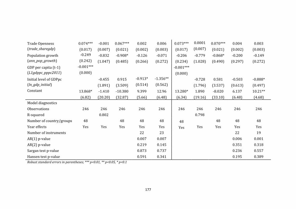
177
Trade Openness 0.074*** -0.001 0.067*** 0.002 0.006 0.073*** 0.0001 0.070*** 0.004 0.003
(trade_sharegdp) (0.017) (0.007) (0.021) (0.002) (0.003) (0.017) (0.007) (0.021) (0.002) (0.003)
Population growth -0.249 -0.832 -0.908* -0.126 -0.071 -0.206 -0.779 -0.868* -0.200 -0.149
(ann_pop_growth) (0.242) (1.047) (0.485) (0.266) (0.272) (0.234) (1.028) (0.490) (0.297) (0.272)
GDP per capita (t-1) -0.001*** -0.001*** (L1gdppc_pppc2011) (0.000) (0.000)
Initial level of GDPpc -0.455 0.915 -0.913* -1.356** -0.728 0.581 -0.503 -0.888*
(ln_gdp_initial) (1.891) (3.509) (0.514) (0.562) (1.796) (3.537) (0.613) (0.497)
Constant 13.868* -1.410 -10.380 9.399 12.96 13.280* 1.890 -8.020 6.137 10.21**
(6.82) (20.20) (32.87) (5.66) (6.48) (6.34) (19.16) (33.10) (6.48) (4.68)
Model diagnostics
Observations 246 246 246 246 246 246 246 246 246 246
R-squared 0.802 0.798 Number of country/groups 48 48 48 48 48 48 48 48
Year effects Yes Yes Yes Yes Yes Yes Yes Yes Yes Yes
Number of instruments
22 23 22 19
AR(1) p-value
0.007 0.007 0.006 0.001
AR(2) p-value
0.219 0.145 0.351 0.318
Sargan test p-value
0.873 0.737 0.236 0.557
Hansen test p-value 0.591 0.341 0.195 0.389
Robust standard errors in parentheses; *** p<0.01, ** p<0.05, * p<0.1
At this stage, we can also provide the long-run effect of high-job growth
entrepreneurial activity on growth. Given the positive and statistically significant
coefficient of lagged dependent variable, we expect that the long-run effects will
be larger than the short-run ones. The long-run effect is indeed larger suggesting
that a 1 percentage point increase in the share of high-job growth
entrepreneurial activity, on average, increases economic growth by 1.15
percentage points, ceteris paribus. In economic terms, this effect seems large
enough, as it suggests that if the share of high-job growth entrepreneurial activity
nearly doubles (from 1.02 to 2.02), the economic growth increases by 57 % (from
2.03 to 3.18). Or in other words, a 10% increase in the share of high-job growth
entrepreneurial activity increases the rate of economic growth by 5.8% (from
2.03 to 2.15), ceteris paribus.
Similarly, columns 6 and 8 (static approach) seem to suggest that economic
growth is positively affected by entrepreneurial activity of businesses expecting
to create at least 5 jobs in five years (L2teayyjg5). The magnitude of this variable
is smaller and ranges from 0.29-0.43 while it turns statistically significant at the
5% (FE-DK and HT). However, the significance of job growth entrepreneurial
activity (L2teayyjg5), in the system GMM, disappears. In column 9, L2teayyjg5 is
claimed as endogenous while in column 10 as exogenous. In both situations, the
variable is statistically insignificant, indicating that the positive relationship does
not hold in the dynamic specification. The FE-DK estimate on (L2teayyjg5)
suggests that a 1 percentage point increase in the share of job growth
entrepreneurial activity is, on average, associated with 0.43 percentage points
increase in economic growth, with the all other variables held constant. In
economic terms, the effect is relatively large, as it suggests that when the share
of job growth entrepreneurial activity increases by 39% (mean=2.58; so, from
2.58 to 3.58) it has a positive impact on economic growth of 21% (from 2.03 to
2.46). In other words, a 10% increase in the share of job growth entrepreneurial
activity increases the rate of economic growth by 5.4% (from 2.03 to 2.14). The
HT estimator suggests a smaller effect, as a 10% increase in the share of job
growth entrepreneurial activity increases the rate of economic growth by only
3.6% (from 2.03 to 2.10).
179
The results do not seem to provide evidence to support the hypothesis that there
is a positive relationship between overall entrepreneurial activity (L1tea) and
economic growth. In some of the specifications, overall entrepreneurial activity
has the expected sign, however it is always statistically insignificant. A possible
explanation for the lack of significant result might be related to the broad
definition and the construction of the overall TEA as discussed in section 4.3 and
in Chapter 1 and 2. The overall TEA includes nascent entrepreneurs, defined as
individuals expecting to be a full or part owner74 and young businesses,
representing individuals involved as owner and manager in new firms (3 to 42
months old).75 In addition, the overall TEA does not make any division with
respect to motivations to start (e.g., opportunity vs necessity), employment
growth expectations, innovation or international trade orientation. Thus, it can
be argued that it becomes difficult for this measure to be associated with
economic growth as it contains many dimensions which might cancel out each
other. For instance, some studies (Wong et al., 2005; Aparicio et al., 2016;
Rodrigues, 2018) have found that while opportunity-driven entrepreneurial
activity is positively associated with economic growth, necessity-driven
entrepreneurial activity is not. At the same time, it is highly unlikely that nascent
entrepreneurial activity, i.e., percentage of people involved in setting-up
businesses, to have strong positive association with economic growth.
Nevertheless, this finding seems to be in line with previous research (Acs and
Varga, 2005; Wong et al., 2005; Baumol, 1990; 2010; Aparicio et al., 2016;
Ferreira et al., 2017), which suggests that not all the types of entrepreneurial
activity positively impact economic growth.
Generally, the results for the main variables of interest, especially those obtained
from static approach seem to be consistent with the respect to the estimator used
and are mainly in line with the previous research findings (Stam and van Stel,
74 GEM definition of nascent entrepreneurship: Percentage of all respondents (18-64): involved in nascent business (new firm start-up), defined as active, expect to be a full or part owner, and no salaries or wages paid for over three months. [NASCENT FIRM PREVALENCE RATE]. 75 GEM definition of baby business: Percentage of all respondents (18-64): involved as owner and manager in new firms for which salaries or wages have been paid between 3 and 42 months. [BABY BUSINESS PREVALENCE RATE]

180
2009; Stam et al., 2009; Acs et al., 2012; Urbano and Aparicio, 2016; Aparicio,
2017) in the entrepreneurship-economic growth literature.
With respect to the control variables, the results indicate that most of the
estimated effects are in accordance with the theory and the previous empirical
literature. In line with the previous empirical research (see e.g., Bjørnskov and
Foss, 2013), a large government size, (gov_consum_sharegdp) is reported to have
a negative impact on economic growth across the all specifications. Recalling the
discussion in section, 4.3.1, large government spending is usually associated with
large budget deficits, public debts and misallocation of scarce resources. On the
other hand, investment to GDP ratio (inv_gdp_grosscapfor) is reported to have a
positive association with economic growth in most of the static estimators. This
finding is in accordance with the previous empirical research (Apergis and Payne,
2010, Bruns et al., 2017; Bosma et al., 2018). However, when the dynamic
approach is used, the effect of the same becomes statistically insignificant.76 The
index of ‘rule of law’ is positive and statistically significant when FE-DK is used
and when the dynamic specifications with all variables treated as exogenous.
Country’s trade openness, measured as the share of exports to GDP, is reported
to have a positive effect on economic growth, only when the FE-DK and HT
estimators are used. Contrary to our expectations, there is no evidence to suggest
that human capital (mean_year_schooling) affects economic growth when high-
job growth is used as a measure of entrepreneurial activity. However, when job
growth is used, the estimates of human capital obtained from the FE-DK and HT
estimator become positive and statistically significant.
Lastly, there is some evidence that population growth is negatively associated to
economic growth in both sets of results. However, this effect is statistically
significant only when the HT estimator is applied and remains insignificant
across all other estimators. On the other hand, the estimate of the first lag of GDP
per capita (L1gdppc_pppc2011) is statistically significant and, as expected, has a
negative sign indicating the presence of ‘catch-up’ effect on growth, i.e., less-
developed economies are growing faster than advanced economies. As discussed
76 However, when some additional model robustness checks are offered below, we will find statistically significant effect of investment to GDP ratio, when system GMM is used.
181
in section 4.3.1 and 4.4, when the estimators handle time-invariant variables,
instead of lagged GDP per capita, the initial level of GDP (ln_gdp_initial2003) is
included. The latter variable displays (mostly) the expected sign, however the
results suggest that it turns statistically significant only when the dynamic
specification is used (columns 4, 5 and 10).
To sum up, there are some significant differences in terms of the results for the
two main variables of interest, high-job growth and job growth entrepreneurial
activity. In general, the set of results obtained from the static approach (FE-DK;
FEVD and HT) seem to be more consistent regardless of the estimator used. When
the dynamic estimator is used, the statistical significance of most of the control
variables disappears. In addition, results of the second set suggest that job
growth entrepreneurial activity, positive and significant in two static estimators,
turns out as insignificant when the system GMM is used, regardless whether the
variable is claimed as being endogenous or exogenous. One potential explanation
for this change in significance is perhaps due to the ability of the lagged
dependent variable to explain a large part of the economic activity. As discussed
earlier, the lagged GDP growth is always positive and statistically significant with
an estimated coefficient of 0.36 in the first set of results and 0.5 in the second,
respectively.
As the dynamic estimator contains the entire historical information of the
independent variables and the fact that the data set time-span includes the period
of financial crisis 2008–2009 (Posner 2009; Solow 2009), these might have had
an additional effect on the significance level of the included variables. The year
dummies are highly significant and have relatively large coefficients (see
Appendix 4.3.2). As Bosma et al. (2018, p.7) claim: “the financial crisis can be
expected to obscure the hypothesised, long-run relationships between
entrepreneurship, institutions, and economic growth”. Further they argue that in
the presence of demand-driven crisis, it becomes difficult to disentangle the
effect of supply-side variables in growth equations. Similarly, Acs et al. (2018),
referring to the effect of financial crisis, argue that depressions cause significant
losses (depreciation) in human capital and drive the technological frontier
inwards. That means that it takes longer time for growth explaining variables to

182
‘pick-up’ the expected positive effect. For robustness checks, when year 2008 and
2009 are dropped from the analysis, the investment to GDP ratio estimate
suggests a positive and significant impact on growth (see Appendix 4.6). In
addition, an interaction between investment to GDP ratio and a year dummy
including only 2009-2014 (to remove the effect of crisis years) is performed,
however results remain stable and investment to GDP ratio insignificant (see
Appendix 4.6.1).
Innovation: new product and new product-market entrepreneurial
activity
The focus of this section is to shed more light on the hypothesised effect of
innovative entrepreneurial activity on economic growth. Results on Table 4.4 are
obtained based on Eq. (4.1) for the FE-DK and FEVD, Eq. (4.2) for the HT and Eq.
(4.3c) and Eq. (4.3d) for the dynamic estimator. Due to high correlation between
the two main variables of interest, namely (L1teayynwp) and (L1teanpm) and the
overall TEA (L1tea), the share of young business (up to 3.5 years old) is initially
used instead of overall TEA. However, the Hansen J statistic performed poorly
under this specification. Finally, high-job growth (L2teahjg) was included
alongside the two measures of innovative activity (in two different
specifications). The new specifications had correct diagnostics and are used to
obtain results.
Columns 1 – 4 of Table 4.4 present results when ‘new product’ (teayynwp) is used
as the measure of innovative entrepreneurial activity while columns 5 – 8 present
results when ‘new product-market’ (teanpm) is used as a proxy for innovative
entrepreneurial activity. In terms of estimators, columns 1 and 5 present results
obtained using the FE-DK estimator, columns 2 and 6 presents results obtained
by FEVD, columns 3 and 7 results obtained by HT, while dynamic specification
results are presented in columns 4 and 8, respectively. As it is elaborated in
section 4.3.1, compared to the ‘employment growth expectations’ equations,
‘innovative entrepreneurial activity’ equations use the first and not the second
lag for the main variables of interest (L1teayynwp) and (L1teanpm). Moreover, as
the normality assumption for the two main variables of interest (L1teanwp) and
(L1teanpm) does not seem to hold (highly skewed distribution), the Tukey
183
Ladder of Power test (Tukey, 1997) suggests the transformation into logarithmic
form (see Appendix 4.7).77 Accordingly, the two main variables of interest enter
the specification after the transformation into logarithmic forms (lnL1teayynwp)
and (lnL1teanpm).
Overall, the same pattern is also identified in this set of results, with the results
of the static estimators being more consistent with each other. The results of the
dynamic specification mostly differ in terms of the significance of the main
variable of interest and of the control variables. Similar to the results in Table 4.3
the lagged dependent variable is positive and highly significant. The estimated
coefficient is highly stable in both sets of results and suggests that 1 percentage
point increase in growth in previous period implies an increase in growth in
current period of 0.42 percentage points in Eq. (4.3c) and 0.41 percentage points
in Eq. (4.3d), ceteris paribus.
With regard to our two main variables of interest, ‘new product’ (lnL1teayynwp)
and ‘new product-market’ (lnL1teanpm), results suggest that the choice of
estimator has a significant influence on their hypothesised impact on economic
growth. While the static estimators mainly suggest a positive and statistically
significant impact of innovative entrepreneurial activity on economic growth, the
dynamic estimator, system GMM, is unable to do so for both sets of results. The
FE-DK estimator suggests that a 10 percent increase in innovative
entrepreneurial activity is, on average, associated with a 0.085 percentage points
increase on economic growth, everything else held constant. This is a rather small
economic effect, as it requires the share of innovative entrepreneurial activity to
increase by 10% (mean=4.2; so, from 4.2 to 4.62) to increase economic growth
by 4.2% (from 2.03 to 2.12), ceteris paribus.
77 The’ ladder’ and ‘gladder’ stata commands are used to perform this test. The same test is also performed in other independent variables, but the test suggests retaining their original form.
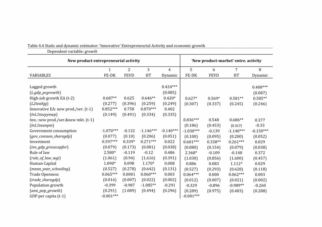
Table 4.4 Static and dynamic estimator: 'Innovative’ Entrepreneurial Activity and economic growth
Dependent variable: growth
New product entrepreneurial activity ‘New product-market’ entre. activity
1 2 3 4 5 6 7 8
VARIABLES FE-DK FEVD HT Dynamic FE-DK FEVD HT Dynamic
Lagged growth 0.424*** 0.408***
(L.gdp_pcgrowth) (0.085) (0.087) High-job growth EA (t-2) 0.687** 0.625 0.646** 0.420* 0.627* 0.569* 0.581** 0.585** (L2teahjg) (0.277) (0.396) (0.259) (0.249) (0.307) (0.337) (0.245) (0.246) Innovative EA: new prod./ser. (t-1) 0.852*** 0.758 0.870*** 0.402
(lnL1teayynwp) (0.149) (0.491) (0.334) (0.335)
Inn.: new prod./ser.&new mkt. (t-1) 0.836*** 0.548 0.686** 0.377 (lnL1teanpm) (0.186) (0.453) (0.317) -0.33
Government consumption -1.070*** -0.132 -1.146*** -0.140*** -1.030*** -0.139 -1.140*** -0.150*** (gov_consum_sharegdp) (0.077) (0.10) (0.206) (0.051) (0.100) (0.095) (0.200) (0.052) Investment 0.597*** 0.339* 0.271*** 0.022 0.601*** 0.338** 0.261*** 0.029 (inv_gdp_grosscapfor) (0.079) (0.173) (0.081) (0.038) (0.080) (0.154) (0.079) (0.038) Rule of law 2.580* -0.119 -0.12 0.486 2.368* -0.109 -0.148 0.372 (rule_of_law_wgi) (1.061) (0.94) (1.616) (0.391) (1.030) (0.856) (1.600) (0.457) Human Capital 1.090* 0.098 1.170* 0.008 0.886 0.083 1.112* 0.029 (mean_year_schooling) (0.527) (0.278) (0.642) (0.131) (0.527) (0.293) (0.628) (0.118) Trade Openness 0.065*** 0.0001 0.060*** 0.003 0.064*** 0.000 0.062*** 0.003 (trade_sharegdp) (0.016) (0.007) (0.022) (0.002) (0.012) (0.007) (0.021) (0.002) Population growth -0.399 -0.987 -1.085** -0.291 -0.329 -0.896 -0.989** -0.260 (ann_pop_growth) (0.291) (1.089) (0.494) (0.296) (0.289) (0.975) (0.483) (0.288) GDP per capita (t-1) -0.001*** -0.001***
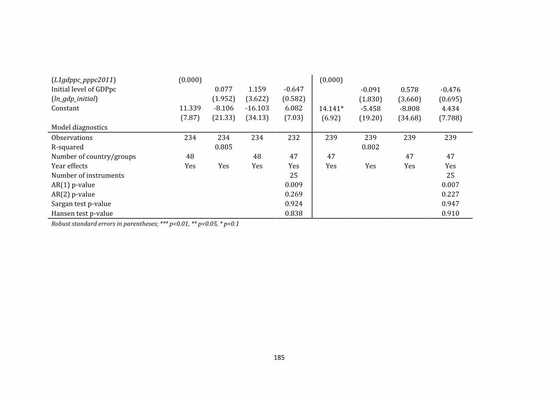
185
(L1gdppc_pppc2011) (0.000) (0.000)
Initial level of GDPpc 0.077 1.159 -0.647 -0.091 0.578 -0.476 (ln_gdp_initial) (1.952) (3.622) (0.582) (1.830) (3.660) (0.695) Constant 11.339 -8.106 -16.103 6.082 14.141* -5.458 -8.808 4.434
(7.87) (21.33) (34.13) (7.03) (6.92) (19.20) (34.68) (7.788)
Model diagnostics
Observations 234 234 234 232 239 239 239 239
R-squared 0.805 0.802
Number of country/groups 48 48 47 47 47 47
Year effects Yes Yes Yes Yes Yes Yes Yes Yes
Number of instruments 25 25
AR(1) p-value 0.009 0.007
AR(2) p-value 0.269 0.227
Sargan test p-value 0.924 0.947
Hansen test p-value 0.838 0.910
Robust standard errors in parentheses; *** p<0.01, ** p<0.05, * p<0.1
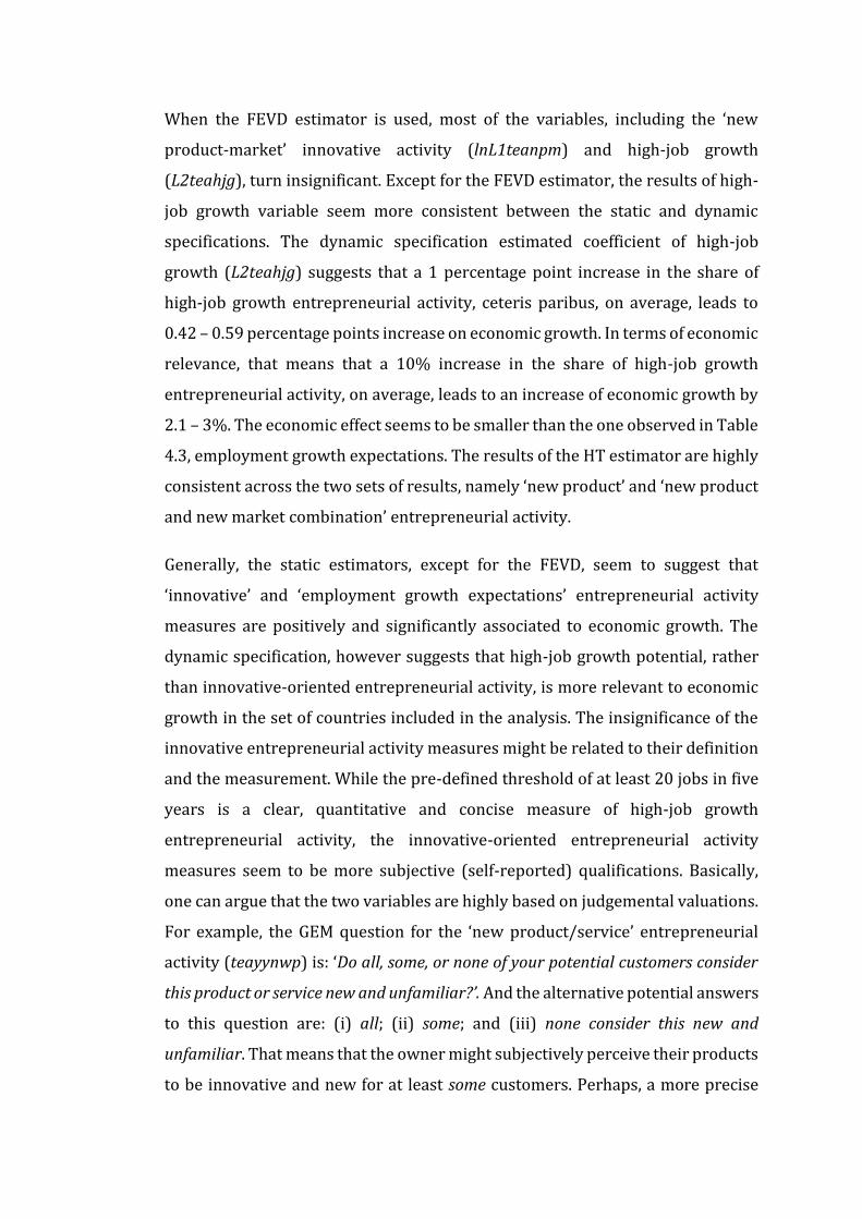
When the FEVD estimator is used, most of the variables, including the ‘new
product-market’ innovative activity (lnL1teanpm) and high-job growth
(L2teahjg), turn insignificant. Except for the FEVD estimator, the results of high-
job growth variable seem more consistent between the static and dynamic
specifications. The dynamic specification estimated coefficient of high-job
growth (L2teahjg) suggests that a 1 percentage point increase in the share of
high-job growth entrepreneurial activity, ceteris paribus, on average, leads to
0.42 – 0.59 percentage points increase on economic growth. In terms of economic
relevance, that means that a 10% increase in the share of high-job growth
entrepreneurial activity, on average, leads to an increase of economic growth by
2.1 – 3%. The economic effect seems to be smaller than the one observed in Table
4.3, employment growth expectations. The results of the HT estimator are highly
consistent across the two sets of results, namely ‘new product’ and ‘new product
and new market combination’ entrepreneurial activity.
Generally, the static estimators, except for the FEVD, seem to suggest that
‘innovative’ and ‘employment growth expectations’ entrepreneurial activity
measures are positively and significantly associated to economic growth. The
dynamic specification, however suggests that high-job growth potential, rather
than innovative-oriented entrepreneurial activity, is more relevant to economic
growth in the set of countries included in the analysis. The insignificance of the
innovative entrepreneurial activity measures might be related to their definition
and the measurement. While the pre-defined threshold of at least 20 jobs in five
years is a clear, quantitative and concise measure of high-job growth
entrepreneurial activity, the innovative-oriented entrepreneurial activity
measures seem to be more subjective (self-reported) qualifications. Basically,
one can argue that the two variables are highly based on judgemental valuations.
For example, the GEM question for the ‘new product/service’ entrepreneurial
activity (teayynwp) is: ‘Do all, some, or none of your potential customers consider
this product or service new and unfamiliar?’. And the alternative potential answers
to this question are: (i) all; (ii) some; and (iii) none consider this new and
unfamiliar. That means that the owner might subjectively perceive their products
to be innovative and new for at least some customers. Perhaps, a more precise

187
definition, using more quantitative expressions, e.g., scaled answers: 10 to 25%;
25% to 50%; 50% - 75%; and more than 75% of customers consider this product as
new, might have improved the objectivity of the respondent. However, as there
are no other measures of innovative entrepreneurial activity in the GEM data, the
analysis must rely only on the two selected measures.
The set of the control variables, in general, shows a similar trend to the ones in
Table 4.3. In this set of results, the two variables controlling for human capital
and trade openness appear significant when FE-DK and HT are used. The FE-DK
estimated coefficient of average years of schooling (mean_year_schooling)
suggest that a 1 unit (year) increase in average schooling, on average, leads to 1.1
percentage points increase on economic growth, ceteris paribus. Similar
magnitude is also suggested by the Hausman and Taylor estimator for both
groups of results in Table 4.4. Similarly, trade as a share of GDP is also positively
associated with economic growth as the estimated coefficient suggests that,
holding other variables constant, a 1 percentage point increase in trade
openness, on average, leads to 0.06 – 0.07 percentage point increase in economic
growth.
Besides these two controls, in this set of results, the variable used as a proxy for
the ‘rule of law’ (rule_of_law_wgi) turns also significant when FE-DK is used for
both sets of results. The estimated coefficient indicates that a 1 unit increase in
the ‘rule of law’ index is, on average, associated with 2.4 – 2.6 percentage points
increase on economic growth, ceteris paribus. Similar to the ‘employment
growth-oriented’ results, and in line with previous empirical and theoretical
literature (see Headey and Hodge, 2009), the annual population growth has a
negative and statistically significant effect on economic growth. When the FE-DK
estimator is used, the estimate of the first lag of GDP per capita
(L1gdppc_pppc2011) is statistically significant and, as expected, has a negative
sign. The initial level of GDP, on the other hand, has the right sign though it is
statistically insignificant across all the results of the two approaches, static and
dynamic estimators.
188
To conclude, this subset of results too, suggests that entrepreneurial activity is
relevant to economic growth. The findings are in line with other empirical
studies, especially those using GEM measures of entrepreneurial activity (see e.g.,
Valliere and Peterson, 2009; Stam et al., 2009; Hessels and van Stel, 2011;
Aparicio et al., 2016; Acs et al., 2018). The static estimators seem to suggest that
innovative entrepreneurial activity is, indeed, a determinant of national
economic growth. Moreover, the positive and statistically significant impact of
high-job growth entrepreneurial activity is reconfirmed as a factor impacting
growth. Also, the control variables included in both groups of estimators,
contribute to the growth equation and, when significant, have the expected sign.
The following section augments the system GMM equations by including
respective dummy variables to account for country differences (economic
context) and uses interaction terms to detect any relationship between these
variables in the entrepreneurship-economic growth relationship.
The moderating impact of stages of development on
entrepreneurship-economic growth relationship
It is argued in Chapter 2 and section 4.5 of this chapter, that entrepreneurial
activity might not have a uniform impact on countries, but rather its effect differs
with respect to the countries’ stage of development (Carree et al., 2002; 2007;
Sternberg and Wennekers, 2005; van Stel et al., 2005; Urbano et al., 2018). One
of the potential reasons for this might be the differences in the overall business
environment and the quality of institutions (van Praag and Versloot, 2007;
Bjørnskov and Foss, 2016). In this respect, Chapter 2, highlights that the
economic context, (the stage of development), namely if the country belongs to
the so-called innovation-driven or efficiency-driven (Porter et al., 2002)
economy, might have an effect on the relationship between entrepreneurship
and growth. Other studies have argued that a positive relationship between
entrepreneurial activity and economic growth is common for OECD countries but
does not seem to hold for non-OECD countries (Urbano and Aparicio, 2016;
Rodrigues, 2018). One way to investigate whether the effect of entrepreneurial
activity depends on the stage of development is by splitting the sample into
different subsamples (e.g., innovation vs efficiency-driven; OECD vs non-OECD).
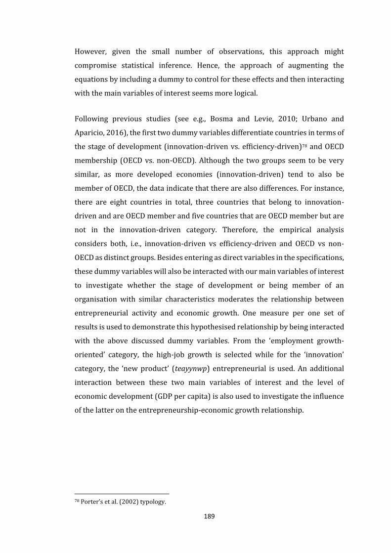
189
However, given the small number of observations, this approach might
compromise statistical inference. Hence, the approach of augmenting the
equations by including a dummy to control for these effects and then interacting
with the main variables of interest seems more logical.
Following previous studies (see e.g., Bosma and Levie, 2010; Urbano and
Aparicio, 2016), the first two dummy variables differentiate countries in terms of
the stage of development (innovation-driven vs. efficiency-driven)78 and OECD
membership (OECD vs. non-OECD). Although the two groups seem to be very
similar, as more developed economies (innovation-driven) tend to also be
member of OECD, the data indicate that there are also differences. For instance,
there are eight countries in total, three countries that belong to innovation-
driven and are OECD member and five countries that are OECD member but are
not in the innovation-driven category. Therefore, the empirical analysis
considers both, i.e., innovation-driven vs efficiency-driven and OECD vs non-
OECD as distinct groups. Besides entering as direct variables in the specifications,
these dummy variables will also be interacted with our main variables of interest
to investigate whether the stage of development or being member of an
organisation with similar characteristics moderates the relationship between
entrepreneurial activity and economic growth. One measure per one set of
results is used to demonstrate this hypothesised relationship by being interacted
with the above discussed dummy variables. From the ‘employment growth-
oriented’ category, the high-job growth is selected while for the ‘innovation’
category, the ‘new product’ (teayynwp) entrepreneurial is used. An additional
interaction between these two main variables of interest and the level of
economic development (GDP per capita) is also used to investigate the influence
of the latter on the entrepreneurship-economic growth relationship.
78 Porter’s et al. (2002) typology.
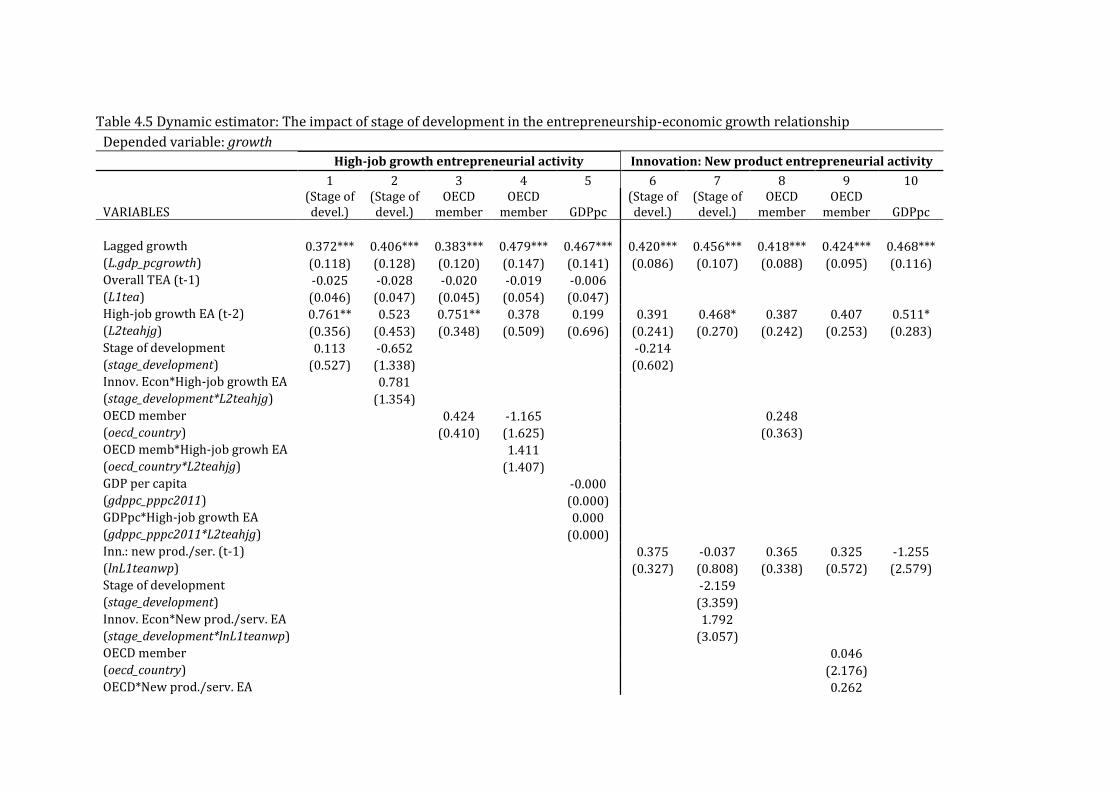
Table 4.5 Dynamic estimator: The impact of stage of development in the entrepreneurship-economic growth relationship
Depended variable: growth
High-job growth entrepreneurial activity Innovation: New product entrepreneurial activity
1 2 3 4 5 6 7 8 9 10
VARIABLES (Stage of devel.)
(Stage of devel.)
OECD member
OECD member GDPpc
(Stage of devel.)
(Stage of devel.)
OECD member
OECD member GDPpc
Lagged growth 0.372*** 0.406*** 0.383*** 0.479*** 0.467*** 0.420*** 0.456*** 0.418*** 0.424*** 0.468*** (L.gdp_pcgrowth) (0.118) (0.128) (0.120) (0.147) (0.141) (0.086) (0.107) (0.088) (0.095) (0.116) Overall TEA (t-1) -0.025 -0.028 -0.020 -0.019 -0.006 (L1tea) (0.046) (0.047) (0.045) (0.054) (0.047) High-job growth EA (t-2) 0.761** 0.523 0.751** 0.378 0.199 0.391 0.468* 0.387 0.407 0.511* (L2teahjg) (0.356) (0.453) (0.348) (0.509) (0.696) (0.241) (0.270) (0.242) (0.253) (0.283) Stage of development 0.113 -0.652 -0.214 (stage_development) (0.527) (1.338) (0.602) Innov. Econ*High-job growth EA 0.781 (stage_development*L2teahjg) (1.354) OECD member 0.424 -1.165 0.248 (oecd_country) (0.410) (1.625) (0.363) OECD memb*High-job growh EA 1.411 (oecd_country*L2teahjg) (1.407) GDP per capita -0.000 (gdppc_pppc2011) (0.000) GDPpc*High-job growth EA 0.000 (gdppc_pppc2011*L2teahjg) (0.000) Inn.: new prod./ser. (t-1) 0.375 -0.037 0.365 0.325 -1.255 (lnL1teanwp) (0.327) (0.808) (0.338) (0.572) (2.579) Stage of development -2.159 (stage_development) (3.359) Innov. Econ*New prod./serv. EA 1.792 (stage_development*lnL1teanwp) (3.057) OECD member 0.046 (oecd_country) (2.176) OECD*New prod./serv. EA 0.262
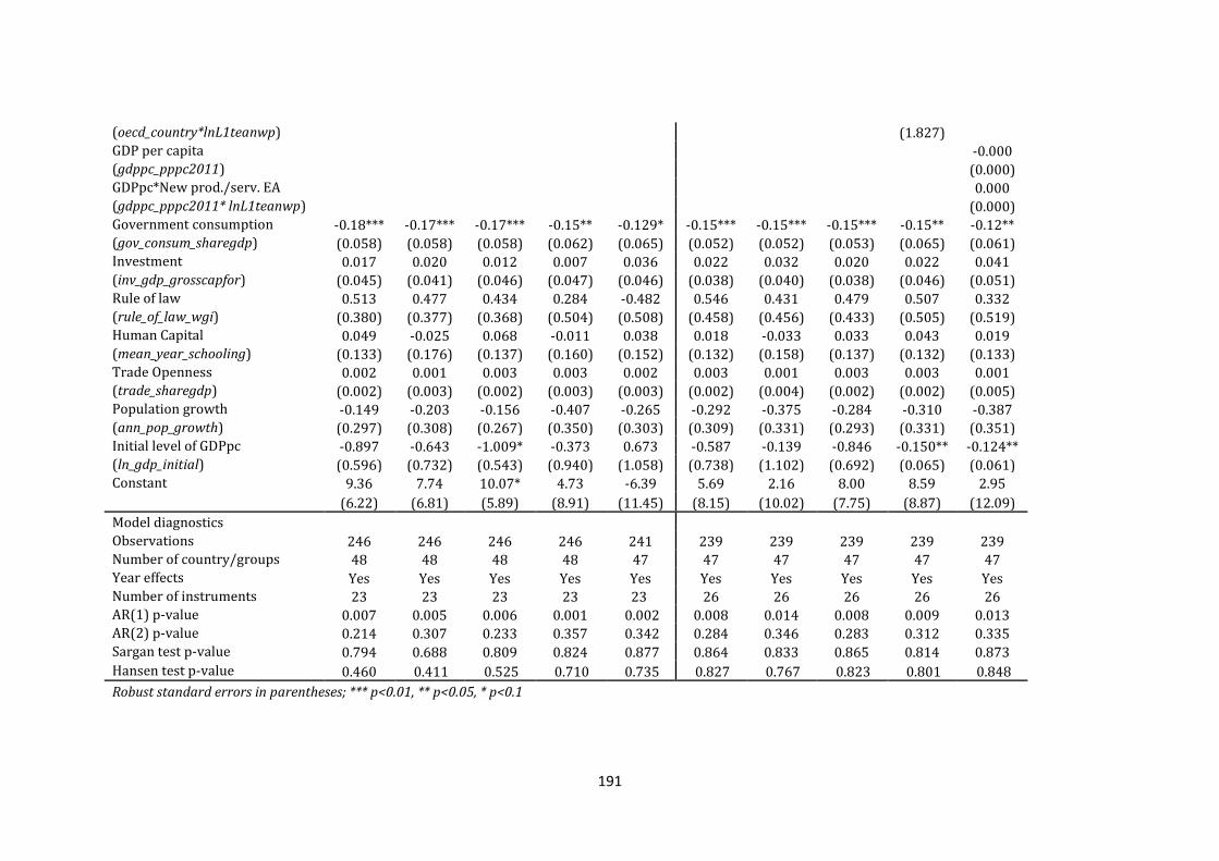
191
(oecd_country*lnL1teanwp) (1.827) GDP per capita -0.000 (gdppc_pppc2011) (0.000) GDPpc*New prod./serv. EA 0.000 (gdppc_pppc2011* lnL1teanwp) (0.000) Government consumption -0.18*** -0.17*** -0.17*** -0.15** -0.129* -0.15*** -0.15*** -0.15*** -0.15** -0.12** (gov_consum_sharegdp) (0.058) (0.058) (0.058) (0.062) (0.065) (0.052) (0.052) (0.053) (0.065) (0.061) Investment 0.017 0.020 0.012 0.007 0.036 0.022 0.032 0.020 0.022 0.041 (inv_gdp_grosscapfor) (0.045) (0.041) (0.046) (0.047) (0.046) (0.038) (0.040) (0.038) (0.046) (0.051) Rule of law 0.513 0.477 0.434 0.284 -0.482 0.546 0.431 0.479 0.507 0.332 (rule_of_law_wgi) (0.380) (0.377) (0.368) (0.504) (0.508) (0.458) (0.456) (0.433) (0.505) (0.519) Human Capital 0.049 -0.025 0.068 -0.011 0.038 0.018 -0.033 0.033 0.043 0.019 (mean_year_schooling) (0.133) (0.176) (0.137) (0.160) (0.152) (0.132) (0.158) (0.137) (0.132) (0.133) Trade Openness 0.002 0.001 0.003 0.003 0.002 0.003 0.001 0.003 0.003 0.001 (trade_sharegdp) (0.002) (0.003) (0.002) (0.003) (0.003) (0.002) (0.004) (0.002) (0.002) (0.005) Population growth -0.149 -0.203 -0.156 -0.407 -0.265 -0.292 -0.375 -0.284 -0.310 -0.387 (ann_pop_growth) (0.297) (0.308) (0.267) (0.350) (0.303) (0.309) (0.331) (0.293) (0.331) (0.351) Initial level of GDPpc -0.897 -0.643 -1.009* -0.373 0.673 -0.587 -0.139 -0.846 -0.150** -0.124** (ln_gdp_initial) (0.596) (0.732) (0.543) (0.940) (1.058) (0.738) (1.102) (0.692) (0.065) (0.061) Constant 9.36 7.74 10.07* 4.73 -6.39 5.69 2.16 8.00 8.59 2.95
(6.22) (6.81) (5.89) (8.91) (11.45) (8.15) (10.02) (7.75) (8.87) (12.09)
Model diagnostics Observations 246 246 246 246 241 239 239 239 239 239 Number of country/groups 48 48 48 48 47 47 47 47 47 47 Year effects Yes Yes Yes Yes Yes Yes Yes Yes Yes Yes Number of instruments 23 23 23 23 23 26 26 26 26 26 AR(1) p-value 0.007 0.005 0.006 0.001 0.002 0.008 0.014 0.008 0.009 0.013 AR(2) p-value 0.214 0.307 0.233 0.357 0.342 0.284 0.346 0.283 0.312 0.335 Sargan test p-value 0.794 0.688 0.809 0.824 0.877 0.864 0.833 0.865 0.814 0.873
Hansen test p-value 0.460 0.411 0.525 0.710 0.735 0.827 0.767 0.823 0.801 0.848
Robust standard errors in parentheses; *** p<0.01, ** p<0.05, * p<0.1

The model diagnostics (see Appendix 4.3.5 and 4.3.6) suggest that there is insufficient
evidence to reject the null hypothesis for validity of overidentifying restrictions. There
is also insufficient evidence to reject the second order autocorrelation (AR(2)), while
there is sufficient evidence to reject the first order autocorrelation (AR(1)) in all the
specifications. The Hansen J statistic suggests instrument validity and the difference-in-
Hansen suggests that steady state assumption holds and there is no evidence of cross-
sectional dependence. In terms of results interpretation, the focus will only be on the
new dummies included and the respective interaction terms.
Results presented in Table 4.5, do not seem to suggest any obvious effect of stage of
development, OECD membership or GDP per capita on the relationship between
entrepreneurship and economic growth. All the interaction terms in all the
specifications in Table 4.5 are statistically insignificant. However, the interaction
coefficients might not be able to show the whole story. The margins of the interaction
terms and the marginplots might contain more information and need to be computed.
Although, none of the interaction terms turns significant, indeed, there are relationships
detected after using these two stata commands.
Fig 4.8 suggests that the effect of high-job growth entrepreneurial activity is higher in
OCED member countries, compared to the non-OECD members. That means that other
country-level contextual circumstances moderate the effect of entrepreneurial activity
on economic growth. This finding is in line with other studies in the entrepreneurship-
economic growth literature (Rodrigues, 2018). In Fig 4.7 however, the relationship
seems not to be the same as we observe that the effect of high values of L2teahjg
(L2teahjg ≥ 3.1) are more positively associated with economic growth in efficiency-
driven economics.79 However, we noticed that there are only ten observations from four
countries (Russia, Chile, China and Colombia) with values of L2teahjg higher than 3.1
and they all belong to the efficiency-driven economies category and that might have
influenced this result. The effect of high-job growth entrepreneurial activity is larger in
innovation-driven economies when L2teahjg ranges between 0.1 and 3.1, which
represents 95% of the cases in this data set. Thus, Fig 4.7, is also suggesting that the
effect of high-job growth entrepreneurial activity is higher in innovation-driven
79 See Appendix 4.3.5
193
economies compared to the efficiency-driven economies, signalling the positive
moderating effect of country context. To further investigate the differences between the
two economic contexts in Fig. 4.7 (innovation-driven vs efficiency-driven economies)
and 4.8 (OECD member vs non-OECD member countries), the contrast test is performed.
The test suggests no differences between the two groups (in both Fig 4.7 and 4.8) (see
Appendix 4.3.7) suggesting that the impression given by CIs alone is not enough when
interpreting differences between categories. Generally, when CIs overlap there is high
probability that the differences between two or more categories are insignificant. Thus,
it is worth noting that the insights from Fig. 4.7 and 4.8 are to be taken with caution.
Figure 4.7 Predictive margins: High-job growth and Stage of Development – Economic growth (growth) - All countries included
Figure 4.8 Predictive margins: High-job growth and OECD membership – Economic growth (growth) - All countries included
Figure 4.9 Average marginal effects: GDP per capita and High-job growth – Economic growth (growth) - All countries included
Besides the two types of classification of countries, innovation-driven vs. efficiency-
driven and OECD vs. non-OECD, the analysis investigates whether the effect of
entrepreneurial activity varies with economic development, i.e., whether
entrepreneurial activity has a higher influence in low per capita GDP or in high per
capita GDP countries. The expectations are that the effect is higher in high-per capita
GDP countries. Fig 4.9 is suggesting that there is a relationship as the highest impact of
-50
51
01
5
Pre
dic
ted e
co
nom
ic g
row
th
.1 .6 1.1 1.6 2.1 2.6 3.1 3.6 4.1 4.6High-job growth EA
stage_development=0 stage_development=1
Predictive margins of stage of development with 90% CIs
-50
51
01
5
Pre
dic
ted e
co
nom
ic g
row
th
.1 .6 1.1 1.6 2.1 2.6 3.1 3.6 4.1 4.6High-job growth EA
oecd_country=0 oecd_country=1
Predictive margins of OECD with 90% CIs
01
23
4
Ave
rage
mar
gina
l effe
cts:
eco
nom
ic g
row
th
10000 15000 20000 25000 30000 35000 40000 45000 50000 55000 60000 65000GDP per capita
Average marginal effects of HJG on growth with 90% CIs
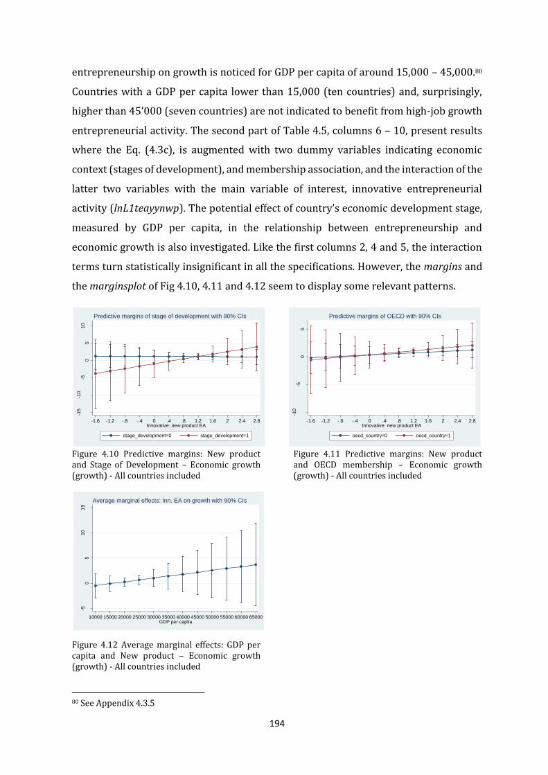
194
entrepreneurship on growth is noticed for GDP per capita of around 15,000 – 45,000.80
Countries with a GDP per capita lower than 15,000 (ten countries) and, surprisingly,
higher than 45’000 (seven countries) are not indicated to benefit from high-job growth
entrepreneurial activity. The second part of Table 4.5, columns 6 – 10, present results
where the Eq. (4.3c), is augmented with two dummy variables indicating economic
context (stages of development), and membership association, and the interaction of the
latter two variables with the main variable of interest, innovative entrepreneurial
activity (lnL1teayynwp). The potential effect of country’s economic development stage,
measured by GDP per capita, in the relationship between entrepreneurship and
economic growth is also investigated. Like the first columns 2, 4 and 5, the interaction
terms turn statistically insignificant in all the specifications. However, the margins and
the marginsplot of Fig 4.10, 4.11 and 4.12 seem to display some relevant patterns.
Figure 4.10 Predictive margins: New product and Stage of Development – Economic growth (growth) - All countries included
Figure 4.11 Predictive margins: New product and OECD membership – Economic growth (growth) - All countries included
Figure 4.12 Average marginal effects: GDP per capita and New product – Economic growth (growth) - All countries included
80 See Appendix 4.3.5
-15
-10
-50
51
0
Pre
dic
ted e
co
nom
ic g
row
th
-1.6 -1.2 -.8 -.4 0 .4 .8 1.2 1.6 2 2.4 2.8Innovative: new product EA
stage_development=0 stage_development=1
Predictive margins of stage of development with 90% CIs
-10
-50
5
Pre
dic
ted e
co
nom
ic g
row
th
-1.6 -1.2 -.8 -.4 0 .4 .8 1.2 1.6 2 2.4 2.8Innovative: new product EA
oecd_country=0 oecd_country=1
Predictive margins of OECD with 90% CIs
-50
51
01
5
Ave
rag
e m
arg
ina
l effe
cts
: eco
no
mic
gro
wth
10000 15000 20000 25000 30000 35000 40000 45000 50000 55000 60000 65000GDP per capita
Average marginal effects: Inn. EA on growth with 90% CIs
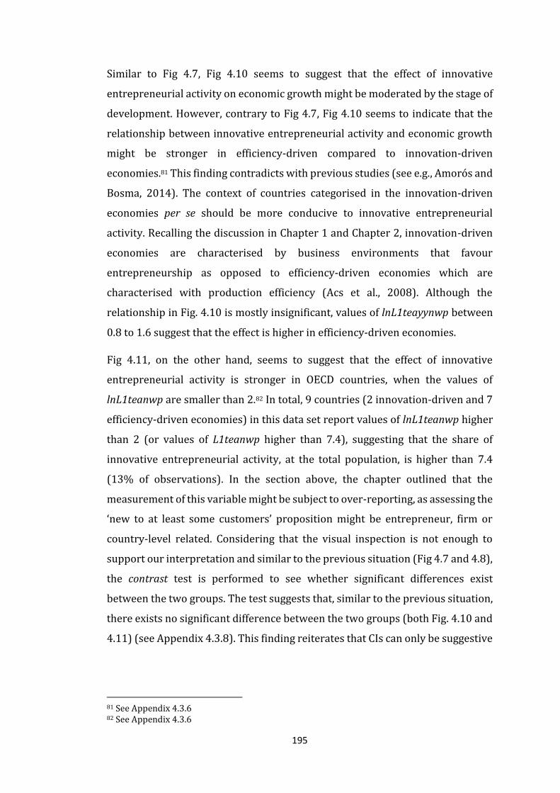
195
Similar to Fig 4.7, Fig 4.10 seems to suggest that the effect of innovative
entrepreneurial activity on economic growth might be moderated by the stage of
development. However, contrary to Fig 4.7, Fig 4.10 seems to indicate that the
relationship between innovative entrepreneurial activity and economic growth
might be stronger in efficiency-driven compared to innovation-driven
economies.81 This finding contradicts with previous studies (see e.g., Amorós and
Bosma, 2014). The context of countries categorised in the innovation-driven
economies per se should be more conducive to innovative entrepreneurial
activity. Recalling the discussion in Chapter 1 and Chapter 2, innovation-driven
economies are characterised by business environments that favour
entrepreneurship as opposed to efficiency-driven economies which are
characterised with production efficiency (Acs et al., 2008). Although the
relationship in Fig. 4.10 is mostly insignificant, values of lnL1teayynwp between
0.8 to 1.6 suggest that the effect is higher in efficiency-driven economies.
Fig 4.11, on the other hand, seems to suggest that the effect of innovative
entrepreneurial activity is stronger in OECD countries, when the values of
lnL1teanwp are smaller than 2.82 In total, 9 countries (2 innovation-driven and 7
efficiency-driven economies) in this data set report values of lnL1teanwp higher
than 2 (or values of L1teanwp higher than 7.4), suggesting that the share of
innovative entrepreneurial activity, at the total population, is higher than 7.4
(13% of observations). In the section above, the chapter outlined that the
measurement of this variable might be subject to over-reporting, as assessing the
‘new to at least some customers’ proposition might be entrepreneur, firm or
country-level related. Considering that the visual inspection is not enough to
support our interpretation and similar to the previous situation (Fig 4.7 and 4.8),
the contrast test is performed to see whether significant differences exist
between the two groups. The test suggests that, similar to the previous situation,
there exists no significant difference between the two groups (both Fig. 4.10 and
4.11) (see Appendix 4.3.8). This finding reiterates that CIs can only be suggestive
81 See Appendix 4.3.6 82 See Appendix 4.3.6
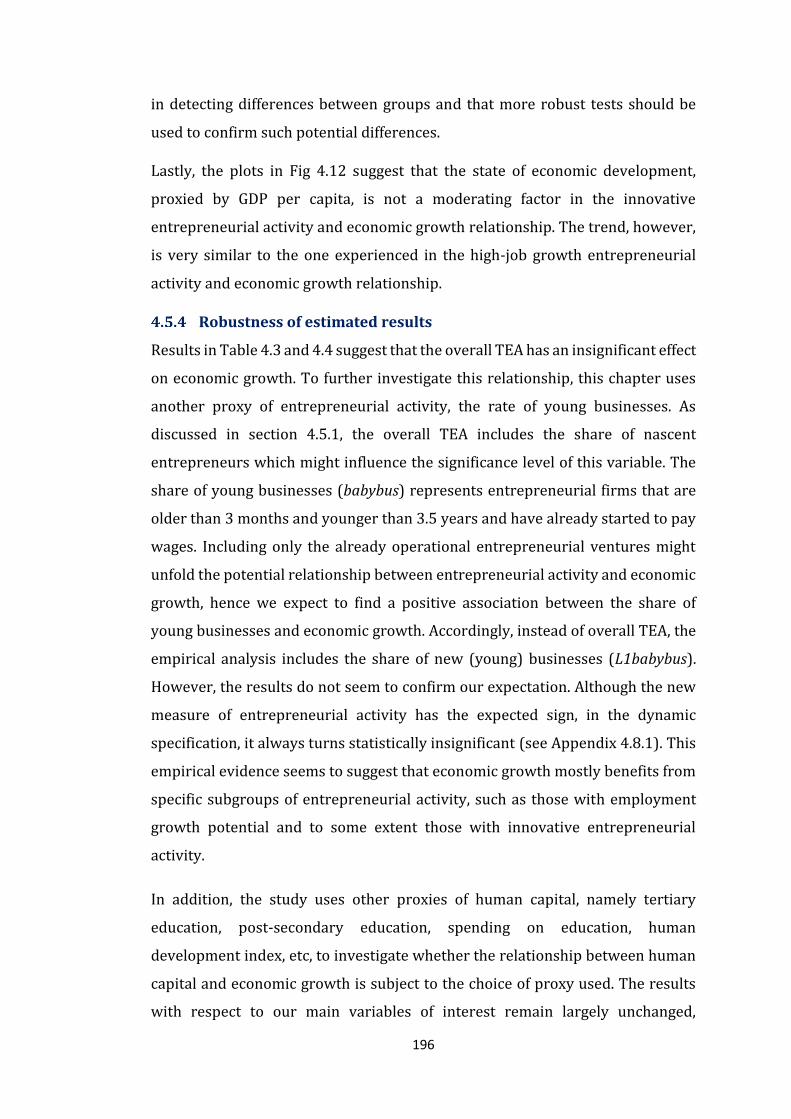
196
in detecting differences between groups and that more robust tests should be
used to confirm such potential differences.
Lastly, the plots in Fig 4.12 suggest that the state of economic development,
proxied by GDP per capita, is not a moderating factor in the innovative
entrepreneurial activity and economic growth relationship. The trend, however,
is very similar to the one experienced in the high-job growth entrepreneurial
activity and economic growth relationship.
Robustness of estimated results
Results in Table 4.3 and 4.4 suggest that the overall TEA has an insignificant effect
on economic growth. To further investigate this relationship, this chapter uses
another proxy of entrepreneurial activity, the rate of young businesses. As
discussed in section 4.5.1, the overall TEA includes the share of nascent
entrepreneurs which might influence the significance level of this variable. The
share of young businesses (babybus) represents entrepreneurial firms that are
older than 3 months and younger than 3.5 years and have already started to pay
wages. Including only the already operational entrepreneurial ventures might
unfold the potential relationship between entrepreneurial activity and economic
growth, hence we expect to find a positive association between the share of
young businesses and economic growth. Accordingly, instead of overall TEA, the
empirical analysis includes the share of new (young) businesses (L1babybus).
However, the results do not seem to confirm our expectation. Although the new
measure of entrepreneurial activity has the expected sign, in the dynamic
specification, it always turns statistically insignificant (see Appendix 4.8.1). This
empirical evidence seems to suggest that economic growth mostly benefits from
specific subgroups of entrepreneurial activity, such as those with employment
growth potential and to some extent those with innovative entrepreneurial
activity.
In addition, the study uses other proxies of human capital, namely tertiary
education, post-secondary education, spending on education, human
development index, etc, to investigate whether the relationship between human
capital and economic growth is subject to the choice of proxy used. The results
with respect to our main variables of interest remain largely unchanged,

197
signalling robustness, while the new added proxies mostly display the same sign
and statistical significance level as their predecessors. Moreover, the study
investigates whether there exists an optimal level of entrepreneurial activity,
which is to be detected by a curvilinear relationship between entrepreneurship
and economic growth. However, the squared terms of the two main variables of
interest (employment growth) added in the equations, do not seem to support
this hypothesis (see Appendix 4.8.4 and 4.8.5). The squared terms are either
insignificant or the ‘nlcom’ stata command suggests that the coefficients are out
of the expected range. Perhaps, in a larger data set, this relationship might be
detected but we fail to confirm it in this chapter.
With respect to the dynamic specification, the study has used a more
conservative approach by claiming other additional variables as being
endogenous. The investment to GDP ratio and the trade openness have both been
considered as endogenous to growth. However, when the two are considered
endogenous, diagnostics tests fail, especially the Sargan and Hansen J statistic
(see Appendix 4.8.6). While when only trade openness is claimed as endogenous,
diagnostics pass the tests, but the results remain unchanged. In addition, in the
dynamic specification, lags of other explanatory variables are used, still results
remain robust to these changes.
To conclude, the results seem robust, especially the significance and the sign of
our main variables of interest remains unchanged, even when new proxies are
added, new lags structure used, or additional endogenous variables claimed.
CONCLUSIONS
In this chapter, unbalanced panel data for the period 2006-2014 are used to
empirically investigate the impact of ‘employment growth expectations’ and
‘innovative’ entrepreneurial activity on economic growth. The MRA indicated
that, although there is still inconclusive evidence with respect to the impact of
entrepreneurship to economic performance, the high-growth potential
entrepreneurial activity is to be further investigated to advance the state of
empirical evidence. The empirical analysis of this chapter benefits from both the
static and dynamic estimators and in total, includes 48 countries (innovation-
198
driven and efficiency-driven economies). Building on the two main growth
theories, the measures of entrepreneurial activity are directly included in the
growth models along with other explanatory variables. The physical and human
capital are proxied by investment to GDP ratio (inv_gdp_grosscapfor) and average
years of schooling (mean_year_schooling), respectively. Following the conceptual
framework of Wennekers and Thurik (1999), and the institutional economics
theory, the influence of institutions (‘rule of law’) and the size of public sector
(government spending). Similarly, the country-level control variables such as the,
trade openness, annual population growth and the lagged or initial GDP per
capita (convergence) are also included in the specifications. The analysis went
beyond the debate of opportunity vs. necessity entrepreneurial activity by
investigating a more specific subgroup of entrepreneurs, namely ‘employment
growth’ and ‘innovation-oriented’ entrepreneurs.
The results of static specifications, by and large, support the hypothesis that both
‘employment growth’ and ‘innovative’ entrepreneurial activity are positively
associated with national level economic growth. The static approach also finds
support that investment to GDP ratio and trade openness have a positive and
significant impact on economic growth. The human capital and the quality of
institutions (‘rule of law’) also seem to be positively associated with economic
growth, though less frequently. On the other hand, a large public size sector is
commonly found to negatively influence growth. In the dynamic specification,
however, the significant impact of most of the explanatory variables disappears.
Still the main variables of interest, especially high-job growth entrepreneurial
activity, remain positive and significant indicating the robustness of the impact
of this type of entrepreneurial activity on economic growth. Moreover, similar to
Acs et al. (2018) and Bosma et al. (2018), the chapter highlights the potential
effect of financial crisis in the specified dynamic growth model. As discussed in
section 4.5, when year 2008 and 2009 are dropped from the analysis, more
explanatory variables exert their significant effect on growth. The effect of
‘employment growth-oriented’ entrepreneurial activity is reported to be higher
in the long-run compared to the short-run. The diagnostics tests and the lagged
199
GDP growth, always significant and positive, indicate that dynamic approach
specification is well-specified.
The interaction terms, although statistically insignificant, seem to indicate that
the stage of economic development and the OECD membership seem to have an
influence on how entrepreneurship affects economic growth. It is suggested that
being a member of OECD might positively moderate the effect of high-job growth
entrepreneurial activity on growth and that innovation-driven economies
compared to the efficiency-driven economies benefit more from high-job growth
entrepreneurial activity. In addition, the analysis suggest that the effect of high-
job growth entrepreneurial activity is stronger in countries with a GDP per capita
of not higher than around 45,000. The results, however do not confirm that
innovation-driven compared to efficiency-driven economies benefit more from
innovative entrepreneurial activity.
With respect to the robustness check, the analysis has used different proxies to
account for innovation, human capital, as well as different lag structures of the
explanatory variables. Generally, the results seem to be stable, mostly suggesting
that the relationship between ‘employment growth-oriented’ and ‘innovative’
entrepreneurial activity is robust to changes in the sets of explanatory variables
used. As discussed in section 4.5, we pointed out that using the overall TEA as a
measure of entrepreneurial activity results in insignificant effect on growth since
it represents a rather wide and general definition of entrepreneurial activity, also
including the nascent category. Another measure of entrepreneurial activity, the
share of new (young) businesses, did not suggest any change in the significance
level either, thus indicating that, in this study, the relationship between
entrepreneurship and economic growth is to be detected only when more
specific measures and nuances of entrepreneurial activity are used.
To conclude, generally, the results seem to confirm the hypothesis that
‘employment growth’ and ‘innovation-oriented’ entrepreneurial activity are
positively associated with economic growth. The finding contributes to the
debate initiated by Baumol (1990), who suggests that not all the types of
entrepreneurial activity affect growth and that it is mostly growth-oriented,

200
opportunity-seeking and innovative entrepreneurial activity (productive
entrepreneurship) that impacts country-level economic growth.
To further explore the high-growth entrepreneurial activity, the next chapter
investigates individual, institutional and country-level determinants of growth
aspirations entrepreneurial activity using a multilevel estimation approach.

201
5. Chapter 5
INDIVIDUAL AND INSTITUTIONAL DETERMINANTS OF
ENTREPRENEURIAL GROWTH ASPIRATIONS: A MULTI-COUNTRY ANALYSIS
INTRODUCTION ...................................................................................................................... 202
THEORETICAL FRAMEWORK ........................................................................................... 203
Entrepreneurial Growth Aspirations ................................................................... 203
Growing vs non-growing firms ............................................................................... 206
5.2.2.1 Dependent variable................................................................................................. 215
5.2.2.2 Individual and young business characteristics and controls ................ 217
5.2.2.3 Institutional variables ............................................................................................ 222
5.2.2.4 Country level characteristics .............................................................................. 228
Descriptive statistics by stages of economic development ......................... 232
ESTIMATION STRATEGY AND MODEL SPECIFICATION ....................................... 235
Model specification ...................................................................................................... 241
EMPIRICAL RESULTS ........................................................................................................... 245
Results ............................................................................................................................... 245
Robustness checks ....................................................................................................... 267
CONCLUSIONS ......................................................................................................................... 268
202
INTRODUCTION
The country-level empirical analysis in Chapter 4 suggested that ‘employment
growth-oriented’ entrepreneurial activity rather than the overall
entrepreneurial activity has the highest impact on economic growth. Thus, in this
chapter, we focus on investigating individual, institutional and macroeconomic
factors that determine entrepreneurial growth aspirations in 55 countries over
the 2006-2013 period. Following Delmar and Wiklud (2008) and Hermans et al.
(2015), the chapter refers to the ‘employment growth expectations’
entrepreneurial activity, as Entrepreneurial Growth Aspirations. In the empirical
analysis, entrepreneurial growth aspirations are operationalised using the
expected growth in employment in a five-year horizon. Two dependent variables
are used to capture growth aspirations, namely: (i) Employment Growth
Aspiration (EGA); and (ii) High-job Growth Aspirations (HJG).
Although, growth aspirations entrepreneurship, in general, has attracted
significant attention in the literature (Wong et al., 2005; McKelvie and Wiklund,
2010; Stam et al., 2011; Mason and Brown, 2013; Wright and Stigliani, 2013;
Hermans et al., 2015; Terjesen et al., 2016; Puente et al., 2017; Capelleras et al.,
2018), yet not enough studies have jointly investigated the key factors
(individual, institutional and macroeconomic or environmental) determining the
main drives of these ventures. Autio and Acs (2010) state that the key aspect in
investigating growth-oriented entrepreneurial ventures is analysing an
individual’s decision to allocate resources, particularly financial and human
resources. It is also suggested that both the quality of institutional settings and
the macroeconomic (country-level) control variables have a significant influence
on an individual’s decision to allocate adequate resources and engage in growth
potential entrepreneurial ventures (Hermans et al., 2015). For instance, a weak
property rights protection environment, might discourage entrepreneurial
growth aspirations (Estrin et al., 2013).
The empirical analysis of this chapter is initially performed in a full sample which
is later divided into two subsamples, according to the phase of a country’s
economic development (entrepreneurship ecosystems). The first subsample
consists of countries classified as innovation-driven economies while the second

203
subsample comprises of countries classified as efficiency-driven economies (see
Porter et al., 2002).83 The individual-level characteristics data is obtained from
the Global Entrepreneurship Monitor - Adult Population Survey (GEM-APS). To
empirically test the influence of individual-level, institutional and
macroeconomic variables, a diversified modelling strategy is adopted. First,
linear mixed-effect multilevel estimation strategy is used to examine key
determinants of employment growth aspirations (EGA). In addition to this
estimation strategy, multilevel logistic regression is used for the second
dependent variable, high-job growth (HJG) aspirations. Both strategies account
for the hierarchical nature (multilevel structure: individual and country-level) of
the data. Shepherd (2011) urges for the use of multilevel research, as the
methodological approach, enabling the conjoint exploration of (i) individual
decision-making; (ii) contextual based decision-making; and (iii) the interplay
between these two levels.
This chapter is organised as follows. The theoretical framework of this chapter is
elaborated in the second section, where the data on growth aspirations of the
surveyed entrepreneurs (young businesses) in the GEM database are also
presented. The third section discusses the methodology and the data, and the
variables included in the model together with the descriptive statistics. Section
four discusses estimation strategy and the model specification, including the
diagnostics, tests for outliers and the issues of concern in different empirical
estimations. The interpretation of the results and the robustness check are
offered in the fifth section while conclusions are presented in the sixth section.
THEORETICAL FRAMEWORK
Entrepreneurial Growth Aspirations
The research and policymaking community mostly agree that entrepreneurship,
and specifically growth aspiration entrepreneurship, is a critical component of
the national economic development (see Naudé, 2013). As Levie and Autio
83 Since 2008, GEM Global reports have categorised the participating economies by phase of economic development, namely factor-driven, efficiency-driven and innovation-driven economies. Due to the relatively small number of countries and observation in the factor-driven economies, this category has not been included in the empirical analyses of this chapter.

204
(2013) and Hermans et al. (2015) point out, researchers use a variety of terms
such as “growth intentions”, “high-expectation entrepreneurship“, “growth
ambition”, “growth aspiration” “high-potential entrepreneurship”, “high-impact
entrepreneurship”, or “strategic entrepreneurship” interchangeably. However,
to avoid any potential confusion, in this chapter, we will use growth aspirations
and high-growth aspirations entrepreneurship as used by Stam et al. (2012 p. 26)
which represents “entrepreneurs who identify and exploit opportunities to create
new products, services, processes, and organizations with high aspirations to
achieve entrepreneurial success - that is, to maximize value creation (beyond self-
sufficiency)“ and try to identify what drives and what hinders this type of
entrepreneurship as this is essential for designing country-level policies and
institutional frameworks (Acs and Correa, 2014; Giotopoulos et al., 2017). As
Davidsson and Wiklund (2000), Autio and Acs (2010, p.234), Levie and Autio
(2013), Oner and Kunday (2016), Capellaras et al. (2018), among other, point out,
growth-seeking entrepreneurial ventures and the individuals’ decision to
allocate energies for such activities are still very relevant topics of study.
Firm growth is not expected to happen spontaneously and for all firms, Studies
have provided evidence that a high percentage of newly-established firms never
aim to grow and never achieve growth (Delmar et al., 2003; Autio, 2007; Autio,
2011; Wright and Stigliani, 2013). The data used in this chapter also suggest that
a significant number of entrepreneurial ventures surveyed expect to have the
same number of employees even after a five-year period. Empirical studies
suggest that entrepreneurial growth aspirations are closely linked to the
individual entrepreneurs’ expectations and ambitions to grow and the
combination of resources, time and efforts employed (Hermans et al., 2015;
Capellaras et al., 2018).
Hermans et al. (2015) provide a synthesis of 28 studies and posit that measuring
growth aspirations entrepreneurship is a complex task as it represents a
multifaceted term, mostly operationalised by: (i) employment growth aspirations,
where entrepreneurial ventures report their employment growth expectations
in the next five years; (ii) innovation-orientation or innovative entrepreneurial
ventures offering new products or services and developing new markets; and (iii)
205
international-orientation, the intention of the entrepreneurial venture to
internationalise (export) their products and services.84 Although all three
dimensions are covered in the GEM-APS questionnaires, the focus of this chapter
is only on the growth dimension (first dimension) operationalised by looking at
the employment growth and high-job growth aspirations of young business
ventures.85
At this point, it is important to clarify the relationship between growth
aspirations and actual firm growth. Empirical research on growth aspiration
entrepreneurship provides substantial evidence on supporting the hypothesis
that the entrepreneurial ambitions matter for subsequent firm growth (Baum et
al., 1998; Baum et al., 2001; Wiklund and Shepherd, 2003; Delmar and Wiklund,
2008; Aidis et al., 2011). In a recent publication, Hermans et al. (2015) highlight
the role of entrepreneurial aspirations and argue that aspirations and intentions
are closely linked to the firms’ actual growth rates. Similarly, Davidsson et al.
(2006), Gilbert et al. (2006) and Stam and Wennberg (2009) provide evidence
that firms’ growth can be predicted by firms’ intentions and aspirations to grow.
Burns (2010) argues that growth is crucial for an established business to survive
in the market.
Generally, research studies refer to three different approaches when analysing
what drives entrepreneurial growth aspirations. The psychological approach
assumes that intrinsic individual characteristics dictate entrepreneurial growth
aspirations. Lumpkin and Dess (1996), Wiklund and Shepherd (2005) and
Shepherd (2015) are among the authors supporting this approach. The second
approach supported by Krueger et al. (2000) suggests that social norms and
social logic determine an individual’s growth aspirations. Recent studies link this
approach to the institutional theory (formal and informal institutions) and
suggest that the quality of institutions has a significant impact on entrepreneurial
growth aspirations (see e.g., Thornton et al., 2011; Bjørnskov and Foss, 2013;
84 The authors present 5 dimensions, including “Finance” and “Wealth”. However, only three out of twenty-eight papers synthetised by Hermans et al. (2015) have considered these two latter dimensions in their analysis. 85 In section 5.3, we provide justifications on why we have used only young businesses and have excluded nascent entrepreneurs.

206
2016; Estrin et al., 2013; Alvarez et al., 2015; Eesley, 2016; Bosma et al., 2018).
The third approach is the economic approach, mostly promoted in the economics
literature (Fiegenbaum and Thomas, 1988; Eisenhauer, 1995; Kirzner; 1997;
Douglas and Shepherd, 2000; Eckhardt and Shane, 2003; Lazear, 2005; Autio and
Acs, 2010; Urbano and Aparicio, 2016; Aparicio, 2017) which maintains that
individuals willingly and rationally seek profit opportunities while considering
the potential risks associated with such business ventures. This chapter benefits
from all the three approaches, as it focuses on investigating the influence of
individual-level characteristics (first approach), institutional variables and
contextual factors (second approach) and the decision of an individual to allocate
resources on entrepreneurial activities with the aim of maximizing their impact
(profits; growth, etc.) (third approach).
Growing vs non-growing firms
Penrose (1959) in her pioneering work, the theory of the growth of the firm,
recognizes the importance of individual characteristics and individual decision-
making to the growth process of the firm. The entrepreneurial decision to
investigate the prospective profitability of expansion and ‘growth’ is perhaps the
most significant decision and one that defines the ‘spirit of enterprise’ (Penrose
1959, p.33). Gilbert et al. (2006, p.929) state that one of the first critical strategic
decisions facing an entrepreneur is the decision to grow the firm. Similarly,
Cooper and Daily (1997, p.97) states that firm growth can be simply defined as
“the very essence of entrepreneurship and a distinguishing factor between small
business and entrepreneurship”. Wiklund et al. (2003) build on Penrose (1959)
and suggests that besides of the motivation of individuals to act upon business
opportunities, growth motivations and aspirations are a significant part of the
puzzle which has not been sufficiently studied. For instance, Gilbert et al. (2006)
argue that some entrepreneurs and businesses have limited desire to grow.
According to Shane and Venkataraman (2000) and Haynie et al. (2009), the
decision to engage in the process of opportunity recognition, evaluation and
exploitation is shaped by both individual and environmental characteristics.
Similarly, Autio and Acs (2010) suggest that entrepreneurial activity is a function
of the interaction between an individual’s characteristics and the business
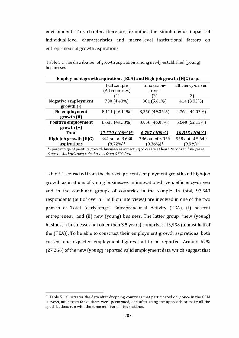
207
environment. This chapter, therefore, examines the simultaneous impact of
individual-level characteristics and macro-level institutional factors on
entrepreneurial growth aspirations.
Table 5.1 The distribution of growth aspiration among newly-established (young) businesses
Table 5.1, extracted from the dataset, presents employment growth and high-job
growth aspirations of young businesses in innovation-driven, efficiency-driven
and in the combined groups of countries in the sample. In total, 97,540
respondents (out of over a 1 million interviews) are involved in one of the two
phases of Total (early-stage) Entrepreneurial Activity (TEA), (i) nascent
entrepreneur; and (ii) new (young) business. The latter group, “new (young)
business” (businesses not older than 3.5 years) comprises, 43,938 (almost half of
the (TEA)). To be able to construct their employment growth aspirations, both
current and expected employment figures had to be reported. Around 62%
(27,266) of the new (young) reported valid employment data which suggest that
86 Table 5.1 illustrates the data after dropping countries that participated only once in the GEM surveys, after tests for outliers were performed, and after using the approach to make all the specifications run with the same number of observations.
Employment growth aspirations (EGA) and High-job growth (HJG) asp.
Full sample (All countries)
(1)
Innovation-driven
(2)
Efficiency-driven
(3) Negative employment
growth (-) 788 (4.48%) 381 (5.61%) 414 (3.83%)
No employment growth (0)
8,111 (46.14%) 3,350 (49.36%) 4,761 (44.02%)
Positive employment growth (+)
8,680 (49.38%) 3,056 (45.03%) 5,640 (52.15%)
Total 17,579 (100%)86 6,787 (100%) 10,815 (100%)
High-job growth (HJG) aspirations
844 out of 8,680 (9.72%)*
286 out of 3,056 (9.36%)*
558 out of 5,640 (9.9%)*
*- percentage of positive growth businesses expecting to create at least 20 jobs in five years Source: Author’s own calculations from GEM data
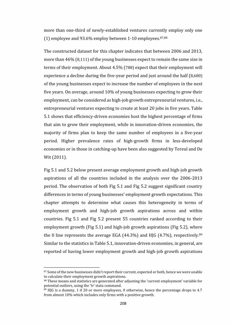
208
more than one-third of newly-established ventures currently employ only one
(1) employee and 93.6% employ between 1-10 employees.87,88
The constructed dataset for this chapter indicates that between 2006 and 2013,
more than 46% (8,111) of the young businesses expect to remain the same size in
terms of their employment. About 4.5% (788) expect that their employment will
experience a decline during the five-year period and just around the half (8,680)
of the young businesses expect to increase the number of employees in the next
five years. On average, around 10% of young businesses expecting to grow their
employment, can be considered as high-job growth entrepreneurial ventures, i.e.,
entrepreneurial ventures expecting to create at least 20 jobs in five years. Table
5.1 shows that efficiency-driven economies host the highest percentage of firms
that aim to grow their employment, while in innovation-driven economies, the
majority of firms plan to keep the same number of employees in a five-year
period. Higher prevalence rates of high-growth firms in less-developed
economies or in those in catching-up have been also suggested by Tereul and De
Wit (2011).
Fig 5.1 and 5.2 below present average employment growth and high-job growth
aspirations of all the countries included in the analysis over the 2006-2013
period. The observation of both Fig 5.1 and Fig 5.2 suggest significant country
differences in terms of young businesses’ employment growth expectations. This
chapter attempts to determine what causes this heterogeneity in terms of
employment growth and high-job growth aspirations across and within
countries. Fig 5.1 and Fig 5.2 present 55 countries ranked according to their
employment growth (Fig 5.1) and high-job growth aspirations (Fig 5.2), where
the 0 line represents the average EGA (44.3%) and HJG (4.7%), respectively.89
Similar to the statistics in Table 5.1, innovation-driven economies, in general, are
reported of having lower employment growth and high-job growth aspirations
87 Some of the new businesses didn’t report their current, expected or both, hence we were unable to calculate their employment growth aspirations. 88 These means and statistics are generated after adjusting the ‘current employment’ variable for potential outliers, using the ‘lv’ stata command. 89 HJG is a dummy, 1 if 20 or more employees, 0 otherwise, hence the percentage drops to 4.7 from almost 10% which includes only firms with a positive growth.
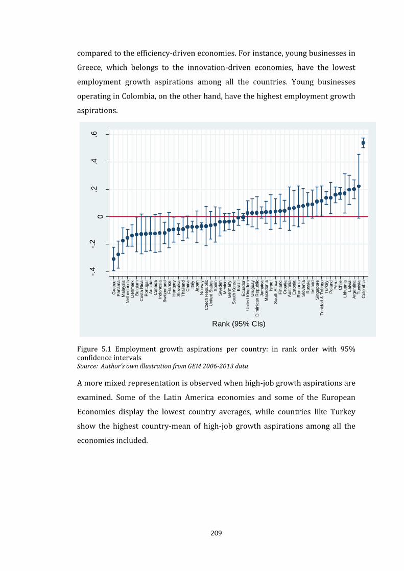
209
compared to the efficiency-driven economies. For instance, young businesses in
Greece, which belongs to the innovation-driven economies, have the lowest
employment growth aspirations among all the countries. Young businesses
operating in Colombia, on the other hand, have the highest employment growth
aspirations.
Figure 5.1 Employment growth aspirations per country: in rank order with 95% confidence intervals Source: Author’s own illustration from GEM 2006-2013 data
A more mixed representation is observed when high-job growth aspirations are
examined. Some of the Latin America economies and some of the European
Economies display the lowest country averages, while countries like Turkey
show the highest country-mean of high-job growth aspirations among all the
economies included.
-.4
-.2
0.2
.4.6
Pre
dic
ted r
an
dom
in
terc
ep
t (E
GA
)
Gre
ece
Pa
na
ma
Ma
laysia
Neth
erla
nd
sD
en
mark
Be
lgiu
mC
osta
Ric
aP
ort
uga
lA
ustr
iaC
an
ad
aIn
don
esia
Sw
itzerl
an
dF
ran
ce
Hun
ga
ryS
lova
kia
Tha
ilan
dC
hin
aIta
lyJa
pa
nN
orw
ay
Czech
Rep
ub
licU
nite
d S
tate
sS
pain
Sw
ed
en
Me
xic
oG
erm
any
So
uth
Kore
aB
razil
Ecu
ad
or
Unite
d K
ingd
om
Uru
gua
yD
imin
ican
Rep
ub
licJa
maic
aM
aced
on
iaIs
rae
lS
outh
Afr
ica
Fin
land
Cro
atia
Au
str
alia
Esto
nia
Rom
ania
Slo
ve
nia
Russia
Irela
nd
Sin
gap
ore
Trin
idad
& T
oba
go
Turk
ey
Po
land
Pe
ruC
hile
Lithu
an
iaL
atv
iaA
rgen
tina
Tun
isia
Colo
mb
ia
Rank (95% CIs)

210
Figure 5.2 High-job Growth Aspirations (HJG) per country: in rank order with 95% confidence intervals
Source: Author’s own calculations from GEM 2006-2013 data
The hypotheses in this chapter are tested in a global setting, using a sample of 55
countries, developed (innovation-driven) and developing (efficiency-driven)
economies that participated in GEM surveys between 2006 and 2013. Using a
large set of countries, at different stages of development, avoids the lack of
variation in the institutional or macroeconomic control variables (Delmar et al.,
2003). Similar to Chapter 4, the main data is obtained from the Global
Entrepreneurship Monitor – Adult Population Survey (GEM – APS). The selection
of GEM, as our main source of entrepreneurship data, has been discussed in detail
in Chapter 1 and Chapter 4.
In the previous chapter, data were at the country-level, whereas in this chapter
they come disaggregated at the individual-level. GEM data is used to construct
the dependent variable and some of the main explanatory variables (all the
individual-level characteristics). In addition to GEM, the Heritage Foundation
-2-1
01
2
Pre
dic
ted r
an
dom
in
terc
ep
t (H
JG
)
Ind
on
esia
Ecu
ad
or
Pa
na
ma
Me
xic
oT
ha
ilan
dC
osta
Ric
aB
razil
Gre
ece
Esto
nia
Ma
laysia
Sw
itzerl
an
dN
orw
ay
Pe
ruJa
maic
aD
en
mark
Sp
ain
Ita
lyC
an
ad
aN
eth
erla
nd
sT
un
isia
Ma
ced
on
iaB
elg
ium
Hun
ga
ryR
ussia
Sw
ed
en
Po
rtu
ga
lA
ustr
iaJa
pa
nU
rug
ua
yS
outh
Kore
aA
ustr
alia
Fra
nce
Czech
Rep
ub
licA
rgen
tina
Fin
land
Irela
nd
Germ
any
Chin
aL
atv
iaU
nite
d S
tate
sT
rin
idad
& T
oba
go
Isra
el
Unite
d K
ingd
om
Slo
ve
nia
Dim
inic
an
Rep
ub
licS
lova
kia
Cro
atia
Chile
Lithu
an
iaS
outh
Afr
ica
Rom
ania
Po
land
Colo
mb
iaS
ing
ap
ore
Turk
ey
Rank (95% CIs)
211
(HF), Polity IV, Index of Economic Freedom (IEF), the World Bank (WB) and the
World Economic Forum (WEF) are used for institutional quality and macro-level
data.
Fig 5.3 and 5.4 below show the country-mean employment growth and high-job
growth aspirations in relation to the overall young business activity. In both Fig
5.3 and Fig 5.4, distinctive differences are observed. The average young business
activity seems to be less than 5% with some exceptions such as Indonesia which
is reported to have the highest young business activity rate of around 17.5%.
Most of the countries are observed to have employment growth aspirations
ranging from 20% to 60% (the mean EGA is 44.3%), i.e., between 20 and 60% of
young businesses report positive employment growth expectations. Similarly,
Fig 5.4 shows that the rate of high-job growth aspiration firms ranges from 3% -
17% (the mean is 4.7%).
Fig 5.3 and specifically Fig. 5.4 do not appear to portray a clear trend that would
clearly link growth aspiration to the young business activity rate. As it is
elaborated in Chapter 2 and 4, the quantity of entrepreneurial activity does not
necessarily lead to job creation or to any significant advancements in economic
performance. Young business activity rate, in this chapter, comprises both
necessity and opportunity entrepreneurial type activity. It is expected that
necessity type entrepreneurs, generally, have lower entrepreneurial growth
aspirations.
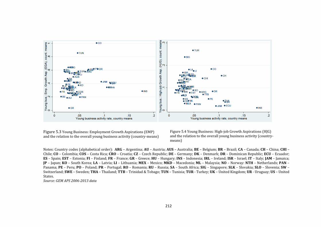
212
Figure 5.3 Young Business: Employment Growth Aspirations (EMP) and the relation to the overall young business activity (country-means)
Figure 5.4 Young Business: High-job Growth Aspirations (HJG) and the relation to the overall young business activity (country-means)
Notes: Country codes (alphabetical order): ARG – Argentina; AU – Austria; AUS – Australia; BE – Belgium; BR – Brazil; CA – Canada; CH – China; CHI – Chile; CO – Colombia; COS – Costa Rica; CRO – Croatia; CZ – Czech Republic; DE – Germany; DK – Denmark; DR – Dominican Republic; ECU – Ecuador; ES – Spain; EST – Estonia; FI – Finland; FR – France; GR – Greece; HU – Hungary; INS – Indonesia; IRL – Ireland; ISR – Israel; IT – Italy; JAM – Jamaica; JP – Japan; KO – South Korea; LA – Latvia; LI – Lithuania; MEX – Mexico; MKD – Macedonia; ML – Malaysia; NO – Norway: NTH – Netherlands; PAN – Panama; PE – Peru; PO – Poland; PR – Portugal; RO – Romania; RU – Russia; SA – South Africa; SIG – Singapore; SLK – Slovakia; SLO – Slovenia; SW – Switzerland; SWE – Sweden; THA – Thailand; TTB – Trinidad & Tobago; TUN – Tunisia; TUR - Turkey; UK – United Kingdom; UR - Uruguay; US – United States. Source: GEM APS 2006-2013 data
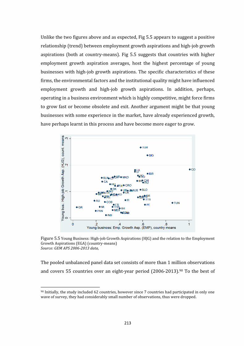
213
Unlike the two figures above and as expected, Fig 5.5 appears to suggest a positive
relationship (trend) between employment growth aspirations and high-job growth
aspirations (both at country-means). Fig 5.5 suggests that countries with higher
employment growth aspiration averages, host the highest percentage of young
businesses with high-job growth aspirations. The specific characteristics of these
firms, the environmental factors and the institutional quality might have influenced
employment growth and high-job growth aspirations. In addition, perhaps,
operating in a business environment which is highly competitive, might force firms
to grow fast or become obsolete and exit. Another argument might be that young
businesses with some experience in the market, have already experienced growth,
have perhaps learnt in this process and have become more eager to grow.
Figure 5.5 Young Business: High-job Growth Aspirations (HJG) and the relation to the Employment Growth Aspirations (EGA) (country-means) Source: GEM APS 2006-2013 data,
The pooled unbalanced panel data set consists of more than 1 million observations
and covers 55 countries over an eight-year period (2006-2013).90 To the best of
90 Initially, the study included 62 countries, however since 7 countries had participated in only one wave of survey, they had considerably small number of observations, thus were dropped.
214
author’s knowledge this study is one of the few to use such a large number of
observations and over such a long period. From the total number of surveyed adult
population, only about 8.86% can be classified under the TEA (nascent and new
(young) businesses as discussed in Chapter 2 and 4). Only 16 out of 55 countries are
represented in all the eight years, most of the countries have between 3 and 5-year
data, while only 2 countries have only 2-year data. Nevertheless, the representation
of countries is balanced with some exception of developed countries such as the UK
and Spain that have a relatively higher number of observations compared to other
countries and some developing countries such as Latvia that has relatively small
number of observations. The number of respondents in different countries and
different years varies, ranging from 43,033 in the UK in 2006 to 2000 in Latvia in
2006. In total, in 2006, there were 42 participating countries and 115,602
observations, whereas in 2013, the number of countries had increased to 57 and the
number of total respondents to 209,821, most of them (31) belonging to the
efficiency-driven economies.91
As previously discussed, GEM’s most commonly used measure of entrepreneurship,
the TEA, used in empirical studies includes nascent entrepreneurs (those involved
in setting up a business) and new (young) entrepreneurial businesses, which have
been active for less than 42 months. Some studies have justified why it makes sense
to analyse growth aspiration of newly established firms, excluding the category of
nascent entrepreneurs. For instance, Estrin et al. (2013) argue that growth
aspirations are a characteristic of existing young entrepreneurial firms and not of
nascent entrepreneurial activity. Similarly, according to Reynolds (2007) nascent
ventures have not yet matured enough to determine their growth aspirations.
Therefore, since in this chapter the key aspect is identifying the drives of
entrepreneurial growth aspirations and the main determinants influencing an
individual’s strategic decision to allocate resources toward growth-oriented
ventures, the empirical analysis excludes nascent entrepreneurs and concentrates
91 These represent the number of respondents interviewed per country and not only young businesses. More than 90% of respondents are not involved in any stages of Total Entrepreneurial Activity (TEA)
215
only on new (young) entrepreneurial businesses. The GEM individual-level data
allow for investigating new (young) business’ entrepreneurial growth aspirations.
In this chapter, in addition to the Adult Population Survey (APS), another set of data
collected by GEM, namely the National Expert Surveys (NES) is also used. The NES
data is gathered by interviewing selected experts with experience of relevance to
the topic under investigation. There are nine components of Entrepreneurial
Framework Conditions (EFC) identified and captured in NES surveys including
government policies and programmes that support entrepreneurial activity,
finance, entrepreneurial education and training, R&D transferability, infrastructure
(commercial, physical and professional), market openness, cultural and social
norms, capacity for entrepreneurship, economic climate, perceived population
composition and political, institutional and social context. In this chapter, one of the
regulatory dimensions of NES data is used to account for the influence of
government policies and activities that support high-growth firms.
5.2.2.1 Dependent variable
Using the information from the APS component of GEM, we can define two
dependent variables:
Dependent Variable (1) - Following Estrin et al. (2013; 2014) and Capellaras et et
al. (2018), young business employment growth aspirations (EGA) is used as the
dependent variable. The EGA represents the expectations of new (young)
businesses (younger than 3.5 years) to increase employment over a five-year
horizon. EGA is calculated as the difference between the natural logarithms of
expected level of employment after five years and the current level of employment.
Autio and Acs (2010) used the natural logarithm of the expected new jobs in the five
years. It is argued that the approach this chapter follows, compared to Autio and Acs
(2010), better approximates the expected rate of employment growth aspirations
(Estrin et al., 2014).
Dependent Variable (2) – The second dependent variable used in this chapter is a
dummy which represents High-Job Growth Aspirations. It takes the value of 1 if the
216
newly established businesses expect to create at least 20 jobs in five years and 0
otherwise. Some studies have used 10 jobs as the threshold for high-growth
aspirations (e.g., Puente et al., 2017), while Giotopoulos et al. (2017a, b) use 5
categories, one of them being 20 or more jobs in 5 years. Although Puente et al.
(2017) and Giotopoulos et al. (2017a, b) use a similar approach, their studies are
considered to be geographically localised (Puente et al., 2017 (Venezuela);
Giotopoulos et al., 2017a (Greece); and Giotopoulos et al., 2017b (only EU
countries)). Our study, on the other hand, covers 55 countries, innovation-driven
and efficiency-driven economies.
The second dependent variable captures the group of entrepreneurs that expect to
drastically increase their employment figures. To control for the influence of current
employment (current in this situation means: at the time of survey), this variable
was conditioned to include only young businesses that currently have a maximum
of 10 employees. The data indicate that 93.62% of the newly established business
currently employ between 1 and 10 employees, thus a firm needs to at least double
their employment in five years to reach to 20 and that can be considered a
significant growth.92
The two dependent variables have sometimes been subject to criticisms,
considering that they only represent growth aspirations and growth expectations
and not realised growth. However, as discussed in section 5.2.2, there exists both
theoretical and empirical evidence suggesting that aspirations are a good predictor
of performance (Wiklund and Davidsson, 2003; Terjesen and Szerb, 2008; Covin and
Wales, 2012). The assertion that entrepreneurial growth aspirations are closely
linked to entrepreneurial outcomes is supported by empirical evidence. Recently,
Levie and Autio (2013) have reviewed 13 studies that investigated business owners’
growth ambitions and at a later point their actual business growth. They find that
growth ambitions can be used to explain a large part of subsequent firm growth.
92 Young business employment statistics include the owner as well (see Parker, 2009).

217
5.2.2.2 Individual and young business characteristics and controls
Shane and Venkataraman (2000) argue that Individual-level factors and
attributes are a significant determinant of entrepreneurial activity. Similarly,
Levie and Autio (2013) argue that there is a high association between individual
beliefs and entrepreneurial growth aspirations. Deciding to engage in
entrepreneurial ventures means that the individual has to go through different
economic trade-offs where opportunity costs are involved (Astbro and
Bernhardt, 2005). Levie and Autio (2013) review of entrepreneurial growth
aspirations, provides a list of different individual-level characteristics that are
associated with growth aspirations. These include: human capital (education),
financial capital (household income), social capital and network (knowing other
entrepreneurs; having a partner in the business; provided financial support to
other entrepreneurs (business angel), work status, prior business experience
(owner/manager of an existing business), demographic characteristics, such as
age and gender. The second group of individual factors includes psychological
factors expressed by individual perceptions and attitudes (entrepreneurial skills
and abilities (perceived capabilities); opportunity recognition (perceived
opportunities). The third category includes motivations (improvement-driven
opportunity; necessity driven) and aspirations (high-job growth; innovation-
orientation, including new technology adoption; international orientation and
social value creation ventures).
Among the individual-level factors, education (human capital) is suggested to
provide an individual with opportunity recognition capabilities (see Shaver and
Scott, 1991), thus providing higher chances in engaging and successfully seizing
entrepreneurial opportunities (Dimov and Shepherd, 2005; Shane and
Vankataraman, 2000). At the country-level, it has been argued that a higher rate
of educational capital provides better conditions for more entrepreneurial
activities (Sternberg, 2005; Wilson et al., 2007). Shane and Venkataraman (2000)
argue that education improves the chances of an individual to success in the
entrepreneurial venture. Similarly, Tereul and De Wit (2011) argue that the
number of high-growth firms in a country is positively influenced by higher levels
of education. Education is considered a long-term investment and a valuable

218
individual characteristic in the job market (Shrader and Sigel, 2007; Wright et al.,
2007). An individual’s wage compensation in the labour market, usually reflects
their education attainments (Jacobs, 2007). The opportunity costs of an
individual with higher education levels are higher compared to those with lower
education level, thus only a high return venture might motivate a highly educated
entrepreneur to start a business (Cassar, 2007; Levie and Autio, 2008; Verheul
and van Mil, 2011). As Autio and Acs (2010) put it, in order to justify their career
switch, new entrepreneurs with high education levels should realise higher
returns compared to the entrepreneurs with less investment in education. Thus,
it is expected that individuals with high education levels will most probably
engage in high-growth entrepreneurial ventures where the gains exceed the high
opportunity costs of pulling-out of the wage labour market (Capelleras et al.,
2018). Hence, in this chapter, we use post-secondary education level
(educ_postgr) and expect to find a positive and significant relationship between
education and entrepreneurial growth aspirations, i.e., higher levels of
educations are associated with higher employment growth and high-job growth
aspirations. Education has also some positive side-effects, one of them being the
social skills and capital which enables entrepreneurs to better mobilise resources
and successfully run new ventures (Stevens et al., 2008). Levie and Autio (2013)
find that studies usually report a positive and robust (although small) association
between education and growth.
Household income (financial capital) – Bowen (2008), Urbano and Guerrero
(2013) and Jinb et al. (2015) have argued that financial capital and financial
availability are a significant determinant of entrepreneurial growth aspirations.
Household income (gemhhincome) is a categorical variable that represents three
levels based on the total household income of the entire household (Autio and
Acs, 2010; Lim et al., 2016). The first category represents individuals that belong
to the lower one-third (0-33%) of the household income country distribution.
The third category represents individuals that belong to the upper one-third (67-
100%) of the household income country distribution. High-income household
individuals become more selective when deciding which occupational alternative
to pursue. A lot of this decision-making process happens before (ex-ante) any
entrepreneurial activity is considered. It is highly likely that high-income
219
household individuals would only settle for high-growth potential
entrepreneurial ventures. Wright et al. (2006) argue that high-income household
individuals have more opportunities to receive venture capital funding and, in
general, are provided with wider financing opportunities. In addition to financial
availability, high-income household individuals might have also enhanced their
social contacts and connectivity and the two conjointly increase an individual’s
abilities for engaging in high-growth entrepreneurial opportunities (Dunn and
Holtz-Eakin, 2000). Moreover, for an individual entrepreneur with higher
financial capital capacities, it might be easier to acquire other crucial resources,
such as human capital (Evans and Jovanovic, 1989). It is highly expected that
resource-rich (with financial, social and human capital) entrepreneurial ventures
have better chances and higher aspirations for faster and higher business growth.
Thus, a positive association between household income and growth aspirations
is suspected also in this chapter.
Business networking (social capital) - The Theory of Planned Behaviour (TPB)
argues that interacting and knowing other entrepreneurs positively influences
an individual’s self-confidence which then improves the chances of engaging and
growing entrepreneurial ventures (Minniti, 2005; Driga et al., 2009). For
instance, access to finance and information is significantly facilitated by being a
member of a business network (Beugelsdijk, 2007; Bauernschuster et al., 2010;
Korosteleva and Mickiewicz, 2011; Kwon et al., 2013; Teckchandani, 2014).
Danis et al. (2011) and Aparicio (2017) find that networking is an important
activity for new business activity and entrepreneurial growth aspirations. Thus,
we hypothesise that (i) knowing other entrepreneurs (KNOWENT_dum),
perhaps through business associations and clubs, who started a business in the
past two years is considered an entrepreneurial characteristic that might
positively influence growth aspirations; and (ii) being a business growth
supporter by serving as a business angel (BUSang_dum) in the previous three
years is also positively associated with entrepreneurial growth aspirations.
In general, belonging to a formal or informal business association or networking
is of a significant relevance, especially in countries with lack of proper
institutions (Estrin et al., 2013b). The interplay between institutions and

220
measures of social capital is also explored in this chapter and result suggest that
the latter moderates the negative impact of insufficient quality of institutions.
Skills and perceived opportunities - According to the model developed by
Shapero and Sokol (1982) entrepreneurial intentions are affected by “perceived
desirability” and “perceived feasibility”. The former represents the ability to act
when opportunities occur while the latter indicates the degree of capabilities that
an individual believes to possess (skills). Van Hemmen et al. (2013) highlight that
there is a positive association between an individual’s self-confidence in skills
and entrepreneurial productive activities. Similarly, Baum and Locke (2004)
Aidis and Mickiewicz (2006) and more recently Capelleres et al. (2018) have
found a positive effect of perceived skill capabilities on growth aspirations in
both developed and developing countries. Similar to previous studies (e.g.,
Stuetzer et al. 2014; Giotopoulos et al. 2017), we use perceived entrepreneurial
skills (suskill_dum), which takes value 1 if the respondent perceives to have the
knowledge, skills and experience required to start-up a new business and 0
otherwise. According to Bosma et al. (2018), consider skills and self-efficacy as
one of the measures of the cognitive dimension of institutions.
Similarly, having good prospects for starting a business in the near future,
positively impacts growth aspirations of existing young businesses (Giotopoulos
et al., 2017; Capellares et al., 2018). According to Cassar (2010), perceiving that
there are good opportunities to start-up a new business venture is a measure of
entrepreneurial optimism. Stam et al. (2012) highlight the positive and strong
effect of perceived opportunities on growth motivations. Similar to other studies,
perceived opportunities (opportunities) is a dummy variable, which takes value
1 if the respondent perceives that there exist good opportunities for starting a
business venture in the next 6 months and 0 otherwise. In this study, perceived
opportunities serve also as a proxy for normative dimension of Scott (2008).
While other studies use fear of failure (Bosma et al., 2018), higher media
attention (Urbano and Alvarez, 2014), or whether entrepreneurship is
considered as a desirable career choice (Lim et al., 2016), we consider that all the
three gravitate to perceived opportunities. Social contexts filled with fear of
failure, bad image for entrepreneurship as a career choice, portrayed also in

221
media, negatively influence one’s beliefs about the overall environment toward
entrepreneurship (Autio et al., 2013). It then becomes less likely for an individual
to identify and pursue any business activity.
Control variables - Among other individual-level characteristics, age and
gender are most commonly used and hence the theory and empirical findings are
largely developed and consistent (Blanchflower, 2004; Levesque and Minniti,
2006). Empirical studies have reported that young individuals are more prone to
engage in high ambitious ventures (Kolvereid, 1992; Estrin et al., 2013;
Capellares et al., 2018). Levesque and Minniti (2006) argue that there is a
curvilinear relationship, suggesting that after a certain point, age has a negative
influence on entrepreneurial entry and growth. In general, male entrepreneurs
are reported to have higher growth aspirations as compared to their female
counterparts (Blanchflower, 2004; Estrin and Mickiewicz, 2011; Levie and Autio,
2013; Terjesen et al., 2016). Employment status – Cassar (2006) argues that an
individual weigh the potential benefits of engaging in an entrepreneurial venture,
be it a high-growth, to the benefits of regular wage employment. Since, the gains
from an entrepreneurial venture are mostly uncertain, individuals usually tend
to share the efforts and resources allocated to entrepreneurship and wage
employment (Dixit, 1989; Sparrowe et al., 2001; Douglass and Shepherd, 2002).
Autio (2007) argues that a high percentage of early stage entrepreneurial
ventures start as part-time jobs. Likewise, Knight (1921) has argued that
opportunities are uncertain ex-ante and can only be determined ex-post. Hence,
a number of young entrepreneurs will try to retain their wage employment until
their businesses generate enough income (Shepherd, 2015). The same pattern is
also present in our sample, where significantly more employed individuals have
been reported to be engaged in establishing new businesses than their
counterpart (the unemployed).93
Being a manager or owning an additional existing business (omestbus_dum) has
also been used as a control variable as it leads to increased opportunity costs if a
93 The GEM question used to construct this variable does not provide enough information on the self-employed category. It is not clear whether the respondent consider themselves as self-employed in the same business that they are being surveyed or self-employed in another business.
222
new venture is considered. However, Harper (2003) argues that individuals with
previous entrepreneurial experience have higher growth aspirations. Similarly,
Capellares et al. (2018) highlight that, prior entrepreneurial experience is crucial
for running and growing a new business. Young businesses with high current (at
the time of survey) level of employment are expected to report a slower rate of
employment growth compared to those with low current level of employment
(curr_employ) (Estrin et al., 2013). This suggests that firm employment, in
general, experiences a diminishing rate of growth. In addition, this chapter also
controls for the impact that having one or more business partners might have on
growth aspirations (bb_owners). The expectations are that if the business has
shared ownership with one or more than one owner/partner, the chances are
that growth aspirations will be higher compared to a business owned by a single
entrepreneur. The availability of resources, human, financial and social, and the
combined experiences of owners, are perhaps higher in businesses with shared
ownership. The data show that more than 71.5% of the young businesses are
owned by only one person, less than 25% will be owned by 2 owners and only
about 5% by 3 or more owners.
5.2.2.3 Institutional variables
Cross-country empirical research confirms the strong influence of national
institutional arrangements on entrepreneurship (Bowen and De Clerq, 2008; De
Clercq et al., 2010; Stenholm et al., 2013; Hermans et al., 2015; Eesley, 2016;
Krasniqi and Desai, 2016; Lim et al., 2016; Bosma et al., 2018; Darnihamedani et
al., 2018). Institutional theory and institutional approach have contributed
significantly to the advancement of entrepreneurship research (Urbano and
Alvarez, 2014). A relevant point made in Baumol (1990; 1993; 2010) and Baumol
and Strom (2007) is that business environments combined with high quality
institutions are more likely to nurture productive entrepreneurship.94 Similarly,
according to Aghion and Festré (2017), the quality of institutions is more
relevant for growth-oriented ventures compared to firms with no growth
intentions. For instance, high-growth ventures benefit more than other firms
94 As discussed in Chapter 4, according to Baumol (1993, p.30), any entrepreneurial activity that contributes directly or indirectly to net output of the economy or to the capacity to produce additional output is considered as productive entrepreneurship.

223
from a strong property protection regime as their investments can be safely
protected. Audretsch et al. (2015) and Hermans et al. (2015) argue that
identifying the fundamental national policies and most influential institutional
variables in shaping high-growth aspiration entrepreneurship remains a viable
research topic.
A number of influential studies have contributed to structuring and categorising
institutions. For instance, North (1990) categorised institutions into formal, the
set of rules and regulations such as procedures, contracts, property rights that
provide the incentive systems, and informal institutions, the norms and other
social arrangements that influence the adoption and applicability of formal
structures (Estrin et al., 2013; Efendic et al., 2015). Informal institutions are
deeply embedded societal values, hence are very difficult to change and adopt to
new circumstances (North, 1990). The role of informal institutions becomes very
distinct in societies with the lack of good quality formal institutions (North 1990;
Belitski et al., 2016). On a later study, Williamson (2000) used a four-level
hierarchical approach to categorising institutions, putting formal and informal
institutions in the top of his hierarchy of institutions.95 Scott (1995; 2005; 2008)
identified the regulatory, cultural-cognitive and normative dimension that
should be carefully examined in order to be able to conceptualise the institutional
context and develop the relationship between individuals, institutional factors
and entrepreneurial activity. The regulatory dimension includes all the
regulative aspects and processes of institutions, such as establishing rules,
obeying to the rules and regulations, and rewarding or punishing the behaviour
of economic agents on the basis of compliance with rules and regulations. The
cognitive dimension pertains to the country-level cognitive structures and social
knowledge. It also includes shared conceptions by which societies frame realities
and meanings (Scott, 2001). Moreover, Scott (2014, p.67) posits that the
cognitive dimension shows that: “external cultural frameworks shape internal
interpretive processes”. The normative dimension includes norms, which define
how things should be done and values, which constitute standards by which
95 (i) informal institutions; (ii) formal institutions; (iii) governance; and (iv) resource allocation (occupational choice)
224
existing structures and behaviours are compared and assessed (Scott, 2014,
p.64). Gnyawali and Fogel (1994, p. 46) framework, suggests five environmental
(institutional) dimensions, namely, (i) government policies and procedures; (ii)
social conditions; (iii) entrepreneurial and business skills; (iv) financial support
to businesses; and (v) non-financial support to businesses should be considered
when studying entrepreneurship development. According to Alvarez and Urbano
(2011), four of these dimensions relate to formal institutions while only social
conditions are related to informal factors. In this chapter, the empirical analysis
benefits from these studies by including variables belonging to the two
categories, formal and informal, the three dimensions of Scott (1995; 2005;
2008), regulatory, cultural-cognitive and normative and the five dimensions
proposed by Gnyawali and Fogel (1994, p. 46).
In the category of informal institutions, studies have included corruption which
represents societal norms and customs which are assumed to shape the
behaviour of an individual (Alvarez et al., 2014; Chowdhury et al., 2015a, b).
Corruption is reported to have a negative and significant impact on
entrepreneurship (Anokhin and Schulze, 2009; Aidis et al., 2012; Dreher and
Gassebner, 2013). Moreover, Anokhin and Schulze (2009) and Estrin et al. (2013)
posit that corruption increases transactions costs and is viewed as an additional
tax on businesses. The state of corruption is particularly important for new
entrants as the incumbent firms have already adopted their market behaviour
and can soften the negative effects of corruption (Tonoyan et al., 2010). It has
also been reported that high-growth ventures suffer more from corruptive
environments compared to small-scale enterprises which in some cases do not
attract enough attention from corrupt officials and manage to fly “below the
radar” (Bowen and De Clercq, 2008; Stam et al., 2012; Estrin et al., 2013; Belitski
et al., 2016; Dutta and Sobel, 2016). The Heritage Foundation Index of ‘Freedom
from Corruption’ (corruption) is used as a proxy for the level of corruption in
each country. According to Beach and Kane (2008, p.41) the indicator provides
an assessment of the perception of corruption in the business environment,
including levels of governmental, legal, judicial, and administrative corruption. It
ranges from 0 to 100 with high values representing less corrupt business

225
environments. However, following Estrin et al. (2013) the indicator is
transformed so that higher values represent more corrupt business
environments.96
Another indicator of the quality of institutions that has an influence on
entrepreneurial activity is freedom of doing business (bussfree). Autio and Fu
(2015, p.77) argue that this index reflects the quality of economic institutions by
assessing the overall regulatory burden and the efficiency of the regulatory
process. The index is based on 10 equally weighted sub-factors sourced from the
World Bank’s Doing Business report (Beach and Kane, 2008).97 Amongst the sub-
factors, procedures, time, cost, capital requirements for start-ups, licensing
procedures and business termination activities are accounted for. Holmes et al.
(2008), Stenholm et al. (2013) and Acs et al. (2014) argue that business freedom
is a measure of the overall quality of business environment that an
entrepreneurial venture faces. The index ranges from 0 to 100, with 100
indicating the freest business environment. A higher score, is thus, expected to
have a positive impact on employment growth aspirations as it is a sign of a more
conducive environment for conducting business activities.
The investigation accounts also for government size and activity (gov_size),
which represents another regulatory dimension and refers to the scale of the
public sector and public investment by government. According to Bosma et al.
(2018) a large government size and activity is negatively associated with
entrepreneurial growth aspirations. As Miller et al. (2018) point out, efficiency
losses might be common, due to the misallocation of key resources from a large
government activity. Moreover, a larger government sector and government size
might lead to the ‘crowding-out’ state of private sector investment98 (Fogel et al.,
2006; Aidis et al., 2012) and in that situation, entrepreneurial growth aspiration
ventures suffer the most (Bosma et al., 2018). New entrepreneurial growth
96 Transformation is done by reversing the scale (subtracting the ‘original’ ‘freedom from corruption’ from 100). 97 Since 2015, the index consists of 13 sub-factors. Procedures, time and costs to get electricity have been added. 98 In addition, a larger public sector puts greater pressure on supply prices (including reservation wages) and increases competition with private sector.

226
ventures might need higher investment and rely more on formal financial sector
rather than on informal channels (Estrin et al., 2013). Furthermore, extensive
government spending in social and welfare systems, discourage private savings
(Henrekson, 2007; Korosteleva and Mickiewicz, 2011) and harms growth
aspirations (Hessels et al., 2008). This chapter uses the Heritage Foundation
‘Government size’ as the proxy for government size and activity. The ‘original’
index represents “freedom from government economic presence”99, hence
following Reynolds (2011) and Estrin et al. (2013), the index is transformed in
order to better reflect the government size and activity. After transformation, the
values range from 0-100 and higher values denote larger government size and
activity.100
Similar to Aidis et al. (2012), Pathak et al. (2013) and Estrin et al. (2016), the
Polity IV indicator of efficient constraints on the arbitrary power of the executive
branch of the government (execons) is used as a proxy for property rights
protection. According to Acemoglu and Johnson (2005, p.949), this indicator
reflects the state of property right protection as it represents the degree by which
citizens are protected against any act of expropriation by the government and
powerful elites. The Polity IV ‘constraints on the executive’ echoes the societal
endeavours to limit government’s and other powerful elites to expropriate
private property rights (Acemoglu and Johnson, 2005). Weak property rights
protection might increase the expropriation activities, thus discouraging
entrepreneurial growth aspirations (Estrin et al., 2013). In a low institutional
quality context, the expectations are that growth aspiring entrepreneurs will be
hurt mostly due the inability to reap-up profits from their operations. The
‘executive constrains’ is measured using a seven-category scale, with higher
scores indicating more constrains, i.e., less acts or attempts of expropriations by
99 See Miller and Holmes (2010) for more details on the ‘freedom from government economic presence’ index 100 Government size is reversed using this approach: Government size = SQRT [(100-government spending)/0.03)]. For a detailed discussion on the methodology of measuring all the 10 Economic Freedom Indexes including government spending see Beach and Kane (2008, pp. 39-55) and Miller and Holmes (2010).

227
governments and powerful elites, and lower scores indicating unlimited
authority, hence higher chances for expropriation activities.
An additional institutional quality variable used in the empirical analysis is the
influence of government specifically designed programmes to support
entrepreneurial activities with high-growth potential, High growth support
government programmes (highgrowth_support). Such programmes and
government policies are designed to target only high and fast-growing firms and
aim in creating a business environment and condition that favour
entrepreneurial growth aspirations. In the GEM´s methodology these conditions
are known as Entrepreneurial Framework Conditions (EFCs). The box below
shows the type of questions that were addressed to country experts when the
National Expert Surveys (NES) data for this dimension were gathered. The High
growth support government programmes represents a summary of the
responses provided by experts, in a 5-point scale, in each country for the
questions below. Higher values represent more favourable government
programmes toward high-growth potential ventures.
Variable High-Growth Support
Questions considered: • In my country, there are many support initiatives
that are specially tailored for high-growth
entrepreneurial activity
• In my country, policy-makers are aware of the
importance of high-growth entrepreneurial activity
• In my country, people working in entrepreneurship
support initiatives have sufficient skills and
competence to support high-growth firms
• In my country, potential for rapid growth is often
used as a selection criterion when choosing
recipients of entrepreneurship support
• In my country, supporting rapid firm growth is a high
priority in entrepreneurship policy

228
5.2.2.4 Country level characteristics
Macroeconomic factors, country and industry contextual characteristics are also
expected to influence entrepreneurial activity and most importantly, to impact
the quality of entrepreneurship activity i.e., leading to more productive as
compared to unproductive ventures (Baumol, 1990; 2010). The classic variables
to account for macro- and contextual characteristics are: the level and stage of
economic development; the pace of economic growth; the rate of established
businesses (business competition); and industry type.101
Accordingly, the empirical analysis of this chapter controls for the country’s GDP
per capita, adjusted for Purchasing Power Parity (PPP) at constant 2011
international dollars from the World Bank (WB). To account for any curvilinear
relationship between entrepreneurial growth aspirations and the level of
economic development, measured by GDP per capita, the study also includes the
square term of GDP per capita. To account for potential multicollinearity between
per capita GDP and some measures of institutional quality, the former control
variable is also structured into five quantiles, reflecting the distribution of GDP
per capita from the lowest 20% to the highest 20% (see Estrin et al., 2013).
Specifically, there is reported a high correlation coefficient (above 0.8) between
corruption and GDP per capita, suggesting that the two variables should not be
included in the same specification at the same time.102 The study expects to find
higher entrepreneurial growth aspirations in low per capita GDP economies (see
also Tereul and De Wit, 2011). GDP growth rate is included to account for the
increase in the demand and the pace of economic development (Galindo and
Méndez, 2014). The prevalence rate of established businesses (estbusrate) at the
country level is included as a proxy for the size of private sector and to account
for the industry structure (Autio and Acs, 2010).
As discussed in the previous chapters, the empirical evidence suggests that there
is a relationship between the stage of economic development and
entrepreneurship (Carree et al., 2002; Wennekers et al., 2005; Bosma et al., 2008;
101 For more details on the types of industries, see Reynolds (2011). 102 See Appendix 5.2
229
Gries and Naude, 2008; Acs 2010). Most studies report a U-shaped relationship
between per capita GDP and entrepreneurial activity (see Wennekers et al.,
2010), but some also report an S-shaped (see Frederic and Monsen, 2011).
Accordingly, in the empirical part of this chapter, country differences in terms of
the phase of economic development will be categorised as suggested by Porter et
al. (2002) typology. The World Economic Forum’s (WEF) Global Competitiveness
Report 2001-2002, drafted by Porter et al. (2002), groups countries into three
categories based on the phase of economic development measured by country’s
per capita GDP and the share of per primary goods relative to total exports. The
categories are: (i) Factor-driven economies; (ii) Efficiency-driven economies;
and (iii) Innovation-driven economies (see Appendix A).103 In this chapter,
because there are just a few countries that belong to the first category, factor-
driven, the analyses were not applied for this group. The two other categories,
innovation-driven and efficiency-driven, have similar and comparable number of
countries and observations. In total, there are 27 countries that belong to the
innovation-driven stage and 30 that belong to the efficiency-driven stage.104 The
research practise of dividing countries according to their phase of economic
development has also been discussed in Chapter 1 and Chapter 4.
103 Since 2008, GEM Global reports have started to use the same practices by categorizing the participating economies by phase of economic development, namely factor-driven, efficiency-driven and innovation-driven economies. Earlier than 2008 reports used a similar approach by dividing countries into High-Income; Middle- and Low-Income. 104 The sum of the two categories gives us 57. The total unique countries included are 55. The difference exists as one country has moved from efficiency to innovation category over the study period concerned.
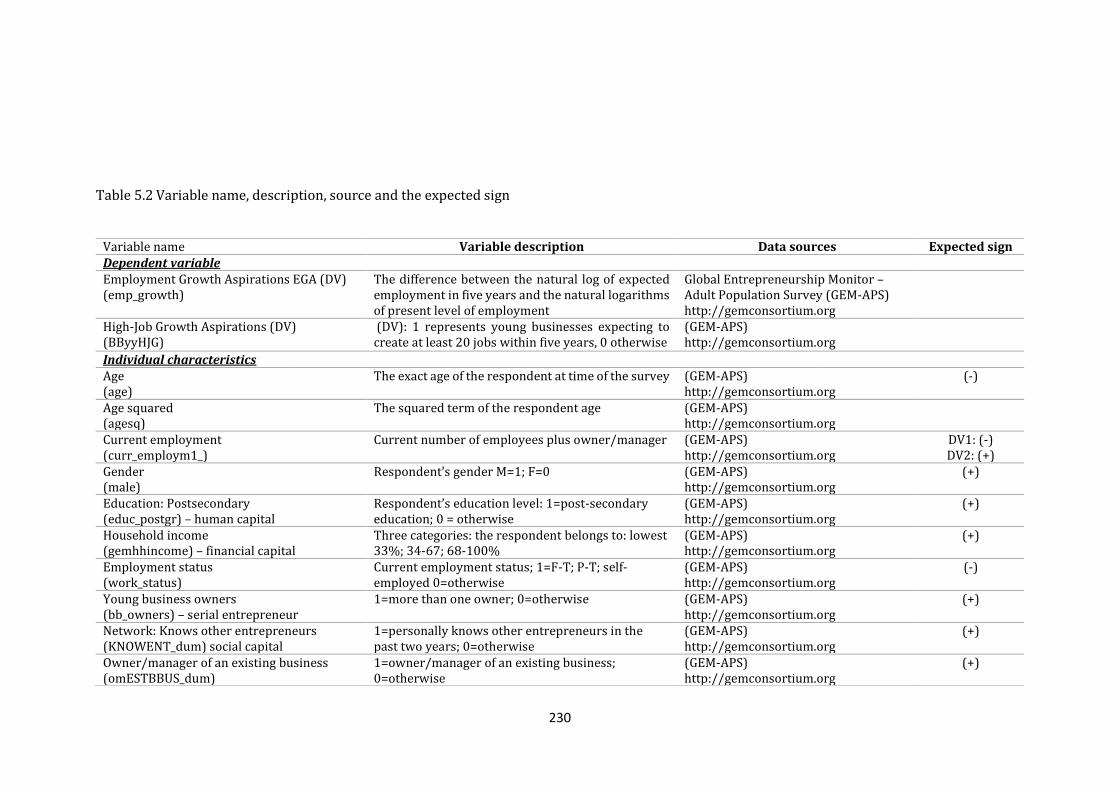
230
Table 5.2 Variable name, description, source and the expected sign
Variable name Variable description Data sources Expected sign Dependent variable Employment Growth Aspirations EGA (DV) (emp_growth)
The difference between the natural log of expected employment in five years and the natural logarithms of present level of employment
Global Entrepreneurship Monitor – Adult Population Survey (GEM-APS) http://gemconsortium.org
High-Job Growth Aspirations (DV) (BByyHJG)
(DV): 1 represents young businesses expecting to create at least 20 jobs within five years, 0 otherwise
(GEM-APS) http://gemconsortium.org
Individual characteristics Age (age)
The exact age of the respondent at time of the survey (GEM-APS) http://gemconsortium.org
(-)
Age squared (agesq)
The squared term of the respondent age (GEM-APS) http://gemconsortium.org
Current employment (curr_employm1_)
Current number of employees plus owner/manager (GEM-APS) http://gemconsortium.org
DV1: (-) DV2: (+)
Gender (male)
Respondent’s gender M=1; F=0 (GEM-APS) http://gemconsortium.org
(+)
Education: Postsecondary (educ_postgr) – human capital
Respondent’s education level: 1=post-secondary education; 0 = otherwise
(GEM-APS) http://gemconsortium.org
(+)
Household income (gemhhincome) – financial capital
Three categories: the respondent belongs to: lowest 33%; 34-67; 68-100%
(GEM-APS) http://gemconsortium.org
(+)
Employment status (work_status)
Current employment status; 1=F-T; P-T; self-employed 0=otherwise
(GEM-APS) http://gemconsortium.org
(-)
Young business owners (bb_owners) – serial entrepreneur
1=more than one owner; 0=otherwise (GEM-APS) http://gemconsortium.org
(+)
Network: Knows other entrepreneurs (KNOWENT_dum) social capital
1=personally knows other entrepreneurs in the past two years; 0=otherwise
(GEM-APS) http://gemconsortium.org
(+)
Owner/manager of an existing business (omESTBBUS_dum)
1=owner/manager of an existing business; 0=otherwise
(GEM-APS) http://gemconsortium.org
(+)
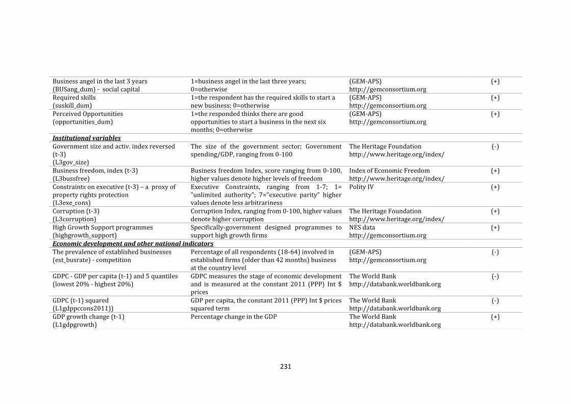
231
Business angel in the last 3 years (BUSang_dum) - social capital
1=business angel in the last three years; 0=otherwise
(GEM-APS) http://gemconsortium.org
(+)
Required skills (suskill_dum)
1=the respondent has the required skills to start a new business; 0=otherwise
(GEM-APS) http://gemconsortium.org
(+)
Perceived Opportunities (opportunities_dum)
1=the responded thinks there are good opportunities to start a business in the next six months; 0=otherwise
(GEM-APS) http://gemconsortium.org
(+)
Institutional variables Government size and activ. index reversed (t-3) (L3gov_size)
The size of the government sector; Government spending/GDP, ranging from 0-100
The Heritage Foundation http://www.heritage.org/index/
(-)
Business freedom, index (t-3) (L3bussfree)
Business freedom Index, score ranging from 0-100, higher values denote higher levels of freedom
Index of Economic Freedom http://www.heritage.org/index/
(+)
Constraints on executive (t-3) – a proxy of property rights protection (L3exe_cons)
Executive Constraints, ranging from 1-7; 1= ”unlimited authority”; 7=”executive parity” higher values denote less arbitrariness
Polity IV
(+)
Corruption (t-3) (L3corruption)
Corruption Index, ranging from 0-100, higher values denote higher corruption
The Heritage Foundation http://www.heritage.org/index/
(+)
High Growth Support programmes (highgrowth_support)
Specifically-government designed programmes to support high growth firms
NES data http://gemconsortium.org
(+)
Economic development and other national indicators The prevalence of established businesses (est_busrate) - competition
Percentage of all respondents (18-64) involved in established firms (older than 42 months) business at the country level
(GEM-APS) http://gemconsortium.org
(-)
GDPC - GDP per capita (t-1) and 5 quantiles (lowest 20% - highest 20%)
GDPC measures the stage of economic development and is measured at the constant 2011 (PPP) Int $ prices
The World Bank http://databank.worldbank.org
(-)
GDPC (t-1) squared (L1gdppccons2011))
GDP per capita, the constant 2011 (PPP) Int $ prices squared term
The World Bank http://databank.worldbank.org
(-)
GDP growth change (t-1) (L1gdpgrowth)
Percentage change in the GDP The World Bank http://databank.worldbank.org
(+)
232
Descriptive statistics by stages of economic development
Table 5.3 below provides the summary statistics of all the included variables,
divided into three categories for the three samples, namely all economies,
innovation-driven and efficiency-driven economies. As expected, notable
differences are observed for the institutional quality variables and
macroeconomic contextual controls, while individual-level characteristics are
relatively similar. For instance, the mean of corruption variable is 25.64 in
innovation-driven economies and 60.40 in efficiency-driven economies.
Similarly, the mean value of business freedom is eighteen (18) points higher in
innovation-driven economies compared to the efficiency-driven economies,
suggesting the more favourable context of doing business in the former group of
economies. The proxy for property rights protection is also significantly different
in innovation-driven compared to efficiency-driven economies. GDP per capita,
which measures the stage of economic development, is almost three times lower
in efficiency-driven compared to innovation-driven economies while GDP
growth is almost four times higher in efficiency-driven compared to innovation-
driven economies, suggesting the presence of catch-up effect.
Table 5.3 also suggests that most of the young businesses are managed and/or
owned by male and middle age (39-41) entrepreneurs. Contrary to our
expectations, the male dominance is mostly expressed in innovation-driven
economies, where less than 40% of young businesses are reported to be owned
by females. In innovation-driven economies, every sixth young entrepreneur has
completed a high level of education compared to every fifteenth new (young)
entrepreneur or manager in efficiency-driven economies. On average, 30% of
young businesses are owned or managed by more than one entrepreneur and at
the time of the survey, employ not more than 4 employees.105 The average
number of employees is influenced by the decision to limit the maximum number
of employees to 100 which represents 99.42% of the total young businesses. In
the original GEM dataset, a very few number of young businesses reported
105 The latter figure comes after adjusting for outliers

233
currently employing more than 100 employees, hence were not included in the
empirical analysis.
Young businesses operating in innovation-driven economies seem to be more
open to partnerships and ownership sharing (33.2%), while the same category
of businesses operating in a different business ecosystem, efficiency-driven
economies, are reported to be more reluctant to ownership sharing (27.5%).
More than 50% of new (young) entrepreneurs (46% in innovation-driven and
59% in efficiency-driven economies) consider that there are good prospects to
start a new business in the next six months and more than 80% of them report
that they have the appropriate skills to start a business venture. These two
variables are included in the model to test whether new (young) entrepreneur’s
perceived opportunities and capabilities influence their employment and high-
job growth aspirations. About 3.9% of young business entrepreneurs in
innovation-driven economies manage and/or own another business and can be
considered serial entrepreneurs. In efficiency-driven economies, only 2.2% of the
surveyed owners manage or own another business. In general, this might
indicate that doing business in the latter contexts is more difficult, perhaps
formal financing opportunities are more rigid in less-developed economies,
therefore entrepreneurs need to be more selective when thinking to start a new
business venture.
With respect to social ties, networking and social capital, Table 5.3 suggest that
9% of young business entrepreneurs, have also financially supported another
business venture in the last three years. The prevalence of business angels is
slightly higher in efficiency-driven economies, perhaps suggesting for the lack of
formal financial financing opportunities in these business environments. Another
component of social capital is the opportunity of young business owners to know
and interact with other entrepreneurs. Knowing other entrepreneurs who might
serve as role models might improve their chances of success, shape their
aspirations toward growth and allow ‘learning-by-seeing’ (Harper, 2003). Sixty
percent of young business owners report that they know other entrepreneurs
who have recently started a business venture.
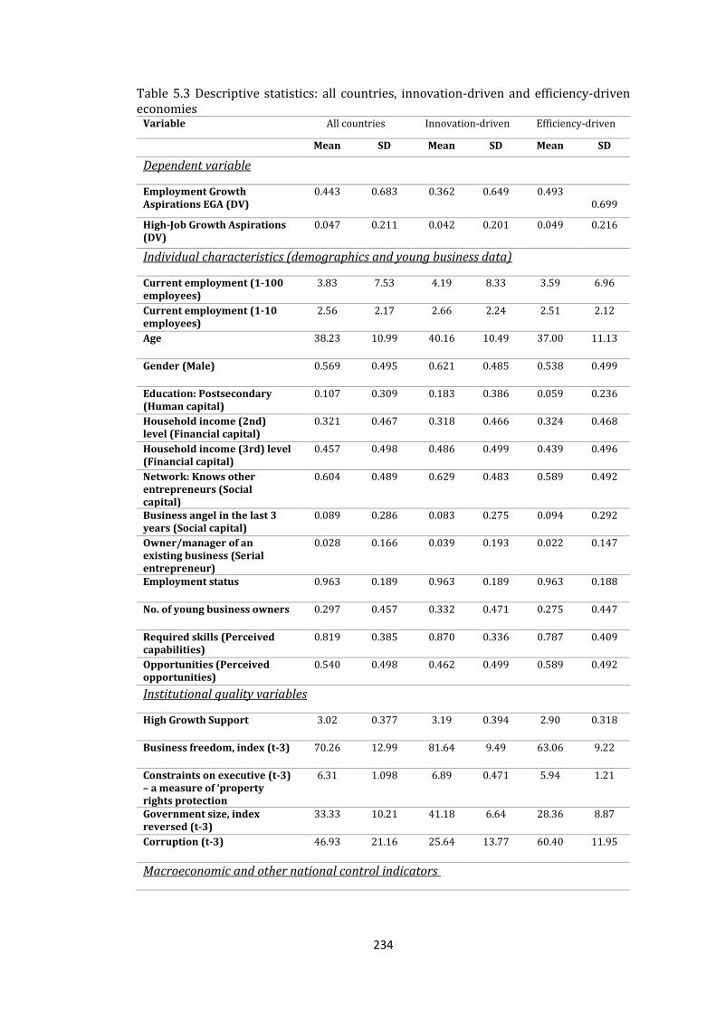
234
Table 5.3 Descriptive statistics: all countries, innovation-driven and efficiency-driven economies
Variable All countries Innovation-driven Efficiency-driven
Mean SD Mean SD Mean SD
Dependent variable
Employment Growth Aspirations EGA (DV)
0.443 0.683 0.362 0.649 0.493 0.699
High-Job Growth Aspirations (DV)
0.047 0.211 0.042 0.201 0.049 0.216
Individual characteristics (demographics and young business data)
Current employment (1-100 employees)
3.83 7.53 4.19 8.33 3.59 6.96
Current employment (1-10 employees)
2.56 2.17 2.66 2.24 2.51 2.12
Age 38.23 10.99 40.16 10.49 37.00 11.13
Gender (Male) 0.569 0.495 0.621 0.485 0.538 0.499
Education: Postsecondary (Human capital)
0.107 0.309 0.183 0.386 0.059 0.236
Household income (2nd) level (Financial capital)
0.321 0.467 0.318 0.466 0.324 0.468
Household income (3rd) level (Financial capital)
0.457 0.498 0.486 0.499 0.439 0.496
Network: Knows other entrepreneurs (Social capital)
0.604 0.489 0.629 0.483 0.589 0.492
Business angel in the last 3 years (Social capital)
0.089 0.286 0.083 0.275 0.094 0.292
Owner/manager of an existing business (Serial entrepreneur)
0.028 0.166 0.039 0.193 0.022 0.147
Employment status 0.963 0.189 0.963 0.189 0.963 0.188
No. of young business owners 0.297 0.457 0.332 0.471 0.275 0.447
Required skills (Perceived capabilities)
0.819 0.385 0.870 0.336 0.787 0.409
Opportunities (Perceived opportunities)
0.540 0.498 0.462 0.499 0.589 0.492
Institutional quality variables
High Growth Support 3.02 0.377 3.19 0.394 2.90 0.318
Business freedom, index (t-3) 70.26 12.99 81.64 9.49 63.06 9.22
Constraints on executive (t-3) – a measure of ‘property rights protection
6.31 1.098 6.89 0.471 5.94 1.21
Government size, index reversed (t-3)
33.33 10.21 41.18 6.64 28.36 8.87
Corruption (t-3) 46.93 21.16 25.64 13.77 60.40 11.95
Macroeconomic and other national control indicators
235
The prevalence rate of established businesses (Competition)
10.24 5.53 7.27 2.31 12.12 6.12
GDPC - GDP per capita (t-1) 23549.56 13486.41 38492.93 8462.43 14088.48 4560.48
GDPC iq1 (lowest 20%) Five quantiles reflecting the distribution of GDP per capita
0.441 0.497 0.720 0.449
GDPC iq2 0.185 0.389 0.047 0.212 0.273 0.445
GDPC iq3 0.168 0.374 0.422 0.494 0.007 0.083
GDPC iq4 0.074 0.262 0.192 0.394
GDPC iq5 (highest20%) 0.131 0.338 0.339 0.473
GDP growth (t-1) 3.32 3.54 1.39 2.95 4.54 3.39
Note: The summary statistics are produced after adjusting for outliers
Source: GEM 2006-2013
ESTIMATION STRATEGY AND MODEL SPECIFICATION
The constructed datasets consist of the data at two different levels, the
individual-level and the country-level. The individual-level data (e.g., individual’s
demographics, entrepreneurial attitudes, etc.) (level 1) are nested within
country-years (level 2) (Sevä et al., 2016). For instance, young businesses
(entrepreneurs) operating in the US in year 2006 are considered a specific cluster
(group) as are a similar group of young businesses (entrepreneurs) operating in
the Netherlands in year 2013. To account for such a hierarchical structure of the
data, when data are nested (clustered) in some way, multilevel modelling
framework is employed which allows for connecting different levels of data
(Rabe-Hesketh and Skrondal, 2008; Hox et al., 2010; Auginis et al., 2013). Besides
the data structure, Shane and Venkataraman (2000), Autio and Acs (2010), and
Shepherd (2011), highlight that entrepreneurial growth aspirations are a
function of both individual characteristics and environmental factors and the
cross-level interplay between the two. The multi-stage structure allows for
investigating the conjoint effect of individual factors (individual-level) and the
institutions (country-level) on newly established firms. Multilevel modelling
provides an extension to the classical linear regression models (CLRM) by
allowing for simultaneous exploration of micro-level (individual data) and
macro-level (country and contextual-level data) in relation to the dependent
variables, which in this chapter both are at the individual level. The conventional

236
multivariate methods, in this case, would fail to account how the environment,
i.e., institutions and other macroeconomic factors influence an individual’s
decision about business growth (Capelleras et al., 2018).
Multilevel (mixed-effects) linear and logistic regressions contain both fixed
effects and random effects allowing for modelling intra-cluster (cross-country-
year) correlation. The individuals (observations) of the same cluster (country-
year) are likely to share common cluster-level random effects, hence are
expected to be correlated (Estrin et al., 2016). For this reason, as Hox et al. (2010)
argue, applying conventional regression models, in the presence of nested
structure of the data, would violate the assumption of independence of
observations. He adds that spatial autocorrelation is a common phenomenon of
the observations that belong to the same level, i.e., correlation between nested or
clustered individuals (level 1) within country-year (level 2). Similarly, Petereson
et al. (2012) suggest that using a multilevel approach, with random effects,
provides a solution to situations where the independence assumption of the
observations does not hold. To sum up, the above outlined arguments indicate
that research highlights at least three advantages of using multilevel modelling
as compared to conventional data settings. First, as it is highlighted above,
multilevel approach analysis allows for investigating the effects of variables at
different levels as well as their cross-level interplay (Guo and Zhao, 2000;
Echambadi et al., 2006; Nezlek, 2011). Second, it addresses the problem of unit
dependencies, thus producing unbiased estimates (Autio and Acs, 2010; Estrin et
al., 2016). Third, as Nezlek (2011) argues, multilevel modelling allows for
quantifying the relative impact of each level in the overall hierarchical system.
However, one disadvantage of using multilevel modelling is the inability of this
estimator to handle dynamics posing a clear trade-off between the highlighted
features of multilevel modelling and the inability of the estimator to model
dynamics (Sevä et al., 2016). As the focus of this chapter is on investigating the
effect of different levels (e.g., country-level variables and individual-level
characteristics), we decided to employ Multilevel estimation despite having to
sacrifice the benefits associated with dynamic modelling.
237
Accordingly, mixed-effect linear regression (Random Intercept Model (RIM)) is
applied to investigate factors influencing the first dependent variable, which is of
continuous nature (expected growth in employment). Given that the second
dependent variable, high-job growth aspirations, is a binary variable taking a
value of 1 if the young business expects to create at least 20 jobs in 5 years period,
and 0 otherwise, the mixed-effect (multilevel) logistic regression (Snijders and
Bosker, 2012; Hamilton, 2012) is employed. According to Hox et al. (2010)
applying a logistic approach for a dichotomous type dependent variable is
critical, as it avoids violating the normally distributed and homoscedastic errors
assumptions. The mixed-effect models allow for many levels of nested clusters of
random effects. In this study, the empirical analysis uses two-levels for both
estimation techniques. Specifically, in the empirical analysis of the first and
second dependent variable, the individuals (entrepreneurs) represent the first
level while the Country-Year represents the second level. Country-Years (level 2)
means that a cluster is considered for each year within a country, e.g., all
individuals in the US in 2006 are expected to be influenced by the same country
contextual environment.
The multilevel modelling approach allows for clustering of the data, within a
Country-Year subsample. There is evidence that entrepreneurial growth
aspirations vary between countries but also within country over different years
(Estrin and Mickiewicz, 2011). Rabe-Hesketh et al. (2005) argue that results
would be biased if such handling, based on the structure of the data, is not taken
into account. Multilevel modelling technique is largely recommended by scholars
of the field (see Busenitz et al., 2003; Phan, 2004; Schendel and Hitt, 2007; Autio
and Acs, 2010; Wiklund and Shepherd, 2011; Wright and Stigliani, 2013; Autio et
al., 2013; Hermans et al., 2015; Estrin et al., 2016; Lim et al., 2016; Pathak and
Muralidharan, 2016; Stephan and Pathak, 2016; Capellares et al., 2018). Fig 5.6
below provides a plot of the estimates of Country-Year effects or residuals (u0j)
and their associated standard errors, obtained from the null model.106 The null or
106 Fig 5.6 is very similar to Fig 5.1 and Fig 5.2 in section 5.3, however they are presented separately as their observation helps in building rather different arguments. The motivation for producing Fig 5.1 and Fig 5.2 is simply to show cross-country differences, while Fig 5.6 shows that fitting our empirical models without accounting for random effects might produce biased estimates.
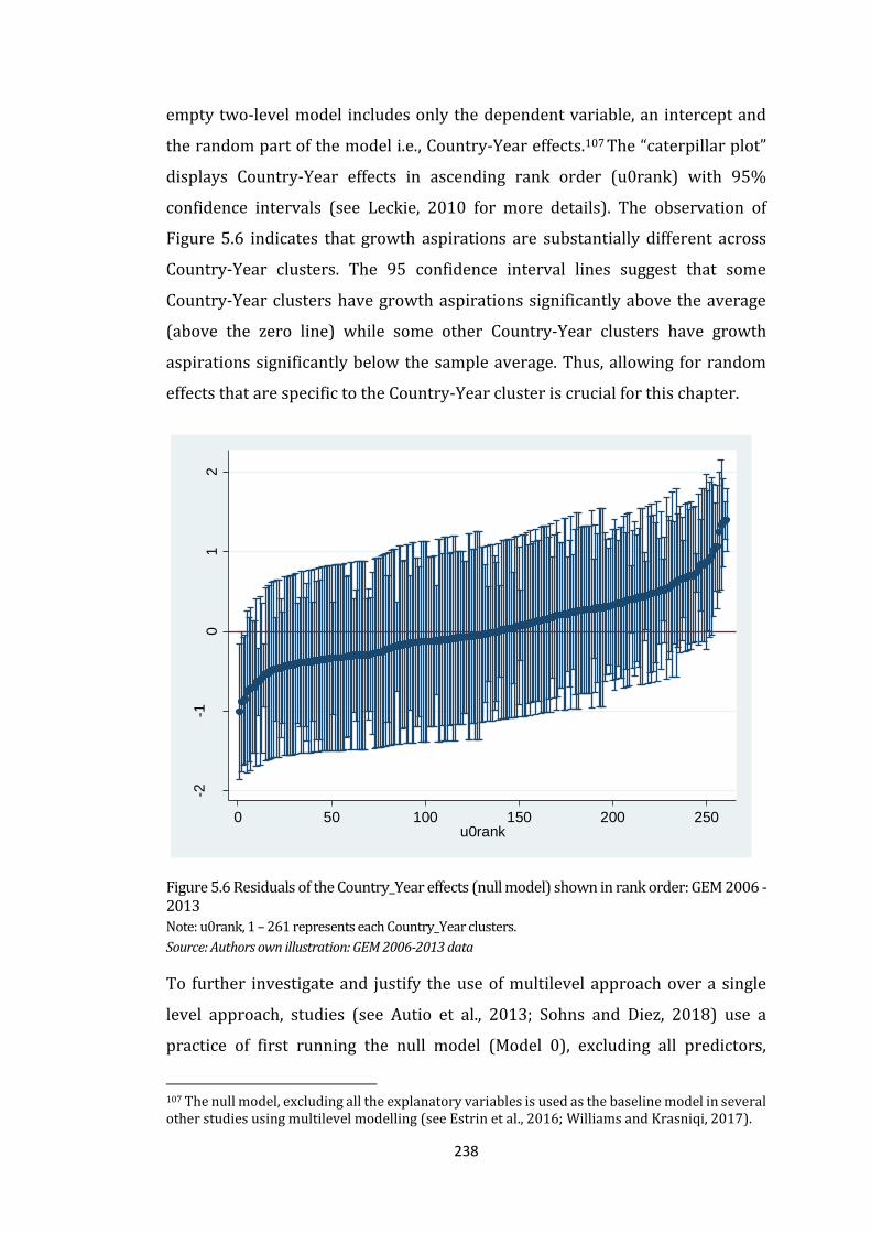
238
empty two-level model includes only the dependent variable, an intercept and
the random part of the model i.e., Country-Year effects.107 The “caterpillar plot”
displays Country-Year effects in ascending rank order (u0rank) with 95%
confidence intervals (see Leckie, 2010 for more details). The observation of
Figure 5.6 indicates that growth aspirations are substantially different across
Country-Year clusters. The 95 confidence interval lines suggest that some
Country-Year clusters have growth aspirations significantly above the average
(above the zero line) while some other Country-Year clusters have growth
aspirations significantly below the sample average. Thus, allowing for random
effects that are specific to the Country-Year cluster is crucial for this chapter.
Figure 5.6 Residuals of the Country_Year effects (null model) shown in rank order: GEM 2006 -2013 Note: u0rank, 1 – 261 represents each Country_Year clusters.
Source: Authors own illustration: GEM 2006-2013 data
To further investigate and justify the use of multilevel approach over a single
level approach, studies (see Autio et al., 2013; Sohns and Diez, 2018) use a
practice of first running the null model (Model 0), excluding all predictors,
107 The null model, excluding all the explanatory variables is used as the baseline model in several other studies using multilevel modelling (see Estrin et al., 2016; Williams and Krasniqi, 2017).
-2-1
01
2
rand
om
effe
cts
for
Co
un
try_Y
ear:
_con
s
0 50 100 150 200 250u0rank

239
individual, institutional characteristics and country-level controls (see Appendix
5.3). The variance component of random intercept of the null model (Model 0)
for multilevel logistic estimator points to 0.467 and is highly significant
(p<0.001). The next specification includes only the individual-level variables (see
Appendix 5.3) and indicates that the variance of the random effect declines to
0.368, suggesting the individual variables explain up to 21.2% of the variance.108
The variance component of random intercept of the full model (Model 1) in Table
5.4, suggests for a variance of the random effect of 0.117. This suggests that
adding country-level controls and institutional variables explains 74.9% of the
overall Country-Year variance.109 This also means that the country-level controls
and institutional variables, collectively explain 53.7% of the total variance,
providing a justification of applying multilevel approach.110
In addition, the superiority of multilevel modelling over a single-level approach
is emphasised by the variance explained by the Country-Year effects. In all the
specifications, the variance explained by the Country-Year effects is highly
significant (p<0.001) (see Tables 5.4, 5.5, 5.6 and Appendices 5.5-5.10). The ICCs
suggest that country-level institutional variables explain a significant part of the
cross-country variance which helps in explaining entrepreneurial growth
aspirations. In the null model, where only the random Country-Year effects are
included, the intra-class correlation (ICC) values indicate that 6.1% to 12.4%
(p<0.000 (see Appendix 5.3 and 5.3.1) of the variance in growth aspirations
resides between Country_Years clusters (see ICC of Model 0 in both sets of results
in Table 5.4). Similar ICC values are also reported by other studies in the context
of growth aspirations (see e.g., Autio et al., 2013). These ICC values support the
application of the multilevel approach over other conventional estimators.
The diagnostics of Model 1 in Table 5.4, where all the variables are included,
suggests that the ICC is still differently from zero but decreases to 0.041 and
0.034, respectively. Although the variance has decreased considerably, the intra-
class correlation of the (ICC=0.041 and 0.034) still indicates that some variation
108 The calculation: (((0.467-0.368)/0.467)*100) 109 The calculation: (((0.368-0.117)/0.368)*100) 110 The calculation: (((0.368-0.117)/0.467)*100)
240
in growth aspirations remains unexplained. Similarly, the likelihood-ratio (LR)
test, in all the specifications, suggests that the null of no cross-country variation
in young firms’ employment growth and high-job growth (HJG) aspirations can
be safely rejected (at 1the % significance level) (see Appendices 5.5 and 5.6).111
Some additional considerations are given to the data and estimation approach
prior to specifying any model and performing any empirical analysis – in
particular the presence of endogeneity. Empirical studies suggest that
endogeneity between entrepreneurs’ growth aspirations and the institutional
and macroeconomic control variables is likely to be present in our analysis (see
Estrin et al., 2013; Capelleras et al., 2018). For instance, the high prevalence rate
of ambitious and growth-oriented entrepreneurs at the country level, might
positively impact GDP per capita and GDP growth rates and also positively impact
the quality of institutions. Following Stuetzer et al. (2014), Estrin et al. (2016)
and Capelleras et al. (2018), to alleviate the presence of potential endogeneity,
this chapter uses the lagged values for the macroeconomic control variables and
lagged values for the country-level institutional quality factors. The
macroeconomic control variables are lagged for one year while institutional
variables are lagged for three years. In addition, to helping alleviate the issue of
endogeneity, lagging institutional quality variables, brings other benefits in this
investigation. As the dependent variables, employment growth and high-job
growth aspirations of young firms, represent young businesses with a maximum
of 3.5 years since start up, the lagged (3 years) institutional quality variables can
explain the impact since the conception of the business.
Further, formal checks for the potential correlation and multicollinearity are
performed in all the three datasets. The Variance Inflation Factor (VIF) indicates
that multicollinearity is not an issue (mean VIF=1.86) as none of the variables has
a VIF value of more than 10 (Hair et al., 2006) (see Appendix 5.4) (only one
variable has a value slightly higher than 5). Goldberger (1991) provides an
extensive discussion of the multicollinearity issue and the risk of
“micronumerosity”, which he defines as the ”problem of small sample size”
111 Although the LR test is conservative and provided only for reference in the mixed-linear regressions, still authors report and use it to guide their model selection (see Farla, 2014).

241
(Wooldridge, 2015). The chances of high multicollinearity in large datasets, such
as the ones used in this chapter, are small (Goldberger, 1991). However, the pair
wise correlation suggests that when full sample is considered, two pairs of
variables, namely freedom of doing business (bussfree) and corruption (0.76);
and GDP per capita and corruption (0.84) are highly correlated (see Appendix
5.2). To account for the high correlation between the latter pair, GDP per capita
is disintegrated according to its distribution, into five dummies (representing five
quintiles of the original GDP per capita variable). For the first pair, the safest decision
is to enter the two variables separately in the model, i.e., dropping corruption when
bussfree is included and vice versa.
Given that the data in this chapter use different units of measurement and
variables are in a very different scale of magnitudes, the chapter uses
standardised values for all the variables apart from dummies (see Autio et al.,
2014; Estrin et al., 2016). The standardisation of variables makes their standard
deviation one and their mean value practically zero (Long and Freese, 2014). The
standardised regression coefficient measures the expected standard deviation
change in the dependent variable associated with a one standard deviation
change in the independent variable (Allen, 1997). To make the interpretation of
results easier, the mixed-effect logistic regression model presents odds ratios
(OR) instead of coefficients. If the OR>1, then there is a positive relationship
between the independent and the dependent variable, high-job growth
aspirations. In an analogy, if the OR<1, it suggests for a negative effect of the
independent variable on high-job growth aspirations of the young business.
Model specification
In a standard Ordinary Least Square (OLS) regression model, the effect of X on Y
is estimated ignoring the group structure. The single random residual adjusts the
prediction to the observed value for each individual observation (Snijders and
Bosker, 2012).
𝑌𝑖𝑗 = 𝛽0 + 𝛽1𝜒𝑖𝑗 + 휀𝑖𝑗 (5.1)
Where 𝑌𝑖𝑗 is the dependent variable; 𝜒𝑖𝑗 explanatory variables at level one; 휀𝑖𝑗 is
the individual-level (level-1) error term; and subscript 𝑖 indicates level-one unit

242
(e.g., individual); 𝑗 indicates level-two unit (e.g., country). In the linear regression
random intercept model, the intercepts 𝛽0𝑗 are random variables representing
random differences between groups, i.e., countries. The following equation
represents the random intercept model:
𝑌𝑖𝑗 = 𝛽0𝑗 + 𝛽1𝑗𝜒𝑖𝑗 + 𝑢𝑗 + 휀𝑖𝑗
(5.2)
where the residual 𝛽0𝑗 is decomposed into two random terms, one for the
individual and the other for the aggregate level (Snijders and Bosker, 2012):
𝛽0𝑗 = 𝛾00 + 𝑈0𝑗 (5.3)
Where 𝛾00 is the random (average) intercept and 𝑈0𝑗 represents the random
deviation (noise), i.e., Country-Year specific component, which corrects the
average intercept of each cluster. The Country-Year specific component, level-2,
is constant for all the individuals in that Country-Year (cluster). The level-1
residual in all the Eqs. is specific for each individual, i.e., varies between
individuals 𝑖 and also between Country-Year clusters 𝑗. In random intercept models,
the constant regression coefficient 𝛽1 is sometimes denoted as 𝛾10. Hence, the final
equation for a multilevel linear regression model including both fixed and
random effects (random intercept), takes the following form:
𝑌𝑖𝑗 = 𝛾00 + 𝛾10𝜒𝑖𝑗
+ 𝑈0𝑗 + 휀𝑖𝑗 (5.4)
Similar to Estrin et al. (2013), in addition to the individual characteristics, the
study includes also the country-means of some variables that might affect
entrepreneurial growth aspirations. The human (educ_postgr), financial (hhinc)
and social (KNOWENT_dum) capital were aggregated at the country level and
included in the specifications. For the innovation-driven economies, the variable
scaled to the country level is the one capturing serial (capturing) entrepreneurs
(omESTBBUS_dum). These means represent the so-called peer-effects and can
help explain the differences across countries and years (see also Estrin et al.,
2016). To accommodate the country-mean variables, the equation below
represents the linear mixed model with separate effects for the original
variable 𝜒𝑖𝑗 and the country-mean �̅�.𝑗.

243
𝑌𝑖𝑗 = 𝛾00 + 𝛾10𝜒𝑖𝑗
+ 𝛾01�̅�.𝑗 + 𝑈0𝑗 + 휀𝑖𝑗 (5.5)
Finally, the complete model with all the explanatory variables is presented below
in Eq. (5.6):
𝑌𝑖𝑗 = 𝛾00 + 𝛾10𝜒1𝑖𝑗
+ 𝛾01�̅�1𝑗 + ⋯ + 𝛾𝑝0𝜒𝑝𝑖𝑗 + 𝛾01𝜒𝑧𝑖𝑗 + ⋯ + 𝛾0𝑞𝑍𝑞𝑗 + 𝑈0𝑗 + 휀𝑖𝑗
(5.6)
Subscript 𝑖𝑗 described: 𝑖 represents individuals (𝑖 =1,…, 𝑛𝑗); 𝑗 a particular country-
year sample (𝑗=1,…, N). 𝜒1𝑖𝑗; 𝜒𝑝𝑖𝑗; 𝜒𝑧𝑖𝑗 represent individual-level variables (level-
one); 𝛾01�̅�1𝑗 represents country-means; and 𝑍𝑞𝑗 represent explanatory variables
at level-2 (country-level variables). Adopting Eq. (5.6) to our context brings this
form of equation:
EGAij= β0 + β1curr_empij + β2ageij + β3maleij + β4educ_postgrij + β5gemhhincomeij + β6KNOWENT_dumij + β7BUSang_dumij + β8omESTBBUS_dumij + β9bb_ownerij + β10work_statusij + β11skills_dumij + β12opportunitiesij + β13estbusrateij + β14meduc_postgrj + β15mhhincj + β16mKNOWENT_dumj + β17momESTBBUS_dumj + β18buss_freej + β19exe_consj + β20gov_sizej + β21corruptionj + β22highgrowth_supportj + β23gdpgrowthj + β24gdppcj + uj + εij (5.7) Where: EGA represents Employment Growth Aspirations (1st DV); and Individual-level characteristics: curr_empij; ageij; maleij; educ_postgrij; gemhhincomeij; KNOWENT_dumij; BUSang_dumij; omESTBBUS_dumij; bb_ownerij; work_statusij; skills_dumij; opportunitiesij: Country mean: meduc_postgrj; mhhincj; mKNOWENT_dumj; momESTBBUS_dumj; Institutional/contextual: buss_freej; exe_consj; gov_sizej; corruptionj; highgrowth_supportj; Macroeconomic controls: estbusratej; gdpgrowthj; gdppcj.
For the multilevel logistic model, the baseline equation accommodating a two-
level model, where for a series of N independent clusters, and conditional on a
set of random effects 𝑢𝑗 is as follows (Statacorp manual 15):
𝑃𝑟 (𝛾𝑖𝑗 = 1|𝑢𝑗) = 𝐻 (𝑥𝑖𝑗𝛽 + 𝑧𝑖𝑗𝑢𝑗) (5.8)
Where, 𝑗 represents country-year cluster (𝑗=1,…,N); and 𝑖 represents individual
observations belonging to these clusters (𝑖 =1,…, 𝑛𝑗). 𝛾𝑖𝑗 represents binary
responses where 𝛾𝑖𝑗=1 if 𝛾𝑖𝑗 ≠ 0, meaning that young businesses expect to create
244
20 jobs in five years, and 𝛾𝑖𝑗 = 0 otherwise. The 𝑥𝑖𝑗𝛽 denotes fixed effect portion
of the model while the 𝑧𝑖𝑗 are the covariates representing the random portion of
this model. In this structure of logistic regression, H (𝑥𝑖𝑗𝛽 + 𝑧𝑖𝑗𝑢𝑗) denotes the
logistic cumulative distribution function, used to predict the probability of
success (𝛾𝑖𝑗=1), with H(var)=exp(var)/{1+exp(var)}. Adopting Eq. (5.8) to the
two-level binary logistic random intercept model, where 𝜋𝑖𝑗=Pr(𝐻𝐽𝐺𝑖𝑗 = 1) gives
the following equation:
𝑙𝑜𝑔𝑖𝑡(𝜋𝑖𝑗) = 𝛽0 + 𝛽𝑝𝜒𝑝𝑖𝑗 + 𝛽01�̅�1𝑗 + ⋯ + 𝛽𝑞𝑍𝑞𝑗 + 𝑈0𝑗 + 휀𝑖𝑗 (5.9)
where, 𝜒𝑝𝑖𝑗 represent individual-level variables (level-one); �̅�1𝑗 represents
country-means; and 𝑍𝑞𝑗 represent explanatory variables at level-2 (country-level
variables). The country-year error term is denoted by 𝑈0𝑗 , while the individual-
level error is 휀𝑖𝑗 .
More specifically:
𝑙𝑜𝑔𝑖𝑡(𝜋𝑖𝑗) = β1curr_empij + β2ageij + β3maleij + β4educ_postgrij +
β5gemhhincomeij + β6KNOWENT_dumij + β7BUSang_dumij + β8omESTBBUS_dumij + β9bb_ownerij + β10work_statusij + β11skills_dumij + β12opportunitiesij + β13estbusrateij + β14meduc_posstgrj + β15mhhincj + β16mKNOWENT_dumj + β17momESTBBUS_dumj + β18buss_freej + β19exe_consj + β20gov_sizej + β21corruptionj + β22highgrowth_supportj + β23gdpgrowthj + β24gdppcj+ uj + εij (5.10)
𝜋𝑖𝑗=Pr(𝐻𝐽𝐺𝑖𝑗 = 1); HJG represents High-job Growth Aspirations (2nd DV); HJG is
equal to 1 if the young businesses expect to create at least 20 jobs within 5 years
and zero otherwise.
The chapter employs the same set of variables also when investigating factors
that influence high-job growth aspiration entrepreneurship. This practice allows
for direct comparison of the influence that the same set of individual, country and
macroeconomic variables have on two relatively different dependent variables.
The emphasis is on the influence that institutional quality variables have on the
two dependent variables and how the individual characteristics might moderate
the influence of institutions on employment growth and on high-job growth
aspirations, respectively. The same approach, of using the same set of variables
245
on two different dependent variables, has also been employed by similar studies
of the field of entrepreneurship (see Autio and Fu, 2015; Estrin and Mickiewicz,
2011).
EMPIRICAL RESULTS
This section reports and interprets the results of the multilevel linear approach
and multilevel logistic estimation methodologies explained in the previous
section. Given the emphasised relevance of different economic context, i.e., stages
of development, in shaping young firms’ growth aspirations, results are
presented into three separate tables, Table 5.4, Table 5.5 and Table 5.6. The first
table presents results when all countries (full sample) are included in the analysis
and no relevance to the role of the stage of economic development is envisaged
(apart from the GDP per capita and GDP growth variables which capture some
differences). Table 5.5, and 5.6 emphasise the differences that the current stage
of economic development has on employment growth and high-growth
aspirations. Table 5.5 reports results of both innovation-driven and efficiency-
driven economies where employment growth aspirations (EGA) and multilevel
linear regression model is used. Table 5.6 reports results of the two subsamples
where high-job growth (HJG) aspirations is used as the dependent variable and
multilevel logistic as the estimation approach. In Table 5.4, a significant focus will
be given to the relatively different role of institutions and individual variables on
the two dependent variables, namely employment growth aspirations (EGA) and
high-job growth aspirations (HJG). In Table 5.5 and 5.6 the main focus will be on
differences between innovation-driven and efficiency-driven economies.
Comparisons of the findings of the three samples will be discussed throughout of
the results sections below and will be highlighted in the conclusions section.
Results
Tables 5.4 reports five specifications for each set of results (Model 0 – Model 4),
i.e., five specifications for employment growth aspirations (EGA) and five for
high-job growth aspirations (HJG). Tables 5.5 and 5.6 report five specifications
for each of the two stages of development. Specifically, when assessing
employment growth aspirations (EGA), Table 5.5 reports five specifications for

246
innovation-driven and five for efficiency-driven economies, respectively.
Similarly, Table 5.6 reports five specifications for innovation-driven and five for
efficiency-driven economies, when presenting the results for high-job growth
aspirations (HJG). In Table 5.4 due to high correlation between business freedom
and corruption and between corruption and GDP per capita, Model 1 includes
business freedom, while Model 2 includes corruption and the four-quantiles and
drops business freedom and GDP per capita to alleviate the potential presence of
multicollinearity. Model 3 and 4 in Table 5.4 and Model 2 – 4 in Tables 5.5 and
5.6 use cross-level interactions, i.e., interactions between individual-level and
institutional variables. Although, the suggested approach, when using
standardised variables in a linear mixed-effect regression, is to interpret results
using a one unit increase in standard deviation of the independent variable, this
chapter transforms the estimated coefficient so that one unit increase in the
independent variable leads to an increase/decrease by (b) percentage points in
the dependent variable. Multilevel logistic results will be interpreted using odds
ratios (OR) and a one unit increase on standard deviation. In addition to the
individual, institutional, and country-level control variables, this chapter uses
country-mean effects of some variables that are hypothesised to impact growth
aspirations. For instance, in Table 5.4, four country-means are included,
accounting for the effect of human, financial and social capital and the experience
of the entrepreneur.
The results indicate that most of the individual-level attributes have a positive
and significant effect on growth aspirations. 112 With respect to the country-level
institutional variables, results indicate that the size of public sector, corruption
levels and the extent of property rights protection are significantly associated
with growth aspirations. A counterintuitive finding is that employment growth
aspirations (EMP) of young businesses operating in efficiency-driven economies
do not appear to be affected by any of the institutional quality variables.
However, young businesses with high-growth aspirations, in efficiency-driven
economies, benefit from a sound property right protection regime.
112 See Appendix 5.5 and 5.6 for Table 5.4; Appendix 5.7 and 5.8 for Table 5.5 and Appendix 5.9 and 5.10 for Table 5.6

247
Table 5.4 Results for entrepreneurial growth aspirations: (EGA - columns 1-5); (HJG - columns 6-10) – All countries included
Employment Growth Aspirations (EGA) Multilevel linear regression
High-job Growth Aspirations (HJG) Multilevel logistic regression
(Model 0) (Model 1) (Model 2) (Model 3) (Model 4) (Model 0) (Model 1) (Model 2) (Model 3) (Model 4)
VARIABLES EGA-All
countries EGA-All
countries EGA-All
countries EGA-All
countries EGA-All
countries HJG-All
countries HJG-All
countries HJG-All
countries HJG-All
countries HJG-All
countries Individual level Current employment -0.046*** -0.047*** -0.046*** -0.047*** 2.175*** 2.170*** 2.176*** 2.173*** (employm_babybus1) (0.009) (0.009) (0.009) (0.009) (0.063) (0.063) (0.063) (0.063) Age -0.075*** -0.076*** -0.076*** -0.075*** 0.976 0.975 0.976 0.976 (age) (0.009) (0.009) (0.009) (0.009) (0.039) (0.039) (0.039) (0.039) Gender (M=1) 0.098*** 0.098*** 0.098*** 0.098*** 1.480*** 1.471*** 1.479*** 1.475*** (male) (0.022) (0.021) (0.022) (0.022) (0.129) (0.128) (0.129) (0.129) Edu. Postsecondary 0.073*** 0.072*** 0.073*** 0.073*** 1.335** 1.321** 1.335** 1.333** (educ_postgr) (0.027) (0.027) (0.027) (0.027) (0.161) (0.160) (0.161) (0.161) Household inc. (2nd level) 0.068*** 0.068*** 0.069*** 0.068*** 0.987 0.991 0.969 0.991 (gemhhincome) (0.017) (0.017) (0.018) (0.017) (0.128) (0.128) (0.126) (0.128) Household inc. (3rd level) 0.098*** 0.099*** 0.100*** 0.099*** 1.254* 1.258* 1.241* 1.265* (gemhhincome) (0.025) (0.025) (0.025) (0.025) (0.152) (0.152) (0.151) (0.153) Knows entrepr. (Netw.) 0.089*** 0.089*** 0.090*** 0.092*** 1.737*** 1.730*** 1.737*** 1.793*** (KNOWENT_dum) (0.015) (0.015) (0.015) (0.015) (0.159) (0.158) (0.159) (0.168) Business angel 0.086*** 0.086*** 0.086*** 0.086*** 1.457*** 1.474*** 1.458*** 1.460*** (BUSang_dum) (0.027) (0.027) (0.027) (0.027) (0.159) (0.161) (0.159) (0.159) Own/mng of exist. Bus -0.251*** -0.252*** -0.251*** -0.250*** 2.345*** 2.352*** 2.351*** 2.372*** (omESTBBUS_dum) (0.045) (0.045) (0.045) (0.045) (0.396) (0.398) (0.397) (0.401) More than 1 owner 0.090*** 0.090*** 0.090*** 0.090*** 1.094 1.101 1.094 1.095 (bb_owners) (0.019) (0.019) (0.019) (0.019) (0.089) (0.090) (0.089) (0.089) Employment status (E=1) 0.106*** 0.106*** 0.106*** 0.106*** 0.760 0.754 0.760 0.762 (work_status) (0.039) (0.039) (0.039) (0.039) (0.145) (0.144) (0.144) (0.145) Skills 0.160*** 0.161*** 0.160*** 0.161*** 1.301** 1.306** 1.303** 1.304** (suskill_dum) (0.017) (0.017) (0.017) (0.017) (0.167) (0.168) (0.167) (0.168) Perceived opportunities 0.185*** 0.186*** 0.185*** 0.184*** 1.638*** 1.658*** 1.641*** 1.635*** (opportunities) (0.021) (0.021) (0.021) (0.021) (0.141) (0.143) (0.142) (0.141)
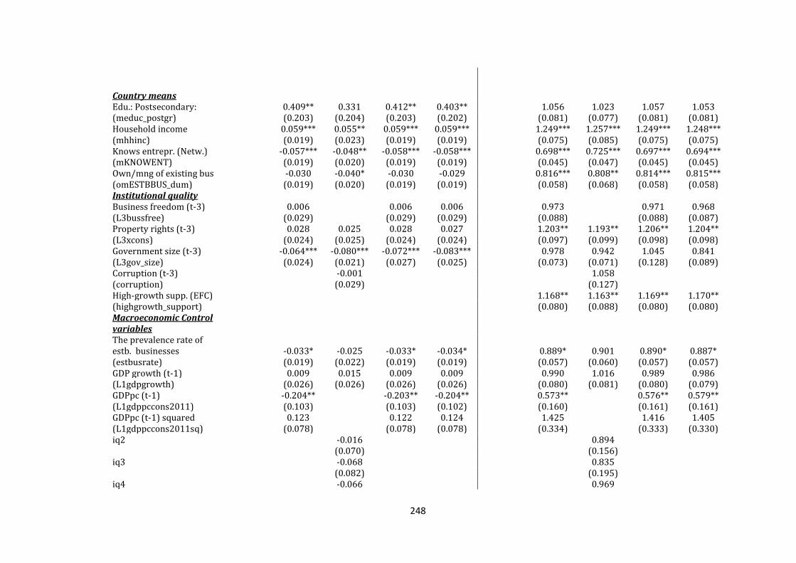
248
Country means Edu.: Postsecondary: 0.409** 0.331 0.412** 0.403** 1.056 1.023 1.057 1.053 (meduc_postgr) (0.203) (0.204) (0.203) (0.202) (0.081) (0.077) (0.081) (0.081) Household income 0.059*** 0.055** 0.059*** 0.059*** 1.249*** 1.257*** 1.249*** 1.248*** (mhhinc) (0.019) (0.023) (0.019) (0.019) (0.075) (0.085) (0.075) (0.075) Knows entrepr. (Netw.) -0.057*** -0.048** -0.058*** -0.058*** 0.698*** 0.725*** 0.697*** 0.694*** (mKNOWENT) (0.019) (0.020) (0.019) (0.019) (0.045) (0.047) (0.045) (0.045) Own/mng of existing bus -0.030 -0.040* -0.030 -0.029 0.816*** 0.808** 0.814*** 0.815*** (omESTBBUS_dum) (0.019) (0.020) (0.019) (0.019) (0.058) (0.068) (0.058) (0.058) Institutional quality Business freedom (t-3) 0.006 0.006 0.006 0.973 0.971 0.968 (L3bussfree) (0.029) (0.029) (0.029) (0.088) (0.088) (0.087) Property rights (t-3) 0.028 0.025 0.028 0.027 1.203** 1.193** 1.206** 1.204** (L3xcons) (0.024) (0.025) (0.024) (0.024) (0.097) (0.099) (0.098) (0.098) Government size (t-3) -0.064*** -0.080*** -0.072*** -0.083*** 0.978 0.942 1.045 0.841 (L3gov_size) (0.024) (0.021) (0.027) (0.025) (0.073) (0.071) (0.128) (0.089) Corruption (t-3) -0.001 1.058 (corruption) (0.029) (0.127) High-growth supp. (EFC) 1.168** 1.163** 1.169** 1.170** (highgrowth_support) (0.080) (0.088) (0.080) (0.080) Macroeconomic Control variables The prevalence rate of estb. businesses -0.033* -0.025 -0.033* -0.034* 0.889* 0.901 0.890* 0.887* (estbusrate) (0.019) (0.022) (0.019) (0.019) (0.057) (0.060) (0.057) (0.057) GDP growth (t-1) 0.009 0.015 0.009 0.009 0.990 1.016 0.989 0.986 (L1gdpgrowth) (0.026) (0.026) (0.026) (0.026) (0.080) (0.081) (0.080) (0.079) GDPpc (t-1) -0.204** -0.203** -0.204** 0.573** 0.576** 0.579** (L1gdppccons2011) (0.103) (0.103) (0.102) (0.160) (0.161) (0.161) GDPpc (t-1) squared 0.123 0.122 0.124 1.425 1.416 1.405 (L1gdppccons2011sq) (0.078) (0.078) (0.078) (0.334) (0.333) (0.330) iq2 -0.016 0.894
(0.070) (0.156) iq3 -0.068 0.835
(0.082) (0.195) iq4 -0.066 0.969
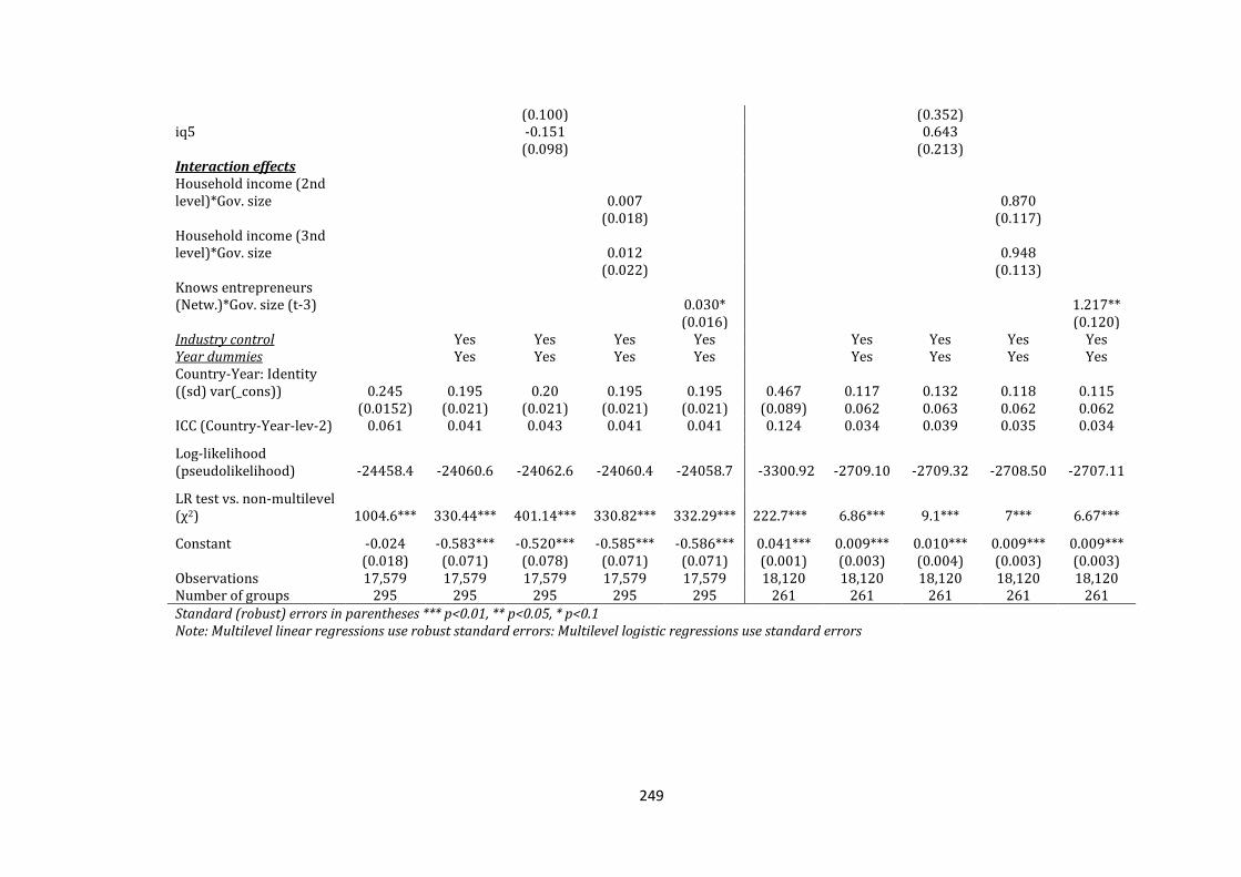
249
(0.100) (0.352) iq5 -0.151 0.643
(0.098) (0.213) Interaction effects Household income (2nd level)*Gov. size 0.007 0.870
(0.018) (0.117) Household income (3nd level)*Gov. size 0.012 0.948
(0.022) (0.113) Knows entrepreneurs (Netw.)*Gov. size (t-3) 0.030* 1.217**
(0.016) (0.120) Industry control Yes Yes Yes Yes Yes Yes Yes Yes Year dummies Yes Yes Yes Yes Yes Yes Yes Yes Country-Year: Identity ((sd) var(_cons)) 0.245 0.195 0.20 0.195 0.195 0.467 0.117 0.132 0.118 0.115 (0.0152) (0.021) (0.021) (0.021) (0.021) (0.089) 0.062 0.063 0.062 0.062 ICC (Country-Year-lev-2) 0.061 0.041 0.043 0.041 0.041 0.124 0.034 0.039 0.035 0.034
Log-likelihood (pseudolikelihood) -24458.4 -24060.6 -24062.6 -24060.4 -24058.7 -3300.92 -2709.10 -2709.32 -2708.50 -2707.11
LR test vs. non-multilevel (χ2) 1004.6*** 330.44*** 401.14*** 330.82*** 332.29*** 222.7*** 6.86*** 9.1*** 7*** 6.67***
Constant -0.024 -0.583*** -0.520*** -0.585*** -0.586*** 0.041*** 0.009*** 0.010*** 0.009*** 0.009***
(0.018) (0.071) (0.078) (0.071) (0.071) (0.001) (0.003) (0.004) (0.003) (0.003) Observations 17,579 17,579 17,579 17,579 17,579 18,120 18,120 18,120 18,120 18,120 Number of groups 295 295 295 295 295 261 261 261 261 261 Standard (robust) errors in parentheses *** p<0.01, ** p<0.05, * p<0.1 Note: Multilevel linear regressions use robust standard errors: Multilevel logistic regressions use standard errors
250
Individual-level and young business characteristics
The estimated results suggest that entrepreneur’s education (human capital), has
a positive and significant impact on employment growth aspirations (EGA) when
all countries are included in the sample. It is estimated that on average, holding
other factors constant, having a post-secondary degree increases young
businesses’ employment growth aspirations by a 5 percentage points. Similarly,
the multilevel logistic estimated results indicate a positive and significant effect
of education on high-job growth aspirations. Namely, the odds ratio (OR=1.34,
p<0.05) suggest that having a post-secondary (higher) degree is mostly
associated with high-job growth (HJG) aspiration. Holding other variables
constant, the odds of an entrepreneur aspiring to create at least 20 jobs in five
years are 33.5% higher compared to the base category (no post-secondary
education) (see model 1, HJG set of results in Table 5.4). The results in Table 5.5
suggest that education has a positive and significant effect on employment
growth aspirations (EGA) for the young businesses operating in innovation-
driven economies but appear to be insignificant for businesses operating in
efficiency-driven economies. The statistical significance switches places when
the results of high-job growth aspirations (HJG) dependent variable are
presented in Table 5.6. It is now the growth aspirations of the young businesses
in efficiency-driven economies that seem to benefit from entrepreneur’s
education, while growth aspirations of young businesses in innovation-driven
economies are not significantly affected. In general, however, these results
provide evidence of the role of human capital on shaping growth aspirations.
Previous studies have also reported positive effects (see e.g., Lim et al., 2016;
Puente et al., 2017; Giotopoulos et al., 2017).
As theorised by many researchers (see Levie and Autio, 2013; Lim et al., 2016;
Giotopoulos et al., 2017), household income (financial capital) has a positive
impact on entrepreneurial growth aspirations. While both levels of household
income are reported to have a positive impact on employment growth
aspirations, only the highest level of household income appears positive and
significant for high-job growth aspirations when all countries are included. The
magnitude of the highest level of household income is larger in both sets of
251
results and in all the three samples, suggesting that the higher the financial
capital (household income) of an entrepreneur, the larger the impact on growth
aspirations. The estimated results, when all countries are included, suggest that
entrepreneurs belonging to a household on the highest level of income, on
average, have growth aspirations higher by 6.7 percentage points compared to
the entrepreneurs of the lowest household income group. Similarly, the odds are
suggested to be 25% higher for a young business to create 20 jobs in five years if
the entrepreneur belongs to the highest category of household income, ceteris
paribus. Table 5.5 suggests that household financial capital is more relevant to
young businesses operating in efficiency-driven economies than to young
businesses operating in innovation-driven economies. As it is pointed out in
section 5.3.1, informal finance is more important for businesses that operate in
economies with weak formal financial sector and insufficient financing
alternatives. It is very likely that most of the efficiency-driven economies lack a
well-developed formal financial sector, hence young businesses, compared to
those operating in innovation-driven economies seem to more heavily rely on
informal or self-financing sources. Table 5.5 suggests that if the owner of a young
business, in efficiency-driven economies, belongs to a household on the highest
level of income, on average, her growth aspirations are higher by 8.04 percentage
points compared to the entrepreneurs of the lowest household income group. In
the innovation-driven economy context, growth aspirations are higher by only
3.2 percentage points compared to the entrepreneurs of the lowest household
income group, ceteris paribus.
The results also suggest that social capital, reflected by knowing other
entrepreneurs (KNOWENT_dum) (role models) who have started a business in
the last two years and providing financial funds (BUSang_dum) to other start-ups
in the last three years positively impacts entrepreneurial growth aspirations.
Results are in accordance with previous research in this field. For instance,
Giotopoulos et al. (2017), find that knowing other entrepreneurs has a positive
and significant impact on high-growth entrepreneurial ventures. Similarly, Estrin
et al. (2013) find that supporting other entrepreneurs by serving as a business
angel is positively associated with entrepreneurial growth aspirations. Holding
252
other factors constant, on average, employment growth aspirations of an
entrepreneur with social contacts are higher by 5.5 percentage points in
innovation-driven and by 6.4 percentage points in efficiency-driven economies
compared to the counterpart. The odds are higher by 56-76% (OR=1.56, p<0.001
in innovation-driven; and OR=1.76, p<0.001 in efficiency-driven economies),
suggesting that social capital and social interaction is a significant determinant
of growth aspirations. Similarly, being a business angel i.e., providing financial
support to other start-ups increases the odds of creating 20 jobs in five years by
46-49% compared to the base category (no financial funds provided). On
average, having provided funds to other start-ups increases employment growth
aspirations by 5.9 percentage points (Table 5.4), holding other factors constant.
In line with the existing literature, results suggest that both, the perceived
capabilities (skills) and opportunities are a significant determinant of growth
aspirations (see Tominc and Rebernik, 2007; Ciravegna et al., 2014; Bosma et al.,
2018; Capelleras et al., 2018). The results indicate that if the entrepreneur
considers having the required skills and knowledge to start and run a business,
on average, her employment growth aspirations increase by 11 percentage
points, holding other factors fixed (Table 5.4). Giotopoulos et al. (2017), find that
if an individual believes having the required skills (they refer to skills as self-
confidence), in general, her growth aspirations are higher. Similarly, if the
entrepreneurs consider that in the next six months, there are good opportunities
to start a new business, on average and holding other factors constant, their
employment growth aspirations increase by 12.6 percentage points (8.3 pp for
innovation-driven; 14.8 pp for efficiency-driven economies). The results are in
line with the findings reported by Giotopoulos et al. (2017) and Capelleras et al.
(2018). Entrepreneurs’ positive outlook for the business opportunities is one of
the key determinants of growth aspirations, regardless of the entrepreneurship
context or the dependent variable used. This finding can be linked to the
opportunity recognition hypothesis (Aidis et al., 2008; Alvarez et al., 2013).
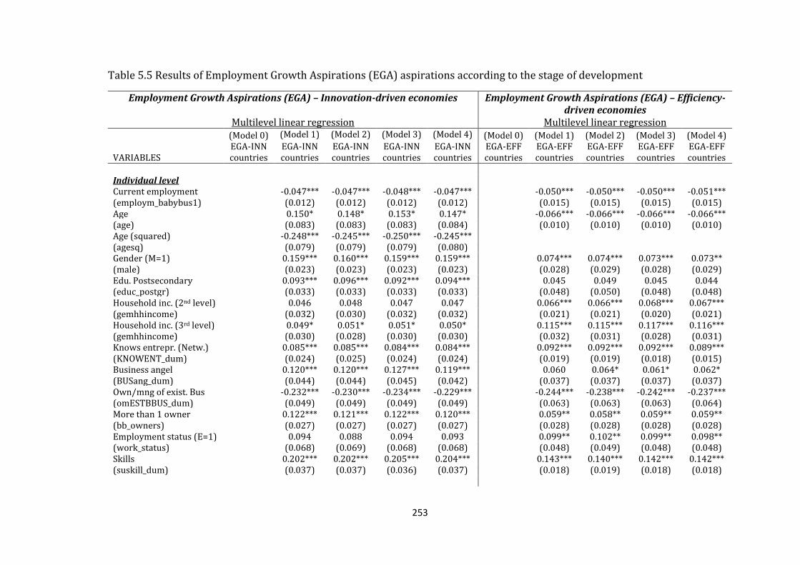
253
Table 5.5 Results of Employment Growth Aspirations (EGA) aspirations according to the stage of development
Employment Growth Aspirations (EGA) – Innovation-driven economies
Multilevel linear regression
Employment Growth Aspirations (EGA) – Efficiency-driven economies
Multilevel linear regression (Model 0) (Model 1) (Model 2) (Model 3) (Model 4) (Model 0) (Model 1) (Model 2) (Model 3) (Model 4)
VARIABLES EGA-INN countries
EGA-INN countries
EGA-INN countries
EGA-INN countries
EGA-INN countries
EGA-EFF countries
EGA-EFF countries
EGA-EFF countries
EGA-EFF countries
EGA-EFF countries
Individual level Current employment -0.047*** -0.047*** -0.048*** -0.047*** -0.050*** -0.050*** -0.050*** -0.051*** (employm_babybus1) (0.012) (0.012) (0.012) (0.012) (0.015) (0.015) (0.015) (0.015) Age 0.150* 0.148* 0.153* 0.147* -0.066*** -0.066*** -0.066*** -0.066*** (age) (0.083) (0.083) (0.083) (0.084) (0.010) (0.010) (0.010) (0.010) Age (squared) -0.248*** -0.245*** -0.250*** -0.245*** (agesq) (0.079) (0.079) (0.079) (0.080) Gender (M=1) 0.159*** 0.160*** 0.159*** 0.159*** 0.074*** 0.074*** 0.073*** 0.073** (male) (0.023) (0.023) (0.023) (0.023) (0.028) (0.029) (0.028) (0.029) Edu. Postsecondary 0.093*** 0.096*** 0.092*** 0.094*** 0.045 0.049 0.045 0.044 (educ_postgr) (0.033) (0.033) (0.033) (0.033) (0.048) (0.050) (0.048) (0.048) Household inc. (2nd level) 0.046 0.048 0.047 0.047 0.066*** 0.066*** 0.068*** 0.067*** (gemhhincome) (0.032) (0.030) (0.032) (0.032) (0.021) (0.021) (0.020) (0.021) Household inc. (3rd level) 0.049* 0.051* 0.051* 0.050* 0.115*** 0.115*** 0.117*** 0.116*** (gemhhincome) (0.030) (0.028) (0.030) (0.030) (0.032) (0.031) (0.028) (0.031) Knows entrepr. (Netw.) 0.085*** 0.085*** 0.084*** 0.084*** 0.092*** 0.092*** 0.092*** 0.089*** (KNOWENT_dum) (0.024) (0.025) (0.024) (0.024) (0.019) (0.019) (0.018) (0.015) Business angel 0.120*** 0.120*** 0.127*** 0.119*** 0.060 0.064* 0.061* 0.062* (BUSang_dum) (0.044) (0.044) (0.045) (0.042) (0.037) (0.037) (0.037) (0.037) Own/mng of exist. Bus -0.232*** -0.230*** -0.234*** -0.229*** -0.244*** -0.238*** -0.242*** -0.237*** (omESTBBUS_dum) (0.049) (0.049) (0.049) (0.049) (0.063) (0.063) (0.063) (0.064) More than 1 owner 0.122*** 0.121*** 0.122*** 0.120*** 0.059** 0.058** 0.059** 0.059** (bb_owners) (0.027) (0.027) (0.027) (0.027) (0.028) (0.028) (0.028) (0.028) Employment status (E=1) 0.094 0.088 0.094 0.093 0.099** 0.102** 0.099** 0.098** (work_status) (0.068) (0.069) (0.068) (0.068) (0.048) (0.049) (0.048) (0.048) Skills 0.202*** 0.202*** 0.205*** 0.204*** 0.143*** 0.140*** 0.142*** 0.142*** (suskill_dum) (0.037) (0.037) (0.036) (0.037) (0.018) (0.019) (0.018) (0.018)
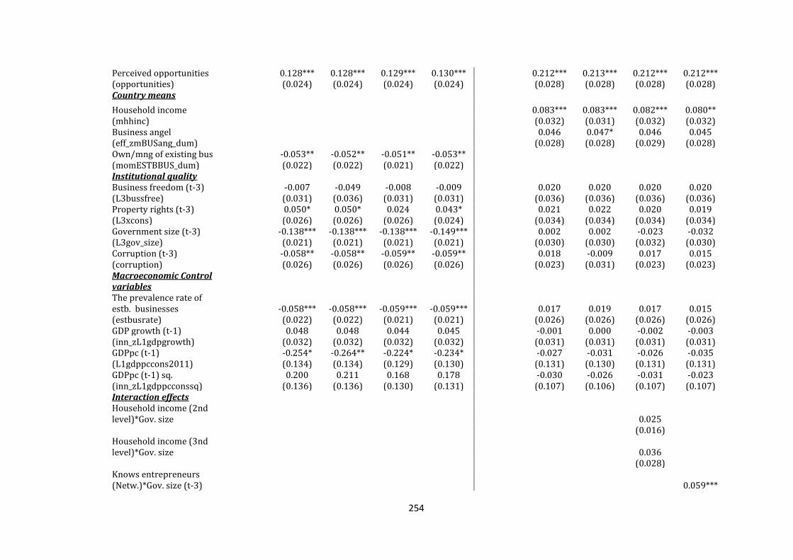
254
Perceived opportunities 0.128*** 0.128*** 0.129*** 0.130*** 0.212*** 0.213*** 0.212*** 0.212*** (opportunities) (0.024) (0.024) (0.024) (0.024) (0.028) (0.028) (0.028) (0.028) Country means
Household income 0.083*** 0.083*** 0.082*** 0.080** (mhhinc) (0.032) (0.031) (0.032) (0.032) Business angel 0.046 0.047* 0.046 0.045 (eff_zmBUSang_dum) (0.028) (0.028) (0.029) (0.028) Own/mng of existing bus -0.053** -0.052** -0.051** -0.053** (momESTBBUS_dum) (0.022) (0.022) (0.021) (0.022) Institutional quality Business freedom (t-3) -0.007 -0.049 -0.008 -0.009 0.020 0.020 0.020 0.020 (L3bussfree) (0.031) (0.036) (0.031) (0.031) (0.036) (0.036) (0.036) (0.036) Property rights (t-3) 0.050* 0.050* 0.024 0.043* 0.021 0.022 0.020 0.019 (L3xcons) (0.026) (0.026) (0.026) (0.024) (0.034) (0.034) (0.034) (0.034) Government size (t-3) -0.138*** -0.138*** -0.138*** -0.149*** 0.002 0.002 -0.023 -0.032 (L3gov_size) (0.021) (0.021) (0.021) (0.021) (0.030) (0.030) (0.032) (0.030) Corruption (t-3) -0.058** -0.058** -0.059** -0.059** 0.018 -0.009 0.017 0.015 (corruption) (0.026) (0.026) (0.026) (0.026) (0.023) (0.031) (0.023) (0.023) Macroeconomic Control variables The prevalence rate of estb. businesses -0.058*** -0.058*** -0.059*** -0.059*** 0.017 0.019 0.017 0.015 (estbusrate) (0.022) (0.022) (0.021) (0.021) (0.026) (0.026) (0.026) (0.026) GDP growth (t-1) 0.048 0.048 0.044 0.045 -0.001 0.000 -0.002 -0.003 (inn_zL1gdpgrowth) (0.032) (0.032) (0.032) (0.032) (0.031) (0.031) (0.031) (0.031) GDPpc (t-1) -0.254* -0.264** -0.224* -0.234* -0.027 -0.031 -0.026 -0.035 (L1gdppccons2011) (0.134) (0.134) (0.129) (0.130) (0.131) (0.130) (0.131) (0.131) GDPpc (t-1) sq. 0.200 0.211 0.168 0.178 -0.030 -0.026 -0.031 -0.023 (inn_zL1gdppcconssq) (0.136) (0.136) (0.130) (0.131) (0.107) (0.106) (0.107) (0.107) Interaction effects Household income (2nd level)*Gov. size 0.025 (0.016) Household income (3nd level)*Gov. size 0.036
(0.028) Knows entrepreneurs (Netw.)*Gov. size (t-3) 0.059***
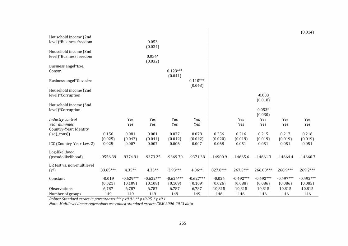
255
(0.014) Household income (2nd level)*Business freedom 0.053
(0.034) Household income (3nd level)*Business freedom 0.054*
(0.032) Business angel*Exe. Constr. 0.123***
(0.041) Business angel*Gov. size 0.110***
(0.043) Household income (2nd level)*Corruption -0.003
(0.018) Household income (3nd level)*Corruption 0.053*
(0.030) Industry control Yes Yes Yes Yes Yes Yes Yes Yes Year dummies Yes Yes Yes Yes Yes Yes Yes Yes Country-Year: Identity ( sd(_cons)) 0.156 0.081 0.081 0.077 0.078 0.256 0.216 0.215 0.217 0.216 (0.025) (0.043) (0.044) (0.042) (0.042) (0.020) (0.019) (0.019) (0.019) (0.019) ICC (Country-Year-Lev. 2) 0.025 0.007 0.007 0.006 0.007 0.068 0.051 0.051 0.051 0.051
Log-likelihood (pseudolikelihood) -9556.39 -9374.91 -9373.25 -9369.70 -9371.38 -14900.9 -14665.6 -14661.3 -14664.4 -14660.7
LR test vs. non-multilevel (χ2) 33.65*** 4.35** 4.33** 3.93*** 4.06** 827.8*** 267.5*** 266.00*** 268.9*** 269.2***
Constant -0.019 -0.629*** -0.622*** -0.624*** -0.627*** -0.024 -0.492*** -0.492*** -0.497*** -0.492***
(0.021) (0.109) (0.108) (0.109) (0.109) (0.026) (0.088) (0.086) (0.086) (0.085)
Observations 6,787 6,787 6,787 6,787 6,787 10,815 10,815 10,815 10,815 10,815
Number of groups 149 149 149 149 149 146 146 146 146 146 Robust Standard errors in parentheses *** p<0.01, ** p<0.05, * p<0.1 Note: Multilevel linear regressions use robust standard errors: GEM 2006-2013 data
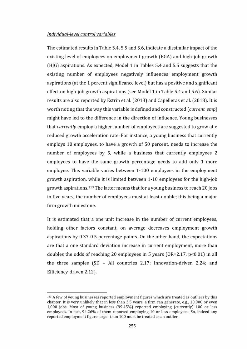
256
Individual-level control variables
The estimated results in Table 5.4, 5.5 and 5.6, indicate a dissimilar impact of the
existing level of employees on employment growth (EGA) and high-job growth
(HJG) aspirations. As expected, Model 1 in Tables 5.4 and 5.5 suggests that the
existing number of employees negatively influences employment growth
aspirations (at the 1 percent significance level) but has a positive and significant
effect on high-job growth aspirations (see Model 1 in Table 5.4 and 5.6). Similar
results are also reported by Estrin et al. (2013) and Capelleras et al. (2018). It is
worth noting that the way this variable is defined and constructed (current_emp)
might have led to the difference in the direction of influence. Young businesses
that currently employ a higher number of employees are suggested to grow at e
reduced growth acceleration rate. For instance, a young business that currently
employs 10 employees, to have a growth of 50 percent, needs to increase the
number of employees by 5, while a business that currently employees 2
employees to have the same growth percentage needs to add only 1 more
employee. This variable varies between 1-100 employees in the employment
growth aspiration, while it is limited between 1-10 employees for the high-job
growth aspirations.113 The latter means that for a young business to reach 20 jobs
in five years, the number of employees must at least double; this being a major
firm growth milestone.
It is estimated that a one unit increase in the number of current employees,
holding other factors constant, on average decreases employment growth
aspirations by 0.37-0.5 percentage points. On the other hand, the expectations
are that a one standard deviation increase in current employment, more than
doubles the odds of reaching 20 employees in 5 years (OR=2.17, p<0.01) in all
the three samples (SD – All countries 2.17; Innovation-driven 2.24; and
Efficiency-driven 2.12).
113 A few of young businesses reported employment figures which are treated as outliers by this chapter. It is very unlikely that in less than 3.5 years, a firm can generate, e.g., 10,000 or even 1,000 jobs. Most of young business (99.45%) reported employing (currently) 100 or less employees. In fact, 94.26% of them reported employing 10 or less employees. So, indeed any reported employment figure larger than 100 must be treated as an outlier.
257
Gender (male) of the entrepreneur is also reported to have a positive and
significant impact on entrepreneurial growth aspirations and the results are in
accordance with previous research findings (see Puente et al., 2017). Holding
other factors constant, being male significantly increase entrepreneur’s
employment growth aspirations by 7 percentage points (5.2 in innovation-driven
and 10.3 percentage points in efficiency-driven economies). The odds ratio
points to the same direction and suggest that the odds of a male entrepreneur
expecting to create 20 jobs in five years is, on average, 48% higher (65% in
innovation-driven and 39% in efficiency-driven economies) than of a female
entrepreneur, ceteris paribus. Results are consistent, for both dependent
variables, across all entrepreneurship ecosystems and are in line with previous
empirical evidence (see Autio and Levie, 2013). Age on the other hand, is
suggested to have a negative and significant impact on employment growth,
when all countries are included or when only efficiency-driven economies are
analysed, but an insignificant, though still negative, impact on high-job growth
aspirations in all the three samples.
The hypothesised curvilinear relationship between age and entrepreneurial
growth aspirations (Levesque and Minniti, 2006) is not suggested when the full
sample and efficiency-driven economies are considered.114 The tests suggested
that the squared term of age is not statically significant and the coefficient is out
of the range when full sample or only efficiency-driven economies are
considered.115 That relationship holds only for innovation-driven economies and
the margins and marginsplot suggest that there is an inverted U-shaped
relationship between owner’s age and growth aspirations and the turning point
is very low at the age of 27.
Turning to the estimated coefficients (the coefficient on age for the efficiency-
driven and the overall sample when the relationship is suggested to be linear), it
114 The squared term of age is included only in the innovation-driven economies sample as the test: nlcom -_b[age]/(2*_b[c.age#c.age]) suggested its significance and within the range coefficient. 115 Age of the respondent was between 14-99, but was censored to include only respondents between 18 and 64 years of age, following the definition of GEM for most of the entrepreneurial activity indicators.

258
is suggested that a one unit increase in age (1 year), holding other variables
constant, on average leads to a decrease of employment growth aspirations by
0.47 percentage points in Table 5.4 (all countries) and 0.41 percentage points
when only efficiency-driven economies are included (p<0.001).
As for the experience of the entrepreneur, the results suggest that, on average,
owning another business that is older than 3.5 years116 decreases employment
growth aspirations by 17 percentage points, ceteris paribus. On the other hand,
the same variable has a significant and positive impact on high-job growth
aspirations. It is suggested that the odds of creating 20 jobs in five years are more
than two times higher for entrepreneurs that already have an established
business, holding other variables constant. This result suggests that being a serial
(experienced) entrepreneur negatively affects employment growth aspirations
of young businesses, while at the same time positively impacting high-job growth
businesses. The concept of “learning-by-doing” seems to perfectly work for high-
job growth ventures, however at the same time harming other not-so-high-
growth-oriented firms. Capelleras et al. (2018), pointing at the ‘learning from the
process of venture creation’, find that experienced entrepreneurs have, in
general, higher growth aspirations.
Having at least another partner in the business, appears to have a positive and
significant impact for the first set of results. It is indicated that sharing
ownership, on average, increases employment growth aspirations by 6.1
percentage points, ceteris paribus. Contrary to the expectations, the results
suggest that the high-job growth aspiration entrepreneurs, do not significantly
benefit from sharing ownership. The odds are always positive but never seem to
appear statistically significant. Cross-tabulation of high-job growth aspiration
and the number of business owners (bb_owners) suggest that almost half (375
out of 844) of young businesses share ownership with at least another owner.
Another difference in influence of the individual-level characteristics is
suggested to be the effect of entrepreneurs’ employment status. Being employed
(full and part-time) is associated with positive and significant impact on
116 This is GEM’s definition of an established business.
259
employment growth aspirations, but with negative, though statistically
insignificant, effect on high-job growth aspirations. Perhaps, this suggests that
high-job growth ventures require full dedication of the entrepreneur and any
other engagement compromises their business growth aspirations. The results
in Table 5.4 (model 1) suggest that holding other variables constant, on average,
employment growth aspirations increase by 7.2 percentage points should the
entrepreneur be employed compared to the base category.117
Institutional variables
The focus is now turned to the effect of institutions, both formal and informal, on
employment growth and high-job growth aspirations. Except for the variable
measuring business friendliness (business freedom), the other four measures of
institutional quality mostly appear with the expected sign. Although statistically
highly insignificant, the negative sign of business freedom, suggests that as the
doing business friendliness improves, entrepreneur’s growth aspirations
decrease.118 Autio and Fu (2015), use this variable as a proxy for the quality of
economic institutions and report that it has a positive and significant impact on
firm entry. Similarly, Acs et al., (2016) emphasise the role of freedom of doing
business in encouraging start up activity but do not relate it to firm growth. It
seems that some of the institutions that encourage entry do not necessarily
influence young business growth aspirations. In the first set of result (columns
1-5 in Table 5.4), where all countries are included, the only statistically
significant institutional quality variable appears to be the size of public sector
(gov_size). It is suggested that an increase in government size by 10 points, on
average and holding other factors constant, decreases employment growth
aspirations by 4.3 percentage points. As it is elaborated in section 5.3.1, a large
public-sector harms growth aspirations mostly due to the negative impact of the
“crowding-out” effect (Beach and Kane 2008). A large public sector leaves no
space for the new ventures to flourish, reduces firm’s financing opportunities and
harms their growth aspirations. Table 5.5 and 5.6 show that a large government
117 This variable, however, does not distinguish between working for another business or for your own. Thus, the high percentage of people report themselves as full- or part-time employed. 118 Considering that the effect is not different from zero, providing any further justifications is not relevant.

260
size is especially harmful to the employment and high-job growth aspirations of
young businesses operating in innovation-driven economies. The result is in line
with most of the previous research findings, including the most recent one of
Bosma et al. (2018). It is estimated, ceteris paribus, that 10 points increase on the
size of public sector, on average lead to a decrease of employment growth
aspirations by 13.4 percentage points. Similarly, if the government size increases
by one standard deviation (6.8 points) the young businesses’ odds of creating 20
jobs in five years decline by more than 20% (OR=0.768, p<0.05), holding other
variables constant. Contrary to our expectations, young businesses operating in
efficiency-driven economies do not seem to be significantly affected by extensive
government activity. One possible explanation might be that as the increased
government activity stimulates demand (Beach and Kane, 2008), the overall
economic dynamics improve, thus creating more opportunities for businesses in
efficiency-driven economies. In most of the efficiency-driven economies, it can be
argued that the public sector spending remains the leading sector of economic
activity.
Results suggest that the quality of property rights protection regime has a
positive and statistically significant influence on growth aspirations. This
variable appears significant and positive in Table 5.4 where all the countries are
included and high-job growth (HJG) aspirations are examined. It is estimated
that, holding other variables constant, if ‘executive constraints’ increases
(improves) by one standard deviation (1.1), the young businesses’ odds of
creating 20 jobs in five years increase by more than 20% (OR=1.203, p<0.05).
Similarly, a one standard deviation increase (1.21) in ‘executive constraints’,
increases the odds of young businesses operating in efficiency-driven economies
of creating 20 jobs in five years by more than 39%, holding other variables
constant. Only employment growth aspirations (EGA) of young businesses
operating in innovation-driven economies are indicated to be significantly
affected by improvements in the property right protection. It is estimated that a
one unit increase in ‘executive constraints’, holding other variables constant,
leads to an increase in employment growth aspiration by almost 7 percentage
points. Employment growth aspirations of young businesses operating in

261
innovation-driven ecosystems appear to also be significantly affected by the level
of corruption. Similar findings are also reported by Anokhin and Schulze (2009),
Aidis et al. (2012), Estrin et al. (2013) and Liñán and Fernandez-Serrano (2014).
The estimated results suggest that a 10 points (unit) increase in ‘corruption’
leads to a decline of growth aspirations by 2.7 percentage points. The
expectations were that high corruption levels negatively affect high-job growth
aspirations, especially of firms residing in efficiency-driven economies, but such
effect is not suggested by the results presented in the three tables.
Finally, the GEM’s National Expert Survey (NES) measure (highgrowth_support)
of specifically designed government programmes that support high-growth
ventures, is also reported to have a positive and statistically significant effect on
high-job growth aspirations. This finding is in line with Sanyang and Huang
(2010) study which suggests that entrepreneurship programmes were effective
in encouraging entrepreneurial activity. Holding other variables fixed, the results
suggest that the odds of creating 20 jobs in five years increase by 17% for full
sample and by 34% for innovation-driven economies, should the
highgrowth_support increases by one standard deviation. All in all, the result
suggests that different institutions and government policies effect growth
aspirations differently. While employment growth aspirations appear to benefit
from small government and small public sector, high-job growth venture
typically benefit from a stronger property right enforcement and from
government policies and activities toward them.
Macroeconomic control variables
The proxy for the size of the private sector, the prevalence rate of established
businesses (businesses older than 3.5 years), appears to have a negative though
insignificant impact on employment growth aspirations. For high-job growth
aspirations, however, the effect is different from zero and suggest that the odds
of creating 20 jobs in five years decrease by 11% if the prevalence rate of
established business increases by one standard deviation. The pace of economic
growth is mostly indicated to have a negative impact on growth aspirations,
however the effect is not different from zero. Similarly, GDP per capita has a
negative sign, however its square term is always insignificant.
262
Table 5.6 Results of High-job Growth (HJG) aspirations according to the stages of development
High-job Growth (HJG) aspirations – Innovation-driven economies
Multilevel logistic regression
High-job Growth (HJG) aspirations – Efficiency-driven economies
Multilevel logistic regression
(Model 0) (Model 1) (Model 2) (Model 3) (Model 4)
VARIABLES HJG-INN countries
HJG-INN countries
HJG-INN countries
HJG-INN countries
HJG-INN countries
HJG-EFF countries
HJG-EFF countries
HJG-EFF countries
HJG-EFF countries
HJG-EFF countries
Individual level Current employment 2.097*** 2.098*** 2.102*** 2.106*** 2.197*** 2.197*** 2.194*** 2.197*** (employm_babybus1) (0.104) (0.104) (0.104) (0.105) (0.081) (0.081) (0.081) (0.081) Age 1.501 1.475 1.538 1.526 0.940 0.939 0.939 0.941 (age) (0.714) (0.702) (0.733) (0.727) (0.048) (0.048) (0.048) (0.048) Age (squared) 0.699 0.712 0.684 0.692 (agesq) (0.335) (0.341) (0.328) (0.332) Gender (M=1) 1.651*** 1.660*** 1.652*** 1.629*** 1.394*** 1.400*** 1.391*** 1.390*** (male) (0.249) (0.250) (0.249) (0.245) (0.152) (0.152) (0.151) (0.151) Edu. Postsecondary 1.239 1.224 1.246 1.235 1.375* 1.383* 1.380* 1.368* (educ_postgr) (0.207) (0.205) (0.209) (0.207) (0.240) (0.241) (0.240) (0.239) Household inc. (2nd level) 1.042 1.004 1.045 1.018 0.964 0.984 0.968 0.969 (gemhhincome) (0.229) (0.223) (0.230) (0.227) (0.158) (0.168) (0.159) (0.159) Household inc. (3rd level) 1.288 1.280 1.285 1.295 1.278 1.363** 1.285* 1.288* (gemhhincome) (0.270) (0.269) (0.270) (0.273) (0.194) (0.214) (0.195) (0.195) Knows entrepr. (Netw.) 1.562*** 1.556*** 1.628*** 1.549*** 1.763*** 1.767*** 1.861*** 1.739*** (KNOWENT_dum) (0.252) (0.251) (0.269) (0.250) (0.199) (0.199) (0.219) (0.196) Business angel 1.496** 1.494** 1.500** 1.496** 1.463*** 1.478*** 1.474*** 1.474*** (BUSang_dum) (0.288) (0.288) (0.289) (0.289) (0.197) (0.199) (0.198) (0.198) Own/mng of exist. Bus 2.381*** 2.333*** 2.417*** 2.393*** 2.128*** 2.163*** 2.130*** 2.160*** (omESTBBUS_dum) (0.613) (0.602) (0.622) (0.614) (0.482) (0.490) (0.483) (0.490) More than 1 owner 1.352** 1.348** 1.343** 1.354** 0.976 0.975 0.973 0.976 (bb_owners) (0.185) (0.185) (0.184) (0.186) (0.100) (0.100) (0.100) (0.101) Employment status (E=1) 0.339*** 0.345*** 0.339*** 0.347*** 1.070 1.102 1.073 1.068 (work_status) (0.105) (0.107) (0.105) (0.106) (0.266) (0.274) (0.267) (0.265) Skills 1.488 1.507 1.491 1.463 1.273 1.256 1.272 1.272 (suskill_dum) (0.384) (0.390) (0.385) (0.376) (0.193) (0.190) (0.193) (0.193)
263
Perceived opportunities 2.024*** 2.032*** 2.026*** 2.055*** 1.501*** 1.508*** 1.503*** 1.502*** (opportunities) (0.292) (0.293) (0.293) (0.297) (0.165) (0.166) (0.165) (0.165) Country mean Household income 1.307** 1.296** 1.302** 1.299** (mhhinc) (0.145) (0.143) (0.146) (0.144) Business angel 0.899 0.897 0.896 0.898 (mBUSang_dum) (0.098) (0.097) (0.098) (0.098) Institutional quality Business freedom (t-3) 1.013 1.006 1.001 0.999 1.039 1.040 1.041 1.045 (L3bussfree) (0.131) (0.130) (0.130) (0.130) (0.117) (0.116) (0.118) (0.117) Property rights (t-3) 1.107 1.114 1.116 1.122 1.397** 1.409** 1.396** 1.389** (L3xcons) (0.133) (0.134) (0.135) (0.137) (0.204) (0.205) (0.205) (0.202) Government size (t-3) 0.768** 0.756** 0.749** 1.052 1.019 1.020 1.020 0.868 (L3gov_size) (0.103) (0.102) (0.102) (0.213) (0.116) (0.116) (0.117) (0.128) Corruption (t-3) 0.855 0.702 1.041 0.850 0.993 0.831 0.852 0.987 (corruption) (0.129) (0.166) (0.191) (0.129) (0.110) (0.132) (0.119) (0.109) High-growth supp. (EFC) 1.338** 1.345** 1.336** 1.342** 0.983 0.992 0.978 0.980 (highgrowth_support) (0.155) (0.156) (0.156) (0.157) (0.110) (0.111) (0.111) (0.110) Macroeconomic Control variables The prevalence rate of estb. businesses 0.781** 0.769** 0.757*** 0.778** 1.091 1.092 1.093 1.089 (estbusrate) (0.082) (0.082) (0.082) (0.083) (0.113) (0.112) (0.114) (0.112) GDP growth (t-1) 1.080 1.078 1.068 1.078 0.998 1.000 0.998 0.993 (inn_zL1gdpgrowth) (0.148) (0.147) (0.147) (0.148) (0.109) (0.109) (0.110) (0.108) GDPpc (t-1) 0.241* 0.237* 0.237* 0.244* 0.774 0.767 0.774 0.753 (L1gdppccons2011) (0.184) (0.181) (0.182) (0.188) (0.369) (0.364) (0.371) (0.358) GDPpc (t-1) sq. 3.282 3.337 3.320 3.214 1.108 1.120 1.105 1.132 (inn_zL1gdppcconssq) (2.561) (2.611) (2.602) (2.533) (0.465) (0.469) (0.468) (0.475) Interaction effects Household income (2nd level)*Gov. size 0.624**
(0.127) Household income (3nd level)*Gov. size 0.716*
(0.138) Knows entrepreneurs (Netw.)*Gov. size (t-3) 1.242*
264
(0.155)
Household income (2nd level)*Corruption 1.459* 1.082
(0.327) (0.167) Household income (3nd level)*Corruption 1.155 1.297*
(0.242) (0.179) Knows entrepreneurs (Netw.)*Corruption (t-3) 0.761* 1.212*
(0.113) (0.129) Industry control Yes Yes Yes Yes Yes Yes Yes Yes Year dummies Yes Yes Yes Yes Yes Yes Yes Yes Country-Year: Identity var(_cons) 0.204 0.103 0.106 0.109 0.107 0.634 0.298 0.289 0.308 0.295 (0.095) (0.08) (0.081) (0.082) (0.082) (0.145) (0.105) (0.104) (0.108) (0.105) ICC (Country-Year-lev. 2) 0.058 0.03 0.03 0.032 0.032 0.162 0.083 0.081 0.086 0.082
Log-likelihood (pseudolikelihood) -1177.51 -953.68 -951.78 -952.00 -950.91 -2119.98 -1738.23 -1735.83 -1736.65 -1736.70
LR test vs. non-multilevel (χ2) 13.22*** 2.63* 2.67* 2.96** 2.8** 211.9*** 30.03*** 28.64*** 31.04*** 29.59***
Constant 0.041*** 0.007*** 0.007*** 0.007*** 0.007*** 0.041*** 0.007*** 0.007*** 0.007*** 0.007***
(0.004) (0.004) (0.004) (0.004) (0.004) (0.0001) (0.003) (0.003) (0.003) (0.003)
Observations 6,753 6,753 6,753 6,753 6,753 11,367 11,367 11,367 11,367 11,367
Number of groups 128 128 128 128 128 133 133 133 133 133 Standard errors in parentheses *** p<0.01, ** p<0.05, * p<0.1 Note: Multilevel logistic regressions use standard errors: GEM 2006-2013 data
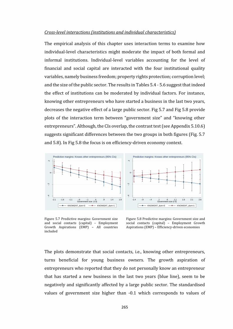
265
Cross-level interactions (institutions and individual characteristics)
The empirical analysis of this chapter uses interaction terms to examine how
individual-level characteristics might moderate the impact of both formal and
informal institutions. Individual-level variables accounting for the level of
financial and social capital are interacted with the four institutional quality
variables, namely business freedom; property rights protection; corruption level;
and the size of the public sector. The results in Tables 5.4 - 5.6 suggest that indeed
the effect of institutions can be moderated by individual factors. For instance,
knowing other entrepreneurs who have started a business in the last two years,
decreases the negative effect of a large public sector. Fig 5.7 and Fig 5.8 provide
plots of the interaction term between “government size” and “knowing other
entrepreneurs”. Although, the CIs overlap, the contrast test (see Appendix 5.10.6)
suggests significant differences between the two groups in both figures (Fig. 5.7
and 5.8). In Fig 5.8 the focus is on efficiency-driven economy context.
Figure 5.7 Predictive margins: Government size and social contacts (capital) – Employment Growth Aspirations (EMP) – All countries included
Figure 5.8 Predictive margins: Government size and social contacts (capital) – Employment Growth Aspirations (EMP) – Efficiency-driven economies
The plots demonstrate that social contacts, i.e., knowing other entrepreneurs,
turns beneficial for young business owners. The growth aspiration of
entrepreneurs who reported that they do not personally know an entrepreneur
that has started a new business in the last two years (blue line), seem to be
negatively and significantly affected by a large public sector. The standardised
values of government size higher than -0.1 which corresponds to values of
-.4
-.2
0.2
Pre
dic
ted E
mp
. G
row
th A
sp
ira
tion
s (
EG
A)
-2.1 -1.6 -1.1 -.6 -.1 .4 .9 1.4 1.9Government size (t-3)
KNOWENT_dum=0 KNOWENT_dum=1
Predictive margins: Knows other entrepreneurs (95% CIs)
-.4
-.2
0.2
Pre
dic
ted E
mp
. G
row
th A
sp
ira
tion
s (
EM
P)
-1.4 -.9 -.4 .1 .6 1.1 1.6 2.1 2.6Government size (t-3)
KNOWENT_dum=0 KNOWENT_dum=1
Predictive margins: Knows other entrepreneurs (95% CIs)
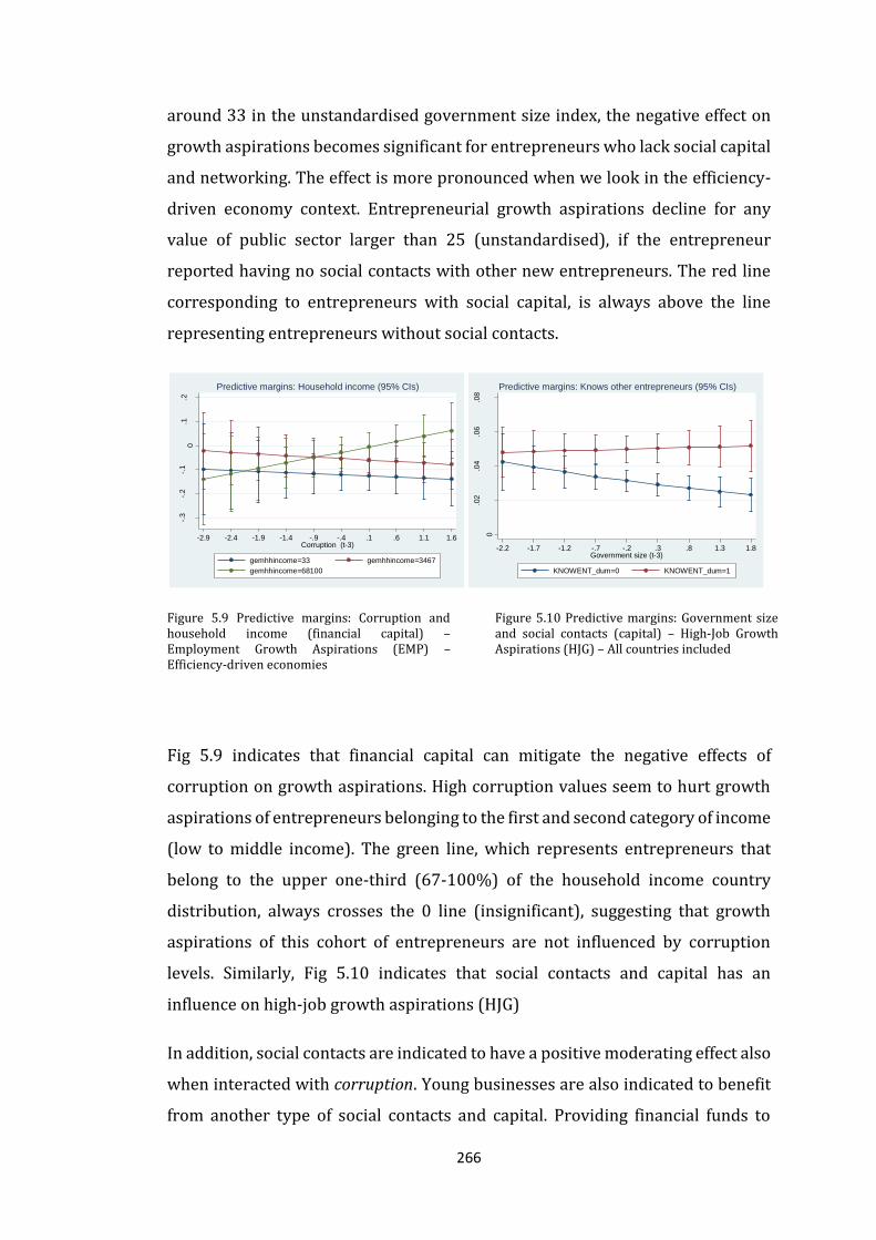
266
around 33 in the unstandardised government size index, the negative effect on
growth aspirations becomes significant for entrepreneurs who lack social capital
and networking. The effect is more pronounced when we look in the efficiency-
driven economy context. Entrepreneurial growth aspirations decline for any
value of public sector larger than 25 (unstandardised), if the entrepreneur
reported having no social contacts with other new entrepreneurs. The red line
corresponding to entrepreneurs with social capital, is always above the line
representing entrepreneurs without social contacts.
Figure 5.9 Predictive margins: Corruption and household income (financial capital) – Employment Growth Aspirations (EMP) – Efficiency-driven economies
Figure 5.10 Predictive margins: Government size and social contacts (capital) – High-Job Growth Aspirations (HJG) – All countries included
Fig 5.9 indicates that financial capital can mitigate the negative effects of
corruption on growth aspirations. High corruption values seem to hurt growth
aspirations of entrepreneurs belonging to the first and second category of income
(low to middle income). The green line, which represents entrepreneurs that
belong to the upper one-third (67-100%) of the household income country
distribution, always crosses the 0 line (insignificant), suggesting that growth
aspirations of this cohort of entrepreneurs are not influenced by corruption
levels. Similarly, Fig 5.10 indicates that social contacts and capital has an
influence on high-job growth aspirations (HJG)
In addition, social contacts are indicated to have a positive moderating effect also
when interacted with corruption. Young businesses are also indicated to benefit
from another type of social contacts and capital. Providing financial funds to
-.3
-.2
-.1
0.1
.2
Pre
dic
ted E
mp
. G
row
th A
sp
ira
tion
s (
EM
P)
-2.9 -2.4 -1.9 -1.4 -.9 -.4 .1 .6 1.1 1.6Corruption (t-3)
gemhhincome=33 gemhhincome=3467
gemhhincome=68100
Predictive margins: Household income (95% CIs)
0
.02
.04
.06
.08
Pre
dic
ted H
igh-j
ob
Gro
wth
Asp. (H
JG
)
-2.2 -1.7 -1.2 -.7 -.2 .3 .8 1.3 1.8Government size (t-3)
KNOWENT_dum=0 KNOWENT_dum=1
Predictive margins: Knows other entrepreneurs (95% CIs)
267
other businesses is also an important social characteristic that decreases the
negative effect of a large size of government and weak property right protection.
Plots of all the other statistically significant interaction terms are provided in
appendices 5.5 – 5.10.
Robustness checks
To check the robustness of the estimation process, we have investigated whether
results would remain stable when a different definition of high-job growth
aspirations is used. Considering that more than 70% of young businesses at the
time of the survey employ 1-3 employees, reaching the threshold of 20
employees in five years seems a high criterion. Therefore, this chapter
constructed an alternative measure of high-job growth aspirations which takes
into account the relative size of the firm. The new variable (emp_growth_dum)
takes the value of 1 if the young business expects to double their employment in
five years, 0 otherwise. Moreover, for this new dependent variable to take the
value of 1, two additional criteria must be met: (i) young businesses have to have
at least three current employees (this is to avoid situations when firms currently
employ 1 or 2 employees and will add another 1 or 2 in 5 years (not high
growth)); and (ii) young businesses expect to create a maximum of 100 jobs in
five years (this is to avoid any potential outliers). Any young business that e.g., is
currently employing seven employees and in five years expects to reach to 14 has
the value of 1 for this new variable. However, a business that currently employs
15 and in five years expects to create an additional 5 new jobs (20 in total) is not
considered a high-job growth business venture in this case. Results obtained
using this new dependent variable do not significantly differ from the ones
obtained from the original high-job growth aspirations (HJG) (see Appendix
5.11). This consistency in the results suggests that focusing only on young
businesses that expect to create 20 jobs in five-years is enough to explain high-
growth aspirations entrepreneurship.
This chapter also checked for the hit rate for the multilevel logistic approach and
the analysis show that the model correctly predicts more than 95% of the
outcomes (see Appendix 5.12).

268
CONCLUSIONS
This chapter provides a multi-country analysis of the impact of the individual-
level characteristics, institutional features and country-level control variables on
employment growth and high-job growth aspiration entrepreneurship. Using the
multilevel modelling strategy, linear (mixed-effects) and multilevel logistic
estimators, the empirical investigation provides a contribution on the topic of
entrepreneurial growth aspirations. The chapter contributes to the existing
literature by extending the current empirical work to include a wide cross-
country investigation. In addition, the empirical analyses of this chapter take into
account the impact of economic context, namely innovation and efficiency-driven
economy contexts when determining key individual and institutional factors
impacting entrepreneurial growth aspiration. Examining the impact of the
quality of institutional arrangements on entrepreneurial growth aspirations
according to the countries’ level of economic development is justified as the
results suggest dissimilar impacts on different groups of countries.
In general, the results provide evidence that entrepreneurial growth aspirations
are significantly determined by individual characteristics. The results indicate
that, regardless of the stage of economic development, most of the individual
characteristics have a positive and significant effect on employment growth and
high-job growth aspirations. The effect of the quality of institutions, although
relevant, seems to be somehow weaker than that of individual factors. This
finding is in line with the outcome of the meta-analysis of Levie and Autio (2013),
who also suggest that entrepreneurial growth aspirations are a consequence of
individual characteristics, while institutional and environmental effects are less
critical for growth aspiring ventures. Most of the individual-factor variables
included in both models and in different specifications have been very consistent
with respect to the sign and the statistical significance. Results indicate that
financial and human capital positively influence growth aspirations. Young and
male entrepreneurs have higher entrepreneurial growth aspirations compared
to their counterparts. Social capital and business networking is another
significant and positive factor determining growth aspirations. Likewise,
opportunity recognition is reported to positively and significantly influence

269
entrepreneurial growth aspirations as is the individual’s own perceptions of
skills and capabilities to run a business.
With regard to the quality of institutions, it is suggested that a strong property
rights protection regime positively influence entrepreneurial growth aspirations
of young firms, while higher levels of corruption, large governments and public
sector have a negative impact on growth aspirations. Entrepreneurial growth
aspirations are also found to benefit from specifically designed government
programmes aiming to support high-growth businesses. Finally, the study
suggests that the effect of both individual characteristics and especially the
institutional settings varies according to the stage of a country’s economic
development and entrepreneurship ecosystem. The cross-level interactions
suggest that some individual characteristics, such as financial and social capital
can moderate the impact of institutional quality on entrepreneurial growth
aspirations. Finaly, entrepreneurial growth aspirations are found to be industry
and sector sensitive and have changed over years. To sum up, the results suggest
that this empirical analysis has relevant policy implications and can be used to
help design policies conducive to entrepreneurial growth aspirations, especially
for efficiency driven-economies.
6. Chapter 6
CONCLUSIONS AND POLICY IMPLICATIONS
Introduction ............................................................................................................................. 271
Main findings ........................................................................................................................... 272
Contribution to knowledge ................................................................................................ 280
Policy implications ................................................................................................................ 284
Limitations and recommendations for future research ......................................... 287

Introduction
The thesis has investigated the effect of entrepreneurship on economic growth
and also the individual-level and institutional determinants of entrepreneurial
growth aspirations. The aim of this concluding chapter is to synthesise the main
findings generated throughout the thesis and outline its contribution to
knowledge. The chapter also aims to provide relevant policy recommendations
and to suggest future avenues of research.
The renewed focus on entrepreneurship and its role in economic growth was
influenced by the shift from a managed (centrally-planned) to an entrepreneurial
market economy (Audretsch and Thurik, 2001). As outlined earlier in the thesis,
the entrepreneurial economy puts more emphasis on the role of new and small
firms, knowledge and innovation. The entrepreneurship literature was also
influenced by the work of Birch (1979; 1987) on fast growing firms, i.e., gazelles.
Busenitz et al. (2014) and Davidsson (2016) argue that in the last three decades,
entrepreneurship research has significantly increased, and the most recent years
have experienced an exponential rate of growth in the research output.
The first chapter has provided some of the influential entrepreneurship concepts
and definitions and has outlined some of the measurement challenges arising
from the multifaceted nature of entrepreneurship. The review of growth theories
and models and the empirical literature linking entrepreneurship with economic
growth, in Chapter 2, indicated a lack of unanimity, although the number of
studies reporting positive effects dominated. The lack of consensus and the
heterogeneity of reported effects motivated the Meta-Regression Analysis (MRA)
in Chapter 3. The MRA chapter addressed three main research questions: (i) to
what extent does the heterogeneity of the characteristics of different studies
moderate the effect of entrepreneurship on economic performance; (ii) is the
entrepreneurship-economic performance literature subject to publication bias; and
(iii) is there a genuine entrepreneurship effect, beyond the ‘publication bias’ and
after controlling for sources of heterogeneity exist.
The MRA chapter was followed by an empirical investigation of the effect of
entrepreneurship on economic growth at the country-level. The focus of this

272
chapter was on answering the following research questions: (i) does the overall
entrepreneurial activity (TEA) impact economic growth: (ii) does the employment
growth-oriented and innovative entrepreneurial activity impact economic growth;
(iii) does the effect of entrepreneurship on economic growth vary with the country’s
stage of development. The findings of this chapter motivated the empirical
investigation in Chapter 5. The individual-level and institutional quality
determinants of entrepreneurial growth aspirations were assessed, using a
multilevel approach. Accordingly, Chapter 5 addressed the following research
questions: (i) do the individual-level attributes affect employment growth
aspirations (EGA) and high-job growth aspirations; (ii) does the quality of
institutions determine employment growth aspirations and high-job growth
aspirations; and (iii) do the entrepreneur’s financial and social capital moderate
the effect of institutions on growth aspirations.
The rest of the chapter is organised as follows. The main empirical findings in
relation with thesis objectives and research questions are presented in section
6.2. The main contribution to knowledge of the thesis are discussed in Section
6.3. Policy implications derived from the findings of the thesis are elaborated in
section 6.4 while section 6.5 highlights some of the limitations of this research
project and concludes the chapter after presenting the potential future avenues
of research.
Main findings
The initial findings of the thesis are related to the review of theoretical and
empirical literature in Chapter 2. The theory of entrepreneurship, advanced by
Schumpeter (1934), highlighted the role of entrepreneurship in generating
economic activity and growth. Motivated by the work of Schumpeter, the
empirical literature has been increasingly growing, especially in the last two
decades, and by and large, has suggested the positive effect of entrepreneurial
activity on economic growth. The early economic growth theories and models, on
the other hand, have remained muted and ignored the role of entrepreneurship.
Chapter 2 highlighted that in the neoclassical growth models of Solow (1956;
1957) and Swan (1956), entrepreneurship played no role, although in a recent
273
publication, Solow (2007) asserts that the incorporation of entrepreneurship
would improve growth models.
The appearance of endogenous growth models is thought to have provided the
theoretical ground for including entrepreneurship measures in the growth
models. Although the early endogenous growth models of Romer (1986; 1990),
outlined the role of knowledge and ideas, they failed to explain how new
knowledge diffusion happens and most importantly how economic agents
commercialise that knowledge. The Knowledge Spillover Theory of
Entrepreneurship (KSTE) extended the endogenous growth model by arguing
that the entrepreneur is responsible for providing the ‘missing link’ in the
process of new knowledge commercialisation, i.e., the process of converting
general knowledge into economically relevant knowledge. In this way,
entrepreneurship contributes to economic growth (Audretsch et al., 2005;
Braunerhjelm et al., 2010). Chapter 2 also found that the growth models
developed by Aghion and Howitt (1992; 1998) allow researchers to explicitly
account for the role of entrepreneurship in economic growth. The Schumpeterian
theory of growth is based on the process of ‘creative destruction’ and on the
expected monopoly power and profits which motivates entrepreneurial activity.
The decision to invest in R&D activities with an uncertain outcome highlights the
role of the ‘entrepreneur’ in the Schumpeterian theory of growth. Overall,
chapter 2 finds that the inclusion of entrepreneurship measures in the exiting
growth models is not straightforward and there is still a need for a more
comprehensible theoretical explanation.
Despite the lack of any uniformly followed theoretical framework, there is extant
empirical literature on the entrepreneurship-economic growth relationship.
Although the review of empirical studies suggested that, in general, there is a
positive association between entrepreneurship and economic growth, there is
still some inconclusiveness about this result. The sources of the heterogeneity in
the reported results point in several directions, one of them being the
appropriate (or not) choice of entrepreneurship and economic growth or
performance measures. Throughout the thesis, the multidimensional nature of
entrepreneurship and the entrepreneur is emphasised and assessed. Moreover,

274
Chapter 2 found that the existing entrepreneurship-economic growth literature
might be subject to misspecification errors and is characterised by the lack of a
robust methodological approach. The relatively large number of studies might be
prone to the omitted variable bias, as it is found that they have left out some of
the standard variables from their empirical models.
The literature that uses employment growth as a measure of economic
performance has mainly been focused on identifying lag structures (patterns) on
how and when (after how many time lags) the effect of entrepreneurship (if any)
is greater on employment creation. Chapter 2 also found that most of the existing
studies have failed to distinguish between different types of entrepreneurial
activity. Overall, the review of empirical literature found that some study
characteristics, such as the choice of estimators and the measures, might have
influenced the results. The review also found that there is lack of more advanced
and rigorous methodological and empirical approaches in the reviewed
literature.
The review of literature in Chapter 2 was followed by a more systematic and
quantitative review of empirical literature through a Meta-Regression Analysis
(MRA) in chapter 3. This approach adds much more rigor to the review of the
literature with heterogenous findings, a diversity of measures, data, theoretical
and methodological approaches used. The MRA allows for a more comprehensive
integration of previous results, a more advanced synthesis and a more accurate
evaluation of the findings of the primary studies, as compared to conventional
literature reviews. To improve coherence, the primary literature was classified
into three subsamples, based on the measure of economic performance used:
‘growth of GDP or GDP per capita’, ’employment growth’ and ‘other’ measures of
economic performance.
The funnel plots, which offer the initial graphical examination of the presence of
publication bias, revealed a level of asymmetry in the reported results, suggesting
a degree of positive publication bias, in all three subsamples. That is an indication
of the preference of research community and the reviewers towards reporting
positive results for the entrepreneurship-economic performance literature. In
addition, the graphical observation indicated that a relatively large number of

275
point estimates were widely scattered in the upper part of the funnel plots (the
area of the graph with the highest precision). This suggested that, beside of
potential sampling errors, the variety of measures, methodological approaches
and estimators used might have influenced the study outcomes. Throughout the
thesis, the use of various measures of entrepreneurship has been pointed out,
mainly because of the different effects they may have on the examined
entrepreneurship-economic performance relationship.
Also, the more advanced approaches of detecting the presence of publication
bias, point to the same direction as the visual inspection of funnel plots. The
bivariate MRA, suggests the studies of the first subsample (growth studies) suffer
from the presence of ‘substantial’ (1≤FAT≥2) publication bias. With regard to the
authentic effect, when the FE estimator (including G-S approach) is used, the
Precision-Effect-Test (PET) indicates a positive and ‘moderate’ effect beyond
publication bias in the entrepreneurship-economic growth literature. The rest of
the estimators report an insignificant PET coefficient, suggesting neither positive
nor negative authentic effect. The entrepreneurship-employment growth
literature (second subsample) is also found to be contaminated as the FAT
suggests a ‘substantial’ positive publication bias when WLS is applied. However,
when the FE (G-S) approach is employed, the FAT estimate suggests a ‘severe’
(larger than 2) negative selectivity in the same literature. The bivariate MRA also
suggests a ‘large’ positive genuine effect of entrepreneurship on employment
growth, when the FE (G-S) approach is used.
The bivariate MRA of the third subsample suggest the presence of a ‘moderate’
positive genuine effect and at same time, the literature is found to be
contaminated with the presence of a ‘moderate’ positive publication bias. The
findings are in line with the suggestions of O’Boyle et al. (2014) and Bosma et al.
(2018) who also warned that the entrepreneurship literature might be prone to
publication selection bias.
The multivariate MRA results of the first subsample (growth studies), uncovered
using the WLS, FE, robust estimator and the indications from the Bayesian Model
Averaging (BMA), are relatively consistent with those reported by the bivariate
MRA. Except of the robust estimator, the WLS, FE estimators and the BMA suggest

276
the presence of publications bias, although WLS is significant only at the 10%
significance level. With regard to the genuine effect, the multivariate MRA results
suggest a ‘moderate’ positive genuine effect, when the FE and the robust
estimator are used. Overall, Chapter 3 finds that the reported estimates of the
studies of the first subsample (growth studies) are likely to be subject to
‘substantial’ positive publication bias and there is also an indication of a
‘moderate’ positive effect of entrepreneurship on economic growth.
For the second subsample, the WLS multivariate MRA results finds insignificant
relationship. The positive publication bias, of the ‘little’ to ‘moderate’ magnitude,
is suggested only by the BMA method, which as highlighted in Chapter 3 serves
only as a weak evidence and should be taken with caution. In terms of the
presence of a genuine effect, the multivariate MRA suggest a ‘moderate’ positive
effect in the literature.
For the third subsample, the analysis is also found to demonstrate a positive
publication bias when WLS is used. and. Regarding the authentic effect in the
literature, Chapter 3 found that a ‘moderate’ positive effect is suggested only
when the BMA approach is used (at the 10% significance level). Overall, it is
found that the literature in the third subsample has been subject of a positive
‘substantial’ to ‘severe’ publication bias. The study asserts that the lack of a
competing theory on the role of entrepreneurship on economic performance, is
partly to be blamed for the contamination of the literature. Chapter 3 provided
an evidence of the importance of adjusting for outliers in the MRA practices, as in
some cases results differed significantly (results after adjusting for outliers from
the results without adjusting for outliers).
Chapter 3 also identifies factors that influence the entrepreneurship-economic
performance relationship. The multivariate MRA results indicate that the choice
of both entrepreneurship and economic performance measures are responsible
for the heterogeneity of results. The choice of the methodology and the
estimators is also suggested to have an influence on the primary literature
results. For instance, ‘growth studies’ that used GMM, on average, tend to report
smaller effects, whereas ‘employment growth’ studies report lager effect if OLS
was their chosen estimator. The economic context of the investigation, i.e., the

277
stage of economic development, is also an influential factor, as is the level of
investigation (country-level vs regional-level). A relevant finding that can serve
the research community is that, in general, good research practice and more
theoretically-driven specifications, i.e., specifications that account for at least
some of the conventional variables, determine the results of the primary studies.
As highlighted in Chapter 3, the use of lags for the measure of entrepreneurship,
can explain part of the heterogeneity of results. Results also found that the period
of the data used, and the publication year have had an influence on the reported
effect sizes. Similarly, the primary literature results are also influenced by the
funding source of the research project (related interest party) and the
publications state, i.e., papers published in the referred journals.
To conclude, the findings of the multivariate MRA, provided an insight into the
study of entrepreneurship-economic performance relationship. The MRA
chapter has informed the methodological and theoretical approach of Chapter 4.
Inspired by the findings of the MRA, Chapter 4 uses different types of
entrepreneurial activity, includes theoretically-motivated variables and applies
a multi-approach econometric modelling.
Chapter 4 provided a country-level investigation of the effect of
entrepreneurship on economic growth using a panel of 48 countries over the
2006-2014 period. The choice of entrepreneurship and economic growth
measures was guided by the measurement and definitional challenges identified
in Chapter 1, the review of literature on Chapter 2, and the findings of the MRA
chapter. Influenced by work of Schumpeter (1934) on innovative
entrepreneurship and by Baumol’s (1990; 1993) on ‘productive
entrepreneurship’, Chapter 4 uses the overall TEA as well as other types of
entrepreneurial activity, i.e., growth-oriented (job creation) and innovative
(product and market) entrepreneurial activity.
The main finding of Chapter 4 is that the relationship between entrepreneurship
and economic growth is to be detected only when more specific types of
entrepreneurial activity are used. The positive and significant effect of high-job
growth activity is, mostly, robust to the choice of estimation method, both

278
between the static estimator and also when the dynamic approach is applied. The
dynamic approach, the system GMM, however, does not point to a positive and
significant effect of innovative entrepreneurial activity. As it is discussed in
Chapter 4, perhaps the questions asked in the GEM surveys, to measure
innovative entrepreneurial activity, can be modified or be more specifically
defined to avoid overreporting. An additional finding, specifically relevant to the
policymaking community, is that the positive effect of ‘employment growth-
oriented’, both job growth and high-job growth entrepreneurial activity is even
higher in the long-run compared to the short-run.
The results, using the static approach estimators, also suggested that institutional
quality variables and a set of control variables have a significant effect on
economic growth. Specifically, physical capital and trade openness are suggested
to have a positive impact on growth. Although less frequently, human capital, and
the quality of institutions (‘rule of law’) are also indicated to have a positive
relationship with economic growth. In line with previous studies, Chapter 4
found that the size of the public sector is negatively related to economic growth.
Throughout the thesis, the hypothesised impact of a country’ stage of
development (Carree et al., 2002) on the relationship between entrepreneurship
and economic growth has been emphasised. This relationship was examined by
the means of interaction terms between entrepreneurship measures and the
stage of development. The margins and margin plots seemed to suggest that the
effect of entrepreneurship may be moderated by the stage of development.
Specifically, OECD member countries are suggested to benefit more, in terms of
economic growth, from the high-job growth entrepreneurial activity, compared
to non-OECD countries. Similarly, the effect of high-job growth entrepreneurial
activity is suggested to be greater in innovation-driven compared to efficiency-
driven economies. It is to be noted that these findings were seen to be suggested
only by margin plots but were not confirmed by formal contrast tests and as such
are to be taken with caution. In addition, Chapter 4 found that it is neither poor
(nine countries (GDP per capita< US$15,000)) nor relatively rich countries
(seven countries (GDP per capita>US$45,0000)) that benefit the most from the
high-job growth entrepreneurial activity. Instead, the effect is higher in
279
economies with a GDP per capita between these two extremes. Finally, in terms
of the result robustness, Chapter 4 found that the effect of employment growth-
oriented and innovative entrepreneurial activity is not influenced by the changes
in the sets of explanatory variables used.
In summary, the findings of Chapter 4 contribute to the debate initiated by
Baumol (1990), by empirically confirming that ‘productive entrepreneurship’,
more than other types of entrepreneurial activity, impacts country-level
economic growth. The findings are also relevant to the policymaking community,
as they suggest that an increased focus on a smaller group of entrepreneurial
firms, i.e., high-growth young businesses, is perhaps a more effective approach to
economic growth, than a general policy toward new businesses.
The robust positive and significant effect of high-job growth entrepreneurial
activity on economic growth in Chapter 4, opened up an avenue for further
empirical investigation: the effect of the individual, institutional and country-
level factors on entrepreneurial growth aspirations. The entrepreneurial growth
aspirations are operationalised using young businesses’ ‘entrepreneurial growth
expectations’ in 55 countries (innovation-driven and efficiency-driven) over the
2006-2013 period. Two different dependent variables were used, (i)
employment growth aspirations (EGA) and (ii) high-job growth (HJG) aspiration.
The use of data at two different levels, namely individual-level and country-level,
required the use of multilevel estimation techniques.
The empirical analysis of Chapter 5 revealed that, regardless of the stage of
economic development (the economic context), individual attributes are
significant determinants of entrepreneurial growth aspirations. The effect of
institutional quality variables, however, is found to vary between the two
variants of growth aspirations and with the stage of development. In addition,
using interaction terms, Chapter 5 found that the negative impact of a large public
sector and high levels of corruption can be moderated by the individual-level
characteristics, such as financial and social capital.
The high consistency, in terms of the sign and statistical significance, of the
individual-level characteristics was regarded as a sign of a robust outcome. The

280
findings indicate that entrepreneur’s human, financial and social capital, are
positively associated with entrepreneurial growth aspirations. More specifically,
individuals (owner/managers) with a post-secondary degree are suggested to
have higher employment growth aspirations and high-job growth aspirations.
Similarly, belonging to a family which is in the second or third highest level of
household income, on average, has a positive impact on entrepreneurial growth
aspirations. Chapter 5 found that the effect of household income is greater in
efficiency-driven compared to innovation-driven economies. It was argued that
the lack of well-developed financial system in efficiency-driven economies is
compensated by higher levels of household income. Social capital, proxied by two
variables, namely, ‘knowing other entrepreneurs’ who have recently (less than
two years) started a business and providing funding to other business ventures
in the last three years, is positively associated with entrepreneurial growth
aspirations.
Chapter 5 also found that growth aspirations are gender sensitive, as the results
suggest that, on average, male individuals have higher entrepreneurial growth
aspirations. The entrepreneur’s age is found to influence employment growth
aspirations but not high-job growth aspirations. Having a positive outlook
toward business opportunities (perceived opportunity), perceiving oneself as a
capable and skilled person, having already established a business before this new
venture, and sharing the ownership of the new venture with others are all found
to be a significant determinant of growth aspirations.
Contribution to knowledge
The thesis has made several contributions to the literature on the relationship
between entrepreneurship and economic growth as well as the literature on the
determinants of entrepreneurial growth aspirations. The complexity of defining
and measuring entrepreneurship and the multidimensionality that the concept
entails have also been elaborated in this research project. The review of the
empirical literature suggested that the heterogeneity of results might be due to
the use of various measures of entrepreneurship from multiple sources. To the
best of author’s knowledge, the MRA is applied for the first time in the

281
entrepreneurship-economic performance literature and, thus, provides an
original contribution to knowledge. The specific contributions of the thesis are
discussed below.
First, the thesis provided an elaboration of the economic growth models and their
application to the entrepreneurship-economic performance literature.
Throughout the thesis, it was highlighted that despite this extant literature the
two traditional economic growth theories and models either completely
neglected or only implicitly assumed the role of entrepreneurship. The more
recent theoretical developments have emphasised the effect of entrepreneurship
and modelled its role as the mechanism to diffuse new knowledge and innovation
or as the ‘missing link’ converting general knowledge into economically-relevant
knowledge. The common premise of these recent developments is that
entrepreneurship serves as the agent channelling new ideas and innovations into
economic activity, generating new jobs, new businesses and ultimately growth.
and development.
Second, the thesis provided the first quantitative literature review on the
entrepreneurship-economic performance literature. The MRA contributed to the
entrepreneurship-economic performance debate by providing an objective and
comprehensive summary of a total of 52 empirical studies conducted between
2000 and 2016 using a variety of estimators including the Bayesian Model
Averaging designed to deal with model uncertainty. The main objectives of using
the MRA were to identify whether the literature has been subject to publication
bias, positive or negative; whether there exists a ‘genuine’ effect beyond
publication selection bias; and to quantify the sources of heterogeneity in the
literature. The presence of publication bias and that of a ‘moderate’ positive
genuine effect were detected in the entrepreneurship-economic growth
literature (subsample I). A similar finding was also reported for the second
subsample, ‘employment growth’ studies. The positive ‘genuine’ effect is
suggested by all the estimators, and at the same time, the presence of positive
publication bias is indicated by BMA, which provides a weak evidence of
publication selection bias. Studies of the third subsample (‘other’ studies), were
found to have suffered from a positive ‘substantial’ to ‘severe’ publication bias.

282
The MRA has also contributed to the identification of sources of heterogeneity in
the entrepreneurship-economic performance literature. A relevant finding was
that the choice of both entrepreneurship and economic performance measures
has a significant impact on the study outcome. In addition, methodological
approaches, the economic context (stages of development), level of investigation,
good research practice, and the presence of a funding body for the research can
also influence the results of the studies.
Faced with the issue of extensive use of lags (up to ten lags per specification) by
primary literature, an innovative approach to weighting effect sizes (point
estimates) was used. In addition to accounting for the cross-study weights, the
’specification weight’ used in this thesis accounts for the pronounced between-
specification heterogeneity. The new weight alleviates the effect that
specifications with extensive use of lags might have on the MRA results. This is
another relevant contribution to knowledge, applicable also to the MRA
literature. The use of BMA, in addition to WLS, FE and the robust estimator,
provided more robustness to the findings of the MRA chapter.
Third, the thesis extends the empirical literature on the entrepreneurship-economic
growth relationship by focusing on an under-researched type of entrepreneurial
activity while also applying a dynamic approach. Unlike previous studies,
reviewed in Chapter 2, in this research project, the focus was on investigating the
effect of growth-oriented and innovative entrepreneurial activity, rather than
total entrepreneurial activity, on economic growth. This type of entrepreneurial
activity better resembles the Schumpeterian type entrepreneur and Baumol’s
‘productive’ entrepreneur. The empirical analysis included 48 countries over the
2006 – 2014 period (the most recent available GEM data). Using a combination
of static and dynamic estimators, results indicate that macro-level growth is
positively influenced by high-job growth entrepreneurial activity, i.e., young
firms expecting to create at least 20 jobs within five years. This finding is robust
to the choice of estimator used, including the dynamic specification which treats
high-job growth activity as being endogenous.
The static estimators, by and large, suggest that job growth (at least five jobs in
five years) and innovative entrepreneurial activity, both product innovation and

283
product-market innovative activity, are a significant determinant of economic
growth. The effect of the former type of entrepreneurial activity is higher in the
long-run, suggesting that the effect is not an incidence but rather a sustained
relationship. The results revealed that neither the overall TEA nor the share of
young businesses (taken as a whole group) can explain cross-country growth
differences. Therefore, the study contributes to knowledge by shedding light and
providing more clarity to the complex relationship between entrepreneurial
activity and macroeconomic growth.
Fourth, the thesis contributes to knowledge by investigating the intensity of
entrepreneurial growth aspirations in a wide range of developed and developing
economies using a multilevel approach and taking into account the quality of
institutions. By investigating the role of institutions, the thesis contributes to the
growing literature on institutions-entrepreneurial growth aspirations literature.
The findings support the hypothesis that the effect of institutions on
entrepreneurial growth aspirations depends on the country’s stage of economic
development (economic context). At the same time, the role of some individual
attributes is also influenced by the economic context. For instance, while
entrepreneur’s education positively affects high-job growth aspirations in
innovation-driven economies, the effect of education is insignificant in efficiency-
driven economies.
Fifth, (a) the thesis contributes to knowledge by providing an analysis of the
moderating effect of individual-level characteristics on institutional quality
variables; and (b) the moderating effect of stages of development on
entrepreneurship-economic growth relationship. The effect of economic context,
i.e., stages of development has been suggested to influence both the
entrepreneurial growth aspirations as well as the effect of the latter on economic
growth. In addition, studies (e.g., Shepherd, 2011) call for accounting for the
cross-level interplay between individual characteristics and institutional quality.
The microlevel data in Chapter 5, allowed us to perform the analysis on two
subsamples, namely innovation-driven (the more developed) and efficiency-
driven (the less developed) economies. The analysis showed significant
differences in the two subsamples in terms of the effect of institutional variables

284
on entrepreneurial growth aspiration. To further explore this relationship, the
individual-level factors, representing financial and social capital were interacted
with institutional quality variables, namely business freedom; ‘property rights
protection’; corruption level; and the size of the public sector. The results suggest
that individual characteristics moderate the effect of institutions on
entrepreneurial growth aspirations. In Chapter 4, too, two main variables of
interest were interacted with the stage of development, demonstrating that
economic context needs to be accounted for when examining the effect of
entrepreneurship on economic growth. In general, more developed economies
benefit more from high-job growth entrepreneurial activity than less developed
economies. Specifically, the analysis revealed that the highest effect is for
countries with a GDP per capita higher than US$15,000 and lower than
US$45,0000.
Policy implications
The increased focus of researchers and policymakers on entrepreneurship as a
factor affecting economic growth, makes the findings of this thesis relevant to
government and policymaking community.
The findings of Chapter 4 suggesting that only specific types of entrepreneurial
activity are positively associated with economic growth, are useful to
policymakers. The findings imply that the relatively small group of high-growth
potential entrepreneurial activity, Schumpeterian type and Baumol’s
‘productive’ entrepreneurship, rather than the much larger general
entrepreneurship, have a positive effect on the national economic growth. A
policy implication derived from these findings is that policies should be directed
toward high-growth potential firms and policymakers should focus more on
high-growth potential entrepreneurial activity rather than overall
entrepreneurial activity.
The findings of Chapter 3, using the FE and robust estimator, suggested that a
‘moderate’ positive genuine effect, beyond publication bias, is present in the
entrepreneurship-economic growth literature. The MRA chapter also found a
positive ‘genuine’ effect of entrepreneurship on employment growth (subsample
285
II) in the investigated literature, implying a positive impact of entrepreneurship
on job creation. As emphasised in previous chapters, job creation is one of the
manifestations of growth-oriented entrepreneurial activity and one of the
channels explaining how entrepreneurship positively affects national economic
growth. Governments, specifically those of countries with high unemployment
rates, should create support schemes for growth-oriented firms with the
potential of increasing employment.
Another relevant finding of Chapter 4, useful to policymaking community, is that
the positive effect of growth-oriented entrepreneurial activity is even larger in
the long-run (both job growth and high-job growth). That implies that high-
growth potential entrepreneurship is essential for sustained economic growth
and that investment in creating a business environment conducive to growth-
oriented entrepreneurial activity pays off. More specifically, the long-run benefits
from growth-oriented entrepreneurial activity should motivate policymakers to
implement strategies and policies that, besides encouraging new entrepreneurial
entry, should also provide the business environment for nurturing growth
aspirations. In the same analysis of Chapter 5, for instance, it has been found that
specifically-designed government programmes toward high-growth firms are
positively associated with entrepreneurial growth aspirations (high-job growth
firms), in innovation-driven economies. The findings of Chapter 5 also indicated
that growth-oriented firms, in innovation driven economies, benefit from small-
scale government involvement, while firms in the efficiency-driven economies
are not significantly influenced by the increased government activity in the
market. Aidis et al. (2012) and Bosma et al. (2018) also found that a large public
sector is harmful for entrepreneurial activity and growth aspirations,
respectively.
High-growth potential young firms in efficiency-driven economies seem to
benefit from improvements on the state of ‘property right protection’. It was
found that a one standard deviation improvement in the ‘rule of law’, on average,
increases the odds of young businesses in efficiency-driven economies of
creating twenty jobs in five years by more than 39%. The policy implications of

286
this finding are straightforward - the enhancement of the ‘rules of the game’,
including better protection of property rights.
The empirical analysis of Chapter 5 has also found that human capital (post-
secondary education) has a positive effect on framing growth aspirations in both
innovation-driven and efficiency-driven economies. The results are in
accordance with previous research findings (see Giotopoulos et al., 2017a;
Martin-Sanchez et al., 2018). The more educated entrepreneurs are perhaps
more alert to new market opportunities and better equipped to grow their
ventures. Education is expected to improve individual’s skills and, therefore,
perceived capabilities to run and grow a business which also have significant
influence on growth aspirations. Therefore, a government policy intervention in
this regard would be to incentivise individuals with post-secondary education to
engage in entrepreneurial activities. A government activity relevant to this,
would be an increased cooperation with higher education institutions and the
establishment of University-Business Incubators that would host growth-
oriented entrepreneurial ventures.
The role of financial capital, measured by household income, was also found to
be positively associated with entrepreneurial growth aspirations.
Entrepreneurs’ financial capital was indicated to be more critical in efficiency-
driven economies compared to innovation-driven economies. With under-
developed and financial markets and the reluctance of financial institutions to
provide funds to new entrepreneurial ventures, the role of alternative sources of
finance becomes crucial for growth and success of new ventures. A relevant
policy recommendation would be to establish schemes that would provide
funding or ease the access to financing for entrepreneurial ventures with high-
growth potentials, specifically.
The findings of Chapter 5 highlighted the positive role of social contacts,
networking and social capital in determining entrepreneurial growth
aspirations. The positive effect of social capital was highlighted when it was
found that it can moderate the negative effect of lack of institutional quality. In
terms of the policy interventions, governments can promote business

287
networking through business associations, business clubs or even clustering,
with the aim of improving information sharing and business cooperation. It is
widely acknowledged that competition motivates firms’ efficiency while also
encouraging firms to innovate, improve productivity, growth and job creation
(see Tirole, 1999 for a more detailed discussion on competition). The latter
explains why the focus of competition policy has remained on prohibiting
collusive behaviour (e.g., cartels) and also on investigating potential mergers &
acquisitions ensuring that a favourable environment for competition is regularly
maintained.
The findings of Chapter 5 do not suggest that firms should restrict competition
or work against market competition, rather it suggests that firms should increase
information sharing creating an anti-collusive business environment. In addition,
it also emphasises the positive effect of networking which can serve as an
additional source of firm growth by allowing inter-firm flow of ideas and
learning. Dana (2001) suggests that small firms use networking and business
associations’ activities to cooperate with larger firms and improve
competitiveness and expand their markets internationally. According to
Harrison (1997), young entrepreneurial firms tend to network with larger
partners to penetrate global markets easier (more quickly and at lower costs).
In a more recent study, Oparaocha (2015) suggests that there is a positive
association between networking and international entrepreneurial activities by
finding that networking has a positive effect on internationalisation prospects of
small and medium-sized enterprises (SMEs) in Sweden and Finland. Networking
can serve as a “door opener” for business ventures aspiring international
entrepreneurship activities. Similarly, Coviello and Cox (2006) and Johanson and
Vahlne (2009) argue that there is a tendency for young entrepreneurial firms to
rely on networking as a mechanism to support their development into
international markets.
Limitations and recommendations for future research
Although this thesis made several contributions to the existing entrepreneurship
literature and body of knowledge, it faced some limitations that need to be

288
acknowledged. In the course of this research, it became clear that there are still
some avenues of research which need to be explored further. The first limitation
is related to the data release policy of the GEM Consortium - the full datasets are
made available to the public only three years after the data collection. Because of
the lack of the most recent data, we were unable to conduct some additional
analysis. For instance, dividing the dataset into innovation-driven and efficiency-
driven economies in Chapter 4 would have provided additional useful
information. The split in Chapter 5, enriched the analysis by pointing the varying
effect of institutions on entrepreneurial growth aspirations. In addition, longer
span of data, especially for the post-crisis years, would have enabled us to specify
a model with only post 2009 data. An extension of the analysis of Chapter 4 and
5 is, therefore, to be conducted in the near future, when long-enough run of data
becomes available.
The construction of GEM data, specifically innovative entrepreneurial activity
measures, might pose some limitations in terms of the accuracy. We noted in
Section 4.5.2 that subjectivity might be an issue in the construction of these
variables, leading to overreporting. GEM uses a more quantitative approach
when collecting employment expectations and we suggested that the same
approach should be used also for innovative entrepreneurial activity. Although
the thesis used this variable (as no other alternative variable was available), it
also acknowledged the limitation of its construction.
Another issue with the GEM data is that some countries took part in the surveys
only infrequently, thus making it impossible to create a balanced panel data
structure. In this research, we excluded countries that had less than two time-
periods over the investigated period to avoid any under-representation issue.
The Panel Study of Entrepreneurial Dynamics (PSED) (see Reynolds and Curtin,
2008) is still very limited in terms of the number of respondents, countries it
covers and the issues it addresses. It might, however, be considered for an
extension of this research in the coming years if a combination of GEM and PSED
microlevel data is used. Besides some of the limitations, the use of GEM data in
investigating the effect of entrepreneurship on national economic growth and to

289
identify cross-country determinants of entrepreneurial activity is expanding (see
Alvarez et al., 2014).
A possible extension of this research could be the use of MRA to quantitatively
assess the effect of institutions and a set of individual-level characteristics on
growth aspirations. As highlighted in Chapter 5, the number of studies examining
the effect of institutions and individual-level attributes is increasing. There are
some studies that provide systematic reviews (e.g., Hermans et al., 2015),
however they are unable to determine if there is a genuine effect, identify and
quantify (if any) the extent of publication bias and if the use of various
methodological approaches in this literature can explain the heterogeneity of
results. In addition, the analysis of Chapter 5 can be extended, in terms of the
effect of institutions on entrepreneurial entry which would enable the
categorisation of institutions based on their effect on entry or growth aspirations.
For instance, Darnihamedani et al. (2018) found that high start-up costs have a
positive effect on the share of innovative entrepreneurship, while Djankov et al.
(2002), found that high start-up costs discourage entrepreneurial entry.
Therefore, a more comprehensible approach to study the effect of institutions on
entrepreneurial entry and growth aspirations could be a useful extension to this
research
Furthermore, future research at the micro level and at the country-level could
also be extended to include export-oriented (international) entrepreneurship,
social entrepreneurship and intrapreneurship. The latter two types of
entrepreneurial activity, in particular, have attracted limited attention.
Therefore, an extension of this research in that direction would provide a
relevant contribution to the existing literature. Investigating the effect of social
entrepreneurship on other measures of progress and prosperity, e.g., on
alleviating poverty and reducing inequality would provide an additional
dimension to the nature of entrepreneurship.

REFERENCES
Acemoglu, D., & Johnson, S. (2005). Unbundling institutions. Journal of political Economy, 113(5), 949-995.
Acemoglu, D., & Robinson, J. (2012). Why nations fail: Origins of power, poverty and prosperity. Crown Business.
Acemoglu, D., & Robinson, J. A. (2002). The political economy of the Kuznets curve. Review of development economics, 6(2), 183-203.
Acemoglu, D., Johnson, S., & Robinson, J. A. (2002). Reversal of fortune: Geography and institutions in the making of the modern world income distribution. The Quarterly journal of economics, 117(4), 1231-1294.
Acs, Z. J. (2008). Foundations of high impact entrepreneurship. Now Publishers Inc.
Acs, Z. J. (2010). High-impact entrepreneurship. In Handbook of entrepreneurship research (pp. 165-182). Springer, New York, NY.
Acs, Z. J., & Armington, C. (2006). Entrepreneurship, geography, and American economic growth. Cambridge University Press.
Acs, Z. J., & Audretsch, D. B. (2003). Innovation and technological change. In Handbook of Entrepreneurship Research (pp. 55-79). Springer, Boston, MA.
Acs, Z. J., & Correa, P. G. (2014). Identifying the Obstacles to High-Impact Entrepreneurship in Latin America and the Caribbean. Available at SSRN.
* Acs, Z. J., & Mueller, P. (2008). Employment effects of business dynamics: Mice, gazelles and elephants. Small Business Economics, 30(1), 85-100.
Acs, Z. J., & Szerb, L. (2010). Global entrepreneurship and the United States. Small Business Administration Washington dc.
Acs, Z. J., & Varga, A. (2005). Entrepreneurship, agglomeration and technological change. Small Business Economics, 24(3), 323-334.
Acs, Z. J., Arenius, P., Hay, M., & Minniti, M. (2004). Global entrepreneurship monitor. Babson College. Massachusetts. US
Acs, Z. J., Audretsch, D. B., & Lehmann, E. E. (2013). The knowledge spillover theory of entrepreneurship. Small Business Economics, 41(4), 757-774.
Acs, Z. J., Audretsch, D. B., Braunerhjelm, P., & Carlsson, B. (2005). Growth and Entrepreneurship: An Empirial Assessment (No. 3205). Papers on Entrepreneurship, Growth and Public Policy.
* Acs, Z. J., Audretsch, D. B., Braunerhjelm, P., & Carlsson, B. (2012). Growth and entrepreneurship. Small Business Economics, 39(2), 289-300.

291
Acs, Z. J., Autio, E., & Szerb, L. (2014). National systems of entrepreneurship: Measurement issues and policy implications. Research Policy, 43(3), 476-494.
Acs, Z. J., Braunerhjelm, P., Audretsch, D. B., & Carlsson, B. (2009). The knowledge spillover theory of entrepreneurship. Small Business Economics, 32(1), 15–30.
Acs, Z. J., Estrin, S., Mickiewicz, T., & Szerb, L. (2018). Entrepreneurship, institutional economics, and economic growth: an ecosystem perspective. Small Business Economics, 1-14.
* Acs, Z., & Armington, C. (2004). Employment growth and entrepreneurial activity in cities. Regional Studies, 38(8), 911-927.
Acs, Z., Audretsch, D., Braunerhjelm, P., & Carlsson, B. (2003). The missing link: the knowledge filter and endogenous growth. Center for Business and Policy Studies. Stockholm, Sweden.
Acs, Z., Desai, S., & Hessels, J. (2008). Entrepreneurship, economic development and institutions. Small Business Economics, 31(3), 219–234.
Acs, Z.J., Desai, S. and Hessels, J., 2008. Entrepreneurship, economic development and institutions. Small business economics, 31(3), pp.219-234.
* Adusei, M. (2016). Does entrepreneurship promote economic growth in Africa?. African Development Review, 28(2), 201-214.
Agarwal, R., Audretsch, D., & Sarkar, M. B. (2010). Knowledge spillovers and strategic entrepreneurship. Strategic Entrepreneurship Journal, 4(4), 271-283.
Aghion, P. (2017). Entrepreneurship and growth: lessons from an intellectual journey. Small Business Economics, 48(1), 9-24.
Aghion, P., & Festré, A. (2017). Schumpeterian growth theory, Schumpeter, and growth policy design. Journal of Evolutionary Economics, 27(1), 25-42.
Aghion, P., & Howitt, P. (1996). Research and development in the growth process. Journal of Economic Growth, 1(1), 49-73.
Aghion, P., & Howitt, P. (1998). Market structure and the growth process. Review of Economic Dynamics, 1(1), 276-305.
Aghion, P., & Howitt, P. (2006). Joseph schumpeter lecture appropriate growth policy: A unifying framework. Journal of the European Economic Association, 4(2‐3), 269-314.
Aghion, P., Bacchetta, P., Ranciere, R., & Rogoff, K. (2009). Exchange rate volatility and productivity growth: The role of financial development. Journal of monetary economics, 56(4), 494-513.

292
Aghion, P., Bloom, N., Blundell, R., Griffith, R., & Howitt, P. (2005). Competition and innovation: An inverted-U relationship. The Quarterly Journal of Economics, 120(2), 701-728.
Aghion, P., Harris, C., & Vickers, J. (1997). Competition and growth with step-by-step innovation: An example. European Economic Review, 41(3-5), 771-782.
Aghion, P., Harris, C., Howitt, P., & Vickers, J. (2001). Competition, imitation and growth with step-by-step innovation. The Review of Economic Studies, 68(3), 467-492.
Aguinis, H., Gottfredson, R. K., & Culpepper, S. A. (2013). Best-practice recommendations for estimating cross-level interaction effects using multilevel modeling. Journal of Management, 39(6), 1490-1528.
Aidis, R., & Mickiewicz, T. (2006). Entrepreneurs, expectations and business expansion: Lessons from Lithuania. Europe-Asia Studies, 58(6), 855-880.
Aidis, R., & Van Praag, M. (2007). Illegal entrepreneurship experience: Does it make a difference for business performance and motivation?. Journal of Business Venturing, 22(2), 283-310.
Aidis, R., Estrin, S., & Mickiewicz, T. (2008). Institutions and entrepreneurship development in Russia: A comparative perspective. Journal of Business Venturing, 23(6), 656-672.
Aidis, R., Estrin, S., & Mickiewicz, T. M. (2012). Size matters: entrepreneurial entry and government. Small Business Economics, 39(1), 119-139.
Aidis, R., Marek Mickiewicz, T., & Sauka, A. (2011). Small-and Medium-Sized Businesses’ Growth Expectations and Financial Performance in Latvia: Does Ethnicity Matter?. Journal of Baltic studies, 42(3), 359-378.
Allen, M. P. (1997). Understanding regression analysis. New York: Plenum Press.
Altman, M. (2004). Statistical significance, path dependency, and the culture of journal publication. The Journal of Socio-Economics, 33(5), 651-663.
Alvarez, C., & Urbano, D. (2011). Environmental factors and entrepreneurial activity in Latin America. Academia. Revista Latinoamericana de Administración, (48).
Álvarez, C., Urbano, D. and Amorós, J.E. (2014). GEM research: achievements and
challenges. Small Business Economics, 42(3), pp.445-465.
Alvarez, F. E., Buera, F. J., & Lucas Jr, R. E. (2013). Idea flows, economic growth, and trade (No. w19667). National Bureau of Economic Research NBER.
Alvarez, S. A., Barney, J. B., McBride, R., & Wuebker, R. (2014). Realism in the study of entrepreneurship. Academy of Management Review, 39(2), 227-231.
293
Alvarez, S. A., Young, S. L., & Woolley, J. L. (2015). Opportunities and institutions: A co-creation story of the king crab industry. Journal of Business Venturing, 30(1), 95-112.
Amemiya, T., & MaCurdy, T. E. (1986). Instrumental-variable estimation of an error-components model. Econometrica: Journal of the Econometric Society, 869-880.
Amorós, J. E., Bosma, N., & Kelley, D. (2014). Global Entrepreneurship Monitor: 2013 Executive Report. London, GB: London Business School, and Wellesley, MA: Babson College.
Amorós, J. E., Bosma, N., & Levie, J. (2013). Ten years of global entrepreneurship monitor: Accomplishments and prospects. International Journal of Entrepreneurial Venturing, 5(2), 120-152.
Amorós, J. E., Fernández, C., & Tapia, J. (2012). Quantifying the relationship between entrepreneurship and competitiveness development stages in Latin America. International Entrepreneurship and Management Journal, 8(3), 249-270.
Anokhin, S., & Schulze, W. S. (2009). Entrepreneurship, innovation, and corruption. Journal of business venturing, 24(5), 465-476.
Aparicio, S. (2017). Linking institutions, entrepreneurship, and economic development: An international study, Doctoral Dissertation, Universitat Autonoma de Barcelona, Spain.
* Aparicio, S., Urbano, D., & Audretsch, D. (2016). Institutional factors, opportunity entrepreneurship and economic growth: Panel data evidence. Technological Forecasting and Social Change, 102, 45-61.
Apergis, N., & Payne, J. E. (2010). Energy consumption and growth in South America: Evidence from a panel error correction model. Energy Economics, 32(6), 1421-1426.
Arellano, M., & Bover, O. (1995). Another look at the instrumental variable estimation of error-components models. Journal of econometrics, 68(1), 29-51.
Arora, A., Fosfuri, A., & Gambardella, A. (2001). Markets for technology and their implications for corporate strategy. Industrial and corporate change, 10(2), 419-451.
Arrow, K. J. (1962). The economic implications of learning by doing. The review of economic studies, 29(3), 155-173.
Åstbro, T., & Bernhardt, I. (2005). The winner’s curse of human capital. Small Business Economics, 24(1), 63-78.
Aubry, M., Bonnet, J., & Renou-Maissant, P. (2015). Entrepreneurship and the business cycle: the “Schumpeter” effect versus the “refugee” effect—a French appraisal based on regional data. The Annals of Regional Science, 54(1), 23-55.

294
Audretsch, D. B. (1995). Innovation and industry evolution. Mit Press.
Audretsch, D. B. (1995). Innovation, growth and survival. International journal of industrial organization, 13(4), 441-457.
Audretsch, D. B. (2007). The entrepreneurial society. Oxford University Press. Oxford.
Audretsch, D. B., & Belitski, M. (2013). The missing pillar: The creativity theory of knowledge spillover entrepreneurship. Small Business Economics, 41(4), 819-836.
Audretsch, D. B., & Feldman, M. P. (1996). R&D spillovers and the geography of innovation and production. The American economic review, 86(3), 630-640.
* Audretsch, D. B., & Fritsch, M. (2002). Growth regimes over time and space. Regional Studies, 36(2), 113-124.
* Audretsch, D., & Keilbach, M. (2004). Entrepreneurship capital and economic performance. Regional studies, 38(8), 949-959.
Audretsch, D. B., & Keilbach, M. (2005). Entrepreneurship capital and regional growth. The Annals of Regional Science, 39(3), 457-469.
Audretsch, D. B., & Keilbach, M. (2007). The theory of knowledge spillover entrepreneurship. Journal of Management Studies, 44(7), 1242-1254.
* Audretsch, D. B., & Keilbach, M. (2008). Resolving the knowledge paradox: Knowledge-spillover entrepreneurship and economic growth. Research Policy, 37(10), 1697-1705.
Audretsch, D. B., & Lehmann, E. E. (2005). Does the knowledge spillover theory of entrepreneurship hold for regions?. Research Policy, 34(8), 1191-1202.
Audretsch, D. B., & Sanders, M. (2009). Technological innovation, entrepreneurship and development, UNU-MERIT working paper series 052. United Nations University, Maastricht Google Scholar.
Audretsch, D. B., & Thurik, A. R. (2000). Capitalism and democracy in the 21st century: from the managed to the entrepreneurial economy. Journal of evolutionary economics, 10(1-2), 17-34.
Audretsch, D. B., & Thurik, A. R. (2001). What's new about the new economy? Sources of growth in the managed and entrepreneurial economies. Industrial and corporate change, 10(1), 267-315.
Audretsch, D. B., & Thurik, A. R. (2004). A model of the entrepreneurial economy. Papers on Entrepreneurship, Growth and Public Policy, No. 1204.
Audretsch, D. B., Aldridge, T. T., & Oettl, A. (2006). The knowledge filter and economic growth: The role of scientist entrepreneurship.

295
Audretsch, D. B., Carree, M. A., & Thurik, A. R. (2001). Does entrepreneurship reduce unemployment?. Tinbergen Institute discussion paper No. 01-074/3.
Audretsch, D. B., Grilo, I., & Thurik, A. R. (2007). Explaining entrepreneurship and the role of policy: a framework. The handbook of research on entrepreneurship policy, 1-17.
Audretsch, D. B., Keilbach, M., & Lehmann, E. (2005). The knowledge spillover theory of entrepreneurship and technological diffusion. In University Entrepreneurship and Technology Transfer (pp. 69-91). Emerald Group Publishing Limited.
* Audretsch, D. B., Belitski, M., & Desai, S. (2015). Entrepreneurship and economic development in cities. The Annals of Regional Science, 55(1), 33-60.
Audretsch, D. B., Thurik, R., Verheul, I., & Wennekers, S. (2002). Entrepreneurship: determinants and policy in a European-US comparison (Vol. 27). Springer Science & Business Media.
Audretsch, D., & Keilbach, M. (2004). Entrepreneurship capital and economic performance. Regional studies, 38(8), 949-959.
Audretsch, D., (2012). Entrepreneurship research. Management Decision, 50(5),
pp.755-764.
Autio, E., & Acs, Z. (2010). Intellectual property protection and the formation of entrepreneurial growth aspirations. Strategic Entrepreneurship Journal, 4(3), 234-251.
Autio, E., & Fu, K. (2015). Economic and political institutions and entry into formal and informal entrepreneurship. Asia Pacific Journal of Management, 32(1), 67-94.
Autio, E., (2007). Global Entrepreneurship Monitor: 2007 Global report on high-growth entrepreneurship. London Business School, Babson College, London, U.K., and Babson Park, MA.
Autio, E., (2011). High-Aspiration Entrepreneurship. In: Minniti, M. (Ed.), The dynamics of entrepreneurship. Oxford University Press, Oxford, pp. 181–208.
Autio, E., Pathak, S., & Wennberg, K. (2013). Consequences of cultural practices
for entrepreneurial behaviors. Journal of International Business Studies, 44(4), 334-362.
Baltagi, B. H. (2005). Econometric Analysis of Data Panel. England: John Wiley & Sons Ltd.
Baltagi, B. H. (2008). Econometric analysis of panel data. John Wiley & Sons.
Barro, R. J. & Sala-i-Martin, X. (1995). Technological diffusion, convergence, and
growth (No. w5151). National Bureau of Economic Research.

296
Barro, R. J. & Sala-i-Martin, X. (2004). Economic Growth, The MIT Press, 2nd edition Cambridge, Massachusetts, London
Barro, R. J. (1990). Government spending in a simple model of endogeneous growth. Journal of political economy, 98(5, Part 2), S103-S125.
Barro, R. J. (1991). Economic growth in a cross section of countries. The quarterly journal of economics, 106(2), 407-443.
Barro, R. J. (1996). Determinants of economic growth: a cross-country empirical study (No. w5698). National Bureau of Economic Research.
Bauernschuster, S., Falck, O., & Heblich, S. (2010). Social capital access and entrepreneurship. Journal of Economic Behavior & Organization, 76(3), 821-833.
Baum, C. F., & Christopher, F. (2006). An introduction to modern econometrics using Stata. Stata press.
Baum, J. R., & Locke, E. A. (2004). The relationship of entrepreneurial traits, skill, and motivation to subsequent venture growth. Journal of applied psychology, 89(4), 587.
Baum, J. R., Locke, E. A., & Kirkpatrick, S. A. (1998). A longitudinal study of the relation of vision and vision communication to venture growth in entrepreneurial firms. Journal of applied psychology, 83(1), 43.
Baum, J. R., Locke, E. A., & Smith, K. G. (2001). A multidimensional model of venture growth. Academy of management journal, 44(2), 292-303.
Baumol, W. J. (1968). Entrepreneurship in economic theory. The American economic review, 64-71.
Baumol, W. J. (1990). Entrepreneurship: Productive, Unproductive, and Destructive. The Journal of Political Economy, 98(5 Part 1), 893-921.
Baumol, W. J. (1993). Entrepreneurship, Management and the Structure of Payoffs. London: MIT Press. Baumol, W. J. (1996). Entrepreneurship: Productive, unproductive, and destructive. Journal of Business Venturing, 11(1), 3-22.
Baumol, W. J. (2002). Entrepreneurship, innovation and growth: The David-Goliath symbiosis. The Journal of Entrepreneurial Finance, 7(2), 1.
Baumol, W. J. (2004). Entrepreneurial enterprises, large established firms and other components of the free-market growth machine. Small business economics, 23(1), 9-21.
Baumol, W. J. (2010). The microtheory of innovative entrepreneurship. Princeton University Press.

297
Baumol, W. J., & Strom, R. J. (2007). Entrepreneurship and economic growth. Strategic entrepreneurship journal, 1(3‐4), 233-237.
Baumol, W. J., Litan, R. E., & Schramm, C. J. (2007). Good capitalism, bad capitalism, and the economics of growth and prosperity. Bad Capitalism, and the Economics of Growth and Prosperity.
Beach, W. W., & Kane, T. (2008). Methodology: Measuring the 10 economic freedoms. 2008 Index of economic freedom, 39-56.
Becheikh, N., Landry, R., & Amara, N. (2006). Lessons from innovation empirical studies in the manufacturing sector: A systematic review of the literature from 1993–2003. Technovation, 26(5-6), 644-664.
Belitski, M., Chowdhury, F., & Desai, S. (2016). Taxes, corruption, and entry. Small Business Economics, 47(1), 201-216.
Bernard, A. B., Jensen, J. B., Redding, S. J., & Schott, P. K. (2007). Firms in international trade. Journal of Economic perspectives, 21(3), 105-130.
Beugelsdijk, S. (2007). The regional environment and a firm’s innovative performance: a plea for a multilevel interactionist approach. Economic Geography, 83(2), 181-199.
* Beugelsdijk, S., & Noorderhaven, N. (2004). Entrepreneurial attitude and economic growth: A cross-section of 54 regions. The Annals of Regional Science, 38(2), 199-218.
Bilbao‐Osorio, B., & Rodríguez‐Pose, A. (2004). From R&D to innovation and economic growth in the EU. Growth and Change, 35(4), 434-455.
Birch, D. (1979). The job generation process, Cambridge, MA: MIT Press.
Birch, D. (1987). Job creation in America: How our smallest companies put the most people to work.
* Bjørnskov, C., & Foss, N. J. (2012). How institutions of liberty promote entrepreneurship and growth. Economic freedom of the world: 2012 Annual Report, 247-270.
* Bjørnskov, C., & Foss, N. (2013). How strategic entrepreneurship and the institutional context drive economic growth. Strategic Entrepreneurship Journal, 7(1), 50-69.
Bjørnskov, C., & Foss, N. J. (2016). Institutions, entrepreneurship, and economic growth: what do we know and what do we still need to know?. Academy of Management Perspectives, 30(3), 292-315.
* Blanchflower, D. G. (2000). Self-employment in OECD countries. Labour economics, 7(5), 471-505.

298
Blanchflower, D. G. (2004). Self-employment: More may not be better (No. w10286). National Bureau of Economic Research.
Bleaney, M., & Nishiyama, A. (2002). Explaining growth: a contest between models. Journal of Economic Growth, 7(1), 43-56.
Block, J. H., Colombo, M. G., Cumming, D. J., & Vismara, S. (2018). New players in entrepreneurial finance and why they are there. Small Business Economics, 50(2), 239-250.
Block, J., Fisch, C., & van Praag, M. (2017). The Schumpeterian entrepreneur: a review of the empirical evidence on the antecedents, behavior, and consequences on innovative en- trepreneurship. Industry and Innovation, 24(1), 61–95.
Blundell, R., & Bond, S. (1998). Initial conditions and moment restrictions in dynamic panel data models. Journal of econometrics, 87(1), 115-143.
Blundell, R., & Bond, S. (2000). GMM estimation with persistent panel data: an application to production functions. Econometric reviews, 19(3), 321-340.
Blundell, R., Griffith, R., & Van Reenen, J. (1995). Dynamic count data models of technological innovation. The Economic Journal, 333-344.
Blundell, R., Griffith, R., & Van Reenen, J. (1999). Market share, market value and innovation in a panel of British manufacturing firms. The Review of Economic Studies, 66(3), 529-554.
Bond, S. R. (2002). Dynamic panel data models: a guide to micro data methods and practice. Portuguese economic journal, 1(2), 141-162.
Bond, S., Hoeffler, A., & Temple, J. (2001). GMM estimation of empirical growth models.
Borenstein, M., Cooper, H., Hedges, L., & Valentine, J. (2009). Effect sizes for continuous data. The handbook of research synthesis and meta-analysis, 2, 221-235.
Bosma, N. (2013a). The Global Entrepreneurship Monitor (GEM) and its impact on entrepreneurship research. Foundations and Trends® in Entrepreneurship, 9(2), 143-248.
* Bosma, N. (2013b). Entrepreneurship, urbanization economies, and productivity of European regions. Handbook of research on entrepreneurship and regional development: National and regional perspectives, 107-132.
Bosma, N. S., & Levie, J. (2010). Global Entrepreneurship Monitor 2009 Executive Report.
Bosma, N., Hessels, J., Schutjens, V., Van Praag, M., & Verheul, I. (2012). Entrepreneurship and role models. Journal of Economic Psychology, 33(2), 410-424.

299
Bosma, N., Sanders, M., & Stam, E. (2018). Institutions, entrepreneurship, and economic growth in Europe. Small Business Economics, 1-17.
Bosma, N., Schutjens, V., & Stam, E. (2009). Entrepreneurship in European Regions: Implications for Public Policy: In Public Policies for fostering Entrepreneurship: A European perspective: Editors: Leitão, J., Baptista, R., (2009) Springer-Verlag: New York
Bosma, N., van Stel, A., & Suddle, K. (2008). The geography of new firm formation: Evidence from independent start-ups and new subsidiaries in the Netherlands. International Entrepreneurship and Management Journal, 4(2), 129-146.
Bound, J., Jaeger, D. A., & Baker, R. M. (1995). Problems with instrumental variables estimation when the correlation between the instruments and the endogenous explanatory variable is weak. Journal of the American statistical association, 90(430), 443-450.
Bowen, G. A. (2008). Naturalistic inquiry and the saturation concept: a research note. Qualitative research, 8(1), 137-152.
Bowen, H. P., & De Clercq, D. (2008). Institutional context and the allocation of entrepreneurial effort. Journal of International Business Studies, 747-768.
* Box, M., Lin, X., & Gratzer, K. (2016). Linking Entrepreneurship and Economic Growth in Sweden, 1850–2000. In Contemporary Entrepreneurship (pp. 31-49). Springer, Cham.
Bradley, S. W., & Klein, P. (2016). Institutions, economic freedom, and entrepreneurship: The contribution of management scholarship. Academy of Management Perspectives, 30(3), 211-221.
Braunerhjelm, P., & Henrekson, M. (2013). Entrepreneurship, institutions, and economic dynamism: lessons from a comparison of the United States and Sweden. Industrial and Corporate Change, 22(1), 107-130.
* Braunerhjelm, P., Acs, Z. J., Audretsch, D. B., & Carlsson, B. (2010). The missing link: knowledge diffusion and entrepreneurship in endogenous growth. Small Business Economics, 34(2), 105-125.
Braunerhjelm, P., Ding, D., & Thulin, P. (2018). The knowledge spillover theory of intrapreneurship. Small business economics, 51(1), 1-30.
Breton, T. R. (2013). The role of education in economic growth: Theory, history and current returns. Educational Research, 55(2), 121-138.
Breusch, T., Ward, M. B., Nguyen, H. T. M., & Kompas, T. (2011). On the fixed-effects vector decomposition. Political Analysis, 19(2), 123-134.
Bruno, G. (2005). Estimation and inference in dynamic unbalanced panel data models with a small number of individuals. Milan: Università commerciale Luigi Bocconi.

300
Bruns, K., Bosma, N., Sanders, M., & Schramm, M. (2017). Searching for the existence of entrepreneurial ecosystems: a regional cross-section growth regression approach. Small Business Economics, 49(1), 31-54.
Bruton, G. D., Ahlstrom, D., & Li, H. L. (2010). Institutional theory and entrepreneurship: where are we now and where do we need to move in the future?. Entrepreneurship theory and practice, 34(3), 421-440.
Bruton, G. D., Ahlstrom, D., & Obloj, K. (2008). Entrepreneurship in emerging economies: Where are we today and where should the research go in the future. Entrepreneurship theory and practice, 32(1), 1-14.
Bruyat, C., & Julien, P. A. (2001). Defining the field of research in entrepreneurship. Journal of business venturing, 16(2), 165-180.
Burns, P. (2010). Entrepreneurship and Small Business: start-up, growth and maturity. Palgrave Macmillan, New York.
Busenitz, L. W., Gomez, C., & Spencer, J. W. (2000). Country institutional profiles: Unlocking entrepreneurial phenomena. Academy of Management journal, 43(5), 994-1003.
Busenitz, L. W., Plummer, L. A., Klotz, A. C., Shahzad, A., & Rhoads, K. (2014). Entrepreneurship research (1985–2009) and the emergence of opportunities.
Busenitz, L. W., West III, G. P., Shepherd, D., Nelson, T., Chandler, G. N., & Zacharakis, A. (2003). Entrepreneurship research in emergence: Past trends and future directions. Journal of management, 29(3), 285-308.
Cameron, A. C., & Trivedi, P. K. (2010). Microeconometrics using stata (Vol. 2). College Station, TX: Stata press.
Capelleras, J. L., Contin-Pilart, I., Larraza-Kintana, M., & Martin-Sanchez, V. (2018). Entrepreneurs’ human capital and growth aspirations: The moderating role of regional entrepreneurial culture. Small Business Economics, 1-23.
* Capello, R., & Lenzi, C. (2016). Relevance and utility of European Union research, technological development and innovation policies for a smart growth. Environment and Planning C: Government and Policy, 34(1), 52-72.
Carlin, W., Fries, S., Schaffer, M., & Seabright, P. (2001). Competition and enterprise performance in transition economies: Evidence from a cross-country survey.
Carree, M. A., & Thurik, A. R. (2003). The impact of entrepreneurship on economic growth. In Handbook of entrepreneurship research (pp. 437-471). Springer, Boston, MA.
* Carree, M. A., & Thurik, A. R. (2008). The lag structure of the impact of business ownership on economic performance in OECD countries. Small Business Economics, 30(1), 101-110.
301
Carree, M. A., & Thurik, A. R. (2010). The impact of entrepreneurship on economic growth. In Handbook of entrepreneurship research (pp. 557-594). Springer, New York, NY.
Carree, M., Van Stel, A., Thurik, R., & Wennekers, S. (2002). Economic development and business ownership: an analysis using data of 23 OECD countries in the period 1976–1996. Small business economics, 19(3), 271-290.
Carree, M., Van Stel, A., Thurik, R., & Wennekers, S. (2007). The relationship between economic development and business ownership revisited. Entrepreneurship & regional development, 19(3), 281-291.
Cassar, G. (2006). Entrepreneur opportunity costs and intended venture growth. Journal of Business Venturing, 21(5), 610-632.
Cassar, G. (2007). Money, money, money? A longitudinal investigation of entrepreneur career reasons, growth preferences and achieved growth. Entrepreneurship and Regional Development, 19(1), 89-107.
Cassar, G. (2010). Are individuals entering self‐employment overly optimistic? An empirical test of plans and projections on nascent entrepreneur expectations. Strategic Management Journal, 31(8), 822-840.
Casson, M. (2005). Entrepreneurship and the theory of the firm. Journal of Economic Behavior & Organization, 58(2), 327-348.
Casson, M. (2010). Entrepreneurship, business culture and the theory of the firm. In Handbook of entrepreneurship research (pp. 249-271). Springer, New York, NY.
Casson, M., & Wadeson, N. (2007). The discovery of opportunities: Extending the economic theory of the entrepreneur. Small Business Economics, 28(4), 285-300.
Castellacci, F., & Lie, C. M. (2015). Do the effects of R&D tax credits vary across industries? A meta-regression analysis. Research Policy, 44(4), 819-832.
Chang, R., Kaltani, L. & Loayza, N. (2005). Openness can be good for Growth: The Role of Policy Complementarities. World Bank Policy Research Working Paper, No. 3763.
Chowdhury, F., Desai, S., Audretsch, D. B., & Belitski, M. (2015a). Does corruption matter for international entrepreneurship? International Entrepreneurship and Management Journal, 11(4), 959–980.
Chowdhury, F., Terjesen, S., & Audretsch, D. (2015b). Varieties of entrepreneurship: institutional drivers across entrepreneurial activity and country. European Journal of Law and Economics, 40(1), 121–148.
Ciravegna, L., Majano, S. B., & Zhan, G. (2014). The inception of internationalization of small and medium enterprises: The role of activeness and networks. Journal of Business Research, 67(6), 1081-1089.

302
Coad, A., Daunfeldt, S. O., Hölzl, W., Johansson, D., & Nightingale, P. (2014). High-growth firms: introduction to the special section. Industrial and Corporate Change, 23(1), 91-112.
Cooper, A. C.; Daily, C. M. (1997). Entrepreneurial teams. In Entrepreneurship 2000, Sexton DL, Smilor Rw. (eds) (pp. (127-150).
Corbett, A., Covin, J. G., O'Connor, G. C., & Tucci, C. L. (2013). Corporate entrepreneurship: State‐of‐the‐art research and a future research agenda. Journal of Product Innovation Management, 30(5), 812-820.
Coviello, N. E., & Cox, M. P. (2006). The resource dynamics of international new venture networks. Journal of International Entrepreneurship, 4(2-3), 113-132.
Covin, J. G., & Wales, W. J. (2012). The measurement of entrepreneurial orientation. Entrepreneurship Theory and Practice, 36(4), 677-702.
Cullen, J. B., Johnson, J. L., & Parboteeah, K. P. (2014). National rates of opportunity entrepreneurship activity: Insights from institutional anomie theory. Entrepreneurship Theory and Practice, 38(4), 775-806.
Dana, L. P. (2001). Networks, internationalization & policy. Small Business Economics, 16(2), 57-62.
Danis, W. M., & Shipilov, A. V. (2002). A comparison of entrepreneurship development in two post-communist countries: The cases of Hungary and Ukraine. Journal of Developmental Entrepreneurship, 7(1), 67.
Danis, W. M., De Clercq, D., & Petricevic, O. (2011). Are social networks more important for new business activity in emerging than developed economies? An empirical extension. International Business Review, 20(4), 394-408.
Darnihamedani, P., Block, J. H., Hessels, J., & Simonyan, A. (2018). Taxes, start-up costs, and innovative entrepreneurship. Small Business Economics, 1-15 pp.355–369.
Davidsson, P. (1989). Entrepreneurship and after? A study of growth willingness in small firms. Journal of business venturing, 4(3), 211-226.
Davidsson, P. (2003). The domain of entrepreneurship research: Some suggestions. In Cognitive approaches to entrepreneurship research (pp. 315-372). Emerald Group Publishing Limited.
Davidsson, P. (2003). The domain of entrepreneurship research: Some suggestions. In Cognitive approaches to entrepreneurship research (pp. 315-372). Emerald Group Publishing Limited.
Davidsson, P. (2015). Entrepreneurial opportunities and the entrepreneurship nexus: A re-conceptualization. Journal of Business Venturing, 30(5), 674-695.
Davidsson, P. (2016). The field of entrepreneurship research: Some significant developments. In Contemporary Entrepreneurship (pp. 17-28). Springer, Cham.
303
Davidsson, P., & Wiklund, J. (2000). Initial conditions as predictors of new venture performance: A replication and extension of the Cooper et al. study. Enterprise and innovation management studies, 1(1), 1-17.
Davidsson, P., Delmar, F., & Wiklund, J. (2006). Entrepreneurship and the Growth of Firms. Edward Elgar Publishing.
De Clercq, D., Danis, W. M., & Dakhli, M. (2010). The moderating effect of institutional context on the relationship between associational activity and new business activity in emerging economies. International Business Review, 19(1), 85-101.
De Hoyos, R. E., & Sarafidis, V. (2006). Testing for cross-sectional dependence in panel-data models. Stata Journal, 6(4), 482.
De Luca, G., & Magnus, J. (2011). Bayesian Model Averaging and Weighted Average Least Squares: Equivariance, Stability, and Numerical Issues (No. 2011-082). Tilburg University, Center for Economic Research.
* Dejardin, M. (2011). Linking net entry to regional economic growth. Small Business Economics, 36(4), 443-460.
Delmar, F., & Wiklund, J. (2008). The effect of small business managers’ growth motivation on firm growth: A longitudinal study. Entrepreneurship Theory and Practice, 32(3), 437-457.
Delmar, F., Davidsson, P., & Gartner, W. B. (2003). Arriving at the high-growth firm. Journal of business venturing, 18(2), 189-216.
Desai, S. (2016). Measuring entrepreneurship: Type, motivation, and growth. IZA World of Labor, (327).
Diao, X., McMillan, M., & Rodrik, D. (2017). The recent growth boom in developing economies: A structural change perspective. National Bureau of Economic Research No. w23132.
Dimitratos, P., Johnson, J. E., Plakoyiannaki, E., & Young, S. (2016). SME internationalization: How does the opportunity-based international entrepreneurial culture matter?. International Business Review, 25(6), 1211-1222.
Dimos, C., & Pugh, G. (2016). The effectiveness of R&D subsidies: A meta-regression analysis of the evaluation literature. Research Policy, 45(4), 797-815.
Dimov, D. P., & Shepherd, D. A. (2005). Human capital theory and venture capital firms: exploring “home runs” and “strike outs”. Journal of Business Venturing, 20(1), 1-21.
Dixit, A. (1989). Entry and exit decisions under uncertainty. Journal of political Economy, 97(3), 620-638.
304
Djankov, S., & Murrell, P. (2002). Enterprise restructuring in transition: A quantitative survey. Journal of Economic Literature, 40(3),739–792.
Doran, J., McCarthy, N., & O’Connor, M. (2016). Entrepreneurship and employment growth across European regions. Regional Studies, Regional Science, 3(1), 121-128.
Doran, J., McCarthy, N., & O’Connor, M. (2018). The role of entrepreneurship in stimulating economic growth in developed and developing countries. Cogent Economics & Finance, 6(1), 1442093.
Doucouliagos, H. (2011). How large is large? Preliminary and relative guidelines for interpreting partial correlations in economics (No. 2011_5). Deakin University, Faculty of Business and Law, School of Accounting, Economics and Finance.
Doucouliagos, H., & Stanley, T. D. (2009). Publication selection bias in minimum‐wage research? A meta‐regression analysis. British Journal of Industrial Relations, 47(2), 406-428.
Doucouliagos, H., Stanley, T. D., & Viscusi, W. K. (2014). Publication selection and the income elasticity of the value of a statistical life. Journal of Health Economics, 33, 67-75.
Doucouliagos, H., Stanley, T.D., (2013). Are all economic facts greatly
exaggerated? Theory competition and selectivity. Journal of Economic Surveys 27
(2), 316–339.
Douglas, E. J., & Shepherd, D. A. (2000). Entrepreneurship as a utility maximizing response. Journal of Business Venturing, 15(3), 231-251.
Douglas, E. J., & Shepherd, D. A. (2002). Self-employment as a career choice: Attitudes, entrepreneurial intentions, and utility maximization. Entrepreneurship theory and practice, 26(3), 81-90.
Dreher, A., & Gassebner, M. (2013). Greasing the wheels? The impact of regulations and corruption on firm entry. Public Choice, 155(3-4), 413-432.
Driga, O., Lafuente, E., & Vaillant, Y. (2009). Reasons for the relatively lower entrepreneurial activity levels of rural women in Spain. Sociologia Ruralis, 49(1), 70-96.
Driscoll, J. C., & Kraay, A. C. (1998). Consistent covariance matrix estimation with spatially dependent panel data. Review of economics and statistics, 80(4), 549-560.
Dunn, T., & Holtz-Eakin, D. (2000). Financial capital, human capital, and the transition to self-employment: Evidence from intergenerational links. Journal of labor economics, 18(2), 282-305.
Dutta, N., & Sobel, R. (2016). Does corruption ever help entrepreneurship?. Small Business Economics, 47(1), 179-199.

305
Echambadi, R., Campbell, B., & Agarwal, R. (2006). Encouraging best practice in quantitative management research: An incomplete list of opportunities. Journal of Management Studies, 43(8), 1801-1820.
Eckhardt, J. T., & Shane, S. A. (2003). Opportunities and entrepreneurship. Journal of management, 29(3), 333-349.
Eesley, C. (2016). Institutional barriers to growth: Entrepreneurship, human capital and institutional change. Organization Science, 27(5), 1290-1306.
Efendic, A., Mickiewicz, T., & Rebmann, A. (2015). Growth aspirations and social capital: Young firms in a post-conflict environment. International Small Business Journal, 33(5), 537-561.
Efendic, A., Pugh, G., & Adnett, N. (2011). Institutions and economic performance: A meta-regression analysis. European Journal of Political Economy, 27(3), 586-599.
Eicher, T. S., Papageorgiou, C., & Raftery, A. E. (2011). Default priors and predictive performance in Bayesian model averaging, with application to growth determinants. Journal of Applied Econometrics, 26(1), 30-55.
Eisenhauer, J. G. (1995). The entrepreneurial decision: Economic theory and empirical evidence. Entrepreneurship: Theory and Practice, 19(4), 67-80.
Enayati, F. (2007). Human capital as a factor of economic growth, Review of
Economic Sciences, Vol. 19 (2), pp. 101–114.
* Erken, H., Donselaar, P., & Thurik, R. (2009). Total Factor Productivity and the
Role of Entrepreneurship. Tinbergen Institute Discussion Paper 09-034/4.
Erken, H., Donselaar, P., & Thurik, R. (2016). Total factor productivity and the role of entrepreneurship. The Journal of Technology Transfer, 1-29.
Estrin S., Korosteleva J., Mickiewicz T. (2014). Entrepreneurial Growth Aspirations, Innovation Propensity and National Knowledge Intensity: Unveiling the Complexity of the Relationship, using GEM data’, GRINCOH Working Paper Series, No. 3.08.2.
Estrin, S., & Mickiewicz, T. (2011). Institutions and female entrepreneurship. Small business economics, 37(4), 397-415.
Estrin, S., Korosteleva, J., & Mickiewicz, T. (2013). Which institutions encourage entrepreneurial growth aspirations?. Journal of Business Venturing, 28(4), 564-580.
Estrin, S., Meyer, K. E., & Bytchkova, M. (2006). Entrepreneurship in transition economies. The Oxford handbook of entrepreneurship, 693-725.
Estrin, S., Mickiewicz, T., & Stephan, U. (2016). Human capital in social and commercial entrepreneurship. Journal of Business Venturing, 31(4), 449-467.
306
European Commission-Enterprise and Industry (2008). European Competitiveness Report. Luxembourg: Office for Official Publications of the European Communities.
Evans, D. S., & Jovanovic, B. (1989). An estimated model of entrepreneurial choice under liquidity constraints. Journal of political economy, 97(4), 808-827.
Faggian, A., Rajbhandari, I., & Dotzel, K. R. (2017). The interregional migration of human capital and its regional consequences: a review. Regional Studies, 51(1), 128-143.
Ferreira, F. A., Marques, C. S., Bento, P., Ferreira, J. J., & Jalali, M. S. (2015). Operationalizing and measuring individual entrepreneurial orientation using cognitive mapping and MCDA techniques. Journal of Business Research, 68(12), 2691-2702.
Ferreira, J. J., Fayolle, A., Fernandes, C., & Raposo, M. (2017). Effects of Schumpeterian and Kirznerian entrepreneurship on economic growth: panel data evidence. Entrepreneurship & Regional Development, 29(1-2), 27-50
Fiegenbaum, A., & Thomas, H. (1988). Attitudes toward risk and the risk–return paradox: prospect theory explanations. Academy of Management journal, 31(1), 85-106.
Fogel, K., Hawk, A., Morck, R., & Yeung, B. (2006). Institutional obstacles to entrepreneurship. In M. Casson, B. Yeung, A., Basu, & N. Wadeson (Eds.), The Oxford handbook of entrepreneurship (pp. 540–579). Oxford: Oxford University Press
Foss, K., & Foss, N. J. (2008). Understanding opportunity discovery and sustainable advantage: The role of transaction costs and property rights. Strategic Entrepreneurship Journal, 2(3), 191-207.
Frank, M. W. (1998). Schumpeter on entrepreneurs and innovation: a reappraisal. Journal of the History of Economic Thought, 20(4), 505-516.
Frankel, J. A., & Romer, D. H. (1999). Does trade cause growth?. American economic review, 89(3), 379-399.
Frederick, H., & Monsen, E. (2011). New Zealand’s perfect storm of entrepreneurship and economic development. Small Business Economics, 37(2), 187-204.
Frees, E.W. (2004). Longitudinal and panel data: Analysis and applications for the social sciences. Cambridge, UK: Cambridge University Press.
Friis, C., Karlsson, C., & Paulsson, T. (2006). Relating entrepreneurship to economic growth. In The emerging digital economy (pp. 83-111). Springer, Berlin, Heidelberg.

307
* Fritsch, M., & Mueller, P. (2004). Effects of new business formation on regional development over time. Regional Studies, 38(8), 961-975.
* Fritsch, M., & Mueller, P. (2008). The effect of new business formation on regional development over time: the case of Germany. Small Business Economics, 30(1), 15-29.
Fritsch, M., & Schmude, J. (Eds.). (2007). Entrepreneurship in the Region (Vol. 14). Springer Science & Business Media.
* Galindo, M. Á., & Méndez, M. T. (2014). Entrepreneurship, economic growth, and innovation: Are feedback effects at work?. Journal of Business Research, 67(5), 825-829.
Gartner, W. B. (1988). “Who is an entrepreneur?” is the wrong question. American journal of small business, 12(4), 11-32.
Gilbert, R. (2006). Looking for Mr. Schumpeter: Where are we in the competition- innovation debate? NBER Working Paper Series, 6, 159-215Gigerenzer, G. (2004). Mindless statistics. The Journal of Socio-Economics, 33(5), 587-606.
Giotopoulos, I., Kontolaimou, A., & Tsakanikas, A. (2017a). Antecedents of growth-oriented entrepreneurship before and during the Greek economic crisis. Journal of Small Business and Enterprise Development, 24(3), 528-544.
Giotopoulos, I., Kontolaimou, A., & Tsakanikas, A. (2017b). Drivers of high-quality entrepreneurship: what changes did the crisis bring about?. Small Business Economics, 48(4), 913-930.
Glaeser, E. L., Kerr, S. P., & Kerr, W. R. (2015). Entrepreneurship and urban growth: An empirical assessment with historical mines. Review of Economics and Statistics, 97(2), 498-520.
Global Entrepreneurship Monitor (GEM). (2012). GEM 2012 Global Report. Babson College, Massachusetts, US. Available at: http://www.gemconsortium.org/
Global Entrepreneurship Monitor (GEM). (2015). GEM 2015 Global Report. Babson College, Massachusetts, US. Available at: http://www.gemconsortium.org/
Global Entrepreneurship Monitor (GEM). (2015). GEM 2015 Global Report. Babson College, Massachusetts, US. Available at: http://www.gemconsortium.org/
Global Entrepreneurship Monitor (GEM). (2017/2018). GEM 2017/2018 Global Report. Babson College, Massachusetts, US. Available at: http://www.gemconsortium.org/

308
Gnyawali, D. R., & Fogel, D. S. (1994). Environments for entrepreneurship development: key dimensions and research implications. Entrepreneurship theory and practice, 18(4), 43-62.
Goldberger, A. S. (1991). A course in econometrics. Harvard University Press.
Goldfarb, R. (1995). The Economist-as-audience needs a methodology of plausible inference. Journal of Economic Methodology, 2(2), 201-22.
* González-Pernía, J. L., & Peña-Legazkue, I. (2015). Export-oriented entrepreneurship and regional economic growth. Small Business Economics, 45(3), 505-522.
Greene, W. H. (2002). The behavior of the fixed effects estimator in nonlinear models.
Greene, W. H. (2011). Fixed effects vector decomposition: A magical solution to the problem of time-invariant variables in fixed effects models?. Political Analysis, 19(2), 135-146.
Greene, W. H. (2012). Econometric analysis, 7th Edition, MPS Limited, Courier/Westford, Essex
Gries, T., & Naude, W. (2008). Trade and endogenous formation of regions in a developing country. Review of Development Economics, 12(2), 248-275.
Grossman, G. M., & Helpman, E. (1991). Trade, knowledge spillovers, and growth. European economic review, 35(2-3), 517-526.
Guerrero, M., Cunningham, J. A., & Urbano, D. (2015). Economic impact of entrepreneurial universities’ activities: An exploratory study of the United Kingdom. Research Policy, 44(3), 748-764.
Gujarati, D. (2004). Basic Econometrics. United States Military Academy, West Point.
Guo, G., & Zhao, H. (2000). Multilevel modelling for binary data. Annual review of sociology, 26(1), 441-462.
Hafer, R. W., & Jones, G. (2015). Are entrepreneurship and cognitive skills related? Some international evidence. Small Business Economics, 44(2), 283-298.
Hair, J. F., Black, B., Babin, B., Anderson, R. E., & Tatham, R. L. (2006). Multivariate Data Analysis (6th ed.). Upper Saddle River: Prentice Hall.
Haltiwanger, J., Jarmin, R. S., & Miranda, J. (2013). Who creates jobs? Small versus large versus young. Review of Economics and Statistics, 95(2), 347-361.
Hamilton, L. (2012). Statistics with STATA: Version 12. Boston, MA: Cengage
Learning.

309
Hanushek, E. A., & Woessmann, L. (2012a). The economics of international differences in educational achievement. In Handbook of the Economics of Education (Vol. 3, pp. 89-200). Elsevier.
Hanushek, E. A., & Woessmann, L. (2012b). Do better schools lead to more growth? Cognitive skills, economic outcomes, and causation. Journal of economic growth, 17(4), 267-321.
* Harbi, S. E., G. Grolleau and I. Bekir (2011), ‘Entrepreneurship and Growth:
What Causes What?’ Advances in the Study of Entrepreneurship, Innovation and Economic Growth, Vol. 22, pp. 73–91.
Harper, D. A. (2003). Foundations of entrepreneurship and economic development. Routledge.
Harris, R., Bradburn, M., Deeks, J., Harbord, R., Altman, D. & Sterne, J. (2008)
metan: fixed- and random-effects meta-analysis. The Stata Journal, 8(1), 3-28.
Harrison, B. (1997). Lean and mean: The changing landscape of corporate power
in the age of flexibility. Guilford Press.
Hasan, I., & Tucci, C. L. (2010). The innovation–economic growth nexus: Global evidence. Research Policy, 39(10), 1264-1276.
Hausman, J. A. (1978). Specification tests in econometrics. Econometrica: Journal of the econometric society, 1251-1271.
Hausman, J. A., & Taylor, W. E. (1981). Panel data and unobservable individual effects. Econometrica: Journal of the Econometric Society, 1377-1398.
Hausmann, R., Hwang, J., & Rodrik, D. (2007). What you export matters. Journal of economic growth, 12(1), 1-25.
Havranek, T., & Irsova, Z. (2017). Do borders really slash trade? A meta-analysis. IMF Economic Review, 65(2), 365-396.
Havranek, T., Horvath, R., & Zeynalov, A. (2016). Natural resources and economic growth: A meta-analysis. World Development, 88, 134-151.
Hayek, F. A. (1945). The use of knowledge in society. The American economic review, 35(4), 519-530.
Haynie, J. M., Shepherd, D. A., & McMullen, J. S. (2009). An opportunity for me? The role of resources in opportunity evaluation decisions. Journal of Management studies, 46(3), 337-361.
Henrekson, M. (2007). Entrepreneurship and institutions. Comparative Law and Policy Journal, 28(4): 717–742.

310
Henrekson, M., & Sanandaji, T. (2014). Small business activity does not measure entrepreneurship. Proceedings of the National Academy of Sciences, 111(5), 1760-1765.
Henrekson, M., & Sanandaji, T. (2018). Stock option taxation: a missing piece in European innovation policy?. Small Business Economics, 1-14.
Henrekson, M., Johansson, D., & Stenkula, M. (2010). Taxation, labor market policy and high-impact entrepreneurship. Journal of Industry, Competition and Trade, 10(3-4), 275-296.
Hermans, J., Vanderstraeten, J., van Witteloostuijn, A., Dejardin, M., Ramdani, D., & Stam, E. (2015). Ambitious Entrepreneurship: A Review of Growth Aspirations, Intentions, and Expectations. In Entrepreneurial Growth: Individual, Firm, and Region (pp. 127-160). Emerald Group Publishing Limited.
* Hessels, J., & van Stel, A. (2011). Entrepreneurship, export orientation, and economic growth. Small business economics, 37(2), 255-268.
Hessels, J., Van Gelderen, M., & Thurik, R. (2008). Entrepreneurial aspirations, motivations, and their drivers. Small Business Economics, 31(3), 323-339.
Higgins, J. P. T., Thompson, S. G., Deeks, J. J. & Altman, D. G. (2003). Measuring
inconsistency in meta-analyses. BMJ: British Medical Journal, 327(7414), 557– 560.
Hitt, M. A., Ireland, R. D., Sirmon, D. G., & Trahms, C. A. (2011). Strategic entrepreneurship: creating value for individuals, organizations, and society. Academy of management perspectives, 25(2), 57-75.
Ho, Y. P., & Wong, P. K. (2007). Financing, regulatory costs and entrepreneurial propensity. Small Business Economics, 28(2-3), 187-204.
Hoaglin, D. C., Mosteller, F., & Tukey, J. W. (1983). Understanding robust and exploratory data analysis. Wiley Series in Probability and Mathematical Statistics, New York: Wiley, 1983, edited by Hoaglin, David C.; Mosteller, Frederick; Tukey, John W.
Hoechle, D. (2007). Robust standard errors for panel regressions with cross-sectional dependence. Stata Journal, 7(3), 281.
Holmes, K.R., Feulner, E.J., O'Grady, M.A., Kim, A.B., Markheim, D., Roberts, J.M. (2008). 2008 Index of Economic Freedom. The Link between Economic Opportunity and Prosperity. The Heritage Foundation and The Wall Street Journal
Hong, J., Song, T. H., & Yoo, S. (2013). Paths to success: how do market orientation and entrepreneurship orientation produce new product success?. Journal of Product Innovation Management, 30(1), 44-55.

311
Howitt, P., & Aghion, P. (1998). Capital accumulation and innovation as complementary factors in long-run growth. Journal of Economic Growth, 3(2), 111-130.
Hox, J. J., Moerbeek, M., & van de Schoot, R. (2010). Multilevel analysis: Techniques and applications. Routledge.
Hsiao, C. (2006). Panel data analysis—advantages and challenges, IEPR Working Papers 06.49, Institute of Economic Policy Research (IEPR).
Hundt, C., & Sternberg, R. (2014). How did the economic crisis influence new firm creation?. Jahrbücher für Nationalökonomie und Statistik, 234(6), 722-756.
Islam, N. (1995). Growth empirics: a panel data approach. The Quarterly Journal of Economics, 110(4), 1127-1170.
Iversen, J., Jorgensen, R., & Malchow-Moller, N. (2008). 3 Measuring entrepreneurship. Foundations and Trends in Entrepreneurship, 4(1), 17-17.
Iyigun, M. F., & Owen, A. L. (1999). Entrepreneurs, professionals, and growth. Journal of Economic Growth, 4(2), 213-232.
Jacobs, B. (2007). Real options and human capital investment. Labour Economics, 14(6), 913-925.
Jinb, B., Wooc, H., & Chungd, J. E. (2015). How Are Born Globals Different from
Non- Born Global Firms? Evidence from Korean Small-and Medium-Sized Enterprises. Journal of Korea Trade, 19(3), 1-19
Johanson, J., & Vahlne, J. E. (2009). The Uppsala internationalization process model revisited: From liability of foreignness to liability of outsidership. Journal of international business studies, 40(9), 1411-1431.
Jones, C. I., & Romer, P. M. (2010). The new Kaldor facts: ideas, institutions, population, and human capital. American Economic Journal: Macroeconomics, 2(1), 224-45.
Kamien, M. I., & Schwartz, N. L. (1982). Market structure and innovation. Cambridge University Press.
King, R. G., & Levine, R. (1993). Finance and growth: Schumpeter might be right. The quarterly journal of economics, 108(3), 717-737.
Kirzner, I. (1973). Competition and entrepreneurship. Chicago: University of Chicago Press.
Kirzner, I. M. (1979). Perception, opportunity, and profit. University.
Kirzner, I. M. (1983). Entrepreneurs and the entrepreneurial function: a commentary.

312
Kirzner, I. M. (1997). Entrepreneurial discovery and the competitive market process: An Austrian approach. Journal of economic Literature, 35(1), 60-85.
Kirzner, I. M. (1999). Creativity and/or alertness: A reconsideration of the Schumpeterian entrepreneur. The Review of Austrian Economics, 11(1-2), 5-17.
Kirzner, I. M. (2000). Austrian Economics. Austrian Economics: Tensions and New Directions, 85.
Kiviet, J. F. (1995). On bias, inconsistency, and efficiency of various estimators in dynamic panel data models. Journal of econometrics, 68(1), 53-78.
Knight, F. H. (1921). Risk, uncertainty and profit. New York: Hart, Schaffner and Marx.
Koellinger, P. (2008). Why are some entrepreneurs more innovative than others?. Small Business Economics, 31(1), 21.
Kolvereid, L. (1992). Growth aspirations among Norwegian entrepreneurs. Journal of business venturing, 7(3), 209-222.
Kolvereid, L., & Bullvag, E. (1996). Growth intentions and actual growth: The impact of entrepreneurial choice. Journal of enterprising Culture, 4(01), 1-17.
Kolvereid, L., & Isaksen, E. J. (2017). Expectations and achievements in new firms. Journal of Small Business and Enterprise Development, 24(3), 649-668.
Korosteleva, J., & Mickiewicz, T. (2011). Start-up financing in the age of globalization. Emerging Markets Finance and Trade, 47(3), 23-49.
Krammer, S. M. (2009). Drivers of national innovation in transition: Evidence from a panel of Eastern European countries. Research Policy, 38(5), 845-860.
Krasniqi, B. A., & Desai, S. (2016). Institutional drivers of high-growth firms: country-level evidence from 26 transition economies. Small Business Economics, 47(4), 1075-1094.
Krueger, N. F. (2003). The cognitive psychology of entrepreneurship. In Handbook of entrepreneurship research (105-140). Springer, Boston, MA.
Krueger, N.F., Reilly, M.D., & Carsrud, A. L. 2000. Competing models of entrepreneurial intentions. Journal of Business Venturing, 15. 411-432.
Kuckertz, A., Berger, E. S., & Mpeqa, A. (2016). The more the merrier? Economic freedom and entrepreneurial activity. Journal of Business Research, 69(4), 1288-1293.
Kwon, S. W., Heflin, C., & Ruef, M. (2013). Community social capital and entrepreneurship. American Sociological Review, 78(6), 980-1008.
Lazear, p. E. (2005). "Entrepreneurship," Journal of Labor Economics 23, no. 4
313
Lazonick, W. (2005). The innovative firm. The Oxford Handbook of Innovation, 29-55.
Le, T., Gibson, J. & Oxley, L. (2005). Measures of human capital: A review of the literature. New Zealand Treasury Working Paper, No. 05/10
Leckie, G. (2010). Module 7: Multi-level models for binary response. Stata practical. LEMMA VLE. Oxford: Centre for Multilevel Modelling, 201-209.
Leibenstein, H. (1968). Entrepreneurship and development. The American Economic Review, 58(2), 72-83.
Levesque, M., & Minniti, M. (2006). The effect of aging on entrepreneurial behavior. Journal of Business Venturing, 21(2), 177-194.
Levie, J., & Autio, E. (2008). A theoretical grounding and test of the GEM model. Small business economics, 31(3), 235-263.
Levie, J., & Autio, E. (2011). Regulatory burden, rule of law, and entry of strategic entrepreneurs: An international panel study. Journal of Management Studies, 48(6), 1392-1419.
Levie, J., & Autio, E. (2013). Growth and growth intentions. In White Paper (Vol. 1).
Levie, J., Autio, E., Acs, Z., & Hart, M. (2014). Global entrepreneurship and institutions: an introduction. Small business economics, 42(3), 437-444.
Levine, R., & Renelt, D. (1992). A sensitivity analysis of cross-country growth regressions. The American economic review, 942-963.
* Li, H., Yang, Z., Yao, X., Zhang, H., & Zhang, J. (2012). Entrepreneurship, private economy and growth: Evidence from China. China Economic Review, 23(4), 948-961.
Lim, D. S., Oh, C. H., & De Clercq, D. (2016). Engagement in entrepreneurship in emerging economies: Interactive effects of individual-level factors and institutional conditions. International Business Review, 25(4), 933-945.
* Liñán, F., & Fernandez-Serrano, J. (2014). National culture, entrepreneurship and economic development: different patterns across the European Union. Small Business Economics, 42(4), 685-701.
Lipsey, M. W., & Wilson, D. B. (2001). Practical meta-analysis. Sage Publications, Inc.
Long, J. S., & Freese, J. (2014). Regression models for categorical dependent
variables using stata. (3rd edition ed.) College Station , TX: US: Stata Press.
Lucas Jr, R. E. (1988). On the mechanics of economic development. Journal of monetary economics, 22(1), 3-42.
314
Lucas, Robert E., Jr. (1988). On the Mechanics of Economic Development J. Monetary Econ. 22, 3-42.
Luger, M. I., & Koo, J. (2005). Defining and tracking business start-ups. Small
Business Economics, 24(1), 17–28.
Lumpkin, G. T., & Dess, G. G. (1996). Clarifying the entrepreneurial orientation construct and linking it to performance. Academy of management Review, 21(1), 135-172.
Magnus, J. R., Powell, O., & Prüfer, P. (2010). A comparison of two model averaging techniques with an application to growth empirics. Journal of Econometrics, 154(2), 139-153. Makki, S. S., & Somwaru, A. (2004). Impact of foreign direct investment and trade on economic growth: Evidence from developing countries. American Journal of Agricultural Economics, 86(3), 795-801.
Mankiw, N. G., Romer, D., & Weil, D. N. (1992). A contribution to the empirics of economic growth. The quarterly journal of economics, 107(2), 407-437.
Manolova, T. S., Eunni, R. V., & Gyoshev, B. S. (2008). Institutional environments for entrepreneurship: Evidence from emerging economies in Eastern Europe. Entrepreneurship Theory and Practice, 32(1), 203-218.
Marshall, A. (1919). Industry and trade: A study of industrial technique and business organization. London: Macmillan.
Marshall, A. (1930). The pure theory of foreign trade: The pure theory of domestic values. Augustus M Kelley Pubs.
Martin-Sanchez, V., Aparicio, S. & Urbano, D. (2018). Entrepreneurial growth aspirations and the role of institutions: a multilevel approach. DRUID Conference Paper. Masanjala, W. H., & Papageorgiou, C. (2008). Rough and lonely road to prosperity: a reexamination of the sources of growth in Africa using Bayesian model averaging. Journal of Applied Econometrics, 23(5), 671-682.
Mason, C., & Brown, R. (2013). Creating good public policy to support high-growth firms. Small Business Economics, 40(2), 211-225.
* Matejovsky, L., Mohapatra, S., & Steiner, B. (2014). The Dynamic Effects of Entrepreneurship on Regional Economic Growth: Evidence from Canada. Growth and Change, 45(4), 611-639.
McKelvie, A., & Wiklund, J. (2010). Advancing firm growth research: A focus on growth mode instead of growth rate. Entrepreneurship theory and practice, 34(2), 261-288.

315
* Méndez-Picazo, M. T., Galindo-Martín, M. Á., & Ribeiro-Soriano, D. (2012). Governance, entrepreneurship and economic growth. Entrepreneurship & Regional Development, 24(9-10), 865-877.
Miller. T., A. B. Kim & J. M. Robertsl. (2018). 2018 Index of Economic Freedom. The Heritage Foundation Report.
Minniti, M. (2005). Entrepreneurship and network externalities. Journal of Economic Behavior & Organization, 57(1), 1-27.
Minniti, M., & Lévesque, M. (2010). Entrepreneurial types and economic growth. Journal of Business Venturing, 25(3), 305-314.
Minniti, M., W. Bygrave and E. Autio. (2006). Global Entrepreneurship Monitor: 2005 Executive Report. London: London Business School
Mises, L. V. (1949). Human action. Ludwig von Mises Institute.
* Mojica, M. N., Gebremedhin, T. G., & Schaeffer, P. V. (2009). An empirical analysis of the link between entrepreneurship and economic growth in West Virginia. Journal of Entrepreneurship Development, 6(3-4), 39-53.
Monastiristis, V. (2011). Regional Growth Dynamics in Central and Eastern Europe. LEQS Paper No. 33.
Moreno, S. G., Sutton, A. J., Ades, A. E., Stanley, T. D., Abrams, K. R., Peters, J. L., & Cooper, N. J. (2009). Assessment of regression-based methods to adjust for publication bias through a comprehensive simulation study. BMC medical research methodology, 9(1), 2.
Moretti, E. (2012). The new geography of jobs. Houghton Mifflin Harcourt. Mrożewski, M., & Kratzer, J. (2017). Entrepreneurship and country-level innovation: investigating the role of entrepreneurial opportunities. The Journal of Technology Transfer, 42(5), 1125-1142. * Mueller, P. (2006). Exploring the knowledge filter: How entrepreneurship and university–industry relationships drive economic growth. Research policy, 35(10), 1499-1508.
* Mueller, P. (2007). Exploiting entrepreneurial opportunities: The impact of entrepreneurship on growth. Small Business Economics, 28(4), 355-362.
* Mueller, P., Van Stel, A., & Storey, D. J. (2008). The effects of new firm formation on regional development over time: The case of Great Britain. Small Business Economics, 30(1), 59-71.
Myrdal, G. (1957). Economic theory and under-developed regions. London: Duckworth.

316
Naudé, W. (2010). Entrepreneurship, developing countries, and development economics: new approaches and insights. Small Business Economics, 34(1), 1.
Naudé, W. (2013). Entrepreneurship and economic development: Theory, evidence and policy. Evidence and Policy. IZA Discussion Paper, (7507).
Nelson, R. R., & Winter, S. G. (1982). The Schumpeterian tradeoff revisited. The American Economic Review, 72(1), 114-132.
Nezlek, J. B. (2011). Multilevel modeling for social and personality psychology. SAGE Publications Ltd.
Nissan, E., Carrasco, I., & Castaño, M. S. (2012). Women entrepreneurship, innovation, and internationalization. In Women’s entrepreneurship and economics (125-142). Springer, New York, NY.
North, D. C. (1990). A transaction cost theory of politics. Journal of theoretical politics, 2(4), 355-367.
North, D. C. (1991). Institutions, ideology, and economic performance. Cato J., 11, 477.
North, D. C. (1995). The new institutional economics and third world development. In The new institutional economics and third world development (Vol. 21). Routledge, London and New York.
North, D. C. (2005). Institutions and the process of economic change. Management International, 9(3), 1-7.
* Noseleit, F. (2013). Entrepreneurship, structural change, and economic growth. Journal of Evolutionary Economics, 23(4), 735-766.
Nyström, K. (2008). The institutions of economic freedom and entrepreneurship: evidence from panel data. Public Choice, 136(3-4), 269-282.
O'Boyle Jr, E. H., Rutherford, M. W., & Banks, G. C. (2014). Publication bias in entrepreneurship research: An examination of dominant relations to performance. Journal of Business Venturing, 29(6), 773-784.
Öner, M. A., & Kunday, Ö. (2016). A study on Schumpeterian and Kirznerian entrepreneurship in Turkey: 2006–2013. Technological Forecasting and Social Change, 102, 62-71.
Oparaocha, G. O. (2015). SMEs and international entrepreneurship: An institutional network perspective. International Business Review, 24(5), 861-873.
Papke, L. E., & Wooldridge, J. M. (2005). A computational trick for delta-method standard errors. Economics Letters, 86(3), 413-417.
Parker, S. C. (2009). Why do small firms produce the entrepreneurs?. The Journal of Socio-Economics, 38(3), 484-494.
317
Pathak, S., & Muralidharan, E. (2016). Informal Institutions and Their Comparative Influences on Social and Commercial Entrepreneurship: The Role of In‐Group Collectivism and Interpersonal Trust. Journal of Small Business Management, 54, 168-188.
Pathak, S., Goltz, S., & W. Buche, M. (2013). Influences of gendered institutions on women's entry into entrepreneurship. International Journal of Entrepreneurial Behaviour & Research, 19(5), 478-502.
Peng, M. W., Sun, S. L., Pinkham, B., & Chen, H. (2009). The Institution-Based View as a Third Leg for a Strategy Tripod. The Academy of Management Perspectives, 23(3), 63-81.
Penrose, E. T. (1959). The Theory of the Growth of the Firm. Oxford University Press, New York.
Peterson, M. F., Arregle, J. L., & Martin, X. (2012). Multilevel models in international business research. Journal of International Business Studies, 43(5), 451-457.
Phan, P. H. (2004). Entrepreneurship theory: Possibilities and future directions.
Pinillos, M. J., & Reyes, L. (2011). Relationship between individualist–collectivist culture and entrepreneurial activity: evidence from Global Entrepreneurship Monitor data. Small Business Economics, 37(1), 23-37.
Plümper, T., & Troeger, V. E. (2007). Efficient estimation of time-invariant and rarely changing variables in finite sample panel analyses with unit fixed effects. Political analysis, 15(2), 124-139.
Plümper, T., & Troeger, V. E. (2011). Fixed-effects vector decomposition: properties, reliability, and instruments. Political Analysis, 19(2), 147-164.
Porter, M., Sachs, J., & Arthur, J. (2002). Executive summary: Competitiveness and stages of economic development. In M. Porter, J. Sachs, P. K. Cornelius, J. W. McArthur, & K. Schwab (Eds.), The global competitiveness report 2001–2002 (pp. 28–51). New York: Oxford University Press.
Posner, R. A. (2009). A failure of capitalism: The crisis of'08 and the descent into depression. Harvard University Press.
Powell, W. W., & DiMaggio, P. (1991). The new institutionalism in organizational analysis.
* Prieger, J. E., Bampoky, C., Blanco, L. R., & Liu, A. (2016). Economic growth and the optimal level of entrepreneurship. World Development, 82, 95-109.
* Primo, D. M., & Green, W. S. (2008). Bankruptcy law, entrepreneurship, and economic performance. Working paper, University of Rochester and University of Miami.

318
Puente, R., Cervilla, M. A., González, C. G., & Auletta, N. (2017). Determinants of the growth aspiration: a quantitative study of Venezuelan entrepreneurs. Small Business Economics, 48(3), 699-726.
Rabe-Hesketh, S., & Skrondal, A. (2008). Multilevel and longitudinal modeling using Stata. STATA press.
Rabe-Hesketh, S., Skrondal, A., & Pickles, A. (2005). Maximum likelihood estimation of limited and discrete dependent variable models with nested random effects. Journal of Econometrics, 128(2), 301-323.
Rarick, C., & Han, T. (2015). The role of culture in shaping an entrepreneurial mindset. International Journal of Entrepreneurship, 19, 119.
Rebelo, S. (1991). Long-run policy analysis and long-run growth. Journal of political Economy, 99(3), 500-521.
Reynolds, P. D. (2007). Entrepreneurship in the United States: The future is now (Vol. 15). Springer Science & Business Media.
Reynolds, P. D. (2011). New firm creation: A global assessment of national, contextual and individual factors. Foundations and Trends® in Entrepreneurship, 6(5–6), 315-496.
Reynolds, P., Bosma, N., Autio, E., Hunt, S., De Bono, N., Servais, I., Lopez-Garcia, P., & Chin, N. (2005). Global entrepreneurship monitor: Data collection design and implementation 1998–2003. Small business economics, 24(3), 205-231.
Rodrigues, (2018). The Impact Of (Opportunity And Necessity) Entrepreneurship On Economic Growth: Does human Capital Matter? Master thesis. University of Porto.
Rodrik, D. (2004). Institutions and economic performance-getting institutions right. CESifo DICE Report, 2(2), 10-15.
Rodrik, D. (2006). Goodbye Washington consensus, hello Washington confusion? A review of the World Bank's economic growth in the 1990s: learning from a decade of reform. Journal of Economic literature, 44(4), 973-987.
Rodrik, D., Subramanian, A., & Trebbi, F. (2004). Institutions rule: the primacy of institutions over geography and integration in economic development. Journal of Economic Growth, 9(2), 131-165.
Romer, D. H. (2000). Keynesian macroeconomics without the LM curve. Journal of economic perspectives, 14(2), 149-169.
Romer, P. M. (1986). Increasing returns and long-run growth. Journal of political economy, 94(5), 1002-1037.
Romer, P. M. (1990). Endogenous technological change. Journal of political Economy, 98(5, Part 2), S71-S102.

319
Roodman, D. (2009a). A note on the theme of too many instruments. Oxford Bulletin of Economics and statistics, 71(1), 135-158.
Roodman, D. (2009b). Estimating fully observed recursive mixed-process models with cmp. Available at SSRN
Roper, S., & Love, J. H. (2002). Innovation and export performance: evidence from the UK and German manufacturing plants. Research policy, 31(7), 1087-1102.
Ruttan, V. W. (1997). Induced innovation, evolutionary theory and path dependence: sources of technical change. The Economic Journal, 107(444), 1520-1529.
* Salgado-Banda, H. (2005). Entrepreneurship and economic growth: An
empirical analysis. Dynamics, Economic Growth, and International Trade - DEGIT Conference Papers.
Sanandaji, T. (2010). Self-employment does not measure entrepreneurship. The Institute for Industrial Economics, University of Chicago.
Santarelli, E., & Vivarelli, M. (2007). Entrepreneurship and the process of firms’ entry, survival and growth. Industrial and corporate change, 16(3), 455-488.
Sanyang, S. E., & Huang, W. C. (2010). Entrepreneurship and economic development: The EMPRETEC showcase. International Entrepreneurship and Management Journal, 6(3), 317-329.
Sarafidis, V., Yamagata, T., & Robertson, D. (2009). A test of cross section dependence for a linear dynamic panel model with regressors. Journal of econometrics, 148(2), 149-161.
Sautet, F., & Kirzner, I. (2006). The nature and role of entrepreneurship in markets: Implications for policy. Policy Primer, (4).
Say, J.B. (1803), Traité d'économie politique: ou, simple exposition de la manière dont se forment, se distribuent et se consomment les richesses,
Say, J.B. (1971). A Treatise on Political Economy or the Production, Distribution and Consumption of Wealth, A.M. Kelley Publishers, New York (First edition 1803).
Schaffer, M. E. (2010). "XTIVREG2: Stata module to perform extended IV/2SLS, GMM and AC/HAC, LIML and k-class regression for panel data models," Statistical Software Components S456501, Boston College Department of Economics, revised 22 Feb 2015.
Schendel, D., & Hitt, M. A. (2007). Introduction to volume 1. Strategic Entrepreneurship Journal, 1(1‐2), 1-6.
Schneider, M. P., & Yaşar, Y. (2016). Is inequality deadly and for whom? A Bayesian Model Averaging analysis. The Social Science Journal, 53(3), 357-370.

320
Schumpeter, J. A. (1934). The theory of economic development: An inquiry into profits, capital, credit, interest, and the business cycle (Vol. 55). Transaction publishers.
Schumpeter, J. A. (1942). Creative destruction. Capitalism, socialism and democracy, 825, 82-85.
Schumpeter, J. A. (1961). The theory of economic developments: an inquiry into profits, capital, credit, interest, and the business cycle. Harvard University Press.
Scott, W. R. (1995). Institutions and organizations. Thousand Oaks, CA: Sage.
Scott, W. R. (2005). Institutional theory: Contributing to a theoretical research program. Great minds in management: The process of theory development, 460-485.
Scott, W. R. (2008). Institutions and organizations: Ideas and interests. Thousand
Oaks, CA: Sage.
Scott, W. R. (2014). Institutions and organizations: Ideas, interests and identity. Thousand Oaks, CA: Sage.
Sevä, I. J., Vinberg, S., Nordenmark, M., & Strandh, M. (2016). Subjective well-being among the self-employed in Europe: macroeconomy, gender and immigrant status. Small Business Economics, 46(2), 239-253.
Shane, S. (2009). Why encouraging more people to become entrepreneurs is bad public policy. Small business economics, 33(2), 141-149.
Shane, S., & Venkataraman, S. (2000). The promise of entrepreneurship as a field of research. Academy of management review, 25(1), 217-226.
Shapero, A., & Sokol, L. (1982). The social dimensions of entrepreneurship. Encyclopedia of entrepreneurship, 72-90.
Shaver, K. G., & Scott, L. R. (1991). Person, process, choice: The psychology of new venture creation. Entrepreneurship theory and practice, 16(2), 23-45.
Shepherd, D. A. (2011). Multilevel Entrepreneurship Research: Opportunities for Studying Entrepreneurial Decision Making. Journal of Management, 37(2), 412–420.
Shepherd, D. A. (2015). Party On! A call for entrepreneurship research that is more interactive, activity based, cognitively hot, compassionate, and prosocial.
Shrader, R., & Siegel, D. S. (2007). Assessing the relationship between human capital and firm performance: evidence from technology‐based new ventures. Entrepreneurship Theory and Practice, 31(6), 893-908.
Snijders, T. A. B, & Bosker, R. J. (2012). Multilevel analysis : an introduction to basic and advanced multilevel modeling. 2nd ed. Los Angeles: SAGE

321
Sohns, F., & Diez, J. R. (2018). Explaining micro entrepreneurship in rural Vietnam—a multilevel analysis. Small Business Economics, 50(1), 219-237.
Solow, R. M. (1956). A contribution to the theory of economic growth. The quarterly journal of economics, 70(1), 65-94.
Solow, R. M. (1957). Technical change and the aggregate production function. The review of Economics and Statistics, 39(3), 312-320.
Solow, R. M. (2007). The last 50 years in growth theory and the next 10. Oxford review of economic policy, 23(1), 3-14.
Solow, R. M. (2009). How to understand the disaster. The New York Review of Books, 56(8), 4-7.
Souitaris, V., Zerbinati, S., & Al-Laham, A. (2007). Do entrepreneurship programmes raise entrepreneurial intention of science and engineering students? The effect of learning, inspiration and resources. Journal of Business venturing, 22(4), 566-591.
Sparrowe, R. T., Liden, R. C., Wayne, S. J., & Kraimer, M. L. (2001). Social networks and the performance of individuals and groups. Academy of management journal, 44(2), 316-325.
Stam, E., & Garnsey, E. (2006). New firms evolving in the knowledge economy; problems and solutions around turning points. Understanding the Dynamics of a Knowledge Economy, Cheltenham, UK and Northampton, MA, USA: Edward Elgar, 102-28.
* Stam, E., & van Stel, A. (2011). Types of entrepreneurship and economic growth. Entrepreneurship, innovation, and economic development, 78-95.
Stam, E., & Wennberg, K. (2009). The roles of R&D in new firm growth. Small Business Economics, 33(1), 77-89.
Stam, E., Bosma, N., van Witteloostuijn, de Jong, J., Bogaert, S., Edwards, N., & Jaspers, F.(2012). Ambitious entrepreneurship: A review of the state of the art. Brussels/The Hague: VRWI/AWT.
* Stam, E., Hartog, C., Van Stel, A., & Thurik, R. (2010). Ambitious entrepreneurship, high-growth firms and macroeconomic growth. EIM, SCALES Working Paper. The Netherlands
* Stam, E., Suddle, K., Hessels, J. and Van Stel, A., (2009). High-growth
entrepreneurs, public policies, and economic growth. In Public policies for fostering entrepreneurship (pp. 91-110). Springer US.
Stam, E., Thurik, R., & Van der Zwan, P. (2010). Entrepreneurial exit in real and imagined markets. Industrial and Corporate Change, 19(4), 1109-1139.

322
Stanley, T. D. (2005). Integrating the empirical tests of the natural rate hypothesis: a meta‐regression analysis. Kyklos, 58(4), 611-634.
Stanley, T. D., & Doucouliagos, H. (2012). Meta-regression analysis in economics and business. Routledge.
Stanley, T. D., & Doucouliagos, H. (2014). Meta‐regression approximations to reduce publication selection bias. Research Synthesis Methods, 5(1), 60-78.
Stanley, T.D., Doucouliagos, H., Giles, M., Heckemeyer, J.H., Johnston, R.J., Laroche, P., Nelson, J.P., Paldam, M., Poot, J., Pugh, G. and Rosenberger, R.S. (2013). Meta‐analysis of economics research reporting guidelines. Journal of Economic Surveys, 27(2), 390-394.
Stanley, T., Doucouliagos, C., & Steel, P. (2015). Does ICT Generate Economic Growth? A Meta-Regression Analysis (No. 2015_9). Deakin University, Faculty of Business and Law, School of Accounting, Economics and Finance.
Stanley, T.D. and Doucouliagos, H., 2012. Meta-regression analysis in economics
and business (Vol. 5). Routledge.
Stanley, T.D., (2008). Meta‐regression methods for detecting and estimating
empirical effects in the presence of publication selection. Oxford Bulletin of Economics and statistics, 70(1), pp.103-127.
Stanley, T.D., Doucouliagos, H., Giles, M., Heckemeyer, J.H., Johnston, R., Laroche,
P.,Nelson, J., Paldam, M., Poot, J., Pugh, G., Rosenberger, R., Rost, K., (2013). Meta-
analysis of economics research: reporting guidelines. Journal of Economic
Surveys 27(2), 390–394.
Stenholm, P., Acs, Z. J., & Wuebker, R. (2013). Exploring country-level institutional arrangements on the rate and type of entrepreneurial activity. Journal of Business Venturing, 28(1), 176-193.
Stephan, U., & Pathak, S. (2016). Beyond cultural values? Cultural leadership ideals and entrepreneurship. Journal of Business Venturing, 31(5), 505-523.
Stephan, U., & Uhlaner, L. M. (2010). Performance-based vs socially supportive culture: A cross-national study of descriptive norms and entrepreneurship. Journal of International Business Studies, 41(8), 1347-1364.
* Stephens, H. M., & Partridge, M. D. (2011). Do entrepreneurs enhance economic growth in lagging regions?. Growth and Change, 42(4), 431-465.
* Stephens, H. M., Partridge, M. D., & Faggian, A. (2013). Innovation, entrepreneurship and economic growth in lagging regions. Journal of Regional Science, 53(5), 778-812.
Sternberg, R. J. (2005). Creativity or creativities?. International Journal of Human-Computer Studies, 63(4-5), 370-382.

323
Sternberg, R., & Wennekers, S. (2005). Determinants and effects of new business creation using global entrepreneurship monitor data. Small business economics, 24(3), 193-203.
Stevens, M. L., Armstrong, E. A., & Arum, R. (2008). Sieve, incubator, temple, hub: Empirical and theoretical advances in the sociology of higher education. Annu. Rev. Sociol, 34, 127-151.
Stoto, M. A., & Emerson, J. D. (1983). Power transformations for data analysis. Sociological methodology, 14, 126-168.
Stuetzer, M., Audretsch, D. B., Obschonka, M., Gosling, S. D., Rentfrow, P. J., & Potter, J. (2018). Entrepreneurship culture, knowledge spillovers and the growth of regions. Regional Studies, 52(5), 608-618.
Stuetzer, M., Obschonka, M., & Schmitt-Rodermund, E. (2013). Balanced skills among nascent entrepreneurs. Small Business Economics, 41(1), 93-114.
Stuetzer, M., Obschonka, M., Brixy, U., Sternberg, R., & Cantner, U. (2014). Regional characteristics, opportunity perception and entrepreneurial activities. Small Business Economics, 42(2), 221-244.
Swan, T. W. (1956). Economic growth and capital accumulation. Economic record, 32(2), 334-361.
Szerb, L., Aidis, R., & Acs, Z. J. (2013). The comparison of the global entrepreneurship monitor and the global entrepreneurship and development index methodologies. Foundations and Trends® in Entrepreneurship, 9(1), 1-142.
Szerb, L., Komlósi, É., & Páger, B. (2017). A multidimensional, comparative analysis of the regional entrepreneurship performance in the Central and Eastern European EU member countries. In Entrepreneurship in Transition Economies (pp. 35-56). Springer, Cham.
Teckchandani, A. (2014). Do membership associations affect entrepreneurship? The effect of type, composition, and engagement. Nonprofit and Voluntary Sector Quarterly, 43(2_suppl), 84S-104S.
Teixeira, A. A. (2011). Mapping the (in) visible college (s) in the field of entrepreneurship. Scientometrics, 89(1), 1.
Terjesen, S., & Szerb, L. (2008). Dice thrown from the beginning? An empirical investigation of determinants of firm level growth expectations. Estudios de economía, 35(2), 153-178.
Terjesen, S., Hessels, J., & Li, D. (2016). Comparative international entrepreneurship: A review and research agenda. Journal of Management, 42(1), 299-344.

324
Teruel, M., & De Wit, G. (2011). Determinants of high‐growth firms: Why do some countries have more high‐growth firms than others?. EIM Research Report H201107
Thornton, P. H., Ribeiro-Soriano, D., & Urbano, D. (2011). Socio-cultural factors and entrepreneurial activity: An overview. International small business journal, 29(2), 105-118.
Tirole, J. (1999). The institutional infrastructure of competition policy. In Toulouse, Institut D’Economie Industrielle, Prepared for World Bank-CAE conference on Governance, Equity and Global Markets.
Tominc, P., & Rebernik, M. (2007). Growth aspirations and cultural support for entrepreneurship: A comparison of post-socialist countries. Small business economics, 28(2-3), 239-255.
Tonoyan, V., Strohmeyer, R., Habib, M., & Perlitz, M. (2010). Corruption and entrepreneurship: How formal and informal institutions shape small firm behavior in transition and mature market economies. Entrepreneurship Theory and Practice, 34(5), 803-831.
Townsend, D. M., Busenitz, L. W., & Arthurs, J. D. (2010). To start or not to start: Outcome and ability expectations in the decision to start a new venture. Journal of Business Venturing, 25(2), 192-202.
Tukey, J. (1977). Exploratory Data Analysis. Reading, MA: Addison–Wesley
Urbano, D., & Alvarez, C. (2014). Institutional dimensions and entrepreneurial activity: An international study. Small Business Economics, 42(4), 703-716.
* Urbano, D., & Aparicio, S. (2016). Entrepreneurship capital types and economic growth: International evidence. Technological Forecasting and Social Change, 102, 34-44.
Urbano, D., & Guerrero, M. (2013). Entrepreneurial universities: Socioeconomic
impacts of academic entrepreneurship in a European region. Economic
Development Quarterly, 27(1), 40-55.
Urbano, D., Aparicio, S., & Audretsch, D. (2018). Twenty-five years of research on institutions, entrepreneurship, and economic growth: what has been learned?. Small Business Economics, 1-29.
* Valliere, D., & Peterson, R. (2009). Entrepreneurship and economic growth: Evidence from emerging and developed countries. Entrepreneurship & Regional Development, 21(5-6), 459-480.
Van der Ploeg, F. (2011). Natural resources: curse or blessing?. Journal of Economic Literature, 49(2), 366-420.
Van Hemmen, S., Urbano, D., & Alvarez, C. (2013). Charismatic leadership and entrepreneurial activity: An empirical analysis. Innovar, 23(50), 53-65.

325
* Van Oort, F. G., & Bosma, N. S. (2013). Agglomeration economies, inventors and entrepreneurs as engines of European regional economic development. The Annals of Regional Science, 51(1), 213-244.
Van Praag, C. M. (1999). Some classic views on entrepreneurship. De economist, 147(3), 311-335.
Van Praag, C. M., & Versloot, P. H. (2007). What is the value of entrepreneurship? A review of recent research. Small business economics, 29(4), 351-382.
Van Praag, C. M., & Versloot, P. H. (2008). The economic benefits and costs of entrepreneurship: A review of the research. Foundations and Trends® in Entrepreneurship, 4(2), 65-154.
Van Stel, A., & Carree, M. (2004). Business ownership and sectoral growth: an empirical analysis of 21 OECD countries. International Small Business Journal, 22(4), 389-419.
* Van Stel, A., & Storey, D. (2004). The link between firm births and job creation: Is there a Upas tree effect?. Regional studies, 38(8), 893-909.
* Van Stel, A., & Suddle, K. (2008). The impact of new firm formation on regional development in the Netherlands. Small Business Economics, 30(1), 31-47.
* Van Stel, A., Carree, M., & Thurik, R. (2005). The effect of entrepreneurial activity on national economic growth. Small business economics, 24(3), 311-321.
* Vázquez, E., Gómes, S., & Vieira, E. (2011). Entrepreneurship and economic growth in Spanish and Portuguese Regions.
Verbeek, M. (2004). A guide to modern econometrics. John Wiley & Sons.
Verheul, I., & Van Mil, L. (2011). What determines the growth ambition of Dutch early-stage entrepreneurs?. International Journal of Entrepreneurial Venturing, 3(2), 183-207.
* Verheul, I., & van Stel, A. (2008). Entrepreneurial Diversity and Economic Growth (No. ERS-2007-070-ORG). Erasmus Research Institute of Management (ERIM), Erasmus University Rotterdam.
Verheul, I., Wennekers, S., Audretsch, D., & Thurik, R. (2002). An eclectic theory of entrepreneurship: policies, institutions and culture. In Entrepreneurship: Determinants and policy in a European-US comparison (pp. 11-81). Springer, Boston, MA.
Verspagen, B. (1992). Endogenous innovation in neoclassical growth models: a survey. Journal of Macroeconomics, 14(4), 631-662.
Von Hayek, F. A. (1937). Economics and knowledge. Economica, 4(13), 33-54.
Wagner, J. (2007). Exports and productivity: A survey of the evidence from firm‐level data. World Economy, 30(1), 60-82.

326
Weitzman, M. L. (1970). Optimal growth with scale economies in the creation of overhead capital. The Review of Economic Studies, 37(4), 555-570.
Wennberg, K., Pathak, S., & Autio, E. (2013). How culture moulds the effects of self-efficacy and fear of failure on entrepreneurship. Entrepreneurship & Regional Development, 25(9-10), 756-780.
Wennekers, S., & Thurik, R. (1999). Linking entrepreneurship and economic growth. Small business economics, 13(1), 27-56.
Wennekers, S., Van Stel, A., Carree, M., & Thurik, R. (2010). The Relationship between Entrepreneurship and Economic Development: is it U-shaped?. Now Publishers Inc.
Wennekers, S., Van Wennekers, A., Thurik, R., & Reynolds, P. (2005). Nascent entrepreneurship and the level of economic development. Small business economics, 24(3), 293-309.
Wiklund, J., & Shepherd, D. (2003). Aspiring for, and achieving growth: the moderating role of resources and opportunities*. Journal of management studies, 40(8), 1919-1941.
Wiklund, J., & Shepherd, D. (2005). Entrepreneurial orientation and small business performance: a configurational approach. Journal of business venturing, 20(1), 71-91.
Wiklund, J., & Shepherd, D. A. (2011). Where to from here? EO-as-experimentation, failure, and distribution of outcomes. Entrepreneurship Theory and Practice, 35(5), 925-946.
Wiklund, J., Davidsson, P., & Delmar, F. (2003). What Do They Think and Feel about Growth? An Expectancy‐Value Approach to Small Business Managers’ Attitudes Toward Growth1. Entrepreneurship theory and practice, 27(3), 247-270.
Wiklund, J., Davidsson, P., Audretsch, D. B., & Karlsson, C. (2011). The future of entrepreneurship research. Entrepreneurship Theory and Practice, 35(1), 1-9.
Williams, C. C., & Krasniqi, B. (2017). Evaluating the individual-and country-level variations in tax morale: evidence from 35 Eurasian countries. Journal of Economic Studies, 44(5), 816-832.
Williamson, O. E. (1985). The economic institutions of capitalism. Simon and Schuster.
Williamson, O. E. (2000). The new institutional economics: taking stock, looking ahead. Journal of economic literature, 38(3), 595-613.
Wilson, F., Kickul, J., & Marlino, D. (2007). Gender, entrepreneurial Self‐Efficacy, and entrepreneurial career intentions: Implications for entrepreneurship Education1. Entrepreneurship theory and practice, 31(3), 387-406.

327
Windmeijer, F. (2005). A finite sample correction for the variance of linear efficient two-step GMM estimators. Journal of econometrics, 126(1), 25-51.
* Wong, P. K., Ho, Y. P., & Autio, E. (2005). Entrepreneurship, innovation and economic growth: Evidence from GEM data. Small business economics, 24(3), 335-350.
Wooldridge, J. M. (2005). Simple solutions to the initial conditions problem in dynamic, nonlinear panel data models with unobserved heterogeneity. Journal of applied econometrics, 20(1), 39-54.
Wooldridge, J. M. (2009). Introductory Econometrics: A Modern Approach. 4th Edition, South-Western Cengage Learning, Mason.
Wooldridge, J. M. (2013) Introductory Econometrics: A modern Approach. 5th edition. South-Western Cengage Learning
Wooldridge, J. M. (2015). Control function methods in applied econometrics. Journal of Human Resources, 50(2), 420-445.
Wright M, Lockett A, Clarysse B, Binks M. 2006. University spin-out companies and venture capital. Research Policy 35(4): 481–501.
Wright, M., & Stigliani, I. (2013). Entrepreneurship and growth. International Small Business Journal, 31(1), 3-22.
Wright, M., & Zahra, S. (2011). The other side of paradise: Examining the dark side of entrepreneurship. Entrepreneurship Research Journal, 1(3).
Wright, M., Hmieleski, K. M., Siegel, D. S., & Ensley, M. D. (2007). The role of human capital in technological entrepreneurship. Entrepreneurship Theory and Practice, 31(6), 791-806.
Yu, T. F. L. (2001). Entrepreneurial alertness and discovery. The Review of Austrian Economics, 14(1), 47-63.
Ziliak, S. T., & McCloskey, D. N. (2004). Size matters: the standard error of regressions in the American Economic Review. The Journal of Socio-Economics, 33(5), 527-546.

328

329
ENTREPRENEURSHIP AND ECONOMIC PERFORMANCE:
INTERNATIONAL EVIDENCE
APPENDICES
Ermal LUBISHTANI

330
Chapter 3
APPENDICES
ENTREPRENEURSHIP AND ECONOMIC PERFORMANCE:
A META-REGRESSION ANALYSIS
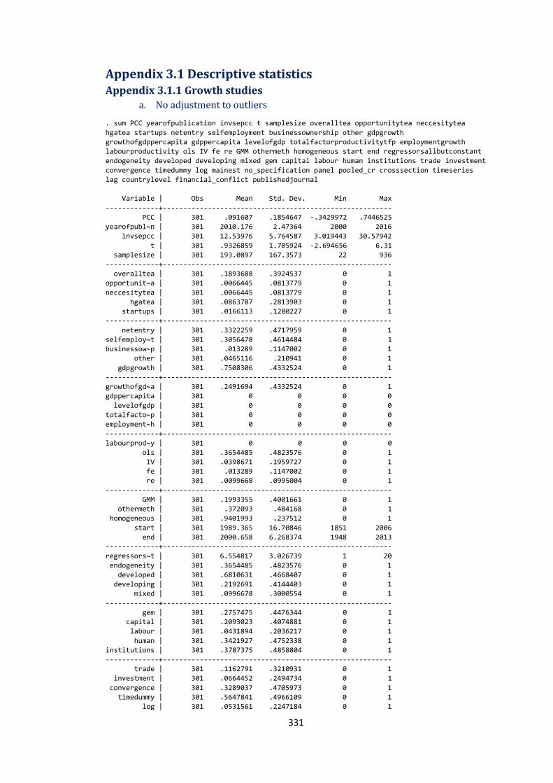
331
Appendix 3.1 Descriptive statistics Appendix 3.1.1 Growth studies
a. No adjustment to outliers
. sum PCC yearofpublication invsepcc t samplesize overalltea opportunitytea neccesitytea
hgatea startups netentry selfemployment businessownership other gdpgrowth
growthofgdppercapita gdppercapita levelofgdp totalfactorproductivitytfp employmentgrowth
labourproductivity ols IV fe re GMM othermeth homogeneous start end regressorsallbutconstant
endogeneity developed developing mixed gem capital labour human institutions trade investment
convergence timedummy log mainest no_specification panel pooled_cr crosssection timeseries
lag countrylevel financial_conflict publishedjournal
Variable | Obs Mean Std. Dev. Min Max
-------------+--------------------------------------------------------
PCC | 301 .091607 .1854647 -.3429972 .7446525
yearofpubl~n | 301 2010.176 2.47364 2000 2016
invsepcc | 301 12.53976 5.764587 3.019443 30.57942
t | 301 .9326859 1.705924 -2.694656 6.31
samplesize | 301 193.0897 167.3573 22 936
-------------+--------------------------------------------------------
overalltea | 301 .1893688 .3924537 0 1
opportunit~a | 301 .0066445 .0813779 0 1
neccesitytea | 301 .0066445 .0813779 0 1
hgatea | 301 .0863787 .2813903 0 1
startups | 301 .0166113 .1280227 0 1
-------------+--------------------------------------------------------
netentry | 301 .3322259 .4717959 0 1
selfemploy~t | 301 .3056478 .4614484 0 1
businessow~p | 301 .013289 .1147002 0 1
other | 301 .0465116 .210941 0 1
gdpgrowth | 301 .7508306 .4332524 0 1
-------------+--------------------------------------------------------
growthofgd~a | 301 .2491694 .4332524 0 1
gdppercapita | 301 0 0 0 0
levelofgdp | 301 0 0 0 0
totalfacto~p | 301 0 0 0 0
employment~h | 301 0 0 0 0
-------------+--------------------------------------------------------
labourprod~y | 301 0 0 0 0
ols | 301 .3654485 .4823576 0 1
IV | 301 .0398671 .1959727 0 1
fe | 301 .013289 .1147002 0 1
re | 301 .0099668 .0995004 0 1
-------------+--------------------------------------------------------
GMM | 301 .1993355 .4001661 0 1
othermeth | 301 .372093 .484168 0 1
homogeneous | 301 .9401993 .237512 0 1
start | 301 1989.365 16.70846 1851 2006
end | 301 2000.658 6.268374 1948 2013
-------------+--------------------------------------------------------
regressors~t | 301 6.554817 3.026739 1 20
endogeneity | 301 .3654485 .4823576 0 1
developed | 301 .6810631 .4668407 0 1
developing | 301 .2192691 .4144403 0 1
mixed | 301 .0996678 .3000554 0 1
-------------+--------------------------------------------------------
gem | 301 .2757475 .4476344 0 1
capital | 301 .2093023 .4074881 0 1
labour | 301 .0431894 .2036217 0 1
human | 301 .3421927 .4752338 0 1
institutions | 301 .3787375 .4858804 0 1
-------------+--------------------------------------------------------
trade | 301 .1162791 .3210931 0 1
investment | 301 .0664452 .2494734 0 1
convergence | 301 .3289037 .4705973 0 1
timedummy | 301 .5647841 .4966109 0 1
log | 301 .0531561 .2247184 0 1

332
-------------+--------------------------------------------------------
mainest | 301 .7940199 .4050894 0 1
no_specifi~n | 301 7.940199 7.425839 1 38
panel | 301 .7408638 .4388902 0 1
pooled_cr | 301 .013289 .1147002 0 1
crosssection | 301 .2259136 .418879 0 1
-------------+--------------------------------------------------------
timeseries | 301 .0199336 .1400047 0 1
lag | 301 .3787375 .4858804 0 1
countrylevel | 301 .5282392 .5000332 0 1
financial_~t | 301 .1428571 .3505098 0 1
publishedj~l | 301 .7242525 .4476344 0 1
b. Adjusted to outliers
. sum PCC yearofpublication invsepcc t samplesize overalltea opportunitytea neccesitytea
hgatea startups netentry selfemployment businessownership other gdpgrowth
growthofgdppercapita gdppercapita levelofgdp totalfactorproductivitytfp employmentgrowth
labourproductivity ols IV fe re GMM othermeth homogeneous start end regressorsallbutconstant
endogeneity developed developing mixed gem capital labour human institutions trade investment
convergence timedummy log mainest no_specification panel pooled_cr crosssection timeseries
lag countrylevel financial_conflict publishedjournal
Variable | Obs Mean Std. Dev. Min Max
-------------+--------------------------------------------------------
PCC | 297 .0860179 .1802681 -.3429972 .7446525
yearofpubl~n | 297 2010.155 2.482966 2000 2016
invsepcc | 297 12.55634 5.801063 3.019443 30.57942
t | 297 .8681766 1.622855 -2.694656 5.157895
samplesize | 297 194.266 168.1651 22 936
-------------+--------------------------------------------------------
overalltea | 297 .1885522 .3918127 0 1
opportunit~a | 297 .006734 .0819223 0 1
neccesitytea | 297 .006734 .0819223 0 1
hgatea | 297 .0875421 .2831048 0 1
startups | 297 .016835 .1288702 0 1
-------------+--------------------------------------------------------
netentry | 297 .3367003 .473379 0 1
selfemploy~t | 297 .3097643 .4631768 0 1
businessow~p | 297 .013468 .1154622 0 1
other | 28 .3928571 .4973475 0 1
gdpgrowth | 297 .7575758 .4292729 0 1
-------------+--------------------------------------------------------
growthofgd~a | 297 .2424242 .4292729 0 1
gdppercapita | 297 0 0 0 0
levelofgdp | 297 0 0 0 0
totalfacto~p | 297 0 0 0 0
employment~h | 297 0 0 0 0
-------------+--------------------------------------------------------
labourprod~y | 297 0 0 0 0
ols | 297 .3670034 .4828009 0 1
IV | 297 .040404 .1972373 0 1
fe | 297 .013468 .1154622 0 1
re | 297 .010101 .1001637 0 1
-------------+--------------------------------------------------------
GMM | 297 .1919192 .3944745 0 1
othermeth | 297 .3771044 .4854794 0 1
homogeneous | 297 .9427609 .2326909 0 1
start | 297 1989.377 16.78418 1851 2006
end | 297 2000.609 6.291536 1948 2013
-------------+--------------------------------------------------------
regressors~t | 297 6.518519 3.015808 1 20
endogeneity | 297 .3569024 .4798942 0 1
developed | 297 .6902357 .4631768 0 1
developing | 297 .2121212 .4095002 0 1
mixed | 297 .0976431 .2973325 0 1
-------------+--------------------------------------------------------
gem | 297 .2760943 .4478185 0 1

333
capital | 297 .2020202 .4021849 0 1
labour | 297 .043771 .2049306 0 1
human | 297 .3367003 .473379 0 1
institutions | 297 .3737374 .4846117 0 1
-------------+--------------------------------------------------------
trade | 297 .1178451 .3229688 0 1
investment | 297 .0606061 .239009 0 1
convergence | 297 .3299663 .4709941 0 1
timedummy | 297 .5589226 .497354 0 1
log | 297 .0538721 .2261461 0 1
-------------+--------------------------------------------------------
mainest | 297 .7946128 .4046661 0 1
no_specifi~n | 297 7.818182 7.356322 1 38
panel | 297 .7373737 .4408037 0 1
pooled_cr | 297 .013468 .1154622 0 1
crosssection | 297 .2289562 .4208701 0 1
-------------+--------------------------------------------------------
timeseries | 297 .020202 .1409282 0 1
lag | 297 .3838384 .4871401 0 1
countrylevel | 297 .5319865 .499818 0 1
financial_~t | 297 .1414141 .3490363 0 1
publishedj~l | 297 .7205387 .4494919 0 1
Appendix 3.1.2 Employment growth studies
a. No Adjustment to outliers
. sum PCC yearofpublication invsepcc t samplesize overalltea opportunitytea neccesitytea
hgatea startups netentry selfemployment businessownership other gdpgrowth
growthofgdppercapita gdppercapita levelofgdp totalfactorproductivitytfp employmentgrowth
labourproductivity ols fe re othermeth homogeneous start end regressorsallbutconstant
endogeneity developed developing mixed gem capital labour human institutions trade investment
convergence timedummy log mainest no_specification panel pooled_cr crosssection timeseries
lag countrylevel financial_conflict publishedjournal
Variable | Obs Mean Std. Dev. Min Max
-------------+--------------------------------------------------------
PCC | 249 .0667995 .1329694 -.2624494 .5012173
yearofpubl~n | 249 2007.173 2.475342 2002 2013
invsepcc | 249 33.29199 14.53781 7.618399 77.24766
t | 249 1.964104 4.040895 -10.77 13.09
samplesize | 249 1300.43 1173.739 59 5868
-------------+--------------------------------------------------------
overalltea | 249 0 0 0 0
opportunit~a | 249 0 0 0 0
neccesitytea | 249 0 0 0 0
hgatea | 249 0 0 0 0
startups | 249 .9116466 .2843798 0 1
-------------+--------------------------------------------------------
netentry | 249 0 0 0 0
selfemploy~t | 249 .0722892 .2594877 0 1
businessow~p | 249 .0160643 .1259759 0 1
other | 12 0 0 0 0
gdpgrowth | 249 0 0 0 0
-------------+--------------------------------------------------------
growthofgd~a | 249 0 0 0 0
gdppercapita | 249 0 0 0 0
levelofgdp | 249 0 0 0 0
totalfacto~p | 249 0 0 0 0
employment~h | 249 1 0 1 1
-------------+--------------------------------------------------------
labourprod~y | 249 0 0 0 0
ols | 249 .4176707 .4941686 0 1
fe | 249 .5461847 .4988651 0 1
re | 249 0 0 0 0
othermeth | 249 .0240964 .1536573 0 1
-------------+--------------------------------------------------------
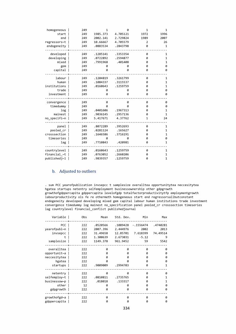
334
homogeneous | 249 1 0 1 1
start | 249 1985.373 4.705121 1972 1996
end | 249 2002.141 2.729824 1989 2007
regressors~t | 249 10.66667 4.705579 2 26
endogeneity | 249 .0883534 .2843798 0 1
-------------+--------------------------------------------------------
developed | 249 .1285141 .3353354 0 1
developing | 249 .0722892 .2594877 0 1
mixed | 249 .7991968 .401408 0 1
gem | 249 0 0 0 0
capital | 249 0 0 0 0
-------------+--------------------------------------------------------
labour | 249 .1204819 .3261799 0 1
human | 249 .1084337 .3115537 0 1
institutions | 249 .0160643 .1259759 0 1
trade | 249 0 0 0 0
investment | 249 0 0 0 0
-------------+--------------------------------------------------------
convergence | 249 0 0 0 0
timedummy | 249 0 0 0 0
log | 249 .0401606 .1967313 0 1
mainest | 249 .9036145 .2957136 0 1
no_specifi~n | 249 5.417671 4.37762 1 24
-------------+--------------------------------------------------------
panel | 249 .8072289 .3952693 0 1
pooled_cr | 249 .0281124 .165627 0 1
crosssection | 249 .1646586 .3716191 0 1
timeseries | 249 0 0 0 0
lag | 249 .7710843 .420981 0 1
-------------+--------------------------------------------------------
countrylevel | 249 .0160643 .1259759 0 1
financial_~t | 249 .0763052 .2660206 0 1
publishedj~l | 249 .9839357 .1259759 0 1
b. Adjusted to outliers
. sum PCC yearofpublication invsepcc t samplesize overalltea opportunitytea neccesitytea
hgatea startups netentry selfemployment businessownership other gdpgrowth
growthofgdppercapita gdppercapita levelofgdp totalfactorproductivitytfp employmentgrowth
labourproductivity ols fe re othermeth homogeneous start end regressorsallbutconstant
endogeneity developed developing mixed gem capital labour human institutions trade investment
convergence timedummy log mainest no_specification panel pooled_cr crosssection timeseries
lag countrylevel financial_conflict publishedjournal
Variable | Obs Mean Std. Dev. Min Max
-------------+--------------------------------------------------------
PCC | 222 .0520566 .1089428 -.1556474 .4740281
yearofpubl~n | 222 2007.396 2.444976 2002 2013
invsepcc | 222 31.49658 12.85701 7.618399 74.49514
t | 222 1.300639 2.673031 -5.12 9
samplesize | 222 1149.378 961.9452 59 5542
-------------+--------------------------------------------------------
overalltea | 222 0 0 0 0
opportunit~a | 222 0 0 0 0
neccesitytea | 222 0 0 0 0
hgatea | 222 0 0 0 0
startups | 222 .9009009 .2994703 0 1
-------------+--------------------------------------------------------
netentry | 222 0 0 0 0
selfemploy~t | 222 .0810811 .2735765 0 1
businessow~p | 222 .018018 .133317 0 1
other | 12 0 0 0 0
gdpgrowth | 222 0 0 0 0
-------------+--------------------------------------------------------
growthofgd~a | 222 0 0 0 0
gdppercapita | 222 0 0 0 0
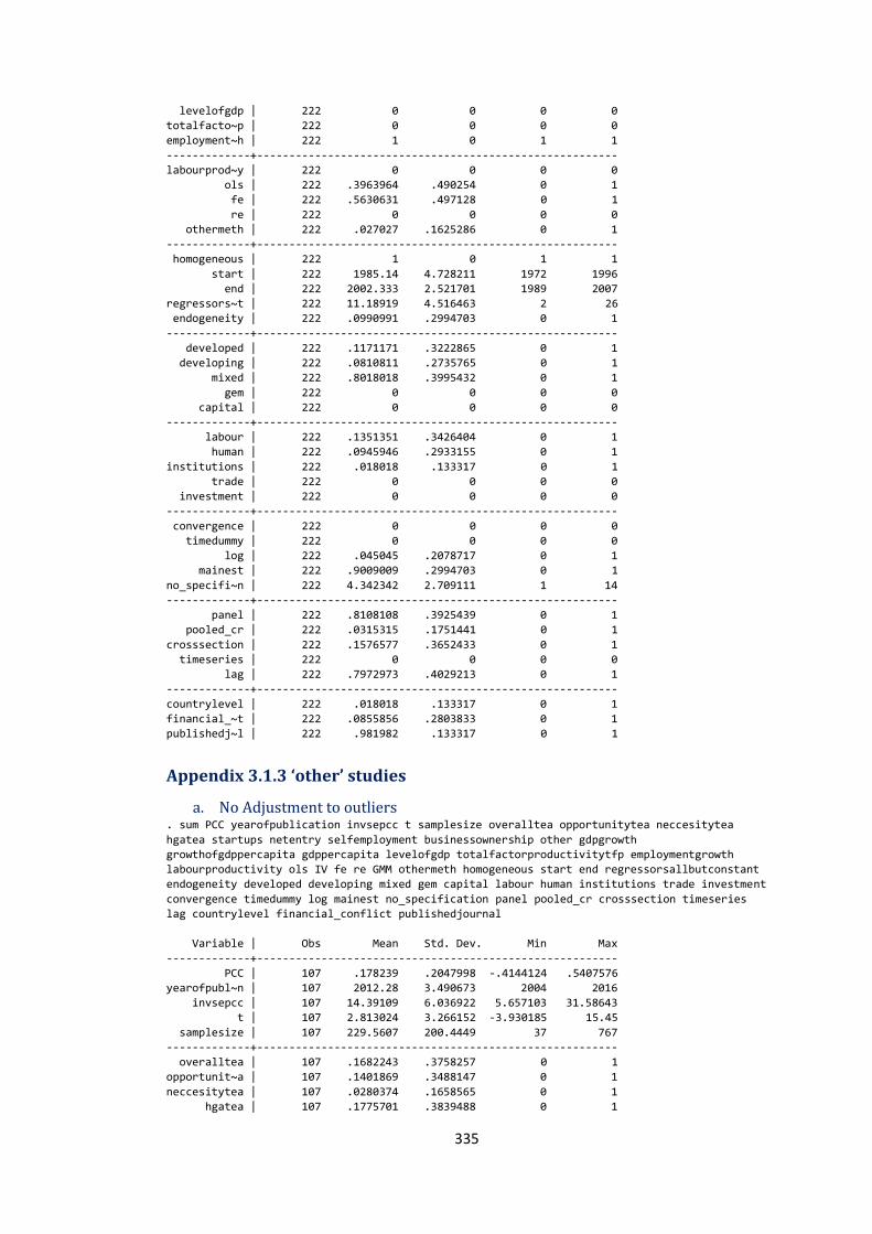
335
levelofgdp | 222 0 0 0 0
totalfacto~p | 222 0 0 0 0
employment~h | 222 1 0 1 1
-------------+--------------------------------------------------------
labourprod~y | 222 0 0 0 0
ols | 222 .3963964 .490254 0 1
fe | 222 .5630631 .497128 0 1
re | 222 0 0 0 0
othermeth | 222 .027027 .1625286 0 1
-------------+--------------------------------------------------------
homogeneous | 222 1 0 1 1
start | 222 1985.14 4.728211 1972 1996
end | 222 2002.333 2.521701 1989 2007
regressors~t | 222 11.18919 4.516463 2 26
endogeneity | 222 .0990991 .2994703 0 1
-------------+--------------------------------------------------------
developed | 222 .1171171 .3222865 0 1
developing | 222 .0810811 .2735765 0 1
mixed | 222 .8018018 .3995432 0 1
gem | 222 0 0 0 0
capital | 222 0 0 0 0
-------------+--------------------------------------------------------
labour | 222 .1351351 .3426404 0 1
human | 222 .0945946 .2933155 0 1
institutions | 222 .018018 .133317 0 1
trade | 222 0 0 0 0
investment | 222 0 0 0 0
-------------+--------------------------------------------------------
convergence | 222 0 0 0 0
timedummy | 222 0 0 0 0
log | 222 .045045 .2078717 0 1
mainest | 222 .9009009 .2994703 0 1
no_specifi~n | 222 4.342342 2.709111 1 14
-------------+--------------------------------------------------------
panel | 222 .8108108 .3925439 0 1
pooled_cr | 222 .0315315 .1751441 0 1
crosssection | 222 .1576577 .3652433 0 1
timeseries | 222 0 0 0 0
lag | 222 .7972973 .4029213 0 1
-------------+--------------------------------------------------------
countrylevel | 222 .018018 .133317 0 1
financial_~t | 222 .0855856 .2803833 0 1
publishedj~l | 222 .981982 .133317 0 1
Appendix 3.1.3 ‘other’ studies
a. No Adjustment to outliers . sum PCC yearofpublication invsepcc t samplesize overalltea opportunitytea neccesitytea
hgatea startups netentry selfemployment businessownership other gdpgrowth
growthofgdppercapita gdppercapita levelofgdp totalfactorproductivitytfp employmentgrowth
labourproductivity ols IV fe re GMM othermeth homogeneous start end regressorsallbutconstant
endogeneity developed developing mixed gem capital labour human institutions trade investment
convergence timedummy log mainest no_specification panel pooled_cr crosssection timeseries
lag countrylevel financial_conflict publishedjournal
Variable | Obs Mean Std. Dev. Min Max
-------------+--------------------------------------------------------
PCC | 107 .178239 .2047998 -.4144124 .5407576
yearofpubl~n | 107 2012.28 3.490673 2004 2016
invsepcc | 107 14.39109 6.036922 5.657103 31.58643
t | 107 2.813024 3.266152 -3.930185 15.45
samplesize | 107 229.5607 200.4449 37 767
-------------+--------------------------------------------------------
overalltea | 107 .1682243 .3758257 0 1
opportunit~a | 107 .1401869 .3488147 0 1
neccesitytea | 107 .0280374 .1658565 0 1
hgatea | 107 .1775701 .3839488 0 1
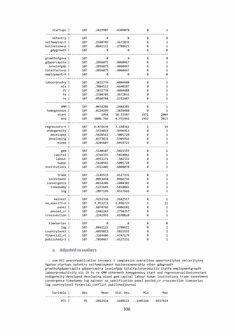
336
startups | 107 .2429907 .4309078 0 1
-------------+--------------------------------------------------------
netentry | 107 0 0 0 0
selfemploy~t | 107 .1588785 .3672831 0 1
businessow~p | 107 .0841121 .2788621 0 1
gdpgrowth | 107 0 0 0 0
-------------+--------------------------------------------------------
growthofgd~a | 107 0 0 0 0
gdppercapita | 107 .2056075 .4060467 0 1
levelofgdp | 107 .2056075 .4060467 0 1
totalfacto~p | 107 .2056075 .4060467 0 1
employment~h | 107 0 0 0 0
-------------+--------------------------------------------------------
labourprod~y | 107 .3831776 .4884488 0 1
ols | 107 .3084112 .4640107 0 1
IV | 107 .3831776 .4884488 0 1
fe | 107 .1588785 .3672831 0 1
re | 107 .0560748 .2311487 0 1
-------------+--------------------------------------------------------
GMM | 107 .0654206 .2484301 0 1
homogeneous | 107 .8224299 .3839488 0 1
start | 107 1994 10.33587 1971 2009
end | 107 2006.766 4.755492 1992 2013
-------------+--------------------------------------------------------
regressors~t | 107 6.476636 3.148362 1 19
endogeneity | 107 .5514019 .4996913 0 1
developed | 107 .5420561 .5005728 0 1
developing | 107 .0373832 .1905916 0 1
mixed | 107 .4205607 .4959721 0 1
-------------+--------------------------------------------------------
gem | 107 .5140187 .5021555 0 1
capital | 107 .4766355 .5018042 0 1
labour | 107 .4953271 .502331 0 1
human | 107 .5420561 .5005728 0 1
institutions | 107 .3551402 .4808078 0 1
-------------+--------------------------------------------------------
trade | 107 .2149533 .4127231 0 1
investment | 107 .0093458 .0966736 0 1
convergence | 107 .0654206 .2484301 0 1
timedummy | 107 .5233645 .5018042 0 1
log | 107 .2897196 .4557669 0 1
-------------+--------------------------------------------------------
mainest | 107 .9252336 .2642517 0 1
no_specifi~n | 107 3.953271 2.496727 1 12
panel | 107 .6074766 .4906101 0 1
pooled_cr | 107 .1682243 .3758257 0 1
crosssection | 107 .2242991 .4190828 0 1
-------------+--------------------------------------------------------
timeseries | 107 0 0 0 0
lag | 107 .0841121 .2788621 0 1
countrylevel | 107 .4859813 .5021555 0 1
financial_~t | 107 .3364486 .4747179 0 1
publishedj~l | 107 .7850467 .4127231 0 1
a. Adjusted to outliers
. . sum PCC yearofpublication invsepcc t samplesize overalltea opportunitytea neccesitytea
hgatea startups netentry selfemployment businessownership other gdpgrowth
growthofgdppercapita gdppercapita levelofgdp totalfactorproductiv itytfp employmentgrowth
labourproductivity ols IV fe re GMM othermeth homogeneous start end regressorsallbutconstant
endogeneity developed developing mixed gem capital labour human institutions trade investment
convergence timedummy log mainest no_specification panel pooled_cr crosssection timeseries
lag countrylevel financial_conflict publishedjournal
Variable | Obs Mean Std. Dev. Min Max
-------------+--------------------------------------------------------
PCC | 95 .2012424 .1440123 -.1485266 .4937419
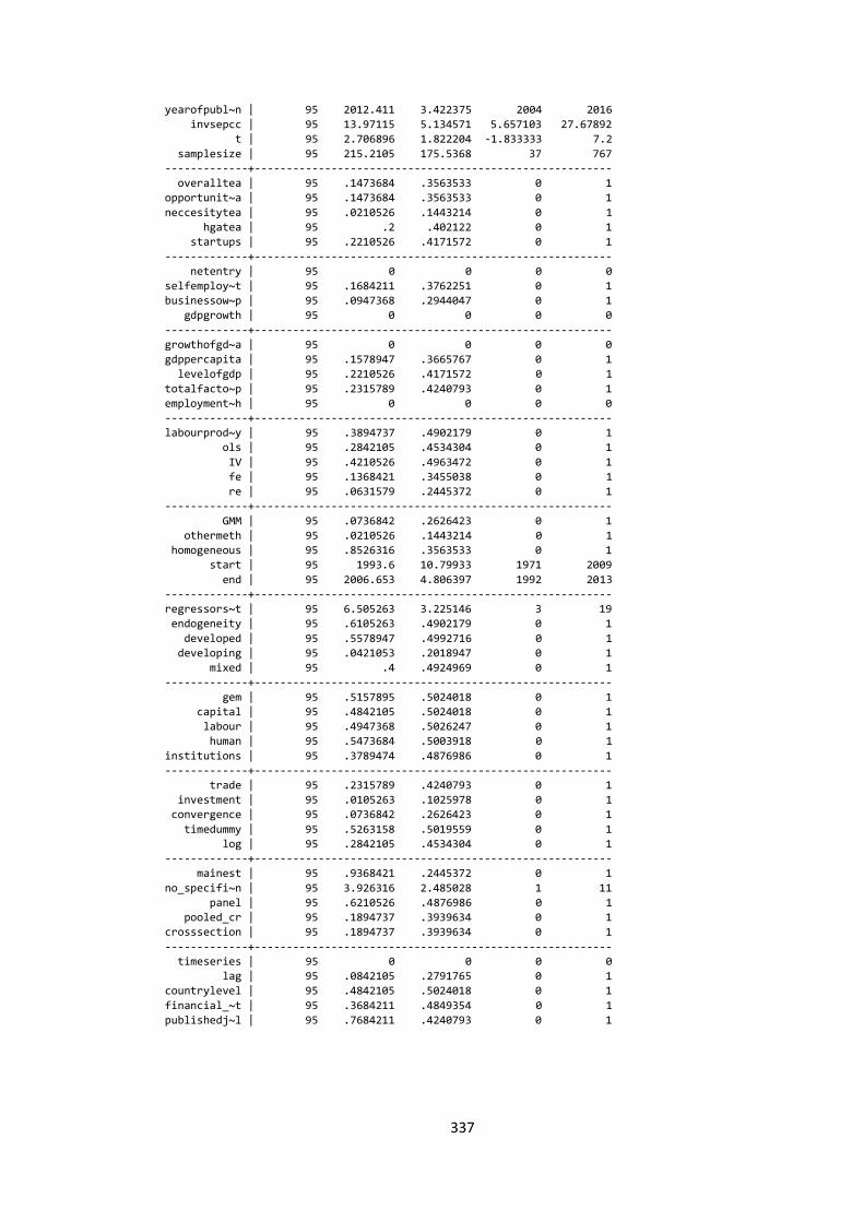
337
yearofpubl~n | 95 2012.411 3.422375 2004 2016
invsepcc | 95 13.97115 5.134571 5.657103 27.67892
t | 95 2.706896 1.822204 -1.833333 7.2
samplesize | 95 215.2105 175.5368 37 767
-------------+--------------------------------------------------------
overalltea | 95 .1473684 .3563533 0 1
opportunit~a | 95 .1473684 .3563533 0 1
neccesitytea | 95 .0210526 .1443214 0 1
hgatea | 95 .2 .402122 0 1
startups | 95 .2210526 .4171572 0 1
-------------+--------------------------------------------------------
netentry | 95 0 0 0 0
selfemploy~t | 95 .1684211 .3762251 0 1
businessow~p | 95 .0947368 .2944047 0 1
gdpgrowth | 95 0 0 0 0
-------------+--------------------------------------------------------
growthofgd~a | 95 0 0 0 0
gdppercapita | 95 .1578947 .3665767 0 1
levelofgdp | 95 .2210526 .4171572 0 1
totalfacto~p | 95 .2315789 .4240793 0 1
employment~h | 95 0 0 0 0
-------------+--------------------------------------------------------
labourprod~y | 95 .3894737 .4902179 0 1
ols | 95 .2842105 .4534304 0 1
IV | 95 .4210526 .4963472 0 1
fe | 95 .1368421 .3455038 0 1
re | 95 .0631579 .2445372 0 1
-------------+--------------------------------------------------------
GMM | 95 .0736842 .2626423 0 1
othermeth | 95 .0210526 .1443214 0 1
homogeneous | 95 .8526316 .3563533 0 1
start | 95 1993.6 10.79933 1971 2009
end | 95 2006.653 4.806397 1992 2013
-------------+--------------------------------------------------------
regressors~t | 95 6.505263 3.225146 3 19
endogeneity | 95 .6105263 .4902179 0 1
developed | 95 .5578947 .4992716 0 1
developing | 95 .0421053 .2018947 0 1
mixed | 95 .4 .4924969 0 1
-------------+--------------------------------------------------------
gem | 95 .5157895 .5024018 0 1
capital | 95 .4842105 .5024018 0 1
labour | 95 .4947368 .5026247 0 1
human | 95 .5473684 .5003918 0 1
institutions | 95 .3789474 .4876986 0 1
-------------+--------------------------------------------------------
trade | 95 .2315789 .4240793 0 1
investment | 95 .0105263 .1025978 0 1
convergence | 95 .0736842 .2626423 0 1
timedummy | 95 .5263158 .5019559 0 1
log | 95 .2842105 .4534304 0 1
-------------+--------------------------------------------------------
mainest | 95 .9368421 .2445372 0 1
no_specifi~n | 95 3.926316 2.485028 1 11
panel | 95 .6210526 .4876986 0 1
pooled_cr | 95 .1894737 .3939634 0 1
crosssection | 95 .1894737 .3939634 0 1
-------------+--------------------------------------------------------
timeseries | 95 0 0 0 0
lag | 95 .0842105 .2791765 0 1
countrylevel | 95 .4842105 .5024018 0 1
financial_~t | 95 .3684211 .4849354 0 1
publishedj~l | 95 .7684211 .4240793 0 1
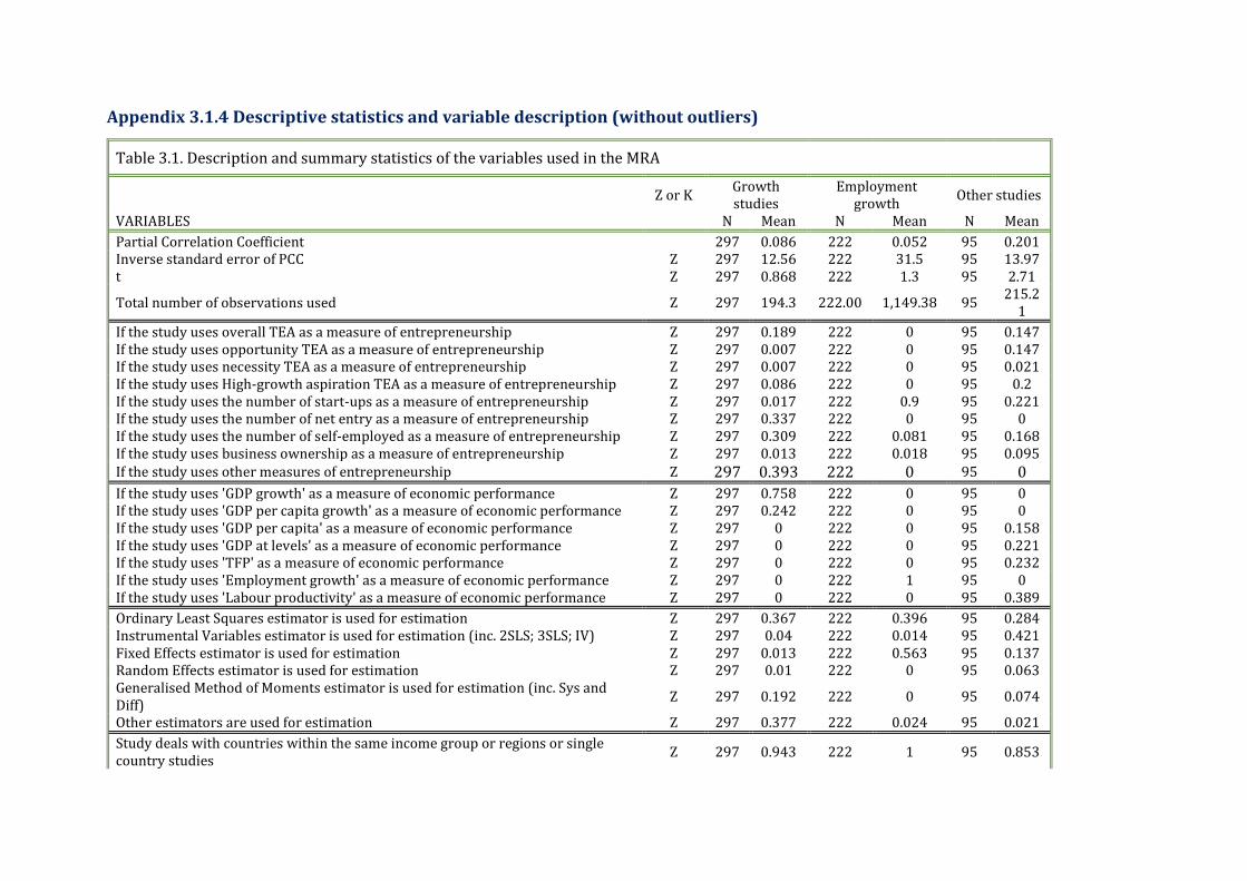
Appendix 3.1.4 Descriptive statistics and variable description (without outliers)
Table 3.1. Description and summary statistics of the variables used in the MRA
Z or K Growth studies
Employment growth
Other studies
VARIABLES N Mean N Mean N Mean
Partial Correlation Coefficient 297 0.086 222 0.052 95 0.201 Inverse standard error of PCC Z 297 12.56 222 31.5 95 13.97 t Z 297 0.868 222 1.3 95 2.71
Total number of observations used Z 297 194.3 222.00 1,149.38 95 215.2
1
If the study uses overall TEA as a measure of entrepreneurship Z 297 0.189 222 0 95 0.147 If the study uses opportunity TEA as a measure of entrepreneurship Z 297 0.007 222 0 95 0.147 If the study uses necessity TEA as a measure of entrepreneurship Z 297 0.007 222 0 95 0.021 If the study uses High-growth aspiration TEA as a measure of entrepreneurship Z 297 0.086 222 0 95 0.2 If the study uses the number of start-ups as a measure of entrepreneurship Z 297 0.017 222 0.9 95 0.221 If the study uses the number of net entry as a measure of entrepreneurship Z 297 0.337 222 0 95 0 If the study uses the number of self-employed as a measure of entrepreneurship Z 297 0.309 222 0.081 95 0.168 If the study uses business ownership as a measure of entrepreneurship Z 297 0.013 222 0.018 95 0.095 If the study uses other measures of entrepreneurship Z 297 0.393 222 0 95 0
If the study uses 'GDP growth' as a measure of economic performance Z 297 0.758 222 0 95 0 If the study uses 'GDP per capita growth' as a measure of economic performance Z 297 0.242 222 0 95 0 If the study uses 'GDP per capita' as a measure of economic performance Z 297 0 222 0 95 0.158 If the study uses 'GDP at levels' as a measure of economic performance Z 297 0 222 0 95 0.221 If the study uses 'TFP' as a measure of economic performance Z 297 0 222 0 95 0.232 If the study uses 'Employment growth' as a measure of economic performance Z 297 0 222 1 95 0 If the study uses 'Labour productivity' as a measure of economic performance Z 297 0 222 0 95 0.389
Ordinary Least Squares estimator is used for estimation Z 297 0.367 222 0.396 95 0.284 Instrumental Variables estimator is used for estimation (inc. 2SLS; 3SLS; IV) Z 297 0.04 222 0.014 95 0.421 Fixed Effects estimator is used for estimation Z 297 0.013 222 0.563 95 0.137 Random Effects estimator is used for estimation Z 297 0.01 222 0 95 0.063 Generalised Method of Moments estimator is used for estimation (inc. Sys and Diff)
Z 297 0.192 222 0 95 0.074
Other estimators are used for estimation Z 297 0.377 222 0.024 95 0.021
Study deals with countries within the same income group or regions or single country studies
Z 297 0.943 222 1 95 0.853
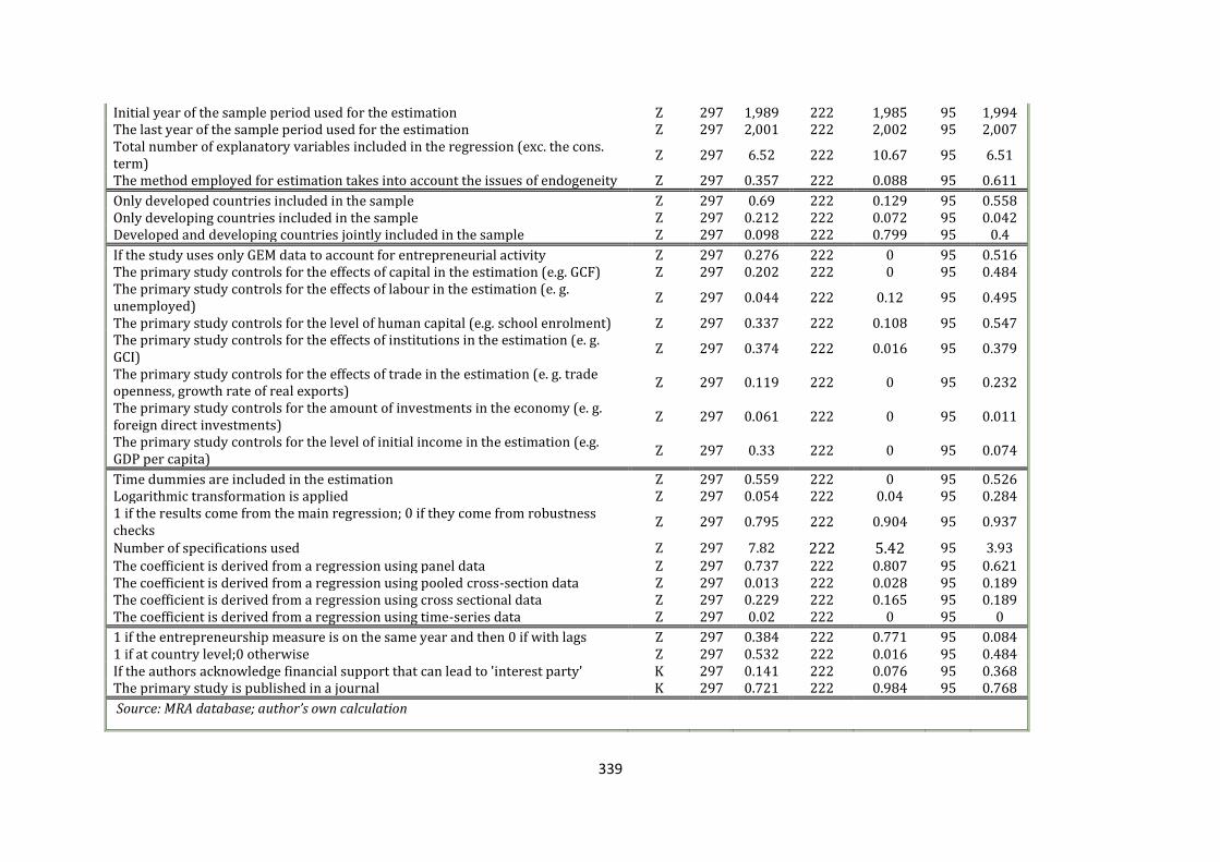
339
Initial year of the sample period used for the estimation Z 297 1,989 222 1,985 95 1,994 The last year of the sample period used for the estimation Z 297 2,001 222 2,002 95 2,007 Total number of explanatory variables included in the regression (exc. the cons. term)
Z 297 6.52 222 10.67 95 6.51
The method employed for estimation takes into account the issues of endogeneity Z 297 0.357 222 0.088 95 0.611
Only developed countries included in the sample Z 297 0.69 222 0.129 95 0.558 Only developing countries included in the sample Z 297 0.212 222 0.072 95 0.042 Developed and developing countries jointly included in the sample Z 297 0.098 222 0.799 95 0.4
If the study uses only GEM data to account for entrepreneurial activity Z 297 0.276 222 0 95 0.516 The primary study controls for the effects of capital in the estimation (e.g. GCF) Z 297 0.202 222 0 95 0.484 The primary study controls for the effects of labour in the estimation (e. g. unemployed)
Z 297 0.044 222 0.12 95 0.495
The primary study controls for the level of human capital (e.g. school enrolment) Z 297 0.337 222 0.108 95 0.547 The primary study controls for the effects of institutions in the estimation (e. g. GCI)
Z 297 0.374 222 0.016 95 0.379
The primary study controls for the effects of trade in the estimation (e. g. trade openness, growth rate of real exports)
Z 297 0.119 222 0 95 0.232
The primary study controls for the amount of investments in the economy (e. g. foreign direct investments)
Z 297 0.061 222 0 95 0.011
The primary study controls for the level of initial income in the estimation (e.g. GDP per capita)
Z 297 0.33 222 0 95 0.074
Time dummies are included in the estimation Z 297 0.559 222 0 95 0.526 Logarithmic transformation is applied Z 297 0.054 222 0.04 95 0.284 1 if the results come from the main regression; 0 if they come from robustness checks
Z 297 0.795 222 0.904 95 0.937
Number of specifications used Z 297 7.82 222 5.42 95 3.93 The coefficient is derived from a regression using panel data Z 297 0.737 222 0.807 95 0.621 The coefficient is derived from a regression using pooled cross-section data Z 297 0.013 222 0.028 95 0.189 The coefficient is derived from a regression using cross sectional data Z 297 0.229 222 0.165 95 0.189 The coefficient is derived from a regression using time-series data Z 297 0.02 222 0 95 0
1 if the entrepreneurship measure is on the same year and then 0 if with lags Z 297 0.384 222 0.771 95 0.084 1 if at country level;0 otherwise Z 297 0.532 222 0.016 95 0.484 If the authors acknowledge financial support that can lead to 'interest party' K 297 0.141 222 0.076 95 0.368 The primary study is published in a journal K 297 0.721 222 0.984 95 0.768
Source: MRA database; author’s own calculation
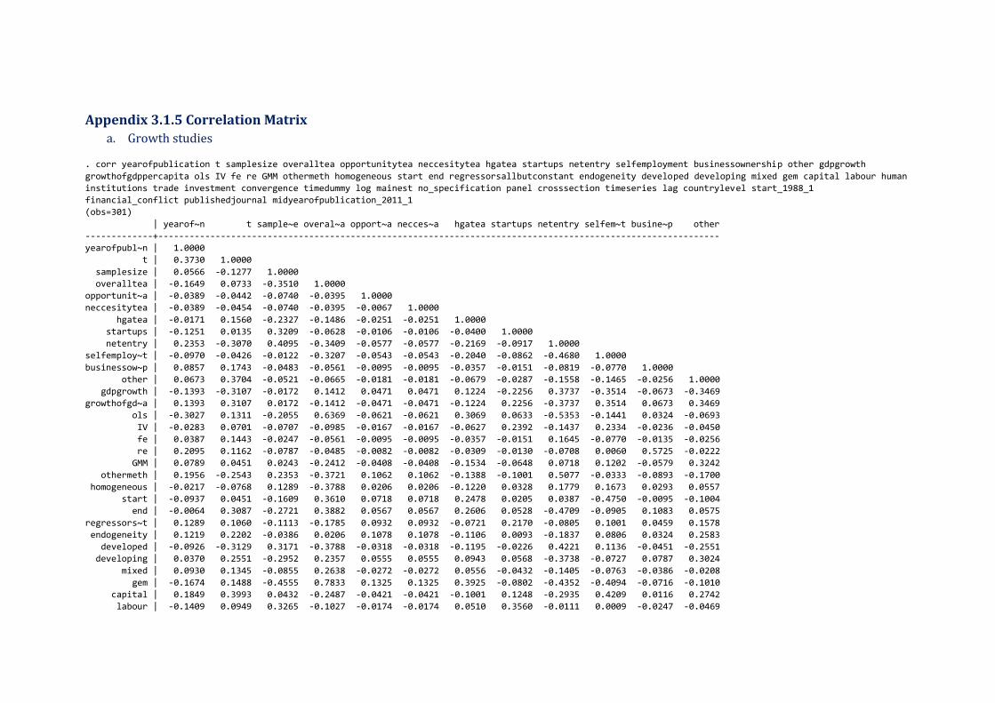
Appendix 3.1.5 Correlation Matrix
a. Growth studies
. corr yearofpublication t samplesize overalltea opportunitytea neccesitytea hgatea startups netentry selfemployment businessownership other gdpgrowth
growthofgdppercapita ols IV fe re GMM othermeth homogeneous start end regressorsallbutconstant endogeneity developed developing mixed gem capital labour human
institutions trade investment convergence timedummy log mainest no_specification panel crosssection timeseries lag countrylevel start_1988_1
financial_conflict publishedjournal midyearofpublication_2011_1
(obs=301)
| yearof~n t sample~e overal~a opport~a necces~a hgatea startups netentry selfem~t busine~p other
-------------+------------------------------------------------------------------------------------------------------------
yearofpubl~n | 1.0000
t | 0.3730 1.0000
samplesize | 0.0566 -0.1277 1.0000
overalltea | -0.1649 0.0733 -0.3510 1.0000
opportunit~a | -0.0389 -0.0442 -0.0740 -0.0395 1.0000
neccesitytea | -0.0389 -0.0454 -0.0740 -0.0395 -0.0067 1.0000
hgatea | -0.0171 0.1560 -0.2327 -0.1486 -0.0251 -0.0251 1.0000
startups | -0.1251 0.0135 0.3209 -0.0628 -0.0106 -0.0106 -0.0400 1.0000
netentry | 0.2353 -0.3070 0.4095 -0.3409 -0.0577 -0.0577 -0.2169 -0.0917 1.0000
selfemploy~t | -0.0970 -0.0426 -0.0122 -0.3207 -0.0543 -0.0543 -0.2040 -0.0862 -0.4680 1.0000
businessow~p | 0.0857 0.1743 -0.0483 -0.0561 -0.0095 -0.0095 -0.0357 -0.0151 -0.0819 -0.0770 1.0000
other | 0.0673 0.3704 -0.0521 -0.0665 -0.0181 -0.0181 -0.0679 -0.0287 -0.1558 -0.1465 -0.0256 1.0000
gdpgrowth | -0.1393 -0.3107 -0.0172 0.1412 0.0471 0.0471 0.1224 -0.2256 0.3737 -0.3514 -0.0673 -0.3469
growthofgd~a | 0.1393 0.3107 0.0172 -0.1412 -0.0471 -0.0471 -0.1224 0.2256 -0.3737 0.3514 0.0673 0.3469
ols | -0.3027 0.1311 -0.2055 0.6369 -0.0621 -0.0621 0.3069 0.0633 -0.5353 -0.1441 0.0324 -0.0693
IV | -0.0283 0.0701 -0.0707 -0.0985 -0.0167 -0.0167 -0.0627 0.2392 -0.1437 0.2334 -0.0236 -0.0450
fe | 0.0387 0.1443 -0.0247 -0.0561 -0.0095 -0.0095 -0.0357 -0.0151 0.1645 -0.0770 -0.0135 -0.0256
re | 0.2095 0.1162 -0.0787 -0.0485 -0.0082 -0.0082 -0.0309 -0.0130 -0.0708 0.0060 0.5725 -0.0222
GMM | 0.0789 0.0451 0.0243 -0.2412 -0.0408 -0.0408 -0.1534 -0.0648 0.0718 0.1202 -0.0579 0.3242
othermeth | 0.1956 -0.2543 0.2353 -0.3721 0.1062 0.1062 -0.1388 -0.1001 0.5077 -0.0333 -0.0893 -0.1700
homogeneous | -0.0217 -0.0768 0.1289 -0.3788 0.0206 0.0206 -0.1220 0.0328 0.1779 0.1673 0.0293 0.0557
start | -0.0937 0.0451 -0.1609 0.3610 0.0718 0.0718 0.2478 0.0205 0.0387 -0.4750 -0.0095 -0.1004
end | -0.0064 0.3087 -0.2721 0.3882 0.0567 0.0567 0.2606 0.0528 -0.4709 -0.0905 0.1083 0.0575
regressors~t | 0.1289 0.1060 -0.1113 -0.1785 0.0932 0.0932 -0.0721 0.2170 -0.0805 0.1001 0.0459 0.1578
endogeneity | 0.1219 0.2202 -0.0386 0.0206 0.1078 0.1078 -0.1106 0.0093 -0.1837 0.0806 0.0324 0.2583
developed | -0.0926 -0.3129 0.3171 -0.3788 -0.0318 -0.0318 -0.1195 -0.0226 0.4221 0.1136 -0.0451 -0.2551
developing | 0.0370 0.2551 -0.2952 0.2357 0.0555 0.0555 0.0943 0.0568 -0.3738 -0.0727 0.0787 0.3024
mixed | 0.0930 0.1345 -0.0855 0.2638 -0.0272 -0.0272 0.0556 -0.0432 -0.1405 -0.0763 -0.0386 -0.0208
gem | -0.1674 0.1488 -0.4555 0.7833 0.1325 0.1325 0.3925 -0.0802 -0.4352 -0.4094 -0.0716 -0.1010
capital | 0.1849 0.3993 0.0432 -0.2487 -0.0421 -0.0421 -0.1001 0.1248 -0.2935 0.4209 0.0116 0.2742
labour | -0.1409 0.0949 0.3265 -0.1027 -0.0174 -0.0174 0.0510 0.3560 -0.0111 0.0009 -0.0247 -0.0469

341
human | -0.0202 0.1820 0.0109 -0.2950 -0.0590 -0.0590 -0.1719 0.1802 -0.4493 0.6919 -0.0226 0.2065
institutions | -0.2997 0.2254 -0.5010 0.4967 0.1047 0.1047 0.3451 0.0057 -0.5507 -0.1166 -0.0308 0.0552
trade | -0.0636 -0.1242 -0.0761 -0.1753 -0.0297 -0.0297 -0.1115 -0.0471 -0.2559 0.5242 0.0484 -0.0801
investment | 0.0944 0.2420 -0.1373 -0.1289 0.3066 0.3066 0.1079 -0.0347 -0.1599 -0.0322 -0.0310 0.3211
convergence | -0.4880 0.0400 -0.5073 0.5641 0.1168 0.1168 0.4392 -0.0910 -0.4938 -0.2189 -0.0195 -0.0539
timedummy | 0.3855 0.1260 0.2142 -0.2598 -0.0932 -0.0932 -0.1117 0.0092 0.0501 0.2333 -0.1322 0.1302
log | 0.4029 0.1223 -0.0422 0.1501 -0.0194 -0.0194 -0.0729 -0.0308 -0.1671 0.0035 0.4898 -0.0523
mainest | 0.0496 -0.0047 0.1060 -0.1522 0.0417 0.0417 -0.2820 0.0662 -0.0593 0.2666 0.0591 0.1125
no_specifi~n | 0.0432 -0.1049 0.0781 -0.2775 -0.0710 -0.0710 -0.1331 -0.1112 0.0304 0.3711 -0.1008 -0.0195
panel | 0.5062 0.0693 0.3787 -0.5117 -0.1432 -0.1432 -0.2090 0.0742 0.4027 0.1276 0.0663 0.0528
crosssection | -0.4793 -0.0370 -0.4365 0.5500 0.1514 0.1514 0.2298 -0.0702 -0.3810 -0.2032 -0.0627 -0.0439
timeseries | -0.1257 -0.1028 0.1391 -0.0689 -0.0117 -0.0117 -0.0439 -0.0185 -0.1006 0.2150 -0.0166 -0.0315
lag | 0.4130 -0.2826 0.4240 -0.2550 -0.0639 -0.0639 -0.2401 -0.1015 0.8452 -0.3842 0.0290 -0.1724
countrylevel | -0.3530 0.0119 -0.4580 0.4568 0.0773 0.0773 0.2432 -0.1375 -0.7464 0.3092 0.1097 -0.2021
start_1988_1 | 0.1065 -0.0983 0.0503 0.3308 0.0560 0.0560 0.2104 0.0889 0.4827 -0.7993 -0.0451 -0.2889
financial_~t | -0.1944 0.1830 -0.2231 0.1904 -0.0334 -0.0334 0.6180 -0.0531 -0.2880 -0.2090 0.1184 -0.0902
publishedj~l | 0.4022 0.0261 0.4084 -0.4038 0.0505 0.0505 -0.3131 -0.0361 0.3721 0.0866 0.0716 0.0657
midyearofp~1 | 0.6892 0.1838 0.2861 -0.3109 -0.0901 -0.0901 -0.2199 -0.1432 0.6404 -0.2381 -0.0112 0.1054
| gdpgro~h growth~a ols IV fe re GMM otherm~h homoge~s start end regres~t
-------------+------------------------------------------------------------------------------------------------------------
gdpgrowth | 1.0000
growthofgd~a | -1.0000 1.0000
ols | 0.1501 -0.1501 1.0000
IV | -0.2752 0.2752 -0.1546 1.0000
fe | -0.0673 0.0673 -0.0881 -0.0236 1.0000
re | -0.1742 0.1742 -0.0761 -0.0204 -0.0116 1.0000
GMM | -0.4047 0.4047 -0.3787 -0.1017 -0.0579 -0.0501 1.0000
othermeth | 0.3481 -0.3481 -0.5842 -0.1569 -0.0893 -0.0772 -0.3841 1.0000
homogeneous | -0.0157 0.0157 -0.3323 0.0514 0.0293 0.0253 0.1258 0.1941 1.0000
start | 0.1015 -0.1015 0.1256 -0.0197 0.0740 0.0539 -0.1575 -0.0156 -0.1902 1.0000
end | -0.2021 0.2021 0.3160 -0.0268 0.1362 0.1444 -0.0897 -0.2918 -0.2354 0.6804 1.0000
regressors~t | -0.2399 0.2399 -0.2626 0.2211 -0.0501 -0.0627 0.2909 -0.0435 0.1808 0.0933 0.1991 1.0000
endogeneity | -0.4879 0.4879 -0.1175 0.2685 -0.0881 -0.0761 0.6575 -0.4986 -0.0123 0.0152 0.1495 0.3264
developed | 0.3639 -0.3639 -0.3096 -0.0063 -0.1696 -0.1466 -0.1225 0.4825 0.3685 -0.2611 -0.4908 -0.2164
developing | -0.3073 0.3073 0.1814 0.0562 -0.0615 0.1085 0.1778 -0.3581 0.1337 0.1732 0.3459 0.2163
mixed | -0.1417 0.1417 0.2311 -0.0678 0.3488 0.0783 -0.0550 -0.2561 -0.7580 0.1669 0.2858 0.0380
gem | 0.2008 -0.2008 0.6896 -0.1257 -0.0716 -0.0619 -0.3079 -0.3520 -0.4087 0.4758 0.5042 -0.1379
capital | -0.3644 0.3644 -0.2209 0.1456 0.2256 0.0306 0.1112 0.0094 0.1298 -0.1430 0.1378 0.2163
labour | -0.1799 0.1799 0.0424 -0.0433 0.5462 0.1432 -0.1060 -0.0959 0.0536 0.0051 0.1317 -0.0444
human | -0.5397 0.5397 -0.2129 0.2825 0.1609 0.0686 0.1309 -0.0627 0.0933 -0.2354 0.1312 0.1827
institutions | -0.0569 0.0569 0.4742 0.2260 -0.0906 -0.0094 -0.1324 -0.4310 -0.2075 0.3393 0.3579 0.0629
trade | -0.1025 0.1025 -0.1246 -0.0209 -0.0421 0.1723 0.0525 0.0638 0.0915 -0.1658 0.0728 0.2661
investment | -0.2472 0.2472 -0.1748 -0.0544 0.0855 -0.0268 0.2008 0.0154 0.0673 0.0229 0.1681 0.3218
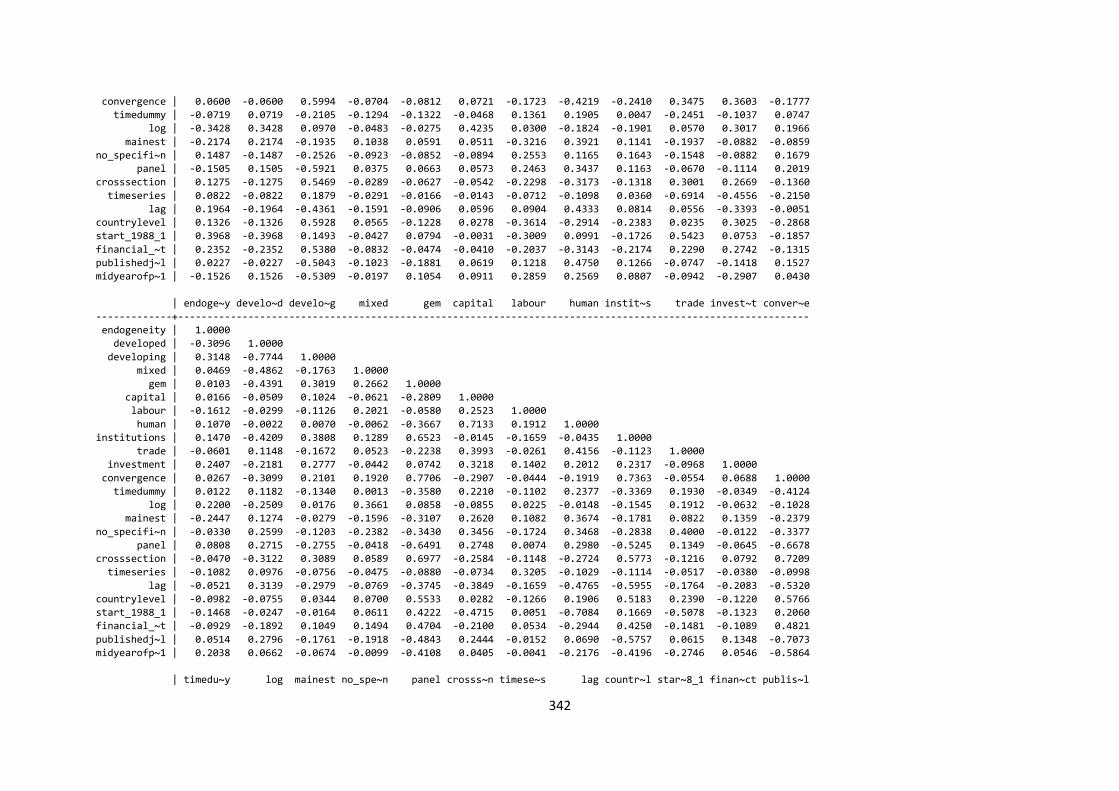
342
convergence | 0.0600 -0.0600 0.5994 -0.0704 -0.0812 0.0721 -0.1723 -0.4219 -0.2410 0.3475 0.3603 -0.1777
timedummy | -0.0719 0.0719 -0.2105 -0.1294 -0.1322 -0.0468 0.1361 0.1905 0.0047 -0.2451 -0.1037 0.0747
log | -0.3428 0.3428 0.0970 -0.0483 -0.0275 0.4235 0.0300 -0.1824 -0.1901 0.0570 0.3017 0.1966
mainest | -0.2174 0.2174 -0.1935 0.1038 0.0591 0.0511 -0.3216 0.3921 0.1141 -0.1937 -0.0882 -0.0859
no_specifi~n | 0.1487 -0.1487 -0.2526 -0.0923 -0.0852 -0.0894 0.2553 0.1165 0.1643 -0.1548 -0.0882 0.1679
panel | -0.1505 0.1505 -0.5921 0.0375 0.0663 0.0573 0.2463 0.3437 0.1163 -0.0670 -0.1114 0.2019
crosssection | 0.1275 -0.1275 0.5469 -0.0289 -0.0627 -0.0542 -0.2298 -0.3173 -0.1318 0.3001 0.2669 -0.1360
timeseries | 0.0822 -0.0822 0.1879 -0.0291 -0.0166 -0.0143 -0.0712 -0.1098 0.0360 -0.6914 -0.4556 -0.2150
lag | 0.1964 -0.1964 -0.4361 -0.1591 -0.0906 0.0596 0.0904 0.4333 0.0814 0.0556 -0.3393 -0.0051
countrylevel | 0.1326 -0.1326 0.5928 0.0565 -0.1228 0.0278 -0.3614 -0.2914 -0.2383 0.0235 0.3025 -0.2868
start_1988_1 | 0.3968 -0.3968 0.1493 -0.0427 0.0794 -0.0031 -0.3009 0.0991 -0.1726 0.5423 0.0753 -0.1857
financial_~t | 0.2352 -0.2352 0.5380 -0.0832 -0.0474 -0.0410 -0.2037 -0.3143 -0.2174 0.2290 0.2742 -0.1315
publishedj~l | 0.0227 -0.0227 -0.5043 -0.1023 -0.1881 0.0619 0.1218 0.4750 0.1266 -0.0747 -0.1418 0.1527
midyearofp~1 | -0.1526 0.1526 -0.5309 -0.0197 0.1054 0.0911 0.2859 0.2569 0.0807 -0.0942 -0.2907 0.0430
| endoge~y develo~d develo~g mixed gem capital labour human instit~s trade invest~t conver~e
-------------+------------------------------------------------------------------------------------------------------------
endogeneity | 1.0000
developed | -0.3096 1.0000
developing | 0.3148 -0.7744 1.0000
mixed | 0.0469 -0.4862 -0.1763 1.0000
gem | 0.0103 -0.4391 0.3019 0.2662 1.0000
capital | 0.0166 -0.0509 0.1024 -0.0621 -0.2809 1.0000
labour | -0.1612 -0.0299 -0.1126 0.2021 -0.0580 0.2523 1.0000
human | 0.1070 -0.0022 0.0070 -0.0062 -0.3667 0.7133 0.1912 1.0000
institutions | 0.1470 -0.4209 0.3808 0.1289 0.6523 -0.0145 -0.1659 -0.0435 1.0000
trade | -0.0601 0.1148 -0.1672 0.0523 -0.2238 0.3993 -0.0261 0.4156 -0.1123 1.0000
investment | 0.2407 -0.2181 0.2777 -0.0442 0.0742 0.3218 0.1402 0.2012 0.2317 -0.0968 1.0000
convergence | 0.0267 -0.3099 0.2101 0.1920 0.7706 -0.2907 -0.0444 -0.1919 0.7363 -0.0554 0.0688 1.0000
timedummy | 0.0122 0.1182 -0.1340 0.0013 -0.3580 0.2210 -0.1102 0.2377 -0.3369 0.1930 -0.0349 -0.4124
log | 0.2200 -0.2509 0.0176 0.3661 0.0858 -0.0855 0.0225 -0.0148 -0.1545 0.1912 -0.0632 -0.1028
mainest | -0.2447 0.1274 -0.0279 -0.1596 -0.3107 0.2620 0.1082 0.3674 -0.1781 0.0822 0.1359 -0.2379
no_specifi~n | -0.0330 0.2599 -0.1203 -0.2382 -0.3430 0.3456 -0.1724 0.3468 -0.2838 0.4000 -0.0122 -0.3377
panel | 0.0808 0.2715 -0.2755 -0.0418 -0.6491 0.2748 0.0074 0.2980 -0.5245 0.1349 -0.0645 -0.6678
crosssection | -0.0470 -0.3122 0.3089 0.0589 0.6977 -0.2584 -0.1148 -0.2724 0.5773 -0.1216 0.0792 0.7209
timeseries | -0.1082 0.0976 -0.0756 -0.0475 -0.0880 -0.0734 0.3205 -0.1029 -0.1114 -0.0517 -0.0380 -0.0998
lag | -0.0521 0.3139 -0.2979 -0.0769 -0.3745 -0.3849 -0.1659 -0.4765 -0.5955 -0.1764 -0.2083 -0.5320
countrylevel | -0.0982 -0.0755 0.0344 0.0700 0.5533 0.0282 -0.1266 0.1906 0.5183 0.2390 -0.1220 0.5766
start_1988_1 | -0.1468 -0.0247 -0.0164 0.0611 0.4222 -0.4715 0.0051 -0.7084 0.1669 -0.5078 -0.1323 0.2060
financial_~t | -0.0929 -0.1892 0.1049 0.1494 0.4704 -0.2100 0.0534 -0.2944 0.4250 -0.1481 -0.1089 0.4821
publishedj~l | 0.0514 0.2796 -0.1761 -0.1918 -0.4843 0.2444 -0.0152 0.0690 -0.5757 0.0615 0.1348 -0.7073
midyearofp~1 | 0.2038 0.0662 -0.0674 -0.0099 -0.4108 0.0405 -0.0041 -0.2176 -0.4196 -0.2746 0.0546 -0.5864
| timedu~y log mainest no_spe~n panel crosss~n timese~s lag countr~l star~8_1 finan~ct publis~l
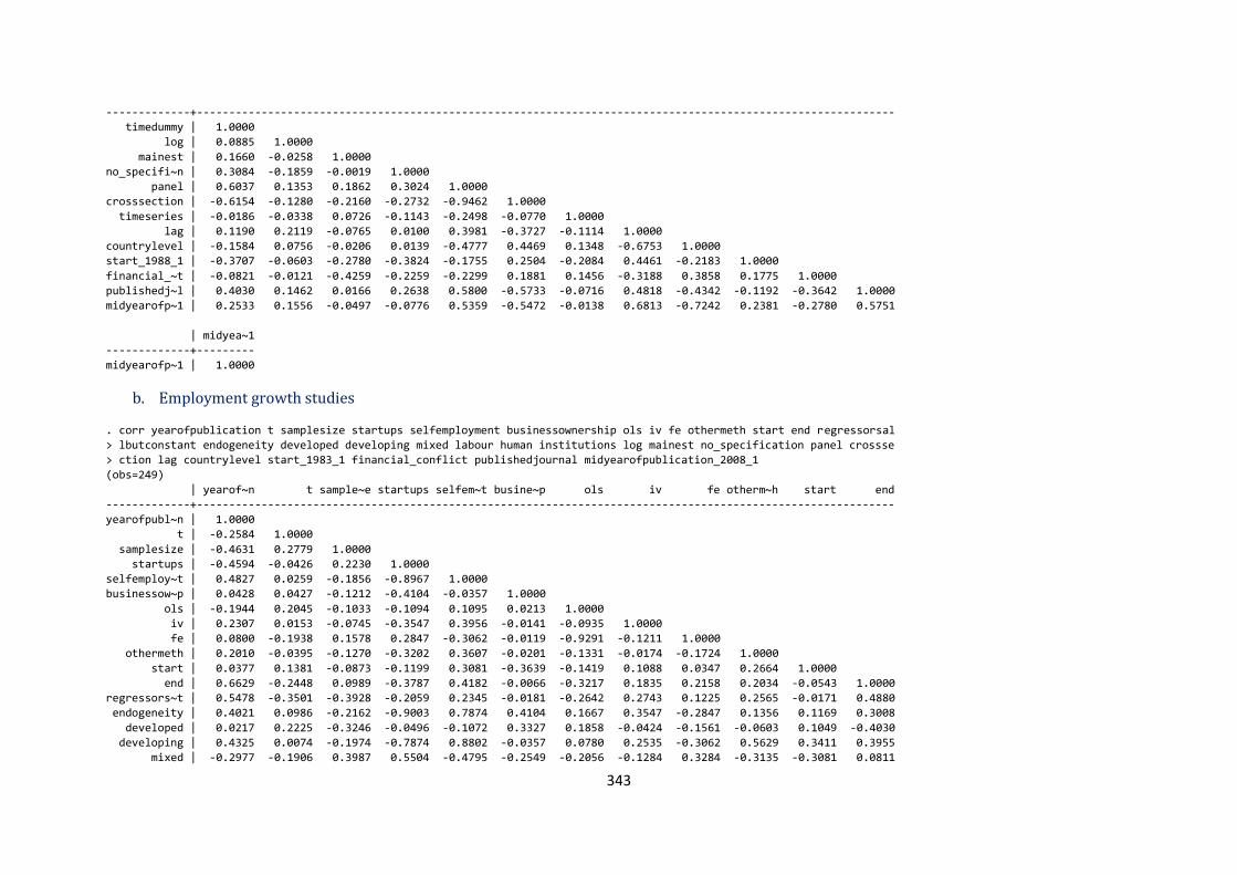
343
-------------+------------------------------------------------------------------------------------------------------------
timedummy | 1.0000
log | 0.0885 1.0000
mainest | 0.1660 -0.0258 1.0000
no_specifi~n | 0.3084 -0.1859 -0.0019 1.0000
panel | 0.6037 0.1353 0.1862 0.3024 1.0000
crosssection | -0.6154 -0.1280 -0.2160 -0.2732 -0.9462 1.0000
timeseries | -0.0186 -0.0338 0.0726 -0.1143 -0.2498 -0.0770 1.0000
lag | 0.1190 0.2119 -0.0765 0.0100 0.3981 -0.3727 -0.1114 1.0000
countrylevel | -0.1584 0.0756 -0.0206 0.0139 -0.4777 0.4469 0.1348 -0.6753 1.0000
start_1988_1 | -0.3707 -0.0603 -0.2780 -0.3824 -0.1755 0.2504 -0.2084 0.4461 -0.2183 1.0000
financial_~t | -0.0821 -0.0121 -0.4259 -0.2259 -0.2299 0.1881 0.1456 -0.3188 0.3858 0.1775 1.0000
publishedj~l | 0.4030 0.1462 0.0166 0.2638 0.5800 -0.5733 -0.0716 0.4818 -0.4342 -0.1192 -0.3642 1.0000
midyearofp~1 | 0.2533 0.1556 -0.0497 -0.0776 0.5359 -0.5472 -0.0138 0.6813 -0.7242 0.2381 -0.2780 0.5751
| midyea~1
-------------+---------
midyearofp~1 | 1.0000
b. Employment growth studies
. corr yearofpublication t samplesize startups selfemployment businessownership ols iv fe othermeth start end regressorsal
> lbutconstant endogeneity developed developing mixed labour human institutions log mainest no_specification panel crossse
> ction lag countrylevel start_1983_1 financial_conflict publishedjournal midyearofpublication_2008_1
(obs=249)
| yearof~n t sample~e startups selfem~t busine~p ols iv fe otherm~h start end
-------------+------------------------------------------------------------------------------------------------------------
yearofpubl~n | 1.0000
t | -0.2584 1.0000
samplesize | -0.4631 0.2779 1.0000
startups | -0.4594 -0.0426 0.2230 1.0000
selfemploy~t | 0.4827 0.0259 -0.1856 -0.8967 1.0000
businessow~p | 0.0428 0.0427 -0.1212 -0.4104 -0.0357 1.0000
ols | -0.1944 0.2045 -0.1033 -0.1094 0.1095 0.0213 1.0000
iv | 0.2307 0.0153 -0.0745 -0.3547 0.3956 -0.0141 -0.0935 1.0000
fe | 0.0800 -0.1938 0.1578 0.2847 -0.3062 -0.0119 -0.9291 -0.1211 1.0000
othermeth | 0.2010 -0.0395 -0.1270 -0.3202 0.3607 -0.0201 -0.1331 -0.0174 -0.1724 1.0000
start | 0.0377 0.1381 -0.0873 -0.1199 0.3081 -0.3639 -0.1419 0.1088 0.0347 0.2664 1.0000
end | 0.6629 -0.2448 0.0989 -0.3787 0.4182 -0.0066 -0.3217 0.1835 0.2158 0.2034 -0.0543 1.0000
regressors~t | 0.5478 -0.3501 -0.3928 -0.2059 0.2345 -0.0181 -0.2642 0.2743 0.1225 0.2565 -0.0171 0.4880
endogeneity | 0.4021 0.0986 -0.2162 -0.9003 0.7874 0.4104 0.1667 0.3547 -0.2847 0.1356 0.1169 0.3008
developed | 0.0217 0.2225 -0.3246 -0.0496 -0.1072 0.3327 0.1858 -0.0424 -0.1561 -0.0603 0.1049 -0.4030
developing | 0.4325 0.0074 -0.1974 -0.7874 0.8802 -0.0357 0.0780 0.2535 -0.3062 0.5629 0.3411 0.3955
mixed | -0.2977 -0.1906 0.3987 0.5504 -0.4795 -0.2549 -0.2056 -0.1284 0.3284 -0.3135 -0.3081 0.0811
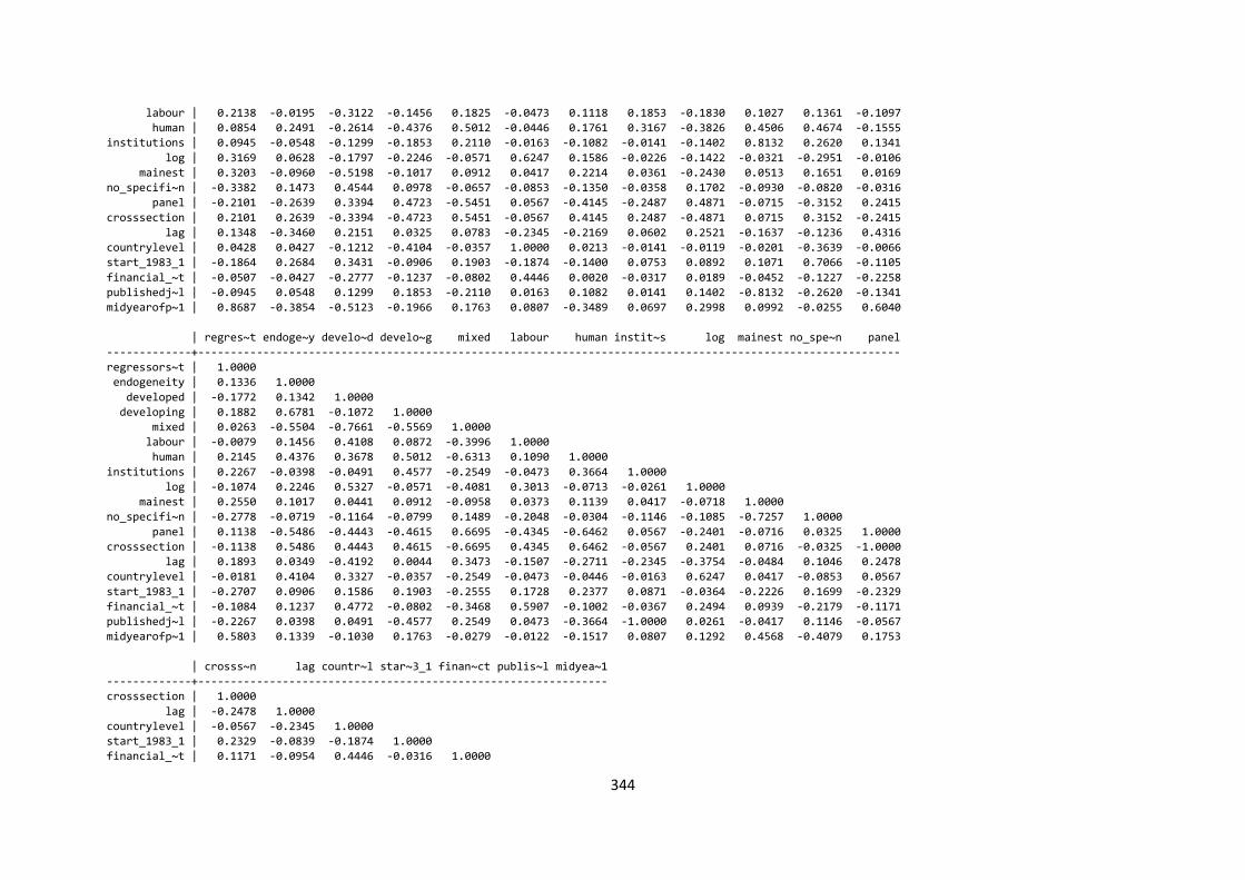
344
labour | 0.2138 -0.0195 -0.3122 -0.1456 0.1825 -0.0473 0.1118 0.1853 -0.1830 0.1027 0.1361 -0.1097
human | 0.0854 0.2491 -0.2614 -0.4376 0.5012 -0.0446 0.1761 0.3167 -0.3826 0.4506 0.4674 -0.1555
institutions | 0.0945 -0.0548 -0.1299 -0.1853 0.2110 -0.0163 -0.1082 -0.0141 -0.1402 0.8132 0.2620 0.1341
log | 0.3169 0.0628 -0.1797 -0.2246 -0.0571 0.6247 0.1586 -0.0226 -0.1422 -0.0321 -0.2951 -0.0106
mainest | 0.3203 -0.0960 -0.5198 -0.1017 0.0912 0.0417 0.2214 0.0361 -0.2430 0.0513 0.1651 0.0169
no_specifi~n | -0.3382 0.1473 0.4544 0.0978 -0.0657 -0.0853 -0.1350 -0.0358 0.1702 -0.0930 -0.0820 -0.0316
panel | -0.2101 -0.2639 0.3394 0.4723 -0.5451 0.0567 -0.4145 -0.2487 0.4871 -0.0715 -0.3152 0.2415
crosssection | 0.2101 0.2639 -0.3394 -0.4723 0.5451 -0.0567 0.4145 0.2487 -0.4871 0.0715 0.3152 -0.2415
lag | 0.1348 -0.3460 0.2151 0.0325 0.0783 -0.2345 -0.2169 0.0602 0.2521 -0.1637 -0.1236 0.4316
countrylevel | 0.0428 0.0427 -0.1212 -0.4104 -0.0357 1.0000 0.0213 -0.0141 -0.0119 -0.0201 -0.3639 -0.0066
start_1983_1 | -0.1864 0.2684 0.3431 -0.0906 0.1903 -0.1874 -0.1400 0.0753 0.0892 0.1071 0.7066 -0.1105
financial_~t | -0.0507 -0.0427 -0.2777 -0.1237 -0.0802 0.4446 0.0020 -0.0317 0.0189 -0.0452 -0.1227 -0.2258
publishedj~l | -0.0945 0.0548 0.1299 0.1853 -0.2110 0.0163 0.1082 0.0141 0.1402 -0.8132 -0.2620 -0.1341
midyearofp~1 | 0.8687 -0.3854 -0.5123 -0.1966 0.1763 0.0807 -0.3489 0.0697 0.2998 0.0992 -0.0255 0.6040
| regres~t endoge~y develo~d develo~g mixed labour human instit~s log mainest no_spe~n panel
-------------+------------------------------------------------------------------------------------------------------------
regressors~t | 1.0000
endogeneity | 0.1336 1.0000
developed | -0.1772 0.1342 1.0000
developing | 0.1882 0.6781 -0.1072 1.0000
mixed | 0.0263 -0.5504 -0.7661 -0.5569 1.0000
labour | -0.0079 0.1456 0.4108 0.0872 -0.3996 1.0000
human | 0.2145 0.4376 0.3678 0.5012 -0.6313 0.1090 1.0000
institutions | 0.2267 -0.0398 -0.0491 0.4577 -0.2549 -0.0473 0.3664 1.0000
log | -0.1074 0.2246 0.5327 -0.0571 -0.4081 0.3013 -0.0713 -0.0261 1.0000
mainest | 0.2550 0.1017 0.0441 0.0912 -0.0958 0.0373 0.1139 0.0417 -0.0718 1.0000
no_specifi~n | -0.2778 -0.0719 -0.1164 -0.0799 0.1489 -0.2048 -0.0304 -0.1146 -0.1085 -0.7257 1.0000
panel | 0.1138 -0.5486 -0.4443 -0.4615 0.6695 -0.4345 -0.6462 0.0567 -0.2401 -0.0716 0.0325 1.0000
crosssection | -0.1138 0.5486 0.4443 0.4615 -0.6695 0.4345 0.6462 -0.0567 0.2401 0.0716 -0.0325 -1.0000
lag | 0.1893 0.0349 -0.4192 0.0044 0.3473 -0.1507 -0.2711 -0.2345 -0.3754 -0.0484 0.1046 0.2478
countrylevel | -0.0181 0.4104 0.3327 -0.0357 -0.2549 -0.0473 -0.0446 -0.0163 0.6247 0.0417 -0.0853 0.0567
start_1983_1 | -0.2707 0.0906 0.1586 0.1903 -0.2555 0.1728 0.2377 0.0871 -0.0364 -0.2226 0.1699 -0.2329
financial_~t | -0.1084 0.1237 0.4772 -0.0802 -0.3468 0.5907 -0.1002 -0.0367 0.2494 0.0939 -0.2179 -0.1171
publishedj~l | -0.2267 0.0398 0.0491 -0.4577 0.2549 0.0473 -0.3664 -1.0000 0.0261 -0.0417 0.1146 -0.0567
midyearofp~1 | 0.5803 0.1339 -0.1030 0.1763 -0.0279 -0.0122 -0.1517 0.0807 0.1292 0.4568 -0.4079 0.1753
| crosss~n lag countr~l star~3_1 finan~ct publis~l midyea~1
-------------+---------------------------------------------------------------
crosssection | 1.0000
lag | -0.2478 1.0000
countrylevel | -0.0567 -0.2345 1.0000
start_1983_1 | 0.2329 -0.0839 -0.1874 1.0000
financial_~t | 0.1171 -0.0954 0.4446 -0.0316 1.0000
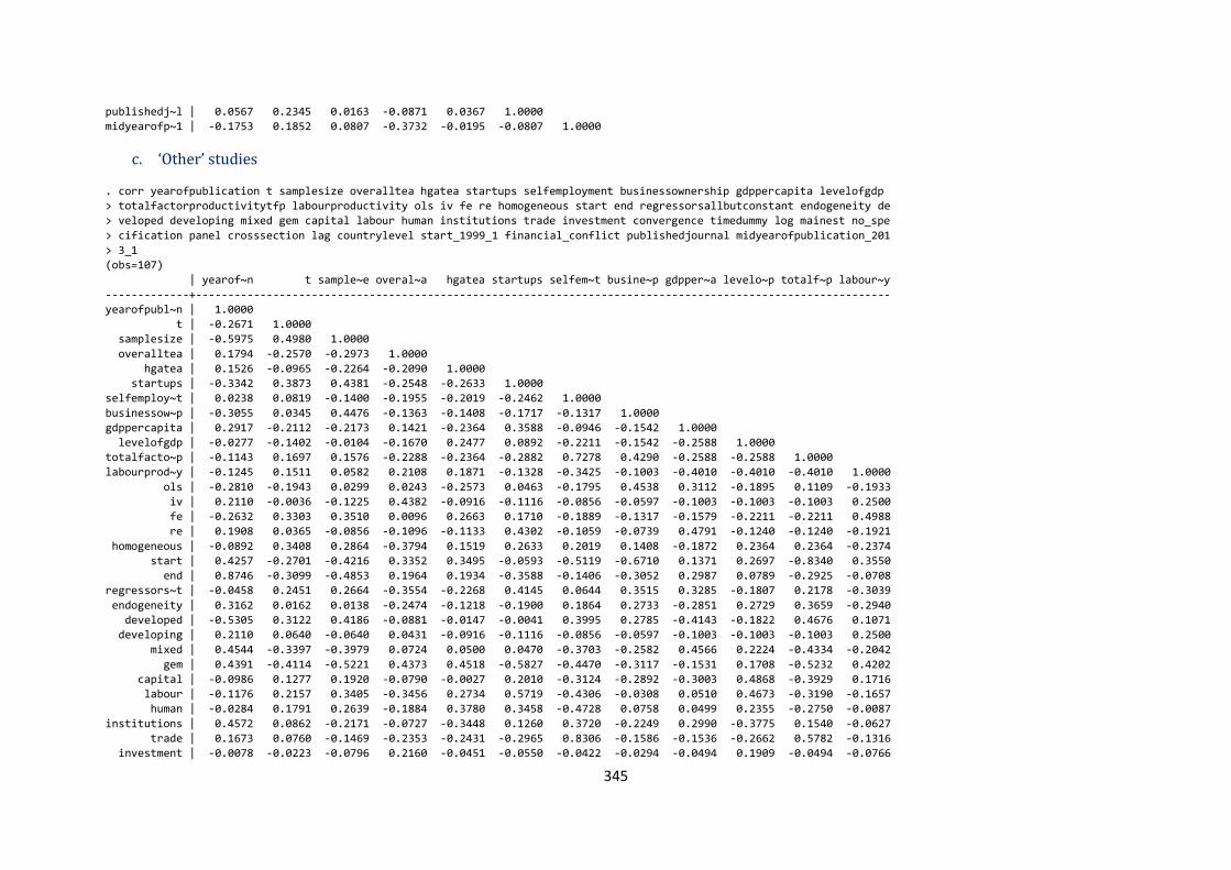
345
publishedj~l | 0.0567 0.2345 0.0163 -0.0871 0.0367 1.0000
midyearofp~1 | -0.1753 0.1852 0.0807 -0.3732 -0.0195 -0.0807 1.0000
c. ‘Other’ studies
. corr yearofpublication t samplesize overalltea hgatea startups selfemployment businessownership gdppercapita levelofgdp
> totalfactorproductivitytfp labourproductivity ols iv fe re homogeneous start end regressorsallbutconstant endogeneity de
> veloped developing mixed gem capital labour human institutions trade investment convergence timedummy log mainest no_spe
> cification panel crosssection lag countrylevel start_1999_1 financial_conflict publishedjournal midyearofpublication_201
> 3_1
(obs=107)
| yearof~n t sample~e overal~a hgatea startups selfem~t busine~p gdpper~a levelo~p totalf~p labour~y
-------------+------------------------------------------------------------------------------------------------------------
yearofpubl~n | 1.0000
t | -0.2671 1.0000
samplesize | -0.5975 0.4980 1.0000
overalltea | 0.1794 -0.2570 -0.2973 1.0000
hgatea | 0.1526 -0.0965 -0.2264 -0.2090 1.0000
startups | -0.3342 0.3873 0.4381 -0.2548 -0.2633 1.0000
selfemploy~t | 0.0238 0.0819 -0.1400 -0.1955 -0.2019 -0.2462 1.0000
businessow~p | -0.3055 0.0345 0.4476 -0.1363 -0.1408 -0.1717 -0.1317 1.0000
gdppercapita | 0.2917 -0.2112 -0.2173 0.1421 -0.2364 0.3588 -0.0946 -0.1542 1.0000
levelofgdp | -0.0277 -0.1402 -0.0104 -0.1670 0.2477 0.0892 -0.2211 -0.1542 -0.2588 1.0000
totalfacto~p | -0.1143 0.1697 0.1576 -0.2288 -0.2364 -0.2882 0.7278 0.4290 -0.2588 -0.2588 1.0000
labourprod~y | -0.1245 0.1511 0.0582 0.2108 0.1871 -0.1328 -0.3425 -0.1003 -0.4010 -0.4010 -0.4010 1.0000
ols | -0.2810 -0.1943 0.0299 0.0243 -0.2573 0.0463 -0.1795 0.4538 0.3112 -0.1895 0.1109 -0.1933
iv | 0.2110 -0.0036 -0.1225 0.4382 -0.0916 -0.1116 -0.0856 -0.0597 -0.1003 -0.1003 -0.1003 0.2500
fe | -0.2632 0.3303 0.3510 0.0096 0.2663 0.1710 -0.1889 -0.1317 -0.1579 -0.2211 -0.2211 0.4988
re | 0.1908 0.0365 -0.0856 -0.1096 -0.1133 0.4302 -0.1059 -0.0739 0.4791 -0.1240 -0.1240 -0.1921
homogeneous | -0.0892 0.3408 0.2864 -0.3794 0.1519 0.2633 0.2019 0.1408 -0.1872 0.2364 0.2364 -0.2374
start | 0.4257 -0.2701 -0.4216 0.3352 0.3495 -0.0593 -0.5119 -0.6710 0.1371 0.2697 -0.8340 0.3550
end | 0.8746 -0.3099 -0.4853 0.1964 0.1934 -0.3588 -0.1406 -0.3052 0.2987 0.0789 -0.2925 -0.0708
regressors~t | -0.0458 0.2451 0.2664 -0.3554 -0.2268 0.4145 0.0644 0.3515 0.3285 -0.1807 0.2178 -0.3039
endogeneity | 0.3162 0.0162 0.0138 -0.2474 -0.1218 -0.1900 0.1864 0.2733 -0.2851 0.2729 0.3659 -0.2940
developed | -0.5305 0.3122 0.4186 -0.0881 -0.0147 -0.0041 0.3995 0.2785 -0.4143 -0.1822 0.4676 0.1071
developing | 0.2110 0.0640 -0.0640 0.0431 -0.0916 -0.1116 -0.0856 -0.0597 -0.1003 -0.1003 -0.1003 0.2500
mixed | 0.4544 -0.3397 -0.3979 0.0724 0.0500 0.0470 -0.3703 -0.2582 0.4566 0.2224 -0.4334 -0.2042
gem | 0.4391 -0.4114 -0.5221 0.4373 0.4518 -0.5827 -0.4470 -0.3117 -0.1531 0.1708 -0.5232 0.4202
capital | -0.0986 0.1277 0.1920 -0.0790 -0.0027 0.2010 -0.3124 -0.2892 -0.3003 0.4868 -0.3929 0.1716
labour | -0.1176 0.2157 0.3405 -0.3456 0.2734 0.5719 -0.4306 -0.0308 0.0510 0.4673 -0.3190 -0.1657
human | -0.0284 0.1791 0.2639 -0.1884 0.3780 0.3458 -0.4728 0.0758 0.0499 0.2355 -0.2750 -0.0087
institutions | 0.4572 0.0862 -0.2171 -0.0727 -0.3448 0.1260 0.3720 -0.2249 0.2990 -0.3775 0.1540 -0.0627
trade | 0.1673 0.0760 -0.1469 -0.2353 -0.2431 -0.2965 0.8306 -0.1586 -0.1536 -0.2662 0.5782 -0.1316
investment | -0.0078 -0.0223 -0.0796 0.2160 -0.0451 -0.0550 -0.0422 -0.0294 -0.0494 0.1909 -0.0494 -0.0766
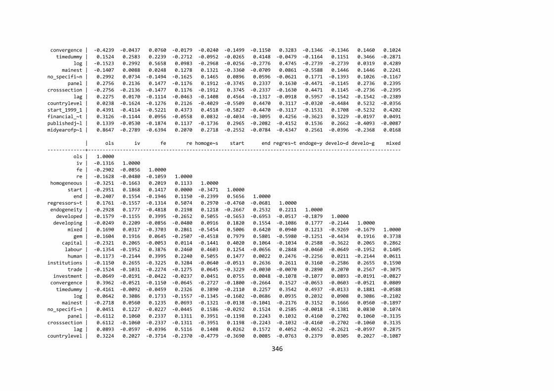
346
convergence | -0.4239 -0.0437 0.0760 -0.0179 -0.0240 -0.1499 -0.1150 0.3283 -0.1346 -0.1346 0.1460 0.1024
timedummy | 0.1524 0.2583 0.2239 -0.2712 -0.0952 -0.0265 0.4148 -0.0479 -0.1164 0.1151 0.3466 -0.2871
log | -0.1523 0.2992 0.5658 0.0983 -0.2968 -0.0256 -0.2776 0.4745 -0.2739 -0.2739 0.0319 0.4289
mainest | -0.1407 0.0088 0.0248 0.1278 0.1321 -0.3360 -0.0709 0.0861 -0.5588 0.1446 0.1446 0.2241
no_specifi~n | 0.2992 0.0734 -0.1494 -0.1625 0.1465 0.0896 0.0596 -0.0621 0.1771 -0.1393 0.1026 -0.1167
panel | 0.2756 0.2136 0.1477 -0.1176 0.1912 -0.3745 0.2337 0.1630 -0.4471 -0.1145 0.2736 0.2395
crosssection | -0.2756 -0.2136 -0.1477 0.1176 -0.1912 0.3745 -0.2337 -0.1630 0.4471 0.1145 -0.2736 -0.2395
lag | 0.2275 0.0170 -0.1114 -0.0463 -0.1408 0.4564 -0.1317 -0.0918 0.5957 -0.1542 -0.1542 -0.2389
countrylevel | 0.0238 -0.1624 -0.1276 0.2126 -0.4029 -0.5509 0.4470 0.3117 -0.0320 -0.4484 0.5232 -0.0356
start_1999_1 | 0.4391 -0.4114 -0.5221 0.4373 0.4518 -0.5827 -0.4470 -0.3117 -0.1531 0.1708 -0.5232 0.4202
financial_~t | 0.3126 -0.1144 0.0956 -0.0558 0.0832 -0.4034 -0.3095 0.4256 -0.3623 0.3229 -0.0197 0.0491
publishedj~l | 0.1339 -0.0530 -0.1874 0.1137 -0.1736 0.2965 -0.2082 -0.4152 0.1536 0.2662 -0.4093 -0.0087
midyearofp~1 | 0.8647 -0.2789 -0.6394 0.2070 0.2718 -0.2552 -0.0784 -0.4347 0.2561 -0.0396 -0.2368 0.0168
| ols iv fe re homoge~s start end regres~t endoge~y develo~d develo~g mixed
-------------+------------------------------------------------------------------------------------------------------------
ols | 1.0000
iv | -0.1316 1.0000
fe | -0.2902 -0.0856 1.0000
re | -0.1628 -0.0480 -0.1059 1.0000
homogeneous | -0.3251 -0.1663 0.2019 0.1133 1.0000
start | -0.2951 0.1868 0.1417 0.0000 -0.3471 1.0000
end | -0.2407 0.1554 -0.1946 0.1150 -0.2399 0.5656 1.0000
regressors~t | 0.1761 -0.1557 -0.1314 0.5074 0.2970 -0.4760 -0.0681 1.0000
endogeneity | -0.2928 0.1777 -0.4818 0.2198 0.1218 -0.2667 0.2532 0.2211 1.0000
developed | -0.1579 -0.1155 0.3995 -0.2652 0.5055 -0.5653 -0.6953 -0.0517 -0.1879 1.0000
developing | -0.0249 0.2209 -0.0856 -0.0480 0.0916 0.1820 0.1554 -0.1086 0.1777 -0.2144 1.0000
mixed | 0.1690 0.0317 -0.3703 0.2861 -0.5454 0.5006 0.6420 0.0940 0.1213 -0.9269 -0.1679 1.0000
gem | -0.1604 0.1916 0.0645 -0.2507 -0.4518 0.7979 0.5801 -0.5980 -0.1251 -0.4434 0.1916 0.3738
capital | -0.2321 0.2065 -0.0053 0.0114 -0.1441 0.4020 0.1064 -0.1034 0.2588 -0.3622 0.2065 0.2862
labour | -0.1354 -0.1952 0.3876 0.2460 0.4603 0.1254 -0.0656 0.2848 -0.0460 -0.0649 -0.1952 0.1405
human | -0.1173 -0.2144 0.3995 0.2240 0.5055 0.1477 0.0022 0.2476 -0.2256 0.0211 -0.2144 0.0611
institutions | -0.1150 0.2655 -0.3225 0.3284 -0.0640 -0.0513 0.2636 0.2611 0.3160 -0.2586 0.2655 0.1590
trade | -0.1524 -0.1031 -0.2274 -0.1275 0.0645 -0.3229 -0.0030 -0.0070 0.2890 0.2070 0.2567 -0.3075
investment | -0.0649 -0.0191 -0.0422 -0.0237 0.0451 0.0755 0.0048 -0.1078 -0.1077 0.0893 -0.0191 -0.0827
convergence | 0.3962 -0.0521 -0.1150 -0.0645 -0.2727 -0.1800 -0.2664 0.1527 -0.0653 -0.0603 -0.0521 0.0809
timedummy | -0.4161 -0.0092 -0.0459 0.2326 0.3890 -0.2110 0.2257 0.3542 0.4937 -0.0133 0.1881 -0.0588
log | 0.0642 0.3086 0.1733 -0.1557 -0.1345 -0.1602 -0.0686 0.0935 0.2032 0.0908 0.3086 -0.2102
mainest | -0.2718 0.0560 0.1235 0.0693 -0.1321 -0.0138 -0.1041 -0.2176 0.3152 0.1666 0.0560 -0.1897
no_specifi~n | 0.0451 0.1227 -0.0227 -0.0445 0.1586 -0.0292 0.1524 0.2585 -0.0018 -0.1381 0.0830 0.1074
panel | -0.6112 0.1060 0.2337 0.1311 0.3951 -0.1198 0.2243 0.1032 0.4160 0.2702 0.1060 -0.3135
crosssection | 0.6112 -0.1060 -0.2337 -0.1311 -0.3951 0.1198 -0.2243 -0.1032 -0.4160 -0.2702 -0.1060 0.3135
lag | 0.0893 -0.0597 -0.0396 0.5116 0.1408 0.0262 0.1572 0.4052 -0.0652 -0.2621 -0.0597 0.2875
countrylevel | 0.3224 0.2027 -0.3714 -0.2370 -0.4779 -0.3690 0.0085 -0.0763 0.2379 0.0305 0.2027 -0.1087

347
start_1999_1 | -0.1604 0.1916 0.0645 -0.2507 -0.4518 0.7979 0.5801 -0.5980 -0.1251 -0.4434 0.1916 0.3738
financial_~t | -0.0044 0.2768 -0.3095 -0.1736 -0.0832 0.0846 0.4196 -0.0010 0.6423 -0.3777 0.2768 0.2749
publishedj~l | 0.0046 0.1031 -0.3327 0.1275 -0.2431 0.3627 0.2337 0.0360 0.0312 -0.4810 0.1031 0.4458
midyearofp~1 | -0.2245 0.1374 -0.0784 0.1699 -0.1155 0.5248 0.7358 -0.1355 0.0520 -0.4809 0.1374 0.4326
| gem capital labour human instit~s trade invest~t conver~e timedu~y log mainest no_spe~n
-------------+------------------------------------------------------------------------------------------------------------
gem | 1.0000
capital | 0.2166 1.0000
labour | -0.1587 0.2148 1.0000
human | 0.0070 0.0133 0.7230 1.0000
institutions | -0.2553 -0.0044 -0.2665 -0.3370 1.0000
trade | -0.2650 -0.1350 -0.5184 -0.5693 0.5149 1.0000
investment | 0.0944 -0.0927 -0.0962 -0.1057 -0.0721 -0.0508 1.0000
convergence | 0.0304 0.0502 -0.1109 -0.0603 -0.1963 -0.1384 -0.0257 1.0000
timedummy | -0.2540 0.2738 0.1221 0.0242 0.2390 0.3627 -0.1018 -0.1259 1.0000
log | -0.0385 0.2567 -0.1795 -0.1159 0.0857 -0.0333 0.1521 0.0810 0.1145 1.0000
mainest | 0.2924 0.2713 -0.1448 -0.1186 -0.3831 -0.0243 0.0276 0.0752 0.1556 0.1816 1.0000
no_specifi~n | -0.0860 -0.2531 0.1916 0.1412 0.2812 0.0281 -0.1154 -0.0254 -0.0255 -0.1787 -0.4057 1.0000
panel | 0.0599 0.0197 -0.0498 0.1803 0.1181 0.2814 0.0522 -0.2202 0.5635 0.3434 0.3583 -0.1093
crosssection | -0.0599 -0.0197 0.0498 -0.1803 -0.1181 -0.2814 -0.0522 0.2202 -0.5635 -0.3434 -0.3583 0.1093
lag | -0.2443 -0.0869 0.2385 0.2785 0.3380 -0.1586 -0.0294 -0.0802 0.0195 -0.1193 -0.4259 0.2902
countrylevel | -0.0273 -0.1791 -0.8137 -0.7952 0.2943 0.5382 0.0999 0.2721 0.0668 0.3683 0.1342 -0.1247
start_1999_1 | 1.0000 0.2166 -0.1587 0.0070 -0.2553 -0.2650 0.0944 0.0304 -0.2540 -0.0385 0.2924 -0.0860
financial_~t | 0.3362 0.3897 0.0067 0.0193 0.0089 -0.0837 -0.0692 0.0516 0.2439 0.5045 0.2024 -0.0582
publishedj~l | 0.1285 0.4538 -0.0731 -0.1157 0.0555 -0.1139 0.0508 -0.1376 0.0473 -0.0169 0.0243 -0.0007
midyearofp~1 | 0.5178 -0.0924 -0.0264 0.1188 0.2260 0.0254 -0.1393 -0.3795 0.0127 -0.3012 -0.0467 0.3476
| panel crosss~n lag countr~l star~9_1 finan~ct publis~l midyea~1
-------------+------------------------------------------------------------------------
panel | 1.0000
crosssection | -1.0000 1.0000
lag | -0.1599 0.1599 1.0000
countrylevel | 0.0297 -0.0297 -0.2273 1.0000
start_1999_1 | 0.0599 -0.0599 -0.2443 -0.0273 1.0000
financial_~t | 0.3829 -0.3829 -0.2158 0.1783 0.3362 1.0000
publishedj~l | -0.2814 0.2814 0.1586 -0.1285 0.1285 0.0356 1.0000
midyearofp~1 | 0.1504 -0.1504 0.2113 -0.1591 0.5178 0.1170 0.3141 1.0000
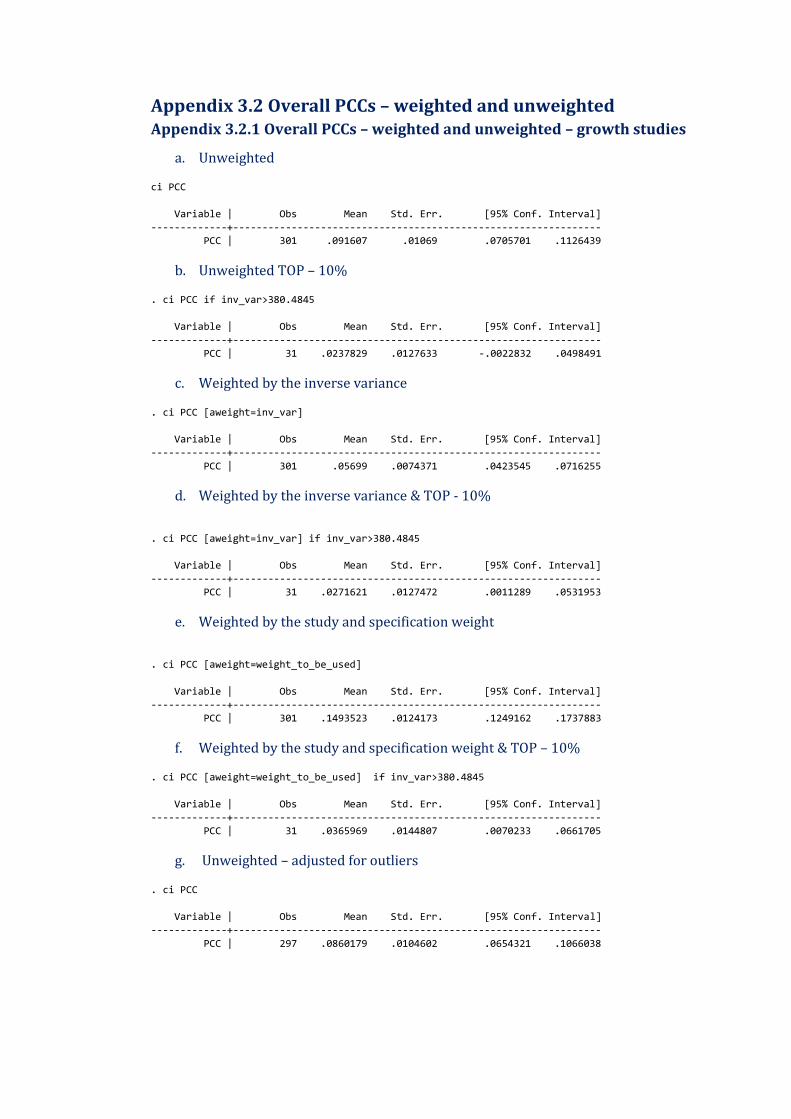
Appendix 3.2 Overall PCCs – weighted and unweighted Appendix 3.2.1 Overall PCCs – weighted and unweighted – growth studies
a. Unweighted
ci PCC
Variable | Obs Mean Std. Err. [95% Conf. Interval]
-------------+---------------------------------------------------------------
PCC | 301 .091607 .01069 .0705701 .1126439
b. Unweighted TOP – 10%
. ci PCC if inv_var>380.4845
Variable | Obs Mean Std. Err. [95% Conf. Interval]
-------------+---------------------------------------------------------------
PCC | 31 .0237829 .0127633 -.0022832 .0498491
c. Weighted by the inverse variance
. ci PCC [aweight=inv_var]
Variable | Obs Mean Std. Err. [95% Conf. Interval]
-------------+---------------------------------------------------------------
PCC | 301 .05699 .0074371 .0423545 .0716255
d. Weighted by the inverse variance & TOP - 10%
. ci PCC [aweight=inv_var] if inv_var>380.4845
Variable | Obs Mean Std. Err. [95% Conf. Interval]
-------------+---------------------------------------------------------------
PCC | 31 .0271621 .0127472 .0011289 .0531953
e. Weighted by the study and specification weight
. ci PCC [aweight=weight_to_be_used]
Variable | Obs Mean Std. Err. [95% Conf. Interval]
-------------+---------------------------------------------------------------
PCC | 301 .1493523 .0124173 .1249162 .1737883
f. Weighted by the study and specification weight & TOP – 10%
. ci PCC [aweight=weight_to_be_used] if inv_var>380.4845
Variable | Obs Mean Std. Err. [95% Conf. Interval]
-------------+---------------------------------------------------------------
PCC | 31 .0365969 .0144807 .0070233 .0661705
g. Unweighted – adjusted for outliers
. ci PCC
Variable | Obs Mean Std. Err. [95% Conf. Interval]
-------------+---------------------------------------------------------------
PCC | 297 .0860179 .0104602 .0654321 .1066038
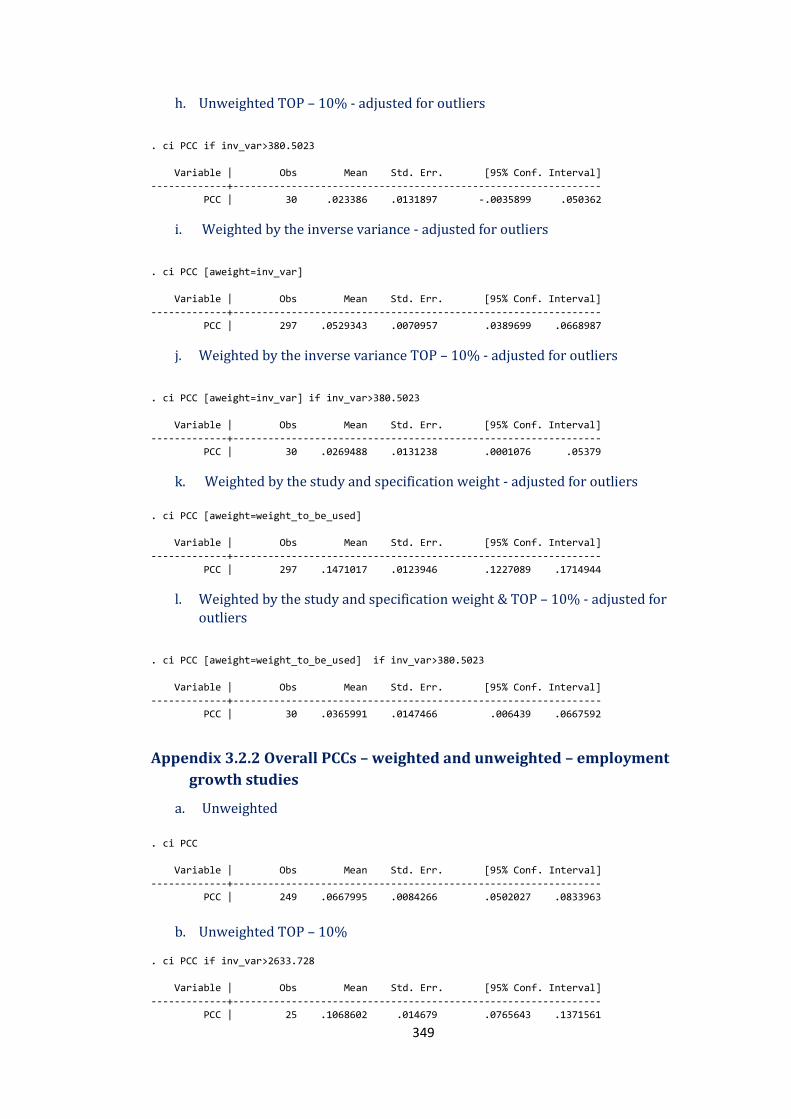
349
h. Unweighted TOP – 10% - adjusted for outliers
. ci PCC if inv_var>380.5023
Variable | Obs Mean Std. Err. [95% Conf. Interval]
-------------+---------------------------------------------------------------
PCC | 30 .023386 .0131897 -.0035899 .050362
i. Weighted by the inverse variance - adjusted for outliers
. ci PCC [aweight=inv_var]
Variable | Obs Mean Std. Err. [95% Conf. Interval]
-------------+---------------------------------------------------------------
PCC | 297 .0529343 .0070957 .0389699 .0668987
j. Weighted by the inverse variance TOP – 10% - adjusted for outliers
. ci PCC [aweight=inv_var] if inv_var>380.5023
Variable | Obs Mean Std. Err. [95% Conf. Interval]
-------------+---------------------------------------------------------------
PCC | 30 .0269488 .0131238 .0001076 .05379
k. Weighted by the study and specification weight - adjusted for outliers
. ci PCC [aweight=weight_to_be_used]
Variable | Obs Mean Std. Err. [95% Conf. Interval]
-------------+---------------------------------------------------------------
PCC | 297 .1471017 .0123946 .1227089 .1714944
l. Weighted by the study and specification weight & TOP – 10% - adjusted for
outliers
. ci PCC [aweight=weight_to_be_used] if inv_var>380.5023
Variable | Obs Mean Std. Err. [95% Conf. Interval]
-------------+---------------------------------------------------------------
PCC | 30 .0365991 .0147466 .006439 .0667592
Appendix 3.2.2 Overall PCCs – weighted and unweighted – employment
growth studies
a. Unweighted
. ci PCC
Variable | Obs Mean Std. Err. [95% Conf. Interval]
-------------+---------------------------------------------------------------
PCC | 249 .0667995 .0084266 .0502027 .0833963
b. Unweighted TOP – 10%
. ci PCC if inv_var>2633.728
Variable | Obs Mean Std. Err. [95% Conf. Interval]
-------------+---------------------------------------------------------------
PCC | 25 .1068602 .014679 .0765643 .1371561
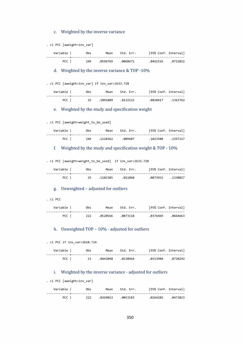
350
c. Weighted by the inverse variance
. ci PCC [aweight=inv_var]
Variable | Obs Mean Std. Err. [95% Conf. Interval]
-------------+---------------------------------------------------------------
PCC | 249 .0596769 .0068671 .0461516 .0732022
d. Weighted by the inverse variance & TOP -10%
. ci PCC [aweight=inv_var] if inv_var>2633.728
Variable | Obs Mean Std. Err. [95% Conf. Interval]
-------------+---------------------------------------------------------------
PCC | 25 .1091089 .0132115 .0818417 .1363762
e. Weighted by the study and specification weight
. ci PCC [aweight=weight_to_be_used]
Variable | Obs Mean Std. Err. [95% Conf. Interval]
-------------+---------------------------------------------------------------
PCC | 249 .1210362 .009487 .1023508 .1397217
f. Weighted by the study and specification weight & TOP - 10%
. ci PCC [aweight=weight_to_be_used] if inv_var>2633.728
Variable | Obs Mean Std. Err. [95% Conf. Interval]
-------------+---------------------------------------------------------------
PCC | 25 .1102385 .011068 .0873952 .1330817
g. Unweighted – adjusted for outliers
. ci PCC
Variable | Obs Mean Std. Err. [95% Conf. Interval]
-------------+---------------------------------------------------------------
PCC | 222 .0520566 .0073118 .0376469 .0664663
h. Unweighted TOP – 10% - adjusted for outliers
. ci PCC if inv_var>2610.724
Variable | Obs Mean Std. Err. [95% Conf. Interval]
-------------+---------------------------------------------------------------
PCC | 23 .0442098 .0138964 .0153904 .0730292
i. Weighted by the inverse variance - adjusted for outliers
. ci PCC [aweight=inv_var]
Variable | Obs Mean Std. Err. [95% Conf. Interval]
-------------+---------------------------------------------------------------
PCC | 222 .0369013 .0053183 .0264202 .0473823
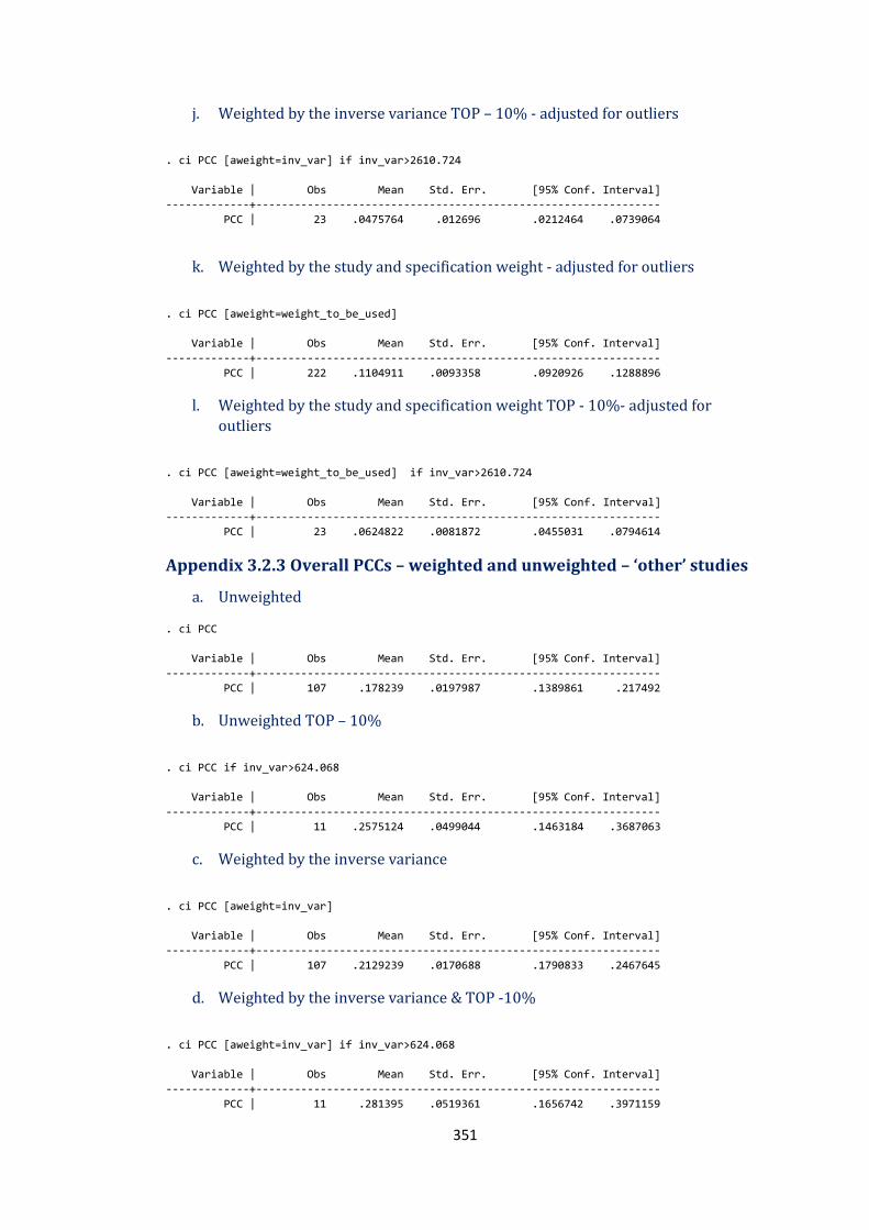
351
j. Weighted by the inverse variance TOP – 10% - adjusted for outliers
. ci PCC [aweight=inv_var] if inv_var>2610.724
Variable | Obs Mean Std. Err. [95% Conf. Interval]
-------------+---------------------------------------------------------------
PCC | 23 .0475764 .012696 .0212464 .0739064
k. Weighted by the study and specification weight - adjusted for outliers
. ci PCC [aweight=weight_to_be_used]
Variable | Obs Mean Std. Err. [95% Conf. Interval]
-------------+---------------------------------------------------------------
PCC | 222 .1104911 .0093358 .0920926 .1288896
l. Weighted by the study and specification weight TOP - 10%- adjusted for
outliers
. ci PCC [aweight=weight_to_be_used] if inv_var>2610.724
Variable | Obs Mean Std. Err. [95% Conf. Interval]
-------------+---------------------------------------------------------------
PCC | 23 .0624822 .0081872 .0455031 .0794614
Appendix 3.2.3 Overall PCCs – weighted and unweighted – ‘other’ studies
a. Unweighted
. ci PCC
Variable | Obs Mean Std. Err. [95% Conf. Interval]
-------------+---------------------------------------------------------------
PCC | 107 .178239 .0197987 .1389861 .217492
b. Unweighted TOP – 10%
. ci PCC if inv_var>624.068
Variable | Obs Mean Std. Err. [95% Conf. Interval]
-------------+---------------------------------------------------------------
PCC | 11 .2575124 .0499044 .1463184 .3687063
c. Weighted by the inverse variance
. ci PCC [aweight=inv_var]
Variable | Obs Mean Std. Err. [95% Conf. Interval]
-------------+---------------------------------------------------------------
PCC | 107 .2129239 .0170688 .1790833 .2467645
d. Weighted by the inverse variance & TOP -10%
. ci PCC [aweight=inv_var] if inv_var>624.068
Variable | Obs Mean Std. Err. [95% Conf. Interval]
-------------+---------------------------------------------------------------
PCC | 11 .281395 .0519361 .1656742 .3971159
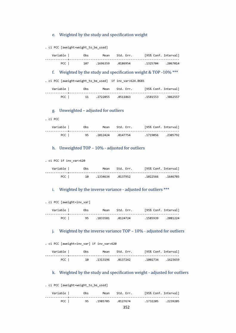
352
e. Weighted by the study and specification weight
. ci PCC [aweight=weight_to_be_used]
Variable | Obs Mean Std. Err. [95% Conf. Interval]
-------------+---------------------------------------------------------------
PCC | 107 .1696359 .0186954 .1325704 .2067014
f. Weighted by the study and specification weight & TOP -10% ***
. ci PCC [aweight=weight_to_be_used] if inv_var>624.0681
Variable | Obs Mean Std. Err. [95% Conf. Interval]
-------------+---------------------------------------------------------------
PCC | 11 .2722055 .0511863 .1581553 .3862557
g. Unweighted – adjusted for outliers
. ci PCC
Variable | Obs Mean Std. Err. [95% Conf. Interval]
-------------+---------------------------------------------------------------
PCC | 95 .2012424 .0147754 .1719056 .2305792
h. Unweighted TOP – 10% - adjusted for outliers
. ci PCC if inv_var>620
Variable | Obs Mean Std. Err. [95% Conf. Interval]
-------------+---------------------------------------------------------------
PCC | 10 .1334634 .0137952 .1022566 .1646703
i. Weighted by the inverse variance - adjusted for outliers ***
. ci PCC [aweight=inv_var]
Variable | Obs Mean Std. Err. [95% Conf. Interval]
-------------+---------------------------------------------------------------
PCC | 95 .1833581 .0124724 .1585939 .2081224
j. Weighted by the inverse variance TOP – 10% - adjusted for outliers
. ci PCC [aweight=inv_var] if inv_var>620
Variable | Obs Mean Std. Err. [95% Conf. Interval]
-------------+---------------------------------------------------------------
PCC | 10 .1313196 .0137242 .1002734 .1623659
k. Weighted by the study and specification weight - adjusted for outliers
. ci PCC [aweight=weight_to_be_used]
Variable | Obs Mean Std. Err. [95% Conf. Interval]
-------------+---------------------------------------------------------------
PCC | 95 .1985705 .0127674 .1732205 .2239205
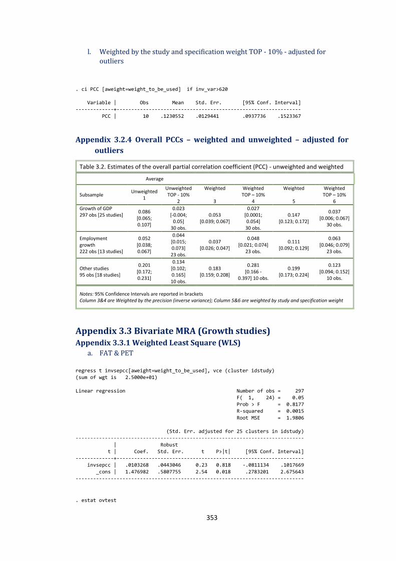
353
l. Weighted by the study and specification weight TOP - 10% - adjusted for
outliers
. ci PCC [aweight=weight_to_be_used] if inv_var>620
Variable | Obs Mean Std. Err. [95% Conf. Interval]
-------------+---------------------------------------------------------------
PCC | 10 .1230552 .0129441 .0937736 .1523367
Appendix 3.2.4 Overall PCCs – weighted and unweighted – adjusted for
outliers
Table 3.2. Estimates of the overall partial correlation coefficient (PCC) - unweighted and weighted
Average
Subsample Unweighted
1
Unweighted TOP - 10%
2
Weighted
3
Weighted TOP – 10%
4
Weighted
5
Weighted TOP – 10%
6
Growth of GDP 297 obs [25 studies]
0.086 [0.065; 0.107]
0.023 [-0.004;
0.05] 30 obs.
0.053 [0.039; 0.067]
0.027 [0.0001; 0.054] 30 obs.
0.147 [0.123; 0.172]
0.037 [0.006; 0.067]
30 obs.
Employment growth 222 obs [13 studies]
0.052 [0.038; 0.067]
0.044 [0.015; 0.073] 23 obs.
0.037 [0.026; 0.047]
0.048 [0.021; 0.074]
23 obs.
0.111 [0.092; 0.129]
0.063 [0.046; 0.079]
23 obs.
Other studies 95 obs [18 studies]
0.201 [0.172; 0.231]
0.134 [0.102; 0.165] 10 obs.
0.183 [0.159; 0.208]
0.281 [0.166 -
0.397] 10 obs.
0.199 [0.173; 0.224]
0.123 [0.094; 0.152]
10 obs.
Notes: 95% Confidence Intervals are reported in brackets Column 3&4 are Weighted by the precision (inverse variance); Column 5&6 are weighted by study and specification weight
Appendix 3.3 Bivariate MRA (Growth studies) Appendix 3.3.1 Weighted Least Square (WLS)
a. FAT & PET
regress t invsepcc[aweight=weight_to_be_used], vce (cluster idstudy)
(sum of wgt is 2.5000e+01)
Linear regression Number of obs = 297
F( 1, 24) = 0.05
Prob > F = 0.8177
R-squared = 0.0015
Root MSE = 1.9806
(Std. Err. adjusted for 25 clusters in idstudy)
------------------------------------------------------------------------------
| Robust
t | Coef. Std. Err. t P>|t| [95% Conf. Interval]
-------------+----------------------------------------------------------------
invsepcc | .0103268 .0443046 0.23 0.818 -.0811134 .1017669
_cons | 1.476982 .5807755 2.54 0.018 .2783201 2.675643
------------------------------------------------------------------------------
. estat ovtest
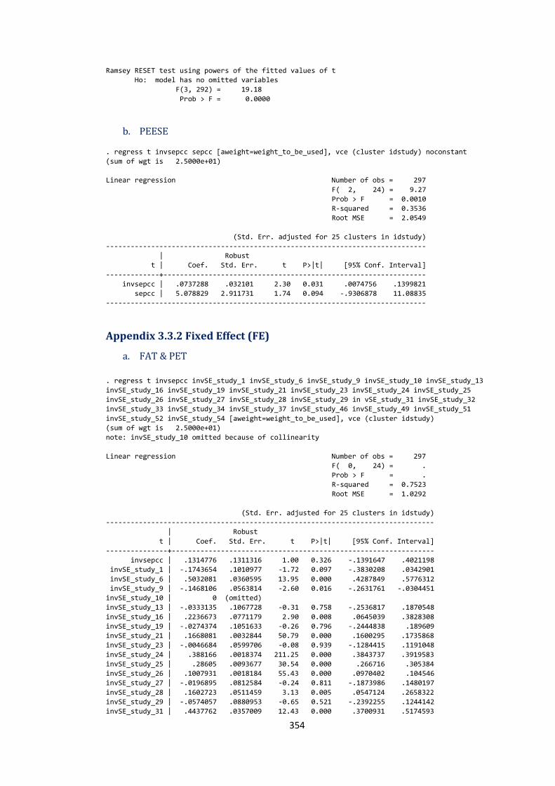
354
Ramsey RESET test using powers of the fitted values of t
Ho: model has no omitted variables
F(3, 292) = 19.18
Prob > F = 0.0000
b. PEESE
. regress t invsepcc sepcc [aweight=weight_to_be_used], vce (cluster idstudy) noconstant
(sum of wgt is 2.5000e+01)
Linear regression Number of obs = 297
F( 2, 24) = 9.27
Prob > F = 0.0010
R-squared = 0.3536
Root MSE = 2.0549
(Std. Err. adjusted for 25 clusters in idstudy)
------------------------------------------------------------------------------
| Robust
t | Coef. Std. Err. t P>|t| [95% Conf. Interval]
-------------+----------------------------------------------------------------
invsepcc | .0737288 .032101 2.30 0.031 .0074756 .1399821
sepcc | 5.078829 2.911731 1.74 0.094 -.9306878 11.08835
------------------------------------------------------------------------------
Appendix 3.3.2 Fixed Effect (FE)
a. FAT & PET
. regress t invsepcc invSE_study_1 invSE_study_6 invSE_study_9 invSE_study_10 invSE_study_13
invSE_study_16 invSE_study_19 invSE_study_21 invSE_study_23 invSE_study_24 invSE_study_25
invSE_study_26 invSE_study_27 invSE_study_28 invSE_study_29 in vSE_study_31 invSE_study_32
invSE_study_33 invSE_study_34 invSE_study_37 invSE_study_46 invSE_study_49 invSE_study_51
invSE_study_52 invSE_study_54 [aweight=weight_to_be_used], vce (cluster idstudy)
(sum of wgt is 2.5000e+01)
note: invSE_study_10 omitted because of collinearity
Linear regression Number of obs = 297
F( 0, 24) = .
Prob > F = .
R-squared = 0.7523
Root MSE = 1.0292
(Std. Err. adjusted for 25 clusters in idstudy)
--------------------------------------------------------------------------------
| Robust
t | Coef. Std. Err. t P>|t| [95% Conf. Interval]
---------------+----------------------------------------------------------------
invsepcc | .1314776 .1311316 1.00 0.326 -.1391647 .4021198
invSE_study_1 | -.1743654 .1010977 -1.72 0.097 -.3830208 .0342901
invSE_study_6 | .5032081 .0360595 13.95 0.000 .4287849 .5776312
invSE_study_9 | -.1468106 .0563814 -2.60 0.016 -.2631761 -.0304451
invSE_study_10 | 0 (omitted)
invSE_study_13 | -.0333135 .1067728 -0.31 0.758 -.2536817 .1870548
invSE_study_16 | .2236673 .0771179 2.90 0.008 .0645039 .3828308
invSE_study_19 | -.0274374 .1051633 -0.26 0.796 -.2444838 .189609
invSE_study_21 | .1668081 .0032844 50.79 0.000 .1600295 .1735868
invSE_study_23 | -.0046684 .0599706 -0.08 0.939 -.1284415 .1191048
invSE_study_24 | .388166 .0018374 211.25 0.000 .3843737 .3919583
invSE_study_25 | .28605 .0093677 30.54 0.000 .266716 .305384
invSE_study_26 | .1007931 .0018184 55.43 0.000 .0970402 .104546
invSE_study_27 | -.0196895 .0812584 -0.24 0.811 -.1873986 .1480197
invSE_study_28 | .1602723 .0511459 3.13 0.005 .0547124 .2658322
invSE_study_29 | -.0574057 .0880953 -0.65 0.521 -.2392255 .1244142
invSE_study_31 | .4437762 .0357009 12.43 0.000 .3700931 .5174593
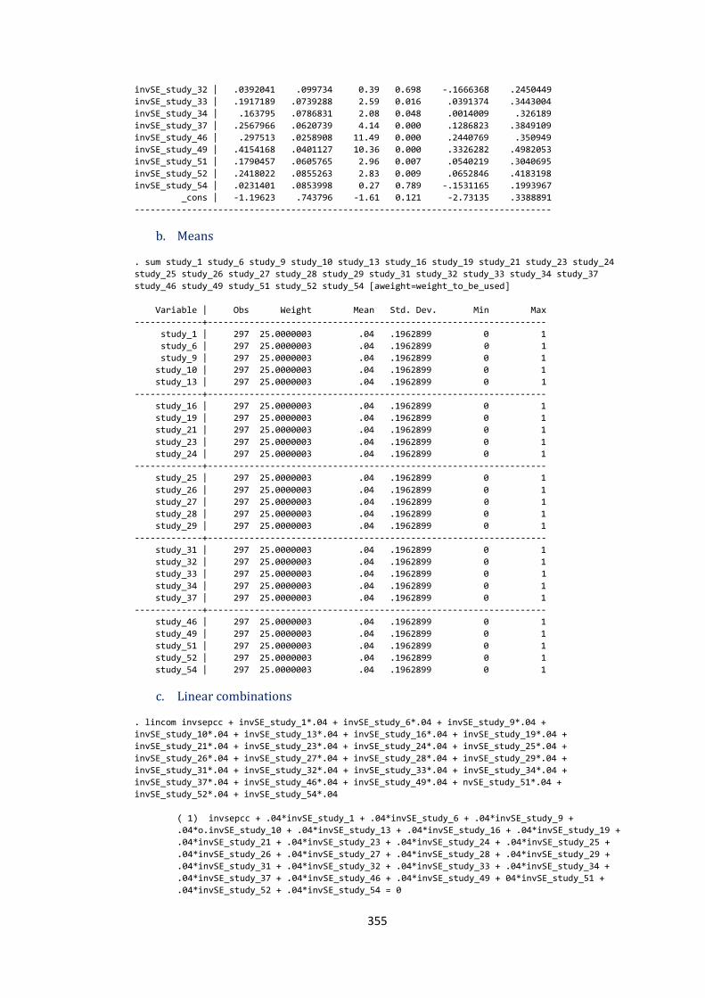
355
invSE_study_32 | .0392041 .099734 0.39 0.698 -.1666368 .2450449
invSE_study_33 | .1917189 .0739288 2.59 0.016 .0391374 .3443004
invSE_study_34 | .163795 .0786831 2.08 0.048 .0014009 .326189
invSE_study_37 | .2567966 .0620739 4.14 0.000 .1286823 .3849109
invSE_study_46 | .297513 .0258908 11.49 0.000 .2440769 .350949
invSE_study_49 | .4154168 .0401127 10.36 0.000 .3326282 .4982053
invSE_study_51 | .1790457 .0605765 2.96 0.007 .0540219 .3040695
invSE_study_52 | .2418022 .0855263 2.83 0.009 .0652846 .4183198
invSE_study_54 | .0231401 .0853998 0.27 0.789 -.1531165 .1993967
_cons | -1.19623 .743796 -1.61 0.121 -2.73135 .3388891
--------------------------------------------------------------------------------
b. Means
. sum study_1 study_6 study_9 study_10 study_13 study_16 study_19 study_21 study_23 study_24
study_25 study_26 study_27 study_28 study_29 study_31 study_32 study_33 study_34 study_37
study_46 study_49 study_51 study_52 study_54 [aweight=weight_to_be_used]
Variable | Obs Weight Mean Std. Dev. Min Max
-------------+-----------------------------------------------------------------
study_1 | 297 25.0000003 .04 .1962899 0 1
study_6 | 297 25.0000003 .04 .1962899 0 1
study_9 | 297 25.0000003 .04 .1962899 0 1
study_10 | 297 25.0000003 .04 .1962899 0 1
study_13 | 297 25.0000003 .04 .1962899 0 1
-------------+-----------------------------------------------------------------
study_16 | 297 25.0000003 .04 .1962899 0 1
study_19 | 297 25.0000003 .04 .1962899 0 1
study_21 | 297 25.0000003 .04 .1962899 0 1
study_23 | 297 25.0000003 .04 .1962899 0 1
study_24 | 297 25.0000003 .04 .1962899 0 1
-------------+-----------------------------------------------------------------
study_25 | 297 25.0000003 .04 .1962899 0 1
study_26 | 297 25.0000003 .04 .1962899 0 1
study_27 | 297 25.0000003 .04 .1962899 0 1
study_28 | 297 25.0000003 .04 .1962899 0 1
study_29 | 297 25.0000003 .04 .1962899 0 1
-------------+-----------------------------------------------------------------
study_31 | 297 25.0000003 .04 .1962899 0 1
study_32 | 297 25.0000003 .04 .1962899 0 1
study_33 | 297 25.0000003 .04 .1962899 0 1
study_34 | 297 25.0000003 .04 .1962899 0 1
study_37 | 297 25.0000003 .04 .1962899 0 1
-------------+-----------------------------------------------------------------
study_46 | 297 25.0000003 .04 .1962899 0 1
study_49 | 297 25.0000003 .04 .1962899 0 1
study_51 | 297 25.0000003 .04 .1962899 0 1
study_52 | 297 25.0000003 .04 .1962899 0 1
study_54 | 297 25.0000003 .04 .1962899 0 1
c. Linear combinations
. lincom invsepcc + invSE_study_1*.04 + invSE_study_6*.04 + invSE_study_9*.04 +
invSE_study_10*.04 + invSE_study_13*.04 + invSE_study_16*.04 + invSE_study_19*.04 +
invSE_study_21*.04 + invSE_study_23*.04 + invSE_study_24*.04 + invSE_study_25*.04 +
invSE_study_26*.04 + invSE_study_27*.04 + invSE_study_28*.04 + invSE_study_29*.04 +
invSE_study_31*.04 + invSE_study_32*.04 + invSE_study_33*.04 + invSE_study_34*.04 +
invSE_study_37*.04 + invSE_study_46*.04 + invSE_study_49*.04 + nvSE_study_51*.04 +
invSE_study_52*.04 + invSE_study_54*.04
( 1) invsepcc + .04*invSE_study_1 + .04*invSE_study_6 + .04*invSE_study_9 +
.04*o.invSE_study_10 + .04*invSE_study_13 + .04*invSE_study_16 + .04*invSE_study_19 +
.04*invSE_study_21 + .04*invSE_study_23 + .04*invSE_study_24 + .04*invSE_study_25 +
.04*invSE_study_26 + .04*invSE_study_27 + .04*invSE_study_28 + .04*invSE_study_29 +
.04*invSE_study_31 + .04*invSE_study_32 + .04*invSE_study_33 + .04*invSE_study_34 +
.04*invSE_study_37 + .04*invSE_study_46 + .04*invSE_study_49 + 04*invSE_study_51 +
.04*invSE_study_52 + .04*invSE_study_54 = 0
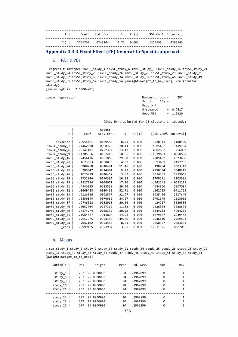
356
------------------------------------------------------------------------------
t | Coef. Std. Err. t P>|t| [95% Conf. Interval]
-------------+----------------------------------------------------------------
(1) | .2761769 .0743144 3.72 0.001 .1227995 .4295543
------------------------------------------------------------------------------
Appendix 3.3.3 Fixed Effect (FE) General-to-Specific approach
a. FAT & PET
. regress t invsepcc invSE_study_1 invSE_study_6 invSE_study_9 invSE_study_16 invSE_study_21
invSE_study_24 invSE_study_25 invSE_study_26 invSE_study_28 invSE_study_29 invSE_study_31
invSE_study_32 invSE_study_33 invSE_study_34 invSE_study_37 invSE_study_46 invSE_study_49
invSE_study_51 invSE_study_52 invSE_study_54 [aweight=weight_to_be_used], vce (cluster
idstudy)
(sum of wgt is 2.5000e+01)
Linear regression Number of obs = 297
F( 1, 24) = .
Prob > F = .
R-squared = 0.7517
Root MSE = 1.0229
(Std. Err. adjusted for 25 clusters in idstudy)
--------------------------------------------------------------------------------
| Robust
t | Coef. Std. Err. t P>|t| [95% Conf. Interval]
---------------+----------------------------------------------------------------
invsepcc | .0954471 .0109563 8.71 0.000 .0728343 .1180599
invSE_study_1 | -.1462608 .0020773 -70.41 0.000 -.1505482 -.1419734
invSE_study_6 | .5141491 .0222302 23.13 0.000 .4682682 .56003
invSE_study_9 | -.1305066 .0152413 -8.56 0.000 -.1619631 -.0990502
invSE_study_16 | .2454436 .0081869 29.98 0.000 .2285467 .2623406
invSE_study_21 | .1673663 .0358095 4.67 0.000 .093459 .2412735
invSE_study_24 | .3900758 .0340401 11.46 0.000 .3198204 .4603312
invSE_study_25 | .289947 .0314394 9.22 0.000 .2250594 .3548347
invSE_study_26 | .1026979 .0340467 3.02 0.006 .0324289 .1729669
invSE_study_28 | .1751946 .0170384 10.28 0.000 .1400291 .2103601
invSE_study_29 | -.0327324 .0046071 -7.10 0.000 -.042241 -.0232238
invSE_study_31 | .4546225 .0223538 20.34 0.000 .4084866 .5007585
invSE_study_32 | .0669488 .0020465 32.71 0.000 .062725 .0711725
invSE_study_33 | .2126536 .0092597 22.97 0.000 .1935426 .2317646
invSE_study_34 | .1859844 .0076636 24.27 0.000 .1701675 .2018012
invSE_study_37 | .2746028 .0132918 20.66 0.000 .24717 .3020356
invSE_study_46 | .3057704 .0257362 11.88 0.000 .2526534 .3588874
invSE_study_49 | .4274274 .0208339 20.52 0.000 .3844283 .4704265
invSE_study_51 | .1964567 .013804 14.23 0.000 .1679667 .2249468
invSE_study_52 | .2657975 .0054182 49.06 0.000 .2546149 .2769801
invSE_study_54 | .047102 .0054588 8.63 0.000 .0358357 .0583683
_cons | -.9999425 .2573934 -3.88 0.001 -1.531176 -.4687086
--------------------------------------------------------------------------------
b. Means
. sum study_1 study_6 study_9 study_16 study_21 study_24 study_25 study_26 study_28 study_29
study_31 study_32 study_33 study_34 study_37 study_46 study_49 study_51 study_52 study_54
[aweight=weight_to_be_used]
Variable | Obs Weight Mean Std. Dev. Min Max
-------------+-----------------------------------------------------------------
study_1 | 297 25.0000003 .04 .1962899 0 1
study_6 | 297 25.0000003 .04 .1962899 0 1
study_9 | 297 25.0000003 .04 .1962899 0 1
study_16 | 297 25.0000003 .04 .1962899 0 1
study_21 | 297 25.0000003 .04 .1962899 0 1
-------------+-----------------------------------------------------------------
study_24 | 297 25.0000003 .04 .1962899 0 1
study_25 | 297 25.0000003 .04 .1962899 0 1
study_26 | 297 25.0000003 .04 .1962899 0 1
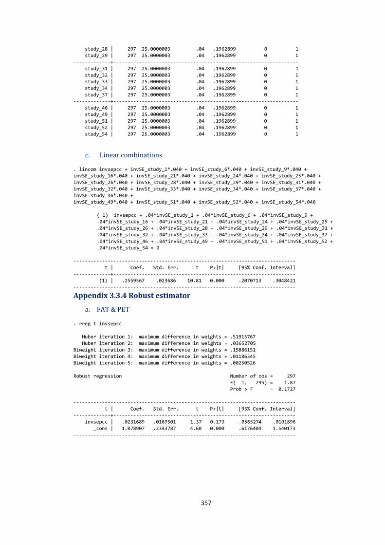
357
study_28 | 297 25.0000003 .04 .1962899 0 1
study_29 | 297 25.0000003 .04 .1962899 0 1
-------------+-----------------------------------------------------------------
study_31 | 297 25.0000003 .04 .1962899 0 1
study_32 | 297 25.0000003 .04 .1962899 0 1
study_33 | 297 25.0000003 .04 .1962899 0 1
study_34 | 297 25.0000003 .04 .1962899 0 1
study_37 | 297 25.0000003 .04 .1962899 0 1
-------------+-----------------------------------------------------------------
study_46 | 297 25.0000003 .04 .1962899 0 1
study_49 | 297 25.0000003 .04 .1962899 0 1
study_51 | 297 25.0000003 .04 .1962899 0 1
study_52 | 297 25.0000003 .04 .1962899 0 1
study_54 | 297 25.0000003 .04 .1962899 0 1
c. Linear combinations
. lincom invsepcc + invSE_study_1*.040 + invSE_study_6*.040 + invSE_study_9*.040 +
invSE_study_16*.040 + invSE_study_21*.040 + invSE_study_24*.040 + invSE_study_25*.040 +
invSE_study_26*.040 + invSE_study_28*.040 + invSE_study_29*.040 + invSE_study_31*.040 +
invSE_study_32*.040 + invSE_study_33*.040 + invSE_study_34*.040 + invSE_study_37*.040 +
invSE_study_46*.040 +
invSE_study_49*.040 + invSE_study_51*.040 + invSE_study_52*.040 + invSE_study_54*.040
( 1) invsepcc + .04*invSE_study_1 + .04*invSE_study_6 + .04*invSE_study_9 +
.04*invSE_study_16 + .04*invSE_study_21 + .04*invSE_study_24 + .04*invSE_study_25 +
.04*invSE_study_26 + .04*invSE_study_28 + .04*invSE_study_29 + .04*invSE_study_31 +
.04*invSE_study_32 + .04*invSE_study_33 + .04*invSE_study_34 + .04*invSE_study_37 +
.04*invSE_study_46 + .04*invSE_study_49 + .04*invSE_study_51 + .04*invSE_study_52 +
.04*invSE_study_54 = 0
------------------------------------------------------------------------------
t | Coef. Std. Err. t P>|t| [95% Conf. Interval]
-------------+----------------------------------------------------------------
(1) | .2559567 .023686 10.81 0.000 .2070713 .3048421
------------------------------------------------------------------------------
Appendix 3.3.4 Robust estimator
a. FAT & PET
. rreg t invsepcc
Huber iteration 1: maximum difference in weights = .51915767
Huber iteration 2: maximum difference in weights = .03652705
Biweight iteration 3: maximum difference in weights = .15886151
Biweight iteration 4: maximum difference in weights = .01186345
Biweight iteration 5: maximum difference in weights = .00250526
Robust regression Number of obs = 297
F( 1, 295) = 1.87
Prob > F = 0.1727
------------------------------------------------------------------------------
t | Coef. Std. Err. t P>|t| [95% Conf. Interval]
-------------+----------------------------------------------------------------
invsepcc | -.0231689 .0169501 -1.37 0.173 -.0565274 .0101896
_cons | 1.078907 .2343787 4.60 0.000 .6176404 1.540173
------------------------------------------------------------------------------

358
Appendix 3.4 Bivariate MRA (Employment growth studies) Appendix 3.4.1 Weighted Least Square (WLS)
a. FAT & PET
. regress t invsepcc[aweight=weight_to_be_used], vce (cluster idstudy)
(sum of wgt is 1.3000e+01)
Linear regression Number of obs = 222
F( 1, 12) = 0.55
Prob > F = 0.4710
R-squared = 0.0088
Root MSE = 2.4784
(Std. Err. adjusted for 13 clusters in idstudy)
------------------------------------------------------------------------------
| Robust
t | Coef. Std. Err. t P>|t| [95% Conf. Interval]
-------------+----------------------------------------------------------------
invsepcc | .0173813 .0233537 0.74 0.471 -.0335021 .0682648
_cons | 1.739638 .8030886 2.17 0.051 -.0101421 3.489417
------------------------------------------------------------------------------
. estat ovtest
Ramsey RESET test using powers of the fitted values of t
Ho: model has no omitted variables
F(3, 217) = 6.38
Prob > F = 0.0004
b. PEESE
. regress t invsepcc sepcc [aweight=weight_to_be_used], vce (cluster idstudy) noconstant
(sum of wgt is 1.3000e+01)
Linear regression Number of obs = 222
F( 2, 12) = 12.41
Prob > F = 0.0012
R-squared = 0.4216
Root MSE = 2.5077
(Std. Err. adjusted for 13 clusters in idstudy)
------------------------------------------------------------------------------
| Robust
t | Coef. Std. Err. t P>|t| [95% Conf. Interval]
-------------+----------------------------------------------------------------
invsepcc | .052054 .0136544 3.81 0.002 .0223036 .0818043
sepcc | 15.57349 7.126061 2.19 0.049 .0471328 31.09984
Appendix 3.4.2 Fixed Effect (FE)
a. FAT & PET . regress t invsepcc invSE_study_3 invSE_study_4 invSE_study_7 invSE_study_8 invSE_study_14
invSE_study_16 invSE_study_17 invSE_study_18 invSE_study_20 invSE_study_23 invSE_study_32
invSE_study_42 invSE_study_43 [aweight=weight_to_be_used], vce (cluster idstudy)
(sum of wgt is 1.3000e+01)
note: invSE_study_8 omitted because of collinearity
Linear regression Number of obs = 222
F( 0, 12) = .
Prob > F = .
R-squared = 0.4800
Root MSE = 1.8463
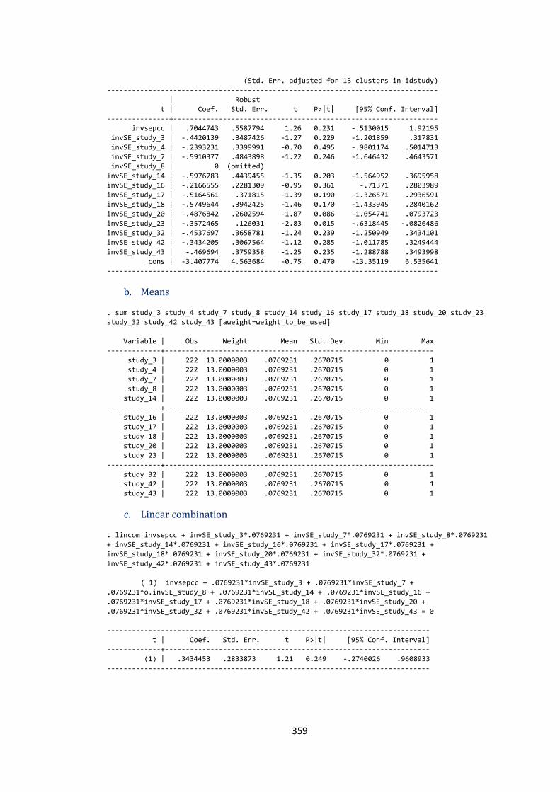
359
(Std. Err. adjusted for 13 clusters in idstudy)
--------------------------------------------------------------------------------
| Robust
t | Coef. Std. Err. t P>|t| [95% Conf. Interval]
---------------+----------------------------------------------------------------
invsepcc | .7044743 .5587794 1.26 0.231 -.5130015 1.92195
invSE_study_3 | -.4420139 .3487426 -1.27 0.229 -1.201859 .317831
invSE_study_4 | -.2393231 .3399991 -0.70 0.495 -.9801174 .5014713
invSE_study_7 | -.5910377 .4843898 -1.22 0.246 -1.646432 .4643571
invSE_study_8 | 0 (omitted)
invSE_study_14 | -.5976783 .4439455 -1.35 0.203 -1.564952 .3695958
invSE_study_16 | -.2166555 .2281309 -0.95 0.361 -.71371 .2803989
invSE_study_17 | -.5164561 .371815 -1.39 0.190 -1.326571 .2936591
invSE_study_18 | -.5749644 .3942425 -1.46 0.170 -1.433945 .2840162
invSE_study_20 | -.4876842 .2602594 -1.87 0.086 -1.054741 .0793723
invSE_study_23 | -.3572465 .126031 -2.83 0.015 -.6318445 -.0826486
invSE_study_32 | -.4537697 .3658781 -1.24 0.239 -1.250949 .3434101
invSE_study_42 | -.3434205 .3067564 -1.12 0.285 -1.011785 .3249444
invSE_study_43 | -.469694 .3759358 -1.25 0.235 -1.288788 .3493998
_cons | -3.407774 4.563684 -0.75 0.470 -13.35119 6.535641
--------------------------------------------------------------------------------
b. Means
. sum study_3 study_4 study_7 study_8 study_14 study_16 study_17 study_18 study_20 study_23
study_32 study_42 study_43 [aweight=weight_to_be_used]
Variable | Obs Weight Mean Std. Dev. Min Max
-------------+-----------------------------------------------------------------
study_3 | 222 13.0000003 .0769231 .2670715 0 1
study_4 | 222 13.0000003 .0769231 .2670715 0 1
study_7 | 222 13.0000003 .0769231 .2670715 0 1
study_8 | 222 13.0000003 .0769231 .2670715 0 1
study_14 | 222 13.0000003 .0769231 .2670715 0 1
-------------+-----------------------------------------------------------------
study_16 | 222 13.0000003 .0769231 .2670715 0 1
study_17 | 222 13.0000003 .0769231 .2670715 0 1
study_18 | 222 13.0000003 .0769231 .2670715 0 1
study_20 | 222 13.0000003 .0769231 .2670715 0 1
study_23 | 222 13.0000003 .0769231 .2670715 0 1
-------------+-----------------------------------------------------------------
study_32 | 222 13.0000003 .0769231 .2670715 0 1
study_42 | 222 13.0000003 .0769231 .2670715 0 1
study_43 | 222 13.0000003 .0769231 .2670715 0 1
c. Linear combination
. lincom invsepcc + invSE_study_3*.0769231 + invSE_study_7*.0769231 + invSE_study_8*.0769231
+ invSE_study_14*.0769231 + invSE_study_16*.0769231 + invSE_study_17*.0769231 +
invSE_study_18*.0769231 + invSE_study_20*.0769231 + invSE_study_32*.0769231 +
invSE_study_42*.0769231 + invSE_study_43*.0769231
( 1) invsepcc + .0769231*invSE_study_3 + .0769231*invSE_study_7 +
.0769231*o.invSE_study_8 + .0769231*invSE_study_14 + .0769231*invSE_study_16 +
.0769231*invSE_study_17 + .0769231*invSE_study_18 + .0769231*invSE_study_20 +
.0769231*invSE_study_32 + .0769231*invSE_study_42 + .0769231*invSE_study_43 = 0
------------------------------------------------------------------------------
t | Coef. Std. Err. t P>|t| [95% Conf. Interval]
-------------+----------------------------------------------------------------
(1) | .3434453 .2833873 1.21 0.249 -.2740026 .9608933
------------------------------------------------------------------------------

360
Appendix 3.4.3 Fixed Effect (FE) General-to-Specific approach
a. FAT & PET
. regress t invsepcc invSE_study_3 invSE_study_7 invSE_study_8 invSE_study_14 invSE_study_16
invSE_study_17 invSE_study_18 invSE_study_20 invSE_study_32 invSE_study_42 invSE_study_43
[aweight=weight_to_be_used], vce (cluster idstudy)
(sum of wgt is 1.3000e+01)
Linear regression Number of obs = 222
F( 1, 12) = .
Prob > F = .
R-squared = 0.4770
Root MSE = 1.8471
(Std. Err. adjusted for 13 clusters in idstudy)
--------------------------------------------------------------------------------
| Robust
t | Coef. Std. Err. t P>|t| [95% Conf. Interval]
---------------+----------------------------------------------------------------
invsepcc | .5576445 .0669675 8.33 0.000 .4117348 .7035541
invSE_study_3 | -.2019081 .0146514 -13.78 0.000 -.2338308 -.1699853
invSE_study_7 | -.4111719 .0482179 -8.53 0.000 -.5162297 -.3061141
invSE_study_8 | .3949804 .0750102 5.27 0.000 .2315472 .5584135
invSE_study_14 | -.3998515 .0380624 -10.51 0.000 -.4827822 -.3169207
invSE_study_16 | .0770133 .0179201 4.30 0.001 .0379686 .1160579
invSE_study_17 | -.2865966 .0201737 -14.21 0.000 -.3305512 -.2426419
invSE_study_18 | -.3550647 .0256784 -13.83 0.000 -.4110131 -.2991163
invSE_study_20 | -.2082835 .0105068 -19.82 0.000 -.2311757 -.1853912
invSE_study_32 | -.2212735 .0187341 -11.81 0.000 -.2620915 -.1804555
invSE_study_42 | -.0846688 .00632 -13.40 0.000 -.098439 -.0708986
invSE_study_43 | -.2416644 .0211781 -11.41 0.000 -.2878076 -.1955212
_cons | -5.434478 1.155918 -4.70 0.001 -7.953008 -2.915948
--------------------------------------------------------------------------------
b. Means
. sum study_3 study_7 study_8 study_14 study_16 study_17 study_18 study_20 study_32 study_42
study_43 [aweight=weight_to_be_used]
Variable | Obs Weight Mean Std. Dev. Min Max
-------------+-----------------------------------------------------------------
study_3 | 222 13.0000003 .0769231 .2670715 0 1
study_7 | 222 13.0000003 .0769231 .2670715 0 1
study_8 | 222 13.0000003 .0769231 .2670715 0 1
study_14 | 222 13.0000003 .0769231 .2670715 0 1
study_16 | 222 13.0000003 .0769231 .2670715 0 1
-------------+-----------------------------------------------------------------
study_17 | 222 13.0000003 .0769231 .2670715 0 1
study_18 | 222 13.0000003 .0769231 .2670715 0 1
study_20 | 222 13.0000003 .0769231 .2670715 0 1
study_32 | 222 13.0000003 .0769231 .2670715 0 1
study_42 | 222 13.0000003 .0769231 .2670715 0 1
-------------+-----------------------------------------------------------------
study_43 | 222 13.0000003 .0769231 .2670715 0 1
c. Linear combination
. lincom invsepcc + invSE_study_3*.0769231 + invSE_study_7*.0769231 + invSE_study_8*.0769231
+ invSE_study_14*.0769231 + invSE_study_16*.0769231 + invSE_study_17*.0769231 +
invSE_study_18*.0769231 + invSE_study_20*.0769231 + invSE_study_32*.0769231 +
invSE_study_42*.0769231 + invSE_study_43*.0769231
( 1) invsepcc + .0769231*invSE_study_3 + .0769231*invSE_study_7 +
.0769231*invSE_study_8 + .0769231*invSE_study_14 + .0769231*invSE_study_16 +
.0769231*invSE_study_17 + .0769231*invSE_study_18 + .0769231*invSE_study_20 +
.0769231*invSE_study_32 + .0769231*invSE_study_42 + 0769231*invSE_study_43 = 0
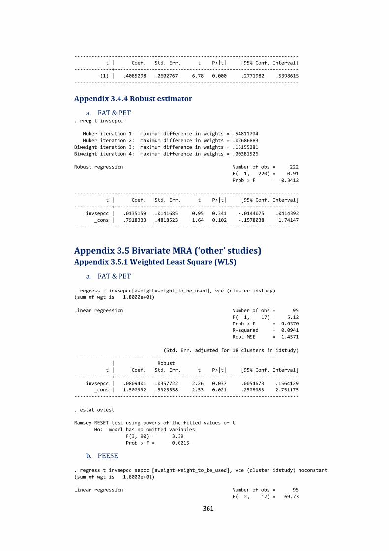
361
------------------------------------------------------------------------------
t | Coef. Std. Err. t P>|t| [95% Conf. Interval]
-------------+----------------------------------------------------------------
(1) | .4085298 .0602767 6.78 0.000 .2771982 .5398615
------------------------------------------------------------------------------
Appendix 3.4.4 Robust estimator
a. FAT & PET . rreg t invsepcc
Huber iteration 1: maximum difference in weights = .54811704
Huber iteration 2: maximum difference in weights = .02686883
Biweight iteration 3: maximum difference in weights = .15155281
Biweight iteration 4: maximum difference in weights = .00381526
Robust regression Number of obs = 222
F( 1, 220) = 0.91
Prob > F = 0.3412
------------------------------------------------------------------------------
t | Coef. Std. Err. t P>|t| [95% Conf. Interval]
-------------+----------------------------------------------------------------
invsepcc | .0135159 .0141685 0.95 0.341 -.0144075 .0414392
_cons | .7918333 .4818523 1.64 0.102 -.1578038 1.74147
------------------------------------------------------------------------------
Appendix 3.5 Bivariate MRA (‘other’ studies) Appendix 3.5.1 Weighted Least Square (WLS)
a. FAT & PET
. regress t invsepcc[aweight=weight_to_be_used], vce (cluster idstudy)
(sum of wgt is 1.8000e+01)
Linear regression Number of obs = 95
F( 1, 17) = 5.12
Prob > F = 0.0370
R-squared = 0.0941
Root MSE = 1.4571
(Std. Err. adjusted for 18 clusters in idstudy)
------------------------------------------------------------------------------
| Robust
t | Coef. Std. Err. t P>|t| [95% Conf. Interval]
-------------+----------------------------------------------------------------
invsepcc | .0809401 .0357722 2.26 0.037 .0054673 .1564129
_cons | 1.500992 .5925558 2.53 0.021 .2508083 2.751175
------------------------------------------------------------------------------
. estat ovtest
Ramsey RESET test using powers of the fitted values of t
Ho: model has no omitted variables
F(3, 90) = 3.39
Prob > F = 0.0215
b. PEESE
. regress t invsepcc sepcc [aweight=weight_to_be_used], vce (cluster idstudy) noconstant
(sum of wgt is 1.8000e+01)
Linear regression Number of obs = 95
F( 2, 17) = 69.73
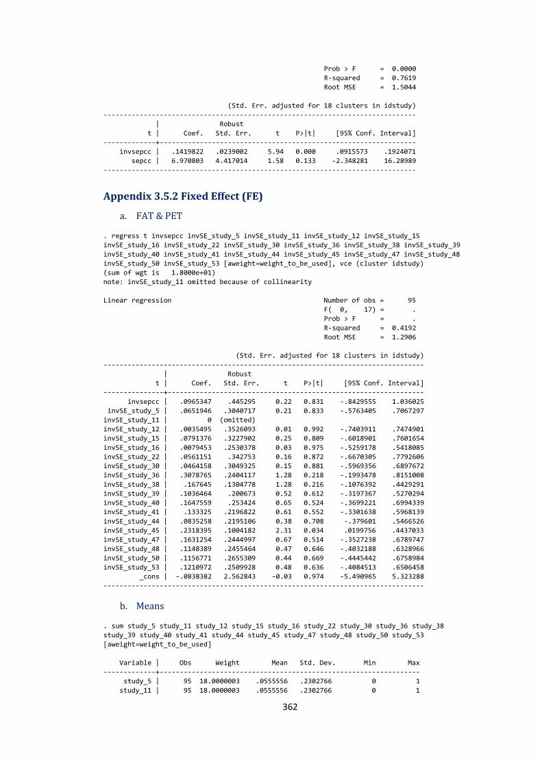
362
Prob > F = 0.0000
R-squared = 0.7619
Root MSE = 1.5044
(Std. Err. adjusted for 18 clusters in idstudy)
------------------------------------------------------------------------------
| Robust
t | Coef. Std. Err. t P>|t| [95% Conf. Interval]
-------------+----------------------------------------------------------------
invsepcc | .1419822 .0239002 5.94 0.000 .0915573 .1924071
sepcc | 6.970803 4.417014 1.58 0.133 -2.348281 16.28989
------------------------------------------------------------------------------
Appendix 3.5.2 Fixed Effect (FE)
a. FAT & PET
. regress t invsepcc invSE_study_5 invSE_study_11 invSE_study_12 invSE_study_15
invSE_study_16 invSE_study_22 invSE_study_30 invSE_study_36 invSE_study_38 invSE_study_39
invSE_study_40 invSE_study_41 invSE_study_44 invSE_study_45 invSE_study_47 invSE_study_48
invSE_study_50 invSE_study_53 [aweight=weight_to_be_used], vce (cluster idstudy)
(sum of wgt is 1.8000e+01)
note: invSE_study_11 omitted because of collinearity
Linear regression Number of obs = 95
F( 0, 17) = .
Prob > F = .
R-squared = 0.4192
Root MSE = 1.2906
(Std. Err. adjusted for 18 clusters in idstudy)
--------------------------------------------------------------------------------
| Robust
t | Coef. Std. Err. t P>|t| [95% Conf. Interval]
---------------+----------------------------------------------------------------
invsepcc | .0965347 .445295 0.22 0.831 -.8429555 1.036025
invSE_study_5 | .0651946 .3040717 0.21 0.833 -.5763405 .7067297
invSE_study_11 | 0 (omitted)
invSE_study_12 | .0035495 .3526093 0.01 0.992 -.7403911 .7474901
invSE_study_15 | .0791376 .3227902 0.25 0.809 -.6018901 .7601654
invSE_study_16 | .0079453 .2530378 0.03 0.975 -.5259178 .5418085
invSE_study_22 | .0561151 .342753 0.16 0.872 -.6670305 .7792606
invSE_study_30 | .0464158 .3049325 0.15 0.881 -.5969356 .6897672
invSE_study_36 | .3078765 .2404117 1.28 0.218 -.1993478 .8151008
invSE_study_38 | .167645 .1304778 1.28 0.216 -.1076392 .4429291
invSE_study_39 | .1036464 .200673 0.52 0.612 -.3197367 .5270294
invSE_study_40 | .1647559 .253424 0.65 0.524 -.3699221 .6994339
invSE_study_41 | .133325 .2196822 0.61 0.552 -.3301638 .5968139
invSE_study_44 | .0835258 .2195106 0.38 0.708 -.379601 .5466526
invSE_study_45 | .2318395 .1004182 2.31 0.034 .0199756 .4437033
invSE_study_47 | .1631254 .2444997 0.67 0.514 -.3527238 .6789747
invSE_study_48 | .1148389 .2455464 0.47 0.646 -.4032188 .6328966
invSE_study_50 | .1156771 .2655309 0.44 0.669 -.4445442 .6758984
invSE_study_53 | .1210972 .2509928 0.48 0.636 -.4084513 .6506458
_cons | -.0838382 2.562843 -0.03 0.974 -5.490965 5.323288
--------------------------------------------------------------------------------
b. Means
. sum study_5 study_11 study_12 study_15 study_16 study_22 study_30 study_36 study_38
study_39 study_40 study_41 study_44 study_45 study_47 study_48 study_50 study_53
[aweight=weight_to_be_used]
Variable | Obs Weight Mean Std. Dev. Min Max
-------------+-----------------------------------------------------------------
study_5 | 95 18.0000003 .0555556 .2302766 0 1
study_11 | 95 18.0000003 .0555556 .2302766 0 1
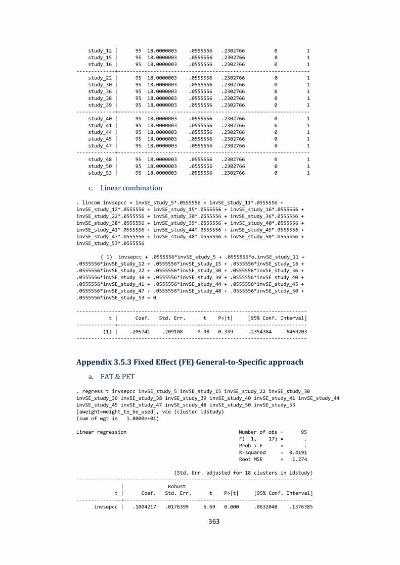
363
study_12 | 95 18.0000003 .0555556 .2302766 0 1
study_15 | 95 18.0000003 .0555556 .2302766 0 1
study_16 | 95 18.0000003 .0555556 .2302766 0 1
-------------+-----------------------------------------------------------------
study_22 | 95 18.0000003 .0555556 .2302766 0 1
study_30 | 95 18.0000003 .0555556 .2302766 0 1
study_36 | 95 18.0000003 .0555556 .2302766 0 1
study_38 | 95 18.0000003 .0555556 .2302766 0 1
study_39 | 95 18.0000003 .0555556 .2302766 0 1
-------------+-----------------------------------------------------------------
study_40 | 95 18.0000003 .0555556 .2302766 0 1
study_41 | 95 18.0000003 .0555556 .2302766 0 1
study_44 | 95 18.0000003 .0555556 .2302766 0 1
study_45 | 95 18.0000003 .0555556 .2302766 0 1
study_47 | 95 18.0000003 .0555556 .2302766 0 1
-------------+-----------------------------------------------------------------
study_48 | 95 18.0000003 .0555556 .2302766 0 1
study_50 | 95 18.0000003 .0555556 .2302766 0 1
study_53 | 95 18.0000003 .0555556 .2302766 0 1
c. Linear combination
. lincom invsepcc + invSE_study_5*.0555556 + invSE_study_11*.0555556 +
invSE_study_12*.0555556 + invSE_study_15*.0555556 + invSE_study_16*.0555556 +
invSE_study_22*.0555556 + invSE_study_30*.0555556 + invSE_study_36*.0555556 +
invSE_study_38*.0555556 + invSE_study_39*.0555556 + invSE_study_40*.0555556 +
invSE_study_41*.0555556 + invSE_study_44*.0555556 + invSE_study_45*.0555556 +
invSE_study_47*.0555556 + invSE_study_48*.0555556 + invSE_study_50*.0555556 +
invSE_study_53*.0555556
( 1) invsepcc + .0555556*invSE_study_5 + .0555556*o.invSE_study_11 +
.0555556*invSE_study_12 + .0555556*invSE_study_15 + .0555556*invSE_study_16 +
.0555556*invSE_study_22 + .0555556*invSE_study_30 + .0555556*invSE_study_36 +
.0555556*invSE_study_38 + .0555556*invSE_study_39 + .0555556*invSE_study_40 +
.0555556*invSE_study_41 + .0555556*invSE_study_44 + .0555556*invSE_study_45 +
.0555556*invSE_study_47 + .0555556*invSE_study_48 + .0555556*invSE_study_50 +
.0555556*invSE_study_53 = 0
------------------------------------------------------------------------------
t | Coef. Std. Err. t P>|t| [95% Conf. Interval]
-------------+----------------------------------------------------------------
(1) | .205741 .209108 0.98 0.339 -.2354384 .6469203
------------------------------------------------------------------------------
Appendix 3.5.3 Fixed Effect (FE) General-to-Specific approach
a. FAT & PET
. regress t invsepcc invSE_study_5 invSE_study_15 invSE_study_22 invSE_study_30
invSE_study_36 invSE_study_38 invSE_study_39 invSE_study_40 invSE_study_41 invSE_study_44
invSE_study_45 invSE_study_47 invSE_study_48 invSE_study_50 invSE_study_53
[aweight=weight_to_be_used], vce (cluster idstudy)
(sum of wgt is 1.8000e+01)
Linear regression Number of obs = 95
F( 1, 17) = .
Prob > F = .
R-squared = 0.4191
Root MSE = 1.274
(Std. Err. adjusted for 18 clusters in idstudy)
--------------------------------------------------------------------------------
| Robust
t | Coef. Std. Err. t P>|t| [95% Conf. Interval]
---------------+----------------------------------------------------------------
invsepcc | .1004217 .0176399 5.69 0.000 .0632048 .1376385
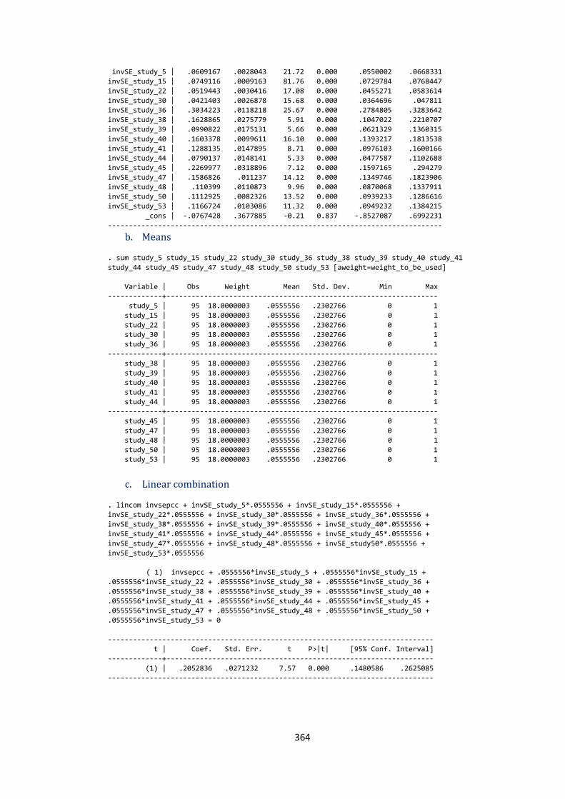
364
invSE_study_5 | .0609167 .0028043 21.72 0.000 .0550002 .0668331
invSE_study_15 | .0749116 .0009163 81.76 0.000 .0729784 .0768447
invSE_study_22 | .0519443 .0030416 17.08 0.000 .0455271 .0583614
invSE_study_30 | .0421403 .0026878 15.68 0.000 .0364696 .047811
invSE_study_36 | .3034223 .0118218 25.67 0.000 .2784805 .3283642
invSE_study_38 | .1628865 .0275779 5.91 0.000 .1047022 .2210707
invSE_study_39 | .0990822 .0175131 5.66 0.000 .0621329 .1360315
invSE_study_40 | .1603378 .0099611 16.10 0.000 .1393217 .1813538
invSE_study_41 | .1288135 .0147895 8.71 0.000 .0976103 .1600166
invSE_study_44 | .0790137 .0148141 5.33 0.000 .0477587 .1102688
invSE_study_45 | .2269977 .0318896 7.12 0.000 .1597165 .294279
invSE_study_47 | .1586826 .011237 14.12 0.000 .1349746 .1823906
invSE_study_48 | .110399 .0110873 9.96 0.000 .0870068 .1337911
invSE_study_50 | .1112925 .0082326 13.52 0.000 .0939233 .1286616
invSE_study_53 | .1166724 .0103086 11.32 0.000 .0949232 .1384215
_cons | -.0767428 .3677885 -0.21 0.837 -.8527087 .6992231
--------------------------------------------------------------------------------
b. Means
. sum study_5 study_15 study_22 study_30 study_36 study_38 study_39 study_40 study_41
study_44 study_45 study_47 study_48 study_50 study_53 [aweight=weight_to_be_used]
Variable | Obs Weight Mean Std. Dev. Min Max
-------------+-----------------------------------------------------------------
study_5 | 95 18.0000003 .0555556 .2302766 0 1
study_15 | 95 18.0000003 .0555556 .2302766 0 1
study_22 | 95 18.0000003 .0555556 .2302766 0 1
study_30 | 95 18.0000003 .0555556 .2302766 0 1
study_36 | 95 18.0000003 .0555556 .2302766 0 1
-------------+-----------------------------------------------------------------
study_38 | 95 18.0000003 .0555556 .2302766 0 1
study_39 | 95 18.0000003 .0555556 .2302766 0 1
study_40 | 95 18.0000003 .0555556 .2302766 0 1
study_41 | 95 18.0000003 .0555556 .2302766 0 1
study_44 | 95 18.0000003 .0555556 .2302766 0 1
-------------+-----------------------------------------------------------------
study_45 | 95 18.0000003 .0555556 .2302766 0 1
study_47 | 95 18.0000003 .0555556 .2302766 0 1
study_48 | 95 18.0000003 .0555556 .2302766 0 1
study_50 | 95 18.0000003 .0555556 .2302766 0 1
study_53 | 95 18.0000003 .0555556 .2302766 0 1
c. Linear combination
. lincom invsepcc + invSE_study_5*.0555556 + invSE_study_15*.0555556 +
invSE_study_22*.0555556 + invSE_study_30*.0555556 + invSE_study_36*.0555556 +
invSE_study_38*.0555556 + invSE_study_39*.0555556 + invSE_study_40*.0555556 +
invSE_study_41*.0555556 + invSE_study_44*.0555556 + invSE_study_45*.0555556 +
invSE_study_47*.0555556 + invSE_study_48*.0555556 + invSE_study50*.0555556 +
invSE_study_53*.0555556
( 1) invsepcc + .0555556*invSE_study_5 + .0555556*invSE_study_15 +
.0555556*invSE_study_22 + .0555556*invSE_study_30 + .0555556*invSE_study_36 +
.0555556*invSE_study_38 + .0555556*invSE_study_39 + .0555556*invSE_study_40 +
.0555556*invSE_study_41 + .0555556*invSE_study_44 + .0555556*invSE_study_45 +
.0555556*invSE_study_47 + .0555556*invSE_study_48 + .0555556*invSE_study_50 +
.0555556*invSE_study_53 = 0
------------------------------------------------------------------------------
t | Coef. Std. Err. t P>|t| [95% Conf. Interval]
-------------+----------------------------------------------------------------
(1) | .2052836 .0271232 7.57 0.000 .1480586 .2625085
------------------------------------------------------------------------------
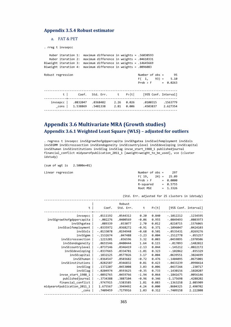
365
Appendix 3.5.4 Robust estimator
a. FAT & PET
. rreg t invsepcc
Huber iteration 1: maximum difference in weights = .56030593
Huber iteration 2: maximum difference in weights = .04610331
Biweight iteration 3: maximum difference in weights = .14645669
Biweight iteration 4: maximum difference in weights = .0096083
Robust regression Number of obs = 95
F( 1, 93) = 5.10
Prob > F = 0.0263
------------------------------------------------------------------------------
t | Coef. Std. Err. t P>|t| [95% Conf. Interval]
-------------+----------------------------------------------------------------
invsepcc | .0832047 .0368482 2.26 0.026 .0100315 .1563779
_cons | 1.538869 .5481338 2.81 0.006 .4503837 2.627354
------------------------------------------------------------------------------
Appendix 3.6 Multivariate MRA (Growth studies) Appendix 3.6.1 Weighted Least Square (WLS) – adjusted for outliers
. regress t invsepcc invSEgrowthofgdppercapita invSEhgatea invSEselfemployment invSEols
invSEGMM invSEcrosssection invSEendogeneity invSEcountrylevel invSEdeveloping invSEcapital
invSEhuman invSEinstitutions invSElog invSElag invse_start_1988_1 publishedjournal
financial_conflict midyearofpublication_2011_1 [aweight=weight_to_be_used], vce (cluster
idstudy)
(sum of wgt is 2.5000e+01)
Linear regression Number of obs = 297
F( 19, 24) = 25.09
Prob > F = 0.0000
R-squared = 0.5755
Root MSE = 1.3326
(Std. Err. adjusted for 25 clusters in idstudy)
---------------------------------------------------------------------------------------------
| Robust
t | Coef. Std. Err. t P>|t| [95% Conf. Interval]
----------------------------+----------------------------------------------------------------
invsepcc | .0111192 .0544312 0.20 0.840 -.1012212 .1234595
invSEgrowthofgdppercapita | -.002276 .0400569 -0.06 0.955 -.0849493 .0803973
invSEhgatea | .089339 .033077 2.70 0.012 .0210715 .1576065
invSEselfemployment | -.0335972 .0368272 -0.91 0.371 -.1096047 .0424103
invSEols | -.0133078 .0194948 -0.68 0.501 -.0535431 .0269276
invSEgmm | -.1532674 .047488 -3.23 0.004 -.2512778 -.055257
invSEcrosssection | .1215201 .036596 3.32 0.003 .0459895 .1970506
invSEendogeneity | .0655546 .0400444 1.64 0.115 -.017093 .1482022
invSEcountrylevel | -.0737146 .0346419 -2.13 0.044 -.145212 -.0022172
invSEdeveloping | -.0337665 .0334781 -1.01 0.323 -.102862 .035329
invSEcapital | .1832125 .0577826 3.17 0.004 .0639551 .3024699
invSEhuman | -.0364547 .0503682 -0.72 0.476 -.1404095 .0675001
invSEinstitutions | .0282587 .0346832 0.81 0.423 -.0433239 .0998414
invSElog | .1372207 .0453008 3.03 0.006 .0437244 .230717
invSElag | -.0204974 .0593625 -0.35 0.733 -.1430156 .1020207
invse_start_1988_1 | -.0892765 .0459766 -1.94 0.064 -.1841675 .0056146
publishedjournal | -.3734388 .3887104 -0.96 0.346 -1.175698 .4288202
financial_conflict | .9747915 .5383585 1.81 0.083 -.1363258 2.085909
midyearofpublication_2011_1 | 1.675567 .3949492 4.24 0.000 .8604325 2.490702
_cons | .7409459 .7179916 1.03 0.312 -.7409158 2.222808
---------------------------------------------------------------------------------------------

366
a. Lenarity test
. estat ovtest
Ramsey RESET test using powers of the fitted values of t
Ho: model has no omitted variables
F(3, 274) = 4.37
Prob > F = 0.0050
b. Normality test
. estat imtest
Cameron & Trivedi's decomposition of IM-test
---------------------------------------------------
Source | chi2 df p
---------------------+-----------------------------
Heteroskedasticity | 210.30 107 0.0000
Skewness | 38.50 19 0.0051
Kurtosis | 1.64 1 0.2008
---------------------+-----------------------------
Total | 250.44 127 0.0000
---------------------------------------------------
c. Histogram of residuals
. predict resid2, res
. histogram resid2
(bin=17, start=-3.2693558, width=.3786325)
. qui regress t invsepcc invSEgrowthofgdppercapita invSEhgatea invSEselfemployment invSEols
invSEgmm invSEcrosssection invSEendogeneity invSEcountrylevel invSEdeveloping invSEcapital
invSEhuman invSEinstitutions invSElog invSElag invse_start_1988_1 publishedjournal
financial_conflict midyearofpublication_2011_1
d. Multicollinerarity
. estat vif
Variable | VIF 1/VIF
-------------+----------------------
invSElag | 14.64 0.068304
0.1
.2.3
.4
Den
sity
-4 -2 0 2 4Residuals
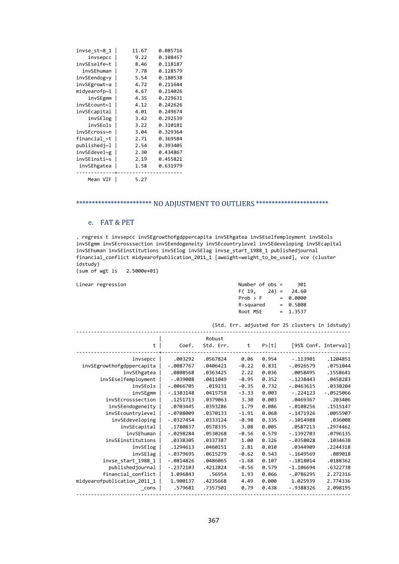
367
invse_st~8_1 | 11.67 0.085716
invsepcc | 9.22 0.108457
invSEselfe~t | 8.46 0.118187
invSEhuman | 7.78 0.128579
invSEendog~y | 5.54 0.180538
invSEgrowt~a | 4.72 0.211644
midyearofp~1 | 4.67 0.214026
invSEgmm | 4.35 0.229631
invSEcount~l | 4.12 0.242626
invSEcapital | 4.01 0.249674
invSElog | 3.42 0.292539
invSEols | 3.22 0.310181
invSEcross~n | 3.04 0.329364
financial_~t | 2.71 0.369584
publishedj~l | 2.54 0.393405
invSEdevel~g | 2.30 0.434867
invSEinsti~s | 2.19 0.455821
invSEhgatea | 1.58 0.631979
-------------+----------------------
Mean VIF | 5.27
************************ NO ADJUSTMENT TO OUTLIERS ***********************
e. FAT & PET
. regress t invsepcc invSEgrowthofgdppercapita invSEhgatea invSEselfemployment invSEols
invSEgmm invSEcrosssection invSEendogeneity invSEcountrylevel invSEdeveloping invSEcapital
invSEhuman invSEinstitutions invSElog invSElag invse_start_1988_1 publishedjournal
financial_conflict midyearofpublication_2011_1 [aweight=weight_to_be_used], vce (cluster
idstudy)
(sum of wgt is 2.5000e+01)
Linear regression Number of obs = 301
F( 19, 24) = 24.60
Prob > F = 0.0000
R-squared = 0.5808
Root MSE = 1.3537
(Std. Err. adjusted for 25 clusters in idstudy)
---------------------------------------------------------------------------------------------
| Robust
t | Coef. Std. Err. t P>|t| [95% Conf. Interval]
----------------------------+----------------------------------------------------------------
invsepcc | .003292 .0567824 0.06 0.954 -.113901 .1204851
invSEgrowthofgdppercapita | -.0087767 .0406421 -0.22 0.831 -.0926579 .0751044
invSEhgatea | .0808568 .0363425 2.22 0.036 .0058495 .1558641
invSEselfemployment | -.039008 .0411049 -0.95 0.352 -.1238443 .0458283
invSEols | -.0066705 .019231 -0.35 0.732 -.0463615 .0330204
invSEgmm | -.1383148 .0415758 -3.33 0.003 -.224123 -.0525066
invSEcrosssection | .1251713 .0379063 3.30 0.003 .0469367 .203406
invSEendogeneity | .0703445 .0393286 1.79 0.086 -.0108256 .1515147
invSEcountrylevel | -.0708009 .0370133 -1.91 0.068 -.1471926 .0055907
invSEdeveloping | -.0327454 .0333124 -0.98 0.335 -.1014988 .036008
invSEcapital | .1780837 .0578335 3.08 0.005 .0587213 .2974462
invSEhuman | -.0298284 .0530268 -0.56 0.579 -.1392703 .0796135
invSEinstitutions | .0338305 .0337387 1.00 0.326 -.0358028 .1034638
invSElog | .1294613 .0460151 2.81 0.010 .0344909 .2244318
invSElag | -.0379695 .0615279 -0.62 0.543 -.1649569 .089018
invse_start_1988_1 | -.0814826 .0486065 -1.68 0.107 -.1818014 .0188362
publishedjournal | -.2372103 .4212824 -0.56 0.579 -1.106694 .6322738
financial_conflict | 1.096843 .56954 1.93 0.066 -.0786295 2.272316
midyearofpublication_2011_1 | 1.900137 .4235668 4.49 0.000 1.025939 2.774336
_cons | .579681 .7357501 0.79 0.438 -.9388326 2.098195
---------------------------------------------------------------------------------------------
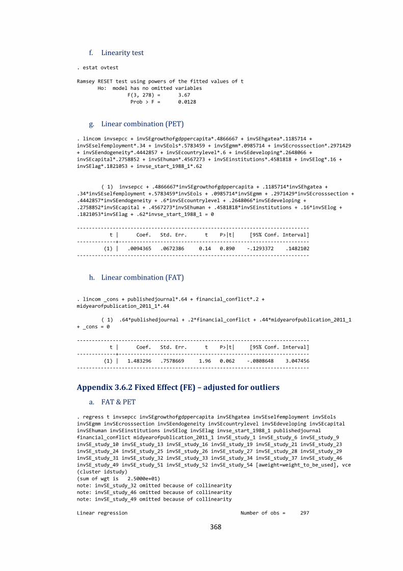
368
f. Linearity test
. estat ovtest
Ramsey RESET test using powers of the fitted values of t
Ho: model has no omitted variables
F(3, 278) = 3.67
Prob > F = 0.0128
g. Linear combination (PET)
. lincom invsepcc + invSEgrowthofgdppercapita*.4866667 + invSEhgatea*.1185714 +
invSEselfemployment*.34 + invSEols*.5783459 + invSEgmm*.0985714 + invSEcrosssection*.2971429
+ invSEendogeneity*.4442857 + invSEcountrylevel*.6 + invSEdeveloping*.2648066 +
invSEcapital*.2758852 + invSEhuman*.4567273 + invSEinstitutions*.4581818 + invSElog*.16 +
invSElag*.1821053 + invse_start_1988_1*.62
( 1) invsepcc + .4866667*invSEgrowthofgdppercapita + .1185714*invSEhgatea +
.34*invSEselfemployment +.5783459*invSEols + .0985714*invSEgmm + .2971429*invSEcrosssection +
.4442857*invSEendogeneity + .6*invSEcountrylevel + .2648066*invSEdeveloping +
.2758852*invSEcapital + .4567273*invSEhuman + .4581818*invSEinstitutions + .16*invSElog +
.1821053*invSElag + .62*invse_start_1988_1 = 0
------------------------------------------------------------------------------
t | Coef. Std. Err. t P>|t| [95% Conf. Interval]
-------------+----------------------------------------------------------------
(1) | .0094365 .0672386 0.14 0.890 -.1293372 .1482102
------------------------------------------------------------------------------
h. Linear combination (FAT)
. lincom _cons + publishedjournal*.64 + financial_conflict*.2 +
midyearofpublication_2011_1*.44
( 1) .64*publishedjournal + .2*financial_conflict + .44*midyearofpublication_2011_1
+ _cons = 0
------------------------------------------------------------------------------
t | Coef. Std. Err. t P>|t| [95% Conf. Interval]
-------------+----------------------------------------------------------------
(1) | 1.483296 .7578669 1.96 0.062 -.0808648 3.047456
------------------------------------------------------------------------------
Appendix 3.6.2 Fixed Effect (FE) – adjusted for outliers
a. FAT & PET
. regress t invsepcc invSEgrowthofgdppercapita invSEhgatea invSEselfemployment invSEols
invSEgmm invSEcrosssection invSEendogeneity invSEcountrylevel invSEdeveloping invSEcapital
invSEhuman invSEinstitutions invSElog invSElag invse_start_1988_1 publishedjournal
financial_conflict midyearofpublication_2011_1 invSE_study_1 invSE_study_6 invSE_study_9
invSE_study_10 invSE_study_13 invSE_study_16 invSE_study_19 invSE_study_21 invSE_study_23
invSE_study_24 invSE_study_25 invSE_study_26 invSE_study_27 invSE_study_28 invSE_study_29
invSE_study_31 invSE_study_32 invSE_study_33 invSE_study_34 invSE_study_37 invSE_study_46
invSE_study_49 invSE_study_51 invSE_study_52 invSE_study_54 [aweight=weight_to_be_used], vce
(cluster idstudy)
(sum of wgt is 2.5000e+01)
note: invSE_study_32 omitted because of collinearity
note: invSE_study_46 omitted because of collinearity
note: invSE_study_49 omitted because of collinearity
Linear regression Number of obs = 297
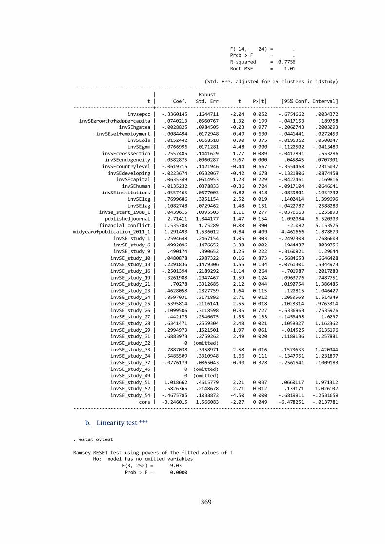
369
F( 14, 24) = .
Prob > F = .
R-squared = 0.7756
Root MSE = 1.01
(Std. Err. adjusted for 25 clusters in idstudy)
---------------------------------------------------------------------------------------------
| Robust
t | Coef. Std. Err. t P>|t| [95% Conf. Interval]
----------------------------+----------------------------------------------------------------
invsepcc | -.3360145 .1644711 -2.04 0.052 -.6754662 .0034372
invSEgrowthofgdppercapita | .0740213 .0560767 1.32 0.199 -.0417153 .189758
invSEhgatea | -.0028825 .0984505 -0.03 0.977 -.2060743 .2003093
invSEselfemployment | -.0084494 .0172948 -0.49 0.630 -.0441441 .0272453
invSEols | .0152442 .0168518 0.90 0.375 -.0195362 .0500247
invSEgmm | -.0766996 .0171281 -4.48 0.000 -.1120502 -.0413489
invSEcrosssection | .2557485 .1441629 1.77 0.089 -.0417891 .553286
invSEendogeneity | .0582875 .0060287 9.67 0.000 .045845 .0707301
invSEcountrylevel | -.0619715 .1421946 -0.44 0.667 -.3554468 .2315037
invSEdeveloping | -.0223674 .0532067 -0.42 0.678 -.1321806 .0874458
invSEcapital | .0635349 .0514953 1.23 0.229 -.0427461 .169816
invSEhuman | -.0135232 .0378833 -0.36 0.724 -.0917104 .0646641
invSEinstitutions | .0557465 .0677003 0.82 0.418 -.0839801 .1954732
invSElog | .7699686 .3051154 2.52 0.019 .1402414 1.399696
invSElag | .1082748 .0729462 1.48 0.151 -.0422787 .2588283
invse_start_1988_1 | .0439615 .0395503 1.11 0.277 -.0376663 .1255893
publishedjournal | 2.71411 1.844177 1.47 0.154 -1.092084 6.520303
financial_conflict | 1.535788 1.75289 0.88 0.390 -2.082 5.153575
midyearofpublication_2011_1 | -1.291493 1.536012 -0.84 0.409 -4.461666 1.878679
invSE_study_1 | .2594648 .2467154 1.05 0.303 -.2497308 .7686603
invSE_study_6 | .4992096 .1476652 3.38 0.002 .1944437 .8039756
invSE_study_9 | .490174 .390652 1.25 0.222 -.3160921 1.29644
invSE_study_10 | .0480878 .2987322 0.16 0.873 -.5684653 .6646408
invSE_study_13 | .2291836 .1479306 1.55 0.134 -.0761301 .5344973
invSE_study_16 | -.2501394 .2189292 -1.14 0.264 -.701987 .2017083
invSE_study_19 | .3261988 .2047467 1.59 0.124 -.0963776 .7487751
invSE_study_21 | .70278 .3312685 2.12 0.044 .0190754 1.386485
invSE_study_23 | .4628058 .2827759 1.64 0.115 -.120815 1.046427
invSE_study_24 | .8597031 .3171892 2.71 0.012 .2050568 1.514349
invSE_study_25 | .5395814 .2116141 2.55 0.018 .1028314 .9763314
invSE_study_26 | .1099506 .3118598 0.35 0.727 -.5336963 .7535976
invSE_study_27 | .442175 .2846675 1.55 0.133 -.1453498 1.0297
invSE_study_28 | .6341471 .2559304 2.48 0.021 .1059327 1.162362
invSE_study_29 | .2994973 .1521501 1.97 0.061 -.014525 .6135196
invSE_study_31 | .6883973 .2759262 2.49 0.020 .1189136 1.257881
invSE_study_32 | 0 (omitted)
invSE_study_33 | .7887038 .3058971 2.58 0.016 .1573633 1.420044
invSE_study_34 | .5485509 .3310948 1.66 0.111 -.1347951 1.231897
invSE_study_37 | -.0776179 .0865043 -0.90 0.378 -.2561541 .1009183
invSE_study_46 | 0 (omitted)
invSE_study_49 | 0 (omitted)
invSE_study_51 | 1.018662 .4615779 2.21 0.037 .0660117 1.971312
invSE_study_52 | .5826365 .2148678 2.71 0.012 .139171 1.026102
invSE_study_54 | -.4675785 .1038872 -4.50 0.000 -.6819911 -.2531659
_cons | -3.246015 1.566083 -2.07 0.049 -6.478251 -.0137781
---------------------------------------------------------------------------------------------
b. Linearity test *** . estat ovtest
Ramsey RESET test using powers of the fitted values of t
Ho: model has no omitted variables
F(3, 252) = 9.03
Prob > F = 0.0000
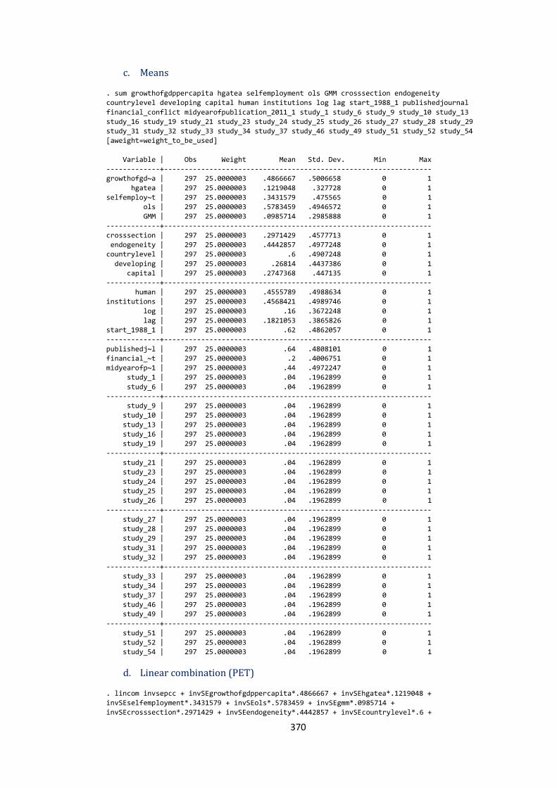
370
c. Means
. sum growthofgdppercapita hgatea selfemployment ols GMM crosssection endogeneity
countrylevel developing capital human institutions log lag start_1988_1 publishedjournal
financial_conflict midyearofpublication_2011_1 study_1 study_6 study_9 study_10 study_13
study_16 study_19 study_21 study_23 study_24 study_25 study_26 study_27 study_28 study_29
study_31 study_32 study_33 study_34 study_37 study_46 study_49 study_51 study_52 study_54
[aweight=weight_to_be_used]
Variable | Obs Weight Mean Std. Dev. Min Max
-------------+-----------------------------------------------------------------
growthofgd~a | 297 25.0000003 .4866667 .5006658 0 1
hgatea | 297 25.0000003 .1219048 .327728 0 1
selfemploy~t | 297 25.0000003 .3431579 .475565 0 1
ols | 297 25.0000003 .5783459 .4946572 0 1
GMM | 297 25.0000003 .0985714 .2985888 0 1
-------------+-----------------------------------------------------------------
crosssection | 297 25.0000003 .2971429 .4577713 0 1
endogeneity | 297 25.0000003 .4442857 .4977248 0 1
countrylevel | 297 25.0000003 .6 .4907248 0 1
developing | 297 25.0000003 .26814 .4437386 0 1
capital | 297 25.0000003 .2747368 .447135 0 1
-------------+-----------------------------------------------------------------
human | 297 25.0000003 .4555789 .4988634 0 1
institutions | 297 25.0000003 .4568421 .4989746 0 1
log | 297 25.0000003 .16 .3672248 0 1
lag | 297 25.0000003 .1821053 .3865826 0 1
start_1988_1 | 297 25.0000003 .62 .4862057 0 1
-------------+-----------------------------------------------------------------
publishedj~l | 297 25.0000003 .64 .4808101 0 1
financial_~t | 297 25.0000003 .2 .4006751 0 1
midyearofp~1 | 297 25.0000003 .44 .4972247 0 1
study_1 | 297 25.0000003 .04 .1962899 0 1
study_6 | 297 25.0000003 .04 .1962899 0 1
-------------+-----------------------------------------------------------------
study_9 | 297 25.0000003 .04 .1962899 0 1
study_10 | 297 25.0000003 .04 .1962899 0 1
study_13 | 297 25.0000003 .04 .1962899 0 1
study_16 | 297 25.0000003 .04 .1962899 0 1
study_19 | 297 25.0000003 .04 .1962899 0 1
-------------+-----------------------------------------------------------------
study_21 | 297 25.0000003 .04 .1962899 0 1
study_23 | 297 25.0000003 .04 .1962899 0 1
study_24 | 297 25.0000003 .04 .1962899 0 1
study_25 | 297 25.0000003 .04 .1962899 0 1
study_26 | 297 25.0000003 .04 .1962899 0 1
-------------+-----------------------------------------------------------------
study_27 | 297 25.0000003 .04 .1962899 0 1
study_28 | 297 25.0000003 .04 .1962899 0 1
study_29 | 297 25.0000003 .04 .1962899 0 1
study_31 | 297 25.0000003 .04 .1962899 0 1
study_32 | 297 25.0000003 .04 .1962899 0 1
-------------+-----------------------------------------------------------------
study_33 | 297 25.0000003 .04 .1962899 0 1
study_34 | 297 25.0000003 .04 .1962899 0 1
study_37 | 297 25.0000003 .04 .1962899 0 1
study_46 | 297 25.0000003 .04 .1962899 0 1
study_49 | 297 25.0000003 .04 .1962899 0 1
-------------+-----------------------------------------------------------------
study_51 | 297 25.0000003 .04 .1962899 0 1
study_52 | 297 25.0000003 .04 .1962899 0 1
study_54 | 297 25.0000003 .04 .1962899 0 1
d. Linear combination (PET)
. lincom invsepcc + invSEgrowthofgdppercapita*.4866667 + invSEhgatea*.1219048 +
invSEselfemployment*.3431579 + invSEols*.5783459 + invSEgmm*.0985714 +
invSEcrosssection*.2971429 + invSEendogeneity*.4442857 + invSEcountrylevel*.6 +
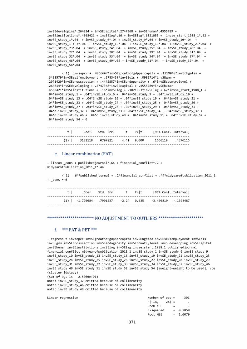
371
invSEdeveloping*.264814 + invSEcapital*.2747368 + invSEhuman*.4555789 +
invSEinstitutions*.4568421 + invSElog*.16 + invSElag*.1821053 + invse_start_1988_1*.62 +
invSE_study_1*.04 + invSE_study_6*.04 + invSE_study_9*.04 + invSE_study_10*.04 +
invSE_study_1 > 3*.04 + invSE_study_16*.04 + invSE_study_19*.04 + invSE_study_21*.04 +
invSE_study_23*.04 + invSE_study_24*.04 + invSE_study_25*.04 + invSE_study_26*.04 +
invSE_study_27*.04 + invSE_study_28*.04 + invSE_study_29*.04 + invSE_study_31*.04 +
invSE_study_32*.04 + invSE_study_33*.04 + invSE_study_34*.04 + invSE_study_37*.04 +
invSE_study_46*.04 + invSE_study_49*.04 + invSE_study_51*.04 + invSE_study_52*.04 +
invSE_study_54*.04
( 1) invsepcc + .4866667*invSEgrowthofgdppercapita + .1219048*invSEhgatea +
.3431579*invSEselfemployment + .5783459*invSEols + .0985714*invSEgmm +
.2971429*invSEcrosssection + .4442857*invSEendogeneity + .6*invSEcountrylevel +
.264814*invSEdeveloping + .2747368*invSEcapital + .4555789*invSEhuman +
.4568421*invSEinstitutions + .16*invSElog + .1821053*invSElag + 62*invse_start_1988_1 +
.04*invSE_study_1 + .04*invSE_study_6 + .04*invSE_study_9 + .04*invSE_study_10 +
.04*invSE_study_13 + .04*invSE_study_16 + .04*invSE_study_19 + .04*invSE_study_21 +
.04*invSE_study_23 + .04*invSE_study_24 + .04*invSE_study_25 + .04*invSE_study_26 +
.04*invSE_study_27 + .04*invSE_study_28 + .04*invSE_study_29 + .04*invSE_study_31 +
.04*o.invSE_study_32 + .04*invSE_study_33 + .04*invSE_study_34 + .04*invSE_study_37 +
.04*o.invSE_study_46 + .04*o.invSE_study_49 + .04*invSE_study_51 + .04*invSE_study_52 +
.04*invSE_study_54 = 0
------------------------------------------------------------------------------
t | Coef. Std. Err. t P>|t| [95% Conf. Interval]
-------------+----------------------------------------------------------------
(1) | .3131118 .0709821 4.41 0.000 .1666119 .4596116
------------------------------------------------------------------------------
e. Linear combination (FAT)
. lincom _cons + publishedjournal*.64 + financial_conflict*.2 +
midyearofpublication_2011_1*.44
( 1) .64*publishedjournal + .2*financial_conflict + .44*midyearofpublication_2011_1
+ _cons = 0
------------------------------------------------------------------------------
t | Coef. Std. Err. t P>|t| [95% Conf. Interval]
-------------+----------------------------------------------------------------
(1) | -1.770084 .7901237 -2.24 0.035 -3.400819 -.1393487
------------------------------------------------------------------------------
************************ NO ADJUSTMENT TO OUTLIERS ***********************
f. *** FAT & PET ***
. regress t invsepcc invSEgrowthofgdppercapita invSEhgatea invSEselfemployment invSEols
invSEgmm invSEcrosssection invSEendogeneity invSEcountrylevel invSEdeveloping invSEcapital
invSEhuman invSEinstitutions invSElog invSElag invse_start_1988_1 publishedjournal
financial_conflict midyearofpublication_2011_1 invSE_study_1 invSE_study_6 invSE_study_9
invSE_study_10 invSE_study_13 invSE_study_16 invSE_study_19 invSE_study_21 invSE_study_23
invSE_study_24 invSE_study_25 invSE_study_26 invSE_study_27 invSE_study_28 invSE_study_29
invSE_study_31 invSE_study_32 invSE_study_33 invSE_study_34 invSE_study_37 invSE_study_46
invSE_study_49 invSE_study_51 invSE_study_52 invSE_study_54 [aweight=weight_to_be_used], vce
(cluster idstudy)
(sum of wgt is 2.5000e+01)
note: invSE_study_32 omitted because of collinearity
note: invSE_study_46 omitted because of collinearity
note: invSE_study_49 omitted because of collinearity
Linear regression Number of obs = 301
F( 14, 24) = .
Prob > F = .
R-squared = 0.7858
Root MSE = 1.0079
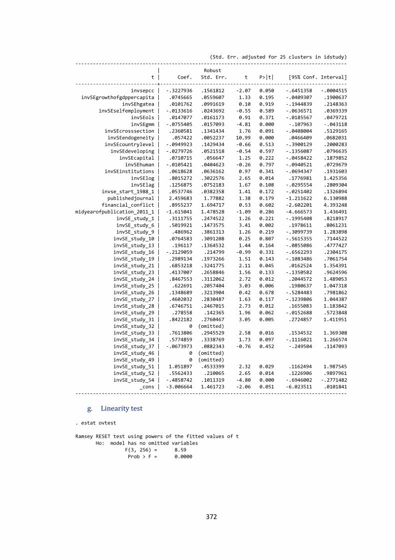
372
(Std. Err. adjusted for 25 clusters in idstudy)
---------------------------------------------------------------------------------------------
| Robust
t | Coef. Std. Err. t P>|t| [95% Conf. Interval]
----------------------------+----------------------------------------------------------------
invsepcc | -.3227936 .1561812 -2.07 0.050 -.6451358 -.0004515
invSEgrowthofgdppercapita | .0745665 .0559607 1.33 0.195 -.0409307 .1900637
invSEhgatea | .0101762 .0991619 0.10 0.919 -.1944839 .2148363
invSEselfemployment | -.0133616 .0243692 -0.55 0.589 -.0636571 .0369339
invSEols | .0147077 .0161173 0.91 0.371 -.0185567 .0479721
invSEgmm | -.0755405 .0157093 -4.81 0.000 -.107963 -.043118
invSEcrosssection | .2360581 .1341434 1.76 0.091 -.0408004 .5129165
invSEendogeneity | .057422 .0052237 10.99 0.000 .0466409 .0682031
invSEcountrylevel | -.0949923 .1429434 -0.66 0.513 -.3900129 .2000283
invSEdeveloping | -.0279726 .0521518 -0.54 0.597 -.1356087 .0796635
invSEcapital | .0710715 .056647 1.25 0.222 -.0458422 .1879852
invSEhuman | -.0105421 .0404623 -0.26 0.797 -.0940521 .0729679
invSEinstitutions | .0618628 .0636162 0.97 0.341 -.0694347 .1931603
invSElog | .8015272 .3022576 2.65 0.014 .1776981 1.425356
invSElag | .1256875 .0752183 1.67 0.108 -.0295554 .2809304
invse_start_1988_1 | .0537746 .0382358 1.41 0.172 -.0251402 .1326894
publishedjournal | 2.459683 1.77882 1.38 0.179 -1.211622 6.130988
financial_conflict | .8955237 1.694717 0.53 0.602 -2.602201 4.393248
midyearofpublication_2011_1 | -1.615041 1.478528 -1.09 0.286 -4.666573 1.436491
invSE_study_1 | .3111755 .2474522 1.26 0.221 -.1995408 .8218917
invSE_study_6 | .5019921 .1473575 3.41 0.002 .1978611 .8061231
invSE_study_9 | .486962 .3861313 1.26 0.219 -.3099739 1.283898
invSE_study_10 | .0764583 .3091208 0.25 0.807 -.5615355 .7144522
invSE_study_13 | .196117 .1364532 1.44 0.164 -.0855086 .4777427
invSE_study_16 | -.2129059 .214799 -0.99 0.331 -.6562293 .2304175
invSE_study_19 | .2989134 .1973266 1.51 0.143 -.1083486 .7061754
invSE_study_21 | .6853218 .3241775 2.11 0.045 .0162524 1.354391
invSE_study_23 | .4137007 .2658846 1.56 0.133 -.1350582 .9624596
invSE_study_24 | .8467553 .3112062 2.72 0.012 .2044572 1.489053
invSE_study_25 | .622691 .2057404 3.03 0.006 .1980637 1.047318
invSE_study_26 | .1348689 .3213904 0.42 0.678 -.5284483 .7981862
invSE_study_27 | .4602032 .2830487 1.63 0.117 -.1239806 1.044387
invSE_study_28 | .6746751 .2467015 2.73 0.012 .1655083 1.183842
invSE_study_29 | .278558 .142365 1.96 0.062 -.0152688 .5723848
invSE_study_31 | .8422182 .2760467 3.05 0.005 .2724857 1.411951
invSE_study_32 | 0 (omitted)
invSE_study_33 | .7613806 .2945529 2.58 0.016 .1534532 1.369308
invSE_study_34 | .5774859 .3338769 1.73 0.097 -.1116021 1.266574
invSE_study_37 | -.0673973 .0882343 -0.76 0.452 -.249504 .1147093
invSE_study_46 | 0 (omitted)
invSE_study_49 | 0 (omitted)
invSE_study_51 | 1.051897 .4533399 2.32 0.029 .1162494 1.987545
invSE_study_52 | .5562433 .210065 2.65 0.014 .1226906 .9897961
invSE_study_54 | -.4858742 .1011319 -4.80 0.000 -.6946002 -.2771482
_cons | -3.006664 1.461723 -2.06 0.051 -6.023511 .0101841
---------------------------------------------------------------------------------------------
g. Linearity test
. estat ovtest
Ramsey RESET test using powers of the fitted values of t
Ho: model has no omitted variables
F(3, 256) = 8.59
Prob > F = 0.0000
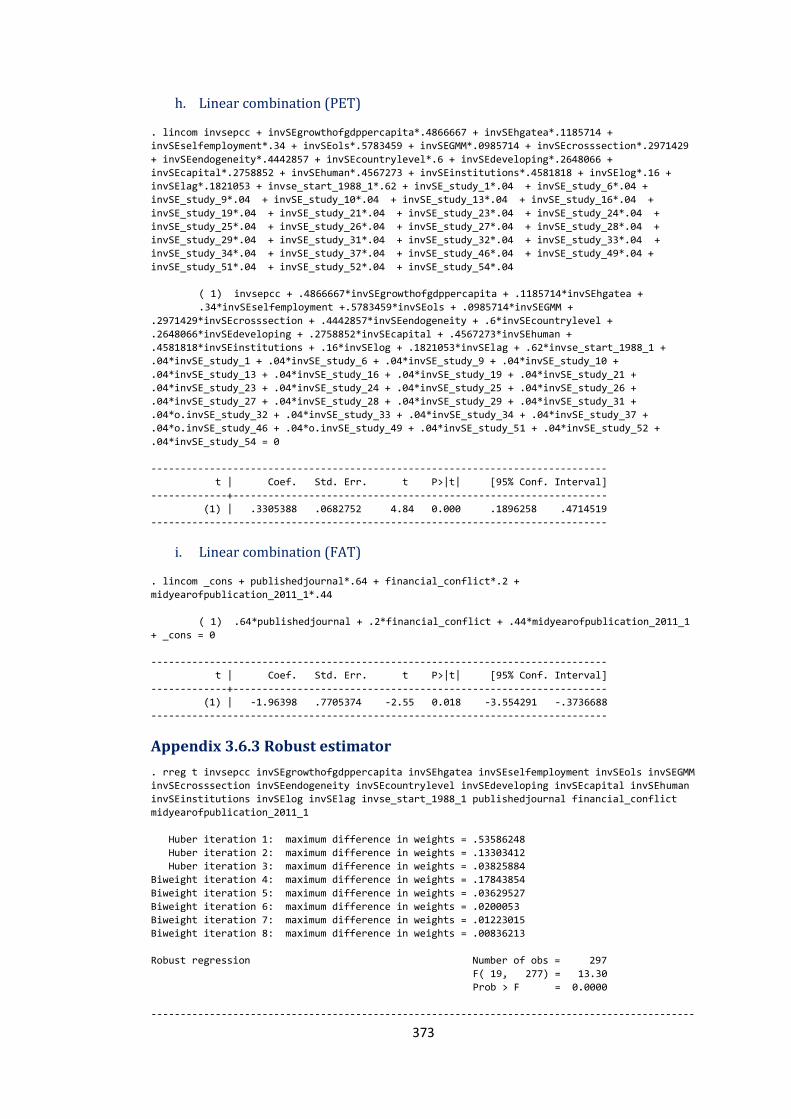
373
h. Linear combination (PET)
. lincom invsepcc + invSEgrowthofgdppercapita*.4866667 + invSEhgatea*.1185714 +
invSEselfemployment*.34 + invSEols*.5783459 + invSEGMM*.0985714 + invSEcrosssection*.2971429
+ invSEendogeneity*.4442857 + invSEcountrylevel*.6 + invSEdeveloping*.2648066 +
invSEcapital*.2758852 + invSEhuman*.4567273 + invSEinstitutions*.4581818 + invSElog*.16 +
invSElag*.1821053 + invse_start_1988_1*.62 + invSE_study_1*.04 + invSE_study_6*.04 +
invSE_study_9*.04 + invSE_study_10*.04 + invSE_study_13*.04 + invSE_study_16*.04 +
invSE_study_19*.04 + invSE_study_21*.04 + invSE_study_23*.04 + invSE_study_24*.04 +
invSE_study_25*.04 + invSE_study_26*.04 + invSE_study_27*.04 + invSE_study_28*.04 +
invSE_study_29*.04 + invSE_study_31*.04 + invSE_study_32*.04 + invSE_study_33*.04 +
invSE_study_34*.04 + invSE_study_37*.04 + invSE_study_46*.04 + invSE_study_49*.04 +
invSE_study_51*.04 + invSE_study_52*.04 + invSE_study_54*.04
( 1) invsepcc + .4866667*invSEgrowthofgdppercapita + .1185714*invSEhgatea +
.34*invSEselfemployment +.5783459*invSEols + .0985714*invSEGMM +
.2971429*invSEcrosssection + .4442857*invSEendogeneity + .6*invSEcountrylevel +
.2648066*invSEdeveloping + .2758852*invSEcapital + .4567273*invSEhuman +
.4581818*invSEinstitutions + .16*invSElog + .1821053*invSElag + .62*invse_start_1988_1 +
.04*invSE_study_1 + .04*invSE_study_6 + .04*invSE_study_9 + .04*invSE_study_10 +
.04*invSE_study_13 + .04*invSE_study_16 + .04*invSE_study_19 + .04*invSE_study_21 +
.04*invSE_study_23 + .04*invSE_study_24 + .04*invSE_study_25 + .04*invSE_study_26 +
.04*invSE_study_27 + .04*invSE_study_28 + .04*invSE_study_29 + .04*invSE_study_31 +
.04*o.invSE_study_32 + .04*invSE_study_33 + .04*invSE_study_34 + .04*invSE_study_37 +
.04*o.invSE_study_46 + .04*o.invSE_study_49 + .04*invSE_study_51 + .04*invSE_study_52 +
.04*invSE_study_54 = 0
------------------------------------------------------------------------------
t | Coef. Std. Err. t P>|t| [95% Conf. Interval]
-------------+----------------------------------------------------------------
(1) | .3305388 .0682752 4.84 0.000 .1896258 .4714519
------------------------------------------------------------------------------
i. Linear combination (FAT)
. lincom _cons + publishedjournal*.64 + financial_conflict*.2 +
midyearofpublication_2011_1*.44
( 1) .64*publishedjournal + .2*financial_conflict + .44*midyearofpublication_2011_1
+ _cons = 0
------------------------------------------------------------------------------
t | Coef. Std. Err. t P>|t| [95% Conf. Interval]
-------------+----------------------------------------------------------------
(1) | -1.96398 .7705374 -2.55 0.018 -3.554291 -.3736688
------------------------------------------------------------------------------
Appendix 3.6.3 Robust estimator
. rreg t invsepcc invSEgrowthofgdppercapita invSEhgatea invSEselfemployment invSEols invSEGMM
invSEcrosssection invSEendogeneity invSEcountrylevel invSEdeveloping invSEcapital invSEhuman
invSEinstitutions invSElog invSElag invse_start_1988_1 publishedjournal financial_conflict
midyearofpublication_2011_1
Huber iteration 1: maximum difference in weights = .53586248
Huber iteration 2: maximum difference in weights = .13303412
Huber iteration 3: maximum difference in weights = .03825884
Biweight iteration 4: maximum difference in weights = .17843854
Biweight iteration 5: maximum difference in weights = .03629527
Biweight iteration 6: maximum difference in weights = .0200053
Biweight iteration 7: maximum difference in weights = .01223015
Biweight iteration 8: maximum difference in weights = .00836213
Robust regression Number of obs = 297
F( 19, 277) = 13.30
Prob > F = 0.0000
---------------------------------------------------------------------------------------------
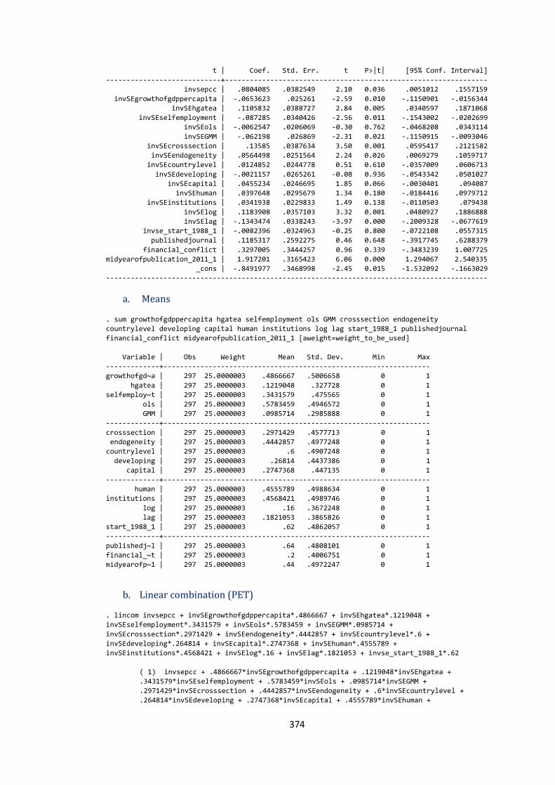
374
t | Coef. Std. Err. t P>|t| [95% Conf. Interval]
----------------------------+----------------------------------------------------------------
invsepcc | .0804085 .0382549 2.10 0.036 .0051012 .1557159
invSEgrowthofgdppercapita | -.0653623 .025261 -2.59 0.010 -.1150901 -.0156344
invSEhgatea | .1105832 .0388727 2.84 0.005 .0340597 .1871068
invSEselfemployment | -.087285 .0340426 -2.56 0.011 -.1543002 -.0202699
invSEols | -.0062547 .0206069 -0.30 0.762 -.0468208 .0343114
invSEGMM | -.062198 .026869 -2.31 0.021 -.1150915 -.0093046
invSEcrosssection | .13585 .0387634 3.50 0.001 .0595417 .2121582
invSEendogeneity | .0564498 .0251564 2.24 0.026 .0069279 .1059717
invSEcountrylevel | .0124852 .0244778 0.51 0.610 -.0357009 .0606713
invSEdeveloping | -.0021157 .0265261 -0.08 0.936 -.0543342 .0501027
invSEcapital | .0455234 .0246695 1.85 0.066 -.0030401 .094087
invSEhuman | .0397648 .0295679 1.34 0.180 -.0184416 .0979712
invSEinstitutions | .0341938 .0229833 1.49 0.138 -.0110503 .079438
invSElog | .1183908 .0357103 3.32 0.001 .0480927 .1886888
invSElag | -.1343474 .0338243 -3.97 0.000 -.2009328 -.0677619
invse_start_1988_1 | -.0082396 .0324963 -0.25 0.800 -.0722108 .0557315
publishedjournal | .1185317 .2592275 0.46 0.648 -.3917745 .6288379
financial_conflict | .3297005 .3444257 0.96 0.339 -.3483239 1.007725
midyearofpublication_2011_1 | 1.917201 .3165423 6.06 0.000 1.294067 2.540335
_cons | -.8491977 .3468998 -2.45 0.015 -1.532092 -.1663029
---------------------------------------------------------------------------------------------
a. Means
. sum growthofgdppercapita hgatea selfemployment ols GMM crosssection endogeneity
countrylevel developing capital human institutions log lag start_1988_1 publishedjournal
financial_conflict midyearofpublication_2011_1 [aweight=weight_to_be_used]
Variable | Obs Weight Mean Std. Dev. Min Max
-------------+-----------------------------------------------------------------
growthofgd~a | 297 25.0000003 .4866667 .5006658 0 1
hgatea | 297 25.0000003 .1219048 .327728 0 1
selfemploy~t | 297 25.0000003 .3431579 .475565 0 1
ols | 297 25.0000003 .5783459 .4946572 0 1
GMM | 297 25.0000003 .0985714 .2985888 0 1
-------------+-----------------------------------------------------------------
crosssection | 297 25.0000003 .2971429 .4577713 0 1
endogeneity | 297 25.0000003 .4442857 .4977248 0 1
countrylevel | 297 25.0000003 .6 .4907248 0 1
developing | 297 25.0000003 .26814 .4437386 0 1
capital | 297 25.0000003 .2747368 .447135 0 1
-------------+-----------------------------------------------------------------
human | 297 25.0000003 .4555789 .4988634 0 1
institutions | 297 25.0000003 .4568421 .4989746 0 1
log | 297 25.0000003 .16 .3672248 0 1
lag | 297 25.0000003 .1821053 .3865826 0 1
start_1988_1 | 297 25.0000003 .62 .4862057 0 1
-------------+-----------------------------------------------------------------
publishedj~l | 297 25.0000003 .64 .4808101 0 1
financial_~t | 297 25.0000003 .2 .4006751 0 1
midyearofp~1 | 297 25.0000003 .44 .4972247 0 1
b. Linear combination (PET)
. lincom invsepcc + invSEgrowthofgdppercapita*.4866667 + invSEhgatea*.1219048 +
invSEselfemployment*.3431579 + invSEols*.5783459 + invSEGMM*.0985714 +
invSEcrosssection*.2971429 + invSEendogeneity*.4442857 + invSEcountrylevel*.6 +
invSEdeveloping*.264814 + invSEcapital*.2747368 + invSEhuman*.4555789 +
invSEinstitutions*.4568421 + invSElog*.16 + invSElag*.1821053 + invse_start_1988_1*.62
( 1) invsepcc + .4866667*invSEgrowthofgdppercapita + .1219048*invSEhgatea +
.3431579*invSEselfemployment + .5783459*invSEols + .0985714*invSEGMM +
.2971429*invSEcrosssection + .4442857*invSEendogeneity + .6*invSEcountrylevel +
.264814*invSEdeveloping + .2747368*invSEcapital + .4555789*invSEhuman +
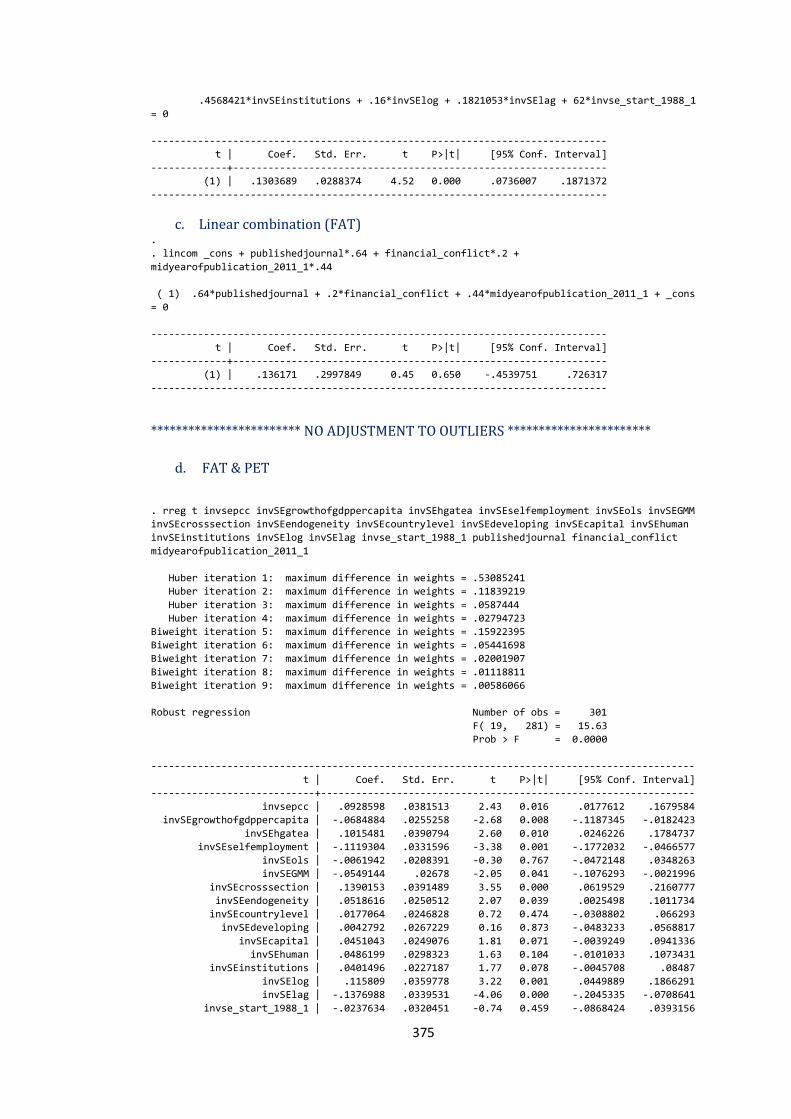
375
.4568421*invSEinstitutions + .16*invSElog + .1821053*invSElag + 62*invse_start_1988_1
= 0
------------------------------------------------------------------------------
t | Coef. Std. Err. t P>|t| [95% Conf. Interval]
-------------+----------------------------------------------------------------
(1) | .1303689 .0288374 4.52 0.000 .0736007 .1871372
------------------------------------------------------------------------------
c. Linear combination (FAT) .
. lincom _cons + publishedjournal*.64 + financial_conflict*.2 +
midyearofpublication_2011_1*.44
( 1) .64*publishedjournal + .2*financial_conflict + .44*midyearofpublication_2011_1 + _cons
= 0
------------------------------------------------------------------------------
t | Coef. Std. Err. t P>|t| [95% Conf. Interval]
-------------+----------------------------------------------------------------
(1) | .136171 .2997849 0.45 0.650 -.4539751 .726317
------------------------------------------------------------------------------
************************ NO ADJUSTMENT TO OUTLIERS ***********************
d. FAT & PET
. rreg t invsepcc invSEgrowthofgdppercapita invSEhgatea invSEselfemployment invSEols invSEGMM
invSEcrosssection invSEendogeneity invSEcountrylevel invSEdeveloping invSEcapital invSEhuman
invSEinstitutions invSElog invSElag invse_start_1988_1 publishedjournal financial_conflict
midyearofpublication_2011_1
Huber iteration 1: maximum difference in weights = .53085241
Huber iteration 2: maximum difference in weights = .11839219
Huber iteration 3: maximum difference in weights = .0587444
Huber iteration 4: maximum difference in weights = .02794723
Biweight iteration 5: maximum difference in weights = .15922395
Biweight iteration 6: maximum difference in weights = .05441698
Biweight iteration 7: maximum difference in weights = .02001907
Biweight iteration 8: maximum difference in weights = .01118811
Biweight iteration 9: maximum difference in weights = .00586066
Robust regression Number of obs = 301
F( 19, 281) = 15.63
Prob > F = 0.0000
---------------------------------------------------------------------------------------------
t | Coef. Std. Err. t P>|t| [95% Conf. Interval]
----------------------------+----------------------------------------------------------------
invsepcc | .0928598 .0381513 2.43 0.016 .0177612 .1679584
invSEgrowthofgdppercapita | -.0684884 .0255258 -2.68 0.008 -.1187345 -.0182423
invSEhgatea | .1015481 .0390794 2.60 0.010 .0246226 .1784737
invSEselfemployment | -.1119304 .0331596 -3.38 0.001 -.1772032 -.0466577
invSEols | -.0061942 .0208391 -0.30 0.767 -.0472148 .0348263
invSEGMM | -.0549144 .02678 -2.05 0.041 -.1076293 -.0021996
invSEcrosssection | .1390153 .0391489 3.55 0.000 .0619529 .2160777
invSEendogeneity | .0518616 .0250512 2.07 0.039 .0025498 .1011734
invSEcountrylevel | .0177064 .0246828 0.72 0.474 -.0308802 .066293
invSEdeveloping | .0042792 .0267229 0.16 0.873 -.0483233 .0568817
invSEcapital | .0451043 .0249076 1.81 0.071 -.0039249 .0941336
invSEhuman | .0486199 .0298323 1.63 0.104 -.0101033 .1073431
invSEinstitutions | .0401496 .0227187 1.77 0.078 -.0045708 .08487
invSElog | .115809 .0359778 3.22 0.001 .0449889 .1866291
invSElag | -.1376988 .0339531 -4.06 0.000 -.2045335 -.0708641
invse_start_1988_1 | -.0237634 .0320451 -0.74 0.459 -.0868424 .0393156
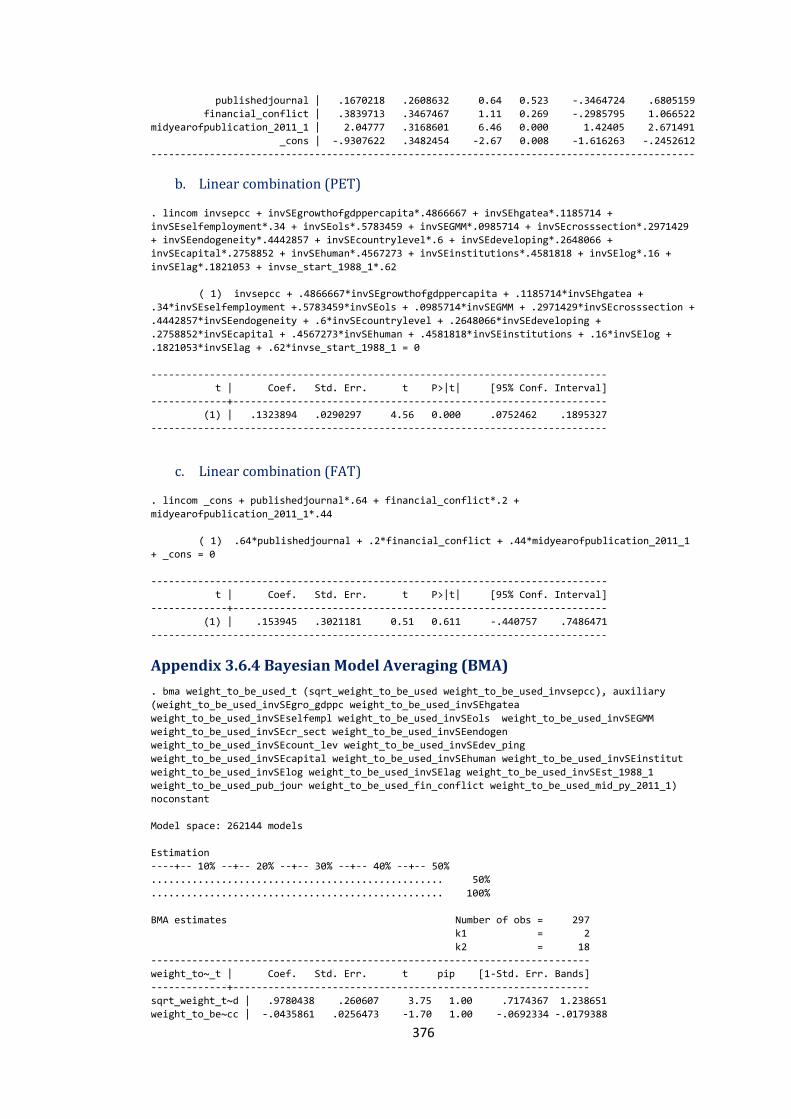
376
publishedjournal | .1670218 .2608632 0.64 0.523 -.3464724 .6805159
financial_conflict | .3839713 .3467467 1.11 0.269 -.2985795 1.066522
midyearofpublication_2011_1 | 2.04777 .3168601 6.46 0.000 1.42405 2.671491
_cons | -.9307622 .3482454 -2.67 0.008 -1.616263 -.2452612
---------------------------------------------------------------------------------------------
b. Linear combination (PET)
. lincom invsepcc + invSEgrowthofgdppercapita*.4866667 + invSEhgatea*.1185714 +
invSEselfemployment*.34 + invSEols*.5783459 + invSEGMM*.0985714 + invSEcrosssection*.2971429
+ invSEendogeneity*.4442857 + invSEcountrylevel*.6 + invSEdeveloping*.2648066 +
invSEcapital*.2758852 + invSEhuman*.4567273 + invSEinstitutions*.4581818 + invSElog*.16 +
invSElag*.1821053 + invse_start_1988_1*.62
( 1) invsepcc + .4866667*invSEgrowthofgdppercapita + .1185714*invSEhgatea +
.34*invSEselfemployment +.5783459*invSEols + .0985714*invSEGMM + .2971429*invSEcrosssection +
.4442857*invSEendogeneity + .6*invSEcountrylevel + .2648066*invSEdeveloping +
.2758852*invSEcapital + .4567273*invSEhuman + .4581818*invSEinstitutions + .16*invSElog +
.1821053*invSElag + .62*invse_start_1988_1 = 0
------------------------------------------------------------------------------
t | Coef. Std. Err. t P>|t| [95% Conf. Interval]
-------------+----------------------------------------------------------------
(1) | .1323894 .0290297 4.56 0.000 .0752462 .1895327
------------------------------------------------------------------------------
c. Linear combination (FAT)
. lincom _cons + publishedjournal*.64 + financial_conflict*.2 +
midyearofpublication_2011_1*.44
( 1) .64*publishedjournal + .2*financial_conflict + .44*midyearofpublication_2011_1
+ _cons = 0
------------------------------------------------------------------------------
t | Coef. Std. Err. t P>|t| [95% Conf. Interval]
-------------+----------------------------------------------------------------
(1) | .153945 .3021181 0.51 0.611 -.440757 .7486471
------------------------------------------------------------------------------
Appendix 3.6.4 Bayesian Model Averaging (BMA)
. bma weight_to_be_used_t (sqrt_weight_to_be_used weight_to_be_used_invsepcc), auxiliary
(weight_to_be_used_invSEgro_gdppc weight_to_be_used_invSEhgatea
weight_to_be_used_invSEselfempl weight_to_be_used_invSEols weight_to_be_used_invSEGMM
weight_to_be_used_invSEcr_sect weight_to_be_used_invSEendogen
weight_to_be_used_invSEcount_lev weight_to_be_used_invSEdev_ping
weight_to_be_used_invSEcapital weight_to_be_used_invSEhuman weight_to_be_used_invSEinstitut
weight_to_be_used_invSElog weight_to_be_used_invSElag weight_to_be_used_invSEst_1988_1
weight_to_be_used_pub_jour weight_to_be_used_fin_conflict weight_to_be_used_mid_py_2011_1)
noconstant
Model space: 262144 models
Estimation
----+-- 10% --+-- 20% --+-- 30% --+-- 40% --+-- 50%
.................................................. 50%
.................................................. 100%
BMA estimates Number of obs = 297
k1 = 2
k2 = 18
---------------------------------------------------------------------------
weight_to~_t | Coef. Std. Err. t pip [1-Std. Err. Bands]
-------------+-------------------------------------------------------------
sqrt_weight_t~d | .9780438 .260607 3.75 1.00 .7174367 1.238651
weight_to_be~cc | -.0435861 .0256473 -1.70 1.00 -.0692334 -.0179388
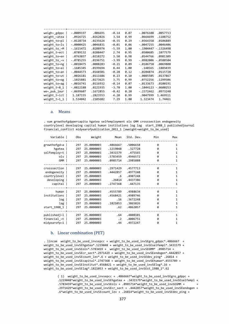
377
-------------+-------------------------------------------------------------
weigh~_gdppc | -.0009197 .006691 -0.14 0.07 -.0076108 .0057713
weight_~atea | .0926725 .0262026 3.54 0.99 .0664699 .1188752
weight_to~pl | -.0128734 .0235624 -0.55 0.29 -.0364358 .0106889
weight_to~ls | -.0000425 .0046831 -0.01 0.06 -.0047255 .0046406
weight_to_~M | -.1615472 .0288974 -5.59 1.00 -.1904447 -.1326498
weight_t~ect | .0789132 .0288447 2.74 0.95 .0500685 .1077579
weight_to~en | .0763037 .0218272 3.50 0.98 .0544766 .0981309
weight_to_~v | -.0785255 .0196751 -3.99 0.99 -.0982006 -.0588504
weight_to~ng | -.0018475 .0088283 -0.21 0.09 -.0106758 .0069808
weight_to~al | .1685345 .0199694 8.44 1.00 .148565 .1885039
weight_to~an | -.0044573 .0160301 -0.28 0.12 -.0204874 .0115728
weight_to~ut | .0026181 .0111686 0.23 0.10 -.0085505 .0137867
weight_to~og | .1025881 .0273625 3.75 0.99 .0752256 .1299506
weight_to~ag | -.0016741 .0116932 -0.14 0.07 -.0133673 .0100191
weight_t~8_1 | -.0822188 .0221935 -3.70 1.00 -.1044123 -.0600253
we~_pub_jour | -.0699607 .1672855 -0.42 0.20 -.2372462 .0973248
weight_t~ict | 1.187155 .2823553 4.20 0.99 .9047999 1.469511
weight_t~1_1 | 1.534042 .2105682 7.29 1.00 1.323474 1.74461
---------------------------------------------------------------------------
a. Means . sum growthofgdppercapita hgatea selfemployment ols GMM crosssection endogeneity
countrylevel developing capital human institutions log lag start_1988_1 publishedjournal
financial_conflict midyearofpublication_2011_1 [aweight=weight_to_be_used]
Variable | Obs Weight Mean Std. Dev. Min Max
-------------+-----------------------------------------------------------------
growthofgd~a | 297 25.0000003 .4866667 .5006658 0 1
hgatea | 297 25.0000003 .1219048 .327728 0 1
selfemploy~t | 297 25.0000003 .3431579 .475565 0 1
ols | 297 25.0000003 .5783459 .4946572 0 1
GMM | 297 25.0000003 .0985714 .2985888 0 1
-------------+-----------------------------------------------------------------
crosssection | 297 25.0000003 .2971429 .4577713 0 1
endogeneity | 297 25.0000003 .4442857 .4977248 0 1
countrylevel | 297 25.0000003 .6 .4907248 0 1
developing | 297 25.0000003 .26814 .4437386 0 1
capital | 297 25.0000003 .2747368 .447135 0 1
-------------+-----------------------------------------------------------------
human | 297 25.0000003 .4555789 .4988634 0 1
institutions | 297 25.0000003 .4568421 .4989746 0 1
log | 297 25.0000003 .16 .3672248 0 1
lag | 297 25.0000003 .1821053 .3865826 0 1
start_1988_1 | 297 25.0000003 .62 .4862057 0 1
-------------+-----------------------------------------------------------------
publishedj~l | 297 25.0000003 .64 .4808101 0 1
financial_~t | 297 25.0000003 .2 .4006751 0 1
midyearofp~1 | 297 25.0000003 .44 .4972247 0 1
b. Linear combination (PET)
. lincom weight_to_be_used_invsepcc + weight_to_be_used_invSEgro_gdppc*.4866667 +
weight_to_be_used_invSEhgatea*.1219048 + weight_to_be_used_invSEselfempl*.3431579 +
weight_to_be_used_invSEols*.5783459 + weight_to_be_used_invSEGMM* .0985714 +
weight_to_be_used_invSEcr_sect*.2971429 + weight_to_be_used_invSEendogen*.4442857 +
weight_to_be_used_invSEcount_lev*.6 + weight_to_be_used_invSEdev_ping* .26814 +
weight_to_be_used_invSEcapital*.2747368 + weight_to_be_used_invSEhuman*.4555789 +
weight_to_be_used_invSEinstitut*.4568421 + weight_to_be_used_invSElog*.16 +
weight_to_be_used_invSElag*.1821053 + weight_to_be_used_invSEst_1988_1*.62
( 1) weight_to_be_used_invsepcc + .4866667*weight_to_be_used_invSEgro_gdppc +
.1219048*weight_to_be_used_invSEhgatea + .3431579*weight_to_be_used_invSEselfempl +
.5783459*weight_to_be_used_invSEols + .0985714*weight_to_be_used_invSEGMM + +
.2971429*weight_to_be_used_invSEcr_sect + .4442857*weight_to_be_used_invSEendogen +
.6*weight_to_be_used_invSEcount_lev + .26814*weight_to_be_used_invSEdev_ping +
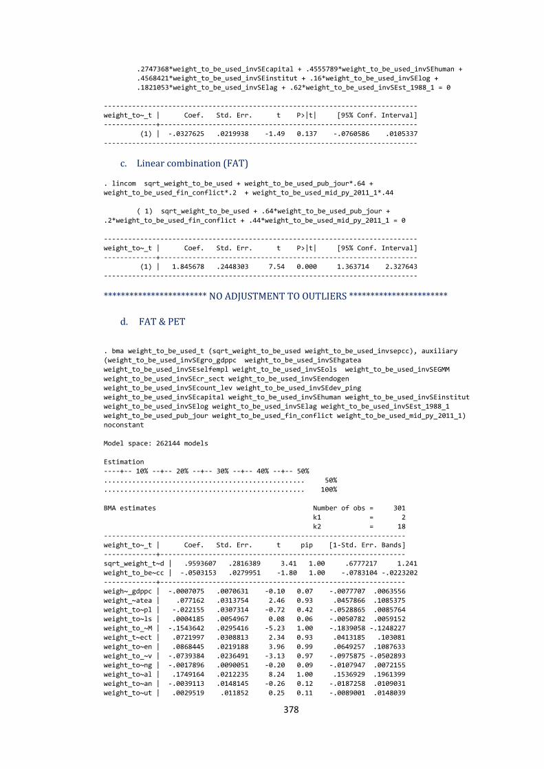
378
.2747368*weight_to_be_used_invSEcapital + .4555789*weight_to_be_used_invSEhuman +
.4568421*weight_to_be_used_invSEinstitut + .16*weight_to_be_used_invSElog +
.1821053*weight_to_be_used_invSElag + .62*weight_to_be_used_invSEst_1988_1 = 0
------------------------------------------------------------------------------
weight_to~_t | Coef. Std. Err. t P>|t| [95% Conf. Interval]
-------------+----------------------------------------------------------------
(1) | -.0327625 .0219938 -1.49 0.137 -.0760586 .0105337
------------------------------------------------------------------------------
c. Linear combination (FAT)
. lincom sqrt_weight_to_be_used + weight_to_be_used_pub_jour*.64 +
weight_to_be_used_fin_conflict*.2 + weight_to_be_used_mid_py_2011_1*.44
( 1) sqrt_weight_to_be_used + .64*weight_to_be_used_pub_jour +
.2*weight_to_be_used_fin_conflict + .44*weight_to_be_used_mid_py_2011_1 = 0
------------------------------------------------------------------------------
weight_to~_t | Coef. Std. Err. t P>|t| [95% Conf. Interval]
-------------+----------------------------------------------------------------
(1) | 1.845678 .2448303 7.54 0.000 1.363714 2.327643
------------------------------------------------------------------------------
************************ NO ADJUSTMENT TO OUTLIERS ***********************
d. FAT & PET
. bma weight_to_be_used_t (sqrt_weight_to_be_used weight_to_be_used_invsepcc), auxiliary
(weight_to_be_used_invSEgro_gdppc weight_to_be_used_invSEhgatea
weight_to_be_used_invSEselfempl weight_to_be_used_invSEols weight_to_be_used_invSEGMM
weight_to_be_used_invSEcr_sect weight_to_be_used_invSEendogen
weight_to_be_used_invSEcount_lev weight_to_be_used_invSEdev_ping
weight_to_be_used_invSEcapital weight_to_be_used_invSEhuman weight_to_be_used_invSEinstitut
weight_to_be_used_invSElog weight_to_be_used_invSElag weight_to_be_used_invSEst_1988_1
weight_to_be_used_pub_jour weight_to_be_used_fin_conflict weight_to_be_used_mid_py_2011_1)
noconstant
Model space: 262144 models
Estimation
----+-- 10% --+-- 20% --+-- 30% --+-- 40% --+-- 50%
.................................................. 50%
.................................................. 100%
BMA estimates Number of obs = 301
k1 = 2
k2 = 18
---------------------------------------------------------------------------
weight_to~_t | Coef. Std. Err. t pip [1-Std. Err. Bands]
-------------+-------------------------------------------------------------
sqrt_weight_t~d | .9593607 .2816389 3.41 1.00 .6777217 1.241
weight_to_be~cc | -.0503153 .0279951 -1.80 1.00 -.0783104 -.0223202
-------------+-------------------------------------------------------------
weigh~_gdppc | -.0007075 .0070631 -0.10 0.07 -.0077707 .0063556
weight_~atea | .077162 .0313754 2.46 0.93 .0457866 .1085375
weight_to~pl | -.022155 .0307314 -0.72 0.42 -.0528865 .0085764
weight_to~ls | .0004185 .0054967 0.08 0.06 -.0050782 .0059152
weight_to_~M | -.1543642 .0295416 -5.23 1.00 -.1839058 -.1248227
weight_t~ect | .0721997 .0308813 2.34 0.93 .0413185 .103081
weight_to~en | .0868445 .0219188 3.96 0.99 .0649257 .1087633
weight_to_~v | -.0739384 .0236491 -3.13 0.97 -.0975875 -.0502893
weight_to~ng | -.0017896 .0090051 -0.20 0.09 -.0107947 .0072155
weight_to~al | .1749164 .0212235 8.24 1.00 .1536929 .1961399
weight_to~an | -.0039113 .0148145 -0.26 0.12 -.0187258 .0109031
weight_to~ut | .0029519 .011852 0.25 0.11 -.0089001 .0148039
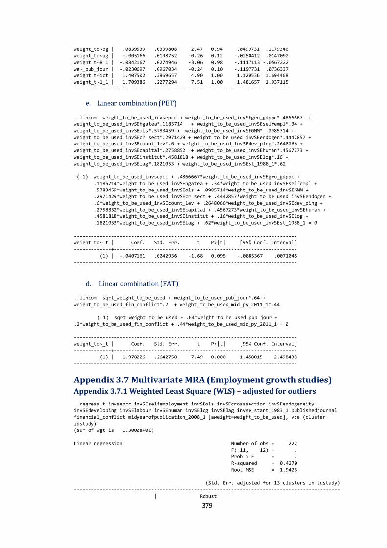
379
weight_to~og | .0839539 .0339808 2.47 0.94 .0499731 .1179346
weight_to~ag | -.005166 .0198752 -0.26 0.12 -.0250412 .0147092
weight_t~8_1 | -.0842167 .0274946 -3.06 0.98 -.1117113 -.0567222
we~_pub_jour | -.0230697 .0967034 -0.24 0.10 -.1197731 .0736337
weight_t~ict | 1.407502 .2869657 4.90 1.00 1.120536 1.694468
weight_t~1_1 | 1.709386 .2277294 7.51 1.00 1.481657 1.937115
---------------------------------------------------------------------------
e. Linear combination (PET)
. lincom weight_to_be_used_invsepcc + weight_to_be_used_invSEgro_gdppc*.4866667 +
weight_to_be_used_invSEhgatea*.1185714 + weight_to_be_used_invSEselfempl*.34 +
weight_to_be_used_invSEols*.5783459 + weight_to_be_used_invSEGMM* .0985714 +
weight_to_be_used_invSEcr_sect*.2971429 + weight_to_be_used_invSEendogen*.4442857 +
weight_to_be_used_invSEcount_lev*.6 + weight_to_be_used_invSEdev_ping*.2648066 +
weight_to_be_used_invSEcapital*.2758852 + weight_to_be_used_invSEhuman*.4567273 +
weight_to_be_used_invSEinstitut*.4581818 + weight_to_be_used_invSElog*.16 +
weight_to_be_used_invSElag*.1821053 + weight_to_be_used_invSEst_1988_1*.62
( 1) weight_to_be_used_invsepcc + .4866667*weight_to_be_used_invSEgro_gdppc +
.1185714*weight_to_be_used_invSEhgatea + .34*weight_to_be_used_invSEselfempl +
.5783459*weight_to_be_used_invSEols + .0985714*weight_to_be_used_invSEGMM +
.2971429*weight_to_be_used_invSEcr_sect + .4442857*weight_to_be_used_invSEendogen +
.6*weight_to_be_used_invSEcount_lev + .2648066*weight_to_be_used_invSEdev_ping +
.2758852*weight_to_be_used_invSEcapital + .4567273*weight_to_be_used_invSEhuman +
.4581818*weight_to_be_used_invSEinstitut + .16*weight_to_be_used_invSElog +
.1821053*weight_to_be_used_invSElag + .62*weight_to_be_used_invSEst_1988_1 = 0
------------------------------------------------------------------------------
weight_to~_t | Coef. Std. Err. t P>|t| [95% Conf. Interval]
-------------+----------------------------------------------------------------
(1) | -.0407161 .0242936 -1.68 0.095 -.0885367 .0071045
------------------------------------------------------------------------------
d. Linear combination (FAT)
. lincom sqrt_weight_to_be_used + weight_to_be_used_pub_jour*.64 +
weight_to_be_used_fin_conflict*.2 + weight_to_be_used_mid_py_2011_1*.44
( 1) sqrt_weight_to_be_used + .64*weight_to_be_used_pub_jour +
.2*weight_to_be_used_fin_conflict + .44*weight_to_be_used_mid_py_2011_1 = 0
------------------------------------------------------------------------------
weight_to~_t | Coef. Std. Err. t P>|t| [95% Conf. Interval]
-------------+----------------------------------------------------------------
(1) | 1.978226 .2642758 7.49 0.000 1.458015 2.498438
------------------------------------------------------------------------------
Appendix 3.7 Multivariate MRA (Employment growth studies) Appendix 3.7.1 Weighted Least Square (WLS) – adjusted for outliers
. regress t invsepcc invSEselfemployment invSEols invSEcrosssection invSEendogeneity
invSEdeveloping invSElabour invSEhuman invSElog invSElag invse_start_1983_1 publishedjournal
financial_conflict midyearofpublication_2008_1 [aweight=weight_to_be_used], vce (cluster
idstudy)
(sum of wgt is 1.3000e+01)
Linear regression Number of obs = 222
F( 11, 12) = .
Prob > F = .
R-squared = 0.4270
Root MSE = 1.9426
(Std. Err. adjusted for 13 clusters in idstudy)
---------------------------------------------------------------------------------------------
| Robust
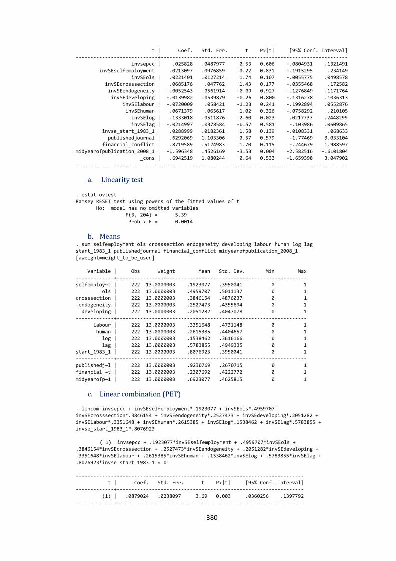
380
t | Coef. Std. Err. t P>|t| [95% Conf. Interval]
----------------------------+----------------------------------------------------------------
invsepcc | .025828 .0487977 0.53 0.606 -.0804931 .1321491
invSEselfemployment | .0213097 .0976859 0.22 0.831 -.1915295 .234149
invSEols | .0221401 .0127214 1.74 0.107 -.0055775 .0498578
invSEcrosssection | .0685176 .047762 1.43 0.177 -.0355468 .172582
invSEendogeneity | -.0052543 .0561914 -0.09 0.927 -.1276849 .1171764
invSEdeveloping | -.0139982 .0539879 -0.26 0.800 -.1316278 .1036313
invSElabour | -.0720009 .058421 -1.23 0.241 -.1992894 .0552876
invSEhuman | .0671379 .065617 1.02 0.326 -.0758292 .210105
invSElog | .1333018 .0511876 2.60 0.023 .0217737 .2448299
invSElag | -.0214997 .0378584 -0.57 0.581 -.103986 .0609865
invse_start_1983_1 | .0288999 .0182361 1.58 0.139 -.0108331 .068633
publishedjournal | .6292069 1.103306 0.57 0.579 -1.77469 3.033104
financial_conflict | .8719589 .5124983 1.70 0.115 -.244679 1.988597
midyearofpublication_2008_1 | -1.596348 .4526169 -3.53 0.004 -2.582516 -.6101804
_cons | .6942519 1.080244 0.64 0.533 -1.659398 3.047902
---------------------------------------------------------------------------------------------
a. Linearity test
. estat ovtest
Ramsey RESET test using powers of the fitted values of t
Ho: model has no omitted variables
F(3, 204) = 5.39
Prob > F = 0.0014
b. Means . sum selfemployment ols crosssection endogeneity developing labour human log lag
start_1983_1 publishedjournal financial_conflict midyearofpublication_2008_1
[aweight=weight_to_be_used]
Variable | Obs Weight Mean Std. Dev. Min Max
-------------+-----------------------------------------------------------------
selfemploy~t | 222 13.0000003 .1923077 .3950041 0 1
ols | 222 13.0000003 .4959707 .5011137 0 1
crosssection | 222 13.0000003 .3846154 .4876037 0 1
endogeneity | 222 13.0000003 .2527473 .4355694 0 1
developing | 222 13.0000003 .2051282 .4047078 0 1
-------------+-----------------------------------------------------------------
labour | 222 13.0000003 .3351648 .4731148 0 1
human | 222 13.0000003 .2615385 .4404657 0 1
log | 222 13.0000003 .1538462 .3616166 0 1
lag | 222 13.0000003 .5783855 .4949335 0 1
start_1983_1 | 222 13.0000003 .8076923 .3950041 0 1
-------------+-----------------------------------------------------------------
publishedj~l | 222 13.0000003 .9230769 .2670715 0 1
financial_~t | 222 13.0000003 .2307692 .4222772 0 1
midyearofp~1 | 222 13.0000003 .6923077 .4625815 0 1
c. Linear combination (PET)
. lincom invsepcc + invSEselfemployment*.1923077 + invSEols*.4959707 +
invSEcrosssection*.3846154 + invSEendogeneity*.2527473 + invSEdeveloping*.2051282 +
invSElabour*.3351648 + invSEhuman*.2615385 + invSElog*.1538462 + invSElag*.5783855 +
invse_start_1983_1*.8076923
( 1) invsepcc + .1923077*invSEselfemployment + .4959707*invSEols +
.3846154*invSEcrosssection + .2527473*invSEendogeneity + .2051282*invSEdeveloping +
.3351648*invSElabour + .2615385*invSEhuman + .1538462*invSElog + .5783855*invSElag +
.8076923*invse_start_1983_1 = 0
------------------------------------------------------------------------------
t | Coef. Std. Err. t P>|t| [95% Conf. Interval]
-------------+----------------------------------------------------------------
(1) | .0879024 .0238097 3.69 0.003 .0360256 .1397792
------------------------------------------------------------------------------

381
d. Linear combination (FAT)
. lincom _cons + publishedjournal*.9230769 + financial_conflict*.2307692 +
midyearofpublication_2008_1*.6923077
( 1) .9230769*publishedjournal + .2307692*financial_conflict +
.6923077*midyearofpublication_2008_1 + _cons = 0
------------------------------------------------------------------------------
t | Coef. Std. Err. t P>|t| [95% Conf. Interval]
-------------+----------------------------------------------------------------
(1) | .3711155 .5866759 0.63 0.539 -.9071415 1.649372
------------------------------------------------------------------------------
************************ NO ADJUSTMENT TO OUTLIERS ***********************
e. FAT & PET
. regress t invsepcc invSEselfemployment invSEols invSEcrosssection invSEendogeneity
invSEdeveloping invSElabour invSEhuman invSElog invSElag invse_start_1983_1 publishedjournal
financial_conflict midyearofpublication_2008_1 [aweight=weight_to_be_used], vce (cluster
idstudy)
(sum of wgt is 1.3000e+01)
Linear regression Number of obs = 249
F( 11, 12) = .
Prob > F = .
R-squared = 0.5584
Root MSE = 2.2512
(Std. Err. adjusted for 13 clusters in idstudy)
---------------------------------------------------------------------------------------------
| Robust
t | Coef. Std. Err. t P>|t| [95% Conf. Interval]
----------------------------+----------------------------------------------------------------
invsepcc | .1069293 .0500671 2.14 0.054 -.0021576 .2160162
invSEselfemployment | .0677769 .1235802 0.55 0.593 -.2014813 .3370351
invSEols | .0617299 .0169105 3.65 0.003 .0248851 .0985747
invSEcrosssection | .1107907 .0524202 2.11 0.056 -.0034231 .2250044
invSEendogeneity | -.0682454 .0694447 -0.98 0.345 -.2195523 .0830616
invSEdeveloping | -.016168 .0657624 -0.25 0.810 -.159452 .127116
invSElabour | -.113606 .077705 -1.46 0.169 -.2829106 .0556985
invSEhuman | .089696 .070641 1.27 0.228 -.0642175 .2436094
invSElog | .0892935 .0493838 1.81 0.096 -.0183046 .1968915
invSElag | -.0690974 .0235047 -2.94 0.012 -.1203096 -.0178851
invse_start_1983_1 | .042806 .0271512 1.58 0.141 -.0163513 .1019634
publishedjournal | .2661305 1.440158 0.18 0.856 -2.871705 3.403966
financial_conflict | 2.436092 .4252243 5.73 0.000 1.509608 3.362576
midyearofpublication_2008_1 | -.7685825 .3437133 -2.24 0.045 -1.517469 -.0196955
_cons | -1.350236 1.061189 -1.27 0.227 -3.662369 .9618969
---------------------------------------------------------------------------------------------
f. Linearity test
. estat ovtest
Ramsey RESET test using powers of the fitted values of t
Ho: model has no omitted variables
F(3, 231) = 7.73
Prob > F = 0.0001
g. Linear combination (PET)
. lincom invsepcc + invSEselfemployment*.1923077 + invSEols*.5179487 +
invSEcrosssection*.3846154 + invSEendogeneity*.2426035 + invSEdeveloping*.2051282 +
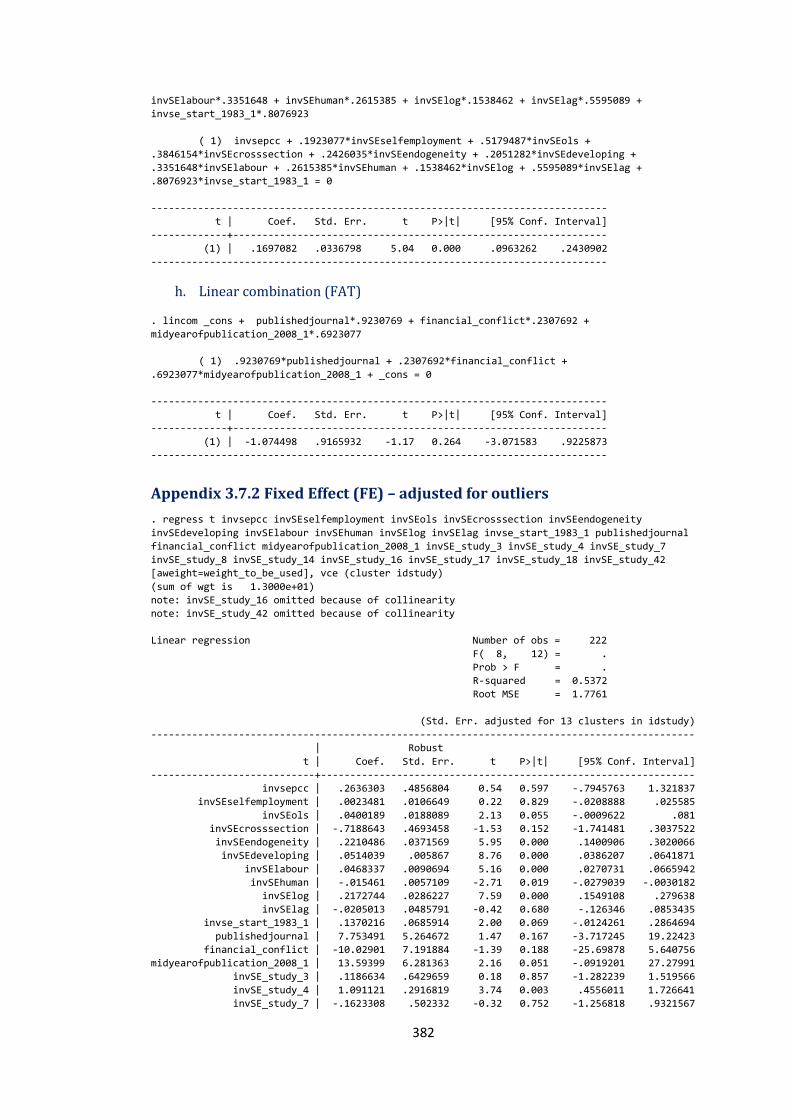
382
invSElabour*.3351648 + invSEhuman*.2615385 + invSElog*.1538462 + invSElag*.5595089 +
invse_start_1983_1*.8076923
( 1) invsepcc + .1923077*invSEselfemployment + .5179487*invSEols +
.3846154*invSEcrosssection + .2426035*invSEendogeneity + .2051282*invSEdeveloping +
.3351648*invSElabour + .2615385*invSEhuman + .1538462*invSElog + .5595089*invSElag +
.8076923*invse_start_1983_1 = 0
------------------------------------------------------------------------------
t | Coef. Std. Err. t P>|t| [95% Conf. Interval]
-------------+----------------------------------------------------------------
(1) | .1697082 .0336798 5.04 0.000 .0963262 .2430902
------------------------------------------------------------------------------
h. Linear combination (FAT)
. lincom _cons + publishedjournal*.9230769 + financial_conflict*.2307692 +
midyearofpublication_2008_1*.6923077
( 1) .9230769*publishedjournal + .2307692*financial_conflict +
.6923077*midyearofpublication_2008_1 + _cons = 0
------------------------------------------------------------------------------
t | Coef. Std. Err. t P>|t| [95% Conf. Interval]
-------------+----------------------------------------------------------------
(1) | -1.074498 .9165932 -1.17 0.264 -3.071583 .9225873
------------------------------------------------------------------------------
Appendix 3.7.2 Fixed Effect (FE) – adjusted for outliers
. regress t invsepcc invSEselfemployment invSEols invSEcrosssection invSEendogeneity
invSEdeveloping invSElabour invSEhuman invSElog invSElag invse_start_1983_1 publishedjournal
financial_conflict midyearofpublication_2008_1 invSE_study_3 invSE_study_4 invSE_study_7
invSE_study_8 invSE_study_14 invSE_study_16 invSE_study_17 invSE_study_18 invSE_study_42
[aweight=weight_to_be_used], vce (cluster idstudy)
(sum of wgt is 1.3000e+01)
note: invSE_study_16 omitted because of collinearity
note: invSE_study_42 omitted because of collinearity
Linear regression Number of obs = 222
F( 8, 12) = .
Prob > F = .
R-squared = 0.5372
Root MSE = 1.7761
(Std. Err. adjusted for 13 clusters in idstudy)
---------------------------------------------------------------------------------------------
| Robust
t | Coef. Std. Err. t P>|t| [95% Conf. Interval]
----------------------------+----------------------------------------------------------------
invsepcc | .2636303 .4856804 0.54 0.597 -.7945763 1.321837
invSEselfemployment | .0023481 .0106649 0.22 0.829 -.0208888 .025585
invSEols | .0400189 .0188089 2.13 0.055 -.0009622 .081
invSEcrosssection | -.7188643 .4693458 -1.53 0.152 -1.741481 .3037522
invSEendogeneity | .2210486 .0371569 5.95 0.000 .1400906 .3020066
invSEdeveloping | .0514039 .005867 8.76 0.000 .0386207 .0641871
invSElabour | .0468337 .0090694 5.16 0.000 .0270731 .0665942
invSEhuman | -.015461 .0057109 -2.71 0.019 -.0279039 -.0030182
invSElog | .2172744 .0286227 7.59 0.000 .1549108 .279638
invSElag | -.0205013 .0485791 -0.42 0.680 -.126346 .0853435
invse_start_1983_1 | .1370216 .0685914 2.00 0.069 -.0124261 .2864694
publishedjournal | 7.753491 5.264672 1.47 0.167 -3.717245 19.22423
financial_conflict | -10.02901 7.191884 -1.39 0.188 -25.69878 5.640756
midyearofpublication_2008_1 | 13.59399 6.281363 2.16 0.051 -.0919201 27.27991
invSE_study_3 | .1186634 .6429659 0.18 0.857 -1.282239 1.519566
invSE_study_4 | 1.091121 .2916819 3.74 0.003 .4556011 1.726641
invSE_study_7 | -.1623308 .502332 -0.32 0.752 -1.256818 .9321567
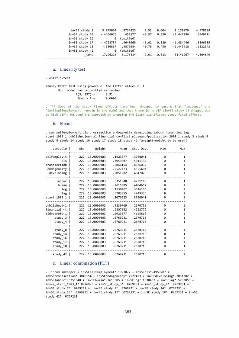
383
invSE_study_8 | 3.075034 .8734825 3.52 0.004 1.171879 4.978188
invSE_study_14 | -.4466076 .459277 -0.97 0.350 -1.447286 .5540711
invSE_study_16 | 0 (omitted)
invSE_study_17 | -.4723737 .4645065 -1.02 0.329 -1.484446 .5396989
invSE_study_18 | -.380857 .4879084 -0.78 0.450 -1.443918 .6822042
invSE_study_42 | 0 (omitted)
_cons | -17.96216 6.176534 -2.91 0.013 -31.41967 -4.504649
---------------------------------------------------------------------------------------------
a. Linearity test
. estat ovtest
Ramsey RESET test using powers of the fitted values of t
Ho: model has no omitted variables
F(3, 197) = 8.91
Prob > F = 0.0000
. *** Some of the study fixed effects have been dropped to ensure that 'invsepcc' and
'invSEselfemployment' remain in the model and that there is no VIF (invSE_study_23 dropped due
to high VIF). We used G-S approach by dropping the least significant study fixed effects.
b. Means
. sum selfemployment ols crosssection endogeneity developing labour human log lag
start_1983_1 publishedjournal financial_conflict midyearofpublication_2008_1 study_3 study_4
study_8 study_14 study_16 study_17 study_18 study_42 [aweight=weight_to_be_used]
Variable | Obs Weight Mean Std. Dev. Min Max
-------------+-----------------------------------------------------------------
selfemploy~t | 222 13.0000003 .1923077 .3950041 0 1
ols | 222 13.0000003 .4959707 .5011137 0 1
crosssection | 222 13.0000003 .3846154 .4876037 0 1
endogeneity | 222 13.0000003 .2527473 .4355694 0 1
developing | 222 13.0000003 .2051282 .4047078 0 1
-------------+-----------------------------------------------------------------
labour | 222 13.0000003 .3351648 .4731148 0 1
human | 222 13.0000003 .2615385 .4404657 0 1
log | 222 13.0000003 .1538462 .3616166 0 1
lag | 222 13.0000003 .5783855 .4949335 0 1
start_1983_1 | 222 13.0000003 .8076923 .3950041 0 1
-------------+-----------------------------------------------------------------
publishedj~l | 222 13.0000003 .9230769 .2670715 0 1
financial_~t | 222 13.0000003 .2307692 .4222772 0 1
midyearofp~1 | 222 13.0000003 .6923077 .4625815 0 1
study_3 | 222 13.0000003 .0769231 .2670715 0 1
study_4 | 222 13.0000003 .0769231 .2670715 0 1
-------------+-----------------------------------------------------------------
study_8 | 222 13.0000003 .0769231 .2670715 0 1
study_14 | 222 13.0000003 .0769231 .2670715 0 1
study_16 | 222 13.0000003 .0769231 .2670715 0 1
study_17 | 222 13.0000003 .0769231 .2670715 0 1
study_18 | 222 13.0000003 .0769231 .2670715 0 1
-------------+-----------------------------------------------------------------
study_42 | 222 13.0000003 .0769231 .2670715 0 1
c. Linear combination (PET)
. lincom invsepcc + invSEselfemployment*.1923077 + invSEols*.4959707 +
invSEcrosssection*.3846154 + invSEendogeneity*.2527473 + invSEdeveloping*.2051282 +
invSElabour*.3351648 + invSEhuman*.2615385 + invSElog*.1538462 + invSElag*.5783855 +
invse_start_1983_1*.8076923 + invSE_study_3* .0769231 + invSE_study_4* .0769231 +
invSE_study_7* .0769231 + invSE_study_8* .0769231 + invSE_study_14* .0769231 +
invSE_study_16* .0769231 + invSE_study_17* .0769231 + invSE_study_18* .0769231 + invSE_
study_42* .0769231
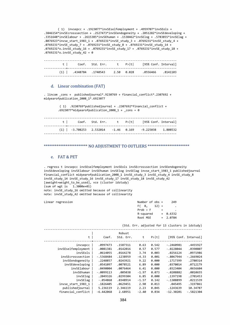
384
( 1) invsepcc + .1923077*invSEselfemployment + .4959707*invSEols +
.3846154*invSEcrosssection + .2527473*invSEendogeneity + .2051282*invSEdeveloping +
.3351648*invSElabour + .2615385*invSEhuman + .1538462*invSElog + .5783855*invSElag +
.8076923*invse_start_1983_1 + .0769231*invSE_study_3 + .0769231*invSE_study_4 +
.0769231*invSE_study_7 + .0769231*invSE_study_8 + .0769231*invSE_study_14 +
.0769231*o.invSE_study_16 + .0769231*invSE_study_17 + .0769231*invSE_study_18 +
.0769231*o.invSE_study_42 = 0
------------------------------------------------------------------------------
t | Coef. Std. Err. t P>|t| [95% Conf. Interval]
-------------+----------------------------------------------------------------
(1) | .4348784 .1740543 2.50 0.028 .0556466 .8141103
------------------------------------------------------------------------------
d. Linear combination (FAT)
. lincom _cons + publishedjournal*.9230769 + financial_conflict*.2307692 +
midyearofpublication_2008_1*.6923077
( 1) .9230769*publishedjournal + .2307692*financial_conflict +
.6923077*midyearofpublication_2008_1 + _cons = 0
------------------------------------------------------------------------------
t | Coef. Std. Err. t P>|t| [95% Conf. Interval]
-------------+----------------------------------------------------------------
(1) | -3.708253 2.532014 -1.46 0.169 -9.225038 1.808532
------------------------------------------------------------------------------
************************ NO ADJUSTMENT TO OUTLIERS ***********************
e. FAT & PET
. regress t invsepcc invSEselfemployment invSEols invSEcrosssection invSEendogeneity
invSEdeveloping invSElabour invSEhuman invSElog invSElag invse_start_1983_1 publishedjournal
financial_conflict midyearofpublication_2008_1 invSE_study_3 invSE_study_4 invSE_study_8
invSE_study_14 invSE_study_16 invSE_study_17 invSE_study_18 invSE_study_42
[aweight=weight_to_be_used], vce (cluster idstudy)
(sum of wgt is 1.3000e+01)
note: invSE_study_16 omitted because of collinearity
note: invSE_study_42 omitted because of collinearity
Linear regression Number of obs = 249
F( 8, 12) = .
Prob > F = .
R-squared = 0.6332
Root MSE = 2.0784
(Std. Err. adjusted for 13 clusters in idstudy)
---------------------------------------------------------------------------------------------
| Robust
t | Coef. Std. Err. t P>|t| [95% Conf. Interval]
----------------------------+----------------------------------------------------------------
invsepcc | .0997473 .1587311 0.63 0.542 -.2460981 .4455927
invSEselfemployment | .0081381 .0142016 0.57 0.577 -.0228044 .0390807
invSEols | .0614055 .0164278 3.74 0.003 .0256124 .0971986
invSEcrosssection | -.5368484 .1238959 -4.33 0.001 -.8067944 -.2669024
invSEendogeneity | .2248857 .0243921 9.22 0.000 .1717399 .2780314
invSEdeveloping | .0541097 .0078521 6.89 0.000 .0370014 .0712179
invSElabour | .0490004 .0076464 6.41 0.000 .0323404 .0656604
invSEhuman | -.0099113 .005038 -1.97 0.073 -.0208882 .0010655
invSElog | .2049326 .0299304 6.85 0.000 .1397198 .2701453
invSElag | -.054868 .0348914 -1.57 0.142 -.1308899 .0211539
invse_start_1983_1 | .1826405 .0629451 2.90 0.013 .045495 .3197861
publishedjournal | 5.236119 2.346119 2.23 0.045 .1243639 10.34787
financial_conflict | -6.442068 2.68951 -2.40 0.034 -12.30201 -.5821304
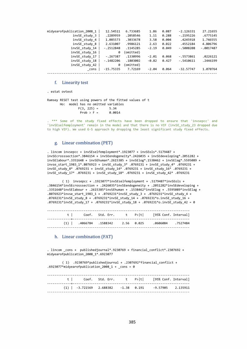
385
midyearofpublication_2008_1 | 12.54511 6.733685 1.86 0.087 -2.126331 27.21655
invSE_study_3 | .2289959 .2058546 1.11 0.288 -.2195226 .6775145
invSE_study_4 | 1.085573 .3033678 3.58 0.004 .4245918 1.746555
invSE_study_8 | 2.631007 .9986121 2.63 0.022 .4552184 4.806796
invSE_study_14 | -.2512848 .1145285 -2.19 0.049 -.5008208 -.0017487
invSE_study_16 | 0 (omitted)
invSE_study_17 | -.267387 .1330996 -2.01 0.068 -.5573861 .0226121
invSE_study_18 | -.1482206 .1803002 -0.82 0.427 -.5410611 .2446199
invSE_study_42 | 0 (omitted)
_cons | -15.75335 7.72169 -2.04 0.064 -32.57747 1.070764
---------------------------------------------------------------------------------------------
f. Linearity test
. estat ovtest
Ramsey RESET test using powers of the fitted values of t
Ho: model has no omitted variables
F(3, 225) = 5.34
Prob > F = 0.0014
. *** Some of the study fixed effects have been dropped to ensure that 'invsepcc' and
'invSEselfemployment' remain in the model and that there is no VIF (invSE_study_23 dropped due
to high VIF). We used G-S approach by dropping the least significant study fixed effects.
g. Linear combination (PET)
. lincom invsepcc + invSEselfemployment*.1923077 + invSEols*.5179487 +
invSEcrosssection*.3846154 + invSEendogeneity*.2426035 + invSEdeveloping*.2051282 +
invSElabour*.3351648 + invSEhuman*.2615385 + invSElog*.1538462 + invSElag*.5595089 +
invse_start_1983_1*.8076923 + invSE_study_3* .0769231 + invSE_study_4* .0769231 +
invSE_study_8* .0769231 + invSE_study_14* .0769231 + invSE_study_16* .0769231 +
invSE_study_17* .0769231 + invSE_study_18* .0769231 + invSE_study_42* .0769231
( 1) invsepcc + .1923077*invSEselfemployment + .5179487*invSEols +
.3846154*invSEcrosssection + .2426035*invSEendogeneity + .2051282*invSEdeveloping +
.3351648*invSElabour + .2615385*invSEhuman + .1538462*invSElog + .5595089*invSElag +
.8076923*invse_start_1983_1 + .0769231*invSE_study_3 + .0769231*invSE_study_4 +
.0769231*invSE_study_8 + .0769231*invSE_study_14 + .0769231*o.invSE_study_16 +
.0769231*invSE_study_17 + .0769231*invSE_study_18 + .0769231*o.invSE_study_42 = 0
------------------------------------------------------------------------------
t | Coef. Std. Err. t P>|t| [95% Conf. Interval]
-------------+----------------------------------------------------------------
(1) | .4066784 .1588342 2.56 0.025 .0606084 .7527484
------------------------------------------------------------------------------
h. Linear combination (FAT)
. lincom _cons + publishedjournal*.9230769 + financial_conflict*.2307692 +
midyearofpublication_2008_1*.6923077
( 1) .9230769*publishedjournal + .2307692*financial_conflict +
.6923077*midyearofpublication_2008_1 + _cons = 0
------------------------------------------------------------------------------
t | Coef. Std. Err. t P>|t| [95% Conf. Interval]
-------------+----------------------------------------------------------------
(1) | -3.721569 2.688382 -1.38 0.191 -9.57905 2.135911
------------------------------------------------------------------------------
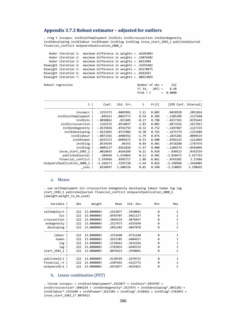
386
Appendix 3.7.3 Robust estimator – adjusted for outliers
. rreg t invsepcc invSEselfemployment invSEols invSEcrosssection invSEendogeneity
invSEdeveloping invSElabour invSEhuman invSElog invSElag invse_start_1983_1 publishedjournal
financial_conflict midyearofpublication_2008_1
Huber iteration 1: maximum difference in weights = .66283883
Huber iteration 2: maximum difference in weights = .14076602
Huber iteration 3: maximum difference in weights = .0421904
Biweight iteration 4: maximum difference in weights = .29295482
Biweight iteration 5: maximum difference in weights = .03270875
Biweight iteration 6: maximum difference in weights = .0182663
Biweight iteration 7: maximum difference in weights = .00653069
Robust regression Number of obs = 222
F( 14, 207) = 8.48
Prob > F = 0.0000
---------------------------------------------------------------------------------------------
t | Coef. Std. Err. t P>|t| [95% Conf. Interval]
----------------------------+----------------------------------------------------------------
invsepcc | .1255372 .0403981 3.11 0.002 .0458928 .2051816
invSEselfemployment | .045613 .0842773 0.54 0.589 -.1205389 .2117648
invSEols | -.0030861 .011489 -0.27 0.788 -.0257365 .0195643
invSEcrosssection | .1565535 .0554037 2.83 0.005 .0473256 .2657813
invSEendogeneity | -.0235036 .0741759 -0.32 0.752 -.1697407 .1227335
invSEdeveloping | -.0221045 .0737886 -0.30 0.765 -.1675779 .1233689
invSElabour | -.0872341 .0488392 -1.79 0.076 -.1835202 .0090519
invSEhuman | .0255372 .0485672 0.53 0.600 -.0702125 .1212869
invSElog | .0534594 .06355 0.84 0.401 -.0718288 .1787476
invSElag | -.0885137 .0161828 -5.47 0.000 -.1204179 -.0566096
invse_start_1983_1 | .0018665 .0164289 0.11 0.910 -.030523 .0342559
publishedjournal | .204644 1.634864 0.13 0.901 -3.018475 3.427763
financial_conflict | 1.599966 .8505717 1.88 0.061 -.0769281 3.27686
midyearofpublication_2008_1 | -1.266173 .5195728 -2.44 0.016 -2.290506 -.2418401
_cons | .0198997 1.608324 0.01 0.990 -3.150895 3.190695
---------------------------------------------------------------------------------------------
a. Means
. sum selfemployment ols crosssection endogeneity developing labour human log lag
start_1983_1 publishedjournal financial_conflict midyearofpublication_2008_1
[aweight=weight_to_be_used]
Variable | Obs Weight Mean Std. Dev. Min Max
-------------+-----------------------------------------------------------------
selfemploy~t | 222 13.0000003 .1923077 .3950041 0 1
ols | 222 13.0000003 .4959707 .5011137 0 1
crosssection | 222 13.0000003 .3846154 .4876037 0 1
endogeneity | 222 13.0000003 .2527473 .4355694 0 1
developing | 222 13.0000003 .2051282 .4047078 0 1
-------------+-----------------------------------------------------------------
labour | 222 13.0000003 .3351648 .4731148 0 1
human | 222 13.0000003 .2615385 .4404657 0 1
log | 222 13.0000003 .1538462 .3616166 0 1
lag | 222 13.0000003 .5783855 .4949335 0 1
start_1983_1 | 222 13.0000003 .8076923 .3950041 0 1
-------------+-----------------------------------------------------------------
publishedj~l | 222 13.0000003 .9230769 .2670715 0 1
financial_~t | 222 13.0000003 .2307692 .4222772 0 1
midyearofp~1 | 222 13.0000003 .6923077 .4625815 0 1
b. Linear combination (PET)
. lincom invsepcc + invSEselfemployment*.1923077 + invSEols*.4959707 +
invSEcrosssection*.3846154 + invSEendogeneity*.2527473 + invSEdeveloping*.2051282 +
invSElabour*.3351648 + invSEhuman*.2615385 + invSElog*.1538462 + invSElag*.5783855 +
invse_start_1983_1*.8076923
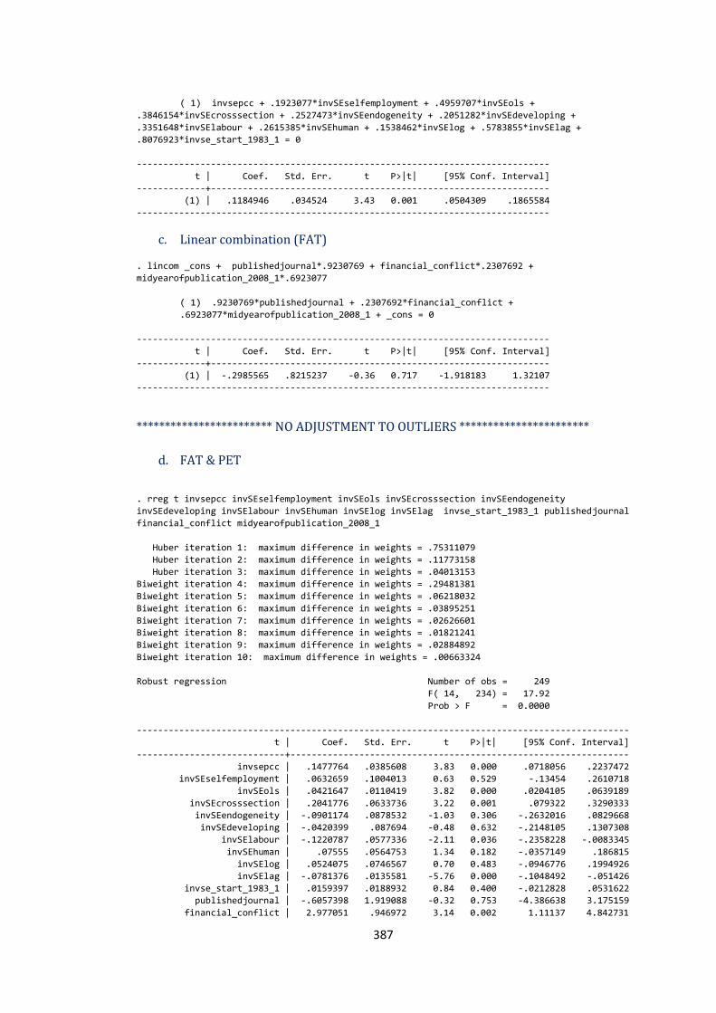
387
( 1) invsepcc + .1923077*invSEselfemployment + .4959707*invSEols +
.3846154*invSEcrosssection + .2527473*invSEendogeneity + .2051282*invSEdeveloping +
.3351648*invSElabour + .2615385*invSEhuman + .1538462*invSElog + .5783855*invSElag +
.8076923*invse_start_1983_1 = 0
------------------------------------------------------------------------------
t | Coef. Std. Err. t P>|t| [95% Conf. Interval]
-------------+----------------------------------------------------------------
(1) | .1184946 .034524 3.43 0.001 .0504309 .1865584
------------------------------------------------------------------------------
c. Linear combination (FAT)
. lincom _cons + publishedjournal*.9230769 + financial_conflict*.2307692 +
midyearofpublication_2008_1*.6923077
( 1) .9230769*publishedjournal + .2307692*financial_conflict +
.6923077*midyearofpublication_2008_1 + _cons = 0
------------------------------------------------------------------------------
t | Coef. Std. Err. t P>|t| [95% Conf. Interval]
-------------+----------------------------------------------------------------
(1) | -.2985565 .8215237 -0.36 0.717 -1.918183 1.32107
------------------------------------------------------------------------------
************************ NO ADJUSTMENT TO OUTLIERS ***********************
d. FAT & PET
. rreg t invsepcc invSEselfemployment invSEols invSEcrosssection invSEendogeneity
invSEdeveloping invSElabour invSEhuman invSElog invSElag invse_start_1983_1 publishedjournal
financial_conflict midyearofpublication_2008_1
Huber iteration 1: maximum difference in weights = .75311079
Huber iteration 2: maximum difference in weights = .11773158
Huber iteration 3: maximum difference in weights = .04013153
Biweight iteration 4: maximum difference in weights = .29481381
Biweight iteration 5: maximum difference in weights = .06218032
Biweight iteration 6: maximum difference in weights = .03895251
Biweight iteration 7: maximum difference in weights = .02626601
Biweight iteration 8: maximum difference in weights = .01821241
Biweight iteration 9: maximum difference in weights = .02884892
Biweight iteration 10: maximum difference in weights = .00663324
Robust regression Number of obs = 249
F( 14, 234) = 17.92
Prob > F = 0.0000
---------------------------------------------------------------------------------------------
t | Coef. Std. Err. t P>|t| [95% Conf. Interval]
----------------------------+----------------------------------------------------------------
invsepcc | .1477764 .0385608 3.83 0.000 .0718056 .2237472
invSEselfemployment | .0632659 .1004013 0.63 0.529 -.13454 .2610718
invSEols | .0421647 .0110419 3.82 0.000 .0204105 .0639189
invSEcrosssection | .2041776 .0633736 3.22 0.001 .079322 .3290333
invSEendogeneity | -.0901174 .0878532 -1.03 0.306 -.2632016 .0829668
invSEdeveloping | -.0420399 .087694 -0.48 0.632 -.2148105 .1307308
invSElabour | -.1220787 .0577336 -2.11 0.036 -.2358228 -.0083345
invSEhuman | .07555 .0564753 1.34 0.182 -.0357149 .186815
invSElog | .0524075 .0746567 0.70 0.483 -.0946776 .1994926
invSElag | -.0781376 .0135581 -5.76 0.000 -.1048492 -.051426
invse_start_1983_1 | .0159397 .0188932 0.84 0.400 -.0212828 .0531622
publishedjournal | -.6057398 1.919088 -0.32 0.753 -4.386638 3.175159
financial_conflict | 2.977051 .946972 3.14 0.002 1.11137 4.842731
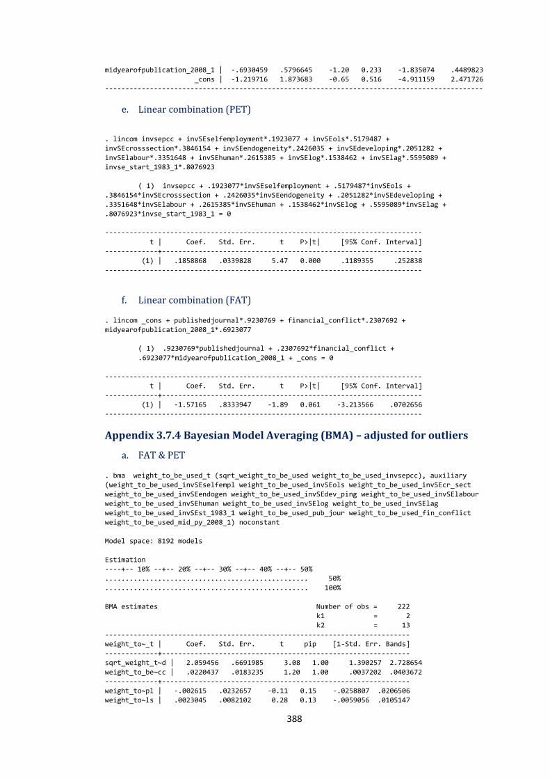
388
midyearofpublication_2008_1 | -.6930459 .5796645 -1.20 0.233 -1.835074 .4489823
_cons | -1.219716 1.873683 -0.65 0.516 -4.911159 2.471726
---------------------------------------------------------------------------------------------
e. Linear combination (PET)
. lincom invsepcc + invSEselfemployment*.1923077 + invSEols*.5179487 +
invSEcrosssection*.3846154 + invSEendogeneity*.2426035 + invSEdeveloping*.2051282 +
invSElabour*.3351648 + invSEhuman*.2615385 + invSElog*.1538462 + invSElag*.5595089 +
invse_start_1983_1*.8076923
( 1) invsepcc + .1923077*invSEselfemployment + .5179487*invSEols +
.3846154*invSEcrosssection + .2426035*invSEendogeneity + .2051282*invSEdeveloping +
.3351648*invSElabour + .2615385*invSEhuman + .1538462*invSElog + .5595089*invSElag +
.8076923*invse_start_1983_1 = 0
------------------------------------------------------------------------------
t | Coef. Std. Err. t P>|t| [95% Conf. Interval]
-------------+----------------------------------------------------------------
(1) | .1858868 .0339828 5.47 0.000 .1189355 .252838
------------------------------------------------------------------------------
f. Linear combination (FAT)
. lincom _cons + publishedjournal*.9230769 + financial_conflict*.2307692 +
midyearofpublication_2008_1*.6923077
( 1) .9230769*publishedjournal + .2307692*financial_conflict +
.6923077*midyearofpublication_2008_1 + _cons = 0
------------------------------------------------------------------------------
t | Coef. Std. Err. t P>|t| [95% Conf. Interval]
-------------+----------------------------------------------------------------
(1) | -1.57165 .8333947 -1.89 0.061 -3.213566 .0702656
------------------------------------------------------------------------------
Appendix 3.7.4 Bayesian Model Averaging (BMA) – adjusted for outliers
a. FAT & PET
. bma weight_to_be_used_t (sqrt_weight_to_be_used weight_to_be_used_invsepcc), auxiliary
(weight_to_be_used_invSEselfempl weight_to_be_used_invSEols weight_to_be_used_invSEcr_sect
weight_to_be_used_invSEendogen weight_to_be_used_invSEdev_ping weight_to_be_used_invSElabour
weight_to_be_used_invSEhuman weight_to_be_used_invSElog weight_to_be_used_invSElag
weight_to_be_used_invSEst_1983_1 weight_to_be_used_pub_jour weight_to_be_used_fin_conflict
weight_to_be_used_mid_py_2008_1) noconstant
Model space: 8192 models
Estimation
----+-- 10% --+-- 20% --+-- 30% --+-- 40% --+-- 50%
.................................................. 50%
.................................................. 100%
BMA estimates Number of obs = 222
k1 = 2
k2 = 13
---------------------------------------------------------------------------
weight_to~_t | Coef. Std. Err. t pip [1-Std. Err. Bands]
-------------+-------------------------------------------------------------
sqrt_weight_t~d | 2.059456 .6691985 3.08 1.00 1.390257 2.728654
weight_to_be~cc | .0220437 .0183235 1.20 1.00 .0037202 .0403672
-------------+-------------------------------------------------------------
weight_to~pl | -.002615 .0232657 -0.11 0.15 -.0258807 .0206506
weight_to~ls | .0023045 .0082102 0.28 0.13 -.0059056 .0105147
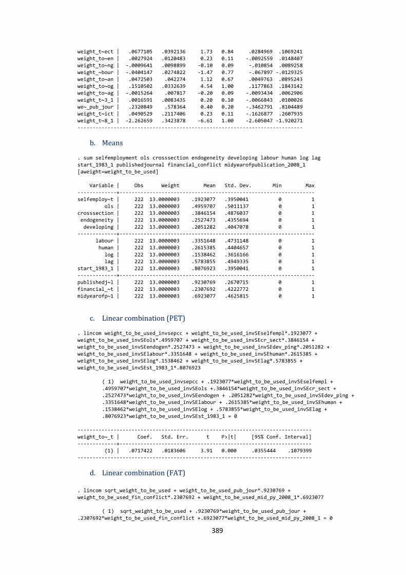
389
weight_t~ect | .0677105 .0392136 1.73 0.84 .0284969 .1069241
weight_to~en | .0027924 .0120483 0.23 0.11 -.0092559 .0148407
weight_to~ng | -.0009641 .0098899 -0.10 0.09 -.010854 .0089258
weight_~bour | -.0404147 .0274822 -1.47 0.77 -.067897 -.0129325
weight_to~an | .0472503 .042274 1.12 0.67 .0049763 .0895243
weight_to~og | .1510502 .0332639 4.54 1.00 .1177863 .1843142
weight_to~ag | -.0015264 .007817 -0.20 0.09 -.0093434 .0062906
weight_t~3_1 | .0016591 .0083435 0.20 0.10 -.0066843 .0100026
we~_pub_jour | .2320849 .578364 0.40 0.20 -.3462791 .8104489
weight_t~ict | .0490529 .2117406 0.23 0.11 -.1626877 .2607935
weight_t~8_1 | -2.262659 .3423878 -6.61 1.00 -2.605047 -1.920271
---------------------------------------------------------------------------
b. Means
. sum selfemployment ols crosssection endogeneity developing labour human log lag
start_1983_1 publishedjournal financial_conflict midyearofpublication_2008_1
[aweight=weight_to_be_used]
Variable | Obs Weight Mean Std. Dev. Min Max
-------------+-----------------------------------------------------------------
selfemploy~t | 222 13.0000003 .1923077 .3950041 0 1
ols | 222 13.0000003 .4959707 .5011137 0 1
crosssection | 222 13.0000003 .3846154 .4876037 0 1
endogeneity | 222 13.0000003 .2527473 .4355694 0 1
developing | 222 13.0000003 .2051282 .4047078 0 1
-------------+-----------------------------------------------------------------
labour | 222 13.0000003 .3351648 .4731148 0 1
human | 222 13.0000003 .2615385 .4404657 0 1
log | 222 13.0000003 .1538462 .3616166 0 1
lag | 222 13.0000003 .5783855 .4949335 0 1
start_1983_1 | 222 13.0000003 .8076923 .3950041 0 1
-------------+-----------------------------------------------------------------
publishedj~l | 222 13.0000003 .9230769 .2670715 0 1
financial_~t | 222 13.0000003 .2307692 .4222772 0 1
midyearofp~1 | 222 13.0000003 .6923077 .4625815 0 1
c. Linear combination (PET)
. lincom weight_to_be_used_invsepcc + weight_to_be_used_invSEselfempl*.1923077 +
weight_to_be_used_invSEols*.4959707 + weight_to_be_used_invSEcr_sect*.3846154 +
weight_to_be_used_invSEendogen*.2527473 + weight_to_be_used_invSEdev_ping*.2051282 +
weight_to_be_used_invSElabour*.3351648 + weight_to_be_used_invSEhuman*.2615385 +
weight_to_be_used_invSElog*.1538462 + weight_to_be_used_invSElag*.5783855 +
weight_to_be_used_invSEst_1983_1*.8076923
( 1) weight_to_be_used_invsepcc + .1923077*weight_to_be_used_invSEselfempl +
.4959707*weight_to_be_used_invSEols +.3846154*weight_to_be_used_invSEcr_sect +
.2527473*weight_to_be_used_invSEendogen + .2051282*weight_to_be_used_invSEdev_ping +
.3351648*weight_to_be_used_invSElabour + .2615385*weight_to_be_used_invSEhuman +
.1538462*weight_to_be_used_invSElog + .5783855*weight_to_be_used_invSElag +
.8076923*weight_to_be_used_invSEst_1983_1 = 0
------------------------------------------------------------------------------
weight_to~_t | Coef. Std. Err. t P>|t| [95% Conf. Interval]
-------------+----------------------------------------------------------------
(1) | .0717422 .0183606 3.91 0.000 .0355444 .1079399
------------------------------------------------------------------------------
d. Linear combination (FAT) . lincom sqrt_weight_to_be_used + weight_to_be_used_pub_jour*.9230769 +
weight_to_be_used_fin_conflict*.2307692 + weight_to_be_used_mid_py_2008_1*.6923077
( 1) sqrt_weight_to_be_used + .9230769*weight_to_be_used_pub_jour +
.2307692*weight_to_be_used_fin_conflict +.6923077*weight_to_be_used_mid_py_2008_1 = 0
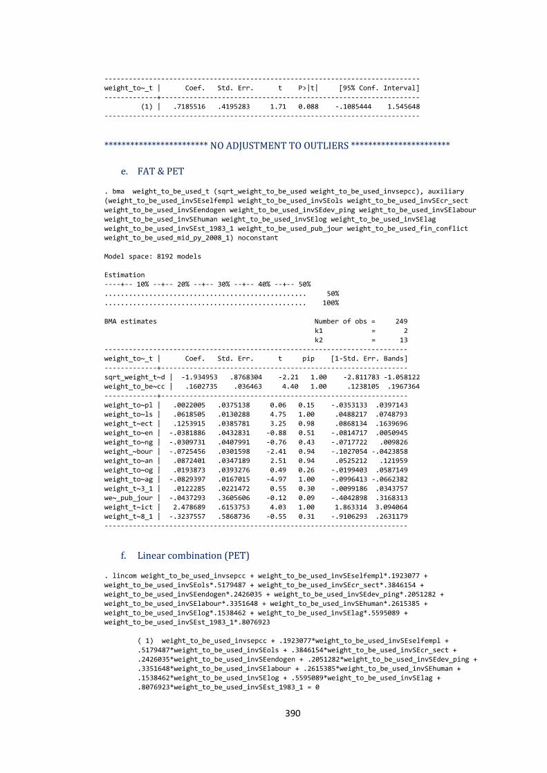
390
------------------------------------------------------------------------------
weight_to~_t | Coef. Std. Err. t P>|t| [95% Conf. Interval]
-------------+----------------------------------------------------------------
(1) | .7185516 .4195283 1.71 0.088 -.1085444 1.545648
------------------------------------------------------------------------------
************************ NO ADJUSTMENT TO OUTLIERS ***********************
e. FAT & PET
. bma weight_to_be_used_t (sqrt_weight_to_be_used weight_to_be_used_invsepcc), auxiliary
(weight_to_be_used_invSEselfempl weight_to_be_used_invSEols weight_to_be_used_invSEcr_sect
weight_to_be_used_invSEendogen weight_to_be_used_invSEdev_ping weight_to_be_used_invSElabour
weight_to_be_used_invSEhuman weight_to_be_used_invSElog weight_to_be_used_invSElag
weight_to_be_used_invSEst_1983_1 weight_to_be_used_pub_jour weight_to_be_used_fin_conflict
weight_to_be_used_mid_py_2008_1) noconstant
Model space: 8192 models
Estimation
----+-- 10% --+-- 20% --+-- 30% --+-- 40% --+-- 50%
.................................................. 50%
.................................................. 100%
BMA estimates Number of obs = 249
k1 = 2
k2 = 13
---------------------------------------------------------------------------
weight_to~_t | Coef. Std. Err. t pip [1-Std. Err. Bands]
-------------+-------------------------------------------------------------
sqrt_weight_t~d | -1.934953 .8768304 -2.21 1.00 -2.811783 -1.058122
weight_to_be~cc | .1602735 .036463 4.40 1.00 .1238105 .1967364
-------------+-------------------------------------------------------------
weight_to~pl | .0022005 .0375138 0.06 0.15 -.0353133 .0397143
weight_to~ls | .0618505 .0130288 4.75 1.00 .0488217 .0748793
weight_t~ect | .1253915 .0385781 3.25 0.98 .0868134 .1639696
weight_to~en | -.0381886 .0432831 -0.88 0.51 -.0814717 .0050945
weight_to~ng | -.0309731 .0407991 -0.76 0.43 -.0717722 .009826
weight_~bour | -.0725456 .0301598 -2.41 0.94 -.1027054 -.0423858
weight_to~an | .0872401 .0347189 2.51 0.94 .0525212 .121959
weight_to~og | .0193873 .0393276 0.49 0.26 -.0199403 .0587149
weight_to~ag | -.0829397 .0167015 -4.97 1.00 -.0996413 -.0662382
weight_t~3_1 | .0122285 .0221472 0.55 0.30 -.0099186 .0343757
we~_pub_jour | -.0437293 .3605606 -0.12 0.09 -.4042898 .3168313
weight_t~ict | 2.478689 .6153753 4.03 1.00 1.863314 3.094064
weight_t~8_1 | -.3237557 .5868736 -0.55 0.31 -.9106293 .2631179
---------------------------------------------------------------------------
f. Linear combination (PET)
. lincom weight_to_be_used_invsepcc + weight_to_be_used_invSEselfempl*.1923077 +
weight_to_be_used_invSEols*.5179487 + weight_to_be_used_invSEcr_sect*.3846154 +
weight_to_be_used_invSEendogen*.2426035 + weight_to_be_used_invSEdev_ping*.2051282 +
weight_to_be_used_invSElabour*.3351648 + weight_to_be_used_invSEhuman*.2615385 +
weight_to_be_used_invSElog*.1538462 + weight_to_be_used_invSElag*.5595089 +
weight_to_be_used_invSEst_1983_1*.8076923
( 1) weight_to_be_used_invsepcc + .1923077*weight_to_be_used_invSEselfempl +
.5179487*weight_to_be_used_invSEols + .3846154*weight_to_be_used_invSEcr_sect +
.2426035*weight_to_be_used_invSEendogen + .2051282*weight_to_be_used_invSEdev_ping +
.3351648*weight_to_be_used_invSElabour + .2615385*weight_to_be_used_invSEhuman +
.1538462*weight_to_be_used_invSElog + .5595089*weight_to_be_used_invSElag +
.8076923*weight_to_be_used_invSEst_1983_1 = 0
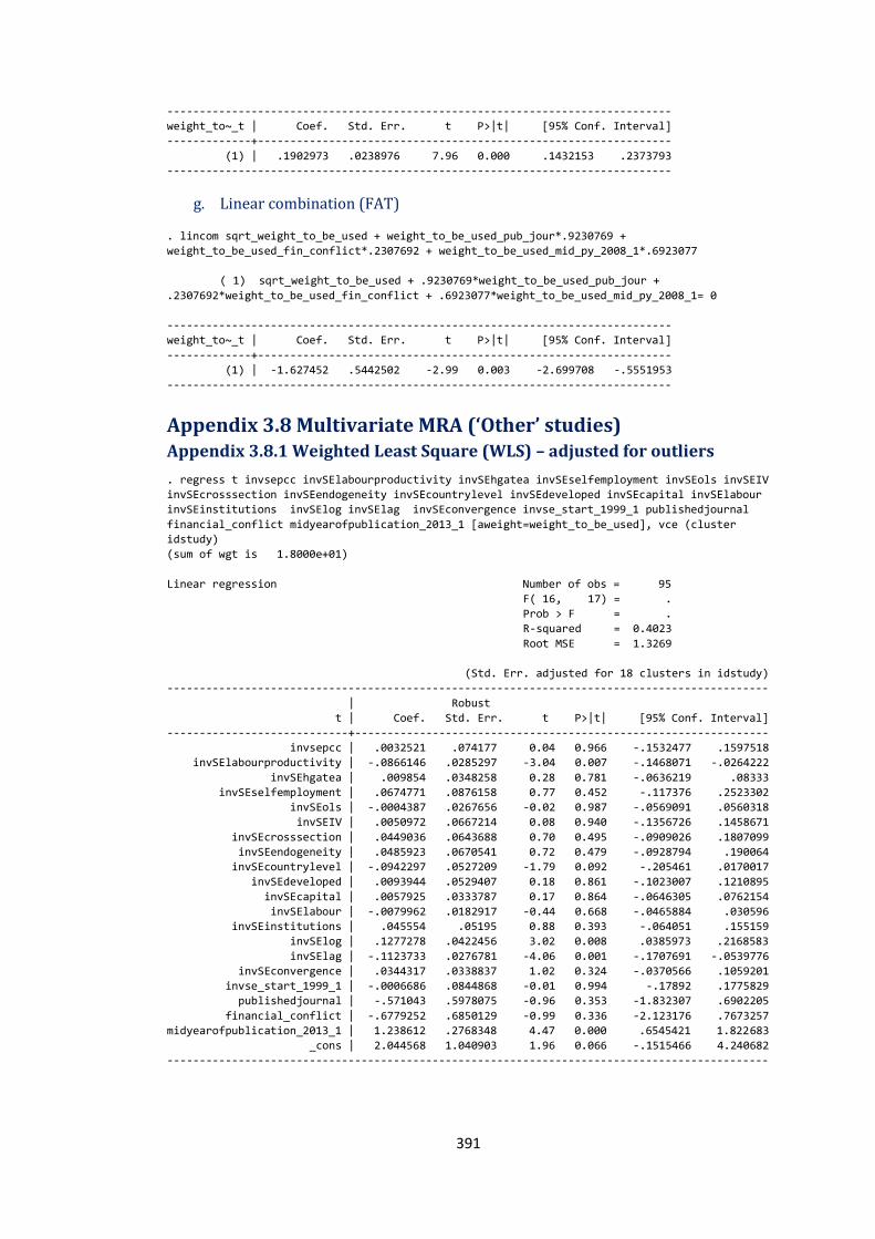
391
------------------------------------------------------------------------------
weight_to~_t | Coef. Std. Err. t P>|t| [95% Conf. Interval]
-------------+----------------------------------------------------------------
(1) | .1902973 .0238976 7.96 0.000 .1432153 .2373793
------------------------------------------------------------------------------
g. Linear combination (FAT)
. lincom sqrt_weight_to_be_used + weight_to_be_used_pub_jour*.9230769 +
weight_to_be_used_fin_conflict*.2307692 + weight_to_be_used_mid_py_2008_1*.6923077
( 1) sqrt_weight_to_be_used + .9230769*weight_to_be_used_pub_jour +
.2307692*weight_to_be_used_fin_conflict + .6923077*weight_to_be_used_mid_py_2008_1= 0
------------------------------------------------------------------------------
weight_to~_t | Coef. Std. Err. t P>|t| [95% Conf. Interval]
-------------+----------------------------------------------------------------
(1) | -1.627452 .5442502 -2.99 0.003 -2.699708 -.5551953
------------------------------------------------------------------------------
Appendix 3.8 Multivariate MRA (‘Other’ studies) Appendix 3.8.1 Weighted Least Square (WLS) – adjusted for outliers
. regress t invsepcc invSElabourproductivity invSEhgatea invSEselfemployment invSEols invSEIV
invSEcrosssection invSEendogeneity invSEcountrylevel invSEdeveloped invSEcapital invSElabour
invSEinstitutions invSElog invSElag invSEconvergence invse_start_1999_1 publishedjournal
financial_conflict midyearofpublication_2013_1 [aweight=weight_to_be_used], vce (cluster
idstudy)
(sum of wgt is 1.8000e+01)
Linear regression Number of obs = 95
F( 16, 17) = .
Prob > F = .
R-squared = 0.4023
Root MSE = 1.3269
(Std. Err. adjusted for 18 clusters in idstudy)
---------------------------------------------------------------------------------------------
| Robust
t | Coef. Std. Err. t P>|t| [95% Conf. Interval]
----------------------------+----------------------------------------------------------------
invsepcc | .0032521 .074177 0.04 0.966 -.1532477 .1597518
invSElabourproductivity | -.0866146 .0285297 -3.04 0.007 -.1468071 -.0264222
invSEhgatea | .009854 .0348258 0.28 0.781 -.0636219 .08333
invSEselfemployment | .0674771 .0876158 0.77 0.452 -.117376 .2523302
invSEols | -.0004387 .0267656 -0.02 0.987 -.0569091 .0560318
invSEIV | .0050972 .0667214 0.08 0.940 -.1356726 .1458671
invSEcrosssection | .0449036 .0643688 0.70 0.495 -.0909026 .1807099
invSEendogeneity | .0485923 .0670541 0.72 0.479 -.0928794 .190064
invSEcountrylevel | -.0942297 .0527209 -1.79 0.092 -.205461 .0170017
invSEdeveloped | .0093944 .0529407 0.18 0.861 -.1023007 .1210895
invSEcapital | .0057925 .0333787 0.17 0.864 -.0646305 .0762154
invSElabour | -.0079962 .0182917 -0.44 0.668 -.0465884 .030596
invSEinstitutions | .045554 .05195 0.88 0.393 -.064051 .155159
invSElog | .1277278 .0422456 3.02 0.008 .0385973 .2168583
invSElag | -.1123733 .0276781 -4.06 0.001 -.1707691 -.0539776
invSEconvergence | .0344317 .0338837 1.02 0.324 -.0370566 .1059201
invse_start_1999_1 | -.0006686 .0844868 -0.01 0.994 -.17892 .1775829
publishedjournal | -.571043 .5978075 -0.96 0.353 -1.832307 .6902205
financial_conflict | -.6779252 .6850129 -0.99 0.336 -2.123176 .7673257
midyearofpublication_2013_1 | 1.238612 .2768348 4.47 0.000 .6545421 1.822683
_cons | 2.044568 1.040903 1.96 0.066 -.1515466 4.240682
---------------------------------------------------------------------------------------------

392
a. Linearity test
. estat ovtest
Ramsey RESET test using powers of the fitted values of t
Ho: model has no omitted variables
F(3, 71) = 0.40
Prob > F = 0.7514
b. Means
. sum labourproductivity hgatea selfemployment ols IV crosssection endogeneity countrylevel
developed capital labour institutions log lag convergence start_1999_1 publishedjournal
financial_conflict midyearofpublication_2013_1 [aweight=weight_to_be_used]
Variable | Obs Weight Mean Std. Dev. Min Max
-------------+-----------------------------------------------------------------
labourprod~y | 95 18.0000003 .3888889 .4900842 0 1
hgatea | 95 18.0000003 .1126543 .3178471 0 1
selfemploy~t | 95 18.0000003 .1666667 .3746551 0 1
ols | 95 18.0000003 .3326599 .4736655 0 1
IV | 95 18.0000003 .3314815 .473243 0 1
-------------+-----------------------------------------------------------------
crosssection | 95 18.0000003 .2474747 .4338343 0 1
endogeneity | 95 18.0000003 .4636364 .5013214 0 1
countrylevel | 95 18.0000003 .6111111 .4900842 0 1
developed | 95 18.0000003 .6746032 .4710085 0 1
capital | 95 18.0000003 .4762626 .5020858 0 1
-------------+-----------------------------------------------------------------
labour | 95 18.0000003 .3650794 .4840066 0 1
institutions | 95 18.0000003 .3111111 .4654041 0 1
log | 95 18.0000003 .3888889 .4900842 0 1
lag | 95 18.0000003 .0909091 .2890049 0 1
convergence | 95 18.0000003 .0793651 .2717417 0 1
-------------+-----------------------------------------------------------------
start_1999_1 | 95 18.0000003 .5 .5026525 0 1
publishedj~l | 95 18.0000003 .7777778 .4179452 0 1
financial_~t | 95 18.0000003 .2777778 .4502794 0 1
midyearofp~1 | 95 18.0000003 .5 .5026525 0 1
c. Linear combination (PET)
. lincom invsepcc + invSElabourproductivity*.3888889 + invSEhgatea*.1126543 +
invSEselfemployment*.1666667 + invSEols*.3326599 + invSEIV*.3314815 +
invSEcrosssection*.2474747 + invSEendogeneity*.4636364 + invSEcountrylevel*.6111111 +
invSEdeveloped*.6746032 + invSEcapital*.4762626 + invSElabour*.3650794 +
invSEinstitutions*.3111111 + invSElog*.3888889 + invSElag*.0909091 +
invSEconvergence*.0793651 + invse_start_1999_1*.5
( 1) invsepcc + .3888889*invSElabourproductivity + .1126543*invSEhgatea +
.1666667*invSEselfemployment + .3326599*invSEols + .3314815*invSEIV +
.2474747*invSEcrosssection + .4636364*invSEendogeneity + .6111111*invSEcountrylevel +
.6746032*invSEdeveloped + .4762626*invSEcapital + .3650794*invSElabour +
.3111111*invSEinstitutions + .3888889*invSElog + .0909091*invSElag + 0793651*invSEconvergence
+ .5*invse_start_1999_1 = 0
------------------------------------------------------------------------------
t | Coef. Std. Err. t P>|t| [95% Conf. Interval]
-------------+----------------------------------------------------------------
(1) | .0217294 .057842 0.38 0.712 -.1003066 .1437653
------------------------------------------------------------------------------
d. Linear combination (FAT)
. lincom _cons + publishedjournal* .7777778 + financial_conflict*.2777778 +
midyearofpublication_2013_1*.5
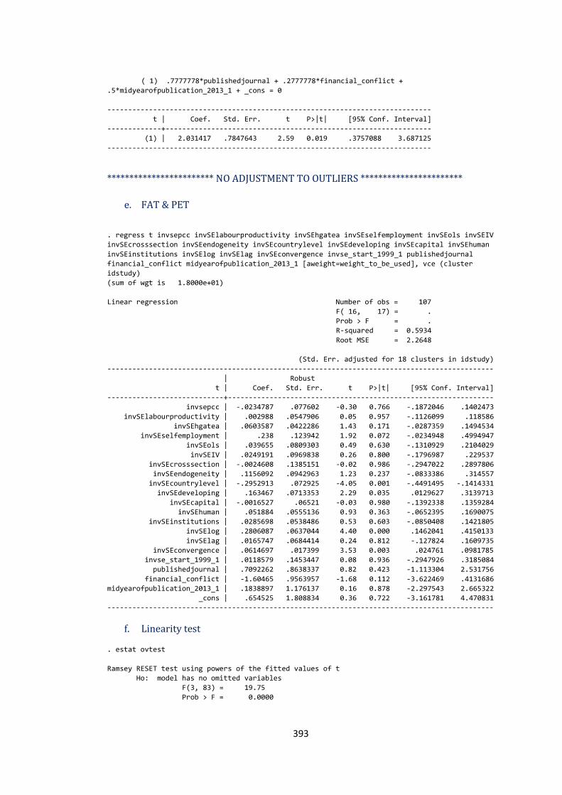
393
( 1) .7777778*publishedjournal + .2777778*financial_conflict +
.5*midyearofpublication_2013_1 + _cons = 0
------------------------------------------------------------------------------
t | Coef. Std. Err. t P>|t| [95% Conf. Interval]
-------------+----------------------------------------------------------------
(1) | 2.031417 .7847643 2.59 0.019 .3757088 3.687125
------------------------------------------------------------------------------
************************ NO ADJUSTMENT TO OUTLIERS ***********************
e. FAT & PET
. regress t invsepcc invSElabourproductivity invSEhgatea invSEselfemployment invSEols invSEIV
invSEcrosssection invSEendogeneity invSEcountrylevel invSEdeveloping invSEcapital invSEhuman
invSEinstitutions invSElog invSElag invSEconvergence invse_start_1999_1 publishedjournal
financial_conflict midyearofpublication_2013_1 [aweight=weight_to_be_used], vce (cluster
idstudy)
(sum of wgt is 1.8000e+01)
Linear regression Number of obs = 107
F( 16, 17) = .
Prob > F = .
R-squared = 0.5934
Root MSE = 2.2648
(Std. Err. adjusted for 18 clusters in idstudy)
---------------------------------------------------------------------------------------------
| Robust
t | Coef. Std. Err. t P>|t| [95% Conf. Interval]
----------------------------+----------------------------------------------------------------
invsepcc | -.0234787 .077602 -0.30 0.766 -.1872046 .1402473
invSElabourproductivity | .002988 .0547906 0.05 0.957 -.1126099 .118586
invSEhgatea | .0603587 .0422286 1.43 0.171 -.0287359 .1494534
invSEselfemployment | .238 .123942 1.92 0.072 -.0234948 .4994947
invSEols | .039655 .0809303 0.49 0.630 -.1310929 .2104029
invSEIV | .0249191 .0969838 0.26 0.800 -.1796987 .229537
invSEcrosssection | -.0024608 .1385151 -0.02 0.986 -.2947022 .2897806
invSEendogeneity | .1156092 .0942963 1.23 0.237 -.0833386 .314557
invSEcountrylevel | -.2952913 .072925 -4.05 0.001 -.4491495 -.1414331
invSEdeveloping | .163467 .0713353 2.29 0.035 .0129627 .3139713
invSEcapital | -.0016527 .06521 -0.03 0.980 -.1392338 .1359284
invSEhuman | .051884 .0555136 0.93 0.363 -.0652395 .1690075
invSEinstitutions | .0285698 .0538486 0.53 0.603 -.0850408 .1421805
invSElog | .2806087 .0637044 4.40 0.000 .1462041 .4150133
invSElag | .0165747 .0684414 0.24 0.812 -.127824 .1609735
invSEconvergence | .0614697 .017399 3.53 0.003 .024761 .0981785
invse_start_1999_1 | .0118579 .1453447 0.08 0.936 -.2947926 .3185084
publishedjournal | .7092262 .8638337 0.82 0.423 -1.113304 2.531756
financial_conflict | -1.60465 .9563957 -1.68 0.112 -3.622469 .4131686
midyearofpublication_2013_1 | .1838897 1.176137 0.16 0.878 -2.297543 2.665322
_cons | .654525 1.808834 0.36 0.722 -3.161781 4.470831
---------------------------------------------------------------------------------------------
f. Linearity test
. estat ovtest
Ramsey RESET test using powers of the fitted values of t
Ho: model has no omitted variables
F(3, 83) = 19.75
Prob > F = 0.0000
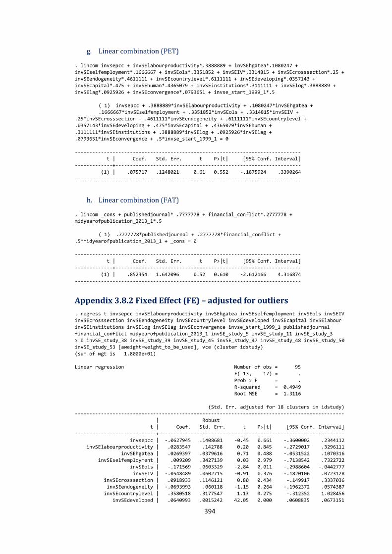
394
g. Linear combination (PET)
. lincom invsepcc + invSElabourproductivity*.3888889 + invSEhgatea*.1080247 +
invSEselfemployment*.1666667 + invSEols*.3351852 + invSEIV*.3314815 + invSEcrosssection*.25 +
invSEendogeneity*.4611111 + invSEcountrylevel*.6111111 + invSEdeveloping*.0357143 +
invSEcapital*.475 + invSEhuman*.4365079 + invSEinstitutions*.3111111 + invSElog*.3888889 +
invSElag*.0925926 + invSEconvergence*.0793651 + invse_start_1999_1*.5
( 1) invsepcc + .3888889*invSElabourproductivity + .1080247*invSEhgatea +
.1666667*invSEselfemployment + .3351852*invSEols + .3314815*invSEIV +
.25*invSEcrosssection + .4611111*invSEendogeneity + .6111111*invSEcountrylevel +
.0357143*invSEdeveloping + .475*invSEcapital + .4365079*invSEhuman +
.3111111*invSEinstitutions + .3888889*invSElog + .0925926*invSElag +
.0793651*invSEconvergence + .5*invse_start_1999_1 = 0
------------------------------------------------------------------------------
t | Coef. Std. Err. t P>|t| [95% Conf. Interval]
-------------+----------------------------------------------------------------
(1) | .075717 .1248021 0.61 0.552 -.1875924 .3390264
------------------------------------------------------------------------------
h. Linear combination (FAT)
. lincom _cons + publishedjournal* .7777778 + financial_conflict*.2777778 +
midyearofpublication_2013_1*.5
( 1) .7777778*publishedjournal + .2777778*financial_conflict +
.5*midyearofpublication_2013_1 + _cons = 0
------------------------------------------------------------------------------
t | Coef. Std. Err. t P>|t| [95% Conf. Interval]
-------------+----------------------------------------------------------------
(1) | .852354 1.642096 0.52 0.610 -2.612166 4.316874
------------------------------------------------------------------------------
Appendix 3.8.2 Fixed Effect (FE) – adjusted for outliers
. regress t invsepcc invSElabourproductivity invSEhgatea invSEselfemployment invSEols invSEIV
invSEcrosssection invSEendogeneity invSEcountrylevel invSEdeveloped invSEcapital invSElabour
invSEinstitutions invSElog invSElag invSEconvergence invse_start_1999_1 publishedjournal
financial_conflict midyearofpublication_2013_1 invSE_study_5 invSE_study_11 invSE_study_3
> 0 invSE_study_38 invSE_study_39 invSE_study_45 invSE_study_47 invSE_study_48 invSE_study_50
invSE_study_53 [aweight=weight_to_be_used], vce (cluster idstudy)
(sum of wgt is 1.8000e+01)
Linear regression Number of obs = 95
F( 13, 17) = .
Prob > F = .
R-squared = 0.4949
Root MSE = 1.3116
(Std. Err. adjusted for 18 clusters in idstudy)
---------------------------------------------------------------------------------------------
| Robust
t | Coef. Std. Err. t P>|t| [95% Conf. Interval]
----------------------------+----------------------------------------------------------------
invsepcc | -.0627945 .1408681 -0.45 0.661 -.3600002 .2344112
invSElabourproductivity | .0283547 .142788 0.20 0.845 -.2729017 .3296111
invSEhgatea | .0269397 .0379616 0.71 0.488 -.0531522 .1070316
invSEselfemployment | .009209 .3427139 0.03 0.979 -.7138542 .7322722
invSEols | -.171569 .0603329 -2.84 0.011 -.2988604 -.0442777
invSEIV | -.0548489 .0602715 -0.91 0.376 -.1820106 .0723128
invSEcrosssection | .0918933 .1146121 0.80 0.434 -.149917 .3337036
invSEendogeneity | -.0693993 .060118 -1.15 0.264 -.1962372 .0574387
invSEcountrylevel | .3580518 .3177547 1.13 0.275 -.312352 1.028456
invSEdeveloped | .0640993 .0015242 42.05 0.000 .0608835 .0673151
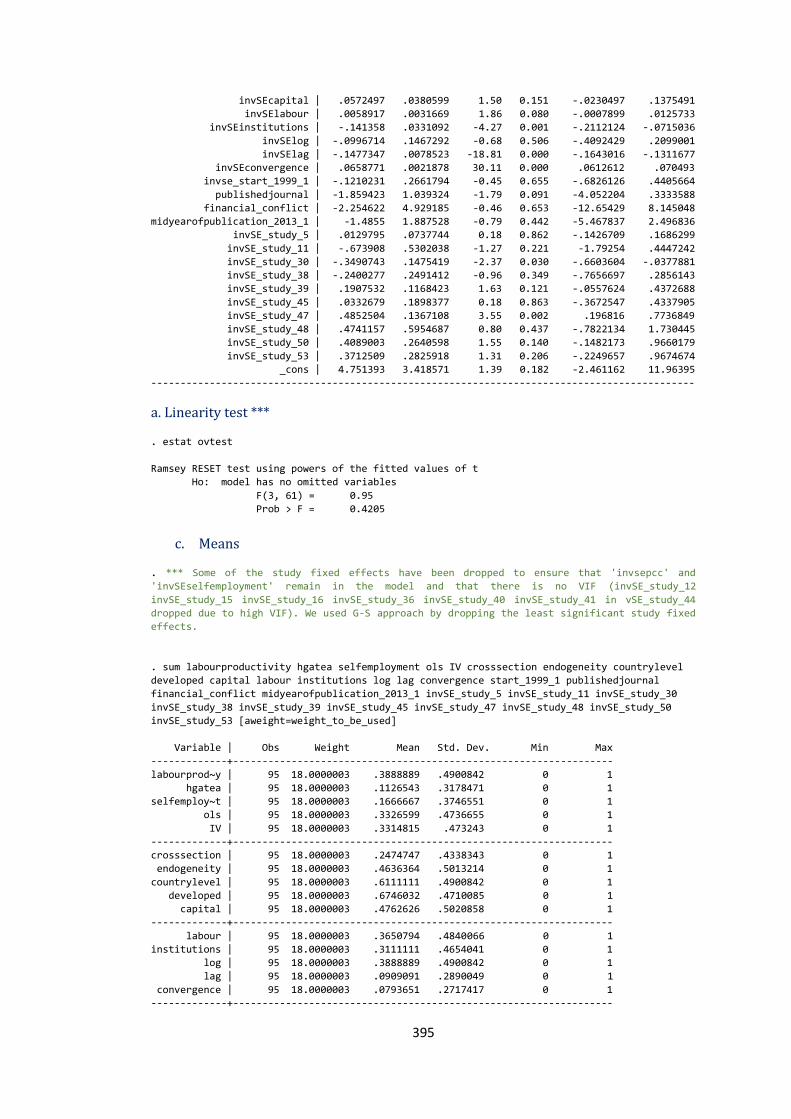
395
invSEcapital | .0572497 .0380599 1.50 0.151 -.0230497 .1375491
invSElabour | .0058917 .0031669 1.86 0.080 -.0007899 .0125733
invSEinstitutions | -.141358 .0331092 -4.27 0.001 -.2112124 -.0715036
invSElog | -.0996714 .1467292 -0.68 0.506 -.4092429 .2099001
invSElag | -.1477347 .0078523 -18.81 0.000 -.1643016 -.1311677
invSEconvergence | .0658771 .0021878 30.11 0.000 .0612612 .070493
invse_start_1999_1 | -.1210231 .2661794 -0.45 0.655 -.6826126 .4405664
publishedjournal | -1.859423 1.039324 -1.79 0.091 -4.052204 .3333588
financial_conflict | -2.254622 4.929185 -0.46 0.653 -12.65429 8.145048
midyearofpublication_2013_1 | -1.4855 1.887528 -0.79 0.442 -5.467837 2.496836
invSE_study_5 | .0129795 .0737744 0.18 0.862 -.1426709 .1686299
invSE_study_11 | -.673908 .5302038 -1.27 0.221 -1.79254 .4447242
invSE_study_30 | -.3490743 .1475419 -2.37 0.030 -.6603604 -.0377881
invSE_study_38 | -.2400277 .2491412 -0.96 0.349 -.7656697 .2856143
invSE_study_39 | .1907532 .1168423 1.63 0.121 -.0557624 .4372688
invSE_study_45 | .0332679 .1898377 0.18 0.863 -.3672547 .4337905
invSE_study_47 | .4852504 .1367108 3.55 0.002 .196816 .7736849
invSE_study_48 | .4741157 .5954687 0.80 0.437 -.7822134 1.730445
invSE_study_50 | .4089003 .2640598 1.55 0.140 -.1482173 .9660179
invSE_study_53 | .3712509 .2825918 1.31 0.206 -.2249657 .9674674
_cons | 4.751393 3.418571 1.39 0.182 -2.461162 11.96395
---------------------------------------------------------------------------------------------
a. Linearity test ***
. estat ovtest
Ramsey RESET test using powers of the fitted values of t
Ho: model has no omitted variables
F(3, 61) = 0.95
Prob > F = 0.4205
c. Means
. *** Some of the study fixed effects have been dropped to ensure that 'invsepcc' and
'invSEselfemployment' remain in the model and that there is no VIF (invSE_study_12
invSE_study_15 invSE_study_16 invSE_study_36 invSE_study_40 invSE_study_41 in vSE_study_44
dropped due to high VIF). We used G-S approach by dropping the least significant study fixed
effects.
. sum labourproductivity hgatea selfemployment ols IV crosssection endogeneity countrylevel
developed capital labour institutions log lag convergence start_1999_1 publishedjournal
financial_conflict midyearofpublication_2013_1 invSE_study_5 invSE_study_11 invSE_study_30
invSE_study_38 invSE_study_39 invSE_study_45 invSE_study_47 invSE_study_48 invSE_study_50
invSE_study_53 [aweight=weight_to_be_used]
Variable | Obs Weight Mean Std. Dev. Min Max
-------------+-----------------------------------------------------------------
labourprod~y | 95 18.0000003 .3888889 .4900842 0 1
hgatea | 95 18.0000003 .1126543 .3178471 0 1
selfemploy~t | 95 18.0000003 .1666667 .3746551 0 1
ols | 95 18.0000003 .3326599 .4736655 0 1
IV | 95 18.0000003 .3314815 .473243 0 1
-------------+-----------------------------------------------------------------
crosssection | 95 18.0000003 .2474747 .4338343 0 1
endogeneity | 95 18.0000003 .4636364 .5013214 0 1
countrylevel | 95 18.0000003 .6111111 .4900842 0 1
developed | 95 18.0000003 .6746032 .4710085 0 1
capital | 95 18.0000003 .4762626 .5020858 0 1
-------------+-----------------------------------------------------------------
labour | 95 18.0000003 .3650794 .4840066 0 1
institutions | 95 18.0000003 .3111111 .4654041 0 1
log | 95 18.0000003 .3888889 .4900842 0 1
lag | 95 18.0000003 .0909091 .2890049 0 1
convergence | 95 18.0000003 .0793651 .2717417 0 1
-------------+-----------------------------------------------------------------
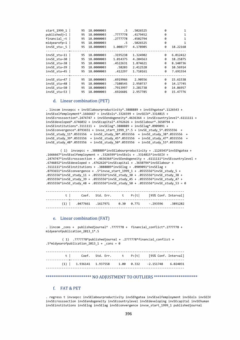
396
start_1999_1 | 95 18.0000003 .5 .5026525 0 1
publishedj~l | 95 18.0000003 .7777778 .4179452 0 1
financial_~t | 95 18.0000003 .2777778 .4502794 0 1
midyearofp~1 | 95 18.0000003 .5 .5026525 0 1
invSE_stu~_5 | 95 18.0000003 1.008177 4.178905 0 18.22168
-------------+-----------------------------------------------------------------
invSE_stu~11 | 95 18.0000003 .3195238 1.324902 0 6.012412
invSE_stu~30 | 95 18.0000003 1.014375 4.204563 0 18.25875
invSE_stu~38 | 95 18.0000003 .4522631 1.874621 0 8.140736
invSE_stu~39 | 95 18.0000003 .58203 2.412528 0 10.56914
invSE_stu~45 | 95 18.0000003 .412297 1.710161 0 7.691554
-------------+-----------------------------------------------------------------
invSE_stu~47 | 95 18.0000003 .6919966 2.90556 0 15.61538
invSE_stu~48 | 95 18.0000003 .7108545 2.950737 0 14.17745
invSE_stu~50 | 95 18.0000003 .7913997 3.281738 0 14.86957
invSE_stu~53 | 95 18.0000003 .6926601 2.957785 0 15.47776
d. Linear combination (PET)
. lincom invsepcc + invSElabourproductivity*.3888889 + invSEhgatea*.1126543 +
invSEselfemployment*.1666667 + invSEols*.3326599 + invSEIV*.3314815 +
invSEcrosssection*.2474747 + invSEendogeneity*.4636364 + invSEcountrylevel*.6111111 +
invSEdeveloped*.6746032 + invSEcapital*.4762626 + invSElabour*.3650794 +
invSEinstitutions*.3111111 + invSElog*.3888889 + invSElag*.0909091 +
invSEconvergence*.0793651 + invse_start_1999_1*.5 + invSE_study_5*.0555556 +
invSE_study_11*.0555556 + invSE_study_30*.0555556 + invSE_study_38*.0555556 +
invSE_study_39*.0555556 + invSE_study_45*.0555556 + invSE_study_47*.0555556 +
invSE_study_48*.0555556 + invSE_study_50*.0555556 + invSE_study_53*.0555556
( 1) invsepcc + .3888889*invSElabourproductivity + .1126543*invSEhgatea +
.1666667*invSEselfemployment + .3326599*invSEols + .3314815*invSEIV +
.2474747*invSEcrosssection + .4636364*invSEendogeneity + .6111111*invSEcountrylevel +
.6746032*invSEdeveloped + .4762626*invSEcapital + .3650794*invSElabour +
.3111111*invSEinstitutions + .3888889*invSElog + .0909091*invSElag +
.0793651*invSEconvergence + .5*invse_start_1999_1 + .0555556*invSE_study_5 +
.0555556*invSE_study_11 + .0555556*invSE_study_30 + .0555556*invSE_study_38 +
.0555556*invSE_study_39 + .0555556*invSE_study_45 + .0555556*invSE_study_47 +
.0555556*invSE_study_48 + .0555556*invSE_study_50 + .0555556*invSE_study_53 = 0
------------------------------------------------------------------------------
t | Coef. Std. Err. t P>|t| [95% Conf. Interval]
-------------+----------------------------------------------------------------
(1) | .0477661 .1617971 0.30 0.771 -.293596 .3891282
------------------------------------------------------------------------------
e. Linear combination (FAT)
. lincom _cons + publishedjournal* .7777778 + financial_conflict*.2777778 +
midyearofpublication_2013_1*.5
( 1) .7777778*publishedjournal + .2777778*financial_conflict +
.5*midyearofpublication_2013_1 + _cons = 0
------------------------------------------------------------------------------
t | Coef. Std. Err. t P>|t| [95% Conf. Interval]
-------------+----------------------------------------------------------------
(1) | 1.936141 1.937558 1.00 0.332 -2.151748 6.024031
------------------------------------------------------------------------------
************************ NO ADJUSTMENT TO OUTLIERS ***********************
f. FAT & PET
. regress t invsepcc invSElabourproductivity invSEhgatea invSEselfemployment invSEols invSEIV
invSEcrosssection invSEendogeneity invSEcountrylevel invSEdeveloping invSEcapital invSEhuman
invSEinstitutions invSElog invSElag invSEconvergence invse_start_1999_1 publishedjournal
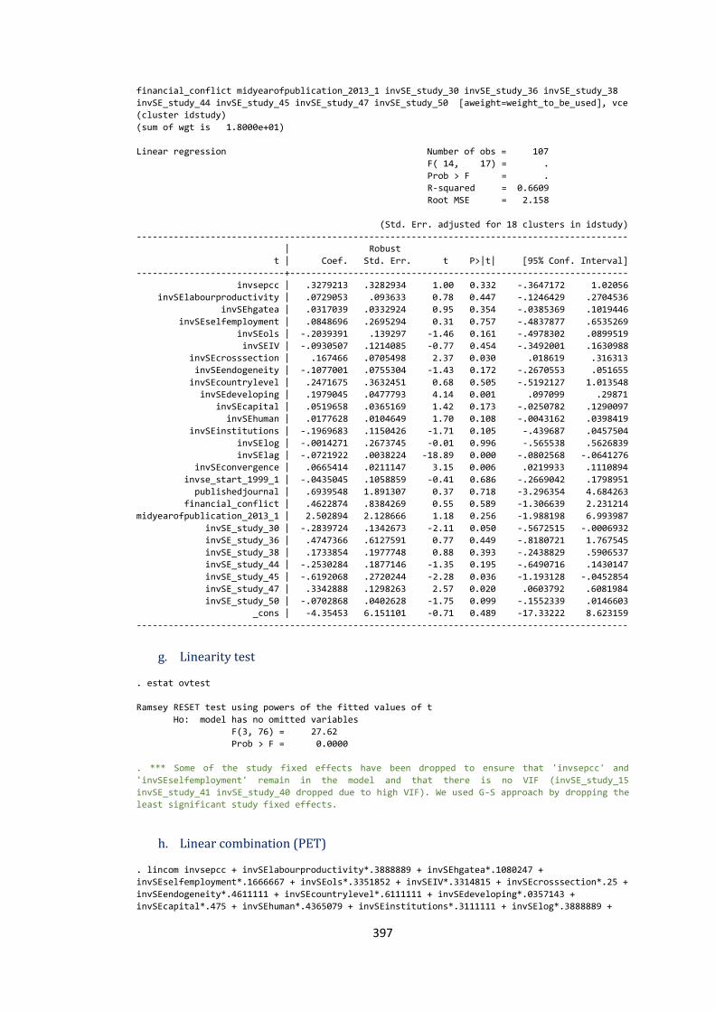
397
financial_conflict midyearofpublication_2013_1 invSE_study_30 invSE_study_36 invSE_study_38
invSE_study_44 invSE_study_45 invSE_study_47 invSE_study_50 [aweight=weight_to_be_used], vce
(cluster idstudy)
(sum of wgt is 1.8000e+01)
Linear regression Number of obs = 107
F( 14, 17) = .
Prob > F = .
R-squared = 0.6609
Root MSE = 2.158
(Std. Err. adjusted for 18 clusters in idstudy)
---------------------------------------------------------------------------------------------
| Robust
t | Coef. Std. Err. t P>|t| [95% Conf. Interval]
----------------------------+----------------------------------------------------------------
invsepcc | .3279213 .3282934 1.00 0.332 -.3647172 1.02056
invSElabourproductivity | .0729053 .093633 0.78 0.447 -.1246429 .2704536
invSEhgatea | .0317039 .0332924 0.95 0.354 -.0385369 .1019446
invSEselfemployment | .0848696 .2695294 0.31 0.757 -.4837877 .6535269
invSEols | -.2039391 .139297 -1.46 0.161 -.4978302 .0899519
invSEIV | -.0930507 .1214085 -0.77 0.454 -.3492001 .1630988
invSEcrosssection | .167466 .0705498 2.37 0.030 .018619 .316313
invSEendogeneity | -.1077001 .0755304 -1.43 0.172 -.2670553 .051655
invSEcountrylevel | .2471675 .3632451 0.68 0.505 -.5192127 1.013548
invSEdeveloping | .1979045 .0477793 4.14 0.001 .097099 .29871
invSEcapital | .0519658 .0365169 1.42 0.173 -.0250782 .1290097
invSEhuman | .0177628 .0104649 1.70 0.108 -.0043162 .0398419
invSEinstitutions | -.1969683 .1150426 -1.71 0.105 -.439687 .0457504
invSElog | -.0014271 .2673745 -0.01 0.996 -.565538 .5626839
invSElag | -.0721922 .0038224 -18.89 0.000 -.0802568 -.0641276
invSEconvergence | .0665414 .0211147 3.15 0.006 .0219933 .1110894
invse_start_1999_1 | -.0435045 .1058859 -0.41 0.686 -.2669042 .1798951
publishedjournal | .6939548 1.891307 0.37 0.718 -3.296354 4.684263
financial_conflict | .4622874 .8384269 0.55 0.589 -1.306639 2.231214
midyearofpublication_2013_1 | 2.502894 2.128666 1.18 0.256 -1.988198 6.993987
invSE_study_30 | -.2839724 .1342673 -2.11 0.050 -.5672515 -.0006932
invSE_study_36 | .4747366 .6127591 0.77 0.449 -.8180721 1.767545
invSE_study_38 | .1733854 .1977748 0.88 0.393 -.2438829 .5906537
invSE_study_44 | -.2530284 .1877146 -1.35 0.195 -.6490716 .1430147
invSE_study_45 | -.6192068 .2720244 -2.28 0.036 -1.193128 -.0452854
invSE_study_47 | .3342888 .1298263 2.57 0.020 .0603792 .6081984
invSE_study_50 | -.0702868 .0402628 -1.75 0.099 -.1552339 .0146603
_cons | -4.35453 6.151101 -0.71 0.489 -17.33222 8.623159
---------------------------------------------------------------------------------------------
g. Linearity test
. estat ovtest
Ramsey RESET test using powers of the fitted values of t
Ho: model has no omitted variables
F(3, 76) = 27.62
Prob > F = 0.0000
. *** Some of the study fixed effects have been dropped to ensure that 'invsepcc' and
'invSEselfemployment' remain in the model and that there is no VIF (invSE_study_15
invSE_study_41 invSE_study_40 dropped due to high VIF). We used G-S approach by dropping the
least significant study fixed effects.
h. Linear combination (PET)
. lincom invsepcc + invSElabourproductivity*.3888889 + invSEhgatea*.1080247 +
invSEselfemployment*.1666667 + invSEols*.3351852 + invSEIV*.3314815 + invSEcrosssection*.25 +
invSEendogeneity*.4611111 + invSEcountrylevel*.6111111 + invSEdeveloping*.0357143 +
invSEcapital*.475 + invSEhuman*.4365079 + invSEinstitutions*.3111111 + invSElog*.3888889 +
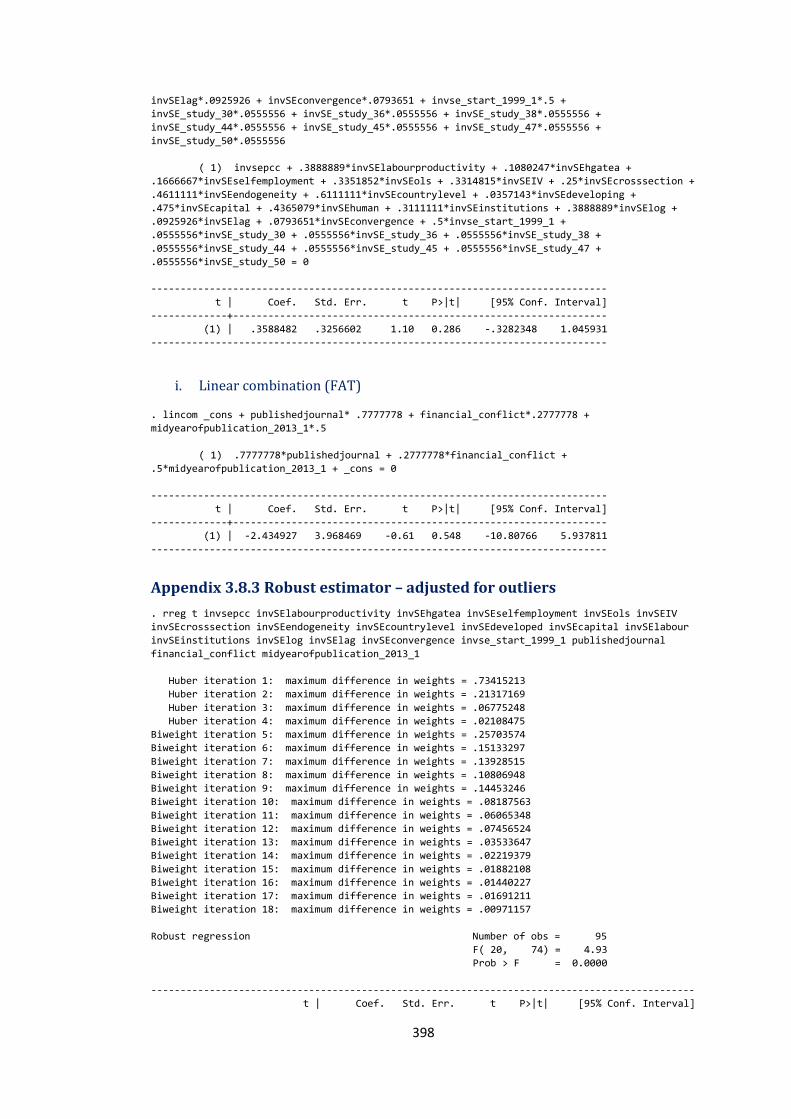
398
invSElag*.0925926 + invSEconvergence*.0793651 + invse_start_1999_1*.5 +
invSE_study_30*.0555556 + invSE_study_36*.0555556 + invSE_study_38*.0555556 +
invSE_study_44*.0555556 + invSE_study_45*.0555556 + invSE_study_47*.0555556 +
invSE_study_50*.0555556
( 1) invsepcc + .3888889*invSElabourproductivity + .1080247*invSEhgatea +
.1666667*invSEselfemployment + .3351852*invSEols + .3314815*invSEIV + .25*invSEcrosssection +
.4611111*invSEendogeneity + .6111111*invSEcountrylevel + .0357143*invSEdeveloping +
.475*invSEcapital + .4365079*invSEhuman + .3111111*invSEinstitutions + .3888889*invSElog +
.0925926*invSElag + .0793651*invSEconvergence + .5*invse_start_1999_1 +
.0555556*invSE_study_30 + .0555556*invSE_study_36 + .0555556*invSE_study_38 +
.0555556*invSE_study_44 + .0555556*invSE_study_45 + .0555556*invSE_study_47 +
.0555556*invSE_study_50 = 0
------------------------------------------------------------------------------
t | Coef. Std. Err. t P>|t| [95% Conf. Interval]
-------------+----------------------------------------------------------------
(1) | .3588482 .3256602 1.10 0.286 -.3282348 1.045931
------------------------------------------------------------------------------
i. Linear combination (FAT)
. lincom _cons + publishedjournal* .7777778 + financial_conflict*.2777778 +
midyearofpublication_2013_1*.5
( 1) .7777778*publishedjournal + .2777778*financial_conflict +
.5*midyearofpublication_2013_1 + _cons = 0
------------------------------------------------------------------------------
t | Coef. Std. Err. t P>|t| [95% Conf. Interval]
-------------+----------------------------------------------------------------
(1) | -2.434927 3.968469 -0.61 0.548 -10.80766 5.937811
------------------------------------------------------------------------------
Appendix 3.8.3 Robust estimator – adjusted for outliers
. rreg t invsepcc invSElabourproductivity invSEhgatea invSEselfemployment invSEols invSEIV
invSEcrosssection invSEendogeneity invSEcountrylevel invSEdeveloped invSEcapital invSElabour
invSEinstitutions invSElog invSElag invSEconvergence invse_start_1999_1 publishedjournal
financial_conflict midyearofpublication_2013_1
Huber iteration 1: maximum difference in weights = .73415213
Huber iteration 2: maximum difference in weights = .21317169
Huber iteration 3: maximum difference in weights = .06775248
Huber iteration 4: maximum difference in weights = .02108475
Biweight iteration 5: maximum difference in weights = .25703574
Biweight iteration 6: maximum difference in weights = .15133297
Biweight iteration 7: maximum difference in weights = .13928515
Biweight iteration 8: maximum difference in weights = .10806948
Biweight iteration 9: maximum difference in weights = .14453246
Biweight iteration 10: maximum difference in weights = .08187563
Biweight iteration 11: maximum difference in weights = .06065348
Biweight iteration 12: maximum difference in weights = .07456524
Biweight iteration 13: maximum difference in weights = .03533647
Biweight iteration 14: maximum difference in weights = .02219379
Biweight iteration 15: maximum difference in weights = .01882108
Biweight iteration 16: maximum difference in weights = .01440227
Biweight iteration 17: maximum difference in weights = .01691211
Biweight iteration 18: maximum difference in weights = .00971157
Robust regression Number of obs = 95
F( 20, 74) = 4.93
Prob > F = 0.0000
---------------------------------------------------------------------------------------------
t | Coef. Std. Err. t P>|t| [95% Conf. Interval]
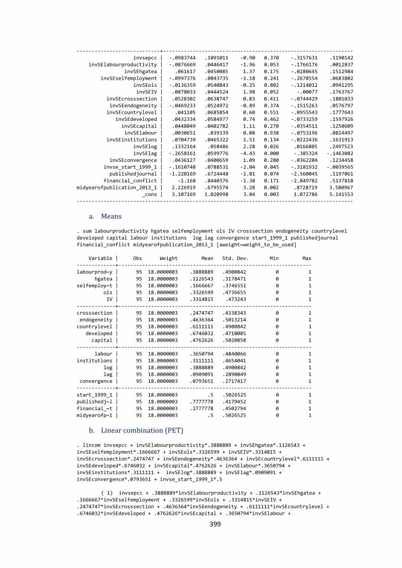
399
----------------------------+----------------------------------------------------------------
invsepcc | -.0983744 .1091011 -0.90 0.370 -.3157631 .1190142
invSElabourproductivity | -.0876669 .0446417 -1.96 0.053 -.1766176 .0012837
invSEhgatea | .061617 .0450085 1.37 0.175 -.0280645 .1512984
invSEselfemployment | -.0997376 .0843735 -1.18 0.241 -.2678554 .0683802
invSEols | -.0136359 .0540843 -0.25 0.802 -.1214012 .0941295
invSEIV | .0878033 .0444524 1.98 0.052 -.00077 .1763767
invSEcrosssection | .0528302 .0638747 0.83 0.411 -.0744429 .1801033
invSEendogeneity | -.0469233 .0524972 -0.89 0.374 -.1515263 .0576797
invSEcountrylevel | .041105 .0685854 0.60 0.551 -.0955543 .1777643
invSEdeveloped | .0432334 .0584977 0.74 0.462 -.0733259 .1597926
invSEcapital | .0448049 .0402782 1.11 0.270 -.0354511 .1250609
invSElabour | .0030651 .039339 0.08 0.938 -.0753196 .0814497
invSEinstitutions | .0704739 .0465322 1.51 0.134 -.0222436 .1631913
invSElog | .1332164 .058486 2.28 0.026 .0166805 .2497523
invSElag | -.2658161 .0599776 -4.43 0.000 -.385324 -.1463082
invSEconvergence | .0436127 .0400659 1.09 0.280 -.0362204 .1234458
invse_start_1999_1 | -.1610748 .0788531 -2.04 0.045 -.3181932 -.0039565
publishedjournal | -1.220169 .6724448 -1.81 0.074 -2.560045 .1197061
financial_conflict | -1.168 .8440376 -1.38 0.171 -2.849782 .5137818
midyearofpublication_2013_1 | 2.226919 .6795574 3.28 0.002 .8728719 3.580967
_cons | 3.107169 1.020998 3.04 0.003 1.072786 5.141553
---------------------------------------------------------------------------------------------
a. Means
. sum labourproductivity hgatea selfemployment ols IV crosssection endogeneity countrylevel
developed capital labour institutions log lag convergence start_1999_1 publishedjournal
financial_conflict midyearofpublication_2013_1 [aweight=weight_to_be_used]
Variable | Obs Weight Mean Std. Dev. Min Max
-------------+-----------------------------------------------------------------
labourprod~y | 95 18.0000003 .3888889 .4900842 0 1
hgatea | 95 18.0000003 .1126543 .3178471 0 1
selfemploy~t | 95 18.0000003 .1666667 .3746551 0 1
ols | 95 18.0000003 .3326599 .4736655 0 1
IV | 95 18.0000003 .3314815 .473243 0 1
-------------+-----------------------------------------------------------------
crosssection | 95 18.0000003 .2474747 .4338343 0 1
endogeneity | 95 18.0000003 .4636364 .5013214 0 1
countrylevel | 95 18.0000003 .6111111 .4900842 0 1
developed | 95 18.0000003 .6746032 .4710085 0 1
capital | 95 18.0000003 .4762626 .5020858 0 1
-------------+-----------------------------------------------------------------
labour | 95 18.0000003 .3650794 .4840066 0 1
institutions | 95 18.0000003 .3111111 .4654041 0 1
log | 95 18.0000003 .3888889 .4900842 0 1
lag | 95 18.0000003 .0909091 .2890049 0 1
convergence | 95 18.0000003 .0793651 .2717417 0 1
-------------+-----------------------------------------------------------------
start_1999_1 | 95 18.0000003 .5 .5026525 0 1
publishedj~l | 95 18.0000003 .7777778 .4179452 0 1
financial_~t | 95 18.0000003 .2777778 .4502794 0 1
midyearofp~1 | 95 18.0000003 .5 .5026525 0 1
b. Linear combination (PET)
. lincom invsepcc + invSElabourproductivity*.3888889 + invSEhgatea*.1126543 +
invSEselfemployment*.1666667 + invSEols*.3326599 + invSEIV*.3314815 +
invSEcrosssection*.2474747 + invSEendogeneity*.4636364 + invSEcountrylevel*.6111111 +
invSEdeveloped*.6746032 + invSEcapital*.4762626 + invSElabour*.3650794 +
invSEinstitutions*.3111111 + invSElog*.3888889 + invSElag*.0909091 +
invSEconvergence*.0793651 + invse_start_1999_1*.5
( 1) invsepcc + .3888889*invSElabourproductivity + .1126543*invSEhgatea +
.1666667*invSEselfemployment + .3326599*invSEols + .3314815*invSEIV +
.2474747*invSEcrosssection + .4636364*invSEendogeneity + .6111111*invSEcountrylevel +
.6746032*invSEdeveloped + .4762626*invSEcapital + .3650794*invSElabour +
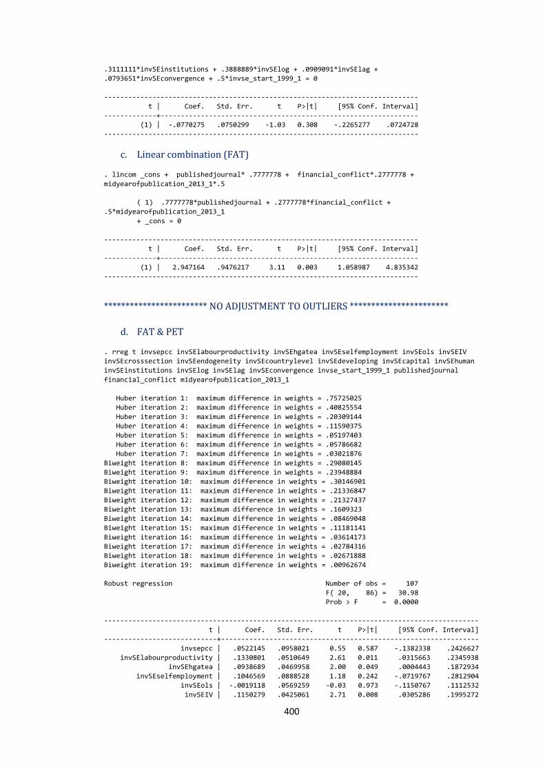
400
.3111111*invSEinstitutions + .3888889*invSElog + .0909091*invSElag +
.0793651*invSEconvergence + .5*invse_start_1999_1 = 0
------------------------------------------------------------------------------
t | Coef. Std. Err. t P>|t| [95% Conf. Interval]
-------------+----------------------------------------------------------------
(1) | -.0770275 .0750299 -1.03 0.308 -.2265277 .0724728
------------------------------------------------------------------------------
c. Linear combination (FAT)
. lincom _cons + publishedjournal* .7777778 + financial_conflict*.2777778 +
midyearofpublication_2013_1*.5
( 1) .7777778*publishedjournal + .2777778*financial_conflict +
.5*midyearofpublication_2013_1
+ _cons = 0
------------------------------------------------------------------------------
t | Coef. Std. Err. t P>|t| [95% Conf. Interval]
-------------+----------------------------------------------------------------
(1) | 2.947164 .9476217 3.11 0.003 1.058987 4.835342
------------------------------------------------------------------------------
************************ NO ADJUSTMENT TO OUTLIERS ***********************
d. FAT & PET
. rreg t invsepcc invSElabourproductivity invSEhgatea invSEselfemployment invSEols invSEIV
invSEcrosssection invSEendogeneity invSEcountrylevel invSEdeveloping invSEcapital invSEhuman
invSEinstitutions invSElog invSElag invSEconvergence invse_start_1999_1 publishedjournal
financial_conflict midyearofpublication_2013_1
Huber iteration 1: maximum difference in weights = .75725025
Huber iteration 2: maximum difference in weights = .40825554
Huber iteration 3: maximum difference in weights = .20309144
Huber iteration 4: maximum difference in weights = .11590375
Huber iteration 5: maximum difference in weights = .05197403
Huber iteration 6: maximum difference in weights = .05786682
Huber iteration 7: maximum difference in weights = .03021876
Biweight iteration 8: maximum difference in weights = .29080145
Biweight iteration 9: maximum difference in weights = .23948884
Biweight iteration 10: maximum difference in weights = .30146901
Biweight iteration 11: maximum difference in weights = .21336847
Biweight iteration 12: maximum difference in weights = .21327437
Biweight iteration 13: maximum difference in weights = .1609323
Biweight iteration 14: maximum difference in weights = .08469048
Biweight iteration 15: maximum difference in weights = .11181141
Biweight iteration 16: maximum difference in weights = .03614173
Biweight iteration 17: maximum difference in weights = .02784316
Biweight iteration 18: maximum difference in weights = .02671888
Biweight iteration 19: maximum difference in weights = .00962674
Robust regression Number of obs = 107
F( 20, 86) = 30.98
Prob > F = 0.0000
---------------------------------------------------------------------------------------------
t | Coef. Std. Err. t P>|t| [95% Conf. Interval]
----------------------------+----------------------------------------------------------------
invsepcc | .0522145 .0958021 0.55 0.587 -.1382338 .2426627
invSElabourproductivity | .1330801 .0510649 2.61 0.011 .0315663 .2345938
invSEhgatea | .0938689 .0469958 2.00 0.049 .0004443 .1872934
invSEselfemployment | .1046569 .0888528 1.18 0.242 -.0719767 .2812904
invSEols | -.0019118 .0569259 -0.03 0.973 -.1150767 .1112532
invSEIV | .1150279 .0425061 2.71 0.008 .0305286 .1995272

401
invSEcrosssection | -.0127404 .0762394 -0.17 0.868 -.1642994 .1388186
invSEendogeneity | -.0589897 .0550379 -1.07 0.287 -.1684015 .0504221
invSEcountrylevel | -.1508314 .0747804 -2.02 0.047 -.29949 -.0021729
invSEdeveloping | .177471 .0651297 2.72 0.008 .0479975 .3069445
invSEcapital | .0569732 .0414032 1.38 0.172 -.0253335 .13928
invSEhuman | .0514715 .0529737 0.97 0.334 -.0538368 .1567799
invSEinstitutions | .0674092 .0358675 1.88 0.064 -.0038931 .1387114
invSElog | .1526169 .0553689 2.76 0.007 .0425471 .2626866
invSElag | .1922743 .0584962 3.29 0.001 .0759876 .3085609
invSEconvergence | .0819286 .0450946 1.82 0.073 -.0077165 .1715738
invse_start_1999_1 | -.3544757 .0800919 -4.43 0.000 -.5136932 -.1952583
publishedjournal | -1.090522 .6392562 -1.71 0.092 -2.361321 .1802775
financial_conflict | .2650769 .7996344 0.33 0.741 -1.324544 1.854697
midyearofpublication_2013_1 | 1.396121 .6545363 2.13 0.036 .0949463 2.697297
_cons | 1.547017 1.048638 1.48 0.144 -.5376058 3.63164
---------------------------------------------------------------------------------------------
e. Linear combination (PET)
. lincom invsepcc + invSElabourproductivity*.3888889 + invSEhgatea*.1080247 +
invSEselfemployment*.1666667 + invSEols*.3351852 + invSEIV*.3314815 + invSEcrosssection*.25 +
invSEendogeneity*.4611111 + invSEcountrylevel*.6111111 + invSEdeveloping*.0357143 +
invSEcapital*.475 + invSEhuman*.4365079 + invSEinstitutions*.3111111 + invSElog*.3888889 +
invSElag*.0925926 + invSEconvergence*.0793651 + invse_start_1999_1*.5
( 1) invsepcc + .3888889*invSElabourproductivity + .1080247*invSEhgatea +
.1666667*invSEselfemployment + .3351852*invSEols + .3314815*invSEIV +
.25*invSEcrosssection + .4611111*invSEendogeneity + .6111111*invSEcountrylevel +
.0357143*invSEdeveloping + .475*invSEcapital + .4365079*invSEhuman +
.3111111*invSEinstitutions + .3888889*invSElog + .0925926*invSElag +
.0793651*invSEconvergence + 5*invse_start_1999_1 = 0
------------------------------------------------------------------------------
t | Coef. Std. Err. t P>|t| [95% Conf. Interval]
-------------+----------------------------------------------------------------
(1) | .0297376 .0712228 0.42 0.677 -.1118487 .1713239
------------------------------------------------------------------------------
f. Linear combination (FAT)
. lincom _cons + publishedjournal* .7777778 + financial_conflict*.2777778 +
midyearofpublication_2013_1*.5
( 1) .7777778*publishedjournal + .2777778*financial_conflict +
.5*midyearofpublication_2013_1 + _cons = 0
------------------------------------------------------------------------------
t | Coef. Std. Err. t P>|t| [95% Conf. Interval]
-------------+----------------------------------------------------------------
(1) | 1.470526 .9154668 1.61 0.112 -.3493614 3.290414
------------------------------------------------------------------------------
Appendix 3.8.4 Bayesian Model Averaging (BMA)
. bma weight_to_be_used_t (sqrt_weight_to_be_used weight_to_be_used_invsepcc), auxiliary (
weight_to_be_used_invSElab_pro weight_to_be_used_invSEhgatea weight_to_be_used_invSEselfempl
weight_to_be_used_invSEols weight_to_be_used_invSEIV weight_to_be_used_invSEcr_sect
weight_to_be_used_invSEendogen weight_to_be_used_invSEcount_lev
weight_to_be_used_invSEdev_ped weight_to_be_used_invSEcapital weight_to_be_used_invSElabour
weight_to_be_used_invSEinstitut weight_to_be_used_invSElog weight_to_be_used_invSElag
weight_to_be_used_invSEconver weight_to_be_used_invSEst_1999_1 weight_to_be_used_pub_jour
weight_to_be_used_fin_conflict weight_to_be_used_mid_py_2013_1 ) noconstant
Model space: 524288 models
Estimation
----+-- 10% --+-- 20% --+-- 30% --+-- 40% --+-- 50%
.................................................. 50%
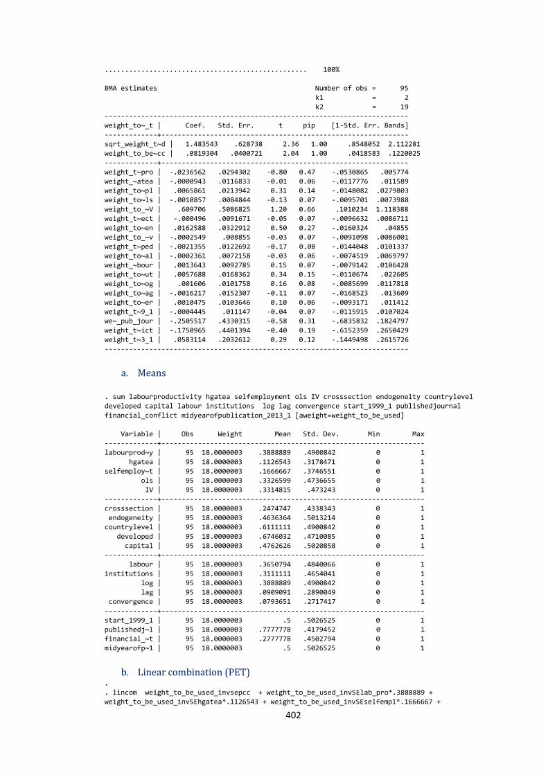
402
.................................................. 100%
BMA estimates Number of obs = 95
k1 = 2
k2 = 19
---------------------------------------------------------------------------
weight_to~_t | Coef. Std. Err. t pip [1-Std. Err. Bands]
-------------+-------------------------------------------------------------
sqrt_weight_t~d | 1.483543 .628738 2.36 1.00 .8548052 2.112281
weight_to_be~cc | .0819304 .0400721 2.04 1.00 .0418583 .1220025
-------------+-------------------------------------------------------------
weight_t~pro | -.0236562 .0294302 -0.80 0.47 -.0530865 .005774
weight_~atea | -.0000943 .0116833 -0.01 0.06 -.0117776 .011589
weight_to~pl | .0065861 .0213942 0.31 0.14 -.0148082 .0279803
weight_to~ls | -.0010857 .0084844 -0.13 0.07 -.0095701 .0073988
weight_to_~V | .609706 .5086825 1.20 0.66 .1010234 1.118388
weight_t~ect | -.000496 .0091671 -0.05 0.07 -.0096632 .0086711
weight_to~en | .0162588 .0322912 0.50 0.27 -.0160324 .04855
weight_to_~v | -.0002549 .008855 -0.03 0.07 -.0091098 .0086001
weight_t~ped | -.0021355 .0122692 -0.17 0.08 -.0144048 .0101337
weight_to~al | -.0002361 .0072158 -0.03 0.06 -.0074519 .0069797
weight_~bour | .0013643 .0092785 0.15 0.07 -.0079142 .0106428
weight_to~ut | .0057688 .0168362 0.34 0.15 -.0110674 .022605
weight_to~og | .001606 .0101758 0.16 0.08 -.0085699 .0117818
weight_to~ag | -.0016217 .0152307 -0.11 0.07 -.0168523 .013609
weight_to~er | .0010475 .0103646 0.10 0.06 -.0093171 .011412
weight_t~9_1 | -.0004445 .011147 -0.04 0.07 -.0115915 .0107024
we~_pub_jour | -.2505517 .4330315 -0.58 0.31 -.6835832 .1824797
weight_t~ict | -.1750965 .4401394 -0.40 0.19 -.6152359 .2650429
weight_t~3_1 | .0583114 .2032612 0.29 0.12 -.1449498 .2615726
---------------------------------------------------------------------------
a. Means . sum labourproductivity hgatea selfemployment ols IV crosssection endogeneity countrylevel
developed capital labour institutions log lag convergence start_1999_1 publishedjournal
financial_conflict midyearofpublication_2013_1 [aweight=weight_to_be_used]
Variable | Obs Weight Mean Std. Dev. Min Max
-------------+-----------------------------------------------------------------
labourprod~y | 95 18.0000003 .3888889 .4900842 0 1
hgatea | 95 18.0000003 .1126543 .3178471 0 1
selfemploy~t | 95 18.0000003 .1666667 .3746551 0 1
ols | 95 18.0000003 .3326599 .4736655 0 1
IV | 95 18.0000003 .3314815 .473243 0 1
-------------+-----------------------------------------------------------------
crosssection | 95 18.0000003 .2474747 .4338343 0 1
endogeneity | 95 18.0000003 .4636364 .5013214 0 1
countrylevel | 95 18.0000003 .6111111 .4900842 0 1
developed | 95 18.0000003 .6746032 .4710085 0 1
capital | 95 18.0000003 .4762626 .5020858 0 1
-------------+-----------------------------------------------------------------
labour | 95 18.0000003 .3650794 .4840066 0 1
institutions | 95 18.0000003 .3111111 .4654041 0 1
log | 95 18.0000003 .3888889 .4900842 0 1
lag | 95 18.0000003 .0909091 .2890049 0 1
convergence | 95 18.0000003 .0793651 .2717417 0 1
-------------+-----------------------------------------------------------------
start_1999_1 | 95 18.0000003 .5 .5026525 0 1
publishedj~l | 95 18.0000003 .7777778 .4179452 0 1
financial_~t | 95 18.0000003 .2777778 .4502794 0 1
midyearofp~1 | 95 18.0000003 .5 .5026525 0 1
b. Linear combination (PET) .
. lincom weight_to_be_used_invsepcc + weight_to_be_used_invSElab_pro*.3888889 +
weight_to_be_used_invSEhgatea*.1126543 + weight_to_be_used_invSEselfempl*.1666667 +
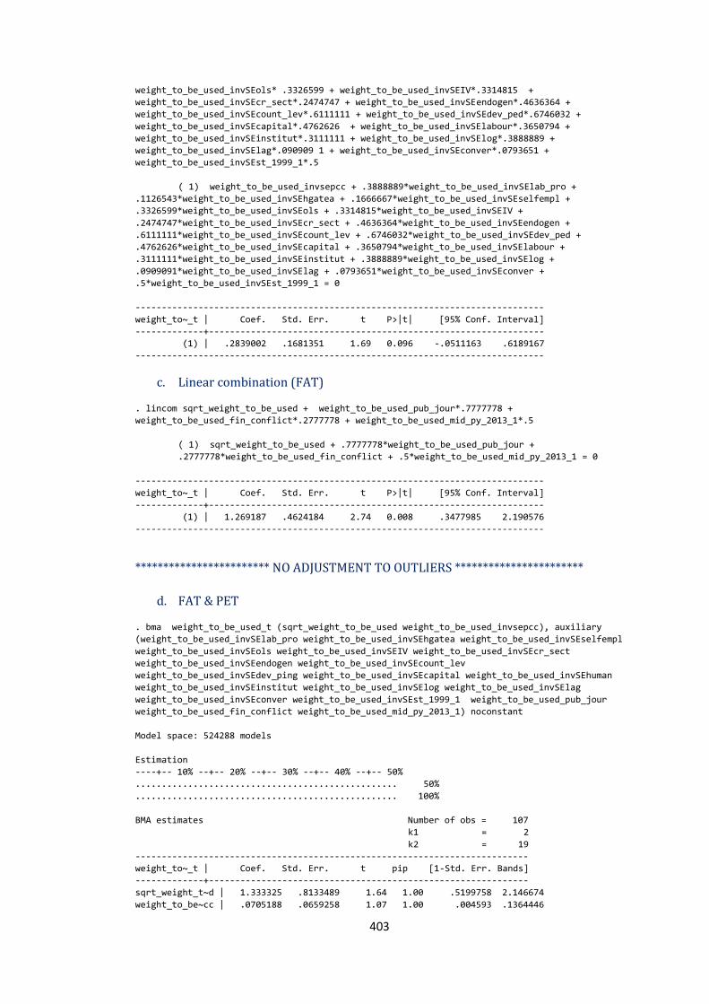
403
weight_to_be_used_invSEols* .3326599 + weight_to_be_used_invSEIV*.3314815 +
weight_to_be_used_invSEcr_sect*.2474747 + weight_to_be_used_invSEendogen*.4636364 +
weight_to_be_used_invSEcount_lev*.6111111 + weight_to_be_used_invSEdev_ped*.6746032 +
weight_to_be_used_invSEcapital*.4762626 + weight_to_be_used_invSElabour*.3650794 +
weight_to_be_used_invSEinstitut*.3111111 + weight_to_be_used_invSElog*.3888889 +
weight_to_be_used_invSElag*.090909 1 + weight_to_be_used_invSEconver*.0793651 +
weight_to_be_used_invSEst_1999_1*.5
( 1) weight_to_be_used_invsepcc + .3888889*weight_to_be_used_invSElab_pro +
.1126543*weight_to_be_used_invSEhgatea + .1666667*weight_to_be_used_invSEselfempl +
.3326599*weight_to_be_used_invSEols + .3314815*weight_to_be_used_invSEIV +
.2474747*weight_to_be_used_invSEcr_sect + .4636364*weight_to_be_used_invSEendogen +
.6111111*weight_to_be_used_invSEcount_lev + .6746032*weight_to_be_used_invSEdev_ped +
.4762626*weight_to_be_used_invSEcapital + .3650794*weight_to_be_used_invSElabour +
.3111111*weight_to_be_used_invSEinstitut + .3888889*weight_to_be_used_invSElog +
.0909091*weight_to_be_used_invSElag + .0793651*weight_to_be_used_invSEconver +
.5*weight_to_be_used_invSEst_1999_1 = 0
------------------------------------------------------------------------------
weight_to~_t | Coef. Std. Err. t P>|t| [95% Conf. Interval]
-------------+----------------------------------------------------------------
(1) | .2839002 .1681351 1.69 0.096 -.0511163 .6189167
------------------------------------------------------------------------------
c. Linear combination (FAT)
. lincom sqrt_weight_to_be_used + weight_to_be_used_pub_jour*.7777778 +
weight_to_be_used_fin_conflict*.2777778 + weight_to_be_used_mid_py_2013_1*.5
( 1) sqrt_weight_to_be_used + .7777778*weight_to_be_used_pub_jour +
.2777778*weight_to_be_used_fin_conflict + .5*weight_to_be_used_mid_py_2013_1 = 0
------------------------------------------------------------------------------
weight_to~_t | Coef. Std. Err. t P>|t| [95% Conf. Interval]
-------------+----------------------------------------------------------------
(1) | 1.269187 .4624184 2.74 0.008 .3477985 2.190576
------------------------------------------------------------------------------
************************ NO ADJUSTMENT TO OUTLIERS ***********************
d. FAT & PET
. bma weight_to_be_used_t (sqrt_weight_to_be_used weight_to_be_used_invsepcc), auxiliary
(weight_to_be_used_invSElab_pro weight_to_be_used_invSEhgatea weight_to_be_used_invSEselfempl
weight_to_be_used_invSEols weight_to_be_used_invSEIV weight_to_be_used_invSEcr_sect
weight_to_be_used_invSEendogen weight_to_be_used_invSEcount_lev
weight_to_be_used_invSEdev_ping weight_to_be_used_invSEcapital weight_to_be_used_invSEhuman
weight_to_be_used_invSEinstitut weight_to_be_used_invSElog weight_to_be_used_invSElag
weight_to_be_used_invSEconver weight_to_be_used_invSEst_1999_1 weight_to_be_used_pub_jour
weight_to_be_used_fin_conflict weight_to_be_used_mid_py_2013_1) noconstant
Model space: 524288 models
Estimation
----+-- 10% --+-- 20% --+-- 30% --+-- 40% --+-- 50%
.................................................. 50%
.................................................. 100%
BMA estimates Number of obs = 107
k1 = 2
k2 = 19
---------------------------------------------------------------------------
weight_to~_t | Coef. Std. Err. t pip [1-Std. Err. Bands]
-------------+-------------------------------------------------------------
sqrt_weight_t~d | 1.333325 .8133489 1.64 1.00 .5199758 2.146674
weight_to_be~cc | .0705188 .0659258 1.07 1.00 .004593 .1364446
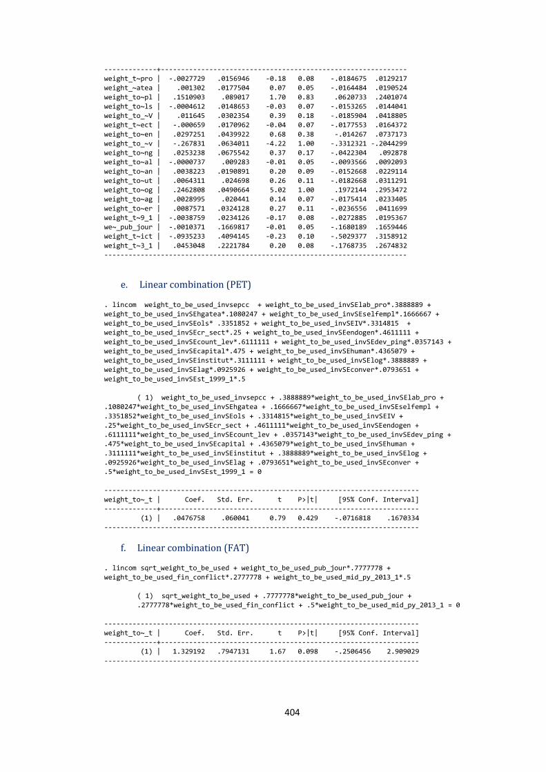
404
-------------+-------------------------------------------------------------
weight_t~pro | -.0027729 .0156946 -0.18 0.08 -.0184675 .0129217
weight_~atea | .001302 .0177504 0.07 0.05 -.0164484 .0190524
weight_to~pl | .1510903 .089017 1.70 0.83 .0620733 .2401074
weight_to~ls | -.0004612 .0148653 -0.03 0.07 -.0153265 .0144041
weight_to_~V | .011645 .0302354 0.39 0.18 -.0185904 .0418805
weight_t~ect | -.000659 .0170962 -0.04 0.07 -.0177553 .0164372
weight_to~en | .0297251 .0439922 0.68 0.38 -.014267 .0737173
weight_to_~v | -.267831 .0634011 -4.22 1.00 -.3312321 -.2044299
weight_to~ng | .0253238 .0675542 0.37 0.17 -.0422304 .092878
weight_to~al | -.0000737 .009283 -0.01 0.05 -.0093566 .0092093
weight_to~an | .0038223 .0190891 0.20 0.09 -.0152668 .0229114
weight_to~ut | .0064311 .024698 0.26 0.11 -.0182668 .0311291
weight_to~og | .2462808 .0490664 5.02 1.00 .1972144 .2953472
weight_to~ag | .0028995 .020441 0.14 0.07 -.0175414 .0233405
weight_to~er | .0087571 .0324128 0.27 0.11 -.0236556 .0411699
weight_t~9_1 | -.0038759 .0234126 -0.17 0.08 -.0272885 .0195367
we~_pub_jour | -.0010371 .1669817 -0.01 0.05 -.1680189 .1659446
weight_t~ict | -.0935233 .4094145 -0.23 0.10 -.5029377 .3158912
weight_t~3_1 | .0453048 .2221784 0.20 0.08 -.1768735 .2674832
---------------------------------------------------------------------------
e. Linear combination (PET)
. lincom weight_to_be_used_invsepcc + weight_to_be_used_invSElab_pro*.3888889 +
weight_to_be_used_invSEhgatea*.1080247 + weight_to_be_used_invSEselfempl*.1666667 +
weight_to_be_used_invSEols* .3351852 + weight_to_be_used_invSEIV*.3314815 +
weight_to_be_used_invSEcr_sect*.25 + weight_to_be_used_invSEendogen*.4611111 +
weight_to_be_used_invSEcount_lev*.6111111 + weight_to_be_used_invSEdev_ping*.0357143 +
weight_to_be_used_invSEcapital*.475 + weight_to_be_used_invSEhuman*.4365079 +
weight_to_be_used_invSEinstitut*.3111111 + weight_to_be_used_invSElog*.3888889 +
weight_to_be_used_invSElag*.0925926 + weight_to_be_used_invSEconver*.0793651 +
weight_to_be_used_invSEst_1999_1*.5
( 1) weight_to_be_used_invsepcc + .3888889*weight_to_be_used_invSElab_pro +
.1080247*weight_to_be_used_invSEhgatea + .1666667*weight_to_be_used_invSEselfempl +
.3351852*weight_to_be_used_invSEols + .3314815*weight_to_be_used_invSEIV +
.25*weight_to_be_used_invSEcr_sect + .4611111*weight_to_be_used_invSEendogen +
.6111111*weight_to_be_used_invSEcount_lev + .0357143*weight_to_be_used_invSEdev_ping +
.475*weight_to_be_used_invSEcapital + .4365079*weight_to_be_used_invSEhuman +
.3111111*weight_to_be_used_invSEinstitut + .3888889*weight_to_be_used_invSElog +
.0925926*weight_to_be_used_invSElag + .0793651*weight_to_be_used_invSEconver +
.5*weight_to_be_used_invSEst_1999_1 = 0
------------------------------------------------------------------------------
weight_to~_t | Coef. Std. Err. t P>|t| [95% Conf. Interval]
-------------+----------------------------------------------------------------
(1) | .0476758 .060041 0.79 0.429 -.0716818 .1670334
------------------------------------------------------------------------------
f. Linear combination (FAT)
. lincom sqrt_weight_to_be_used + weight_to_be_used_pub_jour*.7777778 +
weight_to_be_used_fin_conflict*.2777778 + weight_to_be_used_mid_py_2013_1*.5
( 1) sqrt_weight_to_be_used + .7777778*weight_to_be_used_pub_jour +
.2777778*weight_to_be_used_fin_conflict + .5*weight_to_be_used_mid_py_2013_1 = 0
------------------------------------------------------------------------------
weight_to~_t | Coef. Std. Err. t P>|t| [95% Conf. Interval]
-------------+----------------------------------------------------------------
(1) | 1.329192 .7947131 1.67 0.098 -.2506456 2.909029
------------------------------------------------------------------------------
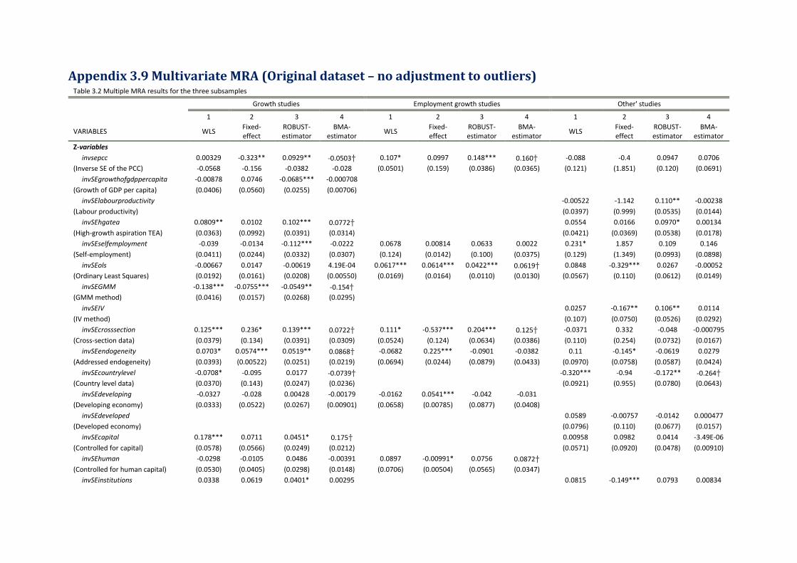
Appendix 3.9 Multivariate MRA (Original dataset – no adjustment to outliers) Table 3.2 Multiple MRA results for the three subsamples
Growth studies Employment growth studies Other' studies
1 2 3 4 1 2 3 4 1 2 3 4
VARIABLES WLS Fixed-effect
ROBUST-estimator
BMA-estimator
WLS Fixed-effect
ROBUST-estimator
BMA-estimator
WLS Fixed-effect
ROBUST-estimator
BMA-estimator
Z-variables
invsepcc 0.00329 -0.323** 0.0929** -0.0503† 0.107* 0.0997 0.148*** 0.160† -0.088 -0.4 0.0947 0.0706
(Inverse SE of the PCC) -0.0568 -0.156 -0.0382 -0.028 (0.0501) (0.159) (0.0386) (0.0365) (0.121) (1.851) (0.120) (0.0691)
invSEgrowthofgdppercapita -0.00878 0.0746 -0.0685*** -0.000708 (Growth of GDP per capita) (0.0406) (0.0560) (0.0255) (0.00706) invSElabourproductivity
-0.00522 -1.142 0.110** -0.00238
(Labour productivity) (0.0397) (0.999) (0.0535) (0.0144)
invSEhgatea 0.0809** 0.0102 0.102*** 0.0772† 0.0554 0.0166 0.0970* 0.00134
(High-growth aspiration TEA) (0.0363) (0.0992) (0.0391) (0.0314) (0.0421) (0.0369) (0.0538) (0.0178)
invSEselfemployment -0.039 -0.0134 -0.112*** -0.0222 0.0678 0.00814 0.0633 0.0022 0.231* 1.857 0.109 0.146
(Self-employment) (0.0411) (0.0244) (0.0332) (0.0307) (0.124) (0.0142) (0.100) (0.0375) (0.129) (1.349) (0.0993) (0.0898)
invSEols -0.00667 0.0147 -0.00619 4.19E-04 0.0617*** 0.0614*** 0.0422*** 0.0619† 0.0848 -0.329*** 0.0267 -0.00052
(Ordinary Least Squares) (0.0192) (0.0161) (0.0208) (0.00550) (0.0169) (0.0164) (0.0110) (0.0130) (0.0567) (0.110) (0.0612) (0.0149)
invSEGMM -0.138*** -0.0755*** -0.0549** -0.154† (GMM method) (0.0416) (0.0157) (0.0268) (0.0295) invSEIV
0.0257 -0.167** 0.106** 0.0114
(IV method) (0.107) (0.0750) (0.0526) (0.0292)
invSEcrosssection 0.125*** 0.236* 0.139*** 0.0722† 0.111* -0.537*** 0.204*** 0.125† -0.0371 0.332 -0.048 -0.000795
(Cross-section data) (0.0379) (0.134) (0.0391) (0.0309) (0.0524) (0.124) (0.0634) (0.0386) (0.110) (0.254) (0.0732) (0.0167)
invSEendogeneity 0.0703* 0.0574*** 0.0519** 0.0868† -0.0682 0.225*** -0.0901 -0.0382 0.11 -0.145* -0.0619 0.0279
(Addressed endogeneity) (0.0393) (0.00522) (0.0251) (0.0219) (0.0694) (0.0244) (0.0879) (0.0433) (0.0970) (0.0758) (0.0587) (0.0424)
invSEcountrylevel -0.0708* -0.095 0.0177 -0.0739† -0.320*** -0.94 -0.172** -0.264†
(Country level data) (0.0370) (0.143) (0.0247) (0.0236) (0.0921) (0.955) (0.0780) (0.0643)
invSEdeveloping -0.0327 -0.028 0.00428 -0.00179 -0.0162 0.0541*** -0.042 -0.031 (Developing economy) (0.0333) (0.0522) (0.0267) (0.00901) (0.0658) (0.00785) (0.0877) (0.0408) invSEdeveloped 0.0589 -0.00757 -0.0142 0.000477
(Developed economy) (0.0796) (0.110) (0.0677) (0.0157)
invSEcapital 0.178*** 0.0711 0.0451* 0.175† 0.00958 0.0982 0.0414 -3.49E-06
(Controlled for capital) (0.0578) (0.0566) (0.0249) (0.0212) (0.0571) (0.0920) (0.0478) (0.00910)
invSEhuman -0.0298 -0.0105 0.0486 -0.00391 0.0897 -0.00991* 0.0756 0.0872† (Controlled for human capital) (0.0530) (0.0405) (0.0298) (0.0148) (0.0706) (0.00504) (0.0565) (0.0347) invSEinstitutions 0.0338 0.0619 0.0401* 0.00295 0.0815 -0.149*** 0.0793 0.00834
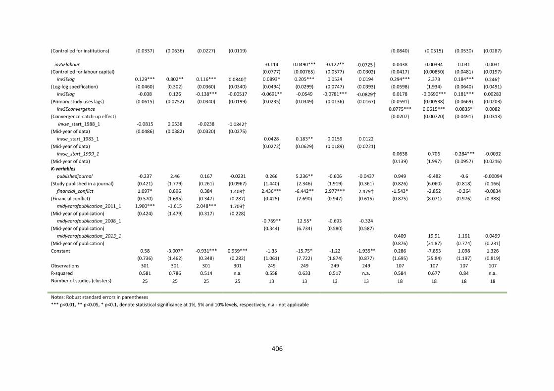
406
(Controlled for institutions) (0.0337) (0.0636) (0.0227) (0.0119) (0.0840) (0.0515) (0.0530) (0.0287)
invSElabour
-0.114
0.0490***
-0.122**
-0.0725†
0.0438
0.00394
0.031
0.0031
(Controlled for labour capital) (0.0777) (0.00765) (0.0577) (0.0302) (0.0417) (0.00850) (0.0481) (0.0197)
invSElog 0.129*** 0.802** 0.116*** 0.0840† 0.0893* 0.205*** 0.0524 0.0194 0.294*** 2.373 0.184*** 0.246†
(Log-log specification) (0.0460) (0.302) (0.0360) (0.0340) (0.0494) (0.0299) (0.0747) (0.0393) (0.0598) (1.934) (0.0640) (0.0491)
invSElag -0.038 0.126 -0.138*** -0.00517 -0.0691** -0.0549 -0.0781*** -0.0829† 0.0178 -0.0690*** 0.181*** 0.00283
(Primary study uses lags) (0.0615) (0.0752) (0.0340) (0.0199) (0.0235) (0.0349) (0.0136) (0.0167) (0.0591) (0.00538) (0.0669) (0.0203)
invSEconvergence 0.0775*** 0.0615*** 0.0835* 0.0082
(Convergence-catch-up effect) (0.0207) (0.00720) (0.0491) (0.0313)
invse_start_1988_1 -0.0815 0.0538 -0.0238 -0.0842† (Mid-year of data) (0.0486) (0.0382) (0.0320) (0.0275) invse_start_1983_1 0.0428 0.183** 0.0159 0.0122
(Mid-year of data) (0.0272) (0.0629) (0.0189) (0.0221)
invse_start_1999_1 0.0638 0.706 -0.284*** -0.0032
(Mid-year of data) (0.139) (1.997) (0.0957) (0.0216)
K-variables
publishedjournal -0.237 2.46 0.167 -0.0231 0.266 5.236** -0.606 -0.0437 0.949 -9.482 -0.6 -0.00094
(Study published in a journal) (0.421) (1.779) (0.261) (0.0967) (1.440) (2.346) (1.919) (0.361) (0.826) (6.060) (0.818) (0.166)
financial_conflict 1.097* 0.896 0.384 1.408† 2.436*** -6.442** 2.977*** 2.479† -1.543* -2.852 -0.264 -0.0834
(Financial conflict) (0.570) (1.695) (0.347) (0.287) (0.425) (2.690) (0.947) (0.615) (0.875) (8.071) (0.976) (0.388)
midyearofpublication_2011_1 1.900*** -1.615 2.048*** 1.709† (Mid-year of publication) (0.424) (1.479) (0.317) (0.228) midyearofpublication_2008_1 -0.769** 12.55* -0.693 -0.324 (Mid-year of publication) (0.344) (6.734) (0.580) (0.587) midyearofpublication_2013_1 0.409 19.91 1.161 0.0499
(Mid-year of publication) (0.876) (31.87) (0.774) (0.231)
Constant 0.58 -3.007* -0.931*** 0.959*** -1.35 -15.75* -1.22 -1.935** 0.286 -7.853 1.098 1.326
(0.736) (1.462) (0.348) (0.282) (1.061) (7.722) (1.874) (0.877) (1.695) (35.84) (1.197) (0.819)
Observations 301 301 301 301 249 249 249 249 107 107 107 107
R-squared 0.581 0.786 0.514 n.a. 0.558 0.633 0.517 n.a. 0.584 0.677 0.84 n.a.
Number of studies (clusters) 25 25 25 25 13 13 13 13 18 18 18 18
Notes: Robust standard errors in parentheses *** p<0.01, ** p<0.05, * p<0.1, denote statistical significance at 1%, 5% and 10% levels, respectively, n.a.- not applicable
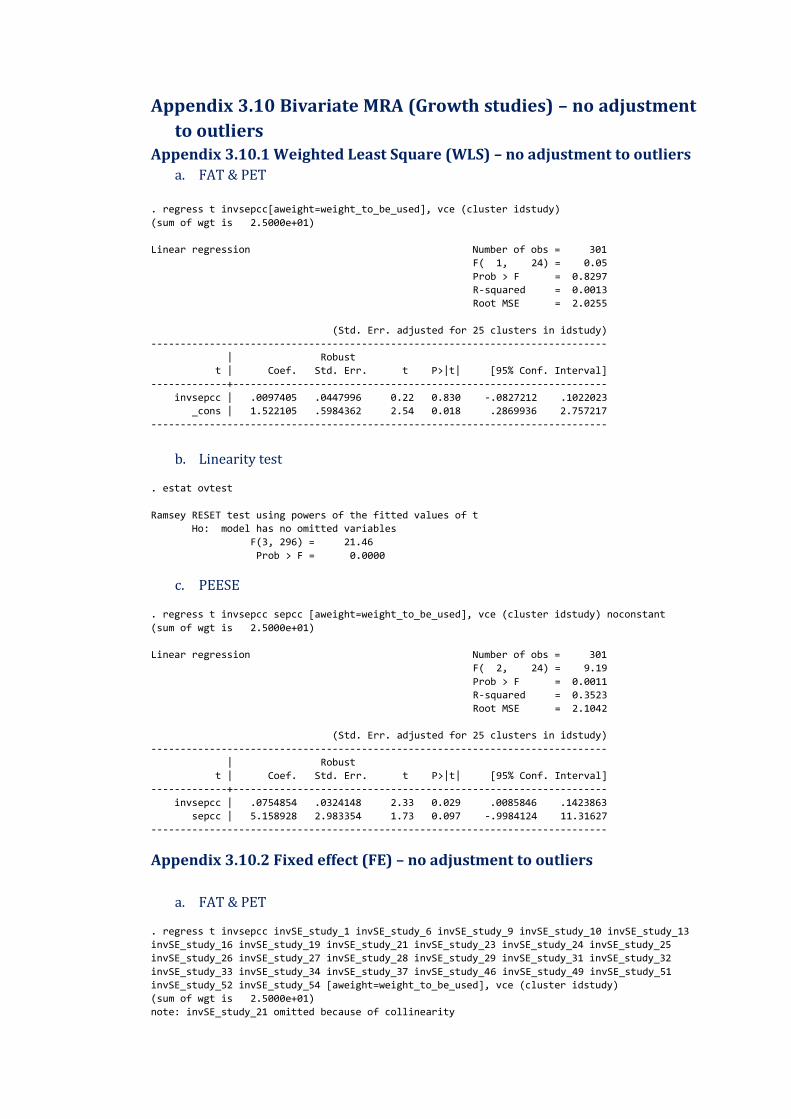
Appendix 3.10 Bivariate MRA (Growth studies) – no adjustment
to outliers Appendix 3.10.1 Weighted Least Square (WLS) – no adjustment to outliers
a. FAT & PET
. regress t invsepcc[aweight=weight_to_be_used], vce (cluster idstudy)
(sum of wgt is 2.5000e+01)
Linear regression Number of obs = 301
F( 1, 24) = 0.05
Prob > F = 0.8297
R-squared = 0.0013
Root MSE = 2.0255
(Std. Err. adjusted for 25 clusters in idstudy)
------------------------------------------------------------------------------
| Robust
t | Coef. Std. Err. t P>|t| [95% Conf. Interval]
-------------+----------------------------------------------------------------
invsepcc | .0097405 .0447996 0.22 0.830 -.0827212 .1022023
_cons | 1.522105 .5984362 2.54 0.018 .2869936 2.757217
------------------------------------------------------------------------------
b. Linearity test
. estat ovtest
Ramsey RESET test using powers of the fitted values of t
Ho: model has no omitted variables
F(3, 296) = 21.46
Prob > F = 0.0000
c. PEESE
. regress t invsepcc sepcc [aweight=weight_to_be_used], vce (cluster idstudy) noconstant
(sum of wgt is 2.5000e+01)
Linear regression Number of obs = 301
F( 2, 24) = 9.19
Prob > F = 0.0011
R-squared = 0.3523
Root MSE = 2.1042
(Std. Err. adjusted for 25 clusters in idstudy)
------------------------------------------------------------------------------
| Robust
t | Coef. Std. Err. t P>|t| [95% Conf. Interval]
-------------+----------------------------------------------------------------
invsepcc | .0754854 .0324148 2.33 0.029 .0085846 .1423863
sepcc | 5.158928 2.983354 1.73 0.097 -.9984124 11.31627
------------------------------------------------------------------------------
Appendix 3.10.2 Fixed effect (FE) – no adjustment to outliers
a. FAT & PET
. regress t invsepcc invSE_study_1 invSE_study_6 invSE_study_9 invSE_study_10 invSE_study_13
invSE_study_16 invSE_study_19 invSE_study_21 invSE_study_23 invSE_study_24 invSE_study_25
invSE_study_26 invSE_study_27 invSE_study_28 invSE_study_29 invSE_study_31 invSE_study_32
invSE_study_33 invSE_study_34 invSE_study_37 invSE_study_46 invSE_study_49 invSE_study_51
invSE_study_52 invSE_study_54 [aweight=weight_to_be_used], vce (cluster idstudy)
(sum of wgt is 2.5000e+01)
note: invSE_study_21 omitted because of collinearity

408
Linear regression Number of obs = 301
F( 0, 24) = .
Prob > F = .
R-squared = 0.7615
Root MSE = 1.032
(Std. Err. adjusted for 25 clusters in idstudy)
--------------------------------------------------------------------------------
| Robust
t | Coef. Std. Err. t P>|t| [95% Conf. Interval]
---------------+----------------------------------------------------------------
invsepcc | .3228306 .133713 2.41 0.024 .0468606 .5988007
invSE_study_1 | -.3602341 .1038362 -3.47 0.002 -.5745415 -.1459267
invSE_study_6 | .3292156 .0391381 8.41 0.000 .2484384 .4099927
invSE_study_9 | -.3245139 .0593537 -5.47 0.000 -.447014 -.2020138
invSE_study_10 | -.1674079 .0032672 -51.24 0.000 -.1741511 -.1606647
invSE_study_13 | -.2202185 .1094816 -2.01 0.056 -.4461775 .0057404
invSE_study_16 | .0421774 .0799818 0.53 0.603 -.1228969 .2072517
invSE_study_19 | -.2140485 .1078805 -1.98 0.059 -.436703 .0086059
invSE_study_21 | 0 (omitted)
invSE_study_23 | -.1830271 .0629241 -2.91 0.008 -.3128962 -.053158
invSE_study_24 | .2204226 .0050951 43.26 0.000 .209907 .2309383
invSE_study_25 | .1169315 .0125859 9.29 0.000 .0909555 .1429076
invSE_study_26 | -.0669468 .0050761 -13.19 0.000 -.0774232 -.0564703
invSE_study_27 | -.2019354 .0841007 -2.40 0.024 -.3755107 -.0283602
invSE_study_28 | -.016475 .0541456 -0.30 0.764 -.128226 .0952761
invSE_study_29 | -.2409001 .0909018 -2.65 0.014 -.4285123 -.0532879
invSE_study_31 | .2960004 .0470156 6.30 0.000 .1989649 .3930358
invSE_study_32 | -.1464156 .1024796 -1.43 0.166 -.3579232 .0650919
invSE_study_33 | .0108114 .0768094 0.14 0.889 -.1477154 .1693381
invSE_study_34 | -.0179808 .0815389 -0.22 0.827 -.1862687 .1503072
invSE_study_37 | .1113512 .0658711 1.69 0.104 -.0246002 .2473025
invSE_study_46 | .1253773 .0290226 4.32 0.000 .0654775 .1852771
invSE_study_49 | .2406842 .0431701 5.58 0.000 .1515854 .329783
invSE_study_51 | .0005763 .0635269 0.01 0.993 -.1305368 .1316894
invSE_study_52 | .0587769 .0883462 0.67 0.512 -.1235608 .2411145
invSE_study_54 | -.1598621 .0882204 -1.81 0.083 -.3419402 .0222159
_cons | -1.332051 .7399061 -1.80 0.084 -2.859142 .1950405
--------------------------------------------------------------------------------
b. Linear combination
. lincom invsepcc + invSE_study_1*0.04 + invSE_study_6*0.04 + invSE_study_9*0.04 +
invSE_study_10*0.04 + invSE_study_13*0.04 + invSE_study_16*0.04 + invSE_study_19*0.04 +
invSE_study_23*0.04 + invSE_study_24*0.04 + invSE_study_25*0.04 + invSE_study_27*0.04 +
invSE_study_28*0.04 + invSE_study_29*0.04 + invSE_study_31*0.04 + invSE_study_32*0.04 +
invSE_study_34*0.04 + invSE_study_37*0.04 + invSE_study_46*0.04 + invSE_study_49*0.04 +
invSE_study_52*0.04 + invSE_study_54*0.04
( 1) invsepcc + .04*invSE_study_1 + .04*invSE_study_6 + .04*invSE_study_9 +
.04*invSE_study_10 + .04*invSE_study_13 + .04*invSE_study_16 + .04*invSE_study_19 +
.04*invSE_study_23 + .04*invSE_study_24 + .04*invSE_study_25 + .04*invSE_study_27 +
.04*invSE_study_28 + .04*invSE_study_29 + .04*invSE_study_31 + .04*invSE_study_32 +
.04*invSE_study_34 + .04*invSE_study_37 + .04*invSE_study_46 + .04*invSE_study_49 +
.04*invSE_study_52 + .04*invSE_study_54 = 0
------------------------------------------------------------------------------
t | Coef. Std. Err. t P>|t| [95% Conf. Interval]
-------------+----------------------------------------------------------------
(1) | .2943473 .0793787 3.71 0.001 .1305178 .4581769
------------------------------------------------------------------------------
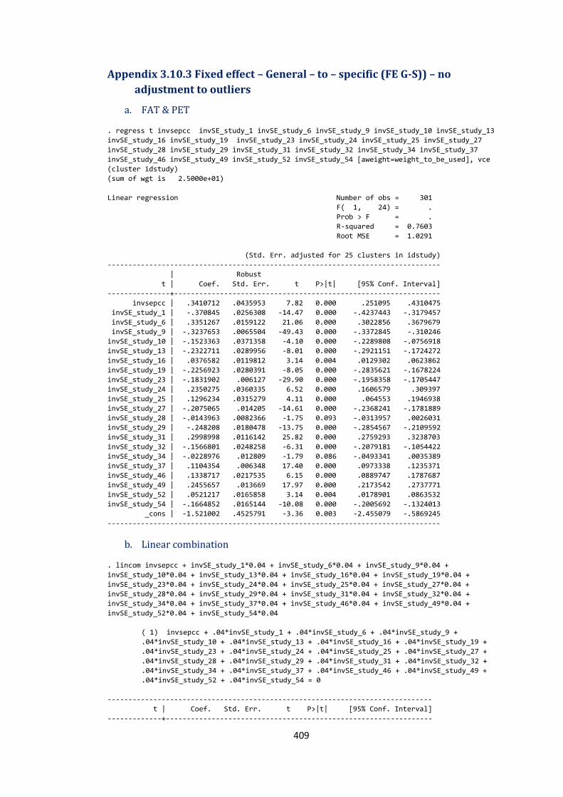
409
Appendix 3.10.3 Fixed effect – General – to – specific (FE G-S)) – no
adjustment to outliers
a. FAT & PET
. regress t invsepcc invSE_study_1 invSE_study_6 invSE_study_9 invSE_study_10 invSE_study_13
invSE_study_16 invSE_study_19 invSE_study_23 invSE_study_24 invSE_study_25 invSE_study_27
invSE_study_28 invSE_study_29 invSE_study_31 invSE_study_32 invSE_study_34 invSE_study_37
invSE_study_46 invSE_study_49 invSE_study_52 invSE_study_54 [aweight=weight_to_be_used], vce
(cluster idstudy)
(sum of wgt is 2.5000e+01)
Linear regression Number of obs = 301
F( 1, 24) = .
Prob > F = .
R-squared = 0.7603
Root MSE = 1.0291
(Std. Err. adjusted for 25 clusters in idstudy)
--------------------------------------------------------------------------------
| Robust
t | Coef. Std. Err. t P>|t| [95% Conf. Interval]
---------------+----------------------------------------------------------------
invsepcc | .3410712 .0435953 7.82 0.000 .251095 .4310475
invSE_study_1 | -.370845 .0256308 -14.47 0.000 -.4237443 -.3179457
invSE_study_6 | .3351267 .0159122 21.06 0.000 .3022856 .3679679
invSE_study_9 | -.3237653 .0065504 -49.43 0.000 -.3372845 -.310246
invSE_study_10 | -.1523363 .0371358 -4.10 0.000 -.2289808 -.0756918
invSE_study_13 | -.2322711 .0289956 -8.01 0.000 -.2921151 -.1724272
invSE_study_16 | .0376582 .0119812 3.14 0.004 .0129302 .0623862
invSE_study_19 | -.2256923 .0280391 -8.05 0.000 -.2835621 -.1678224
invSE_study_23 | -.1831902 .006127 -29.90 0.000 -.1958358 -.1705447
invSE_study_24 | .2350275 .0360335 6.52 0.000 .1606579 .309397
invSE_study_25 | .1296234 .0315279 4.11 0.000 .064553 .1946938
invSE_study_27 | -.2075065 .014205 -14.61 0.000 -.2368241 -.1781889
invSE_study_28 | -.0143963 .0082366 -1.75 0.093 -.0313957 .0026031
invSE_study_29 | -.248208 .0180478 -13.75 0.000 -.2854567 -.2109592
invSE_study_31 | .2998998 .0116142 25.82 0.000 .2759293 .3238703
invSE_study_32 | -.1566801 .0248258 -6.31 0.000 -.2079181 -.1054422
invSE_study_34 | -.0228976 .012809 -1.79 0.086 -.0493341 .0035389
invSE_study_37 | .1104354 .006348 17.40 0.000 .0973338 .1235371
invSE_study_46 | .1338717 .0217535 6.15 0.000 .0889747 .1787687
invSE_study_49 | .2455657 .013669 17.97 0.000 .2173542 .2737771
invSE_study_52 | .0521217 .0165858 3.14 0.004 .0178901 .0863532
invSE_study_54 | -.1664852 .0165144 -10.08 0.000 -.2005692 -.1324013
_cons | -1.521002 .4525791 -3.36 0.003 -2.455079 -.5869245
--------------------------------------------------------------------------------
b. Linear combination
. lincom invsepcc + invSE_study_1*0.04 + invSE_study_6*0.04 + invSE_study_9*0.04 +
invSE_study_10*0.04 + invSE_study_13*0.04 + invSE_study_16*0.04 + invSE_study_19*0.04 +
invSE_study_23*0.04 + invSE_study_24*0.04 + invSE_study_25*0.04 + invSE_study_27*0.04 +
invSE_study_28*0.04 + invSE_study_29*0.04 + invSE_study_31*0.04 + invSE_study_32*0.04 +
invSE_study_34*0.04 + invSE_study_37*0.04 + invSE_study_46*0.04 + invSE_study_49*0.04 +
invSE_study_52*0.04 + invSE_study_54*0.04
( 1) invsepcc + .04*invSE_study_1 + .04*invSE_study_6 + .04*invSE_study_9 +
.04*invSE_study_10 + .04*invSE_study_13 + .04*invSE_study_16 + .04*invSE_study_19 +
.04*invSE_study_23 + .04*invSE_study_24 + .04*invSE_study_25 + .04*invSE_study_27 +
.04*invSE_study_28 + .04*invSE_study_29 + .04*invSE_study_31 + .04*invSE_study_32 +
.04*invSE_study_34 + .04*invSE_study_37 + .04*invSE_study_46 + .04*invSE_study_49 +
.04*invSE_study_52 + .04*invSE_study_54 = 0
------------------------------------------------------------------------------
t | Coef. Std. Err. t P>|t| [95% Conf. Interval]
-------------+----------------------------------------------------------------
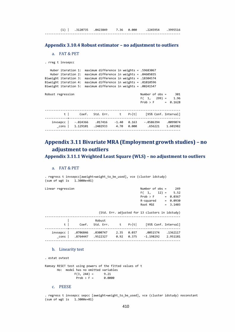
410
(1) | .3120735 .0423849 7.36 0.000 .2245954 .3995516
------------------------------------------------------------------------------
Appendix 3.10.4 Robust estimator – no adjustment to outliers
a. FAT & PET
. rreg t invsepcc
Huber iteration 1: maximum difference in weights = .59683067
Huber iteration 2: maximum difference in weights = .04605035
Biweight iteration 3: maximum difference in weights = .18304574
Biweight iteration 4: maximum difference in weights = .01010596
Biweight iteration 5: maximum difference in weights = .00241547
Robust regression Number of obs = 301
F( 1, 299) = 1.96
Prob > F = 0.1628
------------------------------------------------------------------------------
t | Coef. Std. Err. t P>|t| [95% Conf. Interval]
-------------+----------------------------------------------------------------
invsepcc | -.024366 .017416 -1.40 0.163 -.0586394 .0099074
_cons | 1.129101 .2402933 4.70 0.000 .656221 1.601982
------------------------------------------------------------------------------
Appendix 3.11 Bivariate MRA (Employment growth studies) – no
adjustment to outliers Appendix 3.11.1 Weighted Least Square (WLS) – no adjustment to outliers
a. FAT & PET
. regress t invsepcc[aweight=weight_to_be_used], vce (cluster idstudy)
(sum of wgt is 1.3000e+01)
Linear regression Number of obs = 249
F( 1, 12) = 5.52
Prob > F = 0.0367
R-squared = 0.0930
Root MSE = 3.1403
(Std. Err. adjusted for 13 clusters in idstudy)
------------------------------------------------------------------------------
| Robust
t | Coef. Std. Err. t P>|t| [95% Conf. Interval]
-------------+----------------------------------------------------------------
invsepcc | .0706846 .0300747 2.35 0.037 .0051574 .1362117
_cons | .8764447 .9522327 0.92 0.375 -1.198292 2.951181
------------------------------------------------------------------------------
b. Linearity test
. estat ovtest
Ramsey RESET test using powers of the fitted values of t
Ho: model has no omitted variables
F(3, 244) = 9.21
Prob > F = 0.0000
c. PEESE
. regress t invsepcc sepcc [aweight=weight_to_be_used], vce (cluster idstudy) noconstant
(sum of wgt is 1.3000e+01)
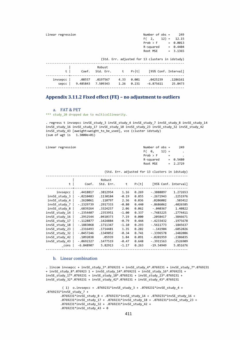
411
Linear regression Number of obs = 249
F( 2, 12) = 12.15
Prob > F = 0.0013
R-squared = 0.4404
Root MSE = 3.1365
(Std. Err. adjusted for 13 clusters in idstudy)
------------------------------------------------------------------------------
| Robust
t | Coef. Std. Err. t P>|t| [95% Conf. Interval]
-------------+----------------------------------------------------------------
invsepcc | .08557 .0197567 4.33 0.001 .0425239 .1286161
sepcc | 9.485843 7.509343 1.26 0.231 -6.875611 25.8473
------------------------------------------------------------------------------
Appendix 3.11.2 Fixed effect (FE) – no adjustment to outliers
a. FAT & PET *** study_20 dropped due to multicollinearity.
. regress t invsepcc invSE_study_3 invSE_study_4 invSE_study_7 invSE_study_8 invSE_study_14
invSE_study_16 invSE_study_17 invSE_study_18 invSE_study_23 invSE_study_32 invSE_study_42
invSE_study_43 [aweight=weight_to_be_used], vce (cluster idstudy)
(sum of wgt is 1.3000e+01)
Linear regression Number of obs = 249
F( 0, 12) = .
Prob > F = .
R-squared = 0.5480
Root MSE = 2.2729
(Std. Err. adjusted for 13 clusters in idstudy)
--------------------------------------------------------------------------------
| Robust
t | Coef. Std. Err. t P>|t| [95% Conf. Interval]
---------------+----------------------------------------------------------------
invsepcc | .4418817 .3812954 1.16 0.269 -.3888897 1.272653
invSE_study_3 | -.0210483 .1130184 -0.19 0.855 -.2672943 .2251976
invSE_study_4 | .2620061 .110797 2.36 0.036 .0206002 .503412
invSE_study_7 | -.2329739 .2917333 -0.80 0.440 -.8686062 .4026585
invSE_study_8 | .6839264 .3324257 2.06 0.062 -.040367 1.40822
invSE_study_14 | -.2354407 .2353951 -1.00 0.337 -.7483225 .2774411
invSE_study_16 | .2952544 .0410373 7.19 0.000 .2058417 .3846671
invSE_study_17 | -.1128877 .1424884 -0.79 0.444 -.4233432 .1975678
invSE_study_18 | -.1883068 .1711347 -1.10 0.293 -.5611773 .1845637
invSE_study_23 | .2316493 .1714481 1.35 0.202 -.141904 .6052026
invSE_study_32 | -.0457246 .1349052 -0.34 0.741 -.3396578 .2482086
invSE_study_42 | .1092038 .05939 1.84 0.091 -.0201959 .2386035
invSE_study_43 | -.0692327 .1477519 -0.47 0.648 -.3911563 .2526909
_cons | -6.848907 5.82913 -1.17 0.263 -19.54949 5.851676
--------------------------------------------------------------------------------
b. Linear combination
. lincom invsepcc + invSE_study_3*.0769231 + invSE_study_4*.0769231 + invSE_study_7*.0769231
+ invSE_study_8*.076923 1 + invSE_study_14*.0769231 + invSE_study_16*.0769231 +
invSE_study_17*.0769231 + invSE_study_18*.0769231 + invSE_study_23*.0769231 +
invSE_study_32*.0769231 + invSE_study_42*.0769231 + invSE_study_43*.0769231
( 1) o.invsepcc + .0769231*invSE_study_3 + .0769231*invSE_study_4 +
.0769231*invSE_study_7 +
.0769231*invSE_study_8 + .0769231*invSE_study_14 + .0769231*invSE_study_16 +
.0769231*invSE_study_17 + .0769231*invSE_study_18 + .0769231*invSE_study_23 +
.0769231*invSE_study_32 + .0769231*invSE_study_42 +
.0769231*invSE_study_43 = 0
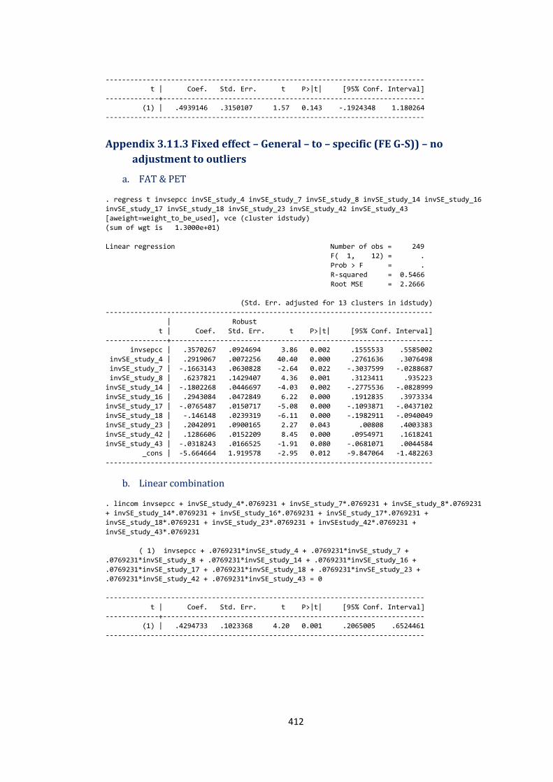
412
------------------------------------------------------------------------------
t | Coef. Std. Err. t P>|t| [95% Conf. Interval]
-------------+----------------------------------------------------------------
(1) | .4939146 .3150107 1.57 0.143 -.1924348 1.180264
------------------------------------------------------------------------------
Appendix 3.11.3 Fixed effect – General – to – specific (FE G-S)) – no
adjustment to outliers
a. FAT & PET
. regress t invsepcc invSE_study_4 invSE_study_7 invSE_study_8 invSE_study_14 invSE_study_16
invSE_study_17 invSE_study_18 invSE_study_23 invSE_study_42 invSE_study_43
[aweight=weight_to_be_used], vce (cluster idstudy)
(sum of wgt is 1.3000e+01)
Linear regression Number of obs = 249
F( 1, 12) = .
Prob > F = .
R-squared = 0.5466
Root MSE = 2.2666
(Std. Err. adjusted for 13 clusters in idstudy)
--------------------------------------------------------------------------------
| Robust
t | Coef. Std. Err. t P>|t| [95% Conf. Interval]
---------------+----------------------------------------------------------------
invsepcc | .3570267 .0924694 3.86 0.002 .1555533 .5585002
invSE_study_4 | .2919067 .0072256 40.40 0.000 .2761636 .3076498
invSE_study_7 | -.1663143 .0630828 -2.64 0.022 -.3037599 -.0288687
invSE_study_8 | .6237821 .1429407 4.36 0.001 .3123411 .935223
invSE_study_14 | -.1802268 .0446697 -4.03 0.002 -.2775536 -.0828999
invSE_study_16 | .2943084 .0472849 6.22 0.000 .1912835 .3973334
invSE_study_17 | -.0765487 .0150717 -5.08 0.000 -.1093871 -.0437102
invSE_study_18 | -.146148 .0239319 -6.11 0.000 -.1982911 -.0940049
invSE_study_23 | .2042091 .0900165 2.27 0.043 .00808 .4003383
invSE_study_42 | .1286606 .0152209 8.45 0.000 .0954971 .1618241
invSE_study_43 | -.0318243 .0166525 -1.91 0.080 -.0681071 .0044584
_cons | -5.664664 1.919578 -2.95 0.012 -9.847064 -1.482263
--------------------------------------------------------------------------------
b. Linear combination
. lincom invsepcc + invSE_study_4*.0769231 + invSE_study_7*.0769231 + invSE_study_8*.0769231
+ invSE_study_14*.0769231 + invSE_study_16*.0769231 + invSE_study_17*.0769231 +
invSE_study_18*.0769231 + invSE_study_23*.0769231 + invSEstudy_42*.0769231 +
invSE_study_43*.0769231
( 1) invsepcc + .0769231*invSE_study_4 + .0769231*invSE_study_7 +
.0769231*invSE_study_8 + .0769231*invSE_study_14 + .0769231*invSE_study_16 +
.0769231*invSE_study_17 + .0769231*invSE_study_18 + .0769231*invSE_study_23 +
.0769231*invSE_study_42 + .0769231*invSE_study_43 = 0
------------------------------------------------------------------------------
t | Coef. Std. Err. t P>|t| [95% Conf. Interval]
-------------+----------------------------------------------------------------
(1) | .4294733 .1023368 4.20 0.001 .2065005 .6524461
------------------------------------------------------------------------------

413
Appendix 3.11.4 Robust estimator – no adjustment to outliers
a. FAT & PET
. rreg t invsepcc
Huber iteration 1: maximum difference in weights = .67591233
Huber iteration 2: maximum difference in weights = .04390935
Biweight iteration 3: maximum difference in weights = .26829939
Biweight iteration 4: maximum difference in weights = .00955361
Robust regression Number of obs = 249
F( 1, 247) = 15.62
Prob > F = 0.0001
------------------------------------------------------------------------------
t | Coef. Std. Err. t P>|t| [95% Conf. Interval]
-------------+----------------------------------------------------------------
invsepcc | .0617536 .0156238 3.95 0.000 .0309808 .0925264
_cons | -.304616 .5673937 -0.54 0.592 -1.422163 .8129309
------------------------------------------------------------------------------
Appendix 3.12 Bivariate MRA (‘other’ studies) – no adjustment
to outliers Appendix 3.12.1 Weighted Least Square (WLS) – no adjustment to outliers
a. FAT & PET
. regress t invsepcc[aweight=weight_to_be_used], vce (cluster idstudy)
(sum of wgt is 1.8000e+01)
Linear regression Number of obs = 107
F( 1, 17) = 6.23
Prob > F = 0.0231
R-squared = 0.2757
Root MSE = 2.7358
(Std. Err. adjusted for 18 clusters in idstudy)
------------------------------------------------------------------------------
| Robust
t | Coef. Std. Err. t P>|t| [95% Conf. Interval]
-------------+----------------------------------------------------------------
invsepcc | .2748956 .1101144 2.50 0.023 .0425746 .5072166
_cons | -1.319181 1.424258 -0.93 0.367 -4.324104 1.685741
------------------------------------------------------------------------------
b. Linearity test
. estat ovtest
Ramsey RESET test using powers of the fitted values of t
Ho: model has no omitted variables
F(3, 102) = 25.00
Prob > F = 0.0000
c. PEESE
. regress t invsepcc sepcc [aweight=weight_to_be_used], vce (cluster idstudy) noconstant
(sum of wgt is 1.8000e+01)
Linear regression Number of obs = 107
F( 2, 17) = 16.15
Prob > F = 0.0001
R-squared = 0.5671
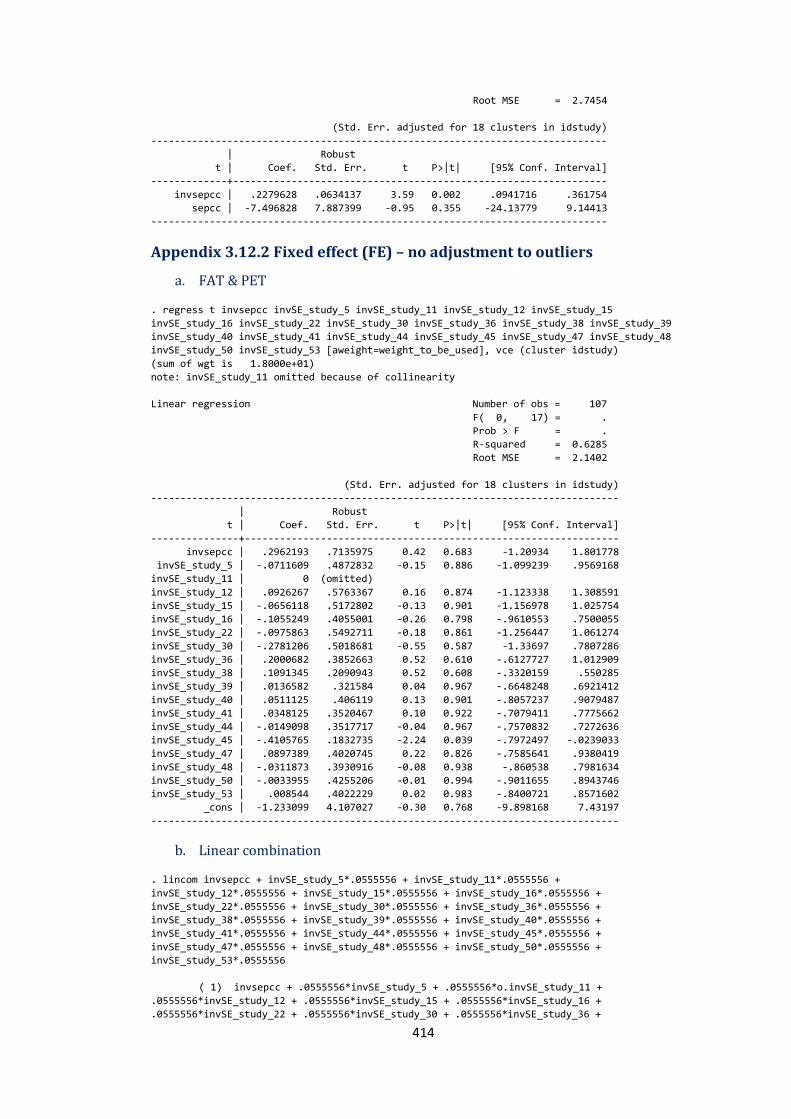
414
Root MSE = 2.7454
(Std. Err. adjusted for 18 clusters in idstudy)
------------------------------------------------------------------------------
| Robust
t | Coef. Std. Err. t P>|t| [95% Conf. Interval]
-------------+----------------------------------------------------------------
invsepcc | .2279628 .0634137 3.59 0.002 .0941716 .361754
sepcc | -7.496828 7.887399 -0.95 0.355 -24.13779 9.14413
------------------------------------------------------------------------------
Appendix 3.12.2 Fixed effect (FE) – no adjustment to outliers
a. FAT & PET
. regress t invsepcc invSE_study_5 invSE_study_11 invSE_study_12 invSE_study_15
invSE_study_16 invSE_study_22 invSE_study_30 invSE_study_36 invSE_study_38 invSE_study_39
invSE_study_40 invSE_study_41 invSE_study_44 invSE_study_45 invSE_study_47 invSE_study_48
invSE_study_50 invSE_study_53 [aweight=weight_to_be_used], vce (cluster idstudy)
(sum of wgt is 1.8000e+01)
note: invSE_study_11 omitted because of collinearity
Linear regression Number of obs = 107
F( 0, 17) = .
Prob > F = .
R-squared = 0.6285
Root MSE = 2.1402
(Std. Err. adjusted for 18 clusters in idstudy)
--------------------------------------------------------------------------------
| Robust
t | Coef. Std. Err. t P>|t| [95% Conf. Interval]
---------------+----------------------------------------------------------------
invsepcc | .2962193 .7135975 0.42 0.683 -1.20934 1.801778
invSE_study_5 | -.0711609 .4872832 -0.15 0.886 -1.099239 .9569168
invSE_study_11 | 0 (omitted)
invSE_study_12 | .0926267 .5763367 0.16 0.874 -1.123338 1.308591
invSE_study_15 | -.0656118 .5172802 -0.13 0.901 -1.156978 1.025754
invSE_study_16 | -.1055249 .4055001 -0.26 0.798 -.9610553 .7500055
invSE_study_22 | -.0975863 .5492711 -0.18 0.861 -1.256447 1.061274
invSE_study_30 | -.2781206 .5018681 -0.55 0.587 -1.33697 .7807286
invSE_study_36 | .2000682 .3852663 0.52 0.610 -.6127727 1.012909
invSE_study_38 | .1091345 .2090943 0.52 0.608 -.3320159 .550285
invSE_study_39 | .0136582 .321584 0.04 0.967 -.6648248 .6921412
invSE_study_40 | .0511125 .406119 0.13 0.901 -.8057237 .9079487
invSE_study_41 | .0348125 .3520467 0.10 0.922 -.7079411 .7775662
invSE_study_44 | -.0149098 .3517717 -0.04 0.967 -.7570832 .7272636
invSE_study_45 | -.4105765 .1832735 -2.24 0.039 -.7972497 -.0239033
invSE_study_47 | .0897389 .4020745 0.22 0.826 -.7585641 .9380419
invSE_study_48 | -.0311873 .3930916 -0.08 0.938 -.860538 .7981634
invSE_study_50 | -.0033955 .4255206 -0.01 0.994 -.9011655 .8943746
invSE_study_53 | .008544 .4022229 0.02 0.983 -.8400721 .8571602
_cons | -1.233099 4.107027 -0.30 0.768 -9.898168 7.43197
--------------------------------------------------------------------------------
b. Linear combination
. lincom invsepcc + invSE_study_5*.0555556 + invSE_study_11*.0555556 +
invSE_study_12*.0555556 + invSE_study_15*.0555556 + invSE_study_16*.0555556 +
invSE_study_22*.0555556 + invSE_study_30*.0555556 + invSE_study_36*.0555556 +
invSE_study_38*.0555556 + invSE_study_39*.0555556 + invSE_study_40*.0555556 +
invSE_study_41*.0555556 + invSE_study_44*.0555556 + invSE_study_45*.0555556 +
invSE_study_47*.0555556 + invSE_study_48*.0555556 + invSE_study_50*.0555556 +
invSE_study_53*.0555556
( 1) invsepcc + .0555556*invSE_study_5 + .0555556*o.invSE_study_11 +
.0555556*invSE_study_12 + .0555556*invSE_study_15 + .0555556*invSE_study_16 +
.0555556*invSE_study_22 + .0555556*invSE_study_30 + .0555556*invSE_study_36 +
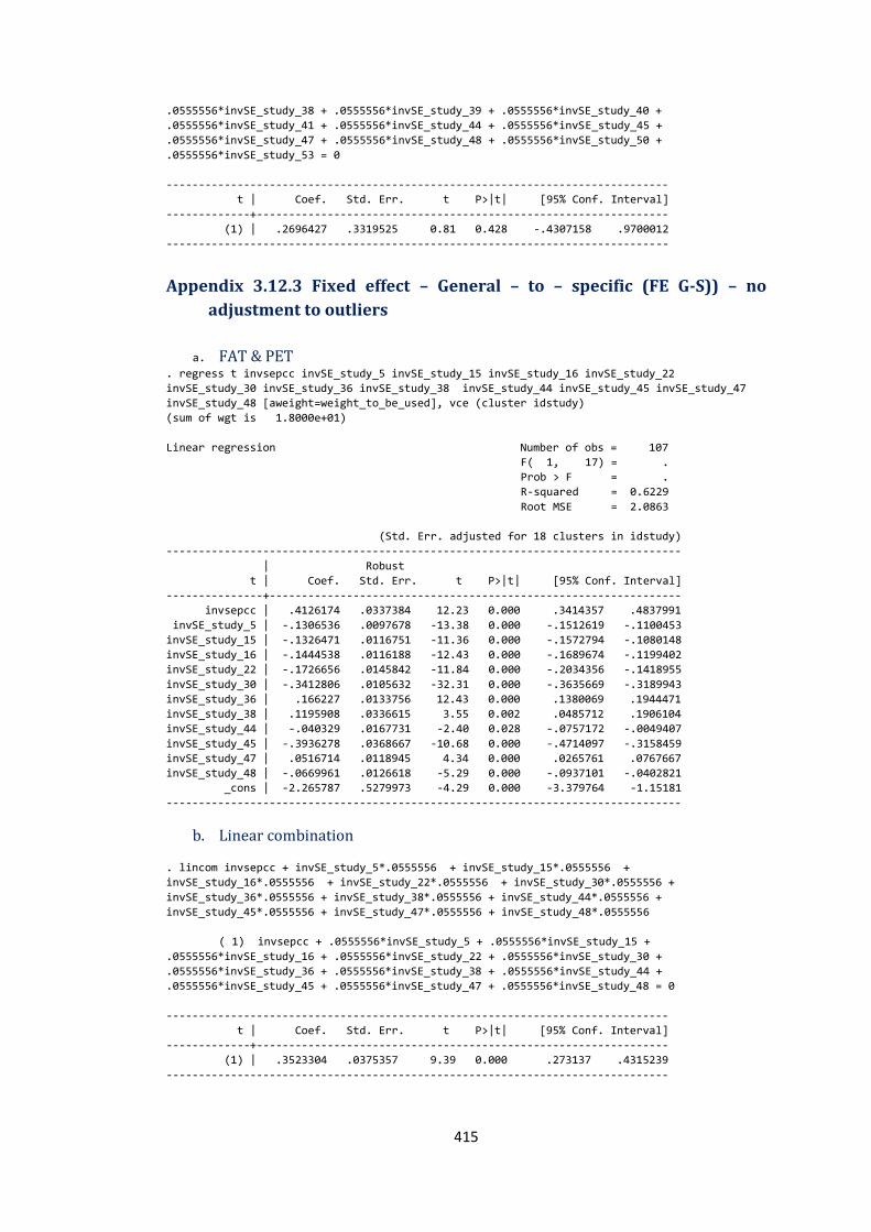
415
.0555556*invSE_study_38 + .0555556*invSE_study_39 + .0555556*invSE_study_40 +
.0555556*invSE_study_41 + .0555556*invSE_study_44 + .0555556*invSE_study_45 +
.0555556*invSE_study_47 + .0555556*invSE_study_48 + .0555556*invSE_study_50 +
.0555556*invSE_study_53 = 0
------------------------------------------------------------------------------
t | Coef. Std. Err. t P>|t| [95% Conf. Interval]
-------------+----------------------------------------------------------------
(1) | .2696427 .3319525 0.81 0.428 -.4307158 .9700012
------------------------------------------------------------------------------
Appendix 3.12.3 Fixed effect – General – to – specific (FE G-S)) – no
adjustment to outliers
a. FAT & PET
. regress t invsepcc invSE_study_5 invSE_study_15 invSE_study_16 invSE_study_22
invSE_study_30 invSE_study_36 invSE_study_38 invSE_study_44 invSE_study_45 invSE_study_47
invSE_study_48 [aweight=weight_to_be_used], vce (cluster idstudy)
(sum of wgt is 1.8000e+01)
Linear regression Number of obs = 107
F( 1, 17) = .
Prob > F = .
R-squared = 0.6229
Root MSE = 2.0863
(Std. Err. adjusted for 18 clusters in idstudy)
--------------------------------------------------------------------------------
| Robust
t | Coef. Std. Err. t P>|t| [95% Conf. Interval]
---------------+----------------------------------------------------------------
invsepcc | .4126174 .0337384 12.23 0.000 .3414357 .4837991
invSE_study_5 | -.1306536 .0097678 -13.38 0.000 -.1512619 -.1100453
invSE_study_15 | -.1326471 .0116751 -11.36 0.000 -.1572794 -.1080148
invSE_study_16 | -.1444538 .0116188 -12.43 0.000 -.1689674 -.1199402
invSE_study_22 | -.1726656 .0145842 -11.84 0.000 -.2034356 -.1418955
invSE_study_30 | -.3412806 .0105632 -32.31 0.000 -.3635669 -.3189943
invSE_study_36 | .166227 .0133756 12.43 0.000 .1380069 .1944471
invSE_study_38 | .1195908 .0336615 3.55 0.002 .0485712 .1906104
invSE_study_44 | -.040329 .0167731 -2.40 0.028 -.0757172 -.0049407
invSE_study_45 | -.3936278 .0368667 -10.68 0.000 -.4714097 -.3158459
invSE_study_47 | .0516714 .0118945 4.34 0.000 .0265761 .0767667
invSE_study_48 | -.0669961 .0126618 -5.29 0.000 -.0937101 -.0402821
_cons | -2.265787 .5279973 -4.29 0.000 -3.379764 -1.15181
--------------------------------------------------------------------------------
b. Linear combination
. lincom invsepcc + invSE_study_5*.0555556 + invSE_study_15*.0555556 +
invSE_study_16*.0555556 + invSE_study_22*.0555556 + invSE_study_30*.0555556 +
invSE_study_36*.0555556 + invSE_study_38*.0555556 + invSE_study_44*.0555556 +
invSE_study_45*.0555556 + invSE_study_47*.0555556 + invSE_study_48*.0555556
( 1) invsepcc + .0555556*invSE_study_5 + .0555556*invSE_study_15 +
.0555556*invSE_study_16 + .0555556*invSE_study_22 + .0555556*invSE_study_30 +
.0555556*invSE_study_36 + .0555556*invSE_study_38 + .0555556*invSE_study_44 +
.0555556*invSE_study_45 + .0555556*invSE_study_47 + .0555556*invSE_study_48 = 0
------------------------------------------------------------------------------
t | Coef. Std. Err. t P>|t| [95% Conf. Interval]
-------------+----------------------------------------------------------------
(1) | .3523304 .0375357 9.39 0.000 .273137 .4315239
------------------------------------------------------------------------------
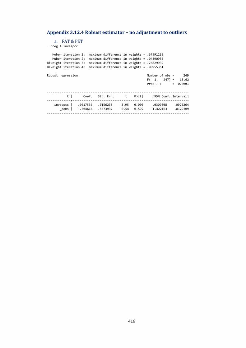
416
Appendix 3.12.4 Robust estimator – no adjustment to outliers
a. FAT & PET . rreg t invsepcc
Huber iteration 1: maximum difference in weights = .67591233
Huber iteration 2: maximum difference in weights = .04390935
Biweight iteration 3: maximum difference in weights = .26829939
Biweight iteration 4: maximum difference in weights = .00955361
Robust regression Number of obs = 249
F( 1, 247) = 15.62
Prob > F = 0.0001
------------------------------------------------------------------------------
t | Coef. Std. Err. t P>|t| [95% Conf. Interval]
-------------+----------------------------------------------------------------
invsepcc | .0617536 .0156238 3.95 0.000 .0309808 .0925264
_cons | -.304616 .5673937 -0.54 0.592 -1.422163 .8129309
------------------------------------------------------------------------------
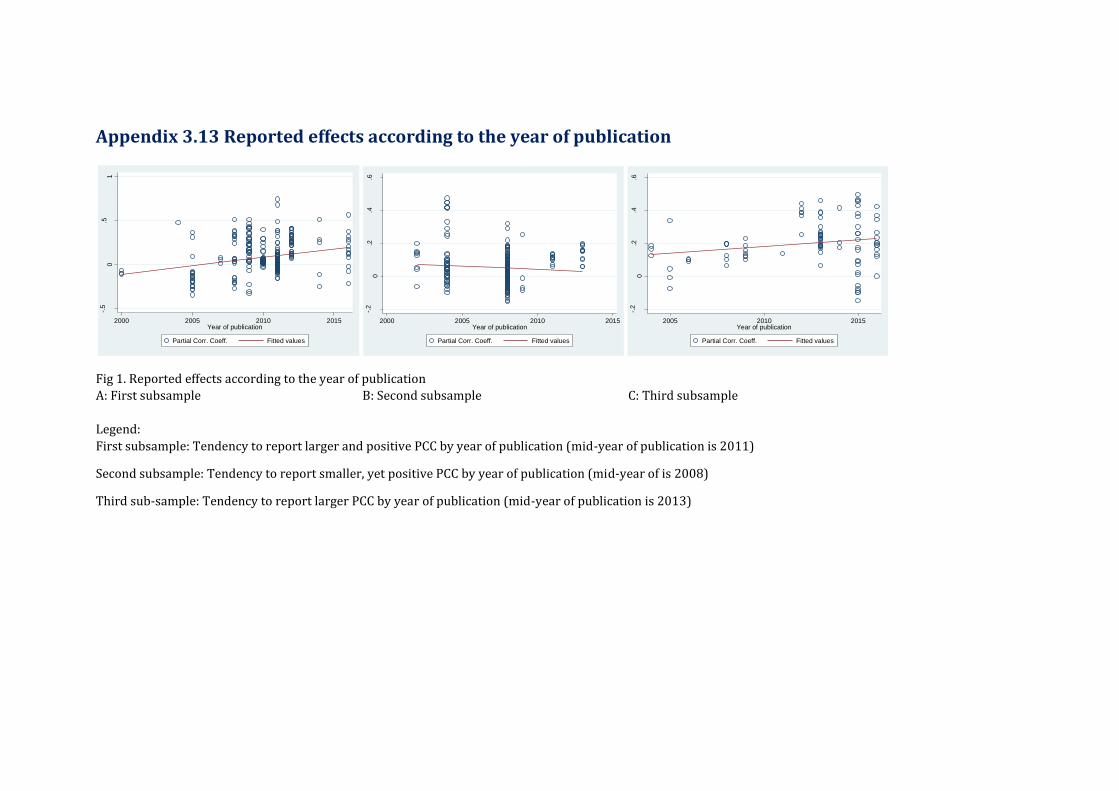
Appendix 3.13 Reported effects according to the year of publication
Fig 1. Reported effects according to the year of publication
A: First subsample B: Second subsample C: Third subsample
Legend:
First subsample: Tendency to report larger and positive PCC by year of publication (mid-year of publication is 2011)
Second subsample: Tendency to report smaller, yet positive PCC by year of publication (mid-year of is 2008)
Third sub-sample: Tendency to report larger PCC by year of publication (mid-year of publication is 2013)
-.5
0.5
1
2000 2005 2010 2015Year of publication
Partial Corr. Coeff. Fitted values
-.2
0.2
.4.6
2000 2005 2010 2015Year of publication
Partial Corr. Coeff. Fitted values
-.2
0.2
.4.6
2005 2010 2015Year of publication
Partial Corr. Coeff. Fitted values
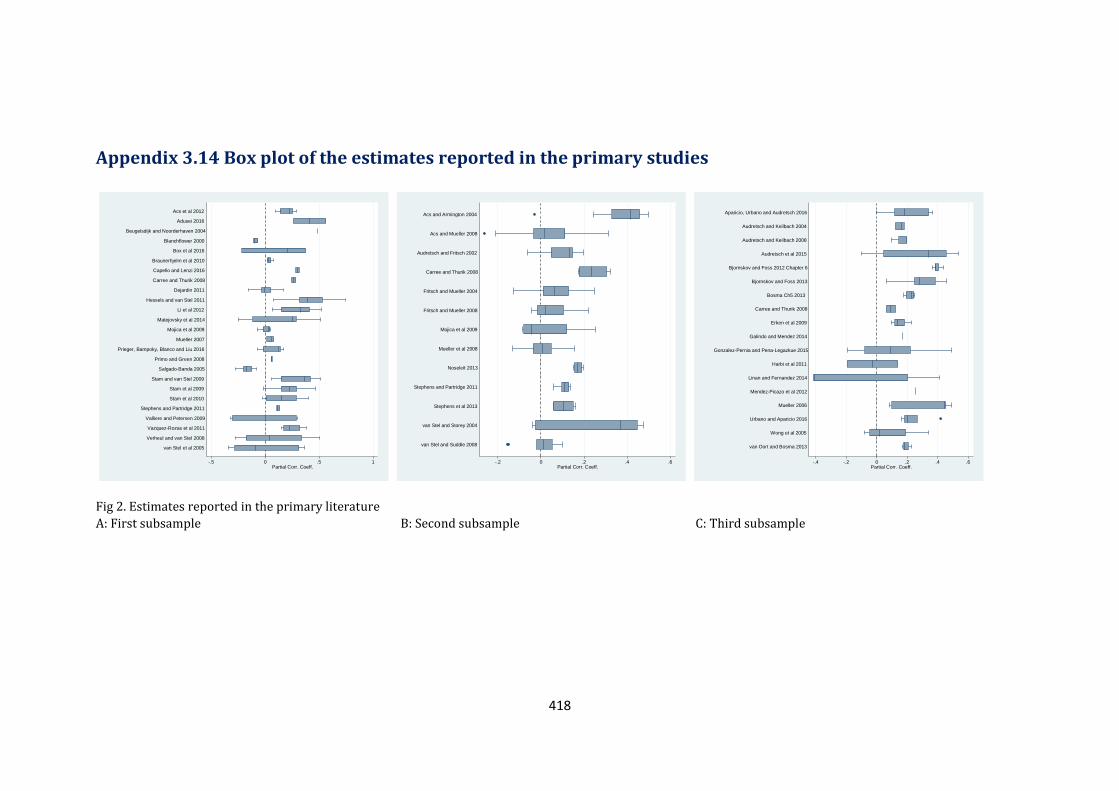
418
Appendix 3.14 Box plot of the estimates reported in the primary studies
Fig 2. Estimates reported in the primary literature
A: First subsample B: Second subsample C: Third subsample
-.5 0 .5 1Partial Corr. Coeff.
van Stel et al 2005
Verheul and van Stel 2008
Vazquez-Rozas et al 2011
Valliere and Petersen 2009
Stephens and Partridge 2011
Stam et al 2010
Stam et al 2009
Stam and van Stel 2009
Salgado-Banda 2005
Primo and Green 2008
Prieger, Bampoky, Blanco and Liu 2016
Mueller 2007
Mojica et al 2009
Matejovsky et al 2014
Li et al 2012
Hessels and van Stel 2011
Dejardin 2011
Carree and Thurik 2008
Capello and Lenzi 2016
Braunerhjelm et al 2010
Box et al 2016
Blanchflower 2000
Beugelsdijk and Noorderhaven 2004
Adusei 2016
Acs et al 2012
-.2 0 .2 .4 .6Partial Corr. Coeff.
van Stel and Suddle 2008
van Stel and Storey 2004
Stephens et al 2013
Stephens and Partridge 2011
Noseleit 2013
Mueller et al 2008
Mojica et al 2009
Fritsch and Mueller 2008
Fritsch and Mueller 2004
Carree and Thurik 2008
Audretsch and Fritsch 2002
Acs and Mueller 2008
Acs and Armington 2004
-.4 -.2 0 .2 .4 .6Partial Corr. Coeff.
van Oort and Bosma 2013
Wong et al 2005
Urbano and Aparicio 2016
Mueller 2006
Mendez-Picazo et al 2012
Linan and Fernandez 2014
Harbi et al 2011
Gonzalez-Pernia and Pena-Legazkue 2015
Galindo and Mendez 2014
Erken et al 2009
Carree and Thurik 2008
Bosma Ch5 2013
Bjornskov and Foss 2013
Bjornskov and Foss 2012 Chapter 6
Audretsch et al 2015
Audretsch and Keilbach 2008
Audretsch and Keilbach 2004
Aparicio, Urbano and Audretsch 2016
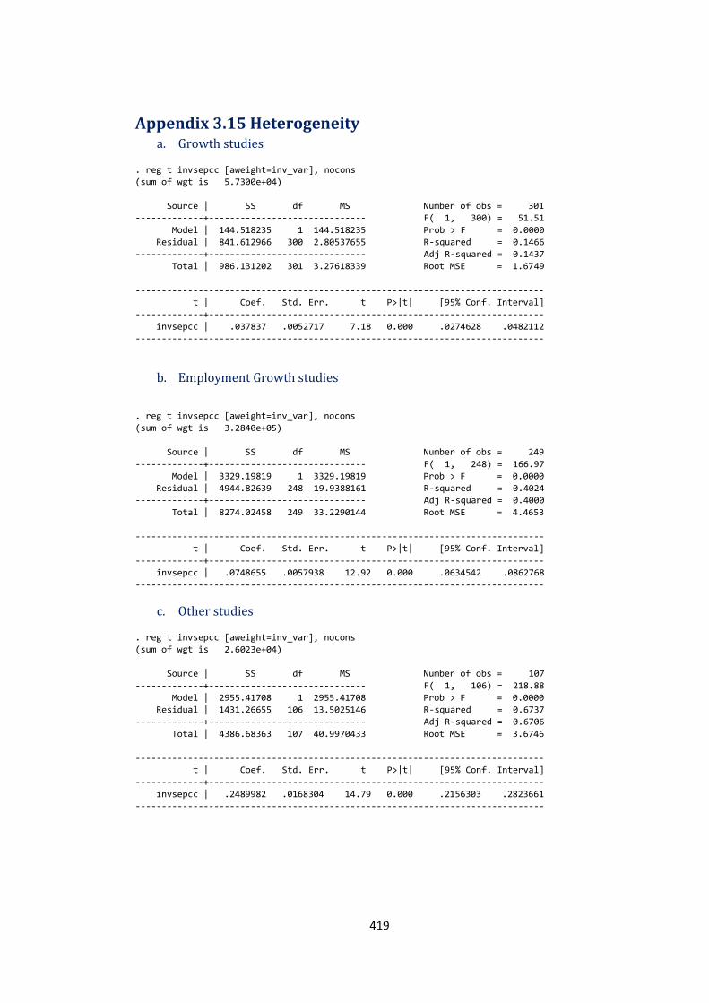
419
Appendix 3.15 Heterogeneity a. Growth studies
. reg t invsepcc [aweight=inv_var], nocons
(sum of wgt is 5.7300e+04)
Source | SS df MS Number of obs = 301
-------------+------------------------------ F( 1, 300) = 51.51
Model | 144.518235 1 144.518235 Prob > F = 0.0000
Residual | 841.612966 300 2.80537655 R-squared = 0.1466
-------------+------------------------------ Adj R-squared = 0.1437
Total | 986.131202 301 3.27618339 Root MSE = 1.6749
------------------------------------------------------------------------------
t | Coef. Std. Err. t P>|t| [95% Conf. Interval]
-------------+----------------------------------------------------------------
invsepcc | .037837 .0052717 7.18 0.000 .0274628 .0482112
------------------------------------------------------------------------------
b. Employment Growth studies
. reg t invsepcc [aweight=inv_var], nocons
(sum of wgt is 3.2840e+05)
Source | SS df MS Number of obs = 249
-------------+------------------------------ F( 1, 248) = 166.97
Model | 3329.19819 1 3329.19819 Prob > F = 0.0000
Residual | 4944.82639 248 19.9388161 R-squared = 0.4024
-------------+------------------------------ Adj R-squared = 0.4000
Total | 8274.02458 249 33.2290144 Root MSE = 4.4653
------------------------------------------------------------------------------
t | Coef. Std. Err. t P>|t| [95% Conf. Interval]
-------------+----------------------------------------------------------------
invsepcc | .0748655 .0057938 12.92 0.000 .0634542 .0862768
------------------------------------------------------------------------------
c. Other studies
. reg t invsepcc [aweight=inv_var], nocons
(sum of wgt is 2.6023e+04)
Source | SS df MS Number of obs = 107
-------------+------------------------------ F( 1, 106) = 218.88
Model | 2955.41708 1 2955.41708 Prob > F = 0.0000
Residual | 1431.26655 106 13.5025146 R-squared = 0.6737
-------------+------------------------------ Adj R-squared = 0.6706
Total | 4386.68363 107 40.9970433 Root MSE = 3.6746
------------------------------------------------------------------------------
t | Coef. Std. Err. t P>|t| [95% Conf. Interval]
-------------+----------------------------------------------------------------
invsepcc | .2489982 .0168304 14.79 0.000 .2156303 .2823661
------------------------------------------------------------------------------

420
Chapter 4
APPENDICES
THE IMPACT OF ENTREPRENEURIAL ACTIVITY ON ECONOMIC GROWTH: A MULTI-COUNTRY ANALYSIS
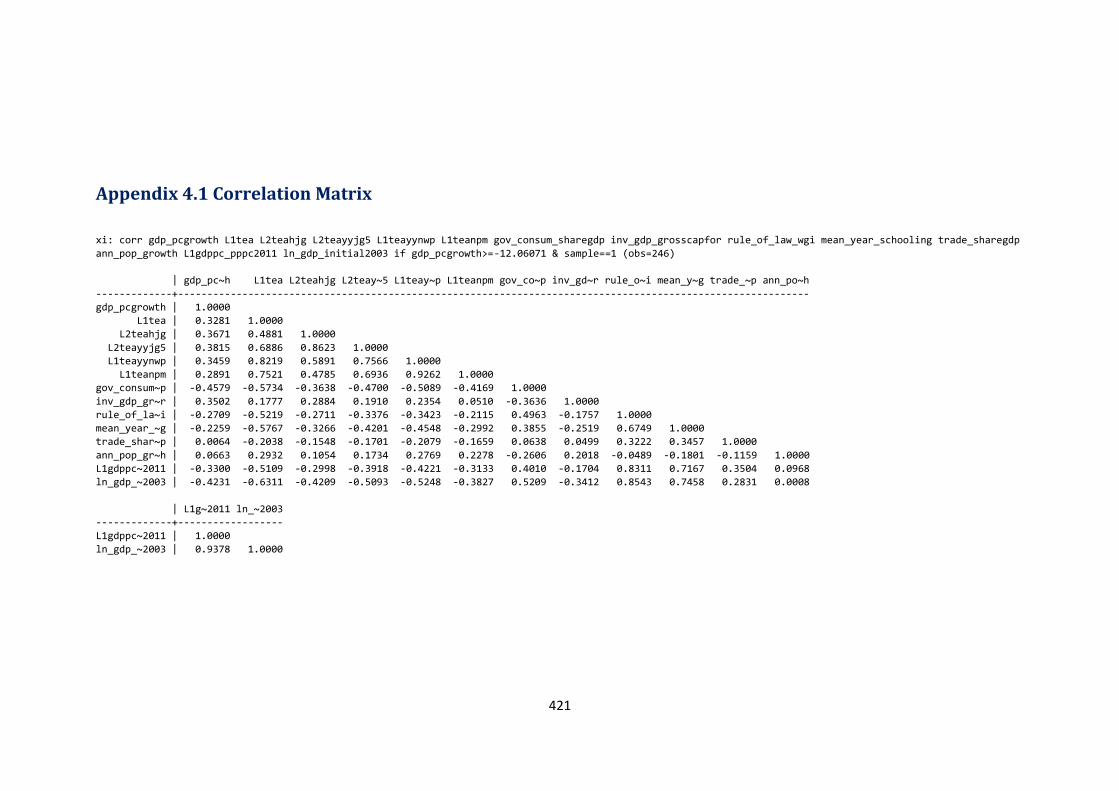
421
Appendix 4.1 Correlation Matrix
xi: corr gdp_pcgrowth L1tea L2teahjg L2teayyjg5 L1teayynwp L1teanpm gov_consum_sharegdp inv_gdp_grosscapfor rule_of_law_wgi mean_year_schooling trade_sharegdp
ann_pop_growth L1gdppc_pppc2011 ln_gdp_initial2003 if gdp_pcgrowth>=-12.06071 & sample==1 (obs=246)
| gdp_pc~h L1tea L2teahjg L2teay~5 L1teay~p L1teanpm gov_co~p inv_gd~r rule_o~i mean_y~g trade_~p ann_po~h
-------------+------------------------------------------------------------------------------------------------------------
gdp_pcgrowth | 1.0000
L1tea | 0.3281 1.0000
L2teahjg | 0.3671 0.4881 1.0000
L2teayyjg5 | 0.3815 0.6886 0.8623 1.0000
L1teayynwp | 0.3459 0.8219 0.5891 0.7566 1.0000
L1teanpm | 0.2891 0.7521 0.4785 0.6936 0.9262 1.0000
gov_consum~p | -0.4579 -0.5734 -0.3638 -0.4700 -0.5089 -0.4169 1.0000
inv_gdp_gr~r | 0.3502 0.1777 0.2884 0.1910 0.2354 0.0510 -0.3636 1.0000
rule_of_la~i | -0.2709 -0.5219 -0.2711 -0.3376 -0.3423 -0.2115 0.4963 -0.1757 1.0000
mean_year_~g | -0.2259 -0.5767 -0.3266 -0.4201 -0.4548 -0.2992 0.3855 -0.2519 0.6749 1.0000
trade_shar~p | 0.0064 -0.2038 -0.1548 -0.1701 -0.2079 -0.1659 0.0638 0.0499 0.3222 0.3457 1.0000
ann_pop_gr~h | 0.0663 0.2932 0.1054 0.1734 0.2769 0.2278 -0.2606 0.2018 -0.0489 -0.1801 -0.1159 1.0000
L1gdppc~2011 | -0.3300 -0.5109 -0.2998 -0.3918 -0.4221 -0.3133 0.4010 -0.1704 0.8311 0.7167 0.3504 0.0968
ln_gdp_~2003 | -0.4231 -0.6311 -0.4209 -0.5093 -0.5248 -0.3827 0.5209 -0.3412 0.8543 0.7458 0.2831 0.0008
| L1g~2011 ln_~2003
-------------+------------------
L1gdppc~2011 | 1.0000
ln_gdp_~2003 | 0.9378 1.0000

422
Appendix 4.2 Diagnostics Appendix 4.2.1 VIF command (Multicollinearity)
. xi: reg gdp_pcgrowth L1tea L2teahjg gov_consum_sharegdp inv_gdp_grosscapfor rule_of_law_wgi
mean_year_schooling trade_sharegdp ann_pop_growth L1gdppc_pppc2011 year2007 year2008 year2009
year2010 year2011 year2012 year2013 year2014 if gdp_pcgrowth>=-12.06071 & sample==1
note: year2007 omitted because of collinearity
note: year2009 omitted because of collinearity
Source | SS df MS Number of obs = 246
-------------+------------------------------ F( 15, 230) = 23.01
Model | 1687.49668 15 112.499779 Prob > F = 0.0000
Residual | 1124.32065 230 4.88835063 R-squared = 0.6001
-------------+------------------------------ Adj R-squared = 0.5741
Total | 2811.81733 245 11.4768054 Root MSE = 2.211
-------------------------------------------------------------------------------------
gdp_pcgrowth | Coef. Std. Err. t P>|t| [95% Conf. Interval]
--------------------+----------------------------------------------------------------
L1tea | .010552 .0368153 0.29 0.775 -.0619863 .0830902
L2teahjg | .7318526 .1856106 3.94 0.000 .3661382 1.097567
gov_consum_sharegdp | -.1782361 .0449017 -3.97 0.000 -.2667074 -.0897648
inv_gdp_grosscapfor | .1227577 .0314555 3.90 0.000 .0607798 .1847355
rule_of_law_wgi | .4900491 .3050806 1.61 0.110 -.1110608 1.091159
mean_year_schooling | .1085489 .1265782 0.86 0.392 -.1408522 .3579499
trade_sharegdp | .0022582 .0032841 0.69 0.492 -.0042126 .008729
ann_pop_growth | .1608583 .2262004 0.71 0.478 -.2848316 .6065482
L1gdppc_pppc2011 | -.000063 .000021 -3.00 0.003 -.0001043 -.0000217
year2007 | 0 (omitted)
year2008 | 4.298038 .6048398 7.11 0.000 3.106303 5.489773
year2009 | 0 (omitted)
year2010 | 6.128557 .5740599 10.68 0.000 4.997469 7.259646
year2011 | 6.303739 .5737387 10.99 0.000 5.173283 7.434195
year2012 | 4.549871 .5670796 8.02 0.000 3.432536 5.667206
year2013 | 5.242889 .5571524 9.41 0.000 4.145114 6.340664
year2014 | 5.354865 .5544371 9.66 0.000 4.26244 6.44729
_cons | -3.996793 2.018443 -1.98 0.049 -7.973796 -.0197895
-------------------------------------------------------------------------------------
. estat vif
Variable | VIF 1/VIF
-------------+----------------------
L1gdppc~2011 | 4.59 0.217670
rule_of_la~i | 3.81 0.262799
mean_year_~g | 2.74 0.364557
L1tea | 2.45 0.407525
year2014 | 2.27 0.440138
year2013 | 2.21 0.452137
year2012 | 2.07 0.483572
year2011 | 1.97 0.506821
year2010 | 1.93 0.519146
gov_consum~p | 1.92 0.520451
year2008 | 1.86 0.538520
L2teahjg | 1.53 0.654571
ann_pop_gr~h | 1.43 0.698830
inv_gdp_gr~r | 1.33 0.750858
trade_shar~p | 1.29 0.775615
-------------+----------------------
Mean VIF | 2.23
. xi: reg gdp_pcgrowth L1tea L2teayyjg5 gov_consum_sharegdp inv_gdp_grosscapfor
rule_of_law_wgi mean_year_schooling trade_sharegdp ann_pop_growth L1gdppc_pppc2011 year2007
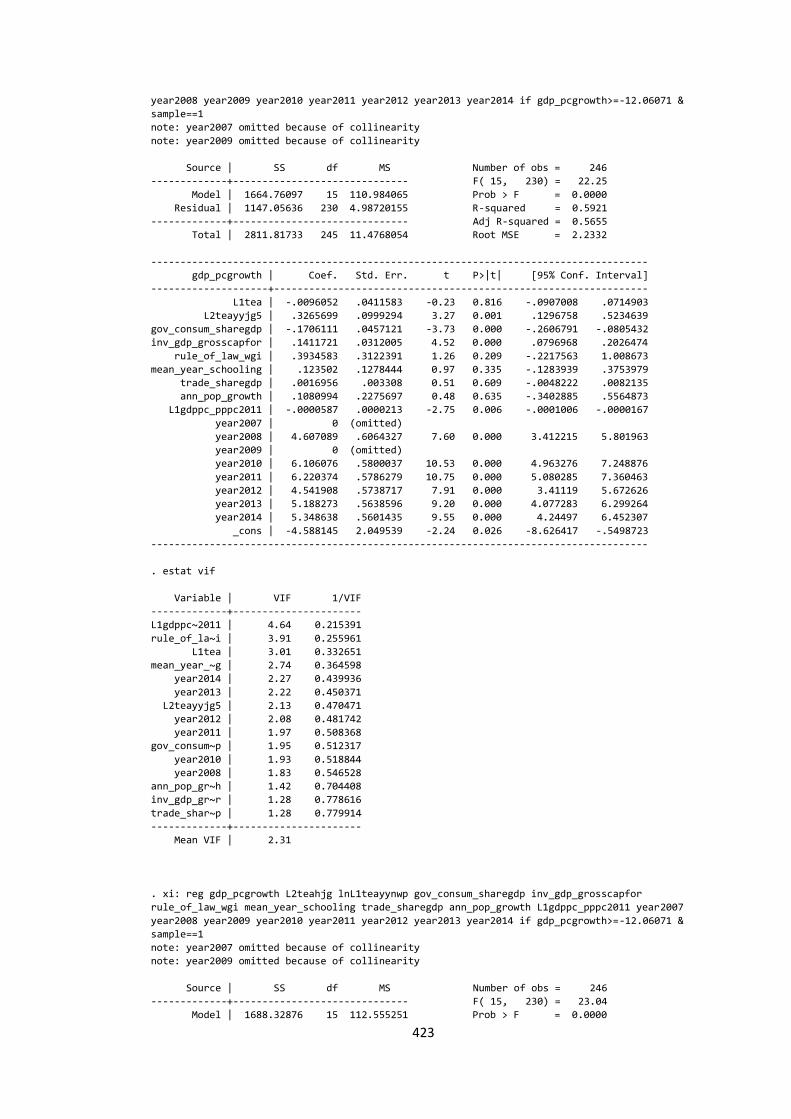
423
year2008 year2009 year2010 year2011 year2012 year2013 year2014 if gdp_pcgrowth>=-12.06071 &
sample==1
note: year2007 omitted because of collinearity
note: year2009 omitted because of collinearity
Source | SS df MS Number of obs = 246
-------------+------------------------------ F( 15, 230) = 22.25
Model | 1664.76097 15 110.984065 Prob > F = 0.0000
Residual | 1147.05636 230 4.98720155 R-squared = 0.5921
-------------+------------------------------ Adj R-squared = 0.5655
Total | 2811.81733 245 11.4768054 Root MSE = 2.2332
-------------------------------------------------------------------------------------
gdp_pcgrowth | Coef. Std. Err. t P>|t| [95% Conf. Interval]
--------------------+----------------------------------------------------------------
L1tea | -.0096052 .0411583 -0.23 0.816 -.0907008 .0714903
L2teayyjg5 | .3265699 .0999294 3.27 0.001 .1296758 .5234639
gov_consum_sharegdp | -.1706111 .0457121 -3.73 0.000 -.2606791 -.0805432
inv_gdp_grosscapfor | .1411721 .0312005 4.52 0.000 .0796968 .2026474
rule_of_law_wgi | .3934583 .3122391 1.26 0.209 -.2217563 1.008673
mean_year_schooling | .123502 .1278444 0.97 0.335 -.1283939 .3753979
trade_sharegdp | .0016956 .003308 0.51 0.609 -.0048222 .0082135
ann_pop_growth | .1080994 .2275697 0.48 0.635 -.3402885 .5564873
L1gdppc_pppc2011 | -.0000587 .0000213 -2.75 0.006 -.0001006 -.0000167
year2007 | 0 (omitted)
year2008 | 4.607089 .6064327 7.60 0.000 3.412215 5.801963
year2009 | 0 (omitted)
year2010 | 6.106076 .5800037 10.53 0.000 4.963276 7.248876
year2011 | 6.220374 .5786279 10.75 0.000 5.080285 7.360463
year2012 | 4.541908 .5738717 7.91 0.000 3.41119 5.672626
year2013 | 5.188273 .5638596 9.20 0.000 4.077283 6.299264
year2014 | 5.348638 .5601435 9.55 0.000 4.24497 6.452307
_cons | -4.588145 2.049539 -2.24 0.026 -8.626417 -.5498723
-------------------------------------------------------------------------------------
. estat vif
Variable | VIF 1/VIF
-------------+----------------------
L1gdppc~2011 | 4.64 0.215391
rule_of_la~i | 3.91 0.255961
L1tea | 3.01 0.332651
mean_year_~g | 2.74 0.364598
year2014 | 2.27 0.439936
year2013 | 2.22 0.450371
L2teayyjg5 | 2.13 0.470471
year2012 | 2.08 0.481742
year2011 | 1.97 0.508368
gov_consum~p | 1.95 0.512317
year2010 | 1.93 0.518844
year2008 | 1.83 0.546528
ann_pop_gr~h | 1.42 0.704408
inv_gdp_gr~r | 1.28 0.778616
trade_shar~p | 1.28 0.779914
-------------+----------------------
Mean VIF | 2.31
. xi: reg gdp_pcgrowth L2teahjg lnL1teayynwp gov_consum_sharegdp inv_gdp_grosscapfor
rule_of_law_wgi mean_year_schooling trade_sharegdp ann_pop_growth L1gdppc_pppc2011 year2007
year2008 year2009 year2010 year2011 year2012 year2013 year2014 if gdp_pcgrowth>=-12.06071 &
sample==1
note: year2007 omitted because of collinearity
note: year2009 omitted because of collinearity
Source | SS df MS Number of obs = 246
-------------+------------------------------ F( 15, 230) = 23.04
Model | 1688.32876 15 112.555251 Prob > F = 0.0000
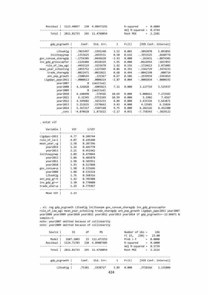
424
Residual | 1123.48857 230 4.88473292 R-squared = 0.6004
-------------+------------------------------ Adj R-squared = 0.5744
Total | 2811.81733 245 11.4768054 Root MSE = 2.2101
-------------------------------------------------------------------------------------
gdp_pcgrowth | Coef. Std. Err. t P>|t| [95% Conf. Interval]
--------------------+----------------------------------------------------------------
L2teahjg | .7015497 .1991248 3.52 0.001 .3092078 1.093892
lnL1teayynwp | .1353625 .2693531 0.50 0.616 -.3953525 .6660774
gov_consum_sharegdp | -.1754305 .0446628 -3.93 0.000 -.263431 -.0874301
inv_gdp_grosscapfor | .1226404 .0310329 3.95 0.000 .0614954 .1837855
rule_of_law_wgi | .4493119 .3155678 1.42 0.156 -.1724613 1.071085
mean_year_schooling | .1055752 .1227449 0.86 0.391 -.1362729 .3474233
trade_sharegdp | .0022471 .0032821 0.68 0.494 -.0042198 .008714
ann_pop_growth | .1500543 .225367 0.67 0.506 -.2939934 .5941019
L1gdppc_pppc2011 | -.0000613 .0000214 -2.87 0.004 -.0001034 -.0000192
year2007 | 0 (omitted)
year2008 | 4.326828 .6085823 7.11 0.000 3.127719 5.525937
year2009 | 0 (omitted)
year2010 | 6.140498 .574566 10.69 0.000 5.008412 7.272583
year2011 | 6.32345 .5751569 10.99 0.000 5.1902 7.4567
year2012 | 4.549602 .5655233 8.04 0.000 3.435334 5.663871
year2013 | 5.252635 .5570662 9.43 0.000 4.15503 6.35024
year2014 | 5.367217 .5507148 9.75 0.000 4.282126 6.452308
_cons | -4.070628 1.871622 -2.17 0.031 -7.758343 -.3829122
-------------------------------------------------------------------------------------
. estat vif
Variable | VIF 1/VIF
-------------+----------------------
L1gdppc~2011 | 4.77 0.209744
rule_of_la~i | 4.07 0.245440
mean_year_~g | 2.58 0.387396
year2014 | 2.24 0.445778
year2013 | 2.21 0.451942
lnL1teayynwp | 2.09 0.479044
year2012 | 2.06 0.485878
year2011 | 1.98 0.503951
year2010 | 1.93 0.517848
gov_consum~p | 1.90 0.525646
year2008 | 1.88 0.531524
L2teahjg | 1.76 0.568316
ann_pop_gr~h | 1.42 0.703488
inv_gdp_gr~r | 1.30 0.770880
trade_shar~p | 1.29 0.775967
-------------+----------------------
Mean VIF | 2.23
. xi: reg gdp_pcgrowth L2teahjg lnL1teanpm gov_consum_sharegdp inv_gdp_grosscapfor
rule_of_law_wgi mean_year_schooling trade_sharegdp ann_pop_growth L1gdppc_pppc2011 year2007
year2008 year2009 year2010 year2011 year2012 year2013 year2014 if gdp_pcgrowth>=-12.06071 &
sample==1
note: year2007 omitted because of collinearity
note: year2009 omitted because of collinearity
Source | SS df MS Number of obs = 246
-------------+------------------------------ F( 15, 230) = 23.00
Model | 1687.1003 15 112.473353 Prob > F = 0.0000
Residual | 1124.71703 230 4.89007405 R-squared = 0.6000
-------------+------------------------------ Adj R-squared = 0.5739
Total | 2811.81733 245 11.4768054 Root MSE = 2.2114
-------------------------------------------------------------------------------------
gdp_pcgrowth | Coef. Std. Err. t P>|t| [95% Conf. Interval]
--------------------+----------------------------------------------------------------
L2teahjg | .75381 .1938727 3.89 0.000 .3718166 1.135804
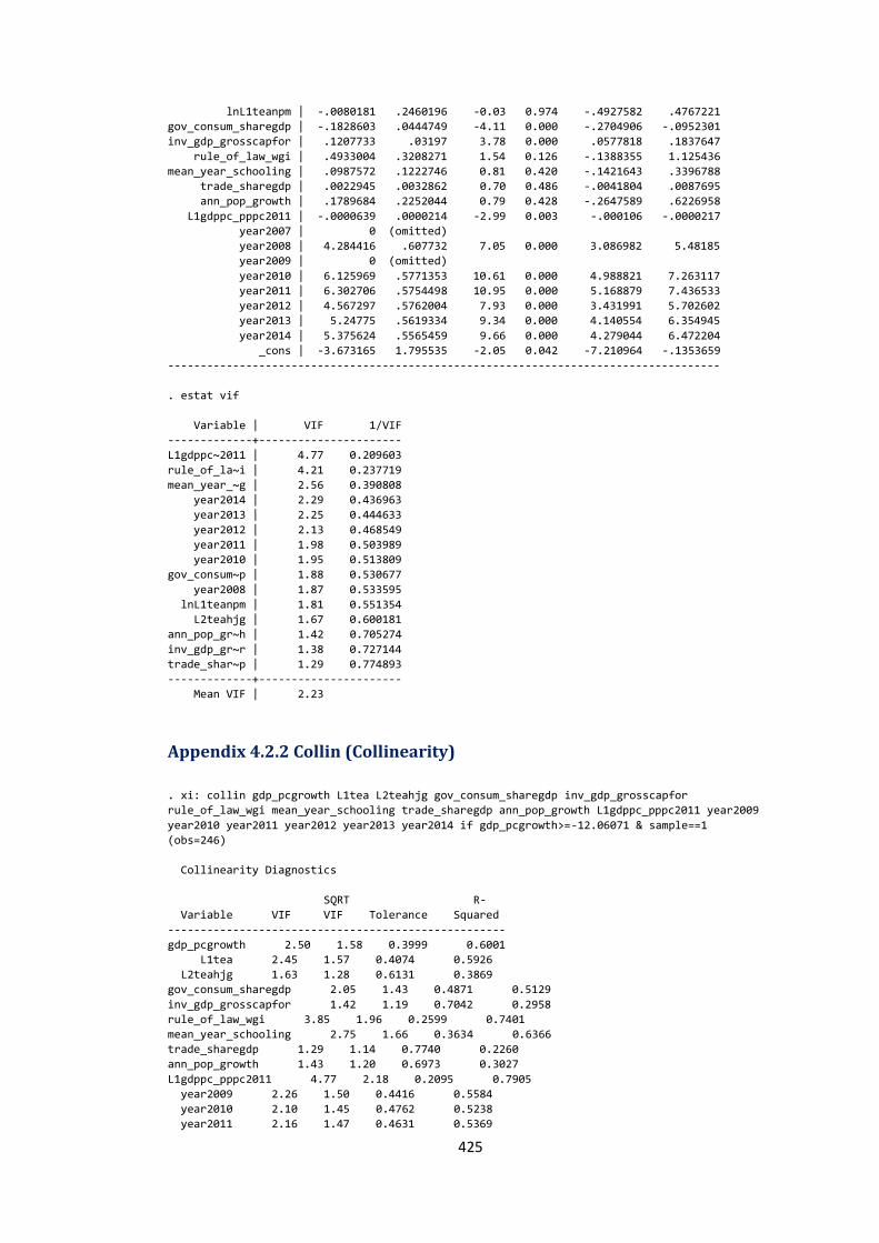
425
lnL1teanpm | -.0080181 .2460196 -0.03 0.974 -.4927582 .4767221
gov_consum_sharegdp | -.1828603 .0444749 -4.11 0.000 -.2704906 -.0952301
inv_gdp_grosscapfor | .1207733 .03197 3.78 0.000 .0577818 .1837647
rule_of_law_wgi | .4933004 .3208271 1.54 0.126 -.1388355 1.125436
mean_year_schooling | .0987572 .1222746 0.81 0.420 -.1421643 .3396788
trade_sharegdp | .0022945 .0032862 0.70 0.486 -.0041804 .0087695
ann_pop_growth | .1789684 .2252044 0.79 0.428 -.2647589 .6226958
L1gdppc_pppc2011 | -.0000639 .0000214 -2.99 0.003 -.000106 -.0000217
year2007 | 0 (omitted)
year2008 | 4.284416 .607732 7.05 0.000 3.086982 5.48185
year2009 | 0 (omitted)
year2010 | 6.125969 .5771353 10.61 0.000 4.988821 7.263117
year2011 | 6.302706 .5754498 10.95 0.000 5.168879 7.436533
year2012 | 4.567297 .5762004 7.93 0.000 3.431991 5.702602
year2013 | 5.24775 .5619334 9.34 0.000 4.140554 6.354945
year2014 | 5.375624 .5565459 9.66 0.000 4.279044 6.472204
_cons | -3.673165 1.795535 -2.05 0.042 -7.210964 -.1353659
-------------------------------------------------------------------------------------
. estat vif
Variable | VIF 1/VIF
-------------+----------------------
L1gdppc~2011 | 4.77 0.209603
rule_of_la~i | 4.21 0.237719
mean_year_~g | 2.56 0.390808
year2014 | 2.29 0.436963
year2013 | 2.25 0.444633
year2012 | 2.13 0.468549
year2011 | 1.98 0.503989
year2010 | 1.95 0.513809
gov_consum~p | 1.88 0.530677
year2008 | 1.87 0.533595
lnL1teanpm | 1.81 0.551354
L2teahjg | 1.67 0.600181
ann_pop_gr~h | 1.42 0.705274
inv_gdp_gr~r | 1.38 0.727144
trade_shar~p | 1.29 0.774893
-------------+----------------------
Mean VIF | 2.23
Appendix 4.2.2 Collin (Collinearity)
. xi: collin gdp_pcgrowth L1tea L2teahjg gov_consum_sharegdp inv_gdp_grosscapfor
rule_of_law_wgi mean_year_schooling trade_sharegdp ann_pop_growth L1gdppc_pppc2011 year2009
year2010 year2011 year2012 year2013 year2014 if gdp_pcgrowth>=-12.06071 & sample==1
(obs=246)
Collinearity Diagnostics
SQRT R-
Variable VIF VIF Tolerance Squared
----------------------------------------------------
gdp_pcgrowth 2.50 1.58 0.3999 0.6001
L1tea 2.45 1.57 0.4074 0.5926
L2teahjg 1.63 1.28 0.6131 0.3869
gov_consum_sharegdp 2.05 1.43 0.4871 0.5129
inv_gdp_grosscapfor 1.42 1.19 0.7042 0.2958
rule_of_law_wgi 3.85 1.96 0.2599 0.7401
mean_year_schooling 2.75 1.66 0.3634 0.6366
trade_sharegdp 1.29 1.14 0.7740 0.2260
ann_pop_growth 1.43 1.20 0.6973 0.3027
L1gdppc_pppc2011 4.77 2.18 0.2095 0.7905
year2009 2.26 1.50 0.4416 0.5584
year2010 2.10 1.45 0.4762 0.5238
year2011 2.16 1.47 0.4631 0.5369
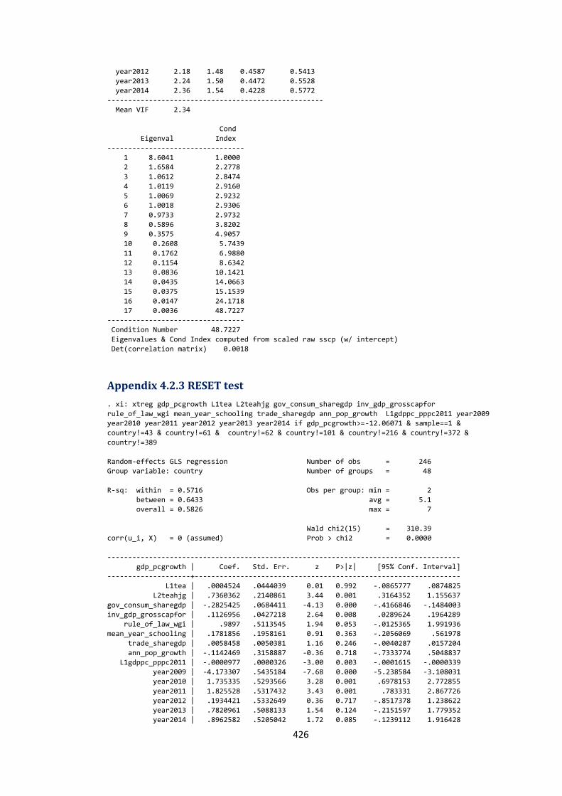
426
year2012 2.18 1.48 0.4587 0.5413
year2013 2.24 1.50 0.4472 0.5528
year2014 2.36 1.54 0.4228 0.5772
----------------------------------------------------
Mean VIF 2.34
Cond
Eigenval Index
---------------------------------
1 8.6041 1.0000
2 1.6584 2.2778
3 1.0612 2.8474
4 1.0119 2.9160
5 1.0069 2.9232
6 1.0018 2.9306
7 0.9733 2.9732
8 0.5896 3.8202
9 0.3575 4.9057
10 0.2608 5.7439
11 0.1762 6.9880
12 0.1154 8.6342
13 0.0836 10.1421
14 0.0435 14.0663
15 0.0375 15.1539
16 0.0147 24.1718
17 0.0036 48.7227
---------------------------------
Condition Number 48.7227
Eigenvalues & Cond Index computed from scaled raw sscp (w/ intercept)
Det(correlation matrix) 0.0018
Appendix 4.2.3 RESET test
. xi: xtreg gdp_pcgrowth L1tea L2teahjg gov_consum_sharegdp inv_gdp_grosscapfor
rule_of_law_wgi mean_year_schooling trade_sharegdp ann_pop_growth L1gdppc_pppc2011 year2009
year2010 year2011 year2012 year2013 year2014 if gdp_pcgrowth>=-12.06071 & sample==1 &
country!=43 & country!=61 & country!=62 & country!=101 & country!=216 & country!=372 &
country!=389
Random-effects GLS regression Number of obs = 246
Group variable: country Number of groups = 48
R-sq: within = 0.5716 Obs per group: min = 2
between = 0.6433 avg = 5.1
overall = 0.5826 max = 7
Wald chi2(15) = 310.39
corr(u_i, X) = 0 (assumed) Prob > chi2 = 0.0000
-------------------------------------------------------------------------------------
gdp_pcgrowth | Coef. Std. Err. z P>|z| [95% Conf. Interval]
--------------------+----------------------------------------------------------------
L1tea | .0004524 .0444039 0.01 0.992 -.0865777 .0874825
L2teahjg | .7360362 .2140861 3.44 0.001 .3164352 1.155637
gov_consum_sharegdp | -.2825425 .0684411 -4.13 0.000 -.4166846 -.1484003
inv_gdp_grosscapfor | .1126956 .0427218 2.64 0.008 .0289624 .1964289
rule_of_law_wgi | .9897 .5113545 1.94 0.053 -.0125365 1.991936
mean_year_schooling | .1781856 .1958161 0.91 0.363 -.2056069 .561978
trade_sharegdp | .0058458 .0050381 1.16 0.246 -.0040287 .0157204
ann_pop_growth | -.1142469 .3158887 -0.36 0.718 -.7333774 .5048837
L1gdppc_pppc2011 | -.0000977 .0000326 -3.00 0.003 -.0001615 -.0000339
year2009 | -4.173307 .5435184 -7.68 0.000 -5.238584 -3.108031
year2010 | 1.735335 .5293566 3.28 0.001 .6978153 2.772855
year2011 | 1.825528 .5317432 3.43 0.001 .783331 2.867726
year2012 | .1934421 .5332649 0.36 0.717 -.8517378 1.238622
year2013 | .7820961 .5088133 1.54 0.124 -.2151597 1.779352
year2014 | .8962582 .5205042 1.72 0.085 -.1239112 1.916428
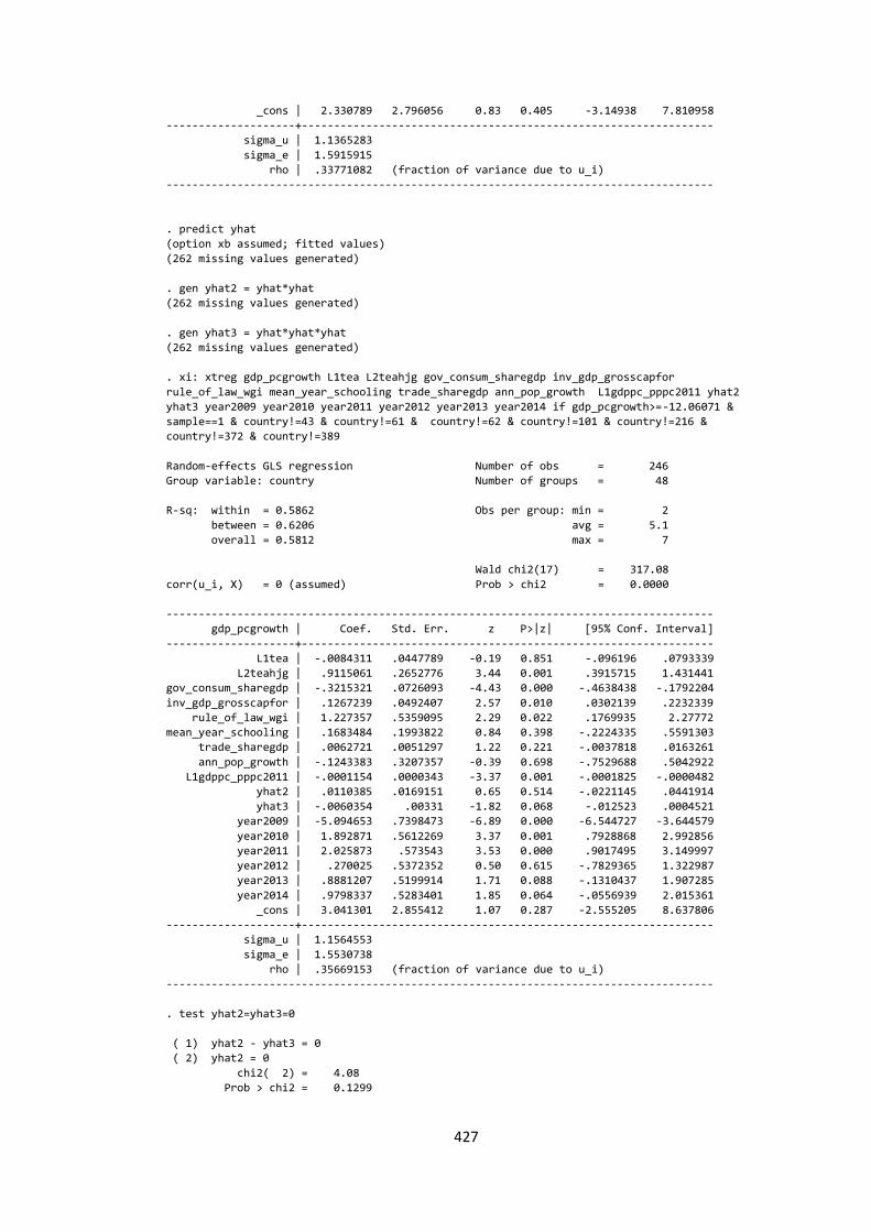
427
_cons | 2.330789 2.796056 0.83 0.405 -3.14938 7.810958
--------------------+----------------------------------------------------------------
sigma_u | 1.1365283
sigma_e | 1.5915915
rho | .33771082 (fraction of variance due to u_i)
-------------------------------------------------------------------------------------
. predict yhat
(option xb assumed; fitted values)
(262 missing values generated)
. gen yhat2 = yhat*yhat
(262 missing values generated)
. gen yhat3 = yhat*yhat*yhat
(262 missing values generated)
. xi: xtreg gdp_pcgrowth L1tea L2teahjg gov_consum_sharegdp inv_gdp_grosscapfor
rule_of_law_wgi mean_year_schooling trade_sharegdp ann_pop_growth L1gdppc_pppc2011 yhat2
yhat3 year2009 year2010 year2011 year2012 year2013 year2014 if gdp_pcgrowth>=-12.06071 &
sample==1 & country!=43 & country!=61 & country!=62 & country!=101 & country!=216 &
country!=372 & country!=389
Random-effects GLS regression Number of obs = 246
Group variable: country Number of groups = 48
R-sq: within = 0.5862 Obs per group: min = 2
between = 0.6206 avg = 5.1
overall = 0.5812 max = 7
Wald chi2(17) = 317.08
corr(u_i, X) = 0 (assumed) Prob > chi2 = 0.0000
-------------------------------------------------------------------------------------
gdp_pcgrowth | Coef. Std. Err. z P>|z| [95% Conf. Interval]
--------------------+----------------------------------------------------------------
L1tea | -.0084311 .0447789 -0.19 0.851 -.096196 .0793339
L2teahjg | .9115061 .2652776 3.44 0.001 .3915715 1.431441
gov_consum_sharegdp | -.3215321 .0726093 -4.43 0.000 -.4638438 -.1792204
inv_gdp_grosscapfor | .1267239 .0492407 2.57 0.010 .0302139 .2232339
rule_of_law_wgi | 1.227357 .5359095 2.29 0.022 .1769935 2.27772
mean_year_schooling | .1683484 .1993822 0.84 0.398 -.2224335 .5591303
trade_sharegdp | .0062721 .0051297 1.22 0.221 -.0037818 .0163261
ann_pop_growth | -.1243383 .3207357 -0.39 0.698 -.7529688 .5042922
L1gdppc_pppc2011 | -.0001154 .0000343 -3.37 0.001 -.0001825 -.0000482
yhat2 | .0110385 .0169151 0.65 0.514 -.0221145 .0441914
yhat3 | -.0060354 .00331 -1.82 0.068 -.012523 .0004521
year2009 | -5.094653 .7398473 -6.89 0.000 -6.544727 -3.644579
year2010 | 1.892871 .5612269 3.37 0.001 .7928868 2.992856
year2011 | 2.025873 .573543 3.53 0.000 .9017495 3.149997
year2012 | .270025 .5372352 0.50 0.615 -.7829365 1.322987
year2013 | .8881207 .5199914 1.71 0.088 -.1310437 1.907285
year2014 | .9798337 .5283401 1.85 0.064 -.0556939 2.015361
_cons | 3.041301 2.855412 1.07 0.287 -2.555205 8.637806
--------------------+----------------------------------------------------------------
sigma_u | 1.1564553
sigma_e | 1.5530738
rho | .35669153 (fraction of variance due to u_i)
-------------------------------------------------------------------------------------
. test yhat2=yhat3=0
( 1) yhat2 - yhat3 = 0
( 2) yhat2 = 0
chi2( 2) = 4.08
Prob > chi2 = 0.1299
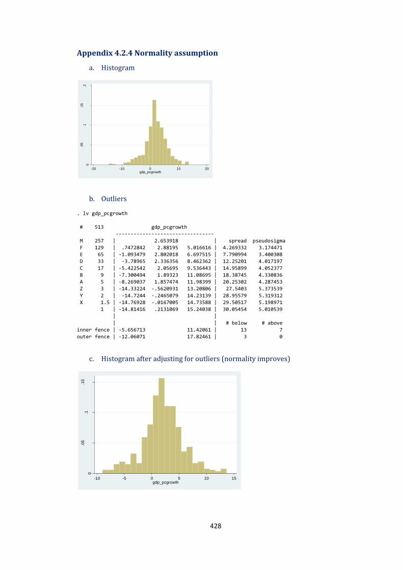
428
Appendix 4.2.4 Normality assumption
a. Histogram
b. Outliers
. lv gdp_pcgrowth
# 513 gdp_pcgrowth
---------------------------------
M 257 | 2.653918 | spread pseudosigma
F 129 | .7472842 2.88195 5.016616 | 4.269332 3.174471
E 65 | -1.093479 2.802018 6.697515 | 7.790994 3.400308
D 33 | -3.78965 2.336356 8.462362 | 12.25201 4.017197
C 17 | -5.422542 2.05695 9.536443 | 14.95899 4.052377
B 9 | -7.300494 1.89323 11.08695 | 18.38745 4.330836
A 5 | -8.269037 1.857474 11.98399 | 20.25302 4.287453
Z 3 | -14.33224 -.5620931 13.20806 | 27.5403 5.373539
Y 2 | -14.7244 -.2465079 14.23139 | 28.95579 5.319312
X 1.5 | -14.76928 -.0167005 14.73588 | 29.50517 5.198971
1 | -14.81416 .2131069 15.24038 | 30.05454 5.010539
| |
| | # below # above
inner fence | -5.656713 11.42061 | 13 7
outer fence | -12.06071 17.82461 | 3 0
c. Histogram after adjusting for outliers (normality improves)
0
.05
.1.1
5.2
Den
sity
-20 -10 0 10 20gdp_pcgrowth
0
.05
.1.1
5
Den
sity
-10 -5 0 5 10 15gdp_pcgrowth
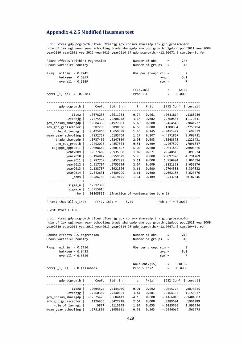
429
Appendix 4.2.5 Modified Hausman test
. xi: xtreg gdp_pcgrowth L1tea L2teahjg gov_consum_sharegdp inv_gdp_grosscapfor
rule_of_law_wgi mean_year_schooling trade_sharegdp ann_pop_growth L1gdppc_pppc2011 year2009
year2010 year2011 year2012 year2013 year2014 if gdp_pcgrowth>=-12.06071 & sample==1, fe
Fixed-effects (within) regression Number of obs = 246
Group variable: country Number of groups = 48
R-sq: within = 0.7241 Obs per group: min = 2
between = 0.5053 avg = 5.1
overall = 0.3029 max = 7
F(15,183) = 32.02
corr(u_i, Xb) = -0.9783 Prob > F = 0.0000
-------------------------------------------------------------------------------------
gdp_pcgrowth | Coef. Std. Err. t P>|t| [95% Conf. Interval]
--------------------+----------------------------------------------------------------
L1tea | .0378236 .0511933 0.74 0.461 -.0631814 .1388286
L2teahjg | .7275574 .2288248 3.18 0.002 .2760833 1.179031
gov_consum_sharegdp | -1.084335 .1927061 -5.63 0.000 -1.464546 -.7041232
inv_gdp_grosscapfor | .5982299 .0898836 6.66 0.000 .4208884 .7755714
rule_of_law_wgi | 2.425866 1.659398 1.46 0.145 -.8481472 5.699879
mean_year_schooling | .7832729 .6185764 1.27 0.207 -.4371857 2.003731
trade_sharegdp | .0737402 .0247859 2.98 0.003 .0248373 .1226431
ann_pop_growth | -.2492075 .4857503 -0.51 0.609 -1.207599 .7091837
L1gdppc_pppc2011 | -.0008643 .0001427 -6.05 0.000 -.0011459 -.0005826
year2009 | -1.077469 .5935308 -1.82 0.071 -2.248513 .093574
year2010 | 3.194847 .5559629 5.75 0.000 2.097926 4.291769
year2011 | 2.787759 .5457821 5.11 0.000 1.710924 3.864594
year2012 | 1.517704 .5755524 2.64 0.009 .3821328 2.653276
year2013 | 2.138757 .5921526 3.61 0.000 .9704333 3.307082
year2014 | 2.342631 .6489799 3.61 0.000 1.062186 3.623076
_cons | 13.86783 8.619125 1.61 0.109 -3.13781 30.87346
--------------------+----------------------------------------------------------------
sigma_u | 12.12399
sigma_e | 1.5915915
rho | .98305852 (fraction of variance due to u_i)
-------------------------------------------------------------------------------------
F test that all u_i=0: F(47, 183) = 5.55 Prob > F = 0.0000
. est store FIXED
. xi: xtreg gdp_pcgrowth L1tea L2teahjg gov_consum_sharegdp inv_gdp_grosscapfor
rule_of_law_wgi mean_year_schooling trade_sharegdp ann_pop_growth L1gdppc_pppc2011 year2009
year2010 year2011 year2012 year2013 year2014 if gdp_pcgrowth>=-12.06071 & sample==1, re
Random-effects GLS regression Number of obs = 246
Group variable: country Number of groups = 48
R-sq: within = 0.5716 Obs per group: min = 2
between = 0.6433 avg = 5.1
overall = 0.5826 max = 7
Wald chi2(15) = 310.39
corr(u_i, X) = 0 (assumed) Prob > chi2 = 0.0000
-------------------------------------------------------------------------------------
gdp_pcgrowth | Coef. Std. Err. z P>|z| [95% Conf. Interval]
--------------------+----------------------------------------------------------------
L1tea | .0004524 .0444039 0.01 0.992 -.0865777 .0874825
L2teahjg | .7360362 .2140861 3.44 0.001 .3164352 1.155637
gov_consum_sharegdp | -.2825425 .0684411 -4.13 0.000 -.4166846 -.1484003
inv_gdp_grosscapfor | .1126956 .0427218 2.64 0.008 .0289624 .1964289
rule_of_law_wgi | .9897 .5113545 1.94 0.053 -.0125365 1.991936
mean_year_schooling | .1781856 .1958161 0.91 0.363 -.2056069 .561978
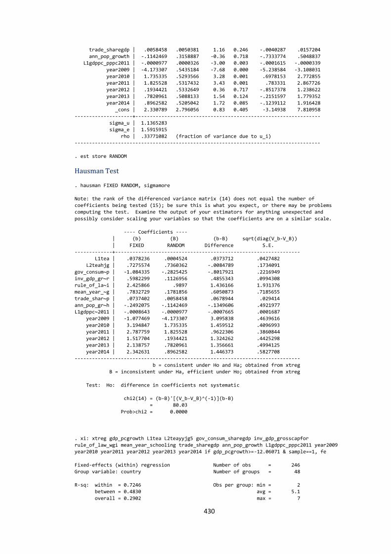
430
trade_sharegdp | .0058458 .0050381 1.16 0.246 -.0040287 .0157204
ann_pop_growth | -.1142469 .3158887 -0.36 0.718 -.7333774 .5048837
L1gdppc_pppc2011 | -.0000977 .0000326 -3.00 0.003 -.0001615 -.0000339
year2009 | -4.173307 .5435184 -7.68 0.000 -5.238584 -3.108031
year2010 | 1.735335 .5293566 3.28 0.001 .6978153 2.772855
year2011 | 1.825528 .5317432 3.43 0.001 .783331 2.867726
year2012 | .1934421 .5332649 0.36 0.717 -.8517378 1.238622
year2013 | .7820961 .5088133 1.54 0.124 -.2151597 1.779352
year2014 | .8962582 .5205042 1.72 0.085 -.1239112 1.916428
_cons | 2.330789 2.796056 0.83 0.405 -3.14938 7.810958
--------------------+----------------------------------------------------------------
sigma_u | 1.1365283
sigma_e | 1.5915915
rho | .33771082 (fraction of variance due to u_i)
-------------------------------------------------------------------------------------
. est store RANDOM
Hausman Test
. hausman FIXED RANDOM, sigmamore
Note: the rank of the differenced variance matrix (14) does not equal the number of
coefficients being tested (15); be sure this is what you expect, or there may be problems
computing the test. Examine the output of your estimators for anything unexpected and
possibly consider scaling your variables so that the coefficients are on a similar scale.
---- Coefficients ----
| (b) (B) (b-B) sqrt(diag(V_b-V_B))
| FIXED RANDOM Difference S.E.
-------------+----------------------------------------------------------------
L1tea | .0378236 .0004524 .0373712 .0427482
L2teahjg | .7275574 .7360362 -.0084789 .1734091
gov_consum~p | -1.084335 -.2825425 -.8017921 .2216949
inv_gdp_gr~r | .5982299 .1126956 .4855343 .0994308
rule_of_la~i | 2.425866 .9897 1.436166 1.931376
mean_year_~g | .7832729 .1781856 .6050873 .7185655
trade_shar~p | .0737402 .0058458 .0678944 .029414
ann_pop_gr~h | -.2492075 -.1142469 -.1349606 .4921977
L1gdppc~2011 | -.0008643 -.0000977 -.0007665 .0001687
year2009 | -1.077469 -4.173307 3.095838 .4639616
year2010 | 3.194847 1.735335 1.459512 .4096993
year2011 | 2.787759 1.825528 .9622306 .3860844
year2012 | 1.517704 .1934421 1.324262 .4425298
year2013 | 2.138757 .7820961 1.356661 .4994125
year2014 | 2.342631 .8962582 1.446373 .5827708
------------------------------------------------------------------------------
b = consistent under Ho and Ha; obtained from xtreg
B = inconsistent under Ha, efficient under Ho; obtained from xtreg
Test: Ho: difference in coefficients not systematic
chi2(14) = (b-B)'[(V_b-V_B)^(-1)](b-B)
= 80.03
Prob>chi2 = 0.0000
. xi: xtreg gdp_pcgrowth L1tea L2teayyjg5 gov_consum_sharegdp inv_gdp_grosscapfor
rule_of_law_wgi mean_year_schooling trade_sharegdp ann_pop_growth L1gdppc_pppc2011 year2009
year2010 year2011 year2012 year2013 year2014 if gdp_pcgrowth>=-12.06071 & sample==1, fe
Fixed-effects (within) regression Number of obs = 246
Group variable: country Number of groups = 48
R-sq: within = 0.7246 Obs per group: min = 2
between = 0.4830 avg = 5.1
overall = 0.2902 max = 7
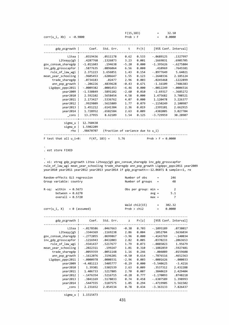
431
F(15,183) = 32.10
corr(u_i, Xb) = -0.9800 Prob > F = 0.0000
-------------------------------------------------------------------------------------
gdp_pcgrowth | Coef. Std. Err. t P>|t| [95% Conf. Interval]
--------------------+----------------------------------------------------------------
L1tea | .0319436 .0511178 0.62 0.533 -.0689125 .1327997
L2teayyjg5 | .4287768 .1326873 3.23 0.001 .1669831 .6905705
gov_consum_sharegdp | -1.011603 .194638 -5.20 0.000 -1.395626 -.6275804
inv_gdp_grosscapfor | .5877635 .0896064 6.56 0.000 .410969 .7645581
rule_of_law_wgi | 2.371223 1.656851 1.43 0.154 -.8977649 5.64021
mean_year_schooling | .9605453 .6206647 1.55 0.123 -.2640336 2.185124
trade_sharegdp | .0734183 .02477 2.96 0.003 .0245468 .1222899
ann_pop_growth | -.206226 .4839628 -0.43 0.671 -1.16109 .7486383
L1gdppc_pppc2011 | -.0009382 .0001453 -6.46 0.000 -.0012249 -.0006516
year2009 | -1.530849 .5891102 -2.60 0.010 -2.69317 -.3685272
year2010 | 2.592102 .5658454 4.58 0.000 1.475682 3.708521
year2011 | 2.173427 .5336762 4.07 0.000 1.120478 3.226377
year2012 | .9929809 .5615809 1.77 0.079 -.1150249 2.100987
year2013 | 1.451212 .6141384 2.36 0.019 .2395101 2.662915
year2014 | 1.728952 .6582584 2.63 0.009 .4302005 3.027704
_cons | 13.27955 8.62109 1.54 0.125 -3.729959 30.28907
--------------------+----------------------------------------------------------------
sigma_u | 12.760438
sigma_e | 1.5902209
rho | .98470707 (fraction of variance due to u_i)
-------------------------------------------------------------------------------------
F test that all u_i=0: F(47, 183) = 5.76 Prob > F = 0.0000
.
. est store FIXED
.
. xi: xtreg gdp_pcgrowth L1tea L2teayyjg5 gov_consum_sharegdp inv_gdp_grosscapfor
rule_of_law_wgi mean_year_schooling trade_sharegdp ann_pop_growth L1gdppc_pppc2011 year2009
year2010 year2011 year2012 year2013 year2014 if gdp_pcgrowth>=-12.06071 & sample==1, re
Random-effects GLS regression Number of obs = 246
Group variable: country Number of groups = 48
R-sq: within = 0.5673 Obs per group: min = 2
between = 0.6278 avg = 5.1
overall = 0.5720 max = 7
Wald chi2(15) = 302.32
corr(u_i, X) = 0 (assumed) Prob > chi2 = 0.0000
-------------------------------------------------------------------------------------
gdp_pcgrowth | Coef. Std. Err. z P>|z| [95% Conf. Interval]
--------------------+----------------------------------------------------------------
L1tea | -.0178586 .0467663 -0.38 0.703 -.1095189 .0738017
L2teayyjg5 | .3344369 .1169238 2.86 0.004 .1052704 .5636034
gov_consum_sharegdp | -.2772055 .0699867 -3.96 0.000 -.4143769 -.140034
inv_gdp_grosscapfor | .1216943 .0432003 2.82 0.005 .0370233 .2063653
rule_of_law_wgi | .9341437 .5217677 1.79 0.073 -.0885023 1.95679
mean_year_schooling | .2022311 .199247 1.01 0.310 -.1882859 .5927481
trade_sharegdp | .0059359 .0051148 1.16 0.246 -.004089 .0159608
ann_pop_growth | -.1612076 .3196201 -0.50 0.614 -.7876516 .4652363
L1gdppc_pppc2011 | -.0000978 .0000331 -2.96 0.003 -.0001626 -.000033
year2009 | -4.481113 .5405777 -8.29 0.000 -5.540625 -3.4216
year2010 | 1.39301 .5302539 2.63 0.009 .3537312 2.432288
year2011 | 1.406733 .5217805 2.70 0.007 .3840619 2.429404
year2012 | -.1476354 .5216715 -0.28 0.777 -1.170093 .8748218
year2013 | .3841169 .5178033 0.74 0.458 -.6307589 1.398993
year2014 | .5447555 .5187575 1.05 0.294 -.4719905 1.561502
_cons | 2.231652 2.854534 0.78 0.434 -3.363133 7.826437
--------------------+----------------------------------------------------------------
sigma_u | 1.1515473

432
sigma_e | 1.5902209
rho | .3439969 (fraction of variance due to u_i)
-------------------------------------------------------------------------------------
.
. est store RANDOM
.
. hausman FIXED RANDOM, sigmamore
Note: the rank of the differenced variance matrix (14) does not equal the number of
coefficients being tested (15); be sure this is what you expect, or there may be problems
computing the test. Examine the output of your estimators for anything unexpected and
possibly consider scaling your variables so that the coefficients are on a similar scale.
---- Coefficients ----
| (b) (B) (b-B) sqrt(diag(V_b-V_B))
| FIXED RANDOM Difference S.E.
-------------+----------------------------------------------------------------
L1tea | .0319436 -.0178586 .0498022 .0406593
L2teayyjg5 | .4287768 .3344369 .0943399 .1104695
gov_consum~p | -1.011603 -.2772055 -.7343979 .2253404
inv_gdp_gr~r | .5877635 .1216943 .4660693 .0996699
rule_of_la~i | 2.371223 .9341437 1.437079 1.93964
mean_year_~g | .9605453 .2022311 .7583142 .7255684
trade_shar~p | .0734183 .0059359 .0674824 .0295898
ann_pop_gr~h | -.206226 -.1612076 -.0450183 .4920024
L1gdppc~2011 | -.0009382 -.0000978 -.0008404 .000173
year2009 | -1.530849 -4.481113 2.950264 .4667141
year2010 | 2.592102 1.39301 1.199092 .4351868
year2011 | 2.173427 1.406733 .7666945 .3825166
year2012 | .9929809 -.1476354 1.140616 .4374354
year2013 | 1.451212 .3841169 1.067095 .5349625
year2014 | 1.728952 .5447555 1.184197 .6063825
------------------------------------------------------------------------------
b = consistent under Ho and Ha; obtained from xtreg
B = inconsistent under Ha, efficient under Ho; obtained from xtreg
Test: Ho: difference in coefficients not systematic
chi2(14) = (b-B)'[(V_b-V_B)^(-1)](b-B)
= 81.43
Prob>chi2 = 0.0000
. xi: xtreg gdp_pcgrowth L2teahjg lnL1teayynwp gov_consum_sharegdp inv_gdp_grosscapfor
rule_of_law_wgi mean_year_schooling trade_sharegdp ann_pop_growth L1gdppc_pppc2011 year2009
year2010 year2011 year2012 year2013 year2014 if gdp_pcgrowth>=-12.06071 & sample==1, fe
Fixed-effects (within) regression Number of obs = 246
Group variable: country Number of groups = 48
R-sq: within = 0.7355 Obs per group: min = 2
between = 0.4955 avg = 5.1
overall = 0.3022 max = 7
F(15,183) = 33.93
corr(u_i, Xb) = -0.9786 Prob > F = 0.0000
-------------------------------------------------------------------------------------
gdp_pcgrowth | Coef. Std. Err. t P>|t| [95% Conf. Interval]
--------------------+----------------------------------------------------------------
L2teahjg | .6749474 .2244864 3.01 0.003 .2320331 1.117862
lnL1teayynwp | .8610772 .2961518 2.91 0.004 .2767663 1.445388
gov_consum_sharegdp | -1.021862 .188907 -5.41 0.000 -1.394578 -.6491463
inv_gdp_grosscapfor | .6000114 .0880088 6.82 0.000 .4263689 .7736539
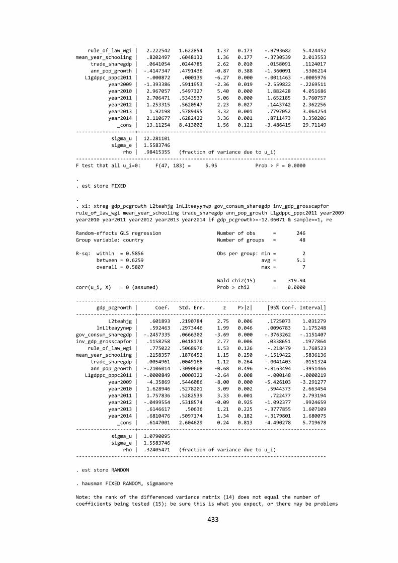
433
rule_of_law_wgi | 2.222542 1.622854 1.37 0.173 -.9793682 5.424452
mean_year_schooling | .8202497 .6048132 1.36 0.177 -.3730539 2.013553
trade_sharegdp | .0641054 .0244785 2.62 0.010 .0158091 .1124017
ann_pop_growth | -.4147347 .4791436 -0.87 0.388 -1.360091 .5306214
L1gdppc_pppc2011 | -.000872 .000139 -6.27 0.000 -.0011463 -.0005976
year2009 | -1.393386 .5911953 -2.36 0.019 -2.559822 -.2269511
year2010 | 2.967057 .5497327 5.40 0.000 1.882428 4.051686
year2011 | 2.706471 .5343537 5.06 0.000 1.652185 3.760757
year2012 | 1.253315 .5620547 2.23 0.027 .1443742 2.362256
year2013 | 1.92198 .5789495 3.32 0.001 .7797052 3.064254
year2014 | 2.110677 .6282422 3.36 0.001 .8711473 3.350206
_cons | 13.11254 8.413002 1.56 0.121 -3.486415 29.71149
--------------------+----------------------------------------------------------------
sigma_u | 12.281101
sigma_e | 1.5583746
rho | .98415355 (fraction of variance due to u_i)
-------------------------------------------------------------------------------------
F test that all u_i=0: F(47, 183) = 5.95 Prob > F = 0.0000
.
. est store FIXED
.
. xi: xtreg gdp_pcgrowth L2teahjg lnL1teayynwp gov_consum_sharegdp inv_gdp_grosscapfor
rule_of_law_wgi mean_year_schooling trade_sharegdp ann_pop_growth L1gdppc_pppc2011 year2009
year2010 year2011 year2012 year2013 year2014 if gdp_pcgrowth>=-12.06071 & sample==1, re
Random-effects GLS regression Number of obs = 246
Group variable: country Number of groups = 48
R-sq: within = 0.5856 Obs per group: min = 2
between = 0.6259 avg = 5.1
overall = 0.5807 max = 7
Wald chi2(15) = 319.94
corr(u_i, X) = 0 (assumed) Prob > chi2 = 0.0000
-------------------------------------------------------------------------------------
gdp_pcgrowth | Coef. Std. Err. z P>|z| [95% Conf. Interval]
--------------------+----------------------------------------------------------------
L2teahjg | .601893 .2190784 2.75 0.006 .1725073 1.031279
lnL1teayynwp | .592463 .2973446 1.99 0.046 .0096783 1.175248
gov_consum_sharegdp | -.2457335 .0666302 -3.69 0.000 -.3763262 -.1151407
inv_gdp_grosscapfor | .1158258 .0418174 2.77 0.006 .0338651 .1977864
rule_of_law_wgi | .775022 .5068976 1.53 0.126 -.218479 1.768523
mean_year_schooling | .2158357 .1876452 1.15 0.250 -.1519422 .5836136
trade_sharegdp | .0054961 .0049166 1.12 0.264 -.0041403 .0151324
ann_pop_growth | -.2106014 .3090608 -0.68 0.496 -.8163494 .3951466
L1gdppc_pppc2011 | -.0000849 .0000322 -2.64 0.008 -.000148 -.0000219
year2009 | -4.35869 .5446086 -8.00 0.000 -5.426103 -3.291277
year2010 | 1.628946 .5278201 3.09 0.002 .5944373 2.663454
year2011 | 1.757836 .5282539 3.33 0.001 .722477 2.793194
year2012 | -.0499554 .5318574 -0.09 0.925 -1.092377 .9924659
year2013 | .6146617 .50636 1.21 0.225 -.3777855 1.607109
year2014 | .6810476 .5097174 1.34 0.182 -.3179801 1.680075
_cons | .6147001 2.604629 0.24 0.813 -4.490278 5.719678
--------------------+----------------------------------------------------------------
sigma_u | 1.0790095
sigma_e | 1.5583746
rho | .32405471 (fraction of variance due to u_i)
-------------------------------------------------------------------------------------
. est store RANDOM
. hausman FIXED RANDOM, sigmamore
Note: the rank of the differenced variance matrix (14) does not equal the number of
coefficients being tested (15); be sure this is what you expect, or there may be problems
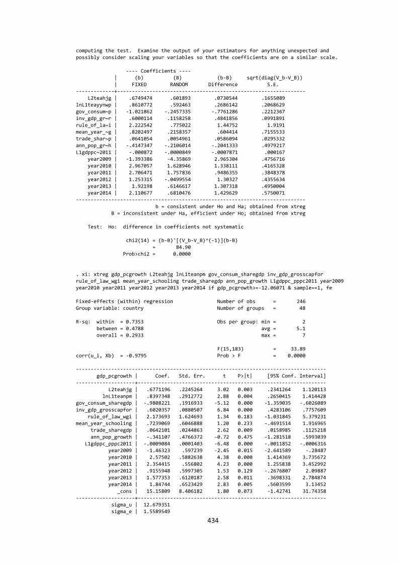
434
computing the test. Examine the output of your estimators for anything unexpected and
possibly consider scaling your variables so that the coefficients are on a similar scale.
---- Coefficients ----
| (b) (B) (b-B) sqrt(diag(V_b-V_B))
| FIXED RANDOM Difference S.E.
-------------+----------------------------------------------------------------
L2teahjg | .6749474 .601893 .0730544 .1655089
lnL1teayynwp | .8610772 .592463 .2686142 .2068629
gov_consum~p | -1.021862 -.2457335 -.7761286 .2212367
inv_gdp_gr~r | .6000114 .1158258 .4841856 .0991891
rule_of_la~i | 2.222542 .775022 1.44752 1.9191
mean_year_~g | .8202497 .2158357 .604414 .7155533
trade_shar~p | .0641054 .0054961 .0586094 .0295332
ann_pop_gr~h | -.4147347 -.2106014 -.2041333 .4979217
L1gdppc~2011 | -.000872 -.0000849 -.0007871 .000167
year2009 | -1.393386 -4.35869 2.965304 .4756716
year2010 | 2.967057 1.628946 1.338111 .4165328
year2011 | 2.706471 1.757836 .9486355 .3848378
year2012 | 1.253315 -.0499554 1.30327 .4355634
year2013 | 1.92198 .6146617 1.307318 .4950004
year2014 | 2.110677 .6810476 1.429629 .5750071
------------------------------------------------------------------------------
b = consistent under Ho and Ha; obtained from xtreg
B = inconsistent under Ha, efficient under Ho; obtained from xtreg
Test: Ho: difference in coefficients not systematic
chi2(14) = (b-B)'[(V_b-V_B)^(-1)](b-B)
= 84.90
Prob>chi2 = 0.0000
. xi: xtreg gdp_pcgrowth L2teahjg lnL1teanpm gov_consum_sharegdp inv_gdp_grosscapfor
rule_of_law_wgi mean_year_schooling trade_sharegdp ann_pop_growth L1gdppc_pppc2011 year2009
year2010 year2011 year2012 year2013 year2014 if gdp_pcgrowth>=-12.06071 & sample==1, fe
Fixed-effects (within) regression Number of obs = 246
Group variable: country Number of groups = 48
R-sq: within = 0.7353 Obs per group: min = 2
between = 0.4788 avg = 5.1
overall = 0.2933 max = 7
F(15,183) = 33.89
corr(u_i, Xb) = -0.9795 Prob > F = 0.0000
-------------------------------------------------------------------------------------
gdp_pcgrowth | Coef. Std. Err. t P>|t| [95% Conf. Interval]
--------------------+----------------------------------------------------------------
L2teahjg | .6771196 .2245264 3.02 0.003 .2341264 1.120113
lnL1teanpm | .8397348 .2912772 2.88 0.004 .2650415 1.414428
gov_consum_sharegdp | -.9808221 .1916933 -5.12 0.000 -1.359035 -.6026089
inv_gdp_grosscapfor | .6020357 .0880507 6.84 0.000 .4283106 .7757609
rule_of_law_wgi | 2.173693 1.624693 1.34 0.183 -1.031845 5.379231
mean_year_schooling | .7239069 .6046888 1.20 0.233 -.4691514 1.916965
trade_sharegdp | .0642101 .0244863 2.62 0.009 .0158985 .1125218
ann_pop_growth | -.341107 .4766372 -0.72 0.475 -1.281518 .5993039
L1gdppc_pppc2011 | -.0009084 .0001403 -6.48 0.000 -.0011852 -.0006316
year2009 | -1.46323 .597239 -2.45 0.015 -2.641589 -.28487
year2010 | 2.57502 .5882638 4.38 0.000 1.414369 3.735672
year2011 | 2.354415 .556802 4.23 0.000 1.255838 3.452992
year2012 | .9155948 .5997305 1.53 0.129 -.2676807 2.09887
year2013 | 1.577353 .6120187 2.58 0.011 .3698331 2.784874
year2014 | 1.84744 .6523429 2.83 0.005 .5603599 3.13452
_cons | 15.15809 8.406182 1.80 0.073 -1.42741 31.74358
--------------------+----------------------------------------------------------------
sigma_u | 12.679351
sigma_e | 1.5589549
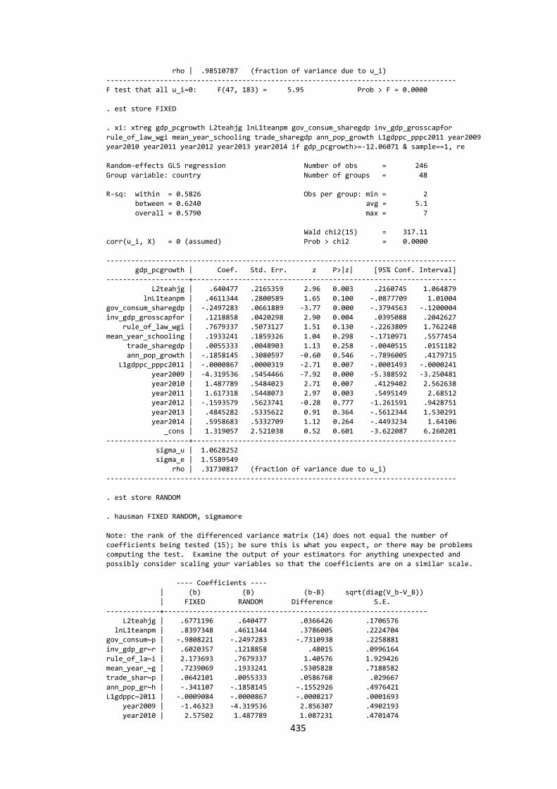
435
rho | .98510787 (fraction of variance due to u_i)
-------------------------------------------------------------------------------------
F test that all u_i=0: F(47, 183) = 5.95 Prob > F = 0.0000
. est store FIXED
. xi: xtreg gdp_pcgrowth L2teahjg lnL1teanpm gov_consum_sharegdp inv_gdp_grosscapfor
rule_of_law_wgi mean_year_schooling trade_sharegdp ann_pop_growth L1gdppc_pppc2011 year2009
year2010 year2011 year2012 year2013 year2014 if gdp_pcgrowth>=-12.06071 & sample==1, re
Random-effects GLS regression Number of obs = 246
Group variable: country Number of groups = 48
R-sq: within = 0.5826 Obs per group: min = 2
between = 0.6240 avg = 5.1
overall = 0.5790 max = 7
Wald chi2(15) = 317.11
corr(u_i, X) = 0 (assumed) Prob > chi2 = 0.0000
-------------------------------------------------------------------------------------
gdp_pcgrowth | Coef. Std. Err. z P>|z| [95% Conf. Interval]
--------------------+----------------------------------------------------------------
L2teahjg | .640477 .2165359 2.96 0.003 .2160745 1.064879
lnL1teanpm | .4611344 .2800589 1.65 0.100 -.0877709 1.01004
gov_consum_sharegdp | -.2497283 .0661889 -3.77 0.000 -.3794563 -.1200004
inv_gdp_grosscapfor | .1218858 .0420298 2.90 0.004 .0395088 .2042627
rule_of_law_wgi | .7679337 .5073127 1.51 0.130 -.2263809 1.762248
mean_year_schooling | .1933241 .1859326 1.04 0.298 -.1710971 .5577454
trade_sharegdp | .0055333 .0048903 1.13 0.258 -.0040515 .0151182
ann_pop_growth | -.1858145 .3080597 -0.60 0.546 -.7896005 .4179715
L1gdppc_pppc2011 | -.0000867 .0000319 -2.71 0.007 -.0001493 -.0000241
year2009 | -4.319536 .5454466 -7.92 0.000 -5.388592 -3.250481
year2010 | 1.487789 .5484023 2.71 0.007 .4129402 2.562638
year2011 | 1.617318 .5448073 2.97 0.003 .5495149 2.68512
year2012 | -.1593579 .5623741 -0.28 0.777 -1.261591 .9428751
year2013 | .4845282 .5335622 0.91 0.364 -.5612344 1.530291
year2014 | .5958683 .5332709 1.12 0.264 -.4493234 1.64106
_cons | 1.319057 2.521038 0.52 0.601 -3.622087 6.260201
--------------------+----------------------------------------------------------------
sigma_u | 1.0628252
sigma_e | 1.5589549
rho | .31730817 (fraction of variance due to u_i)
-------------------------------------------------------------------------------------
. est store RANDOM
. hausman FIXED RANDOM, sigmamore
Note: the rank of the differenced variance matrix (14) does not equal the number of
coefficients being tested (15); be sure this is what you expect, or there may be problems
computing the test. Examine the output of your estimators for anything unexpected and
possibly consider scaling your variables so that the coefficients are on a similar scale.
---- Coefficients ----
| (b) (B) (b-B) sqrt(diag(V_b-V_B))
| FIXED RANDOM Difference S.E.
-------------+----------------------------------------------------------------
L2teahjg | .6771196 .640477 .0366426 .1706576
lnL1teanpm | .8397348 .4611344 .3786005 .2224704
gov_consum~p | -.9808221 -.2497283 -.7310938 .2258881
inv_gdp_gr~r | .6020357 .1218858 .48015 .0996164
rule_of_la~i | 2.173693 .7679337 1.40576 1.929426
mean_year_~g | .7239069 .1933241 .5305828 .7188582
trade_shar~p | .0642101 .0055333 .0586768 .029667
ann_pop_gr~h | -.341107 -.1858145 -.1552926 .4976421
L1gdppc~2011 | -.0009084 -.0000867 -.0008217 .0001693
year2009 | -1.46323 -4.319536 2.856307 .4902193
year2010 | 2.57502 1.487789 1.087231 .4701474
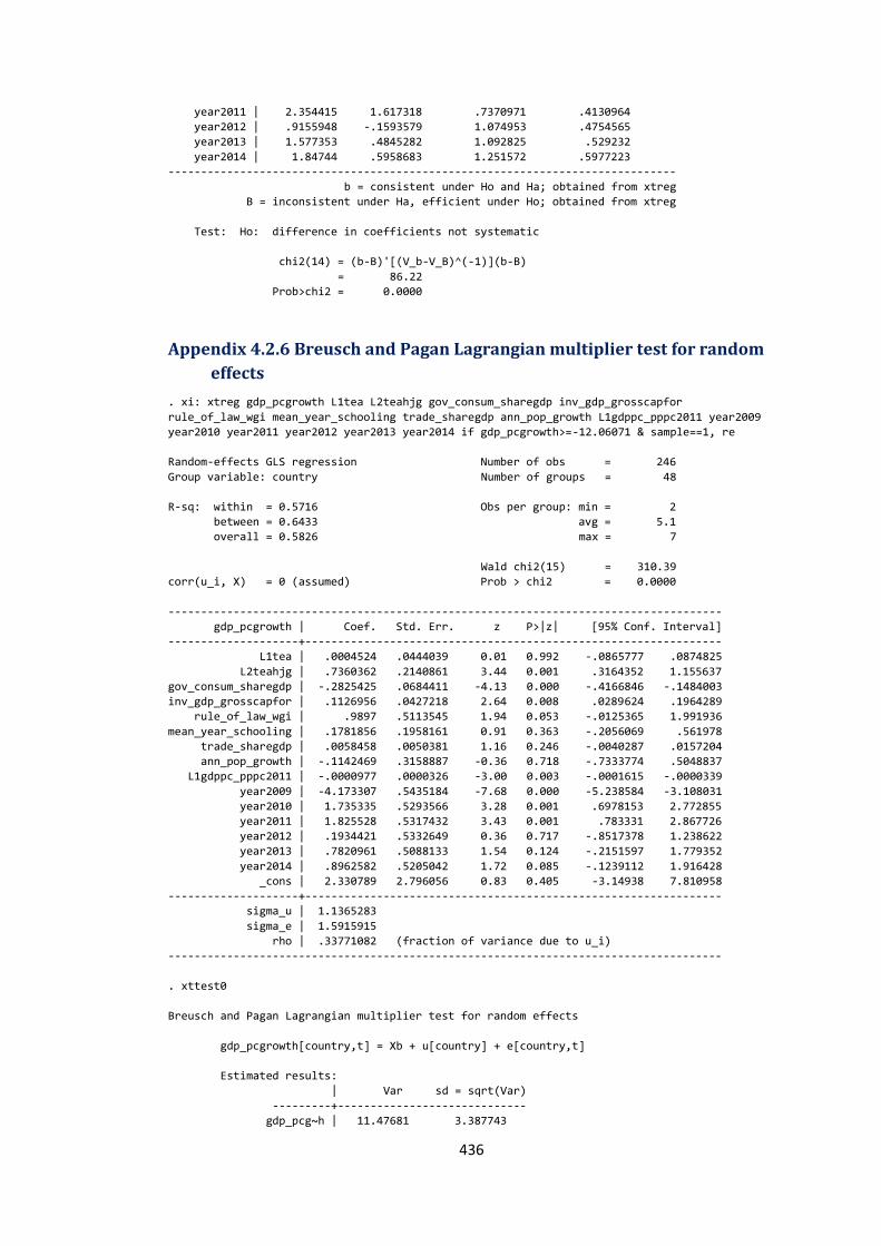
436
year2011 | 2.354415 1.617318 .7370971 .4130964
year2012 | .9155948 -.1593579 1.074953 .4754565
year2013 | 1.577353 .4845282 1.092825 .529232
year2014 | 1.84744 .5958683 1.251572 .5977223
------------------------------------------------------------------------------
b = consistent under Ho and Ha; obtained from xtreg
B = inconsistent under Ha, efficient under Ho; obtained from xtreg
Test: Ho: difference in coefficients not systematic
chi2(14) = (b-B)'[(V_b-V_B)^(-1)](b-B)
= 86.22
Prob>chi2 = 0.0000
Appendix 4.2.6 Breusch and Pagan Lagrangian multiplier test for random
effects
. xi: xtreg gdp_pcgrowth L1tea L2teahjg gov_consum_sharegdp inv_gdp_grosscapfor
rule_of_law_wgi mean_year_schooling trade_sharegdp ann_pop_growth L1gdppc_pppc2011 year2009
year2010 year2011 year2012 year2013 year2014 if gdp_pcgrowth>=-12.06071 & sample==1, re
Random-effects GLS regression Number of obs = 246
Group variable: country Number of groups = 48
R-sq: within = 0.5716 Obs per group: min = 2
between = 0.6433 avg = 5.1
overall = 0.5826 max = 7
Wald chi2(15) = 310.39
corr(u_i, X) = 0 (assumed) Prob > chi2 = 0.0000
-------------------------------------------------------------------------------------
gdp_pcgrowth | Coef. Std. Err. z P>|z| [95% Conf. Interval]
--------------------+----------------------------------------------------------------
L1tea | .0004524 .0444039 0.01 0.992 -.0865777 .0874825
L2teahjg | .7360362 .2140861 3.44 0.001 .3164352 1.155637
gov_consum_sharegdp | -.2825425 .0684411 -4.13 0.000 -.4166846 -.1484003
inv_gdp_grosscapfor | .1126956 .0427218 2.64 0.008 .0289624 .1964289
rule_of_law_wgi | .9897 .5113545 1.94 0.053 -.0125365 1.991936
mean_year_schooling | .1781856 .1958161 0.91 0.363 -.2056069 .561978
trade_sharegdp | .0058458 .0050381 1.16 0.246 -.0040287 .0157204
ann_pop_growth | -.1142469 .3158887 -0.36 0.718 -.7333774 .5048837
L1gdppc_pppc2011 | -.0000977 .0000326 -3.00 0.003 -.0001615 -.0000339
year2009 | -4.173307 .5435184 -7.68 0.000 -5.238584 -3.108031
year2010 | 1.735335 .5293566 3.28 0.001 .6978153 2.772855
year2011 | 1.825528 .5317432 3.43 0.001 .783331 2.867726
year2012 | .1934421 .5332649 0.36 0.717 -.8517378 1.238622
year2013 | .7820961 .5088133 1.54 0.124 -.2151597 1.779352
year2014 | .8962582 .5205042 1.72 0.085 -.1239112 1.916428
_cons | 2.330789 2.796056 0.83 0.405 -3.14938 7.810958
--------------------+----------------------------------------------------------------
sigma_u | 1.1365283
sigma_e | 1.5915915
rho | .33771082 (fraction of variance due to u_i)
-------------------------------------------------------------------------------------
. xttest0
Breusch and Pagan Lagrangian multiplier test for random effects
gdp_pcgrowth[country,t] = Xb + u[country] + e[country,t]
Estimated results:
| Var sd = sqrt(Var)
---------+-----------------------------
gdp_pcg~h | 11.47681 3.387743
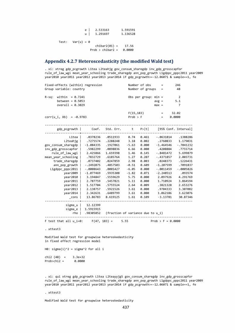
437
e | 2.533163 1.591591
u | 1.291697 1.136528
Test: Var(u) = 0
chibar2(01) = 17.56
Prob > chibar2 = 0.0000
Appendix 4.2.7 Heteroscedasticity (the modified Wald test)
. xi: xtreg gdp_pcgrowth L1tea L2teahjg gov_consum_sharegdp inv_gdp_grosscapfor
rule_of_law_wgi mean_year_schooling trade_sharegdp ann_pop_growth L1gdppc_pppc2011 year2009
year2010 year2011 year2012 year2013 year2014 if gdp_pcgrowth>=-12.06071 & sample==1, fe
Fixed-effects (within) regression Number of obs = 246
Group variable: country Number of groups = 48
R-sq: within = 0.7241 Obs per group: min = 2
between = 0.5053 avg = 5.1
overall = 0.3029 max = 7
F(15,183) = 32.02
corr(u_i, Xb) = -0.9783 Prob > F = 0.0000
-------------------------------------------------------------------------------------
gdp_pcgrowth | Coef. Std. Err. t P>|t| [95% Conf. Interval]
--------------------+----------------------------------------------------------------
L1tea | .0378236 .0511933 0.74 0.461 -.0631814 .1388286
L2teahjg | .7275574 .2288248 3.18 0.002 .2760833 1.179031
gov_consum_sharegdp | -1.084335 .1927061 -5.63 0.000 -1.464546 -.7041232
inv_gdp_grosscapfor | .5982299 .0898836 6.66 0.000 .4208884 .7755714
rule_of_law_wgi | 2.425866 1.659398 1.46 0.145 -.8481472 5.699879
mean_year_schooling | .7832729 .6185764 1.27 0.207 -.4371857 2.003731
trade_sharegdp | .0737402 .0247859 2.98 0.003 .0248373 .1226431
ann_pop_growth | -.2492075 .4857503 -0.51 0.609 -1.207599 .7091837
L1gdppc_pppc2011 | -.0008643 .0001427 -6.05 0.000 -.0011459 -.0005826
year2009 | -1.077469 .5935308 -1.82 0.071 -2.248513 .093574
year2010 | 3.194847 .5559629 5.75 0.000 2.097926 4.291769
year2011 | 2.787759 .5457821 5.11 0.000 1.710924 3.864594
year2012 | 1.517704 .5755524 2.64 0.009 .3821328 2.653276
year2013 | 2.138757 .5921526 3.61 0.000 .9704333 3.307082
year2014 | 2.342631 .6489799 3.61 0.000 1.062186 3.623076
_cons | 13.86783 8.619125 1.61 0.109 -3.13781 30.87346
--------------------+----------------------------------------------------------------
sigma_u | 12.12399
sigma_e | 1.5915915
rho | .98305852 (fraction of variance due to u_i)
-------------------------------------------------------------------------------------
F test that all u_i=0: F(47, 183) = 5.55 Prob > F = 0.0000
. xttest3
Modified Wald test for groupwise heteroskedasticity
in fixed effect regression model
H0: sigma(i)^2 = sigma^2 for all i
chi2 (48) = 3.3e+32
Prob>chi2 = 0.0000
. xi: qui xtreg gdp_pcgrowth L1tea L2teayyjg5 gov_consum_sharegdp inv_gdp_grosscapfor
rule_of_law_wgi mean_year_schooling trade_sharegdp ann_pop_growth L1gdppc_pppc2011 year2009
year2010 year2011 year2012 year2013 year2014 if gdp_pcgrowth>=-12.06071 & sample==1, fe
. xttest3
Modified Wald test for groupwise heteroskedasticity
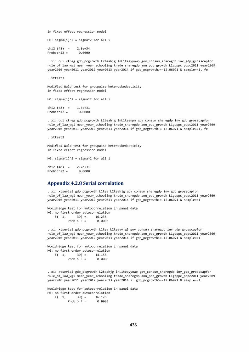
438
in fixed effect regression model
H0: sigma(i)^2 = sigma^2 for all i
chi2 (48) = 2.8e+34
Prob>chi2 = 0.0000
. xi: qui xtreg gdp_pcgrowth L2teahjg lnL1teayynwp gov_consum_sharegdp inv_gdp_grosscapfor
rule_of_law_wgi mean_year_schooling trade_sharegdp ann_pop_growth L1gdppc_pppc2011 year2009
year2010 year2011 year2012 year2013 year2014 if gdp_pcgrowth>=-12.06071 & sample==1, fe
. xttest3
Modified Wald test for groupwise heteroskedasticity
in fixed effect regression model
H0: sigma(i)^2 = sigma^2 for all i
chi2 (48) = 1.5e+31
Prob>chi2 = 0.0000
. xi: qui xtreg gdp_pcgrowth L2teahjg lnL1teanpm gov_consum_sharegdp inv_gdp_grosscapfor
rule_of_law_wgi mean_year_schooling trade_sharegdp ann_pop_growth L1gdppc_pppc2011 year2009
year2010 year2011 year2012 year2013 year2014 if gdp_pcgrowth>=-12.06071 & sample==1, fe
. xttest3
Modified Wald test for groupwise heteroskedasticity
in fixed effect regression model
H0: sigma(i)^2 = sigma^2 for all i
chi2 (48) = 2.7e+31
Prob>chi2 = 0.0000
Appendix 4.2.8 Serial correlation
. xi: xtserial gdp_pcgrowth L1tea L2teahjg gov_consum_sharegdp inv_gdp_grosscapfor
rule_of_law_wgi mean_year_schooling trade_sharegdp ann_pop_growth L1gdppc_pppc2011 year2009
year2010 year2011 year2012 year2013 year2014 if gdp_pcgrowth>=-12.06071 & sample==1
Wooldridge test for autocorrelation in panel data
H0: no first order autocorrelation
F( 1, 39) = 16.236
Prob > F = 0.0003
. xi: xtserial gdp_pcgrowth L1tea L2teayyjg5 gov_consum_sharegdp inv_gdp_grosscapfor
rule_of_law_wgi mean_year_schooling trade_sharegdp ann_pop_growth L1gdppc_pppc2011 year2009
year2010 year2011 year2012 year2013 year2014 if gdp_pcgrowth>=-12.06071 & sample==1
Wooldridge test for autocorrelation in panel data
H0: no first order autocorrelation
F( 1, 39) = 14.158
Prob > F = 0.0006
. xi: xtserial gdp_pcgrowth L2teahjg lnL1teayynwp gov_consum_sharegdp inv_gdp_grosscapfor
rule_of_law_wgi mean_year_schooling trade_sharegdp ann_pop_growth L1gdppc_pppc2011 year2009
year2010 year2011 year2012 year2013 year2014 if gdp_pcgrowth>=-12.06071 & sample==1
Wooldridge test for autocorrelation in panel data
H0: no first order autocorrelation
F( 1, 39) = 16.126
Prob > F = 0.0003
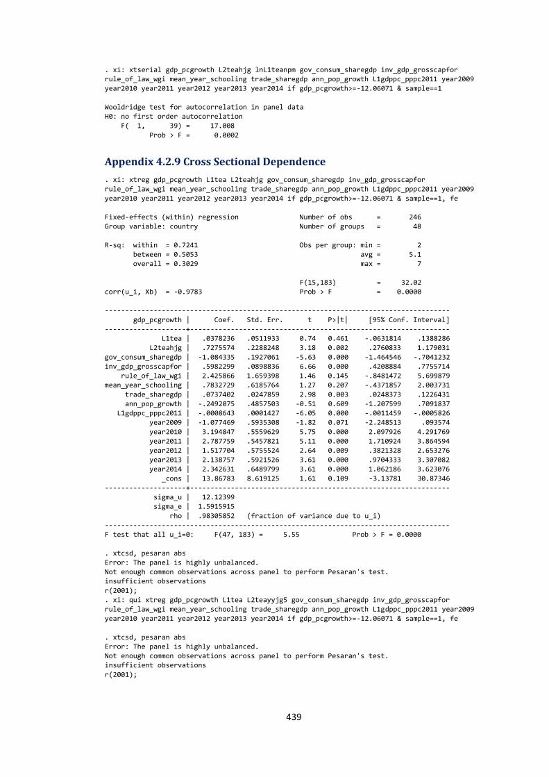
439
. xi: xtserial gdp_pcgrowth L2teahjg lnL1teanpm gov_consum_sharegdp inv_gdp_grosscapfor
rule_of_law_wgi mean_year_schooling trade_sharegdp ann_pop_growth L1gdppc_pppc2011 year2009
year2010 year2011 year2012 year2013 year2014 if gdp_pcgrowth>=-12.06071 & sample==1
Wooldridge test for autocorrelation in panel data
H0: no first order autocorrelation
F( 1, 39) = 17.008
Prob > F = 0.0002
Appendix 4.2.9 Cross Sectional Dependence
. xi: xtreg gdp_pcgrowth L1tea L2teahjg gov_consum_sharegdp inv_gdp_grosscapfor
rule_of_law_wgi mean_year_schooling trade_sharegdp ann_pop_growth L1gdppc_pppc2011 year2009
year2010 year2011 year2012 year2013 year2014 if gdp_pcgrowth>=-12.06071 & sample==1, fe
Fixed-effects (within) regression Number of obs = 246
Group variable: country Number of groups = 48
R-sq: within = 0.7241 Obs per group: min = 2
between = 0.5053 avg = 5.1
overall = 0.3029 max = 7
F(15,183) = 32.02
corr(u_i, Xb) = -0.9783 Prob > F = 0.0000
-------------------------------------------------------------------------------------
gdp_pcgrowth | Coef. Std. Err. t P>|t| [95% Conf. Interval]
--------------------+----------------------------------------------------------------
L1tea | .0378236 .0511933 0.74 0.461 -.0631814 .1388286
L2teahjg | .7275574 .2288248 3.18 0.002 .2760833 1.179031
gov_consum_sharegdp | -1.084335 .1927061 -5.63 0.000 -1.464546 -.7041232
inv_gdp_grosscapfor | .5982299 .0898836 6.66 0.000 .4208884 .7755714
rule_of_law_wgi | 2.425866 1.659398 1.46 0.145 -.8481472 5.699879
mean_year_schooling | .7832729 .6185764 1.27 0.207 -.4371857 2.003731
trade_sharegdp | .0737402 .0247859 2.98 0.003 .0248373 .1226431
ann_pop_growth | -.2492075 .4857503 -0.51 0.609 -1.207599 .7091837
L1gdppc_pppc2011 | -.0008643 .0001427 -6.05 0.000 -.0011459 -.0005826
year2009 | -1.077469 .5935308 -1.82 0.071 -2.248513 .093574
year2010 | 3.194847 .5559629 5.75 0.000 2.097926 4.291769
year2011 | 2.787759 .5457821 5.11 0.000 1.710924 3.864594
year2012 | 1.517704 .5755524 2.64 0.009 .3821328 2.653276
year2013 | 2.138757 .5921526 3.61 0.000 .9704333 3.307082
year2014 | 2.342631 .6489799 3.61 0.000 1.062186 3.623076
_cons | 13.86783 8.619125 1.61 0.109 -3.13781 30.87346
--------------------+----------------------------------------------------------------
sigma_u | 12.12399
sigma_e | 1.5915915
rho | .98305852 (fraction of variance due to u_i)
-------------------------------------------------------------------------------------
F test that all u_i=0: F(47, 183) = 5.55 Prob > F = 0.0000
. xtcsd, pesaran abs
Error: The panel is highly unbalanced.
Not enough common observations across panel to perform Pesaran's test.
insufficient observations
r(2001);
. xi: qui xtreg gdp_pcgrowth L1tea L2teayyjg5 gov_consum_sharegdp inv_gdp_grosscapfor
rule_of_law_wgi mean_year_schooling trade_sharegdp ann_pop_growth L1gdppc_pppc2011 year2009
year2010 year2011 year2012 year2013 year2014 if gdp_pcgrowth>=-12.06071 & sample==1, fe
. xtcsd, pesaran abs
Error: The panel is highly unbalanced.
Not enough common observations across panel to perform Pesaran's test.
insufficient observations
r(2001);
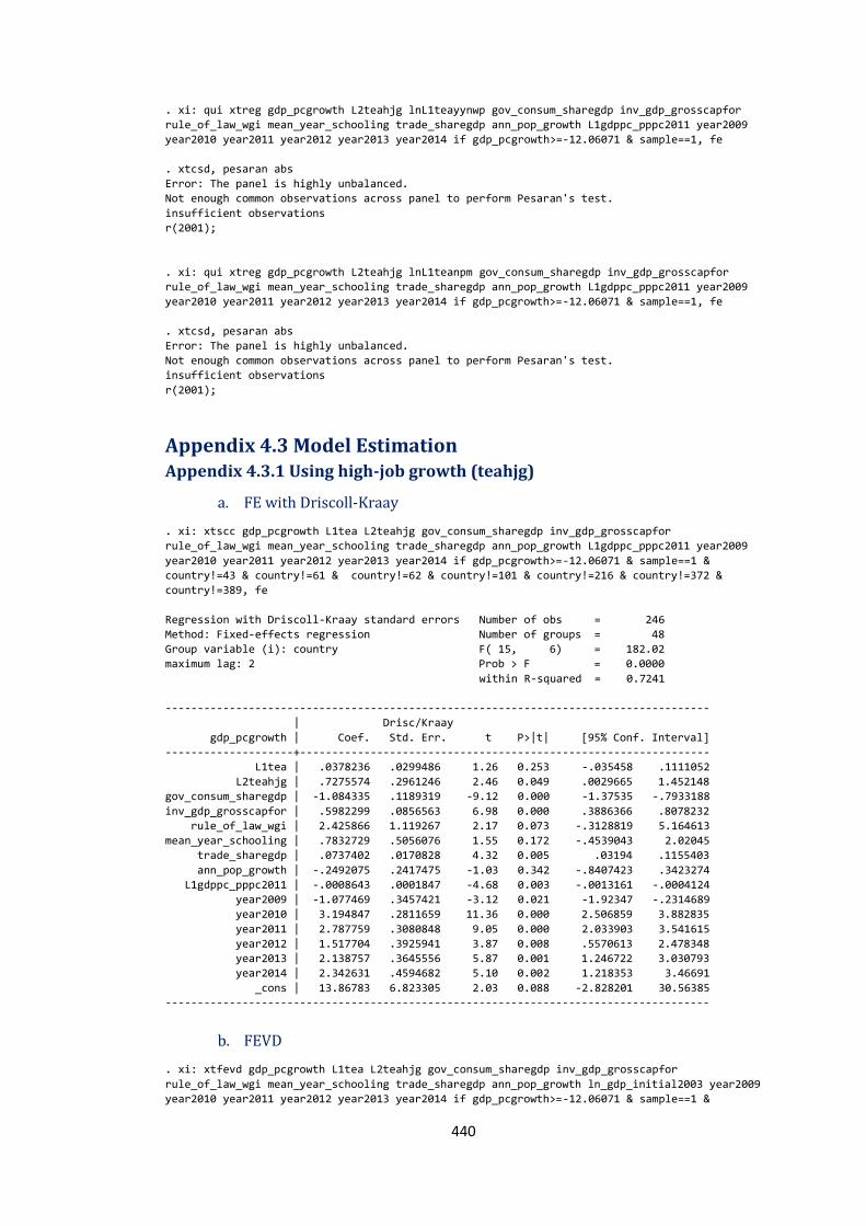
440
. xi: qui xtreg gdp_pcgrowth L2teahjg lnL1teayynwp gov_consum_sharegdp inv_gdp_grosscapfor
rule_of_law_wgi mean_year_schooling trade_sharegdp ann_pop_growth L1gdppc_pppc2011 year2009
year2010 year2011 year2012 year2013 year2014 if gdp_pcgrowth>=-12.06071 & sample==1, fe
. xtcsd, pesaran abs
Error: The panel is highly unbalanced.
Not enough common observations across panel to perform Pesaran's test.
insufficient observations
r(2001);
. xi: qui xtreg gdp_pcgrowth L2teahjg lnL1teanpm gov_consum_sharegdp inv_gdp_grosscapfor
rule_of_law_wgi mean_year_schooling trade_sharegdp ann_pop_growth L1gdppc_pppc2011 year2009
year2010 year2011 year2012 year2013 year2014 if gdp_pcgrowth>=-12.06071 & sample==1, fe
. xtcsd, pesaran abs
Error: The panel is highly unbalanced.
Not enough common observations across panel to perform Pesaran's test.
insufficient observations
r(2001);
Appendix 4.3 Model Estimation Appendix 4.3.1 Using high-job growth (teahjg)
a. FE with Driscoll-Kraay
. xi: xtscc gdp_pcgrowth L1tea L2teahjg gov_consum_sharegdp inv_gdp_grosscapfor
rule_of_law_wgi mean_year_schooling trade_sharegdp ann_pop_growth L1gdppc_pppc2011 year2009
year2010 year2011 year2012 year2013 year2014 if gdp_pcgrowth>=-12.06071 & sample==1 &
country!=43 & country!=61 & country!=62 & country!=101 & country!=216 & country!=372 &
country!=389, fe
Regression with Driscoll-Kraay standard errors Number of obs = 246
Method: Fixed-effects regression Number of groups = 48
Group variable (i): country F( 15, 6) = 182.02
maximum lag: 2 Prob > F = 0.0000
within R-squared = 0.7241
-------------------------------------------------------------------------------------
| Drisc/Kraay
gdp_pcgrowth | Coef. Std. Err. t P>|t| [95% Conf. Interval]
--------------------+----------------------------------------------------------------
L1tea | .0378236 .0299486 1.26 0.253 -.035458 .1111052
L2teahjg | .7275574 .2961246 2.46 0.049 .0029665 1.452148
gov_consum_sharegdp | -1.084335 .1189319 -9.12 0.000 -1.37535 -.7933188
inv_gdp_grosscapfor | .5982299 .0856563 6.98 0.000 .3886366 .8078232
rule_of_law_wgi | 2.425866 1.119267 2.17 0.073 -.3128819 5.164613
mean_year_schooling | .7832729 .5056076 1.55 0.172 -.4539043 2.02045
trade_sharegdp | .0737402 .0170828 4.32 0.005 .03194 .1155403
ann_pop_growth | -.2492075 .2417475 -1.03 0.342 -.8407423 .3423274
L1gdppc_pppc2011 | -.0008643 .0001847 -4.68 0.003 -.0013161 -.0004124
year2009 | -1.077469 .3457421 -3.12 0.021 -1.92347 -.2314689
year2010 | 3.194847 .2811659 11.36 0.000 2.506859 3.882835
year2011 | 2.787759 .3080848 9.05 0.000 2.033903 3.541615
year2012 | 1.517704 .3925941 3.87 0.008 .5570613 2.478348
year2013 | 2.138757 .3645556 5.87 0.001 1.246722 3.030793
year2014 | 2.342631 .4594682 5.10 0.002 1.218353 3.46691
_cons | 13.86783 6.823305 2.03 0.088 -2.828201 30.56385
-------------------------------------------------------------------------------------
b. FEVD
. xi: xtfevd gdp_pcgrowth L1tea L2teahjg gov_consum_sharegdp inv_gdp_grosscapfor
rule_of_law_wgi mean_year_schooling trade_sharegdp ann_pop_growth ln_gdp_initial2003 year2009
year2010 year2011 year2012 year2013 year2014 if gdp_pcgrowth>=-12.06071 & sample==1 &
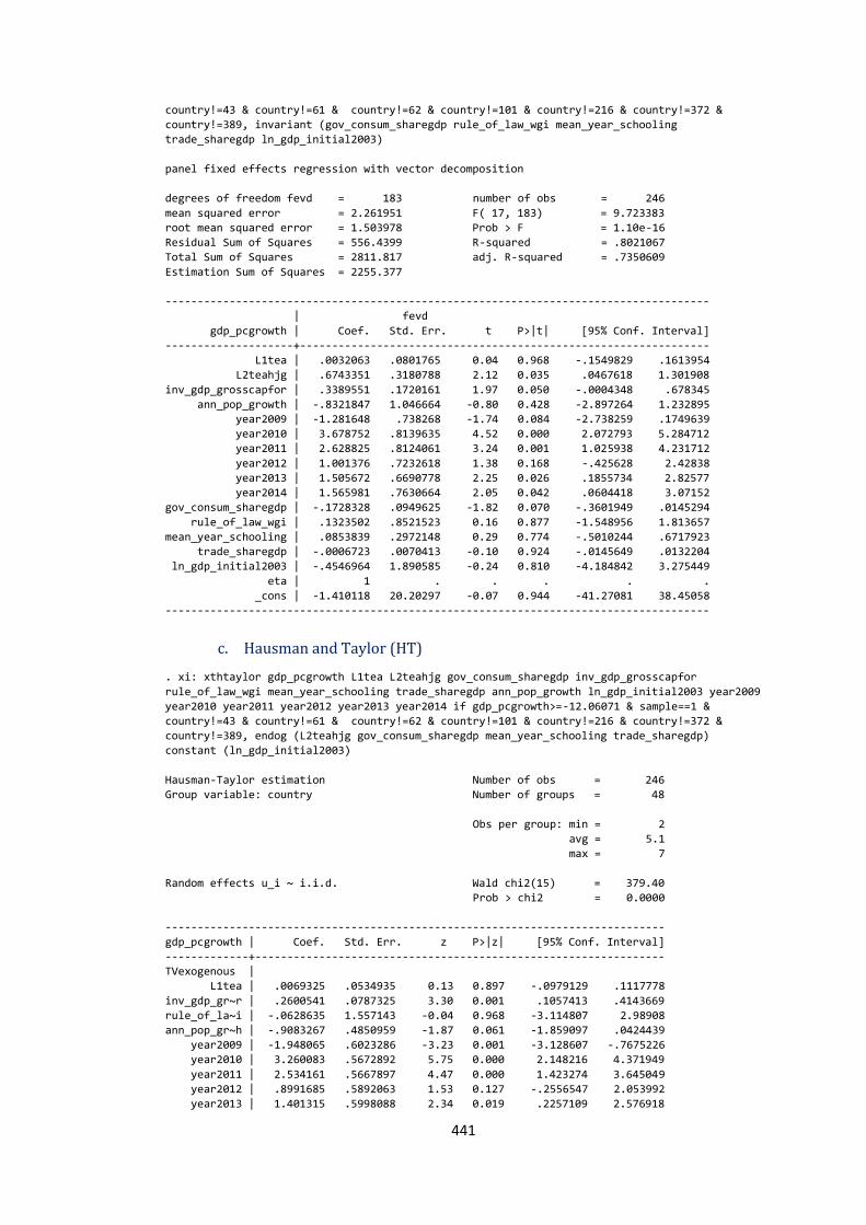
441
country!=43 & country!=61 & country!=62 & country!=101 & country!=216 & country!=372 &
country!=389, invariant (gov_consum_sharegdp rule_of_law_wgi mean_year_schooling
trade_sharegdp ln_gdp_initial2003)
panel fixed effects regression with vector decomposition
degrees of freedom fevd = 183 number of obs = 246
mean squared error = 2.261951 F( 17, 183) = 9.723383
root mean squared error = 1.503978 Prob > F = 1.10e-16
Residual Sum of Squares = 556.4399 R-squared = .8021067
Total Sum of Squares = 2811.817 adj. R-squared = .7350609
Estimation Sum of Squares = 2255.377
-------------------------------------------------------------------------------------
| fevd
gdp_pcgrowth | Coef. Std. Err. t P>|t| [95% Conf. Interval]
--------------------+----------------------------------------------------------------
L1tea | .0032063 .0801765 0.04 0.968 -.1549829 .1613954
L2teahjg | .6743351 .3180788 2.12 0.035 .0467618 1.301908
inv_gdp_grosscapfor | .3389551 .1720161 1.97 0.050 -.0004348 .678345
ann_pop_growth | -.8321847 1.046664 -0.80 0.428 -2.897264 1.232895
year2009 | -1.281648 .738268 -1.74 0.084 -2.738259 .1749639
year2010 | 3.678752 .8139635 4.52 0.000 2.072793 5.284712
year2011 | 2.628825 .8124061 3.24 0.001 1.025938 4.231712
year2012 | 1.001376 .7232618 1.38 0.168 -.425628 2.42838
year2013 | 1.505672 .6690778 2.25 0.026 .1855734 2.82577
year2014 | 1.565981 .7630664 2.05 0.042 .0604418 3.07152
gov_consum_sharegdp | -.1728328 .0949625 -1.82 0.070 -.3601949 .0145294
rule_of_law_wgi | .1323502 .8521523 0.16 0.877 -1.548956 1.813657
mean_year_schooling | .0853839 .2972148 0.29 0.774 -.5010244 .6717923
trade_sharegdp | -.0006723 .0070413 -0.10 0.924 -.0145649 .0132204
ln_gdp_initial2003 | -.4546964 1.890585 -0.24 0.810 -4.184842 3.275449
eta | 1 . . . . .
_cons | -1.410118 20.20297 -0.07 0.944 -41.27081 38.45058
-------------------------------------------------------------------------------------
c. Hausman and Taylor (HT)
. xi: xthtaylor gdp_pcgrowth L1tea L2teahjg gov_consum_sharegdp inv_gdp_grosscapfor
rule_of_law_wgi mean_year_schooling trade_sharegdp ann_pop_growth ln_gdp_initial2003 year2009
year2010 year2011 year2012 year2013 year2014 if gdp_pcgrowth>=-12.06071 & sample==1 &
country!=43 & country!=61 & country!=62 & country!=101 & country!=216 & country!=372 &
country!=389, endog (L2teahjg gov_consum_sharegdp mean_year_schooling trade_sharegdp)
constant (ln_gdp_initial2003)
Hausman-Taylor estimation Number of obs = 246
Group variable: country Number of groups = 48
Obs per group: min = 2
avg = 5.1
max = 7
Random effects u_i ~ i.i.d. Wald chi2(15) = 379.40
Prob > chi2 = 0.0000
------------------------------------------------------------------------------
gdp_pcgrowth | Coef. Std. Err. z P>|z| [95% Conf. Interval]
-------------+----------------------------------------------------------------
TVexogenous |
L1tea | .0069325 .0534935 0.13 0.897 -.0979129 .1117778
inv_gdp_gr~r | .2600541 .0787325 3.30 0.001 .1057413 .4143669
rule_of_la~i | -.0628635 1.557143 -0.04 0.968 -3.114807 2.98908
ann_pop_gr~h | -.9083267 .4850959 -1.87 0.061 -1.859097 .0424439
year2009 | -1.948065 .6023286 -3.23 0.001 -3.128607 -.7675226
year2010 | 3.260083 .5672892 5.75 0.000 2.148216 4.371949
year2011 | 2.534161 .5667897 4.47 0.000 1.423274 3.645049
year2012 | .8991685 .5892063 1.53 0.127 -.2556547 2.053992
year2013 | 1.401315 .5998088 2.34 0.019 .2257109 2.576918

442
year2014 | 1.489453 .6513607 2.29 0.022 .2128094 2.766096
TVendogenous |
L2teahjg | .6908501 .2414973 2.86 0.004 .2175241 1.164176
gov_consum~p | -1.181454 .1948247 -6.06 0.000 -1.563304 -.7996051
mean_year_~g | .9526065 .6206104 1.53 0.125 -.2637675 2.16898
trade_shar~p | .0670515 .0211192 3.17 0.001 .0256586 .1084443
TIexogenous |
ln_gdp_~2003 | .9149535 3.50947 0.26 0.794 -5.963482 7.793389
|
_cons | -10.37984 32.86832 -0.32 0.752 -74.80057 54.04089
-------------+----------------------------------------------------------------
sigma_u | 8.2874576
sigma_e | 1.6763957
rho | .96069081 (fraction of variance due to u_i)
------------------------------------------------------------------------------
Note: TV refers to time varying; TI refers to time invariant.
d. Dynamic approach (xtabond2)
. xi: xtabond2 gdp_pcgrowth l.gdp_pcgrowth l.tea l2.teahjg gov_consum_sharegdp
inv_gdp_grosscapfor rule_of_law_wgi mean_year_schooling trade_sharegdp ann_pop_growth
ln_gdp_initial2003 i.year if gdp_pcgrowth>=-12.06071 & sample==1 & country!=43 & country!=61
& country!=62 & country!=101 & country!=216 & country!=372 & country!=389,
gmm(l.gdp_pcgrowth, lag (1 2) coll) gmm(l2.teahjg, lag(1 3) coll) iv(l.tea
gov_consum_sharegdp inv_gdp_grosscapfor rule_of_law_wgi mean_year_schooling trade_sharegdp
ann_pop_growth ln_gdp_initial2003 i.year) small two orthog robust
i.year _Iyeari2006-2014 (naturally coded; _Iyeari2006 omitted)
Favoring speed over space. To switch, type or click on mata: mata set matafavor space, perm.
_Iyeari2007 dropped due to collinearity
_Iyeari2008 dropped due to collinearity
Warning: Two-step estimated covariance matrix of moments is singular.
Using a generalized inverse to calculate optimal weighting matrix for two-step estimation.
Difference-in-Sargan/Hansen statistics may be negative.
Dynamic panel-data estimation, two-step system GMM
------------------------------------------------------------------------------
Group variable: country Number of obs = 246
Time variable : year Number of groups = 48
Number of instruments = 22 Obs per group: min = 2
F(16, 47) = 36.52 avg = 5.13
Prob > F = 0.000 max = 7
-------------------------------------------------------------------------------------
| Corrected
gdp_pcgrowth | Coef. Std. Err. t P>|t| [95% Conf. Interval]
--------------------+----------------------------------------------------------------
gdp_pcgrowth |
L1. | .362753 .1160823 3.12 0.003 .1292256 .5962804
|
tea |
L1. | -.0222197 .0433011 -0.51 0.610 -.1093302 .0648907
|
teahjg |
L2. | .7329404 .3312117 2.21 0.032 .0666285 1.399252
|
gov_consum_sharegdp | -.1746682 .0575209 -3.04 0.004 -.2903854 -.058951
inv_gdp_grosscapfor | .0185463 .0431369 0.43 0.669 -.068234 .1053265
rule_of_law_wgi | .5263921 .3660763 1.44 0.157 -.2100584 1.262843
mean_year_schooling | .0630678 .1318482 0.48 0.635 -.2021766 .3283122
trade_sharegdp | .0020942 .0022382 0.94 0.354 -.0024084 .0065968
ann_pop_growth | -.1255254 .2661643 -0.47 0.639 -.6609788 .409928
ln_gdp_initial2003 | -.912992 .5136733 -1.78 0.082 -1.946369 .1203853
_Iyeari2009 | -3.725456 .7301103 -5.10 0.000 -5.194249 -2.256664
_Iyeari2010 | 4.614794 .9459917 4.88 0.000 2.711705 6.517884
_Iyeari2011 | 2.507024 .5442871 4.61 0.000 1.41206 3.601989
_Iyeari2012 | .8436565 .4893477 1.72 0.091 -.1407841 1.828097
_Iyeari2013 | 1.890816 .5432372 3.48 0.001 .7979643 2.983669
_Iyeari2014 | 1.759942 .669989 2.63 0.012 .4120978 3.107786

443
_cons | 9.399281 5.658925 1.66 0.103 -1.985007 20.78357
-------------------------------------------------------------------------------------
Instruments for orthogonal deviations equation
Standard
FOD.(L.tea gov_consum_sharegdp inv_gdp_grosscapfor rule_of_law_wgi
mean_year_schooling trade_sharegdp ann_pop_growth ln_gdp_initial2003
_Iyeari2007 _Iyeari2008 _Iyeari2009 _Iyeari2010 _Iyeari2011 _Iyeari2012
_Iyeari2013 _Iyeari2014)
GMM-type (missing=0, separate instruments for each period unless collapsed)
L(1/3).L2.teahjg collapsed
L(1/2).L.gdp_pcgrowth collapsed
Instruments for levels equation
Standard
L.tea gov_consum_sharegdp inv_gdp_grosscapfor rule_of_law_wgi
mean_year_schooling trade_sharegdp ann_pop_growth ln_gdp_initial2003
_Iyeari2007 _Iyeari2008 _Iyeari2009 _Iyeari2010 _Iyeari2011 _Iyeari2012
_Iyeari2013 _Iyeari2014
_cons
GMM-type (missing=0, separate instruments for each period unless collapsed)
D.L2.teahjg collapsed
D.L.gdp_pcgrowth collapsed
------------------------------------------------------------------------------
Arellano-Bond test for AR(1) in first differences: z = -2.72 Pr > z = 0.007
Arellano-Bond test for AR(2) in first differences: z = -1.23 Pr > z = 0.219
------------------------------------------------------------------------------
Sargan test of overid. restrictions: chi2(5) = 1.82 Prob > chi2 = 0.873
(Not robust, but not weakened by many instruments.)
Hansen test of overid. restrictions: chi2(5) = 3.72 Prob > chi2 = 0.591
(Robust, but weakened by many instruments.)
Difference-in-Hansen tests of exogeneity of instrument subsets:
GMM instruments for levels
Hansen test excluding group: chi2(3) = 1.61 Prob > chi2 = 0.657
Difference (null H = exogenous): chi2(2) = 2.11 Prob > chi2 = 0.349
gmm(L.gdp_pcgrowth, collapse lag(1 2))
Hansen test excluding group: chi2(2) = 1.65 Prob > chi2 = 0.439
Difference (null H = exogenous): chi2(3) = 2.07 Prob > chi2 = 0.558
gmm(L2.teahjg, collapse lag(1 3))
Hansen test excluding group: chi2(1) = 0.38 Prob > chi2 = 0.539
Difference (null H = exogenous): chi2(4) = 3.34 Prob > chi2 = 0.503
Appendix 4.3.2 Using job growth (teayyjg5)
a. FE with Driscoll-Kraay
. xi: xtscc gdp_pcgrowth L1tea L2teayyjg5 gov_consum_sharegdp inv_gdp_grosscapfor
rule_of_law_wgi mean_year_schooling trade_sharegdp ann_pop_growth L1gdppc_pppc2011 year2009
year2010 year2011 year2012 year2013 year2014 if gdp_pcgrowth>=-12.06071 & sample==1 &
country!=43 & country!=61 & country!=62 & country!=101 & country!=216 & country!=372 &
country!=389, fe
Regression with Driscoll-Kraay standard errors Number of obs = 246
Method: Fixed-effects regression Number of groups = 48
Group variable (i): country F( 15, 6) = 162.11
maximum lag: 2 Prob > F = 0.0000
within R-squared = 0.7246
-------------------------------------------------------------------------------------
| Drisc/Kraay
gdp_pcgrowth | Coef. Std. Err. t P>|t| [95% Conf. Interval]
--------------------+----------------------------------------------------------------
L1tea | .0319436 .0259383 1.23 0.264 -.0315251 .0954123
L2teayyjg5 | .4287768 .1745265 2.46 0.049 .0017259 .8558277
gov_consum_sharegdp | -1.011603 .1403893 -7.21 0.000 -1.355124 -.6680831
inv_gdp_grosscapfor | .5877635 .082556 7.12 0.000 .3857563 .7897708
rule_of_law_wgi | 2.371223 1.1338 2.09 0.081 -.4030858 5.145531
mean_year_schooling | .9605453 .4179373 2.30 0.061 -.0621103 1.983201
trade_sharegdp | .0734183 .0172244 4.26 0.005 .0312718 .1155648
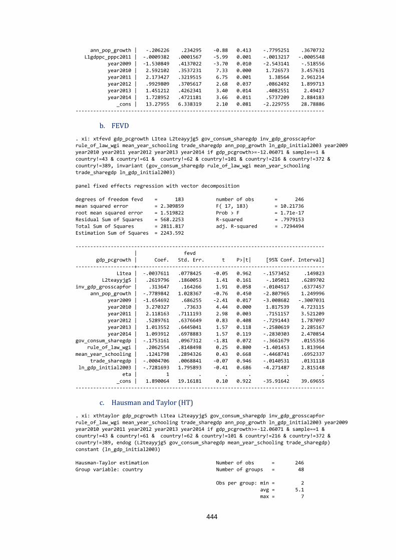
444
ann_pop_growth | -.206226 .234295 -0.88 0.413 -.7795251 .3670732
L1gdppc_pppc2011 | -.0009382 .0001567 -5.99 0.001 -.0013217 -.0005548
year2009 | -1.530849 .4137022 -3.70 0.010 -2.543141 -.518556
year2010 | 2.592102 .3537231 7.33 0.000 1.726573 3.457631
year2011 | 2.173427 .3219515 6.75 0.001 1.38564 2.961214
year2012 | .9929809 .3705617 2.68 0.037 .0862492 1.899713
year2013 | 1.451212 .4262341 3.40 0.014 .4082551 2.49417
year2014 | 1.728952 .4721181 3.66 0.011 .5737209 2.884183
_cons | 13.27955 6.338319 2.10 0.081 -2.229755 28.78886
-------------------------------------------------------------------------------------
b. FEVD
. xi: xtfevd gdp_pcgrowth L1tea L2teayyjg5 gov_consum_sharegdp inv_gdp_grosscapfor
rule_of_law_wgi mean_year_schooling trade_sharegdp ann_pop_growth ln_gdp_initial2003 year2009
year2010 year2011 year2012 year2013 year2014 if gdp_pcgrowth>=-12.06071 & sample==1 &
country!=43 & country!=61 & country!=62 & country!=101 & country!=216 & country!=372 &
country!=389, invariant (gov_consum_sharegdp rule_of_law_wgi mean_year_schooling
trade_sharegdp ln_gdp_initial2003)
panel fixed effects regression with vector decomposition
degrees of freedom fevd = 183 number of obs = 246
mean squared error = 2.309859 F( 17, 183) = 10.21736
root mean squared error = 1.519822 Prob > F = 1.71e-17
Residual Sum of Squares = 568.2253 R-squared = .7979153
Total Sum of Squares = 2811.817 adj. R-squared = .7294494
Estimation Sum of Squares = 2243.592
-------------------------------------------------------------------------------------
| fevd
gdp_pcgrowth | Coef. Std. Err. t P>|t| [95% Conf. Interval]
--------------------+----------------------------------------------------------------
L1tea | -.0037611 .0778425 -0.05 0.962 -.1573452 .149823
L2teayyjg5 | .2619796 .1860053 1.41 0.161 -.105011 .6289702
inv_gdp_grosscapfor | .313647 .164266 1.91 0.058 -.0104517 .6377457
ann_pop_growth | -.7789842 1.028367 -0.76 0.450 -2.807965 1.249996
year2009 | -1.654692 .686255 -2.41 0.017 -3.008682 -.3007031
year2010 | 3.270327 .73633 4.44 0.000 1.817539 4.723115
year2011 | 2.118163 .7111193 2.98 0.003 .7151157 3.521209
year2012 | .5289761 .6376649 0.83 0.408 -.7291443 1.787097
year2013 | 1.013552 .6445041 1.57 0.118 -.2580619 2.285167
year2014 | 1.093912 .6978883 1.57 0.119 -.2830303 2.470854
gov_consum_sharegdp | -.1753161 .0967312 -1.81 0.072 -.3661679 .0155356
rule_of_law_wgi | .2062554 .8148498 0.25 0.800 -1.401453 1.813964
mean_year_schooling | .1241798 .2894326 0.43 0.668 -.4468741 .6952337
trade_sharegdp | -.0004706 .0068841 -0.07 0.946 -.0140531 .0131118
ln_gdp_initial2003 | -.7281693 1.795893 -0.41 0.686 -4.271487 2.815148
eta | 1 . . . . .
_cons | 1.890064 19.16181 0.10 0.922 -35.91642 39.69655
-------------------------------------------------------------------------------------
c. Hausman and Taylor (HT)
. xi: xthtaylor gdp_pcgrowth L1tea L2teayyjg5 gov_consum_sharegdp inv_gdp_grosscapfor
rule_of_law_wgi mean_year_schooling trade_sharegdp ann_pop_growth ln_gdp_initial2003 year2009
year2010 year2011 year2012 year2013 year2014 if gdp_pcgrowth>=-12.06071 & sample==1 &
country!=43 & country!=61 & country!=62 & country!=101 & country!=216 & country!=372 &
country!=389, endog (L2teayyjg5 gov_consum_sharegdp mean_year_schooling trade_sharegdp)
constant (ln_gdp_initial2003)
Hausman-Taylor estimation Number of obs = 246
Group variable: country Number of groups = 48
Obs per group: min = 2
avg = 5.1
max = 7
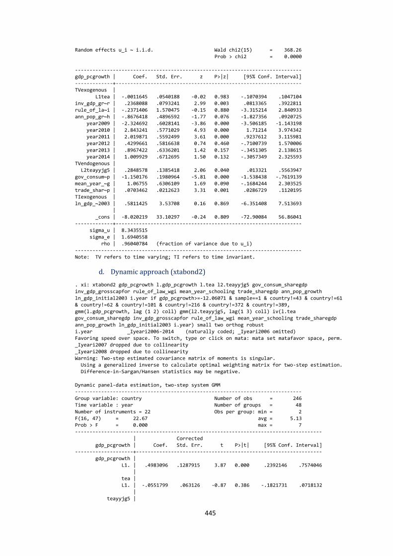
445
Random effects u_i ~ i.i.d. Wald chi2(15) = 368.26
Prob > chi2 = 0.0000
------------------------------------------------------------------------------
gdp_pcgrowth | Coef. Std. Err. z P>|z| [95% Conf. Interval]
-------------+----------------------------------------------------------------
TVexogenous |
L1tea | -.0011645 .0540188 -0.02 0.983 -.1070394 .1047104
inv_gdp_gr~r | .2368088 .0793241 2.99 0.003 .0813365 .3922811
rule_of_la~i | -.2371406 1.570475 -0.15 0.880 -3.315214 2.840933
ann_pop_gr~h | -.8676418 .4896592 -1.77 0.076 -1.827356 .0920725
year2009 | -2.324692 .6028141 -3.86 0.000 -3.506185 -1.143198
year2010 | 2.843241 .5771029 4.93 0.000 1.71214 3.974342
year2011 | 2.019871 .5592499 3.61 0.000 .9237612 3.115981
year2012 | .4299661 .5816638 0.74 0.460 -.7100739 1.570006
year2013 | .8967422 .6336201 1.42 0.157 -.3451305 2.138615
year2014 | 1.009929 .6712695 1.50 0.132 -.3057349 2.325593
TVendogenous |
L2teayyjg5 | .2848578 .1385418 2.06 0.040 .013321 .5563947
gov_consum~p | -1.150176 .1980964 -5.81 0.000 -1.538438 -.7619139
mean_year_~g | 1.06755 .6306109 1.69 0.090 -.1684244 2.303525
trade_shar~p | .0703462 .0212623 3.31 0.001 .0286729 .1120195
TIexogenous |
ln_gdp_~2003 | .5811425 3.53708 0.16 0.869 -6.351408 7.513693
|
_cons | -8.020219 33.10297 -0.24 0.809 -72.90084 56.86041
-------------+----------------------------------------------------------------
sigma_u | 8.3435515
sigma_e | 1.6940558
rho | .96040784 (fraction of variance due to u_i)
------------------------------------------------------------------------------
Note: TV refers to time varying; TI refers to time invariant.
d. Dynamic approach (xtabond2)
. xi: xtabond2 gdp_pcgrowth l.gdp_pcgrowth l.tea l2.teayyjg5 gov_consum_sharegdp
inv_gdp_grosscapfor rule_of_law_wgi mean_year_schooling trade_sharegdp ann_pop_growth
ln_gdp_initial2003 i.year if gdp_pcgrowth>=-12.06071 & sample==1 & country!=43 & country!=61
& country!=62 & country!=101 & country!=216 & country!=372 & country!=389,
gmm(l.gdp_pcgrowth, lag (1 2) coll) gmm(l2.teayyjg5, lag(1 3) coll) iv(l.tea
gov_consum_sharegdp inv_gdp_grosscapfor rule_of_law_wgi mean_year_schooling trade_sharegdp
ann_pop_growth ln_gdp_initial2003 i.year) small two orthog robust
i.year _Iyeari2006-2014 (naturally coded; _Iyeari2006 omitted)
Favoring speed over space. To switch, type or click on mata: mata set matafavor space, perm.
_Iyeari2007 dropped due to collinearity
_Iyeari2008 dropped due to collinearity
Warning: Two-step estimated covariance matrix of moments is singular.
Using a generalized inverse to calculate optimal weighting matrix for two-step estimation.
Difference-in-Sargan/Hansen statistics may be negative.
Dynamic panel-data estimation, two-step system GMM
------------------------------------------------------------------------------
Group variable: country Number of obs = 246
Time variable : year Number of groups = 48
Number of instruments = 22 Obs per group: min = 2
F(16, 47) = 22.67 avg = 5.13
Prob > F = 0.000 max = 7
-------------------------------------------------------------------------------------
| Corrected
gdp_pcgrowth | Coef. Std. Err. t P>|t| [95% Conf. Interval]
--------------------+----------------------------------------------------------------
gdp_pcgrowth |
L1. | .4983096 .1287915 3.87 0.000 .2392146 .7574046
|
tea |
L1. | -.0551799 .063126 -0.87 0.386 -.1821731 .0718132
|
teayyjg5 |
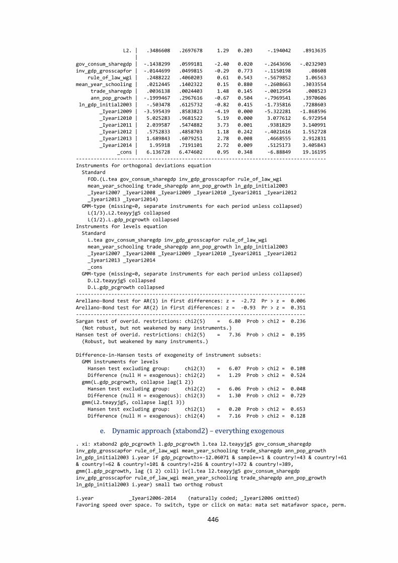
446
L2. | .3486608 .2697678 1.29 0.203 -.194042 .8913635
|
gov_consum_sharegdp | -.1438299 .0599181 -2.40 0.020 -.2643696 -.0232903
inv_gdp_grosscapfor | -.0144699 .0499815 -0.29 0.773 -.1150198 .08608
rule_of_law_wgi | .2488222 .4060203 0.61 0.543 -.5679852 1.06563
mean_year_schooling | .0212445 .1402322 0.15 0.880 -.2608663 .3033554
trade_sharegdp | .0036138 .0024403 1.48 0.145 -.0012954 .008523
ann_pop_growth | -.1999467 .2967616 -0.67 0.504 -.7969541 .3970606
ln_gdp_initial2003 | -.503478 .6125732 -0.82 0.415 -1.735816 .7288603
_Iyeari2009 | -3.595439 .8583823 -4.19 0.000 -5.322281 -1.868596
_Iyeari2010 | 5.025283 .9681522 5.19 0.000 3.077612 6.972954
_Iyeari2011 | 2.039587 .5474882 3.73 0.001 .9381829 3.140991
_Iyeari2012 | .5752833 .4858703 1.18 0.242 -.4021616 1.552728
_Iyeari2013 | 1.689843 .6079251 2.78 0.008 .4668555 2.912831
_Iyeari2014 | 1.95918 .7191101 2.72 0.009 .5125173 3.405843
_cons | 6.136728 6.474602 0.95 0.348 -6.88849 19.16195
-------------------------------------------------------------------------------------
Instruments for orthogonal deviations equation
Standard
FOD.(L.tea gov_consum_sharegdp inv_gdp_grosscapfor rule_of_law_wgi
mean_year_schooling trade_sharegdp ann_pop_growth ln_gdp_initial2003
_Iyeari2007 _Iyeari2008 _Iyeari2009 _Iyeari2010 _Iyeari2011 _Iyeari2012
_Iyeari2013 _Iyeari2014)
GMM-type (missing=0, separate instruments for each period unless collapsed)
L(1/3).L2.teayyjg5 collapsed
L(1/2).L.gdp_pcgrowth collapsed
Instruments for levels equation
Standard
L.tea gov_consum_sharegdp inv_gdp_grosscapfor rule_of_law_wgi
mean_year_schooling trade_sharegdp ann_pop_growth ln_gdp_initial2003
_Iyeari2007 _Iyeari2008 _Iyeari2009 _Iyeari2010 _Iyeari2011 _Iyeari2012
_Iyeari2013 _Iyeari2014
_cons
GMM-type (missing=0, separate instruments for each period unless collapsed)
D.L2.teayyjg5 collapsed
D.L.gdp_pcgrowth collapsed
------------------------------------------------------------------------------
Arellano-Bond test for AR(1) in first differences: z = -2.72 Pr > z = 0.006
Arellano-Bond test for AR(2) in first differences: z = -0.93 Pr > z = 0.351
------------------------------------------------------------------------------
Sargan test of overid. restrictions: chi2(5) = 6.80 Prob > chi2 = 0.236
(Not robust, but not weakened by many instruments.)
Hansen test of overid. restrictions: chi2(5) = 7.36 Prob > chi2 = 0.195
(Robust, but weakened by many instruments.)
Difference-in-Hansen tests of exogeneity of instrument subsets:
GMM instruments for levels
Hansen test excluding group: chi2(3) = 6.07 Prob > chi2 = 0.108
Difference (null H = exogenous): chi2(2) = 1.29 Prob > chi2 = 0.524
gmm(L.gdp_pcgrowth, collapse lag(1 2))
Hansen test excluding group: chi2(2) = 6.06 Prob > chi2 = 0.048
Difference (null H = exogenous): chi2(3) = 1.30 Prob > chi2 = 0.729
gmm(L2.teayyjg5, collapse lag(1 3))
Hansen test excluding group: chi2(1) = 0.20 Prob > chi2 = 0.653
Difference (null H = exogenous): chi2(4) = 7.16 Prob > chi2 = 0.128
e. Dynamic approach (xtabond2) – everything exogenous
. xi: xtabond2 gdp_pcgrowth l.gdp_pcgrowth l.tea l2.teayyjg5 gov_consum_sharegdp
inv_gdp_grosscapfor rule_of_law_wgi mean_year_schooling trade_sharegdp ann_pop_growth
ln_gdp_initial2003 i.year if gdp_pcgrowth>=-12.06071 & sample==1 & country!=43 & country!=61
& country!=62 & country!=101 & country!=216 & country!=372 & country!=389,
gmm(l.gdp_pcgrowth, lag (1 2) coll) iv(l.tea l2.teayyjg5 gov_consum_sharegdp
inv_gdp_grosscapfor rule_of_law_wgi mean_year_schooling trade_sharegdp ann_pop_growth
ln_gdp_initial2003 i.year) small two orthog robust
i.year _Iyeari2006-2014 (naturally coded; _Iyeari2006 omitted)
Favoring speed over space. To switch, type or click on mata: mata set matafavor space, perm.
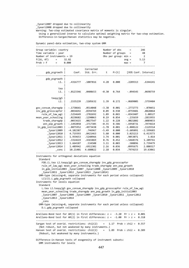
447
_Iyeari2007 dropped due to collinearity
_Iyeari2008 dropped due to collinearity
Warning: Two-step estimated covariance matrix of moments is singular.
Using a generalized inverse to calculate optimal weighting matrix for two-step estimation.
Difference-in-Sargan/Hansen statistics may be negative.
Dynamic panel-data estimation, two-step system GMM
------------------------------------------------------------------------------
Group variable: country Number of obs = 246
Time variable : year Number of groups = 48
Number of instruments = 19 Obs per group: min = 2
F(16, 47) = 32.82 avg = 5.13
Prob > F = 0.000 max = 7
-------------------------------------------------------------------------------------
| Corrected
gdp_pcgrowth | Coef. Std. Err. t P>|t| [95% Conf. Interval]
--------------------+----------------------------------------------------------------
gdp_pcgrowth |
L1. | .4316777 .1007816 4.28 0.000 .2289313 .6344241
|
tea |
L1. | -.0123346 .0408653 -0.30 0.764 -.094545 .0698759
|
teayyjg5 |
L2. | .1535239 .1105632 1.39 0.172 -.0689005 .3759484
|
gov_consum_sharegdp | -.1738641 .0514048 -3.38 0.001 -.2772773 -.070451
inv_gdp_grosscapfor | .0034692 .0394769 0.09 0.930 -.0759481 .0828864
rule_of_law_wgi | .5254649 .2782692 1.89 0.065 -.0343407 1.08527
mean_year_schooling | .0238682 .1290063 0.19 0.854 -.235659 .2833955
trade_sharegdp | .0033615 .0027547 1.22 0.228 -.0021802 .0089033
ann_pop_growth | -.1492058 .2717385 -0.55 0.586 -.6958731 .3974614
ln_gdp_initial2003 | -.8875952 .4973438 -1.78 0.081 -1.888122 .1129314
_Iyeari2009 | -4.102387 .746967 -5.49 0.000 -5.605091 -2.599683
_Iyeari2010 | 4.719393 .8421463 5.60 0.000 3.025213 6.413573
_Iyeari2011 | 1.959653 .5240966 3.74 0.001 .9053071 3.014
_Iyeari2012 | .3314619 .4365869 0.76 0.452 -.5468376 1.209761
_Iyeari2013 | 1.664187 .534508 3.11 0.003 .588896 2.739479
_Iyeari2014 | 1.489942 .6911302 2.16 0.036 .0995675 2.880317
_cons | 10.21401 4.680822 2.18 0.034 .7974153 19.63061
-------------------------------------------------------------------------------------
Instruments for orthogonal deviations equation
Standard
FOD.(L.tea L2.teayyjg5 gov_consum_sharegdp inv_gdp_grosscapfor
rule_of_law_wgi mean_year_schooling trade_sharegdp ann_pop_growth
ln_gdp_initial2003 _Iyeari2007 _Iyeari2008 _Iyeari2009 _Iyeari2010
_Iyeari2011 _Iyeari2012 _Iyeari2013 _Iyeari2014)
GMM-type (missing=0, separate instruments for each period unless collapsed)
L(1/2).L.gdp_pcgrowth collapsed
Instruments for levels equation
Standard
L.tea L2.teayyjg5 gov_consum_sharegdp inv_gdp_grosscapfor rule_of_law_wgi
mean_year_schooling trade_sharegdp ann_pop_growth ln_gdp_initial2003
_Iyeari2007 _Iyeari2008 _Iyeari2009 _Iyeari2010 _Iyeari2011 _Iyeari2012
_Iyeari2013 _Iyeari2014
_cons
GMM-type (missing=0, separate instruments for each period unless collapsed)
D.L.gdp_pcgrowth collapsed
------------------------------------------------------------------------------
Arellano-Bond test for AR(1) in first differences: z = -3.20 Pr > z = 0.001
Arellano-Bond test for AR(2) in first differences: z = -1.00 Pr > z = 0.318
------------------------------------------------------------------------------
Sargan test of overid. restrictions: chi2(2) = 1.17 Prob > chi2 = 0.557
(Not robust, but not weakened by many instruments.)
Hansen test of overid. restrictions: chi2(2) = 1.89 Prob > chi2 = 0.389
(Robust, but weakened by many instruments.)
Difference-in-Hansen tests of exogeneity of instrument subsets:
GMM instruments for levels

448
Hansen test excluding group: chi2(1) = 0.00 Prob > chi2 = 0.968
Difference (null H = exogenous): chi2(1) = 1.89 Prob > chi2 = 0.170
Appendix 4.3.3 Using innovative: new product (teayynwp)
a. FE with Driscoll-Kraay
. xi: xtscc gdp_pcgrowth L2teahjg lnL1teayynwp gov_consum_sharegdp inv_gdp_grosscapfor
rule_of_law_wgi mean_year_schooling trade_sharegdp ann_pop_growth L1gdppc_pppc2011 year2009
year2010 year2011 year2012 year2013 year2014 if gdp_pcgrowth>=-12.06071 & sample==1 &
L1teayynwp<=15.03 & country!=43 & country!=61 & country!=62 & country!=101 & country!=216 &
country!=372 & country!=389 & country!=420 & country!=506, fe
Regression with Driscoll-Kraay standard errors Number of obs = 234
Method: Fixed-effects regression Number of groups = 48
Group variable (i): country F( 15, 6) = 52.97
maximum lag: 2 Prob > F = 0.0000
within R-squared = 0.7374
-------------------------------------------------------------------------------------
| Drisc/Kraay
gdp_pcgrowth | Coef. Std. Err. t P>|t| [95% Conf. Interval]
--------------------+----------------------------------------------------------------
L2teahjg | .6866481 .2765561 2.48 0.048 .0099397 1.363356
lnL1teayynwp | .8518577 .1491736 5.71 0.001 .4868431 1.216872
gov_consum_sharegdp | -1.069859 .0770712 -13.88 0.000 -1.258445 -.8812724
inv_gdp_grosscapfor | .5974881 .0788326 7.58 0.000 .4045918 .7903844
rule_of_law_wgi | 2.580009 1.060522 2.43 0.051 -.0149947 5.175012
mean_year_schooling | 1.090465 .5266903 2.07 0.084 -.1983001 2.37923
trade_sharegdp | .0647369 .0162997 3.97 0.007 .0248529 .1046208
ann_pop_growth | -.3985396 .290897 -1.37 0.220 -1.110339 .3132597
L1gdppc_pppc2011 | -.0008653 .00018 -4.81 0.003 -.0013056 -.000425
year2009 | -1.198805 .2922741 -4.10 0.006 -1.913974 -.4836362
year2010 | 3.095296 .2543811 12.17 0.000 2.472848 3.717744
year2011 | 2.810591 .3194316 8.80 0.000 2.02897 3.592212
year2012 | 1.233438 .3913658 3.15 0.020 .2758005 2.191076
year2013 | 1.893024 .3885028 4.87 0.003 .9423916 2.843656
year2014 | 2.099797 .4840264 4.34 0.005 .915427 3.284167
_cons | 11.33885 7.866121 1.44 0.200 -7.908854 30.58655
-------------------------------------------------------------------------------------
b. FEVD
. xi: xtfevd gdp_pcgrowth L2teahjg lnL1teayynwp gov_consum_sharegdp inv_gdp_grosscapfor
rule_of_law_wgi mean_year_schooling trade_sharegdp ann_pop_growth ln_gdp_initial2003 year2009
year2010 year2011 year2012 year2013 year2014 if gdp_pcgrowth>=-12.06071 & sample==1 &
L1teayynwp<=15.03 & country!=43 & country!=61 & country!=62 & country!=101 & country!=216 &
country!=372 & country!=389 & country!=420 & country!=506, invariant (gov_consum_sharegdp
rule_of_law_wgi mean_year_schooling trade_sharegdp ln_gdp_initial2003)
panel fixed effects regression with vector decomposition
degrees of freedom fevd = 171 number of obs = 234
mean squared error = 2.216907 F( 17, 171) = 10.29061
root mean squared error = 1.488928 Prob > F = 2.84e-17
Residual Sum of Squares = 518.7563 R-squared = .8046415
Total Sum of Squares = 2655.406 adj. R-squared = .7338097
Estimation Sum of Squares = 2136.65
-------------------------------------------------------------------------------------
| fevd
gdp_pcgrowth | Coef. Std. Err. t P>|t| [95% Conf. Interval]
--------------------+----------------------------------------------------------------
L2teahjg | .6249758 .3964854 1.58 0.117 -.1576602 1.407612
lnL1teayynwp | .7581569 .4909743 1.54 0.124 -.210994 1.727308
inv_gdp_grosscapfor | .3390007 .172961 1.96 0.052 -.0024129 .6804144
ann_pop_growth | -.9865976 1.089078 -0.91 0.366 -3.136365 1.16317
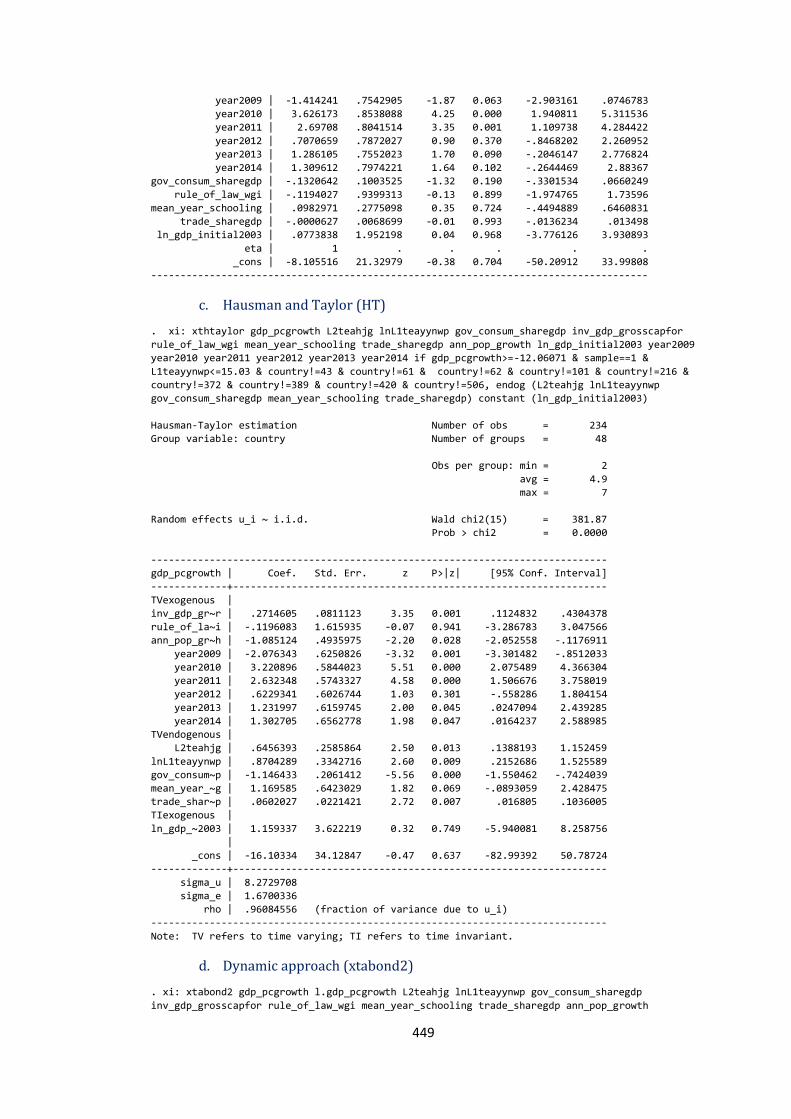
449
year2009 | -1.414241 .7542905 -1.87 0.063 -2.903161 .0746783
year2010 | 3.626173 .8538088 4.25 0.000 1.940811 5.311536
year2011 | 2.69708 .8041514 3.35 0.001 1.109738 4.284422
year2012 | .7070659 .7872027 0.90 0.370 -.8468202 2.260952
year2013 | 1.286105 .7552023 1.70 0.090 -.2046147 2.776824
year2014 | 1.309612 .7974221 1.64 0.102 -.2644469 2.88367
gov_consum_sharegdp | -.1320642 .1003525 -1.32 0.190 -.3301534 .0660249
rule_of_law_wgi | -.1194027 .9399313 -0.13 0.899 -1.974765 1.73596
mean_year_schooling | .0982971 .2775098 0.35 0.724 -.4494889 .6460831
trade_sharegdp | -.0000627 .0068699 -0.01 0.993 -.0136234 .013498
ln_gdp_initial2003 | .0773838 1.952198 0.04 0.968 -3.776126 3.930893
eta | 1 . . . . .
_cons | -8.105516 21.32979 -0.38 0.704 -50.20912 33.99808
-------------------------------------------------------------------------------------
c. Hausman and Taylor (HT)
. xi: xthtaylor gdp_pcgrowth L2teahjg lnL1teayynwp gov_consum_sharegdp inv_gdp_grosscapfor
rule_of_law_wgi mean_year_schooling trade_sharegdp ann_pop_growth ln_gdp_initial2003 year2009
year2010 year2011 year2012 year2013 year2014 if gdp_pcgrowth>=-12.06071 & sample==1 &
L1teayynwp<=15.03 & country!=43 & country!=61 & country!=62 & country!=101 & country!=216 &
country!=372 & country!=389 & country!=420 & country!=506, endog (L2teahjg lnL1teayynwp
gov_consum_sharegdp mean_year_schooling trade_sharegdp) constant (ln_gdp_initial2003)
Hausman-Taylor estimation Number of obs = 234
Group variable: country Number of groups = 48
Obs per group: min = 2
avg = 4.9
max = 7
Random effects u_i ~ i.i.d. Wald chi2(15) = 381.87
Prob > chi2 = 0.0000
------------------------------------------------------------------------------
gdp_pcgrowth | Coef. Std. Err. z P>|z| [95% Conf. Interval]
-------------+----------------------------------------------------------------
TVexogenous |
inv_gdp_gr~r | .2714605 .0811123 3.35 0.001 .1124832 .4304378
rule_of_la~i | -.1196083 1.615935 -0.07 0.941 -3.286783 3.047566
ann_pop_gr~h | -1.085124 .4935975 -2.20 0.028 -2.052558 -.1176911
year2009 | -2.076343 .6250826 -3.32 0.001 -3.301482 -.8512033
year2010 | 3.220896 .5844023 5.51 0.000 2.075489 4.366304
year2011 | 2.632348 .5743327 4.58 0.000 1.506676 3.758019
year2012 | .6229341 .6026744 1.03 0.301 -.558286 1.804154
year2013 | 1.231997 .6159745 2.00 0.045 .0247094 2.439285
year2014 | 1.302705 .6562778 1.98 0.047 .0164237 2.588985
TVendogenous |
L2teahjg | .6456393 .2585864 2.50 0.013 .1388193 1.152459
lnL1teayynwp | .8704289 .3342716 2.60 0.009 .2152686 1.525589
gov_consum~p | -1.146433 .2061412 -5.56 0.000 -1.550462 -.7424039
mean_year_~g | 1.169585 .6423029 1.82 0.069 -.0893059 2.428475
trade_shar~p | .0602027 .0221421 2.72 0.007 .016805 .1036005
TIexogenous |
ln_gdp_~2003 | 1.159337 3.622219 0.32 0.749 -5.940081 8.258756
|
_cons | -16.10334 34.12847 -0.47 0.637 -82.99392 50.78724
-------------+----------------------------------------------------------------
sigma_u | 8.2729708
sigma_e | 1.6700336
rho | .96084556 (fraction of variance due to u_i)
------------------------------------------------------------------------------
Note: TV refers to time varying; TI refers to time invariant.
d. Dynamic approach (xtabond2)
. xi: xtabond2 gdp_pcgrowth l.gdp_pcgrowth L2teahjg lnL1teayynwp gov_consum_sharegdp
inv_gdp_grosscapfor rule_of_law_wgi mean_year_schooling trade_sharegdp ann_pop_growth
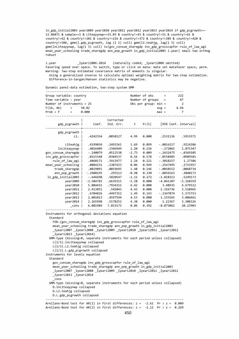
450
ln_gdp_initial2003 year2009 year2010 year2011 year2012 year2013 year2014 if gdp_pcgrowth>=-
12.06071 & sample==1 & L1teayynwp<=15.03 & country!=43 & country!=51 & country!=61 &
country!=62 & country!=101 & country!=216 & country!=372 & country!=389 & country!=420 &
country!=506, gmm(l.gdp_pcgrowth, lag (1 2) coll) gmm(l2.teahjg, lag(1 3) coll)
gmm(lnL1teayynwp, lag(1 3) coll) iv(gov_consum_sharegdp inv_gdp_grosscapfor rule_of_law_wgi
mean_year_schooling trade_sharegdp ann_pop_growth ln_gdp_initial2003 i.year) small two orthog
robust
i.year _Iyeari2006-2014 (naturally coded; _Iyeari2006 omitted)
Favoring speed over space. To switch, type or click on mata: mata set matafavor space, perm.
Warning: Two-step estimated covariance matrix of moments is singular.
Using a generalized inverse to calculate optimal weighting matrix for two-step estimation.
Difference-in-Sargan/Hansen statistics may be negative.
Dynamic panel-data estimation, two-step system GMM
------------------------------------------------------------------------------
Group variable: country Number of obs = 232
Time variable : year Number of groups = 47
Number of instruments = 25 Obs per group: min = 2
F(16, 46) = 50.82 avg = 4.94
Prob > F = 0.000 max = 7
-------------------------------------------------------------------------------------
| Corrected
gdp_pcgrowth | Coef. Std. Err. t P>|t| [95% Conf. Interval]
--------------------+----------------------------------------------------------------
gdp_pcgrowth |
L1. | .4242354 .0850127 4.99 0.000 .2531136 .5953571
|
L2teahjg | .4199034 .2491561 1.69 0.099 -.0816217 .9214286
lnL1teayynwp | .4016409 .3346949 1.20 0.236 -.272065 1.075347
gov_consum_sharegdp | -.140079 .0512538 -2.73 0.009 -.2432475 -.0369105
inv_gdp_grosscapfor | .0215548 .0384537 0.56 0.578 -.0558485 .0989581
rule_of_law_wgi | .4860171 .3913977 1.24 0.221 -.3018257 1.27386
mean_year_schooling | .0084231 .1307433 0.06 0.949 -.2547495 .2715957
trade_sharegdp | .0029091 .0019695 1.48 0.146 -.0010552 .0068734
ann_pop_growth | -.2908195 .295513 -0.98 0.330 -.8856563 .3040173
ln_gdp_initial2003 | -.646698 .5820547 -1.11 0.272 -1.818313 .5249173
year2009 | -3.504783 .6639311 -5.28 0.000 -4.841207 -2.168359
year2010 | 5.084431 .7924311 6.42 0.000 3.48935 6.679512
year2011 | 2.413851 .545043 4.43 0.000 1.316736 3.510965
year2012 | .6704826 .4497352 1.49 0.143 -.2347874 1.575753
year2013 | 2.081013 .4597594 4.53 0.000 1.155565 3.006461
year2014 | 2.265998 .5178252 4.38 0.000 1.22367 3.308326
_cons | 6.081984 7.033175 0.86 0.392 -8.075062 20.23903
-------------------------------------------------------------------------------------
Instruments for orthogonal deviations equation
Standard
FOD.(gov_consum_sharegdp inv_gdp_grosscapfor rule_of_law_wgi
mean_year_schooling trade_sharegdp ann_pop_growth ln_gdp_initial2003
_Iyeari2007 _Iyeari2008 _Iyeari2009 _Iyeari2010 _Iyeari2011 _Iyeari2012
_Iyeari2013 _Iyeari2014)
GMM-type (missing=0, separate instruments for each period unless collapsed)
L(1/3).lnL1teayynwp collapsed
L(1/3).L2.teahjg collapsed
L(1/2).L.gdp_pcgrowth collapsed
Instruments for levels equation
Standard
gov_consum_sharegdp inv_gdp_grosscapfor rule_of_law_wgi
mean_year_schooling trade_sharegdp ann_pop_growth ln_gdp_initial2003
_Iyeari2007 _Iyeari2008 _Iyeari2009 _Iyeari2010 _Iyeari2011 _Iyeari2012
_Iyeari2013 _Iyeari2014
_cons
GMM-type (missing=0, separate instruments for each period unless collapsed)
D.lnL1teayynwp collapsed
D.L2.teahjg collapsed
D.L.gdp_pcgrowth collapsed
------------------------------------------------------------------------------
Arellano-Bond test for AR(1) in first differences: z = -2.61 Pr > z = 0.009
Arellano-Bond test for AR(2) in first differences: z = -1.11 Pr > z = 0.269

451
------------------------------------------------------------------------------
Sargan test of overid. restrictions: chi2(8) = 3.16 Prob > chi2 = 0.924
(Not robust, but not weakened by many instruments.)
Hansen test of overid. restrictions: chi2(8) = 4.20 Prob > chi2 = 0.838
(Robust, but weakened by many instruments.)
Difference-in-Hansen tests of exogeneity of instrument subsets:
GMM instruments for levels
Hansen test excluding group: chi2(5) = 0.91 Prob > chi2 = 0.970
Difference (null H = exogenous): chi2(3) = 3.30 Prob > chi2 = 0.348
gmm(L.gdp_pcgrowth, collapse lag(1 2))
Hansen test excluding group: chi2(5) = 2.04 Prob > chi2 = 0.844
Difference (null H = exogenous): chi2(3) = 2.17 Prob > chi2 = 0.539
gmm(L2.teahjg, collapse lag(1 3))
Hansen test excluding group: chi2(4) = 2.35 Prob > chi2 = 0.671
Difference (null H = exogenous): chi2(4) = 1.85 Prob > chi2 = 0.763
gmm(lnL1teayynwp, collapse lag(1 3))
Hansen test excluding group: chi2(4) = 0.51 Prob > chi2 = 0.972
Difference (null H = exogenous): chi2(4) = 3.69 Prob > chi2 = 0.450
Appendix 4.3.4 Using innovative: new product and new market (teanpm)
a. FE with Driscoll-Kraay
. xi: xtscc gdp_pcgrowth L2teahjg lnL1teanpm gov_consum_sharegdp inv_gdp_grosscapfor
rule_of_law_wgi mean_year_schooling trade_sharegdp ann_pop_growth L1gdppc_pppc2011 year2009
year2010 year2011 year2012 year2013 year2014 if gdp_pcgrowth>=-12.06071 & sample==1 &
country!=43 & country!=51 & country!=61 & country!=62 & country!=101 & country!=216 &
country!=372 & country!=389 & country!=420 & country!=506, fe
Regression with Driscoll-Kraay standard errors Number of obs = 239
Method: Fixed-effects regression Number of groups = 47
Group variable (i): country F( 15, 6) = 871.80
maximum lag: 2 Prob > F = 0.0000
within R-squared = 0.7330
-------------------------------------------------------------------------------------
| Drisc/Kraay
gdp_pcgrowth | Coef. Std. Err. t P>|t| [95% Conf. Interval]
--------------------+----------------------------------------------------------------
L2teahjg | .6272858 .3069325 2.04 0.087 -.1237509 1.378323
lnL1teanpm | .8355222 .1864594 4.48 0.004 .3792725 1.291772
gov_consum_sharegdp | -1.029721 .0997257 -10.33 0.000 -1.273741 -.7857008
inv_gdp_grosscapfor | .6006135 .0798254 7.52 0.000 .4052878 .7959392
rule_of_law_wgi | 2.368002 1.029837 2.30 0.061 -.1519189 4.887924
mean_year_schooling | .8861952 .5265876 1.68 0.143 -.4023182 2.174709
trade_sharegdp | .0643914 .0123215 5.23 0.002 .0342418 .094541
ann_pop_growth | -.3290623 .2894451 -1.14 0.299 -1.037309 .3791843
L1gdppc_pppc2011 | -.0008905 .0001677 -5.31 0.002 -.0013009 -.0004801
year2009 | -1.285907 .3377798 -3.81 0.009 -2.112424 -.4593898
year2010 | 2.737093 .2590154 10.57 0.000 2.103305 3.370881
year2011 | 2.486658 .3023527 8.22 0.000 1.746827 3.226488
year2012 | 1.004311 .38471 2.61 0.040 .0629597 1.945663
year2013 | 1.640098 .3905383 4.20 0.006 .6844847 2.59571
year2014 | 1.885412 .4679235 4.03 0.007 .7404438 3.030379
_cons | 14.14053 6.922114 2.04 0.087 -2.797274 31.07833
-------------------------------------------------------------------------------------
b. FEVD
. xi: xtfevd gdp_pcgrowth L2teahjg lnL1teanpm gov_consum_sharegdp inv_gdp_grosscapfor
rule_of_law_wgi mean_year_schooling trade_sharegdp ann_pop_growth ln_gdp_initial2003 year2009
year2010 year2011 year2012 year2013 year2014 if gdp_pcgrowth>=-12.06071 & sample==1 &
country!=43 & country!=51 & country!=61 & country!=62 & country!=101 & country!=216 &
country!=372 & country!=389 & country!=420 & country!=506, invariant (gov_consum_sharegdp
rule_of_law_wgi mean_year_schooling trade_sharegdp ln_gdp_initial2003)
panel fixed effects regression with vector decomposition
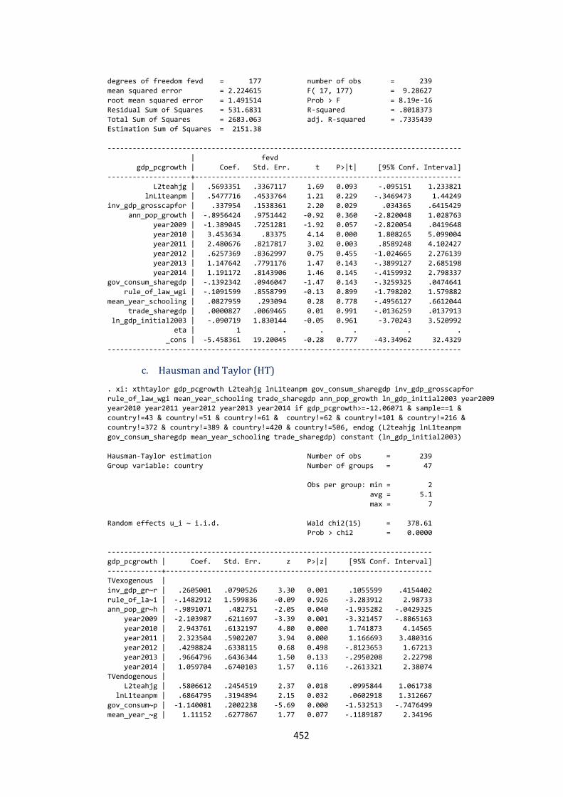
452
degrees of freedom fevd = 177 number of obs = 239
mean squared error = 2.224615 F( 17, 177) = 9.28627
root mean squared error = 1.491514 Prob > F = 8.19e-16
Residual Sum of Squares = 531.6831 R-squared = .8018373
Total Sum of Squares = 2683.063 adj. R-squared = .7335439
Estimation Sum of Squares = 2151.38
-------------------------------------------------------------------------------------
| fevd
gdp_pcgrowth | Coef. Std. Err. t P>|t| [95% Conf. Interval]
--------------------+----------------------------------------------------------------
L2teahjg | .5693351 .3367117 1.69 0.093 -.095151 1.233821
lnL1teanpm | .5477716 .4533764 1.21 0.229 -.3469473 1.44249
inv_gdp_grosscapfor | .337954 .1538361 2.20 0.029 .034365 .6415429
ann_pop_growth | -.8956424 .9751442 -0.92 0.360 -2.820048 1.028763
year2009 | -1.389045 .7251281 -1.92 0.057 -2.820054 .0419648
year2010 | 3.453634 .83375 4.14 0.000 1.808265 5.099004
year2011 | 2.480676 .8217817 3.02 0.003 .8589248 4.102427
year2012 | .6257369 .8362997 0.75 0.455 -1.024665 2.276139
year2013 | 1.147642 .7791176 1.47 0.143 -.3899127 2.685198
year2014 | 1.191172 .8143906 1.46 0.145 -.4159932 2.798337
gov_consum_sharegdp | -.1392342 .0946047 -1.47 0.143 -.3259325 .0474641
rule_of_law_wgi | -.1091599 .8558799 -0.13 0.899 -1.798202 1.579882
mean_year_schooling | .0827959 .293094 0.28 0.778 -.4956127 .6612044
trade_sharegdp | .0000827 .0069465 0.01 0.991 -.0136259 .0137913
ln_gdp_initial2003 | -.090719 1.830144 -0.05 0.961 -3.70243 3.520992
eta | 1 . . . . .
_cons | -5.458361 19.20045 -0.28 0.777 -43.34962 32.4329
-------------------------------------------------------------------------------------
c. Hausman and Taylor (HT)
. xi: xthtaylor gdp_pcgrowth L2teahjg lnL1teanpm gov_consum_sharegdp inv_gdp_grosscapfor
rule_of_law_wgi mean_year_schooling trade_sharegdp ann_pop_growth ln_gdp_initial2003 year2009
year2010 year2011 year2012 year2013 year2014 if gdp_pcgrowth>=-12.06071 & sample==1 &
country!=43 & country!=51 & country!=61 & country!=62 & country!=101 & country!=216 &
country!=372 & country!=389 & country!=420 & country!=506, endog (L2teahjg lnL1teanpm
gov_consum_sharegdp mean_year_schooling trade_sharegdp) constant (ln_gdp_initial2003)
Hausman-Taylor estimation Number of obs = 239
Group variable: country Number of groups = 47
Obs per group: min = 2
avg = 5.1
max = 7
Random effects u_i ~ i.i.d. Wald chi2(15) = 378.61
Prob > chi2 = 0.0000
------------------------------------------------------------------------------
gdp_pcgrowth | Coef. Std. Err. z P>|z| [95% Conf. Interval]
-------------+----------------------------------------------------------------
TVexogenous |
inv_gdp_gr~r | .2605001 .0790526 3.30 0.001 .1055599 .4154402
rule_of_la~i | -.1482912 1.599836 -0.09 0.926 -3.283912 2.98733
ann_pop_gr~h | -.9891071 .482751 -2.05 0.040 -1.935282 -.0429325
year2009 | -2.103987 .6211697 -3.39 0.001 -3.321457 -.8865163
year2010 | 2.943761 .6132197 4.80 0.000 1.741873 4.14565
year2011 | 2.323504 .5902207 3.94 0.000 1.166693 3.480316
year2012 | .4298824 .6338115 0.68 0.498 -.8123653 1.67213
year2013 | .9664796 .6436344 1.50 0.133 -.2950208 2.22798
year2014 | 1.059704 .6740103 1.57 0.116 -.2613321 2.38074
TVendogenous |
L2teahjg | .5806612 .2454519 2.37 0.018 .0995844 1.061738
lnL1teanpm | .6864795 .3194894 2.15 0.032 .0602918 1.312667
gov_consum~p | -1.140081 .2002238 -5.69 0.000 -1.532513 -.7476499
mean_year_~g | 1.11152 .6277867 1.77 0.077 -.1189187 2.34196
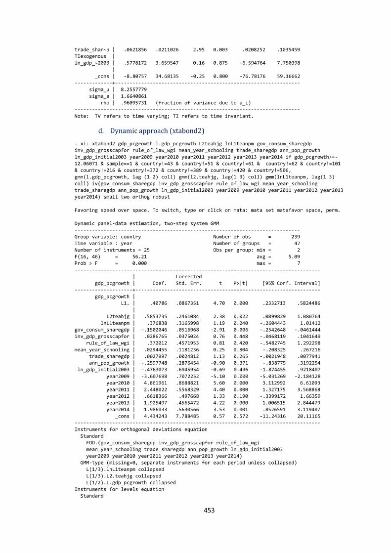
453
trade_shar~p | .0621856 .0211026 2.95 0.003 .0208252 .1035459
TIexogenous |
ln_gdp_~2003 | .5778172 3.659547 0.16 0.875 -6.594764 7.750398
|
_cons | -8.80757 34.68135 -0.25 0.800 -76.78176 59.16662
-------------+----------------------------------------------------------------
sigma_u | 8.2557779
sigma_e | 1.6640861
rho | .96095731 (fraction of variance due to u_i)
------------------------------------------------------------------------------
Note: TV refers to time varying; TI refers to time invariant.
d. Dynamic approach (xtabond2)
. xi: xtabond2 gdp_pcgrowth l.gdp_pcgrowth L2teahjg lnL1teanpm gov_consum_sharegdp
inv_gdp_grosscapfor rule_of_law_wgi mean_year_schooling trade_sharegdp ann_pop_growth
ln_gdp_initial2003 year2009 year2010 year2011 year2012 year2013 year2014 if gdp_pcgrowth>=-
12.06071 & sample==1 & country!=43 & country!=51 & country!=61 & country!=62 & country!=101
& country!=216 & country!=372 & country!=389 & country!=420 & country!=506,
gmm(l.gdp_pcgrowth, lag (1 2) coll) gmm(l2.teahjg, lag(1 3) coll) gmm(lnL1teanpm, lag(1 3)
coll) iv(gov_consum_sharegdp inv_gdp_grosscapfor rule_of_law_wgi mean_year_schooling
trade_sharegdp ann_pop_growth ln_gdp_initial2003 year2009 year2010 year2011 year2012 year2013
year2014) small two orthog robust
Favoring speed over space. To switch, type or click on mata: mata set matafavor space, perm.
Dynamic panel-data estimation, two-step system GMM
------------------------------------------------------------------------------
Group variable: country Number of obs = 239
Time variable : year Number of groups = 47
Number of instruments = 25 Obs per group: min = 2
F(16, 46) = 56.21 avg = 5.09
Prob > F = 0.000 max = 7
-------------------------------------------------------------------------------------
| Corrected
gdp_pcgrowth | Coef. Std. Err. t P>|t| [95% Conf. Interval]
--------------------+----------------------------------------------------------------
gdp_pcgrowth |
L1. | .40786 .0867351 4.70 0.000 .2332713 .5824486
|
L2teahjg | .5853735 .2461084 2.38 0.022 .0899829 1.080764
lnL1teanpm | .376838 .3165998 1.19 0.240 -.2604443 1.01412
gov_consum_sharegdp | -.1502046 .0516968 -2.91 0.006 -.2542648 -.0461444
inv_gdp_grosscapfor | .0286765 .0375024 0.76 0.448 -.0468119 .1041649
rule_of_law_wgi | .372012 .4571953 0.81 0.420 -.5482745 1.292298
mean_year_schooling | .0294455 .1181236 0.25 0.804 -.208325 .267216
trade_sharegdp | .0027997 .0024812 1.13 0.265 -.0021948 .0077941
ann_pop_growth | -.2597748 .2876454 -0.90 0.371 -.838775 .3192254
ln_gdp_initial2003 | -.4763073 .6945954 -0.69 0.496 -1.874455 .9218407
year2009 | -3.607698 .7072252 -5.10 0.000 -5.031269 -2.184128
year2010 | 4.861961 .8688821 5.60 0.000 3.112992 6.61093
year2011 | 2.448022 .5568329 4.40 0.000 1.327175 3.568868
year2012 | .6618366 .497668 1.33 0.190 -.3399172 1.66359
year2013 | 1.925497 .4565472 4.22 0.000 1.006515 2.844479
year2014 | 1.986033 .5630566 3.53 0.001 .8526591 3.119407
_cons | 4.434243 7.788485 0.57 0.572 -11.24316 20.11165
-------------------------------------------------------------------------------------
Instruments for orthogonal deviations equation
Standard
FOD.(gov_consum_sharegdp inv_gdp_grosscapfor rule_of_law_wgi
mean_year_schooling trade_sharegdp ann_pop_growth ln_gdp_initial2003
year2009 year2010 year2011 year2012 year2013 year2014)
GMM-type (missing=0, separate instruments for each period unless collapsed)
L(1/3).lnL1teanpm collapsed
L(1/3).L2.teahjg collapsed
L(1/2).L.gdp_pcgrowth collapsed
Instruments for levels equation
Standard
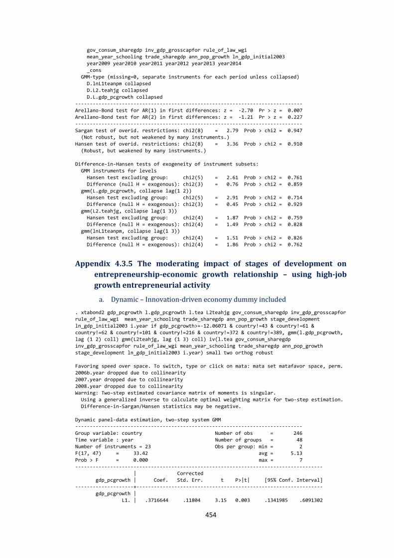
454
gov_consum_sharegdp inv_gdp_grosscapfor rule_of_law_wgi
mean_year_schooling trade_sharegdp ann_pop_growth ln_gdp_initial2003
year2009 year2010 year2011 year2012 year2013 year2014
_cons
GMM-type (missing=0, separate instruments for each period unless collapsed)
D.lnL1teanpm collapsed
D.L2.teahjg collapsed
D.L.gdp_pcgrowth collapsed
------------------------------------------------------------------------------
Arellano-Bond test for AR(1) in first differences: z = -2.70 Pr > z = 0.007
Arellano-Bond test for AR(2) in first differences: z = -1.21 Pr > z = 0.227
------------------------------------------------------------------------------
Sargan test of overid. restrictions: chi2(8) = 2.79 Prob > chi2 = 0.947
(Not robust, but not weakened by many instruments.)
Hansen test of overid. restrictions: chi2(8) = 3.36 Prob > chi2 = 0.910
(Robust, but weakened by many instruments.)
Difference-in-Hansen tests of exogeneity of instrument subsets:
GMM instruments for levels
Hansen test excluding group: chi2(5) = 2.61 Prob > chi2 = 0.761
Difference (null H = exogenous): chi2(3) = 0.76 Prob > chi2 = 0.859
gmm(L.gdp_pcgrowth, collapse lag(1 2))
Hansen test excluding group: chi2(5) = 2.91 Prob > chi2 = 0.714
Difference (null H = exogenous): chi2(3) = 0.45 Prob > chi2 = 0.929
gmm(L2.teahjg, collapse lag(1 3))
Hansen test excluding group: chi2(4) = 1.87 Prob > chi2 = 0.759
Difference (null H = exogenous): chi2(4) = 1.49 Prob > chi2 = 0.828
gmm(lnL1teanpm, collapse lag(1 3))
Hansen test excluding group: chi2(4) = 1.51 Prob > chi2 = 0.826
Difference (null H = exogenous): chi2(4) = 1.86 Prob > chi2 = 0.762
Appendix 4.3.5 The moderating impact of stages of development on
entrepreneurship-economic growth relationship – using high-job
growth entrepreneurial activity
a. Dynamic – Innovation-driven economy dummy included
. xtabond2 gdp_pcgrowth l.gdp_pcgrowth l.tea L2teahjg gov_consum_sharegdp inv_gdp_grosscapfor
rule_of_law_wgi mean_year_schooling trade_sharegdp ann_pop_growth stage_development
ln_gdp_initial2003 i.year if gdp_pcgrowth>=-12.06071 & country!=43 & country!=61 &
country!=62 & country!=101 & country!=216 & country!=372 & country!=389, gmm(l.gdp_pcgrowth,
lag (1 2) coll) gmm(L2teahjg, lag (1 3) coll) iv(l.tea gov_consum_sharegdp
inv_gdp_grosscapfor rule_of_law_wgi mean_year_schooling trade_sharegdp ann_pop_growth
stage_development ln_gdp_initial2003 i.year) small two orthog robust
Favoring speed over space. To switch, type or click on mata: mata set matafavor space, perm.
2006b.year dropped due to collinearity
2007.year dropped due to collinearity
2008.year dropped due to collinearity
Warning: Two-step estimated covariance matrix of moments is singular.
Using a generalized inverse to calculate optimal weighting matrix for two-step estimation.
Difference-in-Sargan/Hansen statistics may be negative.
Dynamic panel-data estimation, two-step system GMM
------------------------------------------------------------------------------
Group variable: country Number of obs = 246
Time variable : year Number of groups = 48
Number of instruments = 23 Obs per group: min = 2
F(17, 47) = 33.42 avg = 5.13
Prob > F = 0.000 max = 7
-------------------------------------------------------------------------------------
| Corrected
gdp_pcgrowth | Coef. Std. Err. t P>|t| [95% Conf. Interval]
--------------------+----------------------------------------------------------------
gdp_pcgrowth |
L1. | .3716644 .11804 3.15 0.003 .1341985 .6091302
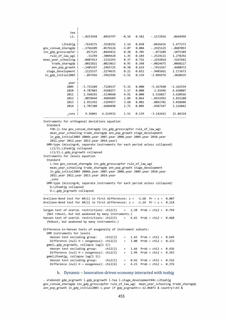
455
|
tea |
L1. | -.0253958 .0456797 -0.56 0.581 -.1172916 .0664999
|
L2teahjg | .7614575 .3558192 2.14 0.038 .0456416 1.477273
gov_consum_sharegdp | -.1766109 .0576126 -3.07 0.004 -.2925125 -.0607093
inv_gdp_grosscapfor | .017125 .0449432 0.38 0.705 -.073289 .1075389
rule_of_law_wgi | .51294 .3804428 1.35 0.184 -.2524121 1.278292
mean_year_schooling | .0487413 .1332293 0.37 0.716 -.2192814 .3167641
trade_sharegdp | .0021821 .0023013 0.95 0.348 -.0024475 .0068117
ann_pop_growth | -.1485297 .2965725 -0.50 0.619 -.7451567 .4480972
stage_development | .1125537 .5274635 0.21 0.832 -.9485661 1.173673
ln_gdp_initial2003 | -.897456 .5962596 -1.51 0.139 -2.096976 .3020635
|
year |
2009 | -3.715104 .7220337 -5.15 0.000 -5.167648 -2.262559
2010 | 4.787883 .9260257 5.17 0.000 2.92496 6.650807
2011 | 2.568292 .5230668 4.91 0.000 1.516017 3.620566
2012 | .8878444 .4689689 1.89 0.064 -.0555992 1.831288
2013 | 1.952392 .5299957 3.68 0.001 .8861781 3.018606
2014 | 1.787388 .6604498 2.71 0.009 .4587347 3.116042
|
_cons | 9.36041 6.214932 1.51 0.139 -3.142421 21.86324
-------------------------------------------------------------------------------------
Instruments for orthogonal deviations equation
Standard
FOD.(L.tea gov_consum_sharegdp inv_gdp_grosscapfor rule_of_law_wgi
mean_year_schooling trade_sharegdp ann_pop_growth stage_development
ln_gdp_initial2003 2006b.year 2007.year 2008.year 2009.year 2010.year
2011.year 2012.year 2013.year 2014.year)
GMM-type (missing=0, separate instruments for each period unless collapsed)
L(1/3).L2teahjg collapsed
L(1/2).L.gdp_pcgrowth collapsed
Instruments for levels equation
Standard
L.tea gov_consum_sharegdp inv_gdp_grosscapfor rule_of_law_wgi
mean_year_schooling trade_sharegdp ann_pop_growth stage_development
ln_gdp_initial2003 2006b.year 2007.year 2008.year 2009.year 2010.year
2011.year 2012.year 2013.year 2014.year
_cons
GMM-type (missing=0, separate instruments for each period unless collapsed)
D.L2teahjg collapsed
D.L.gdp_pcgrowth collapsed
------------------------------------------------------------------------------
Arellano-Bond test for AR(1) in first differences: z = -2.68 Pr > z = 0.007
Arellano-Bond test for AR(2) in first differences: z = -1.24 Pr > z = 0.214
------------------------------------------------------------------------------
Sargan test of overid. restrictions: chi2(5) = 2.38 Prob > chi2 = 0.794
(Not robust, but not weakened by many instruments.)
Hansen test of overid. restrictions: chi2(5) = 4.65 Prob > chi2 = 0.460
(Robust, but weakened by many instruments.)
Difference-in-Hansen tests of exogeneity of instrument subsets:
GMM instruments for levels
Hansen test excluding group: chi2(3) = 1.65 Prob > chi2 = 0.649
Difference (null H = exogenous): chi2(2) = 3.00 Prob > chi2 = 0.223
gmm(L.gdp_pcgrowth, collapse lag(1 2))
Hansen test excluding group: chi2(2) = 1.66 Prob > chi2 = 0.436
Difference (null H = exogenous): chi2(3) = 2.99 Prob > chi2 = 0.393
gmm(L2teahjg, collapse lag(1 3))
Hansen test excluding group: chi2(1) = 0.42 Prob > chi2 = 0.516
Difference (null H = exogenous): chi2(4) = 4.23 Prob > chi2 = 0.376
b. Dynamic – Innovation-driven economy interacted with teahjg
. xtabond2 gdp_pcgrowth l.gdp_pcgrowth l.tea i.stage_development##c.L2teahjg
gov_consum_sharegdp inv_gdp_grosscapfor rule_of_law_wgi mean_year_schooling trade_sharegdp
ann_pop_growth ln_gdp_initial2003 i.year if gdp_pcgrowth>=-12.06071 & country!=43 &
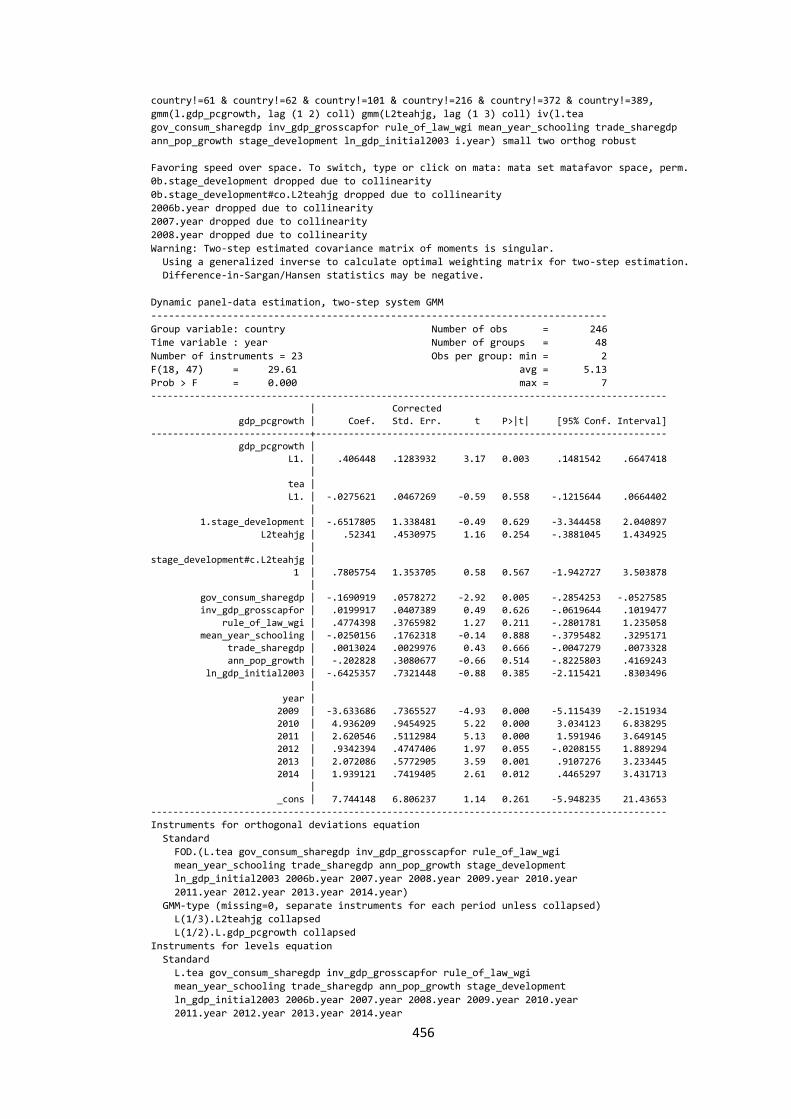
456
country!=61 & country!=62 & country!=101 & country!=216 & country!=372 & country!=389,
gmm(l.gdp_pcgrowth, lag (1 2) coll) gmm(L2teahjg, lag (1 3) coll) iv(l.tea
gov_consum_sharegdp inv_gdp_grosscapfor rule_of_law_wgi mean_year_schooling trade_sharegdp
ann_pop_growth stage_development ln_gdp_initial2003 i.year) small two orthog robust
Favoring speed over space. To switch, type or click on mata: mata set matafavor space, perm.
0b.stage_development dropped due to collinearity
0b.stage_development#co.L2teahjg dropped due to collinearity
2006b.year dropped due to collinearity
2007.year dropped due to collinearity
2008.year dropped due to collinearity
Warning: Two-step estimated covariance matrix of moments is singular.
Using a generalized inverse to calculate optimal weighting matrix for two-step estimation.
Difference-in-Sargan/Hansen statistics may be negative.
Dynamic panel-data estimation, two-step system GMM
------------------------------------------------------------------------------
Group variable: country Number of obs = 246
Time variable : year Number of groups = 48
Number of instruments = 23 Obs per group: min = 2
F(18, 47) = 29.61 avg = 5.13
Prob > F = 0.000 max = 7 ----------------------------------------------------------------------------------------------
| Corrected
gdp_pcgrowth | Coef. Std. Err. t P>|t| [95% Conf. Interval]
-----------------------------+----------------------------------------------------------------
gdp_pcgrowth |
L1. | .406448 .1283932 3.17 0.003 .1481542 .6647418
|
tea |
L1. | -.0275621 .0467269 -0.59 0.558 -.1215644 .0664402
|
1.stage_development | -.6517805 1.338481 -0.49 0.629 -3.344458 2.040897
L2teahjg | .52341 .4530975 1.16 0.254 -.3881045 1.434925
|
stage_development#c.L2teahjg |
1 | .7805754 1.353705 0.58 0.567 -1.942727 3.503878
|
gov_consum_sharegdp | -.1690919 .0578272 -2.92 0.005 -.2854253 -.0527585
inv_gdp_grosscapfor | .0199917 .0407389 0.49 0.626 -.0619644 .1019477
rule_of_law_wgi | .4774398 .3765982 1.27 0.211 -.2801781 1.235058
mean_year_schooling | -.0250156 .1762318 -0.14 0.888 -.3795482 .3295171
trade_sharegdp | .0013024 .0029976 0.43 0.666 -.0047279 .0073328
ann_pop_growth | -.202828 .3080677 -0.66 0.514 -.8225803 .4169243
ln_gdp_initial2003 | -.6425357 .7321448 -0.88 0.385 -2.115421 .8303496
|
year |
2009 | -3.633686 .7365527 -4.93 0.000 -5.115439 -2.151934
2010 | 4.936209 .9454925 5.22 0.000 3.034123 6.838295
2011 | 2.620546 .5112984 5.13 0.000 1.591946 3.649145
2012 | .9342394 .4747406 1.97 0.055 -.0208155 1.889294
2013 | 2.072086 .5772905 3.59 0.001 .9107276 3.233445
2014 | 1.939121 .7419405 2.61 0.012 .4465297 3.431713 |
_cons | 7.744148 6.806237 1.14 0.261 -5.948235 21.43653
----------------------------------------------------------------------------------------------
Instruments for orthogonal deviations equation
Standard
FOD.(L.tea gov_consum_sharegdp inv_gdp_grosscapfor rule_of_law_wgi
mean_year_schooling trade_sharegdp ann_pop_growth stage_development
ln_gdp_initial2003 2006b.year 2007.year 2008.year 2009.year 2010.year
2011.year 2012.year 2013.year 2014.year)
GMM-type (missing=0, separate instruments for each period unless collapsed)
L(1/3).L2teahjg collapsed
L(1/2).L.gdp_pcgrowth collapsed
Instruments for levels equation
Standard
L.tea gov_consum_sharegdp inv_gdp_grosscapfor rule_of_law_wgi
mean_year_schooling trade_sharegdp ann_pop_growth stage_development
ln_gdp_initial2003 2006b.year 2007.year 2008.year 2009.year 2010.year
2011.year 2012.year 2013.year 2014.year
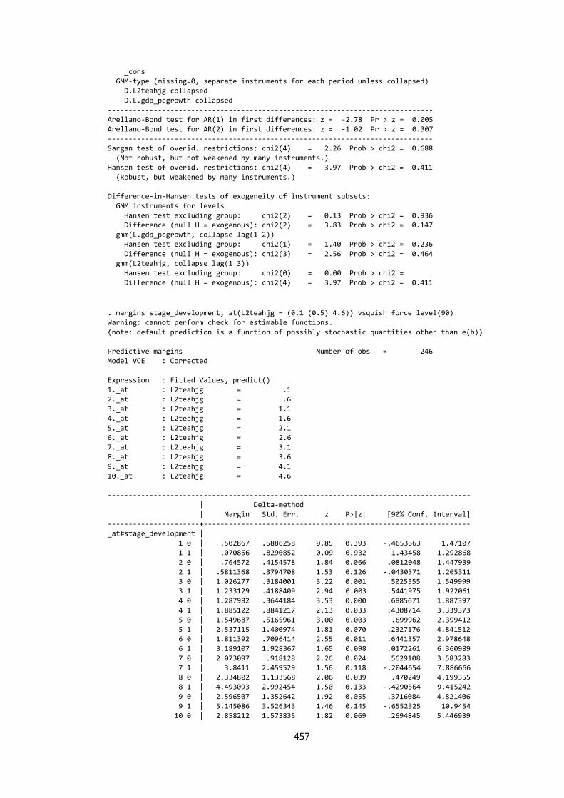
457
_cons
GMM-type (missing=0, separate instruments for each period unless collapsed)
D.L2teahjg collapsed
D.L.gdp_pcgrowth collapsed
------------------------------------------------------------------------------
Arellano-Bond test for AR(1) in first differences: z = -2.78 Pr > z = 0.005
Arellano-Bond test for AR(2) in first differences: z = -1.02 Pr > z = 0.307
------------------------------------------------------------------------------
Sargan test of overid. restrictions: chi2(4) = 2.26 Prob > chi2 = 0.688
(Not robust, but not weakened by many instruments.)
Hansen test of overid. restrictions: chi2(4) = 3.97 Prob > chi2 = 0.411
(Robust, but weakened by many instruments.)
Difference-in-Hansen tests of exogeneity of instrument subsets:
GMM instruments for levels
Hansen test excluding group: chi2(2) = 0.13 Prob > chi2 = 0.936
Difference (null H = exogenous): chi2(2) = 3.83 Prob > chi2 = 0.147
gmm(L.gdp_pcgrowth, collapse lag(1 2))
Hansen test excluding group: chi2(1) = 1.40 Prob > chi2 = 0.236
Difference (null H = exogenous): chi2(3) = 2.56 Prob > chi2 = 0.464
gmm(L2teahjg, collapse lag(1 3))
Hansen test excluding group: chi2(0) = 0.00 Prob > chi2 = .
Difference (null H = exogenous): chi2(4) = 3.97 Prob > chi2 = 0.411
. margins stage_development, at(L2teahjg = (0.1 (0.5) 4.6)) vsquish force level(90)
Warning: cannot perform check for estimable functions.
(note: default prediction is a function of possibly stochastic quantities other than e(b))
Predictive margins Number of obs = 246
Model VCE : Corrected
Expression : Fitted Values, predict()
1._at : L2teahjg = .1
2._at : L2teahjg = .6
3._at : L2teahjg = 1.1
4._at : L2teahjg = 1.6
5._at : L2teahjg = 2.1
6._at : L2teahjg = 2.6
7._at : L2teahjg = 3.1
8._at : L2teahjg = 3.6
9._at : L2teahjg = 4.1
10._at : L2teahjg = 4.6
---------------------------------------------------------------------------------------
| Delta-method
| Margin Std. Err. z P>|z| [90% Conf. Interval]
----------------------+----------------------------------------------------------------
_at#stage_development |
1 0 | .502867 .5886258 0.85 0.393 -.4653363 1.47107
1 1 | -.070856 .8290852 -0.09 0.932 -1.43458 1.292868
2 0 | .764572 .4154578 1.84 0.066 .0812048 1.447939
2 1 | .5811368 .3794708 1.53 0.126 -.0430371 1.205311
3 0 | 1.026277 .3184001 3.22 0.001 .5025555 1.549999
3 1 | 1.233129 .4188409 2.94 0.003 .5441975 1.922061
4 0 | 1.287982 .3644184 3.53 0.000 .6885671 1.887397
4 1 | 1.885122 .8841217 2.13 0.033 .4308714 3.339373
5 0 | 1.549687 .5165961 3.00 0.003 .699962 2.399412
5 1 | 2.537115 1.400974 1.81 0.070 .2327176 4.841512
6 0 | 1.811392 .7096414 2.55 0.011 .6441357 2.978648
6 1 | 3.189107 1.928367 1.65 0.098 .0172261 6.360989
7 0 | 2.073097 .918128 2.26 0.024 .5629108 3.583283
7 1 | 3.8411 2.459529 1.56 0.118 -.2044654 7.886666
8 0 | 2.334802 1.133568 2.06 0.039 .470249 4.199355
8 1 | 4.493093 2.992454 1.50 0.133 -.4290564 9.415242
9 0 | 2.596507 1.352642 1.92 0.055 .3716084 4.821406
9 1 | 5.145086 3.526343 1.46 0.145 -.6552325 10.9454
10 0 | 2.858212 1.573835 1.82 0.069 .2694845 5.446939
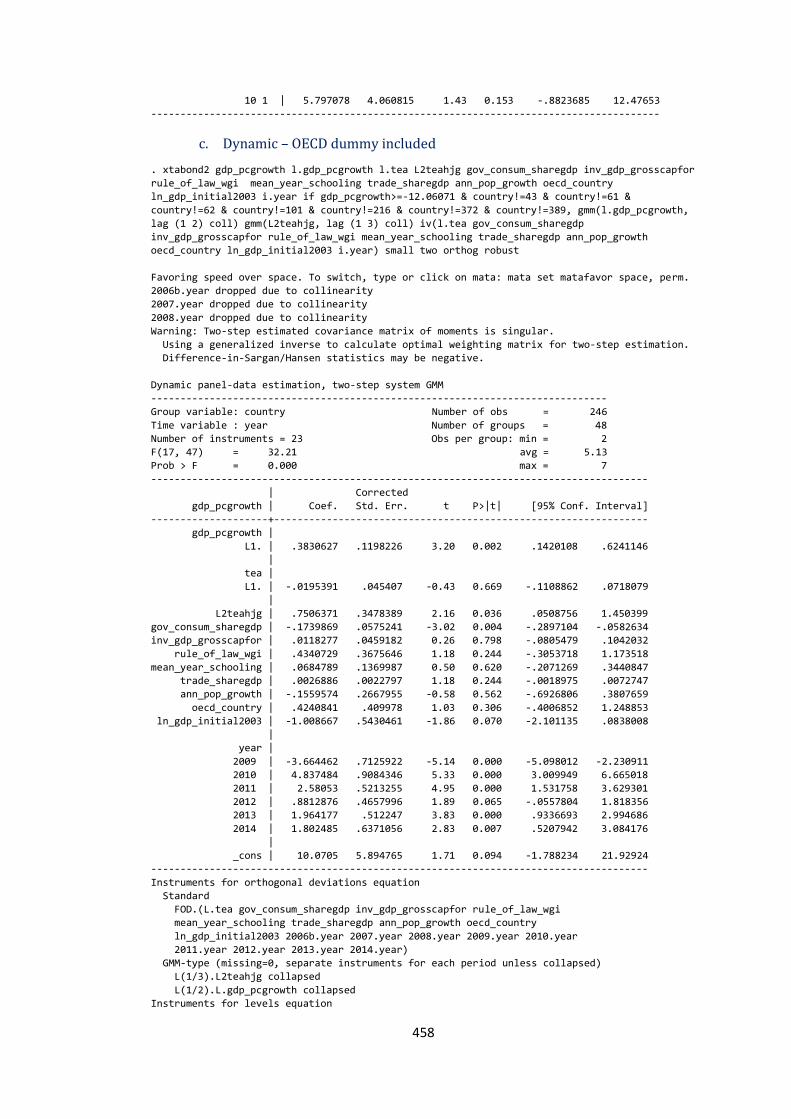
458
10 1 | 5.797078 4.060815 1.43 0.153 -.8823685 12.47653
---------------------------------------------------------------------------------------
c. Dynamic – OECD dummy included
. xtabond2 gdp_pcgrowth l.gdp_pcgrowth l.tea L2teahjg gov_consum_sharegdp inv_gdp_grosscapfor
rule_of_law_wgi mean_year_schooling trade_sharegdp ann_pop_growth oecd_country
ln_gdp_initial2003 i.year if gdp_pcgrowth>=-12.06071 & country!=43 & country!=61 &
country!=62 & country!=101 & country!=216 & country!=372 & country!=389, gmm(l.gdp_pcgrowth,
lag (1 2) coll) gmm(L2teahjg, lag (1 3) coll) iv(l.tea gov_consum_sharegdp
inv_gdp_grosscapfor rule_of_law_wgi mean_year_schooling trade_sharegdp ann_pop_growth
oecd_country ln_gdp_initial2003 i.year) small two orthog robust
Favoring speed over space. To switch, type or click on mata: mata set matafavor space, perm.
2006b.year dropped due to collinearity
2007.year dropped due to collinearity
2008.year dropped due to collinearity
Warning: Two-step estimated covariance matrix of moments is singular.
Using a generalized inverse to calculate optimal weighting matrix for two-step estimation.
Difference-in-Sargan/Hansen statistics may be negative.
Dynamic panel-data estimation, two-step system GMM
------------------------------------------------------------------------------
Group variable: country Number of obs = 246
Time variable : year Number of groups = 48
Number of instruments = 23 Obs per group: min = 2
F(17, 47) = 32.21 avg = 5.13
Prob > F = 0.000 max = 7
-------------------------------------------------------------------------------------
| Corrected
gdp_pcgrowth | Coef. Std. Err. t P>|t| [95% Conf. Interval]
--------------------+----------------------------------------------------------------
gdp_pcgrowth |
L1. | .3830627 .1198226 3.20 0.002 .1420108 .6241146
|
tea |
L1. | -.0195391 .045407 -0.43 0.669 -.1108862 .0718079
|
L2teahjg | .7506371 .3478389 2.16 0.036 .0508756 1.450399
gov_consum_sharegdp | -.1739869 .0575241 -3.02 0.004 -.2897104 -.0582634
inv_gdp_grosscapfor | .0118277 .0459182 0.26 0.798 -.0805479 .1042032
rule_of_law_wgi | .4340729 .3675646 1.18 0.244 -.3053718 1.173518
mean_year_schooling | .0684789 .1369987 0.50 0.620 -.2071269 .3440847
trade_sharegdp | .0026886 .0022797 1.18 0.244 -.0018975 .0072747
ann_pop_growth | -.1559574 .2667955 -0.58 0.562 -.6926806 .3807659
oecd_country | .4240841 .409978 1.03 0.306 -.4006852 1.248853
ln_gdp_initial2003 | -1.008667 .5430461 -1.86 0.070 -2.101135 .0838008
|
year |
2009 | -3.664462 .7125922 -5.14 0.000 -5.098012 -2.230911
2010 | 4.837484 .9084346 5.33 0.000 3.009949 6.665018
2011 | 2.58053 .5213255 4.95 0.000 1.531758 3.629301
2012 | .8812876 .4657996 1.89 0.065 -.0557804 1.818356
2013 | 1.964177 .512247 3.83 0.000 .9336693 2.994686
2014 | 1.802485 .6371056 2.83 0.007 .5207942 3.084176
|
_cons | 10.0705 5.894765 1.71 0.094 -1.788234 21.92924
-------------------------------------------------------------------------------------
Instruments for orthogonal deviations equation
Standard
FOD.(L.tea gov_consum_sharegdp inv_gdp_grosscapfor rule_of_law_wgi
mean_year_schooling trade_sharegdp ann_pop_growth oecd_country
ln_gdp_initial2003 2006b.year 2007.year 2008.year 2009.year 2010.year
2011.year 2012.year 2013.year 2014.year)
GMM-type (missing=0, separate instruments for each period unless collapsed)
L(1/3).L2teahjg collapsed
L(1/2).L.gdp_pcgrowth collapsed
Instruments for levels equation
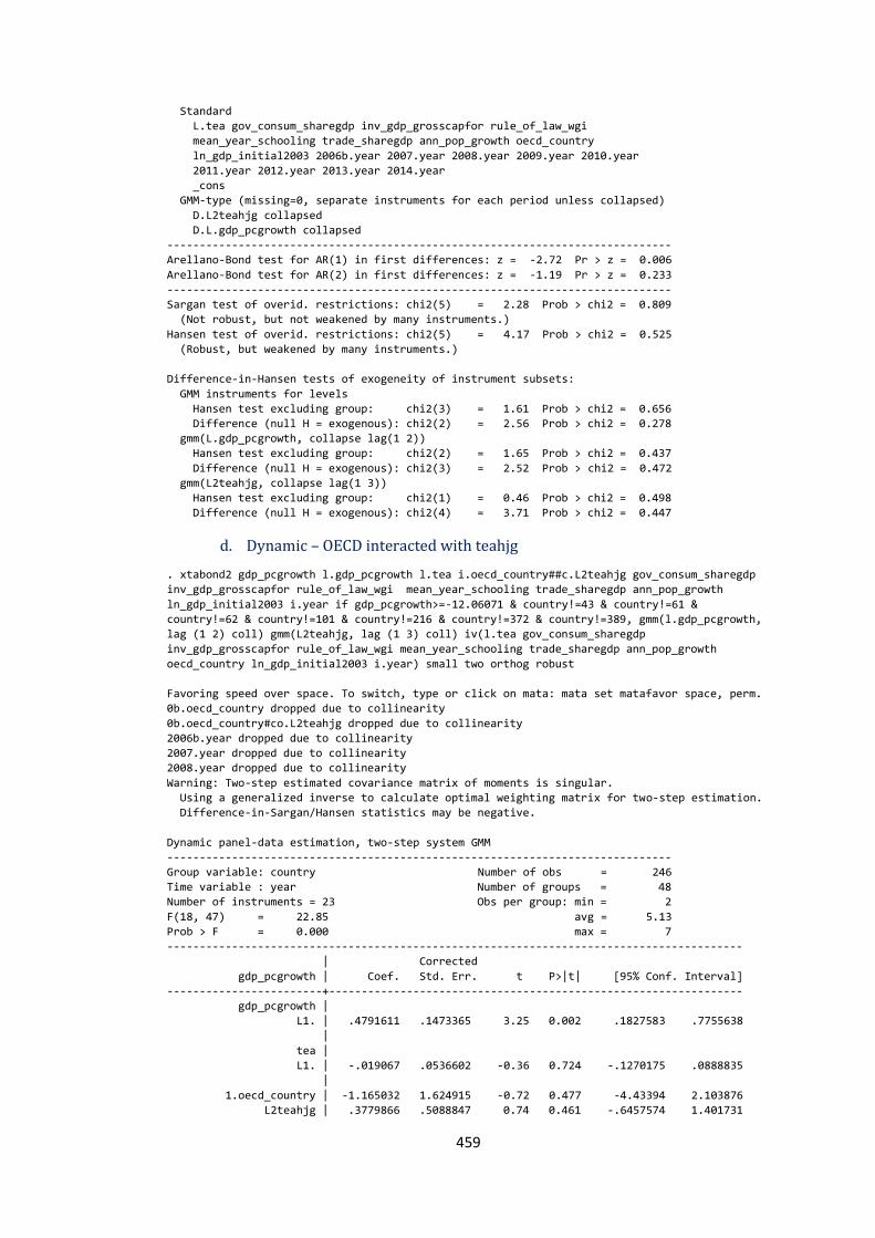
459
Standard
L.tea gov_consum_sharegdp inv_gdp_grosscapfor rule_of_law_wgi
mean_year_schooling trade_sharegdp ann_pop_growth oecd_country
ln_gdp_initial2003 2006b.year 2007.year 2008.year 2009.year 2010.year
2011.year 2012.year 2013.year 2014.year
_cons
GMM-type (missing=0, separate instruments for each period unless collapsed)
D.L2teahjg collapsed
D.L.gdp_pcgrowth collapsed
------------------------------------------------------------------------------
Arellano-Bond test for AR(1) in first differences: z = -2.72 Pr > z = 0.006
Arellano-Bond test for AR(2) in first differences: z = -1.19 Pr > z = 0.233
------------------------------------------------------------------------------
Sargan test of overid. restrictions: chi2(5) = 2.28 Prob > chi2 = 0.809
(Not robust, but not weakened by many instruments.)
Hansen test of overid. restrictions: chi2(5) = 4.17 Prob > chi2 = 0.525
(Robust, but weakened by many instruments.)
Difference-in-Hansen tests of exogeneity of instrument subsets:
GMM instruments for levels
Hansen test excluding group: chi2(3) = 1.61 Prob > chi2 = 0.656
Difference (null H = exogenous): chi2(2) = 2.56 Prob > chi2 = 0.278
gmm(L.gdp_pcgrowth, collapse lag(1 2))
Hansen test excluding group: chi2(2) = 1.65 Prob > chi2 = 0.437
Difference (null H = exogenous): chi2(3) = 2.52 Prob > chi2 = 0.472
gmm(L2teahjg, collapse lag(1 3))
Hansen test excluding group: chi2(1) = 0.46 Prob > chi2 = 0.498
Difference (null H = exogenous): chi2(4) = 3.71 Prob > chi2 = 0.447
d. Dynamic – OECD interacted with teahjg
. xtabond2 gdp_pcgrowth l.gdp_pcgrowth l.tea i.oecd_country##c.L2teahjg gov_consum_sharegdp
inv_gdp_grosscapfor rule_of_law_wgi mean_year_schooling trade_sharegdp ann_pop_growth
ln_gdp_initial2003 i.year if gdp_pcgrowth>=-12.06071 & country!=43 & country!=61 &
country!=62 & country!=101 & country!=216 & country!=372 & country!=389, gmm(l.gdp_pcgrowth,
lag (1 2) coll) gmm(L2teahjg, lag (1 3) coll) iv(l.tea gov_consum_sharegdp
inv_gdp_grosscapfor rule_of_law_wgi mean_year_schooling trade_sharegdp ann_pop_growth
oecd_country ln_gdp_initial2003 i.year) small two orthog robust
Favoring speed over space. To switch, type or click on mata: mata set matafavor space, perm.
0b.oecd_country dropped due to collinearity
0b.oecd_country#co.L2teahjg dropped due to collinearity
2006b.year dropped due to collinearity
2007.year dropped due to collinearity
2008.year dropped due to collinearity
Warning: Two-step estimated covariance matrix of moments is singular.
Using a generalized inverse to calculate optimal weighting matrix for two-step estimation.
Difference-in-Sargan/Hansen statistics may be negative.
Dynamic panel-data estimation, two-step system GMM
------------------------------------------------------------------------------
Group variable: country Number of obs = 246
Time variable : year Number of groups = 48
Number of instruments = 23 Obs per group: min = 2
F(18, 47) = 22.85 avg = 5.13
Prob > F = 0.000 max = 7
-----------------------------------------------------------------------------------------
| Corrected
gdp_pcgrowth | Coef. Std. Err. t P>|t| [95% Conf. Interval]
------------------------+----------------------------------------------------------------
gdp_pcgrowth |
L1. | .4791611 .1473365 3.25 0.002 .1827583 .7755638
|
tea |
L1. | -.019067 .0536602 -0.36 0.724 -.1270175 .0888835
|
1.oecd_country | -1.165032 1.624915 -0.72 0.477 -4.43394 2.103876
L2teahjg | .3779866 .5088847 0.74 0.461 -.6457574 1.401731

460
|
oecd_country#c.L2teahjg |
1 | 1.411076 1.40685 1.00 0.321 -1.41914 4.241292
|
gov_consum_sharegdp | -.148319 .062162 -2.39 0.021 -.2733729 -.0232652
inv_gdp_grosscapfor | .0073292 .0470507 0.16 0.877 -.0873245 .1019829
rule_of_law_wgi | .2840758 .5038719 0.56 0.576 -.7295837 1.297735
mean_year_schooling | -.0106184 .1599678 -0.07 0.947 -.332432 .3111953
trade_sharegdp | .0026638 .0029209 0.91 0.366 -.0032123 .00854
ann_pop_growth | -.4074554 .3495144 -1.17 0.250 -1.110588 .2956769
ln_gdp_initial2003 | -.3733306 .9404874 -0.40 0.693 -2.265347 1.518686
|
year |
2009 | -3.278501 .8423493 -3.89 0.000 -4.97309 -1.583913
2010 | 5.390963 1.009495 5.34 0.000 3.360122 7.421804
2011 | 2.719995 .5180175 5.25 0.000 1.677878 3.762112
2012 | 1.024697 .510514 2.01 0.050 -.0023246 2.051719
2013 | 2.185578 .5391585 4.05 0.000 1.100932 3.270225
2014 | 2.135448 .743712 2.87 0.006 .6392922 3.631603
|
_cons | 4.727348 8.91067 0.53 0.598 -13.19861 22.6533
-----------------------------------------------------------------------------------------
Instruments for orthogonal deviations equation
Standard
FOD.(L.tea gov_consum_sharegdp inv_gdp_grosscapfor rule_of_law_wgi
mean_year_schooling trade_sharegdp ann_pop_growth oecd_country
ln_gdp_initial2003 2006b.year 2007.year 2008.year 2009.year 2010.year
2011.year 2012.year 2013.year 2014.year)
GMM-type (missing=0, separate instruments for each period unless collapsed)
L(1/3).L2teahjg collapsed
L(1/2).L.gdp_pcgrowth collapsed
Instruments for levels equation
Standard
L.tea gov_consum_sharegdp inv_gdp_grosscapfor rule_of_law_wgi
mean_year_schooling trade_sharegdp ann_pop_growth oecd_country
ln_gdp_initial2003 2006b.year 2007.year 2008.year 2009.year 2010.year
2011.year 2012.year 2013.year 2014.year
_cons
GMM-type (missing=0, separate instruments for each period unless collapsed)
D.L2teahjg collapsed
D.L.gdp_pcgrowth collapsed
------------------------------------------------------------------------------
Arellano-Bond test for AR(1) in first differences: z = -3.22 Pr > z = 0.001
Arellano-Bond test for AR(2) in first differences: z = -0.92 Pr > z = 0.357
------------------------------------------------------------------------------
Sargan test of overid. restrictions: chi2(4) = 1.52 Prob > chi2 = 0.824
(Not robust, but not weakened by many instruments.)
Hansen test of overid. restrictions: chi2(4) = 2.14 Prob > chi2 = 0.710
(Robust, but weakened by many instruments.)
Difference-in-Hansen tests of exogeneity of instrument subsets:
GMM instruments for levels
Hansen test excluding group: chi2(2) = 1.05 Prob > chi2 = 0.592
Difference (null H = exogenous): chi2(2) = 1.09 Prob > chi2 = 0.580
gmm(L.gdp_pcgrowth, collapse lag(1 2))
Hansen test excluding group: chi2(1) = 0.91 Prob > chi2 = 0.341
Difference (null H = exogenous): chi2(3) = 1.23 Prob > chi2 = 0.746
gmm(L2teahjg, collapse lag(1 3))
Hansen test excluding group: chi2(0) = 0.00 Prob > chi2 = .
Difference (null H = exogenous): chi2(4) = 2.14 Prob > chi2 = 0.710
. margins oecd_country, at(L2teahjg = (0.1 (0.5) 4.6)) vsquish force level(90)
Warning: cannot perform check for estimable functions.
(note: default prediction is a function of possibly stochastic quantities other than e(b))
Predictive margins Number of obs = 246
Model VCE : Corrected
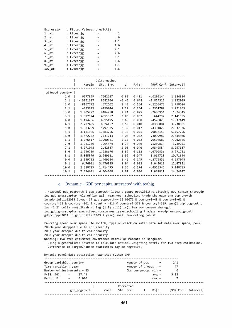
461
Expression : Fitted Values, predict()
1._at : L2teahjg = .1
2._at : L2teahjg = .6
3._at : L2teahjg = 1.1
4._at : L2teahjg = 1.6
5._at : L2teahjg = 2.1
6._at : L2teahjg = 2.6
7._at : L2teahjg = 3.1
8._at : L2teahjg = 3.6
9._at : L2teahjg = 4.1
10._at : L2teahjg = 4.6
----------------------------------------------------------------------------------
| Delta-method
| Margin Std. Err. z P>|z| [90% Conf. Interval]
-----------------+----------------------------------------------------------------
_at#oecd_country |
1 0 | .6277859 .7642627 0.82 0.411 -.6293144 1.884886
1 1 | -.3961387 .8682704 -0.46 0.648 -1.824316 1.032039
2 0 | .8167792 .572602 1.43 0.154 -.1250673 1.758626
2 1 | .4983925 .4459744 1.12 0.264 -.2351702 1.231955
3 0 | 1.005772 .4484758 2.24 0.025 .2680954 1.74345
3 1 | 1.392924 .4551357 3.06 0.002 .644292 2.141555
4 0 | 1.194766 .4515195 2.65 0.008 .4520823 1.937449
4 1 | 2.287455 .8824167 2.59 0.010 .8360084 3.738901
5 0 | 1.383759 .5797335 2.39 0.017 .4301822 2.337336
5 1 | 3.181986 1.383266 2.30 0.021 .9067153 5.457256
6 0 | 1.572752 .7731713 2.03 0.042 .3009987 2.844506
6 1 | 4.076517 1.900381 2.15 0.032 .9506687 7.202365
7 0 | 1.761746 .994474 1.77 0.076 .1259814 3.39751
7 1 | 4.971048 2.42337 2.05 0.040 .9849584 8.957137
8 0 | 1.950739 1.228676 1.59 0.112 -.0702536 3.971731
8 1 | 5.865579 2.949111 1.99 0.047 1.014723 10.71644
9 0 | 2.139732 1.469624 1.46 0.145 -.2775836 4.557048
9 1 | 6.76011 3.476355 1.94 0.052 1.042015 12.47821
10 0 | 2.328725 1.714475 1.36 0.174 -.4913346 5.148785
10 1 | 7.654641 4.004508 1.91 0.056 1.067811 14.24147
----------------------------------------------------------------------------------
e. Dynamic – GDP per capita interacted with teahjg
. xtabond2 gdp_pcgrowth l.gdp_pcgrowth l.tea c.gdppc_pppc2011##c.L2teahjg gov_consum_sharegdp
inv_gdp_grosscapfor rule_of_law_wgi mean_year_schooling trade_sharegdp ann_pop_growth
ln_gdp_initial2003 i.year if gdp_pcgrowth>=-12.06071 & country!=43 & country!=61 &
country!=62 & country!=101 & country!=216 & country!=372 & country!=389, gmm(l.gdp_pcgrowth,
lag (1 2) coll) gmm(L2teahjg, lag (1 3) coll) iv(l.tea gov_consum_sharegdp
inv_gdp_grosscapfor executivecontrain mean_year_schooling trade_sharegdp ann_pop_growth
gdppc_pppc2011 ln_gdp_initial2003 i.year) small two orthog robust
Favoring speed over space. To switch, type or click on mata: mata set matafavor space, perm.
2006b.year dropped due to collinearity
2007.year dropped due to collinearity
2008.year dropped due to collinearity
Warning: Two-step estimated covariance matrix of moments is singular.
Using a generalized inverse to calculate optimal weighting matrix for two-step estimation.
Difference-in-Sargan/Hansen statistics may be negative.
Dynamic panel-data estimation, two-step system GMM
------------------------------------------------------------------------------
Group variable: country Number of obs = 241
Time variable : year Number of groups = 47
Number of instruments = 23 Obs per group: min = 0
F(18, 46) = 27.45 avg = 5.13
Prob > F = 0.000 max = 7
---------------------------------------------------------------------------------------------
| Corrected
gdp_pcgrowth | Coef. Std. Err. t P>|t| [95% Conf. Interval]
----------------------------+----------------------------------------------------------------
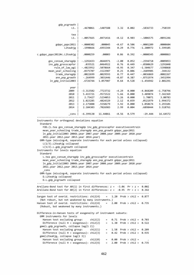
462
gdp_pcgrowth |
L1. | .4670061 .1407588 3.32 0.002 .1836733 .750339
|
tea |
L1. | -.0057665 .0471416 -0.12 0.903 -.1006575 .0891246
|
gdppc_pppc2011 | -.0000302 .000045 -0.67 0.506 -.0001209 .0000604
L2teahjg | .1990666 .6955344 0.29 0.776 -1.200972 1.599105
|
c.gdppc_pppc2011#c.L2teahjg | .0000259 .00003 0.86 0.392 -.0000345 .0000863
|
gov_consum_sharegdp | -.1292433 .0646971 -2.00 0.052 -.2594718 .0009853
inv_gdp_grosscapfor | .035521 .0464922 0.76 0.449 -.0580629 .1291048
rule_of_law_wgi | -.4823952 .5078664 -0.95 0.347 -1.504677 .5398868
mean_year_schooling | .0375707 .1522987 0.25 0.806 -.2689905 .344132
trade_sharegdp | .0022699 .0029593 0.77 0.447 -.0036869 .0082267
ann_pop_growth | -.264999 .3031446 -0.87 0.387 -.8751974 .3451994
ln_gdp_initial2003 | .6726744 1.057987 0.64 0.528 -1.456942 2.802291
|
year |
2009 | -3.313502 .7723732 -4.29 0.000 -4.868209 -1.758796
2010 | 5.415721 .9571522 5.66 0.000 3.489074 7.342369
2011 | 2.75427 .5234053 5.26 0.000 1.70071 3.80783
2012 | 1.023285 .4824329 2.12 0.039 .0521979 1.994372
2013 | 2.175888 .5550279 3.92 0.000 1.058674 3.293101
2014 | 2.104303 .7026983 2.99 0.004 .6898444 3.518761
|
_cons | -6.399138 11.44861 -0.56 0.579 -29.444 16.64572
---------------------------------------------------------------------------------------------
Instruments for orthogonal deviations equation
Standard
FOD.(L.tea gov_consum_sharegdp inv_gdp_grosscapfor executivecontrain
mean_year_schooling trade_sharegdp ann_pop_growth gdppc_pppc2011
ln_gdp_initial2003 2006b.year 2007.year 2008.year 2009.year 2010.year
2011.year 2012.year 2013.year 2014.year)
GMM-type (missing=0, separate instruments for each period unless collapsed)
L(1/3).L2teahjg collapsed
L(1/2).L.gdp_pcgrowth collapsed
Instruments for levels equation
Standard
L.tea gov_consum_sharegdp inv_gdp_grosscapfor executivecontrain
mean_year_schooling trade_sharegdp ann_pop_growth gdppc_pppc2011
ln_gdp_initial2003 2006b.year 2007.year 2008.year 2009.year 2010.year
2011.year 2012.year 2013.year 2014.year
_cons
GMM-type (missing=0, separate instruments for each period unless collapsed)
D.L2teahjg collapsed
D.L.gdp_pcgrowth collapsed
------------------------------------------------------------------------------
Arellano-Bond test for AR(1) in first differences: z = -3.06 Pr > z = 0.002
Arellano-Bond test for AR(2) in first differences: z = -0.95 Pr > z = 0.342
------------------------------------------------------------------------------
Sargan test of overid. restrictions: chi2(4) = 1.20 Prob > chi2 = 0.877
(Not robust, but not weakened by many instruments.)
Hansen test of overid. restrictions: chi2(4) = 2.00 Prob > chi2 = 0.735
(Robust, but weakened by many instruments.)
Difference-in-Hansen tests of exogeneity of instrument subsets:
GMM instruments for levels
Hansen test excluding group: chi2(2) = 0.71 Prob > chi2 = 0.703
Difference (null H = exogenous): chi2(2) = 1.30 Prob > chi2 = 0.522
gmm(L.gdp_pcgrowth, collapse lag(1 2))
Hansen test excluding group: chi2(1) = 1.58 Prob > chi2 = 0.209
Difference (null H = exogenous): chi2(3) = 0.42 Prob > chi2 = 0.935
gmm(L2teahjg, collapse lag(1 3))
Hansen test excluding group: chi2(0) = 0.00 Prob > chi2 = .
Difference (null H = exogenous): chi2(4) = 2.00 Prob > chi2 = 0.735
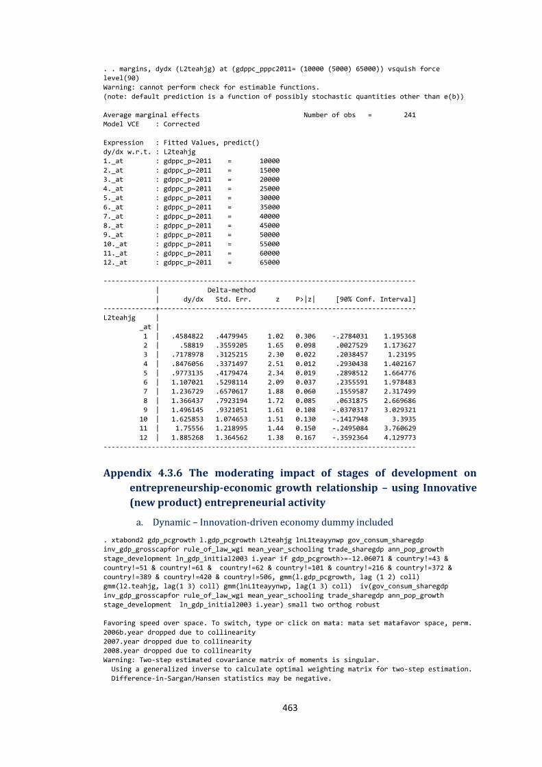
463
. . margins, dydx (L2teahjg) at (gdppc_pppc2011= (10000 (5000) 65000)) vsquish force
level(90)
Warning: cannot perform check for estimable functions.
(note: default prediction is a function of possibly stochastic quantities other than e(b))
Average marginal effects Number of obs = 241
Model VCE : Corrected
Expression : Fitted Values, predict()
dy/dx w.r.t. : L2teahjg
1._at : gdppc_p~2011 = 10000
2._at : gdppc_p~2011 = 15000
3._at : gdppc_p~2011 = 20000
4._at : gdppc_p~2011 = 25000
5._at : gdppc_p~2011 = 30000
6._at : gdppc_p~2011 = 35000
7._at : gdppc_p~2011 = 40000
8._at : gdppc_p~2011 = 45000
9._at : gdppc_p~2011 = 50000
10._at : gdppc_p~2011 = 55000
11._at : gdppc_p~2011 = 60000
12._at : gdppc_p~2011 = 65000
------------------------------------------------------------------------------
| Delta-method
| dy/dx Std. Err. z P>|z| [90% Conf. Interval]
-------------+----------------------------------------------------------------
L2teahjg |
_at |
1 | .4584822 .4479945 1.02 0.306 -.2784031 1.195368
2 | .58819 .3559205 1.65 0.098 .0027529 1.173627
3 | .7178978 .3125215 2.30 0.022 .2038457 1.23195
4 | .8476056 .3371497 2.51 0.012 .2930438 1.402167
5 | .9773135 .4179474 2.34 0.019 .2898512 1.664776
6 | 1.107021 .5298114 2.09 0.037 .2355591 1.978483
7 | 1.236729 .6570617 1.88 0.060 .1559587 2.317499
8 | 1.366437 .7923194 1.72 0.085 .0631875 2.669686
9 | 1.496145 .9321051 1.61 0.108 -.0370317 3.029321
10 | 1.625853 1.074653 1.51 0.130 -.1417948 3.3935
11 | 1.75556 1.218995 1.44 0.150 -.2495084 3.760629
12 | 1.885268 1.364562 1.38 0.167 -.3592364 4.129773
------------------------------------------------------------------------------
Appendix 4.3.6 The moderating impact of stages of development on
entrepreneurship-economic growth relationship – using Innovative
(new product) entrepreneurial activity
a. Dynamic – Innovation-driven economy dummy included
. xtabond2 gdp_pcgrowth l.gdp_pcgrowth L2teahjg lnL1teayynwp gov_consum_sharegdp
inv_gdp_grosscapfor rule_of_law_wgi mean_year_schooling trade_sharegdp ann_pop_growth
stage_development ln_gdp_initial2003 i.year if gdp_pcgrowth>=-12.06071 & country!=43 &
country!=51 & country!=61 & country!=62 & country!=101 & country!=216 & country!=372 &
country!=389 & country!=420 & country!=506, gmm(l.gdp_pcgrowth, lag (1 2) coll)
gmm(l2.teahjg, lag(1 3) coll) gmm(lnL1teayynwp, lag(1 3) coll) iv(gov_consum_sharegdp
inv_gdp_grosscapfor rule_of_law_wgi mean_year_schooling trade_sharegdp ann_pop_growth
stage_development ln_gdp_initial2003 i.year) small two orthog robust
Favoring speed over space. To switch, type or click on mata: mata set matafavor space, perm.
2006b.year dropped due to collinearity
2007.year dropped due to collinearity
2008.year dropped due to collinearity
Warning: Two-step estimated covariance matrix of moments is singular.
Using a generalized inverse to calculate optimal weighting matrix for two-step estimation.
Difference-in-Sargan/Hansen statistics may be negative.
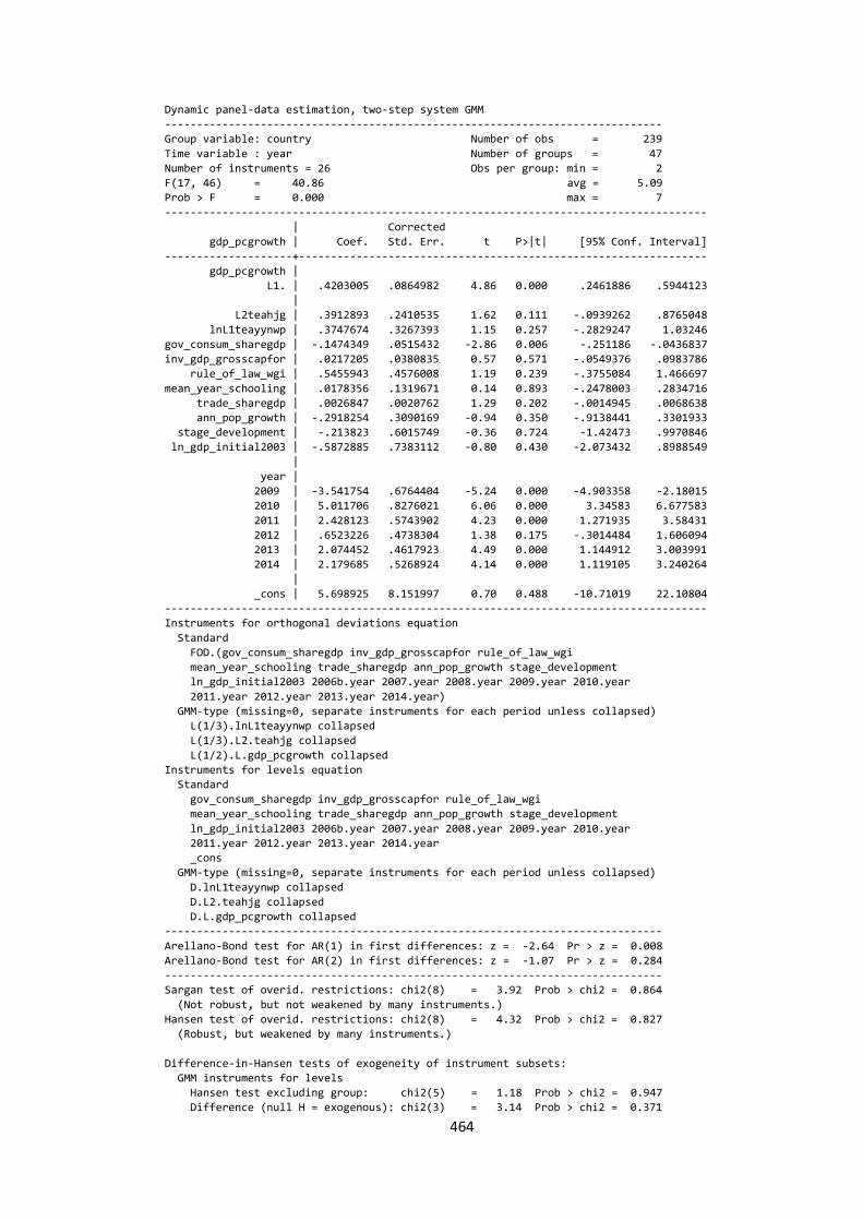
464
Dynamic panel-data estimation, two-step system GMM
------------------------------------------------------------------------------
Group variable: country Number of obs = 239
Time variable : year Number of groups = 47
Number of instruments = 26 Obs per group: min = 2
F(17, 46) = 40.86 avg = 5.09
Prob > F = 0.000 max = 7
-------------------------------------------------------------------------------------
| Corrected
gdp_pcgrowth | Coef. Std. Err. t P>|t| [95% Conf. Interval]
--------------------+----------------------------------------------------------------
gdp_pcgrowth |
L1. | .4203005 .0864982 4.86 0.000 .2461886 .5944123
|
L2teahjg | .3912893 .2410535 1.62 0.111 -.0939262 .8765048
lnL1teayynwp | .3747674 .3267393 1.15 0.257 -.2829247 1.03246
gov_consum_sharegdp | -.1474349 .0515432 -2.86 0.006 -.251186 -.0436837
inv_gdp_grosscapfor | .0217205 .0380835 0.57 0.571 -.0549376 .0983786
rule_of_law_wgi | .5455943 .4576008 1.19 0.239 -.3755084 1.466697
mean_year_schooling | .0178356 .1319671 0.14 0.893 -.2478003 .2834716
trade_sharegdp | .0026847 .0020762 1.29 0.202 -.0014945 .0068638
ann_pop_growth | -.2918254 .3090169 -0.94 0.350 -.9138441 .3301933
stage_development | -.213823 .6015749 -0.36 0.724 -1.42473 .9970846
ln_gdp_initial2003 | -.5872885 .7383112 -0.80 0.430 -2.073432 .8988549
|
year |
2009 | -3.541754 .6764404 -5.24 0.000 -4.903358 -2.18015
2010 | 5.011706 .8276021 6.06 0.000 3.34583 6.677583
2011 | 2.428123 .5743902 4.23 0.000 1.271935 3.58431
2012 | .6523226 .4738304 1.38 0.175 -.3014484 1.606094
2013 | 2.074452 .4617923 4.49 0.000 1.144912 3.003991
2014 | 2.179685 .5268924 4.14 0.000 1.119105 3.240264
|
_cons | 5.698925 8.151997 0.70 0.488 -10.71019 22.10804
-------------------------------------------------------------------------------------
Instruments for orthogonal deviations equation
Standard
FOD.(gov_consum_sharegdp inv_gdp_grosscapfor rule_of_law_wgi
mean_year_schooling trade_sharegdp ann_pop_growth stage_development
ln_gdp_initial2003 2006b.year 2007.year 2008.year 2009.year 2010.year
2011.year 2012.year 2013.year 2014.year)
GMM-type (missing=0, separate instruments for each period unless collapsed)
L(1/3).lnL1teayynwp collapsed
L(1/3).L2.teahjg collapsed
L(1/2).L.gdp_pcgrowth collapsed
Instruments for levels equation
Standard
gov_consum_sharegdp inv_gdp_grosscapfor rule_of_law_wgi
mean_year_schooling trade_sharegdp ann_pop_growth stage_development
ln_gdp_initial2003 2006b.year 2007.year 2008.year 2009.year 2010.year
2011.year 2012.year 2013.year 2014.year
_cons
GMM-type (missing=0, separate instruments for each period unless collapsed)
D.lnL1teayynwp collapsed
D.L2.teahjg collapsed
D.L.gdp_pcgrowth collapsed
------------------------------------------------------------------------------
Arellano-Bond test for AR(1) in first differences: z = -2.64 Pr > z = 0.008
Arellano-Bond test for AR(2) in first differences: z = -1.07 Pr > z = 0.284
------------------------------------------------------------------------------
Sargan test of overid. restrictions: chi2(8) = 3.92 Prob > chi2 = 0.864
(Not robust, but not weakened by many instruments.)
Hansen test of overid. restrictions: chi2(8) = 4.32 Prob > chi2 = 0.827
(Robust, but weakened by many instruments.)
Difference-in-Hansen tests of exogeneity of instrument subsets:
GMM instruments for levels
Hansen test excluding group: chi2(5) = 1.18 Prob > chi2 = 0.947
Difference (null H = exogenous): chi2(3) = 3.14 Prob > chi2 = 0.371
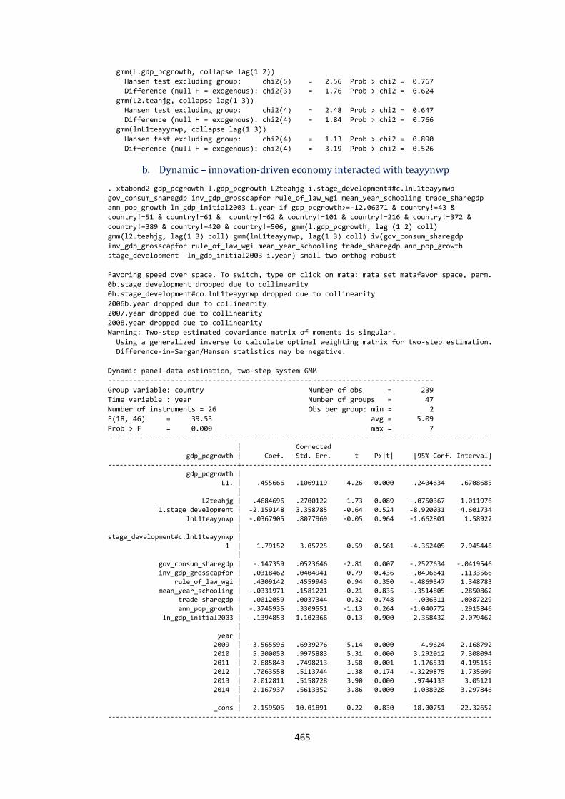
465
gmm(L.gdp_pcgrowth, collapse lag(1 2))
Hansen test excluding group: chi2(5) = 2.56 Prob > chi2 = 0.767
Difference (null H = exogenous): chi2(3) = 1.76 Prob > chi2 = 0.624
gmm(L2.teahjg, collapse lag(1 3))
Hansen test excluding group: chi2(4) = 2.48 Prob > chi2 = 0.647
Difference (null H = exogenous): chi2(4) = 1.84 Prob > chi2 = 0.766
gmm(lnL1teayynwp, collapse lag(1 3))
Hansen test excluding group: chi2(4) = 1.13 Prob > chi2 = 0.890
Difference (null H = exogenous): chi2(4) = 3.19 Prob > chi2 = 0.526
b. Dynamic – innovation-driven economy interacted with teayynwp
. xtabond2 gdp_pcgrowth l.gdp_pcgrowth L2teahjg i.stage_development##c.lnL1teayynwp
gov_consum_sharegdp inv_gdp_grosscapfor rule_of_law_wgi mean_year_schooling trade_sharegdp
ann_pop_growth ln_gdp_initial2003 i.year if gdp_pcgrowth>=-12.06071 & country!=43 &
country!=51 & country!=61 & country!=62 & country!=101 & country!=216 & country!=372 &
country!=389 & country!=420 & country!=506, gmm(l.gdp_pcgrowth, lag (1 2) coll)
gmm(l2.teahjg, lag(1 3) coll) gmm(lnL1teayynwp, lag(1 3) coll) iv(gov_consum_sharegdp
inv_gdp_grosscapfor rule_of_law_wgi mean_year_schooling trade_sharegdp ann_pop_growth
stage_development ln_gdp_initial2003 i.year) small two orthog robust
Favoring speed over space. To switch, type or click on mata: mata set matafavor space, perm.
0b.stage_development dropped due to collinearity
0b.stage_development#co.lnL1teayynwp dropped due to collinearity
2006b.year dropped due to collinearity
2007.year dropped due to collinearity
2008.year dropped due to collinearity
Warning: Two-step estimated covariance matrix of moments is singular.
Using a generalized inverse to calculate optimal weighting matrix for two-step estimation.
Difference-in-Sargan/Hansen statistics may be negative.
Dynamic panel-data estimation, two-step system GMM
------------------------------------------------------------------------------
Group variable: country Number of obs = 239
Time variable : year Number of groups = 47
Number of instruments = 26 Obs per group: min = 2
F(18, 46) = 39.53 avg = 5.09
Prob > F = 0.000 max = 7 --------------------------------------------------------------------------------------------------
| Corrected
gdp_pcgrowth | Coef. Std. Err. t P>|t| [95% Conf. Interval]
---------------------------------+----------------------------------------------------------------
gdp_pcgrowth |
L1. | .455666 .1069119 4.26 0.000 .2404634 .6708685
|
L2teahjg | .4684696 .2700122 1.73 0.089 -.0750367 1.011976
1.stage_development | -2.159148 3.358785 -0.64 0.524 -8.920031 4.601734
lnL1teayynwp | -.0367905 .8077969 -0.05 0.964 -1.662801 1.58922
|
stage_development#c.lnL1teayynwp |
1 | 1.79152 3.05725 0.59 0.561 -4.362405 7.945446
|
gov_consum_sharegdp | -.147359 .0523646 -2.81 0.007 -.2527634 -.0419546
inv_gdp_grosscapfor | .0318462 .0404941 0.79 0.436 -.0496641 .1133566 rule_of_law_wgi | .4309142 .4559943 0.94 0.350 -.4869547 1.348783
mean_year_schooling | -.0331971 .1581221 -0.21 0.835 -.3514805 .2850862
trade_sharegdp | .0012059 .0037344 0.32 0.748 -.006311 .0087229
ann_pop_growth | -.3745935 .3309551 -1.13 0.264 -1.040772 .2915846
ln_gdp_initial2003 | -.1394853 1.102366 -0.13 0.900 -2.358432 2.079462
|
year |
2009 | -3.565596 .6939276 -5.14 0.000 -4.9624 -2.168792
2010 | 5.300053 .9975883 5.31 0.000 3.292012 7.308094
2011 | 2.685843 .7498213 3.58 0.001 1.176531 4.195155
2012 | .7063558 .5113744 1.38 0.174 -.3229875 1.735699
2013 | 2.012811 .5158728 3.90 0.000 .9744133 3.05121
2014 | 2.167937 .5613352 3.86 0.000 1.038028 3.297846
|
_cons | 2.159505 10.01891 0.22 0.830 -18.00751 22.32652
--------------------------------------------------------------------------------------------------
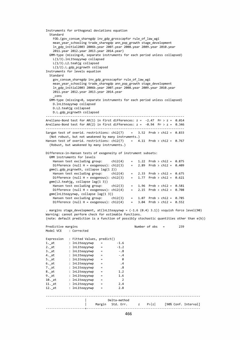
466
Instruments for orthogonal deviations equation
Standard
FOD.(gov_consum_sharegdp inv_gdp_grosscapfor rule_of_law_wgi
mean_year_schooling trade_sharegdp ann_pop_growth stage_development
ln_gdp_initial2003 2006b.year 2007.year 2008.year 2009.year 2010.year
2011.year 2012.year 2013.year 2014.year)
GMM-type (missing=0, separate instruments for each period unless collapsed)
L(1/3).lnL1teayynwp collapsed
L(1/3).L2.teahjg collapsed
L(1/2).L.gdp_pcgrowth collapsed
Instruments for levels equation
Standard
gov_consum_sharegdp inv_gdp_grosscapfor rule_of_law_wgi
mean_year_schooling trade_sharegdp ann_pop_growth stage_development
ln_gdp_initial2003 2006b.year 2007.year 2008.year 2009.year 2010.year
2011.year 2012.year 2013.year 2014.year
_cons
GMM-type (missing=0, separate instruments for each period unless collapsed)
D.lnL1teayynwp collapsed
D.L2.teahjg collapsed
D.L.gdp_pcgrowth collapsed
------------------------------------------------------------------------------
Arellano-Bond test for AR(1) in first differences: z = -2.47 Pr > z = 0.014
Arellano-Bond test for AR(2) in first differences: z = -0.94 Pr > z = 0.346
------------------------------------------------------------------------------
Sargan test of overid. restrictions: chi2(7) = 3.52 Prob > chi2 = 0.833
(Not robust, but not weakened by many instruments.)
Hansen test of overid. restrictions: chi2(7) = 4.11 Prob > chi2 = 0.767
(Robust, but weakened by many instruments.)
Difference-in-Hansen tests of exogeneity of instrument subsets:
GMM instruments for levels
Hansen test excluding group: chi2(4) = 1.22 Prob > chi2 = 0.875
Difference (null H = exogenous): chi2(3) = 2.89 Prob > chi2 = 0.409
gmm(L.gdp_pcgrowth, collapse lag(1 2))
Hansen test excluding group: chi2(4) = 2.33 Prob > chi2 = 0.675
Difference (null H = exogenous): chi2(3) = 1.77 Prob > chi2 = 0.621
gmm(L2.teahjg, collapse lag(1 3))
Hansen test excluding group: chi2(3) = 1.96 Prob > chi2 = 0.581
Difference (null H = exogenous): chi2(4) = 2.15 Prob > chi2 = 0.708
gmm(lnL1teayynwp, collapse lag(1 3))
Hansen test excluding group: chi2(3) = 1.07 Prob > chi2 = 0.785
Difference (null H = exogenous): chi2(4) = 3.04 Prob > chi2 = 0.552
. margins stage_development, at(lnL1teayynwp = (-1.6 (0.4) 3.1)) vsquish force level(90)
Warning: cannot perform check for estimable functions.
(note: default prediction is a function of possibly stochastic quantities other than e(b))
Predictive margins Number of obs = 239
Model VCE : Corrected
Expression : Fitted Values, predict()
1._at : lnL1teayynwp = -1.6
2._at : lnL1teayynwp = -1.2
3._at : lnL1teayynwp = -.8
4._at : lnL1teayynwp = -.4
5._at : lnL1teayynwp = 0
6._at : lnL1teayynwp = .4
7._at : lnL1teayynwp = .8
8._at : lnL1teayynwp = 1.2
9._at : lnL1teayynwp = 1.6
10._at : lnL1teayynwp = 2
11._at : lnL1teayynwp = 2.4
12._at : lnL1teayynwp = 2.8
---------------------------------------------------------------------------------------
| Delta-method
| Margin Std. Err. z P>|z| [90% Conf. Interval]
----------------------+----------------------------------------------------------------
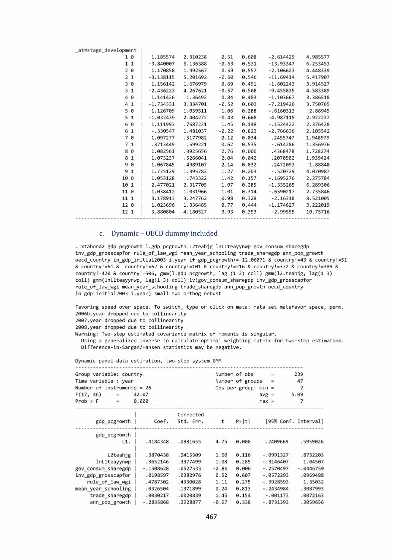
467
_at#stage_development |
1 0 | 1.185574 2.310238 0.51 0.608 -2.614429 4.985577
1 1 | -3.840007 6.136388 -0.63 0.531 -13.93347 6.253453
2 0 | 1.170858 1.992567 0.59 0.557 -2.106623 4.448339
2 1 | -3.138115 5.201692 -0.60 0.546 -11.69414 5.417907
3 0 | 1.156142 1.676979 0.69 0.491 -1.602243 3.914527
3 1 | -2.436223 4.267621 -0.57 0.568 -9.455835 4.583389
4 0 | 1.141426 1.36492 0.84 0.403 -1.103667 3.386518
4 1 | -1.734331 3.334701 -0.52 0.603 -7.219426 3.750765
5 0 | 1.126709 1.059511 1.06 0.288 -.6160313 2.86945
5 1 | -1.032439 2.404272 -0.43 0.668 -4.987115 2.922237
6 0 | 1.111993 .7687221 1.45 0.148 -.1524422 2.376428
6 1 | -.330547 1.481037 -0.22 0.823 -2.766636 2.105542
7 0 | 1.097277 .5177982 2.12 0.034 .2455747 1.948979
7 1 | .3713449 .599221 0.62 0.535 -.614286 1.356976
8 0 | 1.082561 .3925656 2.76 0.006 .4368478 1.728274
8 1 | 1.073237 .5266041 2.04 0.042 .2070502 1.939424
9 0 | 1.067845 .4989107 2.14 0.032 .2472093 1.88848
9 1 | 1.775129 1.395782 1.27 0.203 -.520729 4.070987
10 0 | 1.053128 .743322 1.42 0.157 -.1695276 2.275784
10 1 | 2.477021 2.317705 1.07 0.285 -1.335265 6.289306
11 0 | 1.038412 1.031966 1.01 0.314 -.6590217 2.735846
11 1 | 3.178913 3.247762 0.98 0.328 -2.16318 8.521005
12 0 | 1.023696 1.336485 0.77 0.444 -1.174627 3.222019
12 1 | 3.880804 4.180527 0.93 0.353 -2.99555 10.75716
---------------------------------------------------------------------------------------
c. Dynamic – OECD dummy included
. xtabond2 gdp_pcgrowth l.gdp_pcgrowth L2teahjg lnL1teayynwp gov_consum_sharegdp
inv_gdp_grosscapfor rule_of_law_wgi mean_year_schooling trade_sharegdp ann_pop_growth
oecd_country ln_gdp_initial2003 i.year if gdp_pcgrowth>=-12.06071 & country!=43 & country!=51
& country!=61 & country!=62 & country!=101 & country!=216 & country!=372 & country!=389 &
country!=420 & country!=506, gmm(l.gdp_pcgrowth, lag (1 2) coll) gmm(l2.teahjg, lag(1 3)
coll) gmm(lnL1teayynwp, lag(1 3) coll) iv(gov_consum_sharegdp inv_gdp_grosscapfor
rule_of_law_wgi mean_year_schooling trade_sharegdp ann_pop_growth oecd_country
ln_gdp_initial2003 i.year) small two orthog robust
Favoring speed over space. To switch, type or click on mata: mata set matafavor space, perm.
2006b.year dropped due to collinearity
2007.year dropped due to collinearity
2008.year dropped due to collinearity
Warning: Two-step estimated covariance matrix of moments is singular.
Using a generalized inverse to calculate optimal weighting matrix for two-step estimation.
Difference-in-Sargan/Hansen statistics may be negative.
Dynamic panel-data estimation, two-step system GMM
------------------------------------------------------------------------------
Group variable: country Number of obs = 239
Time variable : year Number of groups = 47
Number of instruments = 26 Obs per group: min = 2
F(17, 46) = 42.07 avg = 5.09
Prob > F = 0.000 max = 7
-------------------------------------------------------------------------------------
| Corrected
gdp_pcgrowth | Coef. Std. Err. t P>|t| [95% Conf. Interval]
--------------------+----------------------------------------------------------------
gdp_pcgrowth |
L1. | .4184348 .0881655 4.75 0.000 .2409669 .5959026
|
L2teahjg | .3870438 .2415309 1.60 0.116 -.0991327 .8732203
lnL1teayynwp | .3652146 .3377499 1.08 0.285 -.3146407 1.04507
gov_consum_sharegdp | -.1508628 .0527533 -2.86 0.006 -.2570497 -.0446759
inv_gdp_grosscapfor | .0198597 .0382976 0.52 0.607 -.0572293 .0969488
rule_of_law_wgi | .4787302 .4330028 1.11 0.275 -.3928593 1.35032
mean_year_schooling | .0326504 .1371899 0.24 0.813 -.2434984 .3087993
trade_sharegdp | .0030217 .0020839 1.45 0.154 -.001173 .0072163
ann_pop_growth | -.2835868 .2928877 -0.97 0.338 -.8731393 .3059656

468
oecd_country | .247831 .3633466 0.68 0.499 -.4835478 .9792098
ln_gdp_initial2003 | -.8458352 .6915737 -1.22 0.228 -2.237901 .5462304
|
year |
2009 | -3.541671 .6737835 -5.26 0.000 -4.897927 -2.185415
2010 | 4.996948 .8250322 6.06 0.000 3.336245 6.657652
2011 | 2.413503 .5736169 4.21 0.000 1.258872 3.568134
2012 | .6398675 .4758247 1.34 0.185 -.3179179 1.597653
2013 | 2.060252 .461714 4.46 0.000 1.13087 2.989634
2014 | 2.165594 .5264225 4.11 0.000 1.10596 3.225227
|
_cons | 8.001019 7.750235 1.03 0.307 -7.599396 23.60143
-------------------------------------------------------------------------------------
Instruments for orthogonal deviations equation
Standard
FOD.(gov_consum_sharegdp inv_gdp_grosscapfor rule_of_law_wgi
mean_year_schooling trade_sharegdp ann_pop_growth oecd_country
ln_gdp_initial2003 2006b.year 2007.year 2008.year 2009.year 2010.year
2011.year 2012.year 2013.year 2014.year)
GMM-type (missing=0, separate instruments for each period unless collapsed)
L(1/3).lnL1teayynwp collapsed
L(1/3).L2.teahjg collapsed
L(1/2).L.gdp_pcgrowth collapsed
Instruments for levels equation
Standard
gov_consum_sharegdp inv_gdp_grosscapfor rule_of_law_wgi
mean_year_schooling trade_sharegdp ann_pop_growth oecd_country
ln_gdp_initial2003 2006b.year 2007.year 2008.year 2009.year 2010.year
2011.year 2012.year 2013.year 2014.year
_cons
GMM-type (missing=0, separate instruments for each period unless collapsed)
D.lnL1teayynwp collapsed
D.L2.teahjg collapsed
D.L.gdp_pcgrowth collapsed
------------------------------------------------------------------------------
Arellano-Bond test for AR(1) in first differences: z = -2.64 Pr > z = 0.008
Arellano-Bond test for AR(2) in first differences: z = -1.07 Pr > z = 0.283
------------------------------------------------------------------------------
Sargan test of overid. restrictions: chi2(8) = 3.92 Prob > chi2 = 0.865
(Not robust, but not weakened by many instruments.)
Hansen test of overid. restrictions: chi2(8) = 4.36 Prob > chi2 = 0.823
(Robust, but weakened by many instruments.)
Difference-in-Hansen tests of exogeneity of instrument subsets:
GMM instruments for levels
Hansen test excluding group: chi2(5) = 1.19 Prob > chi2 = 0.946
Difference (null H = exogenous): chi2(3) = 3.17 Prob > chi2 = 0.366
gmm(L.gdp_pcgrowth, collapse lag(1 2))
Hansen test excluding group: chi2(5) = 2.48 Prob > chi2 = 0.779
Difference (null H = exogenous): chi2(3) = 1.88 Prob > chi2 = 0.598
gmm(L2.teahjg, collapse lag(1 3))
Hansen test excluding group: chi2(4) = 2.45 Prob > chi2 = 0.653
Difference (null H = exogenous): chi2(4) = 1.91 Prob > chi2 = 0.753
gmm(lnL1teayynwp, collapse lag(1 3))
Hansen test excluding group: chi2(4) = 1.29 Prob > chi2 = 0.863
Difference (null H = exogenous): chi2(4) = 3.07 Prob > chi2 = 0.546
d. Dynamic – OECD interacted with teayynwp
. xtabond2 gdp_pcgrowth l.gdp_pcgrowth L2teahjg i.oecd_country##c.lnL1teayynwp
gov_consum_sharegdp inv_gdp_grosscapfor rule_of_law_wgi mean_year_schooling trade_sharegdp
ann_pop_growth ln_gdp_initial2003 i.year if gdp_pcgrowth>=-12.06071 & country!=43 &
country!=51 & country!=61 & country!=62 & country!=101 & country!=216 & country!=372 &
country!=389 & country!=420 & country!=506, gmm(l.gdp_pcgrowth, lag (1 2) coll)
gmm(l2.teahjg, lag(1 3) coll) gmm(lnL1teayynwp, lag(1 3) coll) iv(gov_consum_sharegdp
inv_gdp_grosscapfor rule_of_law_wgi mean_year_schooling trade_sharegdp ann_pop_growth
oecd_country ln_gdp_initial2003 i.year) small two orthog robust
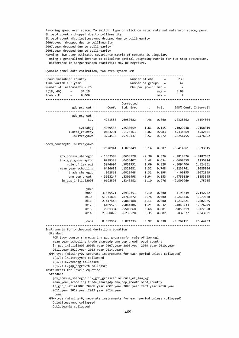
469
Favoring speed over space. To switch, type or click on mata: mata set matafavor space, perm.
0b.oecd_country dropped due to collinearity
0b.oecd_country#co.lnL1teayynwp dropped due to collinearity
2006b.year dropped due to collinearity
2007.year dropped due to collinearity
2008.year dropped due to collinearity
Warning: Two-step estimated covariance matrix of moments is singular.
Using a generalized inverse to calculate optimal weighting matrix for two-step estimation.
Difference-in-Sargan/Hansen statistics may be negative.
Dynamic panel-data estimation, two-step system GMM
------------------------------------------------------------------------------
Group variable: country Number of obs = 239
Time variable : year Number of groups = 47
Number of instruments = 26 Obs per group: min = 2
F(18, 46) = 34.19 avg = 5.09
Prob > F = 0.000 max = 7
---------------------------------------------------------------------------------------------
| Corrected
gdp_pcgrowth | Coef. Std. Err. t P>|t| [95% Conf. Interval]
----------------------------+----------------------------------------------------------------
gdp_pcgrowth |
L1. | .4241583 .0950482 4.46 0.000 .2328362 .6154804
|
L2teahjg | .4069536 .2533059 1.61 0.115 -.1029248 .9168319
1.oecd_country | .0463201 2.176163 0.02 0.983 -4.334069 4.42671
lnL1teayynwp | .3254533 .5716137 0.57 0.572 -.8251455 1.476052
|
oecd_country#c.lnL1teayynwp |
1 | .2620941 1.826749 0.14 0.887 -3.414961 3.93915
|
gov_consum_sharegdp | -.1503589 .0653778 -2.30 0.026 -.2819576 -.0187602
inv_gdp_grosscapfor | .0218328 .0455407 0.48 0.634 -.0698359 .1135014
rule_of_law_wgi | .5074604 .5051931 1.00 0.320 -.5094406 1.524361
mean_year_schooling | .0426632 .1320681 0.32 0.748 -.2231761 .3085024
trade_sharegdp | .002868 .0021948 1.31 0.198 -.00155 .0072859
ann_pop_growth | -.3103247 .3306998 -0.94 0.353 -.9759889 .3553395
ln_gdp_initial2003 | -.9198595 .8343252 -1.10 0.276 -2.599269 .75955
|
year |
2009 | -3.539571 .6939351 -5.10 0.000 -4.93639 -2.142752
2010 | 5.031808 .8760872 5.74 0.000 3.268336 6.79528
2011 | 2.417448 .5885188 4.11 0.000 1.232821 3.602075
2012 | .6109526 .5044106 1.21 0.232 -.4043733 1.626279
2013 | 2.01394 .5509068 3.66 0.001 .9050219 3.122858
2014 | 2.088029 .6239528 3.35 0.002 .832077 3.343981
|
_cons | 8.589957 8.871333 0.97 0.338 -9.267111 26.44703
---------------------------------------------------------------------------------------------
Instruments for orthogonal deviations equation
Standard
FOD.(gov_consum_sharegdp inv_gdp_grosscapfor rule_of_law_wgi
mean_year_schooling trade_sharegdp ann_pop_growth oecd_country
ln_gdp_initial2003 2006b.year 2007.year 2008.year 2009.year 2010.year
2011.year 2012.year 2013.year 2014.year)
GMM-type (missing=0, separate instruments for each period unless collapsed)
L(1/3).lnL1teayynwp collapsed
L(1/3).L2.teahjg collapsed
L(1/2).L.gdp_pcgrowth collapsed
Instruments for levels equation
Standard
gov_consum_sharegdp inv_gdp_grosscapfor rule_of_law_wgi
mean_year_schooling trade_sharegdp ann_pop_growth oecd_country
ln_gdp_initial2003 2006b.year 2007.year 2008.year 2009.year 2010.year
2011.year 2012.year 2013.year 2014.year
_cons
GMM-type (missing=0, separate instruments for each period unless collapsed)
D.lnL1teayynwp collapsed
D.L2.teahjg collapsed
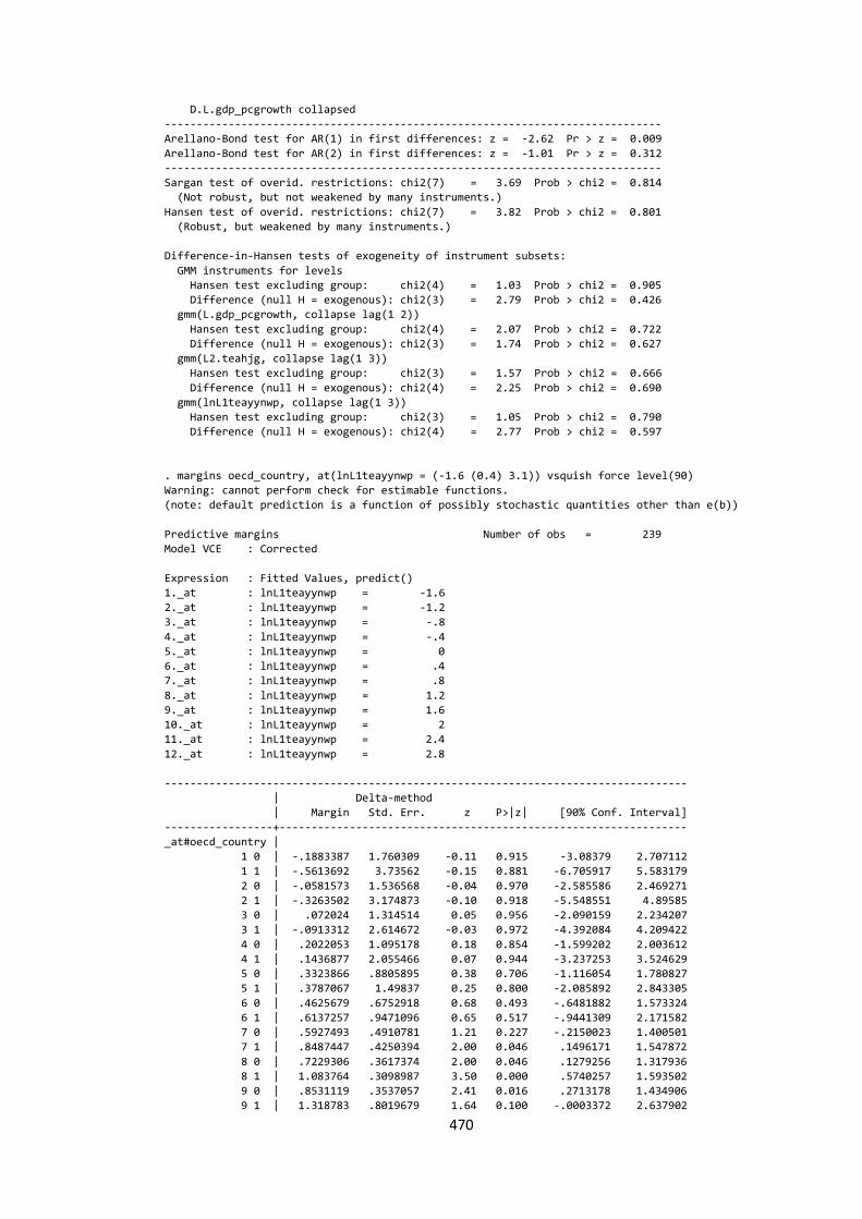
470
D.L.gdp_pcgrowth collapsed
------------------------------------------------------------------------------
Arellano-Bond test for AR(1) in first differences: z = -2.62 Pr > z = 0.009
Arellano-Bond test for AR(2) in first differences: z = -1.01 Pr > z = 0.312
------------------------------------------------------------------------------
Sargan test of overid. restrictions: chi2(7) = 3.69 Prob > chi2 = 0.814
(Not robust, but not weakened by many instruments.)
Hansen test of overid. restrictions: chi2(7) = 3.82 Prob > chi2 = 0.801
(Robust, but weakened by many instruments.)
Difference-in-Hansen tests of exogeneity of instrument subsets:
GMM instruments for levels
Hansen test excluding group: chi2(4) = 1.03 Prob > chi2 = 0.905
Difference (null H = exogenous): chi2(3) = 2.79 Prob > chi2 = 0.426
gmm(L.gdp_pcgrowth, collapse lag(1 2))
Hansen test excluding group: chi2(4) = 2.07 Prob > chi2 = 0.722
Difference (null H = exogenous): chi2(3) = 1.74 Prob > chi2 = 0.627
gmm(L2.teahjg, collapse lag(1 3))
Hansen test excluding group: chi2(3) = 1.57 Prob > chi2 = 0.666
Difference (null H = exogenous): chi2(4) = 2.25 Prob > chi2 = 0.690
gmm(lnL1teayynwp, collapse lag(1 3))
Hansen test excluding group: chi2(3) = 1.05 Prob > chi2 = 0.790
Difference (null H = exogenous): chi2(4) = 2.77 Prob > chi2 = 0.597
. margins oecd_country, at(lnL1teayynwp = (-1.6 (0.4) 3.1)) vsquish force level(90)
Warning: cannot perform check for estimable functions.
(note: default prediction is a function of possibly stochastic quantities other than e(b))
Predictive margins Number of obs = 239
Model VCE : Corrected
Expression : Fitted Values, predict()
1._at : lnL1teayynwp = -1.6
2._at : lnL1teayynwp = -1.2
3._at : lnL1teayynwp = -.8
4._at : lnL1teayynwp = -.4
5._at : lnL1teayynwp = 0
6._at : lnL1teayynwp = .4
7._at : lnL1teayynwp = .8
8._at : lnL1teayynwp = 1.2
9._at : lnL1teayynwp = 1.6
10._at : lnL1teayynwp = 2
11._at : lnL1teayynwp = 2.4
12._at : lnL1teayynwp = 2.8
----------------------------------------------------------------------------------
| Delta-method
| Margin Std. Err. z P>|z| [90% Conf. Interval]
-----------------+----------------------------------------------------------------
_at#oecd_country |
1 0 | -.1883387 1.760309 -0.11 0.915 -3.08379 2.707112
1 1 | -.5613692 3.73562 -0.15 0.881 -6.705917 5.583179
2 0 | -.0581573 1.536568 -0.04 0.970 -2.585586 2.469271
2 1 | -.3263502 3.174873 -0.10 0.918 -5.548551 4.89585
3 0 | .072024 1.314514 0.05 0.956 -2.090159 2.234207
3 1 | -.0913312 2.614672 -0.03 0.972 -4.392084 4.209422
4 0 | .2022053 1.095178 0.18 0.854 -1.599202 2.003612
4 1 | .1436877 2.055466 0.07 0.944 -3.237253 3.524629
5 0 | .3323866 .8805895 0.38 0.706 -1.116054 1.780827
5 1 | .3787067 1.49837 0.25 0.800 -2.085892 2.843305
6 0 | .4625679 .6752918 0.68 0.493 -.6481882 1.573324
6 1 | .6137257 .9471096 0.65 0.517 -.9441309 2.171582
7 0 | .5927493 .4910781 1.21 0.227 -.2150023 1.400501
7 1 | .8487447 .4250394 2.00 0.046 .1496171 1.547872
8 0 | .7229306 .3617374 2.00 0.046 .1279256 1.317936
8 1 | 1.083764 .3098987 3.50 0.000 .5740257 1.593502
9 0 | .8531119 .3537057 2.41 0.016 .2713178 1.434906
9 1 | 1.318783 .8019679 1.64 0.100 -.0003372 2.637902
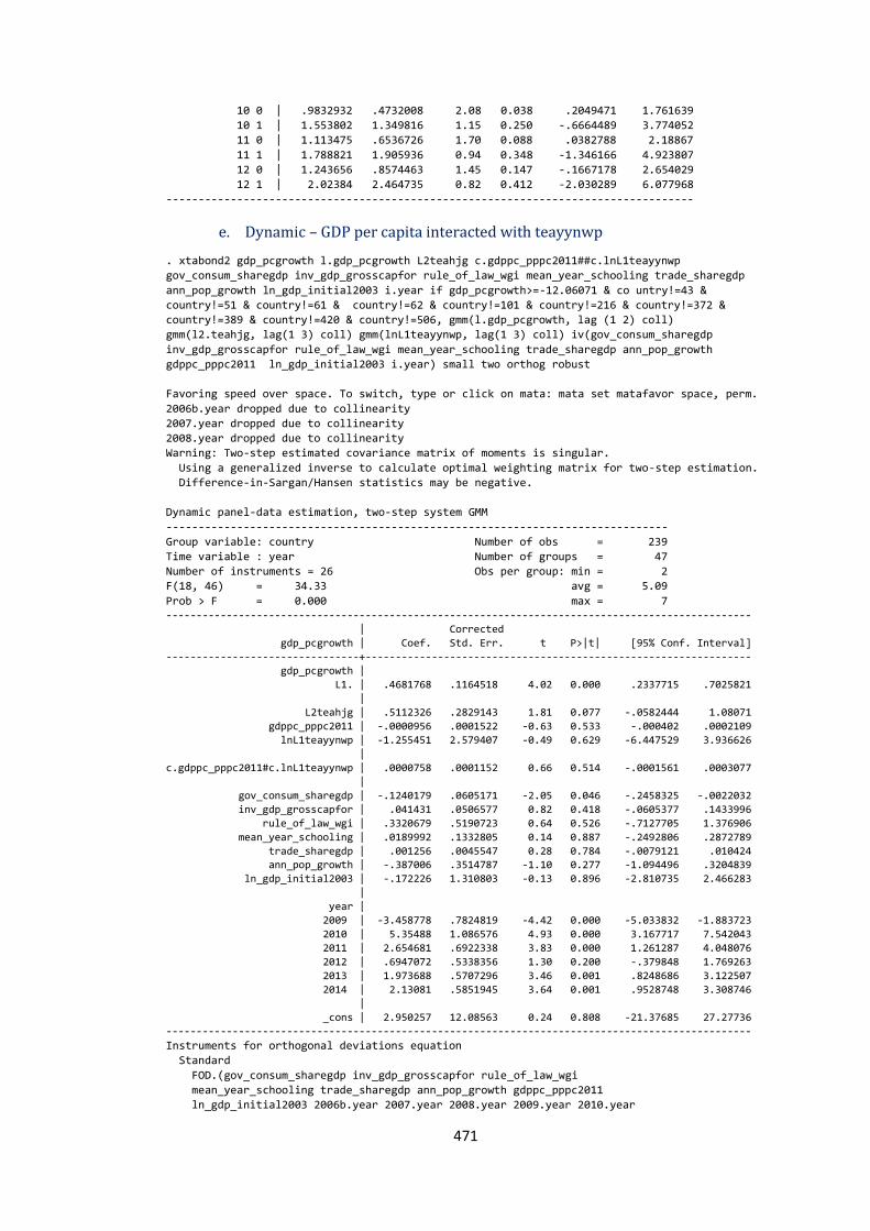
471
10 0 | .9832932 .4732008 2.08 0.038 .2049471 1.761639
10 1 | 1.553802 1.349816 1.15 0.250 -.6664489 3.774052
11 0 | 1.113475 .6536726 1.70 0.088 .0382788 2.18867
11 1 | 1.788821 1.905936 0.94 0.348 -1.346166 4.923807
12 0 | 1.243656 .8574463 1.45 0.147 -.1667178 2.654029
12 1 | 2.02384 2.464735 0.82 0.412 -2.030289 6.077968
----------------------------------------------------------------------------------
e. Dynamic – GDP per capita interacted with teayynwp
. xtabond2 gdp_pcgrowth l.gdp_pcgrowth L2teahjg c.gdppc_pppc2011##c.lnL1teayynwp
gov_consum_sharegdp inv_gdp_grosscapfor rule_of_law_wgi mean_year_schooling trade_sharegdp
ann_pop_growth ln_gdp_initial2003 i.year if gdp_pcgrowth>=-12.06071 & co untry!=43 &
country!=51 & country!=61 & country!=62 & country!=101 & country!=216 & country!=372 &
country!=389 & country!=420 & country!=506, gmm(l.gdp_pcgrowth, lag (1 2) coll)
gmm(l2.teahjg, lag(1 3) coll) gmm(lnL1teayynwp, lag(1 3) coll) iv(gov_consum_sharegdp
inv_gdp_grosscapfor rule_of_law_wgi mean_year_schooling trade_sharegdp ann_pop_growth
gdppc_pppc2011 ln_gdp_initial2003 i.year) small two orthog robust
Favoring speed over space. To switch, type or click on mata: mata set matafavor space, perm.
2006b.year dropped due to collinearity
2007.year dropped due to collinearity
2008.year dropped due to collinearity
Warning: Two-step estimated covariance matrix of moments is singular.
Using a generalized inverse to calculate optimal weighting matrix for two-step estimation.
Difference-in-Sargan/Hansen statistics may be negative.
Dynamic panel-data estimation, two-step system GMM
------------------------------------------------------------------------------
Group variable: country Number of obs = 239
Time variable : year Number of groups = 47
Number of instruments = 26 Obs per group: min = 2
F(18, 46) = 34.33 avg = 5.09
Prob > F = 0.000 max = 7 -------------------------------------------------------------------------------------------------
| Corrected
gdp_pcgrowth | Coef. Std. Err. t P>|t| [95% Conf. Interval]
--------------------------------+----------------------------------------------------------------
gdp_pcgrowth |
L1. | .4681768 .1164518 4.02 0.000 .2337715 .7025821
|
L2teahjg | .5112326 .2829143 1.81 0.077 -.0582444 1.08071
gdppc_pppc2011 | -.0000956 .0001522 -0.63 0.533 -.000402 .0002109
lnL1teayynwp | -1.255451 2.579407 -0.49 0.629 -6.447529 3.936626
|
c.gdppc_pppc2011#c.lnL1teayynwp | .0000758 .0001152 0.66 0.514 -.0001561 .0003077
|
gov_consum_sharegdp | -.1240179 .0605171 -2.05 0.046 -.2458325 -.0022032
inv_gdp_grosscapfor | .041431 .0506577 0.82 0.418 -.0605377 .1433996
rule_of_law_wgi | .3320679 .5190723 0.64 0.526 -.7127705 1.376906
mean_year_schooling | .0189992 .1332805 0.14 0.887 -.2492806 .2872789
trade_sharegdp | .001256 .0045547 0.28 0.784 -.0079121 .010424 ann_pop_growth | -.387006 .3514787 -1.10 0.277 -1.094496 .3204839
ln_gdp_initial2003 | -.172226 1.310803 -0.13 0.896 -2.810735 2.466283
|
year |
2009 | -3.458778 .7824819 -4.42 0.000 -5.033832 -1.883723
2010 | 5.35488 1.086576 4.93 0.000 3.167717 7.542043
2011 | 2.654681 .6922338 3.83 0.000 1.261287 4.048076
2012 | .6947072 .5338356 1.30 0.200 -.379848 1.769263
2013 | 1.973688 .5707296 3.46 0.001 .8248686 3.122507
2014 | 2.13081 .5851945 3.64 0.001 .9528748 3.308746
|
_cons | 2.950257 12.08563 0.24 0.808 -21.37685 27.27736
------------------------------------------------------------------------------------------------- Instruments for orthogonal deviations equation
Standard
FOD.(gov_consum_sharegdp inv_gdp_grosscapfor rule_of_law_wgi
mean_year_schooling trade_sharegdp ann_pop_growth gdppc_pppc2011
ln_gdp_initial2003 2006b.year 2007.year 2008.year 2009.year 2010.year
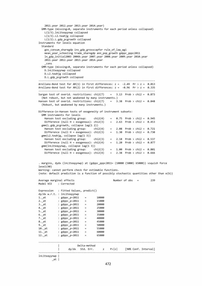
472
2011.year 2012.year 2013.year 2014.year)
GMM-type (missing=0, separate instruments for each period unless collapsed)
L(1/3).lnL1teayynwp collapsed
L(1/3).L2.teahjg collapsed
L(1/2).L.gdp_pcgrowth collapsed
Instruments for levels equation
Standard
gov_consum_sharegdp inv_gdp_grosscapfor rule_of_law_wgi
mean_year_schooling trade_sharegdp ann_pop_growth gdppc_pppc2011
ln_gdp_initial2003 2006b.year 2007.year 2008.year 2009.year 2010.year
2011.year 2012.year 2013.year 2014.year
_cons
GMM-type (missing=0, separate instruments for each period unless collapsed)
D.lnL1teayynwp collapsed
D.L2.teahjg collapsed
D.L.gdp_pcgrowth collapsed
------------------------------------------------------------------------------
Arellano-Bond test for AR(1) in first differences: z = -2.49 Pr > z = 0.013
Arellano-Bond test for AR(2) in first differences: z = -0.96 Pr > z = 0.335
------------------------------------------------------------------------------
Sargan test of overid. restrictions: chi2(7) = 3.13 Prob > chi2 = 0.873
(Not robust, but not weakened by many instruments.)
Hansen test of overid. restrictions: chi2(7) = 3.38 Prob > chi2 = 0.848
(Robust, but weakened by many instruments.)
Difference-in-Hansen tests of exogeneity of instrument subsets:
GMM instruments for levels
Hansen test excluding group: chi2(4) = 0.75 Prob > chi2 = 0.945
Difference (null H = exogenous): chi2(3) = 2.63 Prob > chi2 = 0.453
gmm(L.gdp_pcgrowth, collapse lag(1 2))
Hansen test excluding group: chi2(4) = 2.08 Prob > chi2 = 0.721
Difference (null H = exogenous): chi2(3) = 1.30 Prob > chi2 = 0.730
gmm(L2.teahjg, collapse lag(1 3))
Hansen test excluding group: chi2(3) = 2.18 Prob > chi2 = 0.537
Difference (null H = exogenous): chi2(4) = 1.20 Prob > chi2 = 0.877
gmm(lnL1teayynwp, collapse lag(1 3))
Hansen test excluding group: chi2(3) = 1.00 Prob > chi2 = 0.801
Difference (null H = exogenous): chi2(4) = 2.38 Prob > chi2 = 0.666
. margins, dydx (lnL1teayynwp) at (gdppc_pppc2011= (10000 (5000) 65000)) vsquish force
level(90)
Warning: cannot perform check for estimable functions.
(note: default prediction is a function of possibly stochastic quantities other than e(b))
Average marginal effects Number of obs = 239
Model VCE : Corrected
Expression : Fitted Values, predict()
dy/dx w.r.t. : lnL1teayynwp
1._at : gdppc_p~2011 = 10000
2._at : gdppc_p~2011 = 15000
3._at : gdppc_p~2011 = 20000
4._at : gdppc_p~2011 = 25000
5._at : gdppc_p~2011 = 30000
6._at : gdppc_p~2011 = 35000
7._at : gdppc_p~2011 = 40000
8._at : gdppc_p~2011 = 45000
9._at : gdppc_p~2011 = 50000
10._at : gdppc_p~2011 = 55000
11._at : gdppc_p~2011 = 60000
12._at : gdppc_p~2011 = 65000
------------------------------------------------------------------------------
| Delta-method
| dy/dx Std. Err. z P>|z| [90% Conf. Interval]
-------------+----------------------------------------------------------------
lnL1teayynwp |
_at |
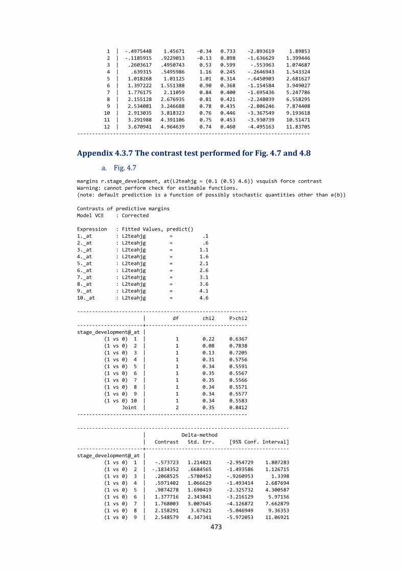
473
1 | -.4975448 1.45671 -0.34 0.733 -2.893619 1.89853
2 | -.1185915 .9229013 -0.13 0.898 -1.636629 1.399446
3 | .2603617 .4950743 0.53 0.599 -.553963 1.074687
4 | .639315 .5495986 1.16 0.245 -.2646943 1.543324
5 | 1.018268 1.01125 1.01 0.314 -.6450903 2.681627
6 | 1.397222 1.551388 0.90 0.368 -1.154584 3.949027
7 | 1.776175 2.11059 0.84 0.400 -1.695436 5.247786
8 | 2.155128 2.676935 0.81 0.421 -2.248039 6.558295
9 | 2.534081 3.246688 0.78 0.435 -2.806246 7.874408
10 | 2.913035 3.818323 0.76 0.446 -3.367549 9.193618
11 | 3.291988 4.391106 0.75 0.453 -3.930739 10.51471
12 | 3.670941 4.964639 0.74 0.460 -4.495163 11.83705
------------------------------------------------------------------------------
Appendix 4.3.7 The contrast test performed for Fig. 4.7 and 4.8
a. Fig. 4.7
margins r.stage_development, at(L2teahjg = (0.1 (0.5) 4.6)) vsquish force contrast
Warning: cannot perform check for estimable functions.
(note: default prediction is a function of possibly stochastic quantities other than e(b))
Contrasts of predictive margins
Model VCE : Corrected
Expression : Fitted Values, predict()
1._at : L2teahjg = .1
2._at : L2teahjg = .6
3._at : L2teahjg = 1.1
4._at : L2teahjg = 1.6
5._at : L2teahjg = 2.1
6._at : L2teahjg = 2.6
7._at : L2teahjg = 3.1
8._at : L2teahjg = 3.6
9._at : L2teahjg = 4.1
10._at : L2teahjg = 4.6
---------------------------------------------------------
| df chi2 P>chi2
----------------------+----------------------------------
stage_development@_at |
(1 vs 0) 1 | 1 0.22 0.6367
(1 vs 0) 2 | 1 0.08 0.7838
(1 vs 0) 3 | 1 0.13 0.7205
(1 vs 0) 4 | 1 0.31 0.5756
(1 vs 0) 5 | 1 0.34 0.5591
(1 vs 0) 6 | 1 0.35 0.5567
(1 vs 0) 7 | 1 0.35 0.5566
(1 vs 0) 8 | 1 0.34 0.5571
(1 vs 0) 9 | 1 0.34 0.5577
(1 vs 0) 10 | 1 0.34 0.5583
Joint | 2 0.35 0.8412
---------------------------------------------------------
-----------------------------------------------------------------------
| Delta-method
| Contrast Std. Err. [95% Conf. Interval]
----------------------+------------------------------------------------
stage_development@_at |
(1 vs 0) 1 | -.573723 1.214821 -2.954729 1.807283
(1 vs 0) 2 | -.1834352 .6684565 -1.493586 1.126715
(1 vs 0) 3 | .2068525 .5780452 -.9260953 1.3398
(1 vs 0) 4 | .5971402 1.066629 -1.493414 2.687694
(1 vs 0) 5 | .9874278 1.690419 -2.325732 4.300587
(1 vs 0) 6 | 1.377716 2.343841 -3.216129 5.97156
(1 vs 0) 7 | 1.768003 3.007645 -4.126872 7.662879
(1 vs 0) 8 | 2.158291 3.67621 -5.046949 9.36353
(1 vs 0) 9 | 2.548579 4.347341 -5.972053 11.06921

474
(1 vs 0) 10 | 2.938866 5.020008 -6.900169 12.7779
-----------------------------------------------------------------------
b. Fig. 4.8
. margins r.oecd_country, at(L2teahjg = (0.1 (0.5) 4.6)) vsquish force contrast
Warning: cannot perform check for estimable functions.
(note: default prediction is a function of possibly stochastic quantities other than e(b))
Contrasts of predictive margins
Model VCE : Corrected
Expression : Fitted Values, predict()
1._at : L2teahjg = .1
2._at : L2teahjg = .6
3._at : L2teahjg = 1.1
4._at : L2teahjg = 1.6
5._at : L2teahjg = 2.1
6._at : L2teahjg = 2.6
7._at : L2teahjg = 3.1
8._at : L2teahjg = 3.6
9._at : L2teahjg = 4.1
10._at : L2teahjg = 4.6
----------------------------------------------------
| df chi2 P>chi2
-----------------+----------------------------------
oecd_country@_at |
(1 vs 0) 1 | 1 0.47 0.4940
(1 vs 0) 2 | 1 0.12 0.7280
(1 vs 0) 3 | 1 0.35 0.5524
(1 vs 0) 4 | 1 1.19 0.2747
(1 vs 0) 5 | 1 1.26 0.2617
(1 vs 0) 6 | 1 1.22 0.2686
(1 vs 0) 7 | 1 1.19 0.2757
(1 vs 0) 8 | 1 1.16 0.2813
(1 vs 0) 9 | 1 1.14 0.2857
(1 vs 0) 10 | 1 1.12 0.2891
Joint | 2 1.26 0.5318
----------------------------------------------------
------------------------------------------------------------------
| Delta-method
| Contrast Std. Err. [95% Conf. Interval]
-----------------+------------------------------------------------
oecd_country@_at |
(1 vs 0) 1 | -1.023925 1.496996 -3.957984 1.910135
(1 vs 0) 2 | -.3183867 .9154282 -2.112593 1.47582
(1 vs 0) 3 | .3871511 .651638 -.8900359 1.664338
(1 vs 0) 4 | 1.092689 1.000434 -.8681255 3.053503
(1 vs 0) 5 | 1.798227 1.602097 -1.341827 4.93828
(1 vs 0) 6 | 2.503764 2.263223 -1.932071 6.9396
(1 vs 0) 7 | 3.209302 2.94402 -2.56087 8.979475
(1 vs 0) 8 | 3.91484 3.633447 -3.206586 11.03627
(1 vs 0) 9 | 4.620378 4.327382 -3.861136 13.10189
(1 vs 0) 10 | 5.325916 5.023958 -4.52086 15.17269
------------------------------------------------------------------
Appendix 4.3.8 The contrast test performed for Fig. 4.10 and 4.11
a. Fig. 4.10
. margins r.stage_development, at(lnL1teayynwp = (-1.6 (0.4) 3.1)) vsquish force contrast
Warning: cannot perform check for estimable functions.
(note: default prediction is a function of possibly stochastic quantities other than e(b))
Contrasts of predictive margins
Model VCE : Corrected
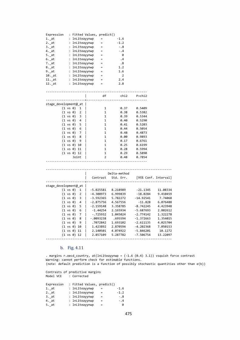
475
Expression : Fitted Values, predict()
1._at : lnL1teayynwp = -1.6
2._at : lnL1teayynwp = -1.2
3._at : lnL1teayynwp = -.8
4._at : lnL1teayynwp = -.4
5._at : lnL1teayynwp = 0
6._at : lnL1teayynwp = .4
7._at : lnL1teayynwp = .8
8._at : lnL1teayynwp = 1.2
9._at : lnL1teayynwp = 1.6
10._at : lnL1teayynwp = 2
11._at : lnL1teayynwp = 2.4
12._at : lnL1teayynwp = 2.8
---------------------------------------------------------
| df chi2 P>chi2
----------------------+----------------------------------
stage_development@_at |
(1 vs 0) 1 | 1 0.37 0.5409
(1 vs 0) 2 | 1 0.38 0.5382
(1 vs 0) 3 | 1 0.39 0.5344
(1 vs 0) 4 | 1 0.40 0.5290
(1 vs 0) 5 | 1 0.41 0.5203
(1 vs 0) 6 | 1 0.44 0.5054
(1 vs 0) 7 | 1 0.48 0.4873
(1 vs 0) 8 | 1 0.00 0.9893
(1 vs 0) 9 | 1 0.17 0.6761
(1 vs 0) 10 | 1 0.25 0.6199
(1 vs 0) 11 | 1 0.28 0.5994
(1 vs 0) 12 | 1 0.29 0.5890
Joint | 2 0.48 0.7854
---------------------------------------------------------
-----------------------------------------------------------------------
| Delta-method
| Contrast Std. Err. [95% Conf. Interval]
----------------------+------------------------------------------------
stage_development@_at |
(1 vs 0) 1 | -5.025581 8.218989 -21.1345 11.08334
(1 vs 0) 2 | -4.308973 6.999839 -18.0284 9.410459
(1 vs 0) 3 | -3.592365 5.782272 -14.92541 7.74068
(1 vs 0) 4 | -2.875756 4.567556 -11.828 6.076488
(1 vs 0) 5 | -2.159148 3.358785 -8.742245 4.423948
(1 vs 0) 6 | -1.44254 2.165934 -5.687693 2.802612
(1 vs 0) 7 | -.725932 1.045024 -2.774142 1.322278
(1 vs 0) 8 | -.0093238 .695594 -1.372663 1.354015
(1 vs 0) 9 | .7072842 1.693102 -2.611135 4.025704
(1 vs 0) 10 | 1.423892 2.870594 -4.202368 7.050153
(1 vs 0) 11 | 2.140501 4.074922 -5.846201 10.1272
(1 vs 0) 12 | 2.857109 5.287782 -7.506754 13.22097
-----------------------------------------------------------------------
b. Fig. 4.11
. margins r.oecd_country, at(lnL1teayynwp = (-1.6 (0.4) 3.1)) vsquish force contrast
Warning: cannot perform check for estimable functions.
(note: default prediction is a function of possibly stochastic quantities other than e(b))
Contrasts of predictive margins
Model VCE : Corrected
Expression : Fitted Values, predict()
1._at : lnL1teayynwp = -1.6
2._at : lnL1teayynwp = -1.2
3._at : lnL1teayynwp = -.8
4._at : lnL1teayynwp = -.4
5._at : lnL1teayynwp = 0
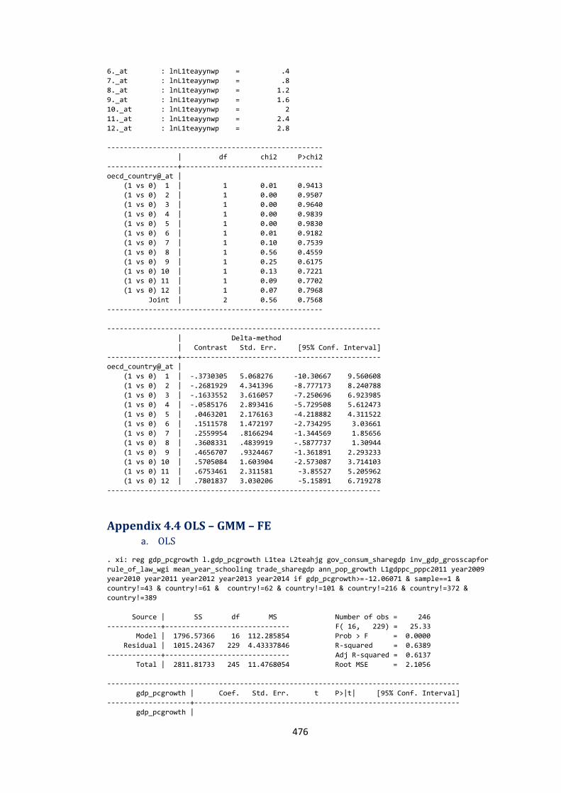
476
6._at : lnL1teayynwp = .4
7._at : lnL1teayynwp = .8
8._at : lnL1teayynwp = 1.2
9._at : lnL1teayynwp = 1.6
10._at : lnL1teayynwp = 2
11._at : lnL1teayynwp = 2.4
12._at : lnL1teayynwp = 2.8
----------------------------------------------------
| df chi2 P>chi2
-----------------+----------------------------------
oecd_country@_at |
(1 vs 0) 1 | 1 0.01 0.9413
(1 vs 0) 2 | 1 0.00 0.9507
(1 vs 0) 3 | 1 0.00 0.9640
(1 vs 0) 4 | 1 0.00 0.9839
(1 vs 0) 5 | 1 0.00 0.9830
(1 vs 0) 6 | 1 0.01 0.9182
(1 vs 0) 7 | 1 0.10 0.7539
(1 vs 0) 8 | 1 0.56 0.4559
(1 vs 0) 9 | 1 0.25 0.6175
(1 vs 0) 10 | 1 0.13 0.7221
(1 vs 0) 11 | 1 0.09 0.7702
(1 vs 0) 12 | 1 0.07 0.7968
Joint | 2 0.56 0.7568
----------------------------------------------------
------------------------------------------------------------------
| Delta-method
| Contrast Std. Err. [95% Conf. Interval]
-----------------+------------------------------------------------
oecd_country@_at |
(1 vs 0) 1 | -.3730305 5.068276 -10.30667 9.560608
(1 vs 0) 2 | -.2681929 4.341396 -8.777173 8.240788
(1 vs 0) 3 | -.1633552 3.616057 -7.250696 6.923985
(1 vs 0) 4 | -.0585176 2.893416 -5.729508 5.612473
(1 vs 0) 5 | .0463201 2.176163 -4.218882 4.311522
(1 vs 0) 6 | .1511578 1.472197 -2.734295 3.03661
(1 vs 0) 7 | .2559954 .8166294 -1.344569 1.85656
(1 vs 0) 8 | .3608331 .4839919 -.5877737 1.30944
(1 vs 0) 9 | .4656707 .9324467 -1.361891 2.293233
(1 vs 0) 10 | .5705084 1.603904 -2.573087 3.714103
(1 vs 0) 11 | .6753461 2.311581 -3.85527 5.205962
(1 vs 0) 12 | .7801837 3.030206 -5.15891 6.719278
------------------------------------------------------------------
Appendix 4.4 OLS – GMM – FE a. OLS
. xi: reg gdp_pcgrowth l.gdp_pcgrowth L1tea L2teahjg gov_consum_sharegdp inv_gdp_grosscapfor
rule_of_law_wgi mean_year_schooling trade_sharegdp ann_pop_growth L1gdppc_pppc2011 year2009
year2010 year2011 year2012 year2013 year2014 if gdp_pcgrowth>=-12.06071 & sample==1 &
country!=43 & country!=61 & country!=62 & country!=101 & country!=216 & country!=372 &
country!=389
Source | SS df MS Number of obs = 246
-------------+------------------------------ F( 16, 229) = 25.33
Model | 1796.57366 16 112.285854 Prob > F = 0.0000
Residual | 1015.24367 229 4.43337846 R-squared = 0.6389
-------------+------------------------------ Adj R-squared = 0.6137
Total | 2811.81733 245 11.4768054 Root MSE = 2.1056
-------------------------------------------------------------------------------------
gdp_pcgrowth | Coef. Std. Err. t P>|t| [95% Conf. Interval]
--------------------+----------------------------------------------------------------
gdp_pcgrowth |
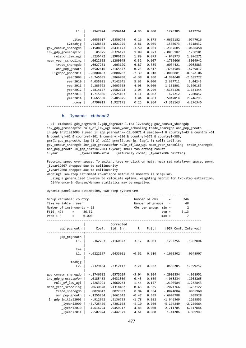
477
L1. | .2947074 .0594144 4.96 0.000 .1776385 .4117762
|
L1tea | .0055917 .0350744 0.16 0.873 -.0635182 .0747016
L2teahjg | .5128553 .1821925 2.81 0.005 .1538673 .8718432
gov_consum_sharegdp | -.1508031 .0431173 -3.50 0.001 -.2357605 -.0658458
inv_gdp_grosscapfor | .05875 .0326172 1.80 0.073 -.0055182 .1230181
rule_of_law_wgi | .5236492 .2906155 1.80 0.073 -.048973 1.096271
mean_year_schooling | .0622668 .1209045 0.52 0.607 -.1759606 .3004942
trade_sharegdp | .0027231 .003129 0.87 0.385 -.0034421 .0088883
ann_pop_growth | .0502616 .2165677 0.23 0.817 -.3764584 .4769817
L1gdppc_pppc2011 | -.0000483 .0000202 -2.39 0.018 -.0000881 -8.52e-06
year2009 | -3.745685 .5866708 -6.38 0.000 -4.901648 -2.589722
year2010 | 4.035081 .7142641 5.65 0.000 2.627711 5.44245
year2011 | 2.285992 .5603958 4.08 0.000 1.181801 3.390183
year2012 | .5814157 .5582324 1.04 0.299 -.5185126 1.681344
year2013 | 1.715866 .5525103 3.11 0.002 .627212 2.80452
year2014 | 1.665538 .5485025 3.04 0.003 .5847814 2.746295
_cons | .4790913 1.927171 0.25 0.804 -3.318163 4.276346
-------------------------------------------------------------------------------------
b. Dynamic – xtabond2
. xi: xtabond2 gdp_pcgrowth l.gdp_pcgrowth l.tea l2.teahjg gov_consum_sharegdp
inv_gdp_grosscapfor rule_of_law_wgi mean_year_schooling trade_sharegdp ann_pop_growth
ln_gdp_initial2003 i.year if gdp_pcgrowth>=-12.06071 & sample==1 & country!=43 & country!=61
& country!=62 & country!=101 & country!=216 & country!=372 & country!=389,
gmm(l.gdp_pcgrowth, lag (1 2) coll) gmm(l2.teahjg, lag(1 3) coll) iv(l.tea
gov_consum_sharegdp inv_gdp_grosscapfor rule_of_law_wgi mean_year_schooling trade_sharegdp
ann_pop_growth ln_gdp_initial2003 i.year) small two orthog robust
i.year _Iyeari2006-2014 (naturally coded; _Iyeari2006 omitted)
Favoring speed over space. To switch, type or click on mata: mata set matafavor space, perm.
_Iyeari2007 dropped due to collinearity
_Iyeari2008 dropped due to collinearity
Warning: Two-step estimated covariance matrix of moments is singular.
Using a generalized inverse to calculate optimal weighting matrix for two-step estimation.
Difference-in-Sargan/Hansen statistics may be negative.
Dynamic panel-data estimation, two-step system GMM
------------------------------------------------------------------------------
Group variable: country Number of obs = 246
Time variable : year Number of groups = 48
Number of instruments = 22 Obs per group: min = 2
F(16, 47) = 36.52 avg = 5.13
Prob > F = 0.000 max = 7
-------------------------------------------------------------------------------------
| Corrected
gdp_pcgrowth | Coef. Std. Err. t P>|t| [95% Conf. Interval]
--------------------+----------------------------------------------------------------
gdp_pcgrowth |
L1. | .362753 .1160823 3.12 0.003 .1292256 .5962804
|
tea |
L1. | -.0222197 .0433011 -0.51 0.610 -.1093302 .0648907
|
teahjg |
L2. | .7329404 .3312117 2.21 0.032 .0666285 1.399252
|
gov_consum_sharegdp | -.1746682 .0575209 -3.04 0.004 -.2903854 -.058951
inv_gdp_grosscapfor | .0185463 .0431369 0.43 0.669 -.068234 .1053265
rule_of_law_wgi | .5263921 .3660763 1.44 0.157 -.2100584 1.262843
mean_year_schooling | .0630678 .1318482 0.48 0.635 -.2021766 .3283122
trade_sharegdp | .0020942 .0022382 0.94 0.354 -.0024084 .0065968
ann_pop_growth | -.1255254 .2661643 -0.47 0.639 -.6609788 .409928
ln_gdp_initial2003 | -.912992 .5136733 -1.78 0.082 -1.946369 .1203853
_Iyeari2009 | -3.725456 .7301103 -5.10 0.000 -5.194249 -2.256664
_Iyeari2010 | 4.614794 .9459917 4.88 0.000 2.711705 6.517884
_Iyeari2011 | 2.507024 .5442871 4.61 0.000 1.41206 3.601989
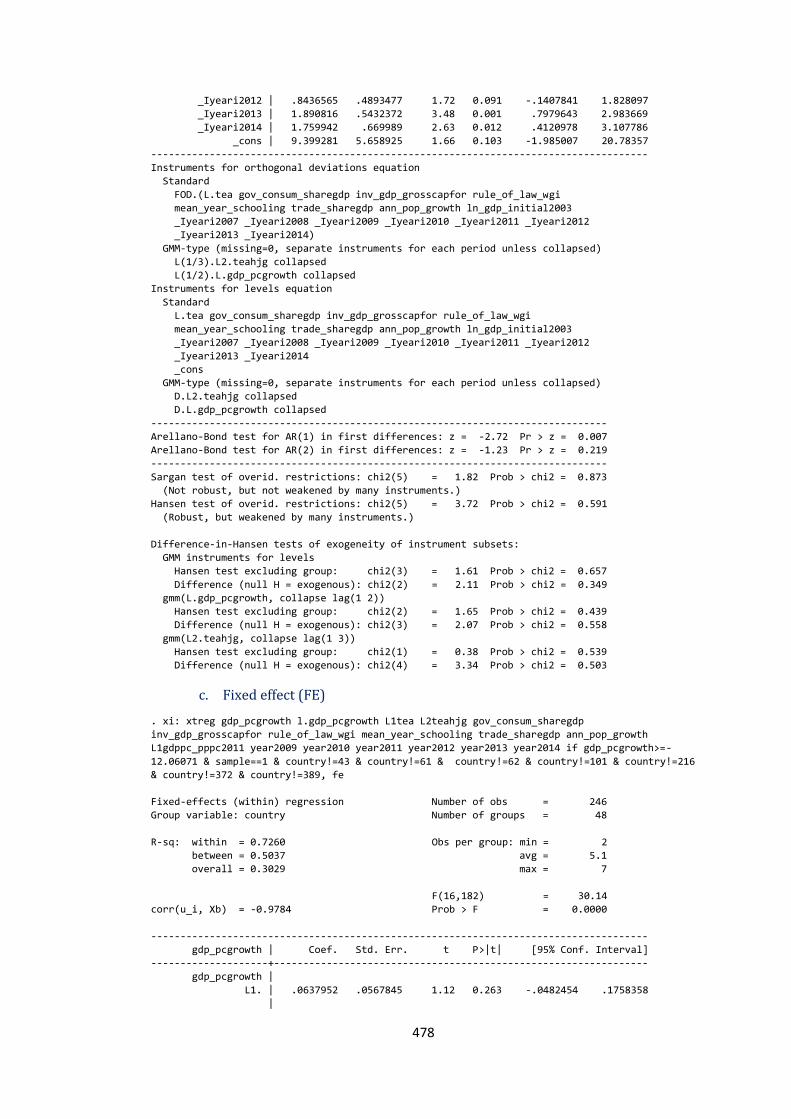
478
_Iyeari2012 | .8436565 .4893477 1.72 0.091 -.1407841 1.828097
_Iyeari2013 | 1.890816 .5432372 3.48 0.001 .7979643 2.983669
_Iyeari2014 | 1.759942 .669989 2.63 0.012 .4120978 3.107786
_cons | 9.399281 5.658925 1.66 0.103 -1.985007 20.78357
-------------------------------------------------------------------------------------
Instruments for orthogonal deviations equation
Standard
FOD.(L.tea gov_consum_sharegdp inv_gdp_grosscapfor rule_of_law_wgi
mean_year_schooling trade_sharegdp ann_pop_growth ln_gdp_initial2003
_Iyeari2007 _Iyeari2008 _Iyeari2009 _Iyeari2010 _Iyeari2011 _Iyeari2012
_Iyeari2013 _Iyeari2014)
GMM-type (missing=0, separate instruments for each period unless collapsed)
L(1/3).L2.teahjg collapsed
L(1/2).L.gdp_pcgrowth collapsed
Instruments for levels equation
Standard
L.tea gov_consum_sharegdp inv_gdp_grosscapfor rule_of_law_wgi
mean_year_schooling trade_sharegdp ann_pop_growth ln_gdp_initial2003
_Iyeari2007 _Iyeari2008 _Iyeari2009 _Iyeari2010 _Iyeari2011 _Iyeari2012
_Iyeari2013 _Iyeari2014
_cons
GMM-type (missing=0, separate instruments for each period unless collapsed)
D.L2.teahjg collapsed
D.L.gdp_pcgrowth collapsed
------------------------------------------------------------------------------
Arellano-Bond test for AR(1) in first differences: z = -2.72 Pr > z = 0.007
Arellano-Bond test for AR(2) in first differences: z = -1.23 Pr > z = 0.219
------------------------------------------------------------------------------
Sargan test of overid. restrictions: chi2(5) = 1.82 Prob > chi2 = 0.873
(Not robust, but not weakened by many instruments.)
Hansen test of overid. restrictions: chi2(5) = 3.72 Prob > chi2 = 0.591
(Robust, but weakened by many instruments.)
Difference-in-Hansen tests of exogeneity of instrument subsets:
GMM instruments for levels
Hansen test excluding group: chi2(3) = 1.61 Prob > chi2 = 0.657
Difference (null H = exogenous): chi2(2) = 2.11 Prob > chi2 = 0.349
gmm(L.gdp_pcgrowth, collapse lag(1 2))
Hansen test excluding group: chi2(2) = 1.65 Prob > chi2 = 0.439
Difference (null H = exogenous): chi2(3) = 2.07 Prob > chi2 = 0.558
gmm(L2.teahjg, collapse lag(1 3))
Hansen test excluding group: chi2(1) = 0.38 Prob > chi2 = 0.539
Difference (null H = exogenous): chi2(4) = 3.34 Prob > chi2 = 0.503
c. Fixed effect (FE)
. xi: xtreg gdp_pcgrowth l.gdp_pcgrowth L1tea L2teahjg gov_consum_sharegdp
inv_gdp_grosscapfor rule_of_law_wgi mean_year_schooling trade_sharegdp ann_pop_growth
L1gdppc_pppc2011 year2009 year2010 year2011 year2012 year2013 year2014 if gdp_pcgrowth>=-
12.06071 & sample==1 & country!=43 & country!=61 & country!=62 & country!=101 & country!=216
& country!=372 & country!=389, fe
Fixed-effects (within) regression Number of obs = 246
Group variable: country Number of groups = 48
R-sq: within = 0.7260 Obs per group: min = 2
between = 0.5037 avg = 5.1
overall = 0.3029 max = 7
F(16,182) = 30.14
corr(u_i, Xb) = -0.9784 Prob > F = 0.0000
-------------------------------------------------------------------------------------
gdp_pcgrowth | Coef. Std. Err. t P>|t| [95% Conf. Interval]
--------------------+----------------------------------------------------------------
gdp_pcgrowth |
L1. | .0637952 .0567845 1.12 0.263 -.0482454 .1758358
|
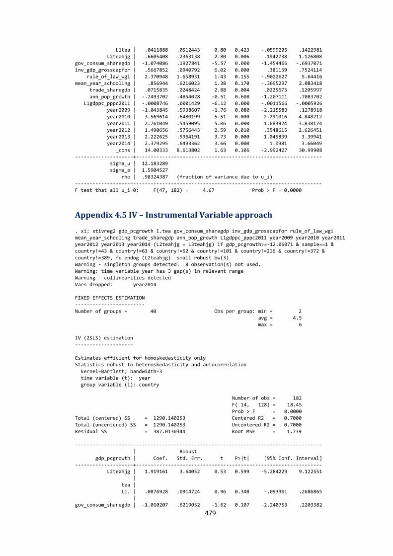
479
L1tea | .0411888 .0512443 0.80 0.423 -.0599205 .1422981
L2teahjg | .6605408 .2363138 2.80 0.006 .1942738 1.126808
gov_consum_sharegdp | -1.074086 .1927841 -5.57 0.000 -1.454466 -.6937071
inv_gdp_grosscapfor | .5667852 .0940792 6.02 0.000 .381159 .7524114
rule_of_law_wgi | 2.370948 1.658931 1.43 0.155 -.9022627 5.64416
mean_year_schooling | .856944 .6216023 1.38 0.170 -.3695297 2.083418
trade_sharegdp | .0715835 .0248424 2.88 0.004 .0225673 .1205997
ann_pop_growth | -.2493702 .4854028 -0.51 0.608 -1.207111 .7083702
L1gdppc_pppc2011 | -.0008746 .0001429 -6.12 0.000 -.0011566 -.0005926
year2009 | -1.043845 .5938607 -1.76 0.080 -2.215583 .1278918
year2010 | 3.569614 .6480199 5.51 0.000 2.291016 4.848212
year2011 | 2.761049 .5459095 5.06 0.000 1.683924 3.838174
year2012 | 1.490656 .5756443 2.59 0.010 .3548615 2.626451
year2013 | 2.222625 .5964191 3.73 0.000 1.045839 3.39941
year2014 | 2.379295 .6493362 3.66 0.000 1.0981 3.66049
_cons | 14.00333 8.613802 1.63 0.106 -2.992427 30.99908
--------------------+----------------------------------------------------------------
sigma_u | 12.183289
sigma_e | 1.5904527
rho | .98324387 (fraction of variance due to u_i)
-------------------------------------------------------------------------------------
F test that all u_i=0: F(47, 182) = 4.67 Prob > F = 0.0000
Appendix 4.5 IV – Instrumental Variable approach . xi: xtivreg2 gdp_pcgrowth l.tea gov_consum_sharegdp inv_gdp_grosscapfor rule_of_law_wgi
mean_year_schooling trade_sharegdp ann_pop_growth L1gdppc_pppc2011 year2009 year2010 year2011
year2012 year2013 year2014 (L2teahjg = L3teahjg) if gdp_pcgrowth>=-12.06071 & sample==1 &
country!=43 & country!=61 & country!=62 & country!=101 & country!=216 & country!=372 &
country!=389, fe endog (L2teahjg) small robust bw(3)
Warning - singleton groups detected. 8 observation(s) not used.
Warning: time variable year has 3 gap(s) in relevant range
Warning - collinearities detected
Vars dropped: year2014
FIXED EFFECTS ESTIMATION
------------------------
Number of groups = 40 Obs per group: min = 2
avg = 4.5
max = 6
IV (2SLS) estimation
--------------------
Estimates efficient for homoskedasticity only
Statistics robust to heteroskedasticity and autocorrelation
kernel=Bartlett; bandwidth=3
time variable (t): year
group variable (i): country
Number of obs = 182
F( 14, 128) = 18.45
Prob > F = 0.0000
Total (centered) SS = 1290.140253 Centered R2 = 0.7000
Total (uncentered) SS = 1290.140253 Uncentered R2 = 0.7000
Residual SS = 387.0130344 Root MSE = 1.739
-------------------------------------------------------------------------------------
| Robust
gdp_pcgrowth | Coef. Std. Err. t P>|t| [95% Conf. Interval]
--------------------+----------------------------------------------------------------
L2teahjg | 1.919161 3.64052 0.53 0.599 -5.284229 9.122551
|
tea |
L1. | .0876928 .0914724 0.96 0.340 -.093301 .2686865
|
gov_consum_sharegdp | -1.010207 .6219052 -1.62 0.107 -2.240753 .2203382
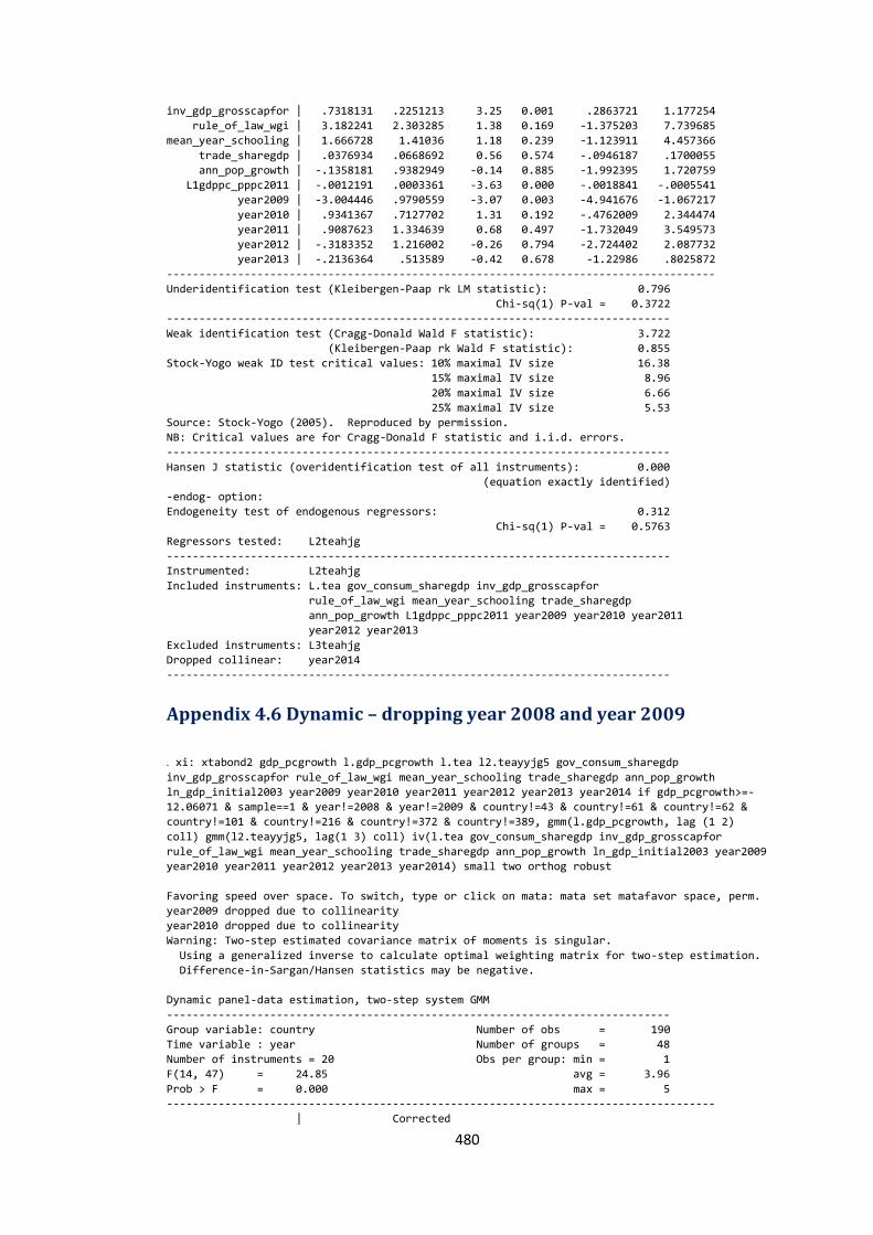
480
inv_gdp_grosscapfor | .7318131 .2251213 3.25 0.001 .2863721 1.177254
rule_of_law_wgi | 3.182241 2.303285 1.38 0.169 -1.375203 7.739685
mean_year_schooling | 1.666728 1.41036 1.18 0.239 -1.123911 4.457366
trade_sharegdp | .0376934 .0668692 0.56 0.574 -.0946187 .1700055
ann_pop_growth | -.1358181 .9382949 -0.14 0.885 -1.992395 1.720759
L1gdppc_pppc2011 | -.0012191 .0003361 -3.63 0.000 -.0018841 -.0005541
year2009 | -3.004446 .9790559 -3.07 0.003 -4.941676 -1.067217
year2010 | .9341367 .7127702 1.31 0.192 -.4762009 2.344474
year2011 | .9087623 1.334639 0.68 0.497 -1.732049 3.549573
year2012 | -.3183352 1.216002 -0.26 0.794 -2.724402 2.087732
year2013 | -.2136364 .513589 -0.42 0.678 -1.22986 .8025872
-------------------------------------------------------------------------------------
Underidentification test (Kleibergen-Paap rk LM statistic): 0.796
Chi-sq(1) P-val = 0.3722
------------------------------------------------------------------------------
Weak identification test (Cragg-Donald Wald F statistic): 3.722
(Kleibergen-Paap rk Wald F statistic): 0.855
Stock-Yogo weak ID test critical values: 10% maximal IV size 16.38
15% maximal IV size 8.96
20% maximal IV size 6.66
25% maximal IV size 5.53
Source: Stock-Yogo (2005). Reproduced by permission.
NB: Critical values are for Cragg-Donald F statistic and i.i.d. errors.
------------------------------------------------------------------------------
Hansen J statistic (overidentification test of all instruments): 0.000
(equation exactly identified)
-endog- option:
Endogeneity test of endogenous regressors: 0.312
Chi-sq(1) P-val = 0.5763
Regressors tested: L2teahjg
------------------------------------------------------------------------------
Instrumented: L2teahjg
Included instruments: L.tea gov_consum_sharegdp inv_gdp_grosscapfor
rule_of_law_wgi mean_year_schooling trade_sharegdp
ann_pop_growth L1gdppc_pppc2011 year2009 year2010 year2011
year2012 year2013
Excluded instruments: L3teahjg
Dropped collinear: year2014
------------------------------------------------------------------------------
Appendix 4.6 Dynamic – dropping year 2008 and year 2009
. xi: xtabond2 gdp_pcgrowth l.gdp_pcgrowth l.tea l2.teayyjg5 gov_consum_sharegdp
inv_gdp_grosscapfor rule_of_law_wgi mean_year_schooling trade_sharegdp ann_pop_growth
ln_gdp_initial2003 year2009 year2010 year2011 year2012 year2013 year2014 if gdp_pcgrowth>=-
12.06071 & sample==1 & year!=2008 & year!=2009 & country!=43 & country!=61 & country!=62 &
country!=101 & country!=216 & country!=372 & country!=389, gmm(l.gdp_pcgrowth, lag (1 2)
coll) gmm(l2.teayyjg5, lag(1 3) coll) iv(l.tea gov_consum_sharegdp inv_gdp_grosscapfor
rule_of_law_wgi mean_year_schooling trade_sharegdp ann_pop_growth ln_gdp_initial2003 year2009
year2010 year2011 year2012 year2013 year2014) small two orthog robust
Favoring speed over space. To switch, type or click on mata: mata set matafavor space, perm.
year2009 dropped due to collinearity
year2010 dropped due to collinearity
Warning: Two-step estimated covariance matrix of moments is singular.
Using a generalized inverse to calculate optimal weighting matrix for two-step estimation.
Difference-in-Sargan/Hansen statistics may be negative.
Dynamic panel-data estimation, two-step system GMM
------------------------------------------------------------------------------
Group variable: country Number of obs = 190
Time variable : year Number of groups = 48
Number of instruments = 20 Obs per group: min = 1
F(14, 47) = 24.85 avg = 3.96
Prob > F = 0.000 max = 5
-------------------------------------------------------------------------------------
| Corrected
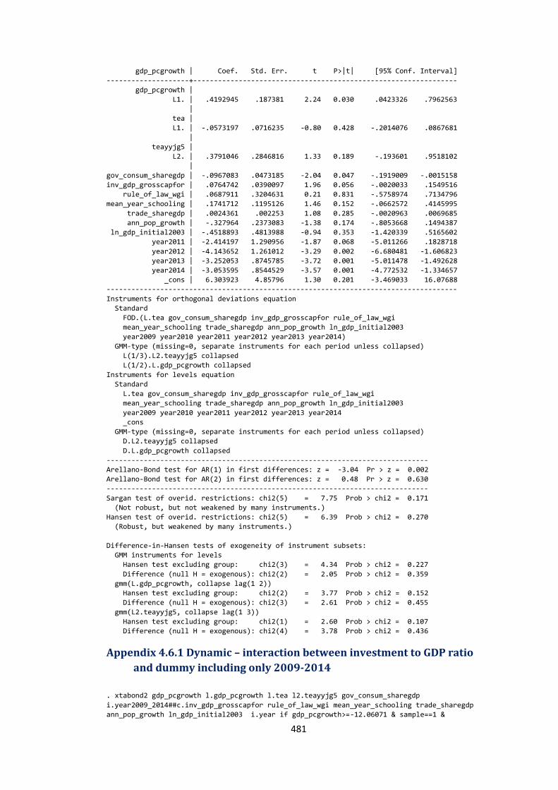
481
gdp_pcgrowth | Coef. Std. Err. t P>|t| [95% Conf. Interval]
--------------------+----------------------------------------------------------------
gdp_pcgrowth |
L1. | .4192945 .187381 2.24 0.030 .0423326 .7962563
|
tea |
L1. | -.0573197 .0716235 -0.80 0.428 -.2014076 .0867681
|
teayyjg5 |
L2. | .3791046 .2846816 1.33 0.189 -.193601 .9518102
|
gov_consum_sharegdp | -.0967083 .0473185 -2.04 0.047 -.1919009 -.0015158
inv_gdp_grosscapfor | .0764742 .0390097 1.96 0.056 -.0020033 .1549516
rule_of_law_wgi | .0687911 .3204631 0.21 0.831 -.5758974 .7134796
mean_year_schooling | .1741712 .1195126 1.46 0.152 -.0662572 .4145995
trade_sharegdp | .0024361 .002253 1.08 0.285 -.0020963 .0069685
ann_pop_growth | -.327964 .2373083 -1.38 0.174 -.8053668 .1494387
ln_gdp_initial2003 | -.4518893 .4813988 -0.94 0.353 -1.420339 .5165602
year2011 | -2.414197 1.290956 -1.87 0.068 -5.011266 .1828718
year2012 | -4.143652 1.261012 -3.29 0.002 -6.680481 -1.606823
year2013 | -3.252053 .8745785 -3.72 0.001 -5.011478 -1.492628
year2014 | -3.053595 .8544529 -3.57 0.001 -4.772532 -1.334657
_cons | 6.303923 4.85796 1.30 0.201 -3.469033 16.07688
-------------------------------------------------------------------------------------
Instruments for orthogonal deviations equation
Standard
FOD.(L.tea gov_consum_sharegdp inv_gdp_grosscapfor rule_of_law_wgi
mean_year_schooling trade_sharegdp ann_pop_growth ln_gdp_initial2003
year2009 year2010 year2011 year2012 year2013 year2014)
GMM-type (missing=0, separate instruments for each period unless collapsed)
L(1/3).L2.teayyjg5 collapsed
L(1/2).L.gdp_pcgrowth collapsed
Instruments for levels equation
Standard
L.tea gov_consum_sharegdp inv_gdp_grosscapfor rule_of_law_wgi
mean_year_schooling trade_sharegdp ann_pop_growth ln_gdp_initial2003
year2009 year2010 year2011 year2012 year2013 year2014
_cons
GMM-type (missing=0, separate instruments for each period unless collapsed)
D.L2.teayyjg5 collapsed
D.L.gdp_pcgrowth collapsed
------------------------------------------------------------------------------
Arellano-Bond test for AR(1) in first differences: z = -3.04 Pr > z = 0.002
Arellano-Bond test for AR(2) in first differences: z = 0.48 Pr > z = 0.630
------------------------------------------------------------------------------
Sargan test of overid. restrictions: chi2(5) = 7.75 Prob > chi2 = 0.171
(Not robust, but not weakened by many instruments.)
Hansen test of overid. restrictions: chi2(5) = 6.39 Prob > chi2 = 0.270
(Robust, but weakened by many instruments.)
Difference-in-Hansen tests of exogeneity of instrument subsets:
GMM instruments for levels
Hansen test excluding group: chi2(3) = 4.34 Prob > chi2 = 0.227
Difference (null H = exogenous): chi2(2) = 2.05 Prob > chi2 = 0.359
gmm(L.gdp_pcgrowth, collapse lag(1 2))
Hansen test excluding group: chi2(2) = 3.77 Prob > chi2 = 0.152
Difference (null H = exogenous): chi2(3) = 2.61 Prob > chi2 = 0.455
gmm(L2.teayyjg5, collapse lag(1 3))
Hansen test excluding group: chi2(1) = 2.60 Prob > chi2 = 0.107
Difference (null H = exogenous): chi2(4) = 3.78 Prob > chi2 = 0.436
Appendix 4.6.1 Dynamic – interaction between investment to GDP ratio
and dummy including only 2009-2014
. xtabond2 gdp_pcgrowth l.gdp_pcgrowth l.tea l2.teayyjg5 gov_consum_sharegdp
i.year2009_2014##c.inv_gdp_grosscapfor rule_of_law_wgi mean_year_schooling trade_sharegdp
ann_pop_growth ln_gdp_initial2003 i.year if gdp_pcgrowth>=-12.06071 & sample==1 &
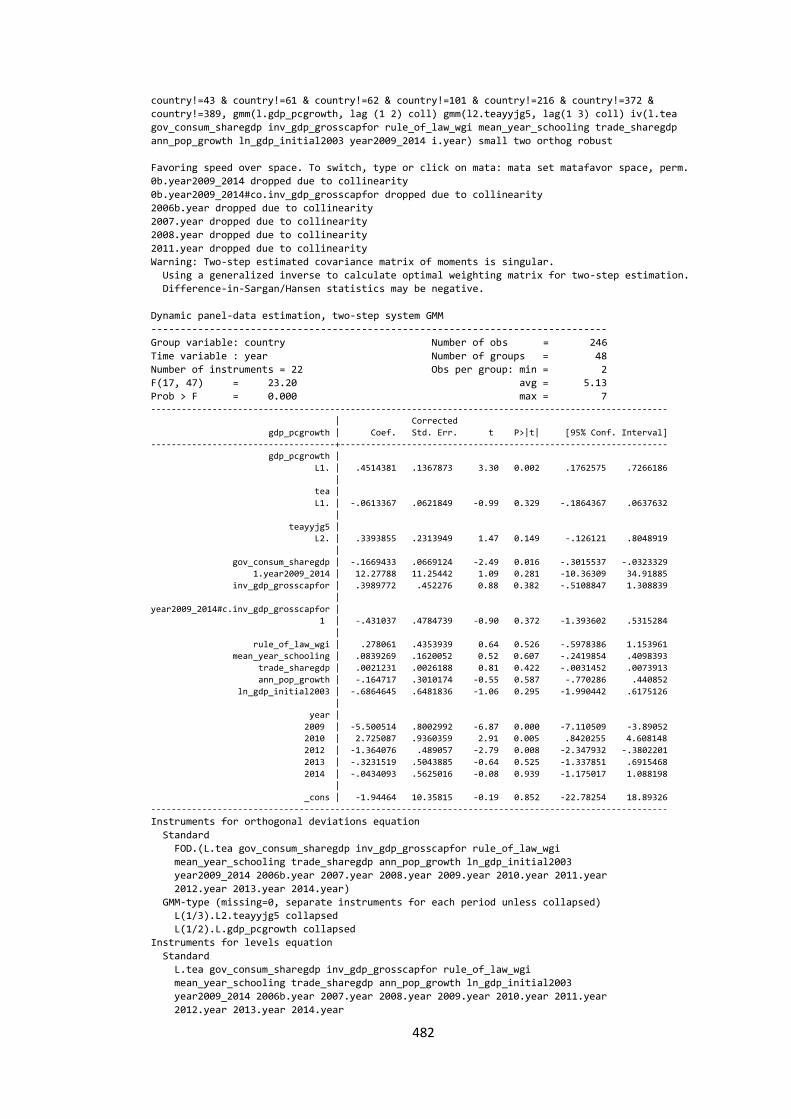
482
country!=43 & country!=61 & country!=62 & country!=101 & country!=216 & country!=372 &
country!=389, gmm(l.gdp_pcgrowth, lag (1 2) coll) gmm(l2.teayyjg5, lag(1 3) coll) iv(l.tea
gov_consum_sharegdp inv_gdp_grosscapfor rule_of_law_wgi mean_year_schooling trade_sharegdp
ann_pop_growth ln_gdp_initial2003 year2009_2014 i.year) small two orthog robust
Favoring speed over space. To switch, type or click on mata: mata set matafavor space, perm.
0b.year2009_2014 dropped due to collinearity
0b.year2009_2014#co.inv_gdp_grosscapfor dropped due to collinearity
2006b.year dropped due to collinearity
2007.year dropped due to collinearity
2008.year dropped due to collinearity
2011.year dropped due to collinearity
Warning: Two-step estimated covariance matrix of moments is singular.
Using a generalized inverse to calculate optimal weighting matrix for two-step estimation.
Difference-in-Sargan/Hansen statistics may be negative.
Dynamic panel-data estimation, two-step system GMM
------------------------------------------------------------------------------
Group variable: country Number of obs = 246
Time variable : year Number of groups = 48
Number of instruments = 22 Obs per group: min = 2
F(17, 47) = 23.20 avg = 5.13
Prob > F = 0.000 max = 7 -----------------------------------------------------------------------------------------------------
| Corrected
gdp_pcgrowth | Coef. Std. Err. t P>|t| [95% Conf. Interval]
------------------------------------+----------------------------------------------------------------
gdp_pcgrowth |
L1. | .4514381 .1367873 3.30 0.002 .1762575 .7266186
|
tea |
L1. | -.0613367 .0621849 -0.99 0.329 -.1864367 .0637632
|
teayyjg5 |
L2. | .3393855 .2313949 1.47 0.149 -.126121 .8048919
|
gov_consum_sharegdp | -.1669433 .0669124 -2.49 0.016 -.3015537 -.0323329
1.year2009_2014 | 12.27788 11.25442 1.09 0.281 -10.36309 34.91885
inv_gdp_grosscapfor | .3989772 .452276 0.88 0.382 -.5108847 1.308839
|
year2009_2014#c.inv_gdp_grosscapfor |
1 | -.431037 .4784739 -0.90 0.372 -1.393602 .5315284
|
rule_of_law_wgi | .278061 .4353939 0.64 0.526 -.5978386 1.153961
mean_year_schooling | .0839269 .1620052 0.52 0.607 -.2419854 .4098393
trade_sharegdp | .0021231 .0026188 0.81 0.422 -.0031452 .0073913
ann_pop_growth | -.164717 .3010174 -0.55 0.587 -.770286 .440852
ln_gdp_initial2003 | -.6864645 .6481836 -1.06 0.295 -1.990442 .6175126
|
year |
2009 | -5.500514 .8002992 -6.87 0.000 -7.110509 -3.89052
2010 | 2.725087 .9360359 2.91 0.005 .8420255 4.608148
2012 | -1.364076 .489057 -2.79 0.008 -2.347932 -.3802201
2013 | -.3231519 .5043885 -0.64 0.525 -1.337851 .6915468
2014 | -.0434093 .5625016 -0.08 0.939 -1.175017 1.088198
|
_cons | -1.94464 10.35815 -0.19 0.852 -22.78254 18.89326
-----------------------------------------------------------------------------------------------------
Instruments for orthogonal deviations equation
Standard
FOD.(L.tea gov_consum_sharegdp inv_gdp_grosscapfor rule_of_law_wgi
mean_year_schooling trade_sharegdp ann_pop_growth ln_gdp_initial2003
year2009_2014 2006b.year 2007.year 2008.year 2009.year 2010.year 2011.year
2012.year 2013.year 2014.year)
GMM-type (missing=0, separate instruments for each period unless collapsed)
L(1/3).L2.teayyjg5 collapsed
L(1/2).L.gdp_pcgrowth collapsed
Instruments for levels equation
Standard
L.tea gov_consum_sharegdp inv_gdp_grosscapfor rule_of_law_wgi
mean_year_schooling trade_sharegdp ann_pop_growth ln_gdp_initial2003
year2009_2014 2006b.year 2007.year 2008.year 2009.year 2010.year 2011.year
2012.year 2013.year 2014.year

483
_cons
GMM-type (missing=0, separate instruments for each period unless collapsed)
D.L2.teayyjg5 collapsed
D.L.gdp_pcgrowth collapsed
------------------------------------------------------------------------------
Arellano-Bond test for AR(1) in first differences: z = -2.39 Pr > z = 0.017
Arellano-Bond test for AR(2) in first differences: z = -0.42 Pr > z = 0.674
------------------------------------------------------------------------------
Sargan test of overid. restrictions: chi2(4) = 6.45 Prob > chi2 = 0.168
(Not robust, but not weakened by many instruments.)
Hansen test of overid. restrictions: chi2(4) = 6.22 Prob > chi2 = 0.183
(Robust, but weakened by many instruments.)
Difference-in-Hansen tests of exogeneity of instrument subsets:
GMM instruments for levels
Hansen test excluding group: chi2(2) = 5.47 Prob > chi2 = 0.065
Difference (null H = exogenous): chi2(2) = 0.76 Prob > chi2 = 0.685
gmm(L.gdp_pcgrowth, collapse lag(1 2))
Hansen test excluding group: chi2(1) = 5.61 Prob > chi2 = 0.018
Difference (null H = exogenous): chi2(3) = 0.62 Prob > chi2 = 0.893
gmm(L2.teayyjg5, collapse lag(1 3))
Hansen test excluding group: chi2(0) = 0.00 Prob > chi2 = .
Difference (null H = exogenous): chi2(4) = 6.22 Prob > chi2 = 0.183
Appendix 4.7 Transformations using ladder and gladder
Appendix 4.7.1 Transformation of L1teayynwp
ladder L1teayynwp
Transformation formula chi2(2) P(chi2)
------------------------------------------------------------------
cubic L1teay~p^3 . 0.000
square L1teay~p^2 . 0.000
identity L1teay~p . 0.000
square root sqrt(L1teay~p) . 0.000
log log(L1teay~p) 9.73 0.008
1/(square root) 1/sqrt(L1teay~p) . 0.000
inverse 1/L1teay~p . 0.000
1/square 1/(L1teay~p^2) . 0.000
1/cubic 1/(L1teay~p^3) . 0.000
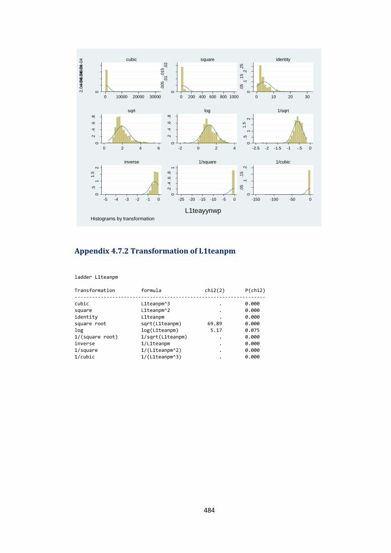
484
Appendix 4.7.2 Transformation of L1teanpm
ladder L1teanpm
Transformation formula chi2(2) P(chi2)
------------------------------------------------------------------
cubic L1teanpm^3 . 0.000
square L1teanpm^2 . 0.000
identity L1teanpm . 0.000
square root sqrt(L1teanpm) 69.89 0.000
log log(L1teanpm) 5.17 0.075
1/(square root) 1/sqrt(L1teanpm) . 0.000
inverse 1/L1teanpm . 0.000
1/square 1/(L1teanpm^2) . 0.000
1/cubic 1/(L1teanpm^3) . 0.000
02.0
e-0
44
.0e
-04
6.0
e-0
48
.0e
-04
0 10000 20000 30000
cubic
0
.005.0
1.0
15.0
2
0 200 400 600 800 1000
square
0
.05
.1.1
5.2
.25
0 10 20 30
identity
0.2
.4.6
.8
0 2 4 6
sqrt
0.2
.4.6
.8
-2 0 2 4
log
0.5
11
.52
-2.5 -2 -1.5 -1 -.5 0
1/sqrt
0.5
11
.52
-5 -4 -3 -2 -1 0
inverse
0.2
.4.6
.81
-25 -20 -15 -10 -5 0
1/square
0
.05
.1.1
5.2
-150 -100 -50 0
1/cubic
De
nsity
L1teayynwpHistograms by transformation
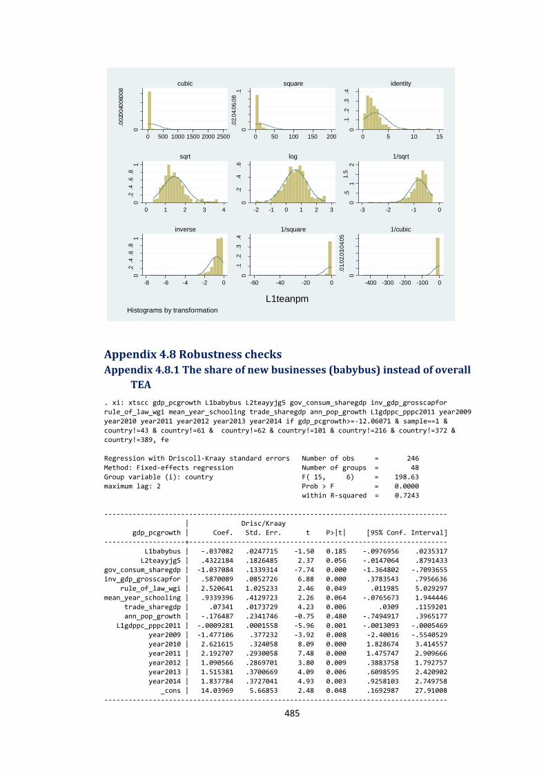
485
Appendix 4.8 Robustness checks
Appendix 4.8.1 The share of new businesses (babybus) instead of overall
TEA
. xi: xtscc gdp_pcgrowth L1babybus L2teayyjg5 gov_consum_sharegdp inv_gdp_grosscapfor
rule_of_law_wgi mean_year_schooling trade_sharegdp ann_pop_growth L1gdppc_pppc2011 year2009
year2010 year2011 year2012 year2013 year2014 if gdp_pcgrowth>=-12.06071 & sample==1 &
country!=43 & country!=61 & country!=62 & country!=101 & country!=216 & country!=372 &
country!=389, fe
Regression with Driscoll-Kraay standard errors Number of obs = 246
Method: Fixed-effects regression Number of groups = 48
Group variable (i): country F( 15, 6) = 198.63
maximum lag: 2 Prob > F = 0.0000
within R-squared = 0.7243
-------------------------------------------------------------------------------------
| Drisc/Kraay
gdp_pcgrowth | Coef. Std. Err. t P>|t| [95% Conf. Interval]
--------------------+----------------------------------------------------------------
L1babybus | -.037082 .0247715 -1.50 0.185 -.0976956 .0235317
L2teayyjg5 | .4322184 .1826485 2.37 0.056 -.0147064 .8791433
gov_consum_sharegdp | -1.037084 .1339314 -7.74 0.000 -1.364802 -.7093655
inv_gdp_grosscapfor | .5870089 .0852726 6.88 0.000 .3783543 .7956636
rule_of_law_wgi | 2.520641 1.025233 2.46 0.049 .011985 5.029297
mean_year_schooling | .9339396 .4129723 2.26 0.064 -.0765673 1.944446
trade_sharegdp | .07341 .0173729 4.23 0.006 .0309 .1159201
ann_pop_growth | -.176487 .2341746 -0.75 0.480 -.7494917 .3965177
L1gdppc_pppc2011 | -.0009281 .0001558 -5.96 0.001 -.0013093 -.0005469
year2009 | -1.477106 .377232 -3.92 0.008 -2.40016 -.5540529
year2010 | 2.621615 .324058 8.09 0.000 1.828674 3.414557
year2011 | 2.192707 .2930058 7.48 0.000 1.475747 2.909666
year2012 | 1.090566 .2869701 3.80 0.009 .3883758 1.792757
year2013 | 1.515381 .3700669 4.09 0.006 .6098595 2.420902
year2014 | 1.837784 .3727041 4.93 0.003 .9258103 2.749758
_cons | 14.03969 5.66853 2.48 0.048 .1692987 27.91008
-------------------------------------------------------------------------------------
0
.002.0
04.0
06.0
08
0 500 1000 1500 2000 2500
cubic
0
.02.
04.
06.
08
.1
0 50 100 150 200
square
0.1
.2.3
.4
0 5 10 15
identity
0.2
.4.6
.81
0 1 2 3 4
sqrt
0.2
.4.6
-2 -1 0 1 2 3
log
0.5
11
.52
-3 -2 -1 0
1/sqrt
0.2
.4.6
.81
-8 -6 -4 -2 0
inverse
0.1
.2.3
.4
-60 -40 -20 0
1/square
0
.01.
02.
03.
04.
05
-400 -300 -200 -100 0
1/cubic
De
nsity
L1teanpmHistograms by transformation
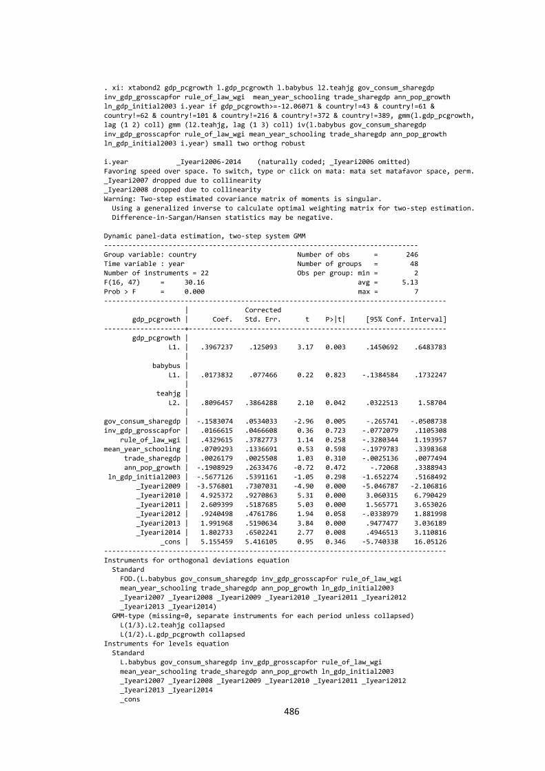
486
. xi: xtabond2 gdp_pcgrowth l.gdp_pcgrowth l.babybus l2.teahjg gov_consum_sharegdp
inv_gdp_grosscapfor rule_of_law_wgi mean_year_schooling trade_sharegdp ann_pop_growth
ln_gdp_initial2003 i.year if gdp_pcgrowth>=-12.06071 & country!=43 & country!=61 &
country!=62 & country!=101 & country!=216 & country!=372 & country!=389, gmm(l.gdp_pcgrowth,
lag (1 2) coll) gmm (l2.teahjg, lag (1 3) coll) iv(l.babybus gov_consum_sharegdp
inv_gdp_grosscapfor rule_of_law_wgi mean_year_schooling trade_sharegdp ann_pop_growth
ln_gdp_initial2003 i.year) small two orthog robust
i.year _Iyeari2006-2014 (naturally coded; _Iyeari2006 omitted)
Favoring speed over space. To switch, type or click on mata: mata set matafavor space, perm.
_Iyeari2007 dropped due to collinearity
_Iyeari2008 dropped due to collinearity
Warning: Two-step estimated covariance matrix of moments is singular.
Using a generalized inverse to calculate optimal weighting matrix for two-step estimation.
Difference-in-Sargan/Hansen statistics may be negative.
Dynamic panel-data estimation, two-step system GMM
------------------------------------------------------------------------------
Group variable: country Number of obs = 246
Time variable : year Number of groups = 48
Number of instruments = 22 Obs per group: min = 2
F(16, 47) = 30.16 avg = 5.13
Prob > F = 0.000 max = 7
-------------------------------------------------------------------------------------
| Corrected
gdp_pcgrowth | Coef. Std. Err. t P>|t| [95% Conf. Interval]
--------------------+----------------------------------------------------------------
gdp_pcgrowth |
L1. | .3967237 .125093 3.17 0.003 .1450692 .6483783
|
babybus |
L1. | .0173832 .077466 0.22 0.823 -.1384584 .1732247
|
teahjg |
L2. | .8096457 .3864288 2.10 0.042 .0322513 1.58704
|
gov_consum_sharegdp | -.1583074 .0534033 -2.96 0.005 -.265741 -.0508738
inv_gdp_grosscapfor | .0166615 .0466608 0.36 0.723 -.0772079 .1105308
rule_of_law_wgi | .4329615 .3782773 1.14 0.258 -.3280344 1.193957
mean_year_schooling | .0709293 .1336691 0.53 0.598 -.1979783 .3398368
trade_sharegdp | .0026179 .0025508 1.03 0.310 -.0025136 .0077494
ann_pop_growth | -.1908929 .2633476 -0.72 0.472 -.72068 .3388943
ln_gdp_initial2003 | -.5677126 .5391161 -1.05 0.298 -1.652274 .5168492
_Iyeari2009 | -3.576801 .7307031 -4.90 0.000 -5.046787 -2.106816
_Iyeari2010 | 4.925372 .9270863 5.31 0.000 3.060315 6.790429
_Iyeari2011 | 2.609399 .5187685 5.03 0.000 1.565771 3.653026
_Iyeari2012 | .9240498 .4761786 1.94 0.058 -.0338979 1.881998
_Iyeari2013 | 1.991968 .5190634 3.84 0.000 .9477477 3.036189
_Iyeari2014 | 1.802733 .6502241 2.77 0.008 .4946513 3.110816
_cons | 5.155459 5.416105 0.95 0.346 -5.740338 16.05126
-------------------------------------------------------------------------------------
Instruments for orthogonal deviations equation
Standard
FOD.(L.babybus gov_consum_sharegdp inv_gdp_grosscapfor rule_of_law_wgi
mean_year_schooling trade_sharegdp ann_pop_growth ln_gdp_initial2003
_Iyeari2007 _Iyeari2008 _Iyeari2009 _Iyeari2010 _Iyeari2011 _Iyeari2012
_Iyeari2013 _Iyeari2014)
GMM-type (missing=0, separate instruments for each period unless collapsed)
L(1/3).L2.teahjg collapsed
L(1/2).L.gdp_pcgrowth collapsed
Instruments for levels equation
Standard
L.babybus gov_consum_sharegdp inv_gdp_grosscapfor rule_of_law_wgi
mean_year_schooling trade_sharegdp ann_pop_growth ln_gdp_initial2003
_Iyeari2007 _Iyeari2008 _Iyeari2009 _Iyeari2010 _Iyeari2011 _Iyeari2012
_Iyeari2013 _Iyeari2014
_cons
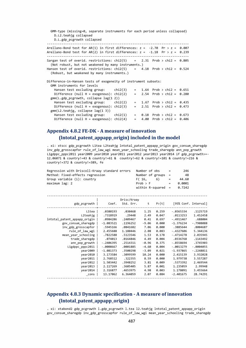
487
GMM-type (missing=0, separate instruments for each period unless collapsed)
D.L2.teahjg collapsed
D.L.gdp_pcgrowth collapsed
------------------------------------------------------------------------------
Arellano-Bond test for AR(1) in first differences: z = -2.70 Pr > z = 0.007
Arellano-Bond test for AR(2) in first differences: z = -1.18 Pr > z = 0.239
------------------------------------------------------------------------------
Sargan test of overid. restrictions: chi2(5) = 2.31 Prob > chi2 = 0.805
(Not robust, but not weakened by many instruments.)
Hansen test of overid. restrictions: chi2(5) = 4.18 Prob > chi2 = 0.524
(Robust, but weakened by many instruments.)
Difference-in-Hansen tests of exogeneity of instrument subsets:
GMM instruments for levels
Hansen test excluding group: chi2(3) = 1.64 Prob > chi2 = 0.651
Difference (null H = exogenous): chi2(2) = 2.54 Prob > chi2 = 0.280
gmm(L.gdp_pcgrowth, collapse lag(1 2))
Hansen test excluding group: chi2(2) = 1.67 Prob > chi2 = 0.435
Difference (null H = exogenous): chi2(3) = 2.51 Prob > chi2 = 0.473
gmm(L2.teahjg, collapse lag(1 3))
Hansen test excluding group: chi2(1) = 0.18 Prob > chi2 = 0.673
Difference (null H = exogenous): chi2(4) = 4.00 Prob > chi2 = 0.406
Appendix 4.8.2 FE-DK - A measure of innovation
(lntotal_patent_appapp_origin) included in the model
. xi: xtscc gdp_pcgrowth L1tea L2teahjg lntotal_patent_appapp_origin gov_consum_sharegdp
inv_gdp_grosscapfor rule_of_law_wgi mean_year_schooling trade_sharegdp ann_pop_growth
L1gdppc_pppc2011 year2009 year2010 year2011 year2012 year2013 year2014 if gdp_pcgrowth>=-
12.06071 & country!=43 & country!=61 & country!=62 & country!=101 & country!=216 &
country!=372 & country!=389, fe
Regression with Driscoll-Kraay standard errors Number of obs = 246
Method: Fixed-effects regression Number of groups = 48
Group variable (i): country F( 16, 6) = 44.60
maximum lag: 2 Prob > F = 0.0001
within R-squared = 0.7242
----------------------------------------------------------------------------------------------
| Drisc/Kraay
gdp_pcgrowth | Coef. Std. Err. t P>|t| [95% Conf. Interval]
-----------------------------+----------------------------------------------------------------
L1tea | .0380193 .030468 1.25 0.259 -.0365334 .1125719
L2teahjg | .7318919 .29448 2.49 0.047 .0113253 1.452458
lntotal_patent_appapp_origin | .0984286 .2409467 0.41 0.697 -.4911467 .688004
gov_consum_sharegdp | -1.083521 .1196252 -9.06 0.000 -1.376234 -.7908088
inv_gdp_grosscapfor | .5945166 .0841682 7.06 0.000 .3885644 .8004687
rule_of_law_wgi | 2.455688 1.180446 2.08 0.083 -.4327606 5.344136
mean_year_schooling | .7822588 .5123546 1.53 0.178 -.4714278 2.035945
trade_sharegdp | .074013 .0164846 4.49 0.004 .0336768 .1143492
ann_pop_growth | -.2406395 .2514311 -0.96 0.375 -.8558694 .3745903
L1gdppc_pppc2011 | -.0008667 .0001885 -4.60 0.004 -.0013279 -.0004055
year2009 | -1.081373 .3500298 -3.09 0.021 -1.937865 -.2248811
year2010 | 3.173584 .3099599 10.24 0.000 2.415139 3.932028
year2011 | 2.768512 .322355 8.59 0.000 1.979738 3.557287
year2012 | 1.503442 .3948252 3.81 0.009 .5373392 2.469544
year2013 | 2.117269 .3605405 5.87 0.001 1.235059 2.99948
year2014 | 2.316877 .4653975 4.98 0.003 1.178091 3.455664
_cons | 13.17062 6.364059 2.07 0.084 -2.401675 28.74291
----------------------------------------------------------------------------------------------
Appendix 4.8.3 Dynamic specification - A measure of innovation
(lntotal_patent_appapp_origin)
. xi: xtabond2 gdp_pcgrowth l.gdp_pcgrowth l.tea l2.teahjg lntotal_patent_appapp_origin
gov_consum_sharegdp inv_gdp_grosscapfor rule_of_law_wgi mean_year_schooling trade_sharegdp
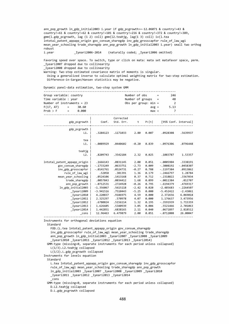
488
ann_pop_growth ln_gdp_initial2003 i.year if gdp_pcgrowth>=-12.06071 & country!=43 &
country!=61 & country!=62 & country!=101 & country!=216 & country!=372 & country!=389,
gmm(l.gdp_pcgrowth, lag (1 2) coll) gmm(l2.teahjg, lag(1 3) coll) iv(l.tea
lntotal_patent_appapp_origin gov_consum_sharegdp inv_gdp_grosscapfor rule_of_law_wgi
mean_year_schooling trade_sharegdp ann_pop_growth ln_gdp_initial2003 i.year) small two orthog
robust
i.year _Iyeari2006-2014 (naturally coded; _Iyeari2006 omitted)
Favoring speed over space. To switch, type or click on mata: mata set matafavor space, perm.
_Iyeari2007 dropped due to collinearity
_Iyeari2008 dropped due to collinearity
Warning: Two-step estimated covariance matrix of moments is singular.
Using a generalized inverse to calculate optimal weighting matrix for two-step estimation.
Difference-in-Sargan/Hansen statistics may be negative.
Dynamic panel-data estimation, two-step system GMM
------------------------------------------------------------------------------
Group variable: country Number of obs = 246
Time variable : year Number of groups = 48
Number of instruments = 23 Obs per group: min = 2
F(17, 47) = 30.60 avg = 5.13
Prob > F = 0.000 max = 7 ----------------------------------------------------------------------------------------------
| Corrected
gdp_pcgrowth | Coef. Std. Err. t P>|t| [95% Conf. Interval]
-----------------------------+----------------------------------------------------------------
gdp_pcgrowth |
L1. | .3284123 .1171033 2.80 0.007 .0928308 .5639937
|
tea |
L1. | -.0089929 .0440602 -0.20 0.839 -.0976306 .0796448
|
teahjg |
L2. | .8209743 .3542184 2.32 0.025 .1083787 1.53357
|
lntotal_patent_appapp_origin | .1666143 .0831145 2.00 0.051 -.0005904 .3338191
gov_consum_sharegdp | -.1733249 .0633751 -2.73 0.009 -.3008192 -.0458307
inv_gdp_grosscapfor | -.0141761 .0524731 -0.27 0.788 -.1197384 .0913862
rule_of_law_wgi | .52058 .381391 1.36 0.179 -.2466797 1.28784
mean_year_schooling | .0524106 .1413168 0.37 0.712 -.2318822 .3367034
trade_sharegdp | .0057843 .0034412 1.68 0.099 -.0011384 .012707
ann_pop_growth | -.0712531 .2724928 -0.26 0.795 -.6194379 .4769317
ln_gdp_initial2003 | -1.356067 .5615118 -2.42 0.020 -2.485683 -.2264507
_Iyeari2009 | -3.941516 .7510443 -5.25 0.000 -5.452422 -2.43061
_Iyeari2010 | 4.220837 .9186975 4.59 0.000 2.372656 6.069018
_Iyeari2011 | 2.325297 .570978 4.07 0.000 1.176637 3.473956
_Iyeari2012 | .6780824 .5156114 1.32 0.195 -.3591939 1.715359
_Iyeari2013 | 1.626605 .5340939 3.05 0.004 .5521466 2.701063
_Iyeari2014 | 1.442851 .6838165 2.11 0.040 .0671897 2.818512
_cons | 12.96463 6.479879 2.00 0.051 -.0712008 26.00047
----------------------------------------------------------------------------------------------
Instruments for orthogonal deviations equation
Standard
FOD.(L.tea lntotal_patent_appapp_origin gov_consum_sharegdp
inv_gdp_grosscapfor rule_of_law_wgi mean_year_schooling trade_sharegdp
ann_pop_growth ln_gdp_initial2003 _Iyeari2007 _Iyeari2008 _Iyeari2009
_Iyeari2010 _Iyeari2011 _Iyeari2012 _Iyeari2013 _Iyeari2014)
GMM-type (missing=0, separate instruments for each period unless collapsed)
L(1/3).L2.teahjg collapsed
L(1/2).L.gdp_pcgrowth collapsed
Instruments for levels equation
Standard
L.tea lntotal_patent_appapp_origin gov_consum_sharegdp inv_gdp_grosscapfor
rule_of_law_wgi mean_year_schooling trade_sharegdp ann_pop_growth
ln_gdp_initial2003 _Iyeari2007 _Iyeari2008 _Iyeari2009 _Iyeari2010
_Iyeari2011 _Iyeari2012 _Iyeari2013 _Iyeari2014
_cons
GMM-type (missing=0, separate instruments for each period unless collapsed)
D.L2.teahjg collapsed
D.L.gdp_pcgrowth collapsed
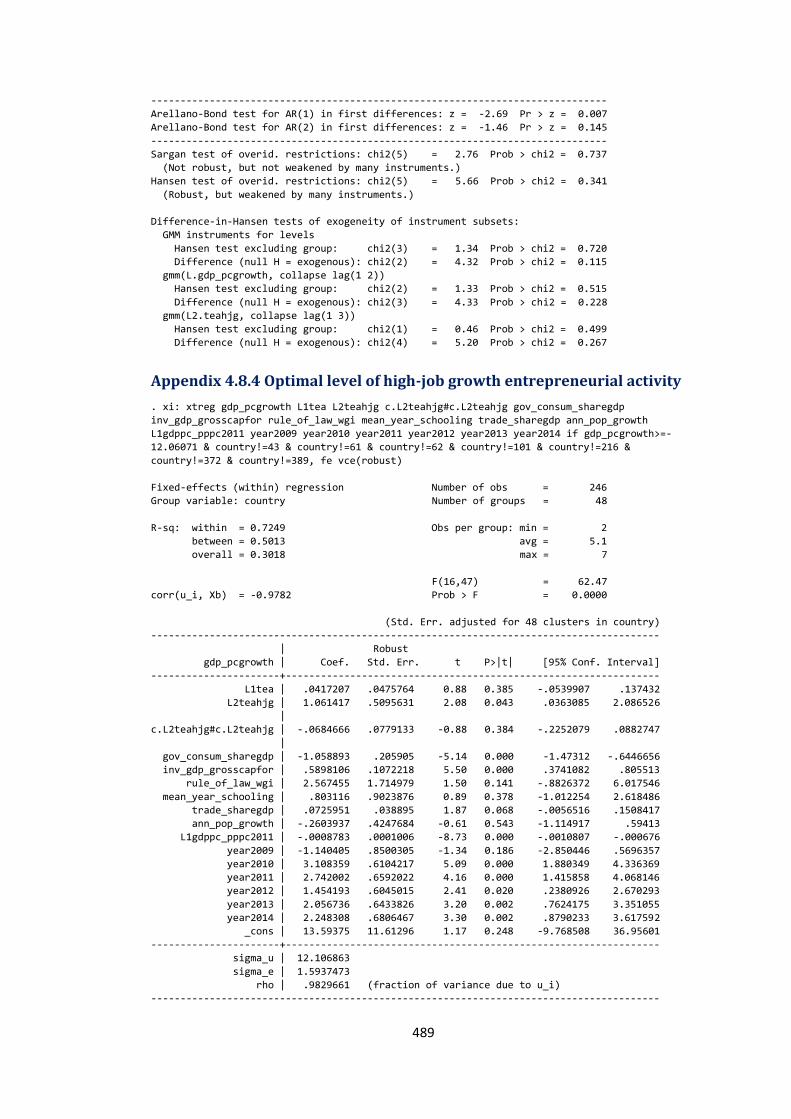
489
------------------------------------------------------------------------------
Arellano-Bond test for AR(1) in first differences: z = -2.69 Pr > z = 0.007
Arellano-Bond test for AR(2) in first differences: z = -1.46 Pr > z = 0.145
------------------------------------------------------------------------------
Sargan test of overid. restrictions: chi2(5) = 2.76 Prob > chi2 = 0.737
(Not robust, but not weakened by many instruments.)
Hansen test of overid. restrictions: chi2(5) = 5.66 Prob > chi2 = 0.341
(Robust, but weakened by many instruments.)
Difference-in-Hansen tests of exogeneity of instrument subsets:
GMM instruments for levels
Hansen test excluding group: chi2(3) = 1.34 Prob > chi2 = 0.720
Difference (null H = exogenous): chi2(2) = 4.32 Prob > chi2 = 0.115
gmm(L.gdp_pcgrowth, collapse lag(1 2))
Hansen test excluding group: chi2(2) = 1.33 Prob > chi2 = 0.515
Difference (null H = exogenous): chi2(3) = 4.33 Prob > chi2 = 0.228
gmm(L2.teahjg, collapse lag(1 3))
Hansen test excluding group: chi2(1) = 0.46 Prob > chi2 = 0.499
Difference (null H = exogenous): chi2(4) = 5.20 Prob > chi2 = 0.267
Appendix 4.8.4 Optimal level of high-job growth entrepreneurial activity
. xi: xtreg gdp_pcgrowth L1tea L2teahjg c.L2teahjg#c.L2teahjg gov_consum_sharegdp
inv_gdp_grosscapfor rule_of_law_wgi mean_year_schooling trade_sharegdp ann_pop_growth
L1gdppc_pppc2011 year2009 year2010 year2011 year2012 year2013 year2014 if gdp_pcgrowth>=-
12.06071 & country!=43 & country!=61 & country!=62 & country!=101 & country!=216 &
country!=372 & country!=389, fe vce(robust)
Fixed-effects (within) regression Number of obs = 246
Group variable: country Number of groups = 48
R-sq: within = 0.7249 Obs per group: min = 2
between = 0.5013 avg = 5.1
overall = 0.3018 max = 7
F(16,47) = 62.47
corr(u_i, Xb) = -0.9782 Prob > F = 0.0000
(Std. Err. adjusted for 48 clusters in country)
---------------------------------------------------------------------------------------
| Robust
gdp_pcgrowth | Coef. Std. Err. t P>|t| [95% Conf. Interval]
----------------------+----------------------------------------------------------------
L1tea | .0417207 .0475764 0.88 0.385 -.0539907 .137432
L2teahjg | 1.061417 .5095631 2.08 0.043 .0363085 2.086526
|
c.L2teahjg#c.L2teahjg | -.0684666 .0779133 -0.88 0.384 -.2252079 .0882747
|
gov_consum_sharegdp | -1.058893 .205905 -5.14 0.000 -1.47312 -.6446656
inv_gdp_grosscapfor | .5898106 .1072218 5.50 0.000 .3741082 .805513
rule_of_law_wgi | 2.567455 1.714979 1.50 0.141 -.8826372 6.017546
mean_year_schooling | .803116 .9023876 0.89 0.378 -1.012254 2.618486
trade_sharegdp | .0725951 .038895 1.87 0.068 -.0056516 .1508417
ann_pop_growth | -.2603937 .4247684 -0.61 0.543 -1.114917 .59413
L1gdppc_pppc2011 | -.0008783 .0001006 -8.73 0.000 -.0010807 -.000676
year2009 | -1.140405 .8500305 -1.34 0.186 -2.850446 .5696357
year2010 | 3.108359 .6104217 5.09 0.000 1.880349 4.336369
year2011 | 2.742002 .6592022 4.16 0.000 1.415858 4.068146
year2012 | 1.454193 .6045015 2.41 0.020 .2380926 2.670293
year2013 | 2.056736 .6433826 3.20 0.002 .7624175 3.351055
year2014 | 2.248308 .6806467 3.30 0.002 .8790233 3.617592
_cons | 13.59375 11.61296 1.17 0.248 -9.768508 36.95601
----------------------+----------------------------------------------------------------
sigma_u | 12.106863
sigma_e | 1.5937473
rho | .9829661 (fraction of variance due to u_i)
---------------------------------------------------------------------------------------
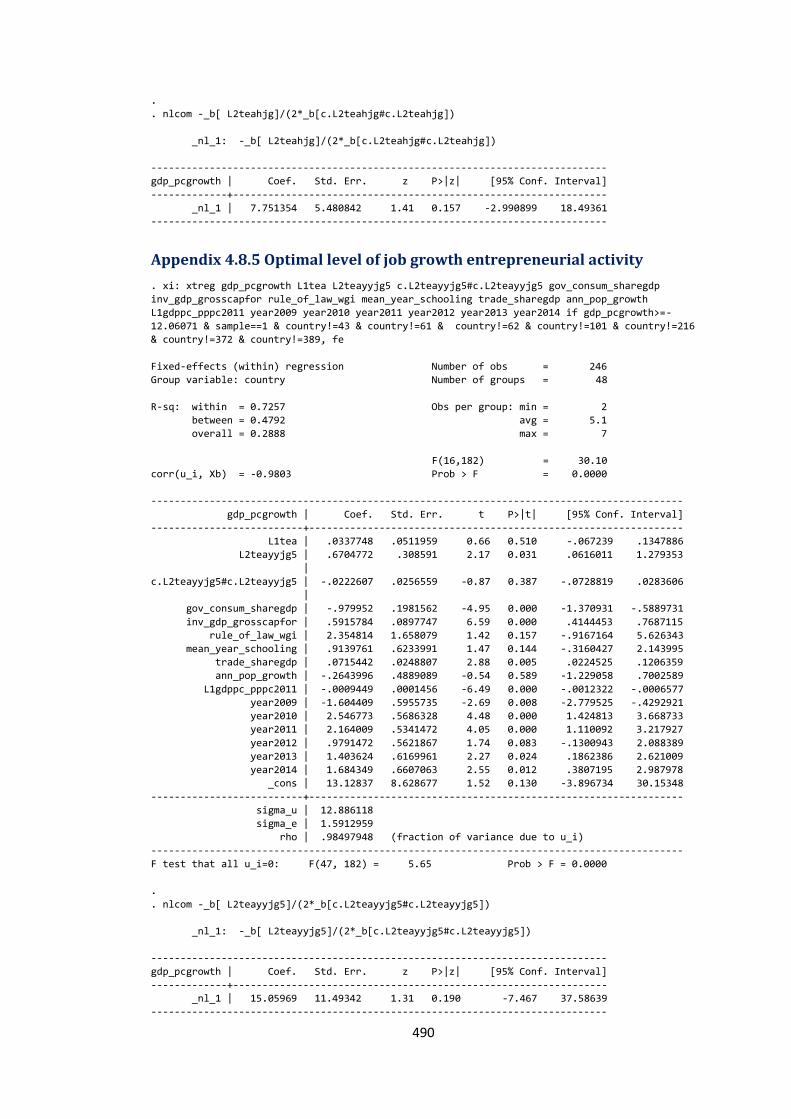
490
.
. nlcom -_b[ L2teahjg]/(2*_b[c.L2teahjg#c.L2teahjg])
_nl_1: -_b[ L2teahjg]/(2*_b[c.L2teahjg#c.L2teahjg])
------------------------------------------------------------------------------
gdp_pcgrowth | Coef. Std. Err. z P>|z| [95% Conf. Interval]
-------------+----------------------------------------------------------------
_nl_1 | 7.751354 5.480842 1.41 0.157 -2.990899 18.49361
------------------------------------------------------------------------------
Appendix 4.8.5 Optimal level of job growth entrepreneurial activity
. xi: xtreg gdp_pcgrowth L1tea L2teayyjg5 c.L2teayyjg5#c.L2teayyjg5 gov_consum_sharegdp
inv_gdp_grosscapfor rule_of_law_wgi mean_year_schooling trade_sharegdp ann_pop_growth
L1gdppc_pppc2011 year2009 year2010 year2011 year2012 year2013 year2014 if gdp_pcgrowth>=-
12.06071 & sample==1 & country!=43 & country!=61 & country!=62 & country!=101 & country!=216
& country!=372 & country!=389, fe
Fixed-effects (within) regression Number of obs = 246
Group variable: country Number of groups = 48
R-sq: within = 0.7257 Obs per group: min = 2
between = 0.4792 avg = 5.1
overall = 0.2888 max = 7
F(16,182) = 30.10
corr(u_i, Xb) = -0.9803 Prob > F = 0.0000
-------------------------------------------------------------------------------------------
gdp_pcgrowth | Coef. Std. Err. t P>|t| [95% Conf. Interval]
--------------------------+----------------------------------------------------------------
L1tea | .0337748 .0511959 0.66 0.510 -.067239 .1347886
L2teayyjg5 | .6704772 .308591 2.17 0.031 .0616011 1.279353
|
c.L2teayyjg5#c.L2teayyjg5 | -.0222607 .0256559 -0.87 0.387 -.0728819 .0283606
|
gov_consum_sharegdp | -.979952 .1981562 -4.95 0.000 -1.370931 -.5889731
inv_gdp_grosscapfor | .5915784 .0897747 6.59 0.000 .4144453 .7687115
rule_of_law_wgi | 2.354814 1.658079 1.42 0.157 -.9167164 5.626343
mean_year_schooling | .9139761 .6233991 1.47 0.144 -.3160427 2.143995
trade_sharegdp | .0715442 .0248807 2.88 0.005 .0224525 .1206359
ann_pop_growth | -.2643996 .4889089 -0.54 0.589 -1.229058 .7002589
L1gdppc_pppc2011 | -.0009449 .0001456 -6.49 0.000 -.0012322 -.0006577
year2009 | -1.604409 .5955735 -2.69 0.008 -2.779525 -.4292921
year2010 | 2.546773 .5686328 4.48 0.000 1.424813 3.668733
year2011 | 2.164009 .5341472 4.05 0.000 1.110092 3.217927
year2012 | .9791472 .5621867 1.74 0.083 -.1300943 2.088389
year2013 | 1.403624 .6169961 2.27 0.024 .1862386 2.621009
year2014 | 1.684349 .6607063 2.55 0.012 .3807195 2.987978
_cons | 13.12837 8.628677 1.52 0.130 -3.896734 30.15348
--------------------------+----------------------------------------------------------------
sigma_u | 12.886118
sigma_e | 1.5912959
rho | .98497948 (fraction of variance due to u_i)
-------------------------------------------------------------------------------------------
F test that all u_i=0: F(47, 182) = 5.65 Prob > F = 0.0000
.
. nlcom -_b[ L2teayyjg5]/(2*_b[c.L2teayyjg5#c.L2teayyjg5])
_nl_1: -_b[ L2teayyjg5]/(2*_b[c.L2teayyjg5#c.L2teayyjg5])
------------------------------------------------------------------------------
gdp_pcgrowth | Coef. Std. Err. z P>|z| [95% Conf. Interval]
-------------+----------------------------------------------------------------
_nl_1 | 15.05969 11.49342 1.31 0.190 -7.467 37.58639
------------------------------------------------------------------------------
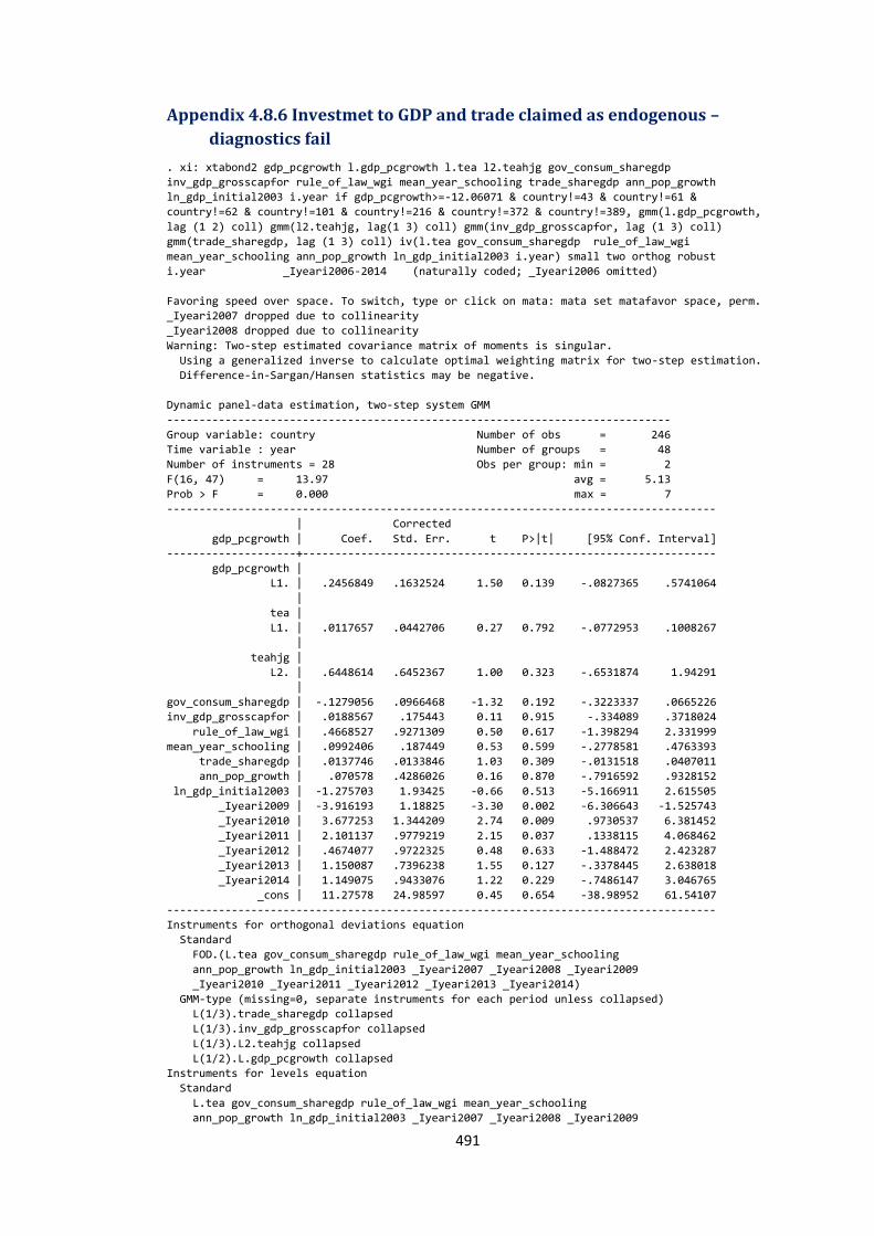
491
Appendix 4.8.6 Investmet to GDP and trade claimed as endogenous –
diagnostics fail
. xi: xtabond2 gdp_pcgrowth l.gdp_pcgrowth l.tea l2.teahjg gov_consum_sharegdp
inv_gdp_grosscapfor rule_of_law_wgi mean_year_schooling trade_sharegdp ann_pop_growth
ln_gdp_initial2003 i.year if gdp_pcgrowth>=-12.06071 & country!=43 & country!=61 &
country!=62 & country!=101 & country!=216 & country!=372 & country!=389, gmm(l.gdp_pcgrowth,
lag (1 2) coll) gmm(l2.teahjg, lag(1 3) coll) gmm(inv_gdp_grosscapfor, lag (1 3) coll)
gmm(trade_sharegdp, lag (1 3) coll) iv(l.tea gov_consum_sharegdp rule_of_law_wgi
mean_year_schooling ann_pop_growth ln_gdp_initial2003 i.year) small two orthog robust
i.year _Iyeari2006-2014 (naturally coded; _Iyeari2006 omitted)
Favoring speed over space. To switch, type or click on mata: mata set matafavor space, perm.
_Iyeari2007 dropped due to collinearity
_Iyeari2008 dropped due to collinearity
Warning: Two-step estimated covariance matrix of moments is singular.
Using a generalized inverse to calculate optimal weighting matrix for two-step estimation.
Difference-in-Sargan/Hansen statistics may be negative.
Dynamic panel-data estimation, two-step system GMM
------------------------------------------------------------------------------
Group variable: country Number of obs = 246
Time variable : year Number of groups = 48
Number of instruments = 28 Obs per group: min = 2
F(16, 47) = 13.97 avg = 5.13
Prob > F = 0.000 max = 7
-------------------------------------------------------------------------------------
| Corrected
gdp_pcgrowth | Coef. Std. Err. t P>|t| [95% Conf. Interval]
--------------------+----------------------------------------------------------------
gdp_pcgrowth |
L1. | .2456849 .1632524 1.50 0.139 -.0827365 .5741064
|
tea |
L1. | .0117657 .0442706 0.27 0.792 -.0772953 .1008267
|
teahjg |
L2. | .6448614 .6452367 1.00 0.323 -.6531874 1.94291
|
gov_consum_sharegdp | -.1279056 .0966468 -1.32 0.192 -.3223337 .0665226
inv_gdp_grosscapfor | .0188567 .175443 0.11 0.915 -.334089 .3718024
rule_of_law_wgi | .4668527 .9271309 0.50 0.617 -1.398294 2.331999
mean_year_schooling | .0992406 .187449 0.53 0.599 -.2778581 .4763393
trade_sharegdp | .0137746 .0133846 1.03 0.309 -.0131518 .0407011
ann_pop_growth | .070578 .4286026 0.16 0.870 -.7916592 .9328152
ln_gdp_initial2003 | -1.275703 1.93425 -0.66 0.513 -5.166911 2.615505
_Iyeari2009 | -3.916193 1.18825 -3.30 0.002 -6.306643 -1.525743
_Iyeari2010 | 3.677253 1.344209 2.74 0.009 .9730537 6.381452
_Iyeari2011 | 2.101137 .9779219 2.15 0.037 .1338115 4.068462
_Iyeari2012 | .4674077 .9722325 0.48 0.633 -1.488472 2.423287
_Iyeari2013 | 1.150087 .7396238 1.55 0.127 -.3378445 2.638018
_Iyeari2014 | 1.149075 .9433076 1.22 0.229 -.7486147 3.046765
_cons | 11.27578 24.98597 0.45 0.654 -38.98952 61.54107
-------------------------------------------------------------------------------------
Instruments for orthogonal deviations equation
Standard
FOD.(L.tea gov_consum_sharegdp rule_of_law_wgi mean_year_schooling
ann_pop_growth ln_gdp_initial2003 _Iyeari2007 _Iyeari2008 _Iyeari2009
_Iyeari2010 _Iyeari2011 _Iyeari2012 _Iyeari2013 _Iyeari2014)
GMM-type (missing=0, separate instruments for each period unless collapsed)
L(1/3).trade_sharegdp collapsed
L(1/3).inv_gdp_grosscapfor collapsed
L(1/3).L2.teahjg collapsed
L(1/2).L.gdp_pcgrowth collapsed
Instruments for levels equation
Standard
L.tea gov_consum_sharegdp rule_of_law_wgi mean_year_schooling
ann_pop_growth ln_gdp_initial2003 _Iyeari2007 _Iyeari2008 _Iyeari2009
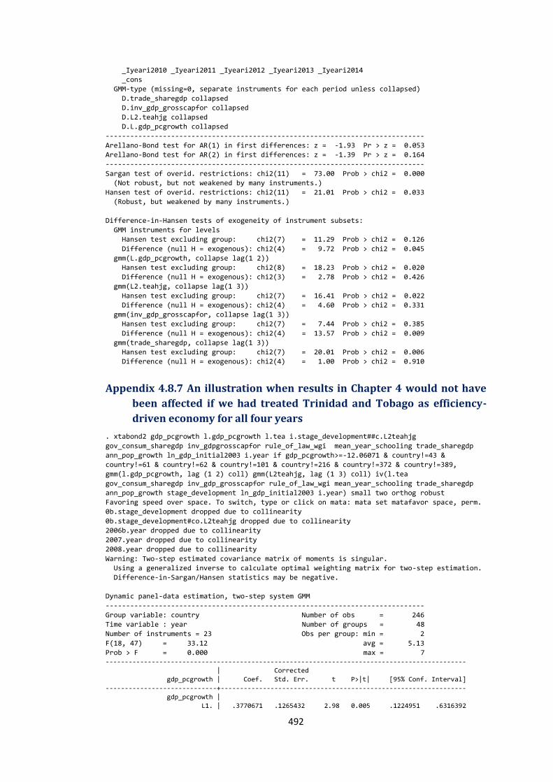
492
_Iyeari2010 _Iyeari2011 _Iyeari2012 _Iyeari2013 _Iyeari2014
_cons
GMM-type (missing=0, separate instruments for each period unless collapsed)
D.trade_sharegdp collapsed
D.inv_gdp_grosscapfor collapsed
D.L2.teahjg collapsed
D.L.gdp_pcgrowth collapsed
------------------------------------------------------------------------------
Arellano-Bond test for AR(1) in first differences: z = -1.93 Pr > z = 0.053
Arellano-Bond test for AR(2) in first differences: z = -1.39 Pr > z = 0.164
------------------------------------------------------------------------------
Sargan test of overid. restrictions: chi2(11) = 73.00 Prob > chi2 = 0.000
(Not robust, but not weakened by many instruments.)
Hansen test of overid. restrictions: chi2(11) = 21.01 Prob > chi2 = 0.033
(Robust, but weakened by many instruments.)
Difference-in-Hansen tests of exogeneity of instrument subsets:
GMM instruments for levels
Hansen test excluding group: chi2(7) = 11.29 Prob > chi2 = 0.126
Difference (null H = exogenous): chi2(4) = 9.72 Prob > chi2 = 0.045
gmm(L.gdp_pcgrowth, collapse lag(1 2))
Hansen test excluding group: chi2(8) = 18.23 Prob > chi2 = 0.020
Difference (null H = exogenous): chi2(3) = 2.78 Prob > chi2 = 0.426
gmm(L2.teahjg, collapse lag(1 3))
Hansen test excluding group: chi2(7) = 16.41 Prob > chi2 = 0.022
Difference (null H = exogenous): chi2(4) = 4.60 Prob > chi2 = 0.331
gmm(inv_gdp_grosscapfor, collapse lag(1 3))
Hansen test excluding group: chi2(7) = 7.44 Prob > chi2 = 0.385
Difference (null H = exogenous): chi2(4) = 13.57 Prob > chi2 = 0.009
gmm(trade_sharegdp, collapse lag(1 3))
Hansen test excluding group: chi2(7) = 20.01 Prob > chi2 = 0.006
Difference (null H = exogenous): chi2(4) = 1.00 Prob > chi2 = 0.910
Appendix 4.8.7 An illustration when results in Chapter 4 would not have
been affected if we had treated Trinidad and Tobago as efficiency-
driven economy for all four years
. xtabond2 gdp_pcgrowth l.gdp_pcgrowth l.tea i.stage_development##c.L2teahjg
gov_consum_sharegdp inv_gdpgrosscapfor rule_of_law_wgi mean_year_schooling trade_sharegdp
ann_pop_growth ln_gdp_initial2003 i.year if gdp_pcgrowth>=-12.06071 & country!=43 &
country!=61 & country!=62 & country!=101 & country!=216 & country!=372 & country!=389,
gmm(l.gdp_pcgrowth, lag (1 2) coll) gmm(L2teahjg, lag (1 3) coll) iv(l.tea
gov_consum_sharegdp inv_gdp_grosscapfor rule_of_law_wgi mean_year_schooling trade_sharegdp
ann_pop_growth stage_development ln_gdp_initial2003 i.year) small two orthog robust
Favoring speed over space. To switch, type or click on mata: mata set matafavor space, perm.
0b.stage_development dropped due to collinearity
0b.stage_development#co.L2teahjg dropped due to collinearity
2006b.year dropped due to collinearity
2007.year dropped due to collinearity
2008.year dropped due to collinearity
Warning: Two-step estimated covariance matrix of moments is singular.
Using a generalized inverse to calculate optimal weighting matrix for two-step estimation.
Difference-in-Sargan/Hansen statistics may be negative.
Dynamic panel-data estimation, two-step system GMM
------------------------------------------------------------------------------
Group variable: country Number of obs = 246
Time variable : year Number of groups = 48
Number of instruments = 23 Obs per group: min = 2
F(18, 47) = 33.12 avg = 5.13
Prob > F = 0.000 max = 7 ----------------------------------------------------------------------------------------------
| Corrected
gdp_pcgrowth | Coef. Std. Err. t P>|t| [95% Conf. Interval]
-----------------------------+----------------------------------------------------------------
gdp_pcgrowth |
L1. | .3770671 .1265432 2.98 0.005 .1224951 .6316392
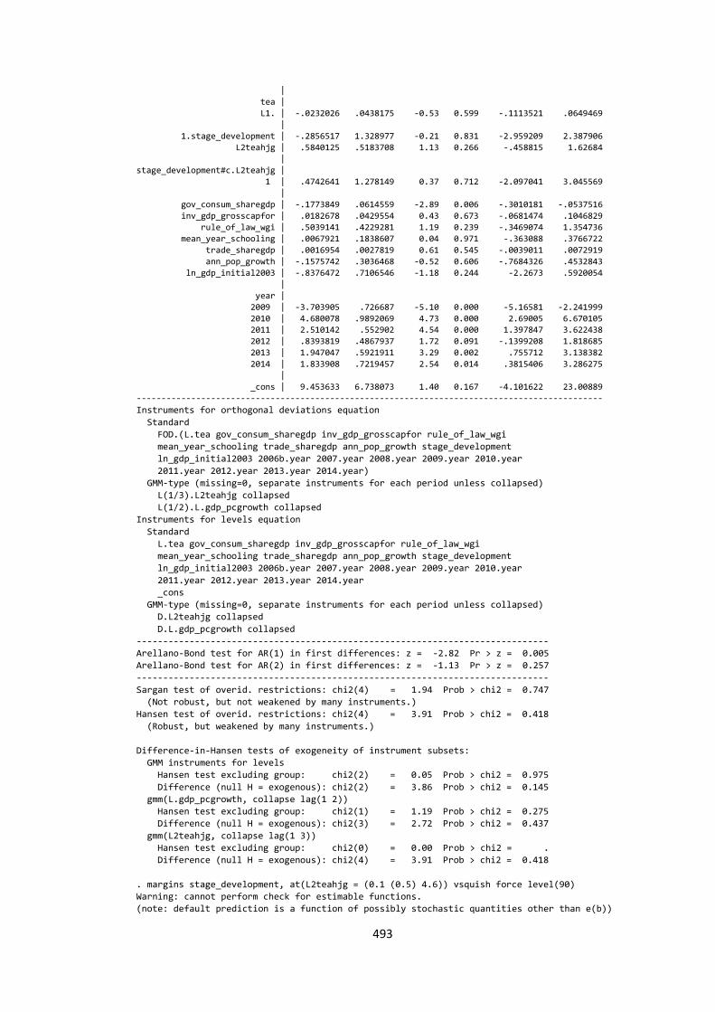
493
|
tea |
L1. | -.0232026 .0438175 -0.53 0.599 -.1113521 .0649469
|
1.stage_development | -.2856517 1.328977 -0.21 0.831 -2.959209 2.387906
L2teahjg | .5840125 .5183708 1.13 0.266 -.458815 1.62684
|
stage_development#c.L2teahjg |
1 | .4742641 1.278149 0.37 0.712 -2.097041 3.045569
|
gov_consum_sharegdp | -.1773849 .0614559 -2.89 0.006 -.3010181 -.0537516
inv_gdp_grosscapfor | .0182678 .0429554 0.43 0.673 -.0681474 .1046829
rule_of_law_wgi | .5039141 .4229281 1.19 0.239 -.3469074 1.354736
mean_year_schooling | .0067921 .1838607 0.04 0.971 -.363088 .3766722
trade_sharegdp | .0016954 .0027819 0.61 0.545 -.0039011 .0072919
ann_pop_growth | -.1575742 .3036468 -0.52 0.606 -.7684326 .4532843
ln_gdp_initial2003 | -.8376472 .7106546 -1.18 0.244 -2.2673 .5920054
|
year |
2009 | -3.703905 .726687 -5.10 0.000 -5.16581 -2.241999
2010 | 4.680078 .9892069 4.73 0.000 2.69005 6.670105 2011 | 2.510142 .552902 4.54 0.000 1.397847 3.622438
2012 | .8393819 .4867937 1.72 0.091 -.1399208 1.818685
2013 | 1.947047 .5921911 3.29 0.002 .755712 3.138382
2014 | 1.833908 .7219457 2.54 0.014 .3815406 3.286275
|
_cons | 9.453633 6.738073 1.40 0.167 -4.101622 23.00889
----------------------------------------------------------------------------------------------
Instruments for orthogonal deviations equation
Standard
FOD.(L.tea gov_consum_sharegdp inv_gdp_grosscapfor rule_of_law_wgi
mean_year_schooling trade_sharegdp ann_pop_growth stage_development
ln_gdp_initial2003 2006b.year 2007.year 2008.year 2009.year 2010.year
2011.year 2012.year 2013.year 2014.year)
GMM-type (missing=0, separate instruments for each period unless collapsed)
L(1/3).L2teahjg collapsed
L(1/2).L.gdp_pcgrowth collapsed
Instruments for levels equation
Standard
L.tea gov_consum_sharegdp inv_gdp_grosscapfor rule_of_law_wgi
mean_year_schooling trade_sharegdp ann_pop_growth stage_development
ln_gdp_initial2003 2006b.year 2007.year 2008.year 2009.year 2010.year
2011.year 2012.year 2013.year 2014.year
_cons
GMM-type (missing=0, separate instruments for each period unless collapsed)
D.L2teahjg collapsed
D.L.gdp_pcgrowth collapsed
------------------------------------------------------------------------------
Arellano-Bond test for AR(1) in first differences: z = -2.82 Pr > z = 0.005
Arellano-Bond test for AR(2) in first differences: z = -1.13 Pr > z = 0.257
------------------------------------------------------------------------------
Sargan test of overid. restrictions: chi2(4) = 1.94 Prob > chi2 = 0.747
(Not robust, but not weakened by many instruments.)
Hansen test of overid. restrictions: chi2(4) = 3.91 Prob > chi2 = 0.418
(Robust, but weakened by many instruments.)
Difference-in-Hansen tests of exogeneity of instrument subsets:
GMM instruments for levels
Hansen test excluding group: chi2(2) = 0.05 Prob > chi2 = 0.975
Difference (null H = exogenous): chi2(2) = 3.86 Prob > chi2 = 0.145
gmm(L.gdp_pcgrowth, collapse lag(1 2))
Hansen test excluding group: chi2(1) = 1.19 Prob > chi2 = 0.275
Difference (null H = exogenous): chi2(3) = 2.72 Prob > chi2 = 0.437
gmm(L2teahjg, collapse lag(1 3))
Hansen test excluding group: chi2(0) = 0.00 Prob > chi2 = .
Difference (null H = exogenous): chi2(4) = 3.91 Prob > chi2 = 0.418
. margins stage_development, at(L2teahjg = (0.1 (0.5) 4.6)) vsquish force level(90)
Warning: cannot perform check for estimable functions.
(note: default prediction is a function of possibly stochastic quantities other than e(b))
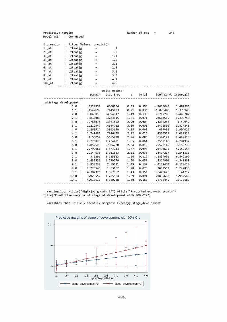
494
Predictive margins Number of obs = 246
Model VCE : Corrected
Expression : Fitted Values, predict()
1._at : L2teahjg = .1
2._at : L2teahjg = .6
3._at : L2teahjg = 1.1
4._at : L2teahjg = 1.6
5._at : L2teahjg = 2.1
6._at : L2teahjg = 2.6
7._at : L2teahjg = 3.1
8._at : L2teahjg = 3.6
9._at : L2teahjg = 4.1
10._at : L2teahjg = 4.6
---------------------------------------------------------------------------------------
| Delta-method
| Margin Std. Err. z P>|z| [90% Conf. Interval]
----------------------+----------------------------------------------------------------
_at#stage_development |
1 0 | .3924952 .6660164 0.59 0.556 -.7030043 1.487995
1 1 | .1542699 .7445483 0.21 0.836 -1.070403 1.378943
2 0 | .6845015 .4594817 1.49 0.136 -.0712786 1.440282
2 1 | .6834083 .3783615 1.81 0.071 .0610589 1.305758
3 0 | .9765078 .3361892 2.90 0.004 .4235258 1.52949
3 1 | 1.212547 .4044712 3.00 0.003 .5472506 1.877843
4 0 | 1.268514 .3863639 3.28 0.001 .633002 1.904026
4 1 | 1.741685 .7846468 2.22 0.026 .4510557 3.032314
5 0 | 1.56052 .5655838 2.76 0.006 .6302177 2.490823
5 1 | 2.270823 1.224491 1.85 0.064 .2567146 4.284932
6 0 | 1.852526 .7904728 2.34 0.019 .5523145 3.152739
6 1 | 2.799961 1.677713 1.67 0.095 .0403695 5.559553
7 0 | 2.144533 1.031583 2.08 0.038 .4477297 3.841336
7 1 | 3.3291 2.135813 1.56 0.119 -.1839996 6.842199
8 0 | 2.436539 1.279779 1.90 0.057 .3314901 4.541588
8 1 | 3.858238 2.59621 1.49 0.137 -.4121474 8.128623
9 0 | 2.728545 1.53162 1.78 0.075 .2092552 5.247835
9 1 | 4.387376 3.057867 1.43 0.151 -.6423673 9.41712
10 0 | 3.020552 1.785564 1.69 0.091 .0835608 5.957542
10 1 | 4.916515 3.520288 1.40 0.163 -.8738442 10.70687
---------------------------------------------------------------------------------------
. marginsplot, xtitle("High-job growth EA") ytitle("Predicted economic growth")
title("Predictive margins of stage of development with 90% CIs")
Variables that uniquely identify margins: L2teahjg stage_development
05
10
Pre
dic
ted e
co
nom
ic g
row
th
.1 .6 1.1 1.6 2.1 2.6 3.1 3.6 4.1 4.6High-job growth EA
stage_development=0 stage_development=1
Predictive margins of stage of development with 90% CIs

495
Chapter 5
APPENDICES
INDIVIDUAL AND INSTITUTIONAL DETERMINANTS OF ENTREPRENEURIAL GROWTH ASPIRATIONS:
A MULTI-COUNTRY ANALYSIS

496
Appendix A Countries and their stage of development
Innovation-driven economies Australia; Austria; Belgium; Canada; Czech Republic;
Denmark; Finland; France; German; Greece; Ireland; Israel;
Italy; Japan; Netherland; Norway; Portugal; Singapore;
Slovakia; Slovenia; South Korea; Spain; Sweden;
Switzerland; Trinidad and Tobago; United Kingdom;
United States
Efficiency-driven economies Argentina; Brazil; Chile; China; Colombia; Costa Rica;
Croatia; Dominican Republic; Ecuador; Estonia; Hungary;
Indonesia; Jamaica; Latvia; Lithuania; Macedonia;
Malaysia; Mexico; Panama; Peru; Poland; Romania; Russia;
Slovakia; South Africa; Thailand; Trinidad and Tobago;
Tunisia; Turkey; Uruguay
Appendix 5.1 Detecting outliers for the main variable of
interest - EGA
. lv emp_growth_asp if age>17 & age<65 & Country_Year!=70103 & Country_Year!=59709 &
Country_Year!=50308 & Country_Year!=50209 & Country_Year!=35209 & Country_Year!=27009 &
Country_Year!=6401
# 27985 New businesses' (young firms) em
---------------------------------
M 13993 | 0 | spread pseudosigma
F 6997 | 0 .3942287 .7884574 | .7884574 .5845168
E 3499 | 0 .6496415 1.299283 | 1.299283 .5647767
D 1750 | 0 .8523741 1.704748 | 1.704748 .5556723
C 875.5 | -.6931472 .6931472 2.079442 | 2.772589 .7443532
B 438 | -.9808292 .7520387 2.484907 | 3.465736 .8046699
A 219.5 | -1.386294 .8291141 3.044523 | 4.430817 .9167173
Z 110 | -1.704748 1.108613 3.921973 | 5.626721 1.058055
Y 55.5 | -2.139874 1.23398 4.607833 | 6.747707 1.17037
X 28 | -2.772589 1.263364 5.299317 | 8.071906 1.3046
1 | -9.779453 -.2845063 9.210441 | 18.98989 2.340282
| |
| | # below # above
inner fence | -1.182686 1.971143 | 242 971
outer fence | -2.365372 3.15383 | 45 186
Appendix 5.2 Pairwise correlation
. xi: pwcorr newemploym_babybus1 age male educ_postgr i.gemhhincome bb_owners work_status
KNOWENT_dum omESTBBUS_dum BUSang_dum suskill_dum estbusrate opportunities L3bussfree L3xcons
L3corruption L3gov_size L1gdppccons2011 L1gdpgrowth if emp_growth_asp>=-2.365372 &
emp_growth_asp<=3.15383 & age>17 & age<65 & Country_Year!=70103 & Country_Year!=59709 &
Country_Year!=50308 & Country_Year!=50209 & Country_Year!=35209 & Country_Year!=27009 &
Country_Year!=6401
i.gemhhincome _Igemhhinco_33-68100(naturally coded; _Igemhhinco_33 omitted)
| newemp~1 age male educ_p~r _Ig~3467 _I~68100 bb_own~s
-------------+---------------------------------------------------------------
newemploym~1 | 1.0000
age | 0.0000 1.0000
male | 0.0920 0.0007 1.0000
educ_postgr | 0.0587 0.0308 0.0204 1.0000
_Igemhh~3467 | -0.0710 -0.0189 -0.0402 -0.0642 1.0000
_Igemh~68100 | 0.1257 -0.0078 0.1012 0.0852 -0.6067 1.0000
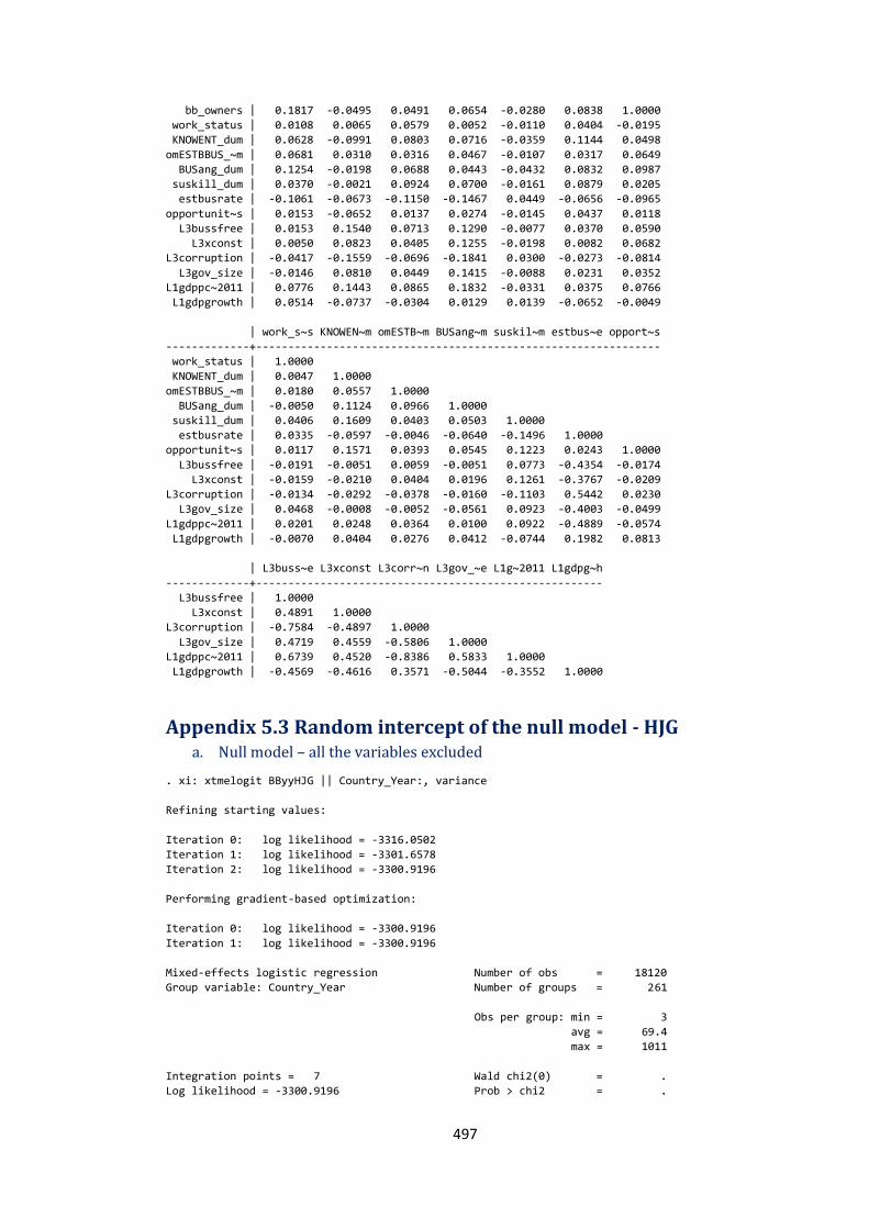
497
bb_owners | 0.1817 -0.0495 0.0491 0.0654 -0.0280 0.0838 1.0000
work_status | 0.0108 0.0065 0.0579 0.0052 -0.0110 0.0404 -0.0195
KNOWENT_dum | 0.0628 -0.0991 0.0803 0.0716 -0.0359 0.1144 0.0498
omESTBBUS_~m | 0.0681 0.0310 0.0316 0.0467 -0.0107 0.0317 0.0649
BUSang_dum | 0.1254 -0.0198 0.0688 0.0443 -0.0432 0.0832 0.0987
suskill_dum | 0.0370 -0.0021 0.0924 0.0700 -0.0161 0.0879 0.0205
estbusrate | -0.1061 -0.0673 -0.1150 -0.1467 0.0449 -0.0656 -0.0965
opportunit~s | 0.0153 -0.0652 0.0137 0.0274 -0.0145 0.0437 0.0118
L3bussfree | 0.0153 0.1540 0.0713 0.1290 -0.0077 0.0370 0.0590
L3xconst | 0.0050 0.0823 0.0405 0.1255 -0.0198 0.0082 0.0682
L3corruption | -0.0417 -0.1559 -0.0696 -0.1841 0.0300 -0.0273 -0.0814
L3gov_size | -0.0146 0.0810 0.0449 0.1415 -0.0088 0.0231 0.0352
L1gdppc~2011 | 0.0776 0.1443 0.0865 0.1832 -0.0331 0.0375 0.0766
L1gdpgrowth | 0.0514 -0.0737 -0.0304 0.0129 0.0139 -0.0652 -0.0049
| work_s~s KNOWEN~m omESTB~m BUSang~m suskil~m estbus~e opport~s
-------------+---------------------------------------------------------------
work_status | 1.0000
KNOWENT_dum | 0.0047 1.0000
omESTBBUS_~m | 0.0180 0.0557 1.0000
BUSang_dum | -0.0050 0.1124 0.0966 1.0000
suskill_dum | 0.0406 0.1609 0.0403 0.0503 1.0000
estbusrate | 0.0335 -0.0597 -0.0046 -0.0640 -0.1496 1.0000
opportunit~s | 0.0117 0.1571 0.0393 0.0545 0.1223 0.0243 1.0000
L3bussfree | -0.0191 -0.0051 0.0059 -0.0051 0.0773 -0.4354 -0.0174
L3xconst | -0.0159 -0.0210 0.0404 0.0196 0.1261 -0.3767 -0.0209
L3corruption | -0.0134 -0.0292 -0.0378 -0.0160 -0.1103 0.5442 0.0230
L3gov_size | 0.0468 -0.0008 -0.0052 -0.0561 0.0923 -0.4003 -0.0499
L1gdppc~2011 | 0.0201 0.0248 0.0364 0.0100 0.0922 -0.4889 -0.0574
L1gdpgrowth | -0.0070 0.0404 0.0276 0.0412 -0.0744 0.1982 0.0813
| L3buss~e L3xconst L3corr~n L3gov_~e L1g~2011 L1gdpg~h
-------------+------------------------------------------------------
L3bussfree | 1.0000
L3xconst | 0.4891 1.0000
L3corruption | -0.7584 -0.4897 1.0000
L3gov_size | 0.4719 0.4559 -0.5806 1.0000
L1gdppc~2011 | 0.6739 0.4520 -0.8386 0.5833 1.0000
L1gdpgrowth | -0.4569 -0.4616 0.3571 -0.5044 -0.3552 1.0000
Appendix 5.3 Random intercept of the null model - HJG a. Null model – all the variables excluded
. xi: xtmelogit BByyHJG || Country_Year:, variance
Refining starting values:
Iteration 0: log likelihood = -3316.0502
Iteration 1: log likelihood = -3301.6578
Iteration 2: log likelihood = -3300.9196
Performing gradient-based optimization:
Iteration 0: log likelihood = -3300.9196
Iteration 1: log likelihood = -3300.9196
Mixed-effects logistic regression Number of obs = 18120
Group variable: Country_Year Number of groups = 261
Obs per group: min = 3
avg = 69.4
max = 1011
Integration points = 7 Wald chi2(0) = .
Log likelihood = -3300.9196 Prob > chi2 = .
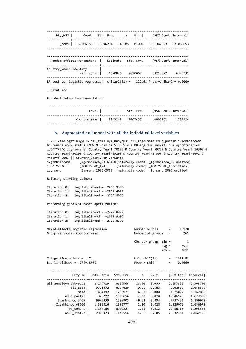
498
------------------------------------------------------------------------------
BByyHJG | Coef. Std. Err. z P>|z| [95% Conf. Interval]
-------------+----------------------------------------------------------------
_cons | -3.206158 .0696264 -46.05 0.000 -3.342623 -3.069693
------------------------------------------------------------------------------
------------------------------------------------------------------------------
Random-effects Parameters | Estimate Std. Err. [95% Conf. Interval]
-----------------------------+------------------------------------------------
Country_Year: Identity |
var(_cons) | .4670826 .0890062 .3215072 .6785731
------------------------------------------------------------------------------
LR test vs. logistic regression: chibar2(01) = 222.68 Prob>=chibar2 = 0.0000
. estat icc
Residual intraclass correlation
------------------------------------------------------------------------------
Level | ICC Std. Err. [95% Conf. Interval]
-----------------------------+------------------------------------------------
Country_Year | .1243249 .0207457 .0890262 .1709924
------------------------------------------------------------------------------
b. Augmented null model with all the individual-level variables
. xi: xtmelogit BByyHJG all_zemploym_babybus1 all_zage male educ_postgr i.gemhhincome
bb_owners work_status KNOWENT_dum omESTBBUS_dum BUSang_dum suskill_dum opportunities
i.OMTYPE4C i.yrsurv if Country_Year!=70103 & Country_Year!=59709 & Country_Year!=50308 &
Country_Year!=50209 & Country_Year!=35209 & Country_Year!=27009 & Country_Year!=6401 &
yrsurv>=2006 || Country_Year:, or variance
i.gemhhincome _Igemhhinco_33-68100(naturally coded; _Igemhhinco_33 omitted)
i.OMTYPE4C _IOMTYPE4C_1-4 (naturally coded; _IOMTYPE4C_1 omitted)
i.yrsurv _Iyrsurv_2006-2013 (naturally coded; _Iyrsurv_2006 omitted)
Refining starting values:
Iteration 0: log likelihood = -2753.9353
Iteration 1: log likelihood = -2732.4021
Iteration 2: log likelihood = -2729.8972
Performing gradient-based optimization:
Iteration 0: log likelihood = -2729.8972
Iteration 1: log likelihood = -2729.8605
Iteration 2: log likelihood = -2729.8605
Mixed-effects logistic regression Number of obs = 18120
Group variable: Country_Year Number of groups = 261
Obs per group: min = 3
avg = 69.4
max = 1011
Integration points = 7 Wald chi2(23) = 1058.58
Log likelihood = -2729.8605 Prob > chi2 = 0.0000
---------------------------------------------------------------------------------------
BByyHJG | Odds Ratio Std. Err. z P>|z| [95% Conf. Interval]
----------------------+----------------------------------------------------------------
all_zemploym_babybus1 | 2.179719 .0639566 26.56 0.000 2.057903 2.308746
all_zage | .9781472 .0394029 -0.55 0.583 .903889 1.058506
male | 1.484892 .1299927 4.52 0.000 1.25077 1.762836
educ_postgr | 1.325222 .1598656 2.33 0.020 1.046178 1.678695
_Igemhhinco_3467 | .9990839 .1302905 -0.01 0.994 .7737431 1.290052
_Igemhhinco_68100 | 1.305816 .1586777 2.20 0.028 1.029076 1.656978
bb_owners | 1.107105 .0902227 1.25 0.212 .9436716 1.298844
work_status | .7328073 .140516 -1.62 0.105 .5032361 1.067107

499
KNOWENT_dum | 1.692496 .1553389 5.73 0.000 1.413851 2.026058
omESTBBUS_dum | 2.317886 .393532 4.95 0.000 1.661784 3.233029
BUSang_dum | 1.481811 .1620095 3.60 0.000 1.195995 1.835932
suskill_dum | 1.297748 .1675133 2.02 0.043 1.007667 1.671334
opportunities | 1.664502 .1440685 5.89 0.000 1.404785 1.972236
_IOMTYPE4C_2 | .9892173 .1937392 -0.06 0.956 .6738807 1.452113
_IOMTYPE4C_3 | .8982376 .1823249 -0.53 0.597 .6034117 1.337115
_IOMTYPE4C_4 | .8031627 .15517 -1.13 0.257 .5499871 1.172883
_Iyrsurv_2007 | 1.565974 .4534933 1.55 0.121 .8877357 2.762394
_Iyrsurv_2008 | 1.17247 .3274897 0.57 0.569 .6781842 2.027011
_Iyrsurv_2009 | 1.356942 .3922458 1.06 0.291 .7700306 2.391194
_Iyrsurv_2010 | 1.01294 .2702748 0.05 0.962 .6004328 1.708847
_Iyrsurv_2011 | 1.224803 .3148972 0.79 0.430 .7399839 2.027265
_Iyrsurv_2012 | .9962058 .2493895 -0.02 0.988 .6099017 1.62719
_Iyrsurv_2013 | 1.212065 .2916239 0.80 0.424 .7563553 1.942342
_cons | .0085103 .0029863 -13.58 0.000 .0042782 .016929
---------------------------------------------------------------------------------------
------------------------------------------------------------------------------
Random-effects Parameters | Estimate Std. Err. [95% Conf. Interval]
-----------------------------+------------------------------------------------
Country_Year: Identity |
var(_cons) | .368087 .0844397 .2347922 .5770551
------------------------------------------------------------------------------
LR test vs. logistic regression: chibar2(01) = 96.09 Prob>=chibar2 = 0.0000
. estat icc
Residual intraclass correlation
------------------------------------------------------------------------------
Level | ICC Std. Err. [95% Conf. Interval]
-----------------------------+------------------------------------------------
Country_Year | .1006264 .020761 .0666141 .1492285
------------------------------------------------------------------------------
c. Model 1 with all the variables
. xi: xtmelogit BByyHJG all_zemploym_babybus1 all_zage male educ_postgr i.gemhhincome
bb_owners work_status KNOWENT_dum omESTBBUS_dum BUSang_dum suskill_dum all_zestbusrate
opportunities all_zmeduc_postgr all_zmhhinc all_zmKNOWENT_dum all_zmomESTBBUS_dum
all_zhighgrowth_support all_zL3bussfree all_zL3xcons all_zL3gov_size all_zL1gdppccons2011
all_zL1gdppccons2011sq all_zL1gdpgrowth i.OMTYPE4C i.yrsurv if Country_Year!=70103 &
Country_Year!=59709 & Country_Year!=50308 & Country_Year!=50209 & Country_Year!=35209 &
Country_Year!=27009 & Country_Year!=6401 & yrsurv>=2006 ||Country_Year:, or variance
i.gemhhincome _Igemhhinco_33-68100(naturally coded; _Igemhhinco_33 omitted)
i.OMTYPE4C _IOMTYPE4C_1-4 (naturally coded; _IOMTYPE4C_1 omitted)
i.yrsurv _Iyrsurv_2006-2013 (naturally coded; _Iyrsurv_2006 omitted)
Refining starting values:
Iteration 0: log likelihood = -2740.3848
Iteration 1: log likelihood = -2723.5897
Iteration 2: log likelihood = -2711.7939
Performing gradient-based optimization:
Iteration 0: log likelihood = -2711.7939
Iteration 1: log likelihood = -2709.2668
Iteration 2: log likelihood = -2709.1034
Iteration 3: log likelihood = -2709.1031
Iteration 4: log likelihood = -2709.1031
Mixed-effects logistic regression Number of obs = 18120
Group variable: Country_Year Number of groups = 261
Obs per group: min = 3
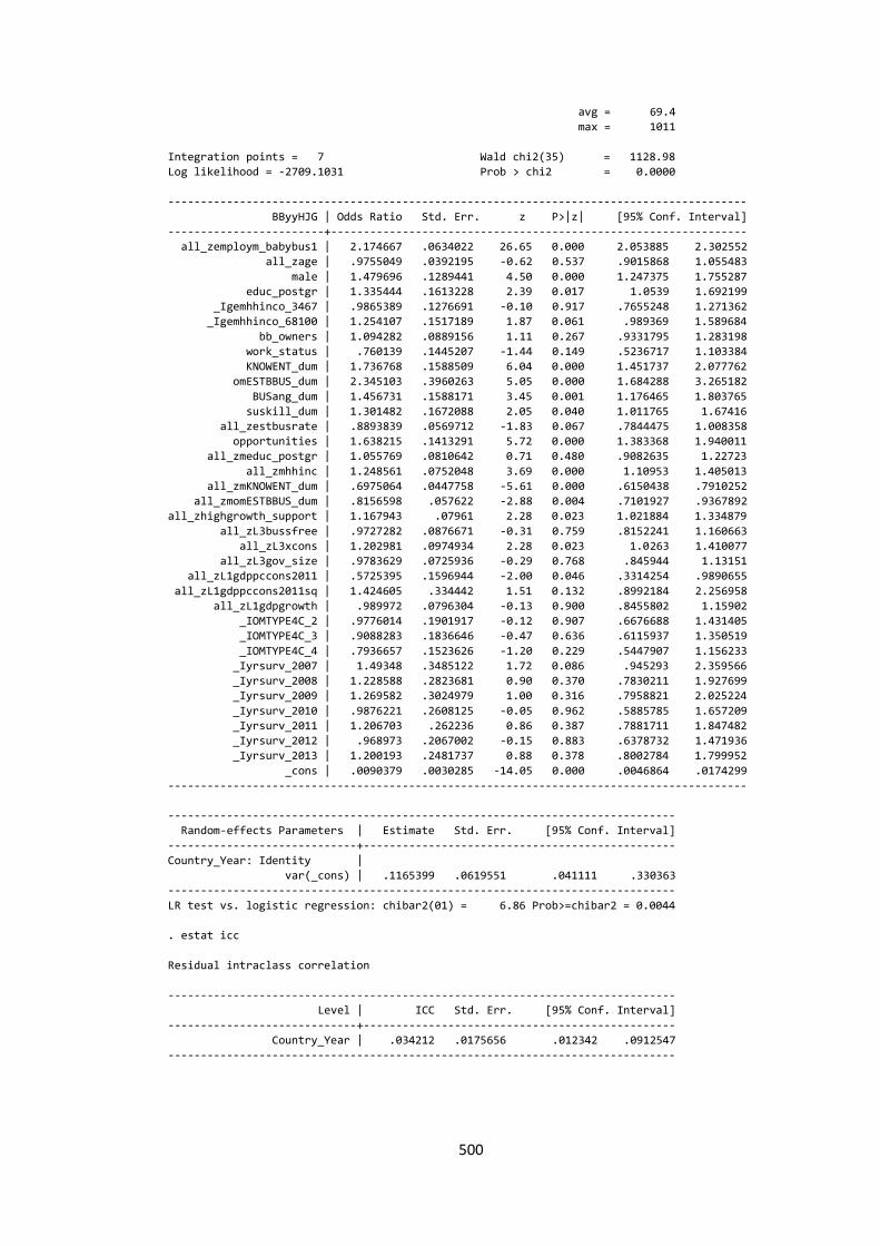
500
avg = 69.4
max = 1011
Integration points = 7 Wald chi2(35) = 1128.98
Log likelihood = -2709.1031 Prob > chi2 = 0.0000
-----------------------------------------------------------------------------------------
BByyHJG | Odds Ratio Std. Err. z P>|z| [95% Conf. Interval]
------------------------+----------------------------------------------------------------
all_zemploym_babybus1 | 2.174667 .0634022 26.65 0.000 2.053885 2.302552
all_zage | .9755049 .0392195 -0.62 0.537 .9015868 1.055483
male | 1.479696 .1289441 4.50 0.000 1.247375 1.755287
educ_postgr | 1.335444 .1613228 2.39 0.017 1.0539 1.692199
_Igemhhinco_3467 | .9865389 .1276691 -0.10 0.917 .7655248 1.271362
_Igemhhinco_68100 | 1.254107 .1517189 1.87 0.061 .989369 1.589684
bb_owners | 1.094282 .0889156 1.11 0.267 .9331795 1.283198
work_status | .760139 .1445207 -1.44 0.149 .5236717 1.103384
KNOWENT_dum | 1.736768 .1588509 6.04 0.000 1.451737 2.077762
omESTBBUS_dum | 2.345103 .3960263 5.05 0.000 1.684288 3.265182
BUSang_dum | 1.456731 .1588171 3.45 0.001 1.176465 1.803765
suskill_dum | 1.301482 .1672088 2.05 0.040 1.011765 1.67416
all_zestbusrate | .8893839 .0569712 -1.83 0.067 .7844475 1.008358
opportunities | 1.638215 .1413291 5.72 0.000 1.383368 1.940011
all_zmeduc_postgr | 1.055769 .0810642 0.71 0.480 .9082635 1.22723
all_zmhhinc | 1.248561 .0752048 3.69 0.000 1.10953 1.405013
all_zmKNOWENT_dum | .6975064 .0447758 -5.61 0.000 .6150438 .7910252
all_zmomESTBBUS_dum | .8156598 .057622 -2.88 0.004 .7101927 .9367892
all_zhighgrowth_support | 1.167943 .07961 2.28 0.023 1.021884 1.334879
all_zL3bussfree | .9727282 .0876671 -0.31 0.759 .8152241 1.160663
all_zL3xcons | 1.202981 .0974934 2.28 0.023 1.0263 1.410077
all_zL3gov_size | .9783629 .0725936 -0.29 0.768 .845944 1.13151
all_zL1gdppccons2011 | .5725395 .1596944 -2.00 0.046 .3314254 .9890655
all_zL1gdppccons2011sq | 1.424605 .334442 1.51 0.132 .8992184 2.256958
all_zL1gdpgrowth | .989972 .0796304 -0.13 0.900 .8455802 1.15902
_IOMTYPE4C_2 | .9776014 .1901917 -0.12 0.907 .6676688 1.431405
_IOMTYPE4C_3 | .9088283 .1836646 -0.47 0.636 .6115937 1.350519
_IOMTYPE4C_4 | .7936657 .1523626 -1.20 0.229 .5447907 1.156233
_Iyrsurv_2007 | 1.49348 .3485122 1.72 0.086 .945293 2.359566
_Iyrsurv_2008 | 1.228588 .2823681 0.90 0.370 .7830211 1.927699
_Iyrsurv_2009 | 1.269582 .3024979 1.00 0.316 .7958821 2.025224
_Iyrsurv_2010 | .9876221 .2608125 -0.05 0.962 .5885785 1.657209
_Iyrsurv_2011 | 1.206703 .262236 0.86 0.387 .7881711 1.847482
_Iyrsurv_2012 | .968973 .2067002 -0.15 0.883 .6378732 1.471936
_Iyrsurv_2013 | 1.200193 .2481737 0.88 0.378 .8002784 1.799952
_cons | .0090379 .0030285 -14.05 0.000 .0046864 .0174299
-----------------------------------------------------------------------------------------
------------------------------------------------------------------------------
Random-effects Parameters | Estimate Std. Err. [95% Conf. Interval]
-----------------------------+------------------------------------------------
Country_Year: Identity |
var(_cons) | .1165399 .0619551 .041111 .330363
------------------------------------------------------------------------------
LR test vs. logistic regression: chibar2(01) = 6.86 Prob>=chibar2 = 0.0044
. estat icc
Residual intraclass correlation
------------------------------------------------------------------------------
Level | ICC Std. Err. [95% Conf. Interval]
-----------------------------+------------------------------------------------
Country_Year | .034212 .0175656 .012342 .0912547
------------------------------------------------------------------------------

501
Appendix 5.3.1 Random intercept of the null model - EGA
a. Null model
. xi: xtmixed all_zemp_growth_asp if insampm==1 || Country_Year:, mle
Performing EM optimization:
Performing gradient-based optimization:
Iteration 0: log likelihood = -24458.442
Iteration 1: log likelihood = -24458.442
Computing standard errors:
Mixed-effects ML regression Number of obs = 17579
Group variable: Country_Year Number of groups = 295
Obs per group: min = 2
avg = 59.6
max = 840
Wald chi2(0) = .
Log likelihood = -24458.442 Prob > chi2 = .
-------------------------------------------------------------------------------------
all_zemp_growth_asp | Coef. Std. Err. z P>|z| [95% Conf. Interval]
--------------------+----------------------------------------------------------------
_cons | -.0238429 .017932 -1.33 0.184 -.058989 .0113032
-------------------------------------------------------------------------------------
------------------------------------------------------------------------------
Random-effects Parameters | Estimate Std. Err. [95% Conf. Interval]
-----------------------------+------------------------------------------------
Country_Year: Identity |
sd(_cons) | .2450013 .0152043 .2169425 .2766892
-----------------------------+------------------------------------------------
sd(Residual) | .9629512 .0051752 .9528612 .9731481
------------------------------------------------------------------------------
LR test vs. linear regression: chibar2(01) = 1004.56 Prob >= chibar2 = 0.0000
. estat icc
Intraclass correlation
------------------------------------------------------------------------------
Level | ICC Std. Err. [95% Conf. Interval]
-----------------------------+------------------------------------------------
Country_Year | .0607977 .0071367 .0482254 .0763846
------------------------------------------------------------------------------
Appendix 5.4 Multicollinearity test
. collin emp_growth_asp employm_babybus1 age male educ_postgr gemhhincome bb_owners
work_status KNOWENT_dum omESTBBUS_dum BUSang_dum suskill_dum estbusrate opportunities
meduc_postgr_c mhhinc_c mKNOWENT_dum_c momESTBBUS_dum_c highgrowth_support L3bussfree
L3xcons L3gov_size L3corruption L1gdppccons2011 L1gdpgrowth if emp_growth_asp>=-2.365372 &
emp_growth_asp<=3.15383 & age>17 & age<65 & Country_Year!=70103 & Country_Year!=59709 &
Country_Year!=50308 & Country_Year!=50209 & Country_Year!=35209 & Country_Year!=27009 &
Country_Year!=6401
(obs=18143)
Collinearity Diagnostics
SQRT R-
Variable VIF VIF Tolerance Squared
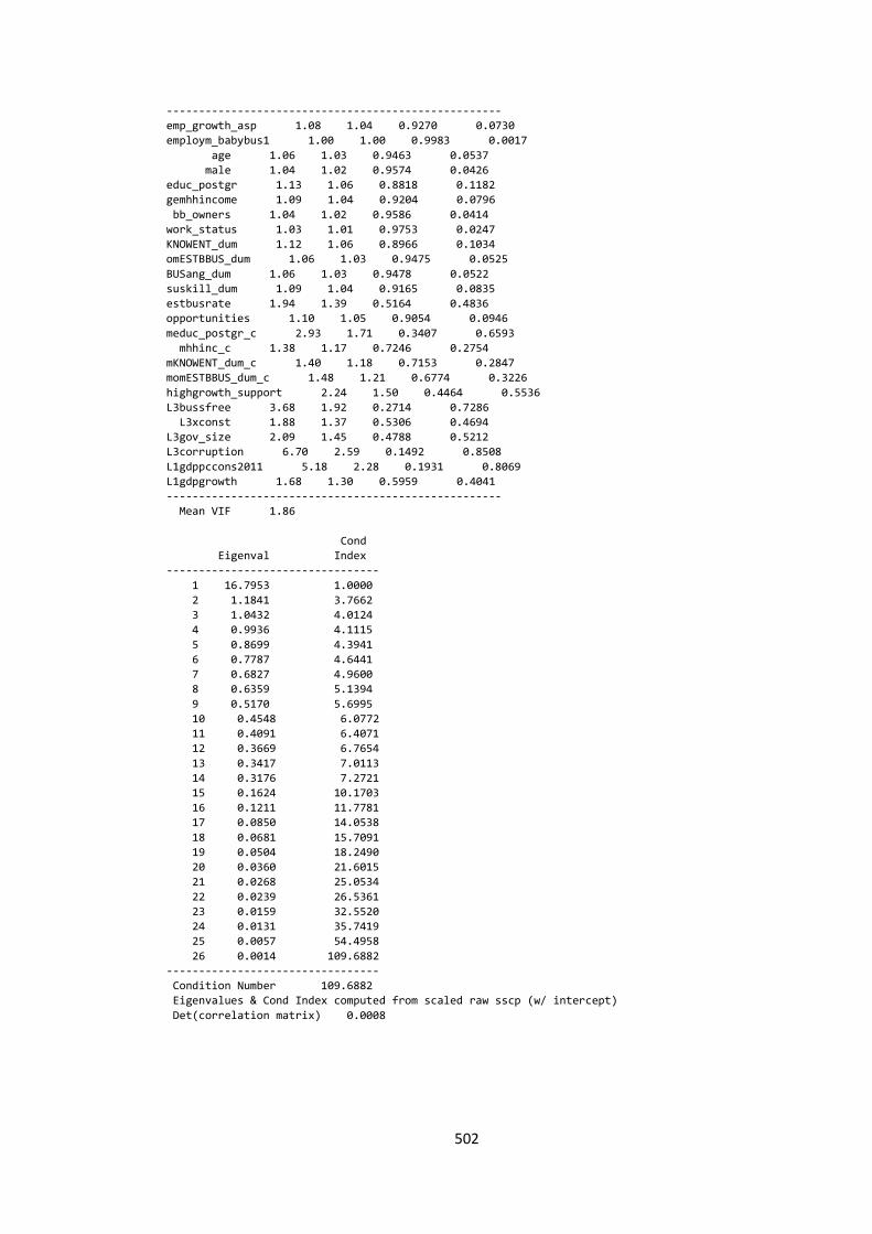
502
----------------------------------------------------
emp_growth_asp 1.08 1.04 0.9270 0.0730
employm_babybus1 1.00 1.00 0.9983 0.0017
age 1.06 1.03 0.9463 0.0537
male 1.04 1.02 0.9574 0.0426
educ_postgr 1.13 1.06 0.8818 0.1182
gemhhincome 1.09 1.04 0.9204 0.0796
bb_owners 1.04 1.02 0.9586 0.0414
work_status 1.03 1.01 0.9753 0.0247
KNOWENT_dum 1.12 1.06 0.8966 0.1034
omESTBBUS_dum 1.06 1.03 0.9475 0.0525
BUSang_dum 1.06 1.03 0.9478 0.0522
suskill_dum 1.09 1.04 0.9165 0.0835
estbusrate 1.94 1.39 0.5164 0.4836
opportunities 1.10 1.05 0.9054 0.0946
meduc_postgr_c 2.93 1.71 0.3407 0.6593
mhhinc_c 1.38 1.17 0.7246 0.2754
mKNOWENT_dum_c 1.40 1.18 0.7153 0.2847
momESTBBUS_dum_c 1.48 1.21 0.6774 0.3226
highgrowth_support 2.24 1.50 0.4464 0.5536
L3bussfree 3.68 1.92 0.2714 0.7286
L3xconst 1.88 1.37 0.5306 0.4694
L3gov_size 2.09 1.45 0.4788 0.5212
L3corruption 6.70 2.59 0.1492 0.8508
L1gdppccons2011 5.18 2.28 0.1931 0.8069
L1gdpgrowth 1.68 1.30 0.5959 0.4041
----------------------------------------------------
Mean VIF 1.86
Cond
Eigenval Index
---------------------------------
1 16.7953 1.0000
2 1.1841 3.7662
3 1.0432 4.0124
4 0.9936 4.1115
5 0.8699 4.3941
6 0.7787 4.6441
7 0.6827 4.9600
8 0.6359 5.1394
9 0.5170 5.6995
10 0.4548 6.0772
11 0.4091 6.4071
12 0.3669 6.7654
13 0.3417 7.0113
14 0.3176 7.2721
15 0.1624 10.1703
16 0.1211 11.7781
17 0.0850 14.0538
18 0.0681 15.7091
19 0.0504 18.2490
20 0.0360 21.6015
21 0.0268 25.0534
22 0.0239 26.5361
23 0.0159 32.5520
24 0.0131 35.7419
25 0.0057 54.4958
26 0.0014 109.6882
---------------------------------
Condition Number 109.6882
Eigenvalues & Cond Index computed from scaled raw sscp (w/ intercept)
Det(correlation matrix) 0.0008
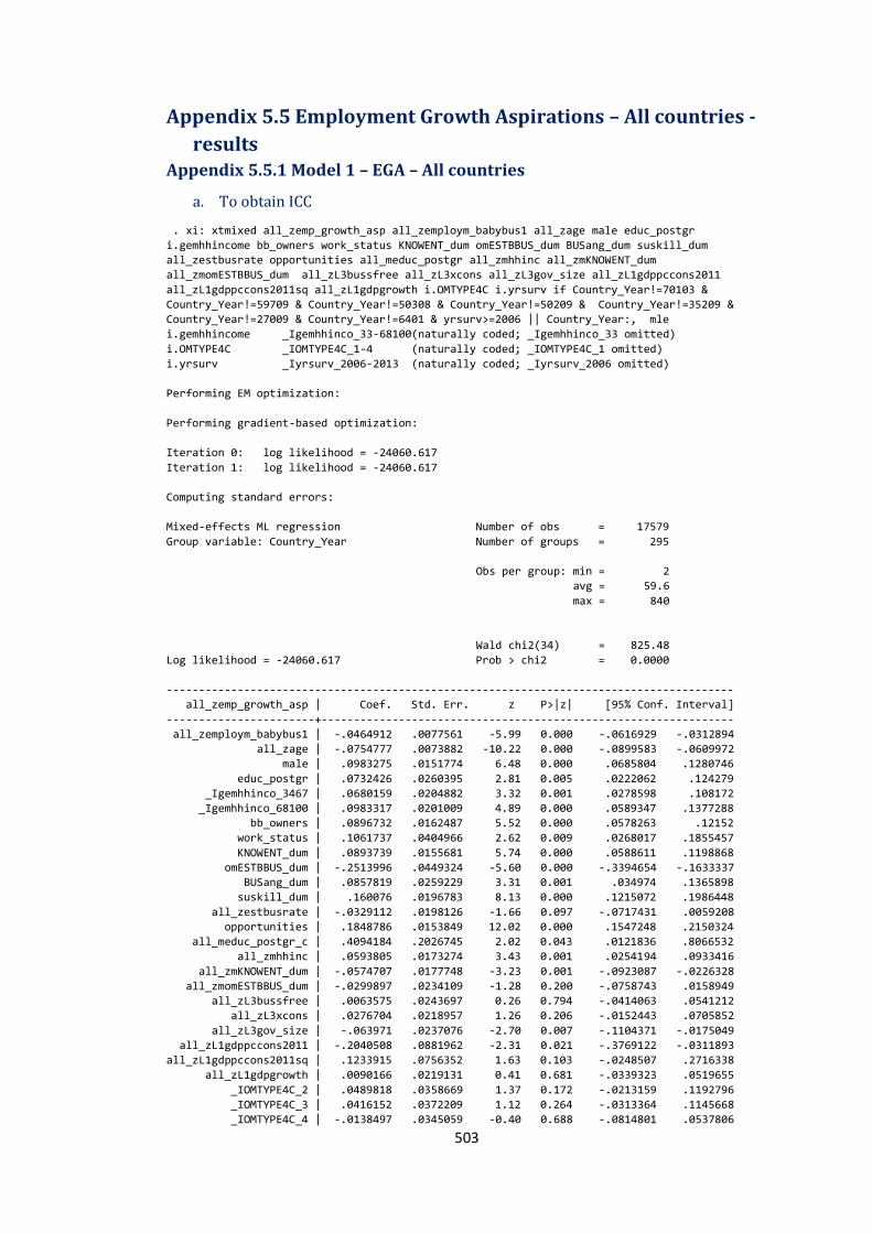
503
Appendix 5.5 Employment Growth Aspirations – All countries -
results Appendix 5.5.1 Model 1 – EGA – All countries
a. To obtain ICC
. xi: xtmixed all_zemp_growth_asp all_zemploym_babybus1 all_zage male educ_postgr
i.gemhhincome bb_owners work_status KNOWENT_dum omESTBBUS_dum BUSang_dum suskill_dum
all_zestbusrate opportunities all_meduc_postgr all_zmhhinc all_zmKNOWENT_dum
all_zmomESTBBUS_dum all_zL3bussfree all_zL3xcons all_zL3gov_size all_zL1gdppccons2011
all_zL1gdppccons2011sq all_zL1gdpgrowth i.OMTYPE4C i.yrsurv if Country_Year!=70103 &
Country_Year!=59709 & Country_Year!=50308 & Country_Year!=50209 & Country_Year!=35209 &
Country_Year!=27009 & Country_Year!=6401 & yrsurv>=2006 || Country_Year:, mle
i.gemhhincome _Igemhhinco_33-68100(naturally coded; _Igemhhinco_33 omitted)
i.OMTYPE4C _IOMTYPE4C_1-4 (naturally coded; _IOMTYPE4C_1 omitted)
i.yrsurv _Iyrsurv_2006-2013 (naturally coded; _Iyrsurv_2006 omitted)
Performing EM optimization:
Performing gradient-based optimization:
Iteration 0: log likelihood = -24060.617
Iteration 1: log likelihood = -24060.617
Computing standard errors:
Mixed-effects ML regression Number of obs = 17579
Group variable: Country_Year Number of groups = 295
Obs per group: min = 2
avg = 59.6
max = 840
Wald chi2(34) = 825.48
Log likelihood = -24060.617 Prob > chi2 = 0.0000
----------------------------------------------------------------------------------------
all_zemp_growth_asp | Coef. Std. Err. z P>|z| [95% Conf. Interval]
-----------------------+----------------------------------------------------------------
all_zemploym_babybus1 | -.0464912 .0077561 -5.99 0.000 -.0616929 -.0312894
all_zage | -.0754777 .0073882 -10.22 0.000 -.0899583 -.0609972
male | .0983275 .0151774 6.48 0.000 .0685804 .1280746
educ_postgr | .0732426 .0260395 2.81 0.005 .0222062 .124279
_Igemhhinco_3467 | .0680159 .0204882 3.32 0.001 .0278598 .108172
_Igemhhinco_68100 | .0983317 .0201009 4.89 0.000 .0589347 .1377288
bb_owners | .0896732 .0162487 5.52 0.000 .0578263 .12152
work_status | .1061737 .0404966 2.62 0.009 .0268017 .1855457
KNOWENT_dum | .0893739 .0155681 5.74 0.000 .0588611 .1198868
omESTBBUS_dum | -.2513996 .0449324 -5.60 0.000 -.3394654 -.1633337
BUSang_dum | .0857819 .0259229 3.31 0.001 .034974 .1365898
suskill_dum | .160076 .0196783 8.13 0.000 .1215072 .1986448
all_zestbusrate | -.0329112 .0198126 -1.66 0.097 -.0717431 .0059208
opportunities | .1848786 .0153849 12.02 0.000 .1547248 .2150324
all_meduc_postgr_c | .4094184 .2026745 2.02 0.043 .0121836 .8066532
all_zmhhinc | .0593805 .0173274 3.43 0.001 .0254194 .0933416
all_zmKNOWENT_dum | -.0574707 .0177748 -3.23 0.001 -.0923087 -.0226328
all_zmomESTBBUS_dum | -.0299897 .0234109 -1.28 0.200 -.0758743 .0158949
all_zL3bussfree | .0063575 .0243697 0.26 0.794 -.0414063 .0541212
all_zL3xcons | .0276704 .0218957 1.26 0.206 -.0152443 .0705852
all_zL3gov_size | -.063971 .0237076 -2.70 0.007 -.1104371 -.0175049
all_zL1gdppccons2011 | -.2040508 .0881962 -2.31 0.021 -.3769122 -.0311893
all_zL1gdppccons2011sq | .1233915 .0756352 1.63 0.103 -.0248507 .2716338
all_zL1gdpgrowth | .0090166 .0219131 0.41 0.681 -.0339323 .0519655
_IOMTYPE4C_2 | .0489818 .0358669 1.37 0.172 -.0213159 .1192796
_IOMTYPE4C_3 | .0416152 .0372209 1.12 0.264 -.0313364 .1145668
_IOMTYPE4C_4 | -.0138497 .0345059 -0.40 0.688 -.0814801 .0537806

504
_Iyrsurv_2007 | -.0095591 .0687278 -0.14 0.889 -.1442632 .1251449
_Iyrsurv_2008 | -.1270394 .0686227 -1.85 0.064 -.2615375 .0074586
_Iyrsurv_2009 | -.0810237 .0710824 -1.14 0.254 -.2203426 .0582953
_Iyrsurv_2010 | -.0396726 .0752447 -0.53 0.598 -.1871495 .1078044
_Iyrsurv_2011 | -.0523109 .0623381 -0.84 0.401 -.1744914 .0698695
_Iyrsurv_2012 | -.0992005 .0605917 -1.64 0.102 -.2179579 .019557
_Iyrsurv_2013 | -.0836403 .0613374 -1.36 0.173 -.2038595 .0365789
_cons | -.58306 .0761954 -7.65 0.000 -.7324002 -.4337199
----------------------------------------------------------------------------------------
------------------------------------------------------------------------------
Random-effects Parameters | Estimate Std. Err. [95% Conf. Interval]
-----------------------------+------------------------------------------------
Country_Year: Identity |
sd(_cons) | .194967 .0143272 .1688147 .2251708
-----------------------------+------------------------------------------------
sd(Residual) | .9433501 .0050722 .9334609 .9533441
------------------------------------------------------------------------------
LR test vs. linear regression: chibar2(01) = 330.44 Prob >= chibar2 = 0.0000
. estat icc
Residual intraclass correlation
------------------------------------------------------------------------------
Level | ICC Std. Err. [95% Conf. Interval]
-----------------------------+------------------------------------------------
Country_Year | .0409648 .0058125 .0309725 .0540011
------------------------------------------------------------------------------
b. Model 1 – results (robust – Standard Errors)
. xi: xtmixed all_zemp_growth_asp all_zemploym_babybus1 all_zage male educ_postgr
i.gemhhincome bb_owners work_status KNOWENT_dum omESTBBUS_dum BUSang_dum suskill_dum
all_zestbusrate opportunities all_meduc_postgr all_zmhhinc all_zmKNOWENT_dum
all_zmomESTBBUS_dum all_zL3bussfree all_zL3xcons all_zL3gov_size all_zL1gdppccons2011
all_zL1gdppccons2011sq all_zL1gdpgrowth i.OMTYPE4C i.yrsurv if Country_Year!=70103 &
Country_Year!=59709 & Country_Year!=50308 & Country_Year!=50209 & Country_Year!=35209 &
Country_Year!=27009 & Country_Year!=6401 & yrsurv>=2006 || Country_Year:, mle vce(robust)
i.gemhhincome _Igemhhinco_33-68100(naturally coded; _Igemhhinco_33 omitted)
i.OMTYPE4C _IOMTYPE4C_1-4 (naturally coded; _IOMTYPE4C_1 omitted)
i.yrsurv _Iyrsurv_2006-2013 (naturally coded; _Iyrsurv_2006 omitted)
Performing EM optimization:
Performing gradient-based optimization:
Iteration 0: log pseudolikelihood = -24060.617
Iteration 1: log pseudolikelihood = -24060.617
Computing standard errors:
Mixed-effects regression Number of obs = 17579
Group variable: Country_Year Number of groups = 295
Obs per group: min = 2
avg = 59.6
max = 840
Wald chi2(34) = 674.60
Log pseudolikelihood = -24060.617 Prob > chi2 = 0.0000
(Std. Err. adjusted for 295 clusters in Country_Year)
----------------------------------------------------------------------------------------
| Robust
all_zemp_growth_asp | Coef. Std. Err. z P>|z| [95% Conf. Interval]
-----------------------+----------------------------------------------------------------
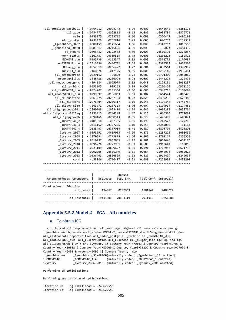
505
all_zemploym_babybus1 | -.0464912 .0093743 -4.96 0.000 -.0648645 -.0281178
all_zage | -.0754777 .0092862 -8.13 0.000 -.0936784 -.0572771
male | .0983275 .0215732 4.56 0.000 .0560449 .1406102
educ_postgr | .0732426 .0267814 2.73 0.006 .020752 .1257332
_Igemhhinco_3467 | .0680159 .0171634 3.96 0.000 .0343762 .1016556
_Igemhhinco_68100 | .0983317 .0245421 4.01 0.000 .05023 .1464335
bb_owners | .0896732 .0192532 4.66 0.000 .0519376 .1274087
work_status | .1061737 .0389555 2.73 0.006 .0298223 .182525
KNOWENT_dum | .0893739 .0153547 5.82 0.000 .0592793 .1194685
omESTBBUS_dum | -.2513996 .0446741 -5.63 0.000 -.3389592 -.1638399
BUSang_dum | .0857819 .0266422 3.22 0.001 .033564 .1379997
suskill_dum | .160076 .017125 9.35 0.000 .1265116 .1936404
all_zestbusrate | -.0329112 .01899 -1.73 0.083 -.0701309 .0043085
opportunities | .1848786 .0206924 8.93 0.000 .1443222 .225435
all_meduc_postgr_c | .4094184 .2025075 2.02 0.043 .0125111 .8063257
all_zmhhinc | .0593805 .019253 3.08 0.002 .0216454 .0971156
all_zmKNOWENT_dum | -.0574707 .0191334 -3.00 0.003 -.0949715 -.0199699
all_zmomESTBBUS_dum | -.0299897 .0186063 -1.61 0.107 -.0664574 .006478
all_zL3bussfree | .0063575 .0287154 0.22 0.825 -.0499236 .0626386
all_zL3xcons | .0276704 .0239317 1.16 0.248 -.0192348 .0745757
all_zL3gov_size | -.063971 .0237363 -2.70 0.007 -.1104934 -.0174486
all_zL1gdppccons2011 | -.2040508 .1025414 -1.99 0.047 -.4050282 -.0030734
all_zL1gdppccons2011sq | .1233915 .0784288 1.57 0.116 -.030326 .2771091
all_zL1gdpgrowth | .0090166 .0260543 0.35 0.729 -.0420489 .0600821
_IOMTYPE4C_2 | .0489818 .037365 1.31 0.190 -.0242523 .122216
_IOMTYPE4C_3 | .0416152 .0357276 1.16 0.244 -.0284096 .11164
_IOMTYPE4C_4 | -.0138497 .0337914 -0.41 0.682 -.0800796 .0523801
_Iyrsurv_2007 | -.0095591 .0609003 -0.16 0.875 -.1289215 .1098032
_Iyrsurv_2008 | -.1270394 .0775898 -1.64 0.102 -.2791127 .0250338
_Iyrsurv_2009 | -.0810237 .0633895 -1.28 0.201 -.2052649 .0432176
_Iyrsurv_2010 | -.0396726 .0773951 -0.51 0.608 -.1913641 .112019
_Iyrsurv_2011 | -.0523109 .0609627 -0.86 0.391 -.1717957 .0671738
_Iyrsurv_2012 | -.0992005 .0536249 -1.85 0.064 -.2043034 .0059024
_Iyrsurv_2013 | -.0836403 .0550539 -1.52 0.129 -.1915439 .0242633
_cons | -.58306 .0710417 -8.21 0.000 -.7222993 -.4438208
----------------------------------------------------------------------------------------
------------------------------------------------------------------------------
| Robust
Random-effects Parameters | Estimate Std. Err. [95% Conf. Interval]
-----------------------------+------------------------------------------------
Country_Year: Identity |
sd(_cons) | .194967 .0207969 .1581847 .2403022
-----------------------------+------------------------------------------------
sd(Residual) | .9433501 .0163119 .911915 .9758688
------------------------------------------------------------------------------
Appendix 5.5.2 Model 2 – EGA – All countries
a. To obtain ICC
. xi: xtmixed all_zemp_growth_asp all_zemploym_babybus1 all_zage male educ_postgr
i.gemhhincome bb_owners work_status KNOWENT_dum omESTBBUS_dum BUSang_dum suskill_dum
all_zestbusrate opportunities all_meduc_postgr all_zmhhinc all_zmKNOWENT_dum
all_zmomESTBBUS_dum all_zL3corruption all_zL3xcons all_zL3gov_size iq2 iq3 iq4 iq5
all_zL1gdpgrowth i.OMTYPE4C i.yrsurv if Country_Year!=70103 & Country_Year!=59709 &
Country_Year!=50308 & Country_Year!=50209 & Country_Year!=35209 & Country_Year!=27009 &
Country_Year!=6401 & yrsurv>=2006 || Country_Year:, mle
i.gemhhincome _Igemhhinco_33-68100(naturally coded; _Igemhhinco_33 omitted)
i.OMTYPE4C _IOMTYPE4C_1-4 (naturally coded; _IOMTYPE4C_1 omitted)
i.yrsurv _Iyrsurv_2006-2013 (naturally coded; _Iyrsurv_2006 omitted)
Performing EM optimization:
Performing gradient-based optimization:
Iteration 0: log likelihood = -24062.556
Iteration 1: log likelihood = -24062.556

506
Computing standard errors:
Mixed-effects ML regression Number of obs = 17579
Group variable: Country_Year Number of groups = 295
Obs per group: min = 2
avg = 59.6
max = 840
Wald chi2(36) = 818.52
Log likelihood = -24062.556 Prob > chi2 = 0.0000
---------------------------------------------------------------------------------------
all_zemp_growth_asp | Coef. Std. Err. z P>|z| [95% Conf. Interval]
----------------------+----------------------------------------------------------------
all_zemploym_babybus1 | -.0466558 .0077586 -6.01 0.000 -.0618623 -.0314492
all_zage | -.0757949 .0073893 -10.26 0.000 -.0902777 -.0613122
male | .0977263 .0151845 6.44 0.000 .0679652 .1274875
educ_postgr | .0718873 .0260434 2.76 0.006 .0208431 .1229315
_Igemhhinco_3467 | .0684529 .0204907 3.34 0.001 .0282918 .108614
_Igemhhinco_68100 | .098835 .0201059 4.92 0.000 .0594283 .1382418
bb_owners | .0899446 .0162466 5.54 0.000 .0581018 .1217874
work_status | .1064677 .0405386 2.63 0.009 .0270135 .1859218
KNOWENT_dum | .0889403 .0155698 5.71 0.000 .058424 .1194567
omESTBBUS_dum | -.2515292 .0449363 -5.60 0.000 -.3396028 -.1634557
BUSang_dum | .0860416 .0259237 3.32 0.001 .0352321 .1368512
suskill_dum | .1607542 .0196795 8.17 0.000 .1221831 .1993254
all_zestbusrate | -.0246416 .020898 -1.18 0.238 -.0656008 .0163177
opportunities | .1858648 .015399 12.07 0.000 .1556833 .2160462
all_meduc_postgr_c | .3309114 .2012516 1.64 0.100 -.0635344 .7253573
all_zmhhinc | .0547525 .0189466 2.89 0.004 .0176178 .0918872
all_zmKNOWENT_dum | -.0482192 .018461 -2.61 0.009 -.0844021 -.0120363
all_zmomESTBBUS_dum | -.0396596 .0255321 -1.55 0.120 -.0897015 .0103823
all_zL3corruption | -.001133 .0324009 -0.03 0.972 -.0646375 .0623716
all_zL3xcons | .0248351 .0221403 1.12 0.262 -.018559 .0682293
all_zL3gov_size | -.079969 .0229674 -3.48 0.000 -.1249843 -.0349538
iq2 | -.0156725 .0548765 -0.29 0.775 -.1232284 .0918835
iq3 | -.0684076 .0718115 -0.95 0.341 -.2091555 .0723404
iq4 | -.066271 .0982434 -0.67 0.500 -.2588245 .1262824
iq5 | -.1513331 .0908004 -1.67 0.096 -.3292986 .0266323
all_zL1gdpgrowth | .0147548 .0221154 0.67 0.505 -.0285905 .0581001
_IOMTYPE4C_2 | .0469567 .0358704 1.31 0.191 -.023348 .1172613
_IOMTYPE4C_3 | .0389005 .0372195 1.05 0.296 -.0340483 .1118493
_IOMTYPE4C_4 | -.0156256 .0345087 -0.45 0.651 -.0832615 .0520103
_Iyrsurv_2007 | -.0122965 .0700194 -0.18 0.861 -.149532 .124939
_Iyrsurv_2008 | -.1330905 .0702888 -1.89 0.058 -.2708539 .004673
_Iyrsurv_2009 | -.0853798 .072722 -1.17 0.240 -.2279124 .0571527
_Iyrsurv_2010 | -.0361336 .0765412 -0.47 0.637 -.1861516 .1138844
_Iyrsurv_2011 | -.0639962 .0634181 -1.01 0.313 -.1882934 .060301
_Iyrsurv_2012 | -.1114385 .0617971 -1.80 0.071 -.2325586 .0096816
_Iyrsurv_2013 | -.0949805 .0627238 -1.51 0.130 -.2179168 .0279559
_cons | -.5196185 .0826215 -6.29 0.000 -.6815536 -.3576835
---------------------------------------------------------------------------------------
------------------------------------------------------------------------------
Random-effects Parameters | Estimate Std. Err. [95% Conf. Interval]
-----------------------------+------------------------------------------------
Country_Year: Identity |
sd(_cons) | .2004885 .0142099 .1744855 .2303667
-----------------------------+------------------------------------------------
sd(Residual) | .9432069 .0050702 .9333217 .9531968
------------------------------------------------------------------------------
LR test vs. linear regression: chibar2(01) = 401.14 Prob >= chibar2 = 0.0000
.
. estat icc
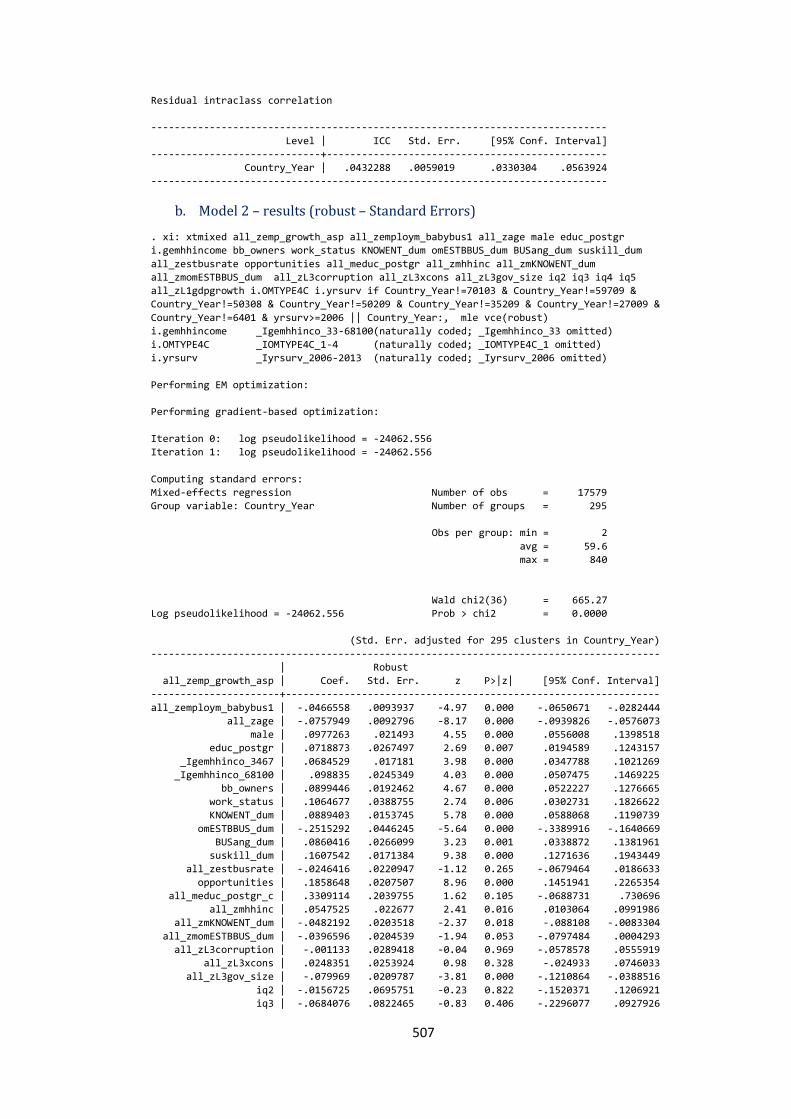
507
Residual intraclass correlation
------------------------------------------------------------------------------
Level | ICC Std. Err. [95% Conf. Interval]
-----------------------------+------------------------------------------------
Country_Year | .0432288 .0059019 .0330304 .0563924
------------------------------------------------------------------------------
b. Model 2 – results (robust – Standard Errors)
. xi: xtmixed all_zemp_growth_asp all_zemploym_babybus1 all_zage male educ_postgr
i.gemhhincome bb_owners work_status KNOWENT_dum omESTBBUS_dum BUSang_dum suskill_dum
all_zestbusrate opportunities all_meduc_postgr all_zmhhinc all_zmKNOWENT_dum
all_zmomESTBBUS_dum all_zL3corruption all_zL3xcons all_zL3gov_size iq2 iq3 iq4 iq5
all_zL1gdpgrowth i.OMTYPE4C i.yrsurv if Country_Year!=70103 & Country_Year!=59709 &
Country_Year!=50308 & Country_Year!=50209 & Country_Year!=35209 & Country_Year!=27009 &
Country_Year!=6401 & yrsurv>=2006 || Country_Year:, mle vce(robust)
i.gemhhincome _Igemhhinco_33-68100(naturally coded; _Igemhhinco_33 omitted)
i.OMTYPE4C _IOMTYPE4C_1-4 (naturally coded; _IOMTYPE4C_1 omitted)
i.yrsurv _Iyrsurv_2006-2013 (naturally coded; _Iyrsurv_2006 omitted)
Performing EM optimization:
Performing gradient-based optimization:
Iteration 0: log pseudolikelihood = -24062.556
Iteration 1: log pseudolikelihood = -24062.556
Computing standard errors:
Mixed-effects regression Number of obs = 17579
Group variable: Country_Year Number of groups = 295
Obs per group: min = 2
avg = 59.6
max = 840
Wald chi2(36) = 665.27
Log pseudolikelihood = -24062.556 Prob > chi2 = 0.0000
(Std. Err. adjusted for 295 clusters in Country_Year)
---------------------------------------------------------------------------------------
| Robust
all_zemp_growth_asp | Coef. Std. Err. z P>|z| [95% Conf. Interval]
----------------------+----------------------------------------------------------------
all_zemploym_babybus1 | -.0466558 .0093937 -4.97 0.000 -.0650671 -.0282444
all_zage | -.0757949 .0092796 -8.17 0.000 -.0939826 -.0576073
male | .0977263 .021493 4.55 0.000 .0556008 .1398518
educ_postgr | .0718873 .0267497 2.69 0.007 .0194589 .1243157
_Igemhhinco_3467 | .0684529 .017181 3.98 0.000 .0347788 .1021269
_Igemhhinco_68100 | .098835 .0245349 4.03 0.000 .0507475 .1469225
bb_owners | .0899446 .0192462 4.67 0.000 .0522227 .1276665
work_status | .1064677 .0388755 2.74 0.006 .0302731 .1826622
KNOWENT_dum | .0889403 .0153745 5.78 0.000 .0588068 .1190739
omESTBBUS_dum | -.2515292 .0446245 -5.64 0.000 -.3389916 -.1640669
BUSang_dum | .0860416 .0266099 3.23 0.001 .0338872 .1381961
suskill_dum | .1607542 .0171384 9.38 0.000 .1271636 .1943449
all_zestbusrate | -.0246416 .0220947 -1.12 0.265 -.0679464 .0186633
opportunities | .1858648 .0207507 8.96 0.000 .1451941 .2265354
all_meduc_postgr_c | .3309114 .2039755 1.62 0.105 -.0688731 .730696
all_zmhhinc | .0547525 .022677 2.41 0.016 .0103064 .0991986
all_zmKNOWENT_dum | -.0482192 .0203518 -2.37 0.018 -.088108 -.0083304
all_zmomESTBBUS_dum | -.0396596 .0204539 -1.94 0.053 -.0797484 .0004293
all_zL3corruption | -.001133 .0289418 -0.04 0.969 -.0578578 .0555919
all_zL3xcons | .0248351 .0253924 0.98 0.328 -.024933 .0746033
all_zL3gov_size | -.079969 .0209787 -3.81 0.000 -.1210864 -.0388516
iq2 | -.0156725 .0695751 -0.23 0.822 -.1520371 .1206921
iq3 | -.0684076 .0822465 -0.83 0.406 -.2296077 .0927926
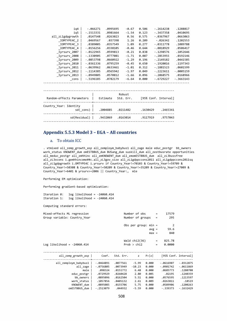
508
iq4 | -.066271 .0995695 -0.67 0.506 -.2614238 .1288817
iq5 | -.1513331 .0981664 -1.54 0.123 -.3437358 .0410695
all_zL1gdpgrowth | .0147548 .0263023 0.56 0.575 -.0367967 .0663063
_IOMTYPE4C_2 | .0469567 .037398 1.26 0.209 -.026342 .1202553
_IOMTYPE4C_3 | .0389005 .0357549 1.09 0.277 -.0311778 .1089788
_IOMTYPE4C_4 | -.0156256 .0338105 -0.46 0.644 -.0818929 .0506417
_Iyrsurv_2007 | -.0122965 .0599813 -0.21 0.838 -.1298576 .1052646
_Iyrsurv_2008 | -.1330905 .0777081 -1.71 0.087 -.2853955 .0192146
_Iyrsurv_2009 | -.0853798 .0660922 -1.29 0.196 -.2149182 .0441585
_Iyrsurv_2010 | -.0361336 .0795259 -0.45 0.650 -.1920016 .1197343
_Iyrsurv_2011 | -.0639962 .0633461 -1.01 0.312 -.1881523 .0601599
_Iyrsurv_2012 | -.1114385 .0565942 -1.97 0.049 -.2223611 -.0005159
_Iyrsurv_2013 | -.0949805 .0570812 -1.66 0.096 -.2068575 .0168966
_cons | -.5196185 .0782179 -6.64 0.000 -.6729227 -.3663143
---------------------------------------------------------------------------------------
------------------------------------------------------------------------------
| Robust
Random-effects Parameters | Estimate Std. Err. [95% Conf. Interval]
-----------------------------+------------------------------------------------
Country_Year: Identity |
sd(_cons) | .2004885 .0211482 .1630429 .2465341
-----------------------------+------------------------------------------------
sd(Residual) | .9432069 .0163014 .9117919 .9757043
------------------------------------------------------------------------------
Appendix 5.5.3 Model 3 – EGA – All countries
a. To obtain ICC
. xtmixed all_zemp_growth_asp all_zemploym_babybus1 all_zage male educ_postgr bb_owners
work_status KNOWENT_dum omESTBBUS_dum BUSang_dum suskill_dum all_zestbusrate opportunities
all_meduc_postgr all_zmhhinc all_zmKNOWENT_dum all_zmomESTBBUS_dum all_zL3bussfree
all_zL3xcons i.gemhhincome##c.all_zL3gov_size all_zL1gdppccons2011 all_zL1gdppccons2011sq
all_zL1gdpgrowth i.OMTYPE4C i.yrsurv if Country_Year!=70103 & Country_Year!=59709 &
Country_Year!=50308 & Country_Year!=50209 & Country_Year!=35209 & Country_Year!=27009 &
Country_Year!=6401 & yrsurv>=2006 || Country_Year:, mle
Performing EM optimization:
Performing gradient-based optimization:
Iteration 0: log likelihood = -24060.414
Iteration 1: log likelihood = -24060.414
Computing standard errors:
Mixed-effects ML regression Number of obs = 17579
Group variable: Country_Year Number of groups = 295
Obs per group: min = 2
avg = 59.6
max = 840
Wald chi2(36) = 825.78
Log likelihood = -24060.414 Prob > chi2 = 0.0000
-----------------------------------------------------------------------------------------------
all_zemp_growth_asp | Coef. Std. Err. z P>|z| [95% Conf. Interval]
------------------------------+----------------------------------------------------------------
all_zemploym_babybus1 | -.0464891 .0077561 -5.99 0.000 -.0616907 -.0312875
all_zage | -.0756805 .0073949 -10.23 0.000 -.0901742 -.0611869
male | .098324 .0151772 6.48 0.000 .0685773 .1280708
educ_postgr | .0729929 .0260428 2.80 0.005 .02195 .1240359
bb_owners | .0895096 .0162504 5.51 0.000 .0576595 .1213597
work_status | .1057856 .0405132 2.61 0.009 .0263811 .18519
KNOWENT_dum | .0895085 .0155706 5.75 0.000 .0589906 .1200263
omESTBBUS_dum | -.2513079 .044932 -5.59 0.000 -.339373 -.1632429
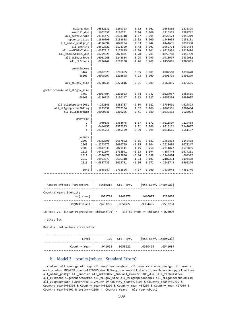
509
BUSang_dum | .0862131 .0259323 3.32 0.001 .0353866 .1370395
suskill_dum | .1602039 .0196791 8.14 0.000 .1216335 .1987742
all_zestbusrate | -.0331477 .0198318 -1.67 0.095 -.0720173 .0057219
opportunities | .1849595 .0153858 12.02 0.000 .1548038 .2151151
all_meduc_postgr_c | .4116994 .2028284 2.03 0.042 .0141631 .8092358
all_zmhhinc | .0592629 .0173399 3.42 0.001 .0252774 .0932484
all_zmKNOWENT_dum | -.0577212 .0177925 -3.24 0.001 -.0925939 -.0228486
all_zmomESTBBUS_dum | -.0299529 .023431 -1.28 0.201 -.0758768 .0159709
all_zL3bussfree | .0061968 .0243864 0.25 0.799 -.0415997 .0539932
all_zL3xcons | .0276442 .0219108 1.26 0.207 -.0153001 .0705885
|
gemhhincome |
3467 | .0692623 .0206665 3.35 0.001 .0287568 .1097678
68100 | .0998997 .0202698 4.93 0.000 .0601715 .1396279
|
all_zL3gov_size | -.0720245 .0275816 -2.61 0.009 -.1260835 -.0179655
|
gemhhincome#c.all_zL3gov_size |
3467 | .0067804 .0201923 0.34 0.737 -.0327957 .0463565
68100 | .0120327 .0190147 0.63 0.527 -.0252354 .0493007
| all_zL1gdppccons2011 | -.202846 .0882787 -2.30 0.022 -.3758691 -.029823
all_zL1gdppccons2011sq | .1223537 .0757104 1.62 0.106 -.0260361 .2707434
all_zL1gdpgrowth | .0090341 .0219265 0.41 0.680 -.0339412 .0520093
|
OMTYPE4C |
2 | .049139 .0358675 1.37 0.171 -.0211599 .119438
3 | .0414453 .0372233 1.11 0.266 -.0315111 .1144017
4 | -.0135214 .0345109 -0.39 0.695 -.0811615 .0541187
|
yrsurv |
2007 | -.0102698 .0687852 -0.15 0.881 -.1450863 .1245468
2008 | -.1273677 .0686709 -1.85 0.064 -.2619602 .0072247
2009 | -.0817533 .071141 -1.15 0.250 -.2211872 .0576805
2010 | -.0401604 .0752991 -0.53 0.594 -.187744 .1074231
2011 | -.0526977 .0623836 -0.84 0.398 -.1749674 .069572
2012 | -.0993873 .0606318 -1.64 0.101 -.2182234 .0194488
2013 | -.0837735 .0613791 -1.36 0.172 -.2040743 .0365274
|
_cons | -.5845347 .0762566 -7.67 0.000 -.7339948 -.4350746
-----------------------------------------------------------------------------------------------
------------------------------------------------------------------------------
Random-effects Parameters | Estimate Std. Err. [95% Conf. Interval]
-----------------------------+------------------------------------------------
Country_Year: Identity |
sd(_cons) | .1951791 .0143373 .1690077 .2254032
-----------------------------+------------------------------------------------
sd(Residual) | .9433295 .0050722 .9334405 .9533234
------------------------------------------------------------------------------
LR test vs. linear regression: chibar2(01) = 330.82 Prob >= chibar2 = 0.0000
. estat icc
Residual intraclass correlation
------------------------------------------------------------------------------
Level | ICC Std. Err. [95% Conf. Interval]
-----------------------------+------------------------------------------------
Country_Year | .041052 .0058221 .0310425 .0541089
------------------------------------------------------------------------------
b. Model 3 – results (robust – Standard Errors)
. xtmixed all_zemp_growth_asp all_zemploym_babybus1 all_zage male educ_postgr bb_owners
work_status KNOWENT_dum omESTBBUS_dum BUSang_dum suskill_dum all_zestbusrate opportunities
all_meduc_postgr all_zmhhinc all_zmKNOWENT_dum all_zmomESTBBUS_dum all_zL3bussfree
all_zL3xcons i.gemhhincome##c.all_zL3gov_size all_zL1gdppccons2011 all_zL1gdppccons2011sq
all_zL1gdpgrowth i.OMTYPE4C i.yrsurv if Country_Year!=70103 & Country_Year!=59709 &
Country_Year!=50308 & Country_Year!=50209 & Country_Year!=35209 & Country_Year!=27009 &
Country_Year!=6401 & yrsurv>=2006 || Country_Year:, mle vce(robust)
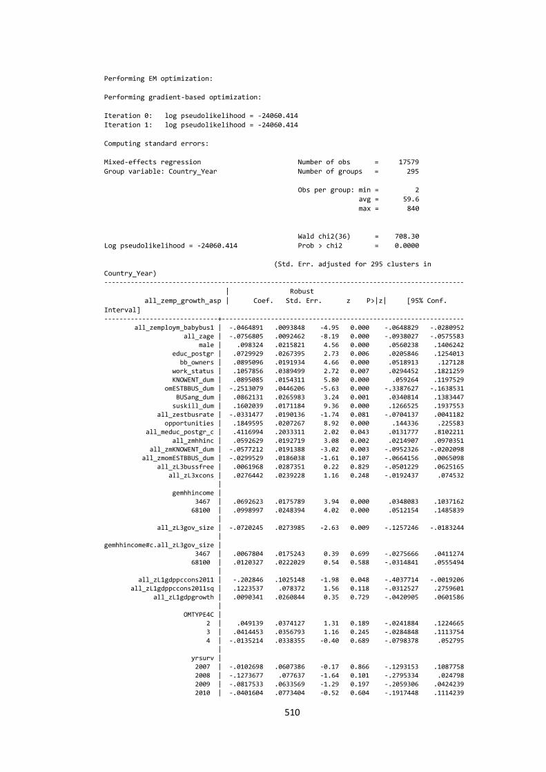
510
Performing EM optimization:
Performing gradient-based optimization:
Iteration 0: log pseudolikelihood = -24060.414
Iteration 1: log pseudolikelihood = -24060.414
Computing standard errors:
Mixed-effects regression Number of obs = 17579
Group variable: Country_Year Number of groups = 295
Obs per group: min = 2
avg = 59.6
max = 840
Wald chi2(36) = 708.30
Log pseudolikelihood = -24060.414 Prob > chi2 = 0.0000
(Std. Err. adjusted for 295 clusters in
Country_Year) -----------------------------------------------------------------------------------------------
| Robust
all_zemp_growth_asp | Coef. Std. Err. z P>|z| [95% Conf.
Interval] ------------------------------+----------------------------------------------------------------
all_zemploym_babybus1 | -.0464891 .0093848 -4.95 0.000 -.0648829 -.0280952
all_zage | -.0756805 .0092462 -8.19 0.000 -.0938027 -.0575583
male | .098324 .0215821 4.56 0.000 .0560238 .1406242
educ_postgr | .0729929 .0267395 2.73 0.006 .0205846 .1254013
bb_owners | .0895096 .0191934 4.66 0.000 .0518913 .127128
work_status | .1057856 .0389499 2.72 0.007 .0294452 .1821259
KNOWENT_dum | .0895085 .0154311 5.80 0.000 .059264 .1197529
omESTBBUS_dum | -.2513079 .0446206 -5.63 0.000 -.3387627 -.1638531
BUSang_dum | .0862131 .0265983 3.24 0.001 .0340814 .1383447
suskill_dum | .1602039 .0171184 9.36 0.000 .1266525 .1937553
all_zestbusrate | -.0331477 .0190136 -1.74 0.081 -.0704137 .0041182
opportunities | .1849595 .0207267 8.92 0.000 .144336 .225583
all_meduc_postgr_c | .4116994 .2033311 2.02 0.043 .0131777 .8102211
all_zmhhinc | .0592629 .0192719 3.08 0.002 .0214907 .0970351
all_zmKNOWENT_dum | -.0577212 .0191388 -3.02 0.003 -.0952326 -.0202098
all_zmomESTBBUS_dum | -.0299529 .0186038 -1.61 0.107 -.0664156 .0065098
all_zL3bussfree | .0061968 .0287351 0.22 0.829 -.0501229 .0625165
all_zL3xcons | .0276442 .0239228 1.16 0.248 -.0192437 .074532
|
gemhhincome |
3467 | .0692623 .0175789 3.94 0.000 .0348083 .1037162
68100 | .0998997 .0248394 4.02 0.000 .0512154 .1485839
|
all_zL3gov_size | -.0720245 .0273985 -2.63 0.009 -.1257246 -.0183244
|
gemhhincome#c.all_zL3gov_size |
3467 | .0067804 .0175243 0.39 0.699 -.0275666 .0411274 68100 | .0120327 .0222029 0.54 0.588 -.0314841 .0555494
|
all_zL1gdppccons2011 | -.202846 .1025148 -1.98 0.048 -.4037714 -.0019206
all_zL1gdppccons2011sq | .1223537 .078372 1.56 0.118 -.0312527 .2759601
all_zL1gdpgrowth | .0090341 .0260844 0.35 0.729 -.0420905 .0601586
|
OMTYPE4C |
2 | .049139 .0374127 1.31 0.189 -.0241884 .1224665
3 | .0414453 .0356793 1.16 0.245 -.0284848 .1113754
4 | -.0135214 .0338355 -0.40 0.689 -.0798378 .052795
|
yrsurv |
2007 | -.0102698 .0607386 -0.17 0.866 -.1293153 .1087758
2008 | -.1273677 .077637 -1.64 0.101 -.2795334 .024798
2009 | -.0817533 .0633569 -1.29 0.197 -.2059306 .0424239
2010 | -.0401604 .0773404 -0.52 0.604 -.1917448 .1114239

511
2011 | -.0526977 .0609094 -0.87 0.387 -.1720779 .0666825
2012 | -.0993873 .0535527 -1.86 0.063 -.2043487 .005574
2013 | -.0837735 .0550022 -1.52 0.128 -.1915758 .0240289
|
_cons | -.5845347 .0714588 -8.18 0.000 -.7245914 -.444478
-----------------------------------------------------------------------------------------------
------------------------------------------------------------------------------
| Robust
Random-effects Parameters | Estimate Std. Err. [95% Conf. Interval]
-----------------------------+------------------------------------------------
Country_Year: Identity |
sd(_cons) | .1951791 .0208636 .1582867 .2406701
-----------------------------+------------------------------------------------
sd(Residual) | .9433295 .0163102 .9118978 .9758448
------------------------------------------------------------------------------
Appendix 5.5.4 Model 4 – EGA – All countries
a. To obtain ICC
. xtmixed all_zemp_growth_asp all_zemploym_babybus1 all_zage male educ_postgr i.gemhhincome
bb_owners work_status omESTBBUS_dum BUSang_dum suskill_dum all_zestbusrate opportunities
all_meduc_postgr all_zmhhinc all_zmKNOWENT_dum all_zmomESTBBUS_dum all_zL3bussfree
all_zL3xcons i.KNOWENT_dum##c.all_zL3gov_size all_zL1gdppccons2011 all_zL1gdppccons2011sq
all_zL1gdpgrowth i.OMTYPE4C i.yrsurv if Country_Year!=70103 & Country_Year!=59709 &
Country_Year!=50308 & Country_Year!=50209 & Country_Year!=35209 & Country_Year!=27009 &
Country_Year!=6401 & yrsurv>=2006 || Country_Year:, mle
Performing EM optimization:
Performing gradient-based optimization:
Iteration 0: log likelihood = -24058.702
Iteration 1: log likelihood = -24058.702
Computing standard errors:
Mixed-effects ML regression Number of obs = 17579
Group variable: Country_Year Number of groups = 295
Obs per group: min = 2
avg = 59.6
max = 840
Wald chi2(35) = 829.57
Log likelihood = -24058.702 Prob > chi2 = 0.0000
-----------------------------------------------------------------------------------------------
all_zemp_growth_asp | Coef. Std. Err. z P>|z| [95% Conf. Interval]
------------------------------+----------------------------------------------------------------
all_zemploym_babybus1 | -.0465883 .0077554 -6.01 0.000 -.0617887 -.0313879
all_zage | -.0753857 .0073875 -10.20 0.000 -.0898649 -.0609064
male | .0979955 .0151767 6.46 0.000 .0682498 .1277413
educ_postgr | .0727943 .0260375 2.80 0.005 .0217618 .1238269
|
gemhhincome |
3467 | .0683263 .0204865 3.34 0.001 .0281734 .1084792
68100 | .0993325 .0201053 4.94 0.000 .0599269 .1387382
|
bb_owners | .0896296 .016247 5.52 0.000 .0577861 .1214731
work_status | .1064109 .0404918 2.63 0.009 .0270485 .1857734
omESTBBUS_dum | -.249844 .0449346 -5.56 0.000 -.3379142 -.1617739
BUSang_dum | .0860511 .0259205 3.32 0.001 .0352479 .1368542
suskill_dum | .1605899 .0196779 8.16 0.000 .1220219 .199158
all_zestbusrate | -.0343408 .0198142 -1.73 0.083 -.0731759 .0044943
opportunities | .1844199 .015385 11.99 0.000 .1542659 .2145739
all_meduc_postgr_c | .4032024 .2026003 1.99 0.047 .006113 .8002917

512
all_zmhhinc | .0589845 .0173194 3.41 0.001 .025039 .09293
all_zmKNOWENT_dum | -.0581779 .0177686 -3.27 0.001 -.0930037 -.0233521
all_zmomESTBBUS_dum | -.0291377 .0234008 -1.25 0.213 -.0750023 .016727
all_zL3bussfree | .0055489 .0243608 0.23 0.820 -.0421974 .0532951
all_zL3xcons | .0270179 .0218866 1.23 0.217 -.0158792 .0699149
1.KNOWENT_dum | .0920447 .0156262 5.89 0.000 .061418 .1226715
all_zL3gov_size | -.0828867 .0255943 -3.24 0.001 -.1330506 -.0327228
|
KNOWENT_dum#c.all_zL3gov_size |
1 | .0298717 .0152654 1.96 0.050 -.0000479 .0597913
|
all_zL1gdppccons2011 | -.2043428 .0881505 -2.32 0.020 -.3771145 -.0315711
all_zL1gdppccons2011sq | .1236055 .0755966 1.64 0.102 -.0245611 .2717721
all_zL1gdpgrowth | .0086777 .0219032 0.40 0.692 -.0342517 .0516071
|
OMTYPE4C |
2 | .0492383 .0358632 1.37 0.170 -.0210523 .119529
3 | .041453 .037217 1.11 0.265 -.0314909 .114397
4 | -.0134917 .0345027 -0.39 0.696 -.0811158 .0541323
|
yrsurv | 2007 | -.0097594 .0686908 -0.14 0.887 -.1443908 .124872
2008 | -.1263833 .0685877 -1.84 0.065 -.2608128 .0080461
2009 | -.0786859 .0710525 -1.11 0.268 -.2179462 .0605744
2010 | -.0382072 .0752082 -0.51 0.611 -.1856125 .1091981
2011 | -.0508765 .0623096 -0.82 0.414 -.1730011 .0712482
2012 | -.0988388 .0605603 -1.63 0.103 -.2175347 .0198572
2013 | -.0831325 .0613051 -1.36 0.175 -.2032882 .0370232
|
_cons | -.5859237 .076185 -7.69 0.000 -.7352436 -.4366039
-----------------------------------------------------------------------------------------------
------------------------------------------------------------------------------
Random-effects Parameters | Estimate Std. Err. [95% Conf. Interval]
-----------------------------+------------------------------------------------
Country_Year: Identity |
sd(_cons) | .1948126 .014309 .1686926 .2249769
-----------------------------+------------------------------------------------
sd(Residual) | .9432534 .0050716 .9333653 .9532462
------------------------------------------------------------------------------
LR test vs. linear regression: chibar2(01) = 332.29 Prob >= chibar2 = 0.0000
. estat icc
Residual intraclass correlation
------------------------------------------------------------------------------
Level | ICC Std. Err. [95% Conf. Interval]
-----------------------------+------------------------------------------------
Country_Year | .0409107 .0058023 .0309354 .0539235
------------------------------------------------------------------------------
b. Model 4 – results (robust – Standard Errors)
. xtmixed all_zemp_growth_asp all_zemploym_babybus1 all_zage male educ_postgr i.gemhhincome
bb_owners work_status omESTBBUS_dum BUSang_dum suskill_dum all_zestbusrate opportunities
all_meduc_postgr all_zmhhinc all_zmKNOWENT_dum all_zmomESTBBUS_dum all_zL3bussfree
all_zL3xcons i.KNOWENT_dum##c.all_zL3gov_size all_zL1gdppccons2011 all_zL1gdppccons2011sq
all_zL1gdpgrowth i.OMTYPE4C i.yrsurv if Country_Year!=70103 & Country_Year!=59709 &
Country_Year!=50308 & Country_Year!=50209 & Country_Year!=35209 & Country_Year!=27009 &
Country_Year!=6401 & yrsurv>=2006 || Country_Year:, mle vce(robust)
Performing EM optimization:
Performing gradient-based optimization:
Iteration 0: log pseudolikelihood = -24058.702
Iteration 1: log pseudolikelihood = -24058.702
Computing standard errors:
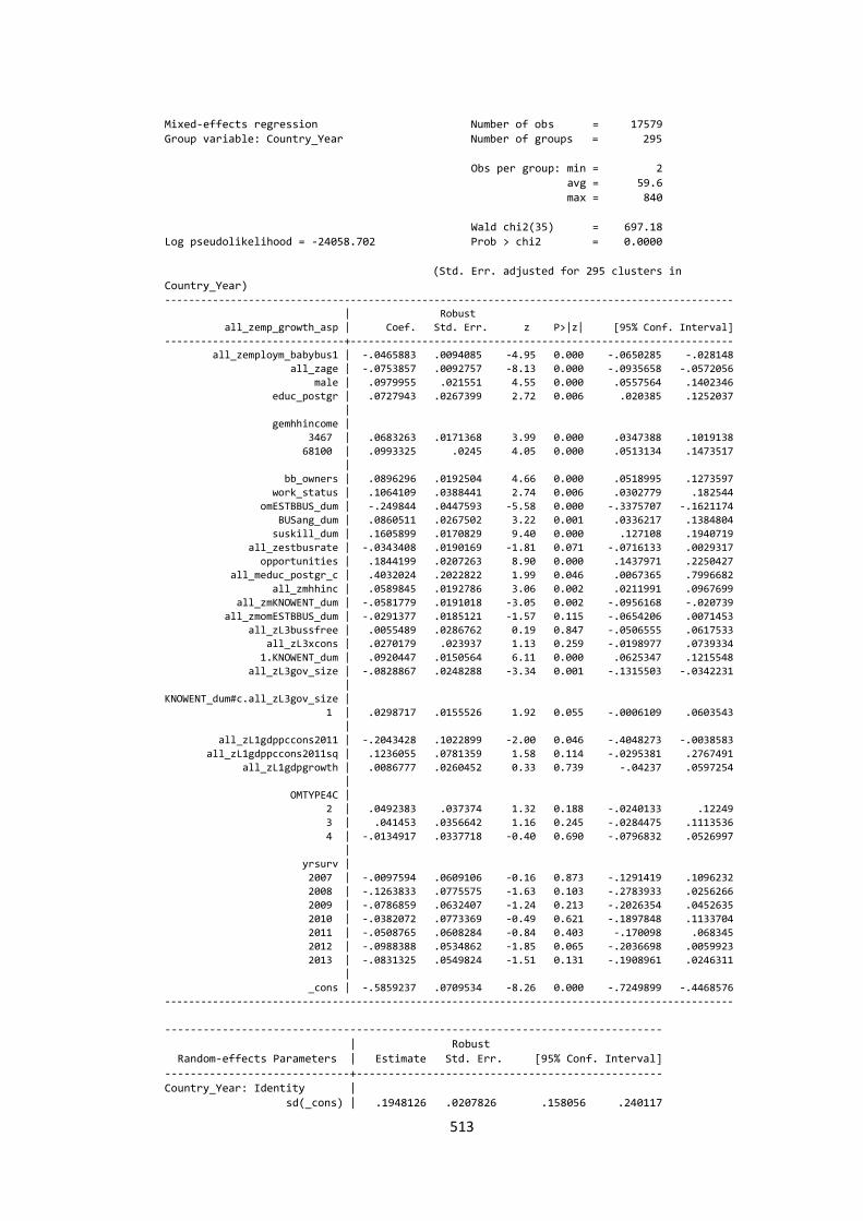
513
Mixed-effects regression Number of obs = 17579
Group variable: Country_Year Number of groups = 295
Obs per group: min = 2
avg = 59.6
max = 840
Wald chi2(35) = 697.18
Log pseudolikelihood = -24058.702 Prob > chi2 = 0.0000
(Std. Err. adjusted for 295 clusters in
Country_Year) -----------------------------------------------------------------------------------------------
| Robust
all_zemp_growth_asp | Coef. Std. Err. z P>|z| [95% Conf. Interval]
------------------------------+----------------------------------------------------------------
all_zemploym_babybus1 | -.0465883 .0094085 -4.95 0.000 -.0650285 -.028148
all_zage | -.0753857 .0092757 -8.13 0.000 -.0935658 -.0572056
male | .0979955 .021551 4.55 0.000 .0557564 .1402346
educ_postgr | .0727943 .0267399 2.72 0.006 .020385 .1252037
|
gemhhincome |
3467 | .0683263 .0171368 3.99 0.000 .0347388 .1019138
68100 | .0993325 .0245 4.05 0.000 .0513134 .1473517
|
bb_owners | .0896296 .0192504 4.66 0.000 .0518995 .1273597
work_status | .1064109 .0388441 2.74 0.006 .0302779 .182544
omESTBBUS_dum | -.249844 .0447593 -5.58 0.000 -.3375707 -.1621174
BUSang_dum | .0860511 .0267502 3.22 0.001 .0336217 .1384804
suskill_dum | .1605899 .0170829 9.40 0.000 .127108 .1940719
all_zestbusrate | -.0343408 .0190169 -1.81 0.071 -.0716133 .0029317
opportunities | .1844199 .0207263 8.90 0.000 .1437971 .2250427
all_meduc_postgr_c | .4032024 .2022822 1.99 0.046 .0067365 .7996682
all_zmhhinc | .0589845 .0192786 3.06 0.002 .0211991 .0967699
all_zmKNOWENT_dum | -.0581779 .0191018 -3.05 0.002 -.0956168 -.020739
all_zmomESTBBUS_dum | -.0291377 .0185121 -1.57 0.115 -.0654206 .0071453
all_zL3bussfree | .0055489 .0286762 0.19 0.847 -.0506555 .0617533 all_zL3xcons | .0270179 .023937 1.13 0.259 -.0198977 .0739334
1.KNOWENT_dum | .0920447 .0150564 6.11 0.000 .0625347 .1215548
all_zL3gov_size | -.0828867 .0248288 -3.34 0.001 -.1315503 -.0342231
|
KNOWENT_dum#c.all_zL3gov_size |
1 | .0298717 .0155526 1.92 0.055 -.0006109 .0603543
|
all_zL1gdppccons2011 | -.2043428 .1022899 -2.00 0.046 -.4048273 -.0038583
all_zL1gdppccons2011sq | .1236055 .0781359 1.58 0.114 -.0295381 .2767491
all_zL1gdpgrowth | .0086777 .0260452 0.33 0.739 -.04237 .0597254
|
OMTYPE4C |
2 | .0492383 .037374 1.32 0.188 -.0240133 .12249
3 | .041453 .0356642 1.16 0.245 -.0284475 .1113536
4 | -.0134917 .0337718 -0.40 0.690 -.0796832 .0526997
|
yrsurv |
2007 | -.0097594 .0609106 -0.16 0.873 -.1291419 .1096232
2008 | -.1263833 .0775575 -1.63 0.103 -.2783933 .0256266
2009 | -.0786859 .0632407 -1.24 0.213 -.2026354 .0452635
2010 | -.0382072 .0773369 -0.49 0.621 -.1897848 .1133704
2011 | -.0508765 .0608284 -0.84 0.403 -.170098 .068345
2012 | -.0988388 .0534862 -1.85 0.065 -.2036698 .0059923
2013 | -.0831325 .0549824 -1.51 0.131 -.1908961 .0246311
|
_cons | -.5859237 .0709534 -8.26 0.000 -.7249899 -.4468576
-----------------------------------------------------------------------------------------------
------------------------------------------------------------------------------
| Robust
Random-effects Parameters | Estimate Std. Err. [95% Conf. Interval]
-----------------------------+------------------------------------------------
Country_Year: Identity |
sd(_cons) | .1948126 .0207826 .158056 .240117
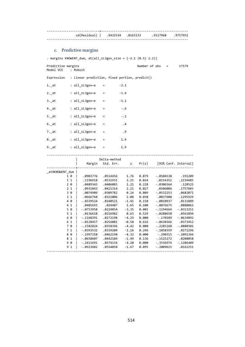
514
-----------------------------+------------------------------------------------
sd(Residual) | .9432534 .0163233 .9117968 .9757952
------------------------------------------------------------------------------
c. Predictive margins
. margins KNOWENT_dum, at(all_zL3gov_size = (-2.1 (0.5) 2.2)) Predictive margins Number of obs = 17579 Model VCE : Robust Expression : Linear prediction, fixed portion, predict() 1._at : all_zL3gov~e = -2.1 2._at : all_zL3gov~e = -1.6 3._at : all_zL3gov~e = -1.1 4._at : all_zL3gov~e = -.6 5._at : all_zL3gov~e = -.1 6._at : all_zL3gov~e = .4 7._at : all_zL3gov~e = .9 8._at : all_zL3gov~e = 1.4 9._at : all_zL3gov~e = 1.9
---------------------------------------------------------------------------------
| Delta-method
| Margin Std. Err. z P>|z| [95% Conf. Interval]
----------------+----------------------------------------------------------------
_at#KNOWENT_dum |
1 0 | .0903776 .0514456 1.76 0.079 -.0104538 .191209
1 1 | .1196918 .0531931 2.25 0.024 .0154352 .2239485
2 0 | .0489343 .0406083 1.21 0.228 -.0306564 .128525
2 1 | .0931843 .0421314 2.21 0.027 .0106084 .1757603
3 0 | .0074909 .0309782 0.24 0.809 -.0532253 .0682071
3 1 | .0666768 .0321006 2.08 0.038 .0037608 .1295929
4 0 | -.0339524 .0240521 -1.41 0.158 -.0810937 .0131889
4 1 | .0401693 .024407 1.65 0.100 -.0076675 .0880062
5 0 | -.0753958 .0224854 -3.35 0.001 -.1194664 -.0313251
5 1 | .0136618 .0216982 0.63 0.529 -.0288658 .0561894
6 0 | -.1168391 .0272198 -4.29 0.000 -.170189 -.0634892
6 1 | -.0128457 .0256081 -0.50 0.616 -.0630366 .0373452
7 0 | -.1582824 .0358396 -4.42 0.000 -.2285268 -.0880381
7 1 | -.0393532 .0339204 -1.16 0.246 -.1058359 .0271296
8 0 | -.1997258 .0462198 -4.32 0.000 -.290315 -.1091366
8 1 | -.0658607 .0442184 -1.49 0.136 -.1525272 .0208058
9 0 | -.2411691 .0574134 -4.20 0.000 -.3536974 -.1286409
9 1 | -.0923682 .0554058 -1.67 0.095 -.2009615 .0162251
---------------------------------------------------------------------------------
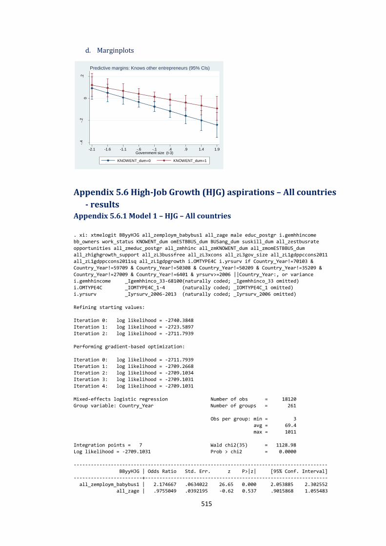
515
d. Marginplots
Appendix 5.6 High-Job Growth (HJG) aspirations – All countries
- results Appendix 5.6.1 Model 1 – HJG – All countries
. xi: xtmelogit BByyHJG all_zemploym_babybus1 all_zage male educ_postgr i.gemhhincome
bb_owners work_status KNOWENT_dum omESTBBUS_dum BUSang_dum suskill_dum all_zestbusrate
opportunities all_zmeduc_postgr all_zmhhinc all_zmKNOWENT_dum all_zmomESTBBUS_dum
all_zhighgrowth_support all_zL3bussfree all_zL3xcons all_zL3gov_size all_zL1gdppccons2011
all_zL1gdppccons2011sq all_zL1gdpgrowth i.OMTYPE4C i.yrsurv if Country_Year!=70103 &
Country_Year!=59709 & Country_Year!=50308 & Country_Year!=50209 & Country_Year!=35209 &
Country_Year!=27009 & Country_Year!=6401 & yrsurv>=2006 ||Country_Year:, or variance
i.gemhhincome _Igemhhinco_33-68100(naturally coded; _Igemhhinco_33 omitted)
i.OMTYPE4C _IOMTYPE4C_1-4 (naturally coded; _IOMTYPE4C_1 omitted)
i.yrsurv _Iyrsurv_2006-2013 (naturally coded; _Iyrsurv_2006 omitted)
Refining starting values:
Iteration 0: log likelihood = -2740.3848
Iteration 1: log likelihood = -2723.5897
Iteration 2: log likelihood = -2711.7939
Performing gradient-based optimization:
Iteration 0: log likelihood = -2711.7939
Iteration 1: log likelihood = -2709.2668
Iteration 2: log likelihood = -2709.1034
Iteration 3: log likelihood = -2709.1031
Iteration 4: log likelihood = -2709.1031
Mixed-effects logistic regression Number of obs = 18120
Group variable: Country_Year Number of groups = 261
Obs per group: min = 3
avg = 69.4
max = 1011
Integration points = 7 Wald chi2(35) = 1128.98
Log likelihood = -2709.1031 Prob > chi2 = 0.0000
-----------------------------------------------------------------------------------------
BByyHJG | Odds Ratio Std. Err. z P>|z| [95% Conf. Interval]
------------------------+----------------------------------------------------------------
all_zemploym_babybus1 | 2.174667 .0634022 26.65 0.000 2.053885 2.302552
all_zage | .9755049 .0392195 -0.62 0.537 .9015868 1.055483
-.4
-.2
0.2
Pre
dic
ted E
mp
. G
row
th A
sp
ira
tion
s (
EM
P)
-2.1 -1.6 -1.1 -.6 -.1 .4 .9 1.4 1.9Government size (t-3)
KNOWENT_dum=0 KNOWENT_dum=1
Predictive margins: Knows other entrepreneurs (95% CIs)
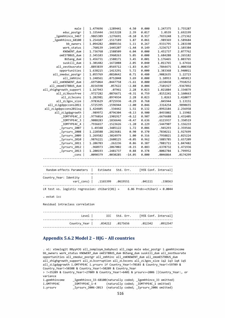
516
male | 1.479696 .1289441 4.50 0.000 1.247375 1.755287
educ_postgr | 1.335444 .1613228 2.39 0.017 1.0539 1.692199
_Igemhhinco_3467 | .9865389 .1276691 -0.10 0.917 .7655248 1.271362
_Igemhhinco_68100 | 1.254107 .1517189 1.87 0.061 .989369 1.589684
bb_owners | 1.094282 .0889156 1.11 0.267 .9331795 1.283198
work_status | .760139 .1445207 -1.44 0.149 .5236717 1.103384
KNOWENT_dum | 1.736768 .1588509 6.04 0.000 1.451737 2.077762
omESTBBUS_dum | 2.345103 .3960263 5.05 0.000 1.684288 3.265182
BUSang_dum | 1.456731 .1588171 3.45 0.001 1.176465 1.803765
suskill_dum | 1.301482 .1672088 2.05 0.040 1.011765 1.67416
all_zestbusrate | .8893839 .0569712 -1.83 0.067 .7844475 1.008358
opportunities | 1.638215 .1413291 5.72 0.000 1.383368 1.940011
all_zmeduc_postgr | 1.055769 .0810642 0.71 0.480 .9082635 1.22723
all_zmhhinc | 1.248561 .0752048 3.69 0.000 1.10953 1.405013
all_zmKNOWENT_dum | .6975064 .0447758 -5.61 0.000 .6150438 .7910252
all_zmomESTBBUS_dum | .8156598 .057622 -2.88 0.004 .7101927 .9367892
all_zhighgrowth_support | 1.167943 .07961 2.28 0.023 1.021884 1.334879
all_zL3bussfree | .9727282 .0876671 -0.31 0.759 .8152241 1.160663
all_zL3xcons | 1.202981 .0974934 2.28 0.023 1.0263 1.410077
all_zL3gov_size | .9783629 .0725936 -0.29 0.768 .845944 1.13151
all_zL1gdppccons2011 | .5725395 .1596944 -2.00 0.046 .3314254 .9890655
all_zL1gdppccons2011sq | 1.424605 .334442 1.51 0.132 .8992184 2.256958
all_zL1gdpgrowth | .989972 .0796304 -0.13 0.900 .8455802 1.15902
_IOMTYPE4C_2 | .9776014 .1901917 -0.12 0.907 .6676688 1.431405
_IOMTYPE4C_3 | .9088283 .1836646 -0.47 0.636 .6115937 1.350519
_IOMTYPE4C_4 | .7936657 .1523626 -1.20 0.229 .5447907 1.156233
_Iyrsurv_2007 | 1.49348 .3485122 1.72 0.086 .945293 2.359566
_Iyrsurv_2008 | 1.228588 .2823681 0.90 0.370 .7830211 1.927699
_Iyrsurv_2009 | 1.269582 .3024979 1.00 0.316 .7958821 2.025224
_Iyrsurv_2010 | .9876221 .2608125 -0.05 0.962 .5885785 1.657209
_Iyrsurv_2011 | 1.206703 .262236 0.86 0.387 .7881711 1.847482
_Iyrsurv_2012 | .968973 .2067002 -0.15 0.883 .6378732 1.471936
_Iyrsurv_2013 | 1.200193 .2481737 0.88 0.378 .8002784 1.799952
_cons | .0090379 .0030285 -14.05 0.000 .0046864 .0174299
-----------------------------------------------------------------------------------------
------------------------------------------------------------------------------
Random-effects Parameters | Estimate Std. Err. [95% Conf. Interval]
-----------------------------+------------------------------------------------
Country_Year: Identity |
var(_cons) | .1165399 .0619551 .041111 .330363
------------------------------------------------------------------------------
LR test vs. logistic regression: chibar2(01) = 6.86 Prob>=chibar2 = 0.0044
. estat icc
Residual intraclass correlation
------------------------------------------------------------------------------
Level | ICC Std. Err. [95% Conf. Interval]
-----------------------------+------------------------------------------------
Country_Year | .034212 .0175656 .012342 .0912547
------------------------------------------------------------------------------
Appendix 5.6.2 Model 2 – HJG – All countries
. xi: xtmelogit BByyHJG all_zemploym_babybus1 all_zage male educ_postgr i.gemhhincome
bb_owners work_status KNOWENT_dum omESTBBUS_dum BUSang_dum suskill_dum all_zestbusrate
opportunities all_zmeduc_postgr all_zmhhinc all_zmKNOWENT_dum all_zmomESTBBUS_dum
all_zhighgrowth_support all_zL3corruption all_zL3xcons all_zL3gov_size iq2 iq3 iq4 iq5
all_zL1gdpgrowth i.OMTYPE4C i.yrsurv if Country_Year!=70103 & Country_Year!=59709 &
Country_Year!=50308 & Country_Year!=50209 & Country_Year
> !=35209 & Country_Year!=27009 & Country_Year!=6401 & yrsurv>=2006 ||Country_Year:, or
variance
i.gemhhincome _Igemhhinco_33-68100(naturally coded; _Igemhhinco_33 omitted)
i.OMTYPE4C _IOMTYPE4C_1-4 (naturally coded; _IOMTYPE4C_1 omitted)
i.yrsurv _Iyrsurv_2006-2013 (naturally coded; _Iyrsurv_2006 omitted)
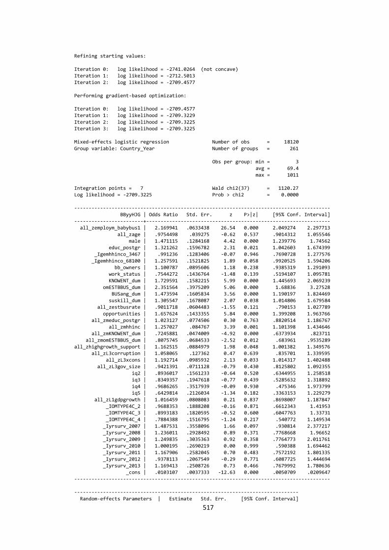
517
Refining starting values:
Iteration 0: log likelihood = -2741.0264 (not concave)
Iteration 1: log likelihood = -2712.5013
Iteration 2: log likelihood = -2709.4577
Performing gradient-based optimization:
Iteration 0: log likelihood = -2709.4577
Iteration 1: log likelihood = -2709.3229
Iteration 2: log likelihood = -2709.3225
Iteration 3: log likelihood = -2709.3225
Mixed-effects logistic regression Number of obs = 18120
Group variable: Country_Year Number of groups = 261
Obs per group: min = 3
avg = 69.4
max = 1011
Integration points = 7 Wald chi2(37) = 1120.27
Log likelihood = -2709.3225 Prob > chi2 = 0.0000
-----------------------------------------------------------------------------------------
BByyHJG | Odds Ratio Std. Err. z P>|z| [95% Conf. Interval]
------------------------+----------------------------------------------------------------
all_zemploym_babybus1 | 2.169941 .0633438 26.54 0.000 2.049274 2.297713
all_zage | .9754498 .039275 -0.62 0.537 .9014312 1.055546
male | 1.471115 .1284168 4.42 0.000 1.239776 1.74562
educ_postgr | 1.321262 .1596782 2.31 0.021 1.042603 1.674399
_Igemhhinco_3467 | .991236 .1283406 -0.07 0.946 .7690728 1.277576
_Igemhhinco_68100 | 1.257591 .1521825 1.89 0.058 .9920525 1.594206
bb_owners | 1.100787 .0895606 1.18 0.238 .9385319 1.291093
work_status | .7544272 .1436764 -1.48 0.139 .5194107 1.095781
KNOWENT_dum | 1.729591 .1582215 5.99 0.000 1.445693 2.069239
omESTBBUS_dum | 2.351564 .3975209 5.06 0.000 1.68836 3.27528
BUSang_dum | 1.473594 .1605834 3.56 0.000 1.190197 1.824469
suskill_dum | 1.305547 .1678087 2.07 0.038 1.014806 1.679584
all_zestbusrate | .9011718 .0604483 -1.55 0.121 .790153 1.027789
opportunities | 1.657624 .1433355 5.84 0.000 1.399208 1.963766
all_zmeduc_postgr | 1.023127 .0774506 0.30 0.763 .8820514 1.186767
all_zmhhinc | 1.257027 .084767 3.39 0.001 1.101398 1.434646
all_zmKNOWENT_dum | .7245881 .0474009 -4.92 0.000 .6373934 .823711
all_zmomESTBBUS_dum | .8075745 .0684533 -2.52 0.012 .683961 .9535289
all_zhighgrowth_support | 1.162515 .0884979 1.98 0.048 1.001382 1.349576
all_zL3corruption | 1.058065 .127362 0.47 0.639 .835701 1.339595
all_zL3xcons | 1.192714 .0985932 2.13 0.033 1.014317 1.402488
all_zL3gov_size | .9421391 .0711128 -0.79 0.430 .8125802 1.092355
iq2 | .8936017 .1561233 -0.64 0.520 .6344955 1.258518
iq3 | .8349357 .1947618 -0.77 0.439 .5285632 1.318892
iq4 | .9686265 .3517939 -0.09 0.930 .475346 1.973799
iq5 | .6429814 .2126034 -1.34 0.182 .3363153 1.229279
all_zL1gdpgrowth | 1.016459 .0808083 0.21 0.837 .8698007 1.187847
_IOMTYPE4C_2 | .9688353 .1888208 -0.16 0.871 .6612343 1.41953
_IOMTYPE4C_3 | .8993183 .1820595 -0.52 0.600 .6047763 1.33731
_IOMTYPE4C_4 | .7884388 .1516795 -1.24 0.217 .540772 1.149534
_Iyrsurv_2007 | 1.487531 .3558096 1.66 0.097 .930814 2.377217
_Iyrsurv_2008 | 1.236011 .2928492 0.89 0.371 .7768668 1.96652
_Iyrsurv_2009 | 1.249835 .3035363 0.92 0.358 .7764773 2.011761
_Iyrsurv_2010 | 1.000195 .2690219 0.00 0.999 .590388 1.694462
_Iyrsurv_2011 | 1.167906 .2582045 0.70 0.483 .7572192 1.801335
_Iyrsurv_2012 | .9378113 .2067549 -0.29 0.771 .6087725 1.444694
_Iyrsurv_2013 | 1.169413 .2508726 0.73 0.466 .7679992 1.780636
_cons | .0103107 .0037333 -12.63 0.000 .0050709 .0209647
-----------------------------------------------------------------------------------------
------------------------------------------------------------------------------
Random-effects Parameters | Estimate Std. Err. [95% Conf. Interval]
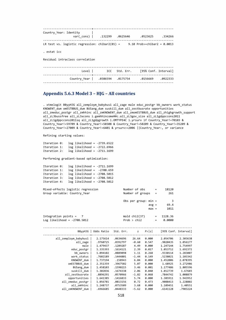
518
-----------------------------+------------------------------------------------
Country_Year: Identity |
var(_cons) | .132299 .0625646 .0523625 .334266
------------------------------------------------------------------------------
LR test vs. logistic regression: chibar2(01) = 9.10 Prob>=chibar2 = 0.0013
. estat icc
Residual intraclass correlation
------------------------------------------------------------------------------
Level | ICC Std. Err. [95% Conf. Interval]
-----------------------------+------------------------------------------------
Country_Year | .0386594 .0175754 .0156669 .0922333
------------------------------------------------------------------------------
Appendix 5.6.3 Model 3 – HJG – All countries
. xtmelogit BByyHJG all_zemploym_babybus1 all_zage male educ_postgr bb_owners work_status
KNOWENT_dum omESTBBUS_dum BUSang_dum suskill_dum all_zestbusrate opportunities
all_zmeduc_postgr all_zmhhinc all_zmKNOWENT_dum all_zmomESTBBUS_dum all_zhighgrowth_support
all_zL3bussfree all_zL3xcons i.gemhhincome##c.all_zL3gov_size all_zL1gdppccons2011
all_zL1gdppccons2011sq all_zL1gdpgrowth i.OMTYPE4C i.yrsurv if Country_Year!=70103 &
Country_Year!=59709 & Country_Year!=50308 & Country_Year!=50209 & Country_Year!=35209 &
Country_Year!=27009 & Country_Year!=6401 & yrsurv>=2006 ||Country_Year:, or variance
Refining starting values:
Iteration 0: log likelihood = -2739.6522
Iteration 1: log likelihood = -2722.6966
Iteration 2: log likelihood = -2711.1699
Performing gradient-based optimization:
Iteration 0: log likelihood = -2711.1699
Iteration 1: log likelihood = -2708.659
Iteration 2: log likelihood = -2708.5015
Iteration 3: log likelihood = -2708.5012
Iteration 4: log likelihood = -2708.5012
Mixed-effects logistic regression Number of obs = 18120
Group variable: Country_Year Number of groups = 261
Obs per group: min = 3
avg = 69.4
max = 1011
Integration points = 7 Wald chi2(37) = 1128.36
Log likelihood = -2708.5012 Prob > chi2 = 0.0000
-----------------------------------------------------------------------------------------------
BByyHJG | Odds Ratio Std. Err. z P>|z| [95% Conf. Interval]
------------------------------+----------------------------------------------------------------
all_zemploym_babybus1 | 2.175614 .0634696 26.64 0.000 2.054706 2.303638
all_zage | .9760725 .0392797 -0.60 0.547 .9020435 1.056177
male | 1.479437 .1289287 4.49 0.000 1.247144 1.754997
educ_postgr | 1.335393 .1614121 2.39 0.017 1.053712 1.692372
bb_owners | 1.094102 .0889098 1.11 0.268 .9330114 1.283007
work_status | .7602189 .1444801 -1.44 0.149 .5238021 1.103342 KNOWENT_dum | 1.737194 .158943 6.04 0.000 1.452006 2.078395
omESTBBUS_dum | 2.351359 .3967502 5.07 0.000 1.68925 3.272986
BUSang_dum | 1.458103 .1590215 3.46 0.001 1.177486 1.805596
suskill_dum | 1.302836 .1674338 2.06 0.040 1.012739 1.67603
all_zestbusrate | .8896291 .0570966 -1.82 0.068 .7844742 1.008879
opportunities | 1.641385 .1416833 5.74 0.000 1.385911 1.943952
all_zmeduc_postgr | 1.056781 .0813156 0.72 0.473 .9088413 1.228802
all_zmhhinc | 1.248737 .0753509 3.68 0.000 1.109451 1.40551
all_zmKNOWENT_dum | .6966685 .0448333 -5.62 0.000 .6141128 .7903224
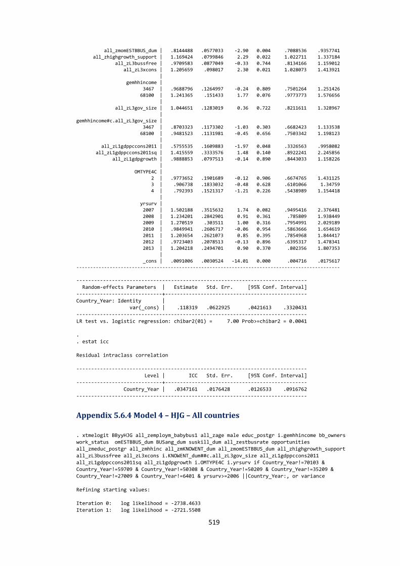
519
all_zmomESTBBUS_dum | .8144488 .0577033 -2.90 0.004 .7088536 .9357741
all_zhighgrowth_support | 1.169424 .0799846 2.29 0.022 1.022711 1.337184
all_zL3bussfree | .9709583 .0877049 -0.33 0.744 .8134166 1.159012
all_zL3xcons | 1.205659 .098017 2.30 0.021 1.028073 1.413921
|
gemhhincome |
3467 | .9688796 .1264997 -0.24 0.809 .7501264 1.251426
68100 | 1.241365 .151433 1.77 0.076 .9773773 1.576656
|
all_zL3gov_size | 1.044651 .1283019 0.36 0.722 .8211611 1.328967
|
gemhhincome#c.all_zL3gov_size |
3467 | .8703323 .1173302 -1.03 0.303 .6682423 1.133538
68100 | .9481523 .1131981 -0.45 0.656 .7503342 1.198123
|
all_zL1gdppccons2011 | .5755535 .1609883 -1.97 0.048 .3326563 .9958082
all_zL1gdppccons2011sq | 1.415559 .3333576 1.48 0.140 .8922241 2.245856
all_zL1gdpgrowth | .9888853 .0797513 -0.14 0.890 .8443033 1.158226
|
OMTYPE4C |
2 | .9773652 .1901689 -0.12 0.906 .6674765 1.431125 3 | .906738 .1833032 -0.48 0.628 .6101066 1.34759
4 | .792393 .1521317 -1.21 0.226 .5438989 1.154418
|
yrsurv |
2007 | 1.502188 .3515632 1.74 0.082 .9495416 2.376481
2008 | 1.234201 .2842901 0.91 0.361 .785809 1.938449
2009 | 1.270519 .303511 1.00 0.316 .7954991 2.029189
2010 | .9849941 .2606717 -0.06 0.954 .5863666 1.654619
2011 | 1.203654 .2621073 0.85 0.395 .7854968 1.844417
2012 | .9723403 .2078513 -0.13 0.896 .6395317 1.478341
2013 | 1.204218 .2494701 0.90 0.370 .802356 1.807353
|
_cons | .0091006 .0030524 -14.01 0.000 .004716 .0175617
-----------------------------------------------------------------------------------------------
------------------------------------------------------------------------------
Random-effects Parameters | Estimate Std. Err. [95% Conf. Interval]
-----------------------------+------------------------------------------------
Country_Year: Identity |
var(_cons) | .118319 .0622925 .0421613 .3320431
------------------------------------------------------------------------------
LR test vs. logistic regression: chibar2(01) = 7.00 Prob>=chibar2 = 0.0041
.
. estat icc
Residual intraclass correlation
------------------------------------------------------------------------------
Level | ICC Std. Err. [95% Conf. Interval]
-----------------------------+------------------------------------------------
Country_Year | .0347161 .0176428 .0126533 .0916762
------------------------------------------------------------------------------
Appendix 5.6.4 Model 4 – HJG – All countries
. xtmelogit BByyHJG all_zemploym_babybus1 all_zage male educ_postgr i.gemhhincome bb_owners
work_status omESTBBUS_dum BUSang_dum suskill_dum all_zestbusrate opportunities
all_zmeduc_postgr all_zmhhinc all_zmKNOWENT_dum all_zmomESTBBUS_dum all_zhighgrowth_support
all_zL3bussfree all_zL3xcons i.KNOWENT_dum##c.all_zL3gov_size all_zL1gdppccons2011
all_zL1gdppccons2011sq all_zL1gdpgrowth i.OMTYPE4C i.yrsurv if Country_Year!=70103 &
Country_Year!=59709 & Country_Year!=50308 & Country_Year!=50209 & Country_Year!=35209 &
Country_Year!=27009 & Country_Year!=6401 & yrsurv>=2006 ||Country_Year:, or variance
Refining starting values:
Iteration 0: log likelihood = -2738.4633
Iteration 1: log likelihood = -2721.5508
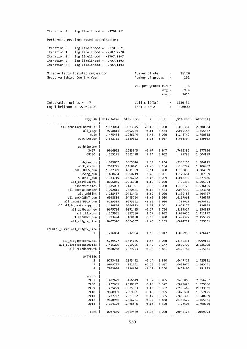
520
Iteration 2: log likelihood = -2709.821
Performing gradient-based optimization:
Iteration 0: log likelihood = -2709.821
Iteration 1: log likelihood = -2707.2778
Iteration 2: log likelihood = -2707.1107
Iteration 3: log likelihood = -2707.1103
Iteration 4: log likelihood = -2707.1103
Mixed-effects logistic regression Number of obs = 18120
Group variable: Country_Year Number of groups = 261
Obs per group: min = 3
avg = 69.4
max = 1011
Integration points = 7 Wald chi2(36) = 1130.31
Log likelihood = -2707.1103 Prob > chi2 = 0.0000
-----------------------------------------------------------------------------------------------
BByyHJG | Odds Ratio Std. Err. z P>|z| [95% Conf. Interval]
------------------------------+----------------------------------------------------------------
all_zemploym_babybus1 | 2.173074 .0633645 26.62 0.000 2.052364 2.300884
all_zage | .9758811 .0392234 -0.61 0.544 .9019548 1.055867
male | 1.475464 .1286144 4.46 0.000 1.243742 1.750358
educ_postgr | 1.332721 .1610962 2.38 0.017 1.051594 1.689003
|
gemhhincome |
3467 | .9914902 .1283945 -0.07 0.947 .7692382 1.277956
68100 | 1.265191 .1532428 1.94 0.052 .99783 1.604189
| bb_owners | 1.095052 .0889846 1.12 0.264 .9338256 1.284115
work_status | .7623725 .1450421 -1.43 0.154 .5250797 1.106902
omESTBBUS_dum | 2.372329 .4011989 5.11 0.000 1.703033 3.304659
BUSang_dum | 1.460404 .1590719 3.48 0.001 1.179661 1.807959
suskill_dum | 1.303719 .1676742 2.06 0.039 1.013232 1.677486
all_zestbusrate | .8866845 .0566888 -1.88 0.060 .782256 1.005054
opportunities | 1.635023 .141021 5.70 0.000 1.380726 1.936155
all_zmeduc_postgr | 1.052811 .080831 0.67 0.503 .9057292 1.223778
all_zmhhinc | 1.248407 .0751443 3.69 0.000 1.109483 1.404727
all_zmKNOWENT_dum | .6938884 .0445764 -5.69 0.000 .6117968 .786995
all_zmomESTBBUS_dum | .8149315 .0575352 -2.90 0.004 .709619 .9358731
all_zhighgrowth_support | 1.169526 .0796552 2.30 0.021 1.023377 1.336548
all_zL3bussfree | .9675724 .0871485 -0.37 0.714 .8109917 1.154385
all_zL3xcons | 1.203901 .097586 2.29 0.022 1.027056 1.411197
1.KNOWENT_dum | 1.793494 .168188 6.23 0.000 1.492372 2.155375
all_zL3gov_size | .8407316 .0894587 -1.63 0.103 .6824717 1.035691
|
KNOWENT_dum#c.all_zL3gov_size |
1 | 1.216884 .12004 1.99 0.047 1.002956 1.476442
|
all_zL1gdppccons2011 | .5789597 .1614135 -1.96 0.050 .3352231 .9999141
all_zL1gdppccons2011sq | 1.405289 .329985 1.45 0.147 .8869302 2.226598
all_zL1gdpgrowth | .9860278 .079273 -0.18 0.861 .8422784 1.15431
|
OMTYPE4C |
2 | .9733452 .1893492 -0.14 0.890 .6647813 1.425131
3 | .9039787 .182732 -0.50 0.617 .6082675 1.343451
4 | .7902966 .1516696 -1.23 0.220 .5425402 1.151193
|
yrsurv |
2007 | 1.492679 .3476649 1.72 0.085 .9456063 2.356257
2008 | 1.227601 .2818927 0.89 0.372 .7827025 1.925386
2009 | 1.275299 .3035333 1.02 0.307 .7998669 2.033321
2010 | .9850981 .2599031 -0.06 0.955 .5873581 1.652175
2011 | 1.207777 .2621902 0.87 0.385 .7892306 1.848289
2012 | .9650906 .2056781 -0.17 0.868 .6355677 1.465461
2013 | 1.194196 .2466846 0.86 0.390 .796605 1.790226
|
_cons | .0087649 .0029439 -14.10 0.000 .0045378 .0169293
-----------------------------------------------------------------------------------------------
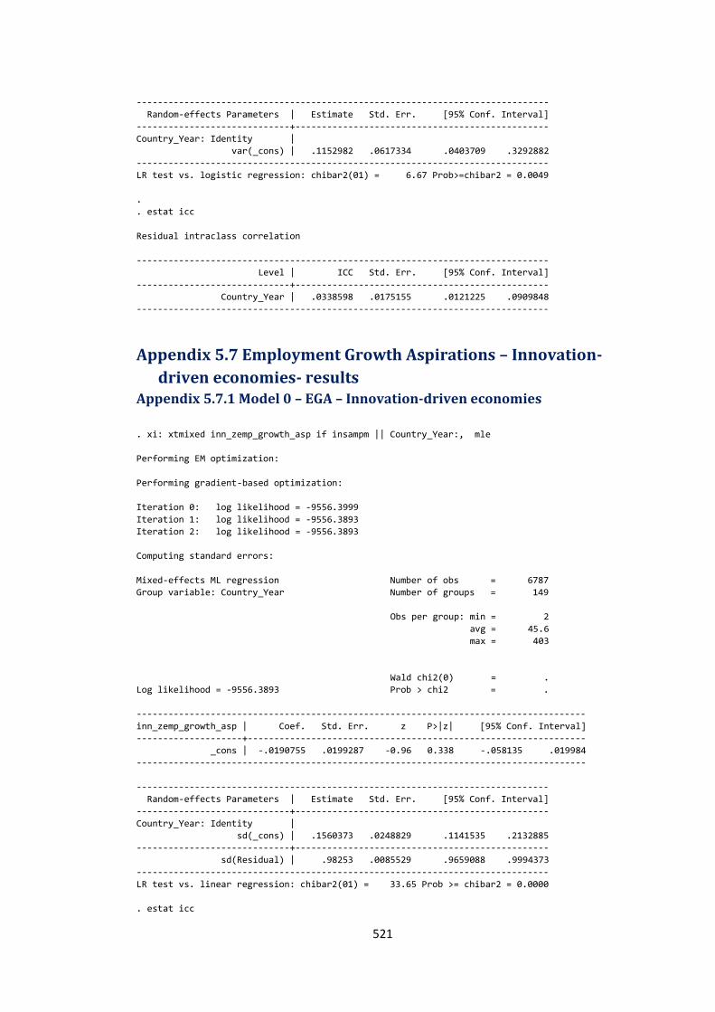
521
------------------------------------------------------------------------------
Random-effects Parameters | Estimate Std. Err. [95% Conf. Interval]
-----------------------------+------------------------------------------------
Country_Year: Identity |
var(_cons) | .1152982 .0617334 .0403709 .3292882
------------------------------------------------------------------------------
LR test vs. logistic regression: chibar2(01) = 6.67 Prob>=chibar2 = 0.0049
.
. estat icc
Residual intraclass correlation
------------------------------------------------------------------------------
Level | ICC Std. Err. [95% Conf. Interval]
-----------------------------+------------------------------------------------
Country_Year | .0338598 .0175155 .0121225 .0909848
------------------------------------------------------------------------------
Appendix 5.7 Employment Growth Aspirations – Innovation-
driven economies- results Appendix 5.7.1 Model 0 – EGA – Innovation-driven economies
. xi: xtmixed inn_zemp_growth_asp if insampm || Country_Year:, mle
Performing EM optimization:
Performing gradient-based optimization:
Iteration 0: log likelihood = -9556.3999
Iteration 1: log likelihood = -9556.3893
Iteration 2: log likelihood = -9556.3893
Computing standard errors:
Mixed-effects ML regression Number of obs = 6787
Group variable: Country_Year Number of groups = 149
Obs per group: min = 2
avg = 45.6
max = 403
Wald chi2(0) = .
Log likelihood = -9556.3893 Prob > chi2 = .
-------------------------------------------------------------------------------------
inn_zemp_growth_asp | Coef. Std. Err. z P>|z| [95% Conf. Interval]
--------------------+----------------------------------------------------------------
_cons | -.0190755 .0199287 -0.96 0.338 -.058135 .019984
-------------------------------------------------------------------------------------
------------------------------------------------------------------------------
Random-effects Parameters | Estimate Std. Err. [95% Conf. Interval]
-----------------------------+------------------------------------------------
Country_Year: Identity |
sd(_cons) | .1560373 .0248829 .1141535 .2132885
-----------------------------+------------------------------------------------
sd(Residual) | .98253 .0085529 .9659088 .9994373
------------------------------------------------------------------------------
LR test vs. linear regression: chibar2(01) = 33.65 Prob >= chibar2 = 0.0000
. estat icc
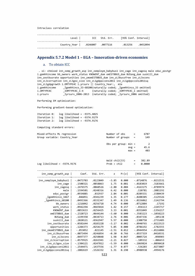
522
Intraclass correlation
------------------------------------------------------------------------------
Level | ICC Std. Err. [95% Conf. Interval]
-----------------------------+------------------------------------------------
Country_Year | .0246007 .0077116 .013256 .0452094
------------------------------------------------------------------------------
Appendix 5.7.2 Model 1 – EGA – Innovation-driven economies
a. To obtain ICC
. xi: xtmixed inn_zemp_growth_asp inn_zemploym_babybus1 inn_zage inn_zagesq male educ_postgr
i.gemhhincome bb_owners work_status KNOWENT_dum omESTBBUS_dum BUSang_dum suskill_dum
inn_zestbusrate opportunities inn_zmomESTBBUS_dum inn_zL3bussfree inn_zL3xcons
inn_zL3corruption inn_zL3gov_size inn_zL1gdppccons2011 inn_zL1gdppccons2011sq
inn_zL1gdpgrowth i.OMTYPE4C i.yrsurv || Country_Year:, mle
i.gemhhincome _Igemhhinco_33-68100(naturally coded; _Igemhhinco_33 omitted)
i.OMTYPE4C _IOMTYPE4C_1-4 (naturally coded; _IOMTYPE4C_1 omitted)
i.yrsurv _Iyrsurv_2006-2013 (naturally coded; _Iyrsurv_2006 omitted)
Performing EM optimization:
Performing gradient-based optimization:
Iteration 0: log likelihood = -9375.4025
Iteration 1: log likelihood = -9374.9179
Iteration 2: log likelihood = -9374.9176
Computing standard errors:
Mixed-effects ML regression Number of obs = 6787
Group variable: Country_Year Number of groups = 149
Obs per group: min = 2
avg = 45.6
max = 403
Wald chi2(33) = 382.89
Log likelihood = -9374.9176 Prob > chi2 = 0.0000
----------------------------------------------------------------------------------------
inn_zemp_growth_asp | Coef. Std. Err. z P>|z| [95% Conf. Interval]
-----------------------+----------------------------------------------------------------
inn_zemploym_babybus1 | -.0473703 .0123049 -3.85 0.000 -.0714876 -.0232531
inn_zage | .1500321 .0858863 1.75 0.081 -.0183019 .3183661
inn_zagesq | -.2476575 .0860526 -2.88 0.004 -.4163175 -.0789974
male | .1594501 .0248316 6.42 0.000 .110781 .2081192
educ_postgr | .0934885 .032937 2.84 0.005 .0289331 .1580439
_Igemhhinco_3467 | .046051 .0341239 1.35 0.177 -.0208305 .1129326
_Igemhhinco_68100 | .0493366 .0331347 1.49 0.136 -.0156062 .1142794
bb_owners | .1216042 .0256718 4.74 0.000 .0712884 .17192
work_status | .0942294 .0665024 1.42 0.157 -.036113 .2245717
KNOWENT_dum | .0853633 .0256425 3.33 0.001 .0351049 .1356217
omESTBBUS_dum | -.2320723 .0644144 -3.60 0.000 -.3583223 -.1058223
BUSang_dum | .1199358 .0434713 2.76 0.006 .0347336 .205138
suskill_dum | .2020121 .0362947 5.57 0.000 .1308758 .2731485
inn_zestbusrate | -.0581644 .0183228 -3.17 0.002 -.0940765 -.0222523
opportunities | .1284373 .0254179 5.05 0.000 .0786192 .1782555
inn_zmomESTBBUS_dum | -.053052 .021145 -2.51 0.012 -.0944954 -.0116086
inn_zL3bussfree | -.0073494 .0246854 -0.30 0.766 -.0557319 .0410331
inn_zL3xcons | .0497377 .0250848 1.98 0.047 .0005724 .098903
inn_zL3corruption | -.0579925 .0261941 -2.21 0.027 -.109332 -.006653
inn_zL3gov_size | -.1384121 .0247812 -5.59 0.000 -.1869824 -.0898418
inn_zL1gdppccons2011 | -.2544471 .1437556 -1.77 0.077 -.536203 .0273087
inn_zL1gdppccons2011sq | .2002619 .1526332 1.31 0.190 -.0988938 .4994176
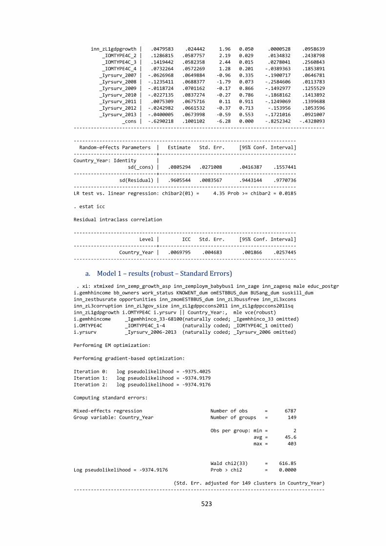
523
inn_zL1gdpgrowth | .0479583 .024442 1.96 0.050 .0000528 .0958639
_IOMTYPE4C_2 | .1286815 .0587757 2.19 0.029 .0134832 .2438798
_IOMTYPE4C_3 | .1419442 .0582358 2.44 0.015 .0278041 .2560843
_IOMTYPE4C_4 | .0732264 .0572269 1.28 0.201 -.0389363 .1853891
_Iyrsurv_2007 | -.0626968 .0649884 -0.96 0.335 -.1900717 .0646781
_Iyrsurv_2008 | -.1235411 .0688377 -1.79 0.073 -.2584606 .0113783
_Iyrsurv_2009 | -.0118724 .0701162 -0.17 0.866 -.1492977 .1255529
_Iyrsurv_2010 | -.0227135 .0837274 -0.27 0.786 -.1868162 .1413892
_Iyrsurv_2011 | .0075309 .0675716 0.11 0.911 -.1249069 .1399688
_Iyrsurv_2012 | -.0242982 .0661532 -0.37 0.713 -.153956 .1053596
_Iyrsurv_2013 | -.0400005 .0673998 -0.59 0.553 -.1721016 .0921007
_cons | -.6290218 .1001102 -6.28 0.000 -.8252342 -.4328093
----------------------------------------------------------------------------------------
------------------------------------------------------------------------------
Random-effects Parameters | Estimate Std. Err. [95% Conf. Interval]
-----------------------------+------------------------------------------------
Country_Year: Identity |
sd(_cons) | .0805294 .0271008 .0416387 .1557441
-----------------------------+------------------------------------------------
sd(Residual) | .9605544 .0083567 .9443144 .9770736
------------------------------------------------------------------------------
LR test vs. linear regression: chibar2(01) = 4.35 Prob >= chibar2 = 0.0185
. estat icc
Residual intraclass correlation
------------------------------------------------------------------------------
Level | ICC Std. Err. [95% Conf. Interval]
-----------------------------+------------------------------------------------
Country_Year | .0069795 .004683 .001866 .0257445
------------------------------------------------------------------------------
a. Model 1 – results (robust – Standard Errors)
. xi: xtmixed inn_zemp_growth_asp inn_zemploym_babybus1 inn_zage inn_zagesq male educ_postgr
i.gemhhincome bb_owners work_status KNOWENT_dum omESTBBUS_dum BUSang_dum suskill_dum
inn_zestbusrate opportunities inn_zmomESTBBUS_dum inn_zL3bussfree inn_zL3xcons
inn_zL3corruption inn_zL3gov_size inn_zL1gdppccons2011 inn_zL1gdppccons2011sq
inn_zL1gdpgrowth i.OMTYPE4C i.yrsurv || Country_Year:, mle vce(robust)
i.gemhhincome _Igemhhinco_33-68100(naturally coded; _Igemhhinco_33 omitted)
i.OMTYPE4C _IOMTYPE4C_1-4 (naturally coded; _IOMTYPE4C_1 omitted)
i.yrsurv _Iyrsurv_2006-2013 (naturally coded; _Iyrsurv_2006 omitted)
Performing EM optimization:
Performing gradient-based optimization:
Iteration 0: log pseudolikelihood = -9375.4025
Iteration 1: log pseudolikelihood = -9374.9179
Iteration 2: log pseudolikelihood = -9374.9176
Computing standard errors:
Mixed-effects regression Number of obs = 6787
Group variable: Country_Year Number of groups = 149
Obs per group: min = 2
avg = 45.6
max = 403
Wald chi2(33) = 616.85
Log pseudolikelihood = -9374.9176 Prob > chi2 = 0.0000
(Std. Err. adjusted for 149 clusters in Country_Year)
----------------------------------------------------------------------------------------
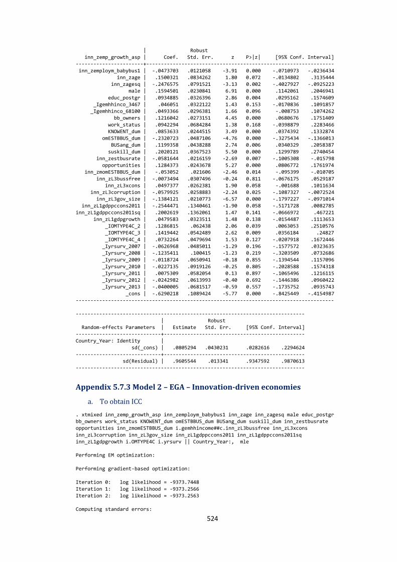
524
| Robust
inn_zemp_growth_asp | Coef. Std. Err. z P>|z| [95% Conf. Interval]
-----------------------+----------------------------------------------------------------
inn_zemploym_babybus1 | -.0473703 .0121058 -3.91 0.000 -.0710973 -.0236434
inn_zage | .1500321 .0834262 1.80 0.072 -.0134802 .3135444
inn_zagesq | -.2476575 .0791521 -3.13 0.002 -.4027927 -.0925223
male | .1594501 .0230841 6.91 0.000 .1142061 .2046941
educ_postgr | .0934885 .0326396 2.86 0.004 .0295162 .1574609
_Igemhhinco_3467 | .046051 .0322122 1.43 0.153 -.0170836 .1091857
_Igemhhinco_68100 | .0493366 .0296381 1.66 0.096 -.008753 .1074262
bb_owners | .1216042 .0273151 4.45 0.000 .0680676 .1751409
work_status | .0942294 .0684284 1.38 0.168 -.0398879 .2283466
KNOWENT_dum | .0853633 .0244515 3.49 0.000 .0374392 .1332874
omESTBBUS_dum | -.2320723 .0487106 -4.76 0.000 -.3275434 -.1366013
BUSang_dum | .1199358 .0438288 2.74 0.006 .0340329 .2058387
suskill_dum | .2020121 .0367523 5.50 0.000 .1299789 .2740454
inn_zestbusrate | -.0581644 .0216159 -2.69 0.007 -.1005308 -.015798
opportunities | .1284373 .0243678 5.27 0.000 .0806772 .1761974
inn_zmomESTBBUS_dum | -.053052 .021606 -2.46 0.014 -.095399 -.010705
inn_zL3bussfree | -.0073494 .0307496 -0.24 0.811 -.0676175 .0529187
inn_zL3xcons | .0497377 .0262381 1.90 0.058 -.001688 .1011634
inn_zL3corruption | -.0579925 .0258883 -2.24 0.025 -.1087327 -.0072524
inn_zL3gov_size | -.1384121 .0210773 -6.57 0.000 -.1797227 -.0971014
inn_zL1gdppccons2011 | -.2544471 .1340461 -1.90 0.058 -.5171728 .0082785
inn_zL1gdppccons2011sq | .2002619 .1362061 1.47 0.141 -.0666972 .467221
inn_zL1gdpgrowth | .0479583 .0323511 1.48 0.138 -.0154487 .1113653
_IOMTYPE4C_2 | .1286815 .062438 2.06 0.039 .0063053 .2510576
_IOMTYPE4C_3 | .1419442 .0542489 2.62 0.009 .0356184 .24827
_IOMTYPE4C_4 | .0732264 .0479694 1.53 0.127 -.0207918 .1672446
_Iyrsurv_2007 | -.0626968 .0485011 -1.29 0.196 -.1577572 .0323635
_Iyrsurv_2008 | -.1235411 .100415 -1.23 0.219 -.3203509 .0732686
_Iyrsurv_2009 | -.0118724 .0650941 -0.18 0.855 -.1394544 .1157096
_Iyrsurv_2010 | -.0227135 .0919126 -0.25 0.805 -.2028588 .1574318
_Iyrsurv_2011 | .0075309 .0582054 0.13 0.897 -.1065496 .1216115
_Iyrsurv_2012 | -.0242982 .0613993 -0.40 0.692 -.1446386 .0960422
_Iyrsurv_2013 | -.0400005 .0681517 -0.59 0.557 -.1735752 .0935743
_cons | -.6290218 .1089424 -5.77 0.000 -.8425449 -.4154987
----------------------------------------------------------------------------------------
------------------------------------------------------------------------------
| Robust
Random-effects Parameters | Estimate Std. Err. [95% Conf. Interval]
-----------------------------+------------------------------------------------
Country_Year: Identity |
sd(_cons) | .0805294 .0430231 .0282616 .2294624
-----------------------------+------------------------------------------------
sd(Residual) | .9605544 .013341 .9347592 .9870613
------------------------------------------------------------------------------
Appendix 5.7.3 Model 2 – EGA – Innovation-driven economies
a. To obtain ICC
. xtmixed inn_zemp_growth_asp inn_zemploym_babybus1 inn_zage inn_zagesq male educ_postgr
bb_owners work_status KNOWENT_dum omESTBBUS_dum BUSang_dum suskill_dum inn_zestbusrate
opportunities inn_zmomESTBBUS_dum i.gemhhincome##c.inn_zL3bussfree inn_zL3xcons
inn_zL3corruption inn_zL3gov_size inn_zL1gdppccons2011 inn_zL1gdppccons2011sq
inn_zL1gdpgrowth i.OMTYPE4C i.yrsurv || Country_Year:, mle
Performing EM optimization:
Performing gradient-based optimization:
Iteration 0: log likelihood = -9373.7448
Iteration 1: log likelihood = -9373.2566
Iteration 2: log likelihood = -9373.2563
Computing standard errors:
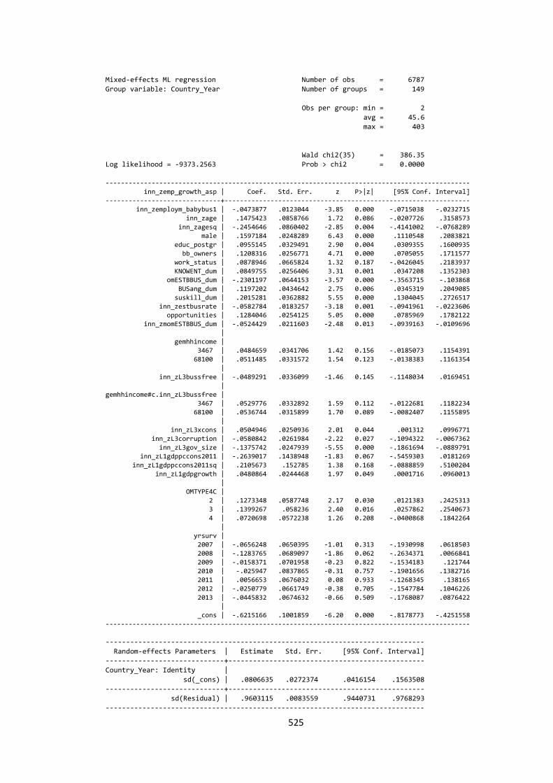
525
Mixed-effects ML regression Number of obs = 6787
Group variable: Country_Year Number of groups = 149
Obs per group: min = 2
avg = 45.6
max = 403
Wald chi2(35) = 386.35
Log likelihood = -9373.2563 Prob > chi2 = 0.0000
-----------------------------------------------------------------------------------------------
inn_zemp_growth_asp | Coef. Std. Err. z P>|z| [95% Conf. Interval]
------------------------------+----------------------------------------------------------------
inn_zemploym_babybus1 | -.0473877 .0123044 -3.85 0.000 -.0715038 -.0232715
inn_zage | .1475423 .0858766 1.72 0.086 -.0207726 .3158573
inn_zagesq | -.2454646 .0860402 -2.85 0.004 -.4141002 -.0768289
male | .1597184 .0248289 6.43 0.000 .1110548 .2083821
educ_postgr | .0955145 .0329491 2.90 0.004 .0309355 .1600935
bb_owners | .1208316 .0256771 4.71 0.000 .0705055 .1711577
work_status | .0878946 .0665824 1.32 0.187 -.0426045 .2183937
KNOWENT_dum | .0849755 .0256406 3.31 0.001 .0347208 .1352303
omESTBBUS_dum | -.2301197 .0644153 -3.57 0.000 -.3563715 -.103868
BUSang_dum | .1197202 .0434642 2.75 0.006 .0345319 .2049085
suskill_dum | .2015281 .0362882 5.55 0.000 .1304045 .2726517
inn_zestbusrate | -.0582784 .0183257 -3.18 0.001 -.0941961 -.0223606 opportunities | .1284046 .0254125 5.05 0.000 .0785969 .1782122
inn_zmomESTBBUS_dum | -.0524429 .0211603 -2.48 0.013 -.0939163 -.0109696
|
gemhhincome |
3467 | .0484659 .0341706 1.42 0.156 -.0185073 .1154391
68100 | .0511485 .0331572 1.54 0.123 -.0138383 .1161354
|
inn_zL3bussfree | -.0489291 .0336099 -1.46 0.145 -.1148034 .0169451
|
gemhhincome#c.inn_zL3bussfree |
3467 | .0529776 .0332892 1.59 0.112 -.0122681 .1182234
68100 | .0536744 .0315899 1.70 0.089 -.0082407 .1155895
|
inn_zL3xcons | .0504946 .0250936 2.01 0.044 .001312 .0996771
inn_zL3corruption | -.0580842 .0261984 -2.22 0.027 -.1094322 -.0067362
inn_zL3gov_size | -.1375742 .0247939 -5.55 0.000 -.1861694 -.0889791
inn_zL1gdppccons2011 | -.2639017 .1438948 -1.83 0.067 -.5459303 .0181269
inn_zL1gdppccons2011sq | .2105673 .152785 1.38 0.168 -.0888859 .5100204
inn_zL1gdpgrowth | .0480864 .0244468 1.97 0.049 .0001716 .0960013
|
OMTYPE4C |
2 | .1273348 .0587748 2.17 0.030 .0121383 .2425313
3 | .1399267 .058236 2.40 0.016 .0257862 .2540673
4 | .0720698 .0572238 1.26 0.208 -.0400868 .1842264
|
yrsurv |
2007 | -.0656248 .0650395 -1.01 0.313 -.1930998 .0618503
2008 | -.1283765 .0689097 -1.86 0.062 -.2634371 .0066841
2009 | -.0158371 .0701958 -0.23 0.822 -.1534183 .121744
2010 | -.025947 .0837865 -0.31 0.757 -.1901656 .1382716
2011 | .0056653 .0676032 0.08 0.933 -.1268345 .138165
2012 | -.0250779 .0661749 -0.38 0.705 -.1547784 .1046226
2013 | -.0445832 .0674632 -0.66 0.509 -.1768087 .0876422
|
_cons | -.6215166 .1001859 -6.20 0.000 -.8178773 -.4251558
-----------------------------------------------------------------------------------------------
------------------------------------------------------------------------------
Random-effects Parameters | Estimate Std. Err. [95% Conf. Interval]
-----------------------------+------------------------------------------------
Country_Year: Identity |
sd(_cons) | .0806635 .0272374 .0416154 .1563508
-----------------------------+------------------------------------------------
sd(Residual) | .9603115 .0083559 .9440731 .9768293
------------------------------------------------------------------------------
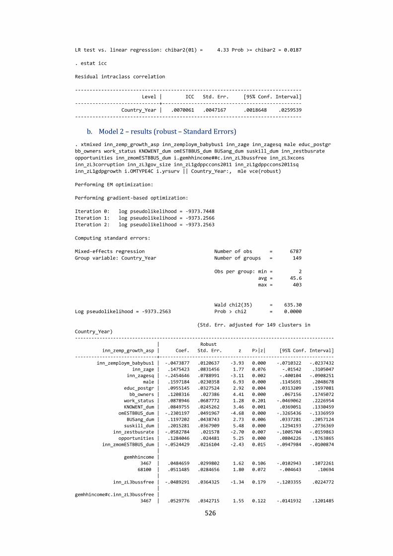
526
LR test vs. linear regression: chibar2(01) = 4.33 Prob >= chibar2 = 0.0187
. estat icc
Residual intraclass correlation
------------------------------------------------------------------------------
Level | ICC Std. Err. [95% Conf. Interval]
-----------------------------+------------------------------------------------
Country_Year | .0070061 .0047167 .0018648 .0259539
------------------------------------------------------------------------------
b. Model 2 – results (robust – Standard Errors)
. xtmixed inn_zemp_growth_asp inn_zemploym_babybus1 inn_zage inn_zagesq male educ_postgr
bb_owners work_status KNOWENT_dum omESTBBUS_dum BUSang_dum suskill_dum inn_zestbusrate
opportunities inn_zmomESTBBUS_dum i.gemhhincome##c.inn_zL3bussfree inn_zL3xcons
inn_zL3corruption inn_zL3gov_size inn_zL1gdppccons2011 inn_zL1gdppccons2011sq
inn_zL1gdpgrowth i.OMTYPE4C i.yrsurv || Country_Year:, mle vce(robust)
Performing EM optimization:
Performing gradient-based optimization:
Iteration 0: log pseudolikelihood = -9373.7448
Iteration 1: log pseudolikelihood = -9373.2566
Iteration 2: log pseudolikelihood = -9373.2563
Computing standard errors:
Mixed-effects regression Number of obs = 6787
Group variable: Country_Year Number of groups = 149
Obs per group: min = 2
avg = 45.6
max = 403
Wald chi2(35) = 635.30
Log pseudolikelihood = -9373.2563 Prob > chi2 = 0.0000
(Std. Err. adjusted for 149 clusters in
Country_Year) -----------------------------------------------------------------------------------------------
| Robust
inn_zemp_growth_asp | Coef. Std. Err. z P>|z| [95% Conf. Interval]
------------------------------+----------------------------------------------------------------
inn_zemploym_babybus1 | -.0473877 .0120637 -3.93 0.000 -.0710322 -.0237432
inn_zage | .1475423 .0831456 1.77 0.076 -.01542 .3105047
inn_zagesq | -.2454646 .0788991 -3.11 0.002 -.400104 -.0908251
male | .1597184 .0230358 6.93 0.000 .1145691 .2048678
educ_postgr | .0955145 .0327524 2.92 0.004 .0313209 .1597081
bb_owners | .1208316 .027386 4.41 0.000 .067156 .1745072
work_status | .0878946 .0687772 1.28 0.201 -.0469062 .2226954
KNOWENT_dum | .0849755 .0245262 3.46 0.001 .0369051 .1330459
omESTBBUS_dum | -.2301197 .0491967 -4.68 0.000 -.3265436 -.1336959
BUSang_dum | .1197202 .0438743 2.73 0.006 .0337281 .2057124
suskill_dum | .2015281 .0367909 5.48 0.000 .1294193 .2736369
inn_zestbusrate | -.0582784 .021578 -2.70 0.007 -.1005704 -.0159863
opportunities | .1284046 .024481 5.25 0.000 .0804226 .1763865
inn_zmomESTBBUS_dum | -.0524429 .0216104 -2.43 0.015 -.0947984 -.0100874
|
gemhhincome |
3467 | .0484659 .0299802 1.62 0.106 -.0102943 .1072261
68100 | .0511485 .0284656 1.80 0.072 -.004643 .10694
|
inn_zL3bussfree | -.0489291 .0364325 -1.34 0.179 -.1203355 .0224772 |
gemhhincome#c.inn_zL3bussfree |
3467 | .0529776 .0342715 1.55 0.122 -.0141932 .1201485
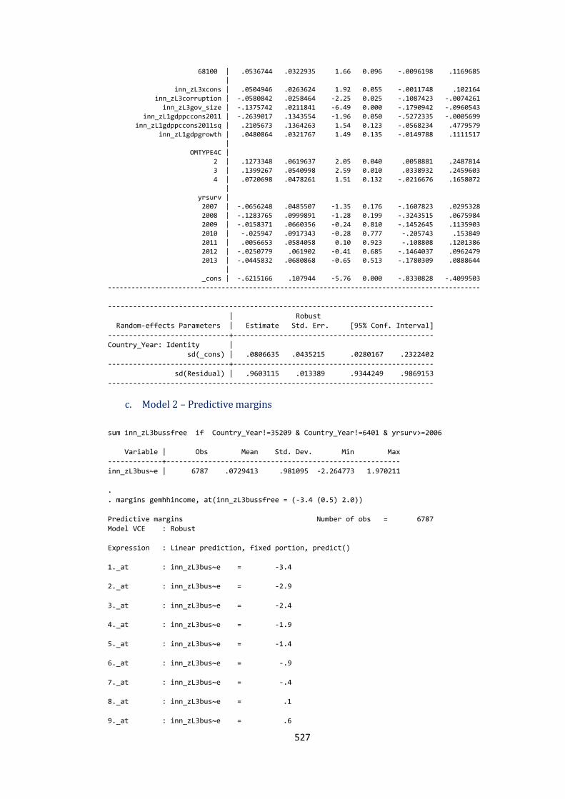
527
68100 | .0536744 .0322935 1.66 0.096 -.0096198 .1169685
|
inn_zL3xcons | .0504946 .0263624 1.92 0.055 -.0011748 .102164
inn_zL3corruption | -.0580842 .0258464 -2.25 0.025 -.1087423 -.0074261
inn_zL3gov_size | -.1375742 .0211841 -6.49 0.000 -.1790942 -.0960543
inn_zL1gdppccons2011 | -.2639017 .1343554 -1.96 0.050 -.5272335 -.0005699
inn_zL1gdppccons2011sq | .2105673 .1364263 1.54 0.123 -.0568234 .4779579
inn_zL1gdpgrowth | .0480864 .0321767 1.49 0.135 -.0149788 .1111517
|
OMTYPE4C |
2 | .1273348 .0619637 2.05 0.040 .0058881 .2487814
3 | .1399267 .0540998 2.59 0.010 .0338932 .2459603
4 | .0720698 .0478261 1.51 0.132 -.0216676 .1658072
|
yrsurv |
2007 | -.0656248 .0485507 -1.35 0.176 -.1607823 .0295328
2008 | -.1283765 .0999891 -1.28 0.199 -.3243515 .0675984
2009 | -.0158371 .0660356 -0.24 0.810 -.1452645 .1135903
2010 | -.025947 .0917343 -0.28 0.777 -.205743 .153849
2011 | .0056653 .0584058 0.10 0.923 -.108808 .1201386
2012 | -.0250779 .061902 -0.41 0.685 -.1464037 .0962479 2013 | -.0445832 .0680868 -0.65 0.513 -.1780309 .0888644
|
_cons | -.6215166 .107944 -5.76 0.000 -.8330828 -.4099503
-----------------------------------------------------------------------------------------------
------------------------------------------------------------------------------
| Robust
Random-effects Parameters | Estimate Std. Err. [95% Conf. Interval]
-----------------------------+------------------------------------------------
Country_Year: Identity |
sd(_cons) | .0806635 .0435215 .0280167 .2322402
-----------------------------+------------------------------------------------
sd(Residual) | .9603115 .013389 .9344249 .9869153
------------------------------------------------------------------------------
c. Model 2 – Predictive margins
sum inn_zL3bussfree if Country_Year!=35209 & Country_Year!=6401 & yrsurv>=2006
Variable | Obs Mean Std. Dev. Min Max
-------------+--------------------------------------------------------
inn_zL3bus~e | 6787 .0729413 .981095 -2.264773 1.970211
.
. margins gemhhincome, at(inn_zL3bussfree = (-3.4 (0.5) 2.0))
Predictive margins Number of obs = 6787
Model VCE : Robust
Expression : Linear prediction, fixed portion, predict()
1._at : inn_zL3bus~e = -3.4
2._at : inn_zL3bus~e = -2.9
3._at : inn_zL3bus~e = -2.4
4._at : inn_zL3bus~e = -1.9
5._at : inn_zL3bus~e = -1.4
6._at : inn_zL3bus~e = -.9
7._at : inn_zL3bus~e = -.4
8._at : inn_zL3bus~e = .1
9._at : inn_zL3bus~e = .6

528
10._at : inn_zL3bus~e = 1.1
11._at : inn_zL3bus~e = 1.6
---------------------------------------------------------------------------------
| Delta-method
| Margin Std. Err. z P>|z| [95% Conf. Interval]
----------------+----------------------------------------------------------------
_at#gemhhincome |
1 33 | .1170541 .1257208 0.93 0.352 -.1293542 .3634624
1 3467 | -.0146039 .1218502 -0.12 0.905 -.2534259 .2242181
1 68100 | -.0142902 .1257208 -0.11 0.910 -.2606985 .232118
2 33 | .0925895 .1080472 0.86 0.391 -.1191791 .3043581
2 3467 | -.0125797 .1051008 -0.12 0.905 -.2185736 .1934142
2 68100 | -.0119176 .1080472 -0.11 0.912 -.2236862 .199851
3 33 | .068125 .0905888 0.75 0.452 -.1094258 .2456758
3 3467 | -.0105554 .08848 -0.12 0.905 -.183973 .1628621
3 68100 | -.009545 .0905888 -0.11 0.916 -.1870958 .1680058
4 33 | .0436604 .0734992 0.59 0.552 -.1003954 .1877162
4 3467 | -.0085312 .0720765 -0.12 0.906 -.1497985 .1327362
4 68100 | -.0071724 .0734992 -0.10 0.922 -.1512282 .1368834
5 33 | .0191958 .0571104 0.34 0.737 -.0927384 .1311301
5 3467 | -.0065069 .0560816 -0.12 0.908 -.1164248 .1034109
5 68100 | -.0047998 .0571104 -0.08 0.933 -.116734 .1071345
6 33 | -.0052687 .042246 -0.12 0.901 -.0880693 .0775318
6 3467 | -.0044827 .0409764 -0.11 0.913 -.084795 .0758296
6 68100 | -.0024271 .042246 -0.06 0.954 -.0852277 .0803734
7 33 | -.0297333 .0311691 -0.95 0.340 -.0908235 .0313569
7 3467 | -.0024584 .0282275 -0.09 0.931 -.0577833 .0528664
7 68100 | -.0000545 .0311685 -0.00 0.999 -.0611437 .0610347
8 33 | -.0541979 .0286699 -1.89 0.059 -.1103898 .0019941
8 3467 | -.0004342 .022323 -0.02 0.984 -.0441865 .0433181
8 68100 | .0023181 .0286699 0.08 0.936 -.0538739 .0585101
9 33 | -.0786624 .0365524 -2.15 0.031 -.1503039 -.007021
9 3467 | .00159 .0279936 0.06 0.955 -.0532765 .0564566
9 68100 | .0046907 .0365524 0.13 0.898 -.0669507 .0763321
10 33 | -.103127 .0501384 -2.06 0.040 -.2013964 -.0048576
10 3467 | .0036143 .0406543 0.09 0.929 -.0760667 .0832953
10 68100 | .0070633 .0501384 0.14 0.888 -.0912061 .1053328
11 33 | -.1275916 .0659947 -1.93 0.053 -.2569388 .0017557
11 3467 | .0056385 .0557289 0.10 0.919 -.103588 .1148651
11 68100 | .009436 .0659947 0.14 0.886 -.1199113 .1387832
---------------------------------------------------------------------------------
d. Model 2 – Marginplots
-.4
-.2
0.2
.4
Pre
dic
ted E
mp
. G
row
th A
sp
ira
tion
s (
EM
P)
-3.4 -2.9 -2.4 -1.9 -1.4 -.9 -.4 .1 .6 1.1 1.6Business freedom (t-3)
gemhhincome=33 gemhhincome=3467
gemhhincome=68100
Predictive margins: Household income (95% CIs)
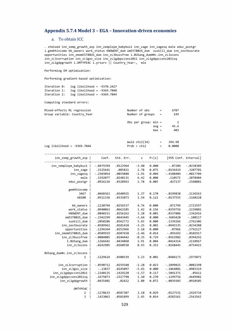
529
Appendix 5.7.4 Model 3 – EGA – Innovation-driven economies
a. To obtain ICC
. xtmixed inn_zemp_growth_asp inn_zemploym_babybus1 inn_zage inn_zagesq male educ_postgr
i.gemhhincome bb_owners work_status KNOWENT_dum omESTBBUS_dum suskill_dum inn_zestbusrate
opportunities inn_zmomESTBBUS_dum inn_zL3bussfree i.BUSang_dum##c.inn_zL3xcons
inn_zL3corruption inn_zL3gov_size inn_zL1gdppccons2011 inn_zL1gdppccons2011sq
inn_zL1gdpgrowth i.OMTYPE4C i.yrsurv || Country_Year:, mle
Performing EM optimization:
Performing gradient-based optimization:
Iteration 0: log likelihood = -9370.2427
Iteration 1: log likelihood = -9369.7048
Iteration 2: log likelihood = -9369.7044
Computing standard errors:
Mixed-effects ML regression Number of obs = 6787
Group variable: Country_Year Number of groups = 149
Obs per group: min = 2
avg = 45.6
max = 403
Wald chi2(34) = 394.98
Log likelihood = -9369.7044 Prob > chi2 = 0.0000
-------------------------------------------------------------------------------------------
inn_zemp_growth_asp | Coef. Std. Err. z P>|z| [95% Conf. Interval]
--------------------------+----------------------------------------------------------------
inn_zemploym_babybus1 | -.0479394 .0122964 -3.90 0.000 -.07204 -.0238389
inn_zage | .1525641 .085821 1.78 0.075 -.0156419 .3207701
inn_zagesq | -.2503054 .0859888 -2.91 0.004 -.4188404 -.0817704
male | .1592077 .0248131 6.42 0.000 .110575 .2078404
educ_postgr | .0916126 .0328963 2.78 0.005 .027137 .1560881
|
gemhhincome |
3467 | .0468363 .0340925 1.37 0.170 -.0199838 .1136563
68100 | .0511336 .0331073 1.54 0.122 -.0137555 .1160228
|
bb_owners | .1220794 .0256537 4.76 0.000 .071799 .1723597
work_status | .0940063 .0663185 1.42 0.156 -.0359756 .2239881
KNOWENT_dum | .0840151 .0256262 3.28 0.001 .0337886 .1342416
omESTBBUS_dum | -.2342299 .0643445 -3.64 0.000 -.3603428 -.108117
suskill_dum | .2050286 .0362772 5.65 0.000 .1339266 .2761306
inn_zestbusrate | -.0589962 .0181418 -3.25 0.001 -.0945535 -.0234388
opportunities | .1294364 .0253966 5.10 0.000 .07966 .1792127
inn_zmomESTBBUS_dum | -.0509919 .0207658 -2.46 0.014 -.091692 -.0102917
inn_zL3bussfree | -.0084805 .0244442 -0.35 0.729 -.0563902 .0394292
1.BUSang_dum | .1266641 .0434868 2.91 0.004 .0414314 .2118967
inn_zL3xcons | .0242985 .0260938 0.93 0.352 -.0268445 .0754415
|
BUSang_dum#c.inn_zL3xcons |
1 | .1229624 .0380339 3.23 0.001 .0484173 .1975075
|
inn_zL3corruption | -.0590712 .0259348 -2.28 0.023 -.1099025 -.0082398
inn_zL3gov_size | -.13837 .0245097 -5.65 0.000 -.1864081 -.0903319
inn_zL1gdppccons2011 | -.2240135 .1429228 -1.57 0.117 -.5041371 .05611
inn_zL1gdppccons2011sq | .1675073 .1517798 1.10 0.270 -.1299756 .4649902
inn_zL1gdpgrowth | .0435401 .02422 1.80 0.072 -.0039303 .0910105
|
OMTYPE4C |
2 | .1278633 .0587307 2.18 0.029 .0127531 .2429734
3 | .1423062 .0581899 2.45 0.014 .0282561 .2563562
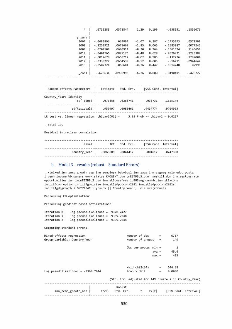
530
4 | .0735283 .0571844 1.29 0.199 -.038551 .1856076
|
yrsurv |
2007 | -.0680896 .063899 -1.07 0.287 -.1933293 .0571501
2008 | -.1252921 .0678669 -1.85 0.065 -.2583087 .0077245
2009 | -.0207508 .0690914 -0.30 0.764 -.1561674 .1146658
2010 | -.0401766 .0829176 -0.48 0.628 -.2026921 .1223389
2011 | -.0012678 .0668217 -0.02 0.985 -.132236 .1297004
2012 | -.0338227 .0654539 -0.52 0.605 -.16211 .0944647
2013 | -.0507324 .066681 -0.76 0.447 -.1814248 .07996
|
_cons | -.623634 .0996993 -6.26 0.000 -.8190411 -.428227
-------------------------------------------------------------------------------------------
------------------------------------------------------------------------------
Random-effects Parameters | Estimate Std. Err. [95% Conf. Interval]
-----------------------------+------------------------------------------------
Country_Year: Identity |
sd(_cons) | .076858 .0268741 .038731 .1525174
-----------------------------+------------------------------------------------
sd(Residual) | .959997 .0083461 .9437774 .9764953
------------------------------------------------------------------------------
LR test vs. linear regression: chibar2(01) = 3.93 Prob >= chibar2 = 0.0237
. estat icc
Residual intraclass correlation
------------------------------------------------------------------------------
Level | ICC Std. Err. [95% Conf. Interval]
-----------------------------+------------------------------------------------
Country_Year | .0063689 .0044417 .001617 .0247398
------------------------------------------------------------------------------
b. Model 3 – results (robust – Standard Errors)
. xtmixed inn_zemp_growth_asp inn_zemploym_babybus1 inn_zage inn_zagesq male educ_postgr
i.gemhhincome bb_owners work_status KNOWENT_dum omESTBBUS_dum suskill_dum inn_zestbusrate
opportunities inn_zmomESTBBUS_dum inn_zL3bussfree i.BUSang_dum##c.inn_zL3xcons
inn_zL3corruption inn_zL3gov_size inn_zL1gdppccons2011 inn_zL1gdppccons2011sq
inn_zL1gdpgrowth i.OMTYPE4C i.yrsurv || Country_Year:, mle vce(robust)
Performing EM optimization:
Performing gradient-based optimization:
Iteration 0: log pseudolikelihood = -9370.2427
Iteration 1: log pseudolikelihood = -9369.7048
Iteration 2: log pseudolikelihood = -9369.7044
Computing standard errors:
Mixed-effects regression Number of obs = 6787
Group variable: Country_Year Number of groups = 149
Obs per group: min = 2
avg = 45.6
max = 403
Wald chi2(34) = 646.38
Log pseudolikelihood = -9369.7044 Prob > chi2 = 0.0000
(Std. Err. adjusted for 149 clusters in Country_Year)
-------------------------------------------------------------------------------------------
| Robust
inn_zemp_growth_asp | Coef. Std. Err. z P>|z| [95% Conf. Interval]
--------------------------+----------------------------------------------------------------

531
inn_zemploym_babybus1 | -.0479394 .0116685 -4.11 0.000 -.0708092 -.0250697
inn_zage | .1525641 .0829209 1.84 0.066 -.009958 .3150861
inn_zagesq | -.2503054 .0786166 -3.18 0.001 -.4043911 -.0962197
male | .1592077 .0230999 6.89 0.000 .1139327 .2044828
educ_postgr | .0916126 .0325764 2.81 0.005 .027764 .1554612
|
gemhhincome |
3467 | .0468363 .0322623 1.45 0.147 -.0163966 .1100691
68100 | .0511336 .029743 1.72 0.086 -.0071616 .1094289
|
bb_owners | .1220794 .027342 4.46 0.000 .06849 .1756688
work_status | .0940063 .068118 1.38 0.168 -.0395026 .2275151
KNOWENT_dum | .0840151 .0243473 3.45 0.001 .0362952 .131735
omESTBBUS_dum | -.2342299 .0488749 -4.79 0.000 -.330023 -.1384368
suskill_dum | .2050286 .036331 5.64 0.000 .1338212 .2762361
inn_zestbusrate | -.0589962 .0214305 -2.75 0.006 -.1009993 -.0169931
opportunities | .1294364 .0242604 5.34 0.000 .0818869 .1769858
inn_zmomESTBBUS_dum | -.0509919 .0214374 -2.38 0.017 -.0930084 -.0089753
inn_zL3bussfree | -.0084805 .0305106 -0.28 0.781 -.0682802 .0513191
1.BUSang_dum | .1266641 .0445684 2.84 0.004 .0393116 .2140165
inn_zL3xcons | .0242985 .0264877 0.92 0.359 -.0276164 .0762133
|
BUSang_dum#c.inn_zL3xcons |
1 | .1229624 .0414551 2.97 0.003 .0417119 .204213
|
inn_zL3corruption | -.0590712 .0255937 -2.31 0.021 -.1092339 -.0089084
inn_zL3gov_size | -.13837 .0207335 -6.67 0.000 -.1790068 -.0977332
inn_zL1gdppccons2011 | -.2240135 .1285297 -1.74 0.081 -.4759272 .0279001
inn_zL1gdppccons2011sq | .1675073 .1296206 1.29 0.196 -.0865443 .4215589
inn_zL1gdpgrowth | .0435401 .0321597 1.35 0.176 -.0194918 .106572
|
OMTYPE4C |
2 | .1278633 .0625532 2.04 0.041 .0052613 .2504652
3 | .1423062 .0543551 2.62 0.009 .0357721 .2488402
4 | .0735283 .0481417 1.53 0.127 -.0208277 .1678843
|
yrsurv |
2007 | -.0680896 .0483152 -1.41 0.159 -.1627856 .0266064
2008 | -.1252921 .0989703 -1.27 0.206 -.3192703 .068686
2009 | -.0207508 .0641952 -0.32 0.747 -.1465711 .1050695
2010 | -.0401766 .0912598 -0.44 0.660 -.2190424 .1386893
2011 | -.0012678 .0579144 -0.02 0.983 -.1147779 .1122423
2012 | -.0338227 .0600016 -0.56 0.573 -.1514237 .0837784
2013 | -.0507324 .0677974 -0.75 0.454 -.1836129 .0821481
|
_cons | -.623634 .1087737 -5.73 0.000 -.8368266 -.4104415
-------------------------------------------------------------------------------------------
------------------------------------------------------------------------------
| Robust
Random-effects Parameters | Estimate Std. Err. [95% Conf. Interval]
-----------------------------+------------------------------------------------
Country_Year: Identity |
sd(_cons) | .076858 .0415999 .0266055 .2220277
-----------------------------+------------------------------------------------
sd(Residual) | .959997 .0133514 .9341821 .9865252
------------------------------------------------------------------------------
c. Model 3 – Predictive margins
. margins BUSang_dum, at(inn_zL3xcons = (-6.5 (0.5) 0.2))
Predictive margins Number of obs = 6787
Model VCE : Robust
Expression : Linear prediction, fixed portion, predict()
1._at : inn_zL3xcons = -6.5
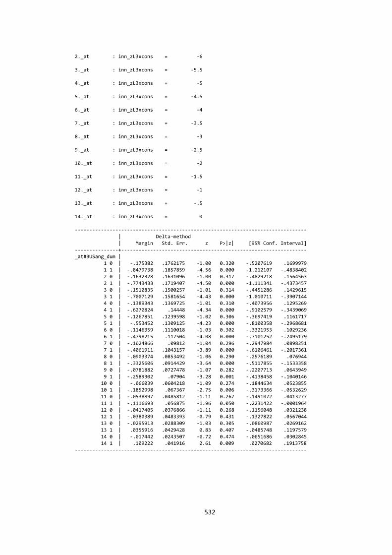
532
2._at : inn_zL3xcons = -6
3._at : inn_zL3xcons = -5.5
4._at : inn_zL3xcons = -5
5._at : inn_zL3xcons = -4.5
6._at : inn_zL3xcons = -4
7._at : inn_zL3xcons = -3.5
8._at : inn_zL3xcons = -3
9._at : inn_zL3xcons = -2.5
10._at : inn_zL3xcons = -2
11._at : inn_zL3xcons = -1.5
12._at : inn_zL3xcons = -1
13._at : inn_zL3xcons = -.5
14._at : inn_zL3xcons = 0
--------------------------------------------------------------------------------
| Delta-method
| Margin Std. Err. z P>|z| [95% Conf. Interval]
---------------+----------------------------------------------------------------
_at#BUSang_dum |
1 0 | -.175382 .1762175 -1.00 0.320 -.5207619 .1699979
1 1 | -.8479738 .1857859 -4.56 0.000 -1.212107 -.4838402
2 0 | -.1632328 .1631096 -1.00 0.317 -.4829218 .1564563
2 1 | -.7743433 .1719407 -4.50 0.000 -1.111341 -.4373457
3 0 | -.1510835 .1500257 -1.01 0.314 -.4451286 .1429615
3 1 | -.7007129 .1581654 -4.43 0.000 -1.010711 -.3907144
4 0 | -.1389343 .1369725 -1.01 0.310 -.4073956 .1295269
4 1 | -.6270824 .14448 -4.34 0.000 -.9102579 -.3439069
5 0 | -.1267851 .1239598 -1.02 0.306 -.3697419 .1161717
5 1 | -.553452 .1309125 -4.23 0.000 -.8100358 -.2968681
6 0 | -.1146359 .1110018 -1.03 0.302 -.3321953 .1029236
6 1 | -.4798215 .117504 -4.08 0.000 -.7101252 -.2495179
7 0 | -.1024866 .09812 -1.04 0.296 -.2947984 .0898251
7 1 | -.4061911 .1043157 -3.89 0.000 -.6106461 -.2017361
8 0 | -.0903374 .0853492 -1.06 0.290 -.2576189 .076944
8 1 | -.3325606 .0914429 -3.64 0.000 -.5117855 -.1533358
9 0 | -.0781882 .0727478 -1.07 0.282 -.2207713 .0643949
9 1 | -.2589302 .07904 -3.28 0.001 -.4138458 -.1040146
10 0 | -.066039 .0604218 -1.09 0.274 -.1844634 .0523855
10 1 | -.1852998 .067367 -2.75 0.006 -.3173366 -.0532629
11 0 | -.0538897 .0485812 -1.11 0.267 -.1491072 .0413277
11 1 | -.1116693 .056875 -1.96 0.050 -.2231422 -.0001964
12 0 | -.0417405 .0376866 -1.11 0.268 -.1156048 .0321238
12 1 | -.0380389 .0483393 -0.79 0.431 -.1327822 .0567044
13 0 | -.0295913 .0288309 -1.03 0.305 -.0860987 .0269162
13 1 | .0355916 .0429428 0.83 0.407 -.0485748 .1197579
14 0 | -.017442 .0243507 -0.72 0.474 -.0651686 .0302845
14 1 | .109222 .041916 2.61 0.009 .0270682 .1913758
--------------------------------------------------------------------------------
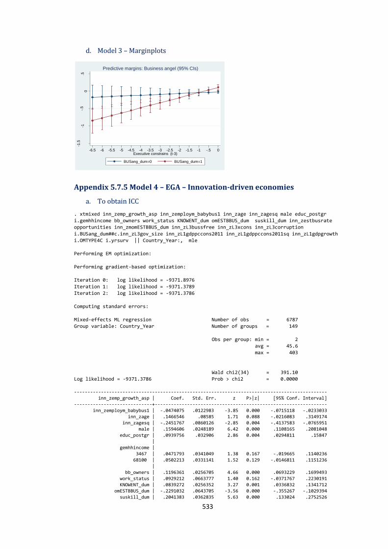
533
d. Model 3 – Marginplots
Appendix 5.7.5 Model 4 – EGA – Innovation-driven economies
a. To obtain ICC
. xtmixed inn_zemp_growth_asp inn_zemploym_babybus1 inn_zage inn_zagesq male educ_postgr
i.gemhhincome bb_owners work_status KNOWENT_dum omESTBBUS_dum suskill_dum inn_zestbusrate
opportunities inn_zmomESTBBUS_dum inn_zL3bussfree inn_zL3xcons inn_zL3corruption
i.BUSang_dum##c.inn_zL3gov_size inn_zL1gdppccons2011 inn_zL1gdppccons2011sq inn_zL1gdpgrowth
i.OMTYPE4C i.yrsurv || Country_Year:, mle
Performing EM optimization:
Performing gradient-based optimization:
Iteration 0: log likelihood = -9371.8976
Iteration 1: log likelihood = -9371.3789
Iteration 2: log likelihood = -9371.3786
Computing standard errors:
Mixed-effects ML regression Number of obs = 6787
Group variable: Country_Year Number of groups = 149
Obs per group: min = 2
avg = 45.6
max = 403
Wald chi2(34) = 391.10
Log likelihood = -9371.3786 Prob > chi2 = 0.0000
----------------------------------------------------------------------------------------------
inn_zemp_growth_asp | Coef. Std. Err. z P>|z| [95% Conf. Interval]
-----------------------------+----------------------------------------------------------------
inn_zemploym_babybus1 | -.0474075 .0122983 -3.85 0.000 -.0715118 -.0233033
inn_zage | .1466546 .08585 1.71 0.088 -.0216083 .3149174
inn_zagesq | -.2451767 .0860126 -2.85 0.004 -.4137583 -.0765951
male | .1594606 .0248189 6.42 0.000 .1108165 .2081048
educ_postgr | .0939756 .032906 2.86 0.004 .0294811 .15847
|
gemhhincome |
3467 | .0471793 .0341049 1.38 0.167 -.019665 .1140236
68100 | .0502213 .0331141 1.52 0.129 -.0146811 .1151236
|
bb_owners | .1196361 .0256705 4.66 0.000 .0693229 .1699493
work_status | .0929212 .0663777 1.40 0.162 -.0371767 .2230191
KNOWENT_dum | .0839272 .0256352 3.27 0.001 .0336832 .1341712
omESTBBUS_dum | -.2291032 .0643705 -3.56 0.000 -.355267 -.1029394
suskill_dum | .2041383 .0362835 5.63 0.000 .133024 .2752526
-1.5
-1-.
50
.5
Pre
dic
ted E
mp
. G
row
th A
sp
ira
tion
s (
EM
P)
-6.5 -6 -5.5 -5 -4.5 -4 -3.5 -3 -2.5 -2 -1.5 -1 -.5 0Executive constrains (t-3)
BUSang_dum=0 BUSang_dum=1
Predictive margins: Business angel (95% CIs)

534
inn_zestbusrate | -.0587546 .0181972 -3.23 0.001 -.0944204 -.0230888
opportunities | .1297322 .0254068 5.11 0.000 .0799357 .1795287
inn_zmomESTBBUS_dum | -.0525795 .0208773 -2.52 0.012 -.0934981 -.0116608
inn_zL3bussfree | -.0087045 .024522 -0.35 0.723 -.0567668 .0393578
inn_zL3xcons | .0433957 .0250545 1.73 0.083 -.0057103 .0925017
inn_zL3corruption | -.0591678 .026016 -2.27 0.023 -.1101583 -.0081773
1.BUSang_dum | .1191978 .0434504 2.74 0.006 .0340366 .204359
inn_zL3gov_size | -.149023 .0249141 -5.98 0.000 -.1978538 -.1001923
|
BUSang_dum#c.inn_zL3gov_size |
1 | .110401 .0414612 2.66 0.008 .0291385 .1916635
|
inn_zL1gdppccons2011 | -.2344608 .143158 -1.64 0.101 -.5150454 .0461238
inn_zL1gdppccons2011sq | .1783451 .1520278 1.17 0.241 -.1196239 .4763141
inn_zL1gdpgrowth | .045424 .0242803 1.87 0.061 -.0021646 .0930126
|
OMTYPE4C |
2 | .1276511 .0587459 2.17 0.030 .0125113 .242791
3 | .1421269 .0582046 2.44 0.015 .028048 .2562057
4 | .0744244 .0572 1.30 0.193 -.0376856 .1865343
| yrsurv |
2007 | -.0654155 .0642264 -1.02 0.308 -.1912969 .060466
2008 | -.1237299 .0681585 -1.82 0.069 -.257318 .0098583
2009 | -.0139351 .0693618 -0.20 0.841 -.1498818 .1220117
2010 | -.0308227 .0831012 -0.37 0.711 -.1936982 .1320527
2011 | .0038126 .0670237 0.06 0.955 -.1275514 .1351765
2012 | -.0270316 .0656215 -0.41 0.680 -.1556474 .1015841
2013 | -.0415524 .0668385 -0.62 0.534 -.1725535 .0894487
|
_cons | -.6269624 .0998183 -6.28 0.000 -.8226026 -.4313221
----------------------------------------------------------------------------------------------
------------------------------------------------------------------------------
Random-effects Parameters | Estimate Std. Err. [95% Conf. Interval]
-----------------------------+------------------------------------------------
Country_Year: Identity |
sd(_cons) | .0779852 .0269139 .0396506 .153382
-----------------------------+------------------------------------------------
sd(Residual) | .9601788 .0083492 .9439533 .9766833
------------------------------------------------------------------------------
LR test vs. linear regression: chibar2(01) = 4.06 Prob >= chibar2 = 0.0219
. estat icc
Residual intraclass correlation
------------------------------------------------------------------------------
Level | ICC Std. Err. [95% Conf. Interval]
-----------------------------+------------------------------------------------
Country_Year | .0065534 .0045104 .0016938 .0250056
------------------------------------------------------------------------------
b. Model 4 – results (robust – Standard Errors)
. xtmixed inn_zemp_growth_asp inn_zemploym_babybus1 inn_zage inn_zagesq male educ_postgr
i.gemhhincome bb_owners work_status KNOWENT_dum omESTBBUS_dum suskill_dum inn_zestbusrate
opportunities inn_zmomESTBBUS_dum inn_zL3bussfree inn_zL3xcons inn_zL3corruption
i.BUSang_dum##c.inn_zL3gov_size inn_zL1gdppccons2011 inn_zL1gdppccons2011sq inn_zL1gdpgrowth
i.OMTYPE4C i.yrsurv || Country_Year:, mle vce(robust)
Performing EM optimization:
Performing gradient-based optimization:
Iteration 0: log pseudolikelihood = -9371.8976
Iteration 1: log pseudolikelihood = -9371.3789
Iteration 2: log pseudolikelihood = -9371.3786
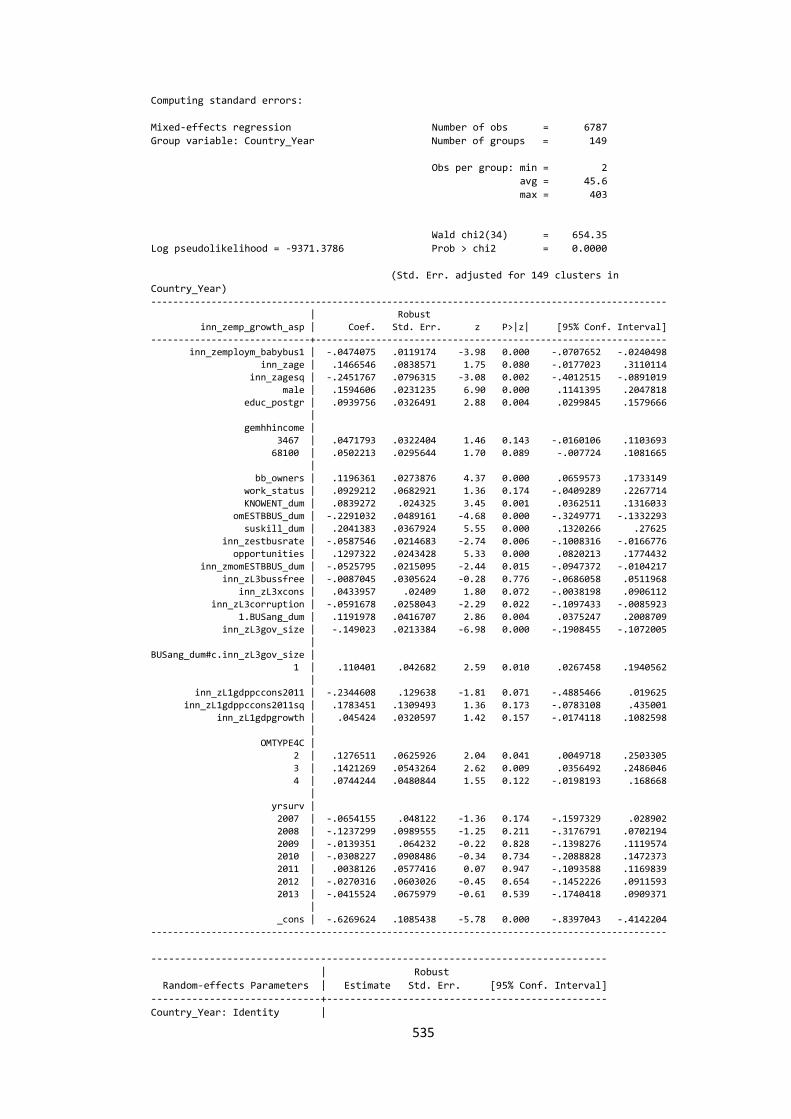
535
Computing standard errors:
Mixed-effects regression Number of obs = 6787
Group variable: Country_Year Number of groups = 149
Obs per group: min = 2
avg = 45.6
max = 403
Wald chi2(34) = 654.35
Log pseudolikelihood = -9371.3786 Prob > chi2 = 0.0000
(Std. Err. adjusted for 149 clusters in
Country_Year) ----------------------------------------------------------------------------------------------
| Robust
inn_zemp_growth_asp | Coef. Std. Err. z P>|z| [95% Conf. Interval]
-----------------------------+---------------------------------------------------------------- inn_zemploym_babybus1 | -.0474075 .0119174 -3.98 0.000 -.0707652 -.0240498
inn_zage | .1466546 .0838571 1.75 0.080 -.0177023 .3110114
inn_zagesq | -.2451767 .0796315 -3.08 0.002 -.4012515 -.0891019
male | .1594606 .0231235 6.90 0.000 .1141395 .2047818
educ_postgr | .0939756 .0326491 2.88 0.004 .0299845 .1579666
|
gemhhincome |
3467 | .0471793 .0322404 1.46 0.143 -.0160106 .1103693
68100 | .0502213 .0295644 1.70 0.089 -.007724 .1081665
|
bb_owners | .1196361 .0273876 4.37 0.000 .0659573 .1733149
work_status | .0929212 .0682921 1.36 0.174 -.0409289 .2267714
KNOWENT_dum | .0839272 .024325 3.45 0.001 .0362511 .1316033
omESTBBUS_dum | -.2291032 .0489161 -4.68 0.000 -.3249771 -.1332293
suskill_dum | .2041383 .0367924 5.55 0.000 .1320266 .27625
inn_zestbusrate | -.0587546 .0214683 -2.74 0.006 -.1008316 -.0166776
opportunities | .1297322 .0243428 5.33 0.000 .0820213 .1774432
inn_zmomESTBBUS_dum | -.0525795 .0215095 -2.44 0.015 -.0947372 -.0104217
inn_zL3bussfree | -.0087045 .0305624 -0.28 0.776 -.0686058 .0511968
inn_zL3xcons | .0433957 .02409 1.80 0.072 -.0038198 .0906112
inn_zL3corruption | -.0591678 .0258043 -2.29 0.022 -.1097433 -.0085923
1.BUSang_dum | .1191978 .0416707 2.86 0.004 .0375247 .2008709
inn_zL3gov_size | -.149023 .0213384 -6.98 0.000 -.1908455 -.1072005
|
BUSang_dum#c.inn_zL3gov_size |
1 | .110401 .042682 2.59 0.010 .0267458 .1940562
|
inn_zL1gdppccons2011 | -.2344608 .129638 -1.81 0.071 -.4885466 .019625
inn_zL1gdppccons2011sq | .1783451 .1309493 1.36 0.173 -.0783108 .435001
inn_zL1gdpgrowth | .045424 .0320597 1.42 0.157 -.0174118 .1082598
|
OMTYPE4C |
2 | .1276511 .0625926 2.04 0.041 .0049718 .2503305
3 | .1421269 .0543264 2.62 0.009 .0356492 .2486046
4 | .0744244 .0480844 1.55 0.122 -.0198193 .168668
|
yrsurv |
2007 | -.0654155 .048122 -1.36 0.174 -.1597329 .028902
2008 | -.1237299 .0989555 -1.25 0.211 -.3176791 .0702194
2009 | -.0139351 .064232 -0.22 0.828 -.1398276 .1119574 2010 | -.0308227 .0908486 -0.34 0.734 -.2088828 .1472373
2011 | .0038126 .0577416 0.07 0.947 -.1093588 .1169839
2012 | -.0270316 .0603026 -0.45 0.654 -.1452226 .0911593
2013 | -.0415524 .0675979 -0.61 0.539 -.1740418 .0909371
|
_cons | -.6269624 .1085438 -5.78 0.000 -.8397043 -.4142204
----------------------------------------------------------------------------------------------
------------------------------------------------------------------------------
| Robust
Random-effects Parameters | Estimate Std. Err. [95% Conf. Interval]
-----------------------------+------------------------------------------------
Country_Year: Identity |
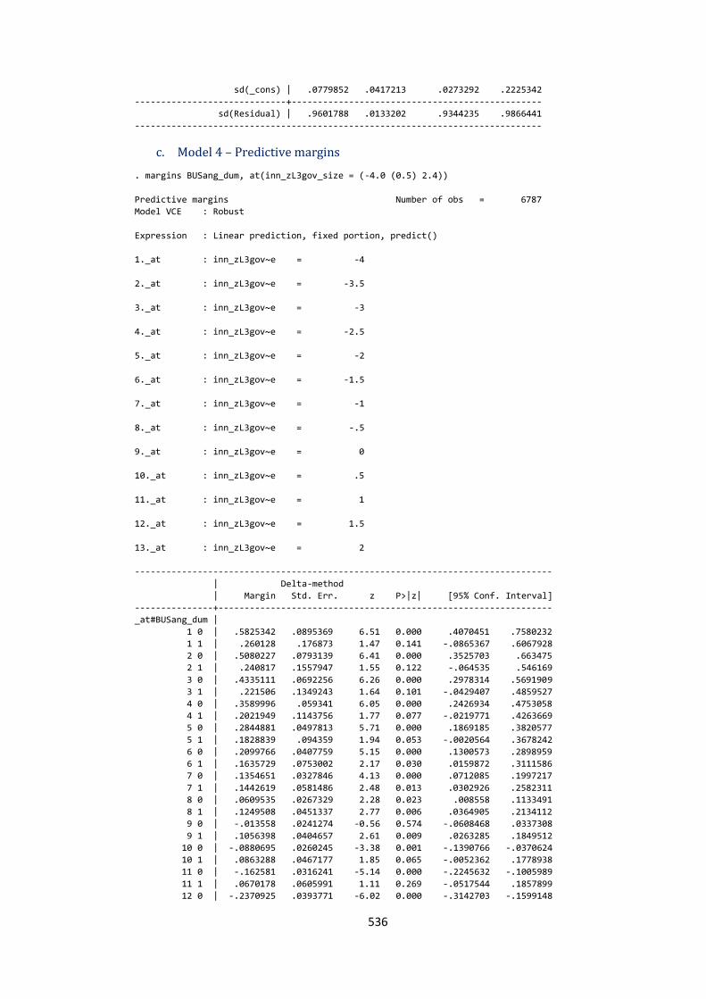
536
sd(_cons) | .0779852 .0417213 .0273292 .2225342
-----------------------------+------------------------------------------------
sd(Residual) | .9601788 .0133202 .9344235 .9866441
------------------------------------------------------------------------------
c. Model 4 – Predictive margins
. margins BUSang_dum, at(inn_zL3gov_size = (-4.0 (0.5) 2.4))
Predictive margins Number of obs = 6787
Model VCE : Robust
Expression : Linear prediction, fixed portion, predict()
1._at : inn_zL3gov~e = -4
2._at : inn_zL3gov~e = -3.5
3._at : inn_zL3gov~e = -3
4._at : inn_zL3gov~e = -2.5
5._at : inn_zL3gov~e = -2
6._at : inn_zL3gov~e = -1.5
7._at : inn_zL3gov~e = -1
8._at : inn_zL3gov~e = -.5
9._at : inn_zL3gov~e = 0
10._at : inn_zL3gov~e = .5
11._at : inn_zL3gov~e = 1
12._at : inn_zL3gov~e = 1.5
13._at : inn_zL3gov~e = 2
--------------------------------------------------------------------------------
| Delta-method
| Margin Std. Err. z P>|z| [95% Conf. Interval]
---------------+----------------------------------------------------------------
_at#BUSang_dum |
1 0 | .5825342 .0895369 6.51 0.000 .4070451 .7580232
1 1 | .260128 .176873 1.47 0.141 -.0865367 .6067928
2 0 | .5080227 .0793139 6.41 0.000 .3525703 .663475
2 1 | .240817 .1557947 1.55 0.122 -.064535 .546169
3 0 | .4335111 .0692256 6.26 0.000 .2978314 .5691909
3 1 | .221506 .1349243 1.64 0.101 -.0429407 .4859527
4 0 | .3589996 .059341 6.05 0.000 .2426934 .4753058
4 1 | .2021949 .1143756 1.77 0.077 -.0219771 .4263669
5 0 | .2844881 .0497813 5.71 0.000 .1869185 .3820577
5 1 | .1828839 .094359 1.94 0.053 -.0020564 .3678242
6 0 | .2099766 .0407759 5.15 0.000 .1300573 .2898959
6 1 | .1635729 .0753002 2.17 0.030 .0159872 .3111586
7 0 | .1354651 .0327846 4.13 0.000 .0712085 .1997217
7 1 | .1442619 .0581486 2.48 0.013 .0302926 .2582311
8 0 | .0609535 .0267329 2.28 0.023 .008558 .1133491
8 1 | .1249508 .0451337 2.77 0.006 .0364905 .2134112
9 0 | -.013558 .0241274 -0.56 0.574 -.0608468 .0337308
9 1 | .1056398 .0404657 2.61 0.009 .0263285 .1849512
10 0 | -.0880695 .0260245 -3.38 0.001 -.1390766 -.0370624
10 1 | .0863288 .0467177 1.85 0.065 -.0052362 .1778938
11 0 | -.162581 .0316241 -5.14 0.000 -.2245632 -.1005989
11 1 | .0670178 .0605991 1.11 0.269 -.0517544 .1857899
12 0 | -.2370925 .0393771 -6.02 0.000 -.3142703 -.1599148
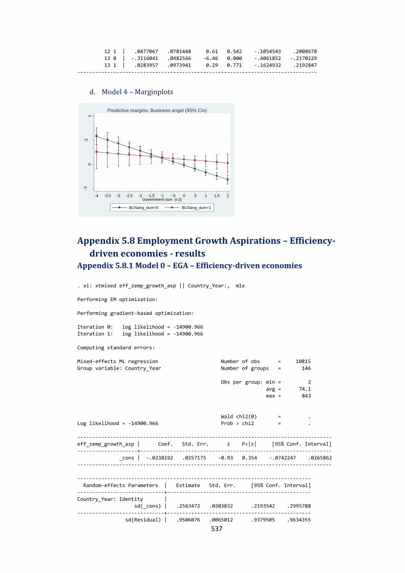
537
12 1 | .0477067 .0781448 0.61 0.542 -.1054543 .2008678
13 0 | -.3116041 .0482566 -6.46 0.000 -.4061852 -.2170229
13 1 | .0283957 .0973941 0.29 0.771 -.1624932 .2192847
--------------------------------------------------------------------------------
d. Model 4 – Marginplots
Appendix 5.8 Employment Growth Aspirations – Efficiency-
driven economies - results Appendix 5.8.1 Model 0 – EGA – Efficiency-driven economies
. xi: xtmixed eff_zemp_growth_asp || Country_Year:, mle
Performing EM optimization:
Performing gradient-based optimization:
Iteration 0: log likelihood = -14900.966
Iteration 1: log likelihood = -14900.966
Computing standard errors:
Mixed-effects ML regression Number of obs = 10815
Group variable: Country_Year Number of groups = 146
Obs per group: min = 2
avg = 74.1
max = 843
Wald chi2(0) = .
Log likelihood = -14900.966 Prob > chi2 = .
-------------------------------------------------------------------------------------
eff_zemp_growth_asp | Coef. Std. Err. z P>|z| [95% Conf. Interval]
--------------------+----------------------------------------------------------------
_cons | -.0238192 .0257175 -0.93 0.354 -.0742247 .0265862
-------------------------------------------------------------------------------------
------------------------------------------------------------------------------
Random-effects Parameters | Estimate Std. Err. [95% Conf. Interval]
-----------------------------+------------------------------------------------
Country_Year: Identity |
sd(_cons) | .2563472 .0203832 .2193542 .2995788
-----------------------------+------------------------------------------------
sd(Residual) | .9506076 .0065012 .9379505 .9634355
-.5
0.5
1
Pre
dic
ted E
mp
. G
row
th A
sp
ira
tion
s (
EM
P)
-4 -3.5 -3 -2.5 -2 -1.5 -1 -.5 0 .5 1 1.5 2Government size (t-3)
BUSang_dum=0 BUSang_dum=1
Predictive margins: Business angel (95% CIs)
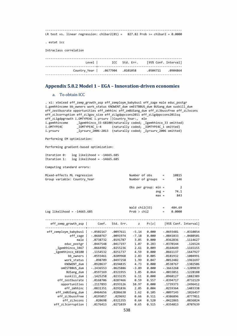
538
------------------------------------------------------------------------------
LR test vs. linear regression: chibar2(01) = 827.82 Prob >= chibar2 = 0.0000
. estat icc
Intraclass correlation
------------------------------------------------------------------------------
Level | ICC Std. Err. [95% Conf. Interval]
-----------------------------+------------------------------------------------
Country_Year | .0677904 .0101058 .0504711 .0904864
------------------------------------------------------------------------------
Appendix 5.8.2 Model 1 – EGA – Innovation-driven economies
a. To obtain ICC
. xi: xtmixed eff_zemp_growth_asp eff_zemploym_babybus1 eff_zage male educ_postgr
i.gemhhincome bb_owners work_status KNOWENT_dum omESTBBUS_dum BUSang_dum suskill_dum
eff_zestbusrate opportunities eff_zmhhinc eff_zmBUSang_dum eff_zL3bussfree eff_zL3xcons
eff_zL3corruption eff_zL3gov_size eff_zL1gdppccons2011 eff_zL1gdppccons2011sq
eff_zL1gdpgrowth i.OMTYPE4C i.yrsurv ||Country_Year:, mle
i.gemhhincome _Igemhhinco_33-68100(naturally coded; _Igemhhinco_33 omitted)
i.OMTYPE4C _IOMTYPE4C_1-4 (naturally coded; _IOMTYPE4C_1 omitted)
i.yrsurv _Iyrsurv_2006-2013 (naturally coded; _Iyrsurv_2006 omitted)
Performing EM optimization:
Performing gradient-based optimization:
Iteration 0: log likelihood = -14665.685
Iteration 1: log likelihood = -14665.685
Computing standard errors:
Mixed-effects ML regression Number of obs = 10815
Group variable: Country_Year Number of groups = 146
Obs per group: min = 2
avg = 74.1
max = 843
Wald chi2(33) = 484.69
Log likelihood = -14665.685 Prob > chi2 = 0.0000
----------------------------------------------------------------------------------------
eff_zemp_growth_asp | Coef. Std. Err. z P>|z| [95% Conf. Interval]
-----------------------+----------------------------------------------------------------
eff_zemploym_babybus1 | -.0502167 .0097611 -5.14 0.000 -.0693481 -.0310854
eff_zage | -.0660767 .0091974 -7.18 0.000 -.0841033 -.0480501
male | .0738732 .0191787 3.85 0.000 .0362836 .1114627
educ_postgr | .0447548 .0417197 1.07 0.283 -.0370144 .126524
_Igemhhinco_3467 | .0664902 .0255236 2.61 0.009 .0164649 .1165155
_Igemhhinco_68100 | .1154532 .0251737 4.59 0.000 .0661137 .1647927
bb_owners | .0593461 .0209968 2.83 0.005 .0181932 .1004991
work_status | .098709 .0497258 1.99 0.047 .0012482 .1961697
KNOWENT_dum | .0920637 .0194835 4.73 0.000 .0538767 .1302506
omESTBBUS_dum | -.2436553 .0625886 -3.89 0.000 -.3663268 -.1209839
BUSang_dum | .0597169 .0321955 1.85 0.064 -.0033851 .1228188
suskill_dum | .1425258 .0233235 6.11 0.000 .0968127 .1882389
eff_zestbusrate | .0168706 .0287466 0.59 0.557 -.0394717 .0732129
opportunities | .2117893 .0193126 10.97 0.000 .1739373 .2496412
eff_zmhhinc | .0831351 .0291836 2.85 0.004 .0259364 .1403338
eff_zmBUSang_dum | .0464656 .0286638 1.62 0.105 -.0097145 .1026457
eff_zL3bussfree | .0195057 .029692 0.66 0.511 -.0386896 .0777011
eff_zL3xcons | .020698 .0321355 0.64 0.520 -.0422865 .0836824
eff_zL3corruption | .0176413 .0271039 0.65 0.515 -.0354813 .0707639
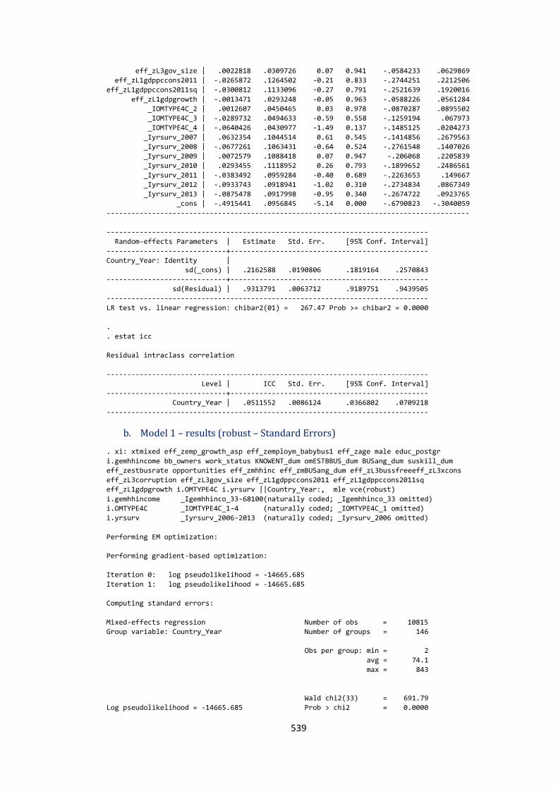
539
eff_zL3gov_size | .0022818 .0309726 0.07 0.941 -.0584233 .0629869
eff_zL1gdppccons2011 | -.0265872 .1264502 -0.21 0.833 -.2744251 .2212506
eff_zL1gdppccons2011sq | -.0300812 .1133096 -0.27 0.791 -.2521639 .1920016
eff_zL1gdpgrowth | -.0013471 .0293248 -0.05 0.963 -.0588226 .0561284
_IOMTYPE4C_2 | .0012607 .0450465 0.03 0.978 -.0870287 .0895502
_IOMTYPE4C_3 | -.0289732 .0494633 -0.59 0.558 -.1259194 .067973
_IOMTYPE4C_4 | -.0640426 .0430977 -1.49 0.137 -.1485125 .0204273
_Iyrsurv_2007 | .0632354 .1044514 0.61 0.545 -.1414856 .2679563
_Iyrsurv_2008 | -.0677261 .1063431 -0.64 0.524 -.2761548 .1407026
_Iyrsurv_2009 | .0072579 .1088418 0.07 0.947 -.206068 .2205839
_Iyrsurv_2010 | .0293455 .1118952 0.26 0.793 -.1899652 .2486561
_Iyrsurv_2011 | -.0383492 .0959284 -0.40 0.689 -.2263653 .149667
_Iyrsurv_2012 | -.0933743 .0918941 -1.02 0.310 -.2734834 .0867349
_Iyrsurv_2013 | -.0875478 .0917998 -0.95 0.340 -.2674722 .0923765
_cons | -.4915441 .0956845 -5.14 0.000 -.6790823 -.3040059
----------------------------------------------------------------------------------------
------------------------------------------------------------------------------
Random-effects Parameters | Estimate Std. Err. [95% Conf. Interval]
-----------------------------+------------------------------------------------
Country_Year: Identity |
sd(_cons) | .2162588 .0190806 .1819164 .2570843
-----------------------------+------------------------------------------------
sd(Residual) | .9313791 .0063712 .9189751 .9439505
------------------------------------------------------------------------------
LR test vs. linear regression: chibar2(01) = 267.47 Prob >= chibar2 = 0.0000
.
. estat icc
Residual intraclass correlation
------------------------------------------------------------------------------
Level | ICC Std. Err. [95% Conf. Interval]
-----------------------------+------------------------------------------------
Country_Year | .0511552 .0086124 .0366802 .0709218
------------------------------------------------------------------------------
b. Model 1 – results (robust – Standard Errors)
. xi: xtmixed eff_zemp_growth_asp eff_zemploym_babybus1 eff_zage male educ_postgr
i.gemhhincome bb_owners work_status KNOWENT_dum omESTBBUS_dum BUSang_dum suskill_dum
eff_zestbusrate opportunities eff_zmhhinc eff_zmBUSang_dum eff_zL3bussfreeeff_zL3xcons
eff_zL3corruption eff_zL3gov_size eff_zL1gdppccons2011 eff_zL1gdppccons2011sq
eff_zL1gdpgrowth i.OMTYPE4C i.yrsurv ||Country_Year:, mle vce(robust)
i.gemhhincome _Igemhhinco_33-68100(naturally coded; _Igemhhinco_33 omitted)
i.OMTYPE4C _IOMTYPE4C_1-4 (naturally coded; _IOMTYPE4C_1 omitted)
i.yrsurv _Iyrsurv_2006-2013 (naturally coded; _Iyrsurv_2006 omitted)
Performing EM optimization:
Performing gradient-based optimization:
Iteration 0: log pseudolikelihood = -14665.685
Iteration 1: log pseudolikelihood = -14665.685
Computing standard errors:
Mixed-effects regression Number of obs = 10815
Group variable: Country_Year Number of groups = 146
Obs per group: min = 2
avg = 74.1
max = 843
Wald chi2(33) = 691.79
Log pseudolikelihood = -14665.685 Prob > chi2 = 0.0000
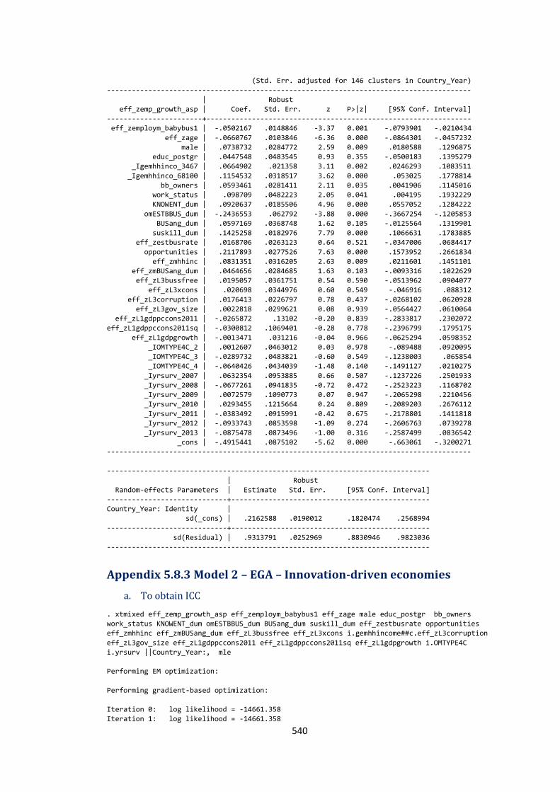
540
(Std. Err. adjusted for 146 clusters in Country_Year)
----------------------------------------------------------------------------------------
| Robust
eff_zemp_growth_asp | Coef. Std. Err. z P>|z| [95% Conf. Interval]
-----------------------+----------------------------------------------------------------
eff_zemploym_babybus1 | -.0502167 .0148846 -3.37 0.001 -.0793901 -.0210434
eff_zage | -.0660767 .0103846 -6.36 0.000 -.0864301 -.0457232
male | .0738732 .0284772 2.59 0.009 .0180588 .1296875
educ_postgr | .0447548 .0483545 0.93 0.355 -.0500183 .1395279
_Igemhhinco_3467 | .0664902 .021358 3.11 0.002 .0246293 .1083511
_Igemhhinco_68100 | .1154532 .0318517 3.62 0.000 .053025 .1778814
bb_owners | .0593461 .0281411 2.11 0.035 .0041906 .1145016
work_status | .098709 .0482223 2.05 0.041 .004195 .1932229
KNOWENT_dum | .0920637 .0185506 4.96 0.000 .0557052 .1284222
omESTBBUS_dum | -.2436553 .062792 -3.88 0.000 -.3667254 -.1205853
BUSang_dum | .0597169 .0368748 1.62 0.105 -.0125564 .1319901
suskill_dum | .1425258 .0182976 7.79 0.000 .1066631 .1783885
eff_zestbusrate | .0168706 .0263123 0.64 0.521 -.0347006 .0684417
opportunities | .2117893 .0277526 7.63 0.000 .1573952 .2661834
eff_zmhhinc | .0831351 .0316205 2.63 0.009 .0211601 .1451101
eff_zmBUSang_dum | .0464656 .0284685 1.63 0.103 -.0093316 .1022629
eff_zL3bussfree | .0195057 .0361751 0.54 0.590 -.0513962 .0904077
eff_zL3xcons | .020698 .0344976 0.60 0.549 -.046916 .088312
eff_zL3corruption | .0176413 .0226797 0.78 0.437 -.0268102 .0620928
eff_zL3gov_size | .0022818 .0299621 0.08 0.939 -.0564427 .0610064
eff_zL1gdppccons2011 | -.0265872 .13102 -0.20 0.839 -.2833817 .2302072
eff_zL1gdppccons2011sq | -.0300812 .1069401 -0.28 0.778 -.2396799 .1795175
eff_zL1gdpgrowth | -.0013471 .031216 -0.04 0.966 -.0625294 .0598352
_IOMTYPE4C_2 | .0012607 .0463012 0.03 0.978 -.089488 .0920095
_IOMTYPE4C_3 | -.0289732 .0483821 -0.60 0.549 -.1238003 .065854
_IOMTYPE4C_4 | -.0640426 .0434039 -1.48 0.140 -.1491127 .0210275
_Iyrsurv_2007 | .0632354 .0953885 0.66 0.507 -.1237226 .2501933
_Iyrsurv_2008 | -.0677261 .0941835 -0.72 0.472 -.2523223 .1168702
_Iyrsurv_2009 | .0072579 .1090773 0.07 0.947 -.2065298 .2210456
_Iyrsurv_2010 | .0293455 .1215664 0.24 0.809 -.2089203 .2676112
_Iyrsurv_2011 | -.0383492 .0915991 -0.42 0.675 -.2178801 .1411818
_Iyrsurv_2012 | -.0933743 .0853598 -1.09 0.274 -.2606763 .0739278
_Iyrsurv_2013 | -.0875478 .0873496 -1.00 0.316 -.2587499 .0836542
_cons | -.4915441 .0875102 -5.62 0.000 -.663061 -.3200271
----------------------------------------------------------------------------------------
------------------------------------------------------------------------------
| Robust
Random-effects Parameters | Estimate Std. Err. [95% Conf. Interval]
-----------------------------+------------------------------------------------
Country_Year: Identity |
sd(_cons) | .2162588 .0190012 .1820474 .2568994
-----------------------------+------------------------------------------------
sd(Residual) | .9313791 .0252969 .8830946 .9823036
------------------------------------------------------------------------------
Appendix 5.8.3 Model 2 – EGA – Innovation-driven economies
a. To obtain ICC
. xtmixed eff_zemp_growth_asp eff_zemploym_babybus1 eff_zage male educ_postgr bb_owners
work_status KNOWENT_dum omESTBBUS_dum BUSang_dum suskill_dum eff_zestbusrate opportunities
eff_zmhhinc eff_zmBUSang_dum eff_zL3bussfree eff_zL3xcons i.gemhhincome##c.eff_zL3corruption
eff_zL3gov_size eff_zL1gdppccons2011 eff_zL1gdppccons2011sq eff_zL1gdpgrowth i.OMTYPE4C
i.yrsurv ||Country_Year:, mle
Performing EM optimization:
Performing gradient-based optimization:
Iteration 0: log likelihood = -14661.358
Iteration 1: log likelihood = -14661.358
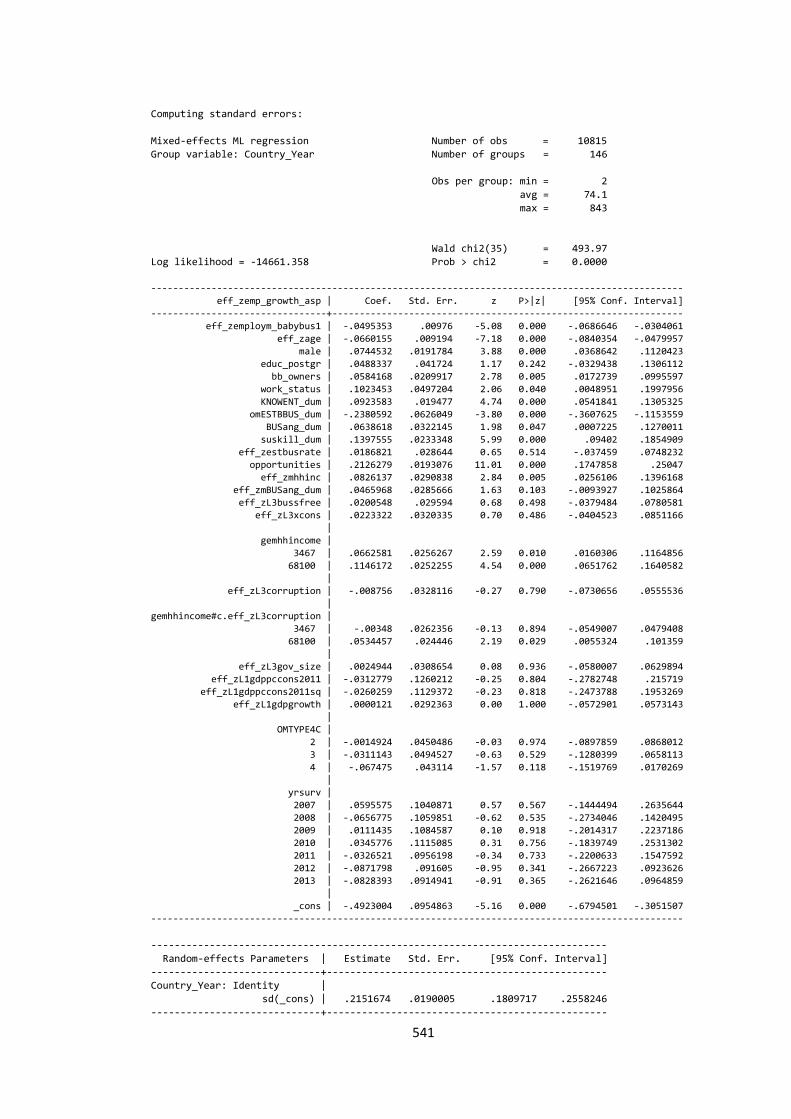
541
Computing standard errors:
Mixed-effects ML regression Number of obs = 10815
Group variable: Country_Year Number of groups = 146
Obs per group: min = 2
avg = 74.1
max = 843
Wald chi2(35) = 493.97
Log likelihood = -14661.358 Prob > chi2 = 0.0000
-------------------------------------------------------------------------------------------------
eff_zemp_growth_asp | Coef. Std. Err. z P>|z| [95% Conf. Interval]
--------------------------------+----------------------------------------------------------------
eff_zemploym_babybus1 | -.0495353 .00976 -5.08 0.000 -.0686646 -.0304061
eff_zage | -.0660155 .009194 -7.18 0.000 -.0840354 -.0479957
male | .0744532 .0191784 3.88 0.000 .0368642 .1120423
educ_postgr | .0488337 .041724 1.17 0.242 -.0329438 .1306112
bb_owners | .0584168 .0209917 2.78 0.005 .0172739 .0995597
work_status | .1023453 .0497204 2.06 0.040 .0048951 .1997956
KNOWENT_dum | .0923583 .019477 4.74 0.000 .0541841 .1305325
omESTBBUS_dum | -.2380592 .0626049 -3.80 0.000 -.3607625 -.1153559
BUSang_dum | .0638618 .0322145 1.98 0.047 .0007225 .1270011
suskill_dum | .1397555 .0233348 5.99 0.000 .09402 .1854909
eff_zestbusrate | .0186821 .028644 0.65 0.514 -.037459 .0748232
opportunities | .2126279 .0193076 11.01 0.000 .1747858 .25047
eff_zmhhinc | .0826137 .0290838 2.84 0.005 .0256106 .1396168
eff_zmBUSang_dum | .0465968 .0285666 1.63 0.103 -.0093927 .1025864
eff_zL3bussfree | .0200548 .029594 0.68 0.498 -.0379484 .0780581
eff_zL3xcons | .0223322 .0320335 0.70 0.486 -.0404523 .0851166
|
gemhhincome |
3467 | .0662581 .0256267 2.59 0.010 .0160306 .1164856
68100 | .1146172 .0252255 4.54 0.000 .0651762 .1640582
|
eff_zL3corruption | -.008756 .0328116 -0.27 0.790 -.0730656 .0555536
|
gemhhincome#c.eff_zL3corruption |
3467 | -.00348 .0262356 -0.13 0.894 -.0549007 .0479408
68100 | .0534457 .024446 2.19 0.029 .0055324 .101359
|
eff_zL3gov_size | .0024944 .0308654 0.08 0.936 -.0580007 .0629894
eff_zL1gdppccons2011 | -.0312779 .1260212 -0.25 0.804 -.2782748 .215719
eff_zL1gdppccons2011sq | -.0260259 .1129372 -0.23 0.818 -.2473788 .1953269
eff_zL1gdpgrowth | .0000121 .0292363 0.00 1.000 -.0572901 .0573143
| OMTYPE4C |
2 | -.0014924 .0450486 -0.03 0.974 -.0897859 .0868012
3 | -.0311143 .0494527 -0.63 0.529 -.1280399 .0658113
4 | -.067475 .043114 -1.57 0.118 -.1519769 .0170269
|
yrsurv |
2007 | .0595575 .1040871 0.57 0.567 -.1444494 .2635644
2008 | -.0656775 .1059851 -0.62 0.535 -.2734046 .1420495
2009 | .0111435 .1084587 0.10 0.918 -.2014317 .2237186
2010 | .0345776 .1115085 0.31 0.756 -.1839749 .2531302
2011 | -.0326521 .0956198 -0.34 0.733 -.2200633 .1547592
2012 | -.0871798 .091605 -0.95 0.341 -.2667223 .0923626
2013 | -.0828393 .0914941 -0.91 0.365 -.2621646 .0964859
|
_cons | -.4923004 .0954863 -5.16 0.000 -.6794501 -.3051507
-------------------------------------------------------------------------------------------------
------------------------------------------------------------------------------
Random-effects Parameters | Estimate Std. Err. [95% Conf. Interval]
-----------------------------+------------------------------------------------
Country_Year: Identity |
sd(_cons) | .2151674 .0190005 .1809717 .2558246
-----------------------------+------------------------------------------------
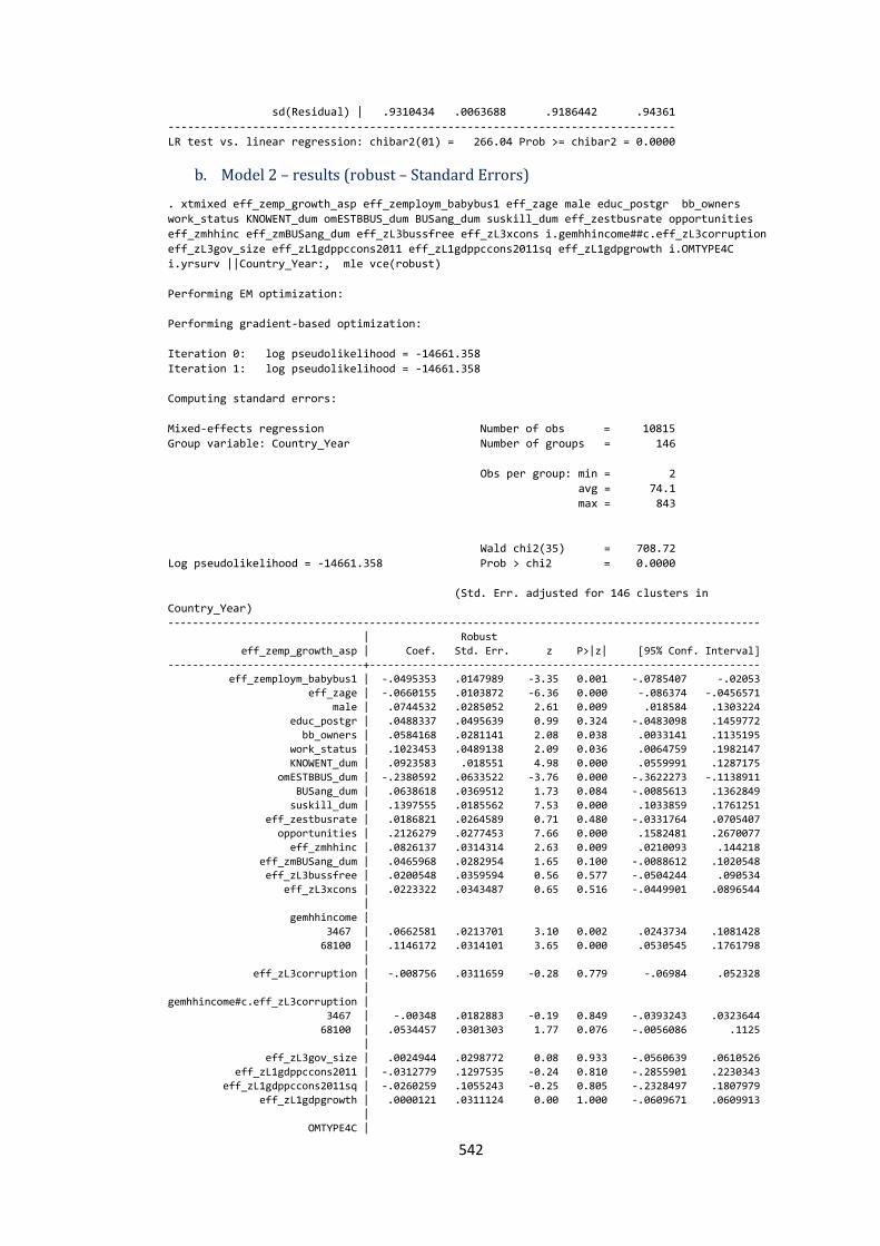
542
sd(Residual) | .9310434 .0063688 .9186442 .94361
------------------------------------------------------------------------------
LR test vs. linear regression: chibar2(01) = 266.04 Prob >= chibar2 = 0.0000
b. Model 2 – results (robust – Standard Errors)
. xtmixed eff_zemp_growth_asp eff_zemploym_babybus1 eff_zage male educ_postgr bb_owners
work_status KNOWENT_dum omESTBBUS_dum BUSang_dum suskill_dum eff_zestbusrate opportunities
eff_zmhhinc eff_zmBUSang_dum eff_zL3bussfree eff_zL3xcons i.gemhhincome##c.eff_zL3corruption
eff_zL3gov_size eff_zL1gdppccons2011 eff_zL1gdppccons2011sq eff_zL1gdpgrowth i.OMTYPE4C
i.yrsurv ||Country_Year:, mle vce(robust)
Performing EM optimization:
Performing gradient-based optimization:
Iteration 0: log pseudolikelihood = -14661.358
Iteration 1: log pseudolikelihood = -14661.358
Computing standard errors:
Mixed-effects regression Number of obs = 10815
Group variable: Country_Year Number of groups = 146
Obs per group: min = 2
avg = 74.1
max = 843
Wald chi2(35) = 708.72
Log pseudolikelihood = -14661.358 Prob > chi2 = 0.0000
(Std. Err. adjusted for 146 clusters in
Country_Year) -------------------------------------------------------------------------------------------------
| Robust
eff_zemp_growth_asp | Coef. Std. Err. z P>|z| [95% Conf. Interval]
--------------------------------+----------------------------------------------------------------
eff_zemploym_babybus1 | -.0495353 .0147989 -3.35 0.001 -.0785407 -.02053
eff_zage | -.0660155 .0103872 -6.36 0.000 -.086374 -.0456571
male | .0744532 .0285052 2.61 0.009 .018584 .1303224
educ_postgr | .0488337 .0495639 0.99 0.324 -.0483098 .1459772
bb_owners | .0584168 .0281141 2.08 0.038 .0033141 .1135195
work_status | .1023453 .0489138 2.09 0.036 .0064759 .1982147
KNOWENT_dum | .0923583 .018551 4.98 0.000 .0559991 .1287175
omESTBBUS_dum | -.2380592 .0633522 -3.76 0.000 -.3622273 -.1138911
BUSang_dum | .0638618 .0369512 1.73 0.084 -.0085613 .1362849
suskill_dum | .1397555 .0185562 7.53 0.000 .1033859 .1761251
eff_zestbusrate | .0186821 .0264589 0.71 0.480 -.0331764 .0705407
opportunities | .2126279 .0277453 7.66 0.000 .1582481 .2670077
eff_zmhhinc | .0826137 .0314314 2.63 0.009 .0210093 .144218
eff_zmBUSang_dum | .0465968 .0282954 1.65 0.100 -.0088612 .1020548 eff_zL3bussfree | .0200548 .0359594 0.56 0.577 -.0504244 .090534
eff_zL3xcons | .0223322 .0343487 0.65 0.516 -.0449901 .0896544
|
gemhhincome |
3467 | .0662581 .0213701 3.10 0.002 .0243734 .1081428
68100 | .1146172 .0314101 3.65 0.000 .0530545 .1761798
|
eff_zL3corruption | -.008756 .0311659 -0.28 0.779 -.06984 .052328
|
gemhhincome#c.eff_zL3corruption |
3467 | -.00348 .0182883 -0.19 0.849 -.0393243 .0323644
68100 | .0534457 .0301303 1.77 0.076 -.0056086 .1125
|
eff_zL3gov_size | .0024944 .0298772 0.08 0.933 -.0560639 .0610526
eff_zL1gdppccons2011 | -.0312779 .1297535 -0.24 0.810 -.2855901 .2230343
eff_zL1gdppccons2011sq | -.0260259 .1055243 -0.25 0.805 -.2328497 .1807979
eff_zL1gdpgrowth | .0000121 .0311124 0.00 1.000 -.0609671 .0609913
|
OMTYPE4C |
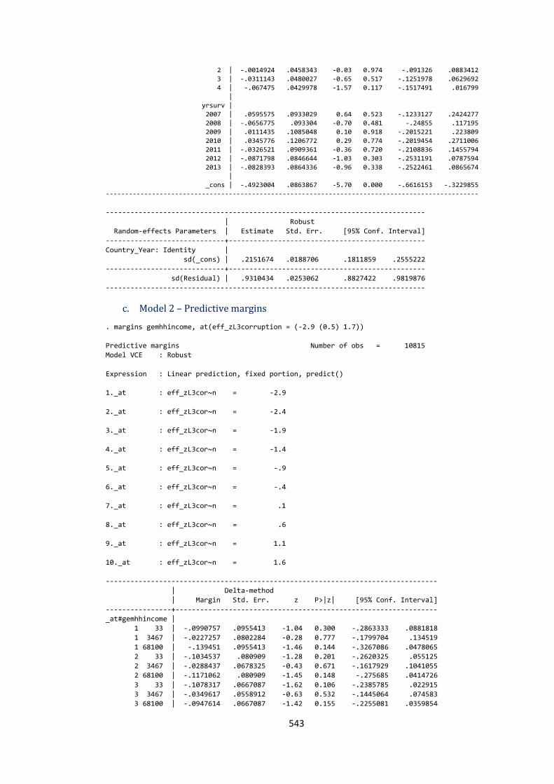
543
2 | -.0014924 .0458343 -0.03 0.974 -.091326 .0883412
3 | -.0311143 .0480027 -0.65 0.517 -.1251978 .0629692
4 | -.067475 .0429978 -1.57 0.117 -.1517491 .016799
|
yrsurv |
2007 | .0595575 .0933029 0.64 0.523 -.1233127 .2424277
2008 | -.0656775 .093304 -0.70 0.481 -.24855 .117195
2009 | .0111435 .1085048 0.10 0.918 -.2015221 .223809
2010 | .0345776 .1206772 0.29 0.774 -.2019454 .2711006
2011 | -.0326521 .0909361 -0.36 0.720 -.2108836 .1455794
2012 | -.0871798 .0846644 -1.03 0.303 -.2531191 .0787594
2013 | -.0828393 .0864336 -0.96 0.338 -.2522461 .0865674
|
_cons | -.4923004 .0863867 -5.70 0.000 -.6616153 -.3229855
-------------------------------------------------------------------------------------------------
------------------------------------------------------------------------------
| Robust
Random-effects Parameters | Estimate Std. Err. [95% Conf. Interval]
-----------------------------+------------------------------------------------
Country_Year: Identity |
sd(_cons) | .2151674 .0188706 .1811859 .2555222
-----------------------------+------------------------------------------------
sd(Residual) | .9310434 .0253062 .8827422 .9819876
------------------------------------------------------------------------------
c. Model 2 – Predictive margins
. margins gemhhincome, at(eff_zL3corruption = (-2.9 (0.5) 1.7))
Predictive margins Number of obs = 10815
Model VCE : Robust
Expression : Linear prediction, fixed portion, predict()
1._at : eff_zL3cor~n = -2.9
2._at : eff_zL3cor~n = -2.4
3._at : eff_zL3cor~n = -1.9
4._at : eff_zL3cor~n = -1.4
5._at : eff_zL3cor~n = -.9
6._at : eff_zL3cor~n = -.4
7._at : eff_zL3cor~n = .1
8._at : eff_zL3cor~n = .6
9._at : eff_zL3cor~n = 1.1
10._at : eff_zL3cor~n = 1.6
---------------------------------------------------------------------------------
| Delta-method
| Margin Std. Err. z P>|z| [95% Conf. Interval]
----------------+----------------------------------------------------------------
_at#gemhhincome |
1 33 | -.0990757 .0955413 -1.04 0.300 -.2863333 .0881818
1 3467 | -.0227257 .0802284 -0.28 0.777 -.1799704 .134519
1 68100 | -.139451 .0955413 -1.46 0.144 -.3267086 .0478065
2 33 | -.1034537 .080909 -1.28 0.201 -.2620325 .055125
2 3467 | -.0288437 .0678325 -0.43 0.671 -.1617929 .1041055
2 68100 | -.1171062 .080909 -1.45 0.148 -.275685 .0414726
3 33 | -.1078317 .0667087 -1.62 0.106 -.2385785 .022915
3 3467 | -.0349617 .0558912 -0.63 0.532 -.1445064 .074583
3 68100 | -.0947614 .0667087 -1.42 0.155 -.2255081 .0359854
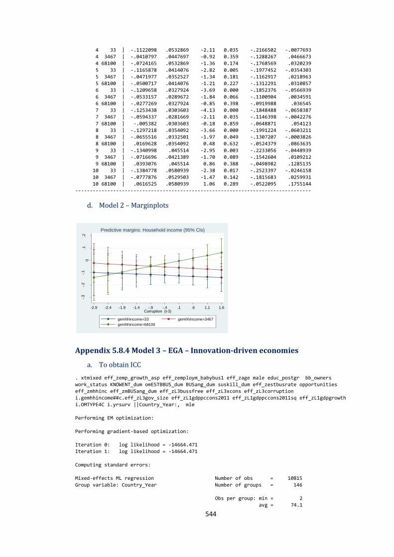
544
4 33 | -.1122098 .0532869 -2.11 0.035 -.2166502 -.0077693
4 3467 | -.0410797 .0447697 -0.92 0.359 -.1288267 .0466673
4 68100 | -.0724165 .0532869 -1.36 0.174 -.1768569 .0320239
5 33 | -.1165878 .0414076 -2.82 0.005 -.1977452 -.0354303
5 3467 | -.0471977 .0352527 -1.34 0.181 -.1162917 .0218963
5 68100 | -.0500717 .0414076 -1.21 0.227 -.1312291 .0310857
6 33 | -.1209658 .0327924 -3.69 0.000 -.1852376 -.0566939
6 3467 | -.0533157 .0289672 -1.84 0.066 -.1100904 .0034591
6 68100 | -.0277269 .0327924 -0.85 0.398 -.0919988 .036545
7 33 | -.1253438 .0303603 -4.13 0.000 -.1848488 -.0658387
7 3467 | -.0594337 .0281669 -2.11 0.035 -.1146398 -.0042276
7 68100 | -.005382 .0303603 -0.18 0.859 -.0648871 .054123
8 33 | -.1297218 .0354092 -3.66 0.000 -.1991224 -.0603211
8 3467 | -.0655516 .0332501 -1.97 0.049 -.1307207 -.0003826
8 68100 | .0169628 .0354092 0.48 0.632 -.0524379 .0863635
9 33 | -.1340998 .045514 -2.95 0.003 -.2233056 -.0448939
9 3467 | -.0716696 .0421389 -1.70 0.089 -.1542604 .0109212
9 68100 | .0393076 .045514 0.86 0.388 -.0498982 .1285135
10 33 | -.1384778 .0580939 -2.38 0.017 -.2523397 -.0246158
10 3467 | -.0777876 .0529503 -1.47 0.142 -.1815683 .0259931
10 68100 | .0616525 .0580939 1.06 0.289 -.0522095 .1755144
---------------------------------------------------------------------------------
d. Model 2 – Marginplots
Appendix 5.8.4 Model 3 – EGA – Innovation-driven economies
a. To obtain ICC
. xtmixed eff_zemp_growth_asp eff_zemploym_babybus1 eff_zage male educ_postgr bb_owners
work_status KNOWENT_dum omESTBBUS_dum BUSang_dum suskill_dum eff_zestbusrate opportunities
eff_zmhhinc eff_zmBUSang_dum eff_zL3bussfree eff_zL3xcons eff_zL3corruption
i.gemhhincome##c.eff_zL3gov_size eff_zL1gdppccons2011 eff_zL1gdppccons2011sq eff_zL1gdpgrowth
i.OMTYPE4C i.yrsurv ||Country_Year:, mle
Performing EM optimization:
Performing gradient-based optimization:
Iteration 0: log likelihood = -14664.471
Iteration 1: log likelihood = -14664.471
Computing standard errors:
Mixed-effects ML regression Number of obs = 10815
Group variable: Country_Year Number of groups = 146
Obs per group: min = 2
avg = 74.1
-.3
-.2
-.1
0.1
.2
Pre
dic
ted E
mp
. G
row
th A
sp
ira
tion
s (
EM
P)
-2.9 -2.4 -1.9 -1.4 -.9 -.4 .1 .6 1.1 1.6Corruption (t-3)
gemhhincome=33 gemhhincome=3467
gemhhincome=68100
Predictive margins: Household income (95% CIs)
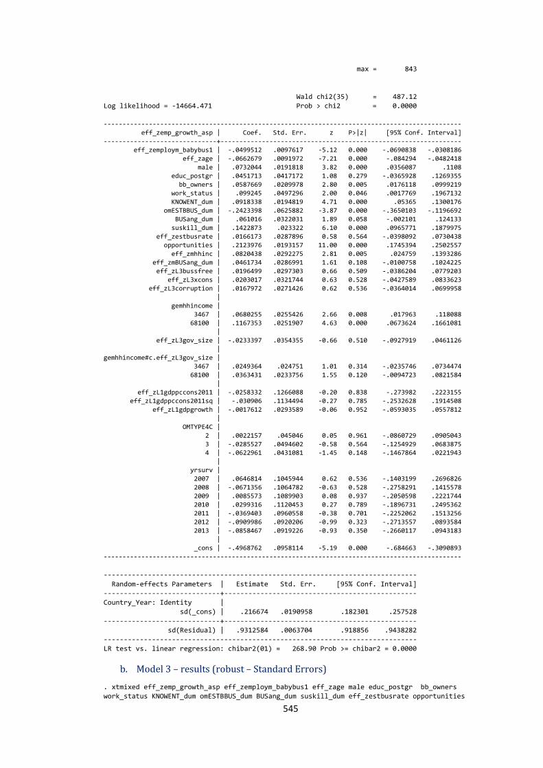
545
max = 843
Wald chi2(35) = 487.12
Log likelihood = -14664.471 Prob > chi2 = 0.0000
-----------------------------------------------------------------------------------------------
eff_zemp_growth_asp | Coef. Std. Err. z P>|z| [95% Conf. Interval]
------------------------------+----------------------------------------------------------------
eff_zemploym_babybus1 | -.0499512 .0097617 -5.12 0.000 -.0690838 -.0308186
eff_zage | -.0662679 .0091972 -7.21 0.000 -.084294 -.0482418
male | .0732044 .0191818 3.82 0.000 .0356087 .1108
educ_postgr | .0451713 .0417172 1.08 0.279 -.0365928 .1269355
bb_owners | .0587669 .0209978 2.80 0.005 .0176118 .0999219
work_status | .099245 .0497296 2.00 0.046 .0017769 .1967132
KNOWENT_dum | .0918338 .0194819 4.71 0.000 .05365 .1300176
omESTBBUS_dum | -.2423398 .0625882 -3.87 0.000 -.3650103 -.1196692
BUSang_dum | .061016 .0322031 1.89 0.058 -.002101 .124133
suskill_dum | .1422873 .023322 6.10 0.000 .0965771 .1879975
eff_zestbusrate | .0166173 .0287896 0.58 0.564 -.0398092 .0730438
opportunities | .2123976 .0193157 11.00 0.000 .1745394 .2502557
eff_zmhhinc | .0820438 .0292275 2.81 0.005 .024759 .1393286
eff_zmBUSang_dum | .0461734 .0286991 1.61 0.108 -.0100758 .1024225
eff_zL3bussfree | .0196499 .0297303 0.66 0.509 -.0386204 .0779203
eff_zL3xcons | .0203017 .0321744 0.63 0.528 -.0427589 .0833623
eff_zL3corruption | .0167972 .0271426 0.62 0.536 -.0364014 .0699958
|
gemhhincome |
3467 | .0680255 .0255426 2.66 0.008 .017963 .118088
68100 | .1167353 .0251907 4.63 0.000 .0673624 .1661081
|
eff_zL3gov_size | -.0233397 .0354355 -0.66 0.510 -.0927919 .0461126
|
gemhhincome#c.eff_zL3gov_size |
3467 | .0249364 .024751 1.01 0.314 -.0235746 .0734474
68100 | .0363431 .0233756 1.55 0.120 -.0094723 .0821584
|
eff_zL1gdppccons2011 | -.0258332 .1266088 -0.20 0.838 -.273982 .2223155
eff_zL1gdppccons2011sq | -.030906 .1134494 -0.27 0.785 -.2532628 .1914508
eff_zL1gdpgrowth | -.0017612 .0293589 -0.06 0.952 -.0593035 .0557812
|
OMTYPE4C |
2 | .0022157 .045046 0.05 0.961 -.0860729 .0905043
3 | -.0285527 .0494602 -0.58 0.564 -.1254929 .0683875 4 | -.0622961 .0431081 -1.45 0.148 -.1467864 .0221943
|
yrsurv |
2007 | .0646814 .1045944 0.62 0.536 -.1403199 .2696826
2008 | -.0671356 .1064782 -0.63 0.528 -.2758291 .1415578
2009 | .0085573 .1089903 0.08 0.937 -.2050598 .2221744
2010 | .0299316 .1120453 0.27 0.789 -.1896731 .2495362
2011 | -.0369403 .0960558 -0.38 0.701 -.2252062 .1513256
2012 | -.0909986 .0920206 -0.99 0.323 -.2713557 .0893584
2013 | -.0858467 .0919226 -0.93 0.350 -.2660117 .0943183
|
_cons | -.4968762 .0958114 -5.19 0.000 -.684663 -.3090893
-----------------------------------------------------------------------------------------------
------------------------------------------------------------------------------
Random-effects Parameters | Estimate Std. Err. [95% Conf. Interval]
-----------------------------+------------------------------------------------
Country_Year: Identity |
sd(_cons) | .216674 .0190958 .182301 .257528
-----------------------------+------------------------------------------------
sd(Residual) | .9312584 .0063704 .918856 .9438282
------------------------------------------------------------------------------
LR test vs. linear regression: chibar2(01) = 268.90 Prob >= chibar2 = 0.0000
b. Model 3 – results (robust – Standard Errors)
. xtmixed eff_zemp_growth_asp eff_zemploym_babybus1 eff_zage male educ_postgr bb_owners
work_status KNOWENT_dum omESTBBUS_dum BUSang_dum suskill_dum eff_zestbusrate opportunities
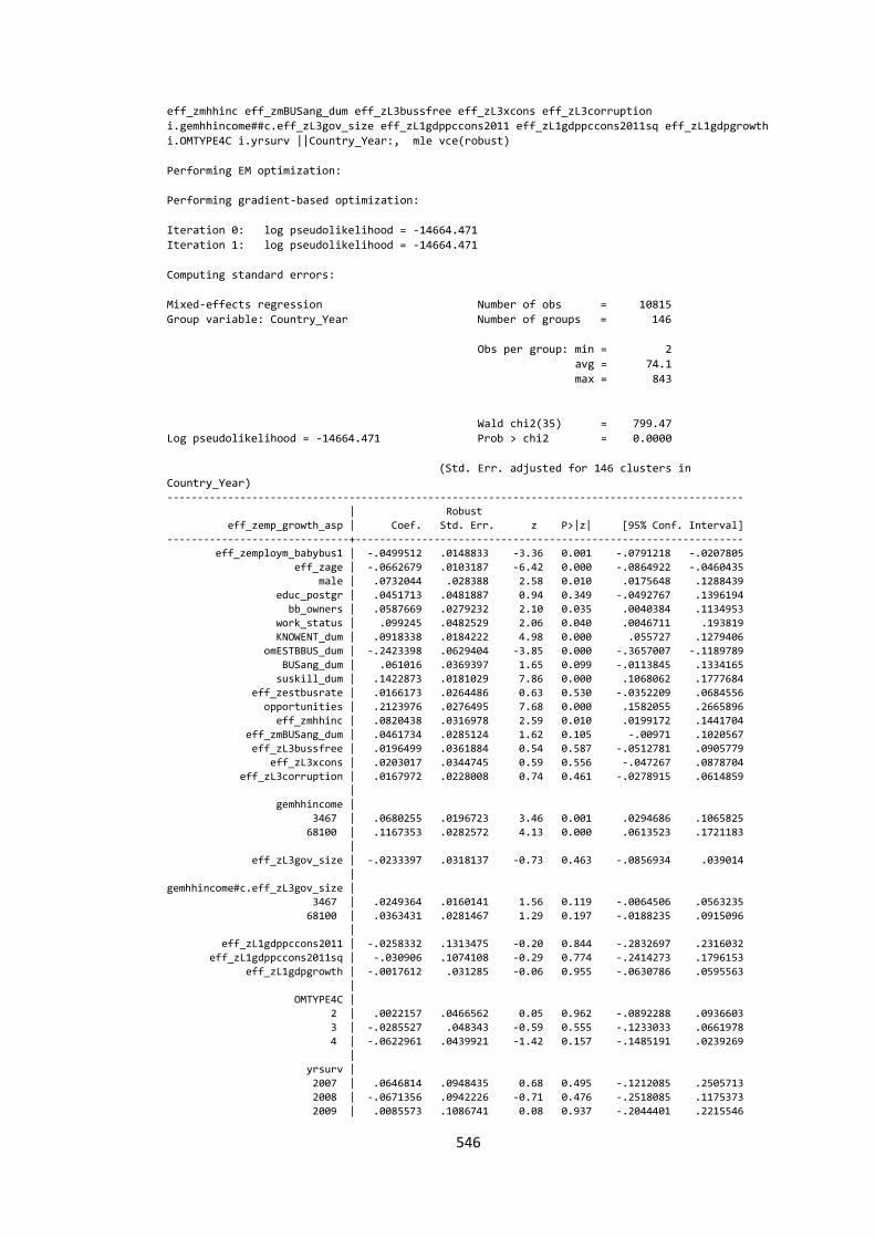
546
eff_zmhhinc eff_zmBUSang_dum eff_zL3bussfree eff_zL3xcons eff_zL3corruption
i.gemhhincome##c.eff_zL3gov_size eff_zL1gdppccons2011 eff_zL1gdppccons2011sq eff_zL1gdpgrowth
i.OMTYPE4C i.yrsurv ||Country_Year:, mle vce(robust)
Performing EM optimization:
Performing gradient-based optimization:
Iteration 0: log pseudolikelihood = -14664.471
Iteration 1: log pseudolikelihood = -14664.471
Computing standard errors:
Mixed-effects regression Number of obs = 10815
Group variable: Country_Year Number of groups = 146
Obs per group: min = 2
avg = 74.1
max = 843
Wald chi2(35) = 799.47
Log pseudolikelihood = -14664.471 Prob > chi2 = 0.0000
(Std. Err. adjusted for 146 clusters in
Country_Year) -----------------------------------------------------------------------------------------------
| Robust
eff_zemp_growth_asp | Coef. Std. Err. z P>|z| [95% Conf. Interval]
------------------------------+----------------------------------------------------------------
eff_zemploym_babybus1 | -.0499512 .0148833 -3.36 0.001 -.0791218 -.0207805
eff_zage | -.0662679 .0103187 -6.42 0.000 -.0864922 -.0460435
male | .0732044 .028388 2.58 0.010 .0175648 .1288439
educ_postgr | .0451713 .0481887 0.94 0.349 -.0492767 .1396194
bb_owners | .0587669 .0279232 2.10 0.035 .0040384 .1134953
work_status | .099245 .0482529 2.06 0.040 .0046711 .193819
KNOWENT_dum | .0918338 .0184222 4.98 0.000 .055727 .1279406
omESTBBUS_dum | -.2423398 .0629404 -3.85 0.000 -.3657007 -.1189789
BUSang_dum | .061016 .0369397 1.65 0.099 -.0113845 .1334165
suskill_dum | .1422873 .0181029 7.86 0.000 .1068062 .1777684
eff_zestbusrate | .0166173 .0264486 0.63 0.530 -.0352209 .0684556
opportunities | .2123976 .0276495 7.68 0.000 .1582055 .2665896
eff_zmhhinc | .0820438 .0316978 2.59 0.010 .0199172 .1441704
eff_zmBUSang_dum | .0461734 .0285124 1.62 0.105 -.00971 .1020567
eff_zL3bussfree | .0196499 .0361884 0.54 0.587 -.0512781 .0905779
eff_zL3xcons | .0203017 .0344745 0.59 0.556 -.047267 .0878704
eff_zL3corruption | .0167972 .0228008 0.74 0.461 -.0278915 .0614859
|
gemhhincome |
3467 | .0680255 .0196723 3.46 0.001 .0294686 .1065825
68100 | .1167353 .0282572 4.13 0.000 .0613523 .1721183
|
eff_zL3gov_size | -.0233397 .0318137 -0.73 0.463 -.0856934 .039014
|
gemhhincome#c.eff_zL3gov_size | 3467 | .0249364 .0160141 1.56 0.119 -.0064506 .0563235
68100 | .0363431 .0281467 1.29 0.197 -.0188235 .0915096
|
eff_zL1gdppccons2011 | -.0258332 .1313475 -0.20 0.844 -.2832697 .2316032
eff_zL1gdppccons2011sq | -.030906 .1074108 -0.29 0.774 -.2414273 .1796153
eff_zL1gdpgrowth | -.0017612 .031285 -0.06 0.955 -.0630786 .0595563
|
OMTYPE4C |
2 | .0022157 .0466562 0.05 0.962 -.0892288 .0936603
3 | -.0285527 .048343 -0.59 0.555 -.1233033 .0661978
4 | -.0622961 .0439921 -1.42 0.157 -.1485191 .0239269
|
yrsurv |
2007 | .0646814 .0948435 0.68 0.495 -.1212085 .2505713
2008 | -.0671356 .0942226 -0.71 0.476 -.2518085 .1175373
2009 | .0085573 .1086741 0.08 0.937 -.2044401 .2215546
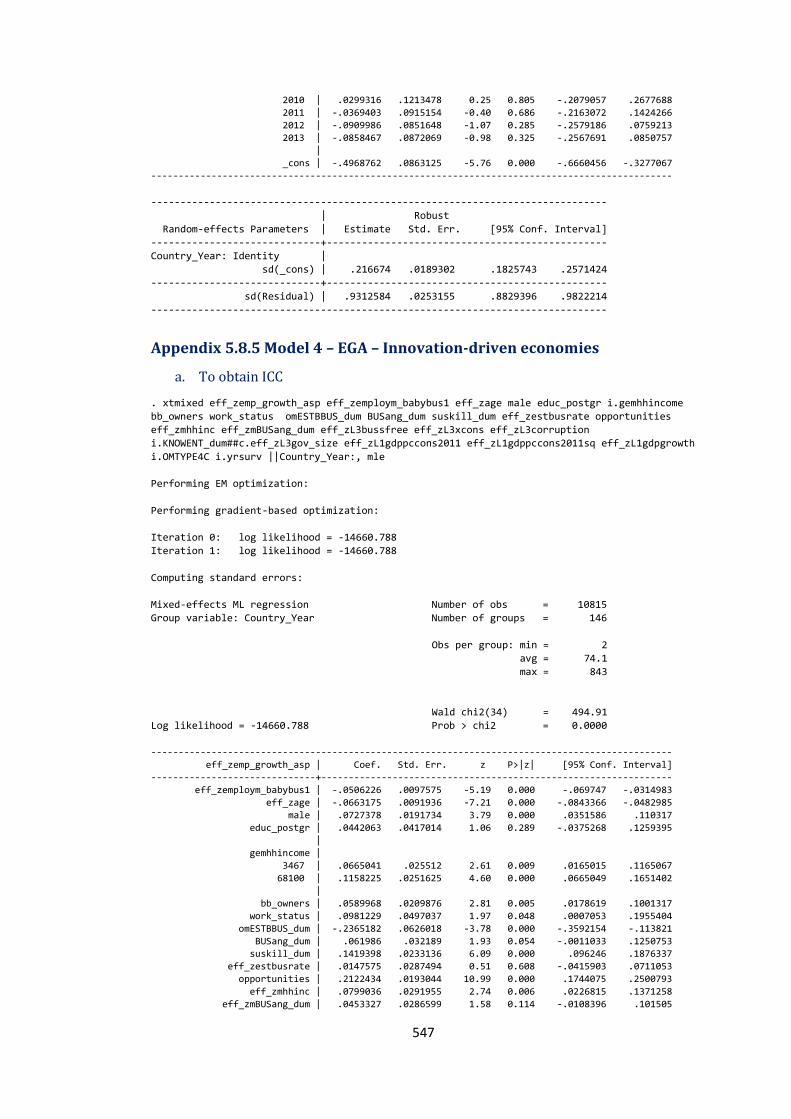
547
2010 | .0299316 .1213478 0.25 0.805 -.2079057 .2677688
2011 | -.0369403 .0915154 -0.40 0.686 -.2163072 .1424266
2012 | -.0909986 .0851648 -1.07 0.285 -.2579186 .0759213
2013 | -.0858467 .0872069 -0.98 0.325 -.2567691 .0850757
|
_cons | -.4968762 .0863125 -5.76 0.000 -.6660456 -.3277067
-----------------------------------------------------------------------------------------------
------------------------------------------------------------------------------
| Robust
Random-effects Parameters | Estimate Std. Err. [95% Conf. Interval]
-----------------------------+------------------------------------------------
Country_Year: Identity |
sd(_cons) | .216674 .0189302 .1825743 .2571424
-----------------------------+------------------------------------------------
sd(Residual) | .9312584 .0253155 .8829396 .9822214
------------------------------------------------------------------------------
Appendix 5.8.5 Model 4 – EGA – Innovation-driven economies
a. To obtain ICC
. xtmixed eff_zemp_growth_asp eff_zemploym_babybus1 eff_zage male educ_postgr i.gemhhincome
bb_owners work_status omESTBBUS_dum BUSang_dum suskill_dum eff_zestbusrate opportunities
eff_zmhhinc eff_zmBUSang_dum eff_zL3bussfree eff_zL3xcons eff_zL3corruption
i.KNOWENT_dum##c.eff_zL3gov_size eff_zL1gdppccons2011 eff_zL1gdppccons2011sq eff_zL1gdpgrowth
i.OMTYPE4C i.yrsurv ||Country_Year:, mle
Performing EM optimization:
Performing gradient-based optimization:
Iteration 0: log likelihood = -14660.788
Iteration 1: log likelihood = -14660.788
Computing standard errors:
Mixed-effects ML regression Number of obs = 10815
Group variable: Country_Year Number of groups = 146
Obs per group: min = 2
avg = 74.1
max = 843
Wald chi2(34) = 494.91
Log likelihood = -14660.788 Prob > chi2 = 0.0000
-----------------------------------------------------------------------------------------------
eff_zemp_growth_asp | Coef. Std. Err. z P>|z| [95% Conf. Interval]
------------------------------+----------------------------------------------------------------
eff_zemploym_babybus1 | -.0506226 .0097575 -5.19 0.000 -.069747 -.0314983
eff_zage | -.0663175 .0091936 -7.21 0.000 -.0843366 -.0482985
male | .0727378 .0191734 3.79 0.000 .0351586 .110317
educ_postgr | .0442063 .0417014 1.06 0.289 -.0375268 .1259395
|
gemhhincome |
3467 | .0665041 .025512 2.61 0.009 .0165015 .1165067
68100 | .1158225 .0251625 4.60 0.000 .0665049 .1651402
|
bb_owners | .0589968 .0209876 2.81 0.005 .0178619 .1001317
work_status | .0981229 .0497037 1.97 0.048 .0007053 .1955404
omESTBBUS_dum | -.2365182 .0626018 -3.78 0.000 -.3592154 -.113821
BUSang_dum | .061986 .032189 1.93 0.054 -.0011033 .1250753 suskill_dum | .1419398 .0233136 6.09 0.000 .096246 .1876337
eff_zestbusrate | .0147575 .0287494 0.51 0.608 -.0415903 .0711053
opportunities | .2122434 .0193044 10.99 0.000 .1744075 .2500793
eff_zmhhinc | .0799036 .0291955 2.74 0.006 .0226815 .1371258
eff_zmBUSang_dum | .0453327 .0286599 1.58 0.114 -.0108396 .101505
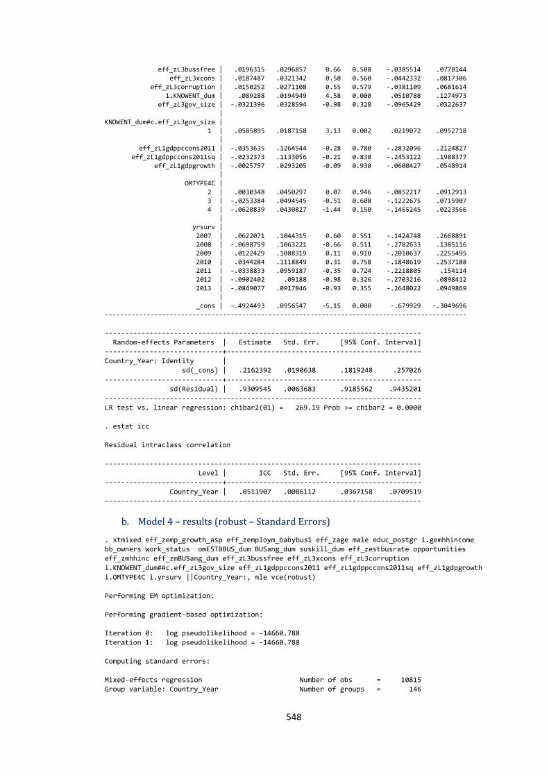
548
eff_zL3bussfree | .0196315 .0296857 0.66 0.508 -.0385514 .0778144
eff_zL3xcons | .0187487 .0321342 0.58 0.560 -.0442332 .0817306
eff_zL3corruption | .0150252 .0271108 0.55 0.579 -.0381109 .0681614
1.KNOWENT_dum | .089288 .0194949 4.58 0.000 .0510788 .1274973
eff_zL3gov_size | -.0321396 .0328594 -0.98 0.328 -.0965429 .0322637
|
KNOWENT_dum#c.eff_zL3gov_size |
1 | .0585895 .0187158 3.13 0.002 .0219072 .0952718
|
eff_zL1gdppccons2011 | -.0353635 .1264544 -0.28 0.780 -.2832096 .2124827
eff_zL1gdppccons2011sq | -.0232373 .1133056 -0.21 0.838 -.2453122 .1988377
eff_zL1gdpgrowth | -.0025757 .0293205 -0.09 0.930 -.0600427 .0548914
|
OMTYPE4C |
2 | .0030348 .0450297 0.07 0.946 -.0852217 .0912913
3 | -.0253384 .0494545 -0.51 0.608 -.1222675 .0715907
4 | -.0620839 .0430827 -1.44 0.150 -.1465245 .0223566
|
yrsurv |
2007 | .0622071 .1044315 0.60 0.551 -.1424748 .2668891
2008 | -.0698759 .1063221 -0.66 0.511 -.2782633 .1385116 2009 | .0122429 .1088319 0.11 0.910 -.2010637 .2255495
2010 | .0344284 .1118849 0.31 0.758 -.1848619 .2537188
2011 | -.0338833 .0959187 -0.35 0.724 -.2218805 .154114
2012 | -.0902402 .09188 -0.98 0.326 -.2703216 .0898412
2013 | -.0849077 .0917846 -0.93 0.355 -.2648022 .0949869
|
_cons | -.4924493 .0956547 -5.15 0.000 -.679929 -.3049696
-----------------------------------------------------------------------------------------------
------------------------------------------------------------------------------
Random-effects Parameters | Estimate Std. Err. [95% Conf. Interval]
-----------------------------+------------------------------------------------
Country_Year: Identity |
sd(_cons) | .2162392 .0190638 .1819248 .257026
-----------------------------+------------------------------------------------
sd(Residual) | .9309545 .0063683 .9185562 .9435201
------------------------------------------------------------------------------
LR test vs. linear regression: chibar2(01) = 269.19 Prob >= chibar2 = 0.0000
. estat icc
Residual intraclass correlation
------------------------------------------------------------------------------
Level | ICC Std. Err. [95% Conf. Interval]
-----------------------------+------------------------------------------------
Country_Year | .0511907 .0086112 .0367158 .0709519
------------------------------------------------------------------------------
b. Model 4 – results (robust – Standard Errors)
. xtmixed eff_zemp_growth_asp eff_zemploym_babybus1 eff_zage male educ_postgr i.gemhhincome
bb_owners work_status omESTBBUS_dum BUSang_dum suskill_dum eff_zestbusrate opportunities
eff_zmhhinc eff_zmBUSang_dum eff_zL3bussfree eff_zL3xcons eff_zL3corruption
i.KNOWENT_dum##c.eff_zL3gov_size eff_zL1gdppccons2011 eff_zL1gdppccons2011sq eff_zL1gdpgrowth
i.OMTYPE4C i.yrsurv ||Country_Year:, mle vce(robust)
Performing EM optimization:
Performing gradient-based optimization:
Iteration 0: log pseudolikelihood = -14660.788
Iteration 1: log pseudolikelihood = -14660.788
Computing standard errors:
Mixed-effects regression Number of obs = 10815
Group variable: Country_Year Number of groups = 146
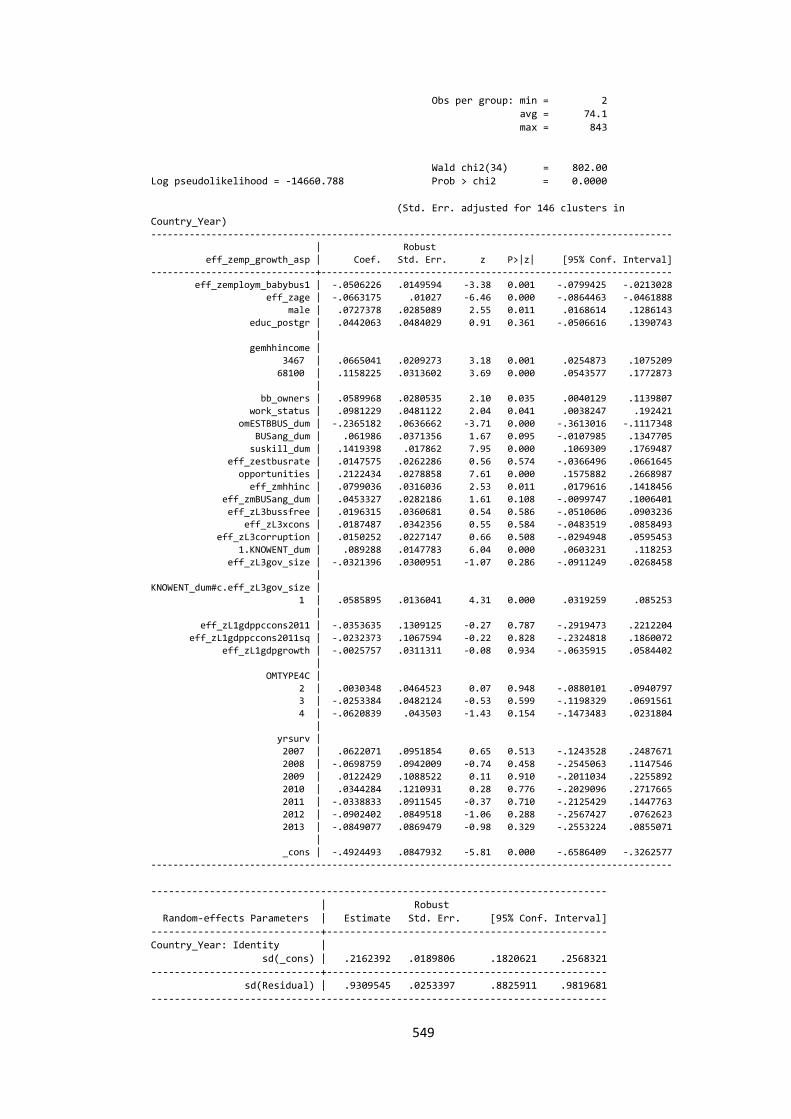
549
Obs per group: min = 2
avg = 74.1
max = 843
Wald chi2(34) = 802.00
Log pseudolikelihood = -14660.788 Prob > chi2 = 0.0000
(Std. Err. adjusted for 146 clusters in
Country_Year) -----------------------------------------------------------------------------------------------
| Robust
eff_zemp_growth_asp | Coef. Std. Err. z P>|z| [95% Conf. Interval]
------------------------------+----------------------------------------------------------------
eff_zemploym_babybus1 | -.0506226 .0149594 -3.38 0.001 -.0799425 -.0213028
eff_zage | -.0663175 .01027 -6.46 0.000 -.0864463 -.0461888
male | .0727378 .0285089 2.55 0.011 .0168614 .1286143
educ_postgr | .0442063 .0484029 0.91 0.361 -.0506616 .1390743
|
gemhhincome |
3467 | .0665041 .0209273 3.18 0.001 .0254873 .1075209
68100 | .1158225 .0313602 3.69 0.000 .0543577 .1772873
|
bb_owners | .0589968 .0280535 2.10 0.035 .0040129 .1139807
work_status | .0981229 .0481122 2.04 0.041 .0038247 .192421
omESTBBUS_dum | -.2365182 .0636662 -3.71 0.000 -.3613016 -.1117348
BUSang_dum | .061986 .0371356 1.67 0.095 -.0107985 .1347705
suskill_dum | .1419398 .017862 7.95 0.000 .1069309 .1769487
eff_zestbusrate | .0147575 .0262286 0.56 0.574 -.0366496 .0661645
opportunities | .2122434 .0278858 7.61 0.000 .1575882 .2668987
eff_zmhhinc | .0799036 .0316036 2.53 0.011 .0179616 .1418456
eff_zmBUSang_dum | .0453327 .0282186 1.61 0.108 -.0099747 .1006401
eff_zL3bussfree | .0196315 .0360681 0.54 0.586 -.0510606 .0903236
eff_zL3xcons | .0187487 .0342356 0.55 0.584 -.0483519 .0858493
eff_zL3corruption | .0150252 .0227147 0.66 0.508 -.0294948 .0595453
1.KNOWENT_dum | .089288 .0147783 6.04 0.000 .0603231 .118253
eff_zL3gov_size | -.0321396 .0300951 -1.07 0.286 -.0911249 .0268458
|
KNOWENT_dum#c.eff_zL3gov_size |
1 | .0585895 .0136041 4.31 0.000 .0319259 .085253
|
eff_zL1gdppccons2011 | -.0353635 .1309125 -0.27 0.787 -.2919473 .2212204
eff_zL1gdppccons2011sq | -.0232373 .1067594 -0.22 0.828 -.2324818 .1860072
eff_zL1gdpgrowth | -.0025757 .0311311 -0.08 0.934 -.0635915 .0584402
|
OMTYPE4C |
2 | .0030348 .0464523 0.07 0.948 -.0880101 .0940797 3 | -.0253384 .0482124 -0.53 0.599 -.1198329 .0691561
4 | -.0620839 .043503 -1.43 0.154 -.1473483 .0231804
|
yrsurv |
2007 | .0622071 .0951854 0.65 0.513 -.1243528 .2487671
2008 | -.0698759 .0942009 -0.74 0.458 -.2545063 .1147546
2009 | .0122429 .1088522 0.11 0.910 -.2011034 .2255892
2010 | .0344284 .1210931 0.28 0.776 -.2029096 .2717665
2011 | -.0338833 .0911545 -0.37 0.710 -.2125429 .1447763
2012 | -.0902402 .0849518 -1.06 0.288 -.2567427 .0762623
2013 | -.0849077 .0869479 -0.98 0.329 -.2553224 .0855071
|
_cons | -.4924493 .0847932 -5.81 0.000 -.6586409 -.3262577
-----------------------------------------------------------------------------------------------
------------------------------------------------------------------------------
| Robust
Random-effects Parameters | Estimate Std. Err. [95% Conf. Interval]
-----------------------------+------------------------------------------------
Country_Year: Identity |
sd(_cons) | .2162392 .0189806 .1820621 .2568321
-----------------------------+------------------------------------------------
sd(Residual) | .9309545 .0253397 .8825911 .9819681
------------------------------------------------------------------------------
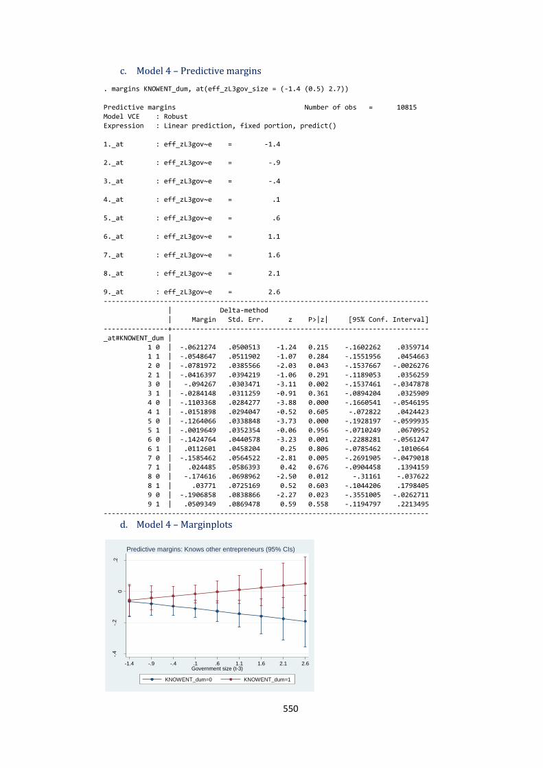
550
c. Model 4 – Predictive margins
. margins KNOWENT_dum, at(eff_zL3gov_size = (-1.4 (0.5) 2.7))
Predictive margins Number of obs = 10815
Model VCE : Robust
Expression : Linear prediction, fixed portion, predict()
1._at : eff_zL3gov~e = -1.4
2._at : eff_zL3gov~e = -.9
3._at : eff_zL3gov~e = -.4
4._at : eff_zL3gov~e = .1
5._at : eff_zL3gov~e = .6
6._at : eff_zL3gov~e = 1.1
7._at : eff_zL3gov~e = 1.6
8._at : eff_zL3gov~e = 2.1
9._at : eff_zL3gov~e = 2.6
---------------------------------------------------------------------------------
| Delta-method
| Margin Std. Err. z P>|z| [95% Conf. Interval]
----------------+----------------------------------------------------------------
_at#KNOWENT_dum |
1 0 | -.0621274 .0500513 -1.24 0.215 -.1602262 .0359714
1 1 | -.0548647 .0511902 -1.07 0.284 -.1551956 .0454663
2 0 | -.0781972 .0385566 -2.03 0.043 -.1537667 -.0026276
2 1 | -.0416397 .0394219 -1.06 0.291 -.1189053 .0356259
3 0 | -.094267 .0303471 -3.11 0.002 -.1537461 -.0347878
3 1 | -.0284148 .0311259 -0.91 0.361 -.0894204 .0325909
4 0 | -.1103368 .0284277 -3.88 0.000 -.1660541 -.0546195
4 1 | -.0151898 .0294047 -0.52 0.605 -.072822 .0424423
5 0 | -.1264066 .0338848 -3.73 0.000 -.1928197 -.0599935
5 1 | -.0019649 .0352354 -0.06 0.956 -.0710249 .0670952
6 0 | -.1424764 .0440578 -3.23 0.001 -.2288281 -.0561247
6 1 | .0112601 .0458204 0.25 0.806 -.0785462 .1010664
7 0 | -.1585462 .0564522 -2.81 0.005 -.2691905 -.0479018
7 1 | .024485 .0586393 0.42 0.676 -.0904458 .1394159
8 0 | -.174616 .0698962 -2.50 0.012 -.31161 -.037622
8 1 | .03771 .0725169 0.52 0.603 -.1044206 .1798405
9 0 | -.1906858 .0838866 -2.27 0.023 -.3551005 -.0262711
9 1 | .0509349 .0869478 0.59 0.558 -.1194797 .2213495
---------------------------------------------------------------------------------
d. Model 4 – Marginplots
-.4
-.2
0.2
Pre
dic
ted E
mp
. G
row
th A
sp
ira
tion
s (
EM
P)
-1.4 -.9 -.4 .1 .6 1.1 1.6 2.1 2.6Government size (t-3)
KNOWENT_dum=0 KNOWENT_dum=1
Predictive margins: Knows other entrepreneurs (95% CIs)

551
Appendix 5.9 High-Job Growth (HJG) aspirations – HJG–
Innovation-driven economies Appendix 5.9.1 Model 0 – HJG – Innovation-driven economies
. xi: xtmelogit BByyHJG ||Country_Year:, or variance
Refining starting values:
Iteration 0: log likelihood = -1189.6229
Iteration 1: log likelihood = -1183.1165
Iteration 2: log likelihood = -1177.5805
Performing gradient-based optimization:
Iteration 0: log likelihood = -1177.5805
Iteration 1: log likelihood = -1177.5056
Iteration 2: log likelihood = -1177.5056
Mixed-effects logistic regression Number of obs = 6753
Group variable: Country_Year Number of groups = 128
Obs per group: min = 3
avg = 52.8
max = 426
Integration points = 7 Wald chi2(0) = .
Log likelihood = -1177.5056 Prob > chi2 = .
------------------------------------------------------------------------------
BByyHJG | Odds Ratio Std. Err. z P>|z| [95% Conf. Interval]
-------------+----------------------------------------------------------------
_cons | .0408562 .0036221 -36.07 0.000 .0343396 .0486093
------------------------------------------------------------------------------
------------------------------------------------------------------------------
Random-effects Parameters | Estimate Std. Err. [95% Conf. Interval]
-----------------------------+------------------------------------------------
Country_Year: Identity |
var(_cons) | .2041617 .0947507 .082212 .5070066
------------------------------------------------------------------------------
LR test vs. logistic regression: chibar2(01) = 13.22 Prob>=chibar2 = 0.0001
. estat icc
Residual intraclass correlation
------------------------------------------------------------------------------
Level | ICC Std. Err. [95% Conf. Interval]
-----------------------------+------------------------------------------------
Country_Year | .0584316 .0255333 .0243802 .1335326
------------------------------------------------------------------------------
Appendix 5.9.2 Model 1 – HJG – Innovation-driven economies
a. Results
. xi: xtmelogit BByyHJG inn_zemploym_babybus1 inn_zage inn_zagesq male educ_postgr
i.gemhhincome bb_owners work_status KNOWENT_dum omESTBBUS_dum BUSang_dum suskill_dum
inn_zestbusrate opportunities inn_zhighgrowth_support inn_zL3bussfree inn_zL3xcons
inn_zL3corruption inn_zL3gov_size inn_zL1gdppccons2011 inn_zL1gdppccons2011sq
inn_zL1gdpgrowth i.OMTYPE4C i.yrsurv ||Country_Year:, or variance
i.gemhhincome _Igemhhinco_33-68100(naturally coded; _Igemhhinco_33 omitted)
i.OMTYPE4C _IOMTYPE4C_1-4 (naturally coded; _IOMTYPE4C_1 omitted)
i.yrsurv _Iyrsurv_2006-2013 (naturally coded; _Iyrsurv_2006 omitted)
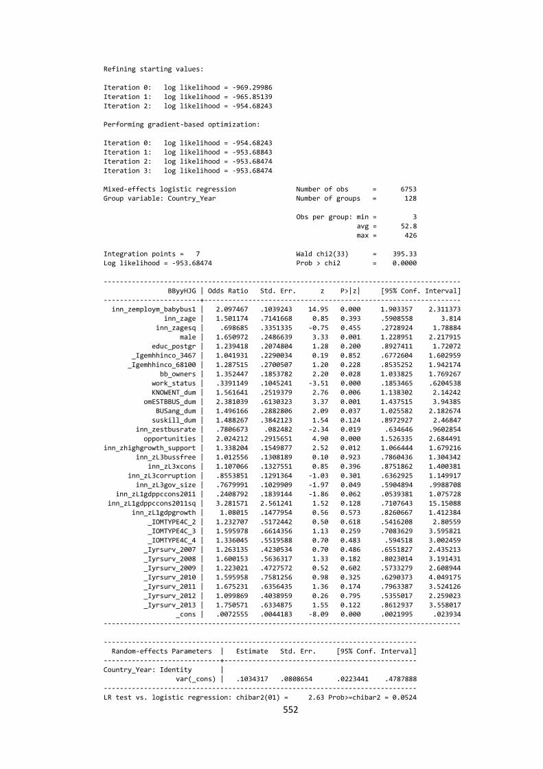
552
Refining starting values:
Iteration 0: log likelihood = -969.29986
Iteration 1: log likelihood = -965.85139
Iteration 2: log likelihood = -954.68243
Performing gradient-based optimization:
Iteration 0: log likelihood = -954.68243
Iteration 1: log likelihood = -953.68843
Iteration 2: log likelihood = -953.68474
Iteration 3: log likelihood = -953.68474
Mixed-effects logistic regression Number of obs = 6753
Group variable: Country_Year Number of groups = 128
Obs per group: min = 3
avg = 52.8
max = 426
Integration points = 7 Wald chi2(33) = 395.33
Log likelihood = -953.68474 Prob > chi2 = 0.0000
-----------------------------------------------------------------------------------------
BByyHJG | Odds Ratio Std. Err. z P>|z| [95% Conf. Interval]
------------------------+----------------------------------------------------------------
inn_zemploym_babybus1 | 2.097467 .1039243 14.95 0.000 1.903357 2.311373
inn_zage | 1.501174 .7141668 0.85 0.393 .5908558 3.814
inn_zagesq | .698685 .3351335 -0.75 0.455 .2728924 1.78884
male | 1.650972 .2486639 3.33 0.001 1.228951 2.217915
educ_postgr | 1.239418 .2074804 1.28 0.200 .8927411 1.72072
_Igemhhinco_3467 | 1.041931 .2290034 0.19 0.852 .6772604 1.602959
_Igemhhinco_68100 | 1.287515 .2700507 1.20 0.228 .8535252 1.942174
bb_owners | 1.352447 .1853782 2.20 0.028 1.033825 1.769267
work_status | .3391149 .1045241 -3.51 0.000 .1853465 .6204538
KNOWENT_dum | 1.561641 .2519379 2.76 0.006 1.138302 2.14242
omESTBBUS_dum | 2.381039 .6130323 3.37 0.001 1.437515 3.94385
BUSang_dum | 1.496166 .2882806 2.09 0.037 1.025582 2.182674
suskill_dum | 1.488267 .3842123 1.54 0.124 .8972927 2.46847
inn_zestbusrate | .7806673 .082482 -2.34 0.019 .634646 .9602854
opportunities | 2.024212 .2915651 4.90 0.000 1.526335 2.684491
inn_zhighgrowth_support | 1.338204 .1549877 2.52 0.012 1.066444 1.679216
inn_zL3bussfree | 1.012556 .1308189 0.10 0.923 .7860436 1.304342
inn_zL3xcons | 1.107066 .1327551 0.85 0.396 .8751862 1.400381
inn_zL3corruption | .8553851 .1291364 -1.03 0.301 .6362925 1.149917
inn_zL3gov_size | .7679991 .1029909 -1.97 0.049 .5904894 .9988708
inn_zL1gdppccons2011 | .2408792 .1839144 -1.86 0.062 .0539381 1.075728
inn_zL1gdppccons2011sq | 3.281571 2.561241 1.52 0.128 .7107643 15.15088
inn_zL1gdpgrowth | 1.08015 .1477954 0.56 0.573 .8260667 1.412384
_IOMTYPE4C_2 | 1.232707 .5172442 0.50 0.618 .5416208 2.80559
_IOMTYPE4C_3 | 1.595978 .6614356 1.13 0.259 .7083629 3.595821
_IOMTYPE4C_4 | 1.336045 .5519588 0.70 0.483 .594518 3.002459
_Iyrsurv_2007 | 1.263135 .4230534 0.70 0.486 .6551827 2.435213
_Iyrsurv_2008 | 1.600153 .5636317 1.33 0.182 .8023014 3.191431
_Iyrsurv_2009 | 1.223021 .4727572 0.52 0.602 .5733279 2.608944
_Iyrsurv_2010 | 1.595958 .7581256 0.98 0.325 .6290373 4.049175
_Iyrsurv_2011 | 1.675231 .6356435 1.36 0.174 .7963387 3.524126
_Iyrsurv_2012 | 1.099869 .4038959 0.26 0.795 .5355017 2.259023
_Iyrsurv_2013 | 1.750571 .6334875 1.55 0.122 .8612937 3.558017
_cons | .0072555 .0044183 -8.09 0.000 .0021995 .023934
-----------------------------------------------------------------------------------------
------------------------------------------------------------------------------
Random-effects Parameters | Estimate Std. Err. [95% Conf. Interval]
-----------------------------+------------------------------------------------
Country_Year: Identity |
var(_cons) | .1034317 .0808654 .0223441 .4787888
------------------------------------------------------------------------------
LR test vs. logistic regression: chibar2(01) = 2.63 Prob>=chibar2 = 0.0524
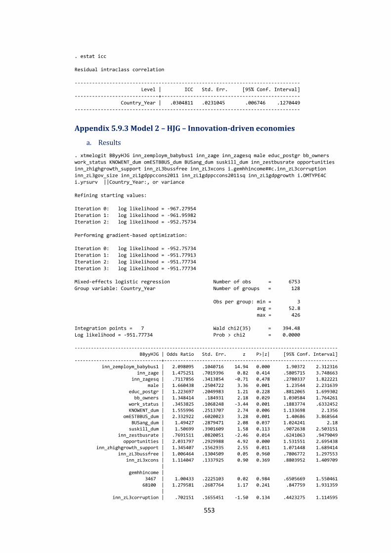
553
. estat icc
Residual intraclass correlation
------------------------------------------------------------------------------
Level | ICC Std. Err. [95% Conf. Interval]
-----------------------------+------------------------------------------------
Country_Year | .0304811 .0231045 .006746 .1270449
------------------------------------------------------------------------------
Appendix 5.9.3 Model 2 – HJG – Innovation-driven economies
a. Results
. xtmelogit BByyHJG inn_zemploym_babybus1 inn_zage inn_zagesq male educ_postgr bb_owners
work_status KNOWENT_dum omESTBBUS_dum BUSang_dum suskill_dum inn_zestbusrate opportunities
inn_zhighgrowth_support inn_zL3bussfree inn_zL3xcons i.gemhhincome##c.inn_zL3corruption
inn_zL3gov_size inn_zL1gdppccons2011 inn_zL1gdppccons2011sq inn_zL1gdpgrowth i.OMTYPE4C
i.yrsurv ||Country_Year:, or variance
Refining starting values:
Iteration 0: log likelihood = -967.27954
Iteration 1: log likelihood = -961.95982
Iteration 2: log likelihood = -952.75734
Performing gradient-based optimization:
Iteration 0: log likelihood = -952.75734
Iteration 1: log likelihood = -951.77913
Iteration 2: log likelihood = -951.77734
Iteration 3: log likelihood = -951.77734
Mixed-effects logistic regression Number of obs = 6753
Group variable: Country_Year Number of groups = 128
Obs per group: min = 3
avg = 52.8
max = 426
Integration points = 7 Wald chi2(35) = 394.48
Log likelihood = -951.77734 Prob > chi2 = 0.0000
-------------------------------------------------------------------------------------------------
BByyHJG | Odds Ratio Std. Err. z P>|z| [95% Conf. Interval]
--------------------------------+----------------------------------------------------------------
inn_zemploym_babybus1 | 2.098095 .1040716 14.94 0.000 1.90372 2.312316
inn_zage | 1.475251 .7019396 0.82 0.414 .5805715 3.748663
inn_zagesq | .7117856 .3413854 -0.71 0.478 .2780337 1.822221
male | 1.660438 .2504722 3.36 0.001 1.23544 2.231639
educ_postgr | 1.223697 .2049983 1.21 0.228 .8812065 1.699302
bb_owners | 1.348414 .184931 2.18 0.029 1.030584 1.764261
work_status | .3453825 .1068248 -3.44 0.001 .1883774 .6332452
KNOWENT_dum | 1.555996 .2513707 2.74 0.006 1.133698 2.1356 omESTBBUS_dum | 2.332922 .6020023 3.28 0.001 1.40686 3.868564
BUSang_dum | 1.49427 .2879471 2.08 0.037 1.024241 2.18
suskill_dum | 1.50699 .3901609 1.58 0.113 .9072638 2.503151
inn_zestbusrate | .7691511 .0820051 -2.46 0.014 .6241063 .9479049
opportunities | 2.031797 .2929988 4.92 0.000 1.531551 2.695438
inn_zhighgrowth_support | 1.345407 .1562935 2.55 0.011 1.071448 1.689414
inn_zL3bussfree | 1.006464 .1304509 0.05 0.960 .7806772 1.297553
inn_zL3xcons | 1.114047 .1337925 0.90 0.369 .8803952 1.409709
|
gemhhincome |
3467 | 1.00433 .2225103 0.02 0.984 .6505669 1.550461
68100 | 1.279581 .2687764 1.17 0.241 .847759 1.931359
|
inn_zL3corruption | .702151 .1655451 -1.50 0.134 .4423275 1.114595
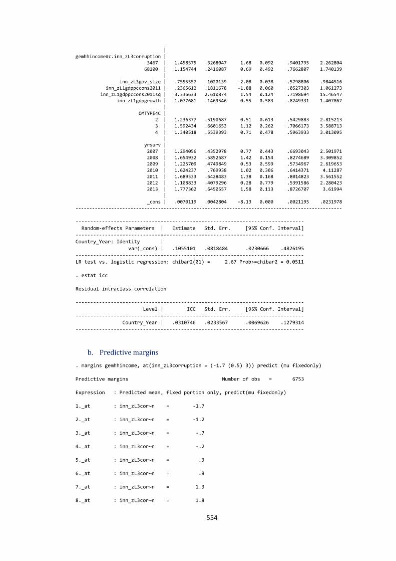
554
|
gemhhincome#c.inn_zL3corruption |
3467 | 1.458575 .3268047 1.68 0.092 .9401795 2.262804
68100 | 1.154744 .2416087 0.69 0.492 .7662807 1.740139
|
inn_zL3gov_size | .7555557 .1020139 -2.08 0.038 .5798806 .9844516
inn_zL1gdppccons2011 | .2365612 .1811678 -1.88 0.060 .0527303 1.061273
inn_zL1gdppccons2011sq | 3.336633 2.610874 1.54 0.124 .7198694 15.46547
inn_zL1gdpgrowth | 1.077681 .1469546 0.55 0.583 .8249331 1.407867
|
OMTYPE4C |
2 | 1.236377 .5190687 0.51 0.613 .5429883 2.815213
3 | 1.592434 .6601653 1.12 0.262 .7066173 3.588713
4 | 1.340518 .5539393 0.71 0.478 .5963933 3.013095
|
yrsurv |
2007 | 1.294056 .4352978 0.77 0.443 .6693043 2.501971
2008 | 1.654932 .5852687 1.42 0.154 .8274689 3.309852
2009 | 1.225709 .4749849 0.53 0.599 .5734967 2.619653
2010 | 1.624237 .769938 1.02 0.306 .6414371 4.11287
2011 | 1.689533 .6428483 1.38 0.168 .8014823 3.561552 2012 | 1.108833 .4079296 0.28 0.779 .5391586 2.280423
2013 | 1.777362 .6450557 1.58 0.113 .8726707 3.61994
|
_cons | .0070119 .0042804 -8.13 0.000 .0021195 .0231978
-------------------------------------------------------------------------------------------------
------------------------------------------------------------------------------
Random-effects Parameters | Estimate Std. Err. [95% Conf. Interval]
-----------------------------+------------------------------------------------
Country_Year: Identity |
var(_cons) | .1055101 .0818484 .0230666 .4826195
------------------------------------------------------------------------------
LR test vs. logistic regression: chibar2(01) = 2.67 Prob>=chibar2 = 0.0511
. estat icc
Residual intraclass correlation
------------------------------------------------------------------------------
Level | ICC Std. Err. [95% Conf. Interval]
-----------------------------+------------------------------------------------
Country_Year | .0310746 .0233567 .0069626 .1279314
------------------------------------------------------------------------------
b. Predictive margins
. margins gemhhincome, at(inn_zL3corruption = (-1.7 (0.5) 3)) predict (mu fixedonly)
Predictive margins Number of obs = 6753
Expression : Predicted mean, fixed portion only, predict(mu fixedonly)
1._at : inn_zL3cor~n = -1.7
2._at : inn_zL3cor~n = -1.2
3._at : inn_zL3cor~n = -.7
4._at : inn_zL3cor~n = -.2
5._at : inn_zL3cor~n = .3
6._at : inn_zL3cor~n = .8
7._at : inn_zL3cor~n = 1.3
8._at : inn_zL3cor~n = 1.8
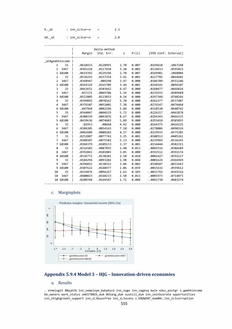
555
9._at : inn_zL3cor~n = 2.3
10._at : inn_zL3cor~n = 2.8
---------------------------------------------------------------------------------
| Delta-method
| Margin Std. Err. z P>|z| [95% Conf. Interval]
----------------+----------------------------------------------------------------
_at#gemhhincome |
1 33 | .0618433 .0228991 2.70 0.007 .0169618 .1067248
1 3467 | .0365218 .0117658 3.10 0.002 .0134613 .0595823
1 68100 | .0619392 .0229296 2.70 0.007 .0169981 .1068804
2 33 | .0536193 .0157354 3.41 0.001 .0227785 .0844601
2 3467 | .0368947 .009298 3.97 0.000 .0186709 .0551186
2 68100 | .0569324 .0165709 3.44 0.001 .0244541 .0894107
3 33 | .0463651 .0103662 4.47 0.000 .0260477 .0666824
3 3467 | .037271 .0069786 5.34 0.000 .0235933 .0509488
3 68100 | .0522805 .0115033 4.54 0.000 .0297344 .0748266
4 33 | .0399892 .0070162 5.70 0.000 .0262377 .0537407
4 3467 | .0376507 .0051001 7.38 0.000 .0276547 .0476468
4 68100 | .047964 .0082196 5.84 0.000 .0318538 .0640742
5 33 | .0344047 .0060119 5.72 0.000 .0226217 .0461878
5 3467 | .0380339 .0043876 8.67 0.000 .0294343 .0466335
5 68100 | .0439636 .0074603 5.89 0.000 .0293418 .0585855
6 33 | .02953 .00668 4.42 0.000 .0164375 .0426225
6 3467 | .0384205 .0054143 7.10 0.000 .0278086 .0490324
6 68100 | .0402609 .0088102 4.57 0.000 .0229933 .0575285
7 33 | .0252887 .0077743 3.25 0.001 .0100513 .0405261
7 3467 | .0388107 .0075582 5.13 0.000 .0239969 .0536245
7 68100 | .0368379 .0109153 3.37 0.001 .0154444 .0582315
8 33 | .0216102 .0087035 2.48 0.013 .0045516 .0386689
8 3467 | .0392043 .0101803 3.85 0.000 .0192512 .0591574
8 68100 | .0336772 .0130281 2.58 0.010 .0081427 .0592117
9 33 | .0184296 .0093202 1.98 0.048 .0001624 .0366969
9 3467 | .0396015 .0130323 3.04 0.002 .0140587 .0651443
9 68100 | .0307622 .0148977 2.06 0.039 .0015632 .0599612
10 33 | .0156876 .0096247 1.63 0.103 -.0031765 .0345516
10 3467 | .0400023 .0160233 2.50 0.013 .0085973 .0714073
10 68100 | .0280768 .0164547 1.71 0.088 -.0041738 .0603274
---------------------------------------------------------------------------------
c. Marginplots
Appendix 5.9.4 Model 3 – HJG – Innovation-driven economies
a. Results
. xtmelogit BByyHJG inn_zemploym_babybus1 inn_zage inn_zagesq male educ_postgr i.gemhhincome
bb_owners work_status omESTBBUS_dum BUSang_dum suskill_dum inn_zestbusrate opportunities
inn_zhighgrowth_support inn_zL3bussfree inn_zL3xcons i.KNOWENT_dum##c.inn_zL3corruption
0
.02
.04
.06
.08
.1
Pre
dic
ted H
igh-j
ob
Gro
wth
Asp. (H
JG
)
-1.7 -1.2 -.7 -.2 .3 .8 1.3 1.8 2.3 2.8Corruption (t-3)
gemhhincome=33 gemhhincome=3467
gemhhincome=68100
Predictive margins: Household income (95% CIs)
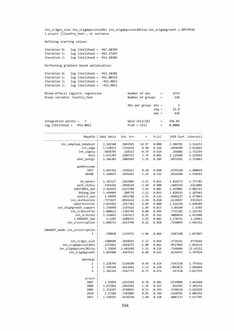
556
inn_zL3gov_size inn_zL1gdppccons2011 inn_zL1gdppccons2011sq inn_zL1gdpgrowth i.OMTYPE4C
i.yrsurv ||Country_Year:, or variance
Refining starting values:
Iteration 0: log likelihood = -967.48399
Iteration 1: log likelihood = -962.27447
Iteration 2: log likelihood = -953.10385
Performing gradient-based optimization:
Iteration 0: log likelihood = -953.10385
Iteration 1: log likelihood = -952.00325
Iteration 2: log likelihood = -952.0011
Iteration 3: log likelihood = -952.0011
Mixed-effects logistic regression Number of obs = 6753
Group variable: Country_Year Number of groups = 128
Obs per group: min = 3
avg = 52.8
max = 426
Integration points = 7 Wald chi2(34) = 396.83
Log likelihood = -952.0011 Prob > chi2 = 0.0000
-------------------------------------------------------------------------------------------------
BByyHJG | Odds Ratio Std. Err. z P>|z| [95% Conf. Interval]
--------------------------------+----------------------------------------------------------------
inn_zemploym_babybus1 | 2.101568 .1042945 14.97 0.000 1.906781 2.316253
inn_zage | 1.538472 .7325658 0.90 0.366 .6050309 3.912025
inn_zagesq | .6838785 .328323 -0.79 0.429 .266886 1.752395
male | 1.651707 .2489723 3.33 0.001 1.229209 2.219422
educ_postgr | 1.246303 .2089203 1.31 0.189 .8972942 1.731061
|
gemhhincome |
3467 | 1.045341 .2296912 0.20 0.840 .6795548 1.608019
68100 | 1.284837 .2695661 1.19 0.232 .8516504 1.938363
|
bb_owners | 1.343117 .1843806 2.15 0.032 1.026272 1.757783
work_status | .3392426 .1050128 -3.49 0.000 .1849356 .6223009
omESTBBUS_dum | 2.416683 .6221708 3.43 0.001 1.459081 4.002765
BUSang_dum | 1.499849 .288778 2.11 0.035 1.028393 2.187441
suskill_dum | 1.49099 .3851788 1.55 0.122 .8986227 2.473843
inn_zestbusrate | .7571637 .0816618 -2.58 0.010 .6128947 .9353923
opportunities | 2.025962 .2927385 4.89 0.000 1.526294 2.689209
inn_zhighgrowth_support | 1.336058 .1555426 2.49 0.013 1.06348 1.6785
inn_zL3bussfree | 1.000621 .1303746 0.00 0.996 .7751102 1.291742
inn_zL3xcons | 1.116022 .1347472 0.91 0.363 .8808454 1.413988
1.KNOWENT_dum | 1.6285 .2688255 2.95 0.003 1.178352 2.25061
inn_zL3corruption | 1.040751 .1913798 0.22 0.828 .7258099 1.492352
|
KNOWENT_dum#c.inn_zL3corruption |
1 | .760838 .1129725 -1.84 0.066 .5687248 1.017847
| inn_zL3gov_size | .7488686 .1018645 -2.13 0.034 .5736161 .9776646
inn_zL1gdppccons2011 | .2371841 .1818275 -1.88 0.061 .0527894 1.065674
inn_zL1gdppccons2011sq | 3.32036 2.601668 1.53 0.126 .7148686 15.42212
inn_zL1gdpgrowth | 1.067808 .1467611 0.48 0.633 .8156475 1.397924
|
OMTYPE4C |
2 | 1.228796 .5158108 0.49 0.624 .5397238 2.797616
3 | 1.599356 .6633816 1.13 0.258 .7093875 3.605844
4 | 1.342326 .5547773 0.71 0.476 .597118 3.017559
|
yrsurv |
2007 | 1.26894 .4292346 0.70 0.481 .6539006 2.462468
2008 | 1.637892 .5816583 1.39 0.165 .816585 3.285256
2009 | 1.231697 .4798016 0.53 0.593 .5740136 2.642928
2010 | 1.57106 .7503806 0.95 0.344 .6160781 4.006356
2011 | 1.710391 .6536538 1.40 0.160 .8087137 3.617395
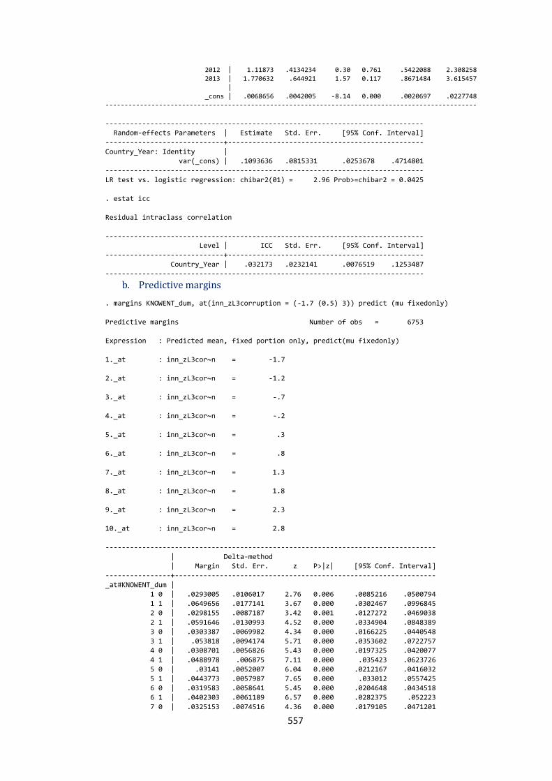
557
2012 | 1.11873 .4134234 0.30 0.761 .5422088 2.308258
2013 | 1.770632 .644921 1.57 0.117 .8671484 3.615457
|
_cons | .0068656 .0042005 -8.14 0.000 .0020697 .0227748
-------------------------------------------------------------------------------------------------
------------------------------------------------------------------------------
Random-effects Parameters | Estimate Std. Err. [95% Conf. Interval]
-----------------------------+------------------------------------------------
Country_Year: Identity |
var(_cons) | .1093636 .0815331 .0253678 .4714801
------------------------------------------------------------------------------
LR test vs. logistic regression: chibar2(01) = 2.96 Prob>=chibar2 = 0.0425
. estat icc
Residual intraclass correlation
------------------------------------------------------------------------------
Level | ICC Std. Err. [95% Conf. Interval]
-----------------------------+------------------------------------------------
Country_Year | .032173 .0232141 .0076519 .1253487
------------------------------------------------------------------------------
b. Predictive margins
. margins KNOWENT_dum, at(inn_zL3corruption = (-1.7 (0.5) 3)) predict (mu fixedonly)
Predictive margins Number of obs = 6753
Expression : Predicted mean, fixed portion only, predict(mu fixedonly)
1._at : inn_zL3cor~n = -1.7
2._at : inn_zL3cor~n = -1.2
3._at : inn_zL3cor~n = -.7
4._at : inn_zL3cor~n = -.2
5._at : inn_zL3cor~n = .3
6._at : inn_zL3cor~n = .8
7._at : inn_zL3cor~n = 1.3
8._at : inn_zL3cor~n = 1.8
9._at : inn_zL3cor~n = 2.3
10._at : inn_zL3cor~n = 2.8
---------------------------------------------------------------------------------
| Delta-method
| Margin Std. Err. z P>|z| [95% Conf. Interval]
----------------+----------------------------------------------------------------
_at#KNOWENT_dum |
1 0 | .0293005 .0106017 2.76 0.006 .0085216 .0500794
1 1 | .0649656 .0177141 3.67 0.000 .0302467 .0996845
2 0 | .0298155 .0087187 3.42 0.001 .0127272 .0469038
2 1 | .0591646 .0130993 4.52 0.000 .0334904 .0848389
3 0 | .0303387 .0069982 4.34 0.000 .0166225 .0440548
3 1 | .053818 .0094174 5.71 0.000 .0353602 .0722757
4 0 | .0308701 .0056826 5.43 0.000 .0197325 .0420077
4 1 | .0488978 .006875 7.11 0.000 .035423 .0623726
5 0 | .03141 .0052007 6.04 0.000 .0212167 .0416032
5 1 | .0443773 .0057987 7.65 0.000 .033012 .0557425
6 0 | .0319583 .0058641 5.45 0.000 .0204648 .0434518
6 1 | .0402303 .0061189 6.57 0.000 .0282375 .052223
7 0 | .0325153 .0074516 4.36 0.000 .0179105 .0471201
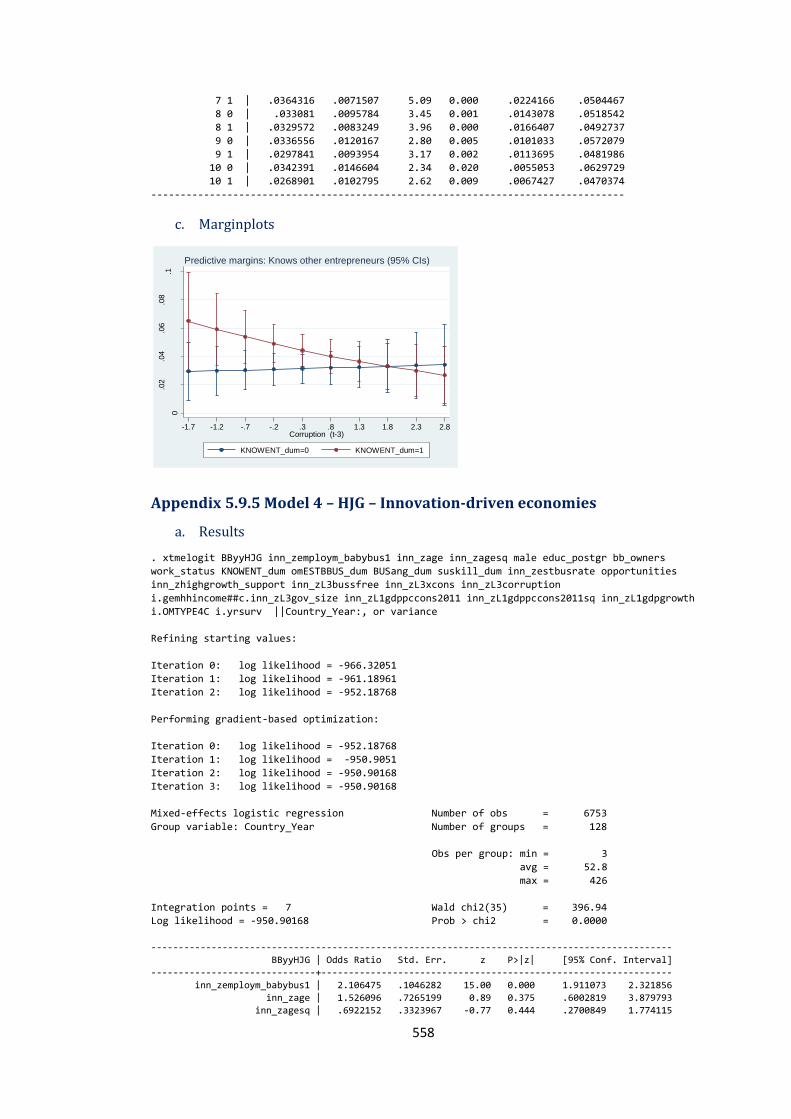
558
7 1 | .0364316 .0071507 5.09 0.000 .0224166 .0504467
8 0 | .033081 .0095784 3.45 0.001 .0143078 .0518542
8 1 | .0329572 .0083249 3.96 0.000 .0166407 .0492737
9 0 | .0336556 .0120167 2.80 0.005 .0101033 .0572079
9 1 | .0297841 .0093954 3.17 0.002 .0113695 .0481986
10 0 | .0342391 .0146604 2.34 0.020 .0055053 .0629729
10 1 | .0268901 .0102795 2.62 0.009 .0067427 .0470374
---------------------------------------------------------------------------------
c. Marginplots
Appendix 5.9.5 Model 4 – HJG – Innovation-driven economies
a. Results
. xtmelogit BByyHJG inn_zemploym_babybus1 inn_zage inn_zagesq male educ_postgr bb_owners
work_status KNOWENT_dum omESTBBUS_dum BUSang_dum suskill_dum inn_zestbusrate opportunities
inn_zhighgrowth_support inn_zL3bussfree inn_zL3xcons inn_zL3corruption
i.gemhhincome##c.inn_zL3gov_size inn_zL1gdppccons2011 inn_zL1gdppccons2011sq inn_zL1gdpgrowth
i.OMTYPE4C i.yrsurv ||Country_Year:, or variance
Refining starting values:
Iteration 0: log likelihood = -966.32051
Iteration 1: log likelihood = -961.18961
Iteration 2: log likelihood = -952.18768
Performing gradient-based optimization:
Iteration 0: log likelihood = -952.18768
Iteration 1: log likelihood = -950.9051
Iteration 2: log likelihood = -950.90168
Iteration 3: log likelihood = -950.90168
Mixed-effects logistic regression Number of obs = 6753
Group variable: Country_Year Number of groups = 128
Obs per group: min = 3
avg = 52.8
max = 426
Integration points = 7 Wald chi2(35) = 396.94
Log likelihood = -950.90168 Prob > chi2 = 0.0000
-----------------------------------------------------------------------------------------------
BByyHJG | Odds Ratio Std. Err. z P>|z| [95% Conf. Interval]
------------------------------+----------------------------------------------------------------
inn_zemploym_babybus1 | 2.106475 .1046282 15.00 0.000 1.911073 2.321856
inn_zage | 1.526096 .7265199 0.89 0.375 .6002819 3.879793
inn_zagesq | .6922152 .3323967 -0.77 0.444 .2700849 1.774115
0
.02
.04
.06
.08
.1
Pre
dic
ted H
igh-j
ob
Gro
wth
Asp. (H
JG
)
-1.7 -1.2 -.7 -.2 .3 .8 1.3 1.8 2.3 2.8Corruption (t-3)
KNOWENT_dum=0 KNOWENT_dum=1
Predictive margins: Knows other entrepreneurs (95% CIs)
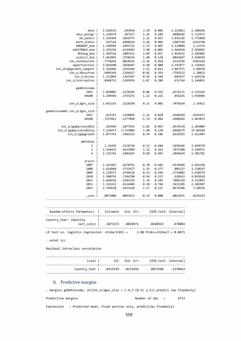
559
male | 1.628552 .245458 3.24 0.001 1.212013 2.188246
educ_postgr | 1.234979 .207257 1.26 0.209 .8888102 1.715972
bb_owners | 1.354364 .1856775 2.21 0.027 1.035236 1.771868
work_status | .347124 .1060329 -3.46 0.001 .1907549 .6316748
KNOWENT_dum | 1.548509 .2495721 2.71 0.007 1.129084 2.12374
omESTBBUS_dum | 2.393236 .6144503 3.40 0.001 1.446918 3.958465
BUSang_dum | 1.495516 .2885311 2.09 0.037 1.024632 2.182801
suskill_dum | 1.463095 .3758134 1.48 0.138 .8843647 2.420549
inn_zestbusrate | .7778262 .0828142 -2.36 0.018 .6313296 .9583164
opportunities | 2.054508 .2968107 4.98 0.000 1.547877 2.726963
inn_zhighgrowth_support | 1.341846 .1565446 2.52 0.012 1.067575 1.68658
inn_zL3bussfree | .9989369 .1296617 -0.01 0.993 .7745552 1.28832
inn_zL3xcons | 1.122049 .1365587 0.95 0.344 .883927 1.424318
inn_zL3corruption | .8504711 .1289939 -1.07 0.286 .631764 1.144891
|
gemhhincome |
3467 | 1.018085 .2270249 0.08 0.936 .6576171 1.576142
68100 | 1.294966 .2733271 1.22 0.221 .856241 1.958486
|
inn_zL3gov_size | 1.052193 .2128298 0.25 0.801 .7078164 1.56412
| gemhhincome#c.inn_zL3gov_size |
3467 | .623767 .1268899 -2.32 0.020 .4186649 .9293475
68100 | .7157821 .1377898 -1.74 0.082 .4908202 1.043853
|
inn_zL1gdppccons2011 | .243949 .1877992 -1.83 0.067 .0539534 1.103009
inn_zL1gdppccons2011sq | 3.214473 2.533086 1.48 0.138 .6860275 15.06184
inn_zL1gdpgrowth | 1.077743 .1483123 0.54 0.586 .8229593 1.411407
|
OMTYPE4C |
2 | 1.24295 .5218728 0.52 0.604 .5458366 2.830378
3 | 1.594433 .6613909 1.12 0.261 .7071588 3.594971
4 | 1.325741 .5482643 0.68 0.495 .5894424 2.981781
|
yrsurv |
2007 | 1.267447 .4278791 0.70 0.483 .6539909 2.456338
2008 | 1.614868 .5733477 1.35 0.177 .805237 3.238547
2009 | 1.229573 .4790226 0.53 0.596 .5729802 2.638574
2010 | 1.580791 .7546788 0.96 0.337 .620163 4.029424
2011 | 1.668216 .6382339 1.34 0.181 .7881258 3.531091
2012 | 1.116311 .4124404 0.30 0.766 .5411205 2.302907
2013 | 1.769638 .6435418 1.57 0.117 .8676388 3.60936
|
_cons | .0071806 .0043615 -8.13 0.000 .0021835 .0236143
-----------------------------------------------------------------------------------------------
------------------------------------------------------------------------------
Random-effects Parameters | Estimate Std. Err. [95% Conf. Interval]
-----------------------------+------------------------------------------------
Country_Year: Identity |
var(_cons) | .1073272 .0818971 .0240543 .478881
------------------------------------------------------------------------------
LR test vs. logistic regression: chibar2(01) = 2.80 Prob>=chibar2 = 0.0471
. estat icc
Residual intraclass correlation
------------------------------------------------------------------------------
Level | ICC Std. Err. [95% Conf. Interval]
-----------------------------+------------------------------------------------
Country_Year | .0315929 .0233456 .0072586 .1270663
------------------------------------------------------------------------------
b. Predictive margins
. margins gemhhincome, at(inn_zL3gov_size = (-4.2 (0.5) 2.5)) predict (mu fixedonly)
Predictive margins Number of obs = 6753
Expression : Predicted mean, fixed portion only, predict(mu fixedonly)
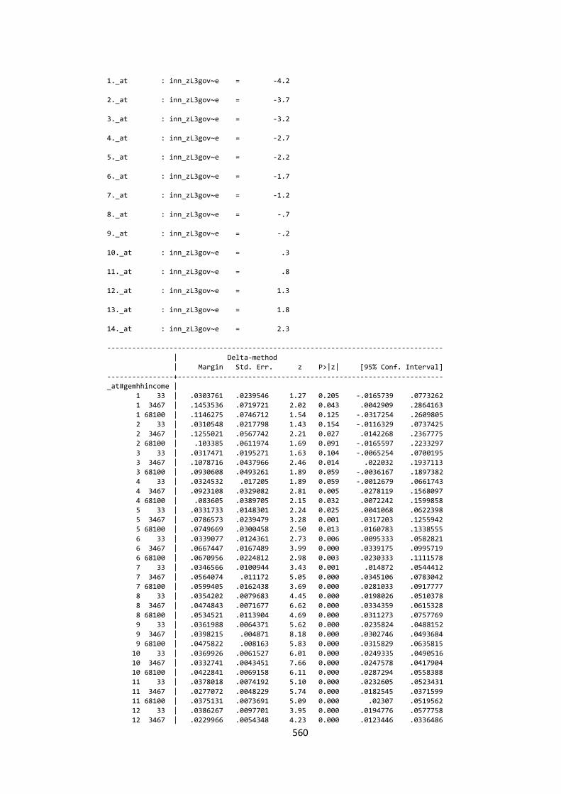
560
1._at : inn_zL3gov~e = -4.2
2._at : inn_zL3gov~e = -3.7
3._at : inn_zL3gov~e = -3.2
4._at : inn_zL3gov~e = -2.7
5._at : inn_zL3gov~e = -2.2
6._at : inn_zL3gov~e = -1.7
7._at : inn_zL3gov~e = -1.2
8._at : inn_zL3gov~e = -.7
9._at : inn_zL3gov~e = -.2
10._at : inn_zL3gov~e = .3
11._at : inn_zL3gov~e = .8
12._at : inn_zL3gov~e = 1.3
13._at : inn_zL3gov~e = 1.8
14._at : inn_zL3gov~e = 2.3
---------------------------------------------------------------------------------
| Delta-method
| Margin Std. Err. z P>|z| [95% Conf. Interval]
----------------+----------------------------------------------------------------
_at#gemhhincome |
1 33 | .0303761 .0239546 1.27 0.205 -.0165739 .0773262
1 3467 | .1453536 .0719721 2.02 0.043 .0042909 .2864163
1 68100 | .1146275 .0746712 1.54 0.125 -.0317254 .2609805
2 33 | .0310548 .0217798 1.43 0.154 -.0116329 .0737425
2 3467 | .1255021 .0567742 2.21 0.027 .0142268 .2367775
2 68100 | .103385 .0611974 1.69 0.091 -.0165597 .2233297
3 33 | .0317471 .0195271 1.63 0.104 -.0065254 .0700195
3 3467 | .1078716 .0437966 2.46 0.014 .022032 .1937113
3 68100 | .0930608 .0493261 1.89 0.059 -.0036167 .1897382
4 33 | .0324532 .017205 1.89 0.059 -.0012679 .0661743
4 3467 | .0923108 .0329082 2.81 0.005 .0278119 .1568097
4 68100 | .083605 .0389705 2.15 0.032 .0072242 .1599858
5 33 | .0331733 .0148301 2.24 0.025 .0041068 .0622398
5 3467 | .0786573 .0239479 3.28 0.001 .0317203 .1255942
5 68100 | .0749669 .0300458 2.50 0.013 .0160783 .1338555
6 33 | .0339077 .0124361 2.73 0.006 .0095333 .0582821
6 3467 | .0667447 .0167489 3.99 0.000 .0339175 .0995719
6 68100 | .0670956 .0224812 2.98 0.003 .0230333 .1111578
7 33 | .0346566 .0100944 3.43 0.001 .014872 .0544412
7 3467 | .0564074 .011172 5.05 0.000 .0345106 .0783042
7 68100 | .0599405 .0162438 3.69 0.000 .0281033 .0917777
8 33 | .0354202 .0079683 4.45 0.000 .0198026 .0510378
8 3467 | .0474843 .0071677 6.62 0.000 .0334359 .0615328
8 68100 | .0534521 .0113904 4.69 0.000 .0311273 .0757769
9 33 | .0361988 .0064371 5.62 0.000 .0235824 .0488152
9 3467 | .0398215 .004871 8.18 0.000 .0302746 .0493684
9 68100 | .0475822 .008163 5.83 0.000 .0315829 .0635815
10 33 | .0369926 .0061527 6.01 0.000 .0249335 .0490516
10 3467 | .0332741 .0043451 7.66 0.000 .0247578 .0417904
10 68100 | .0422841 .0069158 6.11 0.000 .0287294 .0558388
11 33 | .0378018 .0074192 5.10 0.000 .0232605 .0523431
11 3467 | .0277072 .0048229 5.74 0.000 .0182545 .0371599
11 68100 | .0375131 .0073691 5.09 0.000 .02307 .0519562
12 33 | .0386267 .0097701 3.95 0.000 .0194776 .0577758
12 3467 | .0229966 .0054348 4.23 0.000 .0123446 .0336486
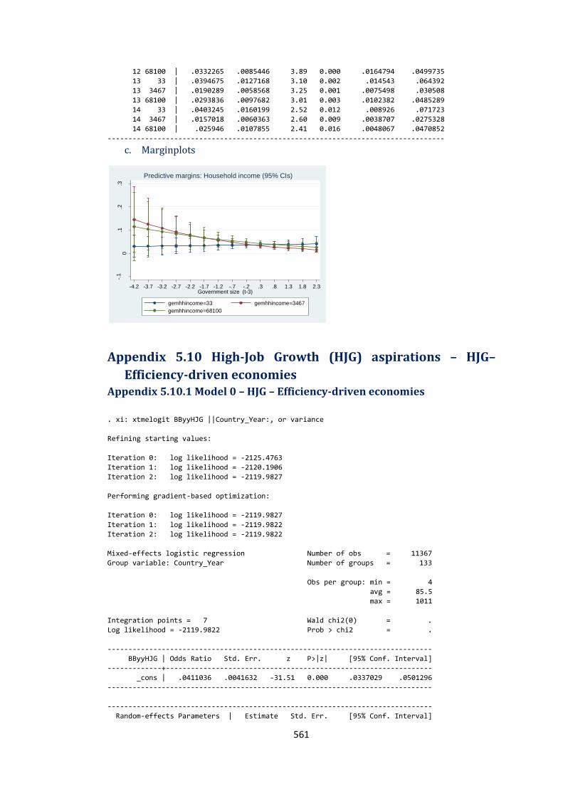
561
12 68100 | .0332265 .0085446 3.89 0.000 .0164794 .0499735
13 33 | .0394675 .0127168 3.10 0.002 .014543 .064392
13 3467 | .0190289 .0058568 3.25 0.001 .0075498 .030508
13 68100 | .0293836 .0097682 3.01 0.003 .0102382 .0485289
14 33 | .0403245 .0160199 2.52 0.012 .008926 .071723
14 3467 | .0157018 .0060363 2.60 0.009 .0038707 .0275328
14 68100 | .025946 .0107855 2.41 0.016 .0048067 .0470852
---------------------------------------------------------------------------------
c. Marginplots
Appendix 5.10 High-Job Growth (HJG) aspirations – HJG–
Efficiency-driven economies Appendix 5.10.1 Model 0 – HJG – Efficiency-driven economies
. xi: xtmelogit BByyHJG ||Country_Year:, or variance
Refining starting values:
Iteration 0: log likelihood = -2125.4763
Iteration 1: log likelihood = -2120.1906
Iteration 2: log likelihood = -2119.9827
Performing gradient-based optimization:
Iteration 0: log likelihood = -2119.9827
Iteration 1: log likelihood = -2119.9822
Iteration 2: log likelihood = -2119.9822
Mixed-effects logistic regression Number of obs = 11367
Group variable: Country_Year Number of groups = 133
Obs per group: min = 4
avg = 85.5
max = 1011
Integration points = 7 Wald chi2(0) = .
Log likelihood = -2119.9822 Prob > chi2 = .
------------------------------------------------------------------------------
BByyHJG | Odds Ratio Std. Err. z P>|z| [95% Conf. Interval]
-------------+----------------------------------------------------------------
_cons | .0411036 .0041632 -31.51 0.000 .0337029 .0501296
------------------------------------------------------------------------------
------------------------------------------------------------------------------
Random-effects Parameters | Estimate Std. Err. [95% Conf. Interval]
-.1
0.1
.2.3
Pre
dic
ted H
igh-j
ob
Gro
wth
Asp. (H
JG
)
-4.2 -3.7 -3.2 -2.7 -2.2 -1.7 -1.2 -.7 -.2 .3 .8 1.3 1.8 2.3Government size (t-3)
gemhhincome=33 gemhhincome=3467
gemhhincome=68100
Predictive margins: Household income (95% CIs)

562
-----------------------------+------------------------------------------------
Country_Year: Identity |
var(_cons) | .6342342 .1459358 .4040082 .9956555
------------------------------------------------------------------------------
LR test vs. logistic regression: chibar2(01) = 211.93 Prob>=chibar2 = 0.0000
. estat icc
Residual intraclass correlation
------------------------------------------------------------------------------
Level | ICC Std. Err. [95% Conf. Interval]
-----------------------------+------------------------------------------------
Country_Year | .1616253 .0311788 .1093724 .23233
------------------------------------------------------------------------------
Appendix 5.10.2 Model 1 – HJG – Efficiency-driven economies
a. Results
. xi: xtmelogit BByyHJG eff_zemploym_babybus1 eff_zage male educ_postgr i.gemhhincome
bb_owners work_status KNOWENT_dum omESTBBUS_dum BUSang_dum suskill_dum eff_zestbusrate
opportunities eff_zmhhinc eff_zmBUSang_dum eff_zhighgrowth_support eff_zL3bussfree
eff_zL3xcons eff_zL3corruption eff_zL3gov_size eff_zL1gdppccons2011 eff_zL1gdppccons2011sq
eff_zL1gdpgrowth i.OMTYPE4C i.yrsurv
||Country_Year:, or variance
i.gemhhincome _Igemhhinco_33-68100(naturally coded; _Igemhhinco_33 omitted)
i.OMTYPE4C _IOMTYPE4C_1-4 (naturally coded; _IOMTYPE4C_1 omitted)
i.yrsurv _Iyrsurv_2006-2013 (naturally coded; _Iyrsurv_2006 omitted)
Refining starting values:
Iteration 0: log likelihood = -1757.6836
Iteration 1: log likelihood = -1742.3706
Iteration 2: log likelihood = -1739.174
Performing gradient-based optimization:
Iteration 0: log likelihood = -1739.174
Iteration 1: log likelihood = -1738.237
Iteration 2: log likelihood = -1738.2293
Iteration 3: log likelihood = -1738.2293
Mixed-effects logistic regression Number of obs = 11367
Group variable: Country_Year Number of groups = 133
Obs per group: min = 4
avg = 85.5
max = 1011
Integration points = 7 Wald chi2(34) = 705.63
Log likelihood = -1738.2293 Prob > chi2 = 0.0000
-----------------------------------------------------------------------------------------
BByyHJG | Odds Ratio Std. Err. z P>|z| [95% Conf. Interval]
------------------------+----------------------------------------------------------------
eff_zemploym_babybus1 | 2.196884 .0812531 21.28 0.000 2.043266 2.362051
eff_zage | .940314 .0475991 -1.22 0.224 .8515002 1.038391
male | 1.393973 .1516356 3.05 0.002 1.126319 1.725233
educ_postgr | 1.374998 .2397927 1.83 0.068 .9769149 1.935295
_Igemhhinco_3467 | .9636366 .1581392 -0.23 0.821 .6985948 1.329233
_Igemhhinco_68100 | 1.278117 .1936042 1.62 0.105 .9498034 1.719916
bb_owners | .9755598 .1004615 -0.24 0.810 .7972574 1.193739
work_status | 1.069693 .2657468 0.27 0.786 .6573445 1.740707
KNOWENT_dum | 1.763361 .1988343 5.03 0.000 1.413712 2.199488
omESTBBUS_dum | 2.128268 .4824873 3.33 0.001 1.364757 3.318924
BUSang_dum | 1.462641 .1968328 2.83 0.005 1.12354 1.904088
suskill_dum | 1.272626 .1930158 1.59 0.112 .945369 1.713169
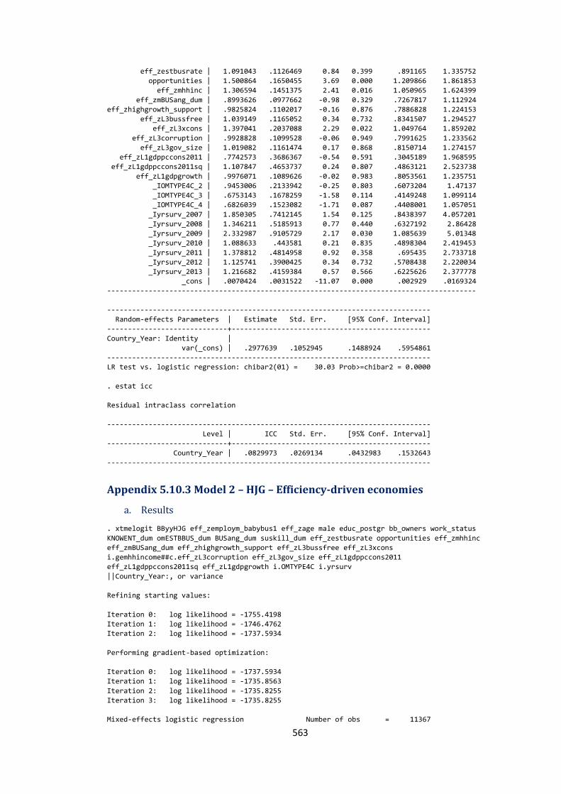
563
eff_zestbusrate | 1.091043 .1126469 0.84 0.399 .891165 1.335752
opportunities | 1.500864 .1650455 3.69 0.000 1.209866 1.861853
eff_zmhhinc | 1.306594 .1451375 2.41 0.016 1.050965 1.624399
eff_zmBUSang_dum | .8993626 .0977662 -0.98 0.329 .7267817 1.112924
eff_zhighgrowth_support | .9825824 .1102017 -0.16 0.876 .7886828 1.224153
eff_zL3bussfree | 1.039149 .1165052 0.34 0.732 .8341507 1.294527
eff_zL3xcons | 1.397041 .2037088 2.29 0.022 1.049764 1.859202
eff_zL3corruption | .9928828 .1099528 -0.06 0.949 .7991625 1.233562
eff_zL3gov_size | 1.019082 .1161474 0.17 0.868 .8150714 1.274157
eff_zL1gdppccons2011 | .7742573 .3686367 -0.54 0.591 .3045189 1.968595
eff_zL1gdppccons2011sq | 1.107847 .4653737 0.24 0.807 .4863121 2.523738
eff_zL1gdpgrowth | .9976071 .1089626 -0.02 0.983 .8053561 1.235751
_IOMTYPE4C_2 | .9453006 .2133942 -0.25 0.803 .6073204 1.47137
_IOMTYPE4C_3 | .6753143 .1678259 -1.58 0.114 .4149248 1.099114
_IOMTYPE4C_4 | .6826039 .1523082 -1.71 0.087 .4408001 1.057051
_Iyrsurv_2007 | 1.850305 .7412145 1.54 0.125 .8438397 4.057201
_Iyrsurv_2008 | 1.346211 .5185913 0.77 0.440 .6327192 2.86428
_Iyrsurv_2009 | 2.332987 .9105729 2.17 0.030 1.085639 5.01348
_Iyrsurv_2010 | 1.088633 .443581 0.21 0.835 .4898304 2.419453
_Iyrsurv_2011 | 1.378812 .4814958 0.92 0.358 .695435 2.733718
_Iyrsurv_2012 | 1.125741 .3900425 0.34 0.732 .5708438 2.220034
_Iyrsurv_2013 | 1.216682 .4159384 0.57 0.566 .6225626 2.377778
_cons | .0070424 .0031522 -11.07 0.000 .002929 .0169324
-----------------------------------------------------------------------------------------
------------------------------------------------------------------------------
Random-effects Parameters | Estimate Std. Err. [95% Conf. Interval]
-----------------------------+------------------------------------------------
Country_Year: Identity |
var(_cons) | .2977639 .1052945 .1488924 .5954861
------------------------------------------------------------------------------
LR test vs. logistic regression: chibar2(01) = 30.03 Prob>=chibar2 = 0.0000
. estat icc
Residual intraclass correlation
------------------------------------------------------------------------------
Level | ICC Std. Err. [95% Conf. Interval]
-----------------------------+------------------------------------------------
Country_Year | .0829973 .0269134 .0432983 .1532643
------------------------------------------------------------------------------
Appendix 5.10.3 Model 2 – HJG – Efficiency-driven economies
a. Results
. xtmelogit BByyHJG eff_zemploym_babybus1 eff_zage male educ_postgr bb_owners work_status
KNOWENT_dum omESTBBUS_dum BUSang_dum suskill_dum eff_zestbusrate opportunities eff_zmhhinc
eff_zmBUSang_dum eff_zhighgrowth_support eff_zL3bussfree eff_zL3xcons
i.gemhhincome##c.eff_zL3corruption eff_zL3gov_size eff_zL1gdppccons2011
eff_zL1gdppccons2011sq eff_zL1gdpgrowth i.OMTYPE4C i.yrsurv
||Country_Year:, or variance
Refining starting values:
Iteration 0: log likelihood = -1755.4198
Iteration 1: log likelihood = -1746.4762
Iteration 2: log likelihood = -1737.5934
Performing gradient-based optimization:
Iteration 0: log likelihood = -1737.5934
Iteration 1: log likelihood = -1735.8563
Iteration 2: log likelihood = -1735.8255
Iteration 3: log likelihood = -1735.8255
Mixed-effects logistic regression Number of obs = 11367
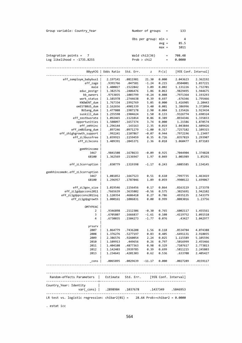
564
Group variable: Country_Year Number of groups = 133
Obs per group: min = 4
avg = 85.5
max = 1011
Integration points = 7 Wald chi2(36) = 708.48
Log likelihood = -1735.8255 Prob > chi2 = 0.0000
-------------------------------------------------------------------------------------------------
BByyHJG | Odds Ratio Std. Err. z P>|z| [95% Conf. Interval]
--------------------------------+----------------------------------------------------------------
eff_zemploym_babybus1 | 2.197141 .0811981 21.30 0.000 2.043623 2.362192
eff_zage | .9391766 .047581 -1.24 0.215 .8504001 1.037221
male | 1.400027 .1522842 3.09 0.002 1.131226 1.732701
educ_postgr | 1.382576 .2406476 1.86 0.063 .9829495 1.944675
bb_owners | .9753035 .1003799 -0.24 0.808 .7971364 1.193293
work_status | 1.101978 .2744638 0.39 0.697 .676346 1.795466
KNOWENT_dum | 1.767334 .1992769 5.05 0.000 1.416905 2.20443
omESTBBUS_dum | 2.162656 .4901339 3.40 0.001 1.386996 3.372094
BUSang_dum | 1.477808 .1987178 2.90 0.004 1.135426 1.923434
suskill_dum | 1.255598 .1904624 1.50 0.133 .9326774 1.690324
eff_zestbusrate | 1.092465 .1121014 0.86 0.389 .8934346 1.335833
opportunities | 1.508097 .1657374 3.74 0.000 1.21586 1.870574
eff_zmhhinc | 1.296144 .143163 2.35 0.019 1.043844 1.609426
eff_zmBUSang_dum | .897246 .0971279 -1.00 0.317 .7257182 1.109315
eff_zhighgrowth_support | .992241 .1107867 -0.07 0.944 .7972196 1.23497
eff_zL3bussfree | 1.039915 .1159459 0.35 0.726 .8357819 1.293907
eff_zL3xcons | 1.409391 .2045371 2.36 0.018 1.060477 1.873103
|
gemhhincome |
3467 | .9841508 .1678633 -0.09 0.925 .7044904 1.374828
68100 | 1.362569 .2136947 1.97 0.049 1.001989 1.85291
|
eff_zL3corruption | .830779 .1319398 -1.17 0.243 .6085585 1.134145
| gemhhincome#c.eff_zL3corruption |
3467 | 1.081852 .1667523 0.51 0.610 .7997735 1.463419
68100 | 1.296957 .1787046 1.89 0.059 .9900122 1.699067
|
eff_zL3gov_size | 1.019546 .1156456 0.17 0.864 .8163119 1.273378
eff_zL1gdppccons2011 | .7665639 .3635802 -0.56 0.575 .3025691 1.942102
eff_zL1gdppccons2011sq | 1.120354 .4686418 0.27 0.786 .4935135 2.543379
eff_zL1gdpgrowth | 1.000161 .1086831 0.00 0.999 .8083016 1.23756
|
OMTYPE4C |
2 | .9346898 .2112306 -0.30 0.765 .6002117 1.455561
3 | .6705807 .1666837 -1.61 0.108 .4119752 1.091518
4 | .6730035 .1504273 -1.77 0.076 .43427 1.042977
|
yrsurv |
2007 | 1.864779 .7436208 1.56 0.118 .8534784 4.074388
2008 | 1.376276 .5277197 0.83 0.405 .6491131 2.918035
2009 | 2.386576 .9260054 2.24 0.025 1.115589 5.105596
2010 | 1.109913 .449656 0.26 0.797 .5016999 2.455466
2011 | 1.404108 .4877363 0.98 0.329 .7107617 2.773813
2012 | 1.142403 .3939785 0.39 0.699 .5811215 2.245803
2013 | 1.234641 .4201303 0.62 0.536 .633708 2.405427
|
_cons | .0065895 .0029639 -11.17 0.000 .0027289 .0159117
-------------------------------------------------------------------------------------------------
------------------------------------------------------------------------------
Random-effects Parameters | Estimate Std. Err. [95% Conf. Interval]
-----------------------------+------------------------------------------------
Country_Year: Identity |
var(_cons) | .2898984 .1037678 .1437349 .5846953
------------------------------------------------------------------------------
LR test vs. logistic regression: chibar2(01) = 28.64 Prob>=chibar2 = 0.0000
. estat icc

565
Residual intraclass correlation
------------------------------------------------------------------------------
Level | ICC Std. Err. [95% Conf. Interval]
-----------------------------+------------------------------------------------
Country_Year | .0809825 .0266399 .0418612 .1509061
------------------------------------------------------------------------------ b. Predictive margins
. margins gemhhincome, at(eff_zL3corruption = (-2.9 (0.5) 1.7)) predict (mu fixedonly)
Predictive margins Number of obs = 11367
Expression : Predicted mean, fixed portion only, predict(mu fixedonly)
1._at : eff_zL3cor~n = -2.9
2._at : eff_zL3cor~n = -2.4
3._at : eff_zL3cor~n = -1.9
4._at : eff_zL3cor~n = -1.4
5._at : eff_zL3cor~n = -.9
6._at : eff_zL3cor~n = -.4
7._at : eff_zL3cor~n = .1
8._at : eff_zL3cor~n = .6
9._at : eff_zL3cor~n = 1.1
10._at : eff_zL3cor~n = 1.6
---------------------------------------------------------------------------------
| Delta-method
| Margin Std. Err. z P>|z| [95% Conf. Interval]
----------------+----------------------------------------------------------------
_at#gemhhincome |
1 33 | .053452 .0190125 2.81 0.005 .0161882 .0907157
1 3467 | .0437853 .0136561 3.21 0.001 .0170198 .0705508
1 68100 | .037036 .0137071 2.70 0.007 .0101706 .0639013
2 33 | .0495808 .0148309 3.34 0.001 .0205128 .0786488
2 3467 | .0418908 .010923 3.84 0.000 .020482 .0632995
2 68100 | .0382167 .0117529 3.25 0.001 .0151814 .061252
3 33 | .0459582 .0112199 4.10 0.000 .0239676 .0679487
3 3467 | .0400692 .0084609 4.74 0.000 .0234862 .0566523
3 68100 | .0394309 .0097824 4.03 0.000 .0202577 .0586041
4 33 | .0425711 .0082276 5.17 0.000 .0264454 .0586968
4 3467 | .0383184 .0063263 6.06 0.000 .0259191 .0507177
4 68100 | .0406792 .0078995 5.15 0.000 .0251966 .0561619
5 33 | .039407 .0060011 6.57 0.000 .027645 .051169
5 3467 | .0366361 .0046622 7.86 0.000 .0274983 .0457738
5 68100 | .0419626 .0063467 6.61 0.000 .0295232 .0544019
6 33 | .0364538 .0048329 7.54 0.000 .0269814 .0459261
6 3467 | .0350199 .0037703 9.29 0.000 .0276302 .0424096
6 68100 | .0432816 .0056207 7.70 0.000 .0322653 .054298
7 33 | .0336996 .0048793 6.91 0.000 .0241363 .043263
7 3467 | .0334678 .0039085 8.56 0.000 .0258074 .0411283
7 68100 | .0446372 .0062319 7.16 0.000 .032423 .0568515
8 33 | .0311334 .0057239 5.44 0.000 .0199148 .0423521
8 3467 | .0319777 .0047993 6.66 0.000 .0225711 .0413842
8 68100 | .0460302 .0080483 5.72 0.000 .0302559 .0618046
9 33 | .0287443 .0068342 4.21 0.000 .0153496 .042139
9 3467 | .0305474 .0059891 5.10 0.000 .0188089 .0422858
9 68100 | .0474614 .0106043 4.48 0.000 .0266774 .0682455
10 33 | .026522 .0079378 3.34 0.001 .0109643 .0420797
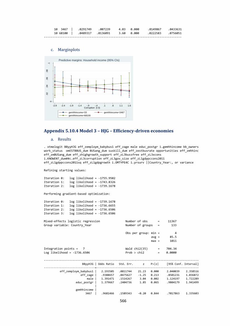
566
10 3467 | .0291749 .007239 4.03 0.000 .0149867 .0433631
10 68100 | .0489317 .0136091 3.60 0.000 .0222583 .0756051
---------------------------------------------------------------------------------
c. Marginplots
Appendix 5.10.4 Model 3 – HJG – Efficiency-driven economies
a. Results
. xtmelogit BByyHJG eff_zemploym_babybus1 eff_zage male educ_postgr i.gemhhincome bb_owners
work_status omESTBBUS_dum BUSang_dum suskill_dum eff_zestbusrate opportunities eff_zmhhinc
eff_zmBUSang_dum eff_zhighgrowth_support eff_zL3bussfree eff_zL3xcons
i.KNOWENT_dum##c.eff_zL3corruption eff_zL3gov_size eff_zL1gdppccons2011
eff_zL1gdppccons2011sq eff_zL1gdpgrowth i.OMTYPE4C i.yrsurv ||Country_Year:, or variance
Refining starting values:
Iteration 0: log likelihood = -1755.9502
Iteration 1: log likelihood = -1743.8326
Iteration 2: log likelihood = -1739.1678
Performing gradient-based optimization:
Iteration 0: log likelihood = -1739.1678
Iteration 1: log likelihood = -1736.6655
Iteration 2: log likelihood = -1736.6506
Iteration 3: log likelihood = -1736.6506
Mixed-effects logistic regression Number of obs = 11367
Group variable: Country_Year Number of groups = 133
Obs per group: min = 4
avg = 85.5
max = 1011
Integration points = 7 Wald chi2(35) = 704.34
Log likelihood = -1736.6506 Prob > chi2 = 0.0000
-------------------------------------------------------------------------------------------------
BByyHJG | Odds Ratio Std. Err. z P>|z| [95% Conf. Interval]
--------------------------------+----------------------------------------------------------------
eff_zemploym_babybus1 | 2.193505 .0811744 21.23 0.000 2.040039 2.358516
eff_zage | .9388657 .0475627 -1.25 0.213 .8501231 1.036872
male | 1.391471 .1514267 3.04 0.002 1.124197 1.722289
educ_postgr | 1.379667 .2404736 1.85 0.065 .9804179 1.941499
|
gemhhincome |
3467 | .9681466 .1589343 -0.20 0.844 .7017863 1.335603
0
.02
.04
.06
.08
.1
Pre
dic
ted H
igh-j
ob
Gro
wth
Asp. (H
JG
)
-2.9 -2.4 -1.9 -1.4 -.9 -.4 .1 .6 1.1 1.6Corruption (t-3)
gemhhincome=33 gemhhincome=3467
gemhhincome=68100
Predictive margins: Household income (95% CIs)
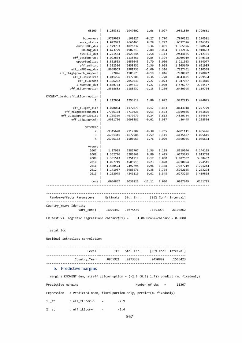
567
68100 | 1.285361 .1947002 1.66 0.097 .9551889 1.729661
|
bb_owners | .9729025 .100227 -0.27 0.790 .7950232 1.190581
work_status | 1.072973 .2666465 0.28 0.777 .6592576 1.746315
omESTBBUS_dum | 2.129783 .4826337 3.34 0.001 1.365976 3.320684
BUSang_dum | 1.473779 .1982713 2.88 0.004 1.132186 1.918433
suskill_dum | 1.271584 .1929844 1.58 0.113 .9444105 1.712101
eff_zestbusrate | 1.092804 .1138361 0.85 0.394 .8909919 1.340328
opportunities | 1.502503 .1653043 3.70 0.000 1.211063 1.864077
eff_zmhhinc | 1.302316 .1458531 2.36 0.018 1.045649 1.621985
eff_zmBUSang_dum | .8958963 .0981733 -1.00 0.316 .7227401 1.110538
eff_zhighgrowth_support | .97826 .1105573 -0.19 0.846 .7838922 1.220822
eff_zL3bussfree | 1.041296 .1177208 0.36 0.720 .8343421 1.299584
eff_zL3xcons | 1.396232 .2050039 2.27 0.023 1.047077 1.861816
1.KNOWENT_dum | 1.860754 .2194213 5.27 0.000 1.476777 2.34457
eff_zL3corruption | .8518682 .1188237 -1.15 0.250 .6480995 1.119704
|
KNOWENT_dum#c.eff_zL3corruption |
1 | 1.212034 .1293812 1.80 0.072 .9832215 1.494095
|
eff_zL3gov_size | 1.020084 .1172073 0.17 0.863 .8143918 1.277729 eff_zL1gdppccons2011 | .7736104 .3713025 -0.53 0.593 .3019806 1.981826
eff_zL1gdppccons2011sq | 1.105359 .4679979 0.24 0.813 .4820734 2.534507
eff_zL1gdpgrowth | .9981756 .1098881 -0.02 0.987 .80445 1.238554
|
OMTYPE4C |
2 | .9345678 .2112207 -0.30 0.765 .6001111 1.455426
3 | .6731341 .1672986 -1.59 0.111 .4135677 1.095611
4 | .6756132 .1508963 -1.76 0.079 .4360985 1.046674
|
yrsurv |
2007 | 1.87903 .7582707 1.56 0.118 .8519946 4.144105
2008 | 1.362776 .5283868 0.80 0.425 .6373673 2.913798
2009 | 2.351543 .9251919 2.17 0.030 1.087567 5.08452
2010 | 1.097719 .4505915 0.23 0.820 .4910094 2.4541
2011 | 1.400524 .492794 0.96 0.338 .7027219 2.791244
2012 | 1.141987 .3985676 0.38 0.704 .5762105 2.263294
2013 | 1.232075 .4243119 0.61 0.545 .6273265 2.419808
|
_cons | .0066867 .0030129 -11.11 0.000 .0027649 .0161715
-------------------------------------------------------------------------------------------------
------------------------------------------------------------------------------
Random-effects Parameters | Estimate Std. Err. [95% Conf. Interval]
-----------------------------+------------------------------------------------
Country_Year: Identity |
var(_cons) | .3079442 .1075469 .1553092 .6105862
------------------------------------------------------------------------------
LR test vs. logistic regression: chibar2(01) = 31.04 Prob>=chibar2 = 0.0000
.
. estat icc
Residual intraclass correlation
------------------------------------------------------------------------------
Level | ICC Std. Err. [95% Conf. Interval]
-----------------------------+------------------------------------------------
Country_Year | .0855921 .0273338 .0450802 .1565423
------------------------------------------------------------------------------
b. Predictive margins
. margins KNOWENT_dum, at(eff_zL3corruption = (-2.9 (0.5) 1.7)) predict (mu fixedonly)
Predictive margins Number of obs = 11367
Expression : Predicted mean, fixed portion only, predict(mu fixedonly)
1._at : eff_zL3cor~n = -2.9
2._at : eff_zL3cor~n = -2.4
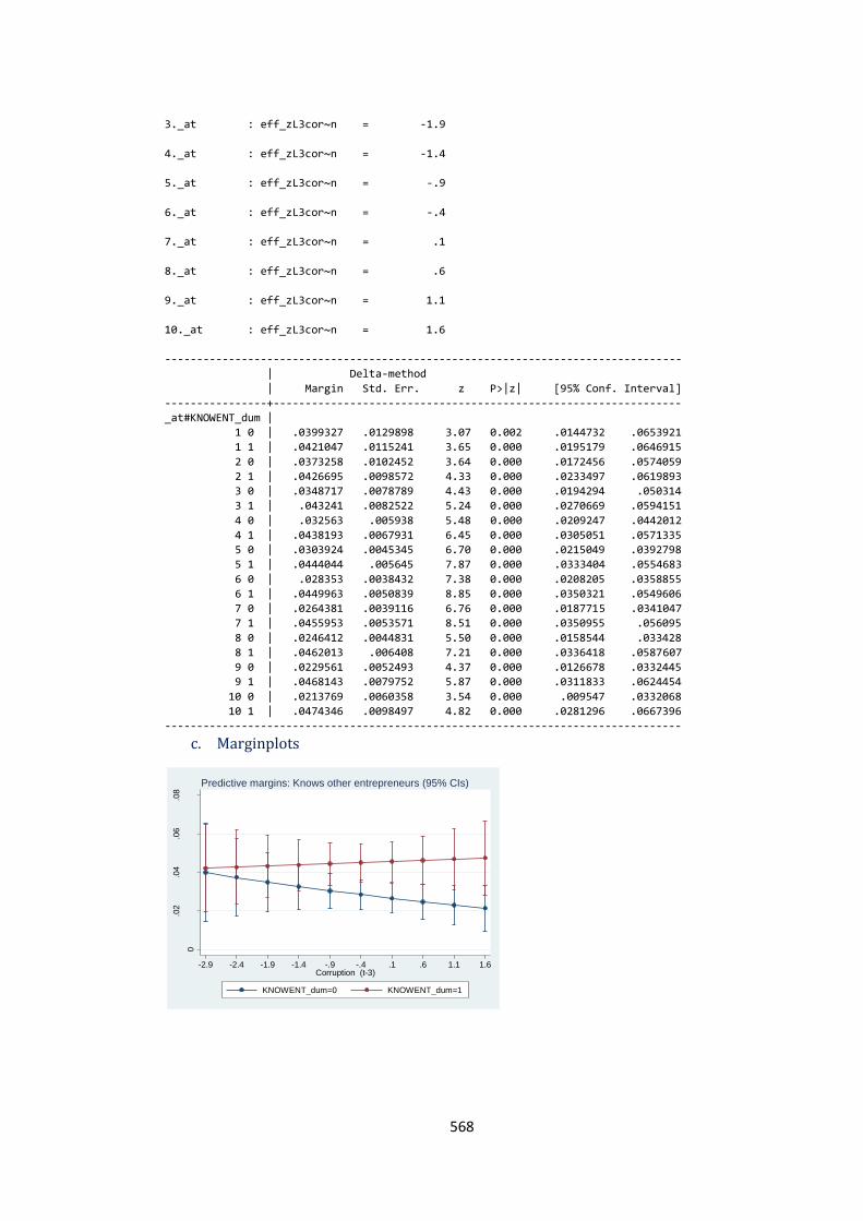
568
3._at : eff_zL3cor~n = -1.9
4._at : eff_zL3cor~n = -1.4
5._at : eff_zL3cor~n = -.9
6._at : eff_zL3cor~n = -.4
7._at : eff_zL3cor~n = .1
8._at : eff_zL3cor~n = .6
9._at : eff_zL3cor~n = 1.1
10._at : eff_zL3cor~n = 1.6
---------------------------------------------------------------------------------
| Delta-method
| Margin Std. Err. z P>|z| [95% Conf. Interval]
----------------+----------------------------------------------------------------
_at#KNOWENT_dum |
1 0 | .0399327 .0129898 3.07 0.002 .0144732 .0653921
1 1 | .0421047 .0115241 3.65 0.000 .0195179 .0646915
2 0 | .0373258 .0102452 3.64 0.000 .0172456 .0574059
2 1 | .0426695 .0098572 4.33 0.000 .0233497 .0619893
3 0 | .0348717 .0078789 4.43 0.000 .0194294 .050314
3 1 | .043241 .0082522 5.24 0.000 .0270669 .0594151
4 0 | .032563 .005938 5.48 0.000 .0209247 .0442012
4 1 | .0438193 .0067931 6.45 0.000 .0305051 .0571335
5 0 | .0303924 .0045345 6.70 0.000 .0215049 .0392798
5 1 | .0444044 .005645 7.87 0.000 .0333404 .0554683
6 0 | .028353 .0038432 7.38 0.000 .0208205 .0358855
6 1 | .0449963 .0050839 8.85 0.000 .0350321 .0549606
7 0 | .0264381 .0039116 6.76 0.000 .0187715 .0341047
7 1 | .0455953 .0053571 8.51 0.000 .0350955 .056095
8 0 | .0246412 .0044831 5.50 0.000 .0158544 .033428
8 1 | .0462013 .006408 7.21 0.000 .0336418 .0587607
9 0 | .0229561 .0052493 4.37 0.000 .0126678 .0332445
9 1 | .0468143 .0079752 5.87 0.000 .0311833 .0624454
10 0 | .0213769 .0060358 3.54 0.000 .009547 .0332068
10 1 | .0474346 .0098497 4.82 0.000 .0281296 .0667396
---------------------------------------------------------------------------------
c. Marginplots
0
.02
.04
.06
.08
Pre
dic
ted H
igh-j
ob
Gro
wth
Asp. (H
JG
)
-2.9 -2.4 -1.9 -1.4 -.9 -.4 .1 .6 1.1 1.6Corruption (t-3)
KNOWENT_dum=0 KNOWENT_dum=1
Predictive margins: Knows other entrepreneurs (95% CIs)
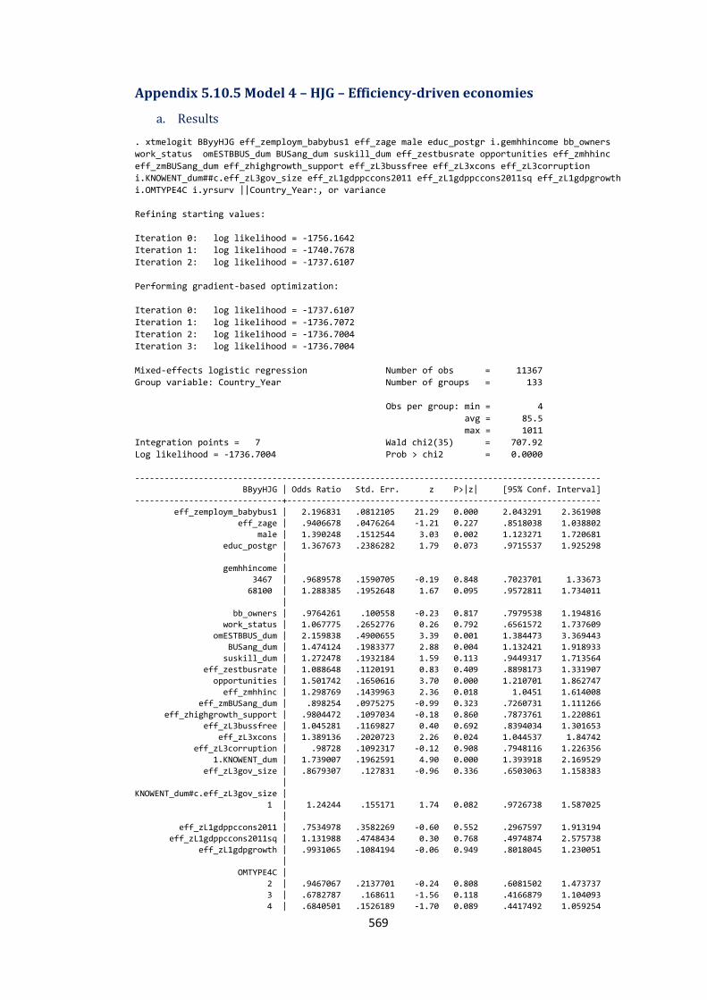
569
Appendix 5.10.5 Model 4 – HJG – Efficiency-driven economies
a. Results
. xtmelogit BByyHJG eff_zemploym_babybus1 eff_zage male educ_postgr i.gemhhincome bb_owners
work_status omESTBBUS_dum BUSang_dum suskill_dum eff_zestbusrate opportunities eff_zmhhinc
eff_zmBUSang_dum eff_zhighgrowth_support eff_zL3bussfree eff_zL3xcons eff_zL3corruption
i.KNOWENT_dum##c.eff_zL3gov_size eff_zL1gdppccons2011 eff_zL1gdppccons2011sq eff_zL1gdpgrowth
i.OMTYPE4C i.yrsurv ||Country_Year:, or variance
Refining starting values:
Iteration 0: log likelihood = -1756.1642
Iteration 1: log likelihood = -1740.7678
Iteration 2: log likelihood = -1737.6107
Performing gradient-based optimization:
Iteration 0: log likelihood = -1737.6107
Iteration 1: log likelihood = -1736.7072
Iteration 2: log likelihood = -1736.7004
Iteration 3: log likelihood = -1736.7004
Mixed-effects logistic regression Number of obs = 11367
Group variable: Country_Year Number of groups = 133
Obs per group: min = 4
avg = 85.5
max = 1011
Integration points = 7 Wald chi2(35) = 707.92
Log likelihood = -1736.7004 Prob > chi2 = 0.0000
-----------------------------------------------------------------------------------------------
BByyHJG | Odds Ratio Std. Err. z P>|z| [95% Conf. Interval]
------------------------------+----------------------------------------------------------------
eff_zemploym_babybus1 | 2.196831 .0812105 21.29 0.000 2.043291 2.361908
eff_zage | .9406678 .0476264 -1.21 0.227 .8518038 1.038802
male | 1.390248 .1512544 3.03 0.002 1.123271 1.720681
educ_postgr | 1.367673 .2386282 1.79 0.073 .9715537 1.925298
|
gemhhincome |
3467 | .9689578 .1590705 -0.19 0.848 .7023701 1.33673
68100 | 1.288385 .1952648 1.67 0.095 .9572811 1.734011
|
bb_owners | .9764261 .100558 -0.23 0.817 .7979538 1.194816 work_status | 1.067775 .2652776 0.26 0.792 .6561572 1.737609
omESTBBUS_dum | 2.159838 .4900655 3.39 0.001 1.384473 3.369443
BUSang_dum | 1.474124 .1983377 2.88 0.004 1.132421 1.918933
suskill_dum | 1.272478 .1932184 1.59 0.113 .9449317 1.713564
eff_zestbusrate | 1.088648 .1120191 0.83 0.409 .8898173 1.331907
opportunities | 1.501742 .1650616 3.70 0.000 1.210701 1.862747
eff_zmhhinc | 1.298769 .1439963 2.36 0.018 1.0451 1.614008
eff_zmBUSang_dum | .898254 .0975275 -0.99 0.323 .7260731 1.111266
eff_zhighgrowth_support | .9804472 .1097034 -0.18 0.860 .7873761 1.220861
eff_zL3bussfree | 1.045281 .1169827 0.40 0.692 .8394034 1.301653
eff_zL3xcons | 1.389136 .2020723 2.26 0.024 1.044537 1.84742
eff_zL3corruption | .98728 .1092317 -0.12 0.908 .7948116 1.226356
1.KNOWENT_dum | 1.739007 .1962591 4.90 0.000 1.393918 2.169529
eff_zL3gov_size | .8679307 .127831 -0.96 0.336 .6503063 1.158383
|
KNOWENT_dum#c.eff_zL3gov_size |
1 | 1.24244 .155171 1.74 0.082 .9726738 1.587025
|
eff_zL1gdppccons2011 | .7534978 .3582269 -0.60 0.552 .2967597 1.913194
eff_zL1gdppccons2011sq | 1.131988 .4748434 0.30 0.768 .4974874 2.575738
eff_zL1gdpgrowth | .9931065 .1084194 -0.06 0.949 .8018045 1.230051
|
OMTYPE4C |
2 | .9467067 .2137701 -0.24 0.808 .6081502 1.473737
3 | .6782787 .168611 -1.56 0.118 .4166879 1.104093
4 | .6840501 .1526189 -1.70 0.089 .4417492 1.059254
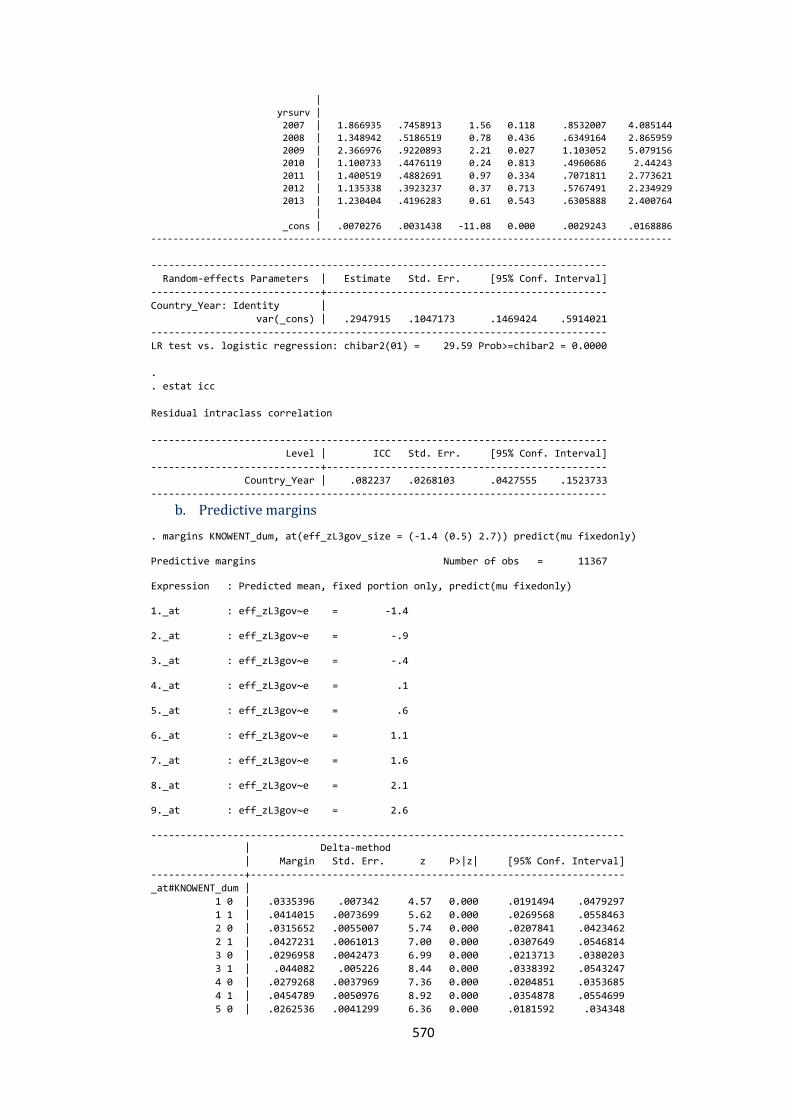
570
|
yrsurv |
2007 | 1.866935 .7458913 1.56 0.118 .8532007 4.085144
2008 | 1.348942 .5186519 0.78 0.436 .6349164 2.865959
2009 | 2.366976 .9220893 2.21 0.027 1.103052 5.079156
2010 | 1.100733 .4476119 0.24 0.813 .4960686 2.44243
2011 | 1.400519 .4882691 0.97 0.334 .7071811 2.773621
2012 | 1.135338 .3923237 0.37 0.713 .5767491 2.234929
2013 | 1.230404 .4196283 0.61 0.543 .6305888 2.400764
|
_cons | .0070276 .0031438 -11.08 0.000 .0029243 .0168886
-----------------------------------------------------------------------------------------------
------------------------------------------------------------------------------
Random-effects Parameters | Estimate Std. Err. [95% Conf. Interval]
-----------------------------+------------------------------------------------
Country_Year: Identity |
var(_cons) | .2947915 .1047173 .1469424 .5914021
------------------------------------------------------------------------------
LR test vs. logistic regression: chibar2(01) = 29.59 Prob>=chibar2 = 0.0000
.
. estat icc
Residual intraclass correlation
------------------------------------------------------------------------------
Level | ICC Std. Err. [95% Conf. Interval]
-----------------------------+------------------------------------------------
Country_Year | .082237 .0268103 .0427555 .1523733
------------------------------------------------------------------------------
b. Predictive margins
. margins KNOWENT_dum, at(eff_zL3gov_size = (-1.4 (0.5) 2.7)) predict(mu fixedonly) Predictive margins Number of obs = 11367 Expression : Predicted mean, fixed portion only, predict(mu fixedonly) 1._at : eff_zL3gov~e = -1.4 2._at : eff_zL3gov~e = -.9 3._at : eff_zL3gov~e = -.4 4._at : eff_zL3gov~e = .1 5._at : eff_zL3gov~e = .6 6._at : eff_zL3gov~e = 1.1 7._at : eff_zL3gov~e = 1.6 8._at : eff_zL3gov~e = 2.1 9._at : eff_zL3gov~e = 2.6 --------------------------------------------------------------------------------- | Delta-method
| Margin Std. Err. z P>|z| [95% Conf. Interval]
----------------+----------------------------------------------------------------
_at#KNOWENT_dum |
1 0 | .0335396 .007342 4.57 0.000 .0191494 .0479297
1 1 | .0414015 .0073699 5.62 0.000 .0269568 .0558463
2 0 | .0315652 .0055007 5.74 0.000 .0207841 .0423462
2 1 | .0427231 .0061013 7.00 0.000 .0307649 .0546814
3 0 | .0296958 .0042473 6.99 0.000 .0213713 .0380203
3 1 | .044082 .005226 8.44 0.000 .0338392 .0543247
4 0 | .0279268 .0037969 7.36 0.000 .0204851 .0353685
4 1 | .0454789 .0050976 8.92 0.000 .0354878 .0554699
5 0 | .0262536 .0041299 6.36 0.000 .0181592 .034348
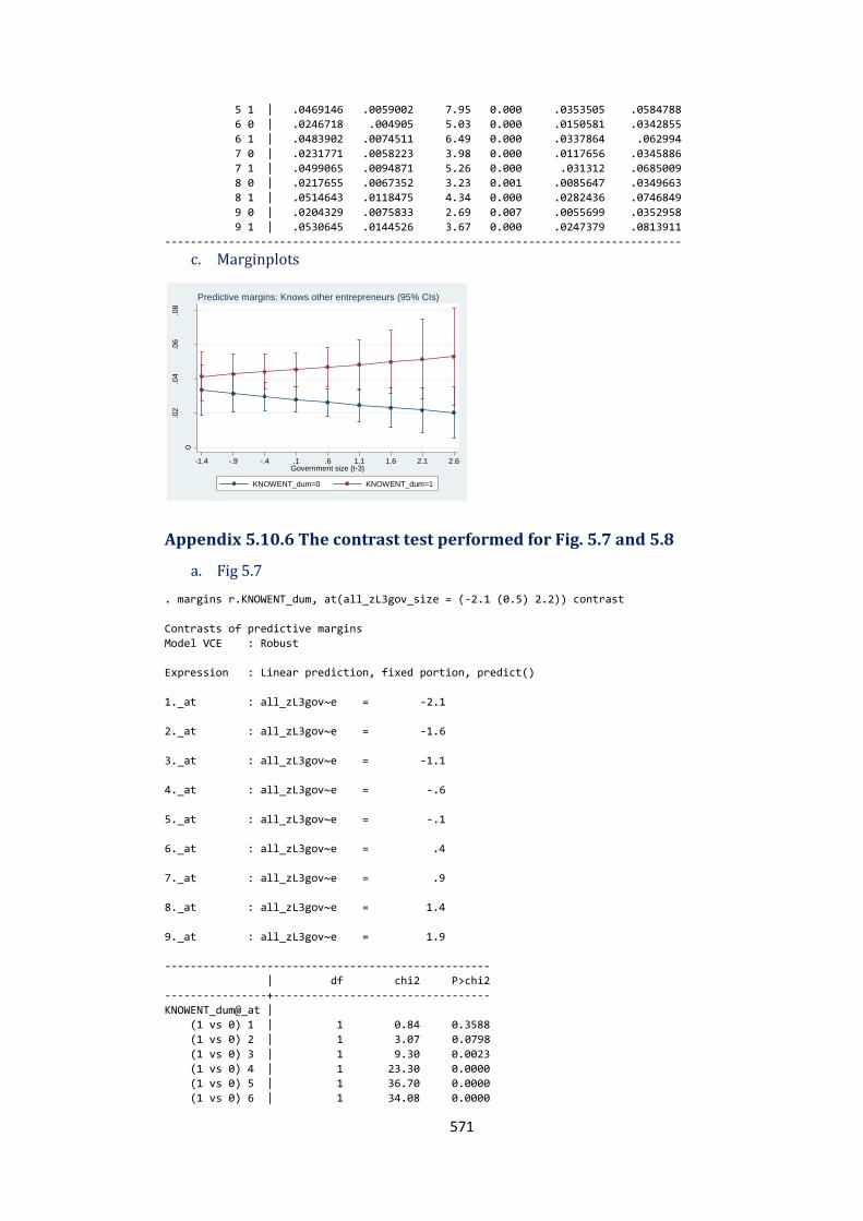
571
5 1 | .0469146 .0059002 7.95 0.000 .0353505 .0584788
6 0 | .0246718 .004905 5.03 0.000 .0150581 .0342855
6 1 | .0483902 .0074511 6.49 0.000 .0337864 .062994
7 0 | .0231771 .0058223 3.98 0.000 .0117656 .0345886
7 1 | .0499065 .0094871 5.26 0.000 .031312 .0685009
8 0 | .0217655 .0067352 3.23 0.001 .0085647 .0349663
8 1 | .0514643 .0118475 4.34 0.000 .0282436 .0746849
9 0 | .0204329 .0075833 2.69 0.007 .0055699 .0352958
9 1 | .0530645 .0144526 3.67 0.000 .0247379 .0813911
--------------------------------------------------------------------------------- c. Marginplots
Appendix 5.10.6 The contrast test performed for Fig. 5.7 and 5.8
a. Fig 5.7
. margins r.KNOWENT_dum, at(all_zL3gov_size = (-2.1 (0.5) 2.2)) contrast
Contrasts of predictive margins
Model VCE : Robust
Expression : Linear prediction, fixed portion, predict()
1._at : all_zL3gov~e = -2.1
2._at : all_zL3gov~e = -1.6
3._at : all_zL3gov~e = -1.1
4._at : all_zL3gov~e = -.6
5._at : all_zL3gov~e = -.1
6._at : all_zL3gov~e = .4
7._at : all_zL3gov~e = .9
8._at : all_zL3gov~e = 1.4
9._at : all_zL3gov~e = 1.9
---------------------------------------------------
| df chi2 P>chi2
----------------+----------------------------------
KNOWENT_dum@_at |
(1 vs 0) 1 | 1 0.84 0.3588
(1 vs 0) 2 | 1 3.07 0.0798
(1 vs 0) 3 | 1 9.30 0.0023
(1 vs 0) 4 | 1 23.30 0.0000
(1 vs 0) 5 | 1 36.70 0.0000
(1 vs 0) 6 | 1 34.08 0.0000
0
.02
.04
.06
.08
Pre
dic
ted H
igh-j
ob
Gro
wth
Asp. (H
JG
)
-1.4 -.9 -.4 .1 .6 1.1 1.6 2.1 2.6Government size (t-3)
KNOWENT_dum=0 KNOWENT_dum=1
Predictive margins: Knows other entrepreneurs (95% CIs)
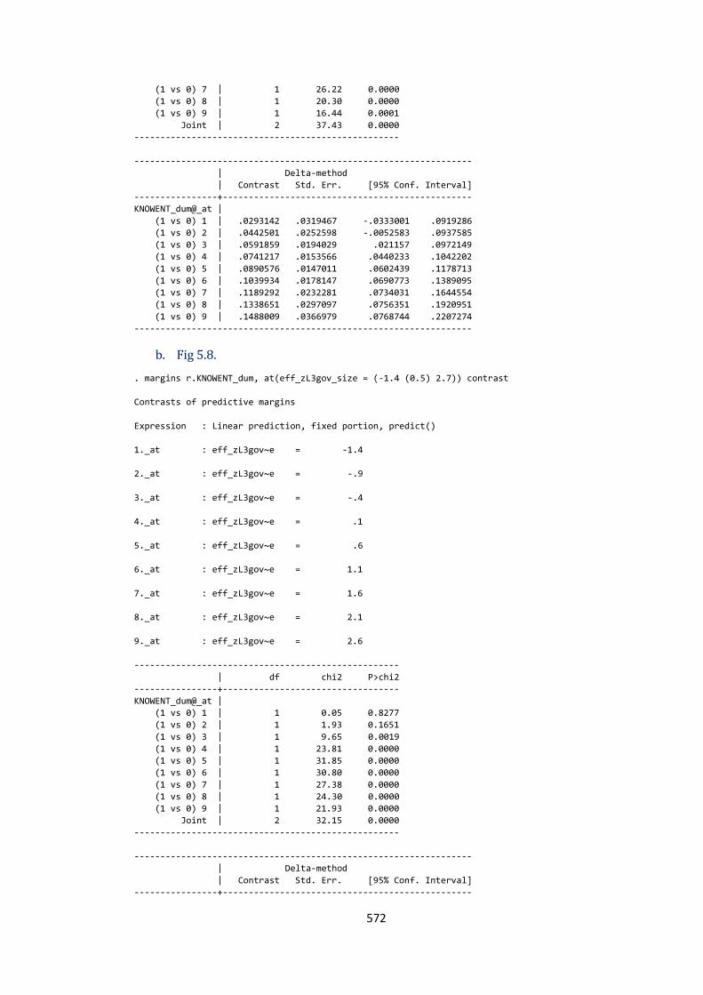
572
(1 vs 0) 7 | 1 26.22 0.0000
(1 vs 0) 8 | 1 20.30 0.0000
(1 vs 0) 9 | 1 16.44 0.0001
Joint | 2 37.43 0.0000
---------------------------------------------------
-----------------------------------------------------------------
| Delta-method
| Contrast Std. Err. [95% Conf. Interval]
----------------+------------------------------------------------
KNOWENT_dum@_at |
(1 vs 0) 1 | .0293142 .0319467 -.0333001 .0919286
(1 vs 0) 2 | .0442501 .0252598 -.0052583 .0937585
(1 vs 0) 3 | .0591859 .0194029 .021157 .0972149
(1 vs 0) 4 | .0741217 .0153566 .0440233 .1042202
(1 vs 0) 5 | .0890576 .0147011 .0602439 .1178713
(1 vs 0) 6 | .1039934 .0178147 .0690773 .1389095
(1 vs 0) 7 | .1189292 .0232281 .0734031 .1644554
(1 vs 0) 8 | .1338651 .0297097 .0756351 .1920951
(1 vs 0) 9 | .1488009 .0366979 .0768744 .2207274
-----------------------------------------------------------------
b. Fig 5.8.
. margins r.KNOWENT_dum, at(eff_zL3gov_size = (-1.4 (0.5) 2.7)) contrast
Contrasts of predictive margins
Expression : Linear prediction, fixed portion, predict()
1._at : eff_zL3gov~e = -1.4
2._at : eff_zL3gov~e = -.9
3._at : eff_zL3gov~e = -.4
4._at : eff_zL3gov~e = .1
5._at : eff_zL3gov~e = .6
6._at : eff_zL3gov~e = 1.1
7._at : eff_zL3gov~e = 1.6
8._at : eff_zL3gov~e = 2.1
9._at : eff_zL3gov~e = 2.6
---------------------------------------------------
| df chi2 P>chi2
----------------+----------------------------------
KNOWENT_dum@_at |
(1 vs 0) 1 | 1 0.05 0.8277
(1 vs 0) 2 | 1 1.93 0.1651
(1 vs 0) 3 | 1 9.65 0.0019
(1 vs 0) 4 | 1 23.81 0.0000
(1 vs 0) 5 | 1 31.85 0.0000
(1 vs 0) 6 | 1 30.80 0.0000
(1 vs 0) 7 | 1 27.38 0.0000
(1 vs 0) 8 | 1 24.30 0.0000
(1 vs 0) 9 | 1 21.93 0.0000
Joint | 2 32.15 0.0000
---------------------------------------------------
-----------------------------------------------------------------
| Delta-method
| Contrast Std. Err. [95% Conf. Interval]
----------------+------------------------------------------------

573
KNOWENT_dum@_at |
(1 vs 0) 1 | .0072627 .0333633 -.058128 .0726535
(1 vs 0) 2 | .0365575 .0263377 -.0150635 .0881784
(1 vs 0) 3 | .0658522 .0211986 .0243037 .1074008
(1 vs 0) 4 | .095147 .0194995 .0569286 .1333653
(1 vs 0) 5 | .1244417 .0220504 .0812238 .1676597
(1 vs 0) 6 | .1537365 .0277011 .0994434 .2080295
(1 vs 0) 7 | .1830312 .0349803 .1144712 .2515912
(1 vs 0) 8 | .2123259 .04307 .1279102 .2967417
(1 vs 0) 9 | .2416207 .0515905 .1405052 .3427362
-----------------------------------------------------------------
Appendix 5.11 A new dummy (emp_growth_dum2) for robustness
checks – all economies . xi: xtmelogit emp_growth_dum2 all_zemploym_babybus1 all_zage male educ_postgr i.gemhhincome
bb_owners work_status KNOWENT_dum omESTBBUS_dum BUSang_dum suskill_dum all_zestbusrate
opportunities all_zmeduc_postgr all_zmhhinc all_zmKNOWENT_dum all_zmomESTBBUS_dum
all_zhighgrowth_support all_zL3bussfree all_zL3xcons all_zL3gov_size all_zL1gdppccons2011
all_zL1gdppccons2011sq all_zL1gdpgrowth i.OMTYPE4C i.yrsurv ||Country_Year:, or variance
i.gemhhincome _Igemhhinco_33-68100(naturally coded; _Igemhhinco_33 omitted)
i.OMTYPE4C _IOMTYPE4C_1-4 (naturally coded; _IOMTYPE4C_1 omitted)
i.yrsurv _Iyrsurv_2006-2013 (naturally coded; _Iyrsurv_2006 omitted)
Refining starting values:
Iteration 0: log likelihood = -3385.9658 (not concave)
Iteration 1: log likelihood = -3356.2962
Iteration 2: log likelihood = -3350.4546
Performing gradient-based optimization:
Iteration 0: log likelihood = -3350.4546
Iteration 1: log likelihood = -3348.1068
Iteration 2: log likelihood = -3347.2519
Iteration 3: log likelihood = -3347.2329
Iteration 4: log likelihood = -3347.2329
Mixed-effects logistic regression Number of obs = 18120
Group variable: Country_Year Number of groups = 261
Obs per group: min = 3
avg = 69.4
max = 1011
Integration points = 7 Wald chi2(35) = 1918.25
Log likelihood = -3347.2329 Prob > chi2 = 0.0000
-----------------------------------------------------------------------------------------
emp_growth_dum2 | Odds Ratio Std. Err. z P>|z| [95% Conf. Interval]
------------------------+----------------------------------------------------------------
all_zemploym_babybus1 | 2.949714 .0827703 38.55 0.000 2.791868 3.116485
all_zage | .8778497 .0314279 -3.64 0.000 .8183635 .9416598
male | 1.40058 .1048148 4.50 0.000 1.209503 1.621844
educ_postgr | 1.132036 .1248042 1.12 0.261 .9120469 1.405086
_Igemhhinco_3467 | 1.004228 .1162702 0.04 0.971 .8003498 1.260043
_Igemhhinco_68100 | 1.645086 .175664 4.66 0.000 1.334432 2.02806
bb_owners | 1.099105 .0778047 1.33 0.182 .9567172 1.262685
work_status | .9700521 .1727874 -0.17 0.864 .6841912 1.375348
KNOWENT_dum | 1.298109 .0988504 3.43 0.001 1.118131 1.507058
omESTBBUS_dum | .7510909 .1430596 -1.50 0.133 .5170885 1.090988
BUSang_dum | 1.318036 .130071 2.80 0.005 1.086241 1.599295
suskill_dum | 1.535683 .1729569 3.81 0.000 1.231501 1.914999
all_zestbusrate | .892673 .0506717 -2.00 0.045 .7986837 .9977231
opportunities | 1.347425 .0987117 4.07 0.000 1.167202 1.555476
all_zmeduc_postgr | 1.139845 .0783266 1.90 0.057 .9962167 1.304181
all_zmhhinc | 1.084504 .0575548 1.53 0.126 .9773673 1.203385
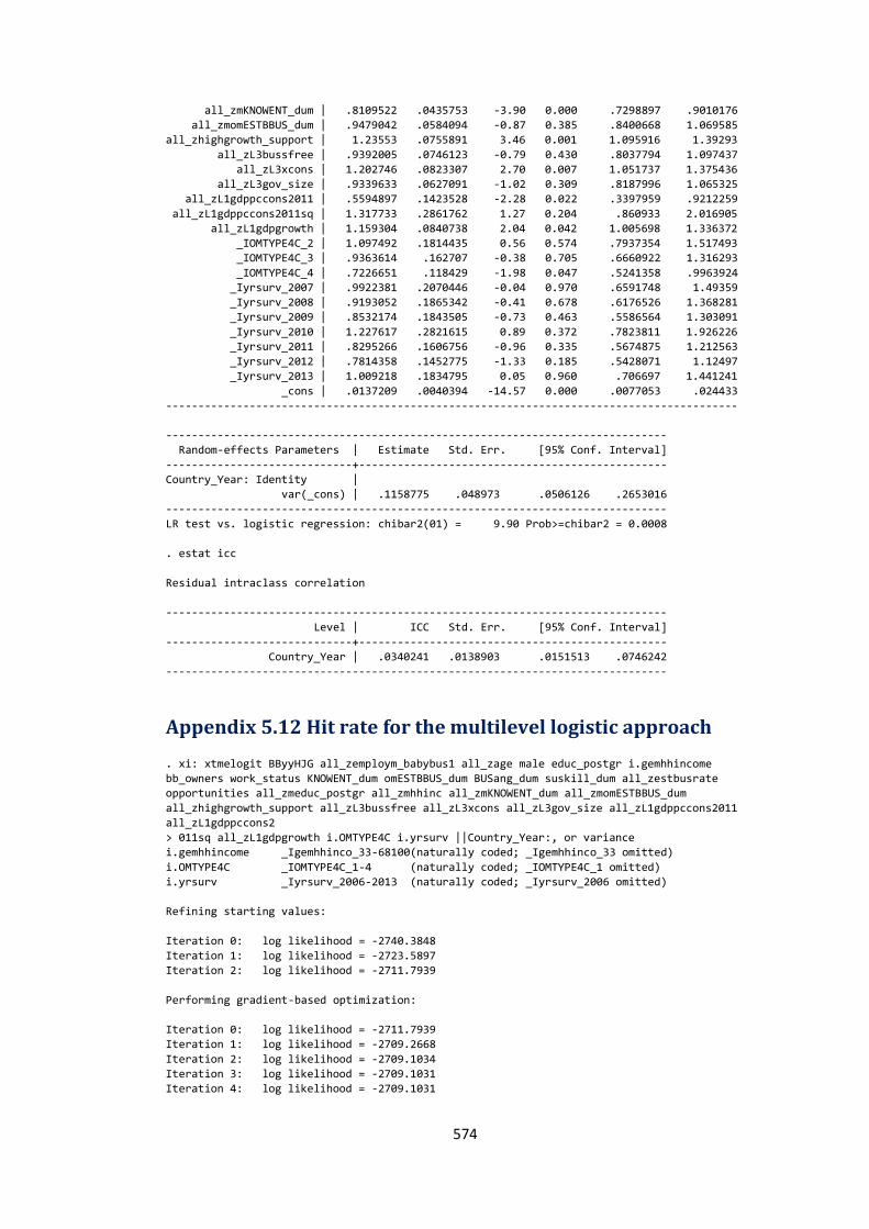
574
all_zmKNOWENT_dum | .8109522 .0435753 -3.90 0.000 .7298897 .9010176
all_zmomESTBBUS_dum | .9479042 .0584094 -0.87 0.385 .8400668 1.069585
all_zhighgrowth_support | 1.23553 .0755891 3.46 0.001 1.095916 1.39293
all_zL3bussfree | .9392005 .0746123 -0.79 0.430 .8037794 1.097437
all_zL3xcons | 1.202746 .0823307 2.70 0.007 1.051737 1.375436
all_zL3gov_size | .9339633 .0627091 -1.02 0.309 .8187996 1.065325
all_zL1gdppccons2011 | .5594897 .1423528 -2.28 0.022 .3397959 .9212259
all_zL1gdppccons2011sq | 1.317733 .2861762 1.27 0.204 .860933 2.016905
all_zL1gdpgrowth | 1.159304 .0840738 2.04 0.042 1.005698 1.336372
_IOMTYPE4C_2 | 1.097492 .1814435 0.56 0.574 .7937354 1.517493
_IOMTYPE4C_3 | .9363614 .162707 -0.38 0.705 .6660922 1.316293
_IOMTYPE4C_4 | .7226651 .118429 -1.98 0.047 .5241358 .9963924
_Iyrsurv_2007 | .9922381 .2070446 -0.04 0.970 .6591748 1.49359
_Iyrsurv_2008 | .9193052 .1865342 -0.41 0.678 .6176526 1.368281
_Iyrsurv_2009 | .8532174 .1843505 -0.73 0.463 .5586564 1.303091
_Iyrsurv_2010 | 1.227617 .2821615 0.89 0.372 .7823811 1.926226
_Iyrsurv_2011 | .8295266 .1606756 -0.96 0.335 .5674875 1.212563
_Iyrsurv_2012 | .7814358 .1452775 -1.33 0.185 .5428071 1.12497
_Iyrsurv_2013 | 1.009218 .1834795 0.05 0.960 .706697 1.441241
_cons | .0137209 .0040394 -14.57 0.000 .0077053 .024433
-----------------------------------------------------------------------------------------
------------------------------------------------------------------------------
Random-effects Parameters | Estimate Std. Err. [95% Conf. Interval]
-----------------------------+------------------------------------------------
Country_Year: Identity |
var(_cons) | .1158775 .048973 .0506126 .2653016
------------------------------------------------------------------------------
LR test vs. logistic regression: chibar2(01) = 9.90 Prob>=chibar2 = 0.0008
. estat icc
Residual intraclass correlation
------------------------------------------------------------------------------
Level | ICC Std. Err. [95% Conf. Interval]
-----------------------------+------------------------------------------------
Country_Year | .0340241 .0138903 .0151513 .0746242
------------------------------------------------------------------------------
Appendix 5.12 Hit rate for the multilevel logistic approach . xi: xtmelogit BByyHJG all_zemploym_babybus1 all_zage male educ_postgr i.gemhhincome
bb_owners work_status KNOWENT_dum omESTBBUS_dum BUSang_dum suskill_dum all_zestbusrate
opportunities all_zmeduc_postgr all_zmhhinc all_zmKNOWENT_dum all_zmomESTBBUS_dum
all_zhighgrowth_support all_zL3bussfree all_zL3xcons all_zL3gov_size all_zL1gdppccons2011
all_zL1gdppccons2
> 011sq all_zL1gdpgrowth i.OMTYPE4C i.yrsurv ||Country_Year:, or variance
i.gemhhincome _Igemhhinco_33-68100(naturally coded; _Igemhhinco_33 omitted)
i.OMTYPE4C _IOMTYPE4C_1-4 (naturally coded; _IOMTYPE4C_1 omitted)
i.yrsurv _Iyrsurv_2006-2013 (naturally coded; _Iyrsurv_2006 omitted)
Refining starting values:
Iteration 0: log likelihood = -2740.3848
Iteration 1: log likelihood = -2723.5897
Iteration 2: log likelihood = -2711.7939
Performing gradient-based optimization:
Iteration 0: log likelihood = -2711.7939
Iteration 1: log likelihood = -2709.2668
Iteration 2: log likelihood = -2709.1034
Iteration 3: log likelihood = -2709.1031
Iteration 4: log likelihood = -2709.1031
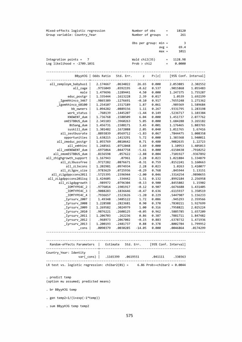
575
Mixed-effects logistic regression Number of obs = 18120
Group variable: Country_Year Number of groups = 261
Obs per group: min = 3
avg = 69.4
max = 1011
Integration points = 7 Wald chi2(35) = 1128.98
Log likelihood = -2709.1031 Prob > chi2 = 0.0000
-----------------------------------------------------------------------------------------
BByyHJG | Odds Ratio Std. Err. z P>|z| [95% Conf. Interval]
------------------------+----------------------------------------------------------------
all_zemploym_babybus1 | 2.174667 .0634022 26.65 0.000 2.053885 2.302552
all_zage | .9755049 .0392195 -0.62 0.537 .9015868 1.055483
male | 1.479696 .1289441 4.50 0.000 1.247375 1.755287
educ_postgr | 1.335444 .1613228 2.39 0.017 1.0539 1.692199
_Igemhhinco_3467 | .9865389 .1276691 -0.10 0.917 .7655248 1.271362
_Igemhhinco_68100 | 1.254107 .1517189 1.87 0.061 .989369 1.589684
bb_owners | 1.094282 .0889156 1.11 0.267 .9331795 1.283198
work_status | .760139 .1445207 -1.44 0.149 .5236717 1.103384
KNOWENT_dum | 1.736768 .1588509 6.04 0.000 1.451737 2.077762
omESTBBUS_dum | 2.345103 .3960263 5.05 0.000 1.684288 3.265182
BUSang_dum | 1.456731 .1588171 3.45 0.001 1.176465 1.803765
suskill_dum | 1.301482 .1672088 2.05 0.040 1.011765 1.67416
all_zestbusrate | .8893839 .0569712 -1.83 0.067 .7844475 1.008358
opportunities | 1.638215 .1413291 5.72 0.000 1.383368 1.940011
all_zmeduc_postgr | 1.055769 .0810642 0.71 0.480 .9082635 1.22723
all_zmhhinc | 1.248561 .0752048 3.69 0.000 1.10953 1.405013
all_zmKNOWENT_dum | .6975064 .0447758 -5.61 0.000 .6150438 .7910252
all_zmomESTBBUS_dum | .8156598 .057622 -2.88 0.004 .7101927 .9367892
all_zhighgrowth_support | 1.167943 .07961 2.28 0.023 1.021884 1.334879
all_zL3bussfree | .9727282 .0876671 -0.31 0.759 .8152241 1.160663
all_zL3xcons | 1.202981 .0974934 2.28 0.023 1.0263 1.410077
all_zL3gov_size | .9783629 .0725936 -0.29 0.768 .845944 1.13151
all_zL1gdppccons2011 | .5725395 .1596944 -2.00 0.046 .3314254 .9890655
all_zL1gdppccons2011sq | 1.424605 .334442 1.51 0.132 .8992184 2.256958
all_zL1gdpgrowth | .989972 .0796304 -0.13 0.900 .8455802 1.15902
_IOMTYPE4C_2 | .9776014 .1901917 -0.12 0.907 .6676688 1.431405
_IOMTYPE4C_3 | .9088283 .1836646 -0.47 0.636 .6115937 1.350519
_IOMTYPE4C_4 | .7936657 .1523626 -1.20 0.229 .5447907 1.156233
_Iyrsurv_2007 | 1.49348 .3485122 1.72 0.086 .945293 2.359566
_Iyrsurv_2008 | 1.228588 .2823681 0.90 0.370 .7830211 1.927699
_Iyrsurv_2009 | 1.269582 .3024979 1.00 0.316 .7958821 2.025224
_Iyrsurv_2010 | .9876221 .2608125 -0.05 0.962 .5885785 1.657209
_Iyrsurv_2011 | 1.206703 .262236 0.86 0.387 .7881711 1.847482
_Iyrsurv_2012 | .968973 .2067002 -0.15 0.883 .6378732 1.471936
_Iyrsurv_2013 | 1.200193 .2481737 0.88 0.378 .8002784 1.799952
_cons | .0090379 .0030285 -14.05 0.000 .0046864 .0174299
-----------------------------------------------------------------------------------------
------------------------------------------------------------------------------
Random-effects Parameters | Estimate Std. Err. [95% Conf. Interval]
-----------------------------+------------------------------------------------
Country_Year: Identity |
var(_cons) | .1165399 .0619551 .041111 .330363
------------------------------------------------------------------------------
LR test vs. logistic regression: chibar2(01) = 6.86 Prob>=chibar2 = 0.0044
. predict temp
(option mu assumed; predicted means)
. br BByyHJG temp
. gen temp2=1/(1+exp(-1*temp))
. sum BByyHJG temp temp2
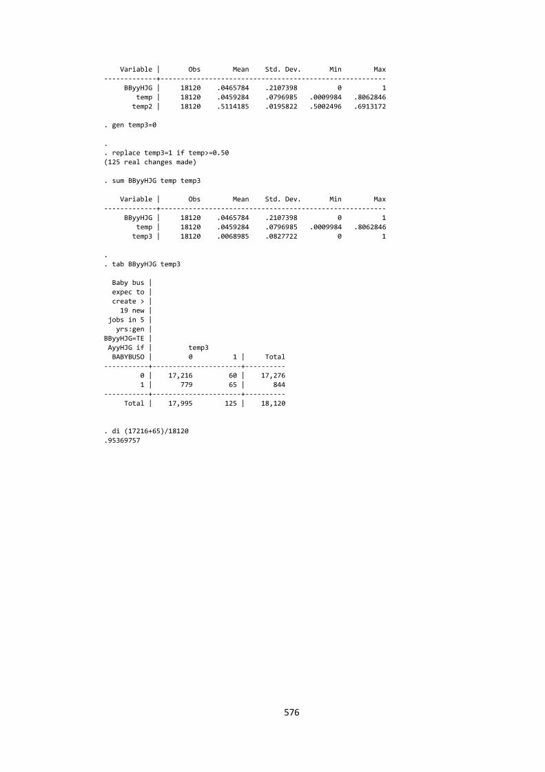
576
Variable | Obs Mean Std. Dev. Min Max
-------------+--------------------------------------------------------
BByyHJG | 18120 .0465784 .2107398 0 1
temp | 18120 .0459284 .0796985 .0009984 .8062846
temp2 | 18120 .5114185 .0195822 .5002496 .6913172
. gen temp3=0
.
. replace temp3=1 if temp>=0.50
(125 real changes made)
. sum BByyHJG temp temp3
Variable | Obs Mean Std. Dev. Min Max
-------------+--------------------------------------------------------
BByyHJG | 18120 .0465784 .2107398 0 1
temp | 18120 .0459284 .0796985 .0009984 .8062846
temp3 | 18120 .0068985 .0827722 0 1
.
. tab BByyHJG temp3
Baby bus |
expec to |
create > |
19 new |
jobs in 5 |
yrs:gen |
BByyHJG=TE |
AyyHJG if | temp3
BABYBUSO | 0 1 | Total
-----------+----------------------+----------
0 | 17,216 60 | 17,276
1 | 779 65 | 844
-----------+----------------------+----------
Total | 17,995 125 | 18,120
. di (17216+65)/18120
.95369757