Entering the Major Leagues: The Effect of ImportCompetition from the United States on Workers and

Firms in an Emerging Economy

Leonardo BonillaBanco de la República

Juan Sebastian Munoz∗

University of Illinoisat Urbana Champaign

October 30, 2019

JOB MARKET PAPER(Click here for latest version)

Abstract

Though abundant evidence shows that import competition from low-wage countriesdecreases manufacturing employment and wages of high-wage countries, less is knownabout the reverse: the impact of import competition from high-wage countries on emergingeconomies. This paper uses a natural experiment to examine the effects of importcompetition from the United States on workers and firms in Colombia. We exploitindustry variation in import exposure and regional variation in import access in the wakeof a free trade agreement that increased import competition in Colombia but left itsexports unaffected. Using administrative employer-employee data to identify proxies forproductivity and skills, we find that a 10 percent increase in import competition from theUnited States decreases employment in Colombia by 6.4 percent in affected industriesand states. The impacts are driven largely by the exit and shrinking of less-productivefirms. Less-skilled workers experience the greatest impacts, with effects on employmentlasting for at least four years. Import competition induces workers to shift from affectedto unaffected industries and states, and decreases the wage of workers employed in less-productive firms.

JEL Classification: J21, J30, F14, O15Keywords: Free-trade Agreements, Import Shocks, Employment, Wages, Firms, Reallo-cation

∗Correponding authors: Juan Sebastian Munoz (email: munozmo2@illinois.edu) and Leonardo Bonilla (email:lbonilme@banrep.gov.co). We especially thank David Albouy, Eliza Forsythe, Rebecca Thornton, Matías Busso,Jason Kerwin, Sergio Ocampo, Juan Herreno, Carlos Rondón, Alex Bartik, Andrew Garin, and Dan Bernhardtfor very valuable comments. We also thank seminar participants at the applied micro research lunch, the graduateseminar at the University of Illinois, the Banco de la República, and the Northeast Universities DevelopmentConsortium. All remaining mistakes are ours. The opinions contained in this document are the sole responsibilityof the authors, and do not commit the Banco de la República or its Board of Directors.

1. Introduction

Emerging economies are plagued by a glut of persistently low-productivity firms, which

can decrease total factor productivity up to 60 percent compared to developed countries (Busso,

Madrigal, and Pagés, 2013; Hsieh and Klenow, 2009, 2014). A less dynamic exit of firms can

therefore affect economic development and explain cross-country differences in employment

growth (Eslava, Haltiwanger, Kugler, and Kugler, 2004; Eslava, Haltiwanger, and Pinzón,

2019). Lack of market competition may induce slow firm exit, and enable less productive firms

to coexist with more productive ones. Trade barriers and protectionist policies in emerging

countries, for instance, are one way in which competition is hindered, benefiting unproductive

firms and reducing productivity and employment (Eslava, Haltiwanger, Kugler, and Kugler,

2013). Import competition from low-wage countries such as China has also been shown to

reduce manufacturing employment and wages in low- and high-wage countries.1 However, it is

still not clear if import competition from high-wage countries induces firm exit and employment

growth within emerging economies.

Estimating the effects of increased competition on firms and workers in emerging economies

has proved challenging, especially because of difficulties in separating the effects of imports

from the effects of exports. Trade is widely believed to increase competition and induce firm

exit (Melitz, 2003; Melitz and Ottaviano, 2008), usually by highlighting the positive effects

of exports, but the role of imports is ambiguous. Several developing countries have adopted

measures to increase trade with developed countries in an effort to increase productivity and

employment. Multiple free trade agreements have been signed between emerging countries and

the United States to induce a more dynamic trade. At the same time, tensions over free trade

between countries of differing economic development levels have emerged, as evidenced by

the U.S.-China tariff wars beginning in 2018.

1For effects among high-income countries, see Autor, Dorn, and Hanson (2013), Autor, Dorn, Hanson, andSong (2014), Bloom, Handley, Kurman, and Luck (2019) ,Bernard, Jensen, and Schott (2006) and Pierce andSchott (2016). For the effects among low-income countries, see Dix-Carneiro and Kovak (2017), Jenkins, Peters,and Moreira (2008), Moreira (2007).

1

In this paper, we analyze how an increase in import competition from the United States

affects the distribution of firms and employment in Colombia. As opposed to previous work

(such as Autor et al. (2013)), we focus on a setting in which import competition from a high-

wage country affects the local labor market effects of a lower-wage country, and use a novel

identification strategy. To the best of our knowledge we are the first to analyze the effect of

imports from a developed country on an emerging economy. Previous literature has struggled

to analyze such a phenomenon due to: 1) empirical difficulties in the identification of an

import competition shock that does not affect exports; and 2) data restrictions that do not allow

longitudinal tracking of firms and workers. This paper overcomes these two difficulties.

First, we use exogenous variation induced by a free trade agreement implemented between

the United States and Colombia, and regional variation in access to imports, to evaluate the

effects of U.S. import competition. The agreement, which took effect in 2010, affected imports

but not exports. Tariffs charged by Colombia fell, but tariffs imposed by the United States

were unaffected because they were already low (or zero) due to previous trade agreements.2

We combine the variation induced by the free trade agreement at the industry level with

state variation across states with and without customs ports. Transportation within Colombia,

which lacks train and river transportation options, relies on an underdeveloped road system

to trade across states. Political neglect and civil conflict hindered historical construction of

roads within the country (Bushnell, 1993; Duranton, 2015), and, as a result, 90 percent of

incoming products from the United States stay within eight states that have customs ports. We

design a triple-difference model by combining variation across industries that reduced tariffs,

variation between states with and without customs ports, and time variation before and after

the implementation of the free trade agreement. We find that the agreement increases import

competition from the United States in around 15 to 18 percent, but, as expected, does not affect

exports. We additionally show that imports increase exclusively among states with customs

ports, which gives strong empirical support to our triple-difference estimates.

2The free trade agreement mainly reduced Colombian tariffs on manufacturing and service goods. It left inplace protections for certain agriculture products for longer periods of time, with protections lasting five years formost products, but continuing for up to 20 years for some products, such as rice.

2

Second, we take advantage of administrative matched, formal-sector employer-employee

data that allow us to identify which firms employ which workers, for what extent of time,

and at what wage level.3 These data include longitudinal earnings records for all workers that

contribute to health or pensions in a given month. The data include firm, municipality, and

four-digit industry identifiers, and are ideal to study the effects of import competition from

the United States on workers and firms in Colombia. We further combine these records with

administrative trade data on Colombian imports and exports at the industry and state levels,

and with information on tariffs charged by Colombia and the United States. Our final data

track individuals and firms from 2008 to 2014 (four years after the tariff reductions in 2010),

and are merged with four-digit industry- and state-level imports and exports.

The data allow us to study the role of employers and employees by estimating high-

dimensional worker and firm-fixed effects models, and identifying low- and high-paid workers

and low- and high-paying firms. We follow Abowd, Kramarz, and Margolis (1999) (here

onward called AKM) –and further Card, Cardoso, Heining, and Kline (2018) and Card,

Heining, and Kline (2013)– to estimate the ex-ante distribution of worker- and firm-specific

wage premiums using the years previous to the tariff reduction. The firm-specific wage

premiums quantify the amount each employer pays to their workers irrespective of the type

of workers hired. This wage premium can be interpreted as a combination of firm-specific

productivity and rent-sharing elasticities (Card, Cardoso, Heining, and Kline, 2018). We

consider it to be a good proxy for firm productivity since these two measures strongly correlate

(Alvarez, Benguria, Engbom, and Moser, 2018; Card, Cardoso, Heining, and Kline, 2018). The

worker-specific wage premium quantifies the amount earned by a given worker irrespective of

where he/she works. We interpret this as a measure of worker skill. From here onward we refer

3The data, accessed through the Colombian central bank, extend through 2016. However, due to confoundingreasons involving currency devaluations and oil prices (explained in greater detail in Section 3.1), we exclude datafrom 2015 and 2016 in our main analysis. We note, however, that results are unchanged when we do include thesedata. In addition, we cannot distinguish if the flows out of the firms go to informality or unemployment sincethe data only include formal workers. We observe steady (or even decreasing) informality rates for agriculture,manufacturing, mining, and services during the analyzed period (2007-2014). Thus, we do not have strongevidence to suspect that our results are driven by informality, and even if this were the case, we still considerthe results to reflect interesting dynamics across good-quality jobs.

3

to the firm-specific wage premium as productivity, and the worker-specific wage premium as

skill. To the best of our knowledge we are the first to estimate the heterogeneous effects of

import competition on wage premiums across the distribution of specific firms and workers.

Our empirical analysis yields three main results. First, we find that a 10 percent increase

in import competition from the United States decreases Colombian employment in around six

percent, a magnitude that is similar to that of Chinese imports on employment in the United

States (Autor, Dorn, and Hanson, 2013). We additionally find that the decrease in employment

is explained by a decrease in both extensive margin (the number of firms) and intensive margin

(the average firm size). These results are driven by low-skilled workers who are more likely to

lose their jobs, whereas more skilled workers remain unaffected.

Second, the decrease in employment is explained by low-productivity firms, which are more

likely to shrink or exit the market. We do not observe any effect on high-productivity firms,

suggesting that missing production from low-productivity firms is not reallocated to more-

productive firms within Colombia. Instead, consumers likely substitute to imports from the

United States. These results contrast to that of Chinese imports on firms in the United States,

where losses in employment were mainly driven by high-wage multinational firms (Bloom,

Handley, Kurman, and Luck, 2019).

Third, we do not find an effect of import competition on wages, but we do find evidence that

import competition induces reallocation of workers from affected to unaffected industries or

states (i.e., from industries that reduced tariffs, and from states with customs ports, to industries

that did not reduce tariffs, and to states without customs ports). However, for workers originally

employed in low-productivity firms (that were most likely to close or shrink), exclusively, we

observe a wage reduction of around 0.75 percent. We interpret this as workers in affected

industries and states shifting into other positions, and moving down the job ladder by accepting

lower-paid offers after a job loss. (Haltiwanger, Hyatt, Kahn, and McEntarfer, 2017).

4

We address two potential threats to identification that could undermine our results. First,

firm- and worker-level regressions would be subject to selection bias if the sample were not

constant in time, and some particular types of workers or firms could be more likely to lose

their jobs, or to exit the market. To deal with this we follow Autor, Dorn, Hanson, and Song

(2014) and restrict the sample to a panel of incumbent workers and firms. We track them over

time by keeping the sample constant. Second, our empirical strategy relies on the assumption

of no differential trends between treated (workers and firms in industries that reduced tariffs,

and in states with customs ports) an untreated (all the rest) units before the tariff reduction.

We estimate event study models around the implementation of the free trade agreement using

imports, employment, number of firms, and firm size as dependent variables. We do not find

evidence of any pre-trends for any of these outcomes

.

In addition, we conduct a large number of robustness checks that highlight the stability of

our results. The estimates include a considerable amount of fixed effects, and the main results

may change depending on the specification chosen. We show, however, that our results do not

change when considering alternative structures of fixed effects, or when using a difference-in-

difference model that accounts only for the changes in tariffs, and excludes variation across

states with and without customs ports. We also control for the value of imported inputs, which,

if omitted, could confound our estimations; our results are robust to this. Finally, we include

the mining sector and two additional years in the sample.4 The results again remain unchanged.

This paper contributes to a large literature quantifying the effects of import competition

on local labor markets. Most of this literature has focused on the effect of low-price imports

from China (an emerging economy) on industries in high-income countries, such as the United

States or countries within Europe.5 Other analysis that does focus on the effect of Chinese

4The mining sector is excluded because of confounding issues with oil prices, whereas the years 2015 and2016 are excluded because of a great devaluation of the Colombian peso.

5The effect on the United States see: Autor, Dorn, and Hanson (2013), Autor, Dorn, and Hanson (2015),Pierce and Schott (2016), Autor, Dorn, Hanson, and Song (2014), Feenstra and Hanson (1999), Bloom, Handley,Kurman, and Luck (2019), Bernard, Jensen, and Schott (2006).For the effect on Europe, see: Bloom, Draca, andVan Reenen (2016), Branstetter, Kovak, Mauro, and Venancio (2019), Hummels, Jørgensen, Munch, and Xiang(2014)

5

imports on emerging economies are largely descriptive, and they do not provide any causal

estimates (Jenkins, Peters, and Moreira, 2008; Moreira, 2007; Wood and Mayer, 2011). In

addition, Dix-Carneiro and Kovak (2017), Dix-Carneiro (2014), and Attanasio, Goldberg, and

Pavcnik (2004) study how unilateral liberalization decreases employment and earnings in Brazil

and Colombia. However, these papers explore incoming import competition from all types

of countries including, for example, China. We contribute directly to this literature in two

ways. First, we analyze patterns by low- and high-productivity firms and low- and high-skilled

workers using the wage premiums estimated from the AKM model. Second, we analyze the

effect of imports coming from the United States, and complement the results by understanding

the importance of firm exit.

We also contribute to the literature that studies the effects of trade on firm productivity

and exit. Melitz (2003) and Melitz and Ottaviano (2008) show theoretically that an increase

in trade increases the productivity of firms by motivating low-productivity firms to exit the

market and high-productivity firms to export. Furthermore, Pavcnik (2002), Forlani (2017),

Halpern, Koren, and Szeidl (2015), and Olper, Curzi, and Raimondi (2017) empirically evaluate

this result finding strong evidence for Chilean, Irish, Hungarian, Italian, and French firms.

Fieler, Eslava, and Xu (2018), Medina (2018), and Bas and Strauss-Kahn (2015) additionally

find that an increase in trade motivates quality upgrading, whereas Egger and Kreickemeier

(2009) theoretically analyze the effect of trade on profits and unemployment. Goldberg,

Khandelwal, Pavcnik, and Topalova (2010) analyze the effects of imported intermediate inputs

on firms’ production. Our results contribute to this literature by showing how imports from the

United States motivate firm exit and shrinkage in emerging countries, where the dispersion of

firm productivity is larger (Hsieh and Klenow, 2009) compared to developed countries where

unproductive firms exit faster (Eslava, Haltiwanger, and Pinzón, 2019).

Finally, we contribute to the literature that explains the importance of firm heterogeneity

by estimating employer- and worker-specific fixed effects. This literature (Abowd, McKinney,

and Zhao, 2018; Card, Cardoso, Heining, and Kline, 2018; Card, Heining, and Kline, 2013)

6

studies the relevance of employers on determining wages and how sorting between firms

explain wage variation.6 We contribute to this literature by estimating heterogeneous effects

of import competition along the distribution of firm- and worker-specific wage premiums. We

find that the responses to import competition are heterogeneous across firms with different wage

structures, and workers earning different wages. Ignoring this heterogeneity can have negative

policy implications because of potential erroneous conclusions about who is really affected by

import competition.

The rest of the paper is organized as follows: Section 2 presents some conceptual consid-

erations relating the heterogeneous effects of increased import competition and its relationship

with the AKM model. Section 3 describes the background as well as the data we use. Section 4

details the empirical strategy that identifies the casual effect of import competition from the

United States on workers’ and firms’ outcomes. Section 5 presents the results. Section 6

provides some robustness checks. Section 7 concludes.

2. Conceptual Framework

Melitz (2003) shows how trade induces high-productivity firms to export, and, simultane-

ously, forces low-productivity firms to exit the market. We analyze a setting in which tariffs

were reduced in one country (Colombia) and not in the other (United States), leading to an

increase in import competition but not in exports. Applying the predictions of Melitz (2003) to

our setting, we expect import competition to heterogeneously affect low-and high-productivity

firms and low- and high-skilled workers. We present a basic framework here (for a more

detailed version, see Appendix A).

6Some recent papers have highlighted the importance of firm-wage premiums on economic phenomena likethe effects of job displacement (Lachowska, Mas, and Woodbury, 2018) and the gender pay gap (Card, Cardoso,and Kline, 2016)

7

2.1. The Heterogeneous Effects of Increased Import Competition

Consider a continuum of J firms indexed by j that combine labor (L) and capital goods

(X) to produce output Y . Labor can be either skilled (LS) or unskilled (LU ), whereas capital

can be foreign (XF ) or national (XN). Each firm is indexed by a level of productivity ϕ j that is

randomly drawn from a distribution G. The production function takes the form of:

Yj = ϕ j f (L(LS,LU),X(XF ,XN)) ,

where f (·) is a production function with usual properties. π j(ϕ) = ϕ jPj(τ)Yj− c j(τ) stands

for the firms’ profits, where c j(τ) is a cost function of firm j, Pj(τ) is the price of goods, and

τ is an ad valorem tariff rate charged to foreign products. Firms have market power and act as

monosopnies in a monopolistic competition framework.

Denote ϕ∗ = inf{ϕ : π(ϕ) ≥ 0} as the threshold that determines firm exit. Any firm with

ϕ < ϕ∗ will exit the market, and any firm with ϕ ≥ ϕ∗ will stay. Formally, we can express this

as:

ϕ∗ =

c j(τ)

Pj(τ)Yj.

The threshold ϕ∗ depends on the tariffs charged to foreign products in two ways: 1) a decrease

in τ decreases ϕ∗ by decreasing the cost of inputs; 2) a decrease in τ increases ϕ∗ by reducing

the demand for local goods and, consequently, decreasing the price Pj(τ). This framework

suggests that a decrease in Colombian tariffs will induce low-productivity firms to exit the

market if the decrease in demand for local goods is larger than the decrease in costs. It is then

expected that import competition affects the likelihood of exiting of low- and high-productivity

firms differently.

In addition, the effects of decreasing τ on employment are also heterogeneous between

skilled and unskilled workers. In this setting, workers can lose employment in two ways.

8

First, if import competition induces the exit of low-productivity firms, then we will expect that

workers in those firms switch to unemployment, move to other firms, or leave the labor force.

If firms’ productivity is correlated with workers’ skills, then the effect of import competition on

employment should be heterogeneous by low- and high-skilled workers. Second, skilled and

unskilled employment can be also affected heterogeneously if there is a differential substitution

between each type of labor and imported goods. Consider the cost function as follows:

c j(τ) =WU jLU j(τ)+WS jLS j(τ)+XNQN(τ)+XFQF(τ),

where Wi j is the wage obtained by individual i ∈ {S,U} and QN and QF are prices of national

and foreign goods, respectively. A decrease in tariffs will increase the demand for foreign

goods, and potentially decrease the demand for skilled and/or unskilled labor. The magnitudes

of L′S(τ) and L′U(τ) depend on the degree of substitution of workers for foreign goods. For

instance, we expect to see a larger effect on unskilled employment if unskilled workers have a

higher degree of substitution with products from the United States.

2.2. Firms and Worker-Specific Wage Premiums

Given this setting, a fundamental task is to account for the heterogeneous effects of

import competition across firms’ levels of productivity and workers’ skills. Both measures are

difficult to empirically quantify, but, following Card, Cardoso, Heining, and Kline (2018), we

suggest a framework that derives close proxies of these measures and can be computed using

matched employer-employee data. Firms have market power and workers have heterogeneous

preferences over firms. As we show in Appendix A, the equilibrium wages for skilled and

unskilled workers can be expressed as:

lnWi j = lnλ + ln(ϕ j fL(L j,X j))︸ ︷︷ ︸FWP

+ ln(L′(Li))︸ ︷︷ ︸WWP

− ln(Mi j(γi j)), (1)

where Mi j is a wage markdown caused by the firms’ monopsonic power, and γi j is the wage

elasticity of labor supply of worker i to firm j.

9

Equation (1) has two important components that proxy for firms’ productivity and workers’

skills. First, the firm-specific wage premium (FWP) is a common measure across all individuals

working in firm j and proxies that firms’ productivity. It is composed of the firm’s level of

productivity and the marginal product of labor in that firm. In other words, it is composed of

the firms’ productivity and a measure of rent sharing from the firm to its workers. Second, the

worker-specific wage premium (WWP) captures the common component among all workers of

skill type i across firms, and accounts for the productivity of individuals with a given level of

skills. It can be therefore considered as a proxy for the worker’s level of skill in production.

These measures can be estimated using the AKM model on matched employer-employee

data (Section 4 provides greater detail), and correspond to proxies of firms’ productivity and

workers’ skills that help account for heterogeneous effects of import competition.

3. Data and Background

3.1. Background

The Free Trade Agreement:- Trade between the United States and Colombia grew remark-

ably after the beginning of the 1990s, when both countries took measures to increase trade.7 In

1991 the United States, under the Andean Trade Preference Act (ATPA), eliminated tariffs on

a large number of Colombian products.8 At the same time, Colombia liberalized markets by

decreasing the tariffs charged to the United States to around 15 percent.9

Later, in 2006, both countries started negotiations on the implementation of a free trade

agreement, that was approved in 2007 by the Colombian government. Four years later, in

7Appendix Figure B.1 presents the evolution of trade between both countries by industries. Colombianexports to the United States are mostly composed of mining products, whereas imports are composed primarily ofmanufactured goods. Imports from the United States are mainly manufacturing goods, while exports correspondprimarily to mining and secondly to manufacturing.

8ATPA was established to promote Colombia’s export industries, as well as to help the fight against drugproduction. It was continuously renewed after 2002, when it was called the Andean Trade Promotion and DrugEradication Act (ATPDEA).

9A more detailed discussion about Colombian liberalization can be found in Eslava, Haltiwanger, Kugler, andKugler (2004).

10

2011, the U.S. senate approved it, and was legally implemented in May 2012. However,

two years before the implementation date, the Colombian government, under Decree 4114 of

2010 (implemented on November 5th, 2010), unilaterally implemented the tariff cuts originally

stipulated in the free trade agreement aiming to boost employment, reduce costs, and increase

production. Therefore, Colombia effectively adopted the tariff reductions two years before it

was officially implemented by the United States.

The free trade agreement renewed the existing tariff exemptions that had been granted

to Colombian products under the ATPA. In return, Colombia reduced tariffs on incoming

products from the United States. Tariffs were eliminated for most manufacturing, services, and

mining products. Some other goods, most of them agricultural products, remained protected

for additional years (in most cases for five years, but for some products such as rice, the tariffs

were set to continue for an additional 20 years), allowing local producers to adapt progressively

to the incoming competition.10

Figure 1 presents the evolution of the tariffs charged by Colombia to the United States

(Panel 1a), and the evolution of tariffs charged by the United States to Colombia (Panel 1b).

Panel 1a shows that tariffs on mining goods decreased with the free trade agreement, whereas

tariffs for manufacturing and service goods decreased after 2010. Such decrease is explained by

Colombian decree 4111 of 2010. A big portion of agriculture goods, on the contrary, remained

protected for some additional years. Panel 1b show that tariff cuts for Colombian products

entering the United States were much lower, and basically renewed the already low tariff rates

imposed years before. Such cuts, nonetheless, were implemented with the agreement in 2012.

Imports from the United States increased strongly between 2010 and 2014 among industries

that reduced tariffs, passing from 9 to 16 billion dollars.11 In figure 2 we present the dollar value

10The main protected products were rice, chicken, milk, cheese, butter, corn, meats, motorcycles (between1500 and 3000 cc.) paper, ink, iron and steel products, glass, and plastics. The agreement additionally regulatedcompetition, customs, environmental rights, intellectual property, and investment procedures.

11Appendix Table C.13 presents a list of the goods most frequently imported from the United States toColombia, and those that are seldom imported from the United States to Colombia, before and after the freetrade agreement.

11

Figure 1: Tariffs Charged by Country

(a) Colombia

Colombia ReducesUSA Reduces

0

2

4

6

8

10

12

1998 2000 2002 2004 2006 2008 2010 2012 2014 2016

Agriculture MiningManufacturing Services

Colombian Tariffs charged to USA (%)

(b) United States

Colombia ReducesUSA Reduces

0

2

4

6

8

10

12

1998 2000 2002 2004 2006 2008 2010 2012 2014 2016

Agriculture MiningManufacturing Services

USA Tariffs charged to Colombia (%)

Notes: These graphs present the average tariffs charged by Colombia and the United States by two-digit industry codes. These industriescorrespond to agriculture, manufactures, mining, and services. The left panel presents the historical tariffs that Colombia charged onproducts from the United States. The right panel plots the historical tariffs charged by the United States on incoming imports fromColombia.

of imports by industries that did and did not reduce tariffs. The solid line depicts a continuous

increase in imports among the industries that experienced tariffs cuts, exclusively. After 2014,

however, the value of imports decreased presumably because of a 30% appreciation of the U.S.

dollar with respect to the Colombian peso or a strong decrease in international oil prices.12

Figure 2: Imports by Industries With and Without Tariff Cuts

Analyzed Period

Colombia ReducesTariffs

USA ReducesTariffs

0

5

10

15

2000 2005 2010 2015Year

States with Customs States with No Customs

Total Value of Imports (in billions USD)

Notes: This graph plots the value of imports in billions USD, by industries were tariffswere and were not reduced. The solid connected line depicts the value of importsamong industries that experienced tariff cuts. The dashed connected line presentsthe value of imports in industries were tariffs did not change. The dashed verticallines depict the period 2008 to 2014, which is the period we analyze herein. The solidvertical lines plot the years in which Colombia and the United States decreased tariffs.

12Appendix Figure B.2 shows the evolution of the exchange rate and oil prices for the analyzed period. Thedecrease in oil prices affected the dollar value of exports, whereas the peso devaluation (of around 30 percent)increased the price of importing goods from the United States.

12

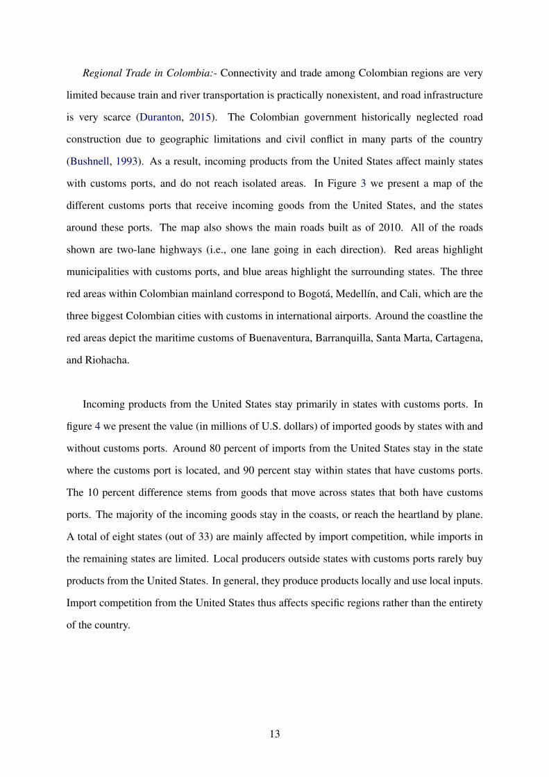
Regional Trade in Colombia:- Connectivity and trade among Colombian regions are very

limited because train and river transportation is practically nonexistent, and road infrastructure

is very scarce (Duranton, 2015). The Colombian government historically neglected road

construction due to geographic limitations and civil conflict in many parts of the country

(Bushnell, 1993). As a result, incoming products from the United States affect mainly states

with customs ports, and do not reach isolated areas. In Figure 3 we present a map of the

different customs ports that receive incoming goods from the United States, and the states

around these ports. The map also shows the main roads built as of 2010. All of the roads

shown are two-lane highways (i.e., one lane going in each direction). Red areas highlight

municipalities with customs ports, and blue areas highlight the surrounding states. The three

red areas within Colombian mainland correspond to Bogotá, Medellín, and Cali, which are the

three biggest Colombian cities with customs in international airports. Around the coastline the

red areas depict the maritime customs of Buenaventura, Barranquilla, Santa Marta, Cartagena,

and Riohacha.

Incoming products from the United States stay primarily in states with customs ports. In

figure 4 we present the value (in millions of U.S. dollars) of imported goods by states with and

without customs ports. Around 80 percent of imports from the United States stay in the state

where the customs port is located, and 90 percent stay within states that have customs ports.

The 10 percent difference stems from goods that move across states that both have customs

ports. The majority of the incoming goods stay in the coasts, or reach the heartland by plane.

A total of eight states (out of 33) are mainly affected by import competition, while imports in

the remaining states are limited. Local producers outside states with customs ports rarely buy

products from the United States. In general, they produce products locally and use local inputs.

Import competition from the United States thus affects specific regions rather than the entirety

of the country.

13

Figure 3: Regional Trade

Notes: This map depicts the Colombian territory with all the municipality boundaries.The areas depicted in red correspond to municipalities with custom ports for productsimported from the United States. They correspond to: Barranquilla, Bogotá,Buenaventura, Cali, Cartagena, Medellín, Riohacha, and Santa Marta. In blue wedepict the states where such municipalities are located. These states correspondto: Atlántico, Bolívar, Cauca, Cundinamarca, La Guajira, Magdalena, and Valle delCauca.

3.2. Data

We use a rich and unique Colombian data set from three different sources. First, we

use yearly matched employer-employee earnings records from 2008 to 2014.13 This is a

confidential, administrative data set that includes all formal-sector workers who contribute to

health or pension in any given month. The data include firm identifiers, four-digit industry

codes, and the municipality where the payment occurred. A primary feature of the data is that

we are able to follow every worker and firm. A limitation, however, is that the data set contains

only formal-sector workers, who correspond to around 60 percent of Colombian workers.14

13The data include the years 2015 and 2016, but we excluded the use of data from these years because of thestrong devaluation (depicted in Appendix Figure B.2a).

14Even though informality is a big issue in Latin America, Appendix Figure B.3 shows that informality bysector in Colombia did not increase during the period we analyze. In fact, during the relevant time frame, weobserve a slight decrease in informal employment in the informal sector. This provides evidence that our resultsare not mainly driven by people moving to informal work. Even if the results were driven by workers shifting fromformal to informal employment, we would still consider formal employment to be a first-best option compared toeither informal employment or unemployment.

14

Figure 4: Imports in States With and Without Customs Ports

Analyzed Period

Colombia ReducesTariffs

USA ReducesTariffs

0

5

10

15

2000 2005 2010 2015Year

States with Customs States with No Customs

Total Value of Imports (in billions USD)

Notes: This graph plots the value of imports in billions USD, by states with andwithout customs ports. The solid connected line depicts the value of imports amongstates with customs ports. The dashed connected line presents the value of importsin states with no customs ports. The dashed vertical lines depict the period 2008 to2014, which is the period we analyze herein. The solid vertical lines plot the years inwhich Colombia and the United States decreased tariffs.

We complement these data using headcounts of workers per state and industry from the 2005

census.15

Second, we use highly detailed administrative records on Colombian imports and exports

from 2008 to 2014. These data, recorded at the 10-digit level, are broken up by state where the

good was bought (in the case of imports) or sold (in the case of exports).16 These data constitute

administrative information from the customs authorities that is sent to the Colombian central

bank. We complement this information with data records on every single imported and exported

product by each firm in 2008.

Finally, we use tariff information from the United Nation’s Trade Analysis Information

System, the World Trade Organization, and the U.S. International Trade Commission. We use

multiple tariff data due to differences in the level of industry code aggregation, and because

individually no single source covers our entire period of study.17

15The 2005 census provided the number of workers for every state and industry. Such information is availableat: http://systema59.dane.gov.co/cgibin/RpWebEngine.exe/PortalAction?BASE=CG2005BASICO.

16Colombia has 33 different states that are very heterogeneous.17These different data sources work with different industry codes. Therefore, we homogenize and merge them

using four-digit industry codes.

15

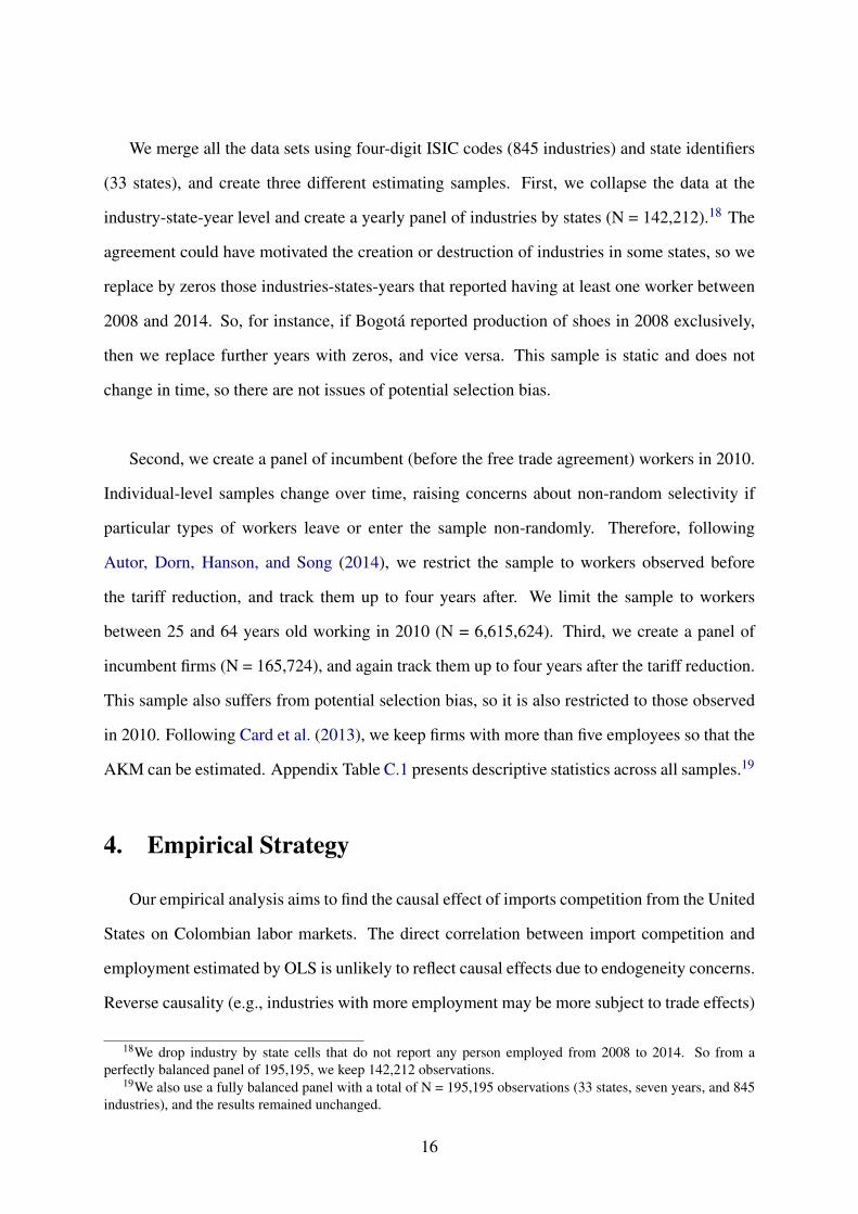
We merge all the data sets using four-digit ISIC codes (845 industries) and state identifiers

(33 states), and create three different estimating samples. First, we collapse the data at the

industry-state-year level and create a yearly panel of industries by states (N = 142,212).18 The

agreement could have motivated the creation or destruction of industries in some states, so we

replace by zeros those industries-states-years that reported having at least one worker between

2008 and 2014. So, for instance, if Bogotá reported production of shoes in 2008 exclusively,

then we replace further years with zeros, and vice versa. This sample is static and does not

change in time, so there are not issues of potential selection bias.

Second, we create a panel of incumbent (before the free trade agreement) workers in 2010.

Individual-level samples change over time, raising concerns about non-random selectivity if

particular types of workers leave or enter the sample non-randomly. Therefore, following

Autor, Dorn, Hanson, and Song (2014), we restrict the sample to workers observed before

the tariff reduction, and track them up to four years after. We limit the sample to workers

between 25 and 64 years old working in 2010 (N = 6,615,624). Third, we create a panel of

incumbent firms (N = 165,724), and again track them up to four years after the tariff reduction.

This sample also suffers from potential selection bias, so it is also restricted to those observed

in 2010. Following Card et al. (2013), we keep firms with more than five employees so that the

AKM can be estimated. Appendix Table C.1 presents descriptive statistics across all samples.19

4. Empirical Strategy

Our empirical analysis aims to find the causal effect of imports competition from the United

States on Colombian labor markets. The direct correlation between import competition and

employment estimated by OLS is unlikely to reflect causal effects due to endogeneity concerns.

Reverse causality (e.g., industries with more employment may be more subject to trade effects)

18We drop industry by state cells that do not report any person employed from 2008 to 2014. So from aperfectly balanced panel of 195,195, we keep 142,212 observations.

19We also use a fully balanced panel with a total of N = 195,195 observations (33 states, seven years, and 845industries), and the results remained unchanged.

16

and potential unobserved confounders (e.g., unobserved productivity in certain industries or

states may correlate positively with trade and labor market outcomes) can upwardly bias the

coefficients. For this reason, we implement the strategy detailed herein.

4.1. Measuring Import Competition

We first introduce a measure for import competition as following:

log(IC)s jt = log

(1+

USD Value of Importss jt

L2005s j

). (2)

This measure accounts for the per capita import competition from the United States faced by

every industry j in state s, and year t in Colombia. We add a one in the logarithm to include all

those sectors and regions that have imports equal to zero. It is important to include the zeros

since some industries and regions may have not imported before the free trade agreement took

effect, and, as a result of the reduction in tariffs, they may have started importing goods. We

normalize by the number of workers in 2005 using data from the Colombian 2005 census at the

state and industry levels.20

The purpose of this measure is to account for the degree of import competition from the

United States across industries and states. We normalize the measure by the size of the

workforce since smaller industries or states are more subject to competition. This measure

varies by state, industry, and year, and it captures the degree of competition faced before and

after the free trade agreement.

Similarly, we define the following measure to evaluate whether the free trade agreement

affects exports:

log(EW)s jt = log

(1+

USD Value of Exportss jt

L2005s j

).

20We divide by workers in 2005 since the free trade agreement may have affected the number of workers inlater years.

17

This measure replaces the value of exports, and accounts for the degree of exports per worker

in each industry, state, and year.

4.2. Industry and State Shocks

To address the endogeneity concerns we introduce some shocks that use the exogenous

decrease in tariffs and state disparities in access to imports. Consider, first, the following

imports and exports penetration shocks:

IMPddjt = 1(COL Reduction) j×Postt (3)

EXPddjt = 1(USA Reduction) j×Postt ,

where 1(COL Reduction) j and 1(USA Reduction) j are categorical variables that take the value

of one if industry j experienced a tariff reduction in Colombia and in the United States,

respectively.21 Postt is a dummy indicator that takes the value of one after 2010, and zero

otherwise. We denote these shocks using the superscript “dd” to indicate that the shocks

correspond to a double difference.

The shocks in (3) do not take into account regional variation. However, as shown in

Section 3.1, Colombia has large regional variation in trade flows, with eight states serving as

the destination for almost 90 percent of the imported goods from the United States. To account

for this, we define the following alternative and more reliable trade shocks:

IMPddds jt = IMPdd

jt ×1(Customs in State)s

EXPddds jt = EXPdd

jt ×1(Customs in State)s,

where 1(Customs in State)s is a categorical variable that takes the value of one if state s has

a customs port that receives imported goods from the United States. We use the superscript

“ddd” to denote that these shocks come from a triple difference.

21We define a reduction in tariffs by comparing tariffs in 2014 with tariffs in 2010. A tariff reduction impliesthat tariffs in 2014 are smaller than tariffs in 2010.

18

These measures rely on temporal, industry, and regional variation. We expect that, after the

implementation of the agreement, industries with lower tariffs and regions with access to import

competition from the United States are more affected than protected industries in isolated

regions. It is expected, therefore, that imported goods have a greater effect on manufacturing

goods in states with customs ports, such as Bogotá, than non-tradable goods in isolated states,

such as the Amazon.

4.3. Triple-Difference Model (First Stage)

Consider now the following differences-in-differences model:

Ys jt = α1IMPddjt +α2EXPdd

jt +µs +µ j +µt + εs jt , (4)

where Ys jt corresponds to an outcome in state s, industry j and year t. Such outcomes include

the measure of import competition from the United States and the measure of export per worker.

This model includes state (µs), industry (µ j), and year (µt) fixed effects to account for within

variation.

Equation 4 pools the effect of the decrease in tariffs across states with and without customs

ports. However, as suggested in Section 3.1, import competition from the United States affects

exclusively those states with customs ports. For this reason, we estimate the following model

that accounts for these differences:

Ys jt = α1IMPddds jt +α2EXPddd

s jt +µs j +µst +µ jt + εs jt . (5)

This model includes state-by-industry (µs j), state-by-year (µst), and industry-by-year (µ jt)

fixed effects and is identified using within industry-by-state variation. The fixed effects account

for potential confounding effects and control for potential pre-existing differences. As treated

units, the model uses industries that experienced a tariff reduction, and that are located in

states with customs ports; as control units, the model uses industries that did not receive tariff

19

reductions, or that are located in states that do not have customs ports. The model treats

industries-by-states as separate units and therefore isolates the effect of the tariff reduction

by states with and without customs ports.

4.4. The Effects of Import Competition (Second Stage)

The results of the triple-difference model quantify the effect of the free trade agreement on

import competition. We take advantage of these results and estimate a second stage that uses

variation induced by the free trade agreement to identify the effects of import competition on

worker and firm outcomes. The richness of the data allows to estimate aggregated (i.e., at the

industry-state-year level) and individual level (i.e., at the worker and firm level) models.

Aggregated Model:- We collapse the data at the state-industry-year level, and use the

variation in import competition to identify aggregated effects by industries and states. These

estimations do not suffer from sample selection since the units of observation remain constant.

Using equation 5 as a first stage, we can find the effect of import competition from the United

States on aggregated measures by estimating:

Ys jt = γddd1 log(IC)s jt + γ

ddd2 log(EW)s jt +µs j +µts +µ jt + es jt , (6)

where Ys jt correspond to an aggregated outcome (employment, number of firms, and average

firm size), log(IC)s jt stands for the predicted import competition, and log(EW)s jt is the

measure of exports per worker.22 We also include state-by-industry (µs j), year-by-state (µts),

and year-by-industry (µt j) fixed effects. Excluding such fixed effects will bias the coefficients

because the instrument may be no longer exogenous. The parameter of interest is γddd1 .

Standard errors are clustered at the industry-by-state level.

Individual Level Model:- We additionally estimate regressions at the worker and firm level.

To deal with selection issues, we restrict the sample to incumbent observations observed before

22In the first stages we drop the term EXPddds jt because it adds noise to the estimations. We also control for the

value of exports on the second stage, but excluding it does not affect any of the results.

20

the implementation of the free trade agreement (i.e., in 2010). Our individual level model takes

the form:

Yis j,t = δ1 log(IC)s j,t +δ2 log(EW)s j,τ +δ3Xi +µs +µ j +ui js,t , (7)

where Yis j,t corresponds to an outcome, that varies for workers or firms i, state s, and industry j.

We measure the outcome year-by-year, up to four years after the tariff reduction, and estimate

separate regressions for each year. The measure on import competition from the United States,

log(IC)s j,t , corresponds to that in equation (2) but included separately for each year. The term

log(EW)s j,t corresponds to the measure exports per worker.23 Note that this model includes

state (µs) and industry (µ j) fixed effects to control for pre-existing differences, and resemble

a differences-in-differences specification with repeated cross sections. We additionally control

for a set of baseline characteristics Xi.24 Standard errors are again clustered at the state–industry

level, and the parameter of interest is δ1.

This specification is of course subject to reverse causality or omitted variable bias, similar

to the aggregated level estimations. To deal with this we instrument using the interaction of the

dummy that takes the value of one for industries that decreased tariffs and a dummy for states

that have customs ports. Formally, this instrument is defined as:

IMPs j = 1(Col Reduction) j×1(Customs in State)s.

4.5. Firm and Worker Wage Premiums

Individual level estimations are useful to estimate heterogeneous effects across workers

and firms. As we showed in Section 2, the effects of import competition are expected to be

heterogeneous across firms’ levels of productivity and workers’ skills. Even though in our data

23Again these results are not sensitive to excluding this control.24For workers we include age, age-squared, gender, earnings averaged from 2008 to 2010, worker wage

premiums averaged from 2008 to 2010, and number of days worked averaged from 2008-2010. For firms weinclude wages, firm wage premiums, and the number of days worked. Each of these measures is averaged acrossall workers within the firm, and then averaged from 2008 to 2010.

21

we are not able to directly measure firm productivity and worker skills, we are still able to

find proxies by extracting information from wages. In particular, we follow Abowd, Kramarz,

and Margolis (1999) and Card, Heining, and Kline (2013) and estimate the following high-

dimensional firm and worker fixed-effect model:

lnWi jt = αi +ψJ(i, j)+X ′i jtβ + εi jt , (8)

where Wimt corresponds to income of individual i, in firm j, in period of time t. Equation (8)

is the sample counterpart of equation (1). The components αi and ψJ(i, j) correspond to the

worker- and firm-specific wage premiums, respectively.25

The firm wage premium is the component of the wage that is common to all the workers

of the firms. Even though it is not an exact measure of productivity, for the purposes of this

paper, it can nevertheless serve as a good proxy for productivity. As shown in Section 2, and

following Card, Cardoso, Heining, and Kline (2018), the firm wage premium can be a function

of the firm’s productivity. Furthermore, it has been shown empirically that firm productivity

and firm wage premiums are highly correlated (Alvarez, Benguria, Engbom, and Moser, 2018;

Card, Cardoso, and Kline, 2016).26

The individual wage premium, on the other hand, measures the workers’ compensation

irrespective of the firm where he/she works. If wages are equivalent to the marginal product

of labor, then the worker wage premium is a measure of worker productivity that is highly

correlated with the level of skills. As in the case of the firm wage premiums, we can interpret

the worker wage premium as a proxy for skills, but, if we do not accept such an interpretation,

then the worker wage premiums still rank workers according to earnings irrespective of the

employer. Such ranking reflects discrepancies among workers that should be reflected in

heterogeneous effects of import competition.

25We additionally control for year fixed effects.26In any case, even if this interpretation of productivity were not accepted, the firm wage premiums still rank

firms between lower- and higher-paying firms, and the effects of imports among them are expected to be different.

22

We classify incumbent firms and workers based on their wage premiums in the period 2008-

2010. To do a more reasonable comparison, and to be in line with our estimation strategy, we

classify the samples by quartiles within industries and states.27 We then follow this set of

incumbents after the tariff reduction, to identify the effect of the policy on firms and workers

of different ex ante ranks.

We estimate heterogeneous effects in three main ways. First, we break down the sample

of firms into quartiles of the distribution of firm-specific wage premiums. Such partition

distinguishes between low- and high-fixed effect firms, which proxy low- and high-productivity

firms. Second, we break down the sample of workers into quartiles of the distribution of firm-

specific wage premiums. This allows us to see what happens to workers who were originally

employed in low- and high-productivity firms. Lastly, we divide the sample of workers by

quartiles of the distribution of worker-specific wage premiums. With this we are able to

distinguish among low- and high-fixed effect workers, which proxy for low- and high- skilled

workers.

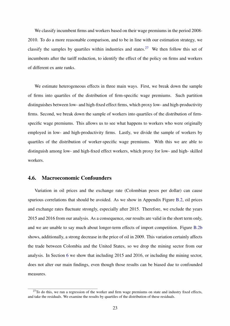
4.6. Macroeconomic Confounders

Variation in oil prices and the exchange rate (Colombian pesos per dollar) can cause

spurious correlations that should be avoided. As we show in Appendix Figure B.2, oil prices

and exchange rates fluctuate strongly, especially after 2015. Therefore, we exclude the years

2015 and 2016 from our analysis. As a consequence, our results are valid in the short term only,

and we are unable to say much about longer-term effects of import competition. Figure B.2b

shows, additionally, a strong decrease in the price of oil in 2009. This variation certainly affects

the trade between Colombia and the United States, so we drop the mining sector from our

analysis. In Section 6 we show that including 2015 and 2016, or including the mining sector,

does not alter our main findings, even though those results can be biased due to confounded

measures.

27To do this, we run a regression of the worker and firm wage premiums on state and industry fixed effects,and take the residuals. We examine the results by quartiles of the distribution of these residuals.

23

5. Results

5.1. Effect of the Free Trade Agreement on Import Competition (First

Stage)

We begin by presenting the results of the free trade agreement on import competition

and exports per worker. Columns (1) to (3) in panel A) of Table 1 present the results of

estimating the differences-in-differences model in equation (4).28 The results suggest that

imports increased among the sectors that reduce tariffs, and that the result is robust to alternative

fixed effects used. In columns (4) and (5), we present the results separately between states

without and with customs ports, respectively, and find that the increase in imports is entirely

driven by a strong effect among states with customs ports. In states without customs ports we

do not see any effects on imports, presumably because road connectivity hindered the access of

these products. We do not observe any effect regarding exports.

These results motivate the estimation the triple-difference model. The results are displayed

in columns (6) to (8) of Table 1. We observe a strong increase in imports from the United States

of around 15 to 18 percent among industries that reduced the tariffs in states with customs ports.

The results are robust to the alternative structure of fixed effects. As expected, imports from

the United States increase remarkably among non-protected industries in states with customs

ports. We again do not observe any effects in exports among industries in which the United

States reduced its tariffs.

In general, Table 1 suggests a strong impact of the free trade agreement on import

competition. No effect on exports was expected because tariffs in the United States remained

low under the agreement. In fact, the F-stats for exports are very low, and the export shocks are

not even significant. Thus, in the rest of the specifications we focus only on imports, and we

use exports as a control to account for potential gains from the free trade agreement.29

28We control for the tariff reductions in the United States, but do not display the point estimates.29When we use alternative specifications with and without exports as controls, the results do not change.

24

Table 1: Effect of the Free-Trade Agreement on Imports and Exports

Differences-in-Differences Het. Effects by States Triple-Differences

No Customs Customs

(1) (2) (3) (4) (5) (6) (7) (8)

A) Log(Import Competition)1(COL reduction)*Post 2.434*** 0.077*** 0.077*** 0.027 0.175***

(0.100) (0.023) (0.023) (0.029) (0.037)1(COL reduction)*Post*1(Customs) 0.172*** 0.175*** 0.150***

(0.037) (0.037) (0.045)

Ind. F 587.714 11.577 11.574 22.035 22.857 10.878

B) Log(Exports per Worker)1(USA reduction)*Post 0.054 -0.060 -0.060 -0.040 -0.096

(0.175) (0.047) (0.047) (0.043) (0.110)1(USA reduction)*Post*1(Customs) -0.095 -0.096 -0.101

(0.109) (0.109) (0.121)

Ind. F .097 1.591 1.591 .76 .776 .698

Observations 142,212 142,212 142,212 100,051 42,161 142,212 142,212 142,212Year FE Yes Yes Yes Yes Yes Yes No NoIndustry FE Yes Yes Yes Yes No No NoState FE Yes Yes Yes No No NoIndustry*State FE Yes Yes YesState*Year FE Yes YesIndustry*Year FE Yes

Note: This table presents the estimation of equation 5 on imports and exports. Panel A uses the import competition measure, definedas equation 2, as dependent variable, and control for the reduction in U.S tariffs. Panel B uses as dependent variable log exports perworker defined as equation 2, but changing the value of imports for the value of exports, and controls for the reduction in Colombiantariffs. Columns (1) to (5) present the results of a difference-in-difference model. Columns (6) to (8) presents the results of a triple-difference model as in equation 5. 1(COL Reduction) and 1(USA Reduction) are categorical variables that take the value of one ifColombia and the USA reduced tariffs in a given industry, respectively. 1(Customs) is a categorical variable that takes the value ofone if the observation is within a state with customs port. Post is a categorical variable that takes the value of one for observationsafter 2010. *** p<0.01, ** p<0.05, * p<0.1

25

5.2. The Effects of Import Competition from the United States (Second

Stage)

5.2.1 Aggregated-Level Results

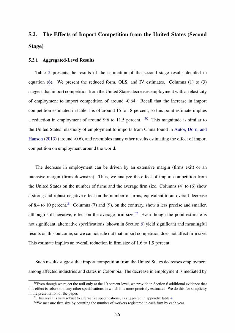
Table 2 presents the results of the estimation of the second stage results detailed in

equation (6). We present the reduced form, OLS, and IV estimates. Columns (1) to (3)

suggest that import competition from the United States decreases employment with an elasticity

of employment to import competition of around -0.64. Recall that the increase in import

competition estimated in table 1 is of around 15 to 18 percent, so this point estimate implies

a reduction in employment of around 9.6 to 11.5 percent. 30 This magnitude is similar to

the United States’ elasticity of employment to imports from China found in Autor, Dorn, and

Hanson (2013) (around -0.6), and resembles many other results estimating the effect of import

competition on employment around the world.

The decrease in employment can be driven by an extensive margin (firms exit) or an

intensive margin (firms downsize). Thus, we analyze the effect of import competition from

the United States on the number of firms and the average firm size. Columns (4) to (6) show

a strong and robust negative effect on the number of firms, equivalent to an overall decrease

of 8.4 to 10 percent.31 Columns (7) and (9), on the contrary, show a less precise and smaller,

although still negative, effect on the average firm size.32 Even though the point estimate is

not significant, alternative specifications (shown in Section 6) yield significant and meaningful

results on this outcome, so we cannot rule out that import competition does not affect firm size.

This estimate implies an overall reduction in firm size of 1.6 to 1.9 percent.

Such results suggest that import competition from the United States decreases employment

among affected industries and states in Colombia. The decrease in employment is mediated by

30Even though we reject the null only at the 10 percent level, we provide in Section 6 additional evidence thatthis effect is robust to many other specifications in which it is more precisely estimated. We do this for simplicityin the presentation of the paper.

31This result is very robust to alternative specifications, as suggested in appendix table 4.32We measure firm size by counting the number of workers registered in each firm by each year.

26

Table 2: Imports from the United States and the Decline in Employment

log (Employment) log (Number of Firms) log (Firm Size)

RF OLS IV RF OLS IV RF OLS IV

(1) (2) (3) (4) (5) (6) (7) (8) (9)

1(COL reduction)*Post*1(Customs) -0.080* -0.064*** -0.023(0.041) (0.016) (0.037)

log(Import Competition) -0.007 -0.640* -0.003 -0.559*** -0.006 -0.105(0.006) (0.331) (0.002) (0.193) (0.005) (0.243)

Observations 142,212 142,212 142,212 142,212 142,212 142,212 142,212 142,212 142,212F-first stage 11.352 11.352 11.352Industry*State FE Yes Yes Yes Yes Yes Yes Yes Yes YesState*Year FE Yes Yes Yes Yes Yes Yes Yes Yes YesIndustry*Year FE Yes Yes Yes Yes Yes Yes Yes Yes Yes

Note: This table presents the estimation of equation 6. Columns (1)-(3) use log of employment as outcome. Columns (4)-(6) usethe log number of firms as outcome. Columns (7)-(9) use the log of the average firm size as outcome. Columns (1), (4), and (7)present reduced form estimates. Columns (2), (5), and (8) presents OLS estimations. Columns (3), (6), and (9) presents two-stageleast squares results. All specifications control for industry–state, state–year, and industry–year fixed effects. Standard errors clusteredat the industry*state level. *** p<0.01, ** p<0.05, * p<0.1

the extensive and the intensive margin, even though the weight of the extensive margin is larger

implying a bigger importance for firm exit rather than for firms shrinking.

5.2.2 Individual-Level Results by Wage Premiums of Firms and Workers

Our main interest is to distinguish the effect between low- and high-productivity firms and

low- and high-skilled workers. So, as detailed in Section 4.5, we estimate heterogeneous effects

across the within industry-state distributions of firm and worker wage premiums.33 As a result,

we have three sets of results: 1) effects on firms by firm wage premiums; 2) effects on workers

by firm wage premiums; and 3) effects on workers by worker wage premiums. The first two

show heterogeneous effects by types of firms, whereas the third shows effects that emerge

according to types of workers.

Effects on Firms by Firm-Specific Wage Premiums: In Figure 5 we present the estimation of

equation 7 on two outcomes at the firm level: Panel 5a uses an indicator variable for whether the

33The results of the first-stage estimation are presented in Appendix Table C.2. We show a very robust firststage with a positive increase in imports.

27

firm exits or not; Panel 5b uses the log of firm size. We estimate heterogeneous effects using the

quartiles of the distribution of firm-specific wage premiums, and track the firms yearly. Quartile

1 corresponds to those firms in the first quartile of the within industry and state distribution of

firm wage premiums.

Figure 5: Effects on Firms’ Outcomes by Quartiles of Firm-Specific Wage Premiums

(a) 1(Firm Exit)

-.02

0

.02

.04

Poin

t Est

imat

es

Quartile 1 Quartile 2 Quartile 3 Quartile 4Quartiles of Firms' Wage Premiums

2011 2012 2013 2014

(b) Firm Size

-.2

-.1

0

.1

Poin

t Est

imat

es

Quartile 1 Quartile 2 Quartile 3 Quartile 4Quartiles of Firms' Wage Premiums

2011 2012 2013 2014

Notes: These graphs present estimates of the parameter δ1 in equation 7 at the firm level by quartiles of the distribution of firm-specific wagepremiums. Panel 5a uses an indicator that takes the value of one if the firm is not observed in year τ as outcome. Appendix table C.3 presentsthe underlying regressions. Panel 5b use the log of firm size as dependent variable, and appendix table C.4 presents the regression results. Allquartiles are defined in the distribution of firm-specific wage premiums within industry and state. Panel A presents estimates of a linearprobability model. 90% confidence intervals displayed.

We observe in Panel 5a that a 10 percent increase in import competition from the United

States increases the probability of exiting among firms in the first quartile by around 0.003

percentage points. We also see a positive effect among firms in the second quartile, although the

magnitude (0.002 percentage points) and the precision are smaller. Firms in the fourth quartile

also show positive point estimates, but these are even less precise and smaller. These results

suggest that import competition motivates an exodus of firms, especially low-productivity

firms. We test for this by grouping below and above the median, and we find that firms below

the median are significantly more likely to exit compared to firms above the median.

We also test for effects in firm size among the firms that do not exit. We find that firm

size decreases among firms in the first quartile, as shown in Panel 5b. As opposed to the

effects of Chinese import competition in the United States (Bloom, Handley, Kurman, and

Luck, 2019), we do not observe that more productive firms increase in size. Such result implies

28

that missing production generated by firms exiting and shrinking is not appropriated by high-

productivity local firms. Instead consumers seem to substitute their previous consumption of

locally produced goods with imported goods from the United States.

In general, these results suggest two effects. First, low-productivity firms are more likely

to be driven out of the market, inducing a decrease in the supply of locally produced goods.

Second, low-productivity firms are likely to shrink, whereas high-productivity firms do not

grow. This provides some evidence that local consumers (either individual consumers or firms)

decrease consumption, or stop buying locally produced goods and begin buying imported

substitutes or other goods from the United States. If this were not the case, then we should

observe increases in the size of high-productivity firms induced by the decrease in the supply

of locally produced goods. This contrasts with the effects of Chinese competition in the United

States, where import competition affects mainly high-paying and bigger firms.

Firm dispersion in productivity is very large in developing countries. Such distribution,

especially in Latin America, is usually bimodal, with a predominance of very low- and very

high- productive firms Busso, Madrigal, and Pagés (2013); Eslava, Haltiwanger, and Pinzón

(2019). The results herein suggest that an increase in import competition from the United

States induces the exit of firms, especially among low-productivity firms, and that remaining

low-productivity firms decrease in size.

Effects on Workers by Firm Wage Premiums: Results this far leave open the question

regarding what happens with the workers who were originally working in firms with different

levels of productivity, especially those who lose their job because the firm exit or shrink.

To answer this we estimate equation 7 on the sample of incumbent workers, and estimate

heterogeneous effects across the firms where these workers were initially employed. Quartile

1 refers to workers who were initially working in a firm in the first quartile of the distribution

of firm-specific wage premiums. Figure 6 presents the results using as outcome a dummy for

whether the worker works (panel 6a), a dummy for whether working in an industry that did not

29

reduce tariffs (panel 6b), an indicator variable for whether the worker works in a state without

customs ports (panel 6c), and the worker’s log daily wage (panel 6d). We again follow the same

format as in Figure 5 separating the results by year and quartiles.

Figure 6: Effects on Workers’ Outcomes by Quartiles of Firm-Specific Wage Premiums ofInitial Firms

(a) 1(Employed)

-.01

0

.01

.02

.03

Poin

t Est

imat

es

Quartile 1 Quartile 2 Quartile 3 Quartile 4Quartiles of Firms' Wage Premiums

2011 2012 2013 2014

(b) 1(Employed in Unaffected Industry)

-.05

0

.05

.1

Poin

t Est

imat

es

Quartile 1 Quartile 2 Quartile 3 Quartile 4Quartiles of Firms' Wage Premiums

2011 2012 2013 2014

(c) 1(Employed in Unaffected State)

0

.005

.01

.015

.02

Poin

t Est

imat

es

Quartile 1 Quartile 2 Quartile 3 Quartile 4Quartiles of Firms' Wage Premiums

2011 2012 2013 2014

(d) log Daily Wage

-.1

-.05

0

.05

Poin

t Est

imat

es

Quartile 1 Quartile 2 Quartile 3 Quartile 4Quartiles of Firms' Wage Premiums

2011 2012 2013 2014

Note: These graphs present estimates of the parameter δ1 in equation 7 by quartiles of the distribution of firm-specific wage premiums ofincumbent firms. Quartile 1 corresponds to workers working in a firm in the first quartile of the within state-industry distribution of firm-specific wage premiums. Panel 6a uses an indicator that takes the value of one if the workers is observed working in year τ as outcome.Appendix table C.5 presents the underlying regressions. Panel 6b uses an indicator variable for whether the worker is an industry that did notreduce tariffs as dependent variable, and appendix table C.7 presents the regression results. Panel 6c uses in indicator variable for whetherthe worker works in a state without a customs port. Appendix Table C.8 presents the point estimates. Panel 6d uses the log of workers’daily wage, and appendix table C.6 presents the point estimates. Panels A, B, and C present estimates of a linear probability model. 90%confidence intervals displayed.

The results in Panel 6a present a small and positive effect on the probability of working

among workers in the first quartile. Surprisingly, we do not observe that workers in low-

productivity firms transition into unemployment (or informality), but instead they are more

likely to remain employed than workers in unaffected industries or states. This can occur if

workers from low-productivity firms in affected industries or states are reallocated into low-

30

productivity firms in unaffected industries and/or states.

We find direct evidence of this by presenting, in panels 6b and 6c, the effect of import

competition on a dummy for working in an industry that did not reduce tariffs and a dummy

for working in a state with no customs ports, respectively. We see that workers in the first and

second quartiles are more likely to move to industries that did not reduce tariffs, whereas there is

a generalized movement across all quartiles to states without customs ports. The point estimates

in panels 6b, nonetheless, are much larger in magnitude, implying a bigger reallocation across

industries than across states. Such reallocation exists more prominently among workers in low-

productivity firms.

This reallocation of workers to unaffected industries and states does not explain entirely

the positive point estimates in panel 6a. In fact, workers can reallocate and that does not

necessarily increase the probability of being employed. A possibility is that workers in

unaffected industries or states are displaced, decreasing therefore their probability of being

employed. This result is equivalent to a situation of job displacement in times of recession as

shown in Haltiwanger et al. (2017).

Theoretically, reallocation of workers mitigates wage losses after a labor demand shock.

We observe in panel 6d that wages are not affected for workers in the top three quartiles,

but workers in the first quartile experience a wage decrease of around -0.05%. Two main

reasons can explain this result: 1) workers who switch jobs accept lower-paid offers; 2)

workers who stay experience wage losses. Unfortunately, we cannot rule out either of these

explanations. However, the evidence in panels 6a, 6b, and 6c shed some light about workers

in low-productivity firm relocating and displacing other workers in low-productivity firms by

accepting lower paid offers.

In general, two results can be derived here. First, workers in low-productivity firms move

into unaffected industries and states, and they can potentially displace former workers by

31

accepting lower-paid job offers. Second, workers in all the other quartiles shift to unaffected

industries and/or states and mitigate wage loses. Those in the second quartile are more likely

to move into other industries, whereas workers in high-productivity firms move geographically,

across states.

Effects on Workers by Worker Wage Premiums: The effects of import competition from the

United States can differ depending on the levels of skills of the workers. Thus, we analyze what

happens to workers with different levels of worker-specific wage premiums, which can proxy

for skills. We analyze the same outcomes included in Figure 6 but now separate the results by

quartiles of the distribution of worker-specific wage premiums. These results are presented in

Figure 7 that follows the same format as Figure 6.

The results in panel 7a show a precise and negative effect on the probability of being

(formally) employed among workers in the first quartile of the workers wage premium dis-

tribution. The workers in this quartile do not shift into unaffected industries (panel 7b) or

into unaffected states (panel 7c), and we do not see any effect in wages among the ones who

remained employed (panel 7d). Such results imply that the losses in employment are mainly

driven by low-skilled workers who transition to informality, unemployment, or leave the labor

force. The results in employment in Table 2 are thus mainly driven by low-skilled workers.

These results contrast with those among workers in other quartiles. We do not observe

any effect on the likelihood of working, but we do observe positive point estimates on the

probability of shifting into industries that did not reduce tariffs (for workers in the third quartile)

and into states without custom ports (for all quartiles except the first). We do not see any effects

on wages, suggesting that reallocation could have mitigated potential wage losses.

In general, we observe four main sets of results. First, the free trade agreement between

Colombia and the United States decreases the amount of import competition but leaves exports

relatively unaffected. Second, import competition reduces employment by decreasing the

32

Figure 7: Effect on Worker Outcomes by Worker-Specific Wage Premiums

(a) 1(Employed)

-.02

-.01

0

.01

Poin

t Est

imat

es

Quartile 1 Quartile 2 Quartile 3 Quartile 4Quartiles of Workers' Wage Premiums

2011 2012 2013 2014

(b) 1(Employed in Unaffected Industry)

-.05

0

.05

.1

Poin

t Est

imat

es

Quartile 1 Quartile 2 Quartile 3 Quartile 4Quartiles of Workers' Wage Premiums

2011 2012 2013 2014

(c) 1(Employed in Unaffected State)

-.005

0

.005

.01

.015

.02

Poin

t Est

imat

es

Quartile 1 Quartile 2 Quartile 3 Quartile 4Quartiles of Workers' Wage Premiums

2011 2012 2013 2014

(d) log Daily Wage

-.02

-.01

0

.01

.02

.03

Poin

t Est

imat

es

Quartile 1 Quartile 2 Quartile 3 Quartile 4Quartiles of Workers' Wage Premiums

2011 2012 2013 2014

Notes: These graphs present estimates of the parameter δ1 in equation 7 by quartiles of the distribution of worker-specific wage premiums.Panel 7a uses an indicator that takes the value of one if the workers is observed working in year τ as outcome. Appendix Table C.9 presentsthe underlying regressions. Panel 7b uses an indicator variable for whether the worker is an industry that did not reduce tariffs as dependentvariable, and Appendix Table C.11 presents the regression results. Panel 7c uses in indicator variable for whether the worker works in astate without custom ports. Appendix Table C.12 presents the point estimates. Panel 7d uses the log of workers’ daily wage, and AppendixTable C.10 presents the point estimates. All quartiles are defined in the distribution of worker-specific wage premiums within industry andstate. Panels A, B, and C present estimates of a linear probability model. 90% confidence intervals displayed.

number of firms, and the average size of remaining ones. Such effects are mainly driven by

low-skilled workers who are more likely to lose their (formal) jobs. Third, low-productivity

firms are more likely to exit the market and shrink in size. We interpret this as evidence of firm

selection due to import competition. Fourth, import competition from the United States induces

worker movement from affected industries (i.e., those in which tariffs on related goods fell) and

states (i.e., those with customs ports) to unaffected industries (i.e., those in which related tariffs

did not fall) and states (i.e., those without customs ports). Such reallocation of labor mitigates

or increases wage loses, depending on the case, and can potentially induce job displacement of

workers who were originally employed in unaffected industries or states.

33

6. Robustness Checks

6.1. Pre-trends

The biggest threat to identification comes by potential pre-trends between our treated and

non-treated units. We test for this estimating event study models that identify potential pre-

trends between the treated and control groups. Figure 8a plots the coefficients of an event study

model, and normalize with respect to 2010, which is when Colombian tariffs were reduced.

Panel 8a uses the measures of import competition from the United States as outcome, and

resembles the first stage of the model. Panels 8b, 8c, and 8d use log employment, log number

of firms, and log average firm size as dependent variables, respectively. These results resemble

the reduced form estimates of Table 2. All the models are estimated in the sample aggregated

at the industry-state-year level.

We do not observe any pre-trends prior to 2010, suggesting that our main results may not

be driven by differentiated trends among industries that experienced tariff reductions nor states

with and without customs ports. We do observe an increase in imports after 2011 among

industries where tariffs were reduced and states with custom ports, as the first stage suggested.

We also see a decrease in employment, number of firms, and the average firm size after 2010.

The effect fades on time, except for the number of firms where we do not see any process of

mean reversion.

These results give strong evidence that our estimations are not driven by differential pre-

trends, and suggest that we are not violating the parallel trends assumption that is necessary for

the proper identification of the double and triple-difference model. Instead, it gives evidence of

the exogeneity of our instrument and the validity of the exclusion restriction.

34

Figure 8: Event Studies to Check Existence of Pre-Trends

(a) Import Competition

-.2

-.1

0

.1

.2

.3

2008 2009 2010 2011 2012 2013 2014Year

Point Estimate 95% CI

(b) Employment

-.2

-.15

-.1

-.05

0

.05

.1

2008 2009 2010 2011 2012 2013 2014Year

Point Estimate 95% CI

(c) Number of Firms

-.15

-.1

-.05

0

.05

2008 2009 2010 2011 2012 2013 2014Year

Point Estimate 95% CI

(d) Average Firm Size

-.15

-.1

-.05

0

.05

.1

.15

2008 2009 2010 2011 2012 2013 2014Year

Point Estimate 95% CI

Notes: These graph presents the point estimates of an event study model using equation 5. Panel 8a uses importcompetition as dependent variable, panel 8b uses log Employment, panel 8c use log of the number of firms, andpanel 8d uses log of average firm size. We interact IMPddd

s jt and EXPddds jt with yearly dummies, and exclude 2010.

We present the coefficients on the interactions of IMPddds jt and the yearly dummies. Standard errors are clustered

at the state*industry level. 95% confidence intervals are shown.

6.2. Differences-in-Differences

Our results are additionally robust to just using a differences-in-differences strategy. In

particular, we use the tariff reduction of the free trade agreement before and after 2010 to

design a differences-in-differences estimator, and ignore differences among states with and

without customs ports. For such we use an import shock as in equation 3 and first identify the

effect of that shock on the measure of import competition. This estimation is the first stage

of the model, and the results are presented in columns (1) to (3) of table 1. Using this as first

35

stage, we instrument the measure of import competition and estimate the following model:

Ys jt = γdd1 log(IC)s jt + γ

dd2 log(EW)s jt +µ j +µs +µt + es jt , (9)

where we control by the measure of exports, and include industry (µ j), state (µs), and year

(µt) fixed effects. Standard errors are clustered at the industry–state level. The results are

presented in table 3. We present reduced forms, OLS, and IV results. Columns (1) to (3) use

log employment as outcome, columns (4) to (6) use the log number of firms, and columns (7)

to (9) use the log of average firm size.

Table 3: Imports from the U.S. and Decline on Employment: D-i-D Model

log (Employment) log (Number of Firms) log (Firm Size)

RF OLS IV RF OLS IV RF OLS IV

(1) (2) (3) (4) (5) (6) (7) (8) (9)

1(COL reduction)*Post -0.268*** -0.135*** -0.130***(0.022) (0.009) (0.018)

log(Import Competition) 0.044*** -2.020*** 0.011*** -0.952*** 0.031*** -1.065***(0.008) (0.379) (0.004) (0.175) (0.006) (0.218)

Observations 142,212 142,212 142,212 142,212 142,212 142,212 142,212 142,212 142,212F-first stage 33.315 33.315 33.315Year FE Yes Yes Yes Yes Yes Yes Yes Yes YesIndustry FE Yes Yes Yes Yes Yes Yes Yes Yes YesState FE Yes Yes Yes Yes Yes Yes Yes Yes Yes

Note: This table presents the estimation of equation 9. Columns (1)-(3) use log of employment as outcome. Columns (4)-(6) use the lognumber of firms as outcome. Columns (7)-(9) use the log of the average firm size as outcome. Columns (1), (4), and (7) present reducedform estimates. Columns (2), (5), and (8) presents OLS estimations. Columns (3), (6), and (9) presents two-stage least squares results. Allspecifications control for industry, state, and year fixed effects. Standard errors clustered at the industry*state level. *** p<0.01, ** p<0.05,* p<0.1

We observe again negative and very precise results in all three estimations. These results

suggest again that the decrease in employment is mediated by firms exiting and shrinking.

The magnitudes are bigger than the triple-difference model, but they mix results in states who

experienced import competition with states that did not. The triple difference accounts for this

issue and gives more reliable estimates.

36

6.3. Moving Fixed Effect Structure

All the estimates so far include a very conservative structure of fixed effects. Our strategy

relies on within industry and state variation as the proper exogenous source of variation that

identifies the model. However, there are alternative combinations of fixed effects that use

different source of time variation to estimate the model. Our results are not altered when

considering alternative less-demanding combinations. We present in Table 4 alternative models

that change the structure of the fixed effects, and therefore the identifying variation.

Columns (1) to (3) show that the result in the difference-in-difference model remains

unchanged when different fixed effects are included. The precision of the estimates is the

same, although the magnitudes change. In columns (5) to (7) we do the same using the

triple-difference model. All specifications include state-by-industry fixed effects since our

instrument is valid exclusively using within state and industry variation. We see that the sign

does not change when including year-by-state not year-by-industry fixed effects. However,

we do observe a decrease in magnitude and precision when industry-by-year fixed effects

are included. This estimate is our preferred specification since it shows more conservative

estimates.

6.4. Input Prices

An increase in imported products from the United States increases competition for local

firms, but also decreases the cost of some inputs. Firms may be harmed if there is an increase

in import competition, but they may also benefit if there is a decrease in the cost of inputs

Goldberg, Khandelwal, Pavcnik, and Topalova (2010). The effects of import competition on

the number of firms, for instance, may be mediated by the direct effect of competition or by a

decrease in the cost of inputs. To account for the effect on input prices and isolate the effect of

import competition, we compute a measure for the cost of inputs and include it as a control.

To construct this measure, we use detailed data on all the goods imported by every firm in

37

2008. These data includes information on the firms’ industry and state. Using this, we compute

the following measure of input prices at the state (s), industry ( j), and year (t) level:

IPs jt =∑k

[Importsks jt×

(T 2008

ks j × log(Import Intensity)2008s j

)]Ks j

,

where k indexes each input and Ks j is the total number of inputs used per industry by state.

Importsks jt correspond to the imported value of input k by industry j, state s, and year t. We

multiply this value times some weights that measure the relevance of input k and the intensity

in imports of industry j by state s. T 2008ks j is a weight equivalent to the percentage imported of

good k with respect to the total imported goods in industry j, state s, in 2008. Formally, the

weights are equivalent to:

T 2008ks j =

Imports2008ks j

∑k Imports2008ks j

.

Import intensity is a measure of how much the output sector j in state s imported in 2008.

We expect that industries that import more are more affected by input prices. Therefore, we

multiply the weights for a measure of import intensity. We normalize such measure by the

number of employees in 2005 and take logs. Formally such measure is equivalent to:

log(Import Intensity)2008s j = log

(∑k Imports2008

ks j

L2005s j

).34

We then average across the k inputs to construct a weighted average of the prices of imported

inputs for each industry, state, and year.

We include this measure as a control, and present the results in columns (4), for the

differences-in-differences model, and columns (8), for the triple-difference model, of Table 4.

For both cases we observe that the measure of input costs do not have much of an effect on the

point estimate of the coefficient associated with the measure of import competition. Therefore,

we are able to conclude that the effect of import competition from the United States is neither

mediated nor affected by a reduction in input prices. Similar results are found in Autor, Dorn,

38

and Hanson (2013) when analyzing the employment effects of Chinese import competition

among labor markets in the United States.

6.5. Mining and additional Years

Finally, we present the results of our main strategy, including the mining sector and

the years 2015 and 2016. Recall that we dropped the mining sector because of potential

confounders due to the high volatility in the price of oil. A decrease in the price of oil can affect

the mining industry, which is one of the biggest industrial sectors in Colombia. Therefore,

imports from this industry could be correlated with fluctuations in oil prices, rather than with

the free trade agreement; this could confound the estimates. Furthermore, recall that data from

2015 and 2016 were also dropped because of a steep devaluation that affected Colombia in

those two years. A peso devaluation (or a dollar appreciation) changes the prices of imports

and, thus, could confound the timing of the free trade agreement’s potential effects. Both forces

could potentially bias our estimations, so we chose not to include them in our main strategy.

However, our main results do not change much when these additional observations are

included. In Table 5 we again present the results of the difference-in-difference and triple dif-

ference models, including the reduced form, OLS, IV, and input cost-controlled specifications.

The results are very close to our main estimates, but they may be somewhat biased due to the

variability in the price of oil in 2009 and 2010.

The same happens when we include data from 2015 and 2016. We present these results in

Table 6, in which we follow the same structure but include these two additional years. Again

the main results do not change much, but these results do show larger point estimates that can

be confounded by exchange rate fluctuations that primarily affect our measure of imports. We

can evidence this by observing the decrease in the F-stat of the first stage compared to the

estimations without 2015 and 2016. Nonetheless, all the estimates maintain the signs, and

precision does not change dramatically.

39

In general, our results are robust to alternative samples, controls, and specifications. The

signs, magnitudes, and precision are not affected. We also show strong evidence about the

non-existence of pre-trends, that validate our identifying assumptions.

40

Table 4: Robustness of the Effects of Import Competition from the U.S.

Differences-in-Differences Triple-Differences

(1) (2) (3) (4) (5) (6) (7) (8)

A) log Employmentlog(IC) -0.697*** -1.874*** -2.020*** -2.057*** -2.176*** -2.258*** -0.640* -0.639*

(0.057) (0.374) (0.379) (0.383) (0.472) (0.484) (0.331) (0.331)

B) log Number of Firmslog(IC) -0.390*** -0.875*** -0.952*** -0.972*** -1.044*** -1.227*** -0.559*** -0.559***

(0.029) (0.173) (0.175) (0.177) (0.217) (0.249) (0.193) (0.193)

C) log Average Firm Sizelog(IC) -0.270*** -1.000*** -1.065*** -1.079*** -1.229*** -1.029*** -0.105 -0.105

(0.029) (0.215) (0.218) (0.220) (0.296) (0.265) (0.243) (0.243)

Observations 142,212 142,212 142,212 142,212 142,212 142,212 142,212 142,212F-first stage 377.439 33.349 33.315 33.418 26.318 27.098 11.352 11.338Year FE Yes Yes Yes Yes Yes No No NoIndustry FE Yes Yes Yes No No No NoState FE Yes Yes No No No NoIndustry*State FE Yes Yes Yes YesState*Year FE Yes Yes YesIndustry*Year FE Yes YesInputs Cost Reduction Yes Yes

Note: This table presents IV estimations using the log of employment as outcome in panel A), the log of number of firms inpanel B), and the log of average firm size in panel C). Log(IC) stands for log of import competition. Columns (1)-(4) presentthe estimates of equation 9, but vary on the fixed effects included. Column (1) includes year fixed effects, column (2) addsindustry fixed effects, and column (3) adds state fixed effects. Column (4) includes the measure of inputs costs. Columns (5)-(8)present the results of the estimation of equation 6. Column (5) includes year and state by industry fixed effects. Column (6)includes state by industry and state by year fixed effects. Column (7) adds state by industry fixed effects. Column (8) includesthe measure of inputs costs. All specifications additionally control for the log of exports per worker. Standard errors clustered atthe industry*state level. *** p<0.01, ** p<0.05, * p<0.1.

41

Table 5: Effects of Trade of Import Competition Including the Mining Sector

Reduced Form OLS IV Inputs CostD-D D-D-D D-D D-D-D D-D D-D-D D-D D-D-D

(1) (2) (3) (4) (5) (6) (7) (8)

A) log Employment1(COL reduction)*Post -0.275***

(0.021)1(COL reduction)*Post*1(Customs) -0.095**

(0.040)log(Import Competition) 0.035*** -0.010* -2.718*** -0.816** -2.706*** -0.816**

(0.009) (0.006) (0.636) (0.393) (0.616) (0.393)

B) log Number of Firms1(COL reduction)*Post -0.134***

(0.009)1(COL reduction)*Post*1(Customs) -0.060***

(0.015)log(Import Competition) 0.009** -0.003 -1.252*** -0.585*** -1.245*** -0.585***

(0.004) (0.002) (0.289) (0.216) (0.279) (0.216)

C) log Average Firm Size1(COL reduction)*Post -0.144***

(0.018)1(COL reduction)*Post*1(Customs) -0.044

(0.035)log(Import Competition) 0.024*** -0.008* -1.503*** -0.269 -1.497*** -0.269

(0.006) (0.005) (0.368) (0.275) (0.359) (0.275)

Observations 149,611 149,611 149,611 149,611 149,611 149,611 149,611 149,611F-first stage 20.59 9.782 21.593Year FE Yes No Yes No Yes No Yes NoIndustry FE Yes Yes Yes YesState FE Yes Yes Yes YesIndustry*State FE Yes Yes Yes YesState*Year FE Yes Yes Yes YesIndustry*Year FE Yes Yes Yes YesInput Import Cost Yes Yes

Note: This table presents estimations using the log of employment as outcome in panel A), the log of number of firms in panel B), andthe log of average firm size in panel C). All specifications include the mining sector. Column (1) and column (2) present the estimatesof equations 4 and 5, respectively. The coefficients on EMPdd

s jt and EMPddds jt are not shown. Column (3) presents the estimation of the

OLS version of equation 9, and column (4) of equation 6. Columns (5) and (6) present the second stage estimates of equations 9 and 6,respectively. Columns (7) and (8) additionally control for input costs. Standard errors clustered at the industry*state level. *** p<0.01,** p<0.05, * p<0.1

42

Table 6: Effects of Trade of Import Competition Including 2015-2016

Reduced Form OLS IV Inputs CostD-D D-D-D D-D D-D-D D-D D-D-D D-D D-D-D

(1) (2) (3) (4) (5) (6) (7) (8)

A) log Employment1(COL reduction)*Post -0.353***

(0.025)1(COL reduction)*Post*1(Customs) -0.107**

(0.046)log(Import Competition) 0.044*** -0.003 -3.731*** -1.165* -3.341*** -1.136*

(0.008) (0.006) (0.914) (0.679) (0.746) (0.660)

B) log Number of Firms1(COL reduction)*Post -0.178***

(0.011)1(COL reduction)*Post*1(Customs) -0.083***

(0.018)log(Import Competition) 0.010*** -0.002 -1.779*** -1.023** -1.574*** -0.977**

(0.003) (0.002) (0.433) (0.478) (0.348) (0.453)

C) log Average Firm Size1(COL reduction)*Post -0.173***

(0.020)1(COL reduction)*Post*1(Customs) -0.026

(0.040)log(Import Competition) 0.033*** -0.002 -1.963*** -0.100 -1.786*** -0.131

(0.006) (0.005) (0.498) (0.393) (0.416) (0.389)

Observations 182,844 182,844 182,844 182,844 182,844 182,844 182,844 182,844F-first stage 17.768 5.203 21.582 5.353Year FE Yes No Yes No Yes No Yes NoIndustry FE Yes Yes Yes YesState FE Yes Yes Yes YesIndustry*State FE Yes Yes Yes YesState*Year FE Yes Yes Yes YesIndustry*Year FE Yes Yes Yes YesInput Import Cost Yes Yes

Note: This table presents estimations using the log of employment as outcome in panel A), the log of number of firms in panel B),and the log of average firm size in panel C). All specifications include 2015-2016. Column (1) and column (2) present the estimatesof equations 4 and 5, respectively. The coefficients on EMPdd

s jt and EMPddds jt are not shown. Column (3) presents the estimation of the

OLS version of equation 9, and column (4) of equation 6. Columns (5) and (6) present the second stage estimates of equations 9 and 6,respectively. Columns (7) and (8) additionally control for input costs. Standard errors clustered at the industry*state level. *** p<0.01,** p<0.05, * p<0.1

43

7. Conclusion

In this paper we explore how import competition from the United States affects firms and

employment in Colombia. We additionally take advantage of a high-dimensional workers and

firms fixed model (i.e., the AKM model) to find proxies for firms’ productivity and workers’

skills, and estimate heterogeneous effects of import competition among them. To the best of

our knowledge we are the first to study the effects of import competition from a developed

country on a developing country, to analyze the empirical effects of free-trade agreements in

general, and to estimate the heterogeneous effects of import competition across the distribution

of firm- and worker-specific wage premiums.

We take advantage of the implementation of a free trade agreement signed between Colom-

bia and the United States, and regional variation in access to trade, to estimate the effect

of increased import competition from the United States on Colombian firms and local labor

markets. The free trade agreement led to increased competition from goods coming from

the United States, but left exports unaffected because already low tariffs on Colombia goods

exported to the United States remained intact. Furthermore, competition from U.S. goods

increased exclusively in specific Colombian regions: those states with access to customs ports.

Colombia’s lack of infrastructure (trains and roads) hinders wider distribution of the imported

products. This unique setting enables us to identify the effect of import competition from the

United States on Colombian firms and formal-sector workers.

We use administrative matched employer-employee that allow us to track job spells for

formal workers up to four years after the tariff reduction. These data also allow us to estimate

high-dimensional firm- and worker-fixed effect models, and estimate the heterogeneous effects

among low- and high-fixed effect firms and workers. These fixed effects account for firm

and worker wage premiums, which can be interpreted as measures of productivity and skills,

respectively. Though the data set excludes informal workers, these data offer a nearly ideal way

to identify the effects of import competition on firm exit and employment.

44

Our results suggest that a 10 percent increase in import competition from the United States

decreases employment on 6.4 percent in Colombia. The decrease in employment is mainly

driven by low-productivity firms that exit or shrink. High-productivity firms do not grow,

suggesting that local consumers substitute locally produced goods for imported products from

the United States. We also observe that workers shift mainly from affected to unaffected

industries and regions. We do not observe effects on wages suggesting that reallocation

mitigates such effects, except for the case of workers originally working in low-productivity

firms who presumably reallocate and displace former workers in unaffected industries and

regions by accepting lower paid jobs. Low-skilled workers seem to be the most affected since

they are more likely to lose their (formal) job.

This paper provides evidence of the positive and the potentially negative effects of import

competition from high-wage countries for developing countries. Spurring the exit of low-

productivity firms can boost employment and development, as many have suggested. However,

this process exacts a price in terms of employment among lower-skilled workers. The question

regarding how long these effects last remains unanswered and should motivate future research

on the topic. Negative effects on employment may be mitigated in a longer run, potentially

boosting the benefits.

45

ReferencesAbowd, J. M., Kramarz, F., and Margolis, D. N. (1999). High Wage Workers and High Wage

Firms. Econometrica, 67(2), 251–333. Retrieved from http://dx.doi.org/10.1111/

1468-0262.00020 doi: 10.1111/1468-0262.00020Abowd, J. M., McKinney, K. L., and Zhao, N. L. (2018). Earnings Inequality and Mobility

Trends in the United States: Nationally Representative Estimates from LongitudinallyLinked Employer-Employee Data. Journal of Labor Economics, 36(S1), S183-S300.Retrieved from https://doi.org/10.1086/694104 doi: 10.1086/694104

Alvarez, J., Benguria, F., Engbom, N., and Moser, C. (2018, January). Firms and theDecline in Earnings Inequality in Brazil. American Economic Journal: Macroeconomics,10(1), 149-89. Retrieved from http://www.aeaweb.org/articles?id=10.1257/

mac.20150355 doi: 10.1257/mac.20150355Attanasio, O., Goldberg, P. K., and Pavcnik, N. (2004). Trade reforms and

wage inequality in colombia. Journal of Development Economics, 74(2), 331 -366. Retrieved from http://www.sciencedirect.com/science/article/pii/

S0304387804000185 doi: https://doi.org/10.1016/j.jdeveco.2003.07.001Autor, D. H., Dorn, D., and Hanson, G. H. (2013, October). The China Syndrome: Local Labor

Market Effects of Import Competition in the United States. American Economic Review,103(6), 2121-68. Retrieved from http://www.aeaweb.org/articles?id=10.1257/

aer.103.6.2121 doi: 10.1257/aer.103.6.2121Autor, D. H., Dorn, D., and Hanson, G. H. (2015). Untangling Trade and Technology: Evidence

from Local Labour Markets. The Economic Journal, 125(584), 621-646. Retrievedfrom https://onlinelibrary.wiley.com/doi/abs/10.1111/ecoj.12245 doi: 10.1111/ecoj.12245

Autor, D. H., Dorn, D., Hanson, G. H., and Song, J. (2014). Trade Adjustment: Worker-LevelEvidence*. The Quarterly Journal of Economics, 129(4), 1799-1860. Retrieved fromhttp://dx.doi.org/10.1093/qje/qju026 doi: 10.1093/qje/qju026

Bas, M., and Strauss-Kahn, V. (2015). Input-Trade Liberalization, Export Pricesand Quality Upgrading. Journal of International Economics, 95(2), 250 -262. Retrieved from http://www.sciencedirect.com/science/article/pii/

S0022199614001500 doi: https://doi.org/10.1016/j.jinteco.2014.12.005Bernard, A. B., Jensen, J. B., and Schott, P. K. (2006). Survival of the best fit:

Exposure to low-wage countries and the (uneven) growth of U.S. manufacturing plants.Journal of International Economics, 68(1), 219 - 237. Retrieved from http://www

.sciencedirect.com/science/article/pii/S0022199605000498 doi: https://doi.org/10.1016/j.jinteco.2005.06.002

Bloom, N., Draca, M., and Van Reenen, J. (2016). Trade Induced Technical Change?The Impact of Chinese Imports on Innovation, IT and Productivity. The Review ofEconomic Studies, 83(1), 87-117. Retrieved from http://dx.doi.org/10.1093/

restud/rdv039 doi: 10.1093/restud/rdv039Bloom, N., Handley, K., Kurman, A., and Luck, P. (2019). The Impact of Chinese Trade on

US Employment: The good, the bad, and the debatable.Branstetter, L. G., Kovak, B. K., Mauro, J., and Venancio, A. (2019, September). The China

Shock and Employment in Portuguese Firms (Working Paper No. 26252). NationalBureau of Economic Research. Retrieved from http://www.nber.org/papers/

w26252 doi: 10.3386/w26252Bushnell, D. (1993). The Making of Modern Colombia: A Nation in Spite of Itself (1st ed.).

46

University of California Press. Retrieved from http://www.jstor.org/stable/10

.1525/j.ctt4cgf7g

Busso, M., Madrigal, L., and Pagés, C. (2013, June). Productivity and Resource Misallocationin Latin America. The B.E. Journal of Macroeconomics, 13(1), 1-30. Retrieved fromhttps://ideas.repec.org/a/bpj/bejmac/v13y2013i1p30n3.html

Card, D., Cardoso, A. R., Heining, J., and Kline, P. (2018). Firms and Labor Market Inequality:Evidence and Some Theory. Journal of Labor Economics, 36(S1), S13-S70. Retrievedfrom https://doi.org/10.1086/694153 doi: 10.1086/694153

Card, D., Cardoso, A. R., and Kline, P. (2016). Bargaining, Sorting, and the Gender Wage Gap:Quantifying the Impact of Firms on the Relative Pay of Women. The Quarterly Journal ofEconomics, 131(2), 633. Retrieved from +http://dx.doi.org/10.1093/qje/qjv038

doi: 10.1093/qje/qjv038Card, D., Heining, J., and Kline, P. (2013). Workplace Heterogeneity and the Rise of West

German Wage Inequality*. The Quarterly Journal of Economics, 128(3), 967-1015.Retrieved from http://dx.doi.org/10.1093/qje/qjt006 doi: 10.1093/qje/qjt006

Dix-Carneiro, R. (2014). Trade Liberalization and Labor Market Dynamics. Econometrica,82(3), 825-885. Retrieved from https://onlinelibrary.wiley.com/doi/abs/10

.3982/ECTA10457 doi: 10.3982/ECTA10457Dix-Carneiro, R., and Kovak, B. K. (2017, October). Trade Liberalization and Regional

Dynamics. American Economic Review, 107(10), 2908-46. Retrieved from http://www

.aeaweb.org/articles?id=10.1257/aer.20161214 doi: 10.1257/aer.20161214Duranton, G. (2015). Roads and trade in Colombia. Economics of Transportation, 4(1),

16 - 36. Retrieved from http://www.sciencedirect.com/science/article/pii/

S2212012214000586 (Special Issue on Collective Contributions in the Honor ofRichard Arnott) doi: https://doi.org/10.1016/j.ecotra.2014.11.003

Egger, H., and Kreickemeier, U. (2009). Firm Heterogeneity and the Labor Market Effectsof Trade Liberalization. International Economic Review, 50(1), 187-216. Retrievedfrom https://onlinelibrary.wiley.com/doi/abs/10.1111/j.1468-2354.2008

.00527.x doi: 10.1111/j.1468-2354.2008.00527.xEslava, M., Haltiwanger, J., Kugler, A., and Kugler, M. (2004, December). The effects

of structural reforms on productivity and profitability enhancing reallocation: evidencefrom Colombia. Journal of Development Economics, 75(2), 333-371. Retrieved fromhttps://ideas.repec.org/a/eee/deveco/v75y2004i2p333-371.html

Eslava, M., Haltiwanger, J., Kugler, A., and Kugler, M. (2013). Trade and Market Selection:Evidence from Manufacturing Plants in Colombia. Review of Economic Dynamics, 16(1),135 - 158. Retrieved from http://www.sciencedirect.com/science/article/

pii/S1094202512000671 (Special issue: Misallocation and Productivity) doi: https://doi.org/10.1016/j.red.2012.10.009

Eslava, M., Haltiwanger, J. C., and Pinzón, A. (2019, February). Job Creation in Colombiavs the U.S.: “up or out dynamics” meets “the life cycle of plants” (Working Paper No.25550). National Bureau of Economic Research. Retrieved from http://www.nber

.org/papers/w25550 doi: 10.3386/w25550Feenstra, R. C., and Hanson, G. H. (1999). The Impact of Outsourcing and High-Technology

Capital on Wages: Estimates For the United States, 1979–1990. The Quarterly Journalof Economics, 114(3), 907-940. Retrieved from https://ideas.repec.org/a/oup/

qjecon/v114y1999i3p907-940..html

Fieler, A. C., Eslava, M., and Xu, D. Y. (2018, January). Trade, Quality Upgrading, andInput Linkages: Theory and Evidence from Colombia. American Economic Review,

47

108(1), 109-46. Retrieved from http://www.aeaweb.org/articles?id=10.1257/

aer.20150796 doi: 10.1257/aer.20150796Forlani, E. (2017). Irish Firms’ Productivity and Imported Inputs, journal = The Manchester

School. , 85(6), 710-743. Retrieved from https://onlinelibrary.wiley.com/doi/

abs/10.1111/manc.12169 doi: 10.1111/manc.12169Goldberg, P. K., Khandelwal, A. K., Pavcnik, N., and Topalova, P. (2010, 11). Imported

Intermediate Inputs and Domestic Product Growth: Evidence from India*. The QuarterlyJournal of Economics, 125(4), 1727-1767. Retrieved from https://doi.org/10

.1162/qjec.2010.125.4.1727 doi: 10.1162/qjec.2010.125.4.1727Halpern, L., Koren, M., and Szeidl, A. (2015). Imported Inputs and Productivity. The American

Economic Review, 105(12), 3660–3703. Retrieved from http://www.jstor.org/

stable/43821389

Haltiwanger, J., Hyatt, H., Kahn, L. B., and McEntarfer, E. (2017, June). Cyclical JobLadders by Firm Size and Firm Wage (Working Paper No. 23485). National Bureauof Economic Research. Retrieved from http://www.nber.org/papers/w23485 doi:10.3386/w23485

Hsieh, C.-T., and Klenow, P. J. (2009, 11). Misallocation and Manufacturing TFP in Chinaand India*. The Quarterly Journal of Economics, 124(4), 1403-1448. Retrieved fromhttps://doi.org/10.1162/qjec.2009.124.4.1403 doi: 10.1162/qjec.2009.124.4.1403

Hsieh, C.-T., and Klenow, P. J. (2014, 05). The Life Cycle of Plants in India and Mexico*.The Quarterly Journal of Economics, 129(3), 1035-1084. Retrieved from https://

doi.org/10.1093/qje/qju014 doi: 10.1093/qje/qju014Hummels, D., Jørgensen, R., Munch, J., and Xiang, C. (2014, June). The Wage Effects of

Offshoring: Evidence from Danish Matched Worker-Firm Data. American EconomicReview, 104(6), 1597-1629. Retrieved from http://www.aeaweb.org/articles?id=

10.1257/aer.104.6.1597 doi: 10.1257/aer.104.6.1597Jenkins, R., Peters, E. D., and Moreira, M. M. (2008). The Impact of China on Latin America

and the Caribbean. World Development, 36(2), 235 - 253. Retrieved from http://www

.sciencedirect.com/science/article/pii/S0305750X07001994 (The Impact ofAsian Drivers on the Developing World) doi: https://doi.org/10.1016/j.worlddev.2007.06.012

Lachowska, M., Mas, A., and Woodbury, S. A. (2018, January). Sources of DisplacedWorkers’ Long-Term Earnings Losses (Working Paper No. 24217). National Bureauof Economic Research. Retrieved from http://www.nber.org/papers/w24217 doi:10.3386/w24217

Medina, P. (2018). Import Competition, Quality, Upgrading and Exporting: Evidence from thePeruvian Apparel Industry.

Melitz, M. J. (2003). The Impact of Trade on Intra-Industry Reallocations and AggregateIndustry Productivity. Econometrica, 71(6), 1695-1725. Retrieved from https://

onlinelibrary.wiley.com/doi/abs/10.1111/1468-0262.00467 doi: 10.1111/1468-0262.00467

Melitz, M. J., and Ottaviano, G. I. P. (2008, 01). Market Size, Trade, and Productivity. TheReview of Economic Studies, 75(1), 295-316. Retrieved from https://doi.org/10

.1111/j.1467-937X.2007.00463.x doi: 10.1111/j.1467-937X.2007.00463.xMoreira, M. M. (2007). Fear of China: Is There a Future for Manufacturing in Latin

America? World Development, 35(3), 355 - 376. Retrieved from http://www

.sciencedirect.com/science/article/pii/S0305750X06002026 doi: https://

48

doi.org/10.1016/j.worlddev.2006.11.001Olper, A., Curzi, D., and Raimondi, V. (2017). Imported Intermediate Inputs and Firms’

Productivity Growth: Evidence from the Food Industry. Journal of AgriculturalEconomics, 68(1), 280-300. Retrieved from https://onlinelibrary.wiley.com/

doi/abs/10.1111/1477-9552.12164 doi: 10.1111/1477-9552.12164Pavcnik, N. (2002). Trade liberalization, exit, and productivity improvements: Evidence

from chilean plants. The Review of Economic Studies, 69(1), 245–276. Retrieved fromhttp://www.jstor.org/stable/2695960

Pierce, J. R., and Schott, P. K. (2016, July). The Surprisingly Swift Decline of USManufacturing Employment. American Economic Review, 106(7), 1632-62. Retrievedfrom http://www.aeaweb.org/articles?id=10.1257/aer.20131578 doi: 10.1257/aer.20131578

Wood, A., and Mayer, J. (2011, Jun 01). Has China de-industrialised other developingcountries? Review of World Economics, 147(2), 325–350. Retrieved from https://

doi.org/10.1007/s10290-011-0088-8 doi: 10.1007/s10290-011-0088-8

49

A. Mathematical Appendix

A.1. WorkersConsider a continuum of skilled (S) and unskilled (U) workers indexed by i endowed with a

unit of time, and a continuum of firms indexed by j. Workers choose between consumption andleisure, and have preferences over the firms as in Card, Cardoso, Heining, and Kline (2018).In this model, workers have heterogeneous preferences for firms who offer differentiated workenvironments. The utility function for each skill group takes the form of:

U(Ci j,Li j) =C

1− 1ν

i j

1− 1ν

−L

1+ 1γi, j

i j

1+ 1γi, j

,

where Ci j corresponds to aggregate consumption and Li j to hours worked. Note that preferencesdepend on the individual, i ∈ {S,U}, and the firm, j, where the individual works. We definethe wage elasticity of labor supply, γi j, as specific to every skill group i who works in a firm j.Individuals have preferences over firms such that the wage elasticity of supply is firm specific.

Aggregate consumption is a composite of national (N) and foreign (F) goods:

Ci =[(Ci

N)ρ +(Ci

F)ρ] 1

ρ ,

where 0 < ρ < 1.35 To determine the consumption of both types of goods, agents solve:

minCi

N ,CiF

PNCiN +PFCi

F s.t.[(Ci

N)ρ +(Ci

F)ρ] 1

ρ =Ci,

where PF = P0F(1+ τ) and τ is an ad-valorem tariff charged to foreign products. The solution

to the worker’s problem yields consumption levels of national and foreign goods for skilled andunskilled workers of the form:

Cik =

P−σ

kP1−σ

Ci for i ∈ {S,U}, and k ∈ {N,F},

where P =[P1−σ

N +[P0F(1+ τ)]1−σ

] 11−σ is the CES price index. National and foreign goods are

substitutes because ρ < 1.36

The allocation of the worker’s unit of time between consumption and leisure determineslabor supply. Formally, agents choose:

maxCi j,Li j

C1− 1

ν

i j

1− 1ν

−L

1+ 1γi j

i j

1+ 1γi j

s.t. PC ≤Wi jLi j,

35This implies that the elasticity of substitution, σ = 11−ρ

, is positive and bigger than one. If ρ > 1 then σ < 0.If ρ < 0 then σ ∈ {0,1}.

36The price elasticity of consumption of national goods with respect to the price of foreign goods (or the thetariff τ) is positive. This implies that a price decrease of foreign goods (or a decrease in tariffs) decreases thedemand of national goods.

50

where the amount of leisure corresponds to Ni j = 1−Li j, and it varies by skill group and firm.Labor supply is thus firm- and worker- specific:

Wi j

P=C

1ν

i L1

γi ji j ,

where γi j corresponds to the wage elasticity and ν to the price elasticity of demand.

A.2. FirmsConsider a continuum of J national firms. Each firm j ∈ J produces output combining

labor and capital goods. Labor can be skilled, LS, or unskilled, LU , whereas capital goods canbe national, XN , or foreign, XF . The production function is formally given by:

Yj(L j,X j) = ϕ j f(L j(LS j,LU j),X j(XN j,XF j)

)where ϕ j is the productivity associated to firm j, and f (·) is the production function of firm jthat combines labor and capital goods to produce output.37

We assume a monopsonic setup in which firms have market power when hiring workers, butare price takers in the capital and output markets. Thus, firms offer a wage bundle {WS j,WU j}that determines labor demand, and choose an optimal amount of national and foreign capitalgoods subject to the labor supply schedules of workers:

minWU j,WS j,XN j,XF j

WU jLU j +WS jLS j +XN jQN j +XF jQF j(1+ τ) s.t. Yj(L j,X j)≥ Y

Li j =

[Wi j

(PC

1ν

i

)−1]γi j

,

where τ corresponds to the ad-valorem tariff charged to foreign goods.

A.2.1 Firm- and Individual- Wage Premiums

The wage setting condition for each skill group gives the following expression:

Wi j

(1+ γLi j

γLi j

)= λϕ j fL(L j,X j)L′(Li),

where fL(L j,X j) is the marginal product of labor which is specific for each firm, L′(Li) is themarginal product of skill type i, and λ is the lagrange multiplier that is constant across allworkers. Note that we substitute L′j(Li j) = L′(Li) because the marginal product of skill type iis the same across all firms.

37Fieler, Eslava, and Xu (2018) present a solution for this model assuming different functional forms of theproduction function. Their main results use a nested CES production function.

51

Reordering terms and taking logarithms yields:

lnWi j = lnλ + ln(ϕ j fL(L j,X j))︸ ︷︷ ︸FWP

+ ln(L′(Li))︸ ︷︷ ︸WWP

− ln(Mi j(γS j))

where Mi j(γi j) =1+γi j

γi jis a markdown that decreases wages from the competitive equilibrium

because of the firm’s market power. Thus, wages can be decomposed into four separatecomponents: 1) A value, lnλ , common to all workers; 2) A component common to all workersin firm j (ln(ϕ j fL(L j,X j)), which we call the “firm-specific wage premium” (FWP); 3) anindividual component determined by the marginal productivity of skill type i (ln(L′j(Li j)), ,which we call the worker-specific wage premium (WWP); and 4) a component that quantifiesthe match between the worker and the firm (ln(mi j(γi j)) that is equivalent to the wagemarkdown and is a function of the wage elasticity of supply of workers to firm j.

Note that the FWP depends on the firm’s inherent productivity and on the marginal productof labor in that specific firm. Thus, following Card, Cardoso, Heining, and Kline (2018) weconsider the FWP as a close proxy for the firm’s productivity level.38 The WWP, on thecontrary, is the marginal product worker type i and is irrespective of the firm. Therefore,workers’ wage is highly mediated by the firm where they work and their own productivity,which is a measure of skill.

In addition, note that the equilibrium wages are affected by tariff changes in two ways: 1)substituting with foreign capital goods; and 2) inducing firms to close (or enter) and workerreallocation. Workers can receive wage increases or decreases by moving to more or lessproductive firms, respectively. If skilled workers (or any particular group) are more likely toreallocate into more productive firms then we can expect wage inequality to rise.

A.2.2 Firms’ Productivity Level

Melitz (2003) suggested that international trade induces less productive firms to exit themarkets and more productive firms to enter. In the setting of this paper, we observe similarpatterns by analyzing the minimum productivity level required to make a firm profitable.

Assume that firms have a level of productivity, ϕ j ∼ G, that is known before entering themarket. A firm will only decide to enter if their own productivity level ,ϕ j, is not below athreshold level ϕ∗j defined by:

ϕ∗j (τ)≡

WU jLU j +WS jLS j +XNQN +XFQF(1+ τ)

PN(τ) f (L j,X j)(A.1)

If a firm’s productivity level is not below ϕ∗j then the firm will enter the market. It can also bethe case that a firm that is already in the market decides to exit if ϕ∗j increases above its ownproductivity ϕ j.

A change in tariffs affects the threshold in two ways. First, it decreases the price offoreign goods used as inputs in production. This implies a reduction in the input costs of firms

38Card, Cardoso, Heining, and Kline (2018) present a discussion on how firm’s productivity relates to the FWPand wages.

52

which will enable less productive firms to enter the market by decreasing ϕ∗j . This reductiondecreases the numerator of (A.1). Second, the reduction in the price of foreign goods alsoaffects the demand for local products. In fact, the price elasticity of consumption of localgoods (CN =CU

N +CSN) with respect to foreign goods’ prices is positive. Therefore, a decrease

in tariffs reduces the demand of national goods and therefore the price PN . Formally P′N(τ)> 0,which implies that a reduction in tariffs reduces PN , increases ϕ∗j , and induces less productivefirms to exit the market.

The change in the threshold with respect to a change in tariffs,∂ϕ∗j (τ)

∂τ, depends on how

these two forces interact. Formally, a change in tariffs motivates less productive firms to exit

the market (i.e.∂ϕ∗j (τ)

∂τ< 0) if PN < (1+ τ)P′N(τ). In words, firm exit depends on the degree

in which national prices adjust to changes in tariffs, on the magnitude of the tariffs, and on themagnitude of the national prices. Therefore, under certain conditions an increase in importspenetration can motivate less productive firms to exit the market. Workers who are able sort tomore productive firms/industries will have wage increases, while workers who are less mobilewill experience wage losses and potentially unemployment.

B. Appendix Figures

Appendix Figure B.1: Colombian Imports and Exports by Industry

(a) Imports

0

5

10

15

1996 1998 2000 2002 2004 2006 2008 2010 2012 2014 2016year

Agriculture MiningManufacturing Services

Value of Imports (in billions USD)

(b) Exports

0

5

10

15

1996 1998 2000 2002 2004 2006 2008 2010 2012 2014 2016year

Agriculture MiningManufacturing Services

Value of Exports (in billions USD)

Notes: These graphs present the value of imports and exports in USD millions by two-digit industry codes. These industries correspondto agriculture, manufacturing, mining, and services. The left panel presents imports, whereas the right presents exports.

53

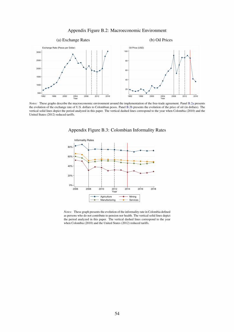
Appendix Figure B.2: Macroeconomic Environment

(a) Exchange Rates

500

1000

1500

2000

2500

3000

1992 1996 2000 2004 2008 2012 2016Year

Exchange Rate (Pesos per Dollar)

(b) Oil Prices

20

40

60

80

100

1992 1996 2000 2004 2008 2012 2016Year

Oil Price (USD)

Notes: These graphs describe the macroeconomic environment around the implementation of the free-trade agreement. Panel B.2a presentsthe evolution of the exchange rate of U.S. dollars to Colombian pesos. Panel B.2b presents the evolution of the price of oil (in dollars). Thevertical solid lines depict the period analyzed in this paper. The vertical dashed lines correspond to the year when Colombia (2010) and theUnited States (2012) reduced tariffs.

Appendix Figure B.3: Colombian Informality Rates

0%

20%

40%

60%

80%

2006 2008 2010 2012 2014 2016 2018Year

Agriculture MiningManufacturing Services

Informality Rates

Notes: These graph presents the evolution of the informality rate in Colombia definedas persons who do not contribute to pension nor health. The vertical solid lines depictthe period analyzed in this paper. The vertical dashed lines correspond to the yearwhen Colombia (2010) and the United States (2012) reduced tariffs.

54

C. Appendix Tables

Appendix Table C.1: Descriptive Statistics Across Samples

Count Mean S.D. Min. Max.(1) (2) (3) (4) (5)

A) Workers1(Male) 5,870,178 0.61 0.49 0.00 1.00Age 5,870,178 41.52 9.36 26.00 63.001(Works at Endline) 5,870,178 0.77 0.42 0.00 1.001(Same 2-digit Ind. at Endline) 4,504,017 0.24 0.43 0.00 1.001(Same firm at Endline) 4,504,017 0.26 0.44 0.00 1.001(Same State) 4,504,017 0.60 0.49 0.00 1.00log(Wage) 5,499,549 15.69 1.17 0.25 22.11log(Daily Wage) 5,482,481 10.57 0.69 0.00 18.841(State that Trades) 5,870,178 0.74 0.44 0.00 1.001(Col Reduction) 5,870,178 0.06 0.23 0.00 1.001(USA Reduction) 5,870,178 0.01 0.11 0.00 1.001(Col Reduction)*1(State that Trades) 5,870,178 0.05 0.21 0.00 1.00log(Output Import Competition) 5,870,178 0.59 2.45 0.00 19.66

B) Firms1(Open at Endline) 165,724 0.76 0.43 0.00 1.00log(Days Worked) 165,724 7.40 1.87 0.22 15.20log(Daily Wage) 165,693 10.48 0.55 0.04 15.92Firm Wage Premium 152,793 -0.04 0.27 -10.75 6.961(State that Trades) 165,724 0.66 0.47 0.00 1.001(Col Reduction) 165,724 0.08 0.26 0.00 1.001(USA Reduction) 165,724 0.02 0.12 0.00 1.001(Col Reduction)*1(State that Trades) 165,724 0.05 0.23 0.00 1.00log(Exports per Worker) 165,724 0.39 1.81 0.00 16.24log(Output Import Competition) 165,724 0.53 2.31 0.00 19.66

C) Industry-State with at least one employee .Employment 142,212 516.82 3,927.06 0.00 298,019.00Wage with zeros (USD) 142,212 303.19 266.62 0.00 13,244.75Number of Firms 142,212 20.90 264.90 0.00 34,465.00Firm Size 142,212 23.46 114.31 0.00 16,671.00Imports Per Worker (in millions) 142,212 0.03 2.36 0.00 384.50Exports Per Worker (in millions) 142,212 0.01 1.09 0.00 179.681(COL reduction) 142,212 0.12 0.32 0.00 1.001(USA reduction) 142,212 0.02 0.14 0.00 1.001(States Trades with US) 142,212 0.30 0.46 0.00 1.001(COL reduction)*Post*1(Customs) 142,212 0.02 0.15 0.00 1.001(USA reduction)*Post*1(Customs) 142,212 0.00 0.06 0.00 1.00

Note: This table presents descriptive statistics of the three samples used. Panel A) describes the sample of incumbent workersobserved in 2010 and tracked until 2014. Panel B) describe the sample of incumbent firms observed in 2010 and tracked until2014. Panel C) describes the sample of industries-states-years from 2008 to 2014. Values of this sample were replaced tozero if that observation was missing for that year but we observed it in any other year. 1() stands for a dummy variable thattakes the value of one if the condition inside parentheses is met.

55

Appendix Table C.2: First Stage at the Worker and Firm Level

(1) (2) (3) (4) (5)

A) Worker Level1(COL reduction)1(Trade) 1.284** 1.277** 1.297** 1.725*** 1.731***

(0.589) (0.589) (0.589) (0.367) (0.361)Log(Exports per Worker) 1.047*** 1.047*** 1.047*** 0.676*** 0.671***

(0.073) (0.073) (0.073) (0.042) (0.042)

Observations 6,615,624 6,615,624 6,615,624 6,615,624 6,615,624F-stat 4.751 4.696 4.696 22.038 22.985

B) Firm Level1(COL reduction)1(Trade) 4.065*** 4.066*** 4.157*** 2.728*** 2.734***

(0.352) (0.352) (0.357) (0.259) (0.254)Log(Exports per Worker) 0.615*** 0.616*** 0.611*** 0.196*** 0.191***

(0.088) (0.088) (0.087) (0.043) (0.043)

Observations 165,724 165,724 165,724 165,724 165,724F-stat 133.367 133.321 135.282 110.66 116.189

Demographics Yes Yes Yes YesIndustry FE Yes YesState FE Yes Yes

Note: This table presents the first stage of equation 7. *** p<0.01, ** p<0.05, * p<0.1

56

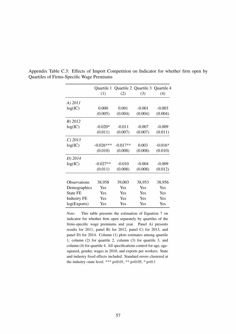
Appendix Table C.3: Effects of Import Competition on Indicator for whether firm open byQuartiles of Firms-Specific Wage Premiums

Quartile 1 Quartile 2 Quartile 3 Quartile 4(1) (2) (3) (4)

A) 2011log(IC) 0.000 0.001 -0.001 -0.003

(0.005) (0.004) (0.004) (0.004)

B) 2012log(IC) -0.020* -0.011 -0.007 -0.009

(0.011) (0.007) (0.007) (0.011)

C) 2013log(IC) -0.026*** -0.017** 0.003 -0.016*

(0.010) (0.008) (0.008) (0.010)

D) 2014log(IC) -0.027** -0.010 -0.004 -0.009

(0.011) (0.008) (0.008) (0.012)

Observations 38,958 39,003 38,953 38,956Demographics Yes Yes Yes YesState FE Yes Yes Yes YesIndustry FE Yes Yes Yes Yeslog(Exports) Yes Yes Yes Yes

Note: This table presents the estimation of Equation 7 onindicator for whether firm open separately by quartiles of thefirms-specific wage premiums and year. Panel A) presentsresults for 2011, panel B) for 2012, panel C) for 2013, andpanel D) for 2014. Column (1) plots estimates among quartile1, column (2) for quartile 2, column (3) for quartile 3, andcolumn (4) for quartile 4. All specifications control for age, age-squared, gender, wages in 2010, and exports per workers. Stateand industry fixed effects included. Standard errors clustered atthe industry–state level. *** p<0.01, ** p<0.05, * p<0.1

57

Appendix Table C.4: Effects of Import Competition on firm size by Quartiles of Firms-SpecificWage Premiums

Quartile 1 Quartile 2 Quartile 3 Quartile 4(1) (2) (3) (4)

A) 2011log(IC) -0.093* 0.031 -0.024 -0.034

(0.053) (0.045) (0.055) (0.057)

B) 2012log(IC) -0.118* -0.017 -0.007 -0.034

(0.071) (0.046) (0.062) (0.075)

C) 2013log(IC) -0.102* 0.005 -0.012 -0.033

(0.053) (0.044) (0.056) (0.051)

D) 2014log(IC) -0.099* 0.022 -0.014 -0.034

(0.055) (0.050) (0.059) (0.056)

Observations 37,505 37,512 37,858 38,013Demographics Yes Yes Yes YesState FE Yes Yes Yes YesIndustry FE Yes Yes Yes Yeslog(Exports) Yes Yes Yes Yes

Note: This table presents the estimation of Equation 7 on firmsize separately by quartiles of the firms-specific wage premiumsand year. Panel A) presents results for 2011, panel B) for 2012,panel C) for 2013, and panel D) for 2014. Column (1) plotsestimates among quartile 1, column (2) for quartile 2, column (3)for quartile 3, and column (4) for quartile 4. All specificationscontrol for age, age-squared, gender, wages in 2010, and exportsper workers. State and industry fixed effects included. Standarderrors clustered at the industry–state level. *** p<0.01, **p<0.05, * p<0.1

58

Appendix Table C.5: Effects of Import Competition on Indicator for whether the individualworks by Quartiles of Firms-Specific Wage Premiums

Quartile 1 Quartile 2 Quartile 3 Quartile 4(1) (2) (3) (4)

A) 2011log(IC) 0.009* 0.001 0.004 0.004

(0.005) (0.004) (0.003) (0.005)

B) 2012log(IC) 0.011 0.002 -0.000 -0.003

(0.007) (0.005) (0.003) (0.005)

C) 2013log(IC) 0.007 -0.002 0.000 -0.003

(0.005) (0.005) (0.004) (0.005)

D) 2014log(IC) 0.004 -0.001 -0.000 -0.001

(0.004) (0.005) (0.004) (0.005)

Observations 1,411,549 1,412,053 1,411,162 1,411,607Demographics Yes Yes Yes YesState FE Yes Yes Yes YesIndustry FE Yes Yes Yes Yeslog(Exports) Yes Yes Yes Yes

Note: This table presents the estimation of Equation 7 on indi-cator for whether the individual works separately by quartiles ofthe workers-specific wage premiums and year. Panel A) presentsresults for 2011, panel B) for 2012, panel C) for 2013, andpanel D) for 2014. Column (1) plots estimates among quartile1, column (2) for quartile 2, column (3) for quartile 3, andcolumn (4) for quartile 4. All specifications control for age, age-squared, gender, wages in 2010, and exports per workers. Stateand industry fixed effects included. Standard errors clustered atthe industry–state level. *** p<0.01, ** p<0.05, * p<0.1

59

Appendix Table C.6: Effects of Import Competition on Worker log Daily Wage by Quartiles ofFirms-Specific Wage Premiums

Quartile 1 Quartile 2 Quartile 3 Quartile 4(1) (2) (3) (4)

A) 2011log(IC) -0.032* -0.002 -0.004 -0.004

(0.017) (0.008) (0.005) (0.008)

B) 2012log(IC) -0.056** 0.016** 0.000 0.000

(0.023) (0.008) (0.006) (0.011)

C) 2013log(IC) -0.045*** 0.009 0.002 -0.001

(0.017) (0.007) (0.005) (0.008)

D) 2014log(IC) -0.028** 0.013* -0.000 0.003

(0.013) (0.008) (0.006) (0.008)

Observations 1,202,821 1,237,696 1,240,444 1,266,747Demographics Yes Yes Yes YesState FE Yes Yes Yes YesIndustry FE Yes Yes Yes Yeslog(Exports) Yes Yes Yes Yes

Note: This table presents the estimation of Equation 7 onworker log daily wage separately by quartiles of the workers-specific wage premiums and year. Panel A) presents results for2011, panel B) for 2012, panel C) for 2013, and panel D) for2014. Column (1) plots estimates among quartile 1, column(2) for quartile 2, column (3) for quartile 3, and column (4)for quartile 4. All specifications control for age, age-squared,gender, wages in 2010, and exports per workers. State andindustry fixed effects included. Standard errors clustered at theindustry–state level. *** p<0.01, ** p<0.05, * p<0.1

60

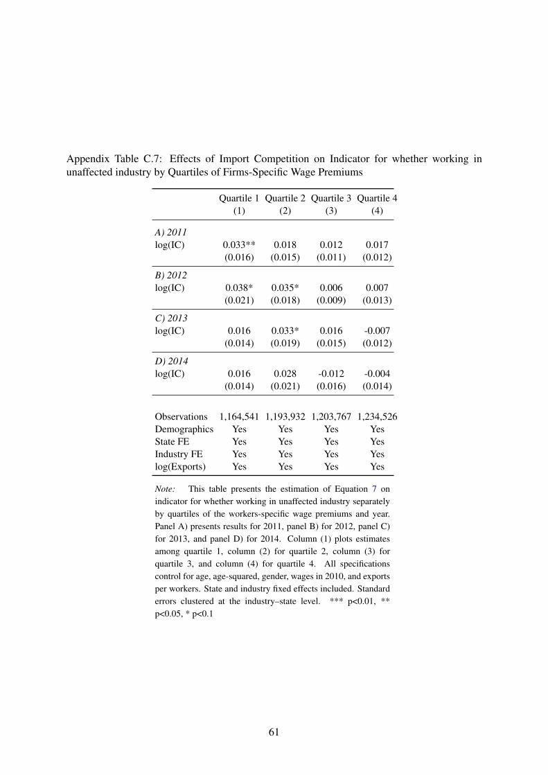
Appendix Table C.7: Effects of Import Competition on Indicator for whether working inunaffected industry by Quartiles of Firms-Specific Wage Premiums

Quartile 1 Quartile 2 Quartile 3 Quartile 4(1) (2) (3) (4)

A) 2011log(IC) 0.033** 0.018 0.012 0.017

(0.016) (0.015) (0.011) (0.012)

B) 2012log(IC) 0.038* 0.035* 0.006 0.007

(0.021) (0.018) (0.009) (0.013)

C) 2013log(IC) 0.016 0.033* 0.016 -0.007

(0.014) (0.019) (0.015) (0.012)

D) 2014log(IC) 0.016 0.028 -0.012 -0.004

(0.014) (0.021) (0.016) (0.014)

Observations 1,164,541 1,193,932 1,203,767 1,234,526Demographics Yes Yes Yes YesState FE Yes Yes Yes YesIndustry FE Yes Yes Yes Yeslog(Exports) Yes Yes Yes Yes

Note: This table presents the estimation of Equation 7 onindicator for whether working in unaffected industry separatelyby quartiles of the workers-specific wage premiums and year.Panel A) presents results for 2011, panel B) for 2012, panel C)for 2013, and panel D) for 2014. Column (1) plots estimatesamong quartile 1, column (2) for quartile 2, column (3) forquartile 3, and column (4) for quartile 4. All specificationscontrol for age, age-squared, gender, wages in 2010, and exportsper workers. State and industry fixed effects included. Standarderrors clustered at the industry–state level. *** p<0.01, **p<0.05, * p<0.1

61

Appendix Table C.8: Effects of Import Competition on Indicator for whether working inunaffected state by Quartiles of Firms-Specific Wage Premiums

Quartile 1 Quartile 2 Quartile 3 Quartile 4(1) (2) (3) (4)

A) 2011log(IC) 0.005* 0.003 0.006*** 0.005

(0.003) (0.002) (0.002) (0.004)

B) 2012log(IC) 0.008 0.005* 0.009*** 0.010**

(0.005) (0.003) (0.002) (0.005)

C) 2013log(IC) 0.006 0.005* 0.010*** 0.008**

(0.004) (0.003) (0.003) (0.003)

D) 2014log(IC) 0.007* 0.004 0.010*** 0.005

(0.004) (0.003) (0.003) (0.004)

Observations 1,209,538 1,240,741 1,245,414 1,273,099Demographics Yes Yes Yes YesState FE Yes Yes Yes YesIndustry FE Yes Yes Yes Yeslog(Exports) Yes Yes Yes Yes

Note: This table presents the estimation of Equation 7 onindicator for whether working in unaffected state separately byquartiles of the workers-specific wage premiums and year. PanelA) presents results for 2011, panel B) for 2012, panel C) for2013, and panel D) for 2014. Column (1) plots estimates amongquartile 1, column (2) for quartile 2, column (3) for quartile3, and column (4) for quartile 4. All specifications controlfor age, age-squared, gender, wages in 2010, and exports perworkers. State and industry fixed effects included. Standarderrors clustered at the industry–state level. *** p<0.01, **p<0.05, * p<0.1

62

Appendix Table C.9: Effects of Import Competition on Indicator for whether the individualworks by Quartiles of Workers-Specific Wage Premiums

Quartile 1 Quartile 2 Quartile 3 Quartile 4(1) (2) (3) (4)

A) 2011log(IC) -0.000 0.005 0.004 0.003

(0.003) (0.004) (0.003) (0.002)

B) 2012log(IC) -0.008** 0.003 0.005 0.001

(0.004) (0.004) (0.004) (0.003)

C) 2013log(IC) -0.011** 0.003 0.004 0.001

(0.004) (0.004) (0.004) (0.003)

D) 2014log(IC) -0.006 0.002 0.005 0.000

(0.004) (0.004) (0.004) (0.003)

Observations 1,411,610 1,411,950 1,411,189 1,411,620Demographics Yes Yes Yes YesState FE Yes Yes Yes YesIndustry FE Yes Yes Yes Yeslog(Exports) Yes Yes Yes Yes

Note: This table presents the estimation of Equation 7 on indi-cator for whether the individual works separately by quartiles ofthe workers-specific wage premiums and year. Panel A) presentsresults for 2011, panel B) for 2012, panel C) for 2013, andpanel D) for 2014. Column (1) plots estimates among quartile1, column (2) for quartile 2, column (3) for quartile 3, andcolumn (4) for quartile 4. All specifications control for age, age-squared, gender, wages in 2010, and exports per workers. Stateand industry fixed effects included. Standard errors clustered atthe industry–state level. *** p<0.01, ** p<0.05, * p<0.1

63

Appendix Table C.10: Effects of Import Competition on Worker log Daily Wage by Quartilesof Workers-Specific Wage Premiums

Quartile 1 Quartile 2 Quartile 3 Quartile 4(1) (2) (3) (4)

A) 2011log(IC) 0.002 -0.010* -0.011* -0.001

(0.011) (0.005) (0.006) (0.005)

B) 2012log(IC) 0.003 -0.002 -0.009 -0.005

(0.014) (0.005) (0.007) (0.005)

C) 2013log(IC) 0.005 -0.002 -0.004 -0.006

(0.012) (0.005) (0.006) (0.006)

D) 2014log(IC) 0.002 0.000 -0.004 -0.001

(0.012) (0.005) (0.007) (0.007)

Observations 1,231,395 1,205,653 1,203,824 1,306,830Demographics Yes Yes Yes YesState FE Yes Yes Yes YesIndustry FE Yes Yes Yes Yeslog(Exports) Yes Yes Yes Yes

Note: This table presents the estimation of Equation 7 onworker log daily wage separately by quartiles of the workers-specific wage premiums and year. Panel A) presents results for2011, panel B) for 2012, panel C) for 2013, and panel D) for2014. Column (1) plots estimates among quartile 1, column(2) for quartile 2, column (3) for quartile 3, and column (4)for quartile 4. All specifications control for age, age-squared,gender, wages in 2010, and exports per workers. State andindustry fixed effects included. Standard errors clustered at theindustry–state level. *** p<0.01, ** p<0.05, * p<0.1

64

Appendix Table C.11: Effects of Import Competition on Indicator for whether working inunaffected industry by Quartiles of Workers-Specific Wage Premiums

Quartile 1 Quartile 2 Quartile 3 Quartile 4(1) (2) (3) (4)

A) 2011log(IC) -0.000 0.013 0.046*** 0.007

(0.011) (0.009) (0.017) (0.007)

B) 2012log(IC) -0.009 0.020* 0.057*** 0.011

(0.010) (0.011) (0.019) (0.007)

C) 2013log(IC) -0.028* 0.014 0.054*** 0.008

(0.014) (0.014) (0.019) (0.010)

D) 2014log(IC) -0.005 -0.008 0.040** 0.004

(0.013) (0.013) (0.018) (0.012)

Observations 1,199,398 1,159,688 1,158,841 1,278,832Demographics Yes Yes Yes YesState FE Yes Yes Yes YesIndustry FE Yes Yes Yes Yeslog(Exports) Yes Yes Yes Yes

Note: This table presents the estimation of Equation 7 onindicator for whether working in unaffected industry separatelyby quartiles of the workers-specific wage premiums and year.Panel A) presents results for 2011, panel B) for 2012, panel C)for 2013, and panel D) for 2014. Column (1) plots estimatesamong quartile 1, column (2) for quartile 2, column (3) forquartile 3, and column (4) for quartile 4. All specificationscontrol for age, age-squared, gender, wages in 2010, and exportsper workers. State and industry fixed effects included. Standarderrors clustered at the industry–state level. *** p<0.01, **p<0.05, * p<0.1

65

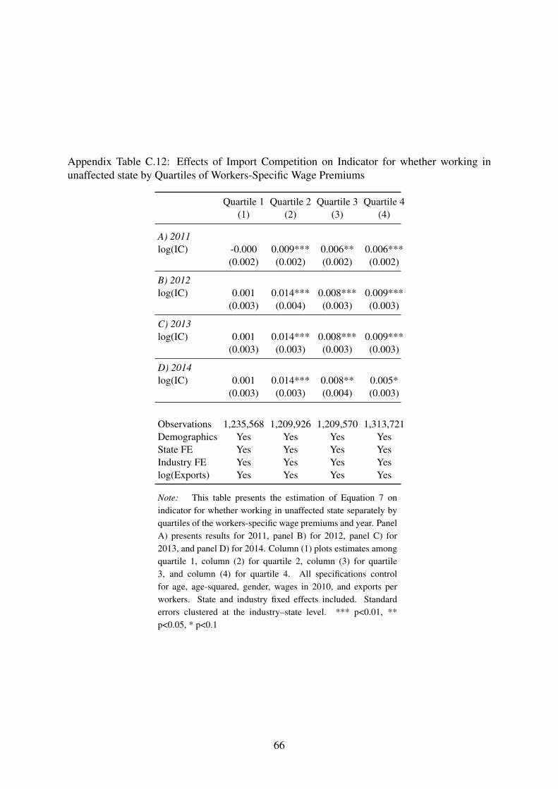
Appendix Table C.12: Effects of Import Competition on Indicator for whether working inunaffected state by Quartiles of Workers-Specific Wage Premiums

Quartile 1 Quartile 2 Quartile 3 Quartile 4(1) (2) (3) (4)

A) 2011log(IC) -0.000 0.009*** 0.006** 0.006***

(0.002) (0.002) (0.002) (0.002)

B) 2012log(IC) 0.001 0.014*** 0.008*** 0.009***

(0.003) (0.004) (0.003) (0.003)

C) 2013log(IC) 0.001 0.014*** 0.008*** 0.009***

(0.003) (0.003) (0.003) (0.003)

D) 2014log(IC) 0.001 0.014*** 0.008** 0.005*

(0.003) (0.003) (0.004) (0.003)

Observations 1,235,568 1,209,926 1,209,570 1,313,721Demographics Yes Yes Yes YesState FE Yes Yes Yes YesIndustry FE Yes Yes Yes Yeslog(Exports) Yes Yes Yes Yes

Note: This table presents the estimation of Equation 7 onindicator for whether working in unaffected state separately byquartiles of the workers-specific wage premiums and year. PanelA) presents results for 2011, panel B) for 2012, panel C) for2013, and panel D) for 2014. Column (1) plots estimates amongquartile 1, column (2) for quartile 2, column (3) for quartile3, and column (4) for quartile 4. All specifications controlfor age, age-squared, gender, wages in 2010, and exports perworkers. State and industry fixed effects included. Standarderrors clustered at the industry–state level. *** p<0.01, **p<0.05, * p<0.1

66

Appendix Table C.13: Most and Less Imported Products

Before free-trade agreement (2008-2010) After free-trade agreement (2011-2014)

Product Value of Product Value ofImports (USD) Imports (USD)

More Imported ProductsManufacture of refined petroleum products 3,454,817,062 Manufacture of refined petroleum products 18,043,048,647Manufacture of basic chemicals, except fertilizers and nitrogen compounds 2,986,627,388 Manufacture of basic chemicals, except fertilizers and nitrogen compounds 4,618,210,761Manufacture of aircraft and spacecraft 2,671,057,996 Manufacture of aircraft and spacecraft 3,904,964,753Growing of cereals and other crops n.e.c. 2,434,170,631 Growing of cereals and other crops n.e.c. 2,918,795,023Manufacture of machinery for mining, quarrying and construction 1,674,661,590 Manufacture of plastics in primary forms and of synthetic rubber 2,424,816,198Manufacture of plastics in primary forms and of synthetic rubber 1,319,655,422 Manufacture of motor vehicles 2,011,364,592Manufacture of pumps, compressors, taps and valves 1,046,711,803 Manufacture of machinery for mining, quarrying and construction 1,984,965,474Manufacture of motor vehicles 1,045,354,478 Manufacture of other chemical products n.e.c. 1,657,742,734Manufacture of other chemical products n.e.c. 901,847,834 Manufacture of pharmaceuticals, medicinal chemicals and botanical products 1,604,872,773

Less Imported ProductsManufacture of pharmaceuticals, medicinal chemicals and botanical products 864,893,890 Manufacture of pumps, compressors, taps and valves 1,578,531,260Dramatic arts, music and other arts activities 485,316 Motion picture and video production and distribution 810,482Manufacture of structural non-refractory clay and ceramic products 351,996 Manufacture of television and radio transmitters 748,602Cutting, shaping and finishing of stone 197,031 Cutting, shaping and finishing of stone 567,766Photographic activities 191,111 Fishing, operation of fish hatcheries and fish farms 521,867Manufacture of tobacco products 134,139 Manufacture of gas; distribution of gaseous fuels through mains 485,745Manufacture of coke oven products 54,830 Manufacture of wooden containers 110,183Manufacture of wooden containers 36,301 Photographic activities 79,673Hairdressing and other beauty treatment 33,667 Manufacture of coke oven products 57,461Dressing and dyeing of fur; manufacture of articles of fur 24,040 Architectural and engineering activities and related technical consultancy 38,926Manufacture of gas; distribution of gaseous fuels through mains 10,515 Dressing and dyeing of fur; manufacture of articles of fur 29,811Architectural and engineering activities and related technical consultancy 9,797 Hairdressing and other beauty treatment 4,214

Note: This table describes the most and less imported products in Colombia from the United States, before and after the free-trade agreement. The values are presented in USD.

67