Enhanced 3D Kinematic Modeling of WheeledMobile Robots

Neal Seegmiller and Alonzo KellyRobotics Institute, Carnegie Mellon University

Abstract—Most fielded wheeled mobile robots (WMRs) todayuse basic 2D kinematic motion models in their planning, control,and estimation systems. On uneven or low traction terrain, orduring aggressive maneuvers, higher fidelity models are requiredwhich account for suspension articulations, wheel slip, and liftoff.In this paper we present a simple, algorithmic method to con-struct 3D kinematic models for any WMR configuration. We alsopresent a novel enhancement to predict the effects of slip on body-level motion. Extensive experimental results are presented tovalidate our model formulation. We show odometry improvementby calibrating to data logs and modeling 3D articulations. We alsoshow comparable predictive accuracy of our enhanced kinematicmodel to a full dynamic model, at much lower computational cost.

I. INTRODUCTION

Motion models predict changes in state given a sequence ofinputs. All wheeled mobile robot (WMR) navigation systemsrely critically on such models. Estimation systems rely onthem for odometry, especially in the absence of GPS orother localization sensors. Model predictive planning/controlsystems repeatedly forward simulate these models to find andfollow optimal trajectories.

Motion models vary widely in complexity. Models can bekinematic, such that body frame velocity is computed fromjoint rate inputs and integrated once to predict pose. Modelscan also be dynamic, such that acceleration is computed fromforce/torque inputs and integrated twice. Models can accountfor 3D suspension deflections, or neglect them in a planarrepresentation. For several reasons, most fielded WMRs todaymake do with basic 2D kinematic models.

First, 2D kinematic models are easy to derive in closedform. Deriving the full 3D dynamics of a WMR from scratchis laborious. One could model the WMR in a general-purposephysics simulator (e.g. Open Dynamics Engine, Bullet), butmost only enforce Coulomb’s law of friction at contact points,whereas real wheel-terrain interaction is much more complex.

Second, 2D kinematic models are computationally cheap.Receding-horizon model predictive planning requires thatmodels be simulated many orders of magnitude faster than realtime, as numerous candidate trajectories are evaluated at eachtime step. Often, only a fraction of a processor is allocated forsuch planning.

Finally, 2D kinematic models are often sufficient, but onlybecause WMRs are used conservatively. Most WMRs arerestricted to driving slowly on flat ground; steep or roughpatches are avoided as obstacles. Greater mobility is possiblewith wheeled locomotion, for example: traversing rubble at

disaster sites, climbing steep mountainsides, or racing whilestaying just within the tire friction envelope. However, tosafely push the limits of mobility, WMR navigation systemsrequire fast, high-fidelity motion models. In this paper wepresent an enhanced formulation of 3D WMR kinematics, thatprovides near dynamic model fidelity at less computationalcost.

II. RELATED WORK

The earliest general approach to deriving WMR kinematicswas published by Muir and Neuman [19]; they assign framesin a transformation graph following the Sheth-Uicker conven-tion, cascade transforms relating wheel to body positions, thensymbolically differentiate them to obtain Jacobians relatingwheel to body velocities. More recently, Kim et al. [13] andFu and Krovi [7] extended methods for parallel manipulators(transfer method, twist-based) to derive the kinematics ofplanar WMRs.

Some recent work concerns the 3D kinematics of articu-lated WMRs on uneven terrain. Tarokh and McDermott [25]present a 3D version of Muir and Neuman’s transform-basedapproach, and demonstrate it on a rocker-bogie rover. Le Mennet al. [16] extend a reciprocal screw-based approach to derivethe 3D kinematics of multi-monocycle robots. Tarokh et al.(in later papers) [26][27], Chang et al. [4], and Kelly andSeegmiller [12] use a velocity propagation-based approach,similar to the one used here. Choi and Sreenivasan [5] andChakraborty and Ghosal [3] do not provide general methodsfor kinematics derivation, but simulate 3D WMR kinematics tovalidate mechanism designs. Lamon and Siegwart [14] providerare experimental 3D odometry results for their articulatedSOLERO platform.

Despite much progress, the literature still lacks modelsproven to be accurate and efficient enough for model predictiveplanning/control for high mobility WMRs. Importantly, noneof the above publications includes a predictive model of wheelslip, even though real WMRs slip significantly, especiallyin low traction, steep, or high-speed conditions. Most justestimate slip as it occurs (e.g. [1],[23]) then rely on feedbackcontrol to correct for it ([8],[17]), but unpredicted wheelslip can cause a collision before the feedback controllercan react, or entrapment [20]. There are many wheel-levelmodels of slip in the literature but few publications incorporatethese into full WMR models. Tian et al. [28] incorporatean empirical tire model into a planar dynamics model of adifferential drive robot. Ishigami et al. [10] incorporate their

own terramechanics-based model for rigid wheels in loose soilinto an Open Dynamics Engine model of an articulated rover.However, computation times were excessive when using thismodel for motion planning [11].

Most wheel-ground contact models relate slip and force,so they are not directly compatible with kinematic modelswhich require velocity (vs. force) inputs. Our prior work [22]included slip in a simplistic kinematic model. We requiredthat WMR kinematics be reduced to a “unicycle” model,which moves instantaneously in the tangent plane to theterrain surface (ignoring suspension deflections). Body-levelslip was parametrized over an ad hoc polynomial of velocityand gravity terms.

III. OVERVIEW OF CONTRIBUTION

In this paper, we present a general method to construct3D kinematic models for any articulated WMR configuration(Sections IV-A through IV-C). While the vector algebra basisof our approach exists in prior work, our exact algorithm isunique and straightforward to implement.

Our most significant theoretical contribution is enhancementof the kinematics to predict the effects of wheel slip onbody frame motion (IV-D). We do so in a principled way,parametrizing slip over inertial force (due to gravity, accelera-tion) and dissipative forces. Calculating the inertial force alsoenables rollover risk assessment (IV-E).

In comparison to related work on 3D WMR kinematics,we provide an unprecedented level of experimental validationof our formulation. In all experiments we calibrate modelparameters to data logs, optimizing predictive accuracy overextended horizons (IV-F). This makes the models suitablefor model predictive control vs. just instantaneous feedbackcontrol.

We show improved odometry results for an articulated rovertraversing obstacles by modeling 3D kinematics (V-A). Ourexperiments are of longer duration than in prior work [14]. Wealso show that our enhanced kinematic models are comparablyaccurate to more computationally expensive dynamic models(V-B). We know of no other experimental comparison ofkinematic vs. dynamic WMR models in the literature.

By replacing the basic models used in most WMR plan-ning/control/estimation systems with higher-fidelity models,autonomous mobility can be improved on uneven, slipperyterrain and during aggressive maneuvers. Some tradeoff be-tween fidelity and computation speed is unavoidable. Ideally,model complexity should vary per application for optimalperformance. We provide a unique model of intermediatecomplexity suitable for many applications.

IV. MODEL CONSTRUCTION

This section explains our systematic approach to modelconstruction and calibration. The kinematics presentation inSections IV-A through IV-C is similar to that in [21] (onWMR dynamics); however, we provide more insight andimplementation detail here.

Table I summarizes the mathematical notation used in thispaper. Regarding Cartesian coordinate vectors, the variablesr , v , and

ω will denote position, linear velocity, and angularvelocity respectively. Sometimes the left superscript is omittedleaving the coordinate system unspecified or to be inferredfrom context; when two or more quantities are operated onthey must be expressed in the same coordinates. The skew-symmetric matrix notation [ ]× explicitly means:

[u]× =

0 −u3 u2u3 0 −u1−u2 u1 0

(1)

Finally, in this document, vector and matrix indexing is one-based (vs. zero-based).

TABLE I. Mathematical Notation

Symbol Meaningu (bold lowercase) column vectoru 3-element Cartesian coordinate vector→u 6-element Plucker coordinate (or spatial) vector[u ]× skew-symmetric matrix formed from the vector

u . Used

for cross products: a ×

b = [a ]×

bcuba the quantity u is of frame a with respect to frame b,

expressed in the coordinates associated with frame cRb

a the rotation matrix of frame a relative to frame b. Usedto transform coordinates: bu = Rb

a(au)

u(i) the ith element of vector u, also called uiu(i...i+ n) the subvector of elements i through i+ n of uM(i, j) the element of M at row i, column j.M(i, ...) row i of MM(..., j) column j of M

A. Specification of the Kinematic Tree

The first step in model construction is the specification offrame information for the kinematic tree. The root is the bodyframe, which has 6 degrees of freedom (DOF) with respect tothe ground-fixed world frame. Additional frames are definedfor each movable rigid body (including the wheels). Eachframe is attached to a single parent frame by a revolute orprismatic joint. Unlike some prior work [26][4] our methoddoes not require the Denavit-Hartenberg convention, whichallows more intuitive frame definitions; joint axes may bealigned with any one of the x, y, or z axes. Wheel framesare attached via revolute joints about their y axes.

Contact frames are automatically appended for each wheel.They are defined with their origin at the wheel-terrain contactpoint. In reality contact occurs over one or more patches onthe wheel surface, but we approximate to a single point. Theirz-axis is aligned with the terrain normal, and their x and y axesare aligned with the longitudinal and lateral slip directions.

Frame information is stored in an ordered list such thatevery frame’s index is greater than its parent’s: i > p(i).As an example, Table II lists frame information for the Zoerover, which is used in the experiments in Section V-A. TheType column specifies whether the associated joint is revolute(R) or prismatic (P) and about the x, y, or z axis. The Act.column indicates if the joint is actuated (Y/N for yes/no). Thelast six columns specify the frame’s position and orientation

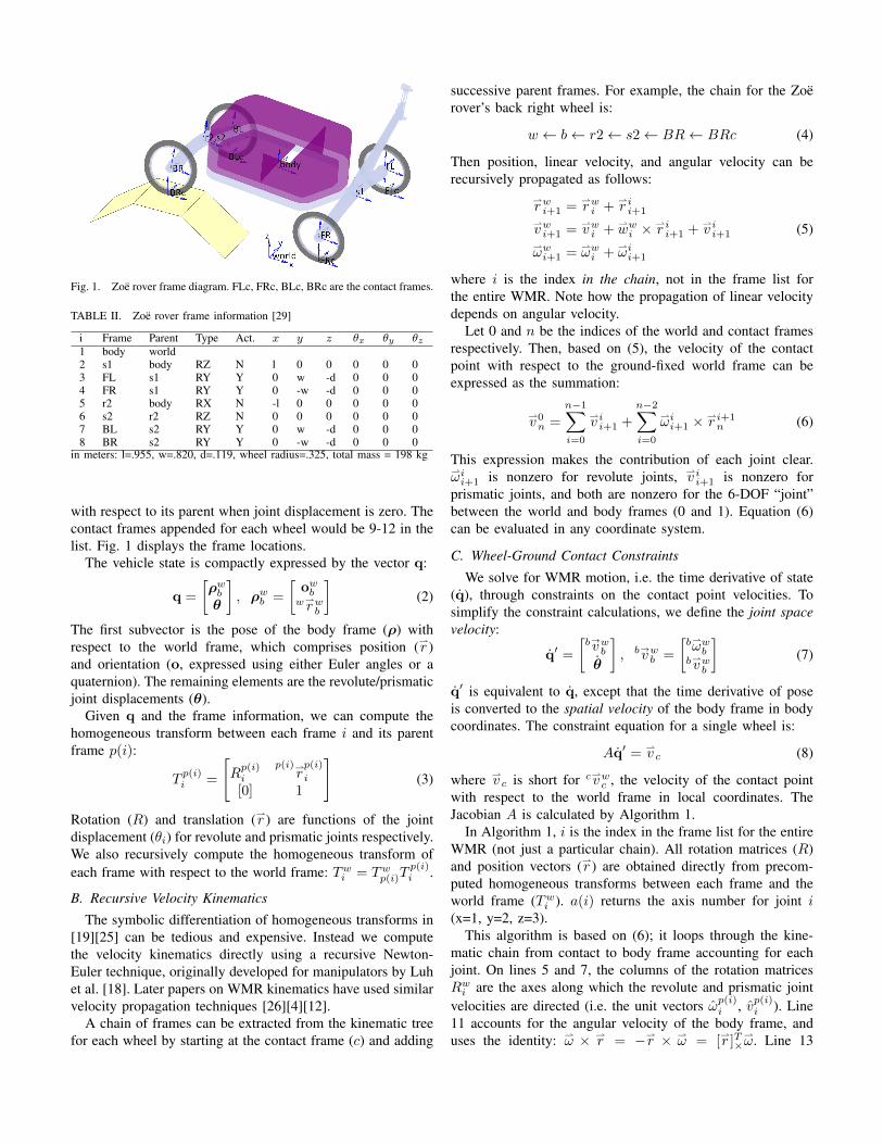
Fig. 1. Zoe rover frame diagram. FLc, FRc, BLc, BRc are the contact frames.

TABLE II. Zoe rover frame information [29]

i Frame Parent Type Act. x y z θx θy θz1 body world2 s1 body RZ N l 0 0 0 0 03 FL s1 RY Y 0 w -d 0 0 04 FR s1 RY Y 0 -w -d 0 0 05 r2 body RX N -l 0 0 0 0 06 s2 r2 RZ N 0 0 0 0 0 07 BL s2 RY Y 0 w -d 0 0 08 BR s2 RY Y 0 -w -d 0 0 0

in meters: l=.955, w=.820, d=.119, wheel radius=.325, total mass = 198 kg

with respect to its parent when joint displacement is zero. Thecontact frames appended for each wheel would be 9-12 in thelist. Fig. 1 displays the frame locations.

The vehicle state is compactly expressed by the vector q:

q =

[ρwb

θ

], ρw

b =

[owb

wrwb

](2)

The first subvector is the pose of the body frame (ρ) withrespect to the world frame, which comprises position (r )and orientation (o, expressed using either Euler angles or aquaternion). The remaining elements are the revolute/prismaticjoint displacements (θ).

Given q and the frame information, we can compute thehomogeneous transform between each frame i and its parentframe p(i):

Tp(i)i =

[R

p(i)i

r

p(i) p(i)

i

[0] 1

](3)

Rotation (R) and translation (r ) are functions of the jointdisplacement (θi) for revolute and prismatic joints respectively.We also recursively compute the homogeneous transform ofeach frame with respect to the world frame: Tw

i = Twp(i)T

p(i)i .

B. Recursive Velocity Kinematics

The symbolic differentiation of homogeneous transforms in[19][25] can be tedious and expensive. Instead we computethe velocity kinematics directly using a recursive Newton-Euler technique, originally developed for manipulators by Luhet al. [18]. Later papers on WMR kinematics have used similarvelocity propagation techniques [26][4][12].

A chain of frames can be extracted from the kinematic treefor each wheel by starting at the contact frame (c) and adding

successive parent frames. For example, the chain for the Zoerover’s back right wheel is:

w ← b← r2← s2← BR← BRc (4)

Then position, linear velocity, and angular velocity can berecursively propagated as follows:

rwi+1 =

rwi +

r ii+1

vwi+1 =

vwi +

ww

i ×r ii+1 +

v ii+1 (5)

ωwi+1 =

ωwi +

ωii+1

where i is the index in the chain, not in the frame list forthe entire WMR. Note how the propagation of linear velocitydepends on angular velocity.

Let 0 and n be the indices of the world and contact framesrespectively. Then, based on (5), the velocity of the contactpoint with respect to the ground-fixed world frame can beexpressed as the summation:

v0n =

n−1∑i=0

v ii+1 +

n−2∑i=0

ωii+1 ×

r i+1n (6)

This expression makes the contribution of each joint clear.ωii+1 is nonzero for revolute joints,

v ii+1 is nonzero for

prismatic joints, and both are nonzero for the 6-DOF “joint”between the world and body frames (0 and 1). Equation (6)can be evaluated in any coordinate system.

C. Wheel-Ground Contact Constraints

We solve for WMR motion, i.e. the time derivative of state(q), through constraints on the contact point velocities. Tosimplify the constraint calculations, we define the joint spacevelocity:

q′ =

[b→vwb

θ

], b→

vwb =

[bωwb

bvwb

](7)

q′ is equivalent to q, except that the time derivative of poseis converted to the spatial velocity of the body frame in bodycoordinates. The constraint equation for a single wheel is:

Aq′ =v c (8)

where v c is short for c

vwc , the velocity of the contact point

with respect to the world frame in local coordinates. TheJacobian A is calculated by Algorithm 1.

In Algorithm 1, i is the index in the frame list for the entireWMR (not just a particular chain). All rotation matrices (R)and position vectors (r ) are obtained directly from precom-puted homogeneous transforms between each frame and theworld frame (Tw

i ). a(i) returns the axis number for joint i(x=1, y=2, z=3).

This algorithm is based on (6); it loops through the kine-matic chain from contact to body frame accounting for eachjoint. On lines 5 and 7, the columns of the rotation matricesRw

i are the axes along which the revolute and prismatic jointvelocities are directed (i.e. the unit vectors ωp(i)

i , vp(i)i ). Line11 accounts for the angular velocity of the body frame, anduses the identity:

ω × r = −

r × ω = [

r ]T×

ω. Line 13

Algorithm 1 Jacobian Calculation for a Single Wheel

1: A← [0]2: c← contact frame index, i← p(c)3: while i > 1 do4: if joint i type = revolute then5: A(..., i+ 5)← Rw

i (..., a(i))× (rwc −

rwi )

6: else if joint i type = prismatic then7: A(..., i+ 5)← Rw

i (..., a(i))8: end if9: i← p(i)

10: end while11: A(..., 1...3)← [

rwc −

rw1 ]T×R

w1

12: A(..., 4...6)← Rw1

13: A← (Rwc )TA

converts from world to contact frame coordinates such thatnonholonomic and holonomic constraints are separated.

The first two rows of (8) constrain the x and y componentsof the contact point velocity; they enforce nonholonomicconstraints on longitudinal/lateral wheel slip. The third rowof (8) constrains the z component of contact point velocity(in the terrain normal direction); it enforces the holonomicconstraint that the wheel not penetrate or lift off of theterrain surface to first-order. Violation of the holonomic con-straint due to numerical drift can be eliminated by usingBaumgarte’s stabilization method (Yun and Sarkar [32]). Setv c = [0 0 − ∆z/τ ]T , where ∆z is the contact height errorand τ is a time constant larger than the integration time step.

Constraint equations for all nw wheels are stacked to obtainan equation with 3nw rows:

Aq′ = vc (9)

Hereafter let A refer to the stacked matrix. Note that additionalconstraints can be appended, for example, to constrain twosuspension joint angles to be symmetric. The degrees offreedom in q′ can be partitioned into free and fixed:

A(..., free)q′(free) = vc +A(..., fixed)q′(fixed) (10)

In a simulation/prediction context, the fixed DOFs includeactuated joint rates, and the free DOFs include passive jointrates and the body frame velocity. Most WMR configurationsare overconstrained, and so (10) must be solved using thepseudoinverse:

q′(free) = A(..., free)+(vc +A(..., fixed)q′(fixed)

)(11)

To integrate WMR motion (i.e. update q), q′ must first beconverted to q, which requires the conversion of body framespatial velocity into the time derivative of pose:

d

dt

[owb

wrwb

]=

[Ω(ow

b ) [0][0] Rw

b

] [bωwb

bvwb

](12)

where Ω converts angular velocity to Euler angle or quaternionrates.

D. Body-Level Slip Prediction

Related work on WMR kinematics seldom accounts fornonzero wheel slip, even though real WMRs can slip signifi-cantly. The obvious way to include slip in our model is to setthe x,y components of

v c in (8) to nonzero values, but to whatvalues? Canonical wheel-ground contact models relate force toslip, but kinematic models provide no information about forceat the wheels. Besides being unknown, wheel slip values maybe unnecessary; in many applications only the motion of thevehicle body matters. Accordingly, we enhance the kinematicsto predict body-level slip.

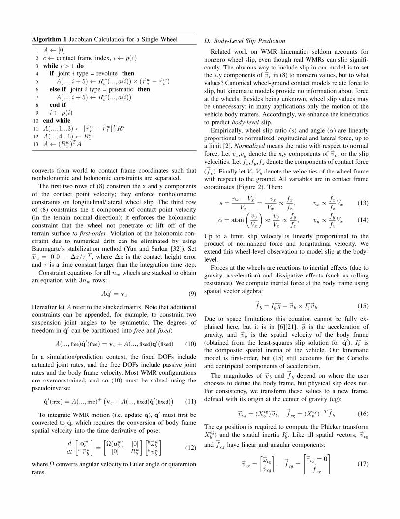
Empirically, wheel slip ratio (s) and angle (α) are linearlyproportional to normalized longitudinal and lateral force, up toa limit [2]. Normalized means the ratio with respect to normalforce. Let vx,vy denote the x,y components of

v c, or the slipvelocities. Let fx,fy ,fz denote the components of contact force(

f c). Finally let Vx,Vy denote the velocities of the wheel framewith respect to the ground. All variables are in contact framecoordinates (Figure 2). Then:

s =rω − VxVx

=−vxVx∝ fxfz, vx ∝

fxfzVx (13)

α = atan

(vyVx

)≈ vyVx∝ fyfz, vy ∝

fyfzVx (14)

Up to a limit, slip velocity is linearly proportional to theproduct of normalized force and longitudinal velocity. Weextend this wheel-level observation to model slip at the body-level.

Forces at the wheels are reactions to inertial effects (due togravity, acceleration) and dissipative effects (such as rollingresistance). We compute inertial force at the body frame usingspatial vector algebra:

→f b = Icb

→g − →

v b × Icb→v b (15)

Due to space limitations this equation cannot be fully ex-plained here, but it is in [6][21]. →

g is the acceleration ofgravity, and →

v b is the spatial velocity of the body frame(obtained from the least-squares slip solution for q′). Icb isthe composite spatial inertia of the vehicle. Our kinematicmodel is first-order, but (15) still accounts for the Coriolisand centripetal components of acceleration.

The magnitudes of →v b and

→f b depend on where the user

chooses to define the body frame, but physical slip does not.For consistency, we transform these values to a new frame,defined with its origin at the center of gravity (cg):

→v cg = (Xcg

b )→v b,

→f cg = (Xcg

b )−T→f b (16)

The cg position is required to compute the Plucker transformXcg

b ) and the spatial inertia Icb . Like all spatial vectors, →v cg

and→f cg have linear and angular components:

→v cg =

[ωcgv cg

],

→f cg =

[τ cg = 0

f cg

](17)

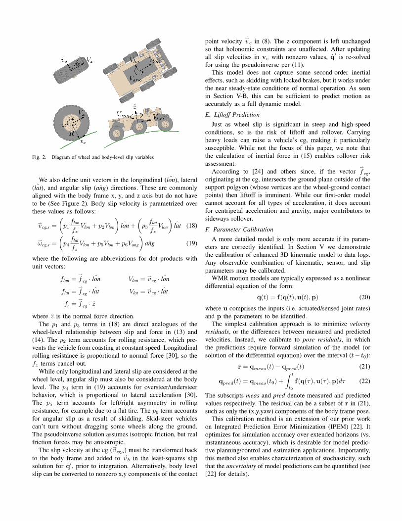
Fig. 2. Diagram of wheel and body-level slip variables

We also define unit vectors in the longitudinal ( ˆlon), lateral( ˆlat), and angular slip ( ˆang) directions. These are commonlyaligned with the body frame x, y, and z axis but do not haveto be (See Figure 2). Body slip velocity is parametrized overthese values as follows:

v cg,s =

(p1flon

fzVlon + p2Vlon

)ˆlon +

(p3flat

fzVlon

)ˆlat (18)

ωcg,s =

(p4flat

fzVlon + p5Vlon + p6Vang

)ˆang (19)

where the following are abbreviations for dot products withunit vectors:

flon =

f cg · ˆlon Vlon =v cg · ˆlon

flat =

f cg · ˆlat Vlat =v cg · ˆlat

fz =

f cg · z

where z is the normal force direction.The p1 and p3 terms in (18) are direct analogues of the

wheel-level relationship between slip and force in (13) and(14). The p2 term accounts for rolling resistance, which pre-vents the vehicle from coasting at constant speed. Longitudinalrolling resistance is proportional to normal force [30], so thefz terms cancel out.

While only longitudinal and lateral slip are considered at thewheel level, angular slip must also be considered at the bodylevel. The p4 term in (19) accounts for oversteer/understeerbehavior, which is proportional to lateral acceleration [30].The p5 term accounts for left/right asymmetry in rollingresistance, for example due to a flat tire. The p6 term accountsfor angular slip as a result of skidding. Skid-steer vehiclescan’t turn without dragging some wheels along the ground.The pseudoinverse solution assumes isotropic friction, but realfriction forces may be anisotropic.

The slip velocity at the cg (→v cg,s) must be transformed backto the body frame and added to →

v b in the least-squares slipsolution for q′, prior to integration. Alternatively, body levelslip can be converted to nonzero x,y components of the contact

point velocity v c in (8). The z component is left unchanged

so that holonomic constraints are unaffected. After updatingall slip velocities in vc with nonzero values, q′ is re-solvedfor using the pseudoinverse per (11).

This model does not capture some second-order inertialeffects, such as skidding with locked brakes, but it works underthe near steady-state conditions of normal operation. As seenin Section V-B, this can be sufficient to predict motion asaccurately as a full dynamic model.

E. Liftoff PredictionJust as wheel slip is significant in steep and high-speed

conditions, so is the risk of liftoff and rollover. Carryingheavy loads can raise a vehicle’s cg, making it particularlysusceptible. While not the focus of this paper, we note thatthe calculation of inertial force in (15) enables rollover riskassessment.

According to [24] and others since, if the vector

f cg,originating at the cg, intersects the ground plane outside of thesupport polgyon (whose vertices are the wheel-ground contactpoints) then liftoff is imminent. While our first-order modelcannot account for all types of acceleration, it does accountfor centripetal acceleration and gravity, major contributors tosideways rollover.

F. Parameter CalibrationA more detailed model is only more accurate if its param-

eters are correctly identified. In Section V we demonstratethe calibration of enhanced 3D kinematic model to data logs.Any observable combination of kinematic, sensor, and slipparameters may be calibrated.

WMR motion models are typically expressed as a nonlineardifferential equation of the form:

q(t) = f(q(t),u(t),p) (20)

where u comprises the inputs (i.e. actuated/sensed joint rates)and p the parameters to be identified.

The simplest calibration approach is to minimize velocityresiduals, or the differences between measured and predictedvelocities. Instead, we calibrate to pose residuals, in whichthe predictions require forward simulation of the model (orsolution of the differential equation) over the interval (t− t0):

r = qmeas(t)− qpred(t) (21)

qpred(t) = qmeas(t0) +

∫ t

t0

f(q(τ),u(τ),p)dτ (22)

The subscripts meas and pred denote measured and predictedvalues respectively. The residual can be a subset of r in (21),such as only the (x,y,yaw) components of the body frame pose.

This calibration method is an extension of our prior workon Integrated Prediction Error Minimization (IPEM) [22]. Itoptimizes for simulation accuracy over extended horizons (vs.instantaneous accuracy), which is desirable for model predic-tive planning/control and estimation applications. Importantly,this method also enables characterization of stochasticity, suchthat the uncertainty of model predictions can be quantified (see[22] for details).

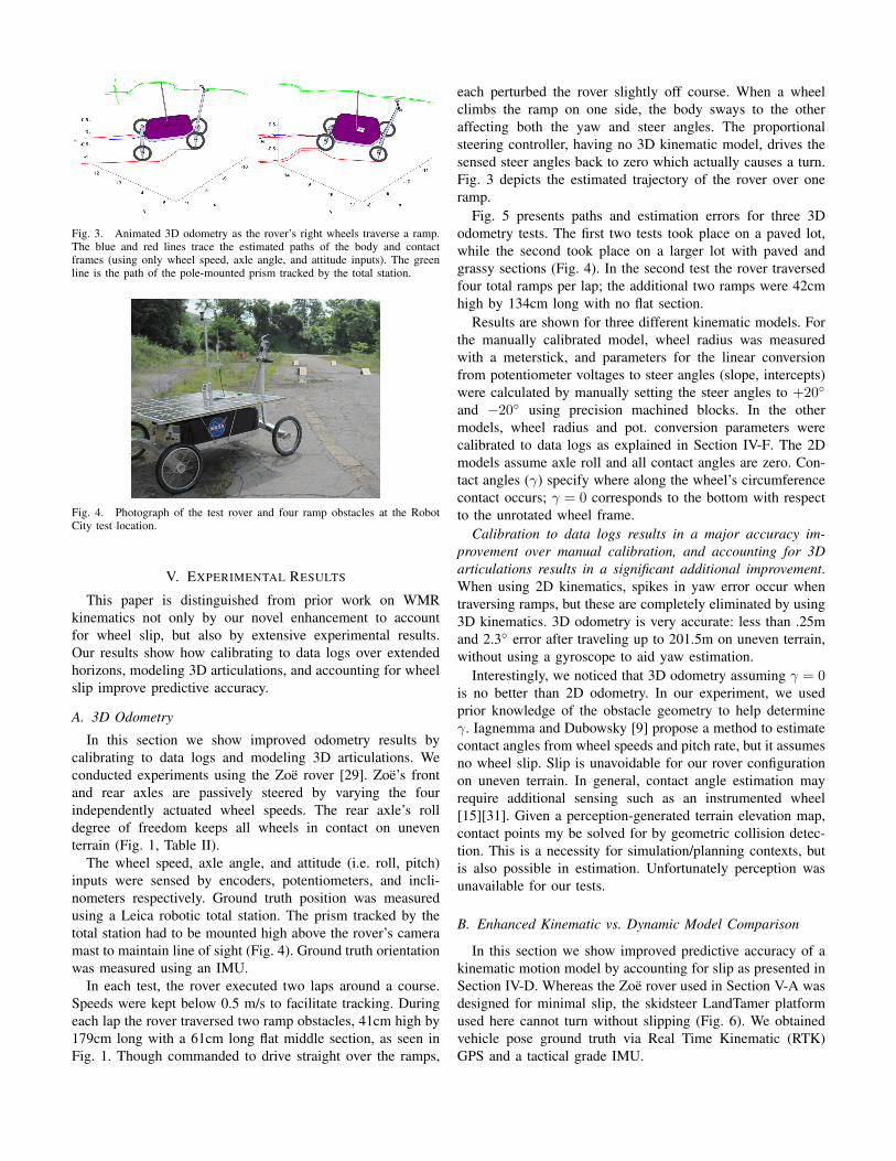
Fig. 3. Animated 3D odometry as the rover’s right wheels traverse a ramp.The blue and red lines trace the estimated paths of the body and contactframes (using only wheel speed, axle angle, and attitude inputs). The greenline is the path of the pole-mounted prism tracked by the total station.

Fig. 4. Photograph of the test rover and four ramp obstacles at the RobotCity test location.

V. EXPERIMENTAL RESULTS

This paper is distinguished from prior work on WMRkinematics not only by our novel enhancement to accountfor wheel slip, but also by extensive experimental results.Our results show how calibrating to data logs over extendedhorizons, modeling 3D articulations, and accounting for wheelslip improve predictive accuracy.

A. 3D Odometry

In this section we show improved odometry results bycalibrating to data logs and modeling 3D articulations. Weconducted experiments using the Zoe rover [29]. Zoe’s frontand rear axles are passively steered by varying the fourindependently actuated wheel speeds. The rear axle’s rolldegree of freedom keeps all wheels in contact on uneventerrain (Fig. 1, Table II).

The wheel speed, axle angle, and attitude (i.e. roll, pitch)inputs were sensed by encoders, potentiometers, and incli-nometers respectively. Ground truth position was measuredusing a Leica robotic total station. The prism tracked by thetotal station had to be mounted high above the rover’s cameramast to maintain line of sight (Fig. 4). Ground truth orientationwas measured using an IMU.

In each test, the rover executed two laps around a course.Speeds were kept below 0.5 m/s to facilitate tracking. Duringeach lap the rover traversed two ramp obstacles, 41cm high by179cm long with a 61cm long flat middle section, as seen inFig. 1. Though commanded to drive straight over the ramps,

each perturbed the rover slightly off course. When a wheelclimbs the ramp on one side, the body sways to the otheraffecting both the yaw and steer angles. The proportionalsteering controller, having no 3D kinematic model, drives thesensed steer angles back to zero which actually causes a turn.Fig. 3 depicts the estimated trajectory of the rover over oneramp.

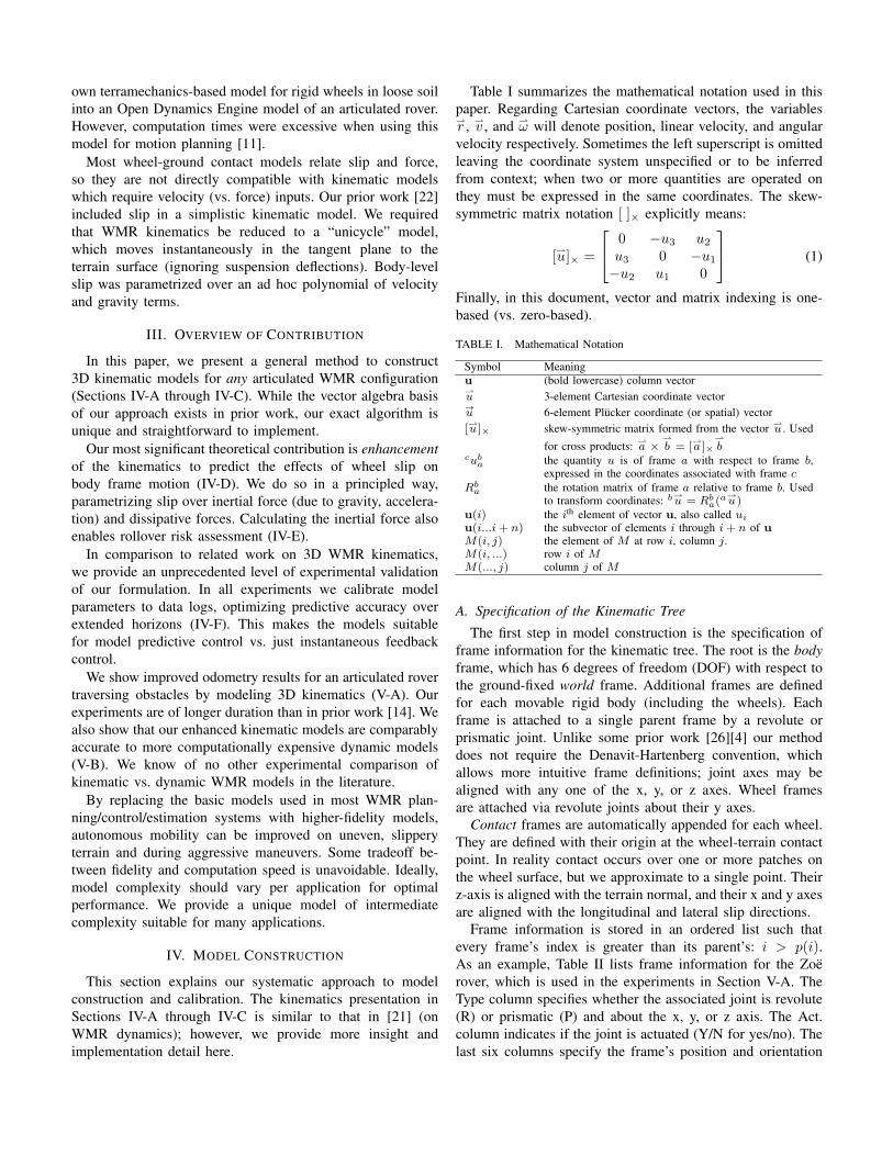
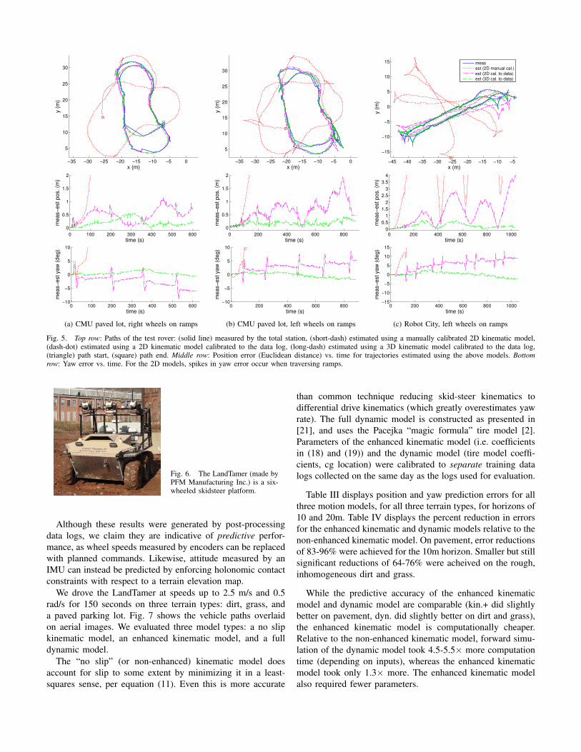
Fig. 5 presents paths and estimation errors for three 3Dodometry tests. The first two tests took place on a paved lot,while the second took place on a larger lot with paved andgrassy sections (Fig. 4). In the second test the rover traversedfour total ramps per lap; the additional two ramps were 42cmhigh by 134cm long with no flat section.

Results are shown for three different kinematic models. Forthe manually calibrated model, wheel radius was measuredwith a meterstick, and parameters for the linear conversionfrom potentiometer voltages to steer angles (slope, intercepts)were calculated by manually setting the steer angles to +20

and −20 using precision machined blocks. In the othermodels, wheel radius and pot. conversion parameters werecalibrated to data logs as explained in Section IV-F. The 2Dmodels assume axle roll and all contact angles are zero. Con-tact angles (γ) specify where along the wheel’s circumferencecontact occurs; γ = 0 corresponds to the bottom with respectto the unrotated wheel frame.

Calibration to data logs results in a major accuracy im-provement over manual calibration, and accounting for 3Darticulations results in a significant additional improvement.When using 2D kinematics, spikes in yaw error occur whentraversing ramps, but these are completely eliminated by using3D kinematics. 3D odometry is very accurate: less than .25mand 2.3 error after traveling up to 201.5m on uneven terrain,without using a gyroscope to aid yaw estimation.

Interestingly, we noticed that 3D odometry assuming γ = 0is no better than 2D odometry. In our experiment, we usedprior knowledge of the obstacle geometry to help determineγ. Iagnemma and Dubowsky [9] propose a method to estimatecontact angles from wheel speeds and pitch rate, but it assumesno wheel slip. Slip is unavoidable for our rover configurationon uneven terrain. In general, contact angle estimation mayrequire additional sensing such as an instrumented wheel[15][31]. Given a perception-generated terrain elevation map,contact points my be solved for by geometric collision detec-tion. This is a necessity for simulation/planning contexts, butis also possible in estimation. Unfortunately perception wasunavailable for our tests.

B. Enhanced Kinematic vs. Dynamic Model Comparison

In this section we show improved predictive accuracy of akinematic motion model by accounting for slip as presented inSection IV-D. Whereas the Zoe rover used in Section V-A wasdesigned for minimal slip, the skidsteer LandTamer platformused here cannot turn without slipping (Fig. 6). We obtainedvehicle pose ground truth via Real Time Kinematic (RTK)GPS and a tactical grade IMU.

−35 −30 −25 −20 −15 −10 −5 0

5

10

15

20

25

30

x (m)

y (

m)

0 100 200 300 400 500 600

0

0.5

1

1.5

2

time (s)

me

as−

est

po

s.

(m)

0 100 200 300 400 500 600−10

−5

0

5

10

time (s)

meas−

est yaw

(deg)

(a) CMU paved lot, right wheels on ramps

−35 −30 −25 −20 −15 −10 −5 0

5

10

15

20

25

30

x (m)

y (

m)

0 200 400 600 800

0

0.5

1

1.5

2

time (s)

me

as−

est

po

s.

(m)

0 200 400 600 800−10

−5

0

5

10

time (s)

meas−

est yaw

(deg)

(b) CMU paved lot, left wheels on ramps

−45 −40 −35 −30 −25 −20 −15 −10 −5

−15

−10

−5

0

5

10

15

x (m)

y (

m)

meas

est (2D manual cal.)

est (2D cal. to data)

est (3D cal. to data)

0 200 400 600 800 10000

0.5

1

1.5

2

2.5

3

3.5

4

time (s)

me

as−

est

po

s.

(m)

0 200 400 600 800 1000−15

−10

−5

0

5

10

15

time (s)

meas−

est yaw

(deg)

(c) Robot City, left wheels on ramps

Fig. 5. Top row: Paths of the test rover: (solid line) measured by the total station, (short-dash) estimated using a manually calibrated 2D kinematic model,(dash-dot) estimated using a 2D kinematic model calibrated to the data log, (long-dash) estimated using a 3D kinematic model calibrated to the data log,(triangle) path start, (square) path end. Middle row: Position error (Euclidean distance) vs. time for trajectories estimated using the above models. Bottomrow: Yaw error vs. time. For the 2D models, spikes in yaw error occur when traversing ramps.

Fig. 6. The LandTamer (made byPFM Manufacturing Inc.) is a six-wheeled skidsteer platform.

Although these results were generated by post-processingdata logs, we claim they are indicative of predictive perfor-mance, as wheel speeds measured by encoders can be replacedwith planned commands. Likewise, attitude measured by anIMU can instead be predicted by enforcing holonomic contactconstraints with respect to a terrain elevation map.

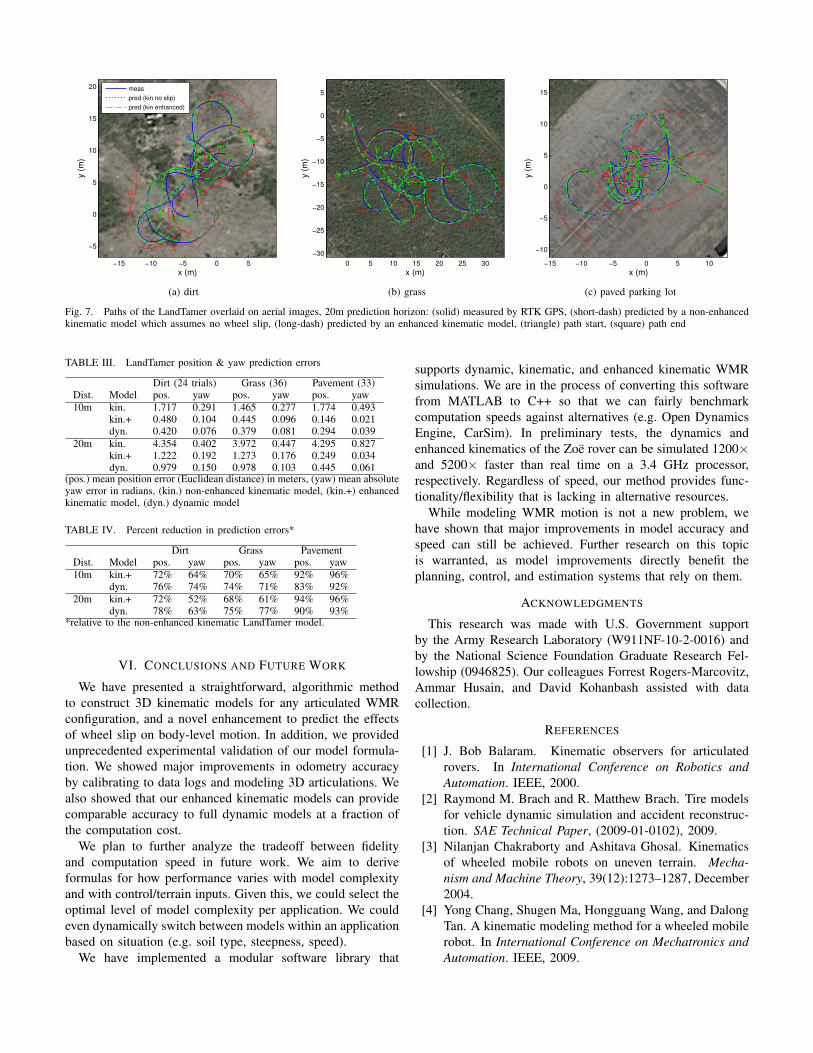
We drove the LandTamer at speeds up to 2.5 m/s and 0.5rad/s for 150 seconds on three terrain types: dirt, grass, anda paved parking lot. Fig. 7 shows the vehicle paths overlaidon aerial images. We evaluated three model types: a no slipkinematic model, an enhanced kinematic model, and a fulldynamic model.

The “no slip” (or non-enhanced) kinematic model doesaccount for slip to some extent by minimizing it in a least-squares sense, per equation (11). Even this is more accurate

than common technique reducing skid-steer kinematics todifferential drive kinematics (which greatly overestimates yawrate). The full dynamic model is constructed as presented in[21], and uses the Pacejka “magic formula” tire model [2].Parameters of the enhanced kinematic model (i.e. coefficientsin (18) and (19)) and the dynamic model (tire model coeffi-cients, cg location) were calibrated to separate training datalogs collected on the same day as the logs used for evaluation.

Table III displays position and yaw prediction errors for allthree motion models, for all three terrain types, for horizons of10 and 20m. Table IV displays the percent reduction in errorsfor the enhanced kinematic and dynamic models relative to thenon-enhanced kinematic model. On pavement, error reductionsof 83-96% were achieved for the 10m horizon. Smaller but stillsignificant reductions of 64-76% were acheived on the rough,inhomogeneous dirt and grass.

While the predictive accuracy of the enhanced kinematicmodel and dynamic model are comparable (kin.+ did slightlybetter on pavement, dyn. did slightly better on dirt and grass),the enhanced kinematic model is computationally cheaper.Relative to the non-enhanced kinematic model, forward simu-lation of the dynamic model took 4.5-5.5× more computationtime (depending on inputs), whereas the enhanced kinematicmodel took only 1.3× more. The enhanced kinematic modelalso required fewer parameters.

x (m)

y (

m)

−15 −10 −5 0 5

−5

0

5

10

15

20 meas

pred (kin no slip)

pred (kin enhanced)

(a) dirt

x (m)

y (

m)

0 5 10 15 20 25 30

−30

−25

−20

−15

−10

−5

0

5

(b) grass

x (m)

y (

m)

−15 −10 −5 0 5 10

−10

−5

0

5

10

15

(c) paved parking lot

Fig. 7. Paths of the LandTamer overlaid on aerial images, 20m prediction horizon: (solid) measured by RTK GPS, (short-dash) predicted by a non-enhancedkinematic model which assumes no wheel slip, (long-dash) predicted by an enhanced kinematic model, (triangle) path start, (square) path end

TABLE III. LandTamer position & yaw prediction errors

Dirt (24 trials) Grass (36) Pavement (33)Dist. Model pos. yaw pos. yaw pos. yaw10m kin. 1.717 0.291 1.465 0.277 1.774 0.493

kin.+ 0.480 0.104 0.445 0.096 0.146 0.021dyn. 0.420 0.076 0.379 0.081 0.294 0.039

20m kin. 4.354 0.402 3.972 0.447 4.295 0.827kin.+ 1.222 0.192 1.273 0.176 0.249 0.034dyn. 0.979 0.150 0.978 0.103 0.445 0.061

(pos.) mean position error (Euclidean distance) in meters, (yaw) mean absoluteyaw error in radians, (kin.) non-enhanced kinematic model, (kin.+) enhancedkinematic model, (dyn.) dynamic model

TABLE IV. Percent reduction in prediction errors*

Dirt Grass PavementDist. Model pos. yaw pos. yaw pos. yaw10m kin.+ 72% 64% 70% 65% 92% 96%

dyn. 76% 74% 74% 71% 83% 92%20m kin.+ 72% 52% 68% 61% 94% 96%

dyn. 78% 63% 75% 77% 90% 93%*relative to the non-enhanced kinematic LandTamer model.

VI. CONCLUSIONS AND FUTURE WORK

We have presented a straightforward, algorithmic methodto construct 3D kinematic models for any articulated WMRconfiguration, and a novel enhancement to predict the effectsof wheel slip on body-level motion. In addition, we providedunprecedented experimental validation of our model formula-tion. We showed major improvements in odometry accuracyby calibrating to data logs and modeling 3D articulations. Wealso showed that our enhanced kinematic models can providecomparable accuracy to full dynamic models at a fraction ofthe computation cost.

We plan to further analyze the tradeoff between fidelityand computation speed in future work. We aim to deriveformulas for how performance varies with model complexityand with control/terrain inputs. Given this, we could select theoptimal level of model complexity per application. We couldeven dynamically switch between models within an applicationbased on situation (e.g. soil type, steepness, speed).

We have implemented a modular software library that

supports dynamic, kinematic, and enhanced kinematic WMRsimulations. We are in the process of converting this softwarefrom MATLAB to C++ so that we can fairly benchmarkcomputation speeds against alternatives (e.g. Open DynamicsEngine, CarSim). In preliminary tests, the dynamics andenhanced kinematics of the Zoe rover can be simulated 1200×and 5200× faster than real time on a 3.4 GHz processor,respectively. Regardless of speed, our method provides func-tionality/flexibility that is lacking in alternative resources.

While modeling WMR motion is not a new problem, wehave shown that major improvements in model accuracy andspeed can still be achieved. Further research on this topicis warranted, as model improvements directly benefit theplanning, control, and estimation systems that rely on them.

ACKNOWLEDGMENTS

This research was made with U.S. Government supportby the Army Research Laboratory (W911NF-10-2-0016) andby the National Science Foundation Graduate Research Fel-lowship (0946825). Our colleagues Forrest Rogers-Marcovitz,Ammar Husain, and David Kohanbash assisted with datacollection.

REFERENCES

[1] J. Bob Balaram. Kinematic observers for articulatedrovers. In International Conference on Robotics andAutomation. IEEE, 2000.

[2] Raymond M. Brach and R. Matthew Brach. Tire modelsfor vehicle dynamic simulation and accident reconstruc-tion. SAE Technical Paper, (2009-01-0102), 2009.

[3] Nilanjan Chakraborty and Ashitava Ghosal. Kinematicsof wheeled mobile robots on uneven terrain. Mecha-nism and Machine Theory, 39(12):1273–1287, December2004.

[4] Yong Chang, Shugen Ma, Hongguang Wang, and DalongTan. A kinematic modeling method for a wheeled mobilerobot. In International Conference on Mechatronics andAutomation. IEEE, 2009.

[5] B. J. Choi and S. V. Sreenivasan. Gross motion char-acteristics of articulated mobile robots with pure rollingcapability on smooth uneven surfaces. Transactions onRobotics, 15(2):340–343, 1999.

[6] Roy Featherstone. Robot Dynamics Algorithms. KluwerAcademic Publishers, Boston/Dordrecht/Lancaster, 1987.

[7] Qiushi Fu and Venkat Krovi. Articulated wheeled robots:Exploiting reconfigurability and redundancy. In DynamicSystems and Control Conference. ASME, 2008.

[8] Daniel M. Helmick, Stergios I. Roumeliotis, Yang Cheng,Daniel S. Clouse, Max Bajracharya, and Larry H.Matthies. Slip-compensated path following for planetaryexploration rovers. Advanced Robotics, 20(11):1257–1280, November 2006.

[9] Karl Iagnemma and Steven Dubowsky. Vehicle wheel-ground contact angle estimation: with application to mo-bile robot traction control. In International Symposiumon Advances in Robot Kinematics, 2000.

[10] Genya Ishigami, Akiko Miwa, Keiji Nagatani, andKazuya Yoshida. Terramechanics-based model for steer-ing maneuver of planetary exploration rovers on loosesoil. Journal of Field Robotics, 24(3):233–250, 2007.

[11] Genya Ishigami, Keiji Nagatani, and Kazuya Yoshida.Path planning and evaluation for planetary rovers basedon dynamic mobility index. In International Conferenceon Intelligent Robots and Systems. IEEE/RSJ, 2011.

[12] A. Kelly and N. Seegmiller. A vector algebra formulationof mobile robot velocity kinematics. In Field and ServiceRobotics, July 2012.

[13] Wheekuk Kim, Byung-Ju Yi, and Dong Jin Lim. Kine-matic modeling of mobile robots by transfer method ofaugmented generalized coordinates. Journal of RoboticSystems, 21(6):301–322, 2004.

[14] P. Lamon and R. Siegwart. 3D position tracking inchallenging terrain. International Journal of RoboticsResearch, 26(2):167–186, February 2007.

[15] Pierre Lamon. 3D-Position Tracking and Control forAll-Terrain Robots, volume 43 of Tracts in AdvancedRobotics. Springer, 2008.

[16] Frederic Le Menn, Philippe Bidaud, and F. Ben Amar.Generic differential kinematic modeling of articulatedmulti-monocycle mobile robots. In International Con-ference on Robotics and Automation. IEEE, 2006.

[17] E. Lucet, C. Grand, D. Salle, and P. Bidaud. Dynamicsliding mode control of a four-wheel skid-steering vehi-cle in presence of sliding. In RoManSy, Tokyo, Japan,2008.

[18] John Y. S. Luh, Michael W. Walker, and Richard P. C.Paul. On-line computational scheme for mechanicalmanipulators. J. Dyn. Sys., Meas., Control, 102(2):69–76, June 1980.

[19] Patrick F. Muir and Charles P. Neuman. Kinematicmodeling of wheeled mobile robots. Tech. Report CMU-RI-TR-86-12, June 1986.

[20] Katharine Sanderson. Mars rover Spirit (2003-10). Na-ture, 463(7281):600, February 2010.

[21] N. Seegmiller and A. Kelly. Modular dynamic simulationof wheeled mobile robots. In Field and Service Robotics,December 2013.

[22] N. Seegmiller, F. Rogers-Marcovitz, G. Miller, andA. Kelly. Vehicle model identification using integratedprediction error minimization. International Journal ofRobotics Research, 32(8):912–931, July 2013.

[23] Xiaojing Song, Zibin Song, Lakmal D Seneviratne, andKaspar Althoefer. Optical flow-based slip and velocityestimation technique for unmanned skid-steered vehicles.In International Conference on Intelligent Robots andSystems. IEEE/RSJ, 2008.

[24] S. Sugano, Q. Huang, and I. Kato. Stability criteria incontrolling mobile robotic systems. In International Con-ference on Intelligent Robots and Systems. IEEE/RSJ,July 1993.

[25] M. Tarokh and G. J. McDermott. Kinematics modelingand analyses of articulated rovers. Transactions onRobotics, 21(4):539–553, August 2005.

[26] Mahmoud Tarokh and Gregory McDermott. A system-atic approach to kinematics modeling of high mobilitywheeled rovers. In International Conference on Roboticsand Automation. IEEE, 2007.

[27] Mahmoud Tarokh, Huy Dang Ho, and AntoniosBouloubasis. Systematic kinematics analysis and bal-ance control of high mobility rovers over rough terrain.Robotics and Autonomous Systems, 61(1):13–24, January2013.

[28] Yu Tian, Naim Sidek, and Nilanjan Sarkar. Modeling andcontrol of a nonholonomic wheeled mobile robot withwheel slip dynamics. In Symposium on ComputationalIntelligence in Control and Automation. IEEE, 2009.

[29] Michael Wagner, Stuart Heys, David Wettergreen, JamesTeza, Dimitrios Apostolopoulos, and George Kantor. De-sign and control of a passively steered, dual axle vehicle.In International Symposium on Artificial Intelligence,Robotics and Automation in Space, 2005.

[30] J. Y. Wong. Theory of Ground Vehicles. Wiley, NewYork, third edition, 2001.

[31] He Xu, Xing Liu, Hu Fu, Bagus Bhirawa Putra, and LongHe. Visual contact angle estimation and traction controlfor mobile robot in rough-terrain. Journal of Intelligent& Robotic Systems, July 2013.

[32] Xiaoping Yun and Nilanjan Sarkar. Unified formulationof robotic systems with holonomic and nonholonomicconstraints. Transactions on Robotics, 14(4):640–650,1998.