Embed Size (px)
Citation preview


Engineering Surveying

This book is dedicated to my late wife Jean and my daughter Zoë
Engineering Surveying
Theory and Examination
Problems for Students
Fifth Edition
W. SchofieldPrincipal Lecturer, Kingston University
OXFORD AUCKLAND BOSTON JOHANNESBURG MELBOURNE NEW DELHI
Butterworth-HeinemannLinacre House, Jordan Hill, Oxford OX2 8DP225 Wildwood Avenue, Woburn, MA 01801-2041A division of Reed Educational and Professional Publishing Ltd
A member of the Reed Elsevier plc group
First published 1972Second edition 1978Third edition 1984Fourth edition 1993Reprinted 1995, 1997, 1998Fifth edition 2001
© W. Schofield 1972, 1978, 1984, 1993, 1998, 2001
All rights reserved. No part of this publicationmay be reproduced in any material form (includingphotocopying or storing in any medium by electronicmeans and whether or not transiently or incidentallyto some other use of this publication) without thewritten permission of the copyright holder except inaccordance with the provisions of the Copyright,Designs and Patents Act 1988 or under the terms of alicence issued by the Copyright Licensing Agency Ltd,90 Tottenham Court Road, London, England W1P 9HE.Applications for the copyright holder’s written permissionto reproduce any part of this publication should beaddressed to the publishers
British Library Cataloguing in Publication Data
Schofield, W. (Wilfred)Engineering surveying: theory and examination problems for students. – 5th ed.1 SurveyingI Title526.9′024624
Library of Congress Cataloguing in Publication Data
Schofield, W. (Wilfred)Engineering surveying: theory and examination problems for students/W. Schofield. – 5th ed.p. cm.ISBN 0 7506 4987 9 (pbk.)1 Surveying I Title.
TA545.S263 2001526.9′024′62–dc21
ISBN 0 7506 4987 9
Typeset in Replika Press Pvt Ltd. 100% EOU, Delhi 110 040, (India)
Printed and bound in Great Britain
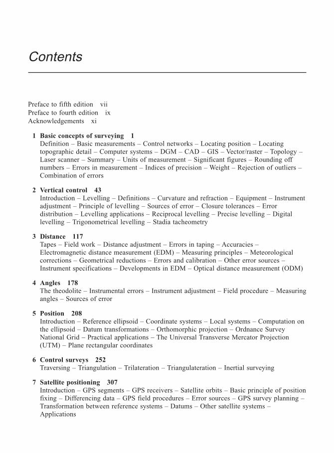
Contents
Preface to fifth edition viiPreface to fourth edition ixAcknowledgements xi
1 Basic concepts of surveying 1
Definition – Basic measurements – Control networks – Locating position – Locatingtopographic detail – Computer systems – DGM – CAD – GIS – Vector/raster – Topology –Laser scanner – Summary – Units of measurement – Significant figures – Rounding offnumbers – Errors in measurement – Indices of precision – Weight – Rejection of outliers –Combination of errors
2 Vertical control 43
Introduction – Levelling – Definitions – Curvature and refraction – Equipment – Instrumentadjustment – Principle of levelling – Sources of error – Closure tolerances – Errordistribution – Levelling applications – Reciprocal levelling – Precise levelling – Digitallevelling – Trigonometrical levelling – Stadia tacheometry
3 Distance 117
Tapes – Field work – Distance adjustment – Errors in taping – Accuracies –Electromagnetic distance measurement (EDM) – Measuring principles – Meteorologicalcorrections – Geometrical reductions – Errors and calibration – Other error sources –Instrument specifications – Developments in EDM – Optical distance measurement (ODM)
4 Angles 178
The theodolite – Instrumental errors – Instrument adjustment – Field procedure – Measuringangles – Sources of error
5 Position 208
Introduction – Reference ellipsoid – Coordinate systems – Local systems – Computation onthe ellipsoid – Datum transformations – Orthomorphic projection – Ordnance SurveyNational Grid – Practical applications – The Universal Transverse Mercator Projection(UTM) – Plane rectangular coordinates
6 Control surveys 252
Traversing – Triangulation – Trilateration – Triangulateration – Inertial surveying
7 Satellite positioning 307
Introduction – GPS segments – GPS receivers – Satellite orbits – Basic principle of positionfixing – Differencing data – GPS field procedures – Error sources – GPS survey planning –Transformation between reference systems – Datums – Other satellite systems –Applications
8 Curves 347
Circular curves – Setting out curves – Compound and reverse curves – Short and/or small-radius curves – Transition curves – Setting-out data – Cubic spiral and cubic parabola –Curve transitional throughout – The osculating circle – Vertical curves
9 Earthworks 420
Areas – Partition of land – Cross-sections – Dip and strike – Volumes – Mass-hauldiagrams
10 Setting out (dimensional control) 464
Protection and referencing – Basic setting-out procedures using coordinates – Technique forsetting out a direction – Use of grids – Setting out buildings – Controlling verticality – Controllinggrading excavation – Rotating lasers – Laser hazards – Route location – Underground surveying– Gyro-theodolite – Line and level – Responsibility on site – Responsibility of the setting-outengineer
Index 517
vi Contents
Preface to the fourth edition
This book was originally intended to combine volumes 1 and 2 of Engineering Surveying, 3rd and2nd editions respectively. However, the technological developments since the last publication date(1984) have been so far-reaching as to warrant the complete rewriting, modernizing and productionof an entirely new book.
Foremost among these developments are the modern total stations, including the automatic self-seeking instruments; completely automated, ‘field to finish’ survey systems; digital levels; land/geographic information systems (L/GIS) for the managing of any spatially based information oractivity; inertial survey systems (ISS); and three-dimensional position fixing by satellites (GPS).
In order to include all this new material and still limit the size of the book a conscious decisionwas made to delete those topics, namely photogrammetry, hydrography and field astronomy, moreadequately covered by specialist texts.
In spite of the very impressive developments which render engineering surveying one of themost technologically advanced subjects, the material is arranged to introduce the reader to elementaryprocedures and instrumentation, giving a clear understanding of the basic concept of measurementas applied to the capture, processing and presentation of spatial data. Chapters 1 and 4 deal with thebasic principles of surveying, vertical control, and linear and angular measurement, in order topermit the student early access to the associated equipment. Chapter 5 deals with coordinatesystems and reference datums necessary for an understanding of satellite position fixing and anappreciation of the various forms in which spatial data can be presented to an L/GIS. Chapter 6deals with control surveys, paying particular attention to GPS, which even in its present incompletestage has had a revolutionary impact on all aspects of surveying. Chapter 7 deals with elementary,least squares data processing and provides an introduction to more advanced texts on this topic.Chapters 8 to 10 cover in detail those areas (curves, earthworks and general setting out on site) ofspecific interest to the engineer and engineering surveyor. Each chapter contains a section of‘Worked Examples’, carefully chosen to clearly illustrate the concepts involved. Student exercises,complete with answers, are supplied for private study. The book is aimed specifically at students ofsurveying, civil, mining and municipal engineering and should also prove valuable for the continuingeducation of professionals in these fields.
W. Schofield

This Page Intentionally Left Blank
Preface to the fifth edition
Since the publication of the fourth edition of this book, major changes have occurred in thefollowing areas:• surveying instrumentation, particularly Robotic Total Stations with Automatic Target Recognition,
reflectorless distance measurement, etc., resulting in turnkey packages for machine guidanceand deformation monitoring. In addition there has been the development of a new instrumentand technique known as laser scanning
• GIS, making it a very prominent and important part of geomatic engineering• satellite positioning, with major improvements to the GPS system, the continuance of the GLONASS
system, and a proposal for a European system called GALILEO• national and international co-ordinate systems and datums as a result of the increasing use of
satellite systems.All these changes have been dealt with in detail, the importance of satellite systems being
evidenced by a new chapter devoted entirely to this topic.In order to include all this new material and still retain a economical size for the book, it was
necessary but regrettable to delete the chapter on Least Squares Estimation. This decision wasbased on a survey by the publishers that showed this important topic was not included in themajority of engineering courses. It can, however, still be referred to in the fourth edition or inspecialised texts, if required.
All the above new material has been fully expounded in the text, while still retaining the manyworked examples which have always been a feature of the book. It is hoped that this new editionwill still be of benefit to all students and practitioners of those branches of engineering whichcontain a study and application of engineering surveying.
W. SchofieldFebruary 2001

This Page Intentionally Left Blank
Acknowledgements
The author wishes to acknowledge and thank all those bodies and individuals who contributed inany way to the formation of this book.
For much of the illustrative material thanks are due to Intergraph (UK) Ltd, Leica (UK) Ltd,Trimble (UK) Ltd, Spectra-Precision Ltd, Sokkisha (UK) Ltd, and the Ordnance Survey of GreatBritain (OSGB).
I am also indebted to OSGB for their truly excellent papers, particularly ‘A Guide to Co-ordinateSystems in Great Britain’, which formed the basis of much of the information in chapter 7.
I must also acknowledge the help received from the many papers, seminars, conferences, andcontinued quality research produced by the IESSG of the University of Nottingham.
Finally, may I say thank you to Pat Affleck of the Faculty of Technology, Kingston University,who freely and unstintingly typed all this new material.

This Page Intentionally Left Blank
1
Basic concepts of surveying
The aim of this chapter is to introduce the reader to the basic concepts of surveying. It is thereforethe most important chapter and worthy of careful study and consideration.
1.1 DEFINITION
Surveying may be defined as the science of determining the position, in three dimensions, ofnatural and man-made features on or beneath the surface of the Earth. These features may then berepresented in analog form as a contoured map, plan or chart, or in digital form as a three-dimensional mathematical model stored in the computer. This latter format is referred to as a digital
ground model (DGM).In engineering surveying, either or both of the above formats may be utilized in the planning,
design and construction of works, both on the surface and underground. At a later stage, surveyingtechniques are used in the dimensional control or setting out of the designed constructional elementsand also in the monitoring of deformation movements.
In the first instance, surveying requires management and decision making in deciding the appropriatemethods and instrumentation required to satisfactorily complete the task to the specified accuracyand within the time limits available. This initial process can only be properly executed after verycareful and detailed reconnaissance of the area to be surveyed.
When the above logistics are complete, the field work – involving the capture and storage of fielddata – is carried out using instruments and techniques appropriate to the task in hand.
The next step in the operation is that of data processing. The majority, if not all, of the computationwill be carried out by computer, ranging in size from pocket calculator to mainframe. The methodsadopted will depend upon the size and precision of the survey and the manner of its recording;whether in a field book or a data logger. Data representation in analog or digital form may now becarried out by conventional cartographic plotting or through a totally automated system using acomputer-driven flat-bed plotter. In engineering, the plan or DGM is used for the planning anddesign of a construction project. This project may comprise a railroad, highway, dam, bridge, oreven a new town complex. No matter what the work is, or how complicated, it must be set out onthe ground in its correct place and to its correct dimensions, within the tolerances specified. To thisend, surveying procedures and instrumentation are used, of varying precision and complexity,depending on the project in hand.
Surveying is indispensable to the engineer in the planning, design and construction of a project,so all engineers should have a thorough understanding of the limits of accuracy possible in theconstruction and manufacturing processes. This knowledge, combined with an equal understandingof the limits and capabilities of surveying instrumentation and techniques, will enable the engineerto successfully complete his project in the most economical manner and shortest time possible.
2 Engineering Surveying
1.2 BASIC MEASUREMENTS
Surveying is concerned with the fixing of position whether it be control points or points of topographicdetail and, as such, requires some form of reference system.
The physical surface of the Earth, on which the actual survey measurements are carried out, ismathematically non-definable. It cannot therefore be used as a reference datum on which to computeposition.
An alternative consideration is a level surface, at all points normal to the direction of gravity.Such a surface would be formed by the mean position of the oceans, assuming them free from allexternal forces, such as tides, currents, winds, etc. This surface is called the geoid and is theequipotential surface at mean sea level. The most significant aspect of this surface is that surveyinstruments are set up relative to it. That is, their vertical axes, which are normal to the plate bubbleaxes used in the setting-up process, are in the direction of the force of gravity at that point. Indeed,the points surveyed on the physical surface of the Earth are frequently reduced to their equivalentposition on the geoid by projection along their gravity vectors. The reduced level or elevation of apoint is its height above or below the geoid as measured in the direction of its gravity vector (orplumb line) and is most commonly referred to as its height above or below mean sea level (MSL).However, due to variations in the mass distribution within the Earth, the geoid is also an irregularsurface which cannot be used for the mathematical location of position.
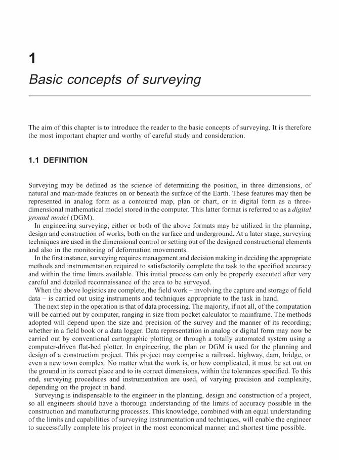
The mathematically definable shape which best fits the shape of the geoid is an ellipsoid formedby rotating an ellipse about its minor axis. Where this shape is used by a country as the surface forits mapping system, it is termed the reference ellipsoid. Figure 1.1 illustrates the relationship of theabove surfaces.
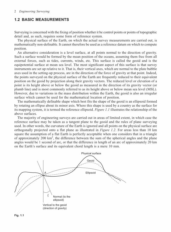
The majority of engineering surveys are carried out in areas of limited extent, in which case thereference surface may be taken as a tangent plane to the geoid and the rules of plane surveyingused. In other words, the curvature of the Earth is ignored and all points on the physical surface areorthogonally projected onto a flat plane as illustrated in Figure 1.2. For areas less than 10 kmsquare the assumption of a flat Earth is perfectly acceptable when one considers that in a triangleof approximately 200 km2, the difference between the sum of the spherical angles and the planeangles would be 1 second of arc, or that the difference in length of an arc of approximately 20 kmon the Earth’s surface and its equivalent chord length is a mere 10 mm.
Fig. 1.1
Physical surface
Geoid
EllipsoidA
ξNormal (to the
ellipsoid)
Vertical to the geoid
(direction of gravity)
Basic concepts of surveying 3
C
B
A
B′
C′
A′
Fig. 1.2 Projection onto a plain surface
The above assumptions of a flat Earth are, however, not acceptable for elevations as the geoidwould deviate from the tangent plane by about 80 mm at 1 km or 8 m at 10 km. Elevations aretherefore referred to the geoid or MSL as it is more commonly termed. Also, from the engineeringpoint of view, it is frequently useful in the case of inshore or offshore works to have the elevationsrelated to the physical component with which the engineer is concerned.
An examination of Figure 1.2 clearly shows the basic surveying measurements needed to locatepoints A, B and C and plot them orthogonally as A′, B′ and C′. In the first instance the measuredslant distance AB will fix the position of B relative to A. However, it will then require the vertical
angle to B from A, in order to reduce AB to its equivalent horizontal distance A′B′ for the purposesof plotting. Whilst similar measurements will fix C relative to A, it requires the horizontal angle
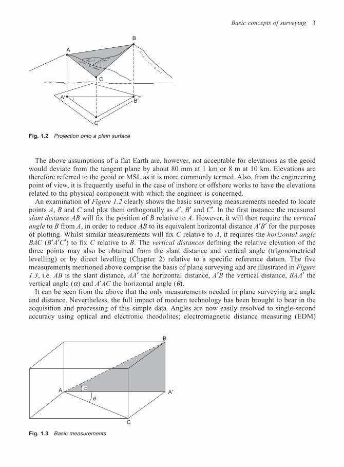
BAC (B′A′C′) to fix C relative to B. The vertical distances defining the relative elevation of thethree points may also be obtained from the slant distance and vertical angle (trigonometricallevelling) or by direct levelling (Chapter 2) relative to a specific reference datum. The fivemeasurements mentioned above comprise the basis of plane surveying and are illustrated in Figure
1.3, i.e. AB is the slant distance, AA′ the horizontal distance, A′B the vertical distance, BAA′ thevertical angle (α) and A′AC the horizontal angle (θ).
It can be seen from the above that the only measurements needed in plane surveying are angleand distance. Nevertheless, the full impact of modern technology has been brought to bear in theacquisition and processing of this simple data. Angles are now easily resolved to single-secondaccuracy using optical and electronic theodolites; electromagnetic distance measuring (EDM)
A′
B
θ
α
C
A
Fig. 1.3 Basic measurements
4 Engineering Surveying
equipment can obtain distances of several kilometres to sub-millimetre precision; lasers and north-seeking gyroscopes are virtually standard equipment for tunnel surveys; orbiting satellites andinertial survey systems, spin-offs from the space programme, are being used for position fixing offshore as well as on; continued improvement in aerial and terrestrial photogrammetric equipmentand remote sensors makes photogrammetry an invaluable surveying tool; finally, data loggers andcomputers enable the most sophisticated procedures to be adopted in the processing and automaticplotting of field data.
1.3 CONTROL NETWORKS
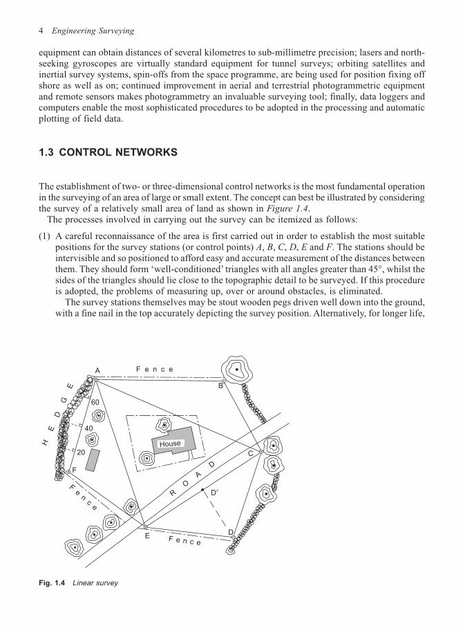
The establishment of two- or three-dimensional control networks is the most fundamental operationin the surveying of an area of large or small extent. The concept can best be illustrated by consideringthe survey of a relatively small area of land as shown in Figure 1.4.
The processes involved in carrying out the survey can be itemized as follows:
(1) A careful reconnaissance of the area is first carried out in order to establish the most suitablepositions for the survey stations (or control points) A, B, C, D, E and F. The stations should beintervisible and so positioned to afford easy and accurate measurement of the distances betweenthem. They should form ‘well-conditioned’ triangles with all angles greater than 45°, whilst thesides of the triangles should lie close to the topographic detail to be surveyed. If this procedureis adopted, the problems of measuring up, over or around obstacles, is eliminated.
The survey stations themselves may be stout wooden pegs driven well down into the ground,with a fine nail in the top accurately depicting the survey position. Alternatively, for longer life,
D′
DE
F
C
B
A F e n c e
20
40
60
House
F e n c e
Fe
nc
e
R O
A
D
H E
D
G
E
Fig. 1.4 Linear survey
Basic concepts of surveying 5
concrete blocks may be set into the ground with some form of fine mark to pinpoint the surveyposition.
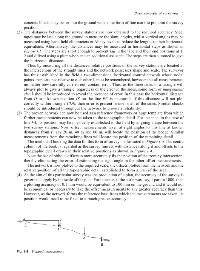
(2) The distances between the survey stations are now obtained to the required accuracy. Steeltapes may be laid along the ground to measure the slant lengths, whilst vertical angles may bemeasured using hand-held clinometers or Abney levels to reduce the lengths to their horizontalequivalents. Alternatively, the distances may be measured in horizontal steps as shown inFigure 1.5. The steps are short enough to prevent sag in the tape and their end positions at 1,2 and B fixed using a plumb-bob and an additional assistant. The steps are then summed to givethe horizontal distances.
Thus by measuring all the distances, relative positions of the survey stations are located atthe intersections of the straight lines and the network possesses shape and scale. The surveyorhas thus established in the field a two-dimensional horizontal control network whose nodalpoints are positioned relative to each other. It must be remembered, however, that all measurements,no matter how carefully carried out, contain error. Thus, as the three sides of a triangle willalways plot to give a triangle, regardless of the error in the sides, some form of independent
check should be introduced to reveal the presence of error. In this case the horizontal distancefrom D to a known position D′ on the line EC is measured. If this distance will not plotcorrectly within triangle CDE, then error is present in one or all of the sides. Similar checksshould be introduced throughout the network to prove its reliability.
(3) The proven network can now be used as a reference framework or huge template from whichfurther measurements can now be taken to the topographic detail. For instance, in the case ofline FA, its position may be physically established in the field by aligning a tape between thetwo survey stations. Now, offset measurements taken at right angles to this line at knowndistances from F, say 20 m, 40 m and 60 m, will locate the position of the hedge. Similarmeasurements from the remaining lines will locate the position of the remaining detail.
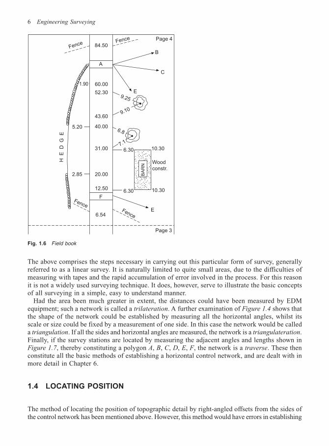
The method of booking the data for this form of survey is illustrated in Figure 1.6. The centrecolumn of the book is regarded as the survey line FA with distances along it and offsets to thetopographic detail drawn in their relative positions as shown in Figure 1.4.
Note the use of oblique offsets to more accurately fix the position of the trees by intersection,thereby eliminating the error of estimating the right angle in the other offset measurements.
The network is now plotted to the required scale, the offsets plotted from the network and therelative position of all the topographic detail established to form a plan of the area.
(4) As the aim of this particular survey was the production of a plan, the accuracy of the survey isgoverned largely by the scale of the plan. For instance, if the scale was, say, 1 part in 1000, thena plotting accuracy of 0.1 mm would be equivalent to 100 mm on the ground and it would notbe economical or necessary to take the offset measurements to any greater accuracy than this.However, as the network forms the reference base from which the measurements are taken, itsposition would need to be fixed to a much greater accuracy.
A1
2
B
Fig. 1.5 Stepped measurement
6 Engineering Surveying
The above comprises the steps necessary in carrying out this particular form of survey, generallyreferred to as a linear survey. It is naturally limited to quite small areas, due to the difficulties ofmeasuring with tapes and the rapid accumulation of error involved in the process. For this reasonit is not a widely used surveying technique. It does, however, serve to illustrate the basic conceptsof all surveying in a simple, easy to understand manner.
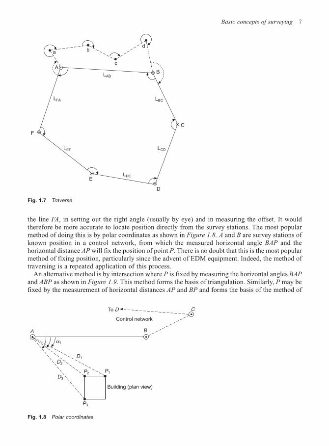
Had the area been much greater in extent, the distances could have been measured by EDMequipment; such a network is called a trilateration. A further examination of Figure 1.4 shows thatthe shape of the network could be established by measuring all the horizontal angles, whilst itsscale or size could be fixed by a measurement of one side. In this case the network would be calleda triangulation. If all the sides and horizontal angles are measured, the network is a triangulateration.Finally, if the survey stations are located by measuring the adjacent angles and lengths shown inFigure 1.7, thereby constituting a polygon A, B, C, D, E, F, the network is a traverse. These thenconstitute all the basic methods of establishing a horizontal control network, and are dealt with inmore detail in Chapter 6.
1.4 LOCATING POSITION
The method of locating the position of topographic detail by right-angled offsets from the sides ofthe control network has been mentioned above. However, this method would have errors in establishing
Fence Fence Page 4
B
C
E
E
F
Wood
constr.
H
E
D
G
E
1.90
5.20
2.85
60.00
52.30
43.60
40.00
31.00
20.00
12.50
A
84.50
9.25
9.10
6.8
7.1
10.306.30
6.30 10.30
Fence
Fence
Page 3
BA
RN
6.54
Fig. 1.6 Field book
Basic concepts of surveying 7
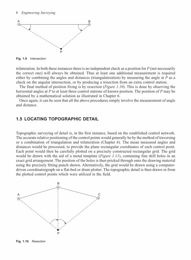
the line FA, in setting out the right angle (usually by eye) and in measuring the offset. It wouldtherefore be more accurate to locate position directly from the survey stations. The most popularmethod of doing this is by polar coordinates as shown in Figure 1.8. A and B are survey stations ofknown position in a control network, from which the measured horizontal angle BAP and thehorizontal distance AP will fix the position of point P. There is no doubt that this is the most popularmethod of fixing position, particularly since the advent of EDM equipment. Indeed, the method oftraversing is a repeated application of this process.
An alternative method is by intersection where P is fixed by measuring the horizontal angles BAP
and ABP as shown in Figure 1.9. This method forms the basis of triangulation. Similarly, P may befixed by the measurement of horizontal distances AP and BP and forms the basis of the method of
LBC
Ac
dba
LAB
LCD
LDE
LEF
LFA
E
F
D
C
B
Fig. 1.7 Traverse
C
A
Building (plan view)
P1
D1
P2D3
P3
Control network
B
To D
α1
D2
Fig. 1.8 Polar coordinates
8 Engineering Surveying
BA
P
Fig. 1.9 Intersection
trilateration. In both these instances there is no independent check as a position for P (not necessarilythe correct one) will always be obtained. Thus at least one additional measurement is requiredeither by combining the angles and distances (triangulateration) by measuring the angle at P as acheck on the angular intersection, or by producing a trisection from an extra control station.
The final method of position fixing is by resection (Figure 1.10). This is done by observing thehorizontal angles at P to at least three control stations of known position. The position of P may beobtained by a mathematical solution as illustrated in Chapter 6.
Once again, it can be seen that all the above procedures simply involve the measurement of angleand distance.
1.5 LOCATING TOPOGRAPHIC DETAIL
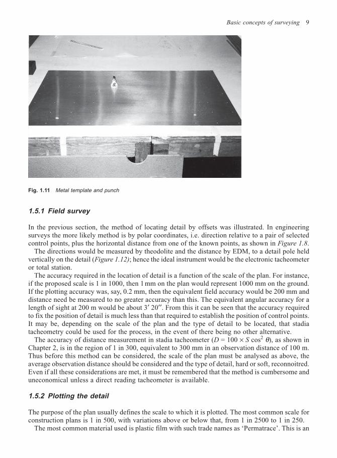
Topographic surveying of detail is, in the first instance, based on the established control network.The accurate relative positioning of the control points would generally be by the method of traversingor a combination of triangulation and trilateration (Chapter 6). The mean measured angles anddistances would be processed, to provide the plane rectangular coordinates of each control point.Each point would then be carefully plotted on a precisely constructed rectangular grid. The gridwould be drawn with the aid of a metal template (Figure 1.11), containing fine drill holes in anexact grid arrangement. The position of the holes is then pricked through onto the drawing materialusing the precisely fitting punch shown. Alternatively, the grid would be drawn using a computer-driven coordinatorgraph on a flat-bed or drum plotter. The topographic detail is then drawn in fromthe plotted control points which were utilized in the field.
Fig. 1.10 Resection
B
CA
P
Basic concepts of surveying 9
1.5.1 Field survey
In the previous section, the method of locating detail by offsets was illustrated. In engineeringsurveys the more likely method is by polar coordinates, i.e. direction relative to a pair of selectedcontrol points, plus the horizontal distance from one of the known points, as shown in Figure 1.8.
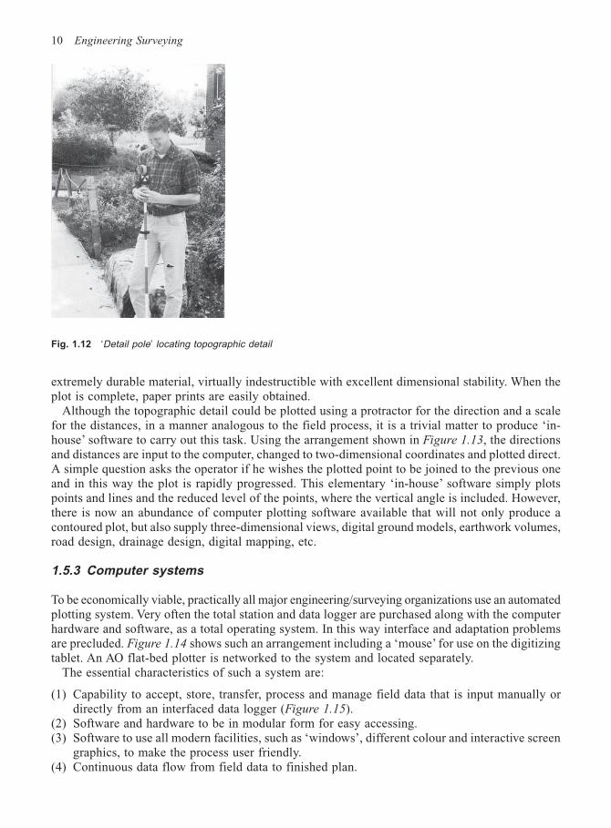
The directions would be measured by theodolite and the distance by EDM, to a detail pole heldvertically on the detail (Figure 1.12); hence the ideal instrument would be the electronic tacheometeror total station.
The accuracy required in the location of detail is a function of the scale of the plan. For instance,if the proposed scale is 1 in 1000, then 1 mm on the plan would represent 1000 mm on the ground.If the plotting accuracy was, say, 0.2 mm, then the equivalent field accuracy would be 200 mm anddistance need be measured to no greater accuracy than this. The equivalent angular accuracy for alength of sight at 200 m would be about 3′ 20′′. From this it can be seen that the accuracy requiredto fix the position of detail is much less than that required to establish the position of control points.It may be, depending on the scale of the plan and the type of detail to be located, that stadiatacheometry could be used for the process, in the event of there being no other alternative.
The accuracy of distance measurement in stadia tacheometer (D = 100 × S cos2 θ), as shown inChapter 2, is in the region of 1 in 300, equivalent to 300 mm in an observation distance of 100 m.Thus before this method can be considered, the scale of the plan must be analysed as above, theaverage observation distance should be considered and the type of detail, hard or soft, reconnoitred.Even if all these considerations are met, it must be remembered that the method is cumbersome anduneconomical unless a direct reading tacheometer is available.
1.5.2 Plotting the detail
The purpose of the plan usually defines the scale to which it is plotted. The most common scale forconstruction plans is 1 in 500, with variations above or below that, from 1 in 2500 to 1 in 250.
The most common material used is plastic film with such trade names as ‘Permatrace’. This is an
Fig. 1.11 Metal template and punch
10 Engineering Surveying
Fig. 1.12 ‘Detail pole’ locating topographic detail
extremely durable material, virtually indestructible with excellent dimensional stability. When theplot is complete, paper prints are easily obtained.
Although the topographic detail could be plotted using a protractor for the direction and a scalefor the distances, in a manner analogous to the field process, it is a trivial matter to produce ‘in-house’ software to carry out this task. Using the arrangement shown in Figure 1.13, the directionsand distances are input to the computer, changed to two-dimensional coordinates and plotted direct.A simple question asks the operator if he wishes the plotted point to be joined to the previous oneand in this way the plot is rapidly progressed. This elementary ‘in-house’ software simply plotspoints and lines and the reduced level of the points, where the vertical angle is included. However,there is now an abundance of computer plotting software available that will not only produce acontoured plot, but also supply three-dimensional views, digital ground models, earthwork volumes,road design, drainage design, digital mapping, etc.
1.5.3 Computer systems
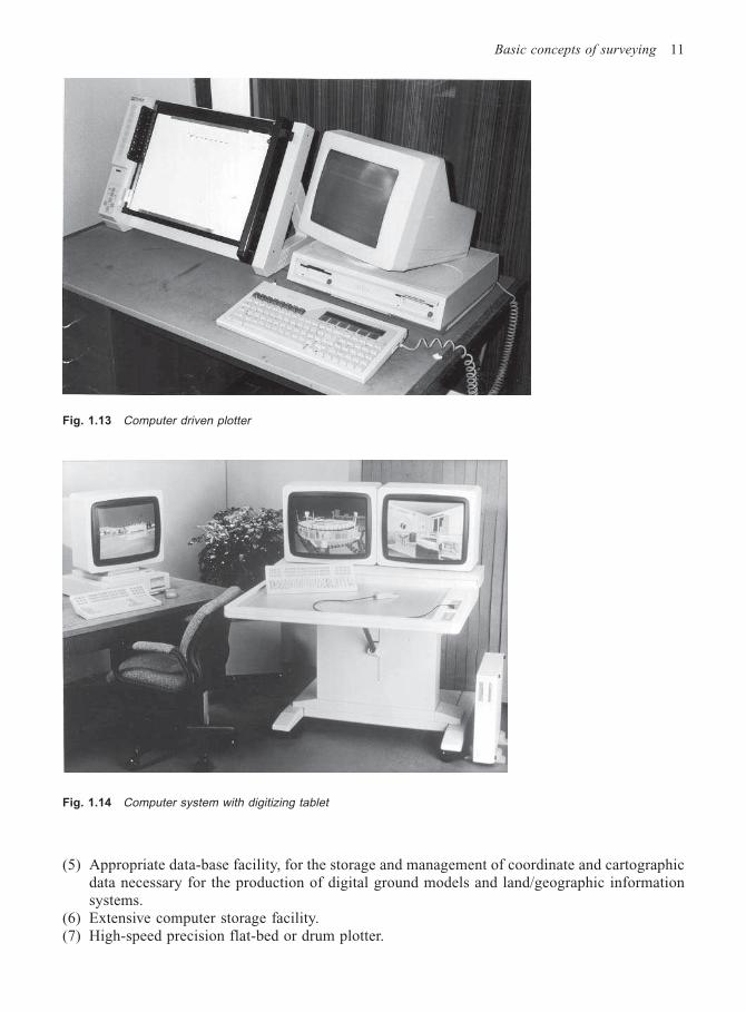
To be economically viable, practically all major engineering/surveying organizations use an automatedplotting system. Very often the total station and data logger are purchased along with the computerhardware and software, as a total operating system. In this way interface and adaptation problemsare precluded. Figure 1.14 shows such an arrangement including a ‘mouse’ for use on the digitizingtablet. An AO flat-bed plotter is networked to the system and located separately.
The essential characteristics of such a system are:
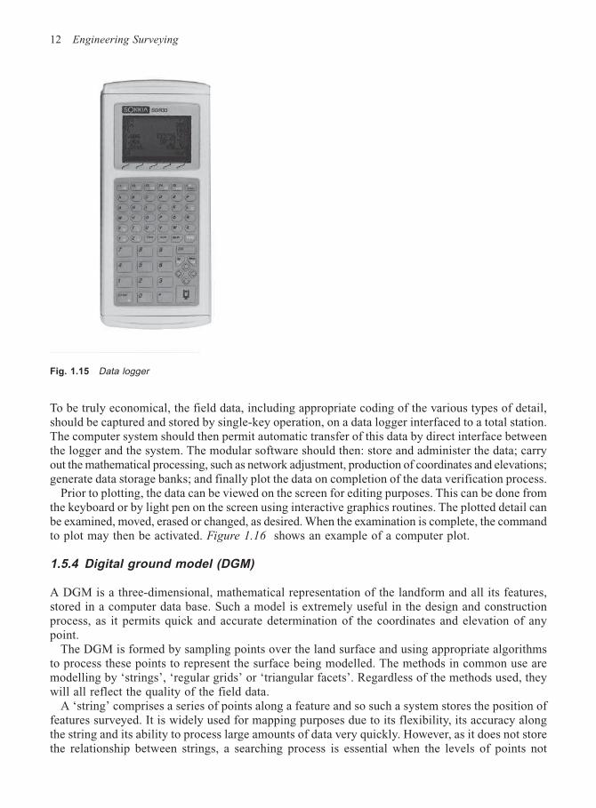
(1) Capability to accept, store, transfer, process and manage field data that is input manually ordirectly from an interfaced data logger (Figure 1.15).
(2) Software and hardware to be in modular form for easy accessing.(3) Software to use all modern facilities, such as ‘windows’, different colour and interactive screen
graphics, to make the process user friendly.(4) Continuous data flow from field data to finished plan.
Basic concepts of surveying 11
Fig. 1.13 Computer driven plotter
Fig. 1.14 Computer system with digitizing tablet
(5) Appropriate data-base facility, for the storage and management of coordinate and cartographicdata necessary for the production of digital ground models and land/geographic informationsystems.
(6) Extensive computer storage facility.(7) High-speed precision flat-bed or drum plotter.
12 Engineering Surveying
To be truly economical, the field data, including appropriate coding of the various types of detail,should be captured and stored by single-key operation, on a data logger interfaced to a total station.The computer system should then permit automatic transfer of this data by direct interface betweenthe logger and the system. The modular software should then: store and administer the data; carryout the mathematical processing, such as network adjustment, production of coordinates and elevations;generate data storage banks; and finally plot the data on completion of the data verification process.
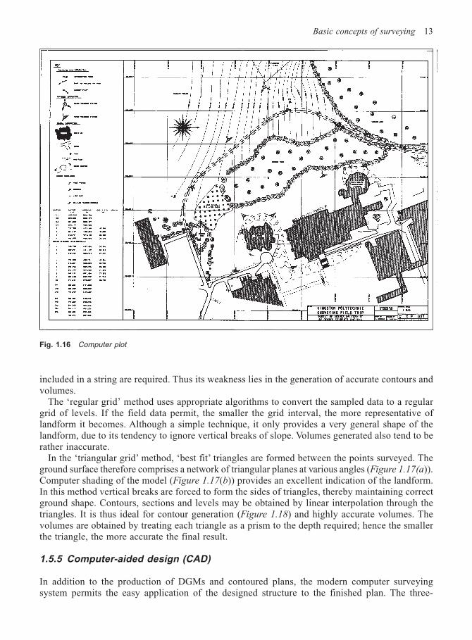
Prior to plotting, the data can be viewed on the screen for editing purposes. This can be done fromthe keyboard or by light pen on the screen using interactive graphics routines. The plotted detail canbe examined, moved, erased or changed, as desired. When the examination is complete, the commandto plot may then be activated. Figure 1.16 shows an example of a computer plot.
1.5.4 Digital ground model (DGM)
A DGM is a three-dimensional, mathematical representation of the landform and all its features,stored in a computer data base. Such a model is extremely useful in the design and constructionprocess, as it permits quick and accurate determination of the coordinates and elevation of anypoint.
The DGM is formed by sampling points over the land surface and using appropriate algorithmsto process these points to represent the surface being modelled. The methods in common use aremodelling by ‘strings’, ‘regular grids’ or ‘triangular facets’. Regardless of the methods used, theywill all reflect the quality of the field data.
A ‘string’ comprises a series of points along a feature and so such a system stores the position offeatures surveyed. It is widely used for mapping purposes due to its flexibility, its accuracy alongthe string and its ability to process large amounts of data very quickly. However, as it does not storethe relationship between strings, a searching process is essential when the levels of points not
Fig. 1.15 Data logger
Basic concepts of surveying 13
Fig. 1.16 Computer plot
included in a string are required. Thus its weakness lies in the generation of accurate contours andvolumes.
The ‘regular grid’ method uses appropriate algorithms to convert the sampled data to a regulargrid of levels. If the field data permit, the smaller the grid interval, the more representative oflandform it becomes. Although a simple technique, it only provides a very general shape of thelandform, due to its tendency to ignore vertical breaks of slope. Volumes generated also tend to berather inaccurate.
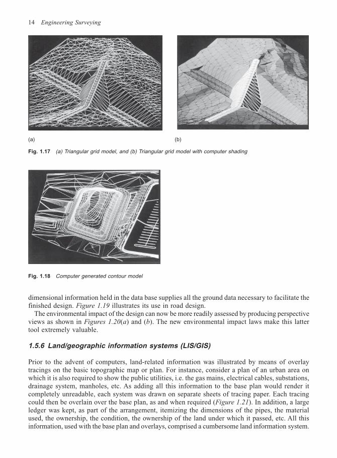
In the ‘triangular grid’ method, ‘best fit’ triangles are formed between the points surveyed. Theground surface therefore comprises a network of triangular planes at various angles (Figure 1.17(a)).Computer shading of the model (Figure 1.17(b)) provides an excellent indication of the landform.In this method vertical breaks are forced to form the sides of triangles, thereby maintaining correctground shape. Contours, sections and levels may be obtained by linear interpolation through thetriangles. It is thus ideal for contour generation (Figure 1.18) and highly accurate volumes. Thevolumes are obtained by treating each triangle as a prism to the depth required; hence the smallerthe triangle, the more accurate the final result.
1.5.5 Computer-aided design (CAD)
In addition to the production of DGMs and contoured plans, the modern computer surveyingsystem permits the easy application of the designed structure to the finished plan. The three-
14 Engineering Surveying
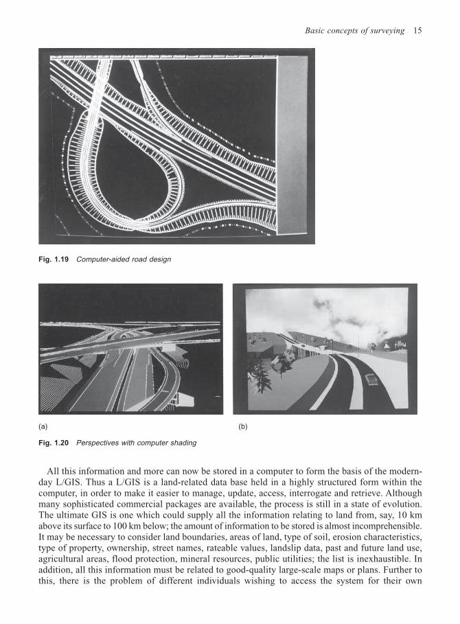
dimensional information held in the data base supplies all the ground data necessary to facilitate thefinished design. Figure 1.19 illustrates its use in road design.
The environmental impact of the design can now be more readily assessed by producing perspectiveviews as shown in Figures 1.20(a) and (b). The new environmental impact laws make this lattertool extremely valuable.
1.5.6 Land/geographic information systems (LIS/GIS)
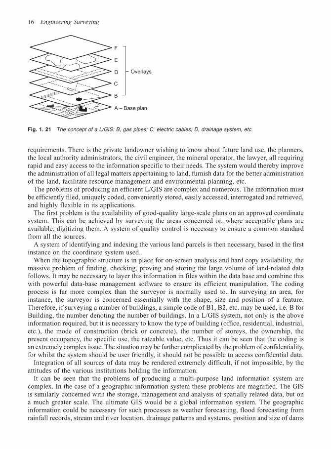
Prior to the advent of computers, land-related information was illustrated by means of overlaytracings on the basic topographic map or plan. For instance, consider a plan of an urban area onwhich it is also required to show the public utilities, i.e. the gas mains, electrical cables, substations,drainage system, manholes, etc. As adding all this information to the base plan would render itcompletely unreadable, each system was drawn on separate sheets of tracing paper. Each tracingcould then be overlain over the base plan, as and when required (Figure 1.21). In addition, a largeledger was kept, as part of the arrangement, itemizing the dimensions of the pipes, the materialused, the ownership, the condition, the ownership of the land under which it passed, etc. All thisinformation, used with the base plan and overlays, comprised a cumbersome land information system.
(a) (b)
Fig. 1.17 (a) Triangular grid model, and (b) Triangular grid model with computer shading
Fig. 1.18 Computer generated contour model
Basic concepts of surveying 15
All this information and more can now be stored in a computer to form the basis of the modern-day L/GIS. Thus a L/GIS is a land-related data base held in a highly structured form within thecomputer, in order to make it easier to manage, update, access, interrogate and retrieve. Althoughmany sophisticated commercial packages are available, the process is still in a state of evolution.The ultimate GIS is one which could supply all the information relating to land from, say, 10 kmabove its surface to 100 km below; the amount of information to be stored is almost incomprehensible.It may be necessary to consider land boundaries, areas of land, type of soil, erosion characteristics,type of property, ownership, street names, rateable values, landslip data, past and future land use,agricultural areas, flood protection, mineral resources, public utilities; the list is inexhaustible. Inaddition, all this information must be related to good-quality large-scale maps or plans. Further tothis, there is the problem of different individuals wishing to access the system for their own
Fig. 1.19 Computer-aided road design
(a) (b)
Fig. 1.20 Perspectives with computer shading
16 Engineering Surveying
requirements. There is the private landowner wishing to know about future land use, the planners,the local authority administrators, the civil engineer, the mineral operator, the lawyer, all requiringrapid and easy access to the information specific to their needs. The system would thereby improvethe administration of all legal matters appertaining to land, furnish data for the better administrationof the land, facilitate resource management and environmental planning, etc.
The problems of producing an efficient L/GIS are complex and numerous. The information mustbe efficiently filed, uniquely coded, conveniently stored, easily accessed, interrogated and retrieved,and highly flexible in its applications.
The first problem is the availability of good-quality large-scale plans on an approved coordinatesystem. This can be achieved by surveying the areas concerned or, where acceptable plans areavailable, digitizing them. A system of quality control is necessary to ensure a common standardfrom all the sources.
A system of identifying and indexing the various land parcels is then necessary, based in the firstinstance on the coordinate system used.
When the topographic structure is in place for on-screen analysis and hard copy availability, themassive problem of finding, checking, proving and storing the large volume of land-related datafollows. It may be necessary to layer this information in files within the data base and combine thiswith powerful data-base management software to ensure its efficient manipulation. The codingprocess is far more complex than the surveyor is normally used to. In surveying an area, forinstance, the surveyor is concerned essentially with the shape, size and position of a feature.Therefore, if surveying a number of buildings, a simple code of B1, B2, etc. may be used, i.e. B forBuilding, the number denoting the number of buildings. In a L/GIS system, not only is the aboveinformation required, but it is necessary to know the type of building (office, residential, industrial,etc.), the mode of construction (brick or concrete), the number of storeys, the ownership, thepresent occupancy, the specific use, the rateable value, etc. Thus it can be seen that the coding isan extremely complex issue. The situation may be further complicated by the problem of confidentiality,for whilst the system should be user friendly, it should not be possible to access confidential data.
Integration of all sources of data may be rendered extremely difficult, if not impossible, by theattitudes of the various institutions holding the information.
It can be seen that the problems of producing a multi-purpose land information system arecomplex. In the case of a geographic information system these problems are magnified. The GISis similarly concerned with the storage, management and analysis of spatially related data, but ona much greater scale. The ultimate GIS would be a global information system. The geographicinformation could be necessary for such processes as weather forecasting, flood forecasting fromrainfall records, stream and river location, drainage patterns and systems, position and size of dams
Overlays
E
D
C
B
A – Base plan
F
Fig. 1. 21 The concept of a L/GIS: B, gas pipes; C, electric cables; D, drainage system, etc.
Basic concepts of surveying 17
and reservoirs, land use and transportation patterns over very wide areas; once again the list isinexhaustible.
Thus, although the formation of a L/GIS is a formidable problem, the necessity for an efficientand accurate source of land-related data makes it mandatory as a powerful land management tool.As good-quality plans form the basis of such a system, it is feasible that surveyors, who are theexperts in measurement and position, should play a prominent part in the design and managementof such systems.
1.5.6.1 GIS data
From the broad introduction given to GIS it can be seen that a GIS is a computer-based system forhandling not only physical location but also the attributes associated with that location. It thuspossesses a graphical display in two or three dimensions of the spatial data, combined with adatabase for the non-spatial data, i.e. the attribute information. The prime aspect in the constructionof a GIS is the acquisition, from many different sources, conversion and entry of the data.
The spatial data may be acquired from a variety of sources: from digitized maps and plans, fromaerial photographs, from satellite imagery, or directly from GPS surveys. However, in order torepresent this complex, three-dimensional reality in a spatial database, it is modelled using points,lines, areas, surfaces and networks. For instance, if we consider an underground drainage system,the pipes would be represented by lines; the manhole positions by points; the parcels of landownership forming closed boundaries whose polygon shape is defined by coordinates would berepresented by areas; whilst the three-dimensional land surface through which the pipes pass wouldbe represented by a surface. Such a GIS would probably incorporate a network, which representsthe whole branching system of pipes (line segments), and is used to simulate flow through the pipesor indicate the buildings affected by a break in the pipe network at a specific point. The attributesattached to this network, such as type and size of pipe, depth below ground, rate of flow, gradients,etc., would be stored in the associated database. The linking of the spatially referenced data withtheir attributes is the basis of GIS.
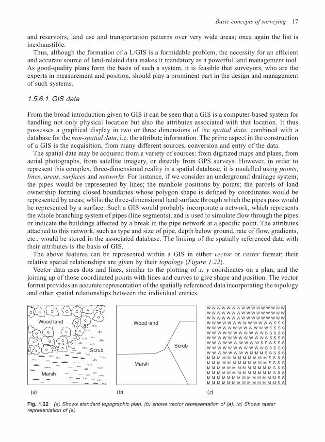
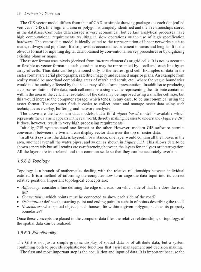
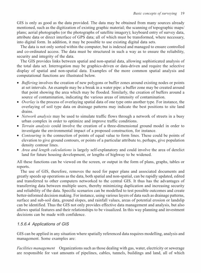
The above features can be represented within a GIS in either vector or raster format; theirrelative spatial relationships are given by their topology (Figure 1.22).
Vector data uses dots and lines, similar to the plotting of x, y coordinates on a plan, and thejoining up of those coordinated points with lines and curves to give shape and position. The vectorformat provides an accurate representation of the spatially referenced data incorporating the topologyand other spatial relationships between the individual entries.
Scrub
Marsh
Wood land
(c)(a) (b)
Marsh
Scrub
Wood land
Fig. 1.22 (a) Shows standard topographic plan. (b) shows vector representation of (a). (c) Shows rasterrepresentation of (a)
W W W W W W W W W W W W W W W W
W W W W W W W W W W W W W W W W
W W W W W W W W W W W W W W W W
W W W W W W W W W W W W W S S S
W W W W W W W W W W W W S S S S
W W W W W W W W W W W S S S S S
W W W W W W W W W W W S S S S S
W W W W W W W W W W S S S S S S
W W W W W W W W W W W S S S S S
W W W W W W W W M M M S S S S S
M M M M M M M M M M M M S S S S
M M M M M M M M M M M M S S S S
M M M M M M M M M M M M M S S S
M M M M M M M M M M M M M S S S
M M M M M M M M M M M M M M S S
M M M M M M M M M M M M M M S S
18 Engineering Surveying
The GIS vector model differs from that of CAD or simple drawing packages as each dot (calledvertices in GIS), line segment, area or polygon is uniquely identified and their relationships storedin the database. Computer data storage is very economical, but certain analytical processes havehigh computational requirements resulting in slow operations or the use of high specificationhardware. The vector data model is ideally suited to the representation of linear networks such asroads, railways and pipelines. It also provides accurate measurement of areas and lengths. It is theobvious format for inputting digital data obtained by conventional survey procedures or by digitizingexisting plans or maps.
The raster format uses pixels (derived from ‘picture elements’) or grid cells. It is not as accurateor flexible as vector format as each coordinate may be represented by a cell and each line by anarray of cells. Thus data can be positioned only to the nearest grid cell. Examples of data in theraster format are aerial photographs, satellite imagery and scanned maps or plans. An example fromreality would be moorland comprising areas of marsh and scrub, etc., where the vague boundarieswould not be unduly affected by the inaccuracy of the format presentation. In addition to producinga coarse resolution of the data, each cell contains a single value representing the attribute containedwithin the area of the cell. The resolution of the data may be improved using a smaller cell size, butthis would increase the computer storage, which tends, in any case, to be uneconomical using theraster format. The computer finds it easier to collect, store and manage raster data using suchtechniques as overlay, buffering and network analysis.
The above are the two main data models, but a third object-based model is available whichrepresents the data as it appears in the real world, thereby making it easier to understand (Figure 1.20).It does, however, result in very high processing requirements.
Initially, GIS systems used one format or the other. However, modern GIS software permitsconversion between the two and can display vector data over the top of raster data.
In all GIS systems, the data is layered. For instance, one layer would contain all the houses in thearea, another layer all the water pipes, and so on, as shown in Figure 1.21. This allows data to beshown separately but still retains cross-referencing between the layers for analyses or interrogation.All the layers are interrelated and to a common scale so that they can be accurately overlain.
1.5.6.2 Topology
Topology is a branch of mathematics dealing with the relative relationships between individualentities. It is a method of informing the computer how to arrange the data input into its correctrelative position. Important topological concepts are:
• Adjacency: consider a line defining the edge of a road: on which side of that line does the roadlie?
• Connectivity: which points must be connected to show each side of the road?• Orientation: defines the starting point and ending point in a chain of points describing the road?• Nestedness: what spatial objects, such houses, lie within a given polygon, such as its property
boundaries?
Once these concepts are placed in the computer data files the relative relationships, or topology, ofthe spatial data can be realized.
1.5.6.3 Functionality
The GIS is not just a simple graphic display of spatial data or of attribute data, but a systemcombining both to provide sophisticated functions that assist management and decision making.
The first and most important step is the acquisition and input of data. It is important because the
Basic concepts of surveying 19
GIS is only as good as the data provided. The data may be obtained from many sources alreadymentioned, such as the digitization of existing graphic material; the scanning of topographic maps/plans; aerial photographs (or the photographs of satellite imagery); keyboard entry of survey data,attribute data or direct interface of GPS data; all of which must be transformed, where necessary,into digital form. In addition, it may be possible to use existing digital data sets.
The data is not only sorted within the computer, but is indexed and managed to ensure controlledand co-ordinated access. The data must be structured in such a way as to ensure the reliability,security and integrity of the data.
The GIS provides links between spatial and non-spatial data, allowing sophisticated analysis ofthe total data set. Interrogation may be graphics-driven or data-driven and require the selectivedisplay of spatial and non-spatial data. Examples of the more common spatial analysis andcomputational functions are illustrated below.
• Buffering involves the creation of new polygons or buffer zones around existing nodes or pointsat set intervals. An example may be a break in a water pipe: a buffer zone may be created aroundthat point showing the area which may be flooded. Similarly, the creation of buffers around asource of contamination, indicating the various areas of intensity of contamination.
• Overlay is the process of overlaying spatial data of one type onto another type. For instance, theoverlaying of soil type data on drainage patterns may indicate the best positions to site landdrains.
• Network analysis may be used to simulate traffic flows through a network of streets in a busyurban complex in order to optimize and improve traffic conditions.
• Terrain analysis could involve the creation of a three-dimensional ground model in order toinvestigate the environmental impact of a proposed construction, for instance.
• Contouring is the connection of points of equal value to form lines. These could be points ofelevation to give ground contours, or points of a particular attribute to, perhaps, give populationdensity contour lines.
• Area and length calculations is largely self-explanatory and could involve the area of derelictland for future housing development, or lengths of highway to be widened.
All these functions can be viewed on the screen, or output in the form of plans, graphs, tables orreports.
The use of GIS, therefore, removes the need for paper plans and associated documents andgreatly speeds up operations as the data, both spatial and non-spatial, can be rapidly updated, editedand transferred to other computers networked to the central GIS. It thus has the advantages oftransferring data between multiple users, thereby minimizing duplication and increasing securityand reliability of the data. Specific scenarios can be modelled to test possible outcomes and createbetter-informed decision making. For instance, using various layers of data such as drainage patterns,surface and sub-soil data, ground slopes, and rainfall values, areas of potential erosion or landslipcan be identified. Thus the GIS not only provides effective data management and analysis, but alsoallows spatial features and their relationships to be visualized. In this way planning and investmentdecisions can be made with confidence.
1.5.6.4 Applications of GIS
GIS can be applied in any situation where spatially referenced data requires modelling, analysis andmanagement. Some examples are:
Facilities management Organizations such as those dealing with gas, water, electricity or sewerageare responsible for vast amounts of pipelines, cables, tunnels, buildings and land, all of which
20 Engineering Surveying
require monitoring, maintenance and management in order to give an efficient and effective serviceto customers.Highways maintenance This situation is very similar to the above but deals with roads, motorways,bridges, road furniture, etc., all of which is spatially referenced and requires maintenance andmanagement. Three-dimensional ground models can be used for design and environmental impactstudies.Housing associations These organizations are responsible for the building, maintenance, leasing,renting or sale of houses on a massive scale. Not only is the geographic distribution of the propertiesrequired, but full details of the properties are also vital. To assist in operational management andstrategic planning such information as rent arrears and the geographic clustering; housing types;properties sold, leased or rented; conditions/repairs; population trends; development sites; bad debthotspots – the list is endless. Thus paper-based land terriers are replaced, there is high-qualityvisual representation of spatial data, improved productivity and more efficient management tools.
The above examples clearly illustrate the importance of GIS and the manner of its application.Other areas which would benefit from its use are environmental management; transportation;market analysis using, say, socio-economic population distribution patterns; and land use patterns.Indeed, wherever the relationship and interaction of various spatially referenced data is required,GIS provides a powerful analytical tool.
1.5.7 Laser scanner
Laser scanning, in a terrestrial or airborne form, is a relatively new and powerful surveying technique.The system provides 3-D location of features and surfaces quickly and accurately, in real time ifnecessary.
The system is a combined hardware and software package. The hardware consists of a tripod-mounted pulsed laser range finder and a mechanical scanner. The time taken by the laser pulse tohit the target and return is measured by the picosecond timing circuitry of the unit’s signal detector,and the range calculated. The amount of energy reflected by the target surface is a function of thetarget’s characteristics, such as roughness, colour, etc. The amplitude of the returned pulse gives anintensity or brightness value. A Class 1, eye safe laser, operating in the near-infrared region at0.9 µm is used, with an operating range of 0.1–350 m and a beam width of about 300 mm at 100 mdistance. The scanning density can be altered and set in increments of 0.25°, 0.5° and 1°. A rotatingpolygonal mirror directs the laser beam in the horizontal and vertical directions. Angle encodersrecord the orientation of the mirror. Thus, each point within the raster image of range and intensityis accurately positioned in 3-D and illustrated via the controlling laptop PC. Data can be acquiredat rates as high as 6000 measurements per second using a laser pulsing at 20 kHz, with accuraciesof ± 5 mm. In some systems, using special targets other than the actual ground or structure surfaces,accuracies of ±2 mm are achievable. If the tripod is set over a point of known coordinates andorientated into the coordinate system in use, then the spatial position of the points scanned can bedefined in that system. At the present time the laser scanning device can vary in weight from13.5 kg to 30 kg, depending on the make of the unit. One particular unit incorporates a colour CCDcamera to capture scenes for later analysis. This latter point indicates the many and varied ways inwhich modern technology is being utilized in spatial data capture.
The laser device is controlled and the data processed by means of a PC connected to it throughserial and parallel cables. The scanner parameters are set by the operator and the data downloadedin real time for 3-D screen viewing. The raster style 3-D picture can be rotated in space for viewingfrom any angle as scanning takes place. The range to points can be queried and inter-distancesbetween points measured. The screen image enables the operator to evaluate the quality of the dataand, if necessary, change the parameter settings or move the scanner to a better site position. If the
Basic concepts of surveying 21
survey area is extensive, reflectors may be used in the scanned portions to allow the co-ordinationand merging of various scans. The intensities of the laser signals, which in effect describe thecharacteristics of the points in question, may be illustrated on the screen using different colours,thereby highlighting variations in the data. The data files are naturally quite large, and a figurequoted for the survey of a room area of 30 m2 with pillars and windows, was 2 Mb. For best resultsthe field data can be transferred to a more powerful graphics workstation for further processing,editing and analysis. Precise 2-D drawings with elevations, or 3-D models can be generated.
Applications of this revolutionary system occur in all aspects of surveying, mining and civilengineering. It is particularly useful in inaccessible locations such as building facades, mine andquarry faces, and areas which are unsafe such as cliff faces, airport runways, busy highways andhazardous areas in chemical and nuclear installations. The applications mentioned are those that areparticularly difficult for conventional surveying procedures. However, this does not preclude itsuse in all those areas of conventional survey, including tunnelling.
The principles outlined above can also be used in airborne situations where the aircraft equippedwith GPS is positioned in space by a single ground-based GPS station and an inertial navigationunit is used for the determination of roll, pitch and yaw. In this way the position and attitude of thescanner is fixed in the GPS coordinate system (WGS84), and so also are the terrain positions.Transformation to a local reference system will also require a geoid model.
The flying height varies from 300–1000 m, with the laser beam scanning at a rate as high as25000 pulses per second across a swath beneath the aircraft.
At the present time, ground-based systems are large, heavy and expensive, but there is no doubtthat, within a very short period by time, they will become smaller, more sophisticated, and a majormethod of 3-D detailing.
1.6 SUMMARY
In the preceding sections an attempt has been made to outline the basic concepts of surveying.Because of their importance they will now be summarized as follows:
(1) Reconnaissance is the first and most important step in the surveying process. Only after acareful and detailed reconnaissance of the area can the surveyor decide upon the techniquesand instrumentation required to economically complete the work and meet the accuracyspecifications.
(2) Control networks not only form a reference framework for locating the position of topographicdetail and setting out constructions, but may also be used as a base for minor control networkscontaining a greater number of control stations at shorter distances apart and to a lower orderof accuracy, i.e. a, b, c, d in Figure 1.7. These minor control stations may be better placed forthe purpose of locating the topographic detail.
This process of establishing the major control first to the highest order of accuracy, as aframework on which to connect the minor control, which is in turn used as a reference frameworkfor detailing, is known as working from the whole to the part and forms the basis of all goodsurveying procedure.
(3) Errors are contained in all measurement procedures and a constant battle must be waged by thesurveyor to minimize their effect.
It follows from this that the greater the accuracy specifications the greater the cost of thesurvey for it results in more observations, taken with greater care, over a longer period of time,using more precise (and therefore more expensive) equipment. It is for this reason that major
22 Engineering Surveying
control networks contain the minimum number of stations necessary and surveyors adhere tothe economic principle of working to an accuracy neither greater than nor less than that required.
(4) Independent checks should be introduced not only into the field work, but also into the subsequentcomputation and reduction of field data. In this way, errors can be quickly recognized and dealtwith.
Data should always be measured more than once. Examination of several measurements willgenerally indicate the presence of blunders in the measuring process. Alternatively, closeagreement of the measurements is indicative of high precision and generally acceptable fielddata, although, as shown later, high precision does not necessarily mean high accuracy, andfurther data processing may be necessary to remove any systematic error that may be present.
(5) Commensurate accuracy is advised in the measuring process, i.e. the angles should be measuredto the same degree of accuracy as the distances and vice versa. The following rule is advocatedby most authorities for guidance: 1′′ of arc subtends 1 mm at 200 m. This means that if distanceis measured to, say, 1 in 200 000, the angles should be measured to 1′′ of arc, and so on.
(6) The model used to illustrate the concepts of surveying is limited in its application and for mostengineering surveys may be considered obsolete. Nevertheless it does serve to illustrate thosebasic concepts in simple, easily understood terms, to which the beginner can more easily relate.
In the majority of engineering projects, sophisticated instrumentation such as ‘total stations’ interfacedwith electronic data loggers is the norm. In some cases the data loggers can directly drive plotters,thereby producing plots in real time.
Further developments are in the use of satellites to fix three-dimensional position. Such is theaccuracy and speed of positioning using the latest GPS satellites that they may be used to establishcontrol points, fix topographic detail, set out position on site and carry out continuous deformationmonitoring. Indeed, in the very near future, the use of networks may be of purely historical interest.
Also, inertial positioning systems (IPS) provide a continuous output of position from a knownstarting point, independent of any external agency, environmental conditions or location. Integrationof GPS and IPS may provide a formidable positioning process in the future.
However, regardless of the technological advances in surveying, attention must always be givento instrument calibration, carefully designed projects and meticulous observation. As surveying isessentially the science of measurement, it is necessary to examine the measured data in more detail,as follows.
1.7 UNITS OF MEASUREMENT
The system most commonly used in the measurement of distance and angle is the ‘SystemeInternationale’, abbreviated to SI. The basic units of prime interest are:
Length in metres (m)
from which we have:
1 m = 103 millimetres (mm)
1 m = 10–3 kilometres (km)
Thus a distance measured to the nearest millimetre would be written as, say, 142.356 m.Similarly for areas we have:
1 m2 = 106 mm2
Basic concepts of surveying 23
104 m2 = 1 hectare (ha)
106 m2 = 1 square kilometre (km2)
and for volumes, m3 and mm3.There are three systems used for plane angles, namely the sexagesimal, the centesimal and
radiants (arc units).The sexagesimal units are used in many parts of the world, including the UK, and measure angles
in degrees (°), minutes (′) and seconds (′′) of arc, i.e.
1° = 60′1′ = 60′′
and an angle is written as, say, 125° 46′ 35′′.The centesimal system is quite common in Europe and measures angles in gons (g), i.e.
1 gon = 100 cgon (centigon)
1 cgon = 10 mgon (milligon)
A radian is that angle subtended at the centre of a circle by an arc on the circumference equal inlength to the radius of the circle, i.e.
2π rad = 360° = 400 gon
Thus to transform degrees to radians, multiply by π /180°, and to transform radians to degrees,multiply by 180°/π. It can be seen that:
1 rad = 57.2957795° = 63.6619972 gon
A factor commonly used in surveying to change angles from seconds of arc to radians is:
α rad = α ′′/206 265
where 206 265 is the number of seconds in a radian.Other units of interest will be dealt with where they occur in the text.
1.8 SIGNIFICANT FIGURES
Engineers and surveyors communicate a great deal of their professional information using numbers.It is important, therefore, that the number of digits used, correctly indicates the accuracy withwhich the field data were measured. This is particularly important since the advent of pocketcalculators, which tend to present numbers to as many as eight places of decimals, calculated fromdata containing, at the most, only three places of decimals, whilst some eliminate all trailing zeros.This latter point is important, as 2.00 m is an entirely different value to 2.000 m. The latter numberimplies estimation to the nearest millimetre as opposed to the nearest 10 mm implied by the former.Thus in the capture of field data, the correct number of significant figures should be used.
By definition, the number of significant figures in a value is the number of digits one is certainof plus one, usually the last, which is estimated. The number of significant figures should not beconfused with the number of decimal places. A further rule in significant figures is that in allnumbers less than unity, the number of zeros directly after the decimal point and up to the first non-zero digit are not counted. For example:
24 Engineering Surveying
Two significant figures: 40, 42, 4.2, 0.43, 0.0042, 0.040
Three significant figures: 836, 83.6, 80.6, 0.806, 0.0806, 0.00800
Difficulties can occur with zeros at the end of a number such as 83600, which may have three, fouror five significant figures. This problem is overcome by expressing the value in powers of ten, i.e.8.36 × 104 implies three significant figures, 8.360 × 10⁴ implies four significant figures and8.3600 × 104 implies five significant figures.
It is important to remember that the accuracy of field data cannot and should not be improved inthe computational processes to which it is subjected.
Consider the addition of the following numbers:
155.4867.08
2183.042.0058
If added on a pocket calculator the answer is 2387.5718; however, the correct answer with dueregard to significant figures is 2387.6. It is rounded off to the most extreme right-hand columncontaining all the significant figures, which in the example is the column immediately after thedecimal point. In the case of 155.486 + 7.08 + 2183 + 42.0058 the answer is 2388. This rule alsoapplies to subtraction.
In multiplication and division, the answer should be rounded off to the number of significantfigures contained in that number having the least number of significant figures in the computationalprocess. For instance, 214.8432 × 3.05 = 655.27176, when computed on a pocket calculator;however, as 3.05 contains only three significant figures, the correct answer is 655. Consider428.4 × 621.8 = 266 379.12, which should now be rounded to 266 400 = 2.664 × 10⁵, which has foursignificant figures. Similarly, 41.8 ÷ 2.1316 = 19.609682 on a pocket calculator and should berounded to 19.6.
When dealing with the powers of numbers the following rule is useful. If x is the value of the firstsignificant figure in a number having n significant figures, its pth power is rounded to:
n – 1 significant figures if p ≤ x
n – 2 significant figures if p ≤ 10x
For example, 1.58314 = 8.97679 when computed on a pocket calculator. In this case x = 1, p = 4 andp ≤ 10x; therefore, the answer should be quoted to n – 2 = 3 significant figures = 8.98.
Similarly, with roots of numbers, let x equal the first significant figure and r the root; the answershould be rounded to:
n significant figures when rx ≥ 10
n – 1 significant figures when rx < 10
For example:
3612 = 6, because r = 2, x = 3, n = 2, thus rx < 10, and answer is to n – 1 = 1 significant figure.
415.3614 = 4.5144637 on a pocket calculator; however, r = 4, x = 4, n = 5, and as rx > 10, the
answer is rounded to n = 5 significant figures, giving 4.5145.
As a general rule, when field data are undergoing computational processing which involves severalintermediate stages, one extra digit may be carried throughout the process, provided the finalanswer is rounded to the correct number of significant figures.
Basic concepts of surveying 25
1.9 ROUNDING OFF NUMBERS
It is well understood that in rounding off numbers, 54.334 would be rounded to 54.33, whilst54.336 would become 54.34. However, with 54.335, some individuals always round up, giving54.34, whilst others always round down to 54.33. This process creats a systematic bias and shouldbe avoided. The process which creates a more random bias, thereby producing a more representativemean value from a set of data, is to round up when the preceding digit is odd but not when it is even.Using this approach, 54.335 becomes 54.34, whilst 54.345 is 54.34 also.
1.10 ERRORS IN MEASUREMENT
It should now be apparent that position fixing simply involves the measurement of angles anddistance. However, all measurements, no matter how carefully executed, will contain error, and sothe true value of a measurement is never known. It follows from this that if the true value is neverknown, the true error can never be known and the position of a point known only within certainerror bounds.
The sources of error fall into three broad categories, namely:
(1) Natural errors caused by variation in or adverse weather conditions, refraction, gravity effects,etc.
(2) Instrumental errors caused by imperfect construction and adjustment of the surveying instrumentsused.
(3) Personal errors caused by the inability of the individual to make exact observations due to thelimitations of human sight, touch and hearing.
1.10.1 Classification of errors
(1) Mistakes are sometimes called gross errors, but should not be classified as errors at all. Theyare blunders, often resulting from fatigue or the inexperience of the surveyor. Typical examplesare omitting a whole tape length when measuring distance, sighting the wrong target in a roundof angles, reading ‘6’ on a levelling staff as ‘9’ and vice versa. Mistakes are the largest of theerrors likely to arise, and therefore great care must be taken to obviate them.
(2) Systematic errors can be constant or variable throughout an operation and are generally attributableto known circumstances. The value of these errors can be calculated and applied as a correctionto the measured quantity. They can be the result of natural conditions, examples of which are:refraction of light rays, variation in the speed of electromagnetic waves through the atmosphere,expansion or contraction of steel tapes due to temperature variations. In all these cases, correctionscan be applied to reduce their effect. Such errors may also be produced by instruments, e.g.maladjustment of the theodolite or level, index error in spring balances, ageing of the crystalsin EDM equipment.
There is the personal error of the observer who may have a bias against setting a micrometeror in bisecting a target, etc. Such errors can frequently be self-compensating; for instance, aperson setting a micrometer too low when obtaining a direction will most likely set it too lowwhen obtaining the second direction, and the resulting angle will be correct.
Systematic errors, in the main, conform to mathematical and physical laws; thus it is arguedthat appropriate corrections can be computed and applied to reduce their effect. It is doubtful,
26 Engineering Surveying
however, whether the effect of systematic errors is ever entirely eliminated, largely due to theinability to obtain an exact measurement of the quantities involved. Typical examples are: thedifficulty of obtaining group refractive index throughout the measuring path of EDM distances;and the difficulty of obtaining the temperature of the steel tape, based on air temperaturemeasurements with thermometers. Thus, systematic errors are the most difficult to deal withand therefore they require very careful consideration prior to, during, and after the survey.Careful calibration of all equipment is an essential part of controlling systematic error.
(3) Random errors are those variates which remain after all other errors have been removed. Theyare beyond the control of the observer and result from the human inability of the observer tomake exact measurements, for reasons already indicated above.
Random variates are assumed to have a continuous frequency distribution called normaldistribution and obey the law of probability. A random variate x, which is normally distributedwith a mean and standard deviation, is written in symbol form as N (µ, σ 2). It should be fullyunderstood that it is random errors alone which are treated by statistical processes.
1.10.2 Basic concept of errors
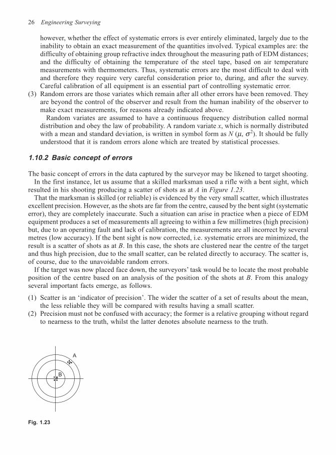
The basic concept of errors in the data captured by the surveyor may be likened to target shooting.In the first instance, let us assume that a skilled marksman used a rifle with a bent sight, which
resulted in his shooting producing a scatter of shots as at A in Figure 1.23.That the marksman is skilled (or reliable) is evidenced by the very small scatter, which illustrates
excellent precision. However, as the shots are far from the centre, caused by the bent sight (systematicerror), they are completely inaccurate. Such a situation can arise in practice when a piece of EDMequipment produces a set of measurements all agreeing to within a few millimetres (high precision)but, due to an operating fault and lack of calibration, the measurements are all incorrect by severalmetres (low accuracy). If the bent sight is now corrected, i.e. systematic errors are minimized, theresult is a scatter of shots as at B. In this case, the shots are clustered near the centre of the targetand thus high precision, due to the small scatter, can be related directly to accuracy. The scatter is,of course, due to the unavoidable random errors.
If the target was now placed face down, the surveyors’ task would be to locate the most probableposition of the centre based on an analysis of the position of the shots at B. From this analogyseveral important facts emerge, as follows.
(1) Scatter is an ‘indicator of precision’. The wider the scatter of a set of results about the mean,the less reliable they will be compared with results having a small scatter.
(2) Precision must not be confused with accuracy; the former is a relative grouping without regardto nearness to the truth, whilst the latter denotes absolute nearness to the truth.
B
A
Fig. 1.23
Basic concepts of surveying 27
(3) Precision may be regarded as an index of accuracy only when all sources of error, other thanrandom errors, have been eliminated.
(4) Accuracy may be defined only by specifying the bounds between which the accidental error ofa measured quantity may lie. The reason for defining accuracy thus is that the absolute error ofthe quantity is generally not known. If it were, it could simply be applied to the measuredquantity to give its true value. The error bound is usually specified as symmetrical about zero.Thus the accuracy of measured quantity x is x ± εx where εx is greater than or equal to the truebut unknown error of x.
(5) Position fixing by the surveyor, whether it be the coordinate position of points in a controlnetwork, or the position of topographic detail, is simply an assessment of the most probableposition and, as such, requires a statistical evaluation of its reliability.
1.10.3 Further definitions
(1) The true value of a measurement can never be found, even though such a value exists. This isevident when observing an angle with a one-second theodolite; no matter how many times theangle is read, a slightly different value will always be obtained.
(2) True error (εx) similarly can never be found, for it consists of the true value (X) minus theobserved value (x), i.e.
X – x = εx
(3) Relative error is a measure of the error in relation to the size of the measurement. For instance,a distance of 10 m may be measured with an error of ±1 mm, whilst a distance of 100 m mayalso be measured to an accuracy of ±1 mm. Although the error is the same in both cases, thesecond measurement may clearly be regarded as more accurate. To allow for this, the termrelative error (Rx) may be used, where
Rx = εx/x
Thus, in the first case x = 10 m, εx = ± 1 mm, and therefore Rx = 1/10 000; in the second case,Rx = 1/100 000, clearly illustrating the distinction. Multiplying the relative error by 100 givesthe percentage error. ‘Relative error’ is an extremely useful definition, and is commonly usedin expressing the accuracy of linear measurement. For example, the relative closing error of atraverse is usually expressed in this way. The definition is clearly not applicable to expressingthe accuracy to which an angle is measured, however.
(4) Most probable value (MPV) is the closest approximation to the true value that can be achievedfrom a set of data. This value is generally taken as the arithmetic mean of a set, ignoring at thisstage the frequency or weight of the data. For instance, if A is the arithmetic mean, X the truevalue, and εn the errors of a set of n measurements, then
A Xnn = –
[ ]ε
where [εn] is the sum of the errors. As the errors are equally as likely to be positive or negative,then for a finite number of observations [εn]/n will be very small and A ≈ X. For an infinitenumber of measurements, it could be argued that A = X. (N.B. The square bracket is Gaussiannotation for ‘sum of’.)
(5) Residual is the closest approximation to the true error and is the difference between the MPVof a set, i.e. the arithmetic mean, and the observed values. Using the same argument as before,it can be shown that for a finite number of measurements, the residual r is approximately equalto the true error ε.
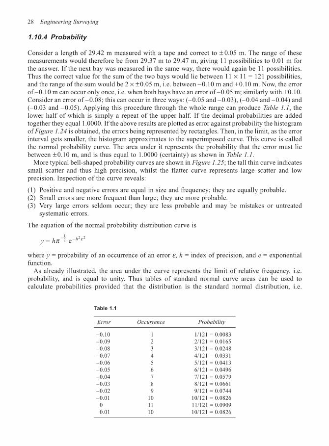
28 Engineering Surveying
Table 1.1
Error Occurrence Probability
–0.10 1 1/121 = 0.0083–0.09 2 2/121 = 0.0165–0.08 3 3/121 = 0.0248–0.07 4 4/121 = 0.0331–0.06 5 5/121 = 0.0413–0.05 6 6/121 = 0.0496–0.04 7 7/121 = 0.0579–0.03 8 8/121 = 0.0661–0.02 9 9/121 = 0.0744–0.01 10 10/121 = 0.0826
0 11 11/121 = 0.09090.01 10 10/121 = 0.0826
1.10.4 Probability
Consider a length of 29.42 m measured with a tape and correct to ± 0.05 m. The range of thesemeasurements would therefore be from 29.37 m to 29.47 m, giving 11 possibilities to 0.01 m forthe answer. If the next bay was measured in the same way, there would again be 11 possibilities.Thus the correct value for the sum of the two bays would lie between 11 × 11 = 121 possibilities,and the range of the sum would be 2 × ±0.05 m, i.e. between –0.10 m and +0.10 m. Now, the errorof –0.10 m can occur only once, i.e. when both bays have an error of –0.05 m; similarly with +0.10.Consider an error of –0.08; this can occur in three ways: (–0.05 and –0.03), (–0.04 and –0.04) and(–0.03 and –0.05). Applying this procedure through the whole range can produce Table 1.1, thelower half of which is simply a repeat of the upper half. If the decimal probabilities are addedtogether they equal 1.0000. If the above results are plotted as error against probability the histogramof Figure 1.24 is obtained, the errors being represented by rectangles. Then, in the limit, as the errorinterval gets smaller, the histogram approximates to the superimposed curve. This curve is calledthe normal probability curve. The area under it represents the probability that the error must liebetween ±0.10 m, and is thus equal to 1.0000 (certainty) as shown in Table 1.1.
More typical bell-shaped probability curves are shown in Figure 1.25; the tall thin curve indicatessmall scatter and thus high precision, whilst the flatter curve represents large scatter and lowprecision. Inspection of the curve reveals:
(1) Positive and negative errors are equal in size and frequency; they are equally probable.(2) Small errors are more frequent than large; they are more probable.(3) Very large errors seldom occur; they are less probable and may be mistakes or untreated
systematic errors.
The equation of the normal probability distribution curve is
y h h = e– –
12
2 2π ε
where y = probability of an occurrence of an error ε, h = index of precision, and e = exponentialfunction.
As already illustrated, the area under the curve represents the limit of relative frequency, i.e.probability, and is equal to unity. Thus tables of standard normal curve areas can be used tocalculate probabilities provided that the distribution is the standard normal distribution, i.e.
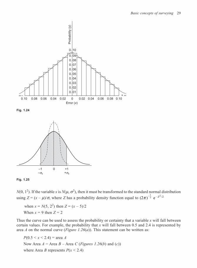
Basic concepts of surveying 29
N(0, 12). If the variable x is N(µ, σ2), then it must be transformed to the standard normal distribution
using Z = (x – µ)/σ, where Z has a probability density function equal to (2 ) e– – /2
12
2π Z
when x = N(5, 22) then Z = (x – 5)/2
When x = 9 then Z = 2
Thus the curve can be used to assess the probability or certainty that a variable x will fall betweencertain values. For example, the probability that x will fall between 0.5 and 2.4 is represented byarea A on the normal curve (Figure 1.26(a)). This statement can be written as:
P(0.5 < x < 2.4) = area A
Now Area A = Area B – Area C (Figures 1.26(b) and (c))
where Area B represents P(x < 2.4)
0. 10
Pro
babili
ty (
y)
0. 09
0. 08
0. 07
0. 06
0. 05
0. 04
0. 03
0. 02
0. 01
0.10 0.08 0.06 0.04 0.02 0 0.02 0.04 0.06 0.08 0.10+ ∞∞ –
Error (x)
Fig. 1.24
–1
–σs
+1
+σs
0
Fig. 1.25
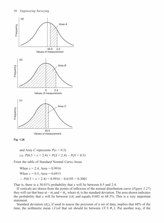
30 Engineering Surveying
and Area C represents P(x < 0.5)
i.e. P(0.5 < x < 2.4) = P(X < 2.4) – P(X < 0.5)
From the table of Standard Normal Curve Areas
When x = 2.4, Area = 0.9916
When x = 0.5, Area = 0.6915
∴ P(0.5 < x < 2.4) = 0.9916 – 0.6195 = 0.3001
That is, there is a 30.01% probability that x will lie between 0.5 and 2.4.If verticals are drawn from the points of inflexion of the normal distribution curve (Figure 1.27)
they will cut that base at – σx and + σx, where σx is the standard deviation. The area shown indicatesthe probability that x will lie between ±σx and equals 0.683 or 68.3%. This is a very importantstatement.
Standard deviation (σx), if used to assess the precision of a set of data, implies that 68% of thetime, the arithmetic mean ( )x of that set should lie between ( x x± σ ). Put another way, if the
Fre
quency
(a)
00.5 2.4Values of measurement
Area A
Values of measurement
(b)
Fre
quency Area B
0 2.4
Fre
quency
(c)
Area C
Values of measurement00.5
Fig. 1.26
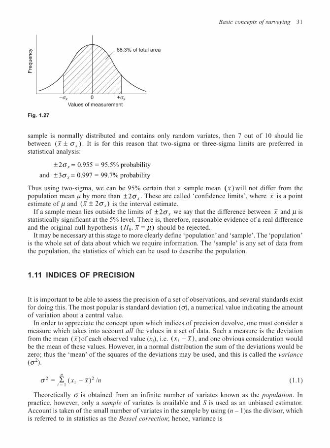
Basic concepts of surveying 31
sample is normally distributed and contains only random variates, then 7 out of 10 should liebetween ( x x± σ ) . It is for this reason that two-sigma or three-sigma limits are preferred instatistical analysis:
± =2 0.955 = 95.5% probabilityσ x
and ± =3 0.997 = 99.7% probabilityσ x
Thus using two-sigma, we can be 95% certain that a sample mean (x ) will not differ from thepopulation mean µ by more than ± 2σ x . These are called ‘confidence limits’, where x is a pointestimate of µ and ( )x x 2± σ is the interval estimate.
If a sample mean lies outside the limits of ± 2σ x we say that the difference between x and µ isstatistically significant at the 5% level. There is, therefore, reasonable evidence of a real differenceand the original null hypothesis (H x0 = ). µ should be rejected.
It may be necessary at this stage to more clearly define ‘population’ and ‘sample’. The ‘population’is the whole set of data about which we require information. The ‘sample’ is any set of data fromthe population, the statistics of which can be used to describe the population.
1.11 INDICES OF PRECISION
It is important to be able to assess the precision of a set of observations, and several standards existfor doing this. The most popular is standard deviation (σ), a numerical value indicating the amountof variation about a central value.
In order to appreciate the concept upon which indices of precision devolve, one must consider ameasure which takes into account all the values in a set of data. Such a measure is the deviationfrom the mean ( )x of each observed value (xi), i.e. ( – )x xi , and one obvious consideration wouldbe the mean of these values. However, in a normal distribution the sum of the deviations would bezero; thus the ‘mean’ of the squares of the deviations may be used, and this is called the variance
(σ 2).
σ ι2
= 1
2 = ( – ) /Σi
n
x x n (1.1)
Theoretically σ is obtained from an infinite number of variates known as the population. Inpractice, however, only a sample of variates is available and S is used as an unbiased estimator.Account is taken of the small number of variates in the sample by using (n – 1)as the divisor, whichis referred to in statistics as the Bessel correction; hence, variance is
Fre
quency 68.3% of total area
Values of measurement
–σx 0 +σx
Fig. 1.27
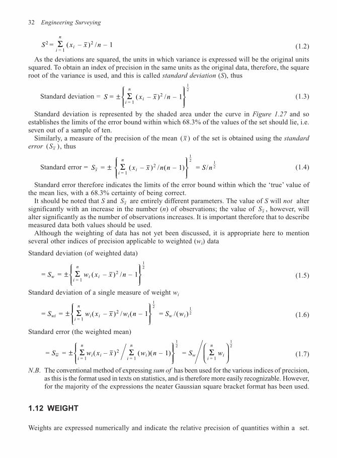
32 Engineering Surveying
S x x ni
n
i2
= 1
2= ( – ) / – 1Σ (1.2)
As the deviations are squared, the units in which variance is expressed will be the original unitssquared. To obtain an index of precision in the same units as the original data, therefore, the squareroot of the variance is used, and this is called standard deviation (S), thus
Standard deviation = S x x ni
n
i = ( – ) – 1 = 1
2
12
±
Σ / (1.3)
Standard deviation is represented by the shaded area under the curve in Figure 1.27 and soestablishes the limits of the error bound within which 68.3% of the values of the set should lie, i.e.seven out of a sample of ten.
Similarly, a measure of the precision of the mean ( )x of the set is obtained using the standard
error ( )Sx , thus
Standard error = S x x n n S nxi
n
i = ( – ) – 1) = / = 1
2
12
12±
Σ / ( (1.4)
Standard error therefore indicates the limits of the error bound within which the ‘true’ value ofthe mean lies, with a 68.3% certainty of being correct.
It should be noted that S and Sx are entirely different parameters. The value of S will not altersignificantly with an increase in the number (n) of observations; the value of Sx , however, willalter significantly as the number of observations increases. It is important therefore that to describemeasured data both values should be used.
Although the weighting of data has not yet been discussed, it is appropriate here to mentionseveral other indices of precision applicable to weighted (wi) data
Standard deviation (of weighted data)
= = ( – ) – 1 = 1
2
12
S w x x nwi
n
i i±
Σ / (1.5)
Standard deviation of a single measure of weight wi
= = ( – ) ( – 1 = ) = 1
2
12 1
2S w x x w n S wwii
n
i i i w i±
Σ / /( (1.6)
Standard error (the weighted mean)
= = – ) ( ) – 1) = = 1
2
= 1 = 1
12
12
S w x x w n S wwi
n
i ii
n
i wi
n
i±
Σ Σ Σ( ( (1.7)
N.B. The conventional method of expressing sum of has been used for the various indices of precision,as this is the format used in texts on statistics, and is therefore more easily recognizable. However,for the majority of the expressions the neater Gaussian square bracket format has been used.
1.12 WEIGHT
Weights are expressed numerically and indicate the relative precision of quantities within a set.
Basic concepts of surveying 33
The greater the weight, the greater the precision of the observation to which it relates. Thus anobservation with a weight of two may be regarded as twice as reliable as an observation with aweight of one. Consider two mean measures of the same angle: A = 50° 50′ 50′′ of weight one, andB = 50° 50′ 47′′ of weight two. This is equivalent to three observations, 50″, 47′′, 47′′, all of equalweight, and having a mean value of
(50′′ + 47′′ + 47′′)/3 = 48′′
Therefore the mean value of the angle = 50° 50′ 48′′.Inspection of this exercise shows it to be identical to multiplying each observation a by its
weight, w, and dividing by the sum of the weights [w], i.e.
Weighted mean = Aa w a w a w
w w w
aw
wmn n
n
= + + . . +
+ + . . + =
[ ][ ]
1 1 2 2
1 2
..
(1.8)
Weights can be allocated in a variety of ways, such as: (a) by personal judgement of the prevailingconditions at the time of measurement; (b) by direct proportion to the number of measurements ofthe quantity, i.e. w ∝ n; (c) by the use of variance and co-variance factors. This last method isrecommended and in the case of the variance factor is easily applied as follows. Equation (1.4)shows
S S nx = /12
That is, error is inversely proportional to the square root of the number of measures. However, asw ∝ n, then
w Sx2 1/∝
i.e. weight is proportional to the inverse of the variance.
1.13 REJECTION OF OUTLIERS
It is not unusual, when taking repeated measurements of the same quantity, to find at least onewhich appears very different from the rest. Such a measurement is called an outlier, which theobserver intuitively feels should be rejected from the sample. However, intuition is hardly a scientificargument for the rejection of data and a more statistically viable approach is required.
As already indicated, standard deviation S represents 68.3% of the area under the normal curveand is therefore representative of 68.3% confidence limits. It follows from this that
±3.29S represents 99.9% confidence limits (0.999 probability)
Thus, any random variate xi, whose residual error ( – )x xi is greater than ±3.29 S, must lie in theextreme tail ends of the normal curve and should therefore be ignored, i.e. rejected from the sample.In practice, this has not proved a satisfactory rejection criterion due to the limited size of thesamples. Logan (Survey Review, No. 97, July 1955) has shown that the appropriate rejection criteriaare relative to sample size, as follows:
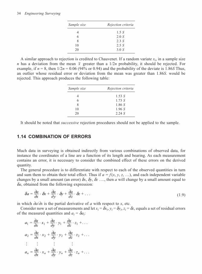
34 Engineering Surveying
Sample size Rejection criteria
4 1.5 S
6 2.0 S
8 2.3 S
10 2.5 S
20 3.0 S
A similar approach to rejection is credited to Chauvenet. If a random variate xi, in a sample sizen has a deviation from the mean x greater than a 1/2n probability, it should be rejected. Forexample, if n = 8, then 1/2n = 0.06 (94% or 0.94) and the probability of the deviate is 1.86S Thus,an outlier whose residual error or deviation from the mean was greater than 1.86S. would berejected. This approach produces the following table:
Sample size Rejection criteria
4 1.53 S
6 1.73 S
8 1.86 S
10 1.96 S
20 2.24 S
It should be noted that successive rejection procedures should not be applied to the sample.
1.14 COMBINATION OF ERRORS
Much data in surveying is obtained indirectly from various combinations of observed data, forinstance the coordinates of a line are a function of its length and bearing. As each measurementcontains an error, it is necessary to consider the combined effect of these errors on the derivedquantity.
The general procedure is to differentiate with respect to each of the observed quantities in turnand sum them to obtain their total effect. Thus if a = f (x, y, z, …), and each independent variablechanges by a small amount (an error) δx, δy, δz …., then a will change by a small amount equal toδa, obtained from the following expression:
δ ∂∂
δ ∂∂
δ ∂∂
δaax
xay
yaz
z = + + + . . .⋅ ⋅ ⋅ (1.9)
in which ∂a/∂x is the partial derivative of a with respect to x, etc.Consider now a set of measurements and let xi = δxi, yi = δyi, zi = δz, equals a set of residual errors
of the measured quantities and ai = δai:
aax
xay
yaz
z1 1 1 1 = + + + . . .∂∂
∂∂
∂∂
⋅ ⋅ ⋅
aax
xay
yaz
z2 2 2 = + + + . . .∂∂
∂∂
∂∂
⋅ ⋅ ⋅2
M M M M
aax
xay
yaz
zn n n n = + + + . . .∂∂
∂∂
∂∂
⋅ ⋅ ⋅
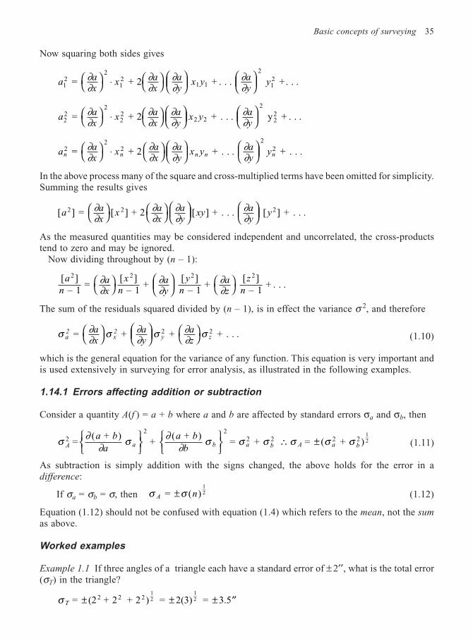
Basic concepts of surveying 35
Now squaring both sides gives
aax
xax
ay
x yay
y12
2
1 1
2
= + 2 + . . + . .∂∂
∂∂
∂∂
∂∂
⋅
1
212. .
aax
xax
ay
x yay2
22
22
2 2
2
22 = + 2 + . . y + . .∂
∂∂∂
∂∂
∂∂
⋅
. .
aax
xax
ay
x yay
yn n n n n2
22
22 = + 2 + . . + . .∂
∂∂∂
∂∂
∂∂
⋅
. .
In the above process many of the square and cross-multiplied terms have been omitted for simplicity.Summing the results gives
[ ] . ] .aax
xax
ay
xyay
y2 2 2 = [ ] + 2 [ ] + . . [ + . .∂∂
∂∂
∂∂
∂∂
As the measured quantities may be considered independent and uncorrelated, the cross-productstend to zero and may be ignored.
Now dividing throughout by (n – 1):
[ ] ].
a
nax
x
nay
y
naz
z
n
2 2 2 2] – 1
= [ – 1
+ [ ] – 1
+ [ – 1
+ . .∂∂
∂∂
∂∂
The sum of the residuals squared divided by (n – 1), is in effect the variance σ 2, and therefore
σ ∂∂
σ ∂∂
σ ∂∂
σa2
x2
y zax
ay
az
= + + + . .2 2
. (1.10)
which is the general equation for the variance of any function. This equation is very important andis used extensively in surveying for error analysis, as illustrated in the following examples.
1.14.1 Errors affecting addition or subtraction
Consider a quantity A(f ) = a + b where a and b are affected by standard errors σa and σb, then
σ ∂∂
σ ∂∂
σ σ σ σ σ σA a b a b A a b
a b
a
a b
b2
22 2 2 2=
( + ) +
( + ) = + = ( + )
12
∴ ±2
(1.11)
As subtraction is simply addition with the signs changed, the above holds for the error in adifference:
If σa = σb = σ, then σ σA n = ( )12± (1.12)
Equation (1.12) should not be confused with equation (1.4) which refers to the mean, not the sum
as above.
Worked examples
Example 1.1 If three angles of a triangle each have a standard error of ± 2′′, what is the total error(σT) in the triangle?
σ T = (2 + 2 + 2 = 2(3) = 3.52 2 212
12± ± ± ′′)
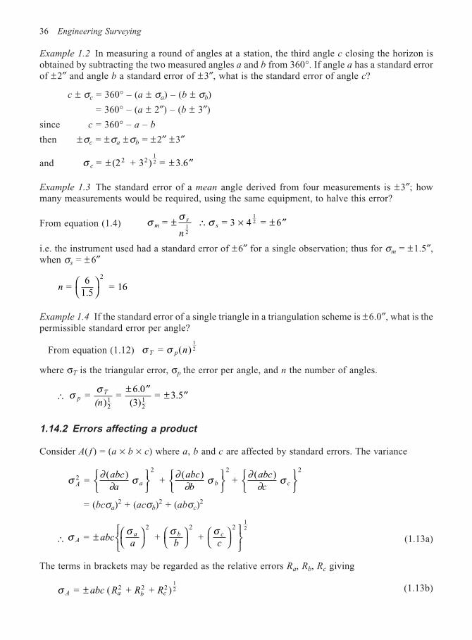
36 Engineering Surveying
Example 1.2 In measuring a round of angles at a station, the third angle c closing the horizon isobtained by subtracting the two measured angles a and b from 360°. If angle a has a standard errorof ±2″ and angle b a standard error of ±3″, what is the standard error of angle c?
c ± σc = 360° – (a ± σa) – (b ± σb)
= 360° – (a ± 2″) – (b ± 3″)
since c = 360° – a – b
then ±σc = ±σa ±σb = ±2″ ±3″
and σ c = (2 + 3 ) = 3.62 21
± ± ′′2
Example 1.3 The standard error of a mean angle derived from four measurements is ±3″; howmany measurements would be required, using the same equipment, to halve this error?
From equation (1.4) σ σ σms
s
n= = 3 4 = 6
12
12± ∴ × ± ′′
i.e. the instrument used had a standard error of ±6″ for a single observation; thus for σm = ±1.5″,when σs = ± 6″
n = 6
1.5 = 16
2
Example 1.4 If the standard error of a single triangle in a triangulation scheme is ±6.0″, what is thepermissible standard error per angle?
From equation (1.12) σ σT p n = ( )12
where σT is the triangular error, σp the error per angle, and n the number of angles.
∴ σ σp
T
(n =
) =
6.0
(3) = 3.5
12
12
± ′′± ′′
1.14.2 Errors affecting a product
Consider A( f ) = (a × b × c) where a, b and c are affected by standard errors. The variance
σ ∂∂
σ ∂∂
σ ∂∂
σA a b c
abc
a
abc
b
abc
c2
2 2 2
= ( )
+ ( )
+ ( )
= (bcσa)2 + (acσb)
2 + (abσc)2
∴ σσ σ σ
Aa b cabc
a b c = + +
212
±
2 2
(1.13a)
The terms in brackets may be regarded as the relative errors Ra, Rb, Rc giving
σ A a b cabc R R R = ( + + )2 212± 2 (1.13b)
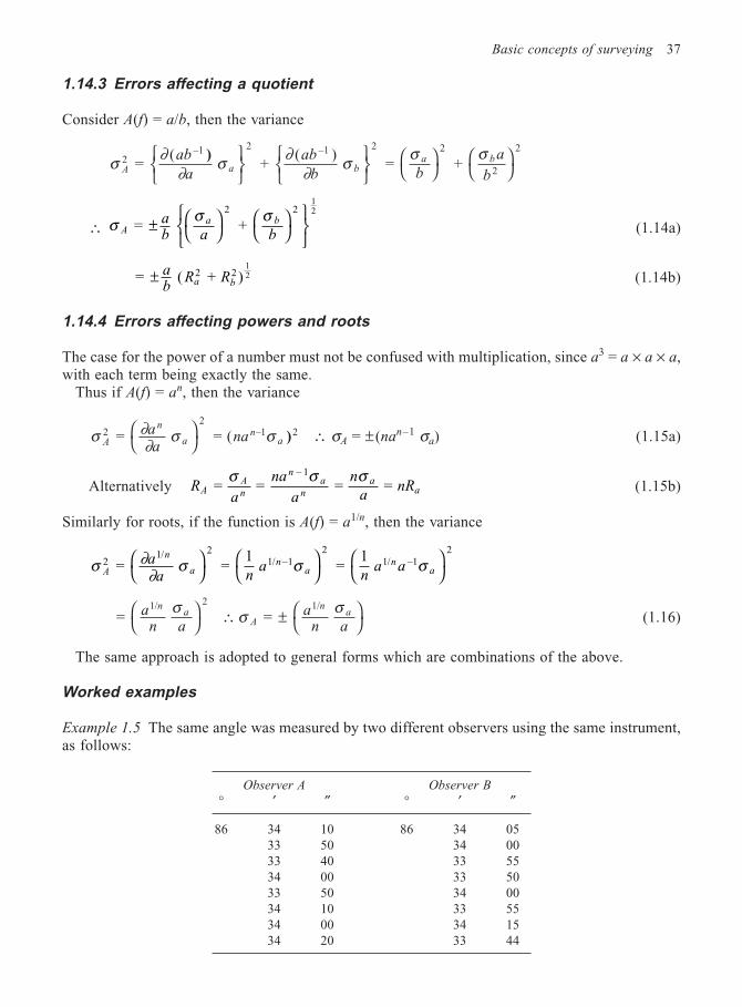
Basic concepts of surveying 37
1.14.3 Errors affecting a quotient
Consider A(f) = a/b, then the variance
σ ∂∂
σ ∂∂
σ σ σA a b
a bab
a
ab
b b
a
b2
–1 –1 2 2
2
2
= (
+ ( )
= + )
2
∴ σ σ σA
a bab a b
= + 2 2
12
±
(1.14a)
= + 2 212± a
bR Ra b( ) (1.14b)
1.14.4 Errors affecting powers and roots
The case for the power of a number must not be confused with multiplication, since a3 = a × a × a,with each term being exactly the same.
Thus if A(f) = an, then the variance
σ ∂∂
σ σA
n
an
aaa
na2 –1 = = (
22) ∴ σA = ± (nan–1 σa) (1.15a)
Alternatively Ra
na
a
n
anRA
A
n
na
n
aa = = = =
– 1σ σ σ(1.15b)
Similarly for roots, if the function is A(f) = a1/n, then the variance
σ ∂∂
σ σ σA
n
an
an
aa
a na
n a a2
1/ 21/ –1 1/ –1
2
= = 1
= 1
2
= = 1/ 1/an a
an a
na
A
naσ σ σ
∴ ±
2
(1.16)
The same approach is adopted to general forms which are combinations of the above.
Worked examples
Example 1.5 The same angle was measured by two different observers using the same instrument,as follows:
Observer A Observer B
° ′ ″ ° ′ ″
86 34 10 86 34 0533 50 34 0033 40 33 5534 00 33 5033 50 34 0034 10 33 5534 00 34 1534 20 33 44
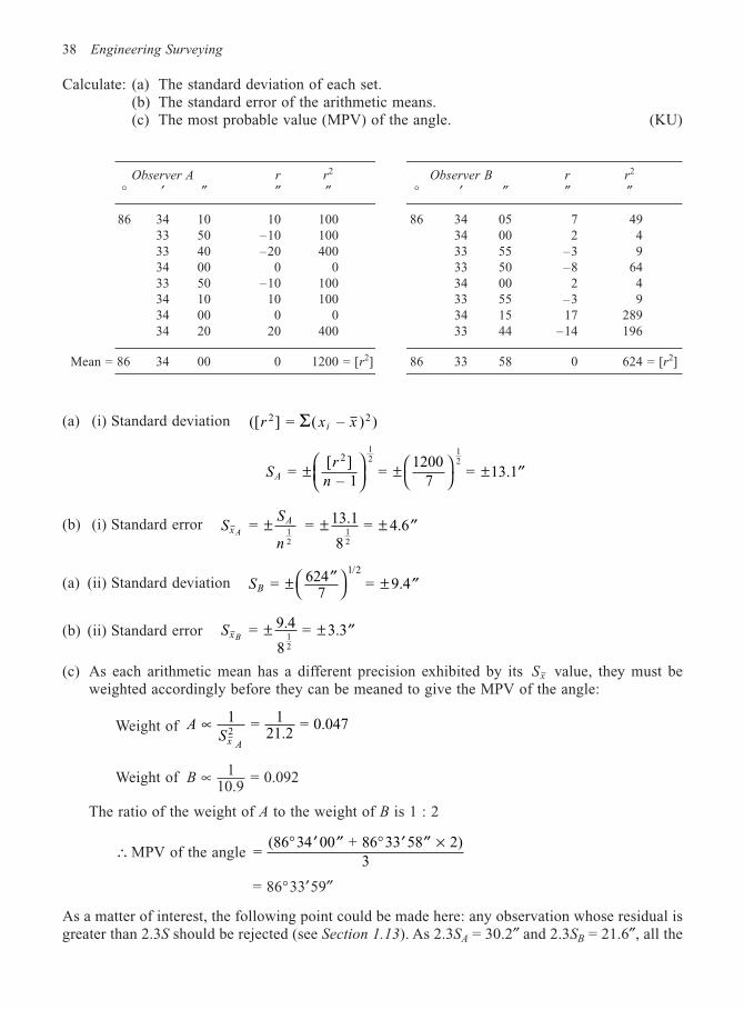
38 Engineering Surveying
Calculate: (a) The standard deviation of each set.(b) The standard error of the arithmetic means.(c) The most probable value (MPV) of the angle. (KU)
Observer A r r2 Observer B r r2
° ′ ″ ″ ″ ° ′ ″ ″ ″
86 34 10 10 100 86 34 05 7 4933 50 –10 100 34 00 2 433 40 –20 400 33 55 –3 934 00 0 0 33 50 –8 6433 50 –10 100 34 00 2 434 10 10 100 33 55 –3 934 00 0 0 34 15 17 28934 20 20 400 33 44 –14 196
Mean = 86 34 00 0 1200 = [r2] 86 33 58 0 624 = [r2]
(a) (i) Standard deviation ([ ]r x xi2 2 = ( – ) )Σ
Sr
nA = [ ] – 1
=1200
7= 13.1
212
12
±
±
± ′′
(b) (i) Standard error SS
nx
AA
= = 13.1
8 = 4.6
12
12
± ± ± ′′
(a) (ii) Standard deviation SB = 6247
= 9.41/2
± ′′
± ′′
(b) (ii) Standard error SxB = 9.4
8 = 3.3
12
± ± ′′
(c) As each arithmetic mean has a different precision exhibited by its Sx value, they must beweighted accordingly before they can be meaned to give the MPV of the angle:
Weight of ASx A
1 = 121.2
= 0.0472
∝
Weight of B1
10.9 = 0.092∝
The ratio of the weight of A to the weight of B is 1 : 2
∴ MPV of the angle =(86 34 00 + 86 33 58 2)
3° ′ ′′ ° ′ ′′ ×
= 86°33′59″
As a matter of interest, the following point could be made here: any observation whose residual isgreater than 2.3S should be rejected (see Section 1.13). As 2.3SA = 30.2″ and 2.3SB = 21.6″, all the
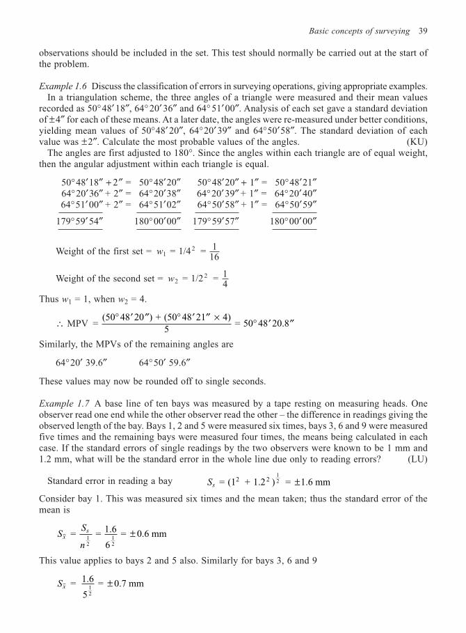
Basic concepts of surveying 39
observations should be included in the set. This test should normally be carried out at the start ofthe problem.
Example 1.6 Discuss the classification of errors in surveying operations, giving appropriate examples.In a triangulation scheme, the three angles of a triangle were measured and their mean values
recorded as 50°48′ 18″, 64° 20′ 36″ and 64° 51′00″. Analysis of each set gave a standard deviationof ±4″ for each of these means. At a later date, the angles were re-measured under better conditions,yielding mean values of 50°48′ 20″, 64°20′ 39″ and 64°50′58″. The standard deviation of eachvalue was ±2″. Calculate the most probable values of the angles. (KU)
The angles are first adjusted to 180°. Since the angles within each triangle are of equal weight,then the angular adjustment within each triangle is equal.
50°48′18″ + 2″ = 50°48′20″ 50°48′20″ + 1″ = 50°48′21″64°20′36″ + 2″ = 64°20′38″ 64°20′39″ + 1″ = 64°20′40″64°51′00″ + 2″ = 64°51′02″ 64°50′58″ + 1″ = 64°50′59″
179°59′54″ 180°00′00″ 179°59′57″ 180°00′00″
Weight of the first set = w12 = 1/4 = 1
16
Weight of the second set = w22 = 1/2 = 1
4
Thus w1 = 1, when w2 = 4.
∴ MPV =(50 48 20 ) + (50 48 21 4)
5 = 50 48 20.8
° ′ ′′ ° ′ ′′ ×° ′ ′′
Similarly, the MPVs of the remaining angles are
64°20′ 39.6″ 64°50′ 59.6″
These values may now be rounded off to single seconds.
Example 1.7 A base line of ten bays was measured by a tape resting on measuring heads. Oneobserver read one end while the other observer read the other – the difference in readings giving theobserved length of the bay. Bays 1, 2 and 5 were measured six times, bays 3, 6 and 9 were measuredfive times and the remaining bays were measured four times, the means being calculated in eachcase. If the standard errors of single readings by the two observers were known to be 1 mm and1.2 mm, what will be the standard error in the whole line due only to reading errors? (LU)
Standard error in reading a bay Ss = (1 + 1.2 ) = 1.6 mm2 212 ±
Consider bay 1. This was measured six times and the mean taken; thus the standard error of themean is
SS
nx
s = = 1.6
6 = 0.6 mm
12
12
±
This value applies to bays 2 and 5 also. Similarly for bays 3, 6 and 9
Sx = 1.6 = 0.7 mm125
±
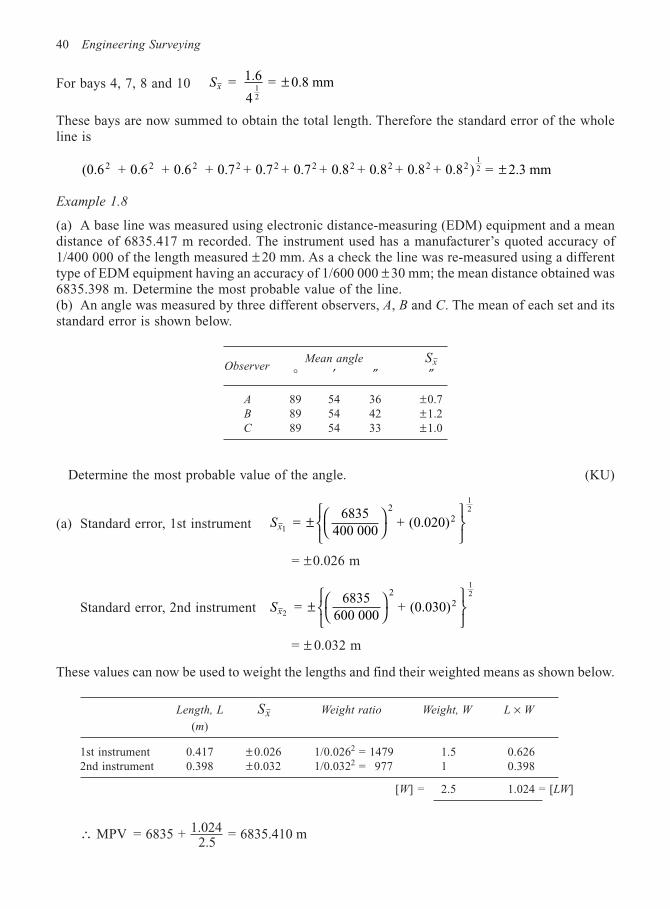
40 Engineering Surveying
For bays 4, 7, 8 and 10 Sx = 1.6 = 0.8 mm124
±
These bays are now summed to obtain the total length. Therefore the standard error of the wholeline is
(0.6 + 0.6 + 0.6 + 0.7 + 0.7 + 0.7 + 0.8 + 0.8 + 0.8 + 0.8 ) = 2.3 mm2 2 2 2 2 2 2 2 2 212 ±
Example 1.8
(a) A base line was measured using electronic distance-measuring (EDM) equipment and a meandistance of 6835.417 m recorded. The instrument used has a manufacturer’s quoted accuracy of1/400 000 of the length measured ± 20 mm. As a check the line was re-measured using a differenttype of EDM equipment having an accuracy of 1/600 000 ± 30 mm; the mean distance obtained was6835.398 m. Determine the most probable value of the line.(b) An angle was measured by three different observers, A, B and C. The mean of each set and itsstandard error is shown below.
Mean angle Sx
° ′ ″ ″
A 89 54 36 ±0.7B 89 54 42 ±1.2C 89 54 33 ±1.0
Determine the most probable value of the angle. (KU)
(a) Standard error, 1st instrument Sx1
2
= 6835
400 000+ (0.020)
22±
1
= ±0.026 m
Standard error, 2nd instrument Sx2
12
= 6835
600 000+ (0.030)
22±
= ± 0.032 m
These values can now be used to weight the lengths and find their weighted means as shown below.
Length, L Sx Weight ratio Weight, W L × W
(m)
1st instrument 0.417 ± 0.026 1/0.0262 = 1479 1.5 0.6262nd instrument 0.398 ±0.032 1/0.0322 = 977 1 0.398
[W] = 2.5 1.024 = [LW]
∴ MPV = 6835 + 1.0242.5
= 6835.410 m
Observer
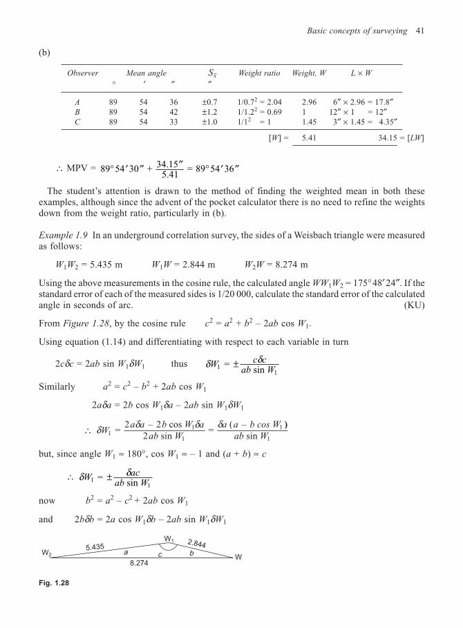
Basic concepts of surveying 41
(b)
Observer Mean angle Sx Weight ratio Weight, W L × W
° ′ ″ ″
A 89 54 36 ±0.7 1/0.72 = 2.04 2.96 6″ × 2.96 = 17.8″B 89 54 42 ±1.2 1/1.22 = 0.69 1 12″ × 1 = 12″C 89 54 33 ±1.0 1/12 = 1 1.45 3″ × 1.45 = 4.35″
[W] = 5.41 34.15 = [LW]
∴ MPV = 89 54 30 + 34.155.41
= 89 54 36° ′ ′′ ′′ ° ′ ′′
The student’s attention is drawn to the method of finding the weighted mean in both theseexamples, although since the advent of the pocket calculator there is no need to refine the weightsdown from the weight ratio, particularly in (b).
Example 1.9 In an underground correlation survey, the sides of a Weisbach triangle were measuredas follows:
W1W2 = 5.435 m W1W = 2.844 m W2W = 8.274 m
Using the above measurements in the cosine rule, the calculated angle WW1W2 = 175°48′24″. If thestandard error of each of the measured sides is 1/20 000, calculate the standard error of the calculatedangle in seconds of arc. (KU)
From Figure 1.28, by the cosine rule c2 = a2 + b2 – 2ab cos W1.
Using equation (1.14) and differentiating with respect to each variable in turn
2cδc = 2ab sin W1δW1 thus δ δW
c cab W1
1 =
sin ±
Similarly a2 = c2 – b2 + 2ab cos W1
2aδa = 2b cos W1δa – 2ab sin W1δW1
∴ δ δ δ δW
a a b W a
ab W
a a b cos W
ab W11
1
1
1 =
2 – 2 cos sin
= ( –
sin 2)
but, since angle W1 ≈ 180°, cos W1 ≈ – 1 and (a + b) ≈ c
∴ δ δW
acab W1
1 =
sin ±
now b2 = a2 – c2 + 2ab cos W1
and 2bδb = 2a cos W1δb – 2ab sin W1δW1
a c b
2.8445.435
8.274
W2 W
W1
Fig. 1.28
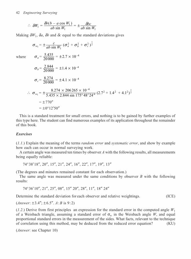
42 Engineering Surveying
∴ δ δ δW
b b a W
ab Wbc
ab W11
1 1 =
( – cos ) sin
= sin
±
Making δW1, δa, δb and δc equal to the standard deviations gives
σ σ σ σw a b cc
ab W1
12=
sin ( + + )
1
2 2 2±
where σ a =000
= 2.7 10 –45 43520
. ± ×
σ b =000
= .4 10 –42 84420
1. ± ×
σ c =000
= .1 10 –48 27420
4. ± ×
∴ σ w1
12=
206 265 10
5.435 2.844 sin 175 48 24 (2.7 + 1.4 + 4.1 )
–42 2 2±
× ×× ° ′ ′′
8 274.
= ± 770″= ±0°12′50″
This is a standard treatment for small errors, and nothing is to be gained by further examples ofthis type here. The student can find numerous examples of its application throughout the remainderof this book.
Exercises
(1.1.) Explain the meaning of the terms random error and systematic error, and show by examplehow each can occur in normal surveying work.
A certain angle was measured ten times by observer A with the following results, all measurementsbeing equally reliable:
74°38′18″, 20″, 15″, 21″, 24″, 16″, 22″, 17″, 19″, 13″
(The degrees and minutes remained constant for each observation.)The same angle was measured under the same conditions by observer B with the following
results:
74°36′10″, 21″, 25″, 08″, 15″ 20″, 28″, 11″, 18″ 24″
Determine the standard deviation for each observer and relative weightings. (ICE)
(Answer: ±3.4″; ± 6.5″. A : B is 9 :2)
(1.2.) Derive from first principles an expression for the standard error in the computed angle W1
of a Weisbach triangle, assuming a standard error of σw in the Weisbach angle W, and equalproportional standard errors in the measurement of the sides. What facts, relevant to the techniqueof correlation using this method, may be deduced from the reduced error equation? (KU)
(Answer: see Chapter 10)
2
Vertical control
2.1 INTRODUCTION
Vertical control refers to the various heighting procedures used to obtain the elevation of points ofinterest above or below a reference datum. The most commonly used reference datum is mean sealevel (MSL). There is no such thing as a common global MSL, as it will vary from place to placedepending on the effect of local conditions. It is important therefore that MSL is clearly definedwherever it is utilized.
The engineer is, in the main, more concerned with the relative height of one point above or belowanother, in order to ascertain the difference in height of the two points, rather than any relationshipto MSL. It is not unusual, therefore, on small local schemes, to adopt a purely arbitrary referencedatum. This could take the form of a permanent, stable position or mark, allocated such a value thatthe level of any point on the site would not be negative. For example, if the reference mark wasallocated a value of 0.000 m, then a ground point 10 m lower would have a negative value of10.000 m. However, if the reference value was 100.000 m, then the level of the ground point inquestion would be 90.000 m. As minus signs in front of a number can be misinterpreted, erased orsimply forgotten about, they should, wherever possible, be avoided.
The vertical heights of points above or below a reference datum are referred to as the reducedlevel or simply the level of a point. Reduced levels are used in practically all aspects of construction:to produce ground contours on the plan; to enable the optimum design of road, railway or canalgradients; to facilitate ground modelling for accurate volumetric calculations. Indeed, there isscarcely any aspect of construction that is not dependent on the relative levels of ground points.
2.2 LEVELLING
Levelling is the most widely used method of obtaining the elevations of ground points relative toa reference datum and is usually carried out as a separate procedure to those used in fixingplanimetric position.
The basic concept of levelling involves the measurement of vertical distance relative to a horizontalline of sight. Hence it requires a graduated staff for the vertical measurements and an instrumentthat will provide a horizontal line of sight.
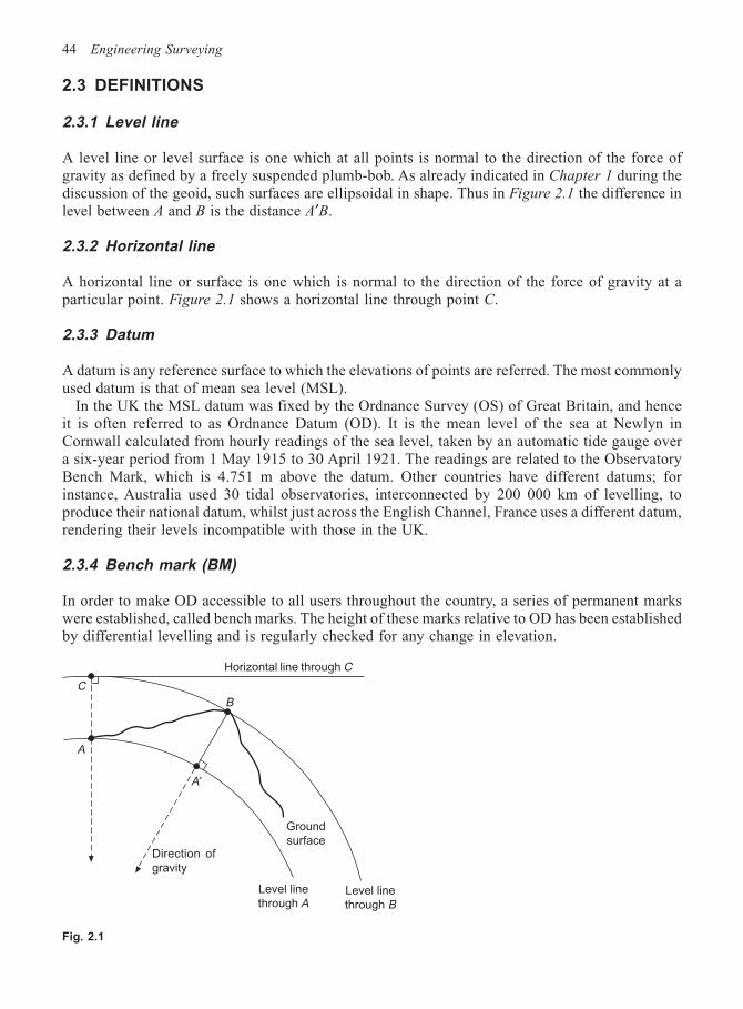
44 Engineering Surveying
2.3 DEFINITIONS
2.3.1 Level line
A level line or level surface is one which at all points is normal to the direction of the force ofgravity as defined by a freely suspended plumb-bob. As already indicated in Chapter 1 during thediscussion of the geoid, such surfaces are ellipsoidal in shape. Thus in Figure 2.1 the difference inlevel between A and B is the distance A′B.
2.3.2 Horizontal line
A horizontal line or surface is one which is normal to the direction of the force of gravity at aparticular point. Figure 2.1 shows a horizontal line through point C.
2.3.3 Datum
A datum is any reference surface to which the elevations of points are referred. The most commonlyused datum is that of mean sea level (MSL).
In the UK the MSL datum was fixed by the Ordnance Survey (OS) of Great Britain, and henceit is often referred to as Ordnance Datum (OD). It is the mean level of the sea at Newlyn inCornwall calculated from hourly readings of the sea level, taken by an automatic tide gauge overa six-year period from 1 May 1915 to 30 April 1921. The readings are related to the ObservatoryBench Mark, which is 4.751 m above the datum. Other countries have different datums; forinstance, Australia used 30 tidal observatories, interconnected by 200 000 km of levelling, toproduce their national datum, whilst just across the English Channel, France uses a different datum,rendering their levels incompatible with those in the UK.
2.3.4 Bench mark (BM)
In order to make OD accessible to all users throughout the country, a series of permanent markswere established, called bench marks. The height of these marks relative to OD has been establishedby differential levelling and is regularly checked for any change in elevation.
Fig. 2.1
Direction of
gravity
Level line
through ALevel line
through B
Ground
surface
A′
A
C
B
Horizontal line through C
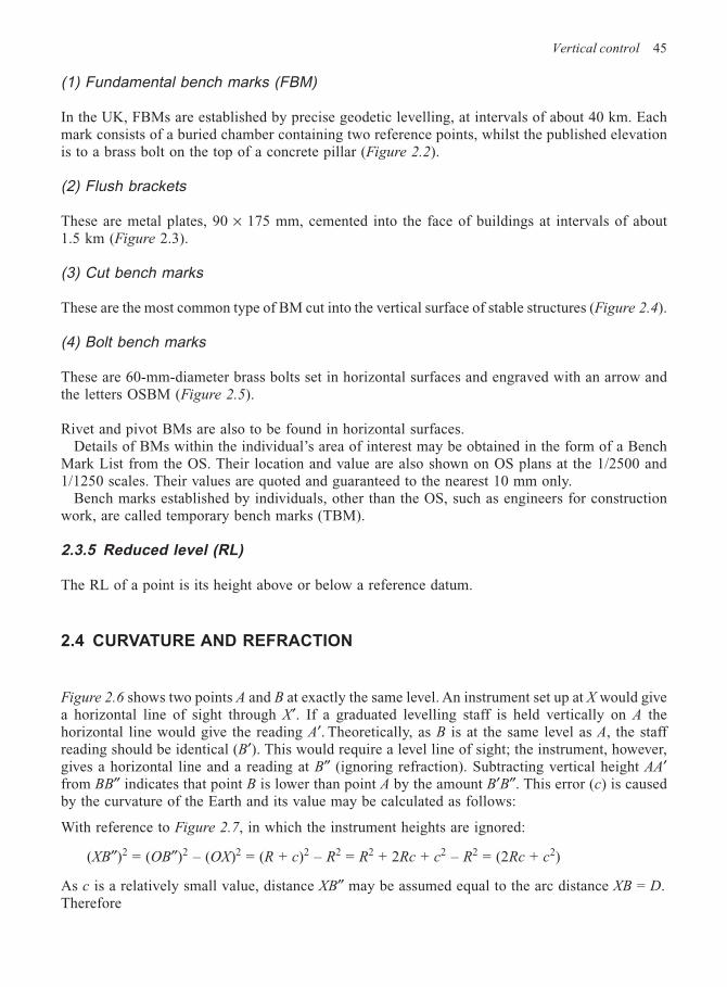
Vertical control 45
(1) Fundamental bench marks (FBM)
In the UK, FBMs are established by precise geodetic levelling, at intervals of about 40 km. Eachmark consists of a buried chamber containing two reference points, whilst the published elevationis to a brass bolt on the top of a concrete pillar (Figure 2.2).
(2) Flush brackets
These are metal plates, 90 × 175 mm, cemented into the face of buildings at intervals of about1.5 km (Figure 2.3).
(3) Cut bench marks
These are the most common type of BM cut into the vertical surface of stable structures (Figure 2.4).
(4) Bolt bench marks
These are 60-mm-diameter brass bolts set in horizontal surfaces and engraved with an arrow andthe letters OSBM (Figure 2.5).
Rivet and pivot BMs are also to be found in horizontal surfaces.Details of BMs within the individual’s area of interest may be obtained in the form of a Bench
Mark List from the OS. Their location and value are also shown on OS plans at the 1/2500 and1/1250 scales. Their values are quoted and guaranteed to the nearest 10 mm only.
Bench marks established by individuals, other than the OS, such as engineers for constructionwork, are called temporary bench marks (TBM).
2.3.5 Reduced level (RL)
The RL of a point is its height above or below a reference datum.
2.4 CURVATURE AND REFRACTION
Figure 2.6 shows two points A and B at exactly the same level. An instrument set up at X would givea horizontal line of sight through X′. If a graduated levelling staff is held vertically on A thehorizontal line would give the reading A′. Theoretically, as B is at the same level as A, the staffreading should be identical (B′). This would require a level line of sight; the instrument, however,gives a horizontal line and a reading at B″ (ignoring refraction). Subtracting vertical height AA′from BB″ indicates that point B is lower than point A by the amount B′B″. This error (c) is causedby the curvature of the Earth and its value may be calculated as follows:
With reference to Figure 2.7, in which the instrument heights are ignored:
(XB″)2 = (OB″)2 – (OX)2 = (R + c)2 – R2 = R2 + 2Rc + c2 – R2 = (2Rc + c2)
As c is a relatively small value, distance XB″ may be assumed equal to the arc distance XB = D.Therefore
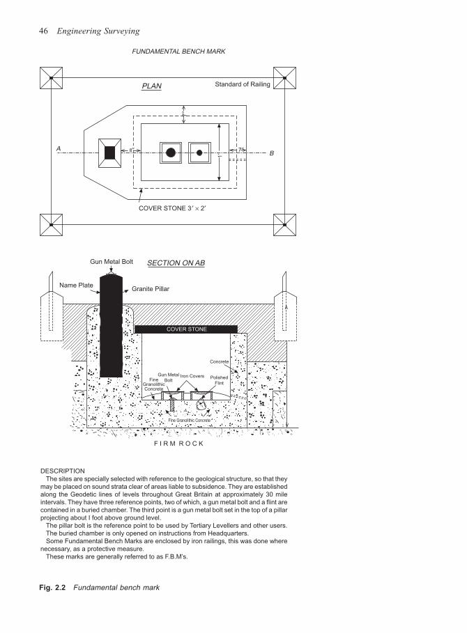
46 Engineering Surveying
Fig. 2.2 Fundamental bench mark
PLAN
A 7″
7″
COVER STONE 3 ′ × 2′
1′
SECTION ON ABGun Metal Bolt
Name PlateGranite Pillar
COVER STONE
FineGranolithicConcrete
Concrete
Polished
Flint
Iron CoversGun Metal
Bolt
F I R M R O C K
Fine Granolithic Concrete
Standard of Railing
B
DESCRIPTION
The sites are specially selected with reference to the geological structure, so that they
may be placed on sound strata clear of areas liable to subsidence. They are established
along the Geodetic lines of levels throughout Great Britain at approximately 30 mile
intervals. They have three reference points, two of which, a gun metal bolt and a flint are
contained in a buried chamber. The third point is a gun metal bolt set in the top of a pillar
projecting about I foot above ground level.
The pillar bolt is the reference point to be used by Tertiary Levellers and other users.
The buried chamber is only opened on instructions from Headquarters.
Some Fundamental Bench Marks are enclosed by iron railings, this was done where
necessary, as a protective measure.
These marks are generally referred to as F.B.M’s.
FUNDAMENTAL BENCH MARK
8″
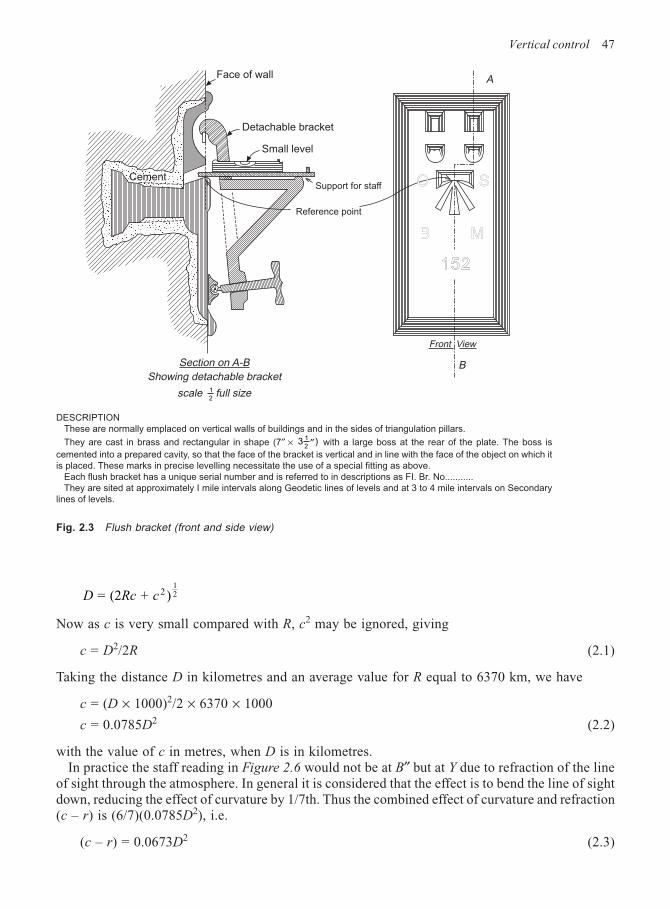
Vertical control 47
D Rc c = (2 + )212
Now as c is very small compared with R, c2 may be ignored, giving
c = D2/2R (2.1)
Taking the distance D in kilometres and an average value for R equal to 6370 km, we have
c = (D × 1000)2/2 × 6370 × 1000
c = 0.0785D2 (2.2)
with the value of c in metres, when D is in kilometres.In practice the staff reading in Figure 2.6 would not be at B″ but at Y due to refraction of the line
of sight through the atmosphere. In general it is considered that the effect is to bend the line of sightdown, reducing the effect of curvature by 1/7th. Thus the combined effect of curvature and refraction(c – r) is (6/7)(0.0785D2), i.e.
(c – r) = 0.0673D2 (2.3)
DESCRIPTION
These are normally emplaced on vertical walls of buildings and in the sides of triangulation pillars.
They are cast in brass and rectangular in shape (7″ × 3 1
2 ′′) with a large boss at the rear of the plate. The boss is
cemented into a prepared cavity, so that the face of the bracket is vertical and in line with the face of the object on which it
is placed. These marks in precise levelling necessitate the use of a special fitting as above.
Each flush bracket has a unique serial number and is referred to in descriptions as FI. Br. No...........
They are sited at approximately I mile intervals along Geodetic lines of levels and at 3 to 4 mile intervals on Secondary
lines of levels.
Fig. 2.3 Flush bracket (front and side view)
Face of wall
Detachable bracket
Small level
Support for staff
Reference point
A
B
152
MMBB
Front View
SS
Section on A-B
Showing detachable bracket
scale 1
2full size
OOCement
48 Engineering Surveying
Substituting a value of 1 mm in (c – r) gives a value for D equal to 122 m. Thus in tertiary levelling,where the length of sights is generally 25–30 m, the effect may be ignored.
It should be noted that although the effect of refraction has been shown to bend the line of sightdown by an amount equal to 1/7th that of the effect of curvature, this is a most unreliable assumption.
Cut bench marks(vertical surfaces)
Cut bench marks(horizontal surfaces)
These are found on horizontal
surfaces such as parapets,
culverts, ledges, steps, etc. In place
of the horizontal bar, the reference
point is usually a small brass or
steel round headed rivet which is
inserted at the point of the arrow.
Some of these marks may have
instead of the rivet, a small pivot
hole at the point of the arrow. When
use is made of this type of mark, a5
8 ′′ ball bearing is placed in the
pivot hole.
Cancelled bench marksStable bench marks
These are to be found on the
vertical faces of buildings, bridges,
walls, milestones, gate posts, etc.
The mark is approximately
4 × 4 inches, and cut to a depth of1
4 ′′ about 18 inches above ground
level.Some very old marks may be
considerably larger than this andInitial Levelling marks 1840–60may have a copper bolt set in themiddle of the horizontal bar oroffset to one side of the mark.
The exact point of reference isthe centre of the V shaped hori-zontal bar.
Bench marks found with the
arrow head extending across the
reference point indicates that
the mark has been considered
unsuitable and cancelled. Such
marks are not included in the re-
survey.
These marks are sometimes
found in the vicinity of coal mines.
They were sited on positions
which were considered to be
stable.
Since 1944 the use of the circle
has been discontinued, but a
number of stable marks bearing
this symbol are still in existence.
They cannot now be definitely
quoted as stable and enquiries in
this respect are referred to the
N.C.B.
Fig. 2.4
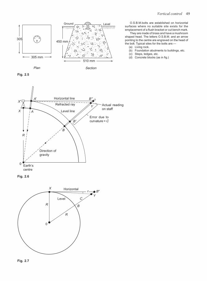
Vertical control 49
Fig. 2.5
Fig. 2.6
Fig. 2.7
R
YC
B
R
0
X
Level
Horizontalr B″
X′A′
X
Actual reading
on staff
Error due to
curvature = C
Horizontal line
Refracted ray
Level line
B″
Y
B ′
A
B
R
Direction of
gravity
0Earth’s
centre
O.S.B.M.bolts are established on horizontal
surfaces where no suitable site exists for the
emplacement of a flush bracket or cut bench mark.
They are made of brass and have a mushroom
shaped head. The letters O.S.B.M. and an arrow
pointing to the centre are engraved on the head of
the bolt. Typical sites for the bolts are:—
(a) Living rock.
(b) Foundation abutments to buildings, etc.
(c) Steps, ledges, etc.
(d) Concrete blocks (as in fig.)305 mm
305450 mm
510 mm
Ground Level
Plan Section
O
S B
M
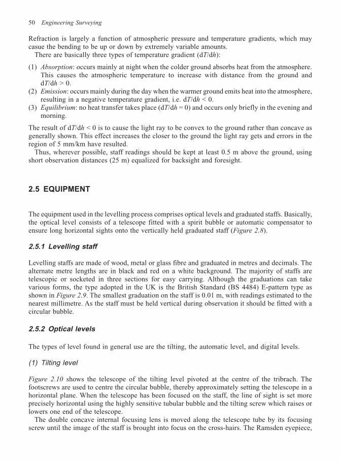
50 Engineering Surveying
Refraction is largely a function of atmospheric pressure and temperature gradients, which maycasue the bending to be up or down by extremely variable amounts.
There are basically three types of temperature gradient (dT/dh):
(1) Absorption: occurs mainly at night when the colder ground absorbs heat from the atmosphere.This causes the atmospheric temperature to increase with distance from the ground anddT/dh > 0.
(2) Emission: occurs mainly during the day when the warmer ground emits heat into the atmosphere,resulting in a negative temperature gradient, i.e. dT/dh < 0.
(3) Equilibrium: no heat transfer takes place (dT/dh = 0) and occurs only briefly in the evening andmorning.
The result of dT/dh < 0 is to cause the light ray to be convex to the ground rather than concave asgenerally shown. This effect increases the closer to the ground the light ray gets and errors in theregion of 5 mm/km have resulted.
Thus, wherever possible, staff readings should be kept at least 0.5 m above the ground, usingshort observation distances (25 m) equalized for backsight and foresight.
2.5 EQUIPMENT
The equipment used in the levelling process comprises optical levels and graduated staffs. Basically,the optical level consists of a telescope fitted with a spirit bubble or automatic compensator toensure long horizontal sights onto the vertically held graduated staff (Figure 2.8).
2.5.1 Levelling staff
Levelling staffs are made of wood, metal or glass fibre and graduated in metres and decimals. Thealternate metre lengths are in black and red on a white background. The majority of staffs aretelescopic or socketed in three sections for easy carrying. Although the graduations can takevarious forms, the type adopted in the UK is the British Standard (BS 4484) E-pattern type asshown in Figure 2.9. The smallest graduation on the staff is 0.01 m, with readings estimated to thenearest millimetre. As the staff must be held vertical during observation it should be fitted with acircular bubble.
2.5.2 Optical levels
The types of level found in general use are the tilting, the automatic level, and digital levels.
(1) Tilting level
Figure 2.10 shows the telescope of the tilting level pivoted at the centre of the tribrach. Thefootscrews are used to centre the circular bubble, thereby approximately setting the telescope in ahorizontal plane. When the telescope has been focused on the staff, the line of sight is set moreprecisely horizontal using the highly sensitive tubular bubble and the tilting screw which raises orlowers one end of the telescope.
The double concave internal focusing lens is moved along the telescope tube by its focusingscrew until the image of the staff is brought into focus on the cross-hairs. The Ramsden eyepiece,
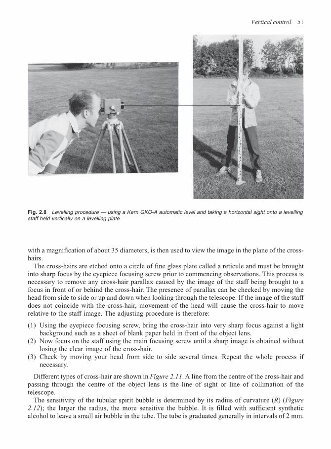
Vertical control 51
with a magnification of about 35 diameters, is then used to view the image in the plane of the cross-hairs.
The cross-hairs are etched onto a circle of fine glass plate called a reticule and must be broughtinto sharp focus by the eyepiece focusing screw prior to commencing observations. This process isnecessary to remove any cross-hair parallax caused by the image of the staff being brought to afocus in front of or behind the cross-hair. The presence of parallax can be checked by moving thehead from side to side or up and down when looking through the telescope. If the image of the staffdoes not coincide with the cross-hair, movement of the head will cause the cross-hair to moverelative to the staff image. The adjusting procedure is therefore:
(1) Using the eyepiece focusing screw, bring the cross-hair into very sharp focus against a lightbackground such as a sheet of blank paper held in front of the object lens.
(2) Now focus on the staff using the main focusing screw until a sharp image is obtained withoutlosing the clear image of the cross-hair.
(3) Check by moving your head from side to side several times. Repeat the whole process ifnecessary.
Different types of cross-hair are shown in Figure 2.11. A line from the centre of the cross-hair andpassing through the centre of the object lens is the line of sight or line of collimation of thetelescope.
The sensitivity of the tubular spirit bubble is determined by its radius of curvature (R) (Figure
2.12); the larger the radius, the more sensitive the bubble. It is filled with sufficient syntheticalcohol to leave a small air bubble in the tube. The tube is graduated generally in intervals of 2 mm.
Fig. 2.8 Levelling procedure — using a Kern GKO-A automatic level and taking a horizontal sight onto a levellingstaff held vertically on a levelling plate
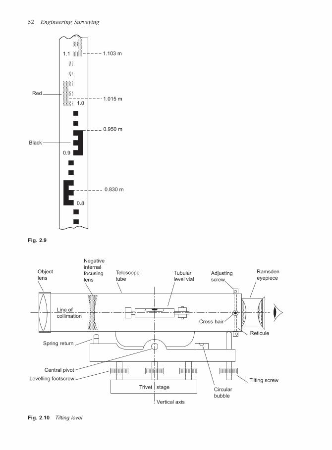
52 Engineering Surveying
0.8
0.830 m
Black
0.9
0.950 m
1.01.015 m
Red
1.1 1.103 m
Fig. 2.9
Line of
collimation
Spring return
Central pivot
Levelling footscrew
Vertical axis
Trivet stage Circular
bubble
Tilting screw
Reticule
Ramsden
eyepieceAdjusting
screw
Tubular
level vial
Telescope
tube
Negative
internal
focusing
lens
Object
lens
Cross-hair
Fig. 2.10 Tilting level
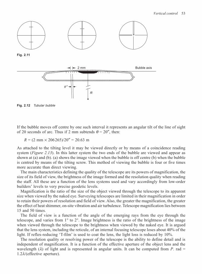
Vertical control 53
If the bubble moves off centre by one such interval it represents an angular tilt of the line of sightof 20 seconds of arc. Thus if 2 mm subtends θ = 20″, then:
R = (2 mm × 206265)/20″ = 20.63 m
As attached to the tilting level it may be viewed directly or by means of a coincidence readingsystem (Figure 2.13). In this latter system the two ends of the bubble are viewed and appear asshown at (a) and (b). (a) shows the image viewed when the bubble is off centre (b) when the bubbleis centred by means of the tilting screw. This method of viewing the bubble is four or five timesmore accurate than direct viewing.
The main characteristics defining the quality of the telescope are its powers of magnification, thesize of its field of view, the brightness of the image formed and the resolution quality when readingthe staff. All these are a function of the lens systems used and vary accordingly from low-orderbuilders’ levels to very precise geodetic levels.
Magnification is the ratio of the size of the object viewed through the telescope to its apparentsize when viewed by the naked eye. Surveying telescopes are limited in their magnification in orderto retain their powers of resolution and field of view. Also, the greater the magnification, the greaterthe effect of heat shimmer, on-site vibration and air turbulence. Telescope magnification lies between15 and 50 times.
The field of view is a function of the angle of the emerging rays from the eye through thetelescope, and varies from 1° to 2°. Image brightness is the ratio of the brightness of the imagewhen viewed through the telescope to the brightness when viewed by the naked eye. It is arguedthat the lens system, including the reticule, of an internal focusing telescope loses about 40% of thelight. If reflex-reducing ‘T-film’ is used to coat the lens, the light loss is reduced by 10%.
The resolution quality or resolving power of the telescope is the ability to define detail and isindependent of magnification. It is a function of the effective aperture of the object lens and thewavelength (λ) of light and is represented in angular units. It can be computed from P. rad =1.2λ/(effective aperture).
Fig. 2.12 Tubular bubble
2 mm
θ ″
R
Bubble axis
Fig. 2.11
+
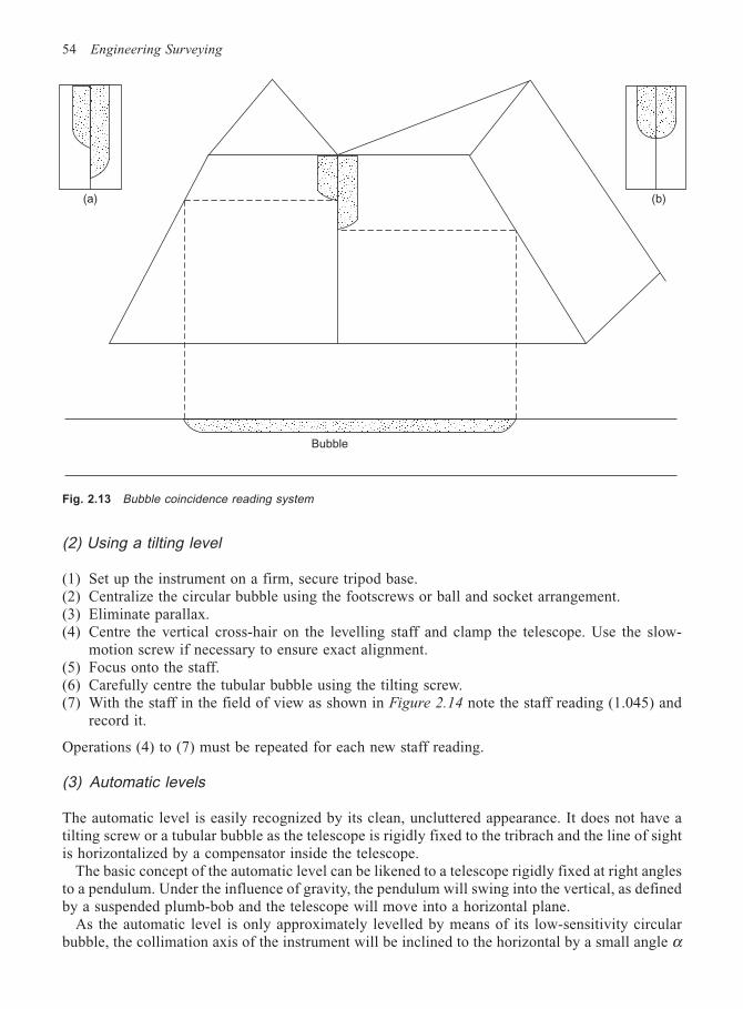
54 Engineering Surveying
(2) Using a tilting level
(1) Set up the instrument on a firm, secure tripod base.(2) Centralize the circular bubble using the footscrews or ball and socket arrangement.(3) Eliminate parallax.(4) Centre the vertical cross-hair on the levelling staff and clamp the telescope. Use the slow-
motion screw if necessary to ensure exact alignment.(5) Focus onto the staff.(6) Carefully centre the tubular bubble using the tilting screw.(7) With the staff in the field of view as shown in Figure 2.14 note the staff reading (1.045) and
record it.
Operations (4) to (7) must be repeated for each new staff reading.
(3) Automatic levels
The automatic level is easily recognized by its clean, uncluttered appearance. It does not have atilting screw or a tubular bubble as the telescope is rigidly fixed to the tribrach and the line of sightis horizontalized by a compensator inside the telescope.
The basic concept of the automatic level can be likened to a telescope rigidly fixed at right anglesto a pendulum. Under the influence of gravity, the pendulum will swing into the vertical, as definedby a suspended plumb-bob and the telescope will move into a horizontal plane.
As the automatic level is only approximately levelled by means of its low-sensitivity circularbubble, the collimation axis of the instrument will be inclined to the horizontal by a small angle α
Fig. 2.13 Bubble coincidence reading system
(b)
Bubble
(a)
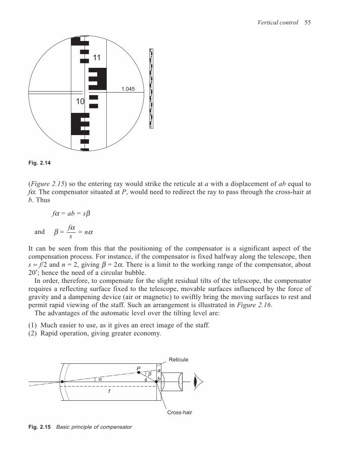
Vertical control 55
(Figure 2.15) so the entering ray would strike the reticule at a with a displacement of ab equal tofα. The compensator situated at P, would need to redirect the ray to pass through the cross-hair atb. Thus
fα = ab = sβ
and βα
α = = f
sn
It can be seen from this that the positioning of the compensator is a significant aspect of thecompensation process. For instance, if the compensator is fixed halfway along the telescope, thens ≈ f/2 and n = 2, giving β = 2α. There is a limit to the working range of the compensator, about20′; hence the need of a circular bubble.
In order, therefore, to compensate for the slight residual tilts of the telescope, the compensatorrequires a reflecting surface fixed to the telescope, movable surfaces influenced by the force ofgravity and a dampening device (air or magnetic) to swiftly bring the moving surfaces to rest andpermit rapid viewing of the staff. Such an arrangement is illustrated in Figure 2.16.
The advantages of the automatic level over the tilting level are:
(1) Much easier to use, as it gives an erect image of the staff.(2) Rapid operation, giving greater economy.
Fig. 2.14
11
10
1.045
Reticule
Cross-hair
a
bsβ
P
α
f
Fig. 2.15 Basic principle of compensator
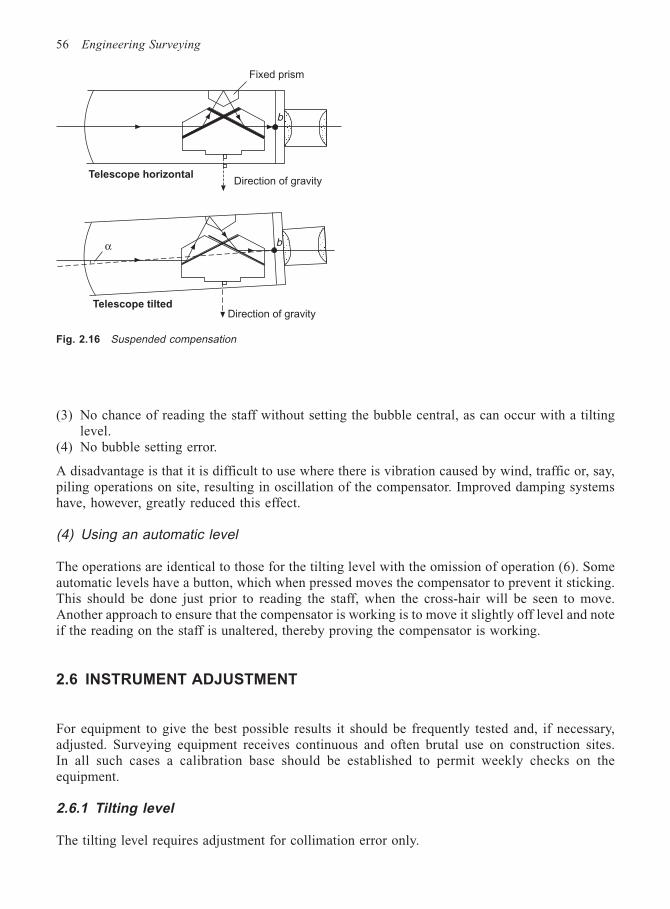
56 Engineering Surveying
(3) No chance of reading the staff without setting the bubble central, as can occur with a tiltinglevel.
(4) No bubble setting error.
A disadvantage is that it is difficult to use where there is vibration caused by wind, traffic or, say,piling operations on site, resulting in oscillation of the compensator. Improved damping systemshave, however, greatly reduced this effect.
(4) Using an automatic level
The operations are identical to those for the tilting level with the omission of operation (6). Someautomatic levels have a button, which when pressed moves the compensator to prevent it sticking.This should be done just prior to reading the staff, when the cross-hair will be seen to move.Another approach to ensure that the compensator is working is to move it slightly off level and noteif the reading on the staff is unaltered, thereby proving the compensator is working.
2.6 INSTRUMENT ADJUSTMENT
For equipment to give the best possible results it should be frequently tested and, if necessary,adjusted. Surveying equipment receives continuous and often brutal use on construction sites.In all such cases a calibration base should be established to permit weekly checks on theequipment.
2.6.1 Tilting level
The tilting level requires adjustment for collimation error only.
Telescope horizontalDirection of gravity
Fixed prism
b
Direction of gravityTelescope tilted
α b
Fig. 2.16 Suspended compensation
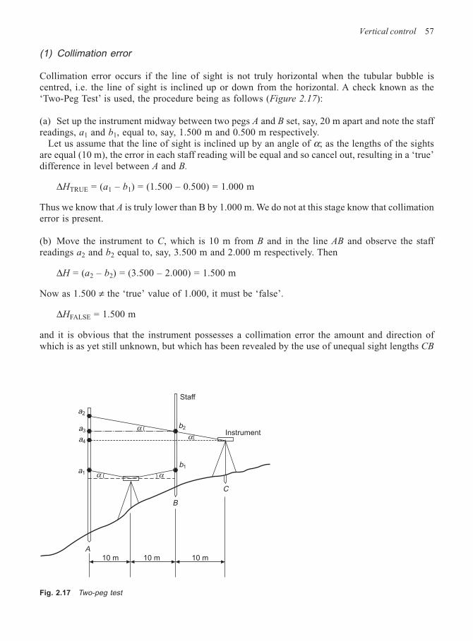
Vertical control 57
(1) Collimation error
Collimation error occurs if the line of sight is not truly horizontal when the tubular bubble iscentred, i.e. the line of sight is inclined up or down from the horizontal. A check known as the‘Two-Peg Test’ is used, the procedure being as follows (Figure 2.17):
(a) Set up the instrument midway between two pegs A and B set, say, 20 m apart and note the staffreadings, a1 and b1, equal to, say, 1.500 m and 0.500 m respectively.
Let us assume that the line of sight is inclined up by an angle of α; as the lengths of the sightsare equal (10 m), the error in each staff reading will be equal and so cancel out, resulting in a ‘true’difference in level between A and B.
∆HTRUE = (a1 – b1) = (1.500 – 0.500) = 1.000 m
Thus we know that A is truly lower than B by 1.000 m. We do not at this stage know that collimationerror is present.
(b) Move the instrument to C, which is 10 m from B and in the line AB and observe the staffreadings a2 and b2 equal to, say, 3.500 m and 2.000 m respectively. Then
∆H = (a2 – b2) = (3.500 – 2.000) = 1.500 m
Now as 1.500 ≠ the ‘true’ value of 1.000, it must be ‘false’.
∆HFALSE = 1.500 m
and it is obvious that the instrument possesses a collimation error the amount and direction ofwhich is as yet still unknown, but which has been revealed by the use of unequal sight lengths CB
Fig. 2.17 Two-peg test
Staff
Instrumentαα
αα
A
B
C
b1
b2
a2
a3
a4
a1
10 m10 m10 m
58 Engineering Surveying
(10 m) and CA (30 m). Had the two values for ∆H been equal, then there is no collimation errorpresent in the instrument.
(c) Imagine a horizontal line from reading b2 (2.000 m) cutting the staff at A at reading a3, becauseA is truly 1.000 m below B, the reading at a3 must be 2.000 + 1.000 = 3.000 m. However, the actualreading was 3.500 m, and therefore the line of sight of the instrument is too high by 0.500 m in20 m (the distance between the two pegs). This is the amount and direction of collimation error.
(d) Without moving the instrument from C, the line of sight must be adjusted down until it ishorizontal. To do this one must compute the reading (a4) on staff A that a horizontal sight from C,distance 30 m away, would give.
By simple proportion, as the error in 20 m is 0.500, the error in 30 m = (0.500 × 30)/20 =0.750 m. Therefore the required reading at a4 is 3.500 – 0.750 = 2.750 m.
(e) (i) Using the ‘tilting screw’, tilt the telescope until it reads 2.750 m on the staff. (ii) Thismovement will cause the tubular bubble to go off centre. Re-centre it by means of its adjustingscrews, which will permit the raising or lowering of one end of the bubble.
The whole operation may be repeated if thought necessary.The above process has been dealt with in great detail, as collimation error is one of the main
sources of error in the levelling process.The diagrams and much of the above detail can be dispensed with if the following is noted:
(1) (∆HFALSE – ∆HTRUE) = the amount of collimation error.(2) If ∆HFALSE > ∆HTRUE then the line of sight is inclined up and vice versa.
An example will now be done to illustrate this approach.
Worked example
Example 2.1 Assume the same separation for A, B and C. With the instrument midway between Aand B the readings are A(3.458), B(2.116). With the instrument at C, the readings are A(4.244),B(2.914).
(i) From ‘midway’ readings, ∆HTRUE = 1.342(ii) From readings at ‘C’, ∆HFALSE = 1.330
Amount of collimation error = 0.012 m in 20 m
(iii) ∆HFALSE < ∆HTRUE, therefore direction of line of sight is down
(iv) With instrument at C the reading on A(4.244) must be raised by (0.012 × 30)/20 =0.018 m to read 4.262 m
Some methods of adjustment advocate placing the instrument close to the staff at B rather than adistance away at C. This can result in error when using the reading on B and is not suitable forprecise levels. The above method is satisfactory for all types of level.
For very precise levels, it may be necessary to account for the effect of curvature and refractionwhen carrying out the above test. Kukkamaki gives the following equation for it:
Vertical control 59
(c – r) = – 1.68 × 10⁻⁴ × D2
where D = distance in metres.
As a distance of 50 m would produce a correction to the staff readings of only –0.42 mm, it can beignored for all but the most precise work.
2.6.2 Automatic level
There are two tests and adjustments necessary for an automatic level:
(1) To ensure that the line of collimation of the telescope is horizontal, within the limits of thebubble, when the circular bubble is central.
(2) The two-peg test for collimation error.
(1) Circular bubble
Although the circular bubble is relatively insensitive, it nevertheless plays an important part in theefficient functioning of the compensator:
(1) The compensator has a limited working range. If the circular bubble is out of adjustment,thereby resulting in excessive tilt of the line of collimation (and the vertical axis), the compensatormay not function efficiently or, as it attempts to compensate, the large swing of the pendulumsystem may cause it to stick in the telescope tube.
(2) The compensator gives the most accurate results near the centre of its movement, so even if thebubble is in adjustment, it should be carefully and accurately centred.
(3) The plane of the pendulum swing of the freely suspended surfaces should be parallel to the lineof sight, otherwise over- and undercompensation may occur. This would result if the circularbubble is in error transversely. Any residual error of adjustment can be eliminated by centringthe bubble with the telescope pointing backwards, whilst at the next instrument set-up it iscentred with the telescope pointing forward. This alternating process is continued throughoutthe levelling.
(4) Inclination of the telescope can cause an error in automatic levels which does not occur intilting levels, known as ‘height shift’. Due to the inclination of the telescope the centre of theobject lens is displaced vertically above or below the centre of the cross-hair, resulting in verysmall reading errors, which cannot be tolerated in precise work.
From the above it can be seen that not only must the circular bubble be in adjustment but it shouldalso be accurately centred when in use.
To adjust the bubble, bring it exactly to centre using the footscrews. Now rotate the bubblethrough 180° about the vertical axis. If the bubble moves off centre, bring it halfway back to centrewith the footscrews and then exactly back to the centre using its adjusting screws.
(2) Two-peg test
This is carried out exactly as for the tilting level. However, the line of sight is raised or lowered toits correct reading by moving the cross-hair by means of its adjusting screws.
If the instrument is still unsatisfactory the fault may lie with the compensator, in which case itshould be returned to the manufacturer.
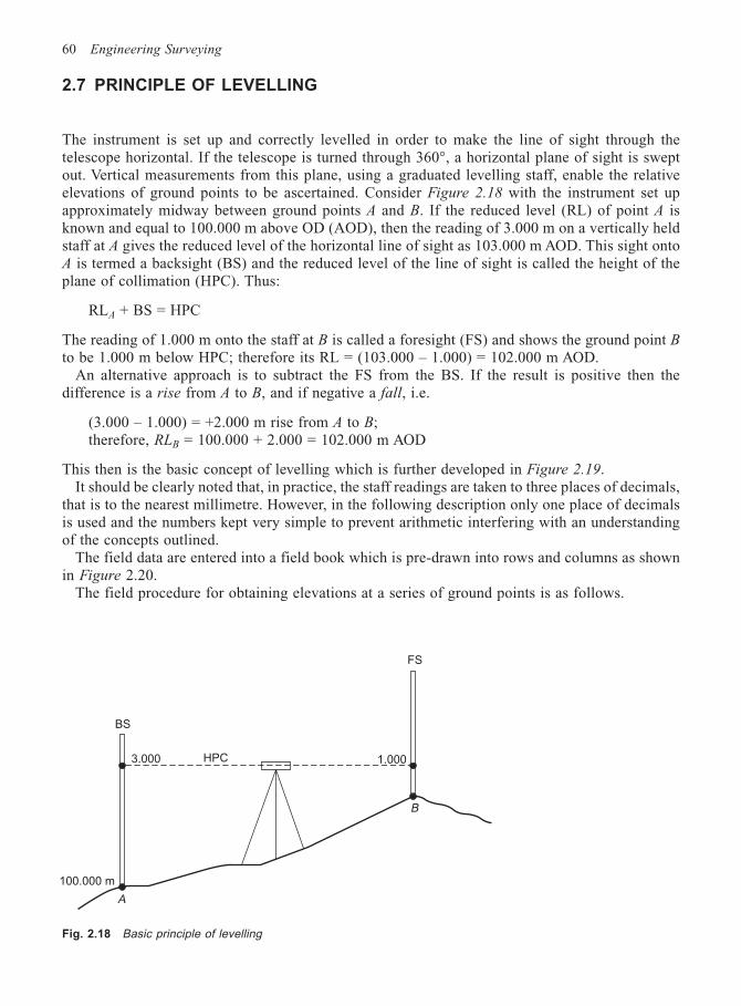
60 Engineering Surveying
2.7 PRINCIPLE OF LEVELLING
The instrument is set up and correctly levelled in order to make the line of sight through thetelescope horizontal. If the telescope is turned through 360°, a horizontal plane of sight is sweptout. Vertical measurements from this plane, using a graduated levelling staff, enable the relativeelevations of ground points to be ascertained. Consider Figure 2.18 with the instrument set upapproximately midway between ground points A and B. If the reduced level (RL) of point A isknown and equal to 100.000 m above OD (AOD), then the reading of 3.000 m on a vertically heldstaff at A gives the reduced level of the horizontal line of sight as 103.000 m AOD. This sight ontoA is termed a backsight (BS) and the reduced level of the line of sight is called the height of theplane of collimation (HPC). Thus:
RLA + BS = HPC
The reading of 1.000 m onto the staff at B is called a foresight (FS) and shows the ground point Bto be 1.000 m below HPC; therefore its RL = (103.000 – 1.000) = 102.000 m AOD.
An alternative approach is to subtract the FS from the BS. If the result is positive then thedifference is a rise from A to B, and if negative a fall, i.e.
(3.000 – 1.000) = +2.000 m rise from A to B;therefore, RLB = 100.000 + 2.000 = 102.000 m AOD
This then is the basic concept of levelling which is further developed in Figure 2.19.It should be clearly noted that, in practice, the staff readings are taken to three places of decimals,
that is to the nearest millimetre. However, in the following description only one place of decimalsis used and the numbers kept very simple to prevent arithmetic interfering with an understandingof the concepts outlined.
The field data are entered into a field book which is pre-drawn into rows and columns as shownin Figure 2.20.
The field procedure for obtaining elevations at a series of ground points is as follows.
FS
1.000HPC3.000
BS
B
100.000 m
A
Fig. 2.18 Basic principle of levelling
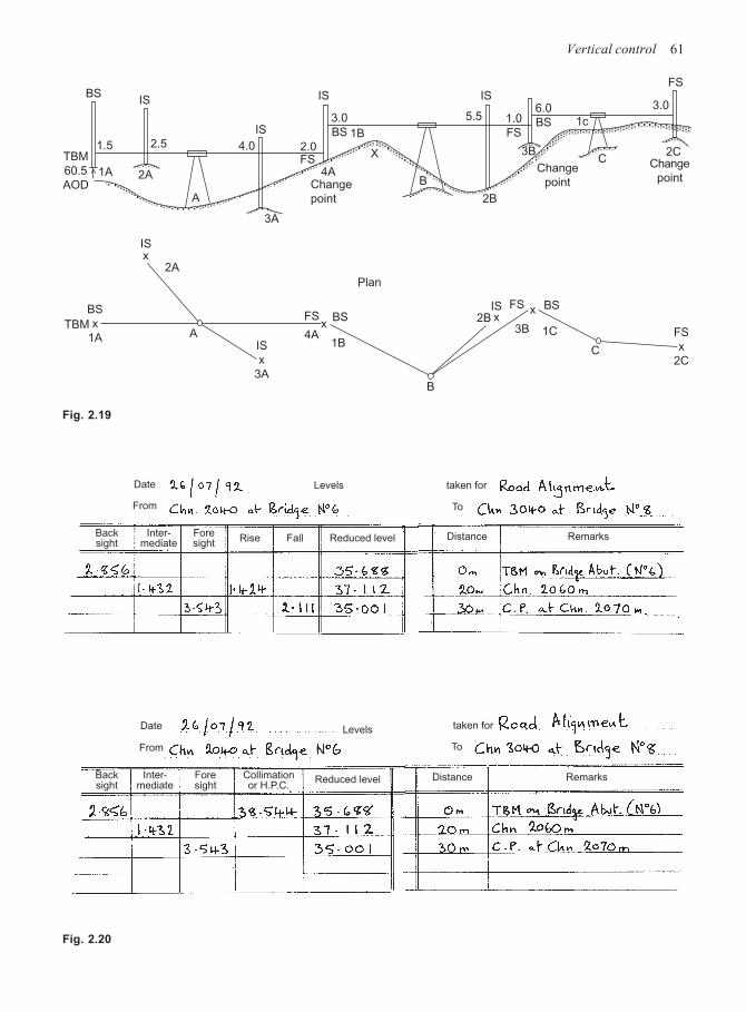
Vertical control 61
Fig. 2.19
Fig. 2.20
BSIS
X2.5
2A
TBM
60.5
AOD1A
1.5
IS
4.0
3A
A
2.0FS
4AChange
point
BChange
point
6.0
BS
3B
2B
IS
5.5
IS
3.0
BS1c
1B
2CChange
point
3.0
FS
C
ISx
A
2A
xBS
1B
BS
x
1ATBM
C
B
IS
x
3A
x
1C3B FS
x
2C
1.0
FS
FS BSISx2BFS
4A
Plan
To
Date
From
Levels taken for
Distance RemarksBacksight
Inter-mediate
Foresight
Rise Fall Reduced level
Date
From
Levels taken for
Distance RemarksBacksight
Inter-mediate
Foresight
Collimationor H.P.C.
Reduced level
To
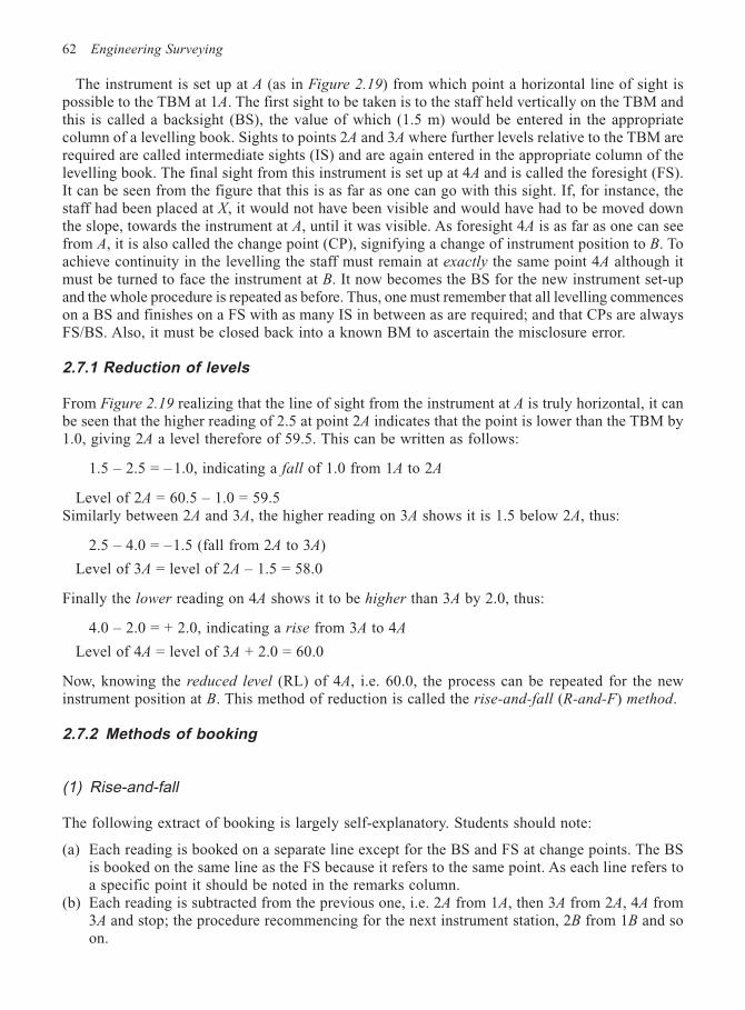
62 Engineering Surveying
The instrument is set up at A (as in Figure 2.19) from which point a horizontal line of sight ispossible to the TBM at 1A. The first sight to be taken is to the staff held vertically on the TBM andthis is called a backsight (BS), the value of which (1.5 m) would be entered in the appropriatecolumn of a levelling book. Sights to points 2A and 3A where further levels relative to the TBM arerequired are called intermediate sights (IS) and are again entered in the appropriate column of thelevelling book. The final sight from this instrument is set up at 4A and is called the foresight (FS).It can be seen from the figure that this is as far as one can go with this sight. If, for instance, thestaff had been placed at X, it would not have been visible and would have had to be moved downthe slope, towards the instrument at A, until it was visible. As foresight 4A is as far as one can seefrom A, it is also called the change point (CP), signifying a change of instrument position to B. Toachieve continuity in the levelling the staff must remain at exactly the same point 4A although itmust be turned to face the instrument at B. It now becomes the BS for the new instrument set-upand the whole procedure is repeated as before. Thus, one must remember that all levelling commenceson a BS and finishes on a FS with as many IS in between as are required; and that CPs are alwaysFS/BS. Also, it must be closed back into a known BM to ascertain the misclosure error.
2.7.1 Reduction of levels
From Figure 2.19 realizing that the line of sight from the instrument at A is truly horizontal, it canbe seen that the higher reading of 2.5 at point 2A indicates that the point is lower than the TBM by1.0, giving 2A a level therefore of 59.5. This can be written as follows:
1.5 – 2.5 = – 1.0, indicating a fall of 1.0 from 1A to 2A
Level of 2A = 60.5 – 1.0 = 59.5Similarly between 2A and 3A, the higher reading on 3A shows it is 1.5 below 2A, thus:
2.5 – 4.0 = –1.5 (fall from 2A to 3A)
Level of 3A = level of 2A – 1.5 = 58.0
Finally the lower reading on 4A shows it to be higher than 3A by 2.0, thus:
4.0 – 2.0 = + 2.0, indicating a rise from 3A to 4A
Level of 4A = level of 3A + 2.0 = 60.0
Now, knowing the reduced level (RL) of 4A, i.e. 60.0, the process can be repeated for the newinstrument position at B. This method of reduction is called the rise-and-fall (R-and-F) method.
2.7.2 Methods of booking
(1) Rise-and-fall
The following extract of booking is largely self-explanatory. Students should note:
(a) Each reading is booked on a separate line except for the BS and FS at change points. The BSis booked on the same line as the FS because it refers to the same point. As each line refers toa specific point it should be noted in the remarks column.
(b) Each reading is subtracted from the previous one, i.e. 2A from 1A, then 3A from 2A, 4A from3A and stop; the procedure recommencing for the next instrument station, 2B from 1B and soon.
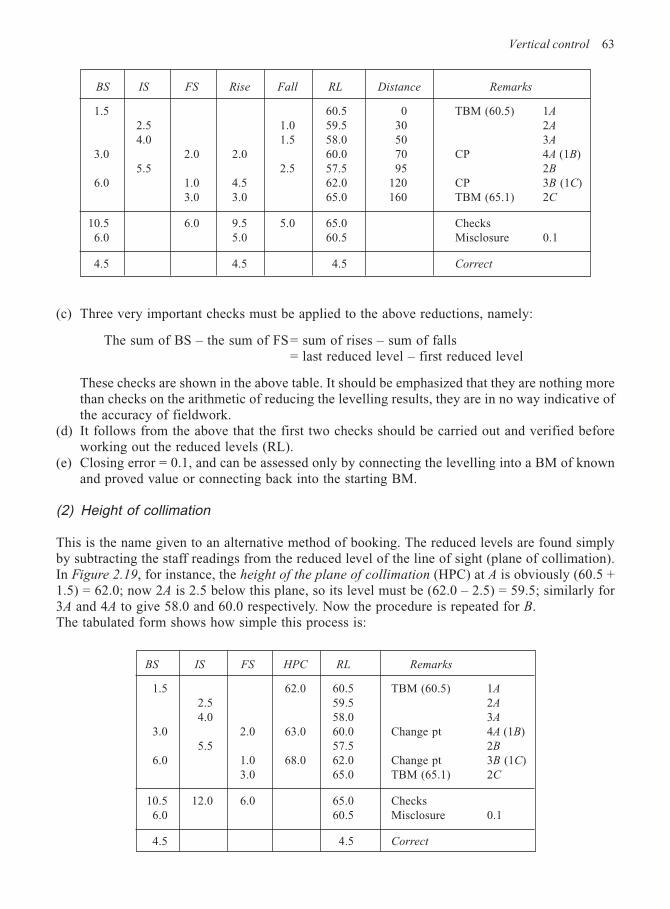
Vertical control 63
(c) Three very important checks must be applied to the above reductions, namely:
The sum of BS – the sum of FS= sum of rises – sum of falls= last reduced level – first reduced level
These checks are shown in the above table. It should be emphasized that they are nothing morethan checks on the arithmetic of reducing the levelling results, they are in no way indicative ofthe accuracy of fieldwork.
(d) It follows from the above that the first two checks should be carried out and verified beforeworking out the reduced levels (RL).
(e) Closing error = 0.1, and can be assessed only by connecting the levelling into a BM of knownand proved value or connecting back into the starting BM.
(2) Height of collimation
This is the name given to an alternative method of booking. The reduced levels are found simplyby subtracting the staff readings from the reduced level of the line of sight (plane of collimation).In Figure 2.19, for instance, the height of the plane of collimation (HPC) at A is obviously (60.5 +1.5) = 62.0; now 2A is 2.5 below this plane, so its level must be (62.0 – 2.5) = 59.5; similarly for3A and 4A to give 58.0 and 60.0 respectively. Now the procedure is repeated for B.The tabulated form shows how simple this process is:
BS IS FS Rise Fall RL Distance Remarks
1.5 60.5 0 TBM (60.5) 1A
2.5 1.0 59.5 30 2A
4.0 1.5 58.0 50 3A
3.0 2.0 2.0 60.0 70 CP 4A (1B)5.5 2.5 57.5 95 2B
6.0 1.0 4.5 62.0 120 CP 3B (1C)3.0 3.0 65.0 160 TBM (65.1) 2C
10.5 6.0 9.5 5.0 65.0 Checks6.0 5.0 60.5 Misclosure 0.1
4.5 4.5 4.5 Correct
BS IS FS HPC RL Remarks
1.5 62.0 60.5 TBM (60.5) 1A
2.5 59.5 2A
4.0 58.0 3A
3.0 2.0 63.0 60.0 Change pt 4A (1B)5.5 57.5 2B
6.0 1.0 68.0 62.0 Change pt 3B (1C)3.0 65.0 TBM (65.1) 2C
10.5 12.0 6.0 65.0 Checks6.0 60.5 Misclosure 0.1
4.5 4.5 Correct
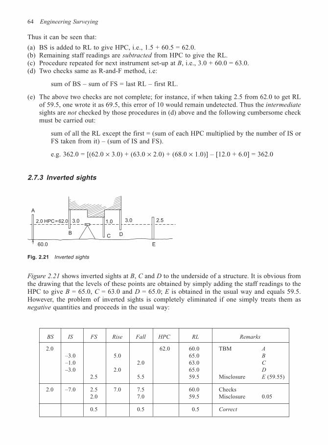
64 Engineering Surveying
Thus it can be seen that:
(a) BS is added to RL to give HPC, i.e., 1.5 + 60.5 = 62.0.(b) Remaining staff readings are subtracted from HPC to give the RL.(c) Procedure repeated for next instrument set-up at B, i.e., 3.0 + 60.0 = 63.0.(d) Two checks same as R-and-F method, i.e:
sum of BS – sum of FS = last RL – first RL.
(e) The above two checks are not complete; for instance, if when taking 2.5 from 62.0 to get RLof 59.5, one wrote it as 69.5, this error of 10 would remain undetected. Thus the intermediate
sights are not checked by those procedures in (d) above and the following cumbersome checkmust be carried out:
sum of all the RL except the first = (sum of each HPC multiplied by the number of IS orFS taken from it) – (sum of IS and FS).
e.g. 362.0 = [(62.0 × 3.0) + (63.0 × 2.0) + (68.0 × 1.0)] – [12.0 + 6.0] = 362.0
2.7.3 Inverted sights
2.0 HPC=62.0 3.0
BC D
1.0 3.0 2.5
E60.0
A
Figure 2.21 shows inverted sights at B, C and D to the underside of a structure. It is obvious fromthe drawing that the levels of these points are obtained by simply adding the staff readings to theHPC to give B = 65.0, C = 63.0 and D = 65.0; E is obtained in the usual way and equals 59.5.However, the problem of inverted sights is completely eliminated if one simply treats them asnegative quantities and proceeds in the usual way:
BS IS FS Rise Fall HPC RL Remarks
2.0 62.0 60.0 TBM A
–3.0 5.0 65.0 B
–1.0 2.0 63.0 C
–3.0 2.0 65.0 D
2.5 5.5 59.5 Misclosure E (59.55)
2.0 –7.0 2.5 7.0 7.5 60.0 Checks2.0 7.0 59.5 Misclosure 0.05
0.5 0.5 0.5 Correct
Fig. 2.21 Inverted sights
Vertical control 65
In the checks, inverted sights are treated as negative quantities; for example check for IS in HPCmethod gives
252.5 = (62.0 × 4.0) – (–7.0 + 2.5)
= (248.0) – (–4.5) = 248.0 + 4.5 = 252.5
2.7.4 Comparison of methods
The rise-and-fall method of booking is recommended as it affords a complete arithmetical check onall the observations. Although the HPC method appears superior where there are a lot of intermediatesights, it must be remembered that there is no simple straightforward check on their reduction.
The HPC method is useful when setting out levels on site. For instance, assume that a constructionlevel, for setting formwork, of 20 m AOD is required. A BS to an adjacent TBM results in an HPCof 20.834 m; a staff reading of 0.834 would then fix the bottom of the staff at the required level.
2.8 SOURCES OF ERROR
Any and all measurement processes will contain errors. In the case of levelling, these errors will be(1) instrumental, (2) observational and (3) natural.
2.8.1 Instrumental errors
(1) The main source of instrumental error is residual collimation error. As already indicated,keeping the horizontal lengths of the backsights and foresights at each instrument positionequal will cancel this error. Where the observational distances are unequal, the error will beproportional to the difference in distances.
The easiest approach to equalizing the sight distances is to pace from backsight to instrumentand then set up the foresight change point the same number of paces away from the instrument.
(2) Parallax error has already been described.(3) Staff graduation errors may result from wear and tear or repairs and should be checked against
a steel tape. Zero error of the staff, caused by excessive wear of the base, will cancel out onbacksight and foresight differences. However, if two staffs are used, errors will result unlesscalibration corrections are applied.
(4) In the case of the tripod, loose wing nuts will cause twisting and movement of the tripod head.Overtight wing nuts make it difficult to open out the tripod correctly. Loose tripod shoes willalso result in unstable set-ups.
R-and-F method HPC method
2.0–(–3.0) = +5.0 = Rise 62.0–(–3.0) = 65.0– 3.0–(–1.0)= –2.0 = Fall 62.0–(–1.0) = 63.0– 1.0–(–3.0) = +2.0 = Rise 62.0–(–3.0) = 65.0
– 3.0– 2.5 = – 5.5 = Fall 62.0–(+2.5) = 59.5
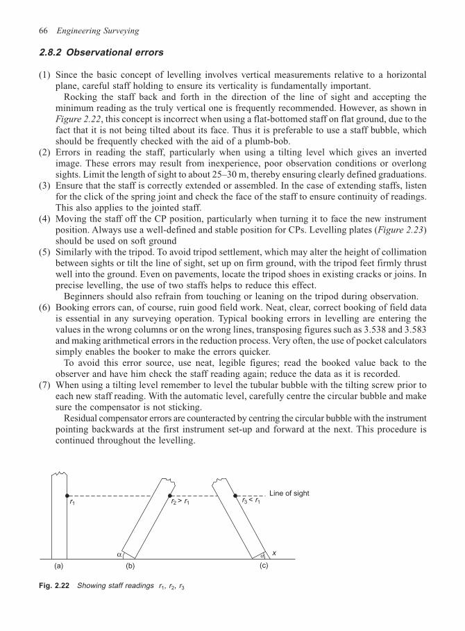
66 Engineering Surveying
2.8.2 Observational errors
(1) Since the basic concept of levelling involves vertical measurements relative to a horizontalplane, careful staff holding to ensure its verticality is fundamentally important.
Rocking the staff back and forth in the direction of the line of sight and accepting theminimum reading as the truly vertical one is frequently recommended. However, as shown inFigure 2.22, this concept is incorrect when using a flat-bottomed staff on flat ground, due to thefact that it is not being tilted about its face. Thus it is preferable to use a staff bubble, whichshould be frequently checked with the aid of a plumb-bob.
(2) Errors in reading the staff, particularly when using a tilting level which gives an invertedimage. These errors may result from inexperience, poor observation conditions or overlongsights. Limit the length of sight to about 25–30 m, thereby ensuring clearly defined graduations.
(3) Ensure that the staff is correctly extended or assembled. In the case of extending staffs, listenfor the click of the spring joint and check the face of the staff to ensure continuity of readings.This also applies to the jointed staff.
(4) Moving the staff off the CP position, particularly when turning it to face the new instrumentposition. Always use a well-defined and stable position for CPs. Levelling plates (Figure 2.23)should be used on soft ground
(5) Similarly with the tripod. To avoid tripod settlement, which may alter the height of collimationbetween sights or tilt the line of sight, set up on firm ground, with the tripod feet firmly thrustwell into the ground. Even on pavements, locate the tripod shoes in existing cracks or joins. Inprecise levelling, the use of two staffs helps to reduce this effect.
Beginners should also refrain from touching or leaning on the tripod during observation.(6) Booking errors can, of course, ruin good field work. Neat, clear, correct booking of field data
is essential in any surveying operation. Typical booking errors in levelling are entering thevalues in the wrong columns or on the wrong lines, transposing figures such as 3.538 and 3.583and making arithmetical errors in the reduction process. Very often, the use of pocket calculatorssimply enables the booker to make the errors quicker.
To avoid this error source, use neat, legible figures; read the booked value back to theobserver and have him check the staff reading again; reduce the data as it is recorded.
(7) When using a tilting level remember to level the tubular bubble with the tilting screw prior toeach new staff reading. With the automatic level, carefully centre the circular bubble and makesure the compensator is not sticking.
Residual compensator errors are counteracted by centring the circular bubble with the instrumentpointing backwards at the first instrument set-up and forward at the next. This procedure iscontinued throughout the levelling.
Fig. 2.22 Showing staff readings r1, r2, r3
Line of sight
α(c)(b)(a)
α x
r2 > r1r1r3 < r1
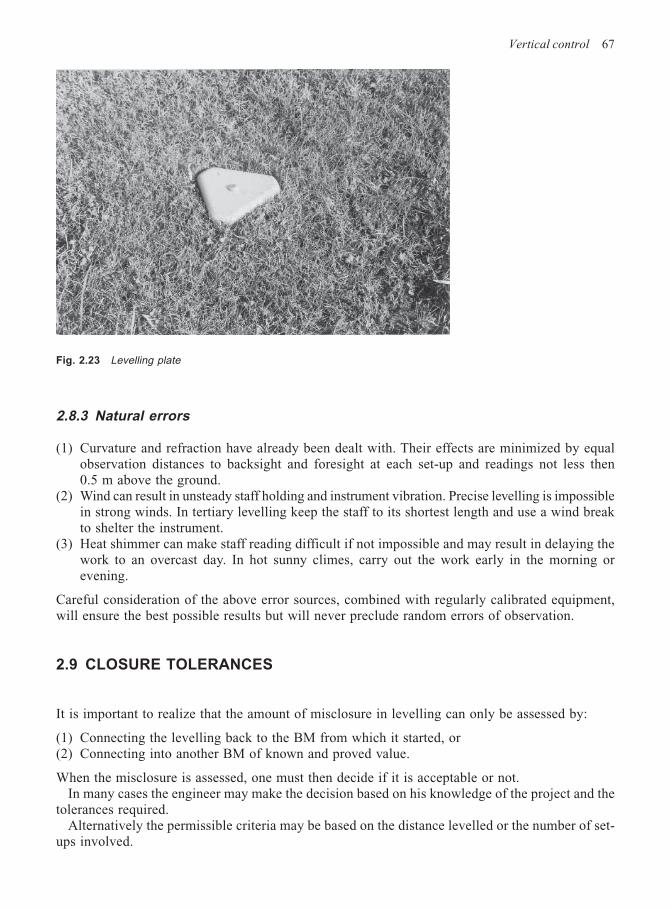
Vertical control 67
2.8.3 Natural errors
(1) Curvature and refraction have already been dealt with. Their effects are minimized by equalobservation distances to backsight and foresight at each set-up and readings not less then0.5 m above the ground.
(2) Wind can result in unsteady staff holding and instrument vibration. Precise levelling is impossiblein strong winds. In tertiary levelling keep the staff to its shortest length and use a wind breakto shelter the instrument.
(3) Heat shimmer can make staff reading difficult if not impossible and may result in delaying thework to an overcast day. In hot sunny climes, carry out the work early in the morning orevening.
Careful consideration of the above error sources, combined with regularly calibrated equipment,will ensure the best possible results but will never preclude random errors of observation.
2.9 CLOSURE TOLERANCES
It is important to realize that the amount of misclosure in levelling can only be assessed by:
(1) Connecting the levelling back to the BM from which it started, or(2) Connecting into another BM of known and proved value.
When the misclosure is assessed, one must then decide if it is acceptable or not.In many cases the engineer may make the decision based on his knowledge of the project and the
tolerances required.Alternatively the permissible criteria may be based on the distance levelled or the number of set-
ups involved.
Fig. 2.23 Levelling plate
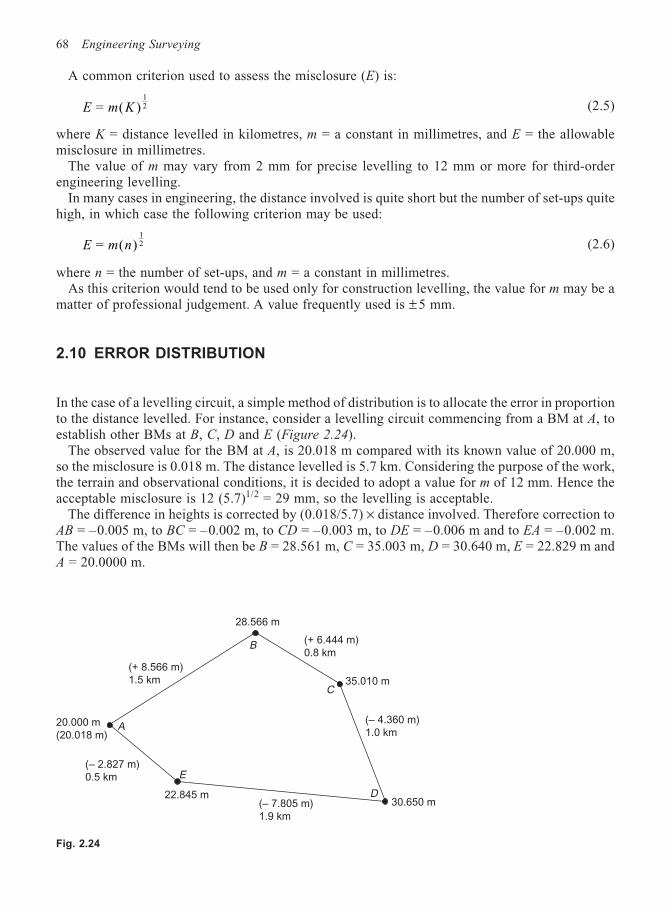
68 Engineering Surveying
A common criterion used to assess the misclosure (E) is:
E m K = ( )12 (2.5)
where K = distance levelled in kilometres, m = a constant in millimetres, and E = the allowablemisclosure in millimetres.
The value of m may vary from 2 mm for precise levelling to 12 mm or more for third-orderengineering levelling.
In many cases in engineering, the distance involved is quite short but the number of set-ups quitehigh, in which case the following criterion may be used:
E m n = ( )12 (2.6)
where n = the number of set-ups, and m = a constant in millimetres.As this criterion would tend to be used only for construction levelling, the value for m may be a
matter of professional judgement. A value frequently used is ± 5 mm.
2.10 ERROR DISTRIBUTION
In the case of a levelling circuit, a simple method of distribution is to allocate the error in proportionto the distance levelled. For instance, consider a levelling circuit commencing from a BM at A, toestablish other BMs at B, C, D and E (Figure 2.24).
The observed value for the BM at A, is 20.018 m compared with its known value of 20.000 m,so the misclosure is 0.018 m. The distance levelled is 5.7 km. Considering the purpose of the work,the terrain and observational conditions, it is decided to adopt a value for m of 12 mm. Hence theacceptable misclosure is 12 (5.7)1/2 = 29 mm, so the levelling is acceptable.
The difference in heights is corrected by (0.018/5.7) × distance involved. Therefore correction toAB = –0.005 m, to BC = –0.002 m, to CD = –0.003 m, to DE = –0.006 m and to EA = –0.002 m.The values of the BMs will then be B = 28.561 m, C = 35.003 m, D = 30.640 m, E = 22.829 m andA = 20.0000 m.
Fig. 2.24
B
A
C
E
D
28.566 m
35.010 m
(– 4.360 m)
1.0 km
30.650 m22.845 m
20.000 m
(20.018 m)
(– 2.827 m)
0.5 km
(– 7.805 m)
1.9 km
(+ 8.566 m)
1.5 km
(+ 6.444 m)
0.8 km
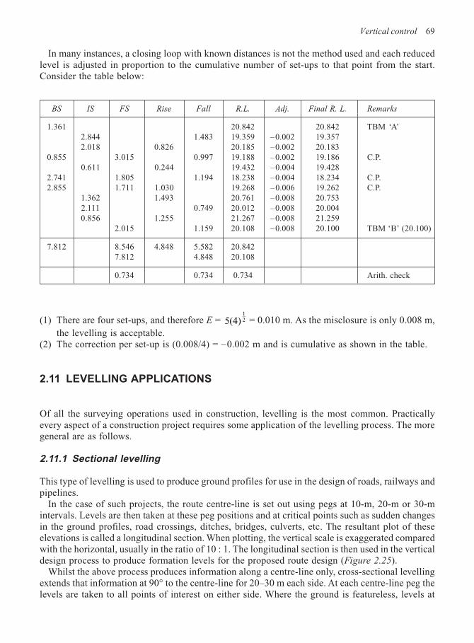
Vertical control 69
(1) There are four set-ups, and therefore E = 5(4)12 = 0.010 m. As the misclosure is only 0.008 m,
the levelling is acceptable.(2) The correction per set-up is (0.008/4) = –0.002 m and is cumulative as shown in the table.
2.11 LEVELLING APPLICATIONS
Of all the surveying operations used in construction, levelling is the most common. Practicallyevery aspect of a construction project requires some application of the levelling process. The moregeneral are as follows.
2.11.1 Sectional levelling
This type of levelling is used to produce ground profiles for use in the design of roads, railways andpipelines.
In the case of such projects, the route centre-line is set out using pegs at 10-m, 20-m or 30-mintervals. Levels are then taken at these peg positions and at critical points such as sudden changesin the ground profiles, road crossings, ditches, bridges, culverts, etc. The resultant plot of theseelevations is called a longitudinal section. When plotting, the vertical scale is exaggerated comparedwith the horizontal, usually in the ratio of 10 : 1. The longitudinal section is then used in the verticaldesign process to produce formation levels for the proposed route design (Figure 2.25).
Whilst the above process produces information along a centre-line only, cross-sectional levellingextends that information at 90° to the centre-line for 20–30 m each side. At each centre-line peg thelevels are taken to all points of interest on either side. Where the ground is featureless, levels at
BS IS FS Rise Fall R.L. Adj. Final R. L. Remarks
1.361 20.842 20.842 TBM ‘A’2.844 1.483 19.359 –0.002 19.3572.018 0.826 20.185 –0.002 20.183
0.855 3.015 0.997 19.188 –0.002 19.186 C.P.0.611 0.244 19.432 –0.004 19.428
2.741 1.805 1.194 18.238 –0.004 18.234 C.P.2.855 1.711 1.030 19.268 –0.006 19.262 C.P.
1.362 1.493 20.761 –0.008 20.7532.111 0.749 20.012 –0.008 20.0040.856 1.255 21.267 –0.008 21.259
2.015 1.159 20.108 –0.008 20.100 TBM ‘B’ (20.100)
7.812 8.546 4.848 5.582 20.8427.812 4.848 20.108
0.734 0.734 0.734 Arith. check
In many instances, a closing loop with known distances is not the method used and each reducedlevel is adjusted in proportion to the cumulative number of set-ups to that point from the start.Consider the table below:
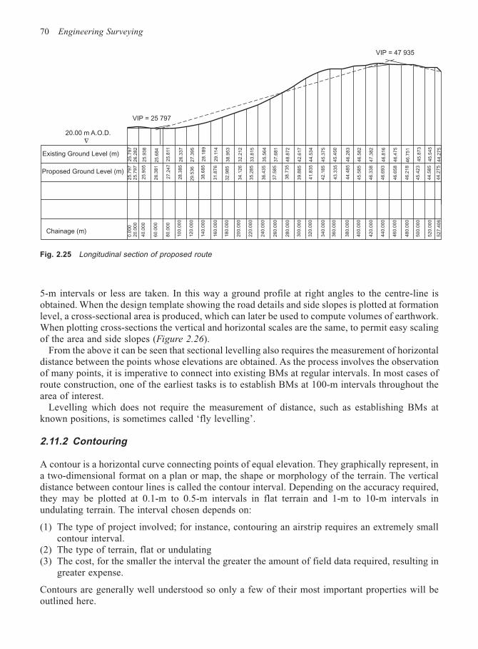
70 Engineering Surveying
5-m intervals or less are taken. In this way a ground profile at right angles to the centre-line isobtained. When the design template showing the road details and side slopes is plotted at formationlevel, a cross-sectional area is produced, which can later be used to compute volumes of earthwork.When plotting cross-sections the vertical and horizontal scales are the same, to permit easy scalingof the area and side slopes (Figure 2.26).
From the above it can be seen that sectional levelling also requires the measurement of horizontaldistance between the points whose elevations are obtained. As the process involves the observationof many points, it is imperative to connect into existing BMs at regular intervals. In most cases ofroute construction, one of the earliest tasks is to establish BMs at 100-m intervals throughout thearea of interest.
Levelling which does not require the measurement of distance, such as establishing BMs atknown positions, is sometimes called ‘fly levelling’.
2.11.2 Contouring
A contour is a horizontal curve connecting points of equal elevation. They graphically represent, ina two-dimensional format on a plan or map, the shape or morphology of the terrain. The verticaldistance between contour lines is called the contour interval. Depending on the accuracy required,they may be plotted at 0.1-m to 0.5-m intervals in flat terrain and 1-m to 10-m intervals inundulating terrain. The interval chosen depends on:
(1) The type of project involved; for instance, contouring an airstrip requires an extremely smallcontour interval.
(2) The type of terrain, flat or undulating(3) The cost, for the smaller the interval the greater the amount of field data required, resulting in
greater expense.
Contours are generally well understood so only a few of their most important properties will beoutlined here.
Fig. 2.25 Longitudinal section of proposed route
VIP = 47 935
VIP = 25 797
Chainage (m)
20.00 m A.O.D.
Proposed Ground Level (m)
Existing Ground Level (m)
25
.79
72
5.7
97
26
.28
2
25
.90
52
5.9
38
26
.38
12
5.6
84
26
.33
7
29
.53
6
38
.68
5
31
.87
629.1
14
32
.98
53
8.9
53
34
.12
6
35
.28
5
36
.43
5
39
.88
54
2.6
17
41
.83
5
42
.18
54
5.3
75
43
.33
5
44
.48
5
45
.58
54
6.5
82
47
.38
2
46
.81
6
46
.47
5
46
.75
1
45
.87
3
45
.54
5
38
.73
54
8.8
72
28
.38
5
27
.24
725.8
11
28
.18
9
40
.00
0
0.0
00
20
.00
0
60
.00
0
80
.00
0
100.0
00
120.0
00
140.0
00
160.0
00
180.0
00
200.0
00
220.0
00
240.0
00
260.0
00
280.0
00
300.0
00
320.0
00
340.0
00
360.0
00
380.0
00
400.0
00
420.0
00
440.0
00
460.0
00
480.0
00
500.0
00
520.0
00
527.4
06
44
.27
54
4.2
75
44
.58
5
45
.42
3
46
.21
8
46
.65
8
46
.69
3
46
.33
8
44
.53
4
32
.21
2
33
.81
5
35
.56
4
37
.68
13
7.5
85
27
.39
5
45
.45
0
46
.28
3
25
.79
7
∇
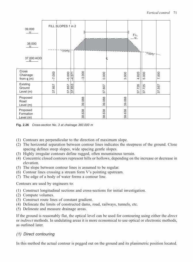
Vertical control 71
(1) Contours are perpendicular to the direction of maximum slope.(2) The horizontal separation between contour lines indicates the steepness of the ground. Close
spacing defines steep slopes, wide spacing gentle slopes.(3) Highly irregular contours define rugged, often mountainous terrain.(4) Concentric closed contours represent hills or hollows, depending on the increase or decrease in
elevation.(5) The slope between contour lines is assumed to be regular.(6) Contour lines crossing a stream form V’s pointing upstream.(7) The edge of a body of water forms a contour line.
Contours are used by engineers to:
(1) Construct longitudinal sections and cross-sections for initial investigation.(2) Compute volumes.(3) Construct route lines of constant gradient.(4) Delineate the limits of constructed dams, road, railways, tunnels, etc.(5) Delineate and measure drainage areas.
If the ground is reasonably flat, the optical level can be used for contouring using either the direct
or indirect methods. In undulating areas it is more economical to use optical or electronic methods,as outlined later.
(1) Direct contouring
In this method the actual contour is pegged out on the ground and its planimetric position located.
Fig. 2.26 Cross-section No. 3 at chainage 360.000 m
39.000
38.000
37.000 AOD
F.L.
Proposed
Road
Level (m)
Existing
Ground
Level (m)
Cross
Chainage
from c (m)L
37.8
57
–7.0
00
37.8
57
–5.0
00
37.8
53
–4.5
71
38.6
38
39.0
88
–3.0
00
38.6
38
39.0
88
37.8
07
0.0
00
38.6
38
39.0
88
3.0
00
37
.72
8
4.8
20
37.7
25
5.0
00
Proposed
Formation
Level (m)
37.5
57
7.0
00
FILL SLOPES 1 in 2
cL
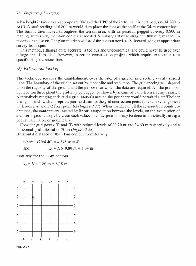
72 Engineering Surveying
A backsight is taken to an appropriate BM and the HPC of the instrument is obtained, say 34.800 mAOD. A staff reading of 0.800 m would then place the foot of the staff at the 34-m contour level.The staff is then moved throughout the terrain area, with its position pegged at every 0.800-mreading. In this way the 34-m contour is located. Similarly a staff reading of 1.800 m gives the 33-m contour and so on. The planimetric position of the contour needs to be located using an appropriatesurvey technique.
This method, although quite accurate, is tedious and uneconomical and could never be used overa large area. It is ideal, however, in certain construction projects which require excavation to aspecific single contour line.
(2) Indirect contouring
This technique requires the establishment, over the site, of a grid of intersecting evenly spacedlines. The boundary of the grid is set out by theodolite and steel tape. The grid spacing will dependupon the rugosity of the ground and the purpose for which the data are required. All the points ofintersection throughout the grid may be pegged or shown by means of paint from a spray canister.Alternatively ranging rods at the grid intervals around the periphery would permit the staff holderto align himself with appropriate pairs and thus fix the grid intersection point, for example, alignmentwith rods B-B and 2-2 fixes point B2 (Figure 2.27). When the RLs of all the intersection points areobtained, the contours are located by linear interpolation between the levels, on the assumption ofa uniform ground slope between each value. The interpolation may be done arithmetically, using apocket calculator, or graphically.
Consider grid points B2 and B3 with reduced levels of 30.20 m and 34.60 m respectively and ahorizontal grid interval of 20 m (Figure 2.28).Horizontal distance of the 31-m contour from B2 = x1
where (20/4.40) = 4.545 m = K
and x1 = K × 0.80 m = 3.64 m
Similarly for the 32-m contour
x2 = K × 1.80 m = 8.18 m
Fig. 2.27
A B C D E F
1
2
3
4
5
6
1
2
3
4
5
6
A B C D E F
B2
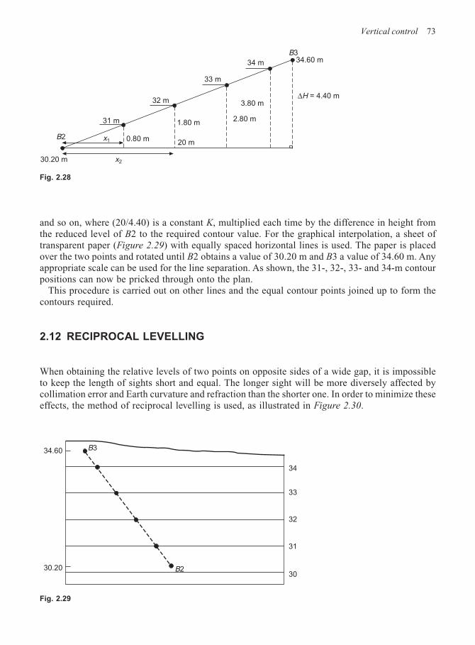
Vertical control 73
and so on, where (20/4.40) is a constant K, multiplied each time by the difference in height fromthe reduced level of B2 to the required contour value. For the graphical interpolation, a sheet oftransparent paper (Figure 2.29) with equally spaced horizontal lines is used. The paper is placedover the two points and rotated until B2 obtains a value of 30.20 m and B3 a value of 34.60 m. Anyappropriate scale can be used for the line separation. As shown, the 31-, 32-, 33- and 34-m contourpositions can now be pricked through onto the plan.
This procedure is carried out on other lines and the equal contour points joined up to form thecontours required.
2.12 RECIPROCAL LEVELLING
When obtaining the relative levels of two points on opposite sides of a wide gap, it is impossibleto keep the length of sights short and equal. The longer sight will be more diversely affected bycollimation error and Earth curvature and refraction than the shorter one. In order to minimize theseeffects, the method of reciprocal levelling is used, as illustrated in Figure 2.30.
Fig. 2.28
3.80 m
2.80 m
30.20 m
B2 x1
x2
0.80 m20 m
1.80 m
32 m
33 m
34 m
31 m
34.60 mB3
∆H = 4.40 m
B2
B334.60
30.20
34
33
32
31
30
Fig. 2.29
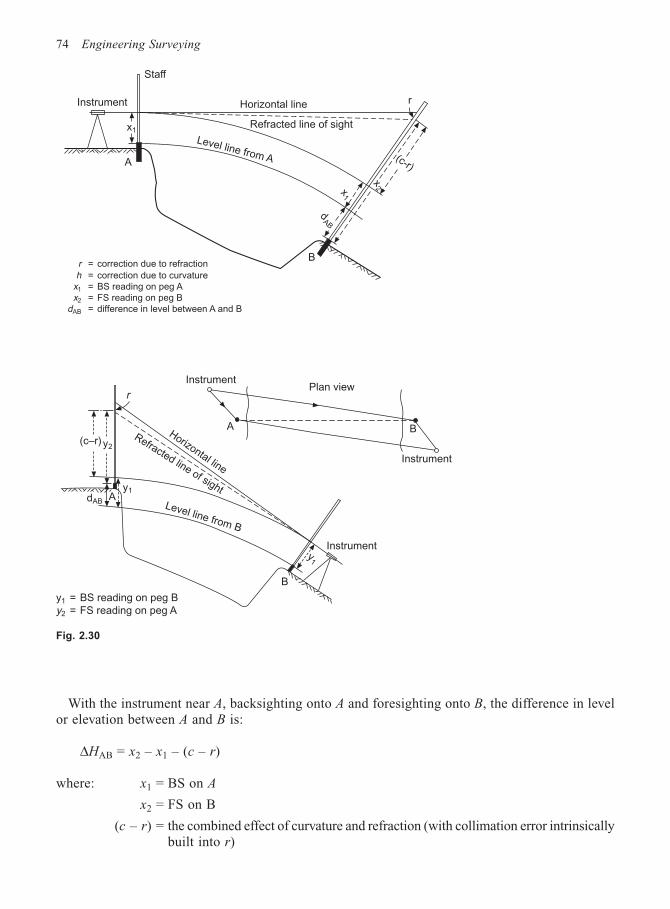
74 Engineering Surveying
With the instrument near A, backsighting onto A and foresighting onto B, the difference in levelor elevation between A and B is:
∆HAB = x2 – x1 – (c – r)
where: x1 = BS on A
x2 = FS on B
(c – r) = the combined effect of curvature and refraction (with collimation error intrinsicallybuilt into r)
Refracted line of sight
rHorizontal line
Staff
Instrument
x1
A
B
Level line from A
x2
(c-r)
x1
dAB
r = correction due to refraction
h = correction due to curvature
x1 = BS reading on peg A
x2 = FS reading on peg B
dAB = difference in level between A and B
B
Instrument
Plan viewInstrument
A
r
y2(c–r)
y1AdAB
Refracted line of sight
Horizontal line
y1
B
Instrument
Level line from B
y1 = BS reading on peg B
y2 = FS reading on peg A
Fig. 2.30
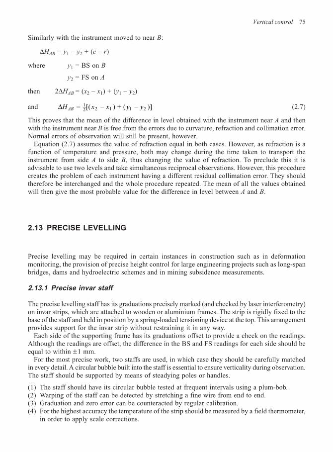
Vertical control 75
Similarly with the instrument moved to near B:
∆HAB = y1 – y2 + (c – r)
where y1 = BS on B
y2 = FS on A
then 2∆HAB = (x2 – x1) + (y1 – y2)
and = [( – ) + ( – )]12 2 1 1 2∆H x x y yAB (2.7)
This proves that the mean of the difference in level obtained with the instrument near A and thenwith the instrument near B is free from the errors due to curvature, refraction and collimation error.Normal errors of observation will still be present, however.
Equation (2.7) assumes the value of refraction equal in both cases. However, as refraction is afunction of temperature and pressure, both may change during the time taken to transport theinstrument from side A to side B, thus changing the value of refraction. To preclude this it isadvisable to use two levels and take simultaneous reciprocal observations. However, this procedurecreates the problem of each instrument having a different residual collimation error. They shouldtherefore be interchanged and the whole procedure repeated. The mean of all the values obtainedwill then give the most probable value for the difference in level between A and B.
2.13 PRECISE LEVELLING
Precise levelling may be required in certain instances in construction such as in deformationmonitoring, the provision of precise height control for large engineering projects such as long-spanbridges, dams and hydroelectric schemes and in mining subsidence measurements.
2.13.1 Precise invar staff
The precise levelling staff has its graduations precisely marked (and checked by laser interferometry)on invar strips, which are attached to wooden or aluminium frames. The strip is rigidly fixed to thebase of the staff and held in position by a spring-loaded tensioning device at the top. This arrangementprovides support for the invar strip without restraining it in any way.
Each side of the supporting frame has its graduations offset to provide a check on the readings.Although the readings are offset, the difference in the BS and FS readings for each side should beequal to within ±1 mm.
For the most precise work, two staffs are used, in which case they should be carefully matchedin every detail. A circular bubble built into the staff is essential to ensure verticality during observation.The staff should be supported by means of steadying poles or handles.
(1) The staff should have its circular bubble tested at frequent intervals using a plum-bob.(2) Warping of the staff can be detected by stretching a fine wire from end to end.(3) Graduation and zero error can be counteracted by regular calibration.(4) For the highest accuracy the temperature of the strip should be measured by a field thermometer,
in order to apply scale corrections.
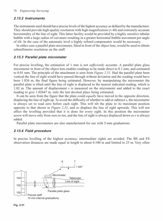
76 Engineering Surveying
2.13.2 Instruments
The instruments used should have precise levels of the highest accuracy as defined by the manufacturer.They should provide high-quality resolution with high magnification (× 40) and extremely accuratehorizontality of the line of sight. This latter facility would be provided by a highly sensitive tubularbubble with a large radius of curvature resulting in a greater horizontal bubble movement per angleof tilt. In the case of the automatic level a highly refined compensator would be necessary.
In either case a parallel plate micrometer, fitted in front of the object lens, would be used to obtainsubmillimetre resolution on the staff.
2.13.3 Parallel plate micrometer
For precise levelling, the estimation of 1 mm is not sufficiently accurate. A parallel plate glassmicrometer in front of the object lens enables readings to be made direct to 0.1 mm, and estimatedto 0.01 mm. The principle of the attachment is seen from Figure 2.31. Had the parallel plate beenvertical the line of sight would have passed through without deviation and the reading would havebeen 1.026 m, the final figure being estimated. However, by manipulating the micrometer theparallel plate is tilted until the line of sight is displaced to the nearest indicated reading, which is1.02 m. The amount of displacement s is measured on the micrometer and added to the exactreading to give 1.02647 m, only the last decimal place being estimated.
It can be seen from the figure that the plate could equally have moved in the opposite direction,displacing the line of sight up. To avoid the difficulty of whether to add or subtract s, the micrometeris always set to read zero before each sight. This will tilt the plate to its maximum positionopposite to that shown in Figure 2.31, and so displace the line of sight upwards. This will notaffect the levelling provided that it is done for every sight. In this position the micrometerscrew will move only from zero to ten, and the line of sight is always displaced down so s is alwaysadded.
Parallel plate micrometers are also manufactured for use with 5-mm graduations.
2.13.4 Field procedure
In precise levelling of the highest accuracy, intermediate sights are avoided. The BS and FSobservation distances are made equal in length to about 0.100 m and limited to 25 m. Very often
Fig. 2.31
104
102
100
S
Precise staff
10 mm interval graduations
Parallel plate glass
TelescopeMicrometer
6 7
= 647
Line of sight
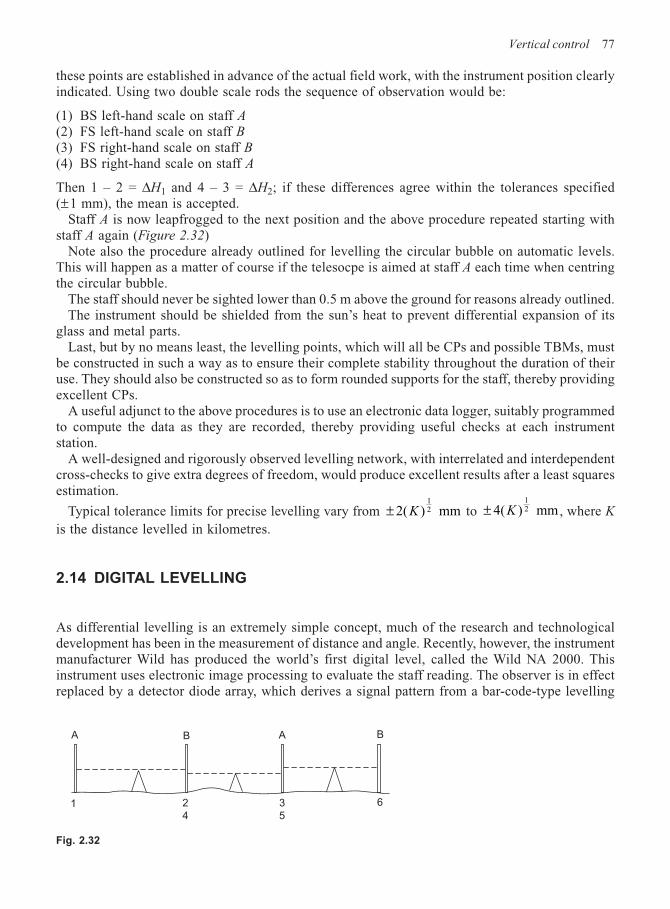
Vertical control 77
these points are established in advance of the actual field work, with the instrument position clearlyindicated. Using two double scale rods the sequence of observation would be:
(1) BS left-hand scale on staff A(2) FS left-hand scale on staff B(3) FS right-hand scale on staff B(4) BS right-hand scale on staff A
Then 1 – 2 = ∆H1 and 4 – 3 = ∆H2; if these differences agree within the tolerances specified(±1 mm), the mean is accepted.
Staff A is now leapfrogged to the next position and the above procedure repeated starting withstaff A again (Figure 2.32)
Note also the procedure already outlined for levelling the circular bubble on automatic levels.This will happen as a matter of course if the telesocpe is aimed at staff A each time when centringthe circular bubble.
The staff should never be sighted lower than 0.5 m above the ground for reasons already outlined.The instrument should be shielded from the sun’s heat to prevent differential expansion of its
glass and metal parts.Last, but by no means least, the levelling points, which will all be CPs and possible TBMs, must
be constructed in such a way as to ensure their complete stability throughout the duration of theiruse. They should also be constructed so as to form rounded supports for the staff, thereby providingexcellent CPs.
A useful adjunct to the above procedures is to use an electronic data logger, suitably programmedto compute the data as they are recorded, thereby providing useful checks at each instrumentstation.
A well-designed and rigorously observed levelling network, with interrelated and interdependentcross-checks to give extra degrees of freedom, would produce excellent results after a least squaresestimation.
Typical tolerance limits for precise levelling vary from ± 2( ) mm12K to ± 4( ) mm
12K , where K
is the distance levelled in kilometres.
2.14 DIGITAL LEVELLING
As differential levelling is an extremely simple concept, much of the research and technologicaldevelopment has been in the measurement of distance and angle. Recently, however, the instrumentmanufacturer Wild has produced the world’s first digital level, called the Wild NA 2000. Thisinstrument uses electronic image processing to evaluate the staff reading. The observer is in effectreplaced by a detector diode array, which derives a signal pattern from a bar-code-type levelling
Fig. 2.32
63
5
2
41
BABA
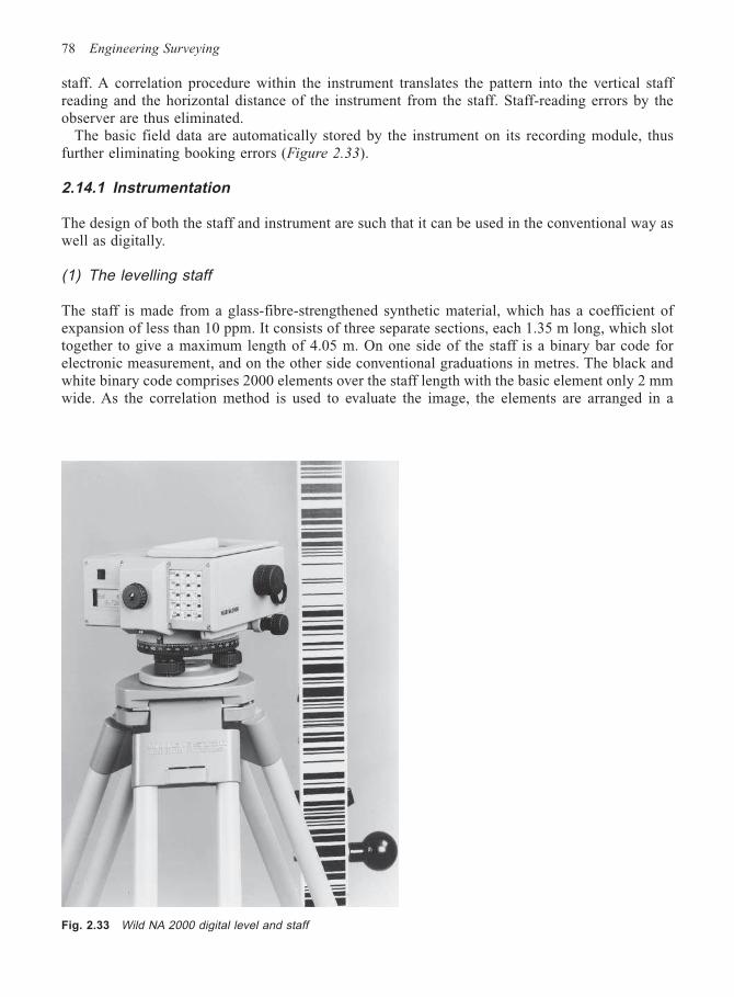
78 Engineering Surveying
staff. A correlation procedure within the instrument translates the pattern into the vertical staffreading and the horizontal distance of the instrument from the staff. Staff-reading errors by theobserver are thus eliminated.
The basic field data are automatically stored by the instrument on its recording module, thusfurther eliminating booking errors (Figure 2.33).
2.14.1 Instrumentation
The design of both the staff and instrument are such that it can be used in the conventional way aswell as digitally.
(1) The levelling staff
The staff is made from a glass-fibre-strengthened synthetic material, which has a coefficient ofexpansion of less than 10 ppm. It consists of three separate sections, each 1.35 m long, which slottogether to give a maximum length of 4.05 m. On one side of the staff is a binary bar code forelectronic measurement, and on the other side conventional graduations in metres. The black andwhite binary code comprises 2000 elements over the staff length with the basic element only 2 mmwide. As the correlation method is used to evaluate the image, the elements are arranged in a
Fig. 2.33 Wild NA 2000 digital level and staff
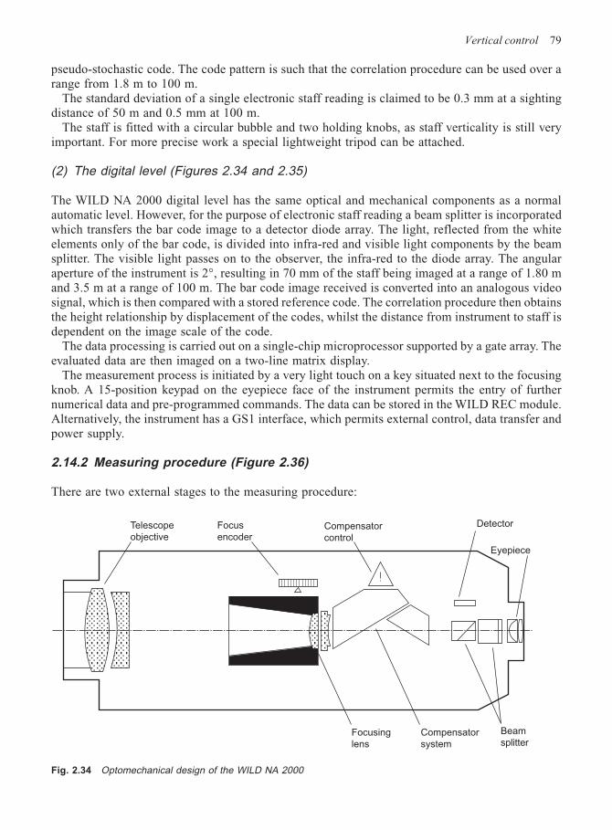
Vertical control 79
pseudo-stochastic code. The code pattern is such that the correlation procedure can be used over arange from 1.8 m to 100 m.
The standard deviation of a single electronic staff reading is claimed to be 0.3 mm at a sightingdistance of 50 m and 0.5 mm at 100 m.
The staff is fitted with a circular bubble and two holding knobs, as staff verticality is still veryimportant. For more precise work a special lightweight tripod can be attached.
(2) The digital level (Figures 2.34 and 2.35)
The WILD NA 2000 digital level has the same optical and mechanical components as a normalautomatic level. However, for the purpose of electronic staff reading a beam splitter is incorporatedwhich transfers the bar code image to a detector diode array. The light, reflected from the whiteelements only of the bar code, is divided into infra-red and visible light components by the beamsplitter. The visible light passes on to the observer, the infra-red to the diode array. The angularaperture of the instrument is 2°, resulting in 70 mm of the staff being imaged at a range of 1.80 mand 3.5 m at a range of 100 m. The bar code image received is converted into an analogous videosignal, which is then compared with a stored reference code. The correlation procedure then obtainsthe height relationship by displacement of the codes, whilst the distance from instrument to staff isdependent on the image scale of the code.
The data processing is carried out on a single-chip microprocessor supported by a gate array. Theevaluated data are then imaged on a two-line matrix display.
The measurement process is initiated by a very light touch on a key situated next to the focusingknob. A 15-position keypad on the eyepiece face of the instrument permits the entry of furthernumerical data and pre-programmed commands. The data can be stored in the WILD REC module.Alternatively, the instrument has a GS1 interface, which permits external control, data transfer andpower supply.
2.14.2 Measuring procedure (Figure 2.36)
There are two external stages to the measuring procedure:
Telescope
objectiveCompensator
control
Focus
encoder
Eyepiece
Detector
Beam
splitterCompensator
system
Focusing
lens
Fig. 2.34 Optomechanical design of the WILD NA 2000
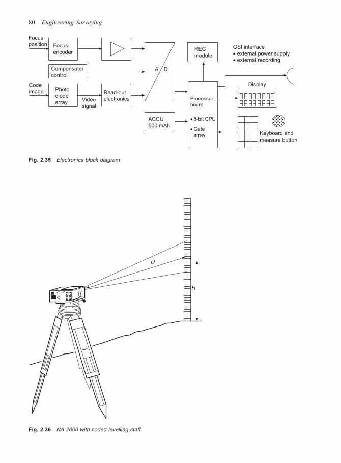
80 Engineering Surveying
Fig. 2.35 Electronics block diagram
Focus
position
Code
image
A D
ACCU
500 mAh
Read-out
electronicsVideo
signal
Photo
diode
array
Compensator
control
Focus
encoderREC
module
Processor
board
• 8-bit CPU
• Gate
array
GSI interface
• external power supply
• external recording
Display
Keyboard and
measure button
D
H
Fig. 2.36 NA 2000 with coded levelling staff

Vertical control 81
(1) Pointing and focusing on the staff.(2) Triggering the digital measurement.
These are followed by two internal stages:
(1) Coarse correlation.(2) Fine correlation.
The whole process takes about four seconds.Triggering the measurement determines the focus position, from which the distance to the staff
is measured, and initiates monitoring of the compensator.The coarse correlation approximately determines the target height and the image scale. The
process takes about one second. In one further second, the fine correlation with the aid of calibrationconstants produces the final staff reading and observation distance.
The results may be further processed in accordance with the accessed program and operatingmode, displayed and recorded. The programs incorporated in the instrument are:
(1) MEASURE ONLY – Staff reading and horizontal distance.(2) START LEVELLING – Commence line levelling.(3) CONTINUE LEVELLING – Line levelling including intermediate sights. Automatic reduction
of data. Setting out of levels.(4) CHECK AND ADJUST – Facilitates the calibration of the instrument (two-peg test).(5) ERASE DATA – Erases contents of REC module.(6) INVERT – Permits use of inverted sights.(7) SET – Enables the parameters of the instrument to be set and is similar to the initializing
procedures used when setting up electronic theodolites.
2.14.3 Factors affecting the measuring procedure
Every operation in a measurement procedure is a possible error source and as such requires carefulconsideration in order to assess the effect on the final result.
(1) Pointing and focusing
It can be shown that at a range of 2 m only 0.3 mm of the staff width need be imaged and at100 m only 14 mm. As the bar code is 50 mm wide, positioning the staff to face the instrument isnot critical and results can be obtained even when the staff is at 45° to the line of sight.
The precision of the height measurement is independent of sharpness of image; however, a clear,sharply focused image reduces the time required for the measurement.
(2) Vibrations and heat shimmer
Vibration of the compensator caused by wind, traffic, etc. has a similar effect on the bar code imageas that of heat shimmer. However, as digital levelling does not require a single reading, but insteadis dependent on a section of the code, the effects of shimmer and vibration are not critical.
Similarly, scale errors on the staff are averaged.
(3) Illumination
As the method relies on reflected light from the white intervals of the bar code, illumination of thestaff is important. During the day, this illumination will be affected by cloud, sun, twilight and the
82 Engineering Surveying
effects of shadows. All these variations are catered for by the instrument and are indicated by anincrease in the measuring time as illumination decreases.
If used in artificial light, its spectral distribution must be comparable with daylight.
(4) Staff coverage
In some conditions part of the bar code section being interrogated by the instrument may beobscured. A minimum of 30 code elements are necessary to determine height and distance, requiringat least 70 mm of the staff section to be available. This means that for ranges greater than 5 m upto 30% of the staff section may be obscured. Below 5 m, all the section is required.
2.14.4 Operating features
(1) Resolution of the measuring system is 0.1 mm for height and 10 mm for distance.(2) Range is from 1.8 m to 100 m.(3) Standard deviation for 1-km double-run levelling at ranges below 50 m:
Digital levelling ±1.5 mm.Optical levelling ±2.0 mm.
(4) Standard deviation of a single electronic staff reading at ranges of:
50 m = ±0.3 mm100 m = ±0.5 mm
(5) Standard deviation of distance measurement:
at 50 m = ±20 mmat 100 m = ±50 mm
(6) Duration of internal battery = 8 h.(7) Weight including battery = 2.5 kg.
2.14.5 Advantages of digital levelling
(1) Fatigue-free observation, as visual staff reading by the observer is excluded.(2) Easy to read, digital display of results, with the last digit selectable 1 mm or 0.1 mm.(3) Measurement of consistent precision and reliability.(4) Automatic data storage eliminates booking and its associated errors.(5) Automatic reduction of data to produce ground levels, thereby eliminating arithmetical errors.(6) User-friendly menus.(7) Fast, economic surveys. As much as 50% saving in time.(8) Increase in range up to 100 m.(9) On-line link to computer, enables the computation and plotting of longitudinal sections and
cross-sections in a very short time.(10) Can be used in all the situations in which a conventional level is used.(11) Can be used as a conventional level if necessary.
Worked examples
Example 2.2 The positions of the pegs which need to be set out for the construction of a slopingconcrete slab are shown in the diagram. Because of site obstructions the tilting level which is used
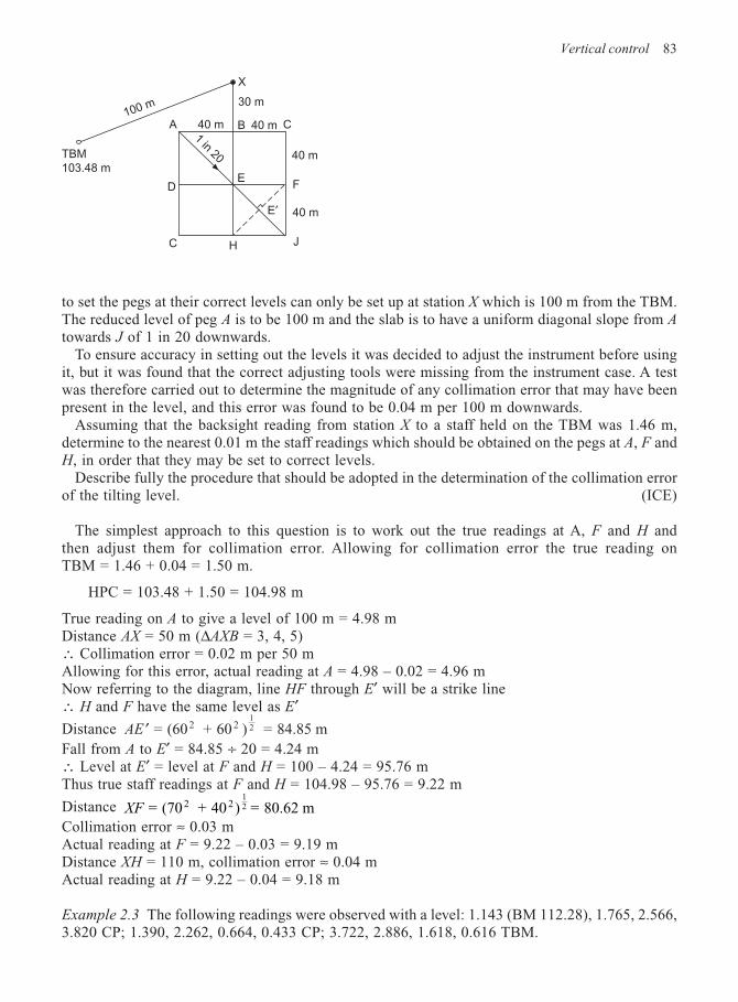
Vertical control 83
to set the pegs at their correct levels can only be set up at station X which is 100 m from the TBM.The reduced level of peg A is to be 100 m and the slab is to have a uniform diagonal slope from Atowards J of 1 in 20 downwards.
To ensure accuracy in setting out the levels it was decided to adjust the instrument before usingit, but it was found that the correct adjusting tools were missing from the instrument case. A testwas therefore carried out to determine the magnitude of any collimation error that may have beenpresent in the level, and this error was found to be 0.04 m per 100 m downwards.
Assuming that the backsight reading from station X to a staff held on the TBM was 1.46 m,determine to the nearest 0.01 m the staff readings which should be obtained on the pegs at A, F andH, in order that they may be set to correct levels.
Describe fully the procedure that should be adopted in the determination of the collimation errorof the tilting level. (ICE)
The simplest approach to this question is to work out the true readings at A, F and H andthen adjust them for collimation error. Allowing for collimation error the true reading onTBM = 1.46 + 0.04 = 1.50 m.
HPC = 103.48 + 1.50 = 104.98 m
True reading on A to give a level of 100 m = 4.98 mDistance AX = 50 m (∆AXB = 3, 4, 5)∴ Collimation error = 0.02 m per 50 mAllowing for this error, actual reading at A = 4.98 – 0.02 = 4.96 mNow referring to the diagram, line HF through E′ will be a strike line∴ H and F have the same level as E′Distance AE ′ = (60 + 60 ) = 84.85 m2 2
12
Fall from A to E′ = 84.85 ÷ 20 = 4.24 m∴ Level at E′ = level at F and H = 100 – 4.24 = 95.76 mThus true staff readings at F and H = 104.98 – 95.76 = 9.22 m
Distance XF = (70 + 40 ) = 80.62 m2 212
Collimation error ≈ 0.03 mActual reading at F = 9.22 – 0.03 = 9.19 mDistance XH = 110 m, collimation error ≈ 0.04 mActual reading at H = 9.22 – 0.04 = 9.18 m
Example 2.3 The following readings were observed with a level: 1.143 (BM 112.28), 1.765, 2.566,3.820 CP; 1.390, 2.262, 0.664, 0.433 CP; 3.722, 2.886, 1.618, 0.616 TBM.
100 m
TBM
103.48 m
A B 40 m C
40 m
F
JHC
DE
E′
30 m
X
40 m1 in 20
40 m
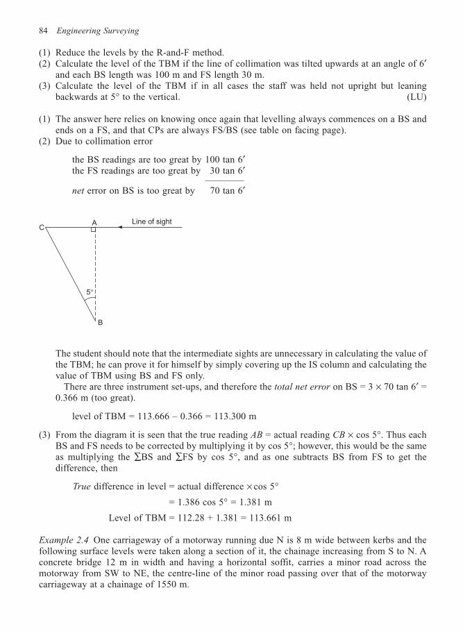
84 Engineering Surveying
(1) Reduce the levels by the R-and-F method.(2) Calculate the level of the TBM if the line of collimation was tilted upwards at an angle of 6′
and each BS length was 100 m and FS length 30 m.(3) Calculate the level of the TBM if in all cases the staff was held not upright but leaning
backwards at 5° to the vertical. (LU)
(1) The answer here relies on knowing once again that levelling always commences on a BS andends on a FS, and that CPs are always FS/BS (see table on facing page).
(2) Due to collimation error
the BS readings are too great by 100 tan 6′the FS readings are too great by 30 tan 6′
————net error on BS is too great by 70 tan 6′
Line of sightAC
5°
B
The student should note that the intermediate sights are unnecessary in calculating the value ofthe TBM; he can prove it for himself by simply covering up the IS column and calculating thevalue of TBM using BS and FS only.
There are three instrument set-ups, and therefore the total net error on BS = 3 × 70 tan 6′ =0.366 m (too great).
level of TBM = 113.666 – 0.366 = 113.300 m
(3) From the diagram it is seen that the true reading AB = actual reading CB × cos 5°. Thus eachBS and FS needs to be corrected by multiplying it by cos 5°; however, this would be the sameas multiplying the ∑BS and ∑FS by cos 5°, and as one subtracts BS from FS to get thedifference, then
True difference in level = actual difference × cos 5°
= 1.386 cos 5° = 1.381 m
Level of TBM = 112.28 + 1.381 = 113.661 m
Example 2.4 One carriageway of a motorway running due N is 8 m wide between kerbs and thefollowing surface levels were taken along a section of it, the chainage increasing from S to N. Aconcrete bridge 12 m in width and having a horizontal soffit, carries a minor road across themotorway from SW to NE, the centre-line of the minor road passing over that of the motorwaycarriageway at a chainage of 1550 m.
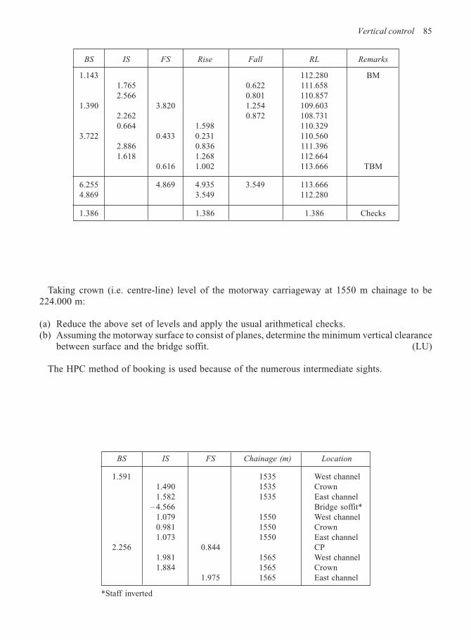
Vertical control 85
Taking crown (i.e. centre-line) level of the motorway carriageway at 1550 m chainage to be224.000 m:
(a) Reduce the above set of levels and apply the usual arithmetical checks.(b) Assuming the motorway surface to consist of planes, determine the minimum vertical clearance
between surface and the bridge soffit. (LU)
The HPC method of booking is used because of the numerous intermediate sights.
BS IS FS Rise Fall RL Remarks
1.143 112.280 BM1.765 0.622 111.6582.566 0.801 110.857
1.390 3.820 1.254 109.6032.262 0.872 108.7310.664 1.598 110.329
3.722 0.433 0.231 110.5602.886 0.836 111.3961.618 1.268 112.664
0.616 1.002 113.666 TBM
6.255 4.869 4.935 3.549 113.6664.869 3.549 112.280
1.386 1.386 1.386 Checks
BS IS FS Chainage (m) Location
1.591 1535 West channel1.490 1535 Crown1.582 1535 East channel
– 4.566 Bridge soffit*1.079 1550 West channel0.981 1550 Crown1.073 1550 East channel
2.256 0.844 CP1.981 1565 West channel1.884 1565 Crown
1.975 1565 East channel
*Staff inverted
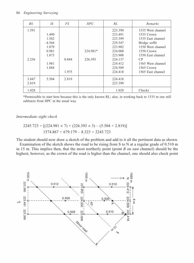
86 Engineering Surveying
Intermediate sight check
2245.723 = [(224.981 × 7) + (226.393 × 3) – (5.504 + 2.819)]
1574.867 + 679.179 – 8.323 = 2245.723
The student should now draw a sketch of the problem and add to it all the pertinent data as shown.Examination of the sketch shows the road to be rising from S to N at a regular grade of 0.510 m
in 15 m. This implies then, that the most northerly point (point B on east channel) should be thehighest; however, as the crown of the road is higher than the channel, one should also check point
BS IS FS HPC RL Remarks
1.591 223.390 1535 West channel1.490 223.491 1535 Crown1.582 223.399 1535 East channel
–4.566 229.547 Bridge soffit1.079 223.902 1550 West channel0.981 224.981* 224.000 1550 Crown1.073 223.908 1550 East channel
2.256 0.844 226.393 224.137 CP1.981 224.412 1565 West channel1.884 224.509 1565 Crown
1.975 224.418 1565 East channel
3.847 5.504 2.819 224.4182.819 223.390
1.028 1.028 Checks
*Permissible to start here because this is the only known RL; also, in working back to 1535 m one stillsubtracts from HPC in the usual way.
1565 m
224.4
12
8 m
224.5
09
224.4
18
N
0.510
0.509
223.9
08
224.0
00
0.509
0.509
0.512
45 °
R
A
12 mcL
0.510
Minor road
223.9
02
1550
m
223.3
99
223.4
91
223.3
90
1535
m
cL
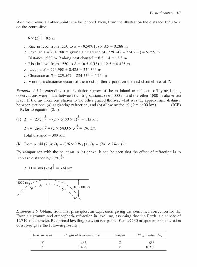
Vertical control 87
A on the crown; all other points can be ignored. Now, from the illustration the distance 1550 to Aon the centre-line.
= 6 (2) = 8.5 m1
× 2
∴ Rise in level from 1550 to A = (0.509/15) × 8.5 = 0.288 m
∴ Level at A = 224.288 m giving a clearance of (229.547 – 224.288) = 5.259 m
Distance 1550 to B along east channel = 8.5 + 4 = 12.5 m
∴ Rise in level from 1550 to B = (0.510/15) × 12.5 = 0.425 m
∴ Level at B = 223.908 + 0.425 = 224.333 m
∴ Clearance at B = 229.547 – 224.333 = 5.214 m
∴ Minimum clearance occurs at the most northerly point on the east channel, i.e. at B.
Example 2.5 In extending a triangulation survey of the mainland to a distant off-lying island,observations were made between two trig stations, one 3000 m and the other 1000 m above sealevel. If the ray from one station to the other grazed the sea, what was the approximate distancebetween stations, (a) neglecting refraction, and (b) allowing for it? (R = 6400 km). (ICE)
Refer to equation (2.1).
(a) D Rc1 1 = (2 ) = (2 6400 1) = 113 km1 1
22 × ×
D Rc2 2= (2 ) = (2 6400 3) = 196 km1 1
22 × ×
Total distance = 309 km
(b) From p. 44 (2.6): = (7/6 2 , = (7/6 2 )1 1 2 2
12
12D Rc D Rc× ×) .
By comparison with the equation in (a) above, it can be seen that the effect of refraction is to
increase distance by (7/6)12 :
∴ D = 309 (7/6) = 334 km12
Instrument at Height of instrument (m) Staff at Staff reading (m)
Y 1.463 Z 1.688Z 1.436 Y 0.991
3000 m
h11000 m
D2
D1 h2
Example 2.6 Obtain, from first principles, an expression giving the combined correction for theEarth’s curvature and atmospheric refraction in levelling, assuming that the Earth is a sphere of12740 km diameter. Reciprocal levelling between two points Y and Z 730 m apart on opposite sidesof a river gave the following results:
88 Engineering Surveying
Determine the difference in level between Y and Z and the amount of any collimation error in theinstrument. (ICE)
(1) ( – ) = 614
= 0.0673 m2
2c rD
RD
(2) With instrument at Y, Z is lower by (1.688 – 1.463) = 0.225 m
With instrument at Z, Z is lower by (1.436 – 0.991) = 0.445 m
True height of Z below Y = 0.225 + 0.4452
= 0.335 m
Instrument height at Y = 1.463 m; knowing now that Z is lower by 0.335 m, then a truly horizontalreading on Z should be (1.463 + 0.335) = 1.798 m; it was, however, 1.688 m, i.e. –0.11 m too low(– indicates low). This error is due to curvature and refraction (c – r) and collimation error of theinstrument (e).
Thus: (c – r) + e = –0.110 m
Now ( – ) = 614
= 6 73014 6370 1000
= 0.036 m2 2
c rD
R×
× ×
∴ e = –0.110 – 0.036 = –0.146 m in 730 m
∴ Collimation error e = 0.020 m down in 110 m
Example 2.7 A and B are 2400 m apart. Observations with a level gave:
A, height of instrument 1.372 m, reading at B 3.359 mB, height of instrument 1.402 m, reading at A 0.219 m
Calculate the difference of level and the error of the instrument if refraction correction is oneseventh that of curvature. (LU)
Instrument at A, B is lower by (3.359 – 1.372) = 1.987 mInstrument at B, B is lower by (1.402 – 0.219) = 1.183 m
————True height of B below A = 0.5 × 3.170 m = 1.585 m
Combined error due to curvature and refraction
= 0.0673D2 m = 0.0673 × 2.42 = 0.388 m
Now using same procedure as in Example 2.6:
Instrument at A = 1.372, thus true reading at B = (1.372 + 1.585)
= 2.957 m
Actual reading at B = 3.359 m————
Actual reading at B too high by + 0.402 m
Thus (c – r) + e = +0.402 m
e = +0.402 – 0.388 = +0.014 m in 2400 m
Collimation error e = +0.001 m up in 100 m
Vertical control 89
Exercises
(2.1) The following readings were taken with a level and a 4.25-m staff:
0.683, 1.109, 1.838, 3.398 [3.877 and 0.451] CP, 1.405, 1.896, 2.676 BM (102.120 AOD), 3.478[4.039 and 1.835] CP, 0.649, 1.707, 3.722
Draw up a level book and reduce the levels by
(a) R-and-F,(b) height of collimation.
What error would occur in the final level if the staff had been wrongly extended and a plain gapof 12 mm occurred at the 1.52-m section joint? (LU)
Parts (a) and (b) are self checking. Error in final level = zero.(Hint: all readings greater than 1.52 m will be too small by 12 mm. Error in final level will be
calculated from BM only.)
(2.2) The following staff readings were observed (in the order given) when levelling up a hillsidefrom a TBM 135.2 m AOD. Excepting the staff position immediately after the TBM, each staffposition was higher than the preceding one.
1.408, 2.728, 1.856, 0.972, 3.789, 2.746, 1.597, 0.405, 3.280, 2.012, 0.625, 4.136, 2.664, 0.994,3.901, 1.929, 3.478, 1.332
Enter the readings in level-book form by both the R-and-F and collimation systems (these maybe combined into a single form to save copying). (LU)
(2.3) The following staff readings in metres were obtained when levelling along the centre-line ofa straight road ABC.
BS IS FS Remarks
2.405 point A (RL = 250.05 m AOD)1.954 1.128 CP0.619 1.466 point B
2.408 point D
–1.515 point E
1.460 2.941 CP2.368 point C
D is the highest point on the road surface beneath a bridge crossing over the road at this point andthe staff was held inverted on the underside of the bridge girder at E, immediately above D. Reducethe levels correctly by an approved method, applying the checks, and determine the headroom at D.If the road is to be regraded so that AC is a uniform gradient, what will be the new headroom at D?The distance AD = 240 m and DC = 60 m. (LU)
(Answer: 3.923 m, 5.071 m)
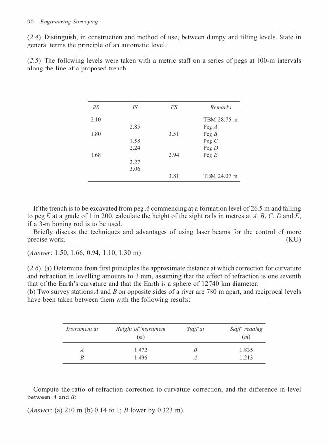
90 Engineering Surveying
(2.4) Distinguish, in construction and method of use, between dumpy and tilting levels. State ingeneral terms the principle of an automatic level.
(2.5) The following levels were taken with a metric staff on a series of pegs at 100-m intervalsalong the line of a proposed trench.
BS IS FS Remarks
2.10 TBM 28.75 m2.85 Peg A
1.80 3.51 Peg B1.58 Peg C
2.24 Peg D
1.68 2.94 Peg E2.273.06
3.81 TBM 24.07 m
If the trench is to be excavated from peg A commencing at a formation level of 26.5 m and fallingto peg E at a grade of 1 in 200, calculate the height of the sight rails in metres at A, B, C, D and E,if a 3-m boning rod is to be used.
Briefly discuss the techniques and advantages of using laser beams for the control of moreprecise work. (KU)
(Answer: 1.50, 1.66, 0.94, 1.10, 1.30 m)
(2.6) (a) Determine from first principles the approximate distance at which correction for curvatureand refraction in levelling amounts to 3 mm, assuming that the effect of refraction is one sevenththat of the Earth’s curvature and that the Earth is a sphere of 12740 km diameter.(b) Two survey stations A and B on opposite sides of a river are 780 m apart, and reciprocal levelshave been taken between them with the following results:
Instrument at Height of instrument Staff at Staff reading
(m) (m)
A 1.472 B 1.835
B 1.496 A 1.213
Compute the ratio of refraction correction to curvature correction, and the difference in levelbetween A and B:
(Answer: (a) 210 m (b) 0.14 to 1; B lower by 0.323 m).
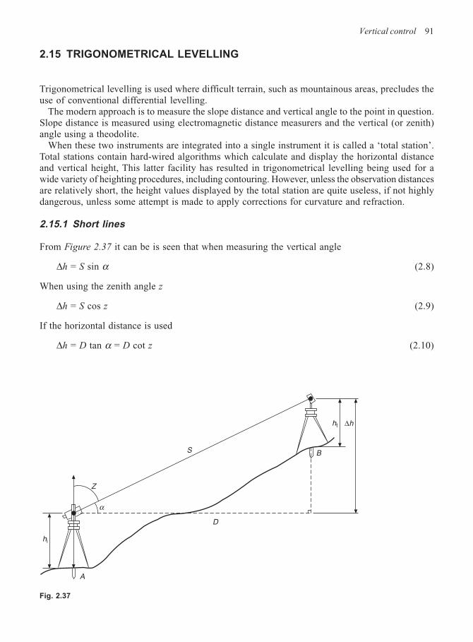
Vertical control 91
2.15 TRIGONOMETRICAL LEVELLING
Trigonometrical levelling is used where difficult terrain, such as mountainous areas, precludes theuse of conventional differential levelling.
The modern approach is to measure the slope distance and vertical angle to the point in question.Slope distance is measured using electromagnetic distance measurers and the vertical (or zenith)angle using a theodolite.
When these two instruments are integrated into a single instrument it is called a ‘total station’.Total stations contain hard-wired algorithms which calculate and display the horizontal distanceand vertical height, This latter facility has resulted in trigonometrical levelling being used for awide variety of heighting procedures, including contouring. However, unless the observation distancesare relatively short, the height values displayed by the total station are quite useless, if not highlydangerous, unless some attempt is made to apply corrections for curvature and refraction.
2.15.1 Short lines
From Figure 2.37 it can be is seen that when measuring the vertical angle
∆h = S sin α (2.8)
When using the zenith angle z
∆h = S cos z (2.9)
If the horizontal distance is used
∆h = D tan α = D cot z (2.10)
Fig. 2.37
ht ∆h
B
D
S
A
α
Z
hi
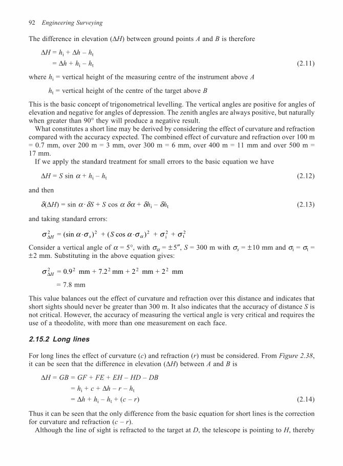
92 Engineering Surveying
The difference in elevation (∆H) between ground points A and B is therefore
∆H = hi + ∆h – ht
= ∆h + hi – ht (2.11)
where hi = vertical height of the measuring centre of the instrument above A
ht = vertical height of the centre of the target above B
This is the basic concept of trigonometrical levelling. The vertical angles are positive for angles ofelevation and negative for angles of depression. The zenith angles are always positive, but naturallywhen greater than 90° they will produce a negative result.
What constitutes a short line may be derived by considering the effect of curvature and refractioncompared with the accuracy expected. The combined effect of curvature and refraction over 100 m= 0.7 mm, over 200 m = 3 mm, over 300 m = 6 mm, over 400 m = 11 mm and over 500 m =17 mm.
If we apply the standard treatment for small errors to the basic equation we have
∆H = S sin α + hi – ht (2.12)
and then
δ(∆H) = sin α · δS + S cos α δα + δhi – δht (2.13)
and taking standard errors:
σ α σ α σ σ σα∆H s S2 2 2i2
t2 = (sin ) + ( cos ) + + ⋅ ⋅
Consider a vertical angle of α = 5°, with σα = ± 5″, S = 300 m with σs = ±10 mm and σi = σt =±2 mm. Substituting in the above equation gives:
σ ∆H2 2 2 2 2 = 0.9 mm + 7.2 mm + 2 mm + 2 mm
= 7.8 mm
This value balances out the effect of curvature and refraction over this distance and indicates thatshort sights should never be greater than 300 m. It also indicates that the accuracy of distance S isnot critical. However, the accuracy of measuring the vertical angle is very critical and requires theuse of a theodolite, with more than one measurement on each face.
2.15.2 Long lines
For long lines the effect of curvature (c) and refraction (r) must be considered. From Figure 2.38,it can be seen that the difference in elevation (∆H) between A and B is
∆H = GB = GF + FE + EH – HD – DB
= hi + c + ∆h – r – ht
= ∆h + hi – ht + (c – r) (2.14)
Thus it can be seen that the only difference from the basic equation for short lines is the correctionfor curvature and refraction (c – r).
Although the line of sight is refracted to the target at D, the telescope is pointing to H, thereby
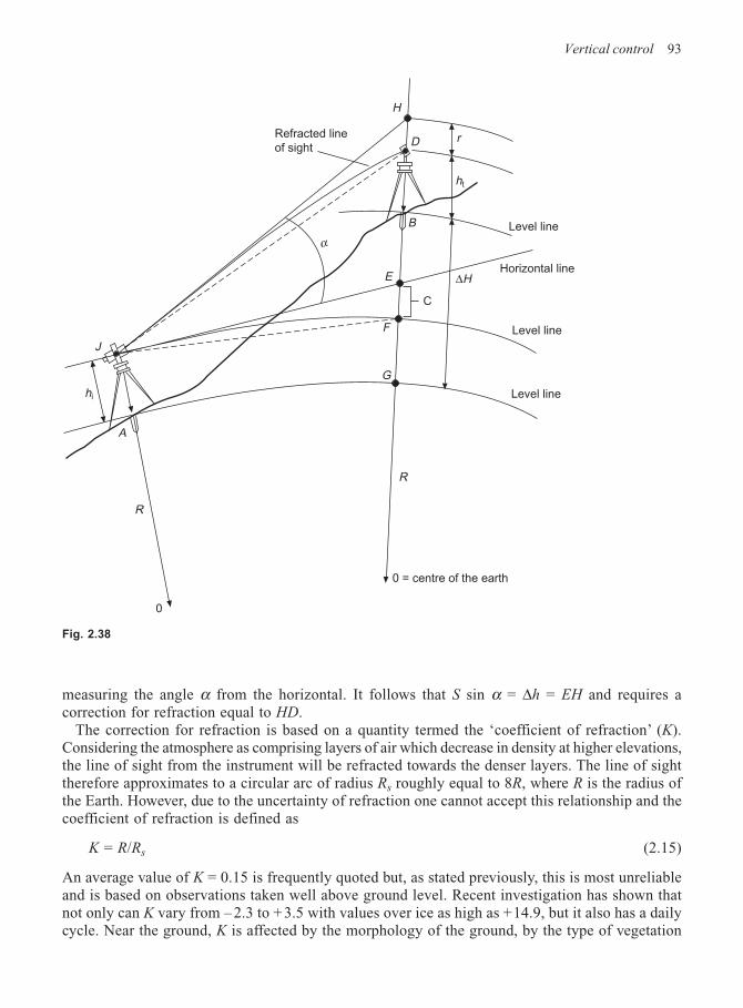
Vertical control 93
measuring the angle α from the horizontal. It follows that S sin α = ∆h = EH and requires acorrection for refraction equal to HD.
The correction for refraction is based on a quantity termed the ‘coefficient of refraction’ (K).Considering the atmosphere as comprising layers of air which decrease in density at higher elevations,the line of sight from the instrument will be refracted towards the denser layers. The line of sighttherefore approximates to a circular arc of radius Rs roughly equal to 8R, where R is the radius ofthe Earth. However, due to the uncertainty of refraction one cannot accept this relationship and thecoefficient of refraction is defined as
K = R/Rs (2.15)
An average value of K = 0.15 is frequently quoted but, as stated previously, this is most unreliableand is based on observations taken well above ground level. Recent investigation has shown thatnot only can K vary from – 2.3 to + 3.5 with values over ice as high as +14.9, but it also has a dailycycle. Near the ground, K is affected by the morphology of the ground, by the type of vegetation
Fig. 2.38
J
A
R
0
R
G
F
C
E
α
B
D
H
r
ht
Level line
Horizontal line∆H
Refracted line
of sight
Level line
Level line
0 = centre of the earth
hi
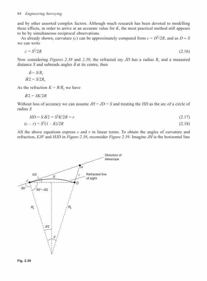
94 Engineering Surveying
and by other assorted complex factors. Although much research has been devoted to modellingthese effects, in order to arrive at an accurate value for K, the most practical method still appearsto be by simultaneous reciprocal observations.
As already shown, curvature (c) can be approximately computed from c = D2/2R, and as D ≈ S
we can write
c = S2/2R (2.16)
Now considering Figures 2.38 and 2.39, the refracted ray JD has a radius Rs and a measureddistance S and subtends angles δ at its centre, then
δ = S/Rs
δ/2 = S/2Rs
As the refraction K = R/Rs we have
δ/2 = SK/2R
Without loss of accuracy we can assume JH = JD = S and treating the HD as the arc of a circle ofradius S
HD = S·δ/2 = S2K/2R = r (2.17)
(c – r) = S2(1 – K)/2R (2.18)
All the above equations express c and r in linear terms. To obtain the angles of curvature andrefraction, EJF and HJD in Figure 2.38, reconsider Figure 2.39. Imagine JH is the horizontal line
90°–δ/2
Rs
δ/2
H
r
D
Rs
90°
SRefracted line
of sight
Direction of
telescope
δ
δ/2
J
Fig. 2.39
Vertical control 95
JE in Figure 2.38 and JD the level line JF of radius R. Then δ is the angle subtended at the centreof the Earth and the angle of curvature is half this value. To avoid confusion let δ = θ and as alreadyshown:
θ /2 = /2 = S R c (2.19)
where the arc distance at MSL approximates to S. Also, as shown:
δ /2 = /2 = SK R r (2.20)
Therefore in angular terms:
( – ) = (1 – )/2 radsˆ ˆc r S K R (2.21)
Note the difference between equations in linear terms and those in angular.
2.15.3 Reciprocal observations
Reciprocal observations are observations taken from A and B, the arithmetic mean result beingaccepted. If one assumes a symmetrical line of sight from each end and the observations are takensimultaneously, then the effect of curvature and refraction is cancelled out. For instance, for elevatedsights, (c – r) is added to a positive value to increase the height difference. For depressed ordownhill sights, (c – r) is added to a negative value and decreases the height difference. Thus theaverage of the two values is free from the effects of curvature and refraction. This statement is notentirely true as the assumption of symmetrical lines of sight from each end is dependent on uniformground and atmospheric conditions at each end, at the instant of simultaneous observation.
In practice, sighting into each others’ object lens forms an excellent target, with some form ofintercommunication to ensure simultaneous observation.
The following numerical example is taken from an actual survey in which the elevation of A andB had been obtained by precise geodetic levelling and was checked by simultaneous reciprocaltrigonometrical levelling.
Worked example
Example 2.8
Zenith angle at A = ZA = 89° 59′ 18.7″ (VA 0°00′ 41.3″)
Zenith angle at B = ZB = 90° 02′ 59.9″ (VA = –0° 02′ 59.9″)
Height of instrument at A = hA = 1.290 m
Height of instrument at B = hB = 1.300 m
Slope distance corrected for meteorological conditions = 4279.446 m
As it is known that the observations are reciprocal, the values for curvature and refraction areignored:
∆HAB = S cos ZA + hi – ht
= 4279.446 cos 89° 59′ 18.7″ + 1.290 – 1.300 = 0.846 m
∆HAB = 4279.446 cos 90° 02′ 59.9″ + 1.300 – 1.290 = –3.722 m
Mean value ∆H = 2.284 m
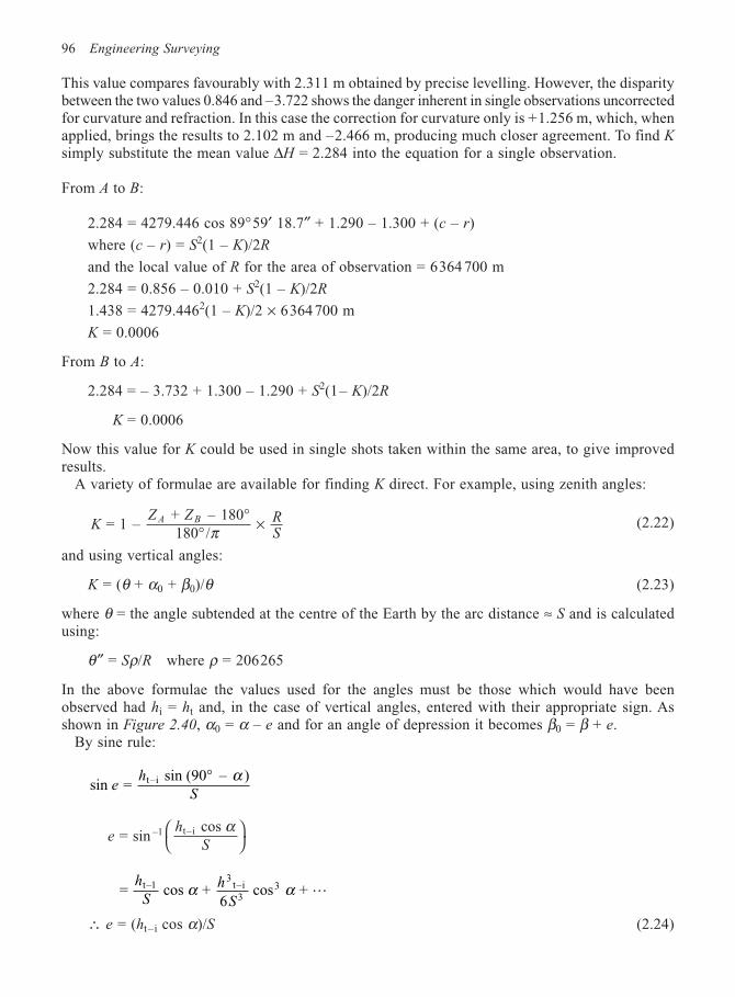
96 Engineering Surveying
This value compares favourably with 2.311 m obtained by precise levelling. However, the disparitybetween the two values 0.846 and –3.722 shows the danger inherent in single observations uncorrectedfor curvature and refraction. In this case the correction for curvature only is +1.256 m, which, whenapplied, brings the results to 2.102 m and –2.466 m, producing much closer agreement. To find Ksimply substitute the mean value ∆H = 2.284 into the equation for a single observation.
From A to B:
2.284 = 4279.446 cos 89°59′ 18.7″ + 1.290 – 1.300 + (c – r)
where (c – r) = S2(1 – K)/2R
and the local value of R for the area of observation = 6364 700 m
2.284 = 0.856 – 0.010 + S2(1 – K)/2R
1.438 = 4279.4462(1 – K)/2 × 6364700 m
K = 0.0006
From B to A:
2.284 = – 3.732 + 1.300 – 1.290 + S2(1– K)/2R
K = 0.0006
Now this value for K could be used in single shots taken within the same area, to give improvedresults.
A variety of formulae are available for finding K direct. For example, using zenith angles:
KZ Z R
SA B = 1 –
+ – 180180 /
°° ×π
(2.22)
and using vertical angles:
K = (θ + α0 + β0)/θ (2.23)
where θ = the angle subtended at the centre of the Earth by the arc distance ≈ S and is calculatedusing:
θ″ = Sρ/R where ρ = 206265
In the above formulae the values used for the angles must be those which would have beenobserved had hi = ht and, in the case of vertical angles, entered with their appropriate sign. Asshown in Figure 2.40, α0 = α – e and for an angle of depression it becomes β0 = β + e.
By sine rule:
sin = sin (90 – )t–ie
h
S
° α
eh
S = sin
cos –1 t–i α
= cos + 6
cos + t–1 t–i3
3h
Sh
Sα α
3
L
∴ e = (ht–i cos α)/S (2.24)
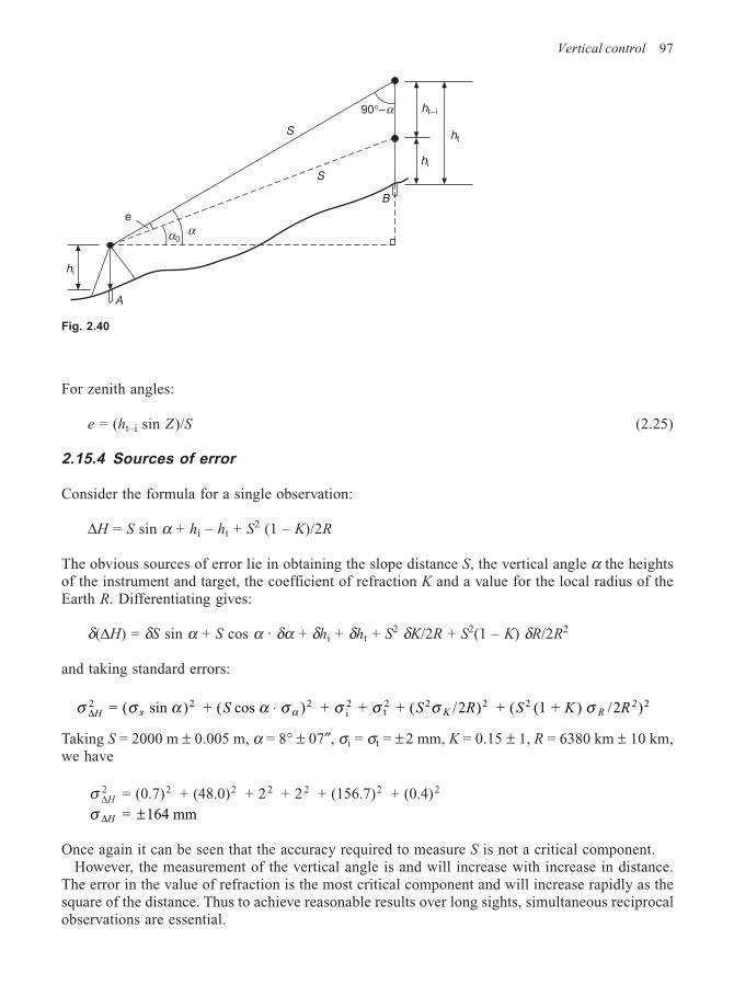
Vertical control 97
For zenith angles:
e = (ht–i sin Z)/S (2.25)
2.15.4 Sources of error
Consider the formula for a single observation:
∆H = S sin α + hi – ht + S2 (1 – K)/2R
The obvious sources of error lie in obtaining the slope distance S, the vertical angle α the heightsof the instrument and target, the coefficient of refraction K and a value for the local radius of theEarth R. Differentiating gives:
δ(∆H) = δS sin α + S cos α · δα + δhi + δht + S2 δK/2R + S2(1 – K) δR/2R2
and taking standard errors:
σ σ α α σ σ σ σ σα∆H s K R2S S R S K R2 2 2
i2
t2 2 2 2 2 = ( sin ) + ( cos ) + + + ( /2 ) + ( (1 + ) /2 )⋅
Taking S = 2000 m ± 0.005 m, α = 8° ± 07″, σi = σt = ± 2 mm, K = 0.15 ± 1, R = 6380 km ± 10 km,we have
σ ∆H2 2 2 2 2 2 2 = (0.7) + (48.0) + 2 + 2 + (156.7) + (0.4)
σ ∆H = 164 mm±
Once again it can be seen that the accuracy required to measure S is not a critical component.However, the measurement of the vertical angle is and will increase with increase in distance.
The error in the value of refraction is the most critical component and will increase rapidly as thesquare of the distance. Thus to achieve reasonable results over long sights, simultaneous reciprocalobservations are essential.
Fig. 2.40
e
α0α
S
S
90°–α
B
A
ht
hi
ht–i
hi
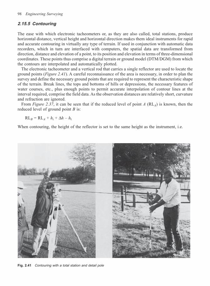
98 Engineering Surveying
2.15.5 Contouring
The ease with which electronic tacheometers or, as they are also called, total stations, producehorizontal distance, vertical height and horizontal direction makes them ideal instruments for rapidand accurate contouring in virtually any type of terrain. If used in conjunction with automatic datarecorders, which in turn are interfaced with computers, the spatial data are transformed fromdirection, distance and elevation of a point, to its position and elevation in terms of three-dimensionalcoordinates. These points thus comprise a digital terrain or ground model (DTM/DGM) from whichthe contours are interpolated and automatically plotted.
The electronic tacheometer and a vertical rod that carries a single reflector are used to locate theground points (Figure 2.41). A careful reconnaissance of the area is necessary, in order to plan thesurvey and define the necessary ground points that are required to represent the characteristic shapeof the terrain. Break lines, the tops and bottoms of hills or depressions, the necessary features ofwater courses, etc., plus enough points to permit accurate interpolation of contour lines at theinterval required, comprise the field data. As the observation distances are relatively short, curvatureand refraction are ignored.
From Figure 2.37, it can be seen that if the reduced level of point A (RLA) is known, then thereduced level of ground point B is:
RLB = RLA + hi + ∆h – ht
When contouring, the height of the reflector is set to the same height as the instrument, i.e.
Fig. 2.41 Contouring with a total station and detail pole
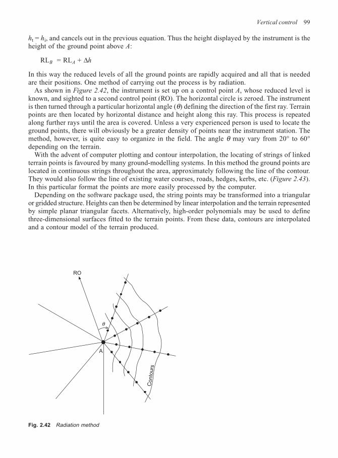
Vertical control 99
ht = hi, and cancels out in the previous equation. Thus the height displayed by the instrument is theheight of the ground point above A:
RLB = RLA + ∆h
In this way the reduced levels of all the ground points are rapidly acquired and all that is neededare their positions. One method of carrying out the process is by radiation.
As shown in Figure 2.42, the instrument is set up on a control point A, whose reduced level isknown, and sighted to a second control point (RO). The horizontal circle is zeroed. The instrumentis then turned through a particular horizontal angle (θ) defining the direction of the first ray. Terrainpoints are then located by horizontal distance and height along this ray. This process is repeatedalong further rays until the area is covered. Unless a very experienced person is used to locate theground points, there will obviously be a greater density of points near the instrument station. Themethod, however, is quite easy to organize in the field. The angle θ may vary from 20° to 60°depending on the terrain.
With the advent of computer plotting and contour interpolation, the locating of strings of linkedterrain points is favoured by many ground-modelling systems. In this method the ground points arelocated in continuous strings throughout the area, approximately following the line of the contour.They would also follow the line of existing water courses, roads, hedges, kerbs, etc. (Figure 2.43).In this particular format the points are more easily processed by the computer.
Depending on the software package used, the string points may be transformed into a triangularor gridded structure. Heights can then be determined by linear interpolation and the terrain representedby simple planar triangular facets. Alternatively, high-order polynomials may be used to definethree-dimensional surfaces fitted to the terrain points. From these data, contours are interpolatedand a contour model of the terrain produced.
Fig. 2.42 Radiation method
Con
tours
RO
θ
A
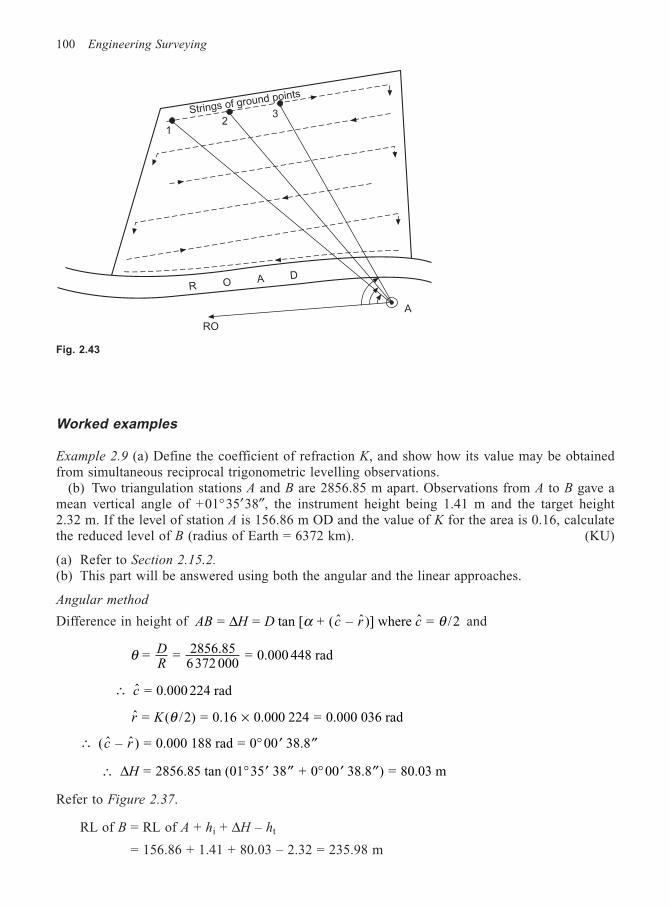
100 Engineering Surveying
Worked examples
Example 2.9 (a) Define the coefficient of refraction K, and show how its value may be obtainedfrom simultaneous reciprocal trigonometric levelling observations.
(b) Two triangulation stations A and B are 2856.85 m apart. Observations from A to B gave amean vertical angle of +01°35′38″, the instrument height being 1.41 m and the target height2.32 m. If the level of station A is 156.86 m OD and the value of K for the area is 0.16, calculatethe reduced level of B (radius of Earth = 6372 km). (KU)
(a) Refer to Section 2.15.2.
(b) This part will be answered using both the angular and the linear approaches.
Angular method
Difference in height of AB H D c r c = = tan [ + ( – )] where = /2∆ α θˆ ˆ ˆ and
θ = = 2856.856372 000
= 0.000 448 radDR
∴ c = 0.000 224 rad
r K = ( /2) = 0.16 0.000 224 = 0.000 036 radθ ×
∴ ( ˆ ˆc r – ) = 0.000 188 rad = 0 00 38.8° ′ ′′
∴ ∆H = 2856.85 tan (01 35 38 + 0 00 38.8 ) = 80.03 m° ′ ′′ ° ′ ′′
Refer to Figure 2.37.
RL of B = RL of A + hi + ∆H – ht
= 156.86 + 1.41 + 80.03 – 2.32 = 235.98 m
Strings of ground points
32
1
A
R O A D
RO
Fig. 2.43
Vertical control 101
Linear method
∆H = D tan α + (c – r)
where ( – ) = 2
(1 – ) = 2856.852 6 372 000
0.84 = 0.54 m2 2
c rD
RK
× ×
D tan α = 2856.85 tan (01° 35′ 39″) = 79.49 m
where ∴ ∆H = 79.49 + 0.54 = 80.03 m
Example 2.10 Two stations A and B are 1713 m apart. The following observations were recorded:height of instrument at A 1.392 m, and at B 1.464 m; height of signal at A 2.199 m, and at B 2 m.Elevation to signal at B 1° 08′ 08″, depression angle to signal at A 1° 06′ 16″. If 1″ at the Earth’scentre subtends 30.393 m at the Earth’s surface, calculate the difference of level between A and Band the refraction correction. (LU)
∆H Dh h h h
= tan + 2
+ ( – ) – ( – )
2t i t iα β
′ ′
where hi = height of instrument at A; ht = height of target at B; ′hi = height of instrument at B;′ht = height of target at A.
∴ ∆H = 1713 tan (1 08 08 ) + (1 06 15 )
2 +
(2.199 – 1.464) – (2.000 – 1.392)2
° ′ ′′ ° ′ ′′
= 33.490 + 0.064 = 33.55 m
Using the alternative approach of reducing α and β to their values if hi = ht
Correction to angle of elevation
′′ ≈ × ′′e1.392 – 2.000
1713.0 206 265 = –73.2
∴ α = (1° 08′ 08″) – (01′ 13.2″) = 1° 06′ 54.8″
Correction to angle of depression
′′ ≈ × ′′e(2.199 – 1.464)
1713.0 206 265 = 88.5
∴ β = (1° 06′ 15″) + (01′28.5″) = 1° 07′ 43.5″
∴ ∆H = 1713 tan1 06 54.8 + 1 07 43.5
2 = 33.55 m
° ′ ′′ ° ′ ′′
Refraction correction r = ( + + )12 θ α β
where θ″ = 1713.0/30.393 = 56.4″
= [56.4 + (1 06 54.8 ) – (1 07 43.5 )] = 3.812 ′′ ° ′ ′′ ° ′ ′′ ′′
and also Kr = /2
= 3.828.2
= 0.14ˆ
θ′′′′
Example 2.11 Two points A and B are 8 km apart and at levels of 102.50 m and 286.50 m OD,respectively. The height of the target at A is 1.50 m and at B 3.00 m, while the height of theinstrument in both cases is 1.50 m on the Earth’s surface subtends 1″ of arc at the Earth’s centre and
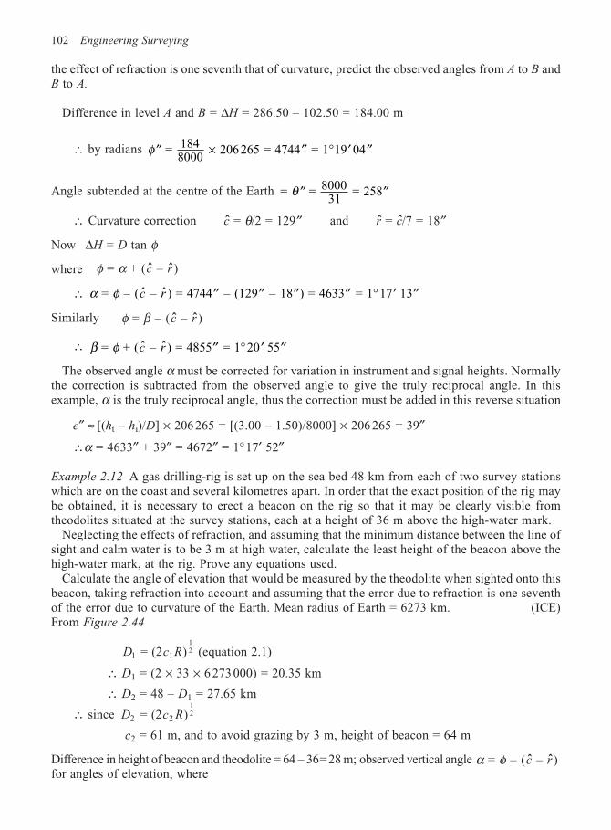
102 Engineering Surveying
the effect of refraction is one seventh that of curvature, predict the observed angles from A to B andB to A.
Difference in level A and B = ∆H = 286.50 – 102.50 = 184.00 m
∴ by radians ′′ × ′′ ° ′ ′′φ = 1848000
206 265 = 4744 = 1 19 04
Angle subtended at the centre of the Earth = = 800031
= 258′′ ′′θ
∴ Curvature correction c = /2 = 129θ ′′ and ˆ ˆr c = /7 = 18′′
Now ∆H = D tan φ
where φ α = + ( – )ˆ ˆc r
∴ α φ = – ( – ) = 4744 – (129 – 18 ) = 4633 = 1 17 13ˆ ˆc r ′′ ′′ ′′ ′′ ° ′ ′′
Similarly φ β = – ( – )ˆ ˆc r
∴ β φ = + ( – ) = 4855 = 1 20 55ˆ ˆc r ′′ ° ′ ′′
The observed angle α must be corrected for variation in instrument and signal heights. Normallythe correction is subtracted from the observed angle to give the truly reciprocal angle. In thisexample, α is the truly reciprocal angle, thus the correction must be added in this reverse situation
e″ ≈ [(ht – hi)/D] × 206 265 = [(3.00 – 1.50)/8000] × 206 265 = 39″
∴α = 4633″ + 39″ = 4672″ = 1°17′ 52″
Example 2.12 A gas drilling-rig is set up on the sea bed 48 km from each of two survey stationswhich are on the coast and several kilometres apart. In order that the exact position of the rig maybe obtained, it is necessary to erect a beacon on the rig so that it may be clearly visible fromtheodolites situated at the survey stations, each at a height of 36 m above the high-water mark.
Neglecting the effects of refraction, and assuming that the minimum distance between the line ofsight and calm water is to be 3 m at high water, calculate the least height of the beacon above thehigh-water mark, at the rig. Prove any equations used.
Calculate the angle of elevation that would be measured by the theodolite when sighted onto thisbeacon, taking refraction into account and assuming that the error due to refraction is one seventhof the error due to curvature of the Earth. Mean radius of Earth = 6273 km. (ICE)From Figure 2.44
D c R1 1 = (2 )12 (equation 2.1)
∴ D1 = (2 × 33 × 6 273 000) = 20.35 km
∴ D2 = 48 – D1 = 27.65 km
∴ since D c R2 2 = (2 )12
c2 = 61 m, and to avoid grazing by 3 m, height of beacon = 64 m
Difference in height of beacon and theodolite = 64 – 36= 28 m; observed vertical angle α φ = – ( – )ˆ ˆc rfor angles of elevation, where
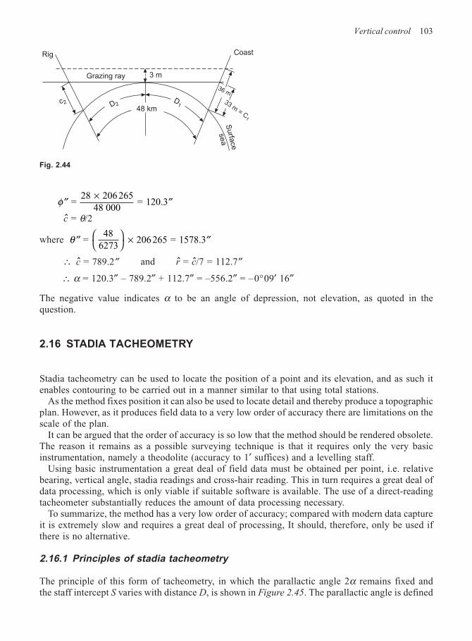
Vertical control 103
′′×
′′φ = 28 206 265
48 000 = 120.3
c = /2θ
where ′′
× ′′θ =
486273
206 265 = 1578.3
∴ c = 789.2 ′′ and ˆ ˆr c = /7 = 112.7′′
∴ α = 120.3″ – 789.2″ + 112.7″ = –556.2″ = –0°09′ 16″
The negative value indicates α to be an angle of depression, not elevation, as quoted in thequestion.
2.16 STADIA TACHEOMETRY
Stadia tacheometry can be used to locate the position of a point and its elevation, and as such itenables contouring to be carried out in a manner similar to that using total stations.
As the method fixes position it can also be used to locate detail and thereby produce a topographicplan. However, as it produces field data to a very low order of accuracy there are limitations on thescale of the plan.
It can be argued that the order of accuracy is so low that the method should be rendered obsolete.The reason it remains as a possible surveying technique is that it requires only the very basicinstrumentation, namely a theodolite (accuracy to 1′ suffices) and a levelling staff.
Using basic instrumentation a great deal of field data must be obtained per point, i.e. relativebearing, vertical angle, stadia readings and cross-hair reading. This in turn requires a great deal ofdata processing, which is only viable if suitable software is available. The use of a direct-readingtacheometer substantially reduces the amount of data processing necessary.
To summarize, the method has a very low order of accuracy; compared with modern data captureit is extremely slow and requires a great deal of processing, It should, therefore, only be used ifthere is no alternative.
2.16.1 Principles of stadia tacheometry
The principle of this form of tacheometry, in which the parallactic angle 2α remains fixed andthe staff intercept S varies with distance D, is shown in Figure 2.45. The parallactic angle is defined
Grazing ray
33 m = C1
D1D2
48 km
3 m
CoastRig
c2
36 m
Surfa
ce
sea
Fig. 2.44
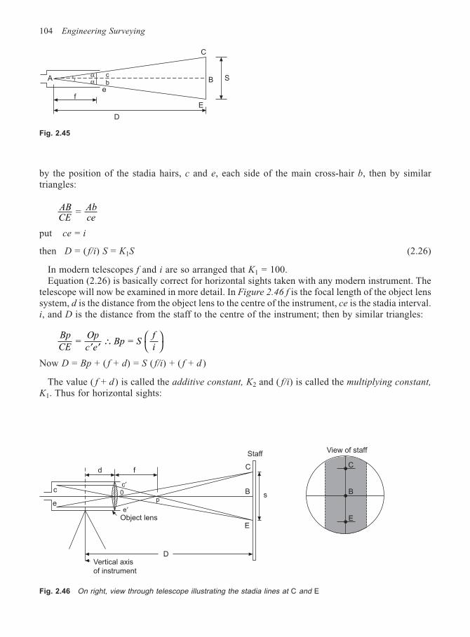
104 Engineering Surveying
by the position of the stadia hairs, c and e, each side of the main cross-hair b, then by similartriangles:
ABCE
Abce
=
put ce = i
then D = ( f/i) S = K1S (2.26)
In modern telescopes f and i are so arranged that K1 = 100.Equation (2.26) is basically correct for horizontal sights taken with any modern instrument. The
telescope will now be examined in more detail. In Figure 2.46 f is the focal length of the object lenssystem, d is the distance from the object lens to the centre of the instrument, ce is the stadia interval.i, and D is the distance from the staff to the centre of the instrument; then by similar triangles:
Bp
CE
Op
c eBp S
f
i = =
′ ′∴
Now D = Bp + ( f + d) = S ( f/i) + ( f + d )
The value ( f + d) is called the additive constant, K2 and ( f/i) is called the multiplying constant,
K1. Thus for horizontal sights:
Fig. 2.46 On right, view through telescope illustrating the stadia lines at C and E
View of staffStaff
s
C
E
B
DVertical axis
of instrument
Object lens
0c
fd
pe
e′
c′
C
B
E
Aαα
ef
D
E
B
C
Sc
b
Fig. 2.45
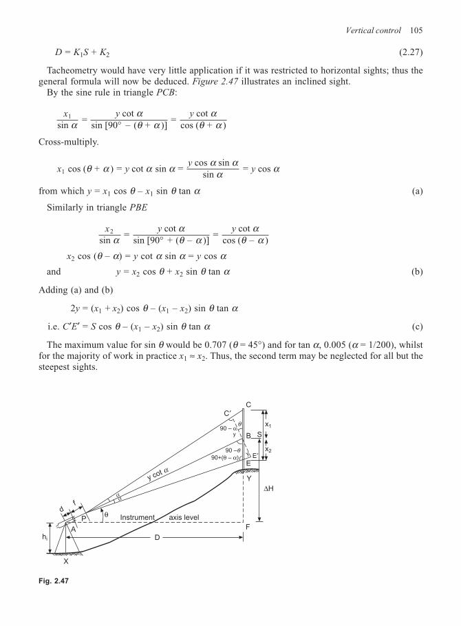
Vertical control 105
D = K1S + K2 (2.27)
Tacheometry would have very little application if it was restricted to horizontal sights; thus thegeneral formula will now be deduced. Figure 2.47 illustrates an inclined sight.
By the sine rule in triangle PCB:
x y y1
sin =
cot sin [90 – ( + )]
= cot
cos ( + )ααθ α
αθ α°
Cross-multiply.
x yy
y1 cos ( + ) = cot sin = cos sin
sin = cos θ α α α
α αα α
from which y = x1 cos θ – x1 sin θ tan α (a)
Similarly in triangle PBE
x y y2
sin =
cot sin [90 + ( – )]
= cot
cos ( – )ααθ α
αθ α°
x2 cos (θ – α) = y cot α sin α = y cos α
and y = x2 cos θ + x2 sin θ tan α (b)
Adding (a) and (b)
2y = (x1 + x2) cos θ – (x1 – x2) sin θ tan α
i.e. C′E′ = S cos θ – (x1 – x2) sin θ tan α (c)
The maximum value for sin θ would be 0.707 (θ = 45°) and for tan α, 0.005 (α = 1/200), whilstfor the majority of work in practice x1 ≈ x2. Thus, the second term may be neglected for all but thesteepest sights.
Fig. 2.47
θ
αα
y cot α
A
P
D
d f
hi
X
F
Y
E
B S
CC′
x2
x1
90+(θ – α)
90 –θ
90 – αy
θ
∆H
Instrument axis level
y E′
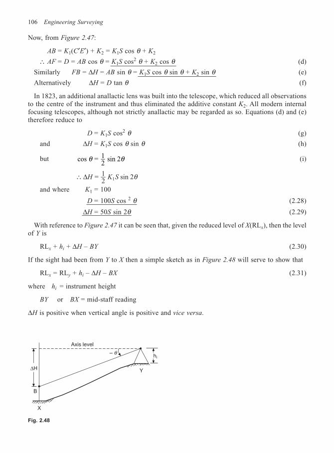
106 Engineering Surveying
Now, from Figure 2.47:
AB = K1(C′E′) + K2 = K1S cos θ + K2
∴ AF = D = AB cos θ = K1S cos2 θ + K2 cos θ (d)
Similarly FB = ∆H = AB sin θ = K1S cos θ sin θ + K2 sin θ (e)
Alternatively ∆H = D tan θ (f)
In 1823, an additional anallactic lens was built into the telescope, which reduced all observationsto the centre of the instrument and thus eliminated the additive constant K2. All modern internalfocusing telescopes, although not strictly anallactic may be regarded as so. Equations (d) and (e)therefore reduce to
D = K1S cos2 θ (g)
and ∆H = K1S cos θ sin θ (h)
but cos = 12
sin 2θ θ (i)
∴ = 12
sin 21∆H K S θ
and where K1 = 100
D = 100S cos 2 θ (2.28)
∆H = 50S sin 2θ (2.29)
With reference to Figure 2.47 it can be seen that, given the reduced level of X(RLx), then the levelof Y is
RLx + hi + ∆H – BY (2.30)
If the sight had been from Y to X then a simple sketch as in Figure 2.48 will serve to show that
RLx = RLy + hi – ∆H – BX (2.31)
where hi = instrument height
BY or BX = mid-staff reading
∆H is positive when vertical angle is positive and vice versa.
Fig. 2.48
– θhi
X
B
∆H
Axis level
Y
Vertical control 107
Students should not attempt to commit equation (2.31) to memory, relying, if in doubt, on a quicksketch. Note that ∆H is always the vertical height from the centre of the transit axis to the mid-staffreading.
Thus, in general:
RLx = (RLy + hi) ± ∆H – mid-staff reading (2.32)
where (RLy + hi) = axis level
2.16.2 Measurements of tacheometric constants
The multiplying constant (K1 = 100) and the additive constant (K2 = 0) may vary due to ageing ofthe theodolite or temperature variations. It is therefore necessary to check them as follows.
Set up the instrument on fairly level ground giving horizontal sights to a series of pegs at knowndistances, D, from the instrument. Now, using the equation D = K1S + K2 and substituting valuesfor D and S, the equations may be solved:
(1) Simultaneously in pairs and the mean taken.(2) As a whole by the method of least squares. For example:
Measured distance (m) 30 60 90 120 150 (D-values)Staff intercept (m) 0.301 0.600 0.899 1.202 1.501 (S-values)
from which K1 = 100 and K2 = 0 by either of the above methods.Errors in the region of 1/1000 can occur in the constants.
2.16.3 Errors in staff holding
The basic formula for horizontal distance (D) is D = K1S · cos2 θ. This is only so if we assume thevertical angle BAF (Figure 2.47) is equal to C′BC. If the staff is not held truly vertical, angle C′BC
≠ θ and the formula is more correctly expessed as:
D = K1 · S · cos θ1 cos θ2
where θ1 = the vertical angle
θ2 = angle C′BC.
Then, adopting the usual procedure for the treatment of small errors, the above expression isdifferentiated with respect to θ2, giving
δD = –K1S cos θ1 sin θ2δθ2
∴ δ θ θ δθθ θ θ δθD
D
K S
K S =
– cos cos cos
– tan 1 1 2 2
1 1 22 2
sin
(2.33)
Using the above expression the following table may be drawn up assuming θ ≈ θ1 = angle ofinclination = θ:
108 Engineering Surveying
(a) Column 2 shows that if the staff is held reasonably plumb this source of error may beignored.
(b) Column 3 shows that the accuracy falls off rapidly as the angle of inclination increases.(c) Column 4 shows that where the staff is used carelessly, the accuracy is radically reduced, even
on fairly level sights. It is obvious from this that all tacheometric staves should befitted with a bubble and regularly checked.
2.16.4 Errors in horizontal distance
The errors in the resultant distance D will now be examined in more detail.
(1) Careless staff holding, which has already been discussed separately due to its importance.(2) Error in reading the stadia intercept, which is immediately multiplied by 100 (K1), thereby
making it very significant. This source of error will decrease with increase in the length ofsight, provided the reading error (δs) remains constant. Thus observation distances should belimited to a maximum of 100 m.
(3) Error in the determination of the instrument constants K1 and K2, resulting in an error indistance directly proportional to the error in the constant K1 and directly as the error in K2.
(4) Effect of differential refraction on the stadia intercept. This is minimized by keeping the lowerreading 1–1.5 m above the ground.
(5) Random error in the measurement of the vertical angle. This has a negligible effect on the staffintercept and consequently on the horizontal distance.
In addition to the above sources of error, there are many others resulting from instrumental errors,failure to eliminate parallax, and natural errors due to high winds, heat shimmer, etc. The lack ofstatistical evidence makes it rather difficult to quote standards of accuracy; however, the usualtreatment for small errors will give some basis for assessment.
Taking the equation for vertical staff tacheometry as in Section 2.16.3 and differentiating withrespect to each of the sources of error, in turn gives
D = K1S cos θ1 cos θ2
thus, δD = S cos θ1 cos θ2 δK1
∴ = cos cos cos cos
= 1 2 1
1 2 1
1
1
δ θ θ δθ θ
δDD
S K
S K
K
K(a)
Similarly, differentiating with respect to S, θ1 and θ2, in turn gives
Table 2.1
θ δθ2 = 10′ δθ2 = 1° δθ2 = 2°
3° 1/6670 1/1090 1/5505° 1/4000 1/650 1/330
10° 1/1960 1/325 1/16015° 1/1280 1/215 1/11020° 1/940 1/160 1/8025° 1/740 1/120 1/6030° 1/600 1/100 1/50
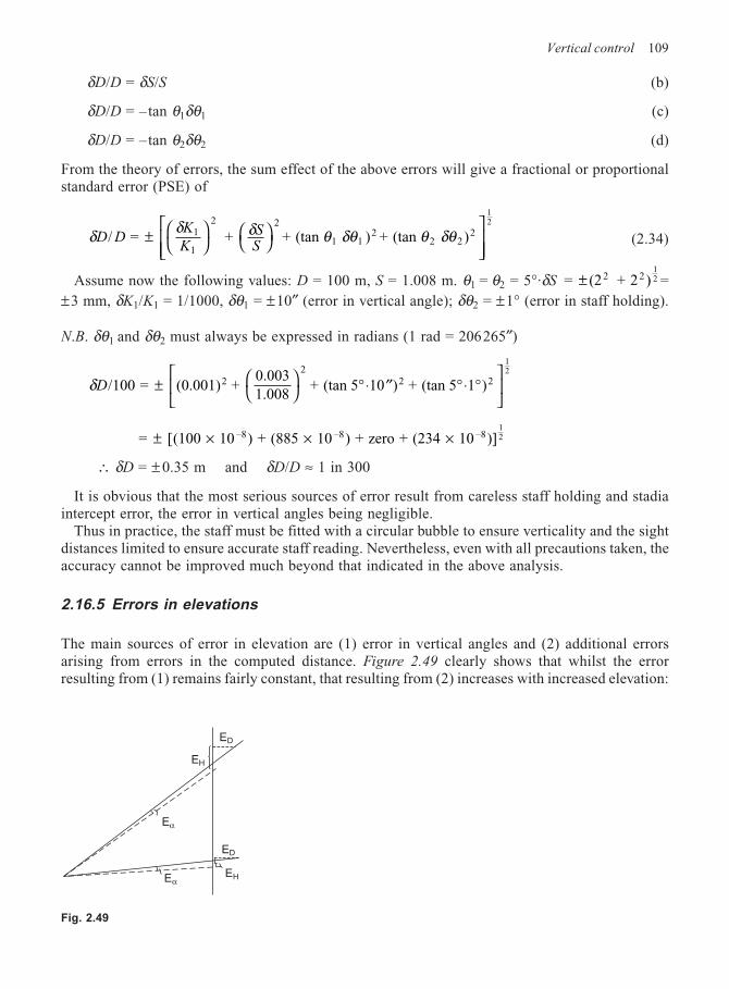
Vertical control 109
δD/D = δS/S (b)
δD/D = –tan θ1δθ1 (c)
δD/D = –tan θ2δθ2 (d)
From the theory of errors, the sum effect of the above errors will give a fractional or proportionalstandard error (PSE) of
δ δ δ θ δθ θ δθD DK
KSS
/ = + + (tan ) + (tan )1
11 1
22 2
2±
2 212
(2.34)
Assume now the following values: D = 100 m, S = 1.008 m. θ1 = θ2 = 5°·δS = (2 + 2 )2 212± =
±3 mm, δK1/K1 = 1/1000, δθ1 = ±10″ (error in vertical angle); δθ2 = ±1° (error in staff holding).
N.B. δθ1 and δθ2 must always be expressed in radians (1 rad = 206265″)
δD/100 = (0.001) + 0.0031.008
+ (tan 5 10 ) + (tan 5 1 )22
2 2
12
±
°⋅ ′′ °⋅ °
= (100 10 ) + (885 10 ) + zero + (234 10 )]–8 –8 –812± × × ×[
∴ δD = ± 0.35 m and δD/D ≈ 1 in 300
It is obvious that the most serious sources of error result from careless staff holding and stadiaintercept error, the error in vertical angles being negligible.
Thus in practice, the staff must be fitted with a circular bubble to ensure verticality and the sightdistances limited to ensure accurate staff reading. Nevertheless, even with all precautions taken, theaccuracy cannot be improved much beyond that indicated in the above analysis.
2.16.5 Errors in elevations
The main sources of error in elevation are (1) error in vertical angles and (2) additional errorsarising from errors in the computed distance. Figure 2.49 clearly shows that whilst the errorresulting from (1) remains fairly constant, that resulting from (2) increases with increased elevation:
Fig. 2.49
Eα
Eα
EH
ED
EH
ED
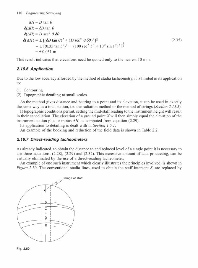
110 Engineering Surveying
∆H = D tan θδ(∆H) = δD tan θδ(∆H) = D sec2 θ δθδ δ θ θ δθ( ) = [( tan ) + ( sec ) ]2 2 2
12∆H D D± (2.35)
= [(0.35 tan 5 ) + (100 sec 5 10 sin 1 ) ]2 2 212± ° ° × ′′ ′′
= ± 0.031 m
This result indicates that elevations need be quoted only to the nearest 10 mm.
2.16.6 Application
Due to the low accuracy afforded by the method of stadia tacheometry, it is limited in its applicationto:
(1) Contouring(2) Topographic detailing at small scales.
As the method gives distance and bearing to a point and its elevation, it can be used in exactlythe same way as a total station, i.e. the radiation method or the method of strings (Section 2.15.5).
If topographic conditions permit, setting the mid-staff reading to the instrument height will resultin their cancellation. The elevation of a ground point X will then simply equal the elevation of theinstrument station plus or minus ∆H, as computed from equation (2.29).
Its application to detailing is dealt with in Section 1.5.1.An example of the booking and reduction of the field data is shown in Table 2.2.
2.16.7 Direct-reading tacheometers
As already indicated, to obtain the distance to and reduced level of a single point it is necessary touse three equations, (2.28), (2.29) and (2.32). This excessive amount of data processing, can bevirtually eliminated by the use of a direct-reading tacheometer.
An example of one such instrument which clearly illustrates the principles involved, is shown inFigure 2.50. The conventional stadia lines, used to obtain the staff intercept S, are replaced by
Image of staff
C
+
D
B
A –
–
Fig. 2.50
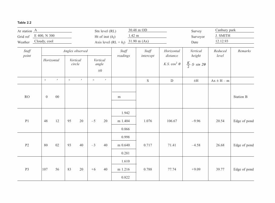
Table 2.2
At station A Stn level (RL) 30.48 m OD Survey Canbury park
Grid ref E 400, N 300 Ht of inst (hi) 1.42 m Surveyor J. SMITH
Weather Cloudy, cool Axis level (RL + hi) 31.90 m (Ax) Date 12.12.93
Staff Angles observed Staff Staff Horizontal Vertical Reduced Remarks
point readings intercept distance height level
Horizontal Vertical Verticalcircle angle K.S. cos2 θ K
S sin2
⋅ ⋅ 2θ
±0
° ′ ° ′ ° ′ S D ±H Ax ± H – m
RO 0 00 m Station B
1.942
P1 48 12 95 20 –5 20 m 1.404 1.076 106.67 –9.96 20.54 Edge of pond
0.866
0.998
P2 80 02 93 40 –3 40 m 0.640 0.717 71.41 –4.58 26.68 Edge of pond
0.281
1.610
P3 107 56 83 20 +6 40 m 1.216 0.788 77.74 +9.09 39.77 Edge of pond
0.822
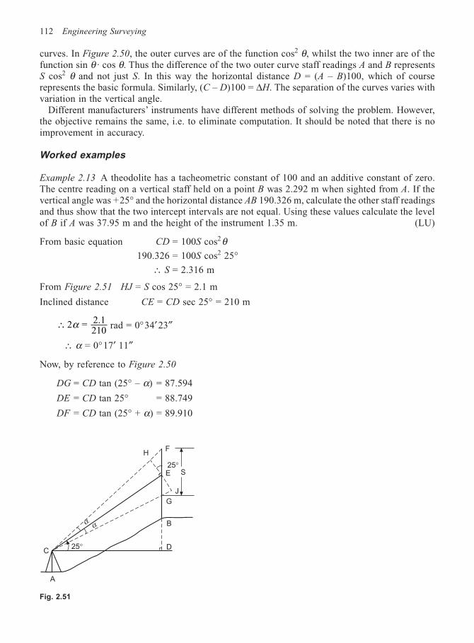
112 Engineering Surveying
curves. In Figure 2.50, the outer curves are of the function cos2 θ, whilst the two inner are of thefunction sin θ · cos θ. Thus the difference of the two outer curve staff readings A and B representsS cos2 θ and not just S. In this way the horizontal distance D = (A – B)100, which of courserepresents the basic formula. Similarly, (C – D)100 = ∆H. The separation of the curves varies withvariation in the vertical angle.
Different manufacturers’ instruments have different methods of solving the problem. However,the objective remains the same, i.e. to eliminate computation. It should be noted that there is noimprovement in accuracy.
Worked examples
Example 2.13 A theodolite has a tacheometric constant of 100 and an additive constant of zero.The centre reading on a vertical staff held on a point B was 2.292 m when sighted from A. If thevertical angle was +25° and the horizontal distance AB 190.326 m, calculate the other staff readingsand thus show that the two intercept intervals are not equal. Using these values calculate the levelof B if A was 37.95 m and the height of the instrument 1.35 m. (LU)
From basic equation CD = 100S cos2θ190.326 = 100S cos2 25°
∴ S = 2.316 m
From Figure 2.51 HJ = S cos 25° = 2.1 m
Inclined distance CE = CD sec 25° = 210 m
∴ 2 = 2.1210
α rad = 0°34′23″
∴ α = 0°17′ 11″
Now, by reference to Figure 2.50
DG = CD tan (25° – α) = 87.594
DE = CD tan 25° = 88.749
DF = CD tan (25° + α) = 89.910
Fig. 2.51
H
A
α
25° D
B
G
E
F
25°S
C
α
J
Vertical control 113
It can be seen that the stadia intervals are
GE S
EF S
= = 1.155
= = 1.161 = 2.316 (check)
1
2
from which it is obvious that the
upper reading = (2.292 + 1.161) = 3.453
lower reading = (2.292 – 1.155) = 1.137
Vertical height DE = ∆H = CD tan 25° = 88.749 (as above)
∴ level of B = 37.95 + 1.35 + 88.749 – 2.292 = 125.757 m
Example 2.14 The following observations were taken with a tacheometer, having constants of 100and zero, from a point A to B and C. The distance BC was measured as 157 m. Assuming the groundto be a plane within the triangle ABC, calculate the volume of filling required to make the area levelwith the highest point, assuming the sides to be supported by vertical concrete walls. Height ofinstrument was 1.4 m, the staff held vertically. (LU)
At To Staff readings (m) Vertical angle
A B 1.48, 2.73, 3.98 +7°36′C 2.08, 2.82, 3.56 – 5°24′
Horizontal distance AB = 100 × S cos2 θ
= 100 × 2.50 cos2 7°36′ = 246 m
Vertical distance AB = 246 tan 7°36′ = +32.8 m
Similarly
Horizontal distance AC = 148 cos2 5°24′ = 147 m
Vertical distance AC = 147 tan 5°24′ = –13.9 m
∴ Area of triangle ABC S S a S b S c = [ ( – ) ( – ) ( – )]12× ×
where S = 12
(157 + 246 + 147) = 275 m
∴ Area = [275(275 – 157) (275 – 147) (275 – 246)]12× ×
= 10 975 m2
Assume level of A = 100 m
then level of B = 100 + 1.4 + 32.8 – 2.73 = 131.47 m
then level of C = 100 + 1.4 – 13.9 – 2.82 = 84.68 m
∴ Depth of fill at A = 31.47 m
Depth of fill at C = 46.79 m
Volume of fill = plan area × mean height
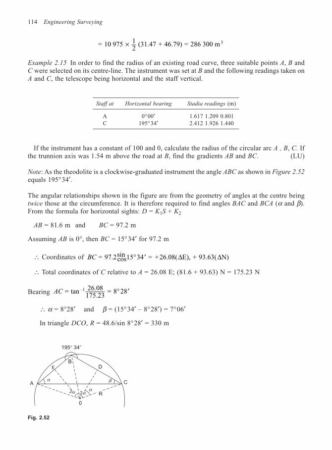
114 Engineering Surveying
= 10 975 12
(31.47 + 46.79) = 286 300 m3×
Example 2.15 In order to find the radius of an existing road curve, three suitable points A, B andC were selected on its centre-line. The instrument was set at B and the following readings taken onA and C, the telescope being horizontal and the staff vertical.
Staff at Horizontal bearing Stadia readings (m)
A 0°00′ 1.617 1.209 0.801C 195°34′ 2.412 1.926 1.440
If the instrument has a constant of 100 and 0, calculate the radius of the circular arc A , B, C. Ifthe trunnion axis was 1.54 m above the road at B, find the gradients AB and BC. (LU)
Note: As the theodolite is a clockwise-graduated instrument the angle ABC as shown in Figure 2.52
equals 195°34′.
The angular relationships shown in the figure are from the geometry of angles at the centre beingtwice those at the circumference. It is therefore required to find angles BAC and BCA (α and β).From the formula for horizontal sights: D = K1S + K2
AB = 81.6 m and BC = 97.2 m
Assuming AB is 0°, then BC = 15°34′ for 97.2 m
∴ Coordinates of BC = 97.2cossin 15 34 = + 26.08( E), + 93.63( N)° ′ ∆ ∆
∴ Total coordinates of C relative to A = 26.08 E; (81.6 + 93.63) N = 175.23 N
Bearing AC = tan 26.08175.23
= 8 28–1 ° ′
∴ α = 8°28′ and β = (15°34′ – 8°28′) = 7°06′
In triangle DCO, R = 48.6/sin 8°28′ = 330 m
Fig. 2.52
195° 34′
E
B
R2αα
0
2α
βC
D
Aα
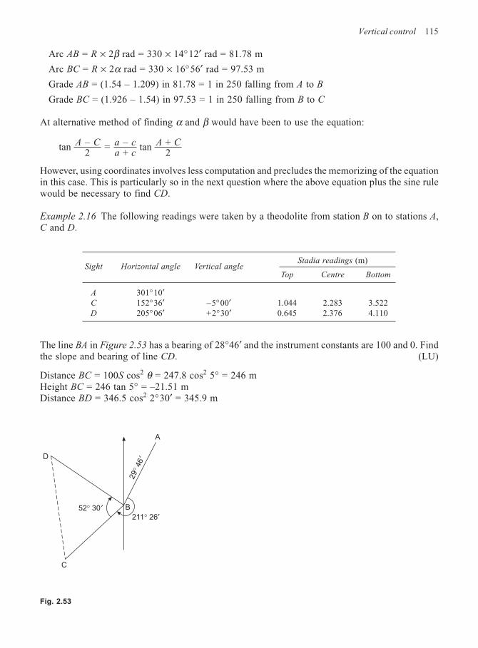
Vertical control 115
Arc AB = R × 2β rad = 330 × 14°12′ rad = 81.78 m
Arc BC = R × 2α rad = 330 × 16°56′ rad = 97.53 m
Grade AB = (1.54 – 1.209) in 81.78 = 1 in 250 falling from A to B
Grade BC = (1.926 – 1.54) in 97.53 = 1 in 250 falling from B to C
At alternative method of finding α and β would have been to use the equation:
tan – 2
= – +
tan + 2
A C a ca c
A C
However, using coordinates involves less computation and precludes the memorizing of the equationin this case. This is particularly so in the next question where the above equation plus the sine rulewould be necessary to find CD.
Example 2.16 The following readings were taken by a theodolite from station B on to stations A,C and D.
The line BA in Figure 2.53 has a bearing of 28°46′ and the instrument constants are 100 and 0. Findthe slope and bearing of line CD. (LU)
Distance BC = 100S cos2 θ = 247.8 cos2 5° = 246 mHeight BC = 246 tan 5° = –21.51 mDistance BD = 346.5 cos2 2°30′ = 345.9 m
Fig. 2.53
A
D
C
B52° 30′
29° 4
6′
211° 26′
Stadia readings (m)
Top Centre Bottom
A 301°10′C 152°36′ –5°00′ 1.044 2.283 3.522D 205°06′ +2°30′ 0.645 2.376 4.110
Sight Horizontal angle Vertical angle
116 Engineering Surveying
Height BD = 345.9 tan 2°30′ = 15.1 mBearing BC = (28°46′ + 211°26′) = 240°12′Bearing BD = (240°12′ + 52°30′) = 292°42′
∴ Coordinates of BC = 246cossin 240 12 = – 213.5 ( E); –122.2 ( N)° ′ ∆ ∆
∴ Coordinates of BD = 345.9cos = –319.2 ( E); + 133.5 ( N)sin 292 42° ′ ∆ ∆∴ Coordinates of C relative to D = –105.7 (∆E); + 255.7 (∆N)
∴ Bearing CD = tan –105.7+ 255.7
= 327 32–1 ° ′
Length CD = 255.7/cos 22° 28′ = 276.75 mDifference in level between C and D = –(21.51 + 2.283) – (15.1 – 2.376) = 36.52 m
∴ Grade CD = 36.52 in 276.75 = 1 in 7.6 rising
Exercises
(2.7 ) In order to survey an existing road, three points A, B, and C were selected on its centre-line.The instrument was set at A and the following observations were taken.
Staff Horizontal angle Vertical angle Stadia readings (m)
B 0°00′ –1°11′ 20″ 1.695 1.230 0.765C 6°29′ –1° 04′ 20″ 2.340 1.500 0.660
Station Sight Horizontal circle Vertical circle Stadia readings (m)
B A 28° 21′ 00″B C 82° 03′ 00″ 20°30′ 1.140 2.292 3.420
If the staff was vertical and the instrument constants 100 and 0, calculate the radius of the curveABC. If the instrument was 1.353 m above A, find the falls A to B and B to C. (LU)
(Answer: R = 337.8 m, A – B = 1.806 m, B – C = 1.482 m)
(2.8) Readings were taken on a vertical staff held at points A, B and C with a tacheometer whoseconstants were 100 and 0. If the horizontal distances from instrument to staff were respectively45.9, 63.6 and 89.4 m, and the vertical angles likewise +5°, +6° and –5°, calculate the staffintercepts. If the mid-hair reading was 2.100 m in each case, what was the difference in levelbetween A, B and C?
(Answer: SA = 0.462, SB = 0.642, SC = 0.900, B is 2.670 m above A, C is 11.835 m below A)
(2.9) A theodolite has a multiplying constant of 100 and an additive constant of zero. When set1.35 m above station B, the following readings were obtained.
The coordinates of A are E 163.86, N 0.0, and those of B, E 163.86, N 118.41. Find the coordinatesof C and its height above datum if the level of B is 27.3 m AOD. (LU)
(Answer: E 2.64 N 0.0, 101.15 m AOD)
3
Distance
Distance is one of the fundamental measurements in surveying. Although frequently measured asa spatial distance (sloping distance) in three-dimensional space, inevitably it is the horizontalequivalent which is required.
Distance is required in many instances, e.g. to give scale to a network of control points, to fix theposition of topographic detail by offsets or polar coordinates, to set out the position of a point inconstruction work, etc.
The basic methods of measuring distance are, at the present time, by taping or by electro-
magnetic (or electro-optical) distance measurement, generally designated as EDM. For very roughreconnaissance surveys or approximate estimates, pacing may be suitable, whilst, in the absence ofany alternative, optical methods may be used.
It may be that in the near future, EDM will be rendered obsolete for distances over 5 km by theuse of GPS satellite methods. These methods can obtain vectors between two points accurate to0.1 ppm.
3.1 TAPES
Tapes come in a variety of lengths and materials. For engineering work the lengths are generally10 m, 30 m, 50 m and 100 m.
For general use, where precision is not a prime consideration, linen or glass fibre tapes may beused. The linen tapes are made from high-class linen, combined with metal fibres to increase theirstrength. They are usually encased in plastic boxes with recessed handles. These tapes are graduatedin 5-mm intervals only.
More precise versions of the above tapes are made of steel and graduated in millimetres.For high-accuracy work, steel bands mounted in an open frame are used. They are standardized
so that they measure their nominal length when the temperature is 20°C and the applied tensionbetween 50 N to 80 N. This information is clearly printed on the zero end of the tape. Figure 3.1
shows a sample of the equipment.For the very highest calibre of work, invar tapes made from 35% nickel and 65% steel are
available. The singular advantage of such tapes is that they have a negligible coefficient of expansioncompared with steel, and hence temperature variations are not critical. Their disadvantages are thatthe metal is soft and weak, whilst the price is more than ten times that of steel tapes. An alternativetape, called a Lovar tape, is roughly, midway between steel and invar.
Much ancillary equipment is necessary in the actual taping process, e.g.
(1) Ranging rods, made of wood or steel, 2 m long and 25 mm in diameter, painted alternately redand white, with a pointed metal shoe to allow it to be thrust into the ground. They are generallyused to align a straight line between two points.
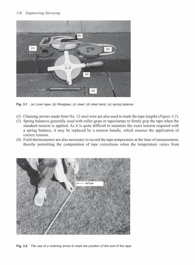
118 Engineering Surveying
(2) Chaining arrows made from No. 12 steel wire are also used to mark the tape lengths (Figure 3.2).(3) Spring balances generally used with roller-grips or tapeclamps to firmly grip the tape when the
standard tension is applied. As it is quite difficult to maintain the exact tension required witha spring balance, it may be replaced by a tension handle, which ensures the application ofcorrect tension.
(4) Field thermometers are also necessary to record the tape temperature at the time of measurement,thereby permitting the computation of tape corrections when the temperature varies from
Fig. 3.1 (a) Linen tape, (b) fibreglass, (c) steel, (d) steel band, (e) spring balance
Fig. 3.2 The use of a chaining arrow to mark the position of the end of the tape
(b)
(c) (a)
(d)
(e)
← Arrow
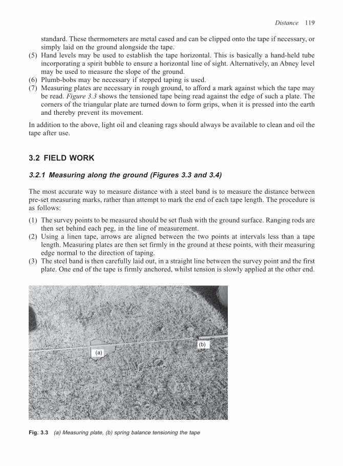
Distance 119
standard. These thermometers are metal cased and can be clipped onto the tape if necessary, orsimply laid on the ground alongside the tape.
(5) Hand levels may be used to establish the tape horizontal. This is basically a hand-held tubeincorporating a spirit bubble to ensure a horizontal line of sight. Alternatively, an Abney levelmay be used to measure the slope of the ground.
(6) Plumb-bobs may be necessary if stepped taping is used.(7) Measuring plates are necessary in rough ground, to afford a mark against which the tape may
be read. Figure 3.3 shows the tensioned tape being read against the edge of such a plate. Thecorners of the triangular plate are turned down to form grips, when it is pressed into the earthand thereby prevent its movement.
In addition to the above, light oil and cleaning rags should always be available to clean and oil thetape after use.
3.2 FIELD WORK
3.2.1 Measuring along the ground (Figures 3.3 and 3.4)
The most accurate way to measure distance with a steel band is to measure the distance betweenpre-set measuring marks, rather than attempt to mark the end of each tape length. The procedure isas follows:
(1) The survey points to be measured should be set flush with the ground surface. Ranging rods arethen set behind each peg, in the line of measurement.
(2) Using a linen tape, arrows are aligned between the two points at intervals less than a tapelength. Measuring plates are then set firmly in the ground at these points, with their measuringedge normal to the direction of taping.
(3) The steel band is then carefully laid out, in a straight line between the survey point and the firstplate. One end of the tape is firmly anchored, whilst tension is slowly applied at the other end.
Fig. 3.3 (a) Measuring plate, (b) spring balance tensioning the tape
(a)
(b)
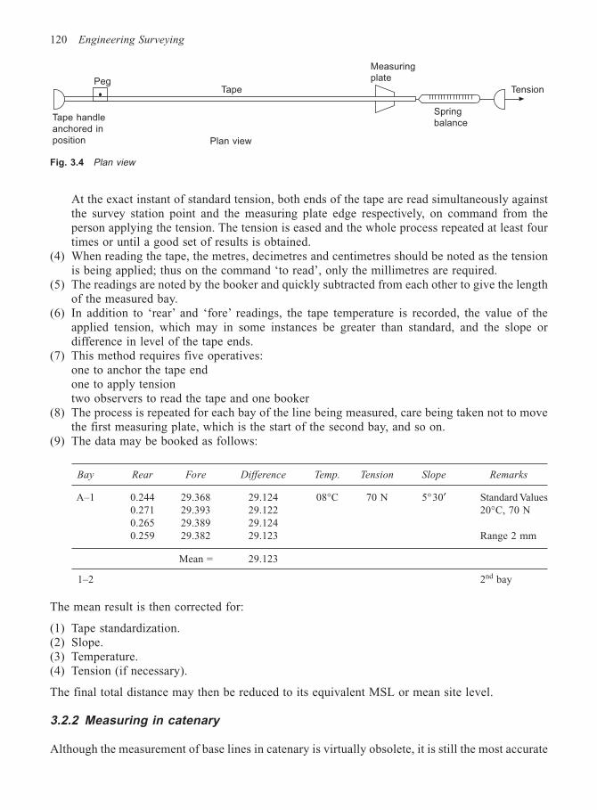
120 Engineering Surveying
At the exact instant of standard tension, both ends of the tape are read simultaneously againstthe survey station point and the measuring plate edge respectively, on command from theperson applying the tension. The tension is eased and the whole process repeated at least fourtimes or until a good set of results is obtained.
(4) When reading the tape, the metres, decimetres and centimetres should be noted as the tensionis being applied; thus on the command ‘to read’, only the millimetres are required.
(5) The readings are noted by the booker and quickly subtracted from each other to give the lengthof the measured bay.
(6) In addition to ‘rear’ and ‘fore’ readings, the tape temperature is recorded, the value of theapplied tension, which may in some instances be greater than standard, and the slope ordifference in level of the tape ends.
(7) This method requires five operatives:one to anchor the tape endone to apply tensiontwo observers to read the tape and one booker
(8) The process is repeated for each bay of the line being measured, care being taken not to movethe first measuring plate, which is the start of the second bay, and so on.
(9) The data may be booked as follows:
Bay Rear Fore Difference Temp. Tension Slope Remarks
A–1 0.244 29.368 29.124 08°C 70 N 5°30′ Standard Values0.271 29.393 29.122 20°C, 70 N0.265 29.389 29.1240.259 29.382 29.123 Range 2 mm
Mean = 29.123
1–2 2nd bay
The mean result is then corrected for:
(1) Tape standardization.(2) Slope.(3) Temperature.(4) Tension (if necessary).
The final total distance may then be reduced to its equivalent MSL or mean site level.
3.2.2 Measuring in catenary
Although the measurement of base lines in catenary is virtually obsolete, it is still the most accurate
Fig. 3.4 Plan view
PegTape
Tape handle
anchored in
position Plan view
Spring
balance
Measuring
plate
Tension
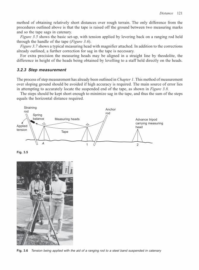
Distance 121
method of obtaining relatively short distances over rough terrain. The only difference from theprocedures outlined above is that the tape is raised off the ground between two measuring marksand so the tape sags in catenary.
Figure 3.5 shows the basic set-up, with tension applied by levering back on a ranging rod heldthrough the handle of the tape (Figure 3.6).
Figure 3.7 shows a typical measuring head with magnifier attached. In addition to the correctionsalready outlined, a further correction for sag in the tape is necessary.
For extra precision the measuring heads may be aligned in a straight line by theodolite, thedifference in height of the heads being obtained by levelling to a staff held directly on the heads.
3.2.3 Step measurement
The process of step measurement has already been outlined in Chapter 1. This method of measurementover sloping ground should be avoided if high accuracy is required. The main source of error liesin attempting to accurately locate the suspended end of the tape, as shown in Figure 3.8.
The steps should be kept short enough to minimize sag in the tape, and thus the sum of the stepsequals the horizontal distance required.
Fig. 3.5
Straining
rodSpring
balance Measuring heads
Tape
A
Applied
tension
1 2
Anchor
rod
Advance tripod
carrying measuring
head
Fig. 3.6 Tension being applied with the aid of a ranging rod to a steel band suspended in catenary
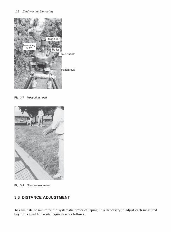
122 Engineering Surveying
3.3 DISTANCE ADJUSTMENT
To eliminate or minimize the systematic errors of taping, it is necessary to adjust each measuredbay to its final horizontal equivalent as follows.
Fig. 3.7 Measuring head
Fig. 3.8 Step measurement
Magnifier
Roller
MeasuringMark
Plate bubble
Footscrews
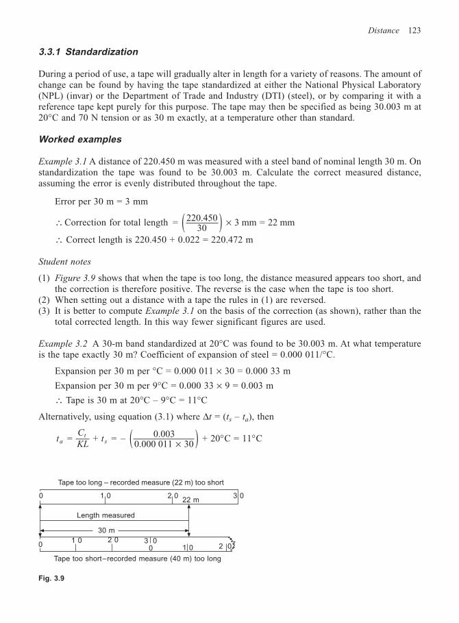
Distance 123
3.3.1 Standardization
During a period of use, a tape will gradually alter in length for a variety of reasons. The amount ofchange can be found by having the tape standardized at either the National Physical Laboratory(NPL) (invar) or the Department of Trade and Industry (DTI) (steel), or by comparing it with areference tape kept purely for this purpose. The tape may then be specified as being 30.003 m at20°C and 70 N tension or as 30 m exactly, at a temperature other than standard.
Worked examples
Example 3.1 A distance of 220.450 m was measured with a steel band of nominal length 30 m. Onstandardization the tape was found to be 30.003 m. Calculate the correct measured distance,assuming the error is evenly distributed throughout the tape.
Error per 30 m = 3 mm
∴ Correction for total length = 220.45030
3 mm = 22 mm( ) ×
∴ Correct length is 220.450 + 0.022 = 220.472 m
Student notes
(1) Figure 3.9 shows that when the tape is too long, the distance measured appears too short, andthe correction is therefore positive. The reverse is the case when the tape is too short.
(2) When setting out a distance with a tape the rules in (1) are reversed.(3) It is better to compute Example 3.1 on the basis of the correction (as shown), rather than the
total corrected length. In this way fewer significant figures are used.
Example 3.2 A 30-m band standardized at 20°C was found to be 30.003 m. At what temperatureis the tape exactly 30 m? Coefficient of expansion of steel = 0.000 011/°C.
Expansion per 30 m per °C = 0.000 011 × 30 = 0.000 33 m
Expansion per 30 m per 9°C = 0.000 33 × 9 = 0.003 m
∴ Tape is 30 m at 20°C – 9°C = 11°C
Alternatively, using equation (3.1) where ∆t = (ts – ta), then
tC
KLta
ts = + = – 0.003
0.000 011 30 + 20 C = 11 C×( ) ° °
Fig. 3.9
Tape too long – recorded measure (22 m) too short
0 1 0 2 0 3 022 m
Length measured
30 m
01 0 2 0 3 0
0 1 0 2 0
Tape too short–recorded measure (40 m) too long
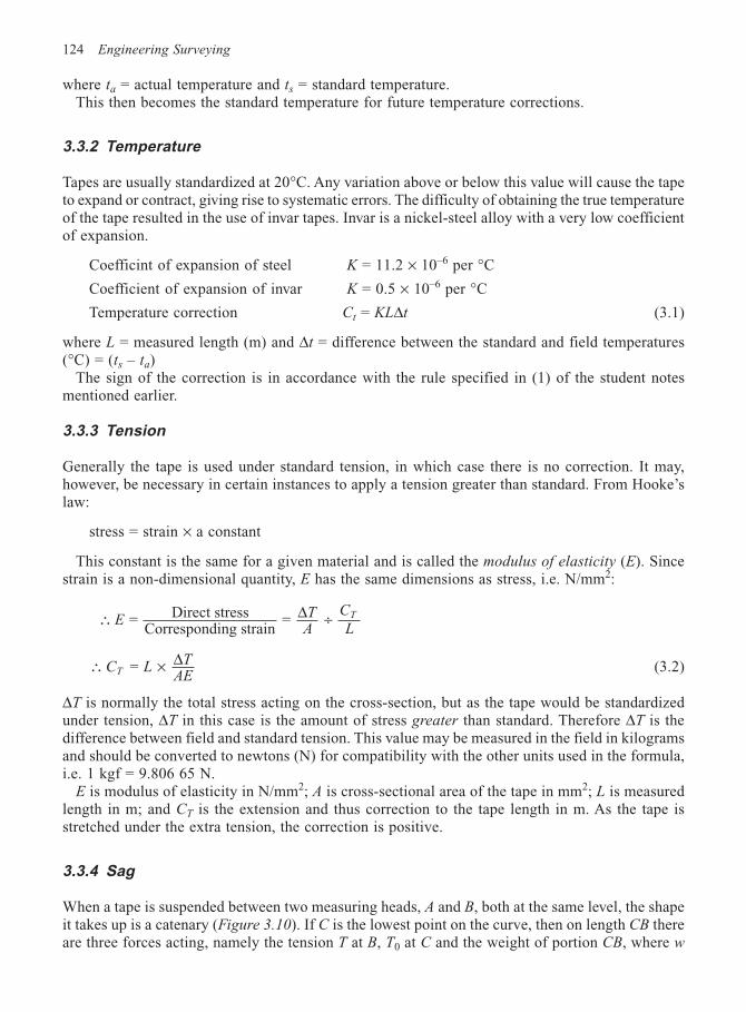
124 Engineering Surveying
where ta = actual temperature and ts = standard temperature.This then becomes the standard temperature for future temperature corrections.
3.3.2 Temperature
Tapes are usually standardized at 20°C. Any variation above or below this value will cause the tapeto expand or contract, giving rise to systematic errors. The difficulty of obtaining the true temperatureof the tape resulted in the use of invar tapes. Invar is a nickel-steel alloy with a very low coefficientof expansion.
Coefficint of expansion of steel K = 11.2 × 10⁻⁶ per °C
Coefficient of expansion of invar K = 0.5 × 10⁻⁶ per °C
Temperature correction Ct = KL∆t (3.1)
where L = measured length (m) and ∆t = difference between the standard and field temperatures(°C) = (ts – ta)
The sign of the correction is in accordance with the rule specified in (1) of the student notesmentioned earlier.
3.3.3 Tension
Generally the tape is used under standard tension, in which case there is no correction. It may,however, be necessary in certain instances to apply a tension greater than standard. From Hooke’slaw:
stress = strain × a constant
This constant is the same for a given material and is called the modulus of elasticity (E). Sincestrain is a non-dimensional quantity, E has the same dimensions as stress, i.e. N/mm2:
∴ ÷ = Direct stressCorresponding strain
= ET
A
C
LT∆
∴ × = C L T
AET∆ (3.2)
∆T is normally the total stress acting on the cross-section, but as the tape would be standardizedunder tension, ∆T in this case is the amount of stress greater than standard. Therefore ∆T is thedifference between field and standard tension. This value may be measured in the field in kilogramsand should be converted to newtons (N) for compatibility with the other units used in the formula,i.e. 1 kgf = 9.806 65 N.
E is modulus of elasticity in N/mm2; A is cross-sectional area of the tape in mm2; L is measuredlength in m; and CT is the extension and thus correction to the tape length in m. As the tape isstretched under the extra tension, the correction is positive.
3.3.4 Sag
When a tape is suspended between two measuring heads, A and B, both at the same level, the shapeit takes up is a catenary (Figure 3.10). If C is the lowest point on the curve, then on length CB thereare three forces acting, namely the tension T at B, T0 at C and the weight of portion CB, where w
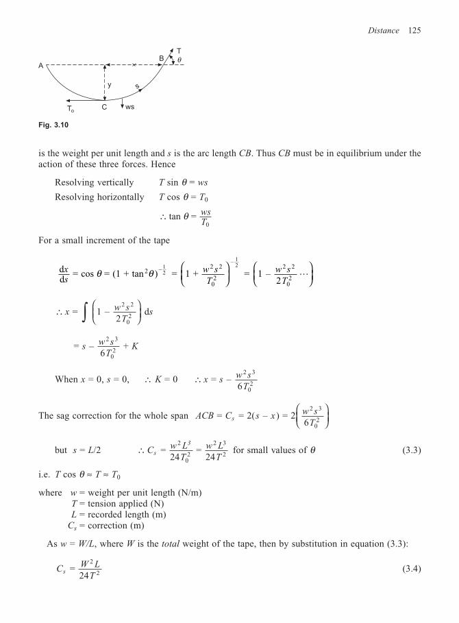
Distance 125
is the weight per unit length and s is the arc length CB. Thus CB must be in equilibrium under theaction of these three forces. Hence
Resolving vertically T sin θ = ws
Resolving horizontally T cos θ = T0
∴ tan = 0
θ wsT
For a small increment of the tape
dd
= cos = (1 + tan ) = 1 + = 1 – 2
2 – 2 2
02
–2 2
02
12
12
xs
w s
T
w s
Tθ θ
L
∴
∫ = 1 –
2 d
2 2
02
xw s
Ts
= – 6
+ 2 3
02
sw s
TK
When x = 0, s = 0, ∴ K = 0 ∴ = – 6
2 3
02
x sw s
T
The sag correction for the whole span ACB C s xw s
Ts = = 2( – ) = 2
6
2 3
02
but s = L/2 ∴ = 24
= 24
2 2 3
Cw L
T
w L
Ts
3
02 2
for small values of θ (3.3)
i.e. T cos θ ≈ T ≈ T0
where w = weight per unit length (N/m)T = tension applied (N)L = recorded length (m)
Cs = correction (m)
As w = W/L, where W is the total weight of the tape, then by substitution in equation (3.3):
CW L
Ts =
24
2
2(3.4)
Fig. 3.10
A
y s
BT
θ
wsToC
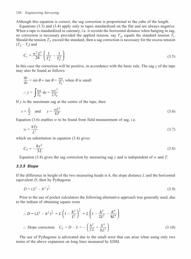
126 Engineering Surveying
Although this equation is correct, the sag correction is proportional to the cube of the length.Equations (3.3) and (3.4) apply only to tapes standardized on the flat and are always negative.
When a tape is standardized in catenary, i.e. it records the horizontal distance when hanging in sag,no correction is necessary provided the applied tension, say TA, equals the standard tension Ts.Should the tension TA exceed the standard, then a sag correction is necessary for the excess tension(TA – Ts) and
Cw L
T Ts
A S
= 24
1 – 12 3
22
(3.5)
In this case the correction will be positive, in accordance with the basic rule. The sag y of the tapemay also be found as follows:
dd
= sin tan = ,0
y
swsT
θ θ≈ when θ is small
∴ ∫ = ds = 20
2
0y
wsT
wsT
If y is the maximum sag at the centre of the tape, then
sL = 2
and ywL
T =
8
2
(3.6)
Equation (3.6) enables w to be found from field measurement of sag, i.e.
wTy
L =
82
(3.7)
which on substitution in equation (3.4) gives
Cy
LS = –83
2
(3.8)
Equation (3.8) gives the sag correction by measuring sag y and is independent of w and T.
3.3.5 Slope
If the difference in height of the two measuring heads is h, the slope distance L and the horizontalequivalent D, then by Pythagoras
D L h = ( – )2 212 (3.9)
Prior to the use of pocket calculators the following alternative approach was generally used, dueto the tedium of obtaining square roots
∴
= ( – ) = 1 – = 1 – 2
– 8
2 22
2
2
2
4
4
12
12
D L h Lh
LL
h
L
h
L
∴ Slope correction C D Lh
Lh
Lh = – = –
2 +
8
2 4
3
(3.10)
The use of Pythagoras is advocated due to the small error that can arise when using only twoterms of the above expansion on long lines measured by EDM.
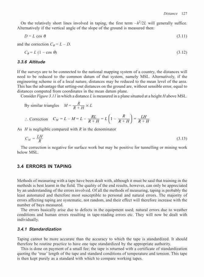
Distance 127
On the relatively short lines involved in taping, the first term –h2/2L will generally suffice.Alternatively if the vertical angle of the slope of the ground is measured then:
D = L cos θ (3.11)
and the correction Cθ = L – D.
Cθ = L (1 – cos θ) (3.12)
3.3.6 Altitude
If the surveys are to be connected to the national mapping system of a country, the distances willneed to be reduced to the common datum of that system, namely MSL. Alternatively, if theengineering scheme is of a local nature, distances may be reduced to the mean level of the area.This has the advantage that setting-out distances on the ground are, without sensible error, equal todistances computed from coordinates in the mean datum plane.
Consider Figure 3.11 in which a distance L is measured in a plane situated at a height H above MSL.
By similar triangles MR
R HL =
+ ×
∴ Correction C L M LRL
R HL
R
R HLH
R HM = – = – +
= 1 – +
= +
As H is negligible compared with R in the denominator
CLHRM = (3.13)
The correction is negative for surface work but may be positive for tunnelling or mining workbelow MSL.
3.4 ERRORS IN TAPING
Methods of measuring with a tape have been dealt with, although it must be said that training in themethods is best learnt in the field. The quality of the end results, however, can only be appreciatedby an understanding of the errors involved. Of all the methods of measuring, taping is probably theleast automated and therefore most susceptible to personal and natural errors. The majority oferrors affecting taping are systematic, not random, and their effect will therefore increase with thenumber of bays measured.
The errors basically arise due to defects in the equipment used; natural errors due to weatherconditions and human errors resulting in tape-reading errors etc. They will now be dealt withindividually.
3.4.1 Standardization
Taping cannot be more accurate than the accuracy to which the tape is standardized. It shouldtherefore be routine practice to have one tape standardized by the appropriate authority.
This is done on payment of a small fee; the tape is returned with a certificate of standardizationquoting the ‘true’ length of the tape and standard conditions of temperature and tension. This tapeis then kept purely as a standard with which to compare working tapes.
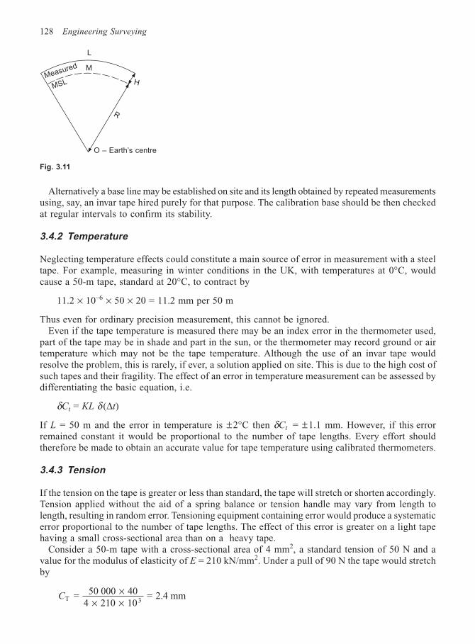
128 Engineering Surveying
Alternatively a base line may be established on site and its length obtained by repeated measurementsusing, say, an invar tape hired purely for that purpose. The calibration base should be then checkedat regular intervals to confirm its stability.
3.4.2 Temperature
Neglecting temperature effects could constitute a main source of error in measurement with a steeltape. For example, measuring in winter conditions in the UK, with temperatures at 0°C, wouldcause a 50-m tape, standard at 20°C, to contract by
11.2 × 10–6 × 50 × 20 = 11.2 mm per 50 m
Thus even for ordinary precision measurement, this cannot be ignored.Even if the tape temperature is measured there may be an index error in the thermometer used,
part of the tape may be in shade and part in the sun, or the thermometer may record ground or airtemperature which may not be the tape temperature. Although the use of an invar tape wouldresolve the problem, this is rarely, if ever, a solution applied on site. This is due to the high cost ofsuch tapes and their fragility. The effect of an error in temperature measurement can be assessed bydifferentiating the basic equation, i.e.
δCt = KL δ (∆t)
If L = 50 m and the error in temperature is ±2°C then δCt = ±1.1 mm. However, if this errorremained constant it would be proportional to the number of tape lengths. Every effort shouldtherefore be made to obtain an accurate value for tape temperature using calibrated thermometers.
3.4.3 Tension
If the tension on the tape is greater or less than standard, the tape will stretch or shorten accordingly.Tension applied without the aid of a spring balance or tension handle may vary from length tolength, resulting in random error. Tensioning equipment containing error would produce a systematicerror proportional to the number of tape lengths. The effect of this error is greater on a light tapehaving a small cross-sectional area than on a heavy tape.
Consider a 50-m tape with a cross-sectional area of 4 mm2, a standard tension of 50 N and avalue for the modulus of elasticity of E = 210 kN/mm2. Under a pull of 90 N the tape would stretchby
CT 3 = 50 000 40
4 210 10 = 2.4 mm×
× ×
Fig. 3.11
M
L
Measured
MSL H
R
O – Earth’s centre
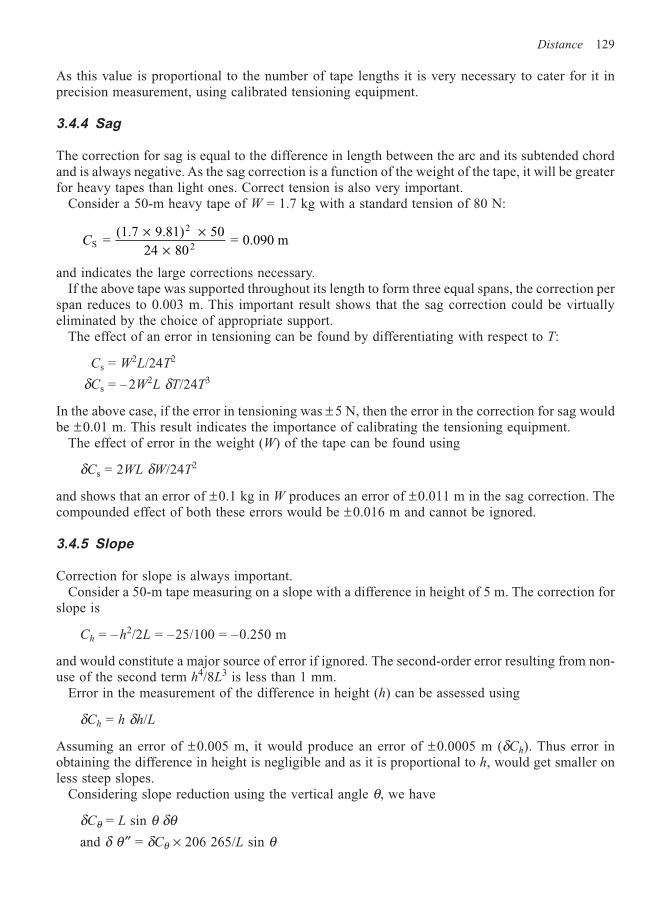
Distance 129
As this value is proportional to the number of tape lengths it is very necessary to cater for it inprecision measurement, using calibrated tensioning equipment.
3.4.4 Sag
The correction for sag is equal to the difference in length between the arc and its subtended chordand is always negative. As the sag correction is a function of the weight of the tape, it will be greaterfor heavy tapes than light ones. Correct tension is also very important.
Consider a 50-m heavy tape of W = 1.7 kg with a standard tension of 80 N:
CS
2
2 =
(1.7 9.81) 50
24 80 = 0.090 m
× ××
and indicates the large corrections necessary.If the above tape was supported throughout its length to form three equal spans, the correction per
span reduces to 0.003 m. This important result shows that the sag correction could be virtuallyeliminated by the choice of appropriate support.
The effect of an error in tensioning can be found by differentiating with respect to T:
Cs = W2L/24T2
δCs = – 2W2L δT/24T3
In the above case, if the error in tensioning was ± 5 N, then the error in the correction for sag wouldbe ±0.01 m. This result indicates the importance of calibrating the tensioning equipment.
The effect of error in the weight (W) of the tape can be found using
δCs = 2WL δW/24T2
and shows that an error of ±0.1 kg in W produces an error of ±0.011 m in the sag correction. Thecompounded effect of both these errors would be ±0.016 m and cannot be ignored.
3.4.5 Slope
Correction for slope is always important.Consider a 50-m tape measuring on a slope with a difference in height of 5 m. The correction for
slope is
Ch = – h2/2L = –25/100 = –0.250 m
and would constitute a major source of error if ignored. The second-order error resulting from non-use of the second term h4/8L3 is less than 1 mm.
Error in the measurement of the difference in height (h) can be assessed using
δCh = h δh/L
Assuming an error of ±0.005 m, it would produce an error of ±0.0005 m (δCh). Thus error inobtaining the difference in height is negligible and as it is proportional to h, would get smaller onless steep slopes.
Considering slope reduction using the vertical angle θ, we have
δCθ = L sin θ δθand δ θ″ = δCθ × 206 265/L sin θ
130 Engineering Surveying
If L = 50 m is required to an accuracy of ±5 mm on a slope of 5° then
δ θ″ = 0.005 × 206265/50 sin 5° = 237″ ≈ 04′
This level of accuracy could easily be achieved using an Abney level to measure slope. As theslopes get less steep the accuracy required is further reduced; however, for the much greaterdistances obtained using EDM, the measurement of vertical angles is much more critical. Indeed,if the accuracy required above is increased to that of precision measurement, say ±1 mm, the angleaccuracy required rises to ±47″ and would require the use of a theodolite.
3.4.6 Misalignment
If the tape is not in a straight line between the two points whose distance apart is being measured,then the error in the horizontal plane will be equivalent to that of slope in the vertical plane. Takingthe amount by which the end of the tape is off line equal to e, then the resultant error is e2/2L.
A 50-m tape, off line by 0.500 m (an excessive amount), would be in error by 2.5 mm. The erroris systematic and will obviously result in a recorded distance longer than the actual. If we considera more realistic error in misalignment of, say, 0.05 m, the resulting error is 0.025 mm and completelynegligible. Thus for the majority of taping, alignment by eye is quite adequate.
3.4.7 Plumbing
If stepped measurement is used, locating the end of the tape by plumb-bob will inevitably result inerror. Plumbing at its best will probably produce a random error of about ±3 mm. In difficult, windyconditions it would be impossible to use, unless sheltered from the wind by some kind of makeshiftwind break, combined with careful steadying of the bob itself.
3.4.8 Incorrect reading of the tape
Reading errors are random and quite prevalent amongst beginners. Care and practice are needed toobviate them.
3.4.9 Booking error
Booking error can be reduced by adopting the process of the booker reading the measurement backto the observer for checking purposes. However, when measuring to millimetres with tensioningequipment, the reading has usually altered by the time it comes to check it. Repeated measurementswill generally reveal booking errors, and thus distances should always be measured more than once.
3.5 ACCURACIES
If a great deal of taping measurement is taking place, then it is advisable to construct graphs of allthe corrections for slope, temperature, tension and sag, for a variety of different conditions. In thisway the values can be rapidly obtained and more easily considered. Such an approach rapidlyproduces in the measurer a ‘feel’ for the effect of errors in taping.
As random errors increase as the square root of the distance, systematic errors are proportionalto distance and reading errors are independent of distance, it is not easy to produce a preciseassessment of taping accuracies under variable conditions. Considering taping with a standardized
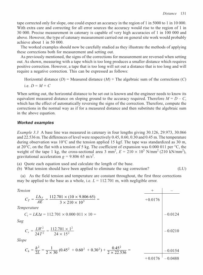
Distance 131
tape corrected only for slope, one could expect an accuracy in the region of 1 in 5000 to 1 in 10 000.With extra care and correcting for all error sources the accuracy would rise to the region of 1 in30 000. Precise measurement in catenary is capable of very high accuracies of 1 in 100 000 andabove. However, the type of catenary measurement carried out on general site work would probablyachieve about 1 in 50 000.
The worked examples should now be carefully studied as they illustrate the methods of applyingthese corrections both for measurement and setting out.
As previously mentioned, the signs of the corrections for measurement are reversed when settingout. As shown, measuring with a tape which is too long produces a smaller distance which requirespositive correction. However, a tape that is too long will set out a distance that is too long and willrequire a negative correction. This can be expressed as follows:
Horizontal distance (D) = Measured distance (M) + The algebraic sum of the corrections (C)
i.e. D = M + C
When setting out, the horizontal distance to be set out is known and the engineer needs to know itsequivalent measured distance on sloping ground to the accuracy required. Therefore M = D – C,which has the effect of automatically reversing the signs of the correction. Therefore, compute thecorrections in the normal way as if for a measured distance and then substitute the algebraic sumin the above equation.
Worked examples
Example 3.3 A base line was measured in catenary in four lengths giving 30.126, 29.973, 30.066and 22.536 m. The differences of level were respectively 0.45, 0.60, 0.30 and 0.45 m. The temperatureduring observation was 10°C and the tension applied 15 kgf. The tape was standardized as 30 m,at 20°C, on the flat with a tension of 5 kg. The coefficient of expansion was 0.000 011 per °C, theweight of the tape 1 kg, the cross-sectional area 3 mm2, E = 210 × 103 N/mm2 (210 kN/mm2),gravitational acceleration g = 9.806 65 m/s2.
(a) Quote each equation used and calculate the length of the base.(b) What tension should have been applied to eliminate the sag correction? (LU)
(a) As the field tension and temperature are constant throughout, the first three correctionsmay be applied to the base as a whole, i.e. L = 112.701 m, with negligible error.
Tension + –
CL
AETT = =
112.701 (10 9.806 65)
3 210 10 =
3
∆ × ×× ×
+0.0176
Temperature
Ct = LK∆t = 112.701 × 0.000 011 × 10 = – 0.0124
Sag
CLW
Ts =
24 = 112.701 1
24 15
2
2
2
2×
×– 0.0210
Slope
Ch
Lh = 2
= 12 30
(0.45 + 0.60 + 0.30 ) + 0.452 22.536
= 2
2 2 22
× × – 0.0154
+ 0.0176 – 0.0488
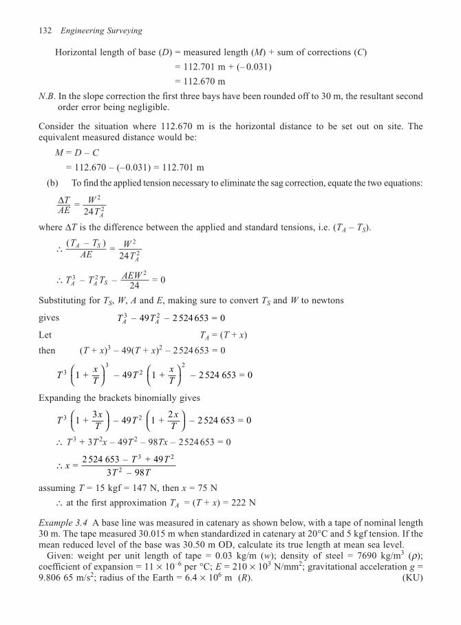
132 Engineering Surveying
Horizontal length of base (D) = measured length (M) + sum of corrections (C)
= 112.701 m + (– 0.031)
= 112.670 m
N.B. In the slope correction the first three bays have been rounded off to 30 m, the resultant secondorder error being negligible.
Consider the situation where 112.670 m is the horizontal distance to be set out on site. Theequivalent measured distance would be:
M = D – C
= 112.670 – (–0.031) = 112.701 m
(b) To find the applied tension necessary to eliminate the sag correction, equate the two equations:
∆TAE
W
TA
= 2
2
24
where ∆T is the difference between the applied and standard tensions, i.e. (TA – TS).
∴( – )
= 24
2T T
AEW
T
A S
A2
∴ – – 24
= 03 22
T T TAEW
A A S
Substituting for TS, W, A and E, making sure to convert TS and W to newtons
gives T TA A3 2 – 49 – 2 524 653 = 0
Let TA = (T + x)
then (T + x)3 – 49(T + x)2 – 2524 653 = 0
Tx
TT
x
T3
32
2
1 + – 49 1 + – 2 524 653 = 0
Expanding the brackets binomially gives
Tx
TT
x
T3 2 1 +
3 – 49 1 +
2 – 2 524 653 = 0
∴ T 3 + 3T 2x – 49T 2 – 98Tx – 2524 653 = 0
∴ = 2 524 653 – + 49
3 – 98
3 2
2x
T T
T T
assuming T = 15 kgf = 147 N, then x = 75 N
∴ at the first approximation TA = (T + x) = 222 N
Example 3.4 A base line was measured in catenary as shown below, with a tape of nominal length30 m. The tape measured 30.015 m when standardized in catenary at 20°C and 5 kgf tension. If themean reduced level of the base was 30.50 m OD, calculate its true length at mean sea level.
Given: weight per unit length of tape = 0.03 kg/m (w); density of steel = 7690 kg/m3 (ρ);coefficient of expansion = 11 × 10–6 per °C; E = 210 × 103 N/mm2; gravitational acceleration g =9.806 65 m/s2; radius of the Earth = 6.4 × 10⁶ m (R). (KU)
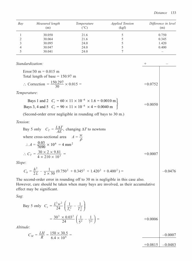
Distance 133
Bay Measured length Temperature Applied Tension Difference in level
(m) (°C) (kgf) (m)
1 30.050 21.6 5 0.7502 30.064 21.6 5 0.3453 30.095 24.0 5 1.4204 30.047 24.0 5 0.4005 30.041 24.0 7 –
Standardization: + –
Error/30 m = 0.015 mTotal length of base = 150.97 m
∴ Correction = 150.29730
0.015× = +0.0752
Temperature:
Bays 1 and 2 = 60 11 10 1.6 = 0.0010 m
Bays 3, 4 and 5 = 90 11 10 4 = 0.0040 m
–6
–6
C
C
t
t
× × ×× × ×
+0.0050
(Second-order error negligible in rounding off bays to 30 m.)
Tension:
Bay 5 only = ,CL TAET∆ changing ∆T to newtons
where cross-sectional area Aw = ρ
∴ × = 7690
10 = 4 mm6 2A0 03.
∴ × ×× ×
= 30 2 9.814 210 103
CT = +0.0007
Slope:
Ch
Lh = 2
– 12 30
(0.750 + 0.345 + 1.420 + 0.400 ) = 2
2 2 2 2
× –0.0476
The second-order error in rounding off to 30 m is negligible in this case also.However, care should be taken when many bays are involved, as their accumulativeeffect may be significant.
Sag:
Bay 5 only CL w
T Ts
s A
= 24
1 – 13 2
22
= 30 0.0324
15
– 17
=3 2
2 2×
+0.0006
Altitude:
CLHRM = = 150 30.5
6.4 10 =
6××
–0.0007
+0.0815 –0.0483
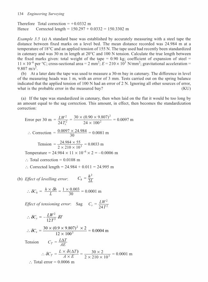
134 Engineering Surveying
Therefore Total correction = + 0.0332 mHence Corrected length = 150.297 + 0.0332 = 150.3302 m
Example 3.5 (a) A standard base was established by accurately measuring with a steel tape thedistance between fixed marks on a level bed. The mean distance recorded was 24.984 m at atemperature of 18°C and an applied tension of 155 N. The tape used had recently been standardizedin catenary and was 30 m in length at 20°C and 100 N tension. Calculate the true length betweenthe fixed marks given: total weight of the tape = 0.90 kg; coefficient of expansion of steel =11 × 10–6 per °C; cross-sectional area = 2 mm2; E = 210 × 103 N/mm2; gravitational acceleration =9.807 m/s2.
(b) At a later date the tape was used to measure a 30-m bay in catenary. The difference in levelof the measuring heads was 1 m, with an error of 3 mm. Tests carried out on the spring balanceindicated that the applied tension of 100 N had an error of 2 N. Ignoring all other sources of error,what is the probable error in the measured bay? (KU)
(a) If the tape was standardized in catenary, then when laid on the flat it would be too long byan amount equal to the sag correction. This amount, in effect, then becomes the standardizationcorrection:
Error per 30 m =24
= 30 (0.90 9.807)
24 100 = 0.0097 m
2
2
2
2LW
Ts
× ××
∴ Correction = 0.0097 24.98430
= 0.0081 m×
Tension = 24.984 552 210 10
= 0.0033 m3
×× ×
Temperature = 24.984 × 11 × 10–6 × 2 = –0.0006 m
∴ Total correction = 0.0108 m
∴ Corrected length = 24.984 + 0.011 = 24.995 m
(b) Effect of levelling error: Ch
Lh = 2
2
= = 1 0.00330
= 0.0001 m∴ × ×δ δC
h hLh
Effect of tensioning error: Sag CLW
Ts =
24
2
2
= –12
2
3∴ δ δC
LW
TTs
∴ × × ××
= 30 (0.9 9.807) 2
12 100 = 0.0004 m
2
3δCs
Tension CL TAET = ∆
∴ ××
×× ×
= (
= 30 22 210 10
= 0.0001 m3
δ δC
L T
A ET
∆ )
∴ Total error = 0.0006 m
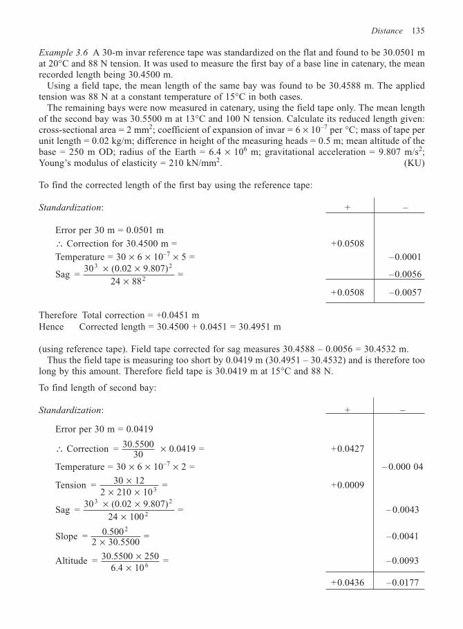
Distance 135
Example 3.6 A 30-m invar reference tape was standardized on the flat and found to be 30.0501 mat 20°C and 88 N tension. It was used to measure the first bay of a base line in catenary, the meanrecorded length being 30.4500 m.
Using a field tape, the mean length of the same bay was found to be 30.4588 m. The appliedtension was 88 N at a constant temperature of 15°C in both cases.
The remaining bays were now measured in catenary, using the field tape only. The mean lengthof the second bay was 30.5500 m at 13°C and 100 N tension. Calculate its reduced length given:cross-sectional area = 2 mm2; coefficient of expansion of invar = 6 × 10⁻⁷ per °C; mass of tape perunit length = 0.02 kg/m; difference in height of the measuring heads = 0.5 m; mean altitude of thebase = 250 m OD; radius of the Earth = 6.4 × 10⁶ m; gravitational acceleration = 9.807 m/s2;Young’s modulus of elasticity = 210 kN/mm2. (KU)
To find the corrected length of the first bay using the reference tape:
Standardization: + –
Error per 30 m = 0.0501 m
∴ Correction for 30.4500 m = +0.0508
Temperature = 30 × 6 × 10–7 × 5 = –0.0001
Sag =30 (0.02 9.807)
24 88 =
3 2
2
× ××
–0.0056
+0.0508 –0.0057
Therefore Total correction = +0.0451 mHence Corrected length = 30.4500 + 0.0451 = 30.4951 m
(using reference tape). Field tape corrected for sag measures 30.4588 – 0.0056 = 30.4532 m.Thus the field tape is measuring too short by 0.0419 m (30.4951 – 30.4532) and is therefore too
long by this amount. Therefore field tape is 30.0419 m at 15°C and 88 N.
To find length of second bay:
Standardization: + –
Error per 30 m = 0.0419
∴ Correction = 30.550030
0.0419 =× +0.0427
Temperature = 30 × 6 × 10–7 × 2 = – 0.000 04
Tension = 30 122 210 10
=3
×× ×
+0.0009
Sag =30 (0.02 9.807)
24 100 =
3 2
2
× ××
– 0.0043
Slope = 0.5002 30.5500
= 2
× –0.0041
Altitude = 30.5500 2506.4 10
=6
××
–0.0093
+0.0436 –0.0177
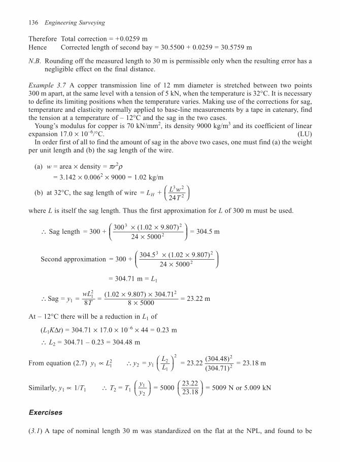
136 Engineering Surveying
Therefore Total correction = +0.0259 mHence Corrected length of second bay = 30.5500 + 0.0259 = 30.5759 m
N.B. Rounding off the measured length to 30 m is permissible only when the resulting error has anegligible effect on the final distance.
Example 3.7 A copper transmission line of 12 mm diameter is stretched between two points300 m apart, at the same level with a tension of 5 kN, when the temperature is 32°C. It is necessaryto define its limiting positions when the temperature varies. Making use of the corrections for sag,temperature and elasticity normally applied to base-line measurements by a tape in catenary, findthe tension at a temperature of – 12°C and the sag in the two cases.
Young’s modulus for copper is 70 kN/mm2, its density 9000 kg/m3 and its coefficient of linearexpansion 17.0 × 10⁻⁶/°C. (LU)
In order first of all to find the amount of sag in the above two cases, one must find (a) the weightper unit length and (b) the sag length of the wire.
(a) w = area × density = πr2ρ= 3.142 × 0.0062 × 9000 = 1.02 kg/m
(b) at 32°C, the sag length of wire = + 24
3 2
LL w
TH 2
where L is itself the sag length. Thus the first approximation for L of 300 m must be used.
∴ Sag length = 300 + 300 (1.02 9.807)
24 5000 = 304.5 m
3 2
2
× ××
Second approximation = 300 + 304.5 (1.02 9.807)
24 5000
3 2
2
× ××
= 304.71 m = L1
∴ Sag = ywL
T112 2
= 8
= (1.02 9.807) 304.71
8 5000 = 23.22 m
× ××
At – 12°C there will be a reduction in L1 of
(L1K∆t) = 304.71 × 17.0 × 10–6 × 44 = 0.23 m
∴ L2 = 304.71 – 0.23 = 304.48 m
From equation (2.7) y L1 12∝ ∴
= = 23.22
(304.48)
(304.71) = 23.18 m2 1
2
1
2 2
2y y
L
L
Similarly, y1 ∝ 1/T1 ∴ T2 = T1y
y1
2
= 5000
23.2223.18
= 5009 N or 5.009 kN
Exercises
(3.1) A tape of nominal length 30 m was standardized on the flat at the NPL, and found to be
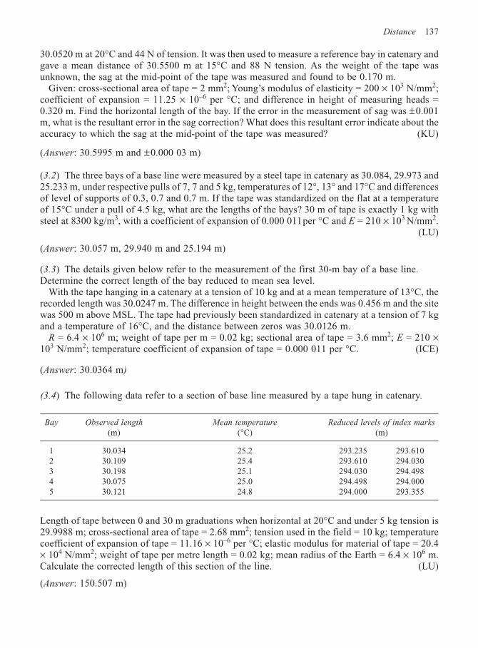
Distance 137
30.0520 m at 20°C and 44 N of tension. It was then used to measure a reference bay in catenary andgave a mean distance of 30.5500 m at 15°C and 88 N tension. As the weight of the tape wasunknown, the sag at the mid-point of the tape was measured and found to be 0.170 m.
Given: cross-sectional area of tape = 2 mm2; Young’s modulus of elasticity = 200 × 103 N/mm2;coefficient of expansion = 11.25 × 10⁻⁶ per °C; and difference in height of measuring heads =0.320 m. Find the horizontal length of the bay. If the error in the measurement of sag was ±0.001m, what is the resultant error in the sag correction? What does this resultant error indicate about theaccuracy to which the sag at the mid-point of the tape was measured? (KU)
(Answer: 30.5995 m and ±0.000 03 m)
(3.2) The three bays of a base line were measured by a steel tape in catenary as 30.084, 29.973 and25.233 m, under respective pulls of 7, 7 and 5 kg, temperatures of 12°, 13° and 17°C and differencesof level of supports of 0.3, 0.7 and 0.7 m. If the tape was standardized on the flat at a temperatureof 15°C under a pull of 4.5 kg, what are the lengths of the bays? 30 m of tape is exactly 1 kg withsteel at 8300 kg/m3, with a coefficient of expansion of 0.000 011per °C and E = 210 × 103 N/mm2.
(LU)
(Answer: 30.057 m, 29.940 m and 25.194 m)
(3.3) The details given below refer to the measurement of the first 30-m bay of a base line.Determine the correct length of the bay reduced to mean sea level.
With the tape hanging in a catenary at a tension of 10 kg and at a mean temperature of 13°C, therecorded length was 30.0247 m. The difference in height between the ends was 0.456 m and the sitewas 500 m above MSL. The tape had previously been standardized in catenary at a tension of 7 kgand a temperature of 16°C, and the distance between zeros was 30.0126 m.
R = 6.4 × 10⁶ m; weight of tape per m = 0.02 kg; sectional area of tape = 3.6 mm2; E = 210 ×103 N/mm2; temperature coefficient of expansion of tape = 0.000 011 per °C. (ICE)
(Answer: 30.0364 m)
(3.4) The following data refer to a section of base line measured by a tape hung in catenary.
Bay Observed length Mean temperature Reduced levels of index marks
(m) (°C) (m)
1 30.034 25.2 293.235 293.6102 30.109 25.4 293.610 294.0303 30.198 25.1 294.030 294.4984 30.075 25.0 294.498 294.0005 30.121 24.8 294.000 293.355
Length of tape between 0 and 30 m graduations when horizontal at 20°C and under 5 kg tension is29.9988 m; cross-sectional area of tape = 2.68 mm2; tension used in the field = 10 kg; temperaturecoefficient of expansion of tape = 11.16 × 10⁻⁶ per °C; elastic modulus for material of tape = 20.4× 10⁴ N/mm2; weight of tape per metre length = 0.02 kg; mean radius of the Earth = 6.4 × 10⁶ m.Calculate the corrected length of this section of the line. (LU)
(Answer: 150.507 m)
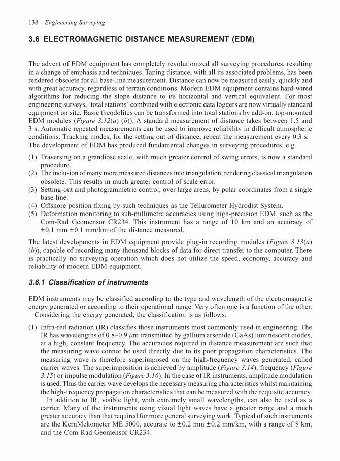
138 Engineering Surveying
3.6 ELECTROMAGNETIC DISTANCE MEASUREMENT (EDM)
The advent of EDM equipment has completely revolutionized all surveying procedures, resultingin a change of emphasis and techniques. Taping distance, with all its associated problems, has beenrendered obsolete for all base-line measurement. Distance can now be measured easily, quickly andwith great accuracy, regardless of terrain conditions. Modern EDM equipment contains hard-wiredalgorithms for reducing the slope distance to its horizontal and vertical equivalent. For mostengineering surveys, ‘total stations’ combined with electronic data loggers are now virtually standardequipment on site. Basic theodolites can be transformed into total stations by add-on, top-mountedEDM modules (Figure 3.12(a) (b)). A standard measurement of distance takes between 1.5 and3 s. Automatic repeated measurements can be used to improve reliability in difficult atmosphericconditions. Tracking modes, for the setting out of distance, repeat the measurement every 0.3 s.The development of EDM has produced fundamental changes in surveying procedures, e.g.
(1) Traversing on a grandiose scale, with much greater control of swing errors, is now a standardprocedure.
(2) The inclusion of many more measured distances into triangulation, rendering classical triangulationobsolete. This results in much greater control of scale error.
(3) Setting-out and photogrammetric control, over large areas, by polar coordinates from a singlebase line.
(4) Offshore position fixing by such techniques as the Tellurometer Hydrodist System.(5) Deformation monitoring to sub-millimetre accuracies using high-precision EDM, such as the
Com-Rad Geomensor CR234. This instrument has a range of 10 km and an accuracy of±0.1 mm ±0.1 mm/km of the distance measured.
The latest developments in EDM equipment provide plug-in recording modules (Figure 3.13(a)(b)), capable of recording many thousand blocks of data for direct transfer to the computer. Thereis practically no surveying operation which does not utilize the speed, economy, accuracy andreliability of modern EDM equipment.
3.6.1 Classification of instruments
EDM instruments may be classified according to the type and wavelength of the electromagneticenergy generated or according to their operational range. Very often one is a function of the other.
Considering the energy generated, the classification is as follows:
(1) Infra-red radiation (IR) classifies those instruments most commonly used in engineering. TheIR has wavelengths of 0.8–0.9 µm transmitted by gallium arsenide (GaAs) luminescent diodes,at a high, constant frequency. The accuracies required in distance measurement are such thatthe measuring wave connot be used directly due to its poor propagation characteristics. Themeasuring wave is therefore superimposed on the high-frequency waves generated, calledcarrier waves. The superimposition is achieved by amplitude (Figure 3.14), frequency (Figure
3.15) or impulse modulation (Figure 3.16). In the case of IR instruments, amplitude modulationis used. Thus the carrier wave develops the necessary measuring characteristics whilst maintainingthe high-frequency propagation characteristics that can be measured with the requisite accuracy.
In addition to IR, visible light, with extremely small wavelengths, can also be used as acarrier. Many of the instruments using visual light waves have a greater range and a muchgreater accuracy than that required for more general surveying work. Typical of such instrumentsare the KernMekometer ME 5000, accurate to ±0.2 mm ±0.2 mm/km, with a range of 8 km,and the Com-Rad Geomensor CR234.
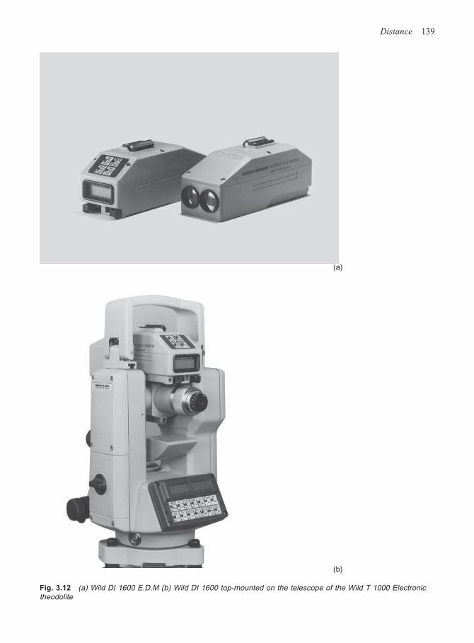
Distance 139
(a)
Fig. 3.12 (a) Wild DI 1600 E.D.M (b) Wild DI 1600 top-mounted on the telescope of the Wild T 1000 Electronictheodolite
(b)
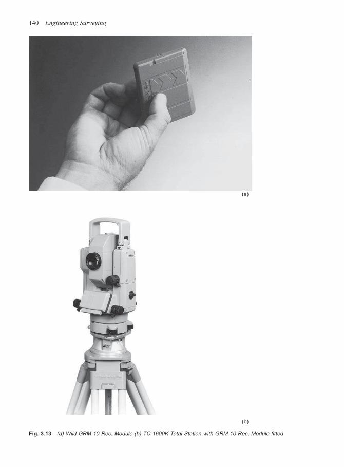
140 Engineering Surveying
Fig. 3.13 (a) Wild GRM 10 Rec. Module (b) TC 1600K Total Station with GRM 10 Rec. Module fitted
(a)
(b)
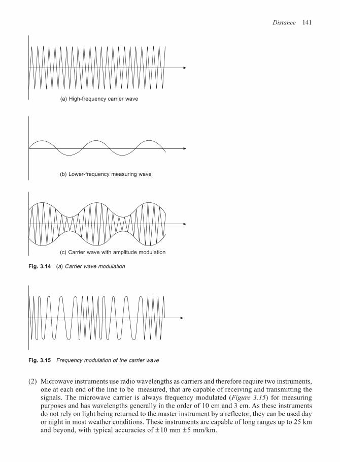
Distance 141
(2) Microwave instruments use radio wavelengths as carriers and therefore require two instruments,one at each end of the line to be measured, that are capable of receiving and transmitting thesignals. The microwave carrier is always frequency modulated (Figure 3.15) for measuringpurposes and has wavelengths generally in the order of 10 cm and 3 cm. As these instrumentsdo not rely on light being returned to the master instrument by a reflector, they can be used dayor night in most weather conditions. These instruments are capable of long ranges up to 25 kmand beyond, with typical accuracies of ±10 mm ±5 mm/km.
(a) High-frequency carrier wave
(b) Lower-frequency measuring wave
(c) Carrier wave with amplitude modulation
Fig. 3.14 (a) Carrier wave modulation
Fig. 3.15 Frequency modulation of the carrier wave
142 Engineering Surveying
(3) The final classification of equipment refers to those instruments which use very long radiowaves with wavelengths of 150 m to 2 km. They are primarily used for position-fixing systemsin hydrographic and oceanographic surveying. Typical examples are the Pulse 8 system and theSyledis system, for offshore position fixing.
The above classification shows that it would also be possible to classify by range, such as:
(a) Short-range, electro-optical instruments using amplitude-modulated infra-red or visible lightwith ranges up to 5 km.
(b) Medium-range microwave equipment, frequency modulated to give ranges up to 25 km.(c) Long-range radio wave equipment with ranges up to 100 km.
3.7 MEASURING PRINCIPLES
Although there is a wide variety of EDM instruments available, there are basically only twomethods of measurement employed, namely the pulse method and the more popular phase difference
method.
3.7.1 Pulse method (Figure 3.17)
A short, intensive pulse of radiation is transmitted to a reflector target, which immediately transmitsit back, along a parallel path, to the receiver. The measured distance is computed from the velocityof the signal multiplied by the time it took to complete its journey, i.e.
Fig. 3.16 Impulse modulation of the carrier wave
Pulse
Emitter
B
A
Receiver
Pulse2D = c · ∆t
D ct
=2
⋅ ∆
PulseReflector
Fig. 3.17 Principle of pulse distance meter
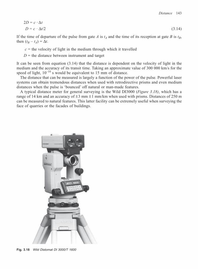
Distance 143
2D = c · ∆t
D = c · ∆t/2 (3.14)
If the time of departure of the pulse from gate A is tA and the time of its reception at gate B is tB,then (tB – tA) = ∆t.
c = the velocity of light in the medium through which it travelled
D = the distance between instrument and target
It can be seen from equation (3.14) that the distance is dependent on the velocity of light in themedium and the accuracy of its transit time. Taking an approximate value of 300 000 km/s for thespeed of light, 10–10 s would be equivalent to 15 mm of distance.
The distance that can be measured is largely a function of the power of the pulse. Powerful lasersystems can obtain tremendous distances when used with retrodirective prisms and even mediumdistances when the pulse is ‘bounced’ off natural or man-made features.
A typical distance meter for general surveying is the Wild DI3000 (Figure 3.18), which has arange of 14 km and an accuracy of ±3 mm ±1 mm/km when used with prisms. Distances of 250 mcan be measured to natural features. This latter facility can be extremely useful when surveying theface of quarries or the facades of buildings.
Fig. 3.18 Wild Distomat DI 3000/T 1600
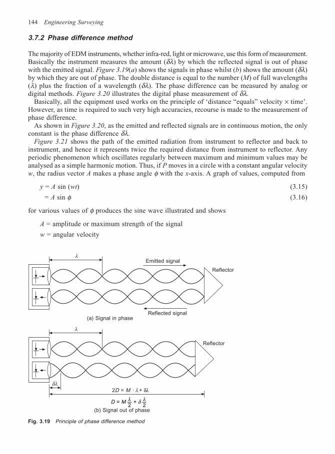
144 Engineering Surveying
3.7.2 Phase difference method
The majority of EDM instruments, whether infra-red, light or microwave, use this form of measurement.Basically the instrument measures the amount (δλ) by which the reflected signal is out of phasewith the emitted signal. Figure 3.19(a) shows the signals in phase whilst (b) shows the amount (δλ)by which they are out of phase. The double distance is equal to the number (M) of full wavelengths(λ) plus the fraction of a wavelength (δλ). The phase difference can be measured by analog ordigital methods. Figure 3.20 illustrates the digital phase measurement of δλ.
Basically, all the equipment used works on the principle of ‘distance “equals” velocity × time’.However, as time is required to such very high accuracies, recourse is made to the measurement ofphase difference.
As shown in Figure 3.20, as the emitted and reflected signals are in continuous motion, the onlyconstant is the phase difference δλ.
Figure 3.21 shows the path of the emitted radiation from instrument to reflector and back toinstrument, and hence it represents twice the required distance from instrument to reflector. Anyperiodic phenomenon which oscillates regularly between maximum and minimum values may beanalysed as a simple harmonic motion. Thus, if P moves in a circle with a constant angular velocityw, the radius vector A makes a phase angle φ with the x-axis. A graph of values, computed from
y = A sin (wt) (3.15)
= A sin φ (3.16)
for various values of φ produces the sine wave illustrated and shows
A = amplitude or maximum strength of the signal
w = angular velocity
Fig. 3.19 Principle of phase difference method
λ
λ
δλ
Emitted signal
Reflector
Reflected signal(a) Signal in phase
Reflector
2D = M · λ + δλ
D M = 2
+ 2
λ δ λ
(b) Signal out of phase
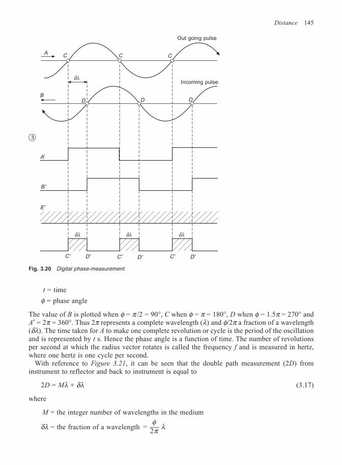
Distance 145
t = time
φ = phase angle
The value of B is plotted when φ = π /2 = 90°, C when φ = π = 180°, D when φ = 1.5π = 270° andA′ = 2π = 360°. Thus 2π represents a complete wavelength (λ) and φ/2π a fraction of a wavelength(δλ). The time taken for A to make one complete revolution or cycle is the period of the oscillationand is represented by t s. Hence the phase angle is a function of time. The number of revolutionsper second at which the radius vector rotates is called the frequency f and is measured in hertz,where one hertz is one cycle per second.
With reference to Figure 3.21, it can be seen that the double path measurement (2D) frominstrument to reflector and back to instrument is equal to
2D = Mλ + δλ (3.17)
where
M = the integer number of wavelengths in the medium
δλ = the fraction of a wavelength =2φπ λ
Out going pulse
CCCA
δλ
B
3
D D D
Incoming pulse
A′
B ′
E ′
δλ δλ δλ
C ′ D ′ C ′ D ′ C ′ D ′
Fig. 3.20 Digital phase-measurement
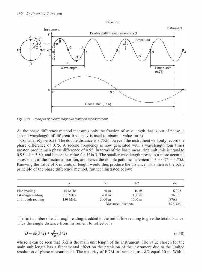
146 Engineering Surveying
As the phase difference method measures only the fraction of wavelength that is out of phase, asecond wavelength of different frequency is used to obtain a value for M.
Consider Figure 3.21. The double distance is 3.75λ; however, the instrument will only record thephase difference of 0.75. A second frequency is now generated with a wavelength four timesgreater, producing a phase difference of 0.95. In terms of the basic measuring unit, this is equal to0.95 × 4 = 3.80, and hence the value for M is 3. The smaller wavelength provides a more accurateassessment of the fractional portion, and hence the double path measurement is 3 + 0.75 = 3.75λ.Knowing the value of λ in units of length would thus produce the distance. This then is the basicprinciple of the phase difference method, further illustrated below:
Instrument
y
P
ωB
AØ
D
A′ A′0
Ø
PB
C A′
Double path measurement = 2D
Reflector
1
A
2
Amplitude
A3 4
Instrument
Phase shift
(0.75)
λWavelength
0B
0.5
Phase shift (0.95)
1
C
D
Fig. 3.21 Principle of electromagnetic distance measurement
f λ λ/2 δλ
Fine reading 15 MHz 20 m 10 m 6.3251st rough reading 1.5 MHz 200 m 100 m 76.332nd rough reading 150 MHz 2000 m 1000 m 876.3
Measured distance 876.325
The first number of each rough reading is added to the initial fine reading to give the total distance.Thus the single distance from instrument to reflector is
D M = ( /2) + ( /2)λφπ λ
2(3.18)
where it can be seen that λ /2 is the main unit length of the instrument. The value chosen for themain unit length has a fundamental effect on the precision of the instrument due to the limitedresolution of phase measurement. The majority of EDM instruments use λ/2 equal 10 m. With a
Distance 147
phase resolution of 3 × 10⁻⁴ errors of 3 mm would result. The Tellurometer MA100 uses λ /2 = 2m, resulting in 0.6 mm error, whilst the Kern Mekometer uses λ /2 = 0.3 m and a resulting error of0.1 mm.
Implicit in the above equation is the assumption that λ is known and constant. However, in mostEDM equipment, this is not so only the frequency f is known and is related to λ as follows:
λ = c/f (3.19)
where
c = the velocity of electromagnetic waves (light) in a medium
This velocity c can only be calculated if the refractive index n of the medium is known, and alsothe velocity of light co in a vacuum:
n = co/c (3.20)
where n is always greater than unity
At the XVIth General Assembly of the International Union for Geodesy and Geophysics in 1975the following value for co was recommended:
co = 299 792 458 ± 1.2 m/s (3.21)
From the standard deviation quoted, it can be seen that this value is accurate to 0.004 mm/km andcan therefore be regarded as error free compared with the most accurate EDM measurement.
The value of n can be computed from basic formulae available. However, Figure 3.14 shows thecarrier wave contained within the modulation envelope. The carrier travels at what is termed thephase velocity, whilst the group of frequencies travel at the slower group velocity. The measurementprocedure is concerned with the modulation and so it is the group refractive index ng with whichwe are concerned.
From equation (3.20) c = co/n and from equation (3.19) λ = co/nf
Replace n with ng and substitute in equation (3.18):
D Mc
n f
c
n f =
( )(2 )
+ 2
( )(2 )
o
g
o
g
φπ (3.22)
Two further considerations are necessary before the final formula can be stated:
(1) The physical centre of the instrument which is plumbed over the survey station does notcoincide with the position within the instrument to which the measurements are made. Thisresults in an instrument constant K1.
(2) Similarly with the reflector. The light wave passing through the atmosphere, whose refractiveindex is approximately unity, enters the glass prism of refractive index about 1.6 and is accordinglyslowed down. This change in velocity combined with the light path through the reflector resultsin a correction to the measured distance called the reflector constant K2.
Both these constants are combined and catered for in the instrument; then
D Mc
n f
c
n fK K =
( )(2 )
+ 2
( )(2 )
+ ( + )o
g
o
g1 2
φπ (3.23)
is the fundamental equation for distances measured with EDM equipment.An examination of the equation shows the errors sources to be:
148 Engineering Surveying
(1) In the measurement of phase φ.(2) In the measurement of group refractive index ng.(3) In the stability of the frequency f.(4) In the instrument/reflector constants K1 and K2.
3.8 METEOROLOGICAL CORRECTIONS
Using EDM equipment, the measurement of distance is obtained by measuring the time of propagationof electromagnetic waves through the atmosphere. Whilst the velocity of these waves in a vacuum(co) is known, its value will be reduced according to the atmospheric conditions through which thewaves travel at the time of measurement. As shown in equation (3.20), the refractive index (n) ofthe prevailing atmosphere is necessary in order to apply a velocity correction to the measureddistance. Thus if D′ is the measured distance, the corrected distance D is obtained from
D = D′/n (3.24)
The value of n is affected by the temperature, pressure and water vapour content of the atmosphereas well as by the wavelength λ of the transmitted electromagnetic waves. It follows from this thatmeasurements of these atmospheric conditions are required at the time of measurement.
As already shown, steel tapes are standardized under certain conditions of temperature andtension. In a similar way, EDM equipment is standardized under certain conditions of temperatureand pressure. For instance, all the Geodimeters (AgaGeotronics) are standardized at 20°C and1013.25 mbar of pressure, whilst Kern equipment is standardized at 12°C and 1013.25 mbar. Underthese respective atmospheric conditions, the measured distances would not require a velocitycorrection. However, measuring with a Geodimeter under typical winter conditions of 0°C and1035 mbar would require a correction of –25 mm/km or –2.5 mm per 100 m. As this error issystematic it would accumulate over a traverse containing many stations. It follows that even onlow-order surveys the measurement of temperature and pressure is important.
The refractive index is related to wavelength via the Cauchy equation:
n AB C = + + 2 4λ λ
(3.25)
where A, B and C are constants relative to specific atmospheric conditions. To afford a correctionin parts per million (ppm) the refractive number or refractivity (N) is used:
N = (n – 1) × 106 (3.26)
If n = 1.000 300, then N = 300.A value for n for standard air (0°C temperature, 1013.25 mbar pressure and dry air with 0.03%
CO2) is given by Barrel and Sears as
( – 1) 10 = 287.604 + 1.6288 + 0.013662 4
n ×
λ λ (3.27)
However, as stated in Section 3.7.2, it is the refractive index of the modulated beam, not the carrier,that is required; hence the use of group refractive index where
N AB C
g 2 4 = + 3 + 5
λ λ(3.28)
Distance 149
and therefore, for group velocity in standard air with λ in µm:
N ng g6
2 4 = ( – 1) 10 = 287.604 + 3 1.6288 + 5 0.0136× × ×
λ λ(3.29)
The above formula is accurate to ± 0.1 ppm at wavelengths between 560 and 900 nm. An alternativeformula derived by B. Edlen is
N ng g6
2 4 = ( – 1) 10 = 287.569 + 3 1.6206 + 5 0.0139× × ×
λ λ(3.30)
It follows that different instruments using different wavelengths will have different values forrefractivity; for example:
λ = 0.910 µm gives Ng = 293.6λ = 0.820 µm gives Ng = 295.0
To accomodate the actual atmospheric conditions under which the distances are measured, equation(3.29) was modified by Barrel and Sears:
′× × ×
NN Q P
TV e
Tgg
=
– (3.31)
where T = absolute temperature in Kelvins (K) = 273.15 + t,t = dry bulb temperature in °C
P = atmospheric pressuree = partial water vapour pressure
with P and e in mbar, Q = 0.2696 and V = 11.27with P and e in mmHg, Q = 0.3594 and V = 15.02
The value for e can be calculated from
e = es – 0.000 662 × P × (t – tw) (3.32)
where t = dry bulb temperaturetw = wet bulb temperaturees = saturation water vapour pressure
The value for es can be calculated from
log = 7.5 + 237.3
+ 0.7857sw
we
t
t(3.33)
Using equation (3.33), the following table can be produced:
tw (°C) 0 10 20 30 40es 6.2 12.3 23.4 42.4 73.7
es is therefore quite significant at high temperatures.Working back through the previous equations it can be shown that at 100% humidity and 30°C
temperature a correction of approximately 2 ppm is necessary for the distance measured. In practice,humidity is generally ignored in the velocity corrections for instruments using light waves as it is
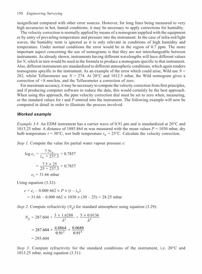
150 Engineering Surveying
insignificant compared with other error sources. However, for long lines being measured to veryhigh accuracies in hot, humid conditions, it may be necessary to apply corrections for humidity.
The velocity correction is normally applied by means of a nomogram supplied with the equipmentor by entry of prevailing temperature and pressure into the instrument. In the case of infra-red/lightwaves, the humidity term is ignored as it is only relevant in conditions of high humidity andtemperature. Under normal conditions the error would be in the region of 0.7 ppm. The moreimportant aspect concerning the use of nomograms is that they are not interchangeable betweeninstruments. As already shown, instruments having different wavelengths will have different valuesfor N, which in turn would be used in the formula to produce a nomogram specific to that instrument.Also, different instruments are standardized to different atmospheric conditions, which again rendersnomograms specific to the instrument. As an example of the error which could arise, Wild use N =282, whilst Tellurometer use N = 274. At 20°C and 1012.5 mbar, the Wild nomogram gives acorrection of +8 mm/km, and the Tellurometer a correction of zero.
For maximum accuracy, it may be necessary to compute the velocity correction from first principles,and if producing computer software to reduce the data, this would certainly be the best approach.When using this approach, the ppm velocity correction dial must be set to zero when, measuring,or the standard values for t and P entered into the instrument. The following example will now becomputed in detail in order to illustrate the process involved.
Worked example
Example 3.8 An EDM instrument has a carrier wave of 0.91 µm and is standardized at 20°C and1013.25 mbar. A distance of 1885.864 m was measured with the mean values P = 1030 mbar, drybulb temperature t = 30°C, wet bulb temperature tw = 25°C. Calculate the velocity correction.
Step 1. Compute the value for partial water vapour pressure e:
log = 7.5 + 237.3
+ 0.7857sw
we
t
t
= 7.5 2525 + 237.3
+ 0.7857×
es = 31.66 mbar
Using equation (3.32):
e = es – 0.000 662 × P × (t – tw)
= 31.66 – 0.000 662 × 1030 × (30 – 25) = 28.25 mbar
Step 2. Compute refractivity (Ng) for standard atmosphere using equation (3.29):
Ng 2 4 = 287.604 + 3 1.6288 + 5 0.0136× ×
λ λ
= 287.604 + 4.88640.91
+ 0.06800.912 4
= 293.604
Step 3. Compute refractivity for the standard conditions of the instrument, i.e. 20°C and1013.25 mbar, using equation (3.31):
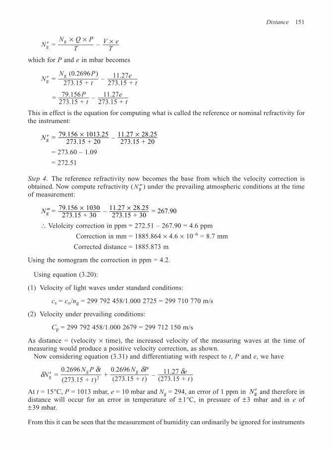
Distance 151
′× × ×
NN Q P
TV e
Tgg
=
–
which for P and e in mbar becomes
′NN P
te
tgg
= (0.2696 )
273.15 + – 11.27
273.15 +
= 79.156273.15 +
– 11.27273.15 +
Pt
et
This in effect is the equation for computing what is called the reference or nominal refractivity forthe instrument:
′ × ×Ng = 79.156 1013.25
273.15 + 20 – 11.27 28.25
273.15 + 20
= 273.60 – 1.09
= 272.51
Step 4. The reference refractivity now becomes the base from which the velocity correction isobtained. Now compute refractivity ( ′′Ng ) under the prevailing atmospheric conditions at the timeof measurement:
′′ × ×Ng = 79.156 1030
273.15 + 30 – 11.27 28.25
273.15 + 30 = 267.90
∴ Velolcity correction in ppm = 272.51 – 267.90 = 4.6 ppm
Correction in mm = 1885.864 × 4.6 × 10–6 = 8.7 mm
Corrected distance = 1885.873 m
Using the nomogram the correction in ppm = 4.2.
Using equation (3.20):
(1) Velocity of light waves under standard conditions:
cs = co/ng = 299 792 458/1.000 2725 = 299 710 770 m/s
(2) Velocity under prevailing conditions:
Cp = 299 792 458/1.000 2679 = 299 712 150 m/s
As distance = (velocity × time), the increased velocity of the measuring waves at the time ofmeasuring would produce a positive velocity correction, as shown.
Now considering equation (3.31) and differentiating with respect to t, P and e, we have
δδ δ δ′N
N P t
t
N P
te
tgg
2
g =
0.2696
(273.15 + ) +
0.2696
(273.15 + ) – 11.27
(273.15 + )
At t = 15°C, P = 1013 mbar, e = 10 mbar and Ng = 294, an error of 1 ppm in ′Ng and therefore indistance will occur for an error in temperature of ±1°C, in pressure of ±3 mbar and in e of±39 mbar.
From this it can be seen that the measurement of humidity can ordinarily be ignored for instruments
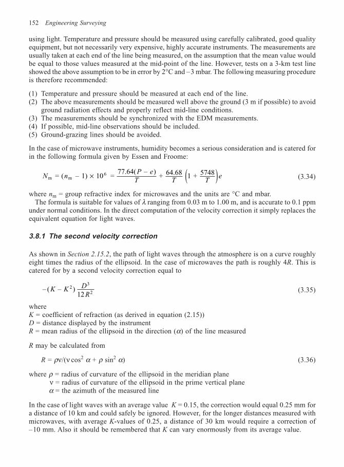
152 Engineering Surveying
using light. Temperature and pressure should be measured using carefully calibrated, good qualityequipment, but not necessarily very expensive, highly accurate instruments. The measurements areusually taken at each end of the line being measured, on the assumption that the mean value wouldbe equal to those values measured at the mid-point of the line. However, tests on a 3-km test lineshowed the above assumption to be in error by 2°C and –3 mbar. The following measuring procedureis therefore recommended:
(1) Temperature and pressure should be measured at each end of the line.(2) The above measurements should be measured well above the ground (3 m if possible) to avoid
ground radiation effects and properly reflect mid-line conditions.(3) The measurements should be synchronized with the EDM measurements.(4) If possible, mid-line observations should be included.(5) Ground-grazing lines should be avoided.
In the case of microwave instruments, humidity becomes a serious consideration and is catered forin the following formula given by Essen and Froome:
N nP e
T T Tem m
6 = ( – 1) 10 = 77.64( – )
+ 64.68 1 + 5748× ( ) (3.34)
where nm = group refractive index for microwaves and the units are °C and mbar.The formula is suitable for values of λ ranging from 0.03 m to 1.00 m, and is accurate to 0.1 ppm
under normal conditions. In the direct computation of the velocity correction it simply replaces theequivalent equation for light waves.
3.8.1 The second velocity correction
As shown in Section 2.15.2, the path of light waves through the atmosphere is on a curve roughlyeight times the radius of the ellipsoid. In the case of microwaves the path is roughly 4R. This iscatered for by a second velocity correction equal to
– ( – ) 12
23
2K K
D
R(3.35)
whereK = coefficient of refraction (as derived in equation (2.15))D = distance displayed by the instrumentR = mean radius of the ellipsoid in the direction (α) of the line measured
R may be calculated from
R = ρν/(ν cos2 α + ρ sin2 α) (3.36)
where ρ = radius of curvature of the ellipsoid in the meridian planeν = radius of curvature of the ellipsoid in the prime vertical planeα = the azimuth of the measured line
In the case of light waves with an average value K = 0.15, the correction would equal 0.25 mm fora distance of 10 km and could safely be ignored. However, for the longer distances measured withmicrowaves, with average K-values of 0.25, a distance of 30 km would require a correction of–10 mm. Also it should be remembered that K can vary enormously from its average value.
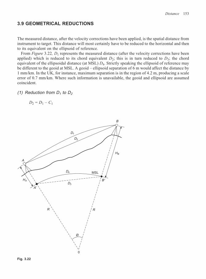
Distance 153
3.9 GEOMETRICAL REDUCTIONS
The measured distance, after the velocity corrections have been applied, is the spatial distance frominstrument to target. This distance will most certainly have to be reduced to the horizontal and thento its equivalent on the ellipsoid of reference.
From Figure 3.22, D1 represents the measured distance (after the velocity corrections have beenapplied) which is reduced to its chord equivalent D2; this is in turn reduced to D3; the chordequivalent of the ellipsoidal distance (at MSL) D4. Strictly speaking the ellipsoid of reference maybe different to the geoid at MSL. A geoid – ellipsoid separation of 6 m would affect the distance by1 mm/km. In the UK, for instance, maximum separation is in the region of 4.2 m, producing a scaleerror of 0.7 mm/km. Where such information is unavailable, the geoid and ellipsoid are assumedcoincident.
(1) Reduction from D1 to D2
D2 = D1 – C1
Fig. 3.22
B
HB
B′
R
Ø
0
R
D3
D4
D1
D2
A
MSL
HA
A′
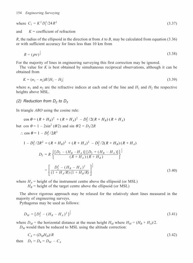
154 Engineering Surveying
where C K D R12
13 2 = /24 (3.37)
and K = coefficient of refraction
R, the radius of the ellipsoid in the direction α from A to B, may be calculated from equation (3.36)or with sufficient accuracy for lines less than 10 km from
R = ( )12ρν (3.38)
For the majority of lines in engineering surveying this first correction may be ignored.The value for K is best obtained by simultaneous reciprocal observations, although it can be
obtained from
K = (n1 – n2)R/|H1 – H2| (3.39)
where n1 and n2 are the refractive indices at each end of the line and H1 and H2 the respectiveheights above MSL.
(2) Reduction from D2 to D3
In triangle ABO using the cosine rule:
cos = ( + ) + ( + ) – /2( + ) ( + )2 222θ R H R H D R H R HB A B A
but cos θ = 1 – 2sin2 (θ/2) and sin θ/2 = D3/2R
∴ cos = 1 – /232 2θ D R
1 – /2 = ( + ) + ( + ) – /2( + ) ( + )32 2 2 2
22D R R H R H D R H R HB A B A
D RD H H D H H
R H R HB A B A
A B3
2 2 = [ – ( – )] [ + ( – )]
( + ) ( + )
12
= – ( – )
(1 + / ) (1 + /22 2
12D H H
H R H R)B A
A B
(3.40)
where HA = height of the instrument centre above the ellipsoid (or MSL)HB = height of the target centre above the ellipsoid (or MSL)
The above rigorous approach may be relaxed for the relatively short lines measured in themajority of engineering surveys.
Pythagorus may be used as follows:
D D H HM B A = [ – ( – ) ]22 2
12 (3.41)
where DM = the horizontal distance at the mean height HM where HM = (HB + HA)/2.DM would then be reduced to MSL using the altitude correction:
CA = (DMHM)/R (3.42)
then D3 = D4 = DM – CA
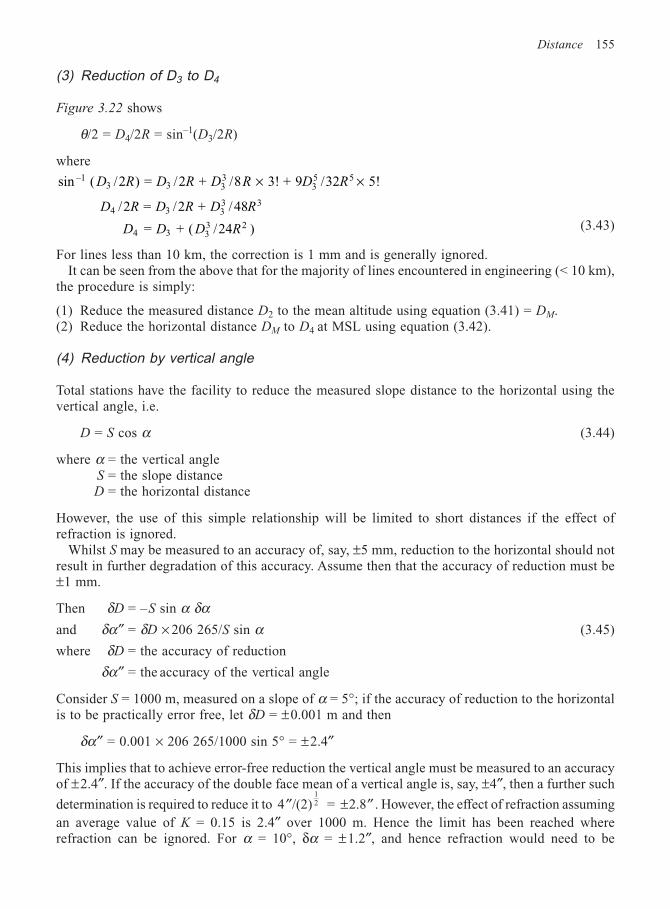
Distance 155
(3) Reduction of D3 to D4
Figure 3.22 shows
θ/2 = D4/2R = sin–1(D3/2R)
where
sin ( /2 ) = /2 + /8 3! + 9 /32 5!–13 3 3 3
5 5D R D R D R D R3 × ×
D R D R D R4 3 33 3/2 = /2 + /48
D D D R4 3 33 2 = + ( /24 ) (3.43)
For lines less than 10 km, the correction is 1 mm and is generally ignored.It can be seen from the above that for the majority of lines encountered in engineering (< 10 km),
the procedure is simply:
(1) Reduce the measured distance D2 to the mean altitude using equation (3.41) = DM.(2) Reduce the horizontal distance DM to D4 at MSL using equation (3.42).
(4) Reduction by vertical angle
Total stations have the facility to reduce the measured slope distance to the horizontal using thevertical angle, i.e.
D = S cos α (3.44)
where α = the vertical angleS = the slope distanceD = the horizontal distance
However, the use of this simple relationship will be limited to short distances if the effect ofrefraction is ignored.
Whilst S may be measured to an accuracy of, say, ±5 mm, reduction to the horizontal should notresult in further degradation of this accuracy. Assume then that the accuracy of reduction must be±1 mm.
Then δD = –S sin α δαand δα″ = δD × 206 265/S sin α (3.45)
where δD = the accuracy of reduction
δα″ = the accuracy of the vertical angle
Consider S = 1000 m, measured on a slope of α = 5°; if the accuracy of reduction to the horizontalis to be practically error free, let δD = ±0.001 m and then
δα″ = 0.001 × 206 265/1000 sin 5° = ±2.4″
This implies that to achieve error-free reduction the vertical angle must be measured to an accuracyof ±2.4″. If the accuracy of the double face mean of a vertical angle is, say, ±4″, then a further such
determination is required to reduce it to ′′ ± ′′4 /(2) = 2.812 . However, the effect of refraction assuming
an average value of K = 0.15 is 2.4″ over 1000 m. Hence the limit has been reached whererefraction can be ignored. For α = 10°, δα = ±1.2″, and hence refraction would need to be
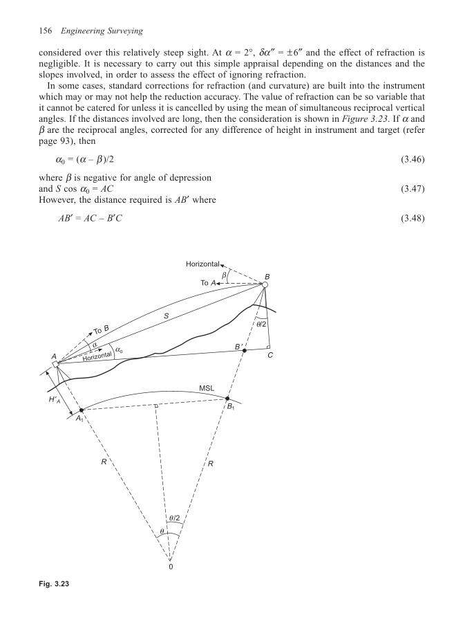
156 Engineering Surveying
considered over this relatively steep sight. At α = 2°, δα″ = ±6″ and the effect of refraction isnegligible. It is necessary to carry out this simple appraisal depending on the distances and theslopes involved, in order to assess the effect of ignoring refraction.
In some cases, standard corrections for refraction (and curvature) are built into the instrumentwhich may or may not help the reduction accuracy. The value of refraction can be so variable thatit cannot be catered for unless it is cancelled by using the mean of simultaneous reciprocal verticalangles. If the distances involved are long, then the consideration is shown in Figure 3.23. If α andβ are the reciprocal angles, corrected for any difference of height in instrument and target (referpage 93), then
α0 = (α – β )/2 (3.46)
where β is negative for angle of depressionand S cos α0 = AC (3.47)However, the distance required is AB′ where
AB′ = AC – B′C (3.48)
Fig. 3.23
BβTo A
Horizontal
θ/2
CB ′
S
To B
α αo
HorizontalA
H ′A
MSL
B1
RR
A1
θ /2
θ
0
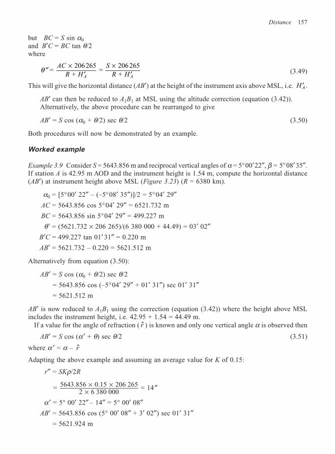
Distance 157
but BC = S sin α0
and B′C = BC tan θ/2where
′′×
′×
′θ =
206 265
+ =
206 265
+
AC
R H
S
R HA A(3.49)
This will give the horizontal distance (AB′) at the height of the instrument axis above MSL, i.e. ′H A .
AB′ can then be reduced to A1B1 at MSL using the altitude correction (equation (3.42)).Alternatively, the above procedure can be rearranged to give
AB′ = S cos (α0 + θ/2) sec θ/2 (3.50)
Both procedures will now be demonstrated by an example.
Worked example
Example 3.9 Consider S = 5643.856 m and reciprocal vertical angles of α = 5°00′22″, β = 5°08′ 35″.If station A is 42.95 m AOD and the instrument height is 1.54 m, compute the horizontal distance(AB′) at instrument height above MSL (Figure 3.23) (R = 6380 km).
α0 = [5°00′ 22″ – (–5°08′ 35″)]/2 = 5°04′ 29″AC = 5643.856 cos 5°04′ 29″ = 6521.732 m
BC = 5643.856 sin 5°04′ 29″ = 499.227 m
θ′ = (5621.732 × 206 265)/(6 380 000 + 44.49) = 03′ 02″B′C = 499.227 tan 01′ 31″ = 0.220 m
AB′ = 5621.732 – 0.220 = 5621.512 m
Alternatively from equation (3.50):
AB′ = S cos (α0 + θ/2) sec θ/2
= 5643.856 cos (–5°04′ 29″ + 01′ 31″) sec 01′ 31″= 5621.512 m
AB′ is now reduced to A1B1 using the correction (equation (3.42)) where the height above MSLincludes the instrument height, i.e. 42.95 + 1.54 = 44.49 m.
If a value for the angle of refraction ( r ) is known and only one vertical angle α is observed then
AB′ = S cos (α ′ + θ) sec θ/2 (3.51)
where α ′ = α – r
Adapting the above example and assuming an average value for K of 0.15:
r″ = SKρ/2R
= 5643.856 0.15 206 2652 6 380 000
= 14× ×× ′′
α ′ = 5° 00′ 22″ – 14″ = 5° 00′ 08″AB′ = 5643.856 cos (5° 00′ 08″ + 3′ 02″) sec 01′ 31″
= 5621.924 m
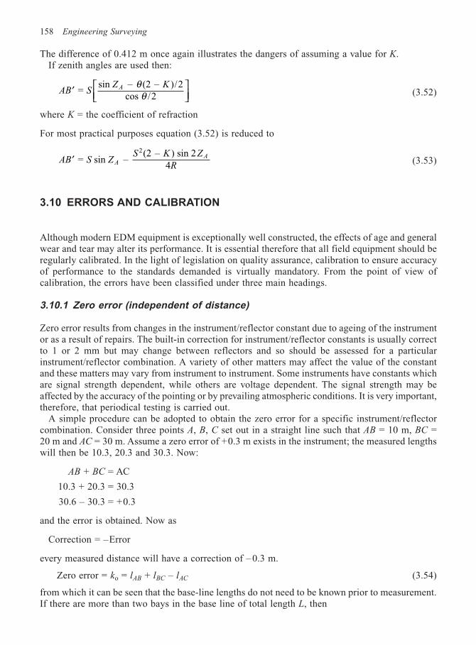
158 Engineering Surveying
The difference of 0.412 m once again illustrates the dangers of assuming a value for K.If zenith angles are used then:
AB SZ KA′
= sin – (2 – )/2
cos /2θθ (3.52)
where K = the coefficient of refraction
For most practical purposes equation (3.52) is reduced to
AB S ZS K Z
RAA′ = sin –
(2 – ) sin 24
2
(3.53)
3.10 ERRORS AND CALIBRATION
Although modern EDM equipment is exceptionally well constructed, the effects of age and generalwear and tear may alter its performance. It is essential therefore that all field equipment should beregularly calibrated. In the light of legislation on quality assurance, calibration to ensure accuracyof performance to the standards demanded is virtually mandatory. From the point of view ofcalibration, the errors have been classified under three main headings.
3.10.1 Zero error (independent of distance)
Zero error results from changes in the instrument/reflector constant due to ageing of the instrumentor as a result of repairs. The built-in correction for instrument/reflector constants is usually correctto 1 or 2 mm but may change between reflectors and so should be assessed for a particularinstrument/reflector combination. A variety of other matters may affect the value of the constantand these matters may vary from instrument to instrument. Some instruments have constants whichare signal strength dependent, while others are voltage dependent. The signal strength may beaffected by the accuracy of the pointing or by prevailing atmospheric conditions. It is very important,therefore, that periodical testing is carried out.
A simple procedure can be adopted to obtain the zero error for a specific instrument/reflectorcombination. Consider three points A, B, C set out in a straight line such that AB = 10 m, BC =20 m and AC = 30 m. Assume a zero error of +0.3 m exists in the instrument; the measured lengthswill then be 10.3, 20.3 and 30.3. Now:
AB + BC = AC
10.3 + 20.3 = 30.3
30.6 – 30.3 = +0.3
and the error is obtained. Now as
Correction = –Error
every measured distance will have a correction of – 0.3 m.
Zero error = ko = lAB + lBC – lAC (3.54)
from which it can be seen that the base-line lengths do not need to be known prior to measurement.If there are more than two bays in the base line of total length L, then
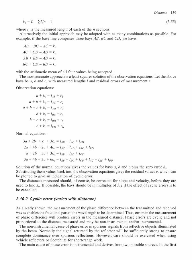
Distance 159
ko = L – ∑li/n – 1 (3.55)
where li is the measured length of each of the n sections.Alternatively the initial approach may be adopted with as many combinations as possible. For
example, if the base line comprises three bays AB, BC and CD, we have
AB + BC – AC = ko
AC + CD – AD = ko
AB + BD – AD = ko
BC + CD – BD = ko
with the arithmetic mean of all four values being accepted.The most accurate approach is a least squares solution of the observation equations. Let the above
bays be a, b and c, with measured lengths l and residual errors of measurement r.
Observation equations:
a + ko = lAB + r1
a + b + ko = lAC + r2
a + b + c + ko = lAD + r3
b + ko = lBC + r4
b + c + ko = lBD + r5
c + ko = lCD + r6
Normal equations:
3a + 2b + c + 3ko = lAB + lAC + lAD
2a + 4b + 2c + 4ko = lAC + lAD + lBC + lBD
a + 2b + 3c + 3ko = lAB + lBD + lCD
3a + 4b + 3c + 6ko = lAB + lBC + lCD + lAC + lAD + lBD
Solution of the normal equations gives the values for bays a, b and c plus the zero error ko.Substituting these values back into the observation equations gives the residual values r, which canbe plotted to give an indication of cyclic error.
The distances measured should, of course, be corrected for slope and velocity, before they areused to find ko. If possible, the bays should be in multiples of λ/2 if the effect of cyclic errors is tobe cancelled.
3.10.2 Cyclic error (varies with distance)
As already shown, the measurement of the phase difference between the transmitted and receivedwaves enables the fractional part of the wavelength to be determined. Thus, errors in the measurementof phase difference will produce errors in the measured distance. Phase errors are cyclic and notproportional to the distance measured and may be non-instrumental and/or instrumental.
The non-instrumental cause of phase error is spurious signals from reflective objects illuminatedby the beam. Normally the signal returned by the reflector will be sufficiently strong to ensurecomplete dominance over spurious reflections. However, care should be exercised when usingvehicle reflectors or Scotchlite for short-range work.
The main cause of phase error is instrumental and derives from two possible sources. In the first
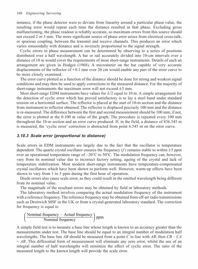
160 Engineering Surveying
instance, if the phase detector were to deviate from linearity around a particular phase value, theresulting error would repeat each time the distance resulted in that phase. Excluding grossmalfunctioning, the phase readout is reliably accurate, so maximum errors from this source shouldnot exceed 2 or 3 mm. The more significant source of phase error arises from electrical cross-talk,or spurious coupling, between the transmit and receive channels. This produces an error whichvaries sinusoidally with distance and is inversely proportional to the signal strength.
Cyclic errors in phase measurement can be determined by observing to a series of positionsdistributed over a half wavelength. A bar or rail accurately divided into 10-cm intervals over adistance of 10 m would cover the requirements of most short-range instruments. Details of such anarrangement are given in Hodges (1968). A micrometer on the bar capable of very accuratedisplacements of the reflector of +0.1 mm over 20 cm would enable any part of the error curve tobe more closely examined.
The error curve plotted as a function of the distance should be done for strong and weakest signalconditions and may then be used to apply corrections to the measured distance. For the majority ofshort-range instruments the maximum error will not exceed ±5 mm.
Most short-range EDM instruments have values for λ /2 equal to 10 m. A simple arrangement forthe detection of cyclic error which has proved satisfactory is to lay a steel band under standardtension on a horizontal surface. The reflector is placed at the start of 10-m section and the distancefrom instrument to reflector obtained. The reflector is displaced precisely 100 mm and the distanceis re-measured. The difference between the first and second measurement should be 100 mm; if not,the error is plotted at the 0.100 m value of the graph. The procedure is repeated every 100 mmthroughout the 10-m section and an error curve produced. If, in the field, a distance of 836.545 mis measured, the ‘cyclic error’ correction is abstracted from point 6.545 m on the error curve.
3.10.3 Scale error (proportional to distance)
Scale errors in EDM instruments are largely due to the fact that the oscillator is temperaturedependent. The quartz crystal oscillator ensures the frequency (f ) remains stable to within ±5 ppmover an operational temperature range of –20°C to 50°C. The modulation frequency can, however,vary from its nominal value due to incorrect factory setting, ageing of the crystal and lack oftemperature stabilization. Most modern short-range instruments have temperature-compensatedcrystal oscillators which have been shown to perform well. However, warm-up effects have beenshown to vary from 1 to 5 ppm during the first hour of operation.
Diode errors also cause scale error, as they could result in the emitted wavelength being differentfrom its nominal value.
The magnitude of the resultant errors may be obtained by field or laboratory methods.The laboratory method involves comparing the actual modulation frequency of the instrument
with a reference frequency. The reference frequency may be obtained from off-air radio transmissionssuch as Droitwich MSF in the UK or from a crystal-generated laboratory standard. The correctionfor frequency is equal to
Nominal frequency – Actual frequencyNominal frequency
ppm
A simple field test is to measure a base line whose length is known to an accuracy greater than themeasurements under test. The base line should be equal to an integral number of modulation halfwavelengths. The base line AB should be measured from a point C in line with AB; then CB – CA
= AB. This differential form of measurement will eliminate any zero error, whilst the use of anintegral number of half wavelengths will minimize the effect of cyclic error. The ratio of themeasured length to the known length will provide the scale error.
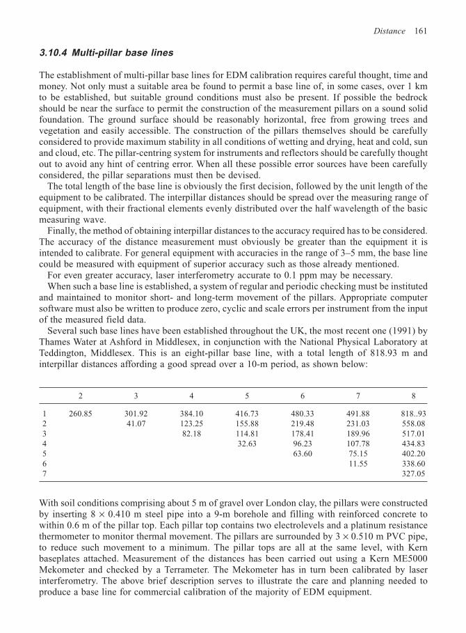
Distance 161
3.10.4 Multi-pillar base lines
The establishment of multi-pillar base lines for EDM calibration requires careful thought, time andmoney. Not only must a suitable area be found to permit a base line of, in some cases, over 1 kmto be established, but suitable ground conditions must also be present. If possible the bedrockshould be near the surface to permit the construction of the measurement pillars on a sound solidfoundation. The ground surface should be reasonably horizontal, free from growing trees andvegetation and easily accessible. The construction of the pillars themselves should be carefullyconsidered to provide maximum stability in all conditions of wetting and drying, heat and cold, sunand cloud, etc. The pillar-centring system for instruments and reflectors should be carefully thoughtout to avoid any hint of centring error. When all these possible error sources have been carefullyconsidered, the pillar separations must then be devised.
The total length of the base line is obviously the first decision, followed by the unit length of theequipment to be calibrated. The interpillar distances should be spread over the measuring range ofequipment, with their fractional elements evenly distributed over the half wavelength of the basicmeasuring wave.
Finally, the method of obtaining interpillar distances to the accuracy required has to be considered.The accuracy of the distance measurement must obviously be greater than the equipment it isintended to calibrate. For general equipment with accuracies in the range of 3–5 mm, the base linecould be measured with equipment of superior accuracy such as those already mentioned.
For even greater accuracy, laser interferometry accurate to 0.1 ppm may be necessary.When such a base line is established, a system of regular and periodic checking must be instituted
and maintained to monitor short- and long-term movement of the pillars. Appropriate computersoftware must also be written to produce zero, cyclic and scale errors per instrument from the inputof the measured field data.
Several such base lines have been established throughout the UK, the most recent one (1991) byThames Water at Ashford in Middlesex, in conjunction with the National Physical Laboratory atTeddington, Middlesex. This is an eight-pillar base line, with a total length of 818.93 m andinterpillar distances affording a good spread over a 10-m period, as shown below:
2 3 4 5 6 7 8
1 260.85 301.92 384.10 416.73 480.33 491.88 818..932 41.07 123.25 155.88 219.48 231.03 558.083 82.18 114.81 178.41 189.96 517.014 32.63 96.23 107.78 434.835 63.60 75.15 402.206 11.55 338.607 327.05
With soil conditions comprising about 5 m of gravel over London clay, the pillars were constructedby inserting 8 × 0.410 m steel pipe into a 9-m borehole and filling with reinforced concrete towithin 0.6 m of the pillar top. Each pillar top contains two electrolevels and a platinum resistancethermometer to monitor thermal movement. The pillars are surrounded by 3 × 0.510 m PVC pipe,to reduce such movement to a minimum. The pillar tops are all at the same level, with Kernbaseplates attached. Measurement of the distances has been carried out using a Kern ME5000Mekometer and checked by a Terrameter. The Mekometer has in turn been calibrated by laserinterferometry. The above brief description serves to illustrate the care and planning needed toproduce a base line for commercial calibration of the majority of EDM equipment.
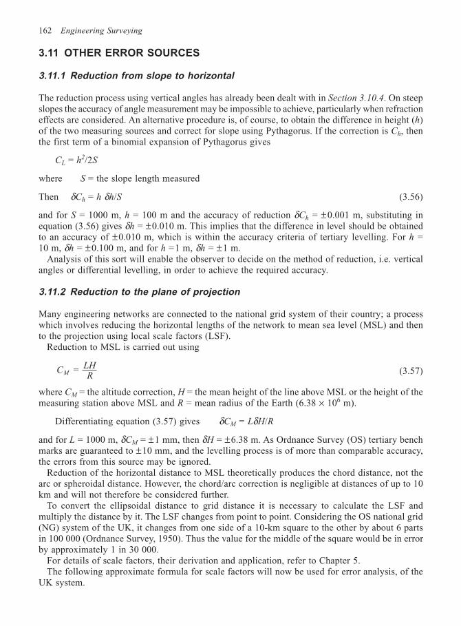
162 Engineering Surveying
3.11 OTHER ERROR SOURCES
3.11.1 Reduction from slope to horizontal
The reduction process using vertical angles has already been dealt with in Section 3.10.4. On steepslopes the accuracy of angle measurement may be impossible to achieve, particularly when refractioneffects are considered. An alternative procedure is, of course, to obtain the difference in height (h)of the two measuring sources and correct for slope using Pythagorus. If the correction is Ch, thenthe first term of a binomial expansion of Pythagorus gives
CL = h2/2S
where S = the slope length measured
Then δCh = h δh/S (3.56)
and for S = 1000 m, h = 100 m and the accuracy of reduction δCh = ±0.001 m, substituting inequation (3.56) gives δh = ±0.010 m. This implies that the difference in level should be obtainedto an accuracy of ±0.010 m, which is within the accuracy criteria of tertiary levelling. For h =10 m, δh = ±0.100 m, and for h =1 m, δh = ±1 m.
Analysis of this sort will enable the observer to decide on the method of reduction, i.e. verticalangles or differential levelling, in order to achieve the required accuracy.
3.11.2 Reduction to the plane of projection
Many engineering networks are connected to the national grid system of their country; a processwhich involves reducing the horizontal lengths of the network to mean sea level (MSL) and thento the projection using local scale factors (LSF).
Reduction to MSL is carried out using
CLHRM = (3.57)
where CM = the altitude correction, H = the mean height of the line above MSL or the height of themeasuring station above MSL and R = mean radius of the Earth (6.38 × 10⁶ m).
Differentiating equation (3.57) gives δCM = LδH/R
and for L = 1000 m, δCM = ±1 mm, then δH = ±6.38 m. As Ordnance Survey (OS) tertiary benchmarks are guaranteed to ±10 mm, and the levelling process is of more than comparable accuracy,the errors from this source may be ignored.
Reduction of the horizontal distance to MSL theoretically produces the chord distance, not thearc or spheroidal distance. However, the chord/arc correction is negligible at distances of up to 10km and will not therefore be considered further.
To convert the ellipsoidal distance to grid distance it is necessary to calculate the LSF andmultiply the distance by it. The LSF changes from point to point. Considering the OS national grid(NG) system of the UK, it changes from one side of a 10-km square to the other by about 6 partsin 100 000 (Ordnance Survey, 1950). Thus the value for the middle of the square would be in errorby approximately 1 in 30 000.
For details of scale factors, their derivation and application, refer to Chapter 5.The following approximate formula for scale factors will now be used for error analysis, of the
UK system.
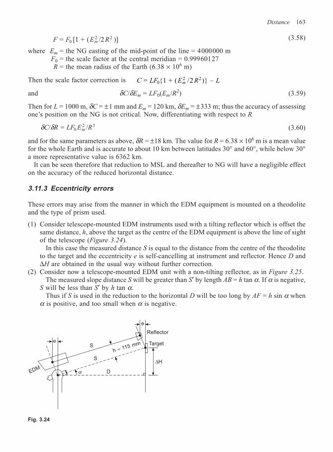
Distance 163
F F E Rm = [1 + ( /2 )]02 2 (3.58)
where Em = the NG easting of the mid-point of the line = 4000000 mF0 = the scale factor at the central meridian = 0.99960127R = the mean radius of the Earth (6.38 × 10⁶ m)
Then the scale factor correction is C LF E R Lm = 1 + ( /2 ) – 02 2
and δC/δEm = LF0(Em/R2) (3.59)
Then for L = 1000 m, δC = ±1 mm and Em = 120 km, δEm = ±333 m; thus the accuracy of assessingone’s position on the NG is not critical. Now, differentiating with respect to R
δ δC R LF E Rm/ = /02 3 (3.60)
and for the same parameters as above, δR = ±18 km. The value for R = 6.38 × 10⁶ m is a mean valuefor the whole Earth and is accurate to about 10 km between latitudes 30° and 60°, while below 30°a more representative value is 6362 km.
It can be seen therefore that reduction to MSL and thereafter to NG will have a negligible effecton the accuracy of the reduced horizontal distance.
3.11.3 Eccentricity errors
These errors may arise from the manner in which the EDM equipment is mounted on a theodoliteand the type of prism used.
(1) Consider telescope-mounted EDM instruments used with a tilting reflector which is offset thesame distance, h, above the target as the centre of the EDM equipment is above the line of sightof the telescope (Figure 3.24).
In this case the measured distance S is equal to the distance from the centre of the theodoliteto the target and the eccentricity e is self-cancelling at instrument and reflector. Hence D and∆H are obtained in the usual way without further correction.
(2) Consider now a telescope-mounted EDM unit with a non-tilting reflector, as in Figure 3.25.The measured slope distance S will be greater than S′ by length AB = h tan α. If α is negative,
S will be less than S′ by h tan α.Thus if S is used in the reduction to the horizontal D will be too long by AF = h sin α when
α is positive, and too small when α is negative.
Fig. 3.24
e
EDM α D
∆H
Target
Reflector
e
h ≈ 115 mm
S
S
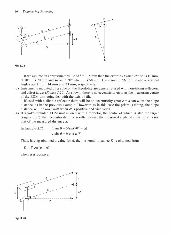
164 Engineering Surveying
If we assume an approximate value of h = 115 mm then the error in D when α = 5° is 10 mm,at 10° it is 20 mm and so on to 30° when it is 58 mm. The errors in ∆H for the above verticalangles are 1 mm, 14 mm and 33 mm, respectively.
(3) Instruments mounted on a yoke on the theodolite are generally used with non-tilting reflectorsand offset target (Figure 3.26). As shown, there is no eccentricity error as the measuring centreof the EDM unit coincides with the axis of tilt.
If used with a tiltable reflector there will be an eccentricity error e = h tan α on the slopedistance, as in the previous example. However, as in this case the prism is tilting, the slopedistance will be too small when α is positive and vice versa.
(4) If a yoke-mounted EDM unit is used with a reflector, the centre of which is also the target(Figure 3.27), then eccentricity error results because the measured angle of elevation α is notthat of the measured distance S.
In triangle ABC h/sin θ = S/sin(90° – α)
∴ sin θ = h cos α /S
Thus, having obtained a value for θ, the horizontal distance D is obtained from
D = S cos(α – θ)
when α is positive.
∆HS′
S
h
αD
e
BA
C
B
FAe
h
α
C
Fig 3.25
Fig. 3.26
h
α
S
S
D
∆H
h
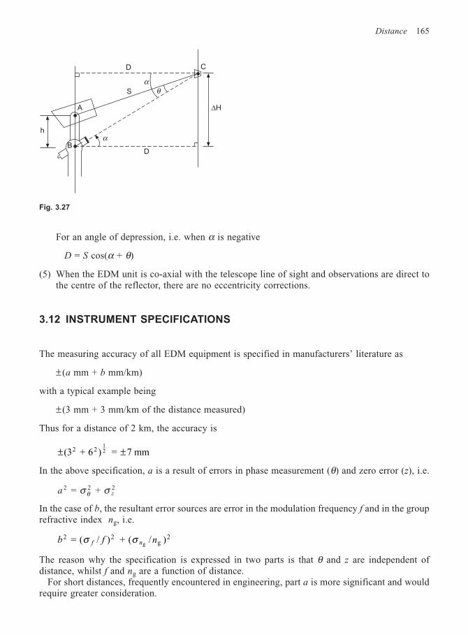
Distance 165
For an angle of depression, i.e. when α is negative
D = S cos(α + θ)
(5) When the EDM unit is co-axial with the telescope line of sight and observations are direct tothe centre of the reflector, there are no eccentricity corrections.
3.12 INSTRUMENT SPECIFICATIONS
The measuring accuracy of all EDM equipment is specified in manufacturers’ literature as
± (a mm + b mm/km)
with a typical example being
± (3 mm + 3 mm/km of the distance measured)
Thus for a distance of 2 km, the accuracy is
± ±(3 + 6 ) = 7 mm2 212
In the above specification, a is a result of errors in phase measurement (θ) and zero error (z), i.e.
a z2 2 = + σ σθ
2
In the case of b, the resultant error sources are error in the modulation frequency f and in the grouprefractive index ng, i.e.
b f nf n2 2
g2 = ( / ) + ( / )
gσ σ
The reason why the specification is expressed in two parts is that θ and z are independent ofdistance, whilst f and ng are a function of distance.
For short distances, frequently encountered in engineering, part a is more significant and wouldrequire greater consideration.
α
∆H
αθ
D C
D
S
A
B
h
Fig. 3.27
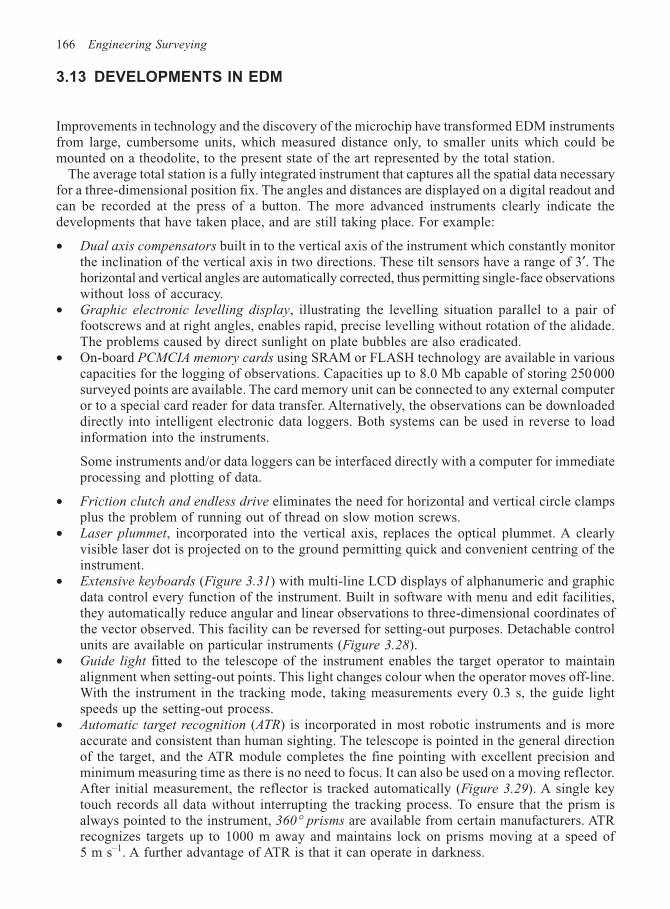
166 Engineering Surveying
3.13 DEVELOPMENTS IN EDM
Improvements in technology and the discovery of the microchip have transformed EDM instrumentsfrom large, cumbersome units, which measured distance only, to smaller units which could bemounted on a theodolite, to the present state of the art represented by the total station.
The average total station is a fully integrated instrument that captures all the spatial data necessaryfor a three-dimensional position fix. The angles and distances are displayed on a digital readout andcan be recorded at the press of a button. The more advanced instruments clearly indicate thedevelopments that have taken place, and are still taking place. For example:
• Dual axis compensators built in to the vertical axis of the instrument which constantly monitorthe inclination of the vertical axis in two directions. These tilt sensors have a range of 3′. Thehorizontal and vertical angles are automatically corrected, thus permitting single-face observationswithout loss of accuracy.
• Graphic electronic levelling display, illustrating the levelling situation parallel to a pair offootscrews and at right angles, enables rapid, precise levelling without rotation of the alidade.The problems caused by direct sunlight on plate bubbles are also eradicated.
• On-board PCMCIA memory cards using SRAM or FLASH technology are available in variouscapacities for the logging of observations. Capacities up to 8.0 Mb capable of storing 250 000surveyed points are available. The card memory unit can be connected to any external computeror to a special card reader for data transfer. Alternatively, the observations can be downloadeddirectly into intelligent electronic data loggers. Both systems can be used in reverse to loadinformation into the instruments.
Some instruments and/or data loggers can be interfaced directly with a computer for immediateprocessing and plotting of data.
• Friction clutch and endless drive eliminates the need for horizontal and vertical circle clampsplus the problem of running out of thread on slow motion screws.
• Laser plummet, incorporated into the vertical axis, replaces the optical plummet. A clearlyvisible laser dot is projected on to the ground permitting quick and convenient centring of theinstrument.
• Extensive keyboards (Figure 3.31) with multi-line LCD displays of alphanumeric and graphicdata control every function of the instrument. Built in software with menu and edit facilities,they automatically reduce angular and linear observations to three-dimensional coordinates ofthe vector observed. This facility can be reversed for setting-out purposes. Detachable controlunits are available on particular instruments (Figure 3.28).
• Guide light fitted to the telescope of the instrument enables the target operator to maintainalignment when setting-out points. This light changes colour when the operator moves off-line.With the instrument in the tracking mode, taking measurements every 0.3 s, the guide lightspeeds up the setting-out process.
• Automatic target recognition (ATR) is incorporated in most robotic instruments and is moreaccurate and consistent than human sighting. The telescope is pointed in the general directionof the target, and the ATR module completes the fine pointing with excellent precision andminimum measuring time as there is no need to focus. It can also be used on a moving reflector.After initial measurement, the reflector is tracked automatically (Figure 3.29). A single keytouch records all data without interrupting the tracking process. To ensure that the prism isalways pointed to the instrument, 360° prisms are available from certain manufacturers. ATRrecognizes targets up to 1000 m away and maintains lock on prisms moving at a speed of5 m s–1. A further advantage of ATR is that it can operate in darkness.
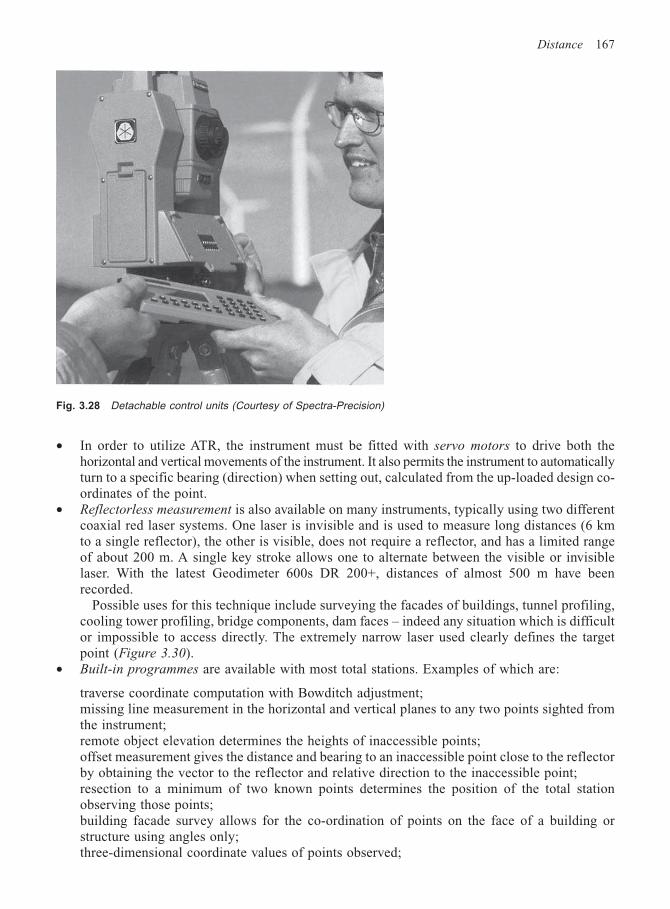
Distance 167
• In order to utilize ATR, the instrument must be fitted with servo motors to drive both thehorizontal and vertical movements of the instrument. It also permits the instrument to automaticallyturn to a specific bearing (direction) when setting out, calculated from the up-loaded design co-ordinates of the point.
• Reflectorless measurement is also available on many instruments, typically using two differentcoaxial red laser systems. One laser is invisible and is used to measure long distances (6 kmto a single reflector), the other is visible, does not require a reflector, and has a limited rangeof about 200 m. A single key stroke allows one to alternate between the visible or invisiblelaser. With the latest Geodimeter 600s DR 200+, distances of almost 500 m have beenrecorded.
Possible uses for this technique include surveying the facades of buildings, tunnel profiling,cooling tower profiling, bridge components, dam faces – indeed any situation which is difficultor impossible to access directly. The extremely narrow laser used clearly defines the targetpoint (Figure 3.30).
• Built-in programmes are available with most total stations. Examples of which are:
traverse coordinate computation with Bowditch adjustment;missing line measurement in the horizontal and vertical planes to any two points sighted fromthe instrument;remote object elevation determines the heights of inaccessible points;offset measurement gives the distance and bearing to an inaccessible point close to the reflectorby obtaining the vector to the reflector and relative direction to the inaccessible point;resection to a minimum of two known points determines the position of the total stationobserving those points;building facade survey allows for the co-ordination of points on the face of a building orstructure using angles only;three-dimensional coordinate values of points observed;
Fig. 3.28 Detachable control units (Courtesy of Spectra-Precision)
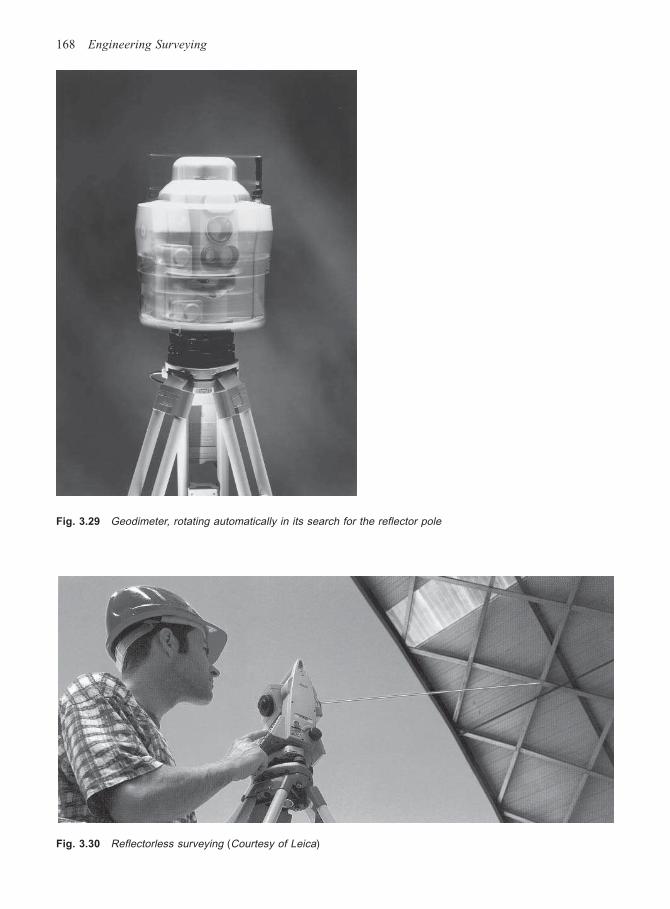
168 Engineering Surveying
Fig. 3.29 Geodimeter, rotating automatically in its search for the reflector pole
Fig. 3.30 Reflectorless surveying (Courtesy of Leica)
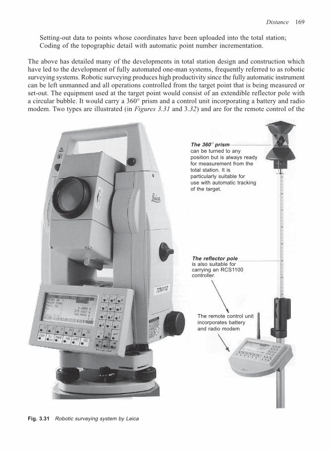
Distance 169
Setting-out data to points whose coordinates have been uploaded into the total station;Coding of the topographic detail with automatic point number incrementation.
The above has detailed many of the developments in total station design and construction whichhave led to the development of fully automated one-man systems, frequently referred to as roboticsurveying systems. Robotic surveying produces high productivity since the fully automatic instrumentcan be left unmanned and all operations controlled from the target point that is being measured orset-out. The equipment used at the target point would consist of an extendible reflector pole witha circular bubble. It would carry a 360° prism and a control unit incorporating a battery and radiomodem. Two types are illustrated (in Figures 3.31 and 3.32) and are for the remote control of the
Fig. 3.31 Robotic surveying system by Leica
The 360° prism
can be turned to any
position but is always ready
for measurement from the
total station. It is
particularly suitable for
use with automatic tracking
of the target.
The reflector poleis also suitable forcarrying an RCS1100controller.
The remote control unit
incorporates battery
and radio modem

170 Engineering Surveying
total station and the storage of data. They have an alphanumeric LCD display and are graphicscapable. Import and export of data is via the radio modem. Storage capacity would be equal to atleast 10 000 surveyed points, plus customized software and the usual facilities to view, edit, code,set-out, etc. The entire measurement procedure is controlled from the reflector pole with facilitiesfor keying the start/stop operation, aiming, changing modes, data registration, calculations and datainput
The control unit on the Geodimeter system (Figure 3.32), which is detachable between the totalstation and reflector pole, is called Geodat Win as it runs under Windows 95. Standard featuresinclude file handling, desktop icons, pull-down menus, etc. Its graphics capability allows thesurvey to be drawn in real time, cross-sections displayed, and points to be set-out shown on thescreen. The software, Geodat Win Base, contains several different modules including Database,Calculations Engine, Coordinate Transformation Engine, Surveying Applications, CAD Applicationsand Instrument Control Manager. In addition to a library of applications programs, Geodat WinBase supports all major coordinate systems, datums and ellipsoids and can supply satellite informationand sky plots. Thus, it can be used with GPS antennae.
The total station unit in robotic surveying must have servo motors, ATR, dual axis compensatorsand a guide light. In the case of the Leica system, a radio modem fits to the tripod and permitscable-less exchange of data between the controllers. The robotic system can be used for both
Fig. 3.32 Robotic surveying system by Spectra-Precision
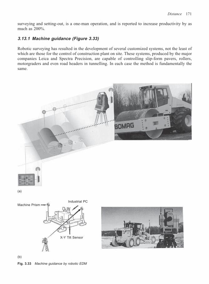
Distance 171
surveying and setting-out, is a one-man operation, and is reported to increase productivity by asmuch as 200%.
3.13.1 Machine guidance (Figure 3.33)
Robotic surveying has resulted in the development of several customized systems, not the least ofwhich are those for the control of construction plant on site. These systems, produced by the majorcompanies Leica and Spectra Precision, are capable of controlling slip-form pavers, rollers,motorgraders and even road headers in tunnelling. In each case the method is fundamentally thesame.
Fig. 3.33 Machine guidance by robotic EDM
(a)
(b)
Machine PrismIndustrial PC
X-Y Tilt Sensor
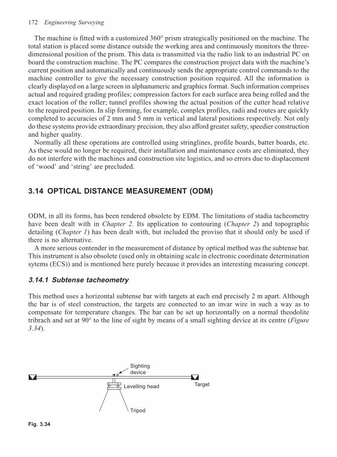
172 Engineering Surveying
The machine is fitted with a customized 360° prism strategically positioned on the machine. Thetotal station is placed some distance outside the working area and continuously monitors the three-dimensional position of the prism. This data is transmitted via the radio link to an industrial PC onboard the construction machine. The PC compares the construction project data with the machine’scurrent position and automatically and continuously sends the appropriate control commands to themachine controller to give the necessary construction position required. All the information isclearly displayed on a large screen in alphanumeric and graphics format. Such information comprisesactual and required grading profiles; compression factors for each surface area being rolled and theexact location of the roller; tunnel profiles showing the actual position of the cutter head relativeto the required position. In slip forming, for example, complex profiles, radii and routes are quicklycompleted to accuracies of 2 mm and 5 mm in vertical and lateral positions respectively. Not onlydo these systems provide extraordinary precision, they also afford greater safety, speedier constructionand higher quality.
Normally all these operations are controlled using stringlines, profile boards, batter boards, etc.As these would no longer be required, their installation and maintenance costs are eliminated, theydo not interfere with the machines and construction site logistics, and so errors due to displacementof ‘wood’ and ‘string’ are precluded.
3.14 OPTICAL DISTANCE MEASUREMENT (ODM)
ODM, in all its forms, has been rendered obsolete by EDM. The limitations of stadia tacheometryhave been dealt with in Chapter 2. Its application to contouring (Chapter 2) and topographicdetailing (Chapter 1) has been dealt with, but included the proviso that it should only be used ifthere is no alternative.
A more serious contender in the measurement of distance by optical method was the subtense bar.This instrument is also obsolete (used only in obtaining scale in electronic coordinate determinationsytems (ECS)) and is mentioned here purely because it provides an interesting measuring concept.
3.14.1 Subtense tacheometry
This method uses a horizontal subtense bar with targets at each end precisely 2 m apart. Althoughthe bar is of steel construction, the targets are connected to an invar wire in such a way as tocompensate for temperature changes. The bar can be set up horizontally on a normal theodolitetribrach and set at 90° to the line of sight by means of a small sighting device at its centre (Figure
3.34).
Sighting
device
Target
Tripod
Levelling head
Fig. 3.34
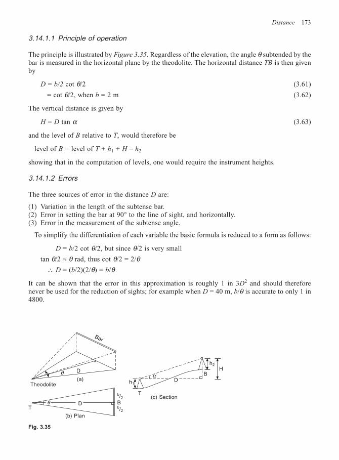
Distance 173
3.14.1.1 Principle of operation
The principle is illustrated by Figure 3.35. Regardless of the elevation, the angle θ subtended by thebar is measured in the horizontal plane by the theodolite. The horizontal distance TB is then givenby
D = b/2 cot θ/2 (3.61)
= cot θ/2, when b = 2 m (3.62)
The vertical distance is given by
H = D tan α (3.63)
and the level of B relative to T, would therefore be
level of B = level of T + h1 + H – h2
showing that in the computation of levels, one would require the instrument heights.
3.14.1.2 Errors
The three sources of error in the distance D are:
(1) Variation in the length of the subtense bar.(2) Error in setting the bar at 90° to the line of sight, and horizontally.(3) Error in the measurement of the subtense angle.
To simplify the differentiation of each variable the basic formula is reduced to a form as follows:
D = b/2 cot θ/2, but since θ/2 is very small
tan θ/2 ≈ θ rad, thus cot θ/2 = 2/θ∴ D = (b/2)(2/θ) = b/θ
It can be shown that the error in this approximation is roughly 1 in 3D2 and should thereforenever be used for the reduction of sights; for example when D = 40 m, b/θ is accurate to only 1 in4800.
Bar
D
(a)Theodolite
θ
DθT
(b) Plan
b/2Bb/2
h1
h2
HB
Dα
T(c) Section
Fig. 3.35
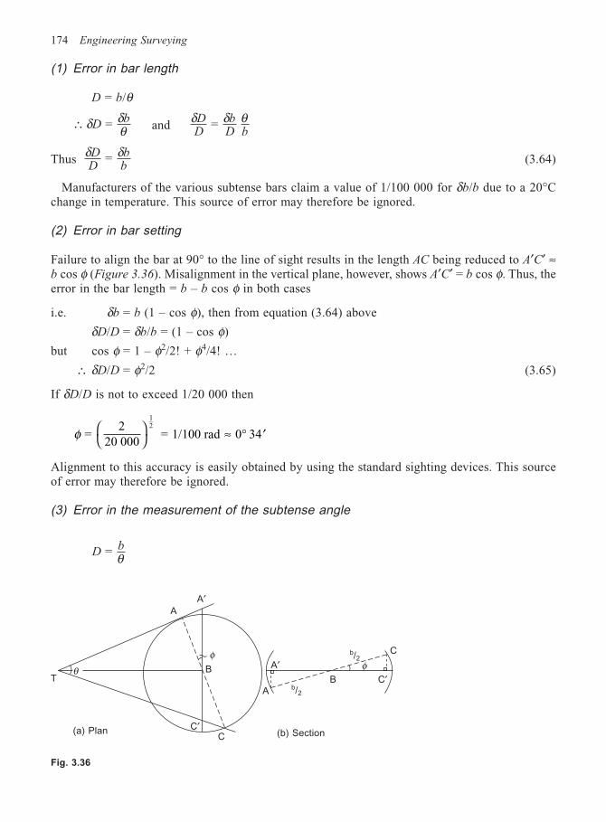
174 Engineering Surveying
(1) Error in bar length
D = b/θ
∴ = δ δθDb
andδ δ θDD
bD b
=
Thusδ δDD
bb
= (3.64)
Manufacturers of the various subtense bars claim a value of 1/100 000 for δb/b due to a 20°Cchange in temperature. This source of error may therefore be ignored.
(2) Error in bar setting
Failure to align the bar at 90° to the line of sight results in the length AC being reduced to A′C′ ≈b cos φ (Figure 3.36). Misalignment in the vertical plane, however, shows A′C′ = b cos φ. Thus, theerror in the bar length = b – b cos φ in both cases
i.e. δb = b (1 – cos φ), then from equation (3.64) above
δD/D = δb/b = (1 – cos φ)
but cos φ = 1 – φ2/2! + φ4/4! …
∴ δD/D = φ2/2 (3.65)
If δD/D is not to exceed 1/20 000 then
φ = 2
20 000 = 1/100 rad 0 34
12
≈ ° ′
Alignment to this accuracy is easily obtained by using the standard sighting devices. This sourceof error may therefore be ignored.
(3) Error in the measurement of the subtense angle
Db = θ
Fig. 3.36
A
A′
θT
C′C
B
φA′
A b/2
B
b/2φ
C
C′
(b) Section(a) Plan
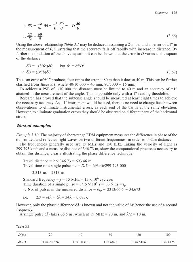
Distance 175
∴ = – = – = –2
δθ
δθ θδθθ
δθθD
b bD
∴ = δ δθθ
DD
(3.66)
Using the above relationship Table 3.1 may be deduced, assuming a 2-m bar and an error of ±1″ inthe measurement of θ, illustrating that the accuracy falls off rapidly with increase in distance. Byfurther manipulation of the above equation it can be shown that the error in D varies as the squareof the distance:
δD = –(b/θ2)δθ but θ2 = b2/D2
∴ δD = (D2/b)δθ (3.67)
Thus, an error of ±1″ produces four times the error at 80 m than it does at 40 m. This can be furtherclarified from Table 3.1, where 40/10 000 = 40 mm, 80/5000 = 16 mm.
To achieve a PSE of 1/10 000 the distance must be limited to 40 m and an accuracy of ±1″attained in the measurement of the angle. This is possible only with a 1″-reading theodolite.
Research has proved that the subtense angle should be measured at least eight times to achievethe necessary accuracy. As a 1″ instrument would be used, there is no need to change face betweenobservations to eliminate instrumental errors, as each end of the bar is at the same elevation.However, to eliminate graduation errors they should be observed on different parts of the horizontalcircle.
Worked examples
Example 3.10 The majority of short-range EDM equipment measures the difference in phase of thetransmitted and reflected light waves on two different frequencies, in order to obtain distance.
The frequencies generally used are 15 MHz and 150 kHz. Taking the velocity of light as299 793 km/s and a measure distance of 346.73 m, show the computational processes necessary toobtain this distance, clearly illustrating the phase difference technique.
Travel distance = 2 × 346.73 = 693.46 mTravel time of a single pulse = t = D/V = 693.46/299 793 000
–2.313 µs = 2313 ns
Standard frequency = f = 15 MHz = 15 × 106 cycles/sTime duration of a single pulse = 1/15 × 106 s = 66.6 ns = tp.
∴ No. of pulses in the measured distance = t/tp = 2313/66.6 = 34.673
i.e. 2D = Mλ + δλ = 34λ + 0.673λ
However, only the phase difference δλ is known and not the value of M; hence the use of a secondfrequency.
A single pulse (λ) takes 66.6 ns, which at 15 MHz = 20 m, and λ/2 = 10 m.
Table 3.1
D(m) 20 40 60 80 100
δD/D 1 in 20 626 1 in 10 313 1 in 6875 1 in 5106 1 in 4125
176 Engineering Surveying
∴ D = M(λ/2) + 0.673 (λ/2) = 6.73 m
Now using f = 150 kHz = 150 × 103 cycles/s, the time duration of a single pulse = 1/150 × 103 =6.667 µs.
At 150 kHz, 6.6674 µs = 1000 m
No. of pulses = t/tp = 2.313/6.667 = 0.347
∴ D = 0.347 × 1000 m = 347 m
Fine measurement using 15 MHz = 6.73 m
Coarse measurement using 15 kHz = 347 m
Measured distance = 346.73 m
Example 3.11 (a) Using EDM, top-mounted on a theodolite, a distance of 1000 m is measured onan angle of inclination of 09°00′ 00″. Compute the horizontal distance.
Now, taking R = 6.37 × 10⁶ m and the coefficient of refraction K = 1.10, correct the vertical anglefor refraction effects, and recompute the horizontal distance.
(b) If the EDM equipment used above was accurate to ± (3 mm + 5 ppm), calculate therequired accuracy of the vertical angle, and thereby indicate whether or not it is necessary to correctit for refraction.
(c) Calculate the equivalent error allowable in levelling the two ends of the above measuredline. (KU)
(a) Horizontal distance = D = S cos α = 1000 cos 9° = 987.688 m
ˆ ′′r = SKρ/2R = 987.69 × 1.10 × 206 265/2 × 6 370 000 = 17.6″Corrected angle = 8°59′ 42″∴ D = 1000 cos 8°59′ 42″ = 987.702 m
Difference = 14 mm
(b) Distance is accurate to ± ±(3 + 5 ) = 5.8 mm2 212
D = S cos αδD = –S sin α δα
δα″ = δDρ/S sin α = 0.0058 × 206 265/10 000 sin 9° = ±7.7″
Vertical angle needs to be accurate to ±7.7″, so refraction must be catered for.
(c) To reduce S to D, apply the correction –h2/2S = Ch
δCh = h δh/S
and δh = δChS/h
where h = S sin α = 1000 sin 9° = 156.43 m
δh = 0.0058 × 1000/156.43 = ±0.037 m
Example 3.12
(a) Modern total stations supply horizontal distance (D) and vertical height (∆H) at the press of abutton.
Distance 177
What corrections must be applied to the initial field data of slope distance and vertical angleto obtain the best possible values for D and ∆H?
(b) When using EDM equipment of a particular make, why is it inadvisable to use reflectors andnomograms from other makes of instrument?
(c) To obtain the zero error of a particular EDM instrument, a base line AD is split into threesections AB, BC and CD and measured in the following combinations:
AB = 20.512, AC = 63.192, AD = 153.303
BC = 42.690, BD = 132.803, CD = 90.1201
Using all possible combinations, compute the zero error: (KU)
(a) Velocity correction using temperature and pressure measurements at the time of measurement.Vertical angle corrected for refraction to give D and for Earth curvature to give ∆H.
(b) Instrument has a built-in correction for the reflector constant and may have been calibrated forthat particular instrument/reflector combination. Instrument standardization may be different fromthat used to produce a nomogram for other instruments.
(c) 20.512 + 42.690 – 63.192 = +0.010
63.192 + 90.120 – 153.303 = +0.009
20.512 + 132.803 – 153.303 = +0.012
42.690 + 90.120 – 132.803 = +0.007
Mean = +0.009 m
Correction = –0.009 m
Example 3.13 Manufacturers specify the accuracy of EDM equipment as
± (a + bD) mm
where b is in ppm of the distance measured, D.
Describe in detail the various errors defined by the variables a and b. Discuss the relativeimportance of a and b with regard to the majority of measurements taken in engineering surveys.
What calibration procedures are required to minimize the effect of the above errors in EDMmeasurement. (KU)
For answer, refer to appropriate sections of the text.
REFERENCES
Hodges, D.J. (1968) ‘Errors in Model 6 Geodimeter Measurements and a Method for Increased Accuracy’,
The Mining Engineer, December.
Ordnance Survey (1950) Constants, Formulae and Methods Used in Transverse Mercator Projection, HMSO.
4
Angles
As shown in Chapter 1, horizontal and vertical angles are fundamental measurements in surveying.The vertical angle, as already illustrated, is used in obtaining the elevation of points (trig levelling)
and in the reduction of slant distance to the horizontal.The horizontal angle is used primarily to obtain relative direction to a survey control point, or to
topographic detail points, or to points to be set out.The instrument used in the measurement of angles is called a theodolite, the horizontal and
vertical circles of which can be likened to circular protractors set in horizontal and vertical planes.It follows that, although the points observed are at different elevations, it is always the horizontalangle and not the space angle which is measured. For example, observations to points A and C fromB (Figure 4.1) will give the horizontal angle ABC = θ. The vertical angle of elevation to A is α andits zenith angle is ZA.
4.1 THE THEODOLITE
There are basically two types of theodolite, the optical microptic type or the electronic digital type,both of which are capable of resolving angles to 1′, 20″, 1″ or 0.1″ of arc, depending upon theaccuracy requirements of the work in hand. The finesse of selecting an instrument specific to thesurvey tolerances is usually overridden by the commercial aspects of the company and a 1″ instrumentmay be used for all work. When one considers that 1″ of arc subtends 1 mm in 200 m, it issufficiently accurate for practically all work carried out in engineering.
Figure 4.2 shows a typical theodolite, whilst Figure 4.3 shows the main components of the newobsolete vernier-type theodolite. This exploded diagram enables the relationships of the variousparts to be more clearly understood along with the relationships of the main axes. In a correctlyadjusted instrument these axes should all be normal to each other, with their point of intersectionbeing the point about which the angles are measured. Neither figure illustrates the complexity of amodern theodolite or the very high calibre of the process of its production. This can be clearly seenfrom Figure 4.4.
The basic features of a typical theodolite are, with reference to Figure 4.3, as follows:
(1) The trivet stage forming the base of the instrument connects it to the tripod head.(2) The tribrach supports the rest of the instrument and with reference to the plate bubble can be
levelled using the footscrews which act against the fixed trivet stage.(3) The lower plate carries the horizontal circle which is made of glass, with graduations from 0°
to 360° photographically etched around the perimeter. This process enables lines of only0.004 mm thickness to be sharply defined on a small-diameter circle (100 mm), therebyresulting in very compact instruments.
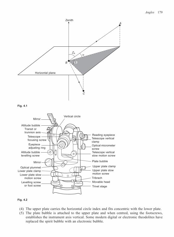
Angles 179
(4) The upper plate carries the horizontal circle index and fits concentric with the lower plate.(5) The plate bubble is attached to the upper plate and when centred, using the footscrews,
establishes the instrument axis vertical. Some modern digital or electronic theodolites havereplaced the spirit bubble with an electronic bubble.
Fig. 4.1
ZenithA
αZA
B
Horizontal plane
C
θ
Mirror
Altitude bubble
Transit or
trunnion axis
Telescope
focusing screw
Eyepiece
adjusting ring
Altitude bubble
levelling screw
Mirror
Optical plummet
Lower plate clamp
Lower plate slow
motion screw
Levelling screw
or foot screw
Vertical circle
Reading eyepiece
Telescope vertical
clamp
Optical micrometer
screw
Telescope vertical
slow motion screw
Plate bubble
Upper plate clamp
Upper plate slow
motion screw
Tribrach
Movable head
Trivet stage
Fig. 4.2
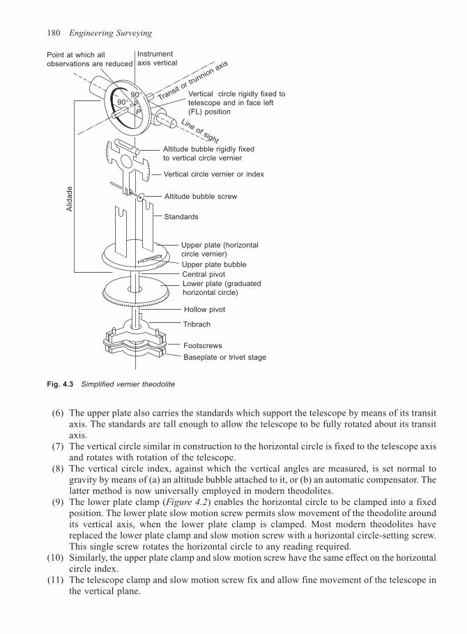
180 Engineering Surveying
(6) The upper plate also carries the standards which support the telescope by means of its transitaxis. The standards are tall enough to allow the telescope to be fully rotated about its transitaxis.
(7) The vertical circle similar in construction to the horizontal circle is fixed to the telescope axisand rotates with rotation of the telescope.
(8) The vertical circle index, against which the vertical angles are measured, is set normal togravity by means of (a) an altitude bubble attached to it, or (b) an automatic compensator. Thelatter method is now universally employed in modern theodolites.
(9) The lower plate clamp (Figure 4.2) enables the horizontal circle to be clamped into a fixedposition. The lower plate slow motion screw permits slow movement of the theodolite aroundits vertical axis, when the lower plate clamp is clamped. Most modern theodolites havereplaced the lower plate clamp and slow motion screw with a horizontal circle-setting screw.This single screw rotates the horizontal circle to any reading required.
(10) Similarly, the upper plate clamp and slow motion screw have the same effect on the horizontalcircle index.
(11) The telescope clamp and slow motion screw fix and allow fine movement of the telescope inthe vertical plane.
Point at which all
observations are reduced
Instrument
axis vertical
90°90° Transit o
r trunnion axis
Line of sight
Vertical circle rigidly fixed to
telescope and in face left
(FL) position
Altitude bubble rigidly fixed
to vertical circle vernier
Vertical circle vernier or index
Altitude bubble screw
Standards
Upper plate (horizontal
circle vernier)
Upper plate bubble
Central pivot
Lower plate (graduated
horizontal circle)
Hollow pivot
Tribrach
Footscrews
Baseplate or trivet stage
Alid
ad
e
P
Fig. 4.3 Simplified vernier theodolite
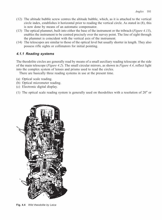
Angles 181
(12) The altitude bubble screw centres the altitude bubble, which, as it is attached to the verticalcircle index, establishes it horizontal prior to reading the vertical circle. As stated in (8), thisis now done by means of an automatic compensator.
(13) The optical plummet, built into either the base of the instrument or the tribrach (Figure 4.13),enables the instrument to be centred precisely over the survey point. The line of sight throughthe plummet is coincident with the vertical axis of the instrument.
(14) The telescopes are similar to those of the optical level but usually shorter in length. They alsopossess rifle sights or collimators for initial pointing.
4.1.1 Reading systems
The theodolite circles are generally read by means of a small auxiliary reading telescope at the sideof the main telescope (Figure 4.2). The small circular mirrors, as shown in Figure 4.4, reflect lightinto the complex system of lenses and prisms used to read the circles.
There are basically three reading systems in use at the present time.
(a) Optical scale reading.(b) Optical micrometer reading.(c) Electronic digital display.
(1) The optical scale reading system is generally used on theodolites with a resolution of 20″ or
Fig. 4.4 Wild theodolite by Leica
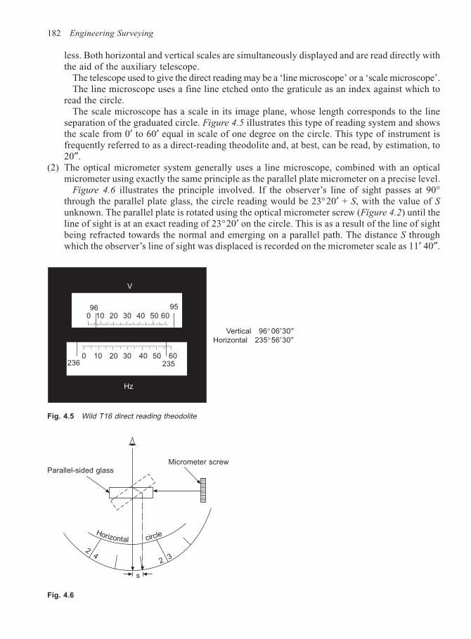
182 Engineering Surveying
less. Both horizontal and vertical scales are simultaneously displayed and are read directly withthe aid of the auxiliary telescope.
The telescope used to give the direct reading may be a ‘line microscope’ or a ‘scale microscope’.The line microscope uses a fine line etched onto the graticule as an index against which to
read the circle.The scale microscope has a scale in its image plane, whose length corresponds to the line
separation of the graduated circle. Figure 4.5 illustrates this type of reading system and showsthe scale from 0′ to 60′ equal in scale of one degree on the circle. This type of instrument isfrequently referred to as a direct-reading theodolite and, at best, can be read, by estimation, to20″.
(2) The optical micrometer system generally uses a line microscope, combined with an opticalmicrometer using exactly the same principle as the parallel plate micrometer on a precise level.
Figure 4.6 illustrates the principle involved. If the observer’s line of sight passes at 90°through the parallel plate glass, the circle reading would be 23°20′ + S, with the value of Sunknown. The parallel plate is rotated using the optical micrometer screw (Figure 4.2) until theline of sight is at an exact reading of 23°20′ on the circle. This is as a result of the line of sightbeing refracted towards the normal and emerging on a parallel path. The distance S throughwhich the observer’s line of sight was displaced is recorded on the micrometer scale as 11′ 40″.
Fig. 4.5 Wild T16 direct reading theodolite
V
0 10 20 30 40 50 6096 95
Hz
0 10 20 30 40 50 60236 235
Vertical 96° 06′30″Horizontal 235°56′30″
Horizontal circle
Micrometer screwParallel-sided glass
2 3
s
2 4
Fig. 4.6
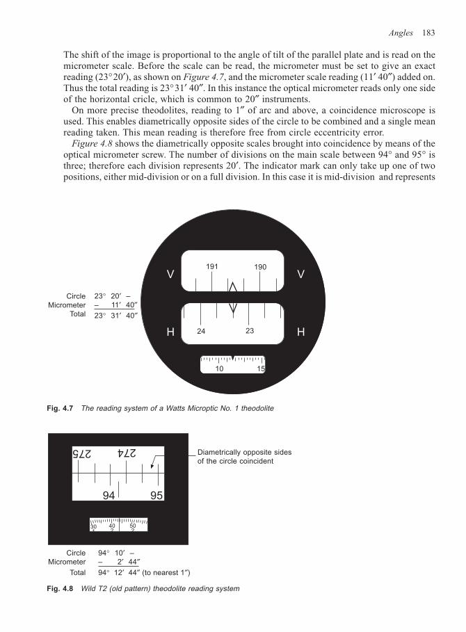
Angles 183
The shift of the image is proportional to the angle of tilt of the parallel plate and is read on themicrometer scale. Before the scale can be read, the micrometer must be set to give an exactreading (23°20′), as shown on Figure 4.7, and the micrometer scale reading (11′ 40″) added on.Thus the total reading is 23°31′ 40″. In this instance the optical micrometer reads only one sideof the horizontal cricle, which is common to 20″ instruments.
On more precise theodolites, reading to 1″ of arc and above, a coincidence microscope isused. This enables diametrically opposite sides of the circle to be combined and a single meanreading taken. This mean reading is therefore free from circle eccentricity error.
Figure 4.8 shows the diametrically opposite scales brought into coincidence by means of theoptical micrometer screw. The number of divisions on the main scale between 94° and 95° isthree; therefore each division represents 20′. The indicator mark can only take up one of twopositions, either mid-division or on a full division. In this case it is mid-division and represents
191 190
24 23
V
H
V
H
10 15
Circle
Micrometer
Total
Fig. 4.7 The reading system of a Watts Microptic No. 1 theodolite
Diametrically opposite sides
of the circle coincident
Circle
Micrometer
Total
301
402
502
9594
274275
94° 10′ –
– 2′ 44″94° 12′ 44″ (to nearest 1″)
Fig. 4.8 Wild T2 (old pattern) theodolite reading system
23° 20′ –
– 11′ 40″23° 31′ 40″
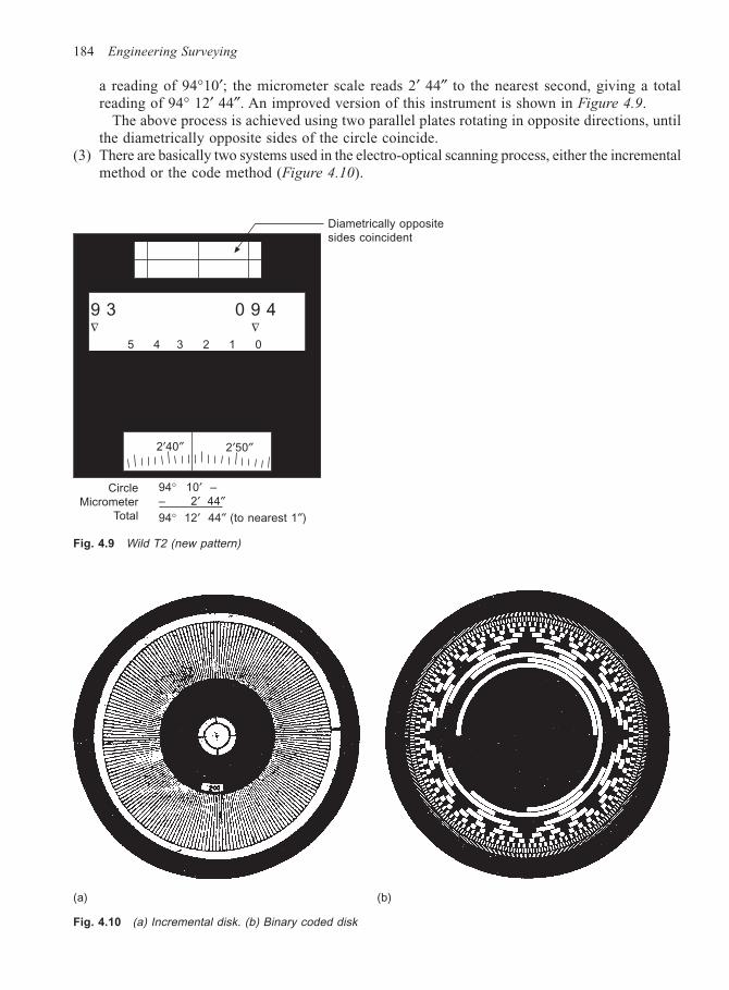
184 Engineering Surveying
a reading of 94°10′; the micrometer scale reads 2′ 44″ to the nearest second, giving a totalreading of 94° 12′ 44″. An improved version of this instrument is shown in Figure 4.9.
The above process is achieved using two parallel plates rotating in opposite directions, untilthe diametrically opposite sides of the circle coincide.
(3) There are basically two systems used in the electro-optical scanning process, either the incrementalmethod or the code method (Figure 4.10).
Fig. 4.9 Wild T2 (new pattern)
Circle
Micrometer
Total
2′40″ 2′50″
Diametrically opposite
sides coincident
0 9 4∇
5 4 3 2 1 0
9 3∇
94° 10′ –
– 2′ 44″94° 12′ 44″ (to nearest 1″)
Fig. 4.10 (a) Incremental disk. (b) Binary coded disk
(a) (b)
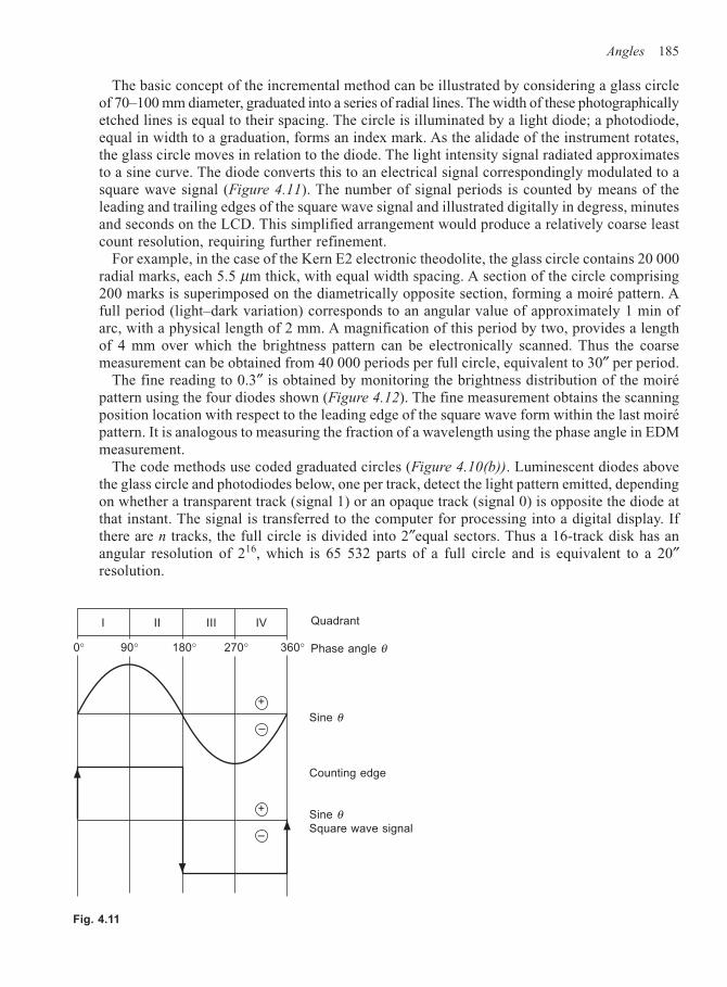
Angles 185
The basic concept of the incremental method can be illustrated by considering a glass circleof 70–100 mm diameter, graduated into a series of radial lines. The width of these photographicallyetched lines is equal to their spacing. The circle is illuminated by a light diode; a photodiode,equal in width to a graduation, forms an index mark. As the alidade of the instrument rotates,the glass circle moves in relation to the diode. The light intensity signal radiated approximatesto a sine curve. The diode converts this to an electrical signal correspondingly modulated to asquare wave signal (Figure 4.11). The number of signal periods is counted by means of theleading and trailing edges of the square wave signal and illustrated digitally in degress, minutesand seconds on the LCD. This simplified arrangement would produce a relatively coarse leastcount resolution, requiring further refinement.
For example, in the case of the Kern E2 electronic theodolite, the glass circle contains 20 000radial marks, each 5.5 µm thick, with equal width spacing. A section of the circle comprising200 marks is superimposed on the diametrically opposite section, forming a moiré pattern. Afull period (light–dark variation) corresponds to an angular value of approximately 1 min ofarc, with a physical length of 2 mm. A magnification of this period by two, provides a lengthof 4 mm over which the brightness pattern can be electronically scanned. Thus the coarsemeasurement can be obtained from 40 000 periods per full circle, equivalent to 30″ per period.
The fine reading to 0.3″ is obtained by monitoring the brightness distribution of the moirépattern using the four diodes shown (Figure 4.12). The fine measurement obtains the scanningposition location with respect to the leading edge of the square wave form within the last moirépattern. It is analogous to measuring the fraction of a wavelength using the phase angle in EDMmeasurement.
The code methods use coded graduated circles (Figure 4.10(b)). Luminescent diodes abovethe glass circle and photodiodes below, one per track, detect the light pattern emitted, dependingon whether a transparent track (signal 1) or an opaque track (signal 0) is opposite the diode atthat instant. The signal is transferred to the computer for processing into a digital display. Ifthere are n tracks, the full circle is divided into 2″equal sectors. Thus a 16-track disk has anangular resolution of 216, which is 65 532 parts of a full circle and is equivalent to a 20″resolution.
I II III IV
0° 90° 180° 270° 360°
Quadrant
Phase angle θ
Sine θ
Counting edge
Sine θSquare wave signal
–
+
+
–
Fig. 4.11
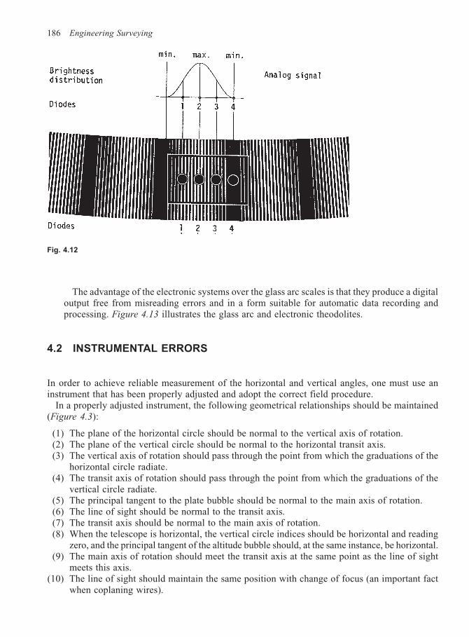
186 Engineering Surveying
The advantage of the electronic systems over the glass arc scales is that they produce a digitaloutput free from misreading errors and in a form suitable for automatic data recording andprocessing. Figure 4.13 illustrates the glass arc and electronic theodolites.
4.2 INSTRUMENTAL ERRORS
In order to achieve reliable measurement of the horizontal and vertical angles, one must use aninstrument that has been properly adjusted and adopt the correct field procedure.
In a properly adjusted instrument, the following geometrical relationships should be maintained(Figure 4.3):
(1) The plane of the horizontal circle should be normal to the vertical axis of rotation.(2) The plane of the vertical circle should be normal to the horizontal transit axis.(3) The vertical axis of rotation should pass through the point from which the graduations of the
horizontal circle radiate.(4) The transit axis of rotation should pass through the point from which the graduations of the
vertical circle radiate.(5) The principal tangent to the plate bubble should be normal to the main axis of rotation.(6) The line of sight should be normal to the transit axis.(7) The transit axis should be normal to the main axis of rotation.(8) When the telescope is horizontal, the vertical circle indices should be horizontal and reading
zero, and the principal tangent of the altitude bubble should, at the same instance, be horizontal.(9) The main axis of rotation should meet the transit axis at the same point as the line of sight
meets this axis.(10) The line of sight should maintain the same position with change of focus (an important fact
when coplaning wires).
Fig. 4.12
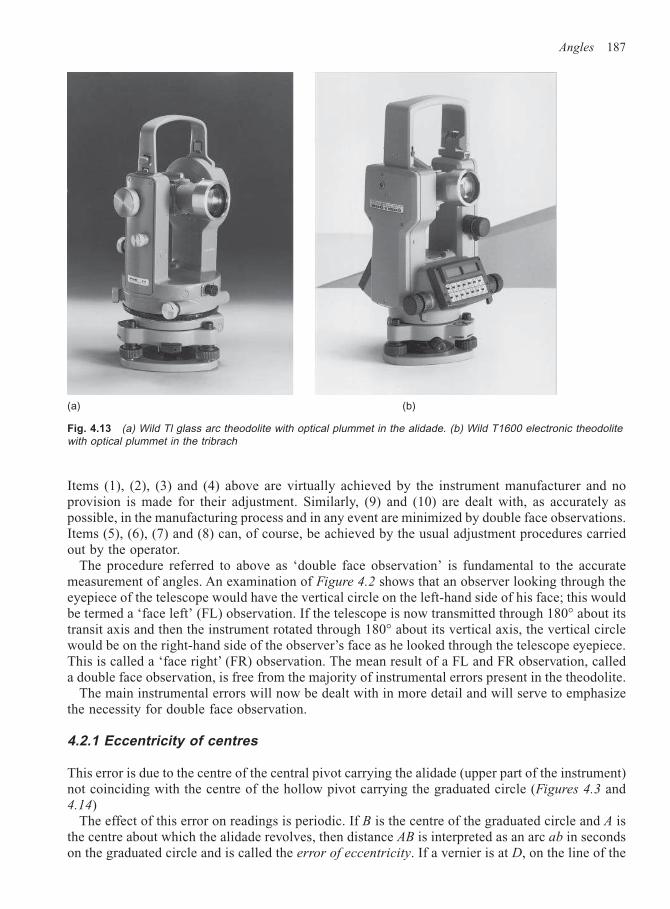
Angles 187
Items (1), (2), (3) and (4) above are virtually achieved by the instrument manufacturer and noprovision is made for their adjustment. Similarly, (9) and (10) are dealt with, as accurately aspossible, in the manufacturing process and in any event are minimized by double face observations.Items (5), (6), (7) and (8) can, of course, be achieved by the usual adjustment procedures carriedout by the operator.
The procedure referred to above as ‘double face observation’ is fundamental to the accuratemeasurement of angles. An examination of Figure 4.2 shows that an observer looking through theeyepiece of the telescope would have the vertical circle on the left-hand side of his face; this wouldbe termed a ‘face left’ (FL) observation. If the telescope is now transmitted through 180° about itstransit axis and then the instrument rotated through 180° about its vertical axis, the vertical circlewould be on the right-hand side of the observer’s face as he looked through the telescope eyepiece.This is called a ‘face right’ (FR) observation. The mean result of a FL and FR observation, calleda double face observation, is free from the majority of instrumental errors present in the theodolite.
The main instrumental errors will now be dealt with in more detail and will serve to emphasizethe necessity for double face observation.
4.2.1 Eccentricity of centres
This error is due to the centre of the central pivot carrying the alidade (upper part of the instrument)not coinciding with the centre of the hollow pivot carrying the graduated circle (Figures 4.3 and4.14)
The effect of this error on readings is periodic. If B is the centre of the graduated circle and A isthe centre about which the alidade revolves, then distance AB is interpreted as an arc ab in secondson the graduated circle and is called the error of eccentricity. If a vernier is at D, on the line of the
(a) (b)
Fig. 4.13 (a) Wild Tl glass arc theodolite with optical plummet in the alidade. (b) Wild T1600 electronic theodolitewith optical plummet in the tribrach
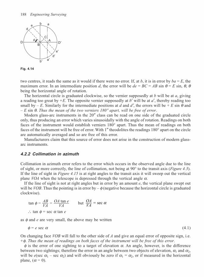
188 Engineering Surveying
two centres, it reads the same as it would if there were no error. If, at b, it is in error by ba = E, themaximum error. In an intermediate position d, the error will be de = BC = AB sin θ = E sin, θ, θbeing the horizontal angle of rotation.
The horizontal circle is graduated clockwise, so the vernier supposedly at b will be at a, givinga reading too great by +E. The opposite vernier supposedly at b′ will be at a′, thereby reading toosmall by – E. Similarly for the intermediate positions at d and d′, the errors will be + E sin θ and– E sin θ. Thus the mean of the two verniers 180° apart, will be free of error.
Modern glass-arc instruments in the 20″ class can be read on one side of the graduated circleonly, thus producing an error which varies sinusoidally with the angle of rotation. Readings on bothfaces of the instrument would establish verniers 180° apart. Thus the mean of readings on bothfaces of the instrument will be free of error. With 1″ theodolites the readings 180° apart on the circleare automatically averaged and so are free of this error.
Manufacturers claim that this source of error does not arise in the construction of modern glass-arc instruments.
4.2.2 Collimation in azimuth
Collimation in azimuth error refers to the error which occurs in the observed angle due to the lineof sight, or more correctly, the line of collimation, not being at 90° to the transit axis (Figure 4.3).If the line of sight in Figure 4.15 is at right angles to the transit axis it will sweep out the verticalplane VOA when the telescope is depressed through the vertical angle α.
If the line of sight is not at right angles but in error by an amount e, the vertical plane swept outwill be VOB. Thus the pointing is in error by – φ (negative because the horizontal circle is graduatedclockwise).
tan = = tan φ ABVA
OA eVA
butOAVA
= sec α
∴ tan φ = sec α tan e
as φ and e are very small, the above may be written
φ = e sec α (4.1)
On changing face VOB will fall to the other side of A and give an equal error of opposite sign, i.e.+φ. Thus the mean of readings on both faces of the instrument will be free of this error.
φ is the error of one sighting to a target of elevation α. An angle, however, is the differencebetween two sightings; therefore the error in an angle between two objects of elevation, α1 and α2,will be e(sec α1 – sec α2) and will obviously be zero if α1 = α2, or if measured in the horizontalplane, (α = 0).
de
b a
θD
CA
BD′
a′b′
d′e′
Fig. 4.14
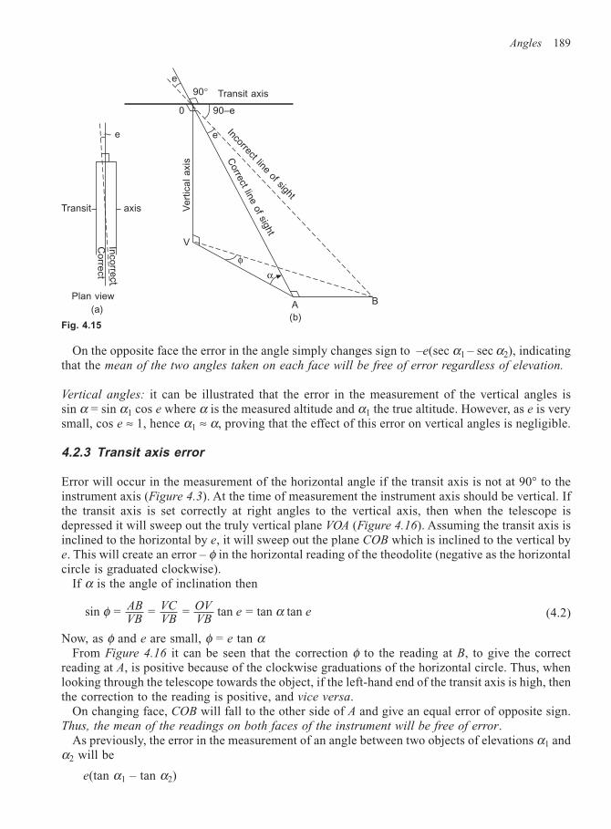
Angles 189
On the opposite face the error in the angle simply changes sign to –e(sec α1 – sec α2), indicatingthat the mean of the two angles taken on each face will be free of error regardless of elevation.
Vertical angles: it can be illustrated that the error in the measurement of the vertical angles issin α = sin α1 cos e where α is the measured altitude and α1 the true altitude. However, as e is verysmall, cos e ≈ 1, hence α1 ≈ α, proving that the effect of this error on vertical angles is negligible.
4.2.3 Transit axis error
Error will occur in the measurement of the horizontal angle if the transit axis is not at 90° to theinstrument axis (Figure 4.3). At the time of measurement the instrument axis should be vertical. Ifthe transit axis is set correctly at right angles to the vertical axis, then when the telescope isdepressed it will sweep out the truly vertical plane VOA (Figure 4.16). Assuming the transit axis isinclined to the horizontal by e, it will sweep out the plane COB which is inclined to the vertical bye. This will create an error – φ in the horizontal reading of the theodolite (negative as the horizontalcircle is graduated clockwise).
If α is the angle of inclination then
sin = = = tan = tan tan φ αABVB
VCVB
OVVB
e e (4.2)
Now, as φ and e are small, φ = e tan αFrom Figure 4.16 it can be seen that the correction φ to the reading at B, to give the correct
reading at A, is positive because of the clockwise graduations of the horizontal circle. Thus, whenlooking through the telescope towards the object, if the left-hand end of the transit axis is high, thenthe correction to the reading is positive, and vice versa.
On changing face, COB will fall to the other side of A and give an equal error of opposite sign.Thus, the mean of the readings on both faces of the instrument will be free of error.
As previously, the error in the measurement of an angle between two objects of elevations α1 andα2 will be
e(tan α1 – tan α2)
Fig. 4.15
e
90° Transit axis
0 90–e
(b)
Incorrect line of sight
e
Corre
ct line o
f sight
BA
α
φ
Ve
rtic
al
axis
VInco
rrect
Co
rrect
Transit axis
(a)
e
Plan view
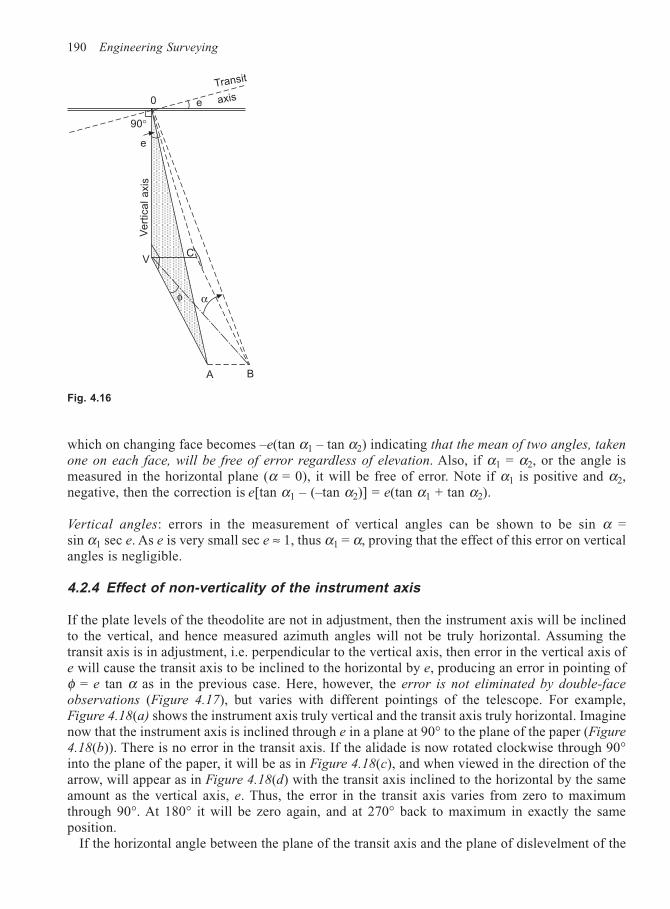
190 Engineering Surveying
which on changing face becomes –e(tan α1 – tan α2) indicating that the mean of two angles, taken
one on each face, will be free of error regardless of elevation. Also, if α1 = α2, or the angle ismeasured in the horizontal plane (α = 0), it will be free of error. Note if α1 is positive and α2,negative, then the correction is e[tan α1 – (–tan α2)] = e(tan α1 + tan α2).
Vertical angles: errors in the measurement of vertical angles can be shown to be sin α =sin α1 sec e. As e is very small sec e ≈ 1, thus α1 = α, proving that the effect of this error on verticalangles is negligible.
4.2.4 Effect of non-verticality of the instrument axis
If the plate levels of the theodolite are not in adjustment, then the instrument axis will be inclinedto the vertical, and hence measured azimuth angles will not be truly horizontal. Assuming thetransit axis is in adjustment, i.e. perpendicular to the vertical axis, then error in the vertical axis ofe will cause the transit axis to be inclined to the horizontal by e, producing an error in pointing ofφ = e tan α as in the previous case. Here, however, the error is not eliminated by double-face
observations (Figure 4.17), but varies with different pointings of the telescope. For example,Figure 4.18(a) shows the instrument axis truly vertical and the transit axis truly horizontal. Imaginenow that the instrument axis is inclined through e in a plane at 90° to the plane of the paper (Figure
4.18(b)). There is no error in the transit axis. If the alidade is now rotated clockwise through 90°into the plane of the paper, it will be as in Figure 4.18(c), and when viewed in the direction of thearrow, will appear as in Figure 4.18(d) with the transit axis inclined to the horizontal by the sameamount as the vertical axis, e. Thus, the error in the transit axis varies from zero to maximumthrough 90°. At 180° it will be zero again, and at 270° back to maximum in exactly the sameposition.
If the horizontal angle between the plane of the transit axis and the plane of dislevelment of the
Fig. 4.16
Transit
axise0
90°
eV
ert
ica
l a
xis
VC
φ α
BA
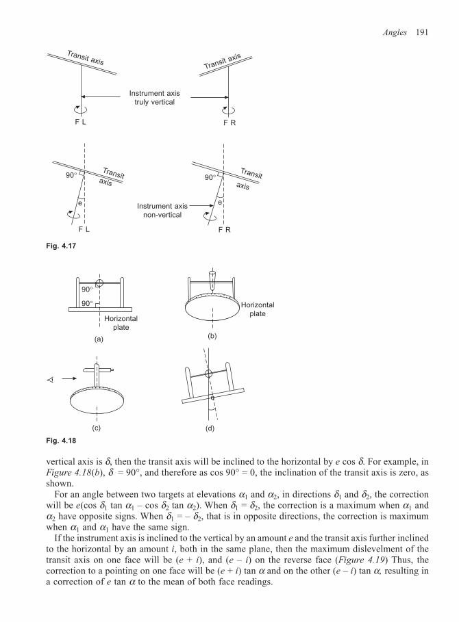
Angles 191
vertical axis is δ, then the transit axis will be inclined to the horizontal by e cos δ. For example, inFigure 4.18(b), δ = 90°, and therefore as cos 90° = 0, the inclination of the transit axis is zero, asshown.
For an angle between two targets at elevations α1 and α2, in directions δ1 and δ2, the correctionwill be e(cos δ1 tan α1 – cos δ2 tan α2). When δ1 = δ2, the correction is a maximum when α1 andα2 have opposite signs. When δ1 = – δ2, that is in opposite directions, the correction is maximumwhen α1 and α1 have the same sign.
If the instrument axis is inclined to the vertical by an amount e and the transit axis further inclinedto the horizontal by an amount i, both in the same plane, then the maximum dislevelment of thetransit axis on one face will be (e + i), and (e – i) on the reverse face (Figure 4.19) Thus, thecorrection to a pointing on one face will be (e + i) tan α and on the other (e – i) tan α, resulting ina correction of e tan α to the mean of both face readings.
Fig. 4.18
Transit axisTransit axis
Instrument axis
truly vertical
F L F R
Transitaxis
90°
e
F L
90°
Instrument axis
non-vertical
F R
e
Transitaxis
Fig. 4.17
Horizontal
plate
90°
(a)
90°
(b)
Horizontal
plate
(d)
e
(c)
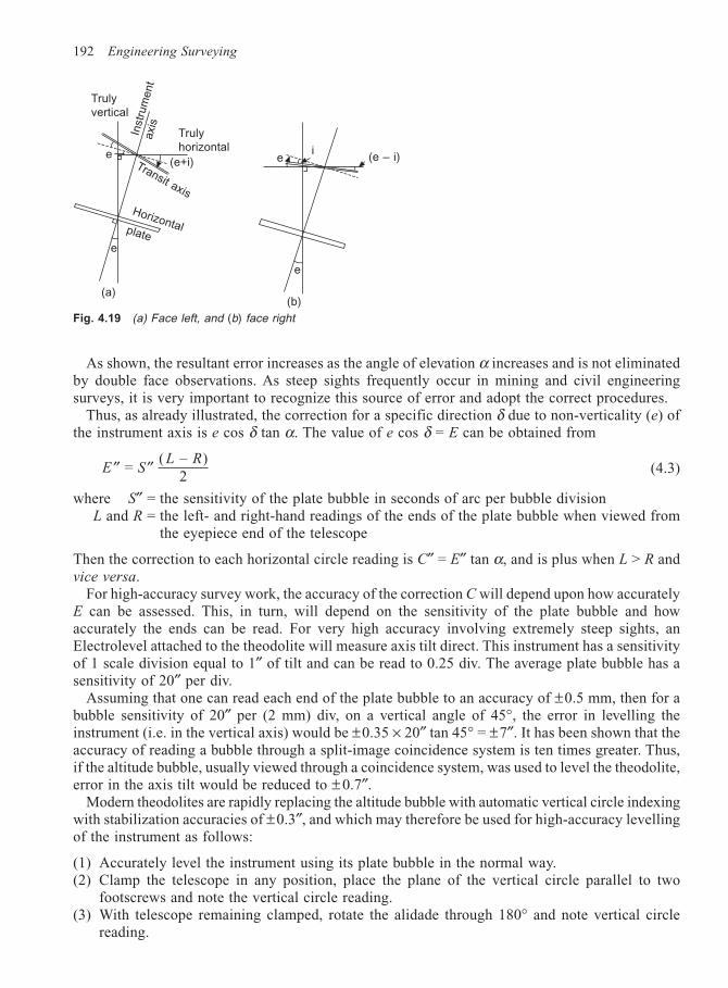
192 Engineering Surveying
As shown, the resultant error increases as the angle of elevation α increases and is not eliminatedby double face observations. As steep sights frequently occur in mining and civil engineeringsurveys, it is very important to recognize this source of error and adopt the correct procedures.
Thus, as already illustrated, the correction for a specific direction δ due to non-verticality (e) ofthe instrument axis is e cos δ tan α. The value of e cos δ = E can be obtained from
′′ ′′E SL R
= ( – )
2(4.3)
where S″ = the sensitivity of the plate bubble in seconds of arc per bubble divisionL and R = the left- and right-hand readings of the ends of the plate bubble when viewed from
the eyepiece end of the telescope
Then the correction to each horizontal circle reading is C″ = E″ tan α, and is plus when L > R andvice versa.
For high-accuracy survey work, the accuracy of the correction C will depend upon how accuratelyE can be assessed. This, in turn, will depend on the sensitivity of the plate bubble and howaccurately the ends can be read. For very high accuracy involving extremely steep sights, anElectrolevel attached to the theodolite will measure axis tilt direct. This instrument has a sensitivityof 1 scale division equal to 1″ of tilt and can be read to 0.25 div. The average plate bubble has asensitivity of 20″ per div.
Assuming that one can read each end of the plate bubble to an accuracy of ±0.5 mm, then for abubble sensitivity of 20″ per (2 mm) div, on a vertical angle of 45°, the error in levelling theinstrument (i.e. in the vertical axis) would be ±0.35 × 20″ tan 45° = ±7″. It has been shown that theaccuracy of reading a bubble through a split-image coincidence system is ten times greater. Thus,if the altitude bubble, usually viewed through a coincidence system, was used to level the theodolite,error in the axis tilt would be reduced to ± 0.7″.
Modern theodolites are rapidly replacing the altitude bubble with automatic vertical circle indexingwith stabilization accuracies of ±0.3″, and which may therefore be used for high-accuracy levellingof the instrument as follows:
(1) Accurately level the instrument using its plate bubble in the normal way.(2) Clamp the telescope in any position, place the plane of the vertical circle parallel to two
footscrews and note the vertical circle reading.(3) With telescope remaining clamped, rotate the alidade through 180° and note vertical circle
reading.
Fig. 4.19 (a) Face left, and (b) face right
Truly
vertical
Instr
um
ent
axis
Truly
horizontal
(e+i)e
Transit axis
Horizontalplatee
(a)
e
(b)
ei
(e – i)
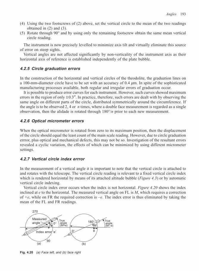
Angles 193
(4) Using the two footscrews of (2) above, set the vertical circle to the mean of the two readingsobtained in (2) and (3).
(5) Rotate through 90° and by using only the remaining footscrew obtain the same mean verticalcircle reading.
The instrument is now precisely levelled to minimize axis tilt and virtually eliminate this sourceof error on steep sights.
Vertical angles are not affected significantly by non-verticality of the instrument axis as theirhorizontal axis of reference is established independently of the plate bubble.
4.2.5 Circle graduation errors
In the construction of the horizontal and vertical circles of the theodolite, the graduation lines ona 100-mm-diameter circle have to be set with an accuracy of 0.4 µm. In spite of the sophisticatedmanufacturing processes available, both regular and irregular errors of graduation occur.
It is possible to produce error curves for each instrument. However, such curves showed maximumerrors in the region of only ±0.3″. In practice, therefore, such errors are dealt with by observing thesame angle on different parts of the circle, distributed symmetrically around the circumference. Ifthe angle is to be observed 2, 4 or n times, where a double face measurement is regarded as a singleobservation, then the alidade is rotated through 180°/n prior to each new measurement.
4.2.6 Optical micrometer errors
When the optical micrometer is rotated from zero to its maximum position, then the displacementof the circle should equal the least count of the main scale reading. However, due to circle graduationerrror, plus optical and mechanical defects, this may not be so. Investigation of the resultant errorsrevealed a cyclic variation, the effects of which can be minimized by using different micrometersettings.
4.2.7 Vertical circle index errror
In the measurement of a vertical angle it is important to note that the vertical circle is attached toand rotates with the telescope. The vertical circle reading is relevant to a fixed vertical circle indexwhich is rendered horizontal by means of its attached altitude bubble (Figure 4.3) or by automaticvertical circle indexing.
Vertical circle index error occurs when the index is not horizontal. Figure 4.20 shows the indexinclined at e to the horizontal. The measured vertical angle on FL is M, which requires a correctionof +e, while on FR the required correction is –e. The index error is thus eliminated by taking themean of the FL and FR readings.
Fig. 4.20 (a) Face left, and (b) face right
Measured
angle
270
0°
Index error ‘e’
90(a)
True angle (M+e)
0°
(b)
180°M
e
True angle (M–e)
M
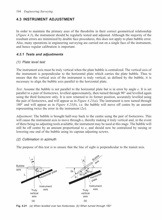
194 Engineering Surveying
4.3 INSTRUMENT ADJUSTMENT
In order to maintain the primary axes of the theodolite in their correct geometrical relationship(Figure 4.3), the instrument should be regularly tested and adjusted. Although the majority of theresultant errors are minimized by double face procedures, this does not apply to plate bubble error.Also, many operations in engineering surveying are carried out on a single face of the instrument,and hence regular calibration is important.
4.3.1 Tests and adjustments
(1) Plate level test
The instrument axis must be truly vertical when the plate bubble is centralized. The vertical axis ofthe instrument is perpendicular to the horizontal plate which carries the plate bubble. Thus toensure that the vertical axis of the instrument is truly vertical, as defined by the bubble, it isnecessary to align the bubble axis parallel to the horizontal plate.
Test: Assume the bubble is not parallel to the horizontal plate but is in error by angle e. It is setparallel to a pair of footscrews, levelled approximately, then turned through 90° and levelled againusing the third footscrew only. It is now returned to its former position, accurately levelled usingthe pair of footscrews, and will appear as in Figure 4.21(a). The instrument is now turned through180° and will appear as in Figure 4.21(b), i.e. the bubble will move off centre by an amountrepresenting twice the error in the instrument (2e).
Adjustment: The bubble is brought half-way back to the centre using the pair of footscrews. Thiswill cause the instrument axis to move through e, thereby making it truly vertical and, in the eventof there being no adjusting tools available, the instrument may be used at this stage. The bubble willstill be off centre by an amount proportional to e, and should now be centralized by raising orlowering one end of the bubble using its capstan adjusting screws.
(2) Collimation in azimuth
The purpose of this test is to ensure that the line of sight is perpendicular to the transit axis.
Fig. 4.21 (a) When levelled over two footscrews. (b) When turned through 180 °
e
s90-e
Bubble
axis
L
(a)
Instrument
axis
Horizontal plate 2e
90-eS
90-e
e Bubble
axis
L
Horizontal
plate
Instrument
axisTruly
vertical
axis
(b)
Truly
vertical
axis
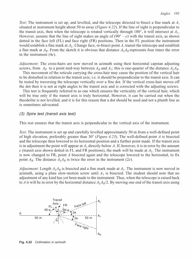
Angles 195
Test: The instrument is set up, and levelled, and the telescope directed to bisect a fine mark at A,situated at instrument height about 50 m away (Figure 4.22). If the line of sight is perpendicular tothe transit axis, then when the telescope is rotated vertically through 180°, it will intersect at A1.However, assume that the line of sight makes an angle of (90° – e) with the transit axis, as showndotted in the face left (FL) and face right (FR) positions. Then in the FL position the instrumentwould establish a fine mark at AL. Change face, re-bisect point A, transit the telescope and establisha fine mark at AR. From the sketch it is obvious that distance ALAR represents four times the errorin the instrument (4e).
Adjustment: The cross-hairs are now moved in azimuth using their horizontal capstan adjustingscrews, from AR to a point mid-way between AR and A1; this is one-quarter of the distance ALAR.
This movement of the reticule carrying the cross-hair may cause the position of the vertical hairto be disturbed in relation to the transit axis; i.e. it should be perpendicular to the transit axis. It canbe tested by traversing the telescope vertically over a fine dot. If the vertical cross-hair moves offthe dot then it is not at right angles to the transit axis and is corrected with the adjusting screws.
This test is frequently referred to as one which ensures the verticality of the vertical hair, whichwill be true only if the transit axis is truly horizontal. However, it can be carried out when thetheodolite is not levelled, and it is for this reason that a dot should be used and not a plumb line asis sometimes advocated.
(3) Spire test (transit axis test)
This test ensures that the transit axis is perpendicular to the vertical axis of the instrument.
Test: The instrument is set up and carefully levelled approximately 50 m from a well-defined pointof high elevation, preferably greater than 30° (Figure 4.23). The well-defined point A is bisectedand the telescope then lowered to its horizontal position and a further point made. If the transit axisis in adjustment the point will appear at A1 directly below A. If, however, it is in error by the amounte (transit axis shown dotted in FL and FR positions), the mark will be made at AL. The instrumentis now changed to FR, point A bisected again and the telescope lowered to the horizontal, to fixpoint AR. The distance ALAR is twice the error in the instrument (2e).
Adjustment: Length ALAR is bisected and a fine mark made at A1. The instrument is now moved inazimuth, using a plate slow-motion screw until A1 is bisected. The student should note that noadjustment of any kind has yet been made to the instrument. Thus, when the telescope is raised backto A it will be in error by the horizontal distance ALAR/2. By moving one end of the transit axis using
Fig. 4.22 Collimation in azimuth
Transit
AxisFL FR
90-e90-eFace left
2e
2e 50 m
Face right
AL
A1
AR
e50 m
A
e
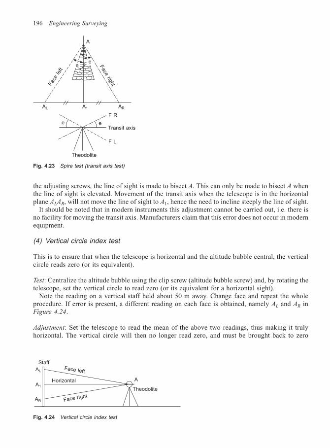
196 Engineering Surveying
the adjusting screws, the line of sight is made to bisect A. This can only be made to bisect A whenthe line of sight is elevated. Movement of the transit axis when the telescope is in the horizontalplane ALAR, will not move the line of sight to A1, hence the need to incline steeply the line of sight.
It should be noted that in modern instruments this adjustment cannot be carried out, i.e. there isno facility for moving the transit axis. Manufacturers claim that this error does not occur in modernequipment.
(4) Vertical circle index test
This is to ensure that when the telescope is horizontal and the altitude bubble central, the verticalcircle reads zero (or its equivalent).
Test: Centralize the altitude bubble using the clip screw (altitude bubble screw) and, by rotating thetelescope, set the vertical circle to read zero (or its equivalent for a horizontal sight).
Note the reading on a vertical staff held about 50 m away. Change face and repeat the wholeprocedure. If error is present, a different reading on each face is obtained, namely AL and AR inFigure 4.24.
Adjustment: Set the telescope to read the mean of the above two readings, thus making it trulyhorizontal. The vertical circle will then no longer read zero, and must be brought back to zero
A
ee
Face rightF
ace
left
AL A1 AR
F L
Transit axis
F R
Theodolite
e e
Fig. 4.23 Spire test (transit axis test)
Staff
AL
A1
AR Face right
Horizontal
Face left
A
Theodolite
Fig. 4.24 Vertical circle index test
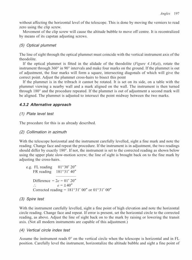
Angles 197
without affecting the horizontal level of the telescope. This is done by moving the verniers to readzero using the clip screw.
Movement of the clip screw will cause the altitude bubble to move off centre. It is recentralizedby means of its capstan adjusting screws.
(5) Optical plummet
The line of sight through the optical plummet must coincide with the vertical instrument axis of thetheodolite.
If the optical plummet is fitted in the alidade of the theodolite (Figure 4.14(a)), rotate theinstrument through 360° in 90° intervals and make four marks on the ground. If the plummet is outof adjustment, the four marks will form a square, intersecting diagonals of which will give thecorrect point. Adjust the plummet cross-hairs to bisect this point
If the plummet is in the tribrach it cannot be rotated. It is set on its side, on a table with theplummet viewing a nearby wall and a mark aligned on the wall. The instrument is then turnedthrough 180° and the procedure repeated. If the plummet is out of adjustment a second mark willbe aligned. The plummet is adjusted to intersect the point midway between the two marks.
4.3.2 Alternative approach
(1) Plate level test
The procedure for this is as already described.
(2) Collimation in azimuth
With the telescope horizontal and the instrument carefully levelled, sight a fine mark and note thereading. Change face and repeat the procedure. If the instrument is in adjustment, the two readingsshould differ by exactly 180°. If not, the instrument is set to the corrected reading as shown belowusing the upper plate slow-motion screw; the line of sight is brought back on to the fine mark byadjusting the cross-hairs.
e.g. FL reading 01°30′ 20″FR reading 181°31′ 40″
—————Difference = 2e = 01′ 20″∴ e = ± 40″Corrected reading = 181°31′ 00″ or 01°31′ 00″
(3) Spire test
With the instrument carefully levelled, sight a fine point of high elevation and note the horizontalcircle reading. Change face and repeat. If error is present, set the horizontal circle to the correctedreading, as above. Adjust the line of sight back on to the mark by raising or lowering the transitaxis. (Not all modern instruments are capable of this adjustment.)
(4) Vertical circle index test
Assume the instrument reads 0° on the vertical circle when the telescope is horizontal and in FLposition. Carefully level the instrument, horizontalize the altitude bubble and sight a fine point of
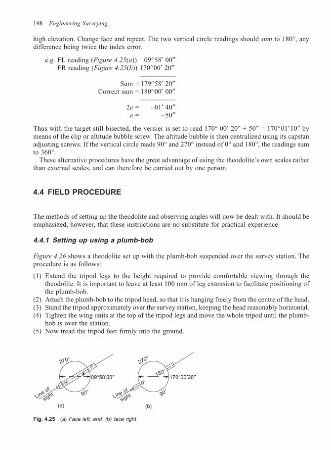
198 Engineering Surveying
high elevation. Change face and repeat. The two vertical circle readings should sum to 180°, anydifference being twice the index error.
e.g. FL reading (Figure 4.25(a)) 09°58′ 00″FR reading (Figure 4.25(b)) 170°00′ 20″
—————Sum = 179°58′ 20″
Correct sum = 180°00′ 00″—————
2e = –01′ 40″e = –50″
Thus with the target still bisected, the vernier is set to read 170° 00′ 20″ + 50″ = 170°01′10″ bymeans of the clip or altitude bubble screw. The altitude bubble is then centralized using its capstanadjusting screws. If the vertical circle reads 90° and 270° instead of 0° and 180°, the readings sumto 360°.
These alternative procedures have the great advantage of using the theodolite’s own scales ratherthan external scales, and can therefore be carried out by one person.
4.4 FIELD PROCEDURE
The methods of setting up the theodolite and observing angles will now be dealt with. It should beemphasized, however, that these instructions are no substitute for practical experience.
4.4.1 Setting up using a plumb-bob
Figure 4.26 shows a theodolite set up with the plumb-bob suspended over the survey station. Theprocedure is as follows:
(1) Extend the tripod legs to the height required to provide comfortable viewing through thetheodolite. It is important to leave at least 100 mm of leg extension to facilitate positioning ofthe plumb-bob.
(2) Attach the plumb-bob to the tripod head, so that it is hanging freely from the centre of the head.(3) Stand the tripod approximately over the survey station, keeping the head reasonably horizontal.(4) Tighten the wing units at the top of the tripod legs and move the whole tripod until the plumb-
bob is over the station.(5) Now tread the tripod feet firmly into the ground.
Fig. 4.25 (a) Face left, and (b) face right
270°0°
180°
Line of
sight 90°
(a)
09°58′00″
Line of
sight 90°
170°00′20″180°
0°
270°
(b)
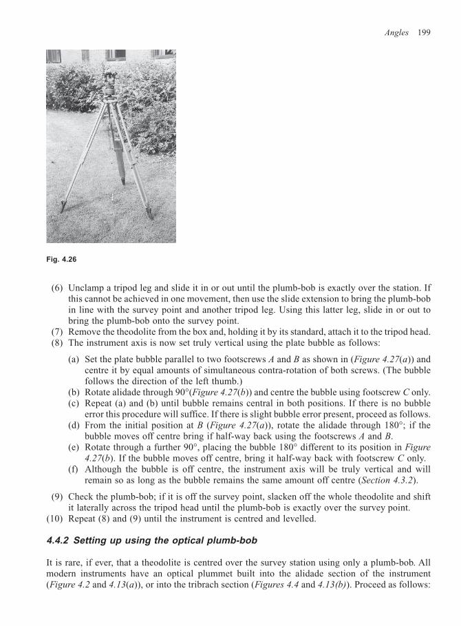
Angles 199
(6) Unclamp a tripod leg and slide it in or out until the plumb-bob is exactly over the station. Ifthis cannot be achieved in one movement, then use the slide extension to bring the plumb-bobin line with the survey point and another tripod leg. Using this latter leg, slide in or out tobring the plumb-bob onto the survey point.
(7) Remove the theodolite from the box and, holding it by its standard, attach it to the tripod head.(8) The instrument axis is now set truly vertical using the plate bubble as follows:
(a) Set the plate bubble parallel to two footscrews A and B as shown in (Figure 4.27(a)) andcentre it by equal amounts of simultaneous contra-rotation of both screws. (The bubblefollows the direction of the left thumb.)
(b) Rotate alidade through 90°(Figure 4.27(b)) and centre the bubble using footscrew C only.(c) Repeat (a) and (b) until bubble remains central in both positions. If there is no bubble
error this procedure will suffice. If there is slight bubble error present, proceed as follows.(d) From the initial position at B (Figure 4.27(a)), rotate the alidade through 180°; if the
bubble moves off centre bring if half-way back using the footscrews A and B.(e) Rotate through a further 90°, placing the bubble 180° different to its position in Figure
4.27(b). If the bubble moves off centre, bring it half-way back with footscrew C only.(f) Although the bubble is off centre, the instrument axis will be truly vertical and will
remain so as long as the bubble remains the same amount off centre (Section 4.3.2).
(9) Check the plumb-bob; if it is off the survey point, slacken off the whole theodolite and shiftit laterally across the tripod head until the plumb-bob is exactly over the survey point.
(10) Repeat (8) and (9) until the instrument is centred and levelled.
4.4.2 Setting up using the optical plumb-bob
It is rare, if ever, that a theodolite is centred over the survey station using only a plumb-bob. Allmodern instruments have an optical plummet built into the alidade section of the instrument(Figure 4.2 and 4.13(a)), or into the tribrach section (Figures 4.4 and 4.13(b)). Proceed as follows:
Fig. 4.26
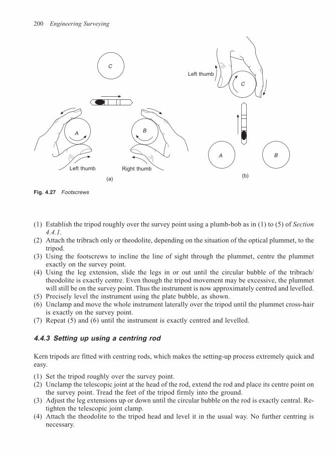
200 Engineering Surveying
(1) Establish the tripod roughly over the survey point using a plumb-bob as in (1) to (5) of Section
4.4.1.(2) Attach the tribrach only or theodolite, depending on the situation of the optical plummet, to the
tripod.(3) Using the footscrews to incline the line of sight through the plummet, centre the plummet
exactly on the survey point.(4) Using the leg extension, slide the legs in or out until the circular bubble of the tribrach/
theodolite is exactly centre. Even though the tripod movement may be excessive, the plummetwill still be on the survey point. Thus the instrument is now approximately centred and levelled.
(5) Precisely level the instrument using the plate bubble, as shown.(6) Unclamp and move the whole instrument laterally over the tripod until the plummet cross-hair
is exactly on the survey point.(7) Repeat (5) and (6) until the instrument is exactly centred and levelled.
4.4.3 Setting up using a centring rod
Kern tripods are fitted with centring rods, which makes the setting-up process extremely quick andeasy.
(1) Set the tripod roughly over the survey point.(2) Unclamp the telescopic joint at the head of the rod, extend the rod and place its centre point on
the survey point. Tread the feet of the tripod firmly into the ground.(3) Adjust the leg extensions up or down until the circular bubble on the rod is exactly central. Re-
tighten the telescopic joint clamp.(4) Attach the theodolite to the tripod head and level it in the usual way. No further centring is
necessary.
Fig. 4.27 Footscrews
C
C
Left thumb
A B
(b)
B
Right thumbLeft thumb
A
(a)
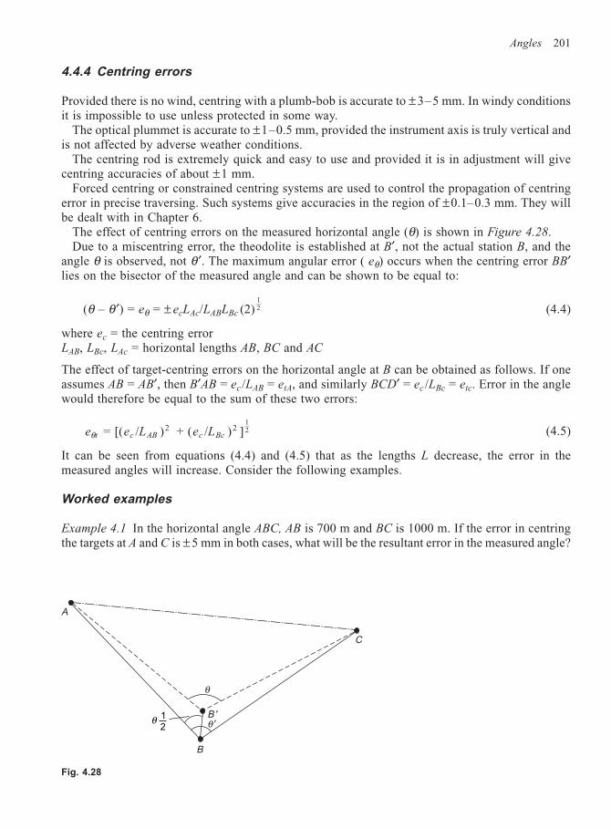
Angles 201
4.4.4 Centring errors
Provided there is no wind, centring with a plumb-bob is accurate to ± 3–5 mm. In windy conditionsit is impossible to use unless protected in some way.
The optical plummet is accurate to ±1–0.5 mm, provided the instrument axis is truly vertical andis not affected by adverse weather conditions.
The centring rod is extremely quick and easy to use and provided it is in adjustment will givecentring accuracies of about ±1 mm.
Forced centring or constrained centring systems are used to control the propagation of centringerror in precise traversing. Such systems give accuracies in the region of ±0.1–0.3 mm. They willbe dealt with in Chapter 6.
The effect of centring errors on the measured horizontal angle (θ) is shown in Figure 4.28.Due to a miscentring error, the theodolite is established at B′, not the actual station B, and the
angle θ is observed, not θ′. The maximum angular error ( eθ) occurs when the centring error BB′lies on the bisector of the measured angle and can be shown to be equal to:
(θ – θ ′) = eθ = ± ecLAc/LABLBc (2)12 (4.4)
where ec = the centring errorLAB, LBc, LAc = horizontal lengths AB, BC and AC
The effect of target-centring errors on the horizontal angle at B can be obtained as follows. If oneassumes AB = AB′, then B′AB = ec /LAB = etA, and similarly BCD′ = ec /LBc = etc. Error in the anglewould therefore be equal to the sum of these two errors:
e e L e Lt c AB c Bcθ = [( / ) + ( / ) ]2 212 (4.5)
It can be seen from equations (4.4) and (4.5) that as the lengths L decrease, the error in themeasured angles will increase. Consider the following examples.
Worked examples
Example 4.1 In the horizontal angle ABC, AB is 700 m and BC is 1000 m. If the error in centringthe targets at A and C is ± 5 mm in both cases, what will be the resultant error in the measured angle?
Fig. 4.28
A
C
θ
B
B ′θ ′θ 1
2
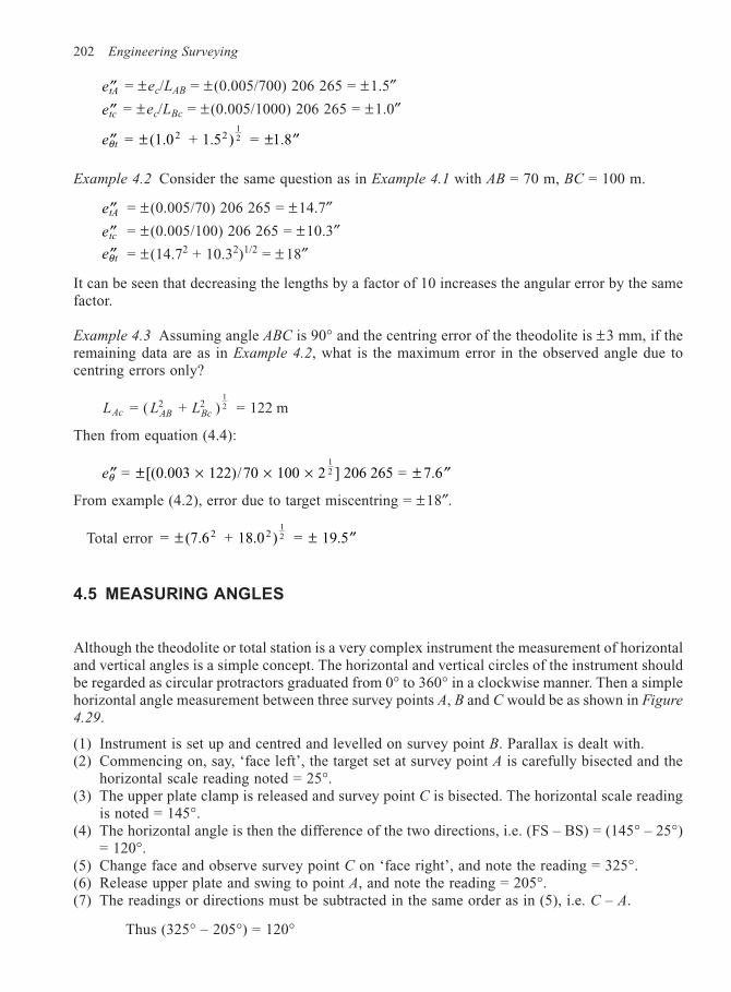
202 Engineering Surveying
′′etA = ±ec/LAB = ± (0.005/700) 206 265 = ±1.5″
′′etc = ±ec/LBc = ± (0.005/1000) 206 265 = ±1.0″
′′ ± ± ′′e tθ = (1.0 + 1.5 ) = 1.82 212
Example 4.2 Consider the same question as in Example 4.1 with AB = 70 m, BC = 100 m.
′′etA = ± (0.005/70) 206 265 = ±14.7″
′′etc = ± (0.005/100) 206 265 = ±10.3″′′e tθ = ± (14.72 + 10.32)1/2 = ± 18″
It can be seen that decreasing the lengths by a factor of 10 increases the angular error by the samefactor.
Example 4.3 Assuming angle ABC is 90° and the centring error of the theodolite is ±3 mm, if theremaining data are as in Example 4.2, what is the maximum error in the observed angle due tocentring errors only?
L L LAc AB Bc = ( + ) = 122 m2 212
Then from equation (4.4):
′′ ± × × × ± ′′eθ = [(0.003 122)/70 100 2 ] 206 265 = 7.612
From example (4.2), error due to target miscentring = ±18″.
Total error = (7.6 + 18.0 ) = 19.52 212± ± ′′
4.5 MEASURING ANGLES
Although the theodolite or total station is a very complex instrument the measurement of horizontaland vertical angles is a simple concept. The horizontal and vertical circles of the instrument shouldbe regarded as circular protractors graduated from 0° to 360° in a clockwise manner. Then a simplehorizontal angle measurement between three survey points A, B and C would be as shown in Figure
4.29.
(1) Instrument is set up and centred and levelled on survey point B. Parallax is dealt with.(2) Commencing on, say, ‘face left’, the target set at survey point A is carefully bisected and the
horizontal scale reading noted = 25°.(3) The upper plate clamp is released and survey point C is bisected. The horizontal scale reading
is noted = 145°.(4) The horizontal angle is then the difference of the two directions, i.e. (FS – BS) = (145° – 25°)
= 120°.(5) Change face and observe survey point C on ‘face right’, and note the reading = 325°.(6) Release upper plate and swing to point A, and note the reading = 205°.(7) The readings or directions must be subtracted in the same order as in (5), i.e. C – A.
Thus (325° – 205°) = 120°
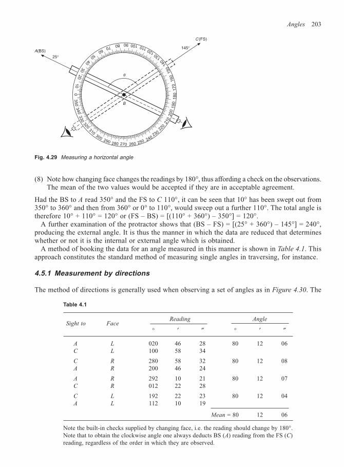
Angles 203
(8) Note how changing face changes the readings by 180°, thus affording a check on the observations.The mean of the two values would be accepted if they are in acceptable agreement.
Had the BS to A read 350° and the FS to C 110°, it can be seen that 10° has been swept out from350° to 360° and then from 360° or 0° to 110°, would sweep out a further 110°. The total angle istherefore 10° + 110° = 120° or (FS – BS) = [(110° + 360°) – 350°] = 120°.
A further examination of the protractor shows that (BS – FS) = [(25° + 360°) – 145°] = 240°,producing the external angle. It is thus the manner in which the data are reduced that determineswhether or not it is the internal or external angle which is obtained.
A method of booking the data for an angle measured in this manner is shown in Table 4.1. Thisapproach constitutes the standard method of measuring single angles in traversing, for instance.
4.5.1 Measurement by directions
The method of directions is generally used when observing a set of angles as in Figure 4.30. The
A(BS)
25°
C (FS)
145°
190
18
0170
20
10
0
350
340
330
320
310300
290 280 270 260
210
220
230
240
250
θ
B
200
160
150
140
130120
110100908070
4030
50
60
Fig. 4.29 Measuring a horizontal angle
Table 4.1
Reading Angle
° ′ ″ ° ′ ″
A L 020 46 28 80 12 06C L 100 58 34
C R 280 58 32 80 12 08A R 200 46 24
A R 292 10 21 80 12 07C R 012 22 28
C L 192 22 23 80 12 04A L 112 10 19
Mean = 80 12 06
Note the built-in checks supplied by changing face, i.e. the reading should change by 180°.Note that to obtain the clockwise angle one always deducts BS (A) reading from the FS (C)reading, regardless of the order in which they are observed.
Sight to Face
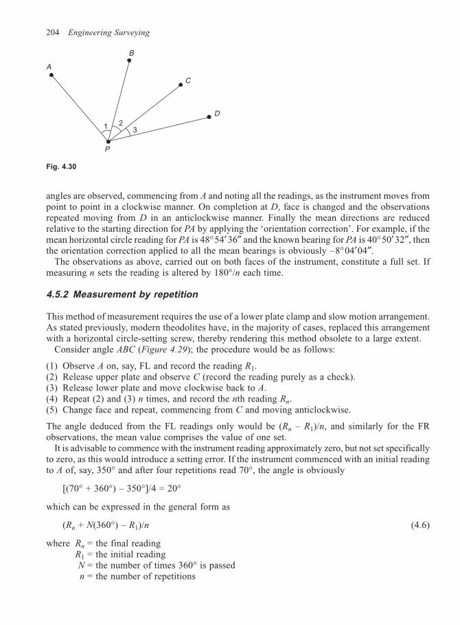
204 Engineering Surveying
angles are observed, commencing from A and noting all the readings, as the instrument moves frompoint to point in a clockwise manner. On completion at D, face is changed and the observationsrepeated moving from D in an anticlockwise manner. Finally the mean directions are reducedrelative to the starting direction for PA by applying the ‘orientation correction’. For example, if themean horizontal circle reading for PA is 48°54′36″ and the known bearing for PA is 40°50′32″, thenthe orientation correction applied to all the mean bearings is obviously –8°04′04″.
The observations as above, carried out on both faces of the instrument, constitute a full set. Ifmeasuring n sets the reading is altered by 180°/n each time.
4.5.2 Measurement by repetition
This method of measurement requires the use of a lower plate clamp and slow motion arrangement.As stated previously, modern theodolites have, in the majority of cases, replaced this arrangementwith a horizontal circle-setting screw, thereby rendering this method obsolete to a large extent.
Consider angle ABC (Figure 4.29); the procedure would be as follows:
(1) Observe A on, say, FL and record the reading R1.(2) Release upper plate and observe C (record the reading purely as a check).(3) Release lower plate and move clockwise back to A.(4) Repeat (2) and (3) n times, and record the nth reading Rn.(5) Change face and repeat, commencing from C and moving anticlockwise.
The angle deduced from the FL readings only would be (Rn – R1)/n, and similarly for the FRobservations, the mean value comprises the value of one set.
It is advisable to commence with the instrument reading approximately zero, but not set specificallyto zero, as this would introduce a setting error. If the instrument commenced with an initial readingto A of, say, 350° and after four repetitions read 70°, the angle is obviously
[(70° + 360°) – 350°]/4 = 20°
which can be expressed in the general form as
(Rn + N(360°) – R1)/n (4.6)
where Rn = the final readingR1 = the initial readingN = the number of times 360° is passedn = the number of repetitions
A
P
1 23
D
C
B
Fig. 4.30
Angles 205
4.5.3 Comparison of the methods
The basic errors in the observation of an angle are ‘pointing’ error and ‘reading’ error, both ofwhich are affected by a variety of factors.
Observing an angle by the method of direction involves two pointings and two readings persingle face. Thus we have
σ σ σθ2
p2
R2 = 2 + 2 (4.7)
where σ p2 = the pointing variance
σ R2 = the reading variance
σ θ2 = the resulting angle variance
For the mean of n such angles:
σσ σ
θM n n2 p
2R2
= 2
+ 2
(4.8)
Considering repetition measurement, if θ is measured n times (n/2 on each face) we have 2n
pointings but only 2 readings. The variance of the sum of the observations is
σ σ σθ2
p2
R2 = 2 + 2n (4.9)
and the variance of the mean of n repetitions is
σσ σ
θM n n2 p
2R2
2 =
2 +
2(4.10)
Comparison of equations (4.8) and (4.10) shows the method of repetition to be more accurate as thereading error is reduced by n2 compared with n. This is particularly significant for instrumentswhich have a large least count. Their performance would be significantly improved by the methodof repetition. However, as previously stated, most instruments are direction theodolites, as theylack the lower plate clamping facility.
4.5.4 Further considerations in angular measurement
Considering Figure 4.30, the angles may be measured by ‘closing the horizon’. This involvesobserving the points in order from A to D and continuing clockwise back to A, thereby completingthe full circle. The difference between the sum of all the angles and 360° is distributed evenlyamongst all the angles to bring their sum to 360°. Repeat anticlockwise on the opposite face.
A method favoured in the measurement of precise networks is to measure all the combinations ofangles. In the case above it would involve measuring APB, APC, APD, BPC, BPD and CPD. Theangles could then be resolved by forming condition equations in a least squares solution (seeChapter 7).
4.5.5 Vertical angles
In the measurement of horizontal angles the concept is of a measuring index moving around aprotractor. In the case of a vertical angle, the situation is reversed and the protractor moves relativeto a fixed horizontal index.
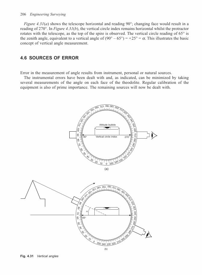
206 Engineering Surveying
Figure 4.31(a) shows the telescope horizontal and reading 90°; changing face would result in areading of 270°. In Figure 4.31(b), the vertical circle index remains horizontal whilst the protractorrotates with the telescope, as the top of the spire is observed. The vertical circle reading of 65° isthe zenith angle, equivalent to a vertical angle of (90° – 65°) = +25° = α. This illustrates the basicconcept of vertical angle measurement.
4.6 SOURCES OF ERROR
Error in the measurement of angle results from instrument, personal or natural sources.The instrumental errors have been dealt with and, as indicated, can be minimized by taking
several measurements of the angle on each face of the theodolite. Regular calibration of theequipment is also of prime importance. The remaining sources will now be dealt with.
Fig. 4.31 Vertical angles
Altitude bubble
Vertical circle index 270°
(a)
90
90°
80
70
50
60
4030
2010 0 350 340 330
320
310
300
290
280
27
0260
250
240
230
220210200190180170160
150140
130120
110
10
0
0350 340 330 320 310
300290
280
270
260
25
02
40
230
220
210
200
190180
170160150140
120
130
110100
90
80
70
60
50
40
30
2010
65°
α
(b)
Angles 207
4.6.1 Personal error
(1) Careless centring of the instrument over the survey point. Always ensure that the opticalplummet or centring rod is in adjustment. Similarly for the targets.
(2) Light clamping of the horizontal and vertical movement. Hard clamping can affect the pointingand is unnecessary.
(3) The final movement of the slow motion screws should be clockwise, thus producing a positivemovement against the spring. An anticlockwise movement which releases the spring may causebacklash.
(4) Failure to eliminate parallax and poor focusing on the target can affect accurate pointing. Keepthe observed target near the centre of the field of view.
(5) Incorrect levelling of the altitude bubble will produce vertical angle error.(6) The plate bubble must also be carefully levelled and regularly checked throughout the measuring
process.(7) Make quick, decisive observations. Too much care can be counterproductive.(8) All movement of the theodolite should be done gently whilst movement around the tripod
should be reduced to a minimum.
4.6.2 Natural errors
(1) Wind vibration may require some form of wind shield to be erected to protect the instrument.Dual axis tilt sensors in modern total stations have greatly minimized this effect.
(2) Vertical and lateral refraction of the line of sight is always a problem. The effect on the verticalangle has already been discussed in Chapter 2. Lateral refraction, particularly in tunnels, cancause excessive error in the horizontal angle. A practical solution in tunnels is to use zig-zagtraverses with frequent gyro-theodolite azimuths included.
(3) Temperature differentials can cause unequal expansion of the various parts of the instrument.Plate bubbles will move off centre towards the hottest part of the bubble tube. Heat shimmermay make accurate pointing impossible. Sheltering the instrument by means of a large surveyumbrella will greatly help in this situation.
(4) Avoid tripod settlement by careful selection of ground conditions. If necessary use pegs to pilethe ground on which the tripod feet are set.
All the above procedures should be included in a pre-set survey routine, which should be strictlyadhered to. Inexperienced observers should guard against such common mistakes as:
(1) Turning the wrong screw.(2) Sighting the wrong target.(3) Using the stadia instead of the cross-hair.(4) Forgetting to set the micrometer.(5) Misreading the circles.(6) Transposing figures when booking the data.
5
Position
5.1 INTRODUCTION
Engineering surveying is concerned essentially with fixing the position of a point in two or threedimensions.
For example, in the production of a plan or map, one is concerned in the first instance with theaccurate location of the relative position of survey points forming a framework, from which theposition of topographic detail is fixed. Such a framework of points is referred to as a controlnetwork.
The same network used to locate topographic detail may also be used to set out points, definingthe position, size and shape of the designed elements of the construction project.
Precise control networks are also used in the monitoring of deformation movements on all typesof structures.
In all these situations the engineer is concerned with relative position, to varying degress ofaccuracy and over areas of varying extent. In order to define position to the high accuraciesrequired in engineering surveying, a suitable homogeneous coordinate system and reference datummust be adopted.
Consideration of Figure 5.1 illustrates that if the area under consideration is of limited extent, theorthogonal projection of AB onto a plane surface may result in negligible distortion. Plane surveyingtechniques could be used to capture field data and plane trigonometry used to compute position.This is the case in the majority of engineering surveys. However, if the area extended from C to D,the effect of the Earth’s curvature is such as to produce unacceptable distortion if treated as a flatsurface. It can also be clearly seen that the use of a plane surface as a reference datum for theelevations of points is totally unacceptable.
If Figure 5.2 is now considered, it can be seen that projecting CD onto a surface (cd) that was thesame shape and parallel to CD would be more acceptable. Further, if that surface was broughtcloser to CD, say c′d′, the distortion would be even less. This then is the problem of the geodeticsurveyor: that of defining a mathematical surface that approximates to the shape of the area underconsideration and then fitting and orientating it to the Earth’s surface. Such a surface is referred toin surveying as a ‘reference ellipsoid’.
5.2 REFERENCE ELLIPSOID
To arrive at the concept of a reference ellipsoid, the various surfaces involved must bereviewed.
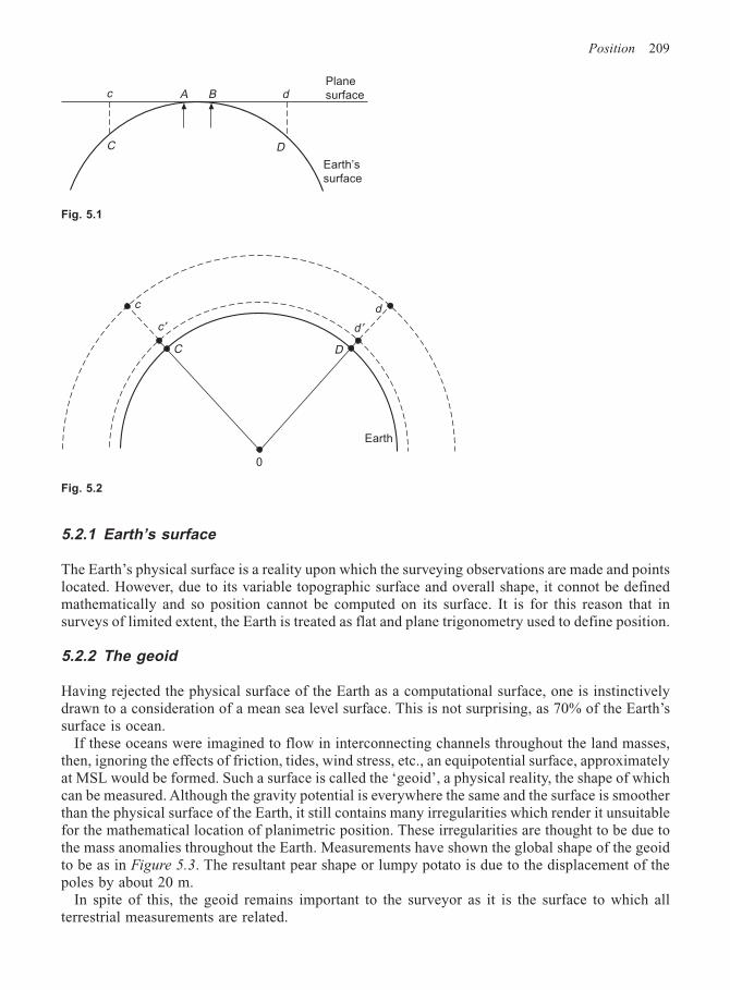
Position 209
5.2.1 Earth’s surface
The Earth’s physical surface is a reality upon which the surveying observations are made and pointslocated. However, due to its variable topographic surface and overall shape, it connot be definedmathematically and so position cannot be computed on its surface. It is for this reason that insurveys of limited extent, the Earth is treated as flat and plane trigonometry used to define position.
5.2.2 The geoid
Having rejected the physical surface of the Earth as a computational surface, one is instinctivelydrawn to a consideration of a mean sea level surface. This is not surprising, as 70% of the Earth’ssurface is ocean.
If these oceans were imagined to flow in interconnecting channels throughout the land masses,then, ignoring the effects of friction, tides, wind stress, etc., an equipotential surface, approximatelyat MSL would be formed. Such a surface is called the ‘geoid’, a physical reality, the shape of whichcan be measured. Although the gravity potential is everywhere the same and the surface is smootherthan the physical surface of the Earth, it still contains many irregularities which render it unsuitablefor the mathematical location of planimetric position. These irregularities are thought to be due tothe mass anomalies throughout the Earth. Measurements have shown the global shape of the geoidto be as in Figure 5.3. The resultant pear shape or lumpy potato is due to the displacement of thepoles by about 20 m.
In spite of this, the geoid remains important to the surveyor as it is the surface to which allterrestrial measurements are related.
Fig. 5.1
Fig. 5.2
c
C
BA
D
dPlane
surface
Earth’s
surface
c
c ′
C
d ′
d
D
0
Earth
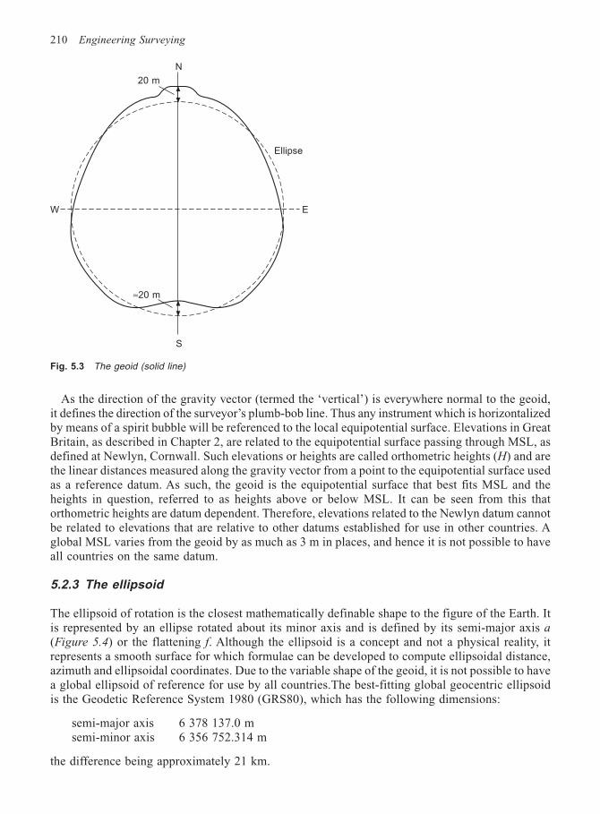
210 Engineering Surveying
As the direction of the gravity vector (termed the ‘vertical’) is everywhere normal to the geoid,it defines the direction of the surveyor’s plumb-bob line. Thus any instrument which is horizontalizedby means of a spirit bubble will be referenced to the local equipotential surface. Elevations in GreatBritain, as described in Chapter 2, are related to the equipotential surface passing through MSL, asdefined at Newlyn, Cornwall. Such elevations or heights are called orthometric heights (H) and arethe linear distances measured along the gravity vector from a point to the equipotential surface usedas a reference datum. As such, the geoid is the equipotential surface that best fits MSL and theheights in question, referred to as heights above or below MSL. It can be seen from this thatorthometric heights are datum dependent. Therefore, elevations related to the Newlyn datum cannotbe related to elevations that are relative to other datums established for use in other countries. Aglobal MSL varies from the geoid by as much as 3 m in places, and hence it is not possible to haveall countries on the same datum.
5.2.3 The ellipsoid
The ellipsoid of rotation is the closest mathematically definable shape to the figure of the Earth. Itis represented by an ellipse rotated about its minor axis and is defined by its semi-major axis a(Figure 5.4) or the flattening f. Although the ellipsoid is a concept and not a physical reality, itrepresents a smooth surface for which formulae can be developed to compute ellipsoidal distance,azimuth and ellipsoidal coordinates. Due to the variable shape of the geoid, it is not possible to havea global ellipsoid of reference for use by all countries.The best-fitting global geocentric ellipsoidis the Geodetic Reference System 1980 (GRS80), which has the following dimensions:
semi-major axis 6 378 137.0 msemi-minor axis 6 356 752.314 m
the difference being approximately 21 km.
Fig. 5.3 The geoid (solid line)
N
20 m
W
S
E
≈20 m
Ellipse
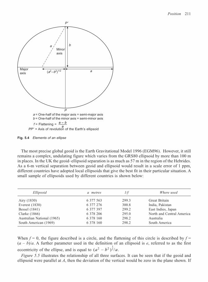
Position 211
The most precise global geoid is the Earth Gravitational Model 1996 (EGM96). However, it stillremains a complex, undulating figure which varies from the GRS80 ellipsoid by more than 100 min places. In the UK the geoid–ellipsoid separation is as much as 57 m in the region of the Hebrides.As a 6-m vertical separation between geoid and ellipsoid would result in a scale error of 1 ppm,different countries have adopted local ellipsoids that give the best fit in their particular situation. Asmall sample of ellipsoids used by different countries is shown below:
Ellipsoid a metres 1/f Where used
Airy (1830) 6 377 563 299.3 Great BritainEverest (1830) 6 377 276 300.8 India, PakistanBessel (1841) 6 377 397 299.2 East Indies, JapanClarke (1866) 6 378 206 295.0 North and Central AmericaAustralian National (1965) 6 378 160 298.2 AustraliaSouth American (1969) 6 378 160 298.2 South America
When f = 0, the figure described is a circle, and the flattening of this circle is described by f =(a – b)/a. A further parameter used in the definition of an ellipsoid is e, referred to as the first
eccentricity of the ellipse, and is equal to ( – ) /2 212a b a .
Figure 5.5 illustrates the relationship of all three surfaces. It can be seen that if the geoid andellipsoid were parallel at A, then the deviation of the vertical would be zero in the plane shown. If
Fig. 5.4 Elements of an ellipse
P ′
baMinor
axis
Major
axis (a2–b2)1/2 a
P
a = One-half of the major axis = semi-major axis
b = One-half of the minor axis = semi-minor axis
f = Flattening = a b
a
–
PP ′ = Axis of revolution of the Earth’s ellipsoid
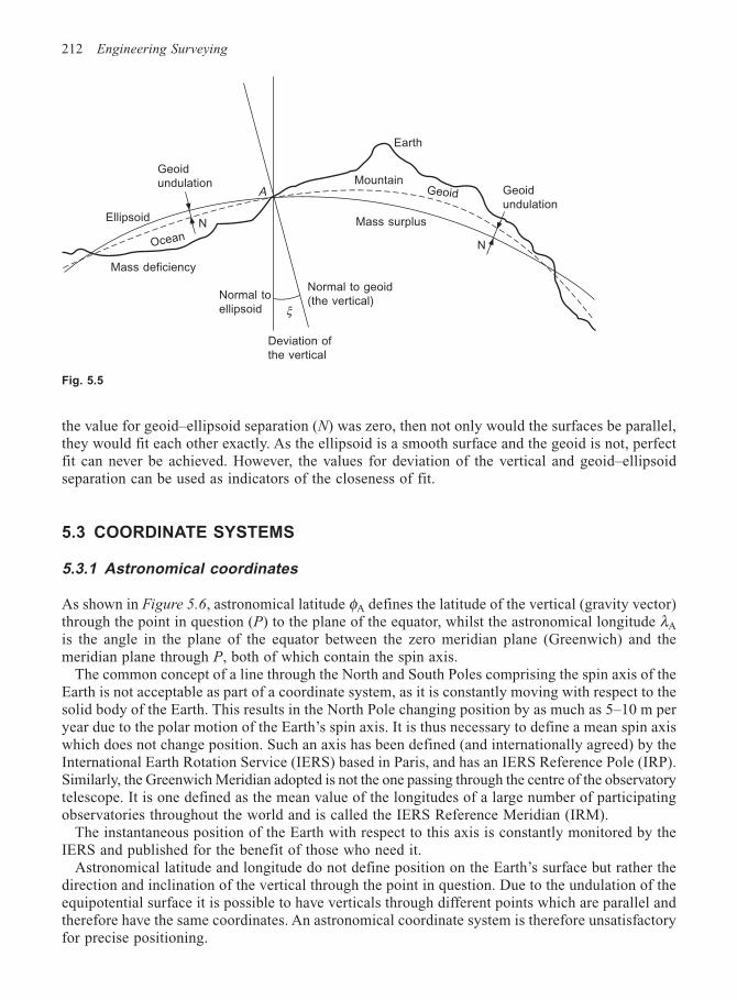
212 Engineering Surveying
the value for geoid–ellipsoid separation (N) was zero, then not only would the surfaces be parallel,they would fit each other exactly. As the ellipsoid is a smooth surface and the geoid is not, perfectfit can never be achieved. However, the values for deviation of the vertical and geoid–ellipsoidseparation can be used as indicators of the closeness of fit.
5.3 COORDINATE SYSTEMS
5.3.1 Astronomical coordinates
As shown in Figure 5.6, astronomical latitude φA defines the latitude of the vertical (gravity vector)through the point in question (P) to the plane of the equator, whilst the astronomical longitude λA
is the angle in the plane of the equator between the zero meridian plane (Greenwich) and themeridian plane through P, both of which contain the spin axis.
The common concept of a line through the North and South Poles comprising the spin axis of theEarth is not acceptable as part of a coordinate system, as it is constantly moving with respect to thesolid body of the Earth. This results in the North Pole changing position by as much as 5–10 m peryear due to the polar motion of the Earth’s spin axis. It is thus necessary to define a mean spin axiswhich does not change position. Such an axis has been defined (and internationally agreed) by theInternational Earth Rotation Service (IERS) based in Paris, and has an IERS Reference Pole (IRP).Similarly, the Greenwich Meridian adopted is not the one passing through the centre of the observatorytelescope. It is one defined as the mean value of the longitudes of a large number of participatingobservatories throughout the world and is called the IERS Reference Meridian (IRM).
The instantaneous position of the Earth with respect to this axis is constantly monitored by theIERS and published for the benefit of those who need it.
Astronomical latitude and longitude do not define position on the Earth’s surface but rather thedirection and inclination of the vertical through the point in question. Due to the undulation of theequipotential surface it is possible to have verticals through different points which are parallel andtherefore have the same coordinates. An astronomical coordinate system is therefore unsatisfactoryfor precise positioning.
Fig. 5.5
Geoid
undulation
N
A
Ocean
Ellipsoid
Mass deficiency
Normal to
ellipsoid
Deviation of
the vertical
ξ
Normal to geoid
(the vertical)
Mass surplus
Geoid
undulation
Earth
Mountain
N
Geoid
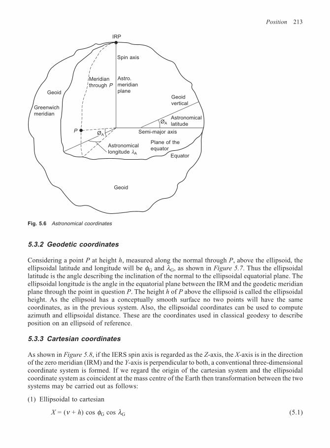
Position 213
5.3.2 Geodetic coordinates
Considering a point P at height h, measured along the normal through P, above the ellipsoid, theellipsoidal latitude and longitude will be φG and λG, as shown in Figure 5.7. Thus the ellipsoidallatitude is the angle describing the inclination of the normal to the ellipsoidal equatorial plane. Theellipsoidal longitude is the angle in the equatorial plane between the IRM and the geodetic meridianplane through the point in question P. The height h of P above the ellipsoid is called the ellipsoidalheight. As the ellipsoid has a conceptually smooth surface no two points will have the samecoordinates, as in the previous system. Also, the ellipsoidal coordinates can be used to computeazimuth and ellipsoidal distance. These are the coordinates used in classical geodesy to describeposition on an ellipsoid of reference.
5.3.3 Cartesian coordinates
As shown in Figure 5.8, if the IERS spin axis is regarded as the Z-axis, the X-axis is in the directionof the zero meridian (IRM) and the Y-axis is perpendicular to both, a conventional three-dimensionalcoordinate system is formed. If we regard the origin of the cartesian system and the ellipsoidalcoordinate system as coincident at the mass centre of the Earth then transformation between the twosystems may be carried out as follows:
(1) Ellipsoidal to cartesian
X = (ν + h) cos φG cos λG (5.1)
Fig. 5.6 Astronomical coordinates
IRP
Spin axis
Astro.
meridian
plane
Meridian
through P
Geoid
Greenwich
meridian
P ØA
Astronomical
longitude λA
Geoid
Equator
Plane of the
equator
Semi-major axis
Astronomical
latitudeØA
Geoid
vertical
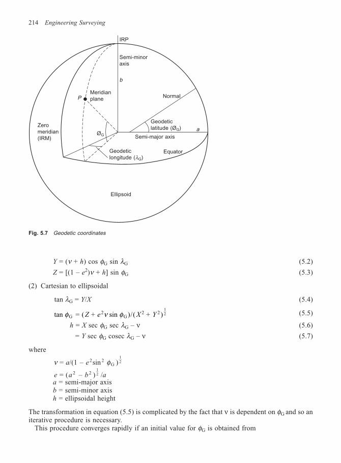
214 Engineering Surveying
Y = (ν + h) cos φG sin λG (5.2)
Z = [(1 – e2)ν + h] sin φG (5.3)
(2) Cartesian to ellipsoidal
tan λG = Y/X (5.4)
tan = ( + sin )/( + )G2
G2 2
12φ ν φZ e X Y (5.5)
h = X sec φG sec λG – ν (5.6)
= Y sec φG cosec λG – ν (5.7)
where
ν φ = /(1 – sin )2 2G
12a e
e a b a = ( – ) /2 212
a = semi-major axisb = semi-minor axish = ellipsoidal height
The transformation in equation (5.5) is complicated by the fact that ν is dependent on φG and so aniterative procedure is necessary.
This procedure converges rapidly if an initial value for φG is obtained from
IRP
Semi-minor
axis
b
NormalMeridian
planeP
ØG
Zero
meridian
(IRM)
Geodetic
longitude (λG)Equator
Semi-major axis
Geodetic
latitude (ØG) a
Ellipsoid
Fig. 5.7 Geodetic coordinates
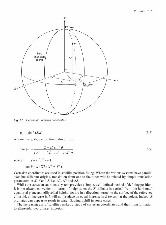
Position 215
φG = sin–1 (Z/a) (5.8)
Alternatively, φG can be found direct from
tan = + sin
( + ) – cos G
3
2 2 2 312
φ ε θ
θ
Z b
X Y e a
(5.9)
where ε = (a2/b2) – 1
tan = / ( + )2 212θ a Z b X Y⋅
Cartesian coordinates are used in satellite position fixing. Where the various systems have parallelaxes but different origins, translation from one to the other will be related by simple translationparameters in X, Y and Z, i.e. ∆X, ∆Y and ∆Z.
Whilst the cartesian coordinate system provides a simple, well-defined method of defining position,it is not always convenient in terms of heights. As the Z ordinate is vertical from the horizontalequatorial plane and ellipsoidal heights (h) are in a direction normal to the surface of the referenceellipsoid, an increase in h will not produce an equal increase in Z (except at the poles). Indeed, Zordinates can appear to result in water flowing uphill in some cases.
The increasing use of satellites makes a study of cartesian coordinates and their transformationto ellipsoidal coordinates important.
Z
IR pole
P
Zp
YpXp Y
Equator
X
Fig. 5.8 Geocentric cartesian coordinates
Zero
meridian
(IRM)
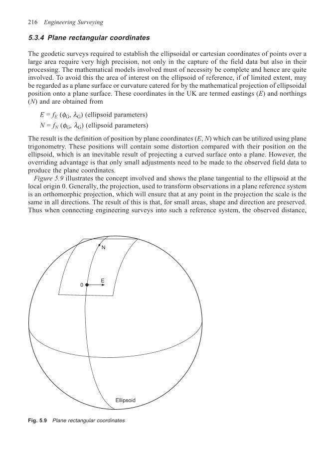
216 Engineering Surveying
5.3.4 Plane rectangular coordinates
The geodetic surveys required to establish the ellipsoidal or cartesian coordinates of points over alarge area require very high precision, not only in the capture of the field data but also in theirprocessing. The mathematical models involved must of necessity be complete and hence are quiteinvolved. To avoid this the area of interest on the ellipsoid of reference, if of limited extent, maybe regarded as a plane surface or curvature catered for by the mathematical projection of ellipsoidalposition onto a plane surface. These coordinates in the UK are termed eastings (E) and northings(N) and are obtained from
E = fE (φG, λG) (ellipsoid parameters)
N = fN (φG, λG) (ellipsoid parameters)
The result is the definition of position by plane coordinates (E, N) which can be utilized using planetrigonometry. These positions will contain some distortion compared with their position on theellipsoid, which is an inevitable result of projecting a curved surface onto a plane. However, theoverriding advantage is that only small adjustments need to be made to the observed field data toproduce the plane coordinates.
Figure 5.9 illustrates the concept involved and shows the plane tangential to the ellipsoid at thelocal origin 0. Generally, the projection, used to transform observations in a plane reference systemis an orthomorphic projection, which will ensure that at any point in the projection the scale is thesame in all directions. The result of this is that, for small areas, shape and direction are preserved.Thus when connecting engineering surveys into such a reference system, the observed distance,
0E
N
Ellipsoid
Fig. 5.9 Plane rectangular coordinates
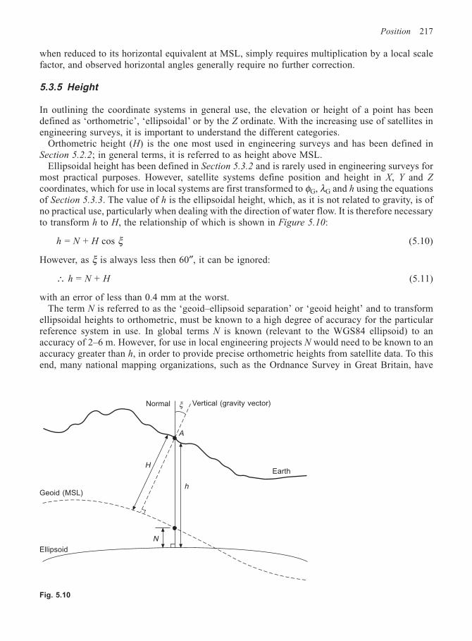
Position 217
when reduced to its horizontal equivalent at MSL, simply requires multiplication by a local scalefactor, and observed horizontal angles generally require no further correction.
5.3.5 Height
In outlining the coordinate systems in general use, the elevation or height of a point has beendefined as ‘orthometric’, ‘ellipsoidal’ or by the Z ordinate. With the increasing use of satellites inengineering surveys, it is important to understand the different categories.
Orthometric height (H) is the one most used in engineering surveys and has been defined inSection 5.2.2; in general terms, it is referred to as height above MSL.
Ellipsoidal height has been defined in Section 5.3.2 and is rarely used in engineering surveys formost practical purposes. However, satellite systems define position and height in X, Y and Z
coordinates, which for use in local systems are first transformed to φG, λG and h using the equationsof Section 5.3.3. The value of h is the ellipsoidal height, which, as it is not related to gravity, is ofno practical use, particularly when dealing with the direction of water flow. It is therefore necessaryto transform h to H, the relationship of which is shown in Figure 5.10:
h = N + H cos ξ (5.10)
However, as ξ is always less then 60″, it can be ignored:
∴ h = N + H (5.11)
with an error of less than 0.4 mm at the worst.The term N is referred to as the ‘geoid–ellipsoid separation’ or ‘geoid height’ and to transform
ellipsoidal heights to orthometric, must be known to a high degree of accuracy for the particularreference system in use. In global terms N is known (relevant to the WGS84 ellipsoid) to anaccuracy of 2–6 m. However, for use in local engineering projects N would need to be known to anaccuracy greater than h, in order to provide precise orthometric heights from satellite data. To thisend, many national mapping organizations, such as the Ordnance Survey in Great Britain, have
Fig. 5.10
Normal Vertical (gravity vector)ξ
A
h
HEarth
N
Geoid (MSL)
Ellipsoid
218 Engineering Surveying
carried out extensive work to produce an accurate model of the geoid and its relationship to thelocal ellipsoid.
5.4 LOCAL SYSTEMS
The many systems established by various countries throughout the world for positioning on andmapping of the Earth’s surface are astrogeodetic systems. Such systems have endeavoured to usereference ellipsoids which most closely fit the geoid of that area and are defined by the followingeight parameters:
(1) The size and shape of the ellipsoid, defined by the semi-major axis a, and one other chosenfrom the semi-minor axis b or the flattening f or the eccentricity e (2 parameters).
(2) The minor axis of the ellipsoid is orientated parallel to the mean spin axis of the Earth asdefined by IERS (2 parameters).
(3) The centre of the ellipsoid is implicitly defined with respect to the mass centre of the Earth, bychoice of geodetic latitude, longitude and ellipsoidal height at the origin of the system(3 parameters).
(4) The zero meridian or X-axis of the system is chosen to be parallel to the mean (Greenwich)meridian, as defined by the IERS (1 parameter).
It follows that all properly defined geodetic systems will have their axes parallel and can be relatedto each other by simple translations in X, Y and Z.
The goodness of fit can be indicated by an examination of values for the deviation of the vertical(ξ) and geoid–ellipsoid separation (N), as indicated in Figure 5.5. Considering a meridianal sectionthrough the geoid–ellipsoid (Figure 5.11), it is obvious that the north–south component of thedeviation of the vertical is a function of the ellipsoidal latitude (φG) and astronomical latitude (φA),i.e.
ξ = φA – φG (5.12)
The deviation of the vertical in the east-west direction (prime vertical) is
η = (λA – λG) cos φ (5.13)
where φ is φA or φG, the difference being negligible. It can be shown that the deviation in anyazimuth α is given by
ψ = –(ξ cos α + η sin α) (5.14)
whilst at 90° to α the deviation is
ζ = (ξ sin α – η cos α) (5.15)
Thus, in very general terms, the process is briefly as follows. A network of points is establishedthroughout the country to a high degree of observational accuracy. One point in the network isdefined as the origin, and its astronomical coordinates, height above the geoid and azimuth to asecond point are obtained. The ellipsoidal coordinates of the origin can now be defined as
φG = φA – ξ (5.16)
λG = λA – η sec φ (5.17)
h = H + N (5.18)
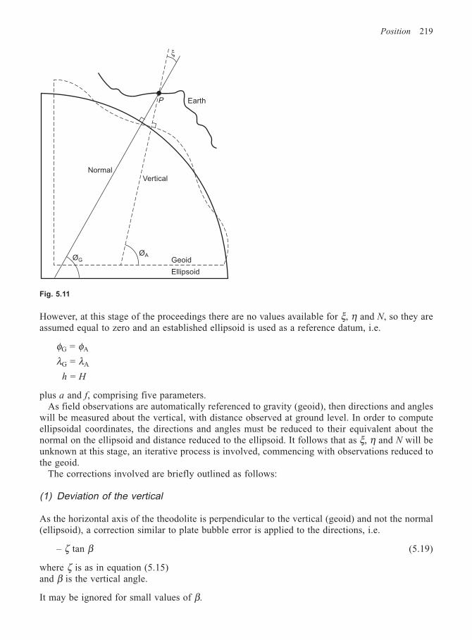
Position 219
However, at this stage of the proceedings there are no values available for ξ, η and N, so they areassumed equal to zero and an established ellipsoid is used as a reference datum, i.e.
φG = φA
λG = λA
h = H
plus a and f, comprising five parameters.As field observations are automatically referenced to gravity (geoid), then directions and angles
will be measured about the vertical, with distance observed at ground level. In order to computeellipsoidal coordinates, the directions and angles must be reduced to their equivalent about thenormal on the ellipsoid and distance reduced to the ellipsoid. It follows that as ξ, η and N will beunknown at this stage, an iterative process is involved, commencing with observations reduced tothe geoid.
The corrections involved are briefly outlined as follows:
(1) Deviation of the vertical
As the horizontal axis of the theodolite is perpendicular to the vertical (geoid) and not the normal(ellipsoid), a correction similar to plate bubble error is applied to the directions, i.e.
– ζ tan β (5.19)
where ζ is as in equation (5.15)and β is the vertical angle.
It may be ignored for small values of β.
Fig. 5.11
ξ
P Earth
VerticalNormal
ØAGeoid
Ellipsoid
ØG
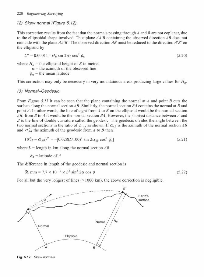
220 Engineering Surveying
(2) Skew normal (Figure 5.12)
This correction results from the fact that the normals passing through A and B are not coplanar, dueto the ellipsoidal shape involved. Thus plane AA′B containing the observed direction AB does notcoincide with the plane AA′B′. The observed direction AB must be reduced to the direction A′B′ onthe ellipsoid by
C″ = 0.00011 · HB sin 2α · cos2 φm (5.20)
where HB = the ellipsoid height of B in metresα = the azimuth of the observed line
φm = the mean latitude
This correction may only be necessary in very mountainous areas producing large values for HB.
(3) Normal–Geodesic
From Figure 5.13 it can be seen that the plane containing the normal at A and point B cuts thesurface along the normal section AB. Similarly, the normal section BA contains the normal at B andpoint A. In other words, the line of sight from A to B on the ellipsoid would be the normal sectionAB; from B to A it would be the normal section BA. However, the shortest distance between A andB is the line of double curvature called the geodesic. The geodesic divides the angle between thetwo normal sections in the ratio of 2 :1, as shown. If αAB is the azimuth of the normal section AB
and ′α AB the azimuth of the geodesic from A to B then
( – )′ ′′α αAB AB = –[0.028(L/100)2 sin 2αAB cos2 φA] (5.21)
where L = length in km along the normal section AB
φA = latitude of A
The difference in length of the geodesic and normal section is
δL mm = 7.7 × 10⁻¹⁷ × L2 sin2 2α cos φ (5.22)
For all but the very longest of lines (>1000 km), the above correction is negligible.
Fig. 5.12 Skew normals
Normal
Normal
Ellipsoid
B
Earth’s
surface
HB
B ′A′
c
A
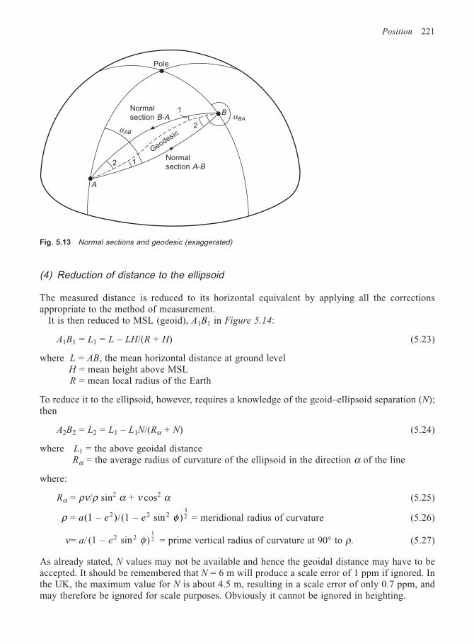
Position 221
(4) Reduction of distance to the ellipsoid
The measured distance is reduced to its horizontal equivalent by applying all the correctionsappropriate to the method of measurement.
It is then reduced to MSL (geoid), A1B1 in Figure 5.14:
A1B1 = L1 = L – LH/(R + H) (5.23)
where L = AB, the mean horizontal distance at ground levelH = mean height above MSLR = mean local radius of the Earth
To reduce it to the ellipsoid, however, requires a knowledge of the geoid–ellipsoid separation (N);then
A2B2 = L2 = L1 – L1N/(Rα + N) (5.24)
where L1 = the above geoidal distanceRα = the average radius of curvature of the ellipsoid in the direction α of the line
where:
Rα = ρν/ρ sin2 α + ν cos2 α (5.25)
ρ φ = (1 – )/(1 – sin )2 2 232a e e = meridional radius of curvature (5.26)
ν= a/ (1 – sin )2 212e φ = prime vertical radius of curvature at 90° to ρ. (5.27)
As already stated, N values may not be available and hence the geoidal distance may have to beaccepted. It should be remembered that N = 6 m will produce a scale error of 1 ppm if ignored. Inthe UK, the maximum value for N is about 4.5 m, resulting in a scale error of only 0.7 ppm, andmay therefore be ignored for scale purposes. Obviously it cannot be ignored in heighting.
Pole
Normal
section B-A αBAB
2
1
αAB
Geodesic
12
A
Normal
section A-B
Fig. 5.13 Normal sections and geodesic (exaggerated)
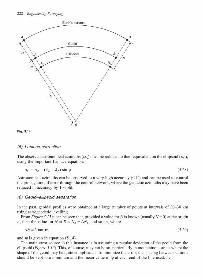
222 Engineering Surveying
(5) Laplace correction
The observed astronomical azimuths (αA) must be reduced to their equivalent on the ellipsoid (αG),using the important Laplace equation:
αG = αA – (λG – λA) sin φ (5.28)
Astronomical azimuths can be observed to a very high accuracy (< 1″) and can be used to controlthe propagation of error through the control network, where the geodetic azimuths may have beenreduced in accuracy by 10-fold.
(6) Geoid–ellipsoid separation
In the past, geoidal profiles were obtained at a large number of points at intervals of 20–30 kmusing astrogeodetic levelling.
From Figure 5.15 it can be seen that, provided a value for N is known (usually N = 0) at the originA, then the value for N at B is NA + ∆N1, and so on, where
∆N ≈ L tan ψ (5.29)
and ψ is given in equation (5.14).The main error source in this instance is in assuming a regular deviation of the geoid from the
ellipsoid (Figure 5.15). This, of course, may not be so, particularly in mountainous areas where theshape of the geoid may be quite complicated. To minimize the error, the spacing between stationsshould be kept to a minimum and the mean value of ψ at each end of the line used, i.e.
A2
A1H
N
Rα
Earth’s surface
Geoid
Ellipsoid
B
h
A
B1
B2
0
Fig. 5.14
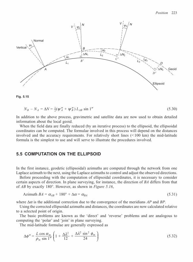
Position 223
N N N LB A A B AB – = = ( + ) sin 112∆ ′′ ′′ ′′ψ ψ (5.30)
In addition to the above process, gravimetric and satellite data are now used to obtain detailedinformation about the local geoid.
When the field data are finally reduced (by an iterative process) to the ellipsoid, the ellipsoidalcoordinates can be computed. The formulae involved in this process will depend on the distancesinvolved and the accuracy requirements. For relatively short lines (<100 km) the mid-latitudeformula is the simplest to use and will serve to illustrate the procedures involved.
5.5 COMPUTATION ON THE ELLIPSOID
In the first instance, geodetic (ellipsoidal) azimuths are computed through the network from oneLaplace azimuth to the next, using the Laplace azimuths to control and adjust the observed directions.
Before proceeding with the computation of ellipsoidal coordinates, it is necessary to considercertain aspects of direction. In plane surveying, for instance, the direction of BA differs from thatof AB by exactly 180°. However, as shown in Figure 5.16,
Azimuth BA = αAB + 180° + ∆α = αBA (5.31)
where ∆α is the additional correction due to the convergence of the meridians AP and BP.Using the corrected ellipsoidal azimuths and distances, the coordinates are now calculated relative
to a selected point of origin.The basic problems are known as the ‘direct’ and ‘reverse’ problems and are analogous to
computing the ‘polar’ and ‘join’ in plane surveying.The mid-latitude formulae are generally expressed as
∆ ∆ ∆′′
′′
φ αρ
λ λ φ =
cos sin 1
1 + 12
+ sin 24
2 2 2L m
m
m (5.32)
Fig. 5.15
ψ1Vertical
Normal
A
L1
ψ1
∆N1
B′
B
ψ2VN
ψ2
L2
C′∆N2
ψ3V
L3ψ3
D′∆N3
D
Ellipsoid
Geoid
N
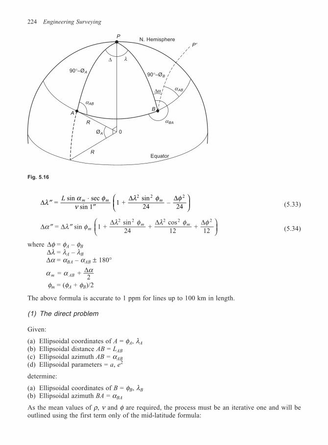
224 Engineering Surveying
∆∆ ∆
′′⋅
′′
λα φ
νλ φ φ
= sin sec
sin 1 1 +
sin 24
– 24
2 2 2L m m m(5.33)
∆ ∆∆ ∆ ∆
′′ ′′
α λ φλ φ λ φ φ
= sin 1 + sin 24
+ cos 12
+ 12
2 2 2 2 2
mm m
(5.34)
where ∆φ = φA – φB
∆λ = λA – λB
∆α = αBA – αAB ± 180°
α α αm AB = +
2∆
φm = (φA + φB)/2
The above formula is accurate to 1 ppm for lines up to 100 km in length.
(1) The direct problem
Given:
(a) Ellipsoidal coordinates of A = φA, λA
(b) Ellipsoidal distance AB = LAB
(c) Ellipsoidal azimuth AB = αAB
(d) Ellipsoidal parameters = a, e2
determine:
(a) Ellipsoidal coordinates of B = φB, λB
(b) Ellipsoidal azimuth BA = αBA
As the mean values of ρ, ν and φ are required, the process must be an iterative one and will beoutlined using the first term only of the mid-latitude formula:
Fig. 5.16
PN. Hemisphere
P ′
∆ λ
90°–ØB
αAB∆α
B
αBA
0ØA
R
R
A
αAB
90°–ØA
Equator
Position 225
(a) Determine ρA and νA from equations (5.26) and (5.27) using φA
(b) Determine ∆φ″ = LAB cos αAB/ρA sin 1″(c) Determine the first value for φm = φA + (∆φ/2)(d) Determine improved values for ρ and ν using φm and iterate until negligible change in ∆φ(e) Determine ∆λ″ = LAB sin αAB sec φm/νm sin 1″(f) Determine ∆α″ = ∆λ″ sin φm and so deduce
αm = αAB + (∆α/2)
(g) Iterate the whole procedure until the differences between successive values of ∆φ, ∆λ and ∆αare insignificant. Three iterations normally suffice.
(h) Using the final accepted values, we have:
φB = φA + ∆φλB = λB + ∆λ
αBA = αAB + ∆α ± 180°
(2) The reverse problem
Given:
(a) Ellipsoidal coordinates of A = φA, λA
(b) Ellipsoidal coordinates of B = φB, λB
(c) Ellipsoidal parameters = a, e2
determine:
(a) Ellipsoidal azimuths = αAB and αBA
(b) Ellipsoidal distance = LAB
This procedure does not require iteration:
(a) Determine φm = (φA + φB)/2
(b) Determine ν φm ma e= /(1 – sin )2 212 and
ρ φm ma e e = (1 – )/(1 – sin )2 2 232
(c) Determine αm = νm · ∆λ cos φm /(ρm · ∆φ)(d) Determine LAB from ∆φ″ = LAB cos αm/ρm sin 1″ which can be checked using ∆λ″(e) Determine ∆α″ = ∆λ″ sin φm, then
αAB = αm – (∆α /2) and αBA = αAB + ∆α ± 180°
Whilst the mid-latitude formula serves to illustrate the procedures involved, computers now permitthe use of the more accurate equations. Such formulae may be obtained direct from the nationalmapping agency for the area concerned.
On completion of all the computation throughout the network, values of ξ, η and N can beobtained at selected stations. The best-fitting ellipsoid is the one for which values of ∑N2 or∑(ξ2 – η2) are a minimum. If the fit is not satisfactory, then the values of ξ, η and N as chosen atthe origin could be altered or a different ellipsoid selected. Although it would be no problem tochange the ellipsoid due to the present use of computers, in the past it was usual to change thevalues of ξ, η and N to improve the fit.
Although the above is a brief description of the classical geodetic approach, the majority ofellipsoids in use throughout the world were chosen on the basis of their availability at the time. For
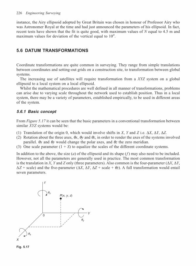
226 Engineering Surveying
instance, the Airy ellipsoid adopted by Great Britain was chosen in honour of Professor Airy whowas Astronomer Royal at the time and had just announced the parameters of his ellipsoid. In fact,recent tests have shown that the fit is quite good, with maximum values of N equal to 4.5 m andmaximum values for deviation of the vertical equal to 10″.
5.6 DATUM TRANSFORMATIONS
Coordinate transformations are quite common in surveying. They range from simple translationsbetween coordinates and setting-out grids on a construction site, to transformation between globalsystems.
The increasing use of satellites will require transformation from a XYZ system on a globalellipsoid to a local system on a local ellipsoid.
Whilst the mathematical procedures are well defined in all manner of transformations, problemscan arise due to varying scale throughout the network used to establish position. Thus in a localsystem, there may be a variety of parameters, established empirically, to be used in different areasof the system.
5.6.1 Basic concept
From Figure 5.17 it can be seen that the basic parameters in a conventional transformation betweensimilar XYZ systems would be:
(1) Translation of the origin 0, which would involve shifts in X, Y and Z i.e. ∆X, ∆Y, ∆Z.(2) Rotation about the three axes, θx, θy and θz, in order to render the axes of the systems involved
parallel. θx and θy would change the polar axes, and θz the zero meridian.(3) One scale parameter (1 + S) to equalize the scales of the different coordinate systems.
In addition to the above, the size (a) of the ellipsoid and its shape ( f ) may also need to be included.However, not all the parameters are generally used in practice. The most common transformationis the translation in X, Y and Z only (three parameters). Also common is the four-parameter (∆X, ∆Y,∆Z + scale) and the five-parameter (∆X, ∆Y, ∆Z + scale + θz). A full transformation would entailseven parameters.
θz
z
P(x, y, z)
0Y
θy
X
θx
Fig. 5.17
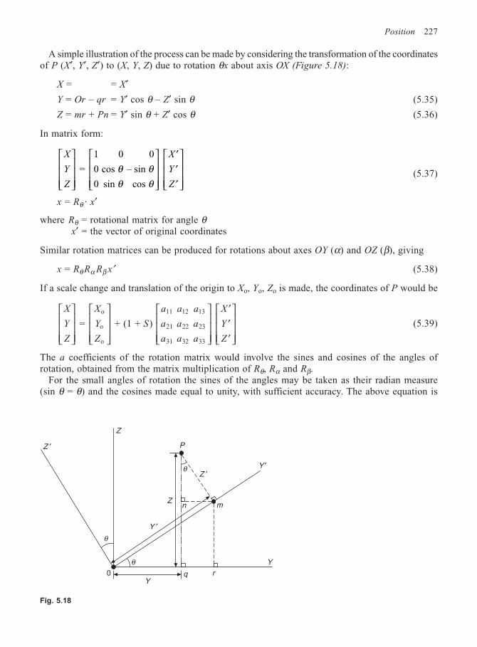
Position 227
A simple illustration of the process can be made by considering the transformation of the coordinatesof P (X′, Y′, Z′) to (X, Y, Z) due to rotation θx about axis OX (Figure 5.18):
X = = X′Y = Or – qr = Y′ cos θ – Z′ sin θ (5.35)
Z = mr + Pn = Y′ sin θ + Z′ cos θ (5.36)
In matrix form:
X
Y
Z
X
Y
Z
′′′
=
0 sin
0
– sin
cos
1
0
0
cos θθ
θθ
(5.37)
x = Rθ · x′
where Rθ = rotational matrix for angle θ x′ = the vector of original coordinates
Similar rotation matrices can be produced for rotations about axes OY (α) and OZ (β), giving
x = Rθ Rα Rβ x′ (5.38)
If a scale change and translation of the origin to Xo, Yo, Zo is made, the coordinates of P would be
X
Y
Z
X
Y
Z
S
a
a
a
a
a
a
a
a
a
X
Y
Z
′′′
= + (1 + )
o
o
o
11
21
31
12
22
32
13
23
33
(5.39)
The a coefficients of the rotation matrix would involve the sines and cosines of the angles ofrotation, obtained from the matrix multiplication of Rθ, Rα and Rβ.
For the small angles of rotation the sines of the angles may be taken as their radian measure(sin θ = θ) and the cosines made equal to unity, with sufficient accuracy. The above equation is
Fig. 5.18
Z ′
Z
P
Z ′θ Y ′
mnZ
Y ′
θ
θ0
Y
Y
rq
228 Engineering Surveying
referred to in surveying as the Helmert transformation and describes the full transformation betweenthe two geodetic datums.
Whilst the X, Y, Z coordinates of three points would be sufficient to determine the seven parameters,in practice as many points as possible are used in a least squares solution. Ellipsoidal coordinates(φ, λ, h) would need to be transformed to X, Y and Z for use in the transformations.
As a translation of the origin of the reference system is the most common, a Molodenskiitransform permits the transformation of ellipsoidal coordinates from one system to another in asingle operation i.e.
φ = φ′ + ∆φ″λ = λ′ + ∆λ″h = h′ + ∆h
where ∆φ″ = (–∆X sin φ′ cos λ′ – ∆Y sin φ′ sin λ′ + ∆Z cos φ′+ (a′ ∆f + f ′ ∆a) sin 2φ′)/(ρ sin 1″) (5.40)
∆λ″ = (–∆X sin λ′ + ∆Y cos λ′)/(ν sin 1″) (5.41)
∆h = (∆X cos φ′ cos λ′ + ∆Y cos φ′ · sin λ′ + ∆Z sin φ′+ (a′ ∆f + f ′ ∆a) sin 2 φ′ – ∆a) (5.42)
In the above formulae:
φ′, λ′, h′ = ellipsoidal coordinates in the first systemφ, λ, h = ellipsoidal coordinates in the required system
a′, f ′ = ellipsoidal parameters of the first system∆a, ∆f = difference between the parameters in each system
∆X, ∆Y, ∆Z = origin translation valuesν = radius of curvature in the prime vertical (equation (5.27))ρ = radius of curvature in the meridian (equation (5.26))
It must be emphasized once again that whilst the mathematics of transformation are rigorouslydefined, the practical problems of varying scale etc. must always be considered.
5.7 ORTHOMORPHIC PROJECTION
The ellipsoidal surface, representing a portion of the Earth’s surface, may be represented on a planeusing a specific form of projection, i.e.
E = fE (φ, λ) (5.43)
N = fN (φ, λ) (5.44)
where E and N on the plane of the projection represent φ, λ on the reference ellipsoid.Representation of a curved surface on a plane must result in some form of distortion, and
therefore the properties required of the projection must be carefully considered. In surveying, theproperties desired are usually:
(1) A line on the projection must contain the same intermediate points as that on the ellipsoid.(2) The angle between the tangents to any two lines on the ellipsoid should have a corresponding
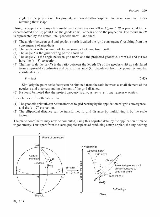
Position 229
angle on the projection. This property is termed orthomorphism and results in small areasretaining their shape.
Using the appropriate projection mathematics the geodesic AB in Figure 5.19 is projected to thecurved dotted line ab; point C on the geodesic will appear at c on the projection. The meridian AP
is represented by the dotted line ‘geodetic north’, and then:
(1) The angle γ between grid and geodetic north is called the ‘grid convergence’ resulting from theconvergence of meridians.
(2) The angle α is the azimuth of AB measured clockwise from north.(3) The angle t is the grid bearing of the chord ab.(4) The angle T is the angle between grid north and the projected geodesic. From (3) and (4) we
have the (t – T) correction.(5) The line scale factor (F) is the ratio between the length (S) of the geodesic AB as calculated
from ellipsoidal coordinates and its grid distance (G) calculated from the plane rectangularcoordinates, i.e.
F = G/S (5.45)
Similarly the point scale factor can be obtained from the ratio between a small element of thegeodesic and a corresponding element of the grid distance.
(6) It should be noted that the project geodesic is always concave to the central meridian.
It can be seen from the above that:
(1) The geodetic azimuth can be transformed to grid bearing by the application of ‘grid convergence’and the ‘t – T’ correction.
(2) The ellipsoidal distance can be transformed to grid distance by multiplying it by the scalefactor.
The plane coordinates may now be computed, using this adjusted data, by the application of planetrigonometry. Thus apart from the cartographic aspects of producing a map or plan, the engineering
Fig. 5.19
Ellipsoid
0 E
A
CB
Geodesic
Central
meridian
NP
N
Plane of projection
E = fE(φ, λ)
N = fN(φ, λ)
Ce
ntr
al
me
rid
ian
0
N = Northings
Geodetic north
Grid north
Chordγ
t
T
a(t –T)A
E=Eastings
Plane
Tangent at a
Projected geodesic ABalways concave to
central meridian
cα
α
b
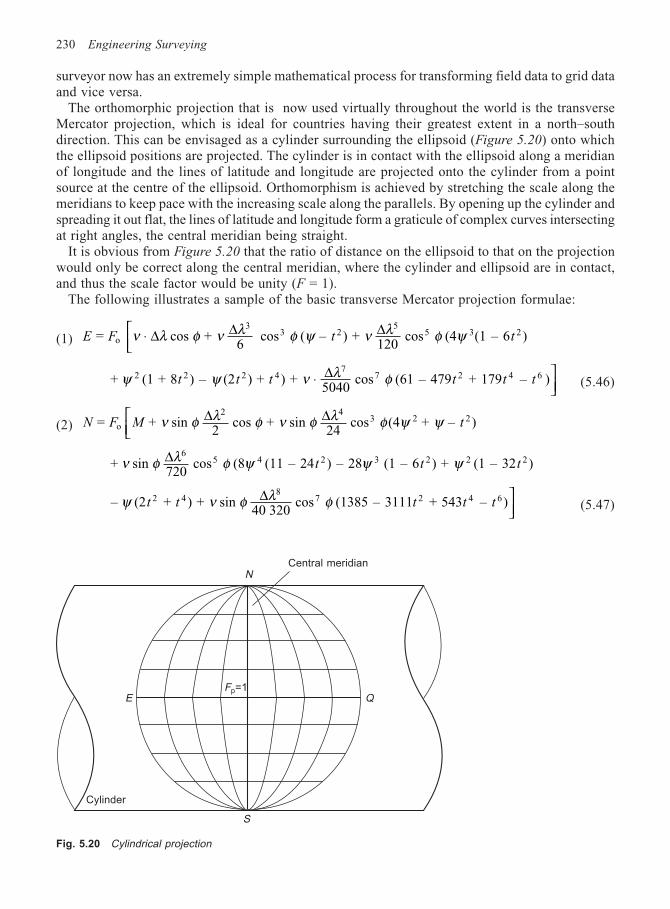
230 Engineering Surveying
surveyor now has an extremely simple mathematical process for transforming field data to grid dataand vice versa.
The orthomorphic projection that is now used virtually throughout the world is the transverseMercator projection, which is ideal for countries having their greatest extent in a north–southdirection. This can be envisaged as a cylinder surrounding the ellipsoid (Figure 5.20) onto whichthe ellipsoid positions are projected. The cylinder is in contact with the ellipsoid along a meridianof longitude and the lines of latitude and longitude are projected onto the cylinder from a pointsource at the centre of the ellipsoid. Orthomorphism is achieved by stretching the scale along themeridians to keep pace with the increasing scale along the parallels. By opening up the cylinder andspreading it out flat, the lines of latitude and longitude form a graticule of complex curves intersectingat right angles, the central meridian being straight.
It is obvious from Figure 5.20 that the ratio of distance on the ellipsoid to that on the projectionwould only be correct along the central meridian, where the cylinder and ellipsoid are in contact,and thus the scale factor would be unity (F = 1).
The following illustrates a sample of the basic transverse Mercator projection formulae:
(1) E F t t = cos + 6
cos ( – ) + 120
cos (4 (1 – 6 )o
33 2
55 3 2ν λ φ ν λ φ ψ ν λ φ ψ⋅
∆ ∆ ∆
+ (1 + 8 ) – (2 ) + ) + 5040
cos (61 – 479 + 179 – )2 2 2 47
7 2 4 6ψ ψ ν λ φt t t t t t⋅
∆(5.46)
(2) N F M t = + sin 2
cos + sin 24
cos (4 + – )o
2 43 2 2ν φ λ φ ν φ λ φ ψ ψ∆ ∆
+ sin 720
cos (8 (11 – 24 ) – 28 (1 – 6 ) + (1 – 32 )6
5 4 2 3 2 2 2ν φ λ φ ψ ψ ψ∆t t t
– (2 + ) + sin 40 320
cos (1385 – 3111 + 543 – )2 48
7 2 4 6ψ ν φ λ φt t t t t∆
(5.47)
Fig. 5.20 Cylindrical projection
NCentral meridian
QEFp=1
S
Cylinder
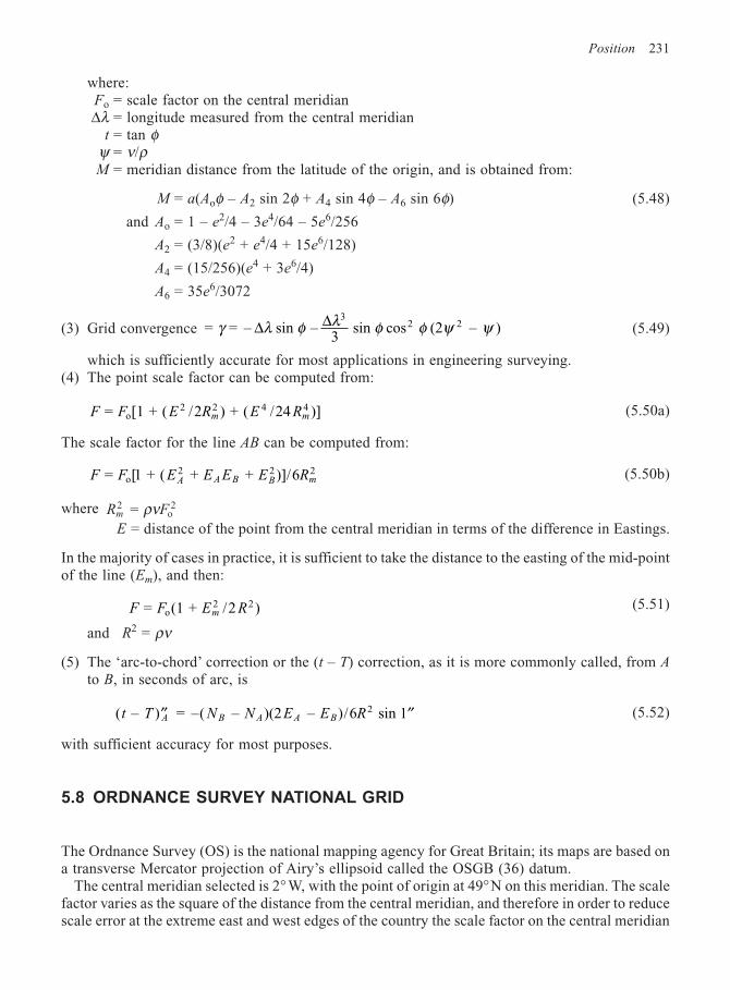
Position 231
where:Fo = scale factor on the central meridian∆λ = longitude measured from the central meridian
t = tan φψ = ν/ρM = meridian distance from the latitude of the origin, and is obtained from:
M = a(Aoφ – A2 sin 2φ + A4 sin 4φ – A6 sin 6φ) (5.48)
and Ao = 1 – e2/4 – 3e4/64 – 5e6/256
A2 = (3/8)(e2 + e4/4 + 15e6/128)
A4 = (15/256)(e4 + 3e6/4)
A6 = 35e6/3072
(3) Grid convergence = = – sin –3
sin cos (2 – )3
2 2γ λ φ λ φ φ ψ ψ∆ ∆ (5.49)
which is sufficiently accurate for most applications in engineering surveying.(4) The point scale factor can be computed from:
F F E R E Rm m = [1 + ( /2 ) + ( /24 )]o2 2 4 4 (5.50a)
The scale factor for the line AB can be computed from:
F F E E E E RA A B B m = [1 + ( + + )]/6o2 2 2 (5.50b)
where R Fm2
o2 = ρν
E = distance of the point from the central meridian in terms of the difference in Eastings.
In the majority of cases in practice, it is sufficient to take the distance to the easting of the mid-pointof the line (Em), and then:
F F E Rm = (1 + /2 )o2 2 (5.51)
and R2 = ρν
(5) The ‘arc-to-chord’ correction or the (t – T) correction, as it is more commonly called, from Ato B, in seconds of arc, is
( – ) = –( – )(2 – )/6 sin 12t T N N E E RA B A A B′′ ′′ (5.52)
with sufficient accuracy for most purposes.
5.8 ORDNANCE SURVEY NATIONAL GRID
The Ordnance Survey (OS) is the national mapping agency for Great Britain; its maps are based ona transverse Mercator projection of Airy’s ellipsoid called the OSGB (36) datum.
The central meridian selected is 2° W, with the point of origin at 49°N on this meridian. The scalefactor varies as the square of the distance from the central meridian, and therefore in order to reducescale error at the extreme east and west edges of the country the scale factor on the central meridian
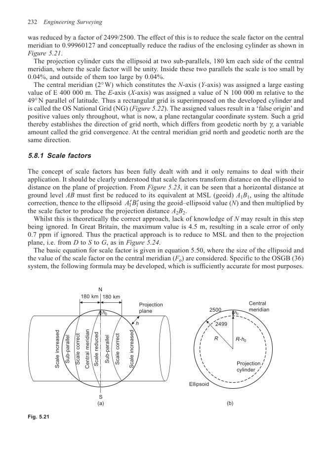
232 Engineering Surveying
was reduced by a factor of 2499/2500. The effect of this is to reduce the scale factor on the centralmeridian to 0.99960127 and conceptually reduce the radius of the enclosing cylinder as shown inFigure 5.21.
The projection cylinder cuts the ellipsoid at two sub-parallels, 180 km each side of the centralmeridian, where the scale factor will be unity. Inside these two parallels the scale is too small by0.04%, and outside of them too large by 0.04%.
The central meridian (2°W) which constitutes the N-axis (Y-axis) was assigned a large eastingvalue of E 400 000 m. The E-axis (X-axis) was assigned a value of N 100 000 m relative to the49° N parallel of latitude. Thus a rectangular grid is superimposed on the developed cylinder andis called the OS National Grid (NG) (Figure 5.22). The assigned values result in a ‘false origin’ andpositive values only throughout, what is now, a plane rectangular coordinate system. Such a gridthereby establishes the direction of grid north, which differs from geodetic north by γ, a variableamount called the grid convergence. At the central meridian grid north and geodetic north are thesame direction.
5.8.1 Scale factors
The concept of scale factors has been fully dealt with and it only remains to deal with theirapplication. It should be clearly understood that scale factors transform distance on the ellipsoid todistance on the plane of projection. From Figure 5.23, it can be seen that a horizontal distance atground level AB must first be reduced to its equivalent at MSL (geoid) A1B1, using the altitudecorrection, thence to the ellipsoid ′ ′A B1 1 using the geoid–ellipsoid value (N) and then multiplied bythe scale factor to produce the projection distance A2B2.
Whilst this is theoretically the correct approach, lack of knowledge of N may result in this stepbeing ignored. In Great Britain, the maximum value is 4.5 m, resulting in a scale error of only0.7 ppm if ignored. Thus the practical approach is to reduce to MSL and then to the projectionplane, i.e. from D to S to G, as in Figure 5.24.
The basic equation for scale factor is given in equation 5.50, where the size of the ellipsoid andthe value of the scale factor on the central meridian (Fo) are considered. Specific to the OSGB (36)system, the following formula may be developed, which is sufficiently accurate for most purposes.
180 km 180 km
N
h0
h
Projection
plane
Sca
le i
ncre
ase
d
Su
b-p
ara
llel
Sca
le c
orr
ect
Ce
ntr
al
me
rid
ian
Sca
le r
ed
uce
d
Su
b-p
ara
l lel
Sca
le c
orr
ect
Sca
le i
ncre
ase
d
S
(a)
2500
R-h0
2499
R
Central
meridian
Projection
cylinder
Ellipsoid
h0
(b)
Fig. 5.21
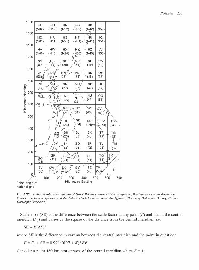
Position 233
Scale error (SE) is the difference between the scale factor at any point (F) and that at the centralmeridian (Fo) and varies as the square of the distance from the central meridian, i.e.
SE = K(∆E)2
where ∆E is the difference in easting between the central meridian and the point in question:
F = Fo + SE = 0.99960127 + K(∆E)2
Consider a point 180 km east or west of the central meridian where F = 1:
1300
1200
1100
1000
900
800
700
600
500
400
300
200
100
0
Kilo
me
tre
s N
ort
hin
g
False origin of
national grid
0 100 200 300 400 500 600 700
Kilometres Easting
HL HM HN HO HP JL
(N02) (N12) (N22) (N32) (N42) (N52)
HQ HR HS HT HU JQ
(N01) (N11) (N21) (N31) (N41) (N51)
HV HW HX HY HZ JV
(N00) (N10) (N20) (N30) (N40) (N50)
NA NB NC ND NE OA
(09) (19) (29) (39) (49) (59)
NF NG NH NJ NK OF
(08) (18) (28) (38) (48) (58)
NL NM NN NO NP OL
(07) (17) (27) (37) (47) (57)
NR
(16)
NS
(26)NT
(36)
NU
(46)OQ
(56)
NW(15) NX
(25)
NY
(35)
NZ
(45)
OV
(55) CW(65)
SB(14)
SE
(44)TB
(64)
SG(13)
SJ(33)
SK(43)
TF
(53)
TG
(63)
SM
(12)
SN
(22)
SO
(32)
SP
(42)
TL
(52)
TM
(62)
SQ(01)
SR
(11)SS
(21)ST
(31)
SU
(41)
TQ
(51)
TR(61)
SV
(00)
SW
(10)
SX
(20)
SY
(30)
SZ
(40)
TV
(50)
NQ(06)
SC
(24)
SD
(34)TA
(54)
SH(23)
Fig. 5.22 National reference system of Great Britain showing 100-km squares, the figures used to designatethem in the former system, and the letters which have replaced the figures. (Courtesy Ordnance Survey, CrownCopyright Reserved)
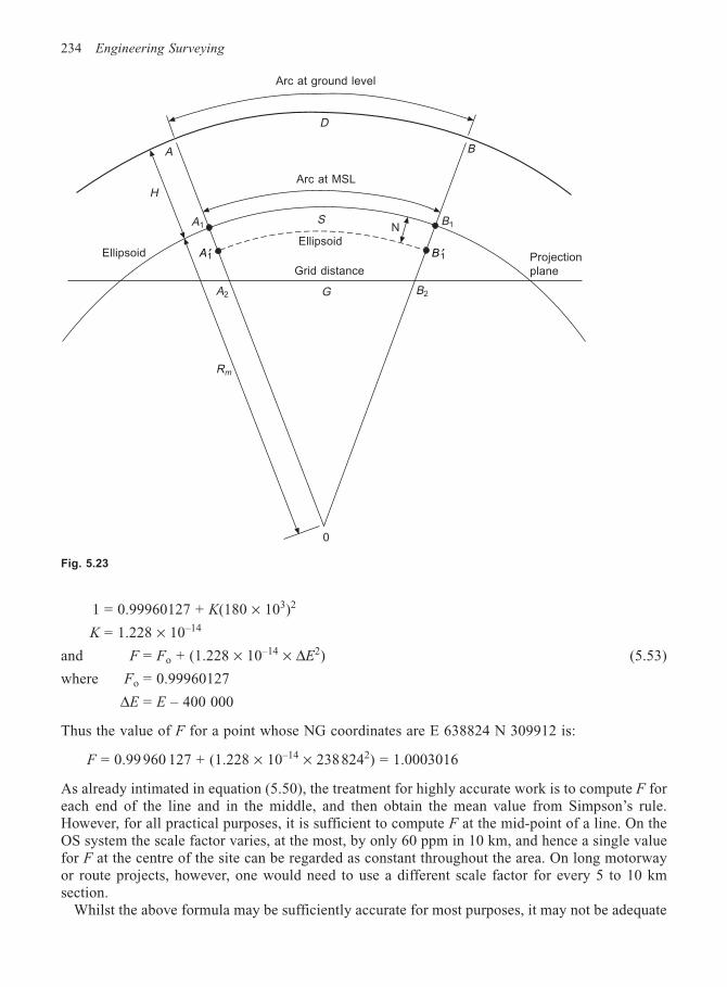
234 Engineering Surveying
1 = 0.99960127 + K(180 × 103)2
K = 1.228 × 10⁻¹⁴
and F = Fo + (1.228 × 10⁻¹⁴ × ∆E2) (5.53)
where Fo = 0.99960127
∆E = E – 400 000
Thus the value of F for a point whose NG coordinates are E 638824 N 309912 is:
F = 0.99 960 127 + (1.228 × 10–14 × 2388242) = 1.0003016
As already intimated in equation (5.50), the treatment for highly accurate work is to compute F foreach end of the line and in the middle, and then obtain the mean value from Simpson’s rule.However, for all practical purposes, it is sufficient to compute F at the mid-point of a line. On theOS system the scale factor varies, at the most, by only 60 ppm in 10 km, and hence a single valuefor F at the centre of the site can be regarded as constant throughout the area. On long motorwayor route projects, however, one would need to use a different scale factor for every 5 to 10 kmsection.
Whilst the above formula may be sufficiently accurate for most purposes, it may not be adequate
Arc at ground level
D
Arc at MSL
Grid distance
G
N
B2
′B1
B1
B
Projection
plane
0
Rm
A2
H
A
A1
Ellipsoid ′A1
S
Ellipsoid
Fig. 5.23
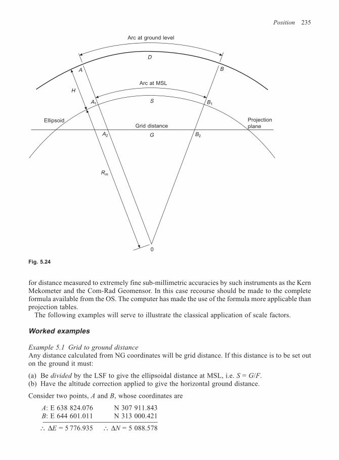
Position 235
Fig. 5.24
Arc at ground level
D
Arc at MSL
S
Grid distance
G
Projection
plane
B
B1
B2
0
Rm
A2
A1
A
H
Ellipsoid
for distance measured to extremely fine sub-millimetric accuracies by such instruments as the KernMekometer and the Com-Rad Geomensor. In this case recourse should be made to the completeformula available from the OS. The computer has made the use of the formula more applicable thanprojection tables.
The following examples will serve to illustrate the classical application of scale factors.
Worked examples
Example 5.1 Grid to ground distance
Any distance calculated from NG coordinates will be grid distance. If this distance is to be set outon the ground it must:
(a) Be divided by the LSF to give the ellipsoidal distance at MSL, i.e. S = G/F.(b) Have the altitude correction applied to give the horizontal ground distance.
Consider two points, A and B, whose coordinates are
A: E 638 824.076 N 307 911.843B: E 644 601.011 N 313 000.421
∴ ∆E = 5 776.935 ∴ ∆N = 5 088.578
236 Engineering Surveying
Grid distance = ( + )2 2∆ ∆E N12 = 7698.481 m = G
Mid-easting of AB = E 641 712 m
∴ F = 1.000 3188 (from equation (5.53))
∴ Ellipsoidal distance at MSL = S = G/F = 7696.027 m
Now assuming AB at a mean height (H) of 250 m above MSL, the altitude correction Cm is
CSHRm = = 7696 250
6 384 100 = + 0.301 m×
∴ Horizontal distance at ground level = 7696.328 m
This situation could arise where the survey and design coordinates of a project are on the OSNG.Distances calculated from the grid coordinates would need to be transformed to their equivalent onthe ground for setting-out purposes.
Example 5.2 Ground to grid distance
When connecting surveys to the national grid, horizontal distances measured on the ground mustbe:
(a) Reduced to their equivalent on the ellipsoid at MSL.(b) Multiplied by the LSF to produce the equivalent grid distance, i.e. G = S × F.
Consider now the previous problem worked in reverse
Horizontal ground distance = 7696.328 mAltitude correction Cm = –0.301 m
—————∴ Ellipsoidal distance S at MSL = 7696.027 m
F = 1.000 3188
—————∴ Grid distance G = S × F = 7698.481 m
This situation could arise in the case of a link traverse connected into the OSNG system. The lengthof each leg of the traverse would need to be reduced from its horizontal distance at ground level toits equivalent distance on the NG.
There is no application of grid convergence as the traverse commences from a grid bearing andconnects into another grid bearing. The application of the (t – T) correction to the angles wouldgenerally be negligible, being a maximum of 7″ for a 10-km line and much less than the observationalerrors of the traverse angles. It would only be necessary to consider both the above effects if theangular error was being controlled by taking gyro-theodolite observations on intermediate lines inthe traverse.
The two applications illustrated in the examples of first reducing to MSL and then to the plane ofthe projection (NG) can be combined to give:
Fa = F(1 – H/R) (5.54)
where H is the ground height relative to MSL and is positive when above and negative when belowMSL.
Then from Example 5.1:
Fa = 1.0003188 (1 – 250/6 384 100) = 1.0002797
Position 237
Fa is then the scale factor adjusted for altitude and can be used directly to transform from groundto grid and vice versa.
From Example 5.2:
7696.328 × 1.0002797 = 7698.481 m
5.8.2 Grid convergence
All grid north lines on the NG are parallel to the central meridian (E400 000 m), whilst themeridians converge to the pole. The difference between these directions is termed the grid convergenceγ.
An approximate formula may be derived from the first term of equation (5.49).
γ = ∆λ sin φ
but ∆λ = ∆E/R cos φm
= tan 206 265
′′×
γφ∆E
Rm (5.55)
where ∆E = distance from the central meridian
R = mean radius of Airy’s ellipsoid = ( )12ρν
φm = mean latitude of the line
The approximate method of computing γ is acceptable only for lines close to the central meridian,where values correct to a few seconds may be obtained. As the distance from the central meridianincreases, so too does the error in the approximate formula and the more rigorous methods arenecessary.
If the NG coordinates of a point are E 626 238 and N 302646 and the latitude, scaled from an OSmap, is N 52° 34′, then taking R = 6 380 847 m gives
′′° ′
× ′′ ° ′ ′′γ = 226 238 tan 52 34
6 380847 206 265 = 9554 = 2 39 14
5.8.3 (t – T) correction
As already shown, the (t – T ) correction results from the fact that the geodesic appears as a curvedline on the projection and differs from the direction of the chord, as computed from plane trigonometry,by a small correction. Figure 5.25 illustrates the angle θ as ‘observed’ and the angle β as computedfrom the grid coordinates; then:
β = θ – (t – T)BA – (t – T )BC
An approximate formula for (t – T) specific to the NG is as follows:
( – )t T A′′ = (2∆EA + ∆EB)(NA – NB)K (5.56)
where ∆E = NG easting – 400 000, expressed in kmN = NG northing expressed in kmA = station at which the correction is requiredB = station observedK = 845 × 10–6
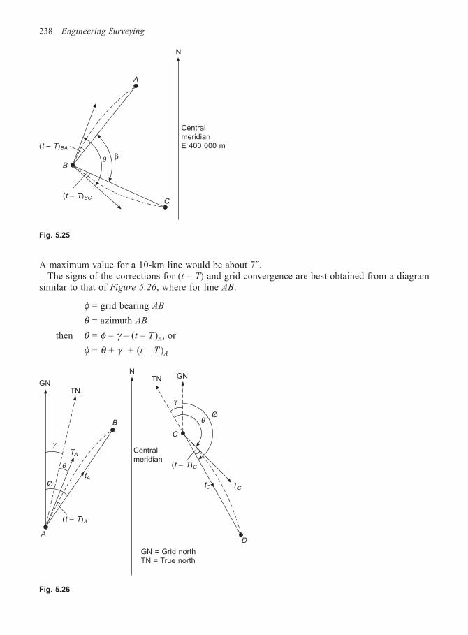
238 Engineering Surveying
A maximum value for a 10-km line would be about 7″.The signs of the corrections for (t – T) and grid convergence are best obtained from a diagram
similar to that of Figure 5.26, where for line AB:
φ = grid bearing AB
θ = azimuth AB
then θ = φ – γ – (t – T)A, or
φ = θ + γ + (t – T )A
Fig. 5.25
N
Central
meridian
E 400 000 m
A
θ β
C
(t – T)BA
B
(t – T)BC
Fig. 5.26
TNGN
NTN GN
tAØ
θ
γ
(t – T)A
A
γ
θØ
tC TC
(t – T)C
Central
meridian
D
GN = Grid north
TN = True north
TA
B
C
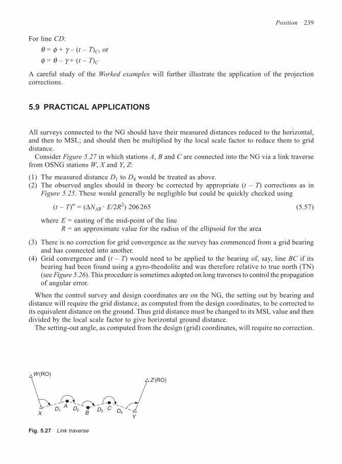
Position 239
For line CD:
θ = φ + γ – (t – T)C, or
φ = θ – γ + (t – T)C
A careful study of the Worked examples will further illustrate the application of the projectioncorrections.
5.9 PRACTICAL APPLICATIONS
All surveys connected to the NG should have their measured distances reduced to the horizontal,and then to MSL; and should then be multiplied by the local scale factor to reduce them to griddistance.
Consider Figure 5.27 in which stations A, B and C are connected into the NG via a link traversefrom OSNG stations W, X and Y, Z:
(1) The measured distance D1 to D4 would be treated as above.(2) The observed angles should in theory be corrected by appropriate (t – T) corrections as in
Figure 5.25. These would generally be negligible but could be quickly checked using
(t – T)″ = (∆NAB · E/2R2) 206 265 (5.57)
where E = easting of the mid-point of the lineR = an approximate value for the radius of the ellipsoid for the area
(3) There is no correction for grid convergence as the survey has commenced from a grid bearingand has connected into another.
(4) Grid convergence and (t – T) would need to be applied to the bearing of, say, line BC if itsbearing had been found using a gyro-theodolite and was therefore relative to true north (TN)(see Figure 5.26). This procedure is sometimes adopted on long traverses to control the propagationof angular error.
When the control survey and design coordinates are on the NG, the setting out by bearing anddistance will require the grid distance, as computed from the design coordinates, to be corrected toits equivalent distance on the ground. Thus grid distance must be changed to its MSL value and thendivided by the local scale factor to give horizontal ground distance.
The setting-out angle, as computed from the design (grid) coordinates, will require no correction.
Fig. 5.27 Link traverse
W (RO)Z (RO)
XD1
A
BD2 D3
CD4
Y
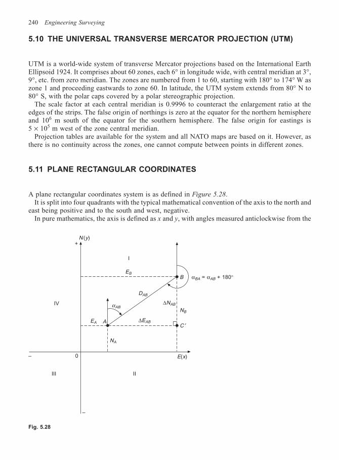
240 Engineering Surveying
5.10 THE UNIVERSAL TRANSVERSE MERCATOR PROJECTION (UTM)
UTM is a world-wide system of transverse Mercator projections based on the International EarthEllipsoid 1924. It comprises about 60 zones, each 6° in longitude wide, with central meridian at 3°,9°, etc. from zero meridian. The zones are numbered from 1 to 60, starting with 180° to 174° W aszone 1 and proceeding eastwards to zone 60. In latitude, the UTM system extends from 80° N to80° S, with the polar caps covered by a polar stereographic projection.
The scale factor at each central meridian is 0.9996 to counteract the enlargement ratio at theedges of the strips. The false origin of northings is zero at the equator for the northern hemisphereand 106 m south of the equator for the southern hemisphere. The false origin for eastings is5 × 105 m west of the zone central meridian.
Projection tables are available for the system and all NATO maps are based on it. However, asthere is no continuity across the zones, one cannot compute between points in different zones.
5.11 PLANE RECTANGULAR COORDINATES
A plane rectangular coordinates system is as defined in Figure 5.28.It is split into four quadrants with the typical mathematical convention of the axis to the north and
east being positive and to the south and west, negative.In pure mathematics, the axis is defined as x and y, with angles measured anticlockwise from the
+N (y)
EB
I
DAB
B αBA = αAB + 180°
NB
∆NABαAB
∆EABAEA
NA
II
IV
– 0
–
C ′
E(x)
III
Fig. 5.28
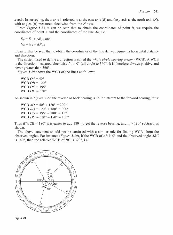
Position 241
x-axis. In surveying, the x-axis is referred to as the east-axis (E) and the y-axis as the north-axis (N),with angles (α) measured clockwise from the N-axis.
From Figure 5.28, it can be seen that to obtain the coordinates of point B, we require thecoordinates of point A and the coordinates of the line AB, i.e.
EB = EA + ∆EAB and
NB = NA + ∆NAB
It can further be seen that to obtain the coordinates of the line AB we require its horizontal distanceand direction.
The system used to define a direction is called the whole circle bearing system (WCB). A WCBis the direction measured clockwise from 0° full circle to 360°. It is therefore always positive andnever greater than 360°.
Figure 5.29 shows the WCB of the lines as follows:
WCB OA = 40°WCB OB = 120°WCB OC = 195°WCB OD = 330°
As shown in Figure 5.29, the reverse or back bearing is 180° different to the forward bearing, thus:
WCB AO = 40° + 180° = 220°WCB BO = 120° + 180° = 300°WCB CO = 195° – 180° = 15°WCB DO = 330° – 180° = 150°
Thus if WCB < 180° it is easier to add 180° to get the reverse bearing, and if > 180° subtract, asshown.
The above statement should not be confused with a similar rule for finding WCBs from theobserved angles. For instance (Figure 5.30), if the WCB of AB is 0° and the observed angle ABC
is 140°, then the relative WCB of BC is 320°, i.e.
Fig. 5.29
D
A
40°
120°
195°B
C
0
330°
2010
30
40
60
50
70
80
90
100
110
120
130
140
150
160170180
190200
210
220
230
240
250
26
02
70
28
0290
300
310
320
330
340350
O
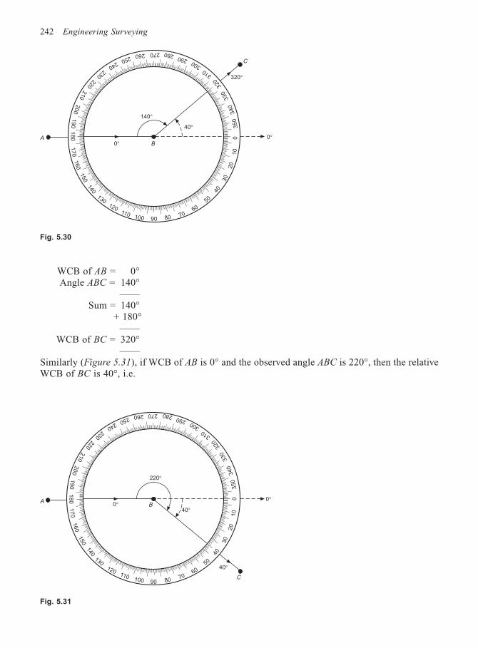
242 Engineering Surveying
WCB of AB = 0° Angle ABC = 140°
——Sum = 140°
+ 180°——
WCB of BC = 320°——
Similarly (Figure 5.31), if WCB of AB is 0° and the observed angle ABC is 220°, then the relativeWCB of BC is 40°, i.e.
Fig. 5.30
C
320°
0°
40°
B0°
140°
A
18
0
210
250
230
220
200
19
01
70
160
150
140
130
110
120
280290
300
310
320
330
340
350
260
240
100 90 80 7060
50
40
30
20
10
270
0
Fig. 5.31
250
230
220
200
19
01
70
280290
300
31032
0
330
340
350
260
240
220°
40°B0°A 0°
40°
C
40
210
18
0160
150
140
130120
110100 90 80 70
60
50
30
20
10
2700
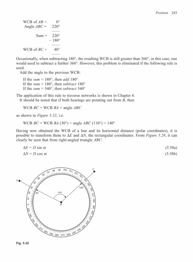
Position 243
WCB of AB = 0°Angle ABC = 220°
——Sum = 220°
– 180°——
WCB of BC = 40°——
Occasionally, when subtracting 180°, the resulting WCB is still greater than 360°, in this case, onewould need to subtract a further 360°. However, this problem is eliminated if the following rule isused.
Add the angle to the previous WCB:
If the sum < 180°, then add 180°If the sum > 180°, then subtract 180°If the sum > 540°, then subtract 540°
The application of this rule to traverse networks is shown in Chapter 6.It should be noted that if both bearings are pointing out from B, then
WCB BC = WCB BA + angle ABC
as shown in Figure 5.32, i.e.
WCB BC = WCB BA (30°) + angle ABC (110°) = 140°
Having now obtained the WCB of a line and its horizontal distance (polar coordinates), it ispossible to transform them to ∆E and ∆N, the rectangular coordinates. From Figure 5.28, it canclearly be seen that from right-angled triangle ABC:
∆E = D sin α (5.58a)
∆N = D cos α (5.58b)
C
140°
110°
B
30°
A
10090110
120
13014
0
150
160
170
18
01
90
200
210
220
230
240
250260270280
290
300
310
320
330
340
350
0
807060
50
4030
20
10
Fig. 5.32
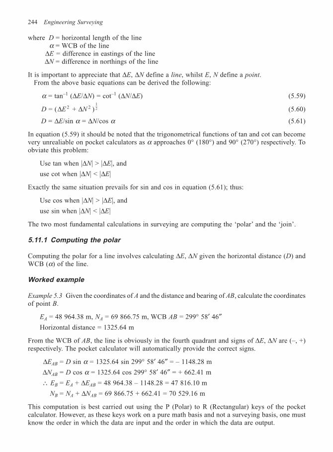
244 Engineering Surveying
where D = horizontal length of the lineα = WCB of the line
∆E = difference in eastings of the line∆N = difference in northings of the line
It is important to appreciate that ∆E, ∆N define a line, whilst E, N define a point.From the above basic equations can be derived the following:
α = tan–1 (∆E/∆N) = cot–1 (∆N/∆E) (5.59)
D E N = ( + )2 212∆ ∆ (5.60)
D = ∆E/sin α = ∆N/cos α (5.61)
In equation (5.59) it should be noted that the trigonometrical functions of tan and cot can becomevery unrealiable on pocket calculators as α approaches 0° (180°) and 90° (270°) respectively. Toobviate this problem:
Use tan when |∆N| > |∆E|, and
use cot when |∆N| < |∆E|
Exactly the same situation prevails for sin and cos in equation (5.61); thus:
Use cos when |∆N| > |∆E|, and
use sin when |∆N| < |∆E|
The two most fundamental calculations in surveying are computing the ‘polar’ and the ‘join’.
5.11.1 Computing the polar
Computing the polar for a line involves calculating ∆E, ∆N given the horizontal distance (D) andWCB (α) of the line.
Worked example
Example 5.3 Given the coordinates of A and the distance and bearing of AB, calculate the coordinatesof point B.
EA = 48 964.38 m, NA = 69 866.75 m, WCB AB = 299° 58′ 46″Horizontal distance = 1325.64 m
From the WCB of AB, the line is obviously in the fourth quadrant and signs of ∆E, ∆N are (–, +)respectively. The pocket calculator will automatically provide the correct signs.
∆EAB = D sin α = 1325.64 sin 299° 58′ 46″ = – 1148.28 m
∆NAB = D cos α = 1325.64 cos 299° 58′ 46″ = + 662.41 m
∴ EB = EA + ∆EAB = 48 964.38 – 1148.28 = 47 816.10 m
NB = NA + ∆NAB = 69 866.75 + 662.41 = 70 529.16 m
This computation is best carried out using the P (Polar) to R (Rectangular) keys of the pocketcalculator. However, as these keys work on a pure math basis and not a surveying basis, one mustknow the order in which the data are input and the order in which the data are output.
Position 245
The following methods apply to the majority of pocket calculators. However, as new types arebeing developed all the time, then individuals may have to adapt to their own specific make.
Using P and R keys;
(1) Enter horizontal distance (D); press P R→ or (x ↔ y)
(2) Enter WCB (α); press = or (R)
(3) Value displayed is ± ∆N
(4) Press x y↔ to get ± ∆E
Operations in brackets are for an alternative type of calculator.
5.11.2 Computing the join
This involves computing the horizontal distance (D) and WCB (α) from the difference in coordinates(∆E, ∆N) of a line.
Worked examples
Example 5.4 Given the following coordinates for two points A and B, compute the length andbearing of AB.
EA = 48 964.38 m NA = 69866.75 mEB = 48 988.66 m NB = 62583.18 m
∆EAB = 24.28 m ∆NAB = –7283.57 m
Note:
(1) A rough plot of the E, N of each point will show B to be south-east of A, and line AB is thereforein the second quadrant.
(2) If the direction is from A to B then:
∆EAB = EB – EA
∆NAB = NB – NA
If the required direction is B to A then:
∆EBA = EA – EB
∆NBA = NA – NB
(3) As ∆N > ∆E use tan:
αAB = tan–1 (∆E/∆N) = tan–1 (24.28/ – 7283.57)
= –0° 11′ 27″
It is obvious that as αAB is in the second quadrant and must therefore have a WCB between 90° and180°, and as we cannot have a negative WCB, –0° 11′ 27″ is unacceptable. Depending on the signsof the coordinates entered into the pocket calculator, it will supply the angles as shown inFigure 5.33.
If in quadrant I + α1 = WCB
246 Engineering Surveying
If in quadrant II – α2, then (–α2 + 180) = WCBIf in quadrant III + α3, then (α3 + 180) = WCBIf in quadrant IV – α4, then (–α4 + 360) = WCB∴ WCB AB = –0° 11′ 27″ + 180° = 179° 48′ 33″
Horizontal distance AB = DAB = ( + )2 212∆ ∆E N
(24.28 + 7283.57 )2 212 = 7283.61 m
Also as ∆N > ∆E use DAB = ∆N/cos α = 7283.57/cos 179° 48′ 33″ = 7283.61 m
Note what happens with some pocket calculators when ∆E/sin α is used:
DAB = ∆E/sin α = 24.28/sin 179° 48′ 33″ = 7 289.84 m
This enormous error of more than 6 m proves that when computing distance it is advisable to use
the Pythagoras equation D E N = ( + )2 212∆ ∆ , at all times. Of the remaining two equations, the
appropriate one may be used as a check.Using R and P keys:
(1) Enter ±∆N; press R P→ or (x ↔ y)
(2) Enter ±∆E; press = or (P)
(3) Value displayed is horizontal distance (D)
(4) Press x y↔ to obtain WCB in degrees and decimals
(5) If value in ‘4’ is negative, add 360°(6) Change to d.m.s. (°, ′, ″)
When using the P and R keys, the angular values displayed in the four quadrants are as inFigure 5.34; thus only a single ‘IF’ statement is necessary as in (5) above.
Fig. 5.33
0°+
–α4
α1
+90°
IV
III
I
II
–270°
180°–
–α2α3
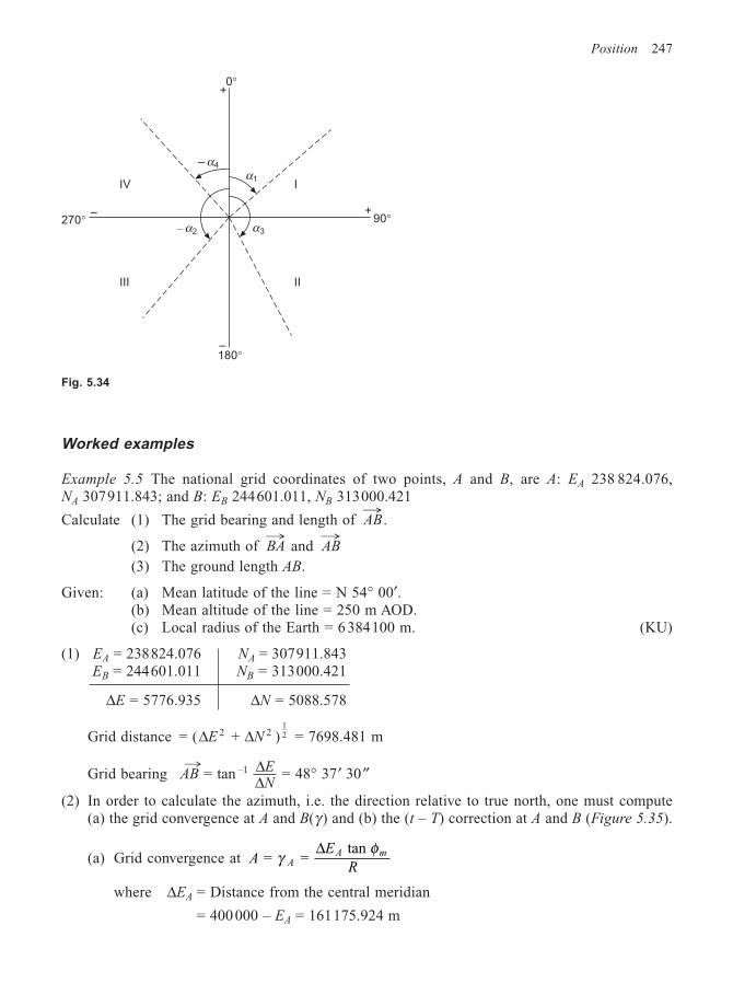
Position 247
Worked examples
Example 5.5 The national grid coordinates of two points, A and B, are A: EA 238 824.076,NA 307911.843; and B: EB 244601.011, NB 313000.421
Calculate (1) The grid bearing and length of AB→
.
(2) The azimuth of BA→
and AB→
(3) The ground length AB.
Given: (a) Mean latitude of the line = N 54° 00′.(b) Mean altitude of the line = 250 m AOD.(c) Local radius of the Earth = 6 384100 m. (KU)
(1) EA = 238824.076 NA = 307911.843EB = 244601.011 NB = 313000.421
∆E = 5776.935 ∆N = 5088.578
Grid distance = ( + )2 212∆ ∆E N = 7698.481 m
Grid bearing = tan = 48 37 30–1ABEN
→° ′ ′′∆
∆(2) In order to calculate the azimuth, i.e. the direction relative to true north, one must compute
(a) the grid convergence at A and B(γ ) and (b) the (t – T) correction at A and B (Figure 5.35).
(a) Grid convergence at AE
RAA m = =
tan γ
φ∆
where ∆EA = Distance from the central meridian
= 400 000 – EA = 161175.924 m
Fig. 5.34
I
II
IV
III
+0°
90°+
α1
– α4
α3– α2
–270°
180°–
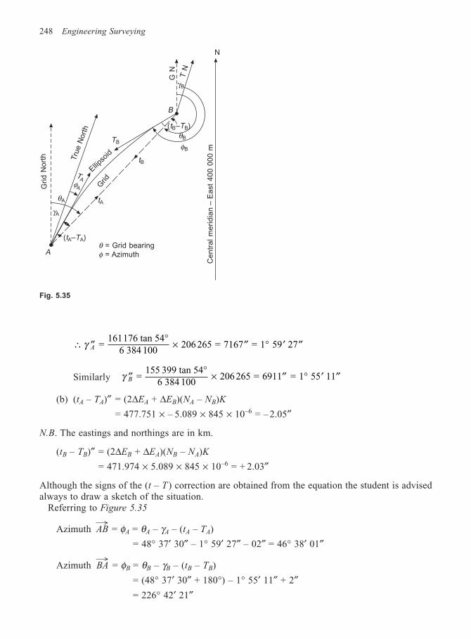
248 Engineering Surveying
∴ ′′°
× ′′ ° ′ ′′ = 161176 tan 54
6 384 100 206 265 = 7167 = 1 59 27γ A
Similarly ′′°
× ′′ ° ′ ′′γ B = 155 399 tan 54
6 384 100 206 265 = 6911 = 1 55 11
(b) (tA – TA)″ = (2∆EA + ∆EB)(NA – NB)K
= 477.751 × – 5.089 × 845 × 10–6 = – 2.05″
N.B. The eastings and northings are in km.
(tB – TB)″ = (2∆EB + ∆EA)(NB – NA)K
= 471.974 × 5.089 × 845 × 10–6 = + 2.03″
Although the signs of the (t – T ) correction are obtained from the equation the student is advisedalways to draw a sketch of the situation.
Referring to Figure 5.35
Azimuth AB→
= φA = θA – γA – (tA – TA)
= 48° 37′ 30″ – 1° 59′ 27″ – 02″ = 46° 38′ 01″
Azimuth BA→
= φB = θB – γB – (tB – TB)
= (48° 37′ 30″ + 180°) – 1° 55′ 11″ + 2″= 226° 42′ 21″
Fig. 5.35
Ce
ntr
al
me
rid
ian
–E
ast
40
0 0
00
m
N
T N
G N
γB
B
(tB–TB)
θB
φB
tB
tA
(tA–TA)
A
γA
θA
TA
φA
TB
Grid
Ellips
oid
Gri
d N
ort
h Tru
e N
ort
h
θ = Grid bearing
φ = Azimuth
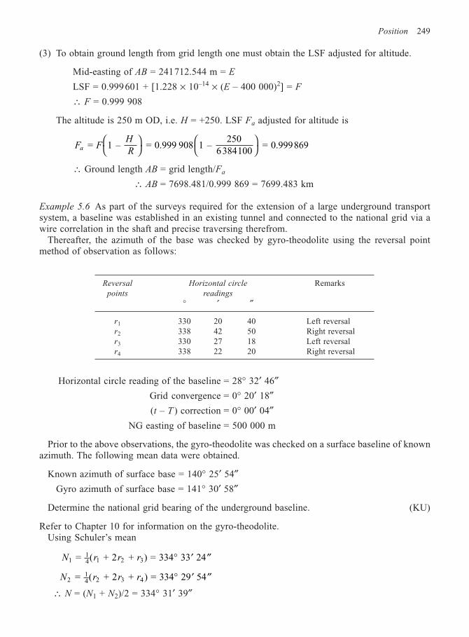
Position 249
(3) To obtain ground length from grid length one must obtain the LSF adjusted for altitude.
Mid-easting of AB = 241712.544 m = E
LSF = 0.999601 + [1.228 × 10⁻¹⁴ × (E – 400 000)2] = F
∴ F = 0.999 908
The altitude is 250 m OD, i.e. H = +250. LSF Fa adjusted for altitude is
F FH
Ra = 1 – = 0.999 908 1 – 250
6384100 = 0.999869
∴ Ground length AB = grid length/Fa
∴ AB = 7698.481/0.999 869 = 7699.483 km
Example 5.6 As part of the surveys required for the extension of a large underground transportsystem, a baseline was established in an existing tunnel and connected to the national grid via awire correlation in the shaft and precise traversing therefrom.
Thereafter, the azimuth of the base was checked by gyro-theodolite using the reversal pointmethod of observation as follows:
Reversal Horizontal circle Remarkspoints readings
° ′ ″
r1 330 20 40 Left reversalr2 338 42 50 Right reversalr3 330 27 18 Left reversalr4 338 22 20 Right reversal
Horizontal circle reading of the baseline = 28° 32′ 46″Grid convergence = 0° 20′ 18″(t – T ) correction = 0° 00′ 04″
NG easting of baseline = 500 000 m
Prior to the above observations, the gyro-theodolite was checked on a surface baseline of knownazimuth. The following mean data were obtained.
Known azimuth of surface base = 140° 25′ 54″Gyro azimuth of surface base = 141° 30′ 58″
Determine the national grid bearing of the underground baseline. (KU)
Refer to Chapter 10 for information on the gyro-theodolite.Using Schuler’s mean
N r r r114 1 2 3 = ( + 2 + ) = 334 33 24° ′ ′′
N r r r214 2 3 4 = ( + 2 + ) = 334 29 54° ′ ′′
∴ N = (N1 + N2)/2 = 334° 31′ 39″
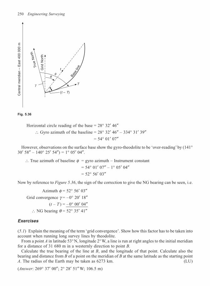
250 Engineering Surveying
Horizontal circle reading of the base = 28° 32′ 46″∴ Gyro azimuth of the baseline = 28° 32′ 46″ – 334° 31′ 39″
= 54° 01′ 07″
However, observations on the surface base show the gyro-theodolite to be ‘over-reading’ by (141°30′ 58″ – 140° 25′ 54″) = 1° 05′ 04″.
∴ True azimuth of baseline φ = gyro azimuth – Instrument constant
= 54° 01′ 07″ – 1° 05′ 04″= 52° 56′ 03″
Now by reference to Figure 5.36, the sign of the correction to give the NG bearing can be seen, i.e.
Azimuth φ = 52° 56′ 03″Grid convergence γ = – 0° 20′ 18″
(t – T ) = – 0° 00′ 04″∴ NG bearing θ = 52° 35′ 41″
Exercises
(5.1) Explain the meaning of the term ‘grid convergence’. Show how this factor has to be taken intoaccount when running long survey lines by theodolite.
From a point A in latitude 53° N, longitude 2° W, a line is run at right angles to the initial meridianfor a distance of 31 680 m in a westernly direction to point B.
Calculate the true bearing of the line at B, and the longitude of that point. Calculate also thebearing and distance from B of a point on the meridian of B at the same latitude as the starting pointA. The radius of the Earth may be taken as 6273 km. (LU)
(Answer: 269° 37′ 00″; 2° 28′ 51″ W; 106.5 m)
Fig. 5.36
Bas
elin
e
Ce
ntr
al m
eri
dia
n –
Ea
st
40
0 0
00
m
γ
θφ
tGri
d N
ort
h
Tru
e N
ort
h
(t – T)
T
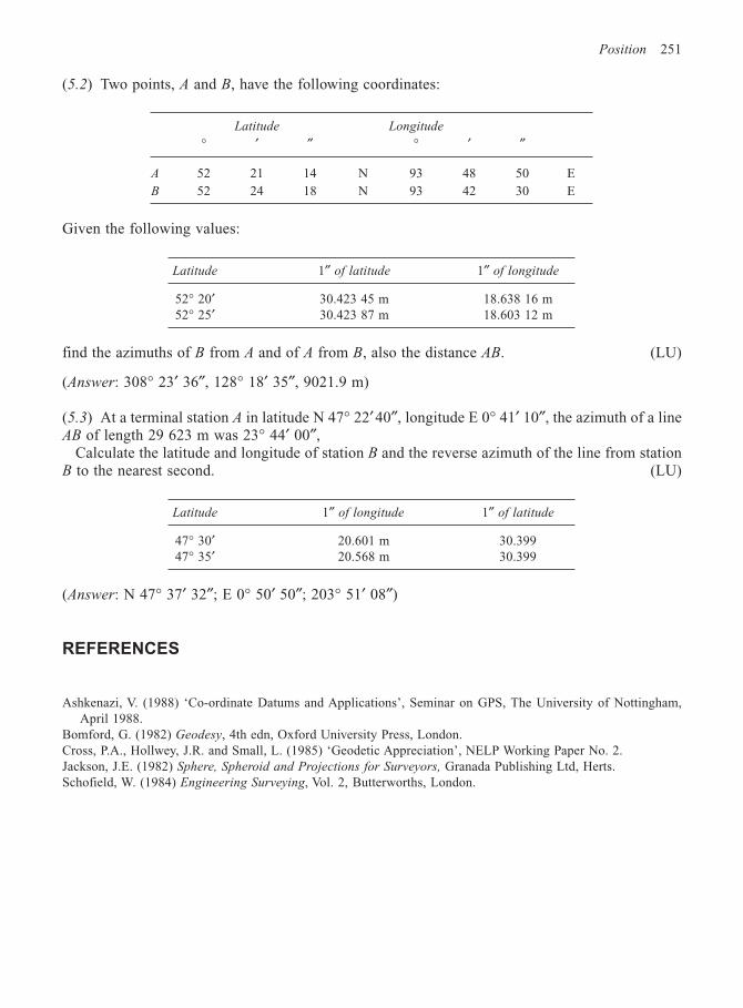
Position 251
(5.2) Two points, A and B, have the following coordinates:
Latitude Longitude
° ′ ″ ° ′ ″
A 52 21 14 N 93 48 50 E
B 52 24 18 N 93 42 30 E
Given the following values:
Latitude 1″ of latitude 1″ of longitude
52° 20′ 30.423 45 m 18.638 16 m52° 25′ 30.423 87 m 18.603 12 m
find the azimuths of B from A and of A from B, also the distance AB. (LU)
(Answer: 308° 23′ 36″, 128° 18′ 35″, 9021.9 m)
(5.3) At a terminal station A in latitude N 47° 22′40″, longitude E 0° 41′ 10″, the azimuth of a lineAB of length 29 623 m was 23° 44′ 00″,
Calculate the latitude and longitude of station B and the reverse azimuth of the line from stationB to the nearest second. (LU)
Latitude 1″ of longitude 1″ of latitude
47° 30′ 20.601 m 30.39947° 35′ 20.568 m 30.399
(Answer: N 47° 37′ 32″; E 0° 50′ 50″; 203° 51′ 08″)
REFERENCES
Ashkenazi, V. (1988) ‘Co-ordinate Datums and Applications’, Seminar on GPS, The University of Nottingham,April 1988.
Bomford, G. (1982) Geodesy, 4th edn, Oxford University Press, London.Cross, P.A., Hollwey, J.R. and Small, L. (1985) ‘Geodetic Appreciation’, NELP Working Paper No. 2.Jackson, J.E. (1982) Sphere, Spheroid and Projections for Surveyors, Granada Publishing Ltd, Herts.Schofield, W. (1984) Engineering Surveying, Vol. 2, Butterworths, London.
6
Control surveys
A control survey provides a framework of survey points, whose relative positions, in two or threedimensions, are known to prescribed degrees of accuracy. The areas covered by these points mayextend over a whole country and form the basis for the national maps of that country. Alternativelythe area may be relatively small, encompassing a construction site for which a large-scale plan isrequired. Although the areas covered in construction are usually quite small, the accuracy may berequired to a very high order. The types of engineering project envisaged are the construction oflong tunnels and/or bridges, deformation surveys for dams and reservoirs, three-dimensional tectonicground movement for landslide prediction, to name just a few. Hence control networks provide areference framework of points for:
(1) Topographic mapping and large-scale plan production.(2) Dimensional control of construction work.(3) Deformation surveys for all manner of structures, both new and old.(4) The extension and densification of existing control networks.
The methods of establishing the vertical control have already been discussed in Chapter 2, so onlytwo-dimensional horizontal control will be dealt with here. Elements of geodetic surveying havebeen dealt with in Chapter 5 and so plane surveying for engineering control will be concentratedupon.
The methods used for control surveys are:
(1) Traversing.(2) Triangulation.(3) Trilateration.(4) A combination of (2) and (3), sometimes referred to as triangulateration.(5) Satellite position fixing (see Chapter 7).(6) Inertial position fixing.
Whilst the above systems establish a network of points, single points may be fixed by intersectionand/or resection.
6.1 TRAVERSING
Since the advent of EDM equipment, traversing has emerged as the most popular method ofestablishing control networks not only in engineering surveying but also in geodetic work. Inunderground mining it is the only method of control applicable whilst in civil engineering it lendsitself ideally to surveys and dimensional control of route-type projects such as highway and pipelineconstruction.
Control surveys 253
Traverse networks are, to a large extent, free of the limitations imposed on the other systems and,compared with them, have the following advantages:
(1) Much less reconnaissance and organization required in establishing a single line of easilyaccessible stations compared with the laying out of well-conditioned geometric figures.
(2) In conjunction with (1), the limitations imposed on the other systems by topographic conditionsdo not apply to traversing.
(3) The extent of observations to only two stations at a time is relatively small and flexiblecompared with the extensive angular and/or linear observations at stations in the other systems.It is thus much easier to organize.
(4) Traverse networks are free of the strength of figure considerations so characteristic of triangularsystems. Thus once again the organizational requirements are reduced.
(5) Scale error does not accrue as in triangulation, whilst the use of longer sides, easily measuredwith EDM equipment, reduces azimuth swing errors.
(6) Traverse stations can usually be chosen so as to be easily accessible, as well as convenient forthe subsequent densification of lower order control.
(7) Traversing permits the control to closely follow the route of a highway, pipline or tunnel, etc.,with the minimum number of stations.
From the accuracy point of view it has been shown (Chrzanowski and Konecny, 1965; Adler andSchmutter, 1971) that traverse is superior to triangulation and trilateration and, in some instances,even to triangulateration. However, it must be said that these findings are disputed by Phillips(1967). Nevertheless, it can be argued that, from the accuracy point of view, traversing comparesmore than favourably with the other methods.
Thus, from a consideration of all the above statements it is obvious that from the logistical pointof view, traversing is far superior to the other methods and offers at least equivalent accuracy.
6.1.1 Types of traverse
Using the technique of traversing, the relative position of the control points is fixed by measuringthe horizontal angle at each point, subtended by the adjacent stations, and the horizontal distancebetween consecutive pairs of stations.
The procedures for measuring angles have been dealt with in Chapter 4 and for measuringdistance in Chapter 3. The majority of traverses carried out today would most probably capture thefield data using a total station. Hence the distance is measured by EDM and the angles by digitalprocesses. Occasionally, steel tapes may be used for distance.
The liability of a traverse to undetected error makes it essential that there should be some externalcheck on its accuracy. To this end the traverse may commence from and connect into known pointsof greater accuracy than the traverse. In this way the error vector of misclose can be quantified anddistributed throughout the network, to produce geometric correctness. Such a traverse is called a‘link’ traverse.
Alternatively, the error vector can be obtained by completing the traverse back to its startingorigin. Such a traverse is called a ‘polygonal’ or ‘loop’ traverse. Both the ‘link’ and ‘polygonal’traverse are generally referred to as ‘closed’ traverses.
The third type of traverse is the ‘free’ or ‘open’ traverse, which does not close back onto anyknown point and which therefore has no way of detecting or quantifying the errors.
(1) Link traverse
Figure 6.1 illustrates a typical link traverse commencing from higher order point Y and closing onto
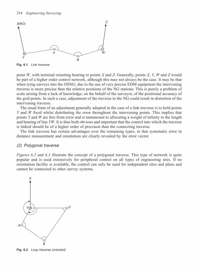
254 Engineering Surveying
point W, with terminal orienting bearing to points X and Z. Generally, points X, Y, W and Z wouldbe part of a higher order control network, although this may not always be the case. It may be thatwhen tying surveys into the OSNG, due to the use of very precise EDM equipment the interveningtraverse is more precise than the relative positions of the NG stations. This is purely a problem ofscale arising from a lack of knowledge, on the behalf of the surveyor, of the positional accuracy ofthe grid points. In such a case, adjustment of the traverse to the NG could result in distortion of theintervening traverse.
The usual form of an adjustment generally adopted in the case of a link traverse is to hold pointsY and W fixed whilst distributing the error throughout the intervening points. This implies thatpoints Y and W are free from error and is tantamount to allocating a weight of infinity to the lengthand bearing of line YW. It is thus both obvious and important that the control into which the traverseis linked should be of a higher order of precision than the connecting traverse.
The link traverse has certain advantages over the remaining types, in that systematic error indistance measurement and orientation are clearly revealed by the error vector.
(2) Polygonal traverse
Figures 6.2 and 6.3 illustrate the concept of a polygonal traverse. This type of network is quitepopular and is used extensively for peripheral control on all types of engineering sites. If noorientation facility is available, the control can only be used for independent sites and plans andcannot be connected to other survey systems.
Fig. 6.1 Link traverse
X(RO)
A
B
W
Z
Y
X
Y C
B
A
Fig. 6.2 Loop traverse (oriented)
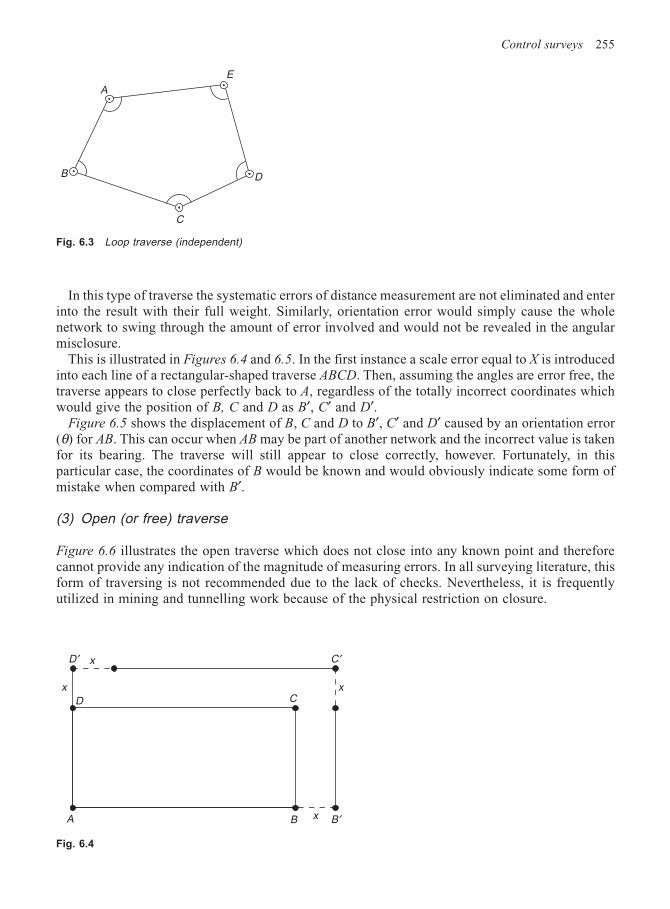
Control surveys 255
In this type of traverse the systematic errors of distance measurement are not eliminated and enterinto the result with their full weight. Similarly, orientation error would simply cause the wholenetwork to swing through the amount of error involved and would not be revealed in the angularmisclosure.
This is illustrated in Figures 6.4 and 6.5. In the first instance a scale error equal to X is introducedinto each line of a rectangular-shaped traverse ABCD. Then, assuming the angles are error free, thetraverse appears to close perfectly back to A, regardless of the totally incorrect coordinates whichwould give the position of B, C and D as B′, C′ and D′.
Figure 6.5 shows the displacement of B, C and D to B′, C′ and D′ caused by an orientation error(θ) for AB. This can occur when AB may be part of another network and the incorrect value is takenfor its bearing. The traverse will still appear to close correctly, however. Fortunately, in thisparticular case, the coordinates of B would be known and would obviously indicate some form ofmistake when compared with B′.
(3) Open (or free) traverse
Figure 6.6 illustrates the open traverse which does not close into any known point and thereforecannot provide any indication of the magnitude of measuring errors. In all surveying literature, thisform of traversing is not recommended due to the lack of checks. Nevertheless, it is frequentlyutilized in mining and tunnelling work because of the physical restriction on closure.
Fig. 6.3 Loop traverse (independent)
D′ x
x
A B B′
x
D C
C′
x
Fig. 6.4
B
A
C
D
E
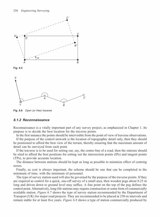
256 Engineering Surveying
6.1.2 Reconnaissance
Reconnaissance is a vitally important part of any survey project, as emphasized in Chapter 1. Itspurpose is to decide the best location for the traverse points.
In the first instance the points should be intervisible from the point of view of traverse observations.If the purpose of the control network is the location of topographic detail only, then they should
be positioned to afford the best view of the terrain, thereby ensuring that the maximum amount ofdetail can be surveyed from each point.
If the traverse is to be used for setting out, say, the centre-line of a road, then the stations shouldbe sited to afford the best positions for setting out the intersection points (IPs) and tangent points(TPs), to provide accurate location.
The distance between stations should be kept as long as possible to minimize effect of centringerrors.
Finally, as cost is always important, the scheme should be one that can be completed in theminimum of time, with the minimum of personnel.
The type of survey station used will also be governed by the purpose of the traverse points. If theyare required as control for a quick, one-off survey of a small area, then wooden pegs about 0.25 mlong and driven down to ground level may suffice. A fine point on the top of the peg defines thecontrol point. Alternatively, long-life stations may require construction or some form of commerciallyavailable station. Figure 6.7 shows the type of survey station recommended by the Department ofTransport (UK) for major road projects. They are recommended to be placed at 250-m intervals andremain stable for at least five years. Figure 6.8 shows a type of station commercially produced by
θ
A B
C′
D′D
C
B′
Fig. 6.6 Open (or free) traverse
Y
X
A
B
C
Fig. 6.5
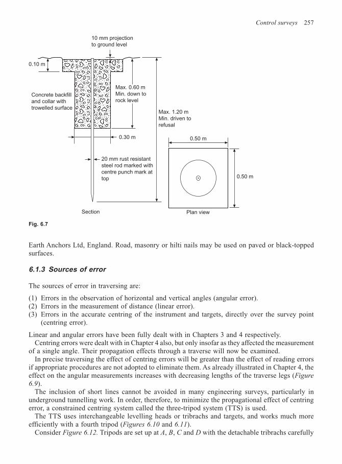
Control surveys 257
Earth Anchors Ltd, England. Road, masonry or hilti nails may be used on paved or black-toppedsurfaces.
6.1.3 Sources of error
The sources of error in traversing are:
(1) Errors in the observation of horizontal and vertical angles (angular error).(2) Errors in the measurement of distance (linear error).(3) Errors in the accurate centring of the instrument and targets, directly over the survey point
(centring error).
Linear and angular errors have been fully dealt with in Chapters 3 and 4 respectively.Centring errors were dealt with in Chapter 4 also, but only insofar as they affected the measurement
of a single angle. Their propagation effects through a traverse will now be examined.In precise traversing the effect of centring errors will be greater than the effect of reading errors
if appropriate procedures are not adopted to eliminate them. As already illustrated in Chapter 4, theeffect on the angular measurements increases with decreasing lengths of the traverse legs (Figure
6.9).The inclusion of short lines cannot be avoided in many engineering surveys, particularly in
underground tunnelling work. In order, therefore, to minimize the propagational effect of centringerror, a constrained centring system called the three-tripod system (TTS) is used.
The TTS uses interchangeable levelling heads or tribrachs and targets, and works much moreefficiently with a fourth tripod (Figures 6.10 and 6.11).
Consider Figure 6.12. Tripods are set up at A, B, C and D with the detachable tribrachs carefully
10 mm projection
to ground level
Concrete backfill
and collar with
trowelled surface
Max. 0.60 m
Min. down to
rock level
0.10 m
0.30 m 0.50 m
0.50 m
Plan view
20 mm rust resistant
steel rod marked with
centre punch mark at
top
Section
Max. 1.20 m
Min. driven to
refusal
Fig. 6.7
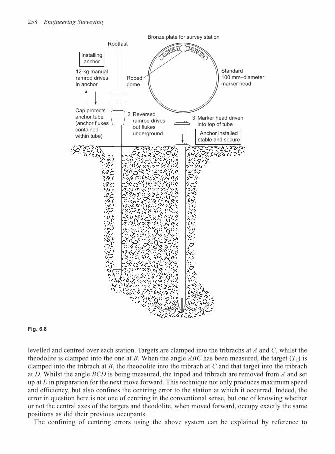
258 Engineering Surveying
levelled and centred over each station. Targets are clamped into the tribrachs at A and C, whilst thetheodolite is clamped into the one at B. When the angle ABC has been measured, the target (T1) isclamped into the tribrach at B, the theodolite into the tribrach at C and that target into the tribrachat D. Whilst the angle BCD is being measured, the tripod and tribrach are removed from A and setup at E in preparation for the next move forward. This technique not only produces maximum speedand efficiency, but also confines the centring error to the station at which it occurred. Indeed, theerror in question here is not one of centring in the conventional sense, but one of knowing whetheror not the central axes of the targets and theodolite, when moved forward, occupy exactly the samepositions as did their previous occupants.
The confining of centring errors using the above system can be explained by reference to
SURVEY MARKER
Bronze plate for survey station
Standard
100 mm–diameter
marker headRobed
dome
2 Reversed
ramrod drives
out flukes
underground
3 Marker head driven
into top of tube
Installing
anchor
12-kg manual
ramrod drives
in anchor
Cap protects
anchor tube
(anchor flukes
contained
within tube)Anchor installed
stable and secure
Rootfast
Fig. 6.8
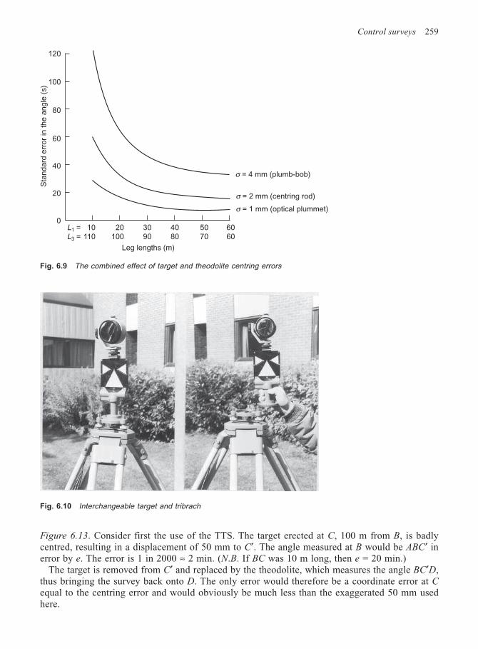
Control surveys 259
Figure 6.13. Consider first the use of the TTS. The target erected at C, 100 m from B, is badlycentred, resulting in a displacement of 50 mm to C′. The angle measured at B would be ABC′ inerror by e. The error is 1 in 2000 ≈ 2 min. (N.B. If BC was 10 m long, then e = 20 min.)
The target is removed from C′ and replaced by the theodolite, which measures the angle BC′D,thus bringing the survey back onto D. The only error would therefore be a coordinate error at Cequal to the centring error and would obviously be much less than the exaggerated 50 mm usedhere.
Fig. 6.9 The combined effect of target and theodolite centring errors
Fig. 6.10 Interchangeable target and tribrach
120
100
80
60
40
20
0L1 = 10 20 30 40 50 60
L3 = 110 100 90 80 70 60
Sta
nda
rd e
rror
in the a
ngle
(s)
Leg lengths (m)
σ = 2 mm (centring rod)
σ = 1 mm (optical plummet)
σ = 4 mm (plumb-bob)
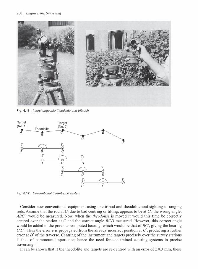
260 Engineering Surveying
Consider now conventional equipment using one tripod and theodolite and sighting to rangingrods. Assume that the rod at C, due to bad centring or tilting, appears to be at C′; the wrong angle,ABC′, would be measured. Now, when the theodolite is moved it would this time be correctlycentred over the station at C and the correct angle BCD measured. However, this correct anglewould be added to the previous computed bearing, which would be that of BC′, giving the bearingC′D′. Thus the error e is propagated from the already incorrect position at C′, producing a furthererror at D′ of the traverse. Centring of the instrument and targets precisely over the survey stationsis thus of paramount importance; hence the need for constrained centring systems in precisetraversing.
It can be shown that if the theodolite and targets are re-centred with an error of ± 0.3 mm, these
Fig. 6.11 Interchangeable theodolite and tribrach
Fig. 6.12 Conventional three-tripod system
Target
(No. 1)Target
(No. 2)Theodolite
AB
C
D
E
FT1 T2
A CB
T2
B DC
T1 T2
C ED
T1 T2
D FE
T1
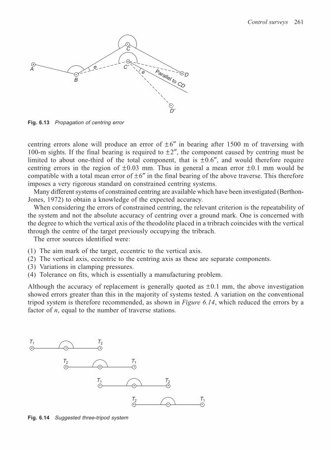
Control surveys 261
centring errors alone will produce an error of ± 6″ in bearing after 1500 m of traversing with100-m sights. If the final bearing is required to ±2″, the component caused by centring must belimited to about one-third of the total component, that is ±0.6″, and would therefore requirecentring errors in the region of ±0.03 mm. Thus in general a mean error ±0.1 mm would becompatible with a total mean error of ±6″ in the final bearing of the above traverse. This thereforeimposes a very rigorous standard on constrained centring systems.
Many different systems of constrained centring are available which have been investigated (Berthon-Jones, 1972) to obtain a knowledge of the expected accuracy.
When considering the errors of constrained centring, the relevant criterion is the repeatability ofthe system and not the absolute accuracy of centring over a ground mark. One is concerned withthe degree to which the vertical axis of the theodolite placed in a tribrach coincides with the verticalthrough the centre of the target previously occupying the tribrach.
The error sources identified were:
(1) The aim mark of the target, eccentric to the vertical axis.(2) The vertical axis, eccentric to the centring axis as these are separate components.(3) Variations in clamping pressures.(4) Tolerance on fits, which is essentially a manufacturing problem.
Although the accuracy of replacement is generally quoted as ±0.1 mm, the above investigationshowed errors greater than this in the majority of systems tested. A variation on the conventionaltripod system is therefore recommended, as shown in Figure 6.14, which reduced the errors by afactor of n, equal to the number of traverse stations.
Fig. 6.13 Propagation of centring error
A
B
C′e
C
D
D′
Parallel to CD
e
Fig. 6.14 Suggested three-tripod system
T2T1
T1T2
T2T1
T1T2
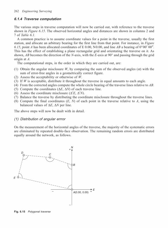
262 Engineering Surveying
6.1.4 Traverse computation
The various steps in traverse computation will now be carried out, with reference to the traverseshown in Figure 6.15. The observed horizontal angles and distances are shown in columns 2 and7 of Table 6.1.
A common practice is to assume coordinate values for a point in the traverse, usually the firststation, and allocate an arbitrary bearing for the first line from that point. For instance, in Figure
6.15, point A has been allocated coordinates of E 0.00, N0.00, and line AB a bearing of 0°00′ 00″.This has the effect of establishing a plane rectangular grid and orientating the traverse on it. Asshown, AB becomes the direction of the N-axis, with the E-axis at 90° and passing through the gridorigin at A.
The computational steps, in the order in which they are carried out, are:
(1) Obtain the angular misclosure W, by comparing the sum of the observed angles (α) with thesum of error-free angles in a geometrically correct figure.
(2) Assess the acceptability or otherwise of W.(3) If W is acceptable, distribute it throughout the traverse in equal amounts to each angle.(4) From the corrected angles compute the whole circle bearing of the traverse lines relative to AB.(5) Compute the coordinates (∆E, ∆N) of each traverse line.(6) Assess the coordinate misclosure (∆′E, ∆′N).(7) Balance the traverse by distributing the coordinate misclosure throughout the traverse lines.(8) Compute the final coordinates (E, N) of each point in the traverse relative to A, using the
balanced values of ∆E, ∆N per line.
The above steps will now be dealt with in detail.
(1) Distribution of angular errror
On the measurement of the horizontal angles of the traverse, the majority of the systematic errorsare eliminated by repeated double-face observation. The remaining random errors are distributedequally around the network, as follows.
Fig. 6.15 Polygonal traverse
DC
B
EA(0.00, 0.00) +
+N
–
–
E
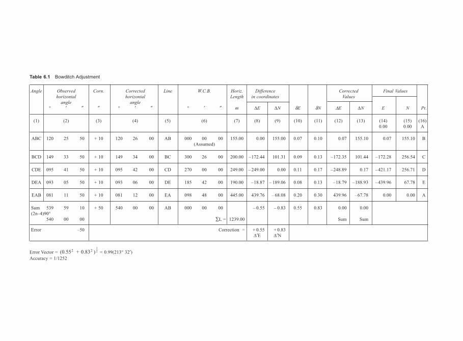
Table 6.1 Bowditch Adjustment
Angle Observed Corn. Corrected Line W.C.B. Horiz. Difference Corrected Final Values
horizontal horizontal Length in coordinates Values
angle angle
° ′ ″ ″ ° ′ ″ ° ′ ″ m ∆E ∆N δE δN ∆E ∆N E N Pt.
(1) (2) (3) (4) (5) (6) (7) (8) (9) (10) (11) (12) (13) (14) (15) (16)0.00 0.00 A
ABC 120 25 50 + 10 120 26 00 AB 000 00 00 155.00 0.00 155.00 0.07 0.10 0.07 155.10 0.07 155.10 B(Assumed)
BCD 149 33 50 + 10 149 34 00 BC 300 26 00 200.00 –172.44 101.31 0.09 0.13 –172.35 101.44 –172.28 256.54 C
CDE 095 41 50 + 10 095 42 00 CD 270 00 00 249.00 – 249.00 0.00 0.11 0.17 –248.89 0.17 –421.17 256.71 D
DEA 093 05 50 + 10 093 06 00 DE 185 42 00 190.00 –18.87 – 189.06 0.08 0.13 –18.79 –188.93 –439.96 67.78 E
EAB 081 11 50 + 10 081 12 00 EA 098 48 00 445.00 439.76 – 68.08 0.20 0.30 439.96 –67.78 0.00 0.00 A
Sum 539 59 10 + 50 540 00 00 AB 000 00 00 – 0.55 – 0.83 0.55 0.83 0.00 0.00 (2n–4)90°
540 00 00 ∑L = 1239.00 Sum Sum
Error –50 Correction = + 0.55 + 0.83∆′E ∆′N
Error Vector = (0.55 + 0.83 )2 212 = 0.99(213° 32′)
Accuracy = 1/1252
264 Engineering Surveying
In a polygon the sum of the internal angles should equal (2n – 4)90°, the sum of the external
angles should equal (2n + 4)90°.
∴ Angular misclosure = W = Σi
n
= 1αi – (2n ± 4)90° = – 50″ (Table 6.1)
where α = mean observed anglen = number of angles in the traverse
The angular misclosure W is now distributed by equal amounts on each angle, thus:
Correction per angle = W/n = + 10″ (Table 6.1)
However, before the angles are corrected, the angular misclosure W must be considered to beacceptable. If W was too great, and therefore indicative of poor observations, the whole traversemay need to be re-measured. A method of assessing the acceptability or otherwise of W is given inSection 2.
(2) Acceptable angular misclosure
The following procedure may be adopted provided that there is evidence of the variance of themean observed angles, i.e.
σ σ σ σw a a an2
12
22 2 = + + . . + .
where σ an2 = variance of the mean observed angle
σ w2 = variance of the sum of the angles of the traverse
Assuming that each angle is measured with equal precision:
σ σ σ σa a an A12
22 2 2 = = . . = = .
then σ σw An2 2 = ⋅ and
σ σw An = 12 ⋅ (6.1)
Angular misclosure = W = Σi
n
= 1αi – [(2n ± 4)90°]
where α = mean observed anglen = number of angles in traverse
then for 95% confidence
P(– 1.96σw < W < +1.96αw) = 0.95 (6.2)
and for 99.73% confidence
P(– 3σw < W < +3σw) = 0.9973 (6.3)
For example, consider a closed traverse of nine angles. Tests prior to the survey showed that theparticular theodolite used had a standard error (σA) of ± 3″. What would be considered an acceptableangular misclosure for the traverse?
σ w = 9 3 = 12 ⋅ ′′ ± ′′ 9
P(– 1.96 × 9″ < W < + 1.96 × 9″) = 0.95
P(– 18″ < W < + 18″) = 0.95
Similarly P(– 27″ < W < + 27″) = 0.9973
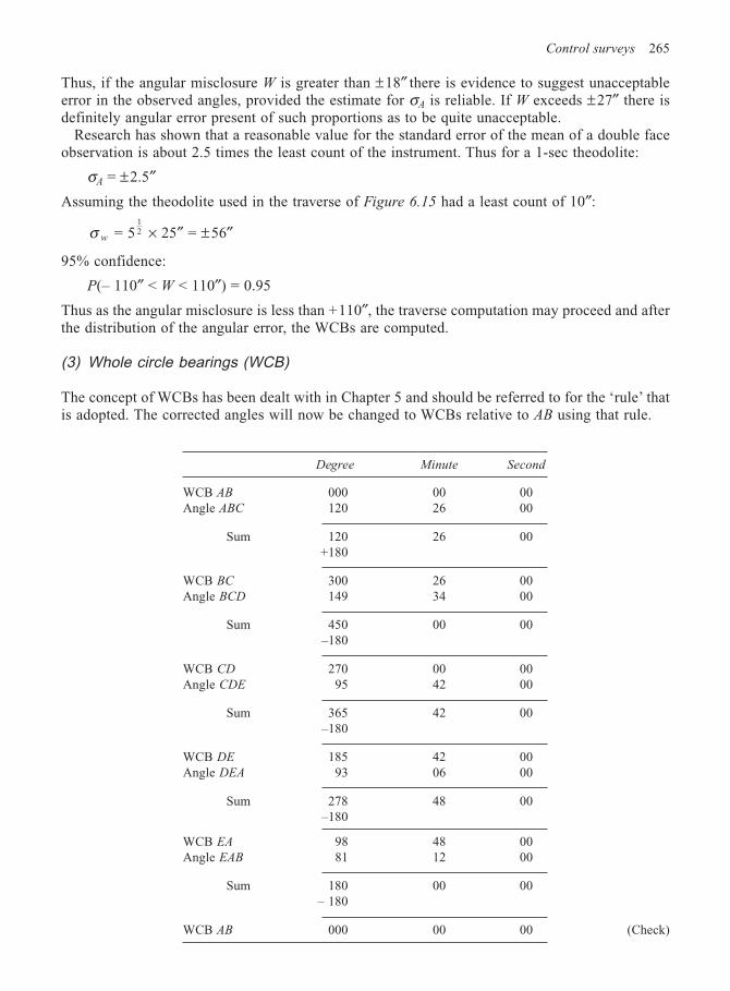
Control surveys 265
Thus, if the angular misclosure W is greater than ±18″ there is evidence to suggest unacceptableerror in the observed angles, provided the estimate for σA is reliable. If W exceeds ±27″ there isdefinitely angular error present of such proportions as to be quite unacceptable.
Research has shown that a reasonable value for the standard error of the mean of a double faceobservation is about 2.5 times the least count of the instrument. Thus for a 1-sec theodolite:
σA = ±2.5″
Assuming the theodolite used in the traverse of Figure 6.15 had a least count of 10″:
σ w = 512 × 25″ = ±56″
95% confidence:
P(– 110″ < W < 110″) = 0.95
Thus as the angular misclosure is less than +110″, the traverse computation may proceed and afterthe distribution of the angular error, the WCBs are computed.
(3) Whole circle bearings (WCB)
The concept of WCBs has been dealt with in Chapter 5 and should be referred to for the ‘rule’ thatis adopted. The corrected angles will now be changed to WCBs relative to AB using that rule.
Degree Minute Second
WCB AB 000 00 00Angle ABC 120 26 00
Sum 120 26 00+180
WCB BC 300 26 00Angle BCD 149 34 00
Sum 450 00 00–180
WCB CD 270 00 00Angle CDE 95 42 00
Sum 365 42 00–180
WCB DE 185 42 00Angle DEA 93 06 00
Sum 278 48 00–180
WCB EA 98 48 00Angle EAB 81 12 00
Sum 180 00 00– 180
WCB AB 000 00 00 (Check)
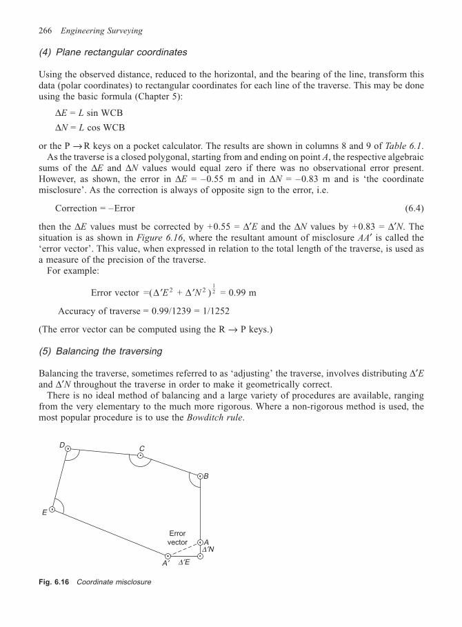
266 Engineering Surveying
(4) Plane rectangular coordinates
Using the observed distance, reduced to the horizontal, and the bearing of the line, transform thisdata (polar coordinates) to rectangular coordinates for each line of the traverse. This may be doneusing the basic formula (Chapter 5):
∆E = L sin WCB
∆N = L cos WCB
or the P → R keys on a pocket calculator. The results are shown in columns 8 and 9 of Table 6.1.As the traverse is a closed polygonal, starting from and ending on point A, the respective algebraic
sums of the ∆E and ∆N values would equal zero if there was no observational error present.However, as shown, the error in ∆E = –0.55 m and in ∆N = –0.83 m and is ‘the coordinatemisclosure’. As the correction is always of opposite sign to the error, i.e.
Correction = –Error (6.4)
then the ∆E values must be corrected by +0.55 = ∆′E and the ∆N values by +0.83 = ∆′N. Thesituation is as shown in Figure 6.16, where the resultant amount of misclosure AA′ is called the‘error vector’. This value, when expressed in relation to the total length of the traverse, is used asa measure of the precision of the traverse.
For example:
Error vector =( + )2 21
′ ′∆ ∆E N 2 = 0.99 m
Accuracy of traverse = 0.99/1239 = 1/1252
(The error vector can be computed using the R → P keys.)
(5) Balancing the traversing
Balancing the traverse, sometimes referred to as ‘adjusting’ the traverse, involves distributing ∆′Eand ∆′N throughout the traverse in order to make it geometrically correct.
There is no ideal method of balancing and a large variety of procedures are available, rangingfrom the very elementary to the much more rigorous. Where a non-rigorous method is used, themost popular procedure is to use the Bowditch rule.
Fig. 6.16 Coordinate misclosure
B
A
A′
∆′N
∆′E
E
DC
Error
vector
Control surveys 267
The ‘Bowditch rule’ was devised by Nathaniel Bowditch, surveyor, navigator and mathematician,as a proposed solution to the problem of compass traverse adjustment, which was posed in theAmerican journal The Analyst in 1807.
The Bowditch rule is as follows:
δEE
Li
i
n
i
=
= 1
′∆
Σ · Li = K1 · Li (6.5)
and
δNN
Li
i
n
i
=
= 1
′∆
Σ · Li = K2 · Li (6.6)
where δEi, δNi = the coordinate corrections∆′E, ∆′N = the coordinate misclosure (constant)
Σi
n
iL = 1
= the sum of the lengths of the traverse (constant)
Li = the horizontal length of the ith traverse legK1, K2 = the resultant constants
From equations (6.5) and (6.6), it can be seen that the corrections made are simply in proportion tothe length of the line.
The correction for each length is now computed in order.For the first line AB:
δE1 = (∆′E/∑L)L1 = K1 · L1
where K1 = +0.55/1239 = 4.4 × 10⁻⁴
∴ δE1 = (4.4 × 10⁻⁴)155.00 = +0.07
Similarly for the second line BC:
δE2 = (4.4 × 10⁻⁴)200.00 = +0.09
and so on:
δE3 = (4.4 × 10⁻⁴)249.00 = +0.11δE4 = (4.4 × 10⁻⁴)190.00 = +0.08δE5 = (4.4 × 10⁻⁴)445.00 = +0.20
———Sum = +0.55 (Check)
———Similarly for the ∆N value of each line:
δN1 = (∆′N/∑L)L1 = K2L1
where K2 = +0.83/1239 = 6.7 × 10⁻⁴
∴ δN1 = (6.7 × 10⁻⁴)155.00 = +0.10
and so on for each line:
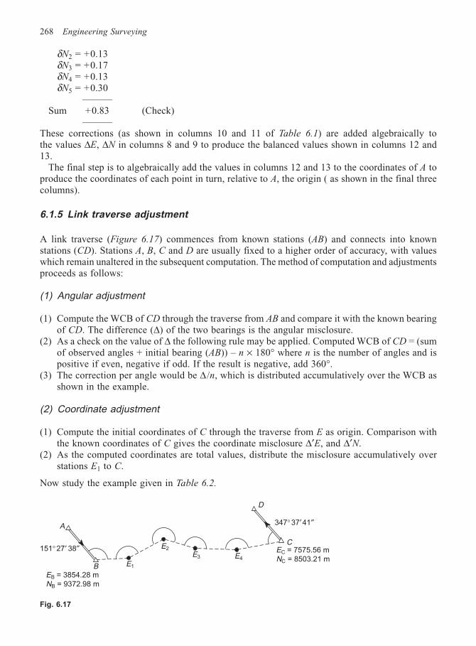
268 Engineering Surveying
δN2 = +0.13δN3 = +0.17δN4 = +0.13δN5 = +0.30
———Sum +0.83 (Check)
———These corrections (as shown in columns 10 and 11 of Table 6.1) are added algebraically tothe values ∆E, ∆N in columns 8 and 9 to produce the balanced values shown in columns 12 and13.
The final step is to algebraically add the values in columns 12 and 13 to the coordinates of A toproduce the coordinates of each point in turn, relative to A, the origin ( as shown in the final threecolumns).
6.1.5 Link traverse adjustment
A link traverse (Figure 6.17) commences from known stations (AB) and connects into knownstations (CD). Stations A, B, C and D are usually fixed to a higher order of accuracy, with valueswhich remain unaltered in the subsequent computation. The method of computation and adjustmentsproceeds as follows:
(1) Angular adjustment
(1) Compute the WCB of CD through the traverse from AB and compare it with the known bearingof CD. The difference (∆) of the two bearings is the angular misclosure.
(2) As a check on the value of ∆ the following rule may be applied. Computed WCB of CD = (sumof observed angles + initial bearing (AB)) – n × 180° where n is the number of angles and ispositive if even, negative if odd. If the result is negative, add 360°.
(3) The correction per angle would be ∆ /n, which is distributed accumulatively over the WCB asshown in the example.
(2) Coordinate adjustment
(1) Compute the initial coordinates of C through the traverse from E as origin. Comparison withthe known coordinates of C gives the coordinate misclosure ∆′E, and ∆′N.
(2) As the computed coordinates are total values, distribute the misclosure accumulatively overstations E1 to C.
Now study the example given in Table 6.2.
Fig. 6.17
B
E2
E1
E3 E4
C
D
EB = 3854.28 m
NB = 9372.98 m
EC = 7575.56 m
NC = 8503.21 m
A 347°37′41″
151°27′ 38″
Control surveys 269
6.1.6 The effect of the balancing procedure
The purpose of this section is to show that balancing a traverse does not in any way improve it; itsimply makes the figure geometrically correct.
The survey stations set in the ground represent the ‘true’ traverse, which in practice is unknown.Observation of the angles and distances is an attempt to obtain the value of the true traverse. It isnever achieved, due to observational error, and hence we have an ‘observed’ traverse, which mayapproximate very closely to the ‘true’, but is not geometrically correct, i.e. there is coordinatemisclosure. Finally, we have the ‘balanced’ traverse after the application of the Bowditch rule. Thistraverse is now geometrically correct, but in the majority of cases will be significantly differentfrom both the ‘true’ and ‘observed’ network.
As field data are generally captured to the highest accuracy possible, relative to the expertise ofthe surveyor and the instrumentation used, it could be argued that the best balancing process is thatwhich alters the field data the least.
Basically the Bowditch rule adjusts the positions of the traverse stations, resulting in changes tothe observed data. For instance, it can be shown that the changes to the angles will be equal to:
δαi = 2cos α i
2 (∆′E cos β + ∆′N sin β)/∑L) (6.7a)
where β is the mean bearing of the lines subtending the angle α. This does not, however, apply tothe first and last angle, where the corrections are
δα1 = –(∆′E sin β1 + ∆′N cos β1)/∑L (6.7b)
δαn = +(∆′E sin βn + ∆′ N cos βn)/∑L (6.7c)
The Bowditch adjustment results in changes to the distances equal to
δL = f L
t (∆′N cos β + ∆′E sin β) (6.7d)
where f = the factor of proportiont = the error vector.
It can be seen from equation (6.7a) that in a relatively straight traverse, where the angle (α)approximates to 180°, the corrections to the angles (δα) will be zero for all but the first and lastangles.
6.1.7 Accuracy of traversing
Computer simulation of all types of network has shown that traversing is generally more accuratethan classical triangulation and trilateration. Due to the weak geometry of a traverse, it generallyhas only three degrees of freedom (that is three redundant observations), it is difficult to arrive atan estimate of accuracy. This, coupled with the effect of the balancing procedure, makes it virtuallyimpossible. Although there have been many attempts to produce equations defining the accuracy ofa traverse, at the present time the best approach is a strength analysis using variance–covariancematrices from a least squares adjustment.
6.1.8 Blunders in the observed data
Blunders or mistakes in the measurement of the angles, results in gross angular misclosure. Providedit is only a single blunder it can easily be located.
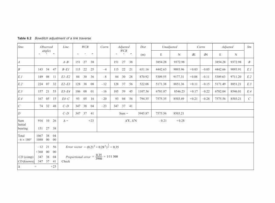
Table 6.2 Bowditch adjustment of a link traverse
Stns Observed Line WCB Corrn Adjusted Dist Unadjusted Corrn Adjusted Stn
angles WCB
° ′ ″ ° ′ ″ ° ′ ″ (m) E N δE δN E N
A A–B 151 27 38 151 27 38 3854.28 9372.98 3854.28 9372.98 B
B 143 54 47 B–E1 115 22 25 –4 115 22 21 651.16 4442.63 9093.96 +0.03 –0.05 4442.66 9093.91 E.1
E.1 149 08 11 E1–E2 84 30 36 –8 84 30 28 870.92 5309.55 9177.31 +0.08 –0.11 5309.63 9711.20 E.2
E.2 224 07 32 E2–E3 128 38 08 –12 128 37 56 522.08 5171.38 8851.36 +0.11 –0.15 5171.49 8851.21 E.3
E.3 157 21 53 E3–E4 106 00 01 –16 105 59 45 1107.36 6781.87 8546.23 +0.17 –0.22 6782.04 8546.01 E.4
E.4 167 05 15 E4–C 93 05 16 –20 93 04 56 794.35 7575.35 8503.49 +0.21 –0.28 7575.56 8503.21 C
C 74 32 48 C–D 347 38 04 –23 347 37 41
D C–D 347 37 41 Sum = 3945.87 7575.56 8503.21
Sum 916 10 26 ∆ = +23 ∆′E, ∆′N – 0.21 + 0.28Initialbearing 151 27 38
Total 1067 38 04– 6 × 180° 1080 00 00
–12 21 56 Error vector = (0.21 + 0.28 ) = 0.352 212
+360 00 00
CD (comp) 347 38 04 Proportional error = 0.353946
= 1/11 300
CD (known) 347 37 41 Check
∆ = +23
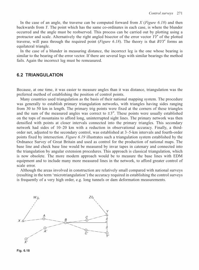
Control surveys 271
In the case of an angle, the traverse can be computed forward from X (Figure 6.18) and thenbackwards from Y. The point which has the same co-ordinates in each case, is where the blunderoccurred and the angle must be reobserved. This process can be carried out by plotting using aprotractor and scale. Alternatively the right angled bisector of the error vector YY′ of the plottedtraverse, will pass through the required point (Figure 6.18). The theory is that BYY′ forms anequilateral triangle.
In the case of a blunder in measuring distance, the incorrect leg is the one whose bearing issimilar to the bearing of the error vector. If there are several legs with similar bearings the methodfails. Again the incorrect leg must be remeasured.
6.2 TRIANGULATION
Because, at one time, it was easier to measure angles than it was distance, triangulation was thepreferred method of establishing the position of control points.
Many countries used triangulation as the basis of their national mapping system. The procedurewas generally to establish primary triangulation networks, with triangles having sides rangingfrom 30 to 50 km in length. The primary trig points were fixed at the corners of these trianglesand the sum of the measured angles was correct to ±3″. These points were usually establishedon the tops of mountains to afford long, uninterrupted sight lines. The primary network was thendensified with points at closer intervals connected into the primary triangles. This secondarynetwork had sides of 10–20 km with a reduction in observational accuracy. Finally, a third-order net, adjusted to the secondary control, was established at 3–5-km intervals and fourth-orderpoints fixed by intersection. Figure 6.19 illustrates such a triangulation system established by theOrdnance Survey of Great Britain and used as control for the production of national maps. Thebase line and check base line would be measured by invar tapes in catenary and connected intothe triangulation by angular extension procedures. This approach is classical triangulation, whichis now obsolete. The more modern approach would be to measure the base lines with EDMequipment and to include many more measured lines in the network, to afford greater control ofscale error.
Although the areas involved in construction are relatively small compared with national surveys(resulting in the term ‘microtriangulation’) the accuracy required in establishing the control surveysis frequently of a very high order, e.g. long tunnels or dam deformation measurements.
Fig. 6.18
X′
A′C′
Y′
Y
Z
CB
A
X
W
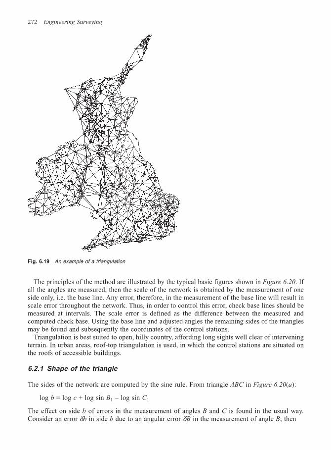
272 Engineering Surveying
The principles of the method are illustrated by the typical basic figures shown in Figure 6.20. Ifall the angles are measured, then the scale of the network is obtained by the measurement of oneside only, i.e. the base line. Any error, therefore, in the measurement of the base line will result inscale error throughout the network. Thus, in order to control this error, check base lines should bemeasured at intervals. The scale error is defined as the difference between the measured andcomputed check base. Using the base line and adjusted angles the remaining sides of the trianglesmay be found and subsequently the coordinates of the control stations.
Triangulation is best suited to open, hilly country, affording long sights well clear of interveningterrain. In urban areas, roof-top triangulation is used, in which the control stations are situated onthe roofs of accessible buildings.
6.2.1 Shape of the triangle
The sides of the network are computed by the sine rule. From triangle ABC in Figure 6.20(a):
log b = log c + log sin B1 – log sin C1
The effect on side b of errors in the measurement of angles B and C is found in the usual way.Consider an error δb in side b due to an angular error δB in the measurement of angle B; then
Fig. 6.19 An example of a triangulation
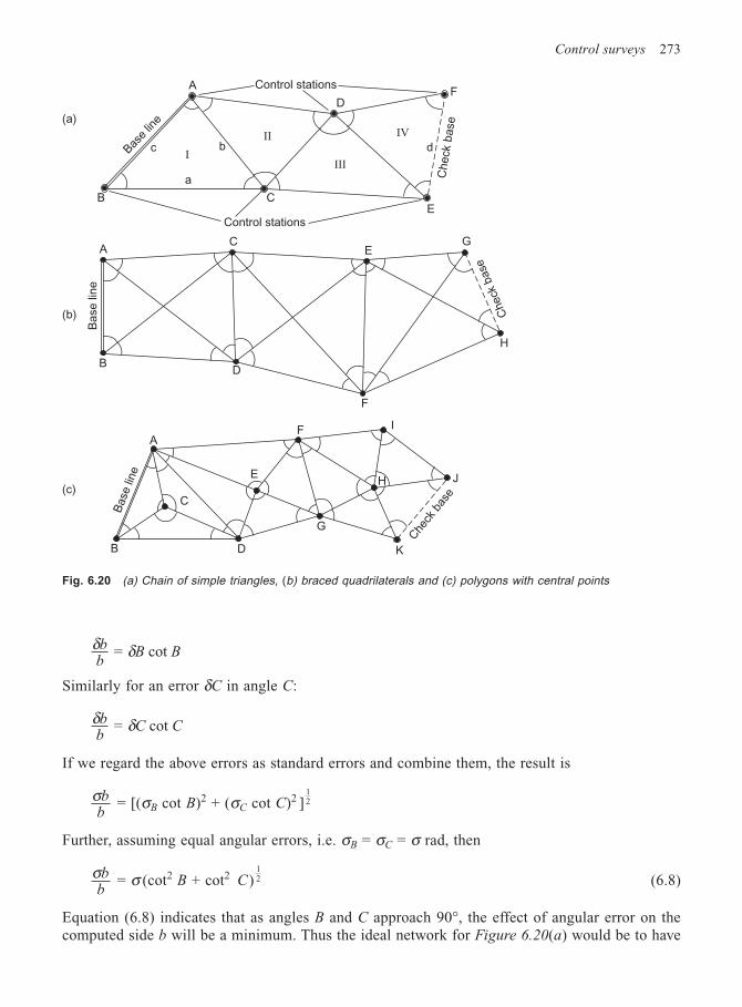
Control surveys 273
δ δbb
B B = cot
Similarly for an error δC in angle C:
δ δbb
C C = cot
If we regard the above errors as standard errors and combine them, the result is
σbb
= [(σB cot B)2 + (σC cot C)2 ]12
Further, assuming equal angular errors, i.e. σB = σC = σ rad, then
σbb
= σ (cot2 B + cot2 C)12 (6.8)
Equation (6.8) indicates that as angles B and C approach 90°, the effect of angular error on thecomputed side b will be a minimum. Thus the ideal network for Figure 6.20(a) would be to have
Fig. 6.20 (a) Chain of simple triangles, (b) braced quadrilaterals and (c) polygons with central points
Control stations
Control stations
Check b
ase
Bas
e lin
e
A
BE
F
C
a
bcI
II IV
III
Base
line
Check
base
Che
ck b
ase
Base lin
eD
A
B
C
D
F
EG
H
A
B
C
D
E
F
G
I
J
K
(a)
(b)
(c)
d
H
274 Engineering Surveying
very small angles opposite the sides which do not enter into the scale error computation, i.e. sidesBC, AD, CE and DF. Such a network would not, however, be a practical proposition due to the verylimited ground coverage, and the best compromise is the use of equilateral triangles where possible.If small angles are inevitable and cannot be fixed so as not to enter the scale computation, theyshould be measured with extra precision.
Assuming now that B = C = 60° and σ = ±1″, then as cot 60° = 3– 1
2 and σ rad ≈ 1/200 000:
σ b
b = 1/200000
23
12
= 1/245000
After n triangles the error will be n12 times the error in each triangle:
∴ = /24500012σ b
bn
Thus, after, say, nine triangles, the scale error would be approximately 1/82000. This result indicatesthe need for maximum accuracy in the measurement of the base line and angles, as well as the needfor regular check bases and well-conditioned triangles. It can be shown that when the angles areadjusted, equation (6.8) becomes
σ σbb
B B C C = 23
(cot + cot cot + cot )2 2
12
(6.9)
which theoretically shows no improvement in the scale error if B = C.
6.2.2 General procedure
(1) Reconnaissance of the area, to ensure the best possible positions for stations and base lines.(2) Construction of the stations.(3) Consideration of the type of target and instrument to be used and also the method of observation.
All of these depend on the precision required and the length of sights involved.(4) Observation of angles and base-line measurements.(5) Computation: base line reduction, station and figural adjustment, coordinates of stations by
direct methods.
A general introduction to triangulation has been presented, aspects of which will now be dealt within detail.
(1) Reconnaissance is the most important aspect of any well-designed surveying project. Its mainfunction is to ensure the best positions for the survey stations commensurate with well-conditionedfigures, ease of access to the stations and economy of observation.
A careful study of all existing maps or plans of the area is essential. The best position for thesurvey stations can be drawn on the plan and the overall shape of the network studied. Whilstchains of single triangles are the most economic to observe, braced quadrilaterals provide manymore conditions of adjustment and are at their strongest when square shaped. Using the contoursof the plan, profiles between stations can be plotted to ensure intervisibility. Stereo-pairs of aerialphotographs, giving a three-dimensional view of the terrain, are useful in this respect. Whilst everyattempt should be made to ensure that there are no angles less than 25°, if a small angle cannot beavoided it should be situated opposite a side which does not enter into the scale computation.
When the paper triangulation is complete, the area should then be visited and the site of everystation carefully investigated. With the aid of binoculars, intervisibility between stations should be
Control surveys 275
checked and ground-grazing rays avoided. Since the advent of EDM, base-line siting is not socritical. Soil conditions should be studied to ensure that the ground is satisfactory for the constructionof long-term survey stations. Finally, whilst the strength of the network is a function of its shape,the purpose of the survey stations should not be forgotten and their position located accordingly.
(2) Stations must be constructed for long-term stability and may take the form of those illustratedin Figures 6.7 and 6.8. A complete referencing of the station should then be carried out in order toensure its location at a future date.
(3) As already stated, the type of target used will depend on the length of sight involved and theaccuracy required. for highly precise networks, the observations may be carried out at night whenrefraction is minimal. In such a case, signal lamps would be the only type of target to use.
For short sights it may be possible to use the precise targets shown in Figure 6.10. Whatever formthe target takes, the essential considerations are that it should be capable of being accuratelycentred over the survey point and afford the necessary size and shape for accurate bisection at theobservation distances used.
(4) The observation of the angles has already been dealt with in Chapter 4. In triangulation themethod of directions would inevitably be used and the horizon closed. An appropriate number ofsets would be taken on each face. The base line and check base would most certainly be measuredby EDM, with all the necessary corrections made to ensure high accuracy, as illustrated in Chapter 3.
(5) Since the use of computers is now well established, there is no reason why a least squaresadjustment using the now standard variation of coordinates method should not be carried out.
Alternatively the angles may be balanced by simpler, less rigorous methods known as ‘equalshifts’. On completion, the sides may be computed using the sine rule and finally the coordinatesof each survey point obtained.
If the survey is to be connected to the national mapping system of the country, then all the base-line measurements must be reduced to MSL and multiplied by the local scale factor. As many of thenational survey points as possible should be included in the scheme.
6.2.3 Figural adjustment by equal shifts
Whilst least squares methods permit the adjustment of the network as a whole, the simpler ‘equalshifts’ approach treats each figure in the network separately. The final values for the angles must,however, satisfy the conditions of adjustment of each figure.
(1) Simple triangle. The condition of adjustment of a plane triangle is that the sum of the anglesshould equal 180°. It is due to this minimum number of conditions that other figures, such as bracedquadrilaterals, are favoured rather than triangles.
For large triangles on an ellipsoid of reference, with sides greater than 10 km, the angles shouldsum to 180° + E. E is the spherical excess of the triangle and may be computed from
′′×
ER
= Area of triangle 206 265
(6.10)
where R = local radius of the Earth
For greater accuracy R2 = ρν may be used, taking the latitude at the centre of the triangle to evaluateρ and ν.
After adjusting the angles to equal (180° + E), Legendre’s theorem stipulates that if one-third ofthe spherical excess is deducted from each angle, the triangle may be treated as a plane triangle for
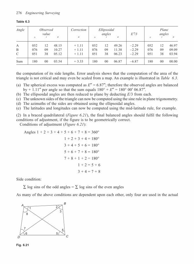
276 Engineering Surveying
the computation of its side lengths. Error analysis shows that the computation of the area of thetriangle is not critical and may even be scaled from a map. An example is illustrated in Table 6.3.
(a) The spherical excess was computed as E″ = 6.87″; therefore the observed angles are balancedby + 1.11″ per angle so that the sum equals 180° + E″ = 180° 00′ 06.87″.
(b) The ellipsoidal angles are then reduced to plane by deducting E/3 from each.(c) The unknown sides of the triangle can now be computed using the sine rule in plane trigonometry.(d) The azimuths of the sides are obtained using the ellipsoidal angles.(e) The latitudes and longitudes can now be computed using the mid-latitude rule, for example.
(2) In a braced quadrilateral (Figure 6.21), the final balanced angles should fulfil the followingconditions of adjustment, if the figure is to be geometrically correct.
Conditions of adjustment (Figure 6.21):
Angles 1 + 2 + 3 + 4 + 5 + 6 + 7 + 8 = 360°
1 + 2 + 3 + 4 = 180°
3 + 4 + 5 + 6 = 180°
5 + 6 + 7 + 8 = 180°
7 + 8 + 1 + 2 = 180°
1 + 2 = 5 + 6
3 + 4 = 7 + 8
Side condition:
∑ log sins of the odd angles = ∑ log sins of the even angles
As many of the above conditions are dependent upon each other, only four are used in the actual
Table 6.3
Angle Observed Correction Ellipsoidal Plane
value angles E″/3 angles
° ′ ″ ″ ° ′ ″ ° ′ ″
A 052 12 48.15 + 1.11 052 12 49.26 –2.29 052 12 46.97B 076 09 10.27 + 1.11 076 09 11.38 –2.29 076 09 09.09C 051 38 05.12 + 1.11 051 38 06.23 –2.29 051 38 03.94
Sum 180 00 03.54 + 3.33 180 00 06.87 –6.87 180 00 00.00
A
D
8
7 4
3
21
C
B
56
Fig. 6.21
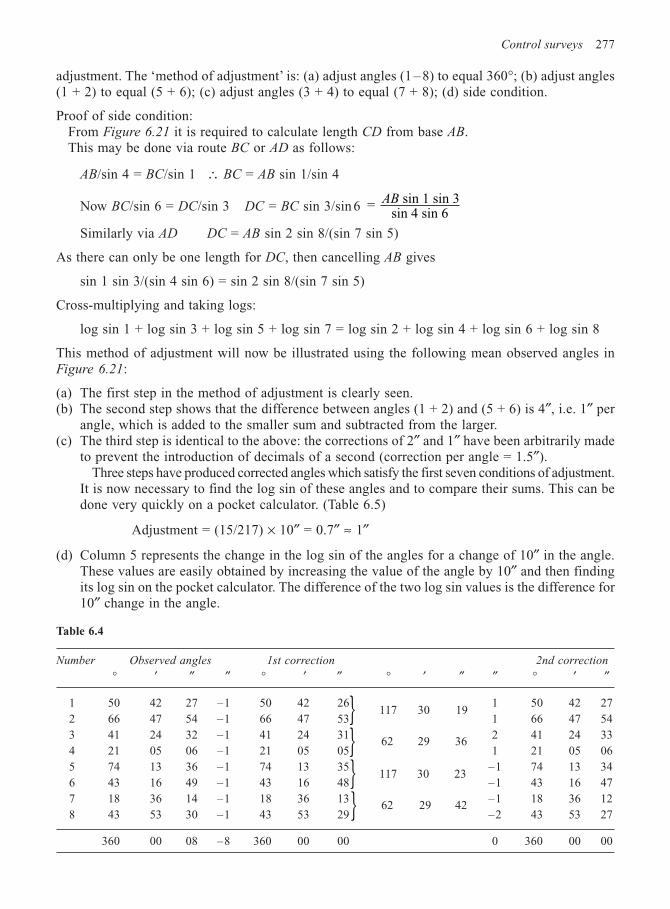
Control surveys 277
adjustment. The ‘method of adjustment’ is: (a) adjust angles (1 – 8) to equal 360°; (b) adjust angles(1 + 2) to equal (5 + 6); (c) adjust angles (3 + 4) to equal (7 + 8); (d) side condition.
Proof of side condition:From Figure 6.21 it is required to calculate length CD from base AB.This may be done via route BC or AD as follows:
AB/sin 4 = BC/sin 1 ∴ BC = AB sin 1/sin 4
Now BC/sin 6 = DC/sin 3 DC = BC sin 3/sin 6 = sin 1 sin 3sin 4 sin 6
AB
Similarly via AD DC = AB sin 2 sin 8/(sin 7 sin 5)
As there can only be one length for DC, then cancelling AB gives
sin 1 sin 3/(sin 4 sin 6) = sin 2 sin 8/(sin 7 sin 5)
Cross-multiplying and taking logs:
log sin 1 + log sin 3 + log sin 5 + log sin 7 = log sin 2 + log sin 4 + log sin 6 + log sin 8
This method of adjustment will now be illustrated using the following mean observed angles inFigure 6.21:
(a) The first step in the method of adjustment is clearly seen.(b) The second step shows that the difference between angles (1 + 2) and (5 + 6) is 4″, i.e. 1″ per
angle, which is added to the smaller sum and subtracted from the larger.(c) The third step is identical to the above: the corrections of 2″ and 1″ have been arbitrarily made
to prevent the introduction of decimals of a second (correction per angle = 1.5″).Three steps have produced corrected angles which satisfy the first seven conditions of adjustment.
It is now necessary to find the log sin of these angles and to compare their sums. This can bedone very quickly on a pocket calculator. (Table 6.5)
Adjustment = (15/217) × 10″ = 0.7″ ≈ 1″
(d) Column 5 represents the change in the log sin of the angles for a change of 10″ in the angle.These values are easily obtained by increasing the value of the angle by 10″ and then findingits log sin on the pocket calculator. The difference of the two log sin values is the difference for10″ change in the angle.
Table 6.4
Number Observed angles 1st correction 2nd correction
° ′ ″ ″ ° ′ ″ ° ′ ″ ″ ° ′ ″
1 50 42 27 –1 50 42 26 1 50 42 27
2 66 47 54 –1 66 47 53 1 66 47 54
3 41 24 32 –1 41 24 31 2 41 24 33
4 21 05 06 –1 21 05 05 1 21 05 06
5 74 13 36 –1 74 13 35 –1 74 13 34
6 43 16 49 –1 43 16 48 –1 43 16 47
7 18 36 14 –1 18 36 13 –1 18 36 12
8 43 53 30 –1 43 53 29 –2 43 53 27
360 00 08 –8 360 00 00 0 360 00 00
117 30 23
62 29 36
117 30 19
62 29 42
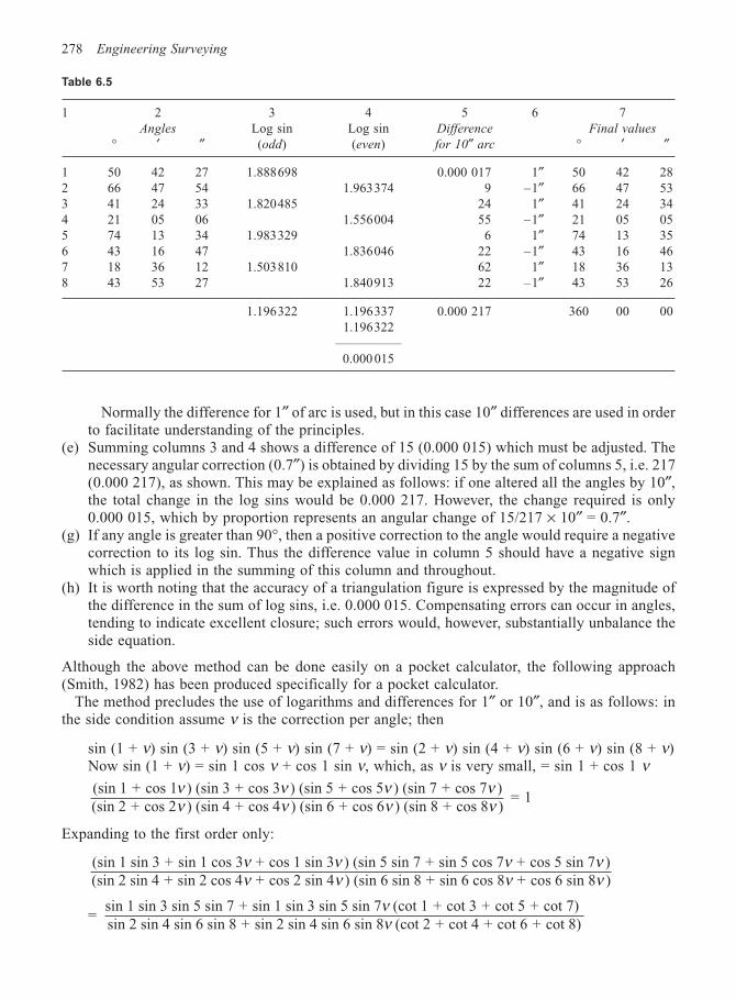
278 Engineering Surveying
Normally the difference for 1″ of arc is used, but in this case 10″ differences are used in orderto facilitate understanding of the principles.
(e) Summing columns 3 and 4 shows a difference of 15 (0.000 015) which must be adjusted. Thenecessary angular correction (0.7″) is obtained by dividing 15 by the sum of columns 5, i.e. 217(0.000 217), as shown. This may be explained as follows: if one altered all the angles by 10″,the total change in the log sins would be 0.000 217. However, the change required is only0.000 015, which by proportion represents an angular change of 15/217 × 10″ = 0.7″.
(g) If any angle is greater than 90°, then a positive correction to the angle would require a negativecorrection to its log sin. Thus the difference value in column 5 should have a negative signwhich is applied in the summing of this column and throughout.
(h) It is worth noting that the accuracy of a triangulation figure is expressed by the magnitude ofthe difference in the sum of log sins, i.e. 0.000 015. Compensating errors can occur in angles,tending to indicate excellent closure; such errors would, however, substantially unbalance theside equation.
Although the above method can be done easily on a pocket calculator, the following approach(Smith, 1982) has been produced specifically for a pocket calculator.
The method precludes the use of logarithms and differences for 1″ or 10″, and is as follows: inthe side condition assume ν is the correction per angle; then
sin (1 + ν) sin (3 + ν) sin (5 + ν) sin (7 + ν) = sin (2 + ν) sin (4 + ν) sin (6 + ν) sin (8 + ν)Now sin (1 + ν) = sin 1 cos ν + cos 1 sin ν, which, as ν is very small, = sin 1 + cos 1 ν(sin 1 + cos 1 ) (sin 3 + cos 3 ) (sin 5 + cos 5 ) (sin 7 + cos 7 )(sin 2 + cos 2 ) (sin 4 + cos 4 ) (sin 6 + cos 6 ) (sin 8 + cos 8 )
ν ν ν νν ν ν ν = 1
Expanding to the first order only:
(sin 1 sin 3 + sin 1 cos 3 + cos 1 sin 3 ) (sin 5 sin 7 + sin 5 cos 7 + cos 5 sin 7 )(sin 2 sin 4 + sin 2 cos 4 + cos 2 sin 4 ) (sin 6 sin 8 + sin 6 cos 8 + cos 6 sin 8 )
ν ν ν νν ν ν ν
=sin 1 sin 3 sin 5 sin 7 + sin 1 sin 3 sin 5 sin 7 (cot 1 + cot 3 + cot 5 + cot 7) sin 2 sin 4 sin 6 sin 8 + sin 2 sin 4 sin 6 sin 8 (cot 2 + cot 4 + cot 6 + cot 8)
νν
Table 6.5
1 2 3 4 5 6 7Angles Log sin Log sin Difference Final values
° ′ ″ (odd) (even) for 10″ arc ° ′ ″
1 50 42 27 1.888698 0.000 017 1″ 50 42 282 66 47 54 1.963374 9 –1″ 66 47 533 41 24 33 1.820485 24 1″ 41 24 344 21 05 06 1.556004 55 –1″ 21 05 055 74 13 34 1.983329 6 1″ 74 13 356 43 16 47 1.836046 22 –1″ 43 16 467 18 36 12 1.503810 62 1″ 18 36 138 43 53 27 1.840913 22 –1″ 43 53 26
1.196322 1.196337 0.000 217 360 00 001.196322
—————0.000 015
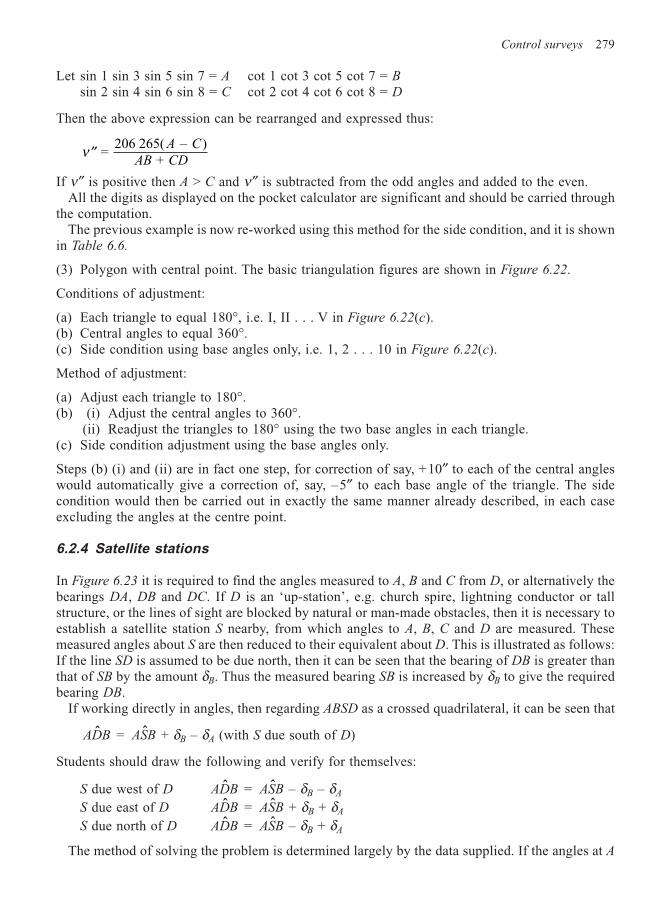
Control surveys 279
Let sin 1 sin 3 sin 5 sin 7 = A cot 1 cot 3 cot 5 cot 7 = Bsin 2 sin 4 sin 6 sin 8 = C cot 2 cot 4 cot 6 cot 8 = D
Then the above expression can be rearranged and expressed thus:
′′ν = 206 265( )
+ A – C
AB CD
If ν″ is positive then A > C and ν″ is subtracted from the odd angles and added to the even.All the digits as displayed on the pocket calculator are significant and should be carried through
the computation.The previous example is now re-worked using this method for the side condition, and it is shown
in Table 6.6.
(3) Polygon with central point. The basic triangulation figures are shown in Figure 6.22.
Conditions of adjustment:
(a) Each triangle to equal 180°, i.e. I, II . . . V in Figure 6.22(c).(b) Central angles to equal 360°.(c) Side condition using base angles only, i.e. 1, 2 . . . 10 in Figure 6.22(c).
Method of adjustment:
(a) Adjust each triangle to 180°.(b) (i) Adjust the central angles to 360°.
(ii) Readjust the triangles to 180° using the two base angles in each triangle.(c) Side condition adjustment using the base angles only.
Steps (b) (i) and (ii) are in fact one step, for correction of say, +10″ to each of the central angleswould automatically give a correction of, say, –5″ to each base angle of the triangle. The sidecondition would then be carried out in exactly the same manner already described, in each caseexcluding the angles at the centre point.
6.2.4 Satellite stations
In Figure 6.23 it is required to find the angles measured to A, B and C from D, or alternatively thebearings DA, DB and DC. If D is an ‘up-station’, e.g. church spire, lightning conductor or tallstructure, or the lines of sight are blocked by natural or man-made obstacles, then it is necessary toestablish a satellite station S nearby, from which angles to A, B, C and D are measured. Thesemeasured angles about S are then reduced to their equivalent about D. This is illustrated as follows:If the line SD is assumed to be due north, then it can be seen that the bearing of DB is greater thanthat of SB by the amount δB. Thus the measured bearing SB is increased by δB to give the requiredbearing DB.
If working directly in angles, then regarding ABSD as a crossed quadrilateral, it can be seen that
ADBˆ = ASBˆ + δB – δA (with S due south of D)
Students should draw the following and verify for themselves:
S due west of D ADBˆ = ASBˆ – δB – δA
S due east of D ADBˆ = ASBˆ + δB + δA
S due north of D ADBˆ = ASBˆ – δB + δA
The method of solving the problem is determined largely by the data supplied. If the angles at A
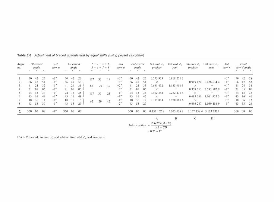
Table 6.6 Adjustment of braced quadrilateral by equal shifts (using pocket calculator)
Angle Observed 1st 1st corr’d 1 + 2 = 5 + 6 2nd 2nd corr’d Sin odd ∠s Cot odd ∠s Sin even ∠s Cot even ∠s 3rd Final
no. angle corr’n angle 3 + 4 = 7 + 8 corr’n angle product sum product sum corr’n corr’d angle
° ′ ″ ° ′ ″ ° ′ ″ ° ′ ″ ° ′ ″
1 50 42 27 –1″ 50 42 26 +1″ 50 42 27 0.773 923 0.818 270 3 +1″ 50 42 282 66 47 54 –1″ 66 47 53 +1″ 66 47 54 × + 0.919 124 0.428 634 4 –1″ 66 47 533 41 24 32 –1″ 41 24 31 +2″ 41 24 33 0.661 432 1.133 911 5 × + +1″ 41 24 344 21 05 06 –1″ 21 05 05 +1″ 21 05 06 × + 0.359 753 2.593 582 9 –1″ 21 05 055 74 13 36 –1″ 74 13 35 –1″ 74 13 34 0.962 342 0.282 479 4 × + +1″ 74 13 356 43 16 49 –1″ 43 16 48 –1″ 43 16 47 × + 0.685 561 1.061 927 3 –1″ 43 16 467 18 36 14 –1″ 18 36 13 –1″ 18 36 12 0.319 014 2.970 867 6 × + +1″ 18 36 138 43 53 30 –1″ 43 53 29 –2″ 43 53 27 0.693 287 1.039 486 9 –1″ 43 53 26
∑ 360 00 08 –8″ 360 00 00 360 00 00 0.157 152 8 5.205 528 8 0.157 158 4 5.123 6315 360 00 00
A B C D
3rd correction =206 265 ( – )
+
A C
AB CD
= 0.7″ ≈ 1″
If A > C then add to even ∠s and subtract from odd ∠s, and vice versa
117 30 23
62 29 36
117 30 19
62 29 42
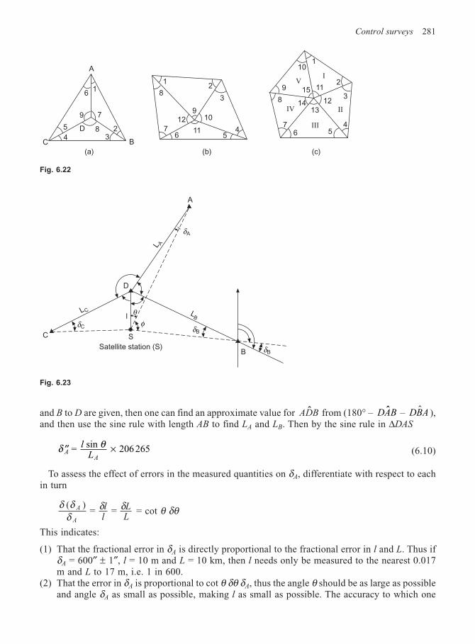
Control surveys 281
and B to D are given, then one can find an approximate value for ADBˆ from (180° – DABˆ – DBAˆ ),and then use the sine rule with length AB to find LA and LB. Then by the sine rule in ∆DAS
′′ ×δ θA
A
lL
= sin 206 265 (6.10)
To assess the effect of errors in the measured quantities on δA, differentiate with respect to eachin turn
δ δδ
δ δ ( ) = = A
A
ll
LL
= cot θ δθ
This indicates:
(1) That the fractional error in δA is directly proportional to the fractional error in l and L. Thus ifδA = 600″ ± 1″, l = 10 m and L = 10 km, then l needs only be measured to the nearest 0.017m and L to 17 m, i.e. 1 in 600.
(2) That the error in δA is proportional to cot θ δθ δA, thus the angle θ should be as large as possibleand angle δA as small as possible, making l as small as possible. The accuracy to which one
Fig. 6.23
φδC δB
δB
δA
θLC
D
l LB
L A
B
S
A
C
Satellite station (S)
Fig. 6.22
A
BC
16
5
9
8D3
2
7
12
3
47
8
910
11
12
1
2
3
46
7
8
9
10
11
12
13 IIIV
III
IV
(a) (b) (c)
4 6 5
14
15
5
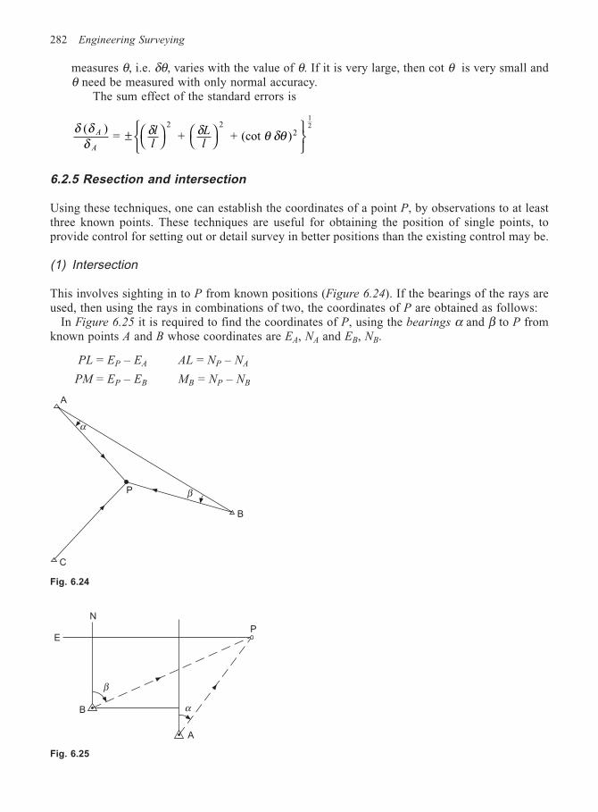
282 Engineering Surveying
measures θ, i.e. δθ, varies with the value of θ. If it is very large, then cot θ is very small andθ need be measured with only normal accuracy.
The sum effect of the standard errors is
δ δδ
δ δ θ δθ ( ) = + + (cot )
2 22
12
A
A
ll
Ll
±
6.2.5 Resection and intersection
Using these techniques, one can establish the coordinates of a point P, by observations to at leastthree known points. These techniques are useful for obtaining the position of single points, toprovide control for setting out or detail survey in better positions than the existing control may be.
(1) Intersection
This involves sighting in to P from known positions (Figure 6.24). If the bearings of the rays areused, then using the rays in combinations of two, the coordinates of P are obtained as follows:
In Figure 6.25 it is required to find the coordinates of P, using the bearings α and β to P fromknown points A and B whose coordinates are EA, NA and EB, NB.
PL = EP – EA AL = NP – NA
PM = EP – EB MB = NP – NB
Fig. 6.24
Fig. 6.25
A
B
E
N
β
α
P
A
P
C
B
α
β
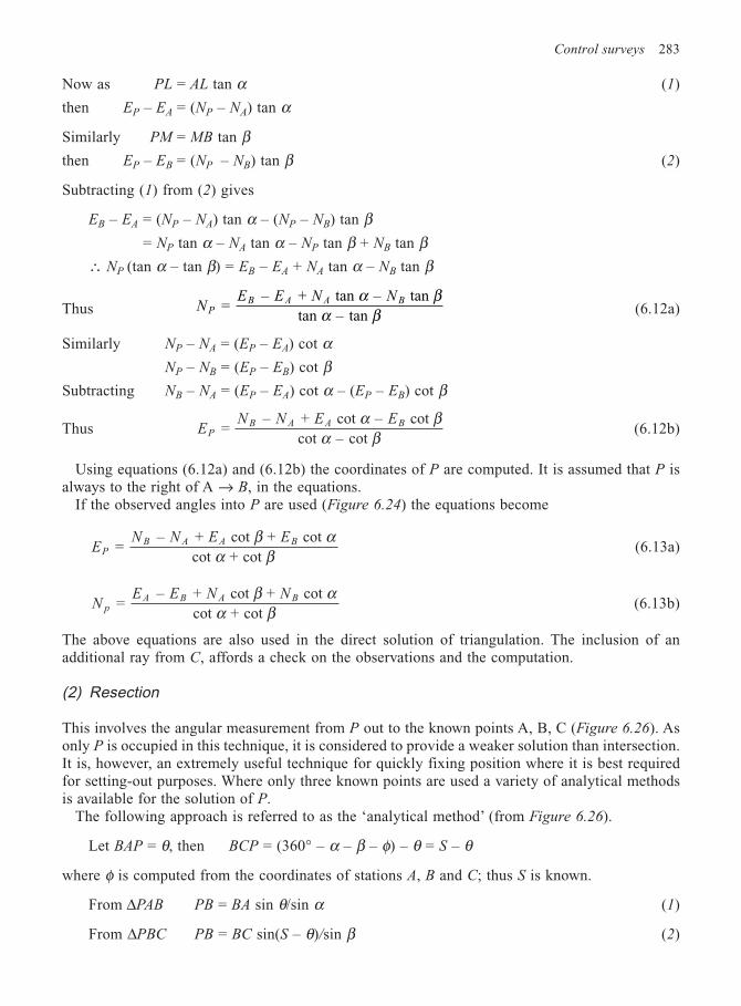
Control surveys 283
Now as PL = AL tan α (1)
then EP – EA = (NP – NA) tan α
Similarly PM = MB tan βthen EP – EB = (NP – NB) tan β (2)
Subtracting (1) from (2) gives
EB – EA = (NP – NA) tan α – (NP – NB) tan β= NP tan α – NA tan α – NP tan β + NB tan β
∴ NP (tan α – tan β) = EB – EA + NA tan α – NB tan β
Thus NE E N N
PB A A B =
– + tan – tan
tan – tan
α βα β (6.12a)
Similarly NP – NA = (EP – EA) cot αNP – NB = (EP – EB) cot β
Subtracting NB – NA = (EP – EA) cot α – (EP – EB) cot β
Thus EN N E E
PB A A B =
– + cot – cot
cot – cot
α βα β
(6.12b)
Using equations (6.12a) and (6.12b) the coordinates of P are computed. It is assumed that P isalways to the right of A → B, in the equations.
If the observed angles into P are used (Figure 6.24) the equations become
EN N E E
PB A A B =
– + cot + cot
cot + cot
β αα β
(6.13a)
NE E N N
pA B A B =
– + cot + cot
cot + cot
β αα β
(6.13b)
The above equations are also used in the direct solution of triangulation. The inclusion of anadditional ray from C, affords a check on the observations and the computation.
(2) Resection
This involves the angular measurement from P out to the known points A, B, C (Figure 6.26). Asonly P is occupied in this technique, it is considered to provide a weaker solution than intersection.It is, however, an extremely useful technique for quickly fixing position where it is best requiredfor setting-out purposes. Where only three known points are used a variety of analytical methodsis available for the solution of P.
The following approach is referred to as the ‘analytical method’ (from Figure 6.26).
Let BAP = θ, then BCP = (360° – α – β – φ) – θ = S – θ
where φ is computed from the coordinates of stations A, B and C; thus S is known.
From ∆PAB PB = BA sin θ/sin α (1)
From ∆PBC PB = BC sin(S – θ)/sin β (2)
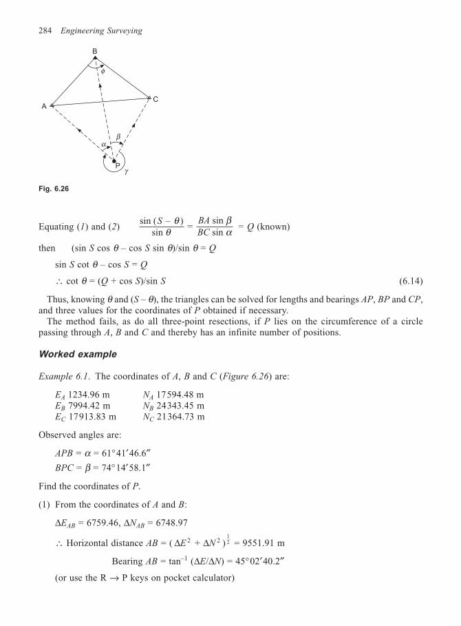
284 Engineering Surveying
Equating (1) and (2)sin ( – )
sin =
sin sin
S BA
BC
θθ
βα = Q (known)
then (sin S cos θ – cos S sin θ)/sin θ = Q
sin S cot θ – cos S = Q
∴ cot θ = (Q + cos S)/sin S (6.14)
Thus, knowing θ and (S – θ), the triangles can be solved for lengths and bearings AP, BP and CP,and three values for the coordinates of P obtained if necessary.
The method fails, as do all three-point resections, if P lies on the circumference of a circlepassing through A, B and C and thereby has an infinite number of positions.
Worked example
Example 6.1. The coordinates of A, B and C (Figure 6.26) are:
EA 1234.96 m NA 17594.48 mEB 7994.42 m NB 24343.45 mEC 17913.83 m NC 21364.73 m
Observed angles are:
APB = α = 61°41′46.6″BPC = β = 74°14′58.1″
Find the coordinates of P.
(1) From the coordinates of A and B:
∆EAB = 6759.46, ∆NAB = 6748.97
∴ Horizontal distance AB = ( ∆ ∆E N2 2 + )12 = 9551.91 m
Bearing AB = tan–1 (∆E/∆N) = 45°02′40.2″
(or use the R → P keys on pocket calculator)
Fig. 6.26
βα
φ
A
B
C
Pγ
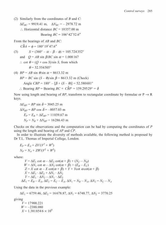
Control surveys 285
(2) Similarly from the coordinates of B and C:
∆EBC = 9919.41 m, ∆NBC = – 2978.72 m
∴ Horizontal distance BC = 10357.00 m
Bearing BC = 106°42′52.6″
From the bearings of AB and BC:
CBAˆ = φ = 180° 19′ 47.6″(3) S = (360° – α – β – φ) = 105.724 352°
and Q = AB sin β/BC sin α = 1.008 167
∴ cot θ = (Q + cos S)/sin S, from which
θ = 52.554505°(4) BP = AB sin θ/sin α = 8613.32 m
BP = BC sin (S – θ)/sin β = 8613.32 m (Check)
Angle CBP = 180° – [β + (S – θ)] = 52.580681°∴ Bearing BP = Bearing BC + CBPˆ = 159.29529° = δ
Now using length and bearing of BP, transform to rectangular coordinate by formulae or P → Rkeys.
∆EBP = BP sin δ = 3045.25 m
∆NBP = BP cos δ = –8057.03 m
EP = EB + ∆EBP = 11039.67 m
NP = NB + ∆NBP = 16286.43 m
Checks on the observations and the computation can be had by computing the coordinates of Pusing the length and bearing of AP and CP.
In order to illustrate the diversity of methods available, the following method is proposed byDr T.L. Thomas of Imperial College, London.
EP = EA + ZV/(V2 + W2)
NP = NA + ZW/(V2 + W2)
where:V = ∆E1 cot α – ∆E2 cot(α + β) + (NC – NB)W = ∆N1 cot α – ∆N2 cot(α + β) + (EB – EC)Z = X cot α – X cot(α + β) + Y + Ycot α cot(α + β)X = ∆E1 · ∆E2 + ∆N1 · ∆N2
Y = ∆E1 · ∆N2 – ∆N1 · ∆E2
∆E1 = EB – EA, ∆E2 = EC – EA, ∆N1 = NB – NA, ∆N2 = NC – NA
Using the data in the previous example:
∆E1 = 6759.46, ∆E2 = 16 678.87, ∆N1 = 6748.77, ∆N2 = 3770.25
givingV = 17900.221W = –2388.080X = 1.381854 6 × 10⁹
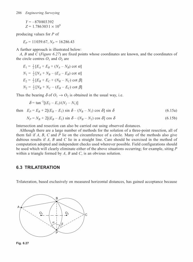
286 Engineering Surveying
Y = –870803392Z = 1.7863031 × 10⁹
producing values for P of
EP = 11039.67, NP = 16286.43
A further approach is illustrated below:A, B and C (Figure 6.27) are fixed points whose coordinates are known, and the coordinates of
the circle centres O1 and O2 are
E1 = 12 [EA + EB + (NA – NB) cot α]
N1 = 12 [NA + NB – (EA – EB) cot α]
E2 = 12 [EB + EC + (NB – NC) cot β]
N2 = 12 [NB + NC – (EB – EC) cot β]
Thus the bearing δ of O1 → O2 is obtained in the usual way, i.e.
δ = tan–1[(E2 – E1)/(N2 – N1)]
then EP = EB + 2[(EB – E1) sin δ – (NB – N1) cos δ] sin δ (6.15a)
NP = NB + 2[(EB – E1) sin δ – (NB – N1) cos δ] cos δ (6.15b)
Intersection and resection can also be carried out using observed distances.Although there are a large number of methods for the solution of a three-point resection, all of
them fail if A, B, C and P lie on the circumference of a circle. Many of the methods also givedubious results if A, B and C lie in a straight line. Care should be exercised in the method ofcomputation adopted and independent checks used wherever possible. Field configurations shouldbe used which will clearly eliminate either of the above situations occurring; for example, siting Pwithin a triangle formed by A, B and C, is an obvious solution.
6.3 TRILATERATION
Trilateration, based exclusively on measured horizontal distances, has gained acceptance because
A
B
C
P
O1 O2
α β
Fig. 6.27
Control surveys 287
of the advent of EDM instrumentation. The geometric figures used are similar to those employedin triangulation, although not as standardized due to greater control of scale error. It was originallyconsidered that trilateration would supersede triangulation as a method of control due to the scaleerror factor. However, subsequent results have shown that the system is liable to a rapid accumulationof azimuth error, ethereby requiring a dense system of control points.
The fact that there is no horizontal angle measurement required in trilateration would appear tomake it more rapid and thus, at first glance, more economical than triangulation. However, muchdepends on the length of line involved and the accuracy requirements.
All EDM equipment measures slope distance, which therefore needs to be reduced to the horizontalat some datum level. This requires then not only the measurement of slope length, but alsothe relative levels of the control points and instrument heights, or the measurement of verticalangles.
EDM instruments are calibrated for the velocity of electromagnetic waves under certain standardmeteorological conditions. Thus actual meteorological conditions along the measured path need tobe known in order to correct the measured distance. At the present time this is not a practicalproposition and one has to be content with the measurement of temperature and pressure at eachend of the line being measured. For the best possible results under these conditions one requirescarefully calibrated thermometers and barometers hung as high as possible by the instruments andread at the same instant of measurement. In order to comply with this latter requirement some formof intercommunication is necessary.
Similar precautions are also required when measuring the vertical angles. In order to achieve theaccuracy required, one needs to use highly precise theodolites, preferably with automatic verticalcircle indexing. Ideally, simultaneous reciprocal observations are necessary. If vertical angles arepossible at only one end of the line, then corrections for curvature and refraction must be applied.Also, depending on the terrain and accuracy requirement, it may be necessary to consider the effectof ‘deviation of the vertical’ on the angles measured.
It would appear, therefore, that not only is trilateration possibly less economical than triangulationbut on consideration of the above error sources (Chrzanowski and Wilson, 1967) it may also proveless accurate. There appears to be conflicting evidence on this point (Burke, 1971), althoughHodges et al. (1967) has shown conclusively that angles computed through a trilateration are asaccurate as those measured with a 1″ theodolite on the same control net.
A further reason why trilateration has not superseded triangulation must be in the superiorinternal checks given by triangulation. For instance, a triangle with three angles measured has anangle check whereas with three sides measured there is none; a braced quadrilateral with anglesobserved has four conditions (three angles, one side) to be satisfied, whereas with the sides thereis only the single condition that the computed total angle at one corner equals the sum of the twocomputed component angles.
Network design is therefore especially critical in trilateration. In order to obtain sufficient redundancyfor checks on the accuracy, the geometric figures become quite complicated. For instance, to obtainthe same redundancy as a triangulation braced quadrilateral, a pentagon with all ten sides measuredwould have to be used. Indeed, experts in trilateration analysis have proposed the use of thehexagon, with all sides measured (20 giving 10 checks) as the basic network figure. However, fromthe practical viewpoint, pentagons and hexagons with all stations intervisible are difficult to establishin the field. Thus, from the logistic viewpoint, trilateration would require as much organization astriangulation. However, all trilateration must include the measurement of some of the angles, toincrease the number of redundant measurements. It follows from this that the modern practice is tocombine trilateration and triangulation, thereby producing very strong networks. The network maybe computed by the method of variation of coordinates or the following less rigorous approachesmay be used.
288 Engineering Surveying
In the figures formed, use the reduced lengths to obtain the angles. This may be done using thehalf-angle equation, i.e.
tan A/2 = S(S – a)/[(S – b)(S – c)]12 (6.16)
where 2S = (a + b + c), the sum of the three sides
The network may then be treated as a triangulation network; the angles adjusted, the lengthscomputed from the adjusted angles and the point coordinates obtained from the length and bearingof each line.
Alternatively, direct coordination of the points may be obtained. To find the coordinates of C,given the coordinates of A and B, and the length of the sides a, b, c of the triangle:
E E Ea b
cE E
cN Nc A B A B A B = ( + ) + –
2 ( – ) – 2 ( – )1
2
2 2
2 2∆ (6.17a)
and N N Na b
cN N
cE Ec A B A B A B = ( + ) + –
2 ( – ) + 2 ( – )1
2
2 2
2 2∆ (6.17b)
where A, B and C are in clockwise order, and
∆ = s(s – a)(s – b)(s – c)12
If the survey is to be tied into the national grid, the local scale factor would need to be found from‘provisional coordinates’ and applied to the ellipsoidal lengths to give the grid lengths. These latterlengths are then used in the formula to give the grid coordinates.
Dr. T.L. Thomas (1971) offers the following alternative equations for trilateration computation:
∆E = EB – EA ∆N = NB – NA c2 = ∆E2 + ∆N2
pEc
= ∆q
Nc
= ∆k
b c a
c =
( + – )2
2 2 2
h b k = ( – )2 212
Then Ec = EA + pk – qh Nc = NA + qk + ph
Checks a2 = (EC – EB)2 + (NC – NB)2
b2 = (EC – EA)2 + (NC – NA)2
It is assumed in the above that C is to the left of AB→
.
6.4 TRIANGULATERATION
As its name implies, triangulateration is simply the combining of triangulation and trilateration toproduce a control system in which all the angles and sides are measured.
From the accuracy point of view, the system should be very strong, possessing all the advantagesof both systems from which it is derived. The improvement in the redundancy checks for a bracedquadrilateral and central point pentagon are shown on the next page:
Control surveys 289
Triangulation Trilateration Triangulateration
Quadrilateral
No. of directions 12 0 12No. of sides 1 6 6No. of checks 4 1 9
Pentagon
No. of directions 20 0 20No. of sides 1 10 10No. of checks 6 4 15
Whilst it is generally acknowledged that triangulateration is more accurate than the previouslymentioned systems, one must consider whether or not it is economically justified. The logistics ofthe system will certainly not be equal to the sum of the previous two methods, for once set up atthe observation station and targets/reflectors have been established on the stations to be observed,a skilled surveyor could acquire all the necessary field data with little extra time and effort. The useof electronic ‘total stations’ makes the prospect even more viable and may justify the initial highcapital expenditure involved. Further, as there would be little or no accumulation of scale andazimuth error, ill-conditioned figures could be utilized, thereby reducing the reconnaissance time.
It should be possible through pre-survey analysis to optimize the system so that every station inthe network need not be occupied, thus further improving the viability. The adjustment of such anetwork containing dissimilar quantities presents no difficulty if computer facilities are available.Using the variation of coordinates method, all the data can be adjusted en masse to produce thecorrected coordinates of the network plus a complete error analysis and a posterior weighting of thefield data.
It is thus evident that triangulateration is to be preferred over the use of classical triangulation ortrilateration and this seems to be modern practice. However, it is unlikely to supersede traversingbecause of the basic difference between the two systems and the accuracy/economy factor.
6.5 INERTIAL SURVEYING
The inertial surveying system (ISS) provides three-dimensional positioning without any of theproblems that beset most position-fixing procedures. It is unaffected by atmospheric refraction, itdoes not require intervisibility between points, it can be operated day or night regardless of weatherconditions and it can progress at the speed of the vehicle in which it is housed.
The system consists basically of an inertial platform with three accelerometers held in threemutually orthogonal axes by three similarly orientated precise gyroscopes (Figure 6.28).
The system is housed in a vehicle or helicopter, and, commencing from a point of knowncoordinates the acceleration components in the direction of the axes are sampled at microscopicintervals. The change in position from the starting point is obtained by double integration of theacceleration with respect to time.
An essential part of the system is a computer which is used for monitoring and controlling theinitial alignment of the system in an Earth-fixed coordinate system and computing relative positionin real time.
The total system is therefore composed of three accelerometers, three gyroscopes, computer,power supply and units for the control, storage and display of field data. The components measured
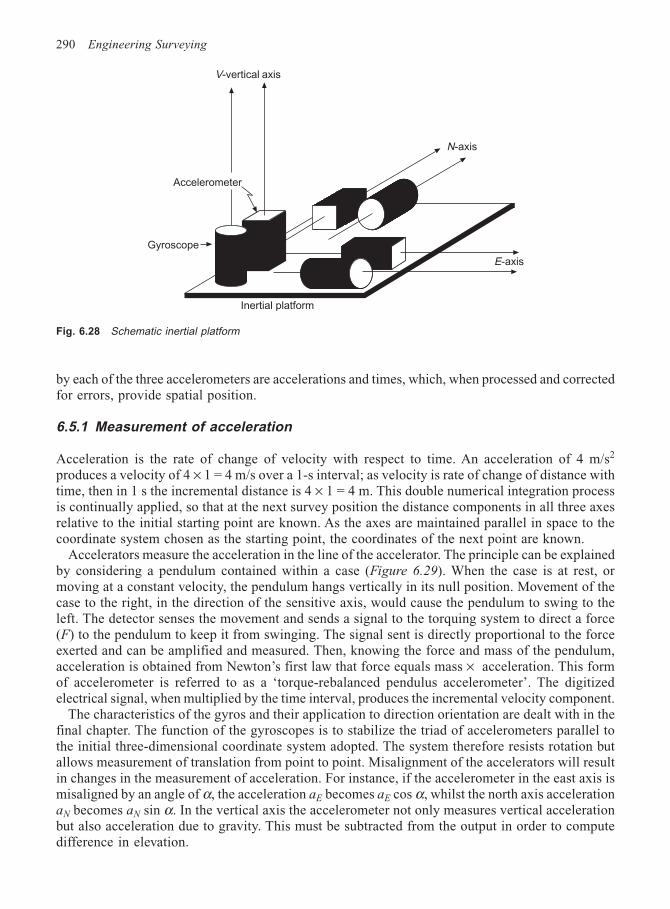
290 Engineering Surveying
by each of the three accelerometers are accelerations and times, which, when processed and correctedfor errors, provide spatial position.
6.5.1 Measurement of acceleration
Acceleration is the rate of change of velocity with respect to time. An acceleration of 4 m/s2
produces a velocity of 4 × 1 = 4 m/s over a 1-s interval; as velocity is rate of change of distance withtime, then in 1 s the incremental distance is 4 × 1 = 4 m. This double numerical integration processis continually applied, so that at the next survey position the distance components in all three axesrelative to the initial starting point are known. As the axes are maintained parallel in space to thecoordinate system chosen as the starting point, the coordinates of the next point are known.
Accelerators measure the acceleration in the line of the accelerator. The principle can be explainedby considering a pendulum contained within a case (Figure 6.29). When the case is at rest, ormoving at a constant velocity, the pendulum hangs vertically in its null position. Movement of thecase to the right, in the direction of the sensitive axis, would cause the pendulum to swing to theleft. The detector senses the movement and sends a signal to the torquing system to direct a force(F) to the pendulum to keep it from swinging. The signal sent is directly proportional to the forceexerted and can be amplified and measured. Then, knowing the force and mass of the pendulum,acceleration is obtained from Newton’s first law that force equals mass × acceleration. This formof accelerometer is referred to as a ‘torque-rebalanced pendulus accelerometer’. The digitizedelectrical signal, when multiplied by the time interval, produces the incremental velocity component.
The characteristics of the gyros and their application to direction orientation are dealt with in thefinal chapter. The function of the gyroscopes is to stabilize the triad of accelerometers parallel tothe initial three-dimensional coordinate system adopted. The system therefore resists rotation butallows measurement of translation from point to point. Misalignment of the accelerators will resultin changes in the measurement of acceleration. For instance, if the accelerometer in the east axis ismisaligned by an angle of α, the acceleration aE becomes aE cos α, whilst the north axis accelerationaN becomes aN sin α. In the vertical axis the accelerometer not only measures vertical accelerationbut also acceleration due to gravity. This must be subtracted from the output in order to computedifference in elevation.
V-vertical axis
Accelerometer
Gyroscope
Inertial platform
E-axis
N-axis
Fig. 6.28 Schematic inertial platform
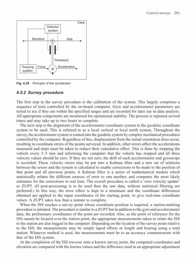
Control surveys 291
6.5.2 Survey procedure
The first step in the survey procedure is the calibration of the system. This largely comprises asequence of tests controlled by the on-board computer. Gyro and accelerometer parameters aretested to see if they are within the specified ranges and are recorded for later use in data analysis.All appropriate components are monitored for operational stability. The process is repeated severaltimes and may take up to two hours to complete.
The next step is the alignment of the accelerometer coordinate system to the geodetic coordinatesystem to be used. This is referred to as a local vertical or local north system. Throughout thesurvey, the accelerometer system is rotated into the geodetic system by complex mechanical procedurescontrolled by the computer. Regardless of this, displacement from the initial orientation does occur,resulting in coordinate errors of the points surveyed. In addition, other errors affect the accelerationsmeasured and steps must be taken to reduce their cumulative effect. This is done by stopping thevehicle every 3–5 min and informing the computer that the vehicle has stopped and all threevelocity values should be zero. If they are not zero, the drift of each accelerometer and gyroscopeis recorded. These velocity errors may be put into a Kalman filter and a new set of relationsbetween the errors and the system is calculated to enable corrections to be made to the position ofthat point and all previous points. A Kalman filter is a series of mathematical models whichstatistically relates the different sources of error to one another, and computes the most likelyestimates for the corrections in real time. The overall procedure is called a ‘zero velocity update’or ZUPT. (If post-processing is to be used then the raw data, without statistical filtering arepreferred.) In this way, the error effect is kept to a minimum and the coordinate differencesobtained are applied to the input coordinates of the starting point, to give real-time coordinatevalues. A ZUPT takes less than a minute to complete.
When the ISS reaches a survey point whose coordinate position is required, a station-markingprocedure is initiated. The procedure is similar to a ZUPT but in addition to the gyro and accelerometerdata, the preliminary coordinates of the point are recorded. Also, as the point of reference for theISS cannot be located over the station point, the appropriate measurements taken to relate the ISSto the station are also logged in the computer. Depending on the location of the survey point relativeto the ISS, the measurements may be simple taped offsets or length and bearing using a totalstation. Whatever method is used, the measurements must be to an accuracy commensurate withthat of the ISS system.
At the completion of the ISS traverse onto a known survey point, the computed coordinates andelevation are compared with the known values and the difference used in an appropriate adjustment
Fig. 6.29 Principle of the accelerator
Detector
system
Sensitive Axis
Pendulum
ForceTorquing
systemM
Acceleration
Case
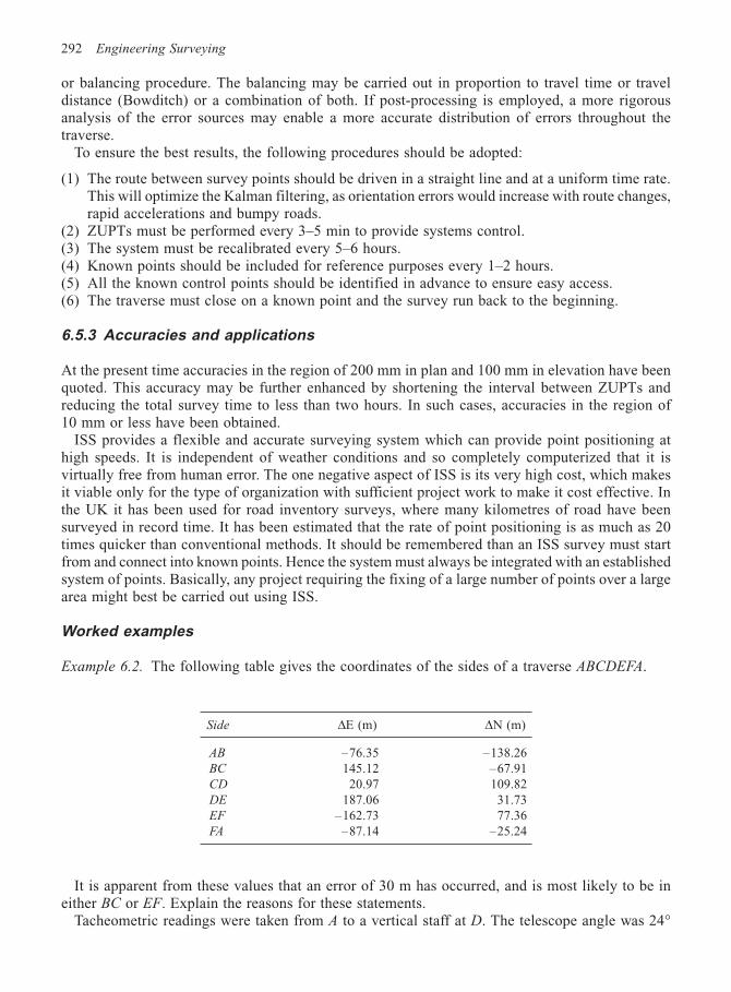
292 Engineering Surveying
or balancing procedure. The balancing may be carried out in proportion to travel time or traveldistance (Bowditch) or a combination of both. If post-processing is employed, a more rigorousanalysis of the error sources may enable a more accurate distribution of errors throughout thetraverse.
To ensure the best results, the following procedures should be adopted:
(1) The route between survey points should be driven in a straight line and at a uniform time rate.This will optimize the Kalman filtering, as orientation errors would increase with route changes,rapid accelerations and bumpy roads.
(2) ZUPTs must be performed every 3–5 min to provide systems control.(3) The system must be recalibrated every 5–6 hours.(4) Known points should be included for reference purposes every 1–2 hours.(5) All the known control points should be identified in advance to ensure easy access.(6) The traverse must close on a known point and the survey run back to the beginning.
6.5.3 Accuracies and applications
At the present time accuracies in the region of 200 mm in plan and 100 mm in elevation have beenquoted. This accuracy may be further enhanced by shortening the interval between ZUPTs andreducing the total survey time to less than two hours. In such cases, accuracies in the region of10 mm or less have been obtained.
ISS provides a flexible and accurate surveying system which can provide point positioning athigh speeds. It is independent of weather conditions and so completely computerized that it isvirtually free from human error. The one negative aspect of ISS is its very high cost, which makesit viable only for the type of organization with sufficient project work to make it cost effective. Inthe UK it has been used for road inventory surveys, where many kilometres of road have beensurveyed in record time. It has been estimated that the rate of point positioning is as much as 20times quicker than conventional methods. It should be remembered than an ISS survey must startfrom and connect into known points. Hence the system must always be integrated with an establishedsystem of points. Basically, any project requiring the fixing of a large number of points over a largearea might best be carried out using ISS.
Worked examples
Example 6.2. The following table gives the coordinates of the sides of a traverse ABCDEFA.
Side ∆E (m) ∆N (m)
AB –76.35 –138.26BC 145.12 –67.91CD 20.97 109.82DE 187.06 31.73EF –162.73 77.36FA –87.14 –25.24
It is apparent from these values that an error of 30 m has occurred, and is most likely to be ineither BC or EF. Explain the reasons for these statements.
Tacheometric readings were taken from A to a vertical staff at D. The telescope angle was 24°
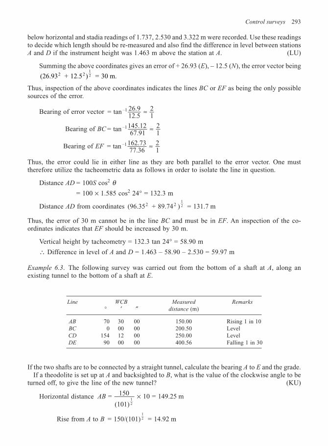
Control surveys 293
below horizontal and stadia readings of 1.737, 2.530 and 3.322 m were recorded. Use these readingsto decide which length should be re-measured and also find the difference in level between stationsA and D if the instrument height was 1.463 m above the station at A. (LU)
Summing the above coordinates gives an error of + 26.93 (E), – 12.5 (N), the error vector being
(26.93 + 12.5 ) = 30 m.2 212
Thus, inspection of the above coordinates indicates the lines BC or EF as being the only possiblesources of the error.
Bearing of error vector = tan 26.912.5
21
–1 ≈
Bearing of BC = tan 145.1267.91
21
–1 ≈
Bearing of EF = tan 162.7377.36
21
–1 ≈
Thus, the error could lie in either line as they are both parallel to the error vector. One musttherefore utilize the tacheometric data as follows in order to isolate the line in question.
Distance AD = 100S cos2 θ= 100 × 1.585 cos2 24° = 132.3 m
Distance AD from coordinates (96.35 + 89.74 ) = 131.7 m2 212
Thus, the error of 30 m cannot be in the line BC and must be in EF. An inspection of the co-ordinates indicates that EF should be increased by 30 m.
Vertical height by tacheometry = 132.3 tan 24° = 58.90 m
∴ Difference in level of A and D = 1.463 – 58.90 – 2.530 = 59.97 m
Example 6.3. The following survey was carried out from the bottom of a shaft at A, along anexisting tunnel to the bottom of a shaft at E.
Line WCB Measured Remarks
° ′ ″ distance (m)
AB 70 30 00 150.00 Rising 1 in 10BC 0 00 00 200.50 LevelCD 154 12 00 250.00 LevelDE 90 00 00 400.56 Falling 1 in 30
If the two shafts are to be connected by a straight tunnel, calculate the bearing A to E and the grade.If a theodolite is set up at A and backsighted to B, what is the value of the clockwise angle to be
turned off, to give the line of the new tunnel? (KU)
Horizontal distance AB = 150
(101) 10 = 149.25 m
12
×
Rise from A to B = 150/(101) = 14.92 m12
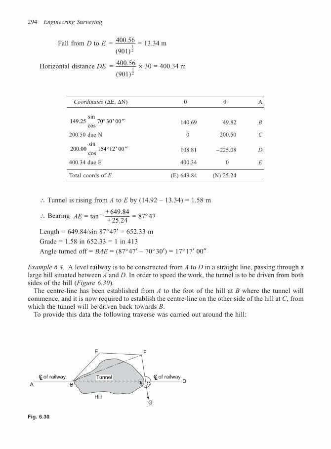
294 Engineering Surveying
Fall from D to E = 400.56
(901) = 13.34 m
12
Horizontal distance DE = 400.56
(901) 30 = 400.34 m
12
×
Coordinates (∆E, ∆N) 0 0 A
149.25sin
cos 70 30 00° ′ ′′ 140.69 49.82 B
200.50 due N 0 200.50 C
200.00sin
cos 154 12 00° ′ ′′ 108.81 –225.08 D
400.34 due E 400.34 0 E
Total coords of E (E) 649.84 (N) 25.24
∴ Tunnel is rising from A to E by (14.92 – 13.34) = 1.58 m
∴ Bearing AE = tan+ 649.84+ 25.24
= 87 47–1 °
Length = 649.84/sin 87°47′ = 652.33 m
Grade = 1.58 in 652.33 = 1 in 413
Angle turned off = BAE = (87°47′ – 70° 30′) = 17°17′ 00″
Example 6.4. A level railway is to be constructed from A to D in a straight line, passing through alarge hill situated between A and D. In order to speed the work, the tunnel is to be driven from bothsides of the hill (Figure 6.30).
The centre-line has been established from A to the foot of the hill at B where the tunnel willcommence, and it is now required to establish the centre-line on the other side of the hill at C, fromwhich the tunnel will be driven back towards B.
To provide this data the following traverse was carried out around the hill:
Fig. 6.30
Tunnel
A B
Hill
CL of railway CL of railway
FE
G
CD
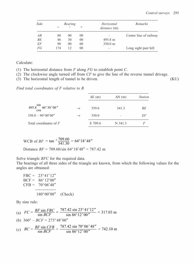
Control surveys 295
Side Bearing Horizontal Remarks
° ′ ″ distance (m)
AB 88 00 00 – Centre line of railwayBE 46 30 00 495.8 mEF 90 00 00 350.0 mFG 174 12 00 – Long sight past hill
Calculate:
(1) The horizontal distance from F along FG to establish point C.(2) The clockwise angle turned off from CF to give the line of the reverse tunnel drivage.(3) The horizontal length of tunnel to be driven. (KU)
Find total coordinates of F relative to B
∆E (m) ∆N (m) Station
495.8sin
cos 46 30 00° ′ ′′ → 359.6 341.3 BE
350.0 – 90°00′00″ → 350.0 – EF
Total coordinates of F E 709.6 N 341.3 F
WCB of BF = tan 709.60341.30
= 64 18 48–1 ° ′ ′′
Distance BF = 709.60/sin 64°18′48″ = 787.42 m
Solve triangle BFC for the required data.The bearings of all three sides of the triangle are known, from which the following values for theangles are obtained:
FBC = 23°41′12″BCF = 86°12′00″CFB = 70°06′48″
180°00′00″ (Check)
By sine rule:
(a) FCBF FBC
BCF = sin
sin =
787.42 sin 23 41 12
sin 86 12 00 = 317.03 m
° ′ ′′° ′ ′′
(b) 360° – BCF = 273°48′ 00″
(c) BCBF CFB
BCF = sin
sin =
787.42 sin 70 06 48
sin 86 12 00 = 742.10 m
° ′ ′′° ′ ′′
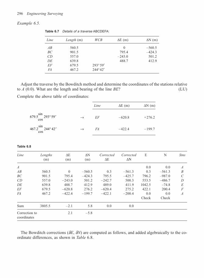
296 Engineering Surveying
Adjust the traverse by the Bowditch method and determine the coordinates of the stations relativeto A (0.0). What are the length and bearing of the line BE? (LU)
Complete the above table of coordinates:
Line ∆E (m) ∆N (m)
679.5sin
cos 293 59° ′ → EF – 620.8 +276.2
467.2sin
cos 244 42° ′ → FA –422.4 –199.7
Table 6.8
Line Lengths ∆E ∆N Corrected Corrected E N Stns
(m) (m) (m) ∆E ∆Ν
A 0.0 0.0 A
AB 560.5 0 –560.5 0.3 –561.3 0.3 –561.3 B
BC 901.5 795.4 –424.3 795.5 –425.7 796.2 –987.0 C
CD 557.0 –243.0 501.2 –242.7 500.3 553.5 –486.7 D
DE 639.8 488.7 412.9 489.0 411.9 1042.5 –74.8 E
EF 679.5 –620.8 276.2 –620.4 275.2 422.1 200.4 F
FA 467.2 –422.4 –199.7 –422.1 –200.4 0.0 0.0 A
Check Check
Sum 3805.5 –2.1 5.8 0.0 0.0
Correction to 2.1 –5.8coordinates
The Bowditch corrections (δE, δN) are computed as follows, and added algebraically to the co-ordinate differences, as shown in Table 6.8.
Example 6.5.
Table 6.7 Details of a traverse ABCDEFA:
Line Length (m) WCB ∆E (m) ∆N (m)
AB 560.5 0 –560.5BC 901.5 795.4 –424.3CD 557.0 –243.0 501.2DE 639.8 488.7 412.9EF 679.5 293° 59′FA 467.2 244°42′
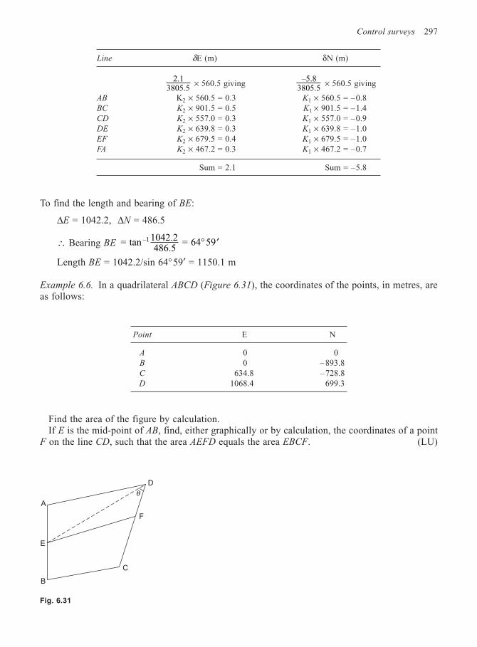
Control surveys 297
Line δE (m) δN (m)
2.13805.5
× 560.5 giving–5.8
3805.5× 560.5 giving
AB K2 × 560.5 = 0.3 K1 × 560.5 = –0.8BC K2 × 901.5 = 0.5 K1 × 901.5 = –1.4CD K2 × 557.0 = 0.3 K1 × 557.0 = –0.9DE K2 × 639.8 = 0.3 K1 × 639.8 = –1.0EF K2 × 679.5 = 0.4 K1 × 679.5 = –1.0FA K2 × 467.2 = 0.3 K1 × 467.2 = –0.7
Sum = 2.1 Sum = –5.8
To find the length and bearing of BE:
∆E = 1042.2, ∆N = 486.5
∴ Bearing BE = tan 1042.2486.5
= 64 59–1 ° ′
Length BE = 1042.2/sin 64°59′ = 1150.1 m
Example 6.6. In a quadrilateral ABCD (Figure 6.31), the coordinates of the points, in metres, areas follows:
Point E N
A 0 0B 0 – 893.8C 634.8 –728.8D 1068.4 699.3
Find the area of the figure by calculation.If E is the mid-point of AB, find, either graphically or by calculation, the coordinates of a point
F on the line CD, such that the area AEFD equals the area EBCF. (LU)
Fig. 6.31
A
E
B
C
F
D
θ
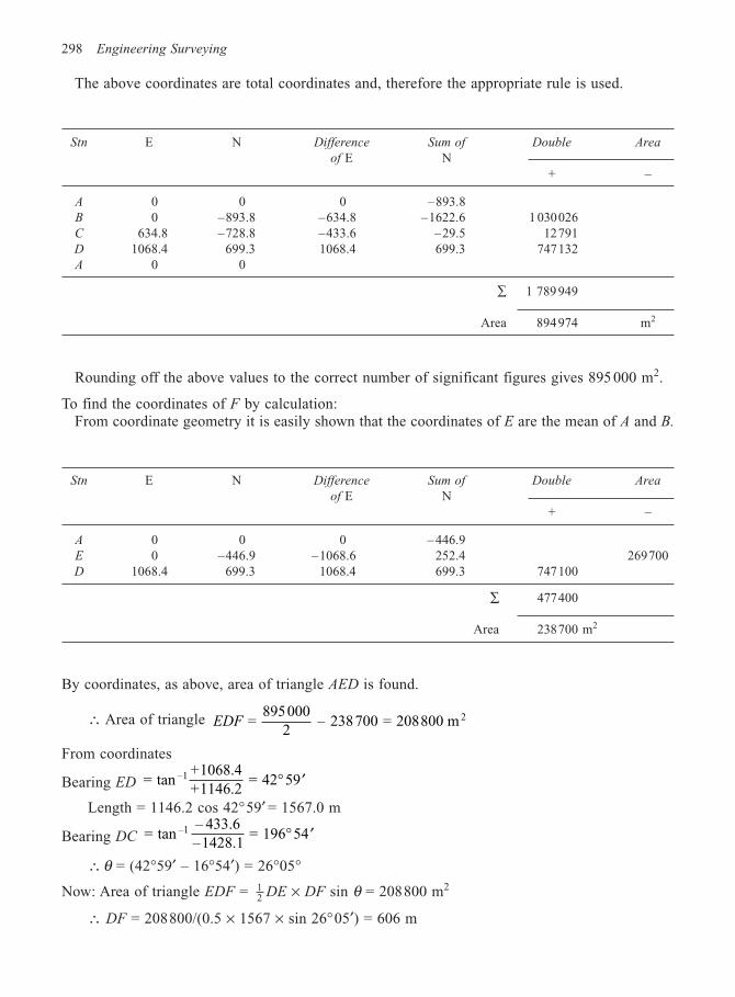
298 Engineering Surveying
The above coordinates are total coordinates and, therefore the appropriate rule is used.
Stn E N Difference Sum of Double Area
of E N+ –
A 0 0 0 –893.8B 0 –893.8 –634.8 –1622.6 1 030026C 634.8 –728.8 –433.6 –29.5 12791D 1068.4 699.3 1068.4 699.3 747132A 0 0
∑ 1 789 949
Area 894974 m2
Rounding off the above values to the correct number of significant figures gives 895 000 m2.
To find the coordinates of F by calculation:From coordinate geometry it is easily shown that the coordinates of E are the mean of A and B.
Stn E N Difference Sum of Double Area
of E N+ –
A 0 0 0 – 446.9E 0 –446.9 –1068.6 252.4 269700D 1068.4 699.3 1068.4 699.3 747100
∑ 477400
Area 238700 m2
By coordinates, as above, area of triangle AED is found.
∴ Area of triangle EDF = 895000
2 – 238700 = 208800 m 2
From coordinates
Bearing ED = tan+1068.4+1146.2
= 42 59–1 ° ′
Length = 1146.2 cos 42°59′ = 1567.0 m
Bearing DC = tan– 433.6–1428.1
= 196 54–1 ° ′
∴ θ = (42°59′ – 16°54′) = 26°05°
Now: Area of triangle EDF = 12 DE × DF sin θ = 208800 m2
∴ DF = 208800/(0.5 × 1567 × sin 26°05′) = 606 m
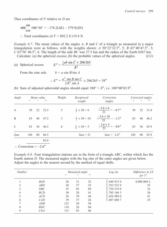
Control surveys 299
Thus coordinates of F relative to D are
606sin
cos 196 54° ′ = –176.2(∆E) – 579.9(∆N)
∴ Total coordinates of F = 892.2 E119.4 N
Example 6.7. The mean values of the angles A, B and C of a triangle as measured in a majortriangulation were as follows, with the weights shown: A 50°22′32.5″, 5; B 65°40′47.5″, 3;C 63°56′ 46.5″, 6. The length of the side BC was 37.5 km and the radius of the Earth 6267 km.
Calculate: (a) the spherical excess; (b) the probable values of the spherical angles. (LU)
(a) Spherical excess ′′×
Eab C
R =
sin 206 26512
2
ˆ
From the sine rule b = a sin B/sin A
∴ ′′ = sin sin 2 sin
2
2E
a B C
R A× 206265 = 39″
(b) Sum of adjusted spheroidal angles should equal 180° + E″, i.e. 180°00′03.9″.
Angle Mean value Weight Reciprocal Correction Corrected angles
° ′ ″ weight angles ° ′ ″
A 50 22 32.5 5 15 × 30 = 6
– 2.6 6
21 = – 0.7
×′′ 50 22 31.8
B 65 40 47.5 3 13 × 30 = 10
– 2.6 10
21 = –1.3
×′′ 65 40 46.2
C 63 56 46.5 6 16 × 30 = 5
– 2.6 521
= – 0.6×
′′ 63 56 45.9
Sum 180 00 06.5 Sum = 21 Sum = –2.6″ 180 00 03.9
03.9
∴ Correction = –2.6″
Example 6.8. Four triangulation stations are in the form of a triangle ABC, within which lies thefourth station D. The measured angles with the log sins of the outer angles are given below.Adjust the angles to the nearest second by the method of equal shifts.
Number Measured angle Log sin Difference in LS
° ′ ″ for 1″
1 BAD 26 31 32 1 .649 915 6 0.000 004 22 ABD 20 57 35 1 .553 532 9 553 DBC 35 05 09 1 .759 519 0 324 BCD 30 28 41 1 .705 186 3 365 ACD 26 59 46 1 .656 989 0 416 CAD 39 57 26 1 .807 680 7 257 ADB 132 30 508 BDC 114 26 049 CDA 113 03 06
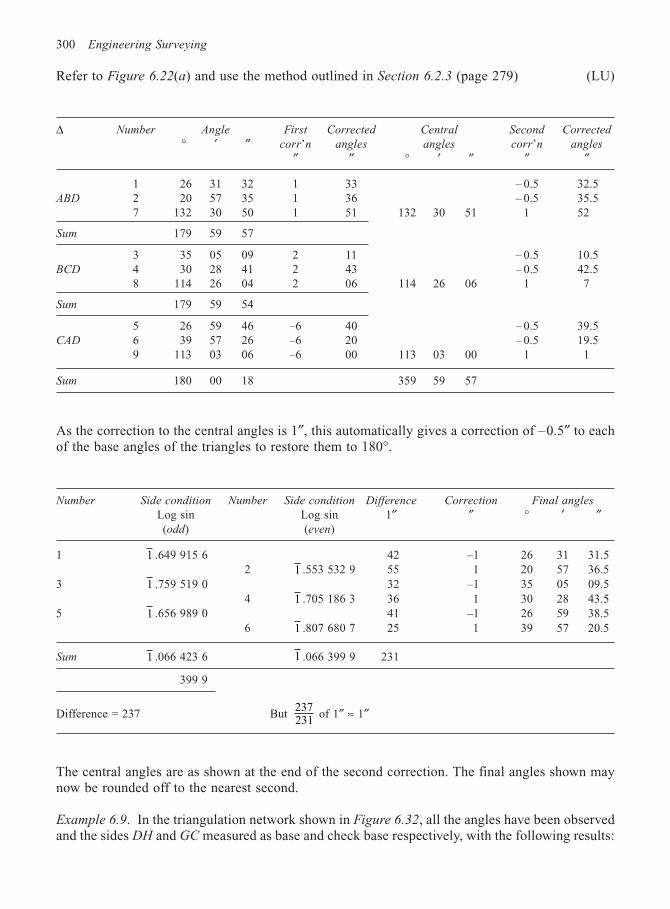
300 Engineering Surveying
Refer to Figure 6.22(a) and use the method outlined in Section 6.2.3 (page 279) (LU)
∆ Number Angle First Corrected Central Second Corrected
° ′ ″ corr’n angles angles corr’n angles
″ ″ ° ′ ″ ″ ″
1 26 31 32 1 33 – 0.5 32.5ABD 2 20 57 35 1 36 – 0.5 35.5
7 132 30 50 1 51 132 30 51 1 52
Sum 179 59 57
3 35 05 09 2 11 – 0.5 10.5BCD 4 30 28 41 2 43 – 0.5 42.5
8 114 26 04 2 06 114 26 06 1 7
Sum 179 59 54
5 26 59 46 –6 40 – 0.5 39.5CAD 6 39 57 26 –6 20 – 0.5 19.5
9 113 03 06 –6 00 113 03 00 1 1
Sum 180 00 18 359 59 57
As the correction to the central angles is 1″, this automatically gives a correction of –0.5″ to eachof the base angles of the triangles to restore them to 180°.
Number Side condition Number Side condition Difference Correction Final angles
Log sin Log sin 1″ ″ ° ′ ″(odd) (even)
1 1 .649 915 6 42 –1 26 31 31.52 1 .553 532 9 55 1 20 57 36.5
3 1 .759 519 0 32 –1 35 05 09.54 1 .705 186 3 36 1 30 28 43.5
5 1 .656 989 0 41 –1 26 59 38.56 1 .807 680 7 25 1 39 57 20.5
Sum 1 .066 423 6 1 .066 399 9 231
399 9
Difference = 237 But237231
of 1″ ≈ 1″
The central angles are as shown at the end of the second correction. The final angles shown maynow be rounded off to the nearest second.
Example 6.9. In the triangulation network shown in Figure 6.32, all the angles have been observedand the sides DH and GC measured as base and check base respectively, with the following results:
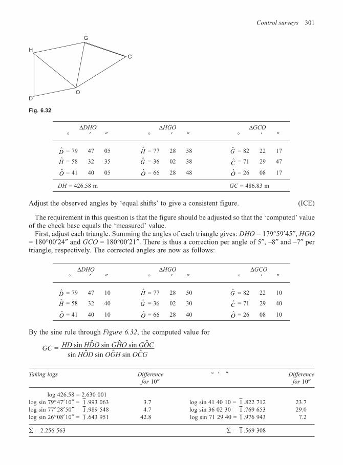
Control surveys 301
∆DHO ∆HGO ∆GCO
° ′ ″ ° ′ ″ ° ′ ″
D = 79 47 05 H = 77 28 58 G = 82 22 17
H = 58 32 35 G = 36 02 38 C = 71 29 47
O = 41 40 05 O = 66 28 48 O = 26 08 17
DH = 426.58 m GC = 486.83 m
Adjust the observed angles by ‘equal shifts’ to give a consistent figure. (ICE)
The requirement in this question is that the figure should be adjusted so that the ‘computed’ valueof the check base equals the ‘measured’ value.
First, adjust each triangle. Summing the angles of each triangle gives: DHO = 179°59′45″, HGO
= 180°00′24″ and GCO = 180°00′21″. There is thus a correction per angle of 5″, –8″ and –7″ pertriangle, respectively. The corrected angles are now as follows:
∆DHO ∆HGO ∆GCO
° ′ ″ ° ′ ″ ° ′ ″
D = 79 47 10 H = 77 28 50 G = 82 22 10
H = 58 32 40 G = 36 02 30 C = 71 29 40
O = 41 40 10 O = 66 28 40 O = 26 08 10
By the sine rule through Figure 6.32, the computed value for
GCHD HDO GHO GOC
HOD OGH OCG = sin sin sin
sin sin sin
ˆ ˆ ˆ
ˆ ˆ ˆ
Taking logs Difference ° ′ ″ Difference
for 10″ for 10″
log 426.58 = 2.630 001log sin 79°47′10″ = 1 .993 063 3.7 log sin 41 40 10 = 1 .822 712 23.7log sin 77°28′50″ = 1 .989 548 4.7 log sin 36 02 30 = 1 .769 653 29.0log sin 26°08′10″ = 1 .643 951 42.8 log sin 71 29 40 = 1 .976 943 7.2
∑ = 2.256 563 ∑ = 1 .569 308
H
D
G
O
C
Fig. 6.32
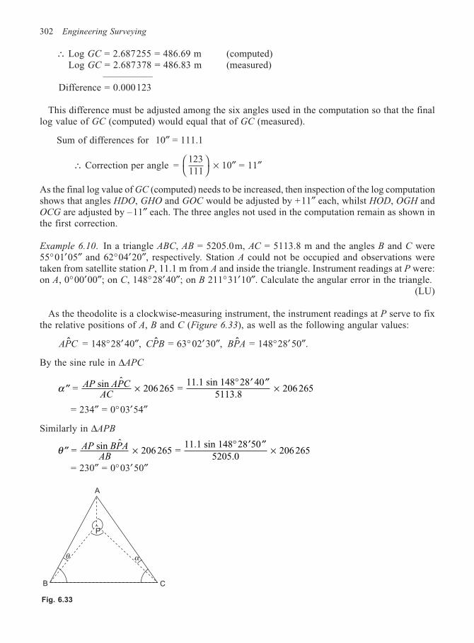
302 Engineering Surveying
∴ Log GC = 2.687255 = 486.69 m (computed)Log GC = 2.687378 = 486.83 m (measured)
—————Difference = 0.000123
This difference must be adjusted among the six angles used in the computation so that the finallog value of GC (computed) would equal that of GC (measured).
Sum of differences for 10″ = 111.1
∴ Correction per angle =123111
× 10″ = 11″
As the final log value of GC (computed) needs to be increased, then inspection of the log computationshows that angles HDO, GHO and GOC would be adjusted by +11″ each, whilst HOD, OGH andOCG are adjusted by –11″ each. The three angles not used in the computation remain as shown inthe first correction.
Example 6.10. In a triangle ABC, AB = 5205.0m, AC = 5113.8 m and the angles B and C were55°01′05″ and 62°04′20″, respectively. Station A could not be occupied and observations weretaken from satellite station P, 11.1 m from A and inside the triangle. Instrument readings at P were:on A, 0°00′00″; on C, 148°28′40″; on B 211°31′10″. Calculate the angular error in the triangle.
(LU)
As the theodolite is a clockwise-measuring instrument, the instrument readings at P serve to fixthe relative positions of A, B and C (Figure 6.33), as well as the following angular values:
APCˆ = 148°28′ 40″, CPBˆ = 63° 02′30″, BPAˆ = 148°28′ 50″.
By the sine rule in ∆APC
′′ ×° ′ ′′
×α = sin 206 265 = 11.1 sin 148 28 40
5113.8 206 265AP APC
AC
ˆ
= 234″ = 0°03′54″
Similarly in ∆APB
′′ ×° ′ ′′
×θ = sin 206 265 = 11.1 sin 148 28 50
5205.0 206 265AP BPA
AB
ˆ
= 230″ = 0°03′50″
Fig. 6.33
A
B C
P
θ α
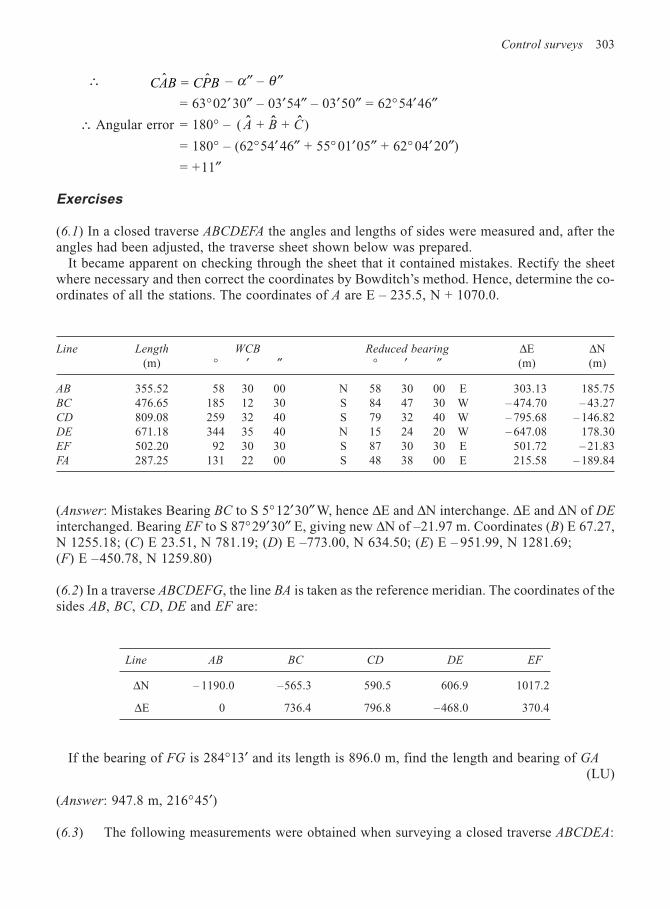
Control surveys 303
∴ CAB CPBˆ ˆ = – α″ – θ ″
= 63°02′ 30″ – 03′54″ – 03′50″ = 62°54′46″∴ Angular error = 180° – ( + + )ˆ ˆ ˆA B C
= 180° – (62°54′ 46″ + 55° 01′05″ + 62° 04′20″)
= +11″
Exercises
(6.1) In a closed traverse ABCDEFA the angles and lengths of sides were measured and, after theangles had been adjusted, the traverse sheet shown below was prepared.
It became apparent on checking through the sheet that it contained mistakes. Rectify the sheetwhere necessary and then correct the coordinates by Bowditch’s method. Hence, determine the co-ordinates of all the stations. The coordinates of A are E – 235.5, N + 1070.0.
Line Length WCB Reduced bearing ∆E ∆N(m) ° ′ ″ ° ′ ″ (m) (m)
AB 355.52 58 30 00 N 58 30 00 E 303.13 185.75BC 476.65 185 12 30 S 84 47 30 W – 474.70 – 43.27CD 809.08 259 32 40 S 79 32 40 W – 795.68 – 146.82DE 671.18 344 35 40 N 15 24 20 W – 647.08 178.30EF 502.20 92 30 30 S 87 30 30 E 501.72 – 21.83FA 287.25 131 22 00 S 48 38 00 E 215.58 – 189.84
(Answer: Mistakes Bearing BC to S 5°12′30″ W, hence ∆E and ∆N interchange. ∆E and ∆N of DE
interchanged. Bearing EF to S 87°29′30″ E, giving new ∆N of –21.97 m. Coordinates (B) E 67.27,N 1255.18; (C) E 23.51, N 781.19; (D) E –773.00, N 634.50; (E) E – 951.99, N 1281.69;(F) E –450.78, N 1259.80)
(6.2) In a traverse ABCDEFG, the line BA is taken as the reference meridian. The coordinates of thesides AB, BC, CD, DE and EF are:
Line AB BC CD DE EF
∆N – 1190.0 –565.3 590.5 606.9 1017.2
∆E 0 736.4 796.8 –468.0 370.4
If the bearing of FG is 284°13′ and its length is 896.0 m, find the length and bearing of GA
(LU)
(Answer: 947.8 m, 216°45′)
(6.3) The following measurements were obtained when surveying a closed traverse ABCDEA:
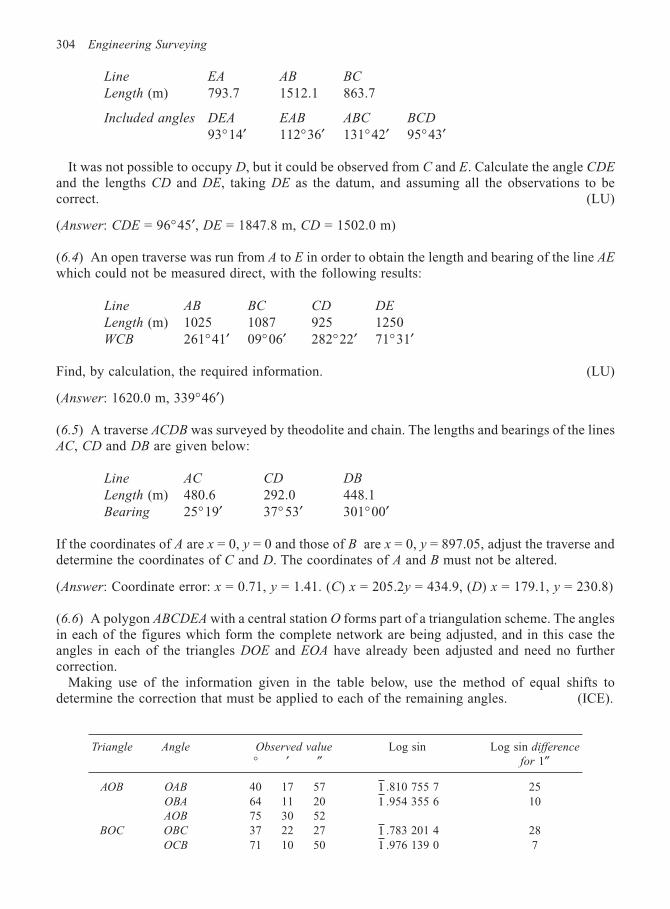
304 Engineering Surveying
Line EA AB BC
Length (m) 793.7 1512.1 863.7
Included angles DEA EAB ABC BCD
93°14′ 112°36′ 131°42′ 95°43′
It was not possible to occupy D, but it could be observed from C and E. Calculate the angle CDE
and the lengths CD and DE, taking DE as the datum, and assuming all the observations to becorrect. (LU)
(Answer: CDE = 96°45′, DE = 1847.8 m, CD = 1502.0 m)
(6.4) An open traverse was run from A to E in order to obtain the length and bearing of the line AE
which could not be measured direct, with the following results:
Line AB BC CD DE
Length (m) 1025 1087 925 1250WCB 261°41′ 09°06′ 282°22′ 71°31′
Find, by calculation, the required information. (LU)
(Answer: 1620.0 m, 339°46′)
(6.5) A traverse ACDB was surveyed by theodolite and chain. The lengths and bearings of the linesAC, CD and DB are given below:
Line AC CD DB
Length (m) 480.6 292.0 448.1Bearing 25°19′ 37° 53′ 301°00′
If the coordinates of A are x = 0, y = 0 and those of B are x = 0, y = 897.05, adjust the traverse anddetermine the coordinates of C and D. The coordinates of A and B must not be altered.
(Answer: Coordinate error: x = 0.71, y = 1.41. (C) x = 205.2y = 434.9, (D) x = 179.1, y = 230.8)
(6.6) A polygon ABCDEA with a central station O forms part of a triangulation scheme. The anglesin each of the figures which form the complete network are being adjusted, and in this case theangles in each of the triangles DOE and EOA have already been adjusted and need no furthercorrection.
Making use of the information given in the table below, use the method of equal shifts todetermine the correction that must be applied to each of the remaining angles. (ICE).
Triangle Angle Observed value Log sin Log sin difference
° ′ ″ for 1″
AOB OAB 40 17 57 1 .810 755 7 25OBA 64 11 20 1 .954 355 6 10AOB 75 30 52
BOC OBC 37 22 27 1 .783 201 4 28OCB 71 10 50 1 .976 139 0 7
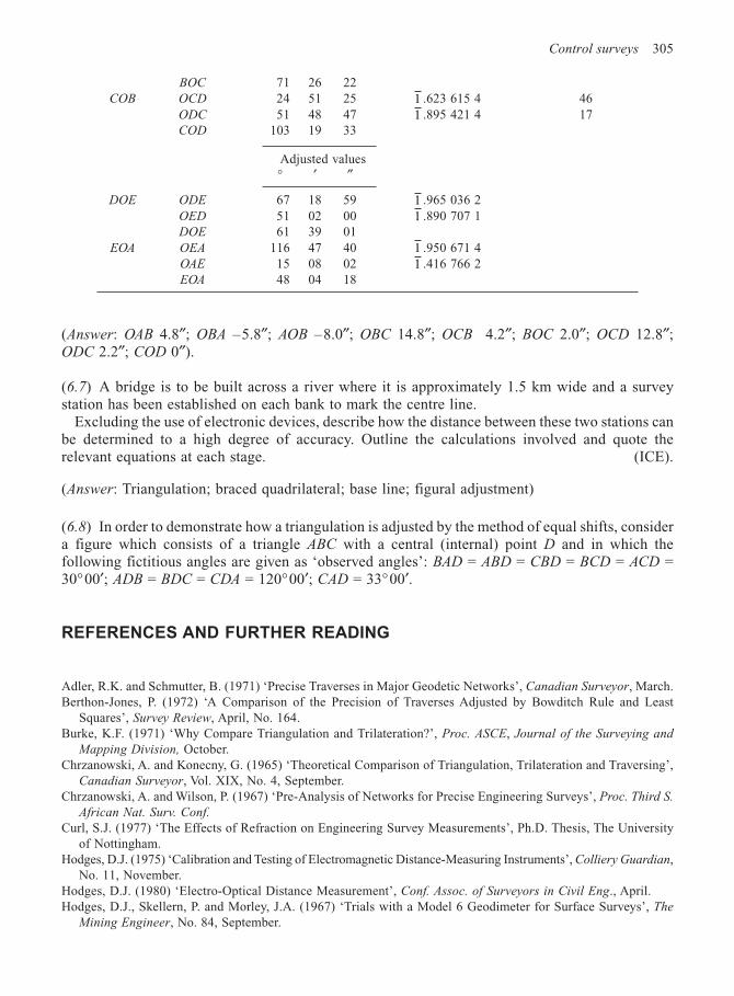
Control surveys 305
BOC 71 26 22COB OCD 24 51 25 1 .623 615 4 46
ODC 51 48 47 1 .895 421 4 17COD 103 19 33
Adjusted values° ′ ″
DOE ODE 67 18 59 1 .965 036 2OED 51 02 00 1 .890 707 1DOE 61 39 01
EOA OEA 116 47 40 1 .950 671 4OAE 15 08 02 1 .416 766 2EOA 48 04 18
(Answer: OAB 4.8″; OBA –5.8″; AOB –8.0″; OBC 14.8″; OCB 4.2″; BOC 2.0″; OCD 12.8″;ODC 2.2″; COD 0″).
(6.7) A bridge is to be built across a river where it is approximately 1.5 km wide and a surveystation has been established on each bank to mark the centre line.
Excluding the use of electronic devices, describe how the distance between these two stations canbe determined to a high degree of accuracy. Outline the calculations involved and quote therelevant equations at each stage. (ICE).
(Answer: Triangulation; braced quadrilateral; base line; figural adjustment)
(6.8) In order to demonstrate how a triangulation is adjusted by the method of equal shifts, considera figure which consists of a triangle ABC with a central (internal) point D and in which thefollowing fictitious angles are given as ‘observed angles’: BAD = ABD = CBD = BCD = ACD =30°00′; ADB = BDC = CDA = 120°00′; CAD = 33°00′.
REFERENCES AND FURTHER READING
Adler, R.K. and Schmutter, B. (1971) ‘Precise Traverses in Major Geodetic Networks’, Canadian Surveyor, March.Berthon-Jones, P. (1972) ‘A Comparison of the Precision of Traverses Adjusted by Bowditch Rule and Least
Squares’, Survey Review, April, No. 164.Burke, K.F. (1971) ‘Why Compare Triangulation and Trilateration?’, Proc. ASCE, Journal of the Surveying and
Mapping Division, October.Chrzanowski, A. and Konecny, G. (1965) ‘Theoretical Comparison of Triangulation, Trilateration and Traversing’,
Canadian Surveyor, Vol. XIX, No. 4, September.Chrzanowski, A. and Wilson, P. (1967) ‘Pre-Analysis of Networks for Precise Engineering Surveys’, Proc. Third S.
African Nat. Surv. Conf.
Curl, S.J. (1977) ‘The Effects of Refraction on Engineering Survey Measurements’, Ph.D. Thesis, The Universityof Nottingham.
Hodges, D.J. (1975) ‘Calibration and Testing of Electromagnetic Distance-Measuring Instruments’, Colliery Guardian,No. 11, November.
Hodges, D.J. (1980) ‘Electro-Optical Distance Measurement’, Conf. Assoc. of Surveyors in Civil Eng., April.Hodges, D.J., Skellern, P. and Morley, J.A. (1967) ‘Trials with a Model 6 Geodimeter for Surface Surveys’, The
Mining Engineer, No. 84, September.

306 Engineering Surveying
Leahy, F.J. (1977) ‘Bowditch Revisited’, Australian Surveyor, December, Vol. 28, No. 8.Murphy, B.T. (1974) ‘The Adjustment of Single Traverses’, Australian Surveyor, December, Vol. 26, No. 4.Ordnance Survey (1950) Constants, Formulae and Methods Used in Traverse Mercator Projection, HMSO, London.Phillips, J.O. (1967) ‘Electronic Traverse versus Triangulation’, Proc. ASCE, Journal of the Surveying and Mapping
Division, October.Schofield, W. (1973) ‘Engineering Surveys on the National Grid’, Journal of the Institution of Highway Engineers,
Vol. XX, No. 10, October.Schwendener, H.R. (1972) ‘Electronic Distancers for Short Ranges: Accuracy and Checking Procedures’, Survey
Review, Vol. XXI, NO. 164, April.Smith, J.R. (1982) ‘Equal Shifts by Pocket Calculator’, Civil Engineering Surveyor, Vol. VII, Issue 5, June 1982.Thomas, T.L. (1971) ‘Desk Computers in Surveying’, Chartered Surveyor, No. 11.
7
Satellite positioning
7.1 INTRODUCTION
Before commencing this chapter, the reader should have studied Chapter 5 and acquired a knowledgeof local and global geoids and ellipsoids, transformations and heights, i.e. Sections 5.1 to 5.8.
The concept of satellite position fixing commenced with the launch of the first Sputnik satelliteby the USSR in October 1957. This was rapidly followed by the development of the Navy NavigationSatellite System (NNSS) by the US navy. This system, commonly referred to as the Transit system,was to provide world-wide navigation capability for the US Polaris submarine fleet. The Transitsystem was made available for civilian use in 1967. However, as it required very long observationperiods and had a rather low accuracy, its application was limited to geodetic and navigation uses.
In 1973, the US Department of Defense commenced the development of NAVSTAR (NavigationSystem with Time and Ranging) global positioning system (GPS), and the first satellites werelaunched in 1978. These satellites were essentially experimental, with the operational systemscheduled for 1987. Now that GPS is fully operational, relative positioning to several millimetres,with extremely short observation periods of a few minutes, has been achieved. For distances inexcess of 5 km GPS has been shown to be more accurate than EDM traversing. It therefore has awide application in engineering surveying, with an effect even greater than the advent of EDM.Apart from the high accuracies attainable, GPS offers the following significant advantages:
(1) Position is determined directly in an X, Y, Z coordinate system.(2) Intervisibility between ground stations is unnecessary.(3) As each point is fixed discretely, there is no error propagation as in networks.(4) Survey points may therefore be selected according to their required function, rather than to
produce a well-conditioned network configuration.(5) Low skill required by the operator.(6) Position may be fixed on land, at sea or in the air. This latter facility may have a profound effect
in aerial photogrammetry.(7) Measurement may be carried out, day or night, anywhere in the world, at any time and in any
type of weather.(8) Continuous measurement may be carried out, resulting in greatly improved deformation
monitoring.
7.2 GPS SEGMENTS
The GPS system can be broadly divided into three segments: the space segment, the control
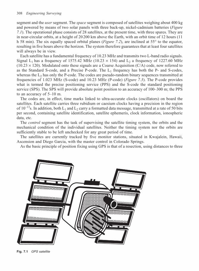
308 Engineering Surveying
segment and the user segment. The space segment is composed of satellites weighing about 400 kgand powered by means of two solar panels with three back-up, nickel-cadmium batteries (Figure
7.1). The operational phase consists of 28 satellites, at the present time, with three spares. They arein near-circular orbits, at a height of 20 200 km above the Earth, with an orbit time of 12 hours (11h 58 min). The six equally spaced orbital planes (Figure 7.2), are inclined at 55° to the equator,resulting in five hours above the horizon. The system therefore guarantees that at least four satelliteswill always be in view.
Each satellite has a fundamental frequency of 10.23 MHz and transmits two L-band radio signals.Signal L1 has a frequency of 1575.42 MHz (10.23 × 154) and L2 a frequency of 1227.60 MHz(10.23 × 120). Modulated onto these signals are a Coarse Acquisition (C/A) code, now referred toas the Standard S-code, and a Precise P-code. The L1 frequency has both the P- and S-codes,whereas the L2 has only the P-code. The codes are pseudo-random binary sequences transmitted atfrequencies of 1.023 MHz (S-code) and 10.23 MHz (P-code) (Figure 7.3). The P-code provideswhat is termed the precise positioning service (PPS) and the S-code the standard positioningservice (SPS). The SPS will provide absolute point position to an accuracy of 100–300 m; the PPSto an accuracy of 5–10 m.
The codes are, in effect, time marks linked to ultra-accurate clocks (oscillators) on board thesatellites. Each satellite carries three rubidium or caesium clocks having a precision in the regionof 10–13s. In addition, both L1 and L2 carry a formatted data message, transmitted at a rate of 50 bitsper second, containing satellite identification, satellite ephemeris, clock information, ionosphericdata, etc.
The control segment has the task of supervising the satellite timing system, the orbits and themechanical condition of the individual satellites. Neither the timing system nor the orbits aresufficiently stable to be left unchecked for any great period of time.
The satellites are currently tracked by five monitor stations, situated in Kwajalein, Hawaii,Ascension and Diego Garcia, with the master control in Colorado Springs.
As the basic principle of position fixing using GPS is that of a resection, using distances to three
Fig. 7.1 GPS satellite
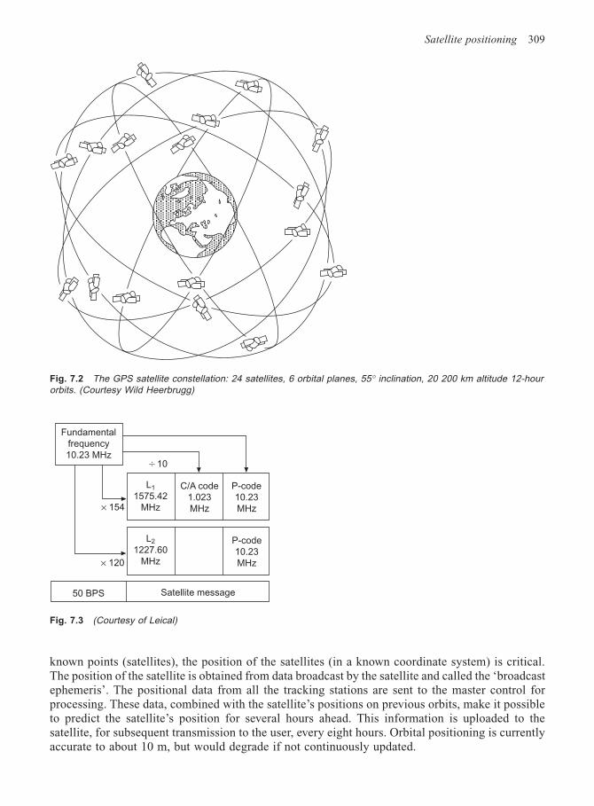
Satellite positioning 309
known points (satellites), the position of the satellites (in a known coordinate system) is critical.The position of the satellite is obtained from data broadcast by the satellite and called the ‘broadcastephemeris’. The positional data from all the tracking stations are sent to the master control forprocessing. These data, combined with the satellite’s positions on previous orbits, make it possibleto predict the satellite’s position for several hours ahead. This information is uploaded to thesatellite, for subsequent transmission to the user, every eight hours. Orbital positioning is currentlyaccurate to about 10 m, but would degrade if not continuously updated.
Fig. 7.2 The GPS satellite constellation: 24 satellites, 6 orbital planes, 55° inclination, 20 200 km altitude 12-hourorbits. (Courtesy Wild Heerbrugg)
Fundamental
frequency
10.23 MHz 10
× 154
× 120
L1
1575.42
MHz
L2
1227.60
MHz
C/A code
1.023
MHz
P-code
10.23
MHz
P-code
10.23
MHz
50 BPS Satellite message
Fig. 7.3 (Courtesy of Leical)
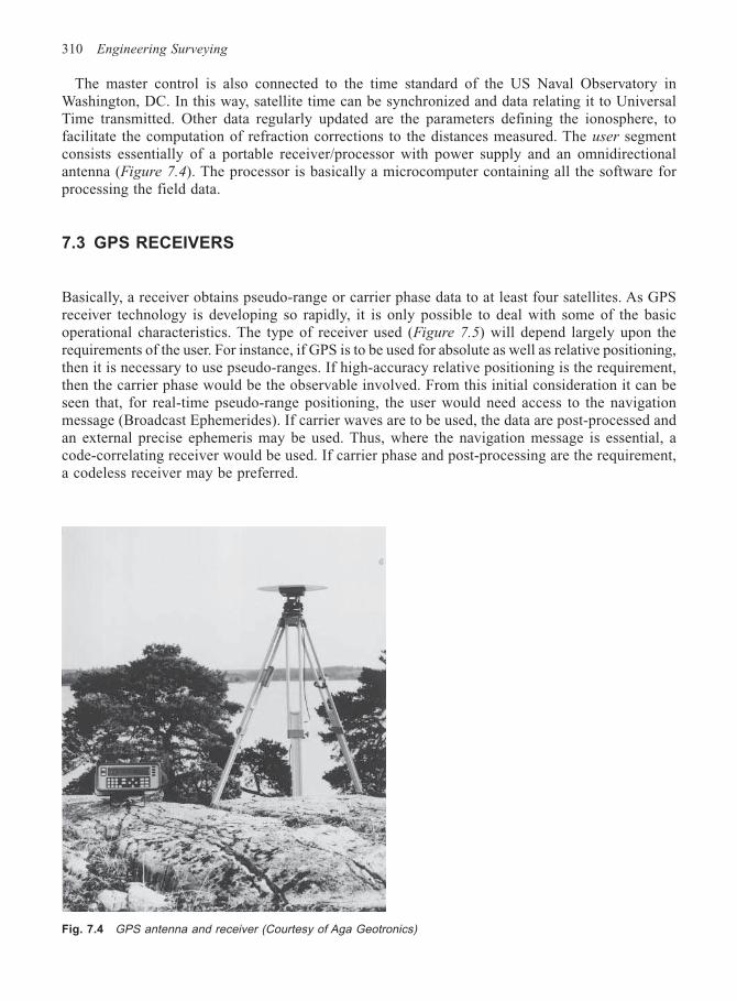
310 Engineering Surveying
The master control is also connected to the time standard of the US Naval Observatory inWashington, DC. In this way, satellite time can be synchronized and data relating it to UniversalTime transmitted. Other data regularly updated are the parameters defining the ionosphere, tofacilitate the computation of refraction corrections to the distances measured. The user segmentconsists essentially of a portable receiver/processor with power supply and an omnidirectionalantenna (Figure 7.4). The processor is basically a microcomputer containing all the software forprocessing the field data.
7.3 GPS RECEIVERS
Basically, a receiver obtains pseudo-range or carrier phase data to at least four satellites. As GPSreceiver technology is developing so rapidly, it is only possible to deal with some of the basicoperational characteristics. The type of receiver used (Figure 7.5) will depend largely upon therequirements of the user. For instance, if GPS is to be used for absolute as well as relative positioning,then it is necessary to use pseudo-ranges. If high-accuracy relative positioning is the requirement,then the carrier phase would be the observable involved. From this initial consideration it can beseen that, for real-time pseudo-range positioning, the user would need access to the navigationmessage (Broadcast Ephemerides). If carrier waves are to be used, the data are post-processed andan external precise ephemeris may be used. Thus, where the navigation message is essential, acode-correlating receiver would be used. If carrier phase and post-processing are the requirement,a codeless receiver may be preferred.
Fig. 7.4 GPS antenna and receiver (Courtesy of Aga Geotronics)
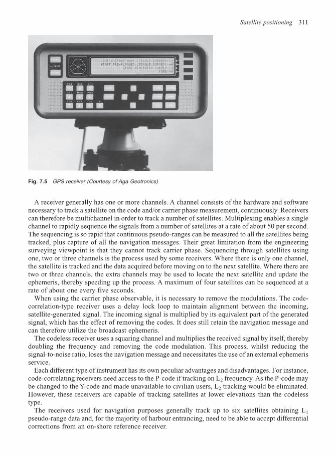
Satellite positioning 311
A receiver generally has one or more channels. A channel consists of the hardware and softwarenecessary to track a satellite on the code and/or carrier phase measurement, continuously. Receiverscan therefore be multichannel in order to track a number of satellites. Multiplexing enables a singlechannel to rapidly sequence the signals from a number of satellites at a rate of about 50 per second.The sequencing is so rapid that continuous pseudo-ranges can be measured to all the satellites beingtracked, plus capture of all the navigation messages. Their great limitation from the engineeringsurveying viewpoint is that they cannot track carrier phase. Sequencing through satellites usingone, two or three channels is the process used by some receivers. Where there is only one channel,the satellite is tracked and the data acquired before moving on to the next satellite. Where there aretwo or three channels, the extra channels may be used to locate the next satellite and update theephemeris, thereby speeding up the process. A maximum of four satellites can be sequenced at arate of about one every five seconds.
When using the carrier phase observable, it is necessary to remove the modulations. The code-correlation-type receiver uses a delay lock loop to maintain alignment between the incoming,satellite-generated signal. The incoming signal is multiplied by its equivalent part of the generatedsignal, which has the effect of removing the codes. It does still retain the navigation message andcan therefore utilize the broadcast ephemeris.
The codeless receiver uses a squaring channel and multiplies the received signal by itself, therebydoubling the frequency and removing the code modulation. This process, whilst reducing thesignal-to-noise ratio, loses the navigation message and necessitates the use of an external ephemerisservice.
Each different type of instrument has its own peculiar advantages and disadvantages. For instance,code-correlating receivers need access to the P-code if tracking on L2 frequency. As the P-code maybe changed to the Y-code and made unavailable to civilian users, L2 tracking would be eliminated.However, these receivers are capable of tracking satellites at lower elevations than the codelesstype.
The receivers used for navigation purposes generally track up to six satellites obtaining L1
pseudo-range data and, for the majority of harbour entrancing, need to be able to accept differentialcorrections from an on-shore reference receiver.
Fig. 7.5 GPS receiver (Courtesy of Aga Geotronics)
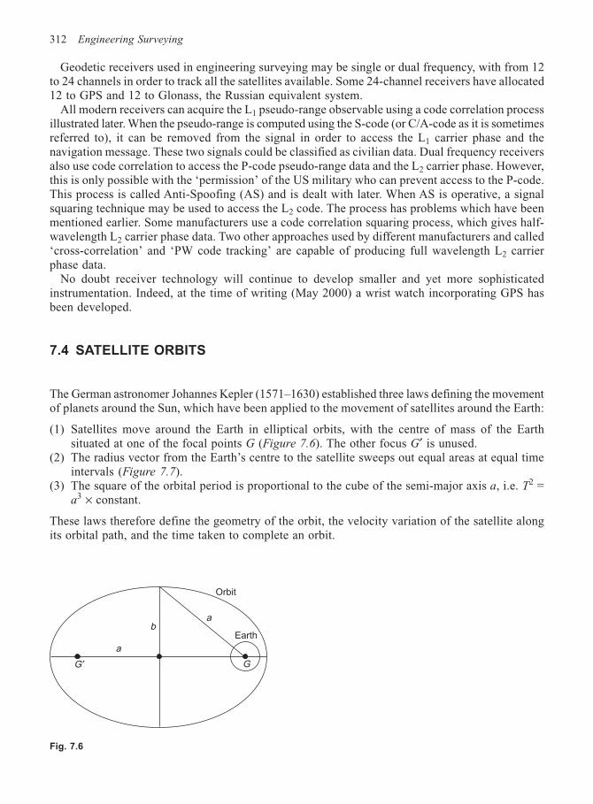
312 Engineering Surveying
Geodetic receivers used in engineering surveying may be single or dual frequency, with from 12to 24 channels in order to track all the satellites available. Some 24-channel receivers have allocated12 to GPS and 12 to Glonass, the Russian equivalent system.
All modern receivers can acquire the L1 pseudo-range observable using a code correlation processillustrated later. When the pseudo-range is computed using the S-code (or C/A-code as it is sometimesreferred to), it can be removed from the signal in order to access the L1 carrier phase and thenavigation message. These two signals could be classified as civilian data. Dual frequency receiversalso use code correlation to access the P-code pseudo-range data and the L2 carrier phase. However,this is only possible with the ‘permission’ of the US military who can prevent access to the P-code.This process is called Anti-Spoofing (AS) and is dealt with later. When AS is operative, a signalsquaring technique may be used to access the L2 code. The process has problems which have beenmentioned earlier. Some manufacturers use a code correlation squaring process, which gives half-wavelength L2 carrier phase data. Two other approaches used by different manufacturers and called‘cross-correlation’ and ‘PW code tracking’ are capable of producing full wavelength L2 carrierphase data.
No doubt receiver technology will continue to develop smaller and yet more sophisticatedinstrumentation. Indeed, at the time of writing (May 2000) a wrist watch incorporating GPS hasbeen developed.
7.4 SATELLITE ORBITS
The German astronomer Johannes Kepler (1571–1630) established three laws defining the movementof planets around the Sun, which have been applied to the movement of satellites around the Earth:
(1) Satellites move around the Earth in elliptical orbits, with the centre of mass of the Earthsituated at one of the focal points G (Figure 7.6). The other focus G′ is unused.
(2) The radius vector from the Earth’s centre to the satellite sweeps out equal areas at equal timeintervals (Figure 7.7).
(3) The square of the orbital period is proportional to the cube of the semi-major axis a, i.e. T2 =a3 × constant.
These laws therefore define the geometry of the orbit, the velocity variation of the satellite alongits orbital path, and the time taken to complete an orbit.
Orbit
Earth
a
GG ′
ba
Fig. 7.6
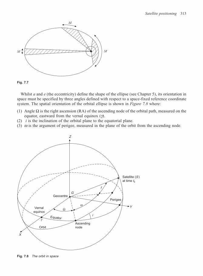
Satellite positioning 313
Whilst a and e (the eccentricity) define the shape of the ellipse (see Chapter 5), its orientation inspace must be specified by three angles defined with respect to a space-fixed reference coordinatesystem. The spatial orientation of the orbital ellipse is shown in Figure 7.8 where:
(1) Angle Ω is the right ascension (RA) of the ascending node of the orbital path, measured on theequator, eastward from the vernal equinox (γ).
(2) i is the inclination of the orbital plane to the equatorial plane.(3) ω is the argument of perigee, measured in the plane of the orbit from the ascending node.
∆t
∆t ∆t
Fig. 7.7
Z
G
Y
X
OrbitAscending
node
Equator
Vernal
equinox
Geocentre
f
ωΩ
γ
Perigee
i
Satellite (S )
at time ts
Fig. 7.8 The orbit in space
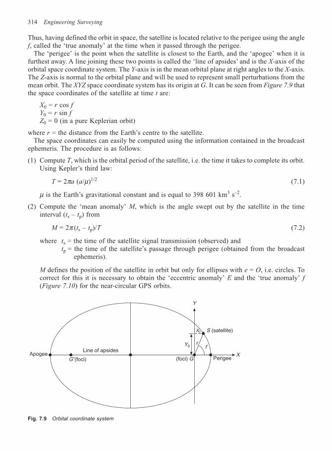
314 Engineering Surveying
Thus, having defined the orbit in space, the satellite is located relative to the perigee using the anglef, called the ‘true anomaly’ at the time when it passed through the perigee.
The ‘perigee’ is the point when the satellite is closest to the Earth, and the ‘apogee’ when it isfurthest away. A line joining these two points is called the ‘line of apsides’ and is the X-axis of theorbital space coordinate system. The Y-axis is in the mean orbital plane at right angles to the X-axis.The Z-axis is normal to the orbital plane and will be used to represent small perturbations from themean orbit. The XYZ space coordinate system has its origin at G. It can be seen from Figure 7.9 thatthe space coordinates of the satellite at time t are:
X0 = r cos fY0 = r sin fZ0 = 0 (in a pure Keplerian orbit)
where r = the distance from the Earth’s centre to the satellite.The space coordinates can easily be computed using the information contained in the broadcast
ephemeris. The procedure is as follows:
(1) Compute T, which is the orbital period of the satellite, i.e. the time it takes to complete its orbit.Using Kepler’s third law:
T = 2πa (a/µ)1/2 (7.1)
µ is the Earth’s gravitational constant and is equal to 398 601 km3 s–2.
(2) Compute the ‘mean anomaly’ M, which is the angle swept out by the satellite in the timeinterval (ts – tp) from
M = 2π (ts – tp)/T (7.2)
where ts = the time of the satellite signal transmission (observed) andtp = the time of the satellite’s passage through perigee (obtained from the broadcast
ephemeris).
M defines the position of the satellite in orbit but only for ellipses with e = O, i.e. circles. Tocorrect for this it is necessary to obtain the ‘eccentric anomaly’ E and the ‘true anomaly’ f(Figure 7.10) for the near-circular GPS orbits.
Fig. 7.9 Orbital coordinate system
Line of apsides
G ′(foci)Apogee
(foci) G
Y0 f
S (satellite)
r
X0
PerigeeX
Y
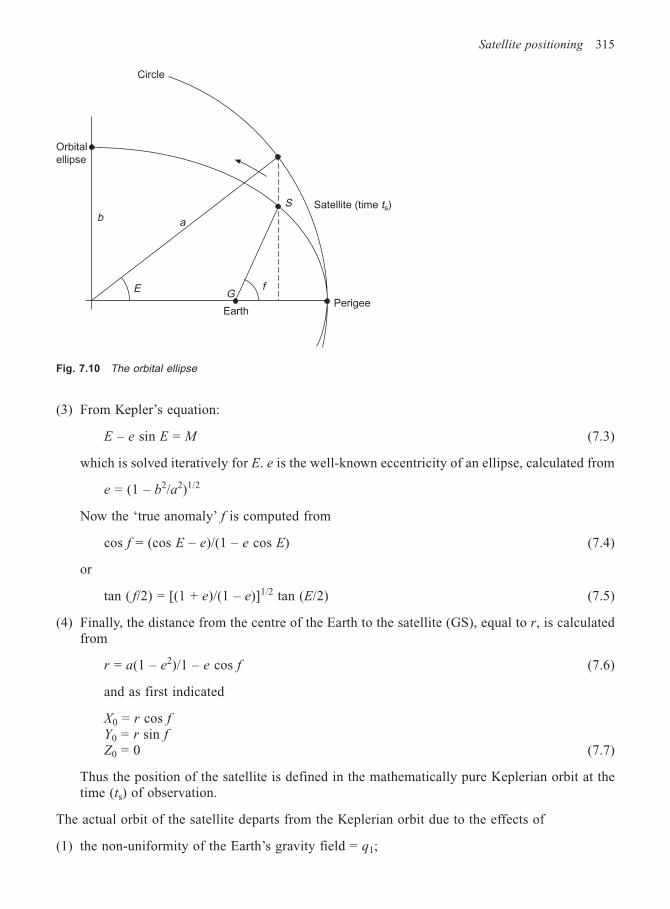
Satellite positioning 315
(3) From Kepler’s equation:
E – e sin E = M (7.3)
which is solved iteratively for E. e is the well-known eccentricity of an ellipse, calculated from
e = (1 – b2/a2)1/2
Now the ‘true anomaly’ f is computed from
cos f = (cos E – e)/(1 – e cos E) (7.4)
or
tan ( f/2) = [(1 + e)/(1 – e)]1/2 tan (E/2) (7.5)
(4) Finally, the distance from the centre of the Earth to the satellite (GS), equal to r, is calculatedfrom
r = a(1 – e2)/1 – e cos f (7.6)
and as first indicated
X0 = r cos fY0 = r sin fZ0 = 0 (7.7)
Thus the position of the satellite is defined in the mathematically pure Keplerian orbit at thetime (ts) of observation.
The actual orbit of the satellite departs from the Keplerian orbit due to the effects of
(1) the non-uniformity of the Earth’s gravity field = q1;
Circle
Orbital
ellipse
EarthPerigee
Satellite (time ts)S
fE
ab
G
Fig. 7.10 The orbital ellipse
316 Engineering Surveying
(2) the attraction of the moon and sun = q2;(3) atmospheric drag = q3;(4) direct and reflected solar radiation pressure = q4 and q5;(5) earth tides = q6;(6) ocean tides = q7.
These forces produce orbital perturbations, the total effect (qt = q1 + q2 + . . . q7) of which must bemathematically modelled to produce a precise position for the satellite at the time of observation.
As already illustrated, the pure, smooth Keplerian orbit is obtained from the elements:
a – semi-major axise – eccentricity
which give the size and shape of the orbit.i – inclinationΩ – right ascension of the ascending node
which orient the orbital plane in space with respect to the Earth.ω – argument of perigeetp – ephemeris reference time
which fixes the position of the satellite.
Additional parameters given in the Broadcast Ephemeris describe the deviations of the satellitemotion from the pure Keplerian form. There are two ephemerides available: the Broadcast, shownbelow, and the Precise.
M0 = Mean anomaly∆n = Mean motion difference
e = Eccentricitya = Square root of semi-major axisΩ = Right ascensioni0 = Inclinationω = Argument of perigeeΩ
•
= Rate of right ascensioni•
= Rate of inclinationCuc, Cus = Correction terms to argument of latitudeCrc, Crs = Correction terms to orbital radiusCic, Cis = Correction terms to inclination
tp = Ephemeris reference time
Using the Broadcast Ephemeris, plus two additional values from the WGS 84 geopotential model,namely:
ωe – the angular velocity of the Earth (7292115 × 10–11 rad s–1)µ – the gravitational/mass constant of the Earth (3986 005 × 108 m3 s–2)
The Cartesian coordinates in a perturbed satellite orbit can be computed using:u – the argument of latitude (the angle in the orbital plane, from the ascending node to the
satellite)r – the geocentric radius, as follows
X0 = r cos u
Y0 = r sin u (7.8)
Z0 = 0
Satellite positioning 317
wherer = a(1 – e cos E) + Crc cos 2 (ω + f ) + Crs sin 2 (ω + f )u = ω + f + Cuc cos 2 (ω + f ) + Cus sin 2 (ω + f )
where a(1 – e cos E ) is the elliptical radius, Crc and Crs the cosine and sine correction terms of thegeocentric radius and Cuc, Cus the correction terms for u.
It is now necessary to rotate the orbital plane about the X0 axis, through the inclination i, to makethe orbital plane coincide with the equatorial plane and the Z0 axis coincide with the Z axis of theEarth fixed system (IRP). Thus:
XE = X0
YE = Y0 cos i (7.9)
ZE = Y0 sin i
where
i = i0 + i•
t + Cic cos 2 (ω + f ) + Cis sin 2 (ω + f)
and i0 is the inclination of the orbit plane at reference time tp.i•
is the linear change in inclination since the reference time,Cic, Cis are the amplitude of the cosine and sine correction terms of the inclination of the
orbital plane.
Finally, although the ZE axis is now correct, the XE axis aligns with the First Point of Aries andrequires a rotation about Z towards the Zero Meridian (IRM) usually referred to as the GreenwichMeridian. The required angle of rotation is Greenwich Apparent Sidereal Time (GAST) and is ineffect the longitude of the ascending node of the orbital plane (λ0) at the time of observation ts.
To compute λ0 we use the right ascension parameter Ω0, the change in GAST using the Earth’srotation rate ωe during the time interval (ts – tp) and change in longitude since the reference time,thus:
λ0 = Ω0 + ( Ω•
– ωe)(ts – tp) – ωetp
and:
X = XE cos λ0 – YE sin λ0
Y = XE sin λ0 – YE cos λ0 (7.10)
Z = ZE
The accuracy of the orbit deduced from the Broadcast Ephemeris is about 10 m at best and isdirectly reflected in the absolute position of points. Whilst this may be adequate for some applications,such as navigation, it would not be acceptable for most engineering surveying purposes. Fortunately,differential procedures and the fact that engineering generally requires relative positioning usingcarrier phase, eliminates the effect of orbital error. However, relative positioning accuracies betterthan 0.1 ppm of the length of the baseline can only be achieved using a Precise Ephemeris.
The GPS satellite coordinates are defined on an ellipsoid of reference called the World GlobalSystem 1984 (WGS 84). As stated, the system has its centre coinciding with the centre of mass ofthe Earth and orientated to coincide with the IERS axes, as described in Chapter 5. Its size andshape is the one that best fits the geoid over the whole Earth, and is identical to the Ellipsoid GRS80with a = 6378137.0 m and 1/f = 298.257223563.
In addition to being a coordinate system, other values, such as a description of the Earth’s gravity
318 Engineering Surveying
field, the velocity of light and the Earth’s angular velocity, are also supplied. Consequently, thevelocity of light as quoted for the WGS 84 model must be used to compute ranges from observerto satellite, and the subsequent position, based on all the relevant parameters supplied.
The WGS 84 reference system was based on TRANSIT doppler measurements at about 1600sites, combined with data from satellite laser ranging (SLR) and very long baseline interferometry(VBLI). The result of this is that, as the position of these points defining the global referencesystem change due to movement of the land masses, the coordinate system will need to be regularlyrevised. The ability to measure this movement to a very high accuracy by use of the satellitesthemselves now results in four-dimensional positioning, possibly including rate of change of position.
The final stage, then, of the positioning process is the transformation of the WGS 84 coordinatesto local geodetic or plane rectangular coordinates and height. This is usually done using theHelmert transformation outlined in Chapter 5. The translation, scale and rotational parametersbetween GPS and national mapping coordinate systems have been published. The practical problemsinvolved have already been mentioned in Chapter 5. If the parameters are unavailable, they can beobtained by obtaining the WGS 84 coordinates of points whose local coordinates are known. A leastsquares solution will produce the parameters required. (The transformation processes are dealt withlater in the chapter.)
It must be remembered that the height obtained from satellites is the ellipsoidal height and willrequire accurate knowledge of the geoid–ellipsoid separation (N) to change it to orthometric.
7.5 BASIC PRINCIPLE OF POSITION FIXING
As previously stated, the principle involves the measurement of distance (or range) to at least threesatellites whose X, Y and Z position is known, in order to define the user’s Xp, Yp and Zp position.
In its simplest form, the satellite transmits a signal on which the time of its departure (tD )fromthe satellite is modulated. The receiver in turn notes the time of arrival (tA) of this time mark. Thenthe time which it took the signal to go from satellite to receiver is (tA – tD ) = ∆t (called the delaytime). The measured range R is obtained from
R1 = (tA – tD) C = ∆t C (7.11)
where c = the velocity of light.
Whilst the above describes the basic principle of range measurement, to achieve it one wouldrequire the receiver to have a clock as accurate as the satellite’s and perfectly synchronized with it.As this would render the receiver impossibly expensive, a correlation procedure, using the pseudo-random binary codes (P or S), usually ‘S’, is adopted. The signal from the satellite arrives at thereceiver and triggers the receiver to commence generating the S-code. The receiver-generated codeis cross-correlated with the satellite code (Figure 7.11). The ground receiver is then able to determinethe time delay (∆t) since it generated the same portion of the code received from the satellite.However, whilst this eliminates the problem of an expensive receiver clock, it does not eliminatethe problem of exact synchronization of the two clocks. Thus, the time difference between the twoclocks, termed clock bias, results in an incorrect assessment of ∆t. The distances computed aretherefore called ‘pseudo-ranges’. The effect of clock bias, however, can be eliminated by the useof four satellites rather than three.
A line in space is defined by its difference in coordinates in an X, Y and Z system:
R = (∆X2 + ∆Y2 + ∆Z2)1/2
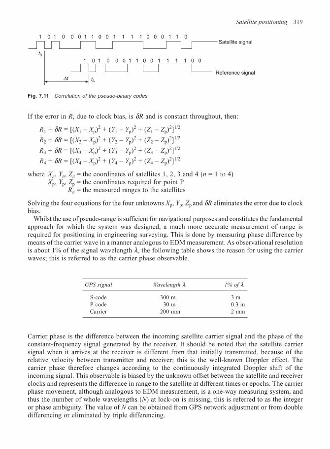
Satellite positioning 319
If the error in R, due to clock bias, is δR and is constant throughout, then:
R1 + δR = [(X1 – Xp)2 + (Y1 – Yp)2 + (Z1 – Zp)
2]1/2
R2 + δR = [(X2 – Xp)2 + (Y2 – Yp)2 + (Z2 – Zp)
2]1/2
R3 + δR = [(X3 – Xp)2 + (Y3 – Yp)2 + (Z3 – Zp)
2]1/2
R4 + δR = [(X4 – Xp)2 + (Y4 – Yp)2 + (Z4 – Zp)
2]1/2
where Xn, Yn, Zn = the coordinates of satellites 1, 2, 3 and 4 (n = 1 to 4)Xp, Yp, Zp = the coordinates required for point P
Rn = the measured ranges to the satellites
Solving the four equations for the four unknowns Xp, Yp, Zp and δR eliminates the error due to clockbias.
Whilst the use of pseudo-range is sufficient for navigational purposes and constitutes the fundamentalapproach for which the system was designed, a much more accurate measurement of range isrequired for positioning in engineering surveying. This is done by measuring phase difference bymeans of the carrier wave in a manner analogous to EDM measurement. As observational resolutionis about 1% of the signal wavelength λ, the following table shows the reason for using the carrierwaves; this is referred to as the carrier phase observable.
GPS signal Wavelength λ 1% of λ
S-code 300 m 3 mP-code 30 m 0.3 mCarrier 200 mm 2 mm
Carrier phase is the difference between the incoming satellite carrier signal and the phase of theconstant-frequency signal generated by the receiver. It should be noted that the satellite carriersignal when it arrives at the receiver is different from that initially transmitted, because of therelative velocity between transmitter and receiver; this is the well-known Doppler effect. Thecarrier phase therefore changes according to the continuously integrated Doppler shift of theincoming signal. This observable is biased by the unknown offset between the satellite and receiverclocks and represents the difference in range to the satellite at different times or epochs. The carrierphase movement, although analogous to EDM measurement, is a one-way measuring system, andthus the number of whole wavelengths (N) at lock-on is missing; this is referred to as the integeror phase ambiguity. The value of N can be obtained from GPS network adjustment or from doubledifferencing or eliminated by triple differencing.
1 0 1 0 0 0 1 1 0 0 1 1 1 1 0 0 0 1 1 0
1 0 1 0 0 0 1 1 0 0 1 1 1 1 0 0
tD
∆t tA
Satellite signal
Reference signal
Fig. 7.11 Correlation of the pseudo-binary codes
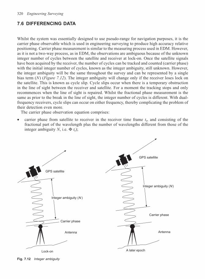
320 Engineering Surveying
7.6 DIFFERENCING DATA
Whilst the system was essentially designed to use pseudo-range for navigation purposes, it is thecarrier phase observable which is used in engineering surveying to produce high accuracy relativepositioning. Carrier phase measurement is similar to the measuring process used in EDM. However,as it is not a two-way process, as in EDM, the observations are ambiguous because of the unknowninteger number of cycles between the satellite and receiver at lock-on. Once the satellite signalshave been acquired by the receiver, the number of cycles can be tracked and counted (carrier phase)with the initial integer number of cycles, known as the integer ambiguity, still unknown. However,the integer ambiguity will be the same throughout the survey and can be represented by a singlebias term (N) (Figure 7.12). The integer ambiguity will change only if the receiver loses lock onthe satellite. This is known as cycle slip. Cycle slips occur when there is a temporary obstructionin the line of sight between the receiver and satellite. For a moment the tracking stops and onlyrecommences when the line of sight is repaired. Whilst the fractional phase measurement is thesame as prior to the break in the line of sight, the integer number of cycles is different. With dual-frequency receivers, cycle slips can occur on either frequency, thereby complicating the problem oftheir detection even more.
The carrier phase observation equation comprises:
• carrier phase from satellite to receiver in the receiver time frame tr, and consisting of thefractional part of the wavelength plus the number of wavelengths different from those of theinteger ambiguity N, i.e. Φ tr);
Fig. 7.12 Integer ambiguity
GPS satellite
Integer ambiguity (N )
GPS satellite
Carrier phase
Carrier phase
AntennaAntenna
Lock-on A later epoch
Integer ambiguity (N )
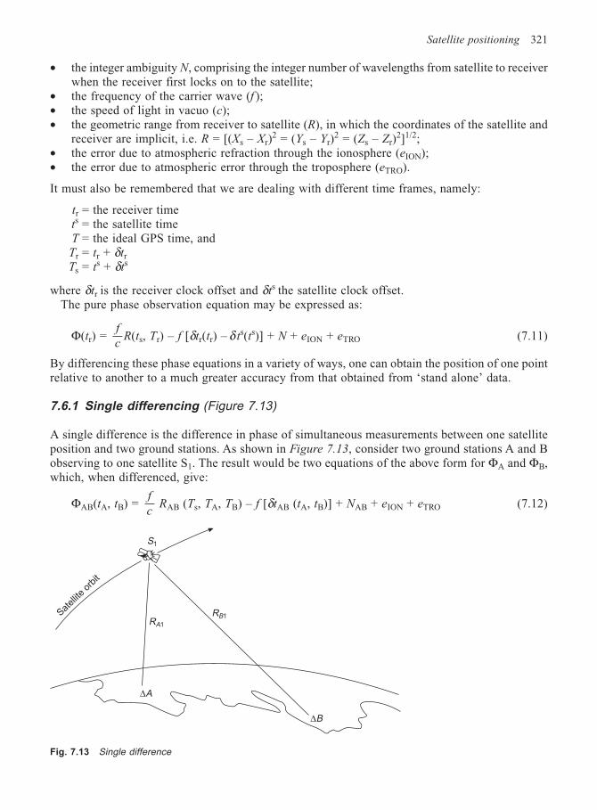
Satellite positioning 321
• the integer ambiguity N, comprising the integer number of wavelengths from satellite to receiverwhen the receiver first locks on to the satellite;
• the frequency of the carrier wave (f );• the speed of light in vacuo (c);• the geometric range from receiver to satellite (R), in which the coordinates of the satellite and
receiver are implicit, i.e. R = [(Xs – Xr)2 = (Ys – Yr)
2 = (Zs – Zr)2]1/2;
• the error due to atmospheric refraction through the ionosphere (eION);• the error due to atmospheric error through the troposphere (eTRO).
It must also be remembered that we are dealing with different time frames, namely:
tr = the receiver timets = the satellite timeT = the ideal GPS time, andTr = tr + δtr
Ts = ts + δts
where δtr is the receiver clock offset and δts the satellite clock offset.The pure phase observation equation may be expressed as:
Φ(tr) = f
cR(ts, Tr) – f [δtr(tr) – δ ts(ts)] + N + eION + eTRO (7.11)
By differencing these phase equations in a variety of ways, one can obtain the position of one pointrelative to another to a much greater accuracy from that obtained from ‘stand alone’ data.
7.6.1 Single differencing (Figure 7.13)
A single difference is the difference in phase of simultaneous measurements between one satelliteposition and two ground stations. As shown in Figure 7.13, consider two ground stations A and Bobserving to one satellite S1. The result would be two equations of the above form for ΦA and ΦB,which, when differenced, give:
ΦAB(tA, tB) = f
cRAB (Ts, TA, TB) – f [δtAB (tA, tB)] + NAB + eION + eTRO (7.12)
Fig. 7.13 Single difference
Satel
lite
orbi
t
S1
RA1
RB1
∆A
∆B
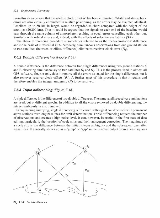
322 Engineering Surveying
From this it can be seen that the satellite clock offset δts has been eliminated. Orbital and atmosphericerrors are also virtually eliminated in relative positioning, as the errors may be assumed identical.Baselines up to 50 km in length would be regarded as short compared with the height of thesatellites (20 200 km). Thus it could be argued that the signals to each end of the baseline wouldpass through the same column of atmosphere, resulting in equal errors cancelling each other out.Similarly with orbital errors and, indeed, with the effects of selective availability (SA).
The above differencing procedure is sometimes referred to as the ‘between-station’ differenceand is the basis of differential GPS. Similarly, simultaneous observations from one ground stationto two satellites (between-satellites difference) eliminates receiver clock error (δtr).
7.6.2 Double differencing (Figure 7.14)
A double difference is the difference between two single differences using two ground stations Aand B observing simultaneously to two satellites S1 and S2. This is the process used in almost allGPS software, for, not only does it remove all the errors as stated for the single difference, but italso removes receiver clock offsets (δtr). A further asset of this procedure is that it retains andtherefore enables the integer ambiguity (N) to be resolved.
7.6.3 Triple differencing (Figure 7.15)
A triple difference is the difference of two double differences. The same satellite/receiver combinationsare used, but at different epochs. In addition to all the errors removed by double differencing, theinteger ambiguity is also removed.
In engineering surveying, single differencing is little used, although it could be used with permanentactive stations over long baselines for orbit determination. Triple differencing reduces the numberof observations and creates a high noise level. It can, however, be useful in the first state of dataediting, particularly the location of cycle slips and their subsequent correction. The magnitude ofa cycle slip is the difference between the initial integer ambiguity and the subsequent one, aftersignal loss. It generally shows up as a ‘jump’ or ‘gap’ in the residual output from a least squares
Fig. 7.14 Double difference
S1
S2
RA1
RB1
RA2
RB2
∆ A
∆B
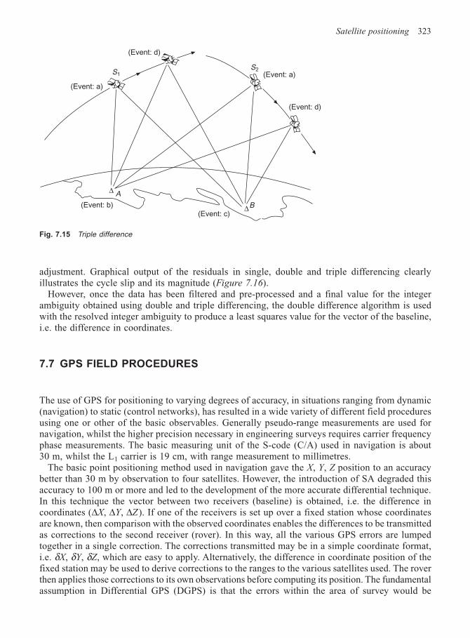
Satellite positioning 323
adjustment. Graphical output of the residuals in single, double and triple differencing clearlyillustrates the cycle slip and its magnitude (Figure 7.16).
However, once the data has been filtered and pre-processed and a final value for the integerambiguity obtained using double and triple differencing, the double difference algorithm is usedwith the resolved integer ambiguity to produce a least squares value for the vector of the baseline,i.e. the difference in coordinates.
7.7 GPS FIELD PROCEDURES
The use of GPS for positioning to varying degrees of accuracy, in situations ranging from dynamic(navigation) to static (control networks), has resulted in a wide variety of different field proceduresusing one or other of the basic observables. Generally pseudo-range measurements are used fornavigation, whilst the higher precision necessary in engineering surveys requires carrier frequencyphase measurements. The basic measuring unit of the S-code (C/A) used in navigation is about30 m, whilst the L1 carrier is 19 cm, with range measurement to millimetres.
The basic point positioning method used in navigation gave the X, Y, Z position to an accuracybetter than 30 m by observation to four satellites. However, the introduction of SA degraded thisaccuracy to 100 m or more and led to the development of the more accurate differential technique.In this technique the vector between two receivers (baseline) is obtained, i.e. the difference incoordinates (∆X, ∆Y, ∆Z). If one of the receivers is set up over a fixed station whose coordinatesare known, then comparison with the observed coordinates enables the differences to be transmittedas corrections to the second receiver (rover). In this way, all the various GPS errors are lumpedtogether in a single correction. The corrections transmitted may be in a simple coordinate format,i.e. δX, δY, δZ, which are easy to apply. Alternatively, the difference in coordinate position of thefixed station may be used to derive corrections to the ranges to the various satellites used. The roverthen applies those corrections to its own observations before computing its position. The fundamentalassumption in Differential GPS (DGPS) is that the errors within the area of survey would be
S1S2
(Event: a)
(Event: d)
(Event: d)
(Event: a)
A∆
B∆(Event: b)(Event: c)
Fig. 7.15 Triple difference
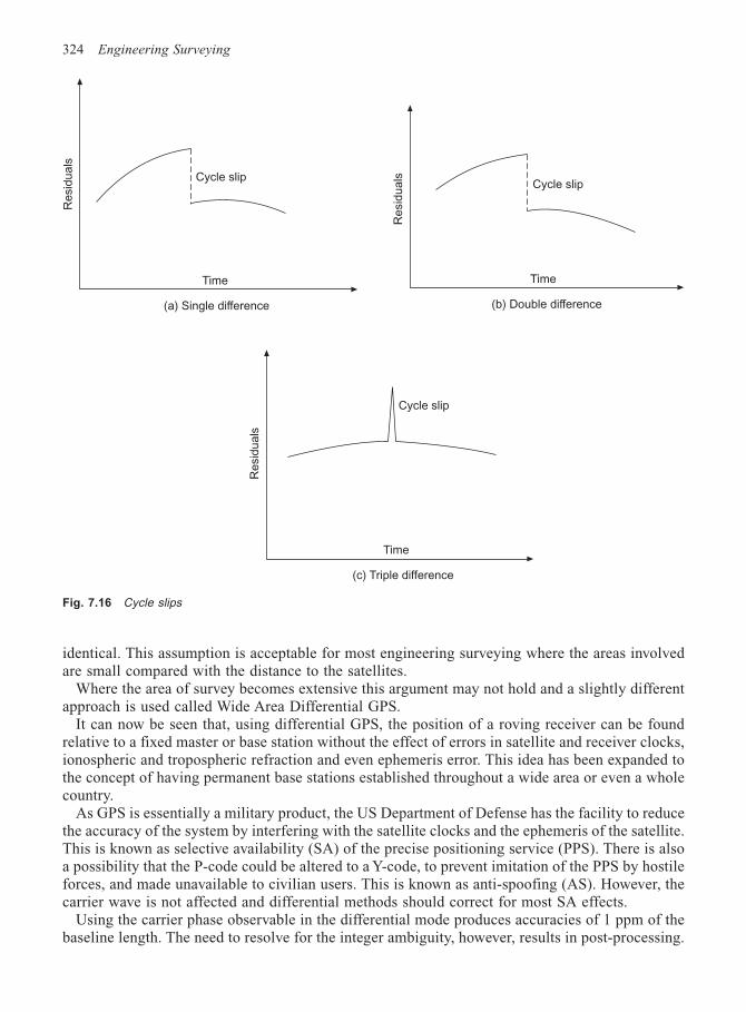
324 Engineering Surveying
identical. This assumption is acceptable for most engineering surveying where the areas involvedare small compared with the distance to the satellites.
Where the area of survey becomes extensive this argument may not hold and a slightly differentapproach is used called Wide Area Differential GPS.
It can now be seen that, using differential GPS, the position of a roving receiver can be foundrelative to a fixed master or base station without the effect of errors in satellite and receiver clocks,ionospheric and tropospheric refraction and even ephemeris error. This idea has been expanded tothe concept of having permanent base stations established throughout a wide area or even a wholecountry.
As GPS is essentially a military product, the US Department of Defense has the facility to reducethe accuracy of the system by interfering with the satellite clocks and the ephemeris of the satellite.This is known as selective availability (SA) of the precise positioning service (PPS). There is alsoa possibility that the P-code could be altered to a Y-code, to prevent imitation of the PPS by hostileforces, and made unavailable to civilian users. This is known as anti-spoofing (AS). However, thecarrier wave is not affected and differential methods should correct for most SA effects.
Using the carrier phase observable in the differential mode produces accuracies of 1 ppm of thebaseline length. The need to resolve for the integer ambiguity, however, results in post-processing.
Fig. 7.16 Cycle slips
Resid
uals
Cycle slip
Time
(a) Single difference
Resid
uals
Time
(c) Triple difference
Cycle slipR
esid
uals
Time
(b) Double difference
Cycle slip
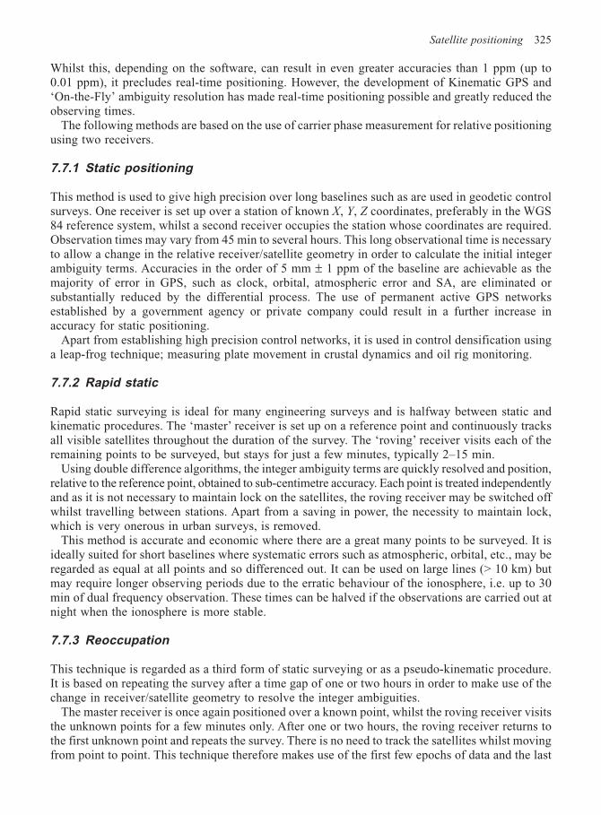
Satellite positioning 325
Whilst this, depending on the software, can result in even greater accuracies than 1 ppm (up to0.01 ppm), it precludes real-time positioning. However, the development of Kinematic GPS and‘On-the-Fly’ ambiguity resolution has made real-time positioning possible and greatly reduced theobserving times.
The following methods are based on the use of carrier phase measurement for relative positioningusing two receivers.
7.7.1 Static positioning
This method is used to give high precision over long baselines such as are used in geodetic controlsurveys. One receiver is set up over a station of known X, Y, Z coordinates, preferably in the WGS84 reference system, whilst a second receiver occupies the station whose coordinates are required.Observation times may vary from 45 min to several hours. This long observational time is necessaryto allow a change in the relative receiver/satellite geometry in order to calculate the initial integerambiguity terms. Accuracies in the order of 5 mm ± 1 ppm of the baseline are achievable as themajority of error in GPS, such as clock, orbital, atmospheric error and SA, are eliminated orsubstantially reduced by the differential process. The use of permanent active GPS networksestablished by a government agency or private company could result in a further increase inaccuracy for static positioning.
Apart from establishing high precision control networks, it is used in control densification usinga leap-frog technique; measuring plate movement in crustal dynamics and oil rig monitoring.
7.7.2 Rapid static
Rapid static surveying is ideal for many engineering surveys and is halfway between static andkinematic procedures. The ‘master’ receiver is set up on a reference point and continuously tracksall visible satellites throughout the duration of the survey. The ‘roving’ receiver visits each of theremaining points to be surveyed, but stays for just a few minutes, typically 2–15 min.
Using double difference algorithms, the integer ambiguity terms are quickly resolved and position,relative to the reference point, obtained to sub-centimetre accuracy. Each point is treated independentlyand as it is not necessary to maintain lock on the satellites, the roving receiver may be switched offwhilst travelling between stations. Apart from a saving in power, the necessity to maintain lock,which is very onerous in urban surveys, is removed.
This method is accurate and economic where there are a great many points to be surveyed. It isideally suited for short baselines where systematic errors such as atmospheric, orbital, etc., may beregarded as equal at all points and so differenced out. It can be used on large lines (> 10 km) butmay require longer observing periods due to the erratic behaviour of the ionosphere, i.e. up to 30min of dual frequency observation. These times can be halved if the observations are carried out atnight when the ionosphere is more stable.
7.7.3 Reoccupation
This technique is regarded as a third form of static surveying or as a pseudo-kinematic procedure.It is based on repeating the survey after a time gap of one or two hours in order to make use of thechange in receiver/satellite geometry to resolve the integer ambiguities.
The master receiver is once again positioned over a known point, whilst the roving receiver visitsthe unknown points for a few minutes only. After one or two hours, the roving receiver returns tothe first unknown point and repeats the survey. There is no need to track the satellites whilst movingfrom point to point. This technique therefore makes use of the first few epochs of data and the last
326 Engineering Surveying
few epochs which reflect the relative change in receiver/satellite geometry and so permit theambiguities and coordinate differences to be resolved.
Using dual frequency data gives values comparable with the rapid static technique. Due to themethod of changing the receiver/satellite geometry, it can be used with cheaper single-frequencyreceivers (although extended measuring times are recommended) and a poorer satellite constellation.
7.7.4 Kinematic positioning
The major problem with static GPS is the time required for an appreciable change in the satellite/receiver geometry so that the initial integer ambiguities can be resolved. However, if the integerambiguities could be resolved (and constrained in a least squares solution) prior to the survey, thena single epoch of data would be sufficient to obtain relative positioning to sub-centimetre accuracy.This concept is the basis of kinematic surveying. It can be seen from this that, if the integerambiguities are resolved initially and quickly, it will be necessary to keep lock on these satelliteswhilst moving the antenna.
7.7.4.1 Resolving the integer ambiguities
The process of resolving the integer ambiguities is called ‘initialization’ and may be done bysetting-up both receivers at each end of a baseline whose coordinates are accurately known. Insubsequent data processing, the coordinates are held fixed and the integers determined using onlya single epoch of data. These values are now held fixed throughout the duration of the survey andcoordinates estimated every epoch, provided there are no cycle slips.
The initial baseline may comprise points of known coordinates fixed from previous surveys, bystatic GPS just prior to the survey, or by transformation of points in a local coordinate system toWGS 84.
An alternative approach is called the ‘antenna swap’ method. An antenna is placed at each end ofa short base (5–10 m) and observations taken over a short period of time. The antennae areinterchanged, lock maintained, and observations continued. This results in a massive change in therelative receiver/satellite geometry and, consequently, rapid determination of the integers. Theantennae are returned to their original position prior to the surveys.
It should be realized that the whole survey will be invalidated if a cycle slip occurs. Thus,reconnaissance of the area is still of vital importance, otherwise re-initialization will be necessary.A further help in this matter is to observe to many more satellites than the minimum four required.
7.7.4.2 Traditional kinematic surveying
Assuming the ambiguities have been resolved, a master receiver is positioned over a referencepoint of known coordinates and the roving receiver commences its movement along the routerequired. As the movement is continuous, the observations take place at pre-set time intervals (lessthan 1 s). Lock must be maintained to at least four satellites, or re-established when lost.
In this technique it is the trajectory of the rover that is surveyed, hence linear detail such as roads,rivers, railways, etc., can be rapidly surveyed. Antennae can be fitted to the roofs of cars, which canbe driven at a slow speed along a road to obtain a three-dimensional profile.
7.7.4.3 Stop and go surveying
As the name implies, this kinematic technique is practically identical to the previous one, only inthis case the rover stops at the point of detail or position required (Figure 7.17). The accent is
Satellite positioning 327
therefore on individual points rather than a trajectory route, so data is collected only at those points.Lock must be maintained, though the data observed when moving is not necessarily recorded. Thismethod is ideal for engineering and topographic surveys.
7.7.4.4 Real-time kinematic (RTK)
The previous methods described all require post-processing of the results. However, RTK providesthe relative position to be determined instantaneously as the roving receiver occupies a position.The essential difference is the use of mobile data communication to transmit information from thereference point to the rover. Indeed, it is this procedure which imposes limitation due to the rangeover which the communication system can operate. Also, the effect of SA on the reference data mayhave changed by the time the data is communicated to the rover, resulting in small positional errors.With the removal of SA (1 May 2000) this is no longer a problem.
The system requires two receivers with only one positioned over a known point. The base stationtransmits code and carrier phase data to the rover. On-board data processing resolves ambiguitiesand solves for a change in coordinate differences between roving and reference receivers. Thistechnique can use single or dual frequency receivers. Loss of lock can be regained by remainingstatic for a short time over a point of known position.
The great advantage of this method for the engineer is that GPS can be used for setting-out onsite. With on-board application software and palm sized processor, the setting-out coordinates canbe keyed in, and graphical output indicates the direction and distance through which the pole-antenna must be moved. The point to be set-out is shown as a dot with a central cross representingthe antenna. When the two coincide, the point of the pole-antenna is at the setting-out position.
Throughout all the procedures described above, it can be seen that initialization or re-initializationcan only be done with the receiver static. This may be impossible in high accuracy hydrographicsurveys or road profiling in a moving vehicle. With this in mind, Leica Ltd of Heerbrugg, Switzerland,have developed, in conjunction with the Astronomical Institute of the University of Berne, a Fast
Fig. 7.17 The roving antenna
328 Engineering Surveying
Ambiguity Resolution Algorithm that enables ambiguity resolution whilst the receiver is moving.The acronym for the algorithm is FARA, used in a technique called Ambiguity Resolution On theFly (AROF). The technique requires L1 and L2 observations from at least five satellites with a goodGDOP. Depending on the level of ionospheric disturbances, the maximum range from the referenceto the rover for resolving ambiguities whilst the rover is in motion is 10 km, with an accuracy of10–20 mm. This relatively recent development will undoubtedly improve the process and role ofkinematic GPS surveying.
7.8 ERROR SOURCES
The final position of the survey station is influenced by:
(1) The error in the range measurement.(2) The satellite–receiver geometry.(3) The accuracy of the satellite ephemerides.(4) The effect of atmospheric refraction.(5) The processing software used.
It is necessary, therefore, to consider the various errors involved, many of which have already beenmentioned.
The majority of the error sources are eliminated or substantially reduced if relative positioningis used, rather than single-point positioning. This fact is common to many aspects of surveying. Forinstance, in simple levelling it is generally the difference in elevation between points that isrequired. Therefore, if we consider two points A and B whose heights HA and HB were obtained atthe same time, by the same observer, using the same equipment, the errors would be identical, i.e.δHA = δHB = δH, then:
∆HAB = (HA + δH) – (HB + δH)
with the result that δH is differenced out and difference in height is much more accurate than theindividual heights. Thus, if the absolute position of point A fixed by GPS was 10 m in error, thesame would apply to point B, so their relative position would be almost error free. Then, knowingthe actual coordinates of A would bring B to its correct relative position. This should be borne inmind when examining the error sources in GPS.
7.8.1 Receiver clock error
This error is a result of the receiver clock not being compatible and in the same time system as thesatellite clock. Range measurement is thus contaminated (pseudo-range). As the speed of light isapproximately 300 000 km s–1, then an error of 0.01 s results in a range error of about 3000 km.
As already shown, this error can be obtained using four satellites or cancelled using differencingsoftware.
7.8.2 Satellite clock error
Excessive temperature variations in space may result in the variation of the satellite clock from GPStime. Careful monitoring allows the amount of drift to be assessed and included in the broadcastmessage and therefore eliminated if the user is using the same data. Differential procedures eliminatethis error.
Satellite positioning 329
7.8.3 Satellite ephemeris error
Orbital data has already been discussed in detail with reference to Broadcast and Precise Ephemeris,and the effect of selective availability (SA). Nevertheless even excluding SA, which at present isno longer applied, errors are still present and influence baseline measurement in the ratio:
δb/b = δS/Rs
whereδb = error in baseline bδS = error in satellite orbitRs = satellite range
The specification for GPS is that orbital errors should not exceed 3.7 m, but this is not alwayspossible. Error in the range of 10–20 m may occur using the Broadcast Ephemeris. Thus, for anorbital error of 10 m on a 10 km baseline with a range of 20 000 km, the error in the baseline wouldbe 5 mm. This error is eliminated over moderate length baselines using differential techniques.
7.8.4 Atmospheric refraction
Atmospheric refraction error is usually dealt with in two parts, namely ionospheric and tropospheric.The effects are substantially reduced by DGPS compared with single-point positioning. Comparablefigures are:
Single point Differential
Ionosphere 15–20 m 2–3 m
Troposphere 3–4 m 1 m
If it was identical at each end of a small baseline, then the total effect would cancel using DGPS.The ionosphere is the region of the atmosphere from 50 to 1000 km in altitude in which
ultraviolet radiation has ionized a fraction of the gas molecules, thereby releasing free electrons.GPS signals are slowed down and refracted from their true path when passing through this medium.The effect on range measurement can vary from 5 to 150 m. As the ionospheric effect is frequencydependent, carrier wave measurement using the different L-band frequencies, i.e. L1 and L2, can beprocessed to eliminate the ionospheric correction. However, it is considered in some circles thatusing frequency doubling to achieve the elimination will not yield the accuracies required, due tothe resultant noise.
If the ionosphere was of constant thickness and electron density, then DGPS, as already mentioned,would eliminate its effect. This, unfortunately, is not so and residual effects remain. Positional andtemporal variation in the electron density makes complete elimination over longer baselines impossibleand may require complex software modelling.
The troposphere is even more variable than the ionosphere and is not frequency dependent.However, being closer to the ground, it can be easily measured and modelled. If conditions areidentical at each end of a baseline, then its effect is completely eliminated by DGPS. Over longerbaselines measurements can be taken and used in an appropriate model to reduce the error by asmuch as 95%.
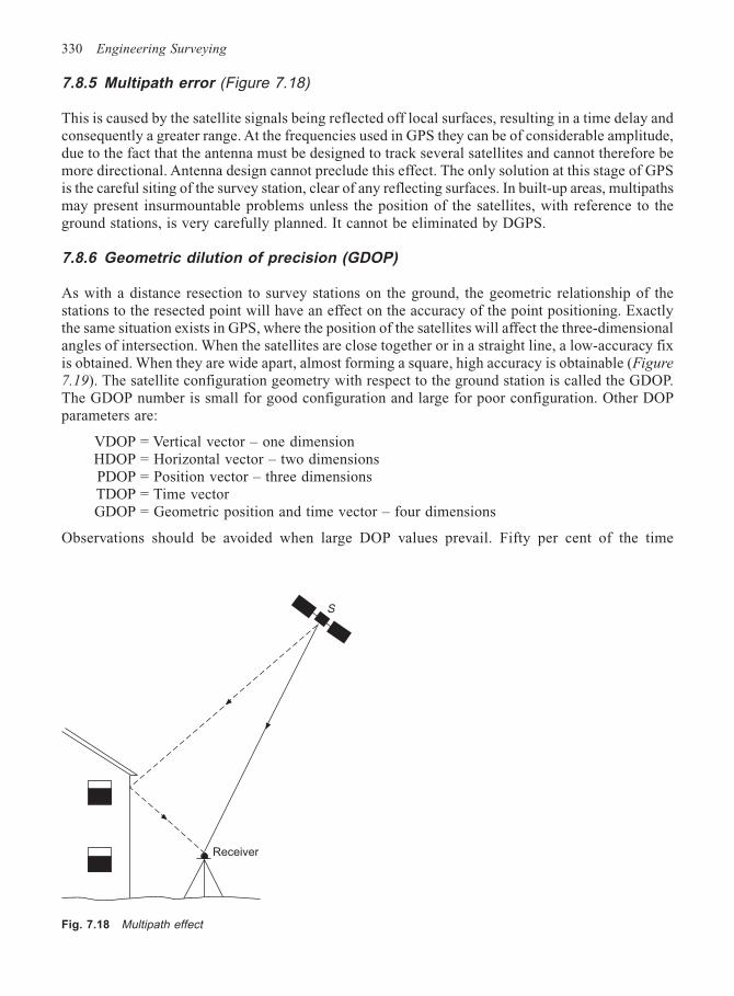
330 Engineering Surveying
7.8.5 Multipath error (Figure 7.18)
This is caused by the satellite signals being reflected off local surfaces, resulting in a time delay andconsequently a greater range. At the frequencies used in GPS they can be of considerable amplitude,due to the fact that the antenna must be designed to track several satellites and cannot therefore bemore directional. Antenna design cannot preclude this effect. The only solution at this stage of GPSis the careful siting of the survey station, clear of any reflecting surfaces. In built-up areas, multipathsmay present insurmountable problems unless the position of the satellites, with reference to theground stations, is very carefully planned. It cannot be eliminated by DGPS.
7.8.6 Geometric dilution of precision (GDOP)
As with a distance resection to survey stations on the ground, the geometric relationship of thestations to the resected point will have an effect on the accuracy of the point positioning. Exactlythe same situation exists in GPS, where the position of the satellites will affect the three-dimensionalangles of intersection. When the satellites are close together or in a straight line, a low-accuracy fixis obtained. When they are wide apart, almost forming a square, high accuracy is obtainable (Figure
7.19). The satellite configuration geometry with respect to the ground station is called the GDOP.The GDOP number is small for good configuration and large for poor configuration. Other DOPparameters are:
VDOP = Vertical vector – one dimensionHDOP = Horizontal vector – two dimensionsPDOP = Position vector – three dimensionsTDOP = Time vectorGDOP = Geometric position and time vector – four dimensions
Observations should be avoided when large DOP values prevail. Fifty per cent of the time
Fig. 7.18 Multipath effect
Receiver
S
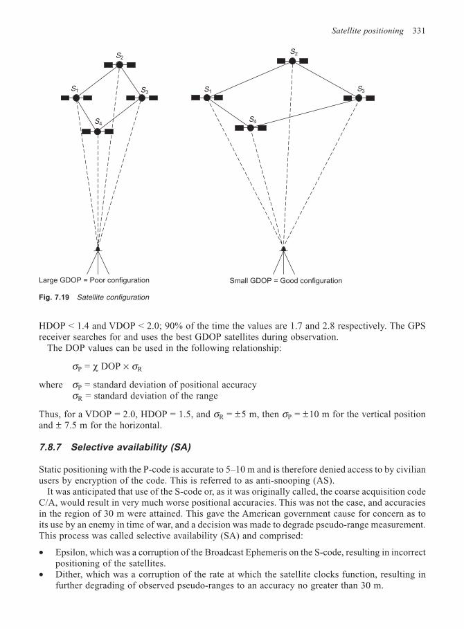
Satellite positioning 331
HDOP < 1.4 and VDOP < 2.0; 90% of the time the values are 1.7 and 2.8 respectively. The GPSreceiver searches for and uses the best GDOP satellites during observation.
The DOP values can be used in the following relationship:
σP = χ DOP × σR
where σP = standard deviation of positional accuracyσR = standard deviation of the range
Thus, for a VDOP = 2.0, HDOP = 1.5, and σR = ±5 m, then σP = ±10 m for the vertical positionand ± 7.5 m for the horizontal.
7.8.7 Selective availability (SA)
Static positioning with the P-code is accurate to 5–10 m and is therefore denied access to by civilianusers by encryption of the code. This is referred to as anti-snooping (AS).
It was anticipated that use of the S-code or, as it was originally called, the coarse acquisition codeC/A, would result in very much worse positional accuracies. This was not the case, and accuraciesin the region of 30 m were attained. This gave the American government cause for concern as toits use by an enemy in time of war, and a decision was made to degrade pseudo-range measurement.This process was called selective availability (SA) and comprised:
• Epsilon, which was a corruption of the Broadcast Ephemeris on the S-code, resulting in incorrectpositioning of the satellites.
• Dither, which was a corruption of the rate at which the satellite clocks function, resulting infurther degrading of observed pseudo-ranges to an accuracy no greater than 30 m.
S4
S2
S3S1 S1
S2
S3
S4
Large GDOP = Poor configuration Small GDOP = Good configuration
Fig. 7.19 Satellite configuration
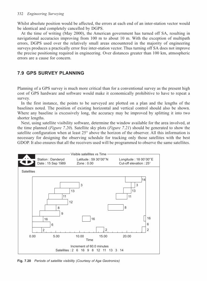
332 Engineering Surveying
Whilst absolute position would be affected, the errors at each end of an inter-station vector wouldbe identical and completely cancelled by DGPS.
At the time of writing (May 2000), the American government has turned off SA, resulting innavigational accuracies improving from 100 m to about 10 m. With the exception of multipatherrors, DGPS used over the relatively small areas encountered in the majority of engineeringsurveys produces a practically error free inter-station vector. Thus turning off SA does not improvethe precise positioning required in engineering. Over distances greater than 100 km, atmosphericerrors are a cause for concern.
7.9 GPS SURVEY PLANNING
Planning of a GPS survey is much more critical than for a conventional survey as the present highcost of GPS hardware and software would make it economically prohibitive to have to repeat asurvey.
In the first instance, the points to be surveyed are plotted on a plan and the lengths of thebaselines noted. The position of existing horizontal and vertical control should also be shown.Where any baseline is excessively long, the accuracy may be improved by splitting it into twoshorter lengths.
Next, using satellite visibility software, determine the window available for the area involved, atthe time planned (Figure 7.20). Satellite sky plots (Figure 7.21) should be generated to show thesatellite configuration when at least 25° above the horizon of the observer. All this information isnecessary for designing the observing schedule for tracking only those satellites with the bestGDOP. It also ensures that all the receivers used will be programmed to observe the same satellites.
Visible satellites vs Time
Station : Danderyd Latitude : 59 30′00″N Longitude : 18 00′00″E
Date : 15 Sep 1989 Zone : 0.00 Cut-off elevation : 25°
3
13
11
12
8
9
16
6
2
16
2
8
11
13
3
14
0.00 5.00 10.00 15.00 20.00Time
Increment of 60.0 minutes
Satellites : 2 6 16 9 8 12 11 13 3 14
Satellites
6
2
16
Fig. 7.20 Periods of satellite visibility (Courtesy of Aga Geotronics)
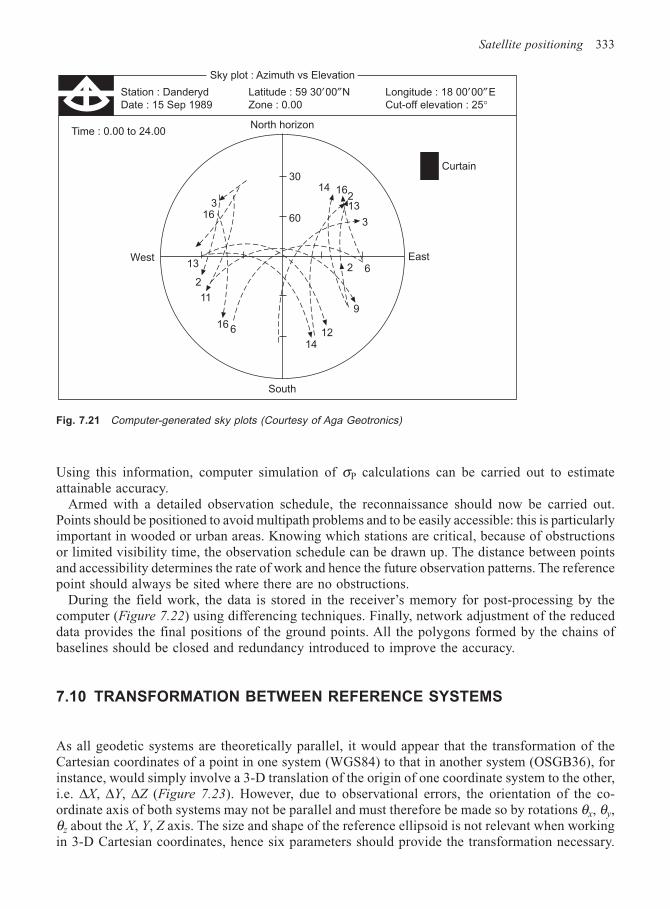
Satellite positioning 333
Using this information, computer simulation of σP calculations can be carried out to estimateattainable accuracy.
Armed with a detailed observation schedule, the reconnaissance should now be carried out.Points should be positioned to avoid multipath problems and to be easily accessible: this is particularlyimportant in wooded or urban areas. Knowing which stations are critical, because of obstructionsor limited visibility time, the observation schedule can be drawn up. The distance between pointsand accessibility determines the rate of work and hence the future observation patterns. The referencepoint should always be sited where there are no obstructions.
During the field work, the data is stored in the receiver’s memory for post-processing by thecomputer (Figure 7.22) using differencing techniques. Finally, network adjustment of the reduceddata provides the final positions of the ground points. All the polygons formed by the chains ofbaselines should be closed and redundancy introduced to improve the accuracy.
7.10 TRANSFORMATION BETWEEN REFERENCE SYSTEMS
As all geodetic systems are theoretically parallel, it would appear that the transformation of theCartesian coordinates of a point in one system (WGS84) to that in another system (OSGB36), forinstance, would simply involve a 3-D translation of the origin of one coordinate system to the other,i.e. ∆X, ∆Y, ∆Z (Figure 7.23). However, due to observational errors, the orientation of the co-ordinate axis of both systems may not be parallel and must therefore be made so by rotations θx, θy,θz about the X, Y, Z axis. The size and shape of the reference ellipsoid is not relevant when workingin 3-D Cartesian coordinates, hence six parameters should provide the transformation necessary.
Fig. 7.21 Computer-generated sky plots (Courtesy of Aga Geotronics)
Sky plot : Azimuth vs Elevation
Station : Danderyd Latitude : 59 30′00″N Longitude : 18 00′00″E
Date : 15 Sep 1989 Zone : 0.00 Cut-off elevation : 25°
Time : 0.00 to 24.00North horizon
Curtain
West
South
316
13
2
11
16 6
1412
9
2 6
3
132
161430
60
East
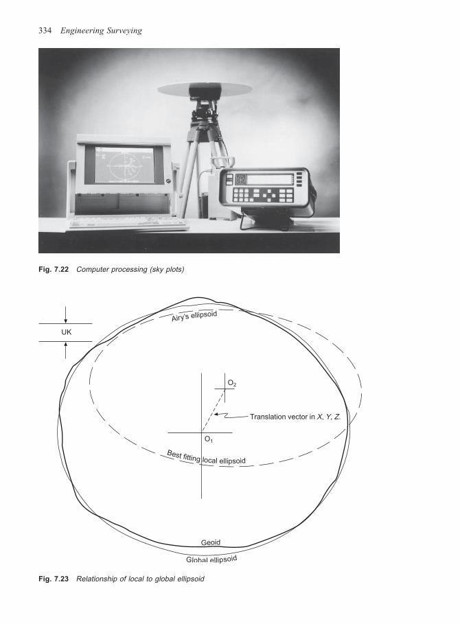
334 Engineering Surveying
Fig. 7.22 Computer processing (sky plots)
Fig. 7.23 Relationship of local to global ellipsoid
Geoid
Global ellipsoid
Best fitting local ellipsoid
Airy’s ellipsoid
UK
O2
O1
Translation vector in X, Y, Z.
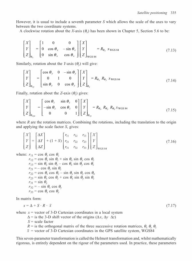
Satellite positioning 335
However, it is usual to include a seventh parameter S which allows the scale of the axes to varybetween the two coordinate systems.
A clockwise rotation about the X-axis (θx) has been shown in Chapter 5, Section 5.6 to be:
X
Y
Z
X
Y
Z
R x
x
xx
x
x
x
θ
θθθ
θθ
=
1
0
0
0
cos
sin
0
– sin
cos
=
WGS 84
WGS 84 (7.13)
Similarly, rotation about the Y-axis (θy) will give:
X
Y
Z
X
Y
Z
R R x
xy x
x y
y
y
y
y
θ θ
θ θ
θ
θ
θ
θ =
cos
0
sin
0 – sin
cos
= WGS 841
0
0(7.14)
Finally, rotation about the Z-axis (θz) gives:
X
Y
Z
X
Y
Z
R R R x
xyz xy
x y z
z
z
z
z
θ θ
θ θ θ
θθ
θθ =
cos
– sin
sin
cos = WGS 84
0 0
0
0
1(7.15)
where R are the rotation matrices. Combining the rotations, including the translation to the originand applying the scale factor S, gives:
X
Y
Z
X
Y
Z
S
r
r
r
r
r
r
r
r
r
X
Y
Z
= + (1 + )
11
21
31
12
22
32
13
23
33 WGS 84
∆∆∆
(7.16)
where: r11 = cos θy cos θz
r12 = cos θx sin θz + sin θx sin θy cos θz
r13 = sin θx sin θz – cos θx sin θy cos θz
r21 = – cos θy sin θz
r22 = cos θx cos θz – sin θx sin θy cos θz
r23 = sin θx cos θz + cos θx sin θy sin θz
r31 = sin θy
r32 = – sin θx cos θy
r33 = cos θx cos θy
In matrix form:
x = ∆ + S · R · x (7.17)
where x = vector of 3-D Cartesian coordinates in a local system∆ = is the 3-D shift vector of the origins (∆ x, ∆y ∆z)S = scale factorR = is the orthogonal matrix of the three successive rotation matrices, θx θy θz
x = vector of 3-D Cartesian coordinates in the GPS satellite system, WGS84
This seven-parameter transformation is called the Helmert transformation and, whilst mathematicallyrigorous, is entirely dependent on the rigour of the parameters used. In practice, these parameters
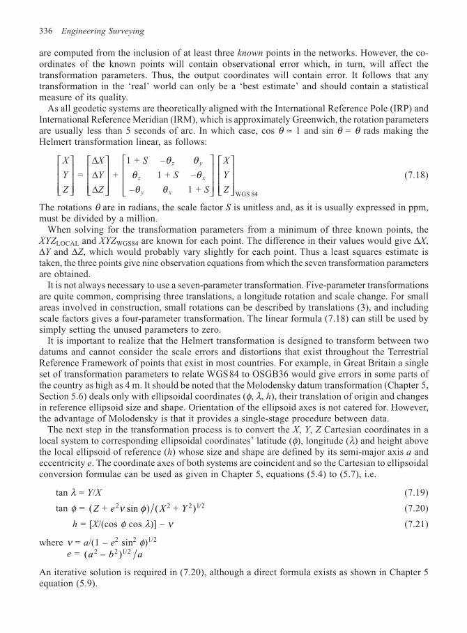
336 Engineering Surveying
are computed from the inclusion of at least three known points in the networks. However, the co-ordinates of the known points will contain observational error which, in turn, will affect thetransformation parameters. Thus, the output coordinates will contain error. It follows that anytransformation in the ‘real’ world can only be a ‘best estimate’ and should contain a statisticalmeasure of its quality.
As all geodetic systems are theoretically aligned with the International Reference Pole (IRP) andInternational Reference Meridian (IRM), which is approximately Greenwich, the rotation parametersare usually less than 5 seconds of arc. In which case, cos θ ≈ 1 and sin θ = θ rads making theHelmert transformation linear, as follows:
X
Y
Z
X
Y
Z
S
S
S
X
Y
Z
z
y
z
x
y
x
= +
1 +
–
–
1 + –
1 + WGS 84
∆∆∆
θθ
θ
θ
θθ (7.18)
The rotations θ are in radians, the scale factor S is unitless and, as it is usually expressed in ppm,must be divided by a million.
When solving for the transformation parameters from a minimum of three known points, theXYZLOCAL and XYZWGS84 are known for each point. The difference in their values would give ∆X,∆Y and ∆Z, which would probably vary slightly for each point. Thus a least squares estimate istaken, the three points give nine observation equations from which the seven transformation parametersare obtained.
It is not always necessary to use a seven-parameter transformation. Five-parameter transformationsare quite common, comprising three translations, a longitude rotation and scale change. For smallareas involved in construction, small rotations can be described by translations (3), and includingscale factors gives a four-parameter transformation. The linear formula (7.18) can still be used bysimply setting the unused parameters to zero.
It is important to realize that the Helmert transformation is designed to transform between twodatums and cannot consider the scale errors and distortions that exist throughout the TerrestrialReference Framework of points that exist in most countries. For example, in Great Britain a singleset of transformation parameters to relate WGS84 to OSGB36 would give errors in some parts ofthe country as high as 4 m. It should be noted that the Molodensky datum transformation (Chapter 5,Section 5.6) deals only with ellipsoidal coordinates (φ, λ, h), their translation of origin and changesin reference ellipsoid size and shape. Orientation of the ellipsoid axes is not catered for. However,the advantage of Molodensky is that it provides a single-stage procedure between data.
The next step in the transformation process is to convert the X, Y, Z Cartesian coordinates in alocal system to corresponding ellipsoidal coordinates’ latitude (φ), longitude (λ) and height abovethe local ellipsoid of reference (h) whose size and shape are defined by its semi-major axis a andeccentricity e. The coordinate axes of both systems are coincident and so the Cartesian to ellipsoidalconversion formulae can be used as given in Chapter 5, equations (5.4) to (5.7), i.e.
tan λ = Y/X (7.19)
tan φ = ( + sin ) ( + )2 2 2 1/2Z e X Yν φ (7.20)
h = [X/(cos φ cos λ)] – ν (7.21)
where ν = a/(1 – e2 sin2 φ)1/2
e = ( – )2 2 1/2a b a
An iterative solution is required in (7.20), although a direct formula exists as shown in Chapter 5equation (5.9).
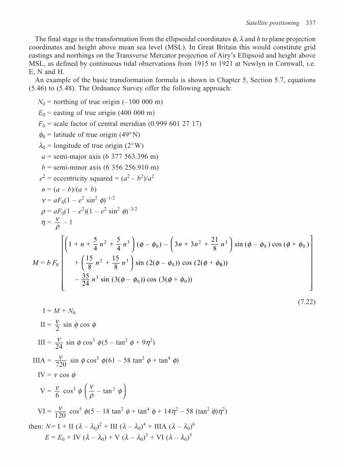
Satellite positioning 337
The final stage is the transformation from the ellipsoidal coordinates φ, λ and h to plane projectioncoordinates and height above mean sea level (MSL). In Great Britain this would constitute grideastings and northings on the Transverse Mercator projection of Airy’s Ellipsoid and height aboveMSL, as defined by continuous tidal observations from 1915 to 1921 at Newlyn in Cornwall, i.e.E, N and H.
An example of the basic transformation formula is shown in Chapter 5, Section 5.7, equations(5.46) to (5.48). The Ordnance Survey offer the following approach:
N0 = northing of true origin (–100 000 m)
E0 = easting of true origin (400 000 m)
F0 = scale factor of central meridian (0.999 601 27 17)
φ0 = latitude of true origin (49°N)
λ0 = longitude of true origin (2°W)
a = semi-major axis (6 377 563.396 m)
b = semi-minor axis (6 356 256.910 m)
e2 = eccentricity squared = (a2 – b2)/a2
n = (a – b)/(a + b)
ν = aF0(1 – e2 sin2 φ)–1/2
ρ = aF0(1 – e2)(1 – e2 sin2 φ)–3/2
η = νρ – 1
M b F
n n n n n n
n n =
1 + + 54
+ 54
( – ) – 3 + 3 + 218
sin ( – ) cos ( + )
+ 158
+ 158
sin 2( – cos 2( + 0
2 30
2 30 0
2 30
φ φ φ φ φ φ
φ φ φ φ( )) ( 00
30 0
))
– 3524
sin 3( – )) cos 3( + ))n ( (φ φ φ φ
(7.22)I = M + N0
II = ν2
sin φ cos φ
III = ν24
sin φ cos3 φ (5 – tan2 φ + 9η2)
IIIA = ν720
sin φ cos5 φ(61 – 58 tan2 φ + tan4 φ)
IV = ν cos φ
V = ν6
cos3 φνρ φ – tan 2
VI = ν120
cos5 φ(5 – 18 tan2 φ + tan4 φ + 14η2 – 58 (tan2 φ)η2)
then: N = I + II (λ – λ0)2 + III (λ – λ0)
4 + IIIA (λ – λ0)6
E = E0 + IV (λ – λ0) + V (λ – λ0)3 + VI (λ – λ0)
5
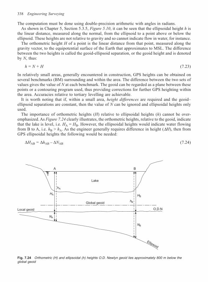
338 Engineering Surveying
The computation must be done using double-precision arithmetic with angles in radians.As shown in Chapter 5, Section 5.3.5, Figure 5.10, it can be seen that the ellipsoidal height h is
the linear distance, measured along the normal, from the ellipsoid to a point above or below theellipsoid. These heights are not relative to gravity and so cannot indicate flow in water, for instance.
The orthometric height H of a point is the linear distance from that point, measured along thegravity vector, to the equipotential surface of the Earth that approximates to MSL. The differencebetween the two heights is called the geoid-ellipsoid separation, or the geoid height and is denotedby N, thus:
h = N + H (7.23)
In relatively small areas, generally encountered in construction, GPS heights can be obtained onseveral benchmarks (BM) surrounding and within the area. The difference between the two sets ofvalues gives the value of N at each benchmark. The geoid can be regarded as a plane between thesepoints or a contouring program used, thus providing corrections for further GPS heighting withinthe area. Accuracies relative to tertiary levelling are achievable.
It is worth noting that if, within a small area, height differences are required and the geoid–ellipsoid separations are constant, then the value of N can be ignored and ellipsoidal heights onlyused.
The importance of orthometric heights (H) relative to ellipsoidal heights (h) cannot be over-emphasized. As Figure 7.24 clearly illustrates, the orthometric heights, relative to the geoid, indicatethat the lake is level, i.e. HA = HB. However, the ellipsoidal heights would indicate water flowingfrom B to A, i.e. hB > hA. As the engineer generally requires difference in height (∆H), then fromGPS ellipsoidal heights the following would be needed:
∆HAB = ∆hAB – ∆NAB (7.24)
Ellipsoid
A
hA
Local geoid
NA
NB
HB
hBGlobal geoid
Lake
HA
B
O.D.N
Fig. 7.24 Orthometric (H) and ellipsoidal (h) heights O.D. Newlyn geoid lies approximately 800 m below theglobal geoid
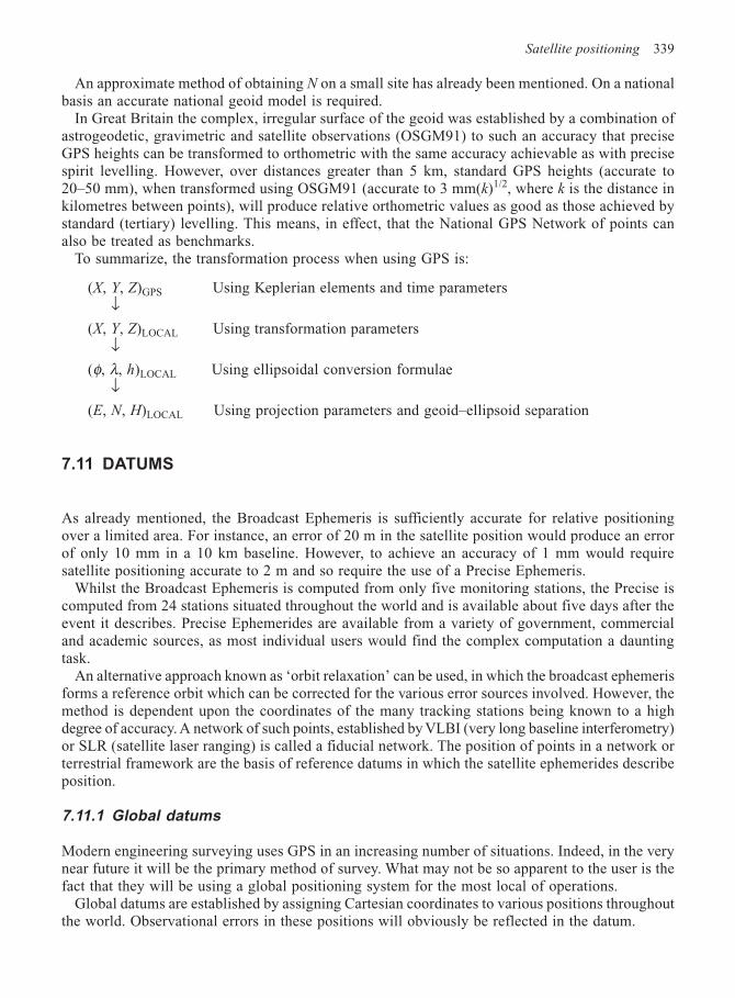
Satellite positioning 339
An approximate method of obtaining N on a small site has already been mentioned. On a nationalbasis an accurate national geoid model is required.
In Great Britain the complex, irregular surface of the geoid was established by a combination ofastrogeodetic, gravimetric and satellite observations (OSGM91) to such an accuracy that preciseGPS heights can be transformed to orthometric with the same accuracy achievable as with precisespirit levelling. However, over distances greater than 5 km, standard GPS heights (accurate to20–50 mm), when transformed using OSGM91 (accurate to 3 mm(k)1/2, where k is the distance inkilometres between points), will produce relative orthometric values as good as those achieved bystandard (tertiary) levelling. This means, in effect, that the National GPS Network of points canalso be treated as benchmarks.
To summarize, the transformation process when using GPS is:
(X, Y, Z)GPS Using Keplerian elements and time parameters↓
(X, Y, Z)LOCAL Using transformation parameters↓
(φ, λ, h)LOCAL Using ellipsoidal conversion formulae↓
(E, N, H)LOCAL Using projection parameters and geoid–ellipsoid separation
7.11 DATUMS
As already mentioned, the Broadcast Ephemeris is sufficiently accurate for relative positioningover a limited area. For instance, an error of 20 m in the satellite position would produce an errorof only 10 mm in a 10 km baseline. However, to achieve an accuracy of 1 mm would requiresatellite positioning accurate to 2 m and so require the use of a Precise Ephemeris.
Whilst the Broadcast Ephemeris is computed from only five monitoring stations, the Precise iscomputed from 24 stations situated throughout the world and is available about five days after theevent it describes. Precise Ephemerides are available from a variety of government, commercialand academic sources, as most individual users would find the complex computation a dauntingtask.
An alternative approach known as ‘orbit relaxation’ can be used, in which the broadcast ephemerisforms a reference orbit which can be corrected for the various error sources involved. However, themethod is dependent upon the coordinates of the many tracking stations being known to a highdegree of accuracy. A network of such points, established by VLBI (very long baseline interferometry)or SLR (satellite laser ranging) is called a fiducial network. The position of points in a network orterrestrial framework are the basis of reference datums in which the satellite ephemerides describeposition.
7.11.1 Global datums
Modern engineering surveying uses GPS in an increasing number of situations. Indeed, in the verynear future it will be the primary method of survey. What may not be so apparent to the user is thefact that they will be using a global positioning system for the most local of operations.
Global datums are established by assigning Cartesian coordinates to various positions throughoutthe world. Observational errors in these positions will obviously be reflected in the datum.
340 Engineering Surveying
The WGS84 was established from the coordinate position of about 1600 points around the globe,fixed largely by TRANSIT satellite observations. At the present time its origin is geocentric (i.e. thecentre of mass of the whole Earth) and its axes virtually coincide with the International ReferencePole and International Reference Meridian. Designed to best fit the global geoid as a whole meansit does not fit many of the local ellipsoids in use by many countries. In Great Britain, for instance,it lies about 50 m below the geoid and slopes from east to west, resulting in the geoid–ellipsoidseparation being 10 m greater in the west than in the east.
It is also worth noting that the axes are stationary with respect to the average motions of thisdynamically changing Earth. For instance, tectonic plate movement causes continents to moverelative to each other by about 10 cm per year. Local movements caused by tides, pressure weathersystems, etc., can result in movement of several centimetres. The result is that the WGS84 datumappears to move relative to the various countries. In Great Britain, the latitudes and longitudes arechanging at a rate of 2.5 cm per year in a north-easterly direction. In time, this effect will benoticeable in large-scale mapping.
It can be seen from the above statements that constant monitoring of the WGS84 system isnecessary to maintain its validity. In 1997, 13 tracking stations situated throughout the globe hadtheir positional accuracies redefined to an accuracy better than 5 cm, thereby bringing the origin,orientation and scale of the system to within the accuracy of its theoretical specification. Untilrecently this accuracy was not available to the civilian user due to the application of selectiveavailability (SA). Thus, using a single receiver, absolute positional accuracy was no better than100 m. However, on 1 May 2000 the US government removed SA, which will no doubt have asignificant effect on some areas of GPS use.
Another global datum almost identical to the WGS84 Reference System is the InternationalTerrestrial Reference Frame (ITRF) produced by the International Earth Rotation Service (IERS)in Paris, France. The system was produced from the positional coordinates of over 500 stationsthroughout the world, fixed by a variety of geodetic space positioning techniques such as satellitelaser ranging (SLR), very long baseline interferometry (VLBI), lunar laser ranging (LLR), Dopplerranging integrated on satellite (DORIS) and GPS. Combined with the constant monitoring of Earthrotation, crustal plate movement and polar motion, the IERS have established a very preciseterrestrial reference frame, the latest version of which is the ITRF96. This TRF has been establishedby the civil GPS community, not the US military. It comprises a list of Cartesian coordinates(X, Y, Z) as of the date 1996, with the change in position (dX, dY, dZ) in metres per year for eachstation. The ITRF96 is available as a SINEX format text file from the IERS internet web site. TheITRF is the most accurate global TRF and for all purposes is identical to the WGS84 TRF.
The ITRF96 is important to GPS users in that it generates a precise ephemeris and stations thatcan be used in a fiducial network, all of which is supplied free on the internet by the InternationalGPS Service (IGS). The precise ephemeris, used in conjunction with any of the 200 IGS trackingstations and the dual-frequency GPS data from those stations, enables single receiver positionalaccuracy to a few millimetres.
7.11.2 Local datums
Historically, the majority of local datums were made accessible to the user by means of a TRF ofpoints coordinated by triangulation. These points gave horizontal position only and the triangulationpillars were situated on hilltops. A vertical TRF of benchmarks, established by spirit levelling,required low-lying, easily traversed routes. Hence, there were two entirely different systems.
A TRF established by GPS gives a single three-dimensional system of easily accessible pointswhich can be transformed to give more accurate position in the local system. As WGS84 iscontinually changing position due to tectonic movement, the local system must be based on a
Satellite positioning 341
certain time in WGS84. Thus, we have local datums like the North American Datum 1983 and theEuropean Terrestrial Reference System 1989 (ETRS89). In 1989 a high precision European Three-Dimensional Reference Frame (EUREF) was established by GPS observations on 93 stationsthroughout Europe (ETRF89). The datum used (ETRS89) was consistent with WGS84/1TRF96and extends into Great Britain, where it forms the datum for the Ordnance Survey National GPSNetwork.
The OS system will be briefly described here as it illustrates a representative model that will beof benefit to the everyday user of GPS. At the present time (May 2000), the National GPS networkTRF comprises two types of GPS station consisting of:
• Active layer: this is a primary network of 30 continuously observing, permanent GPS receiverswhose precise coordinates are known. Using a single dual frequency receiver and data downloadedfrom these stations, which are located within 100 km of any point in Britain, precise positioningcan be achieved to accuracies of 10 mm.
• Passive layer: this is a secondary network of about 900 easily accessible stations at a densityof 20–35 km. These stations can be used in kinematic form using two receivers to obtain real-time positioning to accuracies of 50–100 mm.
The coordinates obtained by the user are ETRS89 and can be transformed to and from WGS84/1TRF96 by a six-parameter transformation published by IERS on their internet site. Of moreinterest to local users would be the transformation from ETRS89 to OSGB36, which is the basicmapping system for the country. The establishment of the OSGB36 TRF by triangulation hasresulted in variable scale changes throughout the framework, which renders the use of a singleHelmert transformation unacceptable. The OS have therefore developed a ‘rubber-sheet’ transformationcalled OSTN97, which copes not only with a change of datum but also with the scale distortionsand removed the need to compute local transformation parameters by the inclusion of at least threeknown points within the survey. As OSTN97 works in National Grid eastings and northings, theETRS89 coordinates must be converted to National Grid coordinates using the map projectionformulae already illustrated, but on the global ellipsoid GRS80 rather than the Airy ellipsoid.Transformation back to Airy can then be done if necessary.
Using the National GPS Network in static, post-processing mode, can produce horizontal accuracyof a few millimetres. The same mode of operation using ‘active’ stations and one hour of datawould give accuracies of about 20 mm. Heighting accuracies would typically be twice these values.However, it must be understood that these accuracies apply to position computed in ETRS89 datumon a suitable projection. Transformation to the National Grid using OSTN97 would degrade theabove accuracy, and positional errors in the region of 200 mm have been quoted. The final accuracywould, nevertheless, be greater than the OS base-map, where errors of 500 mm in the position ofdetail at the 1/1250 scale are the norm. Thus, transformation to the National Grid should only beused when integration to the OS base-map is required.
Thus, from the practical user’s point of view, the National GPS Network can be used to establishfurther control, which can then be transformed to National Grid eastings and northings and heightsabove Newlyn MSL using the OS National Grid Transformation (OSTN97) and the OS NationalGeoid Model (OSGM91) respectively, supplied free on the OS web site.
As a measure of the high regard with which this procedure is held, work is in hand to improveand thereby replace both OSTN97 and OSGM91.
The evolution of GPS technology and future trends have been illustrated by a description of theOS National GPS Network and its application. Other countries are also establishing continuouslyoperating GPS reference station networks. For instance, in Japan a network of about 1000 stationsare deployed throughout the country with a spacing of about 20–30 km (GEONET).
Many innovative techniques have been used in GPS surveying to resolve the problem of ambiguity
342 Engineering Surveying
resolution (AR), reduce observation time and increase accuracy. They involve the development ofsophisticated AR algorithms to reduce the time for static surveying, or carry out ‘on-the-fly’ carrierphase AR whilst the antenna is continually moving. Other techniques such as ‘stop and go’ and‘rapid static’ techniques were also developed. They all, however, require the use of at least two,multi-channel, dual frequency receivers, and there are limitations on the length of baseline observed(< 15 km). However, downloading the data from only one of the ‘active stations’ in the abovenetwork results in the following benefit:
1. For many engineering surveying operations the use of only one single-frequency receiver,thereby reducing costs. However this may result in antenna phase centre variation due to theuse of different autenuae.
2. Baseline lengths greatly extended for rapid static and kinematic procedures.3. ‘On-the-fly’ techniques can be used with ambiguity resolution algorithms from a single epoch.
For many users the use of continuously operating reference stations is still in its early stages(May, 2000) and many problems may still need to be resolved, particularly for real-time users.There may be communication problems if the distances to the active network stations are too great.This may require the establishment of smaller, higher density networks within the area of use,supplied by professional organizations and offered on a ‘fee-for-service’ basis. Although the mobilephone may resolve any such problems. Other problems may result from the use of existing, non-compatible software and turnkey systems, requiring a concerted effort on the part of all involved touse all available technology to produce a thoroughly integrated, user friendly service.
7.12 OTHER SATELLITE SYSTEMS
There are many systems available, mostly based on a small number of satellites in a geosynchronousorbit and used for communications as well as positioning. Such systems are Starfix, Geostar,Locstar, etc., which, due to their geosychronous orbits, do not provide a good geometric configurationwith the receiver and cannot compete with GPS.
One system, however, whose planned constellation was similar to GPS, is the Russian GLONASS,GLObal NAvigation Satellite System. The constellation comprises 24 satellites, with eight in eachof three orbital planes inclined at 64.8° and orbiting at a height of 19 100 km. The satellite signalsconsist of two L-band carrier frequencies at 1250 MHZ (L2) and 1600 MHZ (L1). A precise codewith a bandwidth of 5.11 MHZ is on both L1 and L2, whilst the coarser code of 0.511 MHz is onL1 only. Thus, the satellites permit pseudo-range and carrier phase measurement.
Two differences that exist between GPS and GLONASS are that SA is not possible on GLONASSand the coordinate datum is different, i.e. SGS-85 datum compared with WGS-84. However, boththe UK and Russia are keen to make both systems compatible with each other, although doubts arecast on the ability of Russia, at the present time, to maintain and progress their system as there hasbeen a gradual decline in the number of satellites available. Using a receiver capable of utilizingboth systems would offer the user twice the number of satellites, increased accuracy, savings intime and an independent check on each system.
Whilst the future of GPS looks very bright compared with GLONASS, the European communityare also considering a Global Navigation Satellite System (GNSS) as outlined in a Commissioncommunication (February 1999) entitled ‘GALILEO’.
The American government wish to promote GPS as a global standard within the overridingconsideration of national security requirements.
At the present time (May 2000) SA has been removed, which must be of great benefit to theStandard Positioning Service (SPS) user, and there is a declared intention to continue to provide
Satellite positioning 343
SPS free on a world-wide basis. The US is prepared to co-operate with any government, as evidencedwith GLONASS, to ensure the needs of the civil, commercial and scientific community are met,along with international security. A GPS Executive Board has been established to manage theservices offered by GPS and, at the present time, have evidenced goodwill by giving all users accessto the L2 carrier and agreeing to provide a fully coded navigation signal on that frequency, i.e. aC/A code. There is also a proposal to provide a third civil signal to be called L5, with a carrierfrequency similar to the L2 signal, and studies are in hand to discuss the possibility of civil andmilitary users sharing common frequencies without impeding security measures. A greater numberof satellites are planned, with new operational systems which allow the satellite to maintain its ownephemeris and clock data by ranging to and communicating with other satellites.
In spite of all this obvious goodwill and intention on behalf of the US, the GPS system isfundamentally a military system in complete control of the Department of Defense at times ofnational security. This reason, combined with commercial concerns and the possibility of futureuser charges, has caused the European Commission to consider their own GNSS. Basically, thereare two possibilities. The first is a system of 21 satellites used in conjunction with GPS to meetEuropean user requirements. The second is a system of 36 satellites which would not be in conjunctionwith GPS. Whatever decisions are arrived at, the use of Global Navigation Satellite Systems seemsassured.
7.13 APPLICATIONS
The previous pages have already indicated the basic application of GPS in engineering surveying– that is: the establishment of control surveys, topographic surveys and setting-out on site. Indeed,any three-dimensional spatial data normally captured using conventional surveying techniqueswith a total station can be done by GPS, even during the night, provided sufficient satellites arevisible.
On a national scale, horizontal and, to a certain extent, vertical control, used for mapping purposesand established by classical triangulation with all its built-in scale error, are being replaced bythree-dimensional GPS networks. In relation to Great Britain and the Ordnance Survey, this hasbeen dealt with in previous pages. The great advantage of this to the engineering surveyor is that,when using GPS on a local level, there is no requirement for coordinate transformation and theresultant plans are more consistent. Also, in mapping at a local level there is, in effect, no need toestablish a control network as it already exists in the form of the orbiting satellite. Thus, time andmoney are saved. Kinematic methods can be used for rapid detailing, and real-time kinematic(RTK) for setting-out.
Whilst the above constitutes the main area of interest for the engineering surveyor, other applicationswill be briefly mentioned to illustrate the power and versatility of GPS.
7.13.1 Machine guidance (Figures 7.25 and 7.26)
Earthmoving and grading plant are now being controlled in three dimensions using GPS in the real-time kinematic (RTK) mode. Tests carried out at the IESSG (Nottingham University) using oneantenna on the cab and one at each end of the bulldozer blade gave accuracies of a few millimetres.Combined with in-vehicle digital ground and design models, the machine operator can completethe design without reliance on extraneous equipment such as sight rails, batter boards or lasers.
The advantage of GPS over existing systems that use total stations or lasers is that full three-dimensional information is supplied to the operator permitting alignment positioning as well as
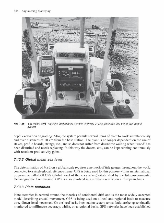
344 Engineering Surveying
depth excavation or grading. Also, the system permits several items of plant to work simultaneouslyand over distances of 10 km from the base station. The plant is no longer dependent on the use ofstakes, profile boards, strings, etc., and so does not suffer from downtime waiting when ‘wood’ hasbeen disturbed and needs replacing. In this way the dozers, etc., can be kept running continuouslywith resultant productivity gains.
7.13.2 Global mean sea level
The determination of MSL on a global scale requires a network of tide gauges throughout the worldconnected to a single global reference frame. GPS is being used for this purpose within an internationalprogramme called GLOSS (global level of the sea surface) established by the IntergovernmentalOceanographic Commission. GPS is also involved in a similar exercise on a European basis.
7.13.3 Plate tectonics
Plate tectonics is centred around the theories of continental drift and is the most widely acceptedmodel describing crustal movement. GPS is being used on a local and regional basis to measurethree-dimensional movement. On the local basis, inter-station vectors across faults are being continuallymonitored to millimetre accuracy, whilst, on a regional basis, GPS networks have been established
Fig. 7.25 ‘Site vision GPS’ machine guidance by Trimble, showing 2 GPS antennae and the in-cab controlsystem
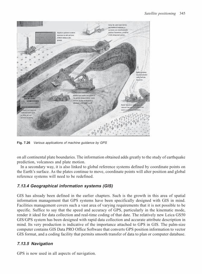
Satellite positioning 345
on all continental plate boundaries. The information obtained adds greatly to the study of earthquakeprediction, volcanoes and plate motion.
In a secondary way, it is also linked to global reference systems defined by coordinate points onthe Earth’s surface. As the plates continue to move, coordinate points will alter position and globalreference systems will need to be redefined.
7.13.4 Geographical information systems (GIS)
GIS has already been defined in the earlier chapters. Such is the growth in this area of spatialinformation management that GPS systems have been specifically designed with GIS in mind.Facilities management covers such a vast area of varying requirements that it is not possible to bespecific. Suffice to say that the speed and accuracy of GPS, particularly in the kinematic mode,render it ideal for data collection and real-time coding of that date. The relatively new Leica GS50GIS/GPS system has been designed with rapid data collection and accurate attribute description inmind. Its very production is indicative of the importance attached to GPS in GIS. The palm-sizecomputer contains GIS Data PRO Office Software that converts GPS position information to vectorGIS format, and a coding facility that permits smooth transfer of data to plan or computer database.
7.13.5 Navigation
GPS is now used in all aspects of navigation.
Fig. 7.26 Various applications of machine guidance by GPS
346 Engineering Surveying
GPS voice navigation systems are now built in to several models of car. Simply typing therequired destination into the on-board computer results in a graphical display of the route, alongwith voiced directions. Similar systems are used by private boats and aeroplanes, whilst hand-heldreceivers are now standard equipment for walkers and cyclists. A wristwatch produced by Casiocontains a GPS system giving position and route information to the wearer.
GPS can be used for fleet management when the position and status of vehicles can be transmittedto a central control, thereby permitting better management of the vehicles, whilst the driver can useit as an aid to route location.
It is used by surveying ships for major offshore hydrographic surveys. Ocean-going liners use itfor navigation purposes, whilst most harbours have a DGPS system to enable precise docking.
At the present time, aircraft landing and navigation are controlled by a variety of disparatesystems. GPS is gradually being introduced and will eventually provide a single system for allaircraft operations.
The uses to which GPS can be put are limited only by the imagination of the user. They can rangefrom the complexities of measuring gravity waves to the simplicity of spreading fertilizer inprecision farming, and include such areas of study as meteorology oceanography, geophysics andin-depth analysis on a local and global basis. As GPS equipment and procedures improve, itsapplications will continue to grow.
REFERENCES
Ackroyd, N. (1999) ‘The Application of GPS to Machine Guidance’, Journal of the ICES, August.Ashkenazi, V. (1988) ‘Global Positioning System’ Seminar on GPS, The University of Nottingham.Ashkenazi, V. and Suterfield, P.J. (1989) ‘Rapid Static and Kinematic GPS Surveying’, Land and Minerals Surveying,
October.Ashkenazi, V. (1989) ‘Positioning by Satellites. Principles, Achievements and Prospects.’ The University of Nottingham.Ashkenazi, V. et al. (1992) ‘Wide Area Differential GPS.’ Institute of Engineering Surveying Space Geodesy
(IESSG), The University of Nottingham.Bingley, R. (1994) ‘GPS Observables and Algorithms.’ IESSG, The University of Nottingham.Bingley, R. (1994) ‘Surveying with GPS.’ IESSG, The University of Nottingham.Cross, P.A. (1988) ‘Geophysical Applications of GPS Surveying.’ Seminar on GPS, The University of Nottingham.Cross, P. A. (2000) ‘Prospects for GPS – new systems, new applications, new techniques’, Engineering Surveying
Showcase 2000, Issue One.Davies, P. (1999) ‘Improving access to the National Coordinate System.’ Surveying World, 7(4).Davies, P. (2000) ‘Information Paper 1/2000 Coordinate Positioning – Ordnance Survey Policy and Strategy’,
Journal of ICES, May.Decker, B. (1984) ‘World Geodetic System 1984.’ Defence Mapping Agency, Aerospace Centre, Missouri, USA.de la Fuente, C. (1988) ‘Kinematic GPS Surveying.’ Seminar on GPS, The University of Nottingham.Moore, T. (1987) ‘The Computation of GPS Satellite Orbits.’ Seminar on GPS, The University of Nottingham.Moore, T. (1994) ‘Coordinate Systems, Frames and Datums.’ IESSG, The University of Nottingham.Moore, T. ‘GPS Orbit Determination and Fiducial Networks.’ IESSG, The University of Nottingham.Moore, T. (1994) ‘An Introduction to Differential GPS.’ IESSG, The University of Nottingham.Ordnance Survey (2000) ‘A Guide to Coordinate Systems in Great Britain’. O.S. Southampton.Pichot, G. (2000) ‘GPS on site – new prospects for machine guidance’. Engineering Surveying Showcase 2000,
Issue One.Roberts, G.W. and Dodson, A.H. (1999) ‘Using RTK GPS to control construction plant’, Journal of the ICES,
November.Stanford, N.M. and Cross, P.A. (1994) ‘A Review of some current and future applications of GPS’, Dept of
Geomatics, The University of Newcastle.
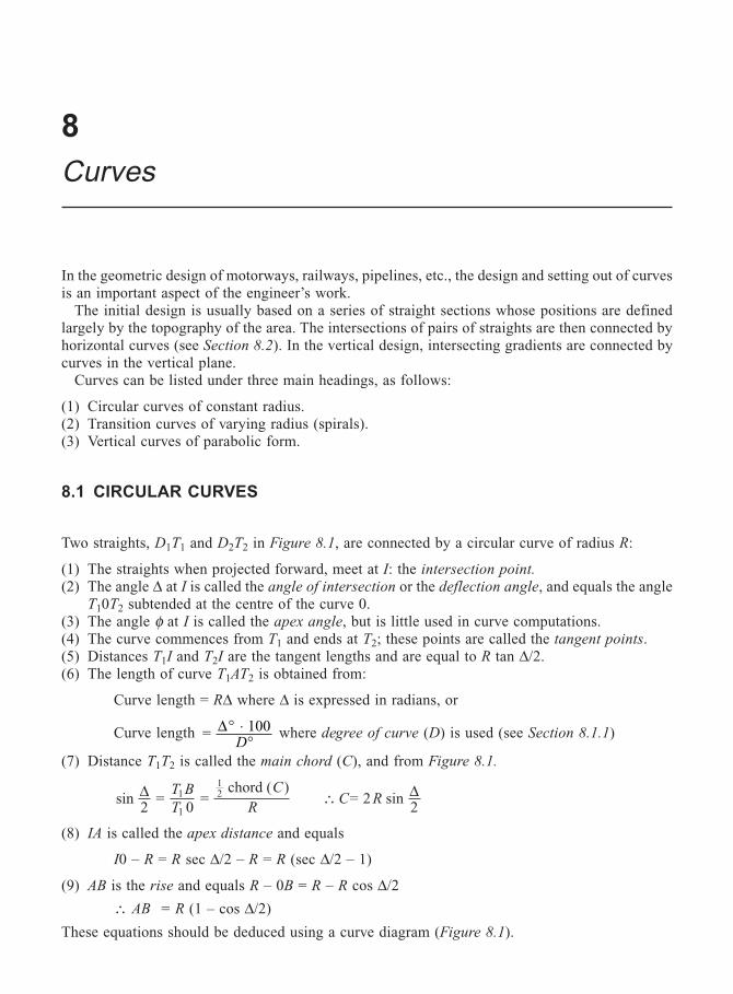
8
Curves
In the geometric design of motorways, railways, pipelines, etc., the design and setting out of curvesis an important aspect of the engineer’s work.
The initial design is usually based on a series of straight sections whose positions are definedlargely by the topography of the area. The intersections of pairs of straights are then connected byhorizontal curves (see Section 8.2). In the vertical design, intersecting gradients are connected bycurves in the vertical plane.
Curves can be listed under three main headings, as follows:
(1) Circular curves of constant radius.(2) Transition curves of varying radius (spirals).(3) Vertical curves of parabolic form.
8.1 CIRCULAR CURVES
Two straights, D1T1 and D2T2 in Figure 8.1, are connected by a circular curve of radius R:
(1) The straights when projected forward, meet at I: the intersection point.
(2) The angle ∆ at I is called the angle of intersection or the deflection angle, and equals the angleT10T2 subtended at the centre of the curve 0.
(3) The angle φ at I is called the apex angle, but is little used in curve computations.(4) The curve commences from T1 and ends at T2; these points are called the tangent points.(5) Distances T1I and T2I are the tangent lengths and are equal to R tan ∆/2.(6) The length of curve T1AT2 is obtained from:
Curve length = R∆ where ∆ is expressed in radians, or
Curve length = 100∆° ⋅°D
where degree of curve (D) is used (see Section 8.1.1)
(7) Distance T1T2 is called the main chord (C), and from Figure 8.1.
sin2
= 0
= chord ( )1
1
12∆ T B
T
C
R∴ = 2 sin
2C R
∆
(8) IA is called the apex distance and equals
I0 – R = R sec ∆/2 – R = R (sec ∆/2 – 1)
(9) AB is the rise and equals R – 0B = R – R cos ∆/2
∴ AB = R (1 – cos ∆/2)
These equations should be deduced using a curve diagram (Figure 8.1).
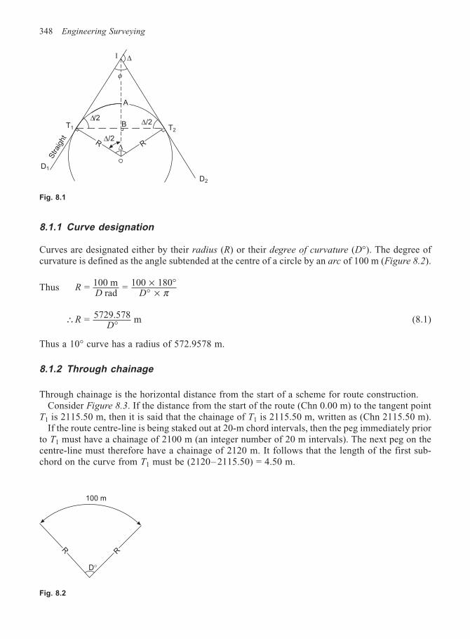
348 Engineering Surveying
8.1.1 Curve designation
Curves are designated either by their radius (R) or their degree of curvature (D°). The degree ofcurvature is defined as the angle subtended at the centre of a circle by an arc of 100 m (Figure 8.2).
Thus RD D
= 100 m rad
= 100 180× °° × π
∴ ° = 5729.578 mRD
(8.1)
Thus a 10° curve has a radius of 572.9578 m.
8.1.2 Through chainage
Through chainage is the horizontal distance from the start of a scheme for route construction.Consider Figure 8.3. If the distance from the start of the route (Chn 0.00 m) to the tangent point
T1 is 2115.50 m, then it is said that the chainage of T1 is 2115.50 m, written as (Chn 2115.50 m).If the route centre-line is being staked out at 20-m chord intervals, then the peg immediately prior
to T1 must have a chainage of 2100 m (an integer number of 20 m intervals). The next peg on thecentre-line must therefore have a chainage of 2120 m. It follows that the length of the first sub-chord on the curve from T1 must be (2120– 2115.50) = 4.50 m.
Fig. 8.1
I ∆
φ
A
∆/2 ∆/2B
∆/2R∆ R
T2T1
D1
Strai
ght
D2
Fig. 8.2
R
R
D°
100 m
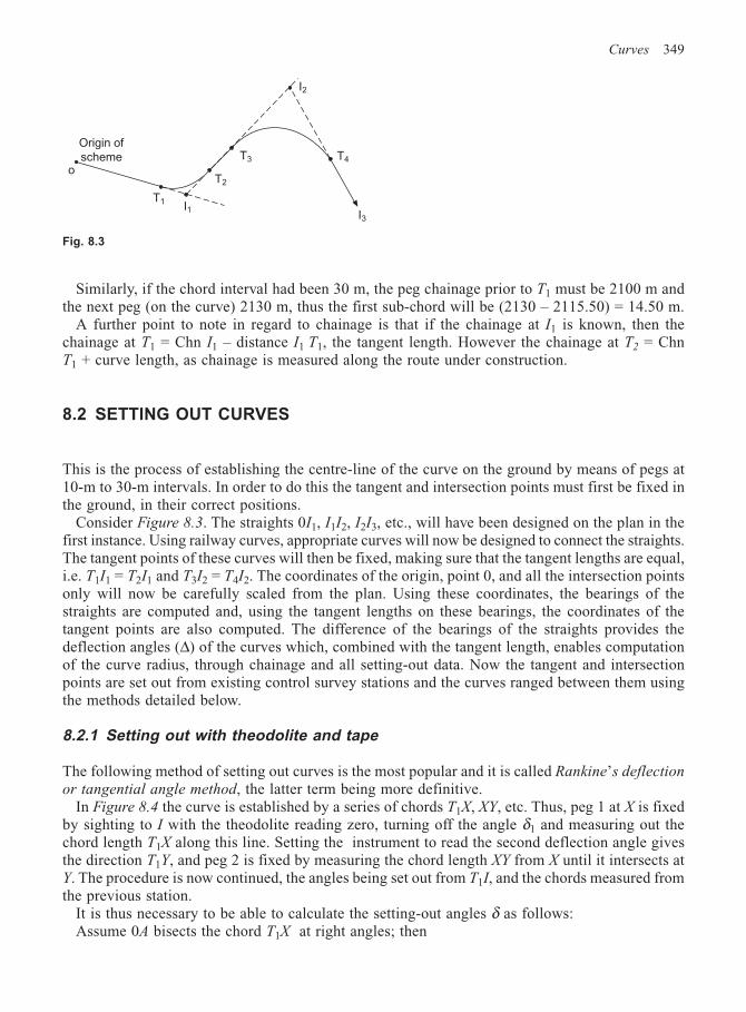
Curves 349
Similarly, if the chord interval had been 30 m, the peg chainage prior to T1 must be 2100 m andthe next peg (on the curve) 2130 m, thus the first sub-chord will be (2130 – 2115.50) = 14.50 m.
A further point to note in regard to chainage is that if the chainage at I1 is known, then thechainage at T1 = Chn I1 – distance I1 T1, the tangent length. However the chainage at T2 = ChnT1 + curve length, as chainage is measured along the route under construction.
8.2 SETTING OUT CURVES
This is the process of establishing the centre-line of the curve on the ground by means of pegs at10-m to 30-m intervals. In order to do this the tangent and intersection points must first be fixed inthe ground, in their correct positions.
Consider Figure 8.3. The straights 0I1, I1I2, I2I3, etc., will have been designed on the plan in thefirst instance. Using railway curves, appropriate curves will now be designed to connect the straights.The tangent points of these curves will then be fixed, making sure that the tangent lengths are equal,i.e. T1I1 = T2I1 and T3I2 = T4I2. The coordinates of the origin, point 0, and all the intersection pointsonly will now be carefully scaled from the plan. Using these coordinates, the bearings of thestraights are computed and, using the tangent lengths on these bearings, the coordinates of thetangent points are also computed. The difference of the bearings of the straights provides thedeflection angles (∆) of the curves which, combined with the tangent length, enables computationof the curve radius, through chainage and all setting-out data. Now the tangent and intersectionpoints are set out from existing control survey stations and the curves ranged between them usingthe methods detailed below.
8.2.1 Setting out with theodolite and tape
The following method of setting out curves is the most popular and it is called Rankine’s deflection
or tangential angle method, the latter term being more definitive.In Figure 8.4 the curve is established by a series of chords T1X, XY, etc. Thus, peg 1 at X is fixed
by sighting to I with the theodolite reading zero, turning off the angle δ1 and measuring out thechord length T1X along this line. Setting the instrument to read the second deflection angle givesthe direction T1Y, and peg 2 is fixed by measuring the chord length XY from X until it intersects atY. The procedure is now continued, the angles being set out from T1I, and the chords measured fromthe previous station.
It is thus necessary to be able to calculate the setting-out angles δ as follows:Assume 0A bisects the chord T1X at right angles; then
o
Origin of
scheme
T1
T2
T3 T4
I1
I2
I3
Fig. 8.3
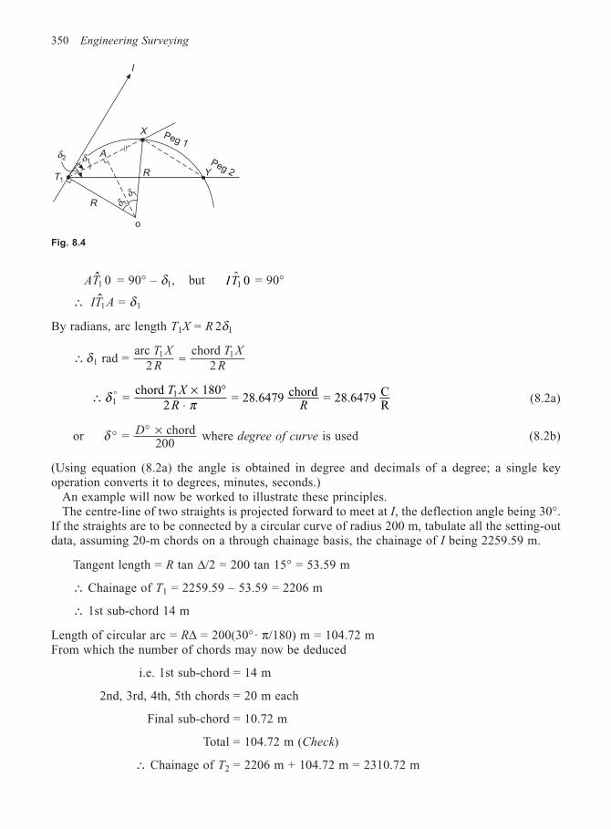
350 Engineering Surveying
AT1 0 = 90° – δ1, but IT1 0 = 90°
∴ IT Aˆ1 1 = δ
By radians, arc length T1X = R 2δ1
∴ ≈ rad = arc
2chord
211 1δ T X
R
T X
R
∴ × °⋅
° = chord 180
2 = 28.6479 chord = 28.6479 C
R11δ π
T X
R R(8.2a)
or δ ° ° × = chord200
D where degree of curve is used (8.2b)
(Using equation (8.2a) the angle is obtained in degree and decimals of a degree; a single keyoperation converts it to degrees, minutes, seconds.)
An example will now be worked to illustrate these principles.The centre-line of two straights is projected forward to meet at I, the deflection angle being 30°.
If the straights are to be connected by a circular curve of radius 200 m, tabulate all the setting-outdata, assuming 20-m chords on a through chainage basis, the chainage of I being 2259.59 m.
Tangent length = R tan ∆/2 = 200 tan 15° = 53.59 m
∴ Chainage of T1 = 2259.59 – 53.59 = 2206 m
∴ 1st sub-chord 14 m
Length of circular arc = R∆ = 200(30° · π/180) m = 104.72 mFrom which the number of chords may now be deduced
i.e. 1st sub-chord = 14 m
2nd, 3rd, 4th, 5th chords = 20 m each
Final sub-chord = 10.72 m
Total = 104.72 m (Check)
∴ Chainage of T2 = 2206 m + 104.72 m = 2310.72 m
Fig. 8.4
δ1
δ 1
δ1
Peg 1
Peg 2YR
R
Aδ2
T1
o
I
X
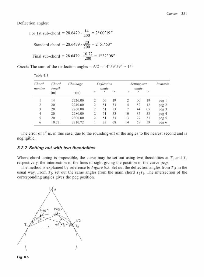
Curves 351
Deflection angles:
For 1st sub-chord = 28.6479 14200
= 2 00 19⋅ ° ′ ′′
Standard chord = 28.6479 20200
= 2 51 53⋅ ° ′ ′′
Final sub-chord = 28.6479 10.72200
= 1 32 08⋅ ° ′ ′′
Check: The sum of the deflection angles = ∆/2 = 14°59′ 59″ ≈ 15°
Fig. 8.5
I ∆
Peg 1 Peg 2
δ2
δ1δ2
δ1T1 T2
∆/2
Table 8.1
Chord Chord Chainage Deflection Setting-out Remarks
number length angle angle
(m) (m) ° ′ ″ ° ′ ″
1 14 2220.00 2 00 19 2 00 19 peg 12 20 2240.00 2 51 53 4 52 12 peg 23 20 2260.00 2 51 53 7 44 05 peg 34 20 2280.00 2 51 53 10 35 58 peg 45 20 2300.00 2 51 53 13 27 51 peg 56 10.72 2310.72 1 32 08 14 59 59 peg 6
The error of 1″ is, in this case, due to the rounding-off of the angles to the nearest second and isnegligible.
8.2.2 Setting out with two theodolites
Where chord taping is impossible, the curve may be set out using two theodolites at T1 and T2
respectively, the intersection of the lines of sight giving the position of the curve pegs.The method is explained by reference to Figure 8.5. Set out the deflection angles from T1I in the
usual way. From T2, set out the same angles from the main chord T2T1. The intersection of thecorresponding angles gives the peg position.
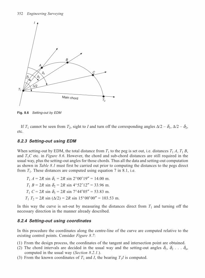
352 Engineering Surveying
If T1 cannot be seen from T2, sight to I and turn off the corresponding angles ∆/2 – δ1, ∆/2 – δ2,etc.
8.2.3 Setting-out using EDM
When setting-out by EDM, the total distance from T1 to the peg is set out, i.e. distances T1 A, T1 B,and T1C etc. in Figure 8.6. However, the chord and sub-chord distances are still required in theusual way, plus the setting-out angles for those chords. Thus all the data and setting-out computationas shown in Table 8.1 must first be carried out prior to computing the distances to the pegs directfrom T1. These distances are computed using equation 7 in 8.1, i.e.
T1 A = 2R sin δ1 = 2R sin 2°00′19″ = 14.00 m.
T1 B = 2R sin δ2 = 2R sin 4°52′12″ = 33.96 m.
T1 C = 2R sin δ3 = 2R sin 7°44′05″ = 53.83 m.
T1 T2 = 2R sin (∆/2) = 2R sin 15°00′00″ = 103.53 m.
In this way the curve is set-out by measuring the distances direct from T1 and turning off thenecessary direction in the manner already described.
8.2.4 Setting-out using coordinates
In this procedure the coordinates along the centre-line of the curve are computed relative to theexisting control points. Consider Figure 8.7:
(1) From the design process, the coordinates of the tangent and intersection point are obtained.(2) The chord intervals are decided in the usual way and the setting-out angles δ1, δ2 . . . δn,
computed in the usual way (Section 8.2.1.).(3) From the known coordinates of T1 and I, the bearing T1I is computed.
Fig. 8.6 Setting-out by EDM
I
T2
δ1
∆/2
δ2
δ3
T1
Main chord
A
B
C
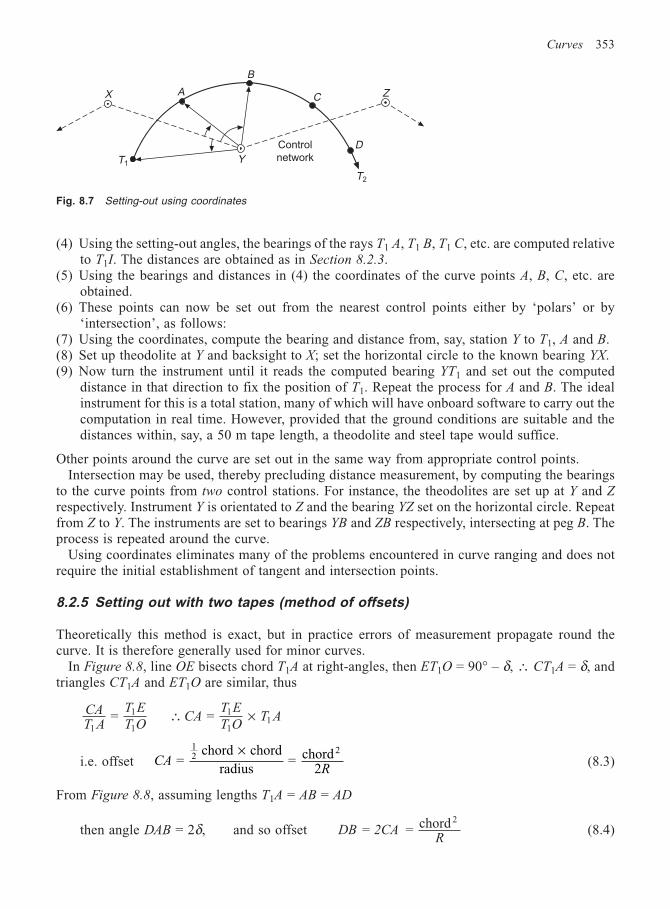
Curves 353
(4) Using the setting-out angles, the bearings of the rays T1 A, T1 B, T1 C, etc. are computed relativeto T1I. The distances are obtained as in Section 8.2.3.
(5) Using the bearings and distances in (4) the coordinates of the curve points A, B, C, etc. areobtained.
(6) These points can now be set out from the nearest control points either by ‘polars’ or by‘intersection’, as follows:
(7) Using the coordinates, compute the bearing and distance from, say, station Y to T1, A and B.(8) Set up theodolite at Y and backsight to X; set the horizontal circle to the known bearing YX.(9) Now turn the instrument until it reads the computed bearing YT1 and set out the computed
distance in that direction to fix the position of T1. Repeat the process for A and B. The idealinstrument for this is a total station, many of which will have onboard software to carry out thecomputation in real time. However, provided that the ground conditions are suitable and thedistances within, say, a 50 m tape length, a theodolite and steel tape would suffice.
Other points around the curve are set out in the same way from appropriate control points.Intersection may be used, thereby precluding distance measurement, by computing the bearings
to the curve points from two control stations. For instance, the theodolites are set up at Y and Zrespectively. Instrument Y is orientated to Z and the bearing YZ set on the horizontal circle. Repeatfrom Z to Y. The instruments are set to bearings YB and ZB respectively, intersecting at peg B. Theprocess is repeated around the curve.
Using coordinates eliminates many of the problems encountered in curve ranging and does notrequire the initial establishment of tangent and intersection points.
8.2.5 Setting out with two tapes (method of offsets)
Theoretically this method is exact, but in practice errors of measurement propagate round thecurve. It is therefore generally used for minor curves.
In Figure 8.8, line OE bisects chord T1A at right-angles, then ET1O = 90° – δ, ∴ CT1A = δ, andtriangles CT1A and ET1O are similar, thus
CAT A
T E
T O1
1
1 = ∴ × = 1
11CA
T E
T OT A
i.e. offset CAR
= chord chord
radius = chord
2
12
2×(8.3)
From Figure 8.8, assuming lengths T1A = AB = AD
then angle DAB = 2δ, and so offset DB = 2CA = R
chord 2
(8.4)
Fig. 8.7 Setting-out using coordinates
X
B
AC Z
Y
D
T2
T1
Control
network
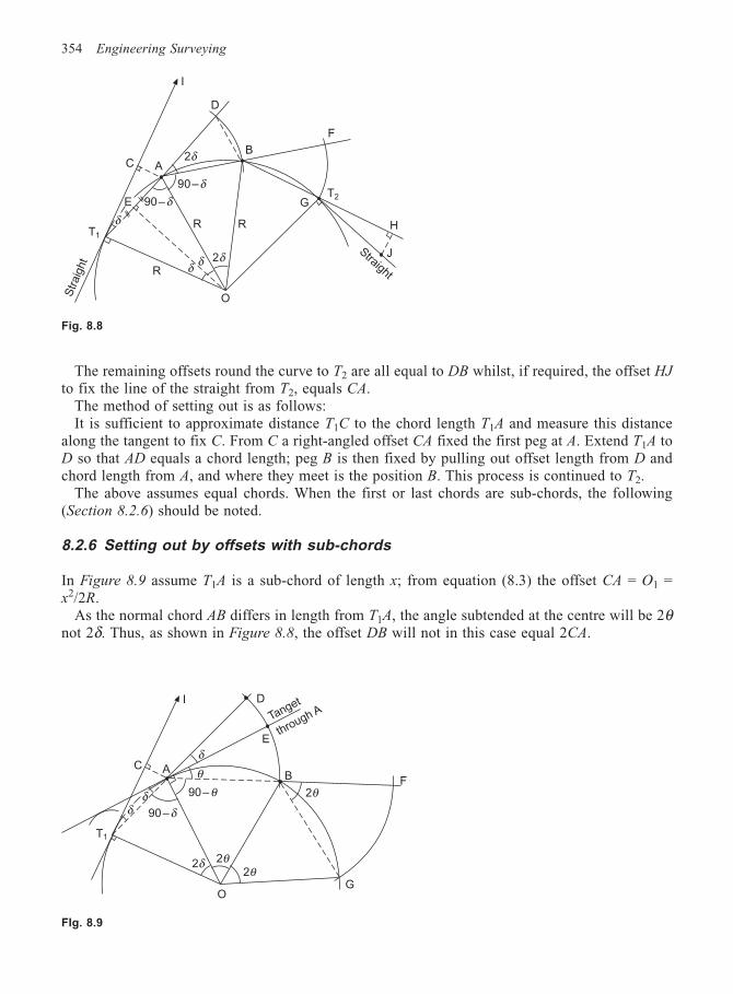
354 Engineering Surveying
The remaining offsets round the curve to T2 are all equal to DB whilst, if required, the offset HJ
to fix the line of the straight from T2, equals CA.The method of setting out is as follows:It is sufficient to approximate distance T1C to the chord length T1A and measure this distance
along the tangent to fix C. From C a right-angled offset CA fixed the first peg at A. Extend T1A toD so that AD equals a chord length; peg B is then fixed by pulling out offset length from D andchord length from A, and where they meet is the position B. This process is continued to T2.
The above assumes equal chords. When the first or last chords are sub-chords, the following(Section 8.2.6) should be noted.
8.2.6 Setting out by offsets with sub-chords
In Figure 8.9 assume T1A is a sub-chord of length x; from equation (8.3) the offset CA = O1 =x2/2R.
As the normal chord AB differs in length from T1A, the angle subtended at the centre will be 2θnot 2δ. Thus, as shown in Figure 8.8, the offset DB will not in this case equal 2CA.
Fig. 8.8
C
Str
aig
ht
T1
I
F
B
G
RR
R
A
E
Straight
T290–δ
90–δ
2δ
J
H
2δδδ
δ
D
O
FIg. 8.9
I
C A
D
T1
δδ
90–δ
90– θ
θ
δE
B
2θ
2δ 2θ2θ
Tanget
through A
F
GO
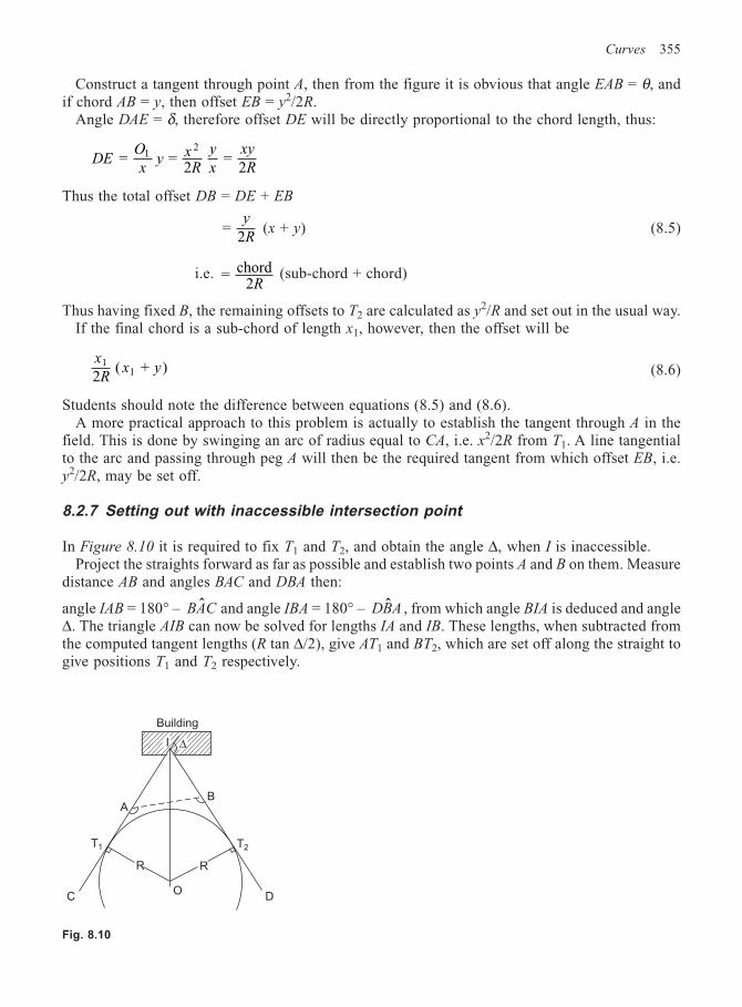
Curves 355
Construct a tangent through point A, then from the figure it is obvious that angle EAB = θ, andif chord AB = y, then offset EB = y2/2R.
Angle DAE = δ, therefore offset DE will be directly proportional to the chord length, thus:
DE O
xy
xR
y
x
xy
R= =
2 =
21
2
Thus the total offset DB = DE + EB
=2y
R (x + y) (8.5)
i.e. = chord2R
(sub-chord + chord)
Thus having fixed B, the remaining offsets to T2 are calculated as y2/R and set out in the usual way.If the final chord is a sub-chord of length x1, however, then the offset will be
x
Rx y1
12 ( + ) (8.6)
Students should note the difference between equations (8.5) and (8.6).A more practical approach to this problem is actually to establish the tangent through A in the
field. This is done by swinging an arc of radius equal to CA, i.e. x2/2R from T1. A line tangentialto the arc and passing through peg A will then be the required tangent from which offset EB, i.e.y2/2R, may be set off.
8.2.7 Setting out with inaccessible intersection point
In Figure 8.10 it is required to fix T1 and T2, and obtain the angle ∆, when I is inaccessible.Project the straights forward as far as possible and establish two points A and B on them. Measure
distance AB and angles BAC and DBA then:
angle IAB = 180° – BACˆ and angle IBA = 180° – DBAˆ , from which angle BIA is deduced and angle∆. The triangle AIB can now be solved for lengths IA and IB. These lengths, when subtracted fromthe computed tangent lengths (R tan ∆/2), give AT1 and BT2, which are set off along the straight togive positions T1 and T2 respectively.
Fig. 8.10
Building
I ∆
AB
R R
O
T1 T2
C D
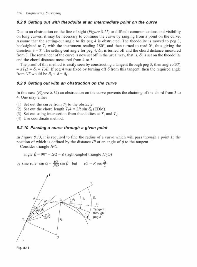
356 Engineering Surveying
8.2.8 Setting out with theodolite at an intermediate point on the curve
Due to an obstruction on the line of sight (Figure 8.11) or difficult communications and visibilityon long curves, it may be necessary to continue the curve by ranging from a point on the curve.Assume that the setting-out angle to fix peg 4 is obstructed. The theodolite is moved to peg 3,backsighted to T1 with the instrument reading 180°, and then turned to read 0°, thus giving thedirection 3 – T. The setting-out angle for peg 4, δ4, is turned off and the chord distance measuredfrom 3. The remainder of the curve is now set off in the usual way, that is, δ5 is set on the theodoliteand the chord distance measured from 4 to 5.
The proof of this method is easily seen by constructing a tangent through peg 3, then angle A3T1
= AT13 = δ3 = T3B. If peg 4 was fixed by turning off δ from this tangent, then the required anglefrom 3T would be δ3 + δ = δ4 .
8.2.9 Setting out with an obstruction on the curve
In this case (Figure 8.12) an obstruction on the curve prevents the chaining of the chord from 3 to4. One may either
(1) Set out the curve from T2 to the obstacle.(2) Set out the chord length T14 = 2R sin δ4 (EDM).(3) Set out using intersection from theodolites at T1 and T2.(4) Use coordinate method.
8.2.10 Passing a curve through a given point
In Figure 8.13, it is required to find the radius of a curve which will pass through a point P, theposition of which is defined by the distance IP at an angle of φ to the tangent.
Consider triangle IPO:
angle β = 90° – ∆/2 – φ (right-angled triangle IT2O)
by sine rule: sin = sin α βIOPO
but IO R = sec 2∆
T1
R
R
O
A
I
1
2
δ3δ4
δ3δ5δ43
5
4 B
Tangent
through
peg 3
Fig. 8.11
T
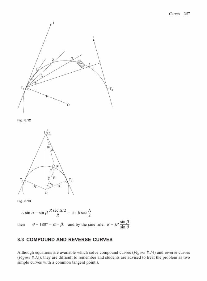
Curves 357
∴ sin = sin sec /2
= sin sec 2
α β βRR
∆ ∆
then θ = 180° – α – β, and by the sine rule: R IP = sinsin
βθ
8.3 COMPOUND AND REVERSE CURVES
Although equations are available which solve compound curves (Figure 8.14) and reverse curves(Figure 8.15), they are difficult to remember and students are advised to treat the problem as twosimple curves with a common tangent point t.
Fig. 8.12
I
I
1
2 3
4
T2T1
R
O
δ4
I ∆
βφ
α
θ
P
R
RR
T1 T2∆/2
O
Fig. 8.13
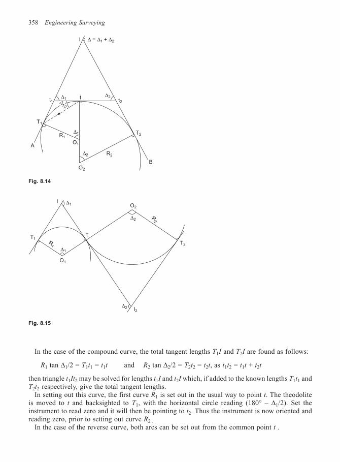
358 Engineering Surveying
In the case of the compound curve, the total tangent lengths T1I and T2I are found as follows:
R1 tan ∆1/2 = T1t1 = t1t and R2 tan ∆2/2 = T2t2 = t2t, as t1t2 = t1t + t2t
then triangle t1It2 may be solved for lengths t1I and t2I which, if added to the known lengths T1t1 andT2t2 respectively, give the total tangent lengths.
In setting out this curve, the first curve R1 is set out in the usual way to point t. The theodoliteis moved to t and backsighted to T1, with the horizontal circle reading (180° – ∆1/2). Set theinstrument to read zero and it will then be pointing to t2. Thus the instrument is now oriented andreading zero, prior to setting out curve R2 .
In the case of the reverse curve, both arcs can be set out from the common point t .
I ∆ = ∆1 + ∆2
t1 t2∆1
∆2
T1
T2
∆2
R1
O1
B
∆1
A
O2
R2
∆1/2
t
Fig. 8.14
I
T1
O1
∆1
R1
∆1
t
O2
∆2 R2
∆2
T2
I2
Fig. 8.15
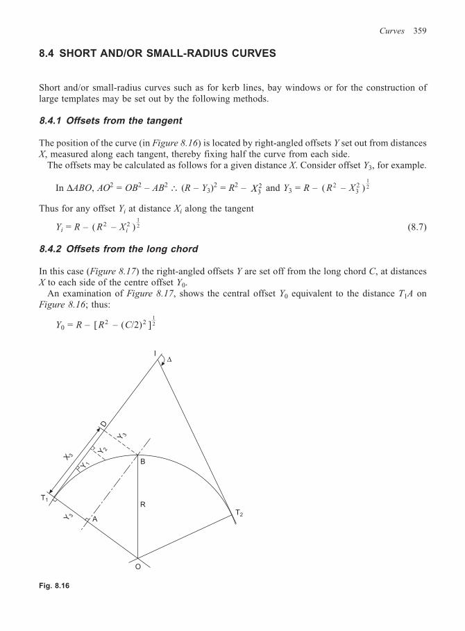
Curves 359
8.4 SHORT AND/OR SMALL-RADIUS CURVES
Short and/or small-radius curves such as for kerb lines, bay windows or for the construction oflarge templates may be set out by the following methods.
8.4.1 Offsets from the tangent
The position of the curve (in Figure 8.16) is located by right-angled offsets Y set out from distancesX, measured along each tangent, thereby fixing half the curve from each side.
The offsets may be calculated as follows for a given distance X. Consider offset Y3, for example.
In ∆ABO, AO2 = OB2 – AB2 ∴ (R – Y3)2 = R2 – X3
2 and Y3 = R – ( – )232
12R X
Thus for any offset Yi at distance Xi along the tangent
Yi = R – ( – )2 212R Xi (8.7)
8.4.2 Offsets from the long chord
In this case (Figure 8.17) the right-angled offsets Y are set off from the long chord C, at distancesX to each side of the centre offset Y0.
An examination of Figure 8.17, shows the central offset Y0 equivalent to the distance T1A onFigure 8.16; thus:
Y0 = R – [ – ( /2) ]2 212R C
Fig. 8.16
I∆
D
Y 3
Y 2
Y 1
T1
Y 3
A
B
R
O
T2
X 3
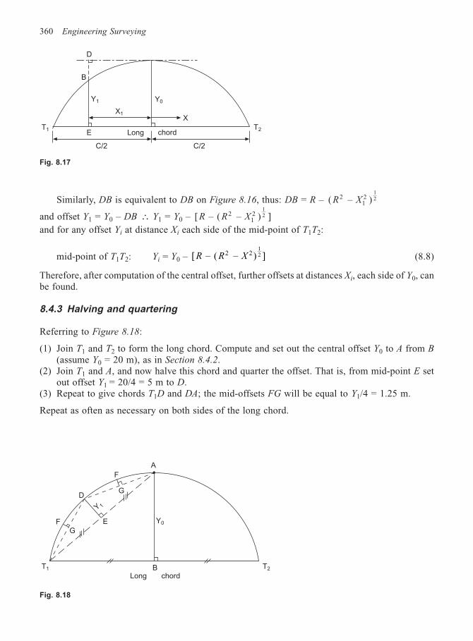
360 Engineering Surveying
Similarly, DB is equivalent to DB on Figure 8.16, thus: DB = R – ( – )212
12R X
and offset Y1 = Y0 – DB ∴ Y1 = Y0 – [ – ( – ) ]212
12R R X
and for any offset Yi at distance Xi each side of the mid-point of T1T2:
mid-point of T1T2: Yi = Y0 – [ – ( – ) ]2 212R R X (8.8)
Therefore, after computation of the central offset, further offsets at distances Xi, each side of Y0, canbe found.
8.4.3 Halving and quartering
Referring to Figure 8.18:
(1) Join T1 and T2 to form the long chord. Compute and set out the central offset Y0 to A from B(assume Y0 = 20 m), as in Section 8.4.2.
(2) Join T1 and A, and now halve this chord and quarter the offset. That is, from mid-point E setout offset Y1 = 20/4 = 5 m to D.
(3) Repeat to give chords T1D and DA; the mid-offsets FG will be equal to Y1/4 = 1.25 m.
Repeat as often as necessary on both sides of the long chord.
Fig. 8.17
Fig. 8.18
D
B
ET1 T2
C/2 C/2
chordLong
Y1
X1
Y0
X
T1 T2B
GF E
DG
F
Y 1
Y0
Long chord
A
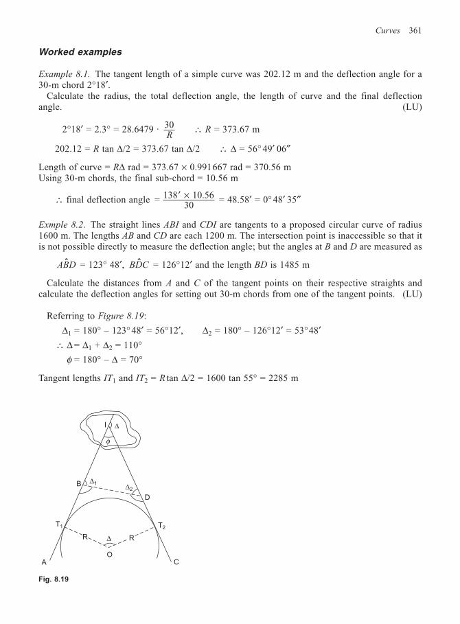
Curves 361
Worked examples
Example 8.1. The tangent length of a simple curve was 202.12 m and the deflection angle for a30-m chord 2°18′.
Calculate the radius, the total deflection angle, the length of curve and the final deflectionangle. (LU)
2°18′ = 2.3° = 28.6479 · 30R
∴ R = 373.67 m
202.12 = R tan ∆/2 = 373.67 tan ∆/2 ∴ ∆ = 56° 49′ 06″
Length of curve = R∆ rad = 373.67 × 0.991667 rad = 370.56 mUsing 30-m chords, the final sub-chord = 10.56 m
∴ final deflection angle = 138 10.5630
′ × = 48.58′ = 0° 48′ 35″
Exmple 8.2. The straight lines ABI and CDI are tangents to a proposed circular curve of radius1600 m. The lengths AB and CD are each 1200 m. The intersection point is inaccessible so that itis not possible directly to measure the deflection angle; but the angles at B and D are measured as
ABDˆ = 123° 48′, BDCˆ = 126°12′ and the length BD is 1485 m
Calculate the distances from A and C of the tangent points on their respective straights andcalculate the deflection angles for setting out 30-m chords from one of the tangent points. (LU)
Referring to Figure 8.19:
∆1 = 180° – 123° 48′ = 56°12′, ∆2 = 180° – 126°12′ = 53°48′∴ ∆ = ∆1 + ∆2 = 110°
φ = 180° – ∆ = 70°
Tangent lengths IT1 and IT2 = R tan ∆/2 = 1600 tan 55° = 2285 m
Fig. 8.19
I ∆
φ
∆1 ∆2B
D
A C
RR ∆
T1 T2
O
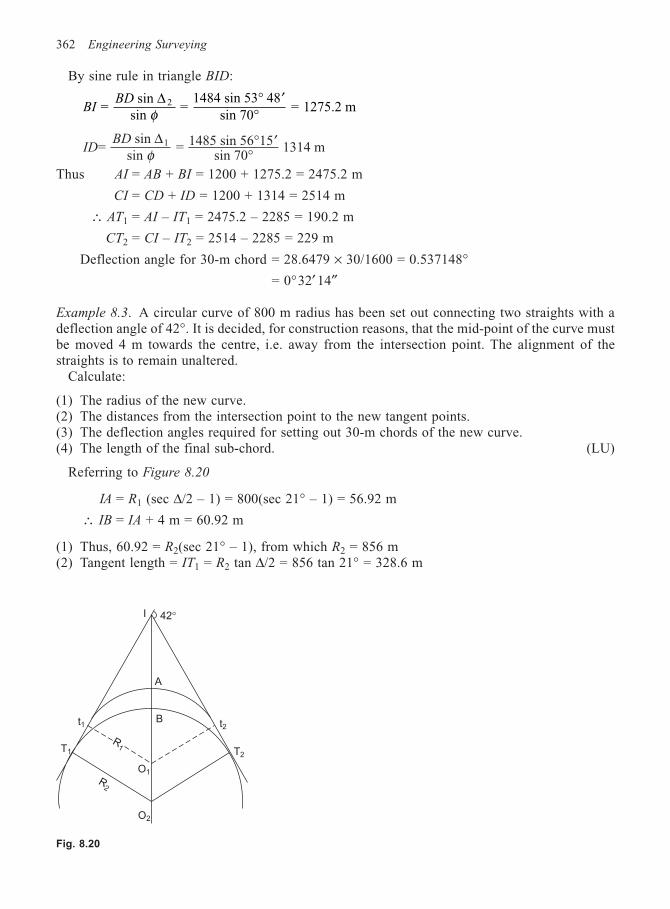
362 Engineering Surveying
By sine rule in triangle BID:
BIBD
= sin
sin =
1484 sin 53 48sin 70
= 1275.2 m2∆φ
° ′°
IDBD
= sin
sin = 1485 sin 56 15
sin 70 1314 m
∆1
φ° ′
°Thus AI = AB + BI = 1200 + 1275.2 = 2475.2 m
CI = CD + ID = 1200 + 1314 = 2514 m
∴ AT1 = AI – IT1 = 2475.2 – 2285 = 190.2 m
CT2 = CI – IT2 = 2514 – 2285 = 229 m
Deflection angle for 30-m chord = 28.6479 × 30/1600 = 0.537148°= 0°32′ 14″
Example 8.3. A circular curve of 800 m radius has been set out connecting two straights with adeflection angle of 42°. It is decided, for construction reasons, that the mid-point of the curve mustbe moved 4 m towards the centre, i.e. away from the intersection point. The alignment of thestraights is to remain unaltered.
Calculate:
(1) The radius of the new curve.(2) The distances from the intersection point to the new tangent points.(3) The deflection angles required for setting out 30-m chords of the new curve.(4) The length of the final sub-chord. (LU)
Referring to Figure 8.20
IA = R1 (sec ∆/2 – 1) = 800(sec 21° – 1) = 56.92 m
∴ IB = IA + 4 m = 60.92 m
(1) Thus, 60.92 = R2(sec 21° – 1), from which R2 = 856 m(2) Tangent length = IT1 = R2 tan ∆/2 = 856 tan 21° = 328.6 m
Fig. 8.20
I 42°
t2
T2
t1
T1
O2
O1
R2
R1
B
A
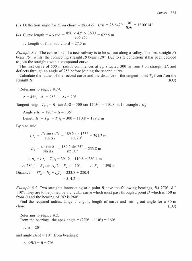
Curves 363
(3) Deflection angle for 30-m chord = 28.6479 · C/R = 28.6479 30856
= 1 00 14⋅ ° ′ ′′
(4) Curve length = R∆ rad = 856 42 3600206 265
= 627.5 m× ° ×
∴ Length of final sub-chord = 27.5 m
Example 8.4. The centre-line of a new railway is to be set out along a valley. The first straight AI
bears 75°, whilst the connecting straight IB bears 120°. Due to site conditions it has been decidedto join the straights with a compound curve.
The first curve of 500 m radius commences at T1, situated 300 m from I on straight AI, anddeflects through an angle of 25° before joining the second curve.
Calculate the radius of the second curve and the distance of the tangent point T2 from I on thestraight IB. (KU)
Referring to Figure 8.14:
∆ = 45°, ∆1 = 25° ∴ ∆2 = 20°
Tangent length T1t1 = R1 tan ∆1/2 = 500 tan 12°30′ = 110.8 m. In triangle t1It2
Angle t2It1 = 180° – ∆ = 135°Length It1 = T1I – T1t1 = 300 – 110.8 = 189.2 m
By sine rule
t tIt t It
1 21 2 1
2 =
sin sin
= 189.2 sin 135sin 20
= 391.2 m∆°
°
ItIt
21 1
2 =
sin sin
= 189.2 sin 25sin 20
= 233.8 m∆
∆°
°
∴ tt2 = t1t2 – T1t1 = 391.2 – 110.8 = 280.4 m
∴ 280.4 = R2 tan ∆2/2 = R2 tan 10°; ∴ R2 = 1590 m
Distance IT2 = It2 + t2T2 = 233.8 + 280.4
= 514.2 m
Example 8.5. Two straights intersecting at a point B have the following bearings, BA 270°, BC
110°. They are to be joined by a circular curve which must pass through a point D which is 150 mfrom B and the bearing of BD is 260°.
Find the required radius, tangent lengths, length of curve and setting-out angle for a 30-mchord. (LU)
Referring to Figure 8.2:From the bearings, the apex angle = (270° – 110°) = 160°
∴ ∆ = 20°
and angle DBA = 10° (from bearings)
∴ OBD = β = 70°
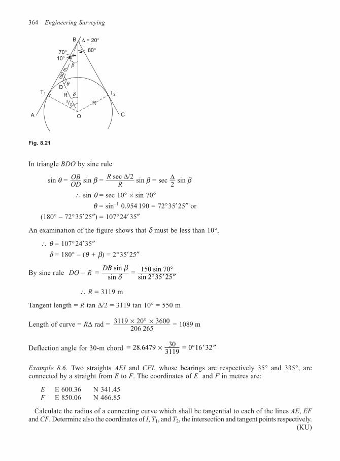
364 Engineering Surveying
In triangle BDO by sine rule
sin = sin = sec /2
sin = sec 2
sin θ β β βOBOD
RR
∆ ∆
∴ sin θ = sec 10° × sin 70°θ = sin–1 0.954 190 = 72°35′25″ or
(180° – 72°35′25″) = 107°24′ 35″
An examination of the figure shows that δ must be less than 10°,
∴ θ = 107°24′35″δ = 180° – (θ + β) = 2°35′25″
By sine rule DO = R = sin
sin = 150 sin 70
sin 2 35 25
DB βδ
°° ′ ′′
∴ R = 3119 m
Tangent length = R tan ∆/2 = 3119 tan 10° = 550 m
Length of curve = R∆ rad = 3119 20 3600206 265
= 1089 m× ° ×
Deflection angle for 30-m chord = 28.6479 303119
= 0 16 32× ° ′ ′′
Example 8.6. Two straights AEI and CFI, whose bearings are respectively 35° and 335°, areconnected by a straight from E to F. The coordinates of E and F in metres are:
E E 600.36 N 341.45F E 850.06 N 466.85
Calculate the radius of a connecting curve which shall be tangential to each of the lines AE, EF
and CF. Determine also the coordinates of I, T1, and T2, the intersection and tangent points respectively.(KU)
70°10°
B ∆ = 20°
80°
θ
δ
β
D
CA O
R
150 m
R∆/2
T1 T2
Fig. 8.21
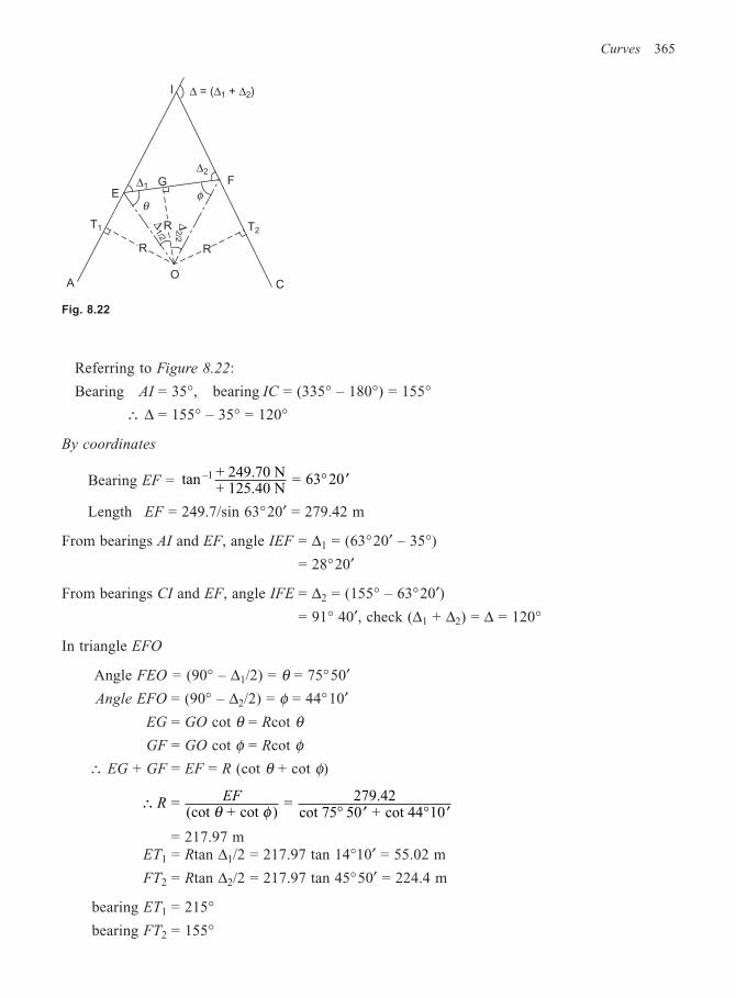
Curves 365
Referring to Figure 8.22:
Bearing AI = 35°, bearing IC = (335° – 180°) = 155°∴ ∆ = 155° – 35° = 120°
By coordinates
Bearing EF = tan + 249.70 N+ 125.40 N
= 63 20–1 ° ′
Length EF = 249.7/sin 63°20′ = 279.42 m
From bearings AI and EF, angle IEF = ∆1 = (63°20′ – 35°)
= 28°20′
From bearings CI and EF, angle IFE = ∆2 = (155° – 63°20′)= 91° 40′, check (∆1 + ∆2) = ∆ = 120°
In triangle EFO
Angle FEO = (90° – ∆1/2) = θ = 75°50′Angle EFO = (90° – ∆2/2) = φ = 44°10′
EG = GO cot θ = Rcot θGF = GO cot φ = Rcot φ
∴ EG + GF = EF = R (cot θ + cot φ)
∴° ′ ° ′
= (cot + cot )
= 279.42cot 75 50 + cot 44 10
REF
θ φ
= 217.97 mET1 = Rtan ∆1/2 = 217.97 tan 14°10′ = 55.02 m
FT2 = Rtan ∆2/2 = 217.97 tan 45°50′ = 224.4 m
bearing ET1 = 215°bearing FT2 = 155°
Fig. 8.22
∆ = (∆1 + ∆2)I
∆1
∆2
R
C
R R
∆1/2
∆2/2
θφ
G
A
T1 T2
O
EF
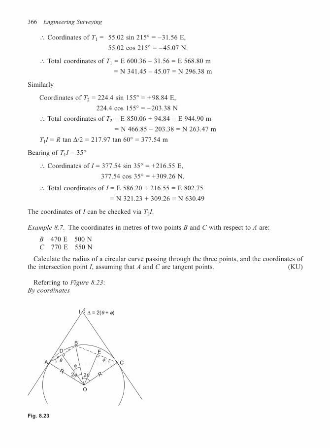
366 Engineering Surveying
∴ Coordinates of T1 = 55.02 sin 215° = –31.56 E,
55.02 cos 215° = – 45.07 N.
∴ Total coordinates of T1 = E 600.36 – 31.56 = E 568.80 m
= N 341.45 – 45.07 = N 296.38 m
Similarly
Coordinates of T2 = 224.4 sin 155° = + 98.84 E,
224.4 cos 155° = – 203.38 N
∴ Total coordinates of T2 = E 850.06 + 94.84 = E 944.90 m
= N 466.85 – 203.38 = N 263.47 m
T1I = R tan ∆/2 = 217.97 tan 60° = 377.54 m
Bearing of T1I = 35°
∴ Coordinates of I = 377.54 sin 35° = +216.55 E,
377.54 cos 35° = +309.26 N.
∴ Total coordinates of I = E 586.20 + 216.55 = E 802.75
= N 321.23 + 309.26 = N 630.49
The coordinates of I can be checked via T2I.
Example 8.7. The coordinates in metres of two points B and C with respect to A are:
B 470 E 500 NC 770 E 550 N
Calculate the radius of a circular curve passing through the three points, and the coordinates ofthe intersection point I, assuming that A and C are tangent points. (KU)
Referring to Figure 8.23:By coordinates
Fig. 8.23
∆ = 2(θ + φ)I
D E
CA
RR
O
2φ 2θ
φ
B
φθ
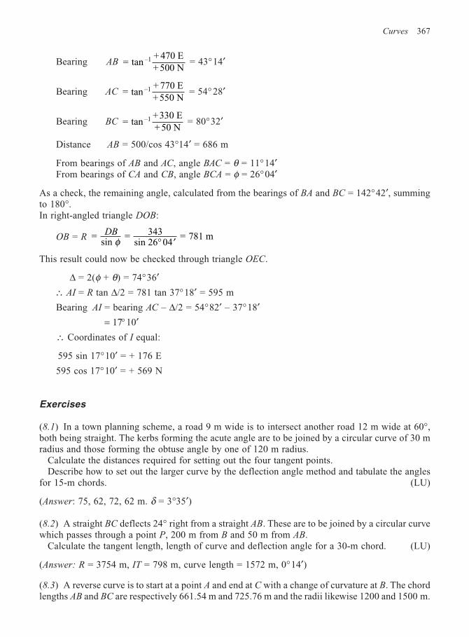
Curves 367
Bearing AB = tan+ 470 E+ 500 N
–1 = 43°14′
Bearing AC = tan+ 770 E+ 550 N
–1 = 54° 28′
Bearing BC = tan+330 E+ 50 N
–1 = 80°32′
Distance AB = 500/cos 43°14′ = 686 m
From bearings of AB and AC, angle BAC = θ = 11°14′From bearings of CA and CB, angle BCA = φ = 26°04′
As a check, the remaining angle, calculated from the bearings of BA and BC = 142°42′, summingto 180°.In right-angled triangle DOB:
OB = R =sin
= 343sin 26 04
= 781 mDBφ ° ′
This result could now be checked through triangle OEC.
∆ = 2(φ + θ) = 74°36′∴ AI = R tan ∆/2 = 781 tan 37°18′ = 595 m
Bearing AI = bearing AC – ∆/2 = 54°82′ – 37°18′= 17° 10′
∴ Coordinates of I equal:
595 sin 17°10′ = + 176 E
595 cos 17°10′ = + 569 N
Exercises
(8.1) In a town planning scheme, a road 9 m wide is to intersect another road 12 m wide at 60°,both being straight. The kerbs forming the acute angle are to be joined by a circular curve of 30 mradius and those forming the obtuse angle by one of 120 m radius.
Calculate the distances required for setting out the four tangent points.Describe how to set out the larger curve by the deflection angle method and tabulate the angles
for 15-m chords. (LU)
(Answer: 75, 62, 72, 62 m. δ = 3°35′)
(8.2) A straight BC deflects 24° right from a straight AB. These are to be joined by a circular curvewhich passes through a point P, 200 m from B and 50 m from AB.
Calculate the tangent length, length of curve and deflection angle for a 30-m chord. (LU)
(Answer: R = 3754 m, IT = 798 m, curve length = 1572 m, 0°14′)
(8.3) A reverse curve is to start at a point A and end at C with a change of curvature at B. The chordlengths AB and BC are respectively 661.54 m and 725.76 m and the radii likewise 1200 and 1500 m.
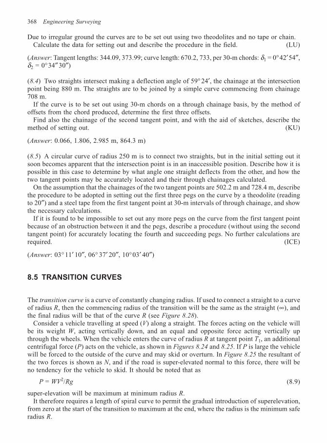
368 Engineering Surveying
Due to irregular ground the curves are to be set out using two theodolites and no tape or chain.Calculate the data for setting out and describe the procedure in the field. (LU)
(Answer: Tangent lengths: 344.09, 373.99; curve length: 670.2, 733, per 30-m chords: δ1 = 0°42′54″,δ2 = 0°34″ 30″)
(8.4) Two straights intersect making a deflection angle of 59° 24′, the chainage at the intersectionpoint being 880 m. The straights are to be joined by a simple curve commencing from chainage708 m.
If the curve is to be set out using 30-m chords on a through chainage basis, by the method ofoffsets from the chord produced, determine the first three offsets.
Find also the chainage of the second tangent point, and with the aid of sketches, describe themethod of setting out. (KU)
(Answer: 0.066, 1.806, 2.985 m, 864.3 m)
(8.5) A circular curve of radius 250 m is to connect two straights, but in the initial setting out itsoon becomes apparent that the intersection point is in an inaccessible position. Describe how it ispossible in this case to determine by what angle one straight deflects from the other, and how thetwo tangent points may be accurately located and their through chainages calculated.
On the assumption that the chainages of the two tangent points are 502.2 m and 728.4 m, describethe procedure to be adopted in setting out the first three pegs on the curve by a theodolite (readingto 20″) and a steel tape from the first tangent point at 30-m intervals of through chainage, and showthe necessary calculations.
If it is found to be impossible to set out any more pegs on the curve from the first tangent pointbecause of an obstruction between it and the pegs, describe a procedure (without using the secondtangent point) for accurately locating the fourth and succeeding pegs. No further calculations arerequired. (ICE)
(Answer: 03° 11′ 10″, 06° 37′ 20″, 10°03′ 40″)
8.5 TRANSITION CURVES
The transition curve is a curve of constantly changing radius. If used to connect a straight to a curveof radius R, then the commencing radius of the transition will be the same as the straight (∞), andthe final radius will be that of the curve R (see Figure 8.28).
Consider a vehicle travelling at speed (V) along a straight. The forces acting on the vehicle willbe its weight W, acting vertically down, and an equal and opposite force acting vertically upthrough the wheels. When the vehicle enters the curve of radius R at tangent point T1, an additionalcentrifugal force (P) acts on the vehicle, as shown in Figures 8.24 and 8.25. If P is large the vehiclewill be forced to the outside of the curve and may skid or overturn. In Figure 8.25 the resultant ofthe two forces is shown as N, and if the road is super-elevated normal to this force, there will beno tendency for the vehicle to skid. It should be noted that as
P = WV2/Rg (8.9)
super-elevation will be maximum at minimum radius R.It therefore requires a length of spiral curve to permit the gradual introduction of superelevation,
from zero at the start of the transition to maximum at the end, where the radius is the minimum saferadius R.
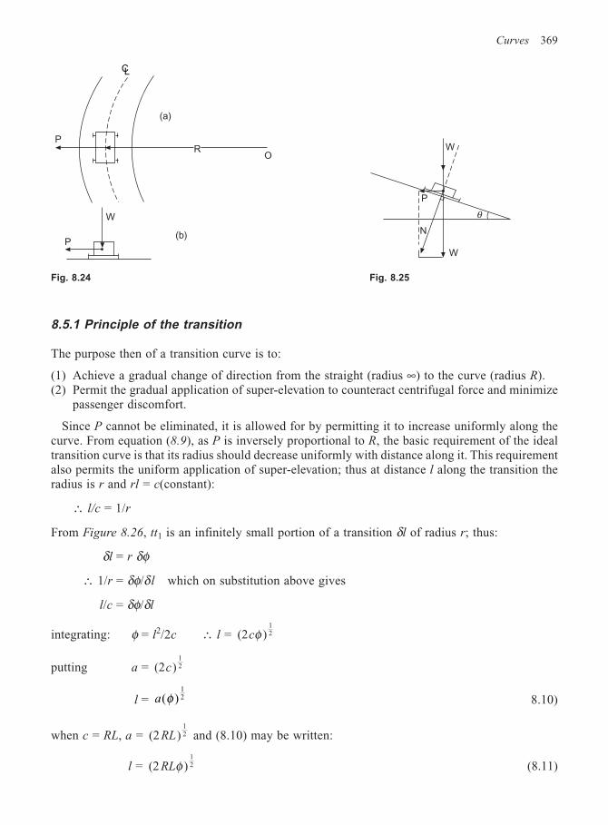
Curves 369
8.5.1 Principle of the transition
The purpose then of a transition curve is to:
(1) Achieve a gradual change of direction from the straight (radius ∞) to the curve (radius R).(2) Permit the gradual application of super-elevation to counteract centrifugal force and minimize
passenger discomfort.
Since P cannot be eliminated, it is allowed for by permitting it to increase uniformly along thecurve. From equation (8.9), as P is inversely proportional to R, the basic requirement of the idealtransition curve is that its radius should decrease uniformly with distance along it. This requirementalso permits the uniform application of super-elevation; thus at distance l along the transition theradius is r and rl = c(constant):
∴ l/c = 1/r
From Figure 8.26, tt1 is an infinitely small portion of a transition δl of radius r; thus:
δl = r δφ
∴ 1/r = δφ/δ l which on substitution above gives
l/c = δφ/δl
integrating: φ = l2/2c ∴ l = (2 )12cφ
putting a = (2 )12c
l = a( )12φ 8.10)
when c = RL, a = (2 )12RL and (8.10) may be written:
l = (2 )12RLφ (8.11)
CL
PR
O
(a)
(b)
W
PW
N
P
W
θ
Fig. 8.24 Fig. 8.25
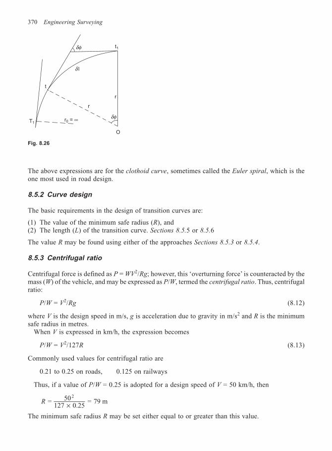
370 Engineering Surveying
The above expressions are for the clothoid curve, sometimes called the Euler spiral, which is theone most used in road design.
8.5.2 Curve design
The basic requirements in the design of transition curves are:
(1) The value of the minimum safe radius (R), and(2) The length (L) of the transition curve. Sections 8.5.5 or 8.5.6
The value R may be found using either of the approaches Sections 8.5.3 or 8.5.4.
8.5.3 Centrifugal ratio
Centrifugal force is defined as P = WV2/Rg; however, this ‘overturning force’ is counteracted by themass (W) of the vehicle, and may be expressed as P/W, termed the centrifugal ratio. Thus, centrifugalratio:
P/W = V2/Rg (8.12)
where V is the design speed in m/s, g is acceleration due to gravity in m/s2 and R is the minimumsafe radius in metres.
When V is expressed in km/h, the expression becomes
P/W = V2/127R (8.13)
Commonly used values for centrifugal ratio are
0.21 to 0.25 on roads, 0.125 on railways
Thus, if a value of P/W = 0.25 is adopted for a design speed of V = 50 km/h, then
R = 50
127 0.25 = 79 m
2
×
The minimum safe radius R may be set either equal to or greater than this value.
Fig. 8.26
δφ
δφ
r
r
t
T1
δ l
r0 = ∞
O
t1
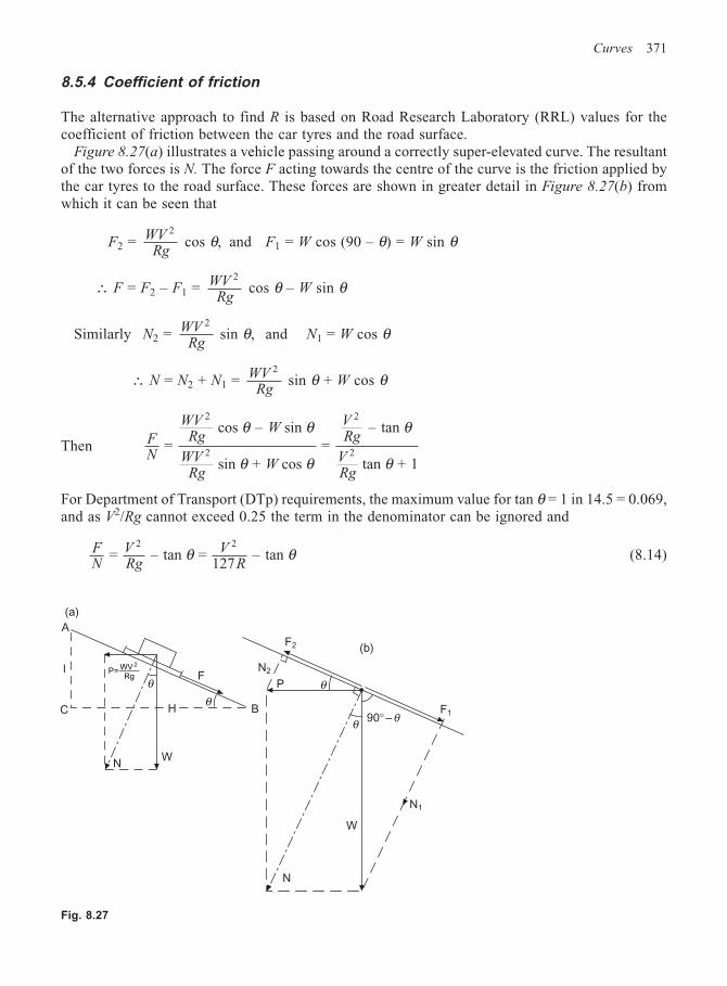
Curves 371
8.5.4 Coefficient of friction
The alternative approach to find R is based on Road Research Laboratory (RRL) values for thecoefficient of friction between the car tyres and the road surface.
Figure 8.27(a) illustrates a vehicle passing around a correctly super-elevated curve. The resultantof the two forces is N. The force F acting towards the centre of the curve is the friction applied bythe car tyres to the road surface. These forces are shown in greater detail in Figure 8.27(b) fromwhich it can be seen that
F2 = WVRg
2
cos θ, and F1 = W cos (90 – θ) = W sin θ
∴ F = F2 – F1 = WVRg
2
cos θ – W sin θ
Similarly N2 = WVRg
2
sin θ, and N1 = W cos θ
∴ N = N2 + N1 = WVRg
2
sin θ + W cos θ
Then FN
WVRg
W
WVRg
W
VRg
VRg
= cos – sin
sin + cos =
– tan
tan + 1
2
2
2
2
θ θ
θ θ
θ
θ
For Department of Transport (DTp) requirements, the maximum value for tan θ = 1 in 14.5 = 0.069,and as V2/Rg cannot exceed 0.25 the term in the denominator can be ignored and
FN
VRg
VR
= – tan = 127
– tan 2 2
θ θ (8.14)
Fig. 8.27
(a)
(b)
A
l
C
NW
Hθ
θ
B
FN2
F2
P θ
θ 90°–θF1
N1
W
N
P=WVRg
2
372 Engineering Surveying
To prevent vehicles slipping sideways, F/N must be greater than the coefficient of friction µbetween tyre and road. The RRL quote value for µ of 0.15, whilst 0.18 may be used up to50 km/h, thus:
V2/127R tan θ + µ (8.15)
For example, if the design speed is to be 100 km/h, super-elevation limited to 1 in 14.5 (0.069) andµ = 0.15, then
100127
2
R = 0.069 + 0.15
∴ R = 360 m
In the UK, the geometric parameters used in design are normally related to design speed. Table
8.3 (p. 398) shows typical desirable and absolute minimum values for horizontal and verticalcurvature; there is also an additional lower level designated ‘limiting radius’, specific of horizontalcurvature.
Designs for new roads should aim to achieve the desirable values for each design parameter.However, absolute minimum values can be used wherever substantial saving in construction orenvironmental costs can be achieved.
DTp Technical Standard TD9/93 advises that in the design of new roads, the use of radii tighterthan the limiting values is undesirable and not recommended.
8.5.5 Rate of application of super-elevation
It is recommended that on motorways super-elevation should be applied at a rate of 1 in 200, on all-purpose roads at 1 in 100, and on railways at 1 in 480. Thus, if on a motorway the super-elevationis computed as 0.5 m, then 100 m of transition curve would be required to accommodate 0.5 m atthe required rate of 1 in 200, i.e. 0.5. in 100 = 1 in 200. In this way the length L of the transitionis found.
The amount of super-elevation is obtained as follows:From the triangle of forces in Figure 8.27(a)
tan θ = V2/Rg = 1/H = 1 in H
thus H = Rg/V2 = 127R/V2, where V is in km/h.
In the UK, the design speed V is replaced by the ‘average speed’ which is 63.6% of V,
and H = 127R/(0.636V)2 = 314R/V2
∴ super-elevation = 1 in 314R/V2 (8.16)
The percentage super-elevation (or crossfall), S may be found from:
S = V2/2.828R (8.17)
The DTp recommend the crossfall should never be greater than 1 in 14.5, or less than 1 in 48, toallow rainwater to run off the road surface.
It is further recommended that adverse camber should be replaced by a favourable crossfall of2.5% when the value of V2/R is greater than 5 and less than 7 (see Table 8.3).
Driver studies have shown that whilst super-elevation is instrumental to driver comfort andsafety, it need not be applied too rigidly. Thus for sharp curves in urban areas with at-gradejunctions and side access, super-elevation should be limited to 5%.
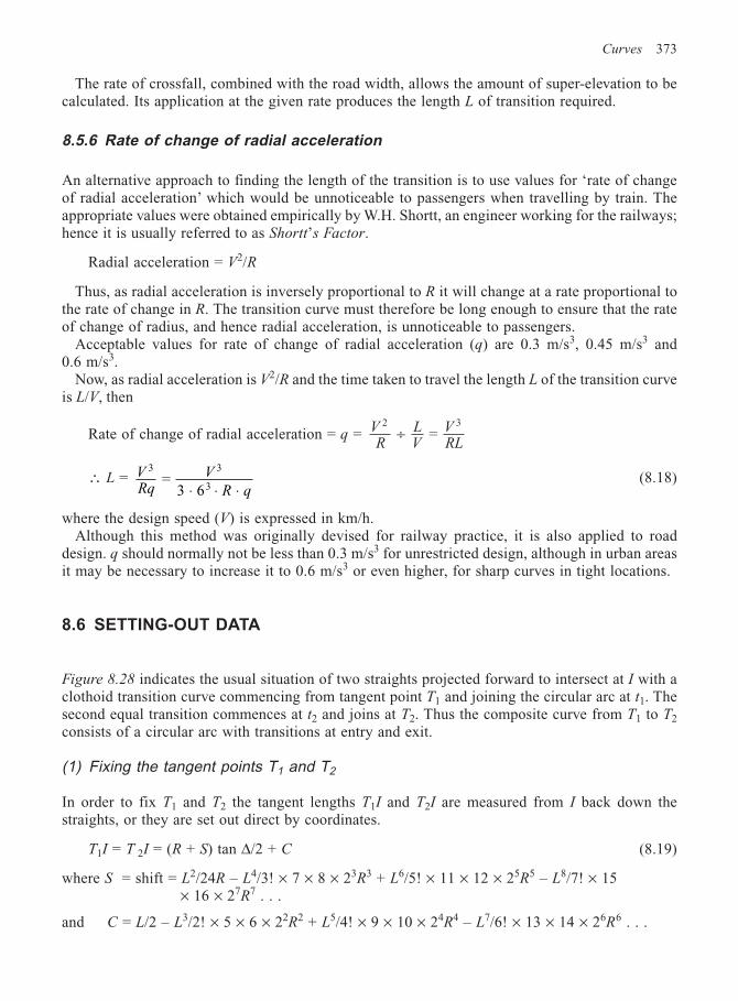
Curves 373
The rate of crossfall, combined with the road width, allows the amount of super-elevation to becalculated. Its application at the given rate produces the length L of transition required.
8.5.6 Rate of change of radial acceleration
An alternative approach to finding the length of the transition is to use values for ‘rate of changeof radial acceleration’ which would be unnoticeable to passengers when travelling by train. Theappropriate values were obtained empirically by W.H. Shortt, an engineer working for the railways;hence it is usually referred to as Shortt’s Factor.
Radial acceleration = V2/R
Thus, as radial acceleration is inversely proportional to R it will change at a rate proportional tothe rate of change in R. The transition curve must therefore be long enough to ensure that the rateof change of radius, and hence radial acceleration, is unnoticeable to passengers.
Acceptable values for rate of change of radial acceleration (q) are 0.3 m/s3, 0.45 m/s3 and0.6 m/s3.
Now, as radial acceleration is V2/R and the time taken to travel the length L of the transition curveis L/V, then
Rate of change of radial acceleration = q = VR
LV
VRL
2 3
= ÷
∴ L = VRq
V
R q
3 3
3 =
3 6 ⋅ ⋅ ⋅(8.18)
where the design speed (V) is expressed in km/h.Although this method was originally devised for railway practice, it is also applied to road
design. q should normally not be less than 0.3 m/s3 for unrestricted design, although in urban areasit may be necessary to increase it to 0.6 m/s3 or even higher, for sharp curves in tight locations.
8.6 SETTING-OUT DATA
Figure 8.28 indicates the usual situation of two straights projected forward to intersect at I with aclothoid transition curve commencing from tangent point T1 and joining the circular arc at t1. Thesecond equal transition commences at t2 and joins at T2. Thus the composite curve from T1 to T2
consists of a circular arc with transitions at entry and exit.
(1) Fixing the tangent points T1 and T2
In order to fix T1 and T2 the tangent lengths T1I and T2I are measured from I back down thestraights, or they are set out direct by coordinates.
T1I = T 2I = (R + S) tan ∆/2 + C (8.19)
where S = shift = L2/24R – L4/3! × 7 × 8 × 23R3 + L6/5! × 11 × 12 × 25R5 – L8/7! × 15× 16 × 27R7 . . .
and C = L/2 – L3/2! × 5 × 6 × 22R2 + L5/4! × 9 × 10 × 24R4 – L7/6! × 13 × 14 × 26R6 . . .
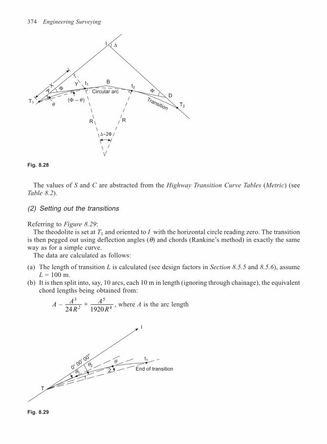
374 Engineering Surveying
The values of S and C are abstracted from the Highway Transition Curve Tables (Metric) (seeTable 8.2).
(2) Setting out the transitions
Referring to Figure 8.29:The theodolite is set at T1 and oriented to I with the horizontal circle reading zero. The transition
is then pegged out using deflection angles (θ) and chords (Rankine’s method) in exactly the sameway as for a simple curve.
The data are calculated as follows:
(a) The length of transition L is calculated (see design factors in Section 8.5.5 and 8.5.6), assumeL = 100 m.
(b) It is then split into, say, 10 arcs, each 10 m in length (ignoring through chainage), the equivalentchord lengths being obtained from:
A – A
R
A
R2
3 5
424 +
1920, where A is the arc length
Fig. 8.28
X
T1
A
θ(Φ – θ )
Y t1 B
Circular arc
Transition
∆–2Φ
Φ
T2
∆I
R R
D
Fig. 8.29
T
0° 00′ 00″
θ1
θ2
1
2
θ t1
End of transition
I
Φ t2
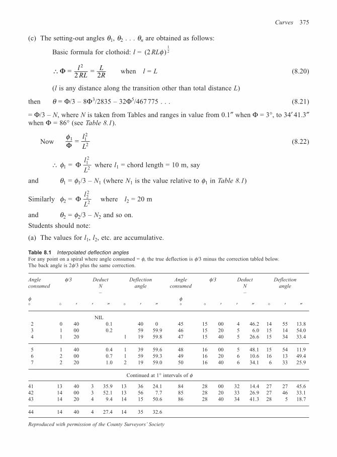
Curves 375
(c) The setting-out angles θ1, θ2 . . . θn are obtained as follows:
Basic formula for clothoid: l = (2 )12RLφ
∴ = 2
= 2
2
Φ lRL
LR
when l = L (8.20)
(l is any distance along the transition other than total distance L)
then θ = Φ/3 – 8Φ3/2835 – 32Φ5/467 775 . . . (8.21)
= Φ/3 – N, where N is taken from Tables and ranges in value from 0.1″ when Φ = 3°, to 34′ 41.3″when Φ = 86° (see Table 8.1).
Nowφ1 1
2
= Φl
L2 (8.22)
∴ φ1 = Φ 12l
L2 where l1 = chord length = 10 m, say
and θ1 = φ1/3 – N1 (where N1 is the value relative to φ1 in Table 8.1)
Similarly φ2 = Φ 22l
L2where l2 = 20 m
and θ2 = φ2/3 – N2 and so on.
Students should note:
(a) The values for l1, l2, etc. are accumulative.
Table 8.1 Interpolated deflection anglesFor any point on a spiral where angle consumed = φ, the true deflection is φ/3 minus the correction tabled below.The back angle is 2φ/3 plus the same correction.
Angle φ/3 Deduct Deflection Angle φ/3 Deduct Deflection
consumed N angle consumed N angle
– –
φ φ° ° ′ ′ ″ ° ′ ″ ° ° ′ ′ ″ ° ′ ″
NIL2 0 40 0.1 40 0 45 15 00 4 46.2 14 55 13.83 1 00 0.2 59 59.9 46 15 20 5 6.0 15 14 54.04 1 20 1 19 59.8 47 15 40 5 26.6 15 34 33.4
5 1 40 0.4 1 39 59.6 48 16 00 5 48.1 15 54 11.96 2 00 0.7 1 59 59.3 49 16 20 6 10.6 16 13 49.47 2 20 1.0 2 19 59.0 50 16 40 6 34.1 6 33 25.9
Continued at 1° intervals of φ
41 13 40 3 35.9 13 36 24.1 84 28 00 32 14.4 27 27 45.642 14 00 3 52.1 13 56 7.7 85 28 20 33 26.9 27 46 33.143 14 20 4 9.4 14 15 50.6 86 28 40 34 41.3 28 5 18.7
44 14 40 4 27.4 14 35 32.6
Reproduced with permission of the County Surveyors’ Society
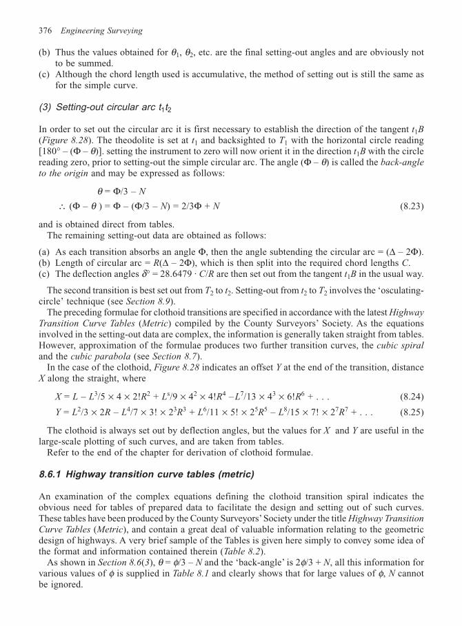
376 Engineering Surveying
(b) Thus the values obtained for θ1, θ2, etc. are the final setting-out angles and are obviously notto be summed.
(c) Although the chord length used is accumulative, the method of setting out is still the same asfor the simple curve.
(3) Setting-out circular arc t1t2
In order to set out the circular arc it is first necessary to establish the direction of the tangent t1B
(Figure 8.28). The theodolite is set at t1 and backsighted to T1 with the horizontal circle reading[180° – (Φ – θ)]. setting the instrument to zero will now orient it in the direction t1B with the circlereading zero, prior to setting-out the simple circular arc. The angle (Φ – θ) is called the back-angle
to the origin and may be expressed as follows:
θ = Φ/3 – N
∴ (Φ – θ ) = Φ – (Φ/3 – N) = 2/3Φ + N (8.23)
and is obtained direct from tables.The remaining setting-out data are obtained as follows:
(a) As each transition absorbs an angle Φ, then the angle subtending the circular arc = (∆ – 2Φ).(b) Length of circular arc = R(∆ – 2Φ), which is then split into the required chord lengths C.(c) The deflection angles δ° = 28.6479 · C/R are then set out from the tangent t1B in the usual way.
The second transition is best set out from T2 to t2. Setting-out from t2 to T2 involves the ‘osculating-circle’ technique (see Section 8.9).
The preceding formulae for clothoid transitions are specified in accordance with the latest Highway
Transition Curve Tables (Metric) compiled by the County Surveyors’ Society. As the equationsinvolved in the setting-out data are complex, the information is generally taken straight from tables.However, approximation of the formulae produces two further transition curves, the cubic spiral
and the cubic parabola (see Section 8.7).In the case of the clothoid, Figure 8.28 indicates an offset Y at the end of the transition, distance
X along the straight, where
X = L – L3/5 × 4 × 2!R2 + Ls/9 × 42 × 4!R4 – L7/13 × 43 × 6!R6 + . . . (8.24)
Y = L2/3 × 2R – L4/7 × 3! × 23R3 + L6/11 × 5! × 25R5 – L8/15 × 7! × 27R7 + . . . (8.25)
The clothoid is always set out by deflection angles, but the values for X and Y are useful in thelarge-scale plotting of such curves, and are taken from tables.
Refer to the end of the chapter for derivation of clothoid formulae.
8.6.1 Highway transition curve tables (metric)
An examination of the complex equations defining the clothoid transition spiral indicates theobvious need for tables of prepared data to facilitate the design and setting out of such curves.These tables have been produced by the County Surveyors’ Society under the title Highway Transition
Curve Tables (Metric), and contain a great deal of valuable information relating to the geometricdesign of highways. A very brief sample of the Tables is given here simply to convey some idea ofthe format and information contained therein (Table 8.2).
As shown in Section 8.6(3), θ = φ/3 – N and the ‘back-angle’ is 2φ/3 + N, all this information forvarious values of φ is supplied in Table 8.1 and clearly shows that for large values of φ, N cannotbe ignored.
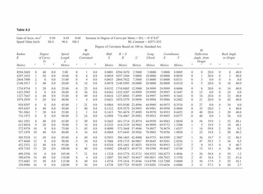
Table 8.2
Gain of Accn. m/s3 0.30 0.45 0.60 Increase in Degree of Curve per Metre = D/L = 0° 8′ 0.0″Speed Value km/h 84.4 96.6 106.3 RL Constant = 42971.835
Degree of Curvature Based on 100 m. Standard ArcΦ Θ
Radius Degree Spiral Angle Shift R + S Long Coordinates Deflection Back Angle
R of Curve Length Consumed S R C Chord X Y Angle from to Origin
D L Origin
Metres ° ′ ″ Metres ° ′ ″ Metres Metres Metres Metres Metres Metres ° ′ ″ ° ′ ″
8594.3669 0 40 0.0 5.00 0 1 0.0 0.0001 8594.3670 2.5000 5.0000 5.0000 0.0005 0 0 20.0 0 0 40.04297.1835 1 20 0.0 10.00 0 4 0.0 0.0010 4297.1844 5.0000 10.0000 10.0000 0.0039 0 1 20.0 0 2 40.02864.7890 2 0 0.0 15.00 0 9 0.0 0.0033 2864.7922 7.5000 15.0000 15.0000 0.0131 0 3 0.0 0 6 0.02148.5917 2 40 0.0 20.00 0 16 0.0 0.0078 2148.5995 10.0000 20.0000 20.0000 0.0310 0 5 20.0 0 10 40.0
1718.8734 3 20 0.0 25.00 0 25 0.0 0.0152 1718.8885 12.5000 24.9999 24.9999 0.0606 0 8 20.0 0 16 40.01432.3945 4 0 0.0 30.00 0 36 0.0 0.0262 1432.4207 14.9999 29.9999 29.9997 0.1047 0 12 0.0 0 24 0.01227.7667 4 40 0.0 35.00 0 49 0.0 0.0416 1227.8083 17.4999 34.9997 34.9993 0.1663 0 16 20.0 0 32 40.01074.2959 5 20 0.0 40.00 1 4 0.0 0.0621 1074.3579 19.9998 39.9994 39.9986 0.2482 0 21 20.0 0 42 40.0
954.9297 6 0 0.0 45.00 1 21 0.0 0.0884 955.0180 22.4996 44.9989 44.9975 0.3534 0 27 0.0 0 54 0.0859.4367 6 40 0.0 50.00 1 40 0.0 0.1212 859.5579 24.9993 49.9981 49.9958 0.4848 0 33 20.0 1 6 40.0781.3061 7 20 0.0 55.00 2 1 0.0 0.1613 781.4674 27.4989 54.9970 54.9932 0.6452 0 40 20.0 1 20 40.0716.1972 8 0 0.0 60.00 2 24 0.0 0.2094 716.4067 29.9982 59.9953 59.9895 0.8377 0 48 0.0 1 36 0.0
661.1051 8 40 0.0 65.00 2 49 0.0 0.2663 661.3714 32.4974 64.9930 64.9843 1.0650 0 56 19.9 1 52 40.1613.8834 9 20 0.0 70.00 3 16 0.0 0.3325 614.2159 34.9962 69.9899 69.9772 1.3300 1 5 19.9 2 10 40.1572.9578 10 0 0.0 75.00 3 45 0.0 0.4090 573.3668 37.4946 74.9857 74.9679 1.6357 1 14 59.8 2 30 0.2537.1479 10 40 0.0 80.00 4 16 0.0 0.4964 537.6443 39.9926 79.9803 79.9556 1.9850 1 25 19.8 2 50 40.2
505.5510 11 20 0.0 85.00 4 49 0.0 0.5953 506.1463 42.4900 84.9733 84.9399 2.3807 1 36 19.7 3 12 40.3477.4648 12 0 0.0 90.00 5 24 0.0 0.7066 478.1715 44.9867 89.9645 89.9201 2.8256 1 47 59.5 3 36 0.5452.3351 12 40 0.0 95.00 6 1 0.0 0.8310 453.1661 47.4825 94.9534 94.8953 3.3227 2 0 19.3 4 0 40.7429.7183 13 20 0.0 100.00 6 40 0.0 0.9692 430.6875 49.9774 99.9398 99.8647 3.8748 2 13 19.1 4 26 40.9
409.2556 14 0 0.0 105.00 7 21 0.0 1.1218 410.3774 52.4712 104.9232 104.8273 4.4846 2 26 58.8 4 54 1.2390.6530 14 40 0.0 110.00 8 4 0.0 1.2897 391.9427 54.9637 109.9031 109.7822 5.1550 2 41 18.4 5 22 41.6373.6681 15 20 0.0 115.00 8 49 0.0 1.4734 375.1416 57.4546 114.8790 114.7280 5.8888 2 56 17.9 5 52 42.1358.0986 16 0 0.0 120.00 9 36 0.0 1.6738 359.7725 59.9439 119.8503 119.6636 6.6886 3 11 57.3 6 24 2.7
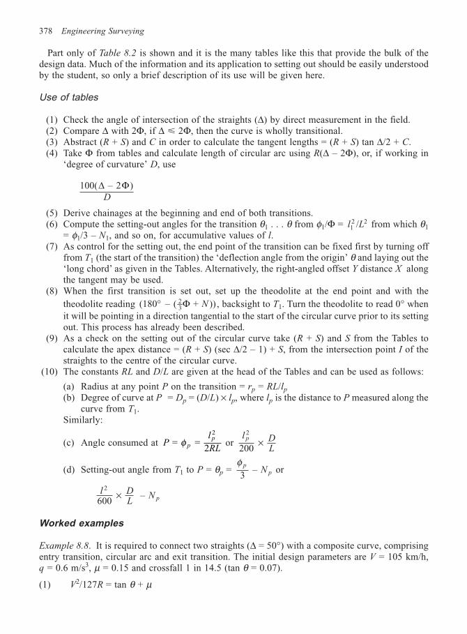
378 Engineering Surveying
Part only of Table 8.2 is shown and it is the many tables like this that provide the bulk of thedesign data. Much of the information and its application to setting out should be easily understoodby the student, so only a brief description of its use will be given here.
Use of tables
(1) Check the angle of intersection of the straights (∆) by direct measurement in the field.(2) Compare ∆ with 2Φ, if ∆ 2Φ, then the curve is wholly transitional.(3) Abstract (R + S) and C in order to calculate the tangent lengths = (R + S) tan ∆/2 + C.(4) Take Φ from tables and calculate length of circular arc using R(∆ – 2Φ), or, if working in
‘degree of curvature’ D, use
100( – 2 )∆ ΦD
(5) Derive chainages at the beginning and end of both transitions.(6) Compute the setting-out angles for the transition θ1 . . . θ from φ1/Φ = l L1
2 2/ from which θ1
= φ1/3 – N1, and so on, for accumulative values of l.(7) As control for the setting out, the end point of the transition can be fixed first by turning off
from T1 (the start of the transition) the ‘deflection angle from the origin’ θ and laying out the‘long chord’ as given in the Tables. Alternatively, the right-angled offset Y distance X alongthe tangent may be used.
(8) When the first transition is set out, set up the theodolite at the end point and with the
theodolite reading (180 – ( + ))23° Φ N , backsight to T1. Turn the theodolite to read 0° when
it will be pointing in a direction tangential to the start of the circular curve prior to its settingout. This process has already been described.
(9) As a check on the setting out of the circular curve take (R + S) and S from the Tables tocalculate the apex distance = (R + S) (sec ∆/2 – 1) + S, from the intersection point I of thestraights to the centre of the circular curve.
(10) The constants RL and D/L are given at the head of the Tables and can be used as follows:
(a) Radius at any point P on the transition = rp = RL/lp
(b) Degree of curve at P = Dp = (D/L) × lp, where lp is the distance to P measured along thecurve from T1.
Similarly:
(c) Angle consumed at Pl
RLpp
= = 2
2
φ or l D
L
p2
200×
(d) Setting-out angle from T1 to P = θp = φ p
pN3
– or
l DL
N p
2
600 – ×
Worked examples
Example 8.8. It is required to connect two straights (∆ = 50°) with a composite curve, comprisingentry transition, circular arc and exit transition. The initial design parameters are V = 105 km/h,q = 0.6 m/s3, µ = 0.15 and crossfall 1 in 14.5 (tan θ = 0.07).
(1) V2/127R = tan θ + µ
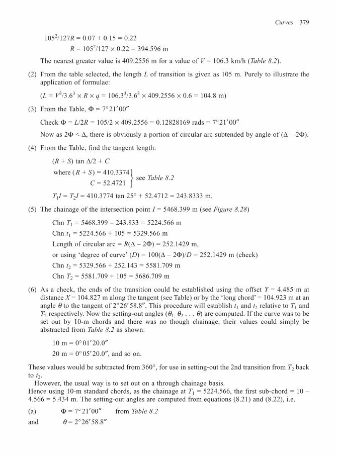
Curves 379
1052/127R = 0.07 + 0.15 = 0.22
R = 1052/127 × 0.22 = 394.596 m
The nearest greater value is 409.2556 m for a value of V = 106.3 km/h (Table 8.2).
(2) From the table selected, the length L of transition is given as 105 m. Purely to illustrate theapplication of formulae:
(L = V3/3.63 × R × q = 106.33/3.63 × 409.2556 × 0.6 = 104.8 m)
(3) From the Table, Φ = 7°21′ 00″
Check Φ = L/2R = 105/2 × 409.2556 = 0.12828169 rads = 7°21′ 00″
Now as 2Φ < ∆, there is obviously a portion of circular arc subtended by angle of (∆ – 2Φ).
(4) From the Table, find the tangent length:
(R + S) tan ∆/2 + C
where ( + ) = 410.3374
= 52.4721
R S
C
see Table 8.2
T1I = T2I = 410.3774 tan 25° + 52.4712 = 243.8333 m.
(5) The chainage of the intersection point I = 5468.399 m (see Figure 8.28)
Chn T1 = 5468.399 – 243.833 = 5224.566 m
Chn t1 = 5224.566 + 105 = 5329.566 m
Length of circular arc = R(∆ – 2Φ) = 252.1429 m,
or using ‘degree of curve’ (D) = 100(∆ – 2Φ)/D = 252.1429 m (check)
Chn t2 = 5329.566 + 252.143 = 5581.709 m
Chn T2 = 5581.709 + 105 = 5686.709 m
(6) As a check, the ends of the transition could be established using the offset Y = 4.485 m atdistance X = 104.827 m along the tangent (see Table) or by the ‘long chord’ = 104.923 m at anangle θ to the tangent of 2°26′ 58.8″. This procedure will establish t1 and t2 relative to T1 andT2 respectively. Now the setting-out angles (θ1, θ2 . . . θ) are computed. If the curve was to beset out by 10-m chords and there was no though chainage, their values could simply beabstracted from Table 8.2 as shown:
10 m = 0° 01′20.0″20 m = 0° 05′20.0″, and so on.
These values would be subtracted from 360°, for use in setting-out the 2nd transition from T2 backto t2.
However, the usual way is to set out on a through chainage basis.Hence using 10-m standard chords, as the chainage at T1 = 5224.566, the first sub-chord = 10 –4.566 = 5.434 m. The setting-out angles are computed from equations (8.21) and (8.22), i.e.
(a) Φ = 7° 21′00″ from Table 8.2
and θ = 2°26′58.8″
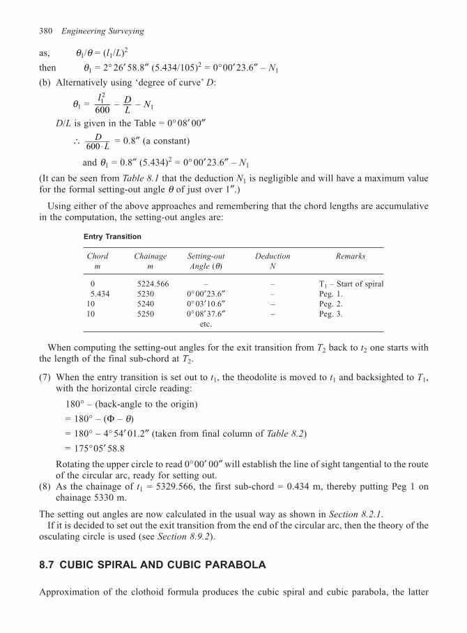
380 Engineering Surveying
as, θ1/θ = (l1/L)2
then θ1 = 2° 26′ 58.8″ (5.434/105)2 = 0°00′23.6″ – N1
(b) Alternatively using ‘degree of curve’ D:
θ1 = l D
LN1
2
1600 – –
D/L is given in the Table = 0° 08′ 00″
∴ DL600 ⋅ = 0.8″ (a constant)
and θ1 = 0.8″ (5.434)2 = 0° 00′23.6″ – N1
(It can be seen from Table 8.1 that the deduction N1 is negligible and will have a maximum valuefor the formal setting-out angle θ of just over 1″.)
Using either of the above approaches and remembering that the chord lengths are accumulativein the computation, the setting-out angles are:
Entry Transition
Chord Chainage Setting-out Deduction Remarks
m m Angle (θ) N
0 5224.566 – – T1 – Start of spiral5.434 5230 0°00′23.6″ – Peg. 1.
10 5240 0°03′10.6″ – Peg. 2.10 5250 0° 08′ 37.6″ – Peg. 3.
etc.
When computing the setting-out angles for the exit transition from T2 back to t2 one starts withthe length of the final sub-chord at T2.
(7) When the entry transition is set out to t1, the theodolite is moved to t1 and backsighted to T1,with the horizontal circle reading:
180° – (back-angle to the origin)
= 180° – (Φ – θ)
= 180° – 4° 54′ 01.2″ (taken from final column of Table 8.2)
= 175°05′ 58.8
Rotating the upper circle to read 0°00′ 00″ will establish the line of sight tangential to the routeof the circular arc, ready for setting out.
(8) As the chainage of t1 = 5329.566, the first sub-chord = 0.434 m, thereby putting Peg 1 onchainage 5330 m.
The setting out angles are now calculated in the usual way as shown in Section 8.2.1.If it is decided to set out the exit transition from the end of the circular arc, then the theory of the
osculating circle is used (see Section 8.9.2).
8.7 CUBIC SPIRAL AND CUBIC PARABOLA
Approximation of the clothoid formula produces the cubic spiral and cubic parabola, the latter
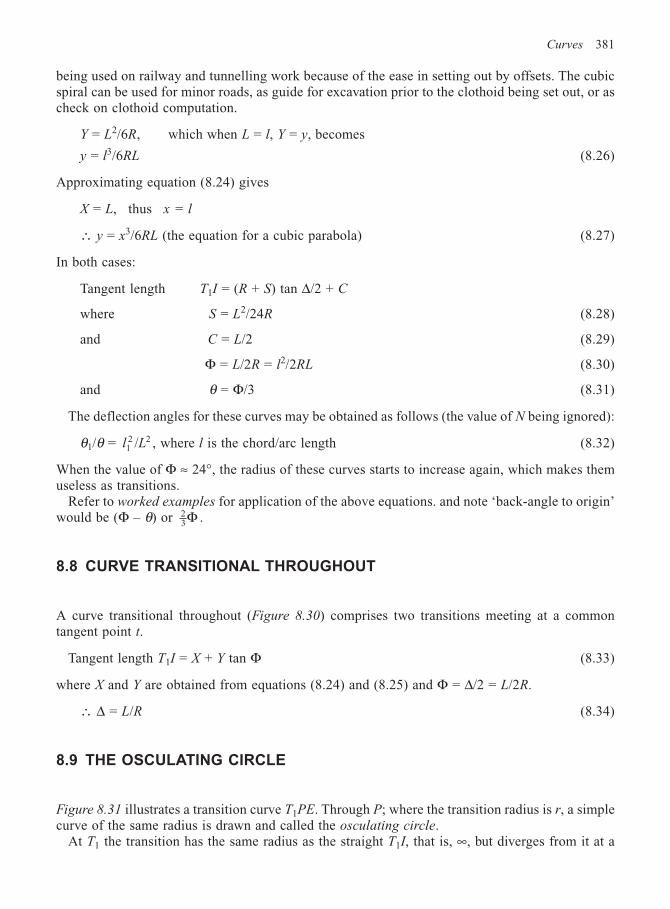
Curves 381
being used on railway and tunnelling work because of the ease in setting out by offsets. The cubicspiral can be used for minor roads, as guide for excavation prior to the clothoid being set out, or ascheck on clothoid computation.
Y = L2/6R, which when L = l, Y = y, becomes
y = l3/6RL (8.26)
Approximating equation (8.24) gives
X = L, thus x = l
∴ y = x3/6RL (the equation for a cubic parabola) (8.27)
In both cases:
Tangent length T1I = (R + S) tan ∆/2 + C
where S = L2/24R (8.28)
and C = L/2 (8.29)
Φ = L/2R = l2/2RL (8.30)
and θ = Φ/3 (8.31)
The deflection angles for these curves may be obtained as follows (the value of N being ignored):
θ1/θ = l L12 2/ , where l is the chord/arc length (8.32)
When the value of Φ ≈ 24°, the radius of these curves starts to increase again, which makes themuseless as transitions.
Refer to worked examples for application of the above equations. and note ‘back-angle to origin’would be (Φ – θ) or 2
3Φ .
8.8 CURVE TRANSITIONAL THROUGHOUT
A curve transitional throughout (Figure 8.30) comprises two transitions meeting at a commontangent point t.
Tangent length T1I = X + Y tan Φ (8.33)
where X and Y are obtained from equations (8.24) and (8.25) and Φ = ∆/2 = L/2R.
∴ ∆ = L/R (8.34)
8.9 THE OSCULATING CIRCLE
Figure 8.31 illustrates a transition curve T1PE. Through P; where the transition radius is r, a simplecurve of the same radius is drawn and called the osculating circle.
At T1 the transition has the same radius as the straight T1I, that is, ∞, but diverges from it at a
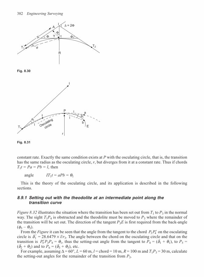
382 Engineering Surveying
constant rate. Exactly the same condition exists at P with the osculating circle, that is, the transitionhas the same radius as the osculating circle, r, but diverges from it at a constant rate. Thus if chordsT1t = Pa = Pb = l, then
angle IT1t = aPb = θ1
This is the theory of the osculating circle, and its application is described in the followingsections.
8.9.1 Setting out with the theodolite at an intermediate point along thetransition curve
Figure 8.32 illustrates the situation where the transition has been set out from T1 to P3 in the normalway. The sight T1P4 is obstructed and the theodolite must be moved to P3 where the remainder ofthe transition will be set out. The direction of the tangent P3E is first required from the back-angle(φ3 – θ3).
From the Figure it can be seen that the angle from the tangent to the chord P P3 4′ on the osculatingcircle is δ1
° = 28.6479 × l/r3. The angle between the chord on the osculating circle and that on thetransition is ′P4 P3P4 = θ1, thus the setting-out angle from the tangent to P4 = (δ1 + θ1), to P5 =(δ2 + θ2) and to P6 = (δ3 + θ3), etc.
For example, assuming ∆ = 60°, L = 60 m, l = chord = 10 m, R = 100 m and T1P3 = 30 m, calculatethe setting-out angles for the remainder of the transition from P3.
Fig. 8.30
T1
X
A
θ
ΦΦ
I
Φt
R
T2
∆ = 2Φ
Fig. 8.31
Y
r
Eb
l
lP
t
θ1
T1
θ1
Osculating
circle
a
I
l
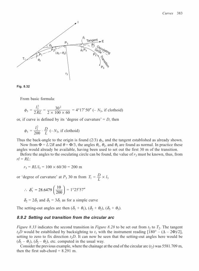
Curves 383
From basic formula:
φ332 2
= 2
= 302 100 60
l
RL × × = 4°17′ 50″ (– N3, if clothoid)
or, if curve is defined by its ‘degree of curvature’ = D, then
φ332
= 200
l DL
⋅ (– N3, if clothoid)
Thus the back-angle to the origin is found (2/3) φ3, and the tangent established as already shown.Now from Φ = L/2R and θ = Φ/3, the angles θ1, θ2, and θ3 are found as normal. In practice these
angles would already be available, having been used to set out the first 30 m of the transition.Before the angles to the osculating circle can be found, the value of r3 must be known, thus, from
rl = RL:
r3 = RL/l3 = 100 × 60/30 = 200 m
or ‘degree of curvature’ at P3 30 m from TDL
l1 3 = ×
∴ δ1 = 28.6479 °
10200
= 1°25′57″
δ2 = 2δ1 and δ3 = 3δ1 as for a simple curve
The setting-out angles are then (δ1 + θ1), (δ2 + θ2), (δ3 + θ3).
8.9.2 Setting out transition from the circular arc
Figure 8.33 indicates the second transition in Figure 8.28 to be set out from t2 to T2. The tangentt2D would be established by backsighting to t1 with the instrument reading [180° – (∆ – 2Φ)/2],setting to zero to fix direction t2D. It can now be seen that the setting-out angles here would be(δ1 – θ1), (δ2 – θ2), etc. computed in the usual way.
Consider the previous example, where the chainage at the end of the circular arc (t2) was 5581.709 m,then the first sub-chord = 8.291 m.
Fig. 8.32
T1
P1
θ3
φ3
P2(φ3 –θ3)
P3
θ1P4
P5
P6
Transition
circle
Osculating
δ1
I
Tangent
′P4
r3
E
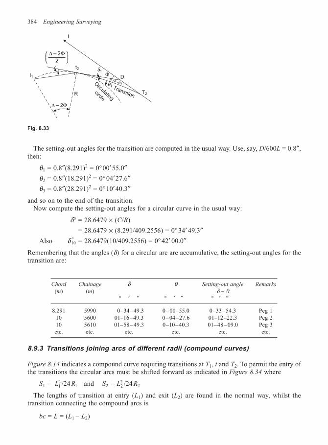
384 Engineering Surveying
The setting-out angles for the transition are computed in the usual way. Use, say, D/600L = 0.8″,then:
θ1 = 0.8″(8.291)2 = 0°00′55.0″θ2 = 0.8″(18.291)2 = 0°04′27.6″θ3 = 0.8″(28.291)2 = 0°10′40.3″
and so on to the end of the transition.Now compute the setting-out angles for a circular curve in the usual way:
δ° = 28.6479 × (C/R)
= 28.6479 × (8.291/409.2556) = 0°34′ 49.3″Also δ10
° = 28.6479(10/409.2556) = 0° 42′ 00.0″
Remembering that the angles (δ) for a circular arc are accumulative, the setting-out angles for thetransition are:
Chord Chainage δ θ Setting-out angle Remarks
(m) (m) δ – θ° ′ ″ ° ′ ″ ° ′ ″
8.291 5990 0–34–49.3 0– 00–55.0 0–33–54.3 Peg 110 5600 01–16–49.3 0– 04–27.6 01–12–22.3 Peg 210 5610 01–58– 49.3 0–10–40.3 01–48 –09.0 Peg 3etc. etc. etc. etc. etc. etc.
8.9.3 Transitions joining arcs of different radii (compound curves)
Figure 8.14 indicates a compound curve requiring transitions at T1, t and T2. To permit the entry ofthe transitions the circular arcs must be shifted forward as indicated in Figure 8.34 where
S1 = L R12
1/24 and S L R2 22
2= /24
The lengths of transition at entry (L1) and exit (L2) are found in the normal way, whilst thetransition connecting the compound arcs is
bc = L = (L1 – L2)
I
t1
t2
R
∆ – 2Φ
Osculating
circle
θ1 Transition
(δ–θ)
Φδ1
T2
D
Fig. 8.33
∆ – 2Φ2
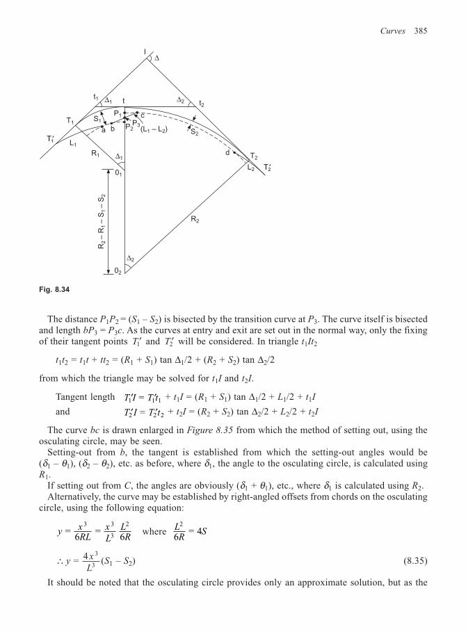
Curves 385
The distance P1P2 = (S1 – S2) is bisected by the transition curve at P3. The curve itself is bisectedand length bP3 = P3c. As the curves at entry and exit are set out in the normal way, only the fixingof their tangent points ′T1 and ′T2 will be considered. In triangle t1It2
t1t2 = t1t + tt2 = (R1 + S1) tan ∆1/2 + (R2 + S2) tan ∆2/2
from which the triangle may be solved for t1I and t2I.
Tangent length ′ ′T I T t1 1 1 = + t1I = (R1 + S1) tan ∆1/2 + L1/2 + t1I
and ′ ′T I T t2 2 2 = + t2I = (R2 + S2) tan ∆2/2 + L2/2 + t2I
The curve bc is drawn enlarged in Figure 8.35 from which the method of setting out, using theosculating circle, may be seen.
Setting-out from b, the tangent is established from which the setting-out angles would be(δ1 – θ1), (δ2 – θ2), etc. as before, where δ1, the angle to the osculating circle, is calculated usingR1.
If setting out from C, the angles are obviously (δ1 + θ1), etc., where δ1 is calculated using R2.Alternatively, the curve may be established by right-angled offsets from chords on the osculating
circle, using the following equation:
yxRL
x
L
LR
= 6
= 6
3 3
3
2
where LR
S2
6 = 4
∴ = 4 3
3y
x
L(S1 – S2) (8.35)
It should be noted that the osculating circle provides only an approximate solution, but as the
Fig. 8.34
∆I
∆2 t2
T2
L2
d
R2
∆2
02
R2
– R
1– S
1– S
2
01
∆1R1
L1
t1
T1
′T1
′T2
S1
P1
a b P2P3
(L1 – L2)
c
S2
∆1 t
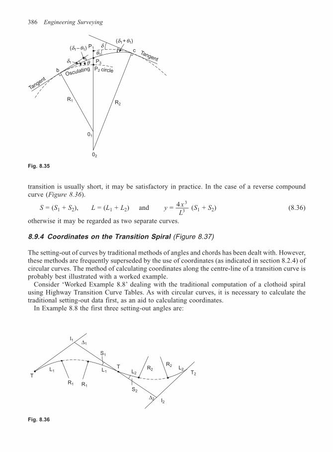
386 Engineering Surveying
transition is usually short, it may be satisfactory in practice. In the case of a reverse compoundcurve (Figure 8.36).
S = (S1 + S2), L = (L1 + L2) and yx
L = 4 3
3 (S1 + S2) (8.36)
otherwise it may be regarded as two separate curves.
8.9.4 Coordinates on the Transition Spiral (Figure 8.37)
The setting-out of curves by traditional methods of angles and chords has been dealt with. However,these methods are frequently superseded by the use of coordinates (as indicated in section 8.2.4) ofcircular curves. The method of calculating coordinates along the centre-line of a transition curve isprobably best illustrated with a worked example.
Consider ‘Worked Example 8.8’ dealing with the traditional computation of a clothoid spiralusing Highway Transition Curve Tables. As with circular curves, it is necessary to calculate thetraditional setting-out data first, as an aid to calculating coordinates.
In Example 8.8 the first three setting-out angles are:
Tangent
b
δ1
P1(δ1–θ1)
P3θ
θ1
δ(δ1+θ1)
c
R2R1
01
02
P2 circle
Tangent
Osculating
Fig. 8.35
T
L1
R1 R1
I1
S1
L2
S2
R2
R2L2
T2
I2∆2
L1
∆1
Fig. 8.36
T
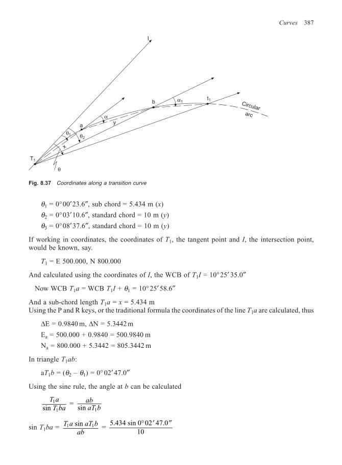
Curves 387
θ1 = 0°00′23.6″, sub chord = 5.434 m (x)
θ2 = 0°03′10.6″, standard chord = 10 m (y)
θ3 = 0°08′37.6″, standard chord = 10 m (y)
If working in coordinates, the coordinates of T1, the tangent point and I, the intersection point,would be known, say.
T1 = E 500.000, N 800.000
And calculated using the coordinates of I, the WCB of T1I = 10°25′ 35.0″
Now WCB T1a = WCB T1I + θ1 = 10° 25′ 58.6″
And a sub-chord length T1a = x = 5.434 mUsing the P and R keys, or the traditional formula the coordinates of the line T1a are calculated, thus
∆E = 0.9840 m, ∆N = 5.3442 m
Ea = 500.000 + 0.9840 = 500.9840 m
Na = 800.000 + 5.3442 = 805.3442 m
In triangle T1ab:
aT1b = (θ2 – θ1) = 0° 02′ 47.0″
Using the sine rule, the angle at b can be calculated
T a
T ba1
1sin = ab
aT bsin 1
sin T1ba = T a aT b
ab1 1 sin
= 5.434 sin 0 02 47.0
10° ′ ′′
Fig. 8.37 Coordinates along a transition curve
T1
t1Circular
arc
α1b
a
x
θ
α
θ1 θ2
y
I
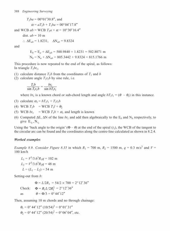
388 Engineering Surveying
T1ba = 00°01′30.8″, and
α = aT1b + T1ba = 00°04′17.8″and WCB ab = WCB T1a + α = 10°30′16.4″
dist. ab = 10 m
∴ ∆Eab = 1.8231, ∆Nab = 9.8324
and
Eb = Ea + ∆Eab = 500.9840 + 1.8231 = 502.8071 m
Nb = Na + ∆Nab = 805.3442 + 9.8324 = 815.1766 m
This procedure is now repeated to the end of the spiral, as follows:In triangle T1bt1,
(1) calculate distance T1b from the coordinates of T1 and b(2) calculate angle T1t1b by sine rule, i.e.
T b
T t b
bt
bT t1
1 1
1
1 1sin =
sin
where bt1 is a known chord or sub-chord length and angle bT1t1 = (θ – θ2) in this instance.
(3) calculate α1 = bT1t1 + T1t1b
(4) WCB T1b = WCB T1l + θ2
(5) WCB bt1 = WCB T1b + α1 and length is known
(6) Computed ∆E, ∆N of the line bt1 and add then algebraically to the Eb and Nb respectively, togive E , N
1 1t t
Using the ‘back angle to the origin’ (Φ – θ) at the end of the spiral (t1), the WCB of the tangent tothe circular arc can be found and the coordinates along the centre-line calculated as shown in 8.2.4.
Worked examples
Example 8.9. Consider Figure 8.35 in which R1 = 700 m, R2 = 1500 m, q = 0.3 m/s3 and V =100 km/h
L1 = V3/3.63R1q = 102 m
L2 = V3/3.63R2q = 48 m
L = (L1 – L2) = 54 m
Setting-out from b:
Φ = L/2R1 = 54/2 × 700 = 2°12′ 36″Check: Φ = /21 1
2R L R = 2°12′ 36″as θ = Φ/3 = 0° 44′ 12″
Then, assuming 10 m chords and no through chainage:
θ1 = 0° 44′ 12″ (10/54)2 = 0° 01′ 31″θ2 = 0° 44′ 12″ (20/54)2 = 0° 06′ 04″, etc.
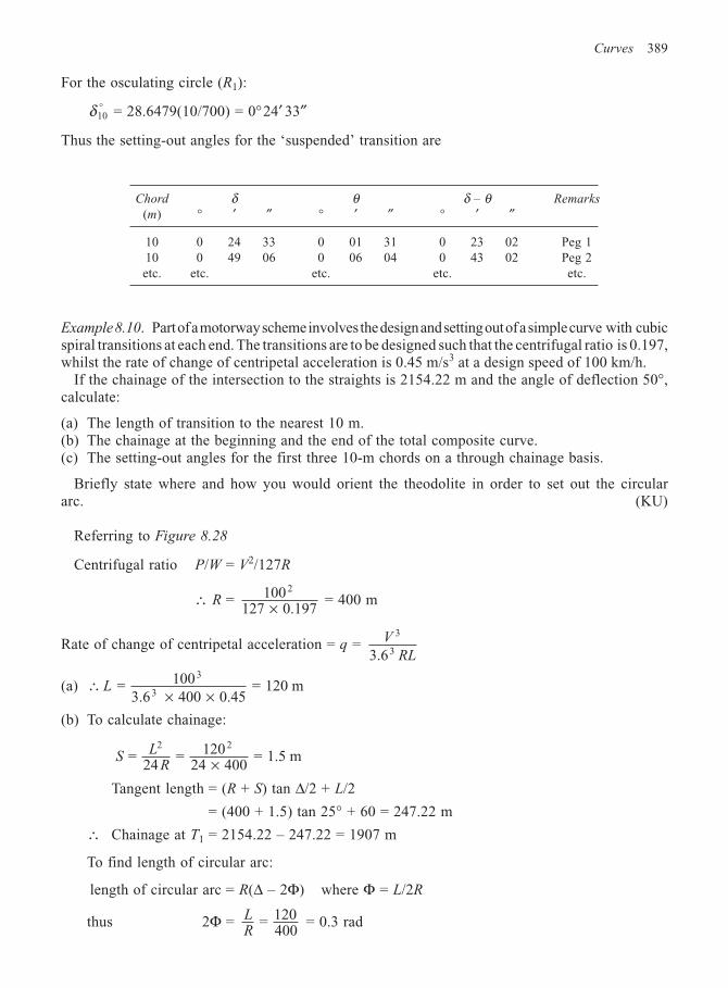
Curves 389
For the osculating circle (R1):
δ10° = 28.6479(10/700) = 0°24′ 33″
Thus the setting-out angles for the ‘suspended’ transition are
Chord δ θ δ – θ Remarks
(m) ° ′ ″ ° ′ ″ ° ′ ″
10 0 24 33 0 01 31 0 23 02 Peg 110 0 49 06 0 06 04 0 43 02 Peg 2etc. etc. etc. etc. etc.
Example 8.10. Part of a motorway scheme involves the design and setting out of a simple curve with cubicspiral transitions at each end. The transitions are to be designed such that the centrifugal ratio is 0.197,whilst the rate of change of centripetal acceleration is 0.45 m/s3 at a design speed of 100 km/h.
If the chainage of the intersection to the straights is 2154.22 m and the angle of deflection 50°,calculate:
(a) The length of transition to the nearest 10 m.(b) The chainage at the beginning and the end of the total composite curve.(c) The setting-out angles for the first three 10-m chords on a through chainage basis.
Briefly state where and how you would orient the theodolite in order to set out the circulararc. (KU)
Referring to Figure 8.28
Centrifugal ratio P/W = V2/127R
∴ R = 100127 0.197
2
× = 400 m
Rate of change of centripetal acceleration = q = V
RL
3
33.6
(a) ∴× ×100
3.6 400 0.45 = 120 m
3
3L =
(b) To calculate chainage:
SL
R =
24 = 120
24 400 = 1.5 m
2 2
×
Tangent length = (R + S) tan ∆/2 + L/2
= (400 + 1.5) tan 25° + 60 = 247.22 m
∴ Chainage at T1 = 2154.22 – 247.22 = 1907 m
To find length of circular arc:
length of circular arc = R(∆ – 2Φ) where Φ = L/2R
thus 2Φ = LR
= 120400
= 0.3 rad
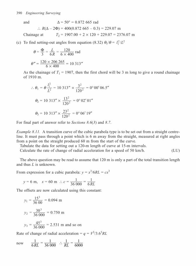
390 Engineering Surveying
and ∆ = 50° = 0.872 665 rad
∴ R(∆ – 2Φ) = 400(0.872 665 – 0.3) = 229.07 m
Chainage at T2 = 1907.00 + 2 × 120 + 229.07 = 2376.07 m
(c) To find setting-out angles from equation (8.32) θ1/θ = l L12 2/
θ = 3
= 6
= 1206 400
radΦ LR ×
′′ ×× ′′θ = 120 206 265
6 400 = 10 313
As the chainage of T1 = 1907, then the first chord will be 3 m long to give a round chainageof 1910 m.
∴ ′′ × = = 10 313 3120
112
2
2
2θ θ
l
L = 0° 00′ 06.5″
θ2 = 10 313″ × 13120
2
2 = 0° 02′ 01″
θ3 = 10 313″ × 23120
2
2 = 0° 06′ 19″
For final part of answer refer to Sections 8.6(3) and 8.7.
Example 8.11. A transition curve of the cubic parabola type is to be set out from a straight centre-line. It must pass through a point which is 6 m away from the straight, measured at right anglesfrom a point on the straight produced 60 m from the start of the curve.
Tabulate the data for setting out a 120-m length of curve at 15-m intervals.Calculate the rate of change of radial acceleration for a speed of 50 km/h. (LU)
The above question may be read to assume that 120 m is only a part of the total transition lengthand thus L is unknown.
From expression for a cubic parabola: y = x3/6RL = cx3
y = 6 m, x = 60 m = 136 000
= 16
∴ cRL
The offsets are now calculated using this constant:
y1
3
= 1536 00
= 0.094 m
y2
3
= 36 000
30 = 0.750 m
y3
3
= 36 000
45 = 2.531 m and so on
Rate of change of radial acceleration = q = V3/3.63RL
now1
6 = 1
36 000 1 = 1
6000RL RL∴
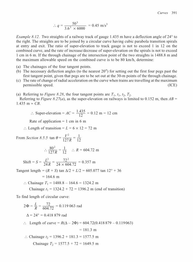
Curves 391
∴×
= 503.6 6000
3
3q = 0.45 m/s3
Example 8.12. Two straights of a railway track of gauge 1.435 m have a deflection angle of 24° tothe right. The straights are to be joined by a circular curve having cubic parabola transition spiralsat entry and exit. The ratio of super-elevation to track gauge is not to exceed 1 in 12 on thecombined curve, and the rate of increase/decrease of super-elevation on the spirals is not to exceed1 cm in 6 m. If the through chainage of the intersection point of the two straights is 1488.8 m andthe maximum allowable speed on the combined curve is to be 80 km/h, determine:
(a) The chainages of the four tangent points.(b) The necessary deflection angles (to the nearest 20″) for setting out the first four pegs past the
first tangent point, given that pegs are to be set out at the 30-m points of the through chainage.(c) The rate of change of radial acceleration on the curve when trains are travelling at the maximum
permissible speed. (ICE)
(a) Referring to Figure 8.28, the four tangent points are T1, t1, t2, T2.Referring to Figure 8.27(a), as the super-elevation on railways is limited to 0.152 m, then AB =
1.435 m ≈ CB.
∴ Super-elevation = AC = 1.43512
= 0.12 m = 12 cm
Rate of application = 1 cm in 6 m
∴ Length of transition = L = 6 × 12 = 72 m
From Section 8.5.5 tan = 127
= 112
2
θ VR
∴ 80 = 112
2
127R∴ R = 604.72 m
Shift = S = LR
2 2
24 = 72
24 604.72× = 0.357 m
Tangent length = (R + S) tan ∆/2 + L/2 = 605.077 tan 12° + 36
= 164.6 m
∴ Chainage T1 = 1488.8 – 164.6 = 1324.2 m
Chainage t1 = 1324.2 + 72 = 1396.2 m (end of transition)
To find length of circular curve:
2 = = 72604.72
Φ LR
= 0.119 063 rad
∆ = 24° = 0.418 879 rad
∴ Length of curve = R(∆ – 2Φ) = 604.72(0.418 879 – 0.119063)
= 181.3 m
∴ Chainage t2 = 1396.2 + 181.3 = 1577.5 m
Chainage T2 = 1577.5 + 72 = 1649.5 m
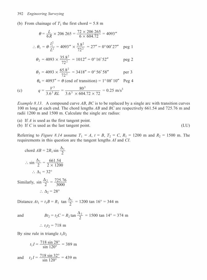
392 Engineering Surveying
(b) From chainage of T1 the first chord = 5.8 m
θ = 6
206 265 = 72 206 2656 604.72
= 4093LR
× ×× ′′
∴ ′′ × = = 4093 5.872
112 2
2θ θ
l
L2 = 27″ = 0° 00′ 27″ peg 1
θ 2
2
2 = 4093 35.8
72× = 1012″ = 0° 16′ 52″ peg 2
θ3
2
2 = 4093 65.8
72× = 3418″ = 0° 56′ 58″ per 3
θ4 = 4093″ = θ (end of transition) = 1° 08′ 10″ Peg 4
(c) qV
RL =
3.6 = 80
3.6 604.72 72
3
3
3
3 × × = 0.25 m/s3
Example 8.13. A compound curve AB, BC is to be replaced by a single arc with transition curves100 m long at each end. The chord lengths AB and BC are respectively 661.54 and 725.76 m andradii 1200 m and 1500 m. Calculate the single arc radius:
(a) If A is used as the first tangent point.(b) If C is used as the last tangent point. (LU)
Referring to Figure 8.14 assume T1 = A, t = B, T2 = C, R1 = 1200 m and R2 = 1500 m. Therequirements in this question are the tangent lengths AI and CI.
chord AB = 2R1 sin2
1∆
∴ × sin 2
= 661.542 1200
1∆
∴ ∆1 = 32°
Similarly, sin 2
= 725.763000
∆ 2
∴ ∆2 = 28°
Distance At1 = t1B = R1 tan2
∆1 = 1200 tan 16° = 344 m
and Bt2 = t2C = R2 tan2
∆ 2 = 1500 tan 14° = 374 m
∴ t1t2 = 718 m
By sine rule in triangle t1It2
t I1 = 718 sin 28sin 120
°° = 389 m
and t I2 = 718 sin 32sin 120
°° = 439 m
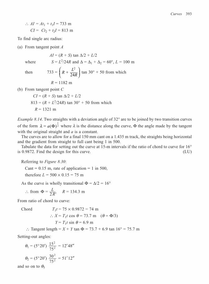
Curves 393
∴ AI = At1 + t1I = 733 m
CI = Ct2 + t2I = 813 m
To find single arc radius:
(a) From tangent point A
AI = (R + S) tan ∆/2 + L/2
where S = L2/24R and ∆ = ∆1 + ∆2 = 60°, L = 100 m
then 733 = RL
R +
24
2
tan 30° + 50 from which
R = 1182 m
(b) From tangent point C
CI = (R + S) tan ∆/2 + L/2
813 = (R + L2/24R) tan 30° + 50 from which
R = 1321 m
Example 8.14. Two straights with a deviation angle of 32° are to be joined by two transition curves
of the form λ = ( )12a Φ where λ is the distance along the curve, Φ the angle made by the tangent
with the original straight and a is a constant.The curves are to allow for a final 150 mm cant on a 1.435 m track, the straights being horizontal
and the gradient from straight to full cant being 1 in 500.Tabulate the data for setting out the curve at 15-m intervals if the ratio of chord to curve for 16°
is 0.9872. Find the design for this curve. (LU)
Referring to Figure 8.30:
Cant = 0.15 m, rate of application = 1 in 500,
therefore L = 500 × 0.15 = 75 m
As the curve is wholly transitional Φ = ∆/2 = 16°
∴ from Φ = 2
,LR
R = 134.3 m
From ratio of chord to curve:
Chord T1t = 75 × 0.9872 = 74 m
∴ X = T1t cos θ = 73.7 m (θ = Φ/3)
Y = T1t sin θ = 6.9 m
∴ Tangent length = X + Y tan Φ = 73.7 + 6.9 tan 16° = 75.7 m
Setting-out angles:
θ1 = (5°20′) 1575
2
2 = 12′48″
θ2 = (5°20′) 302
275 = 51′12″
and so on to θ5
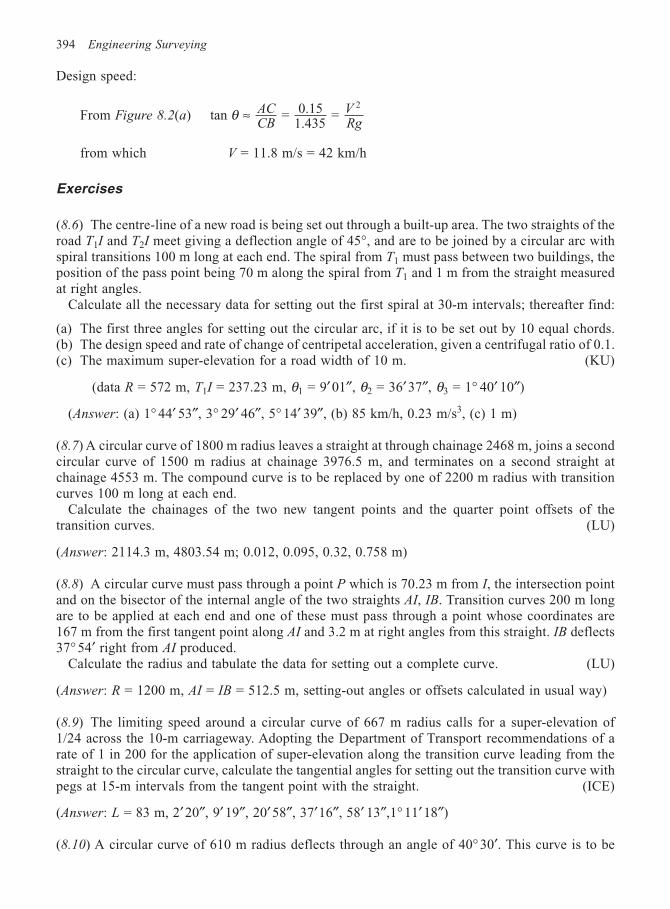
394 Engineering Surveying
Design speed:
From Figure 8.2(a) tan = 0.151.435
= 2
θ ≈ ACCB
VRg
from which V = 11.8 m/s = 42 km/h
Exercises
(8.6) The centre-line of a new road is being set out through a built-up area. The two straights of theroad T1I and T2I meet giving a deflection angle of 45°, and are to be joined by a circular arc withspiral transitions 100 m long at each end. The spiral from T1 must pass between two buildings, theposition of the pass point being 70 m along the spiral from T1 and 1 m from the straight measuredat right angles.
Calculate all the necessary data for setting out the first spiral at 30-m intervals; thereafter find:
(a) The first three angles for setting out the circular arc, if it is to be set out by 10 equal chords.(b) The design speed and rate of change of centripetal acceleration, given a centrifugal ratio of 0.1.(c) The maximum super-elevation for a road width of 10 m. (KU)
(data R = 572 m, T1I = 237.23 m, θ1 = 9′01″, θ2 = 36′37″, θ3 = 1° 40′ 10″)
(Answer: (a) 1° 44′ 53″, 3° 29′ 46″, 5° 14′ 39″, (b) 85 km/h, 0.23 m/s3, (c) 1 m)
(8.7) A circular curve of 1800 m radius leaves a straight at through chainage 2468 m, joins a secondcircular curve of 1500 m radius at chainage 3976.5 m, and terminates on a second straight atchainage 4553 m. The compound curve is to be replaced by one of 2200 m radius with transitioncurves 100 m long at each end.
Calculate the chainages of the two new tangent points and the quarter point offsets of thetransition curves. (LU)
(Answer: 2114.3 m, 4803.54 m; 0.012, 0.095, 0.32, 0.758 m)
(8.8) A circular curve must pass through a point P which is 70.23 m from I, the intersection pointand on the bisector of the internal angle of the two straights AI, IB. Transition curves 200 m longare to be applied at each end and one of these must pass through a point whose coordinates are167 m from the first tangent point along AI and 3.2 m at right angles from this straight. IB deflects37° 54′ right from AI produced.
Calculate the radius and tabulate the data for setting out a complete curve. (LU)
(Answer: R = 1200 m, AI = IB = 512.5 m, setting-out angles or offsets calculated in usual way)
(8.9) The limiting speed around a circular curve of 667 m radius calls for a super-elevation of1/24 across the 10-m carriageway. Adopting the Department of Transport recommendations of arate of 1 in 200 for the application of super-elevation along the transition curve leading from thestraight to the circular curve, calculate the tangential angles for setting out the transition curve withpegs at 15-m intervals from the tangent point with the straight. (ICE)
(Answer: L = 83 m, 2′20″, 9′ 19″, 20′58″, 37′16″, 58′ 13″,1° 11′ 18″)
(8.10) A circular curve of 610 m radius deflects through an angle of 40° 30′. This curve is to be
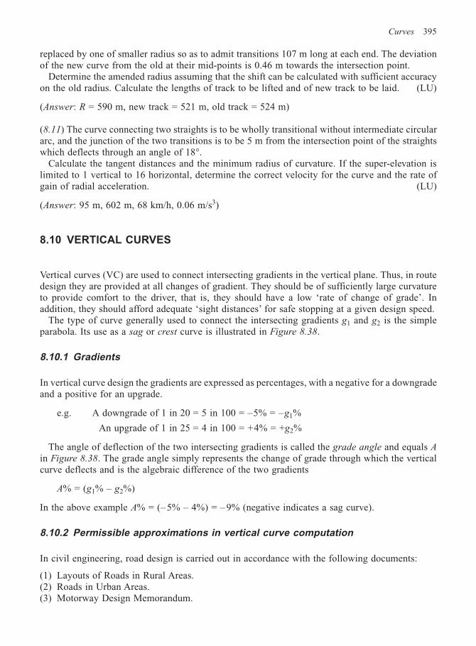
Curves 395
replaced by one of smaller radius so as to admit transitions 107 m long at each end. The deviationof the new curve from the old at their mid-points is 0.46 m towards the intersection point.
Determine the amended radius assuming that the shift can be calculated with sufficient accuracyon the old radius. Calculate the lengths of track to be lifted and of new track to be laid. (LU)
(Answer: R = 590 m, new track = 521 m, old track = 524 m)
(8.11) The curve connecting two straights is to be wholly transitional without intermediate circulararc, and the junction of the two transitions is to be 5 m from the intersection point of the straightswhich deflects through an angle of 18°.
Calculate the tangent distances and the minimum radius of curvature. If the super-elevation islimited to 1 vertical to 16 horizontal, determine the correct velocity for the curve and the rate ofgain of radial acceleration. (LU)
(Answer: 95 m, 602 m, 68 km/h, 0.06 m/s3)
8.10 VERTICAL CURVES
Vertical curves (VC) are used to connect intersecting gradients in the vertical plane. Thus, in routedesign they are provided at all changes of gradient. They should be of sufficiently large curvatureto provide comfort to the driver, that is, they should have a low ‘rate of change of grade’. Inaddition, they should afford adequate ‘sight distances’ for safe stopping at a given design speed.
The type of curve generally used to connect the intersecting gradients g1 and g2 is the simpleparabola. Its use as a sag or crest curve is illustrated in Figure 8.38.
8.10.1 Gradients
In vertical curve design the gradients are expressed as percentages, with a negative for a downgradeand a positive for an upgrade.
e.g. A downgrade of 1 in 20 = 5 in 100 = –5% = –g1%
An upgrade of 1 in 25 = 4 in 100 = +4% = +g2%
The angle of deflection of the two intersecting gradients is called the grade angle and equals Ain Figure 8.38. The grade angle simply represents the change of grade through which the verticalcurve deflects and is the algebraic difference of the two gradients
A% = (g1% – g2%)
In the above example A% = (– 5% – 4%) = – 9% (negative indicates a sag curve).
8.10.2 Permissible approximations in vertical curve computation
In civil engineering, road design is carried out in accordance with the following documents:
(1) Layouts of Roads in Rural Areas.(2) Roads in Urban Areas.(3) Motorway Design Memorandum.
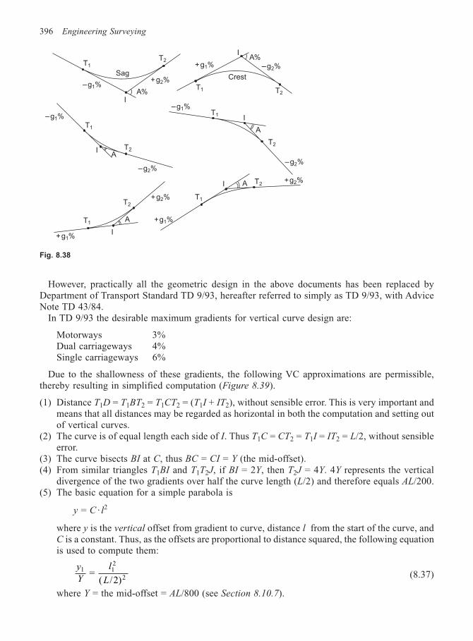
396 Engineering Surveying
However, practically all the geometric design in the above documents has been replaced byDepartment of Transport Standard TD 9/93, hereafter referred to simply as TD 9/93, with AdviceNote TD 43/84.
In TD 9/93 the desirable maximum gradients for vertical curve design are:
Motorways 3%Dual carriageways 4%Single carriageways 6%
Due to the shallowness of these gradients, the following VC approximations are permissible,thereby resulting in simplified computation (Figure 8.39).
(1) Distance T1D = T1BT2 = T1CT2 = (T1I + IT2), without sensible error. This is very important andmeans that all distances may be regarded as horizontal in both the computation and setting outof vertical curves.
(2) The curve is of equal length each side of I. Thus T1C = CT2 = T1I = IT2 = L/2, without sensibleerror.
(3) The curve bisects BI at C, thus BC = CI = Y (the mid-offset).(4) From similar triangles T1BI and T1T2J, if BI = 2Y, then T2J = 4Y. 4Y represents the vertical
divergence of the two gradients over half the curve length (L/2) and therefore equals AL/200.(5) The basic equation for a simple parabola is
y = C · l2
where y is the vertical offset from gradient to curve, distance l from the start of the curve, andC is a constant. Thus, as the offsets are proportional to distance squared, the following equationis used to compute them:
y
Y
l
L
1 12
2 =
( /2)(8.37)
where Y = the mid-offset = AL/800 (see Section 8.10.7).
T1
T2
Sag
–g1%
IA%
+g2%
IA%
–g2%
T2T1
Crest
–g1%T1
I
A
–g2%
T2
+g2%T2AI
T1
+g1%
+g2%T2
I
AT1
+g1%
–g1%
T1
IA
T2
–g2%
Fig. 8.38
+g1%
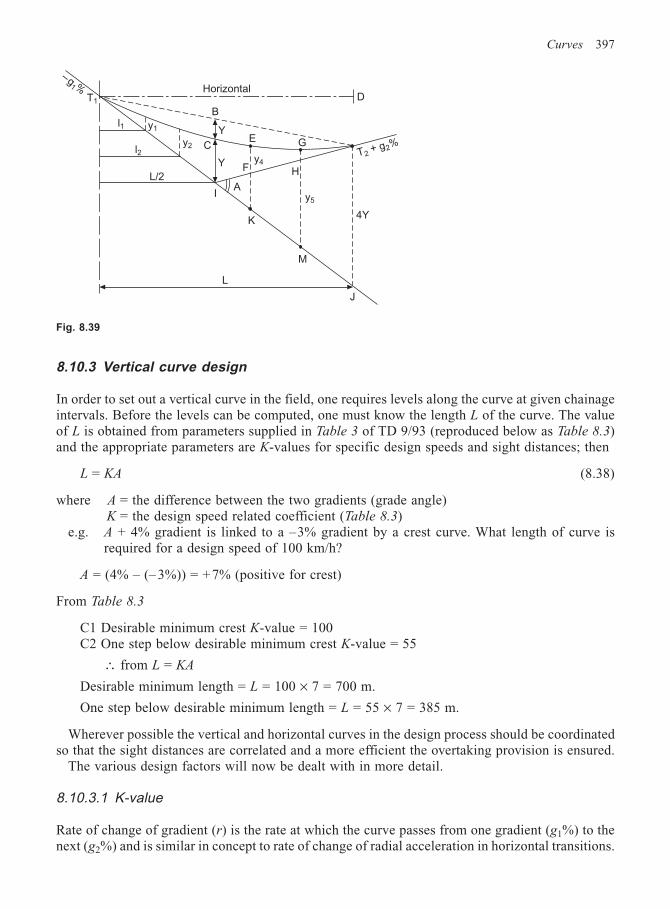
Curves 397
8.10.3 Vertical curve design
In order to set out a vertical curve in the field, one requires levels along the curve at given chainageintervals. Before the levels can be computed, one must know the length L of the curve. The valueof L is obtained from parameters supplied in Table 3 of TD 9/93 (reproduced below as Table 8.3)and the appropriate parameters are K-values for specific design speeds and sight distances; then
L = KA (8.38)
where A = the difference between the two gradients (grade angle)K = the design speed related coefficient (Table 8.3)
e.g. A + 4% gradient is linked to a –3% gradient by a crest curve. What length of curve isrequired for a design speed of 100 km/h?
A = (4% – (– 3%)) = +7% (positive for crest)
From Table 8.3
C1 Desirable minimum crest K-value = 100C2 One step below desirable minimum crest K-value = 55
∴ from L = KA
Desirable minimum length = L = 100 × 7 = 700 m.
One step below desirable minimum length = L = 55 × 7 = 385 m.
Wherever possible the vertical and horizontal curves in the design process should be coordinatedso that the sight distances are correlated and a more efficient the overtaking provision is ensured.
The various design factors will now be dealt with in more detail.
8.10.3.1 K-value
Rate of change of gradient (r) is the rate at which the curve passes from one gradient (g1%) to thenext (g2%) and is similar in concept to rate of change of radial acceleration in horizontal transitions.
–g1 %
T1
HorizontalD
B
y1
y2
y4
4Y
l1
l2
L/2
I
Y
C
Y
A
F
E G
M
K
H
y5
J
L
T2 + g2%
Fig. 8.39
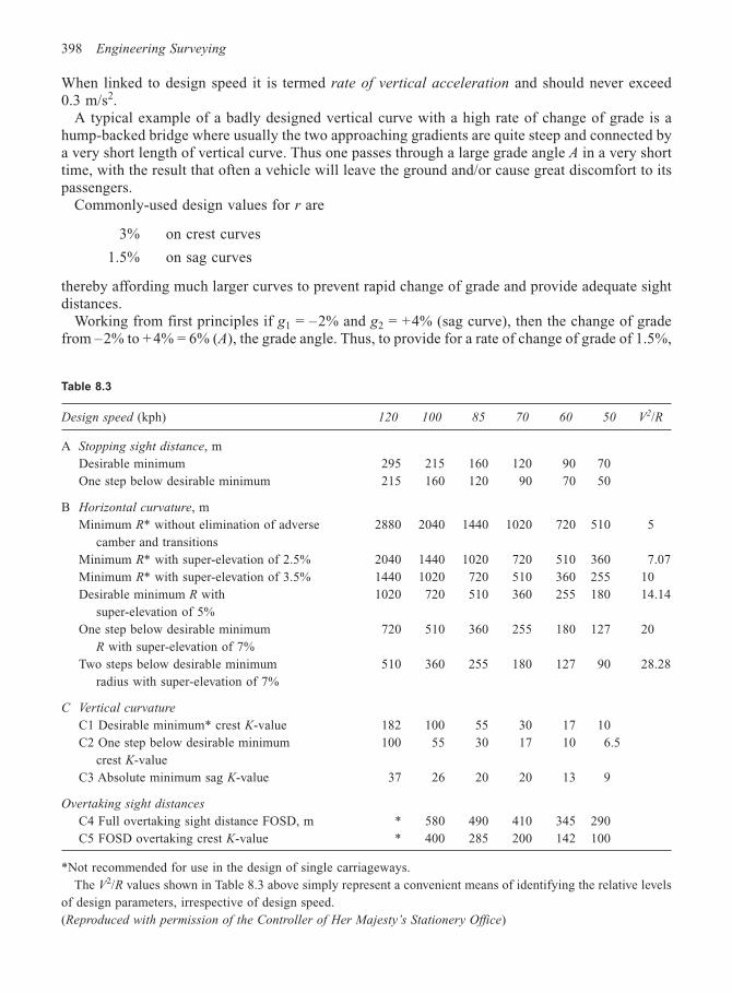
398 Engineering Surveying
When linked to design speed it is termed rate of vertical acceleration and should never exceed0.3 m/s2.
A typical example of a badly designed vertical curve with a high rate of change of grade is ahump-backed bridge where usually the two approaching gradients are quite steep and connected bya very short length of vertical curve. Thus one passes through a large grade angle A in a very shorttime, with the result that often a vehicle will leave the ground and/or cause great discomfort to itspassengers.
Commonly-used design values for r are
3% on crest curves
1.5% on sag curves
thereby affording much larger curves to prevent rapid change of grade and provide adequate sightdistances.
Working from first principles if g1 = –2% and g2 = +4% (sag curve), then the change of gradefrom –2% to + 4% = 6% (A), the grade angle. Thus, to provide for a rate of change of grade of 1.5%,
Table 8.3
Design speed (kph) 120 100 85 70 60 50 V2/R
A Stopping sight distance, m
Desirable minimum 295 215 160 120 90 70
One step below desirable minimum 215 160 120 90 70 50
B Horizontal curvature, m
Minimum R* without elimination of adverse 2880 2040 1440 1020 720 510 5
camber and transitions
Minimum R* with super-elevation of 2.5% 2040 1440 1020 720 510 360 7.07
Minimum R* with super-elevation of 3.5% 1440 1020 720 510 360 255 10
Desirable minimum R with 1020 720 510 360 255 180 14.14
super-elevation of 5%
One step below desirable minimum 720 510 360 255 180 127 20
R with super-elevation of 7%
Two steps below desirable minimum 510 360 255 180 127 90 28.28
radius with super-elevation of 7%
C Vertical curvature
C1 Desirable minimum* crest K-value 182 100 55 30 17 10
C2 One step below desirable minimum 100 55 30 17 10 6.5
crest K-value
C3 Absolute minimum sag K-value 37 26 20 20 13 9
Overtaking sight distances
C4 Full overtaking sight distance FOSD, m * 580 490 410 345 290
C5 FOSD overtaking crest K-value * 400 285 200 142 100
*Not recommended for use in the design of single carriageways.
The V2/R values shown in Table 8.3 above simply represent a convenient means of identifying the relative levels
of design parameters, irrespective of design speed.
(Reproduced with permission of the Controller of Her Majesty’s Stationery Office)
Curves 399
one would require 400 m (L) of curve. If the curve was a crest curve, then using 3% gives 200 m(L) of curve:
∴ L = 100A/r (8.39)
Now, expressing rate of change of grade as a single number we have
K = 100/r (8.40)
and as shown previously, L = KA.
8.10.3.2 Sight distances
Sight distance is a safety design factor which is intrinsically linked to rate of change of grade, andhence to K-values.
Consider once again the hump-backed bridge. Drivers approaching from each side of this particularvertical curve cannot see each other until they arrive, simultaneously, almost on the crest; by whichtime it may be too late to prevent an accident. Had the curve been longer and flatter, thus resultingin a low rate of change of grade, the drivers would have had a longer sight distance and consequentlymore time in which to take avoiding action.
Thus, sight distance, i.e. the length of road ahead that is visible to the driver, is a safety factor,and it is obvious that the sight distance must be greater than the stopping distance in which thevehicle can be brought to rest.
Stopping distance is dependent upon:
(1) Speed of the vehicle.(2) Braking efficiency.(3) Gradient.(4) Coefficient of friction between tyre and road.(5) Road conditions.(6) Driver’s reaction time.
In order to cater for all the above variables, the height of the driver’s eye above the road surfaceis taken as being only 1.05 m; a height applicable to sports cars whose braking efficiency is usuallyvery high. Thus, other vehicles, such as lorries, with a much greater eye height, would have a muchlonger sight distance in which to stop.
8.10.3.3 Sight distances on crests
Sight distances are defined as follows:
(1) Stopping sight distance (SSD) (Figure 8.40)
The SSD is the sight distance required by a driver to stop a vehicle when faced with an unexpectedobstruction on the carriageway. It comprises two elements:
(a) The perception-reaction distance, which is the distance travelled from the time the driver seesthe obstruction to the time it is realized that the vehicle must stop; and
(b) The braking distance, which is the distance travelled before the vehicle halts short of theobstruction.
The above are a function of driver age and fatigue, road conditions, etc. and thus the design
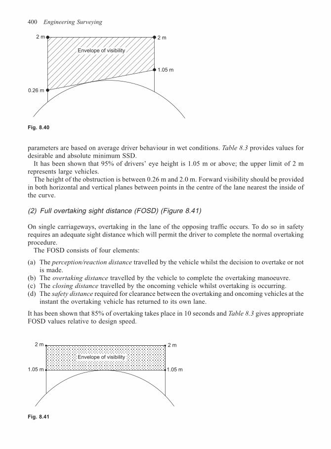
400 Engineering Surveying
parameters are based on average driver behaviour in wet conditions. Table 8.3 provides values fordesirable and absolute minimum SSD.
It has been shown that 95% of drivers’ eye height is 1.05 m or above; the upper limit of 2 mrepresents large vehicles.
The height of the obstruction is between 0.26 m and 2.0 m. Forward visibility should be providedin both horizontal and vertical planes between points in the centre of the lane nearest the inside ofthe curve.
(2) Full overtaking sight distance (FOSD) (Figure 8.41)
On single carriageways, overtaking in the lane of the opposing traffic occurs. To do so in safetyrequires an adequate sight distance which will permit the driver to complete the normal overtakingprocedure.
The FOSD consists of four elements:
(a) The perception/reaction distance travelled by the vehicle whilst the decision to overtake or notis made.
(b) The overtaking distance travelled by the vehicle to complete the overtaking manoeuvre.(c) The closing distance travelled by the oncoming vehicle whilst overtaking is occurring.(d) The safety distance required for clearance between the overtaking and oncoming vehicles at the
instant the overtaking vehicle has returned to its own lane.
It has been shown that 85% of overtaking takes place in 10 seconds and Table 8.3 gives appropriateFOSD values relative to design speed.
Fig. 8.40
Envelope of visibility
2 m
0.26 m
1.05 m
2 m
Fig. 8.41
Envelope of visibility
2 m 2 m
1.05 m1.05 m
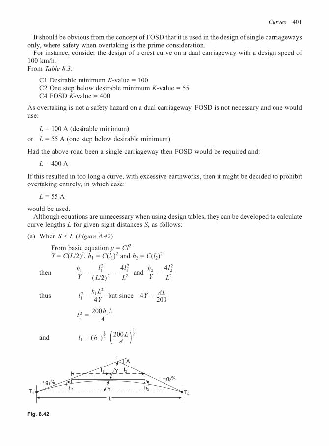
Curves 401
It should be obvious from the concept of FOSD that it is used in the design of single carriagewaysonly, where safety when overtaking is the prime consideration.
For instance, consider the design of a crest curve on a dual carriageway with a design speed of100 km/h.From Table 8.3:
C1 Desirable minimum K-value = 100C2 One step below desirable minimum K-value = 55C4 FOSD K-value = 400
As overtaking is not a safety hazard on a dual carriageway, FOSD is not necessary and one woulduse:
L = 100 A (desirable minimum)
or L = 55 A (one step below desirable minimum)
Had the above road been a single carriageway then FOSD would be required and:
L = 400 A
If this resulted in too long a curve, with excessive earthworks, then it might be decided to prohibitovertaking entirely, in which case:
L = 55 A
would be used.Although equations are unnecessary when using design tables, they can be developed to calculate
curve lengths L for given sight distances S, as follows:
(a) When S < L (Figure 8.42)
From basic equation y = Cl2
Y = C(L/2)2, h1 = C(l1)2 and h2 = C(l2)2
thenh
Y
l
L
l
L
1 12
212
2 =
( /2) =
4 and
h
Y
l
L
2 22
2 =
4
thus = 41
2 12
lh L
Y but since 4 =
200Y
AL
lh L
A12 1 =
200
and l hL
A1 1 = ( ) 200112
2 ( )
Fig. 8.42
IA
l2
h2
Y
Y
L
T2T1
+g1%h1
l1
–g2%
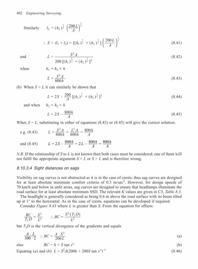
402 Engineering Surveying
Similarly l hL
A2 2 = ( ) 200112
2 ( )∴ S = (l1 + l2) = [( ) + ( ) ]
2001 2
12
12
12
h hL
A
(8.41)
and LS A
h h
= 200 [( ) + ( ) ]
2
1 22
12
12
(8.42)
when h1 = h2 = h
LS A
h =
800
2
(8.43)
(b) When S > L it can similarly be shown that
L SA
h h = 2 – 200 [( ) + ( ) ]1 22
12
12 (8.44)
and when h1 = h2 = h
L Sh
A = 2 – 800 (8.45)
When S = L, substituting in either of equations (8.43) or (8.45) will give the correct solution.
e.g. (8.43) LS A
hL A
hh
A =
800 =
800 = 8002 2
and (8.45) L Sh
AL
hA
hA
= 2 – 800 = 2 – 800 = 800
N.B. If the relationship of S to L is not known then both cases must be considered; one of them willnot fulfil the appropriate argument S < L or S > L and is therefore wrong.
8.10.3.4 Sight distances on sags
Visibility on sag curves is not obstructed as it is in the case of crests; thus sag curves are designedfor at least absolute minimum comfort criteria of 0.3 m/sec2. However, for design speeds of70 km/h and below in unlit areas, sag curves are designed to ensure that headlamps illuminate theroad surface for at least absolute minimum SSD. The relevant K values are given in C3, Table 8.3.
The headlight is generally considered as being 0.6 m above the road surface with its beam tiltedup at 1° to the horizontal. As in the case of crests, equations can be developed if required.
Consider Figure 8.43 where L is greater than S. From the equation for offsets:
BCT D
S
L2
2
2 = ∴ =
( )22BC
S T D
L2
but T2D is the vertical divergence of the gradients and equals
A L⋅⋅100 2
∴ ⋅ = 200
2
BCA S
L(a)
also BC = h + S tan x° (b)
Equating (a) and (b): L = S2A(200h + 200S tan x°)–1 (8.46)
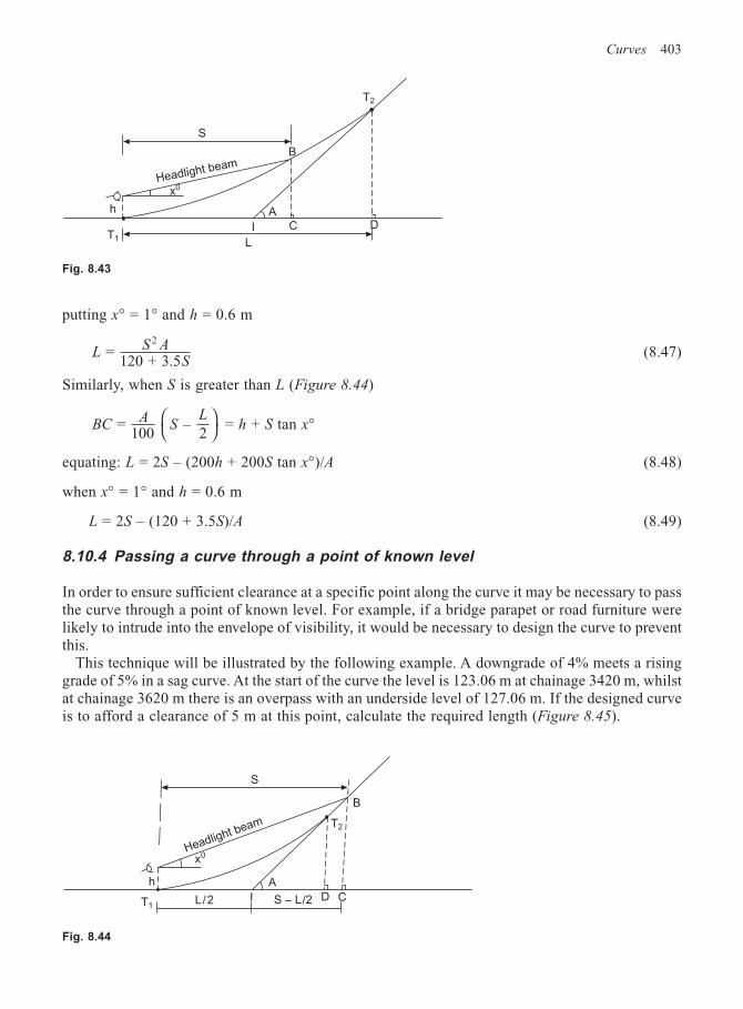
Curves 403
S
Headlight beam
h
T1
x0
C DA
B
T2
I
L
Fig. 8.43
putting x° = 1° and h = 0.6 m
LS A
S =
120 + 3.5
2
(8.47)
Similarly, when S is greater than L (Figure 8.44)
BCA
SL
= 100
– 2
= h + S tan x°
equating: L = 2S – (200h + 200S tan x°)/A (8.48)
when x° = 1° and h = 0.6 m
L = 2S – (120 + 3.5S)/A (8.49)
8.10.4 Passing a curve through a point of known level
In order to ensure sufficient clearance at a specific point along the curve it may be necessary to passthe curve through a point of known level. For example, if a bridge parapet or road furniture werelikely to intrude into the envelope of visibility, it would be necessary to design the curve to preventthis.
This technique will be illustrated by the following example. A downgrade of 4% meets a risinggrade of 5% in a sag curve. At the start of the curve the level is 123.06 m at chainage 3420 m, whilstat chainage 3620 m there is an overpass with an underside level of 127.06 m. If the designed curveis to afford a clearance of 5 m at this point, calculate the required length (Figure 8.45).
Fig. 8.44
S
Headlight beam
h
T1L/2 I
A
S – L/2 CD
T2
B
x0
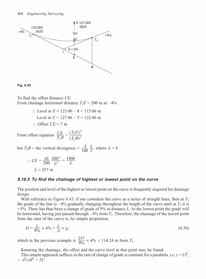
404 Engineering Surveying
To find the offset distance CE:From chainage horizontal distance T1E = 200 m at – 4%
∴ Level at E = 123.06 – 8 = 115.06 m
Level at C = 127.06 – 5 = 122.06 m
∴ Offset CE = 7 m
From offset equation CET B
T E
T B2
12
12
= ( )
( )
but T2B = the vertical divergence = A L100 2
, where A = 9
∴200
200 = 18002
2CE =
AL
L L
L = 257 m
8.10.5 To find the chainage of highest or lowest point on the curve
The position and level of the highest or lowest point on the curve is frequently required for drainagedesign.
With reference to Figure 8.45, if one considers the curve as a series of straight lines, then at T1
the grade of the line is – 4% gradually changing throughout the length of the curve until at T2 it is+5%. There has thus been a change of grade of 9% in distance L. At the lowest point the grade willbe horizontal, having just passed through – 4% from T1. Therefore, the chainage of the lowest pointfrom the start of the curve is, by simple proportion,
DL L
Ag =
9% 4% = 1× × (8.50)
which in the previous example is 2579%
4%× = 114.24 m from T1.
Knowing the chainage, the offset and the curve level at that point may be found.This simple approach suffices as the rate of change of grade is constant for a parabola, i.e. y = Cl2,
∴ d2y/dl2 = 2C.
Fig. 8.45
D 127.060
3620
5m
C
E
IA = 9%
B
T2
+5%T1
–4%
123.060
3420
Curves 405
8.10.6 Vertical curve radius
Due to the very shallow gradients involved in VC design, the parabola may be approximated to acircular curve. In this way vertical curves may be expediently drawn on longitudinal sections usingrailway curves of a given radius, and vertical accelerations (V2/R) easily assessed.
In circular curves (Section 8.1) the main chord from T1 to T2 = 2R sin ∆/2, where ∆ is thedeflection angle of the two straights. In vertical curves, the main chord may be approximated to thelength (L) of the VC and the angle ∆ to the grade angle A, i.e.
∆ ≈ A%
∴ sin ∆ /2 ≈ ∆ /2 rads ≈ A/200
∴ L ≈ 2RA/200 = AR/100 (8.51)
and as K = L/A = R/100, then:
R = 100L/A = 100K (8.52)
It is important to note that the reduced levels of VC must always be computed. Scaling levelsfrom a longitudinal section, usually having a vertical scale different from the horizontal, willproduce a curve that is neither parabolic nor circular. The use of railway curves is simply to indicatethe position and extent of the curve on the section.
Thus, having obtained the radius R of the VC, it is required to know the number of the railwaycurve necessary to draw it on the longitudinal section.
If the horizontal scale of the section is 1 in H and the vertical scale is 1 in V, then the number ofthe railway curve required to draw the VC is:
Number of railway curve in mm = R · V/H2, with R in mm
e.g. If horizontal scale is 1 in 500, vertical scale 1 in 100 and curve radius is 200 m, then
Number of railway curve in mm = 200 000 × 100/5002 = 80
8.10.7 Vertical curve computation
The computation of a vertical curve will now be demonstrated using an example.A ‘2nd difference’ (δ2y/δl2) arithmetical check on the offset computation should automatically be
applied. The check works on the principle that the change of grade of a parabola (y = C · l2) isconstant, i.e. δ2y/δl2 = 2C. Thus, if the first and last chords are sub-chords of lengths different fromthe remaining standard chords, then the change of grade will be constant only for the equal-lengthchords.
For example, a 100-m curve is to connect a downgrade of 0.75% to an upgrade of 0.25%. If thelevel of the intersection point of the two grades is 150 m, calculate:
(1) Curve levels at 20-m intervals, showing the second difference (d2y/dl2) check on the computations.(2) The position and level of the lowest point on the curve.
Method
(a) Find the value of the central offset Y.(b) Calculate offsets.(c) Calculate levels along the gradients.(d) Add/subtract (b) from (c) to get curve levels.
406 Engineering Surveying
(a) Referring to Figure 8.39:Grade angle A = (–0.75 – 0.25) = – 1% (this is seen automatically).
L/2 = 50 m, thus as the grades IT2, and IJ are diverging at the rate of 1% (1 m per 100 m) in50 m, then
T2J = 0.5 m = 4Y and Y = 0.125 m
The computation can be quickly worked mentally by the student. Putting the above thinking intoequation form gives
4 = 100 2
YA L ∴ =
800Y
AL = 1 100800
= 0.125×(8.53)
(b) Offsets from equation (8.37):There are two methods of approach.
(1) The offsets may be calculated from one gradient throughout; i.e. y1, y2, EK, GM, T2J, from thegrade T1J.
(2) Calculate the offsets from one grade, say, T1I, the offsets being equal on the other side from theother grade IT2.
Method (1) is preferred due to the smaller risk of error when calculating curve levels at a constantinterval and grade down T1J.
From equation (8.37): y Yl
L1
12
2 =
( /2)×
1st diff. 2nd diff.
T1 = 0 m———— 0.02
y1 = 0.125 2050
2
2 = 0.02 m ———— 0.04
———— 0.06
y2 = 0.125 4050
2
2 = 0.08 m ———— 0.04
———— 0.10
y3 = 0.125 6050
2
2 = 0.18 m ———— 0.04
———— 0.14
y4 = 0.125 8050
2
2 = 0.32 m ———— 0.04
———— 0.18y2 = T2J = 4Y = 0.50 m
The 2nd difference arithmetical check, which works only for equal chords, should be applied beforeany further computation.
(c) First find level at T1 from known level at I:
Distance from I to T1 = 50 m, grade = 0.75% (0.75 m per 100 m)
Curves 407
∴ Rise in level from I to T1 = 0.752
= 0.375 m
Level at T1 = 150.000 + 0.375 = 150.375 m
Levels are now calculated at 20-m intervals along T1J, the fall being 0.15 m in 20 m. Thus, thefollowing table may be made.
Chainage Gradient Offsets Curve Remarks
(m) levels levels
0 150.375 0 150.375 Start of curve T1
20 150.225 0.02 150.24540 150.075 0.08 150.15560 149.925 0.18 150.10580 149.775 0.32 150.095
100 149.625 0.50 150.125 End of curve T2
Position of lowest point on curve = 100 m1%
× 0.75% = 75 m from T1
∴ Offset at this point = y2 = 0.125 × 752/502 = 0.281 m
Tangent level 75 m from T1 = 150.375 – 0.563 = 149.812 m
∴ Curve level = 149.812 + 0.281 = 150.093 m
8.10.8 Drawing-office practice
(1) Design
(a) Obtain grade angle (algebraic difference of the gradients) A.(b) Extract the appropriate K-value from Design Table in TD 9/93.(c) Length (L) of vertical curve = KA.(d) Compute offsets and levels in the usual way.
(2) Drawing
To select the correct railway curve for drawing the vertical curve on a longitudinal section.
(a) Find equivalent radius (R) of vertical curve from RL
AK= 100 = 100 ⋅ ⋅ .
(b) Number of railway curve in mm = R mm × V/H2.
If horizontal scale of section is say 1/500, then H = 500.If vertical scale of section is say 1/200, then V = 200.If the railway curves used are still in inches, simply express R in inches.
8.10.9 Computer-aided drawing and design (CADD)
The majority of survey packages now available contain a road design module, whilst highly specializedprograms such as BIPS (British Integrated Program System) and MOSS (modelling systems) arestandard tools in many road design offices.
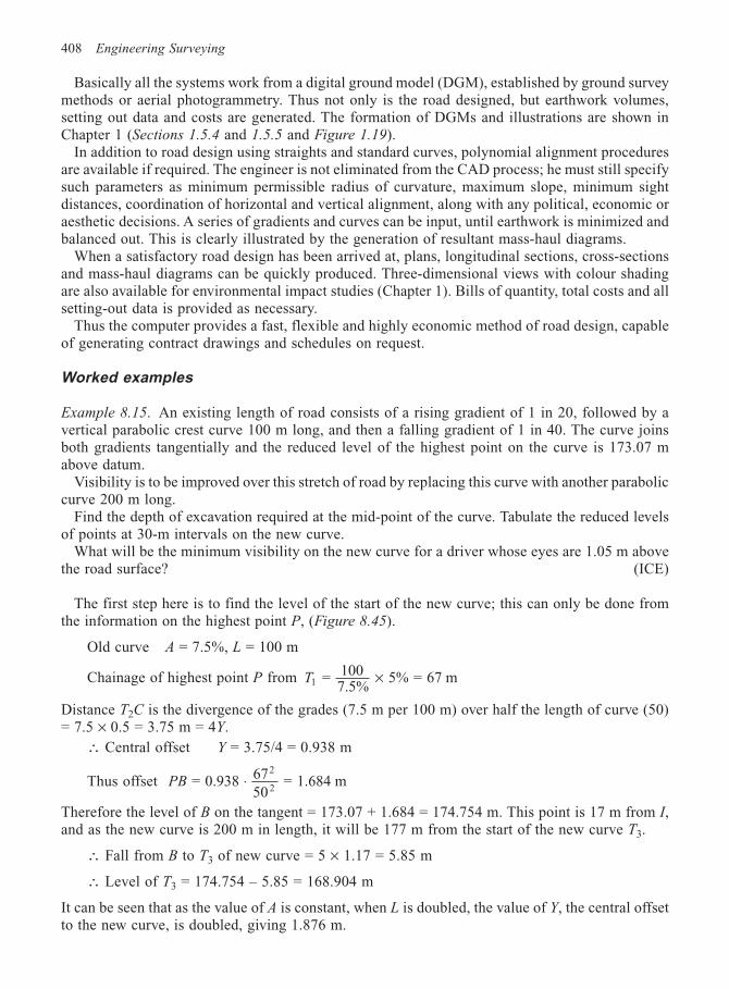
408 Engineering Surveying
Basically all the systems work from a digital ground model (DGM), established by ground surveymethods or aerial photogrammetry. Thus not only is the road designed, but earthwork volumes,setting out data and costs are generated. The formation of DGMs and illustrations are shown inChapter 1 (Sections 1.5.4 and 1.5.5 and Figure 1.19).
In addition to road design using straights and standard curves, polynomial alignment proceduresare available if required. The engineer is not eliminated from the CAD process; he must still specifysuch parameters as minimum permissible radius of curvature, maximum slope, minimum sightdistances, coordination of horizontal and vertical alignment, along with any political, economic oraesthetic decisions. A series of gradients and curves can be input, until earthwork is minimized andbalanced out. This is clearly illustrated by the generation of resultant mass-haul diagrams.
When a satisfactory road design has been arrived at, plans, longitudinal sections, cross-sectionsand mass-haul diagrams can be quickly produced. Three-dimensional views with colour shadingare also available for environmental impact studies (Chapter 1). Bills of quantity, total costs and allsetting-out data is provided as necessary.
Thus the computer provides a fast, flexible and highly economic method of road design, capableof generating contract drawings and schedules on request.
Worked examples
Example 8.15. An existing length of road consists of a rising gradient of 1 in 20, followed by avertical parabolic crest curve 100 m long, and then a falling gradient of 1 in 40. The curve joinsboth gradients tangentially and the reduced level of the highest point on the curve is 173.07 mabove datum.
Visibility is to be improved over this stretch of road by replacing this curve with another paraboliccurve 200 m long.
Find the depth of excavation required at the mid-point of the curve. Tabulate the reduced levelsof points at 30-m intervals on the new curve.
What will be the minimum visibility on the new curve for a driver whose eyes are 1.05 m abovethe road surface? (ICE)
The first step here is to find the level of the start of the new curve; this can only be done fromthe information on the highest point P, (Figure 8.45).
Old curve A = 7.5%, L = 100 m
Chainage of highest point P from T1 = 1007.5%
5% = 67 m×
Distance T2C is the divergence of the grades (7.5 m per 100 m) over half the length of curve (50)= 7.5 × 0.5 = 3.75 m = 4Y.
∴ Central offset Y = 3.75/4 = 0.938 m
Thus offset PB = 0.938 6750
= 1.684 m2
2⋅
Therefore the level of B on the tangent = 173.07 + 1.684 = 174.754 m. This point is 17 m from I,and as the new curve is 200 m in length, it will be 177 m from the start of the new curve T3.
∴ Fall from B to T3 of new curve = 5 × 1.17 = 5.85 m
∴ Level of T3 = 174.754 – 5.85 = 168.904 m
It can be seen that as the value of A is constant, when L is doubled, the value of Y, the central offsetto the new curve, is doubled, giving 1.876 m.
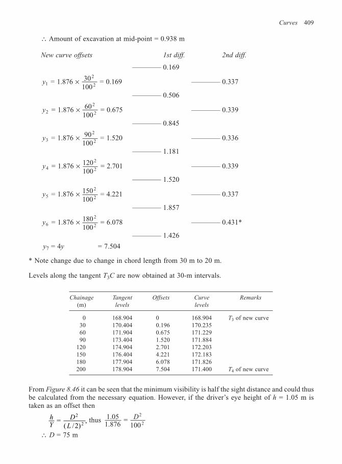
Curves 409
∴ Amount of excavation at mid-point = 0.938 m
New curve offsets 1st diff. 2nd diff.
———— 0.169
y1
2
2 = 1.876 30
100 = 0.169× ———— 0.337
———— 0.506
y2
2
2 = 1.876 60
100 = 0.675× ———— 0.339
———— 0.845
y3
2
2 = 1.876 90
100 = 1.520× ———— 0.336
———— 1.181
y4
2
2 = 1.876 120
100 = 2.701× ———— 0.339
———— 1.520
y5
2
2 = 1.876 150
100 = 4.221× ———— 0.337
———— 1.857
y6
2
2 = 1.876 180
100 = 6.078× ———— 0.431*
———— 1.426
y7 = 4y = 7.504
* Note change due to change in chord length from 30 m to 20 m.
Levels along the tangent T3C are now obtained at 30-m intervals.
Chainage Tangent Offsets Curve Remarks
(m) levels levels
0 168.904 0 168.904 T3 of new curve30 170.404 0.196 170.23560 171.904 0.675 171.22990 173.404 1.520 171.884
120 174.904 2.701 172.203150 176.404 4.221 172.183180 177.904 6.078 171.826200 178.904 7.504 171.400 T4 of new curve
From Figure 8.46 it can be seen that the minimum visibility is half the sight distance and could thusbe calculated from the necessary equation. However, if the driver’s eye height of h = 1.05 m istaken as an offset then
hY
D
L =
( /2),
2
2thus 1.05
1.876 =
100
2
2D
∴ D = 75 m
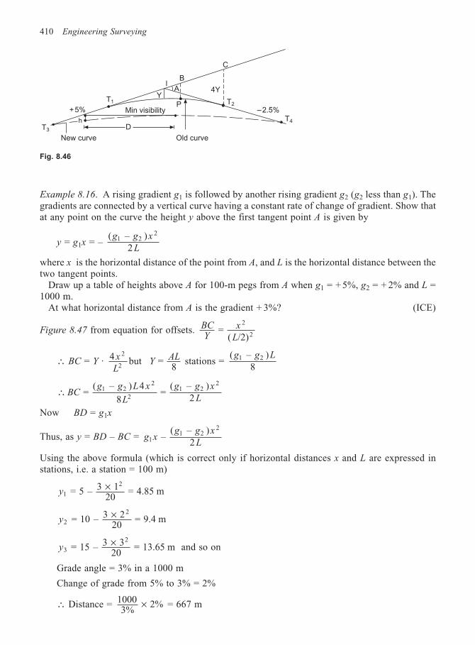
410 Engineering Surveying
Example 8.16. A rising gradient g1 is followed by another rising gradient g2 (g2 less than g1). Thegradients are connected by a vertical curve having a constant rate of change of gradient. Show thatat any point on the curve the height y above the first tangent point A is given by
y = g1x = – ( – )
21 2
2g g x
L
where x is the horizontal distance of the point from A, and L is the horizontal distance between thetwo tangent points.
Draw up a table of heights above A for 100-m pegs from A when g1 = + 5%, g2 = + 2% and L =1000 m.
At what horizontal distance from A is the gradient + 3%? (ICE)
Figure 8.47 from equation for offsets. BCY
x
L =
( /2)
2
2
∴ BC = Y · 4 2
2x
Lbut Y
AL = 8
stations = ( – )
81 2g g L
∴ = ( – ) 4
8 =
( – )2
1 22
21 2
2
BCg g L x
L
g g x
L
Now BD = g1x
Thus, as y = BD – BC = g xg g x
L11 2
2
– ( – )
2
Using the above formula (which is correct only if horizontal distances x and L are expressed instations, i.e. a station = 100 m)
y1
2
= 5 – 3 120
= 4.85 m×
y2
2
= 10 – 3 220
= 9.4 m×
y3
2
= 15 – 3 320
= 13.65 m× and so on
Grade angle = 3% in a 1000 m
Change of grade from 5% to 3% = 2%
∴ Distance = 10003%
2%× = 667 m
Fig. 8.46
C
T2
–2.5%T4
4Y
Bl
T1
Min visibility
D
New curve
T3
+5%
Old curve
P
AY
h
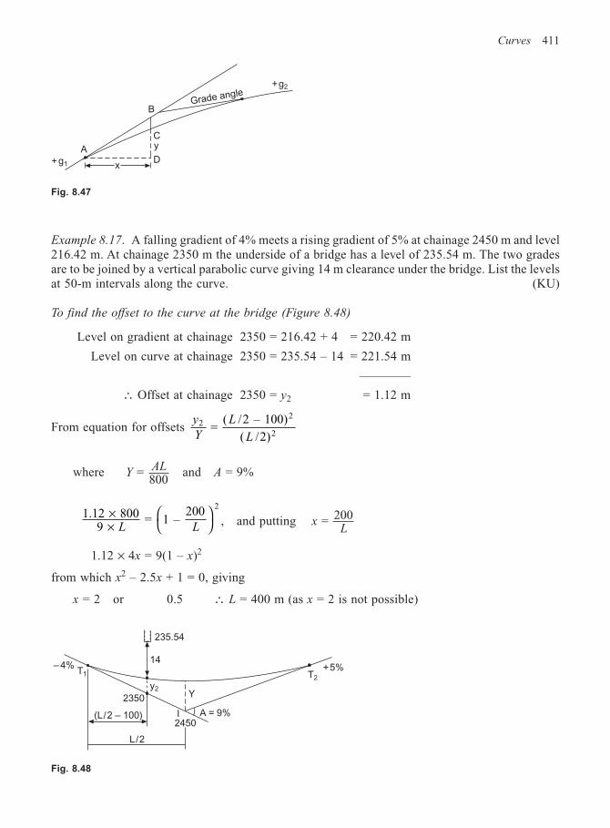
Curves 411
Example 8.17. A falling gradient of 4% meets a rising gradient of 5% at chainage 2450 m and level216.42 m. At chainage 2350 m the underside of a bridge has a level of 235.54 m. The two gradesare to be joined by a vertical parabolic curve giving 14 m clearance under the bridge. List the levelsat 50-m intervals along the curve. (KU)
To find the offset to the curve at the bridge (Figure 8.48)
Level on gradient at chainage 2350 = 216.42 + 4 = 220.42 m
Level on curve at chainage 2350 = 235.54 – 14 = 221.54 m
————
∴ Offset at chainage 2350 = y2 = 1.12 m
From equation for offsets y
Y
L
L
22
2 =
( /2 – 100)
( /2)
where YAL = 800
and A = 9%
1.12 8009
= 1 – 200
2××
L L
, and putting xL
= 200
1.12 × 4x = 9(1 – x)2
from which x2 – 2.5x + 1 = 0, giving
x = 2 or 0.5 ∴ L = 400 m (as x = 2 is not possible)
Fig. 8.47
+g2
Grade angle
D
yC
B
x
A
+g1
+5%
235.54
14
y2
A = 9%2450
L/2
(L/2 – 100)
2350
T1– 4%
T2
Y
I
Fig. 8.48
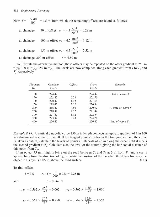
412 Engineering Surveying
Now Y = 9 400800
= 4.5 m× from which the remaining offsets are found as follows:
at chainage 50 m offset y1
2
2 = 4.5 50
200 = 0.28 m
at chainage 100 m offset y2
2
2 = 4.5 100
200 = 1.12 m
at chainage 150 m offset y3
2
2 = 4.5 150
200 = 2.52 m
at chainage 200 m offset Y = 4.50 m
To illustrate the alternative method, these offsets may be repeated on the other gradient at 250 m= y3, 300 m = y2, 350 m = y1. The levels are now computed along each gradient from I to T1 andT2 respectively.
Chainage Gradient Offsets Curve Remarks
(m) levels levels
0 224.42 224.42 Start of curve T50 222.42 0.28 222.70
100 220.42 1.12 221.54150 218.42 2.52 220.94200 216.42 4.50 220.92 Centre of curve I250 218.92 2.52 221.44300 221.42 1.12 222.54350 223.92 0.28 224.20400 226.42 226.42 End of curve T2
Example 8.18. A vertical parabolic curve 150 m in length connects an upward gradient of 1 in 100to a downward gradient of 1 in 50. If the tangent point T1 between the first gradient and the curveis taken as datum, calculate the levels of points at intervals of 25 m along the curve until it meetsthe second gradient at T2. Calculate also the level of the summit giving the horizontal distance ofthis point from T1.
If an object 75 mm high is lying on the road between T1 and T2 at 3 m from T2, and a car isapproaching from the direction of T1, calculate the position of the car when the driver first sees theobject if his eye is 1.05 m above the road surface. (LU)
To find offsets:
A = 3% ∴ × 4 = 200
3% = 2.25 mYL
and Y = 0.562 m
∴ y1 = 0.562 × 2575
2
2 = 0.062 y4 = 0.562 × 1002
275 = 1.000
y2 = 0.562 × 502
275 = 0.250 y5 = 0.562 × 1252
275 = 1.562
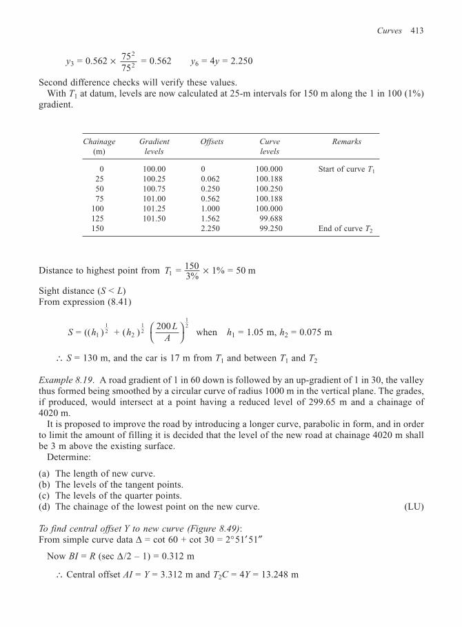
Curves 413
y3 = 0.562 × 752
275 = 0.562 y6 = 4y = 2.250
Second difference checks will verify these values.With T1 at datum, levels are now calculated at 25-m intervals for 150 m along the 1 in 100 (1%)
gradient.
Chainage Gradient Offsets Curve Remarks
(m) levels levels
0 100.00 0 100.000 Start of curve T1
25 100.25 0.062 100.18850 100.75 0.250 100.25075 101.00 0.562 100.188
100 101.25 1.000 100.000125 101.50 1.562 99.688150 2.250 99.250 End of curve T2
Distance to highest point from T1 = 1503%
1% = 50 m×
Sight distance (S < L)From expression (8.41)
S h hL
A = (( ) + ( )
2001 2
12
12
12
when h1 = 1.05 m, h2 = 0.075 m
∴ S = 130 m, and the car is 17 m from T1 and between T1 and T2
Example 8.19. A road gradient of 1 in 60 down is followed by an up-gradient of 1 in 30, the valleythus formed being smoothed by a circular curve of radius 1000 m in the vertical plane. The grades,if produced, would intersect at a point having a reduced level of 299.65 m and a chainage of4020 m.
It is proposed to improve the road by introducing a longer curve, parabolic in form, and in orderto limit the amount of filling it is decided that the level of the new road at chainage 4020 m shallbe 3 m above the existing surface.
Determine:
(a) The length of new curve.(b) The levels of the tangent points.(c) The levels of the quarter points.(d) The chainage of the lowest point on the new curve. (LU)
To find central offset Y to new curve (Figure 8.49):From simple curve data ∆ = cot 60 + cot 30 = 2°51′51″
Now BI = R (sec ∆ /2 – 1) = 0.312 m
∴ Central offset AI = Y = 3.312 m and T2C = 4Y = 13.248 m
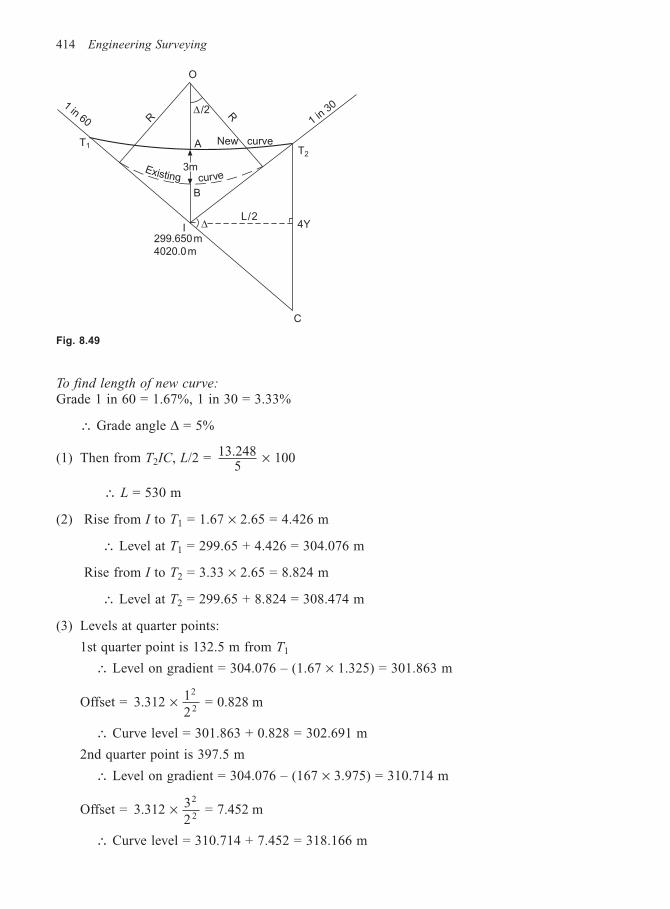
414 Engineering Surveying
To find length of new curve:
Grade 1 in 60 = 1.67%, 1 in 30 = 3.33%
∴ Grade angle ∆ = 5%
(1) Then from T2IC, L/2 = 13.2485
100×
∴ L = 530 m
(2) Rise from I to T1 = 1.67 × 2.65 = 4.426 m
∴ Level at T1 = 299.65 + 4.426 = 304.076 m
Rise from I to T2 = 3.33 × 2.65 = 8.824 m
∴ Level at T2 = 299.65 + 8.824 = 308.474 m
(3) Levels at quarter points:
1st quarter point is 132.5 m from T1
∴ Level on gradient = 304.076 – (1.67 × 1.325) = 301.863 m
Offset = 3.312 12
= 0.828 m2
2×
∴ Curve level = 301.863 + 0.828 = 302.691 m
2nd quarter point is 397.5 m
∴ Level on gradient = 304.076 – (167 × 3.975) = 310.714 m
Offset = 3.3122
= 7.452 m2
2× 3
∴ Curve level = 310.714 + 7.452 = 318.166 m
Fig. 8.49
Existing curve
O
∆ /2
A New curve
B
∆I299.650m
4020.0m
L/2
T2
T1
1 in 60 R
R
1 in 3
0
3m
C
4Y
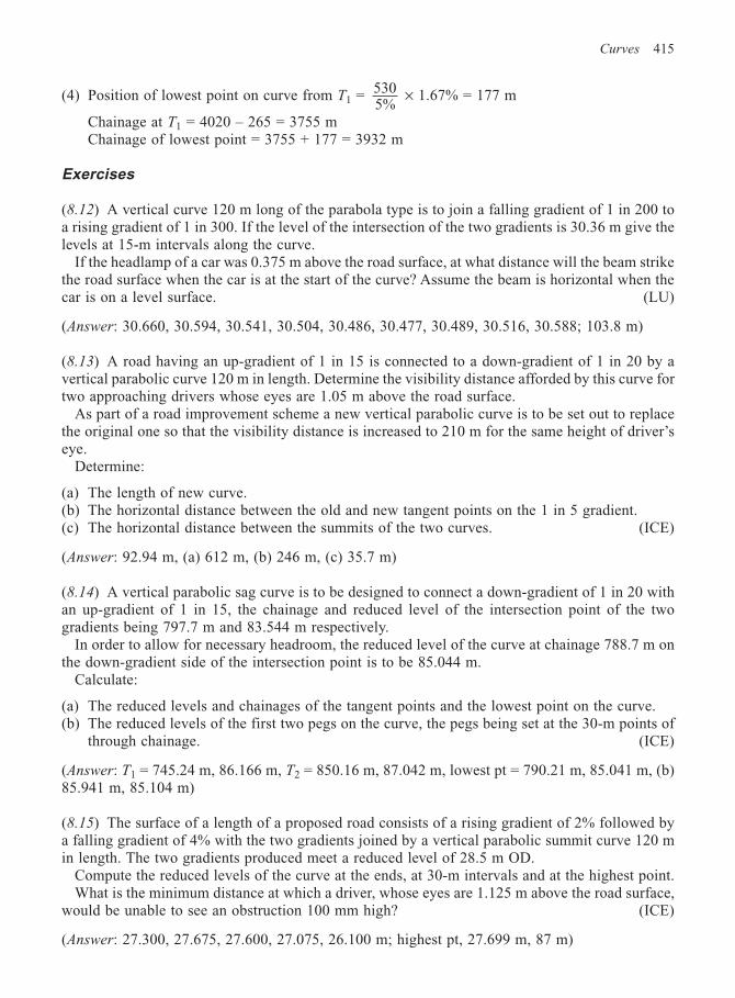
Curves 415
(4) Position of lowest point on curve from T1 = 5305%
× 1.67% = 177 m
Chainage at T1 = 4020 – 265 = 3755 mChainage of lowest point = 3755 + 177 = 3932 m
Exercises
(8.12) A vertical curve 120 m long of the parabola type is to join a falling gradient of 1 in 200 toa rising gradient of 1 in 300. If the level of the intersection of the two gradients is 30.36 m give thelevels at 15-m intervals along the curve.
If the headlamp of a car was 0.375 m above the road surface, at what distance will the beam strikethe road surface when the car is at the start of the curve? Assume the beam is horizontal when thecar is on a level surface. (LU)
(Answer: 30.660, 30.594, 30.541, 30.504, 30.486, 30.477, 30.489, 30.516, 30.588; 103.8 m)
(8.13) A road having an up-gradient of 1 in 15 is connected to a down-gradient of 1 in 20 by avertical parabolic curve 120 m in length. Determine the visibility distance afforded by this curve fortwo approaching drivers whose eyes are 1.05 m above the road surface.
As part of a road improvement scheme a new vertical parabolic curve is to be set out to replacethe original one so that the visibility distance is increased to 210 m for the same height of driver’seye.
Determine:
(a) The length of new curve.(b) The horizontal distance between the old and new tangent points on the 1 in 5 gradient.(c) The horizontal distance between the summits of the two curves. (ICE)
(Answer: 92.94 m, (a) 612 m, (b) 246 m, (c) 35.7 m)
(8.14) A vertical parabolic sag curve is to be designed to connect a down-gradient of 1 in 20 withan up-gradient of 1 in 15, the chainage and reduced level of the intersection point of the twogradients being 797.7 m and 83.544 m respectively.
In order to allow for necessary headroom, the reduced level of the curve at chainage 788.7 m onthe down-gradient side of the intersection point is to be 85.044 m.
Calculate:
(a) The reduced levels and chainages of the tangent points and the lowest point on the curve.(b) The reduced levels of the first two pegs on the curve, the pegs being set at the 30-m points of
through chainage. (ICE)
(Answer: T1 = 745.24 m, 86.166 m, T2 = 850.16 m, 87.042 m, lowest pt = 790.21 m, 85.041 m, (b)85.941 m, 85.104 m)
(8.15) The surface of a length of a proposed road consists of a rising gradient of 2% followed bya falling gradient of 4% with the two gradients joined by a vertical parabolic summit curve 120 min length. The two gradients produced meet a reduced level of 28.5 m OD.
Compute the reduced levels of the curve at the ends, at 30-m intervals and at the highest point.What is the minimum distance at which a driver, whose eyes are 1.125 m above the road surface,
would be unable to see an obstruction 100 mm high? (ICE)
(Answer: 27.300, 27.675, 27.600, 27.075, 26.100 m; highest pt, 27.699 m, 87 m)
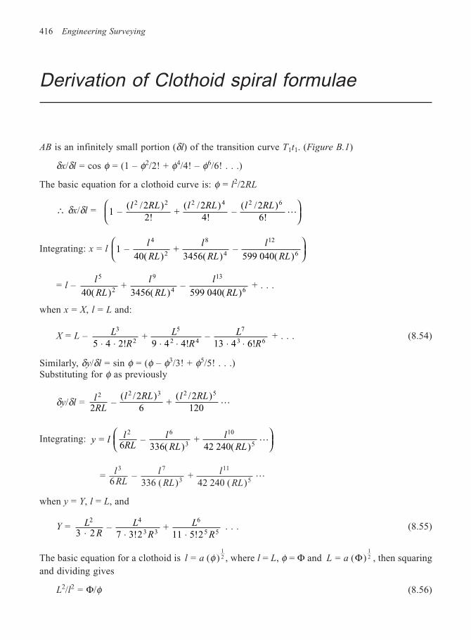
416 Engineering Surveying
Derivation of Clothoid spiral formulae
AB is an infinitely small portion (δl) of the transition curve T1t1. (Figure B.1)
δx/δl = cos φ = (1 – φ2/2! + φ4/4! – φ6/6! . . .)
The basic equation for a clothoid curve is: φ = l2/2RL
∴ δx/δl = 1 – ( /2
2! +
( /2 )4!
– ( /2 )
6!
2 2 4 2 6l RL l RL l RL)2
L
Integrating: x = l 1 – 40( )
+ 3456( )
– 599 040( )
4
2
8
4
12
6
l
RL
l
RL
l
RL
= l – l
RL
l
RL
l
RL
5
2 4
13
640( ) +
3456( ) –
599 040( )
9
+ . . .
when x = X, l = L and:
X = L – L
R
L
R
L
R
3
2
5
2 4
7
3 65 4 2! +
9 4 4! –
13 4 6!⋅ ⋅ ⋅ ⋅ ⋅ ⋅ + . . . (8.54)
Similarly, δy/δl = sin φ = (φ – φ3/3! + φ5/5! . . .)Substituting for φ as previously
δy/δl = lRL
l RL l RL2 2 3 2 5
2 –
( /2 )6
+ ( /2 )
120L
Integrating: y llRL
l
RL
l
RL =
6 –
336( ) +
42 240( )
2 6
3
10
5L
=6
– 336 ( )
+ 42 240 ( )
7
3
11
5
lRL
l
RL
l
RL
3
L
when y = Y, l = L, and
Y = LR
L
R
L
R
2 4
3 3
6
5 5 –
7 3!2 +
11 5!23 2⋅ ⋅ ⋅ . . . (8.55)
The basic equation for a clothoid is l a = ( )12φ , where l = L, φ = Φ and L a = ( )
12Φ , then squaring
and dividing gives
L2/l2 = Φ/φ (8.56)
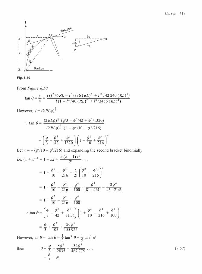
Curves 417
From Figure 8.50
tan = = ( /6 – /336 ( ) + /42 240 ( ) )
(1 – /40 ( ) + /3456 ( ) )
2 6 3 10 5
4 2 8 4θ
y
x
l l RL l RL l RL
l l RL l RL
However, l RL = (2 )12φ
∴ tan θ = (2 ) ( /3 – /42 + /1320)
(2 ) (1 – /10 + /216)
12
12
3 5
2 4
RL
RL
φ φ φ φ
φ φ φ
=φ φ φ φ φ3
– 42
+ 1320
1 – 10
+ 216
3 5 2 4 –1
Let x = – (φ2/10 – φ4/216) and expanding the second bracket binomially
i.e. (1 + x)–1 = 1 – nx + n n x ( – 1)
2! . . .
2
= 1 + 10
– 216
+ 22! 10
– 216
2 4 2 4 2φ φ φ φ
= 1 + 10
– 216
+ 100
+ 81 4!4!
– 2
45 2!4!
2 4 4 8 6φ φ φ φ φ⋅ ⋅
= 1 + 10
– 216
+ 100
2 4 4φ φ φ
∴
tan = 3
– 42
+ 11.5!
1 + 10
– 216
+ 100
3 5 2 4 4
θφ φ φ φ φ φ
=φ φ φ3
+ 105
+ 26
155 925
3 5
However, as θ = tan – 13
tan + 15
tan 3 5θ θ θ
then θ = φ φ φ3
– 82835
– 32
467 775
3 5
. . . (8.57)
=3
– φ
N
Fig. 8.50
Clo
thoi
d
x
φ
y BA t1
rθ
∞Radius
δx
δy
δl
A
Bδl
Tangent
I
T1
φ
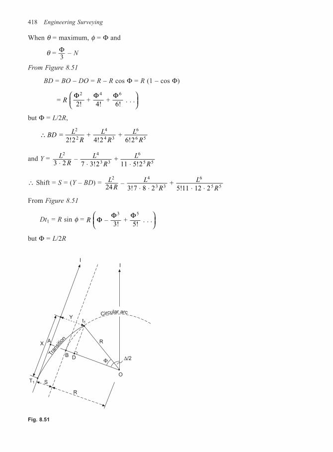
418 Engineering Surveying
When θ = maximum, φ = Φ and
θ = 3
– ΦN
From Figure 8.51
BD = BO – DO = R – R cos Φ = R (1 – cos Φ)
=2!
+ 4!
+ 6!
. .2 4 6
RΦ Φ Φ
.
but Φ = L/2R,
∴2!2
+ 4!2
+ 6!2
2
2
4
4 3
6
6 5BD =
L
R
L
R
L
R
and Y = LR
L
R
L
R
2 4
3 3
6
5 53 2 –
7 3!2 +
11 5!2⋅ ⋅ ⋅
∴ Shift = S = (Y – BD) = LR
L
R
L
R
2 4
3 3
6
5 5 –
3!7 8 2 +
5!11 12 224 ⋅ ⋅ ⋅ ⋅
From Figure 8.51
Dt1 = R sin φ = R – 3!
+ 5!
. .3 5
ΦΦ Φ
.
but Φ = L/2R
Fig. 8.51
Tran
sitio
n
Circular arc
II
Yt1
R
∆/2Φ
S
R
T1
XA
DB
O
Curves 419
∴ Dt1 = L L
R
L
R2 –
3!2 +
5!2
3
3 2
5
5 4 . . .
also X = L – L
R
L
R
3
2
5
2 4 ! +
4 4!5 4 2 9⋅ ⋅ ⋅ ⋅ . . .
Tangent length = TlI = (R + S) tan2∆ + AT1 = (R + S) tan
2∆ + (X – Dt1)
= (R + S) tan2
+ 2
– 2!5 6 2
+ 4!9 10 2
3
2 2
5
4 4∆ L L
R
L
R⋅ ⋅ ⋅ ⋅
= (R + S) tan2
+ ∆C (8.58)
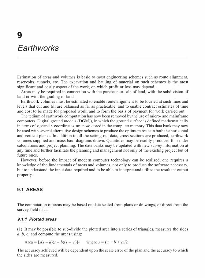
9
Earthworks
Estimation of areas and volumes is basic to most engineering schemes such as route alignment,reservoirs, tunnels, etc. The excavation and hauling of material on such schemes is the mostsignificant and costly aspect of the work, on which profit or loss may depend.
Areas may be required in connection with the purchase or sale of land, with the subdivision ofland or with the grading of land.
Earthwork volumes must be estimated to enable route alignment to be located at such lines andlevels that cut and fill are balanced as far as practicable; and to enable contract estimates of timeand cost to be made for proposed work; and to form the basis of payment for work carried out.
The tedium of earthwork computation has now been removed by the use of micro- and mainframecomputers. Digital ground models (DGM)), in which the ground surface is defined mathematicallyin terms of x, y and z coordinates, are now stored in the computer memory. This data bank may nowbe used with several alternative design schemes to produce the optimum route in both the horizontaland vertical planes. In addition to all the setting-out data, cross-sections are produced, earthworkvolumes supplied and mass-haul diagrams drawn. Quantities may be readily produced for tendercalculations and project planning. The data banks may be updated with new survey information atany time and further facilitate the planning and management not only of the existing project but offuture ones.
However, before the impact of modern computer technology can be realized, one requires aknowledge of the fundamentals of areas and volumes, not only to produce the software necessary,but to understand the input data required and to be able to interpret and utilize the resultant outputproperly.
9.1 AREAS
The computation of areas may be based on data scaled from plans or drawings, or direct from thesurvey field data.
9.1.1 Plotted areas
(1) It may be possible to sub-divide the plotted area into a series of triangles, measures the sidesa, b, c, and compute the areas using:
Area = [s(s – a)(s – b)(s – c)]12 where s = (a + b + c)/2
The accuracy achieved will be dependent upon the scale error of the plan and the accuracy to whichthe sides are measured.
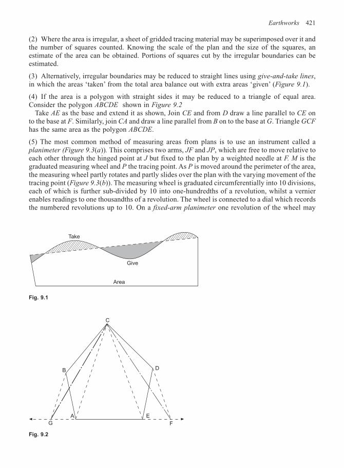
Earthworks 421
(2) Where the area is irregular, a sheet of gridded tracing material may be superimposed over it andthe number of squares counted. Knowing the scale of the plan and the size of the squares, anestimate of the area can be obtained. Portions of squares cut by the irregular boundaries can beestimated.
(3) Alternatively, irregular boundaries may be reduced to straight lines using give-and-take lines,in which the areas ‘taken’ from the total area balance out with extra areas ‘given’ (Figure 9.1).
(4) If the area is a polygon with straight sides it may be reduced to a triangle of equal area.Consider the polygon ABCDE shown in Figure 9.2
Take AE as the base and extend it as shown, Join CE and from D draw a line parallel to CE onto the base at F. Similarly, join CA and draw a line parallel from B on to the base at G. Triangle GCF
has the same area as the polygon ABCDE.
(5) The most common method of measuring areas from plans is to use an instrument called aplanimeter (Figure 9.3(a)). This comprises two arms, JF and JP, which are free to move relative toeach other through the hinged point at J but fixed to the plan by a weighted needle at F. M is thegraduated measuring wheel and P the tracing point. As P is moved around the perimeter of the area,the measuring wheel partly rotates and partly slides over the plan with the varying movement of thetracing point (Figure 9.3(b)). The measuring wheel is graduated circumferentially into 10 divisions,each of which is further sub-divided by 10 into one-hundredths of a revolution, whilst a vernierenables readings to one thousandths of a revolution. The wheel is connected to a dial which recordsthe numbered revolutions up to 10. On a fixed-arm planimeter one revolution of the wheel may
Take
Give
Area
Fig. 9.1
C
B
G
A
F
D
E
Fig. 9.2
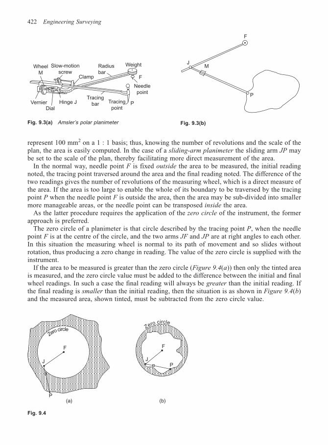
422 Engineering Surveying
represent 100 mm2 on a 1 : 1 basis; thus, knowing the number of revolutions and the scale of theplan, the area is easily computed. In the case of a sliding-arm planimeter the sliding arm JP maybe set to the scale of the plan, thereby facilitating more direct measurement of the area.
In the normal way, needle point F is fixed outside the area to be measured, the initial readingnoted, the tracing point traversed around the area and the final reading noted. The difference of thetwo readings gives the number of revolutions of the measuring wheel, which is a direct measure ofthe area. If the area is too large to enable the whole of its boundary to be traversed by the tracingpoint P when the needle point F is outside the area, then the area may be sub-divided into smallermore manageable areas, or the needle point can be transposed inside the area.
As the latter procedure requires the application of the zero circle of the instrument, the formerapproach is preferred.
The zero circle of a planimeter is that circle described by the tracing point P, when the needlepoint F is at the centre of the circle, and the two arms JF and JP are at right angles to each other.In this situation the measuring wheel is normal to its path of movement and so slides withoutrotation, thus producing a zero change in reading. The value of the zero circle is supplied with theinstrument.
If the area to be measured is greater than the zero circle (Figure 9.4(a)) then only the tinted areais measured, and the zero circle value must be added to the difference between the initial and finalwheel readings. In such a case the final reading will always be greater than the initial reading. Ifthe final reading is smaller than the initial reading, then the situation is as shown in Figure 9.4(b)and the measured area, shown tinted, must be subtracted from the zero circle value.
F
JM
P
Wheel
M
Slow-motion
screwClamp
Radius
bar
Weight
F
Needle
point
PTracing
point
Tracing
barHinge J
DialVernier
Fig. 9.3(a) Amsler’s polar planimeter Fig. 9.3(b)
Fig. 9.4
Zerocircle Zero circle
F
J
P
F
JP
(a) (b)
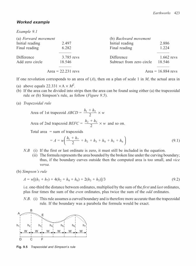
Earthworks 423
Worked example
Example 9.1
(a) Forward movement (b) Backward movement
Initial reading 2.497 Initial reading 2.886Final reading 6.282 Final reading 1.224
——— ———Difference 3.785 revs Difference 1.662 revsAdd zero circle 18.546 Subtract from zero circle 18.546
——— ———Area = 22.231 revs Area = 16.884 revs
If one revolution corresponds to an area of (A), then on a plan of scale 1 in M, the actual area in
(a) above equals 22.331 × A × M2.(b) If the area can be divided into strips then the area can be found using either (a) the trapezoidal
rule or (b) Simpson’s rule, as follow (Figure 9.5).
(a) Trapezoidal rule
Area of 1st trapezoid ABCD = h h
w1 2 + 2
×
Area of 2nd trapezoid BEFC = h h
w2 3 + 2
× and so on.
Total area = sum of trapezoids
= = + 2
+ + + + + 1 72 3 4 5 6A w
h hh h h h h
(9.1)
N.B (i) If the first or last ordinate is zero, it must still be included in the equation.(ii) The formula represents the area bounded by the broken line under the curving boundary;
thus, if the boundary curves outside then the computed area is too small, and vice
versa.
(b) Simpson’s rule
A = w[(h1 + h7) + 4(h2 + h4 + h6) + 2(h3 + h5)]/3 (9.2)
i.e. one-third the distance between ordinates, multiplied by the sum of the first and last ordinates,plus four times the sum of the even ordinates, plus twice the sum of the odd ordinates.
N.B. (i) This rule assumes a curved boundary and is therefore more accurate than the trapezoidalrule. If the boundary was a parabola the formula would be exact.
AB
E
W W W W W W
h1 h2 h3 h4 h7h5 h6
D C F
Fig. 9.5 Trapezoidal and Simpson’s rule
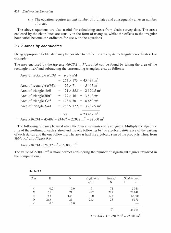
424 Engineering Surveying
(ii) The equation requires an odd number of ordinates and consequently an even numberof areas.
The above equations are also useful for calculating areas from chain survey data. The areasenclosed by the chain lines are usually in the form of triangles, whilst the offsets to the irregularboundaries become the ordinates for use with the equations.
9.1.2 Areas by coordinates
Using appropriate field data it may be possible to define the area by its rectangular coordinates. Forexample:
The area enclosed by the traverse ABCDA in Figure 9.6 can be found by taking the area of therectangle a′cDd and subtracting the surrounding triangles, etc., as follows:
Area of rectangle a′cDd = a′c × a′d= 263 × 173 = 45 499 m2
Area of rectangle a′bBa = 77 × 71 = 5 467 m2
Area of triangle AaB = 71 × 35.5 = 2 520.5 m2
Area of triangle BbC = 77 × 46 = 3 542 m2
Area of triangle Ccd = 173 × 50 = 8 650 m2
Area of triangle DdA = 263 × 12.5 = 3 287.5 m2
—————Total = 23 467 m2
∴ Area ABCDA = 45499 – 23467 = 22032 m2 ≈ 22000 m2
The following rule may be used when the total coordinates only are given. Multiply the algebraicsum of the northing of each station and the one following by the algebraic difference of the eastingof each station and the one following. The area is half the algebraic sum of the products. Thus, fromTable 9.1 and Figure 9.6.
Area ABCDA ≈ 22032 m2 ≈ 22 000 m2
The value of 22 000 m2 is more correct considering the number of significant figures involved inthe computations.
Table 9.1
Stns E N Difference Sum of Double area
of E N + –
A 0.0 0.0 –71 71 5 041B 71 71 –92 219 20 148C 163 148 –100 123 12300D 263 –25 263 –25 6 575A 0.0 0.0 —
∑ 44 064
Area ABCDA = 22032 m2 ≈ 22 000 m2
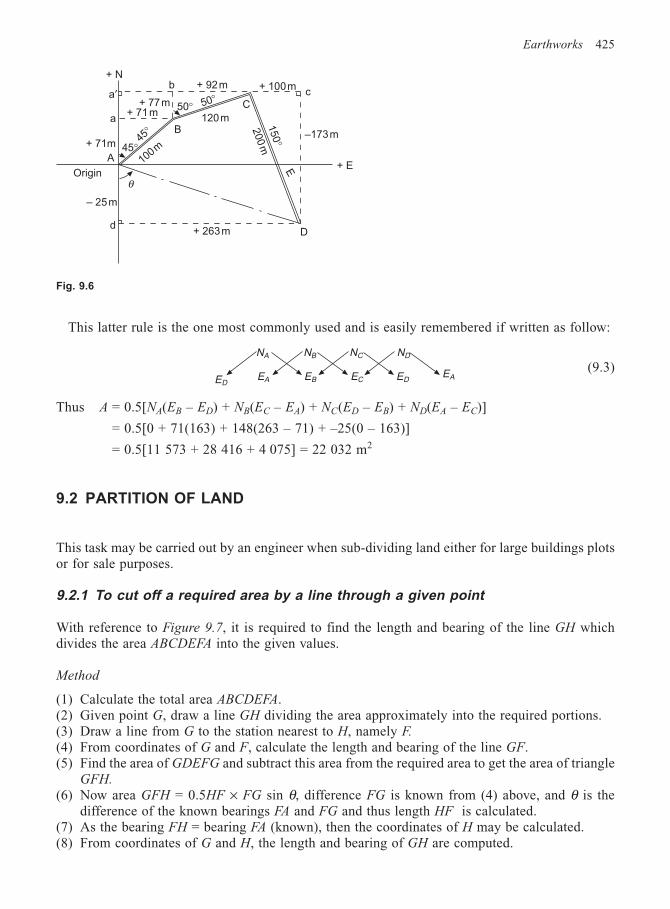
Earthworks 425
This latter rule is the one most commonly used and is easily remembered if written as follow:
(9.3)
Thus A = 0.5[NA(EB – ED) + NB(EC – EA) + NC(ED – EB) + ND(EA – EC)]
= 0.5[0 + 71(163) + 148(263 – 71) + –25(0 – 163)]
= 0.5[11 573 + 28 416 + 4 075] = 22 032 m2
9.2 PARTITION OF LAND
This task may be carried out by an engineer when sub-dividing land either for large buildings plotsor for sale purposes.
9.2.1 To cut off a required area by a line through a given point
With reference to Figure 9.7, it is required to find the length and bearing of the line GH whichdivides the area ABCDEFA into the given values.
Method
(1) Calculate the total area ABCDEFA.(2) Given point G, draw a line GH dividing the area approximately into the required portions.(3) Draw a line from G to the station nearest to H, namely F.
(4) From coordinates of G and F, calculate the length and bearing of the line GF.(5) Find the area of GDEFG and subtract this area from the required area to get the area of triangle
GFH.
(6) Now area GFH = 0.5HF × FG sin θ, difference FG is known from (4) above, and θ is thedifference of the known bearings FA and FG and thus length HF is calculated.
(7) As the bearing FH = bearing FA (known), then the coordinates of H may be calculated.(8) From coordinates of G and H, the length and bearing of GH are computed.
Fig. 9.6
a′
a
+ 71m
+ N
A
Origin
– 25m
d
θ
+ 263m
100m45°45
° B
50° 50°+ 77m+ 71m
b + 92m + 100m
–173m
150°
200
m
E + E
c
120m
C
ED
NA NB NC ND
EDEB ECEAEA
D
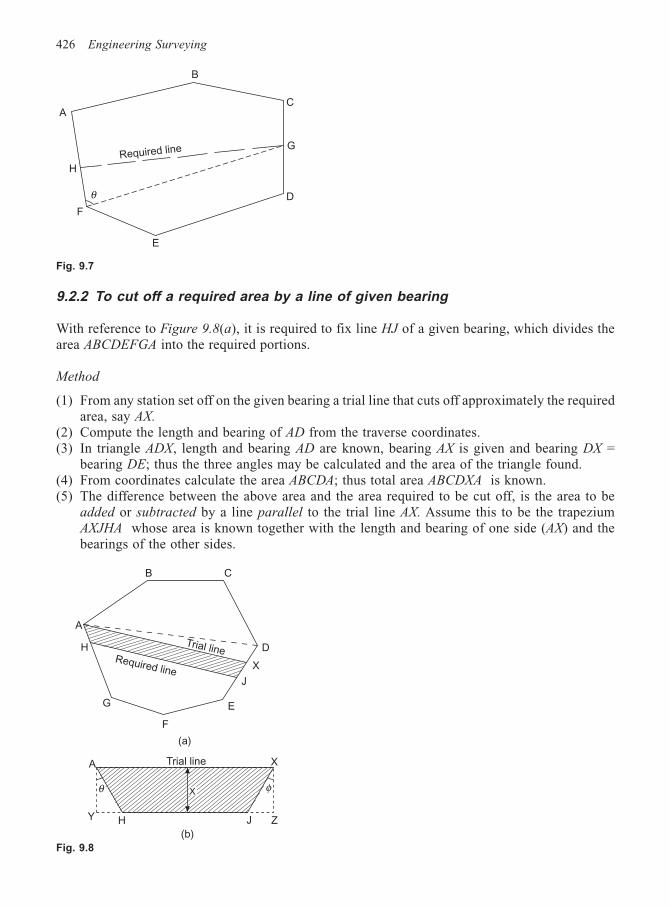
426 Engineering Surveying
X
9.2.2 To cut off a required area by a line of given bearing
With reference to Figure 9.8(a), it is required to fix line HJ of a given bearing, which divides thearea ABCDEFGA into the required portions.
Method
(1) From any station set off on the given bearing a trial line that cuts off approximately the requiredarea, say AX.
(2) Compute the length and bearing of AD from the traverse coordinates.(3) In triangle ADX, length and bearing AD are known, bearing AX is given and bearing DX =
bearing DE; thus the three angles may be calculated and the area of the triangle found.(4) From coordinates calculate the area ABCDA; thus total area ABCDXA is known.(5) The difference between the above area and the area required to be cut off, is the area to be
added or subtracted by a line parallel to the trial line AX. Assume this to be the trapeziumAXJHA whose area is known together with the length and bearing of one side (AX) and thebearings of the other sides.
B
CA
H
G
D
E
F
θ
Required line
Fig. 9.7
Fig. 9.8
B C
D
J
X
E
F
G
H
A
A
Y H J Z
XTrial line
θ
Required line
Trial line
φ
(a)
(b)
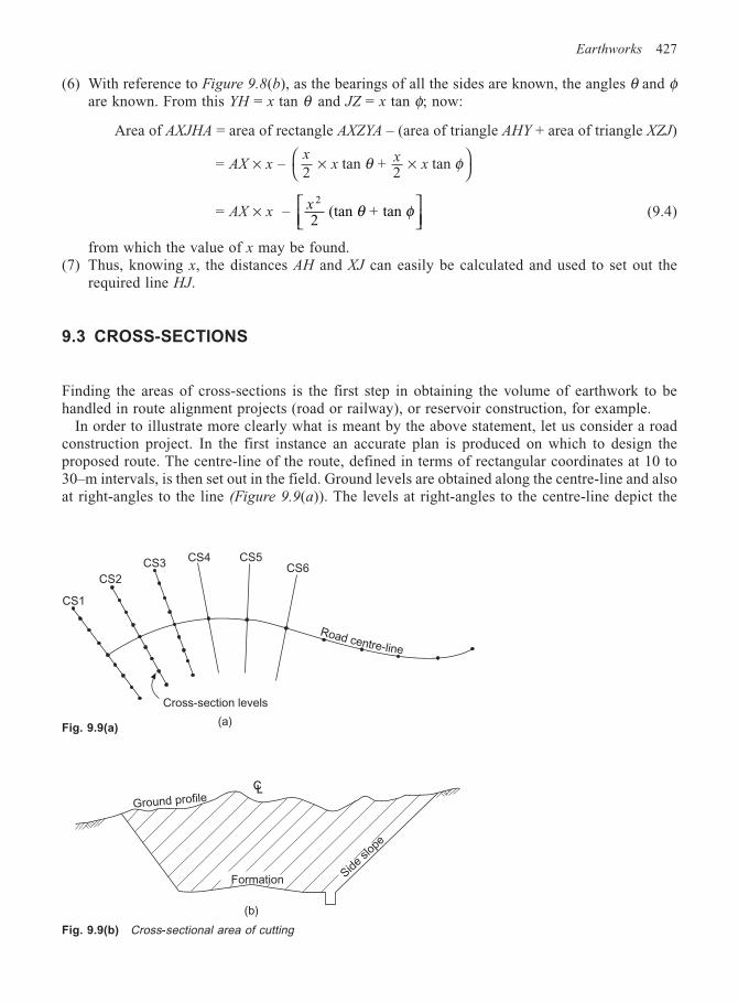
Earthworks 427
Road centre-line
Ground profile
Side
slop
e
(6) With reference to Figure 9.8(b), as the bearings of all the sides are known, the angles θ and φare known. From this YH = x tan θ and JZ = x tan φ; now:
Area of AXJHA = area of rectangle AXZYA – (area of triangle AHY + area of triangle XZJ)
= AX × x – x
xx
x2
tan + 2
tan × ×
θ φ
= AX × x – x 2
2 (tan + tan θ φ
(9.4)
from which the value of x may be found.(7) Thus, knowing x, the distances AH and XJ can easily be calculated and used to set out the
required line HJ.
9.3 CROSS-SECTIONS
Finding the areas of cross-sections is the first step in obtaining the volume of earthwork to behandled in route alignment projects (road or railway), or reservoir construction, for example.
In order to illustrate more clearly what is meant by the above statement, let us consider a roadconstruction project. In the first instance an accurate plan is produced on which to design theproposed route. The centre-line of the route, defined in terms of rectangular coordinates at 10 to30–m intervals, is then set out in the field. Ground levels are obtained along the centre-line and alsoat right-angles to the line (Figure 9.9(a)). The levels at right-angles to the centre-line depict the
Fig. 9.9(a)
Fig. 9.9(b) Cross-sectional area of cutting
CS1
CS2
CS3CS4 CS5
CS6
Cross-section levels
Formation
CL
(a)
(b)
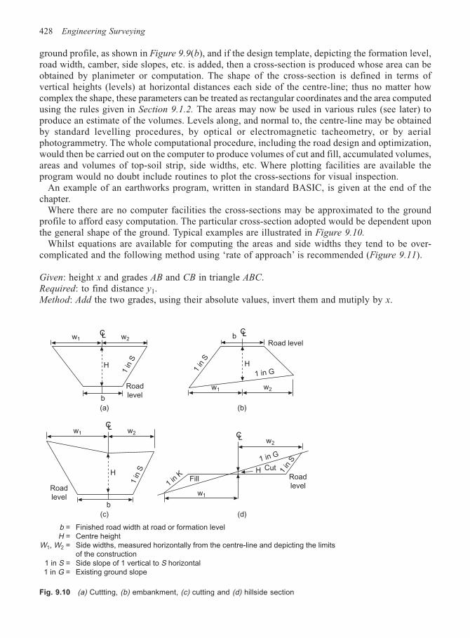
428 Engineering Surveying
ground profile, as shown in Figure 9.9(b), and if the design template, depicting the formation level,road width, camber, side slopes, etc. is added, then a cross-section is produced whose area can beobtained by planimeter or computation. The shape of the cross-section is defined in terms ofvertical heights (levels) at horizontal distances each side of the centre-line; thus no matter howcomplex the shape, these parameters can be treated as rectangular coordinates and the area computedusing the rules given in Section 9.1.2. The areas may now be used in various rules (see later) toproduce an estimate of the volumes. Levels along, and normal to, the centre-line may be obtainedby standard levelling procedures, by optical or electromagnetic tacheometry, or by aerialphotogrammetry. The whole computational procedure, including the road design and optimization,would then be carried out on the computer to produce volumes of cut and fill, accumulated volumes,areas and volumes of top-soil strip, side widths, etc. Where plotting facilities are available theprogram would no doubt include routines to plot the cross-sections for visual inspection.
An example of an earthworks program, written in standard BASIC, is given at the end of thechapter.
Where there are no computer facilities the cross-sections may be approximated to the groundprofile to afford easy computation. The particular cross-section adopted would be dependent uponthe general shape of the ground. Typical examples are illustrated in Figure 9.10.
Whilst equations are available for computing the areas and side widths they tend to be over-complicated and the following method using ‘rate of approach’ is recommended (Figure 9.11).
Given: height x and grades AB and CB in triangle ABC.Required: to find distance y1.Method: Add the two grades, using their absolute values, invert them and mutiply by x.
Fig. 9.10 (a) Cuttting, (b) embankment, (c) cutting and (d) hillside section
CLw1 w2
H
b
Road
level
1 in
S
Road levelb
CL
1 in GH
w1 w2
1 in
S
w1 w2
CL
H
b
Road
level
1 in
S
w2
w1
1 in K Fill
1 in G
HRoad
level
CL
Cut 1 in
S
(a) (b)
(c) (d)
b = Finished road width at road or formation level
H = Centre height
W1, W2 = Side widths, measured horizontally from the centre-line and depicting the limits
of the construction
1 in S = Side slope of 1 vertical to S horizontal
1 in G = Existing ground slope
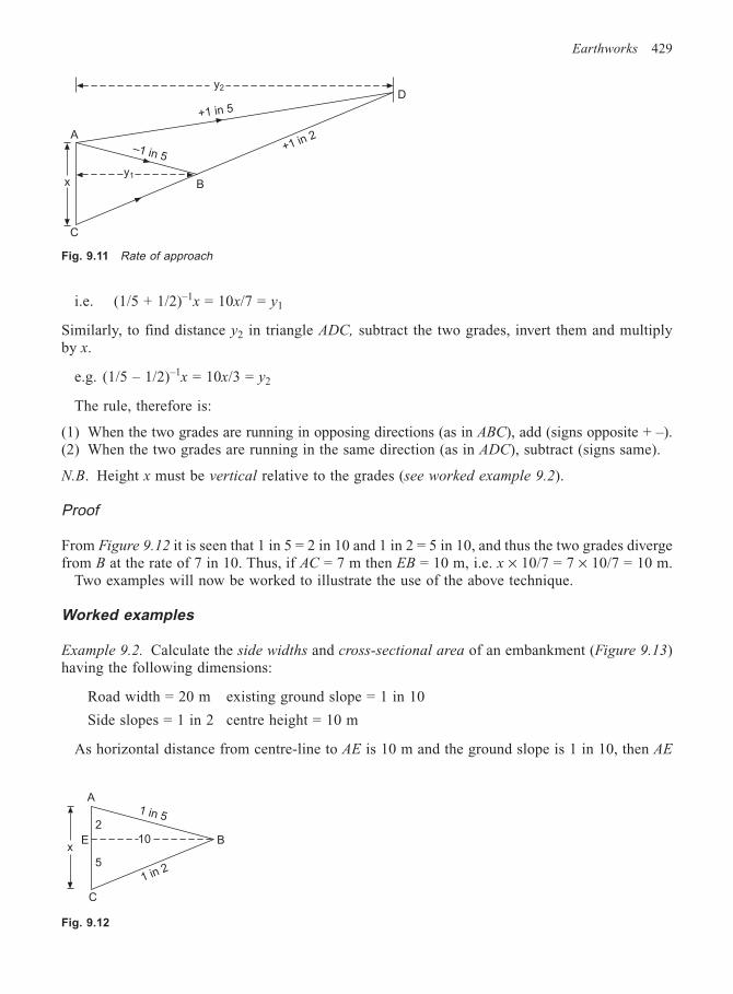
Earthworks 429
i.e. (1/5 + 1/2)–1x = 10x/7 = y1
Similarly, to find distance y2 in triangle ADC, subtract the two grades, invert them and multiplyby x.
e.g. (1/5 – 1/2)–1x = 10x/3 = y2
The rule, therefore is:
(1) When the two grades are running in opposing directions (as in ABC), add (signs opposite + –).(2) When the two grades are running in the same direction (as in ADC), subtract (signs same).
N.B. Height x must be vertical relative to the grades (see worked example 9.2).
Proof
From Figure 9.12 it is seen that 1 in 5 = 2 in 10 and 1 in 2 = 5 in 10, and thus the two grades divergefrom B at the rate of 7 in 10. Thus, if AC = 7 m then EB = 10 m, i.e. x × 10/7 = 7 × 10/7 = 10 m.
Two examples will now be worked to illustrate the use of the above technique.
Worked examples
Example 9.2. Calculate the side widths and cross-sectional area of an embankment (Figure 9.13)having the following dimensions:
Road width = 20 m existing ground slope = 1 in 10
Side slopes = 1 in 2 centre height = 10 m
As horizontal distance from centre-line to AE is 10 m and the ground slope is 1 in 10, then AE
y2D
+1 in 5
–1 in 5
y1x B
+1 in 2A
C
Fig. 9.11 Rate of approach
Fig. 9.12
x
A
C
2
5
E 10 B
1 in 2
1 in 5
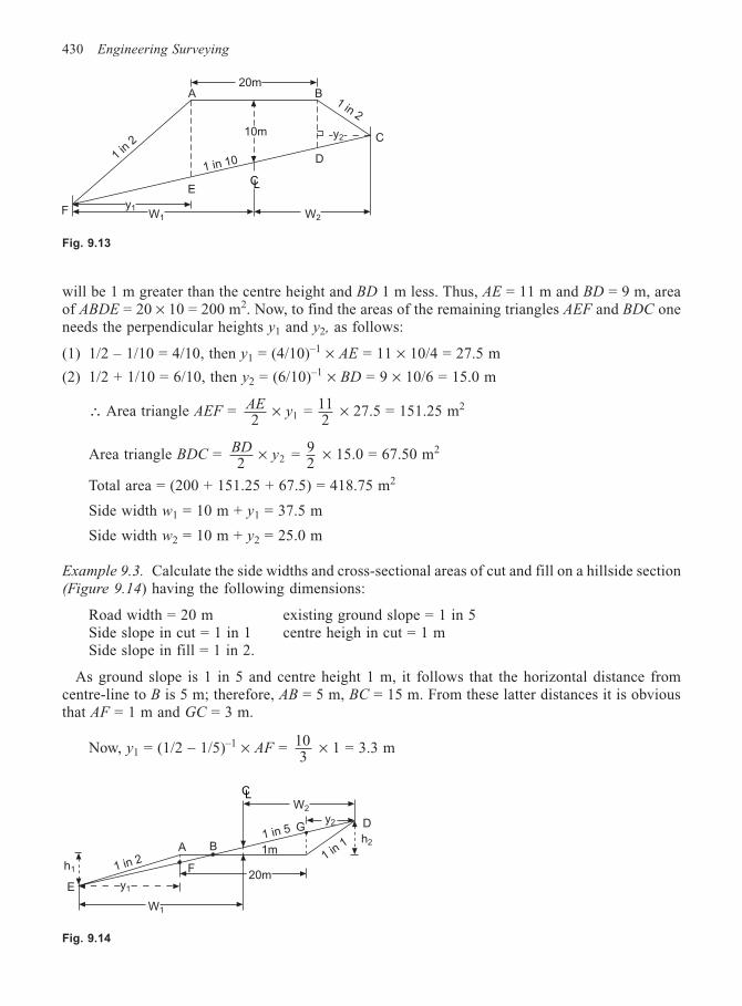
430 Engineering Surveying
will be 1 m greater than the centre height and BD 1 m less. Thus, AE = 11 m and BD = 9 m, areaof ABDE = 20 × 10 = 200 m2. Now, to find the areas of the remaining triangles AEF and BDC oneneeds the perpendicular heights y1 and y2, as follows:
(1) 1/2 – 1/10 = 4/10, then y1 = (4/10)–1 × AE = 11 × 10/4 = 27.5 m
(2) 1/2 + 1/10 = 6/10, then y2 = (6/10)–1 × BD = 9 × 10/6 = 15.0 m
∴ Area triangle AEF = AEy
2 = 11
21× × 27.5 = 151.25 m2
Area triangle BDC = BDy
2 = 9
22× × 15.0 = 67.50 m2
Total area = (200 + 151.25 + 67.5) = 418.75 m2
Side width w1 = 10 m + y1 = 37.5 m
Side width w2 = 10 m + y2 = 25.0 m
Example 9.3. Calculate the side widths and cross-sectional areas of cut and fill on a hillside section(Figure 9.14) having the following dimensions:
Road width = 20 m existing ground slope = 1 in 5Side slope in cut = 1 in 1 centre heigh in cut = 1 mSide slope in fill = 1 in 2.
As ground slope is 1 in 5 and centre height 1 m, it follows that the horizontal distance fromcentre-line to B is 5 m; therefore, AB = 5 m, BC = 15 m. From these latter distances it is obviousthat AF = 1 m and GC = 3 m.
Now, y1 = (1/2 – 1/5)–1 × AF = 103
× 1 = 3.3 m
Fig. 9.13
20mA B
1 in 2
y2
D
10m
CLE
y1W1
F
1 in
2
W2
1 in 10
C
Fig. 9.14
E
h1
y1
W1
1 in 2A
F
B
CLW2
20m
1 in 5 Gy2 D
h2
1 in 11m
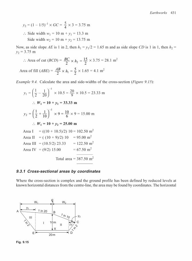
Earthworks 431
y2 = (1 – 1/5)–1 × GC = 54
× 3 = 3.75 m
∴ Side width w1 = 10 m + y1 = 13.3 m
Side width w2 = 10 m + y2 = 13.75 m
Now, as side slope AE is 1 in 2, then h1 = y1/2 = 1.65 m and as side slope CD is 1 in 1, then h2 =y2 = 3.75 m
∴ Area of cut (BCD) = BCh
2 = 15
22× × 3.75 = 28.1 m2
Area of fill (ABE) = ABh
2 = 5
21× × 1.65 = 4.1 m2
Example 9.4. Calculate the area and side-widths of the cross-section (Figure 9.15):
y1
–1
= 12
– 120
10.5 = 209
× × 10.5 = 23.33 m
∴ W1 = 10 + y1 = 33.33 m
y2
–1
= 12
+ 110
9 = 106
× × 9 = 15.00 m
∴ W1 = 10 + y2 = 25.00 m
Area I = ((10 + 10.5)/2) 10 = 102.50 m2
Area II = ( (10 + 9)/2) 10 = 95.00 m2
Area III = (10.5/2) 23.33 = 122.50 m2
Area IV = (9/2) 15.00 = 67.50 m2
————Total area = 387.50 m2
————
9.3.1 Cross-sectional areas by coordinates
Where the cross-section is complex and the ground profile has been defined by reduced levels atknown horizontal distances from the centre-line, the area may be found by coordinates. The horizontal
Fig. 9.15
CLW1 W2
y11 in 20
III
II
B1 in 10
IV
y2
I 10m
X
DE20m
A
1 in 2
1 in
2
C
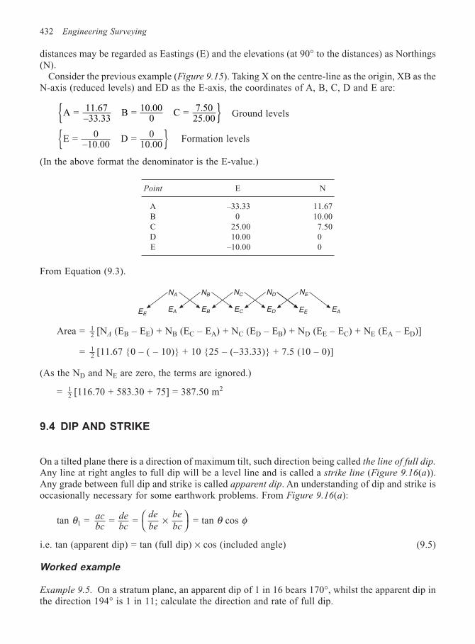
432 Engineering Surveying
distances may be regarded as Eastings (E) and the elevations (at 90° to the distances) as Northings(N).
Consider the previous example (Figure 9.15). Taking X on the centre-line as the origin, XB as theN-axis (reduced levels) and ED as the E-axis, the coordinates of A, B, C, D and E are:
A = 11.67–33.33
B = 10.000
C = 7.5025.00 Ground levels
E = 0–10.00
D = 010.00 Formation levels
(In the above format the denominator is the E-value.)
Point E N
A –33.33 11.67B 0 10.00C 25.00 7.50D 10.00 0E –10.00 0
From Equation (9.3).
Area = 12 [NA (EB – EE) + NB (EC – EA) + NC (ED – EB) + ND (EE – EC) + NE (EA – ED)]
= 12 [11.67 0 – ( – 10) + 10 25 – (–33.33) + 7.5 (10 – 0)]
(As the ND and NE are zero, the terms are ignored.)
= 12 [116.70 + 583.30 + 75] = 387.50 m2
9.4 DIP AND STRIKE
On a tilted plane there is a direction of maximum tilt, such direction being called the line of full dip.
Any line at right angles to full dip will be a level line and is called a strike line (Figure 9.16(a)).Any grade between full dip and strike is called apparent dip. An understanding of dip and strike isoccasionally necessary for some earthwork problems. From Figure 9.16(a):
tan θ1 = acbc
debc
de
be
be
bc = = ×
= tan θ cos φ
i.e. tan (apparent dip) = tan (full dip) × cos (included angle) (9.5)
Worked example
Example 9.5. On a stratum plane, an apparent dip of 1 in 16 bears 170°, whilst the apparent dip inthe direction 194° is 1 in 11; calculate the direction and rate of full dip.
EEECEA EE
NA NB
EB
NC ND
ED
NE
EA
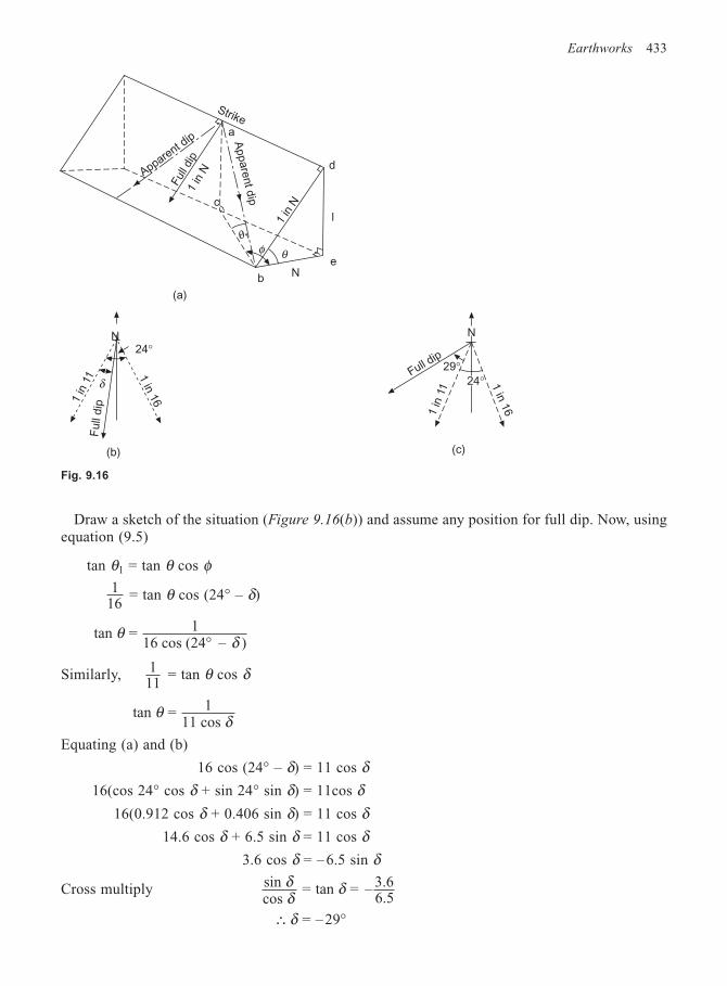
Earthworks 433
Draw a sketch of the situation (Figure 9.16(b)) and assume any position for full dip. Now, usingequation (9.5)
tan θ1 = tan θ cos φ1
16 = tan θ cos (24° – δ)
tan = 116 cos (24 – )
θδ°
Similarly, 111
= tan θ cos δ
tan = 111 cos
θδ
Equating (a) and (b)
16 cos (24° – δ) = 11 cos δ16(cos 24° cos δ + sin 24° sin δ) = 11cos δ
16(0.912 cos δ + 0.406 sin δ) = 11 cos δ14.6 cos δ + 6.5 sin δ = 11 cos δ
3.6 cos δ = – 6.5 sin δ
Cross multiply sincos
= tan = – 3.66.5
δδ
δ
∴ δ = – 29°
Fig. 9.16
Strike
Apparent d
ip
Ful
l dip
1 in
N
1 in
N
d
l
eN
b
θφ
Appare
nt d
ip
a
θ1
c
(c)
N N
1 in
11
Full
dip
δ
24°
24°29°
1 in
11
Full dip
1 in
16
1 in
16
(b)
(a)
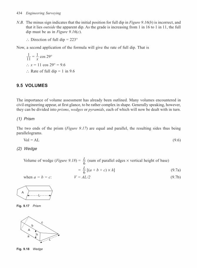
434 Engineering Surveying
N.B. The minus sign indicates that the initial position for full dip in Figure 9.16(b) is incorrect, andthat it lies outside the apparent dip. As the grade is increasing from 1 in 16 to 1 in 11, the fulldip must be as in Figure 9.16(c).
∴ Direction of full dip = 223°
Now, a second application of the formula will give the rate of full dip. That is
111
= 1 cos 29x
°
∴ x = 11 cos 29° = 9.6
∴ Rate of full dip = 1 in 9.6
9.5 VOLUMES
The importance of volume assessment has already been outlined. Many volumes encountered incivil engineering appear, at first glance, to be rather complex in shape. Generally speaking, however,they can be divided into prisms, wedges or pyramids, each of which will now be dealt with in turn.
(1) Prism
The two ends of the prism (Figure 9.17) are equal and parallel, the resulting sides thus beingparallelograms.
Vol = AL (9.6)
(2) Wedge
Volume of wedge (Figure 9.18) = L6
(sum of parallel edges × vertical height of base)
= L6
[(a + b + c) × h] (9.7a)
when a = b = c: V = AL /2 (9.7b)
Fig. 9.17 Prism
Fig. 9.18 Wedge
bc
A
ah
L
AL
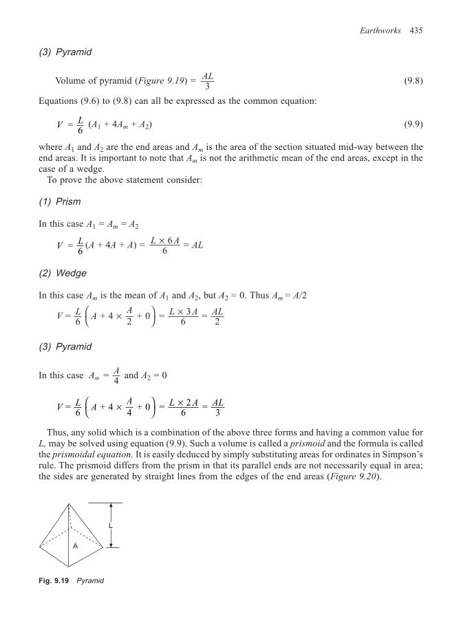
Earthworks 435
(3) Pyramid
Volume of pyramid (Figure 9.19) = AL3
(9.8)
Equations (9.6) to (9.8) can all be expressed as the common equation:
VL = 6
(A1 + 4Am + A2) (9.9)
where A1 and A2 are the end areas and Am is the area of the section situated mid-way between theend areas. It is important to note that Am is not the arithmetic mean of the end areas, except in thecase of a wedge.
To prove the above statement consider:
(1) Prism
In this case A1 = Am = A2
VL = 6
(A + 4A + A) = L AAL
66
= ×
(2) Wedge
In this case Am is the mean of A1 and A2, but A2 = 0. Thus Am = A/2
VL
AA L A AL =
6 + 4
2 + 0 = 3
6 =
2×
×
(3) Pyramid
In this case AA
m = 4
and A2 = 0
VL
AA L A AL =
6 + 4
4 + 0 = 2
6 =
3×
×
Thus, any solid which is a combination of the above three forms and having a common value forL, may be solved using equation (9.9). Such a volume is called a prismoid and the formula is calledthe prismoidal equation. It is easily deduced by simply substituting areas for ordinates in Simpson’srule. The prismoid differs from the prism in that its parallel ends are not necessarily equal in area;the sides are generated by straight lines from the edges of the end areas (Figure 9.20).
Fig. 9.19 Pyramid
A
L
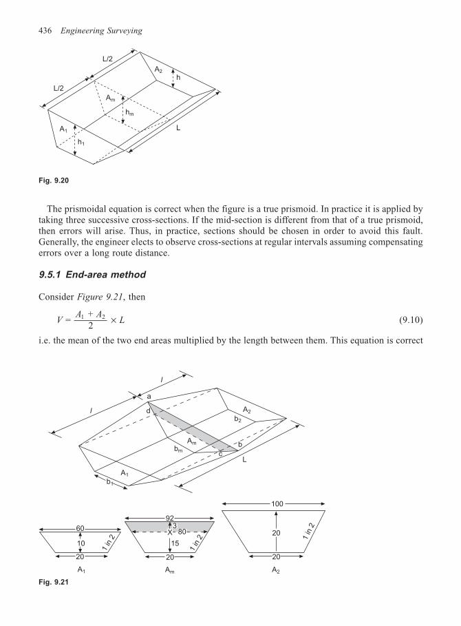
436 Engineering Surveying
The prismoidal equation is correct when the figure is a true prismoid. In practice it is applied bytaking three successive cross-sections. If the mid-section is different from that of a true prismoid,then errors will arise. Thus, in practice, sections should be chosen in order to avoid this fault.Generally, the engineer elects to observe cross-sections at regular intervals assuming compensatingerrors over a long route distance.
9.5.1 End-area method
Consider Figure 9.21, then
VA A
L = + 2
1 2 × (9.10)
i.e. the mean of the two end areas multiplied by the length between them. This equation is correct
Fig. 9.20
Fig. 9.21
L/2
L/2
A1
A2
Am
h1
hm
h
L
XX
l
l
a
d
bm
Am
b2
A2
A1
b1
cL
b
60
10
20
A1
1 in
2
923
X 80
1 in
2
20
15
100
20
20
1 in
2
A2Am
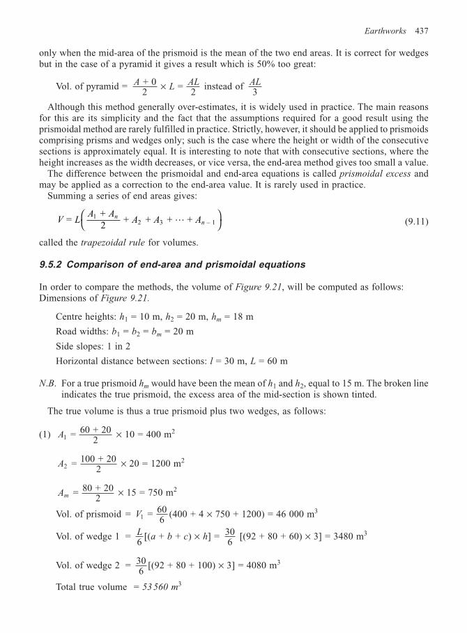
Earthworks 437
only when the mid-area of the prismoid is the mean of the two end areas. It is correct for wedgesbut in the case of a pyramid it gives a result which is 50% too great:
Vol. of pyramid = AL
AL + 02
= 2
× instead of3
AL
Although this method generally over-estimates, it is widely used in practice. The main reasonsfor this are its simplicity and the fact that the assumptions required for a good result using theprismoidal method are rarely fulfilled in practice. Strictly, however, it should be applied to prismoidscomprising prisms and wedges only; such is the case where the height or width of the consecutivesections is approximately equal. It is interesting to note that with consecutive sections, where theheight increases as the width decreases, or vice versa, the end-area method gives too small a value.
The difference between the prismoidal and end-area equations is called prismoidal excess andmay be applied as a correction to the end-area value. It is rarely used in practice.
Summing a series of end areas gives:
V LA A
A A Ann =
+ 2
+ + + + 12 3 – 1L
(9.11)
called the trapezoidal rule for volumes.
9.5.2 Comparison of end-area and prismoidal equations
In order to compare the methods, the volume of Figure 9.21, will be computed as follows:Dimensions of Figure 9.21.
Centre heights: h1 = 10 m, h2 = 20 m, hm = 18 m
Road widths: b1 = b2 = bm = 20 m
Side slopes: 1 in 2
Horizontal distance between sections: l = 30 m, L = 60 m
N.B. For a true prismoid hm would have been the mean of h1 and h2, equal to 15 m. The broken lineindicates the true prismoid, the excess area of the mid-section is shown tinted.
The true volume is thus a true prismoid plus two wedges, as follows:
(1) A1 = 60 + 202
× 10 = 400 m2
A2 = 100 + 202
× 20 = 1200 m2
Am = 80 + 202
× 15 = 750 m2
Vol. of prismoid = V1 = 606
(400 + 4 × 750 + 1200) = 46 000 m3
Vol. of wedge 1 = L6
[(a + b + c) × h] = 306
[(92 + 80 + 60) × 3] = 3480 m3
Vol. of wedge 2 = 306
[(92 + 80 + 100) × 3] = 4080 m3
Total true volume = 53 560 m3
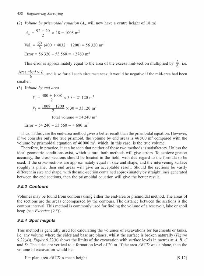
438 Engineering Surveying
(2) Volume by prismoidal equation (Am will now have a centre height of 18 m)
Am = 92 + 202
× 18 = 1008 m2
Vol. = 606
(400 + 4032 + 1200) = 56 320 m3
Error = 56 320 – 53 560 = + 2760 m2
This error is approximately equal to the area of the excess mid-section multiplied by L6
, i.e.
Area 6
abcd L× , and is so for all such circumstances; it would be negative if the mid-area had been
smaller.
(3) Volume by end area
V1 = 400 + 10082
× 30 = 21 120 m3
V2 = 1008 + 12002
× 30 = 33120 m3
Total volume = 54 240 m3
Error = 54 240 – 53 560 = + 680 m3
Thus, in this case the end-area method gives a better result than the prismoidal equation. However,if we consider only the true prismoid, the volume by end areas is 46 500 m3 compared with thevolume by prismoidal equation of 46 000 m3, which, in this case, is the true volume.
Therefore, in practice, it can be seen that neither of these two methods is satisfactory. Unless theideal geometric conditions exist, which is rare, both methods will give errors. To achieve greateraccuracy, the cross-sections should be located in the field, with due regard to the formula to beused. If the cross-sections are approximately equal in size and shape, and the intervening surfaceroughly a plane, then end areas will give an acceptable result. Should the sections be vastlydifferent in size and shape, with the mid-section contained approximately by straight lines generatedbetween the end sections, then the prismoidal equation will give the better result.
9.5.3 Contours
Volumes may be found from contours using either the end-area or prismoidal method. The areas ofthe sections are the areas encompassed by the contours. The distance between the sections is thecontour interval. This method is commonly used for finding the volume of a reservoir, lake or spoilheap (see Exercise (9.3)).
9.5.4 Spot heights
This method is generally used for calculating the volumes of excavations for basements or tanks,i.e. any volume where the sides and base are planes, whilst the surface is broken naturally (Figure
9.22(a)). Figure 9.22(b) shows the limits of the excavation with surface levels in metres at A, B, C
and D. The sides are vertical to a formation level of 20 m. If the area ABCD was a plane, then thevolume of excavation would be:
V = plan area ABCD × mean height (9.12)
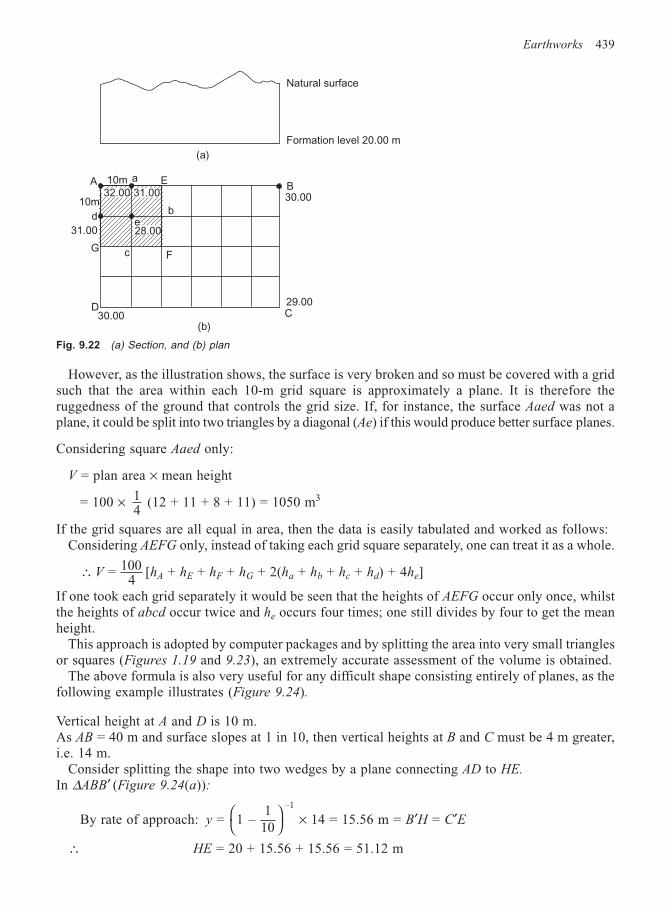
Earthworks 439
However, as the illustration shows, the surface is very broken and so must be covered with a gridsuch that the area within each 10-m grid square is approximately a plane. It is therefore theruggedness of the ground that controls the grid size. If, for instance, the surface Aaed was not aplane, it could be split into two triangles by a diagonal (Ae) if this would produce better surface planes.
Considering square Aaed only:
V = plan area × mean height
= 100 × 14
(12 + 11 + 8 + 11) = 1050 m3
If the grid squares are all equal in area, then the data is easily tabulated and worked as follows:Considering AEFG only, instead of taking each grid square separately, one can treat it as a whole.
∴ = 1004
V [hA + hE + hF + hG + 2(ha + hb + hc + hd) + 4he]
If one took each grid separately it would be seen that the heights of AEFG occur only once, whilstthe heights of abcd occur twice and he occurs four times; one still divides by four to get the meanheight.
This approach is adopted by computer packages and by splitting the area into very small trianglesor squares (Figures 1.19 and 9.23), an extremely accurate assessment of the volume is obtained.
The above formula is also very useful for any difficult shape consisting entirely of planes, as thefollowing example illustrates (Figure 9.24).
Vertical height at A and D is 10 m.As AB = 40 m and surface slopes at 1 in 10, then vertical heights at B and C must be 4 m greater,i.e. 14 m.
Consider splitting the shape into two wedges by a plane connecting AD to HE.
In ∆ABB′ (Figure 9.24(a)):
By rate of approach: y = 1 – 1
10
–1
× 14 = 15.56 m = B′H = C′E
∴ HE = 20 + 15.56 + 15.56 = 51.12 m
Fig. 9.22 (a) Section, and (b) plan
Natural surface
Formation level 20.00 m
10m a E32.00 31.00
db
10m
A
e28.00
GF
B30.00
D30.00
29.00C
c
(a)
(b)
31.00
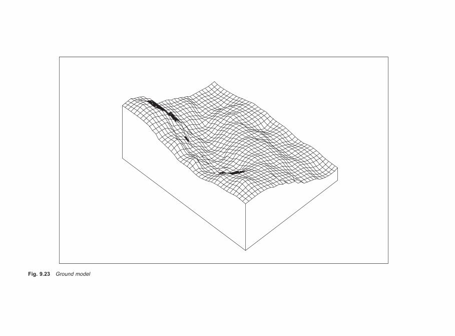
Fig. 9.23 Ground model
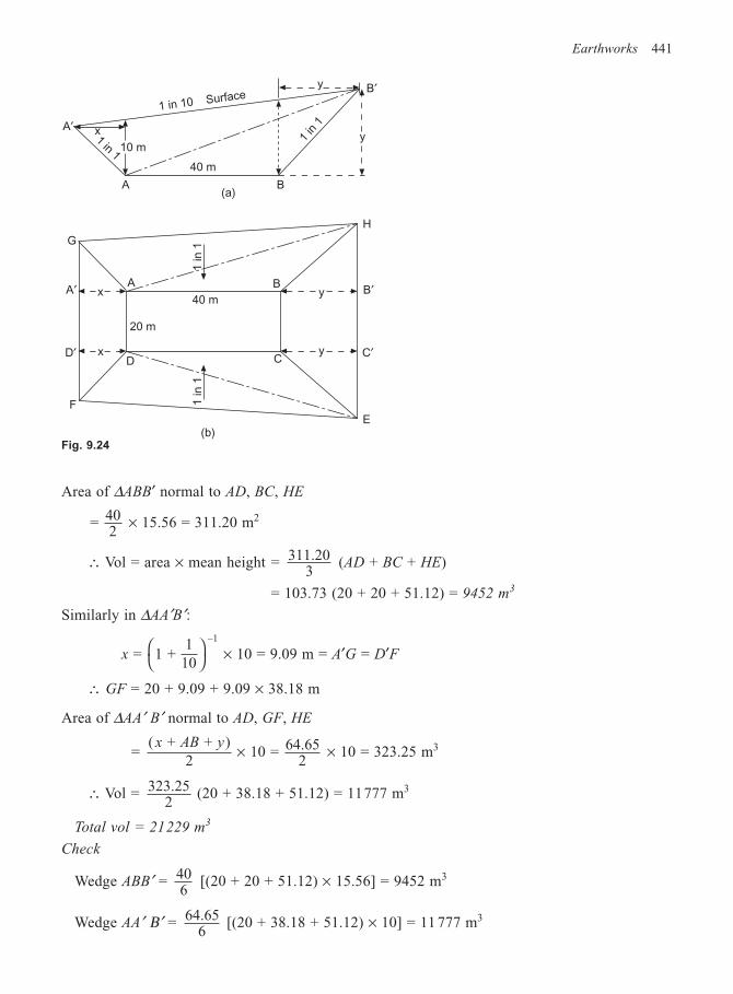
Earthworks 441
Area of ∆ABB′ normal to AD, BC, HE
= 402
× 15.56 = 311.20 m2
∴ Vol = area × mean height = 311.203
(AD + BC + HE)
= 103.73 (20 + 20 + 51.12) = 9452 m3
Similarly in ∆AA′B′:
x = 1 + 1
10
–1
× 10 = 9.09 m = A′G = D′F
∴ GF = 20 + 9.09 + 9.09 × 38.18 m
Area of ∆AA′ B′ normal to AD, GF, HE
=( + + )
2 10 = 64.65
2x AB y
× × 10 = 323.25 m3
∴ Vol = 323.252
(20 + 38.18 + 51.12) = 11777 m3
Total vol = 21229 m3
Check
Wedge ABB′ = 406
[(20 + 20 + 51.12) × 15.56] = 9452 m3
Wedge AA′ Β′ = 64.656
[(20 + 38.18 + 51.12) × 10] = 11 777 m3
Fig. 9.24(b)
1 in 10 Surface
10 m1 in 1
A′
A
40 m
B
y
1 in
1
yx
G
H
E
F
A B
CD
1 in 1
40 m
20 m
1 in 1
xA′
D′ x
y
y
B′
C′
B′
(a)
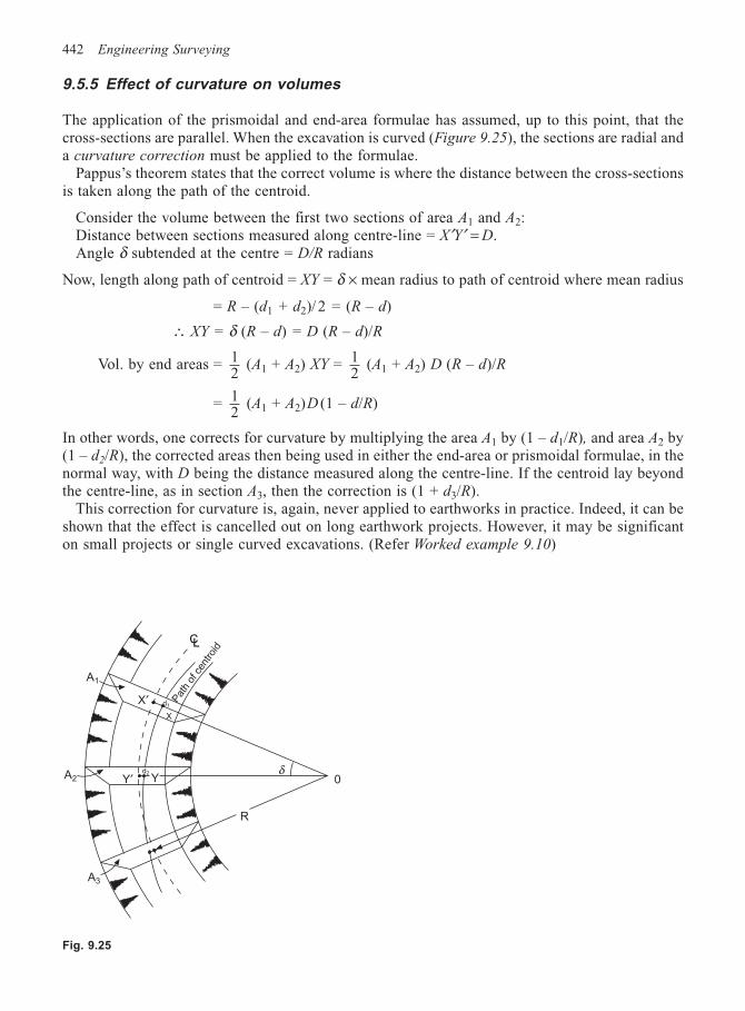
442 Engineering Surveying
9.5.5 Effect of curvature on volumes
The application of the prismoidal and end-area formulae has assumed, up to this point, that thecross-sections are parallel. When the excavation is curved (Figure 9.25), the sections are radial anda curvature correction must be applied to the formulae.
Pappus’s theorem states that the correct volume is where the distance between the cross-sectionsis taken along the path of the centroid.
Consider the volume between the first two sections of area A1 and A2:Distance between sections measured along centre-line = X′Y′ = D.Angle δ subtended at the centre = D/R radians
Now, length along path of centroid = XY = δ × mean radius to path of centroid where mean radius
= R – (d1 + d2)/ 2 = (R – d)
∴ XY = δ (R – d) = D (R – d)/R
Vol. by end areas = 12
(A1 + A2) XY = 12
(A1 + A2) D (R – d)/R
= 12
(A1 + A2)D (1 – d/R)
In other words, one corrects for curvature by multiplying the area A1 by (1 – d1/R), and area A2 by(1 – d2/R), the corrected areas then being used in either the end-area or prismoidal formulae, in thenormal way, with D being the distance measured along the centre-line. If the centroid lay beyondthe centre-line, as in section A3, then the correction is (1 + d3/R).
This correction for curvature is, again, never applied to earthworks in practice. Indeed, it can beshown that the effect is cancelled out on long earthwork projects. However, it may be significanton small projects or single curved excavations. (Refer Worked example 9.10)
Fig. 9.25
A1
A2
A3
X′
Y′ Yd2
d1
X
R
0δ
Pat
h of
cen
troi
d
CL
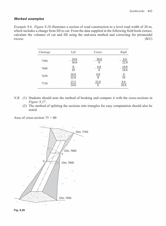
Earthworks 443
Worked examples
Example 9.6. Figure 9.26 illustrates a section of road construction to a level road width of 20 m,which includes a change from fill to cut. From the data supplied in the following field book extract,calculate the volumes of cut and fill using the end-area method and correcting for prismoidalexcess. (KU)
Chainage Left Centre Right
7500 – 10.036.0
– 20.00
– 8.822.0
76000
10– 6.0
0– 14.0
24.6
765016.022.0
4.00
010
775013.524.0
22.00
8.626.0
N.B. (1) Students should note the method of booking and compare it with the cross-sections inFigure 9.27.
(2) The method of splitting the sections into triangles for easy computation should also benoted.
Area of cross-section 75 + 00
Fig. 9.26
Chn. 7500
Chn. 7600
Chn. 7650
Y
Chn. 7750
X
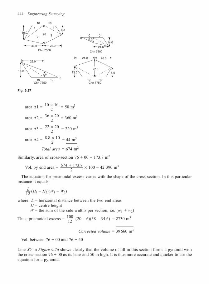
444 Engineering Surveying
area ∆1 = 10 102× = 50 m3
area ∆2 = 36 202× = 360 m3
area ∆3 = 22 202× = 220 m3
area ∆4 = 8.8 102× = 44 m3
Total area = 674 m2
Similarly, area of cross-section 76 + 00 = 173.8 m2
Vol. by end area = 674 + 173.82
× 100 = 42 390 m3
The equation for prismoidal excess varies with the shape of the cross-section. In this particularinstance it equals
L12
(H1 – H2)(W1 – W2)
where L = horizontal distance between the two end areasH = centre heightW = the sum of the side widths per section, i.e. (w1 + w2)
Thus, prismoidal excess = 10012
(20 – 6)(58 – 34.6) = 2730 m3
————Corrected volume = 39660 m3
Vol. between 76 + 00 and 76 + 50
Line XY in Figure 9.26 shows clearly that the volume of fill in this section forms a pyramid withthe cross-section 76 + 00 as its base and 50 m high. It is thus more accurate and quicker to use theequation for a pyramid.
Fig. 9.27
10.0
10 10
20
1
23
48.8
36.0 22.0
10 10
6.014.0
24.6
Chn 7600
22.0
16.0
10 100
4.0
24.0 26.0
13.522.0
10 10
8.6
Chn 7750
Chn 7500
Chn 7650
0
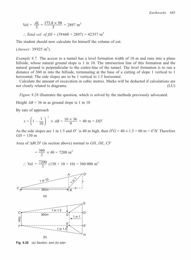
Earthworks 445
Vol = AL3
= 173.8 503
× = 2897 m3
∴ Total vol. of fill = (39 660 + 2897) = 42557 m3
The student should now calculate for himself the volume of cut.
(Answer: 39925 m3).
Example 9.7. The access to a tunnel has a level formation width of 10 m and runs into a planehillside, whose natural ground slope is 1 in 10. The intersection line of this formation and thenatural ground is perpendicular to the centre-line of the tunnel. The level formation is to run adistance of 360 m into the hillside, terminating at the base of a cutting of slope 1 vertical to 1horizontal. The side slopes are to be 1 vertical to 1.5 horizontal.
Calculate the amount of excavation in cubic metres. Marks will be deducted if calculations arenot clearly related to diagrams. (LU)
Figure 9.28 illustrates the question, which is solved by the methods previously advocated.
Height AB = 36 m as ground slope is 1 in 10
By rate of approach
x AB = 1 – 1
10 = 10 36
9
–1
× × = 40 m = DD′
As the side slopes are 1 in 1.5 and D′ is 40 m high, then D′G = 40 × 1.5 = 60 m = E′H. ThereforeGH = 130 m
Area of ∆BCD′ (in section above) normal to GH, DE, CF
= 3602
× 40 = 7200 m2
∴ Vol = 72003
(130 + 10 + 10) = 360 000 m3
Fig. 9.28 (a) Section, and (b) plan
C360m
1 in 10
A
B
1 in 1
x
x
D′
C
F
10m
360m D
G
D′
E′1 in 1.5
E
H
(a)
(b)
1 in 1.5
1 in 1
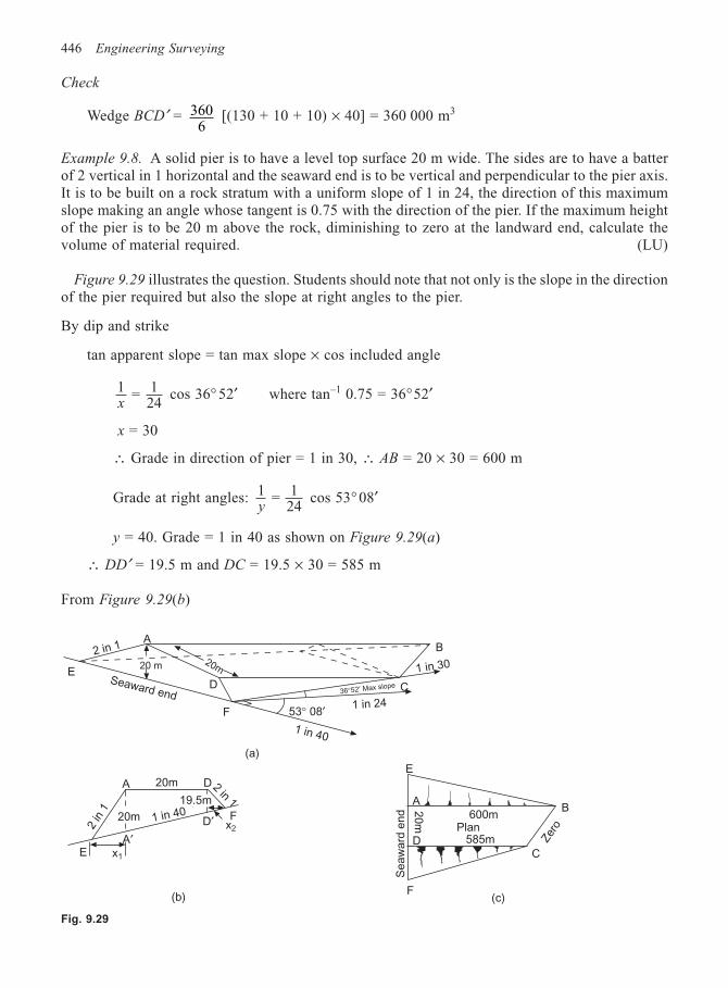
446 Engineering Surveying
Check
Wedge BCD′ = 3606
[(130 + 10 + 10) × 40] = 360 000 m3
Example 9.8. A solid pier is to have a level top surface 20 m wide. The sides are to have a batterof 2 vertical in 1 horizontal and the seaward end is to be vertical and perpendicular to the pier axis.It is to be built on a rock stratum with a uniform slope of 1 in 24, the direction of this maximumslope making an angle whose tangent is 0.75 with the direction of the pier. If the maximum heightof the pier is to be 20 m above the rock, diminishing to zero at the landward end, calculate thevolume of material required. (LU)
Figure 9.29 illustrates the question. Students should note that not only is the slope in the directionof the pier required but also the slope at right angles to the pier.
By dip and strike
tan apparent slope = tan max slope × cos included angle
1 = 124x
cos 36° 52′ where tan–1 0.75 = 36°52′
x = 30
∴ Grade in direction of pier = 1 in 30, ∴ AB = 20 × 30 = 600 m
Grade at right angles: 1 = 124y
cos 53° 08′
y = 40. Grade = 1 in 40 as shown on Figure 9.29(a)
∴ DD′ = 19.5 m and DC = 19.5 × 30 = 585 m
From Figure 9.29(b)
Fig. 9.29
2 in 1A
E
F
Seaward end
20 m 20m
D
B
1 in 30
C36°52′ Max slope
53° 08′ 1 in 24
1 in 40
(a)
(b)
A
A′x1E
2 in
1
20m
20m 1 in 40D′
19.5m
2 in 1
Fx2
E
AB
CD
600mPlan
585m Zer
o
F
Seaw
ard
end
(c)
20m
D
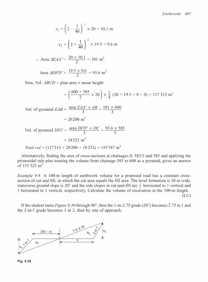
Earthworks 447
x1
–1
= 2 – 140
× 20 = 10.1 m
x2
–1
= 2 + 140
× 19.5 = 9.6 m
∴ Area ∆EAA′ = 20 10.12
× = 101 m2
Area ∆DFD′ = 19.5 9.62× = 93.6 m2
Now, Vol. ABCD = plan area × mean height
=600 + 585
2 20 1
4×
× (20 + 19.5 + 0 + 0) = 117 315 m3
Vol. of pyramid EAB = area 3
= 101 6003
EAA AB′ × ×
= 20 200 m3
Vol. of pyramid DFC = area 3
= 93.6 5853
DFD DC′ × ×
= 18 252 m3
Total vol = (117 315 + 20 200 + 18 252) = 155 767 m3
Alternatively, finding the area of cross-sections at chainages 0, 585/2 and 585 and applying theprismoidal rule plus treating the volume from chainage 585 to 600 as a pyramid, gives an answerof 155 525 m3
Example 9.9. A 100-m length of earthwork volume for a proposed road has a constant cross-section of cut and fill, in which the cut area equals the fill area. The level formation is 30 m wide,transverse ground slope is 20° and the side slopes in cut-and-fill are 1
2 horizontal to 1 vertical and1 horizontal to 1 vertical, respectively. Calculate the volume of excavation in the 100-m length.
(LU)
If the student turns Figure 9.30 through 90°, then the 1-in-2.75 grade (20°) becomes 2.75 in 1 andthe 2-in-1 grade becomes 1 in 2, then by rate of approach:
Fig. 9.30
A1
A2
h1
x
h2
1 in
1
1 in 2.75
2 in
1
(30 – x)
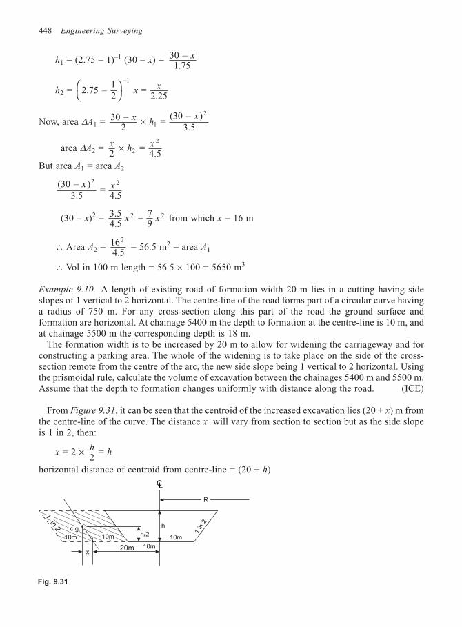
448 Engineering Surveying
h1 = (2.75 – 1)–1 (30 – x) = 30 – 1.75
x
h2 = 2.75 – 12
= 2.25
–1
x
x
Now, area ∆A1 = 30 – 2
= (30 – )
3.51
2x
hx×
area ∆A2 = xh
x2
= 4.52
2
×
But area A1 = area A2
(30 – )3.5
= 4.5
2 2x x
(30 – x)2 = 3.54.5
= 79
2 2x x from which x = 16 m
∴ Area A2 = 164.5
2
= 56.5 m2 = area A1
∴ Vol in 100 m length = 56.5 × 100 = 5650 m3
Example 9.10. A length of existing road of formation width 20 m lies in a cutting having sideslopes of 1 vertical to 2 horizontal. The centre-line of the road forms part of a circular curve havinga radius of 750 m. For any cross-section along this part of the road the ground surface andformation are horizontal. At chainage 5400 m the depth to formation at the centre-line is 10 m, andat chainage 5500 m the corresponding depth is 18 m.
The formation width is to be increased by 20 m to allow for widening the carriageway and forconstructing a parking area. The whole of the widening is to take place on the side of the cross-section remote from the centre of the arc, the new side slope being 1 vertical to 2 horizontal. Usingthe prismoidal rule, calculate the volume of excavation between the chainages 5400 m and 5500 m.Assume that the depth to formation changes uniformly with distance along the road. (ICE)
From Figure 9.31, it can be seen that the centroid of the increased excavation lies (20 + x) m fromthe centre-line of the curve. The distance x will vary from section to section but as the side slopeis 1 in 2, then:
x = 2 × hh
2 =
horizontal distance of centroid from centre-line = (20 + h)
1 in 2 c.g.
10m 10m 10mh/2
h
R
1 in
2
CL
10m20mx
Fig. 9.31
Earthworks 449
At chainage 5400 m, h1 = 10 m ∴ (20 + h) = 30 m = d1
At chainage 5450 m, h2 = 14 m ∴ (20 + h) = 34 m = d2
At chainage 5500 m, h3 = 18 m ∴ (20 + h) = 38 m = d3
Area of extra excavation at 5400 m = 10 × 20 = 200 m2 = A1
Area of extra excavation at 5450 m = 14 × 20 = 280 m2 = A2
Area of extra excavation at 5500 m = 18 × 20 = 360 m2 = A3
The above areas are now corrected for curvature: Ad
R1 +
At chainage 5400 m = 200 1 + 30750
= 208 m2
At chainage 5450 m = 280 1 + 34750
= 292.6 m2
At chainage 5500 m = 360 1 + 38750
= 378 m2
∴ Vol = 1006
(208 + 4 × 292.6 + 378) = 29273 m3
Exercises
(9.1) An access road to a quarry is being cut in a plane surface in the direction of strike, the fulldip of 1 in 12.86 being to the left of the direction of drive. The road is to be constructed throughouton a formation grade of 1 in 50 dipping, formation width 20 m and level, side slopes 1 in 2 and azero depth on the centre-line at chainage 0 m.
At chainage 400 m the direction of the road turns abruptly through a clockwise angle of 40°;calculate the volume of excavation between chainages 400 m and 600 m. (KU)
(Answer: 169 587 m3)
(9.2) A road is to be constructed on the side of a hill having a cross fall of 1 in 50 at right anglesto the centre-line of the road; the side slopes are to be 1 in 2 in cut and 1 in 3 in fill; the formationis 20 m wide and level. Find the position of the centre-line of the road with respect to the point ofintersection of the formation and the natural ground.
(a) To give equality of cut and fill.(b) So that the area of cut shall be 0.8 of the area of fill, in order to allow for bulking. (LU)
(Answer: (a) 0.3 m in cut, (b) 0.2 m in fill)
(9.3) A reservoir is to be formed in a river valley by building a dam across it. The entire area thatwill be covered by the reservoir has been contoured and contours drawn at 1.5-m intervals. Thelowest point in the reservoir is at a reduced level of 249 m above datum, whilst the top water levelwill not be above a reduced level of 264.5 m. The area enclosed by each contour and the upstreamface of the dam is shown in the table below.
450 Engineering Surveying
Contour Area enclosed
(m) (m2)
250.0 1 874251.5 6 355253.0 11 070254.5 14 152256.0 19 310257.5 22 605259.0 24 781260.5 26 349262.0 29 830263.5 33 728265.0 37 800
Estimate by the use of the trapezoidal rule the capacity of the reservoir when full. What will bethe reduced level of the water surface if, in a time of drought, this volume is reduced by 25%?
(ICE)
(Answer: 294 211 m3; 262.3 m)
(9.4) The central heights of the ground above formation at three sections 100 m apart are 10 m,12 m, 15 m, and the cross-falls at these sections are respectively 1 in 30, 1 in 40 and 1 in 20. If theformation width is 40 m and sides slope 1 vertical to 2 horizontal, calculate the volume of excavationin the 200-m length:
(a) If the centre-line is straight.(b) If the centre-line is an arc of 400 m radius. (LU)
(Answer: (a) 158 367 m3, (b) 158 367 ± 1070 m3)
9.6 MASS-HAUL DIAGRAMS
Mass-haul diagrams (MHD) are used to compare the economy of various methods of earthworkdistribution on road or railway construction schemes. By the combined use of the MHD plotteddirectly below the longitudinal section of the survey centre-line, one can find.
(1) The distances over which cut and fill will balance.(2) Quantities of materials to be moved and the direction of movement.(3) Areas where earth may have to be borrowed or wasted and the amounts involved.(4) The best policy to adopt to obtain the most economic use of plant.
9.6.1 Definitions
(1) Haul refers to the volume of material multiplied by the distance moved, expressed in ‘stationmetres’.
(2) Station metre (stn m) is 1 m3 of material moved 100 m
Thus, 20 m3 moved 1500 m is a haul of 20 × 1500/100 = 300 stn m.
Earthworks 451
(3) Freehaul and overhaul can best be defined by example. A contractor may offer to haul materiala distance of, say, 150 m at 50 p per m3, but thereafter for any distance hauled beyond 150 mthe contractor may require an extra 5 p per stn m, i.e. 5 p per m3 moved per 100 m. The distanceof 150 m is called the freehaul distance and is based on the economical hauling distance of theearthmoving plant used. It may range from 100 m for a bulldozer to 3000 m for self-propelledscrapers. The haul beyond the freehaul distance is termed the overhaul.
(4) Waste is the material excavated from cuts but not used for embankment fills.
(5) Borrow is the material needed for the formation of embankments, secured not from roadwayexcavation but from elsewhere. It is said to be obtained from a ‘borrow pit’.
(6) Limit of economical haul is the maximum overhaul distance plus the freehaul distance. Whenthis limit is reached it is more economical to waste and borrow material. For example, assume:
Freehaul distance = 500 m
Overhaul = 10 p per stn m (i.e. 10 p per m3 per 100 m)
Borrow = 30 p per m3
From these figures it can be seen that to overhaul 1 m3 a distance of 300 m would cost 30 p, equalto the cost of borrow; this then is the maximum overhaul distance. However, before overhaul comesinto operation, one may move earth through the freehaul distance of 500 m. Thus the limit ofeconomical haul = (300 + 500) = 800 m.
9.6.2 Bulking and shrinkage
Excavation of material causes it to loosen, and thus its excavated volume will be greater than its insitu volume. However, when filled and compacted, it may occupy a less volume than when originallyin situ. For example, ordinary earth is less by about 10% after filling, whilst rock bulks by some20% to 30%. To allow for this, a correction factor is generally applied to the cut or fill volumes.
9.6.3 Construction of the MHD
A MHD is a continuous curve, whose vertical ordinates, plotted on the same distance scale as thelongitudinal section, represent the algebraic sum of the corrected volumes (cut +, fill –).
9.6.4 Properties of the MHD
Consider Figure 9.32(a)) in which the ground XYZ is to be levelled off to the grade line A′B′.Assuming that the fill volumes, after correction, equal the cut volumes, the MHD would plot asshown in Figure 9.32(b). Thus:
(1) Since the curve of the MHD represents the algebraic sums of the volumes, then any horizontalline drawn parallel to the base AB will indicate the volumes which balance. Such a line is calleda balancing line and may even be represented by AB itself, indicating that the total cut equalsthe total fill.
(2) The rising curve, shown broken, indicates cut (positive), the falling curve indicates fill (negative).
(3) The maximum and minimum points of a MHD occur directly beneath the intersection of thenatural ground and the formation grade; such intersections are called grade points.
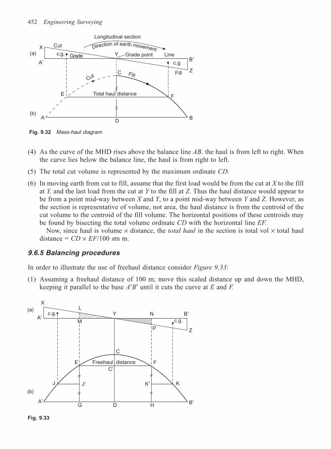
452 Engineering Surveying
(4) As the curve of the MHD rises above the balance line AB, the haul is from left to right. Whenthe curve lies below the balance line, the haul is from right to left.
(5) The total cut volume is represented by the maximum ordinate CD.
(6) In moving earth from cut to fill, assume that the first load would be from the cut at X to the fillat Y, and the last load from the cut at Y to the fill at Z. Thus the haul distance would appear tobe from a point mid-way between X and Y, to a point mid-way between Y and Z. However, asthe section is representative of volume, not area, the haul distance is from the centroid of thecut volume to the centroid of the fill volume. The horizontal positions of these centroids maybe found by bisecting the total volume ordinate CD with the horizontal line EF.
Now, since haul is volume × distance, the total haul in the section is total vol × total hauldistance = CD × EF/100 stn m.
9.6.5 Balancing procedures
In order to illustrate the use of freehaul distance consider Figure 9.33:
(1) Assuming a freehaul distance of 100 m; move this scaled distance up and down the MHD,keeping it parallel to the base A′B′ until it cuts the curve at E and F.
Fig. 9.33
XL
Y B′N
ZP
MA′
c.g.
E
J
A′
J′
C′
K
B′HDG
Freehaul distance
C
(a)
(b)
K′
c.g.
F
Fig. 9.32 Mass-haul diagram
Direction of earth movement
Longitudinal section
Grade point Linec.g. Grade
CutX
A′
Y
C
F
FillCut
Total haul distance
c.g.
Fill Z
B′
BD
A
(a)
(b)
E
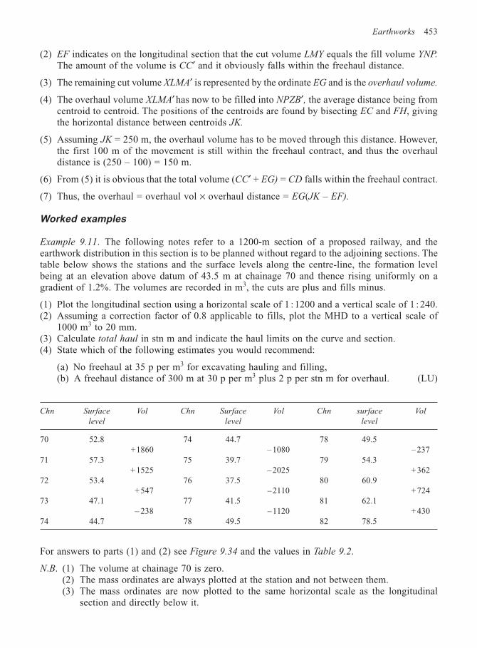
Earthworks 453
(2) EF indicates on the longitudinal section that the cut volume LMY equals the fill volume YNP.
The amount of the volume is CC′ and it obviously falls within the freehaul distance.
(3) The remaining cut volume XLMA′ is represented by the ordinate EG and is the overhaul volume.
(4) The overhaul volume XLMA′ has now to be filled into NPZB′, the average distance being fromcentroid to centroid. The positions of the centroids are found by bisecting EC and FH, givingthe horizontal distance between centroids JK.
(5) Assuming JK = 250 m, the overhaul volume has to be moved through this distance. However,the first 100 m of the movement is still within the freehaul contract, and thus the overhauldistance is (250 – 100) = 150 m.
(6) From (5) it is obvious that the total volume (CC′ + EG) = CD falls within the freehaul contract.
(7) Thus, the overhaul = overhaul vol × overhaul distance = EG(JK – EF).
Worked examples
Example 9.11. The following notes refer to a 1200-m section of a proposed railway, and theearthwork distribution in this section is to be planned without regard to the adjoining sections. Thetable below shows the stations and the surface levels along the centre-line, the formation levelbeing at an elevation above datum of 43.5 m at chainage 70 and thence rising uniformly on agradient of 1.2%. The volumes are recorded in m3, the cuts are plus and fills minus.
(1) Plot the longitudinal section using a horizontal scale of 1 :1200 and a vertical scale of 1 :240.(2) Assuming a correction factor of 0.8 applicable to fills, plot the MHD to a vertical scale of
1000 m3 to 20 mm.(3) Calculate total haul in stn m and indicate the haul limits on the curve and section.(4) State which of the following estimates you would recommend:
(a) No freehaul at 35 p per m3 for excavating hauling and filling,(b) A freehaul distance of 300 m at 30 p per m3 plus 2 p per stn m for overhaul. (LU)
Chn Surface Vol Chn Surface Vol Chn surface Vol
level level level
70 52.8 74 44.7 78 49.5+1860 – 1080 – 237
71 57.3 75 39.7 79 54.3+ 1525 – 2025 + 362
72 53.4 76 37.5 80 60.9+ 547 –2110 + 724
73 47.1 77 41.5 81 62.1– 238 –1120 + 430
74 44.7 78 49.5 82 78.5
For answers to parts (1) and (2) see Figure 9.34 and the values in Table 9.2.
N.B. (1) The volume at chainage 70 is zero.(2) The mass ordinates are always plotted at the station and not between them.(3) The mass ordinates are now plotted to the same horizontal scale as the longitudinal
section and directly below it.
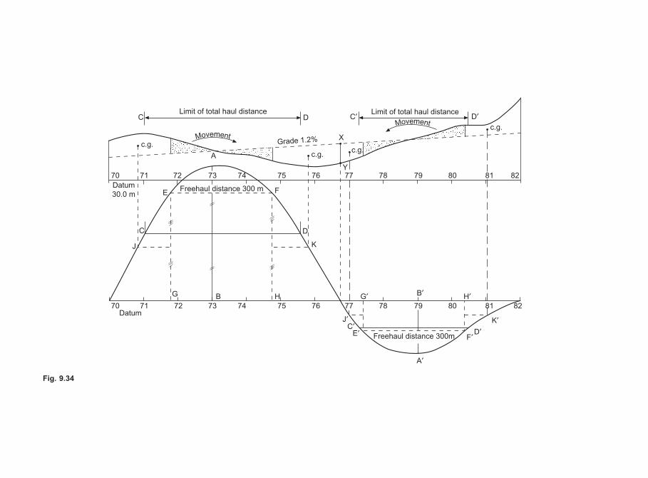
Fig. 9.34
Movement
Movement
Limit of total haul distance Limit of total haul distanceC D C′ D′
Grade 1.2%c.g.
c.g.c.g.
c.g.
X
70 71 72 73 74 75 76 77 78 79 80 81 82
Datum
30.0 m EFreehaul distance 300 m F
D
K
Y
C
J
G B H G′ B′ H′70 71 72 73 74 75 76 77 78 79 80 81 82
DatumJ′
C′E′
A′
F′D′
K′
Freehaul distance 300m
A
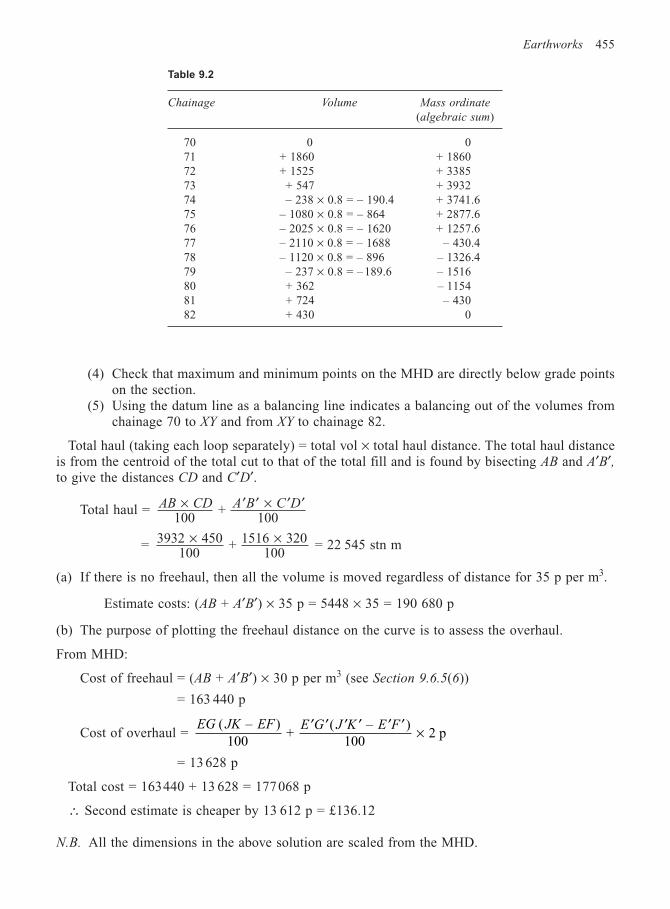
Earthworks 455
(4) Check that maximum and minimum points on the MHD are directly below grade pointson the section.
(5) Using the datum line as a balancing line indicates a balancing out of the volumes fromchainage 70 to XY and from XY to chainage 82.
Total haul (taking each loop separately) = total vol × total haul distance. The total haul distanceis from the centroid of the total cut to that of the total fill and is found by bisecting AB and A′B′,to give the distances CD and C′D′.
Total haul = AB CD A B C D100
+ 100
× ′ ′ × ′ ′
= 3932 450100
+ 1516 320100
× × = 22 545 stn m
(a) If there is no freehaul, then all the volume is moved regardless of distance for 35 p per m3.
Estimate costs: (AB + A′B′) × 35 p = 5448 × 35 = 190 680 p
(b) The purpose of plotting the freehaul distance on the curve is to assess the overhaul.
From MHD:
Cost of freehaul = (AB + A′B′) × 30 p per m3 (see Section 9.6.5(6))
= 163 440 p
Cost of overhaul = EG JK EF E G J K E F( – )
100 +
( – )100
2 p′ ′ ′ ′ ′ ′ ×
= 13 628 p
Total cost = 163440 + 13 628 = 177068 p
∴ Second estimate is cheaper by 13 612 p = £136.12
N.B. All the dimensions in the above solution are scaled from the MHD.
Table 9.2
Chainage Volume Mass ordinate
(algebraic sum)
70 0 071 + 1860 + 186072 + 1525 + 338573 + 547 + 393274 – 238 × 0.8 = – 190.4 + 3741.675 – 1080 × 0.8 = – 864 + 2877.676 – 2025 × 0.8 = – 1620 + 1257.677 – 2110 × 0.8 = – 1688 – 430.478 – 1120 × 0.8 = – 896 – 1326.479 – 237 × 0.8 = – 189.6 – 151680 + 362 – 115481 + 724 – 43082 + 430 0
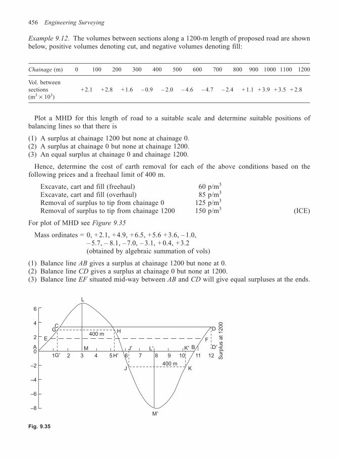
456 Engineering Surveying
Example 9.12. The volumes between sections along a 1200-m length of proposed road are shownbelow, positive volumes denoting cut, and negative volumes denoting fill:
Chainage (m) 0 100 200 300 400 500 600 700 800 900 1000 1100 1200
Vol. betweensections + 2.1 + 2.8 + 1.6 – 0.9 – 2.0 – 4.6 – 4.7 – 2.4 + 1.1 + 3.9 + 3.5 + 2.8(m3 × 103)
Plot a MHD for this length of road to a suitable scale and determine suitable positions ofbalancing lines so that there is
(1) A surplus at chainage 1200 but none at chainage 0.(2) A surplus at chainage 0 but none at chainage 1200.(3) An equal surplus at chainage 0 and chainage 1200.
Hence, determine the cost of earth removal for each of the above conditions based on thefollowing prices and a freehaul limit of 400 m.
Excavate, cart and fill (freehaul) 60 p/m3
Excavate, cart and fill (overhaul) 85 p/m3
Removal of surplus to tip from chainage 0 125 p/m3
Removal of surplus to tip from chainage 1200 150 p/m3 (ICE)
For plot of MHD see Figure 9.35
Mass ordinates = 0, +2.1, +4.9, + 6.5, +5.6 +3.6, – 1.0,– 5.7, – 8.1, – 7.0, – 3.1, + 0.4, +3.2(obtained by algebraic summation of vols)
(1) Balance line AB gives a surplus at chainage 1200 but none at 0.(2) Balance line CD gives a surplus at chainage 0 but none at 1200.(3) Balance line EF situated mid-way between AB and CD will give equal surpluses at the ends.
Fig. 9.35
1 2 3 4 5 6 7 8 9 10 11
6
4
2
0
–2
–4
–6
–8
E
GC
400 mH
H′J′ L′ K′
F
D
D′
12 Surp
lus a
t 1200
J K400 m
A
L
M′
M
G′B
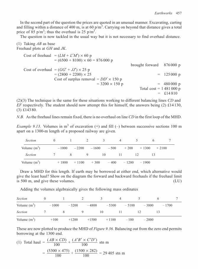
Earthworks 457
In the second part of the question the prices are quoted in an unusual manner. Excavating, cartingand filling within a distance of 400 m, is at 60 p/m3. Carrying on beyond that distance gives a totalprice of 85 p/m3; thus the overhaul is 25 p/m3.
The question is now tackled in the usual way but it is not necessary to find overhaul distance.
(1) Taking AB as baseFreehaul plots at GH and JK.
Cost of freehaul = (LM + L′M′) × 60 p= (6500 + 8100) × 60 = 876 000 p
brought forward 876 000 pCost of overhaul = (GG′ + JJ′) × 25 p
= (2800 + 2200) × 25 = 125 000 pCost of surplus removal = DD′ × 150 p
= 3200 × 150 p = 480 000 pTotal cost = 1 481 000 p
= £14 810
(2)(3) The technique is the same for these situations working to different balancing lines CD andEF respectively. The student should now attempt this for himself, the answers being (2) £14 130,(3) £143 80.
N.B. As the freehaul lines remain fixed, there is no overhaul on line CD in the first loop of the MHD.
Example 9.13. Volumes in m3 of excavation (+) and fill (–) between successive sections 100 mapart on a 1300-m length of a proposed railway are given.
Section 0 1 2 3 4 5 6 7
Volume (m3) – 1000 – 2200 – 1600 – 500 + 200 + 1300 + 2100
Section 7 8 9 10 11 12 13
Volume (m3) + 1800 + 1100 + 300 – 400 – 1200 – 1900
Draw a MHD for this length. If earth may be borrowed at either end, which alternative wouldgive the least haul? Show on the diagram the forward and backward freehauls if the freehaul limitis 500 m, and give these volumes. (LU)
Adding the volumes algebraically gives the following mass ordinates
Section 0 1 2 3 4 5 6 7
Volume (m3) – 1000 – 3200 – 4800 – 5300 – 5100 – 3800 – 1700
Section 7 8 9 10 11 12 13
Volume (m3) +100 +1200 +1500 + 1100 – 100 – 2000
These are now plotted to produce the MHD of Figure 9.36. Balancing out from the zero end permitsborrowing at the 1300 end.
(1) Total haul = ( )
100 +
( )100
AB CD A B C D× ′ ′ × ′ ′ stn m
=(5300 475)
100 +
(1500 282)100
× × = 29 405 stn m
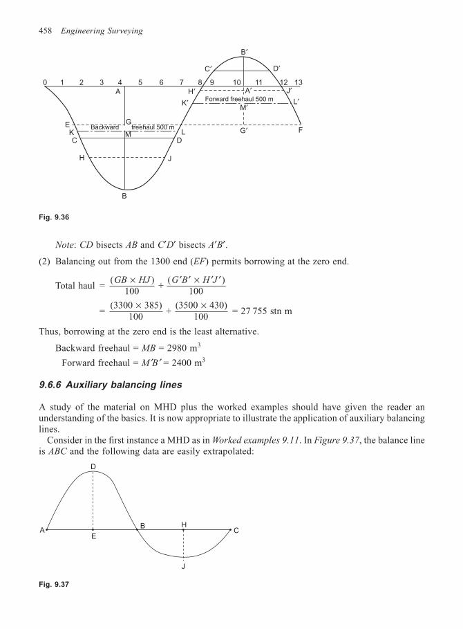
458 Engineering Surveying
Note: CD bisects AB and C′D′ bisects A′B′.
(2) Balancing out from the 1300 end (EF) permits borrowing at the zero end.
Total haul = ( )
100 +
( )100
GB HJ G B H J× ′ ′ × ′ ′
=(3300 385)
100 +
(3500 430)100
× × = 27 755 stn m
Thus, borrowing at the zero end is the least alternative.
Backward freehaul = MB = 2980 m3
Forward freehaul = M′B′ = 2400 m3
9.6.6 Auxiliary balancing lines
A study of the material on MHD plus the worked examples should have given the reader anunderstanding of the basics. It is now appropriate to illustrate the application of auxiliary balancinglines.
Consider in the first instance a MHD as in Worked examples 9.11. In Figure 9.37, the balance lineis ABC and the following data are easily extrapolated:
Fig. 9.36
A
D
E
B H
J
C
Fig. 9.37
B′
C′ D′
H′
K′
A′ J′L′
M′
G′ FLD
J
B
M
G
H
CK
E
A
0 1 2 3 4 5 6 7 8 9 10 11 12 13
Backward freehaul 500 m
Forward freehaul 500 m
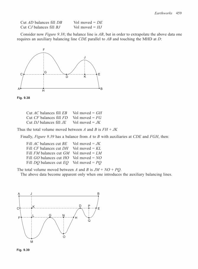
Earthworks 459
Cut AD balances fill DB Vol moved = DE
Cut CJ balances fill BJ Vol moved = HJ
Consider now Figure 9.38; the balance line is AB, but in order to extrapolate the above data onerequires an auxiliary balancing line CDE parallel to AB and touching the MHD at D:
Fig. 9.38
HA
CG
F
D K
J
E
B
K
A
C
F
M
L G N
O
H
D
Q
PE
BJ
Fig. 9.39
Cut AC balances fill EB Vol moved = GH
Cut CF balances fill FD Vol moved = FG
Cut DJ balances fill JE Vol moved = JK
Thus the total volume moved between A and B is FH + JK
Finally, Figure 9.39 has a balance from A to B with auxiliaries at CDE and FGH, then:
Fill AC balances cut BE Vol moved = JK
Fill CF balances cut DH Vol moved = KL
Fill FM balances cut GM Vol moved = LM
Fill GO balances cut HO Vol moved = NO
Fill DQ balances cut EQ Vol moved = PQ
The total volume moved between A and B is JM + NO + PQ.The above data become apparent only when one introduces the auxiliary balancing lines.
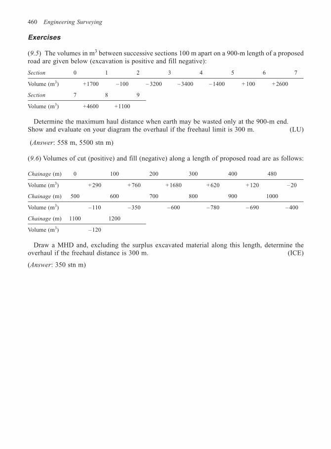
460 Engineering Surveying
Exercises
(9.5) The volumes in m3 between successive sections 100 m apart on a 900-m length of a proposedroad are given below (excavation is positive and fill negative):
Section 0 1 2 3 4 5 6 7
Volume (m3) +1700 –100 – 3200 – 3400 – 1400 + 100 + 2600
Section 7 8 9
Volume (m3) +4600 +1100
Determine the maximum haul distance when earth may be wasted only at the 900-m end.Show and evaluate on your diagram the overhaul if the freehaul limit is 300 m. (LU)
(Answer: 558 m, 5500 stn m)
(9.6) Volumes of cut (positive) and fill (negative) along a length of proposed road are as follows:
Chainage (m) 0 100 200 300 400 480
Volume (m3) + 290 + 760 + 1680 + 620 + 120 – 20
Chainage (m) 500 600 700 800 900 1000
Volume (m3) –110 – 350 – 600 – 780 – 690 – 400
Chainage (m) 1100 1200
Volume (m3) – 120
Draw a MHD and, excluding the surplus excavated material along this length, determine theoverhaul if the freehaul distance is 300 m. (ICE)
(Answer: 350 stn m)
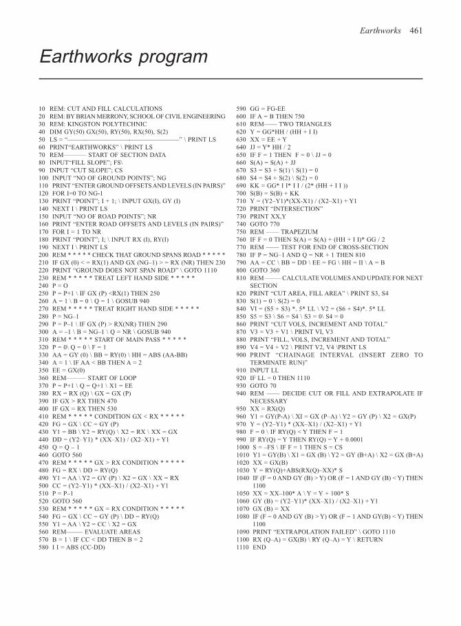
Earthworks 461
Earthworks program
10 REM: CUT AND FILL CALCULATIONS20 REM: BY BRIAN MERRONY, SCHOOL OF CIVIL ENGINEERING30 REM: KINGSTON POLYTECHNIC40 DIM GY(50) GX(50), RY(50), RX(50), S(2)50 LS = “–––––-––—–––––––––-–––––––––––––––” \ PRINT LS60 PRINT“EARTHWORKS” \ PRINT LS70 REM–––—— START OF SECTION DATA80 INPUT“FILL SLOPE”; FS\90 INPUT “CUT SLOPE”; CS100 INPUT “NO OF GROUND POINTS”; NG110 PRINT “ENTER GROUND OFFSETS AND LEVELS (IN PAIRS)”120 FOR I=0 TO NG-1130 PRINT “POINT”; I + 1; \ INPUT GX(I), GY (I)140 NEXT I \ PRINT LS150 INPUT “NO OF ROAD POINTS”; NR160 PRINT “ENTER ROAD OFFSETS AND LEVELS (IN PAIRS)”170 FOR I = 1 TO NR180 PRINT “POINT”; I; \ INPUT RX (I), RY(I)190 NEXT I \ PRINT LS200 REM * * * * * CHECK THAT GROUND SPANS ROAD * * * * *210 IF GX (0) < = RX(1) AND GX (NG–1) > = RX (NR) THEN 230220 PRINT “GROUND DOES NOT SPAN ROAD” \ GOTO 1110230 REM * * * * * TREAT LEFT HAND SIDE * * * * *240 P = O250 P = P+1 \ IF GX (P) <RX(1) THEN 250260 A = 1 \ B = 0 \ Q = 1 \ GOSUB 940270 REM * * * * * TREAT RIGHT HAND SIDE * * * * *280 P = NG–1290 P = P–1 \ IF GX (P) > RX(NR) THEN 290300 A = –1 \ B = NG–1 \ Q = NR \ GOSUB 940310 REM * * * * * START OF MAIN PASS * * * * *320 P = 0\ Q = 0 \ F = 1330 AA = GY (0) \ BB = RY(0) \ HH = ABS (AA-BB)340 A = 1 \ IF AA < BB THEN A = 2350 EE = GX(0)360 REM–––––– START OF LOOP370 P = P+1 \ Q = Q+1 \ X1 = EE380 RX = RX (Q) \ GX = GX (P)390 IF GX > RX THEN 470400 IF GX = RX THEN 530410 REM * * * * * CONDITION GX < RX * * * * *420 FG = GX \ CC = GY (P)430 Y1 = BB \ Y2 = RY(Q) \ X2 = RX \ XX = GX440 DD = (Y2–Y1) * (XX–X1) / (X2–X1) + Y1450 Q = Q – 1460 GOTO 560470 REM * * * * * GX > RX CONDITION * * * * *480 FG = RX \ DD = RY(Q)490 Y1 = AA \ Y2 = GY (P) \ X2 = GX \ XX = RX500 CC = (Y2–Y1) * (XX–X1) / (X2–X1) + Y1510 P = P–1520 GOTO 560530 REM * * * * * GX = RX CONDITION * * * * *540 FG = GX \ CC = GY (P) \ DD = RY(Q)550 Y1 = AA \ Y2 = CC \ X2 = GX560 REM––––– EVALUATE AREAS570 B = 1 \ IF CC < DD THEN B = 2580 I I = ABS (CC-DD)
590 GG = FG-EE600 IF A = B THEN 750610 REM–––– TWO TRIANGLES620 Y = GG*HH / (HH + I I)630 XX = EE + Y640 JJ = Y* HH / 2650 IF F = 1 THEN F = 0 \ JJ = 0660 S(A) = S(A) + JJ670 S3 = S3 + S(1) \ S(1) = 0680 S4 = S4 + S(2) \ S(2) = 0690 KK = GG* I I* I I / (2* (HH + I I ))700 S(B) = S(B) + KK710 Y = (Y2–Y1)*(XX-X1) / (X2–X1) + Y1720 PRINT “INTERSECTION”730 PRINT XX,Y740 GOTO 770750 REM –––– TRAPEZIUM760 IF F = 0 THEN S(A) = S(A) + (HH + I I)* GG / 2770 REM –––– TEST FOR END OF CROSS-SECTION780 IF P = NG–1 AND Q = NR + 1 THEN 810790 AA = CC \ BB = DD \ EE = FG \ HH = II \ A = B800 GOTO 360810 REM ––––– CALCULATE VOLUMES AND UPDATE FOR NEXT
SECTION820 PRINT “CUT AREA, FILL AREA” \ PRINT S3, S4830 S(1) = 0 \ S(2) = 0840 VI = (S5 + S3) *. 5* LL \ V2 = (S6 + S4)*. 5* LL850 S5 = S3 \ S6 = S4 \ S3 = 0\ S4 = 0860 PRINT “CUT VOLS, INCREMENT AND TOTAL”870 V3 = V3 + V1 \ PRINT VI, V3880 PRINT “FILL, VOLS, INCREMENT AND TOTAL”890 V4 = V4 + V2 \ PRINT V2, V4 \PRINT LS900 PRINT “CHAINAGE INTERVAL (INSERT ZERO TO
TERMINATE RUN)”910 INPUT LL920 IF LL = 0 THEN 1110930 GOTO 70940 REM –––– DECIDE CUT OR FILL AND EXTRAPOLATE IF
NECESSARY950 XX = RX(Q)960 Y1 = GY(P-A) \ XI = GX (P–A) \ Y2 = GY (P) \ X2 = GX(P)970 Y = (Y2–Y1) * (XX–X1) / (X2–X1) + Y1980 F = 0 \ IF RY(Q) < Y THEN F = 1990 IF RY(Q) = Y THEN RY(Q) = Y + 0.00011000 S = –FS \ IF F = 1 THEN S = CS1010 Y1 = GY(B) \ X1 = GX (B) \ Y2 = GY (B+A) \ X2 = GX (B+A)1020 XX = GX(B)1030 Y = RY(Q)+ABS(RX(Q)–XX)* S1040 IF (F = 0 AND GY (B) > Y) OR (F = 1 AND GY (B) < Y) THEN
11001050 XX = XX–100* A \ Y = Y + 100* S1060 GY (B) = (Y2–Y1)* (XX–X1) / (X2–X1) + Y11070 GX (B) = XX1080 IF (F = 0 AND GY (B) > Y) OR (F = 1 AND GY(B) < Y) THEN
11001090 PRINT “EXTRAPOLATION FAILED” \ GOTO 11101100 RX (Q–A) = GX(B) \ RY (Q–A) = Y \ RETURN1110 END

462 Engineering Surveying
EARTHWORKS PROGRAM: BASIC
The program is used for earthwork computation and mass-haul data.From offsets and levels of existing ground cross-sections and proposed road cross-sections at
successive chainage points along the centre-line of a route location; cut and fill volumes arecomputed, accumulated volumes for mass haul produced and the chainage and level of the intersectionof the side slopes and existing ground are found.
Input data (the program is interactive and will request input data)
(1) Side slope in FILL; e.g. for 1 in 2, enter 0.5.(2) Side slope in CUT; this may be the same as or different from that adopted for fill.(3) The number of points defining the EXISTING GROUND in the cross-section.(4) The distance from the centre-line and level of the GROUND POINTS. Distances to the left of
the centre-line are negative, those to the right are positive. N.B. They are entered into thecomputer in IN SEQUENCE FROM THE EXTREME LEFT TO RIGHT, of the cross-section.
(5) The number of points defining the proposed ROAD formation.(6) As in (4), but for road points.(7) The chainage interval to the next cross-section. If there are no further cross-sections the entry
of a zero chainage interval terminates the run. (Refer example overleaf).
Output data
(1) Ground/road intersection points
The distance from the centre-line and level at which the road side-slopes intersect the existingground; i.e. the top of the cutting or toe of the embankment (the slope stake position).
(2) Areas
Areas of the cross-sections.
(3) Volumes
The volume at each cross-section and the accumulated volume. The latter is used for mass haulconstruction.
An example of the input and output for a hill-side section in cut-and-fill is given overleaf.

Earthworks 463
————————————————EARTHWORKS————————————————FILL SLOPE ? 0.5CUT SLOPE ? 1.0NO OF GROUND POINTS ? 7ENTER GROUND OFFSETS AND LEVELS (IN PAIRS) INPUT DATA OFPOINT 1 ? –30, 100 CROSS-SECTIONPOINT 2 ? –20, 95.5 LEVELSPOINT 3 ? –10, 102POINT 4 ? 0, 103POINT 5 ? 10, 105.6POINT 6 ? 20, 106.8POINT 7 ? 30, 106.9————————————————NO OF ROAD POINTS? 3ENTER ROAD OFFSETS AND LEVELS (IN PAIRS) INPUT DATA OFPOINT 1 ? –18, 103.7 PROPOSED ROADPOINT 2 ? 0, 104 LEVELSPOINT 3 ? 18, 103.7————————————————INTERSECTION–27.5789 98.9105INTERSECTION3.61445 103.94INTERSECTION21.1111 106.811CUT AREA, FILL AREA28.7184 92.2913CUT VOLS, INCREMENT AND TOTAL0 0 OUTPUTFILL VOLS, INCREMENT AND TOTAL0 0————————————————CHAINAGE INTERVAL (INSERT ZERO TO TERMINATE RUN)? 30FILL SLOPE ? 0.5CUT SLOPE ? 1.0NO OF GROUND POINTS ? 7ENTER GROUND OFFSETS AND LEVELS (IN PAIRS)
etc., etc.... .
10
Setting out (dimensional control)
In engineering the production of an accurate large-scale plan is usually the first step in the planningand design of a construction project. Thereafter the project, as designed on the plan, must be set outon the ground in the correct absolute and relative position and to its correct dimensions. Thus,surveys made in connection with a specific project should be planned with the setting-out processin mind and a system of three-dimensional control stations conveniently sited and adequate innumber should be provided to facilitate easy, economical setting out.
It is of prime importance that the establishment and referencing of survey control stations shouldbe carried out at such places and in such a manner that they will survive the construction processes.This entails careful choice of the locations of the control stations and their construction relative totheir importance and long- or short-term requirements. For instance, those stations required for thetotal duration of the project may be established in concrete or masonry pillars with metal plates orbolts set in on which is punched the station position. Less durable are stout wooden pegs set inconcrete or driven directly into the ground. A system of numbering the stations is essential, andfrequently pegs are painted different colours to denote the particular functions for which they areto be used.
10.1 PROTECTION AND REFERENCING
Most site operatives have little concept of the time, effort and expertise involved in establishingsetting-out pegs. For this reason the pegs are frequently treated with disdain and casually destroyedin the construction process. A typical example of this is the centre-line pegs for route locationwhich are the first to be destroyed when earth-moving commences. It is important, therefore, thatcontrol stations and BMs should be protected in some way (usually as shown in Figure 10.1) andsite operatives, particularly earthwork personnel, impressed with the importance of maintainingthis protection.
Where destruction of the pegs is inevitable, then referencing procedures should be adopted to re-locate their positions to the original accuracy of fixation. Various configurations of reference pegsare used and the one thing that they have in common is that they must be set well outside the areaof construction and have some form of protection, as in Figure 10.1.
A commonly-used method of referencing is from four pegs (A, B, C, D) established such that twostrings stretched between them intersect to locate the required position (Figure 10.2). Distances AB,BC, CD, AD, AC, BD should all be measured as checks on the possible movement of the referencepegs, whilst distances from the reference pegs to the setting-out peg will afford a check on positioning.Intersecting lines of sight from theodolites at, say, A and B may be used where ground conditionsmake string lining difficult.
Where ground conditions preclude taping, the setting-out peg may be referenced by trisection
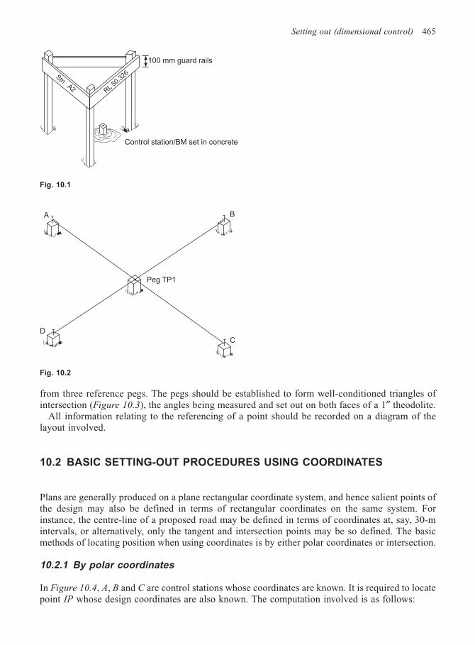
Setting out (dimensional control) 465
from three reference pegs. The pegs should be established to form well-conditioned triangles ofintersection (Figure 10.3), the angles being measured and set out on both faces of a 1″ theodolite.
All information relating to the referencing of a point should be recorded on a diagram of thelayout involved.
10.2 BASIC SETTING-OUT PROCEDURES USING COORDINATES
Plans are generally produced on a plane rectangular coordinate system, and hence salient points ofthe design may also be defined in terms of rectangular coordinates on the same system. Forinstance, the centre-line of a proposed road may be defined in terms of coordinates at, say, 30-mintervals, or alternatively, only the tangent and intersection points may be so defined. The basicmethods of locating position when using coordinates is by either polar coordinates or intersection.
10.2.1 By polar coordinates
In Figure 10.4, A, B and C are control stations whose coordinates are known. It is required to locatepoint IP whose design coordinates are also known. The computation involved is as follows:
Stn A2 RL 5
0.326
100 mm guard rails
Control station/BM set in concrete
Fig. 10.1
A
D
Peg TP1
C
B
Fig. 10.2
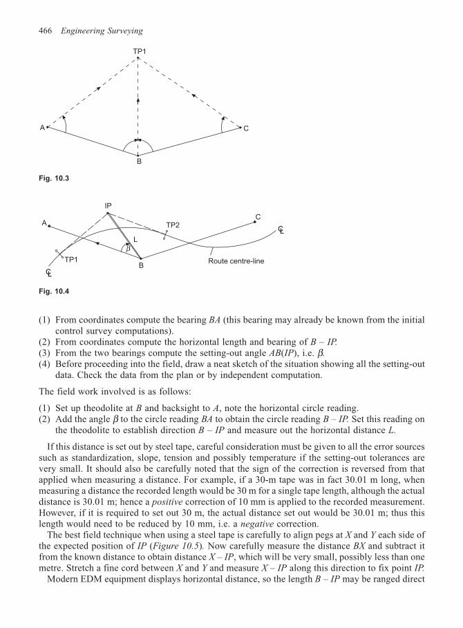
466 Engineering Surveying
(1) From coordinates compute the bearing BA (this bearing may already be known from the initialcontrol survey computations).
(2) From coordinates compute the horizontal length and bearing of B – IP.
(3) From the two bearings compute the setting-out angle AB(IP), i.e. β.
(4) Before proceeding into the field, draw a neat sketch of the situation showing all the setting-outdata. Check the data from the plan or by independent computation.
The field work involved is as follows:
(1) Set up theodolite at B and backsight to A, note the horizontal circle reading.(2) Add the angle β to the circle reading BA to obtain the circle reading B – IP. Set this reading on
the theodolite to establish direction B – IP and measure out the horizontal distance L.
If this distance is set out by steel tape, careful consideration must be given to all the error sourcessuch as standardization, slope, tension and possibly temperature if the setting-out tolerances arevery small. It should also be carefully noted that the sign of the correction is reversed from thatapplied when measuring a distance. For example, if a 30-m tape was in fact 30.01 m long, whenmeasuring a distance the recorded length would be 30 m for a single tape length, although the actualdistance is 30.01 m; hence a positive correction of 10 mm is applied to the recorded measurement.However, if it is required to set out 30 m, the actual distance set out would be 30.01 m; thus thislength would need to be reduced by 10 mm, i.e. a negative correction.
The best field technique when using a steel tape is carefully to align pegs at X and Y each side ofthe expected position of IP (Figure 10.5). Now carefully measure the distance BX and subtract itfrom the known distance to obtain distance X – IP, which will be very small, possibly less than onemetre. Stretch a fine cord between X and Y and measure X – IP along this direction to fix point IP.
Modern EDM equipment displays horizontal distance, so the length B – IP may be ranged direct
Fig. 10.3
TP1
A
B
C
A TP2
TP1
CL
β
C
CL
Route centre-line
IP
L
Fig. 10.4
B
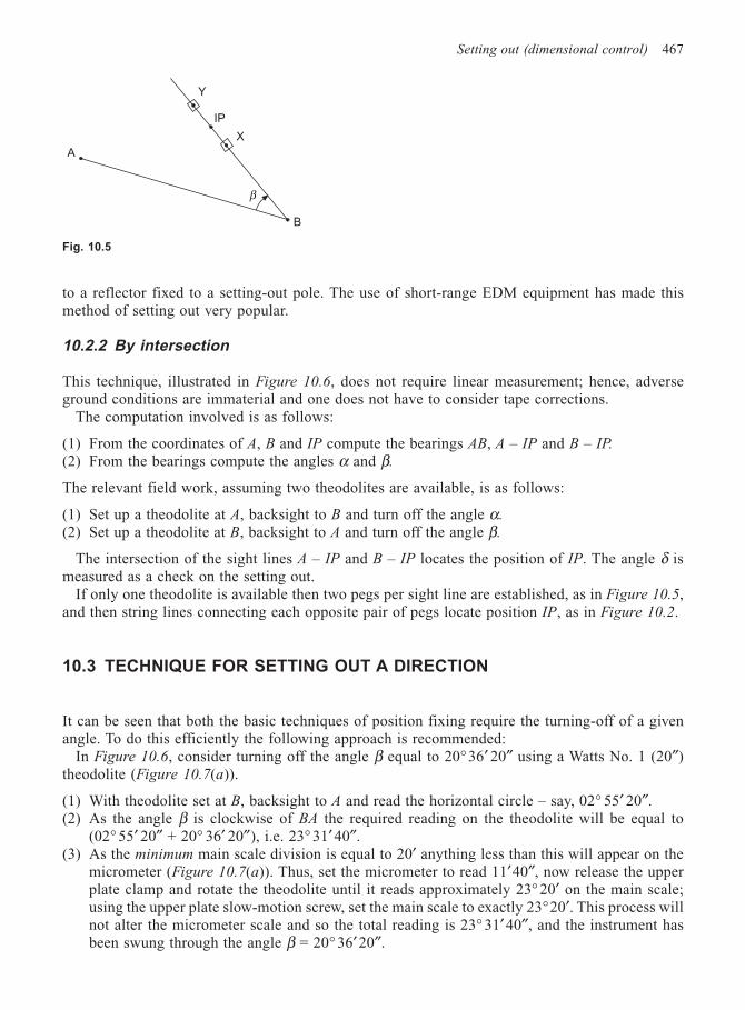
Setting out (dimensional control) 467
to a reflector fixed to a setting-out pole. The use of short-range EDM equipment has made thismethod of setting out very popular.
10.2.2 By intersection
This technique, illustrated in Figure 10.6, does not require linear measurement; hence, adverseground conditions are immaterial and one does not have to consider tape corrections.
The computation involved is as follows:
(1) From the coordinates of A, B and IP compute the bearings AB, A – IP and B – IP.
(2) From the bearings compute the angles α and β.
The relevant field work, assuming two theodolites are available, is as follows:
(1) Set up a theodolite at A, backsight to B and turn off the angle α.
(2) Set up a theodolite at B, backsight to A and turn off the angle β.
The intersection of the sight lines A – IP and B – IP locates the position of IP. The angle δ ismeasured as a check on the setting out.
If only one theodolite is available then two pegs per sight line are established, as in Figure 10.5,and then string lines connecting each opposite pair of pegs locate position IP, as in Figure 10.2.
10.3 TECHNIQUE FOR SETTING OUT A DIRECTION
It can be seen that both the basic techniques of position fixing require the turning-off of a givenangle. To do this efficiently the following approach is recommended:
In Figure 10.6, consider turning off the angle β equal to 20°36′ 20″ using a Watts No. 1 (20″)theodolite (Figure 10.7(a)).
(1) With theodolite set at B, backsight to A and read the horizontal circle – say, 02° 55′ 20″.(2) As the angle β is clockwise of BA the required reading on the theodolite will be equal to
(02° 55′ 20″ + 20° 36′ 20″), i.e. 23° 31′ 40″.(3) As the minimum main scale division is equal to 20′ anything less than this will appear on the
micrometer (Figure 10.7(a)). Thus, set the micrometer to read 11′40″, now release the upperplate clamp and rotate the theodolite until it reads approximately 23° 20′ on the main scale;using the upper plate slow-motion screw, set the main scale to exactly 23°20′. This process willnot alter the micrometer scale and so the total reading is 23° 31′40″, and the instrument hasbeen swung through the angle β = 20° 36′20″.
Fig. 10.5
A
Y
IP
X
B
β
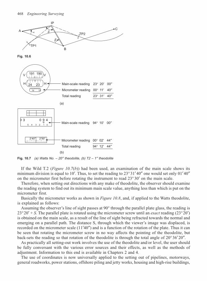
468 Engineering Surveying
If the Wild T.2 (Figure 10.7(b)) had been used, an examination of the main scale shows itsminimum division is equal to 10′. Thus, to set the reading to 23° 31′ 40″ one would set only 01′40″on the micrometer first before rotating the instrument to read 23° 30′ on the main scale.
Therefore, when setting out directions with any make of theodolite, the observer should examinethe reading system to find out its minimum main scale value, anything less than which is put on themicrometer first.
Basically the micrometer works as shown in Figure 10.8, and, if applied to the Watts theodolite,is explained as follows:
Assuming the observer’s line of sight passes at 90° through the parallel plate glass, the reading is23°20′ + S. The parallel plate is rotated using the micrometer screw until an exact reading (23°20′)is obtained on the main scale, as a result of the line of sight being refracted towards the normal andemerging on a parallel path. The distance S, through which the viewer’s image was displaced, isrecorded on the micrometer scale (11′40″) and is a function of the rotation of the plate. Thus it canbe seen that rotating the micrometer screw in no way affects the pointing of the theodolite, butback-sets the reading so that rotation of the theodolite is through the total angle of 20° 36′ 20″.
As practically all setting-out work involves the use of the theodolite and/or level, the user shouldbe fully conversant with the various error sources and their effects, as well as the methods ofadjustment. Information to this end is available in Chapters 2 and 4.
The use of coordinates is now universally applied to the setting out of pipelines, motorways,general roadworks, power stations, offshore piling and jetty works, housing and high-rise buildings,
A
IP
TP2
C
β
δ∝
TP1B
Fig. 10.6
5 4 3 2 1 0
0 9 4
2′40″ 2′50″
24
190
23
191
10 15
V
H
V
H Main-scale reading 23° 20′ 00″
Micrometer reading 00° 11′ 40″
Total reading 23° 31′ 40″
Main-scale reading 94° 10′ 00″
Micrometer reading 00° 02′ 44″
Total reading 94° 12′ 44″
(a)
(b)
Fig. 10.7 (a) Watts No. – 20″ theodolite, (b) T2 – 1″ theodolite
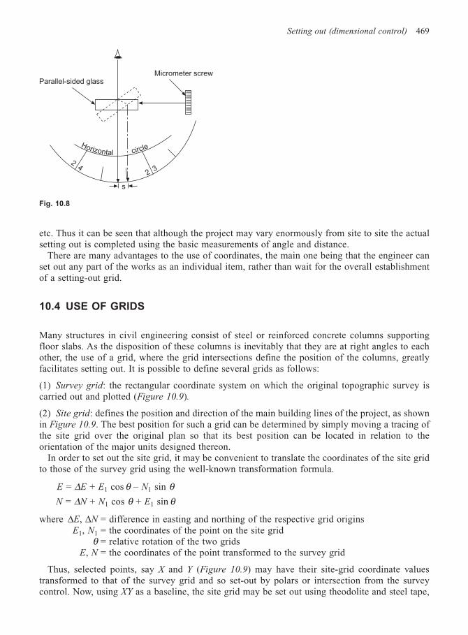
Setting out (dimensional control) 469
etc. Thus it can be seen that although the project may vary enormously from site to site the actualsetting out is completed using the basic measurements of angle and distance.
There are many advantages to the use of coordinates, the main one being that the engineer canset out any part of the works as an individual item, rather than wait for the overall establishmentof a setting-out grid.
10.4 USE OF GRIDS
Many structures in civil engineering consist of steel or reinforced concrete columns supportingfloor slabs. As the disposition of these columns is inevitably that they are at right angles to eachother, the use of a grid, where the grid intersections define the position of the columns, greatlyfacilitates setting out. It is possible to define several grids as follows:
(1) Survey grid: the rectangular coordinate system on which the original topographic survey iscarried out and plotted (Figure 10.9).
(2) Site grid: defines the position and direction of the main building lines of the project, as shownin Figure 10.9. The best position for such a grid can be determined by simply moving a tracing ofthe site grid over the original plan so that its best position can be located in relation to theorientation of the major units designed thereon.
In order to set out the site grid, it may be convenient to translate the coordinates of the site gridto those of the survey grid using the well-known transformation formula.
E = ∆E + E1 cos θ – N1 sin θN = ∆N + N1 cos θ + E1 sin θ
where ∆E, ∆N = difference in easting and northing of the respective grid originsE1, N1 = the coordinates of the point on the site grid
θ = relative rotation of the two gridsE, N = the coordinates of the point transformed to the survey grid
Thus, selected points, say X and Y (Figure 10.9) may have their site-grid coordinate valuestransformed to that of the survey grid and so set-out by polars or intersection from the surveycontrol. Now, using XY as a baseline, the site grid may be set out using theodolite and steel tape,
Fig. 10.8
Horizontal circle
Parallel-sided glassMicrometer screw
s
2 42 3
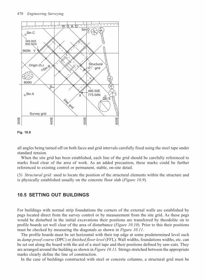
470 Engineering Surveying
all angles being turned off on both faces and grid intervals carefully fixed using the steel tape understandard tension.
When the site grid has been established, each line of the grid should be carefully referenced tomarks fixed clear of the area of work. As an added precaution, these marks could be furtherreferenced to existing control or permanent, stable, on-site detail.
(3) Structural grid: used to locate the position of the structural elements within the structure andis physically established usually on the concrete floor slab (Figure 10.9).
10.5 SETTING OUT BUILDINGS
For buildings with normal strip foundations the corners of the external walls are established bypegs located direct from the survey control or by measurement from the site grid. As these pegswould be disturbed in the initial excavations their positions are transferred by theodolite on toprofile boards set well clear of the area of disturbance (Figure 10.10). Prior to this their positionsmust be checked by measuring the diagonals as shown in Figure 10.11.
The profile boards must be set horizontal with their top edge at some predetermined level suchas damp proof course (DPC) or finished floor level (FFL). Wall widths, foundations widths, etc. canbe set out along the board with the aid of a steel tape and their positions defined by saw-cuts. Theyare arranged around the building as shown in Figure 10.11. Strings stretched between the appropriatemarks clearly define the line of construction.
In the case of buildings constructed with steel or concrete columns, a structural grid must be
Fig. 10.9
Stn C
900N
345.00E905.50N
Stn D
Origin (01)
Stn B
800N
Stn A
Survey grid
θ
Site grid
480.50E
775.00NStn E
Structural
grid
30
0E
60
0E
40
0E
50
0E
R O A D
Y
X
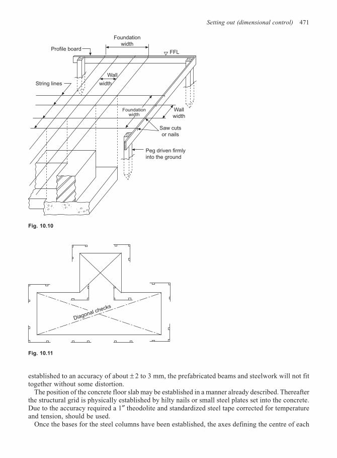
Setting out (dimensional control) 471
established to an accuracy of about ± 2 to 3 mm, the prefabricated beams and steelwork will not fittogether without some distortion.
The position of the concrete floor slab may be established in a manner already described. Thereafterthe structural grid is physically established by hilty nails or small steel plates set into the concrete.Due to the accuracy required a 1″ theodolite and standardized steel tape corrected for temperatureand tension, should be used.
Once the bases for the steel columns have been established, the axes defining the centre of each
Fig. 10.10
Diagonal checks
Fig. 10.11
Profile board
Foundation
width
FFL
String lines
Wall
width
Foundationwidth
Wall
width
Saw cuts
or nails
Peg driven firmly
into the ground
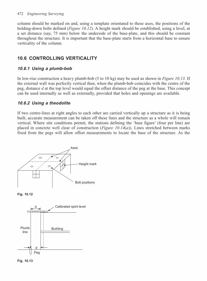
472 Engineering Surveying
column should be marked on and, using a template orientated to these axes, the positions of theholding-down bolts defined (Figure 10.12). A height mark should be established, using a level, ata set distance (say, 75 mm) below the underside of the base-plate, and this should be constantthroughout the structure. It is important that the base-plate starts from a horizontal base to ensureverticality of the column.
10.6 CONTROLLING VERTICALITY
10.6.1 Using a plumb-bob
In low-rise construction a heavy plumb-bob (5 to 10 kg) may be used as shown in Figure 10.13. Ifthe external wall was perfectly vertical then, when the plumb-bob coincides with the centre of thepeg, distance d at the top level would equal the offset distance of the peg at the base. This conceptcan be used internally as well as externally, provided that holes and openings are available.
10.6.2 Using a theodolite
If two centre-lines at right angles to each other are carried vertically up a structure as it is beingbuilt, accurate measurement can be taken off these lines and the structure as a whole will remainvertical. Where site conditions permit, the stations defining the ‘base figure’ (four per line) areplaced in concrete well clear of construction (Figure 10.14(a)). Lines stretched between marksfixed from the pegs will allow offset measurements to locate the base of the structure. As the
Fig. 10.12
Fig. 10.13
Axes
Height mark
Bolt positions
d Calibrated spirit level
BuildingPlumb
line
d
Peg
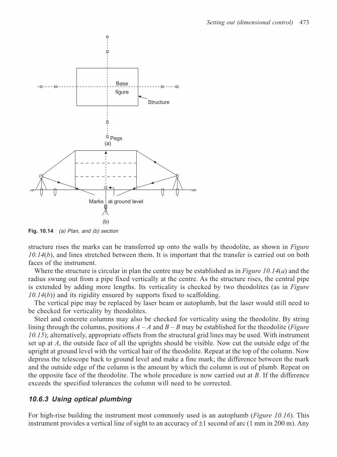
Setting out (dimensional control) 473
structure rises the marks can be transferred up onto the walls by theodolite, as shown in Figure
10.14(b), and lines stretched between them. It is important that the transfer is carried out on bothfaces of the instrument.
Where the structure is circular in plan the centre may be established as in Figure 10.14(a) and theradius swung out from a pipe fixed vertically at the centre. As the structure rises, the central pipeis extended by adding more lengths. Its verticality is checked by two theodolites (as in Figure
10.14(b)) and its rigidity ensured by supports fixed to scaffolding.The vertical pipe may be replaced by laser beam or autoplumb, but the laser would still need to
be checked for verticality by theodolites.Steel and concrete columns may also be checked for verticality using the theodolite. By string
lining through the columns, positions A – A and B – B may be established for the theodolite (Figure
10.15); alternatively, appropriate offsets from the structural grid lines may be used. With instrumentset up at A, the outside face of all the uprights should be visible. Now cut the outside edge of theupright at ground level with the vertical hair of the theodolite. Repeat at the top of the column. Nowdepress the telescope back to ground level and make a fine mark; the difference between the markand the outside edge of the column is the amount by which the column is out of plumb. Repeat onthe opposite face of the theodolite. The whole procedure is now carried out at B. If the differenceexceeds the specified tolerances the column will need to be corrected.
10.6.3 Using optical plumbing
For high-rise building the instrument most commonly used is an autoplumb (Figure 10.16). Thisinstrument provides a vertical line of sight to an accuracy of ±1 second of arc (1 mm in 200 m). Any
Fig. 10.14 (a) Plan, and (b) section
Base
figure
Structure
Pegs
Marks at ground level
(a)
(b)
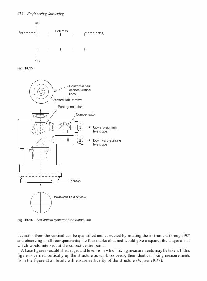
474 Engineering Surveying
deviation from the vertical can be quantified and corrected by rotating the instrument through 90°and observing in all four quadrants; the four marks obtained would give a square, the diagonals ofwhich would intersect at the correct centre point.
A base figure is established at ground level from which fixing measurements may be taken. If thisfigure is carried vertically up the structure as work proceeds, then identical fixing measurementsfrom the figure at all levels will ensure verticality of the structure (Figure 10.17).
Fig. 10.15
I I I I I
I I I I I
A
B
B
A Columns
Fig. 10.16 The optical system of the autoplumb
Horizontal hair
defines vertical
lines
Upward field of view
Pentagonal prism
Compensator
Upward-sighting
telescope
Downward-sighting
telescope
Tribrach
Downward field of view
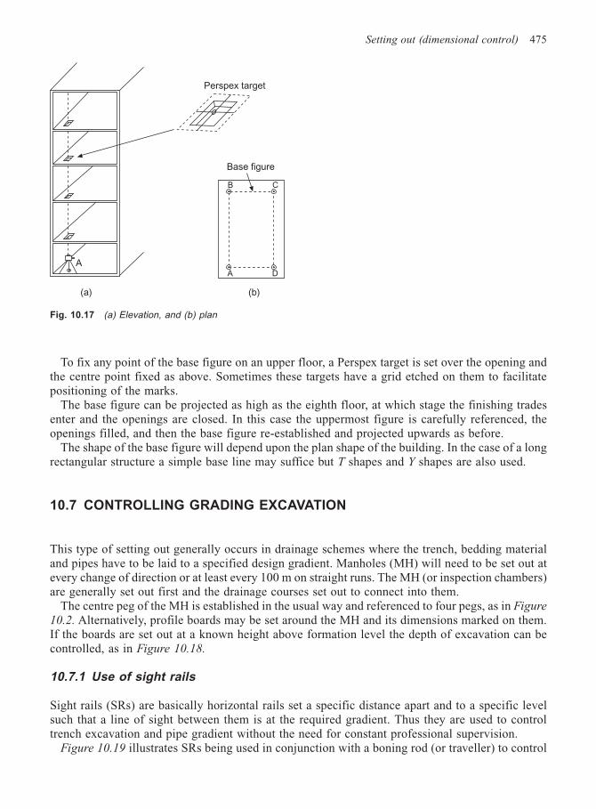
Setting out (dimensional control) 475
To fix any point of the base figure on an upper floor, a Perspex target is set over the opening andthe centre point fixed as above. Sometimes these targets have a grid etched on them to facilitatepositioning of the marks.
The base figure can be projected as high as the eighth floor, at which stage the finishing tradesenter and the openings are closed. In this case the uppermost figure is carefully referenced, theopenings filled, and then the base figure re-established and projected upwards as before.
The shape of the base figure will depend upon the plan shape of the building. In the case of a longrectangular structure a simple base line may suffice but T shapes and Y shapes are also used.
10.7 CONTROLLING GRADING EXCAVATION
This type of setting out generally occurs in drainage schemes where the trench, bedding materialand pipes have to be laid to a specified design gradient. Manholes (MH) will need to be set out atevery change of direction or at least every 100 m on straight runs. The MH (or inspection chambers)are generally set out first and the drainage courses set out to connect into them.
The centre peg of the MH is established in the usual way and referenced to four pegs, as in Figure
10.2. Alternatively, profile boards may be set around the MH and its dimensions marked on them.If the boards are set out at a known height above formation level the depth of excavation can becontrolled, as in Figure 10.18.
10.7.1 Use of sight rails
Sight rails (SRs) are basically horizontal rails set a specific distance apart and to a specific levelsuch that a line of sight between them is at the required gradient. Thus they are used to controltrench excavation and pipe gradient without the need for constant professional supervision.
Figure 10.19 illustrates SRs being used in conjunction with a boning rod (or traveller) to control
Perspex target
Base figure
AA D
B C
(a) (b)
Fig. 10.17 (a) Elevation, and (b) plan
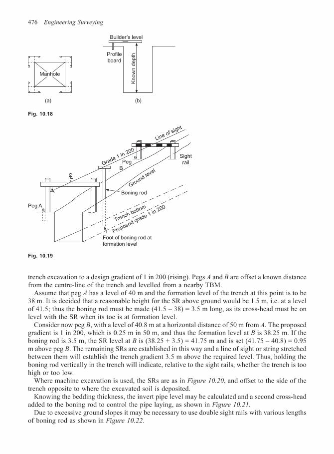
476 Engineering Surveying
Manhole
trench excavation to a design gradient of 1 in 200 (rising). Pegs A and B are offset a known distancefrom the centre-line of the trench and levelled from a nearby TBM.
Assume that peg A has a level of 40 m and the formation level of the trench at this point is to be38 m. It is decided that a reasonable height for the SR above ground would be 1.5 m, i.e. at a levelof 41.5; thus the boning rod must be made (41.5 – 38) = 3.5 m long, as its cross-head must be onlevel with the SR when its toe is at formation level.
Consider now peg B, with a level of 40.8 m at a horizontal distance of 50 m from A. The proposedgradient is 1 in 200, which is 0.25 m in 50 m, and thus the formation level at B is 38.25 m. If theboning rod is 3.5 m, the SR level at B is (38.25 + 3.5) = 41.75 m and is set (41.75 – 40.8) = 0.95m above peg B. The remaining SRs are established in this way and a line of sight or string stretchedbetween them will establish the trench gradient 3.5 m above the required level. Thus, holding theboning rod vertically in the trench will indicate, relative to the sight rails, whether the trench is toohigh or too low.
Where machine excavation is used, the SRs are as in Figure 10.20, and offset to the side of thetrench opposite to where the excavated soil is deposited.
Knowing the bedding thickness, the invert pipe level may be calculated and a second cross-headadded to the boning rod to control the pipe laying, as shown in Figure 10.21.
Due to excessive ground slopes it may be necessary to use double sight rails with various lengthsof boning rod as shown in Figure 10.22.
Builder’s level
Profile
board
Know
n d
epth
(a) (b)
Fig. 10.18
Line of sight
Grade 1 in 200
CL
Peg A
Peg
B
Sight
rail
Ground level
Boning rod
Trench bottom
Proposed grade 1 in 200
Foot of boning rod at
formation level
Fig. 10.19
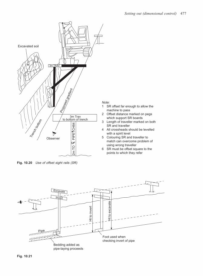
Setting out (dimensional control) 477
3m TRAV
Excavated soil
Tre
nch
bottom
Observer
3m Travto bottom of trench
Pro
pose
d g
radie
nt
2m
TO
C LP
IPE
C
H84
Note:1 SR offset far enough to allow the
machine to pass
2 Offset distance marked on pegs
which support SR boards
3 Length of traveller marked on both
SR and traveller
4 All crossheads should be levelled
with a spirit level
5 Colouring SR and traveller to
match can overcome problem of
using wrong traveller
6 SR must be offset square to the
points to which they refer
Fig. 10.20 Use of offset sight rails (SR)
Fig. 10.21
Excavate
Invert
Pipe
Bedding added as
pipe-laying proceeds
Foot used when
checking invert of pipe
Ht to
exc
ava
te
Ht to
invert
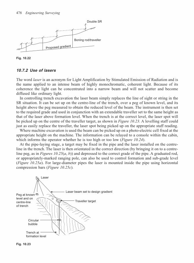
478 Engineering Surveying
10.7.2 Use of lasers
The word laser is an acronym for Light Amplification by Stimulated Emission of Radiation and isthe name applied to an intense beam of highly monochromatic, coherent light. Because of itscoherence the light can be concentrated into a narrow beam and will not scatter and becomediffused like ordinary light.
In controlling trench excavation the laser beam simply replaces the line of sight or string in theSR situation. It can be set up on the centre-line of the trench, over a peg of known level, and itsheight above the peg measured to obtain the reduced level of the beam. The instrument is then setto the required grade and used in conjunction with an extendable traveller set to the same height asthat of the laser above formation level. When the trench is at the correct level, the laser spot willbe picked up on the centre of the traveller target, as shown in Figure 10.23. A levelling staff couldjust as easily replace the traveller, the laser spot being picked up on the appropriate staff reading.
Where machine excavation is used the beam can be picked up on a photo-electric cell fixed at theappropriate height on the machine. The information can be relayed to a console within the cabin,which informs the operator whether he is too high or too low (Figure 10.24).
At the pipe-laying stage, a target may be fixed in the pipe and the laser installed on the centre-line in the trench. The laser is then orientated in the correct direction (by bringing it on to a centre-line peg, as in Figures 10.25(a, b)) and depressed to the correct grade of the pipe. A graduated rod,or appropriately-marked ranging pole, can also be used to control formation and sub-grade level(Figure 10.25a). For large-diameter pipes the laser is mounted inside the pipe using horizontalcompression bars (Figure 10.25c).
Fig. 10.22
Double SR
Boning rod/traveller
Proposed gradient
Laser
Peg at known
level and on
centre-line
of trench
Laser beam set to design gradient
Traveller target
Circular
bubble
Trench at
formation level
θ
Fig. 10.23
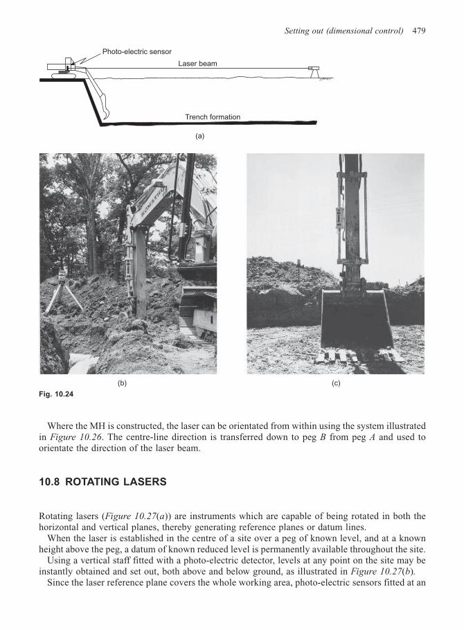
Setting out (dimensional control) 479
Where the MH is constructed, the laser can be orientated from within using the system illustratedin Figure 10.26. The centre-line direction is transferred down to peg B from peg A and used toorientate the direction of the laser beam.
10.8 ROTATING LASERS
Rotating lasers (Figure 10.27(a)) are instruments which are capable of being rotated in both thehorizontal and vertical planes, thereby generating reference planes or datum lines.
When the laser is established in the centre of a site over a peg of known level, and at a knownheight above the peg, a datum of known reduced level is permanently available throughout the site.
Using a vertical staff fitted with a photo-electric detector, levels at any point on the site may beinstantly obtained and set out, both above and below ground, as illustrated in Figure 10.27(b).
Since the laser reference plane covers the whole working area, photo-electric sensors fitted at an
Photo-electric sensor
Laser beam
Trench formation
(a)
Fig. 10.24
(b) (c)
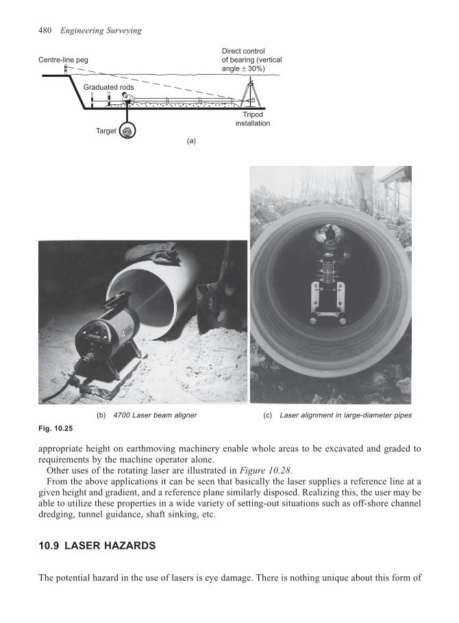
480 Engineering Surveying
appropriate height on earthmoving machinery enable whole areas to be excavated and graded torequirements by the machine operator alone.
Other uses of the rotating laser are illustrated in Figure 10.28.
From the above applications it can be seen that basically the laser supplies a reference line at agiven height and gradient, and a reference plane similarly disposed. Realizing this, the user may beable to utilize these properties in a wide variety of setting-out situations such as off-shore channeldredging, tunnel guidance, shaft sinking, etc.
10.9 LASER HAZARDS
The potential hazard in the use of lasers is eye damage. There is nothing unique about this form of
(a)
Centre-line peg
Graduated rods
Direct control
of bearing (vertical
angle ± 30%)
Tripod
installationTarget
(b) 4700 Laser beam aligner (c) Laser alignment in large-diameter pipes
Fig. 10.25
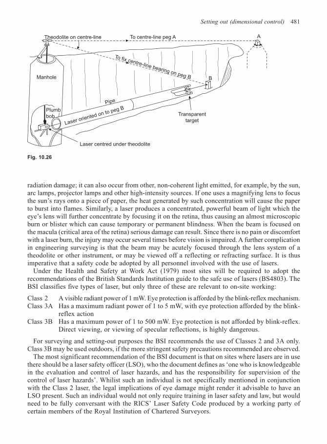
Setting out (dimensional control) 481
radiation damage; it can also occur from other, non-coherent light emitted, for example, by the sun,arc lamps, projector lamps and other high-intensity sources. If one uses a magnifying lens to focusthe sun’s rays onto a piece of paper, the heat generated by such concentration will cause the paperto burst into flames. Similarly, a laser produces a concentrated, powerful beam of light which theeye’s lens will further concentrate by focusing it on the retina, thus causing an almost microscopicburn or blister which can cause temporary or permanent blindness. When the beam is focused onthe macula (critical area of the retina) serious damage can result. Since there is no pain or discomfortwith a laser burn, the injury may occur several times before vision is impaired. A further complicationin engineering surveying is that the beam may be acutely focused through the lens system of atheodolite or other instrument, or may be viewed off a reflecting or refracting surface. It is thusimperative that a safety code be adopted by all personnel involved with the use of lasers.
Under the Health and Safety at Work Act (1979) most sites will be required to adopt therecommendations of the British Standards Institution guide to the safe use of lasers (BS4803). TheBSI classifies five types of laser, but only three of these are relevant to on-site working:
Class 2 A visible radiant power of 1 mW. Eye protection is afforded by the blink-reflex mechanism.Class 3A Has a maximum radiant power of 1 to 5 mW, with eye protection afforded by the blink-
reflex actionClass 3B Has a maximum power of 1 to 500 mW. Eye protection is not afforded by blink-reflex.
Direct viewing, or viewing of specular reflections, is highly dangerous.
For surveying and setting-out purposes the BSI recommends the use of Classes 2 and 3A only.Class 3B may be used outdoors, if the more stringent safety precautions recommended are observed.
The most significant recommendation of the BSI document is that on sites where lasers are in usethere should be a laser safety officer (LSO), who the document defines as ‘one who is knowledgeablein the evaluation and control of laser hazards, and has the responsibility for supervision of thecontrol of laser hazards’. Whilist such an individual is not specifically mentioned in conjunctionwith the Class 2 laser, the legal implications of eye damage might render it advisable to have anLSO present. Such an individual would not only require training in laser safety and law, but wouldneed to be fully conversant with the RICS’ Laser Safety Code produced by a working party ofcertain members of the Royal Institution of Chartered Surveyors.
Theodolite on centre-line To centre-line peg A
To fix centre-line bearing on peg B B
Transparent
target
Pipe
Manhole
Laser oriented on to peg B
Laser centred under theodolite
A
Fig. 10.26
Plumb
bob
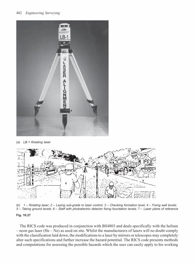
482 Engineering Surveying
The RICS code was produced in conjunction with BS4803 and deals specifically with the helium– neon gas laser (He – Ne) as used on site. Whilst the manufacturers of lasers will no doubt complywith the classification laid down, the modifications to a laser by mirrors or telescopes may completelyalter such specifications and further increase the hazard potential. The RICS code presents methodsand computations for assessing the possible hazards which the user can easily apply to his working
(a) LB-1 Rotating laser
(b) 1 – Rotating laser; 2 – Laying sub-grade to laser control; 3 – Checking formation level; 4 – Fixing wall levels;5 – Taking ground levels; 6 – Staff with photoelectric detector fixing foundation levels; 7 – Laser plane of reference
Fig. 10.27
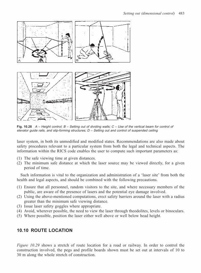
Setting out (dimensional control) 483
laser system, in both its unmodified and modified states. Recommendations are also made aboutsafety procedures relevant to a particular system from both the legal and technical aspects. Theinformation within the RICS code enables the user to compute such important parameters as:
(1) The safe viewing time at given distances.(2) The minimum safe distance at which the laser source may be viewed directly, for a given
period of time.
Such information is vital to the organization and administration of a ‘laser site’ from both thehealth and legal aspects, and should be combined with the following precautions.
(1) Ensure that all personnel, random visitors to the site, and where necessary members of thepublic, are aware of the presence of lasers and the potential eye damage involved.
(2) Using the above-mentioned computations, erect safety barriers around the laser with a radiusgreater than the minimum safe viewing distance.
(3) Issue laser safety goggles where appropriate.(4) Avoid, wherever possible, the need to view the laser through theodolites, levels or binoculars.(5) Where possible, position the laser either well above or well below head height.
10.10 ROUTE LOCATION
Figure 10.29 shows a stretch of route location for a road or railway. In order to control theconstruction involved, the pegs and profile boards shown must be set out at intervals of 10 to30 m along the whole stretch of construction.
Fig. 10.28 A – Height control; B – Setting out of dividing walls; C – Use of the vertical beam for control ofelevator guide rails, and slip-forming structures; D – Setting out and control of suspended ceiling
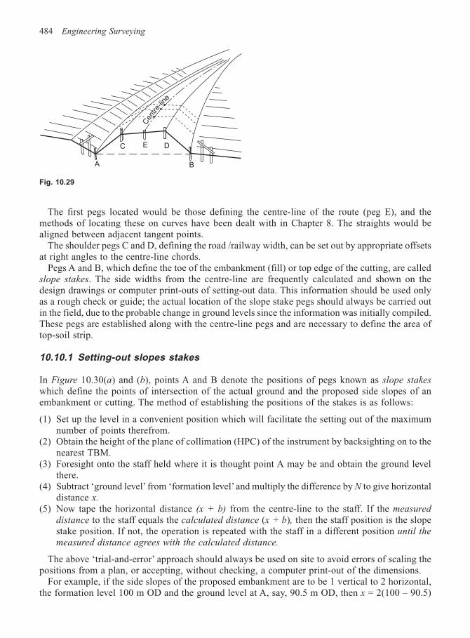
484 Engineering Surveying
The first pegs located would be those defining the centre-line of the route (peg E), and themethods of locating these on curves have been dealt with in Chapter 8. The straights would bealigned between adjacent tangent points.
The shoulder pegs C and D, defining the road /railway width, can be set out by appropriate offsetsat right angles to the centre-line chords.
Pegs A and B, which define the toe of the embankment (fill) or top edge of the cutting, are calledslope stakes. The side widths from the centre-line are frequently calculated and shown on thedesign drawings or computer print-outs of setting-out data. This information should be used onlyas a rough check or guide; the actual location of the slope stake pegs should always be carried outin the field, due to the probable change in ground levels since the information was initially compiled.These pegs are established along with the centre-line pegs and are necessary to define the area oftop-soil strip.
10.10.1 Setting-out slopes stakes
In Figure 10.30(a) and (b), points A and B denote the positions of pegs known as slope stakes
which define the points of intersection of the actual ground and the proposed side slopes of anembankment or cutting. The method of establishing the positions of the stakes is as follows:
(1) Set up the level in a convenient position which will facilitate the setting out of the maximumnumber of points therefrom.
(2) Obtain the height of the plane of collimation (HPC) of the instrument by backsighting on to thenearest TBM.
(3) Foresight onto the staff held where it is thought point A may be and obtain the ground levelthere.
(4) Subtract ‘ground level’ from ‘formation level’ and multiply the difference by N to give horizontaldistance x.
(5) Now tape the horizontal distance (x + b) from the centre-line to the staff. If the measured
distance to the staff equals the calculated distance (x + b), then the staff position is the slopestake position. If not, the operation is repeated with the staff in a different position until the
measured distance agrees with the calculated distance.
The above ‘trial-and-error’ approach should always be used on site to avoid errors of scaling thepositions from a plan, or accepting, without checking, a computer print-out of the dimensions.
For example, if the side slopes of the proposed embankment are to be 1 vertical to 2 horizontal,the formation level 100 m OD and the ground level at A, say, 90.5 m OD, then x = 2(100 – 90.5)
Fig. 10.29
Cen
tre-li
ne
C E D
BA
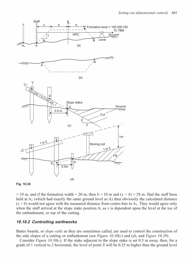
Setting out (dimensional control) 485
= 19 m, and if the formation width = 20 m, then b = 10 m and (x + b) = 29 m. Had the staff beenheld at A1 (which had exactly the same ground level as A) then obviously the calculated distance(x + b) would not agree with the measured distance from centre-line to A1. They would agree onlywhen the staff arrived at the slope stake position A, as x is dependent upon the level at the toe ofthe embankment, or top of the cutting.
10.10.2 Controlling earthworks
Batter boards, or slope rails as they are sometimes called, are used to control the construction ofthe side slopes of a cutting or embankment (see Figure 10.30(c) and (d), and Figure 10.29).
Consider Figure 10.30(c). If the stake adjacent to the slope stake is set 0.5 m away, then, for agrade of 1 vertical to 2 horizontal, the level of point X will be 0.25 m higher than the ground level
Staffx b b
1
N
HPC
A1 A
B Level
Ground
To TBMFormation level = 100.000 OD
AB
Chn 220–1 in 2–4m cut Slope stake
A
X
Cut0.5 m
2
1
1 in 2
Y
X1
X
0.5m
A
Boning rod
1 in 2
Fill
1m
CL
(a)
(b)
(c)
(d)
Y
Ground
Fig. 10.30
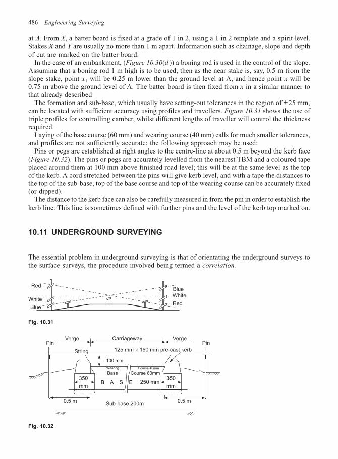
486 Engineering Surveying
at A. From X, a batter board is fixed at a grade of 1 in 2, using a 1 in 2 template and a spirit level.Stakes X and Y are usually no more than 1 m apart. Information such as chainage, slope and depthof cut are marked on the batter board.
In the case of an embankment, (Figure 10.30(d )) a boning rod is used in the control of the slope.Assuming that a boning rod 1 m high is to be used, then as the near stake is, say, 0.5 m from theslope stake, point x1 will be 0.25 m lower than the ground level at A, and hence point x will be0.75 m above the ground level of A. The batter board is then fixed from x in a similar manner tothat already described
The formation and sub-base, which usually have setting-out tolerances in the region of ± 25 mm,can be located with sufficient accuracy using profiles and travellers. Figure 10.31 shows the use oftriple profiles for controlling camber, whilst different lengths of traveller will control the thicknessrequired.
Laying of the base course (60 mm) and wearing course (40 mm) calls for much smaller tolerances,and profiles are not sufficiently accurate; the following approach may be used:
Pins or pegs are established at right angles to the centre-line at about 0.5 m beyond the kerb face(Figure 10.32). The pins or pegs are accurately levelled from the nearest TBM and a coloured tapeplaced around them at 100 mm above finished road level; this will be at the same level as the topof the kerb. A cord stretched between the pins will give kerb level, and with a tape the distances tothe top of the sub-base, top of the base course and top of the wearing course can be accurately fixed(or dipped).
The distance to the kerb face can also be carefully measured in from the pin in order to establish thekerb line. This line is sometimes defined with further pins and the level of the kerb top marked on.
10.11 UNDERGROUND SURVEYING
The essential problem in underground surveying is that of orientating the underground surveys tothe surface surveys, the procedure involved being termed a correlation.
Fig. 10.31
Fig. 10.32
Red
White
Blue
BlueWhite
Red
Verge Carriageway Verge
String
Pin
350
mm
350
mm
125 mm × 150 mm pre-cast kerb
250 mmB A S E
0.5 m 0.5 m
Pin
Wearing Course 40mm
Base Course 60mm
Sub-base 200m
100 mm
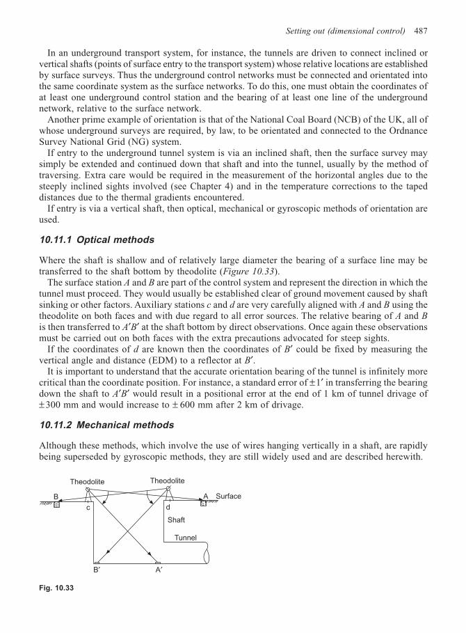
Setting out (dimensional control) 487
In an underground transport system, for instance, the tunnels are driven to connect inclined orvertical shafts (points of surface entry to the transport system) whose relative locations are establishedby surface surveys. Thus the underground control networks must be connected and orientated intothe same coordinate system as the surface networks. To do this, one must obtain the coordinates ofat least one underground control station and the bearing of at least one line of the undergroundnetwork, relative to the surface network.
Another prime example of orientation is that of the National Coal Board (NCB) of the UK, all ofwhose underground surveys are required, by law, to be orientated and connected to the OrdnanceSurvey National Grid (NG) system.
If entry to the underground tunnel system is via an inclined shaft, then the surface survey maysimply be extended and continued down that shaft and into the tunnel, usually by the method oftraversing. Extra care would be required in the measurement of the horizontal angles due to thesteeply inclined sights involved (see Chapter 4) and in the temperature corrections to the tapeddistances due to the thermal gradients encountered.
If entry is via a vertical shaft, then optical, mechanical or gyroscopic methods of orientation areused.
10.11.1 Optical methods
Where the shaft is shallow and of relatively large diameter the bearing of a surface line may betransferred to the shaft bottom by theodolite (Figure 10.33).
The surface station A and B are part of the control system and represent the direction in which thetunnel must proceed. They would usually be established clear of ground movement caused by shaftsinking or other factors. Auxiliary stations c and d are very carefully aligned with A and B using thetheodolite on both faces and with due regard to all error sources. The relative bearing of A and Bis then transferred to A′B′ at the shaft bottom by direct observations. Once again these observationsmust be carried out on both faces with the extra precautions advocated for steep sights.
If the coordinates of d are known then the coordinates of B′ could be fixed by measuring thevertical angle and distance (EDM) to a reflector at B′.
It is important to understand that the accurate orientation bearing of the tunnel is infinitely morecritical than the coordinate position. For instance, a standard error of ±1′ in transferring the bearingdown the shaft to A′B′ would result in a positional error at the end of 1 km of tunnel drivage of± 300 mm and would increase to ± 600 mm after 2 km of drivage.
10.11.2 Mechanical methods
Although these methods, which involve the use of wires hanging vertically in a shaft, are rapidlybeing superseded by gyroscopic methods, they are still widely used and are described herewith.
Fig. 10.33
Theodolite Theodolite
Shaft
Tunnel
SurfaceA
c
B′ A′
B
d
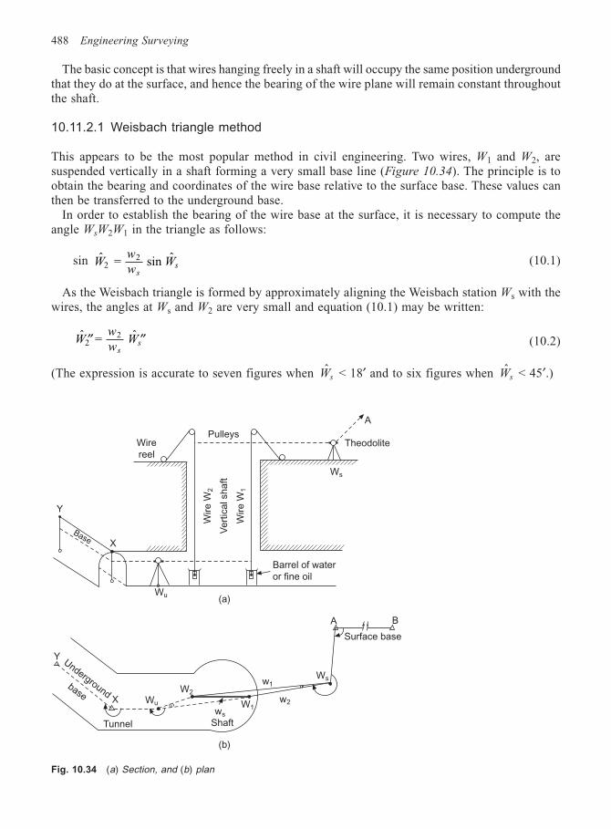
488 Engineering Surveying
The basic concept is that wires hanging freely in a shaft will occupy the same position undergroundthat they do at the surface, and hence the bearing of the wire plane will remain constant throughoutthe shaft.
10.11.2.1 Weisbach triangle method
This appears to be the most popular method in civil engineering. Two wires, W1 and W2, aresuspended vertically in a shaft forming a very small base line (Figure 10.34). The principle is toobtain the bearing and coordinates of the wire base relative to the surface base. These values canthen be transferred to the underground base.
In order to establish the bearing of the wire base at the surface, it is necessary to compute theangle WsW2W1 in the triangle as follows:
sin ˆ ˆWw
wW
ss2
2 = sin (10.1)
As the Weisbach triangle is formed by approximately aligning the Weisbach station Ws with thewires, the angles at Ws and W2 are very small and equation (10.1) may be written:
ˆ ˆ′′ ′′Ww
wW
ss2 = 2
(10.2)
(The expression is accurate to seven figures when Ws < 18′ and to six figures when Ws < 45′.)
Fig. 10.34 (a) Section, and (b) plan
Wire
reel
PulleysTheodolite
A
Ws
Wire W
2
Vert
ical shaft
Wire W
1
Barrel of water
or fine oil
Base
Y
X
Wu
Y Undergroundbase
Tunnel
X Wu
W2
ws
W1
w1
w2
Ws
A B
Surface base
(a)
(b)
Shaft
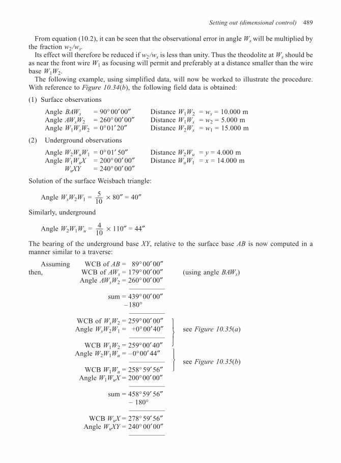
Setting out (dimensional control) 489
From equation (10.2), it can be seen that the observational error in angle Ws will be multiplied bythe fraction w2 /ws.
Its effect will therefore be reduced if w2 /ws is less than unity. Thus the theodolite at Ws should beas near the front wire W1 as focusing will permit and preferably at a distance smaller than the wirebase W1W2.
The following example, using simplified data, will now be worked to illustrate the procedure.With reference to Figure 10.34(b), the following field data is obtained:
(1) Surface observations
Angle BAWs = 90° 00′00″ Distance W1W2 = ws = 10.000 mAngle AWsW2 = 260° 00′ 00″ Distance W1Ws = w2 = 5.000 mAngle W1WsW2 = 0°01′ 20″ Distance W2Ws = w1 = 15.000 m
(2) Underground observations
Angle W2WuW1 = 0° 01′ 50″ Distance W2Wu = y = 4.000 mAngle W1WuX = 200° 00′ 00″ Distance WuW1 = x = 14.000 m
WuXY = 240° 00′ 00″
Solution of the surface Weisbach triangle:
Angle WsW2W1 = 510
× 80″ = 40″
Similarly, underground
Angle W2W1Wu = 410
× 110″ = 44″
The bearing of the underground base XY, relative to the surface base AB is now computed in amanner similar to a traverse:
Assuming WCB of AB = 89° 00′ 00″then, WCB of AWs = 179° 00′ 00″ (using angle BAWs)
Angle AWsW2 = 260° 00′ 00″—————
sum = 439° 00′ 00″ – 180°
—————WCB of WsW2 = 259° 00′ 00″Angle WsW2W1 = +0° 00′40″ see Figure 10.35(a)
—————WCB W1W2 = 259°00′ 40″
Angle W2W1Wu = – 0°00′ 44″————— see Figure 10.35(b)
WCB W1Wu = 258° 59′ 56″Angle W1WuX = 200°00′ 00″
—————sum = 458°59′ 56″
– 180°—————
WCB WuX = 278° 59′ 56″Angle WuXY = 240° 00′ 00″
—————
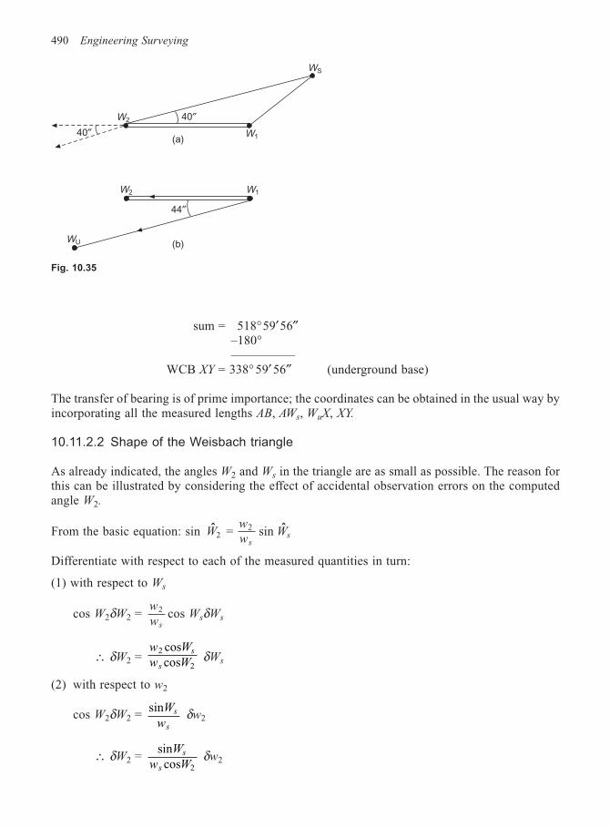
490 Engineering Surveying
sum = 518°59′56″–180°—————
WCB XY = 338° 59′ 56″ (underground base)
The transfer of bearing is of prime importance; the coordinates can be obtained in the usual way byincorporating all the measured lengths AB, AWs, WuX, XY.
10.11.2.2 Shape of the Weisbach triangle
As already indicated, the angles W2 and Ws in the triangle are as small as possible. The reason forthis can be illustrated by considering the effect of accidental observation errors on the computedangle W2.
From the basic equation: sin ˆ ˆWw
wW
ss2
2 = sin
Differentiate with respect to each of the measured quantities in turn:
(1) with respect to Ws
cos W2δW2 =w
ws
2 cos WsδWs
∴ δW2 =w W
w Ws
s
2
2
coscos δWs
(2) with respect to w2
cos W2δW2 =sinW
ws
s
δw2
∴ δW2 =sincos
W
w Ws
s 2δw2
Fig. 10.35
W2
W1
WS
40″
40″
44″
W2 W1
WU (b)
(a)
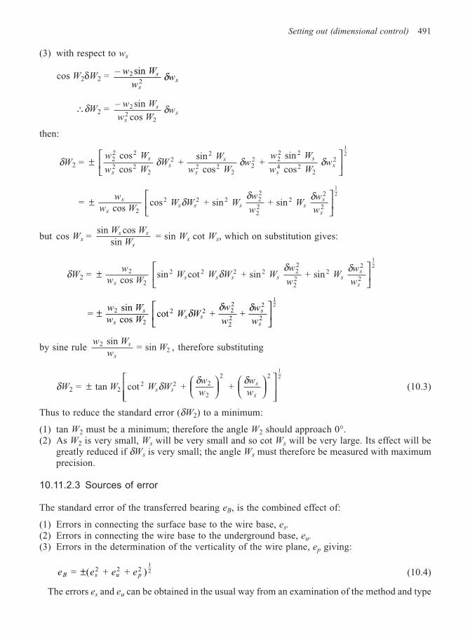
Setting out (dimensional control) 491
(3) with respect to ws
cos W2δW2 =– 2
2
w W
wws
ss
sin δ
∴δW2 =– 2
22
w W
w Wws
ss
sin
cosδ
then:
δW2 = ±
cos
cos +
sin
cos +
sin
cos 22 2
2 22
22
2 22
22 2
2 2
4 22
2
1
w W
w WW
W
w Ww
w W
w Ww
s
ss
s
s
s
ssδ δ δ
2
= ±
cos
cos + sin + sin 2
2 2 2 22
22
22
2
12w
w WW W W
w
wW
w
w
s
ss s s s
s
s
δδ δ
but cos Ws =sin
sinW W
Ws s
s
cos = sin Ws cot Ws, which on substitution gives:
δW2 = ±
cos
sin cot + sin + sin 2
2
2 2 2 2 22
22
22
2
12w
w WW W W W
w
wW
w
wss s s s s
s
s
δδ δ
= sin cos
cot + + 2
2
2 2 22
22
2
2
12
±
w W
w WW W
w
w
w
w
s
ss s
s
s
δδ δ
by sine rule w W
wWs
s
22
sin = sin , therefore substituting
δW2 = ±
tan cot + + 22 2 2
2
2 212
W W Ww
w
w
ws ss
s
δδ δ
(10.3)
Thus to reduce the standard error (δW2) to a minimum:
(1) tan W2 must be a minimum; therefore the angle W2 should approach 0°.(2) As W2 is very small, Ws will be very small and so cot Ws will be very large. Its effect will be
greatly reduced if δWs is very small; the angle Ws must therefore be measured with maximumprecision.
10.11.2.3 Sources of error
The standard error of the transferred bearing eB, is the combined effect of:
(1) Errors in connecting the surface base to the wire base, es.
(2) Errors in connecting the wire base to the underground base, eu.
(3) Errors in the determination of the verticality of the wire plane, ep giving:
e e e eB s u p = ( + + )2 2 212± (10.4)
The errors es and eu can be obtained in the usual way from an examination of the method and type
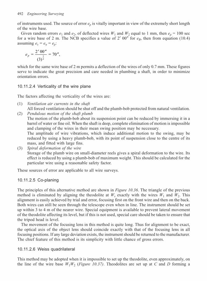
492 Engineering Surveying
of instruments used. The source of error ep is vitally important in view of the extremely short lengthof the wire base.
Given random errors e1 and e2, of deflected wires W1 and W2 equal to 1 mm, then ep = 100 secfor a wire base of 2 m. The NCB specifies a value of 2′ 00″ for eB, then from equation (10.4)assuming es = eu = ep:
e p = 2 00
(3) = 70 ,
12
′ ′′′′
which for the same wire base of 2 m permits a deflection of the wires of only 0.7 mm. These figuresserve to indicate the great precision and care needed in plumbing a shaft, in order to minimizeorientation errors.
10.11.2.4 Verticality of the wire plane
The factors affecting the verticality of the wires are:
(1) Ventilation air currents in the shaft
All forced ventilation should be shut off and the plumb-bob protected from natural ventilation.(2) Pendulous motion of the shaft plumb
The motion of the plumb-bob about its suspension point can be reduced by immersing it in abarrel of water or fine oil. When the shaft is deep, complete elimination of motion is impossibleand clamping of the wires in their mean swing position may be necessary.The amplitude of wire vibrations, which induce additional motion to the swing, may bereduced by using a heavy plumb-bob, with its point of suspension close to the centre of itsmass, and fitted with large fins.
(3) Spiral deformation of the wire
Storage of the plumb wire on small-diameter reels gives a spiral deformation to the wire. Itseffect is reduced by using a plumb-bob of maximum weight. This should be calculated for theparticular wire using a reasonable safety factor.
These sources of error are applicable to all wire surveys.
10.11.2.5 Co-planing
The principles of this alternative method are shown in Figure 10.36. The triangle of the previousmethod is eliminated by aligning the theodolite at Ws exactly with the wires W1 and W2. Thisalignment is easily achieved by trial and error, focusing first on the front wire and then on the back.Both wires can still be seen through the telescope even when in line. The instrument should be setup within 3 to 4 m of the nearer wire. Special equipment is available to prevent lateral movementof the theodolite affecting its level, but if this is not used, special care should be taken to ensure thatthe tripod head is level.
The movement of the focusing lens in this method is quite long. Thus for alignment to be exact,the optical axis of the object lens should coincide exactly with that of the focusing lens in allfocusing positions. If any large deviation exists, the instrument should be returned to the manufacturer.The chief feature of this method is its simplicity with little chance of gross errors.
10.11.2.6 Weiss quadrilateral
This method may be adopted when it is impossible to set up the theodolite, even approximately, onthe line of the wire base W1W2 (Figure 10.37). Theodolites are set up at C and D forming a
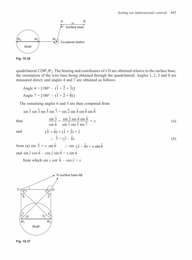
Setting out (dimensional control) 493
quadrilateral CDW1W2. The bearing and coordinates of CD are obtained relative to the surface base,the orientation of the wire base being obtained through the quadrilateral. Angles 1, 2, 3 and 8 aremeasured direct, and angles 4 and 7 are obtained as follows:
Angle 4 = [180° – (1 + 2 + 3)ˆ ˆ ˆ ]
Angle 7 = [180° – (1 + 2 + 8)ˆ ˆ ˆ ]
The remaining angles 6 and 5 are then computed from
sin 1 sin 3 sin 5 sin 7 = sin 2 sin 4 sin 6 sin 8ˆ ˆ ˆ ˆ ˆ ˆ ˆ ˆ
thus sin ˆ
ˆ
ˆ ˆ ˆ
ˆ ˆ ˆ 5
sin 6 = sin 2 sin 4 sin 8
sin 1 sin 3 sin 7 = x (a)
and ( + 6) = (1 + 2) = ˆ ˆ ˆ ˆ ˆ5 y
∴ ˆ ˆ ˆ5 = ( – 6)y (b)
from (a) sin ˆ ˆ5 = sin 6x ∴ sin ( – 6) = sin 6ˆ ˆ ˆy x
and sin cos 6 – cos sin 6 = sin 6ˆ ˆ ˆ ˆ ˆy y x
from which sin y cot ˆ ˆ6 – cos = y x
W1W2
Shaft
Ws
A B
Surface base
Co-planed station
Fig. 10.36
C1
8
2
3
76
45
W1 W2
To surface base AB
Shaft
D
Fig. 10.37
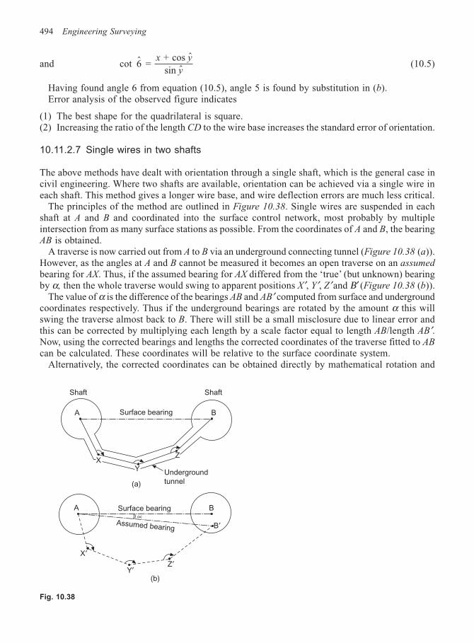
494 Engineering Surveying
and cot ˆ ˆ
ˆ6 =
+ cos
sin
x y
y(10.5)
Having found angle 6 from equation (10.5), angle 5 is found by substitution in (b).Error analysis of the observed figure indicates
(1) The best shape for the quadrilateral is square.(2) Increasing the ratio of the length CD to the wire base increases the standard error of orientation.
10.11.2.7 Single wires in two shafts
The above methods have dealt with orientation through a single shaft, which is the general case incivil engineering. Where two shafts are available, orientation can be achieved via a single wire ineach shaft. This method gives a longer wire base, and wire deflection errors are much less critical.
The principles of the method are outlined in Figure 10.38. Single wires are suspended in eachshaft at A and B and coordinated into the surface control network, most probably by multipleintersection from as many surface stations as possible. From the coordinates of A and B, the bearingAB is obtained.
A traverse is now carried out from A to B via an underground connecting tunnel (Figure 10.38 (a)).However, as the angles at A and B cannot be measured it becomes an open traverse on an assumed
bearing for AX. Thus, if the assumed bearing for AX differed from the ‘true’ (but unknown) bearingby α, then the whole traverse would swing to apparent positions X′, Y′, Z′ and Β′ (Figure 10.38 (b)).
The value of α is the difference of the bearings AB and AB′ computed from surface and undergroundcoordinates respectively. Thus if the underground bearings are rotated by the amount α this willswing the traverse almost back to B. There will still be a small misclosure due to linear error andthis can be corrected by multiplying each length by a scale factor equal to length AB/length AB′.Now, using the corrected bearings and lengths the corrected coordinates of the traverse fitted to AB
can be calculated. These coordinates will be relative to the surface coordinate system.Alternatively, the corrected coordinates can be obtained directly by mathematical rotation and
Fig. 10.38
Shaft Shaft
XY
Z
B
Underground
tunnel
Surface bearing
Assumed bearing
∝
A
A B
B′
X′
Y′Z′
(a)
(b)
Surface bearing
Setting out (dimensional control) 495
translation of the ‘assumed’ values. Therefore, with A as origin, a rotation equal to α and atranslation of AB/AB′, the corrected coordinates are obtained from
Ei = E0 + K ( cos – sin )′ ′E Ni iα α (10.6a)
Ni = N0 + K ( cos + sin )′ ′N Ei iα α (10.6b)
where E0, N0 = coordinates of the origin (in this case A)′ ′E Ni i, = coordinates of the traverse points computed on the assumed bearing
Ei, Ni = transformed coordinates of the underground traverse pointsK = scale factor (length AB/length AB′)
There is no doubt that this is the most accurate and reliable method of surface-to-undergroundorientation. The accuracy of the method is dependent upon.
(1) The accuracy of fixing the position of the wires at the surface.(2) The accuracy of the underground connecting traverse.
The influence of errors in the verticality of the wires, so critical in single-shaft work, is practicallynegligible owing to the long distance separating the two shafts. Provided that the legs of theunderground traverse are long enough, then modern single-second theodolites integrated withEDM equipment would achieve highly accurate surface and underground surveys, resulting in finalorientation accuracies of a few seconds. As the whole procedure is under strict control there is noreason why the final accuracy cannot be closely predicted.
10.11.2.8 Alternatives
In all the above methods the wires could be replaced by autoplumbs or lasers.In the case of the autoplumb, stations at the shaft bottom could be projected vertically up to
specially arranged targets at the surface and appropriate observations taken direct onto these points.Similarly, lasers could be arranged at the surface to project the beam vertically down the shaft to
be picked up on optical or electronic targets. The laser spots then become the shaft stations correlatedin the normal way.
The major problems encountered by using the above alternatives are:
(1) Ensuring the laser beam is vertical.(2) Ensuring correct detection of the centre of the beam.(3) Refraction in the shaft (applies also to autoplumb).
In the first instance a highly sensitive spirit level or automatic compensator could be used;excellent results have been achieved using arrangements involving mercury pools, or photo-electricsensors.
Detecting the centre of the laser is more difficult. Lasers having a divergence of 10″ to 20″ wouldgive a spot of 10 mm and 20 mm diameter respectively at 200 m. This spot also tends to move aboutdue to variations in air density. It may therefore require an arrangement of photocell detectors tosolve the problem.
Due to the turbulence of air currents in shafts the problem of refraction has not proved toodangerous.
10.12 GYRO-THEODOLITE
An alternative to the use of wire methods is the gyro-theodolite. This is a north-seeking gyroscope
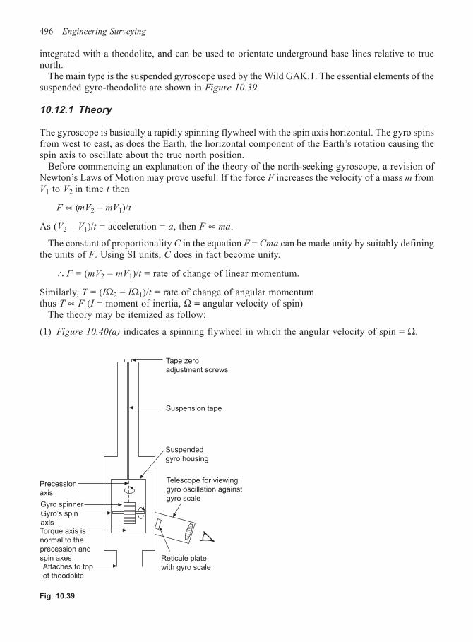
496 Engineering Surveying
integrated with a theodolite, and can be used to orientate underground base lines relative to truenorth.
The main type is the suspended gyroscope used by the Wild GAK.1. The essential elements of thesuspended gyro-theodolite are shown in Figure 10.39.
10.12.1 Theory
The gyroscope is basically a rapidly spinning flywheel with the spin axis horizontal. The gyro spinsfrom west to east, as does the Earth, the horizontal component of the Earth’s rotation causing thespin axis to oscillate about the true north position.
Before commencing an explanation of the theory of the north-seeking gyroscope, a revision ofNewton’s Laws of Motion may prove useful. If the force F increases the velocity of a mass m fromV1 to V2 in time t then
F ∝ (mV2 – mV1)/t
As (V2 – V1)/t = acceleration = a, then F ∝ ma.
The constant of proportionality C in the equation F = Cma can be made unity by suitably definingthe units of F. Using SI units, C does in fact become unity.
∴ F = (mV2 – mV1)/t = rate of change of linear momentum.
Similarly, T = (IΩ2 – IΩ1)/t = rate of change of angular momentumthus T ∝ F (I = moment of inertia, Ω = angular velocity of spin)
The theory may be itemized as follow:
(1) Figure 10.40(a) indicates a spinning flywheel in which the angular velocity of spin = Ω.
Fig. 10.39
Tape zero
adjustment screws
Suspension tape
Suspended
gyro housing
Telescope for viewing
gyro oscillation against
gyro scale
Reticule plate
with gyro scale
Precession
axis
Gyro spinner
Gyro’s spin
axisTorque axis is
normal to the
precession and
spin axesAttaches to top
of theodolite
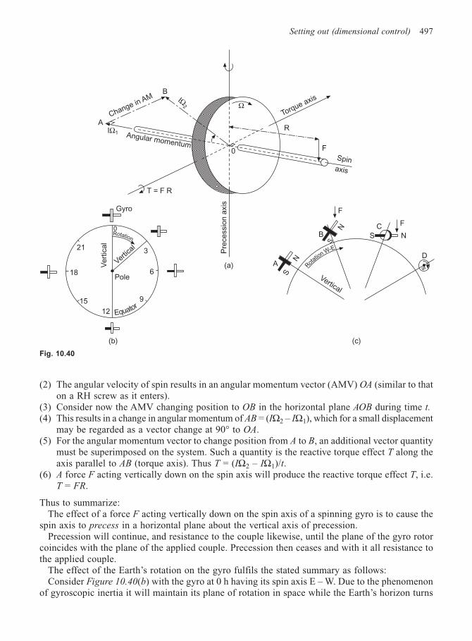
Setting out (dimensional control) 497
Rotation
EquatorR
otatio
n W-E
s
(2) The angular velocity of spin results in an angular momentum vector (AMV) OA (similar to thaton a RH screw as it enters).
(3) Consider now the AMV changing position to OB in the horizontal plane AOB during time t.(4) This results in a change in angular momentum of AB = (IΩ2 – IΩ1), which for a small displacement
may be regarded as a vector change at 90° to OA.(5) For the angular momentum vector to change position from A to B, an additional vector quantity
must be superimposed on the system. Such a quantity is the reactive torque effect T along theaxis parallel to AB (torque axis). Thus T = (IΩ2 – IΩ1)/t.
(6) A force F acting vertically down on the spin axis will produce the reactive torque effect T, i.e.T = FR.
Thus to summarize:The effect of a force F acting vertically down on the spin axis of a spinning gyro is to cause the
spin axis to precess in a horizontal plane about the vertical axis of precession.Precession will continue, and resistance to the couple likewise, until the plane of the gyro rotor
coincides with the plane of the applied couple. Precession then ceases and with it all resistance tothe applied couple.
The effect of the Earth’s rotation on the gyro fulfils the stated summary as follows:Consider Figure 10.40(b) with the gyro at 0 h having its spin axis E – W. Due to the phenomenon
of gyroscopic inertia it will maintain its plane of rotation in space while the Earth’s horizon turns
Fig. 10.40
AChange in AM
BIΩ
2
IΩ1 Angular momentum
ΩTorque axis
R
F
Spinaxis
T = F R
Gyro
(a)
(b)
21
18
15
12
9
6
3
0P
recessio
n a
xis
A
S
N
N
B
S
F
S N
F
D
Vertical
(c)
Vertica
l
0
C
Ve
rtic
al
Pole
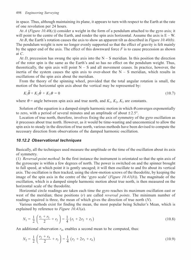
498 Engineering Surveying
in space. Thus, although maintaining its plane, it appears to turn with respect to the Earth at the rateof one revolution per 24 hours.
At A (Figure 10.40(c)) consider a weight in the form of a pendulum attached to the gyro axis; itwill point to the centre of the Earth, and render the spin axis horizontal. Assume the axis is E – W.
At B, the Earth’s rotation causes the axis to show an apparent tilt as described in Figure 10.40(b).The pendulum weight is now no longer evenly supported so that the effect of gravity is felt mainlyby the upper end of the axis. The effect of this downward force F is to cause precession as shownat C.
At D, precession has swung the spin axis into the N – S meridian. In this position the directionof the rotor spin is the same as the Earth’s and so has no effect on the pendulum weight. Thus,theoretically, the spin axis will point N – S and all movement ceases. In practice, however, theinertia of the system causes the spin axis to over-shoot the N – S meridian, which results inoscillations of the spin axis about the meridian.
From the theory of the spinning wheel, provided that the total angular rotation is small, themotion of the horizontal spin axis about the vertical may be represented by:
K K K1 2 3 + + = 0˙ ˙θ θ θ (10.7)
where θ = angle between spin axis and true north, and K1, K2, K3 are constants.
Solution of the equation is a damped simple harmonic motion in which θ converges exponentiallyto zero, with a period of several minutes and an amplitude of about ± 2.5°.
Location of true north, therefore, involves fixing the axis of symmetry of the gyro oscillation asit precesses about true north. However, as it would be time-wasting and uneconomical to allow thespin axis to steady in the direction of true north, various methods have been devised to compute thenecessary direction from observations of the damped harmonic oscillation.
10.12.2 Observational techniques
Basically, all the techniques used measure the amplitude or the time of the oscillation about its axisof symmetry.(1) Reversal-point method: In the first instance the instrument is orientated so that the spin axis ofthe gyroscope is within a few degrees of north. The power is switched on and the spinner broughtto full speed, at which point it is gently uncaged; it will then oscillate to and fro about its verticalaxis. The oscillation is then tracked, using the slow-motion screws of the theodolite, by keeping theimage of the spin axis in the centre of the ‘gyro scale’ (Figure 10.41(b)). The magnitude of theoscillation, which is a damped simple harmonic motion about true north, is then measured on thehorizontal scale of the theodolite.
Horizontal circle readings are taken each time the gyro reaches its maximum oscillation east orwest of the meridian; these positions (r) are called reversal points. The minimum number ofreadings required is three, the mean of which gives the direction of true north (N).
Various methods exist for finding the mean, the most popular being Schuler’s Mean, which isexplained by reference to Figure 10.41(a).
N1 = 12
+ 2
+ = 14
+ 2 + 1 32 1 2 3
r rr r r r
( ) (10.8)
An additional observation r4, enables a second mean to be computed, thus:
N2 = 12
+ 2
+ = 14
+ 2 + 2 43 2 3 4
r rr r r r
( ) (10.9)
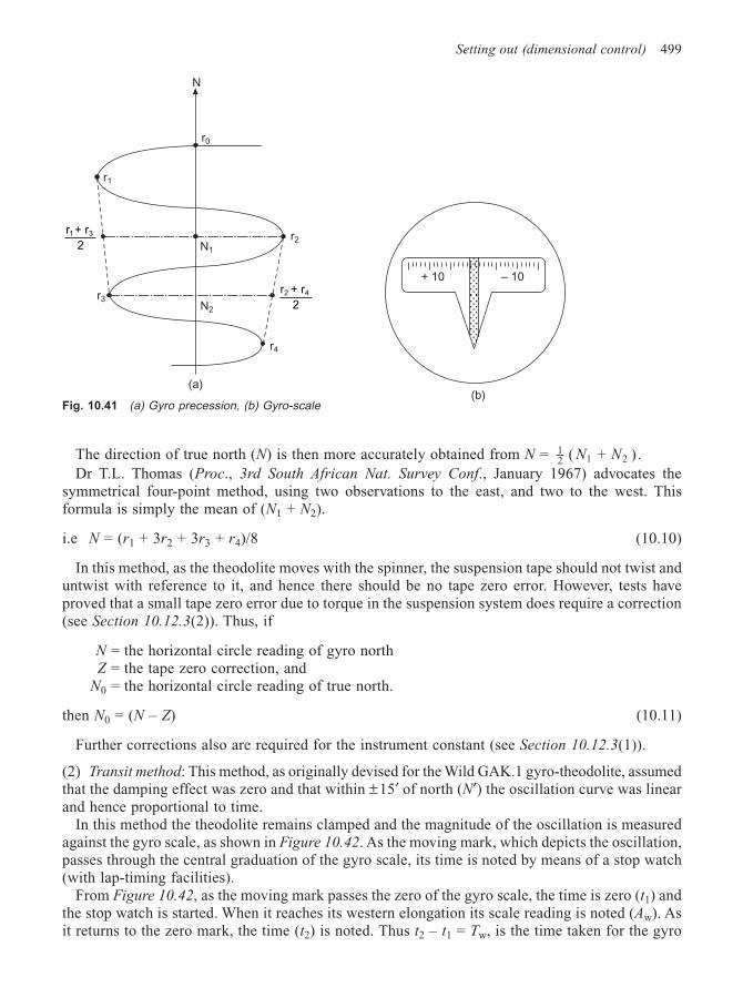
Setting out (dimensional control) 499
The direction of true north (N) is then more accurately obtained from N = 12 1 2 ( + )N N .
Dr T.L. Thomas (Proc., 3rd South African Nat. Survey Conf., January 1967) advocates thesymmetrical four-point method, using two observations to the east, and two to the west. Thisformula is simply the mean of (N1 + N2).
i.e N = (r1 + 3r2 + 3r3 + r4)/8 (10.10)
In this method, as the theodolite moves with the spinner, the suspension tape should not twist anduntwist with reference to it, and hence there should be no tape zero error. However, tests haveproved that a small tape zero error due to torque in the suspension system does require a correction(see Section 10.12.3(2)). Thus, if
N = the horizontal circle reading of gyro northZ = the tape zero correction, and
N0 = the horizontal circle reading of true north.
then N0 = (N – Z) (10.11)
Further corrections also are required for the instrument constant (see Section 10.12.3(1)).
(2) Transit method: This method, as originally devised for the Wild GAK.1 gyro-theodolite, assumedthat the damping effect was zero and that within ±15′ of north (N′) the oscillation curve was linearand hence proportional to time.
In this method the theodolite remains clamped and the magnitude of the oscillation is measuredagainst the gyro scale, as shown in Figure 10.42. As the moving mark, which depicts the oscillation,passes through the central graduation of the gyro scale, its time is noted by means of a stop watch(with lap-timing facilities).
From Figure 10.42, as the moving mark passes the zero of the gyro scale, the time is zero (t1) andthe stop watch is started. When it reaches its western elongation its scale reading is noted (Aw). Asit returns to the zero mark, the time (t2) is noted. Thus t2 – t1 = Tw, is the time taken for the gyro
Fig. 10.41 (a) Gyro precession, (b) Gyro-scale
+ 10 – 10
N
r0
r1
N1
N2
r2
r3
(a)(b)
r + r
21 3
r4
r + r
22 4
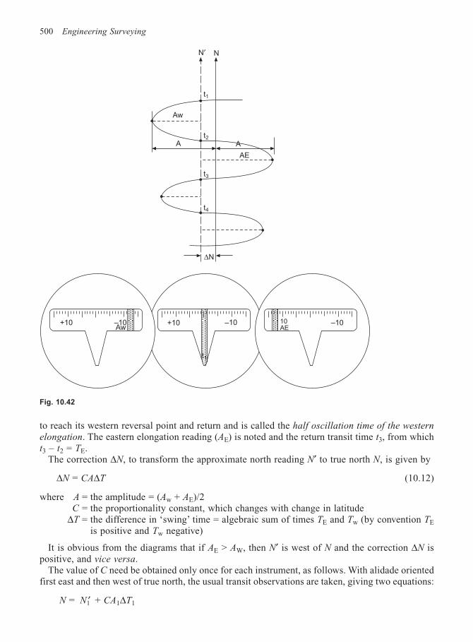
500 Engineering Surveying
to reach its western reversal point and return and is called the half oscillation time of the western
elongation. The eastern elongation reading (AE) is noted and the return transit time t3, from whicht3 – t2 = TE.
The correction ∆N, to transform the approximate north reading N′ to true north N, is given by
∆N = CA∆T (10.12)
where A = the amplitude = (Aw + AE)/2C = the proportionality constant, which changes with change in latitude
∆T = the difference in ‘swing’ time = algebraic sum of times TE and Tw (by convention TE
is positive and Tw negative)
It is obvious from the diagrams that if AE > AW, then N′ is west of N and the correction ∆N ispositive, and vice versa.
The value of C need be obtained only once for each instrument, as follows. With alidade orientedfirst east and then west of true north, the usual transit observations are taken, giving two equations:
N = ′N1 + CA1∆T1
Fig. 10.42
N′ N
t1
t2
t3
t4
∆N
+10 –10Aw
–10+10 10AE
–10
Aw
A A
AE
t1
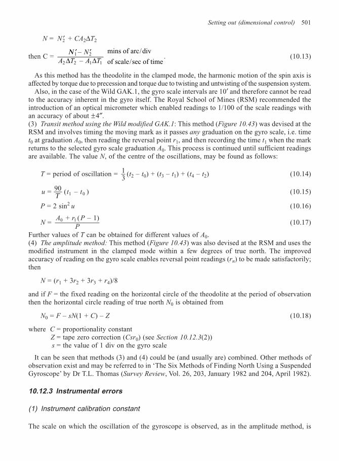
Setting out (dimensional control) 501
N = ′N2 + CA2∆T2
then C = ′ ′Ν 1 2
2 1
– –
mins of arc/div
of scale/sec of time
N
A T A T∆ ∆2 1. (10.13)
As this method has the theodolite in the clamped mode, the harmonic motion of the spin axis isaffected by torque due to precession and torque due to twisting and untwisting of the suspension system.
Also, in the case of the Wild GAK.1, the gyro scale intervals are 10′ and therefore cannot be readto the accuracy inherent in the gyro itself. The Royal School of Mines (RSM) recommended theintroduction of an optical micrometer which enabled readings to 1/100 of the scale readings withan accuracy of about ±4″.(3) Transit method using the Wild modified GAK.1: This method (Figure 10.43) was devised at theRSM and involves timing the moving mark as it passes any graduation on the gyro scale, i.e. timet0 at graduation A0, then reading the reversal point r1, and then recording the time t1 when the markreturns to the selected gyro scale graduation A0. This process is continued until sufficient readingsare available. The value N, of the centre of the oscillations, may be found as follows:
T = period of oscillation = 13
(t2 – t0) + (t3 – t1) + (t4 – t2) (10.14)
u t t = ( – )1 090Τ (10.15)
P = 2 sin2 u (10.16)
N = A r P
P0 + ( – 1)1 (10.17)
Further values of T can be obtained for different values of A0.(4) The amplitude method: This method (Figure 10.43) was also devised at the RSM and uses themodified instrument in the clamped mode within a few degrees of true north. The improvedaccuracy of reading on the gyro scale enables reversal point readings (rn) to be made satisfactorily;then
N = (r1 + 3r2 + 3r3 + r4)/8
and if F = the fixed reading on the horizontal circle of the theodolite at the period of observationthen the horizontal circle reading of true north N0 is obtained from
N0 = F – sN(1 + C) – Z (10.18)
where C = proportionality constantZ = tape zero correction (Csr0) (see Section 10.12.3(2))s = the value of 1 div on the gyro scale
It can be seen that methods (3) and (4) could be (and usually are) combined. Other methods ofobservation exist and may be referred to in ‘The Six Methods of Finding North Using a SuspendedGyroscope’ by Dr T.L. Thomas (Survey Review, Vol. 26, 203, January 1982 and 204, April 1982).
10.12.3 Instrumental errors
(1) Instrument calibration constant
The scale on which the oscillation of the gyroscope is observed, as in the amplitude method, is
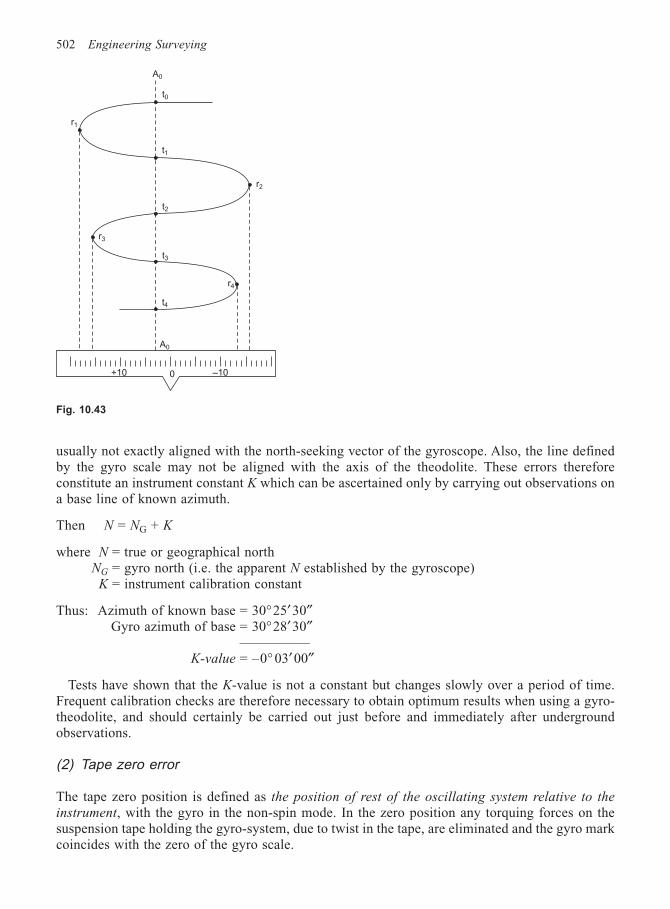
502 Engineering Surveying
usually not exactly aligned with the north-seeking vector of the gyroscope. Also, the line definedby the gyro scale may not be aligned with the axis of the theodolite. These errors thereforeconstitute an instrument constant K which can be ascertained only by carrying out observations ona base line of known azimuth.
Then N = NG + K
where N = true or geographical northNG = gyro north (i.e. the apparent N established by the gyroscope)
K = instrument calibration constant
Thus: Azimuth of known base = 30°25′30″Gyro azimuth of base = 30°28′30″
—————K-value = –0° 03′00″
Tests have shown that the K-value is not a constant but changes slowly over a period of time.Frequent calibration checks are therefore necessary to obtain optimum results when using a gyro-theodolite, and should certainly be carried out just before and immediately after undergroundobservations.
(2) Tape zero error
The tape zero position is defined as the position of rest of the oscillating system relative to the
instrument, with the gyro in the non-spin mode. In the zero position any torquing forces on thesuspension tape holding the gyro-system, due to twist in the tape, are eliminated and the gyro markcoincides with the zero of the gyro scale.
A0
r1
r2
r3
r4
A0
t3
t4
t0
t1
t2
0 –10+10
Fig. 10.43
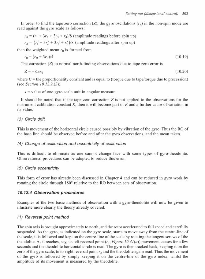
Setting out (dimensional control) 503
In order to find the tape zero correction (Z), the gyro oscillations (rn) in the non-spin mode areread against the gyro scale as follows:
rB = (r1 + 3r2 + 3r3 + r4)/8 (amplitude readings before spin up)
rA = ′ ′ ′ ′( )r r r r1 2 3 4 + 3 + 3 + /8 (amplitude readings after spin up)
then the weighted mean r0 is formed from
r0 = (rB + 3rA)/4 (10.19)
The correction (Z) to normal north-finding observations due to tape zero error is
Z = – Csr0 (10.20)
where C = the proportionality constant and is equal to (torque due to tape/torque due to precession)(see Section 10.12.2.(2)).
s = value of one gyro scale unit in angular measure
It should be noted that if the tape zero correction Z is not applied to the observations for theinstrument calibration constant K, then it will become part of K and a further cause of variation inits value.
(3) Circle drift
This is movement of the horizontal circle caused possibly by vibration of the gyro. Thus the RO ofthe base line should be observed before and after the gyro observations, and the mean taken.
(4) Change of collimation and eccentricity of collimation
This is difficult to eliminate as one cannot change face with some types of gyro-theodolite.Observational procedures can be adopted to reduce this error.
(5) Circle eccentricity
This form of error has already been discussed in Chapter 4 and can be reduced in gyro work byrotating the circle through 180° relative to the RO between sets of observation.
10.12.4 Observation procedures
Examples of the two basic methods of observation with a gyro-theodolite will now be given toillustrate more clearly the theory already covered.
(1) Reversal point method
The spin axis is brought approximately to north, and the rotor accelerated to full speed and carefullysuspended. As the gyro, as indicated on the gyro scale, starts to move away from the centre-line ofthe scale, it is followed and kept on the centre-line of the scale by rotating the tangent screws of thetheodolite. As it reaches, say, its left reversal point (r1, Figure 10.41(a)) movement ceases for a fewseconds and the theodolite horizontal circle is read. The gyro is then tracked back, keeping it on thezero of the gyro scale, to its right reversal point r2 and the theodolite again read. Thus the movementof the gyro is followed by simply keeping it on the centre-line of the gyro index, whilst theamplitude of its movement is measured by the theodolite.
504 Engineering Surveying
Reversal Horiz circle reading
r1 (left) 42°00′31″r2 (right) 49°40′32″r3 (left) 42°04′ 02″r4 (right) 49°37′ 21″
Schuler’s mean N1 = 14
(r1 + 2r2 + r3)
= 14
(42°00′31″ + 99° 21′04″ + 42° 04′ 02″)
= 45°51′24″
N2 = 14
(r2 + 2r3 + r4) = 45°51′ 29″
∴ N = (N1 + N2)/2 = 45° 51′ 26″ (horizontal circle reading of gyro north)
Assuming a tape zero correction (Z) of – 10″, then
N0 = N – Z = 45° 51′ 26″ – 10″ = 45° 51′ 16″
A check on the computation can be applied by combining N1 and N2 to give
N = 18
(r1 + 3r2 + 3r3 + r4)
Assuming that the theodolite is now sighted along the base line and the mean horizontal circlereading was, say, 55° 51′ 16″; then the base is obviously 10° clockwise of gyro north and its bearingrelative to gyro north is therefore 10°.
The application of the instrument constant K equal to, say, – 03′ 00″ will reduce the bearing of thebase line to its correct geographical azimuth, i.e. 09° 57′ 00″ relative to true north.
If the survey is to be connected into the OS National Grid then a correction (δ) for convergenceof meridians (i.e. the difference between grid north and true north) must be made and possibly a(t – T) correction (i.e. the difference between an observed bearing and its corresponding gridbearing). In some instance a Laplace correction may need to be applied where the ‘deviation of thevertical’ is very high; however, in most cases this correction is usually less than 3″ of arc.
In the case of local surveys, of limited extent, on a rectangular Cartesian grid, only the convergenceof meridians need to be considered.
Figure 10.44 shows the relationship of the various corrections.
Gyro bearing AB = β = 10° 00′00″Instrument constant K = –0°03′00″
—————Geographical azimuth θ = 09°57′00″Convergence of meridians δ = + 43′ 09″ computed from(t – T) = +00′04″ geodetic tables
—————NG bearing of base-line AB = 10° 40′ 13″ = φ(N.B. Z is the tape zero correction = – Csr0.)
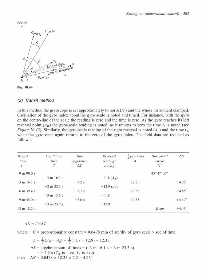
Setting out (dimensional control) 505
(2) Transit method
In this method the gryoscope is set approximately to north (N′) and the whole instrument clamped.Oscillation of the gyro index about the gyro scale is noted and timed. For instance, with the gyroon the centre-line of the scale the reading is zero and the time is zero. As the gyro reaches its leftreversal point (AW) the gyro-scale reading is noted; as it returns to zero the time t2 is noted (seeFigure 10.42). Similarly, the gyro-scale reading of the right reversal is noted (AE) and the time t3,when the gyro once again returns to the zero of the gyro index. The field data are reduced asfollows:
Transit Oscillation Time Reversal 12 (AW +AE) Horizontal ∆N
time time difference readings A circle
t T ‘∆T ’ AW /AE N ′
0 m 00.0 s 45° 47′ 00″– 3 m 16.1 s –11.8 (AW)
3 m 16.1 s +7.2 s 12.35 +4.25′+3 m 23.3 s +12.9 (AE)
6 m 39.4 s +7.7 s 12.35 +4.55′–3 m 15.6 s –11.8
9 m 55.0 s +7.6 s 12.35 +4.49 ′+3 m 23.2 s +12.9
13 m 18.2 s Mean +4.43′
∆N = CA∆T
where C = proportionality constant = 0.0478 min of arc/div of gyro scale × sec of time
A = 12
(AW + AE) = 12
(11.8 + 12.9) = 12.35
∆T = algebraic sum of times = (–3 m 16.1 s + 3 m 23.3 s)= + 7.2 s (TW is – ve, TE is +ve)
then ∆N = 0.0478 × 12.35 × 7.2 = 4.25′
Fig. 10.44
Grid N
Gyro NTrue N
K
δβ
θ
TA
Line of sight
A φ(tA–TA)
Line on projectionB
tA
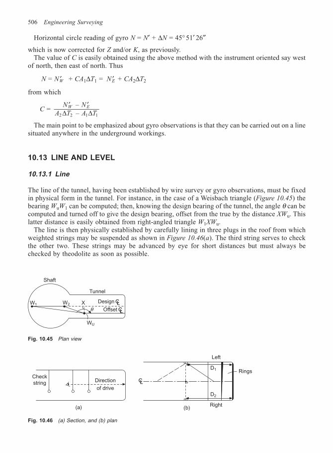
506 Engineering Surveying
Horizontal circle reading of gyro N = N′ + ∆N = 45° 51′ 26″
which is now corrected for Z and/or K, as previously.The value of C is easily obtained using the above method with the instrument oriented say west
of north, then east of north. Thus
N NW = ′ + CA1∆T1 = ′NE + CA2∆T2
from which
C = ′ ′N N
A T A TW E –
– 2 1∆ ∆2 1
The main point to be emphasized about gyro observations is that they can be carried out on a linesituated anywhere in the underground workings.
10.13 LINE AND LEVEL
10.13.1 Line
The line of the tunnel, having been established by wire survey or gyro observations, must be fixedin physical form in the tunnel. For instance, in the case of a Weisbach triangle (Figure 10.45) thebearing WuW1 can be computed; then, knowing the design bearing of the tunnel, the angle θ can becomputed and turned off to give the design bearing, offset from the true by the distance XWu. Thislatter distance is easily obtained from right-angled triangle W1XWu.
The line is then physically established by carefully lining in three plugs in the roof from whichweighted strings may be suspended as shown in Figure 10.46(a). The third string serves to checkthe other two. These strings may be advanced by eye for short distances but must always bechecked by theodolite as soon as possible.
Fig. 10.45 Plan view
Shaft
Tunnel
W1 W2 X
θDesign CL
Offset CL
WU
Fig. 10.46 (a) Section, and (b) plan
Check
stringDirection
of drive
Rings
Left
Right
D1
D2
CL
(a) (b)
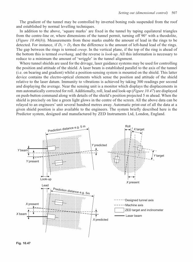
Setting out (dimensional control) 507
The gradient of the tunnel may be controlled by inverted boning rods suspended from the roofand established by normal levelling techniques.
In addition to the above, ‘square marks’ are fixed in the tunnel by taping equilateral trianglesfrom the centre-line or, where dimensions of the tunnel permit, turning off 90° with a theodolite,(Figure 10.46(b)). Measurements from these marks enable the amount of lead in the rings to bedetected. For instance, if D1 > D2 then the difference is the amount of left-hand lead of the rings.The gap between the rings is termed creep. In the vertical plane, if the top of the ring is ahead ofthe bottom this is termed overhang, and the reverse is look-up. All this information is necessary toreduce to a minimum the amount of ‘wriggle’ in the tunnel alignment.
Where tunnel shields are used for the drivage, laser guidance systems may be used for controllingthe position and attitude of the shield. A laser beam is established parallel to the axis of the tunnel(i.e. on bearing and gradient) whilst a position-sensing system is mounted on the shield. This latterdevice contains the electro-optical elements which sense the position and attitude of the shieldrelative to the laser datum. Immunity to vibrations is achieved by taking 300 readings per secondand displaying the average. Near the sensing unit is a monitor which displays the displacements inmm automatically corrected for roll. Additionally, roll, lead and look-up (Figure 10.47) are displayedon push-button command along with details of the shield’s position projected 5 m ahead. When theshield is precisely on line a green light glows in the centre of the screen. All the above data can berelayed to an engineers’ unit several hundred metres away. Automatic print-out of all the data at agiven shield position is also available to the engineers. The system briefly described here is thePredictor system, designed and manufactured by ZED Instruments Ltd, London, England.
Fig. 10.47
Prediction distance e.g. 5 m
Y predicted
Y beam
Y present
Look-up
Lead
X present
X beam
Prediction distance e.g. 5m
X predicted
RollX target
Y target
X present
Designed tunnel axis
Laser beam
ZED target and inclinometer
Machine axis
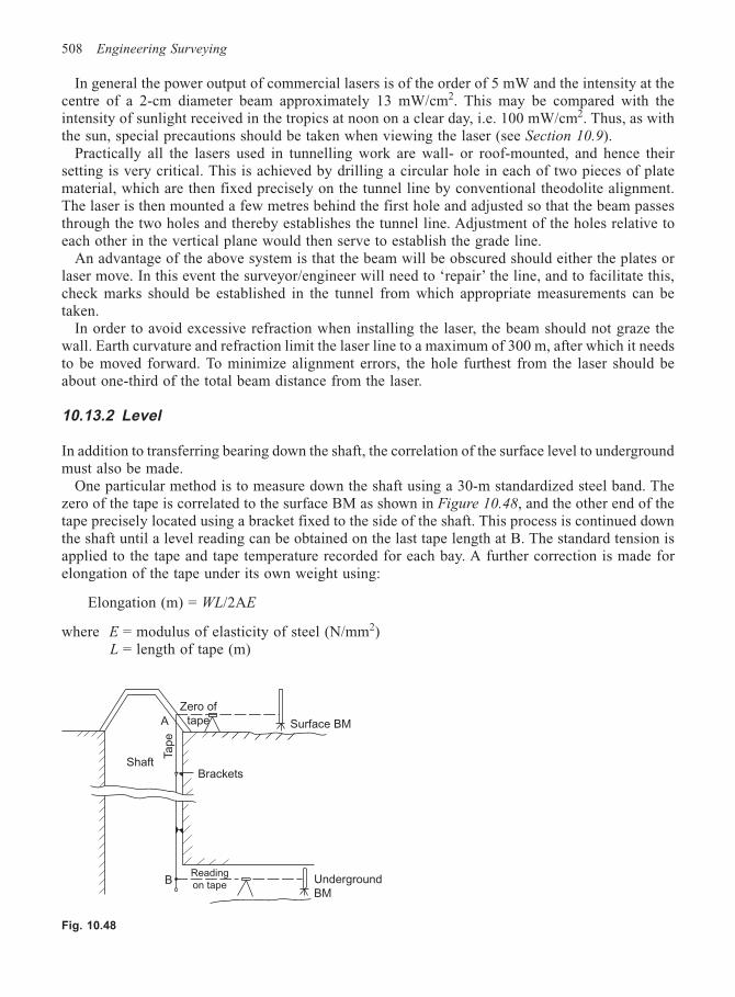
508 Engineering Surveying
In general the power output of commercial lasers is of the order of 5 mW and the intensity at thecentre of a 2-cm diameter beam approximately 13 mW/cm2. This may be compared with theintensity of sunlight received in the tropics at noon on a clear day, i.e. 100 mW/cm2. Thus, as withthe sun, special precautions should be taken when viewing the laser (see Section 10.9).
Practically all the lasers used in tunnelling work are wall- or roof-mounted, and hence theirsetting is very critical. This is achieved by drilling a circular hole in each of two pieces of platematerial, which are then fixed precisely on the tunnel line by conventional theodolite alignment.The laser is then mounted a few metres behind the first hole and adjusted so that the beam passesthrough the two holes and thereby establishes the tunnel line. Adjustment of the holes relative toeach other in the vertical plane would then serve to establish the grade line.
An advantage of the above system is that the beam will be obscured should either the plates orlaser move. In this event the surveyor/engineer will need to ‘repair’ the line, and to facilitate this,check marks should be established in the tunnel from which appropriate measurements can betaken.
In order to avoid excessive refraction when installing the laser, the beam should not graze thewall. Earth curvature and refraction limit the laser line to a maximum of 300 m, after which it needsto be moved forward. To minimize alignment errors, the hole furthest from the laser should beabout one-third of the total beam distance from the laser.
10.13.2 Level
In addition to transferring bearing down the shaft, the correlation of the surface level to undergroundmust also be made.
One particular method is to measure down the shaft using a 30-m standardized steel band. Thezero of the tape is correlated to the surface BM as shown in Figure 10.48, and the other end of thetape precisely located using a bracket fixed to the side of the shaft. This process is continued downthe shaft until a level reading can be obtained on the last tape length at B. The standard tension isapplied to the tape and tape temperature recorded for each bay. A further correction is made forelongation of the tape under its own weight using:
Elongation (m) = WL/2AE
where E = modulus of elasticity of steel (N/mm2)L = length of tape (m)
Fig. 10.48
Zero of
tapeA
Ta
pe
ShaftBrackets
BReading
on tapeUnderground
BM
Surface BM

Setting out (dimensional control) 509
A = cross-sectional area of tape (mm2)W = mass of tape (N)
Then the corrected distance AB is used to establish the value of the underground BM relative tothe surface BM.
If a special shaft tape (1000 m long) is available the operation may be carried out in one step. Theoperation should be carried out at least twice and the mean value accepted. Using the 30-m band,accuracies of 1 in 5000 are possible; the shaft tape gives accuracies of 1 in 10 000.
Electromagnetic distance-measuring (EDM) equipment has also been used to measure shaftdepths. A special reflecting mirror at the top of the shaft is aligned with the EDM instrument andthen rotated in the vertical plane until the measuring beam strikes a reflector at the shaft bottom. Inthis way the distance from the instrument to the reflector is obtained and subsequently adjusted togive the distance from mirror to reflector. By connecting the mirror and reflector to surface andunderground BMs respectively, their values can be correlated. With top-mounted EDM equipmenta reflecting mirror is unnecessary and the distance to a reflector at the shaft bottom could bemeasured direct.
10.14 RESPONSIBILITY ON SITE
Responsibility with regard to setting out is defined in Clause 17 of the ICE Conditions ofContract:
The contractor shall be responsible for the true and proper setting out of the works, and for thecorrectness of the position, levels, dimensions, and alignment of all parts of the works, and forthe provision of all necessary instruments, appliances, and labour in connection therewith. If,at any time during the progress of the works, any error shall appear or arise in the position,levels, dimensions, or alignment of any part of the works, the contractor, on being required soto do by the engineer, shall, at his own cost, rectify such error to the satisfaction of the engineer,unless such error is based on incorrect data supplied in writing by the engineer or the engineer’srepresentative, in which case the cost of rectifying the same shall be borne by the employer. Thechecking of any setting out, or of any line or level, by the engineer or the engineer’s representative,shall not, in any way, relieve the contractor of his responsibility for the correctness thereof, andthe contractor shall carefully protect and preserve all bench-marks, sight rails, pegs, and otherthings used in setting out the works.
The clause specifies three persons involved in the process, namely, the employer, the engineerand the agent, whose roles are as follows:
The employer, who may be a government department, local authority or private individual,requires to carry out and finance a particular project. To this end, he commissions an engineer toinvestigate and design the project, and to take responsibility for the initial site investigation,surveys, plans, designs, working drawings, and setting-out data. On satisfactory completion of hiswork he lets the contract to a contractor whose duty it is to carry out the work.
On site the employer is represented by the engineer or his representative, referred to as theresident engineer (RE), and the contractor’s representative is called the agent.
The engineer has overall responsibility for the project and must protect the employer’sinterest without bias to the contractor. The agent is responsible for the actual construction of theproject.

510 Engineering Surveying
10.15 RESPONSIBILITY OF THE SETTING-OUT ENGINEER
The setting-out engineer should establish such a system of work on site that will ensure the accuratesetting out of the works well in advance of the commencement of construction. To achieve this, thefollowing factors should be considered.
(1) A complete and thorough understanding of the plans, working drawings, setting-out data,tolerances involved and the time scale of operations. Checks on the setting-out data suppliedshould be immediately implemented.
(2) A complete and thorough knowledge of the site, plant and relevant personnel. Communicationsbetween all individuals is vitally important. Field checks on the survey control already establishedon site, possibly by contract surveyors, should be carried out at the first opportunity.
(3) A complete and thorough knowledge of the survey instrumentation available on site, includingthe effect of instrumental errors on setting-out observations. At the first opportunity, a baseshould be established for the calibration of tapes, EDM equipment, levels and theodolites.
(4) A complete and thorough knowledge of the stores available, to ensure an adequate and continuingsupply of pegs, pins, chalk, string, paint, timber, etc.
(5) Office procedure should be so organized as to ensure easy access to all necessary information.Plans should be stored flat in plan drawers, and those amended or superseded should bewithdrawn from use and stored elsewhere. Field and level books should be carefully referencedand properly filed. All setting-out computations and procedures used should be clearly presented,referenced and filed.
(6) Wherever possible, independent checks of the computation, abstraction and extrapolation ofsetting-out data and of the actual setting-out procedures should be made.
It can be seen from this brief itinerary of the requirements of a setting-out engineer, that suchwork should never be allocated, without complete supervision, to junior, inexperienced members ofthe site team.
All site engineers should also make a careful study of the following British Standards, whichwere prepared under the direction of the Basic Data and Performance Criteria for Civil Engineeringand Building Structures Standards Policy Committee:
(1) BS 5964:1990 (ISO 4463–1, 1989)Part 1. Methods of measuring, planning and organization and acceptance criteria.
(2) BS 5606:1990Guide to Accuracy in Building.
(3) BS 7307:1990 (ISO 7976:1989)Part 1. Methods and instruments.Part 2. Position of measuring points.
(4) BS 7308:1990 (ISO 7737:1986)Presentation of dimensional accuracy data in building construction.
(5) BS 7734:1990 (ISO 8322:1989)Part 1. Methods for determining accuracy in use: Theory.Part 2. Methods for determining accuracy in use: Measuring Tapes.Part 3. Methods for determining accuracy in use: Optical Levelling Instruments.Parts 4 to 8 deal with theodolites and EDM.
These documents supply important information coupled with a wealth of excellent, explanatorydiagrams of various setting-out procedures.
For instance BS 5964 provides acceptance criteria for the field data measured, termed permitteddeviation (PD), where PD = 2.5 (SD) (Standard Deviation).
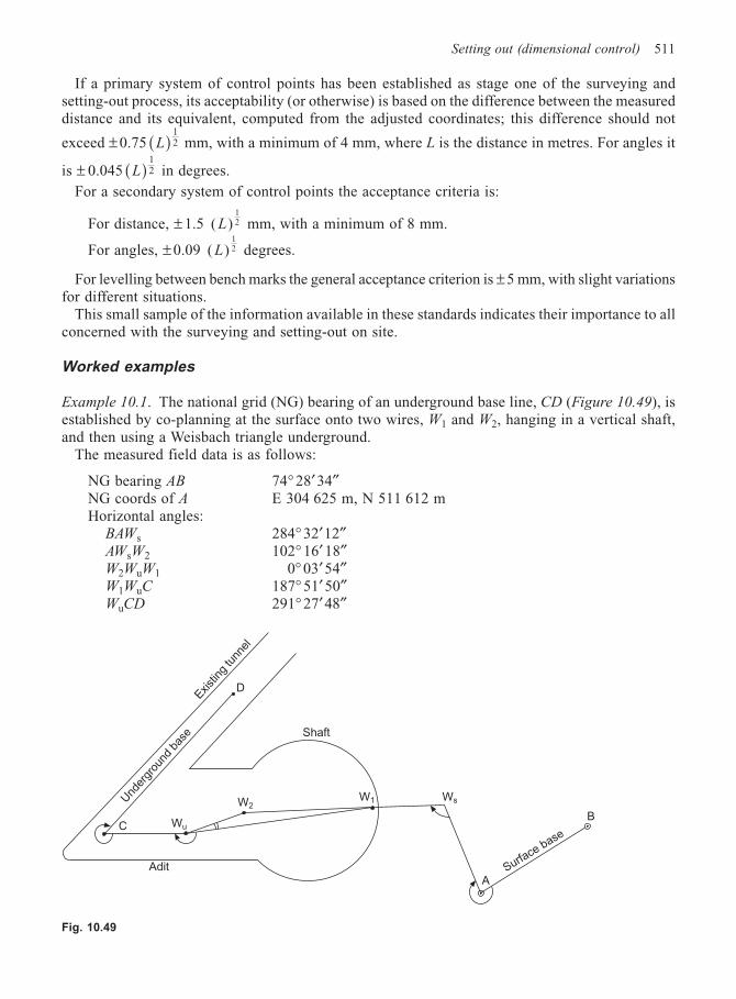
Setting out (dimensional control) 511
If a primary system of control points has been established as stage one of the surveying andsetting-out process, its acceptability (or otherwise) is based on the difference between the measureddistance and its equivalent, computed from the adjusted coordinates; this difference should not
exceed ± 0.75 L( )12 mm, with a minimum of 4 mm, where L is the distance in metres. For angles it
is ± 0.045 L( )12 in degrees.
For a secondary system of control points the acceptance criteria is:
For distance, ± 1.5 ( )12L mm, with a minimum of 8 mm.
For angles, ± 0.09 ( )12L degrees.
For levelling between bench marks the general acceptance criterion is ± 5 mm, with slight variationsfor different situations.
This small sample of the information available in these standards indicates their importance to allconcerned with the surveying and setting-out on site.
Worked examples
Example 10.1. The national grid (NG) bearing of an underground base line, CD (Figure 10.49), isestablished by co-planning at the surface onto two wires, W1 and W2, hanging in a vertical shaft,and then using a Weisbach triangle underground.
The measured field data is as follows:
NG bearing AB 74° 28′34″NG coords of A E 304 625 m, N 511 612 mHorizontal angles:
BAWs 284° 32′12″AWsW2 102° 16′ 18″W2WuW1 0° 03′54″W1WuC 187° 51′ 50″WuCD 291° 27′ 48″
Fig. 10.49
Exist
ing
tunn
el
Und
ergr
ound
bas
e
C
D
Shaft
Wu
W2W1 Ws
A
B
Adit Surface base
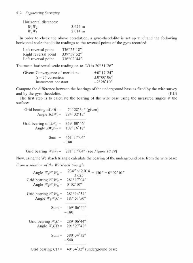
512 Engineering Surveying
Horizontal distances:W1W2 3.625 mWuW2 2.014 m
In order to check the above correlation, a gyro-theodolite is set up at C and the followinghorizontal scale theodolite readings to the reversal points of the gyro recorded:
Left reversal point 336° 25′ 18″Right reversal point 339° 58′ 52″Left reversal point 336° 02′ 44″
The mean horizontal scale reading on to CD is 20° 51′ 26″
Given: Convergence of meridians ± 0° 17′ 24″(t – T) correction ± 0°00′ 06″Instrument constant –2° 28′ 10″
Compute the difference between the bearings of the underground base as fixed by the wire surveyand by the gyro-theodolite. (KU)
The first step is to calculate the bearing of the wire base using the measured angles at thesurface:
Grid bearing of AB = 74° 28′ 34″ (given)Angle BAWs = 284° 32′12″
—————Grid bearing of AWs = 359° 00′ 46″
Angle AWsW2 = 102° 16′ 18″—————
Sum = 461° 17′ 04″– 180
—————Grid bearing W1W2 = 281° 17′04″ (see Figure 10.49)
Now, using the Weisbach triangle calculate the bearing of the underground base from the wire base:
From a solution of the Weisbach triangle
Angle W2W1Wu = 234 2.0143.625
= 130 = 0 02 10′′ × ′′ ° ′ ′′
Grid bearing W1W2 = 281°17′04″Angle W2W1Wu = 0°02′10″
—————Grid bearing W1Wu = 281°14′54″
Angle W1WuC = 187°51′50″—————
Sum = 469° 06′ 44″– 180—————
Grid bearing WuC = 289°06′44″Angle WuCD = 291°27′48″
—————Sum = 580°34′32″
–540—————
Grid bearing CD = 40°34′32″ (underground base)
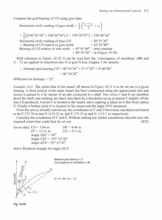
Setting out (dimensional control) 513
Compute the grid bearing of CD using gyro data:
Horizontal circle reading of gyro north = 12
+ 2
+ 1 32
r rr
= 12
[(336°25′18″ + 336°02′44″)/2 + 339°58′52″] = 338°06′ 26″
Horizontal circle reading of base CD = 20°51′26″∴ Bearing of CD reative to gyro north = 42°45′00″Bearing of CD relative to true north = 42°45′ 00″ – instr constant
= 40°16′50″ = φ (Figure 10.50)
With reference to Figure 10.50, it can be seen how the ‘convergence of meridians’ (δθ) and(t – T ) are applied to transform true N to grid N (see Chapter 5 for details).
∴ National grid bearing CD = 40°16′ 50″ + 0° 17′ 24″ + 0°00′ 06″= 40°34′20″
Difference in bearings = 12″.
Example 10.2. The centre-line of the tunnel AB shown in Figure 10.51 is to be set out to a givenbearing. A short section of the main tunnel has been constructed along the approximate line andaccess is gained to it by means of an adit connected to a shaft. Two wires C and D are plumbeddown the shaft, and readings are taken onto them by a theodolite set up at station E slightly off theline CD produced. A point F is located in the tunnel, and a sighting is taken on to this from stationE. Finally a further point G is located in the tunnel and the angle EFG measured.
From the survey initially carried out, the coordinates of C and D have been calculated and foundto be E 375.78 m and N 1119.32 m, and E 375.37 m and N 1115.7 m respectively.
Calculate the coordinates of F and G. Without making any further calculations describe how therequired centre-line could then be set out. (ICE)
Given data: CD = 3.64 m DE = 4.46 mEF = 13.12 m FG = 57.5 mAngle DEC = 38″Angle CEF = 167° 10′ 20″Angle EFG = 87° 23′ 41″
Solve Weisbach triangle for angle ECD
Grid n
ort
h
Tru
e n
ort
h
δθ φ
β(tc – Tc)
tc
Tc
D
National grid bearing = βConvergence of meridians = δθ
β = φ + δθ + (tc – Tc)
C
Fig. 10.50
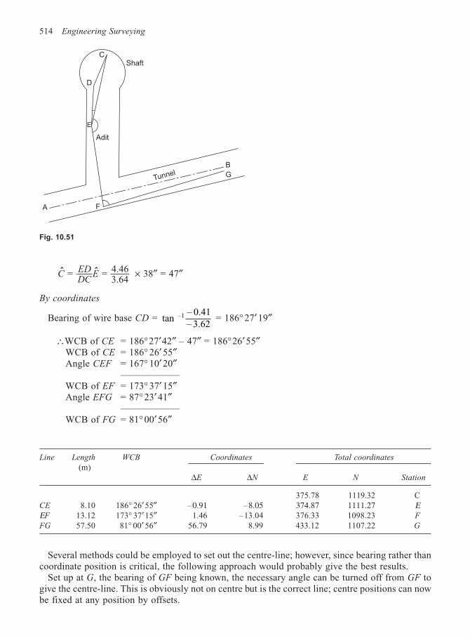
514 Engineering Surveying
ˆ ˆCEDDC
E = = 4.463.64
× 38″ = 47″
By coordinates
Bearing of wire base CD = tan– 0.41– 3.62
–1 = 186° 27′19″
∴WCB of CE = 186°27′42″ – 47″ = 186°26′55″WCB of CE = 186° 26′ 55″Angle CEF = 167° 10′ 20″
——————WCB of EF = 173° 37′ 15″Angle EFG = 87° 23′41″
——————WCB of FG = 81° 00′56″
Line Length WCB Coordinates Total coordinates
(m)∆E ∆N E N Station
375.78 1119.32 CCE 8.10 186° 26′ 55″ – 0.91 – 8.05 374.87 1111.27 ΕΕF 13.12 173° 37′ 15″ 1.46 – 13.04 376.33 1098.23 F
FG 57.50 81° 00′ 56″ 56.79 8.99 433.12 1107.22 G
Several methods could be employed to set out the centre-line; however, since bearing rather thancoordinate position is critical, the following approach would probably give the best results.
Set up at G, the bearing of GF being known, the necessary angle can be turned off from GF togive the centre-line. This is obviously not on centre but is the correct line; centre positions can nowbe fixed at any position by offsets.
Fig. 10.51
ShaftC
D
E
Adit
A F
TunnelB
G
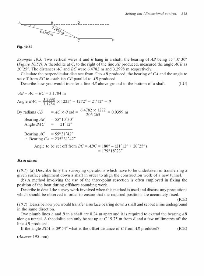
Setting out (dimensional control) 515
Example 10.3. Two vertical wires A and B hang in a shaft, the bearing of AB being 55° 10′ 30″(Figure 10.52). A theodolite at C, to the right of the line AB produced, measured the angle ACB as20′25″. The distances AC and BC were 6.4782 m and 3.2998 m respectively.
Calculate the perpendicular distance from C to AB produced, the bearing of CA and the angle toset off from BC to establish CP parallel to AB produced.
Describe how you would transfer a line AB above ground to the bottom of a shaft. (LU)
AB ≈ AC – BC = 3.1784 m
Angle BAC = 3.29983.1784
× 1225″ = 1272″ = 21′12″ = θ
By radians CD = AC × θ rad = 6.4782 1272206 265
× = 0.0399 m
Bearing AB = 55° 10′ 30″Angle BAC = 21′12″
—————Bearing AC = 55° 31′42″∴ Bearing CA = 235° 31′ 42″
Angle to be set off from BC = ABC = 180° – (21′12″ + 20′25″)= 179° 18′ 23″
Exercises
(10.1) (a) Describe fully the surveying operations which have to be undertaken in transferring agiven surface alignment down a shaft in order to align the construction work of a new tunnel.
(b) A method involving the use of the three-point resection is often employed in fixing theposition of the boat during offshore sounding work.
Describe in detail the survey work involved when this method is used and discuss any precautionswhich should be observed in order to ensure that the required positions are accurately fixed.
(ICE)(10.2) Describe how you would transfer a surface bearing down a shaft and set out a line undergroundin the same direction.
Two plumb lines A and B in a shaft are 8.24 m apart and it is required to extend the bearing AB
along a tunnel. A theodolite can only be set up at C 19.75 m from B and a few millimetres off theline AB produced.
If the angle BCA is 09′54″ what is the offset distance of C from AB produced? (ICE)
(Answer:195 mm)
Fig. 10.52
DBA
C P
6.4782 m
3.2998 m
θ

This Page Intentionally Left Blank

Index
Abney level, 5Altitude correction, 127Areas, 420–424Astrogeodetic systems, 218Astronomical coordinates, 212, 213Automatic level, 54–56Autoplumb, 437–475
Basic concepts, 1Batter boards, 485, 486Bench mark (BM), 44–49Bessel correction, 31Boning rod, 475–477Braced quadrilateral, 276–279British Standards, 510, 511Broadcast Ephemeris, 316, 317, 329Bulkage/shrinkage, 415
CAD, 13, 14, 407, 408Cartesian coordinates, 213, 214Catenary, 120, 121Central meridian, 232Circular curves, 347–360
compound/reverse, 357, 358designation, 348inaccessible IP, 355obstructions, 356passing through a point, 356, 357setting-out, 349–360through chainage, 348, 349using coordinates, 352, 353using EDM, 351, 352using offsets, 353–355, 359, 360
Clock bias, 318, 319, 328Closure tolerances (levelling), 67, 68Collimation error, 56–59Coefficient of friction, 371, 372Commensurate accuracy, 22Contours, 70–72, 438Control networks, 4, 21, 252Controlling verticallity, 472–475Correlation surveys, 486–495
amplitude method, 501co-planing, 492gyro-theodolite, 495–498
instrument constant, 501, 502optical methods, 487reversal point method, 498, 499, 503, 504shape of Weisbach Triangle, 490, 491single wires, 494, 495tape zero error, 502, 503transit method, 499–501, 505, 506Weisbach Triangle, 487–490Weiss Quadrilateral, 492–494wire plane, 492
Creep, 507Cross-sections, 427–432Curvature, 45–47, 92–95Cycle slips, 324
Data logger, 12Datum, 44Datum transformations, 226, 227Delay time, 318Differential GPS (DGPS), 323Digital Ground Model (DGM), 1, 12Digital level, 79Digital levelling, 77–82Digital staff, 78, 79Dip and strike, 432–434Directions, 203, 204Direct Reading Tacheometer, 110, 111Double difference, 322Dual axis compensator, 166
Earth Gravitational Model 1996 (EGM96), 211Earthworks, 420Eccentricity of centres, 187, 188Electromagnetic Distance Measurement (EDM), 138
automatic target recognition, 166calibration, 158–160classification, 138–142dual axis compensator, 166eccentricity error, 163–165errors, 158–160friction clutch, 166geometrical reduction, 153–158machine guidance, 171, 172meteorological corrections, 148–152multi-pillar base line, 161

518 Index
phase difference, 144–147pulse measurement, 142, 143reflectorless measurement, 167robotic systems, 169, 170specifications, 165
Ellipsoid, 2, 3, 208–212Ellipsoidal height, 217, 338, 339End-area method, 436, 437Equal-shift, 275–279Error, 25
accuracy, 26, 27classification, 25combination, 34–37mistakes, 25precision, 26, 27random error, 26relative error, 27residual error, 27systematic error, 25
Error distribution (levelling), 68, 69ETRF 89, 341
Facilities management, 19, 20False origin, 232First eccentricity, 211Flat bed plotter, 10, 11Flattening, 211Freehaul, 451–453Full overtaking sight distance (FOSD), 400–402Functionality, 18, 19
GALILEO, 342, 343Geodetic coordinates, 213Geodetic Reference System 1980 (GRS80), 210, 211,
317, 341Geographic Information Systems (GIS), 14–29, 345
applications, 19, 20buffering, 19coding, 16contouring, 19facilities management, 19, 20functionality, 18, 19global information, 16highway maintenance, 20Housing Association, 20land management, 17network analysis, 19object based model, 18overlay, 19raster, 17–20spatial data, 17terrain analysis, 19topology, 17, 18vector, 17, 18
Geoid, 2, 3, 208–212Geoid-ellipsoid separation, 212, 217, 222, 223Geometric Dilution of Precision (GDOP), 330, 331GEONET, 341Global datums, 339Global MSL, 344Global Positioning System (GPS), 307–346
active layer, 341ambiguities, 326, 328antenna swap, 326Anti-Snooping (AS), 324Broadcast Ephemeris, 316, 317, 329clock bias, 318, 319, 328coarse acquisition (C/A), 308control segment, 308–310cycle slips, 324delay time, 318differencing data, 320, 321Differential GPS (DGPS), 323double difference, 322ETRF 89, 341GALILEO, 342, 343GDOP, 330, 331GEONET, 341global datum, 339, 340global MSL, 344GLONASS, 342, 343Greenwich Apparent Sidereal Time (GAST), 317heights, 338, 339Helmert transformation, 335, 336ionospheric refraction, 329ITRF 96, 340, 341Kepler’s Laws, 312kinematic positioning, 326local datums, 340–342machine guidance, 343–344multipath error, 330navigation, 345, 346orbital perturbations, 315, 316orbits, 312–318OSGM 91, 339, 341O.S. National GPS Network, 341OSTN 97, 341O.S. transformations, 337passive layer, 341planning, 332, 333plate tectonics, 344, 345Precise Acquisition (P) code, 308Precise Ephemeris, 316, 329pseudo range, 319rapid static, 325real time kinematic (RTK), 327receivers, 310–312reference systems, 333re-occupation, 325, 326
Electromagnetic Distance Measurement (Contd)

Index 519
satellite clock error, 328Selective Availability (SA), 324, 331, 332single difference, 321, 322sky plots, 332space segment, 308static positioning, 325stop and go, 326, 327transformation between systems, 333–337TRANSIT Doppler, 318triple difference, 322, 323tropospheric refraction, 329true anomaly, 314, 315user segment, 310WGS 84, 340
Gradients, 395Grid convergence, 229, 231, 238, 239Grids (setting-out), 469, 470Gyro-theodolite, 495–498
Height of Collimation (HPC), 60–64Helmert transformation, 335, 336Highest/lowest point, 404Highway Transition Curve Tables, 376–380Horizontal angle, 2
ICE Conditions of Contract, 509Instrumental errors, 186, 187International Earth Rotation Service (IERS), 212, 218International Reference Meridian (IRM), 212International Reference Pole (IRP), 212Inertial surveying, 289–292Intersection, 7, 282, 283, 467–469Invar staff, 75Inverted sight, 64Ionospheric refraction, 329ITRF 96, 340, 341
Join computation, 245–247
Kalman filter, 291Kepler’s Laws, 312Kinematic positioning, 326K-value, 397
Laplace azimuth, 223Laplace correction, 222Lasers, 478–480Laser alignment (tunnels), 508Laser hazards, 480–483Laser scanner, 20, 21Level line, 44Levelling, 43Levelling staff, 50
Machine guidance, 171, 172, 343, 344
Magnification, 53Mass Haul, 451, 452Mean Sea Level (MSL), 43, 44Measuring plates, 119Meteorological corrections, 148–152Mid-latitude formulae, 223–225Mistakes, 25Molodensky Transformation, 228, 336Multi-pillar base, 161
Natural errors (levelling), 67Normal Distribution, 28, 29Normal-geodesic, 220
Offset, 5, 6Open traverse, 255, 256Optical methods, 487Optical micrometer, 182, 183Optical scale reading, 181, 182Ordnance Survey National Grid, 231–240Orthometric heights, 210, 217, 338, 339Orthomorphic projection, 228Osculating circle, 381, 386O.S. National GPS Network, 341OSTN 97, 341Overhang, 507Overlay, 19
Parallel plate micrometer, 76Passive Layer, 341Planimeter, 421–423Plate bubble error, 190–197Plate tectonics, 344, 345Polars, 244–247Polygonal traverse, 254, 255Precise Acquisition (P) Code, 308Precise Ephemeris, 316, 329Precise levelling, 75–77Prime Vertical, 218Probability, 28Properties of MHD, 451, 452Pseudo-range, 319Pyramid, 435
Rapid static, 325Raster, 17–20Real Time Kinematic (RTK), 327Reference datum, 2, 208Reflectorless measurement, 167Refraction, 45, 47, 50, 92–95Regular grids, 12, 13Re-occupation, 325, 326Repetition, 204, 205Resection, 8Rise and Fall, 62, 63

520 Index
Robotic systems, 169, 170
Sag correction, 124–126, 129Satellite clock error, 328Satellite station, 279–282Scale factor, 229–239Sectional levelling, 69, 70Shortt’s Factor, 373Sight distance on sag, 402, 403Sight-rails, 475–477Significant figures, 23, 24Single difference, 321, 322Single wires, 494, 495Simpson’s Rule, 423–435Slope correction, 126–129Slope stakes, 484, 485Space segment, 308Spherical angles, 2Skew normal, 220Spot-heights, 438–441Square marks, 507Standard Deviation, 32Standard Error, 32Standard Normal Curve Areas, 30Stopping Sight Distance (SSD), 399, 400Strings, 12, 13Subtense tacheometry, 172–175Super-elevation, 372, 373
Tacheometric constants, 107Tapes, 117–137Taping accuracy, 130, 131Tape standardisation, 120, 123, 127Tape zero error, 502, 503Temperature correction, 124, 128Tension correction, 124, 128, 129Terrain analysis, 19Theodolite, 178–207
angles, 202–205centring error, 201, 202collimation in azimuth, 188, 189, 194, 195, 197directions, 203, 204electro-optical scanning, 184–186errors, 206, 207instrumental error, 186, 187optical scale reading, 181, 182optical micrometer, 182, 183plate bubble, 190–197reading systems, 181–186repetition, 204, 205setting-up, 198–201transit axis error, 189, 190, 195–197vertical circle index error, 193, 196–198
Tilting level, 50–54
Topology, 17, 18TRANSIT doppler, 318Transit method, 499–501, 505, 506Transition curves, 368–388
back angle to origin, 376centrifugal force, 368centrifugal ratio, 370clothoid, 369, 370coefficient of friction, 371, 372compound curves, 384–386coordinates on transition, 386–388cubic parabola, 381cubic spiral, 380, 381derivation of formulae, 416–419osculating circle, 381, 386setting-out, 373–376Shortt’s factor, 373super-elevation, 372, 373transitional throughout, 381
Transverse Mercator Projection, 230Trapezoidal Rule, 423Transformation between systems, 333–337Traversing, 252–271
angular misclosure, 264, 265blunders, 269–271Bowditch adjustment, 262–269constrained centring, 257–261errors, 257, 258link traverse, 253, 254, 268open traverse, 255, 256polygonal traverse, 254, 255traverse computation, 262–271
Triangular facets, 12, 13Triangulateration, 288, 289Triangulation, 271–279Trigonometrical levelling, 91–99
contouring, 98–100errors, 97long lines, 92–94reciprocal observations, 95, 96short lines, 91, 92
Trilateration, 286–288computation, 288network design, 287triple difference, 322, 323tropospheric refraction, 329true anomaly, 314, 315tubular bubble, 53tunnel alignment, 506, 507(t-T) correction, 231, 237–239
Underground BM, 508, 509Units of measurement, 22Universal Transverse Mercator (UTM), 240

Index 521
User segment, 310
Vector, 17, 18Vertical angle, 2Verticle circle index error, 193, 196–198Vertical control, 43Vertical curves, 295–408
approximations, 395, 396CAD, 407, 408computation, 405–407design, 397–403Full Overtaking Sight Distance (FOSD), 400–402gradients, 395highest/lowest point, 404K-value, 397radius, 405
sight distance on sags, 402, 403Stopping Sight Distance (SSD), 399, 400TD 9/93, 396
Vertical height, 2Volumes, 434–442
Wedge, 434Weighted data, 32, 33Weisbach Triangle, 487–490Weiss Quadrilateral, 492–494WGS 84, 217, 317, 340, 341Whole Circle Bearing (WCB), 241–247, 265Wire plane, 492
ZUPT, 291, 292


![Curves and Surfacesfp/courses/graphics/pdf-color/09-curves.pdf · Hermite Curves Bezier Curves and Surfaces [Angel 10.1-10.6] Parametric Representations Cubic Polynomial Forms Hermite](https://img.pdfslide.us/doc/110x75/5f56f44d14266d2844621275/curves-and-surfaces-fpcoursesgraphicspdf-color09-hermite-curves-bezier-curves.jpg)


![Curves and Surfacesadair/CG/Notas Aula/Curvas/09-curves.pdf · Bezier Curves and Surfaces [Angel 10.1-10.6] Parametric Representations Cubic Polynomial Forms Hermite Curves Bezier](https://img.pdfslide.us/doc/110x75/5f72f8d58557ce2aea5f374f/curves-and-adaircgnotas-aulacurvas09-curvespdf-bezier-curves-and-surfaces.jpg)