Embed Size (px)
Citation preview

E N G I N E E R I N GVol. 03 / Issue. 02 / 2014
Accelerate Innovation with CFD & Thermal CharacterizationEDGE
mentor.com/mechanical
YamahaRevs your Heart Page 12
SaipemSupporting Offshore Heavy Lift and Pipeline Installations Page 18
JS PumpsWater System Hydraulic Models Page 36

2 mentor.com/mechanical
• 30 Day Instant Free Access to Full Software
• No License Set-up Required
• Each VLab contains Full Support Material
• 4 Hour Sessions*
• Save Work between Sessions
*These sessions can be extended
Virtual LabsFloEFD™ for PTC Creo
Test-drive 20 Powerful CFD Models including LED Thermal Characterization, CPU Cooling, Hydraulic Loss Determination, and more
go.mentor.com/floefd-vl
Flowmaster®
Build & Analyze a Rising Main Network in Flowmaster
go.mentor.com/flowmaster-vl
LED Analysis with FloEFD for PTC Creo
Analyze LED Components & Determine Thermal Characteristics
go.mentor.com/floefd-led-vl
www.mentor.com/mechanical
REGISTER NOW for your instant 30 Day
Free Trialwww.mentor.com/mechanical

mentor.com/mechanical 3
PerspectiveVol. 03, Issue. 02
Greetings readers! This edition of Engineering Edge brings with it our biggest line up of product news and user stories since the magazine’s inception. The cover story from Yamaha, in Japan, shows how Tetsuya Ima cleverly used our T3Ster® hardware as a non-destructive validation technique for PCB delamination in motorbike electronics design. Our interviewee in this edition is a real thought-leader in the 1D CFD space, Sudhi Uppuluri from CSEG in the United States, and he proves it by showing how he used Flowmaster to help patent a clever new automobile dual-use Heater Core for an engine! We do have quite an Asia-Pacific flavor to this Engineering Edge as NAMICS in Japan, Fluid
Systems Consultants in Australia, and Wipro in India all feature in an assortment of industry stories. Saipem in the UK has an interesting Oil & Gas story related to their ever-growing usage of FloEFD™. Our own Jim Petroski offers an interesting story with an LED lighting theme. Finally, our friends at ECS in Silicon Valley have undertaken a fascinating study of IGBT liquid Cooling using FloTHERM® XT.
On the product side, the release of FloVENT® 10.1 gives this targeted HVAC solution a new interface plus Flowmaster® V7.9.3 has some exciting new enhancements added to this highly accurate product. FloEFD 14.0 too has some “big stone” enhancements in moving mesh (for pumps, fans etc), a neat new condensation model and further optical and radiation model enhancements. Looking at our regular features, Doug Kolak has written an excellent article on “How to…analyze surge suppression using Flowmaster”, we have an interesting 3D CFD Thrust Reverser technical article, our Geek Hub investigates Google Glass and Brownian Motion has its unique take on what engineers obsess about. And after the success of our sponsoring of the Harvey Rosten Award for Electronics Thermal Excellence (and deservedly won by Wendy Luiten of Philips this year) for nearly 20 years, it is pleasing to see that we have now kicked off a Don Miller Award for Excellence in 1D Thermo-Fluid System Simulation. I look forward to seeing the winning submissions for years to come. Following our increased focus on Power Electronics and the launch of the MicReD® Power Tester 1500A in May, we have been invited to join the European Centre for Power Electronics (ECPE). The market has welcomed this unique thermal characterization power cycling product with open arms globally.
Finally, many of you may not have spotted it, but we overhauled our website area in May (mentor.com/mechanical) and there’s a wealth of new product, design flow and application content, enhanced educational materials, more videos and animations, and a brilliant new online demo area called Virtual Labs where you can test drive, for free, FloEFD and Flowmaster on the Amazon Cloud without having to download product software or install software keys behind firewalls. For more information visit: go.mentor.com/floefd-vl, and I'm sure you'll be impressed. I commend Engineering Edge to you and I trust we will continue to work with you to produce industrial solutions that meet your current and emerging needs.
Mentor Graphics CorporationPury Hill Business Park,
The Maltings,Towcester, NN12 7TB,
United KingdomTel: +44 (0)1327 306000
email: [email protected]
Editor:Keith Hanna
Managing Editor:Natasha Antunes
Copy Editor:Jane Wade
Contributors: Alexandra Francois-Saint-Cyr, Keith Hanna,
Alexey Kharitonovich, Doug Kolak, Boris Marovic, John Murray, Dirk Niemeier, Adnan Nweilati,
John Parry, Jim Petroski, Jane Wade
With special thanks to:Computer Sciences Expert Group
Electronic Cooling Solutions Inc.Gas Turbine Research Establishment
JS Pump and Fluid System ConsultantsNAMICS Corporation
Saipem S.p.AVisteon Electronics Corporation
Wipro LimitedYamaha Motor Company Limited
©2014 Mentor Graphics Corporation, all rights reserved. This document contains
information that is proprietary to Mentor Graphics Corporation and may be duplicated
in whole or in part by the original recipient for internal business purposes only, provided that this entire notice appears in all copies. In
accepting this document, the recipient agrees to make every reasonable effort to prevent
unauthorized use of this information. All trademarks mentioned in this publication are
the trademarks of their respective owners.
Roland Feldhinkel, General ManagerMechanical Analysis Division, Mentor Graphics
• 30 Day Instant Free Access to Full Software
• No License Set-up Required
• Each VLab contains Full Support Material
• 4 Hour Sessions*
• Save Work between Sessions
*These sessions can be extended
Virtual LabsFloEFD™ for PTC Creo
Test-drive 20 Powerful CFD Models including LED Thermal Characterization, CPU Cooling, Hydraulic Loss Determination, and more
go.mentor.com/floefd-vl
Flowmaster®
Build & Analyze a Rising Main Network in Flowmaster
go.mentor.com/flowmaster-vl
LED Analysis with FloEFD for PTC Creo
Analyze LED Components & Determine Thermal Characteristics
go.mentor.com/floefd-led-vl
www.mentor.com/mechanical
REGISTER NOW for your instant 30 Day
Free Trialwww.mentor.com/mechanical

4 mentor.com/mechanical
News5 New Release: FloTHERM® & FloVENT® V10.16 New Release: FloEFD™ V14.08 New Release: Flowmaster® V7.9.39 Mentor joins ECPE10 Introducing New Virtual Labs10 Harvey Rosten Award Winner11 Introducing The Don Miller Award
Contents
Engineering Edge12 Yamaha Motor Company Limited An Evalutaion of Delamination of Power
Modules using the MicReD T3Ster®
17 Gas Turbine Research Establishment Taking the Heat Out of Gas Turbine Design
18 Moving Offshore with Saipem S.p.A The Company uses FloEFD to Support Operations
20 NAMICS Corporation Case Study Developing High Thermal Conductivity Sintered Silver Paste
24 Visteon Electronics Corporation Unravelling the Complexitites of Automotive Instrument Cluster Design
28 Computer Sciences Expert Group A Modest Proposal for a Dual-Use Heater Core
36 JS Pump and Fluid Systems Consultants Using Flowmaster for Dynamic Water Network Simulations Down Under
40 Electronic Cooling Solutions, Inc. Managing Temperature Differences between IGBT Modules
42 Heat Pipe Heatsink Design in a Wipro Ltd. 3U High-End Server
Technology & Knowledge Bank32 How To Guide: Design for Pressure Surge in Flowmaster
34 Leaving on a Jet Plane Simulation of a Jet Engine Thrust Reverser
44 Advanced Natural Cooling Convection Designs for LED Bulb Systems
Regular Features23 Ask the CSD Expert Custom Mentoring Service from Mentor
31 Interview Sudhi Uppuluri, Computer Sciences Expert Group
48 Geek Hub Google Glass™ gets the FloTHERM XT® Treatment
50 Brownian Motion The random musings of a Fluid Dynamicist
12
48
6
mentor.com/mechanical 5
NewsNew Release:FloTHERM® & FloVENT® V10.1
elivered in three phases, FloTHERM V10.1 brings a new, modern, Windows compliant interface, while retaining the
same paradigms on which FloTHERM is based. It also provides more efficient handling of massive models with 1000s of model objects, 10s of millions of mesh cells and related pre-processing, solving and post-processing.
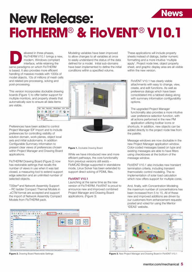
This version incorporates dockable drawing boards (Figure 1) to offer better support for multiple monitors, and property sheets that automatically size to ensure all data items are visible.
Modeling variables have been improved to allow changes to all variables at once to easily understand the status of the data defined for a model. Initial sub-domains have been implemented to define the initial conditions within a specified volume.
These applications will include property sheets instead of dialogs, better numeric formatting and a more intuitive ‘multiple apply’. Project node tree, object property sheet, and graphic display area are all visible within the new version.
D
Preferences have been added to control Project Manager IDF Import and to include preferences for controlling visibility of solution domain, work planes, object local axis and initial subdomains. In addition Configurable Summary information to present clear views of preferences chosen within Project Manager and Drawing Board applications.
FloTHERM Drawing Board (Figure 2) now has restorable settings that recalls the number of views in use when it was last closed, a measuring tool to extend support edge selection and an unlimited number of selected objects.
T3Ster® and Network Assembly Support – RC ladder Compact Thermal Models in .xCTM format are accepted and support the import of Network Assembly Compact Models from FloTHERM pack.
Figure 1. Dockable Drawing Board
Figure 2. Drawing Board Restorable Settings
While we have introduced new and more efficient pathways, the core functionality from previous versions still exists – FloMCAD Bridge supported in standalone mode, Linux Solver has been extended to support direct solving of PDML files.
FloVENT V10.1Launching at the same time as the new version of FloTHERM, FloVENT is proud to announce new and improved combined Project Manager and Drawing Board applications. (Figure 3)
Figure 3. New Project Manager and Drawing Board in FloVENT V10.1
FloVENT V10.1 has clearly visible attachments with easy to change, view, create, and edit functions. As well as preference dialogs which have been consolidated into a tabbed dialog along with summary information configurability options.
The upgraded Project Manager functionality also provides a more intuitive user preference selection function, with all actions performed in the new PM application utilizing toolbar icons or
shortcuts. In addition, new objects can be added directly to the project node tree from the palette.
Message windows are now dockable in the new Project Manager application window. Color-coded messages based on type and existing messages are able to have filters using checkboxes at the bottom of the message window.
FloVENT V10.1 also includes new transient termination criteria, including transient thermostatic control modeling. The re-implementation of solar load calculation which now offers support for multiple cores.
And, finally, with Concentration Modeling the maximum number of concentrations has been increased from 5 to 15. All of these new and improved additions are driven by our customers from enhancement requests posted and voted for using the Mentor ‘IDEAS’ website.
6 mentor.com/mechanical
rom FloEFD’s inception, the ability to simulate moving parts is one of the most demanding requests we receive. Since then, FloEFD
has been extended with a number of capabilities and models that allow the user to take into account moving parts. Among them are moving walls for simulating motion of planar or cylindrical surfaces such as a moving road plane, coordinate dependent conditions for modeling effects of moving parts such as laser beams, the fan compact model for simulating fans or blowers, and the rotating capability for modeling flow in pumps and turbo-machinery equipment. Although these models cover a wide range of moving parts they are all based on the non-moving mesh technology, which by its nature limits the range of applications assessable by FloEFD in the moving world.
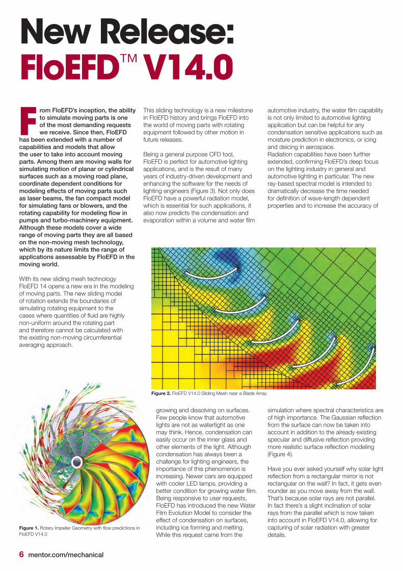
With its new sliding mesh technology FloEFD 14 opens a new era in the modeling of moving parts. The new sliding model of rotation extends the boundaries of simulating rotating equipment to the cases where quantities of fluid are highly non-uniform around the rotating part and therefore cannot be calculated with the existing non-moving circumferential averaging approach.
New Release:FloEFD™ V14.0
Figure 1. Rotary Impeller Geometry with flow predictions in FloEFD V14.0
This sliding technology is a new milestone in FloEFD history and brings FloEFD into the world of moving parts with rotating equipment followed by other motion in future releases.
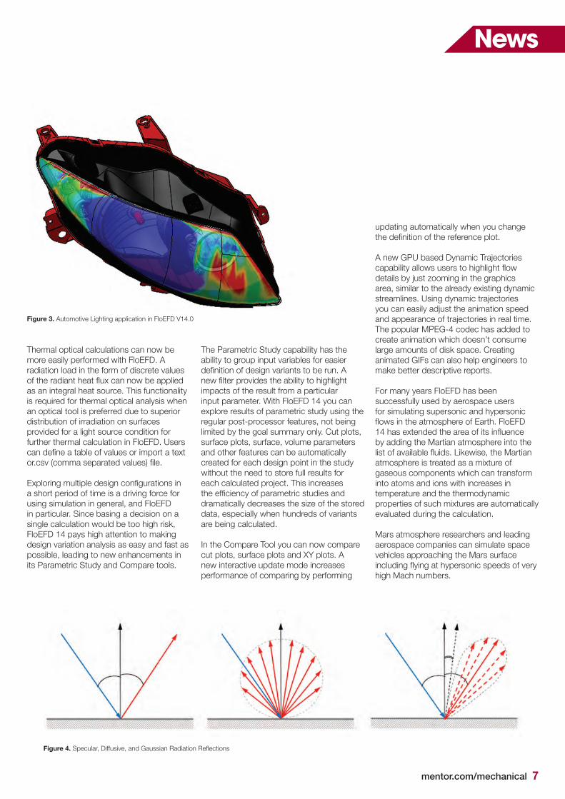
Being a general purpose CFD tool, FloEFD is perfect for automotive lighting applications, and is the result of many years of industry-driven development and enhancing the software for the needs of lighting engineers (Figure 3). Not only does FloEFD have a powerful radiation model, which is essential for such applications, it also now predicts the condensation and evaporation within a volume and water film
automotive industry, the water film capability is not only limited to automotive lighting application but can be helpful for any condensation sensitive applications such as moisture prediction in electronics, or icing and deicing in aerospace.Radiation capabilities have been further extended, confirming FloEFD’s deep focus on the lighting industry in general and automotive lighting in particular. The new ray-based spectral model is intended to dramatically decrease the time needed for definition of wave-length dependent properties and to increase the accuracy of
F
growing and dissolving on surfaces. Few people know that automotive lights are not as watertight as one may think. Hence, condensation can easily occur on the inner glass and other elements of the light. Although condensation has always been a challenge for lighting engineers, the importance of this phenomenon is increasing. Newer cars are equipped with cooler LED lamps, providing a better condition for growing water film. Being responsive to user requests, FloEFD has introduced the new Water Film Evolution Model to consider the effect of condensation on surfaces, including ice forming and melting.While this request came from the
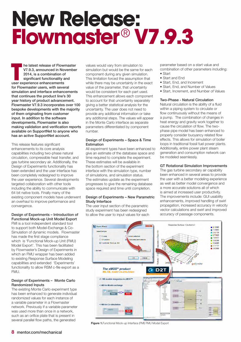
simulation where spectral characteristics are of high importance. The Gaussian reflection from the surface can now be taken into account in addition to the already existing specular and diffusive reflection providing more realistic surface reflection modeling (Figure 4).
Have you ever asked yourself why solar light reflection from a rectangular mirror is not rectangular on the wall? In fact, it gets even rounder as you move away from the wall. That’s because solar rays are not parallel. In fact there’s a slight inclination of solar rays from the parallel which is now taken into account in FloEFD V14.0, allowing for capturing of solar radiation with greater details.
Figure 2. FloEFD V14.0 Sliding Mesh near a Blade Array
mentor.com/mechanical 7
News
Thermal optical calculations can now be more easily performed with FloEFD. A radiation load in the form of discrete values of the radiant heat flux can now be applied as an integral heat source. This functionality is required for thermal optical analysis when an optical tool is preferred due to superior distribution of irradiation on surfaces provided for a light source condition for further thermal calculation in FloEFD. Users can define a table of values or import a text or.csv (comma separated values) file.
Exploring multiple design configurations in a short period of time is a driving force for using simulation in general, and FloEFD in particular. Since basing a decision on a single calculation would be too high risk, FloEFD 14 pays high attention to making design variation analysis as easy and fast as possible, leading to new enhancements in its Parametric Study and Compare tools.
The Parametric Study capability has the ability to group input variables for easier definition of design variants to be run. A new filter provides the ability to highlight impacts of the result from a particular input parameter. With FloEFD 14 you can explore results of parametric study using the regular post-processor features, not being limited by the goal summary only. Cut plots, surface plots, surface, volume parameters and other features can be automatically created for each design point in the study without the need to store full results for each calculated project. This increases the efficiency of parametric studies and dramatically decreases the size of the stored data, especially when hundreds of variants are being calculated.
In the Compare Tool you can now compare cut plots, surface plots and XY plots. A new interactive update mode increases performance of comparing by performing
updating automatically when you change the definition of the reference plot.
A new GPU based Dynamic Trajectories capability allows users to highlight flow details by just zooming in the graphics area, similar to the already existing dynamic streamlines. Using dynamic trajectories you can easily adjust the animation speed and appearance of trajectories in real time. The popular MPEG-4 codec has added to create animation which doesn’t consume large amounts of disk space. Creating animated GIFs can also help engineers to make better descriptive reports.
For many years FloEFD has been successfully used by aerospace users for simulating supersonic and hypersonic flows in the atmosphere of Earth. FloEFD 14 has extended the area of its influence by adding the Martian atmosphere into the list of available fluids. Likewise, the Martian atmosphere is treated as a mixture of gaseous components which can transform into atoms and ions with increases in temperature and the thermodynamic properties of such mixtures are automatically evaluated during the calculation.
Mars atmosphere researchers and leading aerospace companies can simulate space vehicles approaching the Mars surface including flying at hypersonic speeds of very high Mach numbers.
Figure 3. Automotive Lighting application in FloEFD V14.0
Figure 4. Specular, Diffusive, and Gaussian Radiation Reflections
8 mentor.com/mechanical
Figure 1.Functional Mock-up Interface (FMI) FMU Model Export
New Release:Flowmaster® V7.9.3
he latest release of Flowmaster V7.9.3, announced in November 2014, is a combination of significant functionality and
user experience enhancements for Flowmaster users, with several simulation and interface enhancements that continues the product line’s 30 year history of product advancement. Flowmaster V7.9.3 incorporates over 100 bespoke developments with the majority of them originating from customer input. In addition to the software developments, Flowmaster is also making validation and verification reports available on SupportNet to anyone who has an active SupportNet account.
This release features significant enhancements to its core analysis capabilities including two-phase natural circulation, compressible heat transfer, and gas turbine secondary air. Additionally, the Design of Experiments functionality has been extended and the user interface has been completely redesigned to improve the user experience. Several developments targeted collaboration with other tools including the ability to communicate with 64 bit native tools. Finally many of the existing component models have underwent an overhaul to improve performance and convergence.
Design of Experiments – Introduction of Functional Mock-up Unit Model ExportFMI is a tool independent standard tool to support both Model-Exchange & Co-Simulation of dynamic models. Flowmaster has made the first stage compliance which is ‘Functional Mock-up Unit (FMU) Model Export’. This has been facilitated by Flowmaster’s Design of Experiments in which an FMU wrapper has been added to existing Response Surface Modeling capabilities and extended ‘Experiments’ functionality to allow RSM c-file export as a FMU.
Design of Experiments – Monte Carlo Randomized InputsThe existing Monte Carlo experiment type has been enhanced to generate individual randomized values for each instance of a variable parameter in a Flowmaster network. Previously if a variable parameter was used more than once in a network, such as an orifice plate that is present in several parallel flow paths, the generated
T values would vary from simulation to simulation but would be the same for each component during any given simulation. This limitation forced the assumption that while there may be uncertainty in the exact value of the parameter, that uncertainty would be consistent for each part used. This enhancement allows each component to account for that uncertainty separately giving a better statistical analysis for the uncertainty. The user does not need to provide any additional information or take any additional steps. The values will appear in the Monte Carlo interface as separate parameters differentiated by component number.
Design of Experiments – Space & Time EstimationAll experiment types have been enhanced to give an estimate of the database space and time required to complete the experiment. These estimates will be available in the bottom section of the experiment interface with the simulation type, number of simulations, and simulation status. The estimates update as the experiment progresses to give the remaining database space required and time until completion.
Design of Experiments – New Parametric Study InterfaceThe user input section of the parametric study experiment has been redesigned to allow the user to input values for each
parameter based on a start value and combination of other parameters including:• Start • Start and End • Start, End, and Increment • Start, End, and Number of Values• Start, Increment, and Number of Values
Two-Phase - Natural CirculationNatural circulation is the ability of a fluid within a piping system to circulate or flow continuously without the means of a pump. The combination of changes in heat energy and gravity work together to cause the circulation of flow. The two-phase pipe model has been enhanced to properly consider buoyancy related flow effects. This allows for simulation of boiler loops in traditional fossil fuel power plants. Additionally, entire power plant steam generation and consumption network can be modeled seamlessly.
GT Rotational Simulation ImprovementsThe gas turbine secondary air capability been enhanced in several areas to provide the user with a better modeling experience as well as better model convergence and a more accurate solutions all of which is aimed at increased user productivity. The improvements include: GUI usability enhancements, improved handling of swirl propagation, increased accuracy in velocity vector calculations and swirl and improved accuracy of passage components.

mentor.com/mechanical 9
News
Figure 2. Two-phase pipe model enhanced to properly consider buoyancy related flow effects
Mentor Graphics Announces ECPE Membership
entor Graphics Corporation announced its membership in the German - based European Centre for Power Electronics
(ECPE) on August 28th 2014. Mentor Graphics is the only electronic design automation (EDA) company represented in this industry driven research network, comprised of over 150 organizations.
Mentor Graphics was selected as an ECPE member based on its unique expertise in both thermal simulation and test solutions including electronic component and power cycling for reliability prediction, as evidenced by its recently announced MicReD® Industrial Power Tester 1500A technology.
Member companies of the ECPE, such as ABB, Siemens, Bosch and Daimler, are able to access, share, and apply knowledge on innovative technologies such as the MicReD Power Tester system. Dr. John Parry, electronics industry manager for Mentor Graphics Mechanical Analysis Division, has been appointed to represent Mentor Graphics within the ECPE.
Key initiatives of the ECPE are to provide global research on power electronics systems and serve as the “unified voice” for the European power electronics industry. In contributing to the ECPE, Mentor Graphics will focus on its expertise in thermal simulation and test of electronic systems and power cycling technology, which will
provide value to the 150+ organizations in this research network.
“We are honored to have been selected as the only EDA member of the ECPE organization based on our reputation as the only technology company providing both thermal simulation and testing capabilities, particularly power electronics reliability prediction,” stated Roland Feldhinkel, General Manager of Mentor Graphics Mechanical Analysis Division. “Ultimately, from our collaboration with both commercial and research ECPE members, manufacturers will be able to create longer lasting electronics products that will minimize warranty costs”To learn more, visit: www.ecpe.org
M
Fluid Property Enhancement for Super-Critical FluidsPressure and enthalpy curves for complex fluids have been extended to properly consider fluids that operate in super critical regions where the fluid changes phase between liquid and gas without going through a two-phase step.
Improved Compressible Pipe Heat TransferThe equation for the heat transfer between the fluid and the pipe has been updated to use the adiabatic wall temperature instead of the stagnation temperature. While users should see little difference in temperature
calculations at low Mach numbers (M<0.1), it is likely that there will be differences in the results at higher Mach numbers. In addition to the improved results for current values, two new results will be available for review, adiabatic wall temperature and recovery factor.
New T and Y Junction ComponentsV7.9.3 introduces new T and Y junction components that replace the now legacy versions from all previous V7 releases. The new components are based on a different linearization method that provides a more stable solution. This increased stability often will result in a simulation converging in fewer iterations if a solution exists, including cases where the previous components could not find a converged solution.
Net Positive Suction Head (NPSH)Net Positive Suction Head is now reported for centrifugal pumps. This includes NPSH available and optionally NPSH required and NPSH margin if NPSHR curve is supplied. This enhancement provides results in the form that the user gets from the pump supplier and allows for quick comparison of the results to determine if the system is configured for proper operation of the specified pump.
Database Enhancements - PerformanceThe performance of several common interactions with Flowmaster has improved due to more efficient interactions with the associated database. The level of
performance improvements will vary based on individual situations, but the improvements tend to be seen more with large sets of performance data, networks with a large number of components (>1000), remote database configurations, and Oracle.
Simulation Enhancements - Current Simulation Time OutputThe Simulation Data tab has been enhanced to provide a display of the current time step during transient simulations. This information is found next to the Iteration count and is only active during transient simulation.
Simulation Enhancements Combined Warning and Errors - Added an option to show warning in error dialogue at run time
Simulation Enhancements - Vena Contracta Results for Orifices Now provides results at the vena contracta of orifice components. The results include Velocity, Mach No and Static Pressure
Simulation Enhancements - Schematic Label and Table Enhancements The user now has the option to display the units of the result label that they draw on the schematic. Additionally, the results tables are resizable and both results tables and labels now have a persistence option that allows the user to reposition them and save those locations to be reused.
10 mentor.com/mechanical10 mentor.com/mechanical
Introducing Virtual Labs
loud computing has a new application in the Mechanical Analysis Division at Mentor Graphics. Engineers are
now able to test-drive FloEFD and Flowmaster products through Mentor's innovative Virtual Labs in the cloud.
VLabs users can trial our software within a cloud computing environment, hosted by Mentor Graphics without the need to have special equipment, licenses or IT department approval.
Included in the trial is 30 day access to preloaded and configured software on our virtual computer. Access can be gained easily and immediately from any current PC web browser via a downloadable receiver client or any HTML5 compliant browser.Additional users can be added to accounts, to enable further growth of software users
Cwithin single companies or departments, thereby stimulating internal discussion.
Also included are VLab Materials such as video demonstrations and PDF tutorials, all of which are available at work, home or even while traveling.Help and support are visible at all times, with Live Chat on hand to help with any immediate queries. Prompt emails will be sent as reminders of sessions used and how to extend sessions available.
Wendy Luiten wins Prestigious Harvey Rosten Award
he winner of the Harvey Rosten Award for Excellence, presented annually at the SEMITHERM conference in San Jose in
March, was Wendy Luiten MSc., Cooling Consultant with Philips Corporate Research at the High Tech Institute in Eindhoven
Each year the Harvey Rosten Award is presented for a published work in the physical design of electronics judged by an esteemed panel of experts from industry and academics to be excellent. Wendy received the award for her paper “Solder Joint Lifetime of Rapid Cycled LED Components” presented at the THERMINIC Conference in Berlin, in September 2013. The Selection Committee were impressed with the physical insight Wendy’s paper gave into solder joint creep and her method for estimating the accumulated creep per cycle, which ultimately determines the crack growth rate over a range of environmental conditions.
T Wendy told us, “In my wildest dreams I had never thought I would win the Harvey Rosten Award. I’m delighted! I remember being utterly amazed when I was shown the FLIR One at CES this year. I have been
FloEFD for PTC Creo & Flowmaster Thermo-Fluid CFD Labs are live and available now!FloEFD Virtual Lab:go.mentor.com/floefd-vlFloEFD LED Virtual Lab:go.mentor.com/floefd-led-vlFlowmaster Virtual Lab:go.mentor.com/flowmaster-vl
using IR cameras for years of course, and I love the instant overview and feel you get from literally seeing the heat, so it seemed the perfect toy to spend the prize money on.”

mentor.com/mechanical 11
NewsAnnouncing:The Don Miller Award for Excellence in System Level Thermo-Fluid Design
entor Graphics Mechanical Analysis Division is pleased to announce the launch a new annual Don Miller
Award for Excellence in System Level Thermo-Fluid Design. The winner of this inaugural award, will be announced at a U2U event in November 2015 and presented with $2500 and an engraved plaque.
Don Miller is the author of Internal Flow Systems, the book that underpins the Flowmaster software and the de facto standard for fluid system pressure loss data.
Together with Don Miller, the Mechanical Analysis Division have set up the award to not only recognize excellence within System Level Design using Flowmaster software, but also to uncover breakthroughs in research and real-world applications in the field.
Award CriteriaApplications for the award must be based on a practical and realistic approach to 1D CFD. This needs to be both quantifiable and representative of an advance in System Level Thermo-Fluid analysis and modeling.
The panel require that the work demonstrate a relevant, clear and practical approach to system design which must be within the public domain and been circulated publicly within 12 months prior to the cut-off date for nominations – 30th April 2015.
Applicants must have permission from their organization or have relevant authority to apply.
Please provide all entries in full with supporting material by the closing date 30th April 2015 by email to [email protected]
M
The Judging PanelDon Miller After 10 years’ service in the RAF as an engine technician, Don Miller joined the celebrated British aero-engine company Bristol-Siddeley to work on defect
investigation. After completing a Master’s degree in Aeronautical Engineering at Cranfield University, Don went on to join the British Hydromechanics Research Agency (BHRA, now BHR Group) in 1965. While at BHRA, Don was involved in a number of research programmes focussing on areas such as noise, cavitation and pressure surge. Don rose within the organisation to become Head of the Industrial Fluid Mechanics Group before taking up the post as Research Director. He retired in 1995 but maintains an active interest in experimental techniques in fluid dynamics and abrasive water jet cutting.
Morgan Jenkins – Product Line DirectorMorgan has over 15 years of experience in engineering, marketing and management in the CAE and MCAD/PLM market. Morgan held engineering and marketing positions at SDRC, UGS and Siemens PLM before joining the Flowmaster team in 2006.
Keith Hanna – Director of Marketing & Product StrategyKeith brings real-world experience as a Chemical & Process Engineer in both the Mining Industry and at British Steel for several years before 18 years in technical, managerial and directorial roles associated with 3D CFD at Fluent Inc. and CAE at ANSYS Inc. He joined Mentor Graphics in 2009
John Murray – Product ManagerJohn has spent over a decade working in the field of experimental and computational fluid dynamics. He joined Flowmaster in 2008 after a number of years as an Aerodynamicist, working at respected industry consultants QinetiQ and The Aircraft Research Association on behalf of organizations such as Airbus and Rolls Royce amongst others. Since joining Mentor Graphics, John has worked as part of the Mechanical Analysis Division’s marketing team as an Industry Manager for the Power and Process industries. Most recently John has been made the Flowmaster Product Manager and will take responsibility for the product as it moves towards an exciting future.

12 mentor.com/mechanical12 mentor.com/mechanical

mentor.com/mechanical 13
amaha Motor Co. Limited is a Japanese manufacturer of engines for a diverse set of industry sectors
including motorcycles and other motorized products such as scooters, electrically power assisted bicycles, sail boats, personal watercraft, utility boats, fishing boats, outboard motors, 4-wheel ATVs, recreational off-highway vehicles, racing kart engines, golf cars, multi-purpose engines, generators, water pumps, snowmobiles, small-sized snow throwers, automobile engines, surface mounters, intelligent machinery, industrial-use unmanned helicopters, and electrical power units for wheelchairs. Now a major multinational company, it was established in 1955 and has its headquarters in Shizuoka, while employing nearly 54,000 people worldwide and turning over annual revenues of $US14Bn/yr.
Y
Yamaha Revs Your Heart
By Tetsuya Ima System Research Group,
Fundamental Technology Research Div., Research & Development Section,
Technology Center, Yamaha Motor Co. Ltd,
Shizuoka, Japan
An Evaluation of Delamination of Power Modules using the MicReD T3Ster®
Automotive
mentor.com/mechanical 13

14 mentor.com/mechanical
"The use of T3Ster in our delamination stress tests of solder joints therefore allows us to quantify the process of solder crack development more sensitively and quicker than any other methods, and to track the relationship between the change in thermal resistance, ⊿Rth, of the sample under test relative to the number of test cycles it experiences."Tetsuya Ima, System Research Group, Fundamental Technology Research Div., Research & Development Section, Technology Center, Yamaha Motor Co. Ltd, Shizuoka, Japan
Key to Yamaha’s success over the years has been its laser focus on reducing market complaints in its products, hitting defined reliability targets in a cost effective way, and ultimately continuously shortening its new product development times. In the Research & Development Section, Technology Center of Yamaha Motor in particular, there is a recognized need to accelerate testing to speed up general product development and, in particular, electronic control units attached to Yamaha engines and motors. Such PCB electronics can be exposed to high thermal loads during normal operation especially with Yamaha’s high power density products.
Reliability of Yamaha’s products is paramount and temperature related issues due to electrical, mechanical, and thermal effects are critical. Indeed, as Figure 1 illustrates, most domestic automobile recalls in Japan are due to design related errors rather than problems in manufacturing, and the biggest source of design problems can be seen to be due to the lack of a good physical test method to validate and benchmark design approaches.
In general, the use of electronic devices in engine control systems (ECS), safety systems and telecommunications is increasing rapidly across the world (Reference 1). When compared to consumer electronics, electronic devices for motor vehicles and engines are often exposed to much more severe environments such as higher temperatures, fluctuating temperatures, intense vibration, and high humidity. Furthermore, considering the longer product life expected for a motor vehicle, these electronic devices are expected to have a higher level of reliability and be something that lasts over a long period. The normal method used for attaching electronic components like resistors
Figure 1. The Importance of Evaluating Product Reliability for Automobiles - the need for good Testing Criteria to Verify Design ApproachesSource: HS.20(2008) Analysis result of recall notification (Japanese Ministry of Land, Infrastructure, Transport and Tourism
and capacitors to printed circuit boards for ECS electronic devices is soldering. Generally, circuit boards and the electronic components mounted on them have different coefficients of thermal expansion, and the difference in the amount of expansion and contraction they undergo causes thermal stress in the solder connecting them (Figure 2). These in turn will result in “solder cracks” forming within the joint and eventually solder breakage which leads to defective electrical conductivity and ultimately product failure. Thermal stress on wire bonding could cause lethal crack, too. Thermal fatigue characteristics of solder and PCB reliability can be evaluated by means of temperature cycling tests that subject the
Figure 2. Example of Solder Cracking and Wire Bonding Crack
mentor.com/mechanical 15
Automotive
solder to repetitive cycles of high and low temperature conditions, but even these accelerated test cycles can require several months in a laboratory. Hence, there is a need to shorten development time and reduce the number of rework tasks involved, reducing cost by optimizing product quality up front of prototyping is also an important issue, and these two factors increased the need for the manufacturer to devise technology that can estimate the thermal fatigue life of solder joints and the detection of the formation of solder cracks rapidly.
In response to these needs, Yamaha has been developing reliability methods and technologies for evaluating solder joints in electronic devices inside its products focused on temperature fluctuations in particular. In addition, we wanted to accelerate our test methods for detecting and preventing the delamination of power modules for our products to speed up our overall product development efforts. By targeting the reliability of solder joints we needed to target thermal reliability the most because thermal stresses are the biggest source of failure. In this article we describe how we devised an accelerated solder joints thermal benchmarking test methodology that’s validated to:• Reduce market complaint in our products• Help define a Reliability Target that is cost effective• Shorten overall Product Development Time.Our novel approach involved three strands to accelerating our Delamination Testing Methodology (see Figure 3) which we call:1) Stress Acceleration conditions (due to high temperature, high pressure etc.), 2) Judgment Acceleration conditions (i.e. making our judgment on the delamination quicker with the minimum amount of test information possible), and 3) Frequency Acceleration conditions (i.e. more sample cycling tests).
Frequency Acceleration was the easiest to control (Figure 3) as it is part of standard test methodologies. For Stress Acceleration we devised a proprietary Arrhenius type mathematical expression that correlates the relationship between the lifetime of a solder being cycled with its operating temperature range which I will not go into detail here. Our Judgment Acceleration condition relies on a wide set of in-house tests on a wide range of Power Module devices that allows us to produce a database of Yamaha measurements from which we can extrapolate from our existing performance data so we don’t have to do a wide range of measurements for a new Power Module
Set of Accelerated Test Conditions
Environmental ConditionAccelerated TestCondition
Required Quality Test Condition
Type of accelerated test
Stress Acceleration
Reduce the test time for the correlation between test time and the degreeof progress in solder degradation
Use severe stressing and shorten the test time on the basis of the laws of physics
Judgment Accelerated
Shorten the test time by increasing the repetition frequency of stressing
Frequency Acceleration
Figure 3. Yamaha Methodology for Accelerating Test Conditions of Solder Delamination
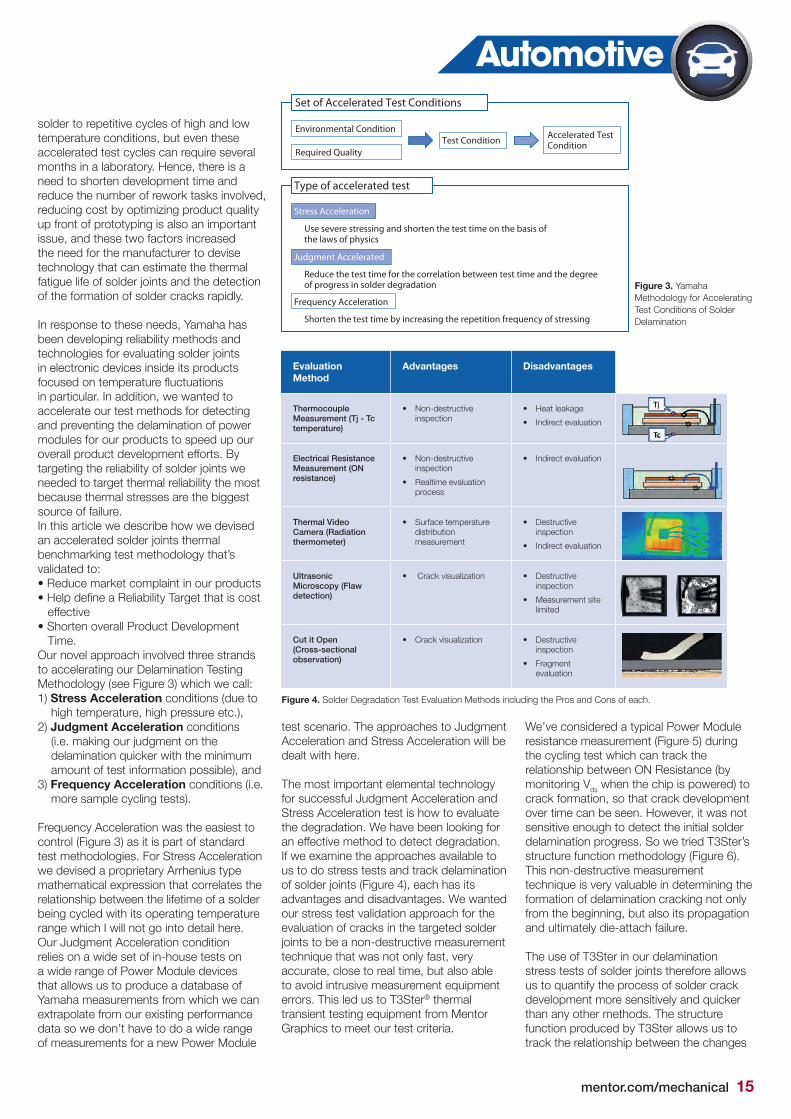
Figure 4. Solder Degradation Test Evaluation Methods including the Pros and Cons of each.
test scenario. The approaches to Judgment Acceleration and Stress Acceleration will be dealt with here.
The most important elemental technology for successful Judgment Acceleration and Stress Acceleration test is how to evaluate the degradation. We have been looking for an effective method to detect degradation. If we examine the approaches available to us to do stress tests and track delamination of solder joints (Figure 4), each has its advantages and disadvantages. We wanted our stress test validation approach for the evaluation of cracks in the targeted solder joints to be a non-destructive measurement technique that was not only fast, very accurate, close to real time, but also able to avoid intrusive measurement equipment errors. This led us to T3Ster® thermal transient testing equipment from Mentor Graphics to meet our test criteria.
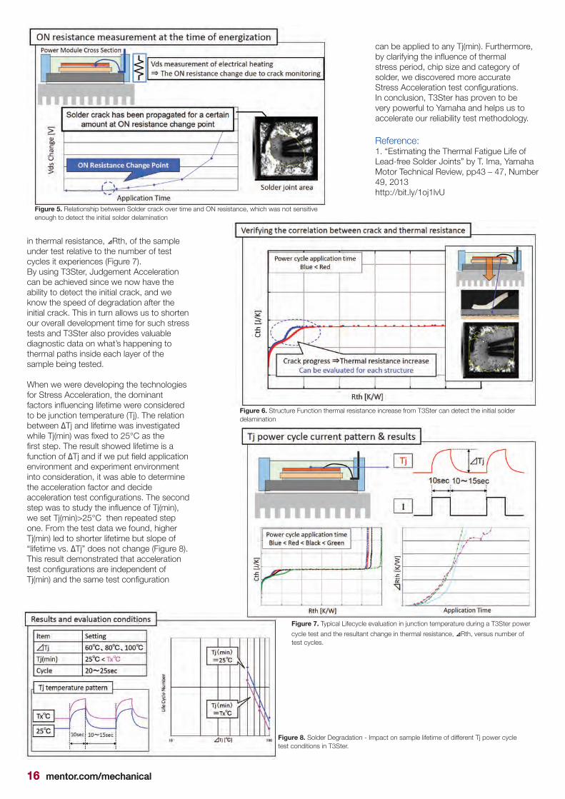
We’ve considered a typical Power Module resistance measurement (Figure 5) during the cycling test which can track the relationship between ON Resistance (by monitoring Vds when the chip is powered) to crack formation, so that crack development over time can be seen. However, it was not sensitive enough to detect the initial solder delamination progress. So we tried T3Ster’s structure function methodology (Figure 6). This non-destructive measurement technique is very valuable in determining the formation of delamination cracking not only from the beginning, but also its propagation and ultimately die-attach failure.
The use of T3Ster in our delamination stress tests of solder joints therefore allows us to quantify the process of solder crack development more sensitively and quicker than any other methods. The structure function produced by T3Ster allows us to track the relationship between the changes
Evaluation Method
Advantages Disadvantages
Thermocouple Measurement (Tj - Tc temperature)
• Non-destructive inspection
• Heat leakage
• Indirect evaluation
Electrical Resistance Measurement (ON resistance)
• Non-destructive inspection
• Realtime evaluation process
• Indirect evaluation
Thermal Video Camera (Radiation thermometer)
• Surface temperature distribution measurement
• Destructive inspection
• Indirect evaluation
Ultrasonic Microscopy (Flaw detection)
• Crack visualization • Destructive inspection
• Measurement site limited
Cut it Open (Cross-sectional observation)
• Crack visualization • Destructive inspection
• Fragment evaluation
16 mentor.com/mechanical16 mentor.com/mechanical
Figure 5. Relationship between Solder crack over time and ON resistance, which was not sensitive enough to detect the initial solder delamination
Figure 7. Typical Lifecycle evaluation in junction temperature during a T3Ster power
cycle test and the resultant change in thermal resistance, ⊿Rth, versus number of test cycles.
Figure 8. Solder Degradation - Impact on sample lifetime of different Tj power cycle test conditions in T3Ster.
in thermal resistance, ⊿Rth, of the sample under test relative to the number of test cycles it experiences (Figure 7). By using T3Ster, Judgement Acceleration can be achieved since we now have the ability to detect the initial crack, and we know the speed of degradation after the initial crack. This in turn allows us to shorten our overall development time for such stress tests and T3Ster also provides valuable diagnostic data on what’s happening to thermal paths inside each layer of the sample being tested.
When we were developing the technologies for Stress Acceleration, the dominant factors influencing lifetime were considered to be junction temperature (Tj). The relation between ΔTj and lifetime was investigated while Tj(min) was fixed to 25°C as the first step. The result showed lifetime is a function of ΔTj and if we put field application environment and experiment environment into consideration, it was able to determine the acceleration factor and decide acceleration test configurations. The second step was to study the influence of Tj(min), we set Tj(min)>25°C then repeated step one. From the test data we found, higher Tj(min) led to shorter lifetime but slope of “lifetime vs. ΔTj” does not change (Figure 8). This result demonstrated that acceleration test configurations are independent of Tj(min) and the same test configuration
Figure 6. Structure Function thermal resistance increase from T3Ster can detect the initial solder delamination
can be applied to any Tj(min). Furthermore, by clarifying the influence of thermal stress period, chip size and category of solder, we discovered more accurate Stress Acceleration test configurations. In conclusion, T3Ster has proven to be very powerful to Yamaha and helps us to accelerate our reliability test methodology.
Reference:1. “Estimating the Thermal Fatigue Life of Lead-free Solder Joints” by T. Ima, Yamaha Motor Technical Review, pp43 – 47, Number 49, 2013 http://bit.ly/1oj1lvU

mentor.com/mechanical 17
Plant & Process
GTRE take the Heat Out of Gas Turbine Design
he Gas Turbine Research Establishment (GTRE) represents the cutting edge of the Indian aeronautical establishment.
Located in Bangalore, its primary function is the research and development of military aero gas-turbines.
Modern aerospace gas-turbines are extremely advanced pieces of machinery, requiring sophisticated design and evaluation tools and processes. Delivering on many – and often conflicting – requirements pushes modern engineering to its limits. For example, modern gas turbine engines are characterized by high pressure ratios and Turbine Entry Temperatures (TET), both of which have a strong influence on the thermal efficiency and specific power
T
By John Murray, Product Marketing Manager, Mentor Graphics
output of the engine. Increasing TET over time (see Figure 1) has meant that the blades themselves must be cooled in order to keep the temperature of the metal within acceptable limits. Successful cooling strategies must use the minimum possible amount of engine bleed air, generate a uniform temperature over the surface of the blade and be feasible for economic production.
It can thus be seen that the design of this one system – one of thousands that must come together to make a successful engine work – is itself intimately linked to a number of other areas of engineering. A carefully managed iterative design process is essential under such circumstances (see Figure 2), underpinned by tools that
lend themselves to automation and output results that can be relied upon and easily analyzed.
Flowmaster complements the existing GTRE inventory by allowing experimental information to be easily integrated into simulations. The ability to set up parametric studies and easily visualize results, enables GTRE engineers to identify undesirable features such as ‘choking’ (reaching local velocities equal to the speed of sound) and has ultimately shortened the design cycle. Confidence in Flowmaster is underwritten by excellent agreement between simulation and experiment (see Figure 3).
Figure 1. Increase in TET over Time (Image courtesy of The Superalloys: Fundamentals and Applications, R.C. Reed, Cambridge University Press (2008))
Figure 2. GTRE Design Loop
Figure 3. Flowmaster vs Measured Mass Flow Rate
No
Cooling AirMass flow and Temp
Cooling DesignLayout
Modify CoolingGeometry
EnginePerformance
Turbine AerofoilGeometry &
Aerodynamics
Secondary AirSystemPc, Tc
Material Properties&
Manufacturingconstraints
INHOUSE ID CODES
Tm,DesignMet?
FEM/CHT Analysis
TmDesignMet?
LIFE/STRESS
TmDesignMet?
No
Data fromElemental experiments
FLOWMASTER
Manufacture
Rig/EngineTest
No
Yes
Yes
Yes
18 mentor.com/mechanical
aipem S.p.A, a subsidiary of Eni S.p.A, is a world leader in the oil and gas industry, providing engineering, construction
and project management services to organizations in some of the most difficult operational environments in the world. Success in this industry requires engineers to balance experience with innovation in order that projects are delivered safely while ensuring that best practice constantly evolves with the latest tools and techniques.
The Naval Analysis Group in Saipem’s London office focusses on supporting offshore heavy lift and pipeline installations for projects around the globe. As exploration has moved into increasingly challenging territory, the engineers and naval architects
S
mentor.com/mechanical 18
Saipem S.p.A moves FloEFD Offshore
have sought to continuously invest in and improve their operational practice in order to better serve the operations they support.
A practical example of this evolution is the integration of FloEFD into their suite of tools. Computational Fluid Dynamics (CFD) has been used in the offshore industry for a number of years, often focusing on specialized applications such as heat transfer or multi-phase flow. However, the wider application of CFD beyond specialist groups has been limited by the complexities involved in geometry handling, meshing, and solution procedure. Not only this, but the hardware and time frames required to deliver solutions on anything other than the most basic geometries renders it difficult to use in operational environments.
Saipem S.p.A take advantage of FloEFD to support operations
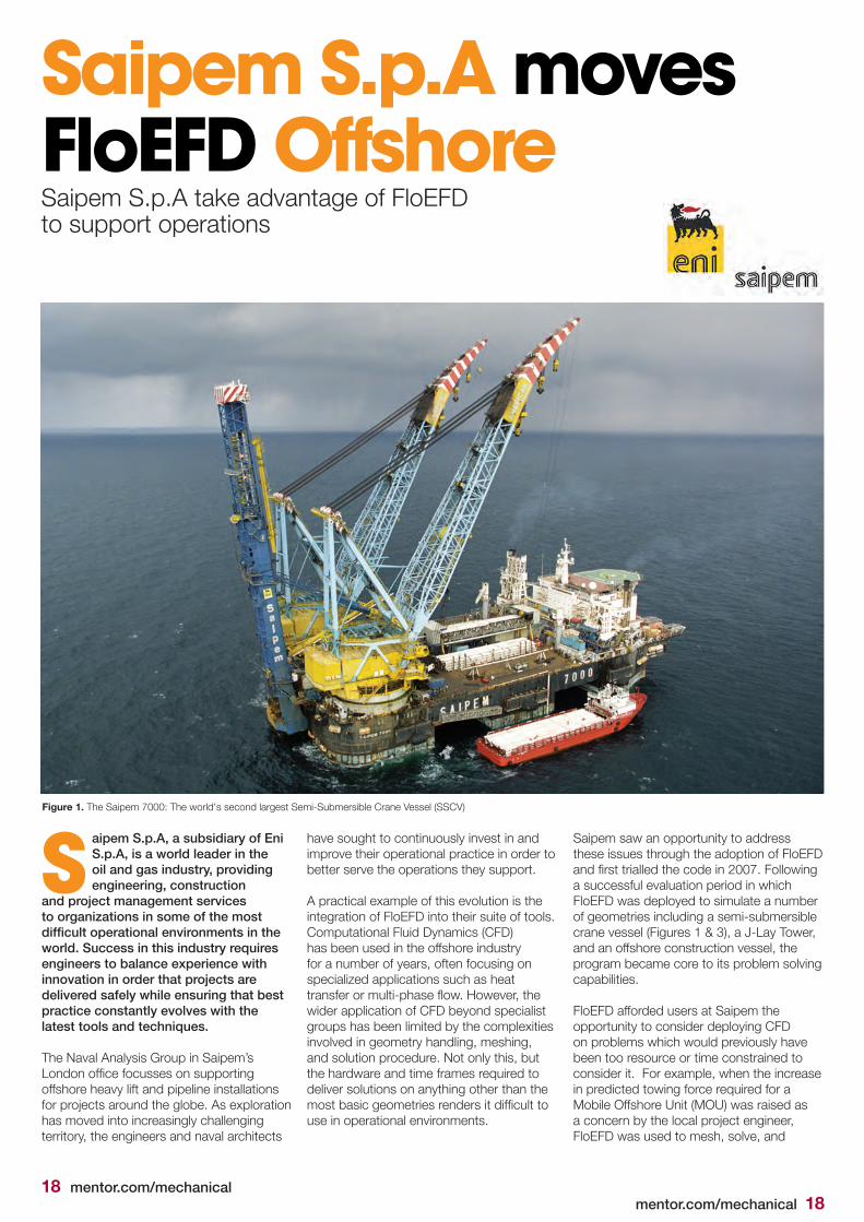
Saipem saw an opportunity to address these issues through the adoption of FloEFD and first trialled the code in 2007. Following a successful evaluation period in which FloEFD was deployed to simulate a number of geometries including a semi-submersible crane vessel (Figures 1 & 3), a J-Lay Tower, and an offshore construction vessel, the program became core to its problem solving capabilities.
FloEFD afforded users at Saipem the opportunity to consider deploying CFD on problems which would previously have been too resource or time constrained to consider it. For example, when the increase in predicted towing force required for a Mobile Offshore Unit (MOU) was raised as a concern by the local project engineer, FloEFD was used to mesh, solve, and
Figure 1. The Saipem 7000: The world's second largest Semi-Submersible Crane Vessel (SSCV)
mentor.com/mechanical 19
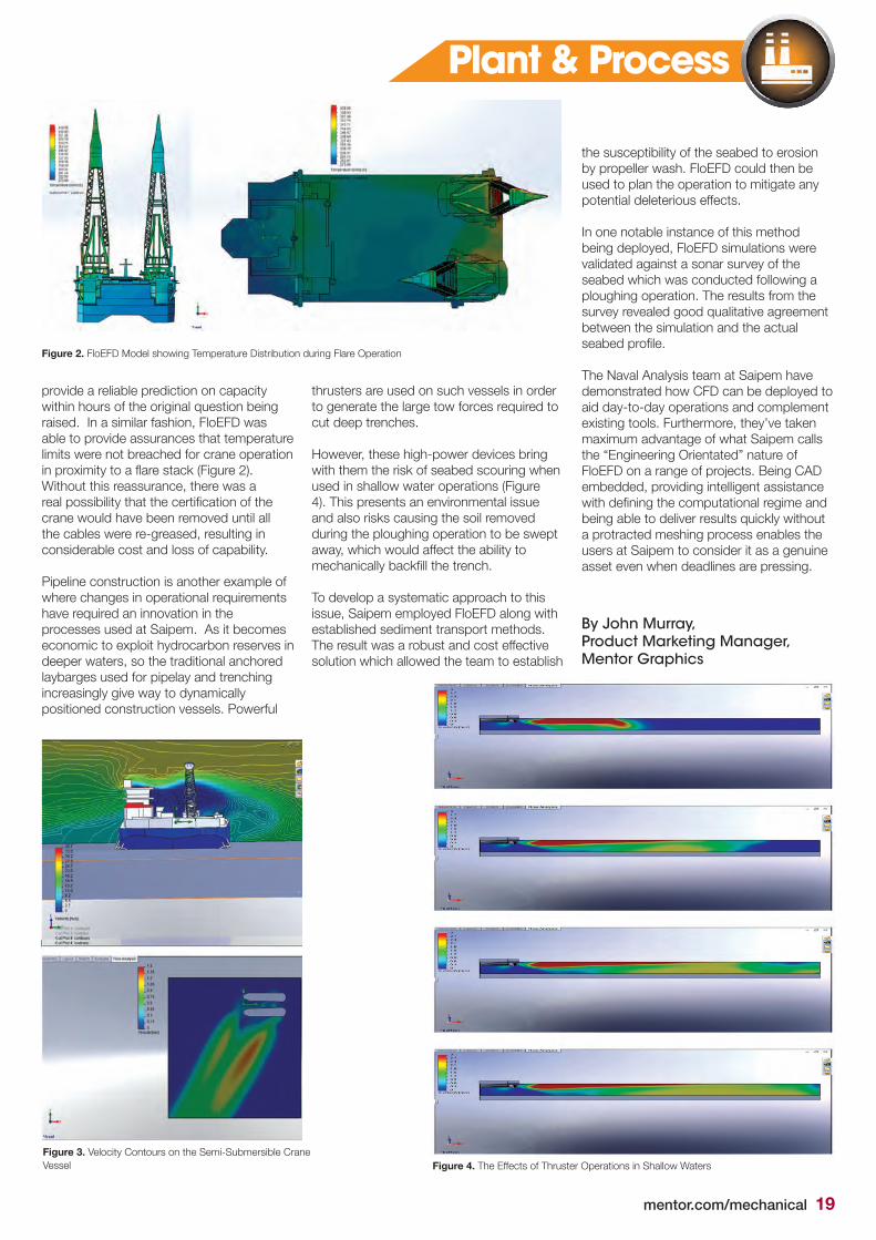
provide a reliable prediction on capacity within hours of the original question being raised. In a similar fashion, FloEFD was able to provide assurances that temperature limits were not breached for crane operation in proximity to a flare stack (Figure 2). Without this reassurance, there was a real possibility that the certification of the crane would have been removed until all the cables were re-greased, resulting in considerable cost and loss of capability.
Pipeline construction is another example of where changes in operational requirements have required an innovation in the processes used at Saipem. As it becomes economic to exploit hydrocarbon reserves in deeper waters, so the traditional anchored laybarges used for pipelay and trenching increasingly give way to dynamically positioned construction vessels. Powerful
the susceptibility of the seabed to erosion by propeller wash. FloEFD could then be used to plan the operation to mitigate any potential deleterious effects.
In one notable instance of this method being deployed, FloEFD simulations were validated against a sonar survey of the seabed which was conducted following a ploughing operation. The results from the survey revealed good qualitative agreement between the simulation and the actual seabed profile.
The Naval Analysis team at Saipem have demonstrated how CFD can be deployed to aid day-to-day operations and complement existing tools. Furthermore, they’ve taken maximum advantage of what Saipem calls the “Engineering Orientated” nature of FloEFD on a range of projects. Being CAD embedded, providing intelligent assistance with defining the computational regime and being able to deliver results quickly without a protracted meshing process enables the users at Saipem to consider it as a genuine asset even when deadlines are pressing.
thrusters are used on such vessels in order to generate the large tow forces required to cut deep trenches.
However, these high-power devices bring with them the risk of seabed scouring when used in shallow water operations (Figure 4). This presents an environmental issue and also risks causing the soil removed during the ploughing operation to be swept away, which would affect the ability to mechanically backfill the trench.
To develop a systematic approach to this issue, Saipem employed FloEFD along with established sediment transport methods. The result was a robust and cost effective solution which allowed the team to establish
Figure 2. FloEFD Model showing Temperature Distribution during Flare Operation
Figure 3. Velocity Contours on the Semi-Submersible Crane Vessel Figure 4. The Effects of Thruster Operations in Shallow Waters
Plant & Process
By John Murray, Product Marketing Manager, Mentor Graphics

20 mentor.com/mechanical
Using the MicReD T3Ster® to Develop High Thermal Conductivity Sintered Silver Paste By Koji Sasaki, NAMICS Corporation, Nigorikawa, Japan
A case study by NAMICS Corporation
ounded in 1947, NAMICS Corporation is headquartered in Niigata just north of Tokyo. It is one of world’s leading manufacturers of both
conductive and insulating thermal interface materials (TIM) for assorted electronics applications. NAMICS is as a consequence, the leading source for under-fills, encapsulants, and adhesives used by producers of semiconductor devices, passive components, solar cells, and a wide array of consumer electronics products. With subsidiaries in the United States, Europe, Singapore, Taiwan, and China, the company boasts annual revenues of approximately $226M and invests heavily in R&D putting them at the cutting edge of research activities and active patenting of new materials.
F As the demand increases for electronics in consumer products and cars with a higher density of components in the same amount of space, there is an ever growing need for better Thermal Interface Materials (TIM) on printed circuit boards. To meet this need, NAMICS has been developing low temperature sintered nano-silver adhesive pastes, using its proprietary Metallo-organic (MO) compound technology in a two stage process for thick film applications (Figure 1). These silver-resin pastes have strong
Figure 1. Schematic View of NAMICS’ 2 Stage Synthesizing Process for Nano-Silver Particles using MO Reduction Reaction Technology
Figure 2. Curing Temperature versus Nano-Silver Quality Produced by the MO Technology
mentor.com/mechanical 21
Electronics
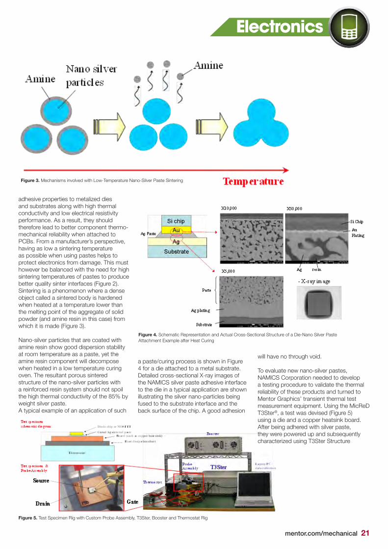
adhesive properties to metalized dies and substrates along with high thermal conductivity and low electrical resistivity performance. As a result, they should therefore lead to better component thermo-mechanical reliability when attached to PCBs. From a manufacturer’s perspective, having as low a sintering temperature as possible when using pastes helps to protect electronics from damage. This must however be balanced with the need for high sintering temperatures of pastes to produce better quality sinter interfaces (Figure 2).Sintering is a phenomenon where a dense object called a sintered body is hardened when heated at a temperature lower than the melting point of the aggregate of solid powder (and amine resin in this case) from which it is made (Figure 3).
Nano-silver particles that are coated with amine resin show good dispersion stability at room temperature as a paste, yet the amine resin component will decompose when heated in a low temperature curing oven. The resultant porous sintered structure of the nano-silver particles with a reinforced resin system should not spoil the high thermal conductivity of the 85% by weight silver paste.A typical example of an application of such
Figure 3. Mechanisms involved with Low-Temperature Nano-Silver Paste Sintering
Figure 5. Test Specimen Rig with Custom Probe Assembly, T3Ster, Booster and Thermostat Rig
Figure 4. Schematic Representation and Actual Cross-Sectional Structure of a Die-Nano Silver Paste Attachment Example after Heat Curing
a paste/curing process is shown in Figure 4 for a die attached to a metal substrate. Detailed cross-sectional X-ray images of the NAMICS silver paste adhesive interface to the die in a typical application are shown illustrating the silver nano-particles being fused to the substrate interface and the back surface of the chip. A good adhesion
will have no through void.
To evaluate new nano-silver pastes, NAMICS Corporation needed to develop a testing procedure to validate the thermal reliability of these products and turned to Mentor Graphics’ transient thermal test measurement equipment. Using the MicReD T3Ster®, a test was devised (Figure 5) using a die and a copper heatsink board. After being adhered with silver paste, they were powered up and subsequently characterized using T3Ster Structure
22 mentor.com/mechanical
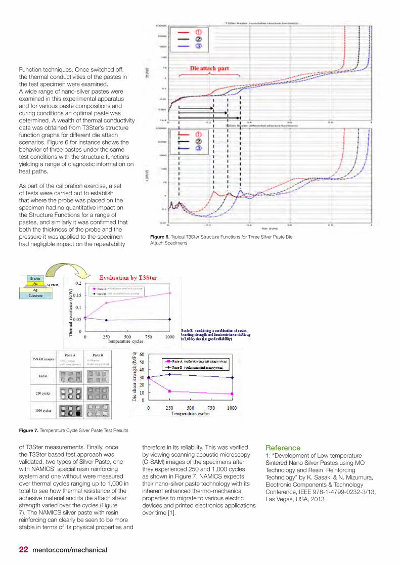
Figure 6. Typical T3Ster Structure Functions for Three Silver Paste Die Attach Specimens
Figure 7. Temperature Cycle Silver Paste Test Results
Function techniques. Once switched off, the thermal conductivities of the pastes in the test specimen were examined.A wide range of nano-silver pastes were examined in this experimental apparatus and for various paste compositions and curing conditions an optimal paste was determined. A wealth of thermal conductivity data was obtained from T3Ster’s structure function graphs for different die attach scenarios. Figure 6 for instance shows the behavior of three pastes under the same test conditions with the structure functions yielding a range of diagnostic information on heat paths.
As part of the calibration exercise, a set of tests were carried out to establish that where the probe was placed on the specimen had no quantitative impact on the Structure Functions for a range of pastes, and similarly it was confirmed that both the thickness of the probe and the pressure it was applied to the specimen had negligible impact on the repeatability
of T3Ster measurements. Finally, once the T3Ster based test approach was validated, two types of Silver Paste, one with NAMICS’ special resin reinforcing system and one without were measured over thermal cycles ranging up to 1,000 in total to see how thermal resistance of the adhesive material and its die attach shear strength varied over the cycles (Figure 7). The NAMICS silver paste with resin reinforcing can clearly be seen to be more stable in terms of its physical properties and
therefore in its reliability. This was verified by viewing scanning acoustic microscopy (C-SAM) images of the specimens after they experienced 250 and 1,000 cycles as shown in Figure 7. NAMICS expects their nano-silver paste technology with its inherent enhanced thermo-mechanical properties to migrate to various electric devices and printed electronics applications over time [1].
Reference 1: “Development of Low temperature Sintered Nano Silver Pastes using MO Technology and Resin Reinforcing Technology” by K. Sasaki & N. Mizumura, Electronic Components & Technology Conference, IEEE 978-1-4799-0232-3/13, Las Vegas, USA, 2013

mentor.com/mechanical 23
hen our customers introduce new technology or a new design process, to improve productivity and/or
quality, it’s important to see the benefits quickly. In the case of electronics cooling analysis, they want to see their model running a simulation as soon as possible. Our Custom Mentoring Service enables exactly that. A Customer Application Engineer (CAE) sits down with the user and helps put a good model together to see some results. Perhaps the most valuable part is the discussion about what those results tell you.
A number of our FloTHERM® customers want to put FloTHERM® XT through its paces. They want to see how to take advantage of FloTHERM XT’s unique abilities with complex geometries, for example.
As always, there’s no better way to learn a new piece of software than using the software in your particular workflow.
Very often there is an existing CAD geometry available. The workflow then consists of five basic steps: • Import and healing the geometry and setting up any necessary project structure• Setting up the project with its boundary conditions and the assignments of physical properties to all parts of the project• Setting up the computational mesh• Running the case• Perform a results evaluation
Typically, these five steps can be completed in one working day of the Mentoring Service. Of course it is not possible to cover all details but a good overview can be given – with a lot of practical exercises performed by the user him/herself.
Importing CAD geometry created in a 3D CAD tool other than FloTHERM XT is straightforward. The typical pitfalls tend to remain the same and once you are aware of them, they can be easily avoided. The most important step after data import
W
Mentoring from Mentor
Ask The CSD Expert
is to test the integrity of the imported data. FloTHERM XT offers several tools to do this and all of them are easy to learn. The data structure might have been lost (i.e. resulting in a flat hierarchy) and needs to be restored manually. However, this part of the process will not take longer than one or two hours if assisted by a Mentor Graphics expert.
Setting up a project and defining physical properties is assisted by an excellent wizard and a clear project tree structure. If you are already a FloTHERM user, you might appreciate these FloTHERM XT features. If you already know FloTHERM and the basic need for a good thermal model, a project setup in FloTHERM XT can be completed very quickly.
Creating a basic computational mesh in FloTHERM XT is usually a simple task. Like in any other CFD software, local refinements might need to be applied to resolve local physical effects. There are some guidelines that you need to learn. However, in a basic session, the automatic mesher settings might be sufficient. We can deal with advanced meshing techniques in another session, if required.
If everything runs well, a first version of the project might be solved during or shortly after lunch. While the solver runs, there’s always some time to discuss either general or project specific questions. Once the simulation has been finished, it’s time to understand the results. FloTHERM XT, for instance, offers easy to use standard templates. There are many options to get the best graphical representations of your results, enabling you to make sound engineering judgments for the success of your project. This is where the experience of our CAE’s really makes a difference. A lot can be accomplished in a day. If you need more, we’re happy to help. An email to [email protected] will find us.
Dirk Niemeier, Customer Application Engineer

24 mentor.com/mechanical
Unravelling the Complexities of Automotive Instrument Cluster DesignBy Sam Gustafson, Thermal Analysis Engineer, Visteon Electronics Corporation
Visteon Electronics Corporation's use of FloTHERM®XT for Validation and Optimization
24 mentor.com/mechanical

mentor.com/mechanical 25
Automotive
isteon Corporation who recently acquired the automotive electronics business of Johnson
Controls Inc. (JCI), has become one of the world’s three largest automotive electronics suppliers of instrument clusters and vehicle cockpit electronics. The combined global electronics enterprise has more than $3 billion in annual revenue, with a No. 2 global position in driver information and above-average growth rates for the cockpit electronics segment, supplying nine of the world’s 10 largest vehicle manufacturers.
In this article, Sam Gustafson, a Thermal Analyst at Visteon , shares the importance of the thermal requirements and their influence on the PCB and mechanical design of a cluster. In particular, how PCB data from Mentor Graphics' Expedition software can be embedded inside a FloTHERM® XT simulation model to investigate the full thermal behavior of the instrument cluster and optimize it.
V Also discussed is a comparison of the PCB layout thermal simulation using Thermography before full enclosure modeling.
In an automotive instrument cluster design, where enclosure shape and internal complexity significantly influences thermal management considerations, engineers focus their attention on areas such as PCB structure/layout and active display dimming to ensure durable performance. Efficient exchange of data between the PCB layout, the Mechanical and Thermal analysis tools therefore becomes key in designing such systems.
As the component most utilized by the driver, the vehicle instrumentation panel greatly impacts the driver experience and therefore consumer satisfaction, Visteon are at the forefront of this technology. The design of instrument panels (Instrumentation Cluster Assemblies) must optimize quality, reduce costs and lead times, and guarantee flawless product launches for their customers.
Thermal integrity becomes a top priority, with heat dissipation the most important consideration for suppliers such as Visteon.
A typical instrumentation cluster (Figure 1 overleaf) consists of two analog gauges on either side of the unit with several LEDs, a significant number of which are bright LEDs. Each system has a Thin Film Transistor (TFT) display (blue section in Figure 1 overleaf), which can only operate 10°C above the maximum ambient air temperature. It is therefore critical to keep this component’s temperature tightly controlled. The cluster is then encased into housing to the dashboard that has limited air openings inhibiting ventilation.
When designing an instrument cluster, the most pertinent consideration is finding an effective way to overcome the temperature sensitivities of most of the components in the assembly. For instance, the LED light and color will degrade if the junction temperature becomes too hot for long periods
mentor.com/mechanical 25
26 mentor.com/mechanical
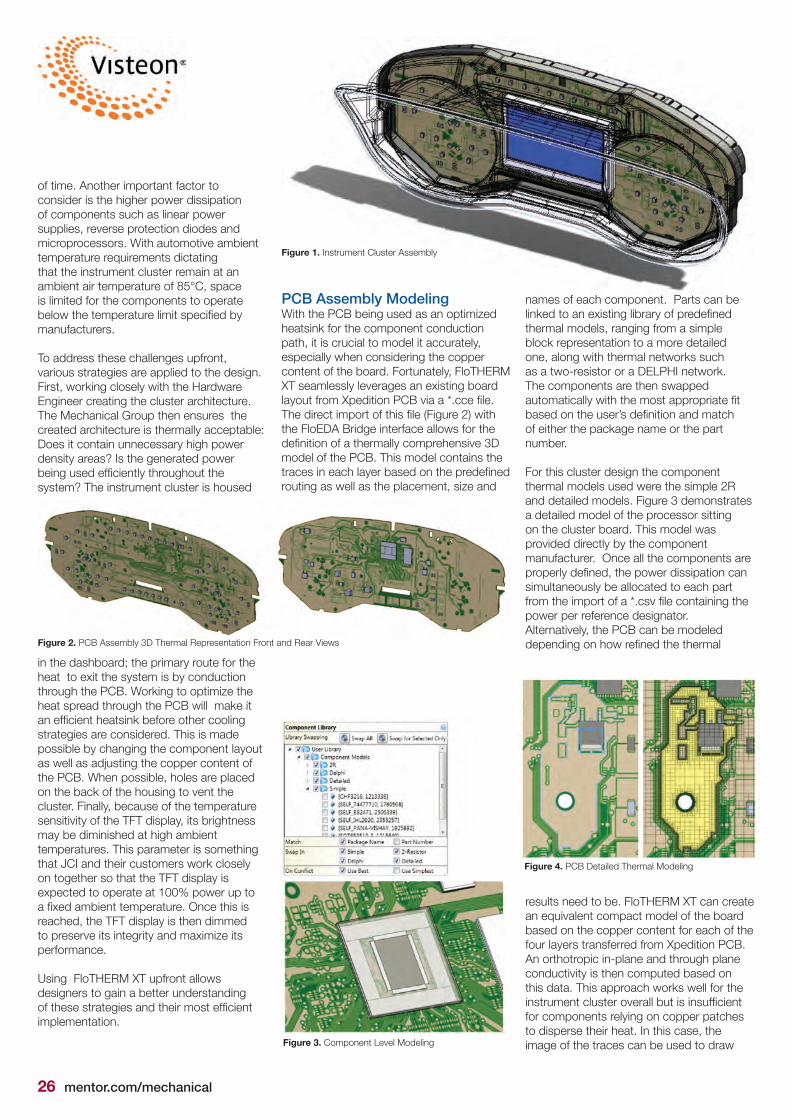
of time. Another important factor to consider is the higher power dissipation of components such as linear power supplies, reverse protection diodes and microprocessors. With automotive ambient temperature requirements dictating that the instrument cluster remain at an ambient air temperature of 85°C, space is limited for the components to operate below the temperature limit specified by manufacturers.
To address these challenges upfront, various strategies are applied to the design. First, working closely with the Hardware Engineer creating the cluster architecture. The Mechanical Group then ensures the created architecture is thermally acceptable: Does it contain unnecessary high power density areas? Is the generated power being used efficiently throughout the system? The instrument cluster is housed
Figure 1. Instrument Cluster Assembly
names of each component. Parts can be linked to an existing library of predefined thermal models, ranging from a simple block representation to a more detailed one, along with thermal networks such as a two-resistor or a DELPHI network. The components are then swapped automatically with the most appropriate fit based on the user’s definition and match of either the package name or the part number.
For this cluster design the component thermal models used were the simple 2R and detailed models. Figure 3 demonstrates a detailed model of the processor sitting on the cluster board. This model was provided directly by the component manufacturer. Once all the components are properly defined, the power dissipation can simultaneously be allocated to each part from the import of a *.csv file containing the power per reference designator. Alternatively, the PCB can be modeled depending on how refined the thermal Figure 2. PCB Assembly 3D Thermal Representation Front and Rear Views
Figure 3. Component Level Modeling
Figure 4. PCB Detailed Thermal Modeling
in the dashboard; the primary route for the heat to exit the system is by conduction through the PCB. Working to optimize the heat spread through the PCB will make it an efficient heatsink before other cooling strategies are considered. This is made possible by changing the component layout as well as adjusting the copper content of the PCB. When possible, holes are placed on the back of the housing to vent the cluster. Finally, because of the temperature sensitivity of the TFT display, its brightness may be diminished at high ambient temperatures. This parameter is something that JCI and their customers work closely on together so that the TFT display is expected to operate at 100% power up to a fixed ambient temperature. Once this is reached, the TFT display is then dimmed to preserve its integrity and maximize its performance.
Using FloTHERM XT upfront allows designers to gain a better understanding of these strategies and their most efficient implementation.
results need to be. FloTHERM XT can create an equivalent compact model of the board based on the copper content for each of the four layers transferred from Xpedition PCB. An orthotropic in-plane and through plane conductivity is then computed based on this data. This approach works well for the instrument cluster overall but is insufficient for components relying on copper patches to disperse their heat. In this case, the image of the traces can be used to draw
PCB Assembly ModelingWith the PCB being used as an optimized heatsink for the component conduction path, it is crucial to model it accurately, especially when considering the copper content of the board. Fortunately, FloTHERM XT seamlessly leverages an existing board layout from Xpedition PCB via a *.cce file. The direct import of this file (Figure 2) with the FloEDA Bridge interface allows for the definition of a thermally comprehensive 3D model of the PCB. This model contains the traces in each layer based on the predefined routing as well as the placement, size and
mentor.com/mechanical 27
Automotive
the outline of the desired copper shape and extrude the corresponding copper patch (Figure 4). Placing the newly created copper pad lower in the FloTHERM XT tree makes it overwrite the PCB area of interest. Thermal resistance values were also defined on the edges of the patch to represent the buffer that the FR4 creates between the detailed shape and the rest of the copper plane.Being able to combine the existing ECAD data with thermal representations of components in FloTHERM XT allows the user to create the thermal analysis model quickly, saving time in the design process.
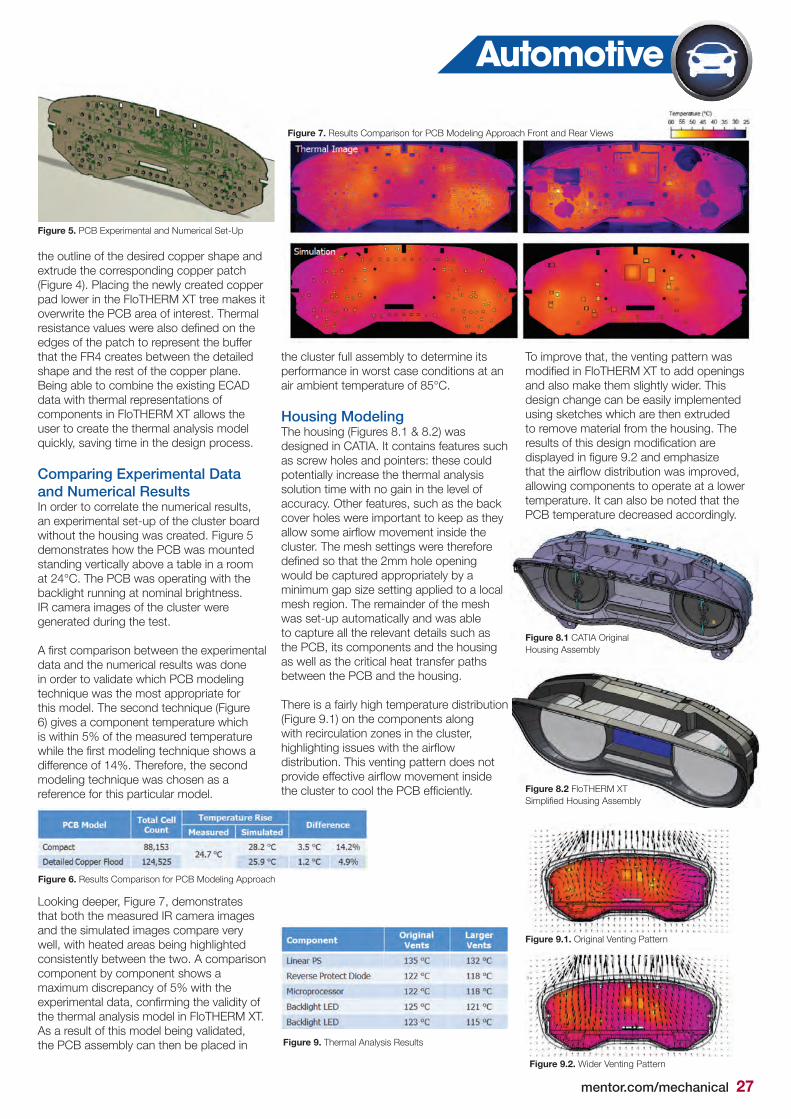
Comparing Experimental Data and Numerical ResultsIn order to correlate the numerical results, an experimental set-up of the cluster board without the housing was created. Figure 5 demonstrates how the PCB was mounted standing vertically above a table in a room at 24°C. The PCB was operating with the backlight running at nominal brightness. IR camera images of the cluster were generated during the test.
A first comparison between the experimental data and the numerical results was done in order to validate which PCB modeling technique was the most appropriate for this model. The second technique (Figure 6) gives a component temperature which is within 5% of the measured temperature while the first modeling technique shows a difference of 14%. Therefore, the second modeling technique was chosen as a reference for this particular model.
the cluster full assembly to determine its performance in worst case conditions at an air ambient temperature of 85°C.
Housing ModelingThe housing (Figures 8.1 & 8.2) was designed in CATIA. It contains features such as screw holes and pointers: these could potentially increase the thermal analysis solution time with no gain in the level of accuracy. Other features, such as the back cover holes were important to keep as they allow some airflow movement inside the cluster. The mesh settings were therefore defined so that the 2mm hole opening would be captured appropriately by a minimum gap size setting applied to a local mesh region. The remainder of the mesh was set-up automatically and was able to capture all the relevant details such as the PCB, its components and the housing as well as the critical heat transfer paths between the PCB and the housing.
There is a fairly high temperature distribution (Figure 9.1) on the components along with recirculation zones in the cluster, highlighting issues with the airflow distribution. This venting pattern does not provide effective airflow movement inside the cluster to cool the PCB efficiently.
To improve that, the venting pattern was modified in FloTHERM XT to add openings and also make them slightly wider. This design change can be easily implemented using sketches which are then extruded to remove material from the housing. The results of this design modification are displayed in figure 9.2 and emphasize that the airflow distribution was improved, allowing components to operate at a lower temperature. It can also be noted that the PCB temperature decreased accordingly.
Figure 5. PCB Experimental and Numerical Set-Up
Figure 6. Results Comparison for PCB Modeling Approach
Figure 7. Results Comparison for PCB Modeling Approach Front and Rear Views
Looking deeper, Figure 7, demonstrates that both the measured IR camera images and the simulated images compare very well, with heated areas being highlighted consistently between the two. A comparison component by component shows a maximum discrepancy of 5% with the experimental data, confirming the validity of the thermal analysis model in FloTHERM XT. As a result of this model being validated, the PCB assembly can then be placed in
Figure 8.2 FloTHERM XT Simplified Housing Assembly
Figure 9. Thermal Analysis Results
Figure 9.1. Original Venting Pattern
Figure 9.2. Wider Venting Pattern
Figure 8.1 CATIA Original Housing Assembly

28 mentor.com/mechanical
A Modest Proposal for a Dual-Use Heater Core
n automotive engine cooling, most manufacturers today have an over design problem. The front-end cooling pack (Figure 1) is usually
sized for an extreme driving condition, e.g. a hot day at 110°F (43°C) while towing a trailer of 3,000lbs or 5,000lbs (1,350kg – 2,300kg) and going up an extreme grade – a scenario that rarely happens. As a consequence, most of
I
By Sudhi Uppuluri, Computer Sciences Experts Group
Better Vehicle Fuel Economy Designed with the Help of Flowmaster
the vehicles on the road in the US that you see are driving around with an oversized cooling pack and an oversized cooling fan just to meet that one extreme condition which over 99% of us will never encounter.
This over design leads to higher drag and lower fuel economy for the everyday driver. Some automotive OEMs have below-the-
headlight heat exchangers (oil coolers, charge-air coolers) to alleviate the thermal load on the cooling pack leading to a smaller cooling pack. But that can be an expensive option.
There is an obvious solution staring us in the face though: the heater core! It is already plumbed into the engine. It has ample coolant flow all the time and it is capable of
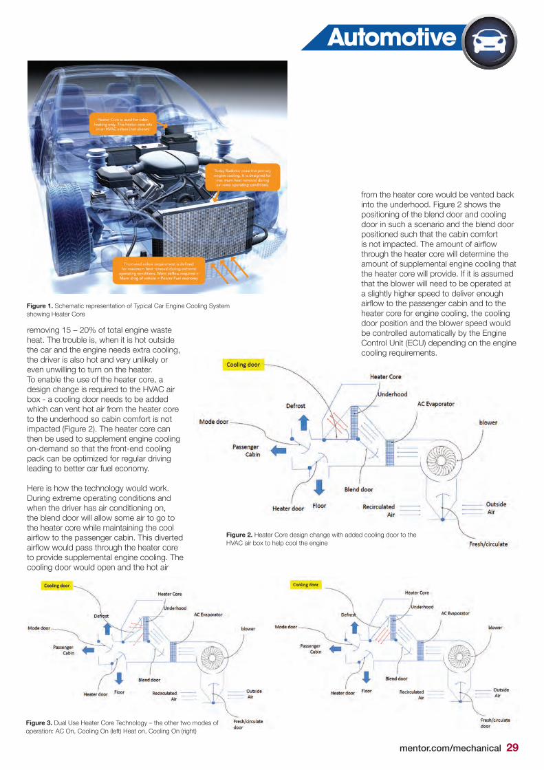
mentor.com/mechanical 29
Automotive
removing 15 – 20% of total engine waste heat. The trouble is, when it is hot outside the car and the engine needs extra cooling, the driver is also hot and very unlikely or even unwilling to turn on the heater.To enable the use of the heater core, a design change is required to the HVAC air box - a cooling door needs to be added which can vent hot air from the heater core to the underhood so cabin comfort is not impacted (Figure 2). The heater core can then be used to supplement engine cooling on-demand so that the front-end cooling pack can be optimized for regular driving leading to better car fuel economy.
Here is how the technology would work. During extreme operating conditions and when the driver has air conditioning on, the blend door will allow some air to go to the heater core while maintaining the cool airflow to the passenger cabin. This diverted airflow would pass through the heater core to provide supplemental engine cooling. The cooling door would open and the hot air
from the heater core would be vented back into the underhood. Figure 2 shows the positioning of the blend door and cooling door in such a scenario and the blend door positioned such that the cabin comfort is not impacted. The amount of airflow through the heater core will determine the amount of supplemental engine cooling that the heater core will provide. If it is assumed that the blower will need to be operated at a slightly higher speed to deliver enough airflow to the passenger cabin and to the heater core for engine cooling, the cooling door position and the blower speed would be controlled automatically by the Engine Control Unit (ECU) depending on the engine cooling requirements.
Figure 1. Schematic representation of Typical Car Engine Cooling System showing Heater Core
Figure 2. Heater Core design change with added cooling door to the HVAC air box to help cool the engine
Figure 3. Dual Use Heater Core Technology – the other two modes of operation: AC On, Cooling On (left) Heat on, Cooling On (right)
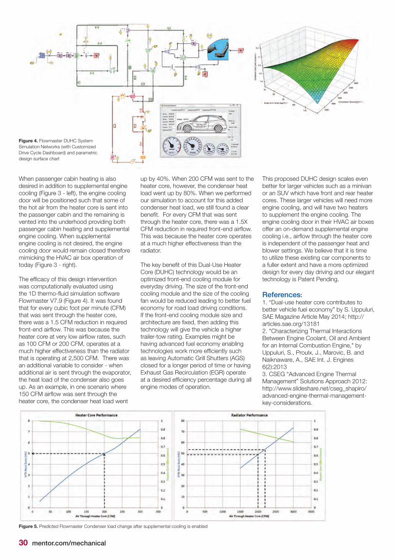
30 mentor.com/mechanical
When passenger cabin heating is also desired in addition to supplemental engine cooling (Figure 3 - left), the engine cooling door will be positioned such that some of the hot air from the heater core is sent into the passenger cabin and the remaining is vented into the underhood providing both passenger cabin heating and supplemental engine cooling. When supplemental engine cooling is not desired, the engine cooling door would remain closed therefore mimicking the HVAC air box operation of today (Figure 3 - right).
The efficacy of this design intervention was computationally evaluated using the 1D thermo-fluid simulation software Flowmaster V7.9 (Figure 4). It was found that for every cubic foot per minute (CFM) that was sent through the heater core, there was a 1.5 CFM reduction in required front-end airflow. This was because the heater core at very low airflow rates, such as 100 CFM or 200 CFM, operates at a much higher effectiveness than the radiator that is operating at 2,500 CFM. There was an additional variable to consider - when additional air is sent through the evaporator, the heat load of the condenser also goes up. As an example, in one scenario where 150 CFM airflow was sent through the heater core, the condenser heat load went
up by 40%. When 200 CFM was sent to the heater core, however, the condenser heat load went up by 80%. When we performed our simulation to account for this added condenser heat load, we still found a clear benefit. For every CFM that was sent through the heater core, there was a 1.5X CFM reduction in required front-end airflow. This was because the heater core operates at a much higher effectiveness than the radiator.
The key benefit of this Dual-Use Heater Core (DUHC) technology would be an optimized front-end cooling module for everyday driving. The size of the front-end cooling module and the size of the cooling fan would be reduced leading to better fuel economy for road load driving conditions. If the front-end cooling module size and architecture are fixed, then adding this technology will give the vehicle a higher trailer-tow rating. Examples might be having advanced fuel economy enabling technologies work more efficiently such as leaving Automatic Grill Shutters (AGS) closed for a longer period of time or having Exhaust Gas Recirculation (EGR) operate at a desired efficiency percentage during all engine modes of operation.
This proposed DUHC design scales even better for larger vehicles such as a minivan or an SUV which have front and rear heater cores. These larger vehicles will need more engine cooling, and will have two heaters to supplement the engine cooling. The engine cooling door in their HVAC air boxes offer an on-demand supplemental engine cooling i.e., airflow through the heater core is independent of the passenger heat and blower settings. We believe that it is time to utilize these existing car components to a fuller extent and have a more optimized design for every day driving and our elegant technology is Patent Pending.
References:1. “Dual-use heater core contributes to better vehicle fuel economy” by S. Uppuluri, SAE Magazine Article May 2014; http://articles.sae.org/131812. "Characterizing Thermal Interactions Between Engine Coolant, Oil and Ambient for an Internal Combustion Engine," by Uppuluri, S., Proulx, J., Marovic, B. and Naiknaware, A., SAE Int. J. Engines 6(2):20133. CSEG “Advanced Engine Thermal Management” Solutions Approach 2012: http://www.slideshare.net/cseg_shapiro/advanced-engine-thermal-management-key-considerations.
Figure 4. Flowmaster DUHC System Simulation Networks (with Customized Drive Cycle Dashboard) and parametric design surface chart
Figure 5. Predicted Flowmaster Condenser load change after supplemental cooling is enabled
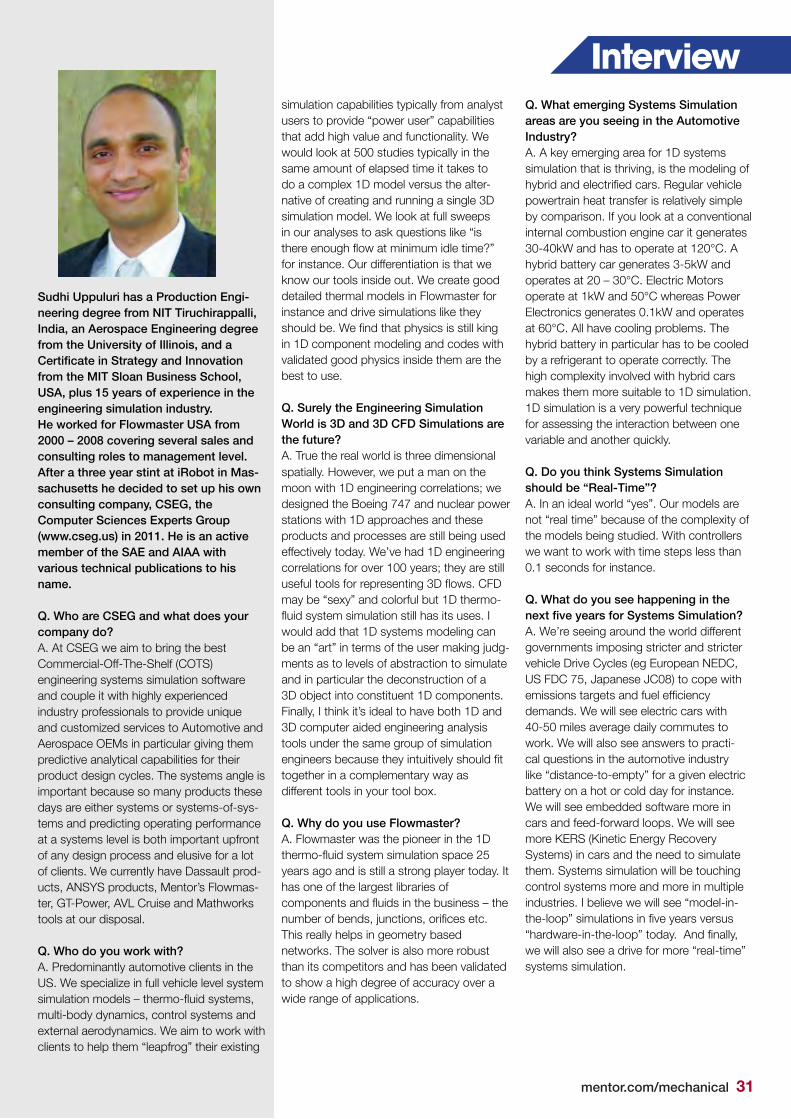
mentor.com/mechanical 31
Interview
Sudhi Uppuluri has a Production Engi-neering degree from NIT Tiruchirappalli, India, an Aerospace Engineering degree from the University of Illinois, and a Certificate in Strategy and Innovation from the MIT Sloan Business School, USA, plus 15 years of experience in the engineering simulation industry. He worked for Flowmaster USA from 2000 – 2008 covering several sales and consulting roles to management level. After a three year stint at iRobot in Mas-sachusetts he decided to set up his own consulting company, CSEG, the Computer Sciences Experts Group (www.cseg.us) in 2011. He is an active member of the SAE and AIAA with various technical publications to his name.
Q. Who are CSEG and what does your company do?A. At CSEG we aim to bring the best Commercial-Off-The-Shelf (COTS) engineering systems simulation software and couple it with highly experienced industry professionals to provide unique and customized services to Automotive and Aerospace OEMs in particular giving them predictive analytical capabilities for their product design cycles. The systems angle is important because so many products these days are either systems or systems-of-sys-tems and predicting operating performance at a systems level is both important upfront of any design process and elusive for a lot of clients. We currently have Dassault prod-ucts, ANSYS products, Mentor’s Flowmas-ter, GT-Power, AVL Cruise and Mathworks tools at our disposal.
Q. Who do you work with?A. Predominantly automotive clients in the US. We specialize in full vehicle level system simulation models – thermo-fluid systems, multi-body dynamics, control systems and external aerodynamics. We aim to work with clients to help them “leapfrog” their existing
Q. What emerging Systems Simulation areas are you seeing in the Automotive Industry?A. A key emerging area for 1D systems simulation that is thriving, is the modeling of hybrid and electrified cars. Regular vehicle powertrain heat transfer is relatively simple by comparison. If you look at a conventional internal combustion engine car it generates 30-40kW and has to operate at 120°C. A hybrid battery car generates 3-5kW and operates at 20 – 30°C. Electric Motors operate at 1kW and 50°C whereas Power Electronics generates 0.1kW and operates at 60°C. All have cooling problems. The hybrid battery in particular has to be cooled by a refrigerant to operate correctly. The high complexity involved with hybrid cars makes them more suitable to 1D simulation. 1D simulation is a very powerful technique for assessing the interaction between one variable and another quickly.
Q. Do you think Systems Simulation should be “Real-Time”?A. In an ideal world “yes”. Our models are not “real time” because of the complexity of the models being studied. With controllers we want to work with time steps less than 0.1 seconds for instance.
Q. What do you see happening in the next five years for Systems Simulation?A. We’re seeing around the world different governments imposing stricter and stricter vehicle Drive Cycles (eg European NEDC, US FDC 75, Japanese JC08) to cope with emissions targets and fuel efficiency demands. We will see electric cars with 40-50 miles average daily commutes to work. We will also see answers to practi-cal questions in the automotive industry like “distance-to-empty” for a given electric battery on a hot or cold day for instance. We will see embedded software more in cars and feed-forward loops. We will see more KERS (Kinetic Energy Recovery Systems) in cars and the need to simulate them. Systems simulation will be touching control systems more and more in multiple industries. I believe we will see “model-in-the-loop” simulations in five years versus “hardware-in-the-loop” today. And finally, we will also see a drive for more “real-time” systems simulation.
simulation capabilities typically from analyst users to provide “power user” capabilities that add high value and functionality. We would look at 500 studies typically in the same amount of elapsed time it takes to do a complex 1D model versus the alter-native of creating and running a single 3D simulation model. We look at full sweeps in our analyses to ask questions like “is there enough flow at minimum idle time?” for instance. Our differentiation is that we know our tools inside out. We create good detailed thermal models in Flowmaster for instance and drive simulations like they should be. We find that physics is still king in 1D component modeling and codes with validated good physics inside them are the best to use.
Q. Surely the Engineering Simulation World is 3D and 3D CFD Simulations are the future?A. True the real world is three dimensional spatially. However, we put a man on the moon with 1D engineering correlations; we designed the Boeing 747 and nuclear power stations with 1D approaches and these products and processes are still being used effectively today. We’ve had 1D engineering correlations for over 100 years; they are still useful tools for representing 3D flows. CFD may be “sexy” and colorful but 1D thermo-fluid system simulation still has its uses. I would add that 1D systems modeling can be an “art” in terms of the user making judg-ments as to levels of abstraction to simulate and in particular the deconstruction of a 3D object into constituent 1D components. Finally, I think it’s ideal to have both 1D and 3D computer aided engineering analysis tools under the same group of simulation engineers because they intuitively should fit together in a complementary way as different tools in your tool box.
Q. Why do you use Flowmaster?A. Flowmaster was the pioneer in the 1D thermo-fluid system simulation space 25 years ago and is still a strong player today. It has one of the largest libraries of components and fluids in the business – the number of bends, junctions, orifices etc. This really helps in geometry based networks. The solver is also more robust than its competitors and has been validated to show a high degree of accuracy over a wide range of applications.
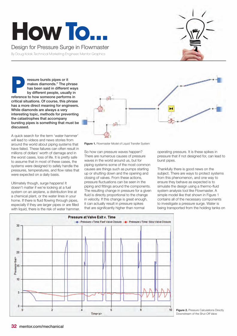
32 mentor.com/mechanical
How To...Design for Pressure Surge in FlowmasterBy Doug Kolak, Technical Marketing Engineer, Mentor Graphics
ressure bursts pipes or it makes diamonds.” The phrase has been said in different ways by different people, usually in
reference to how someone performs in critical situations. Of course, this phrase has a more direct meaning for engineers. While diamonds are always a very interesting topic, methods for preventing the catastrophes that accompany bursting pipes is something that must be discussed.
A quick search for the term ‘water hammer’ will lead to videos and news stories from around the world about piping systems that have failed. These failures can often result in millions of dollars’ worth of damage and in the worst cases, loss of life. It is pretty safe to assume that in most of these cases, the systems were designed to safely handle the pressures, temperatures, and flow rates that were expected on a daily basis.
Ultimately though, surge happens! It doesn’t matter if we’re looking at a fuel system on an airplane, a distribution line at a chemical plant, or the water lines in your home. If there is fluid flowing through pipes, especially if they are larger pipes or are filled with liquid, there is the risk of water hammer.
P
So how can pressure waves happen? There are numerous causes of pressure waves in the world around us, but for piping systems some of the most common causes are things such as pumps starting up or shutting down and the opening and closing of valves. From these actions, pressure fluctuations can be seen in the piping and fittings around the components. The resulting change in pressure for a given fluid is directly proportional to the change in velocity. If this change is great enough, it can actually result in pressure spikes that are significantly higher than normal
operating pressure. It is these spikes in pressure that if not designed for, can lead to burst pipes.
Thankfully there is good news on the subject. There are ways to protect systems from this phenomenon, and one way to ensure they behave as expected is to simulate the design using a thermo-fluid system analysis tool like Flowmaster. A simple model like that shown in Figure 1 contains all of the necessary components to investigate a pressure surge. Water is being transported from the holding tanks on
Figure 1. Flowmaster Model of Liquid Transfer System
Figure 2. Pressure Calculations Directly Downstream of the Shut-Off Valve
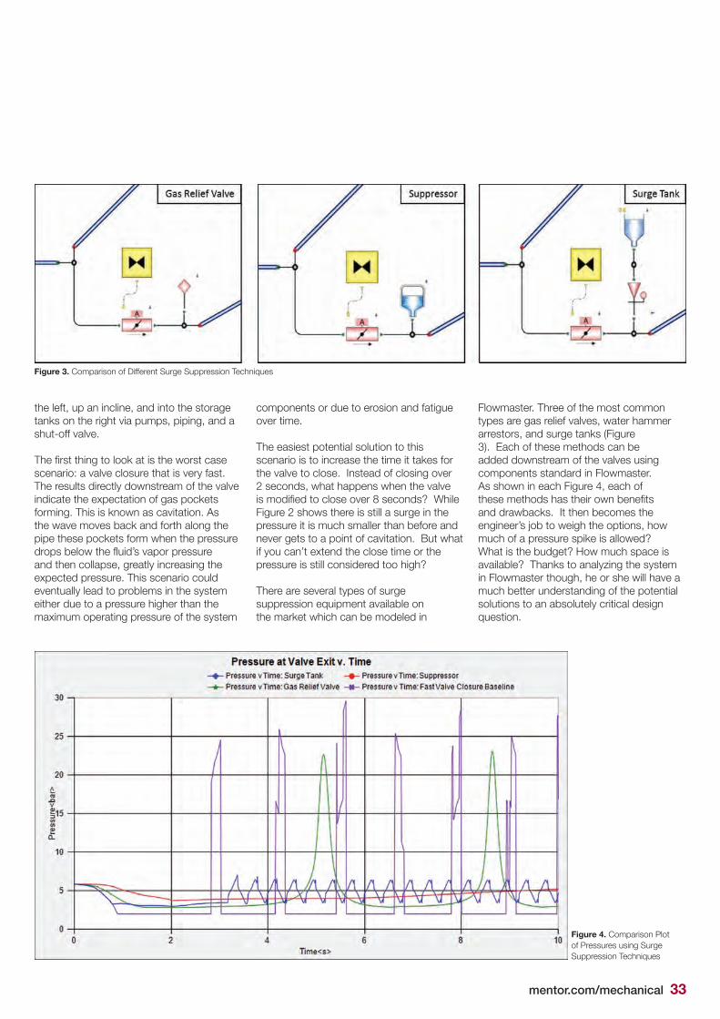
mentor.com/mechanical 33
the left, up an incline, and into the storage tanks on the right via pumps, piping, and a shut-off valve.
The first thing to look at is the worst case scenario: a valve closure that is very fast. The results directly downstream of the valve indicate the expectation of gas pockets forming. This is known as cavitation. As the wave moves back and forth along the pipe these pockets form when the pressure drops below the fluid’s vapor pressure and then collapse, greatly increasing the expected pressure. This scenario could eventually lead to problems in the system either due to a pressure higher than the maximum operating pressure of the system
components or due to erosion and fatigue over time.
The easiest potential solution to this scenario is to increase the time it takes for the valve to close. Instead of closing over 2 seconds, what happens when the valve is modified to close over 8 seconds? While Figure 2 shows there is still a surge in the pressure it is much smaller than before and never gets to a point of cavitation. But what if you can’t extend the close time or the pressure is still considered too high?
There are several types of surge suppression equipment available on the market which can be modeled in
Flowmaster. Three of the most common types are gas relief valves, water hammer arrestors, and surge tanks (Figure 3). Each of these methods can be added downstream of the valves using components standard in Flowmaster. As shown in each Figure 4, each of these methods has their own benefits and drawbacks. It then becomes the engineer’s job to weigh the options, how much of a pressure spike is allowed? What is the budget? How much space is available? Thanks to analyzing the system in Flowmaster though, he or she will have a much better understanding of the potential solutions to an absolutely critical design question.
Figure 3. Comparison of Different Surge Suppression Techniques
Figure 4. Comparison Plot of Pressures using Surge Suppression Techniques
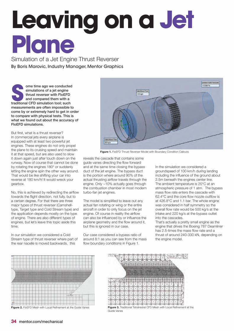
34 mentor.com/mechanical
Leaving on a Jet Plane
S ome time ago we conducted simulations of a jet engine thrust reverser with FloEFD and compared them with a
traditional CFD simulation tool; such measurements are often impossible to come by or extremely hard to get in order to compare with physical tests. This is what we found out about the accuracy of FloEFD simulations.
But first, what is a thrust reverser?In commercial jets every airplane is equipped with at least two powerful jet engines. These engines do not only propel the plane to its cruising speed and maintain it at that speed, but are also used to slow it down again just after touch down on the runway. Now of course that cannot be done by rotating the engines 180° or suddenly letting the engine spin the other way around. That would be like shifting your car into reverse at 180 km/h! It would wreck your gearbox.
No, this is achieved by redirecting the airflow towards the flight direction, not fully, but to a certain degree. For that there are three major types of thrust reverser (Camshell-type, Target type and Cold Stream type) and the application depends mostly on the type of engine. There are also different types of engines, but let’s leave this topic aside this time.
In our simulation we considered a Cold Stream type of thrust reverser where part of the rear nacelle is moved backwards, this
By Boris Marovic, Industry Manager, Mentor Graphics
Simulation of a Jet Engine Thrust Reverser
reveals the cascade that contains some guide vanes directing the flow forward and at the same time closing the bypass duct of the jet engine. The bypass duct is the portion where around 90% of the actual thrusting airflow travels through the engine. Only ~10% actually goes through the combustion chamber in most modern turbo-fan jet engines.
The model is simplified to leave out any actual fan rotating or wing or the entire aircraft in order to only focus on the jet engine. Of course in reality the airflow can also be influenced by or influence the airplane geometry and the flow around it, but this is ignored in our case.
Our case considered a bypass ratio of around 8:1 as you can see from the mass flow boundary conditions in Figure 1.
In the simulation we considered a groundspeed of 100 km/h during landing including the influence of the ground about 2.5m beneath the engines center line. The ambient temperature is 20°C at an atmospheric pressure of 1 atm. The bypass mass flow rate enters the cascade with 62.4°C and the core flow nozzle outflow is at 426.8°C and 1.1 bar. The whole engine was considered in half symmetry so the overall flow rate would be 500 kg/s at the intake and 220 kg/s at the bypass outlet into the cascades.That’s actually a pretty small engine as the engine that drives the Boeing 787 Deamliner has 2.5-times the mass flow rate and a thrust of around 240-330 kN, depending on the engine model.
Figure 1. FloEFD Thrust Reverser Model with Boundary Condition Callouts
Figure 2. FloEFD Mesh with Local Refinement at the Guide Vanes Figure 3. Traditional Tetrahedral CFD Mesh with Local Refinement at the Guide Vanes
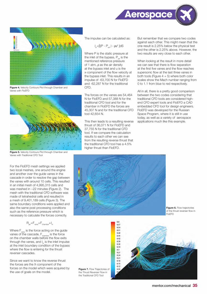
mentor.com/mechanical 35
Aerospace
For the FloEFD mesh settings we applied two local meshes, one around the engine and another over the guide vanes in the cascade in order to resolve the gap between the vanes with around 10 cells. This resulted in an initial mesh of 4,995,315 cells and was meshed in ~22 minutes (Figure 2). The mesh with the traditional CFD software was made of tetrahedral cells and resulted in a mesh of 9,401,189 cells (Figure 3). The same boundary conditions were applied and also the same post processing conditions such as the reference pressure which is necessary to calculate the forces correctly.
Rjet=Fvane+Fchamber+Iin
Where Fvane is the force acting on the guide vanes of the cascade, Fchamber is the force on the chamber walls before the flow exits through the vanes, and Iin is the inlet impulse at the inlet boundary condition of the bypass where the flow is entering for the thrust reverser cascades.
Since we want to know the reverse thrust the forces are the X-component of the forces on the model which were acquired by the use of goals on the model.
The impulse can be calculated as:
Iin=∫[(P - Pref ) - ρu2 ]dS
Where P is the static pressure at the inlet of the bypass, Pref is the mentioned reference pressure of 1 atm, ρ as the air density at the bypass inlet and u is the x-component of the flow velocity at the bypass inlet. This results in an impulse of -63,700 N for FloEFD and -62,287 N for the traditional CFD.
The forces on the vanes are 54,464 N for FloEFD and 57,388 N for the traditional CFD tool and for the chamber in FloEFD the forces are 45,307 N and for the traditional CFD tool 42,654 N.
This then leads to a resulting reverse thrust of 36,071 N for FloEFD and 37,755 N for the traditional CFD tool. If we compare the calculation results to each other we can see from the resulting reverse thrust that the traditional CFD tool has a 4.5% higher thrust than FloEFD.
But remember that we compare two codes against each other. This might mean that the one result is 2.25% below the physical test and the other is 2.25% above. However, the two results are very close to each other.
When looking at the result in more detail we can see that there is flow separation at the first five vanes and the flow reaches supersonic flow at the last three vanes in both tools (Figure 4 + 5) where both color scales show the Mach number ranging from 0 to 1.1 from blue to red respectively.
All in all, there is a pretty good comparison between the two codes considering that traditional CFD tools are considered high-end CFD expert tools and FloEFD a CAD embedded CFD tool for design engineers. FloEFD was developed for the Russian Space Program, where it is still in use today, as well as a variety of aerospace applications much like this example.
Figure 4. Velocity Contours Plot through Chamber and Vanes with FloEFD
Figure 5. Velocity Contours Plot through Chamber and Vanes with Traditional CFD Tool
Figure 6. Flow trajectories of the thrust reverser flow in FloEFD
Figure 7. Flow Trajectories of the Thrust Reverser Flow in the Traditional CFD Tool
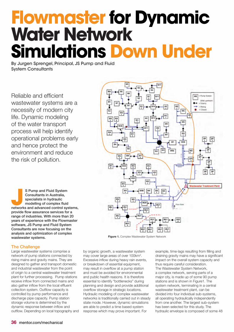
36 mentor.com/mechanical
J S Pump and Fluid System Consultants in Australia, specialists in hydraulic modelling of complex fluid
networks and advanced control systems, provide flow assurance services for a range of industries. With more than 20 years of experience with the Flowmaster software, JS Pump and Fluid System Consultants are now focusing on the analysis and optimization of complex wastewater systems.
The ChallengeLarge wastewater systems comprise a network of pump stations connected by rising mains and gravity mains. They are designed to gather and transport domestic and industrial wastewater from the point of origin to a central wastewater treatment plant for further processing. Pump stations receive inflow from connected mains and also gather inflow from the local effluent collection system. Outflow capacity is controlled by pump performance and discharge pipe capacity. Pump station storage volume is determined by the dynamic response between inflow and outflow. Depending on local topography and
By Jurgen Sprengel, Principal, JS Pump and Fluid System Consultants
Reliable and efficient wastewater systems are a necessity of modern city life. Dynamic modeling of the water transport process will help identify operational problems early and hence protect the environment and reduce the risk of pollution.
Flowmaster for Dynamic Water Network Simulations Down Under
by organic growth, a wastewater system may cover large areas of over 100km2. Excessive inflow during heavy rain events, or breakdown of essential equipment, may result in overflow at a pump station and must be avoided for environmental and public health reasons. It is therefore essential to identify “bottlenecks” during planning and design and provide additional overflow storage in strategic locations.Hydraulic modeling of complex wastewater networks is traditionally carried out in steady state mode. However, dynamic simulations are able to predict a time based system response which may prove important. For
example, time-lags resulting from filling and draining gravity mains may have a significant impact on the overall system capacity and thus require careful consideration. The Wastewater System Network,a complex network, serving parts of a major city, is made up of some 90 pump stations and is shown in Figure1. The system network, terminating in a central wastewater treatment plant, can be divided into four individual sub-systems, all operating hydraulically independently from one another. The largest sub-system has been selected for this study. The hydraulic envelope is composed of some 48
Figure 1. Complex Wastewater System Network
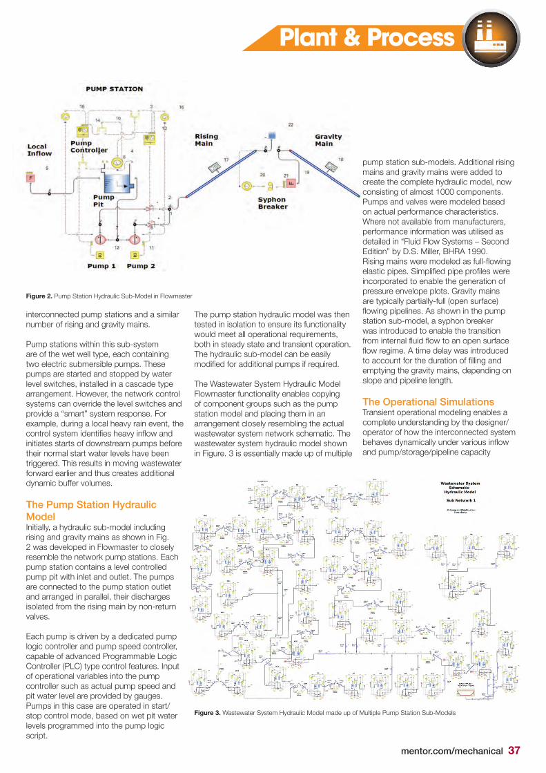
mentor.com/mechanical 37
Plant & Process
interconnected pump stations and a similar number of rising and gravity mains.
Pump stations within this sub-system are of the wet well type, each containing two electric submersible pumps. These pumps are started and stopped by water level switches, installed in a cascade type arrangement. However, the network control systems can override the level switches and provide a “smart” system response. For example, during a local heavy rain event, the control system identifies heavy inflow and initiates starts of downstream pumps before their normal start water levels have been triggered. This results in moving wastewater forward earlier and thus creates additional dynamic buffer volumes.
The Pump Station Hydraulic Model Initially, a hydraulic sub-model including rising and gravity mains as shown in Fig. 2 was developed in Flowmaster to closely resemble the network pump stations. Each pump station contains a level controlled pump pit with inlet and outlet. The pumps are connected to the pump station outlet and arranged in parallel, their discharges isolated from the rising main by non-return valves.
Each pump is driven by a dedicated pump logic controller and pump speed controller, capable of advanced Programmable Logic Controller (PLC) type control features. Input of operational variables into the pump controller such as actual pump speed and pit water level are provided by gauges. Pumps in this case are operated in start/stop control mode, based on wet pit water levels programmed into the pump logic script.
The pump station hydraulic model was then tested in isolation to ensure its functionality would meet all operational requirements, both in steady state and transient operation. The hydraulic sub-model can be easily modified for additional pumps if required.
The Wastewater System Hydraulic Model Flowmaster functionality enables copying of component groups such as the pump station model and placing them in an arrangement closely resembling the actual wastewater system network schematic. The wastewater system hydraulic model shown in Figure. 3 is essentially made up of multiple
pump station sub-models. Additional rising mains and gravity mains were added to create the complete hydraulic model, now consisting of almost 1000 components. Pumps and valves were modeled based on actual performance characteristics. Where not available from manufacturers, performance information was utilised as detailed in “Fluid Flow Systems – Second Edition” by D.S. Miller, BHRA 1990. Rising mains were modeled as full-flowing elastic pipes. Simplified pipe profiles were incorporated to enable the generation of pressure envelope plots. Gravity mains are typically partially-full (open surface) flowing pipelines. As shown in the pump station sub-model, a syphon breaker was introduced to enable the transition from internal fluid flow to an open surface flow regime. A time delay was introduced to account for the duration of filling and emptying the gravity mains, depending on slope and pipeline length.
The Operational SimulationsTransient operational modeling enables a complete understanding by the designer/operator of how the interconnected system behaves dynamically under various inflow and pump/storage/pipeline capacity
Figure 2. Pump Station Hydraulic Sub-Model in Flowmaster
Figure 3. Wastewater System Hydraulic Model made up of Multiple Pump Station Sub-Models
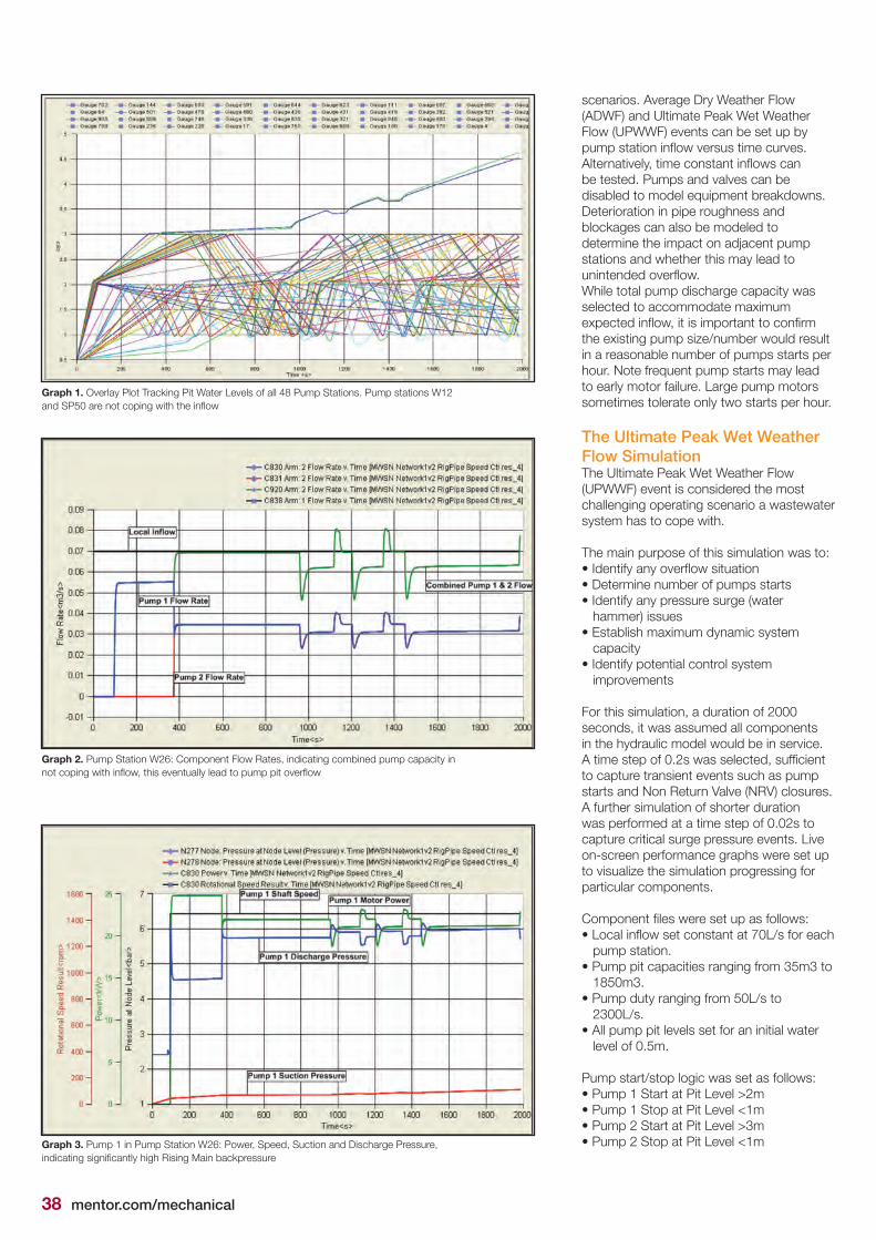
38 mentor.com/mechanical
scenarios. Average Dry Weather Flow (ADWF) and Ultimate Peak Wet Weather Flow (UPWWF) events can be set up by pump station inflow versus time curves. Alternatively, time constant inflows can be tested. Pumps and valves can be disabled to model equipment breakdowns. Deterioration in pipe roughness and blockages can also be modeled to determine the impact on adjacent pump stations and whether this may lead to unintended overflow.While total pump discharge capacity was selected to accommodate maximum expected inflow, it is important to confirm the existing pump size/number would result in a reasonable number of pumps starts per hour. Note frequent pump starts may lead to early motor failure. Large pump motors sometimes tolerate only two starts per hour.
The Ultimate Peak Wet Weather Flow SimulationThe Ultimate Peak Wet Weather Flow (UPWWF) event is considered the most challenging operating scenario a wastewater system has to cope with.
The main purpose of this simulation was to:• Identify any overflow situation• Determine number of pumps starts• Identify any pressure surge (water hammer) issues• Establish maximum dynamic system capacity• Identify potential control system improvements
For this simulation, a duration of 2000 seconds, it was assumed all components in the hydraulic model would be in service. A time step of 0.2s was selected, sufficient to capture transient events such as pump starts and Non Return Valve (NRV) closures. A further simulation of shorter duration was performed at a time step of 0.02s to capture critical surge pressure events. Live on-screen performance graphs were set up to visualize the simulation progressing for particular components. Component files were set up as follows:• Local inflow set constant at 70L/s for each pump station.• Pump pit capacities ranging from 35m3 to 1850m3.• Pump duty ranging from 50L/s to 2300L/s.• All pump pit levels set for an initial water level of 0.5m.
Pump start/stop logic was set as follows:• Pump 1 Start at Pit Level >2m• Pump 1 Stop at Pit Level <1m• Pump 2 Start at Pit Level >3m• Pump 2 Stop at Pit Level <1m
Graph 1. Overlay Plot Tracking Pit Water Levels of all 48 Pump Stations. Pump stations W12 and SP50 are not coping with the inflow
Graph 2. Pump Station W26: Component Flow Rates, indicating combined pump capacity in not coping with inflow, this eventually lead to pump pit overflow
Graph 3. Pump 1 in Pump Station W26: Power, Speed, Suction and Discharge Pressure, indicating significantly high Rising Main backpressure
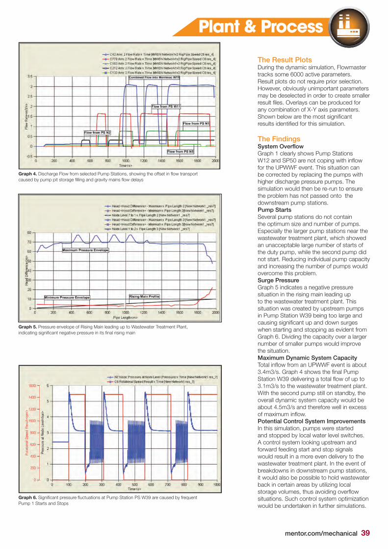
mentor.com/mechanical 39
The Result PlotsDuring the dynamic simulation, Flowmaster tracks some 6000 active parameters. Result plots do not require prior selection. However, obviously unimportant parameters may be deselected in order to create smaller result files. Overlays can be produced for any combination of X-Y axis parameters. Shown below are the most significant results identified for this simulation.
The FindingsSystem Overflow Graph 1 clearly shows Pump Stations W12 and SP50 are not coping with inflow for the UPWWF event. This situation can be corrected by replacing the pumps with higher discharge pressure pumps. The simulation would then be re-run to ensure the problem has not passed onto the downstream pump stations. Pump StartsSeveral pump stations do not contain the optimum size and number of pumps. Especially the larger pump stations near the wastewater treatment plant, which showed an unacceptable large number of starts of the duty pump, while the second pump did not start. Reducing individual pump capacity and increasing the number of pumps would overcome this problem.Surge Pressure Graph 5 indicates a negative pressure situation in the rising main leading up to the wastewater treatment plant. This situation was created by upstream pumps in Pump Station W39 being too large and causing significant up and down surges when starting and stopping as evident from Graph 6. Dividing the capacity over a larger number of smaller pumps would improve the situation.Maximum Dynamic System CapacityTotal inflow from an UPWWF event is about 3.4m3/s. Graph 4 shows the final Pump Station W39 delivering a total flow of up to 3.1m3/s to the wastewater treatment plant. With the second pump still on standby, the overall dynamic system capacity would be about 4.5m3/s and therefore well in excess of maximum inflow.Potential Control System Improvements In this simulation, pumps were started and stopped by local water level switches. A control system looking upstream and forward feeding start and stop signals would result in a more even delivery to the wastewater treatment plant. In the event of breakdowns in downstream pump stations, it would also be possible to hold wastewater back in certain areas by utilizing local storage volumes, thus avoiding overflow situations. Such control system optimization would be undertaken in further simulations.
Plant & Process
Graph 4. Discharge Flow from selected Pump Stations, showing the offset in flow transport caused by pump pit storage filling and gravity mains flow delays
Graph 5. Pressure envelope of Rising Main leading up to Wastewater Treatment Plant, indicating significant negative pressure in its final rising main
Graph 6. Significant pressure fluctuations at Pump Station PS W39 are caused by frequent Pump 1 Starts and Stops

40 mentor.com/mechanical
G uy Diemunsch’s interest in thermal design started while he was preparing his PhD in Physics. He taught how to
build comfortable, low energy homes and buildings in the University of Franche-Comté located in Besancon in the 1980’s. In 1994 he joined Hewlett Packard to manage the thermal design of HP’s range of professional PCs and workstations, where the challenge was to make their operation silent for the European market. In 2002 Guy joined Schneider Electric to optimize the thermal design of high-end UPS (MGE-UPS). Cost reduction was a major objective and this got Guy involved in power electronics. Five years later Guy was invited to join Aavid Thermalloy, a supplier to Schneider Electric, to extend Aavid Thermalloy’s business in Power Electronics. Guy joined Electronic Cooling Solutions Inc. at the beginning of 2013.
I met Guy Diemunsch at THERMINIC in Berlin September 2014 we talked about some work he was doing on cooling IGBTs for high power inverters & converters used in renewable energy applications (wind turbines & photovoltaic power plants), drives and electric networks.
Back in 1994, Guy first came across the challenge of minimizing the temperature difference between different components when he was working on a computer cooling problem for Hewlett Packard. Twenty years on Guy was now faced with the same challenge, this time for a power electronics application cooling IGBTs as a project for a customer of Electronic Cooling Solutions.
Their initial design gave an unacceptable temperature variation between three IGBT modules. To ensure the efficiency of the system was not impacted it was necessary to hold the temperature of the modules to
By John Parry, Industry Manager, Mentor Graphics
Managing Temperature Differences Between IGBT Modules
needed for cooling. Therefore in most cases the focus is on optimizing a serial cooling solution to keep this flow rate as low as possible, with the same air being passed over several components. If however, the aim is to keep components at the same temperature, a very high volume of air flow would be required, so that the temperature rise in the air as it flows through the system is very low, such that all components are cooled by air at the same temperature.As an example, for temperature difference
within 2°C of each other, otherwise the operational performance of the modules would be too different.
Faced with this challenge, a choice would need to be made between air, water, or phase change cooling. The best option depends on how well the chosen solution allows the temperature level and uniformity to be controlled while managing the mass flow and preheating of the cooling fluid.
Phase change cooling is a great solution to reduce the temperature difference between components; however, this solution is often the most expensive when compared with air cooling with a heatsink or water cooling with a Liquid Cold Plate (LCP). Therefore Guy chose to focus his attention on using air or water cooling to control temperature.
The most obvious solution is to arrange to bring the same amount of cooling fluid at the same temperature to each identical component. There are at least two such examples in liquid cooling applied to Power Electronics: the ShowerPower® solution from Danfoss Silicon Power and the parallel cooling patent from Schneider Electric.
With the continuous increase of the system density, thermal and system engineers are very keen to minimize total flow rate
Figure 1. Preliminary Air Cooling (Heatsink) Design
Figure 2. Preliminary Water Cooling (LCP) Design

mentor.com/mechanical 41
below 2°C, for three components generating 500 W per IGBT, serial cooling will then require more cooling fluid than parallel cooling. Is it therefore necessary to use parallel cooling? Guy realized the answer is no, because he can increase the cooling performance of the heatsink for each successive IGBT to account for the increase in air temperature passing over it.To accomplish this from a purely thermal standpoint, each IGBT could have its own heatsink design, and this would be the easiest arrangement to optimize. This solution would increase the Bill of Materials (BoM) and increase assembly costs. However, the most compelling reason for not choosing this approach is the risk of wrong assembly. As the risk of wrong heat sink placement is both high and critical for the system, this is forbidden in all risk analysis. The avoidance of this issue through design would increase the manufacturing and assembly costs substantially.
To solve the problem, Guy created a single heatsink designed to allow the thermal resistance to vary in the flow direction. The constraints imposed by such a design are:• Cooling fluid must be ducted to keep a constant mass flow between chips,• Components must be grouped together.
The two preliminary designs are shown, without the ducts visible, in Figures 1 and 2.
The initial reaction of the customer was that the design of these solutions is complex, so they were concerned that it would be necessary to do many design iterations that may not arrive at an acceptable final solution.
Guy was able to assure them that it would be possible to converge on an acceptable design in two or three iterations by applying the following simple process:Step 1: Define the most critical (i.e. lowest) thermal resistance needed and search for an existing heatsink design that will meet this duty and note the mass flow rate associated with it (A), Step 2: Define the flow rate (B) needed considering the max temperature of the cooling fluid at the intake.Step 3: Iterate 1 & 2 until the two mass flow rates (i.e. A & B) are very close.Step 4: Define each local thermal resistance which is always possible because we have already defined the lowest thermal resistance in Step 1.
Step 5: Validate the solution using simulation.
The solution that Guy arrived at is shown in Figures 3, 4, and 5 where he used FloTHERM XT to simulate the current heat transfer in the cooling channels. The total power is 1.5 kW (500 W per IGBT module). The heatsink is cooled by water with 30% of Glycol. The fluid intake temperature is set to the maximum of 45°C.With 15 g/s of fluid the pressure drop of 22 Pa (0.09 inch H2O) and an average fluid speed of 0.03 m/s, low enough to ensure there is no erosion even with Aluminum. The total temperature elevation of the fluid is 30°C. The three thermal resistances (from the right to the left) are 0.12, 0.10 & 0.08 °C/W.This detailed analysis showed that within each module the average difference between chips in the direction of the flow is 1.6 °C. This arises from the fins being uniform below each IGBT, while as fluid passes through each finned region the boundary layer thickens. The worst case is for the chips in the top and bottom corners on the right in the above plots where the temperature difference is up to 2.9°C. This boundary layer effect was corrected in a subsequent design refinement.
We also see fluid bypasses between fins for the first IGBT. During the design process fin spacing was optimized in laminar & turbulent flow regimes. In fact if the gap is too large the fluid in the middle of the fins is not heated. If the gap is too small, the pressure drop is increased without a corresponding improvement in heat transfer. Another observation Guy made was that within the IGBT modules the temperature difference between the central ICs and those at the edge were up to 7.5°C. This is related to the layout and the module and the packaging design, neither of which were under Guy’s control. Again, this can
be corrected through refinements to the LCP fin design. However, this improvement will require nonstandard folded fins manufacturing, which might not be cost effective.
In conclusion, with care, serial cooling can be used even when it is necessary to respect tight design criteria for temperature differences between components and chips. Using a simple design process it is possible to meet the design goal for temperature control while using a low flow rate with a correspondingly low pressure drop. This maximizes the energy efficiency of the cooling solution.
Figure 3. Chips Temperatures (Liquid Flow from Right to Left)
Figure 4. Fluid Speeds
Figure 5. Fluid Temperatures
Power Electronics

42 mentor.com/mechanical
W ipro Ltd is a global information technology, consulting and outsourcing company with
145,000 employees serving over 900 clients in 61 countries, headquartered in Bangalore, Karnataka, India. Wipro’s Engineering Design Services Group has over 400 experienced professionals with expertise in advanced materials, CAD and CAE tool customization and competence in design, analysis prototyping and testing, covering thermal, vibration, acoustic and shock.
Heat Pipe Heatsink Design in a Wipro Ltd. 3U High-End Server
Two fans were chosen for evaluation. When compared, the components performed almost identically in terms of airflow and so as expected were found to perform the same from a thermal perspective. Therefore, the only further considerations in the evaluation to be made were cost, efficiency, and lifetime. All things considered, this led to the selection of Fan B, which produced slightly less noise and consumed less power.
Having selected Fan B, the impact of fan failure on critical component
under the vendor’s specified junction temperature limit of 96°C for power dissipation, 155W per COMP. This involved pairing the heatsink with a duct design that would ensure a uniform airflow through each COMP for any fan failed condition with minimum pressure drop.
Wipro selected two heatsinks for comparison. The first, heatsink A, is fabricated from copper. Wipro performed flowrate vs pressure drop measurements on the heatsink in order to accurately include it in the FloTHERM model, and found that
Wipro’s team of experts were contracted to provide the thermal design for a 1.5kW, 3U server with a predefined form factor for the enclosure. The system would contain multiple fans, and was required to work when one fan failed (N+1 active-active resilience) to meet operational reliability requirements. Within this specification Wipro were required to perform fan selection and ducting design to optimize the airflow.
temperatures within the system was studied. Using FloTHERM to fail each fan in turn, to examine the impact on system temperatures, revealed that for all fan failed cases the component temperatures remained acceptable.
A key challenge Wipro faced was selecting a heatsink for the two COMPs that would keep the processor junction temperature
a pressure drop of 0.18 inch of H2O is required to deliver the minimum airflow of 33.5CFM.
An alternate, heatsink B, fabricated from aluminum was also measured and its performance in the system simulated. Despite the cost and weight advantages of using aluminium, heatsink B was found not to be suitable for the application. Although it resulted in just over a 3°C increase in temperature, this almost halved the thermal margin for the design from 6.8°C to 3.6°C.
For the IC critical component, which was offset from the main airflow path, a heat pipe was needed to carry heat away from the chip to keep the IC’s junction temperature under the vendor specified junction temperature limit of 105°C at power dissipation 50W. Wipro investigated different designs of chiller block to compare

mentor.com/mechanical 43
By John Parry, Industry Manager, Mentor Graphics
2 x 6mm, 3 x 6mm and 2 x 8mm diameter heat pipe configurations, that connected to a finned region directly behind the COMP’s heatsinks. Simulation showed that the best arrangement was to use 2 x 180mm long 8mm diameter heat pipes with 46 fins and a 3mm fin spacing, which reduced the junction temperature down to 96°C.
When the prototype was built, Wipro found there was only an ~8% variation in airflow rate from simulation to validation, with the measured airflow being lower, due to extra resistance created from the cables inside the system which were ignored in the simulation. This is well within the design margin, experimental uncertainty and fully met the client’s expectations.
Figure 1. FloTHERM Model of Heatsink A in 40 Million Cell System Model (1.2 Million Cells within Heatsink with 5 Cells per Fin Channel)
Figure 2. Detail of Heat Pipe Design for IC
Figure 3. Detail of Heat Pipe Design for IC
Figure 4. Final Simulation Model
Figure 5. Final Model Accuracy Validated Against Experiment(*calculated Tj based on measured case temperature and junction to case thermal resistance).
Electronics
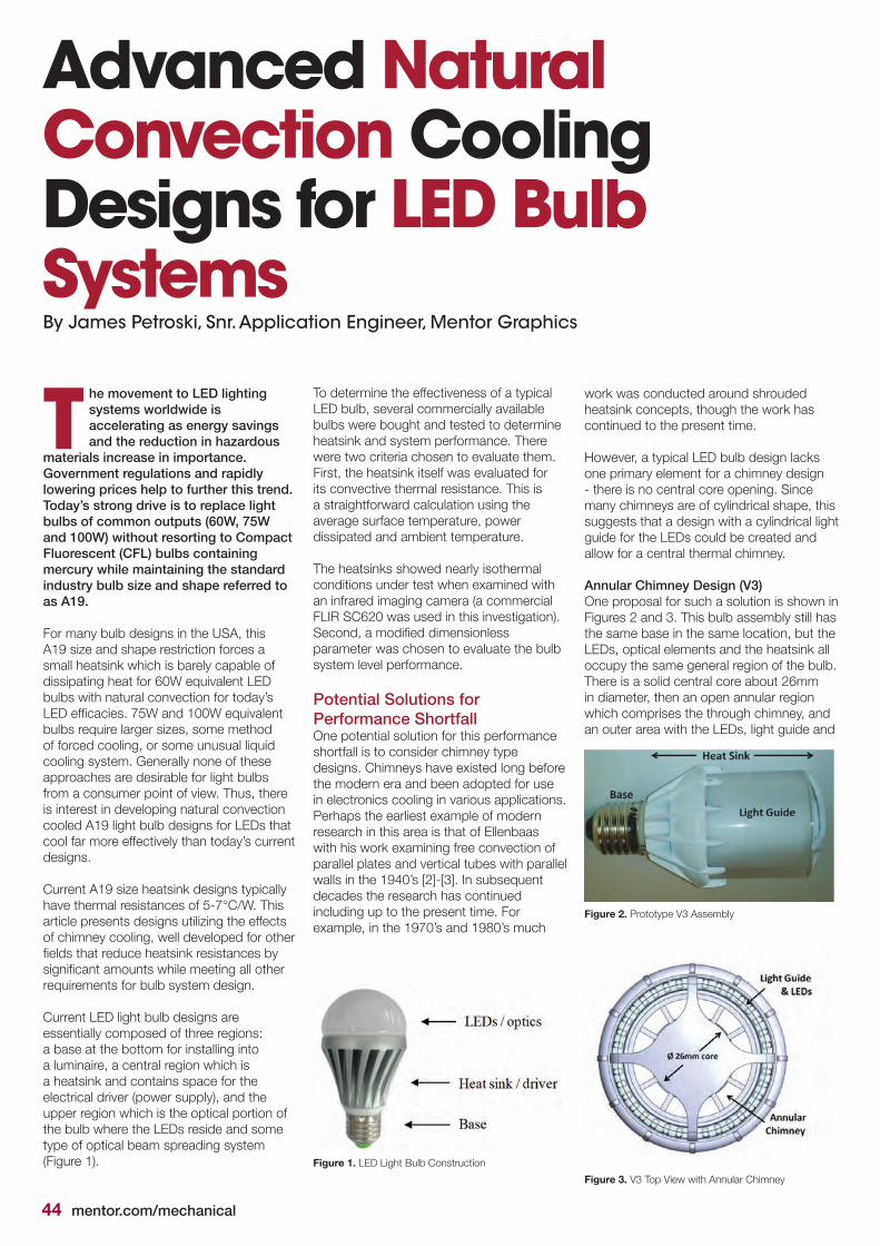
44 mentor.com/mechanical
Advanced Natural Convection Cooling Designs for LED Bulb SystemsBy James Petroski, Snr. Application Engineer, Mentor Graphics
T he movement to LED lighting systems worldwide is accelerating as energy savings and the reduction in hazardous
materials increase in importance. Government regulations and rapidly lowering prices help to further this trend. Today’s strong drive is to replace light bulbs of common outputs (60W, 75W and 100W) without resorting to Compact Fluorescent (CFL) bulbs containing mercury while maintaining the standard industry bulb size and shape referred to as A19.
For many bulb designs in the USA, this A19 size and shape restriction forces a small heatsink which is barely capable of dissipating heat for 60W equivalent LED bulbs with natural convection for today’s LED efficacies. 75W and 100W equivalent bulbs require larger sizes, some method of forced cooling, or some unusual liquid cooling system. Generally none of these approaches are desirable for light bulbs from a consumer point of view. Thus, there is interest in developing natural convection cooled A19 light bulb designs for LEDs that cool far more effectively than today’s current designs.
Current A19 size heatsink designs typically have thermal resistances of 5-7°C/W. This article presents designs utilizing the effects of chimney cooling, well developed for other fields that reduce heatsink resistances by significant amounts while meeting all other requirements for bulb system design.
Current LED light bulb designs are essentially composed of three regions: a base at the bottom for installing into a luminaire, a central region which is a heatsink and contains space for the electrical driver (power supply), and the upper region which is the optical portion of the bulb where the LEDs reside and some type of optical beam spreading system (Figure 1). Figure 1. LED Light Bulb Construction
To determine the effectiveness of a typical LED bulb, several commercially available bulbs were bought and tested to determine heatsink and system performance. There were two criteria chosen to evaluate them. First, the heatsink itself was evaluated for its convective thermal resistance. This is a straightforward calculation using the average surface temperature, power dissipated and ambient temperature.
The heatsinks showed nearly isothermal conditions under test when examined with an infrared imaging camera (a commercial FLIR SC620 was used in this investigation).Second, a modified dimensionless parameter was chosen to evaluate the bulb system level performance.
Potential Solutions for Performance ShortfallOne potential solution for this performance shortfall is to consider chimney type designs. Chimneys have existed long before the modern era and been adopted for use in electronics cooling in various applications. Perhaps the earliest example of modern research in this area is that of Ellenbaas with his work examining free convection of parallel plates and vertical tubes with parallel walls in the 1940’s [2]-[3]. In subsequent decades the research has continued including up to the present time. For example, in the 1970’s and 1980’s much
work was conducted around shrouded heatsink concepts, though the work has continued to the present time.
However, a typical LED bulb design lacks one primary element for a chimney design - there is no central core opening. Since many chimneys are of cylindrical shape, this suggests that a design with a cylindrical light guide for the LEDs could be created and allow for a central thermal chimney.
Annular Chimney Design (V3)One proposal for such a solution is shown in Figures 2 and 3. This bulb assembly still has the same base in the same location, but the LEDs, optical elements and the heatsink all occupy the same general region of the bulb. There is a solid central core about 26mm in diameter, then an open annular region which comprises the through chimney, and an outer area with the LEDs, light guide and
Figure 2. Prototype V3 Assembly
Figure 3. V3 Top View with Annular Chimney

mentor.com/mechanical 45
LED Lighting
other support structure. The entire assembly fits within the A19 envelope defined by the ANSI standard. This particular design was designated prototype V3 (version 3).
As seen in Figure 2, a prototype bulb was constructed. The main heatsink was made by the lost wax casting process with a standard aluminum casting alloy. Other parts except the base were machined, and different printed circuit boards (PCBs) were created for different testing conditions. Two types of PCBs were created: one with actual LEDs, and a second with surface mount resistors. The latter design allowed for more accurate measurement of thermal input energy. LEDs can be used but accurately knowing the thermal input energy is difficult; one must accurately measure the radiometric light output energy for an input electrical energy to measure the difference, and light energy can be reabsorbed into the system and become an input load.
The V3 design was tested to understand overall system performance and compared to computational fluid dynamics (CFD) numerical solutions using FloEFD™.
CFD simulations were conducted to correlate to the various tests. In the vertical orientations, about 150,000 cells were used and horizontally about 100,000 cells were used. Sufficient room above and below
the lamp (as defined by the gravity vector) is used for proper flow development, and one bulb diameter around the sides was adequate for spacing around the bulb without influencing results unduly. Mesh sensitivity studies were conducted primarily by increasing the number of partial cells FloEFD uses, which refines the mesh around the fluid to solid boundaries (partial cells are part solid, part fluid and a unique cell used by FloEFD). Maximum cell counts of five to six hundred thousand cells were solved and compared to coarser meshes; results were found to be 0.1 to 0.2°C different from the coarser meshes so the coarser meshes were deemed acceptable. In all CFD simulations, radiation was selected as part of the solution routine. The heatsinks were painted with a special white paint and the emissivity was measured to be 0.975 on both the heatsinks and a special flat panel painted sample.
A few pertinent observations should be made from these results. First, the thermocouple used to measure the outside heatsink temperature in the Vertical Up orientation was not attached properly and is quite sensitive in this orientation (the “*” entry in Table 1). Although this was found later, the test was not repeated though in other orientations the thermocouples gave reliable results. Other temperature differences are within instrument errors. Second, there is a noticeable improvement in the heatsink thermal resistance (nearly 20% better than any of the commercial bulbs tested). Third, horizontal performance
is worse – not surprizing, since chimneys are meant for vertical operation. As seen in Figure 5, angles from 45° to 0° showed significant increases in temperature for the heatsink (0° indicates horizontal, and 90° is vertical up). This graph is based on the verified CFD model dissipating higher power levels at these angles. Variations between vertical (90°)
and tipped to 45° showed only modest increases in overall thermal resistance.
Other variations of this V3 design were modeled to see how much improvement could be made over this design. They included varying the number of internal fins in the annular chimney and varying the fin height.
Chambered Design with Annular Chimney (V6)Given the limitations of the V3 design, another solution was sought. The vertical solutions needed to be better, and some method to improve the horizontal system performance would be needed for bulbs with higher power levels than used for tests in V3.
An advanced chimney system was devised and prototyped, still remaining within the design outline of an A19 bulb. This system involves a unique chamber internal to the chimney yet is open to the lamp bottom, sides and top. The annular chimney is thus split into separate chimneys – in this case, the “Y” shaped chamber creates the three of them – to allow the chamber access to the various sides of the bulb. This heatsink geometry is shown in Figures 6 and 7. Test results at 11.9W of thermal power showed that the V6 heatsink thermal resistance is 4.0°C/W. This is an improvement of 13% over the V3 performance at a similar power input. It is
Figure 4. CFD Image of V3 Horizontal Position
Table 1. CFD Image of V3 Horizontal Position
Figure 5. V3 Design Orientation Sensitivity
Figure 6. Prototype V6 Assembly
Figure 7. V6 Heatsink Detail
Test Case Location T/C IR Image CFD
Vert Up Outer HS *see text 73.7 73.6 Chimney 71.6 n/a 72.5
Vert Down Outer HS 74.4 75.2 74.4 Chimney 71.3 n/a 73.0
Horizontal Outer HS 78.1 80.7 80.1 Chimney 75.9 n/a 78.6
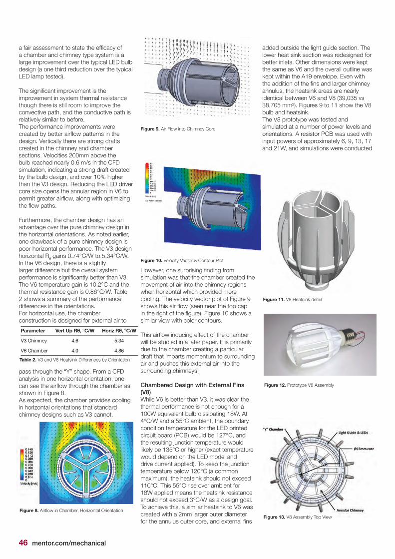
46 mentor.com/mechanical
a fair assessment to state the efficacy of a chamber and chimney type system is a large improvement over the typical LED bulb design (a one third reduction over the typical LED lamp tested).
The significant improvement is the improvement in system thermal resistance though there is still room to improve the convective path, and the conductive path is relatively similar to before.The performance improvements were created by better airflow patterns in the design. Vertically there are strong drafts created in the chimney and chamber sections. Velocities 200mm above the bulb reached nearly 0.6 m/s in the CFD simulation, indicating a strong draft created by the bulb design, and over 10% higher than the V3 design. Reducing the LED driver core size opens the annular region in V6 to permit greater airflow, along with optimizing the flow paths.
Furthermore, the chamber design has an advantage over the pure chimney design in the horizontal orientations. As noted earlier, one drawback of a pure chimney design is poor horizontal performance. The V3 design horizontal Rθ gains 0.74°C/W to 5.34°C/W. In the V6 design, there is a slightly larger difference but the overall system performance is significantly better than V3. The V6 temperature gain is 10.2°C and the thermal resistance gain is 0.86°C/W. Table 2 shows a summary of the performance differences in the orientations.For horizontal use, the chamber construction is designed for external air to
Table 2. V3 and V6 Heatsink Differences by Orientation
pass through the “Y” shape. From a CFD analysis in one horizontal orientation, one can see the airflow through the chamber as shown in Figure 8. As expected, the chamber provides cooling in horizontal orientations that standard chimney designs such as V3 cannot.
Figure 8. Airflow in Chamber, Horizontal Orientation
However, one surprising finding from simulation was that the chamber created the movement of air into the chimney regions when horizontal which provided more cooling. The velocity vector plot of Figure 9 shows this air flow (seen near the top cap in the right of the figure). Figure 10 shows a similar view with color contours.
This airflow inducing effect of the chamber will be studied in a later paper. It is primarily due to the chamber creating a particular draft that imparts momentum to surrounding air and pushes this external air into the surrounding chimneys.
Chambered Design with External Fins (V8)While V6 is better than V3, it was clear the thermal performance is not enough for a 100W equivalent bulb dissipating 18W. At 4°C/W and a 55°C ambient, the boundary condition temperature for the LED printed circuit board (PCB) would be 127°C, and the resulting junction temperature would likely be 135°C or higher (exact temperature would depend on the LED model and drive current applied). To keep the junction temperature below 120°C (a common maximum), the heatsink should not exceed 110°C. This 55°C rise over ambient for 18W applied means the heatsink resistance should not exceed 3°C/W as a design goal.To achieve this, a similar heatsink to V6 was created with a 2mm larger outer diameter for the annulus outer core, and external fins
Figure 9. Air Flow into Chimney Core
Figure 10. Velocity Vector & Contour Plot
added outside the light guide section. The lower heat sink section was redesigned for better inlets. Other dimensions were kept the same as V6 and the overall outline was kept within the A19 envelope. Even with the addition of the fins and larger chimney annulus, the heatsink areas are nearly identical between V6 and V8 (39,035 vs 38,705 mm²). Figures 9 to 11 show the V8 bulb and heatsink. The V8 prototype was tested and simulated at a number of power levels and orientations. A resistor PCB was used with input powers of approximately 6, 9, 13, 17 and 21W, and simulations were conducted
Figure 11. V8 Heatsink detail
Figure 12. Prototype V8 Assembly
Figure 13. V8 Assembly Top View
Parameter Vert Up Rθ, °C/W Horiz Rθ, °C/W
V3 Chimney 4.6 5.34
V6 Chamber 4.0 4.86

mentor.com/mechanical 47
with 9, 13 and 21W of input power. IR and thermocouple data were within 1.5°C for all tests. Simulation mesh dependency studies were conducted similar to the process described for V3 to ensure adequate mesh density for the simulations. Figures 14 and 15 show some of the test and simulation results. The V8 prototype performed significantly
Figure 14. CFD Simulation of V8 Vertical Up Test
Figure 15. Performance of V8 in Vertical Up Orientation
better than the V6 design. As seen in Figure 15, the results show reasonable agreement for the tests and the simulations. By performing an examination across a wider range of thermal input powers, a general performance diagram of the heatsink can be generated. Table 3 shows results for the vertical up orientation. The test data is the average of the thermocouple and the IR image data, and the error estimates based on the possible worst errors for the type of measurement. For each data set, a second order polynomial curve fit was applied and the equations shown.
A few important observations are found
from this performance chart. The simulation solutions are conservative compared to the actual tests though close to the upper end of the experimental error band. Small air currents in the lab may account for this as the simulation assumes perfectly still air. The outer fins are very effective at removing heat in the presence of low air currents. Second, the V8 design performance is a large improvement over the V6 design. At 11.9W of input power, the heatsink resistance is about 3.1°C/W, almost a 25% improvement in the vertical orientation. At the higher power levels for 100W equivalent bulbs (18W input), the heatsink tests just below 3°C/W, meeting the design target. Third, the two key changes in the V8 design account for the improved performance – the larger annular region (2mm larger outer diameter) and the fins. Simulations show the outer fins account for about 2/3 of the improvements, and the larger annular region the other 1/3.
The values for Table 3 use approximately 12W of input power for V3, V6 and V8 designs. The commercial LED lamps ranged from approximately 7W (40W equivalent bulb) to 13W (60W equivalent). Even as the
convective resistances of the new designs are an improvement over the commercial units tested, it is still a significantly higher resistance than the conductive resistance in the system. Finally, the horizontal performance of the V8 prototype is also significantly improved over the V6 design. The external fins provide significant new cooling paths in the horizontal orientation.
Table 3. Heatsink Differences by Orientation (12W power)
ConclusionsSeveral interesting results have been found during this study. First, the current design of LED bulbs performs adequately for the current power dissipations but will not be enough for future 75 and 100W equivalent bulbs. Second, rather than a standard central LED engine design, a cylindrical LED layout and light guide with a chimney enhances thermal performance and can still fit within the desired A19 design envelope. Last, a novel chimney and chamber design was developed for enhanced performance. Unusual air flows were noted as well in horizontal positions and will be evaluated in future work.
Though the V8 prototype design is far better than current designs, it is a bit marginal of a system that will adequately cool the 100W equivalent light bulb at 2.9°C/W. Future work will look at designs beyond the types shown in this paper (and beyond this paper’s scope) that again reduce the overall system thermal resistance – allowing a 100W natural convection cooled LED bulb to fit within the A19 envelope.
References:[1] Proceedings of the ASME 2013 International Technical Conference and Exhibition on Packaging and Integration of Electronic and Photonic MicrosystemsInterPACK2013 July 16-18, 2013, Burlingame, CA, USA[2] W. Ellenbaas, “The Dissipation of Heat by Free Convection from the Inner Surface of Vertical Tubes of Different Shapes of Cross Section,” Physica, 9, pp 865-874, Sept 1942.[3] W. Ellenbaas, “Heat Dissipation of Parallel Plates by Free Convection,” Physica, IX, No. 1, Jan 1942
LED Lighting
Parameter Vert Up Rθ, °C/W Horiz Rθ, °C/W
V3 Chimney 4.6 5.34
V6 Chamber 4.0 4.86
V8 Chamber 3.1 3.83

48 mentor.com/mechanical
Geek HubOur team are
passionate about all things CFD
and love sharing their findings. In this issue,
Student Intern, Adnan Nweilati demonstrates
the capabilities of FloTHERM XT® on
Google Glass™
s a part of my learning process as a student intern at Mentor Graphics, I was assigned to create some
application examples for FloTHERM® XT. The first application example I was given to create was the Google Glass. Since Google Glass was not officially released at that time, a physical model of it could not be obtained. Instead, I searched for pictures that included the inner parts of the glasses such as electronic board, battery, camera and other various small parts.
Fortunately, I found a company that purchase gadgets before the release and disassemble them. However, no dimensions were provided with the pictures. To obtain some basic dimensions of the Google Glass such as length, width and height, I had to take the dimensions of my medical glasses and add a few centimetres to the length since it can be seen that the Google Glass are slightly longer than the regular medical glasses. (My bad eye sight finally came to use).
A
Figure 1. Google Glass
Figure 2. Google Glass Components
Figure 3. CAD Representation of Google Glass Components
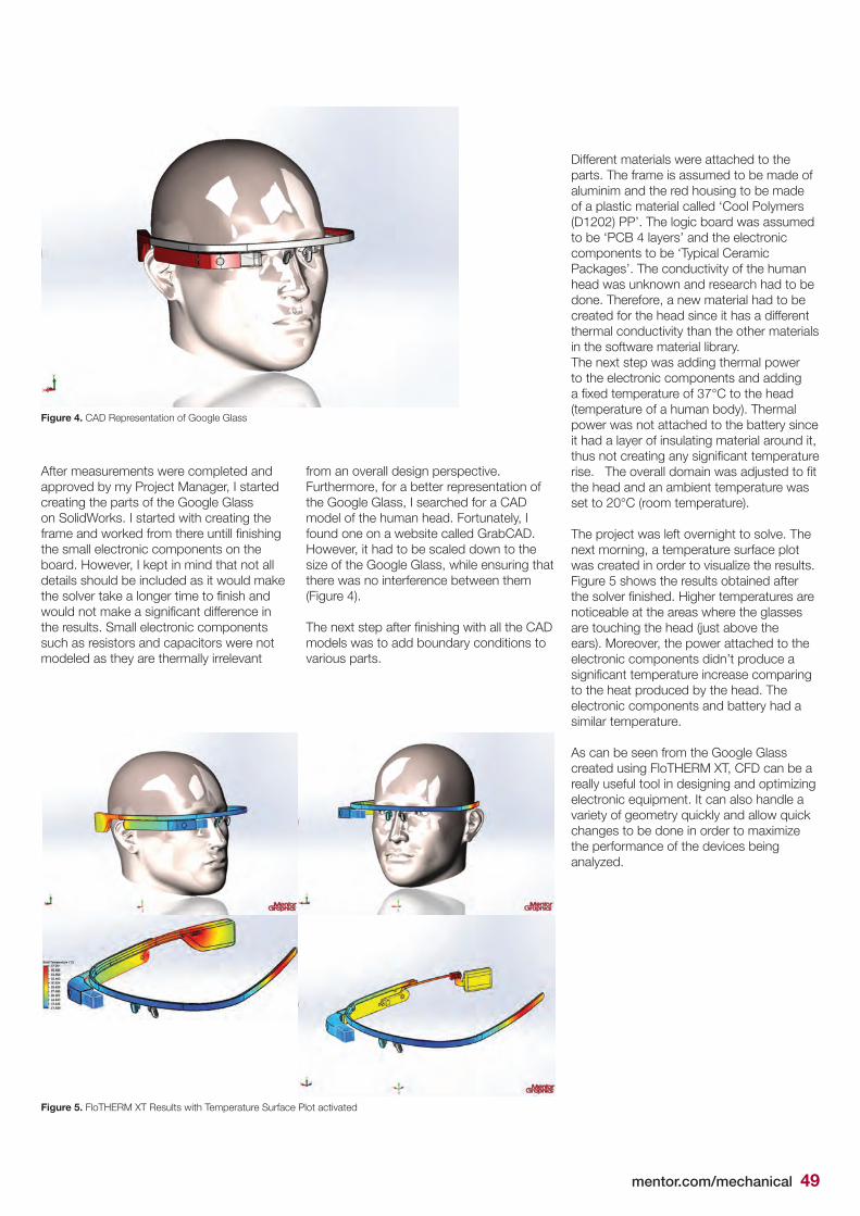
mentor.com/mechanical 49
After measurements were completed and approved by my Project Manager, I started creating the parts of the Google Glass on SolidWorks. I started with creating the frame and worked from there untill finishing the small electronic components on the board. However, I kept in mind that not all details should be included as it would make the solver take a longer time to finish and would not make a significant difference in the results. Small electronic components such as resistors and capacitors were not modeled as they are thermally irrelevant
Different materials were attached to the parts. The frame is assumed to be made of aluminim and the red housing to be made of a plastic material called ‘Cool Polymers (D1202) PP’. The logic board was assumed to be ‘PCB 4 layers’ and the electronic components to be ‘Typical Ceramic Packages’. The conductivity of the human head was unknown and research had to be done. Therefore, a new material had to be created for the head since it has a different thermal conductivity than the other materials in the software material library.The next step was adding thermal power to the electronic components and adding a fixed temperature of 37°C to the head (temperature of a human body). Thermal power was not attached to the battery since it had a layer of insulating material around it, thus not creating any significant temperature rise. The overall domain was adjusted to fit the head and an ambient temperature was set to 20°C (room temperature).
The project was left overnight to solve. The next morning, a temperature surface plot was created in order to visualize the results. Figure 5 shows the results obtained after the solver finished. Higher temperatures are noticeable at the areas where the glasses are touching the head (just above the ears). Moreover, the power attached to the electronic components didn’t produce a significant temperature increase comparing to the heat produced by the head. The electronic components and battery had a similar temperature.
As can be seen from the Google Glass created using FloTHERM XT, CFD can be a really useful tool in designing and optimizing electronic equipment. It can also handle a variety of geometry quickly and allow quick changes to be done in order to maximize the performance of the devices being analyzed.
Figure 4. CAD Representation of Google Glass
Figure 5. FloTHERM XT Results with Temperature Surface Plot activated
from an overall design perspective. Furthermore, for a better representation of the Google Glass, I searched for a CAD model of the human head. Fortunately, I found one on a website called GrabCAD. However, it had to be scaled down to the size of the Google Glass, while ensuring that there was no interference between them (Figure 4).
The next step after finishing with all the CAD models was to add boundary conditions to various parts.

50 mentor.com/mechanical
Brownian Motion...The random musings of a Fluid Dynamicist
learnt everything I need to know about Chaos Theory from Jurassic Park. So I don’t want to tread on the toes of either Jeff Goldbloom or
Lorenz when I offer my own summation: ‘I think you’ll find it’s a little more complicated than that’.
Unfortunately, as a species, we’re not well adapted to accept this fact. Perhaps with good reason, as actions can sometimes speak louder than words; just ask Glaswegian baggage handler and concerned citizen, John Smeaton. Not only did he think on his feet, he also realised that the solution was the percussive and committed use of one of them. More often than not though, scratching the surface reveals a more complicated situation than that which we might like to acknowledge.
Those of us who like to believe we’re of a scientific bent can be particularly guilty of overstating the value of logical thinking and reductionism. For a start, it’s an easy way to beat down your more ‘arty’ or ‘social sciency’ friends in arguments at parties. Culture? Feelings? Pfft.
Now try applying the same logic to the question of why you never get invited back to any of those parties. Exactly. What’s strange about this state of affairs is that a foundation of scientific thinking is
I
Brownian Motion or Pedesis (from Greek: πήδησις Pɛɖeːsɪs 'leaping') is the presumably random moving of particles suspended in a fluid (a liquid or a gas) resulting from their bombardment by the fast-moving atoms or molecules in the gas or liquid. The term 'Brownian Motion' can also refer to the mathematical model used to describe such random movements, which is often called a particle theory.
the ability to deal with complex systems and identify and understand all relevant parameters. Repeatable experiments depend upon it. In other words, engineers and scientists should be the masters at this. What’s more, there’s a reason beyond being the life and soul of the party for being better at this. The dangers of rapidly derived, simple (but wrong) solutions extend much further than an empty social calendar. Reducing every problem down makes for handy sound-bites and better yet, requires no wilful manipulation of the statistics. A simple misinterpretation of them or their worth will do nicely. Which is almost worse as it’s
something that can be done completely innocently. In other words, not only can others fool us; we can fool ourselves.
To my point then: if someone offers you a neat solution to a problem, just make sure that the control volume has been properly defined and that all independent variables are understood. Or, if you want to be a little less pompous (and to each to their own I suppose...), just hit them with ‘I think you’ll find it’s a little more complicated than that’ and wander off to find someone more interesting to talk to over by the cocktail sausages.Turbulent Eddy
Chaos TheoryAnd other Cocktail Party Conversation Topics

mentor.com/mechanical 51

52 mentor.com/mechanical
PLANT & PROCESS
POWERGENERATION
AUTOMOTIVE AEROSPACE
Test Drive Flowmaster and judge for yourself in the Flowmaster Virtual Lab go.mentor.com/flowmaster-vl*In a recent survey of 3500 Flowmaster users, nearly 90% of all respondents said that Flowmaster was as accurate as or more accurate than alternative thermo-fluid system solutions
Real Thermo-Fluid System Simulation
Users said Flowmaster is More Accurate than Alternative Solutions*9/10