Embed Size (px)
Citation preview

Purdue UniversityPurdue e-Pubs
ECE Technical Reports Electrical and Computer Engineering
12-1-1992
Energy Storage for Power Systems with RapidlyChanging LoadsPatrick G. LyonsPurdue University School of Electrical Engineering
Follow this and additional works at: http://docs.lib.purdue.edu/ecetr
This document has been made available through Purdue e-Pubs, a service of the Purdue University Libraries. Please contact [email protected] foradditional information.
Lyons, Patrick G., "Energy Storage for Power Systems with Rapidly Changing Loads" (1992). ECE Technical Reports. Paper 262.http://docs.lib.purdue.edu/ecetr/262
TR-EE 92-50 DECEMBER 1992

Energy Storage for Power Systems with Rapidly Changing Loads
Patrick G. Lyons
School of Electrical Engineering Purdue University
West Lafayette, IN 47907-1285


TABLE OF CONTENTS
Page
LIST OF TABLES ................................................................................. vi . . .............................................................................. LIST OF FIGURES VII
....................................................................................... ABSTRACT x i
CHAPTER 1 . INTRODUCTION ............................................................... 1
1.1 Motivation and Scope ....................................................................... 1 1.2 Reliability Criteria ........................................................................... 3 1.3 Automatic Generation Control ............................................................. 4 1.4 Energy Storage in Electric Utility Companies ............................................ 5 1.5 Energy Storage Devices ................................................................... - 8
............................................. 1.5.1 Pumped Hydroelectric Energy Storage - 9 ........................................ 1.5.2 Superconducting Magnetic Energy Storage 10
............................................................... 1 . 5.3 Battery Energy Storage 14
....................................................... CHAPTER 2 . SYSTEM MODELING -17
.............................................................................. 2.1 Overall Model 17 2.1.1 Dynamic System Model .............................................................. 17
...................................................................... 2.1.2 Governor Model 19 ....................................................... 2.1.3 Steam Turbine System Model 20
....................................................................... 2.1.4 Tie-Line Model 21 .............................................. 2.1.5 Automatic Generation Control Model 21
............................................................................ 2.1.6 Load Model 24 ......................................................... 2.2 Energy Storage System Models 28
............................... 2.2.1 Superconducting Magnetic Energy Storage Model 31 2.2.2 Battery Energy Storage Model ...................................................... 33
CHAPTER 3 . SYSTEM RESPONSE TO RAPIDLY CHANGING LOADS ........... 37
3.1 Simulation of the System Response .................................................... 37 3.2 System Response to Changing Loads .................................................. 39
CHAPTER 4 . ANALYSIS OF THE SYSTEM RESPONSE TO A STEP CHANGE IN LOAD ............................................................ 41
................................................................................ 4.1 Introduction 41

Page
...................... 4.2 Case 1: Step Change in Load with NO Energy Storage Device 42 4.3 Case 2: Step Change in Load with an SMES device present .......................... 47
........ 4.4 Case 3: Step Change in Load with a battery energy storage device present 56
CHAPTER 5 . ANALYSIS OF THE SYSTEM RESPONSE TO A FIVE-STAND ROLLING MILL LOAD .............................................. 65
5.1 Introduction ................................................................................ 65 5.2 Case 4: Rolling Mill Load with No Energy Storage Device .......................... 66 5.3 Case 5: Rolling Mill Load with an SMES Device Present ............................ 75 5.4 Case 6: Rolling Mill Load with a Battery Energy Storage Device Present .......... 89
CHAPTER 6 . CONCLUSIONS ............................................................. 104
LIST OF REFERENCES ....................................................................... 10!3
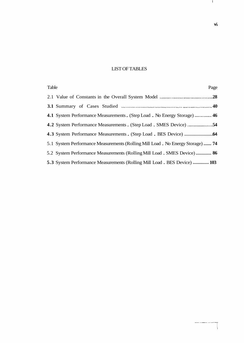
LIST OF TABLES
Table Page
2.1 Value of Constants in the Overall System Model .......................................... 28
3.1 Summary of Cases Studied .................................................................. 40
4.1 System Performance Measurements . (Step Load . No Energy Storage) .............. 46
4.2 System Performance Measurements . (Step Load . SMES Device) ..................... 54
....................... 4.3 System Performance Measurements . (Step Load . BES Device) 64
....... 5.1 System Performance Measurements (Rolling Mill Load . No Energy Storage) 74
............. 5.2 System Performance Measurements (Rolling Mill Load . SMES Device) 86
.............. . 5.3 System Performance Measurements (Rolling Mill Load BES Device) 103

I
vii
LIST OF FIGURES
Figure Page
............................................................... 1 . 1 Typically Weekly Load Curve 6
1 . 2 Revised Weekly Load Curve with a Large Scale Energy Storage Device on the System ..................................................... 7
1.3 The North of Scotland Hydro-Electric Board. Crauchan Station ....................... 10
1.4 Basic Components of an SMES Facility .................................................. 12
.................................... 1.5 Block Diagram of a Battery Energy Storage Facility 16
2.1 Block Diagram of the Dynamic System Model ........................................... 19
2.2 Block Diagram of the Governor Model ................................................... 20
2.3 Block Diagram of the Steam Turbine System ............................................ 21
2.4 Block Diagram of the Tie-Line Power Flow ............................................. 23
2.5 Automatic Generation Control Logic ...................................................... 24
2.6 Step Change in Load ........................................................................ 25
2.7 Five-Stand Rolling Mill Load .............................................................. 26
2.8 Block Diagram of the Overall System Model ............................................. 27
2.9 Block Diagram of the System Model with an Energy Storage Device ................. 30
. ................................. 4.1 Frequency in Area 1 (Step Load No Energy Storage) 43
4.2 Frequency in Area 2 (Step Load . No Energy Storage) ................................. 43
4.3 Tie-Line Power Flow (Step Load . No Energy Storage) ................................ 44
4.4 ACE in Area 1 (Step Load . No Energy Storage) ....................................... 44
4.5 ACE in Area 2 (Step Load . No Energy Storage) ....................................... 45

Figure Page
............. 4.6 Change in Generated Power in Area 1 (Step Load -No Energy Storage) 45
. ............ 4.7 Change in Generated Power in Area 2 (Step Load No Energy Storage) 46
4.8 SMES Converter Voltage . Vd (Step Load) ............................................... 49
4.9 SMES Current . Id (Step Load) ....................................... d 4.10 SMES Power Output . Pd (Step Load) .................................................... 50
.............................. . 4.1 1 Frequency in Area 1 (Step Load SMES Device Present) 50
.............................. . 4.12 Frequency in Area 2 (Step Load SMES Device Present) 51
............................ . 4.13 Tie-Line Power Flow (Step Load SMES Device Present) 51
..................................... . 4.14 ACE in Area 1 (Step Load SMES Device Present) 52
..................................... . 4.15 ACE in Area 2 (Step Load SMES Device Present) 52
. ......... 4.16 Change in Generated Power in Area 1 (Step Load SMES Device Present) 53
. ......... 4.17 Change in Generated Power in Area 2 (Step Load SMES Device Present) 53
. ................................................. 4.18 BES Converter Voltage Vd (Step Load) 58
....................................... . 4.19 BES Common DC Bus Voltage Vb (Step Load) 58
4.20 BES Current . Id (Step Load) ............................................................... 59
4.21 BES Power Output . Pd (Step Load) ...................................................... 59
...................................................... 4.22 BES Energy Stored . W (Step Load) 60
................................ . 4.23 Frequency in Area 1 (Step Load BES Device Present) 60
. ................................ 4.24 Frequency in Area 2 (Step Load BES Device Present) 61
. .............................. 4.25 Tie-Line Power Flow (Step Load BES Device Present) 61
....................................... . 4.26 ACE in Area 1 (Step Load BES Device Present) 62
....................................... 4.27 ACE in Area 2 (Step Load . BES Device Present) 62
. ........... 4.28 Change in Generated Power in Area 1 (Step Load BES Device Present) 63
. ........... 4.29 Change in Generated Power in Area 2 (Step Load BES Device Present) 63
. ........................ 5.1 Frequency in Area 1 (Rolling Mill Load No Energy Storage) 67

Figure Page
........................ . 5.2 Frequency in Area 2 (Rolling Mill Load No Energy Storage) 68
5.3 Tie-Line Power Flow (Rolling Mill Load . No Energy Storage) ...................... 69
5.4 ACE in Area 1 (Rolling Mill Load . No Energy Storage) ............................... 70
5.5 ACE in Area 2(Rolling Mill Load . No Energy Storage) ............................... 71
5.6 Change in Generated Power in Area 1 .................................................. (Rolling Mill Load . No Energy Storage) 72
5.7 Change in Generated Power in Area 2 (Rolling Mill Load . No Energy Storage) ................................................. 73
..................................... . 5.8 SMES Converter Voltage Vd (Rolling Mill Load) 76
5.9 SMES Current . Id (Rolling Mill Load) ................................................... 77
5.10 SMES Power Output . Pd (Rolling Mill Load) ...................... , ..................... 78
. ..................... 5.1 1 Frequency in Area 1 (Rolling Mill Load SMES Device Present) 79
5 . 12 Frequency in Area 2 (Rolling Mill Load . SMES Device Present) ..................... 80
................... 5.13 Tie-Line Power Flow (Rolling Mill Load . SMES Device Present) 81
5.14 ACE in Area 1 (Rolling Mill Load . SMES Device Present) ........................... 82
5.15 ACE in Area 2 (Rolling Mill Load . SMES Device Present) ........................... 83
5.16 Change in Generated Power in Area 1 ............................................. . (Rolling Mill Load SMES Device Present) 84
5.17 Change in Generated Power in Area 2 ............................................. (Rolling Mill Load . SMES Device Present) 85
....................................... . 5.18 BES Converter Voltage Vd (Rolling Mill Load) 91
5.19 BES Common DC Bus Voltage . Vb (Rolling Mill Load) .............................. 92
5.20 BES Current . Id (Rolling Mill Load) ..................................................... 93
5.21 BES Power Output . Pd (Rolling Mill Load) ............................................ 94
5.22 BES Energy Stored -W (Rolling Mill Load) ............................................ 95
...................... . 5.23 Frequency in Area 1 (Rolling Mill Load BES Device Present) 96
. ...................... 5.24 Frequency in Area 2 (Rolling Mill Load BES Device Present) 97

Figure Page
..................... . 5.25 Tie-Line Power Flow (Rolling Mill Load BES Device Present) 98
............................. . 5.26 ACE in Area 1 (Rolling Mill Load BES Device Present) 99
............................. . 5.27 ACE in Area 2 (Rolling Mill Load BES Device Present) 100
5.28 Change in Generated Power in Area 1 ............................................... (Rolling Mill Load - BES Device Present) 101
5.29 Change in Generated Power in Area 2 (Rolling Mill Load - BES Device Present) ................................................ 102

ABSTRACT
In areas with rapidly changing loads of large magnitude, utility companies often
experience large deviations in frequency and area control error. Inadvertent tie-line power
flow also occurs. The purpose of this research is to examine the effects a large scale
energy storage device has on the system response to a rapidly changing load. Two control
areas connected by a tie-line are modelled and simulations are performed to determine the
response to a step change in load and also to a five-stand rolling mill load. For each type of
load, three cases are studied: no energy storage in the system, a superconducting magnetic
energy storage device in the system, and a battery energy storage device in the system.
Each case is analyzed and the improvements in system operation for each of the energy
storage devices is discussed.

CHAPTER 1
INTRODUCTION
1.1 Motivation and Scope
The main objective of utility companies is to provide enough energy to meet the
energy demanded. In doing this, they must concur with a set of environmental,
economic, and regulatory requirements. The energy should be provided at minimum cost
with minimum effect on the environment. System operation should meet all local, state,
and federal requirements, along with any contractual agreements. An effort should be
made to maximize safety for employees and customers and also to maximize power
quality.
There are many measures of quality in the operation of power systems. For
example, system reliability is an integral part of operating philosophies and procedures.
Environmental impact, area control error, and cost minimization are also important
parameters. One of the major concerns of both producers and consumers of power, and
perhaps the most important measure of quality, is the maintenance of the proper system
frequency. System frequency is a major indicator of the robustness of the system. The
above measures of quality are used in developing the control strategies for system
operation. Perhaps the most important of these controls is the automatic generation
control.
The minimization of both area control error and inadvertent tie-line power flow
and the maintenance of system Frequency are accomplished mainly through the use of
automatic generation control. Area control error is defined as the required change in an
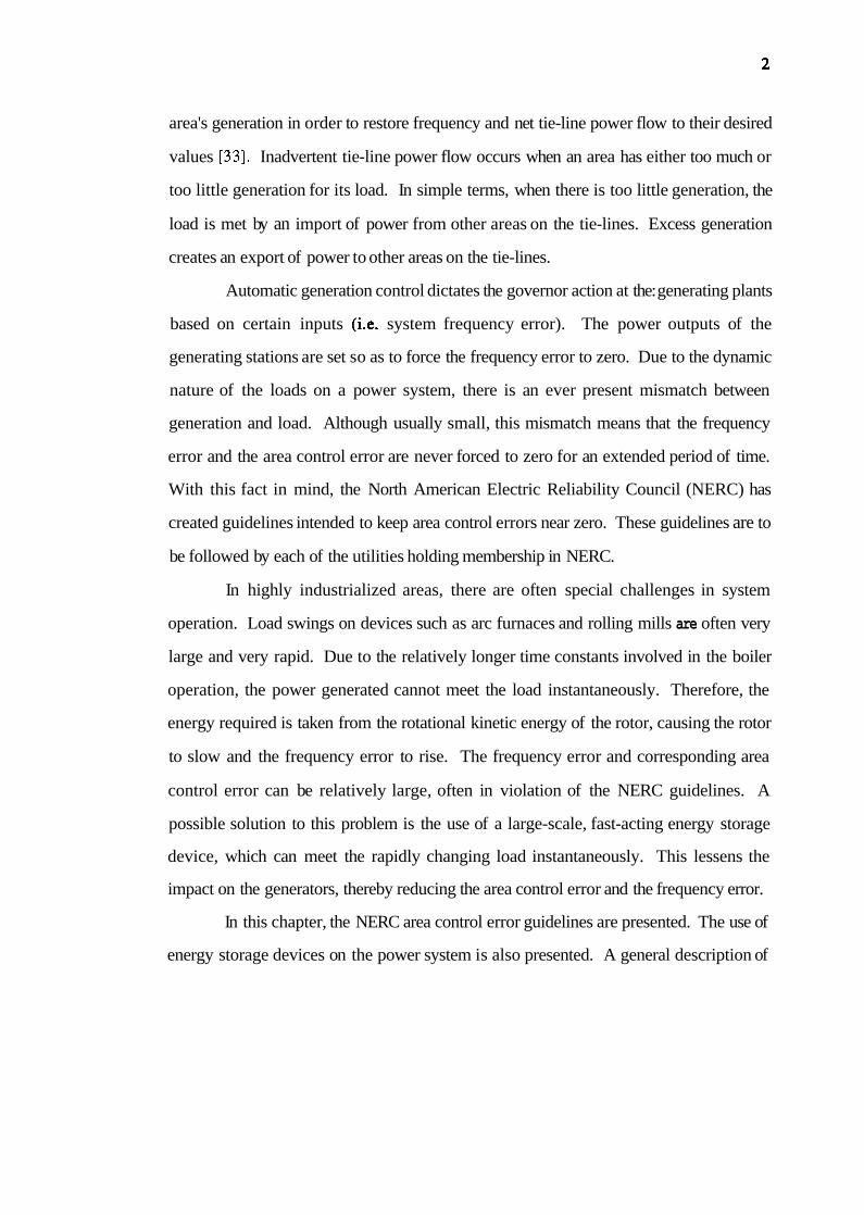
area's generation in order to restore frequency and net tie-line power flow to their desired
values [33]. Inadvertent tie-line power flow occurs when an area has either too much or
too little generation for its load. In simple terms, when there is too little generation, the
load is met by an import of power from other areas on the tie-lines. Excess generation
creates an export of power to other areas on the tie-lines.
Automatic generation control dictates the governor action at the: generating plants
based on certain inputs (i.e. system frequency error). The power outputs of the
generating stations are set so as to force the frequency error to zero. Due to the dynamic
nature of the loads on a power system, there is an ever present mismatch between
generation and load. Although usually small, this mismatch means that the frequency
error and the area control error are never forced to zero for an extended period of time.
With this fact in mind, the North American Electric Reliability Council (NERC) has
created guidelines intended to keep area control errors near zero. These guidelines are to
be followed by each of the utilities holding membership in NERC.
In highly industrialized areas, there are often special challenges in system
operation. Load swings on devices such as arc furnaces and rolling mills are often very
large and very rapid. Due to the relatively longer time constants involved in the boiler
operation, the power generated cannot meet the load instantaneously. Therefore, the
energy required is taken from the rotational kinetic energy of the rotor, causing the rotor
to slow and the frequency error to rise. The frequency error and corresponding area
control error can be relatively large, often in violation of the NERC guidelines. A
possible solution to this problem is the use of a large-scale, fast-acting energy storage
device, which can meet the rapidly changing load instantaneously. This lessens the
impact on the generators, thereby reducing the area control error and the frequency error.
In this chapter, the NERC area control error guidelines are presented. The use of
energy storage devices on the power system is also presented. A general description of

automatic generation control systems and their implementation is provided. Also,
alternative types of energy storage devices will be discussed.
1.2 Reliability Criteria
Due to the large number of interconnections in the power network as it exists
today, each utility company depends on the reliable operation of neighboring utility
companies in order to maintain its own reliability. It is for this reason that the North
American Electric Reliability Council has created control performance criteria which
apply to all North American utilities. These criteria are intended to establish minimum
standards of control performance and provide a means for measuring the relative control
performance for each control area [I]. The control performance criteria used by NERC
consist of two distinct measurements, A1 and A2. They apply under normal operating
conditions (no contingencies).
A1 Criterion
The area control error (ACE) must cross zero within any ten-minute period.
A2 Criterion
The average ACE for each of the 6 ten-minute periods during the hour must be
within specified limits (Id) that are determined from the control area's rate of
change of demand [I].
These requirements are intended to keep system frequencies at desired levels,
minimizing area control error and time error. They are also intended to keep a utility
company from leaning on its tie-lines for any extended period of time.
1.3 Automatic Generation Control
Automatic generation control (AGC) is the means by which frequency is kept to
schedule, generation is balanced with load, and the system is operated at an adequate
level of security and economy [8,25,26,33]. The purpose of AGC is to replace some of
the manual control operations necessary to change generation levels when there is a load
change or a trip. of a generating unit. Numerous papers delve into the different aspects of
AGC and a brief listing is given in references [25-321.
Automatic generation control is essentially a multi-loop feedback controller [26].
It has evolved from the eras of manual and analog control to high speed digital control
schemes. Within the control scheme, several inputs, such as tie-line power flows,
generation operating points, valve points, and frequency deviation, may be taken [26,29].
From this input, the operating levels of the generating stations are determined. Several
other factors are taken into consideration when determining the operating levels. The
type of plant is an important factor to consider when faced with fluctuating loads. For
example, large coal-fired plants and nuclear plants are not designed to change their
operating levels very often. Economics also plays an important role in the control
strategies as the lowest possible fuel cost is always desired [25].
The operating levels of the generating stations are set by sending "raise" or
"lower" signals to each of the plants. The inputs for the AGC system are usually received
at a central system control center. This input is processed and the operating levels of the
individual plants are determined according to the criteria mentioned above. A raise or
lower pulse, or no pulse, is then sent to each of the generating stations indicating,
respectively, an increase, decrease, or maintenance of the current generation level. The
pulse received at each station is used to set the governor, which regulates the power
output at that plant. The pulse is typically sent out every two seconds [30].

Unfortunately, the purposes of AGC are limited by the physical processes
involved. Generating stations are not able to change their power outputs instantaneously
to meet a large, rapidly changing load. The inertia of the rotating shafts in the system are
the only energy storage devices in most power systems so the energy required
instantaneously is taken from there. Energy taken from the inertia of the rotating shafts
results in their deceleration and a consequent frequency error. The effectiveness of AGC
is also limited by deadbands that are set throughout the system. For instance, in most
control areas in the United States, a frequency deviation of 0.2 Hz or more is necessary
before AGC is activated. This means that AGC has a limited role in decreasing the initial
frequency swing associated with a large, rapid change in demand. Trying to maintain a
constant frequency or instantaneously reduce area control error to zero would be an
exercise in futility. Strategies which yield an acceptable area control error trend and an
acceptable range of the unavoidable inadvertent tie-line power flows are preferred [25].
1.4 Energy Storage in Electric Utility Companies
The use of energy storage devices in the electric power system is not a new
concept. Thomas Edison used lead-acid batteries in his early electric power business
[2,20]. They were used to store energy during the daytime for use at night when the
generating stations were shut down. Ironically, the most common use of energy storage
devices in utility companies today is just the opposite. Energy is stored at night when
the cost is low for use during the day when the cost is high.
The need for energy storage in the power industry arises mainly due to the
variations in electric power demand. Electric power demand is constantly changing.
Rapidly changing loads can bring about problems with maintaining the desired system
frequency, large area control errors, and with inadvertent tie-line flow. Most of the
variations are periodic, with periods ranging from a few seconds to a few months [3].

Tha daily load cycle is a dramatic example of the variation of electric power demand. A
typical weekly load curve is shown in Figure 1.1 [4]. The electric power demand may
range from approximately 50% peak load at night to nearly 90% ptak load during the
day. This daily cycle presents special challenges in peak shaving and load leveling.
Large coal-fued plants and nuclear plants are designed to meet the base-load
nacds. These plants are created to run for extended periods of time at maximum or near-
maximum power output. They are not designed to fluctuate in their power output as
dqmand changes and frequent cycling of the plants can greatly reduce their life
expectancy. As demand rises above the base-load level, it is met with older coal-fired
generation, gas-fired generating stations, hydroelectric units, and oil-fired units. These
types of plants are designed to better accommodate changes in their power output.
l,Jnfonunately, these plants, which are used to meet intermediate and peak loads, are
relatively expensive and less efficient to operate [3].
00 - reserve
peak~ng
1 60 \
inlermed~ate
I V V u 40 V
I ( I I I 1 I b o s e l o a d current general Ion mix
I I I I I monday luesday w e d m .thursday 1 frlday lsaturday 1 sunday
Figure 1.1 Typical Weekly Load Curve
In the United States, load factors on base-load generating stations have been
declining in recent years, while peak demands have risen [5] . It is estimated that, on a

yearly basis, utility companies use only about 60% of their generating capacity [6].
Though some generation must be in the form of power plants to meet intermediate and
peak loads, a portion of it could be in the form of energy storage plants 131.
The major application of energy storage devices in the power industry today is
the use of pumped-hydro stations for load leveling. Presently, about 38 pumped-hydro
stations are in operation or being planned in the United States. This represents about 3%
of the total generating capacity in the United States [7]. It has been estimated that
between 5% and 15% of the generating capacity in the United States could be in the fom
of energy storage [3]. Figure 1.2 [4] shows a revised weekly load curve with a large
scale energy storage device on the system.
% - i; 100 0 a B n 80 0 0 -
\ I h l intermediate
----.------.---- --------- - - - o original boseload capac~ty U I I 01 baseload S 20 C
baseload energy to storage o, generot on mix with energy storage 2 t
peaking energy from storage B O I I I 1 I I
Figure 1.2 Revised Weekly Load Curve with a Large Scale Energy Storage Device on the System
With the development of new technologies (i.e. battery energy storage,
superconducting magnetic energy storage), the usefulness of energy storage devices in the
power industry is increasing. Battery energy storage plants and superconducting
magnetic energy storage (SMES) plants with thyristor power converters provide

advantages that pumped hydro cannot offer. Thyristor control, combined with these
types of storage devices, allows for nearly instantaneous change from charge to discharge
mode or vice-versa. This creates a whole new set of applications for energy storage on
the power system. Two of the major applications for this type of fast-acting energy
storage systems are frequency regulation and area control error correction. These
systems are capable of providing instantaneous reserve to meet rapidly changing loads.
The perturbations caused by these sudden changes in load are absorbed by the energy
storage device and not so much the kinetic energy of the rotating shaft ):8]. Therefore, the
effects on system frequency are lessened.
Some other applications of energy storage devices on the power system includq
reactive power compensation, voltage regulation, damping of subsynchronoup
oscillations, and providing black start capability [9].
1.5 Energy Storage Devices
The ability to store energy in large quantities would greatly effect the operatieg
practices and philosophies of electric utilities. Power demand could be met
instantaneously with stored energy and the system would rely less on strategies such as
automatic generation control or load prediction. Large generating stations could be ruq at
their optimum output 24 hours a day, meeting base load during the day and providing
power, along with charging energy storage devices, at night. Pumped hydro plants havo
already proven their worthiness, with about 38 stations existing today [7].
New technologies have arisen providing more options to elecmc utifiw
companies in their use of energy storage devices. Superconducting magnetic energy
storage facilities and battery energy storage facilities with thyristor controlled csnvertq
are capable of providing instantaneous supply or demand of power. This can improve
power quality and improve system operation in terms of frequency maintenance,
reduction of area control error, and inadvertent tie-line flow.
The following subsections discuss the proven technology of pumped
hydroelecmc storage and the largely experimental, but highly promising, technologies of
SMES and battery energy storage.
1.5.1 Pumped Hydroelecmc Energy Storage
Pumped hydro technology is the only truly proven technology available for
energy storage in the power industry. This technology dates back to 1879, when a unit
was put into operation in Zurich, Switzerland [lo]. The first pumped hydro unit installed
in the United States was the Rocky River unit for Connecticut Power and Light in the
year 1929 [l l] . It was not until the early 1950's that pumped hydro became a widely
accepted means of meeting peak demands. This acceptance coincided with the
development of the reversible Francis pump-turbine. Today, there are over 150 plants
worldwide with a total installed capacity of about 100,000 MW. These plants range in
size from a few megawatts to over 2000 MW. In the United States, 38 plants account for
18,000 MW of capacity. This is 18% of worldwide pumped hydro capacity and 3% of
the total generating capacity of the United States [7].
A pumped hydro plant uses potential energy as its means of energy storage. A
diagram of the North of Scotland Hydro-Electric Board, Crauchan Station is shown in
Figure 1.3 [4]. During peak demand hours, the energy contained in the water falling from
the upper reservoir is converted into elecmcity by the turbines. When the demand is low,
the water is pumped back up to the upper reservoir, thereby restoring its potential energy.
The main function of pumped hydro energy storage is that of load leveling. A
large-scale pumped hydro plant is capable of increasing demand during the night, while
in pumping mode, and meet peak demand during the day, while in generating mode. This

results in a revised load curve like the curve shown previously in Figure 1.2. Depending
on the individual plant parameters, pumped hydro plants consume 1.3 - 1.4 kwh in
pumping fgr every 1 kwh generated [lo].
Figure 1.3 The North of Scotland Hydro-Electric Board, Crauchan Station
Some of the major pumped hydro facilities in the United States include:
Northeast Utilities, 1000 MW Nonhfield Mountain Plant in Massachusetts; Pacific Gi-q
and Electric Company, 1200 MW Helms Plant in California; and Virginia Power, 21m
MW Bath County Plant in Virginia [lo].
1.5.2 S uperconduc ting Magnetic Energy Storage
Superconducting magnetic energy storage (SMES) is a relatively new
technology. An early paper by Femer [44] considers the use of a large energy storage
coil for France [3]. In the United States, studies of SMES btgan in the early 1970's at the
University of Wisconsin. Since that time, other groups have undertaken large-scale
feasibility and applicability studies of SMES. These groups include: Los Alamar
Sci~ntific Laboratory, the United States Atomic Energy Commission, Bonneville Power
Administration, and the Elecmc Power Research Institute among others [3].

The principles behind SMES are relatively straightforward. A coiled wire, called
a solenoid, carries current and generates a magnetic field. If the ends of the wire are
connected and there is no circuit resistance or sources, the resulting current does not
decay [14]. The state of no resistance is achieved by using a superconducting wire.
Superconductivity is achieved by cooling certain materials (i.e. Niobium or Titanium) to
their critical temperatures and maintaining those temperatures. The literature on
superconductivity is very extensive with references [36 - 391 being representative of the
low temperature superconductivity phenomena and references [40 - 431 being
representative of the high temperature type. Superconductivity has two main advantages.
First, no heat is generated due to the lack of resistance, meaning large currents can be
carried with little degradation of the wire. Secondly, since their are no resistive losses,
the energy in the magnetic field is maintained without the need for additional energy [14].
An SMES facility would consist of several major subsystems: the
superconducting coil, a Helium refrigeration system, an ACPC converter, a structural
support system, and accompanying control and protection systems [2,15,16]. The basic
components of an SMES facility are shown in Figure 1.4 [8].
The transformers convert the high voltage and low current of the power system to
the lower voltage and higher current required by the coil [3]. The AC/DC converter
changes the alternating current from the power grid to direct current. The controller may
use several inputs from both the AC system and the SMES system. These inputs are used
to dictate the firing angle of the semiconductor-controlled converter, which determines
the voltage across the inductor. The firing angle may be changed rapidly, allowing an 1
SMES unit to change from full charge to full discharge on the order of tens of
milliseconds [3]. The voltage, shown as Vd in Figure 1.4, is positive when charging the
superconducting coil, negative for discharging, and zero for maintaining a constant
energy level in the superconducting coil. The current, Id, fluctuates between maximum


current and some set minimum current. The large forces associated with the
electromagnetic field in the superconducting coil require a large and costly structural
support system for the SMES facility. A Helium refrigeration unit is also a necessity in a
low temperature SMES system to remove heat generated in the coil and maintain
superconducting temperatures. The resistor shown in Figure 1.4 is the "dump" resistor.
When needed, it can be switched in series with the superconducting coil causing the
energy stored in the coil to be dissipated as heat through the resistor.
Obviously, the two major advantages of an SMES unit would be the fast reaction
time of the AC/DC converter and the nearly lossless storage device. It has been estimated
that the efficiency of an SMES unit would be in the range of 92% to 95% [3,14,16]. The
losses would come in the ACDC converter and in the power needed to run the
refrigeration system.
In February of 1983, an 8.4 kwh SMES demonstration unit with a 10 MW
converter was energized at the Tacoma substation of the Bonneville Power
Administration [12,13,17]. It was designed to damp the dominant power swing mode of
the Pacific AC Intertie [12]. The plant was the first major application of superconducting
technology in the utility industry. The plant ran intermittently for over a year and was
retired in March of 1984. Although in service for a relatively short time, tests on the
SMES unit provided valuable information on the control-law d&ign, electrical
characteristics of the device, and its effectiveness as a power system stabilizer [12,13].
The applications of an SMES unit within a power system are numerous. The
following applications are considered in this thesis: minimization of frequency deviation,
minimization of area control error, and minimization of inadvertent tie-line power flow.
Other applications include: load leveling, peak shaving, damping of subsynchronous
oscillations, VAR control, spinning reserve, black start capability, and improvement of
system transient performance [14,18].

1.5.3 Batt~ry Energy Storage
Battery energy storage technology is nearly 200 years old. Alessandro Volta
developed the galvanic battery in the year 1800 [19]. Thomas Edison used Lead-acid
batteries in his early power business to store energy during the daytime fqr use at night
C2.203. It was not until the late 1960s though that large-scale battery energy storage units
were seriously considered for use in the electric power industry in the United States.
A battery facility uses electrochemical energy storage. The operation of a basic
Lead-acid battery is explained by Anderson and Carr [21].
"Each cell of a charged Lead-acid battery comprises a positive electrode of Lead dioxide and a negative electrode of sponge Lead, separated by a microporous material. When these electrodes are immersed in an aqueous sulfuric acid electrolyte, contained in a plastic case, a nominal open circuit voltage of 2 volts is created. When the circuit between the two electrodes is closed, the battery discharges its stored energy; the Lead dioxide on the positive electrode is reduced to Lead oxide, which reacts with sulfuric acid to form lead sulfate; and the sponge Lead on the negative electrode is oxidized to lead ions that react with sulfuric acid to fom Lead sulfate. In this way, chemical energy stored in the battery is converted to electrical energy."
A block diagram of a battery energy storage facility is shown in Figure 1.5 [2]. It
consists of several major subsystems, including: ACDC converter, battery subsystem,
and the control and protection circuitry.
The transformer converts the low current and high voltage of the AC system to a
higher current and lower voltage more suitable for battery operation. The ACJDC
converter is a semiconductor-controlled device, which changes the alternating current to
& i t current. The control system takes inputs from both the battery system and the AC
system. From these inputs, the firing angle of the AC/DC converter is determined. The
firing angle dictates the voltage across the terminals of the battery subsystem. The
battery subsystem usually consists of a large number of cells in some parallel of series
configuration. The series connections set the voltage of the battery subsystem, 'while the
parallel connections are used to increase the storage capacity. If the AC/DC converter

voltage is set greater than the voltage of the batteries, the batteries will be charged. If the
converter voltage is set lower than the voltage of the batteries, the batteries discharge.
As in SMES systems, battery energy storage systems allow for almost
instantaneous reversal of power flow. Although their efficiency is not as high as an
SMES system, it is still relatively good. Efficiencies have been estimated up to 8 4 8
[221.
The applications of a battery energy storage unit on the power system are
numerous and well documented. This thesis focuses on applications in the areas of
minimization of frequency deviation, minimization of area control error, and
minimization of inadvertent tie-line power flow. Other applications include: load
leveling, peak shaving, instantaneous reserve, voltage regulation, damping of
subsynchronous oscillations, providing black start capabilities, and improvement of base-
load efficiencies [2,5,9,23,24].
There are several major battery energy storage facilities at this time. Southern
California Edison uses its Chino 10 MW, 51.2 MWh demonstration plant for load
leveling. In Berlin, a 17 MW, 14.4 MWh battery energy storage facility has been used
since 1987 to regulate frequency [2]. Between 1992 and 1995, the Puerto Rico Electric
Power Authority is scheduled to install over 100 MW of battery energy storage capacity
[21]. These examples, along with several others, point out the feasibility and growing
importance of battery energy storage facilities for utility usage.


CHAPTER 2
SYSTEM MODELING
2.1 Overall Model
In order to determine the effect of an energy storage device on a power system,
it is necessary to devise a model for the system and use this model to simulate system
operation. This section steps through the derivation of the different components of the
overall system model. The objective is to formulate an overall model of a power system
on automatic generation control.
2.1.1 Dynamic System Model
The dynamic model of the rotating mass in a power system essentially relates the
frequency of the system and the net power in the system. It is necessary to assume that
within a specified control area, the ties are strong enough to allow a single frequency to
characterize the entire area [27]. Following a disturbance APd* the net surplus of power
in the area will be APg - APl MW, where Pg is the generated power and Pl fs the demand
power. This power mismatch is absorbed by the system in three ways: the first way is by
increasing (or decreasing) the area kinetic energy. The rate of change of the kinetic
energy is given by [27]

where Wtip is the system total kinetic energy, wm is the rated kinetic energy of the
system (i.e. at rated frequency), f is the area frequency, and f* is the rated fraquency (60
Hz).
A second way the power mismatch is absorbed by the system is by ipcrcased (or
decreased) load consumption. Since motor loads are a major part of the total demand,
their change in load due to change in frequency must be modeled [33]. The relationship
is characterized by a constant D, where
AP1= DAf. (2.4)
The third mans of absorbing the changing load in the system is by varying the
export of power over the t iehes by an amount Aptit.
Therefore, an overall equation can be used to describe the system response
folkwing a disturbance APd 1271
w AP, - AP, = 2-$'- $~f) + DAf +APr.
Dividing by Pr, the total rated power in the specified area, the AP terms arc written in per
unit and the eqvation becomes

APg - APl - APr = 2 H q ~ f ) - D(Af). E dt
where H is the inertia constant in seconds. Taking the Laplace transform,
The block diagram form is shown in Figure 2.1 where
K,=; H 1 and Tp = 2 1 ~
Figure 2.1 Block Diagram of the Dynamic System Model
2.1.2 Governor Model
The governor is a device which adjusts the input valve that controls the steam
flow to the prime mover. The governor control action is usually set by the system
frequency. The governor action increases or decreases the mechanical power output to

restore the system frequency to its desired value. The block diagram of a governor model
is given in Figure 2.2. The load reference input allows the governor characteristic to be
set to give refereqce frequency at any desired unit output 1331. The value of R1
determines the change in the generating unit output for a given change in frequency. The
time constant Tg represents the delays inherent in the opening or closing of the valve.
The output, APvalve, determines the setting of the mechanical power output of the prime
mover.
Figure 2.2 Block Diagram of the Governor Model
2.1.3 Stearn Turbine System Model
Steam turbine system models vary widely depending on the type of system (i.e.
single reheat, double reheat) and the amount of detail desired. A common simplified
model used to represent a steam system with reheat turbines is shown in Figure 2.3.
The input to the system is APvalve, which represents the opening or closing of
the govmor-controlled valves. The time constants Tt and Tr are representative of the

delays introduced by the steam chest, inlet piping, reheaters, and crossover piping [34].
The output, APg, is the mechanical power output of the turbine. This is also assumed to
be the electrical generator output.
Figure 2.3 Block Diagram of the Steam Turbine System
2.1.4 Tie-Line Model
Using the DC load flow method [33], the power flow between two areas across a
tie-line is expressed as
Ptie = 4 e 1 - e*). X tie
where Ptie is the power flowing from area 1 to area 2, Xtie is the impedence of the tie-
line, and 0 1 and % are the phase angles of the respective areas. If a disturbance is
applied, the equation becomes

Then A P h = q A S l - A%).
X tie
The difference of the change in the angles is found by integrating the difference of tho
change in frequencies. The new equation becomes
If the two systems have different power ratings and if Equation (2.1 3) is expressed in per-
unit on a distinctive control area base, a constant must be included to account for these
distinct bases. The block diagram for the tie-line power flow is shown in Figure 2.4. The
term a12 is defined by the power ratings of the two systems
2.1.5 Automatic Generation Control Model
Automatic generation control (AGC) is the control system whose major function
on the power system is to match generated power with demand. There are numerous
factors which could contribute to the AGC configuration. These include: reducing the
static frequency error following a step change in load; keeping the time error within

certain maximum and minimum values; maintaining the correct value of interchange
power between control areas; reducing the area control error to zero in the steady state
[25,27,33].
The selected control scheme was one in which each area control error is driven to
zero in the steady state. The area control enor is defined as
ACE = -Bl('f) - APtie
where B 1 is the frequency bias factor, ~ f l is the frequency deviation in the specified area,
and APhe is the change in tie-line power flowing into the area. In order to reduce the
ACE to zero in the steady state, the ACE is integrated and the resulting signal is used as
the load reference signal to the governor. This signal input can be seen in Figure 2.2.
Ideally, this sets the unit output so as to force the ACE to zero. A block diagram of the
automatic generation control logic is shown in Figure 2.5.
Figure 2.4 Block Diagram of the Tie-Line Power Flow

load reference
tie
Figure 2.5 Automatic Generation Control Logic
2.1.6 Load Model
Two different load models were used in the studies. The first model is a simple
step change in load of 0.025 p.u.. and it is shown in Figure 2.6. This load was applied to
the system in order to observe the system response to a rapid change in load. The second
load models a 5-stand rolling mill with a maximum change in load of 0.025 p.u.. This
type of load is common in the steel indusay. The model, shown in Figure 2.7, is based
on the strip chart recording of the real power demand of an actual 5-stand rolling mill.
2.1 Overall Model
The models of the different parts of the power system are brought together to
form the overall model. This overall model is a modei of two different control areas
connected by a tie-line and it is used in the simulations described in this thesis. Area 1

has 1000 MW of generating capacity and this is used as a per unit base in this area. Area
2 has 3000 MW of generating capacity and its per unit terms are on a 3000 MW base. A
block diagram of the overall model is shown in Figure 2.8. The values for the constants
in the overall model are shown in Table 2.1.
t i m e . (seconds) ( ~ 1 0 ' )
Figure 2.6 Step Change in Load
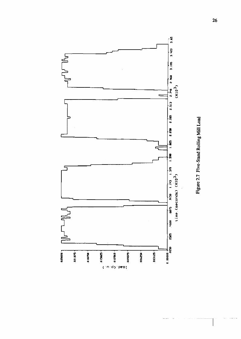


Table 2.1 Values of Constants in the Overall System Model
2.2 Energy Storage System Models
In order to simulate the effect of an energy storage device on a power system, it
is necessary to devise a model for the energy storage device and incorporate this model
into the overall system model shown in Figure 2.8. All of the energy storage devices
discussed in this thesis use an ACDC converters as the interface between the energy
storage device and the electric power system. A typical configuration is a cascaded
bridge converter. The thyristors in the converter are controlled by a firing circuit. The
firing circuit sends pulses to the thyristors, causing them to conduct. The pulse is sent at
a specific time during the 16.67 millisecond cycle. This is done to keep the average
voltage across the converter DC terminals at the desired level [3]. The firing angle,
which can vary over a range of 0 to 180 degrees, determines the value of the average
voltage across the DC terminals of the converter. This average voltage is given by the
equation

where a is the firing angle and Vo is the maximum value of the average voltage. By
changing the firing angle, the average voltage across the energy storage device can be
changed the from maximum positive value to the maximum negative value within a few
milliseconds. Since the voltage across the energy storage device dictates the direction
and magnitude of the power flow, the device can go from maximum charge to maximum
discharge nearly instantaneously.
In the energy storage system models, the voltage across the converter is a
function of the frequency deviation. The Laplace transform of the equation [8] is
where AVd is the change in voltage across the energy storage device and Af is the
frequency deviation. The constants are KO = 30 kV/Hz and Td = 0.026 seconds. The
voltage is set so that when the frequency deviation is negative, the change in the average
voltage across the energy storage device is negative. Therefore, the average voltage, Vd,
decreases and the device discharges. When the frequency deviation is positive, the
change in the average voltage across the energy storage device is positive, the average
voltage increases, and the device charges. In order to avoid operation of the energy
storage device in response to small frequency deviations, a deadband o f f 0.005 Hz was
set. The new overall system model with the energy storage device in place is shown in
Figure 2.9. The output of the energy storage device, APd? is the charge or discharge
power.


2.2.1 Superconducting Magnetic Energy Storage Model
A diagram of a superconducting magnetic energy storage (SMES) unit is shown
in Figure 1.4.
As shown in Equation (2.19), the voltage across the superconducting coil is
continuously controlled by the frequency deviation (unless the frequency deviation lies
within the f0.005 Hz deadband). A rapid increase in load causes the area frequency to
drop. Subsequently, the voltage across the inductor becomes negative and it discharges.
The act of discharging causes the inductor current to drop. The equation
applies. By taking the Laplace transform of the relaxed system and rearranging, the ,
equation becomes
where Aid is the deviation in inductor current, L is the inductance of the coil, and AVd is
the deviation in the average voltage across the superconducting coil given by Equation
(2.19). The equations for the voltage across the DC teminals of the converter, Vd, and
the current in the superconducting coil, Id, are
and
The charging or discharging power is given by
P,=V,&.

The parameters of the SMES unit were based on typical parameters found in
references [3,8, 121. The SMES unit is typically a low voltage, high current device. The
upper and lower limit$ on the converter voltage were chosen as 500 volts and -500 volts
respectively. The maximum power output of this energy storage device is chosen to best
match the type of loads on the system. In this study, the maximum power during charge
or discharge is 25 MW. For the maximum desired power, the maximum current is found
using the equation
The maximum current is found to be 50 kA. In practice, the inductor current, Id, should
not be allowed to reach zero. This prevents the possibility of discontinuous conduction in
the case of a large disturbance [8]. A lower limit of 30% of Ido, which is the rated
conductor current, was chosen. An upper limit on the conductor cumnt must also be
chosen. It ig chosen such that the maximum allowable energy absorption is equql $p the
maximum allowable energy discharge. Using the equal energy charge/discharge criterion
[8] and knowing that the minimum inductor current is 0.3 Id0, the nuximum inductor
current is found to be 1.38 Ido. For the SMES system, Ido is chosen as 36 kA. The
maximum current is then 50 kA and the minimum current is 10.8 kA.
The application of this energy storage deviqe for frequency control does not
require a large amount of energy storage capacity. A maximum storage capacity of 2
MWh is sufficient to supply frequency control for loads such as the, rolling mill load
shown in Figure 2.7. Based on the maximum amount of energy storage capacity required
and the maximum current in the inductor, the inductance of the superconducting coil is
found. The equation is

and the inductance, L, is 5.76 H.
The limits set on the SMES unit effect the energy storage device operation.
When the frequency is within the f 0.005 Hz deadband, the voltage across the inductor is
set to zero and the device is neither charging nor discharging. In this mode, the energy
stored in the magnetic field remains constant because the superconducting coil has zero
resistance. If the current, Id, reaches the maximum value, the voltage across the inductor,
Vd, is set to zero until the frequency deviation is negative once again. Thereupon, the
deviation of the voltage, AVd, is once again dependent on the frequency deviation. If the
current, Id, reaches the minimum allowable current, the voltage across the inductor, Vd,
is set to zero until the frequency deviation is positive again. At this point, the device
resumes normal operation. If the voltage, Vd, reaches its maximum positive (or negative)
value, it is not allowed to increase (or decrease) beyond that value.
The "round-trip" efficiency of the device is 95%. The losses, which occur in the
converter, are modelled by setting the discharge power to
2.2.2 Battery Energy Storage Model
A diagram of a battery energy storage unit is shown in Figure 1.5. The battery
energy storage unit is somewhat different in its operation than the SMES unit. In the
SMES unit, the current is unidirectional and varies between some minimum and
maximum positive values. The voltage across the converter is also the voltage across the
superconducting coil and this voltage is positive or negative depending on whether the
device is charging or discharging. In contrast, the voltage across the batteries is always

positive and is not equal to the voltage across the converter. The current is bidirectional
and its direction depends on whether the unit is charging or discharging. The battery
system is actually a set of 25 series connected smngs of batteries conne:cted in parallel to
a common DC bus. The voltage of the battery units is a function of their state of charqe.
A{ full charge, the batteries are at their maximum voltage level, which demase as the
state of charge of the batteries decreases.
As given in Equation (2.19), the voltage of the converter is a function of tho
frtquency (if it lies outside the *0.005 Hz deadband). A drop in area frequency caused
by a rapid increase in load causes the voltage across the converter to drop. As this
voltage, Vd, drops below the voltage of the batteries, Vb, cumnt flows out of the battey
system and the unit discharges. The equation determining the current flowing in each qf
the strings of batteries is given by
when R is the internal resistance of the battery system, Vd is the average voltage across
the converter, and Vb is the voltage across the battery system. As cu:rrent flows into or
out of the battery system, its state of charge changes. The equation determining cbangc
in the energy stored in the overall battery system is
The factor of 25 is present because the current Id repnsents the cumnt flowing iq each of
the 25 strings of batteries, while AW represents the change in the overall energy stored.
The parameters of the battery energy storage unit are based on the systems
described in references (22, 23, 251. As in the SMES system, the maximum

charge/discharge power and the energy storage capabilities are tailored to fit the load. In
this case, the maximum charge/discharge power is 30 MW and the maximum energy
storage capability is 7200 MWs (2 MWh).
The voltage level of the common DC bus is determined by the sum of the
voltages of the batteries in the parallel strings. These are typically low voltage devices
with very low internal resistances (on the order of a fraction of an ohm) [22, 351. Each
string of batteries on the common bus in the battery system is modelled with an internal
resistance of 1.48 ohms (total) and a voltage which varies between 1020 volts and 1200
volts. As mentioned before, the voltage across the batteries is a function of the state of
charge. In actual batteries, the voltage characteristic resembles a function that is the
square root of the energy stored [35]. In this thesis, the voltage characteristic is
approximated as a linear function of the energy stored, W. The minimum voltage across
the batteries occurs at the minimum energy storage limit of the system. This minimum
voltage is set to 85% of the maximum battery voltage. Between the minimum allowable
energy stored and 83% of the maximum allowable energy stored, the voltage is a linear
function of the stored energy, W, and rises from 85% of maximum voltage to full
maximum voltage. Above 83% of the maximum allowable energy stored, the voltage
across the batteries, Vb, is set to its maximum value. The equation for Vb is given as
Vb = 0.031414W + 1019.058 30 MWs 5 W 5 6030 MWs
Vb= 1200V W 16030 MWs (2.28)
Note that in application, two converter bridges an u s 4 (one for charging i d one for
discharging) in order to accomodate the reversal of current. The voltage across the DC
terminals of the converter in the simulation, Vd, is allowed to vary between 2500 volts

(charge) and -280 volts (discharge). This limits the rnaxirpvrn curnnt per saing of
batteries to 1 0 A. The equation for Vd is given by
where AVd is given in Equation (2.19). The charge/discharge power of the battery
system is given by
As in the SMES unit, the constraints effect the battery energy storage unit
opention. When the fiquency deviation is within the deadband, the voltage of the
converter, Vd, is set equal to the voltage of the battery system, Vb. With the voltages
equal, no cwrent flows in the circuit and no power is transferred, If the energy stor@
roaches its maximum value, only energy discharge is allowed and if the energy stored
reaches the minimum value, only charging is allowed. Wnally, if the c m n t flowing out
of the batteries, Id, reaches maximum value and tttc device continues to discharge, thc
voltage of the converter is set so that the current does not cxceed thig; maximum vlJu9.
Similarly, if the current flowing into the battmies reaches its maximum value and thc
device continues to charge, the voltage of the converter is set so that the cumnt does not
exceed this xnaximum value.
The "round trip" efficiency of the battery energy storage system is 81%.
losses an accounted for in the energy stored and the discharge power. The model is
revised such that during charge the AW is only 90% of the lossless change in energy
shown in Equation (2.27). Also, during discharge, rhe discharge power is only 90% of
the disc- power given by Equation (2.30).

CHAPTER 3
SYSTEM RESPONSE TO RAPIDLY CHANGING LOADS
3.1 Simulation of the System Response
Consider again an interconnected power system containing two control areas. A
block diagram of the two control areas aild the tie-line connecting them is shown in
Figun 2.8 and the derivation of the equations of the system is described in Chapter 2. An
analysis of the system is accomplished using the forward Euler method to approximate
the derivatives in the system equations. Thus, a set of linear difference equations
describe the system. An example of this method is shown using Equation (2.7) which
describes the relationship between frequency deviation and net power in the system.
Equation (2.7) is repeated for convenience,
Rearranging the terms,
and
s Aqs) = KP [AP~(s) - API(s) - AP~~(s)] - A ~ S )
TP (3.3)
This equation can be transformed to the time domain where

Equation (3.3) becomes
The forward Euler approximation is
Using the forward Euler method,.Equation (3.5) is approximated as
41 + dt) - 41) Kp [~Pg(t) - APl(t) - ~~ly( t l1 . - A4t) - - dt TP
Finally,
qt + dt) = dt I Kp [APg(t) - APld - AP*(t)] - A4111 + qt). TP
Similar transformations were performed in order to determine the equations for
the rest of the system parameters in the time domain. These linear difference equations
were then used to perform the simulation. The time step, dt, is 0.001 seconds.

3.2 System Response to Changing Loads
In this thesis, the system response is analyzed for two diffuent typca of load
inputs. These two load inputs are the step change in load, shown in Figwe 2.6, and rhc S-
stand rolling mill load, shown in Figure 2.7. For each of these types d IGds, thra
separate simulations wen performed. The first simulation is the brse case with no amgy
storage device present in the system. The second simulation is the cart where a
stkperconducting magnetic energy storage device is present in area 1 of the system. ' he
third simulation is one in which a battery energy saxage system ia present in u# 1 of the
system.
Chapter 4 contains the analysis of the system response for the step change in load
input. Thc bast case is analyzed in section 4.2; the SMES case in swtkm 4.3; and the
battery energy storage case in section 4.4. Comparisons arc also mde beW& the
diffeslent cases.
Chapter 5 contains the analysis of the system mpdnse to tbe 5 - d d i d g mill
load input. The base oase is analyzed in section 5.2; the S m ca88 in wtbn S6% the
battery energy starage case in section 5.4. In this chapter, a c c m p k m is ladt between
the different cases also.
Due to the large number of plots that arise from the following simulations, a
able has been included to simplify the search for specific plots. Table 3.1 is the main
index and gives reference particular figures for esch specific case.

Table 3.1 Summary of Cases Studied I
; . L , . . 4
1
Figure Numbers
4 1 - 4 .7
4.8 - 4.. 17
4.18-4.29
, 5.1 - '5.7
Case Load Energy Type Storage
5
I
6 .
Mi l l
1 Step None
Rolling M i l l
R o l l ing Mi1 I
I
SMES
Battery
Load
2 I Step -
5.8 - 51 17
5.18- '529
SMES
3
4
Load t Step Load
Ro l ling
Battery
None-

CHAPTER 4
ANALYSIS OF THE SYSTEM RESPONSE TO A STEP CHANGE m LOAD
4.1 Innoduction
In order to provide a basic cmparison between the different casa studied in this
thesis, the first analysis involved a simple step change in load, shown in Figurc 2.6, in
area 1 and no change in load in arca 2 of the system. The three cases studied for this load
arc: the base case with no energy storage device pre*nt, the case with an SMES device
present in m a 1, and the case with a battery energy storage devicc p a m t ht ulea 1. The
parameters of these energy swage devices arc outlhed in Chapter 2.
For each of the t h e cases, the following plots wen made:
l frequency ih area 1
frequency in area 2
tie-line power flow
ACE in arca 1
A C E i n arca2
thange in generated power in area 1
change in generated power in arca 2.
Measurements were also taken to help determine system perf-. For each
case, the following measururnents were taken:
mihimum and maximum frequency in m a 1
minimum and maximum frequency in 2
minimum and maximum ACE in arca 1

minimum and maximum ACE in area 2
maximum tie-line flow into area 1
maximum tie-line flow out of area 1
total energy imported to area 1 across the tie-line
total energy exported from area 1 across the tie-line
net energy across the tie-line.
These measurements were used to compare system performance with and without an
energy storage device. These measurements are important as far as determining the
robustness of the system and the effect of one area's operation on a neighboring area.
4.2 Case 1: Step Change in Load with NO Energy Storage Device
Case 1 is the system response to a step change in load in area 1 with no energy
storage device present in the system. The step load is applied at t = 5 seconds and the
simulation is run for 89.5 seconds. The plots mentioned above (frequency, tie-line
power, ACE, change in generated power) are shown in Figures 4.1 - 4.7. The system
measurements mentioned above (i.e. maximum frequencies, minimum frequencies,
maximum ACE, etc.) are shown in Table 4.1.
The following observations can be made about the system response:
The frequency in area 1 begins its descent simultaneous with the load being
applied. It reaches a minimum of 59.9414 Hertz and begins to rise again as the demand is
met by increased generation and power flowing in across the tie-line (the negative tie-line
power flow shown in Figure 4.3 indicates power flowing from area 2 to area 1). The
frequency overshoots the desired value of 60 Hertz due to the fact that the tie-line power
and the rapid rise in generated power due to the large frequency error have exceeded the
power demand. The area 1 frequency arrives at a maximum value of 60.013 1 Hertz and

L IY. < . U W S I
Figure 4.1 Frequency in Area 1 (Step Load - No Enurgy Storage)
Fifire 4.2 Frequency in Area 2 (Step h a d - No Energy Storage)

Figure 4.3 Tie-Line Power Flow (Step Load - No Energy Storage)
Limo (seconds)
Figure 4.4 ACE in Area 1 (Step Load - No Energy Storage)

9 r o n o .
-* wrsa J a ~ I C e e a . a n 4 7 1 1 3 - 3
iiu (seconds)
Figure 4.5 ACE in Area 2 (Step Load - No En- Storage)
t iu. < s u o d S )
Figun 4.6 Change in Generated Power in Area 1 (Step Load - No Energy Storage)

Figure 4.7 Change in Generated Power in Area 2 (Step Load - No Energy Storage)
Table 4.1 System Performance Measurements - (Step Load - No Energy Storage)

slowly oscillates back to 60 Hertz as the power generated in arca 1 incnases to meet the
10dd and the tie-line flow decrease to zero.
The large and rapid increase in tie-line flow from area 2 to area 1 is essentially
the same as a large increase in load being applied to arca 2. Thmfon, area 2 alod
experiences a drop in frequency to 59.9673 Hertz, although somewhat delayed with
respect to the application of the load in area 1. The change in generated powe in ma 2
incrctises as the frcquency drops due to the tie-line power flow. As the demand is met in
area 1 by area 1 generation, the tie-line flow decreases and the generated power in area 2
goes back to its original value.
The shape of the ACE in area 2, shown in Figure 4.5, is interesting. As the tic.
line flow out of area 2 increases with the application of the load in a m 1, the A= in
area 2 dcctmes slightly. As mentioned above, the change in frcquency in area 2 lags &bt
tie-line power flow slightly so when the frequency in area 2 drops rapidly due to the tie-
line flow, the ACE in area 2 rises to its positive maximum rapidly. As the tie-fihe fldw
decreases and the frequency in area 2 increases, the ACE increases to a positive vale
once again.
4.3 Case 2: Step Change in Load with an SMES Device in Area 1
Case 2 is the system response to a step change in load in area 1 with m S ~ S
device present in area 1. The important parameters in the operation of the SMES device
are plotted. These are: the voltage of the converter, which is also the voltage acrobs the
superconducting coil (Vd); the current in the superconducting coil (h); and the powct
output of the device (Pd). These plots are shown in Figures 4.8 - 4.10. The plot9
mentioned above (frequency, tie-line power, ACE, change in generated power) arc showh
in Figures 4.1 1 -4.17. In these figures, the base case data are superimposed on the 3-S
case data. This allows for a visual comparison of the different system outputs and

simplifies analysis. In each plot, the solid line represents the system output for the case
with the SMES present and the dashed line represents the same system output for the base
case. The system measurements mentioned above (i.e maximum/minimum frequencies,
etc.) are shown in Table 4.2 along with the system measurements for the base case.
The following observations can be made about the response of the SMES device
to the step change in load:
The voltage, Vd, drops to its negative maximum value almost instantaneously
in response to the rapid drop in frequency in area 1 with the application of the step load.
As the frequency increases back to its steady state value of 60 Hertz, the voltage and the
power output of the SMES device decreases. The spikes in the converter voltage and the
power output are evident in Figures 4.8 and 4.10. This occurs as a result of the SMES
device having a deadband of f 0.005 Henz. As the area 1 frequency exceeds the value of
59.995 Henz, the voltage and the power output of the SMES device go to zero as this
frequency is within the deadband. As this power goes to zero, the power produced in area
1 no longer equals the power demand and the frequency drops again. This occurs
because the time constants in the turbine-generator system are much slower than those in
the SMES device, so the rapid initial increase in frequency back towards its steady state
value is due largely in pan to the power produced by the SMES device and not because
there is a more rapid increase in power generated. As stated above, the subsequent power
mismatch occuring at the 59.995 Hertz limit of the deadband as the output power of the
SMES device goes to zero results in a drop in frequency. This drop in frequency causes
the convener to discharge again. These spikes in voltage and power output of the
converter continue to occur until a point where the generated power in area 1 and the
power flowing into area 1 across the tie-line is sufficient to keep the frequency in area 1
at 59.995 Hertz. Again, this time is limited by the slower time constants present in the
turbine-generators.

b i w . < s u ~ s >
Figure 4.8 SMES Converter Voltage - Vd (Stgp Load)
8 .Crr 4
a . r b.* rr.6 . a.r u.1 m.8 am.# b iw. Csuonb.)
Figure 4.9 SMES Current - b (Step Load)

Figure 4.10 SMES Power Output - Pd (Step Load)
I \
U . O L O 0 . I t I L .. I I ' \
, , , , , , , No Energy S toragc *-1 / SMES Device Resent
Figure 4.11 Frequency in Area 1 (Step Load - SMESDevice Present)

1 1 1 I I I I I I I I I I I I I I I I I
- - - - - - - No Energy Storage I I I I
SMES Devict Resent n.wr
Figure 4.12 Frequency in Area 2 (Step Load - SMES Device &sent)
- . a 1 I I Y '
SMESDeviaPnoent -.UIUI '
L iw. <suc*ldS>
Figure 4.13 Tie-Line Power Flow (Step Load - SMES Device m t )

, , , , , , , No Energy Storage
SMES Device Present
Lrme (seconds)
Figure 4.14 ACE in Area 1 (Step Load - SMES Device Present)
- , - - , - - No Energy Storage
SMES Device Resent
Figure 4.15 ACE in Area 2 (Step Load - SMES Device Present)

No Energy Starage
SMES Device Resent
Figure 4.16 Change in Generated Power in Area 1 (Step Load - SMES Device Resent)
Figure 4.17 Change in Generated Power in Area 2 (Step Load - SMES Device Resent)

54
Table 4.2 System Performance Measurements - (Step Load - SMES Device)
By observing Figure 4.9, it is evident that this step change in load reduces the
current in the superconducting coil by only a small amount relative to its overall energy : "
storage capabilities. This suggests that, for a load such as a rolling mill in which the
SMES device will be continuously charging as well as discharging, the energy storage
device can be smaller.
The following observations can be about the system responses when the SMES
device is present in the system:
As seen in Figure 4.11, the initial drop in frequency in area 1 is much less in
this case than the case with no energy storage device in the system. The large initial
frequency drop only goes to 59.9756 Hertz (as opposed to 59.9413 Hertz with no energy
storage). It can also be seen that the frequency does not reach its steady state value of 60
Hertz significantly faster with the SMES device in the system than without the SMES

device. It is also evident thar the system frequency lingers at a value of 59.995 Hem for
about 12 seconds. The 59.995 Hertz value marks the lower limit of the deadband of the
SMES device. At 59.995 Hertz, the SMES device produces just enough power to keep
the fraquency in area 1 at this value until the power generated plus the tie-line power are
sufficient to keep the frequency at 59.995 Hertz. At that point, the power produced by
the SMES device goes to zero.
As the frequency in area 1 is held at 59.995 Hertz, the SMES power output is
slowly &creasing while the change in power generated in area 1 is slowly inmasing.
This keeps the tie-line power flow fairly constant for that period where the frequency is
being held at 59.995 Hertz, as seen in Figure 4.13. At this level of tie-line power flow,
the power being generated in area 2 is equal to that power being exported to area 1.
Because there is no mismatch in power, the frequency in m a 2 =mains fairly constant at
approximately 59.995 Hertz as seen in Figure 4.12. Also, the ACE in areas 1 and 2
remain fairly constant for that same period when the frequency in area 1 is being held at
59.995 Hertz (Figures 4.14 and 4.15).
By observing Figure 4.16, it is seen that the increase in power generated in area
1 with the SMES device in place is not as rapid as in the case with no energy storage
device. This is due to the fact that the governor sets the valve position to increase or
decrease the power output of the generator. The input signal for the governor is
proportional to the ACE of the specified area. In the case with an SMES device in the
system, the ACE is not as large as in the case without an energy storage device, thmf~re
the signal that dictates the power generated will not be as large and the power generated
will increase at a slower rate.
It is evident from the plots that the SMES device acts as a "buffer" between the
load and the system responses. The system responds at a slightly slower rate to the

change in load, and the oscillations in all of the responses are much smaller if not totally
gone.
It is also evident from the plots that the SMES greatly effects the system
operation in the short run by reducing the initial large and rapid changes in frequency,
ACE tie-line flow, and power generated. In the long run though, the system operation is
still constrained by the longer time constants present in the turbine-generator. In effect,
the system response does not reach steady state values faster with an SMES device in the
system (perhaps actually slower), but it greatly reduces the large initial deviations in the
responses.
By observing the amount of energy imported to and exported from area 1
(shown in Table 4.2), it is evident that there is some improvement in this area. There is a
drop in the total energy imported of approximately 8 MWs and a drop in the total energy
exported of about 8 MWs. The net tie-line energy exchange is nearly identical for the
case with an SMES device and the case without an energy storage device.
4.4 Case 3: Step Change in Load With a Battery Energy Storage Device in Area 1
Case 3 is the system response to a step change in load in area 1 with a battery
energy storage (BES) device in operation in area 1. The important parameters of the BES
unit are plotted. These are: the voltage of the converter (Vd); the voltage of the common
DC bus of the battery system (Vb); the current flowing into or out of the device (Id); the
power output of the device (Pd); and the total energy stored in the unit (W). These plots
are shown in Figures 4.18 -4.22. The system response plots (frequency, ACE, tie-line
power flow, change in generated power) are shown in Figures 4.23 - 4.29. In these plots,
the base case data is super-imposed on the BES case data. This allows for a visual
comparison of the different system parameters and simplifies analysis. In each plot, the
solid line represents the system output for the case with the BES present and the dashed
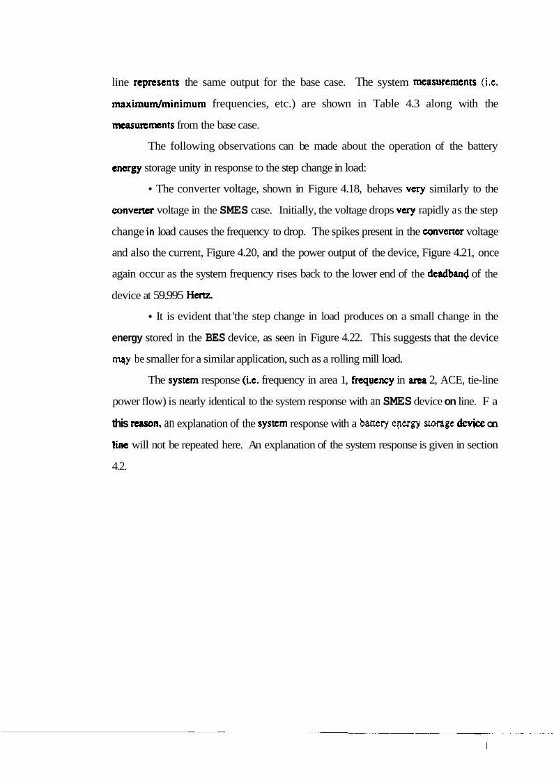
line represents the same output for the base case. The system mtStsuremtnts (i.e.
maximum/rninimum frequencies, etc.) are shown in Table 4.3 along with the
measurements from the base case.
The following observations can be made about the operation of the battery
energy storage unity in response to the step change in load:
The converter voltage, shown in Figure 4.18, behaves vexy similarly to the
convw&r voltage in the SMES case. Initially, the voltage drops very rapidly as the step
change ir, load causes the frequency to drop. The spikes present in the converter voltage
and also the current, Figure 4.20, and the power output of the device, Figure 4.21, once
again occur as the system frequency rises back to the lower end of the deadband of the
device at 59.995 Ha.
It is evident that 'the step change in load produces on a small change in the
energy stored in the BES device, as seen in Figure 4.22. This suggests that the device
mqy be smaller for a similar application, such as a rolling mill load.
The system response (i.e. frequency in area 1, frcqyency in are4 2, ACE, tie-line
power flow) is nearly identical to the system response with an SMES device on line. F a
this nason, an explanation of the system response with a battery epergy storage device on
line will not be repeated here. An explanation of the system response is given in section
4.2.
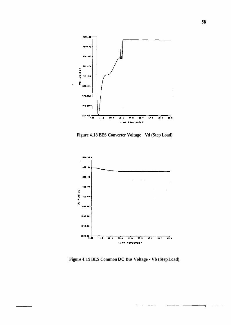
Figure 4.18 BES Converter Voltage - Vd (Step Load)
Figure 4.19 BES Common DC Bus Voltage - Vb (Step Load)

t1w ( s U O ~ O S )
Figure 4.20 BES Current - Id (Step Load)
t i - < s u o n d q )
Figure 4.21 BES Power Output - Pd (Step Load)
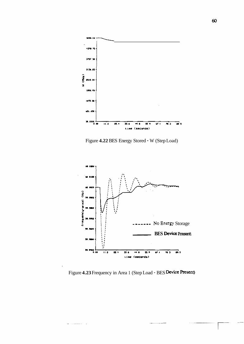
Figure 4.22 BES Energy Stored - W (Step Load)
------- NoEnergy Storage
BES Devia Present
' Figure 4.23 Frequency in Area 1 (Step Load - BES Device &sent)

Figure 4.24 Frequency in Area 2 (Step Load - BES Device Rqxnt)
Figure 4.25 Tie-Line Power Flow (Step Load - BES Device h n t )

, , , , , , , No Energy Storage
BES Device Present
0 0 0 IIE CLV 3 3 6 8 9 6 7 1 7 0 3 893
r ime (seconds)
Figure 4.26 ACE in Area 1 (Step Load - BES Device Present)
- - - - - - - No Energy Storage
BES &via Present
-u .00000 4 o o o 11.1 E Z . ~ 3 . 6 a . 67.1 m a ~ 9 . s
rime (seconds)
Figure 4.27 ACE in Area 2 (Step Load - BES Device -&sent)

------- NoEnngy Storage
BES Device Resent
Figwe 4.28 Change in Generated Power in Ana 1 (Step h a d - BES Device -msent)
Fig- 4.29 Change in Generated Power in Area 2 (Step b a d - BES D e v h Pnsent)

Table 4.3 System Performance Measurements - (Step Load - BES Device)

CHAPTER 5
ANALYSIS OF THE SYSTEM RESPONSE TO A FIVE-STAND ROLLING M U LOAD
5.1 Introduction
In order to provide a more realistic comparison of the different cases studied in
this thesis, the second analysis involved a five-stand rolling mill load, shown in Figure
2.7, applied in area 1 and no change in load in area 2. The three cases studied for this
load are: the base case with no energy storage device present in the system, the case with
an SMES device present in area 1, and the case with a battery energy storage (BES)
device present in area 1. The parameters of these energy storage devices are outlined in
Chapter 2. As mentioned previously, the five-stand rolling mill load is based on a strip
chart recording of an actual five-stand rolling mill.
For each of the three cases, the following plots were made:
frequency in area 1
frequency in area 2
tie-line power flow
ACE in area 1
ACE in area 2
change in generated power in area 1
change in generated power in area 2.
Measurements were also taken to help determine system performance. For each
case, the following measurements were taken:

minimum and maximum frequency in area 1
minimum and maximum frequency in area 2
minimum and maximum ACE in a m 1
minimum and maximum ACE in area 2
maximum tie-line power flow into area 1
maximum tie-line power flow out of area 1
total energy imported to area 1 across the tie-line
total energy exported from area 1 across the tie-line
net energy across the tie-line
These measurements were used to compare system performance with and without an
energy storage device. These measurements are important are far as determining the
robustness of the system and the effects that the energy storage device has on systqn
operation.
5.2 Case 4: Rolling Mill Load with No Energy Storage Device
Case 4 is the system response to a rolling mill load in area 1 with no energy
storage device present in the system. The rolling mill load is shown in Figure 2.7. The
simulation is run for 3647.8 seconds (approximately 61 minutes). The plots mentioned
above arc shown in Figures 5.1 - 5.7. The system maasurements mentioned above (i.e.
minimunJmaximum frequencies, minimurn/rnaximum ACE, etc.) are shown in Table 5.1.
The following observations can be made about the system response:
Since the five-stand rolling mill load resembles a series of "step up" and "step
down" functions, the system behaves essentially the same as in case 1, discussed in
swtion 4,2. With the "step up" in load, the demand in area 1 is now greater than the
power produced and the frequency in area 1 decreases. This drop in frequency causes a
difference in the phase angles between the two areas and causes power to flow across the


Figure 5.6 Change in Generated Power in Area 1 (Rolling Mill Load - No Energy Storage)


I
74
Table 5.1 System Performance Measurements (Rolling Mill Load - No Energy Storage)
tie-line from ana 2 into area 1. The frequency drop also meaqs that the input signal to
the governor is no longer zero, as in steady state. The signal is now positive, producing
an increase in generation. With the "step down" in load, the power generated in area 1
now exceeds the load and the power mismatch drives the frequency upward. This
increased frequency and excess power force power to flow gut of area 1 and into area 2
across the tie-line. The input signal to the governor is now negative and the power
generated in area 1 decreases. The maximum frequency achieved in area 1 for the base
case is 60.031 19 Hertz and the minimum frequency is 59.96938 Hertz. The maximum
tie-line power flow into area 1 is 0.0 1599 p.u. and the maximum tie-line flow out of q a
1 is 0,01495 P.u..
*The power flowing into and out of area 2 along the tie-line produces a power
mismatch ie arca 2 as well as area 1. Subsequently, the frequency in arca 2 vdes as load
is applied in arca 1. This is due to the fact that power flowing into or out of area 2 along

the tie-line is essentially the same as a load being applied or taken away in area 2. The
maximum frequency achieved in area 2 is 60.01726 Hertz and the minimum frequency
achieved in area 2 due to the changes in load in area 1 is 59.983 14 Hertz.
The sharp decrease in frequency in area 1 results in a signal to the governor to
increase generation rapidly. As seen in Figure 5.6, the change in generated power in area
1 rises fairly rapidly and also oscillates as it rises. Although the generation in area 1 is
rising rapidly, its increase is slow relative to the changing load and power is needed from
area 2 across the tie-line in order to meet this demand. The change in generated power in
area 2, shown in Figure 5.7, rises in response to the load change in area 1. As the power
generated in area 1 rises (or falls) to meet the changing demand, the change in generated
power in area 2 returns to zero.
5.3 Case 5: Rolling Mill Load with an SMES Device in Area 1
Case 5 is the system response to a rolling mill load in area 1 with an SMES
device present in area 1. The important parameters of the SMES device are plotted.
These are: the voltage of the converter, which is also the voltage across the
superconducting coil (Vd); the current in the superconducting coil (Id); and the power
output of the device (Pd). These plots are shown in Figures 5.8 - 5.10. The plots
mentioned in 5.1 (frequency, ACE, tie-line power flow, change in generated power) are
shown in Figures 5.1 1 - 5.17. For the sake of clarity, the base case data was not
superimposed on these plots, as in Chapter 4. The figures for the SMES case have been
plotted on the same scales as those in the base case. This allows for visual comparison of
the two cases. The system measurements mentioned above (i.e. minimum/maximum
frequencies, etc.) are shown in Table 5.2 along with the system measurements for the
base case with the rolling mill load.


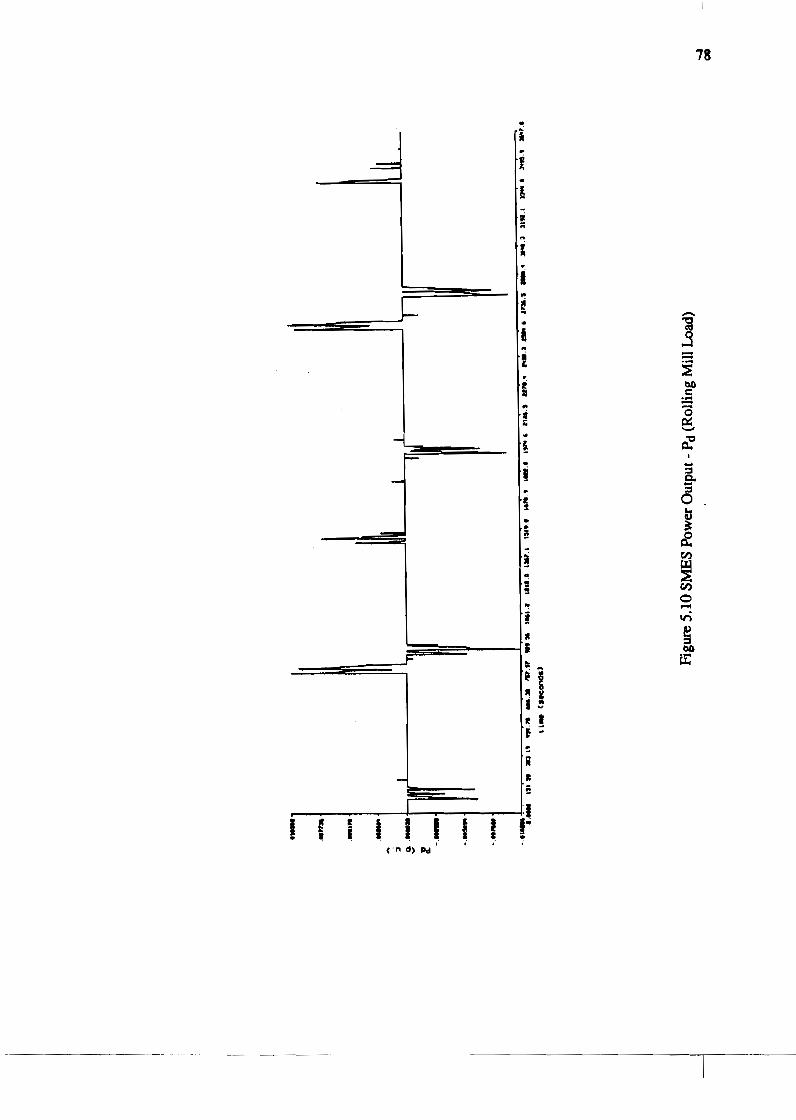

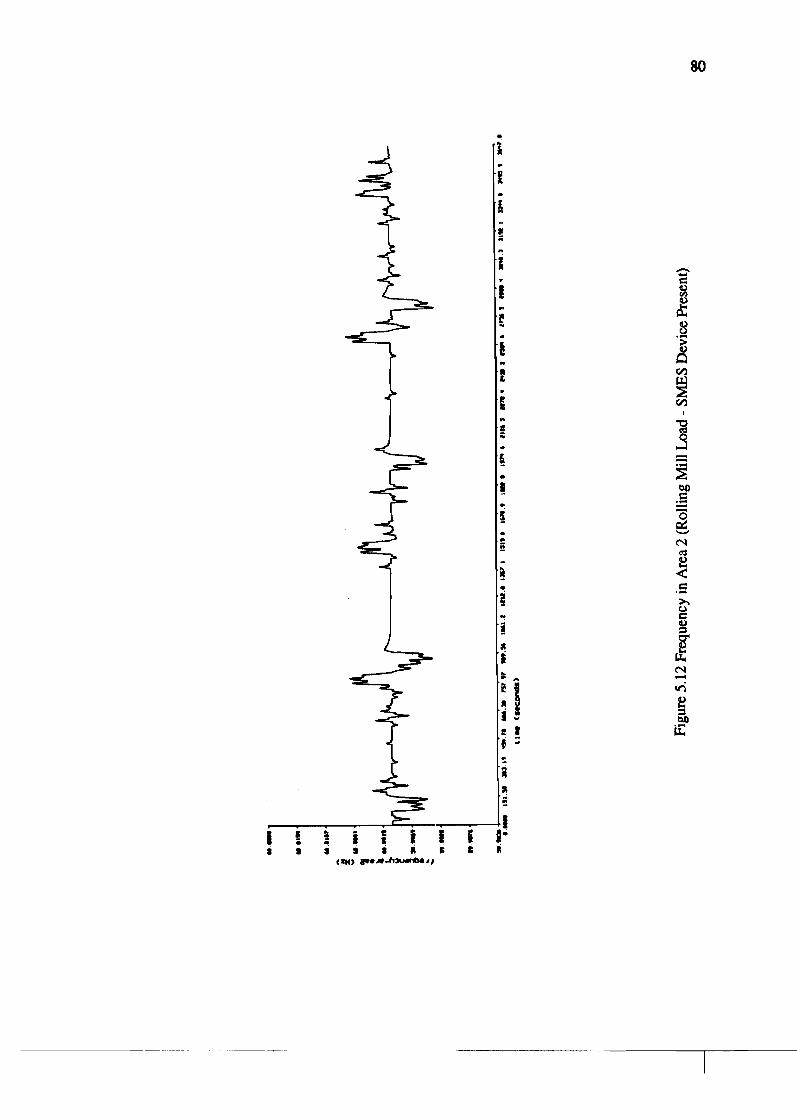


86
Table 5.2 System Performance Measurements (Rolling Mill Load -SMES Device)
The following observations can be made about the response of the SMES device
to the rolling mill load:
When the rolling mill load is applied in area 1, the SMES device responds
essentially in the same way as when a step load is applied. During the "step up" portion
of the rolling mill load, the converter voltage, Vd, drops in response to the dropping
frequency in area 1. As in the step load case, the spikes in voltage and power output are
recognizable as the frequency in area 1 increases to the lower limit of the deadband at
59.995 Hertz. These spikes occur because as the power output of the SMES device goes
to zero at 59.995 Hertz, a mismatch in power in area 1 occurs. This mismatch in power
causes the frequency in area 1 to drop thereby forcing the converter voltage negative
again, which results in the device discharging. These spikes in voltage and power output
continue until the power generated in area 1 plus the power flowing into area 1 across the

tie-line are sufficient to keep the frequency in area 1 within the frequency deadband of
the SMES device.
During the "step down" portion of the rolling mill load, the SMES device
operates in an opposite manner to that described above. During the "step down" portion,
the power generated in area 1 exceeds the demand and forces the frequency above 60
Hertz. The positive frequency deviation causes the converter voltage, Vd, to go positive
and the device charges. Similar to what happens during the "step up" portion of the
rolling mill load, during the "step down"portion, voltage spikes occur as the frequency
enters the frequency deadband of the SMES device. As the frequency in area 1 enters the
deadband, the power output of the device goes to zero. At this point,, there is a power
mismatch i n area I due to excess generation and the area 1 frequency rises above the
60.005 deadband limit and the SMES device begins to charge again. This results in the
spikes present i n the converter voltage and the power output of the SMES device, as seen
in Figures 5.8 and 5.10. These spikes continue until the power generated in area 1 minus
the power flow our of area 1 across the tie-line is sufficient to keep the frequency in area
1 at or below 60.005 Hertz.
As in the step load case, the time between the application of the load and the
time in which the area frequency is within the SMES deadband is limited by the relatively
slower time constants present in the steam system.
By observing Figure 5.10, it is evident that the SMES device is only charging or
discharging during the initial change in load, which is a relatively short time compared to
the overall time. For the majority of the time, the area 1 frequency is within the SMES
device deadband and the device. power output is zero.
By observing Figure 5.9, it is evident that the rolling mill load does not greatly
effect the amount of current in the superconducting coil relative to its overall storage
capabilities. The "step up" and "step down" nature if the load causes the SMES device to

discharge and then to charge back to approximately its original value of current. This
implies that, for this application, the energy storage device can be smaller than originally
es tirnated.
The following observations can be made about the system responses when the
SMES device is present in the system:
*As see-n in Figure 5.1 1, the frequency in area 1 tends to linger at the lower (or
upper) limit of the SMES deadband after the appropriate load is applied (or removed).
These lower and upper limits are 59.995 Hertz and 60.005 Hertz respectively. This
occurrence was explained in section 4.2 for the step load and applies here. At these
frequencies, the SMES device will discharge (or charge) just enough to keep the
frequency in area 1 at the lower (or upper) limit of the deadband. The SMES device
continues discharging (or charging), but by a smaller and smaller amount as the generated
power is increasing. When the generated power in area 1 plus the tie-line power is
sufficient to keep the frequency within the SMES deadband, the power produced (or
absorbed) by the SMES device goes to zero.
With the SMES device on line, the instantaneous power mismatch in area 1 is
not as large as in the case with no energy storage device. Therefore, the frequency
deviations, area control errors, and tie-line power flows do not achieve the same
magnitudes as in the base case. Since the ACE is the input which essentially sets the
output of the turbine-generators, the smaller magnitude in ACE results in a slower change
in the generated power in each area.
As the frequency is held at the lower limit of the SMES deadband, the SMES
power output is slowly decreasing as the generated power in area 1 is slowly increasing.
As a result, the tie-line power flow from area 2 during this time is held fairly constant.
Since there is no change in load in area 2, this tie-line flow to area 1 is equal to the power
generated in area 2. Therefore, the generated power in area 2, along with the frequency
in area 2, is held fairly constant for the period in which the frequency in area 1 is being
held constant. A similar phenomenon is seen when the frequency in area 1 is being held
at the upper limit of the SMES deadband.
.* As mentioned above, the change in generated power is slower with the SMES
device than without it. This results in the system parameters (frequencies, ACE) taking a
longer time in approaching their steady state values. It is also seen in the plots that the
oscillations in the responses are much smaller in the SMES case (or gone altogether) than
in the base case. This is a result of the fact that the SMES device acts as a "buffer"
between the rapidly changing load and the system. Its ability to respond quickly to the
load eliminates the large deviations in the system parameters and many of the oscillations
in the system.
As mentioned in case 2, the SMES device effects the system operation more in
the short run than in the long run. It eliminates the large deviations in frequency, ACE,
and tie-line power flow. It also eliminates the oscillatory nature of rapidly increasing
generation. In the long run though, the system operation is still constrained by the longer
time constants present i n the steam system. In effect, the SMES device does not force the
system parameters to their steady state values any faster , but it greatly reduces the large
initial deviations in the responses.
5.4 Case 6: Rolling Mill Load with a Battery Energy Storage Device in Area 1
Case 6 is the system response to a rolling mill load in area 1 with a battery
energy storage (BES) device present in area 1. The important parameters of the BES
device area plotted. These include: the voltage across the converter (Vd); the voltage of
the common DC bus of the batteries (V b); the current (Id); the power output of the device
(Pd), i n which a negative value indicates a discharge of power; and the total energy stored
(W). These plots are shown in Figures 5.18 - 5.22. The plots of the system outputs

(frequencies, ACE, tie-line power, generation) are shown in Figures 5.23 - 5.29. As in
case 5, the data from the base case was not superimposed on the the case 6 data., although
the figures are plotted on the same scale as the figure from the base case. This allows for
an easier visual comparison of the cases. The system measurements
(minimum/maximum frequencies, etc.) are shown in Table 5.3 along with the system
measurements for the base case with the rolling mill load.
The system response with the battery energy storage system in area 1 is nearly
identical to the system response with the SMES device in area 1. Both are able to charge
or discharge nearly instantaneously and both reduce the initial large deviations in
frequency, area control error, and tie-line flow. The major changes and improvements in
the system response are the same as in the SMES case so they will not be repeated here.
Although it is not clearly visible in this case, the BES device does not supply as much
power as the SMES device does when the initial step up in load occurs. This has several
effects as far as the system response is concerned:
The magnitude of the initial change in frequency at the points of rapidly
changing load for the BES case is slightly larger than in the SMES case. This results in
the initial area control errors being slightly larger and a also a larger initial tie-line power
flow.
Since the initial magnitude of the area control errors is slightly larger in the
BES case than in the SMES case, the signal to increase (or decrease) generation is larger
also. This results in a more rapid change in the generated power in both areas. As
discussed earlier, the time constants of the steam system are the limiting factor for the
frequencies, area control emrs, and tie-line power flow to reach their steady state value.
Therefore, the slight increase in initial frequency deviations and area control emrs results
in an increased rate of change of generated power and an improved settling time for the
system response.


I I D I . H 11.19 r%.m u.r m.rr r r . w 1w1.t ult.r 1 u . 1 Isrro 1m.r ~ p t r 19-6 a 8 a . a an.r - 3 n c . 6 z m . a a . r r w a I m . o -.r m7.m
t i n C s u m d s )
Figure 5.22 BES Energy Stored -W (Rolling Mill h a d )


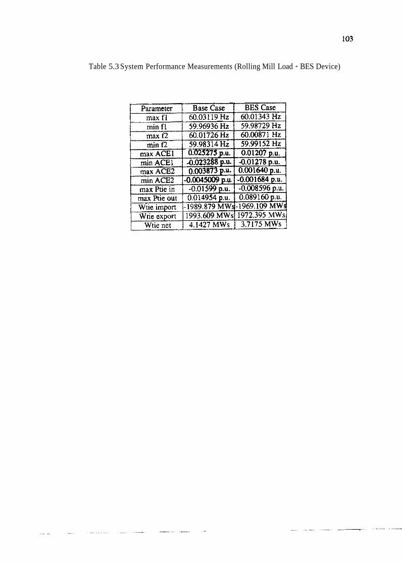
Table 5.3 System Performance Measurements (Rolling Mill Load - BES Device)
CHAPTER 6
CONCLUSIONS
In areas with rapidly changing loads of large magnitude, utility companies
often experience large deviations in frequency and area control error. Inadvertent tie-
line power flow can also be a problem in these situations. A summary was given of
automatic generation control strategies currently used in power systems to: reduce the
deviations in frequency, reduce area control error, and to match the generation with
the demand. Three different types of energy storage devices were discussed. The
most commonly used form of energy storage in the power industry - pumped
hydroelecmc storage - was discussed. An old energy storage technology with new
applications in the power industry - battery energy storage - was also discussed along
with a relatively new technology with many possible applications - superconducting
magnetic energy storage. To study these storage devices effectively requires
integration of models of the devices into an overall power system model.
The focus of this research was to examine the effects that different types of
energy storage devices have on power systems with rapidly changing loads. The
specific loads tested were a step change in load and a five-stand rolling mill load.
The three different cases for each of the two types of load were: no energy storage
device in the system, a superconducting magnetic energy storage device in the
system, and a battery energy storage device in the system.
There are several general conclusions that can be reached by analyzing the
system response with and without an energy storage device on the system. It is

evident that the system response with an SMES device present is very similar to the
system response when a battery energy storage device is present. Although they are
devices with distinctly different methods of operation, they an both able to charge or
discharge nearly instantaneously. The converter voltage, which regulates the power
output of the energy storage device, responds in the same way to the changing loads
regardless of the type of energy storage device. The power output of the two different
devices is nearly identical making the system response nearly identical in both cases.
From the system point of view, the energy storage device is simply a means of
providing or absorbing power instantaneously regardless of what is on the DC side of
the AUDC converter.
An energy storage device in the system is able to respond very quickly to
rapidly changing loads and is able to greatly effect the system operation in the short
term. This means that the large initial deviations in frequency, area control error, and
tie-line power flow are greatly reduced. The long term performance of the system,
though, is constrained by the relatively slower time constants present in the steam
system. Therefore, the system parameters (frequency, tie-line power flow, area
control error) do not reach their steady state values any faster with an energy storage
device in the system than without an energy storage device. In fact, they may take
longer to reach their steady state values because the energy storage device reduces the
large deviation in area control error. This control error is a signal which sets the area
generation. Since the deviation in this signal is smaller than in the case of no energy
storage, the change in generation occurs at a slower rate. Therefore, the tie-line
power flow, frequencies, and area control errors may take a longer time to reach
steady state.
By observing Figures 5.9 and 5.22, it is evident that the energy storage device
for this application has been oversized. The rolling mill load has a "step up - step
down" pattern and allows the energy storage device to charge as well as discharge . Thmfon, the energy level in the device nmains fairly constant throughout the load
cycle, especially in the SMES case whm the losses are only on the order of 5%. For
this application, it is estimated that the energy storage devices could be sized down
from 2 MWh to approximately 0.25 MWh.
The system response was affected by setting a f0.005 Hz deadband on the
energy storage devices. The intent was to keep the energy storage devices from
responding to small deviations in frequency, which are ever-present in the power
system. This is especially important in the battery energy storage device where the
batteries have a limited chargc/discharge cycle life. Although the deadband reduced
the effectiveness of the energy storage devices to some extent and produced "spikes"
in energy chargeldischarge, its elimination produces new problems in the system
response. Without a deadband, the system responds to all deviations in frequency and
is constantly charging or discharging in an attempt to track the system frequency.
This appears to be an inappropriate mode of operation. In the case of a large, rapidly
changing load, the area frequency is driven to its steady state value more rapidly
without the frequency deadband than with the frequency deadband. This is because
the energy storage device supplies (or demands) enough power to eliminate the power
mismatch in the area and thus drives the frequency deviation and area control emr to
approximately zero. Recall, the area control error is a signal that increases or
decreases generation. When the area control emx is near zero, the effect of this input
signal is to change generated power slowly. This means that the energy storage
device will have to charge (or discharge) for a much longer period of time as the
generation slowly increases (or decreases). This qu i res a larger energy storage
capability for the device and a correspondingly higher cost.

There are different types of logic that can be used in controlling the firing
angle of the ACIDC converter i n the SMES and BES systems. One: is a scheme
which uses the area control error as input instead of the frequency error. Another is a
control strategy which may be helpful i n reducing the size of the energy storage
device. I t is a control which uses the frequency or area control error to set the firing
angle during periods of rapidly changing loads, but during periods of relative steady
state, the energy stored is slowly driven to its initial value. At this initial value, the
energy storage device is equally ready to charge or discharge. This could reduce the
chance that the energy stored in the device would reach its upper or lower limit.
It is evident in Figures 4.16, 4.17, 4.28, 4.29, 5.16, 5.17, 5.28, 5.29 that the
rapid increase in generation is less oscillatory when there is an energy storage device
in the system. This is due to the fact that the energy storage device supplies the
power demanded i n the short term and the power generation is able to increase at a
slower and steadier rate.
As mentioned in section 5.4, the initial power output of the BES device in
response to a rapid increase in load is not as great as with the SMES device. This
provides an example of the advantages and disadvantages of a rapid response. If the
frequency deviation and ACE are minimal, the change in generation is slower and the
system parameters take a longer time to reach steady state. If the frequency deviation
and area control error are larger, the change in generation is faster and1 the system
parameters reach steady state faster.
Although large superconducting magnetic energy storage devices are still an
experimental technology, they are certainly feasible. In 1983, the Bonneville Power
Administration successfully built and tested an 8.4 kwh SMES device with a 10 MW
convener. The lossless nature of the device is certainly an advantage as far as
efficiency is concerned (typical estimates range from 92% to 96%). but it is also
advantageous because the lack of resistance eliminates heating of the wire and the
associated degradation of the wire. The rapid response time of an SMES device
would provide a new means of system control in areas with rapidly changing loads.
Different control methodologies could be used to optimize the effectiveness of the
device. The two major drawbacks of an SMES device are the high cost and the fact
that a large-scale device has never been built. The technology exists and numerous
studies have shown the feasibility and advantages of a large-scale SMES device, but
the actual construction of a large-scale device has not been accomplished. Even the
cost of a small-scale device is expensive. A 2800 kVAs SMES device costs on the
order of 2.2 million dollars. As mentioned above, an energy storage (device used to
reduce the detrimental effects of the rolling mill load would be approximately 0.25
MWh. Based on References 13, 15, 161, the cost of an SMES devic:e with energy
storage capacity of 0.25 MWh would be on the order of 100 million dollars.
Large-scale battery energy storage facilities have been used in several
applications in recent history. A 17 MW, 14.4 MWh BES plant in Berlin is used for
frequency regulation. A 10 MW, 51.2 MWh BES plant is used in California for load
leveling. Also, a 20 MW, 10 MWh BES plant is being planned for frequency
regulation in Puerto Rico. Although the efficiency of a BES plant (approximately
80%) is not as high as an SMES plant, battery energy storage technology has the
advantage of being well established and already having several facilities in use. The
BES plant is able to respond as rapidly as an SMES plant to changing loads and it can
provide all of the corresponding advantages as far as new methods of system
operation. One drawback of the BES facility would be the limited cycle life of the
batteries. An advantage when compared to the SMES option would be the relative
inexpense of a BES facility. A 0.25 MWh BES facility would cost on the order of 5
million dollars.

LIST OF REFERENCES
[I] North American Electric Reliability Council Control Performance Criteria, 1991.
[2] G. M. Cook, W.C. Spindler, G. Grefe, "Overview of Battery Power Regulation and Storage," IEEE Transactions on Energy Conversion, v. 6, No. I , pp. 204- 211, March, 1991.
[3] W. Hassenzahl, "Superconducting Magnetic Energy Storage," IEEE Transactions on Magnetics, v. 25, No. 2, pp. 750-757, March. 1989.
[41 J. Jensen, Energv S t o r u , Butterworth Publishers Inc., Boston, 1980.
151 D.S. Cam, "LeadAcid Batteries in U.S.A. Load-Levelling Applications," Journal of Power Sources, v. 3 1, pp. 297-310, May/June, 1990.
., 161 W. Hassenzahl, ElectrochemicgL E l e c t n c a l . t i c Sto-, Hutchinson Ross Publishing Co., New York, 1981.
[7] R.S. Koebbe, "Benefits and Applications of Modular Hydroelectric Pumped Storage," Proceedings of the International Conference on Hydropower, v. 1, pp. 583-592, July, 199 1.
[8] S. Banerjee, J.K. Chatterjee, S.C. Tripathy, "Application of Magnetic Energy Storage Unit as Load-Frequency Stabilizer," IEEE Transactions on Energy Conversion, v. 5, No. 1, pp. 46-51, March, 1990.
191 W .C. Spindler, "LeadAcid Batteries in Utility Energy Storage and Power Control Applications," Journal of Power Sources, v. 35, pp. 395-398, September, 199 1.
[ lo] T. Moore, "Pumped Hydro: Backbone of Utility Storage," EPRI Journal, v. 11, No. 1, pp. 24-31, January/February, 1986.
[ 1 1) J.G. Warnock, "Milestones in Pumped Storage Development," American Society of Civil Engineers, Proceedings of the Engineering Foundation Conference on Converting Existing Hydro-Electric Dams and Reservoirs into Pumped Storage Facilities,Rindge, NH, pp. 163-196, August 18-23, 1974.
1121 H.J. Boenig, J.F. Hauer, "Commissioning Tests of the Bonneville Power Administration 30 MJ Superconducting Magnetic Energy Storage Unit," IEEE Transactions on Power Apparatus and Systems, v. PAS-104, No. 2, pp. 302- 312, February, 1985.

J.F. Hauer, H.J. Boenig, "Control Aspects of the Tacoma Superconducting Magnetic Energy Storage Project," E E E Transactions on Power Systems, v. PWRS-2, No. 2, pp. 443-450, May, 1987.
P.D. Baumann, "Energy Conservation and Environmental Benefits That May Be Realized from Superconducting Magnetic Energy Storage," Proceedings of the EEEPES 1992 Winter Meeting, New York, NY, January, 26-30, 1992.
H.A. Peterson, N. Mohan, R.W. Boom, "Superconductive Energy Storage Inductor - Convener Units for Power Systems," IEEE Transactions on Power Apparatus and Systems, v. PAS-94, No. 4, pp. 1337-1346, JulyIAugust, 1975.
C.A. Luongo, R.J. Loyd, "Superconducting Magnetic Energy Storage for Elecmc Utility Load Leveling: A Study of Cost vs. Stored Energy," Proceedings of the American Power Conference, v. 49, pp. 207-212, 1987.
J.G. DeSteese, D.K. Kreid, J.M. Haner, W.E. Myers, "Assessment of SMES Benefits in Electric Utility Applications," Proceedings of the American Power Conference, v. 53, pp. 1 149- 1 156, 199 1.
K. Tam, A. Yarali, "Operation Principle and Application of Multiterminal Superconductive Energy Storage Systems," IEEEPES 1992 Winter Meeting, New York, January 26-30, 1992.
G.W. Vinal, Storage Batteries, John Wiley & Sons, Inc., New York, 1955.
C.H. Mantell, Batteries and Energy S v s w , McGraw-Hill, Inc., New York, 1983.
M.D. Anderson, D.S. C m , "Battery Energy Storage Technologies"
H.J. Kunisch, K.G. Kramer, H. Dominik, "Battery Energy Storage: Another Option for Load-Frequency-Control and Instantaneous Reserve," IEEE Transactions on Energy Conversion, v. EC-1, No. 3, pp.41-46, September, 1986.
S. Eckroad, B. Radimer, "Review of Engineering Design Considerations for Battery Energy Management Systems," IEEE Transactions on Energy Conversion, v. 6, No. 2, pp. 303-309, June, 1991.
R.C. Reckrodt, M.D. Anderson, R.M. Kluczny, "Economic Model for Battery Energy Storage: Improvements for Existing Methods," IEEE Transactions on Energy Conversion, v. 5, No. 4, pp. 659-665, December, 1990.
N. Jaleeli, L.S. VanSlyck, D.N. Ewart, L.H. Fink, A.G. Hoffmann, "Understanding Automatic Generation Control", IEEE Transactions on Power Systems, v. 7, No. 3, pp. 1 106- 1 1 1 1 , August, 1992.
R. Ramabhadran, G.T. Heydt, R. Shoureshi, R. Kramer, M. Stears, "Active and Reactive Power Flow for Multiarea Systems on Automatic Generation Control", September, 1992.

[27] 0.1. Elgerd, C.E. Fosha, Jr., "Optimum Megawatt Frequency Control of Multiarea Electric Energy Systems," E E E Transactions on Power Apparatus and Systems, v. PAS-89, No. 4, pp. 556-563, April, 1970.
[28] C.E. Fosha, Jr., 0.1. Elgerd, "The Megawatt-Frequency ControI Problem: A New Approach Via Optimal Control Theory," JEEE Transactions on Power Apparatus and Systems, v. PAS-89, No. 4, pp. 563-577, April, 1970.
[29] F.P. deMello, R.J. Mills, W.F. B'Rells, "Automatic Generation Clontrol Part I - Process Modeling" IEEEPES Summer Meeting, San Francisco, July 9-14, 1972.
[30] F.P. deMello, R.J. Mills, W.F. B'Rells, "Automatic Generation Clontrol Part I1 - Digital Control Techniques," EEEPES Summer Meeting, San Francisco, July 9-14, 1972.
131 1 R. Podmore, M.J. Gibbard, D.W. Ross, K.R. Anderson, R.G. Page, K. Argo, K. Coons, "Automatic Generation Control of Jointly-Owned Generating Units," IEEE Transactions on Power Apparatus and Systems, v. PAS-98, No. 1, pp. 207-2 15, JanuaryIFebruary 1979.
1321 W. Prince, "Cost Aspects of AGC, Inadvenant Energy and Time Error," IEEE Transactions on Power Systems, v. PS-5, No. 1, pp. 11 1- 118, February, 1990.
1331 A.J. Wood, B.F. Wollenberg, Power Generation. Operation. and Control, John Wiley & Sons, Inc., New York, 1984.
[34] IEEE Committee Report, "Dynamic Models for Steam and Hydro Turbines in Power System Studies," IEEE Transactions on Power Apparatus and Systems, v. PAS-86, pp. 443-453, April, 1967.
[35] C.L. Mantell, Batteries and Energy Svstem, McGraw-Hill, Inc., New York, 1983.
1 361 W. Buckel, Superconductivitv: Fundamentals and w a t i o m , Weinheim, New York, 1991.
1371 V.Z. Kresin, S.A. Wolf, Fundamentals of Superconductivity, Plenum Press, New York , 1990.
1381 B.S. Deaver, Advances in Superconductivity, Plenum Press, New York, 1983. . .
[39] T. Van Duzer, C. Turner, Principles of Su oerconductlve Candrcuip, Elsevier North Holland, New York, 198 1. '
[40] G. Burns, High Temperature Superconductivitv: &J I n t r o d u ~ , Academic Press, Boston, 1992.
[4 ( 1 C.N.R. Rao, W t r v of F&b T e w r e S ~ o n d u c t o r s , World Scientific, River Edge, New Jersey, 1991.

[42] H.S. Kwok, P. Coppens, Y.H. Kao, ~ r c o n & c t i v y& Its -, . . . . I t
American Institute of Physics, New York, 1991.
1431 L.C. Gupta, moretical and W t a l &mishes to Fkgb-Tc d ~ o n v e n n ~ e r c o n d u c t i v i t v , Nova Science Publishers, New York, 1991.
[44] M. Ferrier, "Stockage d'energie dans un enroulement supraconductor," Low Temperature and Electrical Power, London, pp.425-432, 1970.