Embed Size (px)
Citation preview

ENERGY SAVING VITERBI DECODER FOR FORWARD ERROR
CORRECTION IN MOBILE NETWORKS
A dissertation submitted to The University of Manchester for the degree of
Master of Science
in the Faculty of Engineering and Physical Sciences
2010
ANJALI KUPPAYIL SAJI
School of Computer Science
9 September 2010 P a g e | 2 7537929_AnjaliKuppayilSaji.pdf
CONTENTS
List of Tables & Figures…………………………………………………………..…………………..4
Abstract ………………………………………………………………………………………………..7
Declaration ............................................................................................................................. 9
Copyright Statement ............................................................................................................. 10
Acknowledgements................................................................................................................ 11
1. INTRODUCTION .......................................................................................................... 12
1.1 Motivation .................................................................................................................. 12
1.2 Outline and Context of the Report ............................................................................. 14
1.3 Main Objectives ......................................................................................................... 15
1.4 Scope of the Project ................................................................................................... 16
1.5 Overview of the Report .............................................................................................. 16
1.6 Summary .................................................................................................................... 16
2. ERROR DETECTION AND CORRECTION TECHNIQUES ...... ........................... 17
2.1 Forward Error Correction (FEC)................................................................................ 17
2.2 Block Codes ............................................................................................................... 18
2.3 Convolutional Codes .................................................................................................. 20
2.4 Recent Developments ................................................................................................ 24
2.5 Automatic Repeat Request (ARQ) ............................................................................. 28
2.6 Hybrid Automatic Repeat Request (H-ARQ) ............................................................ 30
2.7 Summary .................................................................................................................... 31
3. THE VITERBI ALGORITHM ..................................................................................... 32
3.1 Encoding Mechanism ............................................................................................... 32
3.2 Decoding Mechanism ............................................................................................... 33
3.3. Applications .............................................................................................................. 37
3.4 Related Work ............................................................................................................ 38
3.5 Summary .................................................................................................................... 42

9 September 2010 P a g e | 3 7537929_AnjaliKuppayilSaji.pdf
4. AN ALTERNATIVE ENERGY SAVING STRATEGY .......... .................................. 43
4.1 Principle ..................................................................................................................... 43
4.2 Summary .................................................................................................................... 46
5. RESEARCH METHODS .............................................................................................. 47
5.1 Research Approach .................................................................................................... 47
5.2 Implementation Tools ................................................................................................ 49
5.3 Research Plan ............................................................................................................. 50
5.4 Likely Issues .............................................................................................................. 50
5.5 Summary .................................................................................................................... 51
6. DESIGN AND IMPLEMENTATION .......................................................................... 52
6.1 The Transmitter Block ............................................................................................... 52
6.2 The Communications Channel ................................................................................... 53
6.3 The Receiver Block .................................................................................................... 53
6.4 Analysis of Failure Cases for Simple Decoder .......................................................... 58
6.5 Summary .................................................................................................................... 64
7. TESTING AND ANALYSIS ......................................................................................... 65
7.1 Overview of Testing................................................................................................... 65
7.2 Results and Analysis .................................................................................................. 66
7.3 Summary .................................................................................................................... 82
8. CONCLUSIONS AND FUTURE WORK .................................................................... 83
8.1 Conclusions ................................................................................................................ 83
8.2 Future Work ............................................................................................................... 84
LIST OF REFERENCES ................................................................................................... 86
Appendix A: Gantt Chart .................................................................................................... 90
Appendix B: General Algorithm for Hamming Codes........................................................ 92
Appendix C: CRC Generator Polynomials ......................................................................... 93
Appendix D: BEP Performance Test Results and Statistics. ............................................... 94

9 September 2010 P a g e | 4 7537929_AnjaliKuppayilSaji.pdf
i. Datalength 10,000. Switching when there are no bit-errors for 7 consecutive slots ...... 94
ii. Datalength 10,000. Switching when there are no bit-errors for 21 consecutive slots .... 97
iii.Comparison of average number of bits decoded between switches ............................. 100
Appendix E: Packet Loss Rate Calculations ..................................................................... 101
Appendix F: Timing Measurements .................................................................................. 102
Appendix G: MATLAB ® code .......................................................................................... 103
1. encoder.m .................................................................................................................... 103
2. modulate.m .................................................................................................................. 103
3. demodulate.m .............................................................................................................. 103
4. simpleDecoder.m ......................................................................................................... 104
5. adapVitDec.m (Adapted Viterbi Decoder) ................................................................. 105
6. MAINFILE.m .............................................................................................................. 110
7. Portion of conVitDec2.m (‘My Viterbi’ Decoder ) ................................................. 113
8. MAINFILE_PacketLoss.m (Modified Main File to Measure Packet Loss) ............... 113
Word Count: 26,586
9 September 2010 P a g e | 5 7537929_AnjaliKuppayilSaji.pdf
List of Tables
Table 2.1: State Transition Table ......................................................................................... 22
Table 2.2: Output Table ........................................................................................................ 22
Table 6.1: Operation of Simple Decoder under Example Sequence 1 ................................. 60
Table 6.2 Operation of Simple Decoder under Example Sequence 2 .................................. 62
Table 6.3: Operation of Simple Decoder under Example Sequence 3 ................................. 62
List of Figures
Figure 2.1: ½, K=3 Convolutional Encoder ......................................................................... 21
Figure 2.2: State Diagram ..................................................................................................... 23
Figure 2.3: Trellis Diagram for a 1/2, K=3,(7,5) convolutional encoder ............................. 23
Figure 2.4: Example of an LDPC Code. Reproduced from [19] .......................................... 25
Figure 2.5: Schematic Diagram of a Turbo Encoder with two identical
Recursive Systematic Encoders, an N-bit Interleaver and Puncturer. .............. 26
Figure 2.6 Schematic Diagram of Turbo Decoder. Reproduced from [16] .......................... 27
Figure 3.1: Rate = ½ K = 7, (171,133) Convolutional Encoder ........................................... 33
Figure 3.2: Schematic representation of the Viterbi decoding block ................................... 34
Figure 3.3 Selected minimum error path for a ½ K = 3 (7, 5) coder .................................... 36
Figure 3.4: Normalized energy estimates for the Viterbi and fixed T-algorithm
(Tf) decoders as code rate and signal to noise ratio (Eb/No) vary. ........................ 39
Figure 3.5: Normalized energy estimates for the Viterbi and adaptive T-algorithm
(Ta) decoders as code rate and signal to noise ratio (Eb/No) vary
while maintaining bit-error rate below 0.0037. ................................................. 40
Figure 4.1: Proposed Simple Decoder .................................................................................. 45
Figure 6.1: Proposed Simple Decoder that will be used when there are no bit-errors ......... 54
Figure 6.2a: Flowchart for the Switching Decoder: Part A .................................................. 56
Figure 6.2b: Flowchart for the Switching Decoder: Part B .................................................. 57
Figure 7.1: Data Length = 10,000, Switched to Simple Decoder when no errors
for 7 consecutive slots ...................................................................................... 69

9 September 2010 P a g e | 6 7537929_AnjaliKuppayilSaji.pdf
Figure 7.2: Average Fractional Difference in number of errors between Switching
Decoder and ‘My Viterbi’ Decoder. Switched to Simple Decoder when
there are no errors for 7 consecutive slots ........................................................ 70
Figure 7.3: Data Length = 10,000. Decoding switched to Simple Decoder when
there are no bit-errors for 35 consecutive slots ................................................ 71
Figure 7.4: Data Length = 10,000. Decoding switched to Simple Decoder when
there are no bit-errors for 21 consecutive slots .................................................... 72
Figure 7.5: Average Fractional difference in errors between the Switching decoder
and ‘My Viterbi’ decoder. Decoding switched to Simple Decoder when
there are no bit-errors 21 consecutive slots ....................................................... 72
Figure 7.6: Percentage of Decoding done by each decoder in the Switching
Decoder. Decoding switched to Simple Decoder when there are no
bit-errors for 7 consecutive slots ....................................................................... 73
Figure 7.7 Percentage of Decoding done by each decoder in the Switching
Decoder. Decoding switched to Simple Decoder when there are no
bit-errors for 21 consecutive slots ...................................................................... 74
Figure 7.8: Average number of bits being decoded per call to each decoder.
Decoding switched to Simple Decoder when there are no bit-errors
for 7 consecutive slots ...................................................................................... 75
Figure 7.9: Average number of bits being decoder per call to each decoder.
Decoding switched to Simple Decoder when there are no bit-errors
for 21 consecutive slots .................................................................................... 76
Figure 7.10: Packet Loss Rate. Decoding switched to Simple Decoder when there
are no bit-errors 21 consecutive slots .............................................................. 78
Figure 7.11: Results of Benchmarking on MATLAB® ........................................................ 80
Figure 7.12: Timing Measurements ..................................................................................... 81

9 September 2010 P a g e | 7 7537929_AnjaliKuppayilSaji.pdf
Abstract
This project is concerned with bit-error control mechanisms that are used in mobile
telephone and wireless computer networks today. The use of Forward Error Correction
(FEC) techniques using convolutional codes is studied along with the Viterbi Algorithm
for decoding convolutional codes. Due to its computational complexity, a major portion
of the energy consumption at a wireless digital receiver results from the Viterbi decoder.
This project investigates a new energy saving strategy that may enable receivers to
decode convolutionally coded transmissions with lower energy utilization.
In practical applications, there can be large variations in the bit-error rate encountered at
a mobile receiver. These variations will be more pronounced when the receiver is in
motion between access-points. The energy saving strategy is to switch to a simpler
decoding mechanism when it is ascertained that bit-errors are not occurring. When the
presence of bit-errors is detected by the simple decoder it switches back to the Viterbi
decoder to try and correct the bit-errors. On switching from the simple decoder to the
Viterbi decoder, the Viterbi decoder must be accurately initialized with the current state
of the simple decoder. Similarly, on switching from the Viterbi decoder to the simple
decoder, the simple decoder must be accurately initialized with the current state of the
Viterbi Decoder. While it is easy for the simple decoder to detect the occurrence of bit-
errors, getting the Viterbi decoder to determine when there are no bit-errors and switch
back to the simple decoder presents a harder problem. These issues are addressed and a
working solution is presented.
Results obtained by MATLAB® simulation demonstrate that, with appropriate settings,
no increase in bit-error probability appears to be introduced by the new method. The
packet loss rate was observed to be identical for all values of signal to noise ratio
(Eb/N0). Evaluating the energy saving capability of the new technique requires the
profiling of its energy consumption in comparison to that of a standard Viterbi decoder.
To do this accurately for a true VLSI implementation would require resources beyond
the scope of the project. However, MATLAB® provides some profiling facilities based
on execution times and these can give some idea of the likely relationship between the
energy consumption of these particular algorithms. Since they perform the same types of
operation, they are likely to be equally affected by interpretation efficiency and the
9 September 2010 P a g e | 8 7537929_AnjaliKuppayilSaji.pdf
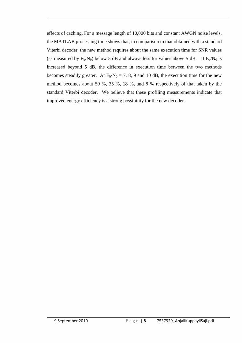
effects of caching. For a message length of 10,000 bits and constant AWGN noise levels,
the MATLAB processing time shows that, in comparison to that obtained with a standard
Viterbi decoder, the new method requires about the same execution time for SNR values
(as measured by Eb/N0) below 5 dB and always less for values above 5 dB. If Eb/N0 is
increased beyond 5 dB, the difference in execution time between the two methods
becomes steadily greater. At Eb/N0 = 7, 8, 9 and 10 dB, the execution time for the new
method becomes about 50 %, 35 %, 18 %, and 8 % respectively of that taken by the
standard Viterbi decoder. We believe that these profiling measurements indicate that
improved energy efficiency is a strong possibility for the new decoder.

9 September 2010 P a g e | 9 7537929_AnjaliKuppayilSaji.pdf
Declaration
No portion of the work referred to in the dissertation has been submitted in support of an
application for another degree or qualification of this or any other university or other
institute of learning.

9 September 2010 P a g e | 10 7537929_AnjaliKuppayilSaji.pdf
Copyright Statement
i. Copyright in text of this dissertation rests with the author. Copies (by any process)
either in full, or of extracts, may be made only in accordance with instructions given
by the author. Details may be obtained from the appropriate Graduate Office. This
page must form part of any such copies made. Further copies (by any process) of
copies made in accordance with such instructions may not be made without the
permission (in writing) of the author.
ii. The ownership of any intellectual property rights which may be described in this
dissertation is vested in the University of Manchester, subject to any prior agreement
to the contrary, and may not be made available for use by third parties without the
written permission of the University, which will prescribe the terms and conditions of
any such agreement.
iii. Further information on the conditions under which disclosures and exploitation may
take place is available from the Head of the School of Computer Science.

9 September 2010 P a g e | 11 7537929_AnjaliKuppayilSaji.pdf
Acknowledgements
I take this opportunity to express my sincere gratitude to Dr. Barry Cheetham for his
constant guidance and support throughout this project. His encouragement helped me
persevere despite setbacks and his valuable suggestions became crucial turning points
towards the success of this project.
I would also like to thank Dr. Linda Brackenbury for her valuable advice and direction
during the course of this project. She provided me with material that was influential in
the success of the project.
I sincerely thank my MSc. program director, Dr. Thierry Scheurer for the opportunity to
undertake this project at the University of Manchester.
I am also deeply indebted to my family and friends who were a constant source of
encouragement and motivation. Without them this project would not have been a
success.

9 September 2010 P a g e | 12 7537929_AnjaliKuppayilSaji.pdf
Chapter 1
INTRODUCTION
This chapter gives an outline of the main motivations and ideas that underpin this
project. The main objectives are then presented along with the scope of the investigation
and an overview of the report organization.
1.1 Motivation
Unlike wired digital networks, wireless digital networks are much more prone to bit-
errors. Packets of bits that are received are more likely to be damaged and considered
unusable in a packetized system. Error detection and correction mechanisms are vital
and numerous techniques exist for reducing the effect of bit-errors and trying to ensure
that the receiver eventually gets an error free version of the packet. The major
techniques used are error detection with Automatic Repeat Request (ARQ) [4], Forward
Error Correction (FEC) [11] and hybrid forms of ARQ and FEC (H-ARQ) [8, 9]. This
project focuses on FEC techniques.
Forward Error Correction (FEC) is the method of transmitting error correction
information along with the message. At the receiver, this error correction information is
used to correct any bit-errors that may have occurred during transmission. The
improved performance comes at the cost of introducing a considerable amount of
redundancy in the transmitted code. There are various FEC codes in use today for the
purpose of error correction. Most codes fall into either of two major categories: block
codes [11] and convolutional codes [6]. Block codes work with fixed length blocks of
code. Convolutional codes deal with data sequentially (i.e. taken a few bits at a time)
with the output depending on both the present input as well as previous inputs.
9 September 2010 P a g e | 13 7537929_AnjaliKuppayilSaji.pdf
In terms of implementation, block codes become very complex as their length increases
and are therefore harder to implement. Convolutional codes, in comparison to block
codes, are less complex and therefore easier to implement. In packetized digital
networks convolutionally coded data would still be transmitted as packets or blocks.
However these blocks would be much larger in comparison to those used by block
codes. The fact that convolutional codes are easier to implement, coupled with the
emergence of a very efficient convolutional decoding algorithm, known as Viterbi
Algorithm [1], is one of the reasons for convolutional codes becoming the preferred
method for real time communication technologies. This project studies the use of
various error detection and correction techniques for mobile networks with a focus on
non-recursive convolutional coding and the Viterbi Algorithm.
The constraint length of a non-recursive convolutional code results from the number of
stages present in the combinatorial logic of the encoder. The error correction power of a
convolutional code increases with its constraint length. However, decoding complexity
increases exponentially as the constraint length increases. Fortunately, the efficiency of
the Viterbi algorithm allows the use of convolutional coding with quite reasonable
constraint lengths in many applications. Due to its high accuracy in finding the most
likely sequence of states, the Viterbi algorithm is used in many applications ranging
from communication networks [27, 30, 31], optical character recognition [26] and even
DNA sequence analysis. Recently, interest has grown in the use of certain error
correction codes that provide much superior performance. Two of these codes are Low
Density Parity Check codes [19] and Turbo Codes [16]. The ideas presented in this
thesis are likely to be relevant to these more advanced codes as well as non-recursive
convolutional codes, but this thesis will concentrate on convolutional codes.
Since preservation of battery energy is a major concern for mobile devices, it is
desirable that the error detection and correction mechanism take the minimum amount
of energy to execute. This project explores the possibility of improving the energy
efficiency of the Viterbi decoder and develops an algorithm to achieve this.

9 September 2010 P a g e | 14 7537929_AnjaliKuppayilSaji.pdf
1.2 Outline and Context of the Report
This project focuses on the use of Viterbi Algorithm for forward error correction in
mobile networks. It is desirable to keep energy consumption at a minimum in order to
optimize use of available battery energy. In order to get good error correcting
capabilities, the constraint length must be kept high and since the complexity of a
convolutional decoder increases exponentially with its constraint length, optimizing the
decoding mechanism with respect to energy consumption becomes a worthwhile goal.
The growing need for improved energy efficiency of decoders has resulted in several
approaches being explored [20, 34]. The main focus of the project is to explore an idea,
proposed by Barry Cheetham [2] which is to switch off the Viterbi decoder and use a
simpler decoder when no bit-errors are occurring. It is possible that by doing this, a
significant amount of energy could be saved. When bit-errors are detected, the Viterbi
decoder can be switched back on to take advantage of its error correction functionality.
This process at the receiver depends on having a memory of previous bits received.
Correctly maintaining and using this previous memory (previous history) when
switching between the two decoders is one of the main technical challenges in the
project.
The energy saving mechanism proposed by Barry Cheetham [2] is based on an earlier
idea published by Wei Shao [3], though it is hoped that the new approach will be easier
to implement. This algorithm can be developed using MATLAB ® though it will require
a custom designed version of the Viterbi algorithm to be developed from scratch, and
then adapted to the new energy saving idea [2]. Possible problems that may affect the
accuracy and energy saving capabilities of the algorithm must be analyzed and solutions
to these problems must be developed. The performance of the resulting algorithm must
be studied in terms of bit-error performance, packet loss rates and processing time.
In principle, evaluating the performance of the new technique requires profiling of the
energy consumption of the two algorithms involved. To do this accurately would
require resources beyond the scope of the project. MATLAB ®, provides some profiling
facilities. But relating information obtained to energy consumption as would be

9 September 2010 P a g e | 15 7537929_AnjaliKuppayilSaji.pdf
observed in a VLSI implementation of the code is a complex issue. Nevertheless, it is
believed that the execution times of particular parts of the algorithms can give some
idea of the likely relationship between the energy consumption of these particular parts.
Hence, in place of quoting estimations of the likely energy consumption of different
techniques, execution times will be quoted with an implicit assumption that this gives a
first order approximation to the likely energy consumption. By comparison with the
standard Viterbi decoder available in MATLAB®, an analysis will be made of whether
this method provides a significant improvement over existing mechanisms.
1.3 Main Objectives
The main objectives of this project are as follows
i. An understanding of the background literature relevant to error detection and error
control mechanisms as currently used in packetized digital communication
networks.
ii. A detailed understanding of the concept of convolutional coding, and decoding using
the Viterbi algorithm.
iii. An implementation of the Viterbi algorithm in MATLAB ® to obtain a ‘custom
designed’ version called ‘My Viterbi’ and check that it is working correctly by
comparing its performance with that of the Viterbi decoder function (vitdec.m)
provided by MATLAB® (A custom designed Viterbi decoder is needed because
MATLAB ® does not provide access to the code for vitdec.m).
iv. A resolution of questions that still need to be answered about the new algorithm [2]
including the correct initialization of component decoders and the stability of the
feedback mechanism
v. An implementation in MATLAB® of the new algorithm [2] as a modification of the
custom designed Viterbi algorithm.
vi. An evaluation of the new algorithm [2] in terms of its accuracy and capacity for
achieving energy saving tAnalysis will be performed on the basis of bit-error
performance, packet loss rates and execution time (considered to provide a first
order approximation to energy consumption).
9 September 2010 P a g e | 16 7537929_AnjaliKuppayilSaji.pdf
1.4 Scope of the Project
This project is intended to further develop and implement the energy saving decoding
algorithm developed by Barry Cheetham [2]. Solutions to some issues that still
remained to be resolved at the beginning of this project. The main focus of this project
is to provide a working demonstration of the algorithm by implementation in
MATLAB ® and to analyze its performance by comparison with the standard Viterbi
decoder available in MATLAB®. The system will be developed using a hard decision
Viterbi decoder but may be extended to using a soft decision decoder. The project does
not consider the circuit level design of the algorithm but uses a high level approach to
test the proposed algorithm. This may be considered in future work if it is found that
this algorithm promises considerable benefits over existing mechanisms.
1.5 Overview of the Report
Chapter 2 provides the background literature relevant to Error Detection and Control
Mechanisms and describes convolutional codes in detail. Chapter 3 is devoted to a study
of the Viterbi algorithm and in particular the Viterbi Decoder. Chapter 4 introduces the
new energy saving strategy proposed by Barry [2] and explains the basic principles that
drive the mechanism. Chapter 5 describes the research methodology that will be
followed to guide the structure of the project. Design and implementation details of the
system to be developed are detailed in Chapter 6. Chapter 7 provides a summary of the
results obtained through testing and provides a detailed analysis of the results. Chapters
8 and 9 describe the conclusions that were made at the end of the project and provide
suggestions for further investigations on the developed algorithm.
1.6 Summary
This chapter has described the motivations behind this project and has defined its main
objectives and scope. The following chapter describes the major classifications of error
detection and correction mechanisms, their advantages and drawbacks.

9 September 2010 P a g e | 17 7537929_AnjaliKuppayilSaji.pdf
Chapter 2
ERROR DETECTION AND CORRECTION
TECHNIQUES
This section describes common methods of error detection and error correction as used in
wireless networks. The methods described include Forward Error Correction (FEC) ,
Automatic Repeat Request (ARQ) and Hybrid- ARQ (H-ARQ)
2.1 Forward Error Correction (FEC)
Forward Error Correction is a method used to improve channel capacity by introducing
redundant data into the message [8]. This redundant data allows the receiver to detect
and correct errors without the need for retransmission of the message. Forward Error
Correction proves advantageous in noisy channels when a large number of
retransmissions would normally be required before a packet is received without error. It
is also used in cases where no backward channel exists from the receiver to the
transmitter. A complex algorithm or function is used to encode the message with
redundant data. The process of adding redundant data to the message is called channel
coding. This encoded message may or may not contain the original information in an
unmodified form. Systematic codes are those that have a portion of the output directly
resembling the input. Non-systematic codes are those that do not.
It was earlier believed that as some degree of noise was present in all communication
channels, it would not be possible to have error free communications. This belief was
proved wrong by Claude Shannon in 1948. In his paper [9] titled “A Mathematical
Theory of Communication”, Shannon proved that channel noise limits transmission rate
and not the error probability. According to his theory, every communication channel has
a capacity C (measured in bits per second), and as long as the transmission rate, R

9 September 2010 P a g e | 18 7537929_AnjaliKuppayilSaji.pdf
(measured in bits per second), is less than C, it is possible to design an error-free
communications system using error control codes. The now famous Shannon-Hartley
theorem, describes how this channel capacity can be calculated. However, Shannon did
not describe how such codes may be developed. This led to a wide spread effort to
develop codes that would produce the very small error probability as predicted by
Shannon. It was only in the 1960’s that these codes were finally discovered [10]. There
were two major classes of codes that were developed, namely block codes and
convolutional codes.
2.2 Block Codes
As described by Proakis [11], linear block codes consist of fixed length vectors called
code words. Block codes are described using two integers k and n, and a generator
matrix or polynomial [6]. The integer k is the number of data bits in the input to the
block encoder. The integer n is the total number of bits in the generated codeword. Also,
each n bit codeword is uniquely determined by the k bit input data.
Another parameter used to describe is its weight. This is defined as the number of non
zero elements in the code word. In general, each code word has its own weight. If all the
M code words have equal weight it is said to be fixed-weight code [11].
Hamming Codes and Cyclic Redundancy Checks are two widely used examples of block
codes. They are described below.
2.2.1. Hamming Codes
A commonly known linear Block Code is the Hamming code. Hamming codes can
detect and correct a single bit-error in a block of data. In these codes, every bit is
included in a unique set of parity bits [12]. The presence and location of a single parity
bit-error can be determined by analyzing parities of combinations of received bits to
produce a table of parities each of which corresponds to a particular bit-error
combination. This table of errors is known as the error syndrome. If all the parities are
correct according to this pattern, it can be concluded that there is not a single bit-error in
the message (there may be multiple bit-errors). If there are errors in the parities caused

9 September 2010 P a g e | 19 7537929_AnjaliKuppayilSaji.pdf
by a single bit-error, the erroneous data bit can be found by adding up the positions of
the erroneous parities. The reference [12] provides the general algorithm used for
creating Hamming codes and is presented in Appendix B.
While Hamming codes are easy to implement, a problem arises if more than one bit in
the received message is erroneous. In some cases, the error may be detected but cannot
be corrected. In other cases, the error may go undetected resulting in an incorrect
interpretation of transmitted information. Hence, there is a need for more robust error
detection and correction schemes that can detect and correct multiple errors in a
transmitted message.
2.2.2 Cyclic codes and Cyclic Redundancy Checks (CRC)
Cyclic Codes are linear block codes that can be expressed by the following
mathematical property. If C = [c n-1 cn-2 … c1 c0] is a code word of a cyclic code, then [c n-2
cn-3 … c0 cn-1], which is obtained by cyclically shifting all the elements to the left, is also a
code word [11]. In other words, every cyclic shift of a codeword results in another
codeword. This cyclic structure is very useful in encoding and decoding operations
because it is very easy to implement in hardware.
A cyclic redundancy check or CRC is a very common form of cyclic code which is used
for error detection purposes in communication systems. At the transmitter, a function is
used to calculate a value for the CRC check bits based on the data to be transmitted.
These check bits are transmitted along with the data to the receiver. The receiver
performs the same calculation on the received data and compares it with the CRC check
bits that it has received. If they match, it is considered that no bit-errors have occurred
during transmission. While it is possible for certain patterns of error to go undetected, a
careful selection of the generator function will minimize this possibility.
Using different kinds of generator polynomials, it is possible to use CRC’s to detect
different kinds of errors such as all single bit-errors, all double bit errors, any odd
number of errors, or any burst error of length less than a particular value. The specific
types of generator polynomials for detecting these errors are listed in Appendix C. Due
9 September 2010 P a g e | 20 7537929_AnjaliKuppayilSaji.pdf
to these properties, the CRC check is a very useful form of error detection. The IEEE
802.11 standard for CRC check polynomial is the CRC-32 [13].
2.3 Convolutional Codes
Convolutional codes are codes that are generated sequentially by passing the information
sequence through a linear finite-state shift register. A convolutional code is described
using three parameters k, n and K. The integer k represents the number of input bits for
each shift of the register. The integer n represents the number of output bits generated at
each shift of the register. K is an integer known as constraint length, which represents
the number of k bit stages present in the encoding shift register [6]. Each possible
combination of shift registers together forms a possible state of the encoder. For a code
of constraint length K, there exist 2K-1 possible states.
Since convolutional codes are processed sequentially, the encoding process can start
producing encoded bits as soon as a few bits have been processed and then carry on
producing bits for as long as required. Similarly, the decoding process can start as soon
as a few bits have been received. In other words, this means is that it is not necessary to
wait for the entire data to be received before decoding is started. This makes it ideal in
situations where the data to be transmitted is very long and possibly even endless! e.g.:
phone conversations.
In packetized digital networks, even convolutional codes are sent as packets of data.
However, these packet lengths are usually considerably longer than what would be
practical for block codes. Additionally, in block codes, all the blocks or packets would be
of the same length. In convolutional codes the packets may have varying lengths.
There are alternative ways of describing a convolutional code. It can be expressed as a
tree diagram, a trellis diagram or a state diagram. For the purpose of this project, trellis
and state diagrams are used. These two diagrams are explained below.

9 September 2010 P a g e | 21 7537929_AnjaliKuppayilSaji.pdf
2.3.1 State Diagram
The state of the encoder (or decoder) refers to a possible combination of register values
in the array of shift registers that the encoder (or decoder) is comprised of. A state-
diagram shows all possible present states of the encoder as well all the possible state
transitions that may occur. In order to create the state diagram, a state transition table
may first be made, showing the next state for each possible combination of the present
state and input to the decoder. The following tables and figures show how a state
diagram is drawn for a convolutional encoder. For the purpose of illustration a 3 stage
encoder with rate ½ has been shown. In the project, the standard rate ½, 7stage encoder
will be used.
Figure 2.1 shows a convolutional encoder with a rate ½ and K =3, (7, 5). Rate ½ is used
to denote the fact that for each bit of input the encoder a two bit output. K, the constraint
length of the encoder being three, establishes that the input persists for 3 clock cycles
[11]. The constraint length can be calculated as one more than the number of serially
connected shift registers in the encoder. Octal numbers seven and five when converted
to binary form represent the generator polynomials signify the shift register connections
to the upper and lower modulo-two adders respectively. 7(8) in binary form is 111. Hence
direct input, output of first shift register and output of second shift register are connected
to the fist modulo-two adder (A in Figure 2.1). Similarly, 5(8) in binary form is 101.
Hence direct input and output of second shift register are connected to the second
modulo-two adder (B in the Figure 2.1)
Figure 2.1: ½, K=3 Convolutional Encoder
9 September 2010 P a g e | 22 7537929_AnjaliKuppayilSaji.pdf
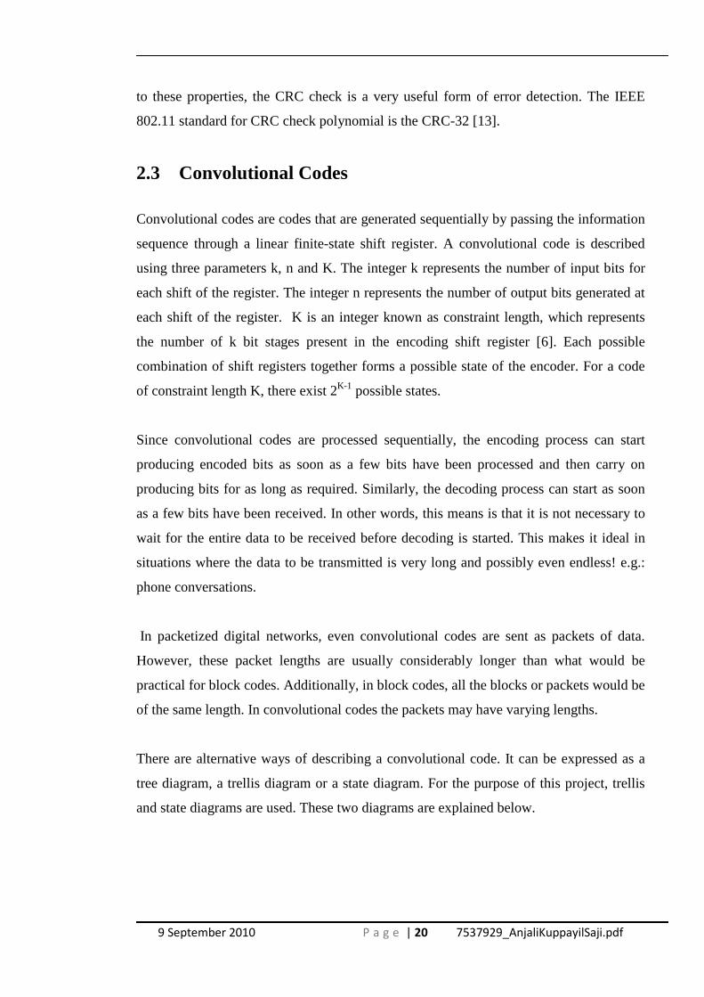
By looking at the transition of shift registers (also known as Flip Flops) FF1 and FF2, the
State transition table is created for each combination of Input and Current State. This is
shown in Table 2.1
Current State (FF1 FF2)
Next State if
Input =0 Input=1
00 00 10
01 00 10
10 01 11
11 01 11
Table 2.1: State Transition Table
Another table can be created to demonstrate the change in output for each combination
of input and previous output. This is called the Output Table and is shown in Table 2.2
Current Output Output Symbols if Input = 0 Input= 1
00 00 11
01 11 00
10 10 01
11 01 10
Table 2.2: Output Table
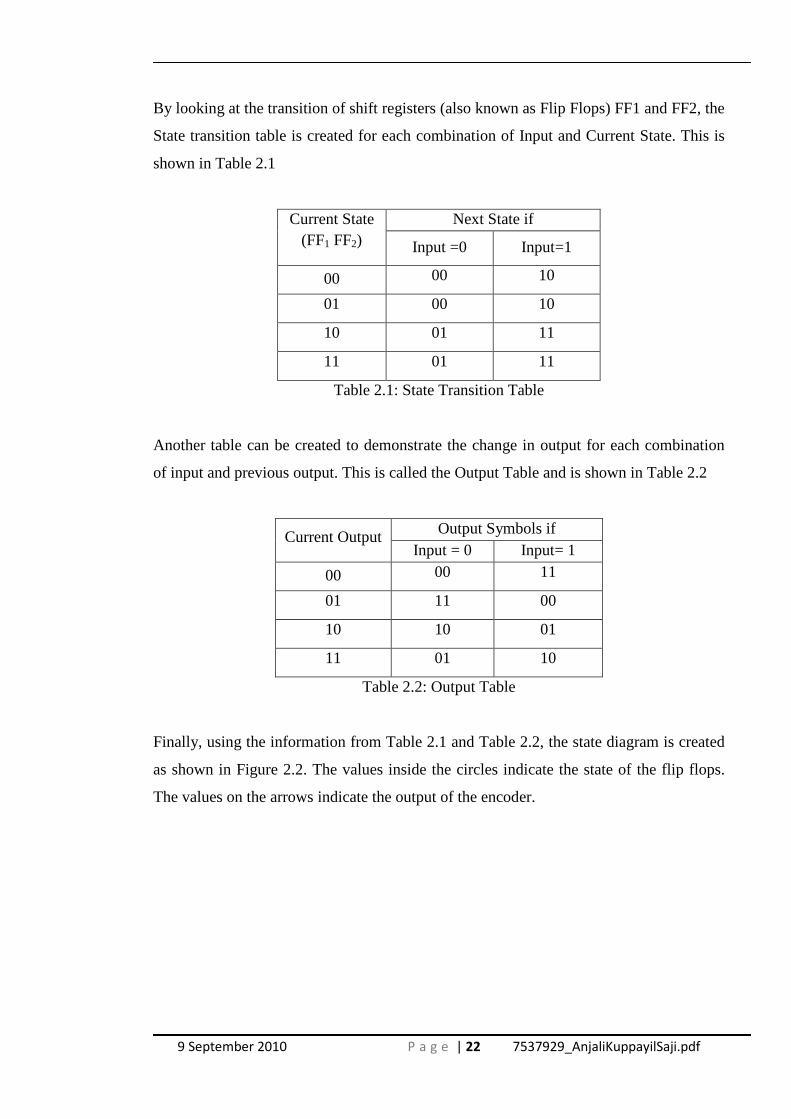
Finally, using the information from Table 2.1 and Table 2.2, the state diagram is created
as shown in Figure 2.2. The values inside the circles indicate the state of the flip flops.
The values on the arrows indicate the output of the encoder.
9 September 2010 P a g e | 23 7537929_AnjaliKuppayilSaji.pdf
Figure 2.2: State Diagram
2.3.2. Trellis Diagram
In a trellis diagram the mappings from current state to next state are done in a slightly
different manner as shown in Figure 2.3. Additionally, the diagram is extended to
represent all the time instances until the whole message is decoded. In the following
Figure 2.3, a trellis diagram is drawn for the above mentioned convolutional encoder.
The complete trellis diagram will replicate this figure for each time instance that is to be
considered.
Figure 2.3: Trellis Diagram for a 1/2, K=3,(7,5) convolutional encoder
The solid lines in Figure 2.3 represent transitions when the input is 1. The dashed lines
represent transitions when input is 0. From this diagram it can be observed that each state
has two possible successor states depending on whether the input bit was 1 or 0. The
diagram also shows that each state has two possible predecessor states.

9 September 2010 P a g e | 24 7537929_AnjaliKuppayilSaji.pdf
The most common convolutional code used in communication systems has a symbol rate
of ½ and constraint length K = 7. The most widely used method for decoding
convolutional codes has been the Viterbi Algorithm .Chapter 4 is devoted towards a
detailed description of the algorithm. Prior to that, some recent developments in this area
are described below.
2.4 Recent Developments
Since its discovery, the Viterbi algorithm has been the most widely used method for
decoding convolutional codes. However, more complex codes are now increasingly
being used to provide superior performance. While understanding these complex codes
in a short amount of time is difficult, an attempt has been made to provide a basic
description of two of these codes, namely Low Density Parity Check Codes and Turbo
Codes.
2.4.1 Low Density Parity Check Codes or LDPC Codes
LDPC codes were first introduced by Gallager in his PhD thesis in 1963[18]. However,
it was a long time before interest grew in these codes. As described by Shokrollahi [19],
LDPC codes are linear block codes obtained from sparse bipartite graphs. A sparse
bipartite graph is a graph with ‘n’ left nodes known as message nodes and ‘r’ right nodes
known as check nodes. The graph creates a linear code of block length n and dimension
at least ‘n – r’ as described below: The n coordinates of the codewords are associated
with the n message nodes. The codewords are those vectors (c1, . . . , cn ) such that for
all check nodes the sum of the neighboring positions among the message nodes is zero.
Shokrollahi provides this example [19] shown in Figure 2.7 to illustrate this concept.

9 September 2010 P a g e | 25 7537929_AnjaliKuppayilSaji.pdf
Figure 2.4: Example of an LDPC Code. Reproduced from [19]
LDPC codes can be mathematically defined in the following way [19].
“Let H be a binary r x n matrix where entry (i, j) is 1 if and only if the ith check node is
connected to the jth message node in the graph. Then the LDPC code may be defined by
the graph as the set of vectors c = (c 1 , . . . , cn ) such that H · cT = 0. Matrix H defined
in this manner is known as the parity check matrix for the code.”
LDPC Codes are not particularly advantageous as compared to other codes in terms of
probability of decoding errors for a particular block length. Also, the maximum rate at
which LDPC Codes can be used is limited below channel capacity. The biggest
advantage of LDPC Codes, as explained by Gallager [18] is that they allow the use of a
simple decoding scheme and this outweighs its drawbacks.
One of the simpler decoding schemes that may be used for Binary Symmetric Channels
is done by calculating all of the parity checks for the code and then reversing the digit
that is contained in more than a certain number of unsatisfied parity check equations.
This process is repeated many times until all the parity checks are satisfied. This
decoding scheme is not optimal. Better schemes which use a posteriori probabilities at
the channel output to decode data are described by Gallager [18].
9 September 2010 P a g e | 26 7537929_AnjaliKuppayilSaji.pdf
2.4.2. Turbo Codes
Concatenated coding schemes combine two or more relatively simple component codes
as a means of achieving large coding gains. Such concatenated codes have the error-
correction capability of much longer codes while at the same time permitting relatively
easy to moderately complex decoding. [6] Turbo codes, first introduced by Berrou,
Glavieux and Thitimajshima, [15] are a modification of the concatenated encoding
structure with an iterative algorithm for decoding the associated sequence. Serial and
parallel concatenated Turbo codes are in fact a type of LDPC codes.
2.4.2.1 Encoder
In most communication links, bit-errors are introduced into the message as short bursts
due to some sudden disturbance in the medium. When many bit-errors occur adjacent to
each other, it is more difficult to correct them. Turbo Codes try to reduce the effect of
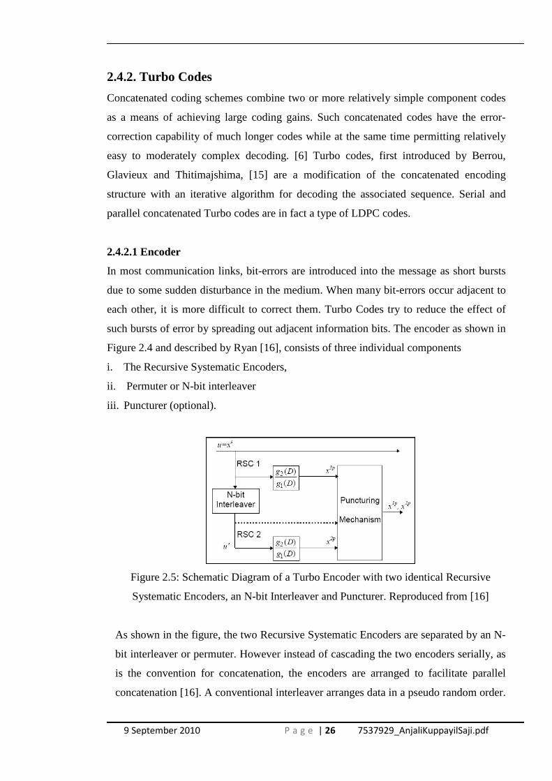
such bursts of error by spreading out adjacent information bits. The encoder as shown in
Figure 2.4 and described by Ryan [16], consists of three individual components
i. The Recursive Systematic Encoders,
ii. Permuter or N-bit interleaver
iii. Puncturer (optional).
Figure 2.5: Schematic Diagram of a Turbo Encoder with two identical Recursive
Systematic Encoders, an N-bit Interleaver and Puncturer. Reproduced from [16]
As shown in the figure, the two Recursive Systematic Encoders are separated by an N-
bit interleaver or permuter. However instead of cascading the two encoders serially, as
is the convention for concatenation, the encoders are arranged to facilitate parallel
concatenation [16]. A conventional interleaver arranges data in a pseudo random order.

9 September 2010 P a g e | 27 7537929_AnjaliKuppayilSaji.pdf
The permuter differs from this in that it takes a block of N bits of data and rearranges
them in a pseudo random manner. It is hence also called an N-bit interleaver. This
rearranged code is then passed to the second encoder.
The advantage is that any bursts of errors that occur will now be spread over a wider
range bits. As the bit-errors are now farther apart there is a higher probability that the
bit-errors may be corrected at the decoder. This method is advantageous when the
medium is known to produce burst errors. There is also a probability that this type of
code adversely affects the outcome. This may happen if bit-errors which would have
been far apart are adjacent to each other as a result of the rearrangement operations.
2.4.2.2 Decoder
Using a maximum likelihood sequence for the decoder would prove too difficult since
the data has been rearranged in a pseudo random fashion. Instead an iterative decoding
algorithm is used to provide similar performance. In order to make full use of this
method, the decoders must produce soft decision outputs as hard decisions will
severely limit its error correcting capability. The decoding algorithm used by Berrou, et
al [15], is based on the symbol-by-symbol maximum a posteriori (MAP) algorithm of
Bahl, et al [17]. In this algorithm, the decoder sets the data input uk as 1 if P( uk = 1| y)
is greater than P(uk = -1 | y ), where y is the received message with bit-errors. In other
words the decision of the value of uk equals sign [L(uk)] which is the log a posteriori
probability (LAPP) ratio given by
L(uk) = log [ (P(uk = +1 | y) / (P(uk = -1 | y )] ---- (Eq.1)
The following figure, Figure 2.5, described by Ryan [16], demonstrates how an
iterative decoder is built using component MAP decoders. The N-bit interleavers and
de-interleavers are used to arrange information in the right sequence for each decoder.
Figure 2.6 Schematic Diagram of Turbo Decoder. Reproduced from [16]

9 September 2010 P a g e | 28 7537929_AnjaliKuppayilSaji.pdf
Berrou, Glavieux and Thitimajshima conducted simulations using parallel concatenation
of Recursive Systematic Encoders and feedback decoding [15]. The results showed a
marked improvement in error correction capabilities as the number of iterations
performed was increased. For binary modulation, a bit error probability of 10-5 and Eb/N0
= 0.2 dB is often used as a practical Shannon limit reference for a rate ½ code. The error
performance of this turbo code at bit error probability 10-5 is within 0.5 dB of the
pragmatic Shannon limit.
2.5 Automatic Repeat Request (ARQ)
Automatic Repeat request or ARQ is a method in which the receiver sends back a
positive acknowledgement if no errors are detected in the received message. In order to
do this, the transmitter sends a Cyclic Redundancy Check or CRC along with the
message. This has been described in Section 2.2.1 The CRC check bits are calculated
based on the data to be transmitted. At the receiver, the CRC is calculated again using
the received bits. If the calculated CRC bits match those received, the data received is
considered accurate and an acknowledgement is sent back to the transmitter.
The sender waits for this acknowledgement. If it does not receive an acknowledgement
(ACK) within a predefined time, or if it receives a negative acknowledgement (NAK), it
retransmits the message [4].This retransmission is done either until it receives an ACK or
until it exceeds a specified number of retransmissions.
This method has a number of drawbacks. Firstly, transmission of a whole message takes
much longer as the sender has to keep waiting for acknowledgements from the receiver.
Secondly, due to this delay, it is not possible to have practical, real-time, two-way
communications. There are a few simple variations to the standard Stop-and-Wait ARQ
such as Go-back-N ARQ, selective repeat ARQ. These are described below.
2.5.1 ‘Stop and Wait’ ARQ
In this method, the transmitter sends a packet and waits for a positive acknowledgement.
Only once it receives this ACK does it proceed to send the next packet [5].This method
results in a lot of delays as the transmitter has to wait for an acknowledgement. It is also

9 September 2010 P a g e | 29 7537929_AnjaliKuppayilSaji.pdf
prone to attacks where a malicious user keeps sending NAK messages continuously. As
a result the transmitter keeps retransmitting the same packet and the communication
channel breaks down.
2.5.2 ‘Continuous’ ARQ
In this method, the transmitter transmits packets continuously until it receives a NAK. A
sequence number is assigned to each transmitted packet so that it may be properly
referenced by the NAK. There are two ways a NAK is processed.
2.5.2.1 ‘Go-back-N’ ARQ
In ‘Go-back-N’ ARQ, the packet that was received in error is retransmitted along with
all the packets that followed after it until the NAK was received. N refers to the number
of packets that have to be traced back to reach the packet that was received in error. In
some cases this value is determined using the sequence number referenced in the NAK.
In others, it is calculated using roundtrip delay [5].The disadvantage of this method is
that even though subsequent packages may have been received without error, they have
to be discarded and retransmitted again resulting in loss of efficiency. This disadvantage
is overcome by using Selective-repeat ARQ.
2.5.2.2 ‘Selective-repeat’ ARQ
In Selective-repeat ARQ, only the packet that was received in error needs to be
retransmitted when an NAK is received. The other packets that have already been sent in
the meantime are stored in a buffer and can be used once the packet in error is
retransmitted correctly [5]. The transmissions then pick up from where they left off.
Continuous ARQ requires a higher memory capacity as compared to Stop and Wait
ARQ. However it reduces delay and increases information throughput [5].
The main advantage of ARQ is that as it detects errors (using CRC check bits) but makes
no attempt to correct them, it requires much simpler decoding equipment and much less
redundancy as compared to Forward Error Correction techniques which are described
below. The huge drawback however, is that the ARQ method may require a large

9 September 2010 P a g e | 30 7537929_AnjaliKuppayilSaji.pdf
number of retransmissions to get the correct packet [6], especially if the medium is
noisy. Hence the delay in getting messages across maybe excessive.
2.6 Hybrid Automatic Repeat Request (H-ARQ)
Hybrid Automatic Repeat Request or H-ARQ is another variation of the ARQ method. In
this technique, error correction information is also transmitted along with the code. This
gives a better performance especially when there are a lot of errors occurring. On the flip
side, it introduces a larger amount of redundancy in the information sent and therefore
reduces the rate at which the actual information can be transmitted. There are two
different kinds of H-ARQ, namely Type I HARQ and Type II HARQ [7].
Type I-HARQ is very similar to ARQ except that in this case both error detection as well
as forward error correction (FEC) bits are added to the information before transmission.
At the receiver, error correction information is used to correct any errors that occurred
during transmission. The error detection information is then used to check whether all
errors were corrected. If the transmission channel was poor and many bit-errors
occurred, errors may be present even after the error correction process. In this case, when
all errors have not been corrected, the packet is discarded and a new packet is requested.
In Type II-HARQ, the first transmission is sent with only error detection information. If
this transmission is not received error free, the second transmission is sent along with
error correction information. If the second transmission is also not error free, information
from the first and second packet can be combined to eliminate the error.
Transmitting FEC information can double or triple the message length. Error detection
information on the other hand requires fewer numbers of additional bits [7]. The
advantage of Type II HARQ therefore, is that it increases the efficiency of the code to
that of simple ARQ when channel conditions are good and provides the efficiency of
Type I HARQ when channel conditions are bad.

9 September 2010 P a g e | 31 7537929_AnjaliKuppayilSaji.pdf
2.7 Summary
This chapter has given a review of background literature pertaining to different error
detection and error control techniques. Some of the more recent approaches including
LDPC codes and Turbo codes are briefly described. In FEC, convolutional codes are
preferred to block codes since they are less complex to decode. The encoding process has
been described in this chapter. The next chapter is devoted to a detailed description of
the Viterbi Algorithm which is one of the most popular algorithms for decoding
convolutional code. Related energy saving techniques that have previously been
investigated to optimize its energy consumption are also described.

9 September 2010 P a g e | 32 7537929_AnjaliKuppayilSaji.pdf
Chapter 3
THE VITERBI ALGORITHM
The Viterbi Algorithm was developed by Andrew J. Viterbi and first published in the
IEEE transactions journal on Information theory in 1967 [1]. It is a maximum likelihood
decoding algorithm for convolutional codes. This algorithm provides a method of finding
the branch in the trellis diagram that has the highest probability of matching the actual
transmitted sequence of bits. Since being discovered, it has become one of the most
popular algorithms in use for convolutional decoding. Apart from being an efficient and
robust error detection code, it has the advantage of having a fixed decoding time. This
makes it suitable for hardware implementation.
3.1 Encoding Mechanism
Data is coded by using a convolutional encoder, as described in Section 2.3.2. It consists
of a series of shift registers and an associated combinatorial logic. The combinatorial
logic is usually a series of exclusive-or gates. The conventional encoder ½ K=7,
(171,133) is used for the purpose of this project. The octal numbers 171 and 133 when
represented in binary form correspond to the connection of the shift registers to the upper
and lower exclusive-or gates respectively. Figure 3.1 represents this convolutional
encoder that will be used for the project.

9 September 2010 P a g e | 33 7537929_AnjaliKuppayilSaji.pdf
Figure 3.1: Rate = ½ K = 7, (171,133) Convolutional Encoder
3.2 Decoding Mechanism
There are two main mechanisms by which Viterbi decoding may be carried out namely,
the Register Exchange mechanism and the Traceback mechanism.
Register exchange mechanisms, as explained by Ranpara and Sam Ha [20] store the
partially decoded output sequence along the path. The advantage of this approach is that
it eliminates the need for traceback and hence reduces latency. However at each stage,
the contents of each register needs to be copied to the next stage. This makes the
hardware complex and more energy consuming than the traceback mechanism.
Traceback mechanisms use a single bit to indicate whether the survivor branch came
from the upper or lower path. This information is used to traceback the surviving path
from the final state to the initial state. This path can then be used to obtain the decoded
sequence. Traceback mechanisms prove to be less energy consuming and will hence be
the approach followed in this project.
Decoding may be done using either hard decision inputs or soft decision inputs. Inputs
that arrive at the receiver may not be exactly zero or one. Having been affected by noise,
they will have values in between and even higher or lower than zero and one. The values
may also be complex in nature. In the hard decision Viterbi decoder, each input that
arrives at the receiver is converted into a binary value (either 0 or 1). In the soft decision

9 September 2010 P a g e | 34 7537929_AnjaliKuppayilSaji.pdf
Viterbi decoder, several levels are created and the arriving input is categorized into a
level that is closest to its value. If the possible values are split into 8 decision levels,
these levels may be represented by 3 bits and this is known as a 3 bit Soft decision. This
project uses a hard decision Viterbi decoder for the purpose of developing and verifying
the new energy saving algorithm. Once the algorithm is verified, a soft decision Viterbi
decoder may be used in place of the hard decision decoder.
Figure 3.2 shows the various stages required to decode data using the Viterbi Algorithm.
The decoding mechanism comprises of three major stages namely the Branch Metric
Computation Unit, the Path Metric Computation and Add-Compare-Select (ACS) Unit
and the Traceback Unit. A schematic representation of the decoder is described below.
Figure 3.2: Schematic representation of the Viterbi decoding block
Block 1. Branch Metric Computation (BMC)
For each state, the Hamming distance between the received bits and the expected bits is
calculated. Hamming distance between two symbols of the same length is calculated as
the number of bits that are different between them. These branch metric values are
passed to Block 2. If soft decision inputs were to be used, branch metric would be
calculated as the squared Euclidean distance between the received symbols [21]. The
squared Euclidean distance is given as (a1-b1)2 + (a2-b2)
2 + (a3-b3)2 where a1, a2, a3 and
b1, b2, b3 are the three soft decision bits of the received and expected bits respectively.
Block 2. Path Metric Computation and Add-Compare-Select (ACS)
Unit
The path metric or error probability for each transition state at a particular time instant is
measured as the sum of the path metric for its preceding state and the branch metric

9 September 2010 P a g e | 35 7537929_AnjaliKuppayilSaji.pdf
between the previous state and the present state. The initial path metric at the first time
instant is infinity for all states except state 0.
For each state, there are two possible predecessors. The mechanism of calculating the
predecessors (and successors) is described below in Section 3.2.1 and Section 3.2.2. The
path metrics from both these predecessors are compared and the one with the smallest
path metric is selected. This is the most probable transition that occurred in the original
message. In addition, a single bit is also stored for each state which specifies whether the
lower or upper predecessor was selected. In cases where both paths result in the same
path metric to the state, either the higher or lower state may consistently be chosen as the
surviving predecessor. For the purpose of this project the higher state is consistently
chosen as the surviving predecessor.
Finally, the state with the least accumulated path metric at the current time instant is
located. This state is called the global winner and is the state from which traceback
operation will begin. This method of starting the traceback operation from the global
winner instead of an arbitrary state was described by Linda Brackenbury [22] in her
design of an asynchronous Viterbi decoder. This greatly improves probability of finding
the correct traceback path quicker and hence reduces the amount of history information
that needs to be maintained. It also reduces the number of updates required to the
surviving path. Both these measures result in improved energy savings. The values for
the surviving predecessors (also called local winners) and the global winner are passed to
Block 3.
Block 3. Traceback Unit
The global winner for the current state is received from Block 2. Its predecessor is
selected in the manner described in Section 3.2.2. In this way, working backwards
through the trellis, the path with the minimum accumulated path metric is selected. This
path is known as the traceback path. A diagrammatic description will help visualize this
process. Figure 3.3 describes the trellis diagram for a ½ K=3 (7, 5) coder with sample
input taken as the received data.

9 September 2010 P a g e | 36 7537929_AnjaliKuppayilSaji.pdf
Transition when Input = 0
Transition when Input = 1
Figure 3.3 Selected minimum error path for a ½ K = 3 (7, 5) coder
The state having minimum accumulated error at the last time instant is State 10 and
traceback is started here. Moving backwards through the trellis, the minimum error path
out of the two possible predecessors from that state is selected. This path is marked in
blue. The actual received data is described at the bottom while the expected data written
in blue along the selected path. It is observed that at time slot three there was an error in
received data (11). This was corrected to (10) by the decoder.
Local winner information must be stored for five times the constraint length. For a K =7
decoder, this results in storing history for 7 x 5 = 35 time slots. The state of the decoder
at the time instant 35 time slots prior can then be accurately determined. This state value
is passed to Block 4. At the next time slot, all the trellis values are shifted left to the
previous time slot. The path metric for the last received data and compute the minimum
error path is then calculated. If the global winner at this stage is not a child of the
previous global winner, the traceback path has to be updated accordingly until the
traceback state is a child of the previous state [22].
Multiple traceback paths are possible and it may be thought that traceback up to the first
bit is necessary to correctly determine the surviving path. However, it was found that all
possible paths converge within a certain distance or depth of traceback [23][24]. This
information is useful as it allows the setting of a certain traceback depth beyond which it
is neither necessary nor advantageous to store path metric and other information. This

9 September 2010 P a g e | 37 7537929_AnjaliKuppayilSaji.pdf
greatly reduces memory storage requirements and hence energy consumption of the
decoder. Empirical observations showed that a depth of five times the constraint length
was sufficient to ensure merging of paths [8, 25]. Therefore, local winner information is
stored for 35 slots (five times seven) in the decoder used for this project.
Block 4. Data Input Determination
Now going forwards through the traceback path, the state transitions at successive time
intervals are studies and the data bit that would have caused this transition (using the
method described in Section 3.2.1) is determined. This represents the decoded output.
3.2.1 Determining Successors to a particular State
Each state is represented by 6 shift registers (in the case of a K=7 encoder or decoder).
The next state can therefore be obtained by a right shift of the values of the shift
registers. The first shift register is given a value of 0. The resulting state represents the
next state of the coder if the input bit was 0. By adding 32 (1x25) to this value, the next
state of the coder if the input bit was 1 is derived.
3.2.2 Determining Predecessors to a particular State
In a similar way, the first predecessor can be calculated this time by a left shift of the
values of the shift registers. By adding one (1x20) to this value, the value of the second
predecessor to the state is derived.
3.3. Applications
The Viterbi algorithm has a wide range of applications ranging from satellite and space
communications, DNA sequence analysis and Optical Character Recognition.
An attempt to perform optical character recognition of text was investigated by Neuhoff
[26]. The initial approach considered was to create a dictionary which simulated
vocabularies. Each time a character was read by the optical reader, it would search the
dictionary for the most likely estimate. The huge amount of computational and storage
requirements required under this approach made it impractical. However, another
approach makes use of statistical information about the language such as relative

9 September 2010 P a g e | 38 7537929_AnjaliKuppayilSaji.pdf
frequency of letter pairs. A maximum a priori probability (MAP) of a word is determined
based on its probability as the output of the source model. The Viterbi algorithm may
then be used to perform this MAP sequence estimation.
An interesting application discussed by Metzner [27] investigated among others, the use
of Viterbi decoding with soft decision to increase the probability of successfully
transmitting a data packet during a meteor burst. Since meteor trails are made up of
ionized material, these can be used for reliable communications. Some characteristics of
such meteor burst communication and descriptions of its practical applications are
detailed in [28, 29]. Metzner showed that convolutional codes with soft decision were
considerably better for meteor burst applications as compared to Reed-Solomon codes.
Low power applications of the Viterbi decoder are particularly relevant to many digital
communication and recording systems today. As described by Kawokgy and Salama [30]
systems like these are increasingly being used in wireless applications which being
battery operated, require low power consumption. In addition, these systems also require
processing speeds of over 100Mbps to allow multimedia transmission. Following this
trend, many papers have been written on designing low power Viterbi decoding
algorithms targeted for next generation wireless applications, particularly CDMA
systems [31, 32, 33]. Some of these energy saving ideas that have been investigated are
described in the next section.
3.4 Related Work
In mobile networks, decoding capabilities are limited by the receiver which is a mobile
handset. As such, it has limited resources of energy and computation power. Another
factor that affects wireless communication is that bandwidth is expensive. Therefore,
there is a high demand for codes that can correct errors very efficiently while at the same
time utilizing minimum energy. Hence, a lot of the past research has been focused on
how this may be achieved.
The fixed T-algorithm algorithm is an optimization of the Viterbi algorithm which
applies a pruning threshold to the accumulated path metrics of the Viterbi decoder.

9 September 2010 P a g e | 39 7537929_AnjaliKuppayilSaji.pdf
Instead of storing all the survivor paths for all 2K-1 states, only some of the most-likely
paths are kept at every trellis stage. This results in fewer paths being found and stored.
The following Figure 3.4 demonstrates the result of an experiment conducted by
Henning and Chakrabarti [34] which compares normalized energy estimates for the
Viterbi and the fixed T-algorithm decoders as it varies with signal to noise ratio (Eb/No)
and code rate.
Figure 3.4: Normalized energy estimates for the Viterbi and fixed T-algorithm (Tf)
decoders as code rate and signal to noise ratio (Eb/No) vary. Reproduced from [34].
From the graph, it is estimated that a 33% to 83 % reduction in energy consumption can
be achieved when the signal to noise ratio is between 2.1 and 4 dB.
One of the other approaches taken has been to develop an adaptive T-algorithm which
adjusts parameters of the decoder based on real-time variations in signal to noise ratio
(SNR), code rate and maximum acceptable bit-error rate. The parameters adjusted are
truncation length and pruning threshold of the T-algorithm along with trace-back
memory management. Henning and Chakrabarti demonstrate in their paper [34] how this
can achieve a potential energy reduction of 70% to 97.5% as compared to Viterbi
decoding. Truncation length refers to the number of bits a path is followed back before a
decision is made on the bit that was encoded. By reducing the truncation length more bits
can be decoded per traceback. Similarly, lowering the pruning threshold means fewer
paths need to be found and stored. Both of these measures can reduce the number of
memory accesses required by the decoder and hence reduce energy consumption.

9 September 2010 P a g e | 40 7537929_AnjaliKuppayilSaji.pdf
However, these measures may cause significant reduction in the error correcting
capability of the decoder.
Nevertheless, adjusting these parameters based on real-time changes in the channel can
optimize energy consumption. The following figure, Figure 3.5 demonstrates the results
of an experiment conducted by Henning and Chakrabarti [34] in which pruning threshold
and truncation length are adapted to maintain bit-error rate below 0.0037. From the
graph, it is estimated that an energy consumption reduction of 70 to 97.5 % compared to
the Viterbi decoder can be achieved when the signal to noise ratio is between 2.1 and 4
dB.
However, the adaptive T-algorithm does require an additional overhead in terms of
monitoring the real-time variations and choosing the appropriate truncation and threshold
parameters from a lookup table. Since these operations are not complex it is assumed that
their energy consumption is negligible.
Figure 3.5: Normalized energy estimates for the Viterbi and adaptive T-algorithm (Ta)
decoders as code rate and signal to noise ratio (Eb/No) vary while maintaining bit-error
rate below 0.0037. Reproduced from [34].
Yet another approach that was put forward by Jie Jin and Chi-Ying Tsui in the 2006
International Symposium on Low Power Electronics and Design, [35] was to integrate
the T-algorithm with a Scarce-State–Transition (SST) decoder structure [36]. The SST

9 September 2010 P a g e | 41 7537929_AnjaliKuppayilSaji.pdf
structure first pre-decodes the received data (Rx) by performing an inverse operation of
the encoder. The pre-decoded signal will contain the original message along with bit-
errors (Pre-Dec). This message Pre-Dec is re-encoded and XOR’ed with Rx, the original
received data. The operation results in an output which consists of mainly 0’s and the
errors in the message. This output is then fed to the Viterbi decoder and the errors are
corrected. In the end, the pre-decoded data (Pre-Dec) is added to the decoded output of
the Viterbi decoder using modulo-2 addition. When channel bit-errors are low, most of
the Viterbi decoder output bits are zero and thus reduces switching activity.
The SST structure was used to reduce the switching activities of the decoder and
combined with the T-algorithm to reduce the average number of Add-Compare Select
calculations. In their experiments, Jie Jin and Chi-Ying Tsui achieved a 30%-76%
reduction in power consumption over the traditional Viterbi design for a range of SNR
values varying from 4 dB to 12 dB.
A different approach investigated by Sherif Welsen Shaker, Salwa Hussein Elramly and
Khaled Ali Shehata [37] at a Telecommunications forum held in Belgrade last year
(2009) was to use the traceback approach with clock gating. In clock gating, the clock of
each register is enabled only when the register updates it survivor path information. This
reduces power dissipation. Their simulations showed a 30% reduction in dynamic power
dissipation which gives a good indication of power reduction on implementation.
A similar approach investigated by Ranpara and Sam Ha [20] and presented in the
International ASIC conference at Washington in 1999 was the use of clock gating in
combination with a concept known as toggle filtering. Signals may arrive at the inputs of
a combinational block at different times and this causes the block to go through several
intermediate transitions before it stabilizes. By blocking early signals, the number of
intermediate transitions can be reduced and hence power disspation can be minimized.
This mechanism of blocking early signals until all input signals arrive, called toggle
filtering, was used by Ranpara, et al, [20] to reduce energy consumption of the Viterbi
decoder.

9 September 2010 P a g e | 42 7537929_AnjaliKuppayilSaji.pdf
Recently a new approach, targeted towards wireless applications has been introduced
[38] and involves a pre-traceback architecture for the survivor path memory unit. The
start state of decoding is obtained directly through a pointer register pointing to the target
traceback state instead of estimating the start state through a recursive traceback
operation. This approach makes use of the similarity between bit write and decode
traceback operation to introduce the pre-traceback operation. Effectively resulting in a
trace forward type of operation, it results in a 50% reduction in survivor memory read
operations. Apart from improving latency by 25%, implementation results predict up to
11.9% better energy efficiency when compared to conventional traceback architecture
for typical wireless applications.
3.5 Summary
This chapter has explained the decoding mechanism of the Viterbi decoder in detail and
described a few of its applications. A number of energy saving techniques that have been
investigated in the past has been discussed. The next chapter gives a detailed description
of the proposed energy saving algorithm that will be used in this project.
9 September 2010 P a g e | 43 7537929_AnjaliKuppayilSaji.pdf
Chapter 4
AN ALTERNATIVE ENERGY SAVING
STRATEGY
Much previous research has been focused on making the Viterbi decoder less energy
consuming (e.g. [20, 34, 35, 36, 37, 38] ). One possible approach is to try to minimize
the amount of time which the Viterbi decoder needs to be switched on. Conventionally,
the decoder is on all the time, even when there are few or no bit-errors. In practice the
bit-error rate with mobile equipment can be very variable especially when the receiver
is moving relative to access-points. Switching off the Viterbi decoder when there are no
bit-errors seems a promising strategy.
Two different ways of doing this have been investigated previously at the University of
Manchester. One method proposed by Wei Shao [3], involves a method of pre-
decoding and identifying no-error code word sequences using an ‘inverse circuit’ [35].
An alternative method, proposed by Barry Cheetham [2], makes use of simple
properties of the Exclusive-Or (XOR) operation in combination with a simple feedback
mechanism for detecting the presence of bit-errors.
An adaptive algorithm is proposed to directly use such pre-decoded data as the decoded
output without the Viterbi decoder having to process them. This makes it possible to
switch on the Viterbi decoder only when bit-errors occur. In this project, the second
approach to reduce energy consumption at the receiver will be investigated.
4.1 Principle
The underlying principle proposed by Barry [2], for the switch off mechanism can be
described in the following way. Taking the case of the ½ K=7, (171, 133) convolutional

9 September 2010 P a g e | 44 7537929_AnjaliKuppayilSaji.pdf
encoder, it is known that each input bit is XOR’ed with flip flops 1,2 , 3 and 6 for the
lower output bit and flip flops 2 ,3 ,5 and 6 for the upper output bit. The lower and
upper bit are then interleaved and transmitted as was shown in Figure 3.1.
Exclusive-Or (XOR) has the property that ((A XOR B) XOR B) = A. This property has
enormous implications and will prove very helpful in our analysis. To understand its
importance, let us take the following example. Consider A to be the information bit that
must be transmitted and B to be the result of the combinatorial logic of the
convolutional encoder before it is XOR’ed with the information bit. A XOR B gives Y,
i.e. the transmitted message. Now it is clear from the above property that Y XOR B
gives A which was the original information bit. In other words, XORing the transmitted
message with the same combinatorial logic result that was used in the encoder gives
back the original information bit. As long as there are no bit-errors, the message can be
decoded this way and the Viterbi decoder need not be switched on.
In the conventional ½ rate encoder, each input bit is XOR’ed with 2 different
combinations of flip flops (FF1, FF2,FF 3 and FF6 for lower bits and FF2, FF3, FF5
and FF6 for upper bits) to produce two output bits. These bits are then interleaved and
transmitted. This is the structure described in Figure 3.1. At the receiver, XORing
alternate arriving bits with the corresponding set of flip flops (FF1, FF2, FF3 and FF6
for lower bits and FF2, FF3, FF5 and FF6 for upper bits), gives back the original
message bit.
It is also understood that each upper received bit and each corresponding lower received
bit were produced, at the transmitter, by the same original information bits. Assume
that a correct copy of all previous information bits is available at the receiver. This
assumption is bound to be correct at the beginning of a packet transmission, since all
previous bits, at both the transmitter and receiver, are assumed to be zero. XORing the
upper received bit with the 'appropriate' correct copies (as held at the receiver) of the
previous information bits should produce the current original information bit. The term
'appropriate' refers to the information bits that were taken into account in the upper part
of the convolutional encoder i.e. the 2nd, 3rd, 5th and 6th bit in this example.

9 September 2010 P a g e | 45 7537929_AnjaliKuppayilSaji.pdf
Similarly, XORing the lower received bit with the 'appropriate' correct receiver copies
of the previous information bits should also produce the same correct information bit. If
there is no bit-error the same correct value for both the upper and lower decoded bits
will be obtained at the receiver. Clearly, in this case, the process can then continue with
the next received upper and lower bits. The diagram for the proposed design is
provided in Figure 4.1.
Figure 4.1: Proposed Simple Decoder
If the upper and lower received bits are found to be different at any stage, it can be
concluded that a single bit-error has just occurred, either in the upper transmission or in
the lower one.
On the other hand, if they are found to be equal, it cannot be concluded that there was
no bit-error introduced in transmission. There may be two bit-errors, one in the upper
transmission and one in the lower transmission. Therefore the occurrence of multiple
bit-errors may not be detected straight away, and it is indeed possible for some bit-error
patterns to pass completely undetected. As will be shown in the following chapters, it is
expected that in these rare cases not even the Viterbi algorithm would be able detect the
presence of bit-errors.
However, in most cases, the occurrence of a bit-error pattern, containing one, two, three
or more bit-errors would create a difference between the upper and lower decoded bits.
9 September 2010 P a g e | 46 7537929_AnjaliKuppayilSaji.pdf
When such a difference is observed, it may be concluded that there has been at least one
bit-error recently (within in the last 14 bits i.e. 7 time slots). However, it is not known
exactly where and how many. When this happens, the current proposal is to go back 14
bits, start up the Viterbi decoder and proceed conventionally. This principle lies at the
heart of the attempt to reduce energy consumption of the Viterbi decoder.
Since this method involves going back 14 bits when an error is detected, it will require
the last 14 received data bits to be stored. When a bit-error occurs, the Viterbi decoder
will be switched on and the 14th previous data bit (that was stored) will be taken as the
next input.
4.2 Summary
This chapter gives only a description of the basic concepts that motivated this approach.
There still remain many issues that have to be addressed in this algorithm such as the
mechanism of switching and determining the initial state of the decoder. These are
described in Section 5.4 as ‘Likely Issues’ and addressed in the Chapter 6. The next
chapter describes the research methods that will be adopted to structure the project.

9 September 2010 P a g e | 47 7537929_AnjaliKuppayilSaji.pdf
Chapter 5
RESEARCH METHODS
The core objectives of the project were discussed in Chapter 1 and in this Chapter the
research methodologies that were adopted to achieve project goals are described. Based
on the strategy described in Chapter 4, the key deliverables and software tools that will
be used are identified. A project plan for the research project has been developed and
summarized with the help of a Gantt chart. The likely issues that may be faced during the
design and implementation of the algorithm are also discussed.
5.1 Research Approach
As discussed in Chapter 1, the main aim of this project is to develop a more energy
efficient method of decoding convolutionally encoded data. Towards this end, the new
algorithm described in Section 4 is developed and tested. A structured research approach
is essential in obtaining reliable results and ensuring that all aspects of the problem to be
solved are addressed. A major portion of this research will require observation and
evaluation of performance of the new algorithm in comparison with conventional
systems. Hence, this project will follow an empirical approach [39, 40]. Some of the
main objectives of this approach are to learn from collective experience of the field and
to identify, explore, confirm and advance theoretical concepts. An emphasis will be laid
on utilizing the appropriate test cases, data collection and analysis techniques.
The project also uses a constructive research methodology. A constructive research
approach is defined as “A research procedure for producing innovative constructions,
intended to solve problems faced in the real world and, by that means, to make a
contribution to the theory of the discipline in which it is applied.” [41]. A construction as
described by the author, may be a new theory, algorithm, model, framework or method.
In this project, the construction is a new algorithm for an energy efficient technique of

9 September 2010 P a g e | 48 7537929_AnjaliKuppayilSaji.pdf
decoding convolutional codes. Some of the fundamental focus points in this type of
research are listed and answered here.
5.1.1 Definition of the research problem.
As described in Section 1.2, with the sudden growth of wireless applications, there is an
inherent need for efficient and less energy consuming decoders. Conventional decoders
such as the Viterbi decoder are computationally expensive and hence consume a lot of
energy. This project seeks to provide a more energy efficient solution that will prolong
battery life of the receiving device.
5.1.2 A general and comprehensive understanding of the topic.
Sections 2.1 -2.5 were devoted to a detailed description of the background surrounding
Error Detection and Forward Error Correction mechanisms and recent developments in
the area.
5.1.3 Construct a solution idea.
The basic solution idea based on the work done by Barry Cheetham [2] has been
described in Section 2.6. Some key issues remain to be solved and these will be pursued
in the following stages. Chapter 4 gives a comprehensive description of the design and
implementation features of the solution. Some of the key deliverables for the project are
i. A MATLAB ® Implementation of the algorithm to turn the Viterbi decoder on/off at the
appropriate time
ii. A mechanism to detect when errors have started/stopped occurring
iii. A communication channel that simulates the effects of AWGN noise over a range of
bit-error rates
iv. A fully functional decoder unit based on the new algorithm and implemented in
MATLAB ®
5.1.4. Demonstrate that the solution works.
Chapter 5 is devoted towards testing and analysis of the designed system. In order to
demonstrate that the proposed system works as expected, it is compared at every stage
with the MATLAB® Viterbi decoder. The criteria that will be used to evaluate the system

9 September 2010 P a g e | 49 7537929_AnjaliKuppayilSaji.pdf
include Bit-Error Probability (BEP) Performance, Packet Loss Rate and Measurement of
Processing Time. Actual design components of the new system need to be defined in
order to explain exactly how this system will be evaluated. Therefore a detailed
statement of evaluation criteria has been deferred to Section 7.1
5.2 Implementation Tools
The configuration of the computer used affects the processing time required by
MATLAB ® to execute its commands. The code was implemented using a DELL Inspiron
6400 Laptop with the following specifications.
Operating System (OS) Name: Microsoft® Windows Vista™ Ultimate
Processor: Intel(R) Core(TM)2 CPU T7200 @ 2.00GHz, 2000 MHz, 2 Core(s), 2
Logical Processor(s)
Random Access Memory (RAM): 2 GB
Total Physical Memory: 2.00 GB
Total Virtual Memory: 4.23 GB
Available Physical Memory: 810 MB
Available Virtual Memory: 2.16 GB
Implementation of the algorithm was done using MATLAB® Version 7.5.0.342
(R2007b), a product of MathWorks. The main toolboxes that were used include the
Signal Processing Toolbox and the Communications Toolbox.
There was an initial consideration to use Simulink, another product of Mathworks to
build a simulation of the system. This would involve building a circuit level
implementation of the Viterbi decoder and then adapting it to meet the requirements of
the new system. We were unable to acquire the detailed knowledge required to do this.
The fact that Embedded MATLAB® Functions do not support variable sized arrays in
MATLAB ® Version R2007b created further complications in using Simulink. It was then
decided to leave this pursuit as a future direction for research.

9 September 2010 P a g e | 50 7537929_AnjaliKuppayilSaji.pdf
5.3 Research Plan
The project has been categorized into four main tasks namely Background Research,
Design and Implementation of the Code, Experimentation with Data and Analysis of
Results and Preparation of Dissertation report. Work on the dissertation report was done
in parallel with the corresponding sections of the project in order to ensure sufficient
time for refinement of the report. A detailed description of the sub-tasks and the expected
timeline is provided in Appendix A Section (i) and (ii).
Reviewing this plan at the end of the project showed that most of the project went on
track as planned. Tasks 2.4 and 2.8 took slightly longer than planned. However this time
was recovered by the time allocated to Task 2.9 which was not implemented. It was also
found that doing parallel work on the report helped in clarifying thoughts and
continuously improving analysis methods. Task 3 therefore, was carried out in
conjunction with the report writing process. Reviewing of the report, Task 4.7 took
slightly longer than expected. However this was completed with remaining time
available before submission.
5.4 Likely Issues
The issues that needed to be addressed in the proposed method are explained below. It
seems easy to detect when bit-errors start occurring. Therefore, switching on the Viterbi
decoder at the appropriate time will not be difficult. However, the initial state of the
decoder must also be known. In a conventional decoder, the initial state is set to 0 before
decoding begins. In this algorithm however, switching to the Viterbi decoder may take
place at any time in the middle of the decoding operation. Therefore, the initial state
must be figured out.
Once switching to the Viterbi decoder is carried out, the question of determining when to
switch off the decoder i.e. determining when errors stop occurring, presents a tougher
problem. Finding a solution to this issue will be a major focus of this project. If it is
possible to detect that bit-errors have stopped occurring, the control must be switched to

9 September 2010 P a g e | 51 7537929_AnjaliKuppayilSaji.pdf
the Simple Decoder. This also requires initializing the Simple Decoder to the correct
state. This presents the next issue that must be taken care of.
Another concern that needs to be tackled is whether the decoder will go into an unstable
state when errors start occurring. Since the decoder employs a feedback mechanism,
there is a possibility that when an error occurs, this error will be propagated through the
system and result in the registers moving to an incorrect state. If this happens, it will not
be possible to decode subsequent bits correctly.
It also remains to be discovered whether this new technique is in fact capable of
providing adequate energy savings. Careful experimentation and analysis of data is
required before this can be ascertained. The Simple Decoder does not need to store state
history and path metrics as the Viterbi decoder does. Therefore it requires far less storage
units and state transitions. It is hence reasonable to expect the Simple Decoder to
consume much less energy. Nevertheless, it is possible that the overheads involved in the
process of switching between the Simple Decoder and the Viterbi decoder is energy
expensive. As a result, there may be an SNR limit below which using the switching
technique is not advantageous.
Of even more importance is an analysis of whether the switching mechanism results in a
considerable degradation of bit-error probability performance. The performance of the
new strategy will depend on how accurately errors can be detected and the corresponding
decoders initialized during switching. Even if the above method does save energy, a poor
BEP performance will severely limit its relevance to applications.
5.5 Summary
This chapter has described the research approach and plan that will be followed along
with the implementation tools that will be used. A description of issues that still remain
to be solved has also been detailed in this chapter. The next chapter describes the design
of the system and its implementation in MATLAB®.

9 September 2010 P a g e | 52 7537929_AnjaliKuppayilSaji.pdf
Chapter 6
DESIGN AND IMPLEMENTATION
This section gives a comprehensive description of the various components of the
developed system and explains how these components are implemented in MATLAB®.
Finally, a flowchart is drawn to provide a visual representation of flow of control through
the significant sections of the system. Appendix G contains the MATLAB® code for all
the modules of the system.
6.1 The Transmitter Block
The transmitter block is designed with the following components
6.1.1 A Data Generating Source
Random binary data is generated using the ‘randsrc’ function. Six ‘0’ bits are appended
to the randomly generated data. These act as zero buffers. Since there are 6 shift registers
in the convolutional encoder, it is necessary to run the encoder for an additional 6 time
slots after the last data input for the last data bit to appear at the output of the encoder.
For this reason, zero buffers are appended to the end of the data bits.
6.1.2. A Convolutional Encoder
A ½ K=7 (171 133) convolutional encoder is used. The six shift registers are initialized
to 0. At each time slot a new data bit is accepted and XOR’ed with values of the
corresponding shift registers as was shown in the Figure 4.1. These connections
represent (171)8 and (133)8 in binary form. In this way the value for the upper encoded
bit and lower encoded bit is determined. The values of all registers are then shifted to the
register on the right. The 2:1 multiplexer outputs the upper encoded bit and lower
encoded bit in alternating sequences.

9 September 2010 P a g e | 53 7537929_AnjaliKuppayilSaji.pdf
6.1.3 A QPSK Modulator
Before transmitting the signal it is modulated into QPSK signals with Gray encoding.
This is implemented via predefined functions available in MATLAB®. An oversampling
rate of 4 is used which results in 4 pulses for each data bit.
6.2 The Communications Channel
In order to simulate the effects of the communication channel Additive White Gaussian
noise is added to the transmitted signal. The signal to noise ratio is reduced by
10×log10(4) in to account for oversampling. It is further reduced by 10×log10(1/code rate)
so that the noise power is scaled to match coded symbol rate. The symbol to noise ratio
is varied over different iterations.
6.3 The Receiver Block
The receiver block contains the following components
6.3.1 A QPSK Demodulator
The demodulator accepts the received signals and demodulates them. The demodulated
signals are then passed to the Simple Decoder.
6.3.2 The Switching Decoder
The Switching Decoder is made up of two components: A Simple Decoder which will be
used when there are no bit-errors and an Adapted Viterbi decoder which will be used
when bit-errors start occurring. The two components are described in detail below.

9 September 2010 P a g e | 54 7537929_AnjaliKuppayilSaji.pdf
Part 1. The Simple Decoder
As shown in Figure 6.1 below, a 1:2 demultiplexer is used to separate alternate arriving
bits into the upper and lower combination of XOR’s. Initially all the flip flops are set to
0. This mirrors the initial state of the transmitter flip flops at start of transition. Therefore
the result of the XOR operations is the correct decoded output as explained by the
principle in Section 4. The result of the upper XOR operation is compared with the result
of the lower XOR operation.
Figure 6.1: Proposed Simple Decoder that will be used when there are no bit-errors
If both bits are equal, Error Flag is set to 0. Either one of the outputs, in this case the
lower branch output, is taken as the decoded output and appended to the decoded output
array. The decoded output is also fed back to the first flip flop. This ensures that the set
of flip flops still mirror the state of the encoder when the next bit arrives.
If the two bits are different, an error has occurred either in the upper or lower branch.
There may also have been a double, triple or a complex combination of errors in the
previous bits which could have resulted in giving the same bit at the output. In order to
reduce the possibility that such errors go undetected, once an error is detected, the input
is retraced by 14 bits, the Error Flag set to 1 and control switched to the Viterbi decoder.
Since a ½ rate encoder is used, going back 14 input bits stops at the 7th previous output.
During the operation of the Simple Decoder, an array of length 7 is also maintained
which contains values of the 7 previous states of the encoder. When errors occur and

9 September 2010 P a g e | 55 7537929_AnjaliKuppayilSaji.pdf
decoding is switched to the Viterbi decoder, the accumulated error metric of the 7th
previous state is set as 0 for the first time slot of the Viterbi decoder. Since a 14 input bit
traceback occurs before starting the Viterbi decoder, the above operation will ensure that
the Viterbi decoder starts from the correct state. If an error occurs before 7 bits are
decoded during a particular function call, the initial state of the Viterbi decoder is set to
the traceback state that gave the last decoded bit.
Part 2. Adapted Viterbi Decoder
A traceback Viterbi decoder with a traceback depth of 35, i.e. five times the constraint
length is used. Instead of setting the accumulated error for the first state to 0 as is the
convention, the accumulated error for 7th previous state of the Simple Decoder is set to 0
for the first time slot. The reasoning behind this is described in Section 6.3 (ii - a).After
this slight adjustment, the conventional procedure is followed.
Two major issues needed to be resolved here. The first problem was to establish when
bit-errors have stopped occurring. The second was to accurately determine the initial
state of the flip flops while switching from the Viterbi decoder to the Simple Decoder.
The following solutions are proposed.
Once data for 35 time slots have been built up using Block 1 and Block 2 as described in
Section 3.2, traceback operations can begin. When this traceback begins, a counter is
also maintained. This counts the number of consecutive time slots for which the
accumulated path metric of the global winner has remained constant. If this path metric
has remained constant for 7 consecutive slots it is fairly certain that bit errors have
stopped occurring. The Viterbi decoder is then stopped and the last traceback state
passed to the Simple Decoder. The Simple Decoder can then resume operations
accurately.
On switching from the Viterbi decoder to the Simple Decoder (when errors stop
occurring), the initial state of the flip flops is set to the binary value representation of the
traceback state that gave the last decoded bit. This ensures that the initial state of the
Simple Decoder is correct and therefore it gives correct outputs.

9 September 2010 P a g e | 56 7537929_AnjaliKuppayilSaji.pdf
A check is also maintained on whether less than 35 time slots are remaining for end of
data. If this condition is satisfied no switch is made to the Simple Decoder even if errors
have stopped occurring. This ensures that if errors do occur shortly afterwards, a
sufficient traceback depth still exists to accurately decode remaining data. However this
check can be performed only if data length is known beforehand.
In order to develop the Adapted Viterbi Decoder, the code for a normal Viterbi decoder
is developed that would function just as the MATLAB® Viterbi decoder would.
Henceforth, this is called ‘My Viterbi’ Decoder. This decoder was then modified into
what will be called an Adapted Viterbi Decoder to enable switching. The flowcharts in
Figure 6.2a and 6.2b will help in summarizing the overall flow of control through the
entire Switching Decoder.
Figure 6.2a: Flowchart for the Switching Decoder: Part A
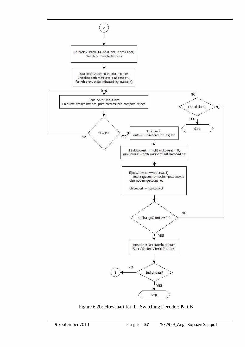
9 September 2010 P a g e | 57 7537929_AnjaliKuppayilSaji.pdf
Figure 6.2b: Flowchart for the Switching Decoder: Part B

9 September 2010 P a g e | 58 7537929_AnjaliKuppayilSaji.pdf
6.4 Analysis of Failure Cases for Simple Decoder
There are certain cases when the Simple Decoder will fail to detect a particular sequence
of bit-errors in the received bit-stream. An analysis of why these sequences exist and
their probabilities of occurrence are provided below. The impact of these cases on the
behaviour of the energy saving decoder [2] is then considered. In all cases, the
convolutional encoder referred to is the ½ K=7, (171, 133) convolutional coder.
6.4.1 Logical evaluation
The presence of bit-errors in the input bit-stream is not detected by the Simple Decoder
until its upper and lower branches give different outputs. With an isolated single bit
error, this will occur straight away, but two consecutive bit-errors can clearly cause the
upper and lower branches to remain equal even though they are both wrong. Hence this
double error will not be detected straight away, though it may be detected when the next
pair of input bits arrives. Extrapolating from this very simple case, it is not difficult to
see that further bit-errors may delay the error detection until the third pair of input bits
arrive, or even the fourth, fifth, sixth or seventh pair. Therefore, if the upper and lower
branches become different at any stage, the bit-errors causing this may occur within the
current pair of input bits or any of the previous six pairs. In any of these cases, the
detection of a difference between upper and lower outputs will cause a switch to the
standard Viterbi decoder with a seven slot trace-back The seven slot trace-back ensures
that the standard Viterbi decoder has the best possible chance of correcting the bit-errors
that have occurred. In fact it has exactly the same chance that a standard Viterbi decoder
would have without the Simple Decoder’s switching mechanism. It may fail, but nothing
is lost by using the Simple Decoder first.
Going back to the Simple Decoder, it is straightforward to invent an input sequence
which causes the presence of bit-errors to remain undetected by the Simple Decoder until
the seventh pair of bits arrives. It is also straightforward to extend such a sequence to 8,
9 pairs or even to infinity. In this case, the switch to standard Viterbi will occur too late,
since we only wind back by 7 pairs, or the switch may never occur at all. So the Simple
Decoder will definitely produce a wrong output which the standard Viterbi Decoder will

9 September 2010 P a g e | 59 7537929_AnjaliKuppayilSaji.pdf
not have any chance to correct. The question arises whether we may now have lost
decoding power by not switching early enough.
The answer is that no decoding power is lost since it can be shown and it is demonstrated
below that a sequence of 8 pairs for which the upper and lower outputs of a Simple
Decoder are identical cannot be corrected by a standard Viterbi decoder because the
inputs will be compatible with a different (incorrect) message bit-stream when it is
received without bit-errors. The incorrect message is that generated by the Simple
Decoder which is guaranteed to produce smaller accumulated distances than the true
message. Looking at this another way, for a constraint length 7 convolutional coder, the
minimum free distance is about 10, and there will be many more than 4 bit-errors in the
sequence.
This argument also shows that there is no point in ‘winding back’ by more than 7 input
pairs when switching from the Simple Decoder (SD) to the standard Viterbi Decoder
(VD). This means that a latency of only 7 message bits is imposed by the SD to VD
switching mechanism.
We must also ask if problems could occur when switching back to the Simple Decoder
from the standard Viterbi decoder. The switching occurs when no changes occur to the
minimum accumulated distance for a suitable number of input pairs, since this is taken as
an indication that there are no bit-errors. But it is possible to invent an input sequence
of pairs, of any desired length, for which there are many bit errors, but yet the minimum
accumulated distance does not change despite the output generated being totally
incorrect. In this case an inappropriate switch to the Simple Decoder may be made.
However, again nothing is lost by this inappropriate switch since the Viterbi Decoder is
failing to correct the bit-errors, so we just replace one incorrect output by another.
6.4.2 Evidence through practical examples
The following examples that were developed manually by logically applying the ‘odd
number of bit inversions to invert output’ rule for 8 consecutive time slots. These
examples demonstrate how certain input sequences delay the detection of bit-errors by
the Simple Decoder. The message bit obtained from the decoder will be incorrect if the
output of BOTH the upper and lower branches have been inverted and thus give the same

9 September 2010 P a g e | 60 7537929_AnjaliKuppayilSaji.pdf
output. Since the output of each branch is the ‘exclusive-or’ of a current input bit and
several previous ones, this inversion occurs when there have been an odd number of bit
inversions (bit-errors) in each branch (a property of XOR). If there is an even number of
bit inversions, the output remains correct. Using this principle, examples of sequences
that delay the bit-error detection of the Simple Decoder may be generated as shown
below. We assume that a pair of input bits are received from the channel at time slot T1,
another pair at time-slot T2, and so on.
Example Sequence 1: Output Bit-Error at slot T1
Message bits: 1 1 1 0 1 0 1 0
Transmitted sequence: 1 1 0 1 1 0 1 0 1 1 0 0 1 0 1 1
Received sequence: 0 0 1 1 0 1 0 1 1 1 0 1 0 0 1 1 (Bit-errors are shown in red)
At the Simple Decoder, the following operations take place:
Lower branch Output = Rx(L) xor FF1 xor FF2 xor FF3 xor FF6
Upper branch Output = Rx(U) xor FF2 xor FF3 xor FF5 xor FF6
where Rx(U) represents the input to the upper branch, Rx(L) represents the input to the
lower branch and FF1 to FF6 are the shift register outputs. The output of the decoder is
fed back to FF1.
Time
Slot Rx(L) Rx(U) FF1 FF2 FF3 FF4 FF5 FF6
Output
(L)
Output
(R)
T1 0 0 0 0
T2 1 1 0 1 1
T3 0 1 1 0 1 1
T4 0 1 1 1 0 0 0
T5 1 1 0 1 1 0 1 1
T6 0 1 1 0 1 1 0 0 0
T7 0 0 0 1 0 1 1 0 1 1
T8 1 1 1 0 1 0 1 1 0 0
Table 6.1: Operation of Simple Decoder under Example Sequence 1
In Table 6.1, we see that the outputs of both branches are identical in all cases despite the
presence of nine bit-errors in the input bit-stream. Hence the two bit-errors in the inputs

9 September 2010 P a g e | 61 7537929_AnjaliKuppayilSaji.pdf
at slot T1 are not detected, and neither are any of the others. This was confirmed by
simulation in MATLAB® and the same sequence, embedded within a longer sequence of
zeros, was also applied the conventional Viterbi decoder. Again as expected, the Viterbi
decoder could not correct the bit-errors. This implies that even if the Simple Decoder had
been able to detect the bit-errors and switch earlier to the Viterbi decoder, the bit-errors
would still not be corrected.
It can now be explained more clearly why, if the Simple Decoder does not detect a
sequence of bit-errors, neither will the Viterbi decoder. Since convolutional codes are
linear, the number of bit-errors in the output depends only on the error sequence in the
input and not on the actual message bits. It is possible to calculate which bit-error
sequences can produce errors in the output of the Simple Decoder.
It is known that the ‘free distance’, the minimum hamming distance (dfree) between any
two possible code sequences, is 10 for a rate ½, constraint length 7 convolutional code
[42]. The number of close proximity errors that can be corrected is calculated as a
function of the code’s free distance. It is given by t = (dfree – 1) / 2 [43]. The Viterbi
Decoder can therefore correct a maximum of 4 errors occurring relatively near each
other.
If it is true that the minimum number of bit-errors required for the Simple Decoder to
give an incorrect output is greater than 4, this implies that any bit-error that the Simple
Decoder cannot detect will not be corrected even by the conventional Viterbi Decoder.
The Error Sequence producing Table 6.1 is E = [1 1 1 0 1 1 1 1 0 0 0 1 1 0 0 0] where 1’s
represent the positions at which bit-errors occur. There are 9 bit-errors in the input to the
decoder within a space of 16 bits. As shown in Example Sequence 1, this results in a
single bit-error in the output at slot T1. There are also sequences which cause more than
one bit-error to occur in the output. Examples are given below
Example Sequence 2: Output Bit-Error at T1 and T3
Decoding of an input stream with the error sequence E = [1 1 1 0 0 0 0 1 1 1 1 0 1 1 0 1]
is represented in Table 6.2. ‘e’ represents a bit inversion (bit-error).

9 September 2010 P a g e | 62 7537929_AnjaliKuppayilSaji.pdf
Time Rx(L) Rx(U) FF1 FF2 FF3 FF4 FF5 FF6 Output
T1 e e e
T2 e e
T3 e e
T4 e e e
T5 e e e e
T6 e e e
T7 e e e e
T8 e e
Table 6.2 Operation of Simple Decoder under Example Sequence 2
Taking into consideration the 7 slot (14 bit) trace-back, once an error is detected, the
final output of the decoder will have at least one error at T1 after which it switches to the
Viterbi decoder. This example requires 10 bit-errors in the input sequence in a space of
16 bits.
Testing in MATLAB® confirmed that both the Switching Decoder and the Viterbi
decoder had 2 bit-errors in their output. Therefore, even the Viterbi decoder could not
correct these errors as expected.
Example Sequence 3: Output Bit-Error at T1 T2 T3 T4 T5 T6 T7 T8
Decoding of error sequence E = [1 1 0 1 1 0 0 1 0 1 0 0 1 1 1 1] is represented in Table
6.3
Time Rx(L) Rx(U) FF1 FF2 FF3 FF4 FF5 FF6 Output
T1 e e e
T2 e e e
T3 e e e e
T4 e e e e e
T5 e e e e e e
T6 e e e e e e
T7 e e e e e e e e e
T8 e e e e e e e e e
Table 6.3: Operation of Simple Decoder under Example Sequence 3

9 September 2010 P a g e | 63 7537929_AnjaliKuppayilSaji.pdf
Taking into consideration the 7 slot (14 bit) trace-back once a bit-error is detected, the
final output of the decoder will have at least one error at T1 after which it switches to the
Viterbi decoder. This example also requires 10 bit-errors in the input sequence in a space
of 16 bits.
Testing in MATLAB® confirmed that both the Switching Decoder and the Viterbi
decoder had 8 bit-errors in their output. Therefore, even the Viterbi decoder could not
correct these errors as expected.
In all the above examples the number of bit-errors required in the input sequence is 9 or
10 and exceeds the number that can be corrected by the conventional Viterbi Decoder
which is 4. Therefore even if the Viterbi Decoder was used conventionally, i.e. without a
Simple Decoder, these bit-errors would not be corrected.
The conclusion is that there has to be an odd number of bit-inversions in BOTH the two
branches for a bit-error not to be detected. The error sequence must be at least 16 bits
long to ensure that at least one bit-error is propagated to the output after the 7 slot (14
bit) trace-back.
Since there is only one input to each of the branches at each slot, there is only one
possible error sequence that can result in a particular combination of errors at the output.
Therefore, by calculating the number of such error combinations, the number of input
error sequences that will not be detected by the Simple Decoder can be calculated.
The number of such error combinations can be calculated in the following way.
Accounting for the 7-bit trace-back, at least one output bit-error goes undetected only if
an error occurs in slot T1 (or Tn) and an error is not detected until after slot T8 (or Tn+8).
There is only one 16-bit error sequence that goes undetected AND results in a single bit-
error at the output (as in the Example Sequence 1 described above). The number of
sequences with double bit-errors having one of the bit-errors at slot T1 (or Tn) is 7C1 (as
in Example sequence 2). The number of sequences with triple bit-errors having one of
the bit-errors at slot T1 is 7C2. Proceeding in a similar fashion, it is found that the total
number of error sequences that go undetected is calculated as

9 September 2010 P a g e | 64 7537929_AnjaliKuppayilSaji.pdf
Number of sequences = 1 + 7C1+7C2+
7C3+7C4+
7C5+7C6+
7C7
= 128 possible 16 bit sequences.
There are 216 possible 16-bit sequences. Among these, only one of them is correct for a
given sequence of message bits, and the rest contain bit-errors. Therefore out of a
possible 216-1 error sequences, only 128 of them go undetected by the Simple Decoder.
The probability of the errors not being detected is therefore 1.95 x 10 -3. It has been
argued that the Viterbi Decoder will not be able to correct ANY of these error sequences,
and the failure has been illustrated by the examples given above [Example Sequence 1, 2
& 3].
6.5 Summary
This chapter has described the flow of control and data processing that takes place in the
system. Solutions to some of the unresolved questions have been proposed. The next
chapter details how the system will be tested and provides an analysis of the results
obtained.
9 September 2010 P a g e | 65 7537929_AnjaliKuppayilSaji.pdf
Chapter 7
TESTING AND ANALYSIS
Now that the system has been developed, adequate testing is required to ensure it works
as expected and also evaluate its performance. This section describes testing and
evaluation criteria for the developed system and provides an analysis of the results
obtained.
7.1 Overview of Testing
In order to ensure that the new algorithm works accurately the following checkpoints are
used.
i. The MATLAB® code for the customized (‘My Viterbi’) decoder, written from
scratch, for any input data the same output as that of a MATLAB® implemented
conventional Viterbi decoder (vitdec.m).
ii. The Simple Decoder should produce correct outputs when no bit-errors occur
iii. With no errors introduced, the switching mechanism from the Simple Decoder to the
Adapted Viterbi Decoder and vice versa should produce no error in the output. For this
test case, switches are forced at equal intervals of 7 in the Simple Decoder. The Adapted
Viterbi decoder automatically switches to the Simple Decoder when the path metric
remains constant for the predetermined number of consecutive bits.
iv. With errors introduced in certain sections of the signal, the Switching Decoder should
produce the same output as that of the MATAB Viterbi decoder. This is done in the
following way. Transmit data at zero bit-error rate. After a short period increase bit-error

9 September 2010 P a g e | 66 7537929_AnjaliKuppayilSaji.pdf
rate to 10 -2 and then bring it back to zero subsequently. This sequence will allow us to
monitor the following cases
a. No bit-errors occur and the Simple Decoder is switched on
b. Bit-errors start occurring and the receiver must switch to the Viterbi decoder
c. Bit errors stop occurring and the receiver must switch to the Simple Decoder
v. Finally, with AWGN added to the signal, the output produced by the Switching
Decoder should closely match the output produced by the ‘My Viterbi’ decoder. This
must be tested over a range of SNR varying from 0.5 to 13 dB.
vi. Estimating energy consumption of the decoder requires detailed knowledge of the
circuitry at transistor level. For the purpose of this project however, a simpler technique
is used as described below. Though this method gives a very rough estimate of the
energy used, it is useful in loosely predicting the conditions at which the Switching
Decoder is likely to give better energy efficiency as compared to the conventional
Viterbi decoder.
The profiler tool available in MATLAB® is used to run the simulation, first with no
errors introduced and then varying SNR from 7 to 4 dB. For each case the simulation is
run 10 times. After each simulation the profiler gives a description of the number of
times a particular function was called and the total CPU time taken to execute that
function for all its function calls. In addition to this information, the number of bits
decoded by each decoder (the Simple Decoder and the adapted Viterbi decoder) is also
displayed by inserting appropriate statements in the code. Using this information, the
total time required by each decoder to decode the bits at different SNR’s can be
calculated.
7.2 Results and Analysis
Once the code for ‘My Viterbi’ decoder was written, it was tested against the MATLAB®
Viterbi Decoder as described in Section 7.1 (i). Multiple tests showed that it followed the
MATLAB ® Viterbi decoder excepting for minor variations. These may have arisen due
to the fact that the way in which MATLAB’s Viterbi decoder selects paths when their

9 September 2010 P a g e | 67 7537929_AnjaliKuppayilSaji.pdf
path metric is equal is not known. In this algorithm, the higher state is consistently
chosen as the surviving state. However, MATLAB® may choose the lower state or even
choose the upper or lower state in a random fashion. Sample graphs are produced and
explained in Section 7.2.1 -7.2.3
The Simple Decoder was then tested without introducing bit-errors as mentioned in
Section 7.1 (ii). In all cases, the decoded output matched transmitted data.
In order to ensure that Switching does not introduce errors in the output, switches were
between the Simple Decoder and the Adapted Viterbi decoder as explained is Section 7.1
(iii). In all 10 tested cases, no errors occurred in the decoded output. This confirmed that
the initialization of states on both decoders was correct.
The process mentioned in Section 7.1(iv) was carried out by separating the transmitted
message a 1000 bit long into 3 parts and introducing errors only to the middle part. Once
errors were introduced the message was concatenated to form a single array. The results
showed that the switching operations occurred at the appropriate places. With one-third
of the message bits subjected to BEP of 10-2, about 44% of the bits were decoded by the
Simple Decoder. The number of resulting errors was the same for the Switching Decoder
and ‘My Viterbi’ Decoder, though the MATLAB® decoder had 3 more errors which
could be accounted for by the explanation in the first paragraph.
The following sections give detailed description and analysis of the test cases described
in Section 7.1 (i), (v) and (vi).
7.2.1 Bit-Error Probability (BEP) Performance
In order to test the performance of the Switching Decoder, the following measures were
adopted. Random data was generated, encoded, modulated and transmitted. Uncoded
data was also modulated and transmitted. Depending on the desired Eb/N0, the
appropriate Additive White Gaussian Noise(AWGN) was added to the signal. At the
receiver, data was demodulated. The encoded data was decoded by the three decoders,
MATLAB ® Viterbi decoder, ‘My Viterbi’ Decoder and the Switching Decoder.
The following parameters are given to the MATLAB® Viterbi Decoder.

9 September 2010 P a g e | 68 7537929_AnjaliKuppayilSaji.pdf
trellis = poly2trellis(7,[171 133]); tblen = 35; matdecodedHard = vitdec(Rx,trellis,tblen, 'term' , 'hard' ); %Rx = Received Data
As with the other two decoders, the traceback depth is set to 35. The parameter ‘term’ is
used since the convolutional encoder appends 6 flushing bits at the end of the data bits.
The parameter ‘hard’ is used so that the Viterbi Decoder uses hard decisions in decoding.
Now the MATLAB® Viterbi Hard Decision decoder can be compared with ‘My Viterbi’
decoder algorithm and subsequently with the Switching Decoder.
The tests were conducted with a data length of 10,000 bits. Eb/N0 was varied from 0.5dB
to 13 dB with an increment of 0.5 dB at each test. The tests were repeated 5 times and
finally the results of the three decoders were compared and analyzed. In order to find the
optimum settings for the Switching Decoder, tests were conducted with three different
settings on the Adapted Viterbi Decoder. In the first round of tests, decoding was
switched to the Simple Decoder if the accumulated path metric for the global winner
remained constant for 7 consecutive slots. In the second round of tests, this value was
increased to 35 which is five times the constraint length and the maximum amount of
state history maintained in the table. In the third round, this value is brought down to 21
which is three times the constraint length. The fact that the accumulated path metric of
the global winner has remained constant for a particular number of slots is taken to mean
that there have been no errors during those slots.
The tabulated results and calculations tables are provided in Appendix D. A couple of
sample graphs are provided below. Since BEP fell to 0 after 6 dB, these data points are
not visible on the log-scale graph. The graph is cropped to show values only up to 10 dB
instead of 13 dB.

9 September 2010 P a g e | 69 7537929_AnjaliKuppayilSaji.pdf
Matlab Decoder
Figure 7.1: Data Length = 10,000, Switched to Simple Decoder when no errors for 7
consecutive slots
Figure 7.1 shows that below 2 dB, the uncoded message performs better than the
encoded messages. This is expected since the very high error rates cause the Viterbi
decoder to follow an incorrect path. Above 2 dB, it is observed that the MATLAB®
decoder and ‘My Viterbi’ Decoder both follow each other closely with only minor
variations. As the SNR increases to 5 dB very few bit-errors occur, less than 10 in the
10,000 bits. This makes the result more unreliable at higher SNR. Also, though the graph
appears to show a larger difference in values at 5dB, this is not true. As the data moves
to lower BEP, the log-scale increases the gap between two consecutive lines from 10-3 to
10-4. This causes the gap between the two lines to appear larger even though difference
in values remains the same.
Comparing the Switching Decoder and ‘My Viterbi’ decoder, both of them follow each
other closely, though there is a slight variation between 3 and 4 dB. Comparison of the
average values over 5 tests show there are differences between 0.5 and 5 dB. The values
are tabulated in Appendix D and plotted in Figure 7.2.

9 September 2010 P a g e | 70 7537929_AnjaliKuppayilSaji.pdf
Figure 7.2: Average Fractional Difference in number of errors between Switching
Decoder and ‘My Viterbi’ Decoder. Switched to Simple Decoder when no errors for 7
consecutive slots
These differences in values show that the presence or absence of errors has not been
accurately detected. The Simple Decoder may have missed the presence of certain
combinations of errors and passed an incorrect initial state to the Viterbi. These
deductions were verified by the fact that at lower SNR, there were a few cases when the
bits decoded by the Simple Decoder were incorrect.
Therefore, the tests are performed with another setting for the Adapted Viterbi decoder.
Since state history is maintained for 35 slots, switching to the Simple Decoder is now
done only after 35 consecutive slots of constant path metric for the global winner. Doing
this causes the switch to the Simple Decoder only if bit-errors haven’t occurred for a
longer period. This means that at lower dB the Simple Decoder will be called much less
frequently and thus reduce the possibility of error. It was found that in this case the
output of the Switching Decoder perfectly matched that of ‘My Viterbi’ decoder. A
sample graph is shown below in Figure 7.3.

9 September 2010 P a g e | 71 7537929_AnjaliKuppayilSaji.pdf
Figure 7.3: Data Length = 10,000. Decoding switched to Simple Decoder when there are
no bit-errors for 35 consecutive slots
However, it may not be necessary to wait for 35 slots. In the third case, Switching to the
Simple Decoder is done when no errors have occurred for more than 21 consecutive
slots. The graph in Figure 7.4 shows the BEP performance with this third setting. It is
observed that the red line for ‘My Viterbi’ Decoder is still not visible as it lies exactly
beneath the green lone for the Switching Decoder. These results seem promising.
As before, the actual fractional difference in errors between the two lines using average
values from 5 tests is studied. Plotted in Figure 7.5, it is observed that the improvement
is remarkable. There is almost no difference between the Switching Decoder and ‘My
Viterbi’ decoder. It was observed that now none of the bits decoded by the Simple
Decoder had errors. This shows that the presence of errors has been detected accurately
and the correct initial state passed to the Viterbi Decoder. Interestingly, at one point the
Switching Decoder has a slightly lesser number errors than ‘My Viterbi’ decoder.

9 September 2010 P a g e | 72 7537929_AnjaliKuppayilSaji.pdf
Figure 7.4: Data Length = 10,000. Decoding switched to Simple Decoder when there are
no bit-errors for 21 consecutive slots
Figure 7.5: Average Fractional difference in errors between the Switching decoder and
‘My Viterbi’ decoder. Decoding switched to Simple Decoder when there are no bit-
errors 21 consecutive slots
Another important observation is that at these settings, the Switching Decoder causes no
deterioration in performance compared to the normal Viterbi decoder. This can also be
explained theoretically due to the fact that during switching no relevant state history is

9 September 2010 P a g e | 73 7537929_AnjaliKuppayilSaji.pdf
lost. The only requirement is that the initial state in both decoders is set correctly and
errors are detected accurately. If this is done properly, the outputs are expected to match
those given by the normal Viterbi Decoder.
However, this improved performance comes with an additional cost. The Simple
Decoder will now be used for only a shorter portion of time. Since the Simple Decoder is
the part that is expected to bring energy savings, it is expected that the overall energy
savings will be lesser as compared with the first setting.
In order to see exactly how effective the Switching algorithm is, it is necessary to look at
how often the Simple Decoder is being used and what percentage of bits are being
decoded by each decoder at each SNR. This analysis will also help us determine whether
there were too many ineffective calls to the Simple Decoder where in effect it could
decode no additional bits. The following graphs in Figure 7.6 and Figure 7.7 show the
percentage of decoding that was done by the Simple Decoder and the Adapted Viterbi
decoder respectively.
Figure 7.6: Percentage of Decoding done by each decoder in the Switching Decoder.
Decoding switched to Simple Decoder when there are no bit-errors for 7 consecutive
slots

9 September 2010 P a g e | 74 7537929_AnjaliKuppayilSaji.pdf
Figure 7.7 Percentage of Decoding done by each decoder in the Switching Decoder.
Decoding switched to Simple Decoder when there are no bit-errors for 21 consecutive
slots
From Figure 7.6, it is observed that even at 1.5 dB, about 1% of decoding is being done
by the Simple Decoder. This increases to 16% at 4 dB and reach 46% by 6 dB. By 9 dB
more than 90% of the decoding is being done by the Simple Decoder. From these results,
it seems likely that there will be considerable energy savings.
Comparing these results with Figure 7.7 it is observed that at lower dB’s the percentage
contribution of the Simple Decoder is lesser. 1% of decoding is done by the Simple
Decoder at 4 dB. This increases to 26% at 6 dB and reaches 46% at 7dB. By 9.5 dB it
crosses 90%. Despite the slightly lower contribution, these results still seem promising
since it provides a BEP performance that matches the Viterbi decoder.
On the basis of these results it is also proposed to use this counter setting of the Adapted
Viterbi Decoder as a variable to optimize operations depending on the specific
application, the importance of data accuracy versus energy savings and the expected
SNR range in which the decoder will operate.

9 September 2010 P a g e | 75 7537929_AnjaliKuppayilSaji.pdf
Using the collected data, the average number of bits that were being decoded between
switches from the Simple Decoder to the Viterbi decoder and vice-versa is calculated.
This helps in understanding how effective the switching mechanisms are. Figure 7.8
shows the results of the analysis done using the first setting (7) for the Adapted Viterbi
decoder. Above 9 dB, only few bit-errors occurred in the channel. Therefore very few
switches took place between the two decoders and almost all decoding was done by the
Simple Decoder. Hence, the number of bits decoded between switches was very high for
the Simple Decoder above 9 dB and it was difficult to scale onto the graph. Since what
happens at lower SNR is of more concern, the graph is drawn only up to 9 dB.
From the results tabulated in Appendix D Section (iii) , it is observed that the Adapted
Viterbi decoder decodes approximately the same number of bits between switches at all
SNR values. This is not ideal. The Simple Decoder, as expected decodes fewer bits
between switches at lower dB. Rounding off to an integer value, at 4 dB four bits are
efffectively decoded before a switch to the Simple Decoder. At 6 dB this value reaches
fifteen bits between switches and crosses to fifty-one bits between switches at 7.5 dB.
Figure 7.8: Average number of bits being decoded per call to each decoder. Decoding
switched to Simple Decoder when there are no bit-errors for 7 consecutive slots

9 September 2010 P a g e | 76 7537929_AnjaliKuppayilSaji.pdf
From these observations it is also clear that at lower SNR, a lot of switches are taking
place since both the Simple Decoder as well as the Adapted Viterbi decoder decode less
than 35 bits per call. As SNR increases above 7 dB, the situation improves and the
Simple Decoder is able to decode a much larger number of bits before it encounters a bit-
error.
Now an analysis is made for the second setting of the Adapted Viterbi decoder, i.e. with
waiting for 21 slots with no bit-errors before switching to the Simple Decoder. Figure 7.9
shows a striking difference from the earlier graph and has many points of interest.
Firstly, attention is drawn to the Y axis of the graph. Unit distances are now 250 bits
instead of 20 bits as in the earlier graph. Straightaway it is observed that at lower dB the
Adapted Viterbi decoder is able to decode a much larger number of bits between
switches. As the SNR improves, decoding switches to the Simple Decoder more often
and therefore number of bits decoded by the Adapted Viterbi decoder between switches
decreases. From the results tabulated in Appendix D Section (iii) that at 4 dB the
Adapted Viterbi decoder decodes an average of 97 bits between switches and this value
decreases to 42 by 7.5 dB.
Figure 7.9: Average number of bits being decoder per call to each decoder. Decoding
switched to Simple Decoder when there are no bit-errors for 21 consecutive slots
9 September 2010 P a g e | 77 7537929_AnjaliKuppayilSaji.pdf
The most interesting observation was that Simple Decoder still decoded almost the same
number of bits between switches. Rounding off to an integer value, at 4 dB three bits are
efffectively decoded per call to the Simple Decoder. At 6 dB this value reaches fifteen
bits between switches and reaches forty-eight bits between switches at 7.5 dB.This
analysis shows that with the second setting it is possible to reduce a large number of
unnecessary switches especially at lower SNR.
7.2.2. Packet Loss Rate
In wireless communications most data is sent as packets. At the receiver, a check
(usually a CRC check) is used to see whether the decoder was able to correct all bit-
errors in the packet. If there is even one bit-error in the packet, the packet is discarded. A
new packet maybe requested as described in Section 2.1 and 2.2. In this case, slight
variations BEP performance will not matter. Whether the packet contained 1 bit-error or
10, the packet will still be discarded.
Packet loss rate may differ from BEP depending on how close the bit-errors occur.
Multiple bit-errors occurring within a single packet will result in only 1 packet loss. If
these bit-errors are spread out into different packets, the packet loss rate increases
considerably. In order to estimate the packet loss rate, 100 packets of 1000 data bits each
were transmitted and the number of packets that were received without error after
decoding using the three decoders was counted separately. Measurements were taken at
each 0.25 dB going from 5 to 7.5 dB. The results are tabulated in Appendix E and plotted
in Figure 7.10.
The results show that both the Switching Decoder and ‘My Viterbi’ decoder give exactly
the same packet loss rate at each data point. This reinforces the fact that the Switching
Decoder does not degrade performance of the Viterbi decoder. On comparing with the
MATLAB Viterbi decoder, there are slight variations in packet loss rate at some points
though in several cases the packet loss rate is the same.
According to the ITU Recommendations (ITU-R M.1079-2) [44], a packet loss rate
(PLR) of less than 3% is acceptable for real time audio communications. For video

9 September 2010 P a g e | 78 7537929_AnjaliKuppayilSaji.pdf
communications, PLR must be less than 1% and data communications require a PLR of
0%. From the graph in Figure 7.10, it is observed that above 5.75 dB packet loss rate is
below 2%. When Eb/N0 drops below this value, packet loss rate increases rapidly.
Figure 7.10: Packet Loss Rate. Decoding switched to Simple Decoder when there are no
bit-errors 21 consecutive slots
7.2.3 Predicting Packet Loss
Keeping the goal of minimizing energy consumption in mind, it would be very
advantageous if there was a way of predicting that a packet was likely to fail. Processing
that packet could then be stopped and a retransmission request sent. An interesting
method of determining a reliability estimate for the decoded data, suitable for use in
Type I HARQ protocols, was described by Harvery and Wicker in their papers [45, 46].
The Yamamoto-Itoh algorithm that they describe [47] performs a comparison of the
surviving path and the best non-surviving path at each state and at every stage of the
decoding process. If the difference in path metric between the two paths falls below a
certain threshold value, the survivor is considered unreliable. If all paths are found to be
unreliable before the end of decoding, a retransmission request is sent. The reliability of
this repeat request technique in combination with Viterbi decoding was found to be
asymptotically twice that of the normal decoding algorithm [47]. This mechanism may
also be incorporated in the Switching Decoder to prevent it from attempting to decode a
packet that is likely to fail, thus saving energy.

9 September 2010 P a g e | 79 7537929_AnjaliKuppayilSaji.pdf
Type II HARQ protocols, mentioned in Section 2.6, use data from multiple
retransmissions to correctly decode data. This reduces number of retransmissions
required and hence delay incurred in receiving a correct packet. Different mechanisms of
combining data from such retransmissions have been investigated by Harvey and Wicker
in another paper on Packet combining systems based on the Viterbi decoder. [48].One of
the techniques used, called the averaged diversity combiner (ADC), combines packets bit
by bit by averaging their soft decision values. This produced results that matched those
of the interleaved code combining technique [49], a method of interleaving symbols
received from multiple copies of a packet to form a single packet at the receiver.
7.2.4 Measurements of Processing Time
In absolute terms, the execution times taken by the MATLAB ® implementations of the
two decoders depend on the configuration of the computer used and its processor. These
specifications of the laptop used for this project are provided in Section 5.2, its main
features being a Microsoft® Windows Vista™ Ultimate OS, Intel(R) Core(TM)2 CPU
T7200 @ 2.00GHz, 2000 MHz Processor and 2 GB RAM. Benchmarking using the
MATLAB function ‘bench’ was used to measure the performance of the MATLAB®
version R2007b on the laptop. Since these tests may give a variation of up to 10%
between successive readings, the tests were repeated 10 times. On average, it took 0.189
seconds to perform standard operations in data structures and M files. The graph of
relative speed for each of the 10 runs as compared to standard values for other machines
is reproduced in Figure 7.11. These figures are given for the convenience of researchers
wishing to reproduce the results presented in this thesis. As may be noted, on most
occasions its speed matched that of a Linux (32 bit) dual 2.6 GHz Opteron.

9 September 2010 P a g e | 80 7537929_AnjaliKuppayilSaji.pdf
Figure 7.11: Results of Benchmarking on MATLAB®
One of the other concerns was how the use of large arrays would affect the memory
requirements and timing of code execution. According to MATLAB® Documentation
[50], if an array is expanded beyond the available contiguous memory of its original
location, MATLAB® has to make a copy of the array in a new location and then set this
array to its new value. This operation may not only result in the program running out of
memory (due to a temporary doubling in the size of memory required), but also create a
variation in the time required to execute the code. In order to solve both these problems,
sizes have been pre-allocated to all the arrays used in the code. This means allocation of
memory spaces occurs at the beginning of program execution. The code does not expand
or reduce the size of the array at any other point in the program but only modifies the
values contained in the memory spaces.
As described in Section 7.1, timing measurements are used to compare the likely energy
consumption of the two decoders. To a first degree of approximation, it is expected that
energy consumption will be proportional to the execution time.
Using a data length of 10000, the decoders were run using the MATLAB® Profiler tool.
Data for the profiler was collected for single packets, each containing 10000 bits, when
bit-errors result from constant AWGN channel noise. Simulations were run for Eb/No

9 September 2010 P a g e | 81 7537929_AnjaliKuppayilSaji.pdf
varying from 1 to 12 dB. For each run the value of Eb/N0 remained constant. The results
are presented in Appendix F and plotted in Figure 7.12.
Figure 7.12: Timing Measurements
It is found that while the conventional Viterbi decoder requires a fixed execution time of
about 48 seconds at all values of Eb/N0, the time taken by the Switching Decoder is
dependent on Eb/N0. At higher Eb/N0 values, where a large portion of the decoding is
being done by the simple decoding part, less time is required to complete the decoding.
As the Eb/N0 value decreases, a greater portion of decoding is done by the Adapted
Viterbi decoding part. Therefore the time required to complete the decoding increases. It
is observed that when Eb/N0 equals 5 dB, the time requirement of the Switching Decoder
is almost equal to that of the standard Viterbi decoder. Below 5 dB the time requirements
for the Switching Decoder and standard Viterbi decoder remain more or less constant
and equal.
When there are no bit-errors, the Switching Decoder is about 44.5 times faster than the
Viterbi Decoder i.e. the Switching Decoder takes about 2.2 % of the execution time
9 September 2010 P a g e | 82 7537929_AnjaliKuppayilSaji.pdf
required by the standard Viterbi decoder. The graph shows that at 5 dB approximately
11% of the decoding is being done by the Simple Decoder. Therefore, it can be estimated
that as long as at least 11% of the decoding is being done by the Simple Decoder, the
Switching Decoder is likely to be advantageous in terms of energy consumption.
Another implication of these results is that whilst the conventional Viterbi decoder
requires a fixed decoding time, the Switching Decoder has a variable decoding time. This
could potentially make hardware implementation of the decoder more difficult. In order
to produce a steady stream of output bits, adequate delays and synchronization between
the two components of the Switching Decoder will be necessary.
7.3 Summary
This chapter has demonstrated by analysis of test results in terms of BEP and packet loss
rates, that appropriate settings allow the Switching Decoder to give exactly the same
results as the standard Viterbi decoder. It was also demonstrated that for Eb/N0 values
above 5 dB, the Switching Decoder takes considerably less execution time in MATLAB®
than the standard Viterbi decoder while for values below 5 dB, execution time remained
roughly constant and equal to that of the standard Viterbi decoder.

9 September 2010 P a g e | 83 7537929_AnjaliKuppayilSaji.pdf
Chapter 8
CONCLUSIONS AND FUTURE WORK
This chapter summarizes the conclusions and inferences made from the project and
recommends points that require further investigation.
8.1 Conclusions
The main objective of this project was to further develop the work started by Barry
Cheetham and investigate an energy efficient method for decoding convolutionally
encoded messages transmitted in a wireless environment, and received by energy limited
devices such as mobiles. One of the major tasks of the project involved understanding
and building the code for the Viterbi Algorithm. This code was then modified and used
as an Adapted Viterbi decoder that could pick up decoding when the Simple Decoder
detected bit-errors. Similarly control is transferred back to the Simple Decoder once
errors stop occurring.
Two significant issues in the development of the switching algorithm were resolved. The
first issue was the problem of switching between the two decoders without introducing
errors. This was solved by correctly initializing the starting states of the decoder based
on the last known state passed by the other decoder. This initialization was a significant
step towards the success of the algorithm as it facilitated switching between to the two
decoders without any loss of information and hence there was no deterioration in the
output.
The second issue was to accurately determine when bit-errors have stopped occurring so
that a switch from the Viterbi Decoder to the Simple Decoder could be initiated. This
issue was solved by using the path metric of the global winner at each time slot to check
if errors had occurred. If the path metric remained constant for a predetermined number

9 September 2010 P a g e | 84 7537929_AnjaliKuppayilSaji.pdf
of slots, it was fairly certain that bit-errors had stopped occurring. It was found that if
this predetermined number was set at 21, switching occurred without causing any
deterioration in the BEP performance. Results obtained also indicate that this setting
may be varied to optimize performance based on the required data accuracy and expected
SNR in the application.
It was also possible to determine the exact error sequences where the Simple Decoder
would fail to detect the presence of errors and determine the probability of these errors
occurring. A strong argument was given to support the belief that the standard Viterbi
decoder would fail to correct these sequences too.
Packet loss rate analysis confirmed the accuracy of the Switching algorithm as both the
Switching Decoder and ‘My Viterbi’ decoder gave exactly the same packet loss rate in
all test cases. This shows that switching had no impact on the error correcting capability
of the decoder.
Measurements on the execution time of the code show that above 5 dB the Switching
Decoder takes lesser time to execute as compared to ‘My Viterbi’ decoder. When there
are no errors, the Switching Decoder takes 44.5 times as many CPU seconds as does ‘My
Viterbi’ decoder. Below 5 dB, the time taken by the Switching Decoder remains roughly
constant and at the same level as that of ‘My Viterbi’ decoder. These results give a good
indication that there will be substantial energy savings above 5 dB. Added to this is the
previous observation that there is no degradation in BEP performance. Combining these
factors, there is strong evidence that the Switching Decoder provides an energy efficient
method of decoding convolutional codes.
8.2 Future Work
The results thus far have been very encouraging and further investigations would help in
fine tuning the decoder to bring maximum benefit. It would be very worthwhile
investigating the use of soft decision input Viterbi decoding in place of hard decision in
the Adapted Viterbi Decoder. Studies have shown that Soft decision inputs quantized to
three or four precision bits provide a 2 dB improvement in BEP performance of the

9 September 2010 P a g e | 85 7537929_AnjaliKuppayilSaji.pdf
Viterbi code [14]. It is expected that soft decision input will further improve the BEP
performance of the new algorithm. This algorithm could also be used in conjunction with
some of the approaches outlined in Section 3.4 to further increase energy efficiency.
In order to accurately measure energy consumption of the new system, VLSI
implementations need to built and tested. This requires a detailed knowledge of the
circuitry involved and synchronization of both the decoders. This analysis will be crucial
in determining the commercial viability of the new system. An important factor that
needs to be investigated is how a variable decoding time will affect implementation
complexity of the algorithm.
Based on the strong argument given in Section 6.4, it would also be helpful to build a
conclusive proof to establish that the standard Viterbi decoder would not be able to
correct any bit-errors that the Simple Decoder does not detect.
9 September 2010 P a g e | 86 7537929_AnjaliKuppayilSaji.pdf
LIST OF REFERENCES
[1] Viterbi, A. J.,1967. Error bounds for convolutional codes and an asymptotically optimum decoding algorithm. IEEE Trans. Inform.Theory., vol. 13 no.2, pp.260-269. [2] Cheetham, B.,2010. Power saving convolutional decoder. University of Manchester. [email] (Personal Communication, 3 March 2010) [3] Shao, W., 2007. Low Power Viterbi Decoder Designs. PhD Thesis, University of Manchester. [4] Peterson and Davie.,2003. Computer Networks: A Systems Approach. 3rd ed. California: Morgan Kaufmann [5] Tanenbaum, Andrew S., 2003. Computer networks. 4th ed. New Jersey: Prentice Hall. [6] Sklar, B., 2001. Digital Communications – Fundamentals and Applications. 2nd ed. New Jersey: Prentice Hall [7] Comroe, R.A; Costello, D.J.Jr., 1984. ARQ schemes for data transmission in mobile radio systems. IEEE Trans. Vehicular Technology, vol. 33 no 3, pp. 88– 97 [8] Clark, G. C. Jr. and Cain. J. B., 1981. Error-Correction Coding for Digital Communications. New York: Plenum Press. [9] Shannon, C.E., 1948. A Mathematical Theory of Communication. Bell System Technical Journal, vol. 27, pp.379-423. [10] Jacobsmeyer, M.J., 1996. Introduction to Error Control Coding. Pericle Communciations Company. [Online]. Available at: <http://www.pericle.com/papers/Error_Control_Tutorial.pdf> [Accessed 10 March 2010] [11] Proakis, J.G., 2003. Digital Communications. 3rd ed. New York: McGraw-Hill, Inc. [12] Wikipedia. General Algorithm - Hamming Codes. [Online]. Available at: <http://en.wikipedia.org/wiki/Hamming_code#General_algorithm> [Accessed 15 May 2010] [13] Brenner, P., 1992. A Technical Tutorial on the IEEE 802.11 Protocol. BreezeCom Wireless Communications. [Online]. Available at: <http://www.sss-mag.com/pdf/802_11tut.pdf> [Accessed 4 July 2010] [14] Fleming, C., 2002. Tutorial on Convolutional Coding with Viterbi Decoding. Spectrum Applications. [Online]. Available at: <http://home.netcom.com/~chip.f/viterbi/algrthms2.html> [Accessed 4 April 2010]

9 September 2010 P a g e | 87 7537929_AnjaliKuppayilSaji.pdf
[15] Berrou, C.; Glavieux, A. and Thitimajshima, P., 1993. Near Shannon Limit Error-Correcting Coding and Decoding: Turbo Codes. IEEE Proceedings of the Int. Conf. on Communications 1993 (ICC 93). Geneva. 23-26 May 1993, vol. 2, pp. 1064-1070. [16] Ryan, W.E., 1997. A Turbo Code Tutorial. [Online]. Available at: <http://www.ece.arizona.edu/~ryan> [Accessed 5 April 2010] [17] Bahl,L.; Cocke, J., Jelinek, F. and Raviv,J., 1974. Optimal decoding of linear codes for minimizing symbol error rate (Corresp.). IEEE Trans. Information Theory, vol.20 no.2, pp. 284-287. [18] Gallager, R. G., 1963. Low-Density Parity-Check Codes. Cambridge, MA: MIT Press. [19] Shokrollahi, A., 2003. LDPC codes: An introduction. Digital Fountain, Inc. [Online]. Available at: < http://www.digitalfountain.com> [Accessed 7 August 2010] [20] Ranpara, S.; Dong Sam Ha, 1999. A low-power Viterbi decoder design for wireless communications applications. IEEE Proceedings of the Twelfth Annual IEEE International Int. ASIC Conference 1999, Washington, DC, 15-18 Sept. 1999, pp. 377-381 [21] Wikipedia. Viterbi Decoder. [Online]. Available at: <http://en.wikipedia.org/wiki/Viterbi_decoder#Euclidean_metric_computation> [Accessed 26 August 2010] [22] Brackenbury, L.E.M., 2001. An Asynchronous Viterbi Decoder. In Sparsø, J. and Furber, S. eds., Principles of Asynchronous Circuit Design – A Systems Perspective. The Netherlands: Kluwer Academic. Ch.14 [23] Forney, G.D.Jr., 1973. The Viterbi algorithm. Proceedings of the IEEE. vol.61 no.3. pp. 268- 278 [24] Cypher, R. and Shung, C., 1990. Generalized trace back techniques for survivor memory management in the Viterbi algorithm. Proc .IEEE Global Telecommun. Conf. (GLOBECOM’90). San Diego, CA, 2-5 Dec 1990, pp. 1318–1322. [25] Truong,T. Shih, M.-T.; Reed, I.S.; Satorius, E.H., 1992. A VLSI design for a trace-back Viterbi Decoder. IEEE Trans. Communications, vol.40 no.3, pp 616-624. [26] Neuhoff, D., 1975. The Viterbi algorithm as an aid in text recognition (Corresp.). IEEE Trans. Information Theory, vol.21 no.2, pp. 222- 226. [27] Metzner, J. J., 1990. Improved coding strategies for meteor-burst communications. IEEE Trans. Communications, vol. 38 no. 2, pp. 133 – 136.
[28] Milstein,L.B.; Schilling, D. L.; Pickholtz, R. L.; Sellman, J.; Davidovici, S.; Pavelcheck, A.; Schneider, A. and Eichmann, G., 1987. Performance of meteor-burst

9 September 2010 P a g e | 88 7537929_AnjaliKuppayilSaji.pdf
communication channels. IEEE Journal Selected Areas in Communications. vol. 5 no 2. pp. 146-154. [29] Oetting, J. D., 1980. An analysis of meteor burst communications for military applications. IEEE Trans. Communications, vol. 28 no 9, pp. 1591-1601. [30] Kawokgy, M.; Salama, C.A.T. 2004. Low-power asynchronous Viterbi decoder for wireless applications. IEEE Int. Symp. Low power Electronics and Design (ISLPED ’04), 9-11 Aug. 2004, pp. 286-289. [31] Kang, I. and Willson, A. N. Jr., 1998. Low-power Viterbi decoder for CDMA mobile terminals. IEEE Journal Solid-State Circuits, vol. 33 no.3, pp. 473 – 482. [32] Suzuki, H.; Chang, Y.-N and Parhi, K. K., 1999. Low-power bit-serial Viterbi decoder for 3rd generation W-CDMA systems. Proc. IEEE Custom Integrated Circuits Conf. San Diego, CA, 16-19 May 1999, pp. 589 – 592. [33] Chun-Yuan Chu; Yu-Chuan Huang; An-Yeu Wu, 2008. Power efficient low latency survivor memory architecture for Viterbi decoder. IEEE Int. Symp. VLSI Design, Automation and Test (VLSI-DAT), Hsinchu, 23-25 Apr. 2008, pp. 228-231 [34] Henning, R. and Chakrabarti,C., 2004. An Approach for Adaptively Approximating the Viterbi Algorithm to Reduce Power Consumption While Decoding Convolutional Codes. IEEE Trans. Signal processing, vol. 52 no.5, pp. 1443-1451. [35] Jin, J., Chi-Ying Tsui., 2006. A low power Viterbi decoder implementation using scarce state transition and path pruning scheme for high throughput wireless applications. Proceedings of the 2006 international symposium on Low power electronics and design, Germany, 4-6 Oct. 2006, pp. 406 – 411. [36] Kubota, S.; Kato, S.; and Ishitani,T., 1993. Novel Viterbi Decoder VLSI Implementation and its Performance. IEEE Trans. VLSI Systems, vol. 41 no.2, pp 1170 – 1178. [37] Shaker, S.W., 2009. Design and Implementation of Low-Power Viterbi Decoder for Software-Defined WiMAX Receiver. 17th Telecommunications forum TELFOR, Belgrade, 24-26 Nov 2009, pp. 468-471. [38] Gang,Y; Erdogan, A.T.; Arslan, T., 2006. An Efficient Pre-Traceback Architecture for the Viterbi Decoder Targeting Wireless Communication Applications. IEEE Trans. Circuits and Systems I: Regular Papers, vol.53 no.9, pp.1918-1927. [ 39] Michelle, A. 2002. Steps in Empirical Research, PPA 696 Research Methods. [Online] California State University. Available at: <http://www.csulb.edu/~msaintg/ppa696/696steps.htm> [Accessed 10 August 2010] [40] Basilead Library. 2006.What is Empirical Research?. Tutorials and Research Guides. [Online]. Manor College. Available at: <http://library.manor.edu/tutorial/empiricalresearch.htm> [Accessed August 2010]

9 September 2010 P a g e | 89 7537929_AnjaliKuppayilSaji.pdf
[41] Caplinskas, A. and Vasilecas, O., 2004. Information Systems Research Methodologies and Models. The 5th international conference on Computer systems and technologies, Bulgaria. pp.1 -6. [42 50] Frenger, P.; Orten, P.; Ottosson, T.; 1999. Convolutional codes with optimum distance spectrum. Communications Letters, IEEE , vol.3 no.11, pp.317-319. [43] Wikipedia. Convolutional Code. [Online]. Available at: <http://en.wikipedia.org/wiki/Convolutional_code#Free_distance_and_error_distribution>[Accessed 4 September 2010] [44] International Telecommunication Union, 2003. ITU-R Recommendation M.1079-2. Performance and quality of service requirements for International Mobile Telecommunications-2000 (IMT-2000) access networks. Geneva: ITU [45] Harvey, B. A. and Wicker, S. B., 1991. Error Trapping Viterbi Decoders for Type-I Hybrid - ARQ Protocols. Canadian Journal of Electrical and Computer Engineering, vol 16. no. 1, pp. 5 – 12. [46] Wicker,S.B., 1988. An Adaptive Type-I Hybrid-ARQ Technique Using the Viterbi Algorithm. IEEE Military Communications Conference (MILCOM 1988), San Diego, CA, 23-26 Oct. 1988, vol 1, pp. 307-311. [47] Yamamoto, H and Itoh, K., 1980. Viterbi Decoding Algorithm for Convolutional Codes with Repeat Request. IEEE Trans. Information Theory, vol 26 no.5, pp. 540 – 547. [48] Harvey, B.A. and Wicker, S.B., 1994. Packet combining systems based on the Viterbi decoder. IEEE Transactions Communications. vol.42 no.234. pp.1544-1557. [49] Kallel,S., 1990. Analysis of a Type-II Hybrid-ARQ Scheme with Code Combining. IEEE Trans. Communications, vol.38 no.8, pp.1133-1137 [50] The MathWorks. MATLAB® Documentation - Memory Allocation.[Online]. Available at: <http://www.mathworks.com/access/helpdesk/help/techdoc/matlab_prog/brh72ex-2.html#brh72ex-5> [Accessed 20 August 2010]
[51] Kassam, S.A., 2004. Cyclic Codes and The CRC (Cyclic Redundancy Check) Code. TCOM 370 Principles of Data Communication. [Online]. University of Pennsylvania. Available at: <http://www.seas.upenn.edu/~kassam/tcom370/n99_9.pdf> [Accessed 10 June 2010] (referred in Appendix C)

9 September 2010 P a g e | 90 7537929_AnjaliKuppayilSaji.pdf
Appendix A – Gantt Chart Referred to in Section 5.3
1 BACKGROUND RESEARCH 69 days 10-Feb-10 14-May-10
1.1 Study of Papers & Other Literature 59 days 10-Feb-10 30-Apr-10
1.2 Familiarization with Software Tool (MATLAB ®)
14 days 24-Mar-10 12-Apr-10
1.3 Preparation of Background Report 25 days 12-Apr-10 14-May-10
2 DESIGN AND IMPLEMENTATION 65 days 12-May-
10 6-Aug-10
2.1 Study Viterbi Algorithm 6 days 12-May-
10 18-May-10
2.2 Break for Exams 14 days 19-May-
10 7-Jun-10
2.3 Implement code to perform simple decoding using Viterbi Algorithm
6 days 8-Jun-10 15-Jun-10
2.4 Design algorithm to perform decoder switch on/ off operation appropriately
7 days 16-Jun-10 24-Jun-10
2.5 Implement code for switch on/off operation
7 days 16-Jun-10 24-Jun-10
2.6 Design algorithm to convolutionally encode input data & introduce errors
7 days 25-Jun-10 5-Jul-10
2.7 Implement code to convolutionally encode data & introduce errors
7 days 1-Jul-10 9-Jul-10
2.8 Design algorithm to estimate energy use 7 days 10-Jul-10 19-Jul-10
2.9 Design simulation of entire communication system in Simulink
14 days 20-Jul-10 6-Aug-10
3 EXPERIMENTATION &ANALYSIS 7 days 9-Aug-10 17-Aug-10
4 PREPARATION OF REPORT 64 days 8-Jun-10 1-Sep-10
4.1 Chapter 1: Introduction 6 days 22-Jul-10 29-Jul-10
4.2 Chapter 2: Background 10 days 30-Jul-10 12-Aug-10
4.3 Chapter 3: FEC in mobile networks 7 days 8-Jun-10 16-Jun-10
4.4 Chapter 4: Design & Implementation of Experiment
40 days 17-Jun-10 10-Aug-10
4.5 Chapter 5: Results & Analysis, Chapter 6: Conclusion
6 days 13-Aug-10 20-Aug-10
4.6 Abstract, References & Formatting of Report
6 days 21-Aug-10 27-Aug-10
4.7 Review & Correction of Report 3 days 30-Aug-10 1-Sep-10
Table A.1: Gantt Chart Task List

9 September 2010 P a g e | 91 7537929_AnjaliKuppayilSaji.pdf
Figure A.1: Gantt Chart

9 September 2010 P a g e | 92 7537929_AnjaliKuppayilSaji.pdf
Appendix B: General Algorithm for Hamming Codes
The general algorithm used to construct hamming codes as stated in [12] has been reproduced below.
S.No: Algorithm Example
1 The bits are numbered starting from 1
Bit 1, 2, 3, 4, 5…
2 The binary representation of the bit positions are written
1, 10, 11, 100, 101…
3
Parity Bits: These are all the bits whose position number is power of 2. They will have only 1 bit having value 1 in their binary representation
Bit 1, 2, 4, 8,16 …
4 Data Bits: These are all the remaining bits having two or more 1 bits in their binary representation
Bit 3,5,6,7,9 …
5 Each data bit is included in a unique set of two or more parity bits, as determined by its binary representation
6 Each parity bit covers all bits where the binary AND of the parity position and the bit position is non-zero.
Table B.1: General algorithm for Hamming Codes [12]
The parity bits and the corresponding bits that they check are listed below as .
Parity Bit Data Bits Covered
Parity Bit 1 Covers all bit positions which have the least significant bit set
bit 1 (the parity bit itself), 3, 5, 7, 9, 11…
Parity Bit 2 Covers all bit positions which have the second least significant bit set
bit 2 (the parity bit itself), 3, 6, 7, 10, 11…
Parity Bit 3 Covers all bit positions which have the third least significant bit set
bits 4–7, 12–15, 20–23…
Parity Bit 4 Covers all bit positions which have the fourth least significant bit set
bits 8–15, 24–31, 40–47…
Table B.2: Table describing the bits covered by each parity bit [12]
A diagrammatic representation of the result is shown in Figure B.1 and helps in understanding the algorithm better.
Figure: B.1: Visual representation of Parity and Data bits

9 September 2010 P a g e | 93 7537929_AnjaliKuppayilSaji.pdf
Appendix C: CRC Generator Polynomials
CRC Check Codes have some properties that make them suitable for use in error detection. The fact that CRC checks are simple to implement has also resulted in CRC checks being widely used as an error detection mechanism in all forms of communications.
There are different kinds of generator polynomials each of which are used for detecting different types of errors.
As elaborated in the article [51], three kinds of errors and their detection mechanisms are briefly described below.
When we divided the received codeword polynomial by the generator polynomial, a non-zero remainder indicates that an error has occurred.
1. Single errors
These errors can be detected using a generator polynomial G(x) that has atleast two terms Xn and 1 where n is the degree of the codeword polynomial.
2. Double errors
These errors can be detected by using a generator polynomial G(x) such that G(x) does not divide Xp + 1 for any value of p <N-1
3. Any odd number of errors
These errors may be detected if the generator polynomial G(x) has a factor 1+X
4. Any error bust having length < n
A generator polynomial of degree n can detect an error burst of length <n
The most commonly used CRC codes are CRC-16 and CRC -32.
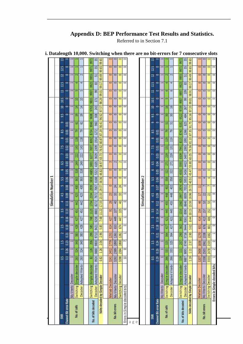
9 September 2010 P a g e | 94 7537929_AnjaliKuppayilSaji.pdf
Appendix D: BEP Performance Test Results and Statistics. Referred to in Section 7.1
i. Datalength 10,000. Switching when there are no bit-errors for 7 consecutive slots

9 September 2010 P a g e | 95 7537929_AnjaliKuppayilSaji.pdf
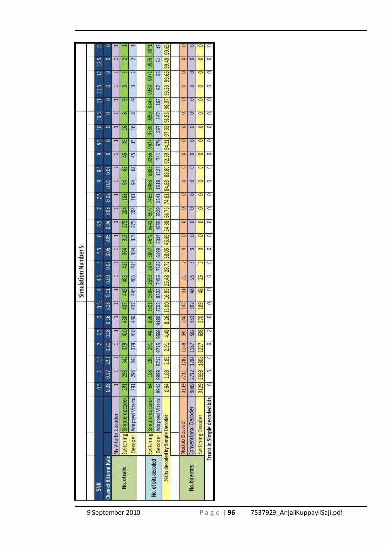
9 September 2010 P a g e | 96 7537929_AnjaliKuppayilSaji.pdf

9 September 2010 P a g e | 97 7537929_AnjaliKuppayilSaji.pdf
ii. Datalength 10,000. Switching when there are no bit-errors for 21 consecutive slots

9 September 2010 P a g e | 98 7537929_AnjaliKuppayilSaji.pdf
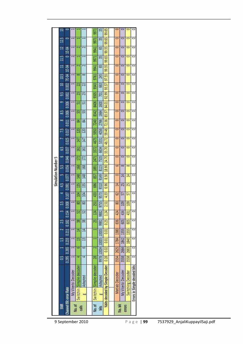
9 September 2010 P a g e | 99 7537929_AnjaliKuppayilSaji.pdf

9 September 2010 P a g e | 100 7537929_AnjaliKuppayilSaji.pdf
iii. Comparison of average number of bits decoded between switches with both
settings. Referred to in Section 7.1.
SNR
Setting 1 - Switch after 7 consecutive
error free slots
Setting 1 - Switch after 21 consecutive
error free slots
Avg number of bits
decoded per call
to Simple Decoder
Avg number of
bits decoded per
call to normal
decoder
Avg number of bits
decoded per call to
Simple Decoder
Avg number of bits
decoded per call to
normal decoder
0.5 0.28 35.43 1.17 2083.42
1 0.37 31.34 0.46 1351.70
1.5 0.70 28.82 0.44 847.53
2 0.90 25.83 0.51 555.38
2.5 1.26 23.00 1.01 323.86
3 1.90 21.57 2.04 205.55
3.5 2.54 19.92 2.31 148.84
4 3.56 18.77 3.32 100.26
4.5 5.23 18.18 5.53 74.78
5 7.37 17.46 7.14 60.56
5.5 10.71 16.94 10.56 50.91
6 14.83 16.75 15.06 44.01
6.5 21.48 16.39 22.11 39.28
7 31.37 16.19 32.94 36.84
7.5 50.93 16.04 47.97 35.42
8 72.10 16.13 70.72 32.86
8.5 111.50 16.13 119.60 31.54
9 186.50 16.05 182.53 31.27
9.5 328.57 16.46 357.05 30.78
10 571.78 16.81 572.49 30.28
10.5 1232.58 18.18 913.45 30.51
11 1905.12 19.12 1822.04 30.93
11.5 3825.15 23.31 5526.11 32.78
12 6225.88 27.88 7111.71 35.43
12.5 8306.50 31.83 9971.00 35.00
13 9971.00 35.00 9971.00 35.00

9 September 2010 P a g e | 101 7537929_AnjaliKuppayilSaji.pdf
Appendix E: Packet Loss Rate Calculations Referred to in Section 7.2.2
Eb/No
Percentage Packet Loss
MATLAB
Decoder
‘My Viterbi’
Decoder
Switching
Decoder
5.0 14.0 16.0 16.0
5.25 7.0 7.0 7.0
5.5 5.0 3.0 3.0
5.75 1.0 1.0 1.0
6.0 1.0 2.0 2.0
6.25 1.0 1.0 1.0
6.5 0.0 1.0 1.0
6.75 0.0 1.0 1.0
7.0 0.0 0.0 0.0
7.25 0.0 0.0 0.0
7.5 0.0 0.0 0.0
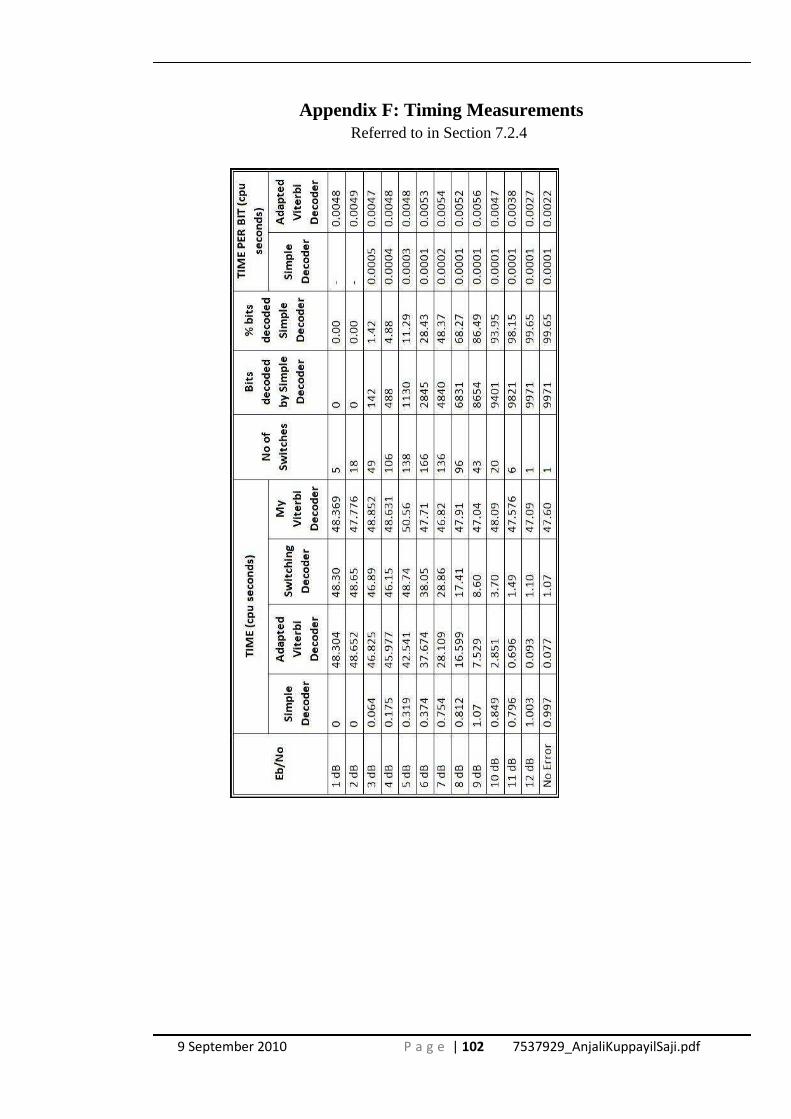
9 September 2010 P a g e | 102 7537929_AnjaliKuppayilSaji.pdf
Appendix F: Timing Measurements Referred to in Section 7.2.4

9 September 2010 P a g e | 103 7537929_AnjaliKuppayilSaji.pdf
Appendix G: MATLAB ® code
1. encoder.m
function Y = encoder(NB,ZInp) X1=0;X2=0;X3=0;X4=0;X5=0;X6=0; % the input at the 6 stages of the % encoder Y = repmat(-1, 2*NB,1); for n=1:NB X=ZInp(n); % the nth input to the encoder YL = xor( xor(X2,X1), xor(X6, X3)); YL = xor(YL,X); %(171) YU = xor( xor(X3,X2), xor(X6,X5)); YU = xor(YU,X); %(133) Y(2*n-1) = YL; %171 Lower output stored at index 2n-1 Y(2*n)=YU; %133 Upper output stored at index 2n X6=X5; X5=X4; X4=X3; X3=X2; X2=X1; X1=X; % All the flip flops % move to the next state. First flip flop gets value of input end ; % disp(sprintf('Output after Conv. encoding: \t')); % disp(sprintf('\b %d ',Y)); 2. modulate.m
function [msg_tx, grayencod] = modulate(Y,M,Nsamp) k= log2(M); msg_enc = bi2de(reshape(Y, ... size(Y,2)*k,size(Y,1) / k)'); grayencod = bitxor(0:M-1, floor((0:M-1)/2)); msg_gr_enc = grayencod(msg_enc+1); msg_tx = modulate(modem.pskmod(M, pi/4), msg_gr_enc ); msg_tx = rectpulse(msg_tx, Nsamp);
3. demodulate.m
function comp_Rx = demodulate(msg_rx,M,Nsamp,grayencod)
k=log2(M); msg_rx_int = intdump(msg_rx, Nsamp); msg_gr_demod = demodulate(modem.pskdemod(M, pi/4), msg_rx_int); [dummy graydecod] = sort(grayencod); graydecod = gr aydecod - 1; msg_demod = graydecod(msg_gr_demod+1)'; comp_Rx = de2bi(msg_demod,k)'; comp_Rx = comp_Rx(:) ;

9 September 2010 P a g e | 104 7537929_AnjaliKuppayilSaji.pdf
4. simpleDecoder.m
function simpleDecoder(NB, Rx,begState) global pState decoded ErrorFlag fLen numCalls_A ACount de cFlag numCalls_A=numCalls_A+1; FF = bitget(uint8(begState), 6:-1:1); % initialize flip flops to binary % value of state t=fLen; % store last index of output array index=fLen+2; %index for output array when there are no errors for i=index:NB lowerInput = Rx(2*i-3); upperInput = Rx(2*i-2); lowerOutput = xor(xor(xor(FF(2),FF(1)), xor(FF( 6),FF(3))), lowerInput); upperOutput = xor(xor(xor(FF(3),FF(2)), xor(FF( 6),FF(5))), upperInput); if ((lowerOutput ~=upperOutput )||(fLen > NB-35+6)) % Conventional viterbi needs traceback depth of atl east 5 times % constraint length fLen=fLen-7; if (fLen <=0) fLen=0; for p = 1:7 pState(p)=0; end end break ; elseif (lowerOutput==upperOutput) % No error in received bits fLen=fLen+1; decoded(fLen)=lowerOutput; for p = 7:-1:2 pState(p)=pState(p-1); end sum=0; for bit = 6:-1:1 sum=sum + FF(bit)*(2^(6-bit)); end pState(1)=sum; for j=6:-1:2 % shift all the flipflop values to the right FF(j)=FF(j-1); end FF(1)=lowerOutput; % first flipflop value is the last % received output end end
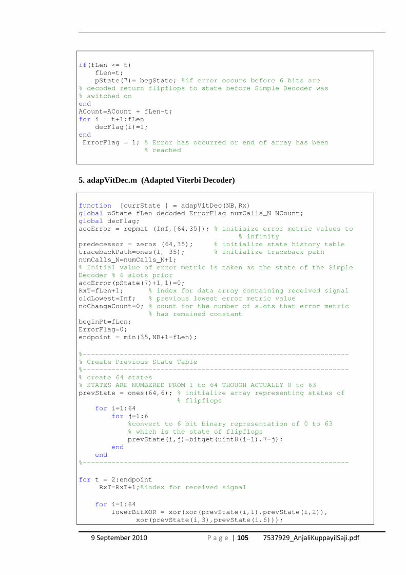
9 September 2010 P a g e | 105 7537929_AnjaliKuppayilSaji.pdf
if (fLen <= t) fLen=t; pState(7)= begState; %if error occurs before 6 bits are % decoded return flipflops to state before Simple D ecoder was % switched on end ACount=ACount + fLen-t; for i = t+1:fLen decFlag(i)=1; end ErrorFlag = 1; % Error has occurred or end of array has been % reached
5. adapVitDec.m (Adapted Viterbi Decoder)
function [currState ] = adapVitDec(NB,Rx) global pState fLen decoded ErrorFlag numCalls_N NCount; global decFlag; accError = repmat (Inf,[64,35]); % initiaize error metric values to % infinity predecessor = zeros (64,35); % initialize state history table tracebackPath=ones(1, 35); % initialize traceback path numCalls_N=numCalls_N+1; % Initial value of error metric is taken as the sta te of the Simple Decoder % 6 slots prior accError(pState(7)+1,1)=0; RxT=fLen+1; % index for data array containing received signal oldLowest=Inf; % previous lowest error metric value noChangeCount=0; % count for the number of slots that error metric % has remained constant beginPt=fLen; ErrorFlag=0; endpoint = min(35,NB+1-fLen); %-------------------------------------------------- --------------- % Create Previous State Table %-------------------------------------------------- --------------- % create 64 states % STATES ARE NUMBERED FROM 1 to 64 THOUGH ACTUALLY 0 to 63 prevState = ones(64,6); % initialize array representing states of % flipflops for i=1:64 for j=1:6 %convert to 6 bit binary representation of 0 to 63 % which is the state of flipflops prevState(i,j)=bitget(uint8(i-1),7-j); end end %-------------------------------------------------- --------------- for t = 2:endpoint RxT=RxT+1; %index for received signal for i=1:64 lowerBitXOR = xor(xor(prevState(i,1),prevSt ate(i,2)), xor(prevState(i,3),prevState(i,6)));

9 September 2010 P a g e | 106 7537929_AnjaliKuppayilSaji.pdf
lowerOutput_IP0 = xor(lowerBitXOR,0); % Lower output if input is 0 lowerOutput_IP1 = xor(lowerBitXOR,1); % Lower output if input is 1 upperBitXOR = xor(xor(prevState(i,2),prevSt ate(i,3)), xor(prevState(i,5),prevState(i,6))); upperOutput_IP0 = xor(upperBitXOR,0); % Upper output if input is 0 upperOutput_IP1 = xor(upperBitXOR,1); % Upper output if input is 1 %-------------------------------------------------- --------------- % BRANCH METRICS: Calculate Hamming Distances %-------------------------------------------------- --------------- HD_IP0= xor(lowerOutput_IP0,Rx(2*RxT-3))+ xor(upperOutput_IP0,Rx(2*RxT-2)); % add hamming distance of each bit if input is 0 HD_IP1= xor(lowerOutput_IP1,Rx(2*RxT-3))+ xor(upperOutput_IP1,Rx(2*RxT-2)); % add hamming distance of each bit if input is 1 %-------------------------------------------------- --------------- % Calculate next state %-------------------------------------------------- --------------- s=i-1; %i=1 implies state 0 and so on nextState_IP0 = bitshift(s,-1,6); % next state if input % is 0. divide i by 2 and round it off nextState_IP1 = nextState_IP0 + 32; % next state if input is 1. %-------------------------------------------------- --------------- % ADD, COMPARE, SELECT : Update Accumalated Error M etric Table and % Surviving State table %-------------------------------------------------- ---------------
if (accError(1+nextState_IP0,t)>(accError(i,t-1)+ HD_I P0)) if (accError(1+nextState_IP0,t)==Inf) predecessor(1+nextState_IP0,t)=0; %lower branch else predecessor(1+nextState_IP0,t)=1; % upper branch end accError(1+nextState_IP0,t)=(accError(i ,t-1)+ HD_IP0); elseif (accError(1+nextState_IP0,t)==(accError(i,t-1)+ HD_IP0)&&(predecessor(1+nextState_IP0,t)< i)) % consistently choose the higher state in cases of % equality predecessor(1+nextState_IP0,t)=1; end if (accError(1+nextState_IP1,t)>(accError(i,t-1)+ HD_I P1)) if (accError(1+nextState_IP1,t)==Inf) predecessor(1+nextState_IP1,t)=0; % lower branch else predecessor(1+nextState_IP1,t)=1; % upper branch end accError(1+nextState_IP1,t)=(accError(i ,t-1)+ HD_IP1);
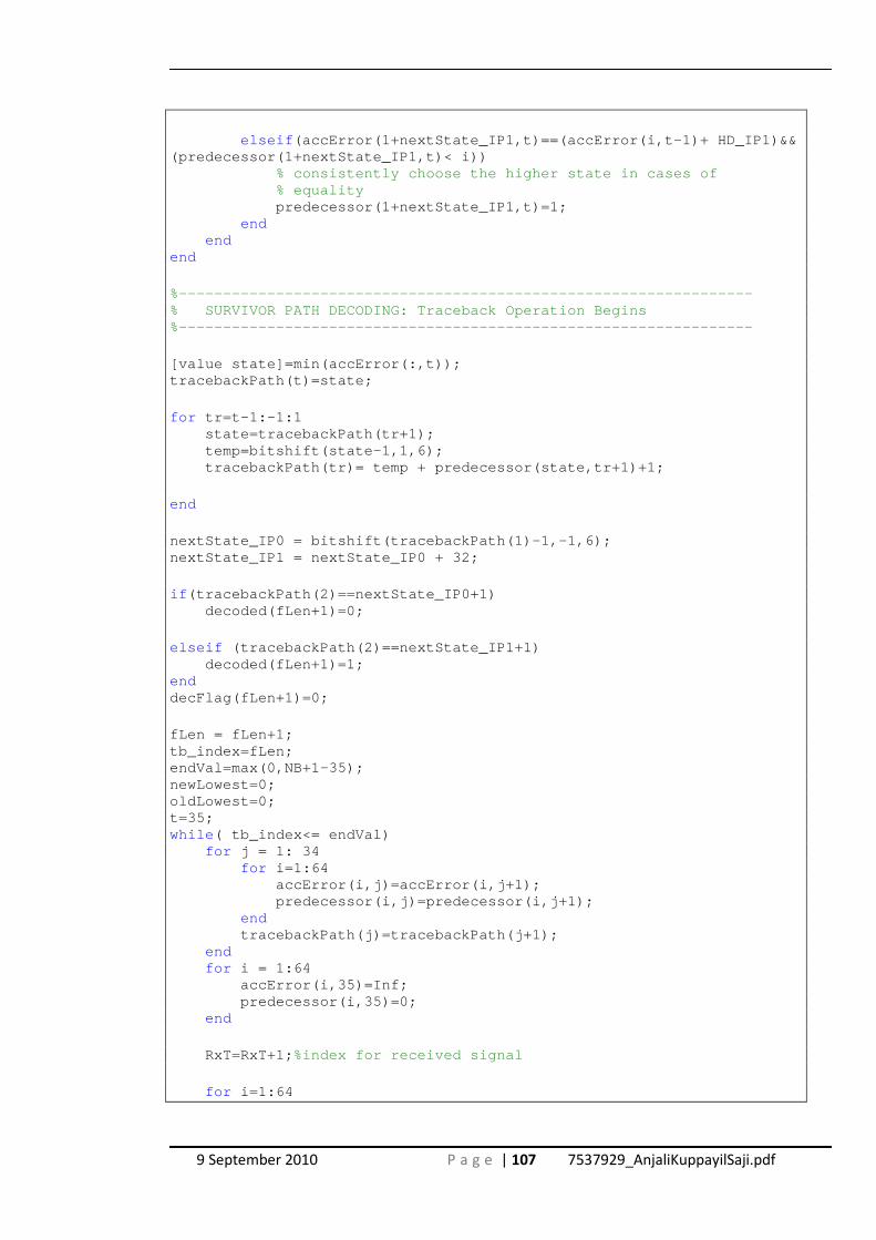
9 September 2010 P a g e | 107 7537929_AnjaliKuppayilSaji.pdf
elseif (accError(1+nextState_IP1,t)==(accError(i,t-1)+ HD_ IP1)&& (predecessor(1+nextState_IP1,t)< i)) % consistently choose the higher state in cases of % equality predecessor(1+nextState_IP1,t)=1; end end end %-------------------------------------------------- --------------- % SURVIVOR PATH DECODING: Traceback Operation Beg ins %-------------------------------------------------- --------------- [value state]=min(accError(:,t)); tracebackPath(t)=state; for tr=t-1:-1:1 state=tracebackPath(tr+1); temp=bitshift(state-1,1,6); tracebackPath(tr)= temp + predecessor(state,tr+ 1)+1; end nextState_IP0 = bitshift(tracebackPath(1)-1,-1,6); nextState_IP1 = nextState_IP0 + 32; if (tracebackPath(2)==nextState_IP0+1) decoded(fLen+1)=0; elseif (tracebackPath(2)==nextState_IP1+1) decoded(fLen+1)=1; end decFlag(fLen+1)=0; fLen = fLen+1; tb_index=fLen; endVal=max(0,NB+1-35); newLowest=0; oldLowest=0; t=35; while ( tb_index<= endVal) for j = 1: 34 for i=1:64 accError(i,j)=accError(i,j+1); predecessor(i,j)=predecessor(i,j+1); end tracebackPath(j)=tracebackPath(j+1); end for i = 1:64 accError(i,35)=Inf; predecessor(i,35)=0; end RxT=RxT+1; %index for received signal for i=1:64

9 September 2010 P a g e | 108 7537929_AnjaliKuppayilSaji.pdf
lowerBitXOR = xor(xor(prevState(i,1),prevSt ate(i,2)), xor(prevState(i,3),prevState(i,6))); lowerOutput_IP0 = xor(lowerBitXOR,0); % Lower output if % input is 0 lowerOutput_IP1 = xor(lowerBitXOR,1); % Lower output if %input is 1 upperBitXOR = xor(xor(prevState(i,2),prevSt ate(i,3)), xor(prevState(i,5),prevState(i,6))); upperOutput_IP0 = xor(upperBitXOR,0); % Upper output if % input is 0 upperOutput_IP1 = xor(upperBitXOR,1); % Upper output if % input is 1 %-------------------------------------------------- --------------- BRANCH METRICS : Calculate Hamming Distances %-------------------------------------------------- --------------- HD_IP0= xor(lowerOutput_IP0,Rx(2*RxT-3))+ xor(upperOutput_IP0,Rx(2*RxT-2)); % add hamming distance of each % bit if input is 0 HD_IP1= xor(lowerOutput_IP1,Rx(2*RxT-3))+ xor(upperOutput_IP1,Rx(2*RxT-2)); % add hamming distance of each % bit if input is 1 %-------------------------------------------------- --------------- % Calculate next state %-------------------------------------------------- --------------- s=i-1; %i=1 implies state 0 and so on nextState_IP0 = bitshift(s,-1,6); % next state if input % is 0. divide i by 2 and round it off nextState_IP1 = nextState_IP0 + 32; % next state if input % is 1. %-------------------------------------------------- --------------- % ADD, COMPARE, SELECT : Update Accumalated Error M etric Table and % Surviving State table %-------------------------------------------------- --------------- if (accError(1+nextState_IP0,t)>(accError(i,t-1)+ HD_I P0)) if (accError(1+nextState_IP0,t)==Inf) predecessor(1+nextState_IP0,t)=0; %lower branch else predecessor(1+nextState_IP0,t)= 1; % upper branch end accError(1+nextState_IP0,t)=(accError(i ,t-1)+ HD_IP0); elseif (accError(1+nextState_IP0,t)==(accError(i,t-1)+ HD_ IP0)) % consistently choose the higher state in cases of % equality predecessor(1+nextState_IP0,t)= 1; end if (accError(1+nextState_IP1,t)>(accError(i,t-1)+ HD_I P1)) if (accError(1+nextState_IP1,t)==Inf) predecessor(1+nextState_IP1,t)=0; % lower branch else predecessor(1+nextState_IP1,t)=1; % upper branch end
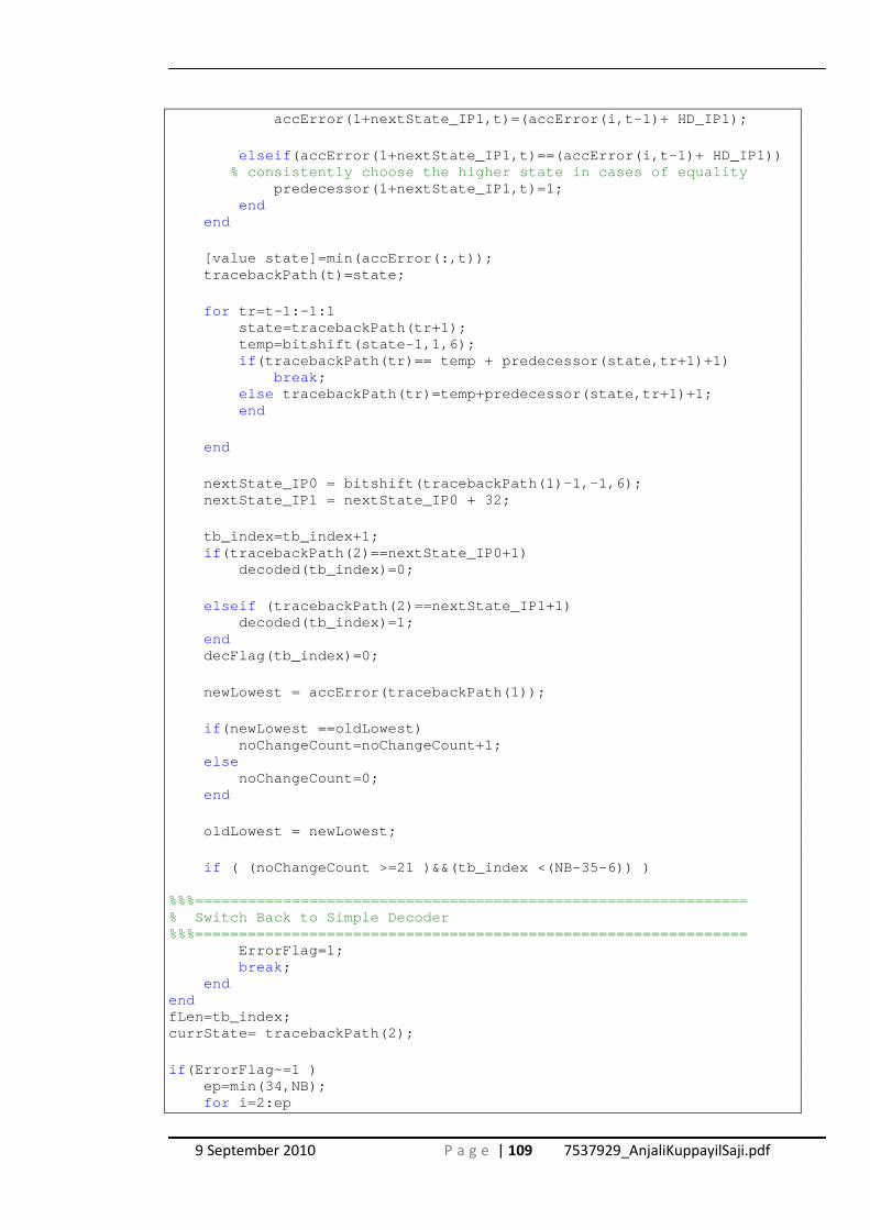
9 September 2010 P a g e | 109 7537929_AnjaliKuppayilSaji.pdf
accError(1+nextState_IP1,t)=(accError(i ,t-1)+ HD_IP1); elseif (accError(1+nextState_IP1,t)==(accError(i,t-1)+ HD_ IP1)) % consistently choose the higher state in cases of equality predecessor(1+nextState_IP1,t)=1; end end [value state]=min(accError(:,t)); tracebackPath(t)=state; for tr=t-1:-1:1 state=tracebackPath(tr+1); temp=bitshift(state-1,1,6); if (tracebackPath(tr)== temp + predecessor(state,tr+1) +1) break ; else tracebackPath(tr)=temp+predecessor(state,tr+1)+1; end end nextState_IP0 = bitshift(tracebackPath(1)-1,-1, 6); nextState_IP1 = nextState_IP0 + 32; tb_index=tb_index+1; if (tracebackPath(2)==nextState_IP0+1) decoded(tb_index)=0; elseif (tracebackPath(2)==nextState_IP1+1) decoded(tb_index)=1; end decFlag(tb_index)=0; newLowest = accError(tracebackPath(1)); if (newLowest ==oldLowest) noChangeCount=noChangeCount+1; else noChangeCount=0; end oldLowest = newLowest; if ( (noChangeCount >=21 )&&(tb_index <(NB-35-6)) ) %%%=============================================================== % Switch Back to Simple Decoder %%%=============================================================== ErrorFlag=1; break ; end end fLen=tb_index; currState= tracebackPath(2); if (ErrorFlag~=1 ) ep=min(34,NB); for i=2:ep

9 September 2010 P a g e | 110 7537929_AnjaliKuppayilSaji.pdf
nextState_IP0 = bitshift(tracebackPath(i)-1 ,-1,6); nextState_IP1 = nextState_IP0 + 32; tb_index=tb_index+1; if (tracebackPath(i+1)==nextState_IP0+1) decoded(tb_index)=0; elseif (tracebackPath(i+1)==nextState_IP1+1) decoded(tb_index)=1; end decFlag(tb_index)=0; end fLen=tb_index; currState=tracebackPath(i+1); end ErrorFlag=0; NCount=NCount+fLen-beginPt;
6. MAINFILE.m
clear all ; clc; global decoded pState fLen ErrorFlag ; global numCalls_A numCalls_N numCalls_C; global ACount NCount CCount; global decFlag NB =10000; % Number of orig bits for testing. Inp = randsrc(NB, 1, 0:1); ZInp=[Inp; 0; 0; 0; 0; 0; 0]; NB=NB+6; %Add 6 extra zeros to flush at end. %-------------------------------------------------- --------------- %Convolutional coder1/2 K= 7 (171,133) %-------------------------------------------------- --------------- Y = encoder(NB,ZInp); %-------------------------------------------------- --------------- % Coded signal Y. Modulate signal QPSK. Store tran smitted signal as msg_tx %-------------------------------------------------- --------------- M=4;k= log2(M);Nsamp=4; [msg_tx grayencod]=modulate(Y,M,Nsamp); [msg_tx_uncoded grayencod]=modulate(ZInp,M,Nsamp); %-------------------------------------------------- --------------- %Initialize matrices EbN0 = zeros(1,26); nErrs_A =zeros(1,26); nErrs_matHard = zeros(1,26); nErrs_Conv = zeros(1,5); nErrs_uncoded = zeros(1,26); nErrs_channel=zeros(1,26); BER_A=zeros(1,26);

9 September 2010 P a g e | 111 7537929_AnjaliKuppayilSaji.pdf
BER_matSoft = zeros(1,26); BER_matHard=zeros(1,26); BER_Conv = zeros(1,26); BER_uncoded=zeros(1,26); BER_channel=zeros(1,26); for runs = 1:26 ErrorFlag=0; % Set Error Flag to 0 decoded = repmat(-1,[NB,1]); % initialize decoded output array decFlag=repmat(-1,[NB,1]); % Flag to check which bits were % decoded by Simple Decoder pState = zeros(7,1); % intitalize last 7 states of the % decoder fLen=0; % initialize last index of % decoded output numCalls_A=0; numCalls_N=0; numCalls_C=0; ACount=0; NCount=0; CCount=0; EbN0(runs)= runs/2 ; EsN0 = EbN0(runs) + 10*log10(2); %-------------------------------------------------- --------------- % Modulated signal msg_tx. Introduce bit-errors. S ignal at Receiver is msg_rx %-------------------------------------------------- --------------- msg_rx = awgn(msg_tx, EsN0-10*log10(2)-10*log10 (Nsamp)); % AWGN % NOISE to Encoded Signal msg_rx_uncoded = awgn(msg_tx_uncoded,EsN0-10*lo g10(2)-10*log10(Nsamp)); %AWGN Noise to Uncoded Signal %---------------------------------------------- ---- % Introduce bit errors to certain parts of the message %---------------------------------------------- ---- % msg_rx=msg_tx; % no noise added % msg_tx_PART1 = msg_tx (1:NB); % msg_tx_PART2=msg_tx(NB+1:2*NB); % msg_tx_PART3 = msg_tx(2*NB+1:3*NB); % msg_tx_PART4=msg_tx(3*NB+1:4*NB); % % msg_rx_PART1=msg_tx_PART1; % msg_rx_PART2=awgn(msg_tx_PART2, EsN0-10*log10(2)-10*log10(Nsamp)); % msg_rx_PART3=awgn(msg_tx_PART3, EsN0-10*log10(2)-10*log10(Nsamp)); % msg_rx_PART4=msg_tx_PART4; % % msg_rx=cat(2,msg_rx_PART1,msg_rx_PART2,msg_rx_PART3 ,msg_rx_PART4); %-------------------------------------------------- --------------- % Demodulate signal received .Store in comp_Rx %-------------------------------------------------- --------------- comp_Rx = demodulate(msg_rx,M,Nsamp,grayencod);
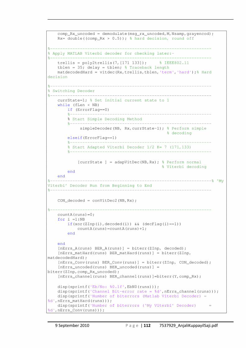
9 September 2010 P a g e | 112 7537929_AnjaliKuppayilSaji.pdf
comp_Rx_uncoded = demodulate(msg_rx_uncoded,M,N samp,grayencod); Rx= double((comp_Rx > 0.5)); % hard decision, round off %-------------------------------------------------- --------------- % Apply MATLAB Viterbi decoder for checking later:- %-------------------------------------------------- --------------- trellis = poly2trellis(7,[171 133]); % IEEE802.11 tblen = 35; delay = tblen; % Traceback length matdecodedHard = vitdec(Rx,trellis,tblen, 'term' , 'hard' ); % Hard decision %-------------------------------------------------- --------------- % Switching Decoder %-------------------------------------------------- --------------- currState=1; % Set initial current state to 1 while (fLen < NB) if (ErrorFlag==0) %-------------------------------------------------- ------- % Start Simple Decoding Method %-------------------------------------------------- ------- simpleDecoder(NB, Rx,currState-1); % Perform simple % decoding elseif (ErrorFlag==1) %-------------------------------------------------- ------- % Start Adapted Viterbi Decoder 1/2 K= 7 (171,133) %-------------------------------------------------- ------- [currState ] = adapVitDec(NB,Rx); % Perform normal % Viterbi decoding end end %-------------------------------------------------- ---------------% ‘My Viterbi’ Decoder Run from Beginning to End %-------------------------------------------------- --------------- CON_decoded = conVitDec2(NB,Rx); %-------------------------------------------------- --------------- countA(runs)=0; for i =1:NB if (xor(ZInp(i),decoded(i)) && (decFlag(i)==1)) countA(runs)=countA(runs)+1; end end [nErrs_A(runs) BER_A(runs)] = biterr(ZInp, deco ded); [nErrs_matHard(runs) BER_matHard(runs)] = biter r(ZInp, matdecodedHard); [nErrs_Conv(runs) BER_Conv(runs)] = biterr(ZInp , CON_decoded); [nErrs_uncoded(runs) BER_uncoded(runs)] = biterr(ZInp,comp_Rx_uncoded); [nErrs_channel(runs) BER_channel(runs)]=biterr( Y,comp_Rx); disp(sprintf( 'Eb/No: %0.1f' ,EbN0(runs))); disp(sprintf( 'Channel Bit-error rate = %d' ,nErrs_channel(runs))); disp(sprintf( 'Number of biterrors (Matlab Viterbi Decoder) = %d' ,nErrs_matHard(runs))); disp(sprintf( 'Number of biterrors (‘My Viterbi’ Decoder) = %d' ,nErrs_Conv(runs)));
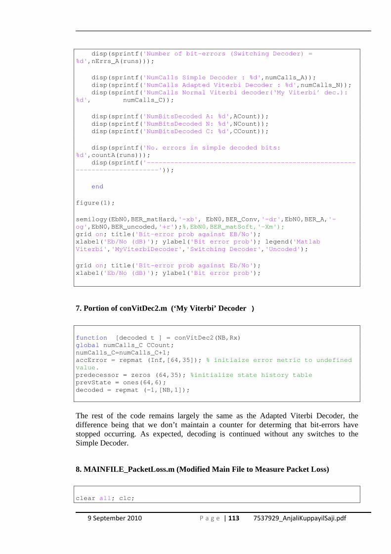
9 September 2010 P a g e | 113 7537929_AnjaliKuppayilSaji.pdf
disp(sprintf( 'Number of bit-errors (Switching Decoder) = %d' ,nErrs_A(runs))); disp(sprintf( 'NumCalls Simple Decoder : %d' ,numCalls_A)); disp(sprintf( 'NumCalls Adapted Viterbi Decoder : %d' ,numCalls_N)); disp(sprintf( 'NumCalls Normal Viterbi decoder(‘My Viterbi’ dec.) : %d' , numCalls_C)); disp(sprintf( 'NumBitsDecoded A: %d' ,ACount)); disp(sprintf( 'NumBitsDecoded N: %d' ,NCount)); disp(sprintf( 'NumBitsDecoded C: %d' ,CCount)); disp(sprintf( 'No. errors in simple decoded bits: %d' ,countA(runs))); disp(sprintf( '-------------------------------------------------- ------------------------' )); end figure(1); semilogy(EbN0,BER_matHard, '-xb' , EbN0,BER_Conv, '-dr' ,EbN0,BER_A, '-og' ,EbN0,BER_uncoded, '+r' ); %,EbN0,BER_matSoft,'-Xm'); grid on; title( 'Bit-error prob against EB/No' ); xlabel( 'Eb/No (dB)' ); ylabel( 'Bit error prob' ); legend( 'Matlab Viterbi' , 'MyViterbiDecoder' , 'Switching Decoder' , 'Uncoded' ); grid on; title( 'Bit-error prob against Eb/No' ); xlabel( 'Eb/No (dB)' ); ylabel( 'Bit error prob' );
7. Portion of conVitDec2.m (‘My Viterbi’ Decoder )
function [decoded t ] = conVitDec2(NB,Rx) global numCalls_C CCount; numCalls_C=numCalls_C+1; accError = repmat (Inf,[64,35]); % initiaize error metric to undefined value. predecessor = zeros (64,35); %initialize state history table prevState = ones(64,6); decoded = repmat (-1,[NB,1]);
The rest of the code remains largely the same as the Adapted Viterbi Decoder, the difference being that we don’t maintain a counter for determing that bit-errors have stopped occurring. As expected, decoding is continued without any switches to the Simple Decoder.
8. MAINFILE_PacketLoss.m (Modified Main File to Measure Packet Loss)
clear all ; clc;
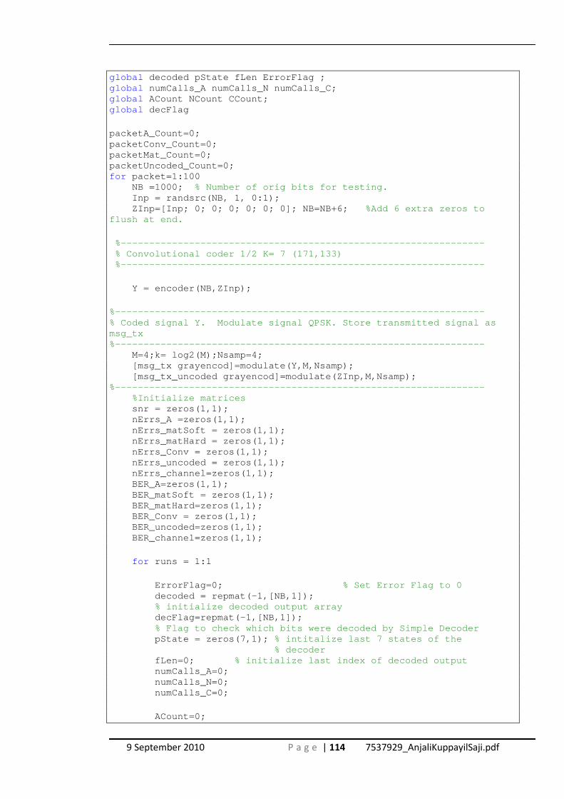
9 September 2010 P a g e | 114 7537929_AnjaliKuppayilSaji.pdf
global decoded pState fLen ErrorFlag ; global numCalls_A numCalls_N numCalls_C; global ACount NCount CCount; global decFlag packetA_Count=0; packetConv_Count=0; packetMat_Count=0; packetUncoded_Count=0; for packet=1:100 NB =1000; % Number of orig bits for testing. Inp = randsrc(NB, 1, 0:1); ZInp=[Inp; 0; 0; 0; 0; 0; 0]; NB=NB+6; %Add 6 extra zeros to flush at end. %-------------------------------------------------- -------------- % Convolutional coder 1/2 K= 7 (171,133) %-------------------------------------------------- -------------- Y = encoder(NB,ZInp); %-------------------------------------------------- --------------- % Coded signal Y. Modulate signal QPSK. Store tran smitted signal as msg_tx %-------------------------------------------------- --------------- M=4;k= log2(M);Nsamp=4; [msg_tx grayencod]=modulate(Y,M,Nsamp); [msg_tx_uncoded grayencod]=modulate(ZInp,M,Nsam p); %-------------------------------------------------- --------------- %Initialize matrices snr = zeros(1,1); nErrs_A =zeros(1,1); nErrs_matSoft = zeros(1,1); nErrs_matHard = zeros(1,1); nErrs_Conv = zeros(1,1); nErrs_uncoded = zeros(1,1); nErrs_channel=zeros(1,1); BER_A=zeros(1,1); BER_matSoft = zeros(1,1); BER_matHard=zeros(1,1); BER_Conv = zeros(1,1); BER_uncoded=zeros(1,1); BER_channel=zeros(1,1); for runs = 1:1 ErrorFlag=0; % Set Error Flag to 0 decoded = repmat(-1,[NB,1]); % initialize decoded output array decFlag=repmat(-1,[NB,1]); % Flag to check which bits were decoded by Simple D ecoder pState = zeros(7,1); % intitalize last 7 states of the % decoder fLen=0; % initialize last index of decoded output numCalls_A=0; numCalls_N=0; numCalls_C=0; ACount=0;
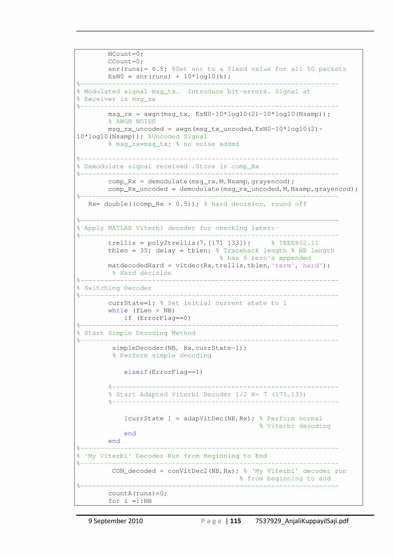
9 September 2010 P a g e | 115 7537929_AnjaliKuppayilSaji.pdf
NCount=0; CCount=0; snr(runs)= 6.5; %Set snr to a fixed value for all 50 packets EsN0 = snr(runs) + 10*log10(k); %-------------------------------------------------- --------------- % Modulated signal msg_tx. Introduce bit-errors. S ignal at % Receiver is msg_rx %-------------------------------------------------- --------------- msg_rx = awgn(msg_tx, EsN0-10*log10(2)-10*l og10(Nsamp)); % AWGN NOISE msg_rx_uncoded = awgn(msg_tx_uncoded,EsN0-1 0*log10(2)-10*log10(Nsamp)); %Uncoded Signal % msg_rx=msg_tx; % no noise added %-------------------------------------------------- --------------- % Demodulate signal received .Store in comp_Rx %-------------------------------------------------- --------------- comp_Rx = demodulate(msg_rx,M,Nsamp,grayenc od); comp_Rx_uncoded = demodulate(msg_rx_uncoded ,M,Nsamp,grayencod); %-------------------------------------------------- --------------- Rx= double((comp_Rx > 0.5)); % hard decision, round off %-------------------------------------------------- --------------- % Apply MATLAB Viterbi decoder for checking later:- %-------------------------------------------------- --------------- trellis = poly2trellis(7,[171 133]); % IEEE802.11 tblen = 35; delay = tblen; % Traceback length % NB length % has 6 zero's appended matdecodedHard = vitdec(Rx,trellis,tblen, 'term' , 'hard' ); % Hard decision %-------------------------------------------------- --------------- % Switching Decoder %-------------------------------------------------- --------------- currState=1; % Set initial current state to 1 while (fLen < NB) if (ErrorFlag==0) %-------------------------------------------------- --------------- % Start Simple Decoding Method %-------------------------------------------------- --------------- simpleDecoder(NB, Rx,currState-1); % Perform simple decoding elseif (ErrorFlag==1) %----------------------------------------------- ---------- % Start Adapted Viterbi Decoder 1/2 K= 7 (171,13 3) %-------------------------------------------------- ------- [currState ] = adapVitDec(NB,Rx); % Perform normal % Viterbi decoding end end %-------------------------------------------------- --------------- % ‘My Viterbi’ Decoder Run from Beginning to End %-------------------------------------------------- --------------- CON_decoded = conVitDec2(NB,Rx); % ‘My Viterbi’ decoder run % from beginning to end %-------------------------------------------------- --------------- countA(runs)=0; for i =1:NB

9 September 2010 P a g e | 116 7537929_AnjaliKuppayilSaji.pdf
if (xor(ZInp(i),decoded(i)) && (decFlag(i)==1)) countA(runs)=countA(runs)+1; end end [nErrs_A(runs) BER_A(runs)] = biterr(ZInp, decoded); [nErrs_matHard(runs) BER_matHard(runs)] = b iterr(ZInp, matdecodedHard); [nErrs_Conv(runs) BER_Conv(runs)] = biterr( ZInp, CON_decoded); [nErrs_uncoded(runs) BER_uncoded(runs)] = biterr(ZInp,comp_Rx_uncoded); [nErrs_channel(runs) BER_channel(runs)]=bit err(Y,comp_Rx); disp(sprintf( 'Channel Bit-error rate = %d' ,nErrs_channel(runs))); disp(sprintf( 'Number of biterrors (matHard-Decoded) = %d' ,nErrs_matHard(runs))); disp(sprintf( 'Number of biterrors (ConvBitDec2) = %d' ,nErrs_Conv(runs))); disp(sprintf( 'Number of bit-errors (Decoded With Switching) = %d' ,nErrs_A(runs))); if nErrs_A(runs) ==0 packetA_Count=packetA_Count+1; end if nErrs_matHard(runs) ==0 packetMat_Count=packetMat_Count+1; end if nErrs_Conv(runs) ==0 packetConv_Count=packetConv_Count+1; end if nErrs_uncoded(runs) ==0 packetUncoded_Count=packetUncoded_Count +1; end disp(sprintf( 'NumBitsDecoded A: %d' ,ACount)); disp(sprintf( 'NumBitsDecoded N: %d' ,NCount)); disp(sprintf( 'NumBitsDecoded C: %d' ,CCount)); disp(sprintf( 'No. errors in simple decoded bits: %d' ,countA(runs))); disp(sprintf( '--------------------------------------------------------------------------' )); %-------------------------------------------------- --------------- end end disp(sprintf( 'Successful Packets - Matlab Viterbi Decoder: %d' ,packetMat_Count)); disp(sprintf( 'Successful Packets - ‘My Viterbi’ Decoder: %d' ,packetConv_Count)); disp(sprintf( 'Successful Packets - Switching decoder %d' ,packetA_Count));