Embed Size (px)
Citation preview

AUTHOR'S PROOF JrnlID 11036 ArtID 656 Proof#1 - 15/10/2015
UNCORRECTEDPROOF
Mobile Netw ApplDOI 10.1007/s11036-015-0656-6
Energy Saving Scheme for Multicarrier HSPA+ UnderRealistic Traffic Fluctuation
1
2
Maliha U. Jada1 · Mario Garcıa-Lozano2 · Jyri Hamalainen13
© Springer Science+Business Media New York 20154
Abstract In the near future, an increase in cellular net-5
work density is expected to be one of the main enablers6
to boost the system capacity. This development will lead7
to an increase in the network energy consumption. In this8
context, we propose an energy efficient dynamic scheme9
for HSDPA+ (High Speed Downlink Packet Access-10
Advanced) systems aggregating several carriers and which11
adapts dynamically to the network traffic. The scheme eval-12
uates whether node-B deactivation is feasible without com-13
promising the user flow throughput. Furthermore, instead of14
progressive de-activation of carriers and/or node-B switch-15
off, we evaluate the approach where feasible combination16
of inter-site distance and number of carriers is searched to17
obtain best savings. This is done by also considering the18
effect of transition delays between network configuration19
changes. The solution exploits the fact that re-activation of20
carriers might permit turning off other BSs earlier at rela-21
tively higher load than existing policies. Remote electrical22
downtilt is also considered as a means to maximize the uti-23
lization of higher modulation and coding schemes in the24
extended cells. This approach promises significant energy25
� Mario Garcı[email protected]
Maliha U. [email protected]
Jyri [email protected]
1 Department of Communications and Networking, AaltoUniversity, Espoo, Finland
2 Department of Signal Theory and Communications,BarcelonaTech (UPC), Barcelona, Spain
savings when compared with existing policies - not only for 26
low traffic hours but also for medium load scenarios. 27
Keywords Multicarrier HSPA+ · Energy saving · Cell 28
switch off · Carrier management 29
1 Introduction 30
Due to the increase in demand for mobile broadband ser- 31
vices, mobile network vendors are preparing to challenging 32
mobile data traffic increases. Whereas the initial forecasts 33
indicated a 1000x traffic explosion between 2010 and 2020 34
[1], recent reports indicate predictions of a 57 % compound 35
annual growth rate (CAGR) from 2014 to 2019 [2]. This is 36
basically nothing new: According to [3] wireless capacity 37
has already increased more than 106× since 1957. Whereas 38
5× comes from improvements in modulation and coding 39
schemes (MCS), 1600× increase is due to the reduction in 40
cell sizes. It is widely accepted that the new capacity objec- 41
tive comes hand in hand with a further reduction in distances 42
between transmission points. Network densification allows 43
higher spatial reuse and so it allows higher area spectral 44
efficiency measured in [bits/s/Hz/km2]. On the other hand, 45
considering that base stations (BSs) contribute the most to 46
the energy consumption [4–6], future hyper-dense network 47
deployments may negatively impact on the operational costs 48
and carbon emissions. 49
It has become an important goal for industry and 50
academia to reduce the energy consumption of mobile net- 51
works over coming years. Important effort has already been 52
taken to address this issue. 3GPP launched several initiatives 53
for energy saving in the radio access part of LTE [7, 8]. Also 54
many research projects have put their focus on energy effi- 55
ciency of mobile broadband systems, outstanding examples 56

AUTHOR'S PROOF JrnlID 11036 ArtID 656 Proof#1 - 15/10/2015
UNCORRECTEDPROOF
Mobile Netw Appl
are TREND [9], EARTH [10] and C2POWER [11]. Energy57
efficiency is also one of the key challenges in the evolution58
towards beyond fourth generation (4G) mobile communica-59
tion systems. Yet, focusing in future systems is not enough60
since High Speed Packet Access (HSPA) and Long Term61
Evolution (LTE) will serve and coexist in the next decade,62
with probably a more tight integration in future releases of63
the standards [12]. In particular, HSPA is currently deployed64
in over 500 networks and it is expected to cover 90 % of the65
world’s population by 2019 [13]. So it will serve the major-66
ity of subscribers during this decade while LTE continues67
its expansion in parallel and gain constantly large share of68
users.69
Among the advantages in the latest releases of HSPA70
(HSPA+), multicarrier utilization is considered as an71
important performance booster [14] but it has not been72
extensively studied from the energy efficiency perspec-73
tive so far. Given this, the focus of our study is in74
the reduction of energy consumption through dynamic75
usage of multiple carriers combined with the BS (node-B)76
switch-off.77
Various BSs turn off strategies have been extensively78
studied as means for energy saving. Since cellular net-79
works are dimensioned to correctly serve the traffic at80
the busy hour, the idea behind these strategies is to man-81
age the activity of BSs in an energy-efficient manner82
while simultaneously being able to respond the traffic83
needs dynamically. Thus, the focus is on strategies where84
underutilized BSs are switched off during low traffic peri-85
ods [6, 15–18]. This cell switch-off technique was also86
utilized in [19] where the focus was on the WCDMA87
energy savings through cell breathing while in [4] the same88
approach was considered along with the impact of femto-89
cells on energy savings. The same technique was studied90
in [20] and the daily variation in traffic load was also91
modeled.92
In order to guarantee coverage, switch-off is usually93
combined with a certain power increase in the remaining94
cells, but still providing a net gain in the global energy sav-95
ing. However, this is not a straight-forward solution from a96
practical perspective: common control channels also require97
a power increase and electromagnetic exposure limits must98
be fulfilled [21]. Remote electrical downtilt lacks these99
problems. It positively impacts received powers and the100
coverage for common control channels could be expanded101
without increasing their power. A reduction of downtilt with102
respect to the horizontal can be used to increase the cover-103
age range. Levels of interference are also modified, so the104
final geometry of the cell will change. For a complete analy-105
sis on the impact of downtilt over UMTS based systems, the106
reader is referred to [22]. More recently, BS cooperation has107
also been proposed to cover the newly introduced coverage108
holes when switch-off is applied [23].109
Algorithms that minimize the energy consumption do 110
also have an impact on the system capacity. The work in 111
[24] studies these conflicting objectives and investigates 112
cell switching off as a multiobjective optimization problem. 113
This tradeoff should be carefully addressed, otherwise the 114
applicability of a particular mechanism would be question- 115
able. Yet, not many works consider the capacity issue in 116
detail and many of the contributions just introduce a mini- 117
mum signal-to-noise plus interference ratio (SINR) thresh- 118
old, which allows to compute a minimum throughput or 119
outage probability to be guaranteed. Consequently, capac- 120
ity does not remain constant before and after the switch 121
off. Indeed [25] strongly questions the applicability of cell 122
switch off combined with power increases as a feasible 123
solution for many scenarios. 124
Very few works evaluate energy saving gains obtained 125
by advantageous use of the multi-carrier option. The works 126
[26] and [27] respectively deal with HSPA and LTE when 127
two carriers are aggregated and evaluate whether the addi- 128
tional carrier can be de-activated when load decreases and 129
BSs are not powered off. LTE also offers a variety of chan- 130
nel bandwidth usage per carrier that ranges from 1.4 MHz 131
to 20 MHz. Thus, several works have leveraged this feature 132
to propose energy savings by using a dynamic adaptation of 133
the bandwidth per carrier [28]. 3GPP initiated Rel12 efforts 134
[29] to define a smaller bandwidth version of UMTS, so 135
similar energy saving techniques could also be a matter of 136
study in the context of HSPA. 137
The current work deals with the reduction of energy 138
consumption in HSPA+ by means of a strategy that com- 139
bines partial and complete node-B switch off with antenna 140
downtilt. Utilization of multiple carriers is evaluated as an 141
additional degree of freedom that allows more energy effi- 142
cient network layouts. The number of available carriers is 143
dynamically managed in combination with full BS turn off. 144
This last action provides the highest energy saving. For 145
this reason, instead of progressive de-activation of carriers 146
until the eventual node-B turn off, we evaluate the combina- 147
tion (inter-site distance, number of carriers) that gives best 148
energy saving. The solution exploits the fact that activa- 149
tion of previously shut-off carriers might permit turning off 150
the BSs earlier at relatively higher load than existing poli- 151
cies. The new scheme promises significant energy savings 152
when compared with existing policies, not only for low traf- 153
fic hours but also for medium load scenarios. The work also 154
provides an insight on the impact of transition times and 155
delays to apply network updates, considering realistic load 156
fluctuations. 157
The paper is organized in five sections. Section 2 dis- 158
cusses about the advantages and possibilities of multicarrier 159
HSPA+. Section 3 describes the system model. In Section 4 160
we discuss about the BS shut-off scheme and Section 5 161
is devoted to results and discussion. Section 5 shows the 162

AUTHOR'S PROOF JrnlID 11036 ArtID 656 Proof#1 - 15/10/2015
UNCORRECTEDPROOF
Mobile Netw Appl
Table 1 Evolution of multicarrier HSDPA
Release Name Aggregation type
R8 Dual cell HSDPA 2 adjacent downlink carriers
R9 Dual band HSDPA 2 carriers from 2 different bands
R10 4C-HSDPA Up to 4 carriers from one or 2 bands
R11 8C-HSDPA Up to 8 carriers from one or 2 bands
effect of switching ON-OFF time delay on system perfor-163
mance and energy savings. Section 6 is devoted to results164
and discussions. Conclusions are drawn in Section 7.165
2 Multicarrier HSPA+166
Latest releases of HSPA offer numerous upgrade options167
with features such as higher order modulation, multi-carrier168
operation and multiple input multiple output (MIMO). Evo-169
lution from initial releases is smooth since MCS update and170
multicarrier are unexpensive features [30]. These advan-171
tages have motivated 65 % of HSPA operators to deploy172
HSPA+, as recorded December 2013 [13].173
HSPA has evolved from a single carrier system to up to174
8-carrier aggregation (8C-HSDPA). So, multicarrier opera-175
tion can be supported in a variety of scenarios depending on176
the release, indicated in Table 1 for the downlink (HSDPA).177
Note that the uplink just allows dual cell since release 9.178
Multicarrier capability is an important advantage that affects179
the system performance [14, 31], in particular:180
– It scales the user throughput with the number of car-181
riers reaching a top theoretical speed of 672 Mbps on182
the downlink when combining 8C-HSDPA with 4 × 4183
MIMO.184
– It also improves spectrum utilization and the system185
capacity because of the load balancing between carriers.186
– Multicarrier operation improves the user throughput for187
a given load at any location in the cell, even at the188
cell edge, where channel conditions are not good. Note189
that other techniques such as high order modulation190
combined with high rate coding or the transmission of191
parallel streams with MIMO require high SINRs. Fur-192
thermore, it is well known that every order of MIMO193
just doubles the rate only for users with good channel194
strength and no line of sight, while on cell edge MIMO195
just provides diversity or beamforming gain.196
Regarding the availability of bandwidth, dual-carrier is197
currently mainstream solution. 8C-HSDPA is a likely option198
for scenarios in which bands from second generation (2G)199
systems are intensively refarmed or the use of unpaired200
bands as supplemental downlink is introduced [32]. On the201
other hand, scalable bandwidth for HSPA would also allow202
a more gradual refarming process and availability of new 203
bandwidth pieces for aggregation [29]. However, the most 204
interesting option would be a holistic management of the 205
operator’s spectrum blocks, with concurrent operation of 206
GSM, HSPA and LTE that would allow an efficient resource 207
sharing among technologies [33]. This multiaccess manage- 208
ment can consider both quality of service (QoS) and energy 209
efficiency as described herein. 210
3 System model 211
The BS shut-off scheme presents a well-defined solution 212
for a problem of underutilized network elements. However, 213
as previously stated, this action should be performed with- 214
out compromising the system performance. This section 215
presents the model to assess coverage and capacity dimen- 216
sioning. 217
3.1 Coverage model 218
Let us assume the downlink of an HSPA+ system. At the 219
link level, 30 modulation and coding schemes (MCS) are 220
adaptively assigned by the scheduler based on the channel 221
quality indicator (CQI) reported by user equipments (UEs). 222
Given the channel condition and the available power for the 223
high speed physical downlink shared channel (HS-PDSCH) 224
PHS-PDSCH, the scheduler selects the MCS that would guar- 225
antee a 10 % block error rate (BLER) for each user per 226
transmission time interval (TTI). 227
The CQI reported on the uplink can be approximated 228
using the SINR (γ in dB) at the UE for the required BLER 229
as [34]: 230
CQI =⎧⎨
⎩
0 if γ ≤ −16dB⌊ γ1.02 + 16.62
⌋if −16dB < γ < 14dB
30 if 14dB ≤ γ
(1)
Throughput of UE i depends on the number of allocated 231
carriers and the SINR (γi in linear units) at each carrier f , 232
given by: 233
γi =NcodePcode
Ls,i
(1 − α)Ptot−Pcode
Ls,i+ ∑
j �=s
(ρj
PtotLj,i
)+ PN
SF16, (2)
where: 234
– For the sake of clarity, index referring to carrier f has 235
been omitted. 236
– Lj,i is the net loss in the link budget between cell j and 237
UE i for carrier f . Note that index s refers to the serving 238
cell. 239
– Ptot is the carrier transmission power. Without loss 240
of generality, it is assumed equal in all cells of the 241
scenario. 242

AUTHOR'S PROOF JrnlID 11036 ArtID 656 Proof#1 - 15/10/2015
UNCORRECTEDPROOF
Mobile Netw Appl
– Intercell interference is scaled by neighbouring cell load243
ρ at f (carrier activity factor).244
– PN is the noise power.245
– Pcode is the power allocated per HS-PDSCH code. Note246
that all codes intended for a certain UE shall be trans-247
mitted with equal power [35]. So, considering an allo-248
cation of Ncode codes and a power PCCH for the control249
channels that are present in f , then Pcode = Ptot−PCCHNcode
.250
– SF16 is the HS-PDSCH (high-speed physical downlink251
shared channel) spreading factor of 16.252
– The orthogonality factor α models the percentage of253
interference from other codes in the same orthogo-254
nal variable spreading factor (OVSF) tree. Our model255
assumes classic Rake receivers, in case of advanced256
devices (Type 2 and Type 3/3i) [36], their ability to par-257
tially suppress self-interference and interference from258
other users would be modelled by properly scaling the259
interfering power [37].260
At the radio planning phase, a cell edge throughput is261
chosen and the link budget is adjusted so that the corre-262
sponding SINR (CQI) is guaranteed with a certain target263
probability pt. Given that both useful and interfering aver-264
age powers are log-normally distributed, the total interfer-265
ence is computed following the method in [38] for the266
summation of log-normal distributions. Coverage can be267
computed for any CQI and so, the boundary in which MCS268
k would be used with probability pt can be estimated. This269
allows finding the area Ak in which k is allocated with prob-270
ability ≥ pt . Figure 1 shows an example for a tri-sectorial271
layout with node-Bs regularly distributed using different272
inter-site distances (ISDs).273
It is important to note that the node-B does not change its274
total power with each downtilt update. The shape of the final275
CQI rings largely depends on the antenna pattern, interfer-276
ence from neighbouring cells and downtilt, whose optimum277
value depends on the ISD. The example considers a multi-278
band commercial antenna and downtilt angles are chosen279
following this criteria:280
1. The minimum MCS is guaranteed at the cell edge.281
2. After the previous constraint is met, the use of the282
highest MCS is maximized in the cell area.283
Under these assumptions, the optimum angles for ISDs284
750, 500 and 250 are 12.4◦, 12.9◦ and 18.5◦ respectively.285
Rings distribution will expand or reduce following the286
load in other cells. Figure 2 shows the pdf for CQIs 10 to 30287
for 2, 4 or 8 carriers and the same cell load, and so differ-288
ent load per carrier ρ(f ). This figure must be read jointly289
with Fig. 1 since the first has no numbers on the size of290
the different areas and the second does not represent how291
these values are geographically distributed Interference is292
spread among the different carriers and so the probability293
Fig. 1 Probabilistic CQI ring distribution in tri-sectorial regular lay-out. With ISD =250m (top right) ISD=500m (bottom left) ISD=750m(bottom right) at same cell load of 0.5 in each case and for theirrespective optimum downtilt angles
of allocating higher CQIs increases with the number of car- 294
riers. This has an impact on cell capacity and so, the next 295
subsection is devoted to describe its model. 296
3.2 Capacity model 297
The capacity model largely follows [39]. We define cell 298
capacity as the maximum traffic intensity that can be served 299
by the cell without becoming saturated. Note that the cell 300
load is evenly distributed among all carriers, so for the sake 301
of clarity and without loss of generality, we will proceed the 302
explanation assuming one single carrier and the index f will 303
be omitted. It is important to note that a round robin sched- 304
uler is assumed. Therefore scheduling time is fairly shared 305
among the users in the cell. Serving time depends on the cell 306
load and allocated MCS, and so the download time is dif- 307
ferent for each user, more refined scheduling options would 308
just shift absolute throughput values. 309
10 15 20 25 300
0.1
0.2
0.3
0.4
CQI
Prob
abili
ty D
ensi
ty F
unct
ion
(PD
F)
(a) ISD=250m
10 15 20 25 300
0.1
0.2
0.3
0.4
CQI
Prob
abili
ty D
ensi
ty F
unct
ion
(PD
F)
(b) ISD=750m
Fig. 2 CQI pdf for 2, 4 and 8 carriers and same cell load

AUTHOR'S PROOF JrnlID 11036 ArtID 656 Proof#1 - 15/10/2015
UNCORRECTEDPROOF
Mobile Netw Appl
3.2.1 Cell capacity310
Let’s assume the traffic to be uniformly distributed in the311
cell. Data flows arrive according to a Poisson process with312
rate λ per area unit. Flow sizes are independent and identi-313
cally distributed with average size E(σ ). So, the cell load or314
fraction of time in which the scheduler must be active is:315
ρ = λAcell ×30∑
k=1
E(σ )
ck
pk ≤ 1 , (3)
where Acell is the cell area, ck is the achievable date rate316
associated to MCS k, and pk is the probability of using MCS317
k, pk = Ak/Acell, being Ak the area in which MCS k is318
allocated. Note that Ak corresponds with the ring in which319
CQI k was reported by mobile users and so, it is just a frac-320
tion of the total Acell. Since the cell load is bounded to one,321
the maximum throughput that can be served (ρ = 1), or cell322
capacity is:323
C =(
30∑
k=1
pk
ck
)−1
. (4)
At any given load, the observed throughput (served)324
would be given by ρ × C.325
3.2.2 Flow throughput326
Actions to provide energy savings should not compromise327
the QoS and so the user flow throughput should not be328
altered. Hence, this has been used as performance metric.329
Since the scheduler is shared among the users in the cell,330
serving time depends on the cell load and allocated MCS,331
and so the download time is different for all users. The con-332
tribution to the cell load (fraction of time that should be333
allocated by the scheduler) from users at Ak is given by334
ρk = λAk × E(σ )
ck
. (5)
Hence, considering the definition of ρ in Eq. 3, it can335
be observed that it is immediate to also express it as ρ =336∑
k ρk . Given that all users in the cell share the same sched-337
uler, by using Little law’s the mean flow duration tk for a338
user in Ak can be computed tk = Nk/λAk where Nk is the339
average number of users in Ak . Then the flow throughput τk340
for users being served with MCS k is:341
τk = E(σ )
tk= λAk × E(σ )
Nk
, (6)
Considering the underlaying Markov process [39], it can342
be found the stationary distribution of the number of active343
users in each Ak and its average value, Nk = ρk
1−ρ, which344
yields:345
τk = ck(1 − ρ) , (7)
and the average flow throughput at cell level: 346
τ =30∑
k=1
pkck(1 − ρ) , (8)
where ρ captures the own cell load and pk is affected by 347
the load in neighbouring cells, which modifies SINR values, 348
CQI rings and so Ak values ∀k. 349
4 Node-B shut off scheme and energy model 350
The network configuration is characterized by the duplet 351
(ISD, Ncar). The transition between two pairs of values, 352
i.e. the transition of a network configuration (in terms of 353
ISD and active number of carriers) takes place at certain 354
load thresholds in which the network can be reconfigured 355
to achieve a more energy efficient layout without compro- 356
mising the required average flow throughput. For any load 357
z the best network configuration is the one which satisfies 358
two conditions: 359
1. The load z is such that with the new configuration the 360
average flow throughput τ is maintained: τnew(z) ≥ 361
τinitial(z). 362
2. The new configuration at load z allows a lower energy 363
consumed per unit area E/A (kWh/km2) than the old 364
configuration: E/Anew(z) ≤ E/Aold(z). 365
Thus that value of load becomes the threshold level at which 366
the network transition should take place. It is important to 367
note that the mechanism not only reduces active sites or 368
carriers progressively. The main contribution is to combine 369
these two mechanisms. For example, at some point it is more 370
beneficial a combination of de-activation of sites + activa- 371
tion of carriers. This is because the power saving due to a 372
complete switch off is dominant over the activation of a cer- 373
tain number of carriers. So, that action would be triggered 374
if the load is low enough to increase the ISD but extra radio 375
resources are yet needed to accommodate the new (higher) 376
cell load. This provides more granularity in the set of possi- 377
ble optimization actions and so higher energy saving gains 378
can be obtained. The set of all possible actions are indi- 379
cated in the two first columns of Table 2, where the arrow 380
indicates the initial and end of the transition. For example, 381
ON → OFF in the first column means a transition in which 382
base stations are deactivated. The rest of the columns will 383
be explained during Section 5. 384
Any BS shut off is followed by an update of downtilt 385
angles in remaining cells to guarantee coverage for cell edge 386
users and to maximize the use of the highest possible MCS 387
under the new conditions. Downtilt angle is reduced (with 388
respect to the horizontal) with the increasing ISD. Note that 389

AUTHOR'S PROOF JrnlID 11036 ArtID 656 Proof#1 - 15/10/2015
UNCORRECTEDPROOF
Mobile Netw Appl
Table 2 Network configuration state that is chosen in the energymodel for all possible network transition combinations
t2.1t2.2
t2.3Base stations Frequency carriers NSTATEs NSTATE
car Tdelay
t2.4No-Change No-Change
NNews NNew
car
null
t2.5OFF → ON No-Change long
t2.6No-Change OFF → ON short
t2.7OFF → ON OFF → ON long
t2.8OFF → ON ON → OFFNNew
s NPrevcar
long
t2.9No-Change ON → OFF short
t2.10ON → OFF OFF → ONNPrev
s NNewcar
long
t2.11ON → OFF No-Change long
t2.12ON → OFF ON → OFF NPrevs NPrev
car long
transmission power remains unchanged no matter the new390
ISD.391
Note that whenever sites are switched off, a readjustment392
of the complete grid of ISD is performed. Thus the method393
is applied over a set of base stations in a particular area394
of the network. Common load variations along the day are395
followed for that particular area. Thus, very short term fluc-396
tuations that individually happen at the sector level are not397
an objective of this method.398
After performing node-B shut off, the higher load of the399
new expanded cells is again evenly distributed over the total400
frequency resources. This high load includes the user traffic401
of the switched off node-Bs, which has to be accommodated402
by the remaining active ones. Considering υ as the ratio403
ISDnew/ISDinitial and that the cell area Acell is proportional404
to the cell square radius, from Eq. 3, the relation between405
the cell load with new ISD ρnew and with initial ISD ρinitial406
is given by,407
ρnew = υ2 × ρinitial . (9)
Although the use of more carriers will account for a408
certain increase in energy consumption, the saving for409
switching off some BSs is much higher.410
The metric used for the analysis of energy consumption411
is energy consumed per unit area (E/A). Assuming an entire412
parallel system at the node-B to handle each carrier, the413
energy consumed per unit area (kWh/km2) is given as [4,414
19, 26, 40]:415
E/A = Ns · Nsec · Ncar · [Poper + (ρ(f, Ns, Ncar) · Pin)
] · T
Atot,
(10)
where:416
– Ns, Nsec, Ncar are the number of sites, sectors (or cell)417
per site and carriers per sector (or cell) respectively.418
– Poper is the operational power, which is the load inde- 419
pendent power to operate the node-B and includes 420
baseband processing. 421
– ρ(f, Ns, Ncar) is the cell load that varies from 0.1 (rel- 422
evant to the minimum transmit pilot power) to 1.0 423
referring to the cell at full load. Note the dependence 424
among variables, any change in Ns and/or Ncar implies 425
the corresponding update in ρ. 426
– Pin is the power consumed to eventually obtain the 427
required power at the antenna connector (PTx). It scales 428
linearly with the load ρ but it is not PTx. Pin is based on 429
the rated power of the power amplifier (PA); such that 430
Pin = PTx/PAEff, where PAEff is the power amplifier 431
efficiency, which we adapt from [40] as 35 %. 432
– T is the time duration in which the particular load 433
remains in the piece of network under study. 434
– Atot is the total evaluated area containing Ns sites. 435
For the case of UMTS, power consumption of cur- 436
rently deployed base stations is mainly dominated by the 437
operational (static) part, the amount of dynamic power is 438
negligible, around 3 % [41]. In our specific calculations 439
we adapt from [19] the UMTS macro base station specific 440
values Poper = 157W, Pin = 57W in this last case, con- 441
veniently weighted by the current load. This means a less 442
unbalanced relationship Poper/Pin with respect to currently 443
widespread technology. It is important to note that this rela- 444
tionship will directly affect the achievable power savings, 445
more details are provided in the results section. 446
5 Impact of switching on-off time-delay on QoS 447
and energy savings 448
The transition in the network configuration, understood as 449
the number of active BSs and frequency carriers, does not 450
occur instantly. There is always some time delay involved 451
in switching ON-OFF the BSs and carriers. During these 452
time periods, when the network is considered to be in 453
a transitional state, the users might have to experience a 454
non-optimal QoS and, on the operational side, the service 455
provider might have to bear some extra energy expenses [42, 456
43]. These switching ON-OFF time periods could be of few 457
seconds to few minutes depending upon the hardware and 458
system capabilities [44]. 459
Considering the importance of this issue, usually missed 460
in the existent literature, this work will also quantify the 461
influence of such time-delays on the QoS and energy con- 462
sumption of the network. 463
Whenever the load levels justify a certain BS or car- 464
rier being from OFF to ON state, the throughput during 465
the transition is given by the previous network configura- 466
tion and the new load. This is because the new resources 467

AUTHOR'S PROOF JrnlID 11036 ArtID 656 Proof#1 - 15/10/2015
UNCORRECTEDPROOF
Mobile Netw Appl
are not fully utilizable until the end of their activation. This468
means that in some cases the network configuration will469
operate under non-optimal conditions with the correspond-470
ing throughput loss. On the other hand, if changes are very471
much anticipated, the system would be implementing less472
energy efficient configurations. In a similar manner, when473
deactivations are required, the BS or frequency resources474
become unavailable instantly after triggering the OFF deci-475
sion but energy savings do not occur until the equipment is476
fully switched off and so until the end of the transition.477
Given this, the energy consumption model requires to478
be updated. In particular, the energy per unit area for the479
transitional time period is given as:480
(E/A)trans = 1
Atot· Nsec · NSTATE
s · NSTATEcar · (11)
·[Poper +
(ρ
(f, NSTATE
s , NSTATEcar
)· Pin
)]· Tdelay,
where, NSTATEs and NSTATE
car are the number of active sites481
and carriers per sector for a particular configuration state482
which is decided based on the action taken: turn ON or OFF483
of BS sites and/or carriers. Thus, if there is no change or484
new base stations are switched on, NSTATEs equals the new485
number of active sites, since operational power consump-486
tion increases since the very first moment of activation, no487
matter the time it takes for the node-B to be completely488
operative to start serving users. Transition time would be489
shorter when there is no node-B (de-)activation, since swith-490
ing on and off a transceiver is far faster and simpler than a491
complete station. Table 2 summarizes the network configu-492
ration state (current or previous) that is chosen in the model493
for all possible network transition combinations (switching494
ON-OFF BSs & carriers) and where NNew/Prevx indicates if495
the new or previous number of resources ‘x’ appear in the496
transition energy model.497
Regarding, the power provided at the antenna connec-498
tor Pin, it must be noted that the load value ρ is also499
updated conveniently. For example, if an activation occurs,500
the load cannot be shared among the new increased num-501
ber of elements (sites and or carriers) until the end of the502
transition time. On the other hand, if de-activation occurs,503
the resources are not available any more from the very504
beginning, no matter how long it takes to de-activate the505
element.506
Given this, it is straight forward that the total energy con-507
sumed for the current load including the transition period is508
given as,509
(E/A)′ = (E/A) · T − Tdelay
T+ (E/A)trans . (12)
Table 3 Evaluated scenarios t3.1
t3.2Scenario 1 Scenario 2 Scenario 3
t3.3Targeted τ 5.76 Mbps 21.80 Mbps 60.53 Mbps
6 Results 510
In order to quantify the gains that can be achieved by an 511
intelligent joint management of carriers and node-Bs, the 512
system performance is evaluated in terms of average flow 513
throughput (τ ). Three cases have been evaluated: 2, 4 and 514
8 carriers are initially used to serve an aggregated cell load 515
of 1. This load is evenly distributed among the carriers, 516
ρ = 0.5, 0.25, and 0.125. Given this, three scenarios are 517
defined considering the τ value to be respected (Table 3). 518
Note that as the load is distributed among more carriers, the 519
average cell flow throughput increases due to a reduction in 520
the utilization of low MCSs and of course to the availability 521
of more radio resources. 522
The reference network has node-Bs regularly deployed 523
and considering an ISD=250 m. Therefore after a first shut 524
off, the new ISD would be 500 m, and a second implies 525
ISD=750 m. Other network parameters are provided in 526
Table 4. 527
Figure 3 represents the power consumption per unit area 528
for decreasing cell load values and showing the transition 529
points that should be used to guarantee the target user flow 530
throughput after the network update. In each subplot four 531
cases are represented: 532
Table 4 Network parameters
Parameter Value
Operating bands 2100 MHz, 900 MHz
Carrier bandwidth 5 MHz
Inter-Site distances 250 m, 500 m, 750 m
Number of sites, for each ISD 108, 27, 12
BS transmission power/sector/carrier 20 W
Transmission power per user 17 W
Control overhead 15 %
BS antenna gain 18 dB
Body loss 2 dB
Cable and connection loss 4 dB
Noise power −100.13 dBm
Propagation model Okumura-Hata
Shadow fading std. deviation 8 dB
Cell edge coverage probability 0.99
Tdelay = long 2 minutes
Tdelay = short 1 minute
AUTHOR'S PROOF JrnlID 11036 ArtID 656 Proof#1 - 15/10/2015
UNCORRECTEDPROOF
Mobile Netw Appl
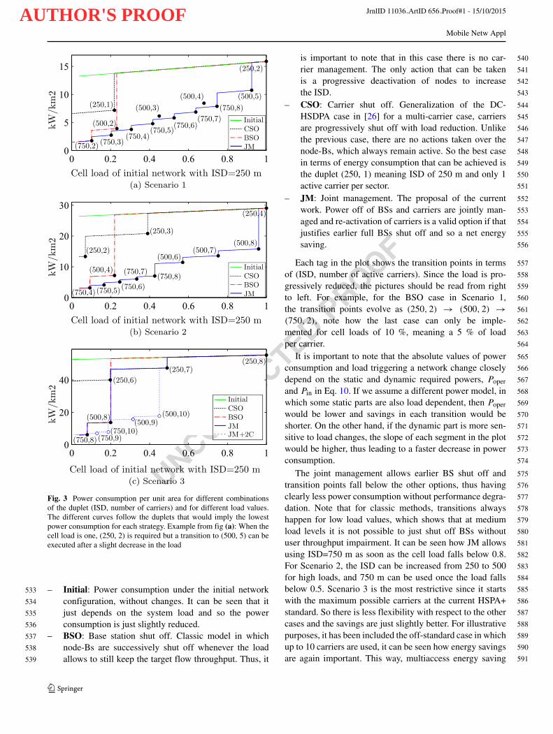
Fig. 3 Power consumption per unit area for different combinationsof the duplet (ISD, number of carriers) and for different load values.The different curves follow the duplets that would imply the lowestpower consumption for each strategy. Example from fig (a): When thecell load is one, (250, 2) is required but a transition to (500, 5) can beexecuted after a slight decrease in the load
– Initial: Power consumption under the initial network533
configuration, without changes. It can be seen that it534
just depends on the system load and so the power535
consumption is just slightly reduced.536
– BSO: Base station shut off. Classic model in which537
node-Bs are successively shut off whenever the load538
allows to still keep the target flow throughput. Thus, it539
is important to note that in this case there is no car- 540
rier management. The only action that can be taken 541
is a progressive deactivation of nodes to increase 542
the ISD. 543
– CSO: Carrier shut off. Generalization of the DC- 544
HSDPA case in [26] for a multi-carrier case, carriers 545
are progressively shut off with load reduction. Unlike 546
the previous case, there are no actions taken over the 547
node-Bs, which always remain active. So the best case 548
in terms of energy consumption that can be achieved is 549
the duplet (250, 1) meaning ISD of 250 m and only 1 550
active carrier per sector. 551
– JM: Joint management. The proposal of the current 552
work. Power off of BSs and carriers are jointly man- 553
aged and re-activation of carriers is a valid option if that 554
justifies earlier full BSs shut off and so a net energy 555
saving. 556
Each tag in the plot shows the transition points in terms 557
of (ISD, number of active carriers). Since the load is pro- 558
gressively reduced, the pictures should be read from right 559
to left. For example, for the BSO case in Scenario 1, 560
the transition points evolve as (250, 2) → (500, 2) → 561
(750, 2), note how the last case can only be imple- 562
mented for cell loads of 10 %, meaning a 5 % of load 563
per carrier. 564
It is important to note that the absolute values of power 565
consumption and load triggering a network change closely 566
depend on the static and dynamic required powers, Poper 567
and Pin in Eq. 10. If we assume a different power model, in 568
which some static parts are also load dependent, then Poper 569
would be lower and savings in each transition would be 570
shorter. On the other hand, if the dynamic part is more sen- 571
sitive to load changes, the slope of each segment in the plot 572
would be higher, thus leading to a faster decrease in power 573
consumption. 574
The joint management allows earlier BS shut off and 575
transition points fall below the other options, thus having 576
clearly less power consumption without performance degra- 577
dation. Note that for classic methods, transitions always 578
happen for low load values, which shows that at medium 579
load levels it is not possible to just shut off BSs without 580
user throughput impairment. It can be seen how JM allows 581
using ISD=750 m as soon as the cell load falls below 0.8. 582
For Scenario 2, the ISD can be increased from 250 to 500 583
for high loads, and 750 m can be used once the load falls 584
below 0.5. Scenario 3 is the most restrictive since it starts 585
with the maximum possible carriers at the current HSPA+ 586
standard. So there is less flexibility with respect to the other 587
cases and the savings are just slightly better. For illustrative 588
purposes, it has been included the off-standard case in which 589
up to 10 carriers are used, it can be seen how energy savings 590
are again important. This way, multiaccess energy saving 591

AUTHOR'S PROOF JrnlID 11036 ArtID 656 Proof#1 - 15/10/2015
UNCORRECTEDPROOF
Mobile Netw Appl
0.2 0.3 0.5 1 2 3 4 5 60
5
10
15
Fig. 4 Transition of cell configuration from initial network setup (sce-nario 1) to new setups at specific load values and maintaining the QoSrequirements (5.75 Mbps)
mechanisms that manage the pool of resources among sev-592
eral systems would make the most of each system load593
variations.594
It is important to note that the horizontal axis repre-595
sents the equivalent cell load that would be obtained if the596
network remained unchanged. But obviously, after carrier597
and/or node-B switch off, the cell load changes. For exam-598
ple, initially the load is 1 (0.5 per carrier) and it is not until599
it is reduced to 0.92 that important energy savings are possi-600
ble, so we transition from (250, 2)@0.92 to (500, 5)@3.7.601
Please note that the value after @ represents the cell load602
when varying the number of carriers and the ISD distance.603
Recall that since the load per carrier is bounded to 1, the604
final aggregated cell load value can be > 1. Besides, it is605
clear that the cell load increases due to its expansion and606
the new users to be served, but the QoS is respected, since607
both (250, 2)@1 and (500, 5)@3.7 provide the same flow608
throughput.609
In order to illustrate how load evolves with every change,610
Fig. 4 represents the average flow throughput as a function611
of the aggregated cell load for each configuration pro-612
posed by JM (solid symbols). Note the logarithmic scale613
in the horizontal axis to improve readability. Their evolu-614
tion (Fig. 3a) is as follows: (250, 2)@1 → (500, 5)@3.7615
→ (750, 8)@6.72 and so on. If no energy savings mecha-616
nisms are implemented, in other words, if we remain with617
the dense node-B deployment, an excess in capacity would618
be obtained due to load decrement. These situations are619
represented by empty symbols.620
Given the previous results, in the following we consider621
a realistic profile of daily HSDPA traffic (load) [26] (Fig. 5)622
and evaluate energy consumption and corresponding sav-623
ings along time.624
Figure 6 represents results for scenarios 1 and 2. In case625
of Scenario 1, the total energy saving percentage is 45.4 %626
with JM, whereas it is just 2.8 % with BSO and 1.8% with627
Fig. 5 Traffic load fluctuations
CSO. For Scenario 2, gains increase up to 55.8 % for JM, 628
and 2.9 %, 5.9 % for BSO and CSO respectively. Scenario 629
3 had an equal saving of just 3.5 % in CSO and JM, with 630
no possible gain with BSO. As previously mentioned this 631
is because scenario 3 is very restrictive and requires a flow 632
throughput of 60.53 Mbps. In the hypothetical off-standard 633
case with up to 10 available carriers, energy savings with JM 634
would reach 19.9 %. From Fig. 6 it is also noticeable how 635
small reductions in the load can lead to important savings 636
as it happens with cell load values around 60 %. So we can 637
conclude that even at mid-high values, interesting savings 638
are possible when applying the JM approach. 639
Given the Tdelay that takes to switch on/off a node-B com- 640
pletely, it is clear that these type of strategies cannot follow 641
the short term fluctuations in the load demands. Besides, 642
as it was previously explained, this delay will also imply 643
a non-optimal operation of the network during transition 644
0 10 200
5
10
15
20
0 10 200
50
100
(a) Scenario 1
0 10 200
10
20
30
40
0 10 200
50
100
(b) Scenario 2
Fig. 6 Comparison between energy savings (%) of BSO, CSO and JM

AUTHOR'S PROOF JrnlID 11036 ArtID 656 Proof#1 - 15/10/2015
UNCORRECTEDPROOF
Mobile Netw Appl
(a) Scenario 1
(b) Scenario 2
Fig. 7 Percentage increase in energy consumption
times, in some cases in terms of QoS, in others in terms of645
energy efficiency. The last set of results aim at quantifying646
the energy and throughput variations due to the fast load647
fluctuations.648
Figure 7 indicates the percentage increase in the energy649
consumption at some of the transitions, for each scheme650
(BSO, CSO, JM) for the first two scenarios. We note that for651
scenario 1 with JM scheme the percentage increase in over-652
all energy consumption is 1.2 % in comparison to the case653
when delay was not considered. Similarly for BSO and CSO654
the percentage increase in energy consumption is 0.4 % and655
0.25 % respectively. For scenario 2 with JM, BSO and CSO656
schemes the percentage increase in energy consumption is657
1 %, 0.4 % and 0.1 % respectively and they are negligi-658
ble for scenario 3 due to the low number of transitions.659
The proposed scheme performs more changes, adapts in a660
finer manner to load changes. But as it is shown, after con-661
sidering the effect of delay transitions and short term load662
fluctuations, the gains are slightly reduced. Nevertheless,663
the impact is far lower than the resulting gains.664
To end this section, Fig. 8 shows the degradation in665
flow throughput values during the transition time. Again,666
although this is not a very significant time period, from the667
user perspective the degradation in QoS for such small time668
periods cannot be ignored. The results are plotted for the669
new proposal JM since it is the case with more transitions670
and so, the strategy that is more affected. In particular, the671
plot compares the throughput evolution without considering672
(a) Scenario 1
(b) Scenario 2
Fig. 8 Flow throughput evolution
time delays (ideal) and including them. It can be observed, 673
how sub-optimum operation leads to important but brief 674
reductions, in some cases reaching zero. This case indicates 675
those situations in which the load would be higher than one, 676
meaning that more than the available frequency resources 677
are needed to have an stable system and be able to serve 678
the offered load. The cases BSO and CSO are less affected 679
since they also imply less network changes. Nevertheless, 680
the energy saving is still much better in JM than existent 681
proposals, as previously discussed. 682
7 Conclusions 683
In this paper we investigated the potential energy savings 684
by shutting off the BSs through the dynamic use of multi- 685
ple carriers in HSDPA. We have proposed an energy saving 686
scheme in which fewer or additional carriers have been 687
used depending upon the network traffic variations. This is 688
combined with remote electrical downtilts to partially cope 689
with the use of a higher number of lower MCSs. Instead of 690
just guaranteeing a power threshold at the cell edge, or an 691
outage probability threshold for data traffic, it is more inter- 692
esting to ensure that QoS remains unchanged whenever a 693
node-B and/or carrier is shut-off, for this reason the study 694
considers user flow throughput as the performance metric 695

AUTHOR'S PROOF JrnlID 11036 ArtID 656 Proof#1 - 15/10/2015
UNCORRECTEDPROOF
Mobile Netw Appl
to be respected, which is closely affected by load varia-696
tions due to cell expansions. Comparison to schemes that697
progressively shut off network elements (BSO and CSO)698
has been done, showing clear energy savings with the JM699
approach. The study includes the effects of transition times700
and delays required to switch between network configura-701
tions. Since JM is a strategy with more frequent updates, the702
negative effects of such delays in terms of QoS and energy703
savings are more present but still far from counteracting704
the gains.705
The main challenge to make the adaptation efficient and706
flexible is that load fluctuations should be correctly fol-707
lowed. Reiterative traffic patterns can be assessed along708
time but abnormal temporal or spatial variations could be709
included in the system by means of a pattern recognition710
system, e.g. a fuzzy logic based system or a neural network.711
Further efforts are required in this direction.712
Acknowledgments This work was supported in part by Academy713of Finland under grant 284634. The work by Mario Garcıa-Lozano714is funded by the Spanish National Science Council through project715TEC2014-60258-C2-2-R.716
References717
1. NSN (2011) 2020: The ubiquitous heterogeneous network -718Beyond 4G, tech. rep., ITU Kaleidoscope, NSN719
2. CISCO VNI forecast (2015) Technical Report, CISCO7203. Chandrasekhar V, Andrews J, Gatherer A (2008) Femtocell net-721
works: a survey. IEEE Comm Mag 46:59–677224. Jada M, Hossain M, Hamalainen J, Jantti R (2010) Impact of fem-723
tocells to the WCDMA network energy efficiency. In: 3rd IEEE724Broadband Network and Multimedia Technology. IC-BNMT, Bei-725jing (China)726
5. Jada M, Hossain M, Hamalainen J, Jantti R (2010) Power effi-727ciency model for mobile access network. In: 21st IEEE Personal,728Indoor and Mobile Radio Communications Workshops. PIMRC729Workshops, Istanbul (Turkey)730
6. Marsan M, Chiaraviglio L, Ciullo D, Meo M (2009) Optimal731energy savings in cellular access networks. In: IEEE Int. Conf. on732Comm. Workshops. ICC Workshops, Dresden (Germany)733
7. 3GPP (2014) TR 36.927 (Release 12) - Evolved Universal Ter-734restrial Radio Access (E-UTRA); Potential Solutions for Energy735Saving for E-UTRAN, Technical Report, 3GPP736
8. 3GPP (2014) TR 36.887 (Release 12) - Study on Energy Saving737Enhancement for E-UTRAN, Technical Report, 3GPP738
9. FP7 EU project TREND, Towards Real Energy-efficient Network739Design. http://www.fp7-trend.eu/. Accessed: 2015-07-01740
10. FP7 EU project EARTH, Energy Aware Radio and Network741Technologies. https://www.ict-earth.eu/. Accessed: 2015-07-01742
11. FP7 EU project C2POWER, Cognitive Radio and Cooperative743Strategies for Power Saving in Multi-standard Wireless Devices.744http://www.ict-c2power.eu/. Accessed: 2015-07-01745
12. Yang R, Chang Y, Xu W, Yang D (2013) Hybrid multi-radio trans-746mission diversity scheme to improve wireless TCP Performance747in an Integrated LTE and HSDPA Networks. In: IEEE Vehicular748Tech. Conf. VTC Spring, Dresden (Germany)749
13. 4G Americas (2014) White paper on 4G mobile broadband evolu- 750tion: 3GPP Release 11 & Release 12 and Beyond, tech. rep., 4G 751Americas 752
14. Johansson K, Bergman J, Gerstenberger D, Blomgren M, Wallen 753A (2009) Multi-carrier HSPA evolution. In: IEEE Vehicular Tech. 754Conf. VTC Spring, Barcelona (Spain) 755
15. Gong J, Zhou S, Niu Z, Yang P (2010) Traffic-aware base station 756sleeping in dense cellular networks. In: Int. Workshop on Quality 757of Service. IWQoS, Beijing (China) 758
16. Niu Z (2011) TANGO: traffic-aware network planning and green 759operation. IEEE Wireless Comm 18:25–29 760
17. Oh E, Krishnamachari B (2010) Energy savings through dynamic 761base station switching in cellular wireless access networks. In: 762Proc. of IEEE Global Telecommunications Conference. GLOBE- 763COM, Miami (United States) 764
18. Zhou S, Gong J, Yang Z, Niu Z, Yang P (2009) Green mobile 765access network with dynamic base station energy saving. In: 766MobiCom, Beijing 767
19. Micallef G, Mogensen P, Scheck HO (2010) Cell size breath- 768ing and possibilities to introduce cell sleep mode. In: European 769Wireless Conference, (Italy) 770
20. Richter F, Fehske AJ, Fettweis GP (2009) Energy efficiency 771aspects of base station deployment strategies for cellular networks. 772In: IEEE Vehicular Technology Conference, (USA) 773
21. Chiaraviglio L, Ciullo D, Meo M, Marsan M (2009) Energy- 774efficient management of UMTS access networks. In: Int. Teletraf- 775fic Congress. ITC, Paris (France) 776
22. Garcia-Lozano M, Ruiz S (2004) Effects of downtilting on RRM 777parameters. In: IEEE Int. Symp. on Personal, Indoor and Mobile 778Radio Comm. PIMRC, Barcelona (Spain) 779
23. Han F, Safar Z, Lin W, Chen Y, Liu K (2012) Energy-efficient 780cellular network operation via base station cooperation. In: IEEE 781Int. Conf. on Communications. ICC, Ottawa (Canada) 782
24. Gonzalez D, Yanikomeroglu GH, Garcia-Lozano M, Ruiz S 783(2014) A novel multiobjective framework for cell switch-off in 784dense cellular networks. In: IEEE Int. Conf. on Comm. ICC, 785Sydney (Australia) 786
25. Wang X, Krishnamurthy P, Tipper D (2012) Cell sleeping 787for energy efficiency in cellular networks: is it viable? In: 788IEEE Wireless Comm. and Networking Conf. WCNC, Paris 789(France) 790
26. Micallef G, Mogensen P, Scheck H-O (2010) Dual-cell HSDPA 791for network energy saving. In: IEEE Vehicular Tech. Conf. VTC 792Spring, Taipei (Taiwan) 793
27. Chung Y-L (2013) Novel energy-efficient transmissions in 4G 794downlink networks. In: Int. Conf. on Innovative Comp. Tech. 795INTECH, London (UK) 796
28. Ambrosy A, Wilhelm M, Wajda W, Blume O (2012) Dynamic 797bandwidth management for energy savings in wireless base sta- 798tions. In: IEEE GLOBECOM 799
29. 3GPP (2014) TR 25.701 v12.1.0 (Release 12) - Study on scalable 800UMTS Frequency Division Duplex (FDD) Bandwidth, Technical 801Report, 3GPP 802
30. Borkowski J, Husikyan L, Husikyan H (2012) HSPA 803evolution with CAPEX considerations. In: Int. Symp. on Comm. 804Systems, Networks Digital Signal Processing. CSNDSP, Poznan 805(Poland) 806
31. Bonald T, Elayoubi SE, El Falou A, Landre JB (2011) Radio 807capacity improvement with HSPA+ dual-cell. In: IEEE Int. Conf. 808on Communications. ICC, Kyoto (Japan) 809
32. 3GPP (2014) RP-140092 - Revised Work Item: L-band for Sup- 810plemental Downlink in E-UTRA and UTRA, tech. rep., 3GPP 811
33. NSN (2014) Answering the network energy challenge (whitepa- 812per), tech. rep., NSN 813

AUTHOR'S PROOF JrnlID 11036 ArtID 656 Proof#1 - 15/10/2015
UNCORRECTEDPROOF
Mobile Netw Appl
34. Brouwer F, de Bruin I, Silva J, Souto N, Cercas F, Cor-814reia A (2004) Usage of link-level performance indicators for815HSDPA network-level simulations in E-UMTS. In: Int. Symp. on816Spread Spectrum Techniques and Applications. ISSSTA, Sydney817(Australia)818
35. 3GPP (2014) TR 25.214 v11.8.0 (Release 11) - Physical layer819procedures (FDD), Technical Specification, 3GPP820
36. 3GPP (2014) TR 25.101 v12.3.0 (Release 12) - User Equip-821ment (UE) Radio Transmission and Reception (FDD), Technical822Report, 3GPP823
37. Rupp M, Caban S, Mehlfuhrer C, Wrulich M (2011) Evaluation824of HSDPA and LTE From Testbed Measurements to System Level825Performance. Wiley826
38. Beeke K (2007) Spectrum planning - analysis of methods for the827summation of log-normal distributions, EBU Technical Review828
39. Bonald T, Proutiere A (2003) Wireless downlink data channels:829user performance and cell dimensioning. In: Annual Int. Conf.830on Mobile Comp. and Networking. MOBICOM, San Diego, CA831(USA)832
40. Arnold O, Richter F, Fettweis G, Blume O (2010) Power con- 833sumption modeling of different base station types in heteroge- 834neous cellular networks. In: Future Network and Mobile Summit, 835Florence (Italy) 836
41. Corliano A, Hufschmid M (2008) Energieverbracuh der mobilen 837kommunikation - energy consumption in mobile communica- 838tions, in German, Technical Report, Federal Office of Energy in 839Switzerland (Technical Report) 840
42. Saker L, Elayoubi SE (2010) Sleep mode implementation issues 841in green base stations. In: 21st Annual IEEE International Sym- 842posium on Personal. Indoor and Mobile Radio Communications, 843Turkey 844
43. Marsan MA, Chiaraviglio L, Ciullo D, Meo M (2011) Switch-off 845transients in cellular access networks with sleep modes. In: Pro- 846ceedings of IEEE International Conference on Communications. 847ICC, Kyoto (Japan) 848
44. Ohmann D, Fehske A, Fettweis G (2013) Transient flow level 849models for interference-coupled cellular networks. In: Fifty-first 850Annual Allerton Conference, USA 851