Embed Size (px)
Citation preview

B O N N E V I L L E P O W E R A D M I N I S T R A T I O N
Energy Management Pilot Impact Evaluation
A Report to the Bonneville Power Administration
February 1, 2013
The Cadmus Group, Inc.

B

Energy Management Pilot Impact Evaluation
FINAL REPORT
February 1, 2013
Prepared for: Bonneville Power Administration Energy Smart Industrial Program
Prepared by: The Cadmus Group, Inc. Energy Services Division 720 SW Washington Street, Suite 400 Portland, OR 97205 503.467.7100


720 SW Washington Street Corporate Headquarters: Suite 400 57 Water Street Portland, OR Watertown, MA 02472 Tel: 503.467.7100 An Employee-Owned Company Tel: 617.673.7000 Fax: 503.228.3696 www.cadmusgroup.com Fax: 617.673.7001
Prepared by: Heidi Ochsner
Jim Stewart, Ph.D. Niko Drake-McLaughlin
Hossein Haeri, Ph.D.

BPA Energy Management Pilot Impact Evaluation February 1, 2013
The Cadmus Group, Inc. / Energy Services Division
This page left blank.
BPA Energy Management Pilot Impact Evaluation February 1, 2013
The Cadmus Group, Inc. / Energy Services Division
Table of Contents EXECUTIVE SUMMARY ................................................................................................. 1
Conclusions .......................................................................................................... 1 Recommendations ................................................................................................ 2
INTRODUCTION ............................................................................................................. 4 Core Components of the Pilot............................................................................... 4 Implementation of the Pilot ................................................................................... 4
Report Organization .................................................................................................. 5
EVALUATION ENERGY SAVINGS ESTIMATION .......................................................... 6 Evaluation Energy Savings Estimation Methodology ............................................ 6
Overview of Pilot Sites .............................................................................................. 6
Document and Data Review ..................................................................................... 8
Modeling ................................................................................................................... 8
Illustration of Savings Estimation .............................................................................14
Facility-Level Energy Savings Estimates ............................................................ 17 Program Savings Estimates ............................................................................... 25
O&M Energy Savings ..............................................................................................25
Capital and O&M Energy Savings ............................................................................27
Fractional Savings Uncertainty ........................................................................... 27 Other Tested Modeling Methodologies ............................................................... 29
PROGRAM COST-EFFECTIVENESS .......................................................................... 31 Cost-Effectiveness Methodology ........................................................................ 31 Cost-Effectiveness Results ................................................................................. 32
CONCLUSIONS AND RECOMMENDATIONS ............................................................. 34 Conclusions ........................................................................................................ 34 Recommendations .............................................................................................. 35
APPENDIX. FIRST-PILOT YEAR SITE SAVINGS ESTIMATES .................................. 38

BPA Energy Management Pilot Impact Evaluation February 1, 2013
The Cadmus Group, Inc. / Energy Services Division
This page left blank.

BPA Energy Management Pilot Impact Evaluation February 1, 2013
The Cadmus Group, Inc. / Energy Services Division 1
EXECUTIVE SUMMARY Bonneville Power Administration’s Energy Smart Industrial (ESI) program was launched in October 2009. The Energy Management Pilot, a component of ESI, is an innovative approach to acquiring conservation resources in the industrial sector through improved operations and maintenance (O&M) practices and capital measures. The program provides long-term energy-management consulting services that educate and train industrial energy users to: (1) develop and execute a long-term energy-planning strategy, and (2) integrate energy management into their business planning permanently.
The pilot has three core components:
• Energy Project Manager Co-Funding: EPM co-funding enables a facility to devote staff time to energy management. EPM co-funding was used in conjunction with the Track and Tune and the High-Performance Energy Management components.
• Track and Tune: T&T projects help industrial facilities improve O&M efficiencies both financially and technically, while establishing a system that allows the program and the facility to track energy performance and savings over several years.
• High-Performance Energy Management: HPEM provides industrial facilities with training and technical support, engaging both upper management and process engineers to implement energy management in their core business practices. HPEM entails the application of the principles and practices of continuous energy improvement and energy management.
At the end of the first program year, BPA contracted with The Cadmus Group, Inc., to evaluate the impacts of the pilot program. The key objectives for the evaluation were these:
• Review the facility savings estimation methodologies and results; • Independently estimate energy savings for each facility; and • Calculate program-level cost-effectiveness.
Based on this impact evaluation, Cadmus offers the following conclusions and provides recommendations for improving future energy savings estimations.
Conclusions BPA and the Energy Performance Tracking (EPT) team have efficiently administered the pilot program during the first year and cost-effectively achieved electricity savings accounting for 4.4% of participants’ electricity consumption before participating in the pilot. Key findings from the evaluation are summarized below.
• The program claimed savings of 14,172 MWh and 34,659 therms for O&M and capital measures installed during participants’ first year in the program. Cadmus verified a total savings of 13,084 MWh and 38,736 therms for capital and O&M measures combined. The electricity savings realization rate for capital and O&M measures is 92%.
• Cadmus verified O&M savings of 8,278 MWh and 38,736 therms. The realization rates

BPA Energy Management Pilot Impact Evaluation February 1, 2013
The Cadmus Group, Inc. / Energy Services Division 2
for the O&M measures were 88% for electricity savings and 112% for gas savings.
• The first-year pilot electricity and gas savings estimates are statistically different from zero. For the electricity savings, there is an 80% chance the realization rate lies within the interval [62%, 115%]. The 80% confidence intervals for electricity and gas savings include the claimed program savings, indicating that the evaluation and MT&R estimates are statistically indistinguishable.
• The program was cost-effective from the Total Resource Cost (TRC) test, Utility Cost Test (UCT), and Participant Cost Test (PCT) perspectives if participants are engaged with the program for at least three years.
In conducting the analysis, we encountered several challenges in estimating energy savings significantly different from zero. These challenges included:
• Data Frequency. We found a relationship between the frequency of the energy consumption and production data and the ability to detect savings. Specifically, higher frequency data increased the probability of detecting savings.
• Capital Measures Confounding the Analysis. At some sites, installation of capital measures just before or after the start of a facility’s participation in HPEM or T&T made it difficult or impossible to isolate O&M savings.
• Implementation Timing of Measures. The energy savings for O&M measures installed near the end of a program year may not be fully estimated, as there may not be enough months of post-implementation data to identify these savings.
Recommendations Based on the challenges we encountered in estimating energy savings, we have these seven recommendations for improving energy savings estimation in the future.
1. Perform a statistical power analysis. When beginning an engagement with a site, perform a statistical power analysis (or fractional savings analysis) to estimate the probability of detecting ex ante savings at the site. The statistical power analysis could be used to assess the sufficiency of the planned baseline and test periods (i.e., the number of days, weeks, or months) to detect savings.
2. Collect additional data. We recommend both collecting data for additional months in the pilot’s second year and performing an evaluation of the second-year pilot savings. Additional data could also decrease the confidence interval range and provide more certainty in the energy savings.
3. Increase the frequency of data collected. When possible, collect higher frequency billing data and production data to provide more certainty in energy savings and decrease the confidence interval range.

BPA Energy Management Pilot Impact Evaluation February 1, 2013
The Cadmus Group, Inc. / Energy Services Division 3
4. Re-estimate the first year pilot savings for sites with insignificant savings. With data for additional periods (months, weeks, days, etc.) in the pilot’s second year, it may be possible to detect savings in the first year. If savings can be detected for these sites, the confidence interval range around the program savings will decrease.
5. Account for autocorrelation. The MT&R models should test and account for autocorrelation, especially if the data are high-frequency daily or weekly data. If autocorrelation is ignored, OLS estimates will still be unbiased and consistent but the standard errors and inference procedures will be invalid.
6. Report the confidence intervals and precision. The MT&R estimates did not report an associated confidence interval and precision level. Including this would help identify sites where reported energy savings were not significantly different from zero.
7. Be aware of analysis impacts when implementing simultaneous capital and O&M measures. Application of regression analysis to measure savings from O&M requires that the savings from O&M and any capital measures be sufficiently independent (uncorrelated). Simultaneous or near-simultaneous implementation of capital and O&M measures increases the savings correlation and makes it difficult to estimate their savings impacts separately.

BPA Energy Management Pilot Impact Evaluation February 1, 2013
The Cadmus Group, Inc. / Energy Services Division 4
INTRODUCTION Bonneville Power Administration’s Energy Smart Industrial (ESI) program was launched in October 2009. The Energy Management Pilot, a component of ESI, is an innovative approach to acquiring conservation resources in the industrial sector through improved operations and maintenance (O&M) practices and capital measures.
The program strategy differs from traditional energy-efficiency programs in that it focuses on implementing a holistic energy-management strategy that extends beyond replacing inefficient equipment. The program provides long-term energy-management consulting services that educate and train industrial energy users to: (1) develop and execute a long-term energy-planning strategy, and (2) integrate energy management into their business planning permanently.
Core Components of the Pilot The pilot has three core components:
• Energy Project Manager Co-Funding: EPM co-funding enables a facility to devote staff time to energy management. This is an important component of the pilot, as limited staff time is the primary market barrier to effective energy-management practices in industrial facilities.1 EPM co-funding was used in conjunction with the Track and Tune and the High-Performance Energy Management components.
• Track and Tune: T&T projects help industrial facilities improve O&M efficiencies both financially and technically, while establishing a system that allows the program and the facility to track energy performance and savings over several years.
• High-Performance Energy Management: HPEM provides industrial facilities with training and technical support, engaging both upper management and process engineers to implement energy management in their core business practices. HPEM entails the application of the principles and practices of continuous energy improvement and energy management within an industrial facility.
Implementation of the Pilot The first year of the Energy Management Pilot ran from July 1, 2010, through June 30, 2011. Two facilities participated in T&T and 15 facilities participated in HPEM.
BPA contracted with Cascade Engineering, Inc., to provide the technical assistance to the program participants. Cascade Engineering worked with Strategic Energy Group (SEG) to estimate the monthly energy savings for each facility.
1 The Cadmus Group. Process Evaluation of California's Continuous Energy Improvement Pilot Program.
October 2012.

BPA Energy Management Pilot Impact Evaluation February 1, 2013
The Cadmus Group, Inc. / Energy Services Division 5
Cascade Engineering and SEG developed a methodology called Monitoring, Targeting, and Reporting (MT&R) to estimate the monthly savings.2 This methodology employs regression analysis of monthly consumption to establish a baseline for the pilot period and to estimate the monthly savings.
At the end of the first program year, BPA contracted with The Cadmus Group, Inc., to evaluate the impacts of the pilot program. The key objectives for the evaluation were these:
• Review the facility savings estimation methodologies and results; • Independently estimate energy savings for each facility; and • Calculate program-level cost-effectiveness.
Report Organization This report presents the methodology, findings, conclusions, and recommendations from Cadmus’ evaluation. The sections following this introduction are organized as follows:
• Evaluation Energy Savings Estimation. This section explains the methodology used for estimating energy savings and presents the energy savings results.
• Cost-Effectiveness. This section presents the methodology and results from cost-effectiveness analyses.
• Conclusions and Recommendations. This section provides conclusions and recommendations drawn from our research.
2 ESI Monitoring, Targeting, and Reporting (MT&R) Reference Guide, Revision 1.0. Prepared by ESI Energy
Performance Tracking (EPT) team. April 12, 2010.

BPA Energy Management Pilot Impact Evaluation February 1, 2013
The Cadmus Group, Inc. / Energy Services Division 6
EVALUATION ENERGY SAVINGS ESTIMATION For this impact evaluation, Cadmus independently performed these essential services: (1) reviewed ESI Program savings claims for each facility and (2) estimated energy savings at each facility. This section presents the methodologies and results for the evaluation’s energy savings estimation.
Evaluation Energy Savings Estimation Methodology The evaluation’s energy savings estimation involved requesting and reviewing the program documentation and data collection for each site. Based on the documentation review and the data, we developed a regression model to estimate energy savings for each facility. Finally, we estimated the savings with data on consumption, production, weather, and program participation. Our evaluation estimation approach also accounted for capital projects completed during the baseline and pilot test periods.
Overview of Pilot Sites Cadmus evaluated the energy savings at 17 pilot sites. Table 1 lists the sites and some key programmatic and evaluation characteristics, including whether the site is receiving Energy Project Manager (EPM) funding through the program.
Table 1. Overview of Pilot Facility Characteristics Site Industry EPM Fuel Data Frequency
HPEM 1 Chemical processor Yes Electricity Monthly HPEM 2 Drinking water plant No Electricity Bi-monthly HPEM 3 Drinking water plant No Electricity Monthly HPEM 4 Machine Manufacturer No Electricity Monthly HPEM 5 Textile manufacturing No Electricity Weekly HPEM 5 Textile manufacturing No Gas Monthly HPEM 6 Food processing No Electricity Weekly HPEM 7 Food processing Yes Electricity Weekly HPEM 8 Lumber mill Yes Electricity Monthly HPEM 9 Lumber mill Yes Electricity Monthly HPEM 10 Open pit mine and mill Yes Electricity Monthly HPEM 11 Electronics manufacturer No Electricity Monthly HPEM 11 Electronics manufacturer No Gas Monthly HPEM 12 Pulp and paper Yes Electricity Daily HPEM 13a Lumber mill - planer No Electricity Monthly HPEM 13b Lumber mill - sawmill No Electricity Monthly HPEM 14 Wastewater treatment facility Yes Electricity Daily HPEM 15 Wastewater treatment facility Yes Electricity Daily T&T 1 Food processing No Electricity Daily T&T 2 Food processing Yes Electricity Daily

BPA Energy Management Pilot Impact Evaluation February 1, 2013
The Cadmus Group, Inc. / Energy Services Division 7
For the HPEM pilot offering, 15 sites participated. For the T&T offering, two sites participated. Within the Energy Management Pilot, there was significant diversity in the types of industry represented:
• 2 drinking water plants, • 4 food processing facilities, • 3 lumber processers (one site, HPEM 13, had two separate meters), and • 2 municipal wastewater facilities.
The remaining sites consisted of a chemical processor; an open pit mine and mill; and manufacturers of custom machinery, synthetic fabrics, electronics, and newsprint.
Cadmus estimated electricity savings at 16 sites and gas savings at two sites. For one site (HPEM 4), the EPT team provided a savings estimate for the O&M measures, however we were not able to verify the estimate so the report includes the capital savings only. A second site (HPEM 13) separately metered two end uses of electricity (a saw mill and a planer), but it was not possible for the EPT team or Cadmus to estimate the O&M savings for the planer (HPEM 13a). The report will include O&M savings from HPEM 13b, but excludes O&M savings for HPEM 13a. At both HPEM 4 and HPEM 13a, the start of HPEM coincided with the installation of capital measures, which meant the HPEM O&M measure savings could not be separately identified from the capital measure savings.
The frequency of the energy use and production data varied from site to site, as Table 1 shows.
• 5 sites had daily billing and production data; • 3 sites had weekly data; • 9 sites had either monthly (8) or bi-monthly (1) data; and • The gas data at HPEM 5 and HPEM 11 were reported monthly.
As we explain in the Facility-Level Energy Savings Estimates section, the frequency of the data significantly affected our ability to detect savings.
About the Test Period For all but three sites, the test period for year 1 was defined as July 1, 2010, to June 30, 2011.
• For one site, the test period was August 1, 2010, to June 30, 2011. • For the two other sites, the test period was the nine months between October 1, 2010, and
June 30, 2011.
We did not estimate the energy savings for the second year of the pilot (July 1, 2011, to June 1, 2012) because consumption and production data after March 2012 were unavailable.

BPA Energy Management Pilot Impact Evaluation February 1, 2013
The Cadmus Group, Inc. / Energy Services Division 8
Document and Data Review Cadmus reviewed information provided by BPA for each of the 17 pilot sites. This information encompassed the following:
• Background information about the industry, site, and program implementation; • Savings estimates for capital projects; • Savings estimates for HPEM and T&T projects; • Monitoring, Tracking, and Reporting (MT&R) process reports and documentation; and • Raw data from the site (billing, weather, production, and other data used in the MT&R
model).
To understand how the program was implemented at each site and to assess the facility data and assumptions of the MT&R models, Cadmus studied all program data and the MT&R savings estimation models. We paid particular attention to the following:
• The completeness and quality of the data series; • The effects of capital projects; • The definitions of the baseline period; and • The potential omission of any variables affecting energy use that might be correlated with
the adoption of program measures.
For most cases, we successfully replicated the MT&R savings analysis.
As we reviewed the documents, we prepared a list of site-specific questions relevant to developing the savings estimation models. We then discussed these questions in meetings with program staff.
Modeling Cadmus used regression analysis of interval meter data to estimate the energy savings at each of the 17 Energy Management Pilot sites. The interval meter data included at least one year of baseline period data and one year of test period data. (Most sites includes more than one year of baseline and test period data.)3
For the first pilot year (July 1, 2010, to June 30, 2011), we estimated the energy savings at the two sites that participated in T&T offering and the 15 sites that participated in HPEM. (As previously noted, we did not estimate energy savings in the second pilot year because consumption and production data after March 2012 were unavailable.) However, to improve the precision of the savings estimates, data from the second pilot year (July 1, 2011, to June 30, 2012) were used in estimating the regressions when available.
3 Cadmus estimated a separate consumption model for each site because industrial sites have very different
outputs and energy-use sensitivities with respect to output and weather. Furthermore, we did not attempt to develop a control group of industrial sites because of not just the uniqueness of sites but also the difficulty of acquiring energy use and output data for nonparticipants.

BPA Energy Management Pilot Impact Evaluation February 1, 2013
The Cadmus Group, Inc. / Energy Services Division 9
To estimate the pilot savings, Cadmus adopted an approach similar to that described in Luneski’s publication (2011),4 which involves developing and estimating regression models of site energy use that reflect both the key attributes of the site and the availability of data. The approach, which we helped develop, was intended specifically to estimate energy savings from changes in O&M and behavior (referred to as “O&M” henceforth) in industrial facilities.5
Regression analysis is appropriate for estimating savings from O&M changes for two main reasons:
• Because the Energy Management Pilot may affect a variety of energy end uses, it may be more practical and cost-effective to measure the savings at the site level rather than at the end-use level.
• As the pilot savings are derived largely from multiple O&M changes over time, there are challenges to developing engineering estimates of the savings for each individual O&M measure.
ESI developed engineering savings estimates for most capital measures installed in the pilot baseline and test periods. Our evaluation approach controls for energy savings from capital measures. We incorporated these engineering savings estimates into our analysis to avoid the double counting of the savings. This is important because savings from these measures were (or will be) claimed by other BPA or utility programs that provided incentives for these measures.
About the Evaluation Estimation Approach Cadmus’ evaluation estimated the O&M savings at each site by comparing that site’s energy consumption in the period before the pilot O&M changes (the baseline period) to its consumption in the period after the changes (the test period). The savings estimates depended on weather, facility production, and other observable factors that can affect energy consumption (including some energy-efficiency capital measures).
Figure 1, on the following page, illustrates our approach, showing monthly consumption for a hypothetical industrial facility.
• The vertical dashed line at month 12 indicates the start of the Energy Management test period.
• The line ABDF indicates observed consumption.
• The segment DF shows consumption with Energy Management.
4 Luneski, R.D. 2011. A Generalized Method for Estimation of Industrial Energy Savings from Capital and
Behavior Programs. Industrial Energy Analysis, 2011. This can be downloaded from: http://industrial-energy.lbl.gov/files/industrial-energy/active/1/A%20generalized%20method%20for%20estimation%20of%20 industrial%20energy%20savings%20from%20capital%20and%20behavioral%20programs.pdf
5 This methodology was first applied to NEEA’s Continuous Energy Improvement program. Cadmus served as the independent evaluator of this program and assisted in development of this methodology. In particular, we significantly contributed to the development of the Intervention Trend model, and we reviewed savings estimates for each participating facility.

BPA Energy Management Pilot Impact Evaluation February 1, 2013
The Cadmus Group, Inc. / Energy Services Division 10
• Reference consumption—what consumption would have been in the test period without the measures—is indicated by BC.
Energy savings are the difference between reference consumption and observed consumption in the test period. The savings are a function of O&M and capital measures.6
• The total energy savings are the area defined by BCEFD.
• Capital measures savings can be estimated using engineering estimates or deemed savings values. These savings are the area defined by BCED.
• O&M savings, which are the difference between total savings and capital measure savings, are the area defined by DEF.
The O&M savings were obtained by subtracting the capital measure savings (obtained from BPA) from the total savings (obtained from the regression analysis).
Figure 1. Illustration of Estimation Approach for a Single Site
Reference consumption is estimated conditionally on output, weather, and other variables affecting energy use. Total savings are estimated as the difference between observed
6 We discuss how we accounted for capital measures in the baseline period in the description of the regression
model specification below.
60
65
70
75
80
85
90
95
100
1 4 7 10 13 16 19 22
kWh
Month
Reference (baseline) consumption
Baseline period Test period
Capital project savings
O&M / EMS savings
Total savings (top - down savings estimate)
Observed consumption
A B C
D E
F

BPA Energy Management Pilot Impact Evaluation February 1, 2013
The Cadmus Group, Inc. / Energy Services Division 11
consumption and reference consumption. O&M savings are the difference between total consumption and savings from capital measures.7
Evaluation Savings Estimation Cadmus’ eight steps for estimating the pilot O&M savings at each facility are described here.
1. Collect billing, production, and program participation data. Cadmus collected billing, production, weather, and program participation data for each site. The billing, production, and program participation data were provided by BPA or its contractors, Cascade Engineering and SEG. The program participation data, which was summarized in the MT&R reports, included this information about the site:
• Background
• Goals
• Capital measures
• O&M Energy Management and other program activities (dates, engineering savings estimates for capital measures), and
• A preliminary savings estimate completed by ESI’s Energy Performance Tracking (EPT) team.
We obtained the weather data from the National Climatic Data Center of the National Oceanic and Atmospheric Administration (NOAA).
The energy billing and production data for each site covered at least the year before and the year after the start of the pilot (July 1, 2010, through June 30, 2011). Most sites had more than two years’ worth of billing and production data available, and some sites had data from as far back as January 2008 and as far forward as March 2012.
2. Clean and prepare billing data and other explanatory variable data for analysis. Cadmus checked the consumption and production data for missing observations and missing or erroneous values. We found that the data were generally clean.
A few sites had one or more missing observations (daily, weekly, or monthly). However, these observations were typically missing from data collected more than one year before the start of the test period, so they were not included and did not affect the analysis.
We also plotted the billing and production data over time to look for anomalously low or high values and to check the series were aligned correctly.
7 In Figure 1, the O&M/EMS savings increase linearly in time. In estimating the models, Cadmus did not
estimate the monthly trend in savings but rather the average monthly savings. If there was an increasing trend in savings, the evaluation estimate of average monthly savings would overstate the savings in the first months of the program and understate the savings in the last few months. But the evaluation estimate of annual savings would equal the total savings.

BPA Energy Management Pilot Impact Evaluation February 1, 2013
The Cadmus Group, Inc. / Energy Services Division 12
To match weather data to the billing and production period, we located the weather station nearest each site and calculated the Cooling Degree Days (CDD), Heating Degree Days (HDD), and average daily temperature for the period, using daily temperature data.
In addition, we created indicator variables for any capital measures implemented before the start of the pilot test period and any capital measures implemented during the test period for which engineering savings estimates were unavailable. These variables equaled one in periods after the measure was installed and zero before the installation date.
3. Identify the baseline period and test period. The baseline period was the time before the start of the energy management pilot. Energy use during this period should be representative of what energy use would have been during the test period without the pilot.
Cadmus determined a baseline period for each site using the information in its MT&R reports. For most sites, the baseline period included data from one or two years before the start of the pilot. For those facilities providing more than one year of test period data, we created variables indicating whether the period was in the first or second year of the energy management pilot. These dummy variables were used in the regression model to estimate the total savings in the first and second years of the test period. The coefficients on these variables reflect both the O&M and any capital measure savings.
For most sites, the Pilot Year 1 variable equaled 1 for periods between July 1, 2010, and June 30, 2011. Some sites started the pilot after July 1, 2010, and we adjusted the definition of the baseline and test periods accordingly. (As previously noted, we did not estimate energy savings in the second pilot year because we did not have consumption and production data for the entire year.)
4. Review facility operations and production data. Cadmus reviewed the MT&R report for each site to understand the drivers of energy use, such as facility production or output and weather. We took note of the different inputs, outputs, and production schedules at each site that may have affected energy use. Information from the MT&R reports about these and other factors was incorporated into the regression model to the extent possible.
We also plotted energy use against different measures of output, weather, and other independent variables. The bivariate plots of energy use and output helped to inform the functional relationships (linear, quadratic, log-linear, etc.) between energy use and the independent variables in the regression models. To gauge the strength of the relationship between these variables, we plotted energy use and output or weather against time.
5. Develop a regression model for the facility. Cadmus developed a regression model of energy consumption for each site to establish a valid baseline in the test period. The regression specification was determined by our understanding of the relationship between a site’s energy use and output, weather, and other drivers of energy use described in the MT&R report.

BPA Energy Management Pilot Impact Evaluation February 1, 2013
The Cadmus Group, Inc. / Energy Services Division 13
The models controlled for output, weather (if energy use was weather-sensitive), Energy Management Pilot period, and capital measures in the baseline period (or in the test period for which an engineering savings estimate was not available). In developing a regression model to estimate the test period savings, we attempted to hew closely to the MT&R model specifications.
A general model of electricity use at a site is this:
energyt = α0 + f(outputt, β) + g(weathert, γ) + θ1pilot_test1t + θ2pilot_test2t + εt (eq. 1)
Where the model variables are defined as follows:
energyt = Electricity or gas use at the site (or for a subset of metered end uses at the site) in period t
outputt = A vector of the amount of different outputs produced at the site in period t. The model might contain several different outputs, and the outputs may enter linearly or non-linearly. The coefficient vector β defines the relationship between the outputs and energy use. In a linear model, the coefficient is the average energy use per unit of output.
weathert = A vector of indicators of weather at the site in period t. The weather indicators included HDDs or CDDs or both or just average daily temperature. The coefficient vector γ shows how energy use depends on weather.
pilot_test1t = An indicator variable for whether period t was in the first year of the test period. This variable equaled one in the first year of the test period and zero in all other periods. θ1 is the average per-period pilot effect on consumption in the first year.
pilot_test2t = An indicator variable for whether period t was in the second year of the test period. This variable was defined similarly to pilot_test1t. θ2 is the average per-period pilot effect on consumption in the second year.
εt = The model error term representing unobservable influences on energy use in period t.
In both the MT&R and the model specified above, the pilot_test variables entered the regression equation linearly, implying the pilot caused a level shift in energy use. An alternative specification would allow pilot savings to depend on output or weather, determined by the types of energy uses targeted. After estimating both specifications for each site, we found little difference between them; therefore, we opted for the models in which the pilot_test variables entered as a level shift.
In developing a regression model specification, we also experimented with different functional relationships between energy use and weather and output. Our choice of a functional relationship was guided by: (1) the plots of output against the different model drivers, and (2) what we knew about the engineering relationships. For most sites, we selected a functional form that was identical or very similar to the functional form in the MT&R model.

BPA Energy Management Pilot Impact Evaluation February 1, 2013
The Cadmus Group, Inc. / Energy Services Division 14
A few sites installed one or more capital projects in the baseline period. To account for the impact of these projects on subsequent consumption, Cadmus included an indicator (either 0 or 1) variable as an independent variable in the regressions. The indicator variable equaled one in periods after the project completion and zero in periods before.
6. Estimate the model parameters and total energy savings. We estimated the site regression models by Ordinary Least Squares (OLS) or Feasible Generalized Least Squares (FGLS). The method we chose was determined by whether there was evidence of autocorrelation conditional on the observed covariates. If the model does not account for autocorrelation, the coefficients would be unbiased and consistent; however, the model standard errors and inferences based on the standard errors would be incorrect.
To test for autocorrelation, we plotted the residuals from OLS regressions and conducted Durbin-Watson tests. If there was autocorrelation (that is, if we could reject the hypothesis of no autocorrelation), we estimated the site regression model by FGLS.
7. Conduct robustness and sensitivity checks of the regression model. We estimated a large number (typically 6 to 15) of different regression model specifications for each site. The model specifications varied the functional relationships between energy use and the energy use drivers and included or excluded different independent variables.
• We checked the signs and statistical significance of the estimated parameters of each model as well as the joint significance of some parameters.
• We rejected model specifications with parameters that were either statistically insignificant or had the wrong signs.
• We also tested the robustness of the pilot_test coefficients to the exclusion or inclusion of different model variables.
• Finally, we considered the model’s overall fit of the data using the adjusted R2 statistic.
8. Estimate O&M savings utilizing information about capital measures’ engineering savings values. Cadmus’ regression analysis yielded an estimate of the per-period (day, week, or month), first-year pilot electricity or gas savings from O&M and test period capital measures for each site. Using the regression result and the appropriate scaling factor, we estimated the annual savings and then, as illustrated in Figure 1, subtracted the engineering estimate of the first pilot year’s capital measure savings to arrive at an estimate of the pilot O&M savings.
We calculated 80% confidence intervals for each pilot site’s savings, which is the confidence level recommended in the Regional Technical Forum (RTF) guidelines for custom projects. In estimating the confidence intervals, we treated the engineering estimates of the capital measure savings as known and non-stochastic.
Illustration of Savings Estimation To illustrate the savings estimation procedure, we present results from our analysis of the consumption of a pilot participant. To preserve the participant’s confidentiality, we removed all identifying information about the site.

BPA Energy Management Pilot Impact Evaluation February 1, 2013
The Cadmus Group, Inc. / Energy Services Division 15
With ESI program assistance, this site initiated a number of O&M improvements in the first pilot year, including forming an energy team, shutting down equipment during low-production periods, and training staff in energy-management procedures.
To estimate the energy savings, BPA provided Cadmus with daily data on electricity use and output at the facility, as well as information about the pilot implementation.
Figure 2 plots daily electricity use against output. The relationship between output and electricity use appears to be non-linear, as the electricity use increases at a decreasing rate with output. We fit a third-degree polynomial in output to capture the non-linearity in electricity use. As demonstrated by the R2 of the cubic regression line, output explains most of the observed changes in energy use.
Figure 2. Example Site Electricity Use vs. Output
Site Energy Use Model Cadmus modeled daily electricity use at the site as follows:
kWht = β0 + β1Output Tonst + β2Output Tonst2 + β3Output Tonst
3
+ β4Cooling Degree Dayst + θ1Pilot_test_year1(1)t + θ2Pilot_test_year1(1)t + εt
Where:
kWht = Total energy use at the site in day t.
Output Tonst = The facility output in tons during day t.
y = 0.0037x3 - 3.2648x2 + 1203.8x + 29445 R² = 0.8552
-
50,000.00
100,000.00
150,000.00
200,000.00
250,000.00
- 100.00 200.00 300.00 400.00 500.00
kWh vs Output
Power (kWh vs Output)

BPA Energy Management Pilot Impact Evaluation February 1, 2013
The Cadmus Group, Inc. / Energy Services Division 16
Pilot_test_year1(1)t = Indicator variable for the High Performance Energy Management Period year 1. This variable equals 1 in July 2010 through June 2011 and 0 otherwise. The coefficient θ is the average kWh change in daily consumption from HPEM and incented capital measures that do not have indicator variables for year 1.
Pilot_test_year2(1)t = Indicator variable for the High Performance Energy Management Period year 2. This variable equals 1 in July 2011 and subsequent months and 0 otherwise. The coefficient θ is the average change in monthly kWh consumption from HPEM and incented capital measures that do not have indicator variables for year 2.
εt = Model error in day t representing unobservable influences on consumption.
Site Model Estimation We estimated the model by FGLS using 710 days of data. Durbin-Watson tests indicated autocorrelation (DW=1.3041) at the 5% significance level.
Table 2 shows the model parameter estimates.
Table 2. Example Site Regression Estimates
Variable Estimate Standard Error t Value Intercept 42,297 4,131 10.24 Output_Tons 1,092 60.5 18.06 Output_Tons_sq (2.87) 0.31 (9.29) Output_Tons_cu 0.0033 0.0005 6.61 CDD65 1,089 505 2.16 Pilot_test_year1(1) (2,948) 1,768 (1.67) Pilot_test_year2(1) (9,372) 1,920 (4.88) DW (1) Test 1.3041
Regression R2 0.8472 N 710
The model R2 (0.85) shows that the independent variables explain most of the variation in energy use over time.
The Pilot_test_year1(1) variable, which reflects energy savings from HPEM (O&M), shows the expected negative relationship with energy use. This indicates that energy use decreased by approximately 2,950 kWh per day for the first year.
The Pilot_test_year1(1) coefficient is statistically significant at the 80% confidence level.
The coefficient on Pilot_test_year2(1) is estimated to be more than three times as large as the Pilot_test_year1(1) coefficient and statistically significant.

BPA Energy Management Pilot Impact Evaluation February 1, 2013
The Cadmus Group, Inc. / Energy Services Division 17
Energy Savings For the example site, the Pilot_test_year1(1) coefficient implies a decrease in energy use of 1,076,020 kWh between July 2010 and June 2011, with an 80% confidence interval of [248,120 kWh, 1,903,320 kWh].
Table 3. Example Site First Year HPEM Savings Annual Energy
Savings 80% CI
Lower Bound 80% CI
Upper Bound Total (regression-based) 1,076,020 kWh 248,120 kWh 1,903,320 kWh Incented capital measures NA HPEM 1,076,020 kWh 248,120 kWh 1,903,320 kWh
The site did not have any incented capital measures in the pilot test period. The HPEM electricity savings equal the total regression-based savings.
Facility-Level Energy Savings Estimates Cadmus estimated energy savings at the facility level and then summarized results at the program level. In the following discussion, the energy savings results are presented for the facility level first and then for the program level.
The point estimates of the facility O&M electricity savings in the first year of the pilot are shown in Figure 3 and savings as a percent of consumption are shown in Figure 4. The point estimates of O&M gas savings for the two facilities are shown in Figure 5 and the savings as a percent of consumption are shown in Figure 6.8 The point estimates of the sum of facility O&M and capital measure electricity savings in the first year of the pilot are shown in Figure 7 and savings as a percent of consumption are shown in Figure 8. In the figures, we also show 80% confidence intervals. Note that HPEM 4 has been excluded from the plot because we were unable to estimate savings for that site. Also, HPEM 13 only contains the savings estimate for HPEM 13b as we were unable to estimate savings for HPEM 13a.
The savings estimates are statistically significant at the 20% significance level if the confidence interval for savings excludes zero. A table showing the O&M and capital measure electricity and gas savings for each site can be found in the Appendix.
Cadmus estimated positive O&M electricity savings at 14 sites (including HPEM 13b) and positive O&M gas savings at both sites. We estimated negative O&M electricity savings at two sites and we were unable to estimate savings at HPEM 4 and HPEM 13a. Negative O&M electricity savings at two sites indicate an increase in electricity use. The negative savings were significantly different from zero at one of the two sites, but these negative savings do not necessarily mean the program increased electricity use. Negative savings means one or more of the following:
• The program caused the facility to use more energy because either: (1) the O&M changes were ineffective and had an effect opposite of what was intended; or (2) the O&M changes increased the efficiency of the facility’s energy use so much that the
8 BPA provided Cadmus with gas consumption for two sites which reported O&M gas savings.

BPA Energy Management Pilot Impact Evaluation February 1, 2013
The Cadmus Group, Inc. / Energy Services Division 18
facility increased its overall use of energy (take-back).
• The engineering estimate of savings from capital measures in the test period is an overestimate. As O&M savings are estimated as the residual between total savings and capital measure savings, an over-estimate of the engineering savings will bias the O&M savings downward. If the estimate of capital measure savings is sufficiently high, the estimate of O&M savings will be negative.
• The data may not allow for an unbiased savings estimate. For example, there may have been unobserved changes at the facility that caused consumption to increase in the test period. It is also possible that the O&M changes and the installation of capital measures may coincide, making it difficult to separately identify the O&M savings.
Although most sites had positive O&M savings, some of the savings were not precisely estimated and, thus, were not statistically significant at the 20% level (80% confidence level). Only nine sites had electricity savings that were positive and statistically significant at the 20% level. Both sites with reported gas savings had statistically significant O&M gas savings.

BPA Energy Management Pilot Impact Evaluation February 1, 2013
The Cadmus Group, Inc. / Energy Services Division 19
Figure 3. First-Year O&M Electricity Savings With 80% Confidence Intervals by Site
Shadowed diamonds denote sites with an Energy Project Manager. HPEM 4 and HPEM 13a have been excluded from the plot as it was not possible to estimate O&M savings for these
sites. HPEM 13 represents O&M savings from HPEM 13b.
239 -74
910
1,596 1,565 993
346 3
416
-906
1,196 395
1,076
60 299 165
-3,000
-2,000
-1,000
0
1,000
2,000
3,000
4,000
HPE
M 1
HPE
M 2
HPE
M 3
T&T
1
T&T
2
HPE
M 5
HPE
M 6
HPE
M 7
HPE
M 8
HPE
M 9
HPE
M 1
0
HPE
M 1
1
HPE
M 1
2
HPE
M 1
3
HPE
M 1
4
HPE
M 1
5
MW
h
Sites Upper Bound 80 % Confidence Interval Lower Bound 80% Confidence Interval
Evaluation Savings Point Estimate ESI (MT&R) Savings Estimate
BPA Energy Management Pilot Impact Evaluation February 1, 2013
The Cadmus Group, Inc. / Energy Services Division 20
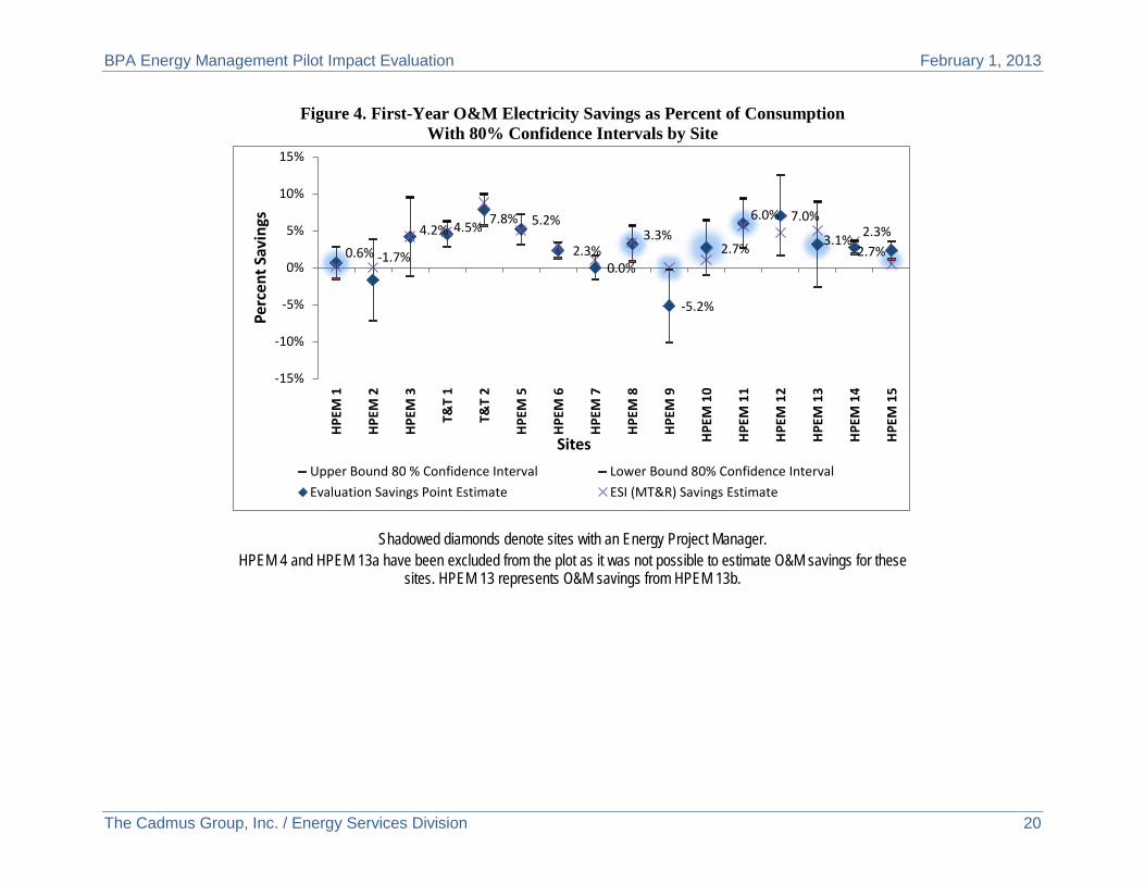
Figure 4. First-Year O&M Electricity Savings as Percent of Consumption With 80% Confidence Intervals by Site
Shadowed diamonds denote sites with an Energy Project Manager. HPEM 4 and HPEM 13a have been excluded from the plot as it was not possible to estimate O&M savings for these
sites. HPEM 13 represents O&M savings from HPEM 13b.
0.6% -1.7%
4.2% 4.5% 7.8% 5.2%
2.3% 0.0%
3.3%
-5.2%
2.7%
6.0% 7.0%
3.1% 2.7% 2.3%
-15%
-10%
-5%
0%
5%
10%
15%
HPE
M 1
HPE
M 2
HPE
M 3
T&T
1
T&T
2
HPE
M 5
HPE
M 6
HPE
M 7
HPE
M 8
HPE
M 9
HPE
M 1
0
HPE
M 1
1
HPE
M 1
2
HPE
M 1
3
HPE
M 1
4
HPE
M 1
5
Perc
ent S
avin
gs
Sites Upper Bound 80 % Confidence Interval Lower Bound 80% Confidence IntervalEvaluation Savings Point Estimate ESI (MT&R) Savings Estimate

BPA Energy Management Pilot Impact Evaluation February 1, 2013
The Cadmus Group, Inc. / Energy Services Division 21
Figure 5. First-Year O&M Gas Savings With 80% Confidence Intervals by Site
19.5 19.2
0
5
10
15
20
25
30
35
40
HPEM
5
HPEM
11
000s
ther
ms
Sites Upper Bound 80 % Confidence Interval Lower Bound 80% Confidence Interval
Evaluation Savings Point Estimate ESI (MT&R) Savings Estimate

BPA Energy Management Pilot Impact Evaluation February 1, 2013
The Cadmus Group, Inc. / Energy Services Division 22
Figure 6. First-Year O&M Gas Savings as Percent of Consumption With 80% Confidence Intervals by Site
63.3%
15.2%
0%
10%
20%
30%
40%
50%
60%
70%
80%
90%
100%
HPEM
5
HPEM
11
Perc
ent S
avin
gs
Sites
Upper Bound 80 % Confidence Interval Lower Bound 80% Confidence Interval
Evaluation Savings Point Estimate ESI (MT&R) Savings Estimate

BPA Energy Management Pilot Impact Evaluation February 1, 2013
The Cadmus Group, Inc. / Energy Services Division 23
Figure 7. First-Year O&M and Capital Measure Electricity Savings With 80% Confidence Intervals by Site
Shadowed diamonds denote sites with an Energy Project Manager. HPEM 4 and HPEM 13a have been excluded from the plot as it was not possible to estimate O&M savings for these
sites. HPEM 13 represents O&M savings from HPEM 13b.
437 -69
910
1,596 1,565 1,276
772
1,770
434
-446
1,672
395 1,076
60 547
198
-2,000
-1,000
0
1,000
2,000
3,000
4,000
HPE
M 1
HPE
M 2
HPE
M 3
T&T
1
T&T
2
HPE
M 5
HPE
M 6
HPE
M 7
HPE
M 8
HPE
M 9
HPE
M 1
0
HPE
M 1
1
HPE
M 1
2
HPE
M 1
3
HPE
M 1
4
HPE
M 1
5
MW
h
Sites Upper Bound 80 % Confidence Interval Lower Bound 80% Confidence Interval
Evaluation Savings Point Estimate ESI (MT&R) Savings Estimate
BPA Energy Management Pilot Impact Evaluation February 1, 2013
The Cadmus Group, Inc. / Energy Services Division 24
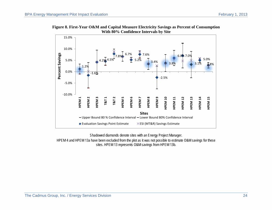
Figure 8. First-Year O&M and Capital Measure Electricity Savings as Percent of Consumption With 80% Confidence Intervals by Site
Shadowed diamonds denote sites with an Energy Project Manager. HPEM 4 and HPEM 13a have been excluded from the plot as it was not possible to estimate O&M savings for these
sites. HPEM 13 represents O&M savings from HPEM 13b.
1.2%
-1.6%
4.2% 4.5% 7.8% 6.7%
5.2% 7.6%
3.4%
-2.5%
3.8%
6.0% 7.0%
3.1% 5.0%
2.8%
-10.0%
-5.0%
0.0%
5.0%
10.0%
15.0%
HPE
M 1
HPE
M 2
HPE
M 3
T&T
1
T&T
2
HPE
M 5
HPE
M 6
HPE
M 7
HPE
M 8
HPE
M 9
HPE
M 1
0
HPE
M 1
1
HPE
M 1
2
HPE
M 1
3
HPE
M 1
4
HPE
M 1
5
Perc
ent S
avin
gs
Sites Upper Bound 80 % Confidence Interval Lower Bound 80% Confidence Interval
Evaluation Savings Point Estimate ESI (MT&R) Savings Estimate

BPA Energy Management Pilot Impact Evaluation February 1, 2013
The Cadmus Group, Inc. / Energy Services Division 25
The ability to detect energy savings at a program site using regression analysis depended on:
• The correlation between program activity and the other independent variables,
• The variance of the dependent variable that is explained by the independent variables, and
• The number of observations.
In turn, the number of observations depends on the data frequency and the length of the baseline and test periods. Although the number of pilot sites was small, we found a relationship between the frequency of energy consumption data and the ability to detect savings. We were able to detect O&M savings at the 20% significance level at seven of the eight sites with daily or weekly data. In contrast, we detected savings at only two of the nine sites with monthly or bi-monthly data. Thus, higher-frequency data appear to increase the probability of detecting savings.
Program Savings Estimates Cadmus used the results of the site electricity savings analyses to estimate the first-year pilot savings. We discuss the results from the estimation of O&M energy savings and then the results of the overall energy savings from both capital and O&M measures.
O&M Energy Savings Table 4 shows the MT&R and evaluation estimates of the total electricity savings in the pilot’s first year (July 1, 2010, to June 30, 2011). The MT&R reported savings of 9,860 MWh for O&M measures at 17 sites.9 Because Cadmus could only estimate O&M savings at 16 sites, the MT&R O&M savings for the same 16 sites are presented in Table 4 for comparison purposes. The table excludes HPEM 4 and HPEM 13a.
Table 4. Pilot O&M Electricity Savings Estimates
Sites (N)
Energy Management O&M Savings
(kWh) LB 80% CI UB 80% CI
Energy Management
O&M as a Percent of
Load Realization
Rate ESI Program Reports (MT&R): All Sites 16
9,366,362 - - 3.1% n/a
Evaluation results: All sites 16
8,277,665
5,765,508
10,789,822 2.7% 88%
Evaluation results: Sites with statistically significant savings 10
5,944,006
4,818,910
7,069,102 3.7% 63%
Evaluation results: Sites with positive savings 14
9,258,345
6,914,114
11,602,575 3.4% 99%
Notes: (1) The MT&R estimates did not include standard errors or confidence intervals. We replicated the MT&R analysis for most sites and calculated standard errors; however, because we could not replicate the analysis exactly for some sites, we did not report confidence intervals for the estimates.
(2) O&M savings for HPEM 4 and HPEM 13a sites are not reported because it was not possible to estimate the O&M savings. (3) The realization rate is the ratio of evaluation O&M savings to ESI reported savings for all 16 sites.
9 The ESI team estimated and reported O&M energy savings for HPEM 4, however Cadmus could not verify the
O&M energy savings for this site.

BPA Energy Management Pilot Impact Evaluation February 1, 2013
The Cadmus Group, Inc. / Energy Services Division 26
The second row of Table 4 shows Cadmus’ estimate of the pilot’s overall electricity O&M savings. The estimate includes savings from 16 sites, regardless of the statistical significance and sign of the site savings. We believe this all-inclusive estimate is the most appropriate and defensible measure of the pilot’s impact. Although the savings estimates for some sites may be imprecise, the point estimates still represent the evaluation’s best estimate of savings. Also, to the extent savings for some sites were imprecisely estimated, the confidence interval for the pilot savings will reflect this uncertainty. Finally, by including savings from all sites, BPA is not open to criticism that it is choosing to count savings only from sites with outcomes most favorable to the program goals.
Cadmus estimated the pilot O&M savings were approximately 8,278 MWh or 2.7% of consumption. The pilot’s electricity savings are statistically significant at the 20% level, although the confidence interval is fairly wide. The wide confidence interval is partially due to including savings for facilities with savings that were not statistically significant. There is an 80% chance the true electricity savings estimate lies within the interval [5,765 MWh, 10,790 MWh]. Note that the MT&R savings estimate lies within this confidence interval, so it is not possible to reject statistically the MT&R savings. The evaluation point estimate implies an electricity savings realization rate of 88% for the pilot’s O&M measures, with an 80% chance the realization rate lies within the interval [62%, 115%].
For comparison, the third row of Table 4 reports electricity savings for the 10 sites with statistically significant results. The statistically significant electricity savings were approximately 5,944 MWh or 3.7% of consumption in these sites, which implies a realization rate for the pilot of 86% compared to the MT&R estimates for the same 10 sites. The electricity savings decrease relative to the estimate in row 2 because row 3 omits positive but statistically insignificant savings for a few sites. The last row of Table 4 reports savings at 14 sites with positive savings. Electricity savings at these sites were 9,258 MWh, which implies a pilot realization rate of 99% for O&M measures. The electricity savings and realization rate in row 4 increase relative to row 2 because row 4 drops two sites with negative savings.
Table 5 reports the MT&R and evaluation estimate of O&M gas savings for the two sites with gas consumption data. The gas savings were positive and statistically significant at each site.
Table 5. Pilot O&M Gas Savings Estimates
Estimate N
(Sites)
Energy Management O&M Savings LB 80% CI UB 80% CI
Energy Management O&M Percent
Savings Realization
Rate ESI Program Reports (MT&R): All Sites 2 34,659 - - 22% n/a Evaluation Results: All sites 2 38,736 22,319 55,153 25% 112% The ESI Program estimated O&M gas savings of 34,659 therms or 22% at the two sites. Cadmus estimated O&M gas savings of 38,736 therms or 25%, for a realization rate of 112%.

BPA Energy Management Pilot Impact Evaluation February 1, 2013
The Cadmus Group, Inc. / Energy Services Division 27
The 80% confidence interval for our gas savings estimate was [22,319 therms, 55,153 therms]. This confidence interval includes the MT&R estimate, so it is not possible to reject the MT&R savings.
Capital and O&M Energy Savings Table 6 lists Cadmus’ estimate of total pilot electricity savings from both capital and O&M measures. This table includes the estimates of O&M savings from the second row of Table 4. Capital measure savings are included for all 17 facilities.
Table 6. Total Pilot Verified O&M and Capital Electricity Savings
Electricity Savings (kWh)
Savings as a Percent of Consumption Realization Rate
Capital Measure Savings 4,806,470 1.6% 100% O&M Savings 8,277,665 2.7% 88% Total Savings 13,084,135 4.4% 92%
The electricity savings from the capital projects in the pilot’s first year equaled approximately 4,806 MWh (1.6% of electricity consumption).10 The combined capital and O&M savings equaled 13,084 MWh (4.4% of electricity consumption).
The 80% confidence interval for the combined savings is [10,572 MWh, 15,596 MWh]. There were no reported gas savings from capital measures in the pilot’s first year.
Fractional Savings Uncertainty Cadmus also performed a fractional savings uncertainty (FSU) analysis, which indicates whether the time series data—in particular, the frequency and series length—are sufficient to detect the expected (ex ante) savings at a particular significance level.11 A site’s FSU is defined as the ratio of the uncertainty about the savings to the total savings. It depends positively on the coefficient of variation of the regression root mean square error (RMSE) and the expected savings as a percentage of total consumption, and it depends negatively on the number of observations in the baseline and test periods. A lower FSU indicates the savings are more likely to be detected; a higher FSU indicates the savings are less likely to be detected.
According to BPA’s Measurement and Verification Protocols, fractional savings uncertainty will be highest when measuring savings at the whole building (instead of for a system or end use) and with longer-interval (less frequent) data.12 ASHRAE guidelines indicate that an FSU of 50% or lower at a confidence level of 68% is a tolerable level of uncertainty.13
10 This estimate includes capital measure savings at the HPEM 4 and HPEM 13a sites, for which it was not
possible to estimate the O&M savings. 11 Bonneville Power Administration, May 2012. Verification by Energy Modeling Protocol. See page 42. 12 Ibid. See page 10. 13 American Society of Heating, Refrigerating and Air-Conditioning Engineers.

BPA Energy Management Pilot Impact Evaluation February 1, 2013
The Cadmus Group, Inc. / Energy Services Division 28
Cadmus estimated the (ex ante) fractional electricity savings uncertainty for each site using the estimated regression model RMSE and assuming expected electricity savings of 5% and a confidence level of 80%. Figure 9 plots a site’s evaluation estimated first-year pilot percentage savings against its FSU. In the figure, sites with statistically significant savings are indicated with diamonds. Sites with monthly or bi-monthly billing data are indicated with shadowed diamonds or squares.
Several patterns are evident.
• Sites with low frequency billing data tended to have high fractional savings uncertainty. The median FSU for sites with monthly or bi-monthly data was 71%. The median FSU for sites with higher frequency data was 18%.
• Sites with positive and significant savings tended to have a smaller FSU, as expected. The median FSU coefficient for these sites was 39%, versus 61% for sites with insignificant or negative savings. As noted above, sites with significant savings tended to have high frequency (weekly or daily) data.
• Sites with significant savings tended to have higher estimated electricity savings. A lower FSU and higher percentage savings would both increase the probability of detecting significant savings.
• We were able to detect savings at two sites with high fractional uncertainty (>60%). This can happen when the true electricity savings are higher than the expected savings of 5%. We estimated the percentage of savings as being greater than 5% at the two sites with high FSU.
Figure 9. Estimated Percent Electricity Savings vs. Site Fractional Savings Uncertainty
Shadowed diamonds or squares denote sites with monthly or bi-monthly data.
-6%
-4%
-2%
0%
2%
4%
6%
8%
10%
0% 20% 40% 60% 80% 100% 120% 140% 160%
Eval
uatio
n %
ele
ctric
ity sa
ving
s
Fractional Electricity Savings Uncertainty
Detectable savings No detectable savings

BPA Energy Management Pilot Impact Evaluation February 1, 2013
The Cadmus Group, Inc. / Energy Services Division 29
Note that even low fractional savings uncertainty does not guarantee savings can be detected. There must also be sufficient variation (a low correlation over time) between capital measure and O&M measure savings. This condition was not always satisfied so, in these cases, we could not estimate the O&M measure savings precisely.
Other Tested Modeling Methodologies As noted above, Cadmus was unable to detect electricity savings at most sites with monthly electric consumption data. To increase the probability of detecting savings, we pooled data from the eight sites and estimated a panel regression model. The goal was to test whether a pooled model would detect savings significantly different from zero, since the individual site models for most sites with monthly data did not estimate electricity savings significantly different from zero. To minimize the impact of differences in the variance of site consumption, we specified a log-linear model, with the dependent variable as the natural logarithm of a site’s monthly consumption. We included site fixed effects to capture differences between sites in average consumption. The model also contained separate variables for each site’s production (that is, the impact of output on consumption was allowed to vary by site), HDDs, CDDs, dummy variables for any capital projects that did not have engineering savings estimates, and indicator variables for the Year 1 and Year 2 pilot test periods. The coefficients on the pilot test indicator variables can be interpreted as approximate percentage of savings effects from pilot O & M projects and capital projects with engineering savings estimates.
Cadmus estimated the model by OLS and corrected the standard errors for serial correlation (clustered at the sites).

BPA Energy Management Pilot Impact Evaluation February 1, 2013
The Cadmus Group, Inc. / Energy Services Division 30
Table 7 shows the results.
• In Model 1, the savings impacts in the first pilot year were estimated imprecisely. The results indicate average site savings of 0.3% with an 80% confidence interval of [-0.8% 1.4%].
• In Model 2, the output and weather independent variables enter the regression in natural logarithmic form. The savings estimate increases slightly but is imprecise. We attempted other specifications and obtained similar results.
Overall, we found the panel data approach did not improve the precision of the savings estimates for the eight sites with monthly data. If in future program years there are more participants which can be grouped into similar industries, then a panel approach could be used with more success and would be a more efficient method than estimating the savings separately for each site. For example, all food processors could be grouped together and an average savings rate for all food processing facilities in the program would be estimated by the model.
Table 7. Summary of Panel Regression Analysis of Pilot Savings Model 1 Model 2
Point estimate of average site percentage of monthly savings1 0.3% 0.5% 80% Confidence interval (-0.8, 1.4) (-0.9 ,1.8) Site fixed effects Yes Yes Weather Yes Yes Output Yes Yes Capital Measures2 Yes Yes R2 0.99 0.99 N 330 330 Notes: Dependent variables are the natural logarithm of monthly consumption. In model 2, output and weather variables except HPEM and capital measure dummy variables are in natural logarithms. Models estimated by OLS with at least 12 months of post-program data. Huber-White model standard errors are adjusted for correlation over time in building consumption. Savings impact of 0-1 indicator variable for HPEM program estimated using Kennedy (1981) and standard error estimated using van Garderen and Shah (2002). 1 Average percentage of monthly savings includes savings from HPEM and capital measures for which we have engineering savings estimates. Savings from these capital measures are subtracted to estimate HPEM savings. 2 Capital measures are those installed in the post-period for which we do not have engineering savings estimates and those installed in the pre-HPEM period.

BPA Energy Management Pilot Impact Evaluation February 1, 2013
The Cadmus Group, Inc. / Energy Services Division 31
PROGRAM COST-EFFECTIVENESS After estimating evaluation energy savings, Cadmus calculated cost-effectiveness for the program. This section presents the methodology and results for the cost-effectiveness analysis.
Cost-Effectiveness Methodology Cost-effectiveness was calculated using Cadmus’ DSM Portfolio Pro model. For each facility, this model treated capital measures separately and combined all O&M and behavioral measures as one measure. This approach corresponded with the resolution of the savings and cost data.
Cost-effectiveness was calculated for the pilot program overall and includes all 17 sites. We calculated the Participant Cost Test (PCT), Utility Cost Test (UCT), and Total Resource Cost (TRC). The PCT calculates a benefit-cost ratio based on the costs and benefits to the participants. The UCT calculates a benefit-cost ratio based on the costs and benefits to the utility. The TRC includes all costs and benefits, regardless of who accrues them, and so includes the costs and benefits to both the participants and the utility. The methodology for calculating cost-effectiveness is described by the California Standard Practice Manual.14
The key model assumptions were these:
• Annual site electricity savings (kWh per year). The evaluated energy savings for O&M measures from row 2 in Table 4 were used in the model. Savings for capital measures installed during the test period were also included.
• Annual site gas savings (therms per year). The evaluated gas savings for O&M measures from Table 5 were included.
• Annual site demand savings (kW). Demand savings were calculated based upon the coincidence factor and the evaluated annual site energy savings. The coincidence factors came from the Sixth Power Plan.
• Line loss. All sites had a line loss of 9.056%.
• Avoided costs. Avoided costs are from the Sixth Power Plan.15
• Measure costs. As the capital measures were custom projects, full measure costs were used. The costs for O&M/behavioral measures were not reported, as they were minimal or zero; thus, they were entered as zero cost in the model.
• Program costs. The costs of administering the program to the participants for five years were provided by BPA. Costs included the technical assistance provided to the participants.
14 California Standard Practice Manual: Economic Analysis of Demand-Side Programs and Projects. October
2001. Can be downloaded from the Website: http://www.energy.ca.gov/greenbuilding/documents/background/07-J_CPUC_STANDARD_PRACTICE_MANUAL.PDF
15 The Sixth Northwest Conservation and Electric Power Plan can be downloaded from the Website: http://www.nwcouncil.org/energy/powerplan/6/default.htm

BPA Energy Management Pilot Impact Evaluation February 1, 2013
The Cadmus Group, Inc. / Energy Services Division 32
• Measure life. For the custom capital projects, the measure life from the Sixth Power Plan was used, corresponding to the technology type. For example, lighting projects have a measure life of 12 years. For O&M measures, the measure life is unknown. Energy-management programs are relatively new and, currently, there are no data on measure persistence after participants exit the program. For that reason, we conservatively assumed that the measure life of the O&M measures would, at a minimum, be equivalent to the number of years that a participant is engaged with the program. BPA expects facilities to participate for an average of five years, and will pay incentives each year for verified energy savings during this period. Therefore, we assumed a measure life of five years for O&M measures.
• Program incentives. BPA provided data on incentives provided for the custom capital projects and for co-funding the energy manager’s salary. Both of these were taken into account in the cost-effectiveness model.
All other model inputs―such as customer retail rate, discount rate, and project start years―were consistent with the Sixth Power Plan. The inputs for the model are summarized in Table 8.
Table 8. Summary of Cost-Effectiveness Inputs Benefits Value Source
Electricity Savings Site and measure specific
(See Appendix) Evaluated Savings Results
Gas Savings Site and measure specific
(See Appendix) Evaluated Savings Results
Demand Savings Site and measure specific Evaluated Savings Results,
Coincidence Factor comes from the Sixth Power Plan Electric Line Loss 9.056% Sixth Power Plan Avoided Costs Varies by time of year Sixth Power Plan Capital Measure Costs $1,933,210 MT&R Reports O&M Measure Costs $0 MT&R Reports Measure Life – Capital Measures Varies by measure type Sixth Power Plan Measure Life – O&M Measures 5 years BPA’s expected length of engagement with site Program Administration Costs
2010: $2,308,668 2011-2014: $182,117 per year BPA
Program Incentives
2010: $251,681 2011: $1,472,189
2012-2014: $213,181 BPA Discount Rate 5% Sixth Power Plan
Cost-Effectiveness Results Cadmus calculated cost-effectiveness at the program level and include both O&M and capital measures installed after facilities began participating in the program. The results are shown in Table 9.
BPA Energy Management Pilot Impact Evaluation February 1, 2013
The Cadmus Group, Inc. / Energy Services Division 33
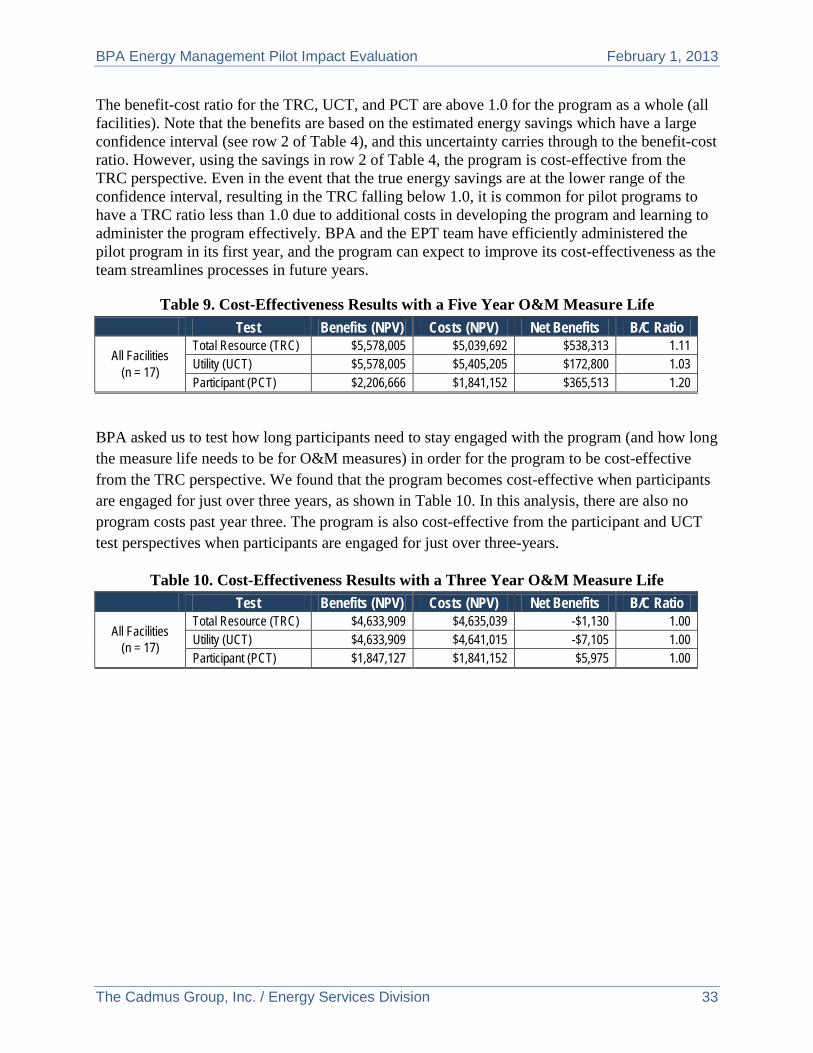
The benefit-cost ratio for the TRC, UCT, and PCT are above 1.0 for the program as a whole (all facilities). Note that the benefits are based on the estimated energy savings which have a large confidence interval (see row 2 of Table 4), and this uncertainty carries through to the benefit-cost ratio. However, using the savings in row 2 of Table 4, the program is cost-effective from the TRC perspective. Even in the event that the true energy savings are at the lower range of the confidence interval, resulting in the TRC falling below 1.0, it is common for pilot programs to have a TRC ratio less than 1.0 due to additional costs in developing the program and learning to administer the program effectively. BPA and the EPT team have efficiently administered the pilot program in its first year, and the program can expect to improve its cost-effectiveness as the team streamlines processes in future years.
Table 9. Cost-Effectiveness Results with a Five Year O&M Measure Life Test Benefits (NPV) Costs (NPV) Net Benefits B/C Ratio
All Facilities (n = 17)
Total Resource (TRC) $5,578,005 $5,039,692 $538,313 1.11 Utility (UCT) $5,578,005 $5,405,205 $172,800 1.03 Participant (PCT) $2,206,666 $1,841,152 $365,513 1.20
BPA asked us to test how long participants need to stay engaged with the program (and how long the measure life needs to be for O&M measures) in order for the program to be cost-effective from the TRC perspective. We found that the program becomes cost-effective when participants are engaged for just over three years, as shown in Table 10. In this analysis, there are also no program costs past year three. The program is also cost-effective from the participant and UCT test perspectives when participants are engaged for just over three-years.
Table 10. Cost-Effectiveness Results with a Three Year O&M Measure Life Test Benefits (NPV) Costs (NPV) Net Benefits B/C Ratio
All Facilities (n = 17)
Total Resource (TRC) $4,633,909 $4,635,039 -$1,130 1.00 Utility (UCT) $4,633,909 $4,641,015 -$7,105 1.00 Participant (PCT) $1,847,127 $1,841,152 $5,975 1.00
BPA Energy Management Pilot Impact Evaluation February 1, 2013
The Cadmus Group, Inc. / Energy Services Division 34
CONCLUSIONS AND RECOMMENDATIONS Based on this impact evaluation, Cadmus offers the following conclusions and provides seven recommendations for improving future energy savings estimations.
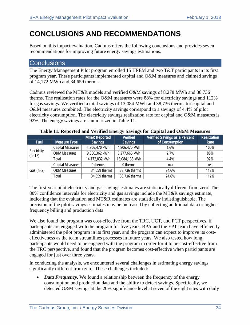
Conclusions The Energy Management Pilot program enrolled 15 HPEM and two T&T participants in its first program year. These participants implemented capital and O&M measures and claimed savings of 14,172 MWh and 34,659 therms.
Cadmus reviewed the MT&R models and verified O&M savings of 8,278 MWh and 38,736 therms. The realization rates for the O&M measures were 88% for electricity savings and 112% for gas savings. We verified a total savings of 13,084 MWh and 38,736 therms for capital and O&M measures combined. The electricity savings correspond to a savings of 4.4% of pilot electricity consumption. The electricity savings realization rate for capital and O&M measures is 92%. The energy savings are summarized in Table 11.
Table 11. Reported and Verified Energy Savings for Capital and O&M Measures
Fuel Measure Type MT&R Reported
Savings Verified Savings
Verified Savings as a Percent of Consumption
Realization Rate
Electricity (n=17)
Capital Measures 4,806,470 kWh 4,806,470 kWh 1.6% 100% O&M Measures 9,366,362 kWh 8,277,665 kWh 2.7% 88% Total 14,172,832 kWh 13,084,135 kWh 4.4% 92%
Gas (n=2) Capital Measures 0 therms 0 therms n/a n/a O&M Measures 34,659 therms 38,736 therms 24.6% 112% Total 34,659 therms 38,736 therms 24.6% 112%
The first-year pilot electricity and gas savings estimates are statistically different from zero. The 80% confidence intervals for electricity and gas savings include the MT&R savings estimate, indicating that the evaluation and MT&R estimates are statistically indistinguishable. The precision of the pilot savings estimates may be increased by collecting additional data or higher-frequency billing and production data.
We also found the program was cost-effective from the TRC, UCT, and PCT perspectives, if participants are engaged with the program for five years. BPA and the EPT team have efficiently administered the pilot program in its first year, and the program can expect to improve its cost-effectiveness as the team streamlines processes in future years. We also tested how long participants would need to be engaged with the program in order for it to be cost-effective from the TRC perspective, and found that the program becomes cost-effective when participants are engaged for just over three years.
In conducting the analysis, we encountered several challenges in estimating energy savings significantly different from zero. These challenges included:
• Data Frequency. We found a relationship between the frequency of the energy consumption and production data and the ability to detect savings. Specifically, we detected O&M savings at the 20% significance level at seven of the eight sites with daily

BPA Energy Management Pilot Impact Evaluation February 1, 2013
The Cadmus Group, Inc. / Energy Services Division 35
or weekly data. In contrast, we could detect savings at only two of the nine sites with monthly or bi-monthly data. Thus, as statistical theory predicts, higher frequency data appears to increase the probability of detecting savings.
• Capital Measures Confounding the Analysis. At some sites, installation of capital measures just before or after the start of a facility’s participation in HPEM or T&T made it difficult or impossible to isolate O&M savings.
• Implementation Timing of Measures. The energy savings for O&M measures installed near the end of a program year may not be fully estimated, as there may not be enough months of post-implementation data to identify these savings.
Recommendations Based on the challenges we encountered in estimating energy savings, we have these recommendations for improving energy savings estimation in the future.
1. Perform a statistical power analysis. A statistical power analysis would estimate the ex ante probability of detecting a site’s true pilot savings. When beginning an engagement with a site, perform a statistical power analysis (or fractional savings analysis) to estimate the probability of detecting savings at the site. The analysis would require assumptions for each site about the significance levels (e.g., 20%), expected percentage of savings, the coefficient of variation (CV) of energy use, the correlation between baseline and test period energy use, and the number of baseline and test period observations. Data on energy use in the baseline period could be used to develop assumptions about the site CV and correlations. The statistical power analysis could be used to assess the sufficiency of the planned baseline and test periods (i.e., the number of days, weeks, or months) to detect savings.
2. Collect additional data. We recommend both collecting data for additional months in the pilot’s second year and performing an evaluation of the second-year pilot savings. We did not report savings for the second pilot year because we did not have a full year of data; however, it was evident that for many sites, the pilot savings increased in the second year. Additional data could also decrease the confidence interval range and provide more certainty in the energy savings.
3. Increase the frequency of data collected. When possible, collect higher frequency billing data and production data. We were able to detect savings at the majority of facilities with weekly billing data, but it became increasingly difficult with bi-monthly and monthly billing data. Higher frequency billing data could also provide more certainty in energy savings and decrease the confidence interval range.
4. Re-estimate the first year pilot savings for sites with insignificant savings. With data for additional periods (months, weeks, days, etc.) in the pilot’s second year, it may be possible to detect savings in the first year. We recommend re-estimating the first-year savings for sites with statistically insignificant savings once more data for the second year are available. If savings can be detected for these sites, the confidence interval range around the program savings will decrease.
BPA Energy Management Pilot Impact Evaluation February 1, 2013
The Cadmus Group, Inc. / Energy Services Division 36
5. Account for autocorrelation. The MT&R models should test and account for autocorrelation, especially if the data are high-frequency daily or weekly data. If autocorrelation is ignored, OLS estimates will still be unbiased and consistent but the standard errors and inference procedures will be invalid.
6. Report the confidence intervals and precision. The MT&R estimates did not report an associated confidence interval and precision level. Including this would help identify sites where reported energy savings were not significantly different from zero.
7. Be aware of analysis impacts when implementing simultaneous capital and O&M measures. Application of regression analysis to measure savings from O&M requires that the savings from O&M and any capital measures be sufficiently independent (uncorrelated). Simultaneous or near-simultaneous implementation of capital and O&M measures increases the savings correlation and makes it difficult to estimate their savings impacts separately. We recognize project timing is often dependent upon plant maintenance schedules; therefore, we only recommend that BPA and its contractors be aware that implementing multiple measures in the same time frame may impact the ability to estimate O&M savings.

BPA Energy Management Pilot Impact Evaluation February 1, 2013
The Cadmus Group, Inc. / Energy Services Division 37
This page left blank.
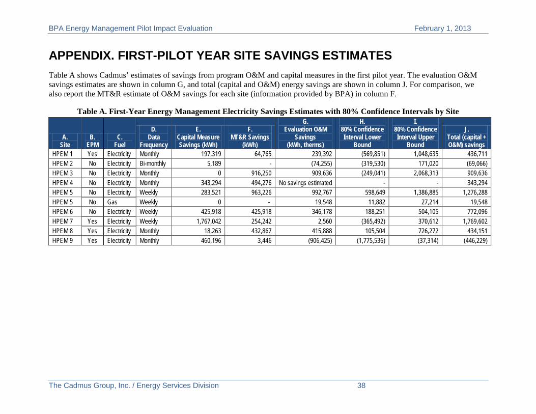
BPA Energy Management Pilot Impact Evaluation February 1, 2013
The Cadmus Group, Inc. / Energy Services Division 38
APPENDIX. FIRST-PILOT YEAR SITE SAVINGS ESTIMATES Table A shows Cadmus’ estimates of savings from program O&M and capital measures in the first pilot year. The evaluation O&M savings estimates are shown in column G, and total (capital and O&M) energy savings are shown in column J. For comparison, we also report the MT&R estimate of O&M savings for each site (information provided by BPA) in column F.
Table A. First-Year Energy Management Electricity Savings Estimates with 80% Confidence Intervals by Site
A. Site
B. EPM
C. Fuel
D. Data
Frequency
E. Capital Measure Savings (kWh)
F. MT&R Savings
(kWh)
G. Evaluation O&M
Savings (kWh, therms)
H. 80% Confidence Interval Lower
Bound
I. 80% Confidence Interval Upper
Bound
J. Total (capital + O&M) savings
HPEM 1 Yes Electricity Monthly 197,319 64,765 239,392 (569,851) 1,048,635 436,711 HPEM 2 No Electricity Bi-monthly 5,189 - (74,255) (319,530) 171,020 (69,066) HPEM 3 No Electricity Monthly 0 916,250 909,636 (249,041) 2,068,313 909,636 HPEM 4 No Electricity Monthly 343,294 494,276 No savings estimated - - 343,294 HPEM 5 No Electricity Weekly 283,521 963,226 992,767 598,649 1,386,885 1,276,288 HPEM 5 No Gas Weekly 0 - 19,548 11,882 27,214 19,548 HPEM 6 No Electricity Weekly 425,918 425,918 346,178 188,251 504,105 772,096 HPEM 7 Yes Electricity Weekly 1,767,042 254,242 2,560 (365,492) 370,612 1,769,602 HPEM 8 Yes Electricity Monthly 18,263 432,867 415,888 105,504 726,272 434,151 HPEM 9 Yes Electricity Monthly 460,196 3,446 (906,425) (1,775,536) (37,314) (446,229)

BPA Energy Management Pilot Impact Evaluation February 1, 2013
The Cadmus Group, Inc. / Energy Services Division 39
A. Site
B. EPM
C. Fuel
D. Data
Frequency
E. Capital
Measure Savings (kWh)
F. MT&R Savings
(kWh)
G. Evaluation O&M
Savings (kWh, therms)
H. 80% Confidence Interval Lower
Bound
I. 80%
Confidence Interval Upper
Bound
J. Total (capital
+ O&M) savings
HPEM 10 Yes Electricity Monthly 476,114 476,114 1,196,110 (451,670) 2,843,890 1,672,224 HPEM 11 No Electricity Monthly 0 374,432 394,572 173,412 615,732 394,572 HPEM 11 No Gas Monthly 0 15,955 19,188 4,671 33,705 19,188 HPEM 12 Yes Electricity Daily 0 717,420 1,076,020 248,720 1,903,320 1,076,020
HPEM 13a No Electricity Monthly
548,587
No savings
estimated No savings
estimated - -
548,587 HPEM 13b No Electricity Monthly 0 95,819 60,216 (51,149) 171,581 60,216 HPEM 14 Yes Electricity Daily 247,558 386,812 299,212 201,935 396,489 546,770 HPEM 15 Yes Electricity Daily 33,469 161,066 164,590 81,070 248,109 198,059 T&T 1 No Electricity Daily 0 1,702,608 1,595,780 989,343 2,202,217 1,595,780 T&T 2 Yes Electricity Daily 0 1,755,008 1,565,424 1,138,764 1,992,084 1,565,424 Notes: Based on individual analysis of each site's electricity or gas consumption. The details of each site's estimation were provided to BPA in a confidential appendix.