Embed Size (px)
Citation preview

Energy harvesting from municipal water management systems: from
storage and distribution to wastewater treatment
Daniele Novara
Thesis to obtain the Master of Science Degree in
Energy Engineering and Management
Supervisors: Prof. Helena Margarida Machado da Silva Ramos
Prof. Wojciech Stanek
Examination Committee
Chairperson: Prof. José Alberto Caiado Falcão de Campos Supervisor: Prof. Helena Margarida Machado da Silva Ramos Member of the Committee: Prof. José Carlos Páscoa Marques
September 2016

II

III
Acknowledgment
First of all, I would like to express all my gratitude towards my supervisor from Instituto Superior
Técnico Professor Helena Ramos. It was during the Hydropower curricular course that I first learnt from her the concept of energy recovery from water networks, which immediately stimulated my interest. Working under her guidance has been extremely pleasant and rewarding: her vast knowledge on the topic together with her empathy, helpfulness and generosity made my efforts in writing the present dissertation much lighter. I really hope to maintain collaboration with her and IST in the future.
I am also grateful with Mariana Simão from IST for her patience and the support provided to me.
My gratitude goes to the staff of ATO5 Astigiano Monferrato, in particular to Eng. Giuseppe Giuliano and Eng. Valentina Ghione, for the interest in my research and the contacts provided. Their collaboration has been essential for the writing of the present thesis.
I would like to thank Riccardo Spriano and Eloisa Fossati from ASP, as well as Andrea Mesturini and Roberto Francone from CCAM water company. They showed interest in my research and devoted some of their valuable time to provide me with data and share their view and expertise. A big thank goes also to Mr. Frank Zammataro CEO of Rentricity Inc. for the precious collaboration and involvement in my work.
The present dissertation wouldn’t exist without the support of KIC InnoEnergy programme, under which I had the unique opportunity of attending this double-degree course. I am particularly grateful towards Prof. Wojciech Stanek and Prof. Krzysztof Pikoń from Politechnika Śląska for their involvement and help.
Last but not least, I am immensely thankful towards my two families: the one from Italy who constantly supported and loved me, and the one from India, Serbia, Poland etc. with whom I had the fortune of sharing unforgettable experiences during the last two years.
Finally, a big thank to Beatrice who has been always on my side.

IV

V
Index
Acknowledgment ....................................................................................................................................... III
Index ............................................................................................................................................................ V
Abstract ...................................................................................................................................................... IX
Resumo ....................................................................................................................................................... X
Nomenclature ............................................................................................................................................ XI
Abbreviations ............................................................................................................................................ XII
Index of Figures ........................................................................................................................................ XIII
Index of Tables ......................................................................................................................................... XVI
1. Scope and structure of the dissertation ................................................................................................. 1
2. From water to energy ............................................................................................................................. 2
2.1. World energy generation overview ................................................................................................. 2
2.2. Hydro sector overview ..................................................................................................................... 4
2.2.1. General facts ............................................................................................................................. 4
2.2.2. Hydroelectric energy generation in Italy .................................................................................. 5
2.2.3. Hydroelectric energy generation in Portugal ............................................................................ 5
2.3. Categories of hydropower plants..................................................................................................... 6
2.4. Basic concepts of hydropower ......................................................................................................... 7
2.5. Turbomachinery affinity laws .......................................................................................................... 8
2.6. Hydraulic energy converters ............................................................................................................ 9
2.6.1. Pressurized flows .................................................................................................................... 10
2.6.1.1. Hydraulic turbines ........................................................................................................ 10
2.6.1.2. Pumps as Turbines (PATs) ............................................................................................ 12
2.6.1.3. Positive Displacement machines.................................................................................. 13
2.6.1.4. In-pipe propellers ......................................................................................................... 13
2.6.2. Open channel flows................................................................................................................. 14

VI
2.6.2.1. Waterwheels ................................................................................................................ 14
2.6.2.2. Hydrostatic pressure wheels ........................................................................................ 14
2.6.2.3. Hydrokinetic turbines ................................................................................................... 15
2.6.2.4. Archimedes screws ...................................................................................................... 16
2.7. PAT background and applications .................................................................................................. 17
2.7.1. Quadrant operations of PAT ................................................................................................... 18
2.7.2. PAT performance prediction ................................................................................................... 19
2.7.2.1. Mathematical methods .................................................................................................... 19
2.7.2.2. Numerical methods (CFD analysis) .................................................................................. 21
3. Water-Energy Nexus ............................................................................................................................. 22
3.1. Introduction ................................................................................................................................... 22
3.2. WEN on large scale: from hundreds of kWs to MWs..................................................................... 22
3.3. WEN on medium scale: from hundreds of Ws to kWs................................................................... 23
3.3.1. General facts ....................................................................................................................... 23
3.3.2. Energy recovery from water supply infrastructures ........................................................... 24
3.3.3. Energy recovery from Wastewater Treatment Plants (WWTPs) ........................................ 26
3.4. WEN on micro scale: mWs ............................................................................................................. 26
3.5. WSS sector in Italy: an overview .................................................................................................... 27
4. Case-study 1: Scurzolengo water tower ............................................................................................... 28
4.1. Context description ........................................................................................................................ 28
4.2. General facts about water towers ................................................................................................. 29
4.3. Scurzolengo water tower ............................................................................................................... 30
4.4. Net head calculations ..................................................................................................................... 32
4.4.1. Basic data ............................................................................................................................ 32
4.4.2. Continuous head losses ...................................................................................................... 32
4.4.3. Singular head losses ............................................................................................................ 32
4.4.4. Net head available .............................................................................................................. 33
4.5. Choice of machinery ...................................................................................................................... 33
VII
4.6. Sizing of machinery ........................................................................................................................ 34
4.7. PAT selection .................................................................................................................................. 37
4.8. Technical analysis ........................................................................................................................... 39
4.9. Economic analysis .......................................................................................................................... 40
4.9.1. Input parameters .................................................................................................................... 40
4.9.2. Results of economic analysis................................................................................................... 42
4.10. Environmental analysis ................................................................................................................ 42
5. Case-study 2: PRV substitution with PAT .............................................................................................. 44
5.1. Rentricity Inc. ................................................................................................................................. 44
5.2. Theoretical background ................................................................................................................. 44
5.3. System description ......................................................................................................................... 47
5.4. Optimization................................................................................................................................... 48
5.4.1. Input data and methodology .................................................................................................. 48
5.4.2. PAT alone, absence of regulation ........................................................................................... 49
5.4.3. PAT in series with PRV and by-pass duct (HR) ........................................................................ 50
5.5. Results ............................................................................................................................................ 51
5.5.1. Results PAT alone, absence of regulation ............................................................................... 51
5.5.2. Results PAT in series with PRV and by-pass duct (HR) ............................................................ 52
5.5.3. Final considerations ................................................................................................................ 54
6. Case-study 3: Asti WWTP ...................................................................................................................... 55
6.1. Context description ........................................................................................................................ 55
6.2. Outlet water channel description .................................................................................................. 56
6.3. Theoretical background of open channel flow .............................................................................. 57
6.4. Venturi Flume theoretical background .......................................................................................... 58
6.5. Design parameters ......................................................................................................................... 60
6.6. Choice of machinery ...................................................................................................................... 61
6.7. HPM Theoretical background ........................................................................................................ 64
6.7.1. Ideal machine .......................................................................................................................... 64

VIII
6.7.2. Real machine ........................................................................................................................... 65
6.8. HPM design .................................................................................................................................... 66
6.9. Installation scheme ........................................................................................................................ 67
6.10. Technical analysis ......................................................................................................................... 68
6.11. Economic analysis ........................................................................................................................ 69
6.11.1. Input parameters .................................................................................................................. 69
6.11.2. Results of economic analysis ................................................................................................ 70
6.12. Environmental analysis ................................................................................................................ 71
7. Conclusions and scope for future research .......................................................................................... 72
7.1. General conclusions and future developments ............................................................................. 72
7.2. Case-study 1: Scurzolengo water tower ........................................................................................ 72
7.3. Case-study 2: PRV substitution with PAT ....................................................................................... 73
7.4. Case-study 3: Asti WWTP ............................................................................................................... 73
References ................................................................................................................................................ 74
Appendix A: Specifications ETANORM 32-160.1 ........................................................................................... i
Structure and method of operations ................................................................................................ i
Characteristic curves ........................................................................................................................ ii
Appendix B: payback time calculations for Case-study 1 ........................................................................... iii
Appendix C: CDCF calculations for Case-study 3......................................................................................... iv

IX
Abstract
Water and energy are among the fundamental resources at the basis of human life and society
development. Their strong interrelation in many human activities has been referred to as “Water-Energy Nexus” and has been subject of growing interest during the last decades. Within the first part of the present dissertation the extents of such nexus are reviewed, providing a description of hydropower sector and relative technologies as well as presenting the scopes and needs of water supply systems.
The second part of the work instead is focused on the investigation of energy recovery potential from water supply and treatment facilities. Such supply systems in fact rely on large amounts of electricity to pump, treat and distribute water. However, situations can occur where fluid holds an excess energy that can be converted back into electricity instead of being dissipated. Three real case-studies have been analyzed in collaboration with water companies from Italy and United States in order to derive a feasibility study of energy harvesting from:
sections of a water distribution network, installing a pump in reverse mode (PAT) as replacement or complement of a Pressure Reducing Valve (PRV);
pressurized water flow at entrance of an elevated storage tank, by installing a PAT in a by-pass duct;
outlet flow from a wastewater treatment plant passing through an open-air channel, by means of a hydrostatic energy converter.
The chosen case-studies have been assessed from different perspectives, including a technical analysis as well as economic and environmental when possible.
Keywords: Hydropower, Hydrostatic Pressure Machine (HPM), Pumps as Turbines (PATs), Water-Energy
Nexus, Water Supply Systems (WSS)

X
Resumo
Água e energia são recursos fundamentais que estão na base da vida humana e no desenvolvimento da
sociedade. A sua forte inter-relação em muitas atividades humanas tem sido referido como Nexo Água-Energia e tem sido objeto de interesse crescente nas últimas décadas. Na primeira parte da presente dissertação faz-se a revisão das extensões desse nexo, fornecendo uma descrição do setor hidroelétrico e suas tecnologias, bem como o âmbito e os requisitos dos sistemas de abastecimento de água.
A segunda parte do trabalho incide na investigação do potencial de recuperação de energia a partir de instalações de abastecimento e de tratamento de água. Esses sistemas de abastecimento dependem de grandes quantidades de eletricidade para bombear, tratar e distribuir água. Contudo, podem ocorrer situações em que o fluido apresenta um excesso de energia que pode ser convertida em energia eléctrica em vez de ser dissipada. Três estudos de casos reais foram analisados em colaboração com as empresas de água da Itália e Estados Unidos a fim de obter um estudo de viabilidade de produção de energia a partir de:
secções de uma rede de distribuição de água, com a instalação de uma bomba em modo inverso (bomba a funcionar como a turbina) como substituto ou complemento de uma valvula redutora de pressão (PRV);
escoamento sob pressão na entrada de um tanque de armazenamento elevado, através da instalação de uma PAT numa conduta de by-pass;
escoamento em canal à saida de uma estação de tratamento de águas residuais, através da instalação de uma roda baseada num conversor hidrostático.
Os estudos de caso escolhidos foram avaliados a partir de diferentes perspectivas, incluindo quando possível uma análise técnica bem como económica e ambiental.
Palavras-chave: Energia Hidroelétrica, Maquina de Pressão Hidrostática (HPM), Bombas como Turbinas
(PAT), Nexo Água-Energia, Sistemas de Abastecimento de Água (WSS)

XI
Nomenclature
Specific diameter number (-) Re Reynolds Number (-)
Cp Power coefficient for hydrokinetic turbines (-)
RH Hydraulic diameter (m)
D Pump impeller diameter (m) S Flow cross-section (m2)
f Electric grid frequency (Hz), Friction factor (-)
T Torque (Nm)
g Gravitational acceleration (m/s2) U Mean flow velocity (m/s)
H Hydraulic head (m) V Flow velocity (m/s)
h Hydraulic head available in a circuit (m), Adimensional head ratio (-)
α PAT utilization factor (-)
J Unit head loss (m/m) γ Specific speed adimensional parameter (-)
ks Relative roughness factor (m) η Efficiency (-)
N Rotational speed (rpm) λ Adimensional efficiency ratio (-)
n Rotational speed (rps) μ Venturi outflow coefficient
Ns,p Specific speed for turbine based on power (m, kW)
ξ Empirical loss factor (-)
Ns,q Specific speed for pump or turbine based on discharge (m, m3/s)
π Adimensional power number (-)
Ns,q,pump Specific speed for pump based on discharge (m, m3/s)
ρ Fluid density (kg/m3)
Ns,q,turbine Specific speed for turbine based on discharge (m, m3/s)
σ Specific speed number (-)
p Adimensional power ratio (-) Φ Adimensional flow number (-)
P Power (W or kW) Φc Adimensional flow number by Cordier (-)
p.e. person equivalent (BOD/day) Ψ Adimensional head number (-)
pp Number of magnetic pole pairs (-) Ψc Adimensional head number by Cordier (-)
Q Flow rate (m3/s)
q Flow rate in hydraulic circuit (m3/s), Adimensional flow ratio (-)

XII
Abbreviations
ATO: Ambito Territoriale Ottimale (“Optimal territorial area”)
BEP: Best Efficiency Point
BOD: Biochemical Oxygen Demand
CDCF: Cumulative Discounted Cash Flow
DCI: Discounted Cash Inflow
DN: Nominal Diameter
ER: Electric Regulation
FSEC: Free Stream Energy Converter
GSE: Gestore dei Servizi Energetici (“Operator of Energy Services”)
GVHP: Gravitational Vortex Hydropower
HAWT: Horizontal Axis Water hydrokinetic Turbines
HER: Hydraulic and electric Regulation
HPM: Hydrostatic Pressure Machine
HPW: Hydrostatic Pressure Wheel
HR: Hydraulic Regulation
LCOE: Levelized Cost Of Electricity
PAT: Pump As Turbine
PD: Positive Displacement
PRV: Pressure Reducing Valve
SCADA: Supervisory Control And Data Acquisition
SDM: Staudruckmaschine
TEL: Total Energy Line
TPES: Total Primary Energy Supply
VAWT: Vertical Axis Water hydrokinetic Turbines
VOS: Variable Operating Strategy
WEN: Water-Energy Nexus
WSS: Water Supply Systems
WWTP: Waste Water Treatment Plant

XIII
Index of Figures FIGURE 1 - STRUCTURE OF THE DISSERTATION ............................................................................................................................... 1
FIGURE 2 – OVERVIEW OF WORLD ENERGY CONSUMPTION BY SOURCE [1] .......................................................................................... 2
FIGURE 3 - COMPARISON BETWEEN CENTRALIZED AND DISTRIBUTED POWER SYSTEMS
[EN.WIKIPEDIA.ORG/WIKI/FILE:CENTRALIZED_DISTRIBUTED.PNG] ............................................................................................ 3
FIGURE 4 - HYDROPOWER INSTALLED CAPACITY BY REGION (% OF TOTAL) (ADAPTED FROM [13]) ............................................................ 4
FIGURE 5 - CUMULATIVE GRAPH OF ENERGY PRODUCTION BY SOURCE IN ITALY BETWEEN 1887 AND 2014 [15] ....................................... 5
FIGURE 6 - CUMULATIVE GRAPH OF ENERGY CONSUMPTION BY SOURCE IN PORTUGAL PER YEAR
[WWW.APREN.PT/PT/DADOSTECNICOS/INDEX.PHP?ID=267] .................................................................................................. 6
FIGURE 7 - OVERVIEW OF HYDROPOWER TECHNOLOGIES ................................................................................................................. 9
FIGURE 8 - APPLICATION CHART FOR SOME UNCONVENTIONAL LOW-POWER HYDRO MACHINERY (ADAPTED FROM [21], [22], [23]) ........... 10
FIGURE 9 - MOST COMMON WATER TURBINE RUNNER TYPES [24] .................................................................................................. 10
FIGURE 10 - INDICATIVE TURBINE SELECTION CHART (ADAPTED FROM [25]) ...................................................................................... 11
FIGURE 11 - DRAWING OF CENTRIFUGAL PAT ............................................................................................................................. 12
FIGURE 12 - VISUAL REPRESENTATION OF A PD MACHINE (LOBE PUMP) [30] .................................................................................... 13
FIGURE 13 - NEW PROPOSED DESIGN OF IN-PIPE PROPELLER [33] ................................................................................................... 13
FIGURE 14 – HYDROSTATIC PRESSURE DISTRIBUTION ON A VERTICAL SURFACE IMMERSED IN FLUID ........................................................ 14
FIGURE 15 - HORIZONTAL AXIS WATER HYDROKINETIC TURBINES (HAWT) [36] ................................................................................ 15
FIGURE 16 - VERTICAL AXIS WATER HYDROKINETIC TURBINES (VAWT) [36] ..................................................................................... 15
FIGURE 17 - SCHEMATIC VIEW OF GVHP [EN.WIKIPEDIA.ORG/WIKI/GRAVITATION_WATER_VORTEX_POWER_PLANT] ............................. 16
FIGURE 18 - REPRESENTATIONS OF INCLINED ARCHIMEDEAN SCREW TURBINE AND HORIZONTAL FLOATING ARCHIMEDEAN CONVERTER [39]. 16
FIGURE 19 - TYPICAL PERFORMANCE CURVES OF PUMPS AND TURBINES [28] .................................................................................... 17
FIGURE 20 - NONDIMENSIONAL CHARACTERISTIC CURVE OF PAT (ADAPTED FROM [41]) ..................................................................... 18
FIGURE 21 – FOUR QUADRANTS OPERATIONS OF A RADIAL FLOW PAT (ADAPTED FROM [42]) .............................................................. 18
FIGURE 22 - CHARACTERISTIC CURVES FOR TURBINE AND PUMP OPERATIONS OF A VARIABLE SPEED PAT (ADAPTED FROM [42]) ................ 19
FIGURE 23 - NONDIMENSIONAL BEP PARAMETERS FOR PATS HAVING DIFFERENT SPECIFIC SPEED [41] .................................................. 20
FIGURE 24 - ALQUEVA CONCRETE GRAVITY DAM (HTTPS://EN.WIKIPEDIA.ORG/WIKI/ALQUEVA_DAM) .................................................. 22
FIGURE 25 – COMPARISON BETWEEN A TYPICAL WATER CONSUMPTION LOAD FACTOR AND ELECTRICITY DAILY LOAD DIAGRAM ................... 24

XIV
FIGURE 26 - MUNICIPAL WATER SUPPLY AND SEWAGE TREATMENT SCHEME (WATERCONSERVATIONWASTING.WEEBLY.COM) ..................... 24
FIGURE 27 - LUCIDPIPE™ POWER SYSTEM [54] ........................................................................................................................... 25
FIGURE 28 - BASIC SCHEME OF WSS HAVING PIPE BRANCHES HOLDING EXCESS WATER PRESSURE .......................................................... 25
FIGURE 29 - TERRITORIAL EXTENSION OF THE MONFERRATO AQUEDUCT. IN RED IS MARKED THE MAIN PIPES NETWORK [61] ..................... 28
FIGURE 30 - PICTURE PORTRAYING THE LAYING OF ONE OF THE MAIN WATER PIPES [62] ..................................................................... 29
FIGURE 31 - A WATER JET DIRECTED VERTICALLY DURING AQUEDUCT INAUGURATION CEREMONY ON 25TH
OCTOBER 1932 [62] ................. 29
FIGURE 32- PICTURE OF SCURZOLENGO WATER TOWER [WWW.PANORAMIO.COM/PHOTO/17862015] ............................................... 30
FIGURE 33 - SCADA VIEW OF FLOW AND WATER LEVEL PARAMETERS .............................................................................................. 30
FIGURE 34 - RECORDED VALUES OF INLET FLOW AND WATER LEVEL (11/2/2016) ............................................................................. 31
FIGURE 35 - RECORDED VALUES OF INLET FLOW AND UPSTREAM PRESSURE (11/2/2016) ................................................................... 31
FIGURE 36 - PAT SELECTION CHART (ADAPTED FROM [28]) ........................................................................................................... 33
FIGURE 37 - SCHEME OF PRESENT SITUATION AND PROPOSED PAT INSTALLATION .............................................................................. 34
FIGURE 38 - CORDIER DIAGRAM RELATIVE TO RADIAL FLOW PATS DEVELOPED BY SINGH (ADAPTED FROM [26]) ..................................... 35
FIGURE 39 - CENTRIFUGAL PAT SELECTION CHART (ADAPTED FROM [26]) ........................................................................................ 36
FIGURE 40 - ETANORM 50-32-160.1 PUMP MODE CHARACTERISTIC CURVES WITH N=2900 RPM [68] ............................................. 37
FIGURE 41 - ETANORM 50-32-160.1 TURBINE MODE CHARACTERISTIC CURVES WITH N=3020 RPM ................................................. 37
FIGURE 42 - ETANORM 50-32-160.1 TURBINE MODE P-Q CURVE WITH N=3020 RPM .................................................................. 38
FIGURE 43 - NONDIMENSIONAL PARAMETERS H AD Q, COMPARISON BETWEEN ACTUAL AND CALCULATED VALUES .................................... 39
FIGURE 44 - VARIATION OF Α PARAMETER OVER A YEAR ................................................................................................................ 39
FIGURE 45 - TOTAL PRODUCIBLE ENERGY OVER A TYPICAL YEAR ....................................................................................................... 40
FIGURE 46 - LCOE OF DIFFERENT ELECTRICITY GENERATION TECHNOLOGIES IN 2013
[ADAPTED FROM EN.WIKIPEDIA.ORG/WIKI/COST_OF_ELECTRICITY_BY_SOURCE] ...................................................................... 42
FIGURE 47 - COMPARISON BETWEEN PRV AND PAT IN PERMANENT REGIMES: PRESSURE DROP AS FUNCTION OF UPSTREAM HEAD AND
DISCHARGE FLOW [74] ................................................................................................................................................... 44
FIGURE 48 - SIMPLIFIED SCHEMES OF A PRV STATION AND ITS SUBSTITUTION OR COMPLEMENT WITH A PAT .......................................... 45
FIGURE 49 - INSTALLATION SCHEME OF PAT WITH HYDRAULIC AND ELECTRIC REGULATION [70] .......................................................... 45
FIGURE 50 - PAT OPERATIONS IN HR (LEFT) AND ER MODE (RIGHT) [70] ........................................................................................ 46
FIGURE 51 - FLOW RATE AND HEAD DROP ACROSS PRV ALONG A TYPICAL DAY ................................................................................... 47

XV
FIGURE 52 - SYSTEM WORKING POINTS OVER H-Q DIAGRAM ......................................................................................................... 47
FIGURE 53 - SUBDIVISION OF H-Q PLANE ACCORDING TO THE PAT CHARACTERISTIC CURVE, NO REGULATION.......................................... 49
FIGURE 54 - SUBDIVISION OF H-Q PLANE ACCORDING TO THE PAT CHARACTERISTIC CURVE, HR ........................................................... 50
FIGURE 55 - OVERALL PLANT EFFICIENCY ΗP VS. IMPELLER DIAMETER D FOR PATS WITH DIFFERENT NS,Q,TURBINE AT N = 1520 RPM ......... 51
FIGURE 56 - OVERALL PLANT EFFICIENCY ΗP VS. IMPELLER DIAMETER D FOR PATS WITH DIFFERENT NS,Q,TURBINE AT N = 3020 RPM ......... 51
FIGURE 57 - CHARACTERISTIC CURVE AND PARAMETERS OF OPTIMAL PAT (NO REGULATION) ............................................................... 52
FIGURE 58 - OVERALL PLANT EFFICIENCY ΗP VS. IMPELLER DIAMETER D FOR PATS WITH DIFFERENT NS,Q,TURBINE AT N = 1520 RPM (HR) . 52
FIGURE 59 - OVERALL PLANT EFFICIENCY ΗP VS. IMPELLER DIAMETER D FOR PATS WITH DIFFERENT NS,Q,TURBINE AT N = 3020 RPM (HR) . 53
FIGURE 60 - CHARACTERISTIC CURVE AND PARAMETERS OF OPTIMAL PAT (HR) ................................................................................ 53
FIGURE 61 - ASTI GEOGRAPHICAL POSITION [WWW.MAPS.GOOGLE.COM] ........................................................................................ 55
FIGURE 62 - AERIAL VIEW OF ASTI WWTP [WWW.MAPS.GOOGLE.COM] ......................................................................................... 55
FIGURE 63 - 3D ISOMETRIC VIEW OF WWTP CHANNEL ................................................................................................................ 56
FIGURE 64 - FLUID MOTION THROUGH THE CHANNEL FOR A FLOW RATE OF 440 L/S ........................................................................... 56
FIGURE 65 - 2D TOP AND SIDE SECTION VIEW OF WWTP CHANNEL (ALL MEASURES IN MM) ................................................................ 56
FIGURE 66 - 3D SCHEME OF A VENTURI FLUME RIGID STRUCTURE [80] ............................................................................................ 58
FIGURE 67 - SIDE VIEW OF FLOW PROFILE [80] ............................................................................................................................ 58
FIGURE 68 - TOP AND SIDE VIEWS OF A VENTURI FLUME [80] ........................................................................................................ 59
FIGURE 69 - CONSTRICTION COEFFICIENT C AS FUNCTION OF M∙T PRODUCT [80] ............................................................................... 59
FIGURE 70 - Q-H1 RELATIONSHIP .............................................................................................................................................. 60
FIGURE 71 - WATER FLOW RATE THROUGH WWTP OUTLET CHANNEL AND DEPTH AT VENTURI INTAKE ON 12/4/2016 ........................... 60
FIGURE 72 - AVERAGE MONTHLY FLOW RATE IN 2015 .................................................................................................................. 61
FIGURE 73 - FREQUENCY DISTRIBUTION OF FLOW RATES DURING A STANDARD RAIN-FREE DAY .............................................................. 62
FIGURE 74 - VISUAL REPRESENTATION OF PROPOSED HPM INSTALLATION ........................................................................................ 63
FIGURE 75 - VISUAL REPRESENTATION OF FSEC AND VAWT UNITS................................................................................................. 63
FIGURE 76 - WORKING SCHEME OF HPM (ADAPTED FROM [84]) ................................................................................................... 64
FIGURE 77 - LATERAL AND AXONOMETRIC VIEWS OF THE DESIGNED HPM ........................................................................................ 66
FIGURE 78 - MIDPLANE DISTRIBUTIONS OF WATER RELATIVE PRESSURE AND VELOCITY ALONG THE CHANNEL AT FLOW RATE OF 380 L/S........ 66

XVI
FIGURE 79 - LATERAL PROJECTIONS AND AXONOMETRIC VIEWS OF THE MAIN CHANNEL WITH HPM UNIT INSTALLED AND SIDE BY-PASS
(DIMENSIONS IN MM) .................................................................................................................................................... 67
FIGURE 80 - CHARACTERISTIC CURVE OF THE DESIGNED HPM UNIT ................................................................................................. 68
FIGURE 81 - CALCULATED ELECTRIC POWER OUTPUT FROM HPM UNIT ALONG AN AVERAGE PRECIPITATION-FREE DAY............................... 68
FIGURE 82 - ENERGY SANKEY DIAGRAM RELATIVE TO Q = 288 L/S .................................................................................................. 69
FIGURE 83 - CDCF PLOTTED VERSUS PROJECT TIMELINE UNDER SIX ANALYZED SCENARIOS .................................................................... 71
Index of Tables
TABLE 1 - OVERVIEW OF HYDRAULIC TURBINE TYPES AND APPLICATION RANGES (ADAPTED FROM [11]) .................................................. 11
TABLE 2 - OVERVIEW OF WATERWHEEL TYPES [23] ...................................................................................................................... 14
TABLE 3 - REVIEW OF METHODS TO DETERMINE NONDIMENSIONAL HEAD AND FLOW PARAMETERS (ADAPTED FROM [15]) ......................... 20
TABLE 4 - SINGLE STAGE CENTRIFUGAL PAT IMPELLER DIAMETER SELECTION RESULTS ......................................................................... 36
TABLE 5 - ETANORM 50-32-160.1 BEP CHARACTERISTICS IN PUMP AND TURBINE MODE ................................................................ 38
TABLE 6 - NONDIMENSIONAL PARAMETERS H AD Q, COMPARISON BETWEEN ACTUAL AND CALCULATED VALUES ....................................... 38
TABLE 7 - ESTIMATED AVOIDED EMISSIONS OVER A YEAR RELATIVE TO THE STUDIED PAT PLANT [71], [72] ............................................. 43
TABLE 8 - SHARE OF ELECTRICITY GENERATION BY SOURCE IN ITALY (2013) [71]................................................................................ 43
TABLE 9 - PRIMARY ENERGY SAVINGS PER YEAR IN TERMS OF ENERGY AND MASS FOR CASE-STUDY 1 ...................................................... 43
TABLE 10 - BEP OF EXPERIMENTALLY TESTED PATS (ADAPTED FROM [15]) ...................................................................................... 48
TABLE 11 - MAXIMUM ATTAINABLE ΗP FOR THE CONSIDERED SCENARIOS ......................................................................................... 54
TABLE 12 - ASTI WWTP OUTLET CHANNEL CHARACTERISTICS ........................................................................................................ 59
TABLE 13 - ESTIMATED AVOIDED EMISSIONS OVER A YEAR RELATIVE TO THE STUDIED HPM SCHEME [68], [69] ....................................... 71
TABLE 14 - PRIMARY ENERGY SAVINGS PER YEAR IN TERMS OF ENERGY AND MASS FOR CASE-STUDY 3 .................................................... 71
TABLE 15 - RESULTS OF ECONOMIC ANALYSIS FOR CASE-STUDY 1 ..................................................................................................... III
TABLE 16 - RESULTS OF ECONOMIC ANALYSIS FOR CASE-STUDY 3 .................................................................................................... IV

1. Scope and structure of the dissertation
_______________________________________________________________________________________
Energy and water are basic resources whose availability and quality are strictly connected to human
lifestyle and development of society. In sight of the future challenges ahead of us and the need to cope with scarcity of such resources is therefore fundamental to optimize their exploitation in an innovative and multidisciplinary way.
The aim of the present dissertation is to investigate opportunities for energy harvesting from water treatment and distribution networks analyzing in details three real case-studies in partnership with industry, providing at the same time an overview of water and energy sectors.
The chosen structure of the document is displayed in Figure 1.
From water to energy
Review of energy sector and hydropower technologies
↓
Water-Energy Nexus and its implications Review of the extents of link between the two resources
↙ ↓ ↘
Case-study 1 Scurzolengo water
tower
Case-study 2 PRV substitution with
PAT
Case-study 3 Asti WWTP outlet
channel
Conclusions and future work
Figure 1 - Structure of the dissertation

2
2. From water to energy
_______________________________________________________________________________________
2.1. World energy generation overview
Along the course of history mankind evolution has always been linked to exploitation of natural resources. During the industrial revolution (18th century) coal established itself as most used thermal energy source to power hydraulic machinery and partially replaced biomass. At the same time, until large scale exploitation and trade of oil and natural gas it was hydropower plants which produced most of electricity consumed worldwide.
Looking at energy sector from a broad perspective, it’s evident how fossil fuels nowadays supply most of the world energy demand. An indicator adopted by International Energy Agency (IEA) to account for global energy balance is the “Total Primary Energy Supply” (TPES), and considers different aspects as production, trade and stocking of energy under different forms [1]. In pie chart of Figure 2a are shown shares of each fuel in total 2014 world TPES. Instead, chart of Figure 2b shows shares relative to electricity production worldwide for the same year. The difference in oil shares of the two figures is due to the large use of oil-based fuels in transportation sector and for heating purposes.
Generally speaking, problems relative to a high dependence on fossil fuels are widely known and acknowledged:
physical limit of resources Natural resources are been depleted at increasing rates. It’s reputed that peak of oil extraction theorized by M. K. Hubbert in the 1950s already took place, and remaining stocks are facing increased extraction and refining costs due to difficult accessibility and lower quality as assessed by Murphy et al. in 2011 [2]. However, economically available stocks of coal and natural gas are expected to last longer.
environmental issues Emissions associated with large-scale use of fossil fuels have proven negative influence on ecosystems and human health. Major concerns are related to water and air contamination (e.g. Particulate Matter, NOx, SOx) as shown, among other sources, by Kampa et al. [3].
economic instabilities due to oil price fluctuations
political concerns about security of supplies and conflicts
a) Shares of TPES by fuel in 2014 b) Shares by fuel in electricity world production in 2014
Figure 2 – Overview of world energy consumption by source [1]
Hydro; 2.30%
Biofuels 5.50%
Other; 1.70%
Coal; 19.30% Oil;
35.70%
Natural Gas;
25.60% Nuclear; 9.90%
Hydro; 16.30%
Other; 5.70%
Coal; 41.30%
Oil; 4.40%
Natural Gas;
21.70%
Nuclear; 10.60%
3
Besides, the fossil-origin CO2 released during combustion processes is considered by most scientists as major cause of greenhouse effect and global warming which is likely to cause adverse health impacts on more vulnerable social groups [4] and increase occurrence of extreme meteorological events [5].
Several international treaties and agreements have been negotiated and signed in the last 20 years by representatives of industrialized countries to mitigate and reduce CO2 emissions, the latter of which being the 2015 Paris Agreement. Such agreement expressed priority of holding the increase of Earth mean temperature “well below 2 °C” respect to pre-industrial era and moving towards a “climate-resilient” development [6]. Policies in support for renewable energy sources and energy efficiency measures have been implemented by many nations, an example of which is the Europe 2020 strategy issued in 2010 by European Commission aimed at creating the conditions for “smart, sustainable and inclusive growth” [7].
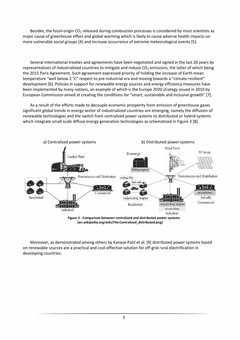
As a result of the efforts made to decouple economic prosperity from emission of greenhouse gases significant global trends in energy sector of industrialized countries are emerging, namely the diffusion of renewable technologies and the switch from centralized power systems to distributed or hybrid systems which integrate small-scale diffuse energy generation technologies as schematized in Figure 3 [8].
a) Centralized power systems b) Distributed power systems
Figure 3 - Comparison between centralized and distributed power systems [en.wikipedia.org/wiki/File:Centralized_distributed.png]
Moreover, as demonstrated among others by Kanase-Patil et al. [9] distributed power systems based on renewable sources are a practical and cost-effective solution for off-grid rural electrification in developing countries.

4
2.2. Hydro sector overview
2.2.1. General facts
Hydropower, together with biomass, is the renewable energy whose technology is more mature and reliable. It is a non-intermittent energy source capable of contributing both to base load and peak load (through building of a reservoir) and, for pumped plants, able to store energy. Hydropower technology has proved to be one of the most cost-effective, with long lifetime and reduced maintenance needs respect to other “green” generation technologies. Although varying depending on project characteristics, cost of energy produced through hydropower usually falls in the range between 50 to 100 USD/MWh, and additionally projects focused on upgrading existing plants can utterly increase cost-effectiveness (IEA Hydropower Report, 2010 [10]).
Large hydro plants have been built in Europe and USA since the end of 19th century, greatly contributing to the development of industrial sector and the electrification process. Nowadays big hydro facilities are still being built in many developing countries, while in industrialized ones most locations with ideal conditions have already been exploited and market for large-scale plants has almost reached saturation. However, current economic conditions and the impulse towards a CO2-free energy generation mix are leading to implementation of small scale hydro plants all over the world [11]. A pie chart representing the hydropower installed capacity by region as percentage of the total is displayed in Figure 4.
Moreover, as shown by Lahimer et al. [12] small hydro plants connected with stand-alone microgrids are seen as optimal solution to address challenge of rural electrification in many developing countries worldwide.
Figure 4 - Hydropower installed capacity by region (% of total) (adapted from [13])
Middle East & North Africa;
1.8%
North America; 17.5%
South America & The Caribbean;
14.8%
South & Central Asia; 6.6%
Africa; 1.5%
Southeast Asia & Pacific; 3.6% East Asia; 29.9%
Europe; 24.3%

5
However, a growing concern is being raised about negative environmental impact of hydropower installations. Namely, public acceptability relative to large facilities with annexed reservoirs worsened in many countries, since such plants are responsible for:
displacing communities previously dwelling in the reservoir area
interfering with local flora and fauna For instance, interrupting the periodical fish migration.
creating conflictuality E.g. disputes between neighboring countries or regions over the water usage of shared resources.
releasing large quantities of methane with high impact on greenhouse effect During the filling up of the reservoir vegetal species present in the submerging basin undergo anaerobic fermentation process. Such phenomenon was mainly analyzed by Fearnside [14] through field observation and calculations on big hydro projects implemented in Southern America.
2.2.2. Hydroelectric energy generation in Italy
As for Italy, until quite recent times (end of 1960’s) most of consumed electricity was generated by hydro sector before rapid growth of thermoelectric installed capacity became necessary to meet the growing demand due to rapid industrialization. As can be seen from Figure 5, from the 1970’s onward the production of electricity from fossil fuels has been growing steadily until 2008 when financial crisis caused a sudden decrease in demand. At the opposite side, in the same graph can be noticed that energy generation from hydro plants has remained almost unvaried from late 1960’s to 2012. Given the long life of such installations, it suggests that no significant increases in hydro production capacity have been made in such timeframe and the biggest contribution to hydro power generation comes from plants mostly installed along the first half of the 20th century.
Figure 5 - Cumulative graph of Energy production by source in Italy between 1887 and 2014 [15]
2.2.3. Hydroelectric energy generation in Portugal
According to data from APREN - Associação Portuguesa De Energias Renováveis (“Portuguese Association of Renewable Energy”) reported in Figure 6 the relative weight of hydropower production over electricity from fossil fuels in Portugal during last two decades is significantly higher than in Italy. What is in
0
50000
100000
150000
200000
250000
300000
350000
1887 1901 1915 1929 1943 1957 1971 1985 1999 2013
GWh / year
Year
Other renewables (wind, solar PV) Nuclear energy productionGeothermal energy production Thermal power plantsHydroelectric energy production

6
common between the two analyzed countries is the stable trend of hydropower production within the selected timeframe.
Figure 6 - Cumulative graph of energy consumption by source in Portugal per year [www.apren.pt/pt/dadostecnicos/index.php?id=267]
2.3. Categories of hydropower plants
Hydropower plants are commonly divided into categories according to the facility type and the range of
installed power. As for the first criteria, four different layouts are usually adopted:
Impoundment hydro plants having associated storage capacity (reservoir);
Run-of-River plants diverting part of river water flow to produce energy without any storage capacity or a limited one;
Pumped storage plants in which water from two reservoirs at different altitudes is either pumped or turbined according to the need of the grid, acting as energy storage facility;
In-stream hydropower schemes where flowing water is directly used to produce energy.
As for the plant size, several categories have been proposed:
Large Hydro definitions range significantly, from an installed power greater than 30MW in the USA or to 1.5MW in Sweden. A generally accepted definition from European Small Hydropower association classifies as “large” plants those with nominal power greater than 10MW;
Small Hydro with installed power in the range between Micro and Large Hydro;
Micro Hydro which generate less than 100kW of power;
Pico Hydro with less than 10kW of installed capacity.

7
2.4. Basic concepts of hydropower
Hydraulic machinery is specifically designed to convert energy of a fluid stream into rotating mechanical energy. Power output of a hydraulic machine is defined as:
𝑃 = 𝜂 𝑔 𝜌 𝐻 𝑄 (1)
where:
P: power output (W) η: machine efficiency (-) g: gravitational acceleration, equal to 9.81 (m/s2) ρ: fluid density (kg/m3) H: net head (m) Q: nominal flow rate (m3/s)
Hydraulic energy is usually expressed as head H with meters of equivalent water column height (m) as measure unit. The complete formulation is displayed in Equation (2) and accounts for contributions arising from fluid pressure, level and velocity.
𝐻 =
𝑝
𝜌𝑔+ 𝑧 +
𝑈2
2𝑔
(2)
where:
p: pressure (Pa) ρ: fluid density (kg/m3) g: gravitational acceleration, equal to 9.81 (m/s2) z: geometric height U: flow mean velocity (m/s)
Instead, to describe operations of hydrokinetic water turbines a notation is used similarly to that for wind turbines. The total kinetic power available is a function of flow velocity V (m/s), rotor cross-section S (m2) and fluid density:
𝑃(𝑊) =
1
2 𝜌 𝑆 𝑉3
(3)
According to the Betz limit, only 59% of kinetic energy can effectively be extracted. Such value is
commonly incorporated into a unique power coefficient Cp (-) which accounts also for mechanical and electric losses. Thus, the power at shaft of a real hydrokinetic turbine can be accounted as:
𝑃(𝑊) =
1
2 𝐶𝑝 𝜌 𝑆 𝑉3
(4)
Hydraulic machines can rely on different physical principles as they can be designed to generate power
from different fluid energy forms, namely:
kinetic energy (e.g. impulse turbines, hydrokinetic turbines)
pressure gradients (e.g. reaction turbines, Hydraulic Pressure Machines HPM)
gravitational potential energy (e.g. overshot waterwheels)

8
2.5. Turbomachinery affinity laws
In turbomachinery performance analysis affinity laws are widely used to express relationship existing between power and other interrelated parameters. The concept of specific speed (Ns) is used to distinguish families of geometrically similar machines, defined as follows:
according to discharge value, for pumps or turbines
𝑁𝑠, 𝑞 = 𝑁
√𝑄
𝐻3
4⁄
(5)
according to power, for turbines
𝑁𝑠, 𝑝 = 𝑁
√𝑃
𝐻5
4⁄
(6)
where:
N: rotational speed (rpm) H: available head (m) Q: flow rate (m3/s) P: power at shaft (kW)
For a family of geometrically similar pumps or turbines (i.e. having the same specific speed) it is possible to relate between them the main characteristic parameters through the following mathematical expressions [16]:
𝑄′
𝑄=
𝑁′
𝑁 (
𝐷′
𝐷)
3
(7)
𝐻′
𝐻= (
𝑁′
𝑁)
2
( 𝐷′
𝐷)
2
(8)
𝑃′
𝑃= (
𝑁′
𝑁)
3
( 𝐷′
𝐷)
5
(9)
According to the presented affinity law the efficiency at the BEP of any similar machine assumes a
constant value η independent from variations in rotational speed and impeller diameter, which isn’t fully representing real PAT behavior. In fact, as studied by Simpson and Marchi in 2013 [17] affinity laws “do not take into account factors that do not scale with velocity” and can possibly lead to inaccurate results with special regard to prediction of power.
However, despite the existence of alternative methods developed to predict behavior of similar PATs as the one recently proposed by Fecarotta et al. in 2016 [18] affinity laws are widely considered as a simple yet quite reliable method to be used in turbomachinery design.

9
2.6. Hydraulic energy converters
Apart from conventional water turbines, a large number of different hydraulic machines has been studied and/or implemented to generate energy exploiting fluid streams having low hydraulic energy. Such condition is generally due to low available heads (H) or reduced volumetric flows (Q), which is a common situation in many practical cases when installation of a traditional turbine unit would prove to be unfeasible or uneconomical. For instance, in 2005 Giesecke and Mosonyi [19] showed that in Europe only 30% of theoretically available hydropower potential remains unexploited, which is mainly constituted of sites with head drops in the range of 1-3 meters. Tidal water flows correspond to those characteristics, as well as the tens of thousands of locations across EU countries where in the past watermills were installed which nowadays remain unused [20]. Also, possibility of harvesting potential of water flowing in pipes or in open channels often depends on the availability of specifically designed equipment.
While large hydro plants around the globe are powered by conventional hydraulic turbines, for schemes with less than 100 kW of installed power a vast range of machinery is either available on the market or being studied. An overview of possible technologies is shown in Figure 7, and more accurate description of the main machine designs is contained in the following sub-chapters.
Figure 7 - Overview of hydropower technologies
Some of the presented technologies are known since antiquity (e.g. waterwheels), while other have been developed in recent times (e.g. HPM, Gravitational Vortex). Instead, most of achievements on conventional turbines design date back to the period between 19th and 20th century. An exemplary chart with application ranges of some hydro converters technologies is shown in Figure 8.

10
Figure 8 - Application chart for some unconventional low-power hydro machinery (adapted from [21], [22], [23])
2.6.1. Pressurized flows
2.6.1.1. Hydraulic turbines
Hydraulic turbines are commonly divided into two categories:
impulse (or “action”) turbines, powered by free jets at atmospheric pressure;
reaction turbines, operating within pressurized flows.
From the 19th century on several turbine models have been designed and industrialized, belonging both to the impulse or reaction class. A visual representation of main water turbine runner types is shown in Figure 9.
Figure 9 - Most common water turbine runner types [24]

11
An overview of turbine types and application ranges is presented in Table 1. Formula describing the specific rotational speed Ns,p is given in Equation (6) at page 8.
Table 1 - Overview of hydraulic turbine types and application ranges (adapted from [11])
Hydraulic turbines H (m) Q (m3/s) P (kW) Ns,p
Reaction Bulb 2-10 3-40 100-2500 200-450
Kaplan and Propeller
2-20 3-50 50-5000 250-700
Francis, high Ns
10-40 0.7-10 100-5000 100-250
Francis, low Ns
40-200 1-20 500-15000 30-100
Action Pelton 60-1000 0.2-5 200-15000 < 30
Turgo 30-200 - 100-6000 -
Crossflow 2-50 0.01-0.12 2-15 -
An indicative application chart relative to low-to-medium power conventional hydraulic turbines is
hereby presented in Figure 10.
Figure 10 - Indicative turbine selection chart (adapted from [25])
Besides traditional turbines, other noticeable and promising technologies include Pumps as Turbines (PATs), Positive displacement machines and in-pipe propellers.

12
2.6.1.2. Pumps as Turbines (PATs)
Pumps as Turbines (PATs) are an unconventional solution for hydro power generation adapt to fit in many scenarios when a conventional turbine unit would not be suitable. Physical behavior of PATs is similar to Francis turbines, but without possibility for flow regulation. A representation of centrifugal PAT is shown in Figure 11.
Figure 11 - Drawing of centrifugal PAT [csmres.co.uk/cs.public.upd/article-images/Fig-3-55016.jpg]
The first industrial use of PATs regarded very specific application fields, namely big units for equipping pumped hydro plants and small units to recover energy from high pressure fluid streams in chemical industries [26]. Instead, within last decades large numbers of PATs have been studied and implemented as power generators in many contexts like small hydropower schemes with low-head properties, water supply systems (WSS) and industrial applications as replacements of throttling valves. In particular, they proved to be very effective if used for micro hydro off-grid plants and in-pipe energy recovery [27], [12].
The use of PATs proved to have several advantages over other turbine types:
generator units composed of pump and shaft-connected induction motor present more compact dimensions than most conventional solutions;
mass manufacturing of pumps makes them easily available in large number of standard sizes and characteristics, suitable to most application cases;
short delivery time;
they present easy installation, operation and maintenance and relative spare parts are easily available;
they have a longer life span with respect to other small-size hydraulic turbines as shown by Williams [27];
the capital requirements needed to cover investment costs are generally lower than traditional turbines which are built as unique units according to site specifications [28];
they are a widely studied technology with proven results [29].
Despite the above mentioned positive aspects, two major challenges need to be overcome to allow for a wider application of PAT technology:
normally producers don’t provide customers with PAT turbine characteristic charts, thus analytical methods need to be applied to estimate them as shown in Chapter 2.7.2.1. However, predictions based on mathematical models could lead to significant errors on head and discharge properties, up to 20% as demonstrated by Singh [26];
due to the rigid geometric configuration of volute case and impeller, centrifugal pumps do not offer possibility for flow rate regulation. As a result, they are characterized by poor part-load performances.

13
2.6.1.3. Positive Displacement machines
Positive Displacement (PD) machines are a type of volumetric machines in which mechanical energy is transferred to or from a fixed portion of working fluid which is confined temporarily inside vanes of changeable geometry. They can be based on either reciprocating or rotary machinery, and they are considered as “constant flow machines” since the net fluid head difference between suction and discharge side do not affect the designed flow rate that can be processed. A visual representation of a PD machine (Lobe pump) is reported in Figure 12.
Figure 12 - Visual representation of a PD machine (Lobe pump) [30]
A 2010 study by Simão and Ramos [21] based on CFD analysis showed that PD machines have an interesting potential when used as hydraulic turbines, and are able to process quite small flows under high head conditions while maintaining an appreciable efficiency (estimated as 87%).
Also a paper by Phommachanh et al. published in 2006 [31] investigated Positive Displacement water turbines and confirmed their suitability for micro-hydropower schemes especially when a low specific speed is required.
2.6.1.4. In-pipe propellers
In order to overcome the commercial unavailability of specifically designed in-pipe micro hydro generators, in the context of HYLOW project (EU’s Seventh Framework Programme, 2007-2013) small four and five blade propeller turbines were developed as shown in the work by Ramos et al. [32] published in 2012. As furtherly investigated by Caxaria et al. [29], such unit connected with a DC permanent magnets generator proved to be viable for installation inside main water pipes or by-pass ducts. A picture of the tested propeller is shown in Figure 13.
Figure 13 - New proposed design of in-pipe propeller [33]

14
2.6.2. Open channel flows
2.6.2.1. Waterwheels
Several machine designs are suitable to exploit open-air water streams. Some of these have a fairly old history, while others have been invented in recent years. The concept of waterwheels has been known for centuries, as they were widely built and deployed all over the European continent since the Middle Ages. Technology of waterwheels was greatly improved during the industrial revolution thanks to the progresses made in hydraulics and materials science; nevertheless along the 20th century they lost importance as power generation units and were progressively dismantled or abandoned [34]. Over the tens of thousands of waterwheel installations present in Europe between 19th and 20th centuries only a few survived up-to-date as shown by Müller et al. [35].
Three types of waterwheel exist: overshot, breastshot and undershot waterwheel. Main features of each category are presented in Table 2.
Table 2 - Overview of waterwheel types [23]
Waterwheel Type Head difference H
(m) Flow rate per unit width q
(m2/s)
Overshot 2.5 to 10 0.1 to 0.2
Breastshot 1.5 to 4 0.35 to 0.65
Undershot or “Zuppinger”
0.5 to 0.25 0.5 to 0.95
2.6.2.2. Hydrostatic pressure wheels
A Hydrostatic pressure wheel operates because of the difference in static pressure from upstream to downstream occurring in a water body when a drop in fluid level is present. Pressure acts on a vertical surface immersed in water with a depth h (m) as the hydrostatic pressure distribution shown in Figure 14, of which vectors can be calculated as:
𝑝 = 𝜌 𝑔 ℎ (10) where:
p: relative pressure (Pa) ρ: fluid density (kg/m3) g: gravitational acceleration (m/s2)
Figure 14 – Hydrostatic pressure distribution on a vertical surface immersed in fluid

15
When there is a change in water level between contiguous upstream and downstream zones, the hydrostatic force applied to the vertical surface (e.g. weir) dividing the two corresponds to:
𝐹 = 𝜌 𝑔 (ℎ1 − ℎ2) (11)
where:
F: force acting on weir (N) ρ: fluid density (kg/m3) g: gravitational acceleration (m/s2) h1: upstream water level (m) h2: downstream water level (m)
Examples of machine relying on hydrostatic pressure are Staudruckmaschine (SDM) and Hydrostatic
Pressure Wheel and Machine (HPW and HPM) presented in Chapter 6.7.
2.6.2.3. Hydrokinetic turbines
Hydrokinetic turbines are designed to generate power by exploiting the kinetic energy possessed by a fluid. As reviewed by Kahn et al. [36], the field of application of such turbines is extremely wide since they have been designed for inland water bodies (e.g. rivers or irrigation channels) or offshore resources (tidal currents, sea waves). A multitude of designs have been tested, the great majority of which are Vertical and Horizontal axis water turbines as stated by Lago et al. [37]. A visual representation of such systems is shown in Figure 15 and Figure 16.
Figure 15 - Horizontal axis water hydrokinetic
turbines (HAWT) [36]
Figure 16 - Vertical axis water hydrokinetic turbines (VAWT)
[36]

16
Another relevant design comprises the construction of a pool with cylindrical or conical section used to create an artificial gravity-driven vortex in entering water. In correspondence of bottom outlet a turbine can be placed to harvest kinetic energy of entrained water, and such technology is often referred to as Gravitational Vortex Hydropower (GVHP). As studied by Power et al. [38], such micro hydro plants could be suitable for Run-of-River schemes or to be implemented within water or wastewater networks.
A representation of whirling pool and turbine is shown in Figure 17.
Figure 17 - Schematic view of GVHP [en.wikipedia.org/wiki/Gravitation_water_vortex_power_plant]
2.6.2.4. Archimedes screws
As stated by Stergiopoulou et al. [39], a whole new generation of hydropower converters based on Archimedean screw principle is emerging and being studied. Inspired by a technology dating back to 23 centuries ago for uplifting water, such machines feature a spiral screw design and are potentially suitable for exploiting sites with available head in the range of 1 to 5 m. Also, a version has been proposed to be fitted on floating platforms to harvest kinetic energy from flowing water. Renderings of such devices are shown in Figure 18.
a) Archimedean inclined turbine b) Archimedean floating horizontal hydrokinetic converter
Figure 18 - Representations of inclined Archimedean Screw turbine and horizontal floating Archimedean converter [39]

17
2.7. PAT background and applications
Centrifugal pumps for water applications are a widely used and mass produced in many countries around the world. First mentions of the possibility of using pumps as turbines (PAT) dates back to the early 1930s and are associated to lab experiments performed by Thoma and Kittredge [40] who first found out that common pumps could work quite efficiently as turbines by reversing the flow.
New impulse to research came from some pump manufacturing industries after the second half of 20st century, which established collaborations with several research institutes in order to gain an in-depth understanding on phenomena associated to PAT utilization. Particular efforts were made to develop methods to predict characteristic curve and efficiency at Best Efficiency Point (BEP) of machines in turbine mode related to its specifications when used as a pump [26]. Due to differences in flow turbulence and friction losses, the working point having highest efficiency in pump mode will differ significantly from the location of BEP in turbine mode. Hydraulically, a PAT will be able to process a bigger flow rate that respect to conventional pumping operations.
A graphical representation of typical performance curves for a centrifugal pump in both operation modes is shown in Figure 19.
Figure 19 - Typical performance curves of pumps and turbines [28]
Conventionally, characteristic nondimensional curves of turbomachinery are created introducing three composite parameters:
Ψ =
𝑔𝐻
𝑛2𝐷2 Φ =
𝑄
𝑛𝐷3 𝜋 =
𝑃
𝜌𝑛3𝐷5
(12)
where:
n: rotational speed (rps) g: gravity acceleration (m/s2) Q: flow rate (m3/s) H: hydraulic head of fluid (m) P: power at shaft (kW) D: impeller diameter (m) ρ: fluid density (kg/m3)

18
An example of PAT nondimensional characteristic curve in turbine and pump mode is hereby presented in Figure 20.
Figure 20 - Nondimensional characteristic curve of PAT (adapted from [41])
2.7.1. Quadrant operations of PAT
As described by Baumgarten et al. [42], the operational area of a pump can be divided into four sectors according to the shaft rotational velocity (N) and the flow rate processed (Q) as appears in the following Figure 21. The signs are conventionally positive when referring to design pumping operations.
Figure 21 – Four quadrants operations of a radial flow PAT (adapted from [42])
0
5
10
15
20
25
-1 -0.5 0 0.5 1
ψ
Φ
Turbine mode Pump mode
Legend: N: rotational speed (rpm) Q: flow rate (m3/s) H: hydraulic head of fluid (m) T: torque at shaft (Nm)

19
The first quadrant refers to normal pumping operations, with positive N, Q, H and applied resistant torque T. However, in the third quadrant the same machine is being operated as turbine by reversing intentionally the flow (-Q): in that case if the available head H is sufficient to overcome the resisting torque T it enables the connected motor/generator unit to produce energy by rotating the shaft at velocity equal to –N.
Figure 22 represents the characteristic curves of a PAT transposed to the H-Q space. It is evident the influence of rotational speed on the operating curves in both turbining and pumping mode for a centrifugal pump. Also, as stated by Singh [26] it can be noticed that turbine operations are limited to an area comprised between “zero-speed” configuration (N=0) and “no-load line”, with the latter corresponding to runaway characteristic (M=0). The runaway condition is one of the major areas of concern when designing a PAT installation, since the increase in impeller velocity could cause water hammer phenomenon representing a risk for penstock and hydraulic machine integrity [26].
Figure 22 - Characteristic curves for Turbine and Pump operations of a variable speed PAT (adapted from [42])
2.7.2. PAT performance prediction
2.7.2.1. Mathematical methods
As stated in Chapter 2.6.1.2. at Page 12, one of the major obstacles to widespread PAT adoption is the little information available regarding turbine operations of commercially available pumps. To overcome such limitation a series of methods have been proposed by various authors. As reviewed by Agarwal [43] and Nautiyal [44], several mathematical methods exist to correlate H-Q coordinates of BEP between pump and turbine mode based on maximum efficiency and specific speed Ns described in Paragraph 2.5.

20
Four nondimensional coefficients relating BEP characteristics in turbine or pump mode have been proposed:
ℎ =
𝐻𝑡,𝐵𝐸𝑃
𝐻𝑝,𝐵𝐸𝑃 𝑞 =
𝑄𝑡,𝐵𝐸𝑃
𝑄𝑝,𝐵𝐸𝑃 𝑝 =
𝑃𝑡,𝐵𝐸𝑃
𝑃𝑝,𝐵𝐸𝑃 𝜆 =
𝜂𝑡,𝐵𝐸𝑃
𝜂𝑝,𝐵𝐸𝑃
(13)
As demonstrated experimentally by Derakhshan et al. [41], the nondimensional parameters above vary
considerably when considering PATs with different specific speed as shown in Figure 23.
Figure 23 - Nondimensional BEP parameters for PATs having different specific speed [41]
Within his PhD dissertation in 2005 Singh [26] reviewed the main existing methods to obtain values of h and q, of which the most commonly used are summed up in Table 3.
Table 3 - Review of methods to determine nondimensional head and flow parameters (adapted from [15])
Method h q
Stepanoff 1
𝜂𝑡,𝐵𝐸𝑃 𝜂𝑝,𝐵𝐸𝑃
1
𝜂𝑝,𝐵𝐸𝑃
Gopalakrishnan 1
(𝜂𝑝,𝐵𝐸𝑃)2
1
𝜂𝑝,𝐵𝐸𝑃
Childs 1
(𝜂𝑝,𝐵𝐸𝑃)2
1
(𝜂𝑝,𝐵𝐸𝑃)2
Sharma 1
(𝜂𝑝,𝐵𝐸𝑃)1.2
1
(𝜂𝑝,𝐵𝐸𝑃)0.8
Alatorre-Frenk 1
0.85 𝜂𝑝,𝐵𝐸𝑃5 + 0.385
0.85 𝜂𝑝,𝐵𝐸𝑃
5 + 0.385
2 𝜂𝑝,𝐵𝐸𝑃9.5 + 0.205
Nautiyal [44] 41.667𝜂𝑝,𝐵𝐸𝑃 − 0.212
𝑙𝑛(𝑁𝑠,𝑞,𝑝𝑢𝑚𝑝)− 5.042 30.303
𝜂𝑝,𝐵𝐸𝑃 − 0.212
𝑙𝑛(𝑁𝑠,𝑞,𝑝𝑢𝑚𝑝)− 3.424
Grover 2.693 − 0.0229 𝑁𝑠,𝑞,𝑡𝑢𝑟𝑏𝑖𝑛𝑒 2.379 − 0.0264 𝑁𝑠,𝑞,𝑡𝑢𝑟𝑏𝑖𝑛𝑒

21
In their paper published in 2008, Derakhshan and Nourbakhsh [41] developed a method to correlate BEP of a PAT to its pump mode characteristics after experimental testing of four centrifugal pumps. Such method is restricted to low-specific speed pumps (Ns,q,pump < 60) and consists of a series of steps:
1. calculate the specific speed of ideal PAT in turbine mode Ns,p,turbine as described in Paragraph 2.5. at Page 8, knowing the working point in turbine mode (Q, H), setting the turbine ηt,BEP and selecting the desired rotational speed N;
2. obtain the specific speed of pump Ns,q,pump through the following correlation:
𝑁𝑠,𝑞,𝑝𝑢𝑚𝑝 = 0.3705 𝑁𝑠,𝑝,𝑡𝑢𝑟𝑏𝑖𝑛𝑒 + 5.083 (14)
3. a dimensionless parameter, γ, can be calculated from pump specific speed:
𝛾 = 0.0233
𝑁𝑠,𝑞,𝑝𝑢𝑚𝑝
𝑔0.75+ 0.6464
(15)
4. if the shaft rotational velocity in pump mode equals the velocity in turbine mode, the following
relationship can be established between γ and the nondimensional head ratio h:
ℎ =
1
𝛾2
(16)
5. after obtaining Hp,BEP by dividing Ht,BEP into h, knowing the rotational velocity N and the specific
speed Ns,q,pump is possible to obtain the adimensional flow parameter q to be compared with the ones obtained through other methods as described in the previous Equations (8).
6. Since the behavior of geometrically similar PATs having different impeller diameter D can differ significantly, the authors proposed three additional correlation factors based on experimental results:
ℎ𝑛𝑒𝑤 = ℎ (
0.25
𝐷)
14⁄
𝑞𝑛𝑒𝑤 = 𝑞 (0.25
𝐷)
16⁄
𝑝𝑛𝑒𝑤 = 𝑝 (0.25
𝐷)
110⁄
(17)
2.7.2.2. Numerical methods (CFD analysis)
As demonstrated by Carravetta et al. [45] and Páscoa et al. [46], Computational Fluid Dynamics (CFD) analysis can be an useful tool for prediction of PAT turbine mode characteristics. In spite of its potentially high computational complexity, it also enables analysis of machine operations under transient hydraulic conditions.
Besides, as stated by Singh [26] and Bogdanović-Jovanović et al. [47], CFD analysis allows for evaluating how internal pressure losses are distributed along the PAT control volume. Such knowledge is extremely valuable in order to identify possibilities for performance optimization as rounding the inlet impeller or enlarging the suction eye.

22
3. Water-Energy Nexus
_______________________________________________________________________________________
3.1. Introduction
The term Water-Energy Nexus (WEN) refers to the relationship between the use of water for energy production and the efforts necessary to collect, treat, and transport water. It’s been a subject of growing interest in academic and industrial contexts along last decades, with efforts aimed at acquiring an integrated and systemic view on the two sectors (water – energy).
As shown, water plays a key role in the energy production portfolios worldwide. Not only hydropower is the most exploited renewable energy source around the globe, but every thermal power plant (both relying on fossil fuels or nuclear fission) requires significant amounts of water to cool down working fluids and perform efficient thermodynamic cycles. Also, satisfying irrigation needs is fundamental for growing crops which provide food or biofuels. At the same time, water companies consume substantial amounts of energy to ensure a safe, reliable and environmental-friendly water supply to the served consumers.
Given the strong relationship between the two sectors it stands out prominently the importance of moving towards innovative integrated systems in which the management of water resources for energy purposes and human consumption matches [48]. At the present time investigations on the Water-Energy Nexus are being carried out by various institutions and companies around the globe, and focus on different solutions ranging from large to small scale. An overview of the state-of-the art is presented in the following subchapters.
3.2. WEN on large scale: from hundreds of kWs to MWs
A well-known example of Water-Energy Nexus on a large scale is the common practice of building artificial reservoirs with dual purpose, able to supply water to nearby communities and feed hydro power plants in a way which is reliable and independent from hydrologic regimes. A recent example of such approach is the Alqueva Multi-purpose Project in the Alentejo region of Portugal. Built in two phases (I and II) and completed in 2013, it consists in the creation of an artificial lake with around 250km2 of surface along Guadiana river whose waters supply a 520MW power station besides satisfying needs for water supply and irrigation over a large territory [49]. A picture of the Alqueva arch dam is shown in Figure 24.
Figure 24 - Alqueva concrete gravity dam (https://en.wikipedia.org/wiki/Alqueva_Dam)

23
Another innovative solution for large-scale integrated systems is the implementation of WSS having water reservoirs located at different altitudes and featuring a set of pumps and hydraulic turbines along the conveying pipes. Such a scheme can effectively be coupled with intermittent renewable energy sources like wind turbines or PV panels in order to build interconnected power and water supply systems as investigated by Gonçalves et al. in 2010 [50]. During periods when natural resources are available (e.g. wind and sun irradiation) the produced clean energy would be utilized to satisfy demand of water company and/or pump liquid to the upper reservoirs. On the opposite, water can be turbined to lower reservoirs in case of energy needs or during peak hours in which electricity tariffs are higher. The main resulting advantages of such arrangement are:
a high system flexibility and reliability, allowing an optimal use or natural resources (water, wind and sun);
a potential reduction of energy bills faced by water companies;
creation of an energy storage capacity which can enable a higher penetration of renewables into the local energy mix.
Example of such a system is the Multi-purpose Socorridos System in the Portuguese Island of Madeira. It became operational in 1994 and was designed to accomplish multiple tasks: supply water to municipalities of Funchal and Camara de Lobos, produce electricity and regulate irrigation. Based on a pumped and hydropower station coupled with reservoirs at different levels, it enables an optimal resource use overcoming the difficulties due to unbalanced demand of resources. For instance, water demand for drinking and agricultural needs peaks during the summer and remains lower along the rest of the year, and at the same time energy production from wind generators is subject to daily oscillations. An in-depth analysis on the cited system can be found in the manual “Pump and Hydropower systems” by Ramos [51].
3.3. WEN on medium scale: from hundreds of Ws to kWs
3.3.1. General facts
On a medium scale, growing interest is been raised on exploiting water for drinking or irrigation purposes flowing in pipes or channels to produce electricity. Such approach presents several advantages:
generally lower infrastructure costs respect to a standard hydro plant No dams or extensive civil works are needed.
energy generated from water networks is constant in time and easily predictable respect to other renewable sources
Patterns of water consumption are cyclically repeated on daily bases instead of being dependent on hydrological regimes.
it can significantly contributes to the reduction of costs faced by water utilities
it would result in a CO2-free and not pollutant energy source, lowering the dependence from fossil fuels
peaks of daily demand of water and energy from standard residential or industrial areas generally present a good matching
During hours of higher demand for electricity the demand for water is also high and vice versa. In the following Figure 25a is shown a typical dimensionless average water load curve. Instead, Figure 25b shows the demand for electrical power along a typical weekday relative to Italy. As can be noticed, the matching of the two hourly profiles is quite evident.
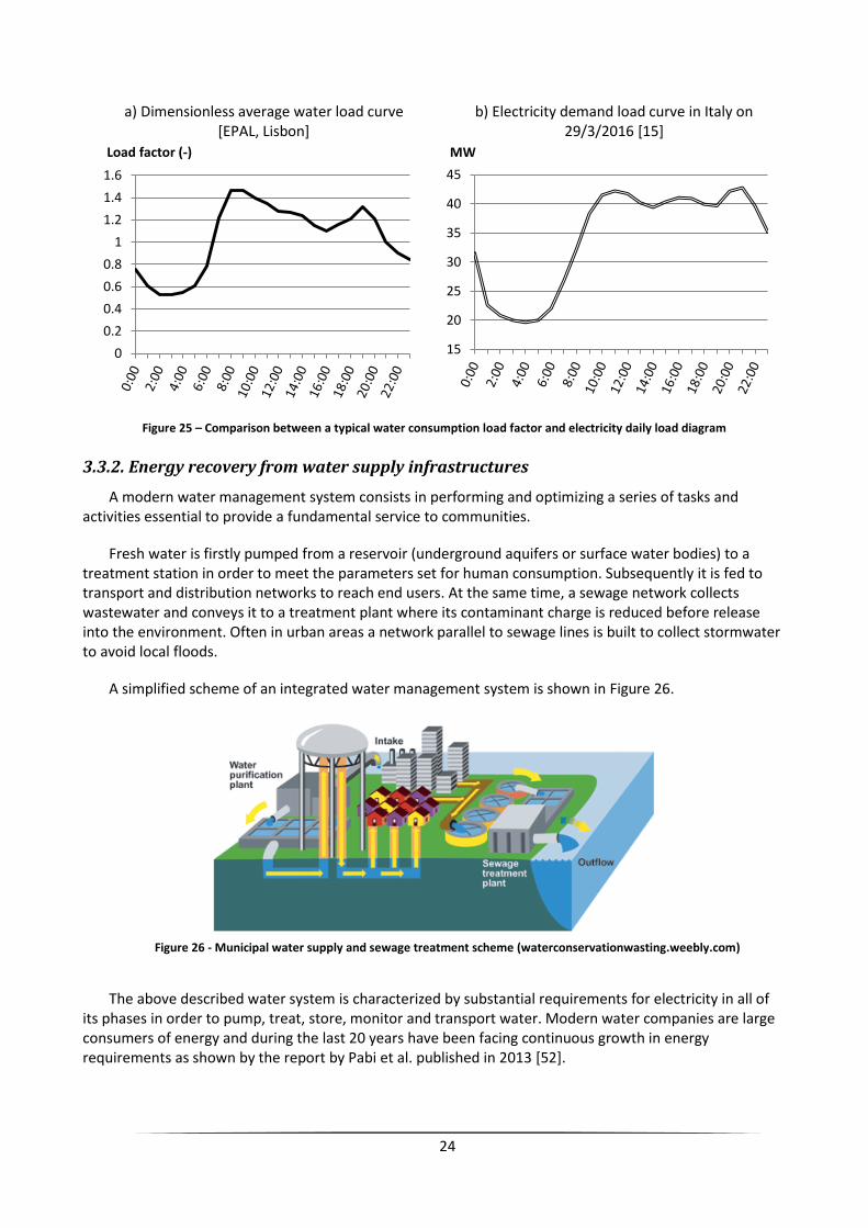
24
a) Dimensionless average water load curve [EPAL, Lisbon]
b) Electricity demand load curve in Italy on 29/3/2016 [15]
Figure 25 – Comparison between a typical water consumption load factor and electricity daily load diagram
3.3.2. Energy recovery from water supply infrastructures
A modern water management system consists in performing and optimizing a series of tasks and activities essential to provide a fundamental service to communities.
Fresh water is firstly pumped from a reservoir (underground aquifers or surface water bodies) to a treatment station in order to meet the parameters set for human consumption. Subsequently it is fed to transport and distribution networks to reach end users. At the same time, a sewage network collects wastewater and conveys it to a treatment plant where its contaminant charge is reduced before release into the environment. Often in urban areas a network parallel to sewage lines is built to collect stormwater to avoid local floods.
A simplified scheme of an integrated water management system is shown in Figure 26.
Figure 26 - Municipal water supply and sewage treatment scheme (waterconservationwasting.weebly.com)
The above described water system is characterized by substantial requirements for electricity in all of its phases in order to pump, treat, store, monitor and transport water. Modern water companies are large consumers of energy and during the last 20 years have been facing continuous growth in energy requirements as shown by the report by Pabi et al. published in 2013 [52].
0
0.2
0.4
0.6
0.8
1
1.2
1.4
1.6
Load factor (-)
15
20
25
30
35
40
45
MW

25
As reviewed by McNabola et al. in 2014 [53], micro-hydropower schemes are an effective solution for energy recovery from WSS and several researches carried out in the past highlighted a series of recurrent situations within water networks from which energy can potentially be recovered:
excessive pressure in correspondence of inlet ducts leading into storage reservoirs Normally, elevated water storage tanks are maintained at atmospheric conditions but are fed with pressurized water.
excessive pressure within gravity-fed water conveyance pipes In order to avoid high pressure levels to be attained inside water transport pipes is a common practice to insert Break Pressure Tanks (BPT) to dissipate the energy excess. Such systems could effectively be replaced by a conventional turbine, a PAT or a hydrokinetic converter inserted within pipes. For instance, the USA-based Lucid Energy company developed a specific turbine to be placed within large gravity-fed water transport pipes [54]. The so-called LucidPipe™ power system consists in a pipe section with pre-installed turbine (hydrokinetic, vertical-axis type) and generator unit that can be inserted along a main existing transport line as shown in Figure 27.
Figure 27 - LucidPipe™ power system [54]
substitution or replacement of Pressure Reducing Valves (PRVs) with PATs One of the main focuses of water companies is to guarantee along all pipe networks a sufficient pressure to reach consumers and avoid contamination. Anyway, situations can occur in which water flowing in a determined pipe branch possesses an excess energy respect to the desired level. Such a case is schematically shown in Figure 28.
Figure 28 - Basic scheme of WSS having pipe branches holding excess water pressure
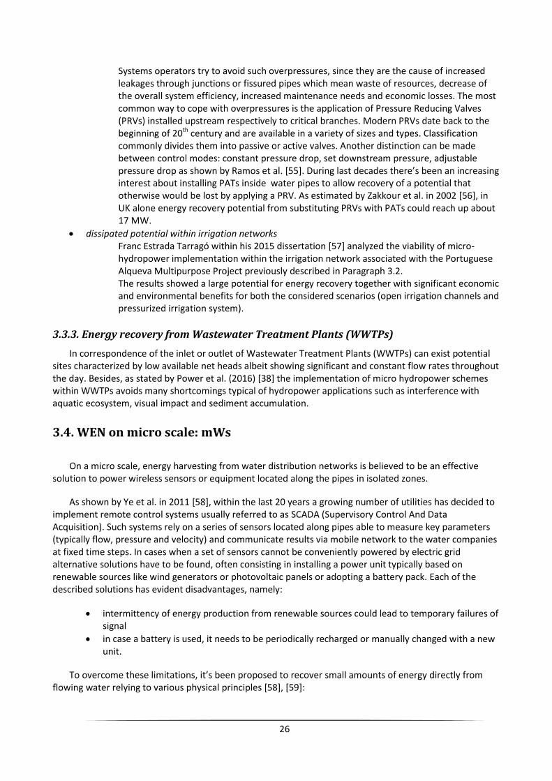
26
Systems operators try to avoid such overpressures, since they are the cause of increased leakages through junctions or fissured pipes which mean waste of resources, decrease of the overall system efficiency, increased maintenance needs and economic losses. The most common way to cope with overpressures is the application of Pressure Reducing Valves (PRVs) installed upstream respectively to critical branches. Modern PRVs date back to the beginning of 20th century and are available in a variety of sizes and types. Classification commonly divides them into passive or active valves. Another distinction can be made between control modes: constant pressure drop, set downstream pressure, adjustable pressure drop as shown by Ramos et al. [55]. During last decades there’s been an increasing interest about installing PATs inside water pipes to allow recovery of a potential that otherwise would be lost by applying a PRV. As estimated by Zakkour et al. in 2002 [56], in UK alone energy recovery potential from substituting PRVs with PATs could reach up about 17 MW.
dissipated potential within irrigation networks Franc Estrada Tarragó within his 2015 dissertation [57] analyzed the viability of micro-hydropower implementation within the irrigation network associated with the Portuguese Alqueva Multipurpose Project previously described in Paragraph 3.2. The results showed a large potential for energy recovery together with significant economic and environmental benefits for both the considered scenarios (open irrigation channels and pressurized irrigation system).
3.3.3. Energy recovery from Wastewater Treatment Plants (WWTPs)
In correspondence of the inlet or outlet of Wastewater Treatment Plants (WWTPs) can exist potential sites characterized by low available net heads albeit showing significant and constant flow rates throughout the day. Besides, as stated by Power et al. (2016) [38] the implementation of micro hydropower schemes within WWTPs avoids many shortcomings typical of hydropower applications such as interference with aquatic ecosystem, visual impact and sediment accumulation.
3.4. WEN on micro scale: mWs
On a micro scale, energy harvesting from water distribution networks is believed to be an effective
solution to power wireless sensors or equipment located along the pipes in isolated zones.
As shown by Ye et al. in 2011 [58], within the last 20 years a growing number of utilities has decided to implement remote control systems usually referred to as SCADA (Supervisory Control And Data Acquisition). Such systems rely on a series of sensors located along pipes able to measure key parameters (typically flow, pressure and velocity) and communicate results via mobile network to the water companies at fixed time steps. In cases when a set of sensors cannot be conveniently powered by electric grid alternative solutions have to be found, often consisting in installing a power unit typically based on renewable sources like wind generators or photovoltaic panels or adopting a battery pack. Each of the described solutions has evident disadvantages, namely:
intermittency of energy production from renewable sources could lead to temporary failures of signal
in case a battery is used, it needs to be periodically recharged or manually changed with a new unit.
To overcome these limitations, it’s been proposed to recover small amounts of energy directly from flowing water relying to various physical principles [58], [59]:

27
kinetic energy By installing a microturbine in a pipe by-pass or in a side pipe and releasing water to the surroundings.
heat flow Through implementation of micro generators based on thermoelectric Seebeck effect which produce electricity from the temperature gradient between water and external air.
pressure fluctuations
For the present dissertation I decided to focus on small-to-medium scale WEN and investigate opportunities for energy generation from WSS studying three existing study-cases.
3.5. WSS sector in Italy: an overview
In Italy integrated water supply systems are operated by private or public companies under the supervision of regulatory authorities. The Law 36/94 established the sub-division of Italian territory in units called ATO – Ambito Territoriale Ottimale (“Optimal territorial area”) setting the geographical limits of local integrated urban water management systems. Each of such land units is supervised by an Autorità d’Ambito (“Territorial Authority”), institution with legal personality which organizes, confides and controls integrated water systems representing collective interest and regulating the existing natural monopoly.
Besides, any Autorità d’Ambito has to elaborate a master plan defining:
quality standard goals and minimum levels of service, in accordance with national legislation;
level of investments required to achieved the defined targets;
optimization of the tariff system to ensure remuneration of utilities and promote improvements in efficiency and service quality;
policies regarding resources saving and environment protection.
The Law n. 42 approved by Italian Parliament on 26/3/2010 [60] set the path for gradual abolition of ATO and Territorial Authorities over the entire national territory, attributing their duties and peculiarities to regional administrations. Nevertheless, as on 2016 the regime of ATO is still actual as a result of several accorded postponements.
The Piedmont administrative region (north-west Italy) is currently divided into six ATOs: ATO1 - Verbano, Cusio, Ossola, Pianura, Novara ATO2 – Biellese – Vercellese - Casalese ATO3 – Torinese ATO4 – Cuneese ATO5 – Astigiano, Monferrato ATO6 – Alessandrino
Collaboration with staff of ATO5 has been vital for the purpose of writing the present dissertation.

28
4. Case-study 1: Scurzolengo water tower
_______________________________________________________________________________________
4.1. Context description
In collaboration with water company CCAM, the opportunity for energy recovery from inlet of an
elevated water tank was evaluated.
The Consortium of Commons for the Monferrato Aqueduct (CCAM) manages integrated water services for 101 member municipalities in the provinces of Asti, Alessandria and Torino covering an area of about 1200 km2. A map showing the territorial extension of the aqueduct network is shown in Figure 29.
Figure 29 - Territorial extension of the Monferrato Aqueduct. In red is marked the main pipes network [61]
The territory served is hilly and non-homogeneous, and until the beginning of 20th century its population could mainly rely on rainwater collection and storage to satisfy its needs. The scarce hygienic features of such systems were the main responsible for endemic Typhus diffusion, causing high death toll between young and old people. To improve living conditions constructions of an aqueduct was initially planned during years 1913-1916, but the outbreak of WWI caused the abandonment of plans.
Eventually works to build the Monferrato water supply system could only retrieve in 1929 and lasted for three years, employing more than 1000 workers without the help of any mechanical excavator. Official inauguration took place on 25th October 1932 at the medieval stronghold of Verrua Savoia [62]. In Figure 30 and Figure 31 are shown historical images relative to aqueduct construction.

29
Figure 30 - Picture portraying the laying of one of the
main water pipes [62]
Figure 31 - A water jet directed vertically during aqueduct
inauguration ceremony on 25th
October 1932 [62]
4.2. General facts about water towers
As stated by Twort et al. [63], within any water supply system there are three basic needs:
delivering to all consumers safe drinkable water
Key factor to reach such target is maintaining in all conditions a minimum pressure within
pipes in order to supply consumption point located at highest geographical altitude and at
the same time avoid contaminants entering the system which could occur in case of sudden
pressure drops.
assure reliability of the supply
A well designed water network must be capable of granting a continuous supply even in
cases of component failure (pipes, pumps) or power cut.
reduce level of investments necessary to build and maintain the system
As seen from the previous Figure 25 at Page 24, normally water consumption in residential
areas isn’t uniform throughout the day but has peaks during early morning and late evening
and deep valleys during night time. As a result, designing pipes and pumps of a water
supply system according to maximum values of consumption would result in high capital
needs and oversized infrastructures along most of the operational time.
The most adopted and intuitive solution to meet such requirements is to connect the pipe network with an elevated storage tank, which can maintain the system pressurized and supply water even in case of power cut thanks to gravity action. Also, water from water tank can be used as a local source of water to supply demand peaks (e.g. high morning and evening demand, or need to feed fire hoses during an emergency) so that the pumping and distribution sections can be designed according to average water demand instead of maximum values.

30
So, besides ensuring resilience to the network the introduction of treated water storage capacity can reduce life cycle costs by allowing pumps to operate near to design duty point and in periods of low demand when ideally also electricity tariffs are lower. Hence, optimization can be performed to select optimal working time of pumps and significantly reduce the energy bill paid by utilities. Example of an approach to pump operation optimization has been proposed by Teresa Salvador using Genetic Algorithms [64], showing a significant potential.
In areas of flat topography an artificial elevated water tank has to be built, commonly referred to as “water tower”. Since second half of 19th century water towers started being built in main European and American cities, and nowadays they are very common and distinctive infrastructures that can easily be found in flat inhabited areas.
4.3. Scurzolengo water tower
The concrete-made water tower analyzed within this research is located in the area of Scurzolengo municipality in Asti administrative region, Italy. It is situated on a hilltop at altitude of 265 m AMSL (Above Mean Sea Level) and stands out of the ground for 24 m. The conic tank capacity is equal to 250 m3 with a maximum inner water height of 3.97 m.
The current regulation method relies on a self-driven valve which opens when water level lowers below 3.55 m and closes when the tank is filled according to the data received from a floating water level sensor placed inside the reservoir. The following Figure 32 and Figure 33 show respectively a view of the water tower from outside and a screenshot of SCADA remote control system visualizing parameters of inlet flow and water level inside the tank as seen from control room.
Figure 32- Picture of Scurzolengo water tower [www.panoramio.com/photo/17862015]
Figure 33 - SCADA view of flow and water level parameters
The daily water consumption of users served by Scurzolengo water tower varies from around 200 m3/day during winter months up to 400 m3/day in summer.

31
The set of sensors to control remotely water tower parameters consists in:
a pressure measuring sensor installed in the inlet pipeline at the basis of the water tower during winter 2015/2016;
a floating device to measure water level in the reservoir;
a water meter which measures the inlet flow.
A sample of pressure and flow parameters is recorded every 15 min and can be observed in real-time by the facilities of the Monferrato aqueduct control room located in the municipality of Moncalvo. Within the stipulated agreement a database containing data from all three sensors covering the timeframe of a week between Tuesday 9th of February 2016 and Monday 15th of February of the same year could be accessed. In the following Figure 34 and Figure 35 are presented diagrams of inlet water flow, upstream pressure and tank level relative to Thursday 11/2/2016.
Figure 34 - Recorded values of inlet flow and water level (11/2/2016)
Figure 35 - Recorded values of inlet flow and upstream pressure (11/2/2016)
3.55
3.6
3.65
3.7
3.75
3.8
3.85
3.9
3.95
4
0
1
2
3
4
5
6
7
8
m l/s
hour of the day
Inlet water flow (l/s) Water level (m)
90
95
100
105
110
115
120
125
130
0
1
2
3
4
5
6
7
8
m l/s
hour of the day
Inlet water flow (l/s) Upstream pressure (m)
32
As can be noticed from the presented documentation, there is a significant overpressure that is being dissipated when water enters the elevated tank, which could possibly be used to produce energy by flowing through a reaction turbine. As a first step, calculations needed to be performed to identify the net available driving head under the current flow conditions.
4.4. Net head calculations
4.4.1. Basic data
The upstream pressure measuring device previously referred to is located at the basis of water tower, in the place where a hypothetic turbine could be placed. It is inserted in a steel DN150 pipe which leads water into the tank having the following features:
40 m of length L
25 m of elevation difference z
three 90° bends
The head losses can be divided into two components:
continuous, due to the friction between pipe walls and moving fluid
concentrated, due to pipe geometric variations
4.4.2. Continuous head losses
Considering a relative roughness factor (ks) equal to 0.046 mm [65] and a water flow equal to 7 l/s the unit friction factor J could be calculated through the Colebrook-White formulation.
𝑆 =
𝜋𝐷2
4
(18)
𝑈 =𝑄
𝑆
(19)
𝑅𝑒 =𝑈𝐷
𝑣
(20)
1
√𝑓2= −2𝑙𝑛 (
𝑘𝑠
3.7𝐷+
5.1286
𝑅𝑒0.89)
(21)
𝐽 =𝑓
𝑈2
2𝑔
𝐷
(22)
Finally, the dimensionless parameter J can be multiplied by length of the pipe in meters (L) to obtain a
measure of continuous head losses with the flow rate of 7 l/s.
∆𝐻𝑐𝑜𝑛𝑡. = 𝐽𝐿 =0.047 m (23)
4.4.3. Singular head losses
Additional losses caused by valves, bends or other types of discontinuities along the fluid flow were found since early experiments to vary with the square of medium flow velocity, and are generally computed by introducing a loss factor (ξ) empirically determined for given flow geometries as follows:

33
∆𝐻𝑠𝑖𝑛𝑔. = 𝜉
𝑈2
2𝑔
(24)
Considering a loss factor equal to 0.5 for 90° pipe bends [65], the calculated singular head losses are equal to 0.012 m.
4.4.4. Net head available
The resulting net head available for energy recovery can be calculated as:
𝐻𝑛𝑒𝑡 = 𝐻𝑢𝑝𝑠𝑡𝑟𝑒𝑎𝑚 − Δ𝑧 − Δ𝐻𝑐𝑜𝑛𝑡. − Δ𝐻𝑠𝑖𝑛𝑔. (25)
It was found to be equal to 74.94 m when considering upstream available head at the basis of the
tower corresponding to 100 m, which is the lowest measured value recorded in the dataset regarding open valve conditions.
4.5. Choice of machinery
The design parameters to proceed with machinery selection are:
H (available head) = 74.94 m
Q (flow rate) = 7 l/s
The site requires for a reaction turbine to be installed in a bypass parallel to the main pipe, and having a positive backpressure. Therefore, small Pelton or Crossflow turbines are not admissible. Possible solutions are either small-size conventional turbines or Pumps as Turbines, and the latter solution was selected in agreement with WSS management because of its advantages previously described in Paragraph 2.6.1.2. Such PATs are generally sold as combined units combining pump volute and rotor connected by shaft to a motor/generator. According to data collected by Chapallaz et al. [28] an approximate PAT selection chart can be drawn as presented in Figure 36. As can be seen, the calculated turbine working point indicated by the red dot is suitable for either a simple radial PAT or a multistage unit.
Figure 36 - PAT selection chart (adapted from [28])

34
A schematic view of the actual situation and the proposed PAT installation is shown in Figure 37 as a) and b) respectively. The number 1 marks the existing self-driven valve regulating water inlet to the tank, while number 2 refers to the manual sectioning valves of proposed installation. Instead, the motor-driven valve of new installation marked as 3 is designed to remain close during normal operations and open only when the level inside water tank lowers below a minimum value set by the water company.
a) Present situation
b) Proposed installation layout
Figure 37 - Scheme of present situation and proposed PAT installation
4.6. Sizing of machinery
The Cordier diagram, named after the German engineer Otto Cordier who firstly presented it in 1953, is a widely used tool for turbomachinery sizing (e.g. compressors, fans, pumps, turbines) [66]. It graphically shows relation existing between nondimensional numbers of specific speed (σ) and specific diameter
number () calculated at BEP and allows for choosing either the optimal rotor diameter or optimal rotational speed for a determined machine.
Cordier introduced a modified version of nondimensional head and discharge numbers described in Equation (12) leading to the new parameters Ψc and Φc.
Ψ𝑐 =
2
𝜋2Ψ
(26)
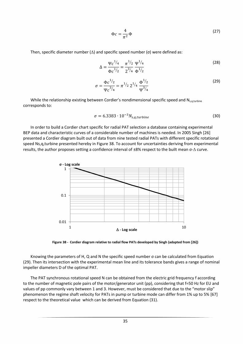
35
Φ𝑐 =
4
𝜋2Φ
(27)
Then, specific diameter number () and specific speed number (σ) were defined as:
Δ =
Ψ𝑐1
4⁄
Φ𝑐1
2⁄=
𝜋1
2⁄
23
4⁄ Ψ
14⁄
Φ1
2⁄
(28)
𝜎 =Φ𝑐
12⁄
Ψ𝑐3
4⁄= 𝜋
12⁄ 2
14⁄
Φ1
2⁄
Ψ3
4⁄
(29)
While the relationship existing between Cordier’s nondimensional specific speed and Ns,q,turbine
corresponds to:
𝜎 = 6.3383 ∙ 10−3𝑁𝑠,𝑞,𝑡𝑢𝑟𝑏𝑖𝑛𝑒 (30)
In order to build a Cordier chart specific for radial PAT selection a database containing experimental
BEP data and characteristic curves of a considerable number of machines is needed. In 2005 Singh [26] presented a Cordier diagram built out of data from nine tested radial PATs with different specific rotational speed Ns,q,turbine presented hereby in Figure 38. To account for uncertainties deriving from experimental
results, the author proposes setting a confidence interval of ±8% respect to the built mean σ- curve.
Figure 38 - Cordier diagram relative to radial flow PATs developed by Singh (adapted from [26])
Knowing the parameters of H, Q and N the specific speed number σ can be calculated from Equation (29). Then its intersection with the experimental mean line and its tolerance bands gives a range of nominal impeller diameters D of the optimal PAT.
The PAT synchronous rotational speed N can be obtained from the electric grid frequency f according to the number of magnetic pole pairs of the motor/generator unit (pp), considering that f=50 Hz for EU and values of pp commonly vary between 1 and 3. However, must be considered that due to the “motor slip” phenomenon the regime shaft velocity for PATs in pump or turbine mode can differ from 1% up to 5% [67] respect to the theoretical value which can be derived from Equation (31).
0.01
0.1
1
1 10
σ - Log scale
- Log scale

36
𝑁(𝑟𝑝𝑚) =
60 𝑓
𝑝𝑝
(31)
By imposing rotational speed corresponding to pp=1,2 and 3 the optimal impeller diameters D of single-
stage centrifugal PATs having BEP matching with flow rate and available head previously calculated can be selected as in Table 4.
Table 4 - Single stage centrifugal PAT impeller diameter selection results
pp (-) N (rpm) Ns,q,turbine (-) Ψ (-) Φ (-) D (m)
1 3000 9.84 12.40 0.038 0.154
2 1500 4.92 17.53 0.016 0.259
3 1000 2.59 13.93 0.005 0.435
It is interesting to compare the results obtained through Cordier diagram with the selection chart for
radial flow PATs developed by Singh [26] using data from 9 tested pumps as shown in Figure 39. The red squares in the figure mark the BEP of tested Pats, while black dots stand for the nondimensional BEP coordinates calculated as Ψ and Φ in Table 4.
Figure 39 - Centrifugal PAT selection chart (adapted from [26])
As can be noticed, the BEP coordinates predicted through Cordier diagram lay in the proximity of the mean Ψ-Φ BEP line interpolated by Singh. However, the specific speed of PATs with pp=2 and pp=3 are rather low when compared to commercially available single-stage units. Therefore, the selected optimal single-stage PAT characteristics that will likely match more closely with design parameters are:
pp = 1
N = 3000 rpm
D = (154 ± 12) mm
The uncertainty in diameter selection is caused by the 8% confidence interval proposed by the author.

37
4.7. PAT selection
Given the commercial unavailability of characteristic curves of multistage pumps adapt to the context, as basis for further calculations was used a centrifugal pump ETANORM 50-32-160.1 by manufacturer KSB having D=176 mm of which turbine mode characteristic curve was reported in Master’s Thesis dissertation by Tânia Calado [16]. Such unit was selected because of its parameters which are similar to the optimal calculated ones and, furthermore, because both characteristic curves as pump and as turbine issued by its producer were available. The characteristic curve of the selected pump is shown in Figure 40 as appears in the KSB catalogue [68]. Circled in red is the actual impeller diameter D, equal to 176 mm.
Figure 40 - ETANORM 50-32-160.1 pump mode characteristic curves with N=2900 rpm [68]
The characteristic curves of chosen PAT in turbine mode are available with generator having pp=2 (corresponding to N=1520 rpm) as shown in Appendix A attached, and through affinity laws presented in Chapter 2.5. the curves corresponding to the generator with pp=1 (and N=3020 rpm) were obtained as presented in Figure 41 and Figure 42. The red dot highlights the working point of the proposed installation as formerly calculated.
Figure 41 - ETANORM 50-32-160.1 turbine mode characteristic curves with N=3020 rpm
0
0.05
0.1
0.15
0.2
0.25
0.3
0.35
0.4
0.45
0.5
0
20
40
60
80
100
120
140
160
4 6 8 10 12
η (-) H (m)
Q (l/s)
Working point H (m) η

38
Figure 42 - ETANORM 50-32-160.1 turbine mode P-Q curve with N=3020 rpm
In Table 5 the BEP characteristics of the analyzed machine in both pump and turbine mode are summed up.
Table 5 - ETANORM 50-32-160.1 BEP characteristics in pump and turbine mode
Q,BEP (l/s) H,BEP (m) η,BEP (-) P,BEP (kW) N (rpm) Ns,q (-)
Pump mode 6.11 29.6 54.1 % 3.28 2900 17.86
Turbine mode 8.6 86.01 46.3 % 3.26 3020 9.92
As stated in the previous Chapter 2.7.2.1., several methods exist to correlate the BEP of a PAT to the best efficiency point of the same machine operated as pump through the nondimensional parameters h and q. In Table 6 are reported such parameters as calculated through the formulations contained in Table 3 at Page 20 compared to the actual values of h and q.
Table 6 - Nondimensional parameters h ad q, comparison between actual and calculated values
Actual PAT
h q
2.91 1.41
Calculated values
Method h q
Stepanoff 3.99 1.85
Gopalakrishnan 3.42 1.85
Childs 3.42 3.42
Sharma 2.09 1.63
Alatorre-Frenk 2.36 2.01
Nautiyal [44] -0.29 0.03
Grover 2.47 2.12
Derakhshan 2.86 3.07
From the presented table is evident how the method proposed by Nautiyal et al. [44] results in the
least accurate results, leading even to negative h value. In Figure 43 instead the values present in Table 6 have been plotted against the h-q space. As can be noticed, none of the presented mathematical correlations in able to predict accurately both h and q for the selected PAT.
0
0.05
0.1
0.15
0.2
0.25
0.3
0.35
0.4
0.45
0.5
0
1
2
3
4
5
6
7
8
4 6 8 10 12
η (-) P (kW)
Q (l/s)
Working point P η

39
Figure 43 - Nondimensional parameters h ad q, comparison between actual and calculated values
For this specific PAT the method developed by Derakhshan et al. [41] predicts quite accurately the head coefficient but fails in identifying the flow coefficient q, as opposed to methods by Sharma, Gopalakrishnan and Stepanoff which show some degree of accuracy with the q parameter but prove ineffective as for the h parameter.
4.8. Technical analysis
As stated in the previous Chapter 4.3., even though the water flow rate directed to the elevated tank remains constant and equal to 7 l/s the daily volume of inlet water varies significantly according to the season because of variations in water consumption. In particular, the daily water demand from Scurzolengo water tower ranges from 250m3/day during February up to about 400m3/day in August. To account for such variability, an additional parameter α was introduced corresponding to the ratio of time in a day with open inlet valve over the total day time.
In absence of more detailed information, to approximate the monthly variation of daily demand over a year a function was created having the same shape of average temperature yearly distribution for the same geographical area, with α ranging from 0.45 in February to 0.65 in August which correspond to the measured daily consumption values for the two months. The graph describing α function is shown in Figure 44.
Figure 44 - Variation of α parameter over a year
Therefore, the potential energy production can be calculated for every month of the year as:
1
1.5
2
2.5
3
3.5
4
1.5 2 2.5 3 3.5 4
q
h
Actual PAT
Stepanoff
Gopalakrishnan
Childs
Sharma
Alatorre-Frenk
Grover
Derakhshan
0.4
0.45
0.5
0.55
0.6
0.65
0.7
1 2 3 4 5 6 7 8 9 10 11 12
α (-)
Month

40
𝐸(𝑘𝑊ℎ) = 𝜂𝑡 9.8 𝐻𝑡 𝑄 (𝛼 𝑡) (32)
where: ηt: PAT efficiency, equal to 0.445 for Q = 7 l/s (-) Ht: head drop through the PAT, equal to 65.85 for Q = 7 l/s (m) Q: design flow rate, equal to 7 l/s (m3/s) t: number of hours per month (h)
As a result, the total producible energy over a typical year results to be equal to 9585 kWh, distributed
over the twelve months as shown in Figure 45.
Figure 45 - Total producible energy over a typical year
Since the operators of Scurzolengo water tower expressively requested for allowing by design a maximum inlet flow rate of 10l/s under extraordinary operations, it’s been proposed the installation within the main pipe of an automated valve meant to open when the water level inside the tank lower below a set limit. Such valve needs to be installed between the by-pass duct where PAT is placed as shown in Figure 37.
4.9. Economic analysis
4.9.1. Input parameters
A simple payback period analysis was carried out based on different scenarios of energy remuneration in order to assess the feasibility of the proposed installation.
0
200
400
600
800
1000
1200
1 2 3 4 5 6 7 8 9 10 11 12
E (kWh)
Month
41
1. Economic profit
Within the current legislation framework existing for Italian energy market the GSE – Gestore dei Servizi Energetici (“Operator of Energy Services”) is the authority responsible for promoting the diffusion of renewable energy sources within the national territory. As stated in the Ministerial Directive issued on 6th July 2012 [69], the incentives supplied to in-pipe hydropower schemes having installed power between 1 and 20 kW are equal to 0.257€ for every kWh exported to the national grid and for a maximum of 20 years. As consequence, the yearly revenue for the proposed installation corresponds to about 2060€. Anyway, since the granting of incentives is subject to availability at the moment when application is submitted a second scenario has been considered when no incentives are available and the produced energy is bought by GSE authority and paid according to the minimum tariff of 0.153 €/kWh through the Ritiro dedicato (“Dedicated withdrawal”) mechanism.
2. PAT costs
Within the paper published in 2013, Carravetta et al. [70] evaluated the purchase cost of PATs as the sum of two factors CPAT and Cgen described as:
CPAT (€) = 230 (€/kW) ∙ PBEP (kW)
which accounts for the turbine unit alone, proportional to the power at BEP
Cgen (€) = 115 (€/kW) ∙ Pmax (kW)
which accounts for the cost of generator unit and is proportional to maximum PAT
power
For the selected PAT, the total purchase cost of turbine and generator unit results into 1550 € which is in good agreement with the value presented by Tânia Calado in her dissertation [16]. The yearly maintenance cost of the machinery has been calculated as 2.5% of initial investment cost [16].
3. Civil works
The cost for construction of bypass duct and installation of flow valves has been evaluated as 500€. Given the small size of the system there is potentially enough space at the basis of the water tower to shelter it without the need of additional construction works.
4. Connection to the national electric grid
The cost for connecting to the national grid a power generation unit based on renewable energies is set by the AEEG, Autorità per l’Energia Elettrica e il Gas (“Authority for electric energy and natural gas”). For installed powers less than 50kW the cost is established as:
𝐶𝑔𝑟𝑖𝑑(€) = 200 + 35 𝑃 + 90 𝑃 𝐷𝐴 (33)
where:
P: installed power (kW), equal to 2.01 in the present analysis DA: linear distance between the plant and the nearest medium-to-low voltage transformer substation (km)
Supposing DA equal to 1 km corresponding to the nearest town center, the expected cost for
plant connection to the grid is expected to be equal to 451€.

42
4.9.2. Results of economic analysis
Given the relatively moderate level of investment required a simple payback time analysis was performed, disregarding effects of inflation and capital remuneration. Regardless of the presence of incentives, the payback time for the needed investment lays between the beginning and the end of Year 2 when the generation plant is considered to start operations in January. The complete results from economic analysis are presented in Table 15 of Appendix B.
Additionally, as it can be observed from the graphs of previous Chapter 4.3., the flow through the proposed PAT can occur both during the night time and daytime with the current inlet valve regulation based on water tank level. However, additional monetary benefit could potentially be achieved if the current inlet valve opening rules were modified allowing for the water level to lower below 3.55 m compatibly with the operational requirements. As a result, the water tank would be filled in mainly during night time allowing pumping stations to operate in periods of low electricity cost.
Another important parameter to assess the convenience of energy systems is the Levelized Cost Of Electricity (LCOE), defined as the ratio between the sum of all costs over the lifetime of a determined production technology and the total generated electrical energy. For the proposed installation, considering the PAT lifetime being 20 years and setting a discount rate equal to 5% a LCOE value of 0.025 €/kWh is obtained which is significantly lower when compared to other energy generation technologies as shown in Figure 46.
Figure 46 - LCOE of different electricity generation technologies in 2013 [adapted from en.wikipedia.org/wiki/Cost_of_electricity_by_source]
4.10. Environmental analysis
Avoided emissions
According to the report Fattori di emissione atmosferica di CO2 e sviluppo delle fonti rinnovabili nel settore elettrico (“CO2 Emission factors and diffusion of renewables in Italian energy sector”) published by ISPRA in 2014 [71], the overall emission factor per unit of consumed electricity by final users was equal to 326.8 g CO2/kWh in year 2013. Such datum includes the imported and exported energy as well as grid losses. Since the designed hydropower installation is expected to generate a total of 9587 kWh of energy

43
per year, it would contribute to avoiding emissions equal to 3.13 tons of CO2 within the same timeframe. Besides, the online tool Foglio di calcolo per le emissioni in atmosfera [72] developed by Piedmont administrative region over the years 2007-2013 allows for an estimation of avoided emissions of particulate matter and NOx relative to new electricity generation plants exploiting renewable resources. For the studied micro-hydro scheme the savings in particulate matter, NOx and CO2 over a year are summed up in Table 7.
Table 7 - Estimated avoided emissions over a year relative to the studied PAT plant [71], [72]
Type of avoided emission Quantity Unit
CO2 3.13 tons/year
Particulate matter 28.76 g/year
NOx 2.97 kg/year
Primary energy savings
According to the cited ISPRA 2015 report [71] a total of 290 TWh of electricity was produced in Italy during 2013, divided by source as described in Table 8.
Table 8 - Share of electricity generation by source in Italy (2013) [71]
Energy sources Share
Renewables 39%
Coal 16%
Natural gas 37%
Other fuels 8%
According to the same document [71], the net plant efficiencies for Italian combined cycles Natural gas
plants and Rankin cycle-based plants in 2013 were respectively 51% and 33% including effects of part-load operations. As a result, within such a scenario the savings of primary energy per year reachable by the studied micro-hydro installation are summarized in Table 9. The category “Other fuels” of Table 8 includes mainly refinery byproducts and refuse-derived fuels which were neglected due to unavailability of detailed information.
Table 9 - Primary energy savings per year in terms of energy and mass for Case-study 1
Fuel Energy units
Corresponding quantity
Natural gas
6955 kWh 687 Nm3
Coal 4648 kWh 837 kg
Conclusions
Despite the relative weight of the singular plant, a large scale diffusion of similar energy recovery device could have a significant impact on emission reduction at national level as well as primary energy savings.
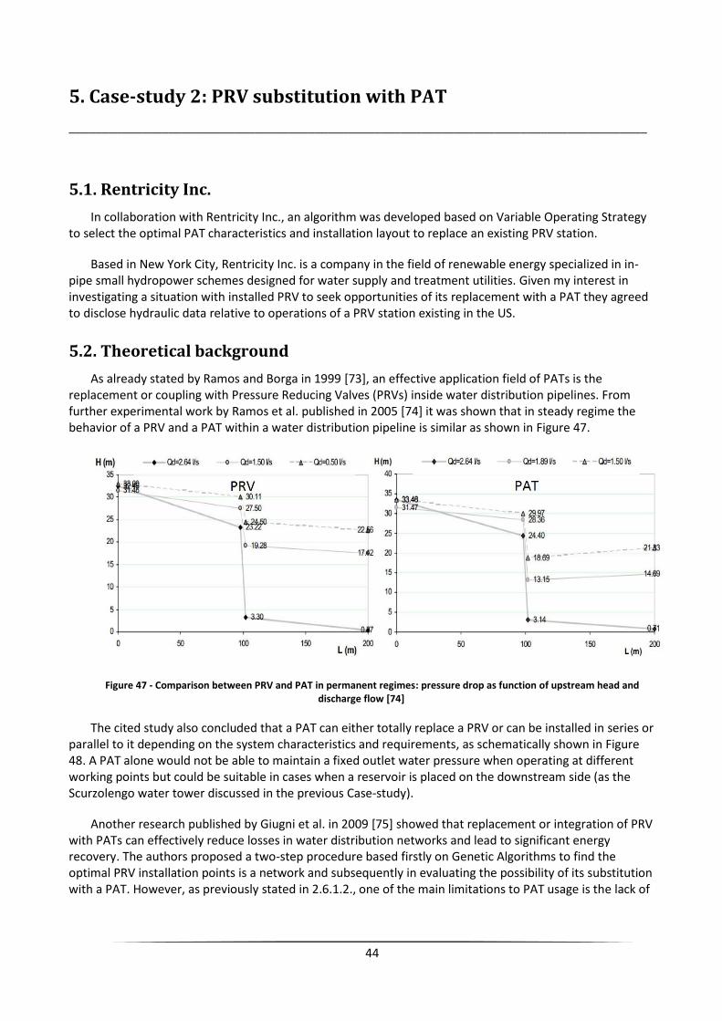
44
5. Case-study 2: PRV substitution with PAT
_______________________________________________________________________________________
5.1. Rentricity Inc.
In collaboration with Rentricity Inc., an algorithm was developed based on Variable Operating Strategy to select the optimal PAT characteristics and installation layout to replace an existing PRV station.
Based in New York City, Rentricity Inc. is a company in the field of renewable energy specialized in in-pipe small hydropower schemes designed for water supply and treatment utilities. Given my interest in investigating a situation with installed PRV to seek opportunities of its replacement with a PAT they agreed to disclose hydraulic data relative to operations of a PRV station existing in the US.
5.2. Theoretical background
As already stated by Ramos and Borga in 1999 [73], an effective application field of PATs is the replacement or coupling with Pressure Reducing Valves (PRVs) inside water distribution pipelines. From further experimental work by Ramos et al. published in 2005 [74] it was shown that in steady regime the behavior of a PRV and a PAT within a water distribution pipeline is similar as shown in Figure 47.
Figure 47 - Comparison between PRV and PAT in permanent regimes: pressure drop as function of upstream head and discharge flow [74]
The cited study also concluded that a PAT can either totally replace a PRV or can be installed in series or parallel to it depending on the system characteristics and requirements, as schematically shown in Figure 48. A PAT alone would not be able to maintain a fixed outlet water pressure when operating at different working points but could be suitable in cases when a reservoir is placed on the downstream side (as the Scurzolengo water tower discussed in the previous Case-study).
Another research published by Giugni et al. in 2009 [75] showed that replacement or integration of PRV with PATs can effectively reduce losses in water distribution networks and lead to significant energy recovery. The authors proposed a two-step procedure based firstly on Genetic Algorithms to find the optimal PRV installation points is a network and subsequently in evaluating the possibility of its substitution with a PAT. However, as previously stated in 2.6.1.2., one of the main limitations to PAT usage is the lack of

45
flow rate regulation possibility due to the absence of guide vane. As a result, their implementation alone within water supply systems characterized by periodical flow rate and available head variations can lead to:
reduced global power output due to low part-load efficiency
impossibility to ensure the required head drop under all operating conditions
a) Existing PRV station c) PAT added in series to PRV plus side by-pass (HR)
b) PAT alone as replacement of PRV
Figure 48 - Simplified schemes of a PRV station and its substitution or complement with a PAT
Recent researches by Carravetta et al. published between 2012 and 2013 [70], [76] aimed at defining a procedure named VOS (Variable Operating Strategy) to enable selection of the optimal PAT to be installed in series or in parallel with PRVs in order to maximize energy production from a specific site while meeting the requirements set by network operator/management. Given the absence of flow regulation possibility within the pump-generator unit, three alternative designs have been investigated:
1. Hydraulic Regulation (HR), in which a PRV placed in series with PAT and a by-pass circuit allow the turbine to work in the surrounding of BEP;
2. Electric Regulation (ER), when the operating pump speed N can be adjusted thanks to a connected inverter;
3. Hydraulic and Electric Regulation (HER), when both previous regulations are implemented.
A simplified installation scheme of both HR and ER configurations is presented in Figure 49 below.
Figure 49 - Installation scheme of PAT with Hydraulic and Electric regulation [70]

46
The operating conditions of a PAT under HR and ER mode are shown in Figure 50.
Figure 50 - PAT operations in HR (left) and ER mode (right) [70]
As target for maximization the plant overall efficiency over “n” working points has been set as:
𝜂𝑝 =
∑ 9.8 𝜂𝑖𝑇 𝑄𝑡,𝑖 𝐻𝑡,𝑖 Δ𝑡𝑖 𝑛
𝑖=1
∑ 9.8 𝑞𝑖 ℎ𝑖 Δ𝑡𝑖 𝑛𝑖=1
(34)
where:
q, h: volumetric flow rate and available head present in the system (m3/s, m) Qt, Ht: volumetric flow rate and head drop through the PAT (m3/s, m) ηi
T: PAT efficiency (-)
t: time interval (h)
The authors of the study also carried out a comparison between HR and ER modes applied to an existing PRV installation testing PATs with different impeller diameters and rotational speed. As described in [70], the results show that Hydraulic Regulation tends to have greater overall efficiency and system flexibility. Also, the HR scheme proved to have shorter payback period than ER in all the considered scenarios.
In a paper published in 2013, Carravetta et al. [77] proposed an upgrade to the VOS method considering as target of optimization for PAT characteristics design a parameter defined as “System Effectiveness” obtained as multiplication of three indicators of performance:
ηp: overall plant efficiency as described in Equation (34);
Φp: system flexibility, measuring the reduction in efficiency attainable when conditions within hydraulic circuit differ from design values;
μp: system reliability, considering relative reduction in average time between failures of PAT equipment when a determined machine is operating at conditions differing from BEP.

47
5.3. System description
The available data about PRV installation includes water flow rate and upstream and downstream pressure variations along a typical day. The profiles of flow rate and head drop across the valve are shown in Figure 51.
Figure 51 - Flow rate and head drop across PRV along a typical day
Instead, in Figure 52 are shown the system operating points across the same timeframe plotting PRV head drop against flow rate.
Figure 52 - System working points over H-Q diagram
73
74
75
76
77
78
79
80
0
5
10
15
20
25
30
35
40
45
50
h (m) q (l/s)
Hour
Flow rate through PRV (l/s) PRV head drop (m)
73
74
75
76
77
78
79
80
15 20 25 30 35 40 45
h (m)
q (l/s)

48
5.4. Optimization
5.4.1. Input data and methodology
Following the methodology developed by Carravetta et al. [70], [76] described in previous Chapter 5.2., it was decided to analyze the most appropriate PAT to be fitted in the system according to two alternative design strategies:
1. PAT alone as replacement of PRV; 2. PAT added in series to the PRV and with flow by-pass channel, to allow for Hydraulic Regulation
which Carravetta et al. [70] showed being the most effective regulation strategy.
The calculations were carried out and aimed at individuation of PAT impeller diameter D and rotational speed N which lead to the maximum overall plant efficiency ηp as described in Equation (34). The characteristic curves of PATs having different D and N were obtained using the turbomachinery affinity laws presented in Chapter 2.5. based upon the data collected by Singh [26] relative to nine centrifugal, single stage machines experimentally tested plus the KSB ETANORM 50-32-160.1 turbine analyzed for previous case-study. The main characteristics of the investigated PATs are shown in Table 10.
Table 10 - BEP of experimentally tested PATs (adapted from [15])
PAT 1 PAT 2 PAT 3 PAT 4 PAT 5 PAT 6 PAT 7 PAT 8 PAT 9 PAT 10 [16]
Ns,q,turbine 18.5 18.6 28.1 30.1 35.7 41.1 38.1 57.6 70 9.91
Ψt 8 11.17 7.64 8 6.7 6.18 7.6 5.748 4.9 10.65
Φt 0.07 0.117 0.151 0.185 0.2 0.235 0.275 0.414 0.48 0.031
ηt,BEP 0.725 0.765 0.81 0.715 0.835 0.795 0.76 0.743 0.755 0.463
D (m) 0.225 0.258 0.206 0.174 0.264 0.2 0.139 0.165 0.224 0.176
N (rpm) 1520 1520 1520 1520 1520 1520 1520 1520 1520 1520
Ht,BEP (m) 26.5 48.6 21.2 15.8 30.5 16.2 9.6 10.2 16.1 21.6
Qt,BEP (m3/s) 0.020 0.051 0.033 0.025 0.093 0.048 0.019 0.047 0.137 0.004
The characteristic curves of head (H) and power (P) against flow rate (Q) for each of the considered PATs have been approximated with second and third order polynomials respectively as proposed by Derakhshan and Nourbakhsh (2008) [41]. Such dimensionless characteristic curves have been determined by the authors based on experimental data, and are considered representatives for PATs having Ns,q,turbine lower than 70. The corresponding equations are:
𝐻𝑡
𝐻𝑡,𝐵𝐸𝑃= 1.0283 (
𝑄𝑡
𝑄𝑡,𝐵𝐸𝑃)
2
− 0.5468 (𝑄𝑡
𝑄𝑡,𝐵𝐸𝑃) + 0.5314
(35)
𝑃𝑡
𝑃𝑡,𝐵𝐸𝑃= −0.3092 (
𝑄𝑡
𝑄𝑡,𝐵𝐸𝑃)
3
+ 2.1472 (𝑄𝑡
𝑄𝑡,𝐵𝐸𝑃)
2
− 0.8865 (𝑄𝑡
𝑄𝑡,𝐵𝐸𝑃) + 0.0452
(36)

49
5.4.2. PAT alone, absence of regulation
In absence of regulation devices, the head drop produced by the PAT corresponds to the point of its characteristic curve at a given flow rate. In the scenario assessing the mere PRV substitution with PAT, an algorithm was developed to assess the producible energy from each investigated PAT having different characteristic curves while inserted in the prescribed system. The H-Q graphic space was divided into three regions as shown in Figure 53.
Figure 53 - Subdivision of H-Q plane according to the PAT characteristic curve, no regulation
For each of the selected regions the producible energy has been evaluated at every system working point as:
Region I (qi < Qt,min): Ei = 0
Region II [qi > Qt,max OR (Qt,min < qi < Qt,max AND Ht(q) > hi)]: error
Region III (Qt,min < qi < Qt,max AND Ht(q) < hi)]: Ei = ti P(qi)
where: qi, hi: volumetric flow rate and available head present in the system at instant “i” (m3/s, m) Qt, Ht: volumetric flow rate and head drop through the PAT (m3/s, m) Ei: energy produced (kWh) P: generated power (kW)
ti: time interval (h)
The subscripts “min” and “max” refer to the extreme values that Qt, can attain. The “error” output indicates that if a working point of the system is situated in Region II the selected PAT is not adapt to be installed alone as proposed in the present scenario.

50
5.4.3. PAT in series with PRV and by-pass duct (HR)
Instead, in the scenario including PAT installation with Hydraulic Regulation in order to calculate the energy producible by a PAT at determined system working point the H-Q space had to be divided into five regions as in Figure 54.
Figure 54 - Subdivision of H-Q plane according to the PAT characteristic curve, HR
For each of the selected regions the producible energy has been evaluated at every system working point as:
Region I (qi < Qt,min OR hi < Ht,min): Ei = 0
Region II (Qt,min < qi < Qt,max AND Ht,min < hi < Ht(qi)): Ei = ti P(Q(hi))
Region III (qi > Qt,min AND Ht,min < hi < Ht,max): Ei = ti P(Qt(hi))
Region IV (Qt,min < qi < Qt,max AND hi > Ht(qi)): Ei = ti P(qi)
Region V (qi > Qt,max AND hi > Ht,max): Ei = ti P(Qt,max)
where: qi, hi: volumetric flow rate and available head present in the system at instant “i” (m3/s, m) Qt, Ht: volumetric flow rate and head drop through the PAT (m3/s, m) Ei: energy produced (kWh) P: generated power (kW)
ti: time interval (h)
The subscripts “min” and “max” refer to the extreme values that Qt, and Ht can attain.

51
5.5. Results
5.5.1. Results PAT alone, absence of regulation
The results of the analysis were plotted showing the overall plant efficiency ηp against the measure of impeller diameter D (m) for PATs having different specific speed Ns,q,turbine. For PATs rotating at N = 1520 rpm the results are shown in Figure 55.
Figure 55 - Overall plant efficiency ηp vs. impeller diameter D for PATs with different Ns,q,turbine at N = 1520 rpm
Instead, the maximum reachable plant efficiency proved to be higher for PATs with shaft rotational speed N equal to 3020 rpm as shown in Figure 56.
Figure 56 - Overall plant efficiency ηp vs. impeller diameter D for PATs with different Ns,q,turbine at N = 3020 rpm
0%
5%
10%
15%
20%
25%
30%
0.12 0.17 0.22 0.27 0.32 0.37
ηp
D (m)
Ns,q,turbine
18.5
18.6
28.1
30.1
35.7
41.1
38.1
57.6
70
0%
5%
10%
15%
20%
25%
30%
35%
40%
45%
0.1 0.12 0.14 0.16 0.18 0.2 0.22 0.24
ηp
D (m)
Ns,q,turbine
28.1
30.1
35.7
41.1
38.1
57.6

52
As seen in Figure 55 for N = 1520 rpm the maximum plant efficiency attainable by PATs of the considered specific speeds corresponds to about 27% and is obtained with machines having Ns,q,turbine equal to 18.5 or 18.6 and impeller diameters of respectively 0.28 and 0.24 m.
Instead, when such set of similar PATs operated with a two-pole generator unit (N = 3020 rpm) the maximum attainable plant efficiency corresponds to 37% when using a PAT having Ns,q,turbine equal to 35.7 and D = 0.15 m. The complete characteristics of such optimal PAT are reported in Figure 57.
Optimal PAT
Ht,BEP (m) 38.93
Qt,BEP (m3/s) 0.034
Pt,BEP (kW) 10.82
Qmax (m3/s) 0.0484
Qmin (m3/s) 0.0153
N (rpm) 3020
Ns,q (-) 35.72
Ns,p (-) 102.17
Pt,max (kW) 24.32
D (m) 0.15
Figure 57 - Characteristic curve and parameters of optimal PAT (No regulation)
5.5.2. Results PAT in series with PRV and by-pass duct (HR)
In the scenario with Hydraulic Regulation, the results for a PATs rotating at N = 1520 rpm are shown in Figure 58
Figure 58 - Overall plant efficiency ηp vs. impeller diameter D for PATs with different Ns,q,turbine at N = 1520 rpm (HR)
0
0.1
0.2
0.3
0.4
0.5
0.6
0.7
0.8
0
20
40
60
80
100
0.015 0.025 0.035 0.045 0.055 0.065
η (-) H (m)
Q (m3/s)
System Q-H points PAT Q-H curve PAT η
0%
5%
10%
15%
20%
25%
30%
35%
40%
0.2 0.25 0.3 0.35 0.4 0.45
ηp
D (m)
Ns,q,turbine
9.91
18.5
18.6
28.1
30.1
35.7
41.1
38.1

53
Instead, the diagram with plant efficiency at N = 3020 rpm is shown in Figure 59.
Figure 59 - Overall plant efficiency ηp vs. impeller diameter D for PATs with different Ns,q,turbine at N = 3020 rpm (HR)
As can be noticed, for both values of N the best attainable plant efficiency in the scenario with Hydraulic Regulation (HR) is always higher than the one reachable when no regulation, with a maximum of around 57% in case of a PAT having Ns,q,turbine equal to 28.1, impeller diameter of 0.15 m and rotating at N = 3020 rpm. The complete characteristic curve and parameters of such optimal PAT are shown in Figure 60.
Optimal PAT
Ht,BEP (m) 44.39
Qt,BEP (m3/s) 0.026
Pt,BEP (kW) 9.04
Qmax (m3/s) 0.037
Qmin (m3/s) 0.01
N (rpm) 3020
Ns,q (-) 79.24
Ns,p (-) 28.12
Pt,max (kW) 21.29
D (m) 0.15
Figure 60 - Characteristic curve and parameters of optimal PAT (HR)
0%
10%
20%
30%
40%
50%
60%
0.12 0.17 0.22 0.27
ηp
D (m)
Ns,q,turbine
9.91
18.5
18.6
28.1
30.1
35.7
41.1
38.1
57.6
70
0
0.1
0.2
0.3
0.4
0.5
0.6
0.7
0.8
0.9
0
20
40
60
80
100
0.01 0.015 0.02 0.025 0.03 0.035 0.04 0.045
η (-) H (m)
Q (m3/s)
System Q-H points PAT Q-H curve PAT η

54
5.5.3. Final considerations
Results of the performed analysis match well with the referenced literature, showing a significant increase in producible energy when possibility of flow regulation is introduced (namely, Hydraulic Regulation). Despite the higher installation and maintenance costs due to addition of a PRV in series to the PAT and the realization of by-pass pipe, the yield of such a configuration is significantly higher than the simple PAT installation as replacement of PRV. Also, another advantage given by HR scenario is the possibility for the water network operator to set and maintain an optimal value of downstream pressure independently of the flow rate which is not possible in the scenario without regulation.
The variations in the maximum attainable value of ηp along the two considered scenarios are summed up in Table 11.
Table 11 - Maximum attainable ηp for the considered scenarios
N = 1520 rpm N = 3020 rpm
No flow regulation
27% 37%
HR 35% 57%
Another significant observable trend is that the adoption of PATs rotating at higher speed N increases the overall plant efficiency for both analyzed scenarios. However, the main reason for such gap in plant efficiency is the limited set of PATs on which the analysis was based upon. With data from more pumps having different specific speed a smaller performance gap would be expected.
Since no further information was available regarding the context of the analyzed PRV station (e.g. location, specific requirements from the network operator, electricity costs, space constraints) it was decided to limit the analysis to technical considerations and disregard the economic and environmental aspects. However, when selecting the PAT characteristics for installation within a precise PRV site it would be appropriate to perform an optimization based on economic parameters instead of merely technical ones (ηp). Also, an appropriate and site-specific environmental analysis is recommendable.

55
6. Case-study 3: Asti WWTP
_______________________________________________________________________________________
6.1. Context description
In collaboration with water company ASP, the installation of an energy recovery device into the outlet of a WWTP was investigated.
The municipal Waste Water Treatment Plant (WWTP) of Asti is operated by ASP, a public-private multiutility active in various sectors: energy, water treatment and distribution, urban hygiene and transports. The WWTP was inaugurated in 1980 and constantly upgraded during following decades by increasing capacity and adding denitrification and dephosphorization sections to meet most recent environmental standards. It serves an equivalent population1 of 95.000 people and is the terminal point of the municipal sewage system consisting in around 220 km of pipes [78]. The purified water exiting the plant is conveyed into the nearby Tanaro river, an affluent of Italy’s largest river basin (Po).
A map representing the geographical position of the plant is showed in Figure 61, while Figure 62 shows an aerial view of WWTP.
Figure 61 - Asti geographical position
[www.maps.google.com]
Figure 62 - Aerial view of Asti WWTP
[www.maps.google.com]
1 The Irish EPA Act, 1996 (Urban Waste Water Treatment Regulations, 1994) defines one population equivalent
(p.e.) as 609 BOD per day. [87]

56
6.2. Outlet water channel description
After a visit to the plant which took place on 11th of February 2016, together with ASP management it was agreed that the site offering the highest potential for energy harvesting is the concrete-made open air channel through which purified water in conveyed. Here, soon after a Venturi Flume flow meter, the channel bed drops by 80 cm and water enters a DN800 pipe. A 3D view of the terminal part of the channel is presented in Figure 63, while 2D top and side section views are shown in Figure 65.
In Figure 64 instead the fluid motion through the same channel for a flow rate of 440 l/s is visible.
Figure 63 - 3D isometric view of WWTP channel
Figure 64 - Fluid motion through the channel for a flow
rate of 440 l/s
Figure 65 - 2D top and side section view of WWTP channel (all measures in mm)
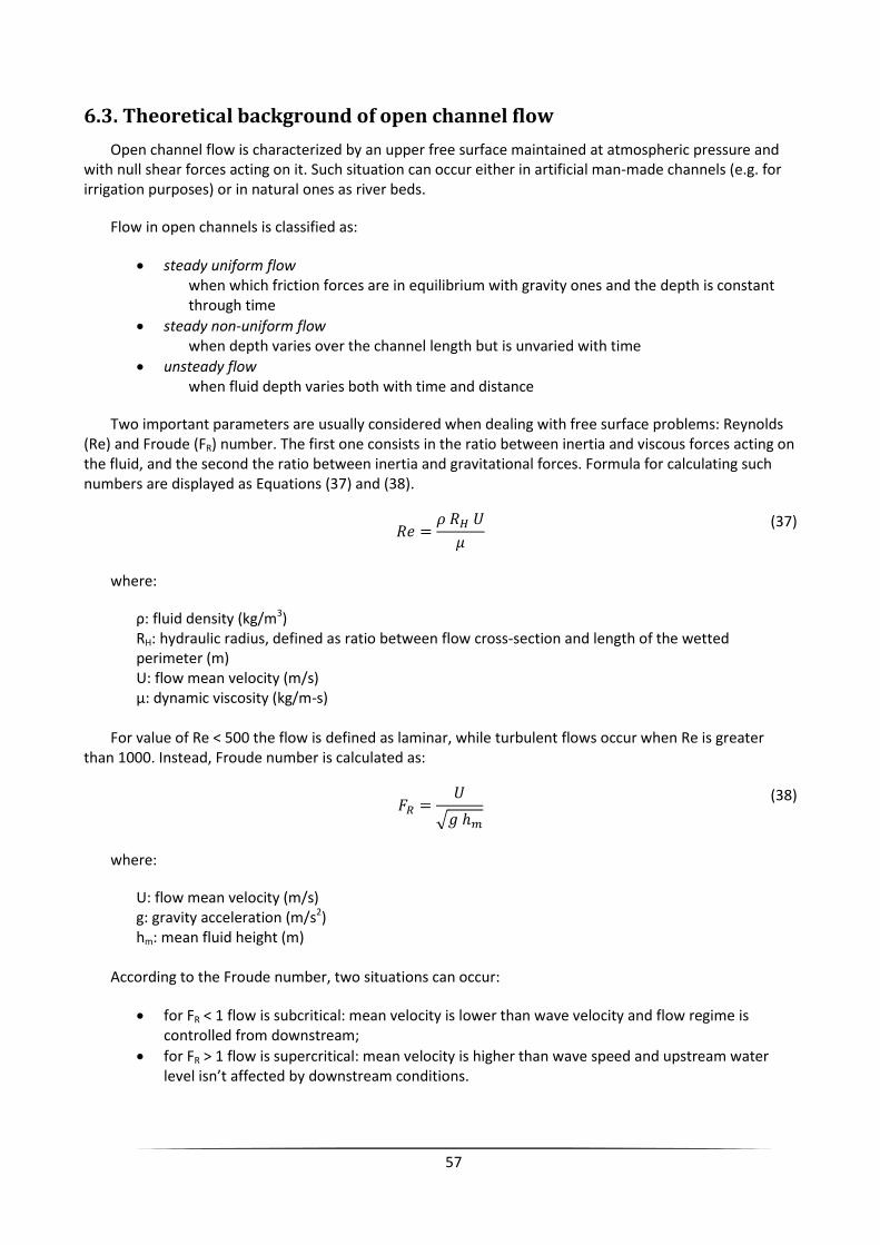
57
6.3. Theoretical background of open channel flow
Open channel flow is characterized by an upper free surface maintained at atmospheric pressure and with null shear forces acting on it. Such situation can occur either in artificial man-made channels (e.g. for irrigation purposes) or in natural ones as river beds.
Flow in open channels is classified as:
steady uniform flow when which friction forces are in equilibrium with gravity ones and the depth is constant through time
steady non-uniform flow when depth varies over the channel length but is unvaried with time
unsteady flow when fluid depth varies both with time and distance
Two important parameters are usually considered when dealing with free surface problems: Reynolds (Re) and Froude (FR) number. The first one consists in the ratio between inertia and viscous forces acting on the fluid, and the second the ratio between inertia and gravitational forces. Formula for calculating such numbers are displayed as Equations (37) and (38).
𝑅𝑒 =
𝜌 𝑅𝐻 𝑈
𝜇
(37)
where:
ρ: fluid density (kg/m3) RH: hydraulic radius, defined as ratio between flow cross-section and length of the wetted perimeter (m) U: flow mean velocity (m/s) μ: dynamic viscosity (kg/m-s)
For value of Re < 500 the flow is defined as laminar, while turbulent flows occur when Re is greater than 1000. Instead, Froude number is calculated as:
𝐹𝑅 =
𝑈
√𝑔 ℎ𝑚
(38)
where:
U: flow mean velocity (m/s) g: gravity acceleration (m/s2) hm: mean fluid height (m)
According to the Froude number, two situations can occur:
for FR < 1 flow is subcritical: mean velocity is lower than wave velocity and flow regime is controlled from downstream;
for FR > 1 flow is supercritical: mean velocity is higher than wave speed and upstream water level isn’t affected by downstream conditions.

58
The energy possessed by a steady uniform free flowing fluid referenced to the bottom of the channel can be expressed through a modified version of Bernoulli’s equation which accounts for atmospheric pressure at air-fluid boundary:
𝐻 = ℎ +
𝑈2
2𝑔
(39)
where:
H: specific fluid energy in meters of water column (m) h: flow depth (m) U: flow mean velocity (m/s) g: gravity acceleration (m/s2)
6.4. Venturi Flume theoretical background
A Venturi Flume is a device commonly installed in open air water channels to measure the volumetric flow rate. It imposes a restriction of channel cross-section through symmetrical side necks in order to achieve a transition from subcritical to supercritical flow conditions. With respect to other technologies used to measure flow in open channels (e.g. measuring weirs) it features smaller gradient losses and doesn’t allow debris sedimentation [79].
Schemes showing the design and functionality of Venturi Flume systems are presented in Figure 66 and Figure 67.
Figure 66 - 3D scheme of a Venturi Flume
rigid structure [80]
Figure 67 - Side view of flow profile [80]
The basic governing equation to describe the operations of a Venturi Flume is the flow continuity. When applied between cross section 1 and 2 as seen in Figure 67 it results is the following equation:
𝑈1𝑏1ℎ1 = 𝑈2𝑏2ℎ2 (40)
where:
U: mean flow velocity (m/s) b: channel width (m) h: flow height (m)

59
After combining with the Bernoulli specific energy law between cross sections 1 and 2 and imposing critical fluid height at section 2, the formula to calculate outflow from the Venturi Flume can be derived as:
𝑄 = 𝜇 𝑏2 √𝑔 𝐶 ℎ1
32⁄
(41)
in which:
Q: water outflow (m3/s) μ: outflow coefficient, equal to 0.985 (-) [80] g: gravity acceleration, equal to 9.81 (m/s2) h1: water level in section 1 (m) C: constriction coefficient (-), whose values are plotted as function of:
m = b2/b1: constriction ratio on the horizontal (-) as shown in Figure 68a; t= (h1-a)/h1: constriction ratio on the perpendicular plane (-) as shown in Figure 68b.
a) Top view b) Side view
Figure 68 - Top and side views of a Venturi Flume [80]
A chart plotting the value of C as function of product (m∙t) is shown in Figure 69.
Figure 69 - Constriction coefficient C as function of m∙t product [80]
Dimensions of the Venturi Flume installed at Asti WWTP outlet channel are shown in Table 12.
Table 12 - Asti WWTP outlet channel characteristics
b1 (m) b2 (m) m (-) t (-) a (m) m∙t (-) C (-)
1.2 0.605 0.504 1 0 0.504 0.58

60
Consequently, a formula to derive flow rate Q as function of upstream water level h1 can be obtained. The correlation between such parameters is shown in Figure 70.
Figure 70 - Q-h1 relationship
In order to have a continuous flow measurement an ultrasonic level sensor is installed in correspondence of section 1 of the Venturi structure, sending data automatically to ASP control system.
6.5. Design parameters
The water flow rate through the investigated WWTP outlet channel presents a high variability during different times of the day, with higher values from 10 a.m. to midnight and lower flow rates between 1 and 9 a.m. as shown in Figure 71 together with the corresponding water depth at Venturi intake. The profile is highly comparable with a typical water consumption shape during a day as seen in Figure 25a, as the two quantities are strictly interrelated.
Figure 71 - Water flow rate through WWTP outlet channel and depth at Venturi intake on 12/4/2016
0
500
1000
1500
2000
2500
3000
0 20 40 60 80
Q (m3/s)
h1 (cm)
0
200
400
600
800
1000
1200
1400
m3/h, mm
Hour of the day
Q (m3/h) Depth at Venturi intake (mm)

61
Moreover, the flow presents a high seasonal variability according to the quantity of precipitation occurring over a certain period, since rainwater is collected in the same network as wastewater. In the graph of Figure 72 is displayed the monthly average flow rate that passed through the channel during 2015.
Figure 72 - Average monthly flow rate in 2015
As can be inferred from Figure 72, in the period from May to September 2015 when precipitation were absent or very limited the average daily flow value ranged from 800 to 1000 m3/h which is compatible with the daily profile recorded on 12/4/2016 showed in Figure 71. Since no precipitation occurred that day, dataset relative to it can be considered representative of water flow resulting from purification of wastewater only. Instead, when large precipitation events occur the values of water mean outflow through the WWTP channel can reach up to more than 1600 m3/h as happened between February and April 2015.
Additionally, another important parameter to consider when designing the energy generation unit is that the maximum admissible flow rate which can pass through the outlet channel is designed as 3000 m3/h (equivalent to water depth of 84 cm). In order to avoid such limit to be exceeded, in case of emergency a by-pass channel located at WWTP entrance will divert part of incoming flow directly to the river without going through the treatment process.
6.6. Choice of machinery
The design characteristics of the analyzed open channel can be summarized as:
flow rate Q ranging from around 0.07 up to 0.83 m3/s during extreme meteorological events
available head comprised between 62 and 744 mm
0
200
400
600
800
1000
1200
1400
1600
1800
1 2 3 4 5 6 7 8 9 10 11 12
Average flow rate (m3/h)
Month

62
The frequency distribution of water flow rate over a standard day without precipitations is displayed in Figure 73.
Figure 73 - Frequency distribution of flow rates during a standard rain-free day
Analyzing the studied and applied hydropower technologies presented in Chapter 2, and as can be inferred from the chart in Figure 8, the most limiting factor for the considered case-study is the extremely low range of available head.
According to work from Müller [34] a class of machinery able to work under comparable conditions are undershot waterwheels, which have been shown able to operate with as little as 0.5 m of head difference. However, the main disadvantage connected with traditional undershot (or “Zuppinger”) waterwheels lays in their large dimensions, with diameter ranging from 1.5 up to 3 meters. Also, they require specific tailored construction and have significant maintenance needs to preserve components from deterioration.
Given the site specifications, the most promising technology was selected to be the Hydrostatic Pressure Machine (HPM) which is an experimental waterwheel design specifically meant for application in open channels with reduced head differences, having the advantages of small size and not requiring additive hydraulic elements (e.g. weirs to regulate fluid depth). Firstly developed by Senior, Müller and Wiemann [20] from University of Southampton and Darmstadt as a development of Staudruckmaschine (SDM) patented by Austrian inventor Adolf Brinnich, the HPM has been subject of further investigations and lab tests at Technische Universität Darmstadt (TUD) under the HYLOW project as part of EU’s Seventh Framework Programme between 2007 and 2013 [81]. Such machine has been proved as suitable for exploiting streams with extremely low head difference yet maintaining an acceptably high efficiency [81]. A visual representation of HPM is displayed in Figure 74, and includes the wheel, a metallic support structure and a bottom shroud to ensure that at any given moment a water section included between two adjacent blades is enclosed and separated from the rest of fluid.
Another relevant design that has been investigated is that of gravitational vortex generator, which however has been considered unsuitable to the context because of the extremely low available head which lays below the application limit of such technology estimated by Power et al. [38] as equal to 0.7 m.
00
100
200
300
400
Q (l/s)
Frequency

63
a) Axonometric view b) Axonometric view of water flow through the Venturi Flume and HPM
Figure 74 - Visual representation of proposed HPM installation
Possibility of installing a hydrokinetic turbine at correspondence of Venturi Flume narrow section b2
was also investigated, in a similar arrangement as the floating Free Stream Energy Converter (FSEC) as studied by Dimke at al. [82]. Also, a Vertical Axis Water Turbine (VAWT) following the Darrieus or Gorlov design could potentially be installed in such position, similar to the one tested by Kassam [83]. A representation of the two units is shown in Figure 75.
a) FSEC unit [82] b) VAWT generator [83]
Figure 75 - Visual representation of FSEC and VAWT units
The main disadvantage of such design strategy is the fact that the potential energy due to channel bed drop located between the Venturi Flume and the outlet pipe intake would not be exploited, which is significantly bigger in magnitude respect to the sole water kinetic energy at Venturi narrow section. As a comparison, with flow conditions of 200 l/s a typical hydrokinetic turbine having power coefficient of 0.3 [82], [83] would result in an output of 77 W while a HPM unit installed in correspondence of water bed jump could produce in the same flow conditions around 640 W with an expected overall efficiency of 65%.

64
6.7. HPM Theoretical background
6.7.1. Ideal machine
The theory behind HPM is based on the formulations developed by Senior et al. [20] regarding the ideal Hydrostatic Pressure Wheel having infinite radius. The HPM is also referred to as “dam effect waterwheel” [20], since the difference in water level from upstream and downstream is equal to the hub diameters and can be maintained by the machine without the need of a sluice gate. The idealized operation scheme of HPM is shown in Figure 76.
Figure 76 - Working scheme of HPM (adapted from [84])
where:
D: hub diameter, corresponding to water level difference d1-d2 (m) v1: upstream velocity (m/s) v2: downstream velocity (m/s) F1: force on the blade along the fluid direction (N) F2: reaction force on the blade (N) d1: upstream water level (m) d2: downstream water level (m) TEL: Total Energy Line (m)
h: head difference due to fluid acceleration from v1 to v2, equal to (𝑣1
2
2𝑔−
𝑣22
2𝑔) (m)
The following assumptions need to be made when building the model:
the driving force of the machine is uniquely the hydrostatic force along the vertical blade;
blades of the wheel are rectangular, placed perpendicularly to the flow, and their midplane velocity equals the mean velocity v2 of the fluid;
there is no leakage between blades and shroud;
wheel is mounted on frictionless bearings;
no losses occur due to water acceleration or turbulence caused by blades.

65
As stated by the report by Schneider et al. [84], the power output per unit width of an ideal machine can be described as:
𝑃𝑖 = 𝑣2(𝐹1 − 𝐹2) = 𝜌 𝑔 𝑑2 𝑣2 [𝑑1 − 𝑑2 −
𝑣12
2𝑔(
𝑑12
𝑑22 − 1)] (42)
Assuming that the maximum flow rate that an ideal machine can process corresponds to a zero power
output and considering the upstream velocity as negligible the maximum flow velocity can be approximated as:
𝑣𝑚𝑎𝑥 = √2 𝑔 (𝑑1 − 𝑑2) (43)
Therefore, the maximum theoretical flow rate per unit width is equal to:
𝑄𝑚𝑎𝑥 = 𝑣𝑚𝑎𝑥 𝑑2 (44)
6.7.2. Real machine
To account for the real working conditions of a similar hydrostatic wheel, according to the research done by Schneider et al. [84], additional terms must be introduced into the previous equations to account for:
Leakage losses, caused by water infiltrating between the blades and the fixed shroud structure. The lab tests of HPM performed at TUD university under EU HYLOW Programme showed that the leakage flow rate can vary from 2% up to 8% of the maximum flow under different head conditions and blade configurations [84].
Turbulence losses caused by interactions between moving blades and water can be accounted as proportional to an empirical nondimensional parameter CL:
𝑃𝑡𝑢𝑟𝑏 =𝜌
2 𝐶𝐿 𝐴 𝑣𝑏
3 (45)
where: ρ: fluid density (kg/m3) CL: loss coefficient (-) A: blade area (m2) vb: blade tip velocity (m/s)
Acceleration losses are caused by the acceleration of water entering the HPM. Similarly to turbulence losses, they are proportional to a nondimensional coefficient Cacc equal to:
𝐶𝑎𝑐𝑐 = 𝑤
1
4(1 +
𝑑1
𝑑2) (1 +
𝑑2
𝑑1) [1 − (
𝑑2
𝑑1)
2
] (46)
where: w: width of HPM (m) d1: upstream water level (m) d2: downstream water level (m)

66
6.8. HPM design
According to the specifications given by the authors who studied on similar devices [20], [84] the ideal HPM configuration corresponds to:
straight blades, radially twisted of 20° respect to the hub axis;
diameter of the hub equal to the nominal head difference;
maximum rotational velocity below 15 rpm for structural reasons;
ratio of 1:1.3 between wheel width and width of the channel, resulting in a width of HPM of 0.92 m within the analyzed channel.
A representation of the wheel designed for the present case-study is given in Figure 77.
Figure 77 - Lateral and axonometric views of the designed HPM
According to the same authors, the power generated at shaft is to be transmitted through a belt to a gearbox (speed multiplier) connected to a permanent magnet generator. A power inverter is subsequently needed in order to match the frequency of produced current to the grid requirements (50 Hz for Europe). The overall efficiency of the powertrain and generation units has been estimated as 80% [85].
In Figure 78 instead are shown the channel midplane distributions of water relative pressure and velocity for a flow rate of 380 l/s obtained through CFD commercial software.
a) Distribution of relative pressure b) water velocity distribution
Figure 78 - Midplane distributions of water relative pressure and velocity along the channel at flow rate of 380 l/s

67
6.9. Installation scheme
Given the design requirements listed in the previous chapter, notably the wheel dimensions and maximum rotational speed, the maximum volumetric flow that can be processed by a similar machine is equal to about 430 l/s which is higher than the maximum flow rate occurring during a precipitation-free day. However, since under exceptional conditions a maximum of 833 l/s must be able to flow through the channel the construction of an additional by-pass is required. The simplest design comprises a side opening in the concrete structure with crest at the same level of the top of HPM hub plus a side chamber discharging to a pipe to be connected to the main DN800 duct. A visual representation of the studied installation is shown in Figure 79.
Figure 79 - Lateral projections and axonometric views of the main channel with HPM unit installed and side by-pass (dimensions in mm)

68
6.10. Technical analysis
The characteristic curve of the studied HPM unit has been evaluated using as inputs the formulae presented in Chapter 6.7. and the nondimensional coefficients estimated during lab testing campaign of the same machine carried out under the HYLOW program [85]. The diagram of Figure 80 shows the power and mechanical efficiency expected from the HPM under different flow conditions. Even though the maximum theoretical flow rate calculated through Equation (44) corresponds to 1153 l/s due to the acceleration and turbulence losses the actual maximum is expected to be lower by about one third.
Figure 80 - Characteristic curve of the designed HPM unit
The predicted producible energy along a standard precipitation-free day is equal to 10.9 kWh, and is the result of unequal power outputs varying along the 24 hours as shown in Figure 81.
Figure 81 - Calculated electric power output from HPM unit along an average precipitation-free day
0
0.1
0.2
0.3
0.4
0.5
0.6
0.7
00
200
400
600
800
1,000
1,200
0 50 100 150 200 250 300 350 400 450 500
η Power (W)
Q (l/s)
Power at shaft (W) Electrical power output (W) η mechanical (-)
00
100
200
300
400
500
600
700
0 1 2 3 4 5 6 7 8 9 10 11 12 13 14 15 16 17 18 19 20 21 22 23
Pel (W)
Hour of the day

69
The occurrence of precipitations can possibly increase the daily producible energy only if they cause an increase on flow rate through the WWTP outlet channel between 1 a.m. and 8 a.m., otherwise excess water would be simply discharged along the side by-pass.
In correspondence with the maximum power output occurring for a discharge Q = 288 l/s the Sankey diagram presented in Figure 82 shows the losses within the whole HPM installation referred to 100 arbitrary units of potential energy.
Figure 82 - Energy Sankey diagram relative to Q = 288 l/s
6.11. Economic analysis
A discounted payback period analysis was carried out based on different scenarios of energy remuneration and discount ratio in order to assess the feasibility of the proposed installation.
6.11.1. Input parameters
1. Economic profit
In a similar way as done for Case-study 1, two scenarios have been analyzed considering the sale of produced energy to the national grid at two different feed-in tariffs:
0.257 €/kWh in presence of incentives;
0.153 €/kWh in absence of incentives.
The mechanisms behind those values are described in Paragraph 4.9.
2. HPM costs
As stated by Dr. Gerald Müller from University of Southampton, indicative unit prices for an HPM converter at present days are:
7500 €/kW for 5 kW of installed power
5000 €/kW for 20 kW of installed power
Linear extrapolation was used to obtain the unit cost corresponding to the designed HPM having a nominal power equal to 650 W. The resulting cost is equal to 8390 €/kW yielding to a total investment cost of around 5454 €. Besides, the yearly maintenance cost of the machinery has been estimated as 2.5% of initial investment cost.

70
3. Civil works
The cost of modification that must be made into the channel terminal section to create the by-pass shown in Figure 79 has been estimated as 400€.
4. Connection to the national electric grid
According to the context presented in Paragraph 4.9., my means of Equation (33) the cost of connection to the national grid has been calculated as 280€ in case of nominal power output of 650W and linear distance between the plant and the nearest medium-to-low voltage transformer substation equal to 1 km.
6.11.2. Results of economic analysis
The discounted payback period analysis allows for the evaluation of an investment taking into consideration the time value of money . As stated by Bhandari [86], the discounted payback period is defined as “period required for the initial cash investment in a project to equal the discounted value of expected cash inflow”.
The value of yearly expected Discounted Cash Inflow (DCI) relative to year “n” can be calculated as:
𝐷𝐶𝐼𝑛 (€) =𝐴𝑐𝑡𝑢𝑎𝑙 𝑐𝑎𝑠ℎ 𝑖𝑛𝑓𝑙𝑜𝑤 𝑖𝑛 𝑦𝑒𝑎𝑟 𝑛
(1 + 𝑖)𝑛 (47)
where:
i: discount rate (-) n: number of year to which cash flow refers
As a result, the Cumulative Discounted Cash Flow (CDCF) is defined as the difference between the sum
of all discounted cash inflows occurring along the duration of a project subtracted by the initial investment cost:
𝐶𝐷𝐶𝐹 (€) = (∑ 𝐷𝐶𝐼𝑛
𝑁
𝑛=0
− 𝐼) (48)
where:
I: investment (€) N: total number of years n: number of year to which cash flow refers
Six different scenarios have been evaluated to estimate the discounted payback period under different assumptions, namely:
availability or unavailability of incentives;
discount ratio equal to 2, 6 or 8 %.
Results from the chosen scenarios are summed up in Figure 83, where values of CDCF are plotted against the project timeline selected as 20-years long. The discounted payback period is graphically equal to the year at which the traced functions intersect the CDCF=0 horizontal line. Tabulated results are instead attached as Table 16 of Annex C.

71
Figure 83 - CDCF plotted versus project timeline under six analyzed scenarios
As can be inferred from Figure 83, in the scenario when incentives to generated electricity are granted the discounted payback period is equal to 8, 10 or 11 years with a discount rate of 2, 6 and 8% respectively. Instead, in case incentives aren’t available the discounted payback period for discount rate of 2% corresponds to 16 years and eventually no return of investment can occur within the 20-years’ timeframe for higher discount rates. The values of CDCF and discounted payback period appear to be highly sensitive to the magnitude of feed-in tariff at which generated electricity would be sold.
The value of LCOE at 5% discount factor correspond to 0.158 €/kWh, more than six times the LCOE of Case-Study 1.
6.12. Environmental analysis
Following the same calculations presented in Paragraph 4.10., the avoided emissions over a year of CO2, particulate matter and NOx relative to the proposed HPM converter are summed up in Table 13 while Table 14 displays the yearly primary energy savings.
Table 13 - Estimated avoided emissions over a year relative to the studied HPM scheme [68], [69]
Type of avoided emission Quantity Unit
CO2 1.30 tons/year
Particulate matter 11.94 g/year
NOx 1.23 kg/year
Table 14 - Primary energy savings per year in terms of energy and mass for Case-study 3
Fuel Energy units
Corresponding quantity
Natural gas
2887 kWh 285 Nm3
Coal 1930 kWh 347 kg
-8000
-6000
-4000
-2000
0
2000
4000
6000
8000
10000
0 1 2 3 4 5 6 7 8 9 10 11 12 13 14 15 16 17 18 19 20
CDCF (€)
Years
Incentives,i=0.02
Incentives,i=0.06
Incentives,i=0.08
Noincentives,i=0.02Noincentives,i=0.06Noincentives,i=0.08

72
7. Conclusions and scope for future research
_______________________________________________________________________________________
7.1. General conclusions and future developments
As clearly emerged both from literature review and the examined case-studies, micro-hydropower installations to be placed within water supply systems can give a significant contribution towards a less energy intensive, CO2-free, sustainable and reliable future water sector. Installing such hydropower plants could allow for the recovery of potential energy otherwise dissipated and provide water utilities and communities with significant economic and environmental benefits.
The development of innovative and efficient technologies for micro and pico-hydropower is a key challenge in order to reach the mentioned targets, since little knowledge and expertise is currently available on such small turbines with respect to the great achievements made in the field of medium-to-big size hydropower converters. Besides, micro-hydropower generators can have a significant application field within rural electrification programs in both developed and developing countries and off-grid distributed energy systems.
Also, new decision support tools and design guidelines must be developed in order to foster a widespread implementation of micro-hydropower schemes within WSS by balancing different aspects relative to such installations: amount of generated energy, economic and environmental benefits, reliability and system adaptability to future scenarios.
Finally, barriers to the diffusion of the presented solutions must be analyzed to elaborate favorable policies able to promote the implementations of “best practices” within water networks.
7.2. Case-study 1: Scurzolengo water tower
The preliminary study carried out to evaluate the installation of a PAT unit to exploit overpressures occurring in correspondence of water inlet into an elevated storage tank showed interesting environmental and economic parameters, with payback period lower than two years within all the analyzed scenarios. As a further advantage, network operator is familiar with the proposed technology and a significant knowledge is available on such installations worldwide.
The present study could be expanded and complemented in order to consider more aspects and increase the accuracy of analysis. Possible future developments may include:
gathering additional data about variation of pressure and flow profiles during summer months, since the higher seasonal water demand could possibly lower the pressure within the network and influence the design parameters;
demanding the operator of national electric grid for a more precise quotation of the grid connection costs;
evaluating the installation of an inverter coupled with the PAT unit to modulate the water flow entering the tank;
planning the installation of a sediment filter upstream respect to the PAT in order to avoid potential damages from gravel or small particulate which could be carried with the flow;
considering the adoption of a multistage unit instead of the analyzed simple centrifugal PAT, which could possibly attain higher efficiencies respect to the considered solution.

73
7.3. Case-study 2: PRV substitution with PAT
The installation of PAT units as a replacement or complement of PRV stations within water networks proved to be a technically feasible and efficient solution. Schemes including a water bypass and a PRV assembled in series with a PAT (HR) showed a higher electricity yield respect to mere PRV substitution with PAT, besides allowing network operators to set and maintain a constant optimal backpressure.
Further developments of the presented study can include:
improving the available database including characteristic curves of additional PATs having different specific speed;
developing an algorithm allowing for finding the optimal characteristics of a PAT in terms of installation scheme, impeller diameter and specific speed based on economic parameters (maximizing CDCF or minimizing the payback period). Results of such analysis could be compared with the PAT characteristics corresponding to highest electricity yield;
considering the coupling of an inverter to the designed PAT allowing for additional possibilities of flow regulation (ER + HR);
performing the analysis based on an increased number of pressure and head samples to estimate more accurately how a PAT would fit into an actual system characterized by continuously varied working points.
7.4. Case-study 3: Asti WWTP
Despite the significant and guaranteed daily water flow passing through the examined WWTP outlet channel, the extremely low available head causes an hypothetical HPM installation to perform low in terms of generated electricity and economic attractiveness. In particular, discounted payback period has been evaluated as equal to 8 years within the most optimistic scenario and higher that 20 years for the worst configuration of parameters.
Additional developments to the actual preliminary study could involve:
computational Fluid Dynamics (CFD) studies to identify the most convenient HPM geometry and configuration to be fitted into the considered channel, and sizing properly the lateral by-pass chamber;
improvements in the knowledge available on HPM converters inserted in a real working environment, since only two practical applications of such technology are known to the author up-to-date;
verification that the operations of Venturi Flume would not be compromised by an HPM unit placed at downstream;
reduction of the uncertainties existing in input parameters to the economic analysis by gathering information about unit cost of HPM installations from different sources;
introduction of a new scenario to contemplate the possibility of self-consumption of the produced energy within the WWTP itself avoiding the necessity of establishing grid interconnection and reducing the energy consumption of the plant;
evaluation of a different type of hydropower converter based on low-head Gravitational Vortex which is currently at experimental level.

74
References
[1] International Energy Agency (IEA), [Online]. Available: https://www.iea.org. [Accessed 12 5 2016].
[2] D. J. Murphy and C. A. Hall, "Energy return on investment, peak oil, and the end of economic growth,"
in Annals of the New York Academy of Sciences, 2011, pp. 52-72.
[3] M. Kampa and E. Castanas, "Human health effects of air pollution," Environmental pollution, vol. 2, no.
151, pp. 362-367, 2008.
[4] A. Haines, R. S. Kovats, D. Campbell-Lendrum and C. Corvalán, "Climate change and human health:
impacts, vulnerability and public health," Public health, vol. 7, no. 120, pp. 585-596, 2006.
[5] C. Rosenzweig, A. Iglesias, X. B. Yang, P. R. Epstein and E. Chivian, "Climate change and extreme
weather events; implications for food production, plant diseases, and pests," Global change & human
health, vol. 2, no. 2, pp. 90-104, 2001.
[6] UN Framework Convention on Climate Change (FCCC), "Adoption of the Paris Agreement," 2015.
[7] European Commission, "EUROPE 2020 Website," [Online]. Available:
http://ec.europa.eu/europe2020/index_en.htm. [Accessed 6 06 2016].
[8] UK Government’s Business Task force on Sustainable Consumption and Production, "Decentralised
Energy: business opportunity in resource efficiency and carbon management," 2008.
[9] A. B. Kanase-Patil, R. P. Saini and M. P. Sharma, "Integrated renewable energy systems for off grid rural
electrification of remote area," Renewable Energy, no. 35, pp. 1342-1349, 2010.
[10] International Energy Agency (IEA), "Renewable Energy Essentials: Hydropower," OECD/IEA, 2010.
[11] O. Paish, "Small hydro power: technology and current status," Renewable and sustainable energy
reviews, vol. 6.6, pp. 537-556, 2002.
[12] A. A. Lahimer and al., "Research and development aspects of pico-hydro power," Renewable and
Sustainable Energy Reviews, vol. 16.8, pp. 5861-5878, 2012.
[13] World Energy Council website, [Online]. Available:
https://www.worldenergy.org/data/resources/resource/hydropower/. [Accessed 5 4 2016].
[14] P. M. Fearnside, "Greenhouse gas emissions from a hydroelectric reservoir (Brazil’s Tucuruí Dam) and
the energy policy implications," Water, Air, and Soil Pollution, pp. 69-96, 2002.
[15] TERNA (Italian electricity transmission system operator), [Online]. Available: https://www.terna.it/it-
it/sistemaelettrico/statisticheeprevisioni/datistatistici.aspx. [Accessed 12 4 2016].
[16] T. V. R. Calado, Diss. - Microprodução de energia, Caso de Loures, Lisbon: Instituto Superior Técnico,

75
2014.
[17] A. R. Simpson and A. Marchi, "Evaluating the approximation of the affinity laws and improving the
efficiency estimate for variable speed pumps," Journal of Hydraulic Engineering, vol. 139, no. 12, pp.
1314-1317, 2013.
[18] O. Fecarotta, A. Carravetta, H. M. Ramos and R. Martino, "An improved affinity model to enhance
variable operating strategy for pumps used as turbines," Journal of Hydraulic Research, vol. 54, no. 3,
pp. 332-341, 2016.
[19] J. Giesecke and E. Mosonyi, Wasserkraftanlagen, Berlin/Heidelberg: Springer Verlag, 2005.
[20] J. A. Senior, G. Muller and P. Wiemann, "The development of the rotary hydraulic pressure machine,"
in Proceedings of the congress IAHR, Venice, 2007.
[21] M. Simão and H. Ramos, "Hydrodynamic and performance of low power turbines: conception,
modelling and experimental tests," International Journal of Energy and Environment, vol. 1, no. 3, pp.
431-444, 2010.
[22] S. J. Williamson, B. H. Stark and J. D. Booker, "Low head pico hydro turbine selection using a multi-
criteria analysis," Renewable Energy, no. 61, pp. 43-50, 2014.
[23] IREM, "Ecowatt Hydro series turbines," [Online]. Available: www.irem.it. [Accessed 20 05 2016].
[24] Public Research Institute, [Online]. Available: http://www.publicresearchinstitute.org/. [Accessed 11 5
2016].
[25] H. M. Ramos and al., Guidelines for Design of Small Hydropower plants, Belfast, North Ireland:
WREAN/DED, 2000.
[26] P. Singh, "Optimization of internal hydraulics and of system design for PUMPS AS TURBINES with field
implementation and evaluation," Diss. Institut für Wasserwirtschaft und Kulturtechnik, Universität
Karlsruhe (TH), 2005.
[27] A. Williams, "Pumps as turbines for low cost micro hydro power," Renewable Energy, vol. I, no. 9, pp.
1227-1234, 1996.
[28] J. M. Chapallaz and al., Manual on Pumps Used as Turbines, Braunschweig: Vieweg, 1992.
[29] G. A. Caxaria, D. d. M. Sousa and H. M. Ramos, "Small scale hydropower: generator analysis and
optimization for water supply systems," Hydropower Applications, vol. 6, p. 1386, 2011.
[30] Frain Industries, [Online]. Available: http://www.fraingroup.com/.
[31] D. Phommachanh and al., "Development of a positive displacement micro-hydro turbine," JSME
International Journal, vol. Series B, no. 49.2, pp. 482-489, 2006.

76
[32] H. M. Ramos, M. Simão and A. Borga, "Experiments and CFD Analyses for a New Reaction Microhydro
Propeller with Five Blades," Journal of Energy Engineering, vol. 2, no. 139, pp. 109-117, 2013.
[33] H. M. Ramos, M. Simão and K. N. Kenov, "Low-head energy conversion: a conceptual design and
laboratory investigation of a microtubular hydro propeller," ISRN Mechanical Engineering, 2012.
[34] G. Müller, Water wheels as a power source, The Queen's, 2013.
[35] G. Müller and C. Wolter, "The breastshot waterwheel: design and model tests," in ICE Proceedings-
Engineering Sustainability, 2004, pp. 203-211.
[36] M. J. Khan and al., "Hydrokinetic energy conversion systems and assessment of horizontal and vertical
axis turbines for river and tidal applications: A technology status review," Applied Energy, vol. 86, no.
10, pp. 1823-1835, 2009.
[37] L. I. Lago, F. L. Ponta and L. Chen, "Advances and trends in hydrokinetic turbine systems," Energy for
Sustainable Development, vol. 14, no. 4, pp. 287-296, 2010.
[38] C. Power, A. McNabola and P. Coughlan, "A Parametric Experimental Investigation of the Operating
Conditions of Gravitational Vortex Hydropower (GVHP)," Journal of Clean Energy Technologies, vol. 4,
no. 2, 2016.
[39] A. Stergiopoulou and al., "Back to the future: Rediscovering the Archimedean screws as modern
turbines for harnessing Greek small hydropower potential," in Proceedings of the Third International
Conference on Environmental Management, Engineering, Planning and Economics, Skiathos, 2011.
[40] D. Thoma and C. P. Kittredge, "Centrifugal pumps operated under abnormal conditions," Power, no.
73, pp. 881-884, 1931.
[41] S. Derakhshan and A. Nourbakhsh, "Experimental study of characteristic curves of centrifugal pumps
working as turbines in different specific speeds," Experimental thermal and fluid science, vol. 3, no. 32,
pp. 800-807, 2008.
[42] S. Baumgarten and W. Guder, "Pumps as Turbines," in Techno Digest - A guide to current technical
developments, KSB, 2005, pp. 2-9.
[43] T. Agarwal, "Review of pump as turbine (PAT) for micro-hydropower," International Journal of
Emerging Technology and Advanced Engineering, no. 2.11, pp. 163-168, 2012.
[44] H. Nautiyal, V. Varun, A. Kumar and S. Y. S. Yadav, "Experimental investigation of centrifugal pump
working as turbine for small hydropower systems. , 1(1), 79-86.," Energy Science and Technology, vol.
1, no. 1, pp. 79-86, 2011.
[45] A. Carravetta, O. Fecarotta and H. M. Ramos, "Numerical simulation on Pump As Turbine: mesh
reliability and performance concerns," in Clean Electrical Power (ICCEP), 2011 International

77
Conference, 2011.
[46] J. C. Páscoa, F. J. Silva, J. S. Pinheiro and D. J. Martins, "A new approach for predicting PAT-pumps
operating point from direct pumping mode characteristics," Journal of Scientific and Industrial
Research, vol. 2, no. 71, pp. 144-148, 2012.
[47] J. Bogdanović-Jovanović, D. R. Milenković, D. M. Svrkota, B. Bogdanović and Z. T. Spasić, "Pumps used
as turbines: power recovery, energy efficiency, CFD analysis," Thermal Science, vol. 18, no. 3, pp. 1029-
1040, 2014.
[48] D. Glassman, M. Wucker, T. Isaacman and C. Champilou, "The Water-Energy nexus: Adding Water to
the Energy Agenda," World Policy Institute, New York, 2011.
[49] EDIA - Empresa de Desenvolvimento e Infraestruturas do Alqueva, SA, [Online]. Available:
www.edia.pt. [Accessed 12 03 2016].
[50] F. V. Gonçalves, H. M. Ramos and L. F. R. Reis, "Hybrid energy system evaluation in water supply
system energy production: neural network approach," International Journal of Energy and
Environment, vol. 1, no. 1, pp. 21-30, 2010.
[51] H. M. Ramos, Pump and Hydropower Systems, Lisbon: Instituto Superior Técnico, 2014.
[52] S. e. a. Pabi, "Electricity use and management in the municipal water supply and wastewater
industries," Electric Power Research Institute & Water Research Foundation, 2013.
[53] A. McNabola, P. Coughlan, L. Corcoran, C. Power, A. P. Williams, I. Harris, J. Gallagher and D. Styles,
"Energy recovery in the water industry using micro-hydropower: an opportunity to improve
sustainability," Water Policy, vol. I, no. 16, pp. 168-183, 2014.
[54] Lucid Energy, [Online]. Available: www.lucidenergy.com. [Accessed 6 05 2016].
[55] H. M. Ramos, D. Covas and L. Araujo, "Válvulas Redutoras de Pressão e Produção de Energia," in 7º
Congresso da Água, LNEC, Lisbon, 2004.
[56] P. D. Zakkour, M. R. Gaterell, P. Griffin, R. J. Gochin and J. N. Lester, "Developing a sustainable energy
strategy for a water utility. Part II: a review of potential technologies and approaches," Journal of
environmental Management, vol. 2, no. 66, pp. 115-125, 2002.
[57] F. Estrada Tarragó, Diss. Micro-hydro solutions in Alqueva Multipurpose Project (AMP) towards water-
energy-environmental efficiency improvements, Lisbon: Instituto Superior Técnico, 2015.
[58] G. Ye and K. Soga, "Energy harvesting from water distribution systems," Journal of Energy Engineering,
vol. 1, no. 138, pp. 7-17, 2011.
[59] D. A. Wang, H. T. Pham, C. W. Chao and J. M. Chen, "A piezoelectric energy harvester based on
pressure fluctuations in Kármán Vortex Street," in Proceedings of the World Renewable Energy

78
Congress, 2011.
[60] Italian Parliament website, "Law 42/2010 (in Italian)," [Online]. Available:
http://www.camera.it/parlam/leggi/10042l.htm. [Accessed 15 5 2016].
[61] C. Calvi and A. Mesturini, "L'analisi dei dati raccolti dal sistema di supervisione come strumento per la
riduzione dei costi gestionali della rete," in Acqua 2.0, Roma, 2013.
[62] "Consortium of Commons for the Monferrato Aqueduct (CCAM)," [Online]. Available:
http://www.ccam.it/. [Accessed 10 6 2016].
[63] A. C. Twort, D. D. Ratnayaka and M. J. Brandt, Water Supply, Butterworth-Heinemann, 2000.
[64] T. I. L. Salvador, "Operating rules and sensitivity analyses towards the energy efficiency of water supply
systems," Diss. Instituto Superior Técnico, Lisbon, 2014.
[65] R. K. McLaughlin, R. C. McLean and W. J. Bonthron, Heating Services Design, Elsevier, 2016.
[66] O. Cordier, Ähnlichkeitsbedingungen für Strömungsmaschinen, BWK Bd 6, 1953.
[67] M. Peltola, "AC Induction Motor Slip - What it is and how to minimize it," ABB Oy, Helsinki, Finland,
2002.
[68] KSB, ETANORM Characteristic Curves Booklet 50 Hz, Frankenthal, 2016.
[69] "DM 6 luglio 2012 [in Italian]," 2012. [Online].
[70] A. Carravetta, G. Del Giudice, O. Fecarotta and H. M. Ramos, "PAT design strategy for energy recovery
in water distribution networks by electrical regulation," Energies, vol. 6, no. 1, pp. 411-424, 2013.
[71] ISPRA, "Fattori di emissione atmosferica di CO2 e sviluppo delle fonti rinnovabili nel settore elettrico,"
2014.
[72] Regione Piemonte, "Foglio di calcolo per le emissioni in atmosfera," [Online]. Available:
www.regione.piemonte.it/industria/dwd/misura1/emissioni_v_1_7.xls. [Accessed 15 06 2016].
[73] H. M. Ramos and A. Borga, "Pumps as turbines: an unconventional solution to energy production,"
Urban Water, vol. 1, no. 3, pp. 261-263, 1999.
[74] H. M. Ramos, D. Covas, L. Araujo and M. Mello, "Available energy assessment in water supply
systems," in XXXI IAHR Congress, Seoul, Korea, 2005.
[75] M. Giugni, N. Fontana and D. Portolano, "Energy saving policy in water distribution networks,"
Renewable Energy Power Qual., vol. J, no. 7, pp. 1-6, 2009.
[76] A. Carravetta, G. Del Giudice, O. Fecarotta and H. M. Ramos, "Energy production in water distribution
networks: A PAT design strategy," Water resources management, vol. 26, no. 13, pp. 3947-3959, 2012.
[77] A. Carravetta, G. Del Giudice, O. Fecarotta and H. M. Ramos, "Pump as turbine (PAT) design in water

79
distribution network by system effectiveness," Water, vol. 5, no. 3, pp. 1211-1225, 2013.
[78] "ASP website," [Online]. Available: http://www.asp.asti.it/. [Accessed 5 5 2016].
[79] A. J. Clemmens, T. L. Wahl, M. G. Bos and J. A. Reploge, Water Measurement with Flumes and Weirs,
Wageningen, Netherlands: International Institute for Land Reclamation and Improvement / ILRI , 2001.
[80] G.U.N.T. Gerätebau GmbH, HM 162.51 Venturi Flume Instruction Manual, Barsbüttel.
[81] J. Senior, N. Saenger and G. Müller, "New hydropower converters for very low-head differences,"
Journal of Hydraulic Research, vol. 48, no. 6, pp. 703-714, 2010.
[82] S. Dimke, F. Weichbrodt and P. Froehle, "Environmentally compatible hydropower potential in the
estuary of the river Ems-Analysis for a floating energy converter," Hydropower Applications, vol. 6, p.
1416, 2011.
[83] S. Kassam, "In-situ testing of a Darrieus hydro kinetic turbine in cold climates," Diss. University of
Manitoba, Winnipeg, 2009.
[84] S. Schneider, G. Müller and N. Saenger, "Optimization of a Hydraulic pressure machine within the
framework of the EU-project HYLOW," in Proceedings to the 10th meeting of young scientists in
German speaking hydraulic research Institute, Innsbruck, 2008.
[85] S. Schneider, V. Hecht, G. Müller and N. Linton, "HYLOW Report Deliverable 2.2: Converter technology
development - HPW and HPC," 2013.
[86] S. B. Bhandari, "Discounted payback: A criterion for capital investment decisions," Journal of Small
Business Management, vol. 24, pp. 16-22, 1986.
[87] Environmental Protection Agency, Urban Waste Water Treatment Regulations 1994, Ireland, 1996, p.
42.
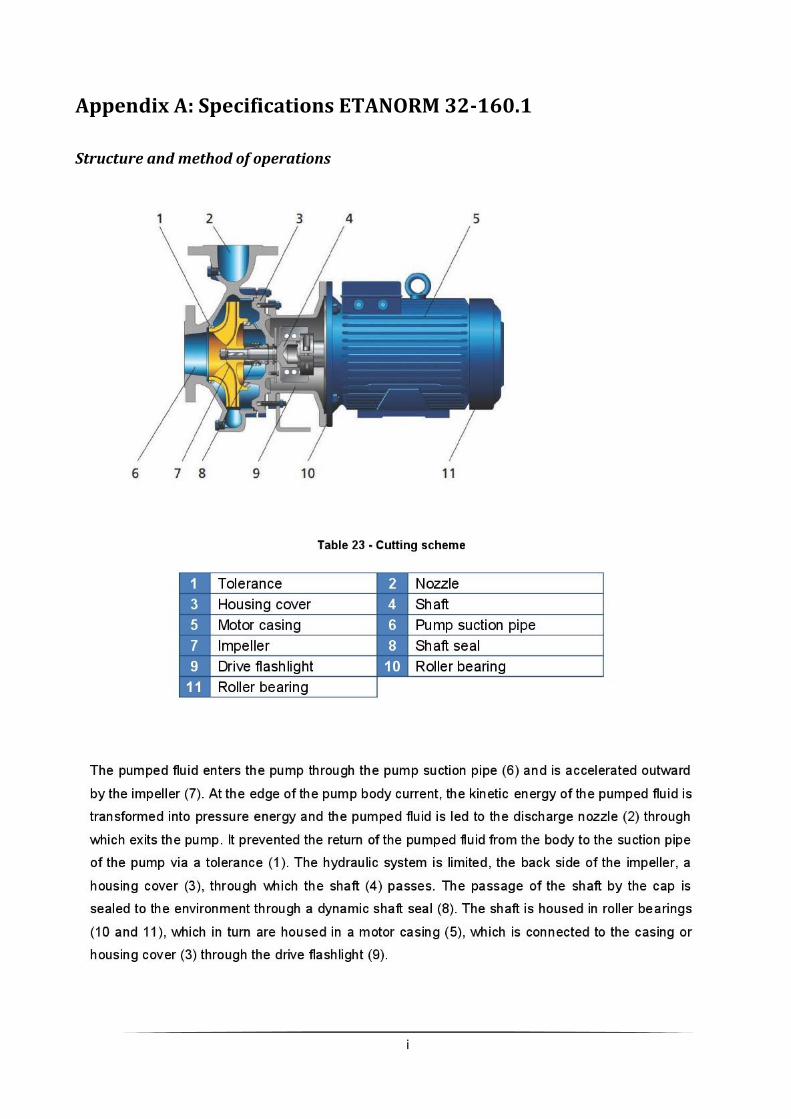
i
Appendix A: Specifications ETANORM 32-160.1
Structure and method of operations

ii
Characteristic curves

iii
Appendix B: payback time calculations for Case-study 1
Table 15 - Results of Economic analysis for Case-study 1
With incentives Without incentives
Cash Flow (€) Cumulative
Cash Flow (€) Cash Flow (€)
Cumulative Cash Flow (€)
Year 0 - -2501 -2501 -2501 -2501
Year 1
Month 1 158 -2343 92 -2409
Month 2 151 -2192 88 -2321
Month 3 185 -2007 108 -2213
Month 4 195 -1811 114 -2099
Month 5 221 -1591 129 -1970
Month 6 228 -1363 134 -1836
Month 7 248 -1114 146 -1690
Month 8 245 -869 144 -1546
Month 9 223 -647 130 -1416
Month 10 207 -440 121 -1295
Month 11 176 -264 103 -1192
Month 12 164 -100 95 -1097
Year 2
Month 1 158 58 92 -1005
Month 2 151 209 88 -917
Month 3 185 394 108 -809
Month 4 195 589 114 -695
Month 5 221 810 129 -566
Month 6 228 1038 134 -432
Month 7 248 1287 146 -286
Month 8 245 1532 144 -142
Month 9 223 1754 130 -12
Month 10 207 1961 121 109
Month 11 176 2137 103 212
Month 12 164 2301 95 307

iv
Appendix C: CDCF calculations for Case-study 3
Table 16 - Results of Economic analysis for Case-study 3
a) Incentives, Discount rate 2% b) Incentives, Discount rate 6% c) Incentives, Discount rate 8%
Year Cash Flow (€)
Discounted Cash Flow (€)
CDCF (€)
0 -6134 -6134 -6134
1 886 869 -5265
2 886 852 -4414
3 886 835 -3579
4 886 819 -2760
5 886 802 -1958
6 886 787 -1171
7 886 771 -400
8 886 756 356
9 886 741 1098
10 886 727 1825
11 886 713 2537
12 886 699 3236
13 886 685 3921
14 886 671 4592
15 886 658 5250
16 886 645 5896
17 886 633 6529
18 886 620 7149
19 886 608 7757
20 886 596 8353
Year Cash Flow (€)
Discounted Cash Flow (€)
CDCF (€)
0 -6134 -6134 -6134
1 886 836 -5298
2 886 789 -4510
3 886 744 -3766
4 886 702 -3064
5 886 662 -2402
6 886 625 -1777
7 886 589 -1188
8 886 556 -632
9 886 524 -108
10 886 495 387
11 886 467 854
12 886 440 1294
13 886 415 1709
14 886 392 2101
15 886 370 2471
16 886 349 2820
17 886 329 3149
18 886 310 3459
19 886 293 3752
20 886 276 4028
Year Cash
Flow (€) Discounted
Cash Flow (€) CDCF (€)
0 -6134 -6134 -6134
1 886 820 -5314
2 886 760 -4554
3 886 703 -3851
4 886 651 -3199
5 886 603 -2596
6 886 558 -2038
7 886 517 -1521
8 886 479 -1042
9 886 443 -599
10 886 410 -189
11 886 380 191
12 886 352 543
13 886 326 869
14 886 302 1170
15 886 279 1450
16 886 259 1708
17 886 239 1948
18 886 222 2169
19 886 205 2375
20 886 190 2565
d) No incentives, Discount rate 2%
e) No incentives, Discount rate 6%
f) No incentives, Discount rate 8%
Year Cash
Flow (€) Discounted
Cash Flow (€) CDCF (€)
0 -6134 -6134 -6134
1 473 464 -5670
2 473 455 -5216
3 473 446 -4770
4 473 437 -4333
5 473 428 -3905
6 473 420 -3485
7 473 412 -3073
8 473 404 -2669
9 473 396 -2273
10 473 388 -1885
11 473 380 -1505
12 473 373 -1132
13 473 366 -766
14 473 358 -408
15 473 351 -56
16 473 345 288
17 473 338 626
18 473 331 957
19 473 325 1282
20 473 318 1600
Year Cash
Flow (€) Discounted
Cash Flow (€) CDCF (€)
0 -6134 -6134 -6134
1 473 446 -5688
2 473 421 -5267
3 473 397 -4870
4 473 375 -4495
5 473 353 -4142
6 473 333 -3808
7 473 315 -3494
8 473 297 -3197
9 473 280 -2917
10 473 264 -2653
11 473 249 -2404
12 473 235 -2168
13 473 222 -1947
14 473 209 -1737
15 473 197 -1540
16 473 186 -1354
17 473 176 -1178
18 473 166 -1013
19 473 156 -856
20 473 147 -709
Year Cash
Flow (€) Discounted
Cash Flow (€) CDCF (€)
0 -6134 -6134 -6134
1 473 438 -5696
2 473 406 -5291
3 473 375 -4915
4 473 348 -4567
5 473 322 -4245
6 473 298 -3947
7 473 276 -3671
8 473 256 -3416
9 473 237 -3179
10 473 219 -2960
11 473 203 -2757
12 473 188 -2569
13 473 174 -2396
14 473 161 -2234
15 473 149 -2085
16 473 138 -1947
17 473 128 -1819
18 473 118 -1701
19 473 110 -1591
20 473 101 -1490