arX

iv:1

701.

0244

4v1

[cs.

IT]

10 J

an 2

017

Energy Harvesting Communication Using

Finite-Capacity Batteries with Internal

Resistance

Rajshekhar Vishweshwar Bhat,Graduate Student Member, IEEE,

Mehul Motani,Senior Member, IEEE,and Teng Joon Lim,Senior Member, IEEE

Abstract

Modern systems will increasingly rely on energy harvested from their environment. Such systems

utilize batteries to smoothen out the random fluctuations inharvested energy. These fluctuations induce

highly variable battery charge and discharge rates, which affect the efficiencies of practical batteries that

typically have non-zero internal resistances. In this paper, we study an energy harvesting communication

system using a finite battery with non-zero internal resistance. We adopt a dual-path architecture, in

which harvested energy can be directly used, or stored and then used. In a frame, both time and power

can be split between energy storage and data transmission. For a single frame, we derive an analytical

expression for the rate optimal time and power splitting ratios between harvesting energy and transmitting

data. We then optimize the time and power splitting ratios for a group of frames, assuming non-causal

knowledge of harvested power and fading channel gains, by giving an approximate solution. When only

the statistics of the energy arrivals and channel gains are known, we derive a dynamic programming based

policy and, propose three sub-optimal policies, which are shown to perform competitively. In summary,

our study suggests that battery internal resistance significantly impacts the design and performance of

energy harvesting communication systems and must be taken into account.

I. INTRODUCTION

Natural energy harvesting (EH) promises near-perpetual operation of electronic devices due

to its renewable nature. But, it poses several challenges insystem design as the power generated

from EH sources varies randomly with time, unlike conventional sources. For example, solar

Rajshekhar Vishweshwar Bhat, Mehul Motani and Teng Joon Limare with the Department of Electrical and Computer

Engineering, National University of Singapore, Singapore117583. Part of this work has been presented at the IEEE GLOBECOM

2015 conference in San Diego, CA, USA, 6-10 December, 2015 [1].

1

power can vary from1 µW to 100mW in a small-sized(approximate area of10 cm2) solar cell

across a day [2], [3]. The harvested energy needs to be storedin storage elements1 such as

batteries and super-capacitors, for reliable system operation. In the process, due to source power

fluctuations, the batteries are subjected to variable charging powers (rates). In addition, it may

be required to vary the battery discharge powers (rates), for instance, to drain the battery quickly

to accommodate the incoming harvested energy and, perhaps,also to cater to the variable power

demand at the load (the wireless transmitter, in our case). Hence, in EH systems, both the charge

and discharge powers are more variable and unpredictable than in conventional systems. This

necessitates a fundamental change in the way we store and usethe harvested energy mainly given

that the battery charge/discharge efficiencies (preciselydefined later) depend on the charge and

discharge powers [4], [5]. This dependency can be easily seen by considering a simple battery

model - a voltage source/sink with a series resistance. Drawing a larger power from the battery

entails a larger current, and hence a larger power loss in theinternal resistance. Therefore charge

and discharge efficiencies decrease with increasing chargeand discharge powers, respectively

[4]–[6].

In this work, we consider a low-power wireless transmitter powered entirely by an EH source

that is equipped with a battery having capacity constraintswith a non-zero internal resistance.

The internal resistances of commercial rechargeable micro-batteries and ultra-capacitors lie in

the range of a few micro ohms to several tens of ohms [7]–[9]. Typically, for small-sized wireless

nodes, the harvested power lies in the range1µW-100mW and the discharge power can vary

from 10µW to a few hundred milliwatts. In these ranges, by considering the simple battery

model presented in [5], it can be easily shown that the chargeefficiency range can be up to 15

percentage points and the discharge efficiency range can be as high as 30 percentage points.

In this paper, we focus on applications that require the nodeto communicateNs channel

symbols per frame over a fading channel. For instance, a sensor network deployed in an Internet

of Things (IoT) application consists of sensor nodes with limited data processing and storage

capabilities [10]. These may be designed to deliver a fixed number of coded symbols per frame,

due to limited data storage capacity at the receiver. The number of bits of information that are

reliably transmitted within a frame can be varied by varyingthe information rate. The harvested

1We use ‘batteries’ to refer to storage elements in general.

2

power in such applications can be very small due to limitations on the harvester size and area. To

illustrate the power management issues involved in such EH-based nodes, suppose for simplicity

that the initial energy stored in the battery is zero. In thiscase, whenever the harvested power

is lower than the power required for system operation, one cannot run the system from the EH

source alone. We must first store the harvested energy in a battery and then, simultaneously

draw power from the battery and the EH source, and run the system from the combined power.

In such a scenario, it is sensible to ask how to optimally divide a frame into two parts – the

first to store energy in the battery, and the next to dischargeenergy from the battery for data

transmission. Further, when the harvested power ishigh, directing all the power to the battery

may result in significant losses across internal resistances. In such cases, it may be beneficial to

charge the battery with only a fraction of the harvested power while the transmission is carried

out with the remaining power. In the second part of the frame,energy from the EH source may

be directed to the load at the same time as energy from the battery, perhaps because neither the

EH source nor the battery are able to power the load on their own. In this paper, we develop

novel policies for managing the battery charging and discharging schedules in such an EH-based

transmitter.

The problem of EH communications has been addressed from a variety of other perspectives

as well. A comprehensive review of recent advances in energyharvesting communications is

presented in [11], [12]. The information capacity of EH systems with infinite capacity batteries

is derived in [13], [14] and [15]–[18] present the EH communication with finite batteries. Other

battery limitations such as, leakage [19], [20], non-linear charging [3] and inefficiency [21], [22]

have also been considered. The optimal policies when the system operation cost is zero and

non-zero are studied in [23]–[28]. We note that the authors of the current paper considered a

similar EH communication problem in [1]. The current work significantly extends the model

in [1] by fully incorporating the effects of the battery internal resistance and providing more

in-depth analysis.

The main contributions of this paper are as follows:

• We identify generic and tractable models for the battery charge and discharge efficiencies

which account for their dependency on charging and discharging rates. This incorporates the

effects of battery internal resistance.

• We then formulate a single frame optimization problem and derive compact expressions for

3

optimal time and power sharing ratios.

• Further, we formulate an off-line optimization problem which assumesa priori knowledge of

the harvested powers and channel gains to obtain optimal time and power sharing ratios in

the multiple frame case. We show that in general, the problemis a non-convex optimization

problem, and propose an iterative algorithm to solve the problem approximately.

• Further, assuming statistical knowledge and causal information of the harvested power and

channel power gain variations, we solve for the optimalon-line policy by using stochastic

dynamic programming. We then propose three sub-optimal on-line algorithms which are prac-

tically feasible. Among them, an algorithm that is inspiredby the approximate off-line solution

achieves a significantly better performance compared to theother two algorithms.

• We also show via numerical simulations that the optimal policy designed for an ideal battery

performs poorly when the internal resistance is not negligible.

The remainder of the paper is organized as follows. The system model and assumptions are

presented in Section II. Section III and Section IV address the single and multiple frame rate

maximization problems respectively. Numerical results are presented in Section V followed by

concluding remarks in Section VI.

II. SYSTEM MODEL AND ASSUMPTIONS

A. Block Diagram and System Operation

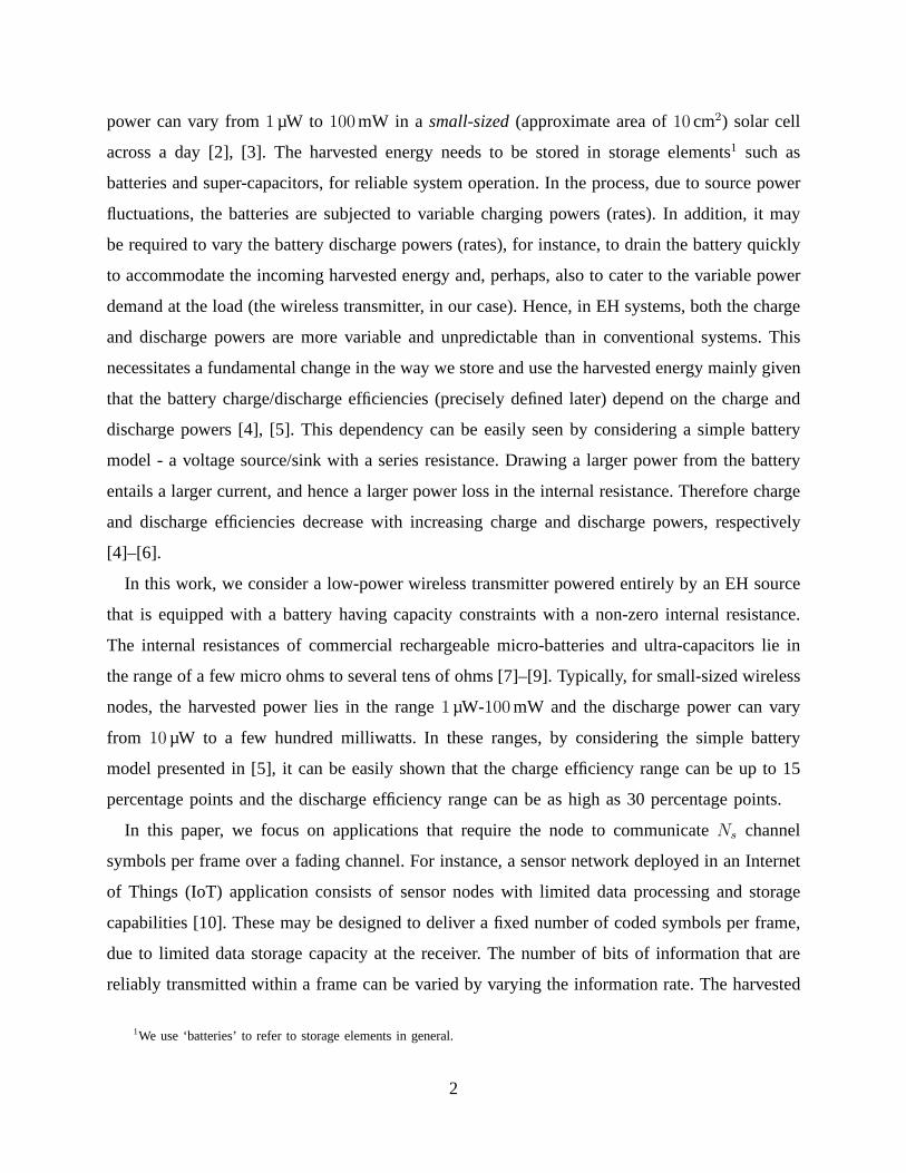
The block diagram of the system is given in Fig. 1. The principal components of the system

are the power splitter, battery, power combiner and the transmitter. The power splitter divides the

instantaneous harvested power to simultaneously charge the battery and power the transmitter

directly through a zero loss direct path. The power combinercombines the power drawn from

the battery and the direct path. The transmitter consumesp W for circuit operation during

transmission but does not consume any power when not transmitting, as in [28]. The structure

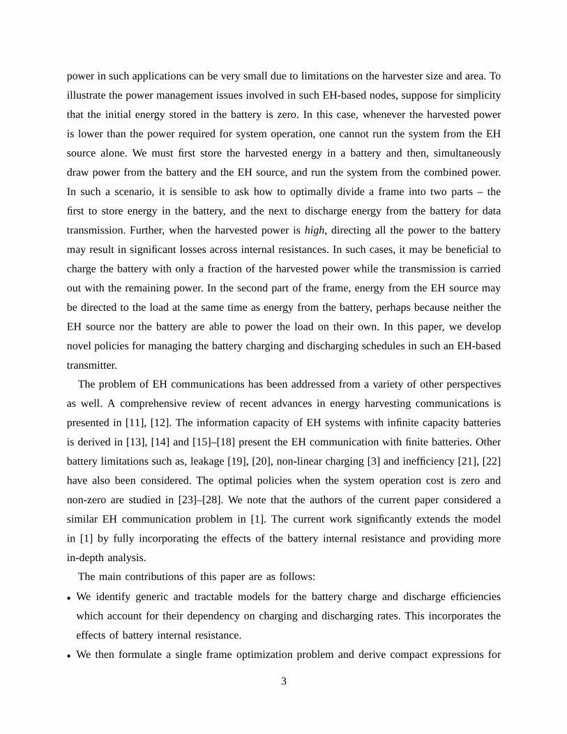
of the communication frame adopted in this work is shown in Fig. 2. The harvested power,

denoted byc, and channel power gain, denoted byh, are assumed to remain constant over the

frame of lengthτ seconds. We also assume that the channel bandwidth isW Hz.

We assume the battery cannot be charged and discharged simultaneously. This assumption

is both practical and without loss of generality. From the practical perspective, charging and

discharging of a battery/capacitor involves the movement of ions/electrons in mutually opposite

4

charvested power Power Splitter

αc

(1 − α)c

direct path with zero losses

Battery (r, B)d

+Power Combinerαc+ d Transmitter

(circuit powerp)

max(αc+ d− p, 0)

Transmit Power

Fig. 1: The dual-path EH communication system. A fraction (0 ≤ α ≤ 1) of the harvested power (c) can be directed to the load through

the direct path. The remaining power is directed to the battery having capacity ofB joules and internal resistance ofr ohms. The battery is

discharged atd W. The transmitter consumesp W for its operation during transmission but does not consumeany power when not transmitting.

α = αa, αa < 1d = da = 0

α = αb

d = db0 τρτ

γNs symbols (1− γ)Ns symbols

Fig. 2: The communication frame structure adopted in the paper. The frame length isτ seconds. During[0, ρτ), the power splitting ratio

α = αa, i.e., the power supplied to the transmitter isαac W. Over this time period, the battery must be charged, i.e.,αa < 1 and the discharge

power is zero, i.e.,d = da = 0 W. During [ρτ, τ ], information must be transmitted, i.e.,(1− γ)Ns, 0 < 1− γ ≤ 1, symbols are transmitted.

The power splitting ratioα = αb, and the battery is charged at(1 − αb)c W and discharged atdb W, with (1 − αb)db = 0, i.e., the battery

cannot be charged and discharged at the same time. We assume that γNs, 0 ≤ γ < 1, symbols are transmitted in the first part of the frame.

directions and the particles can move in only one net direction at a time [29]. Mathematically

one can relax the assumption and prove that charging and discharging a battery simultaneously

is always suboptimal, similar to the arguments in [22].

We assume an infinite backlog of data at the transmitter. Based on the motivation provided in

the introduction, to deal with the situation when the total available energy (the sum of the initial

energy stored in the battery and the harvested energy) in a frame is lower than the total energy

required to operate the system over the entire frame duration, we divide a communication frame

into two phases, a charging phase in which the battery must becharged, and a transmitting

phase, in which information must be transmitted. The frame structure (See Fig. 2) is as follows:

• Over the time duration[0, ρτ), ρ ∈ [0, 1], the battery must be charged, i.e., the charging

rate is (1 − αa)c W with 0 ≤ αa < 1. Since the battery cannot be charged and discharged

simultaneously, the discharge power must be zero, i.e.,d = da = 0 W in this time duration. We

assume thatγNs, 0 ≤ γ < 1, symbols are transmitted by utilizing the remainingαa fraction

of the harvested power from the direct path.

• Over the time duration[ρτ, τ ], information must be transmitted, i.e.,(1−γ)Ns, 0 < 1−γ ≤ 1,

symbols are transmitted. The battery is charged at(1−αb) fraction of the harvested power or

discharged atd = db W. Whether the battery is being charged or discharged,αb fraction of

the harvested power is directly delivered to the transmitter.

The variableρ, referred to astime-splitting ratio(TSR), is the ratio of the length of the charging

5

r Ω

VB V

Charge CurrentP

ower

Sou

rce

+

-

(a) An equivalent circuit diagram in the charge cycle.

Discharge Current

Loa

d

VB V

r Ω

+

-

(b) An equivalent circuit diagram in the discharge cycle.

Nc(cp)

charge power ,cpCp(r2) Cp(r1)

Nc0r = r1

r = r2 > r1

(c) The charging efficiency model based on [5].

Nd(dp)

discharge power,dpDp(r2) Dp(r1)

Nd0

r = r1

r = r2 > r1

(d) The discharging efficiency model based on [6].

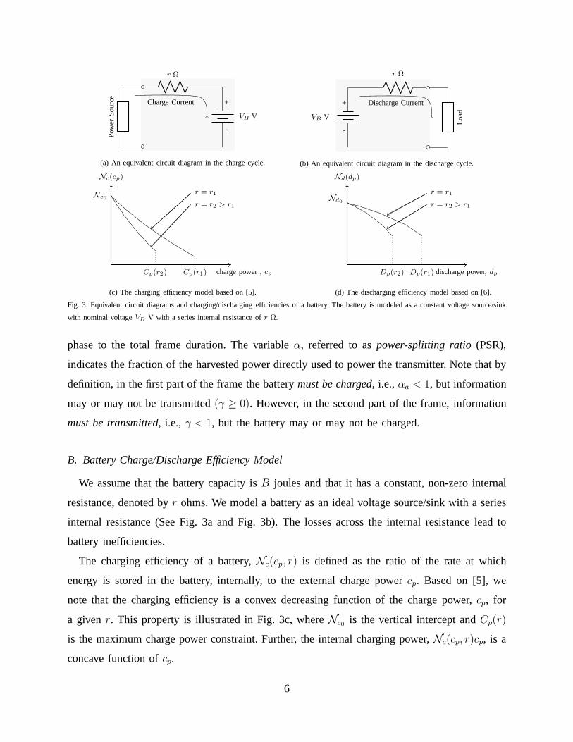
Fig. 3: Equivalent circuit diagrams and charging/discharging efficiencies of a battery. The battery is modeled as a constant voltage source/sink

with nominal voltageVB V with a series internal resistance ofr Ω.

phase to the total frame duration. The variableα, referred to aspower-splitting ratio(PSR),

indicates the fraction of the harvested power directly usedto power the transmitter. Note that by

definition, in the first part of the frame the batterymust be charged, i.e.,αa < 1, but information

may or may not be transmitted(γ ≥ 0). However, in the second part of the frame, information

must be transmitted, i.e., γ < 1, but the battery may or may not be charged.

B. Battery Charge/Discharge Efficiency Model

We assume that the battery capacity isB joules and that it has a constant, non-zero internal

resistance, denoted byr ohms. We model a battery as an ideal voltage source/sink witha series

internal resistance (See Fig. 3a and Fig. 3b). The losses across the internal resistance lead to

battery inefficiencies.

The charging efficiency of a battery,Nc(cp, r) is defined as the ratio of the rate at which

energy is stored in the battery, internally, to the externalcharge powercp. Based on [5], we

note that the charging efficiency is a convex decreasing function of the charge power,cp, for

a givenr. This property is illustrated in Fig. 3c, whereNc0 is the vertical intercept andCp(r)

is the maximum charge power constraint. Further, the internal charging power,Nc(cp, r)cp, is a

concave function ofcp.

6

The discharging efficiency,Nd(dp, r) is defined as the ratio of the power delivered to the load,

dp, to the rate at which energy is drawn from the battery, internally. It is shown to be a concave

decreasing function of the external discharge power (dp), for a givenr in [6]. This property is

illustrated in Fig. 3d, whereNd0 is the vertical intercept and,Dp, a concave decreasing function

of r, is the maximum discharge power. Further, the internal discharging power,dp/Nd(dp, r), is

a convex function ofdp. We also note that it is physically impossible to charge and discharge a

battery beyondCp andDp, respectively. In the rest of the paper, we denoteNc(cp, r) asNc(cp)

andNd(dp, r) asNd(dp) for brevity.

In general, the capacity of a battery varies with charge/discharge rates and this effect is referred

to as the rate-capacity effect. In many cases, the rate-capacity effect can be easily mitigated

with additional circuitry [30] and, by avoiding battery overcharging or undercharging leading to

extreme conditions [5]. Further, [31] argues that the rate-capacity effect is insignificant at low

power levels. Hence, we do not account for the rate-capacityeffect in this work.

III. SINGLE-FRAME RATE OPTIMIZATION

For transmission over an additive white Gaussian noise (AWGN) channel with power gain

h, transmit symbol energyP and unit received noise power spectral density, the maximum

achievable rate islog (1 + hP ) bits per channel symbol [32]. As in [22], [23], we assume that

the channel power gain for the current frame remains constant and its value is known at the start

of the frame. We assume that the number of coded (i.e. channel) symbols to be transmitted in

a frame is fixed atNs.

For any givenρ, the average rates within the two disjoint periods can be obtained as follows.

a) For t ∈ [0, ρτ): Without loss of generality, assume that we transmitγNs, 0 ≤ γ < 1,

symbols within the first part of the frame. Since the transmitter is supplied withαac W (recall

thatda = 0) for ρτ seconds directly from the EH source, the average symbol power Pa = (αac−

p)ρτ/(γNs). If γ = 0, thenPa = 0. Consequently, the information rate isRa = log(1+hPa). Note

that we can transmit symbols only ifPa > 0 implying that(αac− p)ρτ must be strictly greater

than zero for the symbol transmission to take place. Hence, we haveγ = 0 if (αac− p)ρτ < 0.

Since the battery is charged at(1 − αa)c W, the amount of energy stored in the battery over

[0, ρτ) is Bρτ = Nc((1− αa)c)(1− αa)cρτ .

7

b) For t ∈ [ρτ, τ ]: In the second part of the frame, the EH source and the battery supply

αbc W anddb W, respectively, to the transmitter, with(1 − αb)db = 0 as the battery cannot be

charged and discharged at the same time. Since the number of transmitted symbols is(1−γ)Ns,

the average symbol power,Pb = (αbc− p+ db)(1− ρ)τ/((1− γ)Ns) and the information rate is

Rb = log(1+hPb). Since the battery charging power over this time period is(1−αb)c, internally

the harvested energy gets stored in the battery at the rate ofcb = Nc((1 − αb)c)(1 − αb)c W.

Sincedb is the discharge power, internally the battery energy gets drawn atdb = db/Nd(db) W.

Consolidating the information rates within the above two disjoint periods, the average rate in

the frame is given by,

R(ρ, αa, αb, γ, db) = γRa + (1− γ)Rb (1)

Before formulating the optimization problem, we make an important remark on the generality

of the two-phasedframe structure described in Section II-A. In the proposed frame structure,

note that the charging and discharging rates can take at mosttwo values in a frame as per values

of αa, αb, da and db. To understand why it is sufficient to divide the frame into two phases,

consider a frame that is divided into more than two phases with possibly different charging,

discharging and transmit powers in each of the phases. Now, note that the internal charging

powers, discharging powers and information rates are concave, convex and concave functions of

the external charging, discharging and transmit powers, respectively. Hence, the loss across the

internal resistance is minimized and, simultaneously, theinformation rate is maximized when the

battery is charged and discharged at uniform powers. Hence,we can always replace any number

of phases with a single phase without any loss of optimality.As described earlier, it may not be

feasible to have a frame with only one phase as the amount of energy required to run the system

over the entire frame may be more than the amount of energy available. Hence, we conclude

that the frame structure described in Section II-A is completely general and sufficient to extract

the maximum possible performance from the system.

To maximize the information rate per frame, we must thus solve the following optimization

8

problem:

P0 : maximizeρ,αa,αb,γ,db

R(ρ, αa, αb, γ, db) (2a)

subject to (db − cb)(1− ρ)τ − Bρτ − B0 ≤ 0 (2b)

B0 +Bρτ − (db − cb)(1− ρ)τ −B ≤ 0 (2c)

0 ≤ ρ ≤ 1 (2d)

αc ≤ αa, αb ≤ 1 (2e)

0 ≤ db ≤ Dp (2f)

(1− αb)db = 0 (2g)

whereαc = 1− Cp/c and (2b) is the energy causality constraint which says that energy drawn

from the battery (db(1 − ρ)τ ) has to be less than or equal to the energy stored in the battery

(cb(1−ρ)τ+Bρτ+B0). The inequality in (2c) is the battery capacity constraint, (2e) accounts for

the maximum charge rate constraint, i.e., the charge rate(1−α)c must not exceed the maximum

charge rateCp, (2f) is the maximum discharge rate constraint and (2g) captures the fact that the

battery cannot be charged and discharged simultaneously. Recall thatdb and cb are functions of

db andαb, respectively.

We now make the following observation which says that it is not optimal to transmit any

symbols in the first part of the frame in the optimal solution to P0.

Lemma 1. In the optimal solution toP0 in (2),

1) the total number of symbols transmitted and the average rate over [0, ρ∗τ ] are zero, i.e.,

γ∗Ns = 0 andR∗a = 0 and,

2) all Ns symbols are transmitted during[ρ∗τ, τ ] at the average power(α∗bc − p + d∗b)(1 −

ρ∗)τ/Ns.

Proof: See Appendix A.

As a result of the above lemma, the objective function of P0 in(2) can be rewritten as

R(ρ, αa, αb, γ, db) = (1− γ∗)Rb = log((αbc− p+ db)(1− ρ)τ/Ns). Note that the optimal value

of γ∗ = 0, i.e. γ is no longer an optimization variable. The result also highlights that the number

of symbols transmitted in both the phases in the optimal caseis always an integer, thus satisfying

9

requirements of practical applications. Though the objective function now has a simpler form,

due to coupling ofρ, αa, αb anddb, P0 is still a non-convex optimization problem. However, we

exploit the structure of the problem and present the optimalsolution in the following theorem.

Theorem 2. The optimal solution toP0 is γ∗ = 0, α∗a = argmaxαc≤α≤1 (Nc((1− α)c)(1− α)c),

α∗b = 1, ρ∗ = min(ρB, ρr), where ρr = argmaxρ

(

(α∗bc− p+ db(α

∗a, ρ))(1− ρ)

)

and ρB =

(B − B0)/(Nc(c∗p)c

∗pτ), and d∗b = db(α

∗a, ρ

∗), where we definec∗p = (1 − α∗a)c, db(α

∗a, ρ) =

min(db, Dp) : db/Nd(db) = (Nc(c∗p)c

∗pρ+B0/τ)/(1− ρ).

Proof: See Appendix B.

Theorem 2 says that in the optimal solution, the battery is charged at the optimal rate in

the charging phase. Recall that no information is transmitted in the charging phase. In the

transmitting phase, the information is transmitted with the power drawn from the battery and the

EH source. Since the optimal external charging rate of the battery, (1−α∗a)c, may be lower than

the harvested power,c and because the transmission is not carried out in the charging phase, the

remainingα∗ac W gets wasted.

So far we did not impose any constraint on the channel bandwidth. Now, recall that the channel

bandwidth isW Hz and note that we need to transmitNs symbols during[ρτ, τ ], i.e., in (1−ρ)τ

seconds. Hence the Nyquist bandwidth2 is Ns/(1 − ρ)τ . Since, the signal bandwidth has to be

less than the channel bandwidth, we must haveNs/(1− ρ)τ ≤W , i.e.,

ρ ≤ 1−Ns

Wτ= ρW (3)

Hence, the optimal TSR with the bandwidth constraint isρ∗BW = min(ρ∗, ρW ), where ρ∗ is

obtained from Theorem 2.

IV. M ULTIPLE FRAME AVERAGE RATE OPTIMIZATION

In this section, we consider the problem of average rate maximization across multiple commu-

nication frames with the number of frames denoted byN . The harvested power in any framei

is assumed to be a random variableCi with a finite support, i.e.,0 ≤ Ci <∞, i = 1, . . . , N . We

assume that the random variables,C1, C2,. . . , CN , are independent and identically distributed

2considering a raised cosine pulse shaping filter with unity roll-off factor.

10

and that they do not change within a frame. Further, we assumethat the channel power gains,

denoted byH1, H2,. . . , HN , in frames1, 2, . . . , N , respectively, are independent and identically

distributed. The frame duration is assumed to beτ for all the frames.

A. Problem Formulation

First, we consider the off-line optimization under the assumption that the harvested power

and channel gains area priori known at the transmitter as in [22], [23], [26]–[28]. The optimal

throughput under the off-line optimization gives an upper bound for the optimal throughput in all

on-line algorithms. Let the realizations of harvested powers and channel power gains in frames,

1, . . . , N , be c1, . . . , cN , andh1, . . . , hN , respectively. The average throughput acrossN frames

is given by3,

Ravg(ρ,αa,αb,γ,db) =1

N

N∑

i=1

R(ρi, αai , αbi , γi, dbi) (4)

whereR(.) is given by (1) withh = hi for frame i. Note that all the variables carry their usual

meanings except that they are now indexed by the frame indexes.

To maximize the average information rate acrossN frames, we must thus solve the following

optimization problem:

P1 : maximizeρ,αa,αb,γ,db

Ravg(ρ,αa,αb,γ,db) (5a)

subject toi∑

k=1

(

dbk(1− ρk)− cakρk − cbk(1− ρk))

τ − B0 ≤ 0 (5b)

B0 +i∑

k=1

(

cakρk + cbk(1− ρk)− dbk(1− ρk))

τ − B ≤ 0 (5c)

αci ≤ αai , αbi ≤ 1, 0 ≤ ρi ≤ ρW (5d)

(1− αbi)dbi = 0, 0 ≤ dbi ≤ Dp (5e)

for i = 1, . . . , N , whereαci = 1 − Cp/ci and, cak = (1 − αak)ckNc((1 − αak)ck), cbk =

(1−αbk)ckNc((1−αbk)ck) are concave functions inαak andαbk , respectively and, they specify

the internal charging power of the battery over the time durations [0, ρkτ) and [ρkτ, τ ] in any

frame k, respectively. The internal discharge powerdbk = dbk/Nd(dbk) in any framek over

3 where any bold symbolx = x1, . . . , xN.

11

[ρkτ, τ ] is a convex function ofdbk and B0 is the initial energy stored in the battery. The

constraints in (5b) and (5c) are energy causality and battery capacity constraints, respectively.

Note that we have also included the bandwidth constraint, maximum charge and discharge rate

constraints and the constraint that the simultaneous charging and discharging is infeasible in (5d)

and (5e). As in the single frame case, we note the following.

Lemma 3. In the optimal policy,γ∗i = 0 for all i = 1, . . . , N .

Proof: See Appendix C.

Hence,γi’s are no longer optimization variables. Hence, the transmit powerPi in any frame

i is equal to(αbici − p+ dbi)(1− ρi)τ . Clearly, P1 in (5) is a non-convex optimization problem

due to the non-convex constraint in (5c) and due to the coupling of ρi’s with γi’s, dbi ’s, αai ’s

andαbi ’s.

In the following, we first solve the problem when the circuit cost is zero and get some

interesting insights on the optimal solution. We then approximately solve the problem when the

circuit cost is non-zero.

B. Zero Circuit Cost (p = 0) Case

Since energy is not expended for the circuit operation during the transmission, in this case, we

can transmit the coded symbols for the entire frame duration. Hence,ρi’s andαai ’s are no longer

optimization variables. In this case, the optimization problem P1 in (5) can be reformulated as

P2 : minimizeαbi

,dbii=1,...,N

−1

N

N∑

i=1

log (1 + hi(αbici + dbi)τ/Ns) (6a)

subject to (5b), (5c), 0 ≤ dbi ≤ Dp, αci ≤ αbi ≤ 1, i = 1, . . . , N (6b)

where the constraints should be self-explanatory. In general, P2 is non-convex due to the non-

convex constraint (5c).

When the channel gains remain constant across the frames, i.e., hi = h, i = 1, . . . , N and

when the battery capacity is infinite, we make an interestingobservation in the following theorem.

Theorem 4. Consider any two frames,j and k (k > j) such that the battery has a non-zero

residual energy in and between the framesj andk. Then, while the battery is being charged, i.e.,

12

αbj , αbk < 1, or the battery is being discharged, i.e.,dbj , dbk > 0, the optimal transmit power is a

strictly monotonically increasing function of the harvested power, i.e.,cj < ck impliesPj < Pk.

Proof: See Appendix D.

With the assumption that the battery efficiencies are independent of the charge and discharge

rates, it has been shown in [22] that the optimal power allocation has a double threshold structure:

the optimal transmit power does not vary with the harvested power whenever the harvested power

is above an upper threshold or below a lower threshold. It is interesting to note that if the battery

efficiencies vary with the charge and discharge rates as a result of non-zero internal resistance,

the optimal transmit power strictly monotonically increases with the harvested power and does

not exhibit the simple threshold structure observed with the fixed efficiency model in [22].

C. Non-Zero Circuit Cost (p > 0) Case

Recall that P1 in (5) is non-convex when the circuit cost is non-zero. Hence, analytically

solving P1 is challenging. In the rest of the section, we approximately solve P1 by considering

an upper bounding function of the discharge efficiency curvein Fig. 3d. We define the following

bounding function which is referred to as the step dischargemodel:Nd(db) = Nd0 if db ≤ Dp;

Nd(db) = 0 otherwise, whereDp is the maximum discharge rate.

We can now eliminate the coupling betweendbi ’s andρi’s by substitutingebi = dbi(1− ρi)τ .

The constraint on the discharge rate in the step discharge model can be re-written as,

ebi = dbi(1− ρi)τ ≤ Dp(1− ρi)τ, i = 1, . . . , N (7)

To eliminate the coupling betweenρi’s andαai ’s, we make the following observation.

Lemma 5. Let α∗ai= argmaxαci

≤α≤1 (Nc((1− α)ci)(1− α)ci). Then,Ravg(αa) ≤ Ravg(α∗

a) for

any givenρi, αbi, ebiNi=1.

Proof: See Appendix E.

Lemma 5 implies that in the optimal solution to P1, we must have αa = α∗a always. To

eliminate the coupling betweenαbi ’s and ρi’s, we make the following observation which says

that it is not optimal to charge the battery in the second partof the frame wheneverρi > 0.

13

Lemma 6. In the optimal policy, if the optimalρi > 0, then the optimalαbi = 1 and if the

optimal ρi = 0, thenαci ≤ αbi ≤ 1 in the optimal case.

Proof: See Appendix F.

The above result implies that(1 − αbi)ρi = 0. Hence, the rate in framei can be re-written

asR(ρi, αbi, αai , ebi) = log (1 + hi((αbi − ρi)ciτ − p(1− ρi)τ + ebi)/Ns), where we have sub-

stituted dbi(1 − ρi)τ by ebi and αbi(1 − ρi) by αbi − ρi. Hence, P1 can be reformulated as,

P3 : minimizeρi,αbi

,ebii=1,...,N

−1

N

N∑

i=1

log (1 + hi((αbi − ρi)ciτ − p(1− ρi)τ + ebi)/Ns) (8a)

subject toi∑

k=1

ebk/Nd0 − ρkc∗akτ − cbk(1− ρk)τ − B0 ≤ 0 (8b)

B0 +

i∑

k=1

(ρkc∗akτ + cbk(1− ρk)τ − ebk/Nd0 − B ≤ 0 (8c)

0 ≤ ρi ≤ ρW (8d)

0 ≤ ebi ≤ Dp(1− ρi)τ (8e)

(1− αbi)ρi = 0, αci ≤ αbi ≤ 1 (8f)

for i = 1, . . . , N , wherec∗ak = (1−α∗ak)ckNc((1−α∗

ak)ck) and the constraints (3), (7), (5b) and

(5c) are re-written as (8d), (8e), (8b) and (8c), respectively.

As a result of Lemma 6, we need to optimize only overαbi if ρi = 0 and optimize only over

ρi if ρi > 0, because the optimalαbi = 1 wheneverρi > 0. If we know whetherρi = 0 or

ρi > 0 for any framei in the optimal solution,ρi andαbi get decoupled and we can obtain the

solution to P3 by solving the resulting convex optimizationproblem. However, the challenge is

to identify whetherρi > 0 or ρi = 0 for i = 1, . . . , N , as the size of the search space increases

exponentially with the number of frames,N . In the sequel, we give an approximate solution to

P1 by approximately solving P3. To identify ifρi > 0 or ρi = 0 and solve P3 approximately,

we adopt the following technique.

1) In order to eliminate the coupling betweenρi’s andαbi ’s, setαbi = 1 for eachi = 1, . . . , N ,

and solve the modified P3, which now is a convex optimization problem, to obtain the optimal

solutionsρi,αb,1≤j≤N=1, eb,i,αb,1≤j≤N=1Ni=1. LetEi,αb,1≤j≤N=1 andRi,αb,1≤j≤N=1 be

14

the optimal transmit energy and rate in framei, respectively. Let the total energy loss, i.e., sum

of charging and circuit losses to achieve rateRi,αb,1≤j≤N=1 in frame i beLi,αb,1≤j≤N=1.

2) Then, we setρi = 0 and findαbi which results in the same transmit energy ofEi,αb,1≤j≤N=1

as in Step (1) for eachi = 1, . . . , N . Now, αbi may not be feasible due to the maximum

charge rate constraint. Hence, we considerαb,i,ρi=0 = max(αci, αbi) where the termαci

accounts for the maximum charge rate constraint. Let the total loss incurred with PSR of

αb,i,ρi=0 in frame i beLi,ρi=0. For any framei, we setρ∗i = 0 if Li,ρi=0 ≤ Li,αb,1≤j≤N=1;

set α∗bi

= 1 otherwise. In the previous step, due the assumption that thecharging and the

transmission are not done simultaneously, i.e.,αb,1≤j≤N = 1, the charging losses will be

high in frames withhigh harvested powers. In the current step, we try to reduce the loss while

maintaining the transmit power same as the previous step. Further, we note that if any frame

i receives energy in Step (1) above, thenα∗bi= 1 because the frame that receives energy in

Step (1) must receive energy in any other policy that performs better than the performance

of the policy in Step (1). If a frame receives energy, it is notoptimal to charge the battery

while it is being discharged, hence, we setα∗bi= 1, if frame i receives energy in Step (1).

3) Supposee∗bi is the solution in the above steps, then we assignd∗bi = min(dbi, Dp) : dbi(1 −

ρ∗i )τ/Nd(dbi) = e∗bi for all the framesi = 1, . . . , N .

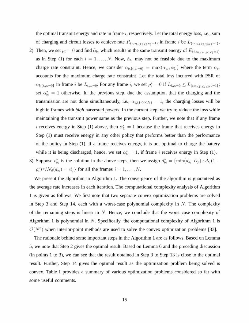
We present the algorithm in Algorithm 1. The convergence of the algorithm is guaranteed as

the average rate increases in each iteration. The computational complexity analysis of Algorithm

1 is given as follows. We first note that two separate convex optimization problems are solved

in Step 3 and Step 14, each with a worst-case polynomial complexity in N . The complexity

of the remaining steps is linear inN . Hence, we conclude that the worst case complexity of

Algorithm 1 is polynomial inN . Specifically, the computational complexity of Algorithm 1is

O(N3) when interior-point methods are used to solve the convex optimization problems [33].

The rationale behind some important steps in the Algorithm 1are as follows. Based on Lemma

5, we note that Step 2 gives the optimal result. Based on Lemma6 and the preceding discussion

(in points 1 to 3), we can see that the result obtained in Step 3to Step 13 is close to the optimal

result. Further, Step 14 gives the optimal result as the optimization problem being solved is

convex. Table I provides a summary of various optimization problems considered so far with

some useful comments.

15

Algorithm 1 Proposed Algorithm for Approximately Solving P1

1: procedure ENERGY-ALLOC(B0 ,c, h, N)

2: Computeα∗ai= argmaxαci

≤α≤1 (Nc((1− α)ci)(1− α)ci) and assignαa = α∗a.

3: Solve P3 withαb1 = . . . = αbN = 1. Obtain transmit powersEi,αb,1≤j≤N=1.

4: for i : 1→ N do

5: If frame i receives energy, thenα∗bi= 1; F ← i.

6: Setρi = 0 and computeαbi that results in transmit energy equal toEi,αb,1≤j≤N=1.

7: Obtainαb,i,ρi=0 = max(αci, αbi).

8: Compute the total lossLi,αb,1≤j≤N=1 andLi,ρi=0 if i /∈ F .

9: if Li,ρi=0 ≤ Li,αb,1≤j≤N=1 then ρ∗i = 0; A← i

10: else α∗bi= 1; B ← i

11: end if

12: Substituteαbi = 1, ∀ i ∈ B ∪ F andρi = 0, ∀ i ∈ A.

13: end for

14: Solve the resultant convex optimization problem to obtainρ∗ ande∗b .

15: d∗bi = min(dbi, Dp) : dbi(1− ρ∗i )τ/Nd(dbi) = e∗bi for eachi ∈ 1, . . . , N.

16: Returnρ∗,α∗a,α

∗b ,d

∗b .

17: end procedure

D. On-line Policies

In practice, it would be unrealistic to have the non-causal knowledge of the harvested power

and the channel state information, but, it is likely that we have statistical information.

The optimization problem P1 in (5) does not apply to systems with only stochastic knowledge

of the energy arrival profile. Here, we develop P1 in three directions below, leading to three

suboptimal policies to select the decision variablesρ,αa,αb,γ,db. The motivation behind

these simplifications and sub-optimal policies is that theyare practical and simple to implement.

We also compare the proposed sub-optimal policies with the optimal off-line and on-line policies.

1) Optimal Online Policy: To obtain the optimal power allocation when only the causal

knowledge and the statistical information of the harvestedpowers and channel power gains

are available, we employ the stochastic dynamic programming based approach [34]. Letsn =

16

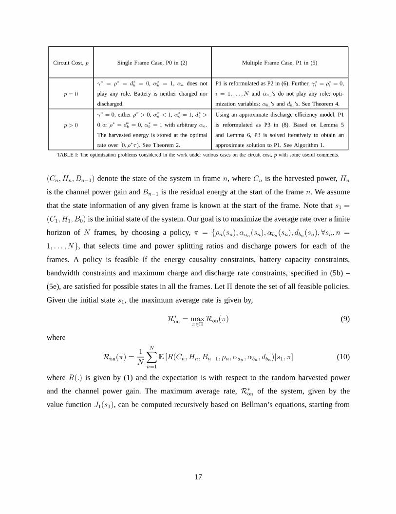
Circuit Cost,p Single Frame Case, P0 in (2) Multiple Frame Case, P1 in (5)

p = 0

γ∗ = ρ∗ = d∗b = 0, α∗b = 1, αa does not

play any role. Battery is neither charged nor

discharged.

P1 is reformulated as P2 in (6). Further,γ∗i = ρ∗i = 0,

i = 1, . . . , N and αai’s do not play any role; opti-

mization variables:αbi ’s anddbi ’s. See Theorem 4.

p > 0

γ∗ = 0, eitherρ∗ > 0, α∗a < 1, α∗

b = 1, d∗b >

0 or ρ∗ = d∗b = 0, α∗b = 1 with arbitraryαa.

The harvested energy is stored at the optimal

rate over[0, ρ∗τ ). See Theorem 2.

Using an approximate discharge efficiency model, P1

is reformulated as P3 in (8). Based on Lemma 5

and Lemma 6, P3 is solved iteratively to obtain an

approximate solution to P1. See Algorithm 1.

TABLE I: The optimization problems considered in the work under various cases on the circuit cost,p with some useful comments.

(Cn, Hn, Bn−1) denote the state of the system in framen, whereCn is the harvested power,Hn

is the channel power gain andBn−1 is the residual energy at the start of the framen. We assume

that the state information of any given frame is known at the start of the frame. Note thats1 =

(C1, H1, B0) is the initial state of the system. Our goal is to maximize theaverage rate over a finite

horizon of N frames, by choosing a policy,π = ρn(sn), αan(sn), αbn(sn), dbn(sn), ∀sn, n =

1, . . . , N, that selects time and power splitting ratios and dischargepowers for each of the

frames. A policy is feasible if the energy causality constraints, battery capacity constraints,

bandwidth constraints and maximum charge and discharge rate constraints, specified in (5b) –

(5e), are satisfied for possible states in all the frames. LetΠ denote the set of all feasible policies.

Given the initial states1, the maximum average rate is given by,

R∗on = max

π∈ΠRon(π) (9)

where

Ron(π) =1

N

N∑

n=1

E [R(Cn, Hn, Bn−1, ρn, αan , αbn, dbn)|s1, π] (10)

whereR(.) is given by (1) and the expectation is with respect to the random harvested power

and the channel power gain. The maximum average rate,R∗on of the system, given by the

value functionJ1(s1), can be computed recursively based on Bellman’s equations,starting from

17

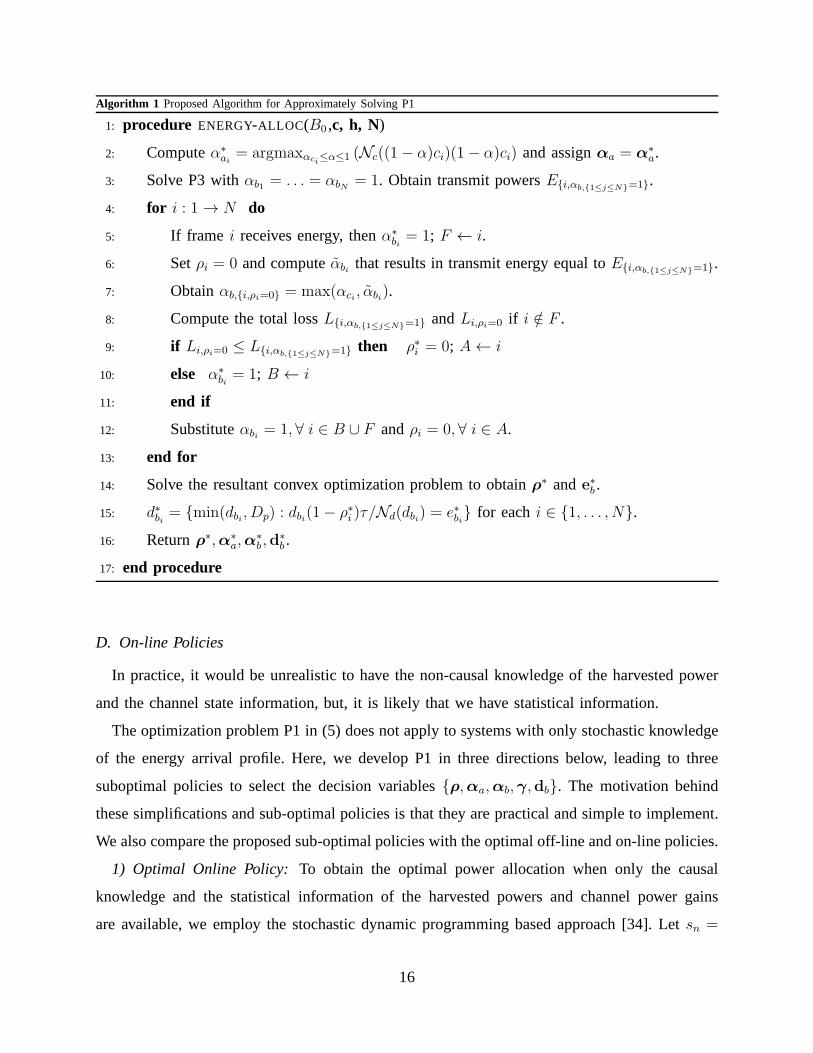
Algorithm 2 Statistical Algorithm

1: procedure STATISTICAL(B0 , c, h, N)

2: Computeα∗ai= argmaxαci

≤α≤1 (Nc((1− α)ci)(1− α)ci). b← B0

3: for i : 1→ N do

4: [ρt,dtb,α

tb] =ENERGY-ALLOC(b, [ci, C], [hi, H], 2)

5: ρi ← ρt(1), dbi ← d

tb(1) andαbi ← α

tb(1).

6: b← energy remaining in the battery in framei.

7: end for

8: end procedure

JN(sN), JN−1(sN−1), and so on untilJ1(s1) as follows:

JN(CN , HN , BN−1) = maxρN ,αaN

,αbN,dbN

R(CN , HN , BN−1, ρN , αaN , αbN , dbN ) (11a)

Jn(Cn, Hn, Bn−1) = maxρn,αan ,αbn ,dbn

R(Cn, Hn, Bn−1, ρn, αan , αbn, dbn) + Jn+1(Cn+1, Hn+1, Bn)

for n = 1, . . . , N − 1 (11b)

whereJn+1(Cn+1, Hn+1, x) = ECn+1,Hn+1 [Jn+1(Cn+1, Hn+1, x)] is the average throughput across

framesn+ 1 to N averaged over all the realizations ofCn+1 andHn+1. Note that in (11b), we

account for the fact thatCi’s andHi’s are independent. Note that the residual energyBn in (11b)

is a function of the decision variablesρn, αan , αbn anddbn . An optimal policy is denoted asπ∗ =

ρ∗n(sn), α∗an(sn), α

∗bn(sn), d

∗bn(sn), ∀sn, n = 1, . . . , N, whereρ∗n(sn), α

∗an(sn), α

∗bn(sn), d

∗bn(sn)

is the optimal solution to (11) when the state of the system issn.

2) Greedy Algorithm:When we only have the instantaneous knowledge of the harvested power

but not the non-causal or statistical information on the power profile, the entire harvested energy

in any frame is utilized in the same frame itself. In each of the frames, the corresponding single

frame optimization problem is solved. Based on Theorem 2, the optimal solution can be easily

found in each of the frames. The algorithm is simple to implement and achieves the optimal

rate when all energy in the battery must be used up within eachframe. But, the instantaneous

optimality comes at the cost of increased circuit energy consumption due to longer duration of

circuit operation.

18

3) Statistical Algorithm (SA):In addition to the instantaneous knowledge, when we have the

statistical information (such as the mean value) of harvested powers and channel gains across the

frames, we propose an algorithm based on Algorithm 1. Let theexpected values of the harvested

power and channel gains beC andH, respectively. Let the TSRs, PSRs and the discharge powers

be represented by(ρi, αbi, dbi) in framesi ∈ 1, . . . , N.

At the beginning of any framei, we have the instantaneous knowledge of the harvested power

and the channel gain, i.e.,(ci, hi), residual energy in the battery and(C, H), but, we do not have

any information on(ci+1, . . . , cN , hi+1, . . . , hN ). To find (ρi, αbi, dbi), we consider a hypothetical

two-frame optimization problem with the first frame being the framei and the second frame

being a hypothetical frame with parameters(C, H). Then, at the beginning of framei, for

i = 1, . . . , N , the transmitter solves the optimization problem P1 in (5) for the above two-frame

hypothetical problem. The statistical algorithm is presented in Algorithm 2.

4) Constant Time/Power Splitting Ratio (CTSR/CPSR) Policies : Though the adaptive policies

described above are simple and practical, simpler systems may not have the capability to measure

the harvested energy and the channel states instantaneously. In such systems, it is not feasible to

compute the suitable TSRs and PSRs for each frame instantaneously, at the frame beginning. It

is more practical to use a single, pre-computed time/power splitting ratio across all the frames.

A sensible choice of the TSRs and PSRs is the one that maximizes the average rate in (5)

with an additional constraint that the TSRs and PSRs in each frame have to be equal i.e.,

ρ = ρi, αa = αai , αb = αbi, for i = 1, . . . , N , with only the stochastic knowledge of energy

arrival rates.

Since, the constraint(1 − αbi)ρi = 0, i = 1, . . . , N , has to be satisfied, we fix eitherαb1 =

. . . = αbN = 1 andαa = . . . , αN = α(c)a = argmaxαE(C)≤α≤1 (Nc((1− α)E(C))(1− α)E(C)),

whereE(C) is the expected value of the harvested power,αE(C) = 1 − Cp/E(C) and, find the

optimalρ, leading toconstant time splitting ratio (CTSR) policy, or fix ρ1 = . . . = ρN = 0 and

find the optimalαb, leading toconstant power splitting ratio (CPSR) policy.

V. NUMERICAL RESULTS

In our simulations, we assume that information rateR = 0.5 log(1 + hPt/(N0W )) bits per

channel use, wherePt is the average transmit power,h is the channel power gain,N0 = 10−15

W/Hz is the AWGN power spectral density andW = 1MHz is the channel bandwidth. We

19

0 20 40 60 80 100

Harvested Power, c (mW)

0

20

40

60

80

100O

pti

mal

Ch

arg

ing R

ate

(m

W) External Charging Rate, r=10 Ω

Internal Charging Rate, r=10 Ω

External Charging Rate, r=50 Ω

Internal Charging Rate, r=50 Ω

(a) Variation with the harvested power forh = 1, VB = 1.5V.

1 1.5 2 2.5 3 3.5 4 4.5 5

Battery Voltage, VB

(V)

0

20

40

60

80

100

Op

tim

al

Ch

arg

ing R

ate

(m

W)

External Charging Rate, r=10 Ω

Internal Charging Rate, r=10 Ω

External Charging Rate, r=50 Ω

Internal Charging Rate, r=50 Ω

(b) Variation with the battery voltage forh = 1, c = 100mW.

Fig. 4: Variation of optimal internal and external chargingrates with (a) the deterministic harvested power and (b) thebattery voltage.

assume thatNs = 106 symbols are transmitted per frame of durationT = 1 s. We assume

that the channel power gain is exponentially distributed with unit mean. Based on [5], we

assume that the charging efficiency,Nc(cp) = 1.5− 0.5√

1 + 4rcp/V 2B, the discharge efficiency,

Nd(dp) = 0.5+0.5√

1− 4rdp/V 2B, the maximum charge power,Cp = 2V 2

B/r and the maximum

discharge power,Dp = V 2B/(4r), whereVB is the nominal voltage of the battery.

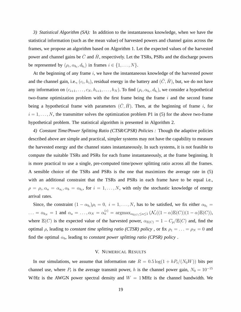
A. Variation of Optimal Charging Rates with the Harvested Power and Nominal Battery Voltage

In Fig. 4, we present the variation of optimal internal and external charging rates with harvested

power (in Fig. 4a) and the nominal battery voltage (in Fig. 4b). The external charging rate, given

by c∗p = (1− α∗a)c, indicates the power directed to the battery after the optimal power splitting,

and the internal charging rate, given byc∗pNc(c∗p, r), indicates the the rate at which energy gets

stored in the battery internally, after the losses in the internal resistance.

We make two important observations from Fig. 4a. First, whenthe internal resistance islow,

the external charging rate linearly increases with the harvested power (in this case,α∗a = 0),

but the internal charging rate increases at a slower rate with the harvested power due to the

resistive losses. Second, when the internal resistance ishigh, then both the external and internal

charging rates increase only up to a threshold, beyond whichthe battery is charged at the optimal

charging rate, which is independent of the harvested power.Similarly, from Fig. 4b, we note that

the internal resistance significantly impacts the externaland internal charging rates for a wide

range of the nominal voltage of the battery.

20

0 20 40 60 80 100

Internal Resistance, Ω

0.6

0.8

1

1.2

1.4

1.6

1.8A

ver

age

Rate

(M

bp

s)p=5 mW, c=10 mW

p=10 mW, c=10 mW

p=5 mW, c=20 mW

p=10 mW, c=20 mW

(a) Optimal Rate for the Single Frame

0 20 40 60 80 100

Internal Resistance, Ω

0

0.2

0.4

0.6

0.8

1

1.2

Tim

e S

pli

ttin

g R

ati

o

p=5 mW, c=10 mW

p=10 mW, c=10 mW

p=5 mW, c=20 mW

p=10 mW, c=20 mW

(b) Optimal Time Splitting Ratio for the Single Frame

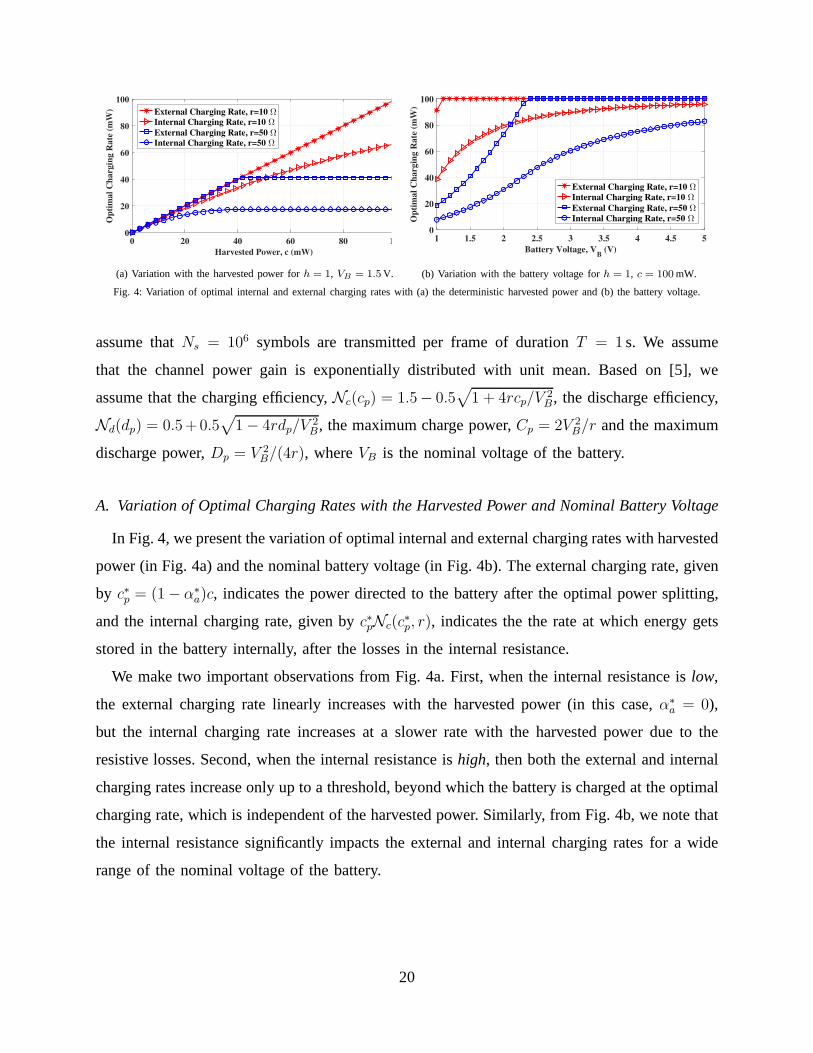
Fig. 5: Comparison of (a) optimal rates and the corresponding (b) optimal time splitting ratios and their variation withthe internal resistance

for two values of the circuit power,p and non-random harvested powers,c with T = 1 s, h = 1, B = 20mJ,VB = 1.5V and ρW = 0.9.

B. The Optimal Rate in the Single Frame Case

Fig. 5a shows the variation of the optimal rate with the battery internal resistance for two

values of the circuit cost and harvested powers and Fig. 5b shows the corresponding optimal

TSRs. From Fig. 5, we make two important observations. First, when the circuit cost is in the

order of the harvested power, the optimal rate decreases with the increasing internal resistance

and the optimal TSR is greater than zero. This is because whenthe circuit cost is in the order

of the harvested power, one can save on the circuit losses by operating the circuit for smaller

amount of time while the harvested energy is stored and drawnfrom the battery. Second, when

the harvested power is few times more than the circuit cost, then the optimal rate decreases up

to a certain point beyond which the rate is independent of theinternal resistance. The reason

is that the battery charge and discharge losses increase as the internal resistance increases. But,

the system continues the transactions (charging and discharging) with the battery to reduce the

circuit losses up to a certain point. This can be seen from Fig. 5b where the TSR is greater

than zero up to a certain value of the internal resistance. Asthe internal resistance increases,

the battery charging and discharging losses surpass the gain obtained by avoiding the circuit

losses and, it turns out that avoiding any transactions withthe battery is optimal. Obviously, the

optimal rate after thecut-off point is independent of battery parameters.

C. Optimal Transmit Power Levels Under Two Different Modelsfor Battery Losses

Due to the non-zero internal resistance, charge/dischargeefficiencies vary with charge/discharge

rates. Hence, it is insightful to compare optimal power allocation in this case with that when

the battery efficiency is a constant as in [22]. We show the optimal transmit powers in these

21

10 20 30 40 50 60 70 80 90 100

Frame Index

0

2

4

6

8

10

12

14

16

18

20

Harv

este

d a

nd

Tra

nsm

it P

ow

ers

(mW

)

Harvested power, c

curve-1: transmit power for battery with internal resistance

curve-2: transmit power for battery with fixed inefficiency

battery is charged in the first 50

frames

battery is discharged in the last

50 frames

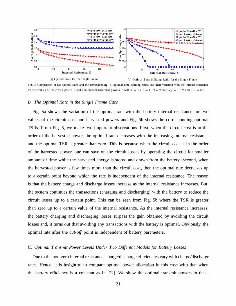
Fig. 6: A comparison of the optimal transmit power levels in two different battery loss models. For curve-1, we assume that the battery has

a non-zero internal resistance (5Ω) which results in battery charge/discharge inefficienciesthat are functions of charge/discharge rates. The

curve-2 is plotted assuming that the battery has a fixed round-trip efficiency (N = NcNd = 0.75) as in [22]. We assume thatB = ∞ and

VB = 1.5V.

0 10 20 30 40 50

Average Harvested Power, mean(C) (mW)

0

0.2

0.4

0.6

0.8

1

1.2

Aver

age

Rate

(M

bp

s)

No-Battery Case

Proposed Solution, r= 0 Ω

Proposed Solution, r= 50

Ideal-Battery Case, r= 0 Ω

Ideal-Battery Case, r= 50

Fig. 7: Variation of the average rate with the average harvested power for various cases in the off-line policy withT = 1 s, B = 100mJ,

VB = 1.5V, p = 10mW, N = 100 andρW = 0.9.

two cases with the harvested power in Fig. 6. It has been shownin [22] that the optimal power

allocation has a double threshold structure as shown in curve-1 of Fig. 6. Unlike in curve-1, it

is interesting to note that if the battery has a non-zero internal resistance, the optimal transmit

power strictly monotonically increases with the harvestedpower as shown in curve-2 and proved

in Theorem 4.

D. Variation of the Average Rate in the Off-Line Policy with the Average Harvested Power

In Fig. 7, we present the variation of the average rate in the off-line policy with the average har-

vested power, obtained by averaging the numerical results from 1000 independent runs of Monte

22

Carlo simulations. The No-Battery Case curve assumes that the system is not equipped with any

battery and the Ideal-Battery Case curve is obtained by adopting the optimal policy in an ideal

battery (with zero internal resistance) to the non-ideal battery case. Note that the rate of increase

in the average rate with the average harvested power is considerably affected by the internal

resistance. This is because as the average harvested power increases, the charging/discharging

rates increase resulting in the increased charging/discharging losses. It is interesting to note that

as the average harvested power increases, the average rate in the Ideal-Battery Case approaches

the average rate in the No-Battery Case implying that the optimal policies designed for an ideal

battery may be strictly suboptimal when the internal resistance is non-zero.

E. Comparison of the Performances of On-line and Off-line Policies

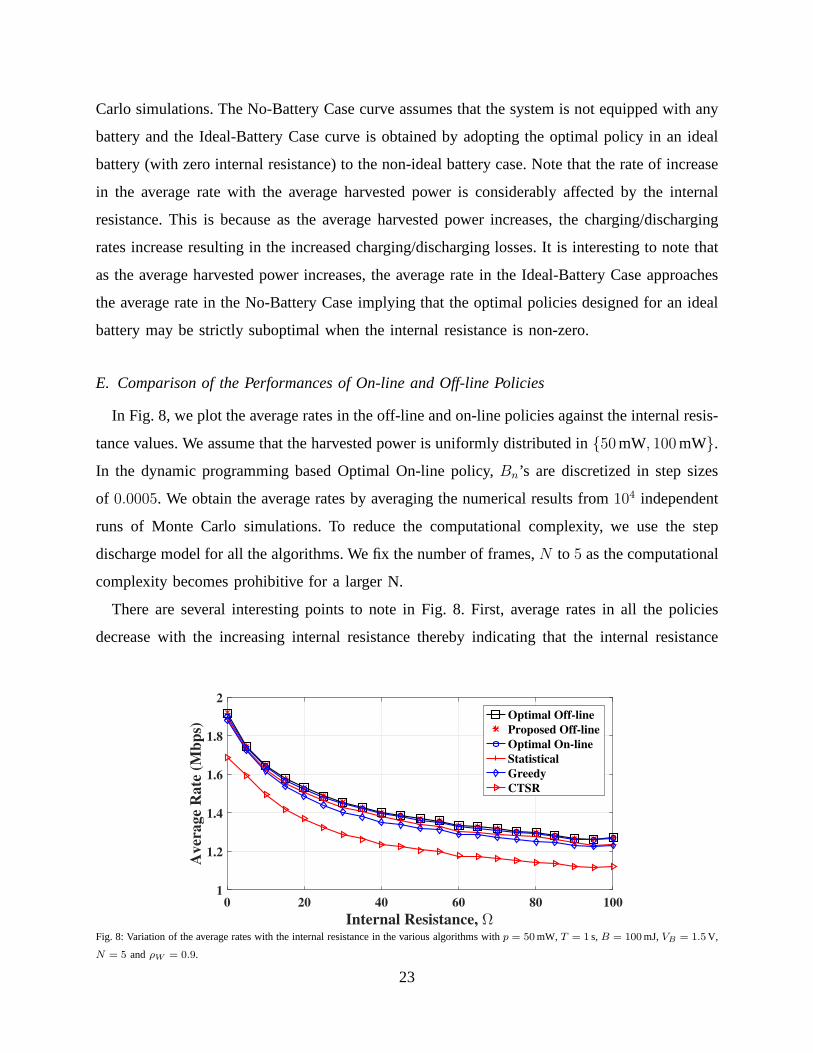
In Fig. 8, we plot the average rates in the off-line and on-line policies against the internal resis-

tance values. We assume that the harvested power is uniformly distributed in50mW, 100mW.

In the dynamic programming based Optimal On-line policy,Bn’s are discretized in step sizes

of 0.0005. We obtain the average rates by averaging the numerical results from 104 independent

runs of Monte Carlo simulations. To reduce the computational complexity, we use the step

discharge model for all the algorithms. We fix the number of frames,N to 5 as the computational

complexity becomes prohibitive for a larger N.

There are several interesting points to note in Fig. 8. First, average rates in all the policies

decrease with the increasing internal resistance thereby indicating that the internal resistance

0 20 40 60 80 100

Internal Resistance, Ω

1

1.2

1.4

1.6

1.8

2

Av

era

ge

Ra

te (

Mb

ps)

Optimal Off-line

Proposed Off-line

Optimal On-line

Statistical

Greedy

CTSR

Fig. 8: Variation of the average rates with the internal resistance in the various algorithms withp = 50mW,T = 1 s,B = 100mJ,VB = 1.5V,

N = 5 andρW = 0.9.

23

Algorithms N = 25 N = 50 N = 75 N = 100

Proposed Offline Algorithm 0.3 s 1.27 s 2.85 s 7.79 s

Statistical Algorithm 0.26 s 0.14 s 0.1 s 0.08 s

Greedy Algorithm 10ms 9ms 5ms 4ms

CTSR Algorithm 13ms 10ms 10ms 10ms

CPSR Algorithm 10ms 10ms 15ms 15ms

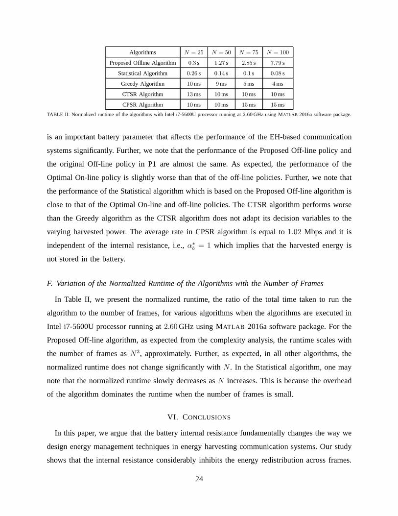
TABLE II: Normalized runtime of the algorithms with Intel i7-5600U processor running at2.60GHz using MATLAB 2016a software package.

is an important battery parameter that affects the performance of the EH-based communication

systems significantly. Further, we note that the performance of the Proposed Off-line policy and

the original Off-line policy in P1 are almost the same. As expected, the performance of the

Optimal On-line policy is slightly worse than that of the off-line policies. Further, we note that

the performance of the Statistical algorithm which is basedon the Proposed Off-line algorithm is

close to that of the Optimal On-line and off-line policies. The CTSR algorithm performs worse

than the Greedy algorithm as the CTSR algorithm does not adapt its decision variables to the

varying harvested power. The average rate in CPSR algorithmis equal to1.02 Mbps and it is

independent of the internal resistance, i.e.,α∗b = 1 which implies that the harvested energy is

not stored in the battery.

F. Variation of the Normalized Runtime of the Algorithms with the Number of Frames

In Table II, we present the normalized runtime, the ratio of the total time taken to run the

algorithm to the number of frames, for various algorithms when the algorithms are executed in

Intel i7-5600U processor running at2.60GHz using MATLAB 2016a software package. For the

Proposed Off-line algorithm, as expected from the complexity analysis, the runtime scales with

the number of frames asN3, approximately. Further, as expected, in all other algorithms, the

normalized runtime does not change significantly withN . In the Statistical algorithm, one may

note that the normalized runtime slowly decreases asN increases. This is because the overhead

of the algorithm dominates the runtime when the number of frames is small.

VI. CONCLUSIONS

In this paper, we argue that the battery internal resistancefundamentally changes the way we

design energy management techniques in energy harvesting communication systems. Our study

shows that the internal resistance considerably inhibits the energy redistribution across frames.

24

This causes a significant reduction in the optimal average communication rate compared to that

obtained using an ideal battery (i.e., zero internal resistance). Furthermore, the optimal policy

designed for an ideal battery performs poorly when the internal resistance is not negligible.

In our work, the charging/discharging efficiencies are modeled as functions of the internal

resistance and charge/discharge powers. We assume a finite capacity battery, non-zero circuit

power and take into account limitations on bandwidth. In this context, we derive compact

expressions for optimal time and power splitting ratios in the single frame case. We then propose

an iterative off-line algorithm to approximately solve thenon-convex optimization problem which

assumesa priori knowledge of the harvested powers and channel gains in the multiple frame

case. We also solve for the optimal on-line policy by using stochastic dynamic programming

assuming statistical knowledge and causal information of the harvested power and channel power

gain variations. We then propose three heuristic on-line algorithms and show that an algorithm

that is inspired by the off-line policy performs significantly better than the other two heuristic

algorithms. Advanced analysis of the proposed algorithms is considered as a future work.

APPENDIX

A. Proof of Lemma 1

Whenαac ≤ p, we cannot operate the circuit during[0, ρτ) for anyρ, hence,max(αac−p, 0) =

0 andRa = 0 for any ρ, including ρ = ρ∗ and the transmission occurs only over[ρτ, τ ] with

constant powerτ(αbc− p+ db)(1− ρ)/Ns. Whenαac > p we have,

R(ρ, αa, αb, γ, db) = γRa + (1− γ)Rb = γ log(1 + hPa) + (1− γ) log(1 + hPb) (12)a≤ log(1 + hτ/Ns (ρ(αac− p) + (1− ρ)(αbc− p+ db))) (13)

b≤ log(1 + hτ/Ns

(

c− p+ db

)

) = Rb|ρ=0 (14)

wheredb = d : dτ/Nd(d) = B0, (a) follows from Jensen’s inequality, (b) holds because ofthe

following. Whendb = 0, the term,ρ(αac−p)+(1−ρ)(αbc−p) ≤ c(ραa+(1−ρ)αb)−p ≤ c−p

as ραa + (1 − ρ)αb ≤ 1; for any db > 0, we haveαb = 1 and, from (2b),db(1 − ρ)τ =

Nd(db)(Bρτ +B0) = Nd(db)Nc((1− αa)c)(1− αa)cρτ +Nd(db)B0 ≤ (1− αa)cρτ +Nd(db)B0

which implies thatρ(αac−p)+(1−ρ)(αbc−p+db) ≤ c−p+Nd(db)B0/τ = c−p+ db, where

the upper bound is attained whenρ = 0.

25

Consolidating the results, for any givenρ and a policy that hasRa > 0, we can always find

another policy with a higher average rate such thatRa = 0, while satisfying all the constraints.

Hence,γ∗ = 0 andR[0,ρ∗τ) = 0 and allNs symbols are transmitted only during[ρ∗τ, τ ] with the

transmit powerτ(α∗bc− p+ d∗b)(1− ρ∗)/Ns. Lemma 1 is thus proved.

B. Proof of Theorem 2

Based on Lemma 1, we haveR = log(1 + h (αbc+ db − p) (1 − ρ)τ/Ns). Since,R is a

monotonically increasing function of the transmit power, in order to maximizeR, we can simply

maximize the transmit power,P = (αbc+ db − p) (1−ρ)τ/Ns. Since,τ andNs are constants, we

instead maximizeE(αa, αb, db, ρ) = (αbc+db−p)(1−ρ). We first solve the problem by relaxing

the battery capacity constraint in (2c). Since, draining the battery completely is optimal and,

noting that(1−αb)db = 0, in the optimal policy we must have,(db/Nd(db)) = (Nc((1−αa)c)(1−

αa)cρτ+B0)/((1−ρ)τ) anddb ≤ Dp, for any feasibleαa andρ, from (2b) and (2f), respectively.

Define db(αa, ρ) = min(db, Dp) : db/Nd(db) = (Nc((1− αa)c)(1− αa)cρτ +B0)/((1− ρ)τ).

For a concave decreasingNd(db), it can be shown thatdb/Nd(db) is a convex increasing function

of db. Hence, ifαa and ρ are given, we can uniquely determinedb(αa, ρ) always. Hence, the

optimal discharge powerd∗b = db(α∗a, ρ

∗). Now, E(.) can be treated as a function of onlyαa, αb

and ρ. Hence,E(αa, αb, ρ) = (αbc − p + db(αa, ρ))(1 − ρ). For anyρ and αa, the quantity

αbc(1 − ρ) achieves its maximum atαb = 1, hence,α∗b = 1. Further,db(αa, ρ) is a monotonic

increasing function ofNc((1−αa)c)(1−αa)c and hence, it attains the maximum atαa = α∗a =

argmaxαc≤α≤1(Nc((1−α)c)(1−α)c) for anyρ. Hence,E(α∗a, α

∗b , ρ) = (αbc−p+db(α

∗a, ρ))(1−ρ).

To obtain the maximum rate, we simply need to maximizeE(α∗a, α

∗b , ρ) over ρ. Now, we note

that the battery capacity constraint simply puts an upper bound on ρ. From (2c), we have,

Nc(c∗p)c

∗pρτ +B0 ≤ B which impliesρ ≤ (B − B0)/(Nc(c

∗p)c

∗pτ). Hence the proof.

C. Proof of Lemma 3

Recall that in Section III we had definedγi = 0 if (αaici−p)ρiτ < 0. Hence, to proveγ∗i = 0

for any i we need to prove(α∗aici − p)+ρ∗i τ = 0 for the i-th frame, where(x)+ = max(x, 0). If

(α∗aici − p) ≤ 0, then, we always have(α∗

aici − p)+ρ∗i τ = 0. But, whenever(α∗

aici − p) > 0, we

need to prove thatρ∗i = 0. To accomplish this, we note that the decision variables arecoupled

across the various frames as energy may get transferred fromone frame to another in the optimal

26

policy. This energy transfer can be accounted for by considering the residual energy available

in the battery at the start of each of the frames. LetBi−1 be the stored energy in the battery at

the start of any framei. Then, the energy consumed by framei from the battery isBi−1 − Bi

(a negative value indicates that energy is stored in the battery) in any framei. By some means,

if we know the value ofBi−1’s, then, we can optimize each frame independent of the other

frames. Assume that for any framei, α∗ai

, ρ∗i > 0, B∗i−1 andB∗

i are the optimal values. As in

the proof of Lemma 1, we can show that for any framei with α∗aic > p and ρ∗i > 0, for any

B∗i−1 andB∗

i values, we can achieve a higher rate in framei, than the rate whenρ∗i > 0, by

selectingρ′∗i = 0 and choosing an arbitraryα′∗ai

. Hence, by contradiction, we must haveρ∗i = 0

in the optimal policy. This proves thatγ∗i = 0 for any i in the optimal policy.

D. Proof of Theorem 4

We first note that whenever the battery capacity is infinite, (5c) is inactive and P2 is convex.

Hence, Karush-Kuhn-Tucker (KKT) conditions are necessaryand sufficient for optimality. The

Lagrangian of P2 is given by

L2 = −1

N

N∑

i=1

log (1 + hi(αbici + dbi)τ/Ns) +

N∑

i=1

λi

(

i∑

k=1

(

dbk − cbk

)

τ −B0

)

−N∑

i=1

ωidbi +N∑

i=1

δi(dbi −Dp)−N∑

i=1

µi(αbi − αci) +N∑

i=1

νi(αbi − 1) (15)

whereλi, ωi, δi, µi and νi are non-negative Lagrange multipliers corresponding to inequalities

(5b), dbi ≤ 0, dbi ≤ Dp, αci − αbi ≤ 0 andαbi − 1 ≤ 0, respectively. We first consider the case

when the battery is being charged. The stationary conditions imply that

Pi =(αbici + dbi) τ

Ns

=ciτ/ ln(2)

−c′2(αbi)τNNs

∑N

j=i (λj)− µi + νi−

1

hi

(16)

Now, consider any two framesj and k(> j) such that the battery has a non-zero amount of

residual energy less than its capacity in all the frames between them.

For any framei, since the battery is charged at(1− αbi)ci W, we must haveαci ≤ αbi < 1.

The transmit powerPi = αbiciτ/Ns as dbi = 0. WheneverPi > 0 and when the battery is

charged at the rate strictly less thanCp, we must haveαbi > αci. Hence, from complementary

slackness conditions, we haveµi = νi = 0. From (16), after rearranging the terms, we have,

gα(αbi, ci) = −c′2(αbi)αbiτN +

−c′2(αbi)NNs

hici=

1

ln(2)∑N

j=i (λj)(17)

27

Note that in the framei between any two frames in which the battery is fully drained,λi = 0.

Hence, the right hand side in (17) and consequently,gα(αbi , ci) remain constant. Recall that

c2(αbi) = (1 − αbi)ciNc((1 − αbi)ci) which implies−c′2(αbi) = Nc((1 − αbi)ci)ci − (1 −

αbi)ciN′c((1− αbi)ci). Hence, for anyck > cj, from (17), we have,

(Nc((1− αbj )cj)− (1− αbj )N′c((1− αbj )cj))

(

αbjcjτN + A)

=

(Nc((1− αbk)ck)− (1− αbk)N′c((1− αbk)ck)) (αbkckτN + A) (18)

(Nc((1− αbj )cj)− (1− αbj )N′c((1− αbj )cj))

(

αbjτN + A)

>

(Nc((1− αbk)ck)− (1− αbk)N′c((1− αbk)ck)) (αbkτN + A) (19)

whereA = NNs/h. Now, by contradiction, we can prove thatNc((1−αbj )cj) > Nc((1−αbk)ck)

(if Nc((1 − αbj )cj) ≤ Nc((1 − αbk)ck), it contradicts (19)). Substituting this result in (16), it

can be shown that thatPk > Pj for any ck > cj. Further, when the battery is charged at its

maximum charge rate ofCp, the result follows straightforward as the excess power is directly

used for the transmission from the direct path.

Using the similar technique, we can derive the result when the battery is discharged at a rate

below the maximum discharge rateDp in the optimal case. If the battery discharge rate is fixed

at Dp in the optimal case, the result is straightforward as the harvested power is directly used

for the transmission from the direct path. Hence, the proof.

E. Proof of Lemma 5

For a given framei with a givenρi, from Theorem 2, it follows thatRi(αai) ≤ Ri(α∗ai) if

ρi > 0 without impacting the rates in the other frames. Ifρi = 0, we note that the value of

αai does not play any role in the optimization problem. The abovetwo statements hold true

irrespective of the optimal values in the other frames. Hence, the result follows.

F. Proof of Lemma 6

For simplicity, we assume that the battery capacity constraint in (5c) is inactive. LetN (y)c =

(1− y)Nc((1− y)c). From Lemma 5 we haveα∗ai= argmaxαci

≤α≤1(Nc((1−α)c)(1−α)c). Let

ρi > 0 andαbi < 1 be the optimal solution for any framei. Whendb > 0, based on our remarks

in the system model, we must haveαbi = 1. Hence, we cannot haveαbi < 1 in the optimal

28

solution. Whendb = 0, let Bi−1 andBi be the residual energy at the start of framei and i+ 1,

respectively. Hence,

Nc((1− αai)c)(1− αai)cρiτ +Nc((1− αbi)c)(1− αbi)c(1− ρi)τ = Bi − Bi−1 (20)

Now, let us considerα′bi= 1 with the correspondingρ′i > ρi such that

Nc((1− αai)c)(1− αai)cρ′τ = Bi − Bi−1 (21)

From (20) and (21), we haveρ′i = ρi+(1−ρi)N

(αbi)

c

N(αai

)c

. Let Eα′bi=1,ρ′i

andEαbi,ρi be the transmit

energyα′bi

and αbi, respectively. Now, consider the difference of transmit energy in the two

cases, i.e.,

Ns

τ(Eα′

bi=1,ρ′i− Eαbi

,ρi) = (ci − p)(1− ρ′i)− (αbici − p)(1− ρi) (22)

a= (ci − p)(1− ρi − (1− ρi)

N(αbi

)c

N(αai

)c

)− (αbici − p)(1− ρi) (23)

= (1− ρi)

(

ci

(

1− αbi −N

(αbi)

c

N(αai

)c

)

+ p

(

N(αbi

)c

N(αai

)c

))

(24)

= (1− ρi)ciN

(αbi)

c

N(αai

)c

(

Nc((1− αai)c)(1− αai)

Nc((1− αbi)ci)− 1 +

p

ci

)

(25)

b≥ (1− ρi)

ciN(αbi

)c

N(αai

)c

(

1−p

ci

)(

1−Nc((1− αbi)ci)

Nc((1− αbi)ci)

)

c≥ 0 (26)

where (a) is obtained by substitution ofρ′i, (b) follows from Theorem 2, and (c) follows because

1−Nc((1− αbi)ci) ≥ 0 and because of the fact that we cannot run the circuitry ifc+ dbi ≤ p.

Hence, the transmit energy whenαbi = 1 is higher than that whenαbi < 1 given all other

parameters remain constant. We have thus shown thatα∗bi= 1 wheneverρi > 0.

REFERENCES

[1] R. V. Bhat, M. Motani, and T. J. Lim, “Dual-Path architecture for energy harvesting transmitters with battery discharge

constraints,” in2015 IEEE Global Commun. Conf., San Diego, USA, Dec. 2015.

[2] A. Kansal et al., “Power management in energy harvesting sensor networks,”ACM Trans. Embed. Comput. Syst., vol. 6,

no. 4, Sep. 2007.

[3] M. Gorlatova, A. Wallwater, and G. Zussman, “Networkinglow-power energy harvesting devices: Measurements and

algorithms,” IEEE Trans. Mobile Comput., vol. 12, no. 9, pp. 1853–1865, Sep. 2013.

[4] M. Mellincovsky et al., “Performance and limitations of a constant power-fed supercapacitor,”IEEE Trans. Energy Convers.,

vol. 29, no. 2, pp. 445–452, June 2014.

29

[5] E. M. Krieger and C. B. Arnold, “Effects of undercharge and internal loss on the rate dependence of battery charge storage

efficiency,” Journal of Power Sources, vol. 210, pp. 286 – 291, 2012.

[6] T. Christen and M. W. Carlen, “Theory of ragone plots,”Journal of Power Sources, vol. 91, no. 2, pp. 210 – 216, 2000.

[7] “Rechargeable button cells: Sales program and technical handbook,” http://www.varta-microbattery.com/applications/mb data/documents/salesliterature varta/HANDBOOK RechargeableNiMH Button en.pdf,

accessed: 2016-08-08.

[8] “Datasheet: Hc series ultracapacitors,” http://www.maxwell.com/images/documents/hcseriesds 1013793-9.pdf, accessed:

2016-08-08.

[9] “Panasonic:electric double layer capacitors (gold capacitor)/ er,” http://www.mouser.com/ds/2/315/Capacitor%20SMT%20Gold%20Cap%20(EEC-ER)-197294.pdf,

accessed: 2016-08-08.

[10] B. Varan and A. Yener, “Energy harvesting communications with energy and data storage limitations,” inIEEE Global

Commun. Conf., Dec. 2014, pp. 1442–1447.

[11] S. Ulukus et al., “Energy harvesting wireless communications: A review of recent advances,”Selected Areas in

Communications, IEEE Journal on, vol. 33, no. 3, pp. 360–381, March 2015.

[12] D. Gunduzet al., “Designing intelligent energy harvesting communicationsystems,”IEEE Commun. Mag., vol. 52, no. 1,

pp. 210–216, Jan. 2014.

[13] O. Ozel and S. Ulukus, “Achieving awgn capacity under stochastic energy harvesting,”IEEE Trans. Inform. Theory, vol. 58,

no. 10, pp. 6471–6483, Oct. 2012.

[14] R. Rajesh, V. Sharma, and P. Viswanath, “Capacity of gaussian channels with energy harvesting and processing cost,”

IEEE Transactions on Information Theory, vol. 60, no. 5, pp. 2563–2575, May 2014.

[15] K. Tutuncuoglu and A. Yener, “Optimum transmission policies for battery limited energy harvesting nodes,”IEEE Trans.

Wireless Commun., vol. 11, no. 3, pp. 1180–1189, March 2012.

[16] V. Jog and V. Anantharam, “An energy harvesting awgn channel with a finite battery,” inIEEE Int. Symp. Inform. Theory,

Jun. 2014, pp. 806–810.

[17] F. Amirnavaei and M. Dong, “Online power control optimization for wireless transmission with energy harvesting and

storage,”IEEE Trans. Wireless Commun., vol. PP, no. 99, pp. 1–1, 2016.

[18] S. Zhang, A. Seyedi, and B. Sikdar, “An analytical approach to the design of energy harvesting wireless sensor nodes,”

IEEE Trans. Wireless Commun., vol. 12, no. 8, pp. 4010–4024, August 2013.

[19] B. Devillers and D. Gunduz, “A general framework for theoptimization of energy harvesting communication systems with

battery imperfections,”J. Commun. & Networks, vol. 14, no. 2, pp. 130–139, Apr. 2012.

[20] N. Su and M. Koca, “Stochastic transmission policies for energy harvesting nodes with random energy leakage,” in

European Wireless 2014; 20th European Wireless Conf.; Proceedings of, May 2014, pp. 1–6.

[21] S. Luo, R. Zhang, and T. J. Lim, “Optimal save-then-transmit protocol for energy harvesting wireless transmitters,” IEEE

Trans. Wireless Commun., vol. 12, no. 3, pp. 1196–1207, Mar. 2013.

[22] K. Tutuncuogluet al., “Optimum policies for an energy harvesting transmitter under energy storage losses,”IEEE J. Sel.

Areas Commun., vol. 33, no. 3, pp. 467–481, March 2015.

[23] O. Ozelet al., “Transmission with energy harvesting nodes in fading wireless channels: Optimal policies,”IEEE J. Sel.

Areas Commun., vol. 29, no. 8, pp. 1732–1743, Sep. 2011.

[24] C. K. Ho and R. Zhang, “Optimal energy allocation for wireless communications with energy harvesting constraints,”

Signal Processing, IEEE Trans. on, vol. 60, no. 9, pp. 4808–4818, Sept 2012.

30

[25] S. Reddy and C. R. Murthy, “Dual-stage power managementalgorithms for energy harvesting sensors,”IEEE Transactions

on Wireless Communications, vol. 11, no. 4, pp. 1434–1445, April 2012.

[26] O. Orhan, D. Gndz, and E. Erkip, “Energy harvesting broadband communication systems with processing energy cost,”

IEEE Trans. Wireless Commun., vol. 13, no. 11, pp. 6095–6107, Nov 2014.

[27] J. Xu and R. Zhang, “Throughput optimal policies for energy harvesting wireless transmitters with non-ideal circuit power,”

IEEE J Select. Areas in Commun., vol. 32, no. 2, pp. 322–332, February 2014.

[28] X. Wang and R. Zhang, “Optimal transmission policies for energy harvesting node with non-ideal circuit power,” inSensing,

Communication, and Networking (SECON), 2014 Eleventh Annual IEEE Int. Conf. on, June 2014, pp. 591–599.

[29] D. Linden and T. B. Reddy,Handbook of batteries 4th Ed.McGraw Hill, 2011.

[30] M. Jensen, “Coin cells and peak current draw)/ er,” http://www.ti.com/lit/wp/swra349/swra349.pdf, accessed: 2016-08-08.

[31] V. Raghunathanet al., “Design considerations for solar energy harvesting wireless embedded systems,” inInformation

Processing in Sensor Networks, 2005. IPSN 2005. Fourth International Symposium on, April 2005, pp. 457–462.

[32] T. M. Cover and J. A. Thomas,Elements of Information Theory. Wiley-Interscience, 2006.

[33] F. A. Potra and S. J. Wright, “Interior-point methods,”J. Comput. Appl. Math., vol. 124, no. 1-2, pp. 281–302, Dec.

2000. [Online]. Available: http://dx.doi.org/10.1016/S0377-0427(00)00433-7

[34] D. P. Bertsekas,Dynamic Programming and Optimal Control, 2nd ed. Athena Scientific, 2000.

31