4640 IEEE TRANSACTIONS ON WIRELESS COMMUNICATIONS, VOL. 14, NO. 8, AUGUST 2015

Power Scheduling for Energy Harvesting WirelessCommunications With Battery Capacity Constraint

Sha Wei, Wei Guan, Student Member, IEEE, and K. J. Ray Liu, Fellow, IEEE

Abstract—Power scheduling is an important issue for energyharvesting systems. In this work, we study the power control policyfor minimizing the weighted sum of the outage probabilities undera set of predetermined transmission rates over a finite horizon.This problem is challenging in that the objective function is non-convex. To make the analysis tractable, we apply the approxima-tion at high signal-to-noise ratios and obtain a near-optimal offlinesolution. In the case of infinite battery capacity, we demonstratethat the allocated power has a piecewise structure, i.e., each powerscheduling cycle should be divided into disjoint segments and thenormalized power should remain constant within each segment.An iterative algorithm is developed to obtain the power solution.In the case of finite battery capacity, we show that the piecewisestructure still holds true, and we develop a divide-and-conquer al-gorithm to recursively solve the power allocation problem. Finally,we obtain a simple online power control policy that is fairly robustto prediction errors of the harvested energy. Simulations demon-strate that the proposed power solution has better performancethan other strategies such as best-effort, fixed-ratio and randomallocation.

Index Terms—Energy harvesting, outage probability, powerscheduling.

I. INTRODUCTION

IN conventional sensor networks, sensors are equipped withbatteries of limited capacity. When the stored energy is

exhausted, it could be inconvenient or even impossible to refillthe energy when, for example, the sensors are scattered in thebroad space or embedded in the human body. Energy harvesting(EH) technology, which allows the sensors to collect energyfrom ambient environments, is an efficient solution to addressthis issue [2]–[6]. When the harvested energy is persistent,the life time of the entire sensor network could be extendedsignificantly.

One big challenge to EH technology is the time-varyingbehavior of the harvested energy. For example, there could besome drained periods during which there is almost no energy toharvest. This may happen when the solar radiation level is very

Manuscript received October 25, 2013; revised May 29, 2014 andDecember 20, 2014; accepted April 12, 2015. Date of publication April 17,2015; date of current version August 10, 2015. Part of this work was presentedat IEEE Globecom, 2013. The associate editor coordinating the review of thispaper and approving it for publication was S. Valaee.

S. Wei was with the Department of Electrical and Computer Engineering,University of Maryland, College Park MD 20740 USA. She is now with theDepartment of Electronic Engineering, Shanghai Jiaotong University, Shanghai200240, China (e-mail: venessa724@sjtu.edu.cn).

W. Guan and K. J. R. Liu are with the Department of Electrical and ComputerEngineering, University of Maryland, College Park, MD 20740 USA (e-mail:wguan@umd.edu; kjrliu@umd.edu).

Color versions of one or more of the figures in this paper are available onlineat http://ieeexplore.ieee.org.

Digital Object Identifier 10.1109/TWC.2015.2424247

low in the rainy days, or during nights when there is almost nosolar energy. Such time-varying energy supply would degradethe system performance, and makes it hard to maintain goodoperation quality over long durations. To tackle this problem,a good practice is to have a smart power management policythat dynamically schedules the power according to real-timesystem states.

Power scheduling plays an important role in the communi-cation systems. For conventional systems with constant energysupply, it is well known that water-filling policy can maximizethe channel capacity [7]. However, water-filling is no longeroptimal for EH systems because of the EH causality constraintand the batter capacity (BC) constraint. EH causality constraintmeans that only the harvested energy that is currently availablecould be used, even if an unlimited amount of energy might beharvested in the future. In practice, the unused energy could bestored in the local battery for future use. However, the storedenergy shall never exceed the battery capacity, which is knownas BC constraint. Those two types of constraints are specific toEH systems and complicate the design of power managementpolicy.

Depending on the knowledge of energy state information(ESI) to the power scheduler, there are two main approachesto managing power usage. The ESI involves information of theenergy arrival time and the amount of harvested energy. For on-line methods, the scheduler only knows causal ESI. Typically,the online power scheduling problem can be solved by dynamicprogramming, but the computational complexity could be veryhigh [8]. For this reason, the low-complexity offline solutionshave been widely studied in the literature. The offline solutionsgenerally require non-causal knowledge of ESI, which nearlyholds true when the harvested energy could be accuratelypredicted based on historical data and advanced modelingtechniques [9]–[11]. The importance of offline methods is two-fold. On the one hand, offline solutions provide performanceupper bounds for the corresponding online solutions. On theother hand, offline solutions can usually be obtained throughsome fast algorithms, which may provide some guidelines fordesigning efficient online solutions. In this work, we focusmainly on offline power scheduling policy, based on which weshall also develop a low-complexity online policy.

A. Related Work

Power scheduling in EH systems has been an active researcharea in the past decade. The established power schedulingpolicies usually differ quite a lot. For different applications, thedesign goals and system models may also vary accordingly.

1536-1276 © 2015 IEEE. Personal use is permitted, but republication/redistribution requires IEEE permission.See http://www.ieee.org/publications_standards/publications/rights/index.html for more information.

WEI et al.: POWER SCHEDULING FOR ENERGY HARVESTING WIRELESS COMMUNICATIONS 4641

In applications with variable-rate transmission, the schedulermay jointly decide the transmission power and transmissionrates over time according to channel state information (CSI)and ESI. As transmission rates could be adjusted dynamically,the allocated power might be arranged in such away for max-imizing the system throughput. For single-user point-to-pointchannels, the throughput maximization problem is respectivelyinvestigated in [12], [13] under continuous-time model andin [14] under discrete-time model. It is demonstrated that thethroughput-optimal offline solutions could be obtained by themodified water-filling algorithm. In [12], [14], [15] the authorssolve the problem of minimizing the transmission completiontime given some fixed number of information bits. Interest-ingly, this problem can be mapped to an equivalent throughputmaximization problem, and the mapping could be establishedthrough the maximum departure curve [12]. The same problemis later studied in the multi-user context of broadcast channels[16], [17] and multiple-access channels [18]. Yet there is alsosome work on network optimization. For example, in [19] theauthors study the joint power, rates and subcarriers allocationpolicy for maximizing the weighted energy efficiency of the cel-lular downlink using orthogonal frequency-division multiplex-ing (OFDM). In [20], the goal of network utility maximizationis pursued by jointly scheduling the power and sampling rate atall sensor nodes in the network. While all the aforementionedwork assumes that the information is ready in the data bufferupfront, the random information arrival model is investigatedin [21], [22]. In [21], the authors seek to minimize the meantransmission delay. Surprisingly, it is shown that the greedypolicy is delay-optimal in the low signal-to-noise ratio (SNR)regions. The constraint of finite data buffer size is introducedin [22], and it is demonstrated that there is a basic trade-off between battery discharge probability and buffer overflowprobability.

Variable-rate transmission could improve throughput by dy-namically adjusting the coding and modulation scheme (MCS),but devices must be equipped with powerful baseband pro-cessors. Moreover, variable-rate transmission requires extrapower and channel use, since the transmitter and the receivermust repeatedly exchange the MCS information. Therefore,variable-rate transmission might not be friendly towards thelow-cost and power-limited EH sensors. In practice, fixed-ratetransmission could be a better choice especially for large-scaledeployments.

For fixed-rate applications, data rates and MCS are pre-determined. As a result, the transmission quality is an importantperformance measure. The average channel outage probabil-ity minimization problem is addressed in [23] by assumingconstant-rate transmission and ignoring BC constraint. In [24],the authors develop a simple save-then-transmit protocol thattakes into account both the channel outage and circuit outageevents. The problem of minimizing the cost of energy use isinvestigated in [25] under the constraint that the outage proba-bility must be below a target threshold. In [26], a probabilisticON-OFF power control policy is investigated for maximiz-ing a general reward function, where the harvested energy issupposed to be a binary-state Markov process. The truncatedchannel inversion policy and constant power policy are studied

in [27]. A two-stage approach is developed for maximizing thenetwork utility under an energy neutrality constraint. Anotherwork on optimizing network utility is [8], in which the authorsobtain an asymptotically optimal power control policy overinfinite horizon by mapping to an equivalent non-EH powerallocation problem.

B. Scope of This Work

In this work, we investigate the problem of minimizing theweighted sum of the outage probabilities over a finite horizon.We focus on fixed-rate transmission because it has lower imple-mentation complexity compared to variable-rate transmission.Our problem formulation is very general in that it could betranslated to a family of design goals. For example, dependingon the choice of weights, the optimization objective could bemaximizing the throughput or minimizing the average outageprobability. The most related work is [23], in which the authorsseek to minimize the average outage probability. However, inthat work the BC constraint is ignored and it is assumed thatdata is transmitted at constant rate. On the contrary, we incor-porate the BC constraint into our problem formulation, and weconsider a more general framework in which the transmissionrates could have arbitrary values. Another related work is [8],which also optimizes a general objective function. However,that work ignores the BC constraint as well. Moreover, theproposed scheme in [8] is only asymptotically optimal overinfinite horizon, whereas in this work we focus on performanceoptimization over a finite horizon.

The formulated power scheduling problem is challenging inthat the objective function is non-convex. As a result, there isno simple solution. To make the analysis tractable, we approachthe original objective function by its high-SNR approximation,which is convex and thus much easier to deal with. We thenstudy the structure of the optimal offline solutions. In the firststage, we ignore the BC constraint and consider the EH causal-ity constraint alone. We show that the entire power schedulingcycle should be divided into small segments, and within eachsegment the normalized power should remain constant. Wedemonstrate that the boundaries of those segments are the slotsin which the harvested energy should be depleted, and wedevelop an iterative algorithm to determine those segments. Inthe second stage, we consider the more general problem withBC constraint. We show that the piecewise structure of optimalpower still holds true. However, there is no closed-form formulato determine those segments. To address this issue, we design adivide-and-conquer algorithm which divides the original prob-lem into a couple of independent and solvable subproblems.Finally, from the offline algorithm we also develop a simpleonline policy that is fairly robust to prediction errors of theharvested energy.

The rest of this paper is organized as follows. We firstdescribe the system model and formulate the power schedulingproblem in Section II. Then in Section III and Section IV, westudy the power scheduling policy without and with BC con-straint, respectively. Simulation results are given in Section V,and conclusions are given in Section VI.

4642 IEEE TRANSACTIONS ON WIRELESS COMMUNICATIONS, VOL. 14, NO. 8, AUGUST 2015

II. SYSTEM MODEL AND PROBLEM FORMULATION

A. System Model

In this work, we consider a point-to-point communicationchannel with a single pair of transmitter and receiver. Thetransmitter is supposed to be an EH sensor node. We areinterested in a single power scheduling cycle that consists ofT time slots. For notational convenience, we assume that theduration of each time slot is one second, such that the value ofenergy is equal to the value of power within a single time slot.

Each time slot consists of two phases, i.e., the transmissionphase and the energy harvesting phase. In the i-th slot for i =1, 2, · · · , T , the transmitter first sends data to the receiver at atransmission rate Ri. The transmission rates are predeterminedbut may vary in different slots. In practice, sensor nodes mayneed to wake up periodically and report different types ofinformation to data center. The information could be packedinto different packets. For example, the signalling packets mayinvolve some control information such as the device status, andthe data packets may contain the measurement data. Practically,those packets could be transmitted with different MCS config-uration and as a result, the data rates of those packets may varyin a predetermined manner.

During the transmission phase of the i-th slot, the receivedsignal is given by

yi = hi

√Pixi + ni, (1)

where xi is the transmitted signal with normalized power, hi

is the Rayleigh fading channel coefficient with zero mean andvariance γ, Pi is the transmitted power, and ni is the complexadditive white Gaussian noise with zero mean and variance σ2.The instantaneous mutual information of the channel is given by

I(xi; yi) = log2

(1 +

|hi|2Pi

σ2

). (2)

As the transmission rate Ri is predetermined, the outage prob-ability is given by

O(Pi, Ri) = Pr [I(xi; yi) < Ri] = 1− exp

(− ηiPi

), (3)

where ηi=(2Ri−1)σ2

γ . At moderate-to-high SNR (i.e., ηi

Pi�1),

the outage probability could be approximated by

O(Pi, Ri) ≈ηiPi

, (4)

Our objective is to minimize the weighted sum of the outageprobabilities over the entire horizon via proper power schedul-ing. Details will be given in the next subsection.

The transmission phase is followed by the energy harvestingphase, in which the transmitter collects energy from the sur-rounding environment. The harvested energy in the i-th slotis denoted by Ei for i = 0, 1, · · · , T , where E0 is the initialenergy stored in the battery before the entire transmission cyclestarts. The harvested energy is first stored in the local batterybefore being consumed in the future. In this work, we assumethat the battery has limited capacity, which is denoted by B. The

harvested energy that exceeds this limit would be abandoned.For this reason, we focus only on the scenario Ei ≤ B fori = 0, 1, · · · , T . Apart from transmitted power, we ignore allother kinds of energy consumption.

In this work, it is assumed that the harvested energy Ei isknown a priori to the scheduler, and we mainly seek to finda sound offline power scheduling policy. Having non-causalknowledge of ESI may correspond to the scenario where theharvested energy could be accurately predicted according tohistorical data and advanced modeling techniques [9]–[11]. Thedeterministic behavior of the harvested energy is a widely usedstudy assumption in the community, which has been justified inthe references [12], [13], [15]–[20], [23], [25]. In practice, it islikely that the scheduler knows only causal ESI and expects anonline policy. A suboptimal yet efficient online policy will begiven at the end of Section IV to deal with this scenario.

B. Problem Formulation

In this subsection, we formulate the power scheduling prob-lem over a finite horizon. Let Bi be the energy stored in thebattery at the beginning of the i-th slot for i = 1, 2, · · · , T ,where B1 = E0 is the initial energy that is available before theentire power allocation cycle starts. As the energy harvestedin the i-th slot is available after the transmission phase, thetransmitted power cannot exceed the initial energy Bi, i.e.,Pi ≤ Bi for i = 1, 2, · · · , T . Once the power Pi is determined,the unused energy after the transmission phase is given byBi − Pi ≥ 0. In the special case of Pi = Bi, all availableenergy would be depleted after the transmission phase, and weshall refer to the i-th time slot as an energy depletion slot. Theunused energy, together with the newly harvested energy Ei,becomes the initial energy of the next slot, which is given by

Bi+1 = min{Bi − Pi + Ei, B} (5)

for i = 1, 2, · · · , T − 1. Because of the BC constraint, someharvested energy could be abandoned along the way if Bi −Pi + Ei > B. As increasing the transmitted power alwayshelps reduce the outage probability, we impose the addi-tional constraint that no energy should be abandoned alongthe way, i.e., Bi − Pi + Ei ≤ B for i = 1, 2, · · · , T − 1. Thisconstraint specifies the minimum amount of power that shouldbe consumed in each slot to avoid battery overflow. After somemanipulation, the afore-mentioned two types of constraintscould be rewritten as

(EHconstraint) :

t∑i=1

Pi ≤t−1∑i=0

Ei, t = 1, 2, · · · , T

(BCconstraint) :

t∑i=1

Pi ≥t∑

i=0

Ei −B, t = 1, 2, · · · , T−1.

(6)

The EH constraint requires that the total amount of transmittedpower should not exceed the total amount of energy harvestedup to slot t. On the other hand, the BC constraint indicates thatduring the energy harvesting phase of slot t, no energy shouldbe abandoned due to overflow.

WEI et al.: POWER SCHEDULING FOR ENERGY HARVESTING WIRELESS COMMUNICATIONS 4643

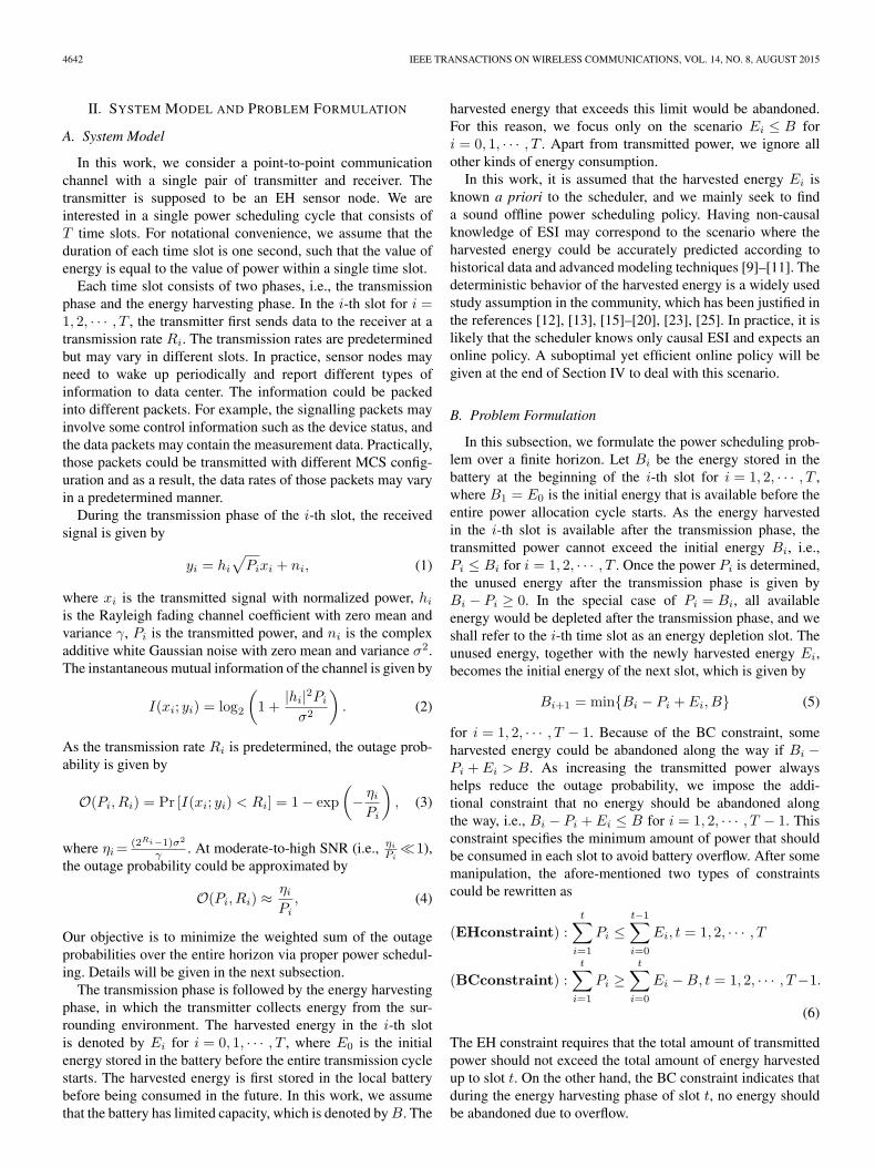
Fig. 1. Outage probability under optimal and suboptimal power solution.

Our design goal is to minimize the weighted sum of theoutage probabilities over T time slots through proper powerthrough proper power scheduling. This optimization problemcould be formulated as

(P1) :min{Pi}

T∑i=1

wiO(Pi, Ri) ≈T∑

i=1

wiηiPi

�T∑

i=1

αi

Pi

s.t.t∑

i=1

Pi ≤t−1∑i=0

Ei, t = 1, 2, · · · , T (7)

t∑i=1

Pi ≥t∑

i=0

Ei −B, t = 1, 2, · · · , T − 1

Pt ≥ 0, t = 1, 2, · · · , T.

Here, the weight wi reflects the relative importance of the i-thpacket, and αi � wiηi is constant. Note that this objective func-tion may represent different performance metrics depending onthe choice of weights {wi}. For example, wi ≡ 1

T means allpackets are equally important and the average outage proba-bility will be minimized. As only one packet is transmitted ineach time slot, this is also an equivalent way to maximize theexpected number of packets that can be successfully deliveredover the entire horizon. Alternatively, we may also choose wi =Ri, in which case we are essentially maximizing the expectedthroughput.

Note that the original objective function (i.e., weighted sumof the exact outage probabilities) is a non-convex function ofpower, which makes it hard to solve this optimization problemdirectly. To make the analysis tractable, we apply the high-SNR approximation given by (4). It is easy to show that afterreplacing the objective function, the new optimization problemis convex, which is easier to deal with. It should be pointed outthat although the optimal power solution to the new problemis strictly suboptimal to the original problem, the performanceloss is actually very small. To give an example, in Fig. 1 wecompare the performance under optimal and suboptimal powersolution for T = 3. The harvested energy is uniformly dis-tributed in the range [0.1, 5], and the system SNR is definedas ρ = 1

σ2 where σ2 is noise power. For simplicity, the channelvariance γ is normalized to 1, and the weight wi ≡ 1

T such that

the objective function represents the average outage probability.The optimal power solution is obtained through exhaustivesearch, and we use the exact outage probability (3) as objectivefunction. On the other hand, the suboptimal power solutioncorresponds to when the approximated outage probability (4)is used as the objective function. It can be observed that there isalmost no performance difference at all SNR values. So, in thesequel, we will instead use the approximated outage probabilityas objective function.1

As a quick overview, in Section III and Section IV we willrespectively study the scenarios with infinite and finite batterycapacity. Along the way we will derive a couple of propertiesthat help demonstrate how the optimal power solution shouldlook like. Readers could safely skip those derivations and findthe general algorithm to obtain the optimal power solution atthe end of Section IV.

III. POWER SCHEDULING WITH

INFINITE BATTERY CAPACITY

In this section, we first study power scheduling with infinitebattery capacity, i.e., B = ∞. The original problem (P1) canthus be simplified as

(P2) :min{Pi}

T∑i=1

αi

Pi(8)

s.t.t∑

i=1

Pi ≤t−1∑i=0

Ei, Pt ≥ 0, t = 1, 2, · · · , T.

Problem (P2) is still a convex optimization problem, whichcan be solved by Lagrange multiplier method. The Lagrangianfunction is given by

L =T∑

i=1

αi

Pi+

T∑i=1

λi

(i∑

k=1

Pk −i−1∑k=0

Ek

)−

T∑i=1

ωiPi, (9)

where λi, ωi ≥ 0 are Lagrange multipliers. The Karush-KuhnTucker (KKT) conditions are given by

∂L∂Pi

= − αi

P 2i

+T∑

k=i

λk − ωi = 0 (10)

for i = 1, 2, · · · , T . The complementary slackness conditionscould be written as

λi

(i∑

k=1

Pk −i−1∑k=0

Ek

)= 0, (11)

ωiPi = 0 (12)

for i = 1, 2, · · · , T . From (10), the optimal power could beexpressed as

P ∗i =

√αi∑T

k=i λk − ωi

. (13)

1In the following sections, whenever we refer to optimal power solution, it iswith respect to the problem which uses the approximated outage probability asobjective function.

4644 IEEE TRANSACTIONS ON WIRELESS COMMUNICATIONS, VOL. 14, NO. 8, AUGUST 2015

Combining (12) and (13), we have ωi=0 for i=1, 2, · · · , T ,such that

P ∗i =

√αi∑Tk=i λk

. (14)

To obtain the optimal power, we need to find the values ofLagrange multipliers λi, which is quite difficult. Instead, wefirst study some structural properties of the optimal powersolution, based on which we may deduce the optimal powervia an iterative algorithm.

Property 1: Suppose the optimal power sequence is given by{P ∗

k}Tk=1. If the i-th EH constraint is not binding, i.e.,

∑ik=1

P ∗k <

∑i−1k=0 Ek, then the optimal power P ∗

i and P ∗i+1 have

the relationship P∗i√αi

=P∗

i+1√αi+1

When the i-th EH constraint isbinding, then λi ≥ 0 and the energy should be depleted after thetransmission phase of the i-th slot, i.e.,

∑ik=1 P

∗i =

∑i−1k=0 Ei.

Proof: According to (11), there could be two outcomesfor the value of λi. If

∑ik=1 P

∗k <

∑i−1k=0 Ek, then λi = 0 and

from (14), we have

P ∗i√αi

=

√1∑T

k=i+1 λk

=P ∗i+1√αi+1

. (15)

The second part is a direct result of complementary slackness. �The above property indicates an iterative way to find the

optimal power sequence. Specifically, suppose somehow wealready know the energy depletion slots tk in which the EHconstraint is binding for k = 1, 2, · · · , N , then we can dividethe entire power allocation cycle into a set of disjoint segments[tk + 1, tk+1] for k = 0, 1, · · · , N−1 with t0 = 0 and tN = T .Within each segment, according to the first part of Property 1the normalized power should be a constant, i.e.,

P ∗j√αj

≡√√√√√

1T∑

i=tk+1

λi

(16)

for j ∈ [tk + 1, tk+1]. Besides, according to the second part ofProperty 1 the sum power is equal to

tk+1∑i=tk+1

P ∗i =

tk+1∑i=1

P ∗i −

tk∑i=1

P ∗i =

tk+1−1∑i=tk

Ei. (17)

From those two equations, we can solve for

P ∗j =

√αj∑tk+1

i=tk+1

√αi

tk+1−1∑j=tk

EjΔ=√αjf(tk+1, tk+1, Etk) (18)

for j ∈ [tk + 1, tk+1], where for notational convenience wedefine the function

f(i, j, x) =1

j∑k=i

√αk

(j−1∑k=i

Ek + x

)(19)

for 1 ≤ i ≤ j ≤ T . From the above result, we observe that theoptimal power solution has a piecewise structure, i.e., withineach segment the normalized power is a constant, and theoptimal power could be calculated once we know all the energy

depletion slots {tk}. Yet we still need a few more properties todetermine those energy depletion slots.

Property 2: In each segment [tk + 1, tk+1], we have f(tk+1,tk+1, Etk) < f(tk + 1, j, Etk) for j = tk+1, · · · , tk+1 − 1.

Proof: In each segment [tk+1, tk+1], EH constraints arenot binding in all slots except the tk+1-th slot, i.e.,

j∑m=1

P ∗m <

j−1∑m=0

Em (20)

for j = tk+1, · · · , tk+1 − 1. Because tk is an energy depletionslot, we also have

tk∑m=1

P ∗m =

tk−1∑m=0

Em. (21)

Subtracting (21) from (20), we can solve for

j∑m=tk+1

P ∗m =

[j∑

m=tk+1

√αm

]f(tk + 1, tk+1, Etk)

<

j−1∑m=tk

Em, (22)

where the equality is due to (18). The above result can berewritten as

f(tk+1, tk+1, Etk)<

∑j−1m=tk

Em∑jm=tk+1

√αm

=f(tk+1, j, Etk), (23)

which completes the proof. �Property 3: The sequence {f(tk−1 + 1, tk, Etk−1

)}Nk=1 isnon-decreasing, i.e.,

f(t0 + 1, t1, Et0) ≤ f(t1 + 1, t2, Et1) ≤ · · ·≤ f

(tN−1 + 1, tN , EtN−1

). (24)

Proof: From Property 1, we learn that the Lagrange mul-tipliers λi are non negative in the energy depletion slot tk fork = 1, 2, · · · , N , and λi = 0 for i ∈ [tk + 1, tk+1 − 1]. Thuswe have

P ∗i√αi

=

√1∑T

k=i λk

≤√

1∑Tk=i+1 λk

=P ∗i+1√αi+1

(25)

for i = 1, 2, · · · , T − 1. That is, the normalized power se-

quence{

P∗i√αi

}is non-decreasing. Within each segment, the

power is given by (18), based on which we can deduce that

f(tk−1 + 1, tk, Etk−1

)=

P ∗tk√αtk

≤P ∗tk+1√αtk+1

= f (tk + 1, tk+1, Etk) (26)

for k = 1, 2, · · · , N − 1. �Using the above two properties, we can determine all energy

depletion slots and then obtain the optimal power solution from(18). We summarize the major results of this section in thefollowing theorem.

WEI et al.: POWER SCHEDULING FOR ENERGY HARVESTING WIRELESS COMMUNICATIONS 4645

Theorem 1: The optimal solution to Problem (P2) is given by

P ∗k =

√αkf

(tj + 1, tj+1, Etj

)(27)

for k ∈ [tj + 1, tj+1] and j = 0, 1, · · · , N − 1, where2

tj = argmintj−1+1≤k≤T

f(tj−1 + 1, k, Etj−1) (28)

for j = 1, 2, · · · , N , with t0 = 0 and tN = T .Proof: Please refer to Appendix A. �

Corollary 1: If the sequence{

Ei−1√αi

}T

i=1is non-decreasing,

the optimal power solution is the best-effort strategy, i.e., P ∗i =

Ei−1 for i = 1, 2, · · · , T . On the other hand, if the sequence{Ei−1√

αi

}T

i=1is non increasing, the optimal power solution is

P ∗i =

√αif(1, T, E0) for i = 1, 2, · · · , T .

Proof: When{

Ei−1√αi

}T

i=1is non increasing, it is easy to

show that the normalized power should be a constant over the

entire horizon. If{

Ei−1√αi

}T

i=1is non-decreasing, each slot is

a separate segment. As a result, the stored energy should bedepleted in each slot. �

Note that the coefficients αi play an important role in thepower allocation. Indeed, αi is monotonically increasing withthe transmission rate Ri. So, roughly speaking, αi is a kindof information measure, and the normalized power Pi√

αican

be regarded as the allocated power per information measurein the i-th slot. Theorem 1 reveals that we should allocate thetotal power over the entire information measure as evenly aspossible. However, this may violate some EH constraints. Asa result, the best we can do is to divide the entire horizoninto disjoint segments, and within each segment to make thenormalized power constant.

IV. POWER SCHEDULING WITH

FINITE BATTERY CAPACITY

So far, we have found the optimal power solution when thebattery capacity is infinite. In this section, we take into accountboth EH and BC constraints. Again, we start by studyingthe necessary optimality conditions and discuss the piecewisestructure of the optimal power solution. Then, we discuss howto divide the entire cycle into a set of disjoint segments througha divide-and conquer algorithm.

In this section, we consider the general problem (P1) thatis subject to both EH and BC constraints. Problem (P1) is aconvex optimization problem, which can be solved by Lagrangemultiplier method. The Lagrangian function is given by

L =

T∑i=1

αi

Pi+

T∑i=1

λi

(i∑

k=1

Pk −i−1∑k=0

Ek

)

−T−1∑i=1

μi

(i∑

k=1

Pk −i∑

k=0

Ek +B

)−

T∑i=1

ωiPi, (29)

2Throughout this work, if there exist multiple minima (maxima), it alwaysrefers to the first minima (maxima).

where λi, μi, ωi ≥ 0 are Lagrange multipliers. The KKT con-ditions are given by

∂L∂Pi

= − αi

P 2i

+

T∑k=i

λk −T−1∑k=i

μk − ωi = 0 (30)

for i = 1, 2, · · · , T . The complementary slackness conditionscan be written as

λi

(i∑

k=1

Pk −i−1∑k=0

Ek

)= 0, i = 1, 2, · · · , T (31)

μi

(i∑

k=1

Pk−i∑

k=0

Ek +B

)= 0, i = 1, 2, · · · , T − 1 (32)

ωiPi = 0, i = 1, 2, · · · , T. (33)

From (30), we can solve for

P ∗i =

√αi∑T

k=i λk −∑T−1

k=i μk − ωi

. (34)

From (33) and (34), we can deduce that ωi = 0 fori = 1, 2, · · · , T . Thus, the optimal transmitted power can berewritten as

P ∗i√αi

=

√1∑T

k=i λk −∑T−1

k=i μk

. (35)

It is very difficult to obtain the Lagrange multipliers di-rectly. Again, we start by studying the structural propertiesof the optimal power solution. For notational convenience,we define two Boolean vectors e = (e1, e2, · · · , eT ) and b =(b1, b2, · · · , bT−1). The value of ei indicates whether the i-thEH constraint is binding under the optimal power solution,i.e., ei = 1 when

∑ik=1 P

∗k =

∑i−1k=0 Ek and ei = 0 otherwise

for i = 1, 2, · · · , T . Due to complementary slackness condition(31), we can deduce that ei = 1 if λi > 0 and λi = 0 if ei = 0.It should be pointed out that the last EH constraint is alwaysbinding because λT > 0. Likewise, bi = 1 means that the i thBC constraint is binding under the optimal power solution(i.e.,

∑ik=1 P

∗k =

∑ik=0 Ek −B) and bi = 0 otherwise for i =

1, 2, · · · , T − 1. From (32), we can also deduce that bi = 1 ifμi > 0 and μi = 0 if bi = 0. In the following, we will say k isan energy depletion slot if ek = 1, and k is a battery overflowslot if bk = 1.

Property 4: Depending on the values of ei and bi for i =1, 2, · · · , T − 1, we have the following properties:

(i) P∗i√αi

≥ P∗i+1√αi+1

if ei = 0 and bi = 1.

(ii) P∗i√αi

=P∗

i+1√αi+1

if ei = 0 and bi = 0.

(iii) P∗i√αi

≤ P∗i+1√αi+1

if ei = 1 and bi = 0.(iv) Ei = B if and only if ei = 1 and bi = 1.

4646 IEEE TRANSACTIONS ON WIRELESS COMMUNICATIONS, VOL. 14, NO. 8, AUGUST 2015

Proof: When ei = 0 and bi = 1, we have λi = 0,μi ≥ 0 and

P ∗i√αi

=

√√√√√ 1T∑

k=i+1

λk −T∑

k=i

μk

≥√√√√√ 1

T∑k=i+1

λk −T∑

k=i+1

μk

=P ∗i+1√αi+1

. (36)

When ei = 0 and bi = 0, we have λi = 0, μi = 0 and

P ∗i√αi

=

√√√√√ 1T∑

k=i+1

λk −T∑

k=i+1

μk

=P ∗i+1√αi+1

. (37)

When ei = 1 and bi = 0, we have λi ≥ 0, μi = 0 and

P ∗i√αi

=

√√√√√ 1T∑

k=i

λk −T∑

k=i+1

μk

≤√√√√√ 1

T∑k=i+1

λk −T∑

k=i+1

μk

=P ∗i+1√αi+1

. (38)

For the last case, when ei = bi = 1 both the i-th EH con-straint and the i-th BC constraint are binding, and we cansolve for Ei = B. Conversely, if Ei = B the two constraints∑i

k=1 P∗k ≤

∑i−1k=0 Ek and

∑ik=1 Pk ≥

∑i−1k=0 Ek must hold

true simultaneously, which indicates that both inequalities mustbe binding. �

The above property indicates that the optimal power se-quence still has a piecewise structure. Specifically, denote allenergy depletion slots by t1, t2, · · · , tN , where tN = T be-cause the last EH constraint must be binding. In particular,we also define t0 = 0 for notational convenience. Supposethere are Lk ≥ 0 battery overflow slots sk,1, sk,2, · · · , sk,Lk

inthe segment [tk + 1, tk+1] for k = 0, 1, · · · , N − 1, and tk <sk,1 < sk,2 < · · · < sk,Lk

< tk+1. Both energy depletion slotsand battery overflow slots are boundary slots that divide theentire power scheduling cycle into disjoint segments. Betweenany two consecutive boundary slots, both EH constraints andBC constraints are not binding. So according to Property 4(ii),the normalized power should be a constant between any twoconsecutive boundary slots. In other words, once all the bound-ary slots are given, we can easily deduce the optimal powersequence as follows.

Theorem 2: If the energy depletion slots and the batteryoverflow slots are known and are given by

0 = t0 < s0,1 < s0,2 < · · · < s0,L0< t1

< s1,1 < s1,2 < · · · < s1,L1< t2 < · · · < tN = T,

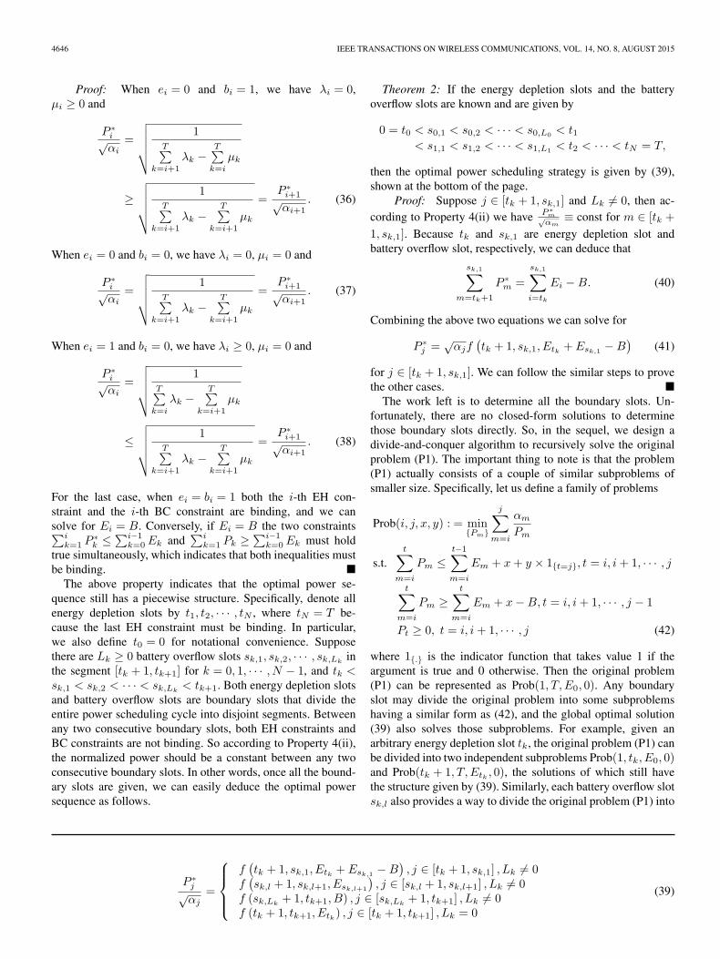
then the optimal power scheduling strategy is given by (39),shown at the bottom of the page.

Proof: Suppose j ∈ [tk + 1, sk,1] and Lk �= 0, then ac-cording to Property 4(ii) we have P∗

m√αm

≡ const for m ∈ [tk +

1, sk,1]. Because tk and sk,1 are energy depletion slot andbattery overflow slot, respectively, we can deduce that

sk,1∑m=tk+1

P ∗m =

sk,1∑i=tk

Ei −B. (40)

Combining the above two equations we can solve for

P ∗j =

√αjf

(tk + 1, sk,1, Etk + Esk,1

−B)

(41)

for j ∈ [tk + 1, sk,1]. We can follow the similar steps to provethe other cases. �

The work left is to determine all the boundary slots. Un-fortunately, there are no closed-form solutions to determinethose boundary slots directly. So, in the sequel, we design adivide-and-conquer algorithm to recursively solve the originalproblem (P1). The important thing to note is that the problem(P1) actually consists of a couple of similar subproblems ofsmaller size. Specifically, let us define a family of problems

Prob(i, j, x, y) : = min{Pm}

j∑m=i

αm

Pm

s.t.t∑

m=i

Pm ≤t−1∑m=i

Em + x+ y × 1{t=j}, t = i, i+ 1, · · · , j

t∑m=i

Pm ≥t∑

m=i

Em + x−B, t = i, i+ 1, · · · , j − 1

Pt ≥ 0, t = i, i+ 1, · · · , j (42)

where 1{.} is the indicator function that takes value 1 if theargument is true and 0 otherwise. Then the original problem(P1) can be represented as Prob(1, T, E0, 0). Any boundaryslot may divide the original problem into some subproblemshaving a similar form as (42), and the global optimal solution(39) also solves those subproblems. For example, given anarbitrary energy depletion slot tk, the original problem (P1) canbe divided into two independent subproblems Prob(1, tk, E0, 0)and Prob(tk + 1, T, Etk , 0), the solutions of which still havethe structure given by (39). Similarly, each battery overflow slotsk,l also provides a way to divide the original problem (P1) into

P ∗j√αj

=

⎧⎪⎪⎨⎪⎪⎩

f(tk + 1, sk,1, Etk + Esk,1

−B), j ∈ [tk + 1, sk,1] , Lk �= 0

f(sk,l + 1, sk,l+1, Esk,l+1

), j ∈ [sk,l + 1, sk,l+1] , Lk �= 0

f (sk,Lk+ 1, tk+1, B) , j ∈ [sk,Lk

+ 1, tk+1] , Lk �= 0f (tk + 1, tk+1, Etk) , j ∈ [tk + 1, tk+1] , Lk = 0

(39)

WEI et al.: POWER SCHEDULING FOR ENERGY HARVESTING WIRELESS COMMUNICATIONS 4647

two independent subproblems Prob(1, sk,l, E0, Esk,l−B) and

Prob(sk,l + 1, T,B, 0). If some boundary slots can be deter-mined, we can first divide the original problem into a couple ofsubproblems and then solve those subproblems separately. Theadvantage of such divide-and-conquer algorithm is that the sub-problems are of smaller size and thus are much simpler to solve.Under some special conditions, we can solve those subproblemsdirectly. Otherwise, we can continue to divide the subproblemsinto even smaller subproblems until they are solvable.

In the sequel, we discuss how to divide the original prob-lem into subproblems, and study the special condition underwhich we can solve the subproblem directly. Without loss ofgenerality, we focus on the general problem Prob(i, j, x, y).Using the Lagrange method, we can show that the optimalsolution to the problem Prob(i, j, x, y) is still given by (35)after replacing T with j, and Property 4 and Theorem 2 stillhold true. Note that if there exists t ∈ [i, j] such that Et = B,then according to Property 4(iv) both EH constraint and BCconstraint must be binding in the t-th slot. So t should be bothenergy depletion slot and battery overflow slot, and we candivide the original problem Prob(i, j, x, y) into Prob(i, t, x, 0)and Prob(t+ 1, j, B, y). In the sequel, we assume such simplepartition has been done and Et < B for all t ∈ [i, j]. We firstgive some results that would be used repeatedly later. The proofis very straightforward and is thus omitted.

Lemma 1: Consider any xi, yi > 0 for i = 1, 2. If x1

y1≤ x2

y2,

or x1

y1≤ x1+x2

y1+y2, or x1+x2

y1+y2≤ x2

y2, then x1

y1≤ x1+x2

y1+y2≤ x2

y2.

Corollary 2: Consider any xi, yi > 0 for i = 1, 2, · · · , N . Ifx1

y1≤ x2

y2≤ · · · ≤ xN

yN, then for any k = 1, 2, · · · , N we have∑k

i=1xi∑k

i=1yi

≤∑N

i=1xi∑N

i=1yi

≤∑N

i=k+1xi∑N

i=k+1yi

.

Corollary 3: Consider any xi, yi > 0 for i = 1, 2, 3. If x2 ≤x3 and y2 ≤ y3, then

(i) x1+x2

y1+y2≤ x1+x3

y1+y3if x1

y1≤ x3

y3and x2

y2≤ x3

y3.

(ii) x1+x2

y1+y2≥ x1+x3

y1+y3if x1

y1≥ x3

y3and x2

y2≥ x3

y3.

The next few properties specify how to divide the originalproblem into subproblems.

Property 5: Consider the general problem Prob(i, j, x, y),where 0 ≤ x ≤ B, −B ≤ y ≤ 0, and Ek < B for all k ∈ [i, j].Denote the optimal solution by {P ∗

k}jk=i.

(i) If t1 is the first energy depletion slot, i.e.,

t1=min

⎧⎨⎩

k : k ∈ [i, j] ,k∑

m=i

P ∗m=

k−1∑m=i

Em+x+y×1{k=j}

⎫⎬⎭ , (43)

then t1 must satisfy the condition

t1 = argmini≤m≤t1

f(i,m, x+ y × 1{m=j}

). (44)

(ii) If s1 is the first battery overflow slot, i.e.,

s1 = min

⎧⎨⎩

k : k ∈ [i, j − 1],k∑

m=i

P ∗m =

k∑m=i

Em + x−B

⎫⎬⎭ , (45)

then s1 must satisfy the condition

s1 = argmaxi≤m≤s1

f(i,m, x+ Em −B). (46)

Proof: Please refer to Appendix B. �Property 6: Consider the general problem Prob(i, j, x, y),

where 0 ≤ x ≤ B, −B ≤ y ≤ 0 and Ek < B for all k ∈[i, j]. Denote the optimal solution by {P ∗

k}jk=i, and let t =

argmini≤k≤j

f(i, k, x+ y × 1{k=j}). Then t must be an energy

depletion slot, i.e.,t∑

m=i

P ∗m =

t−1∑m=i

Em + x+ y × 1{t=j}.

Proof: Please refer to Appendix C. �The above property indicates that the slots obtained iter-

atively through (28) are all energy depletion slots. This isbecause for the original problem Prob(tk + 1, T, Etk , 0), theminimum of f(tk + 1,m,Etk) as a function of m is achievedat tk+1. As a result, we can conclude that if the stored energyshould be depleted in the tk-th slot when ignoring the BCconstraints, in that specific slot the stored energy should stillbe depleted in the presence of BC constraints. Moreover, wecan divide the original problem Prob(1, T, E0, 0) into a coupleof subproblems Prob(tk + 1, tk+1, Etk , 0), where tk are givenby (28). For each subproblem, it has the property that tk+1 =argmin

tk+1≤m≤tk+1

f(tk + 1,m,Etk). In the sequel, we develop an-

other important property to solve subproblems of this kind.Property 7: Consider the general problem Prob(i, j, x, y),

where 0 ≤ x ≤ B, −B ≤ y ≤ 0 and Ek < B for all k ∈ [i, j].Suppose j=argmin

i≤m≤jf(i,m, x+ y × 1{m=j}), and the optimal

solution is denoted by {P ∗k}

jk=i. Let s = argmax

i≤m≤j−1f(i,m,

x+ Em−B). If i = j or f(i, j, x+ y) ≥ f(i, s, x+ Es−B),then all BC constraints are not binding and the optimal power isgiven by P ∗

m =√αmf(i, j, x+ y) for m ∈ [i, j]. Otherwise, s

must be a battery overflow slot, i.e.,s∑

m=i

P ∗m=

s∑m=i

Em+x−B.

Proof: Please refer to Appendix D. �Based on Property 6 and Property 7, we can design a

divide-and-conquer algorithm to solve the original problemProb(1, T, E0, 0). Specifically, for the original problem we firstfind t=argmin

1≤k≤Tf(1, k, E0) and divide the original problem

into two separate subproblems Prob(1, t, E0, 0) and Prob(t+1,T, Et, 0). For each subproblem, we can follow the similar pro-cedure and divide the subproblems into smaller subproblems ofthe similar form. The division continues until all subproblemsProb(i, j, x, y) satisfy j=argmin

i≤k≤jf(i, k, x+y × 1{k=j}). For

each subproblem Prob(i, j, x, y), the optimal power is P ∗m =√

αmf(i, j, x+ y) for m ∈ [i, j] if i = j or f(i, j, x+ y) ≥max

i≤k≤j−1f(i, k, x+ Ek −B). Otherwise, let s = argmax

i≤k≤j−1f(i,

k, x+ Ek −B) and divide the subproblem Prob(i, j, x, y)into two smaller subproblems Prob(i, s, x, Es −B) andProb(s+ 1, j, B, y). This divide-and-conquer procedure con-tinues until all subproblems can be solved. A detailed descrip-tion of the algorithm is summarized in Algorithm 1.

4648 IEEE TRANSACTIONS ON WIRELESS COMMUNICATIONS, VOL. 14, NO. 8, AUGUST 2015

Algorithm 1 Divide-and-conquer algorithm to solve the prob-lem Prob(i, j, x, y)

1: If ∃k ∈ [i, j − 1] such that Ei = B2: Solve the subproblems Prob(i, k, x, 0) and

Prob(k + 1, j, B, y) separately;3: Return;4: End5: Denote t = argmin

i≤k≤jf(i, k, x+ y × 1{k=j});

6: If t < j7: Solve the subproblems Prob(i, t, x, 0) and

Prob(t+ 1, j, Et, y) separately;8: Return;9: End10: Denote s = argmax

i≤k≤j−1f(i, k, x+ Ek −B);

11: If i = j or f(i, j, x+ y) ≥ f(i, s, x+ Es −B)12: The optimal solution is P ∗

m =√αmf(i, j, x+ y) for

m ∈ [i, j];13: Else14: Solve the subproblems Prob(i, s, x, Es −B) and

Prob(s+ 1, j, B, y) separately;15: End16: Return;

A. Online Policy

Note that Algorithm 1 is an offline policy in that the schedulerneeds to know the exact value of the harvested energy Ei

for i = 1, 2, · · · , T . Such offline policy could be obtained byrunning Algorithm 1 once at the beginning of each powerscheduling cycle. In practice, the power scheduler has onlycausal knowledge of ESI and the exact energy Ei is unknown.Nevertheless, the scheduler could still make prediction of theharvested energy and apply Algorithm 1 in an online manner.

Suppose in the t-th time slot for t = 1, 2, · · · , T , the sched-uler knows only the expected energy {Ek}Tk=t that will arrivein the future slots, where Ek = E[Ek] and E[·] stands forexpectation. The available energy at the beginning of the t-thtime slot is still given by Bt, and this quantity is known tothe scheduler. To calculate the power Pt for the t-th timeslot, the scheduler needs to run Algorithm 1 and solve theproblem Prob(t, T,Bt, 0) by plugging in Ek instead of Ek fork = t, t+ 1, · · · , T . Suppose the actual energy harvested in thet-th slot is Et, which may be different from its expected valueEt. Then the energy available at the beginning of the (t+1)-thslot is computed based on the allocated power Pt and theactual harvested energy Et according to Bt+1 = min{Bt −Pt + Et, B}. Afterwards, the scheduler could repeat the sameprocess and calculate the power Pt+1 for the (t+ 1)-th timeslot by solving the problem Prob(t+ 1, T,Bt+1, 0), again byplugging in Ek for k = t+ 1, t+ 2, · · · , T . This procedure isrepeated until the last time slot.

The aforementioned scheme is an online policy in that onlythe predicted value of the harvested energy would be used tocalculate the power. However, as the prediction could be wrong,the scheduler needs to dynamically adjust the allocated power

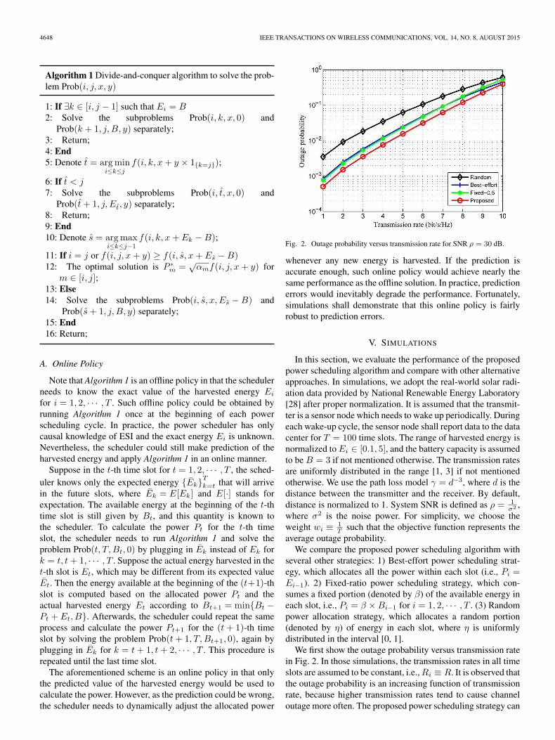
Fig. 2. Outage probability versus transmission rate for SNR ρ = 30 dB.

whenever any new energy is harvested. If the prediction isaccurate enough, such online policy would achieve nearly thesame performance as the offline solution. In practice, predictionerrors would inevitably degrade the performance. Fortunately,simulations shall demonstrate that this online policy is fairlyrobust to prediction errors.

V. SIMULATIONS

In this section, we evaluate the performance of the proposedpower scheduling algorithm and compare with other alternativeapproaches. In simulations, we adopt the real-world solar radi-ation data provided by National Renewable Energy Laboratory[28] after proper normalization. It is assumed that the transmit-ter is a sensor node which needs to wake up periodically. Duringeach wake-up cycle, the sensor node shall report data to the datacenter for T = 100 time slots. The range of harvested energy isnormalized to Ei ∈ [0.1, 5], and the battery capacity is assumedto be B = 3 if not mentioned otherwise. The transmission ratesare uniformly distributed in the range [1, 3] if not mentionedotherwise. We use the path loss model γ = d−3, where d is thedistance between the transmitter and the receiver. By default,distance is normalized to 1. System SNR is defined as ρ = 1

σ2 ,where σ2 is the noise power. For simplicity, we choose theweight wi ≡ 1

T such that the objective function represents theaverage outage probability.

We compare the proposed power scheduling algorithm withseveral other strategies: 1) Best-effort power scheduling strat-egy, which allocates all the power within each slot (i.e., Pi =Ei−1). 2) Fixed-ratio power scheduling strategy, which con-sumes a fixed portion (denoted by β) of the available energy ineach slot, i.e., Pi = β ×Bi−1 for i = 1, 2, · · · , T . (3) Randompower allocation strategy, which allocates a random portion(denoted by η) of energy in each slot, where η is uniformlydistributed in the interval [0, 1].

We first show the outage probability versus transmission ratein Fig. 2. In those simulations, the transmission rates in all timeslots are assumed to be constant, i.e., Ri ≡ R. It is observed thatthe outage probability is an increasing function of transmissionrate, because higher transmission rates tend to cause channeloutage more often. The proposed power scheduling strategy can

WEI et al.: POWER SCHEDULING FOR ENERGY HARVESTING WIRELESS COMMUNICATIONS 4649

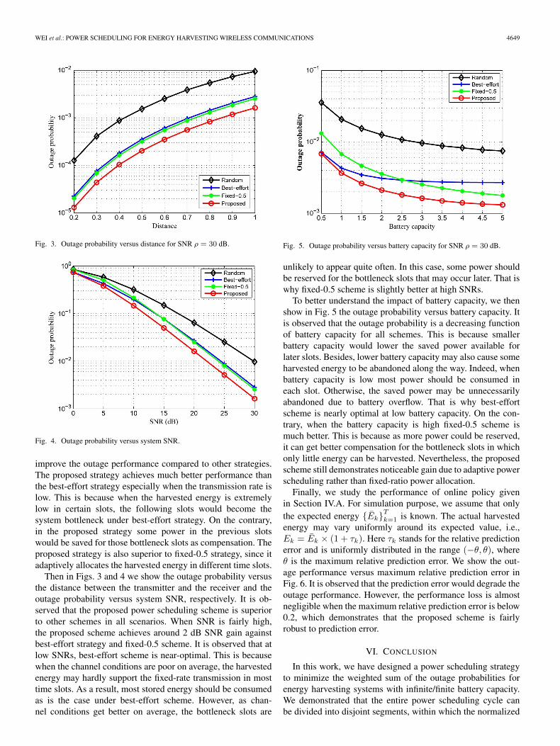
Fig. 3. Outage probability versus distance for SNR ρ = 30 dB.

Fig. 4. Outage probability versus system SNR.

improve the outage performance compared to other strategies.The proposed strategy achieves much better performance thanthe best-effort strategy especially when the transmission rate islow. This is because when the harvested energy is extremelylow in certain slots, the following slots would become thesystem bottleneck under best-effort strategy. On the contrary,in the proposed strategy some power in the previous slotswould be saved for those bottleneck slots as compensation. Theproposed strategy is also superior to fixed-0.5 strategy, since itadaptively allocates the harvested energy in different time slots.

Then in Figs. 3 and 4 we show the outage probability versusthe distance between the transmitter and the receiver and theoutage probability versus system SNR, respectively. It is ob-served that the proposed power scheduling scheme is superiorto other schemes in all scenarios. When SNR is fairly high,the proposed scheme achieves around 2 dB SNR gain againstbest-effort strategy and fixed-0.5 scheme. It is observed that atlow SNRs, best-effort scheme is near-optimal. This is becausewhen the channel conditions are poor on average, the harvestedenergy may hardly support the fixed-rate transmission in mosttime slots. As a result, most stored energy should be consumedas is the case under best-effort scheme. However, as chan-nel conditions get better on average, the bottleneck slots are

Fig. 5. Outage probability versus battery capacity for SNR ρ = 30 dB.

unlikely to appear quite often. In this case, some power shouldbe reserved for the bottleneck slots that may occur later. That iswhy fixed-0.5 scheme is slightly better at high SNRs.

To better understand the impact of battery capacity, we thenshow in Fig. 5 the outage probability versus battery capacity. Itis observed that the outage probability is a decreasing functionof battery capacity for all schemes. This is because smallerbattery capacity would lower the saved power available forlater slots. Besides, lower battery capacity may also cause someharvested energy to be abandoned along the way. Indeed, whenbattery capacity is low most power should be consumed ineach slot. Otherwise, the saved power may be unnecessarilyabandoned due to battery overflow. That is why best-effortscheme is nearly optimal at low battery capacity. On the con-trary, when the battery capacity is high fixed-0.5 scheme ismuch better. This is because as more power could be reserved,it can get better compensation for the bottleneck slots in whichonly little energy can be harvested. Nevertheless, the proposedscheme still demonstrates noticeable gain due to adaptive powerscheduling rather than fixed-ratio power allocation.

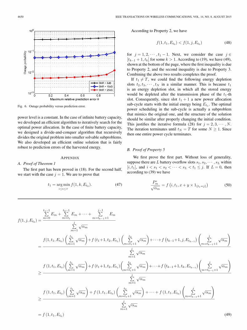
Finally, we study the performance of online policy givenin Section IV.A. For simulation purpose, we assume that onlythe expected energy {Ek}Tk=1 is known. The actual harvestedenergy may vary uniformly around its expected value, i.e.,Ek = Ek × (1 + τk). Here τk stands for the relative predictionerror and is uniformly distributed in the range (−θ, θ), whereθ is the maximum relative prediction error. We show the out-age performance versus maximum relative prediction error inFig. 6. It is observed that the prediction error would degrade theoutage performance. However, the performance loss is almostnegligible when the maximum relative prediction error is below0.2, which demonstrates that the proposed scheme is fairlyrobust to prediction error.

VI. CONCLUSION

In this work, we have designed a power scheduling strategyto minimize the weighted sum of the outage probabilities forenergy harvesting systems with infinite/finite battery capacity.We demonstrated that the entire power scheduling cycle canbe divided into disjoint segments, within which the normalized

4650 IEEE TRANSACTIONS ON WIRELESS COMMUNICATIONS, VOL. 14, NO. 8, AUGUST 2015

Fig. 6. Outage probability versus prediction error.

power level is a constant. In the case of infinite battery capacity,we developed an efficient algorithm to iteratively search for theoptimal power allocation. In the case of finite battery capacity,we designed a divide-and-conquer algorithm that recursivelydivides the original problem into smaller solvable subproblems.We also developed an efficient online solution that is fairlyrobust to prediction errors of the harvested energy.

APPENDIX

A. Proof of Theorem 1

The first part has been proved in (18). For the second half,we start with the case j = 1. We are to prove that

t1 = argmin1≤k≤T

f(1, k, Et0). (47)

According to Property 2, we have

f(1, t1, Et0) < f(1, j, Et0) (48)

for j = 1, 2, · · · , t1 − 1. Next, we consider the case j ∈[tk−1 + 1, tk] for some k > 1. According to (19), we have (49),shown at the bottom of the page, where the first inequality is dueto Property 2, and the second inequality is due to Property 3.Combining the above two results completes the proof.

If t1 �= T , we could find the following energy depletionslots t2, t3, · · · , tN in a similar manner. This is because t1is an energy depletion slot, in which all the stored energywould be depleted after the transmission phase of the t1-thslot. Consequently, since slot t1 + 1 a new power allocationsub-cycle starts with the initial energy being Et1 . The optimalpower scheduling in the sub-cycle is actually a subproblemthat mimics the original one, and the structure of the solutionshould be similar after properly changing the initial condition.This justifies the iterative formula (28) for j = 2, 3, · · · , N .The iteration terminates until tN = T for some N ≥ 1. Sincethen one entire power cycle terminates.

B. Proof of Property 5

We first prove the first part. Without loss of generality,suppose there are L battery overflow slots s1, s2, · · · , sL within[i, t1], and i < s1 < s2 < · · · < sL < t1 ≤ j. If L = 0, thenaccording to (39) we have

P ∗m√αm

= f(i, t1, x+ y × 1{t1=j}

)(50)

f(1, j, Et0) =

t1−1∑m=0

Em +t2−1∑m=t1

Em + · · ·+j−1∑

m=tk−1+1Em

j∑m=1

√αm

=

f(1, t1, Et0)

(t1∑

m=1

√αm

)+f (t1+1, t2, Et1)

(t2∑

m=t1+1

√αm

)+· · ·+f

(tk−1+1, j, Etk−1

)( j∑m=tk−1+1

√αm

)

j∑m=1

√αm

≥f (1, t1, Et0)

(t1∑

m=1

√αm

)+f (t1+1, t2, Et1)

(t2∑

m=t1+1

√αm

)+· · ·+f

(tk−1+1, tk, Etk−1

)( j∑m=tk−1+1

√αm

)

j∑m=1

√αm

≥f (1, t1, Et0)

(t1∑

m=1

√αm

)+ f (1, t1, Et0)

(t2∑

m=t1+1

√αm

)+ · · ·+ f (1, t1, Et0)

(j∑

m=tk−1+1

√αm

)

j∑m=1

√αm

= f (1, t1, Et0) (49)

WEI et al.: POWER SCHEDULING FOR ENERGY HARVESTING WIRELESS COMMUNICATIONS 4651

for m ∈ [i, t1]. Because all EH constraints are not binding form ∈ [i, t1 − 1], we have

m∑k=i

P ∗k =f

(i, t1, x+y × 1{t1=j}

) m∑k=i

√αk<

m−1∑k=i

Ek+x, (51)

which implies that

f(i, t1, x+ y × 1{t1=j}

)<

m−1∑k=i

Ek + x

m∑k=i

√αk

= f(i,m, x) (52)

for m ∈ [i, t1 − 1].Next we consider the case L > 0. According to (39), the

optimal power is

P ∗m√αm

=

⎧⎪⎨⎪⎩f(i, s1, x+Es1−B) ,m∈ [i, s1]

f(sk+1, sk+1, Esk+1

),m∈ [sk+1, sk+1]

f(sL+1, t1, B+y×1{t1=j}

),m∈ [sL+1, t1]

(53)

From Property 4(i), we can deduce that

f (i, s1, x+ Es1 −B) ≥ f (s1 + 1, s2, Es2) ≥ · · ·≥ f

(sL + 1, t1, B + y × 1{t1=j}

). (54)

Using Corollary 2, we can conclude that

f (i, s1, x+ Es1 −B) ≥ f (i, s2, x+ Es2 −B) ≥ · · ·≥ f

(i, t1, x+ y × 1{t1=j}

). (55)

Since f(i, sk, x+ Esk −B) < f(i, sk, x) for k = 1, 2, · · · , L,we have

f (i, sk, x) > f(i, t1, x+ y × 1{t1=j}

). (56)

for k = 1, 2, · · · , L. Next we consider a specific slot m ∈[i, s1 − 1]. Because all EH constraints are not binding for k ∈[i, s1 − 1], we have

m∑k=i

P ∗k =f (i, s1, x+Es1−B)

m∑k=i

√αk<

m−1∑k=i

Ek+x. (57)

As a result, we have

f (i,m, x) =

m−1∑k=i

Ek + x

m∑k=i

√αk

> f(i, s1, x+ Es1 −B)

>f(i, t1, x+ y × 1{t1=j}

)(58)

for m∈ [i, s1−1]. Next we consider a specific slot m∈[sk+1,

sk+1 − 1]. Note that the optimal power {P ∗

n}sk+1

n=sk+1 is also thesolution to the problem Prob

(sk + 1, sk+1, B,Esk+1

−B).

Using the similar argument, we can show that f(sk+1,m,B)>f(sk + 1, sk+1, Esk+1

)for m ∈ [sk + 1, sk+1 − 1]. As a re-

sult, we have (59), shown at the bottom of the page, for m ∈[sk + 1, sk+1 − 1]. Using the similar argument, we can alsoshow that the above inequality also holds true for m ∈ [sL + 1,t1 − 1]. To conclude, we have shown that

f(i,m, x) > f(i, t1, x+ y × 1{t1=j}

)(60)

for any m ∈ [i, t1 − 1], no matter L = 0 or L > 0. The secondpart can be proved in a similar way and the proof is omitted.

C. Proof of Property 6

The conclusion is true when t = j, because all the storedenergy should be depleted in the last slot. In the sequel, weprove by contradiction that this should also be true when t < j.Suppose now that t is not an energy depletion slot. Denote thelargest energy depletion slot before t by tp, and the smallestenergy depletion slot after t by tn, such that tp < t < tnand there are no other energy depletion slots in [tp + 1, tn −1]. Note that for problem Prob

(tp + 1, tn, Etp , y × 1{tn=j}

),

tn is the first and the unique energy depletion slot. FromProperty 5(i), we must have

f(tp + 1, t, Etp

)> f

(tp + 1, tn, Etp+y × 1{tn=j}

). (61)

On the other hand, from the definition of t we have

min(f(i, tp, x), f(i, tn, x+y ×1{tn=j})

)≥f

(i, t, x

). (62)

f (i,m, x) =

f (i, s1, x+ Es1 −B)s1∑n=i

√αn + f (s1 + 1, s2, Es2)

s2∑n=s1+1

√αn + · · ·+ f (sk + 1,m,B)

m∑n=sk+1

√αn

m∑n=i

√αn

>

f (i, s1, x+ Es1 −B)s1∑n=i

√αn + f (s1 + 1, s2, Es2)

s2∑n=s1+1

√αn + · · ·+ f

(sk + 1, sk+1, Esk+1

) m∑n=sk+1

√αn

m∑n=i

√αn

>

f (i, s1, x+ Es1 −B)s1∑n=i

√αn + f (s1 + 1, s2, Es2)

s2∑n=s1+1

√αn + · · ·+ f

(sk + 1, sk+1, Esk+1

) sk+1∑n=sk+1

√αn

sk+1∑n=i

√αn

= f(i, sk+1, x+ Esk+1

−B)> f

(i, t1, x+ y × 1{t1=j}

)(59)

4652 IEEE TRANSACTIONS ON WIRELESS COMMUNICATIONS, VOL. 14, NO. 8, AUGUST 2015

Using Lemma 1, we can deduce that

f(tp + 1, t, Etp

)≤f

(i, t, x

)≤f

(t+1, tn, Et+y × 1{tn=j}

).

(63)

Using Lemma 1 once more, we can conclude that

f(tp + 1, t, Etp

)≤ f

(tp + 1, tn, Etp + y × 1{tn=j}

), (64)

which contradicts (61). Consequently, t must be an energydepletion slot.

D Proof of Property 7

When i = j, only one slot is considered and there is no BCconstraint. As a result, the EH constraint should be binding andP ∗i = x+ y =

√αif (i, i, x+ y).

Next we consider the case i < j and f (i, j, x+ y) ≥f (i, s, x+ Es −B). If we ignore all BC constraints, thenaccording to Theorem 1 the optimal power is P ∗

m =√αmf (i, j, x+ y) for m ∈ [i, j]. This solution happens to

satisfy all BC constraints automatically, because

k∑m=i

P ∗m = f(i, j, x+ y)

k∑m=i

√αm

≥ f(i, s, x+ Es −B)

k∑m=i

√αm

≥ f(i, k, x+ Ek −B)

k∑m=i

√αm

=

k∑m=i

Em + x−B (65)

for k ∈ [i, j − 1]. Consequently, the optimal solution remainsthe same even in the presence of BC constraints.

Finally, we consider the case i < j and f (i, j, x+ y) <f (i, s, x+ Es −B), which implies that there must exist atleast one battery overflow slot within [i, j]. Denote the firstbattery overflow slot by s1. According to Property 5(ii),s1 = argmax

i≤m≤s1

f (i,m, x+ Em −B). This implies that

s1 ≤ s, otherwise we would have f (i, s, x+ Es −B) >f (i, s1, x+ Es1 −B) which leads to contradiction. Next, weprove by contradiction that s must be an battery overflow slot.Suppose now that s is not a battery overflow slot. We first showthat this implies that there would be no battery overflow slotwithin [s, j]. Otherwise, denote the largest battery overflowslot before s by sp, and the smallest battery overflow slot afters by sn, such that sp < s < sn and there are no other batteryoverflow slots within [sp + 1, sn − 1]. Note that for problemProb(sp + 1, j, B, y), sn is the first battery overflow slot. FromProperty 5(ii), we can deduce that

f (sp + 1, sn, Esn) > f (sp + 1, s, Es) . (66)

On the other hand, from the definition of s we have

max(f(i, sp, x+ Esp −B

), f (i, sn, x+ Esn −B)

)≤ f (i, s, x+ Es −B) . (67)

Using Lemma 1, we can deduce that

f(sp+1, s, Es)≥f(i, s, x+Es−B)≥f(s+1, sn, Esn). (68)

Using Lemma 1 once more, we can conclude that

f (sp + 1, s, Es) ≥ f (sp + 1, sn, Esn) , (69)

which contradicts (66).Consequently, if s is not a battery overflow slot, we have

shown that there must exist at least one battery overflow slotbefore s, and there can not exist any battery overflow slot afters. However, we are going to show that this can not happen tooby contradiction. Suppose now that the largest battery overflowslot before s is denoted by sp, and there are no other batteryoverflow slots after s. Those conditions imply that for problemProb (sp + 1, j, B, y), there would be no battery overflow slots.Besides, we must have

f (sp + 1, s, Es) > f (sp + 1, j, B + y) . (70)

Otherwise, according to Corollary 3(i) we would havef (i, s, x+ Es −B) ≤ f (i, j, x+ y), which leads to contra-diction. Suppose there are N energy depletion slots within[sp + 1, j], which are denoted by tk for k = 1, 2, · · · , N andsatisfy sp= t0<t1<t2< · · ·<tN =j. From Property 4(iii) andCorollary 2, we can deduce that

f (sp + 1, t1, B) ≤ f (sp + 1, t2, B) ≤ · · ·≤ f (sp + 1, j, B + y) < f (sp + 1, s, Es) . (71)

Suppose now that s ∈ [tk+1, tk+1] and k>0. Using Lemma 1,we can conclude that

f (sp + 1, tk, B)

≤ min

{f (tk + 1, s, Etk + Es −B) ,f(tk + 1, tk+1, Etk + y × 1{tk+1=j}

)} . (72)

Note that this implies that

f (tk + 1, s, Etk + Es −B)

> f(tk + 1, tk+1, Etk + y × 1{tk+1=j}

). (73)

Otherwise, from Corollary 3 we would have

f (sp+1, s, Es)≤f(sp+1, tk+1, B+y×1{tk+1=j}

), (74)

which contradicts (71). However, (73) indicates that there mustexist some battery overflow slot within [tk + 1, tk+1], whichis a contradiction to the assumption that there are no batteryoverflow slots within [sp + 1, j]. Consequently, the only possi-bility is that s ∈ [sp + 1, t1]. However, this can not occur eitherbecause the inequalities

f(sp + 1, t1, B + y × 1{t1=j}

)≤ f (sp + 1, j, B + y) < f (sp + 1, s, Es) (75)

also imply that there must exist some battery overflow slotwithin [sp + 1, t1], which is a contradiction as well. To con-clude, we have proved that there is no way that s is not a batteryoverflow slot.

WEI et al.: POWER SCHEDULING FOR ENERGY HARVESTING WIRELESS COMMUNICATIONS 4653

REFERENCES

[1] S. Wei, W. Guan, and K. J. R. Liu, “Outage probability optimizationwith equal and unequal transmission rates under energy harvesting con-straints,” in Proc. IEEE GLOBECOM, Atlanta, GA, USA, Dec. 2013,pp. 2530–2525.

[2] X. Jiang, J. Polastre, and D. Culler, “Perpetual environmentally poweredsensor networks,” in Proc. 4th Int. Symp. Inf. Process. Sens. Netw., 2005,pp. 463–468.

[3] J. Taneja, J. Jeong, and D. Culler, “Design, modeling, and capacity plan-ning for micro-solar power sensor networks,” in Proc. 7th Int. Conf. Inf.Process. Sens. Netw., 2008, pp. 407–418.

[4] V. Raghunathan, A. Kansal, J. Hsu, J. Friedman, and M. Srivastava,“Design considerations for solar energy harvesting wireless embed-ded systems,” in Proc. 4th Int. Symp. Inf. Process. Sens. Netw., 2005,pp. 457–462.

[5] C. Park and P. Chou, “Ambimax: Autonomous energy harvesting plat-form for multi-supply wireless sensor nodes,” in Proc. 3rd Annu. IEEECommun. Soc. Sens. Ad Hoc Commun. Netw., 2006, pp. 168–177.

[6] S. Sudevalayam and P. Kulkarni, “Energy harvesting sensor nodes: Sur-vey and implications,” IEEE Commun. Surveys Tuts., vol. 13, no. 3,pp. 443–461, Sep. 2011.

[7] D. Tse and P. Viswanath, Fundamentals of Wireless Communication.Cambridge, U.K.: Cambridge Univ. Press, 2005.

[8] N. Zlatanov, Z. Hadzi-Velkov, and R. Schober, “Asymptotically optimalpower allocation for point-to-point energy harvesting communication sys-tems,” in Proc. IEEE GLOBECOM, Dec. 2013, pp. 2502–2507.

[9] M. Hassan and A. Bermak, “Solar harvested energy prediction algorithmfor wireless sensors,” in Proc. ASQED, Jul. 2012, pp. 178–181.

[10] K. B. Joshi, J. H. Costello, and S. Priya, “Estimation of solar en-ergy harvested for autonomous jellyfish vehicles,” IEEE J. Ocean. Eng.,vol. 36, no. 4, pp. 539–551, Oct. 2011.

[11] A. Cammarano, C. Petrioli, and D. Spenza, “Pro-energy: A novel energyprediction model for solar and wind energy-harvesting wireless sensornetworks,” in Proc. IEEE 9th Int. Conf. MASS, Las Vegas, NV, USA,Oct. 2012, pp. 75–83.

[12] O. Ozel, K. Tutuncuoglu, J. Yang, S. Ulukus, and A. Yener, “Transmis-sion with energy harvesting nodes in fading wireless channels: Optimalpolicies,” IEEE J. Sel. Areas Commun., vol. 29, no. 8, pp. 1732–1743,Sep. 2011.

[13] K. Tutuncuoglu and A. Yener, “Optimum transmission policies for batterylimited energy harvesting nodes,” IEEE Trans. Wireless Commun., vol. 11,pp. 1180–1189, Mar. 2012.

[14] C. K. Ho and R. Zhang, “Optimal energy allocation for wireless communi-cations withe energy harvesting constraints,” IEEE Trans. Signal Process.,vol. 60, no. 9, pp. 4808–4818, Sep. 2012.

[15] J. Yang and S. Ulukus, “Optimal packet scheduling in an energy har-vesting communication system,”IEEE Trans. Commun., vol. 60, no.1,pp. 220–230, Jan. 2012.

[16] M. A. Antepli, E. Uysal-Biyikoglu, and H. Erkal, “Optimal packetscheduling on an energy harvesting broadcast link,” IEEE J. Sel. AreasCommun., vol. 29, no. 8, pp. 1721–1731, Sep. 2011.

[17] O. Ozel, J. Yang, and S. Ulukus, “Optimal broadcast scheduling foran energy harvesting rechargeable transmitter with a finite capacity bat-tery,” IEEE Trans. Wireless Commun., vol. 11, no.6, pp. 2193–2203,Jun. 2012.

[18] J. Yang and S. Ulukus, “Optimal packet scheduling in a multiple accesschannel with energy harvesting transmitters,” J. Commun. Netw., vol. 14,no. 2, pp. 140–150, Apr. 2012.

[19] D. W. K. Ng, E. S. Lo, and R. Schober, “Energy-efficient resource alloca-tion in ofdma systems with hybrid energy harvesting base station,” IEEETrans. Wireless Commun., vol. 12, no. 7, pp. 3412–3427, Jul. 2013.

[20] Y. Zhang, S. He, J. Chen, Y. Sun, and X. Shen, “Distributed sampling ratecontrol for rechargeable sensor nodes with limited battery capacity,” IEEETrans. Wireless Commun., vol. 12, no. 6, pp. 3096–3106, Jun. 2013.

[21] V. Sharma, U. Mukherji, V. Joseph, and S. Gupta, “Optimal energymanagement policies for energy harvesting sensor nodes,” IEEE Trans.Commun., vol. 9, no. 4, pp. 1326–1336, Apr. 2010.

[22] R. Srivastava and C. E. Koksal, “Basic performance limits and tradeoffsin energy-harvesting sensor nodes with finite data and energy storage,”IEEE/ACM Trans. Netw., vol. 21, no.4, pp. 1049–1062, Aug. 2013.

[23] C. Huang, R. Zhang, and S. Cui, “Optimal power allocation for outageprobability minimization in fading channels with energy harvesting con-straints,” IEEE Trans. Wireless Commun., vol. 13, no. 2, pp. 1074–1087,Feb. 2014.

[24] S. Luo, R. Zhang, and T. J. Lim, “Optimal save-then-transmit protocol forenergy harvesting wireless transmitters,” IEEE Trans. Wireless Commun.,vol. 12, no. 3, pp. 1196–1207, Mar. 2013.

[25] X. Kang, Y. K. Chia, C. K. Ho, and S. Sun, “Cost minimization for fadingchannels with energy harvesting and conventional energy,” IEEE Trans.Wireless Commun., vol. 13, no. 8, pp. 4586–4598, Aug. 2014.

[26] N. Michelusi, K. Stamatiou, and M. Zorzi, “Transmission policies for en-ergy harvesting sensors with time-correlated energy supply,” IEEE Trans.Commun., vol. 61, no. 7, pp. 2988–3001, Jul. 2013.

[27] S. Reddy and C. R. Murthy, “Dual-stage power management algorithmsfor energy harvesting sensors,” IEEE Trans. Wireless Commun., vol. 11,no. 4, pp. 1434–1445, Apr. 2012.

[28] “Solar radiation resource information,” Nat. Renew. Energy Lab., Golden,CO, USA, Feb. 2012. [Online]. Available: http://www.nrel.gov/rredc/

Sha Wei received the B.S. and Ph. D degrees inelectronic engineering from the University of Elec-tronic Science and Technology of China (UESTC),Chengdu, and Shanghai Jiao Tong University,Shanghai, China, in 2007 and 2014, respectively.Since 2015, she has been working in the Ministryof Industry and Information Technology of People’sRepublic of China. She served as the reviewer forIEEE TRANSACTIONS ON WIRELESS COMMUNI-CATIONS, ICC and Globecom. Her current researchinterests include energy harvesting, wireless network

coding and cooperative communications.

Wei Guan (S’12) received the B.S. degree in electri-cal engineering and finance (double degree), in 2006,and the M.S. (with highest honor) degree in electricalengineering, in 2009, both from Shanghai JiaoTongUniversity, Shanghai, China. He also received theM.A. degree in mathematical statistics and the Ph.D.degree in electrical and computer engineering, bothfrom University of Maryland, College Park, MD,USA, in 2012 and 2013, respectively. He is nowa Senior Engineer in Qualcomm Inc. working ondevice-to-device communications.

His research interests are in the areas of wireless communications andnetworks, including cooperative communications and network coding. Hereceived the 1st Prize in the 18th National Physics Contest, Shanghai. He alsoreceived the A. James Clark School of Engineering Distinguished GraduateFellowship in 2009, and the Distinguished Dissertation Fellowship in 2013,both from University of Maryland, College Park.

K. J. Ray Liu (F’03) was named a DistinguishedScholar-Teacher of University of Maryland, CollegePark, MD, USA, in 2007, where he is Christine KimEminent Professor of Information Technology. Heleads the Maryland Signals and Information Groupconducting research encompassing broad areas ofinformation and communications technology withrecent focus on future wireless technologies, networkscience, and information forensics and security.

He was a recipient of IEEE Signal Processing So-ciety 2014 Society Award, IEEE Signal Processing

Society 2009 Technical Achievement Award, and various best paper awards.Recognized by Thomson Reuters as a Highly Cited Researcher, he is a Fellowof AAAS.

Dr. Liu is a Director-Elect of IEEE Board of Director. He was Pres-ident of IEEE Signal Processing Society, where he has served as VicePresident—Publications and Board of Governor. He has also served as theEditor-in-Chief of IEEE Signal Processing Magazine.

He also received teaching and research recognitions from University ofMaryland including university-level Invention of the Year Award; and college-level Poole and Kent Senior Faculty Teaching Award, Outstanding FacultyResearch Award, and Outstanding Faculty Service Award, all from A. JamesClark School of Engineering.