Energy Efficiency in Transition Economies:

A Stochastic Frontier Approach

Antonio Carvalho

CEERP Working Paper No. 4 November 2016

Heriot-Watt University

Edinburgh, Scotland

EH14 4AS

ceerp.hw.ac.uk

2

Energy Efficiency in Transition Economies:

A Stochastic Frontier Approach

António Carvalho*

Centre for Energy Economics Research and Policy (CEERP)

Heriot-Watt University

Abstract

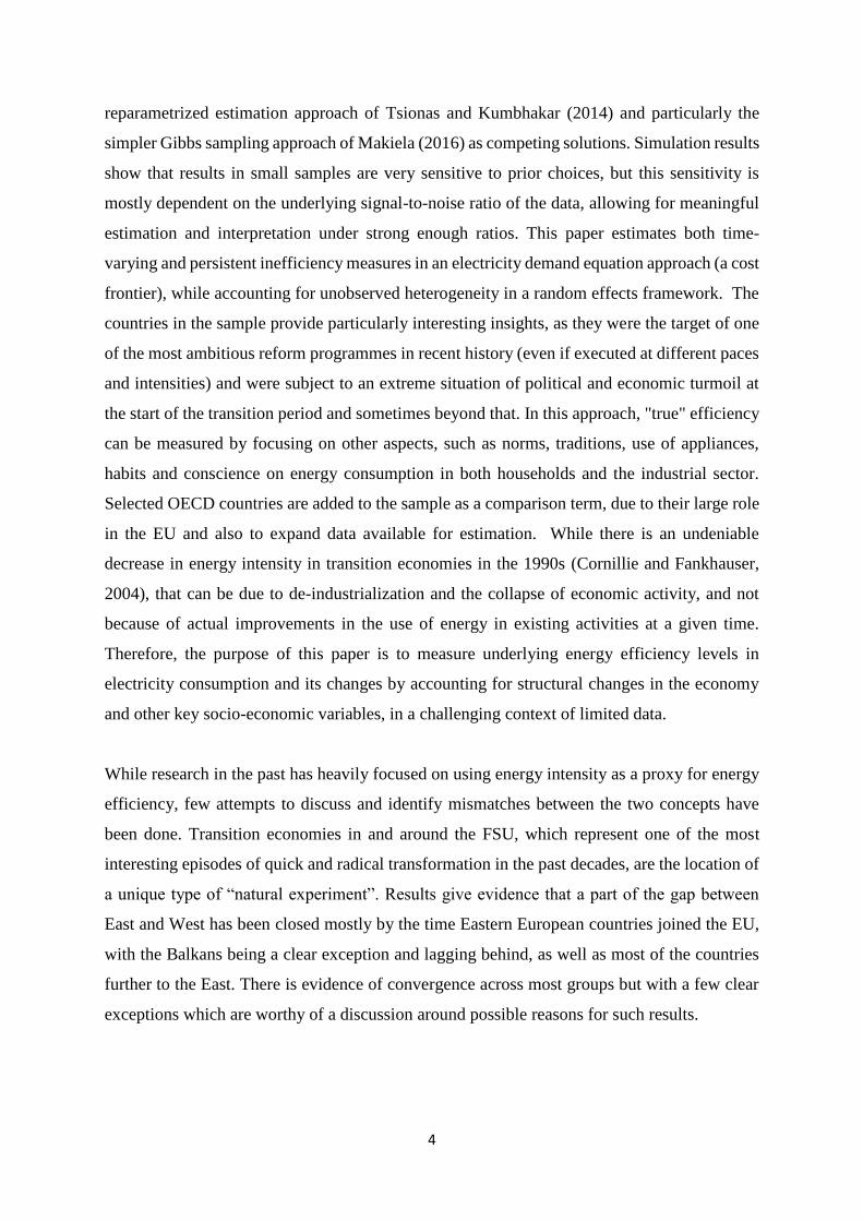
The paper outlines and estimates a measure of underlying efficiency in electricity

consumption for an unbalanced panel of 28 transition economies and 5 Western European OECD

countries in the period 1994-2007, by estimating a Bayesian Generalized True Random Effects

(GTRE) stochastic frontier model that estimates both persistent and transient inefficiency. The

properties of alternative GTRE estimation methods in small samples are explored to guide the

estimation strategy. The paper analyses the behaviour of underlying efficiency in electricity

consumption in these economies after accounting for time-invariant technological differences.

After outlining the specific characteristics of the transition economies and their heterogeneous

structural economic changes, an aggregate electricity demand function is estimated to obtain

efficiency scores that give new insights for transition economies than a simple analysis of energy

intensity. There is some evidence of convergence between the CIS countries and a block of

Eastern European and selected OECD countries, although other country groups do not follow this

tendency, such as the Balkans.

JEL Classification: C23, Q49, P20

Keywords: Electricity Consumption, Transition Economies, Energy Efficiency, Stochastic

Frontier

21/11/2016

*Corresponding author. Heriot-Watt University, Conoco Building, EH14 4AS, Edinburgh, United Kingdom.

Email: A.Carvalho@hw.ac.uk

3

1. Introduction

Energy efficiency and energy-saving measures are a heavily debated topic in recent years, both

in high profile environmental discussions and in the media, as issues like energy security,

energy supply, carbon emissions and climate change take increasing shares of the attention of

policy makers, the media and society in general. The issue has been approached from multiple

perspectives, from renewable energies to changes in consumer behaviour, spanning a large

spectre of research on technical aspects, policy making and economic analysis.

The world energy demand profile has changed in past decades, with some noticeable

geographic differences. The oil shocks of 1973 and 1979 fundamentally changed energy

demand in the OECD, slowing down the growing patterns of energy demand that were ongoing

since WWII (Cooper and Schipper, 1992). Eastern Europe and the USSR were mainly isolated

from price shocks, which allowed the bloc to carry on with its industrial expansion which in

turn came to an end with the collapse of the political and economic system. After this turning

event, the reform packages of the Washington Consensus were applied to try to recover and

transform the economies, with heterogeneous paces of implementation and results across the

region. After 25 years of the process, some countries of the Former Soviet Union (FSU) still

maintain an economy with very fragile market mechanisms and do not seem to be approaching

a free market economy status anytime soon.

Economies that transitioned from a centrally planned economy to a market economy after the

fall of the USSR often experienced rapid improvements in energy intensity as market reforms

alleviated problems such as resource misallocations and price distortions. Research has often

focused on energy intensity as a measure of what impacts energy efficiency, with transition

economies not being an exception. However, deep changes were also ongoing as market

reforms took place, changing the role of the government in the economy and the structure and

key sectors that contribute to the economy. By using energy intensity as a proxy for energy

efficiency, the considerable changes in the structure of these economies are mostly ignored in

the assessment of efficiency. By modelling energy demand for analysis, a measure of

underlying energy efficiency is estimated, as it is separated from some changes in intensity

caused by economic collapse or other deep structural changes of the economy. This is achieved

through recent developments in the estimation of Stochastic Frontier models, using the

Generalized True Random Effects model (Colombi et al., 2011) and exploring the Bayesian

4

reparametrized estimation approach of Tsionas and Kumbhakar (2014) and particularly the

simpler Gibbs sampling approach of Makiela (2016) as competing solutions. Simulation results

show that results in small samples are very sensitive to prior choices, but this sensitivity is

mostly dependent on the underlying signal-to-noise ratio of the data, allowing for meaningful

estimation and interpretation under strong enough ratios. This paper estimates both time-

varying and persistent inefficiency measures in an electricity demand equation approach (a cost

frontier), while accounting for unobserved heterogeneity in a random effects framework. The

countries in the sample provide particularly interesting insights, as they were the target of one

of the most ambitious reform programmes in recent history (even if executed at different paces

and intensities) and were subject to an extreme situation of political and economic turmoil at

the start of the transition period and sometimes beyond that. In this approach, "true" efficiency

can be measured by focusing on other aspects, such as norms, traditions, use of appliances,

habits and conscience on energy consumption in both households and the industrial sector.

Selected OECD countries are added to the sample as a comparison term, due to their large role

in the EU and also to expand data available for estimation. While there is an undeniable

decrease in energy intensity in transition economies in the 1990s (Cornillie and Fankhauser,

2004), that can be due to de-industrialization and the collapse of economic activity, and not

because of actual improvements in the use of energy in existing activities at a given time.

Therefore, the purpose of this paper is to measure underlying energy efficiency levels in

electricity consumption and its changes by accounting for structural changes in the economy

and other key socio-economic variables, in a challenging context of limited data.

While research in the past has heavily focused on using energy intensity as a proxy for energy

efficiency, few attempts to discuss and identify mismatches between the two concepts have

been done. Transition economies in and around the FSU, which represent one of the most

interesting episodes of quick and radical transformation in the past decades, are the location of

a unique type of “natural experiment”. Results give evidence that a part of the gap between

East and West has been closed mostly by the time Eastern European countries joined the EU,

with the Balkans being a clear exception and lagging behind, as well as most of the countries

further to the East. There is evidence of convergence across most groups but with a few clear

exceptions which are worthy of a discussion around possible reasons for such results.

5

2. Energy in Transition: key facts and literature review

Key differences separated the western economies from the centrally planned economies in the

FSU and Former Yugoslavia spheres of influence. Planning and policy in the energy sector

were also fundamentally different from western countries, as the communist regimes focused

on supply-side solutions to meet increasing demand instead of tackling demand issues and

waste (Cooper and Schipper, 1992). This implied large investments were made in fuel

extraction and power generation in order to meet demand, instead of tackling energy efficiency

problems or consumer behaviour with demand driven policies. Serbia and Uzbekistan are still

examples of countries where the main electricity generation firm is deeply involved in coal

extraction and the energy industry is highly integrated. Another important issue was the pricing

system of transition economies. Over 24 million goods had fixed prices in the Soviet Union,

with prices being inflexible and unable to provide any correct information about scarcity.

Microeconomic efficiency was not achievable (Ericson, 1991), cascading into macroeconomic

outcomes.

Some serious problems still persisted in the power sector long after the start of the transition

process. Energy companies mostly continued to function as "quasi-fiscal institutions" after a

decade of transition, providing large implicit subsidies to households and (state-owned)

enterprises through low energy prices, preferential tariffs or free provision of services to

privileged groups, the toleration of payment arrears, and noncash arrangements (Petri et al.,

2002). This generated considerable inefficiencies and distortions. Such arrangements were

necessary, for example in Russia, as bankrupt companies kept doing business and generated a

non-payment crisis (Martinot, 1998). Another consequence is that underinvestment and capital

stock depletion occur under a scenario of tariffs set below cost recovery levels. Although some

tariff rebalancing has taken place, cross-subsidizing was still present in the transition process

as residential tariffs were more expensive than industrial tariffs, especially in the CIS

(Kennedy, 2003). Removing this distortion maximizes economic benefits. Another major issue

is general under-pricing in the power sector, as prices are well below Long Run Marginal Cost

(LMRC) and they should be above LMRC in order to recover past accumulated energy debt,

which is a major component of total sovereign or quasi-sovereign debts in some CIS

economies. While different countries have heterogeneous marginal costs, it is clear from Table

3.1. that there is a gap in prices between countries where regulators are established and others

where that is not the case, and energy intensities are clearly higher in countries with lower

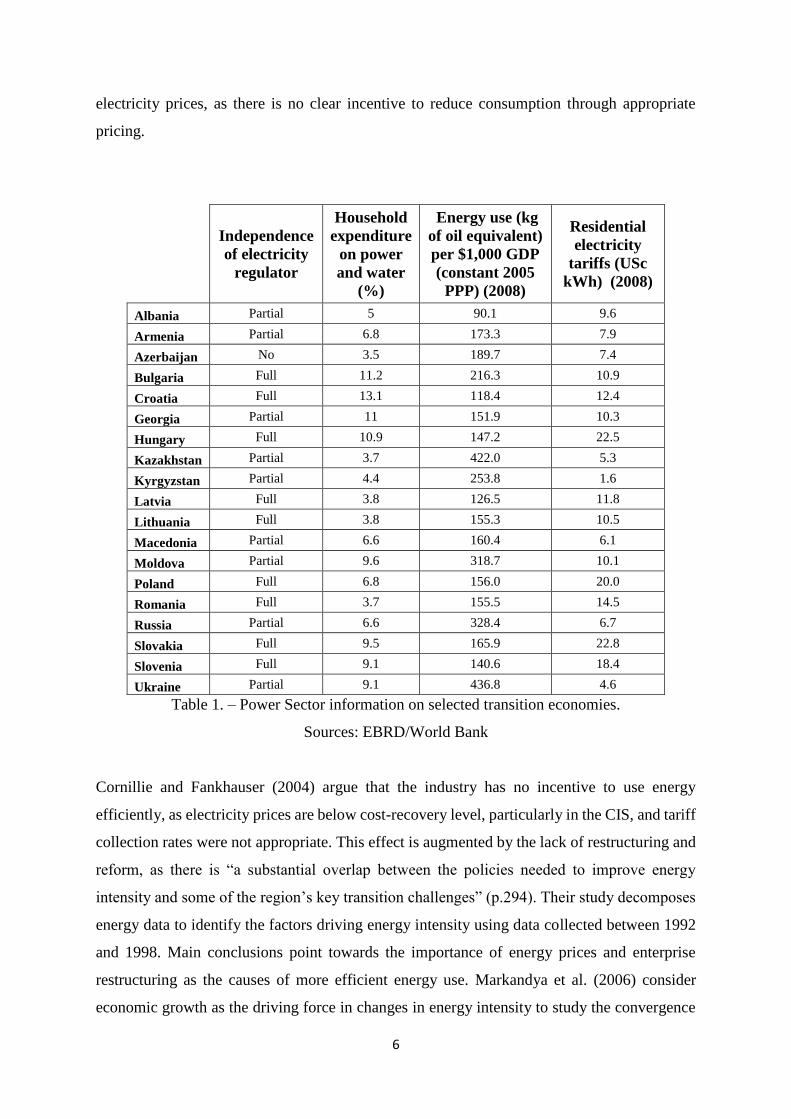
6

electricity prices, as there is no clear incentive to reduce consumption through appropriate

pricing.

Independence

of electricity

regulator

Household

expenditure

on power

and water

(%)

Energy use (kg

of oil equivalent)

per $1,000 GDP

(constant 2005

PPP) (2008)

Residential

electricity

tariffs (USc

kWh) (2008)

Albania Partial 5 90.1 9.6

Armenia Partial 6.8 173.3 7.9

Azerbaijan No 3.5 189.7 7.4

Bulgaria Full 11.2 216.3 10.9

Croatia Full 13.1 118.4 12.4

Georgia Partial 11 151.9 10.3

Hungary Full 10.9 147.2 22.5

Kazakhstan Partial 3.7 422.0 5.3

Kyrgyzstan Partial 4.4 253.8 1.6

Latvia Full 3.8 126.5 11.8

Lithuania Full 3.8 155.3 10.5

Macedonia Partial 6.6 160.4 6.1

Moldova Partial 9.6 318.7 10.1

Poland Full 6.8 156.0 20.0

Romania Full 3.7 155.5 14.5

Russia Partial 6.6 328.4 6.7

Slovakia Full 9.5 165.9 22.8

Slovenia Full 9.1 140.6 18.4

Ukraine Partial 9.1 436.8 4.6

Table 1. – Power Sector information on selected transition economies.

Sources: EBRD/World Bank

Cornillie and Fankhauser (2004) argue that the industry has no incentive to use energy

efficiently, as electricity prices are below cost-recovery level, particularly in the CIS, and tariff

collection rates were not appropriate. This effect is augmented by the lack of restructuring and

reform, as there is “a substantial overlap between the policies needed to improve energy

intensity and some of the region’s key transition challenges” (p.294). Their study decomposes

energy data to identify the factors driving energy intensity using data collected between 1992

and 1998. Main conclusions point towards the importance of energy prices and enterprise

restructuring as the causes of more efficient energy use. Markandya et al. (2006) consider

economic growth as the driving force in changes in energy intensity to study the convergence

7

of energy efficiency and income between 15 EU countries and 12 countries of Eastern Europe.

Conclusions point that there is convergence between the two blocks of countries, but the rate

of convergence differs between countries. Nepal et al. (2014) take an institutional approach to

explain changes in energy efficiency using dynamic panel data (Bias Corrected LSDV method),

using energy intensity as a dependent variable. The authors find that market liberalization,

financial sector and infrastructure industries (excluding the power sector) improved energy

efficiency in these countries, while privatization programmes were only effective in that sense

in South Eastern Europe. However, in this case, energy intensity is directly interpreted as

energy efficiency, an assumption that is not consensual across the literature.

To estimate stochastic frontier models, research is mostly based on the seminal work of Aigner

et al. (1977) that introduces the specification of the error term into two separate components,

one that is normal and the other that has a one-sided half-normal distribution. Greene (2005)

presents several extensions to the stochastic frontier model accounting for unmeasured

heterogeneity and firm inefficiency. These extensions include two noticeable additions: the

true fixed effects model (TRE) and the true random effects model (TFE). The used

methodology in this case will rely on an extension of the true random effects model with an

additional random component (Colombi et al., 2011). However, this is done using Bayesian

estimation techniques, as in Tsionas and Kumbhakar (2014) and Makiela (2016). This

extension allows to consider both time-varying and time invariant inefficiency, unlike the TRE

and TFE models which meant a loss of information about time-invariant inefficiency. This

methodology is sparsely used in the applied econometrics literature, for example in efficiency

measurement of Swiss railways (Filippini and Greene, 2016) or electricity distribution in New

Zealand (Filippini et al., 2016).

A major methodological and conceptual influence for estimation of energy efficiency scores of

this paper is the approach of Filippini and Hunt (2011). Their study conceptualizes a measure

of energy efficiency by estimating a stochastic cost frontier model which tackles the fragilities

of energy intensity as a proxy for energy efficiency. The authors estimate an aggregate energy

demand function to estimate “underlying energy efficiency” after controlling for income and

price effects, climate, technical progress and other exogenous factors, using a pooled model

(Aigner et al., 1977) and the TRE model (Greene, 2005). The authors also argue that without

conducting such analysis it is not possible to know if the changes in energy intensity over time

are a reasonable reflection of actual efficiency improvements. The study concludes that

8

although for a number of countries the proxy is good, that is not always the case, with Italy

being an extreme example. While the study of Filippini and Hunt (2011) focuses on a long

sample period (1978-2006) for 29 OECD economies, the analysis of transition economies leads

to different backgrounds and frameworks, due to the underlying changes in the political system

and the economy. However, the aforementioned study had three countries in common with the

analysis that will be conducted in this paper (Hungary, Poland and Slovakia). This study

overlooks the issue of heterogeneity among countries by choosing an estimation method that

might suffer from heterogeneity bias. It also has an unrefined approach on accounting for

climate and the structure of the economy, which will be discussed in further detail in this paper.

The size of the T dimension of the panel also raises some concerns about the stationarity of the

data and therefore the validity of the obtained results. Another article with similar methodology

by Filippini and Hunt (2012) is an application of stochastic frontier models to estimate

efficiency within the context of residential demand in the USA. Since the TRE model is unable

to capture persistent and time-invariant inefficiency, and the model was rendering very high

and implausible efficiency scores possibly due to the omission of the aforementioned

inefficiency, the chosen method was a Mundlak (1978) version of the model as discussed in

Farsi et al. (2005) in order to tackle the problem of correlation between the individual effects

and the explanatory variables.

Stern (2012) is an influential example in the energy efficiency measurement literature. The

author analyses efficiency trends in 85 countries over a 37 year period. However, due to the

lack of data for FSU countries, those countries are not included. Differences in energy

efficiency are modelled as a stochastic function of explanatory variables (instead of being

considered as random) and the model is estimated using the cross-section of time-averaged

data. One of the key advantages of this method is that no assumptions are made about

technological change over time. The aforementioned paper has two important differences from

Filippini and Hunt (2011). Efficiency is measured using a distance function and estimation is

conducted using random effects, fixed effects and finally a distance function with an auxiliary

regression, using variables that co-vary with the unobserved state of technology (such as state

of democracy, openness, corruption and total factor productivity), in order to reduce omitted

variable bias. Secondly, it contains key conceptual differences - the dependent variable is

energy intensity and the study is also based on the productivity literature instead of the energy

demand modelling literature. Stern (2012) chases the drivers behind changes in both energy

prices and efficiency, while Filippini and Hunt (2011) take policy as given and observe how

9

households and firms react to the economic environment. The complex data building process

includes a series of assumptions in order to include capital and human capital as variables in

the model such as linear growth of years of schooling and assumptions about the rate of

depreciation. Results differ with fixed and random effects estimations.

Other approaches are implemented across the literature. The DEA (Data Envelopment

Analysis) technique is non-parametric which means that it is robust to misspecification of the

functional form (Cornwall and Schmidt, 2008). However, it is more difficult to assess

uncertainty in DEA efficiency measures, making it unclear up to which extent uncertainty

impacts results and conclusions in empirical work. It is also more difficult to assess the impact

of noise in DEA results. Zhou and Ang (2008) used this technique to measure energy efficiency

in 21 OECD countries between 1997 and 2001.

In contrast to most previous work in the literature, this paper will tackle the issue of economy-

wide energy efficiency in the specific context of transition while using up to date Stochastic

Frontier techniques, specifically for efficiency in electricity consumption. The context of these

economies implies that data collection is difficult and the price variable has to be constructed

carefully. Due to the small sample size, investigations on the performance of the estimators are

also conducted. In the next section, the research framework is clarified further.

3. Conceptual Framework

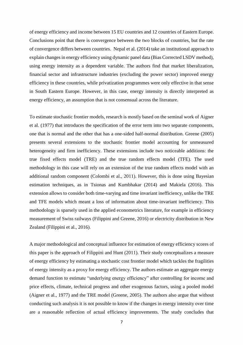
The concepts of energy intensity and energy efficiency are fundamentally different, although

the first is sometimes used as a proxy for the latter. Energy intensity is simply the ratio of total

energy consumption per unit of GDP. This indicator suffered severe changes in transition

economies since 1990, but not homogeneously across transition economies. The same

happened with electricity intensity, the ratio of electricity consumption per unit of GDP. The

Caucasus region countries managed to achieve great reductions in electricity intensity from

high levels since the early 1990s. The current members of the EU have lower electricity

intensities but their levels were already considerably low in the early 1990s. Kazakhstan,

Kyrgyzstan, Russia, Moldova and Ukraine had high energy intensities in 1992 and didn’t

10

manage to considerably bring those levels down by 2007. It is also clear that there is some

heterogeneity in efforts bringing down energy intensity even within the subset of current EU

members, which is easy to spot by comparing Latvia and Czech Republic, as it can be seen in

Figure 3.1 below.

Figure 1. – Electricity use (tonnes of oil equivalent) per $1,000 GDP (constant 2005 PPP).

Data source: World Bank

Energy efficiency is a more complex concept, as it is the activity that can be made with a certain

amount of energy, involving not only structural but also behavioural changes. It depends on a

number of factors that are not considered for energy intensity such as climate, output and

composition of the economy (OECD, 2011). Energy efficiency can fundamentally vary through

behavioural change in both households and industry, as the reform packages applied to

transition economies shifted the public and businesses away from a Soviet supply-side

mentality and also gave an incentive for more efficient use of energy through government

policies, price signals and improved management practices.

The framework outlined in the previous section points for several theoretical and estimation

challenges. It is possible that a decrease in energy intensity is not accompanied by a decrease

in underlying efficiency, as the decrease in energy intensity could have been mostly explained

by deep structural changes in the economy, resulting from large changes in the industrial sector

or a shift of capital and labour to other sectors in the economy with different electricity

0.00

0.03

0.06

0.09

0.12

0.15

0.18

ALB

AN

IA

AR

MEN

IA

AU

STR

IA

AZE

RB

AIJ

AN

BEL

AR

US

CZE

CH

REP

UB

LIC

DEN

MA

RK

FIN

LAN

D

FRA

NC

E

GEO

RG

IA

GER

MA

NY

HU

NG

AR

Y

KA

ZAK

HST

AN

KYR

GYZ

STA

N

LATV

IA

LITH

UA

NIA

MA

CED

ON

IA

MO

LDO

VA

MO

NG

OLI

A

NO

RW

AY

PO

LAN

D

RO

MA

NIA

RU

SSIA

SLO

VA

KIA

SLO

VEN

IA

TAJI

KIS

TAN

TUR

KM

ENIS

TAN

UK

RA

INE

UN

ITED

KIN

GD

OM

UZB

EKIS

TAN

1992 1998 2006

11

consumption profiles and/or value added. As such, the key differences between electricity

intensity and the proposed measure of efficiency should be clearly noticeable when the

structural changes in the economy are not followed by other sort of real efficiency gains that

are channelled through change in traditions and norms, different consumption profiles and

improved government regulations and other incentives for a more rational use of energy, in the

sense that a troubled economy is not necessarily efficient (conditional on its few surviving

activities).

It becomes clear that there is a large overlap between energy intensity and energy efficiency

but the concepts are not interchangeable. The key drivers of changes in energy efficiency that

are highlighted here also impact energy intensity, but are just a component of those changes.

By building an energy demand approach with controls for economic structural changes and

many other factors, the efficiency effect can be separated from other effects and effectively

measured.

The model uses aggregate (final) electricity consumption for the each economy. Demand

translates to demand for several energy services: heating, manufacturing, lighting, etc. This

requires capital equipment for machinery, home appliances, etc. The model takes an input

demand function perspective, so the difference between the observed input and the cost-

minimizing input demand represents both technical as well as allocative inefficiency (Filippini

and Hunt, 2011). This is in line with the fact that technical efficiency is necessary, but not

sufficient, for the achievement of cost efficiency (Kumbhakar and Lovell, 2004).

Due to the changes the economies went through in the transition period, it is important to

consider that there can be large differences in trends between the estimated level of efficiency

and the energy intensity measure. That could lead to dangerous policy advice, for example, if

technological advances, structural change towards services and the purchasing of energy

efficient equipment in the economy leads to a decrease in energy intensity but in fact the use

of such technology is not optimal (in the sense of “underlying” efficient use). Another very

important aspect is the consideration of persistent sources of inefficiency, which can be

particularly large in transition economies due to the economic history and previous economic

systems of these countries. These sources of inefficiency can be larger in countries where no

significant reform efforts were made following the collapse of the Soviet Union. This will be

taken into account in the modelling approach. The productivity approach of Stern (2012) will

12

not be followed for two reasons. First, such an approach would require a set of data that is not

available for those economies – and trying to fill the gaps with approximations increases the

danger of measurement error. Second, the productivity approach intends to find deep drivers

of differences in efficiency and energy prices between countries, but transition economies have

the peculiar framework of a strong reform effort from the conclusions of the Washington

Consensus. As such, policy parameters are taken as given, and an attempt to assess how

households and firms react to the economic environment is made, at the light of the available

data and taking into account unobserved heterogeneity between countries.

4. A stochastic frontier model for transition economies: data and methodology

4.1. Estimation approach

A firm is technically efficient if it uses the minimal level of inputs given output and input mix

or if it produces the maximal level of output given inputs (Cornwell and Schmidt, 2008). In

this context, SFA has been used often in empirical research to estimate firm level technical

efficiency. It can be argued that an SFA approach using electricity consumption as a dependent

variable given a set of inputs can retrieve economy-wide efficiency scores which represent

national aggregate efficiency. Therefore, the seminal SFA research that was originally used

within the neoclassical theory of production is now used at an aggregate level in a cost frontier.

A neo-classical framework for frontier approach is considered, although such a framework is

partially discarded as the concept of stochastic frontier will be used here within the empirical

approach traditionally used in the estimation of an aggregate energy demand function.

However, as pointed by Filippini and Hunt (2011), this still implies a kind of production

process. Further discussion about the conceptual framework first developed by these authors

will follow. The usual regularity conditions need to be assumed (Orea et al., 2014) – and the

functional form is chosen to achieve estimation simplicity.

The role of the random effects is related to heterogeneity in cost functions. They can be

considered as country specific intercepts in the cost function to account for unobserved

13

heterogeneity in electricity consumption across countries. The random effects correct the bias

in the parameters of the cost function so that the frontier is estimated correctly. The DEA

literature already considers a parametric approach to be too restrictive in the description of the

cost function. Naturally, the cost function needs to be identified correctly for accurate results.

In a scenario of constant differences in technology across countries, the GTRE model

presumably works well in finding true measures of cost efficiency. Time-invariant

technological differences between countries are accounted for in this way. One could consider

that this relates to the use of random effects models with large enough T to raise concerns about

what is time-invariant and what is not, so changes in relative technological gaps between

regions could be captured by the inefficiency measure – but a modelling compromise is

necessary given the limitations of the data – and even the existing limitations of Stochastic

Frontier models.

The estimation approach is deeply linked to the issues of country heterogeneity and the possible

persistence of inefficiencies in energy consumption in transition economies. Since the TRE

approach of Greene (2005) cannot disentangle time-persistent inefficiencies from country

heterogeneity and the approach of Aigner et al. (1977) fails to account for country

heterogeneity leading to biased results, the GTRE approach of Colombi et al. (2011) is

followed to solve both issues. The authors point that this approach is particularly appropriate

for cases where firms are heterogeneous (in this case, countries) and the panel is long. As such,

the following model accounts for persistent sources of long-run inefficiency and variable

sources of inefficiency:

𝑦𝑖𝑡 = 𝑥′𝑖𝑡𝛽 + 𝛼𝑖 + 𝜂𝑖 + 𝑢𝑖𝑡 + 𝑣𝑖𝑡 (1)

𝛼𝑖 ~ 𝑖. 𝑖. 𝑑. 𝑁(0; 𝜎𝛼2) 𝑣𝑖𝑡~ 𝑖. 𝑖. 𝑑. 𝑁(0; 𝜎𝑣

2) (2)

𝑢𝑖𝑡~ 𝑖. 𝑖. 𝑑. 𝑁+(0; 𝜎𝑢2) 𝜂𝑖~ 𝑖. 𝑖. 𝑑. 𝑁+(0; 𝜎𝜂

2) (3)

This is a cost frontier model. Note that the assumption for inefficiency is a half-normal

distribution for tractability purposes, although alternatives are available, such as an exponential

distribution (Meeusen and van Den Broeck, 1977). Also, note that in the case of assumed

exponential inefficiencies the draws for time-varying inefficiency require some rejection

14

method as the distribution is not easily simulated in statistical software. This is not an obstacle

found in the case of the half-normal assumption. Here, the frontier gives the minimum level of

energy consumption attainable by a country. The frontier concept is applied to estimate the

baseline energy demand - the frontier reflecting demand of countries that use high efficiency

equipment and have good use practices (Filippini and Hunt, 2011). 𝑥′𝑖𝑡 is a row vector of

regressors and 𝛽 is a column vector of unknown parameters to be estimated (note the model

also has a constant). 𝛼𝑖 captures latent heterogeneity (random effect) and 𝑣𝑖𝑡 is an idiosyncratic

error component. Attention is focused on 𝜂𝑖 and 𝑢𝑖𝑡 , as they represent time-invariant

inefficiency (long-run) sources of inefficiency and time-varying (short-run) inefficiency

respectively. In fact, this model is an extension of the TRE model (Greene, 2005)1, as it adds

another time-invariant random effect to capture persistent inefficiency (𝜑𝑖). In a random effects

model, the effects cannot be correlated with the explanatory variables, as it leads to bias in

estimates. Since there is a possibility of such a problem in applied econometrics, a Mundlak,

(1978) transformation can be conducted to account for correlation between the time-varying

explanatory variables and country-specific effects:

𝛼𝑖 = 𝛾𝑋�� + 𝜑𝑖 Where ��𝑖 = 1

𝑇∑ 𝑋𝑖𝑡

𝑇𝑡=1 and 𝜑𝑖 ~ 𝑁(0, 𝜎𝜑) (4)

Cross-section means for variables with very low variation are not added, such as population

and urbanization rate, as recommended by STATA 14.1 statistical package “mundlak”.

Two econometric approaches to Bayesian estimation of the GTRE model will be considered

and compared in a context of small samples to investigate the robustness of the results. The

first econometric approach follows Tsionas and Kumbhakar (2014) with a Bayesian approach

which involves reparameterizing the model to reduce autocorrelations in the draws of the model

parameters. The model can be rewritten by stacking the time series observations:

𝑦𝑖 = (𝛼𝑖 + 𝜂𝑖) ⊗ 𝑙𝑇 + 𝑥′𝑖𝛽 + (𝑢𝑖𝑡 + 𝑣𝑖𝑡) = 𝛿𝑖 ⊗ 𝑙𝑇 + 𝑥′𝑖𝛽 + 휀𝑖𝑡 (5)

1 The heterogeneity could possibly be dealt with through alternative approaches such as a model with random

slopes, but the estimation would be difficult given the relatively small sample panel size and the large number of

regressors.

15

휀𝑖𝑡 has a skew-normal distribution and all random components are mutually independent as

well as independent of 𝑥𝑖𝑡. Therefore, all the building process of the likelihood function follows

Tsionas and Kumbhakar (2014). Gibbs sampling will be used, keeping latent variables to

increase computational efficiency of MCMC schemes instead of integrating them out. The prior

distributions are:

𝑝(𝛽, 𝜎𝑒 , 𝜎𝑢, 𝜎𝜑 , 𝜎𝛼) = 𝑝(𝛽)𝑝(𝜎𝑣)𝑝(𝜎𝑢)𝑝(𝜎𝜂)𝑝(𝜎𝛼) (6)

With regression parameters assumed to follow the k-variate normal distribution

𝛽~𝑁𝐾( ��, 𝐴−1) with mean vector �� = 0(𝑘𝑥1) and precision matrix2 𝐴 = 10−4. 𝐼𝐾. Therefore,

there is very little information in the prior about the coefficients of the regressors. For scale

parameters, it is assumed that:

Qk

σk2 ~χ2(NK), 𝑓𝑜𝑟 𝐾 = 𝑣, 𝑢, 𝜂, 𝛼 (7)

And setting NK = 1 which represents the length of a prior sample from which a sum of squares

Qk is obtained. For posterior consistency, Qk has to be larger than zero, and Tsionas and

Kumbhakar (2014) set this to be 10−4 in the context of an application to the banking sector

with relatively low estimated inefficiency. However in this application there is a belief that all

variances should be important although there is uncertainty their relative magnitudes. As such,

information in the prior3 is set as Q𝑣 = 10−4, Q𝑢 = 10−3, Q𝛼 = 10−3 and Q𝜂 = 0.25. Further

discussion on the consequences of these choices is in subsequent sections of this paper. A Gibbs

sampler is implemented, with draws being taken from the various posterior conditional

distributions. According to Tsionas and Kumbhakar (2014), the “naïve” Gibbs sampling

scheme will not have good mixing properties and easily collapses. This claim will be debated

later in the paper. To reduce the natural correlations among parameters in the Markov Chain

Monte Carlo (MCMC) scheme, reparametrizations are implemented. First, a 𝛿 -

2 The authors originally define 𝐴 = 10−4. 𝐼𝐾 . This has no impact in any key results and is done for consistency

with the choices of Makiela (2016) 3 Lower values of Q can lead to issues in convergence and density plots of variances that were clearly not

reasonable, due to an unreasonably tight prior, as pointed by Makiela (2016). There is also previous research that

shows that vague priors with small amounts of data can be problematic (Lambert et al., 2005).

16

Parametrization4 is conducted, with 𝛿𝑖 = 𝛼𝑖 + 𝜂𝑖, grouping firm-specific effects and persistent

inefficiency, which would be grouped implicitly in Greene (2005) True Random Effects model

(the reason why persistent inefficiency would be treated as heterogeneity), although it would

be forced to have a mean of zero in the latter. As in Tsionas and Kumbhakar (2014), this allows

to obtain the posterior conditional distributions of 𝛿𝑖, 𝜎𝑢2, 𝜎𝑣

2 and 𝛽 . However, note that

obtaining 𝛿𝑖 does not allow to quantify persistent inefficiencies and only short-run

inefficiencies can be obtained from this first step of analysis. However, it should point for the

magnitude of the mean persistent inefficiency (i.e. mean 𝛿𝑖) . In a second step, a 𝜉 -

Parametrization is conducted (taking the estimates of 𝛽 from the 𝛿-Parametrization as given),

as in panel data GLS, with ξ𝑖𝑡 = 𝛼𝑖 + 𝑣𝑖𝑡. This allows to draw 𝜂𝑖 independently of the draw for

𝛼𝑖, and in turn the conditional distributions of not only 𝜂𝑖 but also 𝑢𝑖𝑡.

Tsionas and Kumbhakar (2014) set a simulation experience to show the good properties of their

reparameterization. However, these results do not hold in simulations attempted in this paper,

even for a similar DGP, with estimation of inefficiencies easily collapsing when signal to noise

rations are not large unless some particular tuning of the priors is applied.

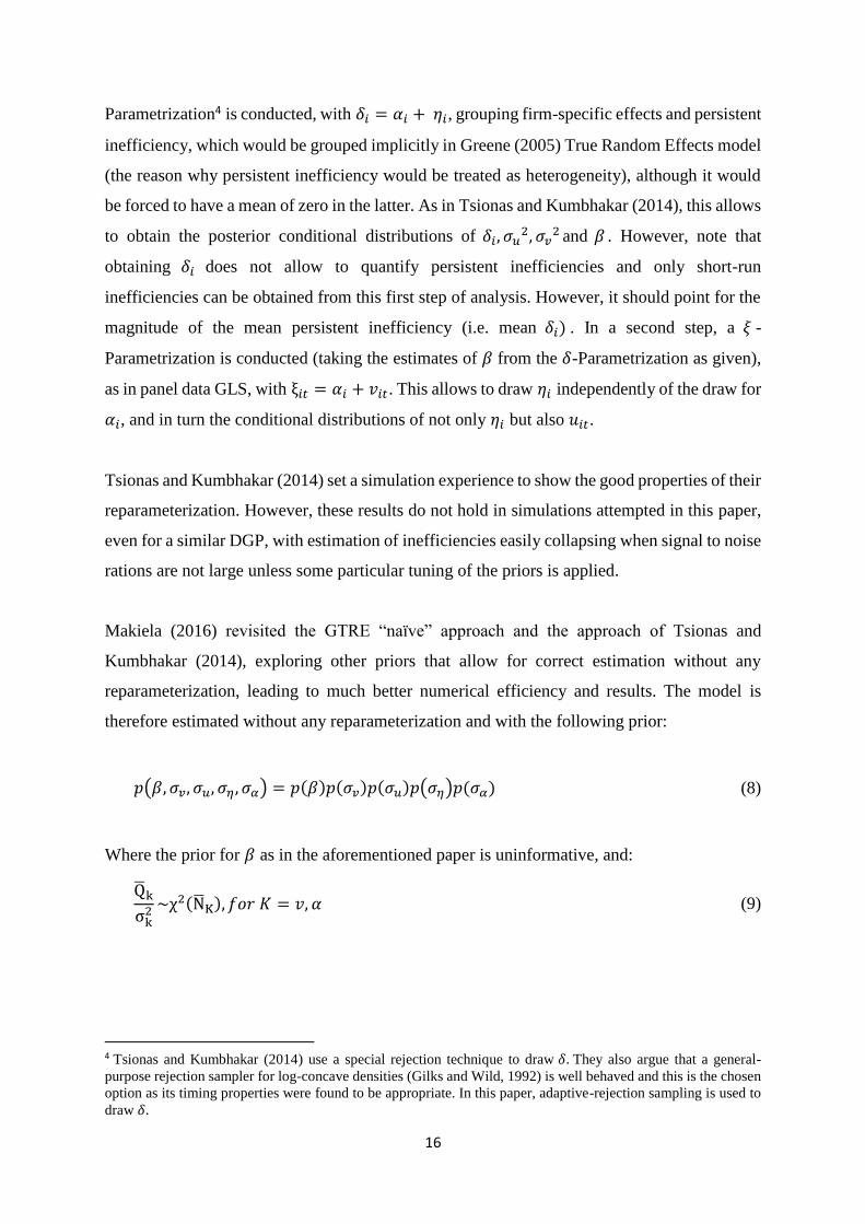
Makiela (2016) revisited the GTRE “naïve” approach and the approach of Tsionas and

Kumbhakar (2014), exploring other priors that allow for correct estimation without any

reparameterization, leading to much better numerical efficiency and results. The model is

therefore estimated without any reparameterization and with the following prior:

𝑝(𝛽, 𝜎𝑣, 𝜎𝑢, 𝜎𝜂 , 𝜎𝛼) = 𝑝(𝛽)𝑝(𝜎𝑣)𝑝(𝜎𝑢)𝑝(𝜎𝜂)𝑝(𝜎𝛼) (8)

Where the prior for 𝛽 as in the aforementioned paper is uninformative, and:

Qk

σk2 ~χ2(NK), 𝑓𝑜𝑟 𝐾 = 𝑣, 𝛼 (9)

4 Tsionas and Kumbhakar (2014) use a special rejection technique to draw 𝛿. They also argue that a general-

purpose rejection sampler for log-concave densities (Gilks and Wild, 1992) is well behaved and this is the chosen

option as its timing properties were found to be appropriate. In this paper, adaptive-rejection sampling is used to

draw 𝛿.

17

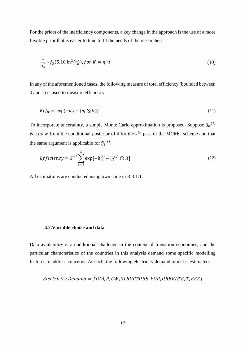
For the priors of the inefficiency components, a key change in the approach is the use of a more

flexible prior that is easier to tune to fit the needs of the researcher:

1

σk2 ~𝑓𝐺(5,10 ln2(𝑟𝐾

∗), 𝑓𝑜𝑟 𝐾 = 𝜂, 𝑢 (10)

In any of the aforementioned cases, the following measure of total efficiency (bounded between

0 and 1) is used to measure efficiency:

𝐸𝑓𝑓𝑖𝑡 = exp(−𝑢𝑖𝑡 − (𝜂𝑖 ⊗ 𝑙𝑡)) (11)

To incorporate uncertainty, a simple Monte Carlo approximation is proposed. Suppose uit(𝑠)

is a draw from the conditional posterior of u for the 𝑠𝑡ℎ pass of the MCMC scheme and that

the same argument is applicable for ��𝑖(𝑠):

𝐸𝑓𝑓𝑖𝑐𝑖𝑒𝑛𝑐𝑦 = 𝑆−1∑ exp [−u𝑖𝑡

(𝑠)− ��𝑖

(𝑠) ⊗ 𝑙𝑡]

𝑆

𝑠=1

(12)

All estimations are conducted using own code in R 3.1.1.

4.2.Variable choice and data

Data availability is an additional challenge in the context of transition economies, and the

particular characteristics of the countries in this analysis demand some specific modelling

features to address concerns. As such, the following electricity demand model is estimated:

𝐸𝑙𝑒𝑐𝑡𝑟𝑖𝑐𝑖𝑡𝑦 𝐷𝑒𝑚𝑎𝑛𝑑 = 𝑓(𝑉𝐴, 𝑃, 𝐶𝑊, 𝑆𝑇𝑅𝑈𝐶𝑇𝑈𝑅𝐸, 𝑃𝑂𝑃, 𝑈𝑅𝐵𝑅𝐴𝑇𝐸, 𝑇, 𝐸𝐹𝐹)

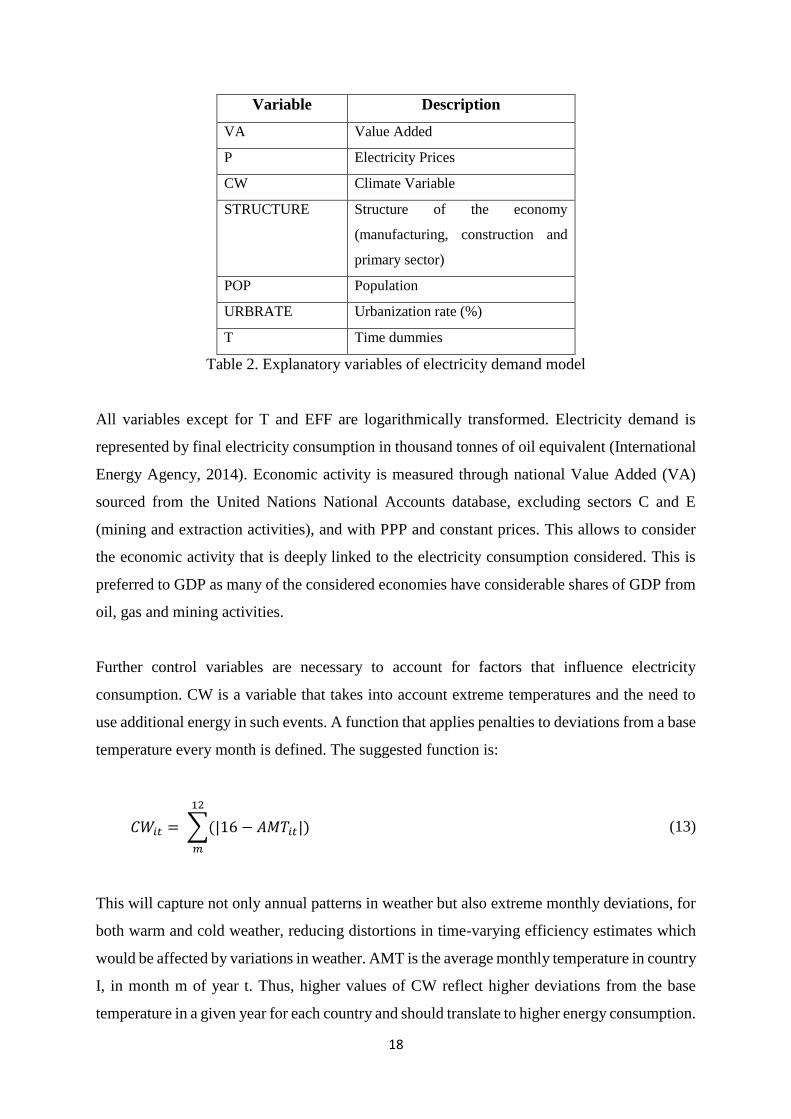
18

Variable Description

VA Value Added

P Electricity Prices

CW Climate Variable

STRUCTURE Structure of the economy

(manufacturing, construction and

primary sector)

POP Population

URBRATE Urbanization rate (%)

T Time dummies

Table 2. Explanatory variables of electricity demand model

All variables except for T and EFF are logarithmically transformed. Electricity demand is

represented by final electricity consumption in thousand tonnes of oil equivalent (International

Energy Agency, 2014). Economic activity is measured through national Value Added (VA)

sourced from the United Nations National Accounts database, excluding sectors C and E

(mining and extraction activities), and with PPP and constant prices. This allows to consider

the economic activity that is deeply linked to the electricity consumption considered. This is

preferred to GDP as many of the considered economies have considerable shares of GDP from

oil, gas and mining activities.

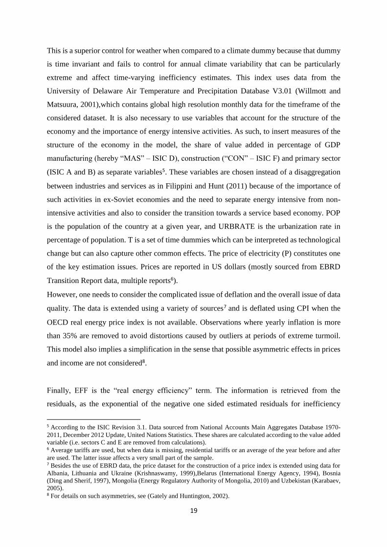
Further control variables are necessary to account for factors that influence electricity

consumption. CW is a variable that takes into account extreme temperatures and the need to

use additional energy in such events. A function that applies penalties to deviations from a base

temperature every month is defined. The suggested function is:

𝐶𝑊𝑖𝑡 = ∑(|16 − 𝐴𝑀𝑇𝑖𝑡|)

12

𝑚

(13)

This will capture not only annual patterns in weather but also extreme monthly deviations, for

both warm and cold weather, reducing distortions in time-varying efficiency estimates which

would be affected by variations in weather. AMT is the average monthly temperature in country

I, in month m of year t. Thus, higher values of CW reflect higher deviations from the base

temperature in a given year for each country and should translate to higher energy consumption.

19

This is a superior control for weather when compared to a climate dummy because that dummy

is time invariant and fails to control for annual climate variability that can be particularly

extreme and affect time-varying inefficiency estimates. This index uses data from the

University of Delaware Air Temperature and Precipitation Database V3.01 (Willmott and

Matsuura, 2001),which contains global high resolution monthly data for the timeframe of the

considered dataset. It is also necessary to use variables that account for the structure of the

economy and the importance of energy intensive activities. As such, to insert measures of the

structure of the economy in the model, the share of value added in percentage of GDP

manufacturing (hereby “MAS” – ISIC D), construction (“CON” – ISIC F) and primary sector

(ISIC A and B) as separate variables5. These variables are chosen instead of a disaggregation

between industries and services as in Filippini and Hunt (2011) because of the importance of

such activities in ex-Soviet economies and the need to separate energy intensive from non-

intensive activities and also to consider the transition towards a service based economy. POP

is the population of the country at a given year, and URBRATE is the urbanization rate in

percentage of population. T is a set of time dummies which can be interpreted as technological

change but can also capture other common effects. The price of electricity (P) constitutes one

of the key estimation issues. Prices are reported in US dollars (mostly sourced from EBRD

Transition Report data, multiple reports6).

However, one needs to consider the complicated issue of deflation and the overall issue of data

quality. The data is extended using a variety of sources7 and is deflated using CPI when the

OECD real energy price index is not available. Observations where yearly inflation is more

than 35% are removed to avoid distortions caused by outliers at periods of extreme turmoil.

This model also implies a simplification in the sense that possible asymmetric effects in prices

and income are not considered8.

Finally, EFF is the “real energy efficiency” term. The information is retrieved from the

residuals, as the exponential of the negative one sided estimated residuals for inefficiency

5 According to the ISIC Revision 3.1. Data sourced from National Accounts Main Aggregates Database 1970-

2011, December 2012 Update, United Nations Statistics. These shares are calculated according to the value added

variable (i.e. sectors C and E are removed from calculations). 6 Average tariffs are used, but when data is missing, residential tariffs or an average of the year before and after

are used. The latter issue affects a very small part of the sample. 7 Besides the use of EBRD data, the price dataset for the construction of a price index is extended using data for

Albania, Lithuania and Ukraine (Krishnaswamy, 1999),Belarus (International Energy Agency, 1994), Bosnia

(Ding and Sherif, 1997), Mongolia (Energy Regulatory Authority of Mongolia, 2010) and Uzbekistan (Karabaev,

2005). 8 For details on such asymmetries, see (Gately and Huntington, 2002).

20

provide a measure of efficiency from 0 to 1 (fully efficient). This can be translated into a score

from 0 to 100%.

This study is based on an unbalanced panel of 33 economies over the period 1994-2007. The

dataset contains 389 observations, with a minimum T of 5, a maximum T of 14 and an average

T of 11.8 across the sample (higher than the conservative T=10 set in simulations in the next

section to assess model performance). The choice of timeframe is mostly associated to the

availability of electricity price data as a proxy for energy prices and also the necessary

information to deflate it (there is lack of economic data for transition economies in many

aspects). The countries in the sample are Albania, Armenia, Azerbaijan, Belarus, Bosnia,

Bulgaria, Czech Republic, Croatia, Estonia, Georgia, Hungary, Latvia, Lithuania, Kazakhstan,

Kyrgyzstan, Macedonia, Moldova, Mongolia, Poland, Russia, Romania, Slovakia, Slovenia,

Tajikistan, Turkmenistan, Ukraine and Uzbekistan (transition) and Austria, UK, France,

Germany, Finland and Denmark (Non Transition OECD members).

5. Artificial examples and performance of GTRE model in small samples

Consider the following data generating process: 𝑦𝑖𝑡 = 1 + 𝑥𝑖𝑡 + 𝛼𝑖 + 𝜂𝑖 + 𝑢𝑖𝑡 + 𝑣𝑖𝑡 , where

𝑥𝑖𝑡 is a standard normal distribution. Different parameters can be set for 𝜎𝑣,𝜎𝑢, 𝜎𝜂 , 𝜎𝛼, with

different scenarios. The panel size is set to be quite small with N=35 and T=10, to resemble

the small-sample issues that the transition data used here might face in estimation. As an

alternative sample size and to assess convergence to true values as the sample size increases,

simulations are repeated with a larger panel of N=100 and T=10.

The following scenarios are created:

Scenario 1: 𝜎𝑣 = 0.1, 𝜎𝑢 = 0.2, 𝜎𝜂 = 0.2, 𝜎𝛼 = 0.5 . This scenario is the same as the case

N=50 of Tsionas and Kumbhakar (2014) and implies moderate signal-to-noise ratios. With not

very strong ratios there is an expectation of bigger performance degradation as the sample size

decreases.

21

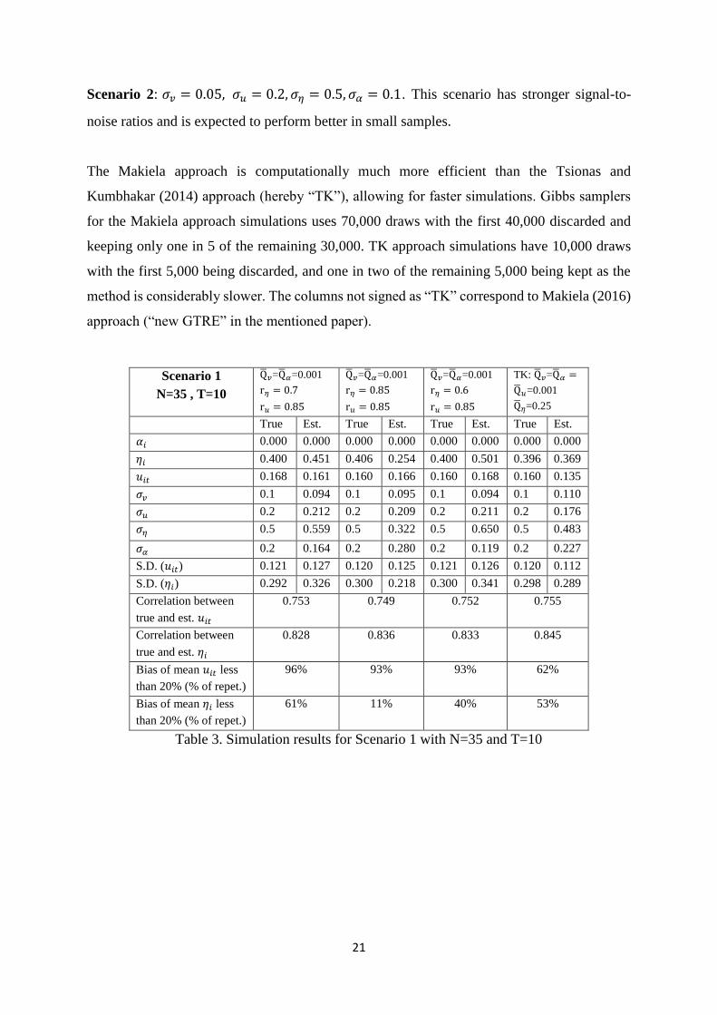
Scenario 2: 𝜎𝑣 = 0.05, 𝜎𝑢 = 0.2, 𝜎𝜂 = 0.5, 𝜎𝛼 = 0.1. This scenario has stronger signal-to-

noise ratios and is expected to perform better in small samples.

The Makiela approach is computationally much more efficient than the Tsionas and

Kumbhakar (2014) approach (hereby “TK”), allowing for faster simulations. Gibbs samplers

for the Makiela approach simulations uses 70,000 draws with the first 40,000 discarded and

keeping only one in 5 of the remaining 30,000. TK approach simulations have 10,000 draws

with the first 5,000 being discarded, and one in two of the remaining 5,000 being kept as the

method is considerably slower. The columns not signed as “TK” correspond to Makiela (2016)

approach (“new GTRE” in the mentioned paper).

Table 3. Simulation results for Scenario 1 with N=35 and T=10

Scenario 1

N=35 , T=10

Q𝑣=Q𝛼=0.001

r𝜂 = 0.7

r𝑢 = 0.85

Q𝑣=Q𝛼=0.001

r𝜂 = 0.85

r𝑢 = 0.85

Q𝑣=Q𝛼=0.001

r𝜂 = 0.6

r𝑢 = 0.85

TK: Q𝑣=Q𝛼 =

Q𝑢=0.001

Q𝜂=0.25

True Est. True Est. True Est. True Est.

𝛼𝑖 0.000 0.000 0.000 0.000 0.000 0.000 0.000 0.000

𝜂𝑖 0.400 0.451 0.406 0.254 0.400 0.501 0.396 0.369

𝑢𝑖𝑡 0.168 0.161 0.160 0.166 0.160 0.168 0.160 0.135

𝜎𝑣 0.1 0.094 0.1 0.095 0.1 0.094 0.1 0.110

𝜎𝑢 0.2 0.212 0.2 0.209 0.2 0.211 0.2 0.176

𝜎𝜂 0.5 0.559 0.5 0.322 0.5 0.650 0.5 0.483

𝜎𝛼 0.2 0.164 0.2 0.280 0.2 0.119 0.2 0.227

S.D. (𝑢𝑖𝑡) 0.121 0.127 0.120 0.125 0.121 0.126 0.120 0.112

S.D. (𝜂𝑖) 0.292 0.326 0.300 0.218 0.300 0.341 0.298 0.289

Correlation between

true and est. 𝑢𝑖𝑡

0.753 0.749 0.752 0.755

Correlation between

true and est. 𝜂𝑖

0.828 0.836 0.833 0.845

Bias of mean 𝑢𝑖𝑡 less

than 20% (% of repet.)

96% 93% 93% 62%

Bias of mean 𝜂𝑖 less

than 20% (% of repet.)

61% 11% 40% 53%

22

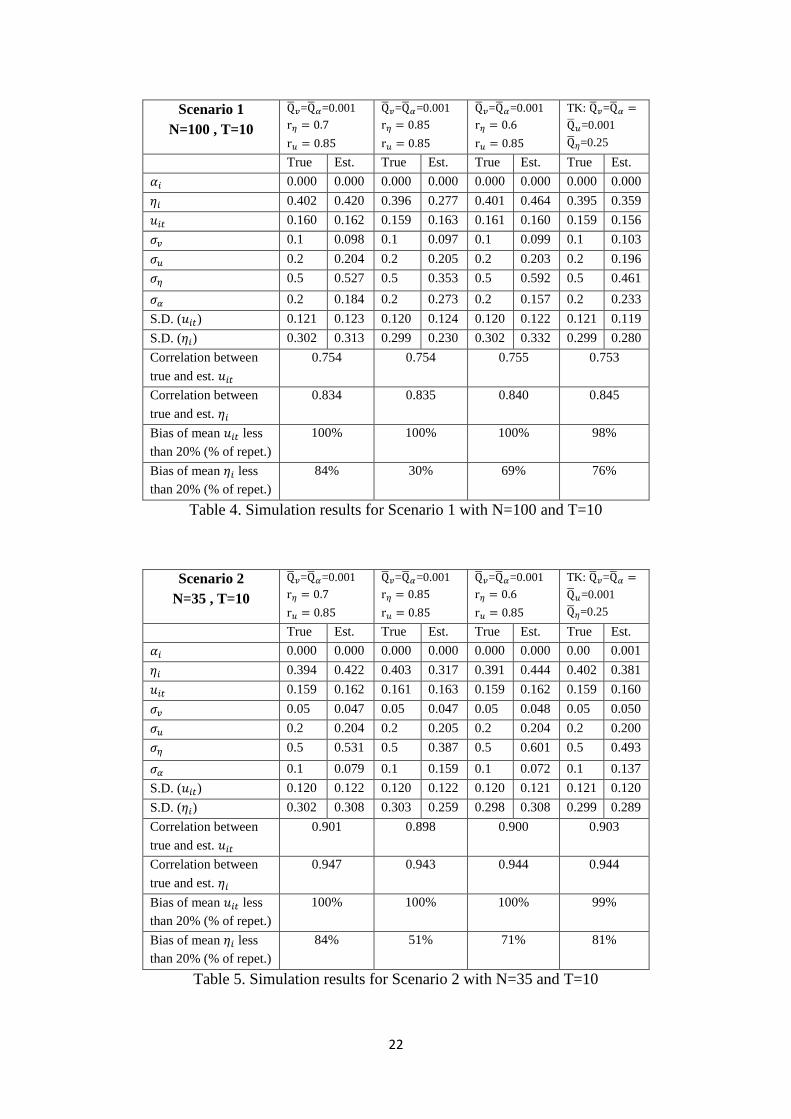
Table 4. Simulation results for Scenario 1 with N=100 and T=10

Table 5. Simulation results for Scenario 2 with N=35 and T=10

Scenario 1

N=100 , T=10

Q𝑣=Q𝛼=0.001

r𝜂 = 0.7

r𝑢 = 0.85

Q𝑣=Q𝛼=0.001

r𝜂 = 0.85

r𝑢 = 0.85

Q𝑣=Q𝛼=0.001

r𝜂 = 0.6

r𝑢 = 0.85

TK: Q𝑣=Q𝛼 =

Q𝑢=0.001

Q𝜂=0.25

True Est. True Est. True Est. True Est.

𝛼𝑖 0.000 0.000 0.000 0.000 0.000 0.000 0.000 0.000

𝜂𝑖 0.402 0.420 0.396 0.277 0.401 0.464 0.395 0.359

𝑢𝑖𝑡 0.160 0.162 0.159 0.163 0.161 0.160 0.159 0.156

𝜎𝑣 0.1 0.098 0.1 0.097 0.1 0.099 0.1 0.103

𝜎𝑢 0.2 0.204 0.2 0.205 0.2 0.203 0.2 0.196

𝜎𝜂 0.5 0.527 0.5 0.353 0.5 0.592 0.5 0.461

𝜎𝛼 0.2 0.184 0.2 0.273 0.2 0.157 0.2 0.233

S.D. (𝑢𝑖𝑡) 0.121 0.123 0.120 0.124 0.120 0.122 0.121 0.119

S.D. (𝜂𝑖) 0.302 0.313 0.299 0.230 0.302 0.332 0.299 0.280

Correlation between

true and est. 𝑢𝑖𝑡

0.754 0.754 0.755 0.753

Correlation between

true and est. 𝜂𝑖

0.834 0.835 0.840 0.845

Bias of mean 𝑢𝑖𝑡 less

than 20% (% of repet.)

100% 100% 100% 98%

Bias of mean 𝜂𝑖 less

than 20% (% of repet.)

84% 30% 69% 76%

Scenario 2

N=35 , T=10

Q𝑣=Q𝛼=0.001

r𝜂 = 0.7

r𝑢 = 0.85

Q𝑣=Q𝛼=0.001

r𝜂 = 0.85

r𝑢 = 0.85

Q𝑣=Q𝛼=0.001

r𝜂 = 0.6

r𝑢 = 0.85

TK: Q𝑣=Q𝛼 =

Q𝑢=0.001

Q𝜂=0.25

True Est. True Est. True Est. True Est.

𝛼𝑖 0.000 0.000 0.000 0.000 0.000 0.000 0.00 0.001

𝜂𝑖 0.394 0.422 0.403 0.317 0.391 0.444 0.402 0.381

𝑢𝑖𝑡 0.159 0.162 0.161 0.163 0.159 0.162 0.159 0.160

𝜎𝑣 0.05 0.047 0.05 0.047 0.05 0.048 0.05 0.050

𝜎𝑢 0.2 0.204 0.2 0.205 0.2 0.204 0.2 0.200

𝜎𝜂 0.5 0.531 0.5 0.387 0.5 0.601 0.5 0.493

𝜎𝛼 0.1 0.079 0.1 0.159 0.1 0.072 0.1 0.137

S.D. (𝑢𝑖𝑡) 0.120 0.122 0.120 0.122 0.120 0.121 0.121 0.120

S.D. (𝜂𝑖) 0.302 0.308 0.303 0.259 0.298 0.308 0.299 0.289

Correlation between

true and est. 𝑢𝑖𝑡

0.901 0.898 0.900 0.903

Correlation between

true and est. 𝜂𝑖

0.947 0.943 0.944 0.944

Bias of mean 𝑢𝑖𝑡 less

than 20% (% of repet.)

100% 100% 100% 99%

Bias of mean 𝜂𝑖 less

than 20% (% of repet.)

84% 51% 71% 81%

23

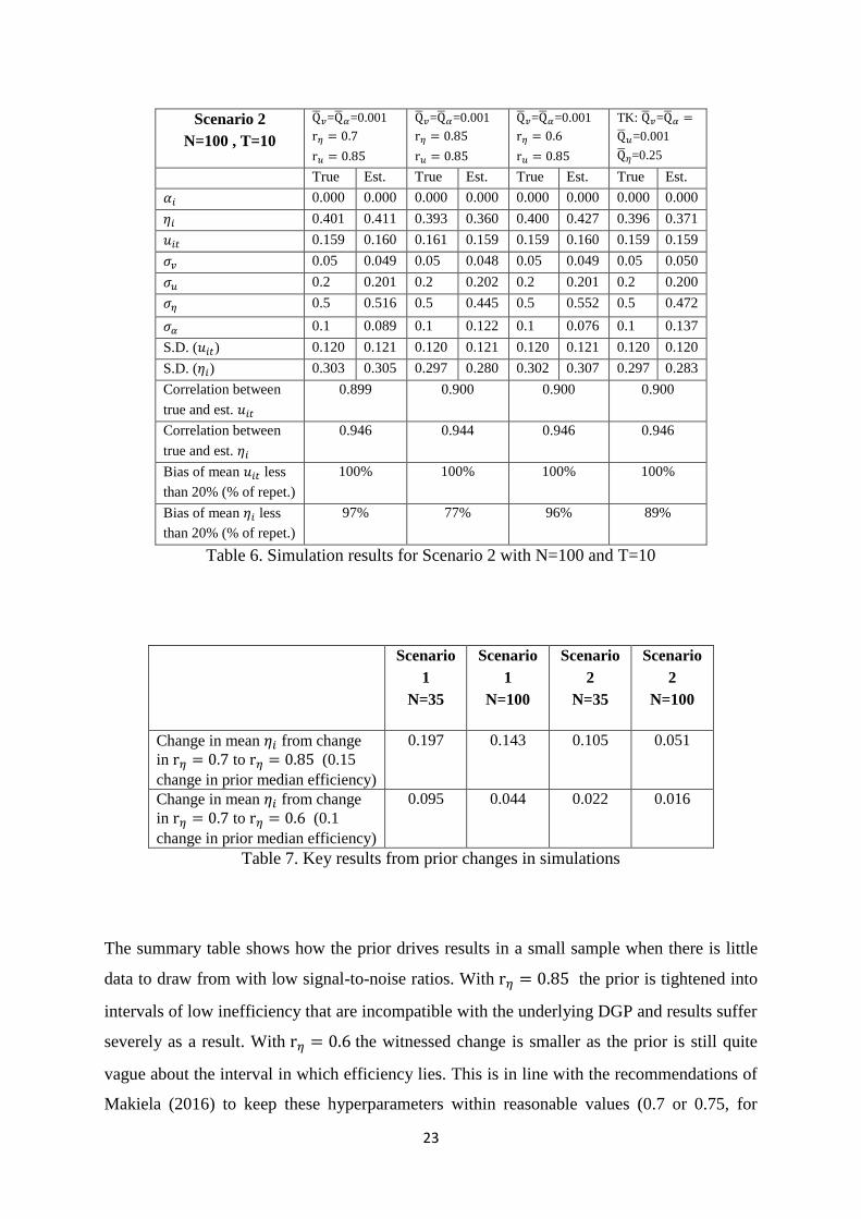
Table 6. Simulation results for Scenario 2 with N=100 and T=10

Scenario

1

N=35

Scenario

1

N=100

Scenario

2

N=35

Scenario

2

N=100

Change in mean 𝜂𝑖 from change

in r𝜂 = 0.7 to r𝜂 = 0.85 (0.15

change in prior median efficiency)

0.197 0.143 0.105 0.051

Change in mean 𝜂𝑖 from change

in r𝜂 = 0.7 to r𝜂 = 0.6 (0.1

change in prior median efficiency)

0.095 0.044 0.022 0.016

Table 7. Key results from prior changes in simulations

The summary table shows how the prior drives results in a small sample when there is little

data to draw from with low signal-to-noise ratios. With r𝜂 = 0.85 the prior is tightened into

intervals of low inefficiency that are incompatible with the underlying DGP and results suffer

severely as a result. With r𝜂 = 0.6 the witnessed change is smaller as the prior is still quite

vague about the interval in which efficiency lies. This is in line with the recommendations of

Makiela (2016) to keep these hyperparameters within reasonable values (0.7 or 0.75, for

Scenario 2

N=100 , T=10

Q𝑣=Q𝛼=0.001

r𝜂 = 0.7

r𝑢 = 0.85

Q𝑣=Q𝛼=0.001

r𝜂 = 0.85

r𝑢 = 0.85

Q𝑣=Q𝛼=0.001

r𝜂 = 0.6

r𝑢 = 0.85

TK: Q𝑣=Q𝛼 =

Q𝑢=0.001

Q𝜂=0.25

True Est. True Est. True Est. True Est.

𝛼𝑖 0.000 0.000 0.000 0.000 0.000 0.000 0.000 0.000

𝜂𝑖 0.401 0.411 0.393 0.360 0.400 0.427 0.396 0.371

𝑢𝑖𝑡 0.159 0.160 0.161 0.159 0.159 0.160 0.159 0.159

𝜎𝑣 0.05 0.049 0.05 0.048 0.05 0.049 0.05 0.050

𝜎𝑢 0.2 0.201 0.2 0.202 0.2 0.201 0.2 0.200

𝜎𝜂 0.5 0.516 0.5 0.445 0.5 0.552 0.5 0.472

𝜎𝛼 0.1 0.089 0.1 0.122 0.1 0.076 0.1 0.137

S.D. (𝑢𝑖𝑡) 0.120 0.121 0.120 0.121 0.120 0.121 0.120 0.120

S.D. (𝜂𝑖) 0.303 0.305 0.297 0.280 0.302 0.307 0.297 0.283

Correlation between

true and est. 𝑢𝑖𝑡

0.899 0.900 0.900 0.900

Correlation between

true and est. 𝜂𝑖

0.946 0.944 0.946 0.946

Bias of mean 𝑢𝑖𝑡 less

than 20% (% of repet.)

100% 100% 100% 100%

Bias of mean 𝜂𝑖 less

than 20% (% of repet.)

97% 77% 96% 89%

24

example), and witnessed irregular behaviour as these approach 0.9 if the true inefficiency is

rather large. As the signal to noise ratio strengthens in Scenario 2, the impact of a change in

priors is greatly reduced.

There are three key conclusions to take from these results. The first conclusion is that in

relevant sample sizes for the analysis of energy efficiency in transition economies, the prior

will drive the results if there is not enough information in the data. However, if the underlying

signal is strong enough, the results should not vary much independently of using the Makiela

or TK approach with different reasonable priors. Although the TK approach can render

reasonable results if priors are tuned enough, the underlying priors are problematic. The

“naïve” approach seems to be more intuitive and much more computationally efficient but both

methods can be used for robustness of the analysis. Either way, it is clear and not unexpected

that with an extremely small sample of N=35 it is difficult to obtain robust results unless the

underlying signal in the data is strong.

The second conclusion relates to the behaviour of efficiency levels and correlations between

true and estimated values. Across both scenarios and all sample sizes and priors, the correlation

of estimated transient inefficiency with true values is at least 0.74 and the correlation of

estimated persistent inefficiency is at least 0.83. This means that the relative rankings within

each type of inefficiency are well preserved even in small samples. However, as the total

efficiency scores are a combination of both types of inefficiency, this also implies that if the

prior drives the mean of persistent inefficiency significantly then a distortion of the true

efficiency rankings is likely, if the size of both inefficiencies is significant. From the behaviour

seen in the tables 3.2 to 3.6, it is recommended that analysis on efficiency scores is only

conducted if the mean persistent inefficiency is not significantly affected by changes in

hyperparameters, as that implies there is sufficient underlying data (strong signal) for

estimation. However, it is also true that if the signal-to-noise ratio grows significantly, it is

likely that the random effects become increasingly irrelevant and barely distort the efficiency

rankings – making the case for estimation of a simpler model in which the random effects are

dropped. This is an interesting outcome to have in mind when estimating the GTRE model in

small samples.

The third and final conclusion is that the TK approach is overall not competitive or attractive

for multiple reasons. First, results are not improved with the reparameterization versus the

25

alternative “naïve” approach in terms of mean bias, the spread of that bias over repetitions and

the overall performance of key parameters. Second, the prior leads to problems in applied

research, as will be explored further in the next section. Finally, the TK approach is

considerably slower computationally due to the additional steps. Also, given that the authors

originally consider all Q to be 0.0001 in their simulations, it is puzzling how their results are

close to the true values, as the chosen prior would lead to very irregular results in the

simulations above.

These results are broadly in line with the findings of the detailed simulation previously

conducted on the (frequentist) GTRE model (Badunenko and Kumbhakar, 2016). The key to

good estimation is the relationship between the sizes of the four components. The authors refer

that unless the noise and the random effects are nearly non-existent, only one of the inefficiency

components can be estimated correctly. In some scenarios, efficiency analysis is not

recommended due to the unreliability of the estimates. The authors also find that the largest

and smallest efficiencies measured are estimated more imprecisely. These findings align well

with the simulations conducted above, although the use of priors in Bayesian econometrics

might give less pessimistic insights about some scenarios, particularly in smaller samples.

6. Results and Discussion

The economic theory in which this cost frontier approach is based requires positive skewness

for inefficiency to exist and have valid interpretation. Preliminary frequentist random effects

estimation shows positive skewness in both the idiosyncratic error and the random effects,

indicating the need to indeed pursuit this modelling approach.

Both Makiela (2016) approach and Tsionas and Kumbhakar (2014) approach (hereby “TK”)

are used to estimate the model. 1,300,000 draws are taken, with a burn-in of 400,000 and taking

one in each twenty of the remaining draws for both approaches, including TK. The latter

method is much slower computationally, taking many hours to run, while the new GTRE takes

about an hour9.

9 Note that this is valid for an unbalanced panel framework such as the one in this application – simulations with

balanced panels require simpler programming which runs slightly faster.

26

Although credible intervals for efficiency estimates can be considered (Horrace and Schmidt,

1996), it is not common to analyse the results from Stochastic Frontier analysis by restricting

statements to events of strong statistical significance due to the naturally high uncertainty of

estimates. The analysis will mostly rely on point estimates and group average analysis over

time. Some coefficients of the cross-sectional means of regressors are significant, justifying

the use of the Mundlak extension in this context. Therefore, estimates without these additional

regressors are not reported as they are expected to be biased.

Two datasets were considered: one excluding the data points where inflation is over 35%,

including Norway, and another where Norway is excluded 10 . For each case, parameter

estimates and efficiency estimates will be presented under multiple priors to assess the

robustness of the results. In all cases, 95% credible intervals are presented in square brackets.

The analysis of results is focused on the column where prior and posterior persistent

inefficiency are rather close, with r𝜂 = 0.6, as explained below.

10 Norway is an advanced economy with large oil exports and a very cold climate, combined with low access to

natural gas. This can distort results. For results summary with Norway included, see Appendix 2.

27

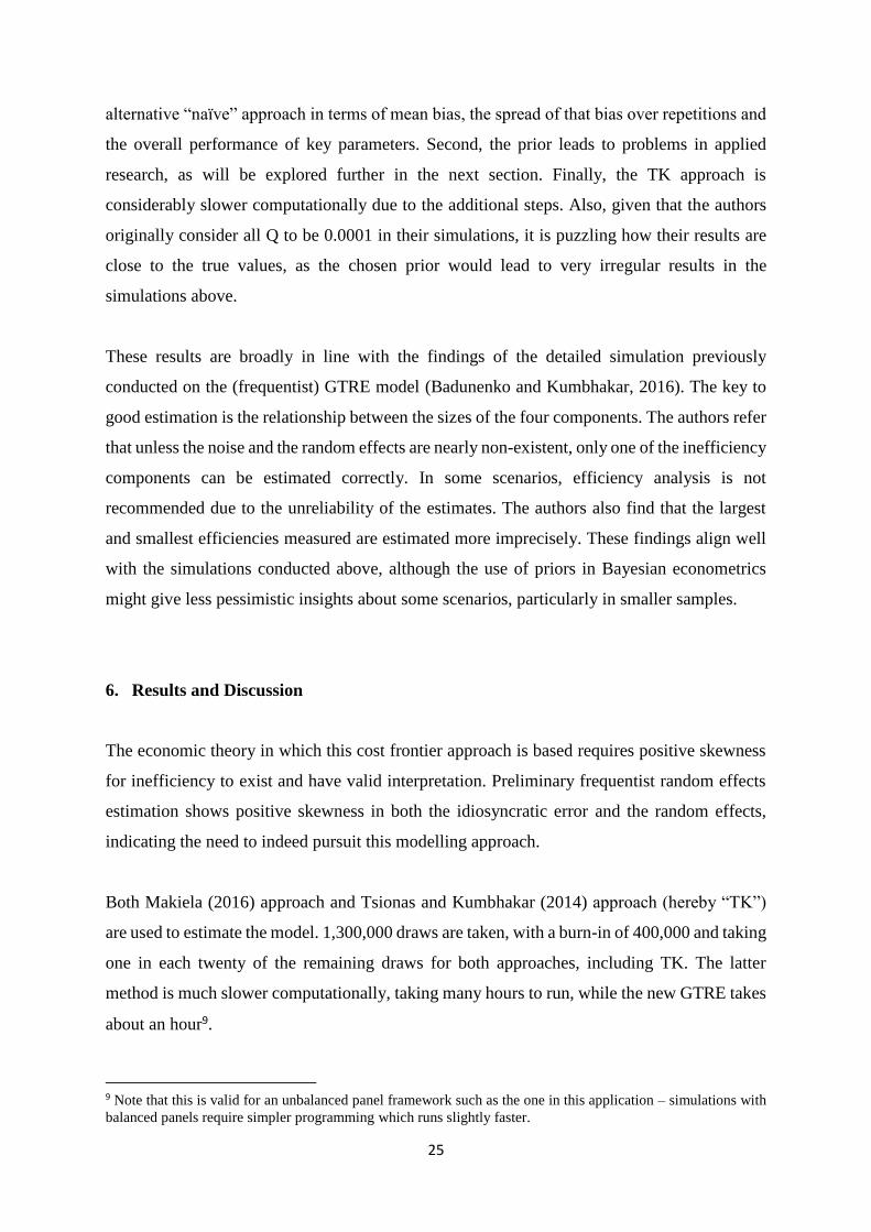
Table 8. Key regression results

The first three columns comfortably show signs of convergence according to the Geweke

convergence diagnostic (Geweke, 1992). This is based on a test for equality of the means of

the first and last part of a Markov chain (the first 10% and the last 50%). The Z-score from the

test is asymptotic normal if the two means from the parts of the chain are stationary. Z-scores

for each parameter are in Appendix 1. However, the convergence results for the TK approach

are very poor, with multiple parameters with higher Z-scores. This highlights the poor mixing

of the model, although the results are not very different.

Parameter estimates are intuitive and show the expected signs, although elasticities of income

and prices are rather small yet plausible. Deviations from an average temperature level also

Dataset 2

(excluding

Norway)

Q𝑣=0.001

Q𝛼=0.01

r𝜂 = 0.7

r𝑢 = 0.85

Q𝑣=0.001

Q𝛼=0.01

r𝜂 = 0.6

r𝑢 = 0.85

Q𝑣=0.001

Q𝛼=0.01

r𝜂 = 0.5

r𝑢 = 0.85

TK:

Q𝑣=0.001

Q𝛼 = 0.01

Q𝑢=0.01

Q𝜂=0.25

𝛽𝐼𝑛𝑡𝑒𝑟𝑐𝑒𝑝𝑡 -15.083

[-21.50;-8.72]

-16.023

[-22.86;-8.81]

-15.794

[-22.55;-8.96]

-15.776

[-22.21;-8.48]

𝛽𝐺𝐷𝑃 0.2080

[0.15;0.27]

0.2054

[0.15;0.26]

0.2042

[0.15;0.26]

0.2075

[0.15;0.26]

𝛽𝐸𝑙𝑒𝑐. 𝑃𝑟𝑖𝑐𝑒 -0.0505

[-0.08;-0.02]

-0.0497

[-0.08;-0.02]

-0.0493

[-0.08;-0.02]

-0.0488

[-0.08;-0.02]

𝛽𝑊𝑒𝑎𝑡ℎ𝑒𝑟 0.0492

[-0.11;0.21]

0.0483

[-0.11;0.21]

0.0479

[-0.11;0.21]

0.0554

[-0.10;0.22]

𝛽𝑈𝑟𝑏.𝑅𝑎𝑡𝑒 1.0470

[0.64;1.45]

1.0970

[0.70;1.47]

1.1357

[0.73;1.55]

1.0834

[0.69;1.46]

𝛽𝑃𝑜𝑝𝑢𝑙𝑎𝑡𝑖𝑜𝑛 0.7581

[0.53;0.96]

0.7340

[0.51;0.98]

0.7215

[0.45;0.98]

0.7256

[0.47;0.96]

𝛽𝑀𝑎𝑛𝑢𝑓. 𝑆ℎ𝑎𝑟𝑒 0.0951

[0.02;0.17]

0.0888

[0.02;0.16]

0.0838

[0.01;0.16]

0.0867

[0.01;0.16]

𝛽𝐶𝑜𝑛𝑠𝑡𝑟. 𝑆ℎ𝑎𝑟𝑒 0.0413

[-0.00;0.09]

0.0391

[-0.01;0.08]

0.0373

[-0.01;0.08]

0.0383

[-0.01;0.08]

𝛽𝑃𝑟𝑖𝑚𝑎𝑟𝑦 𝑆ℎ𝑎𝑟𝑒 -0.0006

[-0.08;0.08]

-0.0021

[-0.09;0.08]

-0.0034

[-0.09;0.08]

-0.0031

[-0.09;0.08]

Mean(𝜂𝑖) 0.484 0.552 0.608 0.481

Mean(𝑢𝑖𝑡) 0.099 0.098 0.098 0.096

𝜎𝑣 0.0177

[0.010;0.028]

0.0176

[0.010;0.028]

0.0176

[0.010;0.028]

0.0200

[0.011;0.032]

𝜎𝑢 0.1348

[0.123;0.147]

0.1346

[0.123;0.147]

0.1344

[0.123;0.147]

0.1280

[0.115;0.141]

𝜎𝜂 0.5912

[0.401;0.828]

0.7018

[0.510;0.942]

0.8217

[0.634;1.073]

0.6049

[0.256;0.981]

𝜎𝛼 0.1896

[0.046;0.424]

0.1573

[0.046;0.383]

0.1237

[0.041;0.307]

0.2042

[0.050;0.459]

Mean

Efficiency

(0-100%)

59.6% 56.7% 54.1% 60.2%

28

show a positive effect on electricity consumption, although the impact is not statistically

significant. The urbanization rate has a strong impact on electricity consumption as people

move from rural to urban areas, which often leads to switches in fuel use and fuel availability.

As expected, population also has a strong positive effect, although the coefficient is smaller

than 1. The manufacturing share of value added seems to be the only activity share variable

that is significant, leading to more consumption than other activities, as expected.

Unsurprisingly, there is larger persistent inefficiency than transient inefficiency in the context

of transition economies. Mean efficiency in the sample is just above 56%, and given the small

sample context, is prone to changes with different priors. As seen in Section 3.5., in comparable

sample sizes the results will be severely affected if the underlying signal-to-noise ratio is not

strong enough (Scenario 1). Therefore, different priors are tested to assess the impact of priors

on results. When the prior median persistent efficiency is changed from 60% to 50% (second

to third column), with both cases showing prior efficiency relatively close to posterior

efficiency, posterior mean efficiency changes from 56.7% to 54.1%, a relatively small change

of 2.6 p.p. caused by a 10 p.p. in median prior inefficiency and comparable to the one seen in

Scenario 2 simulations in Section 5. The median changes by 3.3 p.p. This makes it very likely

that a sufficient amount of information is present in the data for meaningful estimation, given

that it is difficult to get much more robust results than this from such a small sample. Estimation

using the TK method gives reassurance about the robustness of results as they are reasonably

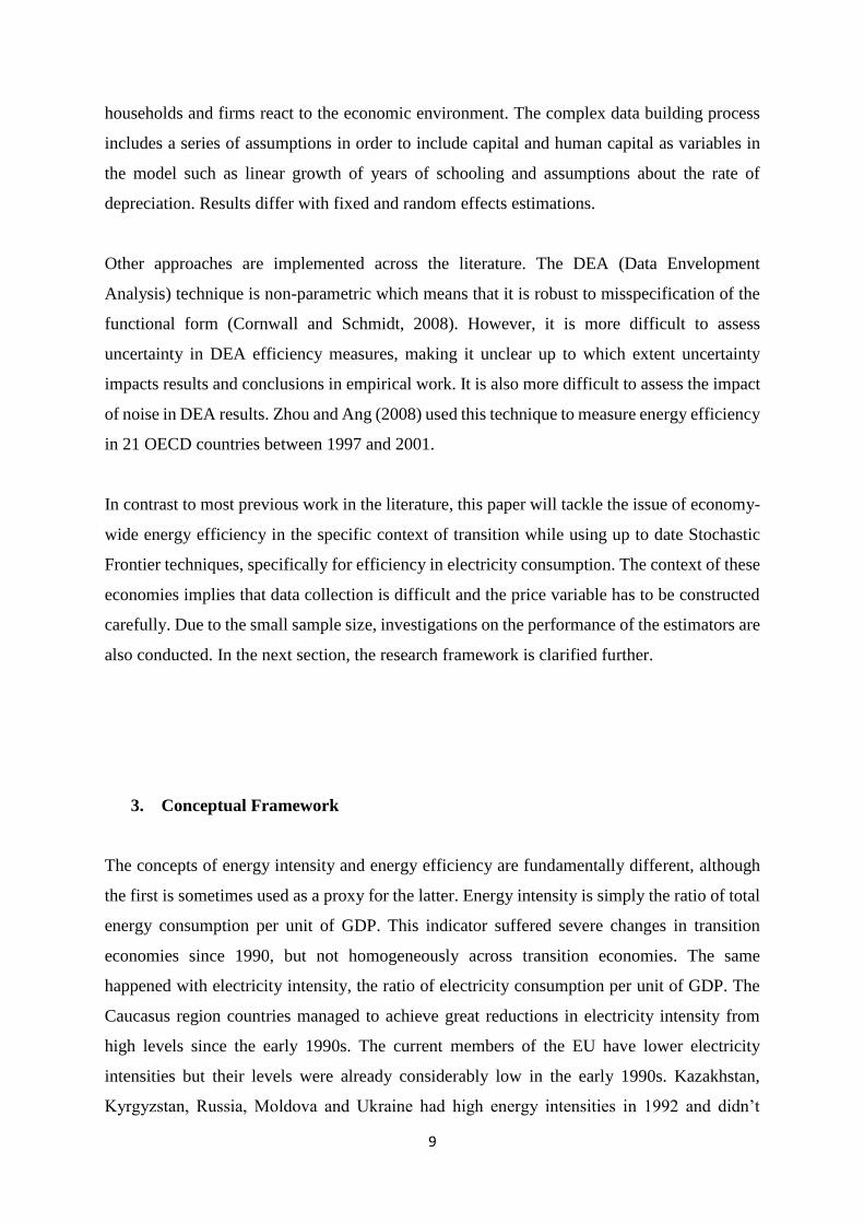
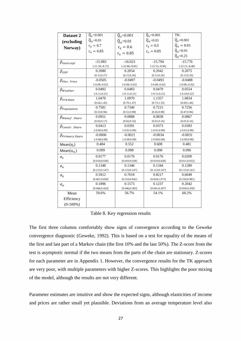
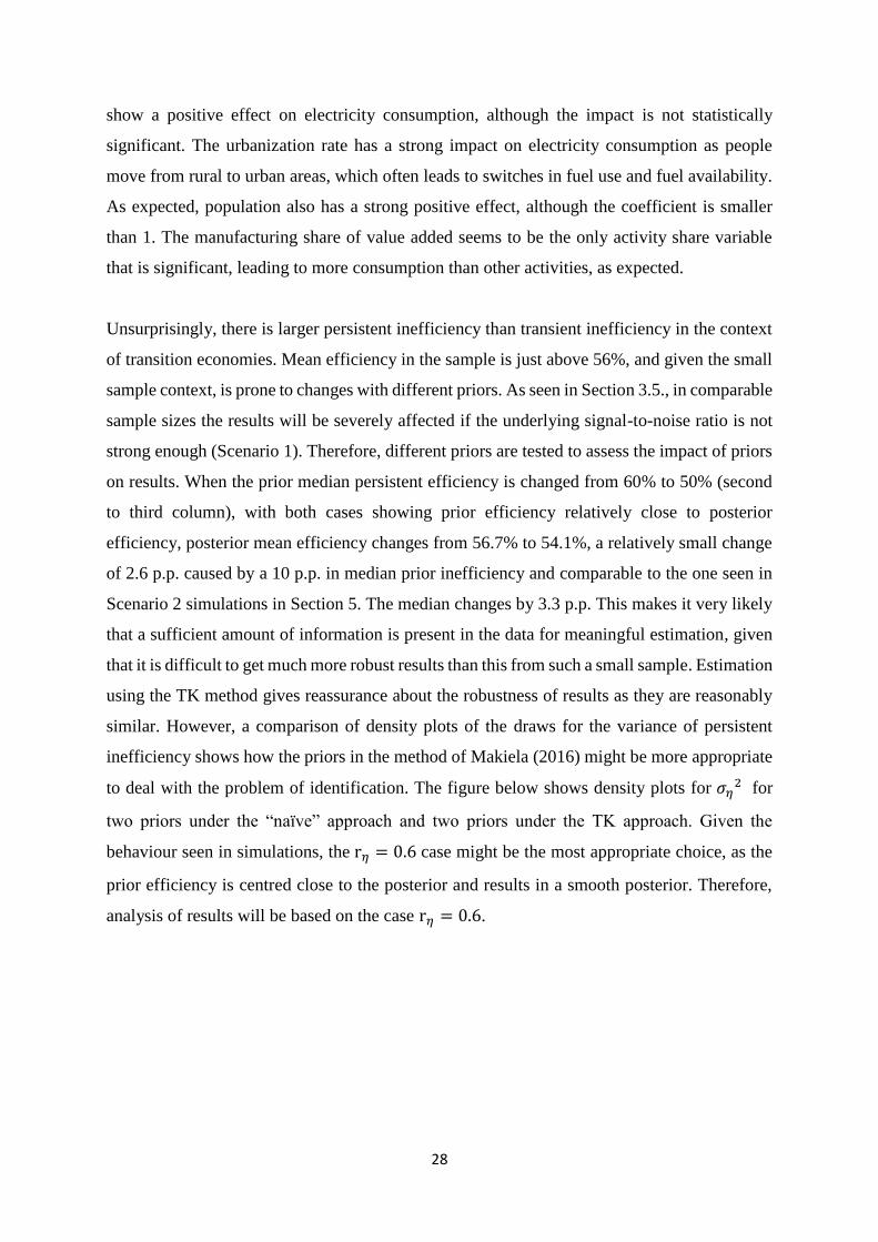
similar. However, a comparison of density plots of the draws for the variance of persistent

inefficiency shows how the priors in the method of Makiela (2016) might be more appropriate

to deal with the problem of identification. The figure below shows density plots for 𝜎𝜂2 for

two priors under the “naïve” approach and two priors under the TK approach. Given the

behaviour seen in simulations, the r𝜂 = 0.6 case might be the most appropriate choice, as the

prior efficiency is centred close to the posterior and results in a smooth posterior. Therefore,

analysis of results will be based on the case r𝜂 = 0.6.

29

Figure 3.2. Posterior densities of 𝜎𝜂2 under different priors and approaches. r𝜂 = 0.7 (black),

r𝜂 = 0.6 (blue) , Q𝜂=0.1 (green), Q𝜂=0.25 (red).

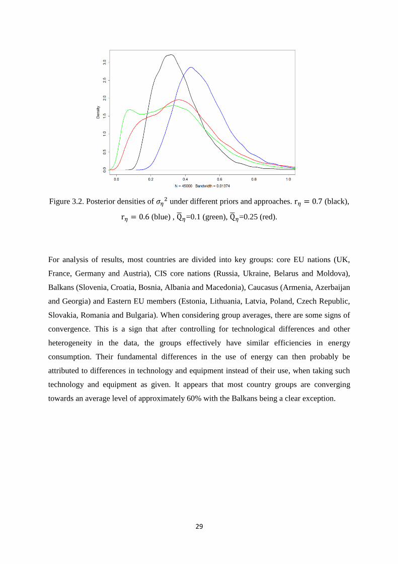
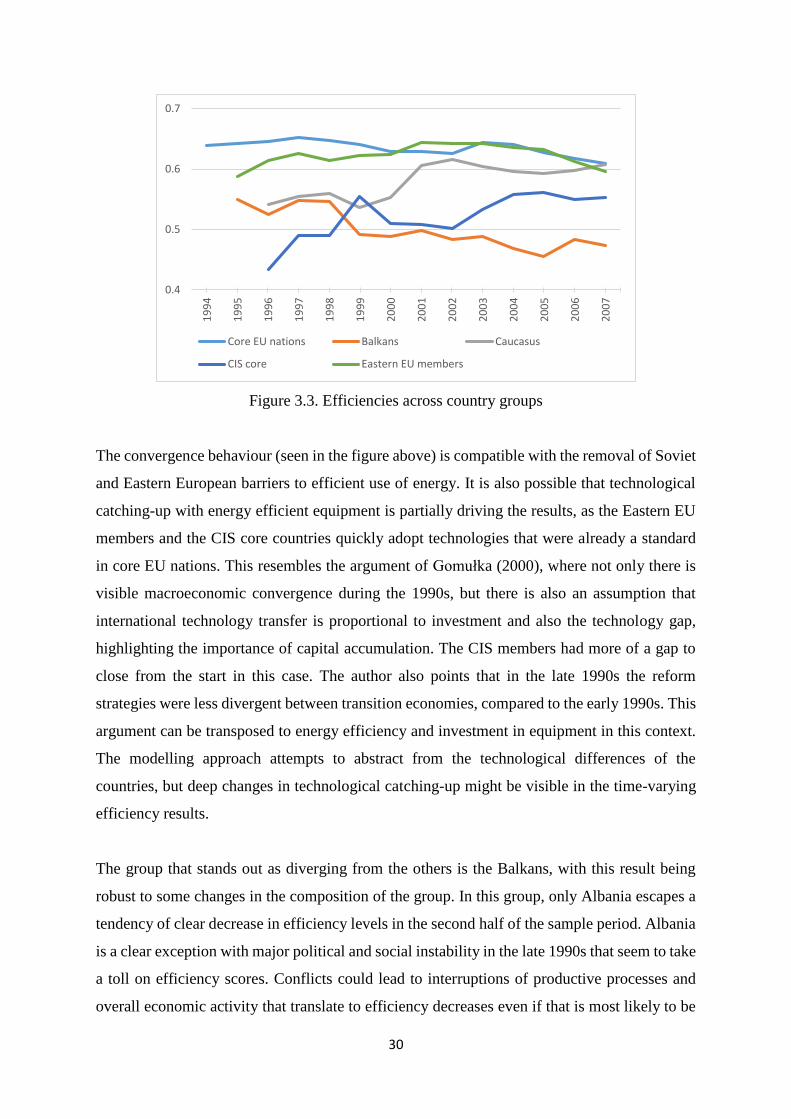
For analysis of results, most countries are divided into key groups: core EU nations (UK,

France, Germany and Austria), CIS core nations (Russia, Ukraine, Belarus and Moldova),

Balkans (Slovenia, Croatia, Bosnia, Albania and Macedonia), Caucasus (Armenia, Azerbaijan

and Georgia) and Eastern EU members (Estonia, Lithuania, Latvia, Poland, Czech Republic,

Slovakia, Romania and Bulgaria). When considering group averages, there are some signs of

convergence. This is a sign that after controlling for technological differences and other

heterogeneity in the data, the groups effectively have similar efficiencies in energy

consumption. Their fundamental differences in the use of energy can then probably be

attributed to differences in technology and equipment instead of their use, when taking such

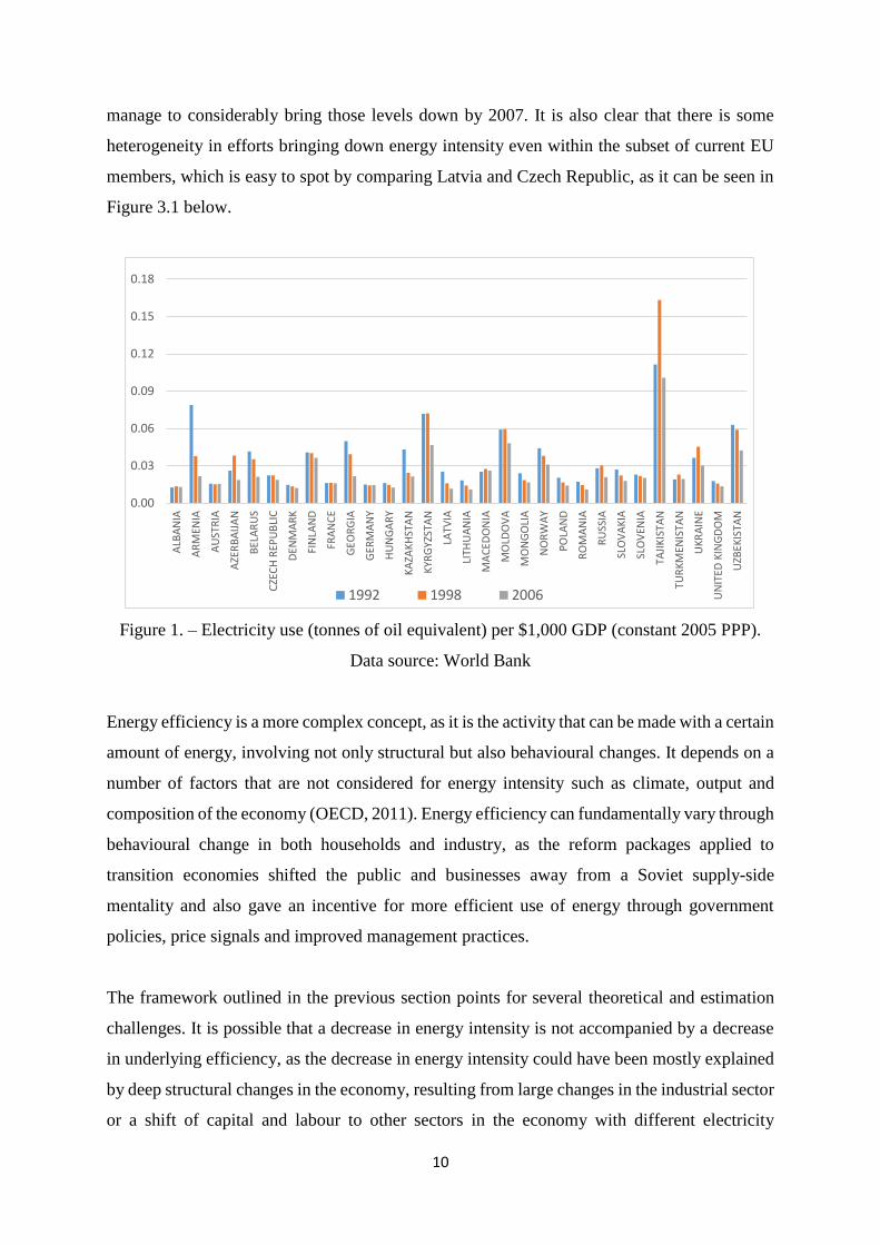
technology and equipment as given. It appears that most country groups are converging

towards an average level of approximately 60% with the Balkans being a clear exception.

30

Figure 3.3. Efficiencies across country groups

The convergence behaviour (seen in the figure above) is compatible with the removal of Soviet

and Eastern European barriers to efficient use of energy. It is also possible that technological

catching-up with energy efficient equipment is partially driving the results, as the Eastern EU

members and the CIS core countries quickly adopt technologies that were already a standard

in core EU nations. This resembles the argument of Gomułka (2000), where not only there is

visible macroeconomic convergence during the 1990s, but there is also an assumption that

international technology transfer is proportional to investment and also the technology gap,

highlighting the importance of capital accumulation. The CIS members had more of a gap to

close from the start in this case. The author also points that in the late 1990s the reform

strategies were less divergent between transition economies, compared to the early 1990s. This

argument can be transposed to energy efficiency and investment in equipment in this context.

The modelling approach attempts to abstract from the technological differences of the

countries, but deep changes in technological catching-up might be visible in the time-varying

efficiency results.

The group that stands out as diverging from the others is the Balkans, with this result being

robust to some changes in the composition of the group. In this group, only Albania escapes a

tendency of clear decrease in efficiency levels in the second half of the sample period. Albania

is a clear exception with major political and social instability in the late 1990s that seem to take

a toll on efficiency scores. Conflicts could lead to interruptions of productive processes and

overall economic activity that translate to efficiency decreases even if that is most likely to be

0.4

0.5

0.6

0.7

19

94

19

95

19

96

19

97

19

98

19

99

20

00

20

01

20

02

20

03

20

04

20

05

20

06

20

07

Core EU nations Balkans Caucasus

CIS core Eastern EU members

31

an artefact due to large decreases in GDP – which can be naturally associated to energy

consumption not translating to output in general. The Balkans countries have not experienced

significant changes in gas supply availability or relative use of natural gas as a fuel over the

sample period. However, this region of Europe is partially dependent on local coal fired

generation for electricity, which is a highly pollutant fuel, but also relatively cheap to obtain

locally. In some countries of the region the national electricity company also has a significant

role in coal mining, and the mining/generation/distribution industries are deeply interlinked.

When considering other fuel availability as well, this region is mostly self-sufficient in terms

of energy consumption. The political and social paradigm of the Balkans differs in multiple

ways of the one in Eastern Europe or the CIS, as there was already a significant private sector

role in the 1990s. It is likely that this region has failed to capitalize as much in terms of

efficiency gains as others in the sample, although the starting point was relatively comparable

to other economies in the mid-1990s.

There are three further groups of countries not displayed in the figure. Kazakhstan and

Kyrgyzstan, who display very volatile and low efficiency scores (average of 0.369), the Far

East CIS group, and Scandinavia. Regarding Far East CIS (Uzbekistan, Tajikistan and

Turkmenistan), this group highlights some of the issues that can arise when fitting stochastic

frontier models in this context. Although Uzbekistan and Tajikistan are some of the most

inefficient countries in the sample as expected, Turkmenistan is the fourth most efficient

country in the sample. This is probably driven by factors other than true underlying efficiency,

such as the abundant and virtually free gas supply which feeds industry and households and

extremely low electricity consumption, although the population access to electricity is close to

100%. Given that electricity consumption per capita is comparable to other countries in the

region and other countries in the sample, this points that there is likely to be much more

inefficiency in gas consumption than in electricity consumption, although an investigation on

such a claim falls out of the scope of this paper.

One of the most noticeable decrease in efficiency throughout the sample is the case of Armenia,

with a drop around 11% mostly concentrated in the last few years of the sample. This happens

at a time of a large construction boom in the country that finds no parallel in the sample –

however, the inclusion of construction shares in the model does not give rise to any strong

significance.

32

Some complications arise when discussing this partial convergence behaviour. There is

possibly some measurement error measurement in some variables, for example in electricity

prices and 1990s macroeconomic variables for poorer countries, although the results that are

obtained are mostly intuitive. Another issue is that the size of the shadow economy in many of

these countries is rather large (Schneider et al., 2010). The underestimation of GDP that varies

across time and across countries could possibly lead to a situation where efficiency results are

distorted by levels and changes in the shadow economy, as that shadow economic activity can

also consume some electricity. However, this theory is somewhat in conflict with the obtained

results. One of the most inefficient country in the sample (Uzbekistan) was one of the countries

in the Former Soviet Union with the smallest shadow economy throughout the 1990’s

(Schneider, 2002). On the other hand, for the example of Hungary, both aforementioned studies

show rather low levels of shadow economy but the economy appears to be quite efficient in

energy consumption. There is no clear correlation between shadow economy sizes and levels

of efficiency and there is no empirical argument supporting that this is distorting results.

Regarding changes throughout time, there are also some further examples to support this

perspective. Poland, for example, sees some rather consistent efficiency gains in periods where

the shadow economy appears to be stabilized or even increasing. Croatia’s level of shadow

economy probably peaked around the year of 2000 but the decrease in efficiency levels is very

consistent throughout time and does not follow the pattern of the size of the shadow economy.

Countries where reform efforts were shy still present efficiency scores that are lower than other

countries in general. One example of that is Uzbekistan, an economy that didn’t make as much

progress as others and remains with very low scores for economic reforms according to the

EBRD. The economy is still focused in agriculture and commodities and large obstacles to

foreign investment and currency convertibility exist, with corruption looming and a clearly

slow paced and gradualist approach towards any economic reform. The efficiency scores for

this country are quite volatile but consistently low.

Another possible issue to consider is a correlation between efficiency scores and fuel

availabilities. If an economy has abundant or cheap gas supply, that might influence electricity

consumption. In the 33 countries considered in the sample, the correlation between individual

efficiency scores and the percentage of electricity consumption in total energy consumption (in

ktoe) varies greatly. 11 of the correlations are positive, with only 10 of the remaining 22

between -0.5 and -1. Although a strong negative correlation might imply that results are being

33

driven by substitution of fuels and fuel availability, these results give little supporting evidence,

even if the overall correlation of the two vectors for the entire sample is -0.497. A possibly

more accurate diagnostic is the correlation between efficiency scores and the share of natural

gas in total energy consumption, with a large positive correlation showing potential problems

(fuel substitution arising as efficiency in consumption of another fuel). This substitution is

more likely than others using fuels such as oil or biomass. However, this overall correlation is

only 0.105, giving no evidence of any serious problems of distorted results. The correlation

between efficiency scores and the relative ratio between electricity consumption and gas

consumption is -0.02.

Possible endogeneity issues might require further work in the future in the stochastic frontier

literature. Mutter et al. (2013) point that it is also important to consider if the endogeneity is

present in the idiosyncratic error or in the inefficiency, and finds that the latter case is much

more dangerous, while endogeneity in the idiosyncratic error does not affect efficiency results

as much. In this case, it would be hard to solve a possible endogeneity issue (i.e. finding and

using appropriate instruments) but preliminary regressions with true random effects approach

(not accounting for inefficiency) do not show the significance of lags of prices or GDP. Tran

and Tsionas (2013) present an alternative for estimation of a simple stochastic frontier model

with GMM and endogenous regressors. A clear restriction from the parametric stochastic

frontier estimation is that a functional form has to be imposed to the cost equation, and it often

has to be a simple form to allow for estimation. More accurate results could in theory be

achieved with a more complex functional form for the cost function, but the number of

parameters in the model is high for such a small sample.

Another important issue worth mentioning is that this frontier concept is closely related to the

concept of the rebound effect. The price reduction that results from a unit cost decrease in

energy services due to increased efficiency can lead to increased consumption, which can

partially offset the savings. Therefore, as Orea et al. (2014) point out, the elasticity of demand

for energy with respect to changes in this energy efficiency measure in this context provides a

direct measure of the rebound effect. The model estimated in this paper implicitly imposes the

restriction of a zero rebound effect, which according to the evidence from past research from

other regions is possibly too restrictive. The issue of rebound effects in transition economies is

not well studied at the moment, so prospective size estimates are unclear. While theory would

point that in least developed countries the unmet demand for energy services could increase

34

the rebound effect, the tight budget constraint that was experienced in transition economies

could lead to this budget relaxation being directed towards increased spending in other goods

and services, which would counter the increase of the effect. It is possible that the first effect

overrides the latter, and the rebound effect is slightly larger on transition economies than in

developed economies, according to evidence from developing countries. While it is true that

the rebound effect might have an important effect which is implicitly ignored in the chosen

estimation procedure, there is also a very large trade-off in choosing another approach to

account for this issue. Since the problem of assuming an elasticity of energy savings with

respect to changes in energy efficiency of -1 affects changes in efficiency, persistent

inefficiency should not be affected by this discussion. One can speculate that in the presence

of a strong rebound effect the convergence effect will be attenuated, leading to some difference

between CIS and OECD countries, for example. That effect should be loosely proportional to

the size of the rebound effect. This can be a topic of future research.

7. Conclusions

This paper presents a methodology to estimate underlying efficiency in electricity consumption

in the context of transition economies after the fall of the Soviet Union, between 1994 and

2007. This methodology focuses on measuring efficiency after accounting for multiple factors

such as economic activity by sector, climate, electricity prices and population. Estimation is

conducted using the Stochastic Frontier GTRE model, which is mostly unexplored in energy

economics applications, even if it displays a diverse literature on technical and estimation

aspects. The Bayesian approach of Makiela (2016) is preferred for analysis of results after a

comparison with an alternative reparameterization method, with additional investigations on

the small sample performance of this model, given the nature of the sample in this context.

Some large differences in efficient use of electricity are found mostly in groups of economies

where market economy reforms were not thoroughly conducted. Convergence behaviour is

apparent between western economies and most transition country groups, with the exception

of the Balkans and countries in the Far East. The importance of the measurement of persistent

inefficiency is particularly strong in the results. The results and their analysis are an important

contribution to the energy efficiency and applied econometrics literature as there is no other

35

significant work in the application of the Bayesian GTRE approach, the region of study and

the discussion of the issues around the estimation of the efficiency measures.

The paper also highlights some of the difficulties and challenges surrounding cost frontier

estimation in an energy demand framework and the trade-off between complex modelling and

tractability. Large uncertainty around estimates leads to a discussion of group averages rather

than a detailed discussion on individual efficiency scores and country rankings. On average,

this average inefficiency level stayed mostly stable through the time frame of this study. The

model clearly distinguishes some countries with a low level of market reforms, such as

Tajikistan and Uzbekistan, as lagging behind in terms of efficiency and containing large

persistent inefficiency which is compatible with the Soviet legacy and its implications, even

after controlling for unobserved heterogeneity.

36

REFERENCES

Aigner, D., Lovell, C.K., Schmidt, P., 1977. Formulation and estimation of stochastic frontier

production function models. Journal of Econometrics 6, 21–37.

Badunenko, O., Kumbhakar, S.C., 2016. When, where and how to estimate persistent and

transient efficiency in stochastic frontier panel data models. European Journal of

Operational Research 255, 272–287. doi:10.1016/j.ejor.2016.04.049

Colombi, R., Martini, G., Vittadini, G., 2011. A stochastic frontier model with short-run and

long-run inefficiency random effects, Department of Economics and Technology

Management. Universita Di Bergamo, Italy.

Cooper, R., Schipper, L., 1992. The efficiency of energy use in the USSR —an international

perspective. Energy 17, 1–24. doi:10.1016/0360-5442(92)90029-Y

Cornillie, J., Fankhauser, S., 2004. The energy intensity of transition countries. Energy

Economics 26, 283–295. doi:10.1016/j.eneco.2004.04.015

Ding, W., Sherif, K., 1997. Bosnia and Herzegovina: From recovery to sustainable growth.,

Country Studies. The World Bank.

Energy Regulatory Authority of Mongolia, 2010. Framework for setting energy tariffs and

prices in Mongolia, and its potential improvement in the future [WWW Document].

URL http://www.carecprogram.org/uploads/events/2010/ESCC-Jul/ESCC1-Setting-

Energy-Tariffs-and-Prices.pdf

Ericson, R.E., 1991. The Classical Soviet-Type Economy: Nature of the System and

Implications for Reform. Journal of Economic Perspectives 5, 11–27.

doi:10.1257/jep.5.4.11

Farsi, M., Filippini, M., Kuenzle, M., 2005. Unobserved heterogeneity in stochastic cost

frontier models: an application to Swiss nursing homes. Applied Economics 37, 2127–

2141. doi:10.1080/00036840500293201

Filippini, M., Greene, W., 2016. Persistent and transient productive inefficiency: a maximum

simulated likelihood approach. Journal of Productivity Analysis 45, 187–196.

doi:10.1007/s11123-015-0446-y

37

Filippini, M., Greene, W., Masiero, G., 2016. Persistent and transient productive inefficiency

in a regulated industry: electricity distribution in New Zealand, IdEP Economic Papers.

USI Università della Svizzera italiana, Faculty of Economics.

Filippini, M., Hunt, L.C., 2012. US residential energy demand and energy efficiency: A

stochastic demand frontier approach. Energy Economics 34, 1484–1491.

doi:10.1016/j.eneco.2012.06.013

Filippini, M., Hunt, L.C., 2011. Energy Demand and Energy Efficiency in the OECD

Countries: A Stochastic Demand Frontier Approach. The Energy Journal 32.

doi:10.5547/ISSN0195-6574-EJ-Vol32-No2-3

Gately, D., Huntington, H.G., 2002. The Asymmetric Effects of Changes in Price and Income

on Energy and Oil Demand. The Energy Journal 23. doi:10.5547/ISSN0195-6574-EJ-

Vol23-No1-2

Geweke, J., 1992. Evaluating the accuracy of sampling-based approaches to calculating

posterior moments. Bayesian Statistics 4, 169–173.

Gilks, W.R., Wild, P., 1992. Adaptive Rejection Sampling for Gibbs Sampling. Applied

Statistics 41, 337. doi:10.2307/2347565

Gomułka, S., 2000. Macroeconomics policies and achievements in transition economies, 1989

- 1999, Discussion paper / Centre for Economic Performance. Centre for Economic

Performance, London School of Economics and Political Science, London.

Greene, W., 2005. Reconsidering heterogeneity in panel data estimators of the stochastic

frontier model. Journal of Econometrics 126, 269–303.

doi:10.1016/j.jeconom.2004.05.003

Griffiths, W.E., Hajargasht, G., 2016. Some models for stochastic frontiers with endogeneity.

Journal of Econometrics 190, 341–348. doi:10.1016/j.jeconom.2015.06.012

Horrace, W.C., Schmidt, P., 1996. Confidence statements for efficiency estimates from

stochastic frontier models. Journal of Productivity Analysis 7, 257–282.

doi:10.1007/BF00157044

International Energy Agency, 2014. World Energy Balances (Edition: 2014).

doi:10.5257/iea/web/2014

38

International Energy Agency, 1994. Feed-in tariffs for renewable energy [WWW Document].

URL http://www.iea.org/policiesandmeasures/pams/belarus/name-24342-en.php

Karabaev, F., 2005. Vertical unbundling. Presented at the First Annual Meeting of CAREC

Members Electricity Regulators Forum (CMERF), 4-6 July 2005, Beijing, People’s

Republic of China.

Kennedy, D., 2003. Power sector regulatory reform in transition economies: Progress and

lessons learned, Working Paper No. 78. European Bank for Reconstruction and

Development, London, UK.

Krishnaswamy, V., 1999. Non-payment in the electricity sector in Eastern Europe and the

Former Soviet Union, World Bank technical paper ; no. WTP 423. Washington, D.C. :

The World Bank.

Kumbhakar, S.C., Lovell, C.A.K., 2004. Stochastic frontier analysis, 1. paperback ed.,

transferred to digital printing. ed. Cambridge Univ. Press, Cambridge.

Lambert, P.C., Sutton, A.J., Burton, P.R., Abrams, K.R., Jones, D.R., 2005. How vague is

vague? A simulation study of the impact of the use of vague prior distributions in

MCMC using WinBUGS. Statistics in Medicine 24, 2401–2428. doi:10.1002/sim.2112

Makiela, K., 2016. Bayesian inference in generalized true random-effects model and Gibbs

sampling, MPRA Paper No. 70422.

Markandya, A., Pedroso-Galinato, S., Streimikiene, D., 2006. Energy intensity in transition

economies: Is there convergence towards the EU average? Energy Economics 28, 121–

145. doi:10.1016/j.eneco.2005.10.005

Martinot, E., 1998. Energy efficiency and renewable energy in Russia. Energy Policy 26, 905–

915. doi:10.1016/S0301-4215(98)00022-6

Meeusen, W., van Den Broeck, J., 1977. Efficiency Estimation from Cobb-Douglas Production

Functions with Composed Error. International Economic Review 18, 435.

doi:10.2307/2525757

Mundlak, Y., 1978. On the Pooling of Time Series and Cross Section Data. Econometrica 46,

69. doi:10.2307/1913646

Mutter, R.L., Greene, W.H., Spector, W., Rosko, M.D., Mukamel, D.B., 2013. Investigating

the impact of endogeneity on inefficiency estimates in the application of stochastic

39

frontier analysis to nursing homes. Journal of Productivity Analysis 39, 101–110.

doi:10.1007/s11123-012-0277-z

Nepal, R., Jamasb, T., Tisdell, C.A., 2014. Market-related reforms and increased energy

efficiency in transition countries: empirical evidence. Applied Economics 46, 4125–

4136. doi:10.1080/00036846.2014.952894

OECD, 2011. OECD Factbook 2011-2012, OECD Factbook. OECD Publishing.

Orea, L., Llorca, M., Filippini, M., 2014. Measuring energy efficiency and rebound effects

using a stochastic demand frontier approach: the US residential energy demand,

Efficiency Series Paper 01/2014. Oviedo Efficiency Group, Department of Economics,

University of Oviedo, Oviedo, Spain.

Petri, M., Taube, G., Tsyvinski, A., 2002. Energy Sector Quasi-Fiscal Activities in the

Countries of the Former Soviet Union. IMF Working Paper 1–34.

Schneider, F., 2002. The Size and Development of the Shadow Economies of 22 Transition

and 21 OECD Countries, Discussion Paper No. 514. Institute for the Study of Labor

(IZA), Bonn, Germany.

Schneider, F., Buehn, A., Montenegro, C.E., 2010. New Estimates for the Shadow Economies

all over the World. International Economic Journal 24, 443–461.

doi:10.1080/10168737.2010.525974

Stern, D.I., 2012. Modeling international trends in energy efficiency. Energy Economics 34,

2200–2208. doi:10.1016/j.eneco.2012.03.009

Tran, K.C., Tsionas, E.G., 2013. GMM estimation of stochastic frontier model with

endogenous regressors. Economics Letters 118, 233–236.

doi:10.1016/j.econlet.2012.10.028

Tsionas, E.G., Kumbhakar, S.C., 2014. Firm heterogeneity, persistent and transient technical

inefficiency: A generalized true random-effects model. Journal of Applied

Econometrics 29, 110–132. doi:10.1002/jae.2300

Willmott, C.J., Matsuura, K., 2001. Terrestrial Air Temperature and Precipitation: Monthly

and Annual Time Series (1950 - 1999) [WWW Document]. URL

http://climate.geog.udel.edu/~climate/html_pages/README.ghcn_ts2.html

40

Zhou, P., Ang, B.W., 2008. Linear programming models for measuring economy-wide energy

efficiency performance. Energy Policy 36, 2911–2916.

doi:10.1016/j.enpol.2008.03.041

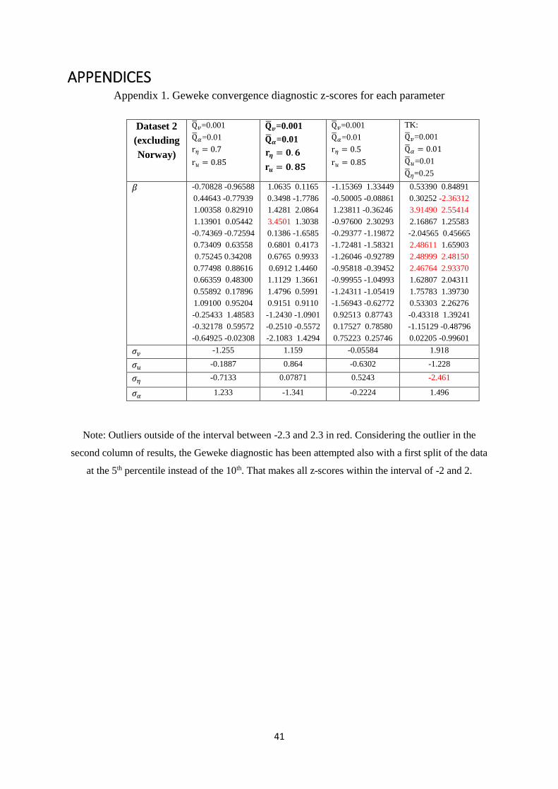
41

APPENDICES Appendix 1. Geweke convergence diagnostic z-scores for each parameter

Note: Outliers outside of the interval between -2.3 and 2.3 in red. Considering the outlier in the

second column of results, the Geweke diagnostic has been attempted also with a first split of the data

at the 5th percentile instead of the 10th. That makes all z-scores within the interval of -2 and 2.

Dataset 2

(excluding

Norway)

Q𝑣=0.001

Q𝛼=0.01

r𝜂 = 0.7

r𝑢 = 0.85

��𝒗=0.001

��𝜶=0.01

𝐫𝜼 = 𝟎. 𝟔

𝐫𝒖 = 𝟎. 𝟖𝟓

Q𝑣=0.001

Q𝛼=0.01

r𝜂 = 0.5

r𝑢 = 0.85

TK:

Q𝑣=0.001

Q𝛼 = 0.01

Q𝑢=0.01

Q𝜂=0.25

𝛽 -0.70828 -0.96588

0.44643 -0.77939

1.00358 0.82910

1.13901 0.05442

-0.74369 -0.72594

0.73409 0.63558

0.75245 0.34208

0.77498 0.88616

0.66359 0.48300

0.55892 0.17896

1.09100 0.95204

-0.25433 1.48583

-0.32178 0.59572

-0.64925 -0.02308

1.0635 0.1165

0.3498 -1.7786

1.4281 2.0864

3.4501 1.3038

0.1386 -1.6585

0.6801 0.4173

0.6765 0.9933

0.6912 1.4460

1.1129 1.3661

1.4796 0.5991

0.9151 0.9110

-1.2430 -1.0901

-0.2510 -0.5572

-2.1083 1.4294

-1.15369 1.33449

-0.50005 -0.08861

1.23811 -0.36246

-0.97600 2.30293

-0.29377 -1.19872

-1.72481 -1.58321

-1.26046 -0.92789

-0.95818 -0.39452

-0.99955 -1.04993

-1.24311 -1.05419

-1.56943 -0.62772

0.92513 0.87743

0.17527 0.78580

0.75223 0.25746

0.53390 0.84891

0.30252 -2.36312

3.91490 2.55414

2.16867 1.25583

-2.04565 0.45665

2.48611 1.65903

2.48999 2.48150

2.46764 2.93370

1.62807 2.04311

1.75783 1.39730

0.53303 2.26276

-0.43318 1.39241

-1.15129 -0.48796

0.02205 -0.99601

𝜎𝑣 -1.255 1.159 -0.05584 1.918

𝜎𝑢 -0.1887 0.864 -0.6302 -1.228

𝜎𝜂 -0.7133 0.07871 0.5243 -2.461

𝜎𝛼 1.233 -1.341 -0.2224 1.496

42

Appendix 2. Results with the inclusion of Norway in the sample

Dataset 1

(including

Norway)

��𝒗=0.001

��𝜶=0.01

𝐫𝜼 = 𝟎. 𝟔

𝐫𝒖 = 𝟎. 𝟖𝟓

𝛽𝐼𝑛𝑡𝑒𝑟𝑐𝑒𝑝𝑡 -18.840

[-26.69;-12.27]

𝛽𝐺𝐷𝑃 0.2138

[0.16;0.27]

𝛽𝐸𝑙𝑒𝑐. 𝑃𝑟𝑖𝑐𝑒 -0.0578

[-0.09;-0.03]

𝛽𝑊𝑒𝑎𝑡ℎ𝑒𝑟 0.0767

[-0.08;0.23]

𝛽𝑈𝑟𝑏.𝑅𝑎𝑡𝑒 0.9978

[0.61;1.36]

𝛽𝑃𝑜𝑝𝑢𝑙𝑎𝑡𝑖𝑜𝑛 0.6435

[0.34;0.89]

𝛽𝑀𝑎𝑛𝑢𝑓. 𝑆ℎ𝑎𝑟𝑒 0.1062

[0.04;0.18]

𝛽𝐶𝑜𝑛𝑠𝑡𝑟. 𝑆ℎ𝑎𝑟𝑒 0.0390

[-0.00;0.08]

𝛽𝑃𝑟𝑖𝑚𝑎𝑟𝑦 𝑆ℎ𝑎𝑟𝑒 -0.0042

[-0.09;0.08]

Mean(𝜂𝑖) 0.601

Mean(𝑢𝑖𝑡) 0.098

𝜎𝑣 0.0172

[0.010;0.027]

𝜎𝑢 0.1339

[0.122;0.146]

𝜎𝜂 0.7495

[0.537;1.037]

𝜎𝛼 0.1659

[0.043;0.407]

Mean

Efficiency

(0-100%)

54.3%