Embed Size (px)
Citation preview
ENERGY-BASED
BINAURAL ACOUSTIC MODELING
Natalie Agus, Hans, Anderson, Jer-Ming Chen, and Simon Lui
Singapore University of Technology and Design
Information Systems Technology and Design
Technical Report Number: 000001
11 April 2017
1
ABSTRACT
In human auditory perception of space, the early part of the reverberation impulse response is more percep-
tually relevant than the later part. This observation has inspired many efficient hybrid acoustic modeling
approaches where the early reflections are modeled in detail and late reflections are generated by efficient
structures that produce a rough approximation. Many existing methods simplify the computation by us-
ing a late reverb unit that doesn’t vary its energy level according to a physical model. This results in an
incorrect balance of energy between the early reflections and late reverb. In this technical report we show
how the late reverb energy can be estimated during the processing of the early reflections model. We apply
that method in geometrical modeling method that uses the Acoustic Rendering Equation [1] to produce a
binaural acoustic simulation. We use a single Feedback Delay Network that simultaneously produces both
precise early reflections and approximate late reverb. With the addition of a delay line with a small number
of taps, we achieve a correct balance of early and late energy. This report also clarifies key concepts related
to the use of the Acoustic Rendering Equation (ARE) and associates all the quantities in the model to
physical units of measurement.
2

Contents
1 NOTATION AND SYMBOLS 5
2 INTRODUCTION 7
2.1 Numerical Acoustics . . . . . . . . . . . . . . . . . . . . . . . . . . . . . . . . . . . . . . . . . 7
2.2 Geometric Acoustics . . . . . . . . . . . . . . . . . . . . . . . . . . . . . . . . . . . . . . . . . 7
2.3 Geometric Acoustics for Reverberation Structures . . . . . . . . . . . . . . . . . . . . . . . . . 8
2.3.1 Parts of Impulse Response . . . . . . . . . . . . . . . . . . . . . . . . . . . . . . . . . . 8
2.3.2 Geometrical Acoustics for Algorithmic Reverb With Convolution . . . . . . . . . . . . 9
2.3.3 Geometrical Acoustics for Algorithmic Reverb Without Convolution . . . . . . . . . . 11
2.4 Motivation . . . . . . . . . . . . . . . . . . . . . . . . . . . . . . . . . . . . . . . . . . . . . . 12
3 THEORETICAL FOUNDATION 13
3.1 Definitions: Intensity, Pressure, and Flux . . . . . . . . . . . . . . . . . . . . . . . . . . . . . 13
3.2 Physical Significance of the Audio Input . . . . . . . . . . . . . . . . . . . . . . . . . . . . . . 14
3.3 Physical Significance of the Signals Inside the FDN . . . . . . . . . . . . . . . . . . . . . . . . 15
3.4 Physical Significance of the Audio Output . . . . . . . . . . . . . . . . . . . . . . . . . . . . . 17
3.5 Definition of Radiance . . . . . . . . . . . . . . . . . . . . . . . . . . . . . . . . . . . . . . . . 17
3.6 The Acoustic Rendering Equation . . . . . . . . . . . . . . . . . . . . . . . . . . . . . . . . . 19
3.7 The Reflection Kernel . . . . . . . . . . . . . . . . . . . . . . . . . . . . . . . . . . . . . . . . 19
4 REVERBERATION STRUCTURE OVERVIEW 21
4.1 Direct Rays . . . . . . . . . . . . . . . . . . . . . . . . . . . . . . . . . . . . . . . . . . . . . . 23
4.2 First Order Reflections . . . . . . . . . . . . . . . . . . . . . . . . . . . . . . . . . . . . . . . . 23
4.3 Second and Higher Order Reflections . . . . . . . . . . . . . . . . . . . . . . . . . . . . . . . . 23
5 METHOD 25
5.1 Azimuth Quantisation, HRTF, and Inter-aural Time Delay . . . . . . . . . . . . . . . . . . . 25
5.2 The Mixing Matrix and Delay Lines . . . . . . . . . . . . . . . . . . . . . . . . . . . . . . . . 25
5.3 Reverberation Time . . . . . . . . . . . . . . . . . . . . . . . . . . . . . . . . . . . . . . . . . 26
5.4 Input and Output Gains . . . . . . . . . . . . . . . . . . . . . . . . . . . . . . . . . . . . . . . 27
5.4.1 Our Use of the ARE . . . . . . . . . . . . . . . . . . . . . . . . . . . . . . . . . . . . . 27
5.4.2 The Point Collection Function . . . . . . . . . . . . . . . . . . . . . . . . . . . . . . . 29
3

5.4.3 Irradiance . . . . . . . . . . . . . . . . . . . . . . . . . . . . . . . . . . . . . . . . . . . 29
5.4.4 Collecting Irradiance at the Listener Location . . . . . . . . . . . . . . . . . . . . . . . 29
5.4.5 Calculation of Higher Order Reflected Radiance . . . . . . . . . . . . . . . . . . . . . . 30
5.4.6 Calculating the Output Gain Coefficients . . . . . . . . . . . . . . . . . . . . . . . . . 33
5.4.7 Calculating the Input Gain Coefficients . . . . . . . . . . . . . . . . . . . . . . . . . . 34
5.4.8 Total Energy Entering the FDN . . . . . . . . . . . . . . . . . . . . . . . . . . . . . . 35
5.5 Direct Rays . . . . . . . . . . . . . . . . . . . . . . . . . . . . . . . . . . . . . . . . . . . . . . 36
6 EVALUATION 38
6.1 BRIR Recording and Simulation . . . . . . . . . . . . . . . . . . . . . . . . . . . . . . . . . . 38
6.2 Objective Evaluation . . . . . . . . . . . . . . . . . . . . . . . . . . . . . . . . . . . . . . . . . 40
6.2.1 Decay Time . . . . . . . . . . . . . . . . . . . . . . . . . . . . . . . . . . . . . . . . . . 40
6.2.2 Balance of Energy Between Early and Late Reflections . . . . . . . . . . . . . . . . . . 41
6.2.3 Spatial Impression . . . . . . . . . . . . . . . . . . . . . . . . . . . . . . . . . . . . . . 41
6.2.4 Performance and Efficiency . . . . . . . . . . . . . . . . . . . . . . . . . . . . . . . . . 43
6.3 Subjective Evaluation . . . . . . . . . . . . . . . . . . . . . . . . . . . . . . . . . . . . . . . . 43
6.3.1 Listening Test Procedure . . . . . . . . . . . . . . . . . . . . . . . . . . . . . . . . . . 43
6.3.2 Test Results . . . . . . . . . . . . . . . . . . . . . . . . . . . . . . . . . . . . . . . . . . 46
7 SUMMARY 48
8 FUTURE WORK 49
9 REFERENCES 50
4
1. NOTATION AND SYMBOLS
Symbol Description
Φ energy flux per unit time
Φ∑ total energy flux of sound source
Φ(Fn) the energy flux output of the nth delay line in the FDN
Φin total energy flux input to the FDN
Φout(An) total energy flux output from the FDN
u,x bold face font indicates that u and x are vectors
Ir radiant intensity (power flux per unit solid angle)
Ia acoustic intensity (power flux per unit surface area)
p acoustic component of pressure
yn output of the nth FDN delay line
dM minimum distance from source or listener to other surfaces
E irradiance, power flux per unit area
G all surface geometry in the room
` radiance, power flux per unit projected area, per unit solid angle
Ω unit solid angle
ω solid angle [steradians]
A unit of surface area
An surface area of patch n
n surface normal vector
c speed of sound
ρ density of sound propagation medium
βn the amount of input gain due to early reflection on the nth delay line
gn gain in the FDN
RT60 reverberation time
υn the amount of output gain due to late reflections on the nth delay line
ξ(u,x) attenuation due to propagation losses in air
V(u,x) visibility function between u and x
g(u,x) the geometry term
Λ[u,x] unit vector pointing from u to x
5

R(Λ[u,x],x,Ω
)reflection kernel that defines reflection from x to an arbitrary direc-
tion Ω from a distant source u
h(x, L) the point collection function, to convert from units of radiance at x
to units of incident energy flux per unit area at L
gp(x, L) geometry term in the point collection function∫4πxdω integration of x by angle over a sphere∫
2πxdω integration of x by angle over a hemisphere on the exterior of a surface
6

2. INTRODUCTION
Computer simulations of reverberant room acoustics have applications in video games, music recording,
research, and movie production. They are also used to render realistic audio-visual scenes for various testing,
training, and rehabilitation exercises. One example is the use of auralization in virtual environments to
investigate the level and impact of aircraft flyover sound [2, 3].
The most accurate way to simulate room acoustics is to convolve a measured binaural room impulse
response (BRIR) with a dry input signal. This transforms a dry signal into a reverberated signal that sounds
as if it were played in the same setting and location where the BRIR was recorded. One disadvantage of this
method is that impossible to record an impulse response for every listener and source location in a room.
Even a moderate subset of all the possible configurations requires Gigabytes of storage [4].
An attractive alternative to recording impulse responses is to simulate them computationally. Methods
for simulating the reverberation in virtual spaces can be classified into two categories, Numerical Acoustics
(NA) and Geometric Acoustics (GA).
2.1. Numerical Acoustics
Numerical Acoustics based approaches use numerical approximation techniques such as Finite Element
Methods, Digital Waveguide Meshes, and Finite Difference Time Domain to solve the wave equation [5, 6, 7].
NA methods model almost all wave phenomena, including specular and diffuse reflection, diffraction, and
scattering. However it requires massive computational power as we need to perform calculation not only in
space but also in frequency domain. Typically, a room will be divided into sections of cubic voxels and the
wave equations for each frequency band will be solved for each voxel. Despite its exact accuracy, in [8], it is
stated that it is yet to be realistic to solve the wave equation for the entire duration of the impulse response.
2.2. Geometric Acoustics
Geometric Acoustics methods assume that sound waves propagate in rectilinear form. Most GA ap-
proaches are comparably faster and more lightweight than NA approaches, but they do not capture the
same extent of detail as NA approaches do. Ray tracing and the Image Source Method (ISM) are the most
commonly used geometric acoustics methods [9]. More complex techniques include Phonon Mapping and
Beam Tracing. Some methods in GA overlap with methods for graphics rendering, such as photon mapping,
shading, and shadowing to account for specular and diffuse reflection. This is due to the assumption that
light and sound rays propagate similarly. However, since sound waves have longer wavelengths, acoustic
7

models of diffraction are necessarily more complicated. Many GA methods ignore diffraction effects for
simplicity.
The choice of an NA or GA approach depends on the target application. NA methods are more commonly
used for applications that require numerical accuracy, such as [2] and [3], or other room modeling softwares
to investigate the effect of sound propagation in a specific settings such as lecture halls or amphitheaters [7].
2.3. Geometric Acoustics for Reverberation Structures
2.3.1. Parts of Impulse Response
Figure 1: A plot of recorded impulse response of 44100 Hz. The initial impulse and the tail are clipped to zoom in the figure.The horizontal axis unit is in terms of samples.
Figure 1 shows a snapshot of a recorded impulse response. A room impulse response may be conceptually
divided into three parts: direct sound, early reflections, and late reverberation [10, 11, 12]. The direct sound
is the sound that reaches the listener without first bouncing off any reflective surface. The distinguishing
factor that sets early reflections apart from late reverb is density in the time domain. Early reflections
usually give way to densely blended late reverb within about 80ms after the direct sound, depending on the
room size [13]. The late reverberation is characterized by densely clustered, low power reflections that have
an exponentially decaying amplitude envelope as shown from figure 1 at 3000th sample onwards. Human ears
do not distinguish the energy of individual reflections during the late reverberation [14]. Localization cues
and other spatial information is mostly conveyed by direct sound and early reflections [8, 15]. However, the
8
very late reflected sound rays, beginning approximately 300ms after the arrival of the directly propagated
impulse, contribute to the listener’s sense of spaciousness in the room [16].
The accuracy of the late reverberation tail is often traded off with computational time, if the intended
application only requires perceptual plausibility. However, the fact that late reverberation also contributes,
to a lesser degree, to our sense of room dimensions and listener location [17] has led some researchers to
develop methods that strive to simulate even the late reverb impulse response in more detail. We can
see in [18] and [19] that attempts are made to model the entire impulse response in greater detail, for
later convolution with the audio input. Due to the exponential complexity of late reverb calculations, it
is computationally infeasible to accurately model individual reflections beyond the 4th order [4]. Therefore
a certain degree of approximation is still necessary to model the late reverberation tail, to prevent the
computational time from growing exponentially. To build an acoustic model that is capable of processing
input audio directly and perform simulation in real time, the accuracy of the reverberation tail must be
sacrificed. This leads to two general types of simulation methods, which is (1) with precomputation of
impulse responses for later convolution and (2) the methods that are able to process the input audio directly.
2.3.2. Geometrical Acoustics for Algorithmic Reverb With Convolution
In some methods, the impulse response is first calculated and later on convolution will be performed with
the audio signal. They typically offer higher physical accuracy than those methods that are able to process
input directly, but at the cost of longer computational time. This is due to the fact that not all of the
methods to synthesize BRIRs are efficient enough to directly process the audio input, especially when high
physical accuracy is required. Many GA methods pre-compute BRIRs for many combinations of listener
and sound source locations and store them for later use in a real-time application. For example, they may
do the acoustic simulation by numerical integration of the scene [7], or by raytracing a computer model of
the room [20]. At run time, the pre-computed BRIRs can be accessed quickly and used for convolution with
the input signal. Since we cannot pre-compute an impulse response for every location, we may interpolate
between BRIRs at neighboring locations [7]. A fast convolution engine combined with double-buffering of
the audio stream enables room modeling with real-time parameter updates[21].
Pre-computation of impulse responses is a viable option only for applications with fixed sound source
locations. If both the sound source and listener move freely, the combined number of possible locations is
an order of magnitude greater than when only the listener is moving. The time required to compute the
impulse responses ranges from several minutes to several hours, depending on the complexity of the method
and the scene [22].
9

Schimmel et. al. used the ISM and diffuse rain algorithm to create a computationally efficient yet
realistic empty ”shoebox” room acoustic simulator [23]. Their technique is able to model both specular and
diffuse reflections simultaneously. It is also comparatively more accurate than other ISM approaches because
the diffuse rain algorithm traces energy rays throughout the virtual environment, producing more than 1
million image sources. This method is highly accurate, but too complex to generate impulse responses in
real time [23, 24].
The following methods generate late reverberation from an acoustic reflection model, rather than using
a filtered version of a generic reverb output [25, 26, 27, 21, 22, 28, 29]. All of these produce BRIRs for
convolution with the input signal and support real time updates only by saving a large library of pre-
computed impulse responses. For instance, [26, 21] and [22] stored extensive beam tracing and ISM results
so that they could render location dependent reverberation effects at run time. The methods in [25, 27] are
standalone auralization programs that produce realistic simulations. They use the ISM for early reflections
and an efficient approximation of ray tracing for late reverberation [25, 27].
The method in [25] allows selective switching between generic artificial reverberation and ray tracing to
allow varying degrees of accuracy in late reverberation. A more computationally exhaustive variant of ray
tracing called the stochastic ray tracing algorithm was used in [27]. In certain instances it can compute
BRIRs fast enough for real time applications without caching a library of pre-computed impulses. In [27],
the authors proposed a framework called RAVEN that can support fast data handling and convolution.
Methods proposed in [26, 21, 22] and [28] use various pre-computed impulse response methods that can
render reverberation effects in video games or other dynamic virtual environments. The methods in [22, 21]
model room acoustics using computer graphics techniques including beam tracing and ray tracing.
Bai proposed the use of acoustic rendering networks (ARN), which was inspired by the acoustic rendering
equation (ARE) and based on the use of a large FDN [29]. Similar to the SDN method, the ARN proposed
by Bai can produce accurate early specular reflections. The ARE is used to calculate the amount of energy
flux that radiates from each discretised reflecting surface going out in various directions. Then, energy-based
ray tracing is used to collect and compute the total amount of energy that reaches the listener. Although
it was shown in [29] that the sound quality of the resulting BRIR is satisfying, it may not be suitable for
applications where efficient real time updates are required. In [29], it is stated that their method needs 16.5s
to render a BRIR for a rectangular shaped room of dimensions 4(W):6(H):4(L).
Regardless of how efficiently we synthesize the impulse response, this type of simulation that requires
convolution may be too computationally intensive for some applications. This is true in some 3d games and
10

virtual reality simulations, where the graphics processing code is designed to consume nearly all available
system resources. In those situations we prefer a room acoustics simulation that gives the user a believable
sense of space and location without taking a significant portion of system resources away from the graphics
thread.
2.3.3. Geometrical Acoustics for Algorithmic Reverb Without Convolution
In this section we discuss methods where the input signal is processed directly rather than first per-
forming pre-computations to produce a BRIR for later convolution. The benefit of doing this is a reduce
in computational time such that real-time processing can be performed, or when in a case where majority
of the resources are not available as they are used to perform other processes. In cases where the room
simulation can be simplified to the extent that directly processing the signal is faster than convolution with
an impulse response, this type of design is more efficient. The most suitable geometric acoustics simulation
methods to support direct input processing is the hybrid approach [30, 31, 32, 33, 34, 35, 36, 37, 38]. This
hybrid approach uses one structure for simulating early reflections and another separate system for doing
the late reverberation. Since the early reflections carry the most important spatial cues, these methods
make a accurate models of the early reflections and use less detailed models for the late reflections. Existing
methods achieve efficient models by simulating only the early reflections in detail. They produce late reverb
using a more generic method that does not respond precisely to room model parameters.
The most efficient methods in the literature use late reflections models that totally ignore the location
and orientation of the listener and sound source [32, 33, 38, 25, 36, 30, 31, 35]. Others ignore the details of
room geometry but use a rough estimate of the room size to determine the density of echoes [33, 37]. They
extend the reverberation time beyond the end of early reflections by mixing the output of a feedback delay
network with the output of the early reverb module. Essentially, these methods replace the late reverb with
a random reflection model. The methods in [30, 31, 33] use the tail end of a reference BRIR to do late
reverb by convolution, filtering the output differently for each ear to produce realistic interaural differences.
De sena et al. [39] used a different type of geometrical approach. It models late reverb in rough
approximation only, taking some aspects of room geometry into account but not modeling late reverb in
great detail. De Sena proposed a method of scattering delay networks (SDN) that is able to exactly produce
first order reflections and progressively make an approximation of higher order reflections. This SDN design
was inspired by the digital waveguide network design in [40]. The network consists of a fully connected mesh
topology, where each node in the network physically represents a scattering junction. For simplicity, they
represented one significant reflecting surface as a single scattering junction in the paper. The advantage of
11
using SDN, compared to using a simple FDN, is that the SDN models reflections between objects in the
room in some detail, rather than simply replacing late reverb with random reflections. This method in [39]
directly processes the anechoic input and can perform in real-time.
2.4. Motivation
One problem with using a generic reverberator to simulate late reflections is that the balance between
the amplitudes of early and late reflections changes depending on the location of the listener and sound
source and on the room geometry. If our late reverb is produced by an FDN that has no significance in our
acoustic model then we have no way of knowing the correct balance between late and early reflected energy.
Methods that consider the balance between late and early reflected energy as discussed in the previous
section, may be computationally to exhaustive to directly produce the input audio. In this report we would
like to approach this problem by deriving a mathematical model, based on the Acoustic Rendering Equation
[1], that accounts for both early and late reflected energy. In the evaluation section of this report we show
that by correcting the energy balance in the model, we can simulate room responses with close perceptual
quality to the recorded response.
12

3. THEORETICAL FOUNDATION
3.1. Definitions: Intensity, Pressure, and Flux
The time-dependent acoustic intensity of the source, Ia, is the power flux that the source projects per
unit area. Acoustic intensity is proportional to the square of acoustic pressure [41],
Ia = np2
ρc, (1)
where n is a unit vector indicating the direction of the energy flux, and ρ and c are the density of the
medium and speed of sound, respectively. Acoustic intensity is defined as a vector quantity so that by
integrating the dot product of acoustic intensity and the surface normal over an area A we find the total
power flux across A [41],
Φ =
∫A
(Ia · n) dA. (2)
We use acoustic intensity to represent the intensity of sound incident on a point receiver. Because the
surface normal of a point receiver is not meaningful, we will assume that the vector n points toward the
listener so that we can work with acoustic intensity as if it were a scalar value. This permits us to use the
following simplified definition,
Ia = p2. (3)
In the simplified definition above, we normalised units from (1) so that ρc = 1. Occasionally, it will be
necessary to recall that acoustic intensity is actually a vector quantity and we will remind the reader when
that time comes.
When working with spherical radiation, it is convenient to measure intensity per unit angle from the
source of radiation, rather than measuring per unit area. We use the symbol Ir to indicate radiant intensity,
the energy flux Φ per unit solid angle Ω, measured in steradians [42],
13

Ir =dΦ
dΩ. (4)
The advantage of measuring radiant intensity per unit angle, rather than per unit area is that in a lossless
medium, the flux per unit angle does not depend on the distance from the source.
By definition, one steradian solid angle on a sphere spans one squared radian of surface area. Therefore,
on the surface of the unit sphere, acoustic intensity and radiant intensity are equal. This is true because
at a distance of one unit from the source, both units measure energy flux per unit area. At a distance of d
units from a point source the relationship between radiant and acoustic intensity is as follows,
Ia =Ird2. (5)
To simplify notation in the following sections, we define Λ[u,x] to be a unit vector pointing in the direction
from u to x,
Λ[u,x] =x− u
‖x− u‖. (6)
3.2. Physical Significance of the Audio Input
At the input of our reverberator is a digital signal that represents a time series measurement of the sound
pressure level at a microphone location denoted by M , positioned at a specified distance from the sound
source location S. It is convenient to model sound emitting objects as point sources. However, this leads us
into mathematical difficulties because the acoustic intensity of any point source S is infinite when measured
at the point S itself. This is evident from equation (5). To eliminate this difficulty, we set a minimum
distance, dM , and we require that the sound source S must stay at least that distance away from all other
geometry in the room.
We further define the input signal p to be a measurement of the sound pressure level at the same minimum
distance of dM from S. Think of this as saying that that the input signal represents the sound recorded by
a microphone placed as closely to the sound source as possible, so that no other objects may be closer to
the sound source than the microphone. We do this to prevent numerical integration errors that would occur
14

if we allowed the sound source to be placed arbitrarily close to surface to surface geometry.
Without loss of generality, we also assume that the recorded source is isotropic. If desired, an anisotropic
model of radiation can be accommodated without much difficulty.
With those assumptions in place, the acoustic intensity of the sound source at S, measured at a point x
is,
Ia(S,x) = p2 dM2
‖S − x‖2. (7)
When x is located on the surface of the unit sphere around S then the acoustic intensity is equal to the
radiant intensity of S directed toward x, which is,
Ir(S,x) = Ia(S,x), (8)
= p2dM2, (9)
Integrating the radiant intensity in (8) over a sphere solid angle, we find the total energy flux radiated
by S as a function of the audio input, p,
Φ(S) =
∫4π
Ir(S,x) dΩ, (10)
= 4πp2dM2. (11)
The symbol 4π in the integration bounds above indicates integration over a sphere solid angle. Later,
we will also use the symbol 2π to indicate integration over a hemi-sphere solid angle.
3.3. Physical Significance of the Signals Inside the FDN
In section 3.2 we explained that the audio input represents a measurement of sound pressure at a location
near the sound source. The signal circulating inside the FDN, can be thought of as a rough simulation of
the square root of energy flux. Recall from (3) that the square root of energy flux is sound pressure. The
15

energy flux output of the nth delay line is,
Φ(Fn) = y2n, (12)
where yn is the output of the nth delay in the FDN.
This total energy flux coming out from the FDN is,
ΦΣ =
N∑n=1
y2n. (13)
Note that the network shown in Fig. 4 has N + 1 delay lines but the N + 1th delay is used only to
compensate the balance between late early reverb so it does not output to the multiplexer. For this reason
we do not include it in ΦΣ.
If we set the FDN decay parameters, gn and the HSF filters to unity, the result is a lossless prototype
FDN, that is a feedback network that circulates energy infinitely while maintaining constant average energy.
In this lossless prototype network, the output of the FDN must be equal to the average energy flux output
of the sound source as given in equation (11),
ΦΣ = 4πp2d2M . (14)
Because N + 1th delay line does not output to the multiplexer, part of the energy flux input to the
FDN is not included in ΦΣ. To achieve the energy output as shown above, the total input flux must be
proportionally greater than PhiΣ. Let Φin be the total input energy flux,
Φin =
(N + 1
N
)ΦΣ (15)
=
(N + 1
N
)4πp2d2
M . (16)
Although we assumed a lossless prototype for the calculation of Φin, the FDN energy flux input should
be exactly the same regardless of the decay rate setting. Therefore, to achieve the correct late reverb energy
level, it is sufficient to ensure that the energy flux entering the FDN is equal to the amount shown above
16

Figure 2: Radiance from the point u propagates toward the point x, located on a differential unit of surface area, dA. Theacoustic radiance, `(x,Ω), quantifies the energy reflecting off x in the direction Ω per differential unit solid angle dΩ, perdifferential unit projected area dA′. The conversion from units of area to units of projected area is defined in (18). The vectornx is the surface normal.
and that the RT60 time is set correctly.
3.4. Physical Significance of the Audio Output
The audio output to the left and right channels represents a measurement of sound pressure level at the
listener’s left and right ears. The square of the audio output signal in the left and right channels represents
the intensity of energy flux at the listener’s left and right ears.
3.5. Definition of Radiance
Radiance modeling has been used for many years in the fields of radiometry and computer graphics.
More recently, it has been adapted for use in acoustic modeling, where it is denoted by the script letter `
[1]. Radiance is a measure of the energy flux per unit solid angle radiated from a unit of projected surface
area [43, 42, 44],
`(x,Ω) =d2Φ(A)
dA′ dΩ, (17)
dA′ = (nx · Ω) dA, (18)
In equations (17,18), Φ(A) is the total energy flux going out from the surface A and x is a point on A.
The surface normal at x is denoted by nx. The symbol A′ indicates a unit of projected surface area from
17

the perspective of an observer positioned at a location distant from x along the direction Ω. The symbol
dΩ is a differential unit solid angle, forming a cone around the unit vector Ω whose center is positioned at
x, as shown in Fig. 2. An equivalent definition of radiance is radiant intensity per unit of projected surface
area. The SI unit of measurement for radiance is Watts per meter squared, per steradian.
Many of the publications in our list of references incorrectly define radiance as the energy flux per unit
area, per unit solid angle. To clarify this point we will explain what it means when we say that radiance is
measured per unit of projected area.
As an example, let A be a surface that emits constant radiance in all directions. If we measure the
intensity of energy flux at a point L, located at some distance along n(x), the surface normal of A with its
tail anchored at the point x, we measure a radiant intensity of α coming from x. Now, consider the radiant
intensity coming from the same point x, seen from a second point L′ that is positioned at a 45 degree angle
relative to the surface normal. Because A is tilted at a 45 degree angle to L′, the projected area of A as
seen from L′ is 1/√
2 times the actual area of A. The radiance projected by x, as observed from L′ is still
the same as before because radiance is measured per unit projected area. However, the energy flux directed
towards L′, per unit of actual surface area, is less than the energy flux directed towards L by a factor of
1/√
2. So if the radiant intensity of x as measured at L is α, then the radiant intensity measured at L′ is,
Ir(x, L′) = α/
√2, (19)
= α (n(x) · Λ(x, L′)). (20)
Since radiance measures energy flux per unit of projected area, not per unit of actual area, when we
want to find the energy flux emitted by a unit of actual area, we need to multiply the radiance by the dot
product of the direction of energy flux with the surface normal,
d2Φ(A)
dA dΩ= (nx · Ω) `(x,Ω). (21)
This relationship defines a conversion between units of radiant intensity per unit actual surface area and
units of radiance, which is the radiant intensity per unit projected surface area,
18

d2Φ(A)
dA dΩ= (nx · Ω)
d2Φ(A)
dA′ dΩ. (22)
3.6. The Acoustic Rendering Equation
Our model discretises the room geometry into a finite set of patches, then it simulates the radiance
reflected off each patch. Our simulation of acoustic radiance is based on the Acoustic Rendering Equation,
abbreviated by the letters, ARE [1], which models the radiance ` going out in a direction Ω from a surface
point x as the sum of emitted radiance plus reflected radiance. We write the ARE as follows,
` (x,Ω) = `0 (x,Ω) +
∫GR(Λ[u,x],x,Ω
)`(u,Λ[u,x]
)du. (23)
In (23), `0 is the emitted radiance at x, and the area integral term is the radiance reflected at x. The
integration region, G, is the set of all points u in the surface geometry of the room and du is a differential
unit of surface area.
The function R (u,x,Ω) in the integral is called the reflection kernel. It determines how much of the
radiance coming from the point u is reflected off x to the direction Ω. Section 3.7 explains the reflection
kernel in more detail.
The product of the functions R and ` in the integral term represents the component of the reflected
energy flux at x going out in the direction Ω that derives its energy from an incident energy flux originating
at point u elsewhere in the surface geometry of the room. Fig. 2 illustrates this. Specifically, `(u,Λ[u,x]) is
the radiance directed at x coming from the point u. Recall that Λ[u,x] is a unit vector from u to x.
3.7. The Reflection Kernel
The reflection kernel is the product of four terms: an absorption function ξ, a visibility function V, a
bidirectional reflection distribution function, abbreviated by the letters BRDF and denoted by the symbol
ρ, and a geometry function g,
R(Λ[u,x],x,Ω) = ξ(u,x) V(u,x) ρ (u,x,Ω) g(u,x). (24)
The absorption function, ξ(u,x) is the attenuation due to propagation losses in air. In [1], the authors
state that for a linear absorptive medium with absorption coefficient ε, the attenuation due to propagation
19
losses is,
ξ(u,x) = e(−ε||u−x||). (25)
The visibility function, V(u,x), is one if u is visible from x and zero otherwise.
The geometry term models the effect of the distance between u and x and the orientation of the respective
surface normals denoted by nu and nx on the magnitude of energy propagation between the two points,
g(u,x) =(nu · Λ[u,x]) (nx · Λ[x,u])
‖u− x‖2. (26)
Conceptually, the geometry function in (26) represents a combination of three effects: angle of emission,
angle of incidence, and propagation distance. The two dot products in the numerator express the relationship
between the intensity of energy flux received or emitted at a point and the angle of propagation relative to
the surface normal. The numerator term expresses the inverse-square-of-distance law for intensity of sound
wave propagation from a point source. Siltanen et. al. [1] include a time delay and absorption operator in
the geometry term. We place the absorption operator outside of the geometry term and omit the time delay
operator.
In the case of a point source, the surface normal nu is undefined. However, we can still use (26) with
point sources by defining the surface normal at the point source nu to be equal to Λ[u,x], the unit vector
that points from u toward x. Defining the surface normal in this way, the first dot product in the numerator
of (26) is always one,
nu · Λ[u,x] = 1. (27)
The BRDF in (24) is denoted by the symbol ρ(u,x,Ω). It defines the reflective properties of the surface,
determining how much radiance is reflected from the u to direction Ω from x. A BRDF can be based on
measurement taken on a physical sample of reflective material or it can be estimated mathematically. We
can define the BRDF to approximate the properties of the surface material to arbitrary accuracy[45].
20

Figure 3: We partition the 3D model of a room into N surface patches of unequal size. We subdivide the mesh into smallerpatches near the midpoint of the line between source and listener so that, viewed from that point, the projected area of allpatches is approximately the same size. This yields more detailed modeling of the earliest reflections in the impulse response.
4. REVERBERATION STRUCTURE OVERVIEW
Our method takes a 3-dimensional model of a room as an input, along with the location of a sound
source and a receiver in the room. It also takes the reverberation time (RT60) directly as an input. If only
the absorption coefficient of each wall are known, we can calculate the reverberation time using Sabine’s
formula derived in [46],
RT60 =0.161V∑i αiSi
, (28)
where V is the volume of the room in m3, αi is the absorption coefficient of wall i, and Si is the surface
area of wall i in the room in m2.
We partition the mesh of a 3D model of the room into N surface patches, one for each delay line in the
network. Fig. 3 shows an example of such a partitioning for a rectangular room. Note that the patch sizes
are unequal because we use an adaptive subdivision algorithm to give more detail near the midpoint of the
line between the listener and source locations. This gives more precision to the modeling of the shortest
distance reflections, thereby increasing precision in the earliest part of the impulse response.
Fig. 4 shows the structure of the proposed system, which consisted of an FDN and tapped delay lines
similar to the design previously published in [47, 34]. The difference is that our system produces both early
and late reflections using the same FDN unit. The additional delay line functions as a special case where
too much input energy is supplied to the FDN, and a small number of early reflections need to be modeled
21

Figure 4: System overview: In the center of the figure is a feedback delay network that mixes its output through a multiplexerinto a head related transfer function (HRTF) filterbank and then into an inter-aural time delay filterbank (ITD). This FDNsimultaneously simulates both early and late reflections. The first impulse out of each delay line is one early reflection, andsubsequent outputs that pass through the mixing matrix represent late reflections. At the top of the figure, we see a multi-tapdelay. If the energy in the early reflections exceeds the energy of late reflections, we use that multi-tap delay to simulate asmall number of early reflections outside the network. This reduces the amount of energy sent into the FDN, thereby reducingthe amount of late reverb energy without reducing the total energy in the early reflections. Alternatively, if the early energyis less than the late energy, we disable the multi-tap delay and inject additional energy into the last delay line in the FDN,denoted by, z−dN+1 . Since this delay does not output to the multiplexer, it allows us to inject extra energy into the FDNwithout increasing the total energy of the early reflections. Section 5.4.8 provides a detailed step on how to set the input gainand the value of the N + 1th delay line. The HRTF and ITD banks simulate the inter-aural differences in timing and spectralenvelope for reflected sound coming from different directions. In the bottom of the figure are two delays that represent directpropagation from a point source to the listener’s left and right ears, also going through HRTF filters before mixing with thereflected ray signals to the left and right audio outputs. The symbols µ, υ, and g are gain attenuation coefficients and z−n isa delay. HSF is a high-shelf filter that decreases the reverberation decay time at high frequencies.
22

separately. During implementation, they can use the same delay line as the one used to model direct sound.
Conceptually, it models three types of signals, direct rays, first order reflections and higher order reflections.
4.1. Direct Rays
Direct Rays go from the sound source to the listener’s ears without reflecting off of surface geometry.
We use a pair of delay lines and a pair of head related transfer function filters (HRTF) to simulate them.
4.2. First Order Reflections
The first order reflections go from source to listener, reflecting only once off the room surface geometry
along the way.
The length of each delay line in the FDN represents the propagation time for a single first order reflection
going from the sound source to the center point of each surface patch and finally to the location of the
listener’s nearest ear. We measure distance only to the nearest of the listener’s two ears because the ITD
bank shown in Fig. 4 will apply the appropriate additional delay to simulate propagation time to the ear
on the far side of the listener’s head.
The network in Fig. 4 uses the signal path through the gain attenuation µn, to the delays z−dn , followed
by three more gain attenuations, gn, HSF , and υn, and out to the multiplexer to represent the first order
reflections. In some cases we also use a separate multi-tap delay line to model a small minority of the first
order reflections, in order to correct the balance of energy between early and late energy. We explain this
in detail in section 5.4.8. The calculation of the attenuation coefficients are explained in section 5.4. f
4.3. Second and Higher Order Reflections
Higher order reflections go from source to listener, reflecting off surface geometry more than once along
the way. We model them using the FDN, which includes the mixing matrix along with the same delay lines
used to model first order reflections. In other words, those delays process both late and early reflections.
Specifically, the first impulse output from each delay line is a first order reflection and subsequent output,
which has passed through the mixing matrix one or more times, represents higher order reflection. Section
5.4 explains how we set the values of the attenuation coefficients µn, βn and υn such that the energy between
early and late reverberation is correctly balanced.
Since the delay times in the FDN do not accurately represent the propagation time of reflections between
surface patches, the FDN does not model individual late reflections in detail. Primarily, this FDN models
the overall energy level of late reverb and the inter-aural differences in timing and spectral envelope. It has
23

Figure 5: The azimuth with respect to the listener is quantized into one of 8 values, corresponding to eight sectors of HRTFfilters for each ear. Pr and Pl indicate the location of the right and left ears respectively.
been shown that in the late reflections part of the reverberation impulse response, the most relevant cues
for aural perception of room geometry are the inter-aural differences in spectra, and timing [16]. This is
because it is not possible to distinguish individual reflections in dense late reverberation [14]. This his idea
also motivated previous authors to use generic reverberators, either FDN or convolution, to produce a late
reverberation model that does not depend on listener location or even totally ignores the room geometry
[38, 33, 25, 37, 36, 30, 31]. Menzer wrote that inter-aural coherence and energy decay relief are the two most
important characteristics of late reverberation [48].
Secondly we made the approximation that although the transfer of energy between patches in the room
surface is time-dependent, the average intensity of late reverberation reaching the listener over a finite time
interval is approximately the same in every direction[49]. Griesinger’s research supported this finding by
stating that the late reverberation is so well mixed that the average amplitude of reverberation at every
point along the wall is approximately the same [50]. In other words, the energy distribution at each patch
region on the wall is uniform, and the late reverberation is diffused. This omits the need for having a full
information on the incident angle of the second and higher order reflections on each patch.
Therefore our method models only head shadowing and inter-aural time difference for higher order
reflections. It does not model the exact arrival time and difference in amplitude of individual higher order
reflections, but it keeps the balance between early and late energy using the input and output coefficients
calculated using the ARE.
24
5. METHOD
5.1. Azimuth Quantisation, HRTF, and Inter-aural Time Delay
In our implementation, the output from the FDN passes through a multiplexer to a bank of K = 16
HRTF filters. K/2 of them mix to the left ear output and K/2 mix to the right ear. Our choice of the
number K = 16 is arbitrary and results in an arrangement of one (HRTF) filter for each 45 degree sector of
angle in the horizontal plane, with the listener at the centre, as shown in Fig. 5. Higher values of K result
in finer resolution of the angle of azimuth in late reverb simulation. For simplicity, Fig. 4 shows only 4
HRTF filters for each ear. The purpose of the HRTF filterbank is to simulate inter-aural spectral difference
in the reverb impulse response.
We use the HRTF filter proposed in [51] that simulates general head-shadowing effects based on incident
angle. The angle from each reflection point to the listener is quantized into the nearest of the eight sectors
shown in Fig. 5. The output of a delay line in the FDN represents all the sound reflecting off of one of the N
patches in the room surface geometry. The multiplexer uses the quantized angle of incidence to determine
which of the eight HRTF filters should process the output from each delay line in the FDN.
The output of each HRTF filter passes into a short delay line to simulate the inter-aural time difference
for sounds coming from the corresponding quantized direction. The purpose of the inter-aural time delay
(ITD) bank is to simulate appropriate inter-aural time differences in the reverb impulse response according
to the angle from which the sound reaches the listener. Since the FDN delay times are calculated based on
the distance to the listener’s nearest ear, half of the inter-aural time delays have a length of zero and can
therefore be omitted from the implementation.
Room geometry for the proposed design is specified in three dimensions. However, the HRTF filterbank
in [51] models the perceived angle of incidence on the listener location only in the horizontal plane so the
information about the vertical angle of incidence on the listener is lost in our simulation. The horizontal
plane typically contains the most significant information regarding spatial and perceptual cues [52].
5.2. The Mixing Matrix and Delay Lines
The mixing matrix shown in Fig. 4 can be any unitary matrix. The use of a unitary matrix ensures
that the gain coefficients gn and the high-shelf filters are the only sources of energy loss in the system. The
physical meaning of the mixing matrix is a representation of the scattering of reflected energy after it strikes
each surface patch. However, a realistic model of the scattering between surface N patches would require
25

N2 delay lines, one to represent the path of reflected energy between each pair of surface patches. That
would not be efficient enough for real-time operation.
Because existing methods achieve useful late reverb models with a generic FDN, we simplify our de-
sign by using a unitary matrix that mixes energy as evenly as possible, rather than physically modeling
energy transfer between patches. Therefore we are using the delay lines to produce accurate timing of early
reflections and then re-using the same delay lines to model late reflections with randomised timing.
There exist several efficient methods for doing the mixing operation without actually multiplying the
output vector by the entire N ×N matrix. One example is the fast Walsh-Hadamard transform, which does
the mixing operation in O(n log n) time [53]. In our implementation, we use the method proposed in [54],
which mixes in O(n) time. This method produces sparser late reflections than other methods but it allows
us to efficiently mix a network with a larger number of delays, resulting in a more detailed early reflections
model. Other efficient mixing methods allow only a restricted set of choices for network size. The fast
Walsh-Hadamard transform, for example, requires that the number of delays, N , be a power of two. The
method in [54] requires only that N be a multiple of four, so it permits greater flexibility with the way we
partition the surface geometry.
5.3. Reverberation Time
The typical strategy for simulating decay in FDN reverberators is to apply a gain attenuation at the
output of each delay line before it feeds into the mixing matrix. These gain coefficients that model full-
spectrum decay are set according to the following formula [55],
G = 10(−3d/T ), (29)
where G is the full-spectrum gain applied at the end of the delay line, d is the length of the delay line in
seconds, and T is the desired RT60 decay time for the full spectrum.
To achieve a faster decay rate at higher frequencies, we also apply a first-order high-shelf filter (HSF )
at the end of each delay line, before the signal goes to the mixing matrix. The high shelf filter has unity
gain at zero Hz (DC), and the adjustable gain at the Nyquist frequency is set to g ∈ (0, 1). The transfer
function of the first order high shelf filter is as shown in equation (30) below.
γ = tan πfcfs
, b0 = g(γ+1)gγ+1 ,
b1 = g(γ−1)gγ+1 , a1 = gγ−1
gγ+1 ,
26

H(z) =b0 + b1z
−1
1− a1z−1. (30)
In the formulae shown above, fc is the corner frequency of the filter, g is the gain of the filter, and fs
is the sampling rate [56, 57, 58, 59]. Applying the gain attenuation to each delay using equation (29), we
achieve an RT60 decay time that is constant across the entire frequency spectrum. With the addition of
a shelf filter with transfer function as shown in equation (30), we increase the high frequency decay rate
without affecting the lower frequency decay rate.
To find the appropriate gain setting for the high shelf filter, let T be the full spectrum RT60 decay time of
the reverberation and let t ≤ T be the desired high frequency decay time. We set the gain of the high-shelf
filter, g, as follows,
g = 10(3d/T−3d/t). (31)
5.4. Input and Output Gains
In Fig. 4 the signal going through the FDN passes through two sets of gain coefficients, µn and υn. The
gain of late reflected energy going from each surface geometry patch to the listener is controlled by the υn
coefficients. The total gain applied to the first order reflection at the nth surface patch is the product µnυn.
We first calculate υn to set the amount of late reflected energy at the nth patch. Then we calculate the
desired gain for each first order reflection, βn, and solve for µn so that µnυn = βn.
To calculate these gain coefficients, we use a method derived from the Acoustic Rendering Equation [1].
In the following subsections, we explain the calculation in more detail. Readers interested in implementation
of the method may skip over the derivation and simply use equation (58) to find υn and (61, 62) to find µn.
5.4.1. Our Use of the ARE
We separate reflected radiance `(x,Ω) into a sum of first order reflections and higher order reflected
radiance, so that we can calculate each one separately,
` (x,Ω) = `1 (x,Ω) + `2+ (x,Ω) . (32)
27
First order reflected radiance, `1, is reflected energy that goes from source to listener, making only one
bounce off of the surface geometry along the way. It is defined as follows,
`1 (x,Ω) = R(Λ[S,x],x,Ω) `0(S,Λ[S,x]), (33)
where `0(S,Λ[S,x]) is the radiance from a point source S, directed towards x.
Because we define the surface normal of a point source to be parallel to the direction of propagation, the
radiance, `0, emitted by a point source is simply the radiant intensity of the source,
`0(S,Λ[S,x]) = Ir(S,x) (34)
In our model, only point sources emit radiance; finite-area surface geometry reflects and absorbs but
does not emit energy. This implies that the first term of the ARE (23) is zero for all surface points,
`0(x,y) = 0,∀ x ∈ G. (35)
This assumption of non-emissive surface geometry permits us to use a simpler version of the ARE in (33)
and (36).
Our expression for higher order reflected radiance, `2+, is similar to expression for first order reflected
radiance in (33) except that it requires integration over the entire surface geometry of the room, G, because
it takes its input energy from reflections coming from everywhere in the room,
`2+ (x,Ω) =
∫GR (u,x,Ω) `
(u,Λ[u,x]
)du. (36)
The ARE in (23) is a recursive definition of `(u,Λ[u,x]). In section 5.4.5 we show how the expression for
`2+ in (36) can be approximated to avoid the recursive calculation of `(u,Λ[u,x]).
28

5.4.2. The Point Collection Function
We use the point-collection-function h(x, L) in our calculation of the acoustic intensity at the listener
location L due to reflections at surface point x. The purpose of the point collection is to convert from
units of radiance at x to units of incident energy flux per unit area at L. The function h(x, L) has two
components: a visibility term, V(x, L), and a point-listener version of the geometry term, gp(x, L),
h(x, L) = ξ(x, L) V(x, L) gp(x, L). (37)
The absorption function and visibility term are defined as in section 3.7. The geometry term is also
similar to the one in section 3.7 except that it ignores the surface normal at the listener location, where
the surface normal is defined to be parallel to the direction of incidence. The geometry term in the point
collection function is defined as follows,
gp(x, L) =(nx · Λ[x,L])
‖L− x‖2. (38)
5.4.3. Irradiance
Irradiance, denoted by the symbol E, is the total incident energy flux per unit area, regardless of the
angle of incidence. The difference between acoustic intensity and irradiance is that acoustic intensity is a
directional, vector quantity while irradiance is scalar. We use the symbol E(x, A) to indicate the component
of irradiance at the point x that from a distance surface A.
5.4.4. Collecting Irradiance at the Listener Location
Our surface geometry is composed of N patches, with the nth patch having a surface area of An. The
symbol E(L,An) indicates the component of irradiance at the listener location, L, due to reflections from
the surface patch An. The irradiance at L from An is the sum of the irradiance due to first order reflections,
E1(L,An), and the irradiance due to second and higher order reflections, E2+(L,An),
E(L,An) = E1(L,An) + E2+(L,An). (39)
29

We calculate E1(L,An) and E2+(L,An) by integrating the product of outgoing radiance with the point
collection function over the area of the surface patch An,
E1(L,An) =
∫An
h(x, L) `1(x,Λ[x,L]) dx, (40)
E2+(L,An) =
∫An
h(x, L) `2+(x,Λ[x,L]) dx. (41)
When the BRDF used to calculate radiance is simple, equations (40) and (41) can be integrated sym-
bolically. Otherwise, we integrate numerically. A simple Monte-carlo integration is sufficient.
If the listener’s ear is in physical contact the surface geometry, then the denominator in the geometry
term of h(x, L) as shown in (38) may be zero at one sampling point. We can avoid a divide-by-zero error
either by forcing the numerical integrator not to sample at L or by forcing L to keep a finite distance from
the surface geometry.
5.4.5. Calculation of Higher Order Reflected Radiance
Equation (41) expresses the irradiance at the listener position in terms of `2+(x,Λ[x,L]) which is the
higher order reflected radiance. However, the network structure in Fig. 4 does not produce a precise model
of higher order reflected radiance. In this section we explain how to approximate `2+(x,Λ[x,L]) within the
limitations of the proposed network structure.
Our mixing matrix mixes energy equally to each delay to model the assumption that energy in the
late reverb is approximately evenly mixed in the reverberant space. This is only a rough approximation,
but there is evidence to support it [60, 61]. Recall that the goal of our late reverb is to model inter-aural
differences of timing and spectrum and to model the correct balance of early and late energy but not to
accurately model individual reflections. In order to model the inter-aural differences, we need to estimate
the portion of the late reflected energy reaches the listener from each direction.
Although the output of each delay line in our FDN is related to the energy flux at each patch of surface
geometry, the two quantities are not equal. We will now define the relationship between them.
For the first order reflections, the BRDF in (24) may include losses due to absorption in the surface
material. But for higher order reflections, we model losses using the decay control parameters of the FDN.
Therefore there should be no loss of energy in our calculation of `2+(x,Λ[x,L]). Accordingly, we set the
absorption coefficient ε in the point collection function h to zero for calculation of `2+. This leads to a
30

conservation of energy requirement: on each patch An, for higher order reflections, the incident energy flux
from is equal to the outgoing energy flux,
Φin(An) = Φout(An). (42)
Since the incoming and outgoing flux for higher order reflections are equal, we use the symbol Φ(An) to
indicate both of them universally.
Let Φ(Fn) be the energy flux output of the nth delay line in the FDN. Then the total energy flux, ΦΣ
coming out of the network is,
ΦΣ =
N+1∑n=1
Φ(Fn). (43)
The mixing matrix described in section 5.2 distributes energy uniformly. Therefore, the average energy
output of each delay line is the same. This allows us to simplify the total energy expression in equation (13)
as follows,
ΦΣ = N Φ(Fn). (44)
To convert from Φ(Fn) to Φ(An), the energy flux at the surface geometry patch An, we have the following
expression,
Φ(An) =AnG
ΦΣ, (45)
=AnGN Φ(Fn), (46)
where An/G is the area of the nth patch divided by the total surface geometry area.
Recall that irradiance is the incident energy flux per unit area. This leads to the following expression
for the irradiance on the patch An,
31

E(An) =Φ(An)
An, (47)
=N
GΦ(Fn). (48)
Having derived this expression for the irradiance, which is energy flux per unit area, we can now approx-
imate the reflected higher order radiance `2+(x,Λ[x,L]) directed towards L.
As mentioned earlier in this section, we require conservation of energy for higher order reflections because
the energy losses are modeled elsewhere. This implies that the irradiance at a point x is related to the
radiance integrated over the hemisphere on the exterior of the surface around x. Recall from section 3.5
that the energy flux output per unit area, per unit solid angle is the radiance times the dot product of the
surface normal with the angle of emission. Therefore the following is our conservation of energy requirement
at all surface points x,
E2+(x) =
∫2π
(nx · Ω) `2+(x,Ω) dΩ, (49)
Our FDN does not preserve information about incoming angles and, as explained in section 4, we assume
that late reverberation is diffuse. Therefore for higher order reflections, the reflected radiance is constant
for all outgoing directions Ω. This allows us to take `2+(x,Λ[x,L]) out of the integral and simplify,
E2+(x) = `2+(x,Λ[x,L])
∫2π
nx · Λ[x,L] dΩ, (50)
= `2+(x,Λ[x,L]) π. (51)
Rearranging terms, we have the following approximation for the higher order radiance at x,
`2+(x,Λ[x,L]) =1
πE2+(x). (52)
Combining (41) with (52) and noting that E2+(x) = E2+(An), ∀x ∈ An, we get the following expression
for the irradiance at the listener location due to reflections from the patch An,
32

E2+(L,An) =
∫An
h(x, L)1
πE2+(An) dx. (53)
Note that the value ε in h(x, L) is zero here because we require conservation of energy as explained
before. Since E2+(An) is constant over the region of integration, we can move it to the left side of the
integral sign,
E2+(L,An) =1
πE2+(An)
∫An
h(x, L) dx. (54)
Combining (48) with (54), we express the irradiance at the listener location as a function of Φ(Fn), the
energy flux output of the nth delay line in the FDN,
E2+(L,An) = Φ(Fn)
(N
πG
)∫An
h(x, L) dx. (55)
5.4.6. Calculating the Output Gain Coefficients
Using the result in (55), we can now find the values for the output gain coefficients, υn, shown in Fig.
4. The output gain coefficient υn is responsible for converting units of measurement between the output at
the nth delay, yn, and the irradiance measured at the listener location due to reflections from the surface
patch An,
E2+(L,An) = (ynυn)2 = Φ(Fn)υ2n. (56)
Combining (55) with (56), we solve for υn,
Φ(Fn)υ2n = Φ(Fn)
N
πG
∫An
h(x, L) dx, (57)
υn =
√N
πG
∫An
h(x, L) dx, (58)
33

for n ∈ [1, N ] ⊂ Z. The integral in (58) can be solved symbolically, but the result is complicated. A
simple Monte-carlo integration is sufficient for an approximation.
5.4.7. Calculating the Input Gain Coefficients
Combining 9, 33, and 40, we arrive at the following expression for irradiance at L due to first order
reflections,
E1(L,An) = p2d2M
∫An
h(x, L) R(Λ[S,x],x,Λ[x,L]) dx. (59)
Let βn be the gain coefficient that scales the square of the input p to achieve the desired acoustic intensity
at L, as shown in (59) above. Using the symbol βn to represent the entire expression to the right of p2 in
(59), we have the following,
E1(L,An) = (p βn)2, (60)
where,
βn =
√d2M
∫An
h(x, L) R(Λ[S,x],x,Λ[x,L]) dx. (61)
Before each of the output from the delay lines enters the multiplexer, it passes through the gain coefficients
gn and υn. As we explained in 5.4.6, υn models the gain for higher order reflections only; it does not depend
on the first order reflection gain. In order to allow the same delay line to simulate both first order reflection
and higher order reflection, we need to set the input coefficient so that it cancels out the effect of υn at the
output and gn in the FDN. Because the higher order reflected energy enters the delay via the mixing matrix
without passing through the input gain coefficient, this allows us to set the gain for the first order reflection
independently of the gain setting for higher order reflections. (This will have an indirect effect on the higher
order gain, which we discuss later in section 5.4.8.) We define the input gain µn as follows,
µn =βngnυn
, (62)
34

for n ∈ [1, N ] ⊂ Z.
5.4.8. Total Energy Entering the FDN
Our FDN models energy loss by producing a reverb output with an exponential decay envelope that has
the decay time as calculated using Sabine’s formula, shown in equation (28). To have a correct balance of
energy between the ARE-based model of early reflections and the FDN-based late reverb model, we need to
ensure that the total energy flux going into the FDN is correct. That is the purpose of this section.
Recall from equation (16) that the total energy flux input entering the FDN, denoted by Φin must be,
Φin =
(N + 1
N
)4πp2d2
M . (63)
If we set the input gain coefficients µn exactly as defined in equation (62), then we can calculate the
total energy entering the FDN, denoted by the symbol φin, as follows,
φin = p2N∑n=1
µ2n. (64)
In general, φin 6= Φin, that is, the actual unmodified energy flux entering the FDN is not equal to the
correct, desired value. This produces an imbalance of energy between the first order reflections and the late
reverb. The actual energy flux input, φin may be either more or less than the desired energy flux input,
Φin. Therefore, we need two different methods for adjusting the energy flux input so that the actual value
equals the desired value. One method is used when the actual value is less than the desired value and the
other is used when the actual value is greater than the desired value.
1. Too much input energy (φin > Φin). To reduce the energy entering the FDN, we set the K largest
input gain coefficients, µn, to zero, choosing the smallest number K such that φin ≤ Φin. In practice,
typically K < (1/10)N . This effectively reduces the energy in the FDN but it also eliminates K first-
order reflections from the impulse response of our reverberator. We replace the missing reflections
using the multi-tap delay shown at the top of Fig. 4. Since the multi-tap delay is not part of the FDN,
it produces first order reflections without contributing to late reverb energy. The gain coefficients on
the K output taps of that multi-tap delay are set to βk, which are the desired gains of those missing
reflections, as computed previously in equation (61). Note that we will have a slight energy deficiency
35

after doing this (φin < Φin). We compensate for the deficiency using the method in step 2, below.
2. Not enough input energy (φin ≤ Φin). Let Φ(FN+1) denote the amount of energy flux we need to
inject into the n + 1th delay line; it is equal to the difference between the desired input flux and the
actual input flux,
Φ(FN+1) = Φin − φin (65)
=
(N + 1
N
)4πp2d2
M − p2N∑n=1
µ2n (66)
= p2
[(N + 1
N
)4πd2
M −N∑n=1
µ2n
](67)
The energy flux input to any delay line with audio input signal, p and input gain µn is p2µ2n. Therefore,
Φ(FN+1) = p2µ2N+1. (68)
Combining equations (67) and (68), we solve for µN+1, the input gain coefficient for the N + 1th delay
line,
µN+1 =
√√√√(N + 1
N
)4πd2
M −N∑n=1
µ2n. (69)
Setting µN+1 as above will yield a total energy flux input to the FDN of Φin. This produces a correct
balance of energy between first order reflections and late reverb.
5.5. Direct Rays
Direct rays propagate directly from the sound source to the listener without reflecting off of surface
geometry. We model two direct rays, one for each ear as shown at the bottom of Fig. 4. The gain coefficient
applied to the delay line for the left ear, gl, is a product of three terms: the air propagation loss, ξ, a
visibility term, V, and the inverse-squared-distance law of energy dissipation,
gl =
√ξ(S, Pl) V(S, Pl)
d2M
||S − Pl||2, (70)
36

where Pl is the location of listener’s left ear and all other symbols are as defined previously. The formula
for the right side is the same. The square root operator is a conversion from units of energy flux to units of
sound pressure. The lengths of the two delay lines modeling direct rays correspond to the propagation time
from the sound source at S to the listener’s ears.
37
6. EVALUATION
6.1. BRIR Recording and Simulation
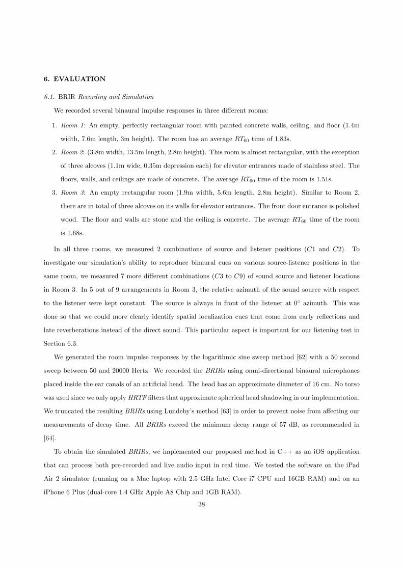
We recorded several binaural impulse responses in three different rooms:
1. Room 1: An empty, perfectly rectangular room with painted concrete walls, ceiling, and floor (1.4m
width, 7.6m length, 3m height). The room has an average RT60 time of 1.83s.
2. Room 2: (3.8m width, 13.5m length, 2.8m height). This room is almost rectangular, with the exception
of three alcoves (1.1m wide, 0.35m depression each) for elevator entrances made of stainless steel. The
floors, walls, and ceilings are made of concrete. The average RT60 time of the room is 1.51s.
3. Room 3: An empty rectangular room (1.9m width, 5.6m length, 2.8m height). Similar to Room 2,
there are in total of three alcoves on its walls for elevator entrances. The front door entrance is polished
wood. The floor and walls are stone and the ceiling is concrete. The average RT60 time of the room
is 1.68s.
In all three rooms, we measured 2 combinations of source and listener positions (C1 and C2). To
investigate our simulation’s ability to reproduce binaural cues on various source-listener positions in the
same room, we measured 7 more different combinations (C3 to C9) of sound source and listener locations
in Room 3. In 5 out of 9 arrangements in Room 3, the relative azimuth of the sound source with respect
to the listener were kept constant. The source is always in front of the listener at 0 azimuth. This was
done so that we could more clearly identify spatial localization cues that come from early reflections and
late reverberations instead of the direct sound. This particular aspect is important for our listening test in
Section 6.3.
We generated the room impulse responses by the logarithmic sine sweep method [62] with a 50 second
sweep between 50 and 20000 Hertz. We recorded the BRIRs using omni-directional binaural microphones
placed inside the ear canals of an artificial head. The head has an approximate diameter of 16 cm. No torso
was used since we only apply HRTF filters that approximate spherical head shadowing in our implementation.
We truncated the resulting BRIRs using Lundeby’s method [63] in order to prevent noise from affecting our
measurements of decay time. All BRIRs exceed the minimum decay range of 57 dB, as recommended in
[64].
To obtain the simulated BRIRs, we implemented our proposed method in C++ as an iOS application
that can process both pre-recorded and live audio input in real time. We tested the software on the iPad
Air 2 simulator (running on a Mac laptop with 2.5 GHz Intel Core i7 CPU and 16GB RAM) and on an
iPhone 6 Plus (dual-core 1.4 GHz Apple A8 Chip and 1GB RAM).
38
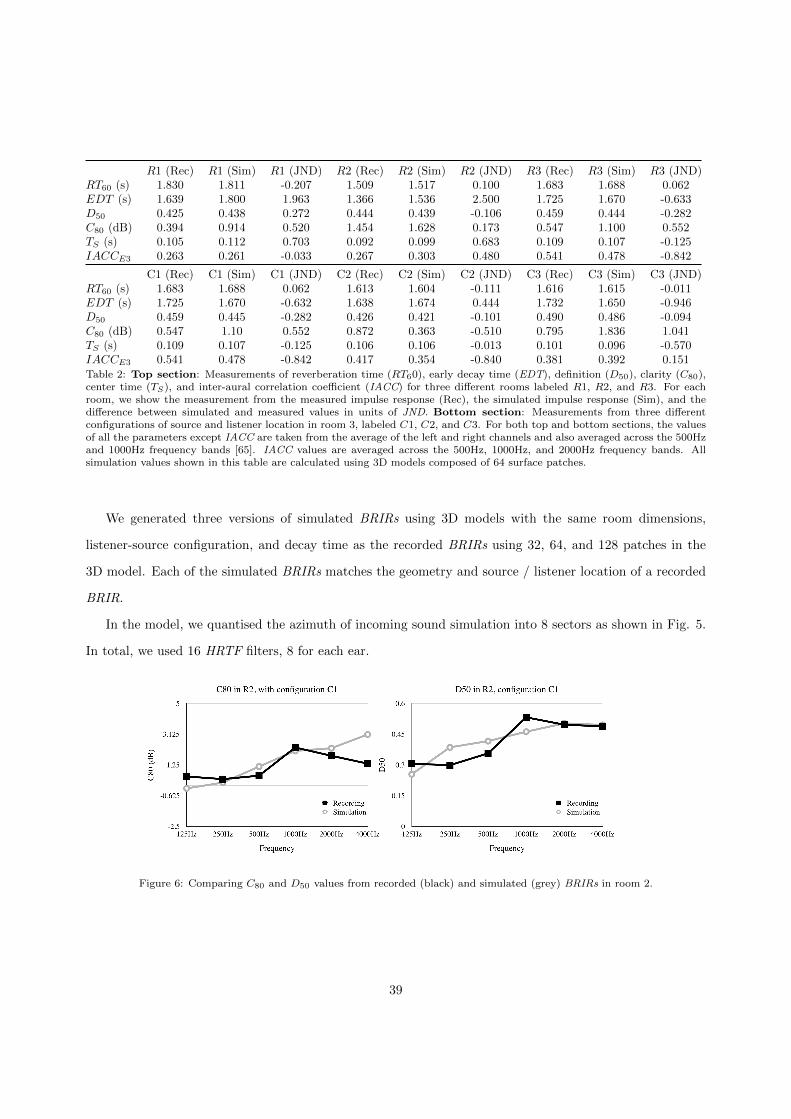
R1 (Rec) R1 (Sim) R1 (JND) R2 (Rec) R2 (Sim) R2 (JND) R3 (Rec) R3 (Sim) R3 (JND)RT60 (s) 1.830 1.811 -0.207 1.509 1.517 0.100 1.683 1.688 0.062EDT (s) 1.639 1.800 1.963 1.366 1.536 2.500 1.725 1.670 -0.633D50 0.425 0.438 0.272 0.444 0.439 -0.106 0.459 0.444 -0.282C80 (dB) 0.394 0.914 0.520 1.454 1.628 0.173 0.547 1.100 0.552TS (s) 0.105 0.112 0.703 0.092 0.099 0.683 0.109 0.107 -0.125IACCE3 0.263 0.261 -0.033 0.267 0.303 0.480 0.541 0.478 -0.842
C1 (Rec) C1 (Sim) C1 (JND) C2 (Rec) C2 (Sim) C2 (JND) C3 (Rec) C3 (Sim) C3 (JND)RT60 (s) 1.683 1.688 0.062 1.613 1.604 -0.111 1.616 1.615 -0.011EDT (s) 1.725 1.670 -0.632 1.638 1.674 0.444 1.732 1.650 -0.946D50 0.459 0.445 -0.282 0.426 0.421 -0.101 0.490 0.486 -0.094C80 (dB) 0.547 1.10 0.552 0.872 0.363 -0.510 0.795 1.836 1.041TS (s) 0.109 0.107 -0.125 0.106 0.106 -0.013 0.101 0.096 -0.570IACCE3 0.541 0.478 -0.842 0.417 0.354 -0.840 0.381 0.392 0.151Table 2: Top section: Measurements of reverberation time (RT60), early decay time (EDT), definition (D50), clarity (C80),center time (TS), and inter-aural correlation coefficient (IACC) for three different rooms labeled R1, R2, and R3. For eachroom, we show the measurement from the measured impulse response (Rec), the simulated impulse response (Sim), and thedifference between simulated and measured values in units of JND. Bottom section: Measurements from three differentconfigurations of source and listener location in room 3, labeled C1, C2, and C3. For both top and bottom sections, the valuesof all the parameters except IACC are taken from the average of the left and right channels and also averaged across the 500Hzand 1000Hz frequency bands [65]. IACC values are averaged across the 500Hz, 1000Hz, and 2000Hz frequency bands. Allsimulation values shown in this table are calculated using 3D models composed of 64 surface patches.
We generated three versions of simulated BRIRs using 3D models with the same room dimensions,
listener-source configuration, and decay time as the recorded BRIRs using 32, 64, and 128 patches in the
3D model. Each of the simulated BRIRs matches the geometry and source / listener location of a recorded
BRIR.
In the model, we quantised the azimuth of incoming sound simulation into 8 sectors as shown in Fig. 5.
In total, we used 16 HRTF filters, 8 for each ear.
Figure 6: Comparing C80 and D50 values from recorded (black) and simulated (grey) BRIRs in room 2.
39
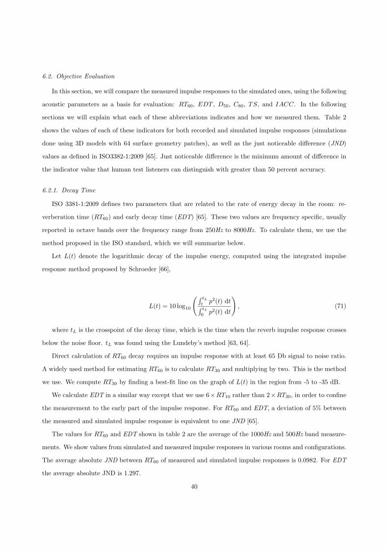
6.2. Objective Evaluation
In this section, we will compare the measured impulse responses to the simulated ones, using the following
acoustic parameters as a basis for evaluation: RT60, EDT , D50, C80, TS, and IACC. In the following
sections we will explain what each of these abbreviations indicates and how we measured them. Table 2
shows the values of each of these indicators for both recorded and simulated impulse responses (simulations
done using 3D models with 64 surface geometry patches), as well as the just noticeable difference (JND)
values as defined in ISO3382-1:2009 [65]. Just noticeable difference is the minimum amount of difference in
the indicator value that human test listeners can distinguish with greater than 50 percent accuracy.
6.2.1. Decay Time
ISO 3381-1:2009 defines two parameters that are related to the rate of energy decay in the room: re-
verberation time (RT60) and early decay time (EDT) [65]. These two values are frequency specific, usually
reported in octave bands over the frequency range from 250Hz to 8000Hz. To calculate them, we use the
method proposed in the ISO standard, which we will summarize below.
Let L(t) denote the logarithmic decay of the impulse energy, computed using the integrated impulse
response method proposed by Schroeder [66],
L(t) = 10 log10
(∫ tLtp2(t) dt∫ tL
0p2(t) dt
), (71)
where tL is the crosspoint of the decay time, which is the time when the reverb impulse response crosses
below the noise floor. tL was found using the Lundeby’s method [63, 64].
Direct calculation of RT60 decay requires an impulse response with at least 65 Db signal to noise ratio.
A widely used method for estimating RT60 is to calculate RT30 and multiplying by two. This is the method
we use. We compute RT30 by finding a best-fit line on the graph of L(t) in the region from -5 to -35 dB.
We calculate EDT in a similar way except that we use 6×RT10 rather than 2×RT30, in order to confine
the measurement to the early part of the impulse response. For RT60 and EDT, a deviation of 5% between
the measured and simulated impulse response is equivalent to one JND [65].
The values for RT60 and EDT shown in table 2 are the average of the 1000Hz and 500Hz band measure-
ments. We show values from simulated and measured impulse responses in various rooms and configurations.
The average absolute JND between RT60 of measured and simulated impulse responses is 0.0982. For EDT
the average absolute JND is 1.297.
40

6.2.2. Balance of Energy Between Early and Late Reflections
The acoustic parameters that measure the balance between early and late reflections energy are definition
(D50), clarity (C80), and center time (TS) [65]. D50 is defined as the ratio between the energy of the first
50ms to the total energy of the impulse response,
D50 =
∫ 0.050
0p2(t) dt∫ tL
0p2(t) dt
. (72)
The second measure of early to late energy balance, C80, is the ratio between the energy of the first 80ms
to the late energy of the impulse response,
C80 = 10 log10
(∫ 0.080
0p2(t) dt∫ tL
0.080p2(t) dt
). (73)
The third parameter, TS , is the center of gravity of the energy of the impulse response,
TS =
∫ tL0tp2(t) dt∫ tL
0p2(t) dt
. (74)
Fig. 6 shows C80 values in room R3 with configuration C1, and D50 values in room R2 with configuration
C1 for octave bands ranging from 125Hz to 4000Hz. ForD50, the simulated values closely follow the measured
result. For C80 values, we observe a deviation in 2000Hz and 4000Hz frequency band.
The JND values for D50, C80, and TS are 0.05, 1 dB, and 0.01 seconds respectively [65]. In table 2, all
except one of the simulation values for these three parameters show a deviation of less than 1 JND from the
measured responses. Note that the study in [67] recommends that the JND value for C80 should be 3 dB,
which is three times higher than the value suggested in the ISO standard [65].
6.2.3. Spatial Impression
The inter-aural correlation coefficient (IACC) measures the correlation between audio signals arriving
at the left and right ear. It is associated with the ‘sensation of space’ [10] or ‘spatial impression’ [65] due
to its correlation to apparent source width (ASW). Hidaka et. al suggested that the IACC values in the
500Hz, 1000Hz, and 2000Hz frequency bands can be used to directly represent ASW [68]. Hence, we report
41
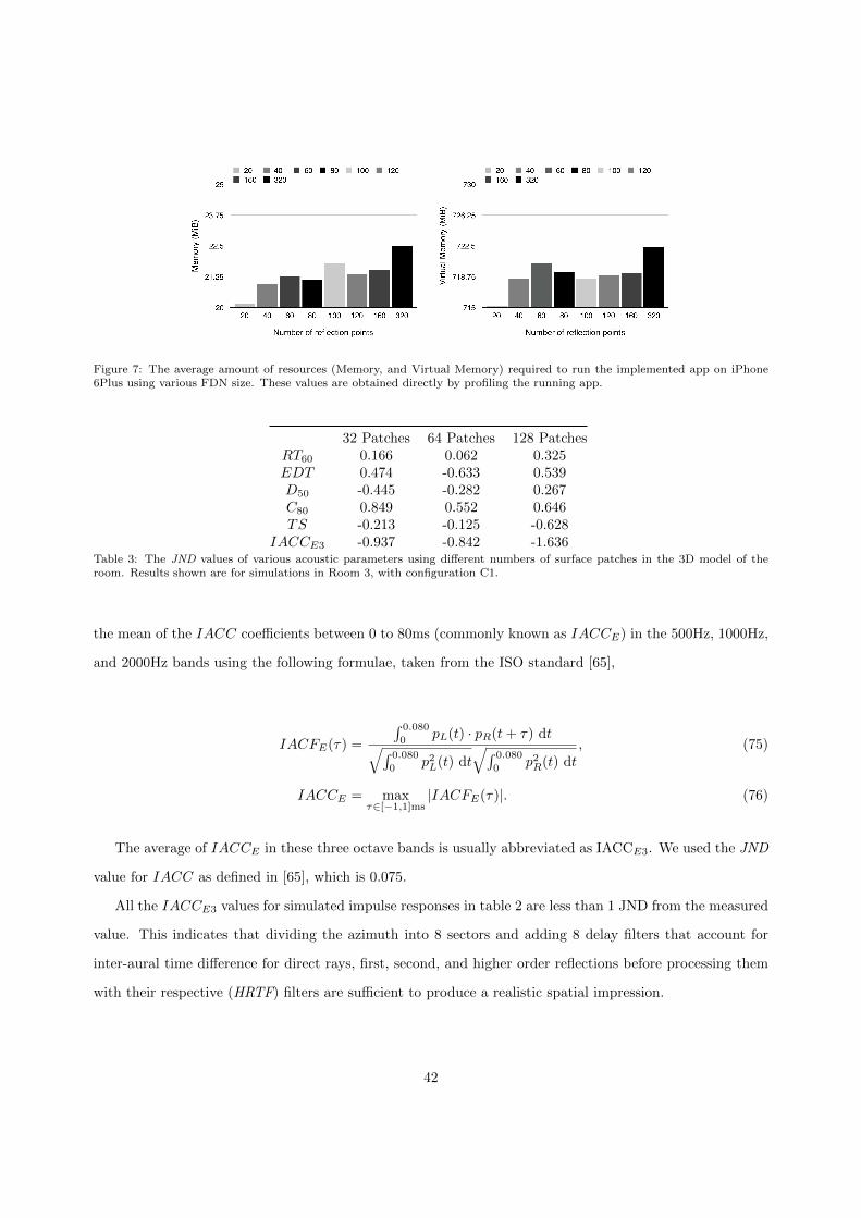
Figure 7: The average amount of resources (Memory, and Virtual Memory) required to run the implemented app on iPhone6Plus using various FDN size. These values are obtained directly by profiling the running app.
32 Patches 64 Patches 128 PatchesRT60 0.166 0.062 0.325EDT 0.474 -0.633 0.539D50 -0.445 -0.282 0.267C80 0.849 0.552 0.646TS -0.213 -0.125 -0.628
IACCE3 -0.937 -0.842 -1.636Table 3: The JND values of various acoustic parameters using different numbers of surface patches in the 3D model of theroom. Results shown are for simulations in Room 3, with configuration C1.
the mean of the IACC coefficients between 0 to 80ms (commonly known as IACCE) in the 500Hz, 1000Hz,
and 2000Hz bands using the following formulae, taken from the ISO standard [65],
IACFE(τ) =
∫ 0.080
0pL(t) · pR(t+ τ) dt√∫ 0.080
0p2L(t) dt
√∫ 0.080
0p2R(t) dt
, (75)
IACCE = maxτ∈[−1,1]ms
|IACFE(τ)|. (76)
The average of IACCE in these three octave bands is usually abbreviated as IACCE3. We used the JND
value for IACC as defined in [65], which is 0.075.
All the IACCE3 values for simulated impulse responses in table 2 are less than 1 JND from the measured
value. This indicates that dividing the azimuth into 8 sectors and adding 8 delay filters that account for
inter-aural time difference for direct rays, first, second, and higher order reflections before processing them
with their respective (HRTF) filters are sufficient to produce a realistic spatial impression.
42
6.2.4. Performance and Efficiency
Table 3 shows the JND values of the aforementioned acoustic parameters for simulation of room 3, in
configuration C1, using different numbers of patches to model the room. The time required to compute the
gain coefficients µn and υn in our model grows as we increase the number of patches. The average time
taken by both devices (iPhone and iPad Air simulator) to perform pre-computations each time any of the
room parameters are updated are 0.005s, 0.020s, and 0.060s using 32, 64, and 128 patches respectively. After
that short delay to update the parameters, our method can directly process the input audio, rather than
producing a BRIR and using convolution to generate the reverberated output signal. The code that we use
to compute the parameter updates is not optimised so there is potential to reduce the delay times between
updates.
In general, using a 3D room model with 64 patches produces a more accurate simulation than the model
with 32 patches. However, the results shown in table 3 indicate that using 128 patches do not yield a further
improvement in the accuracy.
6.3. Subjective Evaluation
6.3.1. Listening Test Procedure
We conducted a listening test with 11 subjects, with ages between 24 and 40 years old. Each test
took between 25 to 40 minutes to complete, and we conducted them using the same hardware (a MacBook
pro, a vacuum tube headphone amplifier, and a pair of AKG Q-701 headphones). All of the subjects are
experienced listeners. Five of them are academic researchers in audio related fields and one of them is a
recording engineer. The other five candidates are gamers, with at least 500 hours of competitive gaming
experience (first person shooting and action games). All of the gamers are familiar with listening to spatial
audio localisation cues.
To produce the recordings used in the listening test, we convolved a thirty-second long sample of a
recording of an acoustic guitar played without reverberation with both simulated and recorded impulse
responses in a variety of arrangements of source and listener locations. The listening test was twenty
questions long. Each question consisted of a pair of sound recordings and a pair of pictures showing the
floor plan of a room with listener and sound source locations marked. The test instructions requested the test
subjects to listen to the two audio recordings and then indicate which of the two recordings corresponded to
which of the two pictures, as shown in figure 8. Test subjects were allowed to replay the recordings as many
times as necessary for them to feel confident about their response, and they need not listen until the end of
43

the sound files. In other words, they are free to click repeat at any time. For each placement configuration
of listener and source locations in the test, there was one question about the measured impulse response and
a second question using the same placement and room geometry, in the simulated reverb. This arrangement
permitted us to do our statistical analysis as a paired t-test [69]. Half of the test subjects answered the
10 questions about simulated responses first, and the other half of test subjects answered the 10 questions
about measured responses first. Afterwards they switch and answer the remaining questions using either
simulated or measured responses that they have yet to be tested with.
In summary we do the following ,
1. Present 10 questions to half of the test subjects with simulated responses, and the other half with
recorded responses.
2. For each question, the subject is allowed to repeat the audio file as much as they like. They need not
listen until the end of the recording.
3. After they are finished with the 10 question, we asked them to repeat the same 10 questions using the
recorded responses first the first half of the test subjects, and the simulated responses for the second
half of the test subjects.
4. Repeat (2).
5. In total, each subject answers 20 questions, which is the same 10 questions for each recording.
The purpose of doing this test is that we would like to compare the performance of our simulation method
in giving localization cues. However we do not want to test the subject’s ability in localization. Therefore
we measure their performance in the simulated response against their performance in the recorded response.
It is easy to determine the location of the source relative to the listener, even without any reverb, simply
by listening to the sound of the direct rays. Because we want to emphasize the perceptual effects of the
reverb, not the direct sound, 12 out of 20 questions on the test maintained the same relative position between
source and listener, moving the pair of source and listener around the room, rather than moving each one
independently. Figure 8 shows this scenario. In this way, we eliminated the possibility that the test subjects
could identify the correct answer to the questions on the basis of direct rays alone.
The remaining 8 questions test the subject’s ability to discriminate between front-back configurations,
where they had to determine whether the sound source was located relatively behind or in front of the
listener that was placed at various locations in the room. In these cases, the two direct rays reach the
listener’s ears at exactly the same time and with the same HRTF for each ear. In these questions we placed
the listener with his back close to the wall and the sound source in front, and with his face to the wall and
44

Figure 8: Example question for the listening test. After hearing the BRIR, subjects are asked to select which location mostlikely resemble the BRIR
Figure 9: The plots of the simulation test scores normalised by recorded test scores for all 10 questions.
45

Figure 10: Normalised listening test scores of 11 test participants, comparing results for measured (black) and simulated (grey)reverb impulse responses.
Recorded-All Simulated-AllMean 0.727 0.764Variance 0.056 0.045Std. Dev 0.237 0.211n 11Deg. of freedom 10t -1.077p 0.307Critical Value 2.228
Table 4: Dependent 2-tailed T-test Summary using all questions (Recorded-All, Simulated-All). Result: Recorded(All) andSimulated(All) are not significantly different at p < 0.05.
the sound source behind. We expect that there will be more errors on these 4 questions, because simple
HRTF filters are known for causing front/back confusion [70]. Front-back localisation cues are known to be
highly individualised because they depend on pinna shape and size [71]. This confusion may be reduced by
using a unique pinna related transfer function (PRTF) filter designed for each individual listener as proposed
by Satarzadeh et al. [71] or Spagnol et al. [72].
6.3.2. Test Results
We summarise the listening test results in Fig. 10. The average score for recorded impulse response
questions is 0.727. For simulated impulse response questions it is 0.764. The average measured impulse
response score, not including the eight front/back questions 0.757. For simulated impulse responses without
front/back questions, the average is 0.772. This confirms the findings in [71, 72], which showed that listeners
are easily confused by front / back questions, especially when the head related transfer function filter does
46

not simulate the pinnae.
In general, candidates that scored well on questions with measured impulse responses also scored better
on questions using simulated impulse responses. To verify this, we conducted a dependent two tailed T-test
(also known as one-way repeated measures within subjects ANOVA [73]). The first and the second dataset
contains the normalised scores of 11 listeners using sound files from the measured and simulated impulses,
respectively. The result is shown in table 4. We found no significant difference between the means of the
two datasets. We also calculated the Pearson Correlation Coefficient for each of the two pairs of datasets.
The R-values between measured and simulated test results is 0.881.This shows a strong positive linear
correlation between their respective pair, and indicates that the measured and simulated impulse responses
yield a similar level of accuracy in perceived spatial location.
We also received the following inputs from the candidates. Firstly, most of the subjects experienced
slight fatigue after competing both tests. This is because the same input signal is used throughout the
test. In total, they had to listen to 40 sound files that play the same sound (2 files per question, two sets
of 10 questions), and allowing them to play each sound as many times as desired before responding to the
question. Hence, the test results may become less accurate as the test gets longer. Secondly, a high-quality
pair of headphones was required in order to clearly notice the spatial localisation cues from both types of
impulse responses. Thirdly, we noticed that test candidates were easily confused if they listened to a single
sound file for too long. Best results were obtained when the candidates rapidly switched between A and
B sound files to listen for differences, rather than listening to an entire file before switching to the other
alternative.
47

7. SUMMARY
We have presented an approach for binaural room modelling using feedback delay network reverberator
that runs on a mobile phone in real time. In this design, first order reflections are explicitly modeled, while
second and higher order reflections are approximated. Unlike existing hybrid methods mentioned in section
2, we simulate the balance between early and late energy. The effects of changing room parameters are
shown in both early reflections and late reverberation. Our method is also able to directly process the audio
input signal without the need to first produce and store the simulated BRIRs for later convolution with the
input. To evaluate our model, we implemented our method as an iOS app in C++.
We used several objective evaluation metrics suggested in [65] to validate our acoustical model. On
average, our results stay within 1 JND of parameters calculated from the recorded BRIR. In the subjective
evaluation, we conducted repeated measures listening tests with 11 experienced candidates. Each of them
were tasked to answer two same sets of question using sound files from convolution products using recorded
and simulated BRIR respectively. Statistical tests on the results showed that there is a strong positive linear
correlation between the two datasets and the means of both datasets are not significantly different.
Results from both objective and subjective evaluations prove that our method is able to simulate BRIR
with similar acoustical characteristics as the recorded BRIR. It is sufficient to accurately compute the first
order reflections and then approximate the second and higher order reflections as long as the energy between
the first and higher order reflections are kept balanced. Although the absolute onset time of individual
reflections in the second and higher order are not accurately modeled, they are still confined within the
room geometry so as to not produce unnatural sounding reverberation. Furthermore, we did not neglect
the inter-aural differences in spectra and timing for the second and higher order reflections. The proposed
method is able to produce convincing results with good computational efficiency for real-time usage in mobile
platforms.
48
8. FUTURE WORK
Section 6.2.4 shows that on average, simulations with 64 delays give better result than 32 delays. However,
having more number of delays in the FDN does not improve the accuracy. In some cases, it even worsens
the simulation result. This may be because large FDNs produce too much echo density in the early part of
the impulse response. Since this method links the accuracy of the 3D model with the size of the FDN, it
would be beneficial to study the effect of the size of the FDN on the density of echoes, to determine if there
is a relationship between the size or complexity of the room geometry and the optimal size of the FDN.
Another key issue is the timing of the onset of second order reflections. Because we use the first order
reflections to set the lengths of the delays, our second order reflections tend to start later than they would in
the real room. We suspect this could be corrected by adding some short delays to the network that do not
output to the multiplexer, in order to shorten the average time for energy to circulate around the mixing
matrix.
The (HRTF) filters we used in this method model the perceptual effect of the angle of incidence at the
listener in a two-dimensional plane. Therefore, reflections off the ceiling or floor do not have realistic spectral
filtering, since our HRTF filters do not simulate reflections off the listener’s shoulders and pinnae. To correct
this, we may consider using pinna filters that take into account the elevation angle between listener and the
reflection point on each patch [71, 72]. This may also reduce the front-back confusion mentioned in section
6.3.
Moreover, we have yet to integrate diffraction effects. We may investigate the usage of filters as proposed
in [74] to simulate diffraction in the future. For example, to enable binaural simulation in rooms where the
source is not visible from the listener location.
49

9. REFERENCES
[1] Samuel Siltanen, Tapio Lokki, Sami Kiminki, and Lauri Savioja. The room acoustic rendering equation. The Journal of
the Acoustical Society of America, 122(3):1624–1635, September 2007.
[2] M. Arntzen, L. Bertsch, and D. G. Simons. Auralization of novel aircraft configurations. In 5th CEAS Air and Space
conference, September 2015.
[3] S. A. Rizzi. NASA technical reports server (NTRS) - an overview of virtual acoustic simulation of aircraft flyover noise.
Technical report, July 2013.
[4] Lakulish Antani and Dinesh Manocha. Aural proxies and directionally-varying reverberation for interactive sound propa-
gation in virtual environments. In IEEE transactions on visualization and computer graphics, volume 19, pages 567–575,
April 2013. http://dx.doi.org/10.1109/TVCG.2013.27.
[5] Eduard Deines, Martin Bertram, Jan Mohring, Jevgenij Jegorovs, Frank Michel, Hans Hagen, and Gregory M. Nielson.
Comparative visualization for wave-based and geometric acoustics. In IEEE Transactions on Visualization and Computer
Graphics, volume 12, pages 1173–1180, Los Alamitos, CA, USA, 2006. IEEE. http://dx.doi.org/10.1109/TVCG.2006.125.
[6] Nikunj Raghuvanshi, Rahul Narain, and Ming C. Lin. Efficient and accurate sound propagation using adaptive rectan-
gular decomposition. In IEEE transactions on visualization and computer graphics, volume 15, pages 789–801, 2009.
https://dx.doi.org/10.1109/TVCG.2009.27.
[7] Nikunj Raghuvanshi, John Snyder, Ravish Mehra, Ming Lin, and Naga Govindaraju. Precomputed wave simulation for
real-time sound propagation of dynamic sources in complex scenes. ACM Transactions on Graphics, 29(4), July 2010.
https://dx.doi.org/10.1145/1778765.1778805.
[8] Vesa Valimaki, Julian D. Parker, Lauri Savioja, Julius O. Smith, and Jonathan S. Abel. Fifty years of artifi-
cial reverberation. IEEE Transactions on Audio, Speech, and Language Processing, 20(5):1421–1448, July 2012.
http://dx.doi.org/10.1109/tasl.2012.2189567.
[9] U. Peter Svensson. Modelling acoustic spaces for audio virtual reality. In Proceedings of the 1st IEEE Benelux Workshop
on Model based Processing and Coding of Audio (MPCA), 2002.
[10] T. Funkhouser, J. M. Jot, and N. Tsingos. Sounds good to me!, 2002.
[11] D. Griesinger. The science of surround, September 1999.
[12] R. Y. Litovsky, H. S. Colburn, W. A. Yost, and S. J. Guzman. The precedence effect. The Journal of the Acoustical
Society of America, 106(4 Pt 1):1633–1654, October 1999. http://dx.doi.org/10.1121/1.427914.
[13] Takayuki Hidaka, Yoshinari Yamada, and Takehiko Nakagawa. A new definition of boundary point between early reflections
and late reverberation in room impulse responses. The Journal of the Acoustical Society of America, 122(1):326–332, July
2007. http://dx.doi.org/10.1121/1.2743161.
[14] Lothar Cremer, Helmut A. Muller, and Richard M. Guernsey. Principles and applications of room acoustics. The Journal
of the Acoustical Society of America, 76(4):1277, October 1984. http://dx.doi.org/10.1121/1.391348.
[15] D. Griesinger. The relationship between audience engagement and the ability to perceive pitch, timbre, azimuth and
envelopment of multiple sources. In Proceedings of the International Symposium on Room Acoustics, ISRA 2010, August
2010.
[16] D. Griesinger. Spaciousness and envelopment in musical acoustics. In Proceedings of 101st Audio Engineering Society
Convention, number 4401, 1996.
50
[17] B. G. Shinn-Cunningham and S. Ram. Identifying where you are in a room: Sensitivity to room acoustics. In Proc.
International Conference on Auditory Display 2002, pages 21–24, 2003.
[18] S. Siltanen, T. Lokki, and L. Savioja. Room acoustics modeling with acoustic radiance transfer. In Proceedings of the
International Symposium on Room Acoustics, ISRA 2010, August 2010.
[19] A. Southern, S. Siltanen, and L. Savioja. Spatial room impulse responses with a hybrid modeling method. In Audio
Engineering Society Convention 130, May 2011.
[20] J. H. Rindel and C. L. Christensen. Room acoustic simulation and auralization - how close can we get to the real room?
In Proceedings of Eighth Western Pacific Acoustics Conference, 2003.
[21] Thomas Funkhouser, Ingrid Carlbom, Gary Elko, Gopal Pingali, Mohan Sondhi, and Jim West. A beam tracing ap-
proach to acoustic modeling for interactive virtual environments. In Proceedings of the 25th Annual Conference on
Computer Graphics and Interactive Techniques, SIGGRAPH ’98, pages 21–32, New York, NY, USA, 1998. ACM.
http://dx.doi.org/10.1145/280814.280818.
[22] Nicolas Tsingos. Pre-computing geometry-based reverberation effects for games. In 35th AES Conference on Audio for
Game, 2009.
[23] Steven M. Schimmel, Martin F. Muller, and Norbert Dillier. A fast and accurate ”shoebox” room acoustics simulator. In
Proceedings of the 2009 IEEE International Conference on Acoustics, Speech and Signal Processing, ICASSP ’09, pages
241–244, Washington, DC, USA, 2009. IEEE Computer Society. http://dx.doi.org/10.1109/ICASSP.2009.4959565.
[24] J. Huopaniemi, L. Savioja, and M. Karjalainen. Modeling of reflections and air absorption in acoustical spaces a digital
filter design approach. In IEEE ASSP Workshop on Applications of Signal Processing to Audio and Acoustics, pages 4
pp.+. IEEE, October 1997. http://dx.doi.org/10.1109/aspaa.1997.625594.
[25] S. Pelzer, L. Aspock, D. Schroder, and M. Vorlander. Interactive Real-Time simulation and auralization for modifiable
rooms. Building Acoustics, 21(1):65–73, March 2014. http://dx.doi.org/10.1260/1351-010X.21.1.65.
[26] M. Monks, B. Oh, and J. Dorsey. Acoustic simulation and visualization using a new unified beam tracing and image
source approach. In Convention of the Audio Engineering Society, ACM, 1996.
[27] D. Schroder and M. Vorlander. Hybrid method for room acoustic simulation in real-time. In Proceedings on the 20th
International Congress on Acoustics (ICA), 2007.
[28] N. Rober, U. Kaminski, and M. Masuch. Ray acoustics using computer graphics technology. In Proceedings 10th Inter-
national Conference on Digital Audio Effects (DAFx), 2007.
[29] Hequn Bai, Gael Richard, and Laurent Daudet. Geometric-based reverberator using acoustic rendering networks. In
Applications of Signal Processing to Audio and Acoustics (WASPAA), 2015 IEEE Workshop on, pages 1–5. IEEE,
October 2015. http://dx.doi.org/10.1109/WASPAA.2015.7336934.
[30] F. Menzer and C. Faller. Binaural reverberation using a modified jot reverberator with Frequency-Dependent interaural
coherence matching. In 126 Audio Engineering Society, number 7765, May 2009.
[31] F. Menzer. Binaural reverberation using two parallel feedback delay networks. In Audio Engineering Society 40th Inter-
national Conference: Spatial Audio: Sense the Sound of Space, number 7-2, October 2010.
[32] T. Wendt, S. Van de Par, and S. Ewert. Perceptual and room acoustical evaluation of a computational efficient binaural
room impulse response simulation method. In Proc. of the EAA Joint Symposium on Auralization and Ambisonics, pages
86–92, April 2014. http://dx.doi.org/10.14279/depositonce-15.
[33] F. Menzer. Efficient binaural audio rendering using independent early and diffuse paths. In 132 Audio Engineering Society
51
Convention, number 8584, April 2012.
[34] Jean-Marc Jot. Efficient models for reverberation and distance rendering in computer music and virtual audio reality.
1997.
[35] Augusto S. Stefano and Stefano Tubaro. Low-Cost Geometry-Based acoustic rendering. In Proc. of the COST G-6
Conference on Digital Audio Effects (DAFX-01), December 2011.
[36] L. Savioja, T. Lokki, and J. Huopaniemi. Auralization applying the parametric room acoustic modeling technique - the
DIVA auralization system. pages 219–224, 2002.
[37] B. Carty and V. Lazzarini. Hrtf-early and hrtf-reverb: Flexible binaural reverberation processing. In International
Computer Music Association, June 2010.
[38] Torben Wendt, Steven van de Par, and Stephan Ewert. A Computationally-Efficient and Perceptually-Plausible algorithm
for binaural room impulse response simulation. Journal of the Audio Engineering Society, 62(11):748–766, December
2014.
[39] Enzo De Sena, Huseyin Hachabiboglu, Zoran Cvetkovic, and Julius O. Smith. Efficient synthesis of room acoustics
via scattering delay networks. IEEE/ACM Trans. Audio, Speech and Lang. Proc., 23(9):1478–1492, September 2015.
http://dx.doi.org/10.1109/taslp.2015.2438547.
[40] J. O. Smith. Physical modelling using digital waveguides. Computer Music Journal, 16(4):74–91, 1992.
[41] M. Schroeder, Thomas D. Rossing, F. Dunn, W. M. Hartmann, D. M. Campbell, and N. H. Fletcher. Springer Handbook
of Acoustics, pages 58+. Springer Publishing Company, Incorporated, 1st edition, 2007.
[42] S. Marschner. Radiometry, January 2012.
[43] Ross McCluney. Introduction to Radiometry and Photometry, Second Edition, pages 7–20. Artech House, 2 edition,
November 2014.
[44] F. E. Nicodemus, J. C. Richmond, J. J. Hsia, I. W. Ginsberg, and T. Limperis. Geometrical Considerations and Nomen-
clature for Reflectance, chapter Geometrical Considerations and Nomenclature for Reflectance, pages 94–145. Jones and
Bartlett Publishers, Inc., USA, 1992.
[45] S. Kiminki. Sound propagation theory for linear ray acoustic modelling. Master’s thesis, Helsinki University of Technology,
2005. http://www.niksula.hut.fi/˜skiminki/D- skiminki.pdf.
[46] Wallace C. Sabine. Collected Papers on Acoustics. Cambridge, Harvard University Press, London: Humphrey Milford,
Oxford University Press, 1922.
[47] L. Savioja, J. Huopaniemi, T. Lokki, and R. Vaananen. Creating interactive virtual acoustic environments. Journal of
the Audio Engineering Society, 47(9):675–705, September 1999.
[48] F. Menzer. Binaural Audio Signal Processing Using Interaural Coherence Matching. PhD thesis, Ecole Polytechnique
Federale de Lausanne (EPFL), Switzerland, April 2010.
[49] Eric J. Angel, V. Ralph Algazi, and Richard O. Duda. On the design of canonical sound localization environments. 2002.
[50] D. Griesinger. Creating reverb algorithms for surround sound, 2000.
[51] C. P. Brown and R. O. Duda. A structural model for binaural sound synthesis. IEEE Transactions on Speech and Audio
Processing, 6(5):476–488, September 1998. http://dx.doi.org/10.1109/89.709673.
[52] Diemer de Vries and Edo M. Hulsebos. Auralization of room acoustics by wave field synthesis based on array measurements
of impulse responses. In Signal Processing Conference, 2004 12th European, pages 1377–1380. IEEE, 2004.
[53] B. J. Fino and V. R. Algazi. Unified matrix treatment of the fast Walsh-Hadamard transform. IEEE Transactions on
52

Computers, C-25(11):1142–1146, November 1976. http://dx.doi.org/10.1109/tc.1976.1674569.
[54] H. Anderson, K. W. E. Lin, C. So, and S. Lui. Flatter frequency response from feedback delay network reverbs. In 41st
International Computer Music Conference 2015, September 2015.
[55] J. M. Jot. An analysis/synthesis approach to real-time artificial reverberation. In Acoustics, Speech, and Signal Pro-
cessing, 1992. ICASSP-92., 1992 IEEE International Conference on, volume 2, pages 221–224 vol.2. IEEE, March 1992.
http://dx.doi.org/10.1109/icassp.1992.226080.
[56] Rusty Allred. Digital Filters for Everyone: Third Edition, chapter 2.3.10. Creative Arts & Sciences House, 3 edition,
March 2015.
[57] J. A. Moorer. The manifold joys of conformal mapping. Journal of the Audio Engineering Society, 31(11):821–841, 1983.
[58] J. A. Moorer. The manifold joys of conformal mapping: Applications to digital filtering in the studio - 2nd try. Unpublished
manuscript : http://www.jamminpower.com/main/unpublished.html.
[59] P. Regalia and S. Mitra. Tunable digital frequency response equalization filters. IEEE Transactions on Acoustics, Speech,
and Signal Processing, 35(1):118–120, January 1987. http://dx.doi.org/10.1109/TASSP.1987.1165037.
[60] Mark Kahrs and Karlheinz Brandenburg. Applications of Digital Signal Processing to Audio and Acoustics, pages 89+.
Springer Publishing Company, Incorporated, 2013.
[61] Heinrich Kuttruff. Room Acoustics, Fifth Edition, pages 25, 127, 202+. CRC Press, 5 edition, June 2009.
[62] A. Farina. Simultaneous measurement of impulse response and distortion with a Swept-Sine technique. In 108th Convention
of the Audio Engineering Society, number 5063, February 2000.
[63] A. Lundeby, T. E. Vigran, H. Bietz, and M. Vorlander. Uncertainties of measurements in room acoustics. Acta Acustica
united with Acustica, pages 344–355, July 1995.
[64] C. C. J. M. Hak, R. H. C. Wenmaekers, and L. C. J. van Luxemburg. Measuring room impulse responses: Impact of the
decay range on derived room acoustic parameters. Acta Acustica united with Acustica, pages 907–915.
[65] ISO 3382-1:2009 - acoustics – measurement of room acoustic parameters – part 1: Performance spaces. Technical report,
International Organization for Standardization, 2009.
[66] M. R. Schroeder. Integrated impulse method measuring sound decay without using impulses. The Journal of the Acoustical
Society of America, 66(2):497–500, August 1979. http://dx.doi.org/10.1121/1.383103.
[67] Michelle C. Vigeant, Robert D. Celmer, Chris M. Jasinski, Meghan J. Ahearn, Matthew J. Schaeffler, Clothilde B.
Giacomoni, Adam P. Wells, and Caitlin I. Ormsbee. The effects of different test methods on the just noticeable dif-
ference of clarity index for musica). The Journal of the Acoustical Society of America, 138(1):476–491, July 2015.
http://dx.doi.org/10.1121/1.4922955.
[68] Takayuki Hidaka, Leo L. Beranek, and Toshiyuki Okano. Interaural crosscorrelation, lateral fraction, and low and highfre-
quency sound levels as measures of acoustical quality in concert halls. The Journal of the Acoustical Society of America,
98(2):988–1007, August 1995. http://dx.doi.org/10.1121/1.412847.
[69] J. H. McDonald. Handbook of Biological Statistics, pages 180–185. Sparky House Publishing, Baltimore, Maryland, third
edition, 2014.
[70] Richard H. So, N. M. Leung, Andrew B. Horner, Jonas Braasch, and K. L. Leung. Effects of spectral manipulation on
nonindividualized head-related transfer functions (HRTFs). Human factors, 53(3):271–283, June 2011.
[71] Patrick Satarzadeh, V. Ralph Algazi, and Richard O. Duda. Physical and filter pinna models based on anthropometry.
In Audio Engineering Society Convention 122, number 7098, May 2007.
53

[72] S. Spagnol and M. Geronazzo. Structural modeling of pinna-related transfer functions. In Proc. 7th Int. Conf. on Sound
and Music Computing (SMC), pages 422–428, July 2010.
[73] M. Khelifa. One-Way repeated measures analysis of variance (Within-Subjects ANOVA). SPSS for Windows Intermediate
& Advanced Applied Statistics.
[74] Tapio Lokki, Peter Svensson, and Lauri Savioja. An efficient auralization of edge diffraction. In In Proceedings of the
Audio Engineering Society 21 st International Conference on Architectural Acoustics and Sound Reinforcement, pages
166–172, 2002.
54