NASA/CR-2002-211753

Development of an Efficient Binaural

Simulation for the Analysis of StructuralAcoustic Data

Aimee L. Lalime and Marly E. Johnson

Virginia Polytechnic I)_stitute and State U)_iversity

Blacksburg, Virginia

July 2002

https://ntrs.nasa.gov/search.jsp?R=20020060763 2018-09-06T20:32:28+00:00Z

The NASA STI Program Office ... in Profile

Since its fotmding, NASA has been dedicated

to the advancement of aeronautics and spacescience. The NASA Scientific and Technical

Irfformation (STI) Program Office plays a key

part in helping NASA maintain this importantrole.

The NASA STI Program Office is operated by

Langley Research Center, the lead center forNASA's scientific and technical information.

The NASA STI Program Off_ce provides

access to the NASA STI Database, the largest

collection of aeronautical and space sdence

STI in the world. The Program Office is alsoNASA's institutional mechanism for

disseminating the results of its research and

development activities. These restflts are

published by NASA in the NASA STI Report

Series, which includes the following report

types:

TECHNICAl, P[JBLICATION. Reports

of completed research or a major

significant phase of research that

presem 1he results of NASA programsand include extensive data or {heore{k;al

analysis. Incltldes compilations of

significant scientific and technical dataand information deemed to be of

continuing reference value. NASA

cotmterpart of peer revie\,ved formal

professional papers, but having less

stringent lirnitations on manuscript

length and extent of graphic

presentations.

TEC} {NICAL MEMOR AND [JM.

Scientific and technical findings that are

prelimina W or of specialized interest,

e.g., quick release reporls, working

papers, and bibliographies that containminimal annotation. Does not contain

extensive analysis.

CONTRACTOR REPORT. Scientific and

technical findings by NASA sponsored

contractors and grantees.

CC)NFERENCE PUBLICATION.

Collected papers from scientific and

technical conferences, symposia,

seminars, or other meetings sponsored

or co sponsored by NASA.

SPECIAL PUBI,ICATION. Scientffk;,

technical, or historical inibrmation from

NASA programs, projects, and missions,

often concerned wilh sut)jecls having

substantial public interest.

TECHNICAl, TRANSLATION. English

language translations of foreignscientific and technical material

pertinent 1o NASA's m_ssion.

Specialized ser_dces that complement the

STI Program Office's diverse offerings

include creating custom thesauri, building

customized dalabases, organizing and

publishing research results ... even

providing videos.

For more information about the NASA STI

Program Office, see the following:

* Access the NASA STI Program Home

Page at http://www.st3.nasa.gov

* E mail your question via {he Internet {o

help@sti.nasa.gov

® Fax your question to the NASA STI

Help Desk at (301) 621 0134

• Phone the NASA STI Help Desk at (301)621 0390

Write to:

NASA STI Help Desk

NASA Center for AeroSpace Information7121 Standard Drive

Hanover, MD 211076 1320

NASA/CR-2002-211753

Development of an Efficient Binaural

Simulation for the Analysis of StructuralAcoustic Data

Aimee L. Lalime and Marly E. Johnson

Virginia Polytechnic Institute and State University

Blacksburg, Virginia

Nallonal Aeronautics and

Space Administra{ion

Langley Research Center Prepared for Langley Research Center

l!tampton, Virginia 23681 2199 under C:ooperative Agreement NCC 1 01029

July 2002

official endorsement, either expressed or implied, of such products or manufacturers by the National Aeronautics

The use of trademarks or names of manufactm'ers in the report is lbr accurate reporting and does not constitute an

and Space Administration.

Available from:

NASA Center for AeroSpace Inl'onnation (CASI)

7121 Standard Drive

t tanover, MD 21076-1320

(301) 621-0390

National Technical Inl'onnation Service (NTIS)

5285 Port Royal Road

Springfield, VA 22161-2171

(703) 605-6000

Foreword

This report summarizes the research accomplishments performed under the NASALangley Research Center research cooperative agreement no. NCC 1-01029 entitled,"Development of an Efficient Binaural Simulation for the Analysis of Structural Acoustic

Data." Funding for the work was provided by the Life Cycle Simulation element of theNASA Intelligent Synthesis Environment Program under the task entitled "StructuralAcoustic Simulation in Operational Environments." Dr. Stephen A. Rizzi of the NASALangley Research Center was the ISE task lead and technical officer of this cooperative

agreement.

Contents

Foreword ................................................................................. 1Abstract ................................................................................... 3Introduction .............................................................................. 3

Theory ..................................................................................... 5Radiation from a Monopole .......................................................................................... 5Head Related Transfer Functions (HRTFs) ................................................................... 6Using Sampled Signals .................................................................................................. 8Multiple Sources ........................................................................................................... 9Modeling a Vibrating Plate ........................................................................................... 9

Exhaustive Method .................................................................... 10Schematic of the Exhaustive Method .......................................................................... 10

Verifying Radiation Model ......................................................................................... 11Verifying HRTF Application ...................................................................................... 15Measurement Consistency ........................................................................................... 15Wavenumber Decomposition ...................................................................................... 16

Reduction Methods .................................................................... 18

Wavenumber Filtering ................................................................................................. 18Equivalent Source Reduction ...................................................................................... 19Singular Value Decomposition .................................................................................... 27ESR and SVD Together .............................................................................................. 32Computation Time ...................................................................................................... 33

Conclusion .............................................................................. 36Future Work ............................................................................ 36

Acknowledgements ................................................................... 37Bibliography ............................................................................ 38

Abstract

Binaural or "virtual acoustic" representation has been proposed as a method of analyzingacoustic and vibro-acoustic data. Unfortunately, this binaural representation can requireextensive computer power to apply the Head Related Transfer Functions (HRTFs) to a

large number of sources, as with a vibrating structure. This work focuses on reducing thenumber of real-time computations required in this binaural analysis through the use ofSingular Value Decomposition (SVD) and Equivalent Source Reduction (ESR). TheSVD method reduces the complexity of the HRTF computations by breaking the HRTFs

into dominant singular values (and vectors). The ESR method reduces the number ofsources to be analyzed in real-time computation by replacing sources on the scale of astructural wavelength with sources on the scale of an acoustic wavelength. It is shown

that the effectiveness of the SVD and ESR methods improves as the complexity of thesource increases. In addition, preliminary auralization tests have shown that the resultsfrom both the SVD and ESR methods are indistinguishable from the results found withthe exhaustive method.

Introduction

Improvements in digital acquisition and sensor technology have led to an increase in theability to acquire large data sets. One potential way of analyzing structural acoustic datais the creation of a three-dimensional audio-visual environment. For example, an audio-visual virtual representation of the inside of the space station could allow designers and

astronauts to experience and analyze the acoustic properties of the space station.Incorporating the visual aspect with the acoustic allows the user to sift rapidly throughnoise data to determine what parts of a vibrating structure are radiating sound to whatareas in an acoustic enclosure.

Unfortunately, the three-dimensional (or binaural) simulation of structural data is notcurrently feasible because of the large number of computations required to analyze a

distributed source. The objective of this research has been to reduce the number ofcalculations required to calculate the binaural signals of an acoustically large source.Both pre-processing and real-time reduction methods will be discussed.

Binaural literally means "two ears", and is a term used to describe three-dimensional

sound [1]. Humans detect the direction of sound using the differences in the sound that isheard by each ear. For example, a sound from the right will be louder in the right earthan in the left. This sound level difference is termed Interaural Intensity Difference(liD) and is one of the most important aural cues for localizing sound. Another

localization cue is the Interaural Time Difference, or ITD [2]. This is the difference inthe amount of time taken for a sound to reach each ear. In the preceding example, thesound coming from the right of the head is heard by the right ear less than lms before

being sensed by the left ear. This small ITD is sensed by the brain and used to determinethe location of the sound source.

IIDandITDaremathematicallydescribedin thetransferfunctionbetweenasoundsourceandtheleftandrightears,termedtheHeadRelatedTransferFunction(HRTF).HRTFsdescribenotonlyIIDandITD,butalsohowsoundisaffectedbyitsinteractionwiththehead,torso,andear.Forexample,assoundapproachesthehead,lowfrequencysoundwrapsaroundthehead,reachingbothears.However,withhighfrequenciesashadowingeffectoccurs,causingthehighfrequencycontenttobesensedononesideoftheheadandnottheother.Soundalsoreflectsoff thesubject'storso,causingtimeandintensitychanges.Theouterearalsoaffectsthesoundenteringtheear,asitsshapecausesthesoundtoresonateatcertainfrequencies.HeadRelatedTransferFunctionscanbeusedto calculatethebinauralsignalsata listener'sears,therebysimulatingathree-dimensionalsoundfieldaroundasubject'shead.[1]

Unfortunately,theapplicationoftheHRTFsiscomputationallyexpensive,andrestrictsreal-timebinauralanalysisofa largenumberof sources(aswithavibratingstructure).Agreatdealofresearchhasbeendoneonthemodelingof HRTFsincludingPrincipalComponentsAnalysis[3,4],Karhunen-LoeveExpansion[5,6],BalancedModelTruncation[7],State-SpaceAnalysis[8,9],RepresentationasSphericalHarmonics[10,11],Pole-ZeroApproximation[12,13],andStructuralModeling[14,15]. Duda[16]presentsacomprehensivesummaryofthesedifferentHRTFmodels,whichhavebeenresearchedforseveralreasons:tobetterunderstandthepropertiesof HRTFs,toreducethenumberofmeasurementsrequiredin orderto createafull setofindividualizedHRTFs,and(aswiththisresearch)toreducethenumberandcomplexityofreal-timecalculations.ThisresearchusesSingularValueDecomposition(SVD)tomodeltheHRTFs,whichisbasedonseriesexpansion,asarePrincipalComponentsAnalysisandKarhunen-LoeveExpansion.

ThisresearchalsousestheEquivalentSourceReduction(ESR)[17]inordertosimplifythebinauralsimulationof adistributedsource.ThisresearchcombinestheESRandSVDmethodsandappliesthemtothebinauralsimulationof structuralacousticdata,whichisanewresearchareainbinauralacoustics.

Thetheorybehindthebinauralsimulationofacousticdataisdiscussedin thefirstsectionof thisreport.Fromthere,thecurrenttechnologyforcalculatingthebinauralsignalsisexaminedin the"ExhaustiveMethod"portionofthereport.Alsoincludedin theExhaustiveMethodsectionisadescriptionofhoweachstepoftheexhaustivemethodwasverifiedbycomparingtheresultswithactualtestdata.Thenextsection,termed"ReductionMethods",detailstheinvestigationoftheproposedmethodsforreducingthecomputationtimeoftheexhaustivemethod.Includedin theReductionMethodssectionarethediscussionsof SVD,ESR,andtheestimatedreductionincomputationtimeresultingfromtheuseofSVDandESR.Lastly,conclusionsaredrawnregardingtheeffectivenessandpotentialuseofthereductionmethodsin real-timestructuralacousticanalysis.

Theory

In order to discuss the exhaustive and reduced methods of simulating the binaural signalsassociated with structural acoustics, there are several topics that must be understood anddiscussed. The first is a discussion on how sound radiates from a monopole source.

Following will be descriptions involving HRTF's use in binaural simulation, including:the binaural simulation of sound radiating from a monopole; how the implementation ofHRTFs changes with sampled signals rather than analog ones; the binaural simulation ofmultiple sources; and the binaural simulation of a vibrating plate.

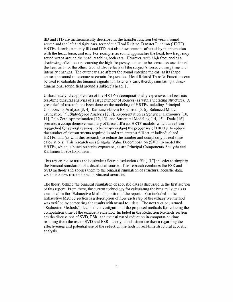
Radiation from a MonopoleThe simplest acoustic source is that of a pulsating sphere, also known as a monopole

(figure 1). According to Fahy's, Engineering Acoustics, the sound pressure at a radialdistance, r, caused by the radiation from a monopole source is defined according toequation 1 [18]:

(1)

where po is the density of air and Q is the volume velocity. Q is defined according toequation 2 [19]:

Q = Su (2)

where S is the surface area of the sphere (47Cro 2) and u is the velocity of the surface of the

sphere.

In the case of a vibrating hemisphere rather than a vibrating sphere, the pressure at somedistance, r, will be

Po O__Qt (3)

(4)

where a is the acceleration of the surface of the pulsating sphere (figure 1). This meansthat the sound at point R (which is a distance, r, from the pulsating sphere) will have a

magnitude that varies inversely with the distance, r, and a time delay equal to the time ittakes for the sound to reach point R, which will be r/c.

Figure 1: Pulsating Sphere

Head Related Transfer Functions (HRTFs)As mentioned in the introduction, HRTFs are a set of transfer functions that describe how

sotmd is reflected off the human torso, wraps around the head, and resonates in the innerand outer ear. Because the human body is not axisymmetric, the HRTFs vary depending

upon the elevation angle, 0, and the circumferential angle, O, of the sound source. Sinceevery human torso, head, and ears are different, each person has their own individualHRTFs. A generalized set of HRTFs can be obtained using the Knowles Electronic

Manikin for Acoustic Research (KEMAR). The KEMAR manikin (figure 2) has a head,torso, and ears that are specifically shaped in order to represent the average human form.

Figure 2: Knowles Electronic Manikin for Acoustic Research

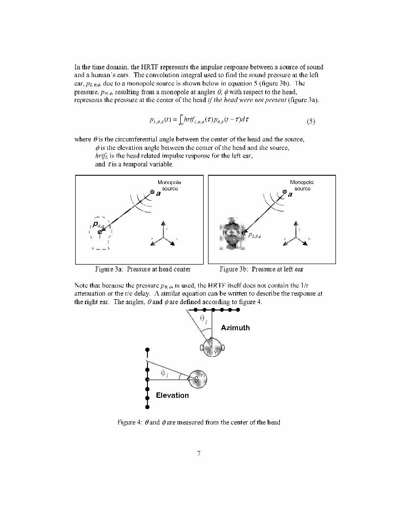
In thetimedomain,theHRTFrepresentstheimpulseresponsebetweenasourceof soundandahuman'sears.Theconvolutionintegralusedtofindthesoundpressureattheleftear,PLo,_ due to a monopole source is shown below in equation 5 (figure 3b). The

pressure, po, _ resulting from a monopole at angles O, 0 with respect to the head,represents the pressure at the center of the head if the head were notpresent (figure 3a).

(t) = hrtf ,o, (r)po, (t - r)dr (5)

where 0 is the circumferential angle between the center of the head and the source,

0 is the elevation angle between the center of the head and the source,hr_ is the head related impulse response for the left ear,

and _is a temporal variable.

Monopolesource

\ , ._ a

i

Monopolesource

Figure 3a: Pressure at head center Figure 3b: Pressure at left ear

Note that because the pressurepo, 0, is used, the HRTF itself does not contain the 1/rattenuation or the r/c delay. A similar equation can be written to describe the response at

the right ear. The angles, 0 and 0 are defined according to figure 4.

__ _uth

Elevation

Figure 4:0 and 0 are measured from the center of the head

Usin_ Sampled Signals

Equation 5 describes the process for finding the sound at the average human's left ear fora continuous signal from a monopole source. Since the binaural signals are calculatedusing a computer, the convolution is actually made up of discrete signals rather thancontinuous ones. This results in the convolution shown in equation 6.

M 1

pL,o,_[i]= _" hrtfL,o,_[j]po,_[i_ j] (6)j=0

Here M is the number of samples used in the HRTF and i is the {h discrete time step.

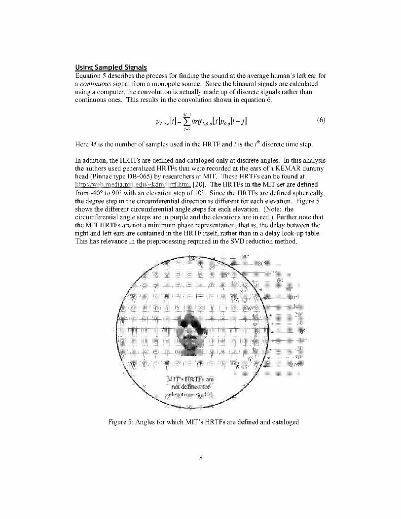
In addition, the HRTFs are defined and cataloged only at discrete angles. In this analysisthe authors used generalized HRTFs that were recorded at the ears ofa KEMAR dummyhead (Pinnae type DB-065) by researchers at MIT. These HRTFs can be found atht_kgt)://web.media.mit.ed_/_,kdm/hrtf.htmI [20]. The HRTFs in the MIT set are defined

from -40 ° to 90 ° with an elevation step of 10°. Since the HRTFs are defined spherically,the degree step in the circumferential direction is different for each elevation. Figure 5shows the different circumferential angle steps for each elevation. (Note: thecircumferential angle steps are in purple and the elevations are in red.) Further note that

the MIT HRTFs are not a minimum phase representation, that is, the delay between theright and left ears are contained in the HRTF itself, rather than in a delay look-up table.This has relevance in the preprocessing required in the SVD reduction method.

Figure 5" Angles for which MIT's HRTFs are defined and cataloged

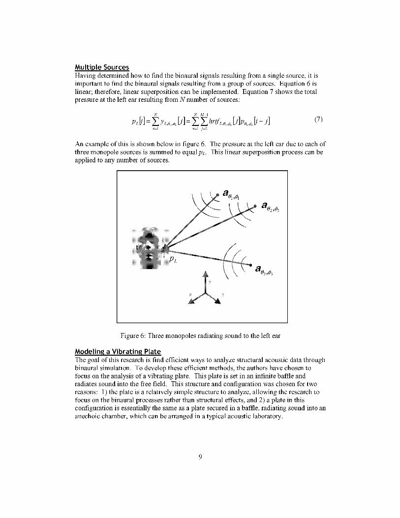
Multiple SourcesHaving determined how to find the binaural signals resulting from a single source, it isimportant to find the binaural signals resulting from a group of sources. Equation 6 islinear; therefore, linear superposition can be implemented. Equation 7 shows the totalpressure at the left ear resulting from N number of sources:

N N M1

PL[i]= Z YL,o_,,_y,[J]= Z Z hrtfL,oy,,_,[J]Po_,,_,[i- j] (7)n=l n=l j=O

An example of this is shown below in figure 6. The pressure at the left ear due to each ofthree monopole sources is summed to equalpL. This linear superposition process can be

applied to any number of sources.

l a02 ,_2

Figure 6: Three monopoles radiating sound to the left ear

Modeling a Vibratinq PlateThe goal of this research is find efficient ways to analyze structural acoustic data throughbinaural simulation. To develop these efficient methods, the authors have chosen to

focus on the analysis of a vibrating plate. This plate is set in an infinite baffle andradiates sound into the flee field. This structure and configuration was chosen for tworeasons: 1) the plate is a relatively simple structure to analyze, allowing the research tofocus on the binaural processes rather than structural effects, and 2) a plate in this

configuration is essentially the same as a plate secured in a baffle, radiating sound into ananechoic chamber, which can be arranged in a typical acoustic laboratory.

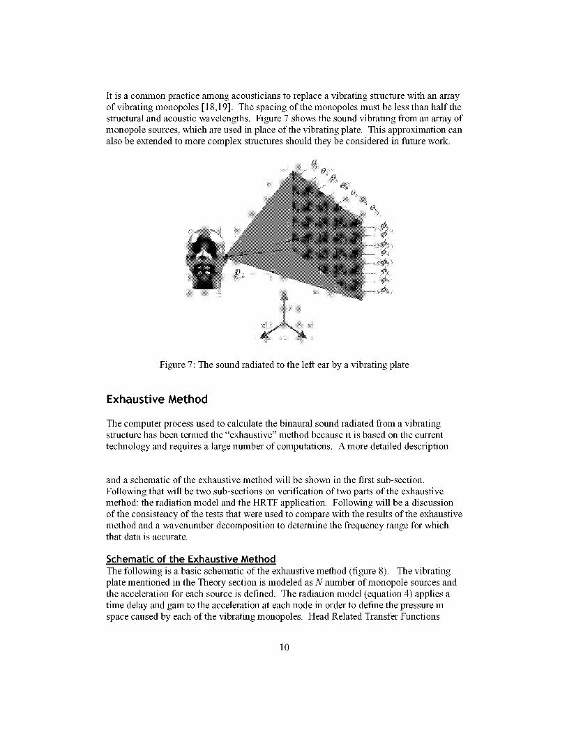
It isacommonpracticeamongacousticianstoreplaceavibratingstructurewithanarrayof vibratingmonopoles[18,19].Thespacingofthemonopolesmustbelessthanhalfthestructuralandacousticwavelengths.Figure7showsthesoundvibratingfromanarrayofmonopolesources,whichareusedinplaceofthevibratingplate.Thisapproximationcanalsobeextendedtomorecomplexstructuresshouldtheybeconsideredin futurework.

Figure7:Thesoundradiatedtotheleftearbyavibratingplate

Exhaustive Method

The computer process used to calculate the binaural sound radiated from a vibratingstructure has been termed the "exhaustive" method because it is based on the current

technology and requires a large number of computations. A more detailed description

and a schematic of the exhaustive method will be shown in the first sub-section.

Following that will be two sub-sections on verification of two parts of the exhaustivemethod: the radiation model and the HRTF application. Following will be a discussionof the consistency of the tests that were used to compare with the results of the exhaustive

method and a wavenumber decomposition to determine the frequency range for whichthat data is accurate.

Schematic of the Exhaustive Method

The following is a basic schematic of the exhaustive method (figure 8). The vibratingplate mentioned in the Theory section is modeled as N number of monopole sources andthe acceleration for each source is defined. The radiation model (equation 4) applies a

time delay and gain to the acceleration at each node in order to define the pressure inspace caused by each of the vibrating monopoles. Head Related Transfer Functions

10

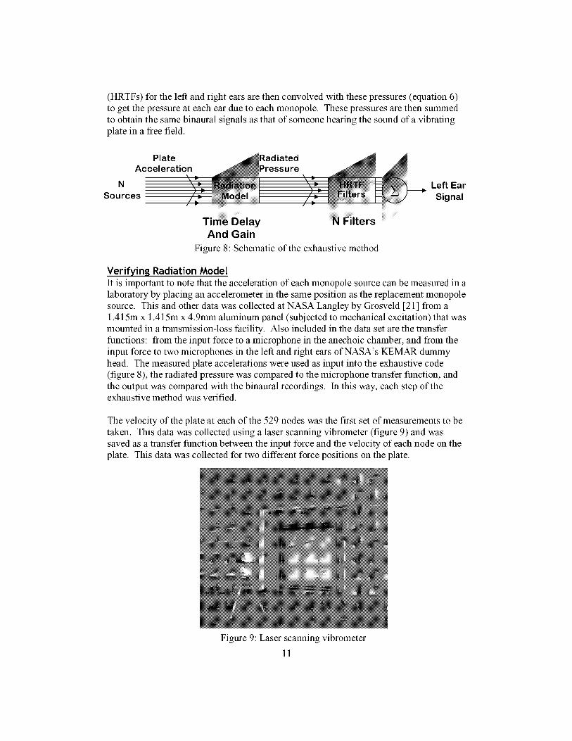
(HRTFs) for the left and right ears are then convolved with these pressures (equation 6)

to get the pressure at each ear due to each monopole. These pressures are then summed

to obtain the same binaural signals as that of someone hearing the sound of a vibrating

plate in a free field.

Plate _Radiated _Acceleration _Pressure _

Sources _;i;,: //'_ !i;,:_

Time Delay N Filters

And Gain

Figure 8: Schematic of the exhaustive method

Left Ear

Signal

Verifyin.q Radiation Model

It is important to note that the acceleration of each monopole source can be measured in a

laboratory by placing an accelerometer in the same position as the replacement monopole

source. This and other data was collected at NASA Langley by Grosveld [21] from a

1.415m x 1.415m x 4.9mm aluminum panel (subj ected to mechanical excitation) that was

mounted in a transmission-loss facility. Also included in the data set are the transfer

functions: from the input force to a microphone in the anechoic chamber, and from the

input force to two microphones in the left and right ears ofNASA's KEMAR dummy

head. The measured plate accelerations were used as input into the exhaustive code

(figure 8), the radiated pressure was compared to the microphone transfer function, and

the output was compared with the binaural recordings. In this way, each step of theexhaustive method was verified.

The velocity of the plate at each of the 529 nodes was the first set of measurements to be

taken. This data was collected using a laser scanning vibrometer (figure 9) and was

saved as a transfer function between the input force and the velocity of each node on the

plate. This data was collected for two different force positions on the plate.

Figure 9: Laser scanning vibrometer

11

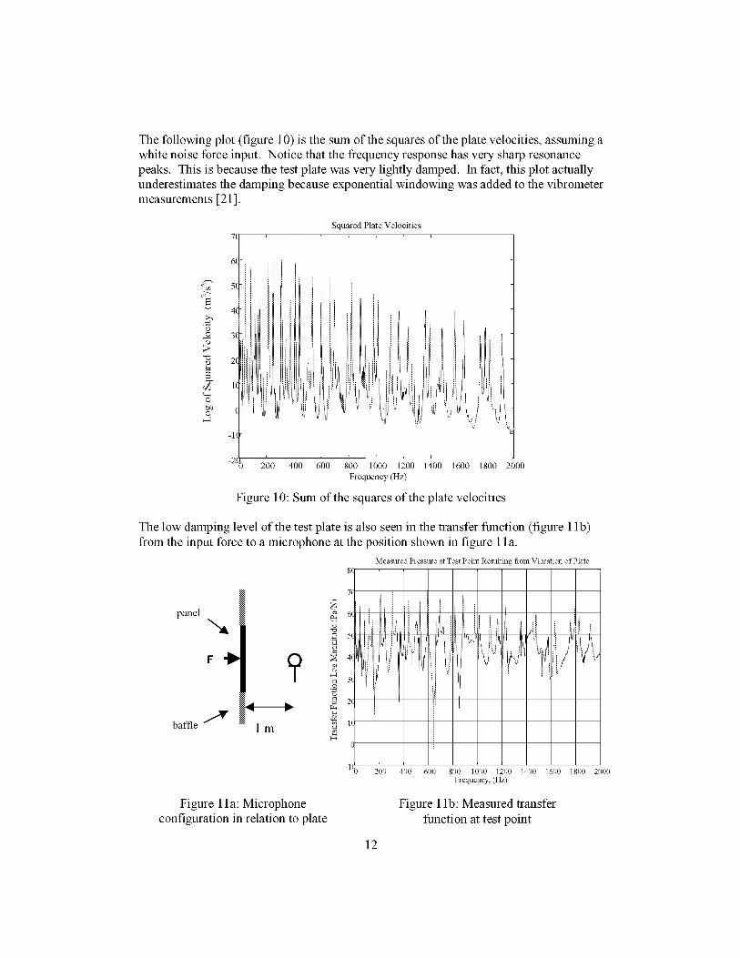
Thefollowingplot(figure10)is thesumofthesquaresoftheplatevelocities,assumingawhitenoiseforceinput.Noticethatthefrequencyresponsehasverysharpresonancepeaks.Thisisbecausethetestplatewasverylightlydamped.Infact,thisplotactuallyunderestimatesthedampingbecauseexponentialwindowingwasaddedtothevibrometermeasurements[21].

cq

O)©

Squared Plate Velocities

r 1 1 r _ 1 I p r

200 400 600 800 1000 1200 1400 1600 1800 2000

Frequency (Hz)

Figure 10: Sum of the squares of the plate velocities

The low damping level of the test plate is also seen in the transfer function (figure 1 lb)

from the input force to a microphone at the position shown in figure 1 la.

Measured Pressure at Test Point Resulting from Vibration of Plate

8(

panel

baffle/*

Q

lm

iii ,i' i i

_ 5( in_ i,i_

_3

2( i

I

200 400 600 800 1000 1200

Frequency,(Hz)

1400 1600 1800 2000

Figure 1 la: Microphone

configuration in relation to plate

Figure 1 lb: Measured transfer

function at test point

12

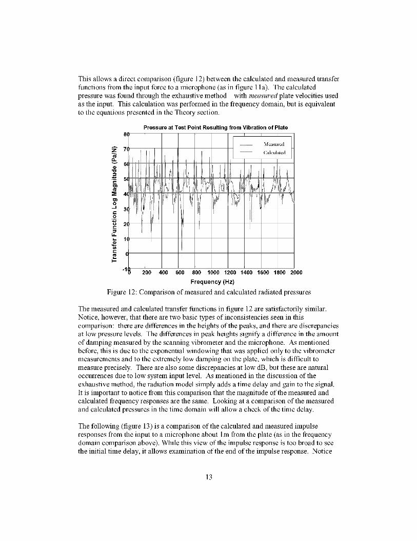
This allows a direct comparison (figure 12) between the calculated and measured transferfunctions from the input force to a microphone (as in figure 1la). The calculatedpressure was found through the exhaustive method--with measured plate velocities usedas the input. This calculation was performed in the frequency domain, but is equivalentto the equations presented in the Theory section.

Pressure at Test Point Resulting from Vibration of Plate

8(

200 400 600 800 1000 1200 1400 1600 1800 2000

Frequency (Hz)

Figure 12: Comparison of measured and calculated radiated pressures

The measured and calculated transfer functions in figure 12 are satisfactorily similar.Notice, however, that there are two basic types of inconsistencies seen in this

comparison: there are differences in the heights of the peaks, and there are discrepanciesat low pressure levels. The differences in peak heights signify a difference in the amountof damping measured by the scanning vibrometer and the microphone. As mentionedbefore, this is due to the exponential windowing that was applied only to the vibrometermeasurements and to the extremely low damping on the plate, which is difficult to

measure precisely. There are also some discrepancies at low dB, but these are naturaloccurrences due to low system input level. As mentioned in the discussion of theexhaustive method, the radiation model simply adds a time delay and gain to the signal.

It is important to notice from this comparison that the magnitude of the measured andcalculated frequency responses are the same. Looking at a comparison of the measuredand calculated pressures in the time domain will allow a check of the time delay.

The following (figure 13) is a comparison of the calculated and measured impulseresponses from the input to a microphone about lm from the plate (as in the frequencydomain comparison above). While this view of the impulse response is too broad to seethe initial time delay, it allows examination of the end of the impulse response. Notice

13

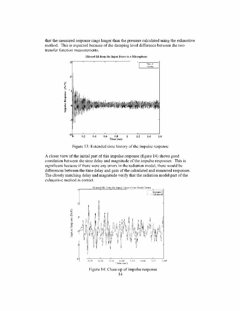
thatthemeasuredresponseringslongerthanthepressurecalculatedusingtheexhaustivemethod.Thisisexpectedbecauseofthedampingleveldifferencebetweenthetwotransferfunctionmeasurements.

Filtered IR from the Input Force to a Microphone

Measured

Calculated

Time (see)

Figure 13: Extended time history of the impulse response

A closer view of the initial part of this impulse response (figure 14) shows good

correlation between the time delay and magnitude of the impulse responses. This issignificant because if there were any errors in the radiation model, there would bedifferences between the time delay and gain of the calculated and measured responses.The closely matching delay and magnitude verify that the radiation model part of theexhaustive method is correct.

i

EJI

Filtered IR from the Input Force to, the Head Center ,

Measured

..... Calculated

t I t t I I I

0.01 0.02 0.03 0.04 0.05 0.06 0.07Time (sec)

Figure 14: Close-up of impulse response14

0.08

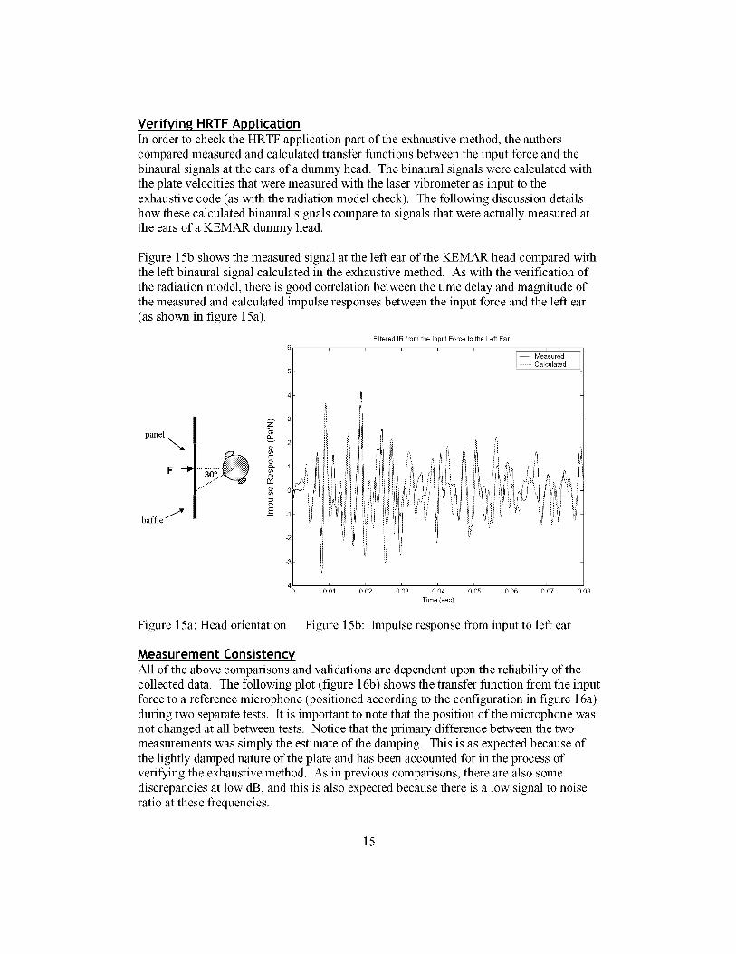
Verifyin.q HRTF ApplicationIn order to check the HRTF application part of the exhaustive method, the authorscompared measured and calculated transfer functions between the input force and thebinaural signals at the ears of a dummy head. The binaural signals were calculated withthe plate velocities that were measured with the laser vibrometer as input to the

exhaustive code (as with the radiation model check). The following discussion detailshow these calculated binaural signals compare to signals that were actually measured atthe ears of a KEMAR dummy head.

Figure 15b shows the measured signal at the left ear of the KEMAR head compared withthe left binaural signal calculated in the exhaustive method. As with the verification ofthe radiation model, there is good correlation between the time delay and magnitude ofthe measured and calculated impulse responses between the input force and the left ear

(as shown in figure 15a).

Filtered IR from the Input Force to the Left Ear

6 i

------- Calculated

baffle 7

g:

E

-3

-40 0.01 0.02 0.03 0.04 0.05 0.06 0.07

Time (sec)

0.08

Figure 15a: Head orientation Figure 15b: Impulse response from input to left ear

Measurement ConsistencyAll of the above comparisons and validations are dependent upon the reliability of thecollected data. The following plot (figure 16b) shows the transfer function from the inputforce to a reference microphone (positioned according to the configuration in figure 16a)

during two separate tests. It is important to note that the position of the microphone wasnot changed at all between tests. Notice that the primary difference between the twomeasurements was simply the estimate of the damping. This is as expected because ofthe lightly damped nature of the plate and has been accounted for in the process ofverifying the exhaustive method. As in previous comparisons, there are also some

discrepancies at low dB, and this is also expected because there is a low signal to noiseratio at these frequencies.

15

p_fflel

baffle./v

?

Figure 16a: Referencemicrophone configuration

2

o_

u_

F-

Transfer Function from the Input Force to the Reference Microphone

8O

7O

6O

5O

4O

3O

2O

10

00

........ Test 22Test 30

100 200 300 400 500 600 700 800 900 1000

Frequency (Hz)

Figure 16a: Reference

microphone transfer function

Wavenumber DecompositionAfter verifying the consistency of measurements, the authors used wavenumberdecomposition [18, 19] to find the frequency range for which the data is accurate. Theplate was measured every 0.06m (figure 17a), which corresponds to a sample

wavenumber of k_,= 2rc/)_= 102 rad/m. Spatial aliasing will occur if the wavenumber onthe plate is greater than half the sampling wavenumber. Figure 17b shows thewavenumber decomposition of the plate velocities at 550 Hz. At this frequency, thewaves on the plate have wavenumbers mainly around k = 22 rad/m, where k is defined

according to equation 8:

11/4__,,_ (8)

Here D is defined as:

Eh 3

D = 12(1_V2) (9)

where E is the modulus of elasticity of the plate, h is the plate thickness, and v is thepoisson's ratio of the plate.

Notice that the acoustic wavenumber, k, = _0/c (which defines the wavenumber

components that actually radiate sound from the plate) is only 10 rad/m, which is smallerthan the structural wavenumber. This will become important in the discussion ofwavenumber filtering later in the text. Figures 17c and 17d show the wavenumber

16

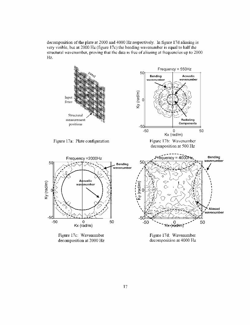
decompositionof theplateat2000and4000Hzrespectively.In figure17daliasingisveryvisible,butat2000Hz(figure17c)thebendingwavenumberisequaltohalfthestructuralwavenumber,provingthatthedatais freeofaliasingatfrequenciesupto 2000Hz.

5¢

EInput -o Cforce v

>,

Structural

measurement

positions

5¢

E"O

v

>,

-5(-50

Figure 17a: Plate configuration

Frequency :2000Hz

_.i/'0:

(:/ / A'oustic

!_ / way _number -

\'

0 IOKx (radlm)

I Bendingwavenumber

Figure 17c: Wavenumber

decomposition at 2000 Hz

-5(-50

Frequency = 550Hz

Bendingwavenumber

.,,!jY_'-t\

<L,_r :):}<

\( -:< i))-_',, _., IZ_

Acoustic

wavenumber

_-7,-,'az

Radiating

Components

0Kx (rad/m)

Figure 17b: Wavenumberdecomposition at 500 Hz

uJnc ---'Z0"0

"" "K_-(r-a@rn)"

Figure 17d: Wavenumberdecomposition at 4000 Hz

5O

Bendingwavenumber

/

Jwavenumber

50

17

Reduction Methods

Having completed and verified the exhaustive method of calculating the binaural signalsresulting from a structural acoustic source, the next step was to examine various methodsfor reducing the computing time and power required to make these calculations. Several

reduction methods were examined, including: Wavenumber filtering, Equivalent SourceReduction, and Singular Value Decomposition. Of the three, wavenumber filtering wasnot used in this research. However, both Equivalent Source Reduction and SingularValue Decomposition were quite useful in reducing the amount of computations required.

All three of these methods will be discussed, and a comparison will be made between thecomputations required in the SVD, ESR, and exhaustive methods.

Wavenumber Filtering

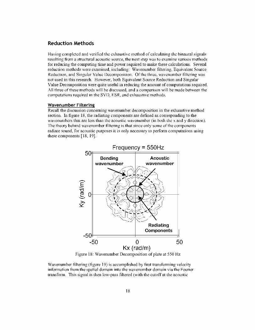
Recall the discussion concerning wavenumber decomposition in the exhaustive methodsection. In figure 18, the radiating components are defined as corresponding to thewavenumbers that are less than the acoustic wavenumber (in both the x and y direction).

The theory behind wavenumber filtering is that since only some of the componentsradiate sound, for acoustic purposes it is only necessary to perform computations usingthese components [18, 19].

5O

E

CI,=.v

>,

Frequency = 550Hz

Bendingwavenumber

) ,,,4i-::,"\_

;Vi'. ii

Acousticwavenumber

_ :_-i;:-,I

RadiatingComponents

0 50

Kx (rad/m)Figure 18: Wavenumber Decomposition of plate at 550 Hz

Wavenumber filtering (figure 19) is accomplished by first transforming velocityinformation from the spatial domain into the wavenumber domain via the Fouriertransform. This signal is then low-pass filtered (with the cutoff at the acoustic

18

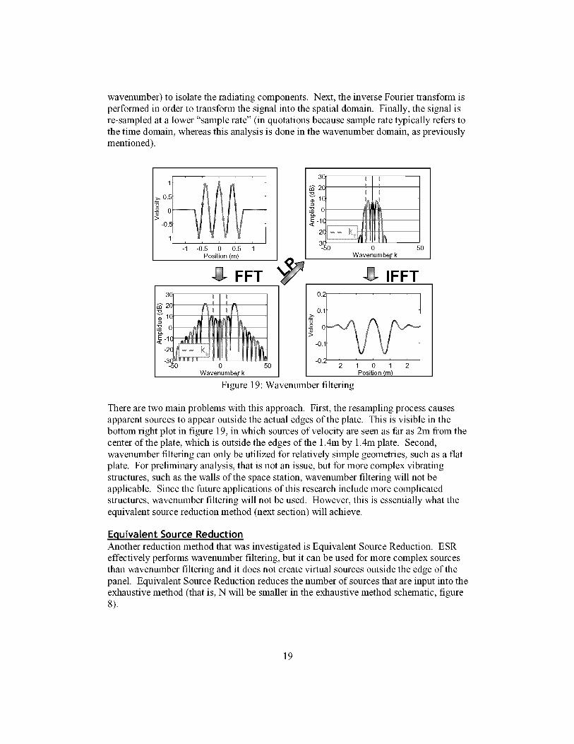
wavenumber)toisolatetheradiatingcomponents.Next,theinverseFouriertransformisperformedin ordertotransformthesignalintothespatialdomain.Finally,thesignalisre-sampledatalower"samplerate"(inquotationsbecausesampleratetypicallyreferstothetimedomain,whereasthisanalysisis donein thewavenumberdomain,aspreviouslymentioned).

VVVV]-1 -0.5 0 0.5 1

Position (m)

FFT

30t

_" 2ol _

Wavenumbe4; k

50

IFFT

-2 -1 0 1 2

Position (m)

Figure 19: Wavenumber filtering

There are two main problems with this approach. First, the resampling process causesapparent sources to appear outside the actual edges of the plate. This is visible in the

bottom right plot in figure 19, in which sources of velocity are seen as far as 2m from thecenter of the plate, which is outside the edges of the 1.4m by 1.4m plate. Second,wavenumber filtering can only be utilized for relatively simple geometries, such as a flatplate. For preliminary analysis, that is not an issue, but for more complex vibrating

structures, such as the walls of the space station, wavenumber filtering will not beapplicable. Since the future applications of this research include more complicatedstructures, wavenumber filtering will not be used. However, this is essentially what the

equivalent source reduction method (next section) will achieve.

Equivalent Source Reduction

Another reduction method that was investigated is Equivalent Source Reduction. ESReffectively performs wavenumber filtering, but it can be used for more complex sourcesthan wavenumber filtering and it does not create virtual sources outside the edge of thepanel. Equivalent Source Reduction reduces the number of sources that are input into theexhaustive method (that is, N will be smaller in the exhaustive method schematic, figure

S).

19

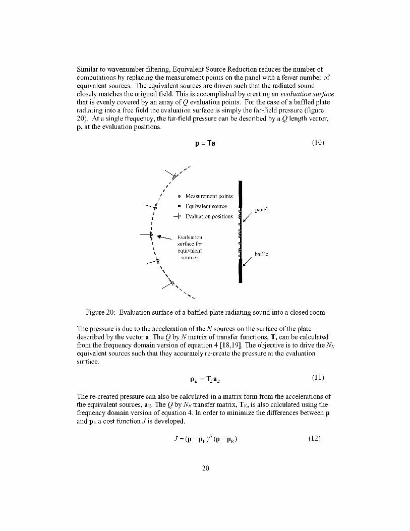
Similarto wavenumberfiltering,EquivalentSourceReductionreducesthenumberofcomputationsbyreplacingthemeasurementpointsonthepanelwithafewernumberofequivalentsources.Theequivalentsourcesaredrivensuchthattheradiatedsoundcloselymatchestheoriginalfield.Thisisaccomplishedbycreatinganevaluation surfacethat is evenly covered by an array of Q evaluation points. For the case of a baffled plateradiating into a free field the evaluation surface is simply the far-field pressure (figure

20). At a single frequency, the far-field pressure can be described by a Q length vector,p, at the evaluation positions.

p -- Ta (10)

.g

f

t o Measurement points

® Equivalent source

@ Evaluation positions

--_ _ Evaluation

surface for

equivalent

_._ SOurces

/I£.

panel

/

baffle

/

Figure 20: Evaluation surface of a baffled plate radiating sound into a closed room

The pressure is due to the acceleration of the N sources on the surface of the platedescribed by the vector a. The Q by Nmatrix of transfer functions, T, can be calculated

from the frequency domain version of equation 4 [18,19]. The objective is to drive the Neequivalent sources such that they accurately re-create the pressure at the evaluationsurface.

PE = TEaE (1 1)

The re-created pressure can also be calculated in a matrix form from the accelerations ofthe equivalent sources, aE. The Q by Ne transfer matrix, TE, is also calculated using thefrequency domain version of equation 4. In order to minimize the differences between p

and pE a cost function J is developed.

J = (P - PE)+ (P -- PE) (12)

20

Thisturnsouttobeaquadraticmatrixproblemwithauniqueminimumwhen[17,22],

aE: [T %]IT "Ta: Wa (13)

The superscript H denotes the Hermitian or conjugate transpose. The term [T_T E]'T_ is

often called the pseudo-inverse of TE. This is performed at all of the frequencies of

interest to create a matrix of filters, W, (in the frequency domain) that transform theaccelerations, a, into the reduced set of accelerations, aE. By transforming the matrix offilters, W, into the time domain, the set of N time domain accelerations can be filtered

into the reduced set of Nu equivalent accelerations (or sources). This can be done in apre-processing stage before any real-time simulation is carried out.

For this technique to work well there must be (i) a sufficient number of evaluation

positions (Q>N) and (ii) there must be at least two equivalent sources per acousticwavelength whereas the measurements need to be every half of a structural wavelength(figure 21). Therefore, this technique will only be useful when the waves on the structureare predominantly subsonic (i.e. shorter than the acoustic wavelengths) as with the test

plate below 2000Hz. It should be noted that the recreated acoustic field does not matchthe near-field of the original source accurately and will not produce good results close tothe panel. However, virtual acoustic applications, in general, do not take into account therefractive effect of the head close to a source of a sound or the effect of near sources on

the HRTFs. Therefore, it is thought that some inaccuracy can be tolerated in thesecircumstances.

Acoustic

wavelength Structural

wavelength

Figure 21:

Equivalent

sourceStructural

measurements

The equivalent source spacing depends on the acoustic wavelength

21

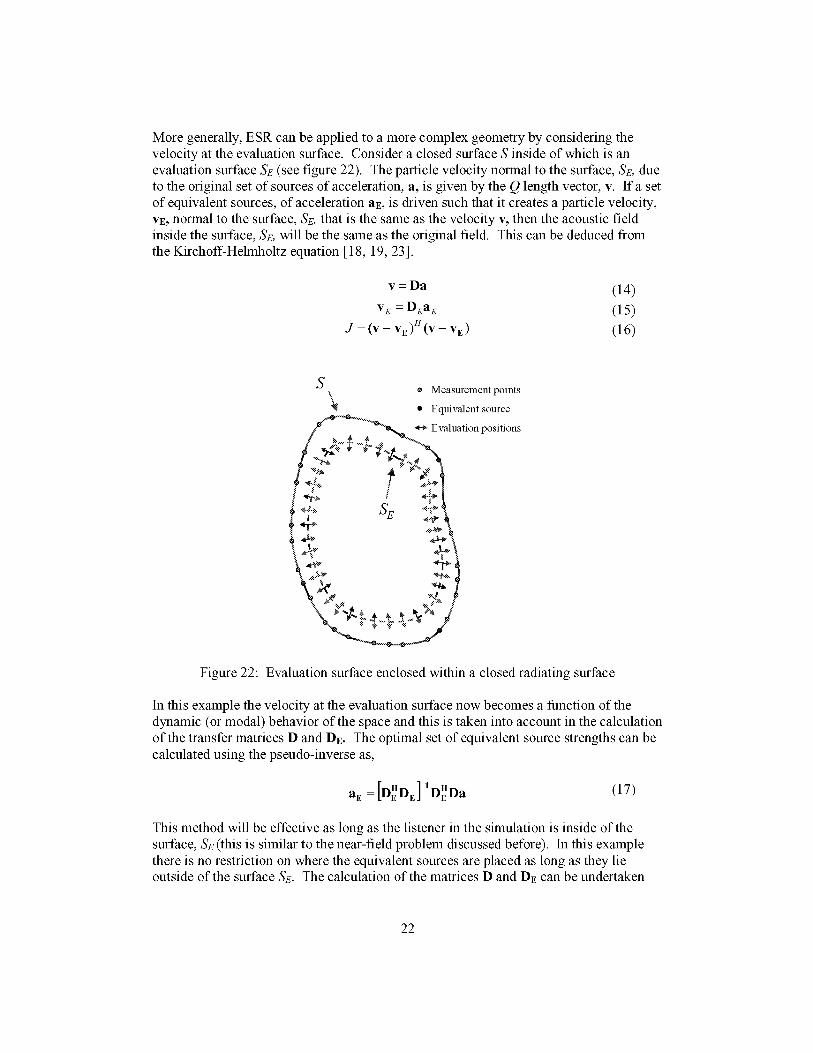
Moregenerally,ESRcanbeappliedtoamorecomplexgeometrybyconsideringthevelocityattheevaluationsurface.ConsideraclosedsurfaceS inside of which is anevaluation surface Se (see figure 22). The particle velocity normal to the surface, Se, dueto the original set of sources of acceleration, a, is given by the Q length vector, v. If a setof equivalent sources, of acceleration aE, is driven such that it creates a particle velocity,VE,normal to the surface, Se, that is the same as the velocity v, then the acoustic field

inside the surface, Se, will be the same as the original field. This can be deduced fromthe Kirchoff-Helmholtz equation [18, 19, 23 ].

v--Da (14)

v_ = D_a_ (15)

J = (v - vE)_ (v- vE) (16)

So Measurement points

e Equivalent source

_-_ Evaluation positions

Figure 22: Evaluation surface enclosed within a closed radiating surface

In this example the velocity at the evaluation surface now becomes a function of thedynamic (or modal) behavior of the space and this is taken into accotmt in the calculation

of the transfer matrices D and DE. The optimal set of equivalent source strengths can becalculated using the pseudo-inverse as,

H 1 Ha E = [DED E] D EDa (17)

This method will be effective as long as the listener in the simulation is inside of the

surface, Se (this is similar to the near-field problem discussed before). In this examplethere is no restriction on where the equivalent sources are placed as long as they lieoutside of the surface Se. The calculation of the matrices D and DE can be undertaken

22

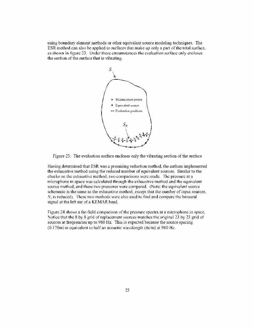
usingboundaryelementmethodsorotherequivalentsourcemodelingtechniques.TheESRmethodcanalsobeappliedto surfacesthatmakeuponlyapartofthetotalsurface,asshownin figure23. Underthesecircumstancestheevaluationsurfaceonlyenclosesthesectionofthesurfacethatisvibrating.

S\

Figure 23: The evaluation surface encloses only the vibrating section of the surface

Having determined that ESR was a promising reduction method, the authors implementedthe exhaustive method using the reduced number of equivalent sources. Similar to the

checks on the exhaustive method, two comparisons were made. The pressure at amicrophone in space was calculated through the exhaustive method and the equivalentsource method, and these two pressures were compared. (Note: the equivalent sourceschematic is the same as the exhaustive method, except that the number of input sources,

N, is reduced). These two methods were also used to find and compare the binauralsignal at the left ear of a KEMAR head.

Figure 24 shows a far-field comparison of the pressure spectra at a microphone in space.

Notice that the 8 by 8 grid of replacement sources matches the original 23 by 23 grid ofsources at frequencies up to 980 Hz. This is expected because the source spacing

(0.176m) is equivalent to half an acoustic wavelength (rcc/_o) at 980 Hz.

23

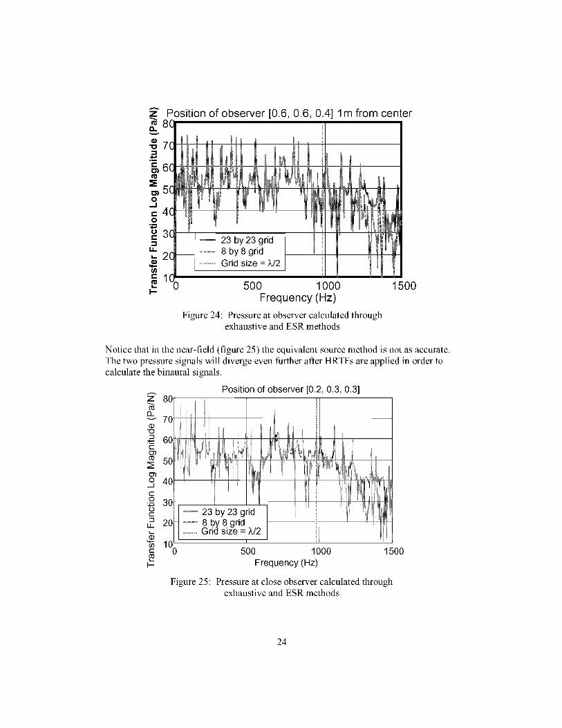
Position of observer [0.6, 0.6, 0.4] lm from center

Figure 24:

_mJ

500 1000 1500

Frequency (Hz)

Pressure at observer calculated throughexhaustive and ESR methods

Notice that in the near-field (figure 25) the equivalent source method is not as accurate.

The two pressure signals will diverge even further after HRTFs are applied in order to

calculate the binaural signals.

Z

[3_v

(D

OJ

t--._o

[a_

t--

80

70

60

50

Position of observer [0.2, 0.3, 0.3]

i

40

30i

_ 23 by 23 grid20 i ........ 8 by 8 grid

Grid size = X/2

100 500 1000 1500

Frequency (Hz)

Figure 25: Pressure at close observer calculated throughexhaustive and ESR methods

24

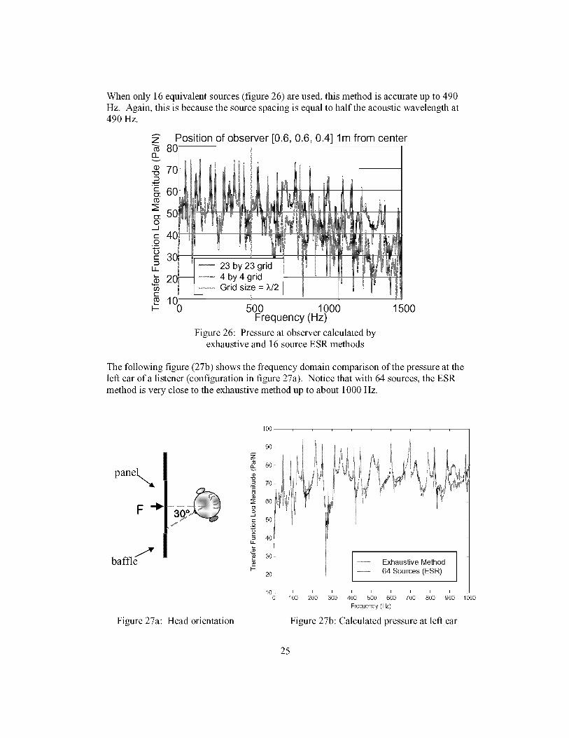
When only 16 equivalent sources (figure 26) are used, this method is accurate up to 490

Hz. Again, this is because the source spacing is equal to half the acoustic wavelength at490 Hz.

Z

t_O_

09

--3,m

gt_

oJ

¢-o

,m

oe-

L.

o0¢-

Position of observer [0.6, 0.6, 0.4] lm from center8O

70-'-'--'--jj

60

40 --_,_U

30 _]

23 by 23 grid

20 4 by 4 gridGrid size = X/2

] q

00 500 1000Frequency (Hz)

Figure 26: Pressure at observer calculated byexhaustive and 16 source ESR methods

H

1500

The following figure (27b) shows the frequency domain comparison of the pressure at theleft ear of a listener (configuration in figure 27a). Notice that with 64 sources, the ESRmethod is very close to the exhaustive method up to about 1000 Hz.

panel_

Figure 27a: Head orientation

lOO

9o

__ 8o

7o

60g

._ 50

= 40ij_

30

2O

100

i_ i_ i''Eiii ' ii

....... Exhaustive Method

64 Sources (ESR)

i i i i i i i i i

100 200 300 400 500 600 700 800 900 lOOO

Frequency (Hz)

Figure 27b: Calculated pressure at left ear

25

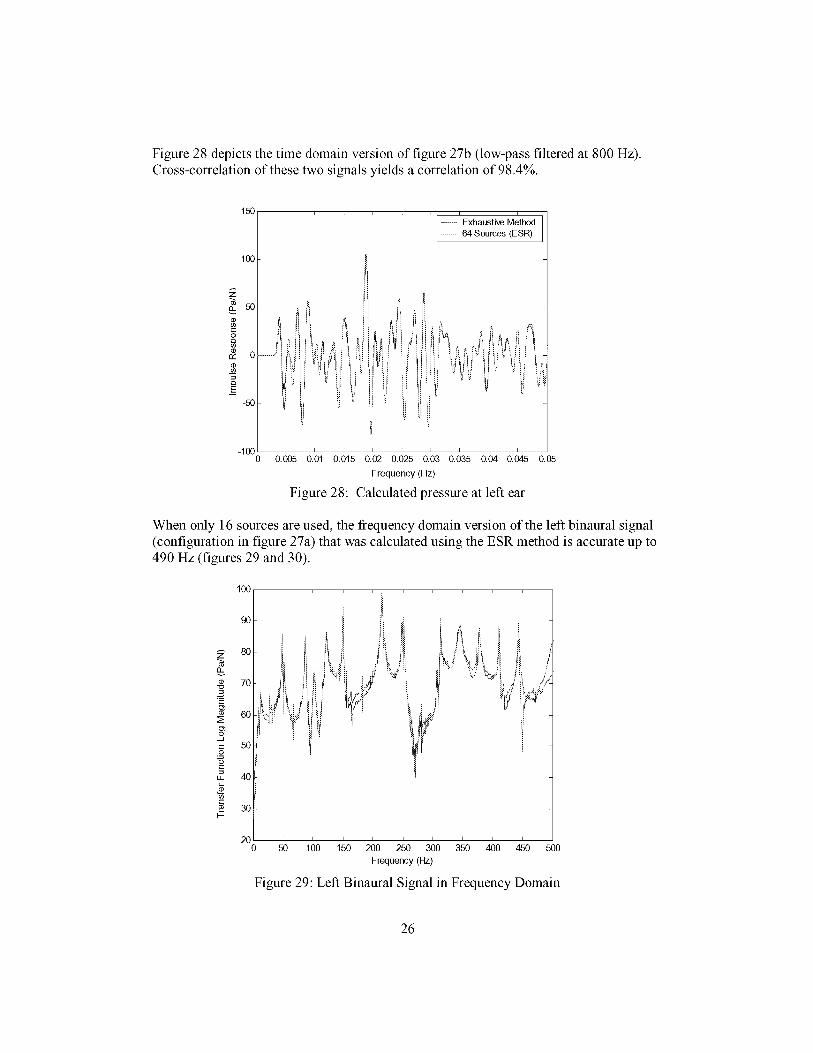
Figure 28 depicts the time domain version of figure 27b (low-pass filtered at 800 Hz).

Cross-correlation of these two signals yields a correlation of 98.4%.

150

100

Z

#: o

-50

-100

lli,i

Exhaustive Method64 Sources (ESR)

i i [ [ [

0.505 0.01 0.015 0.02 0.025 0.03 0.035 0.04 0.045 0.05

Frequency (Hz)

Figure 28: Calculated pressure at left ear

When only 16 sources are used, the frequency domain version of the left binaural signal

(configuration in figure 27a) that was calculated using the ESR method is accurate up to

490 Hz (figures 29 and 30).

Z

_J

Y_

F--

100

9O

80

70

60

50

40

30

20 r i i r i r r i r

0 50 100 150 200 250 300 350 400 450 500

Frequency (Hz)

Figure 29: Left Binaural Signal in Frequency Domain

26

In the time domain (with a low-pass filter at 400 Hz), the correlation is found to be 98%.

ii ' ' _ _'.... Exhau'stiva M;thod] 16 Sources (ESR)

30

-3o

-4O0 0.005 0.01 0.015 0.02 0.025 0.03 0.035 0.04 0.045 0.05

Frequency (Hz)

Figure 30: Left Binaural Signal in Time Domain

Singular Value DecompositionA third reduction method investigated was singular value decomposition [23]. By

breaking down the matrix of HRTFs into three separate matrices, the number ofconvolutions can be greatly reduced. Since convolution is computationally expensive, agreat deal of processing time can be avoided by a small amotmt ofpre-processing. Thisdiscussion will describe how singular value decomposition works, how it applies to theexhaustive method, and the comparisons that were made to verify that the SVD method isaccurate.

Singular value decomposition is simply separating a matrix (in this case a matrix of

HRTFs) into three separate matrices: U, Z, and V (equation 18).

HRTFs = U * Z * V r (18)

U is a matrix of left singular vectors, Z is a diagonal matrix of singular values, and V is amatrix containing right singular vectors. The relative sizes of these matrices are visible

in figure 31. It is important to note that singular value decomposition of the HRTFmatrix can be done in either the time or frequency domain, but for the following analysis,the SVD was performed on a matrix of HRTFs in the time domain.

27

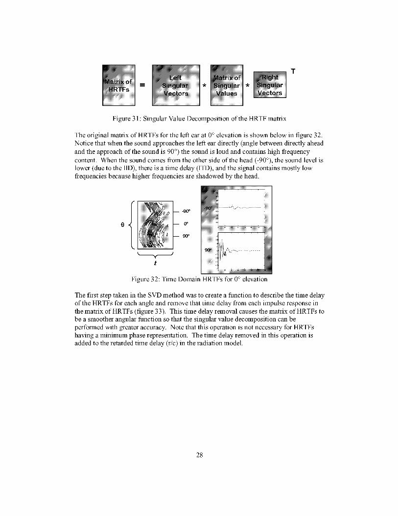
Figure31:SingularValueDecompositionoftheHRTFmatrix

Theoriginalmatrixof HRTFsfortheleft earat0° elevation is shown below in figure 32.

Notice that when the sound approaches the left ear directly (angle between directly ahead

and the approach of the sound is 90 °) the sound is loud and contains high frequency

content. When the sound comes from the other side of the head (-90°), the sound level islower (due to the IID), there is a time delay (ITD), and the signal contains mostly lowfrequencies because higher frequencies are shadowed by the head.

....iiiiiiiiiiiiiiii: _iiii iiiiiiiiiiiiiiii

_9oo

oo

90 °

t

Figure 32: Time Domain HRTFs for 0° elevation

The first step taken in the SVD method was to create a function to describe the time delayof the HRTFs for each angle and remove that time delay from each impulse response in

the matrix of HRTFs (figure 33). This time delay removal causes the matrix of HRTFs tobe a smoother angular function so that the singular value decomposition can beperformed with greater accuracy. Note that this operation is not necessary for HRTFshaving a minimum phase representation. The time delay removed in this operation isadded to the retarded time delay (r/c) in the radiation model.

28

O

Figure 33: Time domain HRTFs with ITD removed

The singular value decomposition of the HRTF matrix (without time delays) is shownbelow in figure 34. Notice that the left singular vector matrix contains angular

information for each singular value _. The matrix of singular values is simply a diagonalmatrix of singular values, which diminish in value as i becomes larger. Time informationper singular value is contained in the right singular vector matrix. When these threematrices are multiplied together, the matrix of HRTFs (without time delays) will be the

result. The advantage of SVD is that an approximate HRTF matrix can be obtained usingonly a few singular values. This will become important as the SVD process is applied tothe exhaustive method.

i_: _i_iiiiiiiiiiiiiiiiiiiiiiiiiiiiiii

iiiiiiiiiiiiiiiiiiiiiiiiiiiiiiiiiiiii

k JY

t

::::::::::::::::::::::::::::::::::::::::::::::_

i_i_iiiii_iiiiii4iiiiii!! I

iliiiiiiii_i° ::iiiiiiiiiiiii!!iliiiii_iiiiioii!iiiiiiiiiiiiiiiiiii)i)i)iiiiiiiiiiioiiii_iio]]ii *t]]]]]!]ii]i!]]]I

Figure 34: SVD of time domain HRTFs

Recall the schematic of the exhaustive code in figure 8. Shown below is a similarschematic of the SVD reduction method (figure 35). Note that instead of simply

convolving the HRTFs with the radiated pressure for each of the N sources, the SVDmethod expands the application of the HRTFs into four faster operations that areperformed for each of M important singular values. The first operation is a scalarmultiplication (radiated pressure times U(i) for i = 1:M) for each of the N sources. The

signals are then summed and convolved only M times with the right singular vectors (V(i)

for i = 1:M). Each filtered signal is then multiplied by its singular value, (_, and thensummed to produce the left ear signal (a similar process is carried out for the right ear

29

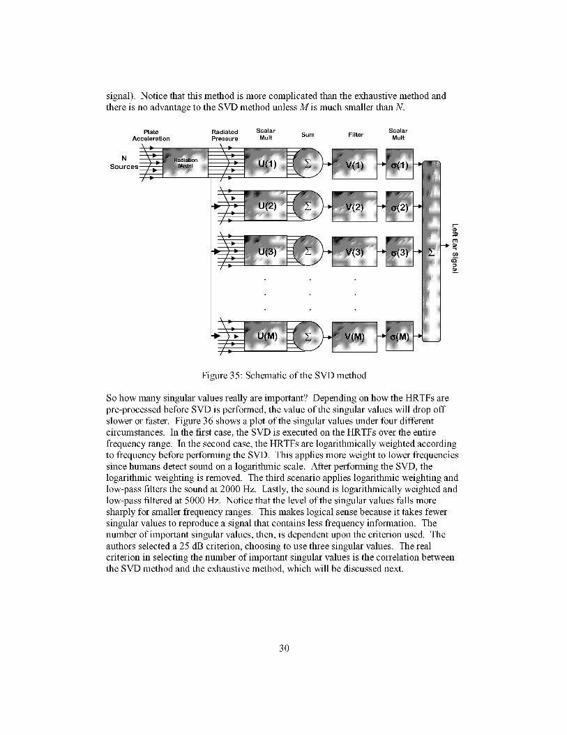
signal).NoticethatthismethodismorecomplicatedthantheexhaustivemethodandthereisnoadvantagetotheSVDmethodunlessM is much smaller than N.

Plate Radiated Scalar Scalar

Acceleration Pressure Mult Sum Filter Mult

[--

m

iiiiiiiiii

Figure 35: Schematic of the SVD method

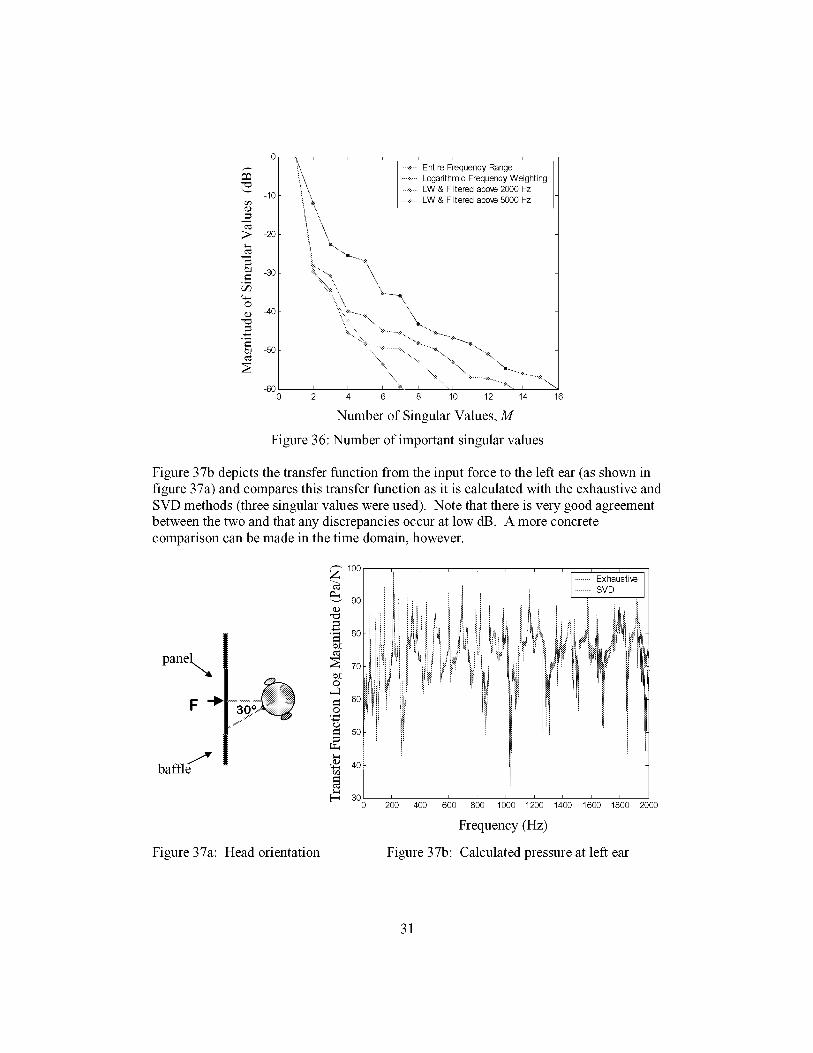
So how many singular values really are important? Depending on how the HRTFs arepre-processed before SVD is performed, the value of the singular values will drop offslower or faster. Figure 36 shows a plot of the singular values under four differentcircumstances. In the first case, the SVD is executed on the HRTFs over the entire

frequency range. In the second case, the HRTFs are logarithmically weighted accordingto frequency before performing the SVD. This applies more weight to lower frequenciessince humans detect sound on a logarithmic scale. After performing the SVD, the

logarithmic weighting is removed. The third scenario applies logarithmic weighting andlow-pass filters the sound at 2000 Hz. Lastly, the sound is logarithmically weighted andlow-pass filtered at 5000 Hz. Notice that the level of the singular values falls moresharply for smaller frequency ranges. This makes logical sense because it takes fewer

singular values to reproduce a signal that contains less frequency information. Thenumber of important singular values, then, is dependent upon the criterion used. Theauthors selected a 25 dB criterion, choosing to use three singular values. The realcriterion in selecting the number of important singular values is the correlation betweenthe SVD method and the exhaustive method, which will be discussed next.

3O

m

>

©

o

-lO

-2o

-3o

4o

-5o

-6o

--", j i L

_)\ ....... Entire Frequency Range

"\ ---_---Logarithmic Frequency Weighting

\ - _ LW & Filtered above 2000 Hzi "_ .....+... LW & Filtered above 5000 Hz

I

2 16

,, ... \\

[ I _, I ", I [ "_, I

4 6 8 10 12 14

Number of Singular Values, M

Figure 36: Number of important singular values

Figure 37b depicts the transfer function from the input force to the left ear (as shown in

figure 37a) and compares this transfer function as it is calculated with the exhaustive andSVD methods (three singular values were used). Note that there is very good agreementbetween the two and that any discrepancies occur at low dB. A more concretecomparison can be made in the time domain, however.

Figure 37a: Head orientation

5O

300

-' Exhaustive

SVD

200 400 600 800 1000 1200 1400 1600 1800 2000

Frequency (Hz)

Figure 37b: Calculated pressure at left ear

31

Figure38showsthesametransferfunctionfromtheinputforceto theleftearasshownabove,butin thetimedomain.Sincethedataisonlygoodupto2000Hz,a low-passfilterat1600Hzwasapplied.ThecorrelationbetweentheSVD(only3singularvaluesused)andexhaustivemethodswasaremarkable97.7%.Fromthisresulttheauthorsconcludedthatsingularvaluedecompositionisanaccuratereductionmethodandcanbeeffectivelyusedinthisresearch.

©

300

250

200

150

100

50

0 i

-50

-100

-150

-200

I ...... Exhaustive Method3 S ngu ar Va ues (SVD)

0 0.001 0.002 0.003 0.004 0.005 0.006 0.007 0.008 0.009

Time (s)

Figure 38: Impulse response between input force and left ear

0.01

ESR and SVD TogetherSince the ESR method works to reduce the number of input sources while the SVD

method changes how HRTFs are applied, the two methods can be used simultaneously toyield an even greater reduction in computation time. Figure 39 shows a time domaincomparison of the combined reduction methods and the exhaustive method. In this case,three singular values and an eight by eight grid of equivalent sources were used. Because

the ESR method for an eight by eight grid is only accurate up to 980 Hz, a low-pass filterat 800 Hz was applied. A correlation of 97% was found between the combined reductionmethod and the exhaustive method. This level of accuracy is sufficient to conclude thatthe combined reduction method can be effectively used in this research.

32

©

150

IO0

5O

o .......-J

-50

-1000

i i i i i

.......... Exhaustive Method3 SVs (SVD) & 64 Sources (ESR)

! ,, , t\;_ IE_[,tt _l ,

- i:! J _ ]

, , , • , • , , ,0.005 0.01 0.015 0.02 0.025 0.03 0.035 0.04 0.045 0.05

Time (s)

Figure 39: Impulse response between input force and left ear

Computation TimeNow that it has been verified that the ESR, SVD, and combined reduction methods can

accurately replace the exhaustive method, it remains to determine if these methodsactually reduce the number of computations in this analysis. To handle this problem, the

authors developed an estimate of the computation time required for each method that isbased solely upon the number of additions and multiplications used in each method.

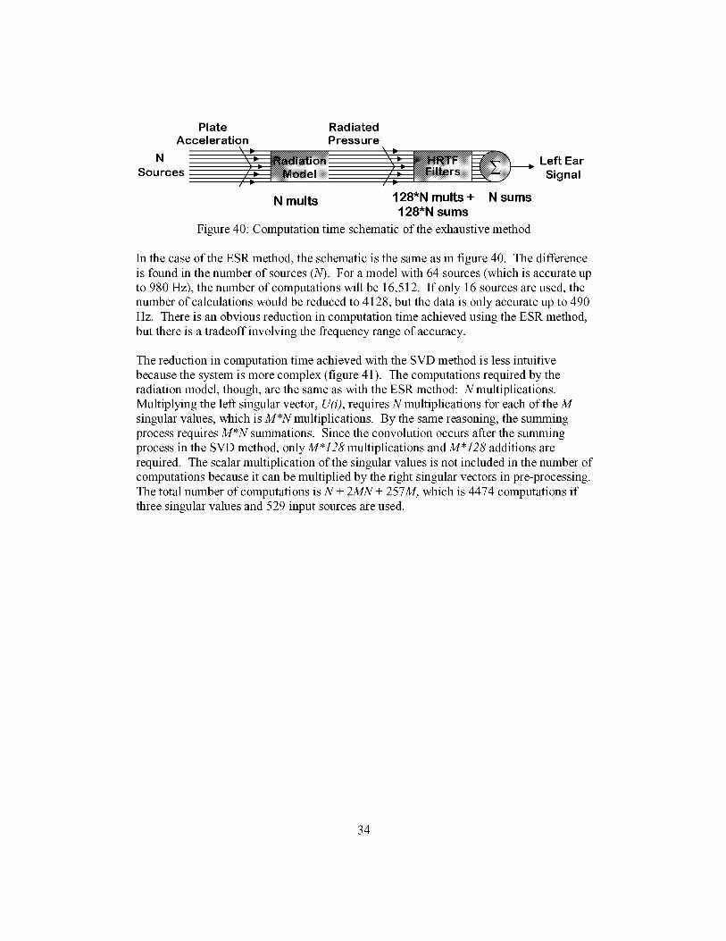
The schematic of the exhaustive method is shown below in figure 40. Since the radiationmodel process is scalar multiplication, the number of computations is modeled to be N

multiplications. Convolution is required in the process of filtering the radiated pressurewith the HRTFs, so the number of computations required will be 128"N multiplicationsplus 128"N additions. Summing the N components of the left ear signal is simply N

summations. In this model, addition and multiplication are estimated to requireapproximately the same amount of computation time. Adding up the number ofsummations and multiplications required by the exhaustive method yields a total of258"N computations. In the case of the original plate, with a 23 by 23 grid of

measurement points, the total number of computations would be 136,482.

33

PlateAcceleration

N

Sources

RadiatedPressure

N mults 128"N mults + N sums128"N sums

Figure 40: Computation time schematic of the exhaustive method

Left Ear

Signal

In the case of the ESR method, the schematic is the same as in figure 40. The difference

is found in the number of sources (N). For a model with 64 sources (which is accurate up

to 980 Hz), the number of computations will be 16,512. If only 16 sources are used, the

number of calculations would be reduced to 4128, but the data is only accurate up to 490

Hz. There is an obvious reduction in computation time achieved using the ESR method,

but there is a tradeoff involving the frequency range of accuracy.

The reduction in computation time achieved with the SVD method is less intuitive

because the system is more complex (figure 41). The computations required by the

radiation model, though, are the same as with the ESR method: Nmultiplications.

Multiplying the left singular vector, U(i), requires N multiplications for each of the M

singular values, which is M*N multiplications. By the same reasoning, the summing

process requires M*N summations. Since the convolution occurs after the summing

process in the SVD method, only M*128 multiplications and M*128 additions are

required. The scalar multiplication of the singular values is not included in the number of

computations because it can be multiplied by the right singular vectors in pre-processing.

The total number of computations is N + 2MN + 257M, which is 4474 computations if

three singular values and 529 input sources are used.

34

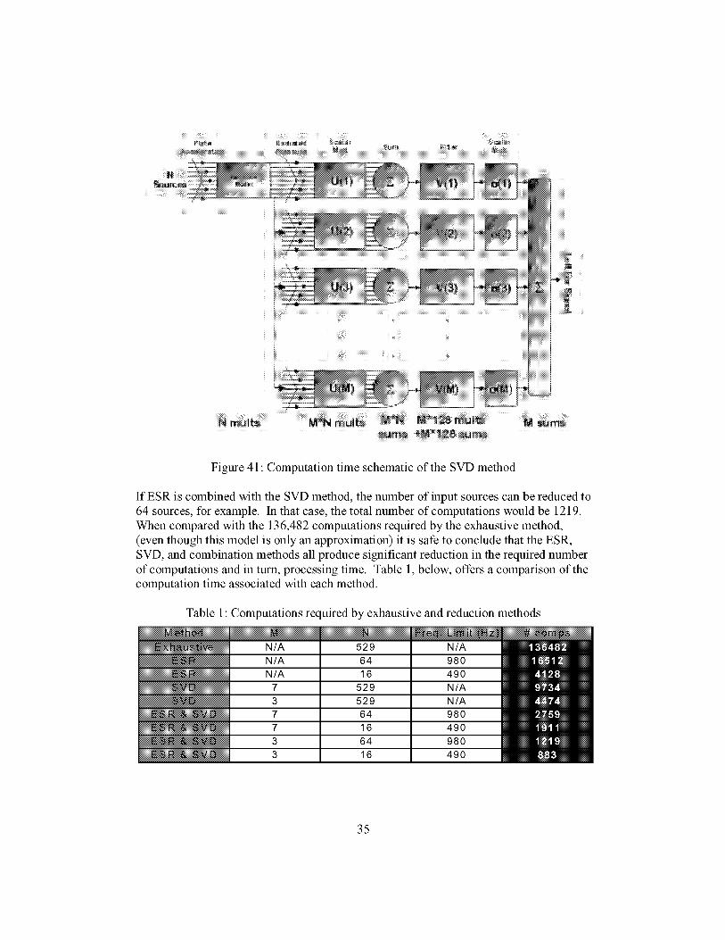
Figure 41: Computation time schematic of the SVD method

If ESR is combined with the SVD method, the number of input sources can be reduced to64 sources, for example. In that case, the total number of computations would be 1219.

When compared with the 136,482 computations required by the exhaustive method,(even though this model is only an approximation) it is safe to conclude that the ESR,SVD, and combination methods all produce significant reduction in the required number

of computations and in turn, processing time. Table 1, below, offers a comparison of thecomputation time associated with each method.

Table 1" Computations required by exhaustive and reduction methods

N/A 529 N/A

N/A 64 980

N/A 16 490

7 529 N/A

3 529 N/A

7 64 980

7 16 490

3 64 980

3 16 490

35

This reduction in computation time is important in order to create a real-time binauralsimulation of structural acoustic data. In a real-time virtual environment, the user's head

orientation is measured by a head-tracking unit and fed into the computer. Typicalupdate rates for head-tracking units are 100 Hz corresponding to one update every 10 ms.Until the computer receives another head orientation from the head-tracking unit, the leftand right ear signals are calculated based upon the current head orientation. However,

the audio and visual outputs are also based on other inputs. For instance, if thesimulation were of a jet flying overhead, the sound input from the simulated jet would beupdated at a sample rate of 44100 samples/second. This means that in order to create astructural acoustics simulation using the exhaustive method, the computer must make an

estimated 136,482 calculations per ear in about 23 _ts. With the combined reductionmethods, only 883 calculations are required per ear in the same amount of time. This isan estimated computation time reduction of 99.4%, making real-time binaural analysis ofstructural acoustic data a possibility.

Conclusion

The goal of this research has been to reduce the computation time required in calculatingthe binaural signals to reproduce the sound radiated from a vibrating structure. This wasaccomplished by developing an exhaustive method to calculate the binaural signals and

by verifying that method through a comparison of the results with actual data. Severalreduction methods were investigated and the ESR and SVD methods showed exceptionalpromise. These two methods were tested by implementing the necessary changes to thecomputer code for the exhaustive method. The results were compared with those in the

exhaustive method and found to have high correlations. In addition, the two reductionmethods can also be combined since each method's changes affect different portions ofthe calculation process. The only limiting factor with either method is that the ESRmethod has a frequency range of accuracy that depends upon the spacing of the

equivalent sources. After the accuracy of the reduction methods was determined, thecomputation time required by each method was estimated. It was found that the ESR,SVD, and combined reduction methods all accurately replace the exhaustive method forcalculating structural acoustic binaural signals while significantly reducing the estimated

computation time.

Future Work

While there is excellent correlation between the results from the reduction methods and

the exhaustive methods in objective tests, this analysis could be supported in the future

with auditory tests. Some preliminary tests have been performed, but more scientifictests involving several subjects would enhance the results of this research. In addition,the effects of an acoustic enclosure and more complex geometries have yet to beinvestigated.

36

AnotherimprovementtothisresearchwouldbetouseindividualizedHRTFsinsteadofgeneralizedones.Thelargestamountof errorintroducedintoeachmethodisprobablytheuseof generalizedHRTFs,becauseeachpersonhasdifferentlyshapedheadsandtorsos.UsingindividualizedHRTFswouldminimizethaterror,allowinglistenersinauditoryteststo distinguishsmallerrors.SincethereductionmethodscausesmallererrorsthanthatofthegeneralizedHRTFs,thiswouldgreatlyimprovethevalidityofauditorytests.

Acknowledgements

The authors would like to gratefully acknowledge the help of Dr. Stephen A. Rizzi andBrenda M. Sullivan of the NASA Langley Research Center and Dr. Ferdinand W.Grosveld of the Lockheed Martin Engineering and Sciences Company in Hampton, VA.

37

Bibliography

[1] Begault, D., 3-D Sound for Virtual Reality and Multimedia (Boston: Academic Press,1994).

[2] Cheng, C.I., and G.H. Wakefield, "Introduction to Head-Related Transfer Functions(HRTF'S): Representations of HRTF's in Time, Frequency, and Space (invited tutorial),"Proceedings of the 107 thAudio Engineering Society (AES) Convention (1999).

[3] Martens, W.L., "Principal Components Analysis and Resynthesis of Spectral Cues toPerceived Direction," 1987 ICMC Proceedings (1987), pp. 274-281.

[4] Kistler, D.J. and F.L. Wightman, "A Model of Head-Related Transfer FunctionsBased on Principal Components Analysis and Minimum-Phase Reconstruction," Journalof the Acoustical Society of America, vol. 91, no. 3 (1992), pp. 1637-1647.

[5] Chen, J., B.D. Van Veen, and K.E. Hecox, "A Spatial Feature Extraction andRegularization Model for the Head Related Transfer Function," Journal of the AcousticalSociety of America, vol. 97, no. 1 (Jan. 1995), pp. 439-452.

[6] Wu, Z., F.H.Y. Chan, F.K. Lam, and J.C.K. Chan, "A Time Domain Binaural Model

Based on Spatial Feature Extraction for the Head-Related Transfer Function," Journal ofthe Acoustical Society of America, vol. 102, no. 4 (Oct. 1997), pp. 2211-2218.

[7] Mackenzie, J., J. Huopaniemi, V. Valimaki, and I. Kale, "Low-Order Modeling of

Head-Related Transfer Functions Using Balanced Model Truncation," IEEE SignalProcessing Letters, vol. 4, no. 2 (Feb. 1997), pp. 39-41.

[8] Georgiou, P.G., and C. Kyriakakis, "Modeling of Head Related Transfer Functions

for Immersive Audio Using a State-Space Approach," Conference Record of the Thirty-Third Asilomar Conference on Signals, Systems & Computers, vol. 1 (1999), pp. 720-724.

[9] Georgiou, P.G., A. Mouchtaris, S.I. Roumeliotis, and C. Kyriakakis, "ImmersiveSound Rendering Using Laser-Based Tracking," Proceedings of the 109 thAudioEngineering Society (AES) Convention, preprint No. 5227 (Sept. 2000).

[10] Evans, M.J., J.A.S. Angus, and A.I. Tew, "Analyzing Head-Related TransferFunction Measurements Using Surface Spherical Harmonics," Journal of the AcousticalSociety of America, vol. 104, no. 4 (Oct. 1998), pp. 2400-2411.

[11] Nelson, P.A., and Y. Kahana, "Spherical Harmonics, Singular-Value Decompositionand the Head-Related Transfer Function," Journal of Sound and Vibration, vol. 239, no.4 (2001), pp. 607-637.

38

[12]Jenison,R.L.,"A SphericalBasisFunctionNeuralNetworkforPole-ZeroModelingof Head-RelatedTransferFunctions,"IEEE ASSP Workshop on Applications of SignalProcessing to Audio and Acoustics (Oct. 1995).

[13] Runkle, P.R., M.A. Blommer, and G.H. Wakefield, "A Comparison of Head RelatedTransfer Function Interpolation Methods," IEEE ASSP Workshop on Applications of

Signal Processing to Audio and Acoustics, IEEE catalog No. 95TH8144 (Oct. 1995).

[14] Brown, C. P., and R. O. Duda, "A Structural Model for Binaural Sound Synthesis,"IEEE Trans. on Speech andAudio Processing, vol. 6, no. 5 (Sept. 1998), pp. 476-488.

[15] Brown, C.P., and R.O. Duda, "An Efficient HRTF Model for 3-D Sound," 1997IEEE ASSP Workshop on Applications of Signal Processing to Audio and Acoustics (Oct.

1997).

[16] Duda, R.O., "Modeling Head Related Transfer Functions," Proc. Twenty-SeventhAsilomar Conference on Signals', Systems and Computers (Oct. 1994), pp. 457-461.

[17] Johnson, M. E., S. J. Elliott, K-H Baek, and J. Garcia-Bonito, "An EquivalentSource Technique for Calculating the Sound Field Inside an Enclosure ContainingScattering Objects," Journal of the Acoustical Society of America, vol. 104, no. 3 (1998),

pp. 1221-1231.

[18] Fahy, F., Foundations of Engineering Acoustics, 1sted. (New York: Academic Press,2001), p. 110.

[19] Fahy, F., Sound and Structural Vibration: Radiation, Transmission and Response,1sted. (New York: Academic Press, 1985), pp. 56, 60-89.

[20] Gardner, W.G., and K.D. Martin, "HRTF Measurements of a KEMAR", Journal of

the Acoustical Society of America, vol. 97, no. 6 (June 1995), pp. 3907-3908.

[21 ] Grosveld, F.W., "Binaural Simulation Experiments in the NASA Langley Structural

Acoustics Loads and Transmission Facility, NASA/CR-2001-211-255,_) :/;'_chreL:_o_'ts.ia;'c._,_asa.gow'#_:_/l'Dl.7200 i /_:r,%_f£4.-200 i-.cr21 ! 2.55_f (Hampton:NASA Langley Research Center, Dec. 2001).

[22] Nelson, P. A. and S.J. Elliott, Active Control of Sound (New York: AcademicPress, 1993).

[23] Kung, S., "A New Identification and Model Reduction Algorithm Via Singular

Value Decompositions," Conference Record of the Twelfth Asilomar Conference onCircuits, Systems and Computers (Nov. 1978), pp. 705-714.

39

REPORT DOCUMENTATION PAGE F(_,,,,Awo,,_c/OMB Ne. 0704-0188

Public reporting burden for this collection of inion]_atlOn is estimated to average 1 hour per response, including the time for reviewing insttzlctions, searching existing data

sources, gathering and maintaining the data needed, and completing and reviewing the collection of infertrlation. Send comments regaldh_g this burden estimate or any other

aspect of this collection of infotv'nation, including suggestions tbr reducing this burden, to k!&shington Headquarters Se_ices, Directolate for intbrmation Opet'_ations and

Reports, 1215 Jefferson Davis Highway, Suite 1204, Arlington, I/A 22202-4302, and to the Office of Management and Budget, Papetwol k Reduction Project (0704..0188),

Washington, DC 20503

1. AGENCY USE ONLY (Leave b/,_t"l/_ 2. REPORT DATE 3. REPORT TYPE AND DATES COVERED

July 2002 Contractor Report

4. TITLE AND SUBTITLE 5. FUNDING NUMBERS

])eveiopment of an Efficient Binaural Simulatiou fbr the Analysis ofStructural Acoustic Data

NCC1-01029

6. AUTHOR(S) 705-30 - 11 - 13Aimee L. Lalime

Marry E. Johnsou

7. PERFORMING ORGANIZATION NAME(S)AND ADDRESS(ES)

Vibrations and Acoustics Laboratories

l)epartmeut of Mechm:]ical Engineering

Virgiuia Polytechnic Iustitute and State University

Blacksburg, VA 24061

9. SPONSORING/MONITORING AGENCY NAME(S) AND ADDRESS(ES)

National Aeronautics aud Space Administration

Langley Research Ceuter

Hampton, VA 23681-2199

8. PERFORMING ORGANIZATION

REPORT NUMBER

10. SPONSORING/MONITORING

AGENCY REPORT NUMBER

NASA.,CR-_00z-z 11 _o3

1 I, SUPPLEMENTARY NOTES

This work was perfbmled under NASA Langley Research Center research cooperative agreement no. NCC 1-

01029 entitled, "Development of an Efficient Binaural Simulation for the Anal ,,sis of Structural Acoustic Data."

Lamzlev Technical Monitor: Stm_hen A. Rizzi

12a. DISTRIBUTION/AVAILABILITY STATEMENT

Unclassified-Llnlimited

Subject Category 71 Distribution: Standard

Availability: NASA CASI (301) 621-0390

12b. DISTRIBUTION CODE

13. ABSTRACT (Max/trlum 200 wottls)

Binaural or "virtual acoustic" representation has been proposed as a method of analyzing acoustic and vibro-

acoustic data. Un_brtunately, this binmtral representation can require extensive computer power to apply the

tiead Related Transfer Functions (H RTt:'s) to a large number of sources, as with a vibrating structure. This work

Ibcuses on reducing the number of real-time computations required m this binaural analysis through the use of

Singular Value I)ecomposition (SVI)) and Equivalent Source Reduction (ESR). The SVI) method reduces the

complexity of the HRTF computations by breaking the HRTFs into dominant singular values (and vectors). The

ESR method reduces the number of sources to be analyzed in real-time computation by replacing sources on the

scale of a structural wavelength with sources on the scale of an acoustic wavelength. It is shown that the

effectiveness of the SVD and ESR methods improves as the complexity of the source increases. In addition,

preliminary auralization tests have shown that the results from both the SVD and ESR methods are

indistinguishable from the results found with the exhaustive method.

14. SUBJECT TERMS 15_ NUMBER OF PAGES

Binaural simulation, Virtual acoustic simulation, Head related transtbr function, 44

Singular value decompositiou, ]i';quivalent source re&tction 16, PRICECODE

17. SECURITY CLASSIFICATION '18, SECURITY CLASSiFICATiON 19, SECURITY CLASSiFiCATiON 20, LIMiTATiON

OF REPORT OF THiS PAGE OF ABSTRACT OF ABSTRACT

l _uclassified Unclassified Unclassi fled l _L

NSN 7540-01-280-5500 Standard Form 298 (Rev. 2-89)

+Prescribed by ANSI &d. Z-3_.-18

298-102