Embed Size (px)
Citation preview

ENERGY-AWARE TIME SYNCHRONIZATION IN
WIRELESS SENSOR NETWORKS
Yanos Saravanos, B.S.
Thesis Prepared for the Degree of
MASTER OF SCIENCE
UNIVERSITY OF NORTH TEXAS
December 2006
APPROVED: Robert Akl, Major Professor Armin Mikler, Committee Member and Graduate
Program Coordinator Steve Tate, Committee Member Krishna Kavi, Chair of the Department of Computer
Science and Engineering Oscar N. Garcia, Dean of the College of
Engineering Sandra L. Terrell, Dean of the Robert B. Toulouse
School of Graduate Studies

Saravanos, Yanos. Energy-Aware Time Synchronization in Wireless Sensor Networks.
Master of Science (Computer Engineering), December 2006, 102 pp., 6 tables, 16 figures,
references, 33 titles.
I present a time synchronization algorithm for wireless sensor networks that aims to
conserve sensor battery power. The proposed method creates a hierarchical tree by flooding the
sensor network from a designated source point. It then uses a hybrid algorithm derived from the
timing-sync protocol for sensor networks (TSPN) and the reference broadcast synchronization
method (RBS) to periodically synchronize sensor clocks by minimizing energy consumption.
In multi-hop ad-hoc networks, a depleted sensor will drop information from all other
sensors that route data through it, decreasing the physical area being monitored by the network.
The proposed method uses several techniques and thresholds to maintain network connectivity.
A new root sensor is chosen when the current one’s battery power decreases to a designated
value.
I implement this new synchronization technique using Matlab and show that it can
provide significant power savings over both TPSN and RBS.

ii
Copyright 2006
by
Yanos Saravanos

iii
ACKNOWLEDGMENTS
I would like to thank my advisor Dr. Robert Akl for his encouragement and advice. The
research and studies I have done with Dr. Rob have been wonderful learning experiences for me.
I also would like to thank my committee members Dr. Armin Mikler and Dr. Steve Tate
not only for their insight and thoughts into my research, but also for their encouragement during
my studies while at the University of North Texas. Thanks also go to all my friends for helping
me smile and relax, regardless of how stressful the day has been. I am fortunate to be surrounded
by such a caring and fun-loving group.
Finally, I want to thank my parents for their continuous love and support throughout my
life. I am very lucky to have had their leadership and values shape my character, and I hope that
someday I develop the wisdom and patience that they have shown with me.

iv
TABLE OF CONTENTS
Page
ACKNOWLEDGMENTS ...........................................................................................................iii LIST OF TABLES........................................................................................................................ v LIST OF FIGURES ..................................................................................................................... vi Chapter
1. INTRODUCTION ................................................................................................ 1 Wireless Sensor Network Overview......................................................... 1 Objectives ................................................................................................. 3 Organization.............................................................................................. 4
2. RELATED WORK IN WSN................................................................................ 5
NTP........................................................................................................... 8 GPS ........................................................................................................... 9 Media Access Control Issues .................................................................. 10
3. WSN TIME SYNCHRONIZATION ALGORITHMS ...................................... 13
RBS......................................................................................................... 13 RBS Algorithm and Analysis ................................................................. 14 RBS Issues .............................................................................................. 17 TPSN....................................................................................................... 18 TPSN Algorithm and Analysis ............................................................... 19 TPSN Issues ............................................................................................ 22
4. ENERGY-AWARE TIME SYNCHRONIZATION .......................................... 24
Hybrid Flooding...................................................................................... 26 Hybrid Synchronization.......................................................................... 28 Energy Depletion .................................................................................... 32
5. RESULTS AND ANALYSIS............................................................................. 34
Hybrid Algorithm Validation.................................................................. 34 Synchronization Power Reduction.......................................................... 39
6. CONCLUSIONS................................................................................................. 51
Summary ................................................................................................. 51 Future Work. ........................................................................................... 53
APPENDIX: MATLAB SIMULATION CODE........................................................................ 55 BIBLIOGRAPHY..................................................................................................................... 100

v
LIST OF TABLES
Page
1. Average Number of Transmissions ................................................................................ 40
2. Standard Deviation for Transmissions............................................................................ 41
3. Average Number of Receptions...................................................................................... 41
4. Standard Deviation for Receptions ................................................................................. 42
5. Average Energy Consumption........................................................................................ 43
6. Standard Deviation of Energy Consumption .................................................................. 44

vi
LIST OF FIGURES
Page
1. RBS synchronization of a wireless sensor network........................................................ 17
2. TPSN synchronization of a wireless sensor network...................................................... 22
3. Uniformly distributed sensors with high transmission power (left) and with lower transmission power (right) .............................................................................................. 24
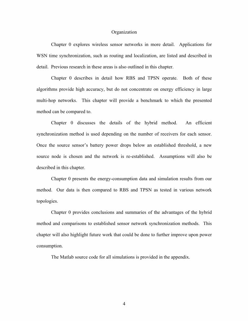
4. Randomly distributed sensors with high transmission power (left) and with lower transmission power (right) .............................................................................................. 25
5. Flooding a wireless sensor network: a sync_req packet is initially transmitted by the root node and is then re-transmitted by each receiver............................................................ 28
6. Hybrid synchronization of a wireless sensor network .................................................... 32
7. Mica2DOT synchronization comparison........................................................................ 35
8. MicaZ synchronization comparison................................................................................ 37
9. Synchronization comparison for architecture with n=6.................................................. 38
10. Synchronization comparison for architecture with n=10................................................ 39
11. Synchronization comparison for 250 sensors ................................................................. 45
12. Synchronization comparison for 500 sensors ................................................................. 46
13. Synchronization comparison for 750 sensors ................................................................. 47
14. Synchronization comparison for 1000 sensors ............................................................... 48
15. Synchronization comparison for 1250 sensors ............................................................... 49
16. Synchronization comparison for 1500 sensors ............................................................... 50

1
CHAPTER 1
INTRODUCTION
Time synchronization is a crucial aspect of any networked system. The majority
of research in this field has concentrated on traditional high-speed computer networks
with few power restraints, leading to the global positioning system (GPS) [1] and the
network time protocol (NTP) [2]. These conventional networks are effective for
communication of large amounts of data, typical of local area networks (LAN).
Wireless Sensor Network Overview
Over the past few years, applications have been developed to monitor
environmental properties such as temperature and humidity; they can also be used to
analyze motion of animals or vehicles. One of the most important requirements for these
monitoring applications is unobtrusiveness; this creates a need for wireless ad-hoc
networks using very small sensing nodes. These special networks are called wireless
sensor networks (WSN). These networks are built from many wireless sensors in a high-
density configuration to provide redundancy and to monitor a large physical area.
WSNs can be used to detect traffic patterns within a city by tracking the number
of vehicles using a designated street. If an emergency arises, the network can relay the
information to the city hall and notify police, fire, and ambulance drivers of congested
streets. An application could even be designed that suggests the fastest route to the
emergency area.

2
Another emergency condition could arise should a chemical plant be damaged
and develop a leak, creating a toxic fume cloud that could endanger an entire city [3].
Sensors could be deployed from the safety of a plane above the cloud. As the sensors fall
through the fumes, they could determine the size of the cloud, as well as the wind speed
which propels the cloud. The sensors could then relay this information either to the plane
or to a unit on the ground, which could then suggest evacuations according to the cloud’s
projected path. Changes in wind speed and direction could be detected from the plane
above the cloud, so the projected path could be updated in real-time as well.
When compared to computer terminals in LANs, wireless sensors must operate on
very low capacity batteries to minimize their size to about that of a quarter. The nodes
use slow processing units to conserve battery power. A typical sensor node such as
Crossbow’s Mica2DOT operates at 4 MHz with 4 Kb of memory and has a radio
transceiver operating at up to 15 Kbps [4]. Radio transmissions consume by far the
majority of the battery’s energy, so even with this low-power hardware, a sensor can
easily be depleted within a few hours if it is continuously sending transmissions.
With the emergence of WSNs, current LAN synchronization methods will not
work efficiently. GPS provides good synchronization accuracy, but requires a very large
amount of power from the sensors. In a power-constrained sensor, this synchronization is
infeasible. NTP is also infeasible since it is designed for traditional computer networks
and will not scale well for wireless sensor networks. Some new synchronization methods
have been developed specifically for sensor networks, such as the timing-sync protocol
for sensor networks (TPSN) and the reference broadcast synchronization method (RBS).

3
Objectives
RBS and TPSN both achieve accurate clock synchronization within a few
microseconds of uncertainty. However, they are both designed for networks with a small
number of sensors and are not specifically geared towards energy conservation; although
these algorithms will work for larger networks, their energy consumption becomes
inefficient and network connectivity is not maintained once nodes begin losing power.
Simulating each of these methods shows that synchronizing a large sensor network
requires an unnecessarily large number of transmissions, which will quickly deplete
sensors and reduce the network’s coverage area.
This work concentrates on the following aspects of WSNs:
1. Design a hybrid method between RBS and TPSN to reduce the number of
transmissions required to synchronize an entire network.
2. Extend single-hop synchronization methods to operate in large multi-hop
networks.
3. Verify that the hybrid method operates as desired by simulating against RBS
and TPSN.
4. Maintain network connectivity and coverage.
4
Organization
Chapter 0 explores wireless sensor networks in more detail. Applications for
WSN time synchronization, such as routing and localization, are listed and described in
detail. Previous research in these areas is also outlined in this chapter.
Chapter 0 describes in detail how RBS and TPSN operate. Both of these
algorithms provide high accuracy, but do not concentrate on energy efficiency in large
multi-hop networks. This chapter will provide a benchmark to which the presented
method can be compared to.
Chapter 0 discusses the details of the hybrid method. An efficient
synchronization method is used depending on the number of receivers for each sensor.
Once the source sensor’s battery power drops below an established threshold, a new
source node is chosen and the network is re-established. Assumptions will also be
described in this chapter.
Chapter 0 presents the energy-consumption data and simulation results from our
method. Our data is then compared to RBS and TPSN as tested in various network
topologies.
Chapter 0 provides conclusions and summaries of the advantages of the hybrid
method and comparisons to established sensor network synchronization methods. This
chapter will also highlight future work that could be done to further improve upon power
consumption.
The Matlab source code for all simulations is provided in the appendix.

5
CHAPTER 2
RELATED WORK IN WSN
When wireless sensor networks were first being developed, the main topic of
research involved reliability and routing. WSNs are usually deployed in relatively
inaccessible environments such as heavily forested areas or within buildings, where using
wired networks are impractical. Consequently, transmissions are unreliable and lost
packets are common. Equation (2.1) shows how signal power fades as it travels further
from the transmitter:
TR c
PPd
= , (2.1)
where PT is the power of the transmitted signal, d is the distance from the transmitter, and
c is the path loss coefficient, which usually varies from between 2 and 5. These typical
environments have large path loss coefficients because of signal fading from diffractions,
reflections, and scattering off of walls and foliage. SCALE (Simple Connectivity
Assessment in Lossy Environments) is a tool developed for Mica2 sensors to measures
packet delivery [5]. Using SCALE, research has verified the above fading effects on
sensor networks. It was shown that outdoor urban environments with large buildings
disrupt wireless signals more so than do doors and walls from within buildings. Flooding
algorithms such as the ones described in [6] and [7] have been used to study multi-hop
routing in WSNs. Unreliable networks have several issues that were uncovered with this
algorithm:
• Backward links: a link that transmits flood packets back towards the source.

6
• Long links: a link that is significantly longer than would be expected given the
transmission power level.
• Stragglers: sensors that do not receive flood packets, despite having a high
probability of reception from a neighboring transmitter.
• Clustering: a node that connects to a very large number of receivers.
Span is an algorithm that reduces a network’s energy consumption while
maintaining its topology as well as its sensing effectiveness [8]. Each node determines
whether it should sleep or become a coordinating node that forwards packets. This
decision is based on an estimation of the number of neighbors that would benefit from the
node’s state. The network’s lifetime increases as more nodes are deployed and as the
sleep time for each node is increased.
ASCENT is an algorithm that changes the network’s topology in an effort to
maximize the lifetime of each sensor [9], [10]. In this case, each node will self-configure
itself based upon its connectivity and its participation in the network’s topology. Timers
are used to switch a sensor’s state between sleep, passive, test, and active. A sleeping
sensor’s radio is turned off to save power, while an active sensor’s radio is turned on to
allow the sensor to communicate with its neighbors. A sensor in the test phase monitors
the number of neighbors and its data loss rate to determine whether it is beneficial to join
the network; if one of these parameters is not above a certain threshold, then the node
will become passive, otherwise it will become active. A passive node will transition back
to the test phase if the data loss rate is low, the number of neighbors is below a threshold,
or if a help packet is received. If none of these parameters are met, the node goes to sleep
and transitions back to the passive phase once a timer expires. When the thresholds and

7
timer lengths are set correctly, ASCENT has reduced packet loss while decreasing energy
consumption. The algorithm must still be tested for large networks to determine its
scalability.
One of the most common uses for wireless sensor networks is for localization and
tracking. Tracking of a single object is relatively simple since data can be handed-off
from sensor to sensor as the object moves through the network. Information-driven
sensor query (IDSQ) is one tracking method that works well, even for multiple targets
[11]. It defines a “belief state,” which contains the position and velocity of each target.
Previous tracking methods scaled very poorly since every sensor would update its belief
state, requiring a large amount of network communication. With IDSQ, only nodes that
have useful and non-redundant information will have their belief state updated.
Furthermore, IDSQ tracks multiple targets more efficiently by splitting up the network
into sub-sections, each of which is assigned a leader node that keeps track of when
objects enter and leave the area. Contour tracking at the boundaries can be accomplished
by using triangulation and a contour threshold [12].
Sensor networks have also been used to monitor conservation habitats for wildlife
[13], [14], [15]. Sensors area being used to monitor the nesting habits of a coastal bird on
Great Duck Island, 10 miles off of the coast of Maine. In the past, researchers would
have to go to the island and physically disrupt the nests to count eggs and to measure
temperature and humidity. Now however, small sensors are able to do these same
observations without disrupting the birds’ nesting habits.
Localization and tracking are also used when attempting to locate a sniper’s
location from the gun’s muzzle blast [16]. Each sensor will detect the blast noise at

8
unique times but within microseconds of each other, so the only way to accurately
compare observations is if all of the sensors are well-synchronized [17]. If the sensors
know their locations relative to one another, then the path of the bullet can be reproduced
from the observations of the blast noise, ultimately finding the point of origin.
Target tracking applications such as the ones just described require some degree
of synchronization amongst nodes to provide useful observation comparisons. A
significant distinction between each application is the degree of synchronization that is
required; when tracking an animal or a vehicle, up to one millisecond of accuracy could
be required, whereas in the case of sniper localization, the sensors must be synchronized
to within a few microseconds. A high-accuracy algorithm will require more
communication amongst nodes, thereby using more energy, whereas a less accurate
method will usually require less energy. Some of the synchronization algorithms are
discussed in Sections Error! Reference source not found., 0, and 0.
NTP
One of the first synchronization protocols used for computer systems is the
network time protocol (NTP), first developed in 1985. This protocol uses a relatively
large amount of memory to store data for synchronization sources, authentication codes,
monitoring options, and access options [18], [19]. As mentioned earlier, typical wireless
sensor nodes have limited onboard memory; for example, Crossbow’s popular Mica2 and
Mica2DOT sensors each have 4KB of configurable memory. A large sensor network will
require large files for synchronization sources and codes. Even if these configuration
files can be programmed into each node, it would leave very little memory to hold the

9
data monitored by the sensor, limiting NTP’s use for WSNs. Furthermore, NTP’s
synchronization accuracy is within 10 ms over the Internet, and up to 200 μs in a LAN;
these specifications are usually adequate for computer networks, but do not meet the
requirements for most sensor network applications.
GPS
Global positioning system (GPS) is another accurate and commonly used
synchronization protocol. The Department of Defense (DoD) began launching
NAVSTAR (Navigation Signal Timing and Ranging) GPS satellites in 1978 to allow the
U.S. military to localize any object on the ground to within a few feet [20]. Although
commercial applications could use GPS when it was first created, the technology was
classified so unauthorized users would have inaccurate results, usually to an accuracy of
100 meters at best. This technology was de-classified in 2000, leading to the
development of commercial GPS navigation systems with an accuracy of a few
centimeters. The NAVSTAR GPS currently consists of 24 active satellites which
continuously transmit their own position and a time code in the microwave spectrum at
1.5 GHz. By measuring the relative arrival times of signals from several satellites and
using triangulation, a GPS receiver can determine its own position. The radio signals are
electromagnetic waves traveling at the speed of light, so the propagation delay is only 50
ms from an altitude of 10,000 miles, so GPS's triangulation method requires very precise
time information from the satellites. The master clock on each satellite is therefore kept
within 1 μs of the U.S. Naval Observatory's Master Clock [21], [22].

10
At first glance, GPS would seem to be an ideal candidate for time synchronization
for wireless sensor networks since the algorithm is wireless and the local node clocks will
always synchronize to 1 μs of each other. However, there are a few requirements that
GPS fails to meet. The receiver is 4.5 inches in diameter, more than 4 times the size of a
typical sensor node, and also requires an external power source [23]. These two traits
counteract the goal of using small and mobile nodes to create a wireless sensor network.
In addition, the GPS receiver draws 120 mA while the Mica2DOT wireless sensor only
uses 25 mA when transmitting at maximum power. Lastly, signal attenuation from
scattering and diffraction is significant since GPS operates at a high frequency, which
forces the receiver to have an unobstructed view of a large portion of the sky to
accurately receive the satellite signals. This line-of-sight requirement cripples GPS’s use
for sensor networks dispersed within a building or in a heavily forested area.
Media Access Control Issues
A significant amount of research has been done on the medium access control
(MAC) layer. These protocols control how sensors access the radio channel to
communicate with neighbors, so energy can be saved by using the channel more
efficiently. Two of the classic MAC protocols are ALOHA [24] and carrier-sense
multiple access (CSMA) [25]. In ALOHA, packets can either be transmitted immediately
after they are generated or on the next available slot. Dropped packets from collisions are
simply re-transmitted later. In CSMA, a sensor will listen to the MAC layer before it
transmits a packet. This MAC protocol is currently being used in many wireless

11
technologies, including 802.11. Both of these protocols use energy very inefficiently, so
new energy-aware modifications to the MAC layer have been created.
Packet collisions are one of the most wasteful phenomena in wireless
communication, since these packets must be re-transmitted in full. One way to greatly
reduce collisions is by using time division multiple access (TDMA), where each sensor
would be given a unique time slot in which to transmit information. Low-energy
adaptive clustering hierarchy (LEACH) is an application of TDMA towards wireless
sensor networks [26]. It organizes nodes into clusters with one head node, and applies
TDMA within each cluster. Bluetooth uses a similar approach [27], using clusters called
piconets, where devices are given the right to transmit only when their time slot becomes
available. Since each sensor requires a unique transmission time slot, LEACH and other
TDMA-type algorithms do not scale very well with larger networks. In addition, sensors
are not allowed to directly communicate with each other, so very accurate time
synchronization is required to ensure that one sensor’s transmissions do not spill over
into another sensor’s time slot.
Instead of using TDMA, contention-based algorithms allow sensors to
communicate directly with each other, removing the dependency on accurate time-
synchronization. S-MAC is a modification to the MAC protocol designed specifically for
WSNs to increase energy efficiency [28]. To do this, a low duty-cycle is first obtained by
scheduling the nodes to transmit depending on their remaining battery life. When
transmitting a packet, the S-MAC adds a duration field to notify other nodes how long of
a packet transmission is needed. The nodes will therefore immediately know for how
long they must refrain from sending their own data, even without requiring

12
synchronization. T-MAC improves upon S-MAC by adding the ability for a variable
duty-cycle to compensate for inconsistent data rates [29].

13
CHAPTER 3
WSN TIME SYNCHRONIZATION ALGORITHMS
Although traditional synchronization methods are effective for computer
networks, they are ineffective in sensor networks. New synchronization algorithms
specifically designed for wireless sensor networks have been developed and can be used
for several applications.
RBS
Clearly GPS and NTP are not very effective in wireless sensor applications. One
of the first major research attempts to create a time synchronization algorithm specifically
tailored for sensor networks led to the development of reference broadcast
synchronization (RBS) in 2002 [30]. This algorithm defines the critical path, which is the
portion of the network where a significant amount of clock uncertainty exists. A long
critical path results in high uncertainty and low accuracy in the synchronization. RBS
improves upon NTP by reducing the length of the critical path, which can improve the
accuracy of the synchronization to 7 μs in light traffic. There are four main sources of
delays that must be accounted for to have accurate time synchronization:
• Send time: this is the time to create the message packet.
• Access time: this is a delay when the transmission medium is busy, forcing
the message to wait.
• Propagation time: this is the delay required for the message to traverse the
transmission medium from sender to receiver.

14
• Receive time: similar to the send time, this is the amount of time required
for the message to be processed once it is received.
RBS Algorithm and Analysis
The RBS algorithm can be split into three major events:
1. Flooding: a transmitter broadcasts a synchronization request packet.
2. Recording: the receivers record their local clock time when they initially
pick up the sync signal from the transmitter.
3. Exchange: the receivers exchange their observations with each other.
RBS synchronizes each set of receivers with each other as opposed to traditional
algorithms that synchronize receivers with senders. These latter algorithms have a long
critical path, starting from the initial send time until the receive time. For this reason,
NTP’s accuracy is severely limited, as discussed previously. RBS uses a relative time
reference between nodes, eliminating the send and access time uncertainties. The
propagation delay of signals is extremely fast from point-to-point; a set of nodes
separated by 100 meters will have a propagation delay of 340 ns, so this delay can be
ignored when dealing in the microsecond scale. Lastly, the receive time is reduced since
RBS uses a relative difference in times between receivers. Also, the time of reception is
taken when the packet is first received in the MAC layer, eliminating uncertainties
introduced by the sensor’s processing unit.
The authors of RBS reported 11.2 μs for the synchronization error on the MICA2
wireless sensors. However, the motes have an integrated transmitter with a processor,
requiring additional CPU cycles and yielding this relatively inaccurate precision (this

15
hypothesis was verified when RBS was tested using much more powerful IPAQs units,
where the errors were 6.3 μs in light traffic and 8.4 μs in heavy traffic). By comparison,
the errors for NTP using the IPAQs were 51 μs in light traffic and 1542 μs in heavy
traffic. RBS clearly outperforms NTP, even on vastly inferior hardware.
There are two unique implementations of RBS. The simplest method is designed
for very high accuracy for sparse networks, where transmitters have at most two
receivers. The transmitter can broadcast a synchronization request to the two receivers,
which will record the times at which they receive the request, just as the algorithm
describes. However, the receivers will exchange their observations with each other
multiple times, using a linear regression to lower the clock offset. After 30 exchanges,
the accuracy is improved from 11 μs to 1.6 μs.
The other version of the RBS algorithm involves the following steps: the
transmitter sends a reference packet to two receivers; each receiver checks the time when
it receives the reference packet; the receivers exchange their recorded times. The main
problems with this scheme are the nondeterminism of the receiver, as well as clock skew.
The receiver’s nondeterminism can be resolved by simply sending more reference
packets. The clock skew is resolved by using the slope of a least-squares linear
regression line to match the timing of the crystal oscillators.
RBS can be adapted to work in multihop environments as well. Assuming a
network has grouped clusters with some overlapping receivers, linear regression can be
used to synchronize between receivers that are not immediate neighbors. However, it is
more complicated than the single-hop scenario since there will be timestamp conversions

16
as the packet is relayed through nodes. This extra complication is manifested in larger
synchronization errors.
Figure 1 shows how a sensor network is synchronized by using RBS.

17
Figure 1: RBS synchronization of a wireless sensor network. The initial solid dark lines represent the network’s topology after flooding; the solid light lines represent transmitter-to-receivers communication; the dashed lines represent receiver-to-receiver transmissions.
RBS Issues
There are some issues with the RBS synchronization algorithm that must be
addressed in an energy-aware sensor network. First, the receiver-to-receiver
synchronization method is effective at reducing the critical path to increase the accuracy,
but RBS scales poorly with dense networks where there are many receivers for each

18
transmitter. Given n receivers for a single transmitter, the number of transmissions
increases linearly with n, but the number of receptions increases as O(n2). The following
numbers of transmissions and receptions exist:
RBSTX n= , (3.1)
21
1
( 1)2 2
n
RBSi
n n n nRX n i n−
=
− += + = + =∑ . (3.2)
For a large number of receivers per transmitter, this method becomes infeasible due to
energy constraints.
Lastly, RBS does not account for lost network coverage when nodes begin losing
power. Should a transmitting node be depleted, all of its receivers will be dropped from
the network, so measures should be taken to re-establish connectivity when the coverage
decreases beyond some threshold value.
TPSN
The timing-sync protocol for sensor networks (TSPN) was developed in 2003 in
an attempt to further refine time synchronization beyond RBS’s capabilities [31], [32].
TPSN uses the same sources of uncertainty as RBS does (send, access, propagation, and
receive), with the addition of two more:
• Transmission time: the time for the packet to be processed and sent
through the RF transceiver during transmission.
• Access time: the time for each bit to be processed from the RF transceiver
during signal reception.

19
TPSN Algorithm and Analysis
The TPSN works in two phases:
1. Level discovery phase: this is a very similar approach to the flooding
phase in RBS, where a hierarchical tree is created beginning from a root
node.
2. Synchronization phase: in this phase, pair-wise synchronization is
performed between each transmitter and receiver.
In the level discovery phase, each sensor node is assigned a level according to the
hierarchical tree. A pre-determined root node is assigned as level 0 and broadcasts a
level_discovery packet. Sensors that receive this packet are assigned as children to the
transmitter and are set as level 1 (they will ignore subsequent level_discovery packets).
Each of these nodes broadcasts a level_discovery packet, and the pattern continues with
the level 2 nodes.
In the synchronization phase, pair-wise synchronization is performed between the
transmitter and receiver nodes using a 2-way handshake. Given a parent node A and a
child node B, node A sends a synchronization_pulse to B, timestamped at T1. Once node
B receives the pulse, it timestamps at T2, then sends an ack packet back to A at T3. The
parent node receives the ack packet and timestamps one last time at T4. These 4
timestamps provide estimates for clock drift (3.3) and propagation delay (3.4):
( ) ( )2 1 4 32
T T T T− − −Δ = , (3.3)
( ) ( )2 1 4 32
T T T Td
− + −= . (3.4)

20
The synchronization error can be calculated from the clock drift between the two nodes
as well as the drift at T4:
4A B
tError D →= Δ − . (3.5)
The following equations characterize T2 and T4:
12 1 A BA A B B tT T S P R D →
→= + + + + , (3.6)
34 3 B AB B A A tT T S P R D →
→= + + + + ,
44 3 A BB B A A tT T S P R D →
→≈ + + + − , (3.7)
where SA, A BP → , and RB refer to the time to send the packet at node A (send time + access
time + transmission time), the propagation time between nodes A and B, and the time to
receive the packet at node B, respectively.
Equations (3.6) and (3.7) can be combined and used in (3.5) to get the theoretical
error for TPSN:
1 44 2 2 2 2
A BUC UC UCA B t t
TPSN tRDS P RError D
→→ →= Δ − = + + + . (3.8)
By contrast, the error for RBS as claimed by the TPSN authors is:
4 1 4A B UC UC A B
RBS t D t tError D P R RD→ →→= Δ − = + + . (3.9)
In equations (3.8) and (3.9), SUC, PUC, and RUC refer to the uncertainty in the send time,
propagation time, and receive time respectively. RD is the relative drift between nodes A
and B from time T1 through T4.
Although RBS removes the uncertainty at the sender by exchanging times
amongst receivers, TPSN reduces the remaining uncertainties by a factor of 2 due to the
handshake process that averages the clock drift and propagation delay. However,

21
TPSN’s uncertainty at the sender can be reduced to an insignificant delay by
timestamping at the MAC layer just before the bits are sent through the transceiver.
Figure 2 shows how a sensor network is synchronized by using TPSN.

22
Figure 2: TPSN synchronization of a wireless sensor network. The initial solid dark lines represent the network’s topology after flooding; the subsequent light lines represent successful transmitter-to-receiver synchronizations.
TPSN Issues
TPSN is a great improvement over RBS in terms of accuracy. Using a 2-way
handshake reduces uncertainty in half since the average of the time differences is used.
The algorithm can be easily applied to multi-hop situations since it scales very well to
dense networks:

23
1TPSNTX n= + , (3.10)
2TPSNRX n= . (3.11)
The main disadvantage that TPSN faces is its energy consumption in sparse networks; a
2-way handshake requires each node to receive a packet and to send one in response. For
a parent node A with two children B and C, node A broadcasts the level_discovery packet,
and then a synchronization_pulse packet. Nodes B and C receive both packets, and then
transmit an ack packet back to node A. This example uses 4 transmissions and 4
receptions for TPSN. In contrast, the same situation would only require 2 transmissions
and 3 receptions when using RBS; node A broadcasts a synchronization request packet
with a timestamp, and then node B sends a second transmission to node C with its
observation (node C can also transmit to node B with the same end result).
In addition, TPSN has the same problem as RBS with respect to lost network
coverage when nodes begin losing power. A dead transmitter node will drop all of its
receivers from the network, lowering the WSN’s coverage area. Network restructuring is
not included in the TPSN algorithm.

24
CHAPTER 4
ENERGY-AWARE TIME SYNCHRONIZATION
The timing-sync protocol for sensor networks (TPSN) and reference broadcast
synchronization (RBS) are some of the first efforts in creating synchronization algorithms
tailored towards low-power sensor networks. They both have unique strengths when
dealing with energy consumption. RBS is most effective in networks where transmitting
sensors have few receivers, while TPSN excels when transmitters have many receivers.
As previously shown in (2.1), the signal’s power increases linearly with the transmitter’s
power and decreases with an inverse power law with respect to distance. This means that
a transmitter will have more children if it transmits at higher power or if the receivers
have higher sensitivity to pick up weaker signals. These properties can be verified by
building a network from uniformly distributed sensors and by changing the transmitter
power or the reception power threshold, as shown in Figure 3.
Figure 3: Uniformly distributed sensors with high transmission power (left) and with lower transmission power (right).

25
However, the sensors are most often randomly distributed and not uniformly
spaced. Manually deploying sensors in a uniform grid is time-consuming and non-covert.
Covertness is critical in battlefield and animal tracking scenarios. It would be best to
drop the wireless sensors from an airplane to avoid disturbing the environment; however,
the sensors would be distributed non-uniformly once they land. Even within buildings,
WSNs are usually non-uniform; nodes can be distributed with uniform distances from
each other, but the path loss is very variable in such an environment, mostly due to
scattering. This property results in a large variance in the number of receivers for each
transmitter, effectively creating a non-uniform sensor distribution. Figure 4 shows how
power affects the flooding in a network with randomly distributed sensors.
Figure 4: Randomly distributed sensors with high transmission power (left) and with lower transmission power (right).
The work presented in this thesis combines the efforts in various areas of research
presented in the previous chapters to create a hybrid time synchronization algorithm that
minimizes power usage by reducing the number of transmissions between sensors.

26
Although this method works for both uniform and non-uniform sensor deployment
scenarios, many of the details are derived to best accommodate random sensor placement.
Hybrid Flooding
Before the sensors can be synchronized, a network topology must be created.
Algorithm 1 is used by each sensor node to efficiently flood the network.
Algorithm 1: Hybrid Flooding Algorithm
Accept flood_packets
Set receiver_threshold to low_power
Set num_receivers to 0
If current_node is root node
Broadcast flood_packet
Else If current_node receives flood_packet and is accepting them
Set parent of current_node to source of broadcast
Set current_node level to parent’s node level + 1
Rebroadcast flood request with current_node ID and level
Broadcast ack_packet with current_node ID
Ignore subsequent flood_packets
Else If current_node receives ack_packet
Increment num_receivers
Each sensor is initially set to accept flood_packets, but will ignore subsequent ones in
order not to be continuously reassigned as the flood broadcast propagates. The

27
num_receivers variable keeps track of the node’s receivers and is used in the
synchronization algorithm. Figure 5 shows the implementation of Algorithm 1.

28
Figure 5: Flooding a wireless sensor network: a sync_req packet is initially transmitted by the root node and is then re-transmitted by each receiver.
Hybrid Synchronization
Once the network flooding has been completed, the network can be synchronized
using the determined hierarchy. In networks where the sensors are dispersed at random,
there will be patches of high density node distribution interspersed with lower density
regions. As shown in Figure 4, a transmitter in a high density area will usually have a

29
large number of receivers, while another transmitter in a lower density section will
usually have 1 or 2 receivers at most. As discussed in section 0, RBS excels when the
transmitter has few receivers. In contrast, TPSN excels with many receivers connected to
each transmitter, as discussed in section 0.
The hybrid algorithm minimizes power regardless of the network’s topology by
choosing the best synchronization technique depending on the number of children
connected to the transmitter. Since the energy required for reception usually differs from
that of a transmission, the ratio of the reception power to the transmission power is
needed in order to find the optimal point at which to switch from receiver-receiver
synchronization to transmitter-receiver synchronization. Equations (3.1), (3.2), (3.10),
and (3.11) are combined below, where α is the ratio of reception-to-transmission power:
RBS RBS TPSN TPSNTX RX TX RXα α+ × = + × . (4.1)
For example, assume that a reception uses approximately half the power of a
transmission, so α = ½.
1 12 2RBS RBS TPSN TPSNTX RX TX RX+ × = + × , (4.2)
( )21 11 2
2 2 2n nn n n
⎛ ⎞++ = + +⎜ ⎟
⎝ ⎠, (4.3)
2
2 14
n nn n++ = + , (4.4)
2 3 4 0n n− − = , (4.5)
( )( )4 1 0n n− + = . (4.6)
Equation (4.6) shows that the energies used by RBS and TPSN on this example platform
are equal when there are 4 receivers per transmitter, so the receiver_threshold value from

30
the previous algorithm is set to 4 (negative values for receiver_threshold are not
applicable here). With fewer than 4 receivers, the RBS algorithm is more efficient, while
TPSN is better with more receivers. Since the ratio of reception-to-transmission power
can vary for different platforms, the current draws for both reception and transmission are
stored as variables and the receiver_threshold value is calculated at every sensor. This
value is assumed to remain constant throughout the network. In general, the following
equation can be used to determine the receiver_threshold:
2 23 0n nα
− − = . (4.7)
Algorithm 2 describes the algorithm used for the hybrid algorithm.
Algorithm 2: Hybrid Synchronization Algorithm
Set receiver_threshold to high_power
If num_receivers < receiver_threshold // Use RBS algorithm
Transmitter broadcasts sync_request
For each receiver
Record local time of reception for sync_request
Broadcast observation_packet
Receive observation_packet from other receivers
Else // Use TPSN algorithm
Transmitter broadcasts sync_request
For each receiver
Record local time of reception for sync_request
Broadcast ack_packet to transmitter with local time

31
Figure 6 shows the implementation of Algorithm 2 in a wireless sensor network which
has already been flooded.

32
Figure 6: Hybrid synchronization of a wireless sensor network. The initial solid dark lines represent the network’s topology after flooding; the solid light lines represent transmitter-to-receivers communication; the dashed lines represent receiver-to-receiver transmissions.
Energy Depletion
Another issue that the hybrid algorithm addresses when synchronizing a sensor
network is the effect that a depleted sensor has on the topology. Once the battery is
exhausted, the node will be dropped from the network, but so will all of the receivers
depending on it. This loss of connectivity cascades through each receiver, so a drastic

33
restructuring can occur when a high-level sensor is drained. The hybrid algorithm keeps
track of the number of powered nodes. Once this number decreases below another user-
defined threshold, the network is re-flooded according using the flooding algorithm
described earlier in this section. Should the source node lose power, a new source node is
chosen from the original one’s receivers. These receivers communicate their power
levels with each other and the one with the most remaining energy is elected as the new
root node, as show in Algorithm 3.
Algorithm 3: Root Node Election Algorithm
If cur_node_level == 1 and cur_node_power allows 1 more TX
Broadcast elect_packet with cur_node_ID
If cur_node_level == 2
Broadcast elect_packet with cur_node_ID, cur_node_power
If cur_node receives elect_packet and elect_packet_power >= cur_node_power
Set elect_packet_ID to root node
In addition, receivers will only analyze the sync_request packets from their
respective transmitters when using the TPSN-style synchronization. This saves
additional battery power since the receivers do not have to analyze packets they overhear
from other broadcasting transmitters. Lastly, the dropped packets are monitored. This is
a useful statistic since it keeps track of algorithm efficiency and wasted energy. Dropped
packets also allow us to compare various network topologies and determine which ones
allow for the most energy conservation.

34
CHAPTER 5
RESULTS AND ANALYSIS
Several simulations were run to compare the power consumption of the timing-
sync protocol for sensor networks (TSPN), the reference broadcast synchronization
(RBS), and the hybrid algorithm developed in chapter 0.
Hybrid Algorithm Validation
The first set of simulations were run to validate (4.7), which is the basis for the
hybrid algorithm’s behavior. Using this equation, a transmitting sensor can dynamically
switch between RBS and TPSN by simply comparing the number of connected receivers
to the reception/transmission power ratio. In this experiment, this ratio is changed in
order to observe how each of the algorithms is affected. All other parameters are kept
constant: 20 simulations are run over a 1000m x 1000m area which is randomly
populated with 500 sensors, and the path loss coefficient is set to 3.5. In each simulation,
the receiver_threshold value is changed from 1 to the largest number of receivers
connected to a sensor. The hybrid synchronization algorithm is executed for each of
these receiver_threshold values and the energy consumption is stored and compared to
the consumption of TPSN, RBS, and the optimal hybrid synchronization algorithm. Each
of the data points is plotted, along with a line representing the average from all of the
simulations.
For the MICA2Dot platform, a reception uses approximately 24 mW of power,
while a transmission requires 75 mW at -5 dBm [4], so:

35
24 0.3275
α = = (5.1)
Equation (4.7) is solved with this value for α to get:
2 22475
2 253 3 04
n n n n− − = − − = (5.2)
3 9 25 4.422
n + += ≈ (5.3)
The hybrid algorithm will use the least amount of energy when the receiver_threshold is
set to 4.42. This means that transmitters with 4 or fewer sensors will use RBS for
synchronization while those with 5 or more receivers will use TPSN. Figure 7 illustrates
how changes in the receiver_threshold value affect the hybrid algorithm.
Figure 7: Mica2DOT synchronization comparison.

36
The energy consumption from the hybrid algorithm when using the optimal
receiver_threshold value is lower than both TPSN and RBS. As expected from (5.3), the
minimum value is found between values of 4 and 5. Lastly, the spread amongst data
points increases dramatically as the receiver threshold increases beyond 13.
More importantly, setting the receiver_threshold value to 1 will force a
transmitter to use TPSN, as shown in Algorithm 2. The hybrid algorithm in this case will
have the same energy consumption as TPSN. On the other hand, a receiver_threshold set
to the largest number of receivers connected to a transmitter will force a transmitter to
use RBS, so this algorithm will consume the same amount of energy as the hybrid one.
The hybrid synchronization algorithm is very dynamic and will adapt itself to
multiple equipment specifications. The power requirements for the MicaZ sensor
platform are drastically different from the Mica2DOT platform; MicaZ uses 59.1 mW for
a reception, but only uses 42 mW for each transmission at -5 dBm [33], so:
59.1 1.40742
α = ≈ (5.4)
Solving equation (4.7) just as before, the following receiver_threshold value is found:
3.42n ≈ (5.5)
Not only does the MicaZ platform have a higher α value, it actually uses more power to
receive information than to transmit it. In order to minimize energy consumption, the
hybrid algorithm will automatically adjust the sensors so that any transmitter with 3 or
fewer receivers will use RBS, while those with 4 or more receivers will use TPSN.
Figure 8 shows the hybrid algorithm’s performance when using the MicaZ platform.

37
Figure 8: MicaZ synchronization comparison.
When using MicaZ, the optimal receiver_threshold value is 3.42. This property is
reflected in the above graph, where the local minimum has shifted further to the left when
compared to the Mica2DOT platform.
Despite the differences in architecture, both of the above examples yield relatively
similar values for the optimal receiver_threshold. Assume that there is an improvement
in the Mica2DOT platform which allows for much lower power in receiving mode. Each
transmission still requires 75 mW at -5 dBm, but only 8 mW is needed for a reception.
The reception/transmission power ratio now becomes:
8 0.10775
α = ≈ (5.6)

38
The optimal receiver_threshold value now becomes:
6.08n ≈ (5.7)
Figure 9 illustrates the energy usage when the receiver_threshold changes.
Figure 9: Synchronization comparison for architecture with n=6.
In this example architecture, the hybrid algorithm produces a local minimum
when using the optimal receiver_threshold, as was expected. It is also interesting to note
that now, RBS becomes more energy efficient than TPSN.
Another example would be an architecture which uses 75 mW for transmitting
and 2 mW for receiving, so α=0.0267 and n=10.29. This new threshold will move the
graph’s local minimum further to the right, as shown in Figure 10.

39
Figure 10: Synchronization comparison for architecture with n=10.
Once again, the hybrid algorithm correctly predicts the minimum for energy
consumption.
Synchronization Power Reduction
The next set of simulations demonstrates the algorithm’s reduction in power
consumption in several network sizes. The number of sensors was changed from 250 up
to 1500, in increments of 250. Just as before, 20 simulations were run over a 1000m x
1000m area which was randomly populated with 500 sensors, and the path loss

40
coefficient was set to 3.5. The Mica2DOT platform was used and the ratio of
reception/transmission power remained fixed.
The receiver_threshold value is once again changed from 1 to the largest number
of receivers connected to a sensor. The hybrid synchronization algorithm is executed for
each of these receiver_threshold values and the energy consumption is stored and
compared to the consumption of TPSN, RBS, and the optimal hybrid synchronization
algorithm. Each of the data points is plotted, along with a line representing the average
from all of the simulations.
Table 1: Average Number of Transmissions Sensors 250 500 750 1000 1250 1500
RBS 249 499 749 999 1249 1499 TPSN 351 664 955 1245 1531 1810 Hybrid 261 533 800 1065 1331 1593
RBS Savings -5.06 % -6.76 % -6.84 % -6.59 % -6.59 % -6.26 % TPSN Savings 25.58 % 19.72 % 16.20 % 14.50 % 13.06 % 12.01 %
Table 1 shows that RBS requires the fewest number of transmissions, while TPSN
uses the most. The results for RBS and for TPSN both increase linearly with network
size, as was expected from (3.1) and (3.10), respectively. The hybrid algorithm is up to
6.8% less efficient than RBS. However, when compared to TPSN, the hybrid algorithm
performs very well. For small networks, there is up to a 25% savings in energy. As the
number of sensors is increased, the hybrid algorithm efficiency drops to a 12% advantage
over TPSN.
Table 2 shows the standard deviation in the number of transmissions for each of
the synchronization algorithms. These results are important in determining how sensitive
an algorithm is to modifications in the network’s topology and sensor density.

41
Table 2: Standard Deviation for Transmissions Sensors 250 500 750 1000 1250 1500
RBS 0.37 0.15%
0.00 0.00 %
0.00 0.00 %
0.00 0.00 %
0.00 0.00 %
0.00 0.00 %
TPSN 7.59 2.16 %
8.88 1.34 %
14.31 1.50 %
14.48 1.16 %
18.22 1.19 %
22.09 1.22 %
Hybrid 1.61 0.61 %
2.29 0.43 %
1.89 0.24 %
5.02 0.47 %
4.29 0.32 %
4.24 0.27 %
It is interesting to note that the standard deviation for RBS transmissions is
usually 0, which shows that the number of transmissions is strictly dependent on the
number of sensors in a network, regardless of network topology. The only exception
occurred when 250 sensors were used, and was most likely caused when some sensors
that did not receive a flood_packet and were therefore not used for synchronization.
The table shows that there is very little variation in the number of transmissions
for TPSN. In fact, the largest standard deviation for TPSN comes from smaller networks.
Similar results appeared when the hybrid algorithm was simulated, but with even less
variability. Both of these algorithms are therefore only slightly affected by changes in
sensor placement and sensor density.
Table 3 shows results for the number of receptions when using each of the
algorithms.
Table 3: Average Number of Receptions Sensors 250 500 750 1000 1250 1500
RBS 615 1709 3421 5510 7833 11128 TPSN 498 998 1498 1998 2498 2998 Hybrid 447 924 1415 1898 2386 2879
RBS Savings 27.44 % 45.94 % 58.65 % 65.55 % 69.54 % 74.13 % TPSN Savings 10.27 % 7.43 % 5.57 % 4.99 % 4.47 % 3.97 %
Although the number of receptions when using TPSN increases linearly with
network size, as would be expected from (3.11), this number increases much more

42
quickly when using RBS, as illustrated in (3.2). The hybrid algorithm greatly reduces the
number of receptions when compared to RBS; for small networks, the advantage is 27%,
but it increases to over 74% in networks with a large number of sensors. In contrast, the
hybrid algorithm has a large advantage over TPSN in small networks, but that advantage
decreases as more sensors are added.
Table 1 and Table 3 both show that the hybrid algorithm mimics RBS’s behavior
for small networks. However, the hybrid algorithm changes its behavior as more sensors
are included and begins resembling TPSN for very large networks.
Table 4 shows the standard deviation in the number of receptions for each of the
synchronization algorithms. Similar to Table 2, these results help to determine how
sensitive an algorithm is to modifications in the network’s topology and sensor density.
Table 4: Standard Deviation for Receptions Sensors 250 500 750 1000 1250 1500
RBS 54.71 8.89 %
150.09 8.78 %
365.43 10.68 %
524.32 9.52 %
614.26 7.84 %
1129.50 10.15 %
TPSN 0.73 0.15 %
0.00 0.00 %
0.00 0.00 %
0.00 0.00 %
0.00 0.00 %
0.00 0.00 %
Hybrid 11.73 2.63 %
13.16 1.42 %
15.89 1.12 %
14.75 0.78 %
15.99 0.67 %
16.77 0.58 %
The table shows that there is very large variation in the number of receptions for
RBS, meaning that the number of receptions when using RBS is highly dependent on the
topology of the network. The table also shows that the deviation in receptions when
using TPSN is usually 0, with the exception once again in the 250 sensor network. Just
as before, this exception is due to orphaned nodes which do not participate in the
synchronization. The hybrid algorithm has a relatively low deviation, which decreases

43
further with large numbers of sensors. This behavior is attributed to the hybrid algorithm
behaving similarly to TPSN when the network is large.
It is important to compare the number of transmissions and receptions amongst
algorithms to understand each one’s advantages and drawbacks, but the ultimate goal in
these experiments is to minimize the total amount of energy expended when
synchronizing the network. Since the transmitted packets are the same size for every
algorithm, the radio and processor will be operating for a constant length of time, so the
energy consumption can be calculated as follows:
energy numTx numRxα= + × . (5.8)
Table 5 compares the energy values amongst algorithms.
Table 5: Average Energy Consumption Sensors 250 500 750 1000 1250 1500
RBS 446 1046 1844 2762 3756 5060 TPSN 511 983 1434 1885 2331 2770 Hybrid 404 828 1253 1672 2095 2514
RBS Savings 9.29% 20.79% 32.04% 39.46% 44.22% 50.31% TPSN Savings 20.80% 15.73% 12.65% 11.28% 10.11% 9.23%
Table 2 shows that all of the standard deviations for transmissions are relatively
low, while RBS usually has a constant number. In contrast, Table 4 shows that while the
standard deviations for receptions when using RBS are very high, TPSN usually has a
constant number of receptions. Finally, Table 6 compares the standard deviation for each
of the algorithms.

44
Table 6: Standard Deviation of Energy Consumption Sensors 250 500 750 1000 1250 1500
RBS 17.38 3.90%
48.03 4.59%
116.94 6.34%
167.78 6.07%
196.56 5.23%
361.44 7.14%
TPSN 7.67 1.50%
8.88 0.90%
14.31 1.00%
14.48 0.77%
18.22 0.78%
22.09 0.80%
Hybrid 4.00 0.99%
4.72 0.57%
5.23 0.42%
6.85 0.41%
6.33 0.30%
6.84 0.27%
Although the standard deviations usually fluctuate with network size, larger
networks generally increase the variance in RBS while decreasing the variance in TPSN.
Furthermore, the deviation for RBS is relatively large, while that for TPSN is much
lower. However, the variance for the hybrid algorithm is always lower than the other
two, and it constantly decreases with larger networks.
These results show that not only is RBS’s energy consumption highly dependent
on network topology, it becomes even more so as the network becomes larger. In
contrast, TPSN and the hybrid algorithm are less affected by the network layout, and both
become even more independent as more sensors are introduced into a given area. The
graphs below show how the energy consumption of all three algorithms compares with
various network sizes.

45
Figure 11: Synchronization comparison for 250 sensors.
As mentioned before, the hybrid algorithm can adapt accordingly to transmission
and reception power usages. TPSN and RBS become special cases of the algorithm. A
receiver_threshold value of 1 will force a transmitter to use TPSN, whereas a
receiver_threshold set to the largest number of receivers connected to a transmitter will
force a transmitter to use RBS. These traits are shown in Figure 11.
For a relatively small network of 250 sensors, TPSN is the most inefficient
algorithm of the three used in this study, followed by RBS. The hybrid algorithm
outperforms TPSN by over 20%, while outperforming RBS by over 9%, as shown in
Table 5.

46
Figure 12: Synchronization comparison for 500 sensors.
One major difference observed when the network grows from 250 sensors to 500
sensors is that RBS becomes less energy efficient than TPSN. The hybrid algorithm
outperforms TPSN by 15.7%, while outperforming RBS by 20.8%.

47
Figure 13: Synchronization comparison for 750 sensors.
Once the network grows to 750 sensors, RBS clearly becomes less efficient than
TPSN. The hybrid algorithm still outperforms TPSN by 12.7%. Since RBS consumes
more energy, the hybrid algorithm now outperforms it by 32%.

48
Figure 14: Synchronization comparison for 1000 sensors.

49
Figure 15: Synchronization comparison for 1250 sensors.

50
Figure 16: Synchronization comparison for 1500 sensors.
As more sensors are introduced into the network, RBS becomes dramatically less
feasible for a wireless sensor network. As shown in Table 5, the hybrid algorithm’s
energy savings over RBS increases from 39% with 1000 sensors to over 50% when the
network uses 1500 sensors.
In contrast, as the network becomes large, the hybrid algorithm mimics TPSN’s
behavior, but uses less energy. The difference is 11% with 1000 sensors and 9% with
1500 sensors.

51
CHAPTER 6
CONCLUSIONS
Summary
Wireless sensor networks have tremendous advantages for monitoring object
movement and environmental properties; their small size makes them very stealthy and
ideal for covert observations. Their size also makes it easy to drop them into a
designated area by plane. Sensors can be deployed within a congested city to monitor
traffic patterns. They can be used to monitor the migration patterns of animals. Should a
chemical plant begin leaking toxic fumes, wireless sensors can monitor the movement
and size of the fume cloud. They can also be deployed within a city or battlefield and can
determine the location of a sniper from a rifle’s blast noise.
All of these applications require some degree of synchronization to achieve the
best results. Tracking animal movement does not require a high degree of accuracy, so
the synchronization between clocks can be kept within a second. The same
synchronization accuracy can be used to monitor traffic congestion patterns and the
movement of a toxic chemical cloud. Determining a bullet’s point of origin from a rifle
blast, however, is much more challenging. The blast will propagate uniformly from the
sniper’s location, so sensors closest to the shot will detect the shock wave first, while
those further away will detect it later. To accurately determine the point of origin, the
sensor clocks should be synchronized within a few microseconds of each other. The
work developed in this thesis not only includes an algorithm for synchronizing each

52
sensor, but also includes algorithms for flooding and electing a new root node when the
current root’s battery is depleted.
The hybrid synchronization algorithm was designed to switch between timing-
sync protocol for sensor networks (TPSN) and the reference broadcast synchronization
algorithm (RBS). These two algorithms allow all the sensors in a network to synchronize
themselves within a few microseconds of each other, while at the same time using the
least amount of energy possible. The savings in energy varies upon the density of the
sensors as well as the reception-to-transmission ratio of energy usage; networks which
are saturated with sensors, for example 1500 sensors in a 1 km2 area, will favor TPSN
over RBS. TPSN also becomes more favorable as receptions consume more power.
The hybrid algorithm compromises between both of these previous algorithms.
The energy savings over RBS can range from 9.3% in small networks of 250 sensors, to
over 50% for large networks using 1500 sensors. In contrast, the hybrid algorithm’s
savings over TPSN range from 20.8% in the same small networks down to 9% in the
large networks. Furthermore, analysis of the standard deviation for each of the
algorithms shows RBS’s energy consumption can vary dramatically, from nearly 4% to
over 7%, generally increasing for larger networks. In contrast, the standard deviation for
TPSN’s energy usage decreases from 1.5% to less than 1%, generally decreasing for
larger networks. The hybrid algorithm’s deviation is always less than 1% and
continuously decreases down to 0.3% as more sensors are used.

53
Future Work
There are a few improvements that can be implemented to the hybrid system in
order to further decrease energy consumption.
• Physical implementation: although the system is designed from algorithms
that have been researched and implemented on physical sensors, the work
presented in this study has only been simulated using Matlab. Physically
testing an algorithm on a sensor network comprised of 1500 sensors is a very
difficult task; even testing a network with 250 sensors is not an easy feat. A
study should be conducted to ensure that the algorithms developed in chapter
0 work correctly.
• Localized re-flooding: in the hybrid algorithm presented in this study, the
entire network is re-flooded once the percentage of unused sensors reaches a
given threshold. This threshold value is important since energy is wasted if
the network topology is continuously updated whenever a sensor’s battery
dies. At the same time, the physical area being monitored decreases as the
algorithm waits for the threshold value to be met. The best way to maintain
network connectivity while using the least amount of energy is to re-flood
only some areas of the network instead of the entire WSN. The hybrid
algorithm is well-suited for localized floods since each transmitting sensor
knows its receivers; when one of its receivers loses power, the transmitter can
send a localized flood packet to re-establish the network’s topology without
disrupting the rest of the WSN.

54
• Non-uniform path loss coefficient: the research conducted here assumes that
the path loss coefficient remains constant over the entire monitored area. This
assumption may be valid in the case where sensors are dropped from a plane
into a dangerous chemical cloud, but the path loss coefficient can drastically
change in urban and heavily forested areas. When simulating a WSN that will
monitor traffic patterns in an area surrounded by tall glass buildings,
deflections and refractions will change the path loss coefficient; the only way
to accurately portray this behavior in a simulation is to allow for a variance in
path loss.
• Network layer modifications: sensor networks are quite different from the
typical computer network being used today. The 5-layer internet architecture
has been adapted to work with wireless sensor networks, but should be
modified as it can be inefficient. Experiments should be conducted to find the
best applicable network layer for sensor networks.

55
APPENDIX
MATLAB SIMULATION CODE

9/22/06 2:49 AM D:\School Archives\UNT Master's Thesis\WSN Simulation\WSNSim.m 1 of 20
% Yanos Saravanos% Energy-Aware Synchronization in Wireless Sensor Networks% Master of Science Thesis% University of North Texas function varargout = WSNSIM(varargin) gui_Singleton = gui_State = struct('gui_Name', mfilename, 'gui_Singleton', gui_Singleton, 'gui_OpeningFcn', @WSNSIM_OpeningFcn, 'gui_OutputFcn', @WSNSIM_OutputFcn, 'gui_LayoutFcn', [], 'gui_Callback', []) if (nargin && ischar(varargin{1})) gui_State.gui_Callback = str2func(varargin{1}) end if (nargout) [varargout{1:nargout}] = gui_mainfcn(gui_State, varargin{:}) else gui_mainfcn(gui_State, varargin{:}) endend % End initialization code % --- Executes just before WSNSim is made visible.function WSNSIM_OpeningFcn(hObject, eventdata, handles, varargin) GlobalVars() clear workspace clc handles.output = hObject guidata(hObject, handles) axes(handles.GridAxes) cla sensorLogoHandle = imshow('sensorLogo.jpg') axis([get(sensorLogoHandle, 'XData') get(sensorLogoHandle, 'YData')]) SetSamples(handles, 'initAll', 'hide') % Set default values if (nodesDispersedF) ClearHandles(handles) end set(handles.syncType_RBS, 'Value',0) set(handles.syncType_TPSN, 'Value',0) set(handles.syncType_Source, 'Value',0) set(handles.syncType_Hybrid, 'Value',0) switch syncType case 'RBS' set(handles.syncType_RBS, 'Value',1) case 'TPSN' set(handles.syncType_TPSN, 'Value',1) case 'source' set(handles.syncType_Source, 'Value',1) case 'hybrid' set(handles.syncType_Hybrid, 'Value',1) end simFileInfo = dir('WSNSim.m') set(handles.clearGrid, 'String','Quit') set(handles.statusText, 'String','Enter Grid parameters...') set(handles.sourceNodeID, 'String','') set(handles.curLocX, 'String','') set(handles.curLocY, 'String','') set(handles.analyzedNode, 'String','') set(handles.pwrRem, 'String','')

9/22/06 2:49 AM D:\School Archives\UNT Master's Thesis\WSN Simulation\WSNSim.m 2 of 20
set(handles.WSNSim, 'Name', sprintf('WSN Simulator 2.0 - %s', simFileInfo.date))end % --- Outputs from this function are returned to the command line.function varargout = WSNSIM_OutputFcn(hObject, eventdata, handles) varargout{1} = handles.output reqVer = '7.1.0.246 (R14) Service Pack 3' if (version ~= reqVer) % Incorrect Matlab version detected msgbox('Matlab R14 SP3 is required to ensure proper GUI performance.') endend % ================= BUTTON FUNCTIONS =================function editParams_Callback(hObject, eventdata, handles) ParamEdit()end function recharge_Callback(hObject, eventdata, handles) GlobalVars() if (nodesDispersedF) nodePower = nodePowerMax .* ones(1, nodeCount) % Maximize the power of each node deadNodes = set(handles.depletedNodes, 'String',sprintf('%g / %.3g%%', deadNodes, 100*deadNodes/nodeCount)) UpdateAnalyzedNode(handles, closestNode) UpdatePowerAxes(handles, 'noCalc') axes(handles.GridAxes) PlotGrid() % Redraw the nodes to refresh their color endend function clearGrid_Callback(hObject, eventdata, handles) GlobalVars() if (networkSyncF) % Clear the sync lines first set(handles.syncTime, 'String','') set(handles.numTX, 'String','') set(handles.numRX, 'String','') set(handles.droppedTX, 'String','') UpdateGridAxes(handles) DrawFlooding(0) PlotGrid() networkSyncF = elseif (networkLvlDiscF) % Clear the lvl-disc lines if no sync has been performed parent = [] closestNode = sourceNode ClearHandles(handles) UpdateGridAxes(handles) PlotGrid() set(handles.orphNodes, 'String','') set(handles.statusText, 'String','Enter Flood parameters...') networkLvlDiscF = elseif (nodesDispersedF) % Clear nodes and reset to the opening screen WSNSIM_OpeningFcn(hObject, eventdata, handles, 1) axes(handles.PwrAxes) cla axis([0 1 0 1]) set(handles.orphNodes, 'String','')

9/22/06 2:49 AM D:\School Archives\UNT Master's Thesis\WSN Simulation\WSNSim.m 3 of 20
set(handles.depletedNodes, 'String','') set(handles.sourceNodeID, 'String','') set(handles.curLocX, 'String','') set(handles.curLocY, 'String','') set(handles.analyzedNode, 'String','') set(handles.pwrRem, 'String','') set(handles.clearGrid, 'String','Quit') nodesDispersedF = else close endend function plotGrid_Callback(hObject, eventdata, handles) GlobalVars() clc set(handles.clearGrid, 'String','Clear Grid') set(handles.statusText, 'String','Initializing Network...') if (~dataLoadedF) % Set variables here to avoid disrupting loaded values SetSamples(handles, 'initArrays', 'hide') % Set default values networkChangedF = nodesDispersedF = networkLvlDiscF = networkSyncF = closestNode = sourceNode else dataLoadedF = end UpdateGridAxes(handles) PlotGrid() if (~networkChangedF && networkLvlDiscF) % Needed in case the data has been loaded and we want the flooding lines...NetworkChangedF flag must be 0 to redraw the flooding lines DrawFlooding(0) end UpdatePowerAxes(handles, 'noCalc') ClearHandles(handles) set(handles.depletedNodes, 'String',sprintf('%g / %.3g%%', deadNodes, 100*deadNodes/nodeCount)) set(handles.statusText, 'String','Enter Flood parameters...') set(handles.analyzedNode, 'String',sourceNode) set(handles.pwrRem, 'String',nodePower(sourceNode)) set(handles.flood, 'Enable','on') set(handles.synchronize, 'Enable','on')end function flood_Callback(hObject, eventdata, handles) GlobalVars() clc if (networkChangedF || ~nodesDispersedF || dataLoadedF) plotGrid_Callback(hObject, eventdata, handles) end if (nodePower(sourceNode) < 2) % If source node can only transmit one more time, elect a new source ElectNewSource(handles, sourceNode)

9/22/06 2:49 AM D:\School Archives\UNT Master's Thesis\WSN Simulation\WSNSim.m 4 of 20
tempStr = get(handles.statusText, 'String') tempColor = get(handles.statusText, 'BackgroundColor') set(handles.statusText, 'String',sprintf('Source node is depleted. New source node is %g', sourceNode)) set(handles.statusText, 'BackgroundColor','red') pause(2) set(handles.statusText, 'String',tempStr) set(handles.statusText, 'BackgroundColor',tempColor) end parent = [] maxDistanceLow = nthroot(PtWLow/PrThresholdWLow, pathLossCoeff) maxDistanceHigh = nthroot(PtWHigh/PrThresholdWHigh, pathLossCoeff) closestNode = sourceNode set(handles.statusText, 'String','Simulating flooding...') set(handles.plotGrid, 'Enable','off') set(handles.clearGrid, 'Enable','off') set(handles.flood, 'Enable','off') set(handles.synchronize, 'Enable','off') set(handles.syncType_RBS, 'Enable','off') set(handles.syncType_TPSN, 'Enable','off') set(handles.syncType_Source, 'Enable','off') set(handles.syncType_Hybrid, 'Enable','off') set(handles.FloodTest, 'Enable','off') set(handles.EnergyTest, 'Enable','off') set(handles.TimeTest, 'Enable','off') set(handles.editParams, 'Enable','off') set(handles.recharge, 'Enable','off') pause(0.001) UpdateGridAxes(handles) PlotGrid() s = cputime BasicDecayFlooding(handles) floodTime = cputime - s DrawFlooding(pauseInt) ClearHandles(handles) PlotGrid() UpdatePowerAxes(handles) UpdateAnalyzedNode(handles, closestNode) UpdateNodeStatus(handles) set(handles.plotGrid, 'Enable','on') set(handles.clearGrid, 'Enable','on') set(handles.flood, 'Enable','on') set(handles.synchronize, 'Enable','on') set(handles.syncType_RBS, 'Enable','on') set(handles.syncType_TPSN, 'Enable','on') set(handles.syncType_Source, 'Enable','on') set(handles.syncType_Hybrid, 'Enable','on') set(handles.FloodTest, 'Enable','on') set(handles.EnergyTest, 'Enable','on') set(handles.TimeTest, 'Enable','on') set(handles.editParams, 'Enable','on') set(handles.recharge, 'Enable','on')

9/22/06 2:49 AM D:\School Archives\UNT Master's Thesis\WSN Simulation\WSNSim.m 5 of 20
set(handles.floodTime, 'String',floodTime) set(handles.numTX, 'String',numTx) set(handles.numRX, 'String',numRx) if (tracebackF) Traceback(closestNode,1) end networkLvlDiscF = networkSyncF = set(handles.statusText, 'String','Flooding complete.')end function synchronize_Callback(hObject, eventdata, handles) GlobalVars() clc networkSyncF = if (networkChangedF || ~networkLvlDiscF) flood_Callback(hObject, eventdata, handles) if (continuousF) pause(1) end end if (nodePower(sourceNode) < 2) % If source node can only transmit one more time, re-flood network (new source is automatically elected) flood_Callback(hObject, eventdata, handles) end set(handles.plotGrid, 'Enable','off') set(handles.clearGrid, 'Enable','off') set(handles.flood, 'Enable','off') set(handles.synchronize, 'Enable','off') set(handles.syncType_RBS, 'Enable','off') set(handles.syncType_TPSN, 'Enable','off') set(handles.syncType_Source, 'Enable','off') set(handles.syncType_Hybrid, 'Enable','off') set(handles.FloodTest, 'Enable','off') set(handles.EnergyTest, 'Enable','off') set(handles.TimeTest, 'Enable','off') set(handles.editParams, 'Enable','off') set(handles.recharge, 'Enable','off') set(handles.statusText, 'String','Synchronizing network...') pause(0.001) UpdateGridAxes(handles) DrawFlooding(0) PlotGrid() initUsedNodes = nodeCount - orphanNodes initOrphNodes = orphanNodes newOrphNodes = initOrphNodes - orphanNodes numTx = numRx = dropTx = s = cputime switch (syncType) case 'hybrid'

9/22/06 2:49 AM D:\School Archives\UNT Master's Thesis\WSN Simulation\WSNSim.m 6 of 20
TimeSyncHybrid() case 'TPSN' TimeSyncTPSN('all') case 'RBS' TimeSyncRBS('all') case 'source' if (parent(closestNode) == 0) % Only synchronize with non-orphaned nodes syncTime = 'Failed' else traceSuccessF = Traceback(closestNode, 1) if (traceSuccessF) % Traceback is successful pause(1) s = cputime syncSuccess = TimeSyncTPSN('toNode', closestNode, sourceNode) if (syncSuccess) syncTime = cputime - s else syncTime = 'Failed' end set(handles.statusText, 'String','Synchronization complete.') else % Traceback failed (one of the intermediate nodes is dead) syncTime = 'Failed' set(handles.statusText, 'String','Synchronization failed.') end end otherwise end syncTime = cputime - s if (~strcmp(syncType, 'source')) % Only continuously synchronize with RBS, TPSN, and hybrid % Continuously synchronize while (continuousF && deadNodes/nodeCount <= 0.9) pause(1) UpdateGridAxes(handles) DrawFlooding(0) PlotGrid() UpdatePowerAxes(handles) pause(1) % Re-flood when: % - Only 1 node is used % - Source node can only transmit one more time % - Number of orphaned nodes reaches threshold percentage if (initUsedNodes <= 1 || nodePower(sourceNode) < 2 || 100*newOrphNodes/initUsedNodes >= refloodLimit) flood_Callback(hObject, eventdata, handles) initUsedNodes = nodeCount - orphanNodes initOrphNodes = orphanNodes newOrphNodes = orphanNodes - initOrphNodes end numTx = numRx = dropTx = UpdateGridAxes(handles)
9/22/06 2:49 AM D:\School Archives\UNT Master's Thesis\WSN Simulation\WSNSim.m 7 of 20
DrawFlooding(0) PlotGrid() s = cputime switch (syncType) case 'hybrid' TimeSyncHybrid() case 'TPSN' TimeSyncTPSN('all') case 'RBS' TimeSyncRBS('all') otherwise end syncTime = cputime - s newOrphNodes = orphanNodes - initOrphNodes % Update the number of orphaned nodes from this iteration UpdateAnalyzedNode(handles, closestNode) UpdateNodeStatus(handles) networkSyncF = end end UpdatePowerAxes(handles) UpdateAnalyzedNode(handles, closestNode) UpdateNodeStatus(handles) set(handles.plotGrid, 'Enable','on') set(handles.clearGrid, 'Enable','on') set(handles.flood, 'Enable','on') set(handles.synchronize, 'Enable','on') set(handles.syncType_RBS, 'Enable','on') set(handles.syncType_TPSN, 'Enable','on') set(handles.syncType_Source, 'Enable','on') set(handles.syncType_Hybrid, 'Enable','on') set(handles.FloodTest, 'Enable','on') set(handles.EnergyTest, 'Enable','on') set(handles.TimeTest, 'Enable','on') set(handles.editParams, 'Enable','on') set(handles.recharge, 'Enable','on') set(handles.syncTime, 'String',syncTime) set(handles.numTX, 'String',numTx) set(handles.numRX, 'String',numRx) set(handles.droppedTX, 'String',dropTx) set(handles.statusText, 'String','Synchronization complete.')end % ------------------- NON-BUTTON CALLBACKS -------------------function continuous_Callback(hObject, eventdata, handles) GlobalVars() continuousF = get(gco,'Value')end function changeSourceNode_Callback(hObject, eventdata, handles) GlobalVars() changeSourceNodeF = get(gco,'Value')

9/22/06 2:49 AM D:\School Archives\UNT Master's Thesis\WSN Simulation\WSNSim.m 8 of 20
end function traceback_Callback(hObject, eventdata, handles) GlobalVars() tracebackF = get(gco,'Value') if (networkLvlDiscF) handles = guidata(hObject) UpdateGridAxes(handles) DrawFlooding(0) PlotGrid() if (tracebackF && networkLvlDiscF && parent(closestNode) ~= 0) % Traceback only on non-orphaned nodes traceSuccessF = Traceback(closestNode,1) % Create a traceback to the source node if (traceSuccessF) set(handles.statusText, 'String','Traceback Successful.') else set(handles.statusText, 'String','Traceback Failed.') end else set(handles.statusText, 'String','') end endend function syncType_RBS_Callback(hObject, eventdata, handles) GlobalVars() set(handles.syncType_RBS, 'Value',1) set(handles.syncType_TPSN, 'Value',0) set(handles.syncType_Source, 'Value',0) set(handles.syncType_Hybrid, 'Value',0) syncType = 'RBS'end function syncType_TPSN_Callback(hObject, eventdata, handles) GlobalVars() set(handles.syncType_RBS, 'Value',0) set(handles.syncType_TPSN, 'Value',1) set(handles.syncType_Source, 'Value',0) set(handles.syncType_Hybrid, 'Value',0) syncType = 'TPSN'end function syncType_Source_Callback(hObject, eventdata, handles) GlobalVars() set(handles.syncType_RBS, 'Value',0) set(handles.syncType_TPSN, 'Value',0) set(handles.syncType_Source, 'Value',1) set(handles.syncType_Hybrid, 'Value',0) syncType = 'source'end function syncType_Hybrid_Callback(hObject, eventdata, handles) GlobalVars() set(handles.syncType_RBS, 'Value',0)

9/22/06 2:49 AM D:\School Archives\UNT Master's Thesis\WSN Simulation\WSNSim.m 9 of 20
set(handles.syncType_TPSN, 'Value',0) set(handles.syncType_Source, 'Value',0) set(handles.syncType_Hybrid, 'Value',1) syncType = 'hybrid'end function GridAxes_ButtonDownFcn(hObject, eventdata, handles) GlobalVars()% Check to make sure that the nodes have been plotted and the user has either performed network level discovery or wants to change the source node if (networkChangedF || dataLoadedF) plotGrid_Callback(hObject, eventdata, handles) tempStr = get(handles.statusText, 'String') tempColor = get(handles.statusText, 'BackgroundColor') set(handles.statusText, 'String','Network parameters changed') set(handles.statusText, 'BackgroundColor','red') pause(2) set(handles.statusText, 'String',tempStr) set(handles.statusText, 'BackgroundColor',tempColor) networkChangedF = dataLoadedF = elseif (nodesDispersedF) pt = get(gca,'currentpoint') % Find the nearest node to the mouse-click closestDist = xDistance for i = 1 : nodeCount d = CalcDistance(pt(1,1), pt(1,2), nodeList(i,1), nodeList(i,2)) if (d < closestDist) closestNode = i % Nearest node to mouse-click after loop is complete closestDist = d end end if (changeSourceNodeF) % Change source node sourceNode = closestNode set(handles.sourceNodeID, 'String',sourceNode) set(handles.curLocX, 'String',sprintf('X = %g', nodeList(sourceNode, 1))) set(handles.curLocY, 'String',sprintf('Y = %g', nodeList(sourceNode, 2))) parent = [] closestNode = sourceNode ClearHandles(handles) axes(handles.GridAxes) cla axis([0 xDistance 0 yDistance]) axis on axis xy axis fill axis manual hold all PlotGrid() set(handles.orphNodes, 'String','') set(handles.statusText, 'String','Enter Flood parameters...') networkLvlDiscF = networkSyncF = UpdateAnalyzedNode(handles, closestNode) else % Analyze node's properties PlotGrid() UpdateAnalyzedNode(handles, closestNode) if (networkLvlDiscF) PlotGrid()

9/22/06 2:49 AM D:\School Archives\UNT Master's Thesis\WSN Simulation\WSNSim.m 10 of 20
if (tracebackF && parent(closestNode) ~= 0) UpdateGridAxes(handles) DrawFlooding(0) PlotGrid() Traceback(closestNode, 1) % Create a traceback to the source node end end end endend function PwrAxes_ButtonDownFcn(hObject, eventdata, handles) GlobalVars() pt = get(gca,'currentpoint') % Find the nearest node to the mouse-click closestDist = length(gridPower) for i = 1 : length(gridPower) d = CalcDistance(pt(1,1), pt(1,2), i, gridPower(i)) if (d < closestDist) closestPt = i % Nearest event to mouse-click after loop is complete closestDist = d end endend % =================== MENU FUNCTIONS ===================function Menu_LoadPar_Callback(hObject, eventdata, handles) % FILE FUNCTIONS GlobalVars() [fname pname]= uigetfile('*.mat', 'Open') if ((ischar(fname))& (ischar(pname))) curdir = pwd cd(pname) load(fname) % Load the entire workspace cd(curdir) SetSamples(handles, 'load','hide') dataLoadedF = msgbox('Parameters loaded succesfully!') endend function Menu_SavePar_Callback(hObject, eventdata, handles) GlobalVars() [fname pname] = uiputfile('parameters.mat', 'Save As') if ((ischar(fname))& (ischar(pname))) curdir = pwd cd(pname) fid = fopen(fname,'wt') save(fname, '*') % Save the entire workspace fclose(fid) cd(curdir) networkLvlDiscF msgbox(sprintf('%s%s', 'Parameters successfully saved to ', fname)) endend function Menu_Exit_Callback(hObject, eventdata, handles)

9/22/06 2:49 AM D:\School Archives\UNT Master's Thesis\WSN Simulation\WSNSim.m 11 of 20
clear all if (isdeployed) close all quit force else close all endend function Menu_View_NodeIDs_Callback(hObject, eventdata, handles) % VIEW FUNCTIONS GlobalVars() if strcmp(get(gcbo,'Checked'),'on') viewNodeIDF = set(gcbo, 'Checked','off') else viewNodeIDF = set(gcbo, 'Checked','on') end if (nodesDispersedF) % Update the grid axes only if the nodes have been dispersed UpdateGridAxes(handles) if (networkLvlDiscF) % Draw flooding lines only if network has already been lvl-discovered DrawFlooding(0) end PlotGrid() endend function Menu_MatlabVer_Callback(hObject, eventdata, handles) % HELP FUNCTIONS msgbox(sprintf('Current Matlab Version:\n%s', version), 'Matlab Version')end function Menu_Info_Callback(hObject, eventdata, handles) titleStr = 'WSN Clock Synchronization Simulator' authorStr = sprintf('%s\n%s', 'Dr. Robert Akl, Ph.D.', 'Yanos Saravanos, M.S.') simFileInfo = dir('WSNSim.m') msgbox(sprintf('%s\n%s\n\nLast Updated on %s', titleStr, authorStr, simFileInfo.date), 'Info')end % =================== OTHER FUNCTIONS ===================function ElectNewSource(handles, currentSource) GlobalVars() axes(handles.GridAxes) TimeSyncRBS('children', currentSource) maxPower = max(nodePower(children(currentSource,1:numChildren(currentSource)))) for i = 1 : numChildren(currentSource) if (nodePower(children(currentSource,i)) == maxPower) sourceNode = children(currentSource,i) end endend function UpdateAnalyzedNode(handles, node) GlobalVars()

9/22/06 2:49 AM D:\School Archives\UNT Master's Thesis\WSN Simulation\WSNSim.m 12 of 20
set(handles.analyzedNode, 'String',node) set(handles.pwrRem, 'String',nodePower(node)) if (networkLvlDiscF) % Output flooding details set(handles.level, 'String',nodeLevel(node)) if (parent(node) == 0) set(handles.parentNode, 'String','Orphan') else set(handles.parentNode, 'String',num2str(parent(node))) end if (numChildren(node) == 0) set(handles.childNodes, 'String','') else set(handles.childNodes, 'String',num2str(children(node, 1:numChildren(node)))) end if (nodePower(node) <= 0) set(handles.pwrRem, 'String','Depleted') else set(handles.pwrRem, 'String',num2str(nodePower(node))) end endend function UpdateNodeStatus(handles) GlobalVars() deadNodes = orphanNodes = for i = 1 : nodeCount if (nodePower(i) <= 0) deadNodes = deadNodes + end if (parent(i) == 0) orphanNodes = orphanNodes + end end set(handles.depletedNodes, 'String',sprintf('%g / %.3g%%', deadNodes, 100*deadNodes/nodeCount)) set(handles.orphNodes, 'String',sprintf('%g / %.3g%%', orphanNodes, 100*orphanNodes/nodeCount))end function UpdateGridAxes(handles) GlobalVars() axes(handles.GridAxes) cla axis([0 xDistance 0 yDistance]) axis on axis xy axis fill axis manual hold allend function UpdatePowerAxes(handles, x) GlobalVars() if (nargin == 2 & x == 'noCalc') gridPower = [1] else gridPower = [gridPower sum(nodePower)/(nodePowerMax*nodeCount)] % Calculate new normalized grid power
9/22/06 2:49 AM D:\School Archives\UNT Master's Thesis\WSN Simulation\WSNSim.m 13 of 20
end axes(handles.PwrAxes) cla axis([1 length(gridPower)+1 0 1]) set(handles.PwrAxes, 'YGrid','on', 'YMinorGrid','on') axis on axis xy axis fill axis manual hold all plot(gridPower, '-b*')end function ClearHandles(handles) GlobalVars() set(handles.analyzedNode, 'String','') set(handles.parentNode, 'String','') set(handles.childNodes, 'String','') set(handles.level, 'String','') set(handles.pwrRem, 'String','') set(handles.floodTime, 'String','') set(handles.syncTime, 'String','') set(handles.numTX, 'String','') set(handles.numRX, 'String','') set(handles.droppedTX, 'String','') if (sourceNode > nodeCount) sourceNode = end set(handles.sourceNodeID, 'String',sourceNode) set(handles.curLocX, 'String',sprintf('X = %g', nodeList(sourceNode,1))) set(handles.curLocY, 'String',sprintf('Y = %g', nodeList(sourceNode,2)))end % =================== TEST FUNCTIONS ===================function FloodTest_Callback(hObject, eventdata, handles) GlobalVars() clc nodeCount = i = while (i<20) i = i + 1 plotGrid_Callback(hObject, eventdata, handles) networkLvlDiscF = networkSyncF = if (nodePower(sourceNode) < 2) % If source node can only transmit one more time, elect a new source ElectNewSource(handles, sourceNode) tempStr = get(handles.statusText, 'String') tempColor = get(handles.statusText, 'BackgroundColor') set(handles.statusText, 'String',sprintf('Source node is depleted. New source node is %g', sourceNode)) set(handles.statusText, 'BackgroundColor','red') pause(2) set(handles.statusText, 'String',tempStr) set(handles.statusText, 'BackgroundColor',tempColor) end parent = [] maxDistanceLow = nthroot(PtWLow/PrThresholdWLow, pathLossCoeff) maxDistanceHigh = nthroot(PtWHigh/PrThresholdWHigh, pathLossCoeff) closestNode = sourceNode

9/22/06 2:49 AM D:\School Archives\UNT Master's Thesis\WSN Simulation\WSNSim.m 14 of 20
set(handles.plotGrid, 'Enable','off') set(handles.clearGrid, 'Enable','off') set(handles.flood, 'Enable','off') set(handles.synchronize, 'Enable','off') set(handles.syncType_RBS, 'Enable','off') set(handles.syncType_TPSN, 'Enable','off') set(handles.syncType_Source, 'Enable','off') set(handles.syncType_Hybrid, 'Enable','off') set(handles.FloodTest, 'Enable','off') set(handles.EnergyTest, 'Enable','off') set(handles.TimeTest, 'Enable','off') set(handles.editParams, 'Enable','off') set(handles.recharge, 'Enable','off') set(handles.statusText, 'String','Simulating flooding...') pause(0.001) UpdateGridAxes(handles) PlotGrid() s = cputime BasicDecayFlooding(handles) floodTime = cputime - s DrawFlooding(pauseInt) ClearHandles(handles) PlotGrid() UpdatePowerAxes(handles) UpdateAnalyzedNode(handles, closestNode) UpdateNodeStatus(handles) set(handles.statusText, 'String','Flooding complete.') set(handles.plotGrid, 'Enable','on') set(handles.clearGrid, 'Enable','on') set(handles.flood, 'Enable','on') set(handles.synchronize, 'Enable','on') set(handles.syncType_RBS, 'Enable','on') set(handles.syncType_TPSN, 'Enable','on') set(handles.syncType_Source, 'Enable','on') set(handles.syncType_Hybrid, 'Enable','on') set(handles.FloodTest, 'Enable','on') set(handles.EnergyTest, 'Enable','on') set(handles.TimeTest, 'Enable','on') set(handles.editParams, 'Enable','on') set(handles.recharge, 'Enable','on') set(handles.floodTime, 'String',floodTime) set(handles.numTX, 'String',numTx) set(handles.numRX, 'String',numRx) fname = strcat('Flood', num2str(nodeCount), '_', num2str(pathLossCoeff), '_', num2str(i), '.mat') save(fname, '*') % Save the entire workspace recharge_Callback(hObject, eventdata, handles) syncType = 'hybrid' synchronize_Callback(hObject, eventdata, handles) fname = strcat('Hybrid', num2str(nodeCount), '_', num2str(pathLossCoeff), '_',

9/22/06 2:49 AM D:\School Archives\UNT Master's Thesis\WSN Simulation\WSNSim.m 15 of 20
num2str(i), '.mat') save(fname, '*') % Save the entire workspace recharge_Callback(hObject, eventdata, handles) syncType = 'TPSN' synchronize_Callback(hObject, eventdata, handles) fname = strcat('TPSN', num2str(nodeCount), '_', num2str(pathLossCoeff), '_', num2str(i), '.mat') save(fname, '*') % Save the entire workspace recharge_Callback(hObject, eventdata, handles) syncType = 'RBS' synchronize_Callback(hObject, eventdata, handles) fname = strcat('RBS', num2str(nodeCount), '_', num2str(pathLossCoeff), '_', num2str(i), '.mat') save(fname, '*') % Save the entire workspace endend function EnergyTest_Callback(hObject, eventdata, handles) GlobalVars() clc nodeCount = energy = [] numSims = for j = 1 : numSims j fname = strcat('Flood', num2str(nodeCount), '_', num2str(pathLossCoeff), '_', num2str(j), '.mat') cd('../Data/') filevars = {'parent', 'nodeLevel', 'maxGens', 'nodePower', ... 'nodeList', 'children', 'numChildren', 'receiver_threshold', ... 'nodesDispersedF', 'networkChangedF', 'networkLvlDiscF', 'dataLoadedF'} load(fname, filevars{:}) cd('../WSN Simulation/') setEnergy = [] numSets = max(numChildren) + RXtoTXratio = receiver_threshold = (3 + sqrt(9 + 8/RXtoTXratio)) / if (dataLoadedF) plotGrid_Callback(hObject, eventdata, handles) end if (networkChangedF || ~networkLvlDiscF) flood_Callback(hObject, eventdata, handles) end set(handles.plotGrid, 'Enable','off') set(handles.clearGrid, 'Enable','off') set(handles.flood, 'Enable','off') set(handles.synchronize, 'Enable','off') set(handles.syncType_RBS, 'Enable','off') set(handles.syncType_TPSN, 'Enable','off') set(handles.syncType_Source, 'Enable','off') set(handles.syncType_Hybrid, 'Enable','off') set(handles.FloodTest, 'Enable','off') set(handles.EnergyTest, 'Enable','off')

9/22/06 2:49 AM D:\School Archives\UNT Master's Thesis\WSN Simulation\WSNSim.m 16 of 20
set(handles.TimeTest, 'Enable','off') set(handles.editParams, 'Enable','off') set(handles.recharge, 'Enable','off') set(handles.statusText, 'String','Synchronizing network...') pause(0.001) initUsedNodes = nodeCount - orphanNodes initOrphNodes = orphanNodes newOrphNodes = initOrphNodes - orphanNodes numTx = numRx = dropTx = s = cputime numTx = numRx = UpdateGridAxes(handles) DrawFlooding(0) PlotGrid() TimeSyncHybrid() hybridEnergy(j) = numTx + numRx * RXtoTXratio set(handles.numTX, 'String',numTx) set(handles.numRX, 'String',numRx) numTx = numRx = UpdateGridAxes(handles) DrawFlooding(0) PlotGrid() recharge_Callback(hObject, eventdata, handles) TimeSyncTPSN('all') TPSNEnergy(j) = numTx + numRx * RXtoTXratio set(handles.numTX, 'String',numTx) set(handles.numRX, 'String',numRx) numTx = numRx = UpdateGridAxes(handles) DrawFlooding(0) PlotGrid() recharge_Callback(hObject, eventdata, handles) TimeSyncRBS('all') RBSEnergy(j) = numTx + numRx * RXtoTXratio set(handles.numTX, 'String',numTx) set(handles.numRX, 'String',numRx) for k = 1 : numSets numTx = numRx = UpdateGridAxes(handles) DrawFlooding(0) PlotGrid() recharge_Callback(hObject, eventdata, handles) UpdateGridAxes(handles) DrawFlooding(0)

9/22/06 2:49 AM D:\School Archives\UNT Master's Thesis\WSN Simulation\WSNSim.m 17 of 20
PlotGrid() receiver_threshold = k TimeSyncHybrid() setEnergy(k) = numTx + numRx * RXtoTXratio energy(j,k) = setEnergy(k) set(handles.numTX, 'String',numTx) set(handles.numRX, 'String',numRx) end UpdatePowerAxes(handles) UpdateAnalyzedNode(handles, closestNode) UpdateNodeStatus(handles) set(handles.plotGrid, 'Enable','on') set(handles.clearGrid, 'Enable','on') set(handles.flood, 'Enable','on') set(handles.synchronize, 'Enable','on') set(handles.syncType_RBS, 'Enable','on') set(handles.syncType_TPSN, 'Enable','on') set(handles.syncType_Source, 'Enable','on') set(handles.syncType_Hybrid, 'Enable','on') set(handles.FloodTest, 'Enable','on') set(handles.EnergyTest, 'Enable','on') set(handles.TimeTest, 'Enable','on') set(handles.editParams, 'Enable','on') set(handles.recharge, 'Enable','on') set(handles.syncTime, 'String',syncTime) set(handles.numTX, 'String',numTx) set(handles.numRX, 'String',numRx) set(handles.droppedTX, 'String',dropTx) set(handles.statusText, 'String','Synchronization complete.') networkSyncF = end for i = 1 : numSims for j = 1 : size(energy,2) if (energy(i,j) == 0) energy(i,j) = energy(i,j-1) end end end figure for i = 1 : numSims plot(energy(i,:), 'k.', 'LineStyle','none') hold on end plot(mean(energy), '-b', 'Marker','none', 'LineWidth',2) hold off xlabel('Receiver Threshold Cutoff Value') ylabel('Energy Usage') title(sprintf('Average synchronization with %d sensors', nodeCount)) set(gca, 'XGrid', 'on') set(gca, 'XTick', 1:2:size(energy,2)) xScale = get(gca, 'XLim') yScale = get(gca, 'YLim')

9/22/06 2:49 AM D:\School Archives\UNT Master's Thesis\WSN Simulation\WSNSim.m 18 of 20
line(xScale, [mean(hybridEnergy) mean(hybridEnergy)], 'Color','green', 'LineStyle','--', 'LineWidth',2) text(mean(xScale), (mean(hybridEnergy)+yScale(1))/2, 'Hybrid Energy Usage', 'FontSize',10, 'FontWeight','bold', 'HorizontalAlignment','center') line(xScale, [mean(TPSNEnergy) mean(TPSNEnergy)], 'Color','red', 'LineStyle','--', 'LineWidth',2) text(1, mean(TPSNEnergy)+yScale(2)/100, 'TPSN Energy Usage', 'FontSize',10, 'FontWeight','bold', 'HorizontalAlignment','left') line(xScale, [mean(RBSEnergy) mean(RBSEnergy)], 'Color','red', 'LineStyle','--', 'LineWidth',2) text(xScale(2), mean(RBSEnergy)+yScale(2)/100, 'RBS Energy Usage', 'FontSize',10, 'FontWeight','bold', 'HorizontalAlignment','right')end function TimeTest_Callback(hObject, eventdata, handles) GlobalVars() clc numSims = numSets = syncTimeHybrid = [] syncTimeTPSN = [] syncTimeRBS = [] for i = 1 : numSims nodeCount = i * setSyncTimeHybrid = [] setSyncTimeTPSN = [] setSyncTimeRBS = [] for j = 1 : numSets fname = strcat('Flood', num2str(nodeCount), '_', num2str(pathLossCoeff), '_', num2str(j), '.mat') cd('../Data/') filevars = {'parent', 'nodeLevel', 'maxGens', 'nodePower', ... 'nodeList', 'children', 'numChildren', 'receiver_threshold', ... 'nodesDispersedF', 'networkChangedF', 'networkLvlDiscF', 'dataLoadedF'} load(fname, filevars{:}) cd('../WSN Simulation/') UpdateGridAxes(handles) PlotGrid() DrawFlooding(0) set(handles.plotGrid, 'Enable','off') set(handles.clearGrid, 'Enable','off') set(handles.flood, 'Enable','off') set(handles.synchronize, 'Enable','off') set(handles.syncType_RBS, 'Enable','off') set(handles.syncType_TPSN, 'Enable','off') set(handles.syncType_Source, 'Enable','off') set(handles.syncType_Hybrid, 'Enable','off') set(handles.FloodTest, 'Enable','off') set(handles.EnergyTest, 'Enable','off') set(handles.TimeTest, 'Enable','off') set(handles.editParams, 'Enable','off') set(handles.recharge, 'Enable','off') set(handles.statusText, 'String','Synchronizing network...') pause(0.001)

9/22/06 2:49 AM D:\School Archives\UNT Master's Thesis\WSN Simulation\WSNSim.m 19 of 20
runSyncTimeHybrid = [] runSyncTimeTPSN = [] runSyncTimeRBS = [] for k = 1 : 3 numTx = numRx = UpdateGridAxes(handles) DrawFlooding(0) PlotGrid() s = cputime TimeSyncHybrid() syncTime = cputime - s runSyncTimeHybrid(k) = syncTime set(handles.numTX, 'String',numTx) set(handles.numRX, 'String',numRx) set(handles.syncTime, 'String',syncTime) numTx = numRx = UpdateGridAxes(handles) DrawFlooding(0) PlotGrid() recharge_Callback(hObject, eventdata, handles) s = cputime TimeSyncTPSN('all') syncTime = cputime - s runSyncTimeTPSN(k) = syncTime set(handles.numTX, 'String',numTx) set(handles.numRX, 'String',numRx) set(handles.syncTime, 'String',syncTime) numTx = numRx = UpdateGridAxes(handles) DrawFlooding(0) PlotGrid() recharge_Callback(hObject, eventdata, handles) s = cputime TimeSyncRBS('all') syncTime = cputime - s runSyncTimeRBS(k) = syncTime set(handles.numTX, 'String',numTx) set(handles.numRX, 'String',numRx) set(handles.syncTime, 'String',syncTime) end setSyncTimeHybrid(j) = mean(runSyncTimeHybrid) setSyncTimeTPSN(j) = mean(runSyncTimeTPSN) setSyncTimeRBS(j) = mean(runSyncTimeRBS) UpdatePowerAxes(handles) UpdateAnalyzedNode(handles, closestNode) UpdateNodeStatus(handles) set(handles.plotGrid, 'Enable','on') set(handles.clearGrid, 'Enable','on')

9/22/06 2:49 AM D:\School Archives\UNT Master's Thesis\WSN Simulation\WSNSim.m 20 of 20
set(handles.flood, 'Enable','on') set(handles.synchronize, 'Enable','on') set(handles.syncType_RBS, 'Enable','on') set(handles.syncType_TPSN, 'Enable','on') set(handles.syncType_Source, 'Enable','on') set(handles.syncType_Hybrid, 'Enable','on') set(handles.FloodTest, 'Enable','on') set(handles.EnergyTest, 'Enable','on') set(handles.TimeTest, 'Enable','on') set(handles.editParams, 'Enable','on') set(handles.recharge, 'Enable','on') set(handles.droppedTX, 'String',dropTx) set(handles.statusText, 'String','Synchronization complete.') networkSyncF = end syncTimeHybrid(i) = mean(setSyncTimeHybrid) syncTimeTPSN(i) = mean(setSyncTimeTPSN) syncTimeRBS(i) = mean(setSyncTimeRBS) end figure plot(syncTimeHybrid, '-g+') hold on plot(syncTimeTPSN, '-.ro') hold on plot(syncTimeRBS, ':bx') hold off legend('Hybrid', 'TPSN', 'RBS', 'Location','NorthWest') xlabel('Number of sensors') ylabel('Synchronization Time (sec)') title('Synchronization speeds') set(gca, 'XGrid', 'on') set(gca, 'XTick', 1:1:numSims)end

9/22/06 2:50 AM D:\School Archives\UNT Master's Thesis\WSN Simulation\ParamEdit.m 1 of 3
% Yanos Saravanos% Energy-Aware Synchronization in Wireless Sensor Networks% Master of Science Thesis% University of North Texas function varargout = ParamEdit(varargin) gui_Singleton = gui_State = struct('gui_Name', mfilename, 'gui_Singleton', gui_Singleton, 'gui_OpeningFcn', @ParamEdit_OpeningFcn, 'gui_OutputFcn', @ParamEdit_OutputFcn, 'gui_LayoutFcn', [], 'gui_Callback', []) if (nargin && ischar(varargin{1})) gui_State.gui_Callback = str2func(varargin{1}) end if (nargout) [varargout{1:nargout}] = gui_mainfcn(gui_State, varargin{:}) else gui_mainfcn(gui_State, varargin{:}) endend % End initialization code % --- Executes just before the editor is made visible.function ParamEdit_OpeningFcn(hObject, eventdata, handles, varargin) GlobalVars() handles.output = hObject guidata(hObject, handles) SetSamples(handles, 'load', 'show')end % --- Outputs from this function are returned to the command line.function varargout = ParamEdit_OutputFcn(hObject, eventdata, handles) varargout{1} = handles.outputend function gridParams_Callback(hObject, eventdata, handles) GlobalVars() if (str2double(get(handles.xDist, 'String')) == 0) set(hObject, 'String', xDistance) end if (str2double(get(handles.yDist, 'String')) == 0) set(hObject, 'String', yDistance) end if (str2double(get(handles.nodeCount, 'String')) == 0) set(hObject, 'String', nodeCount) end if (str2double(get(handles.xDist, 'String')) ~= xDistance || ... str2double(get(handles.yDist, 'String')) ~= yDistance || ... str2double(get(handles.nodeCount, 'String')) ~= nodeCount) networkChangedF = endend function gridMode_Callback(hObject, eventdata, handles) GlobalVars() set(handles.gridMode, 'Value', 1) set(handles.randMode, 'Value', 0)

9/22/06 2:50 AM D:\School Archives\UNT Master's Thesis\WSN Simulation\ParamEdit.m 2 of 3
end function randMode_Callback(hObject, eventdata, handles) GlobalVars() set(handles.gridMode, 'Value', 0) set(handles.randMode, 'Value', 1)end function signalParams_Callback(hObject, eventdata, handles) GlobalVars() pathLossCoeffTemp = str2double(get(handles.pathLossCoeff, 'String')) PtLTemp = str2double(get(handles.TxPwrLow, 'String')) PtWLTemp = 10^(PtLTemp/10) / % Convert to watts PrThresholdLTemp = str2double(get(handles.RxThreshLow, 'String')) PrThresholdWLTemp = 10^(PrThresholdLTemp/10) / % Convert to watts set(handles.maxTxDistLow, 'String', nthroot(PtWLTemp/PrThresholdWLTemp, pathLossCoeffTemp)) PtHTemp = str2double(get(handles.TxPwrHigh, 'String')) PtWHTemp = 10^(PtHTemp/10) / % Convert to watts PrThresholdHTemp = str2double(get(handles.RxThreshHigh, 'String')) PrThresholdWHTemp = 10^(PrThresholdHTemp/10) / % Convert to watts set(handles.maxTxDistHigh, 'String', nthroot(PtWHTemp/PrThresholdWHTemp, pathLossCoeffTemp))end function resetParams_Callback(hObject, eventdata, handles) GlobalVars() SetSamples(handles, 'mica2dot433', 'show') closeend function cancelParams_Callback(hObject, eventdata, handles) networkChangedF = closeend function saveParams_Callback(hObject, eventdata, handles) GlobalVars() if (xDistance ~= str2double(get(handles.xDist, 'String')) ... || yDistance ~= str2double(get(handles.yDist, 'String')) ... || nodeCount ~= str2double(get(handles.nodeCount, 'String'))) networkChangedF = else networkChangedF = end xDistance = str2double(get(handles.xDist, 'String')) yDistance = str2double(get(handles.yDist, 'String')) nodeCount = str2double(get(handles.nodeCount, 'String')) if (get(handles.gridMode, 'Value')) nodeDistribMode = 'grid' else nodeDistribMode = 'rand' end

9/22/06 2:50 AM D:\School Archives\UNT Master's Thesis\WSN Simulation\ParamEdit.m 3 of 3
PtLow = str2double(get(handles.TxPwrLow, 'String')) PtWLow = 10^(PtLow/10) / PrThresholdLow = str2double(get(handles.RxThreshLow, 'String')) PrThresholdWLow = 10^(PrThresholdLow/10) / PtHigh = str2double(get(handles.TxPwrHigh, 'String')) PtWHigh = 10^(PtHigh/10) / PrThresholdHigh = str2double(get(handles.RxThreshHigh, 'String')) PrThresholdWHigh = 10^(PrThresholdHigh/10) / pathLossCoeff = str2double(get(handles.pathLossCoeff, 'String')) maxDistanceLow = nthroot(PtWLow/PrThresholdWLow, pathLossCoeff) maxDistanceHigh = nthroot(PtWHigh/PrThresholdWHigh, pathLossCoeff) guarDistance = str2double(get(handles.guarDist, 'String')) pauseInt = str2double(get(handles.pauseInt, 'String')) moteClockSpd = str2double(get(handles.moteCPU, 'String')) radioFreq = str2double(get(handles.radioFreq, 'String')) TXCurDraw = str2double(get(handles.TXCurDraw, 'String')) RXCurDraw = str2double(get(handles.RXCurDraw, 'String')) RXtoTXratio = RXCurDraw / TXCurDraw receiver_threshold = (3 + sqrt(9 + 8/RXtoTXratio)) / % Calculate point at which hybrid sync'ing switches from RBS to TPSN nodePowerMax = str2double(get(handles.nodePowerMax, 'String')) nodePowerWarn = str2double(get(handles.nodePowerWarn, 'String')) refloodLimit = str2double(get(handles.refloodLimit, 'String')) closeend % ------------------- SAMPLE FUNCTIONS -------------------function Menu_mica2dot433_Callback(hObject, eventdata, handles) SetSamples(handles, 'mica2dot433', 'show') SetSamples(handles, 'initArrays', 'hide')end function Menu_mica2dot916_Callback(hObject, eventdata, handles) SetSamples(handles, 'mica2dot916', 'show') SetSamples(handles, 'initArrays', 'hide')end function Menu_micaz_Callback(hObject, eventdata, handles) SetSamples(handles, 'micaz', 'show') SetSamples(handles, 'initArrays', 'hide')end
9/22/06 2:49 AM D:\School Archives\UNT Master's Thesis\WSN S...\UpdateNodePower.m 1 of 1
% Yanos Saravanos% Energy-Aware Synchronization in Wireless Sensor Networks% Master of Science Thesis% University of North Texas function UpdateNodePower() GlobalVars() for i = 1 : nodeCount if (nodePower(i) <= 0) % Node i has run out of energy if (parent(i) ~= 0) parent(i) = % Set i to orphaned node nodeLevel(i) = end end endend

9/22/06 2:49 AM D:\School Archives\UNT Master's Thesis\WSN Simulation\Traceback.m 1 of 1
% Yanos Saravanos% Energy-Aware Synchronization in Wireless Sensor Networks% Master of Science Thesis% University of North Texas function [d] = trace(n, draw)% Recursive function to draw the transmission path from the source to the selected node GlobalVars() if (parent(n) ~= 0) if (n ~= sourceNode) x1 = nodeList(n,1) y1 = nodeList(n,2) x2 = nodeList(parent(n),1) y2 = nodeList(parent(n),2) if (draw) line([x1 x2], [y1 y2], 'Color', 'black', 'LineWidth', 3) end if (nodePower(parent(n)) <= 0) d = % Parent node is dead so traceback fails else d = Traceback(parent(n), draw) end else if (nodePower(n) <= 0) d = % Root node is dead so traceback fails else d = % Root node is dead so traceback fails end end else d = % Traceback from orphaned node automatically fails endend

9/22/06 2:49 AM D:\School Archives\UNT Master's Thesis\WSN Simu...\TimeSyncTPSN.m 1 of 3
% Yanos Saravanos% Energy-Aware Synchronization in Wireless Sensor Networks% Master of Science Thesis% University of North Texas function [s] = TimeSyncTPSN(method, startNode, endNode)% Function synchronizes the network using TPSN according to which method was chosen:% Method 'all' synchronizes the entire network, from the top -> down% Method 'children' synchronizes the children of the given node% Method 'toNode' synchronizes only between two nodes GlobalVars() switch (method) case 'toNode' % Synchronize from one node back to the root node s = % Flag for synchronization success if (endNode ~= startNode && nodePower(parent(startNode)) >= 1 && nodePower(startNode) > 0) curDropTx = prevGenNode = parent(startNode) x1 = nodeList(startNode,1) y1 = nodeList(startNode,2) x2 = nodeList(parent(startNode),1) y2 = nodeList(parent(startNode),2) dist = CalcDistance(x1, y1, x2, y2) numTx = numTx + nodePower(parent(startNode)) = nodePower(parent(startNode)) - while (~IsReceived(dist, 'sync') && curDropTx < 5) curDropTx = curDropTx + dropTx = dropTx + disp(sprintf('Dropped packet from node %g to node %g', startNode, parent(startNode))) numTx = numTx + nodePower(parent(startNode)) = nodePower(parent(startNode)) - end if (curDropTx < 5) numRx = numRx + nodePower(startNode) = nodePower(startNode) - RXtoTXratio drawLine(x1, x2, y1, y2, 'Tx') s = TimeSyncTPSN('toNode', prevGenNode, endNode) % Recursively synchronize drawLine(x2, x1, y2, y1, 'Rx') drawLine(x1, x2, y1, y2, 'complete') else s = % Traceback sync failed end end case 'children' % Synchronize all of the children to the given start node if (children(startNode) ~= 0) UpdateNodePower() SyncReqTPSN(startNode) % Transmitter sends sync_req packet UpdateNodePower() SyncAck(startNode) % Receivers send sync_ack packets UpdateNodePower() SyncComp(startNode) % Successful synchronization

9/22/06 2:49 AM D:\School Archives\UNT Master's Thesis\WSN Simu...\TimeSyncTPSN.m 2 of 3
end case 'all' % Synchronize the entire network for i = 1 : maxGens - 1 UpdateNodePower() for j = 1 : nodeCount if (nodeLevel(j) == i) SyncReqTPSN(j) end end if (pauseInt ~= 0) pause(pauseInt) end UpdateNodePower() for j = 1 : nodeCount if (nodeLevel(j) == i) SyncAck(j) end end if (pauseInt ~= 0) pause(pauseInt) end UpdateNodePower() for j = 1 : nodeCount if (nodeLevel(j) == i) SyncComp(j) end end end PlotGrid() otherwise endend function SyncReqTPSN(parentNode)% Send sync packets from the given node to all of its children GlobalVars() orphanNodes = orphanNodes - transmittedF = for i = 1 : numChildren(parentNode) if (nodePower(parentNode) >= 1 && nodePower(children(parentNode,i)) > 0) transmittedF = x1 = nodeList(parentNode,1) y1 = nodeList(parentNode,2) x2 = nodeList(children(parentNode,i),1) y2 = nodeList(children(parentNode,i),2) nodePower(children(parentNode,i)) = nodePower(children(parentNode,i)) - RXtoTXratio drawLine(x1, x2, y1, y2, 'Tx') numRx = numRx + end end if (transmittedF) numTx = numTx +

9/22/06 2:49 AM D:\School Archives\UNT Master's Thesis\WSN Simu...\TimeSyncTPSN.m 3 of 3
nodePower(parentNode) = nodePower(parentNode) - endend function SyncAck(parentNode)% Send ack packets from given the given node's children back to the given node GlobalVars() transmittedF = for i = 1 : numChildren(parentNode) if (nodePower(children(parentNode,i)) >= 1 && nodePower(parentNode) > 0) x1 = nodeList(parentNode,1) y1 = nodeList(parentNode,2) x2 = nodeList(children(parentNode,i),1) y2 = nodeList(children(parentNode,i),2) nodePower(parentNode) = nodePower(parentNode) - nodePower(children(parentNode,i)) = nodePower(children(parentNode,i)) - RXtoTXratio drawLine(x2, x1, y2, y1, 'Rx') numRx = numRx + numTx = numTx + end endend function SyncComp(node)% Send ack packets from given the given node's children to the given node GlobalVars() for i = 1 : numChildren(node) if (nodePower(children(node,i)) > 0) x1 = nodeList(node,1) y1 = nodeList(node,2) x2 = nodeList(children(node,i),1) y2 = nodeList(children(node,i),2) drawLine(x2, x1, y2, y1, 'complete') end endend function drawLine(startX, endX, startY, endY, direction) GlobalVars() switch (direction) case 'Tx' lineColor = 'cyan' case 'Rx' lineColor = 'yellow' case 'complete' lineColor = 'green' otherwise end line([startX endX], [startY endY], 'Color',lineColor, 'LineWidth',2)end

9/22/06 2:49 AM D:\School Archives\UNT Master's Thesis\WSN Simul...\TimeSyncRBS.m 1 of 3
% Yanos Saravanos% Energy-Aware Synchronization in Wireless Sensor Networks% Master of Science Thesis% University of North Texas function TimeSyncRBS(method, startNode)% Function synchronizes the network using RBS% Method 'all' synchronizes the entire network, from the top -> down% (parent node sends sync_req, then children exchange observations)% Method 'children' uses RBS to synchronize the given node's receivers GlobalVars() switch (method) case 'children' % Synchronize all of the children to the given start node UpdateNodePower() SyncReqRBS(startNode) % Transmitter sends sync_req packet UpdateNodePower() ExObservations(startNode) % Receivers exchange observations case 'all' % Synchronize the entire network for i = 1 : maxGens - 1 for j = 1 : nodeCount % Transmitter node if (nodeLevel(j) == i) UpdateNodePower() SyncReqRBS(j) end end if (pauseInt ~= 0) pause(pauseInt) end for j = 1 : nodeCount if (nodeLevel(j) == i) ExObservations(j) end end if (pauseInt ~= 0) pause(pauseInt) end end PlotGrid() otherwise endend function SyncReqRBS(parentNode)% Send sync packets from the given node to all of its children GlobalVars() orphanNodes = orphanNodes - transmittedF = for i = 1 : numChildren(parentNode) if (nodePower(parentNode) >= 1 && nodePower(children(parentNode,i)) > 0) transmittedF = x1 = nodeList(parentNode,1) y1 = nodeList(parentNode,2) x2 = nodeList(children(parentNode,i),1)

9/22/06 2:49 AM D:\School Archives\UNT Master's Thesis\WSN Simul...\TimeSyncRBS.m 2 of 3
y2 = nodeList(children(parentNode,i),2) nodePower(children(parentNode,i)) = nodePower(children(parentNode,i)) - RXtoTXratio drawLine(x1, x2, y1, y2, 'TxRx') numRx = numRx + end end if (transmittedF) numTx = numTx + nodePower(parentNode) = nodePower(parentNode) - endend function ExObservations(parentNode)% Receiver-receiver transmissions to compare observations GlobalVars() for i = 1 : numChildren(parentNode) % Transmitting child node transmittedF = for j = i+1 : numChildren(parentNode) % Receiving child node if (nodePower(children(parentNode,i)) >= 1 && nodePower(children(parentNode,j)) > 0) % Transmit data between non-depleted nodes with the same parent (skip orphans and the source node) transmittedF = numRx = numRx + x1 = nodeList(children(parentNode,i),1) y1 = nodeList(children(parentNode,i),2) x2 = nodeList(children(parentNode,j),1) y2 = nodeList(children(parentNode,j),2) nodePower(children(parentNode,i)) = nodePower(children(parentNode,i)) - RXtoTXratio drawLine(x1, x2, y1, y2, 'RxRx') end end if (transmittedF) % Transmitter only transmits once numTx = numTx + nodePower(children(parentNode,i)) = nodePower(children(parentNode,i)) - end endend function drawLine(startX, endX, startY, endY, type) GlobalVars() switch (type) case 'TxRx' lineColor = 'green' style = '-' case 'RxRx' lineColor = 'red' style = '--' otherwise end line([startX endX], [startY endY], 'Color',lineColor, 'LineWidth',2, 'LineStyle',style)end

9/22/06 2:49 AM D:\School Archives\UNT Master's Thesis\WSN Simul...\TimeSyncRBS.m 3 of 3

9/22/06 2:50 AM D:\School Archives\UNT Master's Thesis\WSN Si...\TimeSyncHybrid.m 1 of 1
% Yanos Saravanos% Energy-Aware Synchronization in Wireless Sensor Networks% Master of Science Thesis% University of North Texas function TimeSyncHybrid()% Function synchronizes the network using the hybrid method GlobalVars() for i = 1 : maxGens - 1 for j = 1 : nodeCount UpdateNodePower() if (nodeLevel(j) == i) if (numChildren(j) < receiver_threshold && numChildren(j) ~= 0) TimeSyncRBS('children', j) % Use RBS else TimeSyncTPSN('children', j) % Use TPSN end end end if (pauseInt ~= 0) pause(pauseInt) end end PlotGrid()end

9/22/06 2:50 AM D:\School Archives\UNT Master's Thesis\WSN Simula...\SetSamples.m 1 of 3
% Yanos Saravanos% Energy-Aware Synchronization in Wireless Sensor Networks% Master of Science Thesis% University of North Texas function SetSamples(handles, sampleID, visibility) GlobalVars() switch sampleID case 'initAll' SetSamples(handles, 'mica2dot433', 'hide') % Set default values propSpd = pauseInt = xDistance = yDistance = nodeCount = nodeDistribMode = 'rand' pathLossCoeff = nodePowerMax = nodePowerWarn = refloodLimit = syncType = 'hybrid' % Set flags and source node dataLoadedF = nodesDispersedF = networkChangedF = networkLvlDiscF = networkSyncF = viewNodeIDF = changeSourceNodeF = selectNodeF = tracebackF = continuousF = sourceNode = SetSamples(handles, 'initArrays', 'hide') case 'initArrays' nodeList = [] parent = [] numChildren = [] children = [] deadNodeList = [] deadNodes = orphanNodes = numTx = numRx = dropTx = RXtoTXratio = RXCurDraw / TXCurDraw receiver_threshold = (3 + sqrt(9 + 8/RXtoTXratio)) / % Calculate point at which hybrid sync'ing switches from RBS to TPSN nodePower = nodePowerMax .* ones(1, nodeCount) % Set the power of each node to max gridPower = [1] % Set the grid's initial normalized power to 1 (sum of all fully charged nodes) closestNode = sourceNode

9/22/06 2:50 AM D:\School Archives\UNT Master's Thesis\WSN Simula...\SetSamples.m 2 of 3
PtWLow = 10 ^ (PtLow/10) % Convert to watts PrThresholdWLow = 10 ^ (PrThresholdLow/10) % Convert to watts maxDistanceLow = nthroot(PtWLow/PrThresholdWLow, pathLossCoeff) PtWHigh = 10 ^ (PtHigh/10) % Convert to watts PrThresholdWHigh = 10 ^ (PrThresholdHigh/10) % Convert to watts maxDistanceHigh = nthroot(PtWHigh/PrThresholdWHigh, pathLossCoeff) if (nodeDistribMode == 'rand') % Random distribution nodeList = rand([nodeCount 2]) for i = 1 : nodeCount nodeList(i,1) = nodeList(i,1) * xDistance nodeList(i,2) = nodeList(i,2) * yDistance end elseif (nodeDistribMode == 'grid') % Uniform grid distribution dist = sqrt(xDistance*yDistance / nodeCount) xCount = floor(xDistance / dist) yCount = floor(yDistance / dist) if (xCount*yCount < nodeCount) if (xDistance > yDistance) xCount = xCount + if (xCount*yCount < nodeCount) yCount = yCount + end else yCount = yCount + if (xCount*yCount < nodeCount) xCount = xCount + end end end dist = min(xDistance/xCount, yDistance/yCount) for j = 1 : yCount for i = 1 : xCount nodeList = [nodeList i*dist - 0.5*dist j*dist - 0.5*dist] end end end case 'mica2dot433' moteClockSpd = radioFreq = TXCurDraw = RXCurDraw = PtLow = PrThresholdLow = PtHigh = PrThresholdHigh = guarDistance = case 'mica2dot916' moteClockSpd = radioFreq = TXCurDraw = RXCurDraw = PtLow = PrThresholdLow = PtHigh =

9/22/06 2:50 AM D:\School Archives\UNT Master's Thesis\WSN Simula...\SetSamples.m 3 of 3
PrThresholdHigh = guarDistance = case 'micaz' moteClockSpd = radioFreq = TXCurDraw = RXCurDraw = PtLow = PrThresholdLow = PtHigh = PrThresholdHigh = guarDistance = case 'load' % Leave variables as they are otherwise end if (visibility == 'show') set(handles.xDist, 'String', xDistance) set(handles.yDist, 'String', yDistance) set(handles.nodeCount, 'String', nodeCount) if (nodeDistribMode == 'grid') set(handles.gridMode, 'Value',1) set(handles.randMode, 'Value',0) elseif (nodeDistribMode == 'rand') set(handles.randMode, 'Value',1) set(handles.gridMode, 'Value',0) end set(handles.TxPwrLow, 'String',PtLow) set(handles.RxThreshLow, 'String',PrThresholdLow) set(handles.TxPwrHigh, 'String',PtHigh) set(handles.RxThreshHigh, 'String',PrThresholdHigh) set(handles.pathLossCoeff, 'String',pathLossCoeff) set(handles.guarDist, 'String',guarDistance) set(handles.pauseInt, 'String',pauseInt) set(handles.maxTxDistLow, 'String',maxDistanceLow) set(handles.maxTxDistHigh, 'String',maxDistanceHigh) set(handles.moteCPU, 'String',moteClockSpd) set(handles.radioFreq, 'String',radioFreq) set(handles.TXCurDraw, 'String',TXCurDraw) set(handles.RXCurDraw, 'String',RXCurDraw) set(handles.nodePowerMax, 'String',nodePowerMax) set(handles.nodePowerWarn, 'String',nodePowerWarn) set(handles.refloodLimit, 'String',refloodLimit) endend
9/22/06 2:50 AM D:\School Archives\UNT Master's Thesis\WSN Simulation\PlotGrid.m 1 of 2
% Yanos Saravanos% Energy-Aware Synchronization in Wireless Sensor Networks% Master of Science Thesis% University of North Texas function PlotGrid()% Plot each of the nodes according to their role and status in the network GlobalVars() for i = 1 : nodeCount s = sprintf('%d', i) if (i == sourceNode) % Source node nodeColor = checkNodePwrLevel(i, 'b') if (viewNodeIDF) plot(nodeList(i,1), nodeList(i,2), '.', 'MarkerEdgeColor',nodeColor, 'LineWidth',2) text(nodeList(i,1) + xDistance/100, nodeList(i,2), s, 'FontSize',8, 'FontWeight','bold', 'HorizontalAlignment','left', 'Color',nodeColor) else plot(nodeList(i,1), nodeList(i,2), '^', 'MarkerEdgeColor',nodeColor, 'LineWidth',2) end elseif (numel(parent) ~= 0 && parent(i) == 0) % Orphaned node nodeColor = checkNodePwrLevel(i, 'm') if (viewNodeIDF) plot(nodeList(i,1), nodeList(i,2), '.', 'MarkerEdgeColor',nodeColor, 'LineWidth',2) text(nodeList(i,1) + xDistance/100, nodeList(i,2), s, 'FontSize',8, 'HorizontalAlignment','left', 'Color',nodeColor) else plot(nodeList(i,1), nodeList(i,2), 'o', 'MarkerEdgeColor',nodeColor, 'LineWidth',2) end elseif (i == closestNode) % Closest node to clicked area nodeColor = checkNodePwrLevel(i, 'g') if (viewNodeIDF) plot(nodeList(i,1), nodeList(i,2), '.', 'MarkerEdgeColor',nodeColor, 'LineWidth',2) text(nodeList(i,1) + xDistance/100, nodeList(i,2), s, 'FontSize',8, 'HorizontalAlignment','left', 'Color',nodeColor) else plot(nodeList(i,1), nodeList(i,2), 'o', 'MarkerEdgeColor',nodeColor, 'LineWidth',2) end else % Non-orphaned node nodeColor = checkNodePwrLevel(i, 'k') if (viewNodeIDF) plot(nodeList(i,1), nodeList(i,2), '.', 'MarkerEdgeColor',nodeColor, 'LineWidth',2) text(nodeList(i,1) + xDistance/100, nodeList(i,2), s, 'FontSize',8, 'HorizontalAlignment','left', 'Color',nodeColor) else plot(nodeList(i,1), nodeList(i,2), 'o', 'MarkerEdgeColor',nodeColor, 'LineWidth',2) end end

9/22/06 2:50 AM D:\School Archives\UNT Master's Thesis\WSN Simulation\PlotGrid.m 2 of 2
endend function [color] = checkNodePwrLevel(curNode, stdColor)% Change the node's color if its power level has decreased below the warning level GlobalVars() if (nodePower(curNode) > nodePowerWarn) color = stdColor elseif (nodePower(curNode) <= nodePowerWarn && nodePower(curNode) > 0) color = 'y' % Yellow for warning else color = 'r' % Red for depleted endend

9/22/06 2:50 AM D:\School Archives\UNT Master's Thesis\WSN Simula...\IsReceived.m 1 of 1
% Yanos Saravanos% Energy-Aware Synchronization in Wireless Sensor Networks% Master of Science Thesis% University of North Texas function [r] = IsReceived(dist, packetType)% Return 1 for successful TX or 0 for failed TX GlobalVars() r = if (strcmp(packetType, 'flood')) maxDist = maxDistanceLow else maxDist = maxDistanceHigh end gDist = min(guarDistance, maxDist) % Guaranteed TX distance if (dist <= gDist) r = elseif (dist <= maxDist) prob = 1 - (dist - gDist) / (maxDist - gDist) if (rand() < prob) r = end endend
9/22/06 2:51 AM D:\School Archives\UNT Master's Thesis\WSN Simula...\GlobalVars.m 1 of 2
% Yanos Saravanos% Energy-Aware Synchronization in Wireless Sensor Networks% Master of Science Thesis% University of North Texas global verDate % Version number for the simulatorglobal propSpd % Speed of light (in m/s) % Grid Parametersglobal xDistance % Length of x-axis on gridglobal yDistance % Length of y-axis on gridglobal nodeCount % Number of nodes in the gridglobal nodeDistribMode % Type of grid distribution for nodes (grid or random) % Hardware Parametersglobal moteClockSpd % Speed of mote's CPU (in MHz)global radioFreq % Throughput of mote's transceiver (in Kbps)global TXCurDraw % Current draw for a transmission (in mA)global RXCurDraw % Current draw for a reception (in mA)global receiver_threshold % Number of receivers needed where TPSN becomes more efficient than RBSglobal nodePowerMax % Max power for each nodeglobal nodePowerWarn % Power where node shows low-power warningglobal nodePower % [1 x nodeCount] array holding power for each nodeglobal gridPower % [1 x *] array holding the grid's total power (index is number of energy-consuming events)global deadNodes % Number of total dead nodes in the network % Flood Parametersglobal PtLow % Transmission power (in dB) for flood packetsglobal PtWLow % Transmission power (in W) for flood packetsglobal PrThresholdLow % Threshold power (in dB) for flood packetsglobal PrThresholdWLow % Threshold power (in W) for flood packetsglobal PtHigh % Transmission power (in dB) for sync packetsglobal PtWHigh % Transmission power (in W) for sync packetsglobal PrThresholdHigh % Threshold power (in dB) for sync packetsglobal PrThresholdWHigh % Threshold power (in W) for sync packetsglobal pathLossCoeff % Path loss coefficient for transmission equationglobal guarDistance % Guaranteed distance for successful transmissionglobal maxDistanceLow % Maximum distance nodes are capable of transmitting a flood packetglobal maxDistanceHigh % Maximum distance nodes are capable of transmitting a sync packetglobal RXtoTXratio % Ratio of reception power to transmission powerglobal pauseInt % Length of time between plotting generations % Flood Variablesglobal nodeList % nodeCount x nodeCount array holding x and y coordinates for each nodeglobal parent % [1 x nodeCount] array showing parent node (i.e. parent(6) returns the parent node of node 6)global numChildren % [1 x nodeCount] array showing a node's number of childrenglobal children % [nodeCount x nodeCount] array showing each node's childrenglobal nodeLevel % [1 x nodeCount] array showing the generation of a given node (-1 means it is an orphan)global maxGens % Maximum number of generations possible in the floodglobal sourceNode % Root node for transmissionsglobal closestNode % Closest node user clicked to

9/22/06 2:51 AM D:\School Archives\UNT Master's Thesis\WSN Simula...\GlobalVars.m 2 of 2
global orphanNodes % Variable to keep track of the number of orphaned nodesglobal floodTime % Time used to flood the network % Time Sync Variablesglobal syncType % Type of synchronization being usedglobal numTx % Number of transmissions used to perform synchronizationglobal numRx % Number of receptions used to perform synchronizationglobal dropTx % Number of transmissions used to perform synchronizationglobal refloodLimit % Percentage of dead nodes at which network must refloodglobal syncTime % Time used to synchronize the network % Flagsglobal dataLoadedF % =1 when the parameters are loaded from a .mat fileglobal nodesDispersedF % =1 when the nodes have been plottedglobal networkChangedF % =1 when the xDist, yDist, or nodeCount are changed and the plot has not been updatedglobal continuousF % =1 when the "Continuous" checkbox is selectedglobal changeSourceNodeF % =1 when the "Change Source" checkbox is selectedglobal tracebackF % =1 when the "Trace back to Root" checkbox is selectedglobal viewNodeIDF % =1 when the "View Node IDs" menu item is selectedglobal networkLvlDiscF % =1 when the network has done the level discovery (flooding)global networkSyncF % =1 when the network has been completely synchronized

9/22/06 2:51 AM D:\School Archives\UNT Master's Thesis\WSN Simu...\DrawFlooding.m 1 of 1
% Yanos Saravanos% Energy-Aware Synchronization in Wireless Sensor Networks% Master of Science Thesis% University of North Texas function DrawFlooding(delay)% Draw the flooding lines GlobalVars Color_Map = [ 0.0 0.0 0.0 ] for i = 1 : maxGens [Color_Map_Rows, Color_Map_Cols] = size(Color_Map) current_color = Color_Map(mod(i,Color_Map_Rows) + 1, :) for j = 1 : nodeCount UpdateNodePower() if (nodeLevel(j) == i) if (Traceback(j,0)) % Check for valid traceback only when the parent is found orphanNodes = orphanNodes - x1 = nodeList(parent(j),1) y1 = nodeList(parent(j),2) x2 = nodeList(j,1) y2 = nodeList(j,2) line([x1 x2], [y1 y2], 'Color', current_color, 'LineWidth', 2) else parent(j) = % If traceback fails, one of the parent nodes is depleted, making this node an orphan nodeLevel(j) = end end end if (delay ~= 0) pause(delay) end endend

9/22/06 2:52 AM D:\School Archives\UNT Master's Thesis\WSN Simu...\CalcDistance.m 1 of 1
% Yanos Saravanos% Energy-Aware Synchronization in Wireless Sensor Networks% Master of Science Thesis% University of North Texas function [d] = dist(x1, y1, x2, y2) d = sqrt(double((x1-x2)^2 + (y1-y2)^2))end

9/22/06 2:52 AM D:\School Archives\UNT Master's Thesis\WS...\BasicDecayFlooding.m 1 of 2
% Yanos Saravanos% Energy-Aware Synchronization in Wireless Sensor Networks% Master of Science Thesis% University of North Texas function BasicDecayFlooding (handles) GlobalVars() parent = zeros(1, nodeCount) numChildren = zeros(1, nodeCount) nodeLevel = zeros(1, nodeCount) - parent(sourceNode) = sourceNode nodeLevel(sourceNode) = transmit_list(1) = sourceNode current_transmitter = maxGens = while (length(transmit_list) > 0) childList = [] maxGens = maxGens + while (current_transmitter <= length(transmit_list)) i = transmit_list(current_transmitter) % Transmitter node if (nodeLevel(i) > 0 && nodeLevel(i) < maxGens) % Make sure that already linked nodes are not re-used numTx = numTx + nodePower(i) = nodePower(i) - for j = 1 : nodeCount % Receiver node if (parent(j) == 0 && nodePower(i) >= 1 && nodePower(j) >= RXtoTXratio) dist = CalcDistance(nodeList(i,1), nodeList(i,2), nodeList(j,1), nodeList(j,2)) PrWLow = PtWLow / (dist ^ pathLossCoeff) % Calculate reception power if (IsReceived(dist, 'flood')) % If successful connection is made numRx = numRx + nodePower(j) = nodePower(j) - RXtoTXratio numChildren(i) = numChildren(i) + children(i, numChildren(i)) = j parent(j) = i nodeLevel(j) = maxGens childList = [childList j] end end end end current_transmitter = current_transmitter + end transmit_list = [Shuffle(childList)] current_transmitter = end maxGens = maxGens - end function [out_list] = Shuffle(in_list) p = randperm(length(in_list)) out_list = []

9/22/06 2:52 AM D:\School Archives\UNT Master's Thesis\WS...\BasicDecayFlooding.m 2 of 2
for i = 1 : length(p) out_list(i) = in_list(p(i)) end end

100
BIBLIOGRAPHY [1] US Coast Guard Navigation Center, http://www.gps.gov/.
[2] NTP: The Network Time Protocol, http://www.ntp.org/.
[3] F. Zhao, L. Guibas. “Wireless Sensor Networks: An Information Processing Approach,” Morgan
Kaufmann Publishers, pp. 12-13, 2004.
[4] Crossbow MICA2Dot Wireless Microsensor Mote, Document Part Number 6020-0043-05 Rev A,
http://www.xbow.com/Products/Product_pdf_files/Wireless_pdf/MICA2DOT_Datasheet.pdf.
[5] A. Cerpa, N. Busek, D. Estrin. “SCALE: A tool for Simple Connectivity Assessment in Lossy
Environments,” CENS Technical Report #21, September 5, 2003.
[6] D. Ganesan, B. Krishnamachari, A. Woo, D. Culler, D. Estrin and S. Wicker. “Complex Behavior at
Scale: An Experimental Study of Low-Power Wireless Sensor Networks,” Technical Report
UCLA/CSD-TR 02-0013, 2002.
[7] M. Maroti, B. Kusy, G. Simon, A. Ledeczi. “The Flooding Time Synchronization Protocol,”
Proceedings of the Second ACM Conference on Embedded Networked Sensor Systems (Sensys),
November 2004.
[8] B. Chen, K. Jamieson, H. Balakrishnan, and R. Morris. “Span: An Energy-Efficient Coordination
Algorithm for Topology Maintenance in Ad Hoc Wireless Networks,” ACM Wireless Networks
Journal, Volume 8, Section 5, September 2002.
[9] A. Cerpa, D. Estrin. “ASCENT: Adaptive Self-Configuring sEnsor Networks Topologies,”
INFOCOM 2002, Proceedings of the IEEE, Volume 3, June 23-27 2002.
[10] D. Estrin, R. Govindan, J. Heidemann. “Special Issue on Embedding the Internet,” Communications.
of the ACM, Volume 43, Number 5, May 2000.
[11] F. Zhao, J. Liu, J. Liu, L. Guibas, and J. Reich. “Collaborative Signal and Information Processing: An
Information Directed Approach,” Proceedings of the IEEE, Volume 91, Issue 8, August 2003.
[12] J. Liu, P. Cheung, L. Guibas, and F. Zhao. “A dual-space approach to tracking and sensor
management in wireless sensor networks,” Proceedings of 1st ACM Int’l Workshop on Wireless Sensor
Networks and Applications, pp. 131-139, April 2002.

101
[13] F. Zhao, L. Guibas. “Wireless Sensor Networks: An Information Processing Approach,” Morgan
Kaufmann Publishers, pp. 10-12, 2004.
[14] A. Mainwaring, J. Polastre, R. Szewczyk, D. Culler, and J. Anderson. “Wireless sensor networks for
habitat monitoring,” Proceedings of the 1st ACM International Workshop on Wireless Sensor Networks
and Applications, pages 88-97, Atlanta, 2002.
[15] F. Zhao, J. Brown. “Ecological computing,” B. Olson and D. Rejeski editors, The Environmental
Future: Environmental Policy for a New World. Island Press.
[16] G. Simon, A. Ledeczi, and M. Maroti, “Sensor Network-Based Countersniper Systems,” ACM SenSys
‘04, 2004.
[17] A. Mahajan, M. Walworth. “3-D Position Sensing Using the Differences in the Time-of-Flights from a
Wave Source to Various Receivers,” IEEE Trans. on Robotics and Automation, Vol. 17, No. 1,
February 2001, pp. 91-94.
[18] Time Synchronization with NTP, http://www.akadia.com/services/ntp_synchronize.html.
[19] D. Mills. “Internet time synchronization: The Network Time Protocol,” Global States and Time in
Distributed Systems. IEEE Computer Society Press, 1994.
[20] Navstar Global Positioning System, http://www.globalsecurity.org/space/systems/gps.htm.
[21] Elliott D. Kaplan. “Understanding GPS: Principles and Applications,” Artech House, 1996.
[22] J. Mannermaa, K. Kalliomaki, T. Mansten, and S. Turunen. “Timing performance of various GPS
receivers,” Proceedings of the 1999 Joint Meeting of the European Frequency and Time Forum and
the IEEE International Frequency Control Symposium, pp. 287–290, April 1999.
[23] GPS Clock Synchronization Clock, http://www.gpsclock.com/specs.html.
[24] N. Abramson. “Development of the ALOHANET,” IEEE Transactions on Information Theory,
Volume 31, Number 2, March 1985.
[25] L. Kleinrock, F. Tobagi. “Packet Switching in Radio Channels: Part I - Carrier Sense Multiple Access
Modes and their Throughput Delay Characteristics,” IEEE Transactions on Communications, Volume
23, Number 12, December 1975.

102
[26] W. Heinzelman, A. Chandrakasan, H. Balakrishnan. “Energy-Efficient Communication Protocols for
Wireless Microsensor Networks,” Proceedings of the Hawaii International Conference on Systems
Sciences, January 2000.
[27] J. Haartsen, “The Bluetooth Radio System,” IEEE Personal Communications Magazine, February
2000.
[28] W Ye, J. Heidemann, D. Estrin, “An Energy-Efficient MAC Protocol for Wireless Sensor Networks,”
Proceedings of the IEEE Infocom, New York, NY, June 2002.
[29] T. van Dam, K. Langendoen. “An Adaptive Energy Efficient MAC Protocol for Wireless Sensor
Networks,” ACM SenSys ’03, 2003.
[30] J. Elson, L. Girod, D. Estrin. “Fine-Grained Network Time Synchronization using Reference
Broadcasts,” Proceedings of the Fifth Symposium on Operating Systems Design and Implementation
(OSDI 2002), December 2002.
[31] S. Ganeriwal, R. Kumar, M. Srivastava. ”Timing Sync Protocol for Sensor Networks,” ACM SenSys
’03, 2003.
[32] S. Ganeriwal, M. Srivastava, “Timing-sync Protocol for Sensor Networks (TPSN) on Berkeley
Motes”, NESL, 2003.
[33] Crossbow MICAz Wireless Measurement System, Document Part Number 6020-0060-03 Rev A,
http://www.xbow.com/Products/Product_pdf_files/Wireless_pdf/MICAz_Datasheet.pdf.