ENERGETICS, THERMAL AND STRUCTURAL

PROPERTIES OF HAFNIUM CLUSTERS VIA

MOLECULAR DYNAMICS SIMULATION

by

NG WEI CHUN

Thesis submitted in fulfillment of the requirements

for the degree of

Master of Science

September 2016

ii

ACKNOWLEDGEMENT

First of all, I wish to express my gratitude to my supervisor, Dr. Yoon Tiem

Leong, and my co-supervisor, Dr. Lim Thong Leng, for their professional guidance

and suggestions throughout the whole period of my project and thesis writing. Their

motivation and valuable ideas, as well as the tireless commitment in this research, are

utmost helpful, especially in leading my learning path as a researcher. For their help

and concerns in my studies, I am greatly indebted to both of them.

I would like to thank the Ministry of Higher Education for financial support in

term of Fundamental Research Grant Scheme (FRGS) (Project number:

203/PFIZIK/6711348) as well as MyMaster scholarship in covering the tuition fees.

For the immediate colleagues from the theoretical and computational group, I

would like to thank them for helping me in my research and pleasantly accommodate

my presence. We shared many fruitful discussions that involved a lot of general

knowledge, essentially a wide coverage on the latest world news that brings insights

to each of us. Special thanks to Mr. Min Tjun Kit, my senior who has offered all kinds

of operational and technical support in LAMMPS. Next in line are juniors Ms. Soon

Yee Yeen and Ms. Ong Yee Pin for their help in organizing various meetings and

sharing of paperwork.

I would like to acknowledge the collaborating group from Taiwan National

Central University, Prof. Lai San Kiong and his fellow students, especially Peter Yen

for their academic support. Their ideas and comments are the most valuable in helping

the competing of this thesis.

iii

Last but not least, I am grateful for my family who supports me in all aspects.

They understand and respect my decisions during the completion of my project, and

thesis. The hard works and sacrifices they have made encourage me even more to

succeed both in life and in academic.

iv

TABLE OF CONTENTS

Acknowledgement ii

Table of Contents iv

List of Tables viii

List of Figures ix

List of Abbreviations xii

List of Symbols xiv

Abstrak xviii

Abstract xx

CHAPTER 1:

INTRODUCTION

1

1.1 Computational Simulation of Atomic Cluster 2

1.2 Objectives of Study 4

1.3 Organization of Thesis 5

CHAPTER 2:

REVIEWS ON RELATED TOPICS

7

2.1 All about Nanoclusters 8

v

2.2 Melting in Bulk and Cluster 12

2.3 Chemical Similarity and Shape Recognition 22

2.4 Empirical Interatomic Potential 30

2.5 The Method of Basin Hopping 36

CHAPTER 3:

METHODOLOGY

41

3.1 PTMBHGA 42

3.2 Molecular Dynamics Simulation of Hafnium Clusters 47

3.2.1 Simulated Annealing Process 47

3.2.2 COMB Potential 52

3.2.3 Cluster Structures Generation 56

3.2.4 Chemical Similarity Comparison 60

3.2.5 Flying Ice Cube Problem 63

3.3 Post-Processing 68

3.3.1 Global Similarity Index 71

vi

CHAPTER 4: DEPENDABILITY OF COMB POTENTIAL 83

4.1 Geometrical Re-Optimization of Hafnium Clusters 83

4.2 Structural Confirmation of Hafnium Clusters 90

CHAPTER 5:

SIMULATED ANNEALING OF THE HAFNIUM

CLUSTERS

94

5.1 The Melting Point of Hafnium Clusters 94

5.2 Melting Temperature and Cluster Sizes 102

5.3 Similarity Index and Cluster Melting 106

5.3.1 Hf30 107

5.3.2 Hf50 109

5.3.3 Hf99 111

CHAPTER 6:

CONCLUSIONS AND FUTURE STUDIES

114

6.1 Conclusions 114

6.2 Future Studies 115

vii

REFERENCES

118

APPENDIX A

Functionality Form of COMB Potential

125

viii

LIST OF TABLES

Page

Table 2.1 The example parameters of LJ potential for the noble gases. 14

Table 3.1 The potential parameters of Hf for the COMB potential. 53

Table 4.1 Comparing the clusters obtained via COMB potential after 1 K

relaxation and those via DFT geometrical re-optimization with

B3LYP basis set (the plmp intra-line comparison).

84

Table 4.2 Comparing the structures of clusters obtained via plmp with

COMB (left) and those upon DFT geometrical re-optimization

(right) side by side. The size of the cluster is labeled just below

the respective pairs of clusters in comparison.

88

Table 4.3 The hafnium clusters of size Hf4 to Hf8 in stage 2 of the pg3

process line, along with their DFT total energy value in hartree.

(*) indicates structures with lowest energy, while (**) indicates

similar structures that are also obtained in the plmp process line.

91

Table 5.1 The melting and pre-melting temperatures obtained from three

different approaches. The first four columns are obtained from

caloric curves and 𝑐𝑣 curves

103

ix

LIST OF FIGURES

Page

Figure 2.1 Schematic diagram used by Ihsan Boustani (1997) to illustrate

the growth of boron cluster from the basic unit of hexagonal

pyramid B7. By adding the repetitive geometrical motif, the

cluster eventually forms the infinite quasi-planar surfaces or

nanotubes.

11

Figure 2.2 Sample of SCOP2 graph viewer result given by Andreeva et

al. (2013), showing the Cro types protein sequence and

structure.

23

Figure 2.3 Commonly in use interatomic potential in increasing

computational cost Ng et al. (2015a).

35

Figure 2.4 A schematic sketch to illustrate the effect of BH

transformation to the PES of a one-dimensional example.

37

Figure 2.5 A schematic sketch indicating the strategy to obtain true

global minimum by the way of sampling LLS at a coarse level

search with BH method without structural optimization (stage

1), and subsequently undergo a refined geometrical re-

optimization of these LLS using DFT method (stage 2). The

doted profile in stage 1 represent the simplified staircase

topology of the PES.

40

Figure 3.1 Flow chart of the general layout of methodology 41

Figure 3.2 Flow chart for the algorithm in the hybrid PTMBHGA +

(LAMMPS / G03) package.

45

Figure 3.3 The melting point and pre-melting point of Hf50 with various

heating rate. The circle region marks the convergence of

melting point lower than certain heating rate.

50

Figure 3.4 The plots of temperature, 𝑇 against the simulation time step,

∆𝑡 a) without and b) with time averaging in each 300∆𝑡 time

interval.

51

x

Figure 3.5 A schemetic flow chart of the two parallel process lines. The

plmp process line in the left and the pg3 process line in the

right. Quantum refinement (geometrical re-optimization)

steps are carried out with G03 using the same basis sets and

settings in both process lines.

57

Figure 3.6 A schemetic flow chart of intra-line comparison within the

plmp process line.

62

Figure 3.7 A schemetic flow chart of inter-line comparison between the

plmp and pg3 process lines.

63

Figure 3.8 The condition of Hf13 cluster during the heating procedure

which encountered flying ice cube artifact, generating

excessive kinetic energy. a). The cluster begin to spin in a

clockwise manner along the red arrows direction shown, at

the beginning of heating procedure. b). The Hf13 cluster

around 1800K~1900K where the whole cluster start to drift

across the simulation box, in addition to the rotation motion,

while remain closely bonded like an ‘ice’ body. The dynamic

bonding shown in the figure is kept below 3.2Å, slightly

longer than the actual bond length in bulk hafnium.

64

Figure 3.9 The condition of Hf13 cluster, showing the bond breaking and

bond formation at a) ~850 K, b) ~900 K, c) ~1100 K and d)

~2050 K. Along the simulation time, the cluster did not rotate

nor drift across the simulation box, each atom vibrate relative

to one another, carry the kinetic energy in them.

68

Figure 3.10 The LLS of Hf7 cluster. a) The ground state structure. b) The

second lowest energy isomer. c) A slight modification was

made based on the ground state structure where the bipyramid

top was moved closer to the pentagonal base. The green cross

indicates center of mass.

73

Figure 4.1 Plot of graphs comparing a) the average bond length and b)

the global similarity indexd between COMB structures and

that after DFT re-optimization.

85

Figure 5.1 a) The caloric curve and b) 𝑐𝑣 curve of Hf20 obtained via

prolonged annealing process (TNA = total number of atoms

in the cluster). The green arrow indicates the pre-melting

temperature at 𝑇𝑝𝑟𝑒 = 1400 K, and the red arrow indicates the

melting point at 𝑇𝑚 = 1850 K.

96

xi

Figure 5.2 a) The caloric curve and b) 𝑐𝑣 curve of Hf10 obtained via

direct heating process. The green arrow indicates the pre-

melting temperature at 𝑇𝑝𝑟𝑒 = 1350 K , and the red arrow

indicates the melting point at 𝑇𝑚 = 2200 K.

99

Figure 5.3 a) The similarity index 𝜉𝑖 and b) fluctuation of similarity

index 𝑆𝜉𝑖 of Hf13 obtain via a direct heating process. The

green arrow indicates the pre-melting temperature at 𝑇𝑝𝑟𝑒 =

1600 K, and the red arrow indicates the melting point at 𝑇𝑚 =

2050 K.

101

Figure 5.4 Plotting together the estimated pre-melting temperature, 𝑇𝑝𝑟𝑒

and the exact melting point, 𝑇𝑚 of Hf clusters of various size

𝑛 for a) prolonged simulated annealing, b) direct heating

process, and c) the global similarity index.

104

Figure 5.5 The estimated melting point of the hafnium cluster against the

cluster size 𝑛, based on three different approaches.

105

Figure 5.6 a) Similarity index 𝜉𝑖 curve and b) fluctuation of the similarity

index 𝑆𝜉𝑖 of Hf30. The screenshots show the configuration of

the cluster Hf30 during that particular temperature.

108

Figure 5.7 a) Similarity index 𝜉𝑖 curve and b) fluctuation of the similarity

index 𝑆𝜉𝑖 of Hf50. The screenshots shows the configurations

of the cluster Hf50 during that particular temperature.

109

Figure 5.8 The artifact of single atom drifting away observed in the case

of a) Hf18 and b) Hf26.

111

Figure 5.9 a) Similarity index 𝜉𝑖 curve and b) fluctuation of the similarity

index 𝑆𝜉𝑖 of Hf99. The screenshots shows the configurations

of the cluster Hf99 during that particular temperature

112

Figure 5.10 Hf99 upon the equilibration at 𝑇 = 3000K. 113

xii

LIST OF ABBREVIATIONS

AIREBO Adaptive Intermolecular Reactive Empirical Bond Order Potential

BCC Body-Centered Cubic

BH Basin Hopping

BOP Bond Order Potential

B3LYP Becke Three Parameter Hybrid Functionals with Correlation functional

of Lee, Yang, and Parr

CM Center of Mass

CNT Carbon Nanotubes

COMB Charged-Optimized Many-Body Potential

COR Center of Reference (Generalized Center of Mass)

DFT Density Functional Theory

eFF Electron Force Field

FCC Face-Centered Cubic

GA Genetic Algorithm

G03 Gaussian 03 Program

LAMMPS Large-scale Atomic/Molecular Massively Parallel Simulator

.lammpstrj LAMMPS Output Trajectory File

xiii

LanL2DZ Los Alamos ECP Plus DZ Pseudopotential for Hafnium

LJ Lennard-Jones Potential

LLS Low-Lying Structures

.log LAMMPS Output Log File

MD Molecular Dynamics

PES Potential Energy Surface

pg3 PTMBHGA + G03 Hybrid Package

plmp PTMBHGA + LAMMPS Hybrid Package

PTMBHGA Parallel Tempering Multi-Canonical Basin Hopping and Genetic

Algorithm

Qeq Charge Equilibration

ReaxFF Reactive Force Field

REBO Reactive Empirical Bond Order Potential

SCF Self-Consistent Field Procedure

SW Stillinger-Weber

TEA Tersoff-Erhart-Albe Potential

USR Ultrafast Shape Recognition

VMD Visual Molecular Dynamics Software

xiv

LIST OF SYMBOLS

Ca Center of mass of cluster a

𝑐𝑣 Constant temperature specific heat capacity

𝐷𝑎𝑣𝑒𝜒

Average bond length

𝑑𝑚𝜒

Distance between atoms in a cluster 𝜒, by sorting sequence of 𝑚

𝑑𝑁(𝐴, 𝐵) Rogan similarity measure for cluster 𝐴 and 𝐵; 𝐷𝑁(𝐴, 𝐵) the

normalized form

𝑑𝑆(𝐴, 𝐵) Springborg similarity measure for cluster 𝐴 and 𝐵; 𝐷𝑆(𝐴, 𝐵) the

normalized form

𝑑𝑠,𝑖 Distance of atom 𝑠 from the center of mass of 𝑖th cluster

�̃�(𝑋) Transformed energy topology

𝐸𝑡 or 𝐸𝑇 Total energy

𝐹 Force

𝑓𝑖 Fitness value of candidate cluster 𝑖

𝑘𝐵 Boltzmann constant

𝑘𝑠,𝑖 Difference between the distances of atom 𝑠 from 𝑖th cluster and 0th

cluster

𝑚𝑖 Mass of atom 𝑖

xv

𝑀𝑙 Moments of shape descriptors

𝑀𝑝(𝑥1, … , 𝑥𝑛) Generalized Mean of variables 𝑥

𝑛 Cluster size, or number of atoms

𝑃 Pressure

𝑝 Power of generalized mean, a non-zero real number

𝑝𝑖 Gaussian weight

𝑞𝑖 Charge of atom 𝑖

𝑟 Distance or position

𝑟𝑏 Dynamic bond length imposed in visualization

𝑆𝐴𝐵 Normalized similarity index, Tanimoto similarity index

𝑆𝑞𝑖 USR similarity index

𝑆𝜉𝑖 Fluctuation of global similarity index 𝜉𝑖

𝑇 Temperature

𝑇𝑐 Critical temperature in a phase diagram

𝑇𝑚 Melting Temperature

𝑇𝑚𝑏𝑢𝑙𝑘 Bulk melting point

𝑇𝑝𝑟𝑒 Pre-melting temperature

xvi

𝑉𝐴𝐵 Overlapping volume of structure 𝐴 and 𝐵

𝑉𝑒𝑓𝑓(1, … , 𝑛) Effective interatomic potential for 𝑛 interacting particles

𝑉𝑖 Potential energy of the cluster 𝑖

𝑉𝑖𝑗 Interaction potential between atom 𝑖 and 𝑗

𝑣𝑖𝑔

Volume of an atom 𝑖; 𝑣𝑖𝑗𝑔

is the intersection volume of the pair of atoms

𝑖 and 𝑗

𝑉𝐿𝐽 Lennard-Jones potential

𝑉𝑛 𝑛-body Gupta potential

𝑉𝑝𝑎𝑖𝑟 Pair-wise potential

𝑤𝑖 Weightage factor

𝛿 Lindemann index

Δ𝑡 MD simulation timestep

휀 Depth of the potential well

𝜉𝑖 Global similarity index

𝜌 Density

𝜌𝑖𝑔(𝒓𝒊) Spherical Gaussian as a function of vector position 𝒓𝒊 of atom 𝑖

𝜌𝜒𝑔

Gaussian densities

𝜎 Interatomic separation at equilibrium

xvii

𝜎𝑖 ‘Radius’ of an atom

⟨𝜎𝑖(𝑡)⟩𝑠𝑡𝑎 Short-time average distance

𝜒 Structures label, such as 𝜒 = 𝐴 or 𝐵

𝜒𝑖 Chemical potential of atom 𝑖

xviii

CIRI-CIRI BERTENAGA, HABA, DAN STRUKTUR BAGI GUGUSAN

HAFNIUM MELALUI SIMULASI DINAMIK MOLEKUL

ABSTRAK

Kelakuan keleburan gugusan hafnium (saiz 2 < 𝑛 < 99 ) dikaji melalui

simulasi dinamik molekul (MD). Interaksi antara atom hafnium diperihalkan dengan

keupayaan Charged-Optimized Many-Body (COMB). Keupayaan COMB yang sama

digunakan bersama dengan algoritma pengoptimuman global yang dikenali

PTMBHGA untuk menjanakan struktur input pada keadaan asas untuk proses MD.

Struktur keadaan asas yang diandai telah disahkan apabila berbanding dengan rujukan

dan pengiraan prinsip pertama. Selanjutnya, mengesahkan pergantungan potensi

COMB dalam proses MD. Biasanya, parameter tenaga digunakan untuk menilai sifat-

sifat gugusan. Tesis ini telah menggunakan geometri gugusan selain daripada profil

kalori untuk mengaji dinamik semasa keleburan gugusan. Untuk mencapai matlamat

ini, algoritma indeks keserupaan global telah direka untuk mengukur tahap persamaan

antara dua gugusan. Ia diperoleh berasalkan keserupaan kimia bagi molekul dan

mematuhi prinsip sifat serupa. Proses pemanasan MD dijalankan sama ada

menggunakan pemanasan langsung atau penyepuhlindapan simulasi berpanjangan.

Takat lebur dikenalpasti dengan menggunakan lengkungan kalori, keluk isipadu malar

muatan haba dan indeks keserupaan global. Takat lebur gugusan hafnium berubah

dengan saiz gugusan, 𝑛. Di samping itu, peralihan takat lebur berlaku di pelbagai suhu,

bermula dengan peringkat pra-lebur pada suhu 𝑇𝑝𝑟𝑒 sampai peringkat terlebur pada

suhu 𝑇𝑚 yang lebih tinggi. Ketiga-tiga kaedah bersetuju dengan satu sama lain untuk

julat suhu lebur untuk gugusan hafnium. Walau bagaimanapun, didapati bahawa

xix

indeks keserupaan global lebih unggul, kerana ia juga dapat mengesan mekanisme

lebur gugusan hafnium.

xx

ENERGETICS, THERMAL AND STRUCTURAL PROPERTIES OF

HAFNIUM CLUSTERS VIA MOLECULAR DYNAMICS SIMULATION

ABSTRACT

The melting behavior of hafnium clusters (of sizes 2 < 𝑛 < 99) are studied via

molecular dynamics (MD) simulation. The interaction between the hafnium atoms is

described by Charged-Optimized Many-Body (COMB) potential. The same COMB

potential is used with a global optimization algorithm called PTMBHGA to generate

the input ground state structures for MD processes. These assumed ground state

structures are verified as compared to the literature and first-principles calculation,

which further confirm the dependability of COMB potential within the MD processes.

Conventionally, the energy parameters are used to evaluate the properties of a cluster.

This thesis implements the use of geometry of the clusters in additional to the caloric

profile to evaluate the dynamics during cluster melting. Global similarity index, a

purpose-designed algorithm to quantify the degree of similarity between two clusters

is formulated to achieve this objective. It is derived based on the chemical similarity

of molecule and fulfil similar property principle. The heating MD process is carried

out either using direct heating or prolonged simulated annealing. Melting point is

identified by caloric curve, heat capacity curve and global similarity index. The

melting point of hafnium cluster changes with the size of the cluster, 𝑛. In addition to

that, the melting transition happens across a range of temperature, starting with a pre-

melting stage at temperature 𝑇𝑝𝑟𝑒 to total melting at a higher temperature 𝑇𝑚. All the

three methods agree with each other for the range of melting temperature for hafnium

xxi

clusters. However, it is found that global similarity index is much more superior, as it

also traces the melting mechanism of hafnium clusters.

1

CHAPTER 1

INTRODUCTION

We have already entered into an age of uncertainty about Moore’s Law.

(The key conclusion of a presentation by some of the leading technologists at the

Intel Corporation during a press conference dated 4th May 2011.)

The world has lived through the digital revolution, and it is still progressing

rapidly. The shrinking of the silicon microchips is expected to meet its end in these

few years. This is one of the major topics of interest discussed during the latest 2015

International Solid-State Circuits Conference (ISSCC 2015) (Antoniadis, 2015). To

date, one of the latest models is the 14 nm 6th generation core processor

microarchitecture with the codename Skylake by Intel. Beyond the sub-10 nm,

Moore’s Law poses many challenges to microchip manufacturer, such as a more

demanding device geometry design, higher packing density of transistors, and better

performance per cost of manufacturing (Kim, 2015). To resolve the 10 nm

technological bottleneck in the near future, researchers are hoping for a new material

as a replacement for silicon. Schlom et al. (2008) reported the existing problems within

the silicon oxides transistors and a possible replacement by a hafnium-based dielectric.

Some other possible candidates do exist, such as the rare-earth LaLuO3 which has a

higher dielectric constant. However, the high melting temperature of the proposed

alternative substances increases the cost of fabricating transistors made of these

substances.

2

The understanding of the properties of hafnium is essential in order to fully

utilize this element in microchip manufacturing. In particular, the properties and

thermal behavior of nanoscale hafnium allotropes have not been well studied so far.

Studying the properties of hafnium at the nanoscale is experimentally challenging.

Theoretical modeling and computational simulation hence provide a convenient and

viable approach to complement experimental investigation of nanoscale hafnium.

This work studied the element hafnium in the form of nanoclusters with ranges

from 2 to 99 atoms. The stable ground state structures of hafnium clusters are sought,

and their thermal properties, including their melting behavior, are numerically studied

using molecular dynamics (MD) simulation.

1.1 Computational Simulation of Atomic Cluster

The recent progress in nanotechnology has caused a surge in the interest of

searching for a new generation of nanomaterials with exotic or desirable functionalities.

Some of these newly established materials are nanoclusters and nanoalloys.

Nanoclusters are comprised of fixed number of atoms or molecules that are closely

bonded to each other by atomic forces. The number of atoms or molecules that makes

up a cluster, 𝑛, is normally referred as the size of the nanocluster. Nanoalloys are

clusters which composed of more than one element. In such form, an element is no

longer behaving like an individual atom, molecule or bulk solid. On top of its varying

properties, the structural and energetic behavior of the cluster may also change with

size 𝑛 (Taherkhani and Rezania, 2012).

3

Besides attempts to understand the behavior of the cluster which is dependent

on the size 𝑛 , attention is also focused on addressing the issue of engineering

applications in nanotechnology. In fact, the purpose of studying these nanoclusters is

to obtain a better theoretical understanding at atomic level, and to better control the

production and their application (Baletto and Ferrando, 2005). One trait of nanocluster

is that the properties of the cluster vary as 𝑛 changes. This enables effective tuning of

cluster properties by controlling the size, 𝑛. In some cases, certain properties of the

cluster could be strongly amplified when the size takes on some specific ‘magic

number’. The size-dependent properties and existence of magic number provide a

handy way for nanomaterial design. The second trait of nanocluster is the exhibition

of unique properties that do not occur in their elemental form.

Nanoclusters find their applications in catalysis, magnets design and medical

uses (Ferrando et al., 2006). The catalytic effect of nanoclusters is strongly related to

their geometry, such as the core-shell structures which are commonly found in

bimetallic nanoalloy. For example, Son et al. (2004) demonstrated the example of

Ni/Pd core-shell nanoparticles in catalyzing the Sonogashira coupling reactions in a

more economical way. The magnetic behavior of some bulk metals sometimes displays

a useful nature when they are in the form of a cluster. For example, Park and Choen

(2001) managed to synthesize a magnetic nanoalloy of cobalt-platinum via

experiments. They claimed that these nanoclusters could be used in nanodevice

applications. In biomedical applications, Sun et al. (2006) reported a theoretical study

of the effects of gold coating on the magnetic and structural properties of iron clusters

of various sizes. In particularly gold metal clusters are of interest in the medical field

due to their enhanced optical properties and inert nature of chemical reactions

(Giasuddin et al. 2012).

4

Experiments on a free-standing atomic cluster are rarely reported. For that

reason, the understanding of various properties of the nanoclusters requires

complementary input through computational simulations and theoretical modeling.

The validity of computational simulations founded on the theories of condensed matter.

MD, for instance, required the microscopic variables of the ensemble to rescale

correctly and the interactions between the particles to be appropriately described by an

interatomic potential. Computational simulations of condensed matter systems only

become an intensive and active field of research in recent years due to improving CPU

capability.

The main aim of the studies mentioned above, among others, include

understanding and predicting the properties of material systems at the nanoscale. There

are also studies aimed to improve the technique of simulation. This thesis is an

endeavor to contribute to the research field of computational nanomaterials by

targeting a specific system, the hafnium clusters. Specifically, this thesis attempts an

unbiased search algorithm that is able to locate the global minimum of a free-standing

cluster in a vacuum and performs MD simulations on the cluster systems at elevated

temperatures. The detailed dynamics of the system are analyzed by a novel quantifying

method that detects the chemical similarity of the candidate structures.

1.2 Objectives of Study

This work predicts the melting point and analyze the melting behavior of a

hafnium nanocluster via MD simulations. The interaction is described by an

interatomic potential developed recently, the Charged-Optimized Many-Body (COMB)

potential. The dependability of COMB potential in generating the ground state

5

structures and later on in MD simulations is verified by chemical similarity properties

of clusters. In this thesis, the detailed melting behavior of a nanocluster can be

visualized in a frame by frame video mode by putting together the coordinates of the

atoms in each time step. This approach is successfully being represented by a similarity

index analysis created in this study for the visualized trajectory of clusters’ geometry.

Some of the commonly recognized properties of cluster such as the repetitive geometry

motif and size-dependent melting point are being considered in this thesis as well. The

simulation is capable of yielding quantitative information and providing convenient

qualitative visualization of the atomistic behavior of the cluster during heating process

and melting transition.

1.3 Organization of Thesis

Chapter 1 briefly laid out the recent progress of microchips architect as well as

some background for the computational simulation of nanoclusters. Moreover, the

objectives of study are described in this chapter. The thermal characteristics of a

nanocluster, especially those relevant to the melting transition, are discussed in

Chapter 2. This chapter also introduced the concept of shape recognition, the role of

interatomic potential in molecular dynamics simulation and the method of basin-

hopping as a global optimization method. Chapter 3 covered the computational

methodology used to define the compatibility of COMB potential as well as the MD

simulated annealing procedures for hafnium cluster. The dynamics of heating and

melting transition of hafnium clusters are simulated by using the LAMMPS package.

This chapter also illustrated the steps taken to overcome the problems arose during the

simulation. In Chapter 4, the appropriateness of the choice of COMB potential is

6

discussed by using the obtained ground state hafnium clusters. The results from MD

simulations are then discussed in Chapter 5 by using different post-processing

approaches. Lastly, the conclusions and suggestions are given in Chapter 6.

7

CHAPTER 2

REVIEWS ON RELATED TOPICS

Silicon has played an important part in our lives. However, the jamming of a

circuit will soon become one of the obstacles to bring the world another steps forward.

According to Moore’s Law, the observed number of transistors in an integrated circuit

doubles every two years. Researchers are looking for a replacement for silicon as a

possible way out to overcome the die shrinkage limit of the silicon transistors. Hafnium

was expected as one of the possible element that fulfills all the preliminary tests

according to Schlom et al. (2008). Different allotropes of hafnium might provide a

possible candidate as a replacement for the silicon. To date, the search for silicon

substitution relentlessly continues. This thesis was an effort to investigate the

properties of one of the possible substitutes, hafnium, in the form of nanoclusters. The

result of this study shall contribute a better understanding of hafnium from the

atomistic point of view.

In the first two sections in this chapter, some of the past studies on nanoclusters

and their thermal properties are discussed in general. Section 2.3 gives a brief

introduction of chemical similarity and some of its latest progress. Furthermore, this

thesis also proposes a novel method of similarity index which was derived from the

shape recognition method of chemical similarity. This tool is used to study the detailed

melting mechanism during the phase change in addition to locating the melting point.

Furthermore, the interatomic potential, which is an essential aspect in every MD

8

simulation, is also discussed in the next section. Finally, the last section of this chapter

covers the method of Basin Hopping (BH) which was implemented in a global

optimization algorithm known as PTMBHGA (were further discussed in Section 3.1)

to generate the ground state structures of hafnium clusters.

2.1 All about Nanoclusters

The keyword atomic nanoclusters refer to a group of atoms with the number of

atom, 𝑛, larger than two but smaller than the bulk sized thermodynamic limit. The

main interest of studying nanoclusters was to find the link that relates the properties of

material between the molecular and bulk level. Despite much advancement in the

research front, there were still limited experimental data available on cluster. Even if

there was, most of the studies on atomic nanoclusters were theoretical and simulations.

As a matter of fact, using computational simulation to investigate microscopic system

at the atomic level was consensually accepted as an efficacious tool, as the numerical

modelling used were parameterized based on the experimental data or first-principles

calculations. Commonly accepted methods for first-principles calculation are the

density functional theory (DFT) and the Hartree-Fock method.

Predicting the correct ground state structure of a cluster was a non-trivial task.

From the point of view of computational simulation, the ground state structure

obtained had to be in high geometrical resemblance with the predictions by the first-

principles calculations (Soulé et al., 2004). The set of parameters in particular

interatomic potential that produces the correct structure can later be used to predict

some other physical properties of the nanoclusters. This statement applied generally

9

for all range of empirical interatomic potential and even the high precision quantum

mechanical tight binding approaches.

The small value of 𝑛 in a cluster gave rise to certain unique properties not

present in the bulk solid. The unique symmetry arrangement in the cluster directly

influenced the way electrons were arranged, specifically the valence electrons. For

instance, the electrical conductivity of carbon nanotubes (CNT) can be modulated by

varying the structural orientation of the carbon atoms (Ebbesen et al., 1996). In a

metallic solid, the electrons were scattered on the surface of the atoms as a sea of

electrons. The mobility of electrons on the surface gave rise to the electronic behavior,

such as electrical and heat conductivity. However, the electrons in the nanoclusters

were arranged into ‘shell’ and ‘core’ sites that were induced from the small value of

𝑛. Gould et al. (2015) named this as ‘onion’ like shells of arrangement. The non-

uniform distribution of valence electrons in atomic nanoclusters is a phenomenon

known as the electronic charge transfer, which in turn gives rise to certain electronic

properties that vary independently from their bulk counterpart.

From computational point of view, the limit of the number of atoms, 𝑛 in a

single cluster was limited by the computing power. However, this was not the case in

experiment. Martin et al. (1993) have attempted experimentally to determine the

relationship between melting temperature of sodium clusters and the size up to 𝑛~104.

In fact, 𝑛~104 was not large enough to be considered as a bulk, as the melting

temperature was still lower than the bulk melting temperature, 𝑇𝑚𝑏𝑢𝑙𝑘. Nonetheless, a

group of atoms as large as this was difficult to be processed with computational

simulation.

10

The study of clusters through molecular dynamics simulations was mostly

focused on thermodynamical investigation (Calvo and Spiegelmann, 1999). The

methodology to do this was well established and diverse, but obtaining the lowest

energy structures had always been the primary objective.

The most apparent difference between a cluster and a bulk is the relative

binding energy of the structures. An atomic cluster has a higher surface-atoms-to-

body-atoms ratio as compared to the bulk. Hence, the surface effect in a cluster is

relatively stronger. This causes the atoms in a cluster to be less bonded to each other.

Often the atoms are arranged in core-shell order, and some are stable with only the

shell, without the core atoms. For examples, nanotubes and fullerenes which were

discovered as early as in year 1985. Kroto et al. (1985) showed that C60, which has a

unique geometry, is more stable than all other allotropes of carbon.

Some chemists would describe the arrangement of electrons into a new set of

orbitals. These orbitals are attributed to the entire group of atoms which act as a single

entity. The clusters sometime work as a new chemical species referred to as

superatoms, such as the case of Al13 which acted like a super chlorine discovered by

Bergeron et al. (2004). This cluster was known to be a magic cluster, with magic

number 𝑛 = 13. Magic clusters are clusters that are chemically more stable than other

non-magic clusters.

In order to obtain the resultant orbitals, the construction of a cluster often

involves the imposition of a-priori symmetry constraints. On the other hand, physicists

rely on unbiased search algorithm to obtain not a single structure but sometimes

multiple lowest energy structures. Chuang et al. (2006) reported a few highly

symmetry candidates for the case of Al13, and extended the magic number to 𝑛 = 7,

11

13, 20, and 22. They also showed that the motif of geometry in single elemental

clusters always shows a repetitive unit.

Beside Chuang et al. (2006), Kiran et al. (2005) also confirmed the notion of

the geometrical motif in clusters. They showed that boron nanotubes were formed with

B20 as the cradle motif. B20 was found to have a double ring structure. They showed a

strong connection between the ring and double ring structures for being the ‘embryo’

of single-walled nanotubes. In fact, pure boron clusters have been studied earlier by

Boustani (1997) and Boustani et al. (1999) via a systematic ab-initio method. It was

reported that the boron clusters can be constructed with either hexagonal or pentagonal

pyramids, as shown in Figure 2.1. The nanotubular and the quasi-planar structures

were shown to be relatively stable and acted as basic building motif of larger boron

clusters. Another similar evidence was the case of C20, where the repetitive geometry

motif was observed in the ring-to-fullerene transition (Taylor et al., 1994).

Figure 2.1: Schematic diagram used by Boustani (1997) to illustrate the growth of

boron cluster from the basic unit of hexagonal pyramid B7. By adding the repetitive

geometrical motif, the cluster eventually forms the infinite quasi-planar surfaces or

nanotubes.

12

Besides single element nanocluster, dual element cluster was also interested in

this field of research. Clusters with multiple elements showed larger varieties of

geometrical motifs. Ions in these clusters may arranged themselves into core-shell,

pancake (top-bottom or left-right) or even completely randomized arrangements

(Rossi et al., 2005). Hsu and Lai (2006) arrived at the same groups of geometries after

an extensive search. They included the mixing energy of the clusters to ensure that the

potential energy surface (PES) is thoroughly searched for CunAu38-n (0 ≤ 𝑛 ≤ 38).

The magic number also work on bimetallic clusters such as 𝑛 = 15 and 𝑛 = 38. A

more recent study by Wu et al. (2011) has laid out the exact combination of atom

numbers for Ag-Pd clusters, where the interactions of atoms were modelled with Gupta

potential. In that study, Wu et al. prepared two different sets of parameters for the

Gupta potential. The first one was fitted using experimental data while the second set

was obtained from DFT fitting. They compared the cluster structures for both sets of

parameters and found that silver atoms have the tendency to stay at the surface.

2.2 Melting in Bulk and Cluster

The term bulk solid refers to a collection of sufficiently large number of atoms,

𝑛. On the other hand, the number of atom of a cluster is less as compared to a bulk.

When 𝑛 grows to a certain large number, transition from a cluster to a bulk will occur.

Thus, at this thermodynamic limit of 𝑛, the cluster will eventually behave like a bulk

solid. Crystals and the amorphous solid are two general types of bulk solid. Bulk

metallic solid refers to atoms or ions that occupy the Bravais lattice and possess

periodical symmetry of translation in all the axes. For a perfect crystal, all ions have

the same arrangement and orientation along every direction. Their arrangements are

13

classified into distinctive space group. However, in reality, it is implausible to arrange

a group of 𝑛 atoms in such a uniformity over a wide range of displacement. There are

always imperfections and dislocations within a crystal. Following that, an amorphous

solid does not possess any systematic order in the arrangement of the atoms. The

random arrangement of the atoms of an amorphous solid gives rise to a totally different

macroscopic behavior as compared to the crystalline solid. Some of the common

examples showing such distinctly different behaviors are the existence of high thermal

conductivity, electrical conductivity and magnetism in metallic crystals but not in

amorphous solid.

Atomic nanoclusters share some characteristics of a bulk solid. On top of this,

atomic nanoclusters also resemble the characteristics of a molecule (Menard et al.,

2006). Although nanoclusters do not have finite periodicity in the arrangement of

atoms, they carry a system of their own symmetry similar to that of the molecular

symmetry, which is also known as the point group symmetry. Perfect symmetry only

happens to certain magic number clusters. Aside from these magic numbers, some

clusters are arranged obviously more random than the others (Ahlrichs and Elliott,

1999). This might result in a behavior integrating both crystalline and the amorphous

state.

The crystallization of liquid is a rather complex process, despite the existence

of well-tabulated experimental data. Earlier simulations showed that noble gas (e.g.

helium gas) forms a face-centered cubic structure with the Lennard-Jones (LJ)

potential when the system was cooled. The simulation result agreed with known

experimental observation. However, Barron and Domb (1955) predicted the possibility

of a different form of liquid crystallization at a lower temperature. This complicates

14

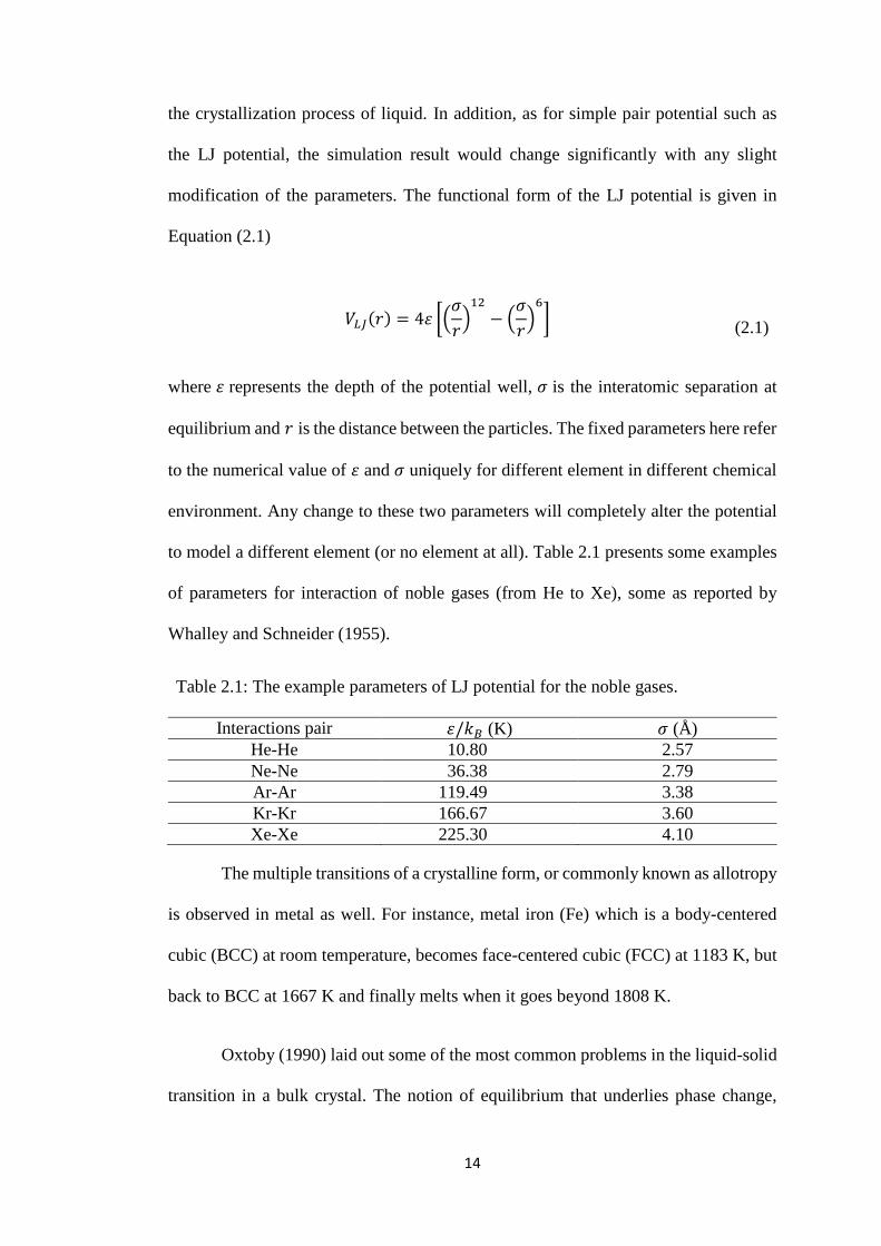
the crystallization process of liquid. In addition, as for simple pair potential such as

the LJ potential, the simulation result would change significantly with any slight

modification of the parameters. The functional form of the LJ potential is given in

Equation (2.1)

𝑉𝐿𝐽(𝑟) = 4휀 [(𝜎

𝑟)

12

− (𝜎

𝑟)

6

] (2.1)

where 휀 represents the depth of the potential well, 𝜎 is the interatomic separation at

equilibrium and 𝑟 is the distance between the particles. The fixed parameters here refer

to the numerical value of 휀 and 𝜎 uniquely for different element in different chemical

environment. Any change to these two parameters will completely alter the potential

to model a different element (or no element at all). Table 2.1 presents some examples

of parameters for interaction of noble gases (from He to Xe), some as reported by

Whalley and Schneider (1955).

Table 2.1: The example parameters of LJ potential for the noble gases.

Interactions pair 휀/𝑘𝐵 (K) 𝜎 (Å)

He-He 10.80 2.57

Ne-Ne 36.38 2.79

Ar-Ar 119.49 3.38

Kr-Kr 166.67 3.60

Xe-Xe 225.30 4.10

The multiple transitions of a crystalline form, or commonly known as allotropy

is observed in metal as well. For instance, metal iron (Fe) which is a body-centered

cubic (BCC) at room temperature, becomes face-centered cubic (FCC) at 1183 K, but

back to BCC at 1667 K and finally melts when it goes beyond 1808 K.

Oxtoby (1990) laid out some of the most common problems in the liquid-solid

transition in a bulk crystal. The notion of equilibrium that underlies phase change,

15

namely the coexistence of phases at critical temperature, 𝑇𝑐 is widely accepted. During

the latent heat of fusion (melting), the thermodynamic properties are easily

documented, but the microscopic changes to the structures between the coexisting

phases are not quite understood. There are still some unsolved phenomena such as the

local nucleation within a bulk or the dislocation of impurities and surfaces. The

dynamical studies of non-equilibrium growth in the microscopic level are very

different from the macroscopic observables.

In fact, some of the known premonitory effects close to the melting transition

are observed in bulk crystal. For example, substantial changes in volume,

compressibility, heat capacity and electric conductivity are observed in bulk crystal

long before the bulk melting point 𝑇𝑚𝑏𝑢𝑙𝑘 (Dash, 2002). These changes are more

apparent in clusters, and are known as pre-melting effect. It happens at a temperature

𝑇𝑝𝑟𝑒 before the actual melting point 𝑇𝑚. Breaux et al. (2005) studied the pre-melting

effect in aluminium clusters, where the surface melting is observed to occur at a

temperature much lower than 𝑇𝑚.

Surface melting occurs as a major event in clusters. In fact, surface melting is

an important observation that leads to a complete theory of bulk melting. Faraday

(1859) pointed out that the surface melting occurs naturally in any bulk solid. For

instance, the melting of water on the surface of ice causes it to be slippery. In fact, this

finding can be explained indirectly as the wetting of a solid surface. During this

process, any liquid remaining on the solid surface is actually melted from its own

surface. There is a model describing the surface energy in term of contact angle

(Subedi, 2011). Thus, the macroscopic measurable contact angle becomes a direct

measure of the microscopic free energy of the surface liquid layer. Through this

16

approach, we are able to predict more properties of surface melting and the existence

of the metastable state.

Naturally, the interest of study is to find out the asymptotic behavior of atom

to bulk. The gradual change of thermal properties with the of size of the clusters, 𝑛, is

not fully understood. Nevertheless, melting temperature of a cluster being size-

dependent is widely accepted, due to most findings supporting the statement (Duan et

al., 2007; Liu et al., 2013; Neyts and Bogaerts, 2009; Zhao et al., 2001). However, as

reported by Martin et al. (1993), even at 𝑛~104, the melting temperature of sodium

clusters is still lower than the bulk value. It was stated otherwise by Calvo and

Spiegelmann (1999) where they suggested the pre-melting, 𝑇𝑝𝑟𝑒 effect to be taken into

consideration. From their findings, the melting transition in sodium clusters is said to

be at 𝑛 > 93. The core-shell structures of the clusters contribute a significant effect to

the surface melting and thus the pre-melting phenomena. Experiments have led to a

homogeneous melting model (Effremov et al., 2000) that relates the reduced melting

point of a cluster, 𝑇𝑚 to that of the bulk, 𝑇𝑚𝑏𝑢𝑙𝑘 using

𝑇𝑚 = 𝑇𝑚𝑏𝑢𝑙𝑘 −

𝛼

𝑟 (2.2)

where 𝛼 is a positive quantity with the dimension of [L][θ] which can be determined

experimentally, and 𝑟 is the radius of the particle or cluster. This relationship was

derived by Buffat and Borel (1976) from Gibbs-Duhem equation. In the following year,

Couchman and Jesser (1977) outlined a direct theoretical study on Sn, In and Au

clusters to predict their surface melting. The thermodynamic theory has successfully

quantified three features of cluster melting:

1. Melting is initiated at the surface.

17

2. The existence of an upper and lower limit of the range of melting

temperature, 𝑇𝑚.

3. Characteristics of surface nucleation and liquid layer growth are

qualitatively captured.

The thermal properties of bulk solid can be obtained through some

macroscopically measurable quantities, specifically thermodynamics quantities such

as pressure, 𝑃, density, 𝜌, and temperature, 𝑇. The thermal properties of a cluster, on

the other hand, needs to be obtained by indirect means. Schmidt and Haberland (2002)

revised an approach to measure the melting temperature, latent heat, and entropy of

some bigger sodium clusters of size ranging from 𝑛 = 55 to 𝑛 = 357 , which are

derived indirectly from the caloric curve.

Many experimental studies (Schmidt and Haberland, 2002; Martin et al. 1993)

have established the following fact regarding the melting of free cluster in comparison

to bulk counterpart, namely:

1. The melting temperature, 𝑇𝑚 of a cluster is generally lower than the

bulk value, 𝑇𝑚𝑏𝑢𝑙𝑘.

2. The latent heat of transformation is smaller than the bulk.

3. The melting stage does not occur at a fixed temperature, but begin with

pre-melting, 𝑇𝑝𝑟𝑒 over a finite range of temperature.

4. The heat capacity of the finite-sized system can sometimes take a

negative value.

In fact, statement one and two are analogous, since the melting temperature,

𝑇𝑚 and the latent heat of a cluster show similar fluctuations, while pre-melting is

18

widely observed though experiments. The first three statements were discussed earlier,

but the fourth seems unnatural. A negative heat capacity implies that energy is

absorbed with decreasing in the cluster temperature. Heat absorption during melting is

commonly understood in terms of latent heat of transformation, where the mean kinetic

energy tends to remain constant. In their paper, Schmidt and Haberland (2002) have

explained that a finite sized system tends to convert some of the kinetic energy into

potential energy in order to avoid partially molten states. Phenomenological

observations related to the thermal behavior of cluster will be further discussed in the

next chapter from the view point of computational simulation.

In computational simulation, the concept of melting as applicable in the bulk

can be similarly applied in microscopic systems. This is a benefit to molecular dynamic

simulation whereby the same set of equations of motion is used to solve the interatomic

interaction for any kind of system, be it bulk or microscopic.

In a bulk system which is typified by a size of ~1023 atoms, MD simulation is

performed by imposing periodic boundary condition to mimic an extensive body

which is formed by a periodic repetition of supercells. However, for finite system such

as a cluster, it is possible to simulate the movement of every single atom. The

microscopic properties, such as binding energy, temperature, entropy and density of

the cluster could be easily computed by sampling the trajectory of every atom for every

time step. As far as molecular dynamics are concerned, a free-standing cluster in the

vacuum which is practically difficult to set up in experiment can be computationally

simulated by choosing a proper empirical interatomic potential. In many occasions,

the computational simulation can become relatively cheap to perform. With the ease

19

of acquiring simulation data, the focus of research effort can hence be devoted to the

extraction of physical information from the cluster system.

A cluster behaves differently from both crystals and amorphous solid. The

commonly accepted Lindemann criterion of melting is not completely accurate to

predict the phase change in cluster. One particular reason for this discrepancy is that

the thermal instability of a free-standing cluster creates some errors within the effective

range of the interatomic potential in the simulation. This arises due to the existence of

multiple basins along the PES. Thus, the initial structure for the simulation has to be

ensured such that it lies within the basin of the global minimum (Leary 2000).

However, for an expensive interatomic potential, the time required to globally

optimize the initial structure is tremendously long and computationally expensive. The

numerous approximations and functional form of empirical interatomic potential

become a limiting factor as to how accurate a simulation can resemble the real system.

This also gives rise to error while solving the equation of motions.

MD simulations allow us to study various characteristics, such as the surface

and the core-shells models. Duan et al. (2007) in their molecular simulation of pure Fe

cluster showed that for large clusters such as Fe300, the surface can exist as molten

phase while the core as solid phase at the same time. The temperature range of melting

is, however, narrow and precise. This coexistence of different phases on the surface

and in the core proves that the melting of different shells at a different temperature is

probable even for pure element clusters. Logically, one would expect that only a core-

shell clusters of different elements to undergo this kind of melting pattern. Duan et al.

(2007) also made a conclusion that the coexistence is over time for small clusters;

whereas the coexistence is over space for big clusters.

20

When the cluster size is relatively small, the values of melting point, 𝑇𝑚 ,

instead of decreasing with √𝑛3

, could show oscillation. The peaks in the oscillation can

be explained by the existence of magic number in finite sized clusters. Such

observation was made by Schmidt et al. (1998) in their experiment where the melting

point of Na147 is higher than Na130 by ~60 K. The experiment by Schmidt et al. (1998)

was considered very sophisticated at that time. It can be said that when the cluster size

is very small, the experimental studies become extremely difficult. On the other hand,

computational simulation enables easy manipulation of cluster species which will be

a complement to the experimental limit.

Another benefit of computational simulation is that the composition and

geometrical constraint can be controlled to create a large variety of structures. Kuntová

et al. (2008) performed extensive studies on Ag-Ni and Ag-Co bimetallic nanoalloys.

They picked only the highly symmetric magic clusters as their candidates, namely

Ag72Ni55, Ag72Co55, Ag32Ni13, and Ag32Co13. According to the simulation result Ag

atoms tend to be sitting in the shell while both the Ni and Co atoms were in the core.

Even though the structures of the nanoalloys are similar, the melting behaviors are

different. Melting of clusters is greatly affected by the nature of the potential energy

surface (PES) that causes a large behavioral change.

The melting data obtained via simulation can be used to study the dynamics of

phase change. Comparison between commonly used post-processing methods were

discussed by Lu et al. (2009). The most commonly used post-processing method is

caloric curves, whereby the binding energy (or binding energy per atom) is plotted

against temperature. Another method is the constant temperature specific heat capacity,

21

𝑐𝑣, as a function of temperature, which is actually the fluctuations of the caloric curve,

given by the equation

𝑐𝑣 =⟨𝐸𝑡

2⟩𝑇 − ⟨𝐸𝑡⟩𝑇2

2𝑛𝑘𝐵𝑇2

(2.3)

where 𝐸𝑡 is the total energy of cluster, 𝑘𝐵 the Boltzmann constant, 𝑛 the total number

of atoms in the cluster and ⟨ ⟩𝑇 represent the thermal average at temperature 𝑇. A

typical 𝑐𝑣 curve appears in the form of a sharp peak at the melting temperature, 𝑇𝑚.

Nevertheless, the two methods mentioned above are not the only methods for

quantifying the melting behavior of clusters. Some characteristics from simulated

annealing process have to be obtained with special treatments. Lu et al. (2009) showed

that there is a mismatched in the melting temperature of Co13 and Co14 clusters, if

Lindemann index, 𝛿, was used as a mean to gauge the melting process, as compared

to 𝑐𝑣 curve. Lindemann index is given by the equations

𝛿 =1

𝑛∑ 𝛿𝑖

𝑖

(2.4)

𝛿𝑖 =1

𝑛 − 1∑

(⟨𝑟𝑖𝑗2⟩𝑇 − ⟨𝑟𝑖𝑗⟩𝑇

2 )12

⟨𝑟𝑖𝑗⟩𝑇𝑗≠𝑖

(2.5)

where 𝑟𝑖𝑗 is the distance between the 𝑖th and 𝑗th atoms. Lastly, the dynamics during

the cluster melting is studied by short-time averaged distance ⟨𝜎𝑖(𝑡)⟩𝑠𝑡𝑎, given by the

equation

⟨𝜎𝑖(𝑡)⟩𝑠𝑡𝑎 = ∑|𝑟𝑖(𝑡) − 𝑟𝑗(𝑡)|

𝑗

(2.6)

22

where 𝑟𝑖(𝑡) represents the position of the 𝑖th atom at time 𝑡, while ⟨ ⟩𝑠𝑡𝑎 denotes that

the average is taken for a short interval of time steps and then plotted against the time.

Similar method had been used earlier by Aguado et al. (2001) on Na cluster.

Computing the time-average value is troublesome but somewhat could be a solution

to the thermal instability in the simulated annealing procedure. The problem of thermal

stability is a big obstacle in simulation of cluster melting. Details on molecular

dynamics methods used in this thesis were discussed further in Chapter 3.

2.3 Chemical Similarity and Shape Recognition

The method of molecular shape comparison is used in comparing the geometry

or spatial configuration of two or more molecular structures to identify the chemical

similarity between them (Grant et al., 1996). Molecular shape comparison is an

important field of research and application. It is a method with a wide range of

applications in the field of informatics, cheminformatics and bioinformatics, such as

drug discovery, screening in pharmaceutical studies, nucleic acid sequencing of

biological data, protein classifications and identification. The development of

structural classification of proteins remain important today, and it is continually

improving. Andreeva et al. (2013) recently improved their prototype of structural

classification of proteins to the second generation SCOP2 (http://scop2.mrc-

lmb.cam.ac.uk/ 1st March 2016). A sample screenshot of using SCOP2 graph viewer

is attached in Figure 2.2, showing the classification of Cro regulator proteins based on

structural properties and relationships.

The usefulness of molecular shape comparison lies in its ability to transform

data into information which in turn leads to a better decision making in drug lead

23

identification and optimization (Brown, 2005). Shape recognition is by far a method

most suitably applied on static molecules. One practical example of dynamical system

is the sequential changes of biological molecules across generations. However, it lacks

the flexibility to make pattern prediction in dynamical systems which involve constant

change in their configuration throughout their historical evolution.

Figure 2.2: Sample of SCOP2 graph viewer result given by Andreeva et al. (2013),

showing the Cro types protein sequence and structure.

24

Virtual screening is a computational procedure to search for chemical

similarity to identify and compare the structures of molecules or coupounds from a

standard database library, such as the protein data bank. There are different approaches

to virtual screening, one of which is similarity-based virtual screening. The formalism

of similarity based virtual screening is based on the similar property by Johnson and

Maggiora (1990), which stated that the coupounds with higher structural similarity

tend to have similar chemical and biological activities. With a suitable approach, one

can assign a probability to the activity of the structure under study with reference to

the known sample from the database of compounds. However, in the field of

informatics, different organizations or companies provide their own unique ways to

test for chemical similarity. The degree of similarity between the compared structures

predicted by different approach can be differed from one another.

The selected structures for shape identification are normally represented by a

binary molecular fingerprint of descriptors, also known as structural keys that containt

various visualisable information. For example, the size of the molecule, the number of

bonds or type of bondings involved, the active functional groups and the pattern of

target structure or substructure (http://www.daylight.com, 1st March 2016). Some

descriptors might carry a certain portion of information that outweight others and

become less universal for a certain group of compounds. Thus, certain descriptors can

work better and faster when the information density is lower, which does not always

necessarily so. The descriptors are generally calssified into three types based on the

dimensionality of the descriptors. The two-dimensional descriptors such as MACCS,

MDL keys, and Daylight are said to perform better than the three-dimensional ones

(Oprea, 2002). These two-dimensional descriptors are mostly patented under their own

company signature. MDL two dimensional descriptors have been designed to be used

25

for the saearch of substructures. Durant et al. (2002) managed to re-optimize the

existing 166 bit and 960-bit keysets of the time to increase the number of success

measurements. The newly designed descriptor was found to have equal performance

although the keysets are composed differently without overlapping. It seems that the

construction of the keysets is bound to some known constraints, thus prompting a

possibility of further studies to enable the construction of keyset that is data size

independent (Zhu et al., 2016).

Three-dimensional descriptors were difficult to compute until Ballester and

Richards (2007) proposed the ultrafast shape recognition (USR) method based on four

sets of distance distribution of the atoms in a molecule defined at different points of

reference. The geometries of the atomic configurations are described by a total of three

statistical moments, namely the mean, variance and skewness. It turns out that these

USR descriptors are orientation independent, so that molecules being screened do not

need to be aligned. USR is said to perform at least three order of magnitude faster than

other descriptors. The similarity index is denoted as 𝑆𝑞𝑖 ∈ (0,1) . A value of 1

represents “totally identical” while 0 means “vastly differed”. 𝑆𝑞𝑖 is given by the

equation

𝑆𝑞𝑖 = (1 +1

12∑|𝑀𝑙

𝑞 − 𝑀𝑙𝑖|

12

𝑙=1

)

−1

(2.7)

where the moments of shape descriptors 𝑀𝑞 and 𝑀𝑖 represent the query and the 𝑖th

molecule.

Later in the same year, Cannon et al. (2008) attempted to combine the binary

166 bit MACCS keys and the USR with an additional four extra moments based on

26

kurtosis of the distributions. The hybrid descriptors were shown to yield a better result

as compared to binary 166 bit MACCS keys or USR. The performance of the above

hybrid descriptors was assessed by considering the accuracy and effectiveness of the

algorithm. The performance is tabulated according to different measures, such as the

percentage of actives recalled in the top 1% and top 5% of the ranked validation sets,

precision of predicted positives, area under the Receiver Operating Characteristic

curve (AUC), the F-measure and Matthew Correlation Coefficient (MCC). All these

methods are statistical set-up to measures the performance of the algorithm.

To get a glimpse of how robust the work of Ballester and Cannon is, other

works with similar task were referred. The details of the formulation will not be fully

discussed here; only the concept of matching is explained, along with the commons

and differences as compared to other similarity indices. The choice of notation may be

modified from the references for easy comparison. Grant et al. (1996) were among the

earlier successes, where the process of matching two molecules was worked out by

aligning two structures A and B in order to obtain a maximum intersection volume.

The alignment problem was solved by optimizing the rotation and translation of the

comparing structures with respect to one another. Then, the normalized similarity

index, 𝑆𝐴𝐵 can be obtained via the equation

𝑆𝐴𝐵 =2 ∫ 𝑑𝒓𝜌𝐴

𝑔𝜌𝐵

𝑔

∫ 𝑑𝒓(𝜌𝐴2 + 𝜌𝐵

2)≡

2𝑉𝐴𝐵𝑔

𝑉𝐴2 + 𝑉𝐵

2 (2.8)

where the volume of intersection, 𝑉𝐴𝐵𝑔

is the numerator part of the 𝑆𝐴𝐵, which is given

by

27

𝑉𝐴𝐵𝑔

= ∫ 𝑑𝒓𝜌𝐴𝑔

𝜌𝐵𝑔

(2.9)

The term 𝜌𝜒𝑔

, 𝜒 = 𝐴 or 𝐵 are the Gaussian densities and can be represented in terms

of the spherical Gaussian, 𝜌𝑖𝑔(𝑟𝑖) as the product formula

𝜌𝜒𝑔

= 1 − ∏(1 − 𝜌𝑖𝑔

)

𝑖∈𝜒

, 𝜒 = 𝐴 𝑜𝑟 𝐵

(2.10)

𝜌𝑖𝑔(𝒓𝒊) = 𝑝𝑖𝑒

−(3𝑝𝑖𝜋

12⁄

4𝜎𝑖3 )

23⁄

(𝑟−𝒓𝒊)2

(2.11)

where 𝜎𝑖 is the radius of the atom and the Gaussian weight is assumed to be 𝑝𝑖 = 2.70.

The difficulties in shape matching of dissimilar molecules are solved by the idea of

shape multipoles, where each atom is described by merely two parameters, 𝜎𝑖 and 𝑝𝑖.

The shape multipoles are the product of radius and the Gaussian density.

Another recent work by Yan et al. (2013) saw the implementation of the

weighted Gaussian function instead of the common Gaussian approximation with the

use of Tanimoto similarity index. Tanimoto similarity index (Bajusz et al., 2015) is

said to be the most widely used measure of chemical similarity, given by the equation

𝑆𝐴𝐵 =𝑉𝐴𝐵

𝑉𝐴𝐴 + 𝑉𝐵𝐵 − 𝑉𝐴𝐵

(2.12)

In this study, the overlapping volume of the two molecules are given by

𝑉𝐴𝐵𝑔

= ∑ 𝑤𝑖𝑤𝑗𝑣𝑖𝑗𝑔

𝑖∈𝐴,𝑗∈𝐵

(2.13)

The difference from previous works lies in the existence of the weighting factor

28

𝑤𝑖 =𝑣𝑖

𝑔

𝑣𝑖𝑔

+ 𝑘 ∑ 𝑣𝑖𝑗𝑔

𝑗≠𝑖

(2.14)

where 𝑘 is a constant fitted to hard-sphere volume, while the volume terms 𝑣𝑖𝑔

for

atom 𝑖 and 𝑣𝑖𝑗𝑔

for the volume of atom pair intersection are given by equations

𝑣𝑖𝑔

= ∫ 𝑑𝒓𝒊𝜌𝑖𝑔(𝒓𝒊)

(2.15)

𝑣𝑖𝑗𝑔

= ∫ 𝑑𝒓 𝜌𝑖𝑔(𝒓)𝜌𝑗

𝑔(𝒓) (2.16)

Lastly, the spherical Gaussian 𝜌𝑖𝑔(𝒓𝒊) is the same as introduced by Grant et al. (1996),

but the Gaussian weight 𝑝 = 2√2 is multiplied with the same weightage factor, 𝑤𝑖.

Apparently, both the Grant et al. (1996) and Yan et al. (2013) version of 𝑆𝐴𝐵 satisfy

the condition 0 ≤ 𝑆𝐴𝐵 ≤ 1 with same representations of 𝑆𝑞𝑖 by Ballester and Richards

(2007).

The three-dimensional descriptors introduced can be separated into two types.

The first is the direct alignment and explicit shape comparison. This method is said to

be less efficient but fulfills the similar property principle (Fang et al., 2009). The

second method is indirect comparison using the shape descriptor such as the USR.

Although it could be computed rather easily and fast, the representation of the shape

is incomplete. The fast computing USR method has led Hsu (2014) to adopt it in the

study of melting of finite size clusters. The simplicity of USR method is required in

order to handle up to 108 frames of coordinate profile. Another advantage of using

shape recognition method in the study of melting transition is that it can handle any

type of structural sampling. This is due to the fact that this approach concerns solely

29

the geometry of the structures without the need to consider of the nature of the atoms.

The fundamental characteristics of the atoms such as the atomic radius and atomic

mass do not affect how the method is applied to the task. It could reveal the interaction

behavior that is difficult to be detected by other methods as its job only involve

observing the evolution of the trajectories. The effect of shape recognition method in

tracking the trajectory can be viewed as though each frame of coordinates is being

traced like a movie.

Besides the direct shape comparison method, Rogan et al. (2013) revised an

approach for cluster conformation which is based on the distances between atoms in

the cluster. The similarity measure is actually an idea originally proposed by Grigoryan

and Springborg (2003), where the original definitions are given by the equations

𝑑𝑆(𝐴, 𝐵) = [2

𝑛(𝑛 − 1)∑ (𝑑𝑚

𝐴 − 𝑑𝑚𝐵 )2

𝑛(𝑛−1) 2⁄

𝑚=1

]

12⁄

(2.17)

𝑆𝐴𝐵 =1

1 + 𝑑𝑆(𝐴, 𝐵)

(2.18)

where 𝑑𝑚𝜒

is the distance between the atoms in the cluster 𝜒, 𝜒 is the label for cluster

in comparison: 𝐴 𝑜𝑟 𝐵, while 𝑚 labels the distances in ascending order within the

cluster 𝜒. The suffix 𝑆 stands for Springborg. The modified version by Rogan et al.

(2013) is given by the equation

𝑑𝑁(𝐴, 𝐵) = [2

𝑛(𝑛 − 1)∑ (

𝑑𝑚𝐴

𝐷𝑎𝑣𝑒𝐴

−𝑑𝑚

𝐵

𝐷𝑎𝑣𝑒𝐵

)

2𝑛(𝑛−1) 2⁄

𝑚=1

]

12⁄

(2.19)

30

where 𝐷𝑎𝑣𝑒𝜒

represents the average bond length for clusters 𝜒 = 𝐴 𝑜𝑟 𝐵 . Note that

𝑑𝑆(𝐴, 𝐵) has a dimension of length [L] but 𝑑𝑁(𝐴, 𝐵) is dimensionless, and it also

includes a scaling effect by including the sum of the ratio in its definition. Rogan et al.

(2013) tried to plot the comparison of clusters with a color map instead of taking the

same approach of calculating the similarity index 𝑆𝐴𝐵 . Hence, the normalization is

done the other way round with 0 and 1 for maximum and minimum similarity

respectively. The normalization is given by the equations

𝐷𝑆(𝐴, 𝐵) =𝑑𝑆(𝐴, 𝐵) − 𝑑𝑆,𝑚𝑖𝑛

𝑑𝑆,𝑚𝑎𝑥 − 𝑑𝑆,𝑚𝑖𝑛

(2.20)

𝐷𝑁(𝐴, 𝐵) =𝑑𝑁(𝐴, 𝐵) − 𝑑𝑁,𝑚𝑖𝑛

𝑑𝑁,𝑚𝑎𝑥 − 𝑑𝑁,𝑚𝑖𝑛

(2.21)

2.4 Empirical Interatomic Potential

It has become a common practice in the research community whereby

computer simulations are performed to complement experimental investigation. When

a system is approaching microscopic level, molecular dynamics (MD) simulations can

play a crucial role in their theoretical study as experiments became relatively difficult

to be conducted. Over the years, theoretical approaches are based on mathematical

methods developed during earlier time with lots of assumptions and approximations.

On the other hand, MD simulations have attempted to solve the root problem as it is.

Many MD applications are still facing challenges to completely represent the quantum

mechanical problems. MD practitioners try to overcome this problem by working

backward from the existing experimental data. This approach is widely known as the

fitting of parameters empirically or reversed engineering. The confidence in a MD

31

simulation result relies on the choice of a good theoretical model coupled with a

sensible methodology.

In MD simulations involving interatomic interactions, the functional form of

the equations of motion depend on the choice of potential energy term (a.k.a. force

field) that appear in the Hamiltonian of the system. A simulation is bound by a set of

approximations. The approximation methods can be classified into three main types

according to their formulations, namely the first-principle or ab initio, semi-empirical

and empirical (classical). The most widely used first-principles methods are either

density functional theory (DFT) or Hartree-Fock (HF) methods. Although the results

from first-principle calculations agree well with the experiment, it is computationally

expensive and time-consuming. The semi-empirical method uses a certain amount of

experimental data as input parameters for the calculation. The added approximations

and constraints speed up the computational time, but sometimes reduce the accuracy

of the modeling itself. Within this modeling framework, the parameters are

parameterized such that the results agree best with either experimental data or ab-initio

results. Empirical approach presumes systems of balls and springs connected to each

other. The interatomic interaction can be either operating between a pair of atoms, or

include a third entry (angles). Some more advance interaction is many-body in nature

(dihedral).

One of the most commonly used pair potentials is the LJ potential, 𝑉𝐿𝐽(𝑟),

which has been introduced by Equation (2.1) in Section 2.2. Although being less

accurate, the simplicity of calculation has led to its extensive use in many simulations.

The term 𝑟−12 is the short range Pauli repulsion while the term 𝑟−6 is the long range

attraction such as Van der Waals’ interaction and the London dispersion force. Some

32

studies require the LJ potential to work with other effective short range potential to

model a large system with long range interaction. Due to its simple interaction that

resembles the inert system, one of the early motivations of LJ potential in clusters was

to calculate the gas-liquid nucleation of noble gases (Zeng and Oxtoby, 1990). In fact,

the MD study of gas-liquid nucleation of LJ fluid has never stop but continue to gain

more interest in search for better nucleation theories (Laasonen, 2000). Another

notable pair potential is the Morse potential, sometimes replacing the LJ potential for

a better description of long range interaction.

Gupta (1981) has succeeded in improving the classical interaction to account

for the surface separation correction of face-centered-cubic metals. The electronic

charge transfer at the surface was corrected earlier by Finnis and Heine (1974). The 𝑛-

body Gupta potential is fast to compute and converge, according to the equation

𝑉𝑛 = ∑ { ∑ 𝐴𝑖𝑗𝑒𝑥𝑝 (−𝑝𝑖𝑗 (𝑟𝑖𝑗

𝑟𝑖𝑗(0)

− 1))

𝑛

𝑗=1(𝑗≠𝑖)

𝑛

𝑖=1

− [ ∑ 𝜉𝑖𝑗2 𝑒𝑥𝑝 (−2𝑞𝑖𝑗 (

𝑟𝑖𝑗

𝑟𝑖𝑗(0)

− 1))

𝑛

𝑗=1(𝑗≠𝑖)

]

1 2⁄

}

(2.22)

where 𝐴𝑖𝑗, 𝜉𝑖𝑗, 𝑝𝑖𝑗, 𝑞𝑖𝑗 and 𝑟𝑖𝑗(0)

are the parameters to be fitted with bulk values. The

fitting enables a certain degree of correction to the classical potential. As can be seen

in the form of equation, Gupta potential remains intact as pair-wise potential with the

following general form of equation

𝑉𝑝𝑎𝑖𝑟 = ∑(𝑉𝑟𝑒𝑝𝑢𝑙𝑠𝑒 + 𝑉𝑎𝑡𝑡𝑟𝑎𝑐𝑡) (2.23)

33

A recent study by Rogan et al. (2013) demonstrated that the choice of pair

potential is almost subtle when quantum refinement is introduced. The comparison

was done on the Gupta, Sutton-Chen, and the LJ potentials, where these three

potentials basically yield almost similar structures for small clusters of Ni and Cu after

a further re-optimization with DFT. The most concerned objective of MD simulation

is the accuracy of an empirical interatomic potential being able to predict the dynamics

of its respective system. The outcome of the prediction need to be tally with the DFT

(at zero Kelvin) or the experimental result as well. In this thesis, this procedure is used

to ensure the appropriateness of the choice of interatomic potential.

One can generalize the interaction for 𝑛 interacting particles beyond the pair

potential as the sum of contributions from one-body, two-body, three-body terms, etc.

as the serie,

𝑉𝑒𝑓𝑓(1, … , 𝑛) = ∑ 𝑣1(𝑖)

𝑖

+ ∑ 𝑣2(𝑖, 𝑗)

𝑖,𝑗>𝑖

+ ∑ 𝑣3(𝑖, 𝑗, 𝑘)

𝑖,𝑗>𝑖,𝑘>𝑗

+ ⋯

+ 𝑣𝑛(1, … , 𝑛) (2.24)

For an effective representation, 𝑣𝑛 should converge to zero as 𝑛 increases. The

first term corresponds to the external forces and is normally not included in the

Hamiltonian. Many recent popular interatomic potentials are derived based on this

form of equation with their own significant successes. To name a few, there are

Stillinger-Weber (SW) potential (Stillinger and Weber, 1985), Tersoff potential

(Tersoff, 1988), the improved version of both Reactive Empirical Bond Order (REBO)

potential (Brenner et al., 2002) and the Adaptive Intermolecular Reactive Empirical

Bond Order (AIREBO) potential (Stuart et al., 2000). The term ‘generation’ is usually

adopted to differentiate the version of their development, such as the first generation

34

Brenner potential for the 1990 REBO potential (Brenner, 1990) for hydrocarbons and

second generation Brenner potential in 2002. Nevertheless, for Brenner case, the first

generation REBO potential underwent a drastic improvement in both the analytical

equation and the extension in the fitting database.

The practicality of many-body potentials has been routinely demonstrated

whereby numerous structures are successfully predicted. One of the latest examples is

the growth of graphene on a silicon carbide substrate by the simulated annealing

process (Yoon et al., 2013). In the study, Tersoff potential and a modified version of

Tersoff-Erhart-Albe (TEA) (Erhard and Albe, 2005) potential were compared with the

formation of the graphene layers. Even though graphene was not discovered during

1988, Tersoff was able to predict every possible combinations and permutations of

carbon-carbon interaction. The capabilities of the potentials to predict structure rely

on the parameters during fitting. These type of potentials are known as bond order

potentials (BOP). In MD, BOP are best suited to describe the bonding states of the

atoms to includes various bonding states between a pair of atoms. The fitting of the

parameters includes the consideration from the number of bonds, angles, and bond

length.

Pair potential is not suitable to describe directional interaction where a third

particle is involved. The shortcoming can be solved by incorporating a term, 𝑣3, which

works to include more properties of the structures by taking into account the

contribution from more experimental data. Consequently, the additional terms stabilize

the structure. Thus, most MD simulations are carried out with many body potentials.

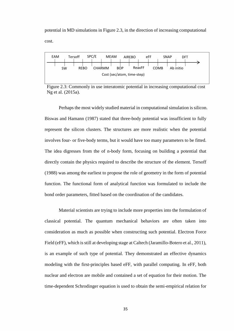
Ng et al. (2015a) discussed some of the widely used semi-empirical interatomic

35

potential in MD simulations in Figure 2.3, in the direction of increasing computational

cost.

Figure 2.3: Commonly in use interatomic potential in increasing computational cost

Ng et al. (2015a).

Perhaps the most widely studied material in computational simulation is silicon.

Biswas and Hamann (1987) stated that three-body potential was insufficient to fully

represent the silicon clusters. The structures are more realistic when the potential

involves four- or five-body terms, but it would have too many parameters to be fitted.

The idea digresses from the of n-body form, focusing on building a potential that

directly contain the physics required to describe the structure of the element. Tersoff

(1988) was among the earliest to propose the role of geometry in the form of potential

function. The functional form of analytical function was formulated to include the

bond order parameters, fitted based on the coordination of the candidates.

Material scientists are trying to include more properties into the formulation of

classical potential. The quantum mechanical behaviors are often taken into

consideration as much as possible when constructing such potential. Electron Force

Field (eFF), which is still at developing stage at Caltech (Jaramillo-Botero et al., 2011),

is an example of such type of potential. They demonstrated an effective dynamics

modeling with the first-principles based eFF, with parallel computing. In eFF, both

nuclear and electron are mobile and contained a set of equation for their motion. The

time-dependent Schrodinger equation is used to obtain the semi-empirical relation for

SW Ab initio

EAM Tersoff

REBO

SPC/E

CHARMM

MEAM

BOP

AIREBO

ReaxFF

eFF

COMB

SNAP DFT

Cost (sec/atom, time-step)

36

their independent motion. This consideration enables eFF to be applied in any

calculations that involve electron excitation.

Rather than relying on a computationally expensive interatomic potential, an

improved MD method will help to boost up the performance of simulations as well.

Rick et al. (1994) revised an additional step in MD by enabling point charges to be

considered in the interaction via electronegativity equalization (Qeq) method. This

additional charge equilibration step has been included in the formulation of Charge-

Optimized Many-Body (COMB) potential by Yu et al. (2007) for the system of Si and

SiO2. It is effective in predicting the correct properties of the elements. The COMB

potential is modified by the Tersoff potential. The fitting procedure of the parameters

is similar to that of Tersoff potential.

This thesis uses the second generation COMB potential (Shan et al., 2010) in

predicting the structure of clusters. The development of COMB potential and the key

characteristics were discussed in details in Chapter 3 along with the methodology

involved.

2.5 The Method of Basin Hopping

Basin-Hopping (BH) is an unbiased global optimization method introduced by

Wales and Doye (1997). The complexity of the PES determines the complication in

obtaining the global minimum structure, which corresponds to the structure with the

lowest energy. The objective of BH is to scan and later transform the PES into a

simplified staircase topology. Hence, it is very efficient to locate the minima. The

transformed energy �̃�(𝑋) is defined by

37

�̃�(𝑋) = 𝑚𝑖𝑛{𝐸(𝑋)} (2.25)

where 𝐸(𝑋) represents a certain point on the PES with 𝑋 being the 3𝑛-dimensional

position coordinates of the atoms, {𝑟1, 𝑟2, … , 𝑟𝑛} . {𝑟𝑖} carries the set of Cartesian

coordinate of atom 𝑖 in the form of {𝑥𝑖, 𝑦𝑖 , 𝑧𝑖}.

Figure 2.4: A schematic sketch to illustrate the effect of BH transformation to the

PES of a one-dimensional example.

Wales and Doye (1997) presented a schematic example to illustrate the effect

of the BH method in a one-dimensional PES as shown in Figure 2.4. The solid line is

the original energy profile while the dashed line is the staircase topology after the

transformation of Equation (2.25). Based on the sketch, the effect of scanning through

the PES should yield the same minima as the staircase topology. Essentially, the BH

method works in combining the deterministic and stochastic methods in a Monte Carlo

approach.

The BH method was adopted as part of a global search algorithm by Hsu and

Lai (2006), in their full-length algorithm called parallel tempering multi-canonical

basin hopping plus genetic algorithm, PTMBHGA. The effect of transforming the PES

simplifies the dynamics of geometrical search, even with much more complicated

38

potential such as Gupta potential instead of the simplified LJ potential. The tendency

of trapping in saddle point was also solved by working the multi-canonical BH (MBH)

together with Genetic Algorithm (GA) and parallel tempering Monte-Carlo (PT)

method, hence the name PTMBHGA.

Many who study cluster structures have come to realize that the global

minimum of an interatomic potential does not always correspond to the result obtained

from DFT calculations. Oganov and Valle (2009) proposed that there are probabilities

that the low-lying structures (LLS) might include the global minimum. Sometimes, the

quantum refined global minimum happens to coincide with one of the higher energy

local minimum instead of the global minimum of the empirical potential. Hence, the

method of BH became even more powerful because the purpose of searching the

minimum was aimed at locating a set of minima along the PES. This approach is

adopted in this thesis to locate the unique ground state structures of hafnium cluster.

During the search for the global minimum structure of a cluster, the effect of

electronic charge transfer is an important factor affecting the outcome of the structural

geometry (Mollenhauer and Gaston, 2016). However, the effect of electronic charge

transfer is not taken in account in most of the less computationally intensive potentials.

Hence, the global minimum obtained from empirical interatomic potentials may not

always be the one correspond to the real case.

The use of LLS was introduced by Hartke (1996, 1998) in an attempt to

improve the global minimum search based on ab initio methods such as DFT. The

example of using LLS in the global minimum search can be explained in a schematic

sketch as shown in Figure 2.5. Bear in mind that the final aim is to obtain the true

global minimum of given cluster size at DFT level. In practice, the true global

39

minimum is formidably difficult to identify directly with finite computational resource.

The overall strategy is to arrive at this true global minimum via an indirect route. In

stage 1 of Figure 2.5, BH method is used to transform the PES into a simplified

staircase topology which contains a collection of LLS in different basins. These LLS

are indicated as green triangles in Figure 2.5. The LLS obtained in this stage will not

be minimized into the local minimum of each basin as only a minimal default setting

for energy calculation will be used (where no powerful minimization algorithm will

be called) so that the PES can be scanned through at a higher efficiency (at a fixed

computational resource constraint). Stage 1 is a slightly faster process as compared to

stage 2. In stage 2, the LLS from stage 1 are geometrically re-optimized (opt; indicated

as down arrows in Figure 2.5) into their corresponding local minima using an

expensive computational setting. These geometrically re-optimized structures are

labelled by red diamonds in Figure 2.5 which are seen sitting at the local minimum of

each basin. These red diamond are originally the LLS at stage 2 level. Geometrical re-

optimization process in this strategy provides a mechanism to transform the LLS in

stage 1 into the local minimum in each basin. Now, each basin contains a cluster

structure with unique geometry. The lowest energy structure among these LLS is

considered as the true global minimum structure.

The same strategy as described above was employed to generate free-standing

hafnium cluster for geometrical comparison in this thesis, which was discussed in

detail in Chapter 4.

40

Figure 2.5: A schematic sketch indicating the strategy to obtain true global

minimum by the way of sampling LLS at a coarse level search with BH method

without structural optimization (stage 1), and subsequently undergo a refined

geometrical re-optimization of these LLS using DFT method (stage 2). The doted

profile in stage 1 represent the simplified staircase topology of the PES.

Computationally expensive

process

Relatively fast process

Stage 1

Stage 2

PES

Basin containing the global minimum.

True global minimum

LLS of BH scanning at stage 1 Local minimum of each basin

upon geometrical optimization Opt

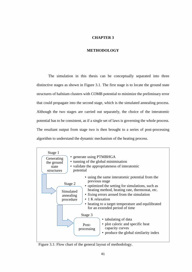
41

CHAPTER 3

METHODOLOGY

The simulation in this thesis can be conceptually separated into three

distinctive stages as shown in Figure 3.1. The first stage is to locate the ground state

structures of hafnium clusters with COMB potential to minimize the preliminary error

that could propagate into the second stage, which is the simulated annealing process.

Although the two stages are carried out separately, the choice of the interatomic

potential has to be consistent, as if a single set of laws is governing the whole process.

The resultant output from stage two is then brought to a series of post-processing

algorithm to understand the dynamic mechanism of the heating process.

Figure 3.1: Flow chart of the general layout of methodology.

Generating the ground

state structures

• generate using PTMBHGA

• tunning of the global minimisation

• validate the appropriateness of interatomic potential

Simulated annealing procedure

• using the same interatomic potential from the previous stage

• optimized the setting for simulations, such as heating method, heating rate, thermostat, etc.

• fixing errors arosed from the simulation

• 1 K relaxation

• heating to a target temperature and equilibrated for an extended period of time

Post-processing

• tabulating of data

• plot caloric and specific heat capacity curves

• produce the global similarity index

Stage 1

Stage 2

Stage 3

42

3.1 PTMBHGA

As mentioned in Section 2.2, the initial structure (input structure) of MD

processes should lie within the basin which contains the global minimum. In cluster

science, the geometry of the cluster should agree well from those obtained from DFT.

This means that the input structure is expected to yield the global minimum after the

quantum refinement, an issue which was discussed earlier in Section 2.5. The success

of a global optimization search algorithm depends on its ability to align the PES of the

empirical potential in use against a reliable DFT reference. MD simulation is

computationally cheaper than DFT. The former has another advantage over the latter

for being able to measure the temperature-dependent dynamics at a much lower

computational cost. The reliability of an interatomic potential depends on its ability to

obtain an accurate ground state structure which should agree well with the DFT result.

Locating a correct ground state structure is the prerequisites in any MD simulation of

a cluster. In fact, this is the first step as indicated in Figure 3.1.

To accurately locate the global minimum of a cluster, this thesis adopts part of

the global searching algorithm developed by Lai et al. (2002) called parallel tempering

multi-canonical basin hopping plus genetic algorithm (PTMBHGA). The algorithm

contains two global optimizers that complement each other. The basin hoping (BH)

scans through the PES and generates 20 parent candidates which are scattered over the

minima of the PES. Genetic algorithm (GA) would then discard 5 and regenerate new

candidates to explore the PES in a guided way so that a new breed of next-generation

atomic clusters is formed. The process is then repeated, i.e. for every generation, 5

‘genetically’ unfit candidates are discarded and 5 new candidates are generated

through GA, making the collection of atomic clusters always fixed at 20. GA also helps

43

BH to escape the trap in saddle point by introducing new offspring which diverges into

the different basin. This BH-GA process will cease once the number of similar

structure, all having local minimum energy value, achieved a predefined value, 7

structures to be exact. Overall, the fitness value 𝑓𝑖 of the candidates is evaluated during

all stages as a normalized control in deciding which candidates are to be discarded

based on the equations

𝑓𝑖 =𝐹𝑖

∑ 𝐹𝑗20𝑗=1

(3.1)

𝐹𝑖 =𝑉𝑚𝑎𝑥 − 𝑉𝑖

𝑉𝑚𝑎𝑥 − 𝑉𝑚𝑖𝑛

(3.2)

where 𝑉𝑖 is the potential energy of the cluster 𝑖, to be calculated using COMB potential

in this thesis.

It can be seen that from the equation for 𝑓𝑖, the fitness value is defined for a

particular cluster 𝑖 by comparing it to the group of currently available candidates at

that particular generation. Basically, the single structure might have different fitness

value when some candidates were being discarded and replaced. Hence, the same

fitness value can also act as a tolerance control in the loop, as to when the algorithm is

expected to yield the global minimum. The loop control of this current work requests

more than 6 lowest candidates with identical fitness to simultaneously exist.

The PTMBHGA code is comprised of two independent parts, the global-search

algorithm part (comprised of GA and BH search algorithm) and an ‘energy calculator’

part which calculates the energy of any given cluster configuration generated by the

global search algorithm. The original energy calculator in the PTMBHGA code was a

built-in Gupta potential. In the current study, the code was extended and modified in

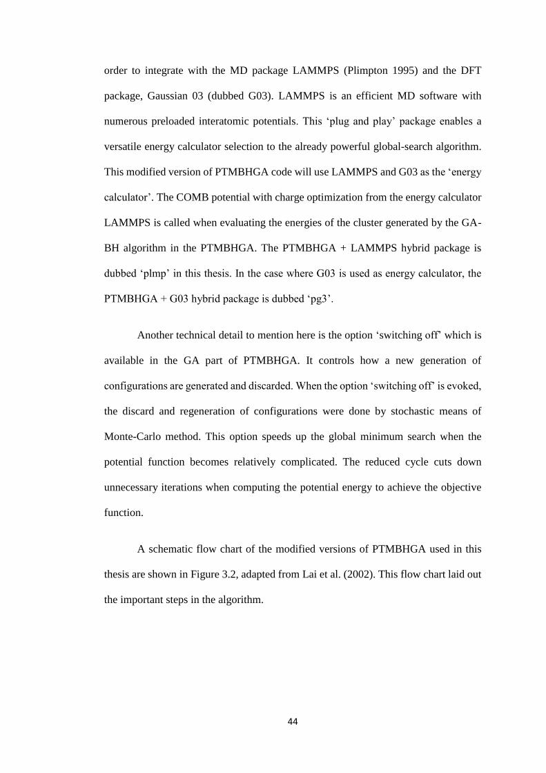
44

order to integrate with the MD package LAMMPS (Plimpton 1995) and the DFT

package, Gaussian 03 (dubbed G03). LAMMPS is an efficient MD software with

numerous preloaded interatomic potentials. This ‘plug and play’ package enables a

versatile energy calculator selection to the already powerful global-search algorithm.

This modified version of PTMBHGA code will use LAMMPS and G03 as the ‘energy

calculator’. The COMB potential with charge optimization from the energy calculator

LAMMPS is called when evaluating the energies of the cluster generated by the GA-

BH algorithm in the PTMBHGA. The PTMBHGA + LAMMPS hybrid package is

dubbed ‘plmp’ in this thesis. In the case where G03 is used as energy calculator, the

PTMBHGA + G03 hybrid package is dubbed ‘pg3’.

Another technical detail to mention here is the option ‘switching off’ which is

available in the GA part of PTMBHGA. It controls how a new generation of

configurations are generated and discarded. When the option ‘switching off’ is evoked,

the discard and regeneration of configurations were done by stochastic means of

Monte-Carlo method. This option speeds up the global minimum search when the

potential function becomes relatively complicated. The reduced cycle cuts down

unnecessary iterations when computing the potential energy to achieve the objective

function.

A schematic flow chart of the modified versions of PTMBHGA used in this

thesis are shown in Figure 3.2, adapted from Lai et al. (2002). This flow chart laid out

the important steps in the algorithm.

45

Figure 3.2: Flow chart for the algorithm in the hybrid PTMBHGA + (LAMMPS /

G03) package.

After they are obtained from plmp (using the COMB potential) or pg3, the

clusters are geometrically re-optimized with G03. The geometry re-optimization

implementation is a powerful function offered by G03 based on the Berny algorithm

(Li and Frisch, 2006). This quantum refinement algorithm enables a local

START

Initialize stochastically a population of 20 candidates. The

distances between the atoms in

cluster are within the cutoff distance

imposed by the COMB potential.

Calculate the individual

potential energy Vi

for each candidates i by

COMB potential or G03 and locally

minimize the candidates by

applying the BH method.

Calculate the fitness value fi for each candidates.

Discard 5 candidates with the lowest value of fi.

5 new candidates are generated

again via stochastic means. The value of Vi are

calculated for these new candidates.

Calculate the fitness value, fi

again for every candidates.

Check if 6 or more candidates have the same lowest fitness value fi.

Output global minimum energy

and the coordinates of the

lowest energy candidate cluster.

STOP

YES

NO

46

minimization of the structure at DFT level by adjusting the relative position of every

atom in the cluster. For the case of hafnium cluster, the method and basis set used in

the re-optimization are B3LYP/LanL2DZ pseudopotential (Hay and Wadt, 1985) as

suggested by (Sun et al., 2010).

As discussed earlier in Section 2.2, Kuntová et al. (2008) mentioned that the

similarity in geometry is the key to relate whether the structures of different PES lie in

the same basin. Comparing the chemical similarity of the structures lying in an

empirical potential PES and that in a DFT PES is a convenient way to computationally

access the correspondence between two PES, specifically, whether both PES share a

common basin. As a matter of principle, the structures obtained from plmp are the

global minima in the COMB PES (COMB structures) only. In theory they are not to

be taken as presenting the global minima in the DFrT PES. In this work, it is

hypothesizing that the COMB structures lies within the basin containing the global

minima of the DFT PES. Additional tests were then carried out to justify the hypothesis

by systematically comparing the structures obtained from the quantum refinement of

COMB structures and the global minimum structures obtained from DFT approach.

Basically the comparison involves the global similarity index, symmetry point

group, as well as the average bond length. Global similarity index is a novel quantity

specifically developed in this thesis based on the principle of molecular shape

comparison discussed in Section 2.3. It is a very effective measure to quantify the

similarity in the structural geometry between two clusters with the same number of

atoms (see details in Section 3.3.1). A high degree of similarity between the COMB

structures and the global minimum structures obtain from DFT approach indicates that

the structures lying at certain point in the COMB PES are close to some local minimum

47

of that DFT basin. The overall details were laid out in Section 3.2.4. By justifying the

scheme as mentioned above, COMB can then be used for simulated annealing process

later. The scheme also provides a convenient and cheap method to generate global

cluster structures with DFT accuracy using empirical potential in place of the

computationally expensive full DFT approach.

In this thesis, the minimum structures obtained via pg3 were taken as

representing the true global minimum, which were made as the reference structures.

To date, experimental data on small hafnium cluster is yet to be available. Therefore,

the minimal structures obtained via pg3 are predictions to be experimentally justified.

3.2 Molecular Dynamics Simulation of Hafnium Clusters

Ab initio method such as DFT gives detailed result for the properties of a

system. This method is bounded to zero Kelvin temperature and applicable up to only

hundreds of atom sizes because it is computationally expensive and time consuming

(Charles, 2008). Thus, classical MD is a more practical approach to simulate the

melting of hafnium cluster. In addition to the capability to handle large system, MD

also allows the user to keep track of the thermal behavior sensitively.

3.2.1 Simulated Annealing Process

Simulated annealing process refers to heating and quenching procedures in MD.

In this thesis, it involved the heating of candidate structures from 1 K to the desired

target temperature, and then equilibrating the system at that temperature for an

48

extended period of time during which the simulated data is sampled for statistical

analysis. The overall process described in this section is the second stage shown in the

flow chart of Figure 3.1.

Simulated annealing process was performed using LAMMPS package with the

COMB potential to describe the interactions among the hafnium atoms. The hafnium

clusters were positioned at the center of a simulation box with fixed boundary

condition to resemble a vacuum condition. The vacuum condition is essential to

simulate a free-standing cluster model. Each hafnium cluster is essentially the ground

state structure obtained from the procedure as described in Section 3.1 with plmp.

The simulation box is fixed with reflective walls at 100Å from the origin in

each direction. The simulation timestep, Δ𝑡 is 0.5 fs . The temperature control is

carried out with canonical (NVT) Nose-Hoover thermostat, by constantly rescale the

velocities of every atom in the sample.

The output of MD simulation was continuously monitored at various stages to

assure that the dynamics of the cluster during simulated annealing process closely

resemble the real situation. Proper preparation of ground state structures prior to the

annealing simulation has been mentioned in Section 2.1. However, to give the hafnium

cluster some initial configuration of microstates, the whole simulation need to undergo

relaxation at 0~1 K before the actual heating process commence. Next, the heating

rate is repeatedly revised to ensure the ergodicity of the system during melting. The

size of the cluster was taken into consideration as well when deciding the heating rate.

The following criteria were used to decide the choice of heating rate:

49

1. Beyond the optimum heating rate, any slower rate of heating gives a 𝑐𝑣

curve that clearly shows a consistent range of melting point for clusters of all

sizes (applied to both 𝑇𝑚 and 𝑇𝑝𝑟𝑒).

2. The computational time is not too demanding in order to heat up the

system to the desired target temperature, and equilibrate it at that temperature

for an extended period of time.

3. The pre-melting behavior should be visibly observed in every samples.

4. The melting point is within a reasonable range for the cluster of

neighboring sizes. The difference should be below 15% deviation.

Figure 3.3 shows the resultant plot of melting and pre-melting point for Hf50 against

the heating rate. Apparently, the first three statement converge once the heating rate

come close to 7 × 1012 Ks−1 (the melting points become constant value, as shown in

the marked area of Figure 3.3). It is found that, for smaller cluster size 𝑛, the difference

in melting point tends to be larger as compared to the neighboring size. But the forth

statement is met even for higher heating rate, up to > 10 × 1012 Ks−1. The heating

rate is set at slightly lower than the converge point as indicates by the red arrow in

Figure 3.3, which is 5 × 1012 Ks−1 (≡ 400 Δ𝑡K−1).

50

Figure 3.3: The melting point and pre-melting point of Hf50 with various heating

rate. The circle region marks the convergence of melting point lower than certain

heating rate.

The temperatures in the simulated annealing of a small cluster display noises

with large fluctuation over a broad range of temperature. As shown in Figure 3.4a, the

spread in the value of the temperature over the course of simulation is very large. The

reason of the temperature fluctuations is due to the thermostat effect on a very small

sized cluster. The plot in Figure 3.4a represents the temperature readings that are

recorded once every 300Δ𝑡. The large fluctuation in simulated temperature can be

artificially reduced to that shown in Figure 3.4b by performing time averaging over

the course of annealing procedure (Berry and Smirnov, 2004). To be consistent, the

average value of temperature is evaluated over a time window of 300Δ𝑡. Thus, instead

of just taking the reading once every 300Δ𝑡, calculating time averages enable the

temperature data to be recorded every timesteps. During the simulation, time averaging

procedure do not take away the fluctuations in temperature, but it acts as a tool to

dissolve the fluctuations. As seen in Figure 3.4b, the noise becomes relatively smaller.

Taking time averages are also useful to avoid information lost during the logging of

51

data while saving up the disk space. In addition to the temperature readings, time

averaging was applied to every measurement in the simulation, include energy value,

pressure, forces and coordinates of each atom in the cluster. At the meantime, the

atomic configurations (coordinates of every particle) of the clusters are recorded in a

separated trajectory file every 300Δ𝑡 for post-processing purposes.

a)

b)

Figure 3.4: The plots of temperature, 𝑇 against the simulation time step, ∆𝑡 a)

without and b) with time averaging in each 300∆𝑡 time interval.

52

As a rule of thumb, the melting temperature, 𝑇𝑚, is expected to increase with

the number of atoms in the clusters, 𝑛. The surface-to-body-atom ratio will decrease

with cluster size, 𝑛 . Due to the reduction of surface-to-body-atom ratio, 𝑇𝑚 will

converge to bulk melting temperature, 𝑇𝑚𝑏𝑢𝑙𝑘 beyond certain size, whereby thermal

behavior starts to resemble those of bulk value. It is beyond the scope of this thesis to

go as big as 104 in size, but the size effect is being studied up to 𝑛 = 50. An additional

cluster of size 𝑛 = 99 is designed to compare the results.

In addition to the temperature profile, LAMMPS has enabled more information,

such as the energy profile and atomic positions of each time step. To maintain

consistency, all the calculated data (to be used for post-processing) are recorded every

300∆𝑡.

3.2.2 COMB Potential

The COMB2 potential adopted in LAMMPS is based on the work of Shan et

al. (2010). Its parameters are as indicated in Table 3.1. The numbers are fit into the

total potential energy in the following equations

𝐸𝑇 = ∑ [𝐸𝑖𝑠𝑒𝑙𝑓(𝑞𝑖) +

1

2∑ 𝑉𝑖𝑗(𝑟𝑖𝑗, 𝑞𝑖, 𝑞𝑗)

𝑗≠𝑖

+ 𝐸𝑖𝐵𝐵]

𝑖

(3.3)

𝑉𝑖𝑗(𝑟𝑖𝑗, 𝑞𝑖 , 𝑞𝑗) = 𝑈𝑖𝑗𝑅(𝑟𝑖𝑗) + 𝑈𝑖𝑗

𝐴(𝑟𝑖𝑗, 𝑞𝑖 , 𝑞𝑗) + 𝑈𝑖𝑗𝐼 (𝑟𝑖𝑗, 𝑞𝑖 , 𝑞𝑗) + 𝑈𝑖𝑗

𝑉(𝑟𝑖𝑗) (3.4)

where 𝐸𝑖𝑠𝑒𝑙𝑓

is the self-energy of atom 𝑖, 𝐸𝑖𝐵𝐵 is the bond-bending energy of atom 𝑖,

𝑉𝑖𝑗 is the interaction potential between the 𝑖 th and 𝑗th atom, 𝑟𝑖𝑗 is the interatomic

53

distance and 𝑞𝑖 and 𝑞𝑗 are the charges of the atom 𝑖 and atom 𝑗. The 𝑉𝑖𝑗 comprises of

four parts: short-range repulsion, 𝑈𝑖𝑗𝑅 , short-range attraction, 𝑈𝑖𝑗

𝐴 , long-range

Coulombic, 𝑈𝑖𝑗𝐼 , and long range van der Waals force, 𝑈𝑖𝑗

𝑉 . Full description of the

functional form of COMB potential can be found in Appendix A.

Table 3.1: The potential parameters of Hf for the COMB potential.

𝐴(eV) 707.5303 𝑅𝑠 3.40 𝜒 0 𝐾𝐿𝑃6 0.008

𝐵(eV) 55.94216 𝑆𝑠 4.20 𝐽 3.13952 𝑅Ω 0.14

𝜆(Å-1) 2.069563 𝑄𝐿 -4.0 𝐾 0 𝐸0 0.16

𝛼(Å-1) 0.959614 𝑄𝑈 4.0 𝐿 0.00941 𝛾 0.10

𝛽 0.046511 𝐷𝐿 0.26152 𝜉 0.679131

𝑛 1.011011 𝐷𝑈 -0.25918 𝜌1 -3.928750

𝑚 1 𝑛𝐵 10 𝜌2 4.839580

𝑐 0 𝐶𝑉𝐷𝑊 0

𝑑 1

ℎ 0

Yu et al. (2007) were the first to develop the COMB potential based on the

Tersoff potential for Si and SiO2. Tersoff (1998a) is a bond order potential and is able

to correctly predict the bond breaking and bond formation of the Si systems. The

original Tersoff (1988b) was able to predict many properties of Si and Si base system,

but the charge distribution was not included in the Tersoff formalism. Yusakawa (1996)

then proposed an extension of the Tersoff model by including charge determination

and electrostatic terms which work similarly like the Rappé and Goddard (1991)

version of charge equilibration (QEq). COMB is effective such that the charge transfer

scheme was a separate procedure in MD. As a comparison, other charge optimized

potentials such as ReaxFF (Duin et al., 2003) proposed an extra constraint in the fitting

of the parameters. The functional form of ReaxFF comprised of a total of nine

separable functions. Duin et al. (2003) optimized the parameters by using the essential

training sets to meet all the parameter search requirements. The target of the

54

optimization was aimed to reproduce the heats of formation, the bond lengths and bond

angles based on the experimental values.

Yusakawa’s version of Tersoff potential includes charge transfer properties to

the existing short-range covalent bond, which is contained in the 𝐸𝑖𝑠𝑒𝑙𝑓

term

(Yusakawa, 1996). The early form of the potential was

𝐸𝑇 = ∑ [𝐸𝑖𝑠𝑒𝑙𝑓(𝑞𝑖) +

1

2∑ 𝑉𝑖𝑗(𝑟𝑖𝑗, 𝑞𝑖 , 𝑞𝑗)

𝑗≠𝑖

]

𝑖

(3.5)

The self-energy term 𝐸𝑖𝑠𝑒𝑙𝑓(𝑞𝑖) as suggested by Rappé and Goddard (1991) is a second

order function of 𝑞𝑖. The charges are treated classically in the self-consistent equations

of motion with Euler-Lagrange equations in the form

𝑚𝑖�̈�𝑖 = −𝜕

𝜕𝑟𝑖𝑇(𝑟𝑖, 𝑞𝑖)

(3.6)

𝑠𝑖�̈�𝑖 = −𝜕

𝜕𝑞𝑖𝑇(𝑟𝑖, 𝑞𝑖)

(3.7)

where 𝑇 is the kinetic energy with an additional term contributed by the charge,

𝑇 =1

2∑ 𝑚𝑖�̇�𝑖

2

𝑖

+1

2∑ 𝑠𝑖�̇�𝑖

2

𝑖

(3.8)

The variable 𝑠𝑖 holds the same significance as 𝑚𝑖, and it is assumed as the mass of the

charge particle, 𝑚𝑞 . QEq requires the derivatives 𝜕𝑇

𝜕𝑞𝑖 which is the microscopic

chemical potential, 𝜒𝑖, to remain constant over the course of the simulation, such that

55

𝜒1 = 𝜒2 = ⋯ = 𝜒𝑛. The equality of 𝜒𝑖 can also be seen as the mean value of chemical

potential, namely

𝜒𝑖 = �̅� =1

𝑛∑ 𝜒𝑖

𝑖

(3.9)

At equilibrium, the force acting on the charge transfer should be zero, thus, the

condition of the charge transfer can be written as

𝑚𝑞�̈�𝑖 = 𝜒𝑖 − �̅� (3.10)

along with the constraint imposed for the charge to be always a constant, 𝐶 (𝐶 = 0 in

this case),

∑ 𝑞𝑖

𝑛

𝑖

= 𝐶 (3.11)

The extension by Yu et al. (2007) was made to account for the additional

properties concerning the energy state, geometrical stability, bond length and the bond

angles of the Si and SiO2 polymorphs. Thus, the first generation COMB potential

(COMB1) has the same form of equation as COMB2. This enables the COMB2

potential to be applicable equally across generations to some of the elements

previously fitted with COMB1. COMB2 and COMB1 are distinguished from each

other, where COMB2 has been improved by including the amorphous properties of

silica (Shan et al., 2010b).

COMB potential is an empirical potential with parameters fitting to

experimental data. The dependability of COMB potential to finally lead to the correct

ground state structures, which provides justification for its further use in subsequent

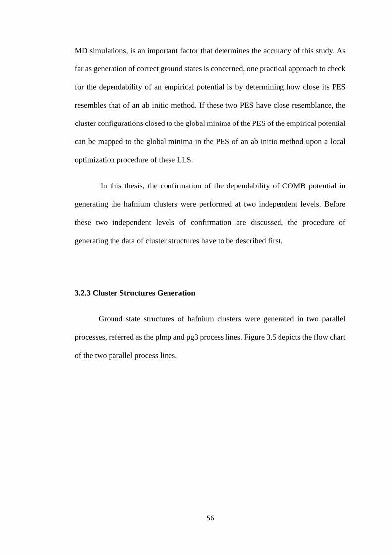
56

MD simulations, is an important factor that determines the accuracy of this study. As

far as generation of correct ground states is concerned, one practical approach to check

for the dependability of an empirical potential is by determining how close its PES

resembles that of an ab initio method. If these two PES have close resemblance, the

cluster configurations closed to the global minima of the PES of the empirical potential

can be mapped to the global minima in the PES of an ab initio method upon a local

optimization procedure of these LLS.

In this thesis, the confirmation of the dependability of COMB potential in

generating the hafnium clusters were performed at two independent levels. Before

these two independent levels of confirmation are discussed, the procedure of

generating the data of cluster structures have to be described first.

3.2.3 Cluster Structures Generation

Ground state structures of hafnium clusters were generated in two parallel

processes, referred as the plmp and pg3 process lines. Figure 3.5 depicts the flow chart

of the two parallel process lines.

57

Figure 3.5: A schemetic flow chart of the two parallel process lines. The plmp

process line in the left and the pg3 process line in the right. Quantum refinement

(geometrical re-optimization) steps are carried out with G03 using the same basis

sets and settings in both process lines.

The plmp process line: The PTMBHGA + LAMMPS process line has already

been mentioned briefly in Section 3.1. Candidate trial structures were generated by the

PTMBHGA algorithm with the GA part switched off, while the total energy of these

structures were calculated using the COMB potential implemented with the LAMMPS

package. COMB potential has been discussed previously (Section 3.2.2). All the trial

structures generated by PTMBHGA were allowed to undergo a short interval of

relaxation using LAMMPS package at 𝑇 = 1 K. Each hafnium atom was allowed to

equilibrate with a minimal vibration. The total energy of these clusters (which solely

depend on the coordinates of the atoms in a cluster) were determined as it is without

any sophisticated geometrical optimization. LAMMPS in this case played the role of

so-called ‘energy calculator’. Due to the built-in global search algorithm of

PTMBHGA + LAMMPS (plmp)

COMB structures

DFT optimized structures

PTMBHGA + G03 (pg3)

LLS of fast DFT procedure

DFT optimized structures

Stage 1 Stage 1

Stage 2 Stage 2

Geometrical re-

optimization with

G03

Geometrical re-

optimization with

G03

58

PTMBHGA, a collection of low energy structures was generated upon a sufficiently

long period of time subjected to a controllable pre-set stopping criteria in PTMBHGA.

The resultant structure was the global minimum of the COMB PES (this structure is

referred as COMB structure). This was the first stage of cluster generation in the plmp

process line. The computational bottle neck of the first stage of the plmp process line

lies in the PTMBHGA generation of candidate configurations, not in the energy

calculator. In the second stage, the COMB structures from the first stage was

geometrically re-optimized using the DFT software package G03 by activating the

option ‘UltraFine’ in the integral grid size. This switched on the algorithm to

implement two-electron integral computation in the package for the purpose of high

accuracy calculation. The quadratically convergent self-consistent field (SCF)

procedure (Bacskay, 1981) was activated in this stage as well. The basis set

B3LYP/LanL2DZ was used in stage 2.

The output from stage 1 in the plmp process line was a collection of LLS for

COMB PES. However, in practice, it was found that, the output structures were often

unique in most cases. Hence, only one COMB structure (which was also the global

minimum of the COMB PES) was fed into G03 for geometrical re-optimization,

yielding the sole lowest energy structure as the final output for the plmp process line.

The pg3 process line: As for the plmp process line, the pg3 process line was

separated into two stages, a relative less computationally intensive PES scan in stage

1, followed by a more computationally intensive geometrical re-optimization in the

second stage. The common basis set B3LYP/LanL2Dz was used in both stages (recall

that the same basis set was also used in the second stage in the plmp process line).

59

In the PES scan in the first stage, candidate clusters generated via the

PTMBHGA algorithm were fed into the G03 package (which acts as the energy

calculator) so that the total energy of these clusters were determined as it is without

any geometrical optimization. This was a relatively fast but coarse PES scan procedure,

as each round of total energy determination does not involve the operation of local

optimization. As such, it is possible to sample (despite at a relatively coarse degree)

the DFT structures as much as practically possible. This has the practical significance

that, given limited available computing resource, the first stage in pg3 line can perform

a reasonably good mapping of the PES to provide better quality candidate structures

for geometrical optimization in the next stage. As an illustration, for 𝑛 = 7 hafnium

cluster, the pg3 stage 1 process run for ~100 hours using eight computing cores

(Intel® Xeon® Processor E5-1620 v2, 10Mb cache, 3.70 GHz) in parallel mode. During

this period, all stochastically generated configurations by PTMBHGA were scanned

through by the energy calculator, of which only 999 converged structures with the

lowest energies are kept for record. These were the LLS generated in stage 1. In

contrast to the stage 1 in the plmp process line, the computational bottle neck of the

stage 1 of the pg3 process line was lied in the energy calculator but not in the

generation of candidate configurations by PTMBHGA.

The second stage in pg3 was similar to the second stage in the plmp process

line, except that the input candidate LLS for geometrical re-optimization were

generated in stage 1 in which G03 was used as energy calculator. Geometrical re-

optimization in the second stage yield geometrically optimized structures at the DFT

level at the end of stage 2.

60

The pg3 process to generate true ground state structures has been proven

workable in an early study reported in Ng et al. (2015b) for the boron clusters. It is

part of the work of this thesis at the early stage to verify the workability of the pg3

process line. However, this process line is only for small-size cluster due to the

expensive computational cost.

3.2.4 Chemical Similarity Comparison

While visual inspection provides a convenient and qualitative way to compare

the geometrical configurations between two clusters, an unambiguous quantitative

algorithm to quantify the degree of similarity is a necessity. Some past studies on

chemical similarity have been laid out in Section 2.3. The quantitative resemblance

between two clusters with the same atom number 𝑛 is referred as chemical similarity.

In this thesis, a purpose-specific algorithm that could capture certain global features of

the geometrical configuration between two clusters in comparison was proposed. It

was referred as the ‘global similarity index’, denoted as 𝜉𝑖 . The proposed global

similarity index is just one possible form of chemical similarity. More technical details

of the global similarity index were deferred to Section 3.3.1.

In the context of this thesis, chemical similarity comparison is to be carried out

at two independent levels, which were referred as the inter-line comparison and intra-

line comparison. Each of these two comparisons has its own physical interpretation.

The intra-line chemical similarity comparison was performed to determine

whether the COMB structures generated by the COMB potential lie within the basin

of the global minimum (or one of the lowest energy local minimum) at the DFT level.

61

If the comparison returns a high similarity measure, the previous statement is deemed

positive. Whereas, the inter-line comparison is a process to determine whether the

ground state structures obtained at the end of the stage 2 of the two independent process

lines agree with each other. In this way, the dependability of COMB potential in

generating true ground state structures of hafnium clusters can be quantitatively and

objectively accessed.

The process of performing chemical similarity comparison was discussed in

more details in the following paragraphs.

Intra-line comparison within the plmp process: Figure 3.6 depicts the flow

chart of the intra-line comparison. Comparison was made for the hafnium clusters

before and after re-optimization (i.e., comparing the structures from stage 1 against

that from stage 2). In the intra-line comparison, the following three measures were

numerically monitored, namely (i) the global similarity index, (ii) the symmetry point

group, and (iii) the differences in relative average bond lengths. These comparisons

stated the degree of chemical similarity of a specific cluster with fixed atom number 𝑛

before and after geometrical re-optimization. The results from the chemical similarity

comparison indicated the dependability of COMB potential as an empirical potential

to obtain structures close to ab-initio method, at least for the hafnium clusters.

62

Figure 3.6: A schemetic flow chart of intra-line comparison within the plmp

process line.

Inter-line comparison between the plmp and pg3 process lines: Figure 3.7

depicts the flow chart of the inter-line comparison. The final structures obtained after

the quantum refinement from the plmp process line were compared directly with those

obtained from the pg3 process line. This were a direct comparison between the

structures in stage 2 from both process lines which use a common G03 local

optimization. The chemical similarity between the clusters in stage 2 in both process

lines indicated the dependability of COMB potential in generating the ground state

structures as well as in MD simulation.

PTMBHGA + LAMMPS (plmp)

COMB structures

DFT optimized structures

Stage 1

Stage 2

Geometrical re-

optimization with

G03

Chemical

similarity

comparison

63

Figure 3.7: A schemetic flow chart of inter-line comparison between the plmp and

pg3 process lines.

3.2.5 Flying Ice Cube Problem

In this thesis, the flying ice cube problem was encountered during the simulated

annealing procedure. Solving the flying ice cube problem was one of the major part of

the second stage as shown in Figure 3.1. Figure 3.8 shows the condition of a sample

Hf13 cluster during the occurrence of flying ice cube problem.

PTMBHGA + LAMMPS (plmp)

COMB structures

DFT optimized structures

PTMBHGA + G03 (pg3)

LLS of fast DFT procedure

DFT optimized structures

Stage 1 Stage 1

Stage 2 Stage 2

Geometrical re-

optimization with

G03

Geometrical re-

optimization with

G03

Chemical

similarity

comparison

64

a)

b)

Figure 3.8: The condition of Hf13 cluster during the heating procedure which

encountered flying ice cube artifact, generating excessive kinetic energy. a). The

cluster begin to spin in a clockwise manner along the red arrows direction shown,

at the beginning of heating procedure. b). The Hf13 cluster around 1800K~1900K

where the whole cluster start to drift across the simulation box, in addition to the

rotation motion, while remain closely bonded like an ‘ice’ body. The dynamic

bonding shown in the figure is kept below 3.2Å, slightly longer than the actual

bond length in bulk hafnium.

In MD simulation, flying ice cube problem refers to the situation in which the

system under simulation as a whole is rotating and drifting in the vacuum, while

remaining closely bounded to each other (Harvey et al., 1998). The name has its origin

65

due to the visualization as if a rigid iced body flying across the simulation box.

According to the theory of equipartition, when the average energy is not equally

distributed among various form (for kinetic energy, the contributions aroused from the

vibration, translation and rotation of the atoms, etc. …), the system is not in thermal

equilibrium. Flying ice cube problem happens when the individual velocity of each

particle are drained into the momentum of the center of mass. This process happens

due to repeated temperature (velocity) rescaling by imposing a thermostat, especially

during the annealing stages.

The excessive momentum is observed visually for both linear and angular

momentum of the center of mass. To describe how such problems are causing errors

to the outcome of the calculations, certain simulated examples are used to demonstrate

them. First, by imposing the command ‘fix recenter’ in the LAMMPS code, the cluster

as a whole will constantly reposition the center of mass to its original spot in every

time step. This will not affect the outcome since the cluster is in vacuum and does not

interact with anything else. Should flying ice cube artifact happen, each microscopic

vibration of all particles would diminish even though the temperature of the system

continues to rise. The excessive energy is carried in the form linear velocity of the

center of mass, causing the cluster to remain bonded together. At some point, the

system might even start to rotate on its own, converting a portion of the energy into

rotatory motion. As a result, the temperature of the simulation box rose, but not the

cluster.

There are two approaches to correct the errors caused by the flying ice cube

problem. One is by using the Langevin dynamics (thermostat) and another one is by

66

removing the excessive momentum along the calculation via the ‘fix momentum’

command in LAMMPS package.

Langevin dynamics are able to capture the random stochastic fluctuation,

normally arises from interaction with the background implicit solvent. For the cluster

during the occurrence of flying ice cube phenomenon, this approach controls the

perturbation of the omitted degree of freedom. Based on the LAMMPS documentation,

the force on each atom has the form of

𝐹 = 𝐹𝑐 + 𝐹𝑓 + 𝐹𝑟 (3.12)

where 𝐹𝑐 is the conservative force computed via the usual interatomic interactions and

𝐹𝑓 is the frictional drag or viscous damping term proportional to the particles’ velocity.

The proportionality constant for each atom is computed as 𝑚

𝑑𝑎𝑚𝑝, with 𝑚 being the

mass of particle and 𝑑𝑎𝑚𝑝 is the damping factor, and thus

𝐹𝑓 = − (𝑚

𝑑𝑎𝑚𝑝) 𝑣

(3.13)

𝐹𝑟 is the force due to solvent atom at temperature 𝑇 randomly bumping into another

particle. 𝐹𝑟 is proportional to

𝐹𝑟 ∝ √𝑘𝐵𝑇

𝑑𝑡∙

𝑚

𝑑𝑎𝑚𝑝

(3.14)

where 𝑘𝐵 is the Boltzmann constant.

At the same time while solving the flying ice cube problem, the Langevin

dynamics also approximate the canonical ensemble that act as a thermostat. The

67

approach affects the system in such a way that it modifies the forces to effect

thermostatting, which is different from Nose-Hoover thermostat and its time

integration.

In this thesis, the second method was used to retain the thermostat in use. Thus,

the ‘fix momentum’ command was used instead of Langevin dynamics. On the other

hand, by constantly zeroing both the linear and angular momentum of the system, the

errors in controlling the excessive (removing the residual) velocities could be kept to

a minimum. When the momentum was zero, the force was adjusted accordingly for

every time step, thus, the modification will not affect the canonical ensemble. Thus,

the immediate state of the system and temperature were preserved.

The command ‘fix momentum’ will zero the momentum (linear or angular or

both) of the clusters every time step by adjusting the velocities of every single atom

relative to the velocity of the center of mass. After imposing ‘fix momentum’

command, the cluster was not rotating and drifting anymore at low temperature, but

every atom will vibrate with the increasing temperature. The bond breaking and bond

formation were displayed accordingly, as shown in Figure 3.9 for Hf13 cluster.

In order to avoid further complication from flying ice cube problem, the

zeroing of ‘fix momentum’ option is applied thoroughly for every single simulated

annealing process in this thesis. Overall, every MD process was checked to be

consistent to each samples and runs.

68

a) ~850 K c) ~1100 K

b) ~900 K d) ~2050 K

Figure 3.9: The condition of Hf13 cluster, showing the bond breaking and bond

formation at a) ~850 K, b) ~900 K, c) ~1100 K and d) ~2050 K. Along the

simulation time, the cluster neither rotate nor drift across the simulation box, each

atom vibrate relative to one another, carry the kinetic energy in them.

3.3 Post-Processing

The widely accepted method to study the thermal properties of a heating

process is by plotting the caloric curve and the 𝑐𝑣 vs. temperature curve (𝑐𝑣 curve). In

this thesis, both curves were plotted to obtain the melting temperature of hafnium

clusters. The melting temperature is compared to that obtained via the global similarity

index, which was introduced in the next subsection. Together, both method set up the

69

third and final part of the thesis as shown in Figure 3.1. The caloric curve of a hafnium

cluster under thermal annealing can be obtained by plotting its potential energy as a

function of temperature. This information is readily extracted from the log file (.log)

from LAMMPS package. Next to the caloric curve, the 𝑐𝑣 value can be calculated

using Equation (2.3) in Section 2.2, which is restated below,

𝑐𝑣 =⟨𝐸𝑡

2⟩𝑇 − ⟨𝐸𝑡⟩𝑇2

2𝑛𝑘𝐵𝑇2

(3.15)

The caloric profile can be obtained from ‘direct heating’ and ‘prolonged

annealing’. In the direct heating procedure, the cluster is heated directly to a high

temperature with a slow heating rate. To ensure the melting dynamics is well

represented by caloric profile, the heating rate is pre-defined as discussed in Section

3.2.1, which is 5 × 1012 Ks−1 . A slow hearing rate is able to minimize the error

accumulated due to rapid velocity rescaling at every time step. The value of 𝑇∆𝑡 and

𝐸∆𝑡 are taken directly from the readings of a single log file. The subscript ∆𝑡 refer to

the values each taken at the same timestep.

In the second approach, each point on the caloric curve was obtained from a

single annealing process. In this procedure, the candidate structure was heated to the

desired target temperature and allowed to equilibrate for a very long time to ensure the

ergodicity of the microstate, specifically the temperature and the potential energy value.

For example, to obtain a caloric profile from 1000 K to 3000 K, with a temperature

windows of 50 K, a total of 41 simulated annealing processes need to be performed.

The first simulation correspond to the heating to the target temperature of 1000 K, and

equilibrate at 1000 K for an extended period of time and yield the average value of

70

⟨𝐸1000 K⟩ for 𝑇 = 1000 K. The next will be ⟨𝐸1050 K⟩ for 𝑇 = 1050 K, and so on, till

the 41st simulation of ⟨𝐸3000 K⟩ for 𝑇 = 3000 K.

Comparing both heating procedures, although the prolonged annealing process

is very lengthy to simulate, the direct heating process is comparatively trickier to

handle. However, both methods were used in this thesis to compare both approaches.

The outcome of the comparison was presented in Chapter 5.

The other output of LAMMPS package is the trajectory file (.lammpstrj) that

records all the screenshots of the structures over the course of the simulation with fixed

time interval. When the simulation is done accordingly, the trajectories and the log file

should tally with each other. Thus, the thermal behavior can be observed through the

trajectory file while melting temperature is pinpointed using the log file. One of the

benefits in simulated annealing is that one can visualize the simulation by using

visualization program. The screenshots of the trajectory when physically significant

variation occurred during the simulation were presented in Chapter 4.

In this thesis, the dynamical information of the simulation was traced by

comparing the similarity index of each frame along the heating process. The

comparisons are made with respect to the initial configuration at 0 K (after relaxation)

prior to the heating process. The trajectories were recorded every 300Δ𝑡 , which

corresponds to 0.15 ps of simulation time. With the heating rate of 5 × 1012 Ks−1, the

simulated data were expected to cover at least one record per unit temperature.

71

3.3.1 Global Similarity Index

The global similarity index, 𝜉𝑖 proposed in this thesis is a novel approach and

derived based on generic chemical similarity idea to detect the changes along the

trajectory of the heating process. This is a new measure deserving an

acknowledgement of novelty, an original idea first proposed in this thesis. The global

similarity index proposed in this thesis is used to identify the chemical similarity

between the clusters of the same size. It is used as a measure to determine the

dependability of COMB potential as well as to detect changes in the structures during

the heating procedure. As compared to all the existing method, global similarity index

is able to predict the detailed melting mechanism which was discussed later in this

section.

The functional form of 𝜉𝑖 is proposed to take the form of

𝜉𝑖 =1

𝑛∑(𝑘𝑠,𝑖 + 1)

−1𝑛

𝑠=1

(3.16)

𝑘𝑠,𝑖 = |√𝑑𝑠,𝑖 − √𝑑𝑠,0| (3.17)

where 𝑑𝑠,𝑖 and 𝑑𝑠,0 represent the sorted distance of atoms relative to the average

positions (center of mass) of all the atoms in the cluster for the 𝑖th (denoted as the

subscript 𝑖) and the 0th frame (for the simulated annealing process, this is the input

structure), while 𝑛 corresponds to the number of atoms, which is an integer equals to

the number of pairs of 𝑘𝑠,𝑖. The value of 𝜉𝑖 = 1 corresponds to totally identicalness

and 𝜉𝑖 → 0 for vast difference.

72

The application of 𝜉𝑖 was demonstrated in the example using the LLS of Hf7.

Figure 3.10 shows the visualization of Hf7 clusters by using Visual Molecular

Dynamics (VMD) (Humphrey et al., 1996) software. In this example, the similarity

index is applied to the structures in Figure 3.10b and 3.10c relative to 3.10a. In this

illustration, the structure of Figure 3.10a play the role as the 0th frame. The Hf7 in

Figure 3.10a is the ground state structure as obtained in this thesis, while 3.10b is the

second lowest energy isomer. Figure 3.10c was obtained via modification to the

ground state Hf7 where both the top and bottom atoms of the pentagonal bipyramid is

moved closer to the pentagonal base. Minor movement of atoms such as the case of

Figure 3.10c from 3.10a were expected during the heating process of the cluster. In

these figures, a visualisation setting known as dynamic bonds is enabled. In this

visualisation setting, bonds will be automatically shown as a connection between two

atoms that are separated at a distance of equal or less than a specified value 𝑟𝑏. In this

illustration, a value of 𝑟𝑏 = 3.2Å was to distinguish visually the differences between

the structures (notice the connection appeared for the top-bottom atoms in Figure

3.10c). Figure 3.10c was artificially prepared for the purpose to demonstrate the

characteristics of 𝜉𝑖.

73

a) c)

b)

Figure 3.10: The LLS of Hf7 cluster. a) The ground state structure. b) The second

lowest energy isomer. c) A slight modification was made based on the ground state

structure where the bipyramid top was moved closer to the pentagonal base. The

green cross indicates center of mass.

The average position of each structures in Figure 3.10 was marked as the center

of mass (CM) with a green cross. For 3.10a, which was the ground state structure, the

center of mass was located right at the center of the bipyramid frame, say at Ca (0, 0,

0). In order to apply Equation (3.17) to Figure 3.10a, the distance of each atom from

Ca is calculated and sorted in ascending order. The sorted distances in this example are

{𝑑𝑠,0}={1.62966, 1.62967, 2.4062, 2.40638, 2.40712, 2.40729, 2.40807}, where 𝑠 =

1, 2, … , 7. The same calculations when applied to the other two structures, give {𝑑𝑠,1}

(Cb as the center of mass, Figure 3.10b) and {𝑑𝑠,2} (Cc as the center of mass, Figure

3.10c). Once 𝑑𝑠,0 , 𝑑𝑠,1 and 𝑑𝑠,2 have been calculated, 𝑘𝑠,𝑖 can be evaluated as

Equation (3.17) for 𝑖 = 1, 2 in this illustration. By applying Equation (3.16), the value

74

of 𝜉𝑖 for the structure of Figure 3.10b as compared to Figure 3.10a is 𝜉1 =0.988913

while for Figure 3.10c is 𝜉2 =0.979697. In actual case, 𝑖 = 1, 2, … until a very large

number of frames.

The pair of structures in Figure 3.10a and 3.10c clearly appear more alike than

the pair of structures in Figure 3.10a and 3.10b. However, the similarity measure as

defined by Equation (3.16) reveals the otherwise. This means the definition of 𝜉𝑖 as

stated in Equation (3.16) did not correctly reproduce the similarity measure. Some

improvement was deemed necessary so that 𝜉𝑖 could sensitively accommodate the

changes such as that occurred in Figure 3.10c. To achieve this purpose, the functional

form of 𝜉𝑖 was modified according to the prescription below.

Instead of a single, conventionally defined center of mass, this thesis used three

special cases of generalized mean positions to act as the center of mass of a cluster,

namely the arithmetic mean, the harmonic mean, and the quadratic mean (a.k.a. root

mean square). Each of mean is viewed as a center of reference (COR) for the

immediate state of clusters. The idea of COR works like the center of mass, where the

whole cluster is represented by a single point mass. With this generalization, there are

now three COR for each frame of cluster. The generalized mean, also known as the

power mean, can be expressed in the following form

𝑀𝑝(𝑥1, … , 𝑥𝑛) = (1

𝑛∑ 𝑥𝑖

𝑝

𝑛

𝑖=1

)

1𝑝

(3.18)

where 𝑝 must be a non-zero real number, and 𝑥1, … , 𝑥𝑛 are variables. The special cases

of Equation (3.18) when 𝑝 takes on the value 𝑝 = 1, −1, 2 are arithmetic mean,

75

harmonic mean, and quadratic mean respectively. These are just the common

definition of means which we are all familiar with, i.e.,

𝑀1(𝑥1, … , 𝑥𝑛) =𝑥1 + ⋯ + 𝑥𝑛

𝑛

(3.19)

𝑀−1(𝑥1, … , 𝑥𝑛) =𝑛

1𝑥1

+ ⋯ +1

𝑥𝑛

(3.20)

𝑀2(𝑥1, … , 𝑥𝑛) = √𝑥1

2 + ⋯ + 𝑥𝑛2

𝑛

(3.21)

The cluster was quantified by three different sets of 𝑘𝑠,𝑖 , each based on a

different COR. The definitions of Equation (3.16, 3.17) ware hence generalized to

include an COR index to indicate which COR is being referred to when evaluating a

𝜉𝑖,

𝜉𝑖𝐶𝑂𝑅 =

1

𝑛∑(𝑘𝑠,𝑖

𝐶𝑂𝑅 + 1)−1

𝑛

𝑠=1

(3.22)

𝑘𝑠,𝑖𝐶𝑂𝑅 = |√𝑑𝑠,𝑖

𝐶𝑂𝑅 − √𝑑𝑠,0𝐶𝑂𝑅|

(3.23)

In each COR, there are 𝑛 sorted atomic distances, giving a total of 3𝑛 pairs of

𝑘𝑠,𝑖. The distances of atoms from the mean position are sorted in ascending order from

the shortest to the longest. The difference in Equation (3.17, 3.23) are measured with

respect to the distance of atoms in the 0 K frame of the same sorting sequence. After

the value of 𝜉𝑖 is calculated for each COR, averaging of 𝜉𝑖 over these COR was then

obtained, via

76

𝜉�̅� =1

𝑁𝐶𝑂𝑅∑ 𝜉𝑖

𝐶𝑂𝑅

𝐶𝑂𝑅

=1

3∑

1

𝑛∑(𝑘𝑠,𝑖

𝐶𝑂𝑅 + 1)−1

𝑛

𝑠=1𝐶𝑂𝑅

=1

3𝑛∑ ∑(𝑘𝑠,𝑖

𝐶𝑂𝑅 + 1)−1

𝑛

𝑠=1𝐶𝑂𝑅

(3.24)

where 𝑁𝐶𝑂𝑅 = 3 , the number of COR used in this thesis. With the inclusion of

additional COR, the quadratic mean of the structure in Figure 3.10a was calculated to

be (1.43865, 1.43828, 0.871093). The sorted distances in ascending order of every

atom from this COR were {0.945749, 2.1706, 2.76504, 2.77303, 3.22416, 4.31185,

4.31648}. The harmonic mean and the corresponding sorted distances for Figure 3.10a

can also be similarly calculated (figures were not provided for the sake of brevity).

The same calculation was also applied to the structures 3.10b and 3.10c. Finally, by

applying Equation (3.24), the 𝜉�̅� measured the for structure in Figure 3.10c as

compared to 3.10a yields a value of 𝜉2̅ = 0.93887 while for Figure 3.10b yields 𝜉1̅ =

0.911066. Apparently, this generalization improves the sensibility of 𝜉𝑖 in accessing

the similarity of the clusters. In the subsequent discussion, the bar in the 𝜉�̅� symbol

shall be dropped, with the understanding that whenever global similarity index is

mentioned, it is referring to the COR-averaged version of 𝜉�̅�, unless it is explicitly

stated otherwise. As demonstrated in Chapter 5 by using COR-averaged Equation

(3.24), the pre-melting phase can be distinctively identified as a sharp transition in 𝜉𝑖.

It was found that taking the square of Equation (3.24) improves the sensitivity

of 𝜉𝑖 in detecting similarity in the clusters. Since a 𝜉𝑖 ranges from 0 → 1, squaring

Equation (3.24) does not change the normalization property of 𝜉𝑖. In fact, by squaring

Equation (3.24), the variation in 𝜉𝑖2

becomes numerically more pronounced and

77

sensitive due to the parabolic behavior of squaring a number within the range of (0,1).

For the structure in Figure 3.10c, the value of 𝜉𝑖2 is 𝜉2

2 = 0.938872 = 0.881477;

while for the structure in Figure 3.10b, 𝜉12 = 0.9110662 = 0.830042. In practice, the

value of 𝜉𝑖 tends to vary only very slightly especially when comparing the structures

before and after geometrical re-optimization with G03. Hence, squaring the 𝜉𝑖 is a

convenient way to enhance the visibility of the variation effect. The squared version

of similarity index, 𝜉𝑖2 was adopted in the subsequent chapters.

It is instructive to compare Equation (3.24) to Equation (2.7), which is the USR

defined by Ballester and Richards (2007)

𝑆𝑞𝑖 = (1 +1

12∑|𝑀𝑙

𝑞 − 𝑀𝑙𝑖|

12

𝑙=1

)

−1

𝑆𝑞𝑖 as defined in the definition of USR has a very different working principle from that

of the global similarity index. 𝑆𝑞𝑖 has the general form of

𝑆𝑞𝑖~1

1 +1

12∑ (⋯ )𝑙

12𝑙=1

, (⋯ )𝑙 ≡ |𝑀𝑙𝑞 − 𝑀𝑙

𝑖|

(3.25)

whereas 𝜉𝑖 has the general form

𝜉𝑖~1

3𝑛∑ ∑

1

1 + (⋯ )𝑠

𝑛

𝑠=1𝐶𝑂𝑅

, (⋯ )𝑠 ≡ |√𝑑𝑠,𝑖𝐶𝑂𝑅 − √𝑑𝑠,0

𝐶𝑂𝑅| (3.26)

The fraction of 1

12 in 𝑆𝑞𝑖 is sitting inside the reciprocal, whereas the fraction

1

3𝑛 in 𝜉𝑖 is

placed outside the reciprocal. This will ensure that 𝑘𝑠,𝑖𝐶𝑂𝑅 is not averaged before the

index 𝑠 is summed over. As it was originally proposed by Ballester and Richards

78

(2007), the 𝑀𝑙 terms as appear in 𝑆𝑞𝑖 have to undergo a prescribed normalization

procedure so that they give values with the same order of magnitude for all 𝑙 (𝑀𝑙 will

give values with different order of magnitude for different 𝑙 if not normalized). On the

other hand, normalization procedure is not required for 𝜉𝑖 as each 𝑘𝑠,𝑖𝐶𝑂𝑅 , being the

differences in the distances of atoms from the COR, has the same order of magnitude.

The main idea of the global similarity index is to compare the configuration of

one image of the molecule (cluster) to another. Imagine two images of identical cluster

with one of them is obtained by performing a linear transformation (including

translation, rotation, reflection and rescaling) on the other. The global similarity index

must be able to discern the fact that these two images, despite having different

coordinates, are in fact the same cluster, and returns a unique value of 𝜉𝑖 = 1. In

general, when two images are being compared, the transformational relation between

them have to be factored in while evaluating the global similarity index.

Now, consider two images (atomic configurations of two clusters) which are

related to each other via a linear transformation. The transformation is said to be

congruent if it undergoes mapping operation of translation, rotation, reflection, or the

combination of more than one of these. If the image also undergoes rescaling, it is

similar but not congruent. Conceptually, congruence is a subset to similarity. The

primary aim of the 𝜉𝑖 measure as defined in this thesis was to recognize whether the

transformation falls into any group of equality, and numerically quantify the degree of

congruence or similarity. If one wishes to identify two congruent images, the definition

of their 𝑘𝑠,𝑖𝐶𝑂𝑅 have to fulfill the following requirements: 𝑘𝑠,𝑖

𝐶𝑂𝑅 should be

79

1) invariant under translational, rotational or reflection transformations,

i.e., 𝑘𝑠,𝑖𝐶𝑂𝑅 = 𝑘𝑠,𝑖′

𝐶𝑂𝑅, where 𝑖, 𝑖′ refer to two images related by a

congruent transformation;

2) of the same order of magnitude;

3) able to capture any perturbation to the position of any atomic points in

an image.

For 2) to be true would require |𝑑𝑠,𝑖𝐶𝑂𝑅|~|𝑑𝑠,𝑖′

𝐶𝑂𝑅|, where 𝑠 refers to the same points

(atoms) in image 𝑖 and 𝑖’ . Requirement 3) can be achieved by including various

independent COR into the definition of 𝜉𝑖 . There is a possibility that certain

perturbation may be insensitive to a particular COR but sensitive to other. By including

various COR, perturbation missed by one particular COR could be picked up by the

other COR which is more susceptible to this perturbation. The example as discussed

for Figure 3.10 was designed to illustrate the improved discerning ability of 𝜉𝑖 with

the inclusion of various COR into its definition. In fact, the three theoretical criterion

discussed above form the basic working principle on which the global similarity index

was originally proposed.

If two images are similar, in addition to the three requirements as stated above,

𝑘𝑠,𝑖𝐶𝑂𝑅 also needs to be invariant under rescaling transformation. The effect of rescaling

operator shall also be considered in the definition of 𝑘𝑠,𝑖𝐶𝑂𝑅, such that it returns a value

of close to 0 (≡ 𝜉𝑖 → 1). However, it would be in general not possible for requirement

2), i.e., |𝑑𝑠,𝑖𝐶𝑂𝑅|~|𝑑𝑠,𝑖′

𝐶𝑂𝑅|, to be fulfilled due to rescaling transformation. For example, if

𝑖′ corresponds to an enlarged frame of a cluster 𝑖 , |𝑑𝑠,𝑖′𝐶𝑂𝑅| will be way larger than

|𝑑𝑠,𝑖𝐶𝑂𝑅|. Hence 𝜉𝑖 will not return a value close to 1 even though they are in fact similar.

80

Hence, the definition of 𝑘𝑠,𝑖𝐶𝑂𝑅 as defined in Equation (3.23) has to be supplanted by a

new form, 𝑘′𝑠,𝑖𝐶𝑂𝑅

, when calculating global similarity index for rescaled images:

𝑘′𝑠,𝑖𝐶𝑂𝑅 = |√

𝑑𝑠,𝑖𝐶𝑂𝑅

𝐷𝑖𝐶𝑂𝑅 − √

𝑑𝑠,0𝐶𝑂𝑅

𝐷0𝐶𝑂𝑅|

(3.27)

𝐷𝑖𝐶𝑂𝑅 is defined as a characteristic length of the 𝑖th frame, such that when the image 𝑖

is blown up by an arbitrary scale, 𝑑𝑠,𝑖

𝐶𝑂𝑅

𝐷𝑖𝐶𝑂𝑅 would remain unchanged. The choice of 𝐷𝑖

𝐶𝑂𝑅

that could provide such an invariant effect can be conveniently taken to be, without

loss of generality, 𝐷𝑖𝐶𝑂𝑅 = |𝑑𝑚

𝐶𝑂𝑅 − 𝑑𝑚−1𝐶𝑂𝑅 | for any 𝑚 ∈ [2, 𝑛].

As it turns out, in the MD heating simulation to be carried out on the hafnium

clusters, the clusters in general do not undergo rescaling transformation up to the point

before they become completely melted. Their sizes are maintained throughout the MD

heating process up to the melting point. In a MD heating simulation, rescaling of

cluster structures is a natural outcome. Hence, in order for the global similarity index

to correctly quantify the characteristics of the cluster evolution, it must be able to

capture the rescaling effect. In other words, if a cluster’s geometry remains the same

but its overall size gets blow up by some factor, the global similarity index must show

a variation in its numerical value, signifying the occurrence of rescaling in the cluster.

On the other hand, in the case of intra-line comparison, COMB structures tend to be

rescaled by geometrical re-optimization by G03. However, these structures actually

remain in the same basin of the DFT PES. Thus, in this case, global similarity index

used to compare the clusters before and after the re-optimization operation should be

treated as similar.

81

Global similarity index should be able to recognize the congruence of the

cluster frames in the MD heating process, while in the plmp intra-line comparison, it

must be able to recognize both congruence and similarity between the structures. In

practical terms, this means when rescaling effect is considered as a change in chemical

similarity e.g., in a heating process, the definition for 𝑘𝑠,𝑖𝐶𝑂𝑅 in Equation (3.23) is used.

Otherwise, e.g., in the case of geometrical re-optimization of a cluster by G03,

Equation (3.27) is used instead. As a note, the inter-line comparison is a direct yes-or-

no problem; the resultant structures from both process lines are either the same or

otherwise. The answer does not require the application of global similarity index.

The measurement protocol of the similarity index 𝜉𝑖 can be further studied by

computing the fluctuation of 𝜉𝑖 over the course of simulation. In general, 𝜉𝑖, which is

related to the microscopic property, is not directly measurable via experiment.

However, its fluctuation could be related to a macroscopic observable. As in the case

of 𝑐𝑣, it is a measure of fluctuation in the binding energy. The fluctuation of 𝜉𝑖 remains

a prospect for future study. The fluctuation equation is considered to be proportional

to the variance of 𝜉𝑖 as

𝑆𝜉𝑖∝ 𝜎2(𝜉𝑖) (3.28)

The 𝑆𝜉𝑖 curve shows a sudden change in the similarity index 𝜉𝑖 in the form of sharp

peaks at the particular moment when major transition occurs in the configuration.

In this thesis, the global similarity index 𝜉𝑖 was used to study the dynamics of

hafnium clusters during the simulated annealing processes. The value of 𝜉𝑖 in each

instance 𝑖 is a measure of similarity of the cluster structure in that instance as compared

to the ground state structure (the structure during the initial 1 K equilibration) in the

82

0th frame. During the early part of the heating-up process, only little variation in 𝜉𝑖 is

detected, indicating that only minor change to the geometry is happening in the cluster.

Up to this point, 𝜉𝑖 tends to measure an almost constant value close to 1. The abrupt

change to the global similarity index will only happen during (or close to) the melting

temperature. Visually, the melting transition happens with a total distortion in the

structure spanning the whole cluster. Following the sequential evolution of 𝜉𝑖 allows

one to locate the sudden change in the structure of the clusters during a heating process.

After the melting point, the whole cluster is expected to be fluid-like and each atom

tends to roam across the simulation box randomly. Thus, the global similarity index is

expected to be constantly close to 0. Note that, 𝜉𝑖 stays almost constant during most of

the simulated annealing process, except during the range of temperature in which the

melting process occurs. Thus, the fluctuation of similarity index 𝑆𝜉𝑖 becomes useful to

locate the temperature where these transition happened.

In addition to the melting transition, patterns of distortion to the clusters during

the simulated annealing process are also detectable by the global similarity index based

on the fluctuation curve 𝑆𝜉𝑖. This was discussed in Chapter 5.

83

CHAPTER 4

DEPENDABILITY OF COMB POTENTIAL

4.1 Geometrical Re-Optimization of Hafnium Clusters

The structures obtained at the end of the stage 1 of the plmp process line (the

COMB structures) were geometrically re-optimized with G03 package using B3LYP

and basis set LanL2DZ. This is the intra-line comparison mentioned in Section 3.2.4.

The comparison procedure has to be carried out in order to evaluate the chemical

similarity of the hafnium clusters before subjecting them for MD simulation.

Specifically, the average bond length, symmetry point group and global similarity

index were compared. Intra-line comparison accessed the dependability of the COMB

potential in MD simulations to be carried subsequently.

The outcome of intra-line comparison was numerically tabulated in Table 4.1

for the clusters with the size of 𝑛 = 2 to 𝑛 = 20. The plots as shown in Figure 4.1

were graphical representation of Table 4.1 for the average bond length and global

similarity index.

The average bond lengths were calculated by considering only the nearest

neighbor atoms in the clusters. The calculated bond lengths were similar for this

sample of hafnium clusters. As shown in Figure 4.1a, the difference in the bond lengths

for the clusters of neighboring sizes remains minimal as 𝑛 increases. However, COMB

structures ded not show gradual increment in term of 𝑛 as the structures of DFT

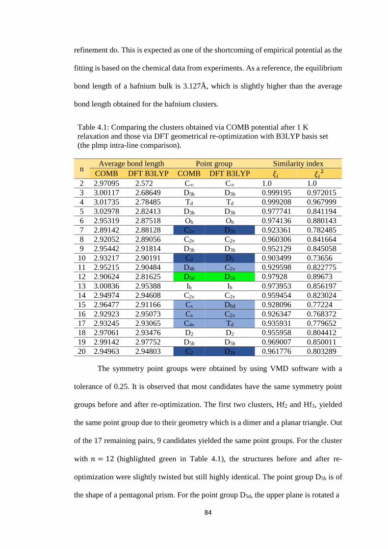
84

refinement do. This is expected as one of the shortcoming of empirical potential as the

fitting is based on the chemical data from experiments. As a reference, the equilibrium

bond length of a hafnium bulk is 3.127Å, which is slightly higher than the average

bond length obtained for the hafnium clusters.

Table 4.1: Comparing the clusters obtained via COMB potential after 1 K

relaxation and those via DFT geometrical re-optimization with B3LYP basis set

(the plmp intra-line comparison).

n Average bond length Point group Similarity index

COMB DFT B3LYP COMB DFT B3LYP 𝜉𝑖 𝜉𝑖2

2 2.97095 2.572 C∞ C∞ 1.0 1.0

3 3.00117 2.68649 D3h D3h 0.999195 0.972015

4 3.01735 2.78485 Td Td 0.999208 0.967999

5 3.02978 2.82413 D3h D3h 0.977741 0.841194

6 2.95319 2.87518 Oh Oh 0.974136 0.880143

7 2.89142 2.88128 C2v D5h 0.923361 0.782485

8 2.92052 2.89056 C2v C2v 0.960306 0.841664

9 2.95442 2.91814 D3h D3h 0.952129 0.845058

10 2.93217 2.90191 C2 D2 0.903499 0.73656

11 2.95215 2.90484 D4h C2v 0.929598 0.822775

12 2.90624 2.81625 D5d D5h 0.97928 0.89673

13 3.00836 2.95388 Ih Ih 0.973953 0.856197

14 2.94974 2.94608 C2v C2v 0.959454 0.823024

15 2.96477 2.91166 Cs D6d 0.928096 0.77224

16 2.92923 2.95073 Cs C2v 0.926347 0.768372

17 2.93245 2.93065 C4v Td 0.935931 0.779652

18 2.97061 2.93476 D2 D2 0.955958 0.804412

19 2.99142 2.97752 D5h D5h 0.969007 0.850011

20 2.94963 2.94803 C2 D2h 0.961776 0.803289

The symmetry point groups were obtained by using VMD software with a

tolerance of 0.25. It is observed that most candidates have the same symmetry point

groups before and after re-optimization. The first two clusters, Hf2 and Hf3, yielded

the same point group due to their geometry which is a dimer and a planar triangle. Out

of the 17 remaining pairs, 9 candidates yielded the same point groups. For the cluster

with 𝑛 = 12 (highlighted green in Table 4.1), the structures before and after re-

optimization were slightly twisted but still highly identical. The point group D5h is of

the shape of a pentagonal prism. For the point group D5d, the upper plane is rotated a

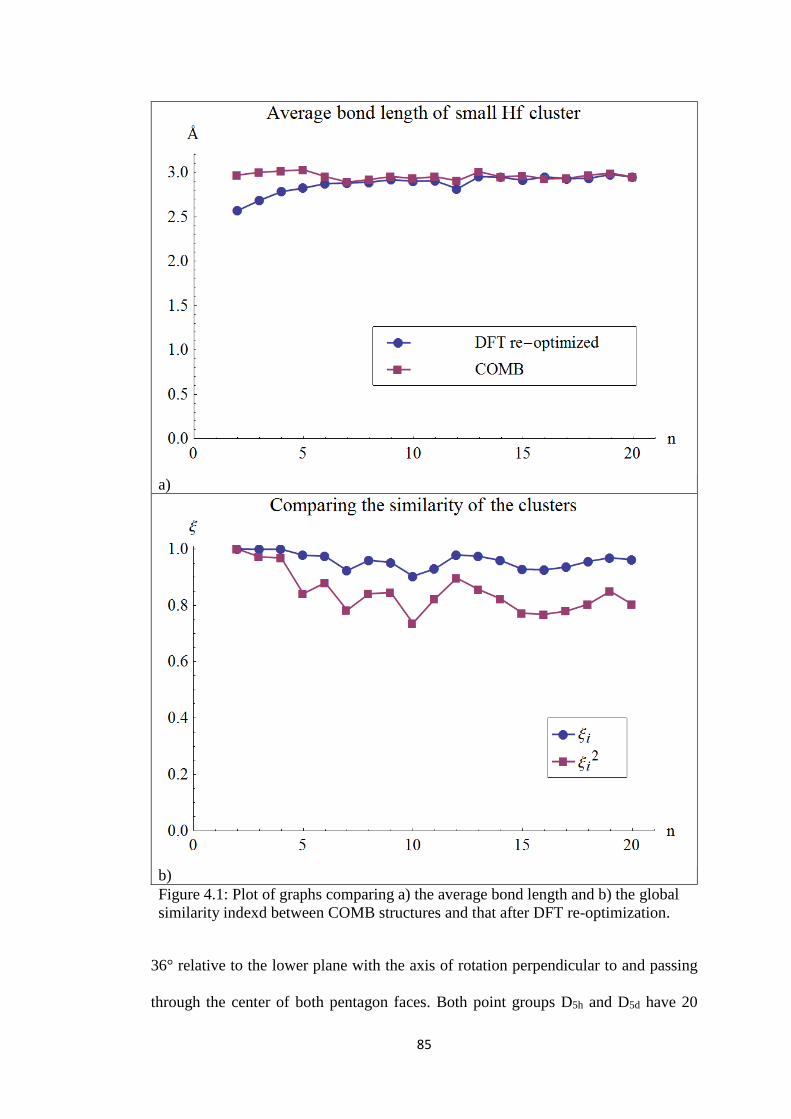
85

36° relative to the lower plane with the axis of rotation perpendicular to and passing

through the center of both pentagon faces. Both point groups D5h and D5d have 20

a)

b)

Figure 4.1: Plot of graphs comparing a) the average bond length and b) the global

similarity indexd between COMB structures and that after DFT re-optimization.

86

symmetry elements. Hf12 cluster was identical before and after the geometrical re-

optimization. Four other structures are slightly deviated (𝑛 = 11, 15, 16, 17; shaded

light blue in Table 4.1), and only three are heavily re-orientated (𝑛 = 7, 10, 20; shaded

dark blue). The order of dissimilarity in the point group symmetries were highlighted

with the increasing color intensity in Table 4.1 according to their order of differences.

Symmetry point group can only give a qualitative estimation to the structural similarity

and is somewhat lacking of quantitative preciseness. Nonetheless, this method still

predicts a good agreement to the other two methods, which were discussed in the

following paragraphs. Another way to access structural likeliness is by calculating the

global similarity index for the structures before and after re-optimization. In this

context, both the congruent and similar identifiers were applied. The role and

characteristic of both identifiers have been explained in Section 3.3.1.

Geometrical optimization in the G03 package has the tendency to rescale the

size of the cluster, and this effect has been taken into consideration in the global

similarity index by using the definition of 𝑘′𝑠,𝑖𝐶𝑂𝑅 as described in Equation (3.27). The

rescaling effect is seen, e.g., in the Hf2 to Hf6 clusters. As explained in Section 3.3.1,

since the variation in these structures before and after the geometrical re-optimization

is generally very minimum (very similar to each other), the function of the global

similarity index 𝜉𝑖 is to be squared to provide a more sensitive and visible reading

while monitoring the comparison process. In this case, Equation (3.24) can be written

as

𝜉𝑖2 =

1

9𝑛2∑ ∑(𝑘′𝑠,𝑖

𝐶𝑂𝑅 + 1)−2

𝑛

𝑠=1𝐶𝑂𝑅

(4.1)

87

As an illustration, Figure 4.1b shows the scores of global similarity index with

and without squaring. It can be seen that 𝜉𝑖2

displays a more visually distinctive

variation in its spectrum than 𝜉𝑖 . Despite both 𝜉𝑖2 and 𝜉𝑖 contains identical amount of

information, it was visually more convenient to monitor 𝜉𝑖2

, instead of 𝜉𝑖 , for

identifying abrupt changes in the evolution of the cluster structures. Hence, the choice

of 𝜉𝑖2 was merely due to visual convenience.

Table 4.2 displays the snapshots of the 19 structures obtained from plmp with

COMB potential and their corresponding DFT re-optimized counterparts. In Table 4.2,

two clusters of the same size are displayed side by side for the ease of direct

comparison. The left structures are those obtained from plmp, while the right ones are

the corresponding structures which have underwent DFT geometrical re-optimization

process. Observing the frames of structures tabulated in Table 4.2, it is visually

obvious that cluster with 𝑛 = 7,10,15,16,17 will yield the lowest similarity score.

This observation tallies well with the results tabulated in Table 4.1 and Figure 4.1b

(𝜉𝑖 = 1 is for total identity while 𝜉𝑖 → 0 for full structural dissimilarity).

Repetitive motif of pure elemental cluster can be observed in Hf7, Hf13 and

Hf19, which showed pentagonal bi-pyramidal like structure. It is shown in the next

section that this repetitive motif of Hf7 is in fact the lowest energy isomers for hafnium

cluster.

To sum up the plmp intra-line comparison, COMB potential produced COMB

structures that are geometrically close to the structures after G03 re-optimization. This

can be seen from the high degree of chemical similarity between them. This provided

the first part for the confirmation of the dependability of COMB potential in terms of

producing true global minimum of hafnium clusters. The full verification for COMB

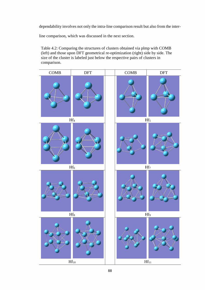
88

dependability involves not only the intra-line comparison result but also from the inter-

line comparison, which was discussed in the next section.

Table 4.2: Comparing the structures of clusters obtained via plmp with COMB

(left) and those upon DFT geometrical re-optimization (right) side by side. The

size of the cluster is labeled just below the respective pairs of clusters in

comparison.

COMB DFT COMB DFT

Hf4 Hf5

Hf6 Hf7

Hf8 Hf9

Hf10 Hf11

89

COMB DFT COMB DFT

Hf12 Hf13

Hf14 Hf15

Hf16 Hf17

Hf18 Hf19

Hf20

90

4.2 Structural Confirmation of Hafnium Clusters

The previous section concluded that the reliability of COMB potential in

obtaining structures of hafnium clusters close to the local minimum in the DFT PES.

The objective of this section, on the other hand, is to determine, by way of inter-line

comparison, whether these local minimum are the global minimum or one of the lowest

energy isomers for the hafnium clusters in the DFT PES. As shown in schematic sketch

of Figure 3.5, both the process lines underwent geometrical re-optimization with the

same method and same basis set to ensure the consistency during comparison.

The hafnium clusters generated via pg3 (stage 1 in the pg3 process line) are

shown in Table 4.3. Due to the expensive computational cost, only small clusters of

Hf4, Hf5, Hf6, Hf7, and Hf8 are generated for the pg3 process line. As it is known a

priori, Hf2 and Hf3 will surely yield dimer and planar triangle structures. Each column

in Table 4.3 was filled with the screenshot of the geometry of the hafnium clusters, the

SCF energy in atomic units (hartree) rounded down to four decimal places, and the

cluster size. It was found that for smaller cluster sizes (Hf4, Hf5 and Hf6), only one

unique structure is resulted upon re-optimization by G03 (stage 2 in the pg3 process

line). In other words, the generally different structures (of a fixed 𝑛-sized cluster, with

𝑛 = 4, 5, 6) in stage 1 converged to the same geometry upon re-optimization in stage

2. On the other hand, Hf7 yields two while Hf8 yields four distinctive yet energetically

close-by structures in stage 2. The resultant clusters (with size 𝑛 = 4, 5, 6, 7, 8 )

obtained at the end of stage 2 in the pg3 process line are tabulated in Table 4.3.

91

Table 4.3: The hafnium clusters of size Hf4 to Hf8 in stage 2 of the pg3 process

line, along with their DFT total energy value in hartree. (*) indicates structures

with lowest energy, while (**) indicates similar structures that are also obtained in

the plmp process line.

-195.3351 -244.2367

Hf4 (*, **) Hf5 (*, **)

-293.1347 -341.9995

Hf6 (*, **) Hf7

-342.0305 -390.8634

Hf7 (*, **) Hf8

-390.8866 -390.8891

Hf8 (**) Hf8

-390.9112

Hf8 (*)

92

A single asterisk (*) in Table 4.3 indicates structures with lowest energy, while

double asterisk (**) indicates coincidental structures that are also obtained in stage 2

of the plmp process line. In general, the structural geometry of hafnium clusters

obtained via the pg3 process line agreed well with the findings by Charles (2008).

Besides Hf6, the remaining hafnium clusters generated in this thesis have the same

lowest energy structures as presented by Charles (2008). The overall agreement of the

resultant global structures of the hafnium clusters with the findings from the literature

provides a justification, albeit only for the limited range of cluster size, to the pg3

process line as a reliable method to generate true global minimum structures, if not for

the expansive computing cost.

The hafnium clusters marked with (**) are clear evidence that these ground

state structures produced via the COMB potential coincide with that generated via the

pg3 approach. The only exception is Hf8, where the structure predicted by the plmp

process line is in fact one of the low lying structures given by the pg3 approach.

Although the accuracy of COMB potential in predicting ground state structure is not

100%, but it is acceptable to a reliable extend. Four out of five ground state structures

obtained via the plmp process line are highly similar or coincidental with that produced

via the DFT approach, the pg3 process line, whereas the only exception happened to

be coincidental with one of LLS in the pg3 prcoess line. The largest cluster size which

COMB can reproduce the correct global structures can only be verified up to a size of

𝑛 = 8, within the affordability of the computational resource in this work. Due to the

expensive computational cost, ground state structures of larger cluster size from pg3

were not generated to provide comparison (and justification) to that generated via the

COMB potential. On the other hand, the structures obtained from COMB are also

supported by previous findings in the literature (Charles, 2008), further supported the

93

COMB potential for hafnium is in fact suitable to be used in finding the global

minimum structure of a cluster. As stated in the discussion of COMB potential, the

empirical potential used to generate the input structures was subsequently used for the

MD simulation.

To sum up, the intra-line and inter-line comparisons as discussed in this

Chapter have provided combine verifications to the dependability of the COMB

potential. Taken together, COMB potential is suitable to describe inter-atomic

interactions of hafnium atom in cluster environment, which agree with that obtained

with ab initio methods (pg3). After verifying the dependability of the COMB potential,

it was further used in MD simulation in the next Chapter.

94

CHAPTER 5

SIMULATED ANNEALING OF THE HAFNIUM CLUSTERS

5.1 The Melting Point of Hafnium Clusters

In previous chapter, the dependability of COMB potential has been verified. In

this chapter, the melting behavior of the hafnium clusters upon simulated annealing at

elevated temperatures using COMB potential was investigated. The converged COMB

structures (the global minimum in the stage 1 of the plmp process line) were used as

input in the subsequent annealing MD simulation. The output of MD heating

simulation by using COMB as the input potential was examined in detail in the

following discussions.

The results of simulated annealing presented in this chapter are based on the

few post-processing methods mentioned in Section 3.3. The COMB structures were

used as input for the simulated annealing to ensure that the same set of laws governing

the geometry of the structures were also used to govern the dynamic interactions

between the hafnium atoms during the simulated annealing procedure. There is a subtle

weak connection between the initial input structure and the end resultant melting

configuration. In fact, Lu et al. (2013) recently proved that the choice of input structure

essentially affects the outcome of simulated annealing procedure.

To begin, the MD heating simulation of Hf20 as an illustrative example was

discussed. The caloric and 𝑐𝑣 curves of Hf20 generated by prolonged annealing process

95

were presented in Figure 5.1. Each point on the caloric curve has a corresponding

counterpart on the 𝑐𝑣 curve at the same temperature. It is easy to understand the

connection between the two graphs based on thermodynamic interpretation for the

constant volume specific heat capacity 𝑐𝑣, which is given by the gradient of the caloric

curve according to the following equation

𝑐𝑣 = (𝜕𝐸

𝜕𝑇)

𝑣

(5.1)

where 𝐸 are the potential energy value, 𝑇 the temperature, and the subscript 𝑣 denotes

the derivatives taken under constant volume thermosetting. However, the method used

to obtain the 𝑐𝑣 curve in this thesis is by calculating the fluctuations of the caloric

curve with Equation 2.3.

Melting transition is expected to happen when the potential energy of the

cluster changed drastically during the melting point, 𝑇𝑚. This temperature corresponds

to the latent heat of fusion. Based on the definition of Equation 5.1, this drastic change

of 𝐸 value is expecting to return a relatively larger value of 𝑐𝑣 in the vicinity of 𝑇𝑚.

Thus, melting transition corresponds to a large peak in 𝑐𝑣 curve. Apparently, from

Figure 5.1, the caloric curve was less effective in giving the exact temperature for both

the melting point and pre-melting point as compared to the 𝑐𝑣 curve. There were

many random peaks in the 𝑐𝑣 curve (Figure 5.1b), the first apparent peak is the pre-

melting, while the highest peak is the melting point. The melting point corresponds to

the most obvious transition in the caloric curve (Figure 5.1a). The green arrow

indicates the pre-melting temperature 𝑇𝑝𝑟𝑒 = 1400 K while the red arrow indicates the

melting temperature 𝑇𝑚 = 1850 K in both graphs.

96

a)

b)

Figure 5.1: a) The caloric curve and b) 𝑐𝑣 curve of Hf20 obtained via prolonged

annealing process (TNA = total number of atoms in the cluster). The green arrow

indicates the pre-melting temperature at 𝑇𝑝𝑟𝑒 = 1400 K, and the red arrow

indicates the melting point at 𝑇𝑚 = 1850 K.

In addition to the prolonged annealing method, an independent method to

obtain melting behaviour of the clusters was also attempted, as discussed in Section

3.3, which is the direct heating method. The overall idea of direct heating process was

described in Section 3.3. The purposes for conducting this procedure on top of the

97

prolonged method are two-fold: (1) it was used as an independent check to the results

obtained via the prolonged method, and (2) to generate the evolutional history of global

similarity index of the clusters, which carries the dynamical information throughout

the evolutionary history of a MD simulation. (2) can be obtained via post-processing

the LAMMPS trajectory file (.lammpstrj). The trajectory file contained the frames of

the atoms that reflect the heating process as recorded in the corresponding log (.log)

file. However, in the prolonged annealing simulation, in which the target temperatures

were generally set to a very high value, e.g. 𝑇 = 3000 K, a large fluctuation in the

temperature is usually present throughout the equilibration steps (see the example in

Figure 3.4). Due to the large fluctuation in the temperature, the trajectory of the atoms

also fluctuates rigorously. Over an extended equilibration time step, the trajectory of

each individual hafnium atom in the cluster will move all over the simulation box and

tends to be ergodic. The ergodicity is not desired for the coordinates of the cluster

system as the average position of each atom will overlap in the confined space of

simulation box. The coordinates as recorded in the trajectory file throughout the

equilibration stage do not corresponds to the target temperature at which the system is

in. Therefore, global similarity index cannot be used in the prolonged heating

procedure to quantify the heating process.

In contrast, the direct heating method, due to the imposition of the 300∆𝑡 time

averaging protocol, the fluctuations of all recorded data in both the LAMMPS output

files (.log and .lammpstrj) were confined within the 300∆𝑡 time window. As a result,

the original thick slope in Figure 3.4a was now transformed into a much refined and

narrower slope in Figure 3.4b. The coordinates as recorded in the trajectory file in the

300∆𝑡 time window do correspond to the temperature at which the system is currently

98

in. This allowed the information of heating mechanism to be extracted by using global

similarity index in the direct heating procedure.

In addition, the direct heating method is also able to predict the melting

temperature 𝑇𝑚 and pre-melting temperature 𝑇𝑝𝑟𝑒 by plotting the caloric curve and the

𝑐𝑣 curve. In this respect, the caloric and 𝑐𝑣 curve are known as ‘indicators’, meaning

MD quantities from which thermodynamically interesting transitions can be monitored.

In fact, the caloric profile is readily to be extracted from the log file of LAMMPS

output, since both 𝐸 and 𝑇 are recorded in separated columns of the log file. Figure

5.2 shows the caloric curve and 𝑐𝑣 curve of Hf10 via direct heating method. The 𝑐𝑣

curve shows a lot of peaks (Figure 5.2b). The first apparent peak is the pre-melting

and the tallest peak is the melting point. The melting point corresponds to the largest

transition in caloric curve (Figure 5.2a). By using the same color code as for Figure

5.1, green arrow indicates the pre-melting temperature 𝑇𝑝𝑟𝑒 = 1350 K, and the red

arrow indicates the melting point 𝑇𝑚 = 2200 K. Both curves provide complementary

information to help locating the transition temperatures. Only one unique transition

temperature was reported based on these two indicators after comparing and

contrasting both curves to estimate the most precise value for the transition

temperatures. Due to its higher sensitivity, the transition temperatures reported in this

thesis were in all cases read off from the 𝑐𝑣 curve. As it turns out, indication of

transition in the caloric curve is relatively less distinctive (hence higher in uncertainty),

hence it was used only as a supplimentary confirmation to the transition value reported

from the 𝑐𝑣 curve.

99

a)

b)

Figure 5.2: a) The caloric curve and b) 𝑐𝑣 curve of Hf10 obtained via direct heating

process. The green arrow indicates the pre-melting temperature at 𝑇𝑝𝑟𝑒 = 1350 K,

and the red arrow indicates the melting point at 𝑇𝑚 = 2200 K.

The identification of transition temperatures can also be made based on another

independent indicator, which is the global similarity index. In this case, 𝜉𝑖 shall

consider only the congruent identifier (rescaling is expected to be observed during

heating procedure) as described by Equation (3.24), where 𝑘𝑠,𝑖𝐶𝑂𝑅 takes the form of

𝑐𝑣(eV/K)

100

Equation 3.23. It also reveals the structural changes occurring in the clusters during

the heating procedure. The trajectory file used to obtain the similarity index profile has

based on the direct heating method. The dynamical evolution of global similarity index

as a function of temperature is shown in Figure 5.3 for Hf13 as a sample candidate.

Figure 5.3a shows the similarity index 𝜉𝑖 profile for each frames during the heating

process as compared to the ground state structure (the 0th frame) by using Equation

3.22. Figure 5.3b is the fluctuation (variance) of similarity index 𝑆𝜉𝑖 corresponds to the

same trajectory calculated by using Equation 3.28.

The features which are thermodynamical interest in the example of Figure 5.3

is now interpreted. Melting and pre-melting features can be identified from both the

𝑆𝜉𝑖 vs 𝑇 and 𝜉𝑖 vs 𝑇 curves, albeit with different sensitivity. The pre-melting transition

is not obvious in the 𝑆𝜉𝑖 curve due to the suppression of the overall scale in 𝑆𝜉𝑖

by the

high peak at 𝑇 ≈ 2050 K. The pre-melting transition can merely become visible by

zooming in to the 𝑆𝜉𝑖 curve at around 𝑇 ≈ 1050 K, as displayed by the inset of Figure

5.3b. As is observed throughout the MD calculations in this thesis, it was found that

usually the signal of pre-melting or melting in the 𝑆𝜉𝑖 curve waas moderate unless the

transitions in the clusters happened in a really abrupt manner. In practice, both the 𝑆𝜉𝑖

and 𝜉𝑖 curves have to be simultaneously deployed so that the complementary features

in both curves can pinpoint a transition with a more reliable precision. As in the case

of Figure 5.3, the pre-melting point correspond to the first obvious drop in the

similarity index (indicated by the green arrow) at 𝑇𝑝𝑟𝑒 = 1600 K. On the other hand,

the melting point was visibly apparent in both graphs (indicated by the red arrow) at

𝑇𝑚 = 2050 K.

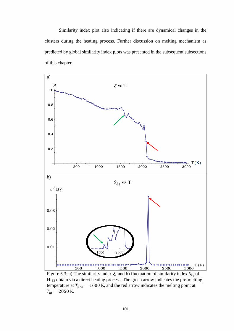
101

Similarity index plot also indicating if there are dynamical changes in the

clusters during the heating process. Further discussion on melting mechanism as

predicted by global similarity index plots was presented in the subsequent subsections

of this chapter.

a)

b)

Figure 5.3: a) The similarity index 𝜉𝑖 and b) fluctuation of similarity index 𝑆𝜉𝑖

of

Hf13 obtain via a direct heating process. The green arrow indicates the pre-melting

temperature at 𝑇𝑝𝑟𝑒 = 1600 K, and the red arrow indicates the melting point at

𝑇𝑚 = 2050 K.

102

5.2 Melting Temperature and Cluster Sizes

Three different indicators were used in this thesis to identify melting transitions

in two independent heating procedures. In the prolonged heating method, only two

indicators were used to identify melting transitions, namely the caloric and 𝑐𝑣 curves.

In the direct heating method, the caloric, the 𝑐𝑣 curves and global similarity index were

used as indicators. In this section, the transition temperatures as a function of cluster

size 𝑛 were reported.

Table 5.1 shows the results of melting and pre-melting temperatures in both

heating procedures. The first two columns were the melting temperatures obtained

from prolonged annealing methods. The third and fourth columns were directly

extracted from a direct heating simulation elevated from 0 K to 3000 K at the

optimum rate of 5 × 1012 Ks−1. These transition temperatures were determined from

the 𝑐𝑣 curve but not the caloric curve (for the reason already explained in the previous

subsection). Meanwhile the last two are transition temperatures deduced from the

graph of fluctuations in the global similarity index, 𝑆𝜉𝑖. Recall that global similarity

index is only applicable in the direct heating process. The distinctions between the

prolonged annealing and the direct heating process have been mentioned in Section

3.3. In fact, the prolonged simulated annealing method involves compilation of many

heating processes equilibrated at different target temperatures. Every single data point

in the caloric curve was the result of statistically sampling a cluster’s energy over a

lengthy period of equilibration at the fixed temperature. The pre-melting temperature,

𝑇𝑝𝑟𝑒 , and the exact melting temperature, 𝑇𝑚, were plotted in the same graph in Figure

5.4 for each method. The melting temperature 𝑇𝑚 vs 𝑛 obtained from the three

103

different approaches listed in Table 5.1 were also compiled into a single graph as

shown in Figure 5.5 for a better comparison.

Table 5.1: The melting and pre-melting temperatures obtained from three different

approaches. The first four columns are obtained from caloric curves and 𝑐𝑣 curves.

𝑛

Prolonged simulated

annealing

Direct heating

process

Fluctuation of the

similarity index, 𝑆𝜉𝑖

curves

𝑇𝑝𝑟𝑒 (K) 𝑇𝑚 (K) 𝑇𝑝𝑟𝑒 (K) 𝑇𝑚 (K) 𝑇𝑝𝑟𝑒 (K) 𝑇𝑚 (K)

6 1250 1750 1250 2000 1250 1950

10 1500 1750 1350 2200 1850 2250

14 1550 1800 1200 1900 1700 2200

17 1200 1900 1250 2250 1700 2100

18 1450 1700 1450 2200 1850 2100

20 1400 1850 1500 2150 1750 2150

22 1600 1850 1500 2150 1750 2150

24 1350 1800 1700 2050 1800 2100

26 1500 1850 1950 2300 2050 2250

30 1650 1750 1650 2250 1750 1850

34 1500 1800 1950 2300 1850 2100

38 1550 1850 1650 2500 1850 2000

39 1600 1900 1700 2350 1600 2000

40 1350 1900 1400 2100 1800 2150

42 1650 1950 1800 2100 1800 1950

46 1600 1850 1800 2250 1800 2200

50 1450 1900 1600 2250 1800 2150

99 1650 2050 2150 2500 1900 2300

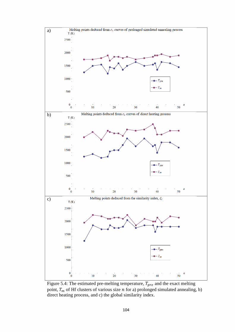
104

a)

b)

c)

Figure 5.4: The estimated pre-melting temperature, 𝑇𝑝𝑟𝑒 and the exact melting

point, 𝑇𝑚 of Hf clusters of various size 𝑛 for a) prolonged simulated annealing, b)

direct heating process, and c) the global similarity index.

105

Figure 5.5: The estimated melting point of the hafnium cluster against the cluster

size 𝑛, based on three different approaches.

As mentioned in Section 3.3, direct heating of the structure to a high

temperature allows one to yield detailed dynamics of the clusters. It can be seen from

Figure 5.5 that this approach overall predicts a higher melting point than that from the

prolonged annealing method, but the prediction still agreed well with expectation as

compared to the bulk melting of hafnium, which is 𝑇𝑚𝑏𝑢𝑙𝑘(Hf)~2504 K according to

the periodic table. Nevertheless, both simulation approaches agreed that the melting

temperature of hafnium cluster increases with the size 𝑛.

One of the most important results obtained from this thesis is that global

similarity index, 𝜉𝑖, has the capacity to predict the dynamics of the heating process

from the MD trajectory of clusters. A few samples of 𝜉 plotted against the temperature

𝑇 were shown in next section, along with their respective fluctuations, 𝑆𝜉𝑖. Snapshots

of the coordinates of the clusters were presented directly from VMD visualization.

Based on the 𝜉𝑖 graph (Figure 5.3 for example), every obvious drop in the average

value corresponds to a significant change in trajectory, starting with changes from

106

surface and slowly to the core of the whole cluster. In general, the pre-melting effect

take place at the first significant peak of 𝑆𝜉𝑖, whereby the exterior of the cluster is

usually heavily distorted, but the particle is still bounded relatively close to each other.

As the heating continues, the cluster would be a de-fragmented and start drifting in

random direction, entering the fluidic phase. Section 5.3 presented some of the

screenshots of the clusters over the course of simulation, which corresponds to the

points represented in the similarity index curves for the case of Hf30, Hf50, and Hf99. In

order to portray the distance between atoms in the clusters, the dynamic bond length

was set to be around 3.127Å.

5.3 Similarity Index and Cluster Melting

In the selected cases of the following subsections, the plots of similarity index

𝜉𝑖 were compared to its fluctuation plot 𝑆𝜉𝑖 as a function of temperature. Every major

transitions in 𝜉𝑖 correspond to a significant change in cluster geometry which were

shown by VMD screenshots, add-ons to each graph signified the happening of certain

event during heating process. These transitions were sometimes less apparent in 𝜉𝑖

graphs, but are indicated clearly in the fluctuation plot, 𝑆𝜉𝑖.

As mentioned earlier in the first section of this chapter, the direct heating

procedure enables LAMMPS package to record the dynamic changes of candidate

structures in both the .log and .lammpstrj files. The global similarity index method

used in this thesis enabled the coordinates of the system to be recorded in the trajectory

file to be portrayed graphically such as that shown in the example of Figure 5.3. In

107

fact, the original purpose of the trajectory file was to allow the visualization of the

dynamics of the system.

The following subsections of Section 5.3 focused only to a few specific sizes

of hafnium clusters. The figures shown in each subsection were discussed in details in

the following paragraphs. The choice of the hafnium clusters in the discussions

included all the events that were detected by both the similarity index 𝜉𝑖 plot and the

fluctuation of the similarity index 𝑆𝜉𝑖 plot.

5.3.1 Hf30

From Figure 5.6, the first significant change of Hf30 cluster in the heating

process occurs around 𝑇 = 1000 K to 1300 K, indicated by the sudden drop of 𝜉𝑖. The

outermost layer atoms become further apart from each other but remain intact with the

‘core’ atoms. The pre-melting took place at the first peak of the 𝑆𝜉𝑖, at around 𝑇𝑝𝑟𝑒 =

1750 K with the ‘shell’ atoms begin to drift apart from the cluster. The highest peak

of 𝑆𝜉𝑖, corresponds to a temperature around 𝑇𝑚 = 1850 K, showing a total breakdown

of the cluster. The screenshot at 𝑇𝑚 = 1850 K has not included a drifted hafnium atom

far towards the edge of the simulation box. A final screenshot at 𝑇 = 2150 K showed

the remnant cluster ‘core’ after many surface atoms have drifted away.

108

a)

b)

Figure 5.6: a) Similarity index 𝜉𝑖 curve and b) fluctuation of the similarity index

𝑆𝜉𝑖 of Hf30. The screenshots show the configuration of the cluster Hf30 during that

particular temperature.

109

5.3.2 Hf50

a)

b)

Figure 5.7: a) Similarity index 𝜉𝑖 curve and b) fluctuation of the similarity index

𝑆𝜉𝑖 of Hf50. The screenshots shows the configurations of the cluster Hf50 during

that particular temperature.

For the case of Hf50 as shown in Figure 5.7, the 𝜉𝑖 curve displays some unique

features, which were the sudden droped at around 𝑇 = 1850 K and a sudden rose at

around 𝑇 = 1900 K. This behavior was observed to be the effect of a single hafnium

atom leaving the cluster drifting to the wall of the simulation box and bouncing back

to the cluster. This behavioral change was the result of kinetic energy accumulated

110

within a single atom that causes it to escape from the cluster. In order to ensure that

this artifact is not a random error in the simulation, the overall simulated annealing

procedure was re-run with slightly different initial condition (different random initial

velocity). The same feature was showed up when different initial condition is imposed.

The sharp change was also detected by the fluctuation plot against temperature

showing two sharp peaks at about the same temperature. The left one corresponded to

a sudden drop in 𝜉𝑖 while the right one corresponds to a sudden rise of 𝜉𝑖 value. The

true melting is at around 𝑇𝑚 = 2150 K when the cluster broke down completely and

drifted apart. In fact, the same scenario was also observed in the case of Hf18 and Hf26.

Along with their respective graph of similarity index, 𝜉𝑖 curve, Figure 5.8 shows the

particular snapshot where the drifting of a single atom begins to take place. For all

these cases, the drifting of single atom happened close to the melting point, 𝑇𝑚. Other

than atoms leaving the cluster one at a time, the more common observation is that the

clusters were being tore down into few groups and slowly dissolve into a mist of atoms

cloud in liquid-gaseous like phase.

111

a)

b)

Figure 5.8: The artifact of single atom drifting away observed in the case of a) Hf18

and b) Hf26.

5.3.3 Hf99

Cluster size Hf99 was used to describe the complete trace of dynamics during

the single annealing process from 𝑇 = 0 K to 3000 K, as shown in Figure 5.9. The

atomic vibration slowly increased in magnitude upon velocity rescaling. As observed

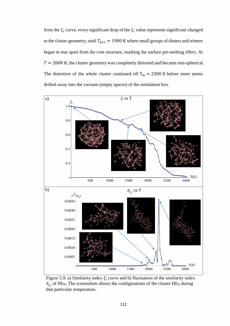
112

from the 𝜉𝑖 curve, every significant drop of the 𝜉𝑖 value represents significant changed

to the cluster geometry, until 𝑇𝑝𝑟𝑒 = 1900 K where small groups of dimers and trimers

began to tear apart from the core structure, marking the surface pre-melting effect. At

𝑇 = 2000 K, the cluster geometry was completely distorted and became non-spherical.

The distortion of the whole cluster continued till 𝑇𝑚 = 2300 K before more atoms

drifted away into the vacuum (empty spaces) of the simulation box.

a)

b)

Figure 5.9: a) Similarity index 𝜉𝑖 curve and b) fluctuation of the similarity index

𝑆𝜉𝑖 of Hf99. The screenshots shows the configurations of the cluster Hf99 during

that particular temperature.

113

Figure 5.10 shows the state of cluster Hf99 upon some long equilibration at 𝑇 =

3000 K. In order to visualize the appearance of the whole cluster Hf99 after it is

completely melted and stayed in fluidic phase at the end of 𝑇 = 3000 K equilibration,

the snapshot is enlarged four times as compared to the previous examples. The frame

of Figure 5.10 was set roughly to the size of the simulation box.

Figure 5.10: Hf99 upon the equilibration at 𝑇 = 3000K.

114

CHAPTER 6

CONCLUSIONS AND FUTURE STUDIES

6.1 Conclusions

In this thesis, the MD simulations have been carried out to yield the detailed

dynamics of the hafnium cluster systems in heating processes. Each part of the

simulations was verified with careful examinations. Chapter 4 laid out the verification

to show that COMB potential is an appropriate interatomic potential in describing

hafnium clusters. The hafnium clusters obtained via the plmp algorithm with COMB

potential for the size 𝑛 = 2 to 𝑛 = 8 were in a good agreement to that reported in the

literatures. COMB potential also produced structures close to the ground state of DFT

method, justified by the principle of chemical similarity. Clusters Hf7, Hf13, and Hf19

showed repetitive geometry motif of pentagonal bipyramid. The plmp algorithm

proved to be very efficient in searching the global minimum structures of the given

interatomic potential. The BH-GA part of the algorithm was capable to handle various

class of empirical potential with well-established convergence. In principle, the

process lines comparison algorithm as described in Chapter 4 can also be adopted as a

practically implementable protocol to verify or falsify the dependability of any generic

empirical potentials for producing true ground state structures at the DFT accuracy.

Chapter 5 reported the melting transition of hafnium clusters for the size of

clusters up to 𝑛 = 99. The melting point of hafnium cluster showed gradual increment

with the increasing of number of atoms, 𝑛, but remained lower than the bulk value of

𝑇𝑚𝑏𝑢𝑙𝑘(𝐻𝑓)~2504 K. This showed the size dependent melting behavior of a cluster. In

addition, hafnium clusters experienced surface atom pre-melting effect at some

115

temperature 𝑇𝑝𝑟𝑒 lower than that of its melting point 𝑇𝑚. Other than the surface pre-

melting, some cluster sizes such as Hf18, Hf26 and Hf50 displayed a featured pre-melting

stage in which a single hafnium atom was observed to escape from the cluster in a brief

moment before the clusters melted thoroughly.

6.2 Future Studies

During the generation of candidate structures for hafnium clusters, both plmp

and pg3 process line come in handy. The process lines comparison algorithm to search

and confirm the global minimum of given empirical potential can be used as a good

addition to the technique currently available in the field of cluster science. If an

empirical potential is found to pass the test of the process line comparisons, then

ground state structures of large cluster size at DFT accuracy could be generated via the

computationally economical plmp procedure. Extended work to gather simulation data

on clusters formed by different types of element, for a variety of interatomic potential

is verified by the protocol, and large size ground state structures at DFT accuracy are

correctly generated via the plmp process. The robustness of the process lines algorithm,

if established with empirical evidences, shall be a very powerful tool for large size,

DFT-accurate, ground state cluster search.

The MD procedures used in this thesis were successful. These include the

solution to some of the fundamental problems such as the flying ice cube problem and

the broad fluctuations in thermodynamic variables for the heating of small size systems.

The MD procedures used in this thesis can be used to study any cluster system of

interest provided a good interatomic potential to describe the system is available. In

fact, MD method is very powerful and is able to perform more than just heating and

116

quenching, bearing a good complement to the experiments. In many instances, MD is

able to mimic ‘experiment’ on small sizes system, such as the work of this thesis.

In this thesis, the method of global similarity index succeeded in studying the

dynamic of the system during heating and melting. The visualization was simplified

into graphs that trace the trajectories of the coordinates of each hafnium atom during

the MD process. The general idea of global similarity index was based upon the

chemical similarity principle. It was rather simplified in term of functional form as

well as working principle aiming to detect any characteristic transition throughout the

evolutional history of a cluster in a MD simulation. The idea and application of global

similarity index has the potential to be further developed into a powerful fingerprint

descriptor that could unambiguously and uniquely recognize the identity of a three

dimensional molecule, such as protein molecule or other large, biochemically

interested molecules, from a numerical database containing some arbitrary,

unidentified molecular structures. The proposed descriptor could find its application

in computational drug design. For example, the design of a drug targeting a particular

protein. Firstly, catalogue all the fingerprint of (the improved version of) the global

similarity index of a list of candidate drugs. Meanwhile, an algorithm can be developed

to computationally scan the entire 3D morphology of a target protein for local sites

containing any signature of complementary fingerprint of the drugs in the catalogue.

If candidate local sites on the protein with complementary similarity to any of the drugs

in the catalogue was reported, then a full scale biomolecular MD can be followed up,

where these drugs can be placed close to the local site to monitor the resultant

interactions between them.

117

The global similarity index can also be expanded independently to take into

consideration of additional physical properties other than the atomic position that has]

been used in this thesis.

118

REFERENCES

Aguado A., López J.M., Alonso J.A. and Stott M.J. (2001). Melting in large sodium

clusters: An orbital-free molecular dynamics study, J. Phys. Chem. B 105: 2386.

Ahlrichs R. and Elliott S.D. (1999). Clusters of aluminium, a density functional study,

Phys. Chem. Chem. Phys. 1: 13.

Andreeva A., Howorth D., Chothia C., Kulesha E. and Muezin A.G. (2013). SCOP2

prototype: a new approach to protein structure mining, Nucl. Acid Res. 42: D310.

Antoniadis D. (2015). EP1: Moore’s Law Challenges Below 10nm: Technology,

Design and Economic Implications, ISSCC 2015, Evening Session, EP1.

Bacskay G.B. (1981). A quadratically convergent Hartree-Fock (QC-SCF) method.

Application to closed shell systems, Chem. Phys. 61: 385.

Bajusz D., Rácz A. and Héberger K. (2015). Why is tanimoto index an appropriate

choice for fingerprint-based similarity calculations? J. Cheminf. 7: 20.

Ballester P.J. and Richards W.G. (2007). Ultrafast shape recognition for similarity

search in molecular databases, Proc. R. Soc. A 463: 1307.

Balleto F. and Ferrando R. (2005). Structural properties of nanoclusters: Energetic,

thermodynamic, and kinetic effects, Rev. Mod. Phys. 77: 371.

Barron T.H.K. and Domb C. (1955). On the cubic and hexagonal close-packed lattices,

Proc. Roy. Soc. A227: 447.

Berry R.S. and Smirnov B.M. (2004). Heat capacity of isolated clusters, J. Exp. Theor.

Phys. 98: 366.

Bergeron D.E., Castleman A.W. Jr, Marisato T. and Khanna S.N. (2004). Formation

of Al13I-: evidence for the superhalogen character of Al13, Science 304: 84.

Biswas R. and Hamann D.R. (1987). New classical models for silicon structural

energies, Phys. Rev. B 36: 6434.

Boustani I. (1997). Systematic ab initio investigation of bare boron clusters:

Determination of the geometry and electronic structures of Bn (n=2-14), Phys. Rev.

B 55: 16426.

Boustani I., Quandt A., Hernández E. and Rubio A. (1999). New boron based

nanostructured materials, J. Chem. Phys. 110: 3176.

Breaux G.A., Neal C.M., Cao B. and Jarrold M.F. (2005). Melting, premelting and

structural transitions in size-selected aluminium clusters with around 55 atoms,

Phys. Rev. Lett. 94: 173401.

119

Brenner D.W. (1990). Empirical potential for hydrocarbons for use in simulating the

chemical vapor deposition of diamond films, Phys. Rev. B 42: 9458.

Brenner D.W., Shenderova O.A., Harrison J.A., Stuart S.J., Ni B. and Sinnott S.B.

(2002). A second-generation reactive empirical bond order (REBO) potential

energy expression for hydrocarbons, J. Phys.: Condens. Matter 14: 783.

Brown F. (2005). Editorial opinion: chemoinformatics – a ten year update, Curr. Opin.

Drug Discov. Dev. 8: 298.

Buffat Ph. and Borel J-P. (1975). Size effect on the melting temperature of gold

particles, Phys. Rev. A 13: 2287.

Calvo F. and Spiegelmann F. (1999). Mechanism of phase transitions in sodium

clusters: From molecular to bulk behavior, J. Chem. Phys. 112: 2888.

Cannon E.O., Nigsch F. and Mitchell J.BO (2008). A novel hybrid ultrafast shape

descriptor method for use in virtual screening, Chem. Cent. J. 2:3.

Charles W.B. Jr. (2008). Clusters of hafnium, Hfn 𝑛 = 2 − 8, Chem. Phys. Lett. 462:

183.

Chuang F.C., Wang C.Z. and Ho K.H. (2006). Structure of neutral aluminium clusters

Aln (2≤n≤23): Genetic algorithm tight-binding calculations, Phys. Rev. B 73:

125431.

Couchman O.R. and Jesser W.A. (1977). Thermodynamic theory of size dependence

of melting temperature in metals, Nature 269: 481.

Dash J.G. (2002). Melting from one to two to three dimensions, Contemp. Phys. 43:

427.

Duan H., Ding F., Rosén A., Harutyunyan A.R., Curtarolo S. and Bolton K. (2007).

Size dependent melting mechanism of iron nanoclusters, Chem. Phys. 333: 57.

Duin A.C.T., Strachan A., Stewman S., Zhang Q., Xu X. and Goddard W.A. III (2003).

ReaxFFsio reactive force field for silicon and silicon oxide systems, J. Phys. Chem.

A 107: 3803.

Durant J.L., Leland B.A., Henry D.R. and Nourse J.G. (2002). Reoptimization of MDL

keys for use in drug discovery, J. Chem. Inf. Comput. Sci. 42: 1273.

Ebbesen T.W., Lezec H.J., Hiura H., Bennett J.W., Ghaemi H.F. and Thio T. (1996).

Electrical conductivity of individual carbon nanotubes, Nature 382: 54.

Efremov M.Y., Schiettekatte F., Zhang M., Olson E.A., Kwan A.T., Berry R.S. and

Allen L.H. (2000). Discrete periodic melting point observations for nanostructure

ensembles, Phys. Rev. Lett. 85: 3560.

Ellis W.Y, Notsch J.D. and McGreevy P.B. (2003). Chemical information systems,

U.S. Patent No. 6,654,736.

120

Erhart P. and Albe K. (2005). Analytical potential for atomistic simulations of silicon,

carbon and silicon carbide, Phys. Rev. B 71: 035211.

Fang Y., Liu Y-S. and Ramani K. (2009). Three dimensional shape comparison of

flexible proteins using the local-diameter descriptor, BMC Struct. Bio. 9: 29.

Faraday M. (1859). Note on regelation, Proc. Roy. Soc. 10: 440.

Ferrando R., Jellinek J. and Johnston R.L. (2008). Nanoalloys: From theory to

applications of alloy clusters and nanoparticles, Chem. Rev. 108: 845.

Finnis M.W. and Heine V. (1974). Theory of lattice contraction at aluminium surface,

J. Phys. F 4: L37.

Giasuddin ASM, Jhuma K.A. and Mujibul Haq A.M. (2012). Use of gold nanoparticles

in diagnostics, surgery and medicine: a review, Bangladesh J. Med. Biochem. 5(2):

56.

Gould A.L., Logsdail A.J. and Catlow C.R.A. (2015). Influence of composition and

chemical arrangement on the kinetic stability of 147-atom Au-Ag bimetallic

nanoclusters, J. Phys. Chem. C 119: 23685.

Grant J.A., Gallardo M.A. and Pickup B.T. (1996). Comparison: A simple application

of a gaussian description of molecular shape, J. Comput. Chem. 17: 1653.

Grigoryan V.G. and Springborg M. (2003). Structure and energetics of Ni clusters with

up to 150 atoms, Chem. Phys. Lett. 375: 219.

Gupta R.P. (1981). Lattice relaxation at a metal surface, Phys. Rev. B 23: 6265.

Hartke B. (1996). Global geometry optimization of clusters guided by N-dependent

model potentials, Chem. Phys. Lett. 258: 144.

Hartke B. (1998). Global geometry optimization of small silicon clusters at the level

of density functional theory, Theor. Chem. Acc. 99: 241.

Harvey S.C., Tan K.Z.R. and Cheatham T.E. III. (1998). The flying ice cube: velocity

rescaling in molecular dynamics leads to violation of energy equipartition, J.

Comput. Chem. 19: 726.

Hay P.J. and Wadt W.R. (1985). Ab initio effective core potentials for molecular

calculations. Potentials for the transition metal atom Sc to Hg, J. Chem. Phys. 82:

270.

Hsu P.J. and Lai S.K. (2006). Structures of bimetallic clusters, J. Chem. Phys. 124:

044711.

Hsu P.J. (2014). A new perspective of shape recognition to discover the phase

transition of finite size clurters, J. Comput. Chem. 35: 1082.

Humphrey W., Dalke A. and Schulten K. (1996). VMD – visual molecular dynamics,

J. Mol. Graphics 14: 33.

121

Jaramillo-Botero A., Su J., Qi A. and WGoddard A. 3rd (2011). Large-scale, long-

term non-adiabatic electron molecular dynamics for describing material properties

and phenomena in extreme environments, J. Comp. Chem. 32: 497.

Johnson A.M. and Maggiora G.M. (1990). Concepts and Applications of Molecular

Similarity, New York: John Willey & Sons.

Khan A, Rahman K, Kim D.S. and Choi K.H. (2012). Direct printing of copper

conductive micro-tracks by multi-nozzle electrohydrodynamic inkjet printing

process, J. Mat. Process. Technol. 212: 700.

Kim D.S., Rahman K., Khan A. and Choi K.H. (2012). Direct Fabrication of Copper

Nanoparticle Patterns through Electrohydrodynamic Printing in Cone-Jet Mode,

Mater. Manuf. Process. 27: 1295.

Kim K. (2015). Silicon Technologies and Solutions for the Data-Driven World, ISSCC

2015, Session 1, Plenary 1.1.

Kiran B., Bulusu S., Zhai H.J., Yoo S., Zeng X.C. and Wang L.S. (2005). Planar-to-

tubular structural transition in boron clusters: B20 as the embryo of single-walled

boron nanotubes, Proc. Natl. Acad. Sci. U.S.A. 102: 961.

Kroto H.W., Heath J.R., O’Brien S.C., Curl R.F. and Smalley R.E. (1985). C60:

Buckminsterfullerene, Nature 318: 162.

Kuntová Z., Rossi G. and Ferrando R. (2008). Melting of core-shell Ag-Ni and Ag-Co

nanoclusters studied via molecular dynamics simulations, Phys. Rev. B 77: 205431.

Laasonen K., Wonczak S., Strey R. and Laaksonen A. (2000). Molecular dynamics

simulations of gas-liquid nucleation of Lennard-Jones fluid, J. Chem. Phys. 113:

9471.

Lai S.K., Hsu P.J., Wu K.L., Liu W.K. and Iwamatsu M. (2002). Structures of metallic

clusters: Mono- and polyvalent metals, J. Chem. Phys. 117: 10715.

Leary R.H. (2000). Global optimization of funneling landscapes, J. Global. Optim. 18:

367.

Li X. and Frisch M.J. (2006). Energy-represented DIIS within a hybrid geometry

optimization method, J. Chem. Theory and Comput. 2: 835.

Liu C-M., Xu C., Cheng Y., Chen X-R. and Cai L-C. (2013). Size-dependent melting

and coalescence of tungsten nanoclusters via molecular dynamics simulation, Phys.

Chem. Chem. Phys. 15: 14069.

Lu S., Zhang J. and Duan H. (2009). Melting behaviors of CoN (N=13, 14, 38, 55, 56)

clusters, Chem. Phys. 363: 7.

Lv M.B., Cheng Yan and Fu Min. (2013). A new global search for the ground state

structure of small cluster: application to S6, J. At. Mol. Sci. 4: 357.

122

Martin T.P., Näher U., Schaber H., and Zimmermann (1993). Evidence for a size-

dependent melting of sodium clusters, J. Chem. Phys. 100: 2322.

Menard L.D., Gao S.P., Xu H., Twesten R.D., Harper A.S., Song Y., Wang G.,

Douglas A.D., Yang J.C., Frenkel A.I., Nuzzo R.G. and Murray R.W. (2006). Sub-

nanometer Au monolayer-protected clusters exhibiting molecule-like electronic

behavior: quantitative high-angle annular dark-field scanning transmission electron

microscopy and electrochemical characterization of clusters with precise atomic

stoichiometry, J. Phys. Chem. B 110: 12874.

Mollenhauer D. and Gaston N., (2016). Phosphine passivated gold clusters: how

charge transfer affects electronic structure and stability, Phys. Chem. Chem. Phys.

2016, advance article.

Neyts E.C. and Bogaerts A. (2009). Numerical study of the size-dependent melting

mechanisms of nickel nanoclusters, J. Phys. Chem. C 113(7): 2771.

Ng W.C., Lim T.L. and Yoon T.L. (2015a). Ground-state structures of hafnium

clusters, AIP Conf. Proc. 1657: 070003.

Ng W.C., Yoon T.L. and Lim T.L. (2015b). Guided basin-hopping search of small

boron clusters with density functional theory, AIP Conf. Proc. 1657: 070004.

Oganov A.R. and Valle M. (2009). How to quantify energy landscapes of solids, J.

Chem. Phys 130: 104504.

Oprea T.I. (2002). On the information content of 2D and 3D descriptors for QSAR, J.

Braz. Chem. Soc. 13: 811.

Oxtoby D.W. (1990). New perspectives on freezing and melting, Nature 347: 725.

Park J. and Cheon J. (2001). Synthesis of “solid solution” and “core-shell” type cobalt-

platinum magnetic nanoparticles via transmetalation reactions, J. Am. Chem. Soc.

123: 5743.

Plimpton S. (1995). Fast parallel algorithms for short-range molecular dynamics, J.

Comp. Phys. 117: 1.

Rappé A.K. and Goddard W.A. III. (1991). Charge equilibration of molecular

dynamics simulations, J. Phys. Chem. 95: 3358.

Rick S.W., Stuart S.J. and Berne B.J. (1994). Dynamical fluctuating charge force fields:

Application to liquid water, J. Chem. Phys. 101: 6141.

Rogan J., Ramírez M., Varas A. and Kiwi M. (2013). How relevant is the choice of

classical potentials in finding minimal energy cluser conformations? Comp. Theor.

Chem. 1021: 155.

Rossi G., Ferrando R., Rapallo A., Fortunelli A., Curley B.C., Lloyd L.D. and Johnston

R.L. (2005). Global optimization of bimetallic cluster structures. II. Size-matched

Ag-Pd, Ag-Au, and Pd-Pt systems, J. Chem. Phys. 122: 194309.

123

Schlom D.G., Guha S. and Datta S. (2008). Gate Oxides beyond SiO2, MRS Bulletin

33: 1017.

Schmidt M., Kusche R., Issendorff B. and Haberland H. (1998). Irregular variations in

the melting point of size-selected atomic clusters, Nature 393: 238.

Schmidt M. and Haberland H. (2002). Phase transition in clusters, C. R. Physique 3:

327.

Shan T.R., Devine B.D., Kemper T.W., Sinnott S.B. and Phillpot S.R. (2010a).

Charge-optimized many-body potential for the hafnium/hafnium oxide system,

Phys. Rev. B 81: 125328.

Shan T.R., Devine B.D., Hawkins J.M., Asthagiri A. Phillpot S.R. and Sinnott S.B.

(2010b). Second-generation charge-optimized many body potential for Si/SiO2 and

amorphous silica, Phys. Rev. B 82: 235302.

Son S.U., Jang Y., Park J., Na H.B., Park H.M., Yun H.J., Lee J. and Hyeon T. (2004).

Designed synthesis of atom-economical Pd/Ni bimetallic nanoparticle-based

catalysts for sonogashira coupling reactions, J. Am. Chem. Soc. 126: 5026.

Soulé B. de B., Ford M.J. and Cortie M.B. (2004). Low energy structures of gold

nanoclusters in the size range 3-38 atoms, J. Mol. Struct. Theochem 686: 193.

Stillinger F.H. and Weber T.A. (1984). Computer simulation of local order in

condensed phases of silicon, Phys. Rev. B 31: 5262.

Stuart S.J., Tutein A.B. and Harrison J.A. (2000). A reactive potential for

hydrocarbons with intermolecular interactions, J. Chem. Phys. 112: 6472.

Subedi D.P. (2011). Contact angle measurement for the surface characterization of

solids, The Himalayan Physics Vol. II: 1.

Sun Q., Kandalam A.K., Wang Q., Jena P., Kawazoe Y. and Marquez M. (2006).

Effect of Au coating on the magnetic and structural properties of Fe nanoclusters

for use in biomedical applications: A density-functional theory study, Phys. Rev. B

73: 134409.

Sun X., Du J., Zhang P. and Jiang G. (2010). A systemic DFT study on several 5d-

electron element dimers: Hf2, Ta2, Re2, W2, and Hg2, J. Clust. Sci. 21: 619.

Taylor P.R., Bylaska E., Weare J.H. and Kawai R. (1995). C20: fullerene, bowl or ring?

New results from coupled-cluster calculations, Chem. Phys. Lett. 235: 558.

Taherkhani F. and Rezania H. (2012). Temperature and size dependency of thermal

conductivity of aluminium nanocluster, J. Nanopart. Res. 14: 1222.

Tersoff J. (1988a). New empirical approach for the structure and energy of covalent

systems, Phys. Rev. B 37: 6991.

124

Tersoff J. (1988b). Empirical interatomic potential for silicon with improved elastic

properties, Phys. Rev. B 38: 9902.

Wales D.J. and Doye J.P.K. (1997). Global optimization by basin-hopping and the

lowest energy structures of Lennard-Jones clusters containing up to 110 atoms, J.

Phys. Chem. A 101: 5111.

Walters W.P., Stahl M.T. and Murcko M.A. (1998). Virtual screening - an overview,

Drug Discov. Today 3: 160.

Whalley E. and Schneider W.G. (1955). Intermolecular potentials of Argon, Krypton

and Xenon, J. Chem. Phys. 23: 1644.

Wu X., Wu Y., Kai X., Wu G. and Chen Y. (2011). Structural optimization of Ag-Pd

clusters based on different potential parameterizations, Chem. Phys. 390: 36.

Yan X., Li J., Liu Z., Zheng M., Ge H. and Xu J. (2013). Enhancing molecular shape

comparison by weighted gaussian functions, J. Chem. Inf. Model. 53: 1967.

Yoon T.L., Lim T.L., Min T.K., Hung S.H., Jakse N. and Lai S.K. (2013). Epitaxial

growth of graphene on 6H-silicon carbide substrate by simulated annealing method,

J. Chem. Phys. 139: 204702.

Yu J.G., Sinnott S.B. and Phillpot S.R. (2007). Charge optimized many-body potential

for the Si/SiO2 system, Phys. Rev. B 75: 085311.

Yusakawa A. (1996). Using an extended Tersoff interatomic potential to analyze the

static-fatigue strength of SiO2 under atmospheric influence, JSME Int. J., Ser. A 39:

313.

Zeng X.C. and Oxtoby D.W. (1990). Gas-liquid nucleation in Lennard-Jones fluids, J.

Chem. Phys. 94: 4472.

Zhao S., Wang S. and Ye H. (2001). Size-dependent melting properties of free silver

nanoclusters, J. Phys. Soc. Jpn. 70: 2953.

Zhou X.W., Zimmerman J.A., Wong B.M. and Hoyt J.J. (2007). An embedded-atom

method interatomic potential for Pd-H alloys, J. Mater. Res. 23: 704.

Zhu L., Amsler M., Fuhrer T., Schaefer B., Faraji S., Rostami S., Ghasemi S.A.,

Sadeghi A., Grauzinyte M., Wolverton C. and Goedecker S. (2016). A fingerprint

based metric for measureing similarities in crystalline structures, J. Chem. Phys.

144: 034203.

125

APPENDIX A

FUNCTIONALITY FORM OF COMB POTENTIAL

The functional form of COMB2 potential is discussed briefly in Section 3.2.2,

given by equations (3.3) and (3.4). The details of each term will be discussed further

in this section according to Shan et al. (2010). The general form of the potential is as

follow,

𝐸𝑇 = ∑ [𝐸𝑖𝑠𝑒𝑙𝑓(𝑞𝑖) +

1

2∑ 𝑉𝑖𝑗(𝑟𝑖𝑗, 𝑞𝑖, 𝑞𝑗)

𝑗≠𝑖

+ 𝐸𝑖𝐵𝐵]

𝑖

(A1)

where 𝐸𝑇 is the total energy of the system, 𝐸𝑖𝑠𝑒𝑙𝑓

is the self-energy of atom 𝑖, 𝐸𝑖𝐵𝐵 is

the bond-bending energy of atom 𝑖, 𝑉𝑖𝑗 is the interaction potential between the 𝑖th and

𝑗th atoms, 𝑟𝑖𝑗 is the interatomic distance and 𝑞𝑖 and 𝑞𝑗 are the charges of the atom 𝑖

and atom 𝑗.

𝑉𝑖𝑗(𝑟𝑖𝑗, 𝑞𝑖, 𝑞𝑗) = 𝑈𝑖𝑗𝑅(𝑟𝑖𝑗) + 𝑈𝑖𝑗

𝐴(𝑟𝑖𝑗, 𝑞𝑖, 𝑞𝑗) + 𝑈𝑖𝑗𝐼 (𝑟𝑖𝑗 , 𝑞𝑖, 𝑞𝑗) + 𝑈𝑖𝑗

𝑉(𝑟𝑖𝑗) (A2)

The 𝑉𝑖𝑗 comprises of four parts: short-range repulsion 𝑈𝑖𝑗𝑅 , short-range

attraction 𝑈𝑖𝑗𝐴, long-range Coulombic 𝑈𝑖𝑗

𝐼 , and long range van der Waals force 𝑈𝑖𝑗𝑉 ,

which are defined as,

𝑈𝑖𝑗𝑅(𝑟𝑖𝑗) = 𝑓𝑠𝑖𝑗

𝐴𝑖𝑗𝑒(−𝜆𝑖𝑗𝑟𝑖𝑗) (A3)

𝑈𝑖𝑗𝐴(𝑟𝑖𝑗, 𝑞𝑖 , 𝑞𝑗) = −𝑓𝑠𝑖𝑗

𝑏𝑖𝑗𝐵𝑖𝑗𝑒(−𝛼𝑖𝑗𝑟𝑖𝑗) (A4)

126

𝑈𝑖𝑗𝐼 (𝑟𝑖𝑗, 𝑞𝑖 , 𝑞𝑗) = 𝐽𝑖𝑗(𝑟𝑖𝑗)𝑞𝑖𝑞𝑗 (A5)

𝑈𝑖𝑗𝑉(𝑟𝑖𝑗) =

𝑓𝐿𝑖𝑗(𝐶𝑉𝐷𝑊𝐶𝑉𝐷𝑊)1 2⁄

𝑟𝑖𝑗6

(A6)

Firstly, we will lay out the definitions of the parameters governing the short-

range attractions given in equations (A3) and (A4). The bond-order term 𝑏𝑖𝑗 is given

by the equations in the following,

𝑏𝑖𝑗 = {1 + [𝛽𝑖 ∑ 𝜉𝑖𝑗𝑘𝑔(𝜃𝑗𝑖𝑘)

𝑘≠𝑖,𝑗

]

𝑛𝑖

}

−1 (2𝑛𝑖)⁄

(A7)

𝜉𝑖𝑗𝑘 = 𝑓𝑠𝑖𝑘𝑒

[𝛼𝑖𝑗

𝑚𝑖(𝑟𝑖𝑗−𝑟𝑖𝑘)𝑚𝑖]

(A8)

𝑔(𝜃𝑗𝑖𝑘) = 1 +𝑐𝑖

2

𝑑𝑖2 −

𝑐𝑖2

[𝑑𝑖2 + (ℎ𝑖 − cos 𝜃𝑗𝑖𝑘)

2]

(A9)

where 𝜉𝑖𝑗𝑘 is the symmetry function and 𝑔(𝜃𝑗𝑖𝑘) is the angular function. The 𝜃𝑗𝑖𝑘 is

the angle between bonds 𝑖𝑗 and 𝑖𝑘. Next, the inverse decay lengths 𝜆𝑖𝑗 and 𝛼𝑖𝑗 as well

as the leading coefficients 𝐴𝑖𝑗 and 𝐵𝑖𝑗 are based on the Lorentz-Berthelot mixing rules

(Allen and Tildesley 1989). They are given by the following set of equations,

𝜆𝑖𝑗 =1

2(𝜆𝑖 + 𝜆𝑗) (A10)

𝛼𝑖𝑗 =1

2(𝛼𝑖 + 𝛼𝑗) (A11)

𝐴𝑖𝑗 = √𝐴𝑆𝑖𝐴𝑆𝑗

(A12)

127

𝐵𝑖𝑗 = √𝐵𝑆𝑖𝐵𝑆𝑗

(A13)

The terms 𝐴𝑆𝑖 and 𝐵𝑆𝑖

are charge dependence,

𝐴𝑆𝑖= 𝐴𝑖𝑒(𝜆𝑖𝐷𝑖) (A14)

𝐵𝑆𝑖= 𝐵𝑖𝑒

(𝛼𝑖𝐷𝑖)[𝛼𝐵𝑖− |𝑏𝐵𝑖

(𝑞𝑖 − 𝑄𝑂𝑖)|

𝑛𝐵𝑖] (A15)

𝐷𝑖 = 𝐷𝑈𝑖+ |𝑏𝐷𝑖

(𝑄𝑈𝑖− 𝑞𝑖)|

𝑛𝐷𝑖 (A16)

𝑏𝐷𝑖=

(𝐷𝐿𝑖− 𝐷𝑈𝑖

)1 𝑛𝐷𝑖

⁄

(𝑄𝑈𝑖− 𝑄𝐿𝑖

)

(A17)

𝑛𝐷𝑖=

ln⌊𝐷𝑈𝑖𝐷𝑈𝑖

− 𝐷𝐿𝑖⁄ ⌋

ln⌊𝑄𝑈𝑖𝑄𝑈𝑖

− 𝑄𝐿𝑖⁄ ⌋

(A18)

𝑏𝐵𝑖=

|𝑎𝐵𝑖|

1 𝑛𝐵𝑖⁄

Δ𝑄𝑖

(A19)

𝑎𝐵𝑖= (1 − |

𝑄𝑂𝑖

Δ𝑄𝑖|

𝑛𝐵𝑖

)

−1

(A20)

Δ𝑄𝑖 =𝑄𝑈𝑖

− 𝑄𝐿𝑖

2 (A21)

𝑄𝑂𝑖=

𝑄𝑈𝑖+ 𝑄𝐿𝑖

2 (A22)

The cutoff function 𝑓𝑠𝑖𝑗 exists to truncate the potential in term of radii 𝑟 = 𝑅 and 𝑟 =

𝑆, according to the piecewise function,

128

𝑓𝑠𝑖𝑗= 𝑓𝑐 ⌊𝑟𝑖𝑗, (𝑅𝑆𝑖

𝑅𝑆𝑗)

1 2⁄

, (𝑆𝑆𝑖𝑆𝑆𝑗

)1 2⁄

⌋ (A23)

𝑓𝑐(𝑟, 𝑅, 𝑆) = {1

{1 2⁄ + 1 2⁄ cos[𝜋(𝑟 − 𝑅) (𝑆 − 𝑅)⁄ ]}0

} ,𝑟 ≤ 𝑅

𝑅 < 𝑟 < 𝑆𝑟 ≥ 𝑆

(A24)

The long-range Coulombic interaction is described by the charge coupling

factor 𝐽𝑖𝑗(𝑟𝑖𝑗) with the following Coulomb integral,

𝐽𝑖𝑗(𝑟𝑖𝑗) = ∫ 𝑑3𝑟𝑖 ∫ 𝑑3𝑟𝑗

𝜌𝑖(𝑟𝑖, 𝑞𝑖)𝜌𝑗(𝑟𝑗 , 𝑞𝑗)

𝑟𝑖𝑗

(A25)

𝜌𝑖(𝑟𝑖, 𝑞𝑖) = 𝑞𝑖

𝜉𝑖3

𝜋𝑒(−2𝜉𝑖|𝑟𝑖𝑗−𝑟𝑖|)

(A26)

where 𝜉𝑖 is an orbital exponent that controls the radial decay of the density.

The energy of charge formation is described by the self-energy term 𝐸𝑖𝑠𝑒𝑙𝑓(𝑞𝑖)

in the following form,

𝐸𝑖𝑠𝑒𝑙𝑓(𝑞𝑖) = 𝜒𝑖𝑞𝑖 + 𝐽𝑖𝑞𝑖

2 + 𝐾𝑖𝑞𝑖3 + 𝐿𝑖𝑞𝑖

4 (A27)

where the coefficients 𝜒𝑖 , 𝐽𝑖 , 𝐾𝑖 and 𝐿𝑖 are fitted to ionization energies and electron

affinities of elements hafnium and oxygen.

Lastly, the bond-bending term 𝐸𝑖𝐵𝐵 of Hf-Hf-Hf bonds is defined as,

𝐸𝐻𝑓−𝐻𝑓−𝐻𝑓 = ∑ ∑ ∑ 𝑓𝑠𝑖𝑗𝑓𝑠𝑖𝑘

[𝐾𝐿𝑃𝑃6(cos 𝜃𝐻𝑓−𝐻𝑓−𝐻𝑓)]

𝑘≠𝑖,𝑗𝑗≠𝑖𝑖

(A28)

129

where 𝑃6 is the third order Legendre polynomial function of the Hf-Hf-Hf bond angle

and 𝐾𝐿𝑃 is the coefficient fitted to the difference in cohesive energies of Hf in different

phases.