encoding fullerenes and geodesic domes - Syracuse University

ENCODING FULLERENES AND GEODESIC DOMES∗

JACK E. GRAVER†

SIAM J. DISCRETE MATH. c© 2004 Society for Industrial and Applied MathematicsVol. 17, No. 4, pp. 596–614

Abstract. Coxeter’s classification of the highly symmetric geodesic domes (and, by duality,the highly symmetric fullerenes) is extended to a classification scheme for all geodesic domes andfullerenes. Each geodesic dome is characterized by its signature: a plane graph on twelve verticeswith labeled angles and edges. In the case of the Coxeter geodesic domes, the plane graph is theicosahedron, all angles are labeled one, and all edges are labeled by the same pair of integers (p, q).Edges with these “Coxeter coordinates” correspond to straight line segments joining two vertices ofΛ, the regular triangular tessellation of the plane, and the faces of the icosahedron are filled in withequilateral triangles from Λ whose sides have coordinates (p, q).

We describe the construction of the signature for any geodesic dome. In turn, we describe howeach geodesic dome may be reconstructed from its signature: the angle and edge labels around eachface of the signature identify that face with a polygonal region of Λ and, when the faces are filledby the corresponding regions, the geodesic dome is reconstituted. The signature of a fullerene is thesignature of its dual. For each fullerene, the separation of its pentagons, the numbers of its vertices,faces, and edges, and its symmetry structure are easily computed directly from its signature. Also,it is easy to identify nanotubes by their signatures.

Key words. fullerenes, geodesic domes, nanotubes

AMS subject classifications. 05C10, 92E10, 52A25

DOI. 10.1137/S0895480101391041

1. Introduction. By a fullerene, we mean a trivalent plane graph Φ = (V,E, F )with only hexagonal and pentagonal faces. It follows easily from Euler’s formula thateach fullerene has exactly 12 pentagonal faces. In this paper, we work with the duals tothe fullerenes: geodesic domes, i.e., triangulations of the sphere with vertices of valence5 and 6. It is in this context that Coxeter [3], Caspar and Klug [2], and Goldberg[7] parameterized the geodesic domes/fullerenes that include the full rotational groupof the icosahedron among their symmetries. These highly symmetric geodesic domesare obtained by filling in each face of the icosahedron with a fixed equilateral triangleinscribed in Λ, the regular triangular tessellation of the plane. Coxeter’s classificationboils down to classifying the equilateral triangles of Λ.

Our plan is to extend Coxeter’s approach to other plane graphs with 12 vertices,filling in their faces with regions from Λ such that the original 12 vertices are thevertices of valence 5 in the resulting geodesic dome. These special planar graphswith 12 vertices will be called signature graphs. The signature graph along with thelabeling of the edges and angles that determines just how the faces are to be filled inwill be called the signature of the resulting geodesic dome.

Let Φ = (V,E) be any graph with a set of edge weights, ω : E → R+. The

structure graph of the weighted graph Φ, ω is the union of all shortest spanning treesof Φ. Now let Γ = (V,E, F ) be a geodesic dome and let P denote the set of the 12,5-valent vertices of Γ. The first step in constructing the signature graph of Γ is toconstruct the complete graph on the vertex set P and assign to each of its edges thedistance between its endpoints, as vertices in Γ. This weighted graph is called thefirst auxiliary graph of Γ and is denoted by A1(Γ). The second step is to construct

∗Received by the editors June 20, 2001; accepted for publication (in revised form) September 8,2003; published electronically May 17, 2004.

http://www.siam.org/journals/sidma/17-4/39104.html†Department of Mathematics, Syracuse University, Syracuse, NY 13244-1150 ([email protected]).

596

ENCODING FULLERENES AND GEODESIC DOMES 597

the structure graph of A1(Γ). This graph is called the second auxiliary graph of Γand is denoted by A2(Γ). This graph, A2(Γ), has a natural drawing on the sphere butmay admit crossing edges. To eliminate any crossings, we make a slight alteration inthe weight function and construct the structure graph of A2(Γ) with this new weightfunction to get a third graph. This third graph also has a natural drawing on thesphere and it admits no crossings. The plane graph consisting of this third graphand its natural planar embedding is called the signature graph of Γ and is denoted byS(Γ). Each edge of S(Γ) may be identified with a line segment joining two vertices inΛ. This identification leads to a labeling system for the edges and angles of S(Γ). Thesignature graph of Γ along with this labeling is called the signature of Γ. We shouldnote that Coxeter’s approach has been generalized to some other triangulations of thesphere by Fowler, Cremona, and Steer [4] and by Fowler and Cremona [5] using anentirely different labeling system.

Each geodesic dome Γ is completely determined by its signature. Using the sig-nature of Γ as a blueprint, one can construct a polygonal region or a set of polygonalregions in Λ with sides corresponding to the edges of S(Γ) and then glue them togetherto reconstruct Γ. Since all signature graphs of geodesic domes have exactly 12 verticesand since any planar graph admits only a finite number of distinct planar embeddings,there are only a finite number of plane graphs which could be the signature graph ofa geodesic dome. This leads to a partition of the collection of all geodesic domes intoa finite number of classes each corresponding to a different signature graph. We maylabel the angles of a given signature graph in a finite number of ways and we maylabel the edges with variables in a finite number of ways. Hence, within each class, wehave a finite number of families. Each family corresponds to a signature graph withlabeled angles and with variable labels on the edges. Each choice of the variables,satisfying an included set of equalities and inequalities, will then yield the signatureof a specific geodesic dome or fullerene. The geodesic domes described by Coxeterform such a family.

We develop the signature in a more general setting defining it for each planetriangulation, that is for each plane graph with only triangular faces. To carry outthese tasks, we will need several tools. We start our investigation with a short sectionon the basic properties of structure graphs followed by an extensive development ofthe “geometry” of Λ.

2. Structure graphs.Lemma 1. Let Θ be the structure graph of the weighted graph Φ, ω.

i. If u, v, w are vertices of a 3-circuit in Φ with ω(u,w) < ω(v, w) andω(u, v) < ω(v, w), then the edge v, w is not in Θ.

ii. Deleting the edges of maximum weight from Θ disconnects Θ.iii. If the edges of Θ of maximum weight are deleted from Θ, then each of the re-

sulting components is the structure graph of the corresponding vertex inducedweighted subgraph of Φ.

iv. If Ω is any connected subgraph of Θ, then deleting the edges of maximumweight from Ω disconnects Ω.

Proof. Let Φ = (V,E) and Θ = (V, F ).Part i. Suppose that the edge e = v, w is in Θ and let (V, T ) be a shortest

spanning tree of Φ containing e. Delete e from (V, T ). The vertex u is either in thecomponent of (V, T − e) which contains v or in the component which contains w. If itis in the component containing v, then (V, T − e+ e′), where e′ = u,w, is a shorterspanning tree; if u is in the component containing w, then (V, T − e + e′′), where

598 JACK E. GRAVER

e′′ = u, v, is a shorter spanning tree. Since both possibilities contradict the factthat (V, T ) is a shortest spanning tree, our supposition must be false.

Part ii. Let m denote the maximum among the weights of the edges of Θ and lete = v, w be an edge of Θ with weight m. Let (V, T ) be a shortest spanning tree ofΦ which contains e. Delete e from (V, T ). We show that each edge in the cutset ofthe edges of Θ joining the two components of (V, T − e) has weight m. Let e′ be anyedge of Θ with an endpoint in each of the two components. Thus (V, T − e + e′) isalso a spanning tree of Φ. This new tree has weight ω(T ) − m + ω(e′), where ω(T )denotes the sum of the weights of the edges in T . Since (V, T ) is a shortest spanningtree ω(T ) ≤ ω(T ) −m + ω(e′) or m ≤ ω(e′). But, ω(e′) ≤ m; hence e′ has weight m.

Part iii. Let m denote the maximum weight of the edges in Θ and let U be thevertex set of a component of the subgraph of Θ obtained by deleting all edges ofweight m. Let Φ′ = (U,G) and Θ′ = (U,H) be the subgraphs of Φ and Θ induced byU . We show that Θ′ is the structure graph of Φ′. Let (V, T ) be a shortest spanningtree of Φ and let (U, T ′) be the subgraph of this tree induced by U . We assert that(U, T ′) is a shortest spanning tree of Φ′.

Suppose that (U, T ′) is not connected. If e is any edge of Θ′ joining two compo-nents of (U, T ′) and e′ is any edge in T − T ′ incident to one of these components, wehave that ω(e) < m = ω(e′) and that (V, T − e′ + e) is a shorter spanning tree of Φ.Thus (U, T ′) is a spanning tree of Φ′. Let (U, T ′′) be any shortest spanning tree ofΦ′. Then (V, T −T ′ +T ′′) is a spanning tree of Φ and ω(T ′′) ≤ ω(T ′). It follows thatω(T ′′) = ω(T ′), that (U, T ′) is a shortest spanning tree of Φ′ and that (V, T −T ′+T ′′)is a shortest spanning tree of Φ. Thus Θ′ is the union of the shortest spanning treesof Φ′.

Part iv. We proceed by induction on the number of vertices of Φ. Let Ω beany connected subgraph of Θ. If the maximum weight of the edges in Ω equalsthe maximum weight of the edges in Θ, then, by part ii, deleting the edges of thismaximum weight disconnects Ω. If the maximum weight of the edges in Ω is less thanthe maximum weight of the edges in Θ, then Ω is a subgraph of the structure graph ofthe smaller weighted graph Φ′ induced by the vertex set of the component containingΩ of the graph obtained by deleting all edges of maximum weight from Θ. We maynow apply the induction hypothesis.

3. The regular triangular tessellation of the plane. Consider Λ, the regu-lar triangular tessellation of the plane. We think of Λ as the infinite plane graph withall vertex valences 6 and all face valences 3. The automorphisms of this graph corre-spond with the congruences of Λ as a geometric object in the plane: the translations,rotations, reflections, and glide reflections that map Λ onto Λ. Two vertex sets of Λare said to be congruent if there is an automorphism of Λ which maps one onto theother. By a segment of Λ we simply mean a pair of vertices of Λ and we visualize asegment as the straight line segment joining the two vertices. To each segment whichdoes not coincide with a “line” of the tessellation, we assign Coxeter coordinates (p, q)as follows: select one endpoint of the segment to be the origin; take the edge of thegraph to the right of the segment as the unit vector in the p direction; take the edgeof the graph to the left of the segment as the unit vector in the q direction; finally,assign to the segment the coordinates of its other endpoint in this coordinate system.If the segment coincides with a “line” of the tessellation, that segment is assigned thesingle Coxeter coordinate (p), where p is the number of edges of Λ in the segment. InFigure 1, we illustrate this definition by giving the Coxeter coordinates assigned tothe sides of several different regions in Λ. The length of a segment σ with endpoints


v and w is defined to be the graph-theoretic distance between the endpoints in thegraph Λ; it is denoted by δ(v, w) or |σ|. Collected in the next lemma are severalobservations about this labeling of segments. The proofs are straightforward.

Lemma 2. Let σ denote a segment with endpoints v and w and let (p, q) [or (p)]denote its Coxeter coordinates as computed from v.

i. The Coxeter coordinates of σ computed from w are also (p, q) [(p)].ii. p and q are positive integers (p is a positive integer).iii. |σ| = p + q (|σ| = p).iv. The segments σ, with Coxeter coordinates (p, q), and σ′, with Coxeter coor-

dinates (p′, q′), are congruent if and only if either p′ = p and q′ = q or p′ = qand q′ = p. Furthermore, p′ = p and q′ = q if and only if σ′ is the image ofσ under a rotation or translation of the tessellation and p′ = q and q′ = p ifand only if σ′ is the image of σ under a reflection or glide reflection of thetessellation.

v. The segments σ, with Coxeter coordinate (p), and σ′, with Coxeter coordinate(p′), are congruent if and only if p′ = p. Furthermore, any two segments withcoordinates (p) are images of one another under both a translation or rotationand a reflection or glide reflection.

(2,1)1 (4,2)

(1,4)2

0

(1,3)

1

1.5 0.5

(4,4)

(5)

0

2.54

1.5

1

(4,2)

(4,2)

(7,2)

(2,7)

(6)

Fig. 1.

We are particularly interested in angles. Much of the information about an angleis coded in the Coxeter coordinates of its sides, but not all. Suppose that we have twosegments forming an angle at a common endpoint v; denote them, in clockwise order,by σ and σ′, denoting their Coxeter coordinates by (p, q) and (p′, q′), respectively.The missing information is the multiple of 60 degrees between the edge from v alongwhich p is measured and the edge along which p′ is measured. This multiple is easilyseen to be the number of edges from v which lie between the two segments. Hence, wedefine the type of the angle between two segments with a common endpoint v to be thenumber of edges from v which lie between the two segments. Segments with Coxetercoordinates of the form (p) coincide with an edge; in this case, the edge contributes 1

2to each of the types of the angles on either side of the segment. These definitions areillustrated in Figure 1 and the next lemma lists some useful properties of angle type.

Lemma 3.

i. Given segments α, β, and γ in clockwise order around a common endpoint,

600 JACK E. GRAVER

the type of the angle between α and γ is the sum of the types of the anglesbetween α and β and between β and γ.

ii. Given segments σ1, σ2, . . . , σn with a common endpoint, the sum of the typesof the angles between them is 6.

iii. Given an n-gon with angle types A1, A2, . . . , An, we haveA1 + · · · + An = 3n− 6.

Proof. Part i follows directly from the definition of angle type, and part ii followsdirectly from part i.

Turning to part iii, consider a triangle with vertices labeled vA, vB , vC in clockwiseorder with corresponding angle types A, B, and C. Let α denote the segment oppositevA; β, the segment opposite vB ; and γ, the segment opposite vC . For any segmentσ with Coxeter coordinates (p, q), let θσ denote the measure, in degrees, of the anglebetween the segment and the lattice edge in the direction along which p is measured;note that θσ is independent of the endpoint of σ at which it is measured. For a segmentwith Coxeter coordinate (p), define θσ to be 30. We observe that, in degrees, themeasure of the angle at vA is 60A− θβ + θγ ; see Figure 2. Similarly, the measure ofthe angle at vB is 60B− θγ + θα and the measure of the angle at vC is 60C− θα + θβ .Summing the measures of these three angles gives 60A + 60B + 60C = 180 or A +B + C = 3.

Since each n-gon can be partitioned into n − 2 triangles, the result follows fromthis special case and part i.

vA vA vA

γ γ

θγ θγ

β βθβ θβ

γ β

Fig. 2.

Our next task is to explore the structure of Λ in the neighborhood of a seg-ment. We start by characterizing shortest paths in Λ and certain shortest paths in anarbitrary plane triangulation Γ. To do this, we introduce some additional terminology.Let v = v0, v1, . . . , vn = w be any path from v to w in Λ or any v, w-path in Γ suchthat v1, . . . , vn−1 are 6-valent. Consider the vertex vi, i = 1, . . . , n− 1, and considerthe vertices adjacent to vi clockwise from vi−1. If vi+1 is in the first position, we saythe path takes a sharp left turn at vi; vi+1 in the second position corresponds to a leftturn; vi+1 in the fourth position corresponds to a right turn; vi+1 in the fifth positioncorresponds to a sharp right turn; otherwise we say the path continues straight onat vi.

vi−1

vi

vi+1vi−1

ui ui+1 ui+2 uj−1

vi vi+1 vi+2 vj−1 vj

vj+1

Fig. 3.

First, observe that if there is a sharp right (sharp left) turn at vi, then v =v0, v1, . . . , vi−1, vi+1, . . . , vn = w is a shorter v, w-path. This is pictured at the left inFigure 3. Next, suppose that the path takes a right (left) turn at vi, then continuesstraight on to vj , where it takes another right (left) turn, pictured at the right in


Figure 3. Let ui be the vertex adjacent to vi−1, vi, vi+1; then let uk be the vertexadjacent to uk−1, vk, vk+1, for k = i + 1, . . . , j − 1 (see Figure 3). Again we see thatwe have a shorter v, w-path:

v = v0, v1, . . . , vi−1, ui, . . . , ui−1, vi+1, . . . , vn = w.

Now suppose that we have a v, w-path Π in Λ which makes no sharp turns and inwhich the turns alternate between left and right. One easily verifies that this is ashortest v, w-path. We have the following lemma.

Lemma 4. Let Π denote a shortest path in Λ or a shortest path in a planetriangulation Γ that has only 6-valent interior vertices. Then Π makes no sharp turnsand consecutive turns alternate between left and right. Furthermore, a path in Λwhich makes no sharp turns and in which the turns alternate between left and right isa shortest path between its endpoints.

Consider a segment σ in Λ with endpoints v and w and Coxeter coordinates(p, q). From this lemma, we easily see that all shortest paths from v to w lie in theparallelogram with antipodal vertices v and w and with sides parallel to the p and qdirections. Furthermore, all v, w-paths in this parallelogram using only edges in thep or q directions are shortest v, w-paths. We call these the family of shortest pathsassociated with the segment σ and denote this family of paths and the parallelogramcontaining them by Gσ.

v

w

Hv

Hw

Hσ

Hσ

Gσ

p p

p pσ

p

q

q

p

q

q

Fig. 4.

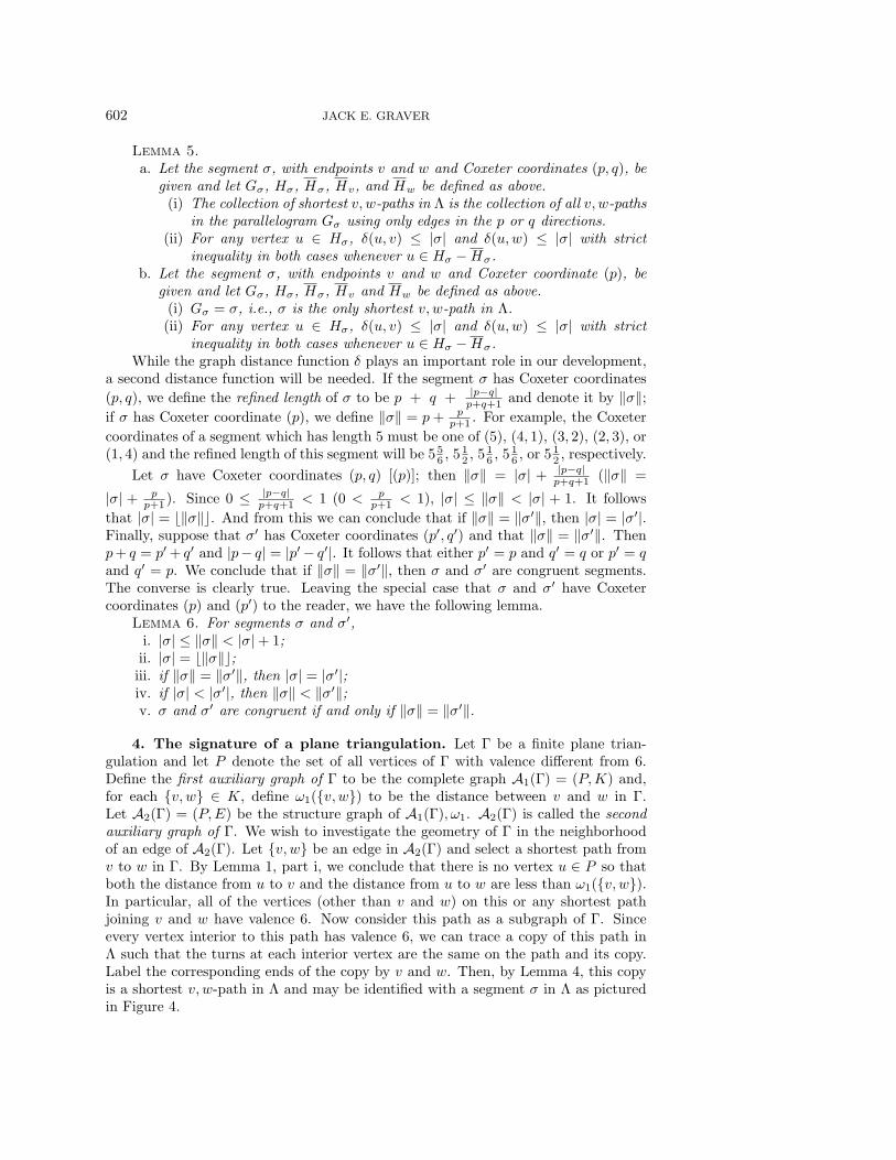
Now construct the hexagonal circuit Hv about v spanned by the vertices at adistance of p + q from v and let Hv denote the finite subgraph of Λ bounded by Hv.Define Hw and Hw similarly. Let Hσ = Hv ∩ Hw and denote its bounding circuitby Hσ. We have pictured the various regions and boundaries of this constructionin Figure 4. In drawing this picture, we have made some assumptions, namely that0 < q < p. If q = p, the picture is the same but with the segment vertical and, ifq > p, the picture is the mirror image of this picture with the p and q labels reversed.Hσ is a hexagon with opposite sides parallel and equal in length. The points v andw are antipodal on this boundary dividing the sides containing them into segmentsof length p and q. If σ has Coxeter coordinate (p), Hσ consists of the union of twoequilateral triangles with the given segment as the common side. In this case, Hσ isa rhombus with sides of length p and may be visualized by letting q = 0 in Figure 4.Some easily checked but useful properties of this configuration are listed in the nextlemma.

602 JACK E. GRAVER

Lemma 5.

a. Let the segment σ, with endpoints v and w and Coxeter coordinates (p, q), begiven and let Gσ, Hσ, Hσ, Hv, and Hw be defined as above.(i) The collection of shortest v, w-paths in Λ is the collection of all v, w-paths

in the parallelogram Gσ using only edges in the p or q directions.(ii) For any vertex u ∈ Hσ, δ(u, v) ≤ |σ| and δ(u,w) ≤ |σ| with strict

inequality in both cases whenever u ∈ Hσ −Hσ.b. Let the segment σ, with endpoints v and w and Coxeter coordinate (p), be

given and let Gσ, Hσ, Hσ, Hv and Hw be defined as above.(i) Gσ = σ, i.e., σ is the only shortest v, w-path in Λ.(ii) For any vertex u ∈ Hσ, δ(u, v) ≤ |σ| and δ(u,w) ≤ |σ| with strict

inequality in both cases whenever u ∈ Hσ −Hσ.While the graph distance function δ plays an important role in our development,

a second distance function will be needed. If the segment σ has Coxeter coordinates

(p, q), we define the refined length of σ to be p + q + |p−q|p+q+1 and denote it by ‖σ‖;

if σ has Coxeter coordinate (p), we define ‖σ‖ = p + pp+1 . For example, the Coxeter

coordinates of a segment which has length 5 must be one of (5), (4, 1), (3, 2), (2, 3), or(1, 4) and the refined length of this segment will be 55

6 , 5 12 , 5 1

6 , 5 16 , or 51

2 , respectively.

Let σ have Coxeter coordinates (p, q) [(p)]; then ‖σ‖ = |σ| + |p−q|p+q+1 (‖σ‖ =

|σ| + pp+1 ). Since 0 ≤ |p−q|

p+q+1 < 1 (0 < pp+1 < 1), |σ| ≤ ‖σ‖ < |σ| + 1. It follows

that |σ| = ‖σ‖. And from this we can conclude that if ‖σ‖ = ‖σ′‖, then |σ| = |σ′|.Finally, suppose that σ′ has Coxeter coordinates (p′, q′) and that ‖σ‖ = ‖σ′‖. Thenp+ q = p′ + q′ and |p− q| = |p′ − q′|. It follows that either p′ = p and q′ = q or p′ = qand q′ = p. We conclude that if ‖σ‖ = ‖σ′‖, then σ and σ′ are congruent segments.The converse is clearly true. Leaving the special case that σ and σ′ have Coxetercoordinates (p) and (p′) to the reader, we have the following lemma.

Lemma 6. For segments σ and σ′,i. |σ| ≤ ‖σ‖ < |σ| + 1;ii. |σ| = ‖σ‖;iii. if ‖σ‖ = ‖σ′‖, then |σ| = |σ′|;iv. if |σ| < |σ′|, then ‖σ‖ < ‖σ′‖;v. σ and σ′ are congruent if and only if ‖σ‖ = ‖σ′‖.

4. The signature of a plane triangulation. Let Γ be a finite plane trian-gulation and let P denote the set of all vertices of Γ with valence different from 6.Define the first auxiliary graph of Γ to be the complete graph A1(Γ) = (P,K) and,for each v, w ∈ K, define ω1(v, w) to be the distance between v and w in Γ.Let A2(Γ) = (P,E) be the structure graph of A1(Γ), ω1. A2(Γ) is called the secondauxiliary graph of Γ. We wish to investigate the geometry of Γ in the neighborhoodof an edge of A2(Γ). Let v, w be an edge in A2(Γ) and select a shortest path fromv to w in Γ. By Lemma 1, part i, we conclude that there is no vertex u ∈ P so thatboth the distance from u to v and the distance from u to w are less than ω1(v, w).In particular, all of the vertices (other than v and w) on this or any shortest pathjoining v and w have valence 6. Now consider this path as a subgraph of Γ. Sinceevery vertex interior to this path has valence 6, we can trace a copy of this path inΛ such that the turns at each interior vertex are the same on the path and its copy.Label the corresponding ends of the copy by v and w. Then, by Lemma 4, this copyis a shortest v, w-path in Λ and may be identified with a segment σ in Λ as picturedin Figure 4.


Now consider the mapping from our path in Γ into Λ. We wish to extend thismapping to as large a region of Γ as is possible. Since both Λ and Γ are triangulations,we can extend this map to all vertices and edges which complete a triangle with oneedge on the path or are adjacent to one vertex interior to the path. We continue toextend the domain of this map outward from the path by including adjacent verticesof degree 6. In view of Lemma 1, part i and Lemma 5, parts a(ii) and b(ii), we seethat this mapping may be extended to a region of Γ which is mapped onto Hσ. Wemay think of the hexagonal region Hσ, pictured in Figure 4, as a region in Γ with theunderstanding that some of the vertices on the boundary may belong to P . We willcall such a region a hexagonal region of Γ and we will use the same notation for thisregion and its various subsets as is used for their images in Λ.

Using this construction, each edge v, w of A2(Γ) may be identified with asegment in a hexagonal region of Γ. However, this identification depends on thechoice of a shortest v, w-path in Γ. If σ is the segment associated with a givenv, w-path, then any of the paths in Gσ will give the same hexagonal region. ButΓ is a finite planar graph and perhaps there is another shortest v, w-path running“around the back.” This can indeed happen, in which case we would have anothersegment σ′ associated with the edge v, w in A2(Γ) and another hexagonal regionHσ′ in Γ with v and w on its boundary. When this occurs we will add anotherv, w-edge to A2(Γ) associated with σ′. Thus A2(Γ), as amended, is a multigraphand we label each edge with the Coxeter coordinates of the segments associated withthat edge. Note, if σ and σ′ are the segment associated with multiple edges, then|σ| = |σ′|.

We may actually draw this amended A2(Γ) on the sphere by superimposing iton the given drawing of Γ: for each edge of A2(Γ), draw in the associated segment σas it appears in Hσ. If these segments do not cross, this will be a planar embeddingof A2(Γ). Unfortunately, some of the edges of this drawing of A2(Γ) may cross. Wesolve this problem by replacing the weight function ω1 with the weight function ω2:for each edge e in A2(Γ), let σe denote its associated segment and let ω2(e) = ‖σe‖.The structure graph of A2(Γ) with weight function ω2 is called the signature graphof Γ and is denoted by S(Γ). We must keep in mind that S(Γ) could actually bea multigraph. However, we will continue to abuse notation and call it simply thesignature graph of Γ. Since S(Γ) is obtained from A2(Γ) by simply deleting someof its edges, S(Γ) inherits a natural drawing in the plane, and conveniently we havedeleted enough edges to eliminate all crossings.

Lemma 7. For a plane triangulation Γ, the drawing of S(Γ) on the sphere de-scribed above is a planar embedding.

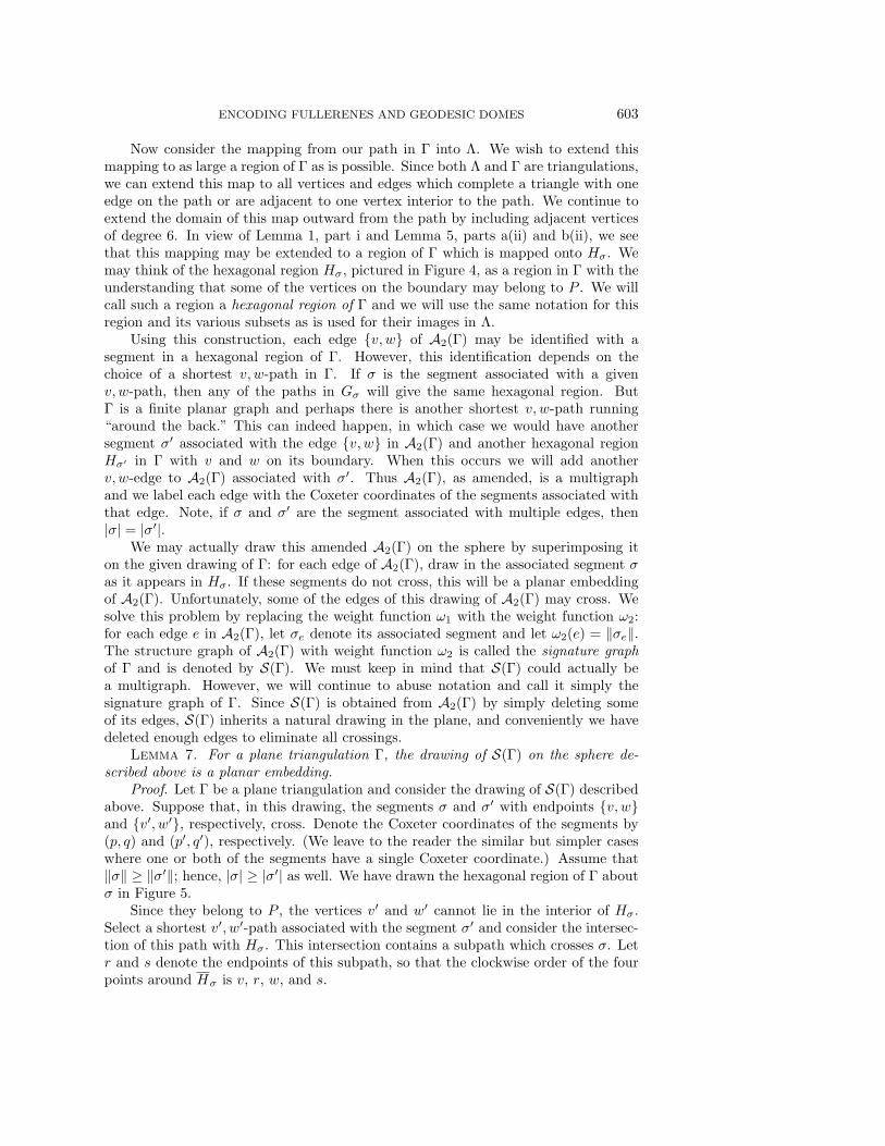
Proof. Let Γ be a plane triangulation and consider the drawing of S(Γ) describedabove. Suppose that, in this drawing, the segments σ and σ′ with endpoints v, wand v′, w′, respectively, cross. Denote the Coxeter coordinates of the segments by(p, q) and (p′, q′), respectively. (We leave to the reader the similar but simpler caseswhere one or both of the segments have a single Coxeter coordinate.) Assume that‖σ‖ ≥ ‖σ′‖; hence, |σ| ≥ |σ′| as well. We have drawn the hexagonal region of Γ aboutσ in Figure 5.

Since they belong to P , the vertices v′ and w′ cannot lie in the interior of Hσ.Select a shortest v′, w′-path associated with the segment σ′ and consider the intersec-tion of this path with Hσ. This intersection contains a subpath which crosses σ. Letr and s denote the endpoints of this subpath, so that the clockwise order of the fourpoints around Hσ is v, r, w, and s.

604 JACK E. GRAVER

v

w

Hσ

Hσ

Fσ

p

pσ

p − qq

q

q

p − q q

q

q

v1

v2

v3 v4 v5

v6

v7v8

Fig. 5.

First, suppose that r lies on the section of the boundary from v3 to w while slies on the boundary from w to v7. In this case, w lies on a shortest r, s-path and,hence, on a shortest v′, w′-path, which is impossible. Likewise, the possibility that rlies between v and v3 while s lies on the boundary from v to v7 can be eliminated.

Next, suppose that r lies on the section of the boundary from v1 to v3 while slies on the boundary from v5 to v7. In this case, |σ| ≥ |σ′| ≥ δ(r, s) ≥ p + q = |σ|and equality must hold throughout. But equality can hold only if v′, w′ = r, s =v1, v7 or v′, w′ = r, s = v3, v5, and both options have already been excluded.

We conclude that one of r and s lies on the top boundary of Hσ and the other onthe bottom boundary of Hσ. Thus we again have |σ| ≥ |σ′| ≥ δ(r, s) ≥ p + q = |σ|,and again equality must hold throughout. Thus v′, w′ = r, s and we are free toassume r = v′ and s = w′.

Note that the segments joining v to v4 and w to v8 are reflections of σ and hencehave the same refined length as σ. Now, if v′ were to lie between v4 and w, we easilysee that the refined lengths from v′ to v and v′ to w are both less than ‖σ‖, violatingLemma 1, part i. If v′ were to lie between v3 and v4, the refined length from v′ tov would be greater than ‖σ‖, and ‖σ′‖ would be even larger, violating our originalassumption. All that remains is the case where v′ lies between v1 and v while w′ liesbetween w and v5. Again one can easily see that, in this case, ‖σ′‖ > ‖σ‖, violatingour original assumption.

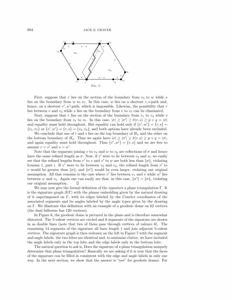
We may now give the formal definition of the signature a plane triangulation Γ. Itis the signature graph S(Γ) with the planar embedding given by the natural drawingof it superimposed on Γ, with its edges labeled by the Coxeter coordinates of theassociated segments and its angles labeled by the angle types given by the drawingon Γ. We illustrate this definition with an example of a geodesic dome on 62 vertices(the dual fullerene has 120 vertices).

In Figure 6, the geodesic dome is pictured in the plane and is therefore somewhatdistorted. The 5-valent vertices are circled and 6 segments of the signature are drawnin as double lines (note that two of them pass through vertices of valence 6). Theremaining 14 segments of the signature all have length 1 and join adjacent 5-valentvertices. The signature graph is then redrawn on the left in Figure 7 with the segmentand angle labels: the two lobes are identical and, to minimize clutter, we have includedthe angle labels only in the top lobe and the edge labels only in the bottom lobe.

The natural question to ask is, Does the signature of a plane triangulation uniquelydetermine that plane triangulation? Basically we are asking if it is true that the facesof the signature can be filled in consistent with the edge and angle labels in only oneway. In the next section, we show that the answer is “yes” for geodesic domes. For


!!!!!

"""""

###

Fig. 6.

!!!!

""""

!!!!

""""

1

02 2

32

32

32

32

1 1

1 11 1

4 2 4

(2,4) (4,2)

(2,1) (1,2)

(1)

(1)←→(1) (1)

(1) (1)

1

02 2

a b

c d

e

f

g

h

i

j

a

b

c

d

e

f

g h

i j

Fig. 7.

now, we simply continue with this example. On the right in Figure 7, we have drawnthe faces of the signature in Λ with several of the segments identified. To build athree-dimensional model of Γ, simply cut along the unidentified segments and makethe identifications indicated by the vertex labels.

5. The signature of a fullerene. The first part of the problem posed in thelast section is to rebuild a plane triangulation from its signature. This boils down tofilling in each face of the signature with a region from Λ that is consistent with thesegment and angle labels of that face. The second part of the problem is to showthat this can be done in only one way. The natural approach to filling in the facesis to select a face of the signature and then simply reconstruct its boundary in Λ

606 JACK E. GRAVER

as prescribed by its segment and angle labels: denote the segments by σ1, . . . , σk inclockwise order around the face; draw a segment σ′

1 in Λ congruent to σ1; draw in asegment σ′

2 congruent to σ2 sharing an endpoint so that the angles between σ1 andσ2 and σ′

1 and σ′2 have the same type; and so on. Ultimately this is precisely what

we will do; but at the outset it is not even clear that this “dead reckoning” approachwill result in a closed polygonal region of Λ. To aid in our investigation we introducesome additional notation. Following Brinkmann, Friedrichs, and Nathusius [1], wedefine an (m,k)-patch to be a plane graph such that

• all faces are k-gons, except for one n-gon,• the boundary of the n-gon is an elementary circuit and is called the boundary

of the patch,• all vertices not on the boundary have valence m while those on the boundary

have valence at most m.For a simple example of a (6,3)-patch, consider any region of Λ bounded by an elemen-tary circuit. For a more complicated example, consider a long narrow region whichcurves around and overlaps itself. For the (6,3)-patch, we consider the overlappingportions of the region to be distinct. Now let Γ be a geodesic dome and consider aface of S(Γ). Replace each segment σ in the boundary of this face by a shortest pathjoining its endpoints that lies in Gσ. If the angle between consecutive segments σ andσ′ is small, Gσ and Gσ′ may overlap. In this case, we select the paths in Gσ ∪Gσ′ sothat they do not intersect. Next, label the vertices and edges on these paths clock-wise around the face; vertices and edges which lie on paths corresponding to segmentsthat bound the face on two sides are labeled twice, once from each side. Consideringdoubly labeled vertices and edges as two distinct vertices or edges, we have associateda (6,3)-patch with the given face.

By a drawing of a (6,3)-patch, ∆, in Λ, we mean a graph homomorphism from∆ into Λ such that distinct triangular faces sharing a common edge are mapped ontodistinct triangular faces sharing a common edge. Up to an automorphism of Λ, a given(6,3)-patch has a unique drawing in Λ: select any triangular face of ∆ and map intoΛ; this mapping extends uniquely to its neighboring triangular faces and then to theirneighbors, etc., until the entire patch is drawn. Let ∆ be a (6,3)-patch with boundaryΩ and let v0, . . . , vn−1, vn = v0 be the vertices of Ω in cyclic order around the patch.The cyclic sequence of valences ρ(v0), . . . , ρ(vn−1, ρ(vn) = ρ(v0) is called the boundarycode for Ω. Note that, by the definition of (m, k)-patch, 2 ≤ ρ(vi) ≤ 6, for eachi = 1, . . . , n. Given the boundary code of ∆, we may inductively draw this boundaryin Λ: in Λ, select any two adjacent vertices v′0 and v′1 to be the images of v0 and v1;once the edge v′i−1, v

′i has been drawn, let v′i+1 be the ρ(vi)th vertex adjacent to

v′i counting counterclockwise starting with v′i−1 and draw in v′i, v′i+1. At each step,the drawing of this circuit must match with the boundary of the appropriate drawingof the entire patch ∆. Thus, the drawing of Ω in Λ is unique up to an automorphismof Λ and depends only on the boundary code for Ω.

Now let ∆ be a (6,3)-patch associated with a face of the signature of a geodesicdome Γ, as constructed above, and draw its boundary in Λ. The image of the boundarymay then be partitioned into paths corresponding to the segments in S(Γ) from whichthey came. Clearly, the endpoints of each such path define a segment in Λ with thesame Coxeter coordinates its corresponding segment in S(Γ). Replacing these pathsby segments in Λ, results in a (perhaps overlapping) polygonal region of Λ boundedby segments corresponding to the segments bounding the given face. Furthermore,the angle labels match. We have proved the following lemma.


Lemma 8. Up to an automorphism of Λ, the polygonal boundary of the faceof the signature of a plane triangulation has a unique drawing in Λ with the samesequence of Coxeter coordinates and angle types.

The next question is, Is the polygonal region of a face of the signature of ageodesic dome uniquely determined by its boundary? X. Guo, P. Hansen, and M.Zheng [8] constructed two distinct (3, 6)-patches with the same boundary sequenceand his example is easily altered to produce two distinct (6, 3)-patches with the sameboundary. We say that a boundary sequence is ambiguous if there exist two distinct(6, 3)-patches with the same boundary sequence. We say that the face of the signatureof a plane triangulation is ambiguous if there exist two distinct polygonal regions withthe boundary of that face. The next lemma follows at once from Lemma 8.

Lemma 9. A geodesic dome with a signature that admits no ambiguous faces isuniquely determined by its signature.

If the drawing of the boundary of a (6,3)-patch is an elementary circuit, then itsinterior is uniquely determined and the patch is not ambiguous. Hence the drawingof an ambiguous (6,3)-patch in Λ must be self-overlapping. The drawings of faces oftriangulations with vertices of valence more than 6 may well be self-overlapping andpossibly ambiguous. In the remainder of this section, we sketch the proof that a faceof the signature of a geodesic dome cannot yield a self-overlapping region when drawnin Λ thereby verifying:

Theorem 1. A geodesic dome is uniquely determined by its signature.The basic idea is that a face of the signature of a geodesic dome cannot curve

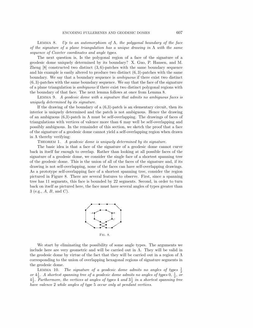
back in itself far enough to overlap. Rather than looking at all possible faces of thesignature of a geodesic dome, we consider the single face of a shortest spanning treeof the geodesic dome. This is the union of all of the faces of the signature and, if itsdrawing is not self-overlapping, none of the faces can have self-overlapping drawings.As a prototype self-overlapping face of a shortest spanning tree, consider the regionpictured in Figure 8. There are several features to observe. First, since a spanningtree has 11 segments, this face is bounded by 22 segments. Second, in order to turnback on itself as pictured here, the face must have several angles of types greater than3 (e.g., A, B, and C).

$$$

A B

C

Fig. 8.

We start by eliminating the possibility of some angle types. The arguments weinclude here are very geometric and will be carried out in Λ. They will be valid inthe geodesic dome by virtue of the fact that they will be carried out in a region of Λcorresponding to the union of overlapping hexagonal regions of signature segments inthe geodesic dome.

Lemma 10. The signature of a geodesic dome admits no angles of types 12

or 4 12 . A shortest spanning tree of a geodesic dome admits no angles of types 0, 1

2 , or4 1

2 . Furthermore, the vertices at angles of types 4 and 3 12 in a shortest spanning tree

have valence 2 while angles of type 5 occur only at pendant vertices.

608 JACK E. GRAVER

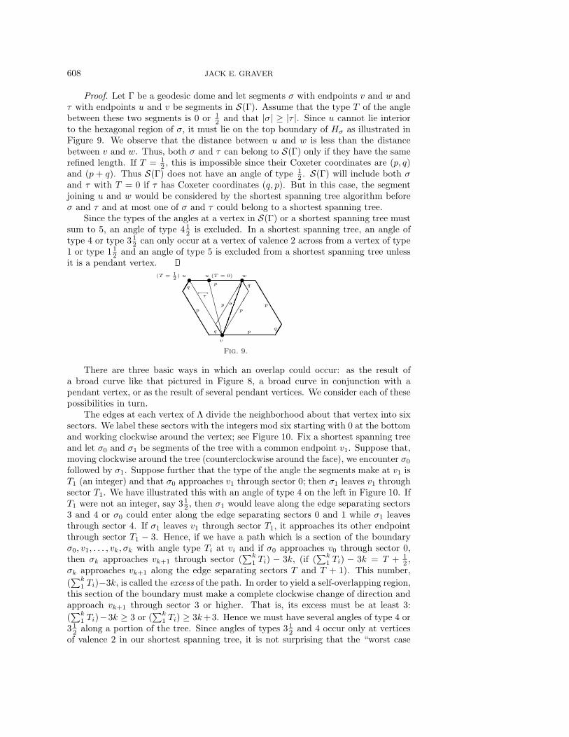
Proof. Let Γ be a geodesic dome and let segments σ with endpoints v and w andτ with endpoints u and v be segments in S(Γ). Assume that the type T of the anglebetween these two segments is 0 or 1

2 and that |σ| ≥ |τ |. Since u cannot lie interiorto the hexagonal region of σ, it must lie on the top boundary of Hσ as illustrated inFigure 9. We observe that the distance between u and w is less than the distancebetween v and w. Thus, both σ and τ can belong to S(Γ) only if they have the samerefined length. If T = 1

2 , this is impossible since their Coxeter coordinates are (p, q)and (p + q). Thus S(Γ) does not have an angle of type 1

2 . S(Γ) will include both σand τ with T = 0 if τ has Coxeter coordinates (q, p). But in this case, the segmentjoining u and w would be considered by the shortest spanning tree algorithm beforeσ and τ and at most one of σ and τ could belong to a shortest spanning tree.

Since the types of the angles at a vertex in S(Γ) or a shortest spanning tree mustsum to 5, an angle of type 41

2 is excluded. In a shortest spanning tree, an angle oftype 4 or type 31

2 can only occur at a vertex of valence 2 across from a vertex of type1 or type 11

2 and an angle of type 5 is excluded from a shortest spanning tree unlessit is a pendant vertex.

p pp p

v

w

σ

p

q

q

p

q

q

(T = 12) u u (T = 0)

τ←→

Fig. 9.

There are three basic ways in which an overlap could occur: as the result ofa broad curve like that pictured in Figure 8, a broad curve in conjunction with apendant vertex, or as the result of several pendant vertices. We consider each of thesepossibilities in turn.

The edges at each vertex of Λ divide the neighborhood about that vertex into sixsectors. We label these sectors with the integers mod six starting with 0 at the bottomand working clockwise around the vertex; see Figure 10. Fix a shortest spanning treeand let σ0 and σ1 be segments of the tree with a common endpoint v1. Suppose that,moving clockwise around the tree (counterclockwise around the face), we encounter σ0

followed by σ1. Suppose further that the type of the angle the segments make at v1 isT1 (an integer) and that σ0 approaches v1 through sector 0; then σ1 leaves v1 throughsector T1. We have illustrated this with an angle of type 4 on the left in Figure 10. IfT1 were not an integer, say 3 1

2 , then σ1 would leave along the edge separating sectors3 and 4 or σ0 could enter along the edge separating sectors 0 and 1 while σ1 leavesthrough sector 4. If σ1 leaves v1 through sector T1, it approaches its other endpointthrough sector T1 − 3. Hence, if we have a path which is a section of the boundaryσ0, v1, . . . , vk, σk with angle type Ti at vi and if σ0 approaches v0 through sector 0,then σk approaches vk+1 through sector (

∑k1 Ti) − 3k, (if (

∑k1 Ti) − 3k = T + 1

2 ,σk approaches vk+1 along the edge separating sectors T and T + 1). This number,

(∑k

1 Ti)−3k, is called the excess of the path. In order to yield a self-overlapping region,this section of the boundary must make a complete clockwise change of direction andapproach vk+1 through sector 3 or higher. That is, its excess must be at least 3:

(∑k

1 Ti)−3k ≥ 3 or (∑k

1 Ti) ≥ 3k+3. Hence we must have several angles of type 4 or3 1

2 along a portion of the tree. Since angles of types 312 and 4 occur only at vertices

of valence 2 in our shortest spanning tree, it is not surprising that the “worst case


%

%

0

1

2

3

4

5

v0

σ0

σ1

←− FACE −→

0

1

2

3

4

5

vi

σi

σi−1

Fig. 10.

scenario” is that our shortest spanning tree is a simple path. So think of a subpath ofour tree along which the angles have types 4, 31

2 , and 3. We investigate this subpathby considering the angles on the other side of the path.

We are interested in constructing a path in our shortest spanning tree of length kso that the sum of the types of the angles along this path is at most 5k − (3k + 3) =2k−3. In Figure 11, we have drawn an angle of type 1 at vertex v0. Around the vertexv−1, we have constructed a hexagon; any vertex in this hexagon has its distance tov−1 less than |σ0|. Thus v1 is outside (or on) the hexagon; were it inside, the segmentjoining v−1 to v1 would have been selected in place of σ0 or σ1 when constructingthe shortest spanning tree. If the next segment, σ2 (from v1 to v2), were to make anangle of type 1, it would either (1) force v2 to lie in the hexagon; (2) force σ2 to be solong that it completely crosses the hexagon; (3) force σ2 to be so short that it neverintersects the hexagon. In the first case, we have the previous contradiction. In thesecond case, v2 is closer to v−1 than to v1, resulting in another contradiction. Thethird case is impossible since v2 must lie outside the corresponding hexagon aroundv1. The same argument will exclude an angle of type 11

2 . Thus, the angle at v1 isof type at least 2. At this point we note that the angle at v0 would be of type 11

2if σ1 were horizontal. And the above arguments would still preclude the angle at v1

being of type 1. However, two successive angles of type 1 12 are possible. We continue

considering the case of angles of integer type and simply note that our arguments canbe adapted to the cases involving angles of fractional type.

v−1

v0

v1

FACE

σ0

σ1

Fig. 11.

In Figure 12, we have added σ2 with an angle of type 2 at v1 and σ3 with anangle of type 2 at v2. Neither of these aid in our goal of a path with type sum 2k− 3.It would seem that the only way to make a sharp, type 1 turn to the left is to firstpull away from the hexagon and then turn toward it but not into it. To pull away,we could include a type 3 angle; but this would nullify the initial type 1 angle inthe sum. The only other option is to make a segment like σ3 much longer than theside of the hexagon. However, this won’t work either. For example, the distancebetween v3 and v−1 must be as long or longer than |σ0|, |σ1|, |σ2|, and |σ3|; otherwise

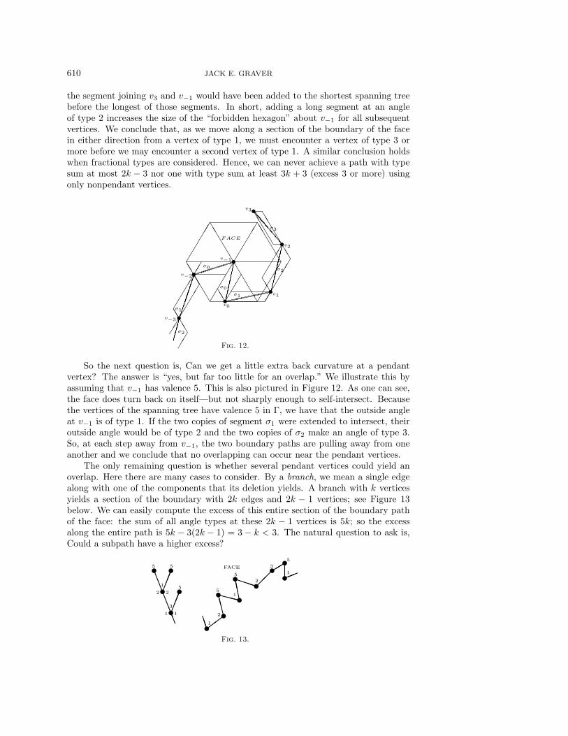
610 JACK E. GRAVER

the segment joining v3 and v−1 would have been added to the shortest spanning treebefore the longest of those segments. In short, adding a long segment at an angleof type 2 increases the size of the “forbidden hexagon” about v−1 for all subsequentvertices. We conclude that, as we move along a section of the boundary of the facein either direction from a vertex of type 1, we must encounter a vertex of type 3 ormore before we may encounter a second vertex of type 1. A similar conclusion holdswhen fractional types are considered. Hence, we can never achieve a path with typesum at most 2k − 3 nor one with type sum at least 3k + 3 (excess 3 or more) usingonly nonpendant vertices.

v−1

v0

v1

FACE

σ0

σ1

v2

σ2

v3

σ3

v−2

v−3

σ0

σ1

σ2

Fig. 12.

So the next question is, Can we get a little extra back curvature at a pendantvertex? The answer is “yes, but far too little for an overlap.” We illustrate this byassuming that v−1 has valence 5. This is also pictured in Figure 12. As one can see,the face does turn back on itself—but not sharply enough to self-intersect. Becausethe vertices of the spanning tree have valence 5 in Γ, we have that the outside angleat v−1 is of type 1. If the two copies of segment σ1 were extended to intersect, theiroutside angle would be of type 2 and the two copies of σ2 make an angle of type 3.So, at each step away from v−1, the two boundary paths are pulling away from oneanother and we conclude that no overlapping can occur near the pendant vertices.

The only remaining question is whether several pendant vertices could yield anoverlap. Here there are many cases to consider. By a branch, we mean a single edgealong with one of the components that its deletion yields. A branch with k verticesyields a section of the boundary with 2k edges and 2k − 1 vertices; see Figure 13below. We can easily compute the excess of this entire section of the boundary pathof the face: the sum of all angle types at these 2k − 1 vertices is 5k; so the excessalong the entire path is 5k − 3(2k − 1) = 3 − k < 3. The natural question to ask is,Could a subpath have a higher excess?

5 5

2

1

2

3

5

1 1

1

2

51

5

2

FACE 3

5

1

Fig. 13.


Among all possible subpaths of the face boundaries of branches, consider thosewith largest possible excess. Suppose that v is a pendant vertex of the branch andis interior to the subpath of the face boundary. Let T, 5, T ′ be the angle types ofthe three vertices on the subpath centered at v. These three vertices contributeT +5+T ′ − 9 = T +T ′ − 4 to the excess of the path. Now delete this pendant vertexfrom the branch and adjust the subpath accordingly. The three vertices are replacedby a single vertex of type T +T ′ which contributes T +T ′−3 to the excess. Thus thesmaller branch has a subpath with a larger excess. We have carried out this reductionon the branch in Figure 13 and recorded the result in Figure 14. We conclude thatthe branches with a subpath having a largest possible excess have just two pendantvertices and that the subpath with largest possible excess runs from one pendantvertex to the other. Checking our examples, we see that the subpath in Figure 13between the extreme pendant vertices has an excess of 3 while the correspondingsubpath in Figure 14 has an excess of 4.

5

52 3

3

1 1

1

2

5

FACE

33 5

1

Fig. 14.

As we have noted the sum of the angle types along the entire path around abranch with k vertices is 5k. Assume that we have a branch with just two pendantvertices. To make the excess of the subpath that runs from one pendant vertex to theother as large as is possible, we should make the sum of the types along the outsideof paths from the trivalent vertex to the pendant vertices as small as possible. Aswe have already shown, the sum of the types along such a path will be as small as ispossible when we have one angle of type 1 (or two of type 11

2 ) and the rest of type 2.This smallest sum is then 2(k − 2). So the sum of the angle types along the subpathjoining the two pendant vertices is 5k − 2(k − 2) = 3k + 4 and its excess is 4.

Finally, we note that a pendant vertex gives rise to two sides of an equilateraltriangle along the face boundary. If we add the triangle to the face replacing the twoedges by the third side of the triangle, we get a region of Λ that contains the face.We note further that making this substitution in the subpath results in decreasingthe excess by 1. Carrying out this reduction throughout the entire face results in aregion containing the face which has the property that no subpath of the boundaryhas excess 3 or more and hence is nonoverlapping. Hence the face is nonoverlapping.

6. Using the signature. It follows from Theorem 1 that the signature S(Γ)of a geodesic dome carries complete information about the geodesic dome Γ and itsfullerene dual. It would be convenient if we could read some of this information di-rectly from S(Γ). In An Atlas of Fullerenes [6], Fowler and Manolopoulos indicate thatwhether or not pentagonal faces are adjacent is an important feature of a fullerene.Clearly, the relative positions of the pentagonal faces can be read directly from itssignature. Another feature of a geodesic dome/fullerene that can be easily deducedfrom its signature is its symmetry structure.

Let the geodesic dome Γ be given. Any automorphism α of Γ must permute the5-valent vertices, and hence it induces a permutation of the vertices of A1(Γ) which wealso denote by α. Since α preserves distance, it is an automorphism of the weighted

612 JACK E. GRAVER

graph A1(Γ), ω1. It must then map spanning trees of A1(Γ) onto spanning trees ofA1(Γ). It follows that α must map A2(Γ), the structure graph of A1(Γ), onto itself.Suppose that v and w are vertices in P joined by the segment σ in A2(Γ). Clearly, αmaps the hexagonal region of Γ determined by v and w onto the hexagonal region ofΓ determined by α(v) and α(w). Thus α(σ) is congruent to σ and α preserves refinedlength.

Applying the above arguments to A2(Γ), ω2, we conclude that α induces an au-tomorphism of its structure graph, namely S(Γ). Furthermore, if the original α is anorientation preserving automorphism of Γ, the induced α is an orientation preserv-ing automorphism of S(Γ) that maps segments onto segments with the same Coxetercoordinates and, if the original α is an orientation reversing automorphism of Γ, theinduced α is an orientation reversing automorphism of S(Γ) that maps segments ontosegments with reversed Coxeter coordinates. In both cases α preserves angle types.Thus we are led to define an automorphism of a signature to be an automorphism ofthe signature graph (as a plane graph) that preserves angle types and preserves orreverses the Coxeter coordinates of the edges, according to whether it is orientationpreserving or orientation reversing.

Now suppose that α is an automorphism of the signature of Γ. Since the edgeand angle labels around a face determine a unique region of Λ up to an automorphismof Λ, α has a natural extension to an automorphism of Γ. Thus this mapping of theautomorphism group of Γ into the automorphism group of its signature is onto. Is itone-to-one? Surprisingly, the answer is “not always.” We explore these exceptionalcases next.

Let α and β be automorphisms of Γ which induce the same automorphism on itssignature. Since Γ is a triangulation of the plane, two automorphisms which agree ona single triangular face agree everywhere. Let v and w be any two vertices in P joinedby an edge in the signature. Then α and β map the hexagonal region determinedby v and w onto the hexagonal region determined by α(v) = β(v) and α(w) = β(w).If they agree on this hexagonal region, they would agree everywhere. Hence thehexagonal region must be symmetric and the two images of the v, w-hexagonal regionmust be reflections of one another. This is only possible if the edge is of type (p)or (p, p). Next, suppose that u, v, and w are the vertices of a path of length two inthe signature. Since the image of this path must be invariant under reflection, v hasvalence two in S(Γ) and the angles at v are both of type ρ

2 , where ρ is the valenceof v in Γ. It follows that S(Γ) is either a path or a circuit, that its edge labels areof the forms (p) and (p, p) and that the angle types are equal at each vertex. If Γis a plane triangulation with such a signature, one easily sees that both the identityand the reflection through the line or circuit of its signature induce the identity onits signature. An example of such a geodesic dome is worked out at the end of thissection. We have proved the following theorem.

Theorem 2. Let Γ be a plane triangulation.i. If S(Γ) is not a path or circuit with the special labeling described above, then

its automorphism group and the automorphism group of its signature are iso-morphic.

ii. If S(Γ) is a path or circuit with the special labeling described above, then itsautomorphism group is isomorphic to the direct product of the automorphismgroup of its signature and the reflection through its signature.

The next question we tackle is, How can we compute the number of vertices, edgesand faces of a plane triangulation from its signature? To answer this question, consider


a polygonal region with vertices v0, v1, . . . , vn in counterclockwise order around theregion. Fix the coordinate system with v0 at the origin, with the horizontal edge tothe right at v0 as the unit vector in the x direction and the next edge counterclockwiseas the unit vector in the y direction. The x, y-coordinates of the segment directedfrom the point v to the point w is simply the coordinates of w minus the coordinates ofv. It should be clear that the x, y-coordinates of a segment can be computed directlyfrom its orientation and its Coxeter coordinates. Returning to our polygonal region,the orientations of the bounding segments are determined, in order, by the orientationof the previous segment and the type of the angle between them. For i = 1, . . . , n,let (xi, yi) denote the x, y-coordinates of the segment joining vi−1 and vi. It follows

that the coordinates of the vertex vi are (xi, yi) = (∑i

j=1 xj ,∑i

j=1 yj). The standard

formula for the area of such a polygonal region is 12

∑1≤i<n(xiyi+1 − xi+1yi). Note

that a unit square in the x, y coordinate system consist of two lattice triangles andthus the area of the region is equal to the area of

∑1≤i<n(xiyi+1 − xi+1yi) lattice

triangles. Finally, substituting the x, y values for x, y in this formula gives the area,in lattice triangles, as

∑

1≤i<j≤n

(xiyj − xjyi).

Using this formula, we compute the area of each face of the signature of a planetriangulation Γ. The sum t of these areas will then be the number of the triangles orfaces of Γ and the numbers of edges and vertices will be given by the formulas e = 3t

2and v = t+4

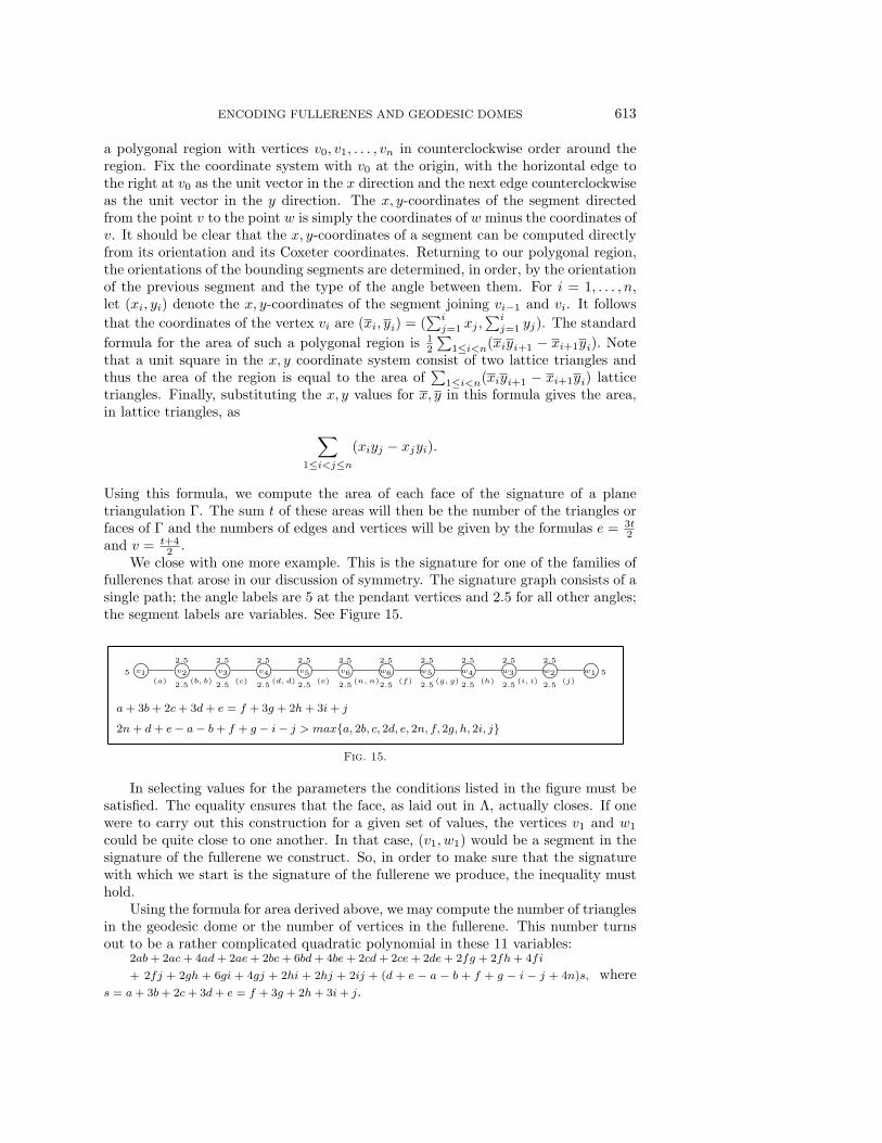
2 .We close with one more example. This is the signature for one of the families of

fullerenes that arose in our discussion of symmetry. The signature graph consists of asingle path; the angle labels are 5 at the pendant vertices and 2.5 for all other angles;the segment labels are variables. See Figure 15.

v1 v2 v3 v4 v5 v6 w6 w5 w4 w3 w2 w15 5

2.5 2.5 2.5 2.5 2.5 2.5 2.5 2.5 2.5 2.5

2.5 2.5 2.5 2.5 2.5 2.5 2.5 2.5 2.5 2.5(a) (b, b) (c) (d, d) (e) (n, n) (f) (g, g) (h) (i, i) (j)

a + 3b + 2c + 3d + e = f + 3g + 2h + 3i + j

2n + d + e− a− b + f + g − i− j > maxa, 2b, c, 2d, e, 2n, f, 2g, h, 2i, j

Fig. 15.

In selecting values for the parameters the conditions listed in the figure must besatisfied. The equality ensures that the face, as laid out in Λ, actually closes. If onewere to carry out this construction for a given set of values, the vertices v1 and w1

could be quite close to one another. In that case, (v1, w1) would be a segment in thesignature of the fullerene we construct. So, in order to make sure that the signaturewith which we start is the signature of the fullerene we produce, the inequality musthold.

Using the formula for area derived above, we may compute the number of trianglesin the geodesic dome or the number of vertices in the fullerene. This number turnsout to be a rather complicated quadratic polynomial in these 11 variables:

2ab + 2ac + 4ad + 2ae + 2bc + 6bd + 4be + 2cd + 2ce + 2de + 2fg + 2fh + 4fi

+ 2fj + 2gh + 6gi + 4gj + 2hi + 2hj + 2ij + (d + e − a − b + f + g − i − j + 4n)s, wheres = a + 3b + 2c + 3d + e = f + 3g + 2h + 3i + j.

614 JACK E. GRAVER

One final observation: The fullerenes in this family are nanotubes. Select anyfullerene in this family, i.e., select values for the parameters that satisfy the equalityand the inequality and note that n can be increased without limit while keeping theremaining parameters fixed. In general, a nanotube will have a signature containingan edge cut set consisting of congruent segments that partition the vertices into twoclasses of six vertices each and have a parameter that may be enlarged independentof all other parameters. Our first example, pictured in Figures 6 and 7, is also ananotube. The cut set consists of the double edges connecting the vertices labeled eand f in the right-hand picture of Figure 7. Replace their Coxeter coordinates with(n, 4) and (4, n); increasing n beyond 2 simply moves the top configuration (verticesa through e) up and to the right along the line of the tessellation.

REFERENCES

[1] G. Brinkmann, O. D. Friedrichs, and U. V. Nathusius, Numbers of faces and boundary encod-ings of patches, to appear in Graphs and Discovery, Proceedings of the DIMACS Workshopon Computer-Generated Conjectures from Graph Theoretic and Chemical Databases.

[2] D. L. D. Caspar and A. Klug, Physical principles in the construction of regular viruses, ColdSpring Harbor Symp. Quant. Biol., 27 (1962), pp. 1–24.

[3] H. S. M. Coxeter, Virus macromolecules and geodesic domes, in A Spectrum of Mathematics,J. C. Butcher, ed., Oxford University Press, Oxford, UK, 1971, pp. 98–107.

[4] P. W. Fowler, J. E. Cremona, and J. I. Steer, Systematics of bonding in non-icosahedralcarbon clusters, Theor. Chim. Acta, 73 (1988), pp. 1–26.

[5] P. W. Fowler and J. E. Cremona, Fullerenes containing fused triples of pentagonal rings, J.Chem. Soc., Faraday Trans., 93 (1997), pp. 2255–2262.

[6] P. W. Fowler and D. E. Manolopoulos, An Atlas of Fullerenes, Clarenden Press, Oxford,UK, 1995.

[7] M. Goldberg, A class of multi-symmetric polyhedra, Tohoku Math. J., 43 (1937), pp. 104–108.[8] X. Guo, P. Hansen, and M. Zheng, Boundary Uniqueness of Fusenes, Tech. report G-99-37,

GERAD, Montreal, Quebec, Canada, 1999.

Documents

encoding fullerenes and geodesic domes - Syracuse University