Enabling Healthcare Delivery Through Vehicle Maintenance

Li ChenSamuel Curtis Johnson Graduate School of Management, Cornell University, Ithaca, NY 14853, li.chen@cornell.edu

Sang-Hyun KimYale School of Management, Yale University, New Haven, CT 06520, sang.kim@yale.edu

Hau L. LeeGraduate School of Business, Stanford University, Stanford, CA 94305, haulee@stanford.edu

Difficulties in healthcare delivery in developing economies arise from poor road infrastructure of rural com-

munities, where the bulk of the population reside. Although motorcycles are an effective means for delivering

healthcare products, governments in developing economies lack expertise in providing proper maintenance

and support services, resulting in frequent vehicle breakdowns. Riders for Health, a nonprofit social enter-

prise, has developed specialized capabilities that enable significant enhancements in vehicle maintenance. The

organization has engaged with the governments and provided its services using different contract schemes,

with different performance outcomes in vehicle availability and costs. In this paper we develop an analytical

model based on reliability theory to compare the outcomes of these contracts, and relate the findings to data

collected from a 2.5-year implementation by Riders for Health in Zambia. We also study how different ele-

ments of operational enhancements impact vehicle availability, and identify the conditions under which their

interactions give rise to compromised performance. Interestingly, we find that prevention of minor failures,

i.e., failures that can be addressed through vehicle repairs, always increases vehicle availability unlike other

enhancements. This unambiguous benefit suggests that such basic tasks as following proper maintenance

protocols and stocking the right amount of the right service parts are of utmost importance.

Key words : Public Healthcare, Developing Economies, Social Responsibility, Reliability Theory

History : August 30, 2016

1. Introduction

Populations in developing economies face big challenges in their living standards. Besides poor

economic conditions, healthcare provisions are often grossly inefficient or simply lacking, leading

to low life expectancy. Such is the case of Sub-Saharan Africa, where the average life expectancy

for men and women was reported to be about 53 years, compared to 78 years in the United States

(World Health Organization 2013). The fraction of the population infected by diseases such as

HIV/AIDS, malaria, measles, pneumonia, tuberculosis, and dehydrating diarrhea were much higher

than that of the rest of the world (Lee et al. 2013). Maternal mortality rate exceeded 500 per

100,000 live births (Hogan et al. 2010). Despite the enormous needs, health provisions have been

dismal, contributed by the fact that the majority of the population reside in rural areas where

logistics infrastructures are inadequate or nonexistent.

1

2

The United Nations (2014) reports that 60 percent of Africans lived in rural communities, defined

to be the ones without adequate infrastructure (e.g., paved roads, electricity, piped water or sew-

ers), education, or health services. Yet, 53 percent of the roads in Africa were unpaved (African

Development Bank 2014). As a result, many communities are accessible only by single-lane sand

or dirt paths. People requiring medical care are often forced to walk or be carried in a wheelbarrow

pushed by a relative in order to get to the nearest clinic, as doctors and nurses are unable to visit

such communities on a regular basis.

Well-maintained vehicles and motorcycles have therefore become a crucial missing link in the

healthcare delivery supply chain. In fact, given the poor road infrastructure, motorcycles are often

the most effective means of transport that allow health workers to visit sick patients and deliver

healthcare products such as medicines, test samples and results, education kits, condoms, and

malaria nets. Running a cost-effective operation of a vehicle fleet consisting of well-maintained and

reliable motorcycles requires specialized expertise and management control. Unfortunately, health

ministries of developing economies do not always possess these skills. This is why a social enterprise

(SE) with such capabilities can make a difference, as it supplements the health ministries’ efforts

in this endeavor and offers improvements. However, because the goals of an SE and a government

agency are not exactly aligned, the effectiveness of such a joint effort depends on the structure of

the contract established between the two parties. This is the subject of our study.

Our work is motivated by an SE named Riders for Health (Riders), a nonprofit organization set

up to provide African health ministries with cost-effective operations of consistently reliable vehicle

fleets used for healthcare deliveries. Before Riders’ involvement, the vehicles were managed by

local governments. Vehicles suffered from high operating costs and low availability due to a variety

of inefficiencies, such as lack of training and expertise, inconsistent maintenance procedures, and

shortages of service parts. With poor maintenance, vehicles needed repairs often, or they simply

stopped working. With poor repair skills and shortages of service parts, it took excessive amount

of time to repair or replace vehicles, leading to low vehicle availability.

Riders addressed these issues in multiple ways. The backgrounds of Riders’ cofounders were

instrumental, as they were a group of professional motorcycle racers with deep knowledge of the

operating characteristics of motorcycles. They were able to transform such knowledge into mainte-

nance and repair procedures, which were then passed onto technicians. They trained health workers

to perform simple self-maintenance procedures. They also set up an elaborate hub-and-spoke ser-

vice parts management system to ensure that service parts are supplied and replenished quickly

when needed. Armed with these innovations, the organization worked with health ministries of the

Zimbabwean, Gambian, and Zambian governments and produced very positive results: increased

3

vehicle availability, extended vehicle life, improved health access and interventions, and enhanced

cost effectiveness (Tayan 2007, Mehta et al. 2016).

Despite the success, Riders faced important decisions in its work that raised interesting research

questions. When Riders engaged with local governments, it employed two different contracting

approaches. An approach called Transport Resource Management, which we refer to as Repair

Only Contract (ROC) in this paper, was the basis of standard outsourcing arrangements used in

most of earlier implementations in Zimbabwe and Gambia. Under ROC, Riders is responsible for

maintenance and repair of vehicles (and other maintenance-related tasks such as worker train-

ing), while the government controls vehicle replacements and purchases. A newer approach called

Transport Asset Management, which we refer to as Repair and Replacement Contract (RRC) in

this paper, was more prominently used in a later implementation in Gambia and Zambia, and

it became Riders’ preferred choice. Under RRC, in addition to the same maintenance and repair

tasks as under ROC, Riders is also responsible for vehicle replacements and purchases. The running

costs of this added responsibility can be spread over time and be reimbursed by health ministries

in multiple payment installments. The main benefit of RRC for Riders is that vehicles can be

replaced at time intervals deemed optimal by Riders. Another benefit is that RRC allows Riders

to standardize vehicle models, enabling streamlined fleet management and reduction of complexity

in the overall supply chain. Both ROC and RRC are performance-based contracts, as Riders are

compensated based on the actual mileage used; no payment is made for the duration of vehicle

downtime. Hence, successful implementations of the two contracting approaches depend on the

level of vehicle availability that Riders can provide through its share of fleet operation.

Why does Riders prefer RRC, which actually involves added work and challenges? It is not

easy to secure necessary funding for purchasing a fleet and pay for the setup, and doing so often

requires a long-term contractual commitment from the governments, who might be reluctant to

agree to such an arrangement. For example, financing for the RRC fleet in Gambia involved a

pioneering arrangement among Riders, Africa-based GT Bank, US-based Skoll Foundation, and

the Gambian Ministry of Health. (This is in contrast to ROC, under which the government is

free to switch on and off the services provided by Riders.) This question has a general implication

to a key decision in service outsourcing, namely whether to outsource a service process with or

without control of assets. A parallel can be made to the case of Crocs, a footwear company; Crocs’

outsourced production normally relied on the assets owned by contract manufacturers, but in one

case, it elected to retain control of production assets and lease them to a contract manufacturer

(Hoyt and Silverman 2007). Although differences exist between outsourcing of manufacturing and

outsourcing of services, the issue of controlling and replacing key assets arises in both.

4

In addition to contract choices, the impacts of various operational enhancements offered by Riders

warrant an in-depth examination because they are the key determinants of vehicle availability.

These enhancements include preventive measures aimed at reducing the rate of minor repairs as

well as the rate of fatal vehicle failures, and remedial measures aimed at reducing downtimes

such as: training of technicians and provision of service parts to enable quick repair turnaround;

institutional support and process improvements to shorten the lead time to acquire new vehicles.

In this paper, we explore the research questions that arose from Riders’ experience. How do the

two contracting approaches compare in improving vehicle availability and cost effectiveness? What

causes the differences in the two approaches? How does each element of operational enhancements

offered by Riders impact vehicle availability and costs? Are all these elements equally important,

or does improvement of one lessens the need for another?

To answer these questions, we formulate a model of vehicle maintenance with two decision mak-

ers: an SE and a government. It is the SE who possess the capabilities for operational enhancements

and proposes a contract to the government. The two parties have different objective functions, and

they agree to divide responsibilities for managing a fleet of vehicles used for a healthcare delivery

program. Analyzing this model, we demonstrate how ROC and RRC give rise to different perfor-

mance outcomes, and explain why an SE would prefer pushing for a RRC-like contract. We use a

2.5-year dataset from an empirical study in Zambia sponsored by the Gates Foundation (Mehta et

al. 2015 and 2016) to see if our model predictions are corroborated by the data.

Our analysis also reveals that, in general, an operational enhancement in a single dimension

does not necessarily increase vehicle availability. For example, there are conditions under which

prevention of major failures or reduction of repair lead time lowers availability. This happens

because one element of operational enhancements may interact nontrivially with another element,

sometimes compromising the effectiveness of the latter. Interestingly, prevention of minor failures

always leads to higher availability. This observation indicates that priority should be given to

preventing minor failures, involving such tasks as following proper maintenance protocols, checking

tire pressure and inspecting vehicle conditions on a regular basis, changing oil filters periodically

and using correct motor oils, and employing sound inventory control of oil filters and lug nuts. It

is these simple, mundane tasks that bring unambiguous benefits to vehicle availability.

2. Related Literature

The logistics systems of healthcare delivery in developing economies, the focus of our paper, have

been a topic of recent research from the perspectives of organizational structure, skills, capacity,

inventory, and fleet management. Bossert et al. (2007) examine the organizational structure of the

logistics system, and evaluate the effectiveness of decentralized systems in Ghana and Guatemala.

5

Matome et al. (2008) also find evidence in East Africa that having the right skill sets of the

operations management staffs can make a big difference. Deo et al. (2015) study capacity allocation

problem for infant HIV diagnosis networks in sub-Saharan Africa, the same geographical region as

considered in our paper. Inventory control to ensure availability of medicine in Zambia is the focus

of the study by Leung et al. (2016). Building on a number of cases and projects, Pedraza-Martinez

and Wassenhove (2012) identify challenges in health care delivery arising from fleet management:

aging fleets, excessive fleet sizes, low fleet standardization, and service delays.

There are several references that are more germane to our paper. Pedraza-Martinez and Wassen-

hove (2013) examine empirical field data of vehicle replacement for the International Committee

of Red Cross, and find that, due to incentive issues, the practice was quite different from the

replacement guideline of the International Committee of Red Cross. The case of Riders for Health,

which motivates our research, has been studied from different angles. These include McCoy and

Lee (2014) who focus on the equity issue of allocating vehicles to different villages, and Mehta et

al. (2016) who empirically evaluate Riders’ contribution to health worker productivity.

Our work is distinct from these papers not only in the modeling approach but also in our focus

on operational decisions that determine vehicle availability, the key enabler of Riders’ success.

The modeling approach we adopt this paper is based on the framework developed in the theory

of reliability and machine maintenance (e.g., Barlow and Proschan 1996, Nakagawa 2005). The

decisions faced by Riders are naturally captured by the standard modeling approaches found in

this literature, as vehicle repairs and replacements play central roles in Riders’ operations. Among

the numerous articles published in this area of research (see Wang 2002 for a survey), the model

developed by Beichelt (1976, 2006) is particularly relevant to our work because it generalizes

the model of Barlow and Hunter (1960) and others by including both major and minor types of

machine failures that trigger replacements and repairs, a key challenge faced by Riders. We adopt

the model of Beichelt (1976, 2006) and customize it to fit our problem setting, using it as a basis

for characterizing equilibrium of a contracting problem and performing comparative statics.

Contracting has been one of the main areas of research in operations management. Our paper

extends this tradition, but in a non-standard setting where incentives for social responsibility bring

new dynamics. The contracts we study in this paper are performance-based, i.e., payments for

outsourced services are based on realized service outcomes. Kim et al. (2007, 2010, 2016) and

Guajardo et al. (2012) investigate merits and risks of implementing such contracts, and they

discuss the “servicization” business model in which a service provider assumes asset ownership

and transforms itself as a total solution provider. This concept is similar to the RRC approach

that Riders has actively pursued in recent years. Our paper also contributes to the emerging area

of sustainability and social responsibility in supply chain management, where research has gone

6

beyond the usual cost and profit measures to include environmental and welfare impacts, thus

demonstrating that the actions and incentives of supply chain firms have far-reaching consequences.

Recent examples of this stream of research include Chen et al. (2013), Kim (2015), Chen and Lee

(2016), Cho et al. (2016), and Chen et al. (2016).

3. Model

We consider a contractual relationship between two risk-neutral entities: a nonprofit social enter-

prise (“SE,” such as Riders) and a government agency in charge of its country’s public healthcare

policies (“government,” such as the Ministry of Health in Zambia). The government funds and

operates a healthcare delivery program (“program”) aimed at distributing healthcare products and

services to the population in remote regions. The government, who used to run the program on its

own, considers running the program in collaboration with SE, who brings an expertise in vehicle

maintenance and management. A contract that defines the program’s division of responsibilities

and payment terms is set up between the two parties. For expositional convenience, we use the

pronoun “she” to refer to SE and “he” to refer to the government.

Under the program, health workers are deployed to remote regions by means of light transporta-

tion vehicles such as motorcycles (“vehicles”). A key driver of the program’s success is vehicle

uptime, as health workers cannot be deployed if vehicles are inoperative. This is especially impor-

tant because vehicles are subject to frequent breakdowns due to harsh road conditions in remote

regions. Vehicle uptime can be managed through careful maintenance planning, which SE has an

expertise on. A fleet of vehicles is owned and maintained by either the government or SE, depending

on a contractual arrangement.

Although the government and SE share a common interest in running a successful healthcare

delivery program, they differ in several aspects. First, they possess different levels of knowledge

and capabilities for maintaining vehicles, such as an understanding of industry best-practices or

an exclusive access to a service parts distribution network. We assume that SE is endowed with

superior knowledge and techniques at the time of contracting. (We operationalize this idea in

§3.2 using model parameters.) Second, whereas the government can support the program through

its fiscal budget, SE relies on external financial sources to run its part of the program. In this

paper we assume that SE’s operating costs are covered entirely by the government through a

contractual agreement. Third, the goals of the two entities are not exactly aligned. Whereas the

government weighs benefits and costs of the program in relation to those of other concurrent

healthcare initiatives that compete for a finite pool of budget, SE—for whom collaborating with

the government in this program is the only way she can accomplish her mission of improving health

access for as many lives as possible—focuses on creating the maximum vehicle uptime as long as

her operating costs are covered.

7

3.1 Vehicle Repairs and Replacements

In order to highlight the main tradeoff in vehicle maintenance decisions, we focus on a simplified

setting where the size of vehicle fleet is normalized to one, i.e., at any given point in time, the

fleet consists of a single vehicle. (Note that this normalization does not mean the same vehicle

remains in the fleet indefinitely, because an existing vehicle can be replaced by a new vehicle.)

This simplification allows us to clearly define performance measures that are amenable to a game-

theoretic analysis.

At a given point in time, a vehicle in the fleet is either available for service (“up”) or unavailable

after experiencing a random failure and being disabled (“down”). The vehicle can create value only

if it is available and utilized. Reliability of the vehicle degrades over time as it ages, becoming more

prone to random breakdowns (“failures”) as it gains mileage. It is important to distinguish vehicle

age from calendar time; since the vehicle ages only when it is used, aging is suspended while it is

down. Since failures occur only when the vehicle is used, the time unit on which the failure arrival

process is based is vehicle age, not calendar time. The same assumption is commonly found in the

reliability theory literature and others, including Pedraza-Martinez and Wassenhove (2013).

A vehicle experiences two types of failures: minor failure and major failure. A minor failure

disables the vehicle temporarily but is non-fatal, as the vehicle can be eventually fixed and restored

to service (e.g., a flat tire that can be replaced by a spare tire). On the other hand, a major failure

is fatal and it disables the vehicle permanently (e.g., failure of an engine that cannot be swapped).

We assume that the rates at which these two types of failures occur are independent and increase

with age. Specifically, we assume that the failure rates take the form of ph (t) for major failures

and qh (t) for minor failures. The common age-dependent function of the failure rates, h (t), is an

increasing function that starts from h(0) = 0 and diverges to h(∞) =∞. Let H (t) ≡∫ t0h (y)dy.

The parameters p≥ 0 and q≥ 0 are scaling factors for h (t) that determine the total rate of failures

as well as relative prevalence of the two failure types.

Once a failure occurs, it is addressed by either a repair or a replacement. A repair is performed

on a vehicle disabled by a minor failure, and it restores the vehicle back to working condition. If,

on the other hand, a repair cannot be done because the vehicle suffers a major failure, the disabled

vehicle is scrapped and replaced by a new unit. To be precise, a vehicle replacement triggered by a

major failure (vehicle’s “premature death”) is categorized as an unscheduled replacement because

such a replacement cannot be planned in advance due to the random nature of failure events.

By contrast, a scheduled replacement refers to a planned replacement of a vehicle that reaches

its end-of-life (vehicle’s “retirement”). Whereas repairs and unscheduled replacements are reactive

responses triggered by unpredictable random events (minor failures and major failures), scheduled

replacements are preventive in nature.

8

A repair and a replacement have different impacts on the age of a vehicle in the fleet. Whereas

completion of a replacement resets the age of a vehicle in the fleet to zero as a new vehicle is

brought in, completion of a repair does not change the age; the age at repair completion remains

the same as that at the repair start because the vehicle does not gain mileage during repairs. (In

the reliability theory literature such repairs are called minimal repairs; see Nakagawa 2005.) We

assume that a fixed cost k is incurred each time a repair is performed, while a fixed cost K is

incurred whenever a vehicle is replaced, regardless of whether it is unscheduled or scheduled. With

the latter assumption, we implicitly assume that the majority of what constitutes K is the cost of

acquiring a new vehicle, with other overhead costs ignored.

A scheduled replacement is done whenever the age of a vehicle currently in the fleet reaches τ

time units, provided that no major failure has occurred by then. We refer to τ as vehicle retirement

age. (Recall that the age τ does not include vehicle downtimes due to repairs.) If a major failure

occurs before τ is reached, then an unscheduled replacement is triggered and the vehicle age is

reset to zero. We assume that a scheduled replacement is completed instantaneously because τ

is known in advance and therefore a replacement vehicle can be procured early. By contrast, it

takes positive lead times to complete a repair and an unscheduled replacement because they are

prompted by unpredictable failures. A repair lead time depends on such factors as labor capacity

or service parts inventory. A replacement lead time depends on accessibility to a vehicle provider,

complexity of customs clearance process if the vehicle is to be imported, and vehicle registration

and documentation, etc. A vehicle is down during these lead times. We use the notations l and L

to denote expected lead times for a repair and for an unscheduled replacement, respectively.

The retirement age τ is the decision variable that we focus on in this paper (the same focus is

commonly found in the reliability theory literature). It is the most impactful managerial decision

in practice, and its choice reflects the tradeoffs among key performance outcomes including vehicle

availability, repair cost, and replacement cost. All other variables are assumed to be exogenously

given. Among them, the variables that directly impact vehicle availability—l, L, q, and p—play

important roles in our analysis, as we discuss next.

3.2 Operational Enhancements

SE contributes to the program by bringing an expertise in fleet operations, which we call operational

enhancements. We consider four ways in which an enhancement can be made, divided into two

groups: (a) prevention and remediation of minor failures, and (b) prevention and remediation of

major failures. With the first group of enhancements, SE brings parameter values l and q—repair

lead time and the rate of minor failures—that are smaller than what the government is endowed

with, denoted by l0 and q0. In other words, SE’s involvement in the program will mitigate the impact

9

of minor failures by shortening the time it takes to restore a vehicle (remediation) and reducing the

frequency of minor failures (prevention). Similarly, for the second group of enhancements SE brings

parameter values L and p—unscheduled replacement lead time and the rate of major failures—that

are smaller than the government’s endowments L0 and p0, mitigating the impact of major failures.

SE will bring a combination of these enhancements when she participates in the program. As such,

it is of managerial interest to find out which combination works better than others.

3.3 Performance Measures

All performance measures are defined in long-run time averages, evaluated by applying the renewal-

reward theorem. Recall that the age of a vehicle in the fleet is reset to zero whenever a replacement

is complete; this event marks the start of a renewal cycle. Because a replacement is done on

either a scheduled or an unscheduled basis, the length of a renewal cycle depends on both the

vehicle retirement age τ and the probability that a major failure occurs before τ . The expected

cycle length consists of three components: 1) expected vehicle age at the time of replacement; 2)

expected cumulative repair downtimes until replacement; 3) expected downtime after an unsched-

uled replacement. To evaluate these components, let Y be the random variable of vehicle age at

the time of first major failure conditional on no vehicle retirement (τ =∞). Let F (t)≡Pr(Y < t)

and define F (t) ≡ 1− F (t) and M (τ) ≡∫ τ0F (t)dt. Because major failures occur at rate ph (t)

(see §3.1), the following relationships hold: F′(t)/F (t) =−ph (t) and F (t) = exp(−pH (t)) where

H (t) =∫ t0h (y)dy. The mean of Y is denoted by µ≡E [Y ] =M (∞). In addition, define

S (t)≡ h (t)M (t)− (1/p)F (t) , (1)

which appears frequently in our analysis (its properties are presented in Lemma A1 found in the

Online Appendix). Note that F (t), M (t), and S (t) all depend on the failure rate scaling factor p,

unlike h (t) and H (t).

With finite retirement age τ <∞, a vehicle is replaced at age min{Y, τ}. Hence, the expected

replacement age is equal to E [min{Y, τ}] = M (τ), which also represents the expected vehicle

uptime in a single cycle. This is the first component of the expected cycle length. The second

component, expected cumulative repair downtimes until replacement, is equal to l×N (τ) where l is

the expected repair lead time and N (τ) is the expected number of minor failures until replacement

at vehicle age min{Y, τ}. The latter is evaluated as N (τ) =∫ τ0qh (t)Pr (Y > t)dt= (q/p)F (τ) (see

Beichelt 2006, pp. 138-140). Finally the last component, expected downtime after an unscheduled

replacement, is equal to L×Pr(Y < τ) = LF (τ) where L is the expected replacement lead time.

Adding up the three components yields the expected cycle length

T (τ)≡M (τ) + (L+ lq/p)F (τ) . (2)

10

Three performance measures are used in our analysis: 1) long-run average vehicle availability,

denoted by A (τ); 2) long-run average vehicle repair cost, denoted by C (τ); 3) long-run average

vehicle replacement cost due to both scheduled and unscheduled replacements, denoted by R(τ).

Vehicle availability A (τ) measures the fraction of time that the fleet has an operating vehicle, and

as such, it is proportional to M (τ), the expected vehicle uptime in a cycle. Repair cost C (τ) is

equal to fixed cost k times the expected number of repairs in a cycle, N (τ). Replacement cost R (τ)

is equal to fixed cost K times the number of replacements in a cycle, which is exactly one because

each renewal cycle ends with a replacement. Using the expression of N (τ) evaluated above, we

apply the renewal-reward theorem to obtain

A (τ) =M (τ)/T (τ) , C (τ) = (kq/p)F (τ)/T (τ) , R (τ) =K/T (τ) . (3)

The government and SE make decisions based on the performance measures in (3). As we noted

above, the goals of the government and SE are not exactly aligned. Whereas the government

makes a decision to balance the benefits and costs of the program, SE tries to maximize vehicle

availability to the fullest extent. We capture this difference by assuming that the two parties have

heterogeneous valuations for vehicle availability; the government assigns a finite valuation v <∞

to each unit of vehicle uptime, whereas SE effectively assigns an infinite valuation to uptime. The

government’s valuation v reflects the opportunity cost of fund spent on ensuring vehicle availability

(e.g., the same fund could be used to support other competing social welfare programs). We assume

throughout the paper that v is common knowledge.

3.4 Contracting

For expositional convenience, we assume that the government already has the program running,

performing all fleet management tasks by himself including vehicle repairs and replacements. We

refer to this “do-it-alone” approach by the government as his default option. In general, the gov-

ernment will be better off by switching from the default option to using the service offered by SE,

because SE’s involvement brings efficiency gain that can be shared through operational enhance-

ments. At time zero, SE proposes a take-it-or-leave-it contract to the government. The contract

specifies the division of tasks and payment terms, and the government accepts the contract if it

is preferable to maintaining the default option. We assume that the government is the only entity

capable of financing the program, and therefore payments are transferred from the government to

SE. Although the government has a financial advantage, it is SE who can provide solutions that

improve the program. Hence, we assume that a contract proposal is made by SE who offers the

terms that the government finds acceptable.

11

We consider two contracting scenarios that differ by contracting parties’ responsibilities. They

are summarized as follows, with the default option added to the list in order to highlight the

differences.

0. Default Option: The government owns the fleet and replaces vehicles by determining τ . The

government also performs vehicle repairs.

1. Repair Only Contract (ROC): The government owns the fleet and replaces vehicles by

determining τ . Vehicle repairs are outsourced to SE. The government compensates SE based on

realized vehicle uptime.

2. Repair and Replacement Contract (RRC): Fleet ownership is transferred to SE. SE

replaces vehicles by determining τ and performs vehicle repairs. The government compensates SE

based on realized vehicle uptime.

As we noted in §1, ROC and RRC capture the essence of Transport Resource Management

and Transport Asset Management contracts employed by Riders. Under ROC, SE is responsible

for vehicle maintenance including repairs, but not vehicle replacements. Under RRC, by contrast,

SE is responsible for entire fleet operations including vehicle repairs and replacements. The lat-

ter arrangement requires a transfer of fleet ownership, because only the rightful owner of assets

can make decisions on replacing them periodically and incur associated costs; decisions on asset

acquisitions cannot be outsourced without ceding control of them. Comparing the two contractual

arrangements through the lens of contract theory, we expect RRC to create higher efficiency than

ROC does because SE becomes the residual claimant under RRC; by internalizing both repair

costs and replacement costs, SE will make decisions that bring a net efficiency improvement to

the overall system. Despite the expected advantage of RRC, ROC has been more widely used by

Riders, especially in the earlier implementations in Zimbabwe and Gambia (Tayan 2007).

Under both ROC and RRC, SE is compensated based on realized vehicle uptime. (In practice, the

compensation can also be based on actual usage of the vehicle. Because usage and uptime are often

directly correlated, for simplicity, we assume that the compensation is based on uptime.) Therefore,

all contracts are performance-based: SE’s compensation depends on realized performance outcome

rather than the amount of resources consumed. Such performance-based contracts are gaining

popularity in a number of industries for managing outsourced maintenance operations (Kim et al.

2007, 2010, 2016, Guajardo et al. 2012, Jain et al. 2013), and Riders has adopted the same practice.

To be consistent with observed contracts, we only consider a linear contract that stipulates the

government to transfer a constant dollar amount r for each unit of realized vehicle uptime.

SE’s goal is maximizing vehicle availability. She sets the terms of ROC and RRC such that

they achieve this goal while satisfying a few conditions that ensure a successful implementation

of the contract. The conditions are the following. First, SE receives sufficient funding from the

12

government to cover the cost of running her share of fleet operations, be it repairs only (under

ROC) or repairs and replacements together (under RRC). We call this SE’s surplus constraint.

Second, the government will not incur costs beyond what he is already spending under the default

option. This is called the government’s budget constraint. Third, the level of vehicle availability

attained under the contract exceeds the level that can be achieved by the government employing

the default option. This is called availability constraint. SE designs a contract that meets all of these

criteria by adjusting her offer of compensation rate r, augmenting it with her optimal choice of

vehicle retirement age τ under RRC. In summary, SE solves the following constrained optimization

problem under both ROC and RRC:

max A s.t. Π≥ψ and B ≤ b0 and A≥ a0. (4)

The three constraints in (4) are SE’s surplus constraint, government’s budget constraint, and

availability constraint, in the stated order. Here, Π denotes SE’s expected surplus and B denotes

the government’s expected total costs incurred under the proposed contract. The exact forms of

Π and B depend on whether ROC or RRC is employed, and we specify them later when the

contracts are analyzed. The constant ψ appearing in SE’s surplus constraint Π≥ψ represents the

cost of maintaining her levels of operational enhancements. We assume that ψ is sufficiently small

such that it does not exceed b0, the government’s total cost in the default option. Because social

enterprises such as Riders operate on a nonprofit basis, in reality this constraint should be binding:

Π = ψ. We assume inequality Π ≥ ψ instead, and examine later if the binding constraint—SE’s

break-even condition—emerges as an equilibrium outcome.

The right hand-side of the government’s budget constraint, b0, which we call baseline budget, rep-

resents the total cost that the government incurs if he employs the default option. By imposing the

budget constraint, we assume that the government is unwilling to increase spending beyond what

he already incurs under the default option, a common constraint faced by government agencies.

While the budget constraint is demanded by the government, the availability constraint A≥ a0 is

required by SE. Because SE hopes to improve vehicle availability by running the program jointly

with the government, a contract should not be offered if it does not raise vehicle availability above

baseline availability a0, the level already achieved by the government under the default option. Note

that the availability constraint together with the budget constraint ensure that the government is

better off contracting with SE; the government finds that his spending will not increase (B ≤ b0)

and availability will go up (A≥ a0), leading him accept the offer and earn higher expected utility

than under the default option (vA−B ≥ va0− b0).

13

4. Equilibrium Analysis

In this section we characterize the equilibria under ROC and RRC and discuss their properties. We

first study the government’s optimal decision in the default option, which establishes the baseline

budget b0 and the baseline availability a0 that SE takes into account when she designs a contract.

This is followed by specification of equilibria under ROC and RRC. Comparison of the equilibria

is presented at the end of the section.

4.1 Default Option: Repairs and Replacements by Government

We first consider the government’s default option. The government is endowed with failure rates

q0h (t) and p0h (t) for minor and major failures, and it is expected that each repair will take l0 time

units and each unscheduled replacement will take L0 time units. For clarity, we use the subscript

“0” to denote the functions defined in §3 that are evaluated at these parameter values. For example,

S0 (t) denotes the function S (t) defined in (1) evaluated at p= p0, and similarly we write A0 (τ),

C0 (τ), and R0 (τ) for the performance measures in (3) with l= l0, L=L0, q= q0, and p= p0.

Recall that the government assigns the value v to each unit of vehicle uptime. Hence, his long-run

average value of social benefits is equal to vA0 (τ). In addition, the government incurs the repair

cost C0 (τ) and replacement cost R0 (τ) because he performs both repairs and replacements under

the default option. As a result, the government’s expected utility is

U0 (τ)≡ vA0 (τ)−C0 (τ)−R0 (τ) . (5)

The government optimally chooses the vehicle retirement age τ to maximize this function, which

we denote as τ ∗0 .

To see how the optimal decision is made, it is instructive to examine the tradeoff contained in

the utility function U0 (τ). The following intuitive results can be shown: A′0 (τ)< 0, C ′0 (τ)> 0, and

R′0 (τ)< 0 (see Lemma A2 found in the Online Appendix). That is, delaying vehicle retirements

(larger τ) results in lower availability, higher repair cost, and lower replacement cost; availability

goes down and repair cost goes up because a vehicle experiences more failures as it waits longer

before being retired, and replacement cost goes down as replacements are scheduled less frequently.

Thus, a government that considers delaying vehicle replacements trades off lower value of social

benefits and higher repair cost against the savings in replacement cost. These opposing forces are

balanced at the optimal value τ = τ ∗0 , which is specified as follows.

Proposition 1 (Optimum under default option) The government’s expected utility U0 (τ) in

(5) has a unique positive maximum at τ = τ ∗0 > 0 if

v > kq0h(S−10 (K/ (kq0))

). (6)

14

The optimal τ ∗0 satisfies Q0(τ∗0 ) = 0 and Q′0(τ

∗0 ) > 0 where Q0 (τ) ≡ (vL0p0 + (vl0 + k) q0)S0 (τ)−

K (L0p0 + l0q0)h (τ)−K.

The condition (6) in the proposition ensures U0(τ∗0 ) > 0, i.e., the government earns a positive

utility by choosing the optimal τ that maximizes U0 (τ). Such a maximum exists if v, the govern-

ment’s valuation of vehicle uptime, is sufficiently large, which we assume in the remainder of the

paper. The government’s optimal choice of vehicle retirement age τ ∗0 identified in Proposition 1

then determines the baseline budget b0 and the baseline availability a0. Because b0 represents the

government’s expected total cost in the default option, it is equal to b0 =C0(τ∗0 )+R0(τ

∗0 ). Similarly,

availability in the default option is a0 =A0(τ∗0 ). They enter into the constraints of SE’s contract

design problem, which we discuss in the next two subsections.

4.2 Repair Only Contract (ROC)

Under ROC, the government retains ownership of the fleet and is responsible for periodically

replacing an aging vehicle in the fleet, choosing vehicle retirement age τ . SE offers a take-it-or-

leave-it contract at time zero that specifies a fixed payment rate r per uptime in return for her

vehicle maintenance and repair service. In response, the government sets τ that will maximize his

expected utility. SE chooses a value of r anticipating this response, the combination of which should

satisfy the three constraints in (4): SE’s operating costs will be covered by the compensation,

the government will not incur higher cost than he currently does under the default option, and

availability will increase (all in expectation). If a contract that satisfies all of these constraints is

presented, then the government accepts the offer. As we discussed in §3.2, SE’s contract offer is

based on operational enhancements, i.e., parameter values l≤ l0, L≤L0, q≤ q0, and p≤ p0, where

l0, L0, q0, and p0 are what the government is endowed with.

To characterize the equilibrium of this two-stage game, we first consider the government’s optimal

response. The government enjoys social benefits that he values at v per unit of vehicle uptime but

pays SE by the rate r. Additionally, he incurs replacement costs but not repair costs, since repairs

are now SE’s responsibility. The government’s expected utility is therefore V (τ)≡ (v− r)A (τ)−

R (τ). From this utility function it is clear that SE has to offer the rate r smaller than v; oth-

erwise V (τ)< 0 and therefore the government has no incentive to accept the contract offer. The

government’s optimal response is as follows.

Lemma 1 Given r < v, the government sets τ = τ (r) that uniquely solves the equation

(v− r) (Lp+ lq)S (τ)−K (Lp+ lq)h (τ)−K = 0 and satisfies τ ′ (r)> 0.

Observe from the lemma that the government increases vehicle retirement age τ in response to

a higher payment rate r, i.e., τ ′ (r)> 0. This happens because the government tries to offset higher

15

payment to SE with savings in replacement cost, accomplished by holding onto an existing vehicle

and delaying replacement. This illustrates the fundamental inefficiency that exists under ROC.

While SE prefers receiving a larger compensation to fund her maintenance operation aimed at

maximizing vehicle availability, requesting a higher rate discourages the government from replacing

vehicles frequently. As a result, SE will find herself spending more time and money on repairing an

aging vehicle prone to breakdowns, a situation that could have been avoided had a lower payment

rate been offered. This phenomenon has been reported by Riders (see Tayan 2007).

Aware of this consequence, SE sets the payment rate r to induce the government’s optimal

choice τ (r) that leads to maximum availability, subject to the three constraints in (4). Because

SE receives uptime-based payment and incurs repair cost, her expected surplus is equal to Π =

rA(τ (r))−C(τ (r)). In addition, the government expects to spend B = rA(τ (r)) +R(τ (r)), sum

of payment to SE and replacement cost. Thus, SE’s contract design problem (4) becomes

max0≤r<v

A(τ (r)) s.t. rA(τ (r))−C(τ (r))≥ψ and rA(τ (r)) +R(τ (r))≤ b0 and A(τ (r))≥ a0. (7)

This optimization problem over r can be converted into an equivalent problem of optimizing over

τ , using monotonicity of the government’s best response τ (r) proved in Lemma 1. Inverting τ (r)

yields r (τ)≡ v−K (h (τ) + 1/ (Lp+ lq))/S (τ), which allows the problem (7) to become

maxτ≥0

A (τ) s.t. r (τ)A (τ)−C (τ)≥ψ and r (τ)A (τ) +R (τ)≤ b0 and A (τ)≥ a0. (8)

Although this conversion improves analytical tractability, a complete characterization of the

solution to this problem proves difficult because the functions appearing on the left hand-sides of

the constraints in (8) feature multiple critical points that do not permit sharp characterizations.

Through numerical examples, however, we observe that the first constraint in (8)—SE’s surplus

constraint—binds at the optimum if a feasible solution exists: r (τ)A (τ)−C (τ) = ψ. This has an

intuitive interpretation. Knowing that availability can be raised by incentivizing the government

to replace vehicles frequently (choose a small τ), SE lowers the payment rate r and induce such

an outcome until he receives a compensation just enough to cover his cost. In other words, it is

optimal for SE to operate as a nonprofit entity.

Based on this observation, we state the following proposition that provides a necessary condition

for the existence of the equilibrium under ROC and a sufficient condition under which a feasible

ROC leaves SE break-even in equilibrium. Define

Ψ(τ)≡ (v−ψ) (Lp+ lq)S (τ)− (ψL+ (k+ψl) q/p) (Lp+ lq)F (τ)S (τ)

M (τ)−K (Lp+ lq)h (τ)−K

(9)

and

Φ(τ)≡ (v− b0) (Lp+ lq)S (τ)− b0(Lp+ lq)

2

p

F (τ)S (τ)

M (τ)−KLp+ lq

p

F (τ)

M (τ)−K, (10)

that are used to characterize the equilibrium.

16

Proposition 2 (Equilibrium under ROC) A feasible ROC exists only if Ψ(τ) has a positive

root. Let τ † > 0 be the smallest root, which satisfies Ψ′(τ †) > 0. If τ † ≤ A−1 (a0) and Φ(τ †) <

0, then in equilibrium the government sets τ = τ † in response to SE’s offer of r = r† ≡ ψ +

(ψL+ (k+ψl) q/p)F (τ †)/M(τ †) that leaves SE break-even.

In an equilibrium where the first constraint in (8) binds, the remaining two constraints do not

bind. In other words, an equilibrium in which SE is left break-even raises availability and reduces the

government’s spending compared to the levels under the default option. Thus, a win-win outcome

for the government can be achieved under ROC. On the other hand, the stringent conditions listed

in Proposition 2 indicate that it may be challenging to reach such an outcome, i.e., a feasible ROC

may not exist even with SE’s operational enhancements.

Although the government may be strictly better off under ROC, it also indicates an efficiency loss

for SE. This is because ROC only allows SE to raise availability in return for the government’s cost

savings; had the savings been transferred to SE, they could have been invested in raising availability

further. ROC lacks a mechanism to enable such a transfer. Clearly, such an efficiency loss for SE

is rooted in misaligned incentives and the fact that the decision rights and operating costs are

distributed. Whereas SE is solely focused on maximizing availability when she sets a contract term,

the government tries to balance the benefits of availability against the cost of replacing vehicles

when he chooses the vehicle retirement schedule. The gap between these divergent goals cannot be

fully overcome by ROC because of its limitation. As we find out next, the impact of this distortion

is alleviated under the alternative contracting approach, RRC.

4.3 Repair and Replacement Contract (RRC)

Under RRC, SE determines both vehicle retirement age τ and the contract payment term r. This

arrangement is more advantageous than ROC to SE because controlling both variables allows her

to decouple the goal of achieving maximum availability from the need to receive sufficient funding.

The downside is that SE has to assume ownership of the fleet under RRC, and as a result she

incurs replacement costs as well as repair costs.

The only decision that the government makes under RRC is whether to accept SE’s contract

offer. If a feasible RRC is offered then the government accepts it, because doing so will increase his

expected utility above that under the default option (see the discussion at the end of §3.4). This

is enabled by the government’s budget constraint B ≤ b0 and availability constraint A≥ a0 found

in (4). Since the only cost that the government incurs under RRC is uptime-based payment to SE,

the government’s expected spending is equal to B = rA (τ). In addition, SE’s expected surplus is

equal to Π = rA (τ)−C (τ)−R (τ) because she receives the payment rA (τ) and incurs the sum of

repair and replacement costs C (τ) +R (τ). Thus, SE’s contract design problem (4) becomes

maxr≥0,τ≥0

A (τ) s.t. rA (τ)−C (τ)−R (τ)≥ψ and rA (τ)≤ b0 and A (τ)≥ a0. (11)

17

In contrast to the case of ROC, we obtain a complete analytical characterization of the solution to

this problem. Define

Θ(τ)≡ (b0−ψ)M (τ)− [kq/p− (b0−ψ) (L+ lq/p)]F (τ)−K, (12)

which is used to characterize the equilibrium.

Proposition 3 (Equilibrium under RRC) The function Θ(τ) has at most two roots. A feasible

RRC exists if and only if Θ(τ) has a root τ ‡ > 0 that satisfies Θ′(τ ‡) > 0 and τ ‡ ≤ A−1 (a0). In

equilibrium, SE sets τ = τ ‡ and r= r‡ = b0 + b0 (L+ lq/p)F (τ ‡)/M(τ ‡), leaving SE break-even and

the government’s budget constraint binding.

The proposition proves that the equilibrium under a feasible RRC, if it exists, has a simple

property: SE’s surplus constraint and the government’s budget constraint bind simultaneously. In

other words, it is optimal under a feasible RRC that SE operates on a nonprofit basis and the

government is expected to have spending identical to that under the default option. By examining

(11), we see that this property reduces SE’s optimal choice of vehicle retirement age τ simply as

a solution of the equation C (τ) +R (τ) = b0−ψ, i.e., find τ such that the system-wide total cost

C (τ) + R (τ) is fixed at the government’s baseline budget b0, offset by the cost of maintaining

operational enhancements ψ. In effect, RRC allows SE to achieve maximum vehicle availability

without incurring extra agency cost in contracting with the government.

4.4 Comparison of Equilibria

Comparing the results of Propositions 2 and 3, we see that the equilibria under ROC and RRC

share a common feature, namely that SE operates on a nonprofit basis; she reinvests all of her

surplus in increasing vehicle availability. The difference between the two is that ROC requires SE

to offer a contract term that reduces the government’s cost, whereas RRC allows SE to offer a term

that leaves the government’s cost unchanged from the default option. The latter is possible because

SE directly controls vehicle replacements and determines τ , freeing herself from having to use the

contract lever r as an indirect mechanism for inducing a desired value of τ (as was done under

ROC). Although the government enjoys dual benefits of lower cost and higher availability under

a feasible ROC, there is efficiency loss because the government’s cost savings are not transferred

to further increasing vehicle availability. Because RRC rectifies this inefficiency by letting the

government spend the same amount as he does under the default option, we infer that it will lead

to higher availability in equilibrium. We formalize this conjecture in the next result.

Proposition 4 (Comparison of equilibria) In the equilibria under feasible ROC and RRC

described in Propositions 2 and 3, the following relationships hold: τ † ≥ τ ‡, A(τ †)≤A(τ ‡), C(τ †)≥C(τ ‡), R(τ †)≤R(τ ‡), and C(τ †) +R(τ †)≤C(τ ‡) +R(τ ‡).

18

Table 1 Cost Per Kilometer (CPK) Comparisons in US Dollars (Source: Mehta et al. 2015)

Riders ROC, Riders RRC, Government Default,Test Regions Test Regions Control Regions

Number of motorcycles 3 70 47Fuel CPK $0.072 $0.072 $0.082Maintenance/Repair CPK $0.060 $0.073 $0.062Overhead/Management CPK $0.022 $0.078 N/AInsurance CPK $0.032 $0.017 $0.028Depreciation CPK $0.015 $0.055 $0.279Total CPK $0.201 $0.295 $0.451

Proposition 4 reveals how SE takes advantage of her ability to eliminate agency cost under RRC:

she invests it in vehicle replacements, shortening vehicle retirement age (τ † ≥ τ ‡) and bringing new

vehicles to the fleet more often than what the government might have done under ROC. As a result,

replacement cost is higher under RRC (R(τ †) ≤ R(τ ‡)) but vehicle breakdowns occur less often

than under ROC, lowering repair cost (C(τ †)≥C(τ ‡)) and increasing availability (A(τ †)≤A(τ ‡)).

A caveat is that total cost of the entire system—sum of repair cost and replacement cost—is higher

under RRC: C(τ †) +R(τ †)≤C(τ ‡) +R(τ ‡).

We now relate these results to empirical observations made by Mehta et al. (2015), who report

findings from their 2.5-year field study of Riders’ operations in Zambia. They collected data on

fleet operations under the government default, ROC, and RRC. The study was based on a ran-

domized field experiment in which test regions had vehicles managed by Riders as well as some

by the government, and control regions with vehicles managed by the government. There were 70

motorcycles tracked under RRC, and 3 under ROC. Table 1 summarizes the key observations. Note

that the unit of measure reported in Table 1—commonly used by governments—is CPK (Cost Per

Kilometer). This measure directly captures cost efficiency, but it captures vehicle availability as

well. The linkage is that, all else being equal, a shortened distance travelled by a vehicle due to

low availability increases CPK.

From Table 1, we see that total CPK for maintenance/repair, insurance, and depreciation under

ROC was $0.107, whereas the corresponding CPK under RRC was $0.145. Moreover, the depreci-

ation part under ROC was $0.015 whereas that under RRC was $0.055. We do not have detailed

data on the availability levels of ROC versus RRC, but assuming that they do not differ signifi-

cantly, a higher CPK would imply a higher average cost under the cost measure used in our model.

Hence, higher total CPK and higher depreciation CPK under RRC over ROC noted above indi-

cate C(τ †) +R(τ †)≤ C(τ ‡) +R(τ ‡) and R(τ †)≤R(τ ‡), respectively, as predicted by Proposition

4. Given the small sample size of the vehicles under ROC, we cannot attach concrete statistical

significance to these results. But directionally, they corroborate our analytical findings.

In addition to the comparison between ROC and RRC, we also see from Table 1 that total

CPK was higher under the government default than under ROC and RRC ($0.451 vs. $0.201 and

19

$0.295). What contributes to this difference is that the level of vehicle availability was much lower

under the government default (as we shall see later from the numbers reported in Table 2 for RRC),

which shortened the distance travelled by vehicles.

The findings in Proposition 4 indicate that RRC equips SE with better ability to further her

goal of maximizing vehicle availability, by allowing SE to serve as a “total solution provider” who

manages entire aspects of fleet operations. This explains why RRC has become Riders’ preferred

choice. Despite the advantage, practical hurdles make it difficult to implement RRC because it

requires a significant upfront capital investment to allow SE’s vehicle ownership and purchases. For

example, Riders’ RRC implementation in Gambia was made possible by loan guarantees from the

Africa-based GT Bank and the US-based Skoll Foundation (Lee et al. 2013). Similar arrangements

were required in other countries, such as financial support from the Gates Foundation for RRC

implementation in Zambia (Mehta et al. 2015).

5. Impact of Operational Enhancements

Thus far we have focused on the properties of equilibria, with fixed levels of SE’s operational

enhancements. These enhancements are captured by model parameters l, L, q, and p; these rep-

resent enhancements because their values are smaller than l0, L0, q0, and p0 that the government

possesses under the default option. In this section, we investigate how these enhancements impact

the optimal choice of vehicle retirement age τ and vehicle availability.

Table 2 summarizes performance outcomes of Riders’ operations in Zambia reported by Mehta

et al. (2016). As the table shows, 19% of the motorcycles managed by the government died over the

study period. By contrast, motorcycles managed by Riders under RRC had 0% major failures over

the same period. This corresponds to p < p0. Riders also invested in training healthcare workers

to self-check the vehicles and follow standard protocols, such as ensuring that the filters are clean

and tires have adequate pressure. These efforts correspond to q < q0. In addition, Riders built a

hub-and-spoke system for service parts inventory management to improve responsiveness to repair

requests. This corresponds to l < l0. Finally, Riders standardized vehicle models in the fleet, pre-

arranged vehicle purchases with financial institutions, and streamlined the documentation and

vehicle preparation processes, so that vehicle replacements can be done quickly when a need arises.

This corresponds to L<L0.

As expected from these enhancements, Table 2 shows that vehicle availability increased under

Riders’ management, going up from 1.3 days per week under the government’s management to 5.5

days per week. We can also see from the table that the benefits of increased vehicle availability

resulted in higher productivity of health workers, measured in terms of number of outreach trips,

patient visits, immunizations, child growth monitoring, and health education sessions. (Note that

20

Table 2 Performance Comparisons (Source: Mehta et al. 2016)

Riders RRC, Government Default,Test Regions Control Regions

Number of motorcycles 70 47Uptime days per week 5.5 1.3% of Vehicles died at end of study period 0% 19%No. of outreach trips per week 1.0 0.1No. of patient visits per week 34.3 8.6No. of immunizations per week 10.3 0.08No. of child growth monitoring per week 13.7 10.3No. of health education sessions per week 23.0 2.4

the importance attached to the numbers on these healthcare interventions can be viewed as a

reflection of v, the value placed by the government on vehicle availability.)

Building on the equilibrium analysis of the last section, we now study how these enhancements

influence the optimal choice of τ which in turn determine availability and costs. In particular, we

perform comparative statics and study the isolated impact of varying each of the four parameters.

This analysis allows us to answer questions such as: How does reducing repair lead time l change

vehicle availability? Does eliminating major failures (reduce p to zero) lead to higher availability?

Is there a particular combination of enhancements that is preferred to others?

We define “enhancement variables” that represent the magnitudes of enhancements as el ≡ l0− l,

eL ≡L0−L, eq ≡ q0−q, and ep ≡ p0−p and use them as a basis of our discussions. For example, ep =

0 means no enhancement is made in reducing major failures, while ep = p0 means that maximum

enhancement is made, since major failures are eliminated at that value (p= 0). To improve clarity,

we group these four variables in two categories and investigate each category separately. The

variables el and eq are grouped together as enhancements in prevention and remediation of minor

failures (discussed in §5.1); greater eq prevents occurrences of minor failures, and larger el remedies

the aftereffect of a minor failure, i.e., larger el shortens downtime while a vehicle is undergoing a

repair. Similarly, eL and ep are grouped together as enhancements in prevention and remediation

of major failures (discussed in §5.2).

As we observed in the last section, RRC represents an improvement over ROC because of the

former’s ability to eliminate efficiency loss. In fact, it can be shown using the results of Propositions

2 and 3 that a feasible ROC does not exist in a wider range of parameter combinations compared

to RRC. Reflecting this advantage of RRC and a trend towards more RRC adoption in practice

(e.g., Riders’ case), in the remainder of this section we focus exclusively on RRC. Additionally, for

expositional ease, henceforth we normalize the parameter ψ to zero.

5.1 Prevention and Remediation of Minor Failures

We first study the impact of prevention and remediation of minor failures, captured by the vari-

ables eq and el. Increasing these variables have both direct and indirect impacts on performance

21

outcomes. Direct impact refers to exogenous effects on performance measures A (τ), C (τ), and

R (τ) when τ is fixed; for example, all else being equal, we expect that availability will increase

as failures occur less often (larger eq) or repairs are completed more quickly (larger el). On the

other hand, indirect impact refers to the endogenous effects on performance measures due to an

adjustment in the optimal choice of τ . It is the net of these two impacts that determines the system

behavior. We examine the direct impact first.

Lemma 2 For given τ , the performance measures defined in (3) change in el and eq as follows.

(a) ∂A (τ)/∂el > 0; ∂C (τ)/∂el > 0; ∂R (τ)/∂el > 0; ∂ [C (τ) +R (τ)]/∂el > 0.

(b) ∂A (τ)/∂eq > 0; ∂C (τ)/∂eq < 0; ∂R (τ)/∂eq > 0; ∂ [C (τ) +R (τ)]/∂eq > 0 if and only if

M (τ) +LF (τ)<Kl/k.

The direct impacts of el and eq on availability A (τ) are as expected; higher el and eq raise

availability. As the lemma reveals, however, their impacts on cost functions are not straightforward.

Consider el, repair lead time reduction. Lemma 2(a) states that higher el increases both repair

cost C (τ) and replacement cost R (τ), thus resulting in higher total cost C (τ) + R (τ). Thus,

shortening repair lead time has both positive and negative consequences: it raises availability, but

it also increases the costs. Costs go up because quicker repairs allow a vehicle to spend more time

up and running for healthcare delivery, exposing the vehicle to more wear-and-tear that increases

the chance of failures. As a result, repairs and replacements are needed more frequently, leading to

higher costs.

In contrast to el that increases both repair and replacement costs, eq—prevention of minor

failures—has opposite impacts on the two costs: repair cost is lowered but replacement cost goes

up (see Lemma 2(b)). A saving in repair cost is obvious because fewer occurrences of minor failures

mean less frequent repairs. The reason for higher replacement cost, on the other hand, is more

nuanced and it resembles the earlier observation. Without encountering many minor failures (due

to larger eq), a vehicle spends more time delivering healthcare, gaining mileage more quickly.

This in turn makes the vehicle more susceptible to a major failure that requires an unscheduled

replacement. As a result, lower rate of minor failures leads to an outcome where more frequent

replacements are needed, increasing the replacement cost. This reasoning hints to us that the

interaction between minor and major failures plays an important role, which we discuss more in

§5.2. Because one cost component increases and the other decreases with increased eq, the impact

of eq on the total cost C (τ) +R (τ) is ambiguous and it depends on parameter values.

Changes in the total cost C (τ) +R (τ) have an effect on equilibrium availability A(τ ‡), because

the optimal τ = τ ‡ under RRC is determined by the equation C (τ) +R (τ) = b0 where b0 is the

government’s baseline budget (recall the discussion in §4.3). This describes indirect and net impacts

of enhancements el and eq, summarized next.

22

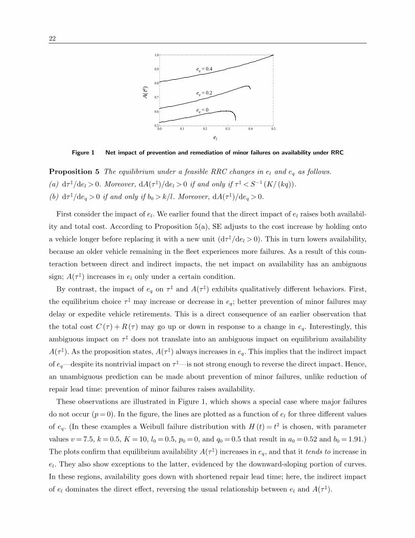
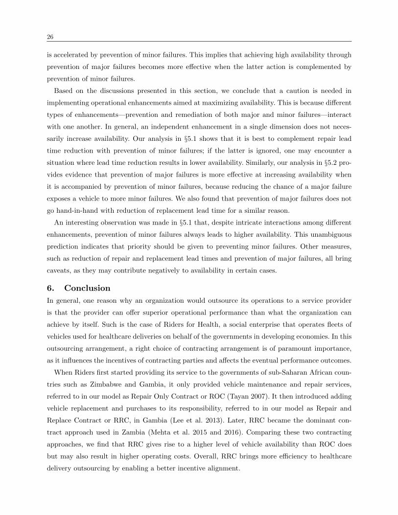
0.0 0.1 0.2 0.3 0.4 0.50.5

0.6

0.7

0.8

0.9

1.0

el

eq = 0

eq = 0.2

eq = 0.4

A(τ

‡ )Figure 1 Net impact of prevention and remediation of minor failures on availability under RRC

Proposition 5 The equilibrium under a feasible RRC changes in el and eq as follows.

(a) dτ ‡/del > 0. Moreover, dA(τ ‡)/del > 0 if and only if τ ‡ <S−1 (K/ (kq)).

(b) dτ ‡/deq > 0 if and only if b0 >k/l. Moreover, dA(τ ‡)/deq > 0.

First consider the impact of el. We earlier found that the direct impact of el raises both availabil-

ity and total cost. According to Proposition 5(a), SE adjusts to the cost increase by holding onto

a vehicle longer before replacing it with a new unit (dτ ‡/del > 0). This in turn lowers availability,

because an older vehicle remaining in the fleet experiences more failures. As a result of this coun-

teraction between direct and indirect impacts, the net impact on availability has an ambiguous

sign; A(τ ‡) increases in el only under a certain condition.

By contrast, the impact of eq on τ ‡ and A(τ ‡) exhibits qualitatively different behaviors. First,

the equilibrium choice τ ‡ may increase or decrease in eq; better prevention of minor failures may

delay or expedite vehicle retirements. This is a direct consequence of an earlier observation that

the total cost C (τ) +R (τ) may go up or down in response to a change in eq. Interestingly, this

ambiguous impact on τ ‡ does not translate into an ambiguous impact on equilibrium availability

A(τ ‡). As the proposition states, A(τ ‡) always increases in eq. This implies that the indirect impact

of eq—despite its nontrivial impact on τ ‡—is not strong enough to reverse the direct impact. Hence,

an unambiguous prediction can be made about prevention of minor failures, unlike reduction of

repair lead time: prevention of minor failures raises availability.

These observations are illustrated in Figure 1, which shows a special case where major failures

do not occur (p= 0). In the figure, the lines are plotted as a function of el for three different values

of eq. (In these examples a Weibull failure distribution with H (t) = t2 is chosen, with parameter

values v= 7.5, k= 0.5, K = 10, l0 = 0.5, p0 = 0, and q0 = 0.5 that result in a0 = 0.52 and b0 = 1.91.)

The plots confirm that equilibrium availability A(τ ‡) increases in eq, and that it tends to increase in

el. They also show exceptions to the latter, evidenced by the downward-sloping portion of curves.

In these regions, availability goes down with shortened repair lead time; here, the indirect impact

of el dominates the direct effect, reversing the usual relationship between el and A(τ ‡).

23

The reversal happens for the following reason. Although shortened lead time increases availability

through the direct impact, it also raises the costs. If the latter effect is large, SE pays more attention

to mitigating the cost increase (in order to meet SE’s surplus constraint and the government’s

budget constraint), which is accomplished by delaying vehicle replacements. But this action lowers

availability, and if this effect is severe enough, then the initial availability increase is negated. From

Figure 1 we see that this reversal disappears when eq is large, i.e., when repair lead time reduction

is complemented by prevention of minor failures.

From these discussions we see that the two ways of addressing minor failures, namely preven-

tion of failures and remediation through lead time reduction, have subtle and contrasting effects

on vehicle availability. Whereas prevention of minor failures unambiguously increases availability,

reduction of repair lead time does not. For the remediation effort to have a desired effect, it has to

be complemented by prevention efforts.

5.2 Prevention and Remediation of Major Failures

Next, we study the impact of prevention and remediation of major failures, captured by the

variables ep and eL. As in the case of minor failures, both direct and indirect impacts play important

roles. The direct impacts are summarized in the following lemma.

Lemma 3 For given τ , the performance measures defined in (3) vary with eL and ep as follows.

(a) ∂A (τ)/∂eL > 0; ∂C (τ)/∂eL > 0; ∂R (τ)/∂eL > 0; ∂ [C (τ) +R (τ)]/∂eL > 0.

(b) ∂A (τ)/∂ep > 0 if and only if∣∣∣∣∂m (τ)/∂p

m (τ)/p

∣∣∣∣> lq

Lp+ lqwhere m (τ)≡ M (τ)

F (τ); (13)

∂C (τ)/∂ep > 0; ∂R (τ)/∂ep < 0 if

L<[∫ τ

0H (t)F (t)dt

]/[H (τ)F (τ)

]; (14)

∂ [C (τ) +R (τ)]/∂ep < 0 if (14) is satisfied and M (τ) +LF (τ)<Kl/k.

Comparing the results in part (a) of this lemma with Lemma 2(a), we see that the direct impact

of eL, enhancement in replacement speed, mirrors that of el, enhancement in repair speed. In both

cases, shorter lead time leads to higher availability as well as higher repair and replacement costs.

Hence, the insights we derived in the last subsection with regards to el apply equally to eL. We

therefore focus on the impact of ep, prevention of major failures.

Lemma 3(b) shows that increased ep results in higher repair cost C (τ) and lower replacement cost

R (τ), the latter under the condition (14). (This condition is satisfied in most reasonable settings

where the replacement lead time L is sufficiently small compared to vehicle retirement age τ .)

24

Replacement cost is lowered because fewer occurrences of major failures mean fewer unscheduled

replacements. On the other hand, repair cost increases because smaller chance of a major failure

prolongs the average life of an existing vehicle in the fleet, exposing the vehicle to more minor

failures that require repairs. Notice that these directional results are opposites of what we found

for the impact of eq, prevention of minor failures.

As it turns out, this reversal is not the only departure. According to Lemma 3(b), availability

A (τ) may or may not increase in ep, depending on whether the condition (13) is satisfied. (Note

that the quantity appearing on the left hand-side of the inequality in (13) is the elasticity of m(τ)

with respect to p, where m(τ) represents mean time to a major failure conditional on retirement

age τ .) In other words, it is possible that prevention of major failures results in lower availability

when τ is fixed. This is in contrast to the direct impact of prevention of minor failures (higher eq),

which was shown in the last subsection to unambiguously increase availability.

This seemingly contradictory relationship between major failures and availability originates from

the interaction between the two types of failures: reducing a chance of a major failure invites more

occurrences of minor failures. This happens because a vehicle accumulates more mileage as its life

is prolonged and becomes more susceptible to minor failures. Although a major failure results in

a more severe consequence than a minor failure does (premature vehicle death versus temporary

downtime), it actually brings a benefit, namely, renewal of the fleet. By triggering a replacement

of an old vehicle with a new unit, a major failure “injects youth” to the fleet, thereby allowing it

to experience minor failures less often. This beneficial effect of a major failure counters its harmful

effect on availability, explaining the ambiguity stated in Lemma 3(b).

The subtle dynamics we have uncovered thus far only represent direct impacts of ep. A com-

plete picture emerges when we examine the net impact, the sum of direct and indirect impacts.

Unfortunately, a complete analytical specification of the net impact of ep is prohibitive due to the

complex structure outlined in Lemma 3. For completeness, in the next proposition we summarize

analytical results that can be derived under certain conditions, along with a description of the net

impacts of eL.

Proposition 6 The equilibrium under a feasible RRC changes in eL and eq as follows.

(a) dτ ‡/deL > 0. Moreover, dA(τ ‡)/deL > 0 if and only if τ ‡ <S−1 (K/ (kq)).

(b) dτ ‡/dep < 0 if b0 >k/l and (14) is satisfied at τ = τ ‡.

We now examine the net impact of ep on equilibrium availability A(τ ‡) via numerical examples.

Each of the two figures in Figure 2 plots A(τ ‡) as a function of ep for three different values of eL.

Plots in Figure 2(a) are drawn under the assumption that no enhancement is made in preventing

minor failures (eq = 0), whereas plots in Figure 2(b) are drawn under the assumption of maximum

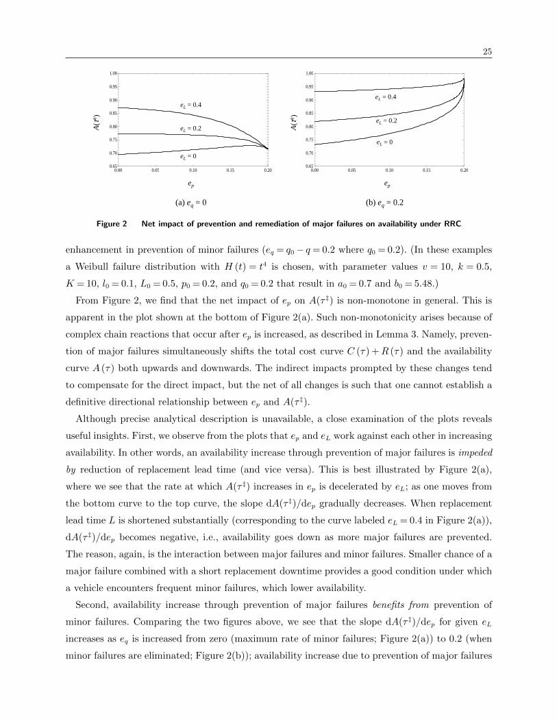
25

0.00 0.05 0.10 0.15 0.200.65

0.70

0.75

0.80

0.85

0.90

0.95

1.00

0.00 0.05 0.10 0.15 0.200.65

0.70

0.75

0.80

0.85

0.90

0.95

1.00

A(τ

‡ )

A(τ

‡ )

ep ep

eL = 0

eL = 0.2

eL = 0.4

eL = 0

eL = 0.2

eL = 0.4

(a) eq = 0 (b) eq = 0.2

Figure 2 Net impact of prevention and remediation of major failures on availability under RRC

enhancement in prevention of minor failures (eq = q0− q = 0.2 where q0 = 0.2). (In these examples

a Weibull failure distribution with H (t) = t4 is chosen, with parameter values v = 10, k = 0.5,

K = 10, l0 = 0.1, L0 = 0.5, p0 = 0.2, and q0 = 0.2 that result in a0 = 0.7 and b0 = 5.48.)

From Figure 2, we find that the net impact of ep on A(τ ‡) is non-monotone in general. This is

apparent in the plot shown at the bottom of Figure 2(a). Such non-monotonicity arises because of

complex chain reactions that occur after ep is increased, as described in Lemma 3. Namely, preven-

tion of major failures simultaneously shifts the total cost curve C (τ) +R (τ) and the availability

curve A (τ) both upwards and downwards. The indirect impacts prompted by these changes tend

to compensate for the direct impact, but the net of all changes is such that one cannot establish a

definitive directional relationship between ep and A(τ ‡).

Although precise analytical description is unavailable, a close examination of the plots reveals

useful insights. First, we observe from the plots that ep and eL work against each other in increasing

availability. In other words, an availability increase through prevention of major failures is impeded

by reduction of replacement lead time (and vice versa). This is best illustrated by Figure 2(a),

where we see that the rate at which A(τ ‡) increases in ep is decelerated by eL; as one moves from

the bottom curve to the top curve, the slope dA(τ ‡)/dep gradually decreases. When replacement

lead time L is shortened substantially (corresponding to the curve labeled eL = 0.4 in Figure 2(a)),

dA(τ ‡)/dep becomes negative, i.e., availability goes down as more major failures are prevented.

The reason, again, is the interaction between major failures and minor failures. Smaller chance of a

major failure combined with a short replacement downtime provides a good condition under which

a vehicle encounters frequent minor failures, which lower availability.

Second, availability increase through prevention of major failures benefits from prevention of

minor failures. Comparing the two figures above, we see that the slope dA(τ ‡)/dep for given eL

increases as eq is increased from zero (maximum rate of minor failures; Figure 2(a)) to 0.2 (when

minor failures are eliminated; Figure 2(b)); availability increase due to prevention of major failures

26

is accelerated by prevention of minor failures. This implies that achieving high availability through

prevention of major failures becomes more effective when the latter action is complemented by

prevention of minor failures.

Based on the discussions presented in this section, we conclude that a caution is needed in

implementing operational enhancements aimed at maximizing availability. This is because different

types of enhancements—prevention and remediation of both major and minor failures—interact

with one another. In general, an independent enhancement in a single dimension does not neces-

sarily increase availability. Our analysis in §5.1 shows that it is best to complement repair lead

time reduction with prevention of minor failures; if the latter is ignored, one may encounter a

situation where lead time reduction results in lower availability. Similarly, our analysis in §5.2 pro-

vides evidence that prevention of major failures is more effective at increasing availability when

it is accompanied by prevention of minor failures, because reducing the chance of a major failure

exposes a vehicle to more minor failures. We also found that prevention of major failures does not

go hand-in-hand with reduction of replacement lead time for a similar reason.

An interesting observation was made in §5.1 that, despite intricate interactions among different

enhancements, prevention of minor failures always leads to higher availability. This unambiguous

prediction indicates that priority should be given to preventing minor failures. Other measures,

such as reduction of repair and replacement lead times and prevention of major failures, all bring

caveats, as they may contribute negatively to availability in certain cases.

6. Conclusion

In general, one reason why an organization would outsource its operations to a service provider

is that the provider can offer superior operational performance than what the organization can

achieve by itself. Such is the case of Riders for Health, a social enterprise that operates fleets of

vehicles used for healthcare deliveries on behalf of the governments in developing economies. In this

outsourcing arrangement, a right choice of contracting arrangement is of paramount importance,

as it influences the incentives of contracting parties and affects the eventual performance outcomes.

When Riders first started providing its service to the governments of sub-Saharan African coun-

tries such as Zimbabwe and Gambia, it only provided vehicle maintenance and repair services,

referred to in our model as Repair Only Contract or ROC (Tayan 2007). It then introduced adding

vehicle replacement and purchases to its responsibility, referred to in our model as Repair and

Replace Contract or RRC, in Gambia (Lee et al. 2013). Later, RRC became the dominant con-

tract approach used in Zambia (Mehta et al. 2015 and 2016). Comparing these two contracting

approaches, we find that RRC gives rise to a higher level of vehicle availability than ROC does

but may also result in higher operating costs. Overall, RRC brings more efficiency to healthcare

delivery outsourcing by enabling a better incentive alignment.

27

Despite the benefits of RRC, its implementation requires a deeper level of trust and commitment

between the two contracting parties. For example, since the social enterprise has to spread its

cost of acquiring a vehicle across the lifetime of the vehicle, a long term contractual agreement

has to be reached so that the social enterprise is guaranteed to continue providing services to the

government. To facilitate this, an arrangement with financial institutions can be made to finance

vehicle acquisitions, as Riders has done.

As a social enterprise, Riders can continue to innovate in operational enhancements. In doing so,

a caution is needed because different elements of operational enhancements—reduction of vehicle

repair and replacement lead times, prevention of major and minor failures—interact with one

another. While in some situations they are complementary, there are other situations where they

work against each other. For example, our analysis reveals that it is best to complement repair

lead time reduction with prevention of minor failures; if the latter is ignored, one may encounter

a situation where lead time reduction results in lower availability. Similarly, our analysis provides

evidence that prevention of major failures is more effective at increasing availability when it is

accompanied by prevention of minor failures. We also find that prevention of major failures do not

go hand-in-hand with reduction of replacement lead time, because their joint interaction exposes

a vehicle to more minor failures.

Although nontrivial interactions exist, an unambiguous prediction emerges from our analysis:

prevention of minor failures always increases vehicle availability. Hence, an enhancement aimed at

reducing the rate of minor failures gives rise to ultimate performance improvements, and should

therefore be given a high priority. This means that even simple, mundane procedures like tire

pressure checks, periodic oil filter replacements, and inventory control of oil filters and lug nuts, can

make a big difference—it is no coincidence that one of the talks given by the cofounders of Riders

at universities and professional conferences is aptly titled: “How Can Oil Filters Save Africa?”

References

African Development Bank (2014) Infrastructure development. Tracking African Progress in Fig-

ures, Tunis, Tunisia.

Barlow RE, Hunter L (1960) Optimum preventive maintenance policies. Operations Research. 8(1),

90–100.

Barlow RE, Proschan F (1996) Mathematical Theory of Reliability (SIAM).

Beichelt F (1976) A general preventive maintenance policy. Mathematische Operationsforschung

und Statistik, 7(6), 927–932.

Beichelt F (2006) Stochastic Processes in Science, Engineering and Finance, Chapman and

Hall/CRC.

28

Bossert TJ, Bowser DM, Amenyah JK (2007) Is decentralization good for logistics systems? Evi-

dence on essential medicine logistics in Ghana and Guatemala. Health Policy and Planning 22,

73–82.

Chen L, Lee HL (2016) Sourcing under supplier responsibility risk: The effects of certification,

audit, and contingency payment. Management Sci. Forthcoming.

Chen L, Yao S, Zhu K (2016) Should brands tighten certification standards? Sourcing under

supplier-certifier collusion risk. Working Paper, Cornell University.

Chen Y, Shanthikumar JG, Shen ZM (2013) Training, production, and channel separation in ITC’s

e-Choupal network. Prod. and Oper. Management. 22(2), 348–364.

Cho S-H, Fang X, Tayur S, Xu Y (2016) Combating child labor: Incentives and information trans-

parency in global supply chains. Working paper, Carnegie Mellon University.

Deo S, Gallien J, Jonasson JO (2015) Improving HIV early infant diagnosis supply chains in

sub-Saharan Africa: Models and application to Mozambique. Working paper, Indian School of

Business.

Guajardo J, Cohen MA, Kim S-H, Netessine S (2012) Impact of performance-based contracting on

product reliability: An empirical analysis. Management Sci. 58(5), 961–979.

Hogan MC, Foreman KJ, Naghavi M, Ahn SY, Wang M, Makela SM, Lopez AD, Lozano R, Murray

CJ (2010) Maternal mortality for 181 countries, 1980–2008: A systematic analysis of progress

towards millennium development goal 5. Lancet. 375, 9726, 1609-1623.

Hoyt D, Silverman A (2011) Crocs (A): Revolutionizing an industry supply chain model for com-

petitive advantage. Stanford Graduate School of Business, Case GS-57A.

Jain N, Hasija S, Popescu DG (2013) Optimal contracts for outsourcing of repair and restoration

services. Operations Research. 61(6), 1295–1311.

Kim S-H, Cohen MA, Netessine S (2007) Performance contracting in after-sales service supply

chains. Management Sci. 53(12), 1843–1858.

Kim S-H, Cohen MA, Netessine S, Veeraraghavan S (2010) Contracting for infrequent restoration

and recovery of mission-critical systems. Management Sci. 56(9), 1551–1567.

Kim S-H, Cohen MA, Netessine S (2016) Reliability or inventory? An analysis of performance-

based contracts for product support services. Handbook of Information Exchange in Supply Chain

Management. Eds. Ha A, Tang C. Springer, New York.

Kim S-H (2015) Time to come clean? Disclosure and inspection policies for green production. Oper.

Res. 63(1), 1–20.

29

Lee HL, Rammohan SV, Sept L (2013) Innovative logistics in extreme conditions: The case of

health care delivery in gambia. Handbook of Global Logistics, edited by Bookbinder JH, Springer,

New York, 297–322.

Leung NHZ, Chen A, Yadav P, Gallien J (2016) The impact of inventory management on stock-outs

of essential drugs in sub-Saharan Africa: Secondary analysis of a field experiment in Zambia.

PLoS ONE 11(5): e0156026. doi:10.1371/journal.pone.0156026.

Matowe L, Waako P, Adome RO, Kibwage I, Minzi O, Bienvenu E (2008) A strategy to improve

skills in pharmaceutical supply management in East Africa: The regional technical resource

collaboration for pharmaceutical management. Human Resources for Health. 6, 30–35.

McCoy JH, Lee HL (2014) Using fairness models to improve equity in health delivery fleet man-

agement. Production and Oper. Management, 23(6), 965–977.

Mehta KM, Rammohan SV, Albohm DC, Muwowo G, Sept L, Lee HL, Bendavid E (2015) Evaluat-

ing the effectiveness and efficiency of outsourcing vehicle fleet management to strengthen health

delivery: An evaluation of riders for health. Final Presentation to the Gates Foundation.

Mehta KM, Rerolle F, Rammohan SV, Albohm DC, Muwowo G, Moseson H, Sept L, Lee HL,

Bendavid E (2016) Systematic motorcycle management and health care delivery: A field trial.

American Journal of Public Health, 106(1), 87–94.

Nakagawa T (2005) Maintenance Theory of Reliability. Springer, London.

Pedraza-Martinez AJ, Wassenhove LNV (2012) Transportation and vehicle fleet management in

humanitarian logistics: Challenges for future research. EURO Journal on Transportation and

Logistics. 1(1), 185–196.

Pedraza-Martinez AJ, Wassenhove LNV (2013) Vehicle replacement in the international committee

of the Red Cross. Production Operations Management. 22(2), 365–376.

Tayan B (2007) Riders for Health: Health care distribution solutions in sub-Saharan Africa. Stan-

ford Graduate School of Business, Case GS-58.

United Nations (2014) World Urbanization Prospects: The 2014 Revision Highlights. New York.

Wang H (2002) A survey of maintenance policies of deteriorating systems. European Journal of

Operational Research. 139, 469–489.

World Health Organization (2010) World health statistics 2010 (part II). http://www.who.int/

whosis/whostat/EN_WHS10_Part2.pdf.

30

Appendix: Proofs of Main Results

(Proofs of Proposition 1 and Lemmas 1-3 are found in the accompanying Online Appendix, along

with the Lemmas and equations labeled “A”.)

Proof (Proposition 2) Since A′ (τ) < 0 (see Lemma A2), maximizing A (τ) is equiva-

lent to minimizing τ . Using this and rewriting the constraints in (8), we can rewrite (8) as

min0≤τ≤A−1(a0)τ s.t. Ψ(τ) ≥ 0 and Φ(τ) ≤ 0, where Ψ(τ) and Φ(τ) are defined in (9) and (10).

Note S (τ), F (τ)/M (τ), and F (τ)S (τ)/M (τ) that appear in the expressions of Ψ(τ) and

Φ(τ) are all increasing functions that start from zero at τ = 0 with the slopes h′ (τ)M (τ) > 0,

pF (τ)S (τ)/M (τ)2> 0, and pF (τ)S (τ)

2/M (τ)

2+ h′ (τ)F (τ) > 0, respectively. Thus, Ψ(0) =

Φ(0) = −K < 0. Because Ψ(τ) starts from a negative number, for the constraint Ψ(τ) ≥ 0 to

be feasible, Ψ(τ) has to cross zero at least once and its smallest root τ † satisfies Ψ(τ †) = 0 and

Ψ′(τ †) > 0. Because Ψ(τ) < 0 for all τ < τ †, the solution to the above optimization problem is

τ = τ † (at which the constraint Ψ(τ) ≥ 0 binds) provided that τ † satisfies the remaining two

constraints: τ † ≤A−1 (a0) and Φ(τ †)≤ 0. The corresponding r that induces τ = τ † is then r= r(τ †)

where r (τ) ≡ v − K (h (τ) + 1/ (Lp+ lq))/S (τ). Substituting the condition Ψ(τ †) = 0, we can

rewrite this as r(τ †) =ψ+ (ψL+ (k+ψl) q/p)F (τ †)/M(τ †). �

Proof (Proposition 3) Note that a feasible solution to the problem (11) exists only for r ≤

b0/a0 < b0 because the two constraints rA (τ)≤ b0 and A (τ)≥ a0 cannot be satisfied simultaneously

if r > b0/a0. Since A′ (τ) < 0 (see Lemma A2), maximizing A (τ) is equivalent to minimizing τ .

Moreover, A (τ)≥ a0 can be rewritten as τ ≤A−1 (a0). Therefore, the problem (11) is equivalent to

min0≤r≤b0/a0,0≤τ≤A−1(a0)

τ s.t. rA (τ)−C (τ)−R (τ)≥ψ and rA (τ)≤ b0. (15)

We establish that the optimal solution to this problem exists only for b0 ≤ r≤ b0/a0 and specify it.

(i) Suppose r < b0. Then rA (τ) < b0A (τ) ≤ b0 because A (τ) ≤ 1, and therefore the

constraint rA (τ) ≤ b0 is satisfied and nonbinding. Hence, the problem (15) reduces to

min0≤r<b0,0≤τ≤A−1(a0)τ s.t. rA (τ)−C (τ)−R (τ)≥ψ. Lemma A5 proves that rA (τ)−C (τ)−R (τ)

for a given r is a quasiconcave function of τ with an unique interior maximum that starts from

−∞ at τ = 0 and approaches η ≡ ((rµ−K)p− kq)/ ((µ+L)p+ lq) as τ →∞. This implies that

the constraint rA (τ)−C (τ)−R (τ)≥ ψ can be rewritten as either τ ≥ τ (r) (if η − ψ ≥ 0) or as

τ (r)≤ τ ≤ τ (r) (if η−ψ < 0), where τ (r)> 0 and τ (r)≤∞ are the two possible solutions to the

equation rA (τ)−C (τ)−R (τ) = ψ, provided that they exist; otherwise a feasible solution to the

above minimization problem does not exist. Combining τ (r)≤ τ ≤ τ (r) with 0≤ τ ≤A−1 (a0), we

31

see that a feasible solution that minimizes τ exists only if τ (r) < A−1 (a0) and that the optimal

solution is τ = τ (r), i.e., the smallest τ in the feasible region τ (r)≤ τ <min{τ (r) ,A−1 (a0)}. Sup-

pose that such a region exists. Then the problem is reduced to min0≤r<b0 τ (r), where τ (r) satisfies

the equation rA(τ (r)) − C(τ (r)) − R(τ (r)) = ψ by definition. By implicitly differentiating this

equation, we find τ ′ (r)< 0. Thus, the optimal solution to the problem min0≤r<b0 τ (r) is found at

the largest value of r allowed in the considered interval [0, b0). However, because the upper bound

is open, the optimal solution does not exist in this interval.

(ii) Suppose b0 ≤ r ≤ b0/a0. The constraints rA (τ)≤ b0 and rA (τ)−C (τ)−R (τ)≥ ψ in (15)

can be rewritten as τ ≥A−1 (b0/r)> 0 and τ (r)≤ τ ≤ τ (r), where τ (r)> 0 and τ (r) are the two

possible solutions to the equation rA (τ) − C (τ) − R (τ) = ψ if they exist. Hence, the problem

(15) reduces to finding the smallest τ in the interval [max{τ (r) ,A−1 (b0/r)},min{τ (r) ,A−1 (a0)}]

for b0 ≤ r ≤ b0/a0 provided that the interval is nonempty. The smallest value of τ , if it

exists, is therefore either τ (r) or A−1 (b0/r). Suppose A−1 (b0/r) ≤ τ (r) and therefore the

optimal solution is τ = max{τ (r) ,A−1 (b0/r)} = τ (r). Then the problem is further reduced to

minb0≤r≤b0/a0 τ (r) s.t. A−1 (b0/r) ≤ τ (r) . Recall τ ′ (r) < 0 from part (i). Moreover, A−1 (b0/r)

increases in r because A (·) is a decreasing function. These observations together imply that the

smallest τ (r) satisfying the constraint A−1 (b0/r) ≤ τ (r) is found by increasing r until either r

reaches its upper bound b0/a0 or the constraint A−1 (b0/r) ≤ τ (r) binds. The former case never

arises, because r = b0/a0 and A−1 (b0/r) < τ (r) together imply A−1 (a0) < τ (r) which precludes

existence of a feasible solution residing in the nonempty interval [τ (r) ,min{τ (r) ,A−1 (a0)}].

Thus, A−1 (b0/r) = τ (r) at the optimum. Next, suppose τ (r) ≤ A−1 (b0/r) and therefore the

optimal solution is τ = max{τ (r) ,A−1 (b0/r)} = A−1 (b0/r). Then the problem is reduced to

minb0≤r≤b0/a0 A−1 (b0/r) s.t. τ (r)≤ A−1 (b0/r) . Since A−1 (b0/r) increases in r and τ ′ (r)< 0, the

optimal solution is found by reducing r until either r reaches its lower bound b0 or the constraint

τ (r)≤A−1 (b0/r) binds. The former never arises, because r= b0 implies τ =A−1 (b0/r) =A−1 (1) =

0 at the optimum, which violates the supposition 0 < τ (r) ≤ A−1 (b0/r) where the condition

τ (r) > 0 was proved in part (i). Thus, τ (r) = A−1 (b0/r) at the optimum. In sum, we proved

that τ (r) = A−1 (b0/r) at the optimum in all cases. The optimal values for r and τ are then

obtained from the system of equations rA (τ) = b0 and rA (τ)−C (τ)−R (τ) =ψ, with the smaller

of the two solutions to the latter equation chosen. Combining the two equations we obtain the

optimality condition for τ as C (τ) + R (τ) = b0 − ψ. Using the expressions for C (τ) and R (τ)

given in (3), we can rewrite this equation as Θ(τ) = 0 where Θ(τ) is defined in (12). Lemma A6

proves that Θ(τ) has at most two roots, the smaller root crossing zero from below and the larger

root (if it exists) crossing zero from above. Since the optimal solution τ ‡ is equal to the smallest

of the solution to the equation C (τ) +R (τ) = b0 − ψ, it then follows that τ ‡ corresponds to the

32

smallest root of Θ(τ) = 0 if it exists. Optimal solution r‡ is then determined from the equation

τ ‡ = τ (r) =A−1 (b0/r) or equivalently r‡ = b0/A(τ ‡) = b0 + b0 (L+ lq/p)F (τ ‡)/M(τ ‡). �

Proof (Proposition 4) Recall from Propositions 2 and 3 that τ † and τ ‡ satisfy Ψ(τ †) = 0,

Ψ′(τ †) > 0, Φ(τ †) ≤ 0, Θ(τ ‡) = 0, and Θ′(τ ‡) > 0. The functions Ψ(τ), Φ (τ), and Θ(τ), defined

in (9), (10), and (12), are related as follows: Ψ(τ)− Φ(τ) = (Lp+ lq)Θ(τ)S (τ)/M (τ). It then

immediately follows that Θ(τ †)≥ 0. Because Θ(τ)< 0 for all τ < τ ‡ (see Lemma A6) and Θ(τ ‡) = 0

and Θ′(τ ‡) > 0, the result Θ(τ †) ≥ 0 implies τ † ≥ τ ‡. Since A′ (τ) < 0, C ′ (τ) > 0, and R′ (τ) < 0

(see Lemma A2), τ † ≥ τ ‡ implies A(τ †)≤A(τ ‡), C(τ †)≥ C(τ ‡), R(τ †)≤R(τ ‡). To show the last

result in the proposition, recall from Proposition 3 that the first two constraints in (11) bind in

equilibrium. They are combined to become C(τ ‡)+R(τ ‡) = b0−ψ. On the other hand, Proposition

2 states that the first constraint in (7) binds in equilibrium but the second does not. Combining

the two yields C(τ †) +R(τ †)≤ b0−ψ. Therefore, C(τ †) +R(τ †)≤C(τ ‡) +R(τ ‡). �

Proof (Proposition 5) According to Lemma A6, Θ′(τ ‡) = [b0 + (b0 (Lp+ lq)− kq)h(τ ‡)]F (τ ‡)>

0. Implicitly differentiating the equilibrium condition Θ(τ ‡) = 0 yields dτ ‡/dl =

−b0 (q/p)F (τ ‡)/Θ′(τ ‡) < 0 and dτ ‡/dq = − (b0− k/l) (l/p)F (τ ‡)/Θ′(τ ‡). We see that dτ ‡/dq < 0

if b0 > k/l and dτ ‡/dq ≥ 0 otherwise. Combining the expressions of Θ′(τ ‡), dτ ‡/dl, and dτ ‡/dq

written above with A′ (τ) from (A1) and collecting terms using the condition Θ(τ ‡) = 0 yield

dA(τ ‡)

dl=

(q/p)F (τ ‡)F (τ ‡) [kqS(τ ‡)−K]

Θ′(τ ‡)T (τ ‡)2and

dA(τ ‡)

dq=−F (τ ‡)F (τ ‡) [kLS(τ ‡) +Kl/p]

Θ′(τ ‡)T (τ ‡)2< 0,

where T (τ) is defined in (2). We see that the sign of dA(τ ‡)/dl is the same as the sign of

kqS(τ ‡) −K. The statements in parts (a) and (b) in the proposition follow after reversing the

signs of obtained results using change of variables el = l0− l and eq = q0− q. �

Proof (Proposition 6) According to Lemma A6, Θ′(τ ‡) = [b0 + (b0 (Lp+ lq)− kq)h(τ ‡)]F (τ ‡)>

0. Implicitly differentiating the equilibrium condition Θ(τ ‡) = 0 yields dτ ‡/dL, which is com-

bined with ∂A (τ)/∂L and A′ (τ) as follows: dτ ‡/dL = −b0F (τ ‡)/Θ′(τ ‡) < 0 and dA(τ ‡)/dL =

F (τ ‡)F (τ ‡) [kqS(τ ‡)−K]/[Θ′(τ ‡)T (τ)2]. Similarly,

dτ ‡

dp=b0

(∫ τ‡0H (t)F (t)dt−LH (τ ‡)F (τ ‡)

)+ (lq/p2) (b0− k/l)

[F (τ ‡)− pH (τ ‡)F (τ ‡)

]Θ′(τ ‡)

. (16)

From this expression we see that the conditions (14) and b0 > k/l together imply dτ ‡/dp > 0,

because pH (τ) ≤ F (τ)/F (τ) (see Nakagawa 2005, p. 6). The statements in parts (a) and (b)

in the proposition follow after reversing the signs of obtained results using change of variables

el = l0− l and eq = q0− q. �

1

Online Appendix to: “Enabling Healthcare Delivery Through VehicleMaintenance”

Lemma A1 The function S (t) defined in (1) has the following properties: S′ (t) = h′ (t)M (t)> 0

with S (0) = 0 and S (∞) =∞. Consequently, S (t)≥ 0. Moreover, ∂S (t)/∂p< 0 for each t > 0.

Proof Recall H (t) =∫ t0h (y)dy and F (t) = exp(−pH (t)) and the assumptions h (0) = 0,

h (∞) =∞, and h′ (t)> 0. Clearly, S (0) = 0 and S (∞) =∞. Using the identity F′(t) =−ph (t)F (t)

we obtain S′ (t) = h′ (t)M (t) > 0 for τ > 0. The results S (0) = 0 and S′ (t) > 0 together imply

S (t) > 0 for all t > 0. Differentiating S (t) with respect to p yields ∂S (t)/∂p = σ (t)/p2 where

σ (t)≡ 1− F (t)− pH (t)F (t)− p2h (t)∫ t0H (y)F (y)dy. Since h (0) =H (0) = 0 and F (0) = 1, we

have σ (0) = 0. Moreover, using the identities H ′ (t) = h (t) and F′(t) = −ph (t)F (t) we obtain

σ′ (t) =−p2h′ (t)∫ t0H (y)F (y)dy < 0. The results σ (0) = 0 and σ′ (t)< 0 together imply σ (t)< 0

for all t > 0. Therefore, ∂S (t)/∂p= σ (t)/p2 < 0 for t > 0. �

Lemma A2 A (τ), C (τ), and R (τ) defined in (3) satisfy the following: A′ (τ)< 0, C ′ (τ)> 0, and

R′ (τ)< 0 for τ > 0.

Proof Using the identity F′(τ) = −ph (τ)F (τ), differentiate A (τ), C (τ), and R (τ) in (3) to

obtain

A′ (τ) =−(Lp+ lq)F (τ)S (τ)

T (τ)2 , C ′ (τ) =

kqF (τ)S (τ)

T (τ)2 , R′ (τ) =−KF (τ) [1 + (Lp+ lq)h (τ)]

T (τ)2 ,

(A1)

where S (τ) and T (τ) are defined in (1) and (2). Since S (τ)> 0 (see Lemma A1), it follows that

A′ (τ)< 0, C ′ (τ)> 0, and R′ (τ)< 0. �

Lemma A3 The function v (p, q)≡ kqh (S−1 (K/ (kq))), where S (·) is defined in (1), increases in

p and q and satisfies v (p, q)≥K/µ.

Proof Let τ is the solution to the equation S (τ) =K/ (kq). Then v= kqh (τ). According to Lemma

A1, S (τ) increases from zero to ∞ and ∂S (τ)/∂p< 0 for each τ > 0. This implies ∂τ/∂p > 0, and

therefore ∂v/∂p= kqh′ (τ) (∂τ/∂p)> 0. The result ∂v/∂q > 0 is obtained by implicit differentiation

using the identities S′ (τ) = h′ (τ)M (τ) from Lemma A1 and S (τ) = K/ (kq), along with the

definition of S (τ) in (1):

∂v

∂q= kh (τ) + kqh′ (τ)

∂τ

∂q= kh (τ) + kq

h′ (τ)

S′ (τ)

(− K

kq2

)= k

h (τ)M (τ)−S (τ)

M (τ)=k

p

F (τ)

M (τ)> 0.

2

To show v (p, q)≥K/µ, first observe that τ →∞ as q→ 0 because limq→0S (τ) = limq→0K/ (kq) =

∞ = S (∞), where the last relationship was established in Lemma A1. From this result and the

above observation v (p, q)≥ v (p,0), we see that

v (p, q)≥ v (p,0) = limq→0

kqh (τ) = limτ→∞

Kh (τ)

S (τ)= lim

τ→∞

K

M (τ)−F (τ)/ (ph (τ))=

K

M (∞)=K

µ.

�

Lemma A4 Under the condition (6), the function

Q (τ)≡ (vLp+ (vl+ k) q)S (τ)−K (Lp+ lq)h (τ)−K (A2)

is a quasiconvex function that starts from Q (0) =−K and diverges to Q (∞) =∞, with a unique

interior minimum occurring at τ = τ o > 0 where

τ o =M−1(

K (Lp+ lq)

vLp+ (vl+ k) q

).

As a result, Q (τ) crosses zero exactly once at τ = τ ∗ > τ o such that Q (τ) < 0 for τ < τ ∗ and

Q (τ)> 0 for τ > τ ∗, with Q′(τ ∗)> 0.

Proof Note that the condition (6) implies vµ>K according to Lemma A3. We can rewrite Q (τ)

as Q (τ) = χ (τ)h (τ)− (vL+ (vl+ k) q/p)F (τ)−K where

χ (τ)≡ (vLp+ (vl+ k) q)M (τ)−K (Lp+ lq) . (A3)

Using the relation F′(t) = −ph (t)F (t), we obtain Q′ (τ) = χ (τ)h′ (τ). Since h′ (τ) > 0, we

see that the sign of Q′ (τ) is equal to the sign of χ (τ). Observe χ (0) = −K (Lp+ lq) < 0 and

χ (∞) = (Lp+ lq) (vµ−K) + kqµ > 0, where µ = M (∞) and we used the condition vµ > K

noted above. Moreover, χ′ (τ) = (vLp+ (vl+ k) q)F (τ) > 0. Since χ (τ) increases from χ (0) < 0

to χ (∞)> 0, there exists a unique τ o > 0 satisfying χ(τ o) = 0 such that χ (τ)< 0 for τ < τ o and

χ (τ)> 0 for τ > τ o. This implies that Q′ (τ)< 0 for τ < τ o and Q′ (τ)> 0 for τ > τ o, i.e., Q (τ) is

a quasiconvex function with a unique interior minimum occurring at τ = τ o. Combining this with

Q (0) = −K < 0 and Q (∞) = χ (∞)h (∞) − (vL+ (vl+ k) q/p) −K =∞ > 0, we thus conclude

that Q (τ) crosses zero exactly once at τ = τ ∗ > τ o such that Q(τ ∗) = 0 and Q′(τ ∗)> 0. �

Lemma A5 Under the condition (6), the function

U (τ)≡ vA (τ)−C (τ)−R (τ) = u (τ)/T (τ) , (A4)

where u (τ) = vM (τ)− (kq/p)F (τ)−K and T (τ) =M (τ) + (L+ lq/p)F (τ) are found from the

expressions of A (τ), C (τ), R (τ) from (3), has the following properties.

3

(a) U (τ) is a quasiconcave function that starts from U (0) = −∞ and converges to U (∞) =

((vµ−K)p− kq)/ ((µ+L)p+ lq), peaking at τ = τ ∗ > 0, a unique root of the function Q (τ)

defined in (A2).

(b) U(τ ∗)> 0 for all v > v ≡ kqh (S−1 (K/ (kq))), where S (τ) is defined in (1). Given v > v, the

maximizer τ ∗ satisfies τ− < τ∗ <S−1 (K/ (kq))<h−1 (v/ (kq)) where τ− > 0 is the smallest root

of u (τ) such that u′(τ−)> 0.

Proof (a) Taking the limit τ → 0 that results in H (0) = F (0) = 0 and substituting them in U (τ),

we find U (0) =−∞ for all p≥ 0. Taking the limit τ →∞ that results in H (∞) =∞, F (∞) = 1,

and M (∞) = µ, we find U (∞) = (vµ− kq/p−K)/ (µ+L+ lq/p) for p > 0 and U (∞) =−k/l for

p = 0, where we used the result limτ→∞ τ/H (τ) = 0 obtained by l’Hopital’s rule. Differentiating

U (τ) using the identity F′(τ) =−ph (τ)F (τ) yields U ′ (τ) =−F (τ)Q (τ)/T (τ)

2, where Q (τ) is

defined in (A2). In Lemma A4 it is proved that Q (τ)< 0 for τ < τ ∗ and Q (τ)> 0 for τ > τ ∗, which

implies that U ′ (τ)> 0 for τ < τ ∗ and U ′ (τ)< 0 for τ > τ ∗. Hence, U (τ) quasiconcave and has a

unique maximum at τ = τ ∗.

(b) Since U (τ) = u (τ)/T (τ) and T (τ) > 0, the sign of U (τ) is determined by the sign of

u (τ). Thus, we examine the properties of u (τ) to find a condition under which U(τ ∗)> 0. Note

u′ (τ) = [v− kqh (τ)]F (τ). Because h′ (τ)> 0, the term v − kqh (τ) in u′ (τ) changes sign exactly

once from positive to negative at τ = τ (v)≡ h−1 (v/ (kq)). This implies that u (τ) is quasiconcave

with a unique interior maximum occurring at τ = τ (v). Substituting τ = τ (v) in u (τ) and

rewriting it as a function of τ by inverting the monotone function τ (v) yields u (τ) = kqS (τ)−K,

which traces u (τ) evaluated at its maximizer for varying values of v. (Note S (τ) is defined in

(1).) In Lemma A1 it is proved that S (τ) increases from S (0) = 0 to S (∞) =∞; hence, u (τ)

increases from u (0) = −K to u (∞) =∞, crossing zero exactly once at τ = τ ≡ S−1 (K/ (kq))

that satisfies u(τ) = 0. This implies that u (τ (v)) increases from −K to ∞ as v goes from zero

to ∞, crossing zero exactly once at v = kqh(τ) that satisfies u(τ(v)) = u(τ) = 0. Therefore,

u (τ (v)) > 0 for all v > v. This implies U (τ (v)) > 0 for all v > v, and because U(τ ∗) > U (τ) for

all τ 6= τ ∗, it follows that U(τ ∗) > 0 for all v > v. Fix v > v and write τ (v) as τ , which satisfies

u(τ) > 0. Recall that u (τ) is a quasiconcave function that peaks at τ = τ with u (0) = −K < 0

and u (∞) = vµ− kq/p−K. This implies that u (τ) has either one or two roots and that u (τ)> 0

if and only if τ− < τ < τ+, where τ− > 0 is the first root satisfying u′ (τ−) > 0 and τ+ is either

the second root satisfying u′ (τ+) < 0 if u (∞) < 0 or ∞ otherwise. Clearly, τ− < τ < τ+. We

now show that τ ∗, the maximizer of U (τ), satisfies τ− < τ ∗ < τ < τ where τ is the root of the

function u(τ) = kqS (τ) − K. We show this result in three steps: (i) τ < τ , (ii) τ ∗ < τ , and

(iii) τ− < τ ∗. To prove τ < τ , recall that the condition v > v requires u (τ) = u (τ) > 0 = u(τ),

4

which implies τ < τ as desired because u (τ) > 0 if and only if τ > τ . To prove τ ∗ < τ , evaluate

Q (τ) defined in (A2) at τ = τ , which satisfies both kqS (τ) = K and kqh (τ) = v, to obtain

Q (τ) = (K/ (kq)) (v− v) (Lp+ lq) > 0. This result implies τ ∗ < τ as desired, because Q (τ) > 0

if and only if τ > τ ∗ (see Lemma A4). Finally, to prove τ− < τ ∗, evaluate Q (τ) at τ = τ− that

satisfies u (τ−) = 0 to obtain Q (τ−) =− [(vL+ (vl+ k) q/p)F (τ−) +K] [1− kqh (τ−)/v]< 0, where

the inequality follows from τ− < τ combined with the earlier observation that v − kqh (τ) > 0 if

and only if τ < τ . The result Q (τ−)< 0 implies τ− < τ∗ as desired, because Q (τ)< 0 if and only if

τ < τ ∗. In summary, τ− < τ∗ < τ = S−1 (K/ (kq))< τ = h−1 (v/ (kq)). �

Lemma A6 Let β1 ≡ kq/ (Lp+ lq) and β2 ≡ (Kp+ kq)/ ((µ+L)p+ lq). The function Θ(τ)

defined in (12) for τ > 0 and b0−ψ > 0 is either increasing or quasiconcave with a unique maximum

occurring at

τ c ≡ h−1(

b0−ψ(Lp+ lq) (β1− (b0−ψ))

), (A5)

and it has the following properties.

(a) If b0−ψ > β2, then Θ(τ) crosses zero exactly once at τ = τ1 > 0 such that Θ(τ)< 0 for τ < τ1

and Θ(τ)> 0 for τ > τ1, with Θ′(τ1)> 0.

(b) If 0< b0−ψ <min{β1, β2} and the condition

S(τ c)>K

(Lp+ lq) (β1− (b0−ψ))(A6)

is satisfied, then Θ(τ) crosses zero exactly twice at τ = τ1 and τ = τ2 with 0< τ1 < τ2 such that

Θ(τ)< 0 for τ < τ1 and τ > τ2 and Θ(τ)> 0 for τ1 < τ < τ2, with Θ′(τ1)> 0 and Θ′(τ2)< 0.

(c) If either b0−ψ <min{β1, β2} and (A6) is not satisfied or β1 ≤ b0−ψ ≤ β2, then Θ(τ)≤ 0 for

all τ ≥ 0.

Proof Using F′(τ) = −ph (τ)F (τ), we differentiate Θ(τ) from (12) to obtain Θ′ (τ) =

[(b0−ψ) + (Lp+ lq) ((b0−ψ)−β1)h (τ)]F (τ) where β1 = kq/ (Lp+ lq). From this result we see

that Θ′ (τ)< 0 for all τ > 0 if b0−ψ≤ 0 and Θ′ (τ)> 0 for all τ ≥ 0 if b0−ψ≥ β1. If 0< b0−ψ < β1,

then Θ′ (τ)> 0 if and only if h (τ)< (b0−ψ)/ [(Lp+ lq) (β1− (b0−ψ))]. Since h (τ) increases from

zero to infinity, this implies the sign of Θ′ (τ) changes from positive to negative exactly once at τ c

defined in (A5), i.e., Θ(τ) is quasiconcave with a unique maximum occurring at τ = τ c. Moreover,

Θ(0) =−K and Θ(∞) = (b0−ψ) (µ+L+ lq/p)− kq/p−K, from which we see that Θ(∞)> 0 if

and only if b0−ψ > β2 = (Kp+ kq)/ [(µ+L)p+ lq]. In summary, Θ(τ) having b0−ψ > 0 is either

an increasing function or a quasiconcave function with a unique interior maximum that starts from

negative and ends in either positive or negative. From these observations we prove the following.

5

(a) Suppose b0 − ψ > β2. In this case Θ(τ) is either increasing or quasiconcave with Θ(0) < 0

and Θ(∞)> 0, and therefore Θ(τ) crosses zero exactly once from below.

(b) Suppose 0 < b0 − ψ < min{β1, β2} and the condition (A6) is satisfied. In this case Θ(τ)

is quasiconcave with Θ(0) < 0 and Θ(∞) < 0. Hence, Θ(τ) either never crosses zero or crosses

zero exactly twice. The latter happens if and only if Θ(τ c) > 0 where τ c is given in (A5). This

is verified by evaluating Θ(τ c) using the relationship S (τ) = h (τ)M (τ)− F (τ)/p which yields

Θ(τ c) = (b0−ψ)S(τ c)/h(τ c)−K > 0, where we used (A5) and (A6).

(c) Suppose b0 − ψ ≤ 0. Then Θ′ (τ) < 0 starting at Θ(0) = −K < 0 and therefore Θ(τ) < 0

for all τ ≥ 0. Suppose 0< b0 − ψ <min{β1, β2} and (A6) is not satisfied. Then Θ(τ c)≤ 0 by the

reasoning in part (b) and therefore Θ(τ)≤ 0 for all τ ≥ 0. Suppose β1 ≤ b0−ψ≤ β2. Then Θ(τ) is

increasing with Θ(0)< 0 and Θ(∞)≤ 0, and therefore Θ(τ)≤ 0 for all τ ≥ 0. �

Lemma A7 Recall the definitions of β1and β2 from Lemma A6. The function C (τ) + R (τ) is

quasiconvex, starting from ∞ at τ = 0 and converging to β2 as τ →∞. The function is decreas-

ing if µ = M (∞) < K/β1. Otherwise, it has a unique minimum at τ = τn > 0 that solves the

equation kqS (τ)−K (Lp+ lq)h (τ)−K = 0. The minimum value at τ = τn is C(τn) +R(τn) =

kq/ [1/h(τn) +Lp+ lq]<β1. Moreover:

(a) C(τm) +R(τm) = k/l where τm < τn uniquely solves the equation M (τ) +LF (τ) =Kl/k.

(b) τ ∗ < τn, where τ ∗ is the root of Q (τ) specified in Lemma A4.

(c) C(τ ‡) +R(τ ‡) = b0−ψ where τ ‡ ≤ τn is the root of Θ(τ) specified in Proposition 3.

Proof The first statement in the lemma is a corollary to Lemma A5, obtained by setting v =

0. The condition Qn (τ) ≡ kqS (τ) −K (Lp+ lq)h (τ) −K = 0 that identifies the minimum τ =

τn is also obtained from Lemma A5, after setting v = 0 in the optimality condition Q (τ) = 0

where Q (τ) is defined in (A2). Note Qn (τ) = (Lp+ lq) [β1M (τ)−K]h (τ) − (kq/p)F (τ) − K

and Q′n (τ) = (Lp+ lq) [β1M (τ)−K]h′ (τ) (since S (τ) = h (τ)M (τ) − (1/p)F (τ) and S′ (τ) =

h′ (τ)M (τ); see Lemma A1), from which we find that Qn (τ) is a quasiconvex function that

starts from −K < 0 at τ = 0 and either remains in negative or diverges to ∞ as τ →∞; the

former happens when β1M (∞) −K = β1µ −K ≤ 0 and the latter happens when β1µ −K > 0.

This implies that Qn (τ) crosses zero at most once and that the crossing happens if and only if

β1µ−K > 0, i.e., a unique local minimum exists if and only if µ > K/β1. The minimum value

C(τn) +R(τn) = kq/ [1/h(τn) +Lp+ lq] is obtained by rewriting the condition Qn (τ) = 0 as K =

kqS(τn)/ [1 + (Lp+ lq)h(τn)] and substituting it in C (τ)+R (τ) = [(kq/p)F (τ) +K]/T (τ) where

T (τ) =M (τ) + (L+ lq/p)F (τ) (see (3)).

6

(a) Note C ′ (τ) +R′ (τ) = [F (τ)/T (τ)2] [kqS (τ)−K (Lp+ lq)h (τ)−K]. Substituting M(τm) +

LF (τm) = Kl/k using the identity S (τ) = h (τ)M (τ)− (1/p)F (τ) yields C(τm) + R(τm) = k/l

and C ′(τm) +R′(τm)< 0. The latter implies τm < τn because C (τ) +R (τ) is quasiconvex.

(b) Recall from Lemma A4 that τ ∗ solves the equation Q (τ) = 0 where Q (τ) defined in

(A2) satisfies the following: Q (τ) < 0 for τ < τ ∗ and Q (τ) > 0 for τ > τ ∗. Since Q(τn) ≡

(vLp+ (vl+ k) q)S(τn)−K (Lp+ lq)h(τn)−K = v (Lp+ lq)S(τn)> 0, we have τn > τ ∗.

(c) Recall from Proposition 3 that τ ‡ satisfies Θ(τ ‡) = 0 and Θ′(τ ‡)> 0 where Θ(τ) is defined in

(12). Substituting the condition Θ(τ ‡) = 0 in C (τ)+R (τ) = [(kq/p)F (τ) +K]/T (τ) yields C(τ ‡)+

R(τ ‡) = b0−ψ. Since C (τ)+R (τ) is minimized at τ = τn with the minimum value C(τn)+R(τn) =

kq/ [1/h(τn) +Lp+ lq], as we proved above, it is required that C(τ ‡) +R(τ ‡) ≥ C(τn) +R(τn),

which is equivalent to b0 − ψ ≥ kq/ [1/h(τn) +Lp+ lq]. Using this inequality and the first-order

condition kqS(τn)−K [1 + (Lp+ lq)h(τn)] = 0, we evaluate Θ(τ) at τ = τn to obtain

Θ(τn) = (b0−ψ) [M (τ) + (L+ lq/p)F (τn)]− (kq/p)F (τn)−K

≥ kqh(τn)

1 + (Lp+ lq)h(τn)[M(τn) + (L+ lq/p)F (τn)]− (kq/p)F (τn)−K

= Kh(τn) [M(τn) + (L+ lq/p)F (τn)]−S (τn)

S (τn)− (kq/p)F (τn)

= K[1 + (Lp+ lq)h(τn)]F (τn)

pS (τn)− (kq/p)F (τn) = (kq/p)F (τn)− (kq/p)F (τn) = 0.

According to Lemma A6, Θ(τn)≥ 0 together with Θ(τ ‡) = 0 and Θ′(τ ‡)> 0 implies τ ‡ ≤ τn. �

Lemma A8 The elasticity

ε (τ)≡∣∣∣∣∂m (τ)/∂p

m (τ)/p

∣∣∣∣of m (τ) =M (τ)/F (τ) is a decreasing function that starts from ε (0) = 0. Hence, ε (τ)≤ 1.

Proof The following inequalities are useful in the proofs: F (τ) ≤ pH (τ) ≤ F (τ)/F (τ)

and ph (t)m (t) − 1 ≥ 0 (see Nakagawa 2005, pp. 6-8). Using the identity ∂F (t)/∂p =

∂ exp (−pH (τ))/∂p=−H (t)F (t), we evaluate ε (τ) as

ε (τ) =

∣∣∣∣∂m (τ)/∂p

m (τ)/p

∣∣∣∣= p∫ τ0H (t)F (t)dt

M (τ)+pH (τ)F (τ)

F (τ).

Using the identity F′(τ) =−ph (τ)F (τ) and applying l’Hopital’s rule yields ε (0) = 1. To complete

the proof, it remains to show ε′ (τ) < 0 for τ > 0. Differentiating ε (τ) and applying the identity∫ τ0H (t)F (t)dt=H (τ)M (τ)−

∫ τ0h (t)M (t)dt obtained from integration by parts yield

ε′ (τ) =pF (τ)

M (τ)2

(∫ τ

0

h (t)M (t)dt− [pH (τ)−F (τ)]h (τ)m (τ)2

)<pF (τ)h (τ) ξ (τ)

M (τ)2 ,

7

where

ξ (τ)≡∫ τ

0

M (t)dt− [pH (τ)−F (τ)]m (τ)2

and the inequality follows from h (t) < h (τ) for all t < τ because h′ (t) > 0. Thus, ε′ (τ) <

0 if and only if ξ (τ) ≤ 0 for all τ > 0. Observe that ξ (τ) = 0. Hence, ξ (τ) ≤ 0 for all

τ > 0 if ξ′ (τ) ≤ 0. To prove this, differentiate ξ (τ) and substitute the identity m′ (τ) =

−[F (τ)/F (τ)

][ph (τ)m (τ)− 1]≤ 0 in it, which yields ξ′ (τ) =m (τ) [ph (τ)m (τ)− 1] ζ (τ) where

ζ (τ)≡ 2pH (τ)F (τ)

F (τ)−F (τ)− 1.

Because ph (τ)m (τ)− 1 ≥ 0, the sign of ξ′ (τ) is determined by the sign of ζ (τ). Note ζ (0) = 0

(proved by l’Hopital’s rule) and ζ ′ (τ) = −ph (τ)[F (τ)/F (τ)

2](

2pH (τ)− 2F (τ)−F (τ)2)≤ 0,

where the inequality follows from the fact that 2pH (τ)− 2F (τ)− F (τ)2

increases from zero at

τ = 0 with the slope equal to 2ph (τ)F (τ)2 ≥ 0. Together, ζ (0) = 0 and ζ ′ (τ)≤ 0 imply ζ (τ)≤ 0

for all τ ≥ 0. It then follows that ξ′ (τ)≤ 0, which we set out to prove in order to show ε′ (τ)< 0

for τ > 0. �

Corollary A1 (Corollary to Proposition 6) dA(τ ‡)/dep > 0 if q= 0 or if L= 0 and b0 >k/l.

Proof Differentiating A (τ) defined in (3) with respect to p yields

∂A (τ)

∂p=− (L+ lq/p)

[F (τ)

∫ τ0H (t)F (t)dt+H (τ)F (τ)M (τ)

]+ (lq/p2)F (τ)M (τ)

T (τ)2 .

Setting q= 0 in ∂A (τ)/∂p and dτ ‡/dp evaluated in (16) and combining them with A′ (τ) evaluated

in (A1) result in

dA (τ)

dp=∂A (τ)

∂p+A′ (τ)

dτ ‡

dp=−

L [M(τ ‡) +LF (τ ‡)](ph(τ ‡)

∫ τ‡0H (t)F (t)dt+H(τ ‡)F (τ ‡)

)[1 +Lph(τ ‡)]T (τ ‡)2

< 0.

Similarly, setting L= 0 and combining the terms yield

dA (τ)

dp=∂A (τ)

∂p+A′ (τ)

dτ ‡

dp=lqF (τ ‡) [b0M(τ ‡) + (lq/p) (b0− k/l)F (τ ‡)]

Θ′(τ ‡)T (τ ‡)2ϕ(τ ‡)

where ϕ (τ)≡−h (τ)∫ τ0H (t)F (t)dt+ 1

p2

[F (τ)− pH (τ)F (τ)

]. It is straightforward to show that

ϕ (0) = 0 and ϕ′ (τ) < 0, together implying ϕ (τ) < 0 for τ > 0. Hence, dA (τ)/dp < 0 if b0 > k/l.

�

Proof (Proposition 1) The result follows directly from Lemma A4 and Lemma A5. �

8

Proof (Lemma 1) Comparing the utility function V (τ) = (v− r)A (τ) − R (τ) with U (τ) =

vA (τ)−C (τ)−R (τ) defined in (A4), we see that V (τ) is a special case of U (τ) with v replaced

by v − r and k set to zero. Thus the results from Lemma A4 and Lemma A5 apply with

the substitutions, including the optimality condition Q (τ) = 0 where Q (τ) is defined in (A2).

The result τ ′ (r) > 0 is obtained by implicitly differentiating Q (τ (r)) = 0 and using the result

Q′ (τ (r))> 0 proved in Lemma A4. �

Proof (Lemma 2) Using the expressions of C (τ) and R (τ) given in (3), we get

∂

∂eq[C (τ) +R (τ)] =− ∂

∂q[C (τ) +R (τ)] =−(k/p)F (τ) [M (τ) +LF (τ)−Kl/k]

[M (τ) + (L+ lq/p)F (τ)]2 ,

from which the last result of the lemma follows. The remaining results are straightforward,

obtained by inspecting the expressions in (2) and (3). �

Proof (Lemma 3) The results in part (a) are straightforward, obtained by examining

the expressions in (2) and (3). To prove part (b), first note m (τ) = M (τ)/F (τ) satis-

fies ∂m (τ)/∂p = − (1/F (τ))[∫ τ

0H (t)F (t)dt+H (τ)F (τ)m (τ)

]< 0, which is derived by using

the identity ∂F (t)/∂p = ∂ exp (−pH (τ))/∂p = −H (t)F (t). Rewriting A (τ) in (3) as A (τ) =

pm (τ)/ (Lp+ lq+ pm (τ)) and differentiating it with respect to p, we find that ∂A (τ)/∂p < 0 if

the condition (13) is satisfied and ∂A (τ)/∂p ≥ 0 otherwise. Similarly, rewriting C (τ) in (3) as

C (τ) = kq/ (Lp+ lq+ pm (τ)) and differentiating it with respect to p yields

∂C (τ)

∂p=− kqm (τ)

[Lp+ lq+ pm (τ)]2

(L

m (τ)+ 1−

∣∣∣∣∂m (τ)/∂p

m (τ)/p

∣∣∣∣)< 0,

where the inequality follows from the result in Lemma A8. Next, assume that (14) is true. Then

T (τ) defined in (2) satisfies

∂T (τ)

∂p=LH (τ)F (τ)−

∫ τ

0

H (t)F (t)dt− lq

p2F (τ)

(F (τ)

F (τ)− pH (τ)

)< 0,

where we used the inequality pH (τ) ≤ F (τ)/F (τ) to prove the result (Nakagawa 2005,

p. 6). This implies ∂R (τ)/∂p > 0 because R (τ) = K/T (τ) (see (3)). Finally, assume that

the conditions (14) and M (τ) + LF (τ) < Kl/k are satisfied. Differentiating C (τ) + R (τ) =

[kqF (τ) +Kp]/ [pM (τ) + (Lp+ lq)F (τ)] with respect to p and applying these conditions yield

∂

∂p[C (τ) +R (τ)]>−

kq [M (τ) +LF (τ)−Kl/k][F (τ)− pH (τ)F (τ)

][pM (τ) + (Lp+ lq)F (τ)]

2 > 0,

where we used the aforementioned inequality pH (τ)≤ F (τ)/F (τ). The statements in the lemma

follow after reversing the signs of the obtained results using change of variables eL = L0 −L and

ep = p0− p. �