Empirical Study of Risk Premiums in the JGB Market and Its ... · Cor(FSPn,BRPn) Source: Nikko Salomon Smith Barney Limited. Figure 4. Correlations of FSPn with D Sn-1 During the

Empirical Study of Risk Premiums in the JGB Market

and Its Application to Investment Strategies

Satoshi Yamada

NIKKO SALOMON SMITH BARNEY

Ø An Empirical Study of JGB Market Risk Premiums

Ø Forecasting the Excess Bond Returns and the Dynamic Strategy

Ø Rolling Yield Maximization Strategy

c 2001, The Security Analysts Association of Japan R

March 1999 Empirical Study of Risk Premiums in the JGB Market and Its Application to Investment Strategies

2

Pure Expectations Hypothesis and Risk Premium Hypothesis 5 Theoretical background 5

The definition of forward rates 5

The interpretation of forward rates 5

The condition that all bonds earn the same returns 5

Rising rate expectation and risk premium 6

Empirical evidence 7

Empirical Evidence About the Bond Risk Premium in the JGB Market 9 Estimating the risk premium from historical data 9

Average return difference 9

Short- and long-term JGB yields during the sample period 9

The results 10

Evidence from JGB returns 10

Subperiod average returns and volatilities 11

Forecasting Excess Bond Returns 13

Are excess bond returns predictable? 13 Definitions of four predictors 14

The term spread 14

The inverse wealth 14

Real yield 15

Momentum 15

Combining the information of several predictors 15

The average returns in subsamples 15

Out-of-sample estimation of return predictions 16

Dynamic Strategy 19 Performance of the dynamic strategy 19

Stability of the predictive relations 20

Contents


3

Impact of forecast signal’s strength on return predictability 22

Impact of investment horizon 23 Practical considerations 24

Duration targeting 25

Rolling Yield Max Strategy 27 The Concept of Rolling Yield 27

Decomposing the expected returns 28

Extracting the yield income (rolling yield) 30

Rolling yield maximization strategy 31

Rolling yield maximization strategy performance relative to benchmark 32

How long a horizon is long enough for investors to be confident that this strategy outperforms the benchmark 32

Excess return attribution of RollMax 33

Summary 37

The pure expectations hypothesis and the bond risk premium 37

Empirical evidence about the bond risk premium in the JGB market 37

Predicting the bond risk premium and the dynamic strategy 37

Rolling yield maximization strategy 37

Appendix: Computation of rolling yield 38 References 40


4

Many studies have been done on the term structure of interest rates and the bond risk premium. However, those studies do not deal with practical investment applications, and it is very hard to find studies such investment applications in the JGB market. In this report, empirical studies of the bond risk premium in the JGB market are done. Then, its findings are applied to investment strategies. First, by exploiting the bond excess return predictability, a dynamic strategy is shown. This is a tactical asset allocation strategy between cash and long-term bonds based on the predictions that use information in positive carry with active duration management. Second, the rolling yield maximization strategy is introduced. This strategy’s objective is to pick up rolling yield relative to a benchmark with modified duration constraints. This strategy exploits information in positive carry in duration-neutral environment.

Summary


5

The upward sloping yield curve is best explained by the rising rate expectations (pure expectations hypothesis) or high reward for risk taking (risk premium hypothesis). We evaluate these two hypotheses empirically in the JGB market in this section.

Theoretical background The definition of forward rates A forward rate is the interest rate for a loan between two future dates and is determined today. If a series of spot rates Sn(n=1,2,3,....), which are the interest rates for loans

between today and a future date (n years from now), are given, a (n-m) years forward rate m years from now Fm,n is computed as in the following equation:

(1+ Fm,n)n-m = (1+ Sn)/(1+Sm) -> Fm,n ≅(nSn-mSm)/(n-m) (n>m) (1)1

Note: when n-m=1, Fn-1,n is called one year forward, when m=1 F1,n is called implied forward.

The interpretation of forward rates When the spot curve is upward sloping, every maturity point on the implied forward curve rises relative to corresponding points on the spot curve. The PEH argues that the forward rates imply rising spot rates, while the risk premium hypothesis states that the yield advantages of forward rates over spot rates are likely to be earned. The difference between forward rates and spot rates are interpreted as break-even yield rises over the next year to make all bonds earn the same rate of return that is the short-term rate.

The condition that all bonds earn the same returns (n-1)-year implied rates one-year forward are computed, if m=1 is substituted in Equation (1)as:

F1,n ≅(nSn-S1)/(n-1) (1)’

Note: Sn denotes the n-year spot rate and S1 denotes 1-year short-term rate.

N year zero coupon bonds earn Hn over one period:

Hn≅Sn+(n-1)(Sn -S*n-1) (2)

where the holding period return is the sum of its initial yield Sn and the capital

gains/losses realized which is approximated by the product of the zero’s duration at horizon (n-1) and its yield change over the period (S*n-1 denotes the horizon yield of n-year zero coupon bond) .If S*n-1= F1,n, substituting (1)’ into (2) gives Hn= S1. This

1 If you take a natural logarithm of both sides of the first equation and approximate by Taylor series expansion of ln(1+x) = x -

1/2x2+1/3x3 +....., you get equation (1).

Pure Expectations Hypothesis and Risk Premium Hypothesis


6

means that if all bonds horizon yield match implied forwards, all bonds earn the short-term rate.

Rising rate expectation and risk premium We rearrange Equation (2) and solve for nSn to get the following equation:

F1,n = S*n-1+(Hn-S1)/(n-1)

Taking expectation of sides of the equation, we get

F1,n = E(S*n-1)+E(Hn-S1)/(n-1).≡E(S*n-1)+BRPn/(n-1) (3)

where BRPn is the expected holding-period return of an n-year zero in excess of the riskless one-year rate. Subtracting Sn-1 from both sides of Equation (3) gives the break-

even change in the n-1 year spot rate:

F1,n - Sn-1 = E(∆Sn-1)+BRPn/(n-1) (4)

where ∆Sn-1= S*n-1 -Sn-1. Equation (4) states that higher implied forwards relative to spot rates (or break-even change in the spot rate)reflect expected future yield changes or expected bond risk premium or some combination of the two. Since PEH assumes BRP=0, it follows from Equation (4) that implied forwards reflect only the market’s expectations of future rate changes. By contrast, the risk premium hypothesis assumes

that E(∆Sn-1)=0. Thus, implied forwards reflect only expected return differences

among bonds(=expected risk premium). Similarly, multiplying both sides of Equation (4) by (n-1), we get the similar equation using the one-year forwards:

Fn-1,n -S1 = (n-1)E(∆Sn-1)+BRPn ≡FSPn (5)2

The forward-spot premium (FSPn) is also expressed as a sum of the expected yield

change and the bond risk premium.

2 Please note that Fn-1,n = nSn-(n-1) Sn-1 and F1,n =(nSn-S1)/ (n-1)


7

Figure 2. The Implications of the Two Hypotheses

Pure Expectations Hypothesis Risk Premium Hypothesis

The Interpretation of Forward Rates

Expected Future Rates Expected Risk Premium

What Forward Rates Forecast? Future Rate Changes Near-term Return Differentials Across Bonds

The Best Forecast of an N-year Zero’s One-Period Expected Return

Riskless Short-term Rate(S1) One-Period Forward Rate(Fn-1,n)

The Best Forecast of Next Period’s Spot Rates

Implied Forward Rates(F1,n) Current Spot Rates(Sn-1)

Correlation(FSPn,∆Sn-1) Positive 0 Correlation(FSPn,Realized BRPn) 0 Positive Source: Nikko Salomon Smith Barney Limited.

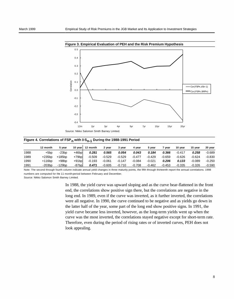
Empirical evidence Figure 3 plots the correlation of the forward-spot premium (implied 3 month rates (n-0.25) year forward=FSPn), first, with the subsequent change in the (n-0.25) year spot

rate(∆Sn-1) over the next 3 months and, second, with the n-year zero’s subsequent

realized return over the next 3 months in excess of the 3 months rates. We compute these correlations for nine different maturities using monthly JGB spot rate data from the Jan. 1988 – Sep. 1998 period. Figure 3 shows that the forward-spot premiums are negatively correlated with the future rate changes, whereas the forward-spot premiums are positively correlated with future bond risk premiums. In the front end of the curve, the rates tend to move at least in the direction that forwards imply, but not to the extent that forwards imply, which is why the forward also has a positive correlation with the risk premium. In the longer end of the curve, forwards seem to be inverse indicators of future rate changes. These evidences are clearly inconsistent with PEH. To further verify inconsistency of PEH, we investigate the same correlations in rising rate environments. Because most of the sample period, spot curves are positively sloped and rates are going down, we extract the period when rates are rising or spot curves are inverted that is considered to favor PEH. Figure 4 reports the annual correlation between forwards and the subsequent rate changes for the same maturities as before along with annual yield changes at different points on the curve from the 1988-1991 period.


8

Figure 3. Empirical Evaluation of PEH and the Risk Premium Hypothesis

-0.4

-0.3

-0.2

-0.1

0.0

0.1

0.2

0.3

0.4

0.5

12m 2yr 3yr 4yr 5yr 7yr 10yr 15yr 20yr

Corr

elat

ion

Cor(FSPn,dSn-1)

Cor(FSPn,BRPn)

Source: Nikko Salomon Smith Barney Limited.

Figure 4. Correlations of FSPn with ∆ Sn-1 During the 1988-1991 Period

12 month 5 year 10 year 12 month 2 year 3 year 4 year 5 year 7 year 10 year 15 year 20 year

1988 +5bp -23bp +46bp 0.281 0.565 0.054 0.043 0.184 0.366 -0.417 0.258 -0.689 1989 +235bp +185bp +79bp -0.509 -0.529 -0.529 -0.477 -0.429 -0.659 -0.626 -0.624 -0.830 1990 +116bp +98bp +91bp -0.193 -0.061 -0.147 -0.084 -0.021 0.206 0.133 -0.089 -0.250 1991 -203bp -129bp -87bp 0.471 -0.605 -0.710 -0.708 -0.462 -0.453 -0.335 -0.326 -0.590 Note: The second through fourth column indicate annual yield changes in three maturity points, the fifth through thirteenth report the annual correlations. 1998 numbers are computed for the 11 month-period between February and December. Source: Nikko Salomon Smith Barney Limited.

In 1988, the yield curve was upward sloping and as the curve bear-flattened in the front end, the correlations show positive sign there, but the correlations are negative in the long end. In 1989, even if the curve was inverted, as it further inverted, the correlations were all negative. In 1990, the curve continued to be negative and as yields go down in the latter half of the year, some part of the long end show positive signs. In 1991, the yield curve became less inverted, however, as the long-term yields went up when the curve was the most inverted, the correlations stayed negative except for short-term rate. Therefore, even during the period of rising rates or of inverted curves, PEH does not look appealing.


9

In the previous section, we find that PEH is inconsistent with the historical market data and the bond risk premium hold most of the time. In this section, we focus on the risk premium in the JGB market and try to estimate its magnitude empirically.

Estimating the risk premium from historical data We use historical return data to estimate the average risk premium.

Average return difference The average return differences is a more direct measure to estimate the expected risk premium. Realized excess return can be split into an expected part and an unexpected part. But when many observations are averaged over time, the positive and negative unexpected part begin to offset each other. Thus, the historical average of realized excess returns is a good measure of the long-run expected risk premium if the unexpected parts exactly wash out. This tend to happen if the sample period is long and does not contain an excessively bearish or bullish bias (=neutral period).

Figure 5. Yield Levels, 1985-2000

0

1

2

3

4

5

6

7

8

9

12/2

8/84

06/2

9/85

12/2

8/85

06/3

0/86

12/2

7/86

06/3

0/87

12/2

8/87

06/3

0/88

12/2

8/88

06/3

0/89

12/2

9/89

06/2

9/90

12/2

8/90

06/2

8/91

12/3

0/91

06/3

0/92

12/3

0/92

06/3

0/93

12/3

0/93

06/3

0/94

12/3

0/94

06/3

0/95

12/2

9/95

06/2

8/96

12/3

0/96

06/3

0/97

12/3

0/97

06/3

0/98

12/3

0/98

06/3

0/99

12/3

0/99

06/3

0/00

Yiel

d(%

)

1yr JGB

10yr JGB

Neutral Period


Short- and long-term JGB yields during the sample period We use two sample periods, one is the December 1984- September 2000 period which is the longest history available at hand, and the other is the neutral period of December 1986 and February 1995 as illustrated in Figure 5.

Empirical Evidence About the Bond Risk Premium in the JGB Market


10

The results Evidence from JGB returns Figure 7 shows the risk-reward trade-off in the JGB market by plotting the annualized geometric mean returns of different maturity sectors on their return volatilities. The maturity sectors are 1-2, 2-3, 3-4, 4-5, 5-6, 6-7, 7-8, 8-9, 9-10 and 19-20 year in the JGB sector of Salomon Smith Barney World Government Bond Index. Over the neutral period, the geometric mean return curve increases almost monotonically until the 5-6 year sector (with volatility of 4.878%). There seems to be a positive risk premium at the front end of the curve: 115bp between the 1-2 year sector and 5-6 year sector. Beyond this medium-term sector, the mean return curve becomes flat and even decreasing beyond the 7-8 year sector (with volatility of 6.378%). Thus, it is unclear whether the marginal risk premium exists in the long end of the curve. The steep marginal pickup between 9-10 year and 19-20 year sector (the longest end of the mean curve) is an exceptional sector: the marginal pick-up of 90bp relative to the 9-10-year sector3. The benchmark effect caused by high liquidity of JGB market's benchmark issues makes the 9-10 year sector rich, while there appears to be a liquidity premium (cheapness caused by poor liquidity) added in the 19-20 year sector. The Sharpe ratio (the average excess return adjusted by volatility) increases up to the 3-4 year sector, but it starts to flatten beyond that point and decreases beyond 9 year. The Shape ratio of 19-20 year sector does not reach the level of the 5-6 year sector (the peak).

3 In U.S. Treasury market, on the other hand, the longest end of the mean return curve decrease because certain clientele such as pension funds, prefer to buy this sector with their long -duration liabilities.


11

Figure 7. Average Returns and Volatility

0

1

2

3

4

5

6

7

8

0 2 4 6 8 10 12

Annualized Return Volatility(%)

Annu

aliz

ed G

eom

etric

Mea

n Re

turn

(%)

0

1

2

3

4

5

6

7

8

Annu

aliz

ed G

eom

etric

Mea

n Re

turn

(%)

Dec 1986 - Sep 2000(left axis)

Dec 1986 - Feb1995(right axis)

Note: Annual average geometric returns and annual return volatilities of 10 different maturity sectors are computed based on historical monthly returns of Salomon Smith Barney World Government Bond Index JGB sector. Source: Nikko Salomon Smith Barney Lim ited.

Figure 8. Average Returns and Return Volatilities

Maturity Sector 1-2yr 2-3yr 3-4yr 4-5yr 5-6yr 6-7yr 7-8yr 8-9yr 9-10yr 19-20yr

Arithmetic Mean 4.841 5.096 5.507 5.817 6.093 6.125 6.421 6.348 6.238 7.342 Geometric Mean 4.831 5.066 5.452 5.729 5.974 5.971 6.217 6.108 5.959 6.846 Marginal Increase 0.079 0.235 0.386 0.277 0.245 -0.003 0.246 -0.109 -0.150 0.888 Volatility 1.451 2.436 3.311 4.196 4.878 5.551 6.378 6.920 7.478 9.923

Geometric Mean Excess Return

0.079 0.315 0.700 0.977 1.222 1.218 1.465 1.355 1.206 2.090

Shape Ratio 0.065 0.144 0.230 0.255 0.276 0.248 0.262 0.231 0.199 0.261

note: Geometric mean excess returns are the mean returns of each maturity sector in excess of returns from Salomon Smith Barney World Money Market Index Japanese CD sector. The Shape ratio is the annualized mean-to-volatility ratio of each maturity sector. Arithmetic Mean = (H1 +H2 +H3 +.........+HN)/N Geometric Mean = ((1+ H1)*(1+H2)*(1+H3)*.........*(1+HN))1/N-1. Source: Nikko Salomon Smith Barney Limited.

Subperiod average returns and volatilities Even if the historical average risk premium is the optimal predictor of the long-run future risk premium, it is not necessarily the optimal predictor of the near-term risk premium unless the risk premium is constant over time. In fact, the near-term risk premium is not constant empirically. Figure 9 shows separate reward-risk curves for six two-year subperiods. This illustrates the time-variation in the risk premium. The recent two subperiods(1997-1998, 1999-Sep 2000) have stable risk premium pattern in a low rate environment


12

Figure 9. Return-Risk Trade-Off in the JGB market in Six Subperiods

-6

-4

-2

0

2

4

6

8

10

12

14

0 2 4 6 8 10 12 14 16

Annualized Return Volatility(%)

Annu

aliz

ed M

ean

Retu

rn(%

) 1997-1998

1989-1990

1986-1988

1991-1992

1993-1994

1995-1996

1999-Sep 2000



13

In the previous section, we showed the evidence which suggests that the long-run bond risk premium is positive. However, we also showed that near-term risk premium is not constant and is time-varying. Then, can we forecast near-term excess bond returns?

Are excess bond returns predictable? In the previous section, we saw that the bond risk premium is consistent with the empirical data most of the time over PEH. Then, if the yield curve is steep, that can be interpreted as the long-term bond’s expected returns being higher that that for short-term bonds. Thus, we can use the term spread as an overall proxy for the bond risk premium. However, sometimes, some part of the yield curve is influenced by the market’s rate expectations. Because the rate expectations are unobservable, we cannot know how much noise they introduce to our risk premium proxy. In order to filter out the noise, we introduce the second variable called inverse wealth that is the inverse of the recent stock performance. This variable measures the unobservable aggregate level of risk aversion. The third predictor is the real bond yield, which is sometimes used as the overall proxy for the bond risk premium. This measure incorporates the inflation rate into the forecasting process. Our fourth predictor, momentum, is a dummy variable that simulates a simple moving average trading rule. Figure 10 shows the correlations between the excess bond return and various predictor variables4.

Figure 10. Correlation of Various Predictors with Subsequent Monthly Excess Bond Return, 1986-98

-0.05

0.00

0.05

0.10

0.15

0.20

0.25

0.30

Yield Level Lagged Return ReturnVolatility

Term Spread Real Yield Inverse Wealth Momentum Combination(Fit4)

Combination(Fit4,3 mo)

Cor

rela

tion


4 Real yield has somewhat lower correlation over this particular sample period than the correlation in the US case. Because real yield is the most long-term value indicator, its predictive power tend to decrease over a period that ends at a long bull market such as this.

Forecasting Excess Bond Returns


14

Figure 10 shows that a bond’s yield level, its lagged monthly return and its past volatility (measured by the 12-month rolling standard deviation of monthly excess returns) all have low correlations (-0.01∼0.10). In contrast, the four predictors in our model have correlations with the subsequent month excess returns between 0.04 and 0.21. The combination of our four predictors gives the higher correlation of any of the individual predictors of 0.23 with the subsequent month returns and 0.25 with the subsequent quarter returns.

Definitions of four predictors The term spread If the risk premium hypothesis holds, the term spread is the direct proxy for the risk premium. The n-term spot rate is expressed as Equation (6) 5:

N-term Spot Rate

=(N-term)Average Expected Inflation Rate + Average Short-term Real Rate+Average Bond Risk Premium + Residual

=(N-term) Expected Nominal Short-term Rate +Average Bond Risk Premium + Residual (6)

Thus, the term spread (which is the n-term spot rate minus the n-term expected nominal return in the above expression) should move with the bond risk premium. We define the term spread as follows:

JGB Benchmark Compound Yield - Overnight Call Rate

The inverse wealth The inverse wealth is the inverse of the recent stock market return and we define this predictor as the following using Nikkei 225 index:6

((Wt-1+ 0.9xWt-2+0.92xWt-3+0.93xWt-4+.............)x0.1)/Wt

where Wt denotes Nikkei 225 index level at t month, Wt-1 denotes the level one month

prior and so forth.

This formula computes the ratio of the exponentially weighted past stock market level to the current stock market level and exceeds 1 when the stock market recently fell and becomes less than 1 when the stock market rises.

5 See Time-Varying Expected Returns in International Bond Market, Antti Illmanen, The Journal of Finance, June 1995.

6 Using the formula for sum of geometrical series, 0.9+0.9 2+0.93+............. =10. We chose 0.9 somewhat subjectively to capture economic cycles. With 0.9, the cumulative weight amounts to70% from the last 12 months and 95% from the last 36 months.


15

Real yield From Equation (6), the difference between long-term bond yield and the average expected inflation rate is the average short-term real rate plus the bond risk premium. If inflation rates move at random and the average short-term real rate is constant, the difference should reflect the movement of the bond risk premium. We define the real yield as follows:

JGB Benchmark Compound Yield - CPI Year on Year Change

where CPI is the nation-wide core CPI on the 1995 standard adjusted for the consumer tax hikes.

Momentum While the previous three variables are value indicators, this one is trending indicator. The trends in bond markets reflect slow declines (and increases) in the bond risk premium.

Momentum

=-1 if the current bond yield > the six-month average yield +5bp

= 0 if the six -month ave.-5bp<the current yield< the six-month ave.+5bp

= +1 if the current bond yield < the six -month average yield -5bp

To reduce trading when yields are oscillating within a narrow range, we impose a neutral trading range (plus or minus 5bps from the six-month average) in which no position is held. When the yield move out from this range, we recognize the positive or negative momentum in the market.7

Combining the information of several predictors We combine the information contained in several predictor variables to improve the future bond return forecasts.

The average returns in subsamples We examine the average monthly returns in subsamples that are based on the beginning-of-month values of the term spread and inverse wealth. Figure 11 reports that the average excess return is +0.444% in months that begin with an upward-sloping curve (positive term spread) and +0.094% in months that begin with an inverted curve (negative term spread). This means that periods of steep yield curves and high required risk premium coincide with periods of the high realized bonds returns, while periods of flat or inverted yield curves and low risk premium tend to coincide with low realized bond returns on average. Future bond returns also tend to be higher when inverse wealth is more than 1(the stock market is depressed) than when it is less than 1 (low).

7 In figure 10, the realized excess returns correlation with lagged returns is higher than with momentum. However, the combination of the

four predictors in our model has larger R2 than the combination of the fi rst three plus lagged returns.


16

Combining the information in these two predictors sharpens our return predictions further. The average excess bond return is higher when an upward-sloping yield curve coincides with a depressed stock market (+0.926%) than when it coincides with a strong stock market (+0.136%).

Figure 11. Excess Bond Return in Subsamples, Jul 85-Dec 98

All Cases

Average 0.308% No. of Months 162

Months Begin With

Term Spread >0 Term Spread <0

Average 0.385% 0.094% No. of Months 119 43

Months Begin With

Inverse Wealth >1

Inverse Wealth <1

Average 0.550% 0.114% No. of Months 72 90

Months Begin With

Term Sp .> 0 and Inv. Wealth >1

Term Sp.>0 and Inv. Wealth<1

Term Sp.<0 and Inv. Wealth>1

Term Sp.<0 and Inv. Wealth<1

Average 0.766% 0.136% 0.145% 0.023% No. of Months 47 72 25 18

Note: Average is the average monthly return of 7-10 year sector of Salomon Smith Barney World Government Bond Index JGB sector in excess of overnight call rate/12 at the beginning of each month. Source: Nikko Salomon Smith Barney Limited.

Out-of-sample estimation of return predictions To combine the information in the four predictors, we run a multiple regression of the realized excess bond return on the term spread, the real bond yield, the inverse wealth and the momentum variables. The regression splits each month’s excess bond return to a fitted part and a residual. The fitted part can be viewed as the expected excess bond return and the residual as the unexpected excess bond return. Because the current value of each predictor is known, we can compute the current forecast for the near-term excess bond return by using the following equation:

Expected Excess Bond Return

= -6.82 + 0.57xTerm Spread + 0.63xReal Yield + 4.30xInverse Wealth + 0.38xMomentum

We use only available information to make this forecast; we combine current values of predictors with the historical estimates of the regression coefficients (out-of-sample). As an example, when we make the forecast of the monthly JGB excess bond return for May 1986, we run a regression of historical excess returns from February 1985 to April 1986 on the historical predictors’ values from January 1985 to March 1986. The forecast combines the estimated regression coefficients with the values of the predictors at the end of April 1986. To make the forecast for June 1986, we ran another regression which uses predictors’ data from January 1985 to April 1986 and the excess bond


17

returns from February 1985 to May 1986. We run these monthly rolling regressions with an expanding historical sample until December 1998. This process gives us a series of monthly out-of-sample excess bond return forecasts. Figure 12 reports the regression results for our whole sample period. All four predictors are statistically significantly related to subsequent excess bond returns. The regression coefficients show that the expected excess bond returns are high when the yield curve is steep, the real yield is high, the stock market is depressed, and the bond market has positive momentum. Together, the four predictors capture 15% of the monthly variation in excess bond returns8.

Figure 12. Results from Regressing Excess Bond Return on Four Predictors

Coefficient T-statistic

Constant -6.82 -4.06 Term Spread 0.57 3.49

Real Yield 0.63 2.97 Inverse Wealth 4.30 3.70 Momentum 0.38 1.61

R-squared 0.167 Adjusted R-squared 0.146 F-Statistic 7.34

Note: T-statistics measure the coefficient’s statistical significance. Given that the number of the independent variable is 4 and the number of sample is 150, the degree of freedom is 145.For the significance level of 95%, t -statistic confidence limit is 1.645. The above figure shows all four t -statistics exceed this level. F-statistic validate the correlations between the independent and the dependent variables. For a degree of freedom of 145 and a significance level of 95%, confidence limit is 2.37, which the above number exceeds. Source: Nikko Salomon Smith Barney Limited.

Figure 13 shows a scatter plot of realized monthly excess bond returns on the out-of-sample predictions.

8 The same four predictors capture 10% of the monthly variation of excess U.S. government bond returns from 1965 to 1995.


18

Figure 13. Realized Excess Return versus Predicted Excess Return, May 86-Dec98

-8.0

-6.0

-4.0

-2.0

0.0

2.0

4.0

6.0

8.0

-2.0 -1.0 0.0 1.0 2.0 3.0 4.0

Forecast Return(%)

Rea

lized

Ret

urn(

%)

40%

22%

20%

18%


If the forecasts tend to have correct signs (realized excess returns are positive when they were predicted to be positive and negative when they are were predicted to be negative), more observations will lie in the upper-right quadrant or in the lower-left quadrant. Figure 13 shows that the forecasts have the correct sign in 58.0% (=40+18)9. These odds are better than 50-50, but clearly the forecasts are not infallible.

On a relative term, however, these odds may look good as interest rate forecasts based on fundamental macro analysis tend to be only correct 50% of the time at best10 Yet this only decent predictability reflects the fact that most of the short-term fluctuations in excess bond returns are unpredictable. Perhaps the longer-term fluctuations are more predictable; averaging more monthly returns will smooth the return series and may raise the share of the predictable returns.

9 Until the end of 1997, the forecasts have the correct sign in about 60% of the months.

10 See Interest Rate Forecasting Strategy, Newsletter on Pensions and Investment, Mariko Tsugane, February 16, 1998.


19

In the previous section, the four predictors appear to have some ability to forecast excess bond returns in an out-of-sample setting. In this section, we investigate whether investment strategies that exploit the return predictability produce economically significant profits.

Performance of the dynamic strategy The dynamic strategies adjust the allocation of the portfolio between cash and the long bond (7-10 year sector of JGB index) each month, based on the predicted value of next month’s excess bond return. The two dynamic strategies are called “1/0” and “leveraged.” The “1/0” strategy is simple: It involves holding one unit of the long bond when its predicted excess return is positive and zero when it is negative (thus, holding cash). In contrast, the leveraged strategy involves buying more long bonds the larger the predicted excess bond return is: If the predicted excess return is more than 1%, the strategy involves buying two units of the long bond by using leverage (borrowing cash). If the predicted return is less than -1%, it involves short-selling one unit of the long bond and investing the sale proceeds in cash. If the predicted excess return is within plus or minus 1%, it involves the same process as “1/0”. For a comparison, we also have the static strategy that involves always holding a long bond (7-10 year sector of JGB index) with monthly rebalancing. The figure 15 reports, for each strategy, the annualized average excess return, the volatility of excess returns as well as the Shape ratio. Note that a cash portfolio earns zero excess return by definition.

Figure 15. Performance of Self-Financed Dynamic and Static Strategies

May 1986- October2000 December 1986- February 1995

Dynamic Strategies

1/0 Strategy

Average Excess Return 3.49% 3.68% Volatility 4.83 5.42 Shape Ratio 0.72 0.68

Leveraged Strategy

Average Excess Return 6.48% 7.99% Volatility 7.41 7.83 Shape Ratio 0.87 1.02

Static Strategy

Average Excess Return 3.30% 1.73% Volatility 6.55 6.86

Shape Ratio 0.50 0.25

Note: Average excess return is the annualized average excess return of 7-10 year sector of Salomon Smith Barney World Government Bond Index JGB sector over the overnight call rate. Volatility is the annualized standard deviation of the excess return series. The Shape ratio is the ratio of the annualized average excess return to volatility. December 1986-February 1995 is the neutral period. Source: Nikko Salomon Smith Barney Limited.

Dynamic Strategy


20

The static strategy yielded only insignificant excess return over the neutral period (over the whole period in the second column, the static strategy performed almost as well as “1/0”, but this is largely due to the continuous bull market for the last three years or so). The dynamic strategies performed much better. The leveraged strategy earned almost an 8% average annual excess return (over the neutral period) while the 1/0 strategy earned about half of that. Also the rewards to volatility (Shape ratios) of the dynamic strategies are much larger than those of the static strategy (especially over the neutral period).

Stability of the predictive relations The analysis above shows that strategies that exploit the predictability of excess bond returns have earned economically meaningful profits. In this section, we examine the stability of these findings over time by studying three types of evidence: Rolling correlations; subperiod analysis of average returns; and cumulative performance of various investment strategies.

Figure 16 shows that estimated rolling 36-Month correlations between the predictors and the subsequent bond return are not constant, but they are positive in most subperiods. Even though individual predictors have had inconsistent forecasting abilities over different periods, the combined predictor tends to have better forecasting ability: its correlation ranges from 0.00 to 0.40. In the last one year, the correlation turned slightly negative 11.

Figure 16. Rolling 36-month Correlation of Various Predictors with Subsequent Excess Bond Return

-0.4

-0.3

-0.2

-0.1

0.0

0.1

0.2

0.3

0.4

0.5

0.6

0.7

0.8

0.9

1.0

8804

30

8811

30

8906

30

9001

31

9008

31

9103

29

9110

31

9205

29

9212

30

9307

30

9402

28

9409

30

9504

28

9511

30

9606

28

9701

31

9708

29

9803

31

9810

30

9905

31

9912

30

2000

0731

Term SpreadReal YieldInverse WealthMomentumCombination


11 Even though the JGB yield curve has flattened and the real yield has decreased substantially and the predicted excess bond return has gone down, the JGB market has kept going up. Adding to these four predictors a variable like CRB index would enhance its predictability for the last year or so.

Cor

rela

tion

Coe

ffici

ent


21

Figure 17 reports the statistics from Figure 15 for three year-long subsamples and for the 1998 subperiod. Except for the 1998 period, the observed pattern is stable across three year-long subsamples.

In particular, both the dynamic strategies earned high positive excess returns during the bear-market of 1989-1991 period by avoiding long bonds.

Figure 17. Subperiod Performance of Various Investment Strategies

1986-1988 1989-1991 1992-1994 1995-1997 1998-Oct 2000

Dynamic Strategies

1/0 Strategy Average Excess return

5.57% 1.57% 3.70% 7.00% -0.39%

Volatility 6.47 4.57 4.67 5.24 1.71 Sharpe Ratio 0.86 0.34 0.79 1.34 -0.23 Leveraged Strategy

Average Excess return

10.19% 5.05% 5.16% 12.12% -0.08%

Volatility 8.14 8.64 5.87 9.33 1.79 Sharpe Ratio 1.25 0.58 0.88 1.30 -0.04 Static Strategy Average Excess return

3.29% -2.71% 3.97% 9.44% 2.48%

Volatility 8.36 6.67 5.18 5.53 6.24 Sharpe Ratio 0.39 -0.41 0.77 1.71 0.40 Note: The 1998 subperiod includes from January 1998 to December 1998. Source: Nikko Salomon Smith Barney Limited.

The most informative way to display the stability of a predictive relation is to plot the cumulative wealth of an investment strategy that exploits the predictive relation. Such a graph shows how the profits from the strategy grow over time. Figure 18 shows the cumulative wealth growth of both static and dynamic strategies. Because the lines cumulate each strategy’s monthly returns in excess of cash, we also can interpret these lines as relative performance versus cash (if the lines lie above 100, it means overperformance over cash).


22

Figure 18. Cumulative Wealth Growth from Three Self-financed Strategies

80

100

120

140

160

180

200

220

240

260

86/0

5/31

'

86/1

1/29

'

87/0

5/30

'

87/1

1/30

'

88/0

5/31

'

88/1

1/30

'

89/0

5/31

'

89/1

1/30

'

90/0

5/31

'

90/1

1/30

'

91/0

5/31

'

91/1

1/29

'

92/0

5/29

'

92/1

1/30

'

93/0

5/31

'

93/1

1/30

'

94/0

5/31

'

94/1

1/30

'

95/0

5/31

'

95/1

1/30

'

96/0

5/31

'

96/1

1/29

'

97/0

5/30

'

97/1

1/28

'

98/0

5/29

'

98/1

1/30

'

99/0

5/31

'

99/1

1/30

'

2000

/05/

31'

Cum

ulat

ive

Retu

rn I

ndex

I/0 Strategy

Leveraged Strategy

Allways Bond

Note: Cumulative index starts in May 1986 at 100.00. Source: Nikko Salomon Smith Barney Limited.

Both the dynamic strategies outperform cash most of the times cumulatively 12. Also, Figure 18 shows that both dynamic strategies outperform the statistic strategy, a more realistic benchmark, most of the time.

Impact of forecast signal’s strength on return predictability As Figure 15 shows, the dynamic strategies offer higher returns than the static strategies, but they excel even more when the comparison is made between risk-adjusted returns (=Shape ratio). The volatility of the leveraged strategy is higher than that of the static bond strategy, but its reward-to-volatility ratio is four times higher (over neutral period).The Shape ratio of the leveraged strategy is also higher than that of 1/0 strategy. This suggests that the magnitude of the predicted excess return contains valuable information beyond the sign. Figure 19 studies whether the return predictions become more reliable when the forecast deviates much from zero. It also reports the average returns at different levels of predicted excess returns. We can see that the frequency of correct-sign forecasts is related to the absolute value of the forecast. The average excess returns also show patterns: large negative values when the predictions are very negative (less than -1) and large positive values when the predictions are very positive (more than +0.5).

12 The leveraged strategy underperformed cash during June 1986-October 1986 period, which is considered to come fr om lack of historical data to make a forecast out-of -sample up to this point. However, 1/0 strategy never underperforms cash.


23

Figure 19. Magnitude of Prediction vs Predictability

F f<-1 -1<f<-0.5 -0.5<f<0 0<f<0.5 0.5<f<1 1<f

Freq. of Correct Sign 58.3 31.8 46.3 51.2 68.0 77.4 Average Excess Return -0.752 0.414 -0.068 0.263 0.197 1.108

Percentage of Total Months

6.90 12.64 23.56 24.71 14.37 17.82

Note: f is the beginning-of -month out -of -sample forecast of the long bond’s excess return, expressed in percent. Source: Nikko Salomon Smith Barney Limited.

Thus, if some investors find the dynamic strategy too risky to be used systematically, they may want to use it selectively, when the signal is more than +0.5 or less than -1.

Impact of investment horizon We stress that that the dynamic strategies may involve an unacceptably high risk of short-term underperformance. However, the long-run performance of these strategies should make them very appealing for investors who can afford to take a long investment horizon. Figure 20 reports, for various horizons, the frequency at which the dynamic strategies outperformed or matched cash, the long bond, or both. The longer horizon numbers are based on overlapping monthly data.

Figure 20. Impact of the Horizon Length to the Strategy’s Success Rate

1/0 Strategy Leveraged Strategy

Horizon Beat/Match Cash

Beat/Match Bond

Beat/Match Both

Beat/Match Cash

Beat/Match Bond

Beat/Match Both

Month 79.3% 75.9% 55.2% 76.4% 71.8% 55.2% Quarter 71.5% 54.7% 39.5% 70.3% 59.9% 47.1%

Year 81.6% 47.2% 36.2% 85.3% 61.3% 54.0% Two Years 75.5% 43.7% 31.1% 88.7% 65.6% 64.9% Three Years 92.1% 46.0% 45.3% 97.1% 69.1% 69.1%

Five Years 100.0% 46.1% 46.1% 100.0% 92.2% 92.2%


Both the dynamic strategies outperform or match cash more often as the horizon gets longer and for the five-year horizon, the frequency increases to 100%. This means that one can make profit for sure if one continues to implement the dynamic strategies on a self-financed basis for five years. The 1/0 strategy outperformed or match that of static strategy only 46% of the time for five-year horizon13, while the leveraged strategy outperformed the static strategy in 92% of the five-year periods in the sample. Figure 21 illustrates this point by showing the rolling 60-month excess return for each strategy. If the leveraged strategy outperform both cash and the static strategy, its excess return should lie above the zero line (cash) and the static strategy. This is exactly what we see in the graph.

13 1/0 strategy, by definition, could only match the static strategy during the recent strong and long bull market.


24

Figure 21. Rolling 60-Month Excess Return of Three Self-financed Strategies

-20

-10

0

10

20

30

40

50

60

70

80

9104

30

9108

30

9112

30

9204

30

9208

31

9212

30

9304

30

9308

31

9312

30

9404

28

9408

31

9412

30

9504

28

9508

31

9512

29

9604

30

9608

30

9612

30

9704

30

9708

29

9712

30

9804

30

9808

31

9812

30

9904

30

9908

31

9912

30

2000

0428

2000

0831

60 M

onth

Cum

ulat

ive

Exce

ss R

etur

n(%

)

I/0 Strategy

Leveraged Strategy

Static Strategy


Practical considerations The transaction costs will reduce the profitability of any investment strategy. However, government bonds have such small transaction costs for institutional investors that their impact on the reported returns should be small. In particular, the results of the 1/0 strategy are hardly affected because this strategy involves very infrequent trading: On average 1.3 trades per year as shown in Figure 22. Assuming 7.5c for one turnover of the portfolio 14.

Figure 22. The Average Turnover and The Transaction Cost

1/0 Strategy Leveraged Strategy

Average Annual Turnover 1.35 Times 2.85 Times Average Annual Transaction Cost

9c 20c

Average Excess Return 3.49 Yen 6.48 Yen

Note: Average Excess Return is before transaction cost. Source: Nikko Salomon Smith Barney Limited.

Implementing the dynamic strategies using JGB futures contract would reduce the transaction cost further more and its implementation is easier because the futures

14 The average modified duration for the 7 -10 year sector from the JGB sector of Salomon Smith Barney World Government Bond Index is roughly 7.5 years. Thus, if bid-offer spread in yields is 1bp round trip, the transaction cost will be 7.5c per turnover.


25

contract is easy to go short. In fact, the backtest result of this implementation is slightly better15.

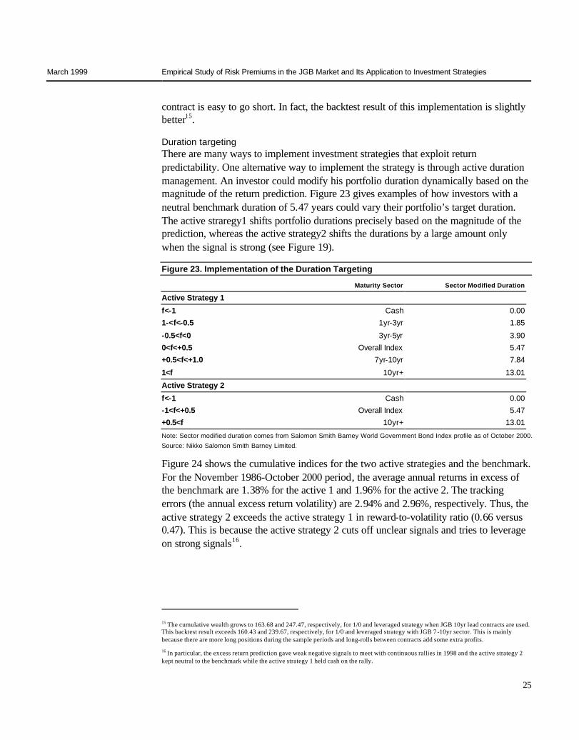
Duration targeting There are many ways to implement investment strategies that exploit return predictability. One alternative way to implement the strategy is through active duration management. An investor could modify his portfolio duration dynamically based on the magnitude of the return prediction. Figure 23 gives examples of how investors with a neutral benchmark duration of 5.47 years could vary their portfolio’s target duration. The active straregy1 shifts portfolio durations precisely based on the magnitude of the prediction, whereas the active strategy2 shifts the durations by a large amount only when the signal is strong (see Figure 19).

Figure 23. Implementation of the Duration Targeting

Maturity Sector Sector Modified Duration

Active Strategy 1

f<-1 Cash 0.00 1-<f<-0.5 1yr-3yr 1.85

-0.5<f<0 3yr-5yr 3.90 0<f<+0.5 Overall Index 5.47 +0.5<f<+1.0 7yr-10yr 7.84

1<f 10yr+ 13.01

Active Strategy 2

f<-1 Cash 0.00 -1<f<+0.5 Overall Index 5.47 +0.5<f 10yr+ 13.01

Note: Sector modified duration comes from Salomon Smith Barney World Government Bond Index profile as of October 2000. Source: Nikko Salomon Smith Barney Limited.

Figure 24 shows the cumulative indices for the two active strategies and the benchmark. For the November 1986-October 2000 period, the average annual returns in excess of the benchmark are 1.38% for the active 1 and 1.96% for the active 2. The tracking errors (the annual excess return volatility) are 2.94% and 2.96%, respectively. Thus, the active strategy 2 exceeds the active strategy 1 in reward-to-volatility ratio (0.66 versus 0.47). This is because the active strategy 2 cuts off unclear signals and tries to leverage on strong signals16.

15 The cumulative wealth grows to 163.68 and 247.47, respectively, for 1/0 and leveraged strategy when JGB 10yr lead contracts are used. This backtest result exceeds 160.43 and 239.67, respectively, for 1/0 and leveraged strategy with JGB 7 -10yr sector. This is mainly because there are more long positions during the sample periods and long-rolls between contracts add some extra profits.

16 In particular, the excess return prediction gave weak negative signals to meet with continuous rallies in 1998 and the active strategy 2 kept neutral to the benchmark while the active strategy 1 held cash on the rally.


26

Figure 24. The Cumulative Performance of the Duration Targeting Strategies

40

60

80

100

120

140

160

180

200

220

240

260

280

300

87/0

5/31

87/1

1/30

88/0

5/31

88/1

1/30

89/0

5/31

89/1

1/30

90/0

5/31

90/1

1/30

91/0

5/31

91/1

1/30

92/0

5/31

92/1

1/30

93/0

5/31

93/1

1/30

94/0

5/31

94/1

1/30

95/0

5/31

95/1

1/30

96/0

5/31

96/1

1/30

97/0

5/31

97/1

1/30

98/0

5/29

98/1

1/30

99/0

5/31

99/1

1/30

2000

/05/

31

2000

/11/

30

2001

/05/

31

Cum

ulat

ive

Perf

orm

ance

Ind

ex

Posi

tion

Active 1 Active 2

Benchmark Position1

Position2

0

1

2

3

45

Note: The above index cumulate absolute returns, not excess returns. Benchmark is the Salomon Smith Barney World Government Bond Index JGB sector. Source: Nikko Salomon Smith Barney Limited.


27

In the previous section, we tried to capitalize on buying and selling the risk premium by forecasting the time-varying bond risk premium. For some fund managers, however, this active duration strategy may be too risky. We now show lower risk strategy in a duration-neutral framework.

The Concept of Rolling Yield A rolling yield is a holding-period return given an unchanged yield curve17. When the bond risk premium hypothesis holds, the rolling yield is a bond’s near-term expected return. The n-year zero’s rolling yield is expressed in (2)’:

Rolling Yield = Sn+(n-1)x(Sn-Sn-1)=Fn-1,n (2)’

This formula is obtained by substituting S*n-1 =Sn-1 in Equation (2) , where S*n-1 is

the n-year zero’s yield level one year from now. This also equal to 1-year forward rate (n-1) year from now18.

Figure 25. Splitting a Zero’s One-period Yield Change into Two Parts

0.0

0.2

0.4

0.6

0.8

1.0

1.2

1.4

1.6

1.8

2.0

0 1 2 3 4 5 6 7 8 9 10

Maturity

Spot

Rat

e(%

)

Today's Spot Curve

Next Period's Spot Curve

Sn

Sn-1

S*n-1

A Bond's Rolldown Yield Change

The Change in a Constant-Maturity Rate at Horizon


17 This concept was introduced in Total Return Management, Martin L. Leibowitz, Salomon Brothers Inc, 1979.

18 Substituting m=n-1 in Equation (1), Fn-1,n =nSn+(n-1)x-Sn-1=Sn+(n-1)x(Sn-Sn-1).

Rolling Yield Max Strategy


28

As is shown in Figure 26, a coupon bond’s rolling yield (see Appendix) is some weighted average19 of its all cash-flow’s rolling yields, where a cash-flow’s rolling yield is a zero-coupon bond’s rolling yield computed by Equation (2)’.

Decomposing the expected returns A bond’s (expected) return is decomposed into the yield income Y, the duration impact and the value of convexity, where the duration impact is the end-of-horizon duration times ∆Y(the yield change) and the value of convexity is the end-of-horizon convexity times (∆Y)2 divided by two. We split ∆Y into ∆Yrd (=the rolldown yield change) and ∆Ycmt (=S*n-1-Sn-1 :its remainder)20. The following equation gives this

decomposition:

A bond’s return

=Y - Duration x ∆Y + 0.5xConvexityx(∆Y)2

=Y - Duration x (∆Yrd+∆Ycmt)+0.5xConvexity x (∆Yrd+∆Ycmt)2

=Rolling Yield - Duration x ∆Ycmt+0.5x Convexity x (∆Ycmt)2

Taking the expectation of both sides of the above equation and noting E(∆Ycmt)=0 if

PEH holds, we have the following equation:

A bond’s expected return = Rolling Yield + Expected value of Convexity

Next, we investigate whether this decomposition is consistent with empirical evidence. Figure 27 decomposes the realized returns from Salomon Smith Barney World Government Bond Index JGB sector for the neutral period of February 1988-December 1992.The return volatility decomposition shows that the duration impact largely drives the return: it is the main source of the monthly return fluctuations. However, yield increases and decreases tend to offset each other over time and have little impact on the long-term average returns (see Figure 28). In fact, Figure 27 shows that yield income dominates the average return over this period and the duration impact and the value of convexity occupy tiny fractions. The residual term has a small mean and volatility, indicating that the decomposition in the above formula works well empirically.

19 Equation (2)’ holds approximately for coupon bonds if we substitute their end-of-horizon durations for n -1 and their yields for spot rates(Sn). Yields of coupon bonds are the weighted average of the spot rates, and durations are the average maturities weighted by the

present values of the bond’s cash flows.

20 ∆Ycmt is originally a constant -maturity yield change, but here we also add to this, a yield change coming from the bond’s local spread

change, if any.


29

Figure 27. Decomposing Returns to Yield, Duration and Convexity Effects, Feb 88-Dec 92

0

1

2

3

4

5

6

Total Return Yield Income Dur.Impact Value of Conv. Residual

Average Return

Volatility of Return

Note: The February 1988-December 1992 is a neutral period that incorporates both yield rises and falls. Source: Nikko Salomon Smith Barney Limited.

Figure 28. Subperiod Decomposition of Bond Returns

-10.0

-5.0

0.0

5.0

10.0

15.0

Total Return Yield Income Dur.Impact Value of Conv. Residual

Feb. 1988-Dec. 1988 Jan.1989-Dec. 1989 Jan.1990-Dec.1990

Jan.1991-Dec.1991 Jan.1992-Dec.1992


Ann

ual A

vera

ge R

etur

n/V

olat

ility(

%)

Ann

ual A

vera

ge R

etur

n(%

)


30

Extracting the yield income (rolling yield) Figure 28 implies that we may be able to accumulate yield income alone by a portfolio whose yield income (or rolling yield) is greater than a certain benchmark (say our JGB index) while matching the portfolio’s duration with that of the benchmark, thereby avoiding duration impact differentials. The fact that the expected bond risk premium has been realized empirically in JGB market suggests the chances that this type of portfolio strategy works.

When the yield curve is concave overall, the kind of portfolio that pick up the rolling yield relative to the market (index) tend to be a bullet type. Thus, the portfolio gives up the convexity against the index. In addition to this convexity risk, the portfolio is vulnerable to curve flattening risk. When the yield curve is convex over all, by contrast, the rolling yield pick-up portfolio tends to be a barbell type where the portfolio pick up the convexity against the index, but is vulnerable to curve steepening.

If PEH is applied to duration-neutral bullets and barbells, concave yield curves imply curve-flattening expectations of the market: they accept a lower initial yield for barbell positions than duration-matched bullets to equate their near-term expected returns. As we saw in the earlier sections, PEH does not hold empirically. Thus, the curve flattening that would offset bullet’s initial yield advantage has not been realized on average, smoothing curve flattening risks for rolling yield pick-up bullet type portfolio in the concave curve environment. Similarly, convex yield curves imply curve steepening making barbell positions advantageous to bullets. The curve steepening that offset the barbell’s initial advantage has not materialized on average. Therefore the curve reshaping disadvantages for rolling yield pick-up portfolio will not overcome advantages of it on average. Also, Figure 27 and 28 illustrate that the convexity risk of the rolling yield pick-up portfolio (especially, when it is bullet type is minimal).


31

Rolling yield maximization strategy We implement the rolling yield maximization strategy relative to Salomon Smith Barney World Government Bond Index JGB sector to backtest our idea. We set a duration constraint and sector constraints as in Figure 30.

Figure 30. Constraints for Rolling Yield Maximization Strategy

Attribution Constraint (relative to benchmark)

Overall Average Modified Duration -0.2%∼+0.2% Sector Market Value Distribution -100%∼+200%

Sector Duration-dollar Distribution -100%∼+200%

Note: Sector is 1-3 year, 3-5 year, 5-7 year, 7-10 year, and 10 year + maturity sectors.


We constrain the overall portfolio duration within plus or minus 0.2% of the benchmark average duration, while we leave the sector constraints loose: each sector can occupy from 0 to 200% of the corresponding benchmark allocations in market values and duration dollars (as shown in the lower diagram of Figure 30).

The rolling yield maximization portfolio would invest in the sector of rolling yield peaks with such weights as to meet the overall duration constraint as in the Figure 31.

Figure 31. Constructing Rolling Yield Maximization Portfolio

0.0

0.5

1.0

1.5

2.0

2.5

3.0

0 1 2 3 4 5 6 7 8 9 10 11 12 13 14 15 16

Modified Duration

Rolling Yield

Yield to Maturity

Average Duration of The Benchmark

Rolling Yield of the Benchmark

Rolling Yield of the Portfolio

Note: Rolling yield curve is three-month rolling yield curve for coupon bonds from 1998. Source: Nikko Salomon Smith Barney Limited.

Rol

ling

Yie

ld(%

)


32

Rolling yield maximization strategy performance relative to benchmark Figure 32 reports the performance of the Rolling Yield Maximization Strategy (RollMax) for the February 1988- November 1998 period. The performance is based on monthly rebalancing and for 10 billion yen portfolio with the maximum single issue holding being 2.5 billion. Thus, the portfolio has at least four issues.

Figure 32. Performance for Rolling Yield Maximization Strategy

Feb 88-Sep

00

Feb 88-Dec 89 Jan 90-Dec 91 Jan 92-Dec 93 Jan 94-Dec 95 Jan 96-Dec 97 Jan 98-Dec 99

Average Excess 0.876% 1.942% 0.196% 1.549% 0.573% 0.842% 0.296%

Tracking Error 0.717% 1.196% 0.615% 0.577% 0.652% 0.491% 0.504%

Shape Ratio 1.222 1.624 0.318 2.682 0.879 1.714 0.587

Note: Average Excess Return is the annual average return in excess of the benchmark and Tracking error is the annual average excess return volatility. Source: Nikko Salomon Smith Barney Limited.

The average excess return for the whole period is 0.876%21 and the reward to its volatility is 1.222, which is quite good. Figure 32 also reports five 2-year subperiod performances, where all subperiod average excess returns are constantly positive.

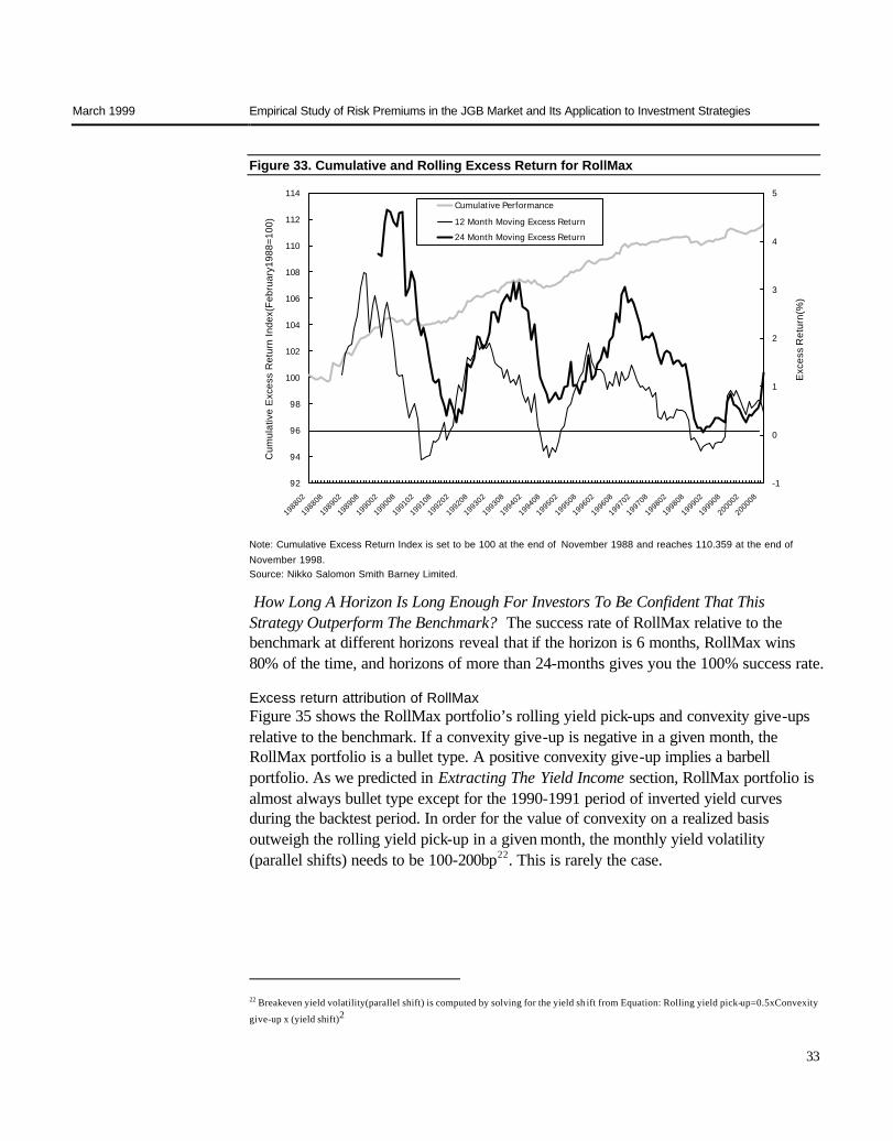
How long a horizon is long enough for investors to be confident that this strategy outperforms the benchmark Figure 33 shows the cumulative wealth growth of RollMax in excess of the benchmark. If RollMax outperform the benchmark on a cumulative basis, the line should always lie above 100 line. This is roughly what we see in the graph. Figure 33 also shows the rolling 12-month and 24-month excess return for RollMax. Though the 12-month line falls below zero line a couple of times, the 24-month line always lie above the zero line. This means that RollMax outperforms the benchmark on 24-month horizons 100% of the time during the sample period.

21 The average turnover was approximately seven times for the monthly rebalancing. Because the portfolio duration is matched with benchmark all the time, it ranges from 5 to 6 years. Thus, assuming a transaction cost of 6c a turnover, the annual estimated cost is 40c as opposed to 90c of annual profit. Unpublished simulation for quarterly rebalancing reveals three times a year turnover and the performance is almost the same as the monthly rebalancing.


33

Figure 33. Cumulative and Rolling Excess Return for RollMax

92

94

96

98

100

102

104

106

108

110

112

114

1988

02

1988

08

1989

02

1989

08

1990

02

1990

08

1991

02

1991

08

1992

02

1992

08

1993

02

1993

08

1994

02

1994

08

1995

02

1995

08

1996

02

1996

08

1997

02

1997

08

1998

02

1998

08

1999

02

1999

08

2000

02

2000

08

-1

0

1

2

3

4

5

Exce

ss R

etur

n(%

)

Cumulative Performance

12 Month Moving Excess Return

24 Month Moving Excess Return

Note: Cumulative Excess Return Index is set to be 100 at the end of November 1988 and reaches 110.359 at the end of November 1998. Source: Nikko Salomon Smith Barney Limited.

How Long A Horizon Is Long Enough For Investors To Be Confident That This Strategy Outperform The Benchmark? The success rate of RollMax relative to the benchmark at different horizons reveal that if the horizon is 6 months, RollMax wins 80% of the time, and horizons of more than 24-months gives you the 100% success rate.

Excess return attribution of RollMax Figure 35 shows the RollMax portfolio’s rolling yield pick-ups and convexity give-ups relative to the benchmark. If a convexity give-up is negative in a given month, the RollMax portfolio is a bullet type. A positive convexity give-up implies a barbell portfolio. As we predicted in Extracting The Yield Income section, RollMax portfolio is almost always bullet type except for the 1990-1991 period of inverted yield curves during the backtest period. In order for the value of convexity on a realized basis outweigh the rolling yield pick-up in a given month, the monthly yield volatility (parallel shifts) needs to be 100-200bp22. This is rarely the case.

22 Breakeven yield volatility(parallel shift) is computed by solving for the yield sh ift from Equation: Rolling yield pick-up=0.5xConvexity

give-up x (yield shift)2

Cum

ulat

ive

Exc

ess

Ret

urn

Inde

x(Fe

brua

ry19

88=1

00)

Exc

ess

Ret

urn(

%)


34

Figure 35. Rolling Yield Pick-up and Convexity Give-up

-0.20

-0.15

-0.10

-0.05

0.00

0.05

0.10

0.15

0.20

1988

02

1988

07

1988

12

1989

05

1989

10

1990

03

1990

08

1991

01

1991

06

1991

11

1992

04

1992

09

1993

02

1993

07

1993

12

1994

05

1994

10

1995

03

1995

08

1996

01

1996

06

1996

11

1997

04

1997

09

1998

02

1998

07

1998

12

1999

05

1999

10

2000

03

2000

08

Conv

exity

Giv

eup(

%)

-1.0

-0.8

-0.6

-0.4

-0.2

0.0

0.2

0.4

0.6

0.8

1.0

1.2

1.4

1.6

1.8

2.0

Rolli

ng Y

ield

Pic

kup(

%)

Convexity Giveup

Rolling Yield Pickup


Next, we examine the curve reshaping risk: the curve flattening for bullet portfolios and the curve steepening for barbell portfolios.

Figure 36 decomposes RollMax’s average excess return relative to the benchmark in subperiods.


35

Figure 36. Decomposition of RollMax Excess Return

-1.0

-0.5

0.0

0.5

1.0

1.5

2.0

Total Return Yield imcome Rolldown Impact Curve Reshaping

Effect

Value of Convexity Residual

Exce

ss R

etur

n to

Ind

ex(%

)

Feb.1988-Dec.1989

Jan.1990-Dec.1991

Jan.1992-Dec.1993

Jan.1994-Dec.1995

Jan.1996-Dec.1997

Jan.1998-Dec.1999


Using notations from Page 27, we have:

Yield income=Y(P)-Y(I);

Rolldown Impact=-(∆Yrd(P)xDur(P)-∆Yrd(I)xDur(I))

≅-(∆Yrd(P)-∆Yrd(I))xDur(P,I)

Curve Reshaping Effect=-(∆Ycmt(P)xDur(P)-∆Ycmt(I)xDur(I))

≅-(∆Ycmt(P)-∆Ycmt(I))xDur(P,I)

Value of Convexity=0.5x(Convx(P)x(∆Y(P))2-Convx(I)x(∆Y(I))2)

where P and I in parenthesis denote portfolio and index, respectively; Dur and Convx denote modified duration and convexity. Also, note ∆Y=∆Yrd+∆Ycmt. The approximation holds in Rolldown Impact and

Curve Reshaping Effect, because we constrain Dur(P)≈ Dur(I) in this strategy.

Figure 36 shows that the contributions from yield income and the rolldown impact(combined is the rolling yield impact) are constantly positive. This is natural because we maximize rolling yields. The differential between the portfolio yield change and the benchmark yield change is divided into two portions: one is attributed to the difference in rolldowns and the others. The other portion is mainly attributed to the curve reshaping. For instance, if the curve flattens when RollMax strategy holds a bullet portfolio in a given month, the portfolio yield goes up relative to the overall market (the benchmark). The curve reshaping effect is, then, negative in the month. As Figure 36


36

and 37 illustrates, the curve reshaping effects over different subperiods offset each other to have little impact over a long horizon, just like the duration impact (RollMax has negligible duration impact because of the duration constraint) does to the absolute bond returns.

Figure 37 displays the cumulative impact of each attribution. The curve reshaping cumulative effect goes up and down to revert to the positive mean (this is consistent with the denial of PEH for duration-matched bullets and barbells), while the yield income and the rolldown impact cumulates constantly. The longer horizon makes the rolling yield attribution more dominant in the overall cumulative excess return relative to the benchmark.

Figure 37. Cumulative Impact of Each Attribution

-4

-2

0

2

4

6

8

10

12

1988

02

1988

07

1988

12

1989

05

1989

10

1990

03

1990

08

1991

01

1991

06

1991

11

1992

04

1992

09

1993

02

1993

07

1993

12

1994

05

1994

10

1995

03

1995

08

1996

01

1996

06

1996

11

1997

04

1997

09

1998

02

1998

07

1998

12

1999

05

1999

10

2000

03

2000

08

Cum

ulat

ive

Exce

ss R

etur

n At

trib

utio

n(%

)

Total_Return

Yield Impact

Rolldown

Yield Chg

Convexity Impact

Res..



37

In this section, we summarize what we have found throughout this report.

The pure expectations hypothesis and the bond risk premium Empirical Evidence in the JGB market suggests that one-period forwards (=Fn-1,n) are

comparatively better predictors for expected bond returns a lot more than the implied forward rates(=F1,n) are predictors for future spot rates. Thus, the bond risk premium

holds rather than PEH over a long period.

Empirical evidence about the bond risk premium in the JGB market We have found that the positive bond risk premium exists over a long and neutral period in the JGB market. We plot the geometric mean returns on the return volatilities and see a monotonical increase in the mean return up to 5-6 year sector. Beyond this maturity sector, however, we do not observe further increases in the mean return. As a peculiar phenomenon in the JGB market, we observe the extra average bond return in 19-20 year super-long JGB sector that is associated with the liquidity premium. Also, the subperiod analysis shows that the magnitude of the bond risk premium varies over time.

Predicting the bond risk premium and the dynamic strategy We have shown that long-term bond returns are predictable. A set of four predictors- yield curve steepness, real bond yield, recent stock market performance (inverse wealth), and bond market momentum- is able to forecast 15% of the monthly variation in long-term bonds’ excess returns. The dynamic strategies (especially the leveraged strategy) that exploit the excess bond return predictability have consistently outperformed the cash and the static bond investment strategy over long investment horizons. The leveraged strategy that takes into account the magnitude of the forecasts, not just the sign, excels in the reward to volatility of all strategies, highlighting that the significance of the predictor's magnitude. The subperiod performances show stability of the dynamic strategies, with positive performances during bear markets by avoiding long bonds.

Rolling yield maximization strategy While the dynamic strategies take duration risks based on the return forecasts, the RollMax strategy stay duration neutral to the benchmark and try to cumulate the bond risk premium (= rolling yields). Though this strategy takes curve reshaping risks and convexity risks, we have demonstrated that the RollMax outperform the benchmark 100% over two-year or longer horizons. We observe that the convexity risks are minimal and the curve reshaping risks cancel out over time.

Summary


38

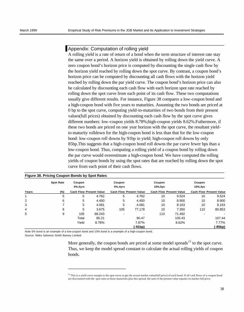
Appendix: Computation of rolling yield A rolling yield is a rate of return of a bond when the term structure of interest rate stay the same over a period. A horizon yield is obtained by rolling down the yield curve. A zero coupon bond’s horizon price is computed by discounting the single cash flow by the horizon yield reached by rolling down the spot curve. By contrast, a coupon bond’s horizon price can be computed by discounting all cash flows with the horizon yield reached by rolling down the par yield curve. The coupon bond’s horizon price can also be calculated by discounting each cash flow with each horizon spot rate reached by rolling down the spot curve from each point of its cash flow. These two computations usually give different results. For instance, Figure 38 compares a low-coupon bond and a high-coupon bond with five years to maturities. Assuming the two bonds are priced at 0 bp to the spot curve, computing yield-to-maturities of two bonds from their present values(full prices) obtained by discounting each cash flow by the spot curve gives different numbers: low-coupon yields 8.78%;high-coupon yields 8.62%.Futhermore, if these two bonds are priced on one year horizon with the spot curve, the resultant yield-to-maturity rolldown for the high-coupon bond is less than that for the low-coupon bond: low-coupon roll downs by 91bp in yield; high-coupon roll downs by only 85bp.This suggests that a high-coupon bond roll downs the par curve fewer bps than a low-coupon bond. Thus, computing a rolling yield of a coupon bond by rolling down the par curve would overestimate a high-coupon bond. We have computed the rolling yields of coupon bonds by using the spot rates that are reached by rolling down the spot curve from each point of their cash flows.

Figure 38. Pricing Coupon Bonds by Spot Rates

Spot Rate Coupon 5%,5yrs

Coupon 5%,4yrs

Coupon 10%,5ys

Coupon 10%,4ys

Years (%) Cash Flow Present Value Cash Flow Present Value Cash Flow Present Value Cash Flow Present Value

1 5 5 4.762 5 4.762 10 9.524 10 9.524 2 6 5 4.450 5 4.450 10 8.900 10 8.900 3 7 5 4.081 5 4.081 10 8.163 10 8.163 4 8 5 3.675 105 77.178 10 7.350 110 80.853 5 9 105 68.243 - - 110 71.492 - - Total 85.21 90.47 105.43 107.44 Yield 8.78% 7.87%

(-91bp) 8.62% 7.77%

(-85bp) Note 5% bond is an example of a low-coupon bond and 10% bond is a example of a high-coupon bond. Source: Nikko Salomon Smith Barney Limited.

More generally, the coupon bonds are priced at some model spreads23 to the spot curve. Thus, we keep the model spread constant to calculate the actual rolling yields of coupon bonds.

23 This is a yield curve margin to the spot curve to get the actual market value(full price) of each bond. If all cash flows of a coupon bond are discounted with the spot rates at those maturities plus this spread, the sum of the present value equates its market full price.


39

Figure 39. Rolling Yields Based On Spot Curves and Par Curves

0

0.2

0.4

0.6

0.8

1

1.2

1.4

1.6

1.8

0 2 4 6 8 10 12 14 16 18 20

Maturity

Rolli

ng Y

ield

(%)

Based on Par Curve

Based on Spot Curve

Note: As of fall 1998. Source: Nikko Salomon Smith Barney Limited.

Figure 39 displays the difference between par curve based and spot curve based rolling yields for coupon bonds (JGBs). Eleven to 15 year sector is the most obviously different, because the super-long JGBs in this sector have higher coupons (therefore deep overpar in price) and the immediate curves are upward sloping. These bonds illustrate overestimation of par based rolling yields relative to spot-based equivalents. In 19-year - 20-year sector (the long end of the curve), the bonds are priced at overpar but the immediate curve is inverted (rollup rather than roll down). In this case, the par curve-based rolling yields are underestimated. Ten year #207 is among the few underpar priced (=low coupon bond) bond at this point and because the immediate curve is upward sloping, its par curve-based rolling yield is underestimated24.

24 At the end of 1998, we saw an example of underpar priced low-coupon bonds whose adjacent curve is inverted when the JGB market crashed, their par curve based rolling yields were overestimated relative to the spot curve based counterparts.


40

References Overview of Forward Rate Analysis (Part 1), Ilmanen, A., May 1995.

Market’s Rate Expectations and Forward Rates (Part 2), Ilmanen, A., June 1995.

Does Duration Extension Enhance Long-term Expected Returns? (Part 3), Ilmanen, A., July 1995.

Forecasting U.S. Bond Returns (Part 4), Ilmanen, A., August 1995.

Convexity Bias and the Yield Curve (Part 5), Ilmanen, A., September 1995.

A Framework for Analyzing Yield Curve Trades (Part 6), Ilmanen, A., November 1995.

Modern Fixed-income Investment Analysis, Takuma Takahashi, Nikkei Publishing, July 1988.

Estimating and Interpreting the Yield Curve, Nicola Anderson, Francis Breedon, Mark Deacon, Andrew Derry and Gareth Murphy, Wiley 1996.

Yield Curve and The Term Structure of Interest Rates, Salomon Brothers Asia Ltd., August 1988.

Satoshi Yamada, 1999. “Risk Premiums in the JGB Market and Application to Investment Strategies”, The Journal of Fixed Income, vol.9, no.2

Empirical Study of Risk Premiums in the JGB Market and Its Application to Investment Strategies

41

ADDITIONAL INFORMATION AVAILABLE UPON REQUEST

This report was prepared by Nikko Salomon Smith Barney Limited (“Nikko Salomon Smith Barney”).

Nikko Salomon Smith Barney is affiliated for certain U.S. regulatory purposes with Citibank, N.A. and its subsidiaries and branches worldwide (collectively "Citibank"). Despite those affiliations, securities recommended, offered, sold by, or held at, Nikko Salomon Smith Barney, or its affiliates: (i) are not insured by the Federal Deposit Insurance Corporation; (ii) are not deposits or other obligations of any insured depository institution (including Citibank); and (iii) are subject to investment risks, including the possible loss of the principal amount invested.

Nikko Salomon Smith Barney, including its parent, subsidiaries and/or affiliates (the “Firm”), may from time to time perform investment banking or other services for, or solicit investment banking or other business from, any company mentioned in this report. For the securities discussed in this report, the Firm may make a market and may sell to or buy from customers on a principal basis. The Firm, or any individuals preparing this report, may at any time have a position in any securities or options of any of the issuers in this report. An employee of the Firm may be a director of a company mentioned in this report.

Although the statements of fact in this report have been obtained from and are based upon sources we believe to be reliable, we do not guarantee their accuracy, and any such information may be incomplete or condensed. All opinions and estimates included in this report constitute our judgment as of the date of this report and are subject to change without notice. This report is for informational purpos es only and is not intended as an offer or solicitation with respect to the purchase or sale of a security. # Within the past three years, Nikko Salomon Smith Barney Limited, Salomon Smith Barney Inc. and/or The Nikko Securities Co., Ltd., and/or their respective subsidiaries and/or affiliates, have acted as manager or co-manager of a public offering of this company.

Salomon Smith Barney is a service mark of Salomon Smith Barney Inc.

Nikko is a service mark of The Nikko Securities Co., Ltd.

© Nikko Salomon Smith Barney Limited, 1999. All rights reserved. Any unauthorized use, duplication or disclosure is prohibited by law and will result in prosecution.

First Class Mail

US Postage

PAID

New York, NY

Permit No. 8155

JP-1999-1001

Documents

Empirical Study of Risk Premiums in the JGB Market and Its ... · Cor(FSPn,BRPn) Source: Nikko Salomon Smith Barney Limited. Figure 4. Correlations of FSPn with D Sn-1 During the