Embed Size (px)
Citation preview

Sensors 2008, 8, 4915-4947; DOI: 10.3390/s8084915
sensors ISSN 1424-8220
www.mdpi.org/sensors Article
Empirical Retrieval of Surface Melt Magnitude from Coupled MODIS Optical and Thermal Measurements over the Greenland Ice Sheet during the 2001 Ablation Season
Derrick Lampkin * and Rui Peng
Department of Geography, College of Earth and Mineral Sciences, Pennsylvania State University,
USA; E-Mails: [email protected] (F. L.); [email protected] (F. L.)
* Author to whom correspondence should be addressed; Tel.: (814)-865-2493; Fax: (814)-863-7943
Received: 3 July 2008; in revised form: 22 July 2008 / Accepted: 15 August 2008 /
Published: 22 August 2008
Abstract: Accelerated ice flow near the equilibrium line of west-central Greenland Ice
Sheet (GIS) has been attributed to an increase in infiltrated surface melt water as a response
to climate warming. The assessment of surface melting events must be more than the
detection of melt onset or extent. Retrieval of surface melt magnitude is necessary to
improve understanding of ice sheet flow and surface melt coupling. In this paper, we report
on a new technique to quantify the magnitude of surface melt. Cloud-free dates of June 10,
July 5, 7, 9, and 11, 2001 Moderate Resolution Imaging Spectroradiometer (MODIS) daily
reflectance Band 5 (1.230-1.250µm) and surface temperature images rescaled to 1km over
western Greenland were used in the retrieval algorithm. An optical-thermal feature space
partitioned as a function of melt magnitude was derived using a one-dimensional thermal
snowmelt model (SNTHERM89). SNTHERM89 was forced by hourly meteorological data
from the Greenland Climate Network (GC-Net) at reference sites spanning dry snow,
percolation, and wet snow zones in the Jakobshavn drainage basin in western GIS. Melt
magnitude or effective melt (E-melt) was derived for satellite composite periods covering
May, June, and July displaying low fractions (0-1%) at elevations greater than 2500m and
fractions at or greater than 15% at elevations lower than 1000m assessed for only the upper
5 cm of the snow surface. Validation of E-melt involved comparison of intensity to dry and
wet zones determined from QSCAT backscatter. Higher intensities (> 8%) were distributed
in wet snow zones, while lower intensities were grouped in dry zones at a first order
accuracy of ~ ±2%.
OPEN ACCESS

Sensors 2008, 8
4916
Keywords: Greenland, remote sensing, surface melt.
1. Introduction
The changing masses of Greenland and Antarctica represent the largest unknown in predictions of
global sea-level rise over the coming decades (Dowdeswell, 2006). Recent analysis suggests that the
contribution of the Greenland and Antarctic Ice Sheets to present-day sea level rise is more than 0.3
millimeters per year (Krabill et al., 2000; Rignot and Thomas, 2002; Shepherd and Wingham, 2007).
Changes in surface temperature on these large ice masses can affect the rate of ice deformation or basal
sliding (Zwally et al., 2002). Rapid increases in the extent and duration of surface melt have been
detected using satellite imagery along the surface of southern Greenland and parts of Antarctica (Jezek
et al., 1992; Ridley, 1993; Zwally and Fiegles, 1994; Abdalati and Steffen, 1995; Mote and Anderson,
1995, and several others.) Zwally et al. (2002) have demonstrated that ice flow speed increases during
the summer melt season. Rignot and Kanagaratnam (2006) have confirmed acceleration of ice flow
over a large part of coastal Greenland between 1996 and 2000 from radar interferometry and attribute
this to recent climate warming.
In recent years, observations of ice sheet physical properties and dynamic behavior have shifted
from in-situ observations towards satellite techniques (Lubin and Masson, 2006). The ability of
satellite systems to acquire data over vast areas of remote terrain, during the day or night and in all
weather conditions has facilitated this shift (IGOS, 2007). A variety of satellite instruments sensitive to
different parts of the electromagnetic (EM) spectrum provide rich data sets of elevation, motion,
accumulation on ice sheets (Bindschadler, 1998). Understanding the mechanism and features of the
current approaches of modeling of ice sheet melt is critical to improve the assessment of melt dynamics
over Greenland Ice Sheet (GIS). This work demonstrates a novel approach to improve the assessment
of melt dynamics by expanding satellite derived estimates of melt from a binary measure of occurrence
to melt magnitude or intensity.
2. Background
Snow is a mixture of ice, liquid water and air. The dielectric constant of snow is derived from a
weighted average of the dielectric constants of these components (Matzler et al, 1984). The real part of
the dielectric constant of ice has a value of 3.17 throughout the microwave region. Specifically,
microwave emission in dry snow is dominated by scattering (Cumming, 1952; Tiuri et al., 1984; Rees,
2006). Consequently, liquid water in wet snow increases the dielectric constant of snow and thus
enhances emissivity and absorption of microwave radiation (Chang et al., 1976; Tiuri et al., 1984;
Hallikainen, 1986). Given these relationships between microwave emission and ice properties, airborne
and satellite based systems have been used successfully to map ice properties and assess surface and
near-surface melt conditions. Active radar systems such as Synthetic Aperture Radar (SAR) provide
high-resolution observations of microwave radar backscatter, and have been applied to study GIS
surface and near-surface properties and ice dynamics (Fahnestock et al., 1993). Ranging radars
operating at 5.3 GHz and 13.3 GHz have been used and compared with in-situ data by Jezek et al.
(1994) to interpret melt-related processes on the GIS. NASA Scatterometer data (NSCAT) were

Sensors 2008, 8
4917
combined with Seasat Scatterometer (SASS) data and ERS-1/2 Scatterometer data (ESCAT) to map ice
sheet melt extent (Long and Drinkwater, 1999). Due to its ability to penetrate into snow, normalized
radar cross section (NRCS) measurements from C-band (5.3 GHz) scatterometers were used to monitor
seasonal snowmelt on Greenland by Wismann (2000).
Rapid increases in the extent and duration of surface melt on the GIS from 1978 to the present have
been detected from passive microwave systems such as the Scanning Multi-channel Microwave
Radiometer (SMMR) and the Special Sensor Microwave/Imager (SSM/I) deployed on several Defense
Meteorological Satellite platforms (http://cires.colorado.edu/steffen/).
The presence of liquid water has a dramatic effect on the microwave properties of snow. The
Rayleigh-Jeans approximation for radiation in the microwave part of the EM spectrum is
TTb ελ =)( (1)
where Tb is the brightness temperature, ε is the microwave emissivity, and T is the effective physical
temperature of the snow (Abdalati and Steffen, 1997). Compared with dry snow, whose dielectric
constant is a function of density only in the microwave region, the dielectric behavior of wet snow is a
function of its physical parameters and frequency (Hallikainen et al., 1986). Therefore, according to the
Rayleigh-Jeans approximation, the emissivity is relatively constant over time for dry snow, in which
case the Tb is approximately a linear function of T. When melt occurs, liquid water causes a large
increase in the emissivity of snow and results in a corresponding increase in Tb (Ashcraft and Long,
2003).
Changes in Tb at 19 and 37 GHz have been used as a metric for determining melt onset (Zwally and
Fiegles, 1994; Ridley, 1993, and Mote and Anderson, 1995). Steffen et al., (1993) identified wet snow
regions using AVHRR (Advanced Very High Resolution Radiometer), SMMR, SSM/I and in-situ data,
based on the relationships between in-situ measurements and horizontally polarized 19 and 37 GHz
observation. Specifically, the cross-polarization gradient ratio (XPGR) (Abdalati and Steffen, 1995)
approach was used to assess melt zones. XPGR indicates melt when the snow surface contains greater
than 1% liquid water by volume. To study seasonal and inter-annual variations in snow melt extent of
the ice sheet, Abdalati and Steffen (1997) established melt thresholds in the XPGR by comparing
passive microwave satellite data to field observations. Ashcraft and Long (2005) studied the
differentiation between melt and freeze stages of the melt cycle using the SSM/I channel ratios. In
2006, these authors assessed melt detection performance from SSM/I, SeaWinds on QuikSCAT
(QSCAT), and the European Remote Sensing (ERS) Advanced Microwave Instrument (AMI) in
scatterometer mode, and concluded that melt estimates from different sensors were highly correlated.
The difference between ascending and descending brightness temperatures (DAV) (Ramage and Isacks,
2002) measured either at 19.35- or 37- GHz by SSM/I was applied to map melt extent in Greenland,
and the results compared with those obtained from QSCAT (Nghiem et al., 2001; Tedesco, 2007).
Although active and passive microwave systems have performed well in monitoring melt conditions
over the GIS, they are limited in the amount of detail that can be either spatially or temporally resolved.
Passive systems have relatively coarse spatial resolution and generally results from maintaining high
radiometric resolution, while active systems demonstrate limited or lower temporal resolution

Sensors 2008, 8
4918
(Campbell, 2007). Active systems such as SAR in high-resolution observations of microwave radar
backscatter have 16-day ground track repeat cycle, which is too infrequent to capture dynamic melt
conditions.
Other parts of the EM spectrum offer potential advantages for monitoring melt over the GIS, and
may augment the shortcomings of microwave systems. Data from optical satellites have been used to
map surface dynamics related to the melt process over the GIS at higher spatial resolutions. Hall et al.
(1990) compared in-situ measurements with Landsat Thematic Mapper (TM)-derived reflectance on
Greenland and concluded that Landsat TM was viable to obtain the physical reflectance of snow and
ice. AVHRR visible and near-infrared radiances were used to derive surface albedo over the GIS and
were validated by in-situ data (Stroeve et al., 1997). Products from the Moderate Resolution Imaging
Spectroradiometer (MODIS) were also widely used to retrieve snow albedo over Greenland, and have
been compared with in-situ measurements and with other instruments such as Multi-angle Imaging
SpectroRadiometer (MISR) separately (Stroeve and Nolin, 2002a; Stroeve et al., 2004). Stroeve and
Nolin (2002b) developed two different methods to derive the snow albedo over the GIS: one utilizing
the spectral information from MISR and one based on angular information from the MISR instrument.
Their results indicated that the accuracy of either of those two methods was within 6% compared of in-
situ measurements. Hall et al. (2004) compared MODIS with SSM/I-derived melt extent in summer of
2002 and concluded that the results are not, and should not necessarily be, the same. They also
suggested that MODIS and SSM/I data were complementary in providing detailed information about
the maximum snow melt on the GIS.
Satellite derived thermal information over GIS has been addressed over the past two decades (Key
and Haefliger, 1992; Haefliger et al., 1993; Comiso et al., 2003 and others). Specifically, Hall et al.
(2006) examined mean clear-sky MODIS derived surface temperature over GIS from 200 to 2005
during the melt season and have determined that during periods of intense melting, surface
temperatures were highest in 2002 (-8.29 ± 5.29°C) and 2005 (-8.29 ± 5.43°C) relative to the 6-year
mean (-9.04 ± 5.59°C). More Recently, Hall et al. (2008) assessed the relationship between ice sheet
mass balance and the spatio-temporal variability of MODIS retrieved surface temperature over GIS
from 2000 to 2006. Daily, clear-sky MODIS land-surface temperature (LST) was compared to changes
in mass concentration derived from the Gravity Recovery and Climate Experiment (GRACE) system
and assessed that a mean LST increase (~0.27°C per year) over this period was associated with an
increase in melt season length and rapid mass loss during significant warming events, particularly at
elevations below 2000 meters in 2004 and 2005.
Surface melt patterns and their duration are an important component of ice sheet mass balance, and
have been successfully measured, however estimation of ice sheet surface melt amount is still under-
determined from passive microwave approaches. The missing link in improved modeling of ice sheet
response to an increase in temperature is a full assessment of surface melt amount.
2.1. Optical and Thermal Radiative Theory
Surface albedo, which influences the amount of absorbed solar radiation, can vary due to several
factors such as grain-size, emission angle, snow density, surface impurities, and liquid water content
(Dozier and Warren, 1982). Previous work has examined the strong relationship between snow spectral

Sensors 2008, 8
4919
reflectance and grain-size, and modeled snow reflectance from the optical properties of snow and ice
(Bohren and Barkstrom, 1974; Wiscombe and Warren, 1981; Nolin and Dozier, 2000; Painter et al.,
2003). The optical properties of snow indicate high reflectance in the visible (0.4-0.7µm), and parts of
the Near Infrared (NIR) (0.7-1.3µm) regions of the EM spectrum. Snow reflectance demonstrates
substantial decrease in the Shortwave Infrared (SWIR) (1.3-3µm) due to increase in absorption.
In the visible and NIR regions of EM spectrum, the optical properties of snow depend, in large part,
on the refractive index of ice (Dozier, 1989). Absorption is due to variation in the imaginary part of the
complex refractive index of ice given as:
where n = real part of the refractive index, k = imaginary part of refractive index.
The absorption coefficient (i.e., the imaginary part of the refractive index) varies substantially in the
wavelengths from 0.4 to 2.4 um. In the near-infrared region of EM spectrum, the reflectance of wet
snow is lower than that of dry snow, but mainly because of micro-structural changes caused by the
water (Dozier, 1989).
Specifically, in wet snow with high liquid water content, heat flow from large grains causes smaller
particles, which are at lower temperature, to melt and merge into larger clusters (Colbeck, 1982;
Colbeck, 1989). As bulk grain cluster radius increases, an incident photon will have a high probability
of being scattered when it transverses the air-ice interface, but a greater chance of absorption while
passing through the ice grain (Warren, 1982). Grain clusters optically behave as single grains,
increasing the mean photon path length, subsequently increasing the opportunity for absorption and
reduction in reflectance. Larger grains increase the degree of absorption, particularly in the shortwave
infrared region, causing a substantial reduction in reflectance. The maximum sensitivity of reflectance
to changes in grain size is in the shortwave (SWIR) region of the EM spectrum at approximately 1.1
um (Nolin and Dozier, 2000).
The use of snow surface reflectance alone to track the surface melt process is not sufficient, because
substantial decreases in reflectance are not due solely to grain enlargement associated with entrained
liquid water. For example, small amounts of absorbing impurities can also reduce snow reflectance in
the visible wavelength (Warren and Wiscombe, 1981). As low as 0.1 ppmw (parts per million by
weight) of soot concentrations are enough to reduce reflectance perceptibly, and the effect is
significantly enhanced when the impurities are inside the snow grains, because refraction focuses the
light on the absorber (Grenfell et al., 1981; Bohren, 1986). In this case, surface temperature can be used
as a plausible mechanism in isolating the component in reduced reflectance that is due to the melt
process.
Snow-cover melt dynamics in the thermal infrared region (8-14um) of the EM spectrum are a
function of incident radiation as well as surface longwave emission, which is a function of snow
surface temperature and emissivity (Marks and Dozier, 1992). The relationship is given as follows:
ikn +=ε (1)

Sensors 2008, 8
4920
where Tb is brightness temperature, which is defined as the temperature of a blackbody for a given
wavelength that emits the same amount of radiation at that wavelength as does the snow; T is surface
temperature; ε is the emissivity of snow; λ is wavelength; and h, c, k are constants(Dozier and Warren,
1982).
Therefore, the combination of optical and thermal signatures is an effective way to monitor the
evolution of surface melt dynamics. Lampkin and Yool (2004a) have evaluated MODIS visible and
NIR bands for monitoring snowpack ripeness and suggested that couple optical/thermal measurements
have the potential to detect snowpack evolution during the melt season. Furthermore, Lampkin and
Yool (2004b) have assessed surface snowmelt by developing a near-surface moisture index (NSMI)
that uses optical and thermal variables.
3. Methods
3.1 Data
MODIS 8-day composite, 1 km2 resolution Land Surface Temperature (LST) (MOD11A2) version 5
(Wan et al., 2002) and 500m resolution Surface Reflectance (MOD09A1) version 5 (Vermote et al.,
2002) products were used in this project. The primary advantage using optical and thermal
measurements over passive microwave is the enhanced spatial resolution, while a major disadvantage
is the reduced spatial coverage due to clouds. The effect of cloud cover is a major source of noise due
to similar radiative behavior of clouds and snow in VIS, NIR, and SWIR regions of EM spectrum
except at around 1.6 um. Generally, snow is a collection of ice grains, air, and liquid water, and often
includes particulate and chemical impurities. Similarly, clouds contain water droplets, ice crystals and
usually some impurities (Dozier, 1989). This similarity makes it difficult to distinguish snow and cloud
in those regions of the EM spectrum. In addition, persistent cloud cover over Greenland is a severe
limitation to full coverage daily acquisitions (Klein and Stroeve, 2002). The 8-day composite products
were selected because they have fewer cloud cover than daily images, and increase coverage of the
study area. MOD09A1 provides Bands 1-7 in an 8-day gridded level-3 product. Each MOD09A1 pixel
was selected based on high observation coverage, low sensor view angle, the absence of clouds or
cloud shadowing, and aerosol loading, producing the best possible daily observation during an 8-day
period (http://edcdaac.usgs.gov/modis/mod09a1v5.asp). MOD11A2 were composited from the daily
1km LST product and stored on a 1km grid as the average values of clear-sky LST during an 8-day
period (http://edcdaac.usgs.gov/modis/mod11a2v5.asp). There are a total of three 8-day composite
scenes during the study period, spanning the period May 25 to June 17, 2001. All MODIS products
used in this analysis were acquired over tiles H15V02, H16V02, H16V01, and H17V01. There are two
tiles (H16V00, H17V00) of reflectance data over the GIS missing for the entire period.
−+=
εελ
µλ λ 1elnk
hc),(T
T)hc/(kvb (2)

Sensors 2008, 8
4921
QSCAT backscatter data were used to derive an estimate of wet and dry firn regions as a relative
validation of the melt magnitude retrieval algorithm. QSCAT Enhanced Resolution Image products
have wide swath and frequent over- flights, which permit generation of a wide variety of products.
QSCAT is a dual-pencil-beam conically scanning scatterometer with the outer beam V-pol and the
inner beam H-pol (http://www.scp.byu.edu/data/Quikscat/SIR/Quikscat_sir.html). The 2.225 km
QSCAT Greenland H-pol and V-pol all-pass products were used for the comparison due to their high
spatial resolution. Local overpass times for QSCAT ascending and descending orbits were
approximately 6am and 6pm. Nghiem et al. (2001) have mapped snowmelt regions on GIS using
SeaWinds Ku-band (13.4GHz) scatterometer on the QSCAT satellite by thresholding the difference in
day and night backscatter images. This method defines the dry-snow zone on the ice sheet when the
diurnal backscatter change is less than 1.8dB, and the wet-snow zone when the diurnal backscatter
change is larger than 1.8dB (Nghiem et al., 2001).
The Greenland Climate Network (GC-Net), established in 1995 monitors the climatology of GIS,
and consisted of 18 Automatic Weather Stations (AWS) by 2001 (Figure 1) (Steffen and Box, 2001).
Each AWS is equipped with a number of meteorological instruments (Table 1) that measure
precipitation, incoming and outgoing shortwave and net radiation, air temperature, relative humidity,
barometric pressure, wind speed and direction as well as snow pack temperature (Steffen and Box,
2001). Data from CP1 (Crawford Point 1), JAR1, and JAR2 stations were selected for this analyses
because they span a range in elevation from 2022 to 568 meters, which represents a range of melt
conditions from the accumulation to the ablation zones of the ice sheet (Table 2).
Figure 1. Location of stations in the Greenland Climate Network (GC-NET) as well as
ice sheet elevation (Source: http://cires.colorado.edu/science/groups/steffen/gcnet/).

Sensors 2008, 8
4922
Table 1. Greenland Climate Network Automatic Weather Station Instruments
Parameter Instrument Instrument Accuracy Sample Interval Air temperature Air temperature Relative humidity Wind speed * Wind direction Station pressure Surface height change Shortwave radiation Net radiation Snow temperature Data logger Multiplexer GPS Solar panel
Vaisala CS-500 Type-E Thermocouple Vaisala Intercap RM Young Propeller-type Vane RM Young Vaisala PTB 101B Campbell SR-50 Li Core SI Photodiode REBS Q7 Type-T Thermocouple Campbell Scientific 10X Campbell Scientific Am25T Garmin Campbell Scientific 20 w
0.1ºC 0.1ºC 5%<90%, 10%>90% 0.1m s-1
5º 0.1mb 1mm 5-15% 5-50% 0.1º 1s
60 s*, 15 s 60 s*, 5 s
60 s 60 s*, 15 s
60 s 60 min 10 min
15 s 15 s 15 s
1day
Sample was taken each 15 s after 1999 site visit except NGRIP AWS. (Steffen and Box, 2001)
Table 2. GC-Net Stations used in Calibration Modeling Phase
Station Name Latitude and Longitude Altitude (m) Crawford Point 1 JAR1 JAR2
69.8819N, 46.9736W 69.4984N, 49.6816W 69.4200N, 50.0575W
2022 962 568
3.2 Model Development Scheme
Retrieval of melt magnitude is derived from coupled satellite surface reflectance and temperature
observations, calibrated by model snowmelt estimates of liquid water content. Figure 2 depicts the
algorithm development process, which is divided into the Calibration and Spectral modeling phases.
The Calibration modeling phase produces estimates of snow pack near surface bulk liquid water
content using the physical-based snowmelt model SNTHERM89. SNTHERM89 is a one-dimensional
mass and energy balance model for estimating mass and energy flux through strata of snow and soil. It
is comprehensive in scope, capable of simulating dynamic processes (Jordan, 1991). The version used
in this project was adapted to estimate model snow melt conditions over glacier ice, which involved
adding ice material properties to the SNTHERM89 material library (modifications courtesy of S.
Frankenstein, CRREL). SNTHERM89 is initialized using snow pack stratigraphy and measured
meteorological conditions over a given period, and computes mass and energy flux through the strata
using a finite-difference scheme. SNTHERM89 divides the snow and underlying soil into n
horizontally infinite plane-parallel control volumes of area A and variable thickness Δz. Generally the
grid is constructed so that volume boundaries correspond to the natural layering of the snow cover, but
the grid is allowed to compress as snow compacts over time (Jordan, 1991).

Sensors 2008, 8
4923
Figure 2. Algorithm Development Schematic depicting Calibration phase involving use
of physical-based snowmelt model (SNTHERM89) initialized with stratigraphic data
and forced by meteorological data. The Spectral modeling phase includes the
construction of bi-spectral feature space from coupled shortwave infrared reflectance
(1.230um < λ <1.250um) and surface temperature from MODIS.
Cloud cover affects the net radiation balance to a large degree. Additionally, cloud-cover shifts the
spectral distribution of incident radiation towards lower λ as a function of cloud absorption in the NIR
spectrum (Grenfell and Maykut, 1977; Wiscombe and Warren, 1981). Therefore, assessment of cloud
cover amount was necessary to be derived during the Calibration Phase. Streamer was used to derive
an atmospheric effective opacity (Oe) index, developed by Box (1997), as an indicator of percent
radiative depletion of downwelling solar radiation by clouds. Streamer is a radiative transfer model
which can be used for computing either radiances (intensities) or irradiance (fluxes) for a wide variety
of atmospheric and surface conditions (Key and Schweiger, 1998). Effective opacity is given by:
where S↓ is theoretical clear-sky downwelling solar radiation flux, estimated from Streamer; DSRF is
downwelling solar radiation flux measured from GC-NET stations. Effective opacity is a standardized
measure ranging between 0 (completely clear conditions) to 1 for optically thick cloudy conditions
(Box, 1997).
↓−↓=S
DSRFSOe (3)
Sensors 2008, 8
4924
The Calibration Phase also involves preparation of meteorological data from Greenland Climate
Network (GC-NET) stations to force SNTHERM89 over a test period spanning May 25 to June 17,
2001 melt season. This year was selected due to significant snow accumulation in the ablation zone
within the last seven years (K. Steffen, personal communication, 2007).
Near surface bulk liquid water fraction (LWF), derived from SNTHERM89, was used to calibrate
satellite derived optical-thermal signatures in the Spectral modeling phase. LWF is calculated by:
where bl is Nodal Bulk Liquid Density (kg/m3), bt is Nodal Bulk Total Density (kg/m3). <bl> or <bt>
is the 8-day average value of bl or bt for the upper 5 cm layers of snow focusing on the hours from
14:00 to 18:00, corresponding to MODIS local satellite overpass times. The liquid water fraction is
only calculated from the upper 5 cm layers of snow, because 5 cm depth is the semi-infinite depth for
optical bands, which means that an increase of snow depth beyond this value does not have any effect
on the snow reflectance (Zhou et al., 2003). Though the effective depth for thermal emission is likely
shallower than 5 cm (primarily < 1cm) (Dozier and Warren, 1982), the difference between liquid water
fractions from SNTHERM89 less than 5 cm was not substantially different from those within 5 cm.
In this phase, MODIS 8-day composite, 500 meter reflectance at (1.230um <λ<1.250um) are
rescaled to 1km and coupled with MODIS 1km 8-day composite surface temperature data. Reflectance
data at this range (1.230um <λ<1.250um) is used because they are close to that part of the SWIR region
where reflectance is highly sensitive to changes in grain size (Nolin and Dozier, 2000). Reflectance and
temperature values were extracted from MODIS data at pixels corresponding to JAR1, JAR2, and CP1
stations (Table3). These pixels were extracted over three different composite periods 145 (May 25 -
June 1), 153 (June 2 - June 9), and 161 (June 10 - June 17), in order to increase the number of samples
upon which empirical linear models were to be created. Mean LWF was calculated for each site over
the composite periods using Equation [5].
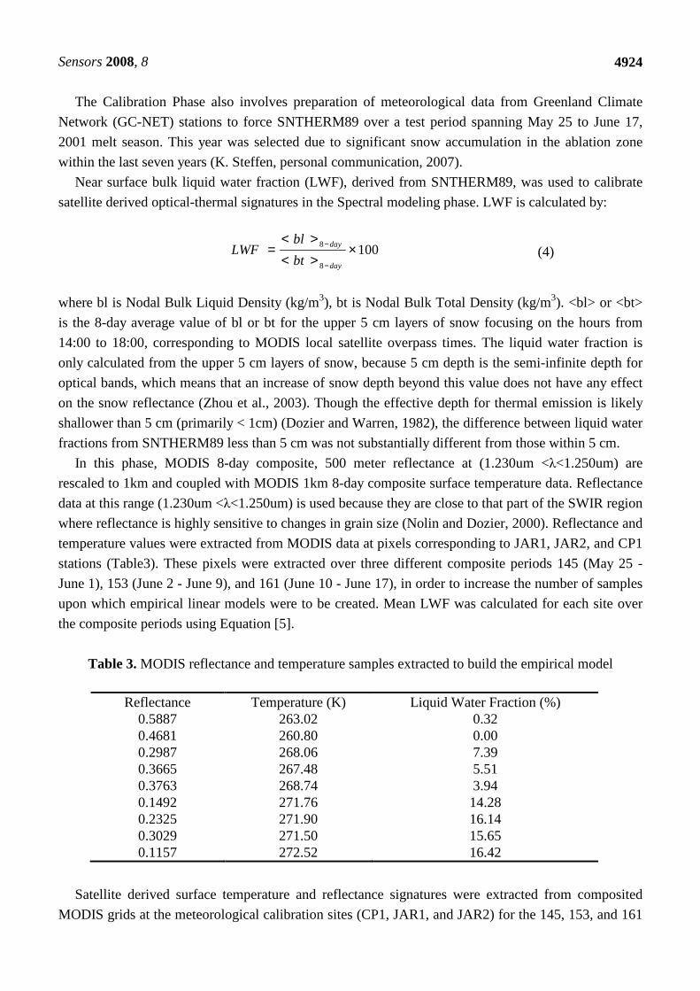
Table 3. MODIS reflectance and temperature samples extracted to build the empirical model
Reflectance Temperature (K) Liquid Water Fraction (%)
0.5887 0.4681 0.2987 0.3665 0.3763 0.1492 0.2325 0.3029 0.1157
263.02 260.80 268.06 267.48 268.74 271.76 271.90 271.50 272.52
0.32 0.00 7.39 5.51 3.94 14.28 16.14 15.65 16.42
Satellite derived surface temperature and reflectance signatures were extracted from composited
MODIS grids at the meteorological calibration sites (CP1, JAR1, and JAR2) for the 145, 153, and 161
1008
8 ×><><
=−
−
day
day
bt
blLWF (4)

Sensors 2008, 8
4925
composite periods (Table 3). A linear empirical model was developed with LWF as the dependent
variable and MODIS extracted surface temperature and SWIR reflectance as independent variables
(Table 4). This model was used to estimate surface melt magnitude or “effective” melt magnitude (E-
melt) at 1 km2 spatial resolution across the GIS. For clarification, LWF is distinguished from E-melt as
the magnitude of simulated bulk liquid water fraction estimated from SNTHERM89, while E-melt is a
temporally integrated assessment of LWF fraction over 8-day composite periods retrieved from
coupled MODIS optical/thermal signatures.
Table 4. Linear empirical model parameters used to derive effective melt intensity
Model Dependent
Variable Independent
Variable Coefficient
of Reflectance
Coefficient of
Temperature
Constant
I <LWF> Reflectance, Temperature
-0.136 0.011 -2.822
3.3 Sensitivity of SNTHERM89 to Initial Conditions
Stratigraphy from Swiss Camp (ETH/CU) (Figure 3), courtesy of K. Steffen (CIRES/CU Boulder),
excavated on May 16, 2001, was the only data available for this season in the study region. Therefore,
SNTHERM89 was initialized at each calibration site (JAR1, JAR2, and CP1) using the same
stratigraphy. It was assumed that estimated parameters derived from the snowmelt model will represent
local meteorological conditions if the model was executed sufficiently ahead of the analysis period
(May 25 to June 17, 2001). If this were true, then the use of stratigraphic data from ETH/CU camp
would not bias the model output. This assumption was tested by comparing the difference between
SNTHERM89 outputs derived from starting the model with stratigraphy from ETH/CU with model
output initialized with several test stratigraphy. These stratigraphy sensitivity tests were executed using
meteorological forcing data from two GC-NET stations that represent high (JAR1) and low (CP1) melt
magnitude conditions, during the period from May 26 to Jun 16, when station data from these two sites
overlap. Given that JAR1 lacked data from the period before May 26, a combined data set was created
using meteorological data from ETH/CU. Because ETH/CU is the nearest station to JAR1, it is
assumed that meteorological conditions at JAR1 were not much different from those at ETH/CU.

Sensors 2008, 8
4926
Figure 3. Snow pack and upper firn stratigraphy at Swiss camp excavated by K. Steffen
on May 16, 2001.
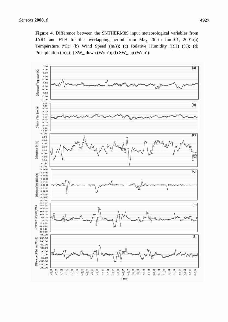
Difference in forcing variables derived from these two station were examined in order to create a
combined meteorological forcing data set from JAR1 and ETH/CU stations during an overlapping
period (Figure 4). Data at these two stations demonstrated some short duration differences in wind
speed, incident solar radiation (SW _ down), and upwelling solar radiation (SW _ up). Conversely,
temperature, relative humidity, and precipitation did not exhibit significant differences.
Sensors 2008, 8
4927
Figure 4. Difference between the SNTHERM89 input meteorological variables from
JAR1 and ETH for the overlapping period from May 26 to Jun 01, 2001.(a)
Temperature (ºC); (b) Wind Speed (m/s); (c) Relative Humidity (RH) (%); (d)
Precipitation (m); (e) SW_ down (W/m2); (f) SW_ up (W/m2).

Sensors 2008, 8
4928
Comparison of simulated LWF from SNTHERM89, forced with GC-NET data from ETH/CU and
JAR1, and initialized with ETH/CU stratigraphy during the overlapping test period, demonstrated a
Root Mean Square Error (RMSE) of 2.72% (Figure 5). This seems sufficiently low to support merging
meteorological forcing data from ETH/CU and JAR1 to provide a seamless and uninterrupted time
series.
Figure 5. Comparison of estimated LWF at ETH\CU and JAR1 GCNET stations
initialized with ETH stratigraphy from May 26 to Jun 01, 2001 demonstrating a RMSE
of 2.72%.
Several test strata (Table 5) were designed by varying the values of temperature and grain size. Test
1 stratigraphic information (Figure 6) was designed to be different from the ETH/CU stratigraphy with
larger variability of temperature and grain size than ETH/CU stratigraphy. Historic strata were used to
evaluate a greater range in initialization modes. These strata were excavated by C. Benson (Benson,
1962) during the 1955 traverse, over 4 years.

Sensors 2008, 8
4929
Table 5. Summary of test strata used to evaluate SNTHERM89 sensitivity to initial
conditions (data below is for upper 10-12cm within effective radiative zones that
contribute to reflectance and temperature).
* Strata were borrowed from 1955 traverse data archive (Benson, 1962)
Strata Description Mean Temperature (°K)
Mean Density (kg/m3)
Mean Grain Size (m)
Swiss Camp
(SC)
Stratigraphy excavated at Swiss Camp on May 16, 2001 at an elevation of 1149 m
263.3 174.3 0.0003
Test 1 Fabricated strata with fewer layers, higher temp gradient and larger change in grain size near surface than Swiss Camp stratigraphy
264.8 107.0 0.0002
Test 2* Low temperatures, greater range in grain size at depth, and higher densities near top and lower near bottom relative to SC from firn at lower elevation (~1000m) near the north-eastern coast
259.3 250 0.0005
Test 3* Inverted near surface gradient, similar density profile as Test 2, most stratified and derived from firn in the percolation zone (~2200m)
258.0 250.0 0.001
Test 4* A near linear temperature gradient, derived from firn in the accumulation zone of the ice sheet at an elevation of ~2800 m
261.2 263.3 0.0005

Sensors 2008, 8
4930
Figure 6. Fabricated test stratigraphy used to test SNTHERM89 temporal sensitivity to
initial conditions in Test 1. Both temperature and grain size in this test stratigraphy were
in a wider range than the ETH/CU stratigraphy.
Several pits were excavated (146) during the traverse. Yet only three strata were sampled from this
stratigraphy database derived from locations on the ice sheet that represent a range in firn conditions
during the 4-year period (Test 2 (Figure 7), Test 3 (Figure 8), and Test 4 (Figure 9)).

Sensors 2008, 8
4931
Figure 7. Snow pack and upper firn stratigraphy used to test SNTHERM89 temporal
sensitivity to initial conditions in Test 2. This stratigraphy was excavated by C. Benson
on May 17, 1955 at a site in northern Greenland with the elevation of 1310 meter.

Sensors 2008, 8
4932
Figure 8. Snow pack and upper firn stratigraphy used to test SNTHERM89 temporal
sensitivity to initial conditions in Test 3. This stratigraphy was excavated by C. Benson
on August 18, 1955 at a site in Greenland inland with the elevation of 1963 meters.

Sensors 2008, 8
4933
Figure 9. Snow pack and upper firn stratigraphy used to test SNTHERM89 temporal
sensitivity to initial conditions in Test 4. This stratigraphy was excavated by C. Benson
on June 27, 1955 at a site in western Greenland with the elevation of 2918 meters.
Figure 10 depicts the location of these sample strata. Differences in LWF in the upper 5 cm of
SNTHERM89 output derived from runs initialized with ETH/CU stratigraphy versus the test strata, at
JAR1 and CP1 were approximately zero (Figure 11, and Figure 12).

Sensors 2008, 8
4934
Figure 10. Location of stations where stratigraphy for Test 2 (blue), Test 3 (red), and
Test 4 (green) were excavated. (Source: Benson, 1962).

Sensors 2008, 8
4935
Figure 11. Difference between liquid water fractions (LWF) from upper 5 cm of
simulated snow pack derived from SNTHERM89 using stratigraphy from Swiss camp
and the test stratigraphy, composited over May 26 to Jun 16 for JAR1.

Sensors 2008, 8
4936
Figure 12. Difference between liquid water fractions (LWF) from upper 5 cm of
simulated snow pack derived from SNTHERM89 using stratigraphy from Swiss camp
and the test stratigraphy, composited over May 26 to Jun 16 for CP1.

Sensors 2008, 8
4937
4. Results
E-melt for composite periods 145, 153, and 161 was estimated using MODIS derived surface
reflectance and temperature grids as input into the linear empirical inversion model. Figure 13 (a-c)
depict maps of E-melt for periods 145 (May 25 - June 1), 153 (June 2 - June 9), and 161 (June 10 -
June 17). E-melt maps display the spatial variability in surface melt magnitude patterns and indicate an
increasing extent in melt amount from late spring through early summer. Variations in melt magnitude
appear to be constrained by elevation.
Figure 13. Melt intensity over the Greenland Ice Sheet for composite periods (a) 145
(May 25 - June 1), (b) 153 (June 2 - June 9), and (c) 161 (June 10 - June 17) during the
2001 summer season. Location of GCNET meteorological stations (in yellow) used in
this analysis.
Higher elevation regions experienced lower magnitudes of LWF as evident by consistently low
LWF estimates at Summit and South Dome stations. Lower elevation regions experienced the highest
E-melt estimates with a strong latitudinal gradient in intensity from north to south. White spots on the
maps indicate cloud cover, which were extracted from MODIS 8-day surface reflectance 500m QA
(Quality Assessment) data sets. Histograms (Figure 14) reveal the number of pixels of LWF classified
in 1% increment bins for composite periods 145, 153, and 161 and shift to higher fractions from May
through June.

Sensors 2008, 8
4938
Figure 14. Histograms of effective melt intensity derived from Model I for composite
periods 145 (May 25 - June 1), 153 (June 2 - June 9), and 161 (June 10 - June 17) over
Greenland ice sheet in 2001.
4.1 E-melt Model Validation and Sensitivity
Evaluation of melt retrieval performance involved comparison of MODIS derived E-melt to those
estimated from SNTHERM89 at other GC-NET stations (Table 6), not used to develop the E-melt
retrieval model. Additionally, E-melt estimates were compared to scatterometer derived maps of wet

Sensors 2008, 8
4939
and dry firn zones. SNTHERM89 was executed at each of the point validation stations over composite
period 161. This period was used because it had higher LWF compared with the other two composite
periods (145 and 153).
Table 6. GC-Net Stations used for Model Validation
Station Name Latitude and Longitude Elevation (m) Humboldt Gl. Summit Tunu-N NASA-E NGRIP South-D NASA-SE
78.5266N, 56.8305W 72.5794N, 38.5042W 78.0168N, 33.9939W 75.0000N, 29.9997W 75.0998N, 42.3326W 63.1489N, 44.8167W 66.4797N, 42.5002W
1995 3208 2020 2631 2950 2922 2579
Mean LWF was calculated over this composite period from SNTHERM89 outputs in the upper 5cm
using Equation [5]. Standard deviation of LWF for the eight day composite period was calculated for
each site. SNTHERM89 derived LWF estimated at the point validation sites were compared with
satellite derived E-melt (Figure 15). E-melt estimates tend to fall within the variance for each station
corresponding to mean LWF derived from SNTHERM89 except station South-D, where E-melt
significantly overestimates LWF.
Figure 15. Comparison between mean LWF from SNTHERM89 output and estimated
LWF from Model I for the point validation GCNET stations for composite period 161.

Sensors 2008, 8
4940
An 8-day composite QSCAT scene was produced by averaging backscatter values of daily QSCAT
products for the same composite period of MODIS products. Diurnal backscatter change was
calculated for each composite period (Figure 16).
Figure 16. Wet and Dry snow facies on the Greenland ice sheet detected from QSCAT
for composite periods (a) 145 (May 25 - June 1), (b) 153 (June 2 - June 9), and (c) 161
(June 10 - June 17) during the summer season. Wet snow zones were determined by a
diurnal backscatter change larger than 1.8dB. Dry snow zones were mapped when the
diurnal backscatter change was smaller than 1.8dB.
E-melt maps were resampled to 2.225km in spatial resolution, and compared with the QSCAT-
derived wet and dry snow zones. A 1000 meter contour was used to mask sample pixels from both the
MODIS and QSCAT images. The 1000 meter contour contains more than 99% of the ice sheet and is
sufficient to separate the ice from the rocky coast. Histograms representing dry and wet conditions for
each class of MODIS-derived E-melt (Figure 17) display results for all three composite periods. As the
summer advances, the distribution of wet zones shifts to higher E-melt magnitudes. Later in the
summer (over composite period 161) the distribution of wet snow zones largely corresponds to higher
E-melt values.
The E-melt model is solely contingent on MODIS derived 8-day composite, surface temperature and
SWIR reflectance as independent variables. MODIS SWIR reflectance products have an estimated
relative error of approximately ± 2%
(http://modisgsfc.nasa.gov/data/atbd/atbd_mod08.pdf), with typical values less than 5% (Liang et al.,
2002). Examination of MODIS LST products through a comparison with automatic weather station
temperatures on the GIS, generally indicate fairly reasonable accuracy (1 < 1 ºC), but can be as high as
2° (Wan et al., 2002; Hall et al., 2004). We evaluate the impact of MODIS 8-day surface LST and
reflectance product accuracy on E-melt retrievals by adding error bias to these variables individually (±
2% for reflectance and ± 1° C for LST) and assess combined error on E-melt magnitudes for early in

Sensors 2008, 8
4941
the melt season (composite period 145) and later (composite period 161). The impact of error biased
MODIS products were separately evaluated by inputting maximum positive and negative error grids
into the linear retrieval model while holding the other variable fixed to unbiased (measured reflectance
or LST) values. This produces estimates of E-melt error when reflectance varies from positive to
negative 2% bias while LST is input as unbiased and vice versa for LST averaged over the entire ice
sheet.
Figure 17. Comparison of E-melt with QSCAT-derived snow facies zones for
composite periods 145, 153, and 161.
Therefore, accuracy estimates on E-melt retrievals based on error in reflectance of was ~0.1% and
~0.4% based on error in LST for early in the melt season, with combined accuracy of ~0.7%
(reflectance and LST). For later in the melt season, E-melt accuracy based on reflectance is ~0.2% and

Sensors 2008, 8
4942
~1.1% and as high as 2% for LST with combined accuracy as high as ~2%. These errors represent a
first order assessment of the maximum error based on accuracy of input variables.
5. Discussion and Conclusion
E-melt retrievals are heavily contingent on the accuracy of both MODIS derived surface reflectance
and temperature products. An assessment of the maximum impact of accuracy from these products
indicates relatively low errors. The errors increase from the earlier part of the melt season when the
magnitude of melt is low to the warmer part of the season where the melt amount is higher.
Additionally, errors due to the accuracy of the LST product are larger and become more important later
in the melt season. Though late melt season variability in temperatures is lower than the early part of
the season, the greater influence temperature has in E-melt retrievals later in the season are likely due
to the fact that as surface temperature approach the melting point, significant error in LST can make the
difference between melt and no melt conditions. Also, the relationship among temperature, reflectance
and melt production can vary throughout the season. Early in the season, the correlation between
surface reflectance and temperature can be high (~ -0.8) at lower elevation and diminishes later in the
season due more sustained negative sensible heat flux that stabilize and reduce temperature variability
relative to surface albedo (Veenhuis, 2006). Our linear retrieval model does not account for this
dynamic and may exhibit seasonally dependent performance.
Point validation analysis, using meteorological data from GC-NET stations that were not used in
the E-melt algorithm, indicates relatively good performance with E-melt retrievals within one standard
deviation of the mean LWF derived from SNTHERM89 outputs for each point validation station
except the South-D station. E-melt overestimated LWF at South-D by 4%. During the 161 period
South-D demonstrates very low LWF and stable conditions with little variability. E-melt performed
quite well at other stations that demonstrated low variability during the 8-day composite periods and
very low mean LWF (approximately zero), therefore, retrieval performance at South-D could be the
result of potentially contaminated pixels given the South-D station is bordering a region heavily
obscured by cloud cover. Additionally, this bias might be due to the accuracy of the MODIS LST
product.
High E-melt magnitudes tend to correspond to QSCAT wet zones, where the highest percentage of
wet zones occupy between 10.5-12.0% LWF in composite period 145, and shift to 12.0-13.5% in
composite period 153 and 161. Changes in the spatial patterns in wet and dry snow zones throughout
the melt season show comparable changes in E-melt although some inconsistencies are apparent. There
are dry snow zones near the ice sheet margin that do not correspond to low E-melt values. This may not
be solely related to problems with the E-melt algorithm. This inconsistency may be attributed to how
radiative information from the optical/thermal parts of the EM spectrum differs from the microwave
region. Microwave derived backscatter radiation can be dominated by deeper ice structures such as
lenses, pipes, and layers (Baumgartner et al., 1999), while surface temperatures are heavily contingent
on surface emission derived from no deeper than several centimeters. Additionally, backscatter can be
dominated by subsurface depth hoar and coarse-grain firn (Jezek et al., 1994). Ku-band scatterometers
are very sensitive to increased wetness in firn surface layers, resulting in masking backscattering from
deeper layers (Nghiem et al., 2001). Therefore, wet snow zones corresponding to lower temperatures

Sensors 2008, 8
4943
(Figure 16) are likely indicative of subsurface melt. Performance issues in the E-melt retrieval may also
be related to how the dynamic melt process was simulated in SNTHERM89. Though our model was
initialized with a ‘glacier ice’ substrate with snow layers overlying, the melt infiltration and runoff
process is not adequately represented in such simulations. SNTHERM89 does not have the capacity to
partition melt into run and infiltration and has no specification for preferential flow paths characteristic
of melt infiltration in nature.
This retrieval scheme does not take into account melt production during cloud covered periods
where downward cloud-forced radiation may be significant in amplifying melt. To assess the impact of
clouds on melt a more comprehensive analysis will have to be implemented and is currently under
analysis through the use of mesoscale atmospheric model estimates of surface net cloud forced
radiation and its relationship to melt extent and occurrence derived from passive microwave systems.
The strong relationship between melt production and surface temperatures may indicate that LST
alone could be a suitable variable for this retrieval approach. Retrieval models using LST and
reflectance as independent variables singularly were explored and it was determined that the model
using coupled optical/thermal independent variables out performed those models that used only a
single variable (Peng, 2007).
This novel empirical retrieval scheme can provide valuable information about the spatio-
temporal variability of surface melt dynamics that have a significant impact on the mass balance of the
GIS. Assessments of melt extent have been informative but have failed to provide vital knowledge
amount the amount of melt. This nascent approach can fulfill this need with additional work on
validation and refinement. Comparison to traditional passive microwave melt extent and number of
melt days will help provide insight into E-melt retrieval performance in addition to exploring
application of this retrieval scheme to other years within the MODIS data archive.
Acknowledgements
This work has been partially supported under NASA grant number NNX06AE50G. We would like
to acknowledge significant feedback from Dr. Anne Nolin, Oregon State University for her input on
the initial approach. Special thanks to Dr. Konrad Steffen, CIRES, for access to meteorological data
and feedback. We are very grateful for feedback from Dr. Richard Alley and the Pennsylvania State
University Ice and Climate (PICE) Group for valued feedback and support. We would also like to
thank Dr. Dorothy Hall for her insights, particularly on the performance of the MODIS surface
temperature product. Special thanks to the two anonymous reviewers for their vital feedback and
suggestions, which improved the quality of this manuscript.
References and Notes 1. Abdalati, W.; Steffen, K. Passive microwave-derived snow melt regions on the Greenland Ice
Sheet. Geophys. Res. Lett. 1995, 22, 787-790.
2. Abdalati, W.; Steffen, K. Snowmelt on the Greenland ice sheet as derived from passive microwave
satellite data. J. Clim. 1997, 10, 165-175.

Sensors 2008, 8
4944
3. Ashcraft, I.; D. Long, D. Increasing temporal resolution in Greenland ablation estimation using
passive and active microwave data, In Proceedings of the IEEE International Geoscience and
Remote Sensing Symposium (IGARSS), Toulouse, France, July 2003; pp. 1604-1606.
4. Ashcraft, I.; Long, D. Differentiation between melt and freeze stages of the melt cycle using SSM/I
channel ratios. IEEE Trans. Geosci. Remote Sens. 2005, 43, 1317-1323.
5. Ashcraft, I.; Long, D. Comparison of methods for melt detection over Greenland using active and
passive microwave measurements. Int. J. Remote Sens. 2006, 27, 2469-2488.
6. Baumgartner, F.; Jezek, K.; Forster, R.; Gogineni, S.; Zabel, I. Spectral and angular ground-based
radar backscatter measurements of Greenland snow facies, In proceedings of the International
Geoscience and Remote Sensing Symposium (IGARSS), Hamburg,Germany, August 1999; pp.
1053-1055.
7. Benson, C. S. Stratigraphic Studies in snow and firn of the Greenland Ice Sheet. U. S. Army cold
regions research and engineering laboratory (CRREL) research report no. 70, 1962, 120.
8. Bindschadler, R. Monitoring ice sheet behavior from space. Rev. Geophys. 1998, 36, 79-104.
9. Bohren, C. Applicability of effective-medium theories to problems of scattering and absorption by
nonhomogeneous atmospheric particles. J. Atmos. Sci. 1986, 43, 468-475.
10. Bohren, C.; Barkstrom, B. Theory of the optical properties of snow. J. Geophys. Res. 1974, 79,
4527-4535.
11. Box, J. Polar Day Effective Cloud opacity in the Arctic from measured and modeled solar
radiation fluxes, M.A. thesis, Department of Geography, University of Colorado, Boulder, CO,
Cooperative Institute for Research in Environmental Sciences, 1997
12. Campbell, J., Introduction to Remote Sensing, 4th ed.; New York, Guilford Press, 2007, pp. 256.
13. Chang, A.; Gloersen, A.P.; Schmugge, T.; Wilheit, T.; Zwally, H. Microwave emission from snow
and glacier ice. J. Glaciol. 1976, 16, 23-29.
14. Colbeck, S. Snow-crystal growth with varying surface temperatures and radiation penetration. J.
Glaciol. 1989, 35, 23-29.
15. Colbeck, S. The geometry and permittivity of snow at high frequencies. J. Appl. Phys. 1982, 53,
4495-4500.
16. Comiso, J.; Yang, J.; Honjo, S.; Krishfield, R.A. Detection of change in the Arctic using satellite
and in situ data. J. Geophys. Res. 2003, 108(C12), 3384, doi:10.1029/2002JC001347.
17. Cryosphere Theme Report, Integrated Global Observing Strategy (IGOS), 2007, pp 45.
18. Cumming, W. The dielectric properties of ice and snow at 3.2 centimeters. J. Appl. Phys, 1952, 23,
768-773.
19. Dowdeswell, J. The Greenland Ice Sheet and global sea-level rise. Science, 2006, 311, 963-964.
20. Dozier, J., Spectral signature of alpine snow cover from the Landsat Thematic Mapper. Remote
Sens. Environ. 1989, 28, 9-22.
21. Dozier, J.; Warren, S. Effect of view angle on the infrared brightness temperature of snow. Water
Resour.Res. 982, 18, 1424-1434.
22. Fahnestock, M.; Bindschadler, R.; Kwok, R.; Jezek, K. Greenland Ice Sheet surface properties and
ice dynamics from ERS-1 SAR imagery. Science. 1993, 262, 1530-1534.
Sensors 2008, 8
4945
23. Grenfell, T.; Perovich, D.; Ogren, J. Spectral albedo of an alpine snowpack. Cold Reg. Sci.
Technol. 1981, 4, 121-127.
24. Grenfell, T.; Maykut, G. The optical properties of ice and snow in the arctic basin. J. Glaciol. 1977,
18, 445-463.
25. Haefliger, M.; Steffen, K.; Fowler, C. AVHRR surface temperature and narrow-band albedo
comparison with ground measurements for the Greenland Ice Sheet. Ann. Glaciol. 1993, 17, 49-
54.
26. Hall, D.; Bindschadler, R.; Foster, J.; Chang, A.; Siddalingaiah, H. Comparison of in situ and
satellite-derived reflectance of Forbindels Glacier, Greenland. Int. J. Remote Sens. 1990, 11, 493-
504.
27. Hall, D.; Williams, Jr., R.S.;Steffen, K.; Chien, J. Analysis of summer 2002 melt extent on the
Greenland Ice Sheet using MODIS and SSM/I data, In proceedings of the International Geoscience
and Remote Sensing Symposium (IGARSS), Anchorage, Alaska, 2004, pp. 3029-3032.
28. Hall, D.K.; Williams, Jr., R.S.; Casey, K.A.; DiGirolamo, N.E.; Wan, Z. Satellite-derived, melt-
season surface temperature of the Greenland Ice Sheet (2000-2005) and its relationship to mass
balance. Geophys. Res. Lett. 2006, 33, L11501, doi:10.1029/2006GL026444.
29. Hall, D.K.; Williams, Jr., R.S.; Luthcke, S.B.; DiGirolamo, N.E. Greenland Ice Sheet surface-
temperature, melt and mass loss: 2000 – 2006. Journal of Glaciol. 2008, 54(184), 81-93.
30. Hallikainen, M.; Ulaby, F.; Abdelrazik, M. Dielectric properties of snow in the 3 to 37 GHz range.
IEEE Trans. Antennas Propag. 1986, 34, 1329-1340.
31. Jezek, K.; Gogineni, P.; Shanableh, M. Radar measurements of melt zones on the Greenland Ice
Shee. Geophys. Res. Lett. 1994, 21, 33-36.
32. Jordan, R. A one-dimensional temperature model for snow cover, Technical Documentation for
SNTHERM89, 1991. 33. Key, J.; Schweiger, A.J. Tools for atmospheric radiative transfer: Streamer and FluxNet. Comput.
Geosci. 1998, 24(5), 443-451.
34. Key, J.; Haefliger, M. Arctic ice surface temperature retrieval from AVHRR thermal channels. J.
Geophys. Res. 1992, 97(D5), 5885-5893.
35. Klein, A.; Stroeve, J. Development and validation of a snow albedo algorithm for the MODIS
Instrument. Ann. Glaciol. 2002, 34, 45-52.
36. Krabill, W.; Abdalati, W.; Frederick, E.; Manizade, S.; Martin, C.; Sonntag, J.; Swift, R.; Thomas,
R.; Wright, W.; Yungel, J. Greenland Ice Sheet: high-elevation balance and peripheral thinning.
Science. 2000, 289, 428-430.
37. Lampkin, D.; Yool, S. Numerical simulations of MODIS sensitivity potential for assessing near
surface mountain snow melt. Geocarto International. 2004a , 19, 13-24.
38. Lampkin, D.; Yool, S. Monitoring mountain snowpack evolution using near-surface optical and
thermal properties. Hydrol. Processes. 2004b, 18, 3527-3542.
39. Liang, S.; Fang, H.; Chen, M.; Shuey, C.J.; Walthall, C.; Daughtry, C.; Morisette, J.; Schaaf, C.;
Strahler, A. Validating MODIS land surface reflectance and albedo products: methods and
preliminary results. Remote Sens. Environ. 2002, 83, 149-162.

Sensors 2008, 8
4946
40. Long, D.; Drinkwater, M. Cryosphere applications of NSCAT data. IEEE Trans. Geosci. Remote
Sens. 1999, 37, 1671-1684.
41. Lubin, D.; Massom, R. Polar Remote Sensing, Volume 1: Atmosphere and Polar Oceans, Praxis-
Springer. Chichester, England, and Berlin, Germany, 2006, pp. 756.
42. Marks, D.; Dozier, J. Climate and energy exchange at the snow surface in the alpine region of the
Sierra Nevada, 2. Snow cover energy balance. Water Resour. Res. 1992, 28, 3043-3054.
43. Matzler C.; Aebischer, H.; Schanda, E. Microwave dielectric properties of surface snow. IEEE J.
Oceanic Eng. 1984, OE-9, 366-371.
44. Mote, T.; Anderson, M. Variations in snowpack melt on the Greenland Ice Sheet based on passive
microwave-measurements. J. Glaciol. 1995, 41, 51-60.
45. Nghiem, S.; Steffen, K.; Kwok, R.; Tsai, W. Detection of snowmelt regions on the Greenland Ice
Sheet using diurnal backscatter change. J. Glaciol. 2001, 47, 539-547.
46. Nolin, A.; Dozier, J. A hyperspectral method for remote sensing of grain size of snow. Remote
Sens. Environ. 2000, 74, 207-216.
47. Painter, T.; Dozier, J.; Roberts, D., Davis, R.; Green, R. Retrieval of subpixel snow-covered area
and grain size from imaging spectrometer data. Remote Sens. Environ. 2003, 85, 64-77.
48. Peng, R. Estimation of surface melt intensity using optical and thermal measurements over the
Greenland Ice Sheet, M.S. thesis, Department of Geography, Pennsylvania State University, 2007. 49. Ramage, J.; Isacks, B. Determination of melt-onset and refreeze timing on southeast Alaskan
icefields using SSM/I diurnal amplitude variations. Ann. Glaciol. 2002, 34, 391-398.
50. Rees, W. Remote Sensing of Snow and Ice, CRC Press, 2006, pp. 109-118.
51. Ridley, J. Surface Melting on Antarctic Peninsula Ice Shelves Detected by Passive Microwave
Sensors. Geophys. Res. Lett. 1993, 20, 2639-2642.
52. Rignot, E.; Kanagaratnam, P. Changes in the Velocity Structure of the Greenland Ice Sheet.
Science, 2006, 311, 986-990.
53. Rignot, E.; Thomas, R. Mass Balance of Polar Ice Sheets. Science. 2002, 297, 1502-1506.
54. Shepherd, A.; Wingham, D. Recent Sea-Level Contributions of the Antarctic and Greenland Ice
Sheets. Science. 2007, 315, 1529-1532.
55. Steffen, K.; Box, J. Surface Climatology of the Greenland Ice Sheet: Greenland Climate Network
1995-1999. J. Geophys. Res. 2001, 106, 33951-33964.
56. Steffen, K.; Abdalati, W.; Stroeve, J. Climate Sensitivity Studies of the Greenland Ice Sheet using
Satellite AVHRR, SMMR, SSM/I and in situ Data. Meteorol. Atmos. Phys. 1993, 51, 239-258.
57. Stroeve, J.; Nolin, A. Comparison of MODIS and MISR-derived Surface Albedo with in situ
Measurement in Greenland, In Proceedings of EARSeL-LISSIG-Workshop Observing our
Cryosphere from Space, Bern, Switzerland. 2002a ,pp. 89-96.
58. Stroeve, J.; Nolin, A. New methods to infer snow from the MISR instrument with applications to
the Greenland ice sheet. IEEE Trans. Geosci. Remote Sens. 2002b, 40, 1616-1625.
59. Stroeve, J.; Nolin, A.; Steffen, K. Comparison of AVHRR-derived and in situ Surface Albedo over
the Greenland Ice Sheet. Remote Sens. Environ. 1997, 62, 262-276.

Sensors 2008, 8
4947
60. Stroeve, J.; Box, J.; Gao, F.; Liang, S.; Nolin, A.; Schaaf, C. Accuracy Assessment of the MODIS
16-day Albedo Product for Snow: Comparisons with Greenland in situ Measurements. Remote
Sens. Environ. 2004, 94, 46-60.
61. Tedesco, M. Snowmelt Detection over the Greenland Ice Sheet from SSM/I Brightness
Temperature Daily Variations. Geophys. Res. Lett. 2007, 34, L02504.
62. Tiuri, M.; Sihvola, A.; Nyfors, E.; Hallikaiken, M. The Complex Dielectric Constant of Snow at
Microwave Frequencies. IEEE J. Oceanic Eng. 1984, OE-9, 377-382.
63. Veenhuis, B.A., Variability in Surface Reflectance of the Greenland Ice Sheet (1982-2005) using
Satellite Remote Sensing, senior thesis. Ohio State University, 2006. 64. Vermote, E.; El Saleous, N.Z.; Justice, C.O.. Atmospheric Correction of MODIS Data in the
Visible to Middle Infrared: First Results. Remote Sens. Environ. 2002, 97-111.
65. Wan, Z., Zhang, Y.; Zhang, Q.; Li, Z.L.. Validation of the Land-Surface Temperature Products
Retrieved from Terra Moderate Resolution Imaging Spectroradiometer Data. Remote Sens.
Environ. 2002, 83, 63-180.
66. Warren, S. Optical properties of snow. Rev. Geophys. Space Phys. 1982, 20, 67-89.
67. Warren, S.; Wiscombe, W. A Model for the Spectral Albedo of Snow II: Snow Containing
Atmospheric Aerosols. J. Atmos. Sci. 1981, 37, 2734-2745.
68. Wiscombe, W.; Warren, S. A Model for the Spectral Albedo of Snow I: Pure Snow. J. Atmos. Sci.
1981, 37, 2712-2733.
69. Wismann, V. Monitoring of Seasonal Snowmelt on Greenland with ERS Scatterometer Data.
IEEE Trans. Geosci. Remote Sens. 2000, 38, 1821-1826.
70. Zhou, X.; Li, S.; Stamnes, K. Effects of Vertical Inhomogeneity on Snow Spectral Albedo and its
Implication for Optical Remote Sensing of Snow. J. Geophys. Res. 2003, 108, NO. D23.
71. Zwally, H.; Fiegles, S. Extent and Duration of Antarctic Surface Melt. J. Glaciol. 1994, 40, 463-
476.
72. Zwally, H.; Abdalati, W.; Herring, T.; Larson, K.; Saba, J.; Steffen, K. Surface Melt-Induced
Acceleration of Greenland Ice Sheet Flow. Science. 2002, 297, 218-222.
© 2008 by the authors; licensee Molecular Diversity Preservation International, Basel, Switzerland.
This article is an open-access article distributed under the terms and conditions of the Creative
Commons Attribution license (http://creativecommons.org/licenses/by/3.0/).