Emergent Gravity

and the Dark Universe

Erik Verlinde1

Delta-Institute for Theoretical PhysicsInstitute of Physics,

University of AmsterdamScience Park 904, 1090 GL Amsterdam

The Netherlands

Abstract

Recent theoretical progress indicates that spacetime and gravity emerge

together from the entanglement structure of an underlying microscopic theory.

These ideas are best understood in Anti-de Sitter space, where they rely on the

area law for entanglement entropy. The extension to de Sitter space requires

taking into account the entropy and temperature associated with the cosmolog-

ical horizon. Using insights from string theory, black hole physics and quantum

information theory we argue that the positive dark energy leads to a thermal

volume law contribution to the entropy that overtakes the area law precisely at

the cosmological horizon. Due to the competition between area and volume law

entanglement the microscopic de Sitter states do not thermalise at sub-Hubble

scales: they exhibit memory effects in the form of an entropy displacement caused

by matter. The emergent laws of gravity contain an additional ‘dark’ gravita-

tional force describing the ‘elastic’ response due to the entropy displacement. We

derive an estimate of the strength of this extra force in terms of the baryonic

mass, Newton’s constant and the Hubble acceleration scale a0 = cH0, and pro-

vide evidence for the fact that this additional ‘dark gravity force’ explains the

observed phenomena in galaxies and clusters currently attributed to dark matter.

1 e.p.verlinde@uva.nl

arX

iv:1

611.

0226

9v2

[he

p-th

] 8

Nov

201

6

Contents

1 Introduction and Summary 21.1 Emergent spacetime and gravity from quantum information . . . . . . . 21.2 Emergent gravity in de Sitter space . . . . . . . . . . . . . . . . . . . . 31.3 Hints from observations: the missing mass problem . . . . . . . . . . . 51.4 Outline: from emergent gravity to apparent dark matter . . . . . . . . 6

2 Dark Energy and the Entropy in de Sitter Space 72.1 De Sitter space as a data hiding quantum network . . . . . . . . . . . . 72.2 The entropy content of de Sitter space . . . . . . . . . . . . . . . . . . 102.3 Towards a string theoretic microscopic description . . . . . . . . . . . . 11

3 Glassy Dynamics and Memory Effects in Emergent Gravity 133.1 The glassy dynamics of emergent gravity in de Sitter space . . . . . . . 133.2 Memory effects and the ‘dark’ elastic phase of emergent gravity . . . . 14

4 The Effect of Matter on the Entropy and Dark Energy 164.1 Entropy and entanglement reduction due to matter . . . . . . . . . . . 174.2 An entropic criterion for the dark phase of emergent gravity . . . . . . 184.3 Displacement of the entropy content of de Sitter space . . . . . . . . . 204.4 A heuristic derivation of the Tully-Fisher scaling relation . . . . . . . . 23

5 The First Law of Horizons and the Definition of Mass 255.1 Wald’s formalism in de Sitter space . . . . . . . . . . . . . . . . . . . . 255.2 An approximate ADM definition of mass in de Sitter . . . . . . . . . . 27

6 The Elastic Phase of Emergent Gravity 286.1 Linear elasticity and the definition of mass . . . . . . . . . . . . . . . . 286.2 The elasticity/gravity correspondence in the sub-Newtonian regime . . 30

7 Apparent Dark Matter from Emergent Gravity 337.1 From an elastic memory effect to apparent dark matter . . . . . . . . . 337.2 A formula for apparent dark matter density in galaxies and clusters . . 37

8 Discussion and Outlook 428.1 Particle dark matter versus emergent gravity . . . . . . . . . . . . . . . 428.2 Emergent gravity and apparent dark matter in cosmological scenarios . 43

9 Acknowledgements 45

1

1 Introduction and Summary

According to Einstein’s theory of general relativity spacetime has no intrinsic propertiesother than its curved geometry: it is merely a stage, albeit a dynamical one, on whichmatter moves under the influence of forces. There are well motivated reasons, comingfrom theory as well as observations, to challenge this conventional point of view. Fromthe observational side, the fact that 95% of our Universe consists of mysterious formsof energy or matter gives sufficient motivation to reconsider this basic starting point.And from a theoretical perspective, insights from black hole physics and string theoryindicate that our ‘macroscopic’ notions of spacetime and gravity are emergent from anunderlying microscopic description in which they have no a priori meaning.

1.1 Emergent spacetime and gravity from quantum information

The first indication of the emergent nature of spacetime and gravity comes fromthe laws of black hole thermodynamics [1]. A central role herein is played by theBekenstein-Hawking entropy [2, 3] and Hawking temperature [4, 5] given by

S =A

4G~and T =

~κ2π. (1.1)

Here A denotes the area of the horizon and κ equals the surface acceleration. In thepast decades the theoretical understanding of the Bekenstein-Hawking formula has ad-vanced significantly, starting with the explanation of its microscopic origin in stringtheory [6] and the subsequent development of the AdS/CFT correspondence [7]. Inthe latter context it was realized that this same formula also determines the amountof quantum entanglement in the vacuum [8]. It was subsequently argued that quan-tum entanglement plays a central role in explaining the connectivity of the classicalspacetime [9]. These important insights formed the starting point of the recent theoret-ical advances that have revealed a deep connection between key concepts of quantuminformation theory and the emergence of spacetime and gravity.

Currently the first steps are being taken towards a new theoretical framework inwhich spacetime geometry is viewed as representing the entanglement structure of themicroscopic quantum state. Gravity emerges from this quantum information theoreticviewpoint as describing the change in entanglement caused by matter. These novelideas are best understood in Anti-de Sitter space, where the description in terms of adual conformal field theory allows one to compute the microscopic entanglement in awell defined setting. In this way it was proven [10, 11] that the entanglement entropyindeed obeys (1.1), when the vacuum state is divided into two parts separated by aKilling horizon. This fact was afterwards used to extend earlier work on the emergenceof gravity [12, 13, 14] by deriving the (linearized) Einstein equations from generalquantum information theoretic principles [15, 16, 17].

2

The fact that the entanglement entropy of the spacetime vacuum obeys an area lawhas motivated various proposals that represent spacetime as a network of entangledunits of quantum information, called ‘tensors’. The first proposal of this kind is theMERA approach [18, 19] in which the boundary quantum state is (de-)constructed bya multi-scale entanglement renormalization procedure. More recently it was proposedthat the bulk spacetime operates as a holographic error correcting code [20, 21]. In thisapproach the tensor network representing the emergent spacetime produces a unitarybulk to boundary map defined by entanglement. The language of quantum error cor-recting codes and tensor networks gives useful insights into the entanglement structureof spacetime. In particular, it suggests that the microscopic constituents from whichspacetime emerges should be thought of as basic units of quantum information whoseshort range entanglement gives rise to the Bekenstein-Hawking area law and providesthe microscopic ‘bonds’ or ‘glue’ responsible for the connectivity of spacetime.

1.2 Emergent gravity in de Sitter space

The conceptual ideas behind the emergence of spacetime and gravity appear to begeneral and are in principle applicable to other geometries than Anti-de Sitter space.Our goal is to identify these general principles and apply them to a universe closerto our own, namely de Sitter space. Here we have less theoretical control, since atpresent there is no complete(ly) satisfactory microscopic description of spacetimes witha positive cosmological constant. Our strategy will be to apply the same general logicas in AdS, but to make appropriate adjustments to take into account the differencesthat occur in dS spacetimes. The most important aspect we have to deal with isthat de Sitter space has a cosmological horizon. Hence, it carries a finite entropy andtemperature given by (1.1), where the surface acceleration κ is given in terms of theHubble parameter H0 and Hubble scale L by [22]

κ = cH0 =c2

L= a0. (1.2)

The acceleration scale a0 will play a particularly important role in this paper.2

The fact that de Sitter space has no boundary at spatial infinity casts doubt on thepossible existence of a holographic description. One may try to overcome this difficultyby viewing dS as an analytic continuation of AdS and use a temporal version of theholographic correspondence [23] or use the ideas of [24]. We will not adopt such a holo-graphic approach, since we interpret the presence of the cosmological horizon and theabsence of spatial (or null) infinity as signs that the entanglement structure of de Sitterspace differs in an essential way from that of AdS (or flat space). The horizon entropy

2In most of this paper we set c = 1, but in the later sections we take a non-relativistic limit andwrite our equations in terms of a0 so that they are dimensionally correct without having to introduce c.

3

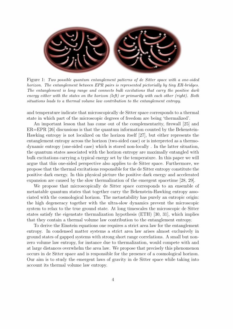
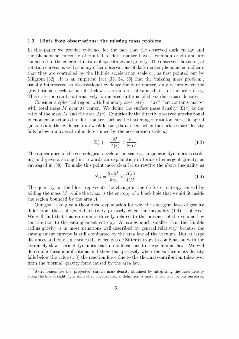
Figure 1: Two possible quantum entanglement patterns of de Sitter space with a one-sidedhorizon. The entanglement between EPR pairs is represented pictorially by tiny ER-bridges.The entanglement is long range and connects bulk excitations that carry the positive darkenergy either with the states on the horizon (left) or primarily with each other (right). Bothsituations leads to a thermal volume law contribution to the entanglement entropy.

and temperature indicate that microscopically de Sitter space corresponds to a thermalstate in which part of the microscopic degrees of freedom are being ‘thermalized’.

An important lesson that has come out of the complementarity, firewall [25] andER=EPR [26] discussions is that the quantum information counted by the Bekenstein-Hawking entropy is not localized on the horizon itself [27], but either represents theentanglement entropy across the horizon (two-sided case) or is interpreted as a thermo-dynamic entropy (one-sided case) which is stored non-locally . In the latter situation,the quantum states associated with the horizon entropy are maximally entangled withbulk excitations carrying a typical energy set by the temperature. In this paper we willargue that this one-sided perspective also applies to de Sitter space. Furthermore, wepropose that the thermal excitations responsible for the de Sitter entropy constitute thepositive dark energy. In this physical picture the positive dark energy and acceleratedexpansion are caused by the slow thermalization of the emergent spacetime [28, 29].

We propose that microscopically de Sitter space corresponds to an ensemble ofmetastable quantum states that together carry the Bekenstein-Hawking entropy asso-ciated with the cosmological horizon. The metastability has purely an entropic origin:the high degeneracy together with the ultra-slow dynamics prevent the microscopicsystem to relax to the true ground state. At long timescales the microscopic de Sitterstates satisfy the eigenstate thermalization hypothesis (ETH) [30, 31], which impliesthat they contain a thermal volume law contribution to the entanglement entropy.

To derive the Einstein equations one requires a strict area law for the entanglemententropy. In condensed matter systems a strict area law arises almost exclusively inground states of gapped systems with strong short range correlations. A small but non-zero volume law entropy, for instance due to thermalization, would compete with andat large distances overwhelm the area law. We propose that precisely this phenomenonoccurs in de Sitter space and is responsible for the presence of a cosmological horizon.Our aim is to study the emergent laws of gravity in de Sitter space while taking intoaccount its thermal volume law entropy.

4

1.3 Hints from observations: the missing mass problem

In this paper we provide evidence for the fact that the observed dark energy andthe phenomena currently attributed to dark matter have a common origin and areconnected to the emergent nature of spacetime and gravity. The observed flattening ofrotation curves, as well as many other observations of dark matter phenomena, indicatethat they are controlled by the Hubble acceleration scale a0, as first pointed out byMilgrom [32]. It is an empirical fact [33, 34, 35] that the ‘missing mass problem’,usually interpreted as observational evidence for dark matter, only occurs when thegravitational acceleration falls below a certain critical value that is of the order of a0.This criterion can be alternatively formulated in terms of the surface mass density.

Consider a spherical region with boundary area A(r) = 4πr2 that contains matterwith total mass M near its center. We define the surface mass density3 Σ(r) as theratio of the mass M and the area A(r). Empirically the directly observed gravitationalphenomena attributed to dark matter, such as the flattening of rotation curves in spiralgalaxies and the evidence from weak lensing data, occur when the surface mass densityfalls below a universal value determined by the acceleration scale a0

Σ(r) =M

A(r)<

a08πG

. (1.3)

The appearance of the cosmological acceleration scale a0 in galactic dynamics is strik-ing and gives a strong hint towards an explanation in terms of emergent gravity, asenvisaged in [38]. To make this point more clear let us rewrite the above inequality as

SM =2πM

~a0<A(r)

4G~. (1.4)

The quantity on the l.h.s. represents the change in the de Sitter entropy caused byadding the mass M , while the r.h.s. is the entropy of a black hole that would fit insidethe region bounded by the area A.

Our goal is to give a theoretical explanation for why the emergent laws of gravitydiffer from those of general relativity precisely when the inequality (1.4) is obeyed.We will find that this criterion is directly related to the presence of the volume lawcontribution to the entanglement entropy. At scales much smaller than the Hubbleradius gravity is in most situations well described by general relativity, because theentanglement entropy is still dominated by the area law of the vacuum. But at largedistances and long time scales the enormous de Sitter entropy in combination with theextremely slow thermal dynamics lead to modifications to these familiar laws. We willdetermine these modifications and show that precisely when the surface mass densityfalls below the value (1.3) the reaction force due to the thermal contribution takes overfrom the ‘normal’ gravity force caused by the area law.

3Astronomers use the ‘projected’ surface mass density obtained by integrating the mass densityalong the line of sight. Our somewhat unconventional definition is more convenient for our purposes.

5

1.4 Outline: from emergent gravity to apparent dark matter

The central idea of this paper is that the volume law contribution to the entanglemententropy, associated with the positive dark energy, turns the otherwise “stiff” geometryof spacetime into an elastic medium. We find that the elastic response of this ‘darkenergy’ medium takes the form of an extra ‘dark’ gravitational force that appears tobe due to ‘dark matter’. For spherical situations and under the right circumstancesit is shown that the surface mass densities of the baryonic and apparent dark matterobey the following scaling relation in d spacetime dimensions

2π

~a0M2

D =A(r)

4G~MB

d− 1or Σ2

D(r) =a0

8πG

ΣB(r)

d− 1. (1.5)

The first equation connects to the criterion (1.4) and makes the thermal and entropicorigin manifest. The second relation can alternatively be written in terms of the grav-itational acceleration gD and gB due to the apparent dark matter and baryons, whichare related to ΣD and ΣB by

ΣD =d− 2

d− 3

gD8πG

and ΣB =d− 2

d− 3

gB8πG

. (1.6)

Hence these accelerations obey the scaling relation

gD =√gBaM with aM =

(d− 3)

(d− 2)(d− 1)a0. (1.7)

In d = 4 these equations are equivalent to the baryonic Tully-Fisher relation [36] thatrelates the velocity of the flattening galaxy rotation curves and the baryonic mass MB.In this case one finds aM = a0/6, which is indeed the acceleration scale that appears inMilgrom’s phenomenological fitting formula [34, 35]. We like to emphasise that thesescaling relations are not new laws of gravity or inertia, but appear as estimates of thestrength of the extra dark gravitational force. From our derivation it will become clearin which circumstances these relations hold, and when they are expected to fail. Thispoint will be further clarified in the concluding section.

This paper is organized as follows. In section 2 we present our main hypothesisregarding the entropy content of de Sitter space. In section 3 we discuss several con-ceptual issues related to the glassy dynamics and memory effects that occur in emergentde Sitter gravity. We determine the effect of matter on the entropy content in section4, and explain the origin of the criterion (1.4). We also give a heuristic derivation of thescaling relation (1.5). In section 5 we relate the definition of mass in de Sitter to thereduction of the total entropy using the Wald formalism. This serves as a preparationfor section 6, where we give a detailed correspondence between the gravitational andelastic equations. Section 7 contains the main result of our paper: here we derive theapparent dark matter density in terms of the baryonic mass distribution and compareour findings with known observational facts. Finally, the discussion and conclusionsare presented in section 8.

6

2 Dark Energy and the Entropy in de Sitter Space

The main hypothesis from which we will derive the emergent gravitational laws inde Sitter space, and the effects that lead to phenomena attributed to dark matter, iscontained in the following two statements.

(i) There exists a microscopic bulk perspective in which the area law for the entan-glement entropy is due to the short distance entanglement of neighboring degreesof freedom that build the emergent bulk spacetime.

(ii) The de Sitter entropy is evenly divided over the same microscopic degrees offreedom that build the emergent spacetime through their entanglement, and iscaused by the long range entanglement of part of these degrees of freedom.

We begin in subsection 2.1 by explaining these two postulates from a quantum in-formation theoretic perspective, and by analogy with condensed matter systems. Insubsection 2.2 we will provide a quantitative description of the entropy content of deSitter space. We will associate the entropy with the excitations that carry the positivedark energy. This interpretation will be motivated in subsection 2.3 by using insightsfrom string theory and AdS/CFT. The details of the microscopic description will notbe important for the rest of this paper. We will therefore be somewhat brief, andpostpone a detailed discussion of the microscopic perspective to a future publication.

2.1 De Sitter space as a data hiding quantum network

According to our first postulate each region of space is associated with a tensor factorof the microscopic Hilbert space, so that the entanglement entropy obtained by tracingover its complement satisfies an area law given by the Bekenstein-Hawking formula.So the microscopic building blocks of spacetime are (primarily) short range entangled.This postulate is directly motivated by the Ryu-Takanayagi formula and the tensornetwork constructions of emergent spacetime [18, 20, 21], and is in direct analogy withcondensed matter systems that exhibit area law entanglement.

A strict area law is known to hold in condensed matter systems with gapped groundstates. Indeed, we conjecture that from a microscopic bulk perspective AdS spacetimescorrespond to the gapped ground states of the underlying quantum system. The build-ing blocks of de Sitter spacetime are, according to our second postulate, not exclusivelyshort range entangled, but also exhibit long range entanglement at the Hubble scale.Again by analogy with condensed matter physics this indicates that these de Sitterstates correspond to excited energy eigenstates. Hence, the entanglement entropy con-tains in addition to the area law also a volume law contribution. In terms of a tensornetwork picture this means these states contain an amount of quantum informationwhich is evenly divided over all tensors in the network.

7

This can be formulated more precisely using the language of quantum error correc-tion. Quantum error correction is based on the principle that the quantum informationcontained in k ‘logical’ qubits can be encoded in n>k entangled ‘physical’ qubits, insuch a way that the logical qubits can be recovered even if a subset of the physicalqubits is erased. A particularly intuitive class of error correcting codes makes use ofso-called ‘stabilizer conditions’ [40], each of which reduces the Hilbert space of physicalqubits by a factor of 2. By imposing n − k stabilizer conditions the product Hilbertspace of n-qubits is reduced to the so-called ‘code subspace’ in which the k logicalqubits are stored. The encoded information is robust against erasure of one or morephysical qubits, if n is much larger than k and the transition between two differentstates in the code subspace requires the rearrangement of many physical qubits.

These same principles apply to the entanglement properties of emergent spacetime.For AdS this idea led to the construction of holographic error correcting tensor networks[20, 21]. These networks are designed so that they describe an encoding map from the‘logical’ bulk states onto the Hilbert space of ‘physical’ boundary states [39]. Thetensors in the bulk of the network are usually not considered to be part of the spaceof physical qubits, since they do not participate in storing the quantum informationassociated with the logical qubits.

With our first postulate we take an alternative point of view by regarding all thesebulk tensors as physical qubits, and interpreting the short distance entanglement im-posed by the network as being due to stabilizer conditions. Schematically, the Hilbertstates of physical qubits are of the form∏

x

|Vx〉 ∈ H with |Vx〉 =∑

α,β,γ,...

V αβγ...x |α〉|β〉|γ〉 · · · (2.8)

where x runs over all vertices of the network, and α, β, γ, . . . represent indices with acertain finite range D. In a holographic tensor network the stabilizer conditions are sorestrictive that the bulk qubits are put into a unique ‘stabilizer state’ |φ0〉, obtained bymaximally entangling all bulk indices with neighbouring tensors. Again schematically,

|φ0〉 =∏〈xy〉

|xy〉 where |xy〉 =1√D

D∑α=1

|α〉x|α〉y. (2.9)

The Hilbert space of logical qubits is generated by local bulk operators that act onindividual tensors. The network defines a unitary encoding map from the logical bulkqubits to the physical boundary qubits, by ‘pushing’ the bulk operators through thenetwork and representing them as boundary operators. For this one makes use of thefact that the bulk states are maximally entangled with the boundary states [20, 21].This can only be achieved if the entanglement entropy in the bulk obeys an area law.In other words, area law entanglement is a necessary condition for a holographic mapfrom the bulk to the boundary. The negative curvature is also crucial for a holographicdescription, since it ensures that after tracing out the auxiliary tensors in the network,

8

bulk excitations remain maximally entangled with the boundary.Thermal excitations compete with the boundary state for the entanglement of other

bulk excitations. An individual excitation can lose its entanglement connection withthe boundary by becoming maximally entangled with other bulk excitations. Sim-ply stated: if the excited bulk states contain more information than the number ofboundary states, the bulk states take over the entanglement and the holographic cor-respondence breaks down. This statement holds in every part of the network, and isequivalent to the holographic bound: it puts a limit on how much information can becontained in bulk excitations before the network loses its holographic properties.

Our second postulate states that the quantum information measured by the area ofde Sitter horizon spreads over all physical qubits in the bulk and hence becomes delo-calized into the long range correlations of the microscopic quantum state of the tensornetwork. By relaxing the stabilizer conditions, the quantum state of all bulk tensorsis allowed to occupy a set of states |φI〉 with a non-zero entropy density. Concretelythis means that the tensors not only carry short range entanglement, but contain someindices that participate in the long range entanglement as well. The code subspace isthus contained in the microscopic bulk Hilbert space instead of the boundary Hilbertspace. Since the quantum information is shared by all tensors, it is protected againstdisturbances created by local bulk operators, and therefore remains hidden for bulkobservers. These delocalized states are counted by the de Sitter entropy, and containthe extremely low energy excitations that are responsible for the positive dark energy.

When the volume becomes larger, due to the positive curvature of de Sitter space,the total quantum information stored by the collective state of the bulk tensors even-tually exceeds the holographic bound. At that moment the bulk states take overthe entanglement, and local bulk operators are no longer mapped holographically toboundary operators. The breakdown of the area law entanglement at the horizon thusimplies that de Sitter space does not have a holographic description at the horizon.The would-be horizon states themselves become maximally entangled with the thermalexcitations that carry the volume law entropy. As a result they become delocalizedand are spread over the entangled degrees of freedom that build the bulk spacetime.Note that these arguments are closely related to the discussions that led to the fire-wall paradox [25], EPR=ER proposal [26] and the ideas of fast scrambling [29] andcomputational complexity [41]. The size of the Hilbert space of bulk states is exactlygiven by the horizon area, since this is where the volume law exceeds the area lawentanglement entropy. In other words, de Sitter space contains exactly the limit of itsstorage capacity determined by the horizon area. In the condensed matter analogy, thebreakdown of holography corresponds to a localization/de-localization transition [48]from the localized boundary states into delocalized states that occupy the bulk.

9

2.2 The entropy content of de Sitter space

Next we give a quantitative description of the entropy content of de Sitter space forthe static coordinate patch described by the metric

ds2 = −f(r)dt2 +dr2

f(r)+ r2dΩ2 (2.10)

where the function f(r) is given by

f(r) = 1− r2

L2. (2.11)

We take the perspective of an observer near the origin r = 0, so that the edge of hiscausal domain coincides with the horizon at r = L. The horizon entropy equals

SDE(L) =A(L)

4G~with A(L) = Ωd−2L

d−2, (2.12)

where Ωd−2 is the volume of a (d− 2)-dimensional unit sphere. Our hypothesis is thatthis entropy is evenly distributed over microscopic degrees of freedom that make upthe bulk spacetime. To determine the entropy density we view the spatial section att = 0 as a ball with radius L bounded by the horizon. The total de Sitter entropy isdivided over this volume so that a ball of radius r centered around the origin containsan entropy SDE(r) proportional to its volume

SDE(r) =1

V0V (r) with V (r) =

Ωd−2rd−1

d− 1. (2.13)

The subscript DE indicates that the entropy is carried by excitations of the microscopicdegrees of freedom that lift the negative ground state energy to the positive valueassociated with the dark energy. This point will be further explained below.

The value of the volume V0 per unit of entropy follows from the requirement thatthe total entropy SDE(L), where we put r = L, equals the Bekenstein-Hawking entropyassociated with the cosmological horizon. By comparing (2.13) for r = L with (2.12)one obtains that V0 takes the value

V0 =4G~Ld− 1

(2.14)

where the factor (d−1)/L originates from the relative normalization of the horizon areaA(L) and the volume V (L). This entropy density is thus determined by the Planckarea and the Hubble scale. In fact, this value of the entropy density has been proposedas a holographic upper bound in a cosmological setting.

An alternative way to write the entropy SDE(r) is in terms of the area A(r) as

SDE(r) =r

L

A(r)

4G~with A(r) = Ωd−2r

d−2. (2.15)

From this expression it is immediately clear that when we put r = L we recover theBekenstein-Hawking entropy (2.12).

10

2.3 Towards a string theoretic microscopic description

We now like to give a more string theoretic interpretation of these formulas and alsofurther motivate why we associate this entropy with the positive dark energy. For thispurpose it will be useful to make a comparison between de Sitter space with radius Land a subregion of AdS that precisely fits in one AdS radius L. We can write the AdSmetric in the same form as (2.10) except with f(r) = 1 + r2/L2. For AdS it is known[7, 42] that the number of quantum mechanical degrees of freedom associated with asingle region of size L is determined by the central charge of the CFT

C(L) =A(L)

16πG~= # of degrees of freedom. (2.16)

This is the analogue of the famous Brown-Henneaux formula [43]: for AdS3/CFT2 itequals c/24, while in other dimensions it is the central charge defined via the two-pointfunctions of the stress tensor. In string theory these degrees of freedom describe amatrix or quiver quantum mechanics obtained by dimensional reduction of the CFT.

We postulated that A(L)/4G~ corresponds to the entanglement entropy of thevacuum state when we divide the state into two subsystems inside and outside of thesingle AdS regions. This quantity can also be computed in the boundary CFT, where itcorresponds to the so-called ‘differential entropy’ [44]. To obtain this result as a genuineentanglement entropy one has to extend the microscopic Hilbert space by associatingto each AdS region a tensor factor. This tensor factor represents the Hilbert space ofthe (virtual) excitations of the C(L) quantum mechanical degrees of freedom.

Let us compute the ‘vacuum’ energy in (A)dS contained inside a sphere of radius r

E(A)dS(r) = ±(d− 1)(d− 2)

16πGL2V (r) = ±

( rL

)d−1~d− 2

LC(L). (2.17)

The negative vacuum energy in AdS can be understood as the Casimir energy as-sociated with the number of microscopic degrees of freedom; indeed, this is what itcorresponds to in the CFT. We interpret the positive dark energy in de Sitter space asthe excitation energy that lifts the vacuum energy from its ground state value. To mo-tivate this assumption, let us give a heuristic derivation of the entropy of de Sitter spaceas follows. Let us take r = L and write the ‘vacuum’ energy for AdS in terms of C(L) as

EAdS(L) = − ~d− 2

LC(L). (2.18)

For dS we write the ‘vacuum’ energy in a similar way in terms of the number ofexcitations N (L) of energy ~(d− 2)/L that have been added to the ground state

EdS(L) = ~d− 2

L

(N (L)− C(L)

)where N (L) = 2 C(L). (2.19)

We now label the microscopic states by all possible ways in which the N (L) excitationscan be distributed over the C(L) degrees of freedom. The computation of the entropy

11

then reduces to a familiar combinatoric problem, whose answer is given by the Hardy-Ramanujan formula4

SDE(L) = 4π

√C(L)

(N (L)− C(L)

). (2.20)

One easily verifies that this agrees with (2.12). From a string theoretic perspective thisindicates that the C(L) microscopic degrees of freedom live entirely on the so-calledHiggs branch of the underlying matrix or quiver quantum mechanics.

These C(L) quantum mechanical degrees of freedom do not suffice to explain thearea law entanglement at sub-AdS scales. For this it is necessary to extend the Hilbertspace even further by introducing additional auxiliary degrees of freedom that representadditional tensor factors for much smaller regions, say of size ` <L. The total numberof degrees of freedom has increased by a factor L/` and equals(

Ld−1

`d−1

)A(`)

16πG~= # of auxiliary degrees of freedom. (2.21)

In the tensor network ` represents the spacing between the vertices of a fine grained net-work, while in the quiver matrix quantum mechanics one can view ` as the ‘fractionalstring scale’ of a fine grained matrix quiver quantum mechanics model. The precisevalue of the UV scale ` turns out to be unimportant for the macroscopic description ofthe emergent spacetime. For instance, in the tensor network one can combine severaltensors to form a larger tensor without changing the large scale entanglement proper-ties, while in the string theoretic description one can view ` as the ‘fractional stringscale’ of a fine grained matrix quiver quantum mechanics model.

By increasing the number of degrees of freedom by a factor L/` one also has in-creased the energy gap required to excite a single auxiliary degree of freedom with thesame factor. Hence, instead of (d − 2)/L the energy gap is now equal to (d − 2)/`.This means that the number of excitations has decreased by a factor `/L, since thetotal energy has remained the same. One can show that this combined operation leavesthe total entropy SDE(L) invariant. In string theory this procedure is known as the‘fractional string’ picture, which is the inverse of the ‘long string phenomenon’. Eachregion of size ` in de Sitter space contains a fraction (`/L)d−1 of the total numberof auxiliary degrees of freedom, as well as a fraction (`/L)d−1 of the total number ofexcitations. This means it also carries a fraction (`/L)d−1 of the total entropy

SDE(`) =`

L

A(`)

4G~. (2.22)

Since the scale ` can be chosen freely, we learn that the entropy content of a sphericalregion with arbitrary radius r is found by putting ` = r in (2.22). A more detaileddiscussion of this string theoretic perspective will be presented elsewhere.

4 The result (2.20) looks identical to the Cardy formula, but does not require the existence of2d-CFT. Similar expressions for the holographic entropy have been found in [45, 46].

12

3 Glassy Dynamics and Memory Effects in Emergent Gravity

In this section we address an important conceptual question. How can a theory ofemergent gravity lead to observable consequences at astronomical and cosmologicalscales? We also discuss important features of the microscopic de Sitter states suchas their glassy behaviour and occurrence of memory effects. These phenomena play acentral role in our derivation of the emergent laws of gravity at large scales.

3.1 The glassy dynamics of emergent gravity in de Sitter space

The idea that emergent gravity has observational consequences at cosmological scalesmay be counter-intuitive and appears to be at odds with the common believe thateffective field theory gives a reliable description of all infrared physics. With the fol-lowing discussion we like to point out a loophole in this common wisdom. In short, thestandard arguments overlook the fact that it is logically possible that the laws whichgovern the long time and distance scale dynamics in our universe are decoupled fromthe emergent local laws of physics described by our current effective field theories.

The physics that drives the evolution of our universe at large scales is, accordingto our proposal, hidden in the slow dynamics of a large number of delocalized stateswhose degeneracy, presence and dynamics are invisible at small scales. Together thesestates carry the de Sitter entropy, but they store this information in a non-local way.So our universe contains a large amount of quantum information in extremely longrange correlations of the underlying microscopic degrees of freedom. The present locallaws of physics are not capable of detecting or describing these delocalized states.

The basic principle that prevents a local observer from accessing these states issimilar to the way a quantum computer protects its quantum information from localdisturbances. It is also analogous to the slow dynamics of a glassy system that isunobservable on human timescales. At short observation times a glassy state is indis-tinguishable from a crystalline state, and its effective description would be identical.Its long timescale dynamics, however, differs drastically. Glassy systems exhibit exoticlong timescale behavior such as slow relaxation, aging and memory effects. At theglass transition the fast short distance degrees of freedom fall out of equilibrium, whilethe slow long distance dynamics remains ergodic. Therefore, the long time phenomenaof a glassy system cannot be derived from the same effective description as the shorttime behavior, since the latter is identical to that of the crystalline state. To developan effective theory for the slow dynamics of a glassy state one has to go back to themicroscopic description and properly understand the origin of its glassy behavior.

We propose that microscopically the same physical picture applies to our universe.De Sitter space behaves as a glassy system with a very high information density that isslowly being manipulated by the microscopic dynamics. The short range ‘entanglementbonds’ between the microscopic degrees of freedom, which give rise to the area law

13

entanglement entropy, are very hard to change without either invoking extremely highenergies or having to overcome huge entropic barriers. The slow dynamics togetherwith the large degeneracy causes the microscopic states to remain trapped in a localminimum of an extremely large free energy landscape. Quantum mechanically thismeans these states violate ETH at short distance and time scales. We believe this canbe understood as a manifestation of many-body localization: a quantum analogue ofthe glass transition known to imply area law entanglement [47, 48].

3.2 Memory effects and the ‘dark’ elastic phase of emergent gravity

Matter normally arises by adding excitations to the ground state. In our description ofde Sitter space there is an alternative possibility, since it already contains delocalizedexcitations that constitute the dark energy. Matter particles correspond to localizedexcitations. Hence, it is natural to assume that at some moment in the cosmologicalevolution these localized excitations appeared via some transition in the delocalizeddark energy excitations. The string theoretic perspective described in section 2.3 sug-gests that the dark energy excitations are the basic constituents in our universe. Matterparticles correspond to bound states of these basic excitations, that have escaped thedark energy medium. In string theory jargon these degrees of freedom have escapedfrom the ‘Higgs branch’ onto the ‘Coulomb branch’.

The dark energy medium corresponds to the entropic phase in which the excitationsdistribute themselves freely over all available degrees of freedom: this is known as theHiggs branch. Particles correspond to bound states that can move freely in the vacuumspacetime. These excitations live on the Coulomb branch and carry a much smallerentropy. Hence, the transition from dark energy to matter particles is associated witha reduction of the energy and entropy content of the dark energy medium.

After the transition the total system contains a dark energy component as wellas localized particle states. This means that the microscopic theory corresponds to amatrix or quiver quantum mechanics that is in a mixed Coulomb-Higgs phase.5 Weare interested in the question how the forces that act on the particles on the Coulombbranch are influenced by the presence of the excitations on the Higgs branch. Insteadof trying to solve this problem using a microscopic description, we will use an effectivemacroscopic description based on general physics arguments.

The transition by which matter appeared has removed an amount of energy andentropy from the underlying microscopic state. The resulting redistribution of theentropy density with respect to its equilibrium position is described by a displacementvector ui. Since we have a system with a non-zero temperature, the displacement ofentropy leads to a change in the free energy density. The effective theory that describesthe response due to the displacement of the free energy density already exists for a longtime, and is older than general relativity itself: it is the theory of elasticity.

5The possibility of a mixed Higgs-Coulomb branch in matrix QM was first pointed out in [49].

14

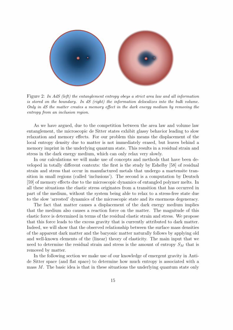
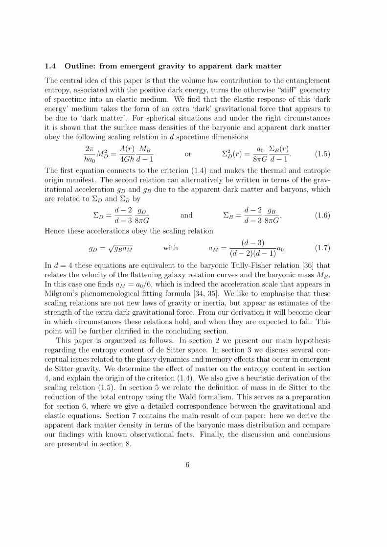
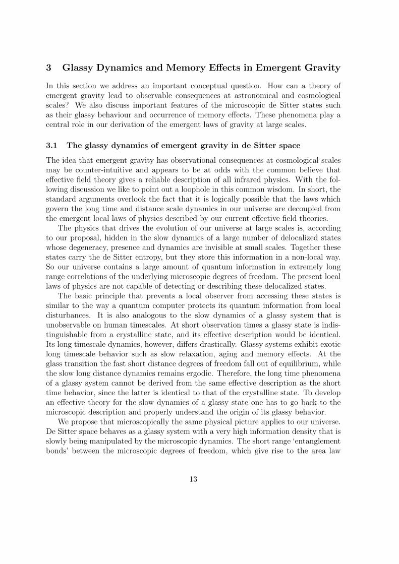
Figure 2: In AdS (left) the entanglement entropy obeys a strict area law and all informationis stored on the boundary. In dS (right) the information delocalizes into the bulk volume.Only in dS the matter creates a memory effect in the dark energy medium by removing theentropy from an inclusion region.

As we have argued, due to the competition between the area law and volume lawentanglement, the microscopic de Sitter states exhibit glassy behavior leading to slowrelaxation and memory effects. For our problem this means the displacement of thelocal entropy density due to matter is not immediately erased, but leaves behind amemory imprint in the underlying quantum state. This results in a residual strain andstress in the dark energy medium, which can only relax very slowly.

In our calculations we will make use of concepts and methods that have been de-veloped in totally different contexts: the first is the study by Eshelby [58] of residualstrain and stress that occur in manufactured metals that undergo a martensite tran-sition in small regions (called ‘inclusions’). The second is a computation by Deutsch[59] of memory effects due to the microscopic dynamics of entangled polymer melts. Inall these situations the elastic stress originates from a transition that has occurred inpart of the medium, without the system being able to relax to a stress-free state dueto the slow ‘arrested’ dynamics of the microscopic state and its enormous degeneracy.

The fact that matter causes a displacement of the dark energy medium impliesthat the medium also causes a reaction force on the matter. The magnitude of thiselastic force is determined in terms of the residual elastic strain and stress. We proposethat this force leads to the excess gravity that is currently attributed to dark matter.Indeed, we will show that the observed relationship between the surface mass densitiesof the apparent dark matter and the baryonic matter naturally follows by applying oldand well-known elements of the (linear) theory of elasticity. The main input that weneed to determine the residual strain and stress is the amount of entropy SM that isremoved by matter.

In the following section we make use of our knowledge of emergent gravity in Anti-de Sitter space (and flat space) to determine how much entropy is associated with amass M . The basic idea is that in these situations the underlying quantum state only

15

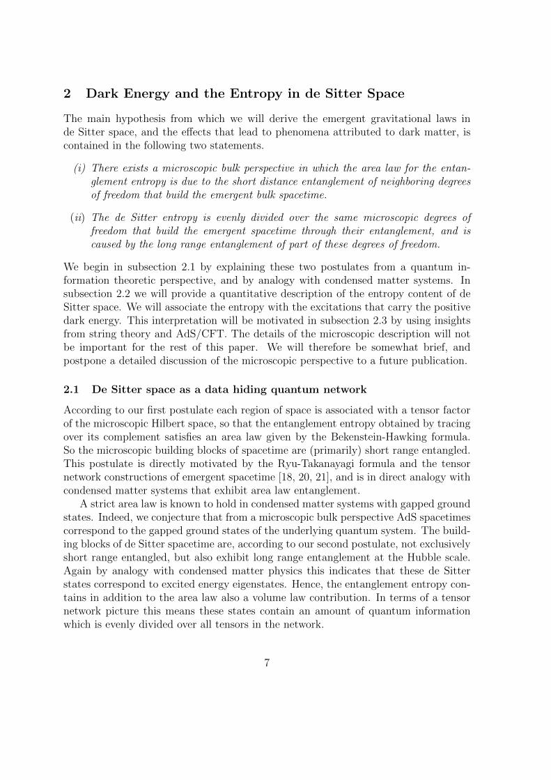
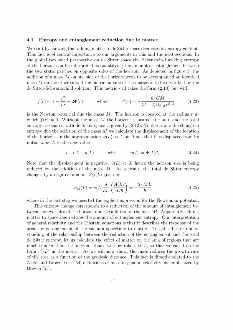
Figure 3: The Penrose diagram of global de Sitter space with a mass in the center of thestatic patch. The global solution requires that an equal mass is put at the anti-podal point.

carries area law entanglement. Hence, we can determine the entropy SM associatedwith the mass M by studying first the effect of matter on the area entanglement usinggeneral relativity. Once we know this amount, we subsequently apply this in de Sitterspace to determine the reduction of the entropy density. From there it becomes astraightforward application of linear elasticity to derive the stress and the elastic force.

To derive the strength of this dark gravitational force we assume that a transitionoccurs in the medium by which a certain amount SM of the entropy is being removedfrom the underlying microscopic state locally inside a certain region VM . Following[58] we will refer to the region VM as the ‘inclusion’. It is surrounded by the originalmedium, which will be called the ‘matrix’.

4 The Effect of Matter on the Entropy and Dark Energy

In this section we determine the effect of matter on the entropy content in de Sitterspace. First we will determine the change in the total de Sitter entropy when matterwith a total mass M is added at or near the center of the causal domain. After thatwe also derive an estimate of the change in the entanglement entropy by computingthe deficit in (growth of the) the area as a function of distance. We will find that thisquantity is directly related to the ADM and Brown-York definitions of mass in generalrelativity. We subsequently determine the reduction of the entropy content of de Sitterspace within a radius r due to (the appearance of) matter and compute the resultingdisplacement field. Using an analogy with the theory of elasticity we then present aheuristic derivation of the Tully-Fisher scaling law.

16

4.1 Entropy and entanglement reduction due to matter

We start by showing that adding matter to de Sitter space decreases its entropy content.This fact is of central importance to our arguments in this and the next sections. Inthe global two sided perspective on de Sitter space the Bekenstein-Hawking entropyof the horizon can be interpreted as quantifying the amount of entanglement betweenthe two static patches on opposite sides of the horizon. As depicted in figure 3, theaddition of a mass M on one side of the horizon needs to be accompanied an identicalmass M on the other side, if the metric outside of the masses is to be described by thede Sitter-Schwarzschild solution. This metric still takes the form (2.10) but with

f(r) = 1− r2

L2+ 2Φ(r) where Φ(r) = − 8πGM

(d− 2)Ωd−2 rd−3. (4.23)

is the Newton potential due the mass M . The horizon is located at the radius r atwhich f(r) = 0. Without the mass M the horizon is located at r = L and the totalentropy associated with de Sitter space is given by (2.12). To determine the change inentropy due the addition of the mass M we calculate the displacement of the locationof the horizon. In the approximation Φ(L) << 1 one finds that it is displaced from itsinitial value L to the new value

L→ L+ u(L) with u(L) = Φ(L)L. (4.24)

Note that the displacement is negative, u(L) < 0, hence the horizon size is beingreduced by the addition of the mass M . As a result, the total de Sitter entropychanges by a negative amount SM(L) given by

SM(L) = u(L)d

dL

(A(L)

4G~

)= −2πML

~(4.25)

where in the last step we inserted the explicit expression for the Newtonian potential.This entropy change corresponds to a reduction of the amount of entanglement be-

tween the two sides of the horizon due the addition of the mass M . Apparently, addingmatter to spacetime reduces the amount of entanglement entropy. Our interpretationof general relativity and the Einstein equations is that it describes the response of thearea law entanglement of the vacuum spacetime to matter. To get a better under-standing of the relationship between the reduction of the entanglement and the totalde Sitter entropy, let us calculate the effect of matter on the area of regions that aremuch smaller than the horizon. Hence we now take r <<L, so that we can drop theterm r2/L2 in the metric. As we will now show, the mass reduces the growth rateof the area as a function of the geodesic distance. This fact is directly related to theADM and Brown-York [54] definitions of mass in general relativity, as emphasized byBrewin [55].

17

So let us compare the increase of the area as a function of the geodesic distance inthe situation with and without the mass. To match the two geometries we take sphereswith equal area, hence the same value of r. Without the mass the geodesic distanceis equal to r, while in the presence of the mass M a small increment dr leads to anincrease in the geodesic distance ds, since dr = (1 + Φ(r))ds, as is easily verified fromthe Schwarzschild metric. It then follows that

d

ds

(A(r)

4G~

)∣∣∣∣M 6=0

M=0

= Φ(r)d

dr

(A(r)

4G~

)= −2πM

~. (4.26)

The notation on the l.h.s. indicates that we are taking the difference between thesituations with and without the mass.

We reinterpret (4.26) as an equation for the amount of entanglement entropy SM(r)that the mass M takes away from a spherical region with size r. This quantity issomewhat tricky to define, since one has to specify how to identify the two geometrieswith and without the mass. To circumvent this issue we define SM(r) through itsderivative with respect to r, which we identify with the left hand side of equation(4.26). In other words, we propose that the following relation holds

dSM(r)

dr= −2πM

~. (4.27)

Here we used the fact that in the weak gravity regime the increase in geodesic distanceds and dr are approximately equal. Now note that by integrating this equation onefinds

SM(r) = −2πMr

~, (4.28)

which up to a sign is the familiar Bekenstein bound [56], which together with the re-sults of [57] suggests that the definition of mass in emergent gravity is given in terms ofrelative entropy. We conclude that the mass M reduces the amount of entanglement en-tropy of the surrounding spacetime by SM(r). This happens in all spacetimes, whetherit is AdS, flat space or de Sitter, hence it is logically different from the reduction ofthe total de Sitter entropy. Nevertheless, the results agree: when we put r = L wereproduce the change of the de Sitter entropy (4.25). We find that the mass M reducesthe entanglement entropy of the region with radius r by a fraction r/L of SM(L).

4.2 An entropic criterion for the dark phase of emergent gravity

Consider a spherical region with radius r that is close to the center of the de Sitterstatic patch. According to our hypothesis in section 2 the de Sitter entropy inside aspherical region with radius r is given by

SDE(r) =1

V0V (r) =

r

L

A(r)

4G~. (4.29)

18

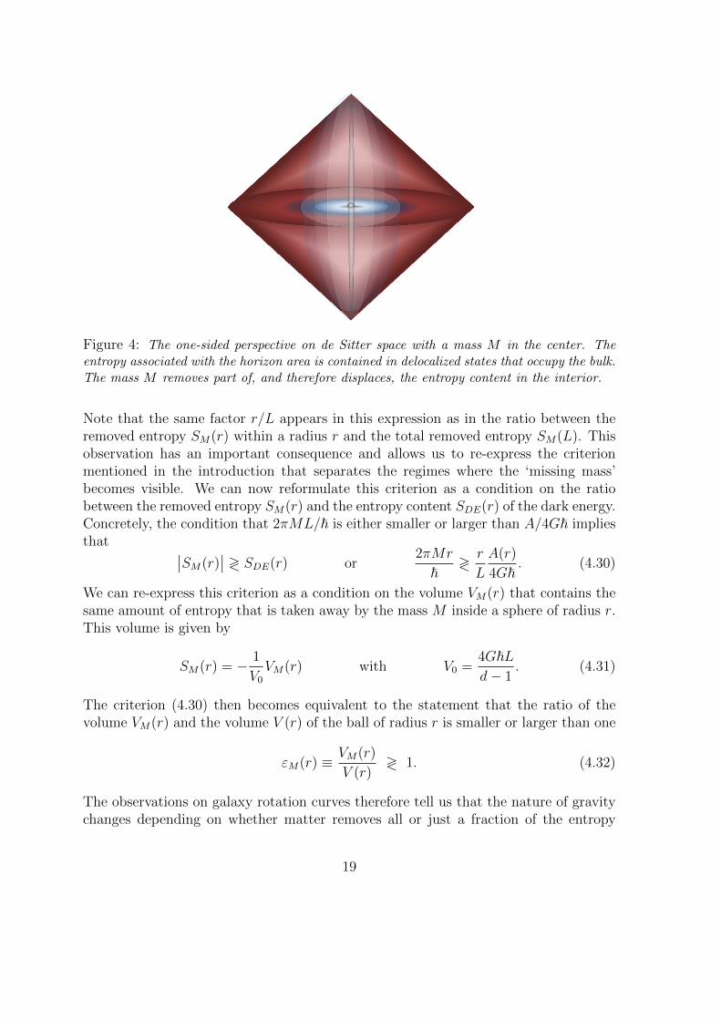
Figure 4: The one-sided perspective on de Sitter space with a mass M in the center. Theentropy associated with the horizon area is contained in delocalized states that occupy the bulk.The mass M removes part of, and therefore displaces, the entropy content in the interior.

Note that the same factor r/L appears in this expression as in the ratio between theremoved entropy SM(r) within a radius r and the total removed entropy SM(L). Thisobservation has an important consequence and allows us to re-express the criterionmentioned in the introduction that separates the regimes where the ‘missing mass’becomes visible. We can now reformulate this criterion as a condition on the ratiobetween the removed entropy SM(r) and the entropy content SDE(r) of the dark energy.Concretely, the condition that 2πML/~ is either smaller or larger than A/4G~ impliesthat ∣∣SM(r)

∣∣ ≷ SDE(r) or2πMr

~≷r

L

A(r)

4G~. (4.30)

We can re-express this criterion as a condition on the volume VM(r) that contains thesame amount of entropy that is taken away by the mass M inside a sphere of radius r.This volume is given by

SM(r) = − 1

V0VM(r) with V0 =

4G~Ld− 1

. (4.31)

The criterion (4.30) then becomes equivalent to the statement that the ratio of thevolume VM(r) and the volume V (r) of the ball of radius r is smaller or larger than one

εM(r) ≡ VM(r)

V (r)≷ 1. (4.32)

The observations on galaxy rotation curves therefore tell us that the nature of gravitychanges depending on whether matter removes all or just a fraction of the entropy

19

content of de Sitter. One finds that the volume VM(r) is given by

VM(r) =8πG

a0

Mr

d− 1. (4.33)

Here we replaced the Hubble length L by the acceleration scale a0 to arrive at a formulathat is dimensionally correct. In other words, this volume does not depend on ~ or c.In fact, as we will see, the elastic description that we are about to present only dependson the constants G and a0 and hence naturally contains precisely those parameters thatare observed in the phenomena attributed to dark matter.

A related comment is that the ratio εM(r) can be used to determine the value ofthe surface mass density ΣM(r) = M/A(r) in terms of a0 and G via

εM(r) =8πG

a0ΣM(r). (4.34)

This relation follows immediately by inserting the expressions (4.31) and the result(4.28) for the removed entropy SM(r) into (4.32). We also reinstated factors of thespeed of light to obtain an expression that is dimensionally correct. The regime whereSM(r) < SDE(r) corresponds to εM(r) < 1, hence in this regime we are dealing withlow surface mass density and low gravitational acceleration. For this reason it will bereferred to as the ‘sub-Newtonian’ or ‘dark gravity’ regime.

4.3 Displacement of the entropy content of de Sitter space

In the regime where only part of the de Sitter entropy is removed by matter, theremaining entropy contained in the delocalized de Sitter states starts to have a non-negligible effect. This leads to modifications to the usual gravitational laws, since thelatter only take into account the effect of the area law entanglement. To determinethese modifications we have to keep track of the displacement of the entropy contentdue to matter. In the present context, where we are dealing with a central mass Mwe can represent this displacement as a scalar function u(r) that keeps track of thedistance over which the information is displaced in the radial direction.

In an elastic medium one encounters a purely radial displacement u(r) when oneremoves (or adds) a certain amount of the medium in a symmetric way from insidea spherical region. The value of the displacement field u(r) determines how much ofthe medium has been removed. If we assume that the medium outside of the regionwhere the volume is removed is incompressible, the change in volume is given by thatof a thin shell with thickness u(r) and area A(r). The sign of u(r) determines whetherthe change in volume was positive or negative. We further assume that the change involume is proportional to the removed entropy SM(r). In this way we obtain a relationof the form

SM(r) =1

V ∗0u(r)A(r) (4.35)

20

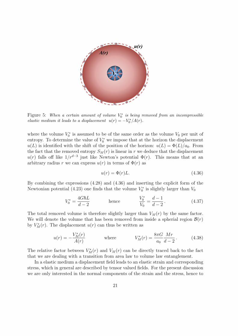
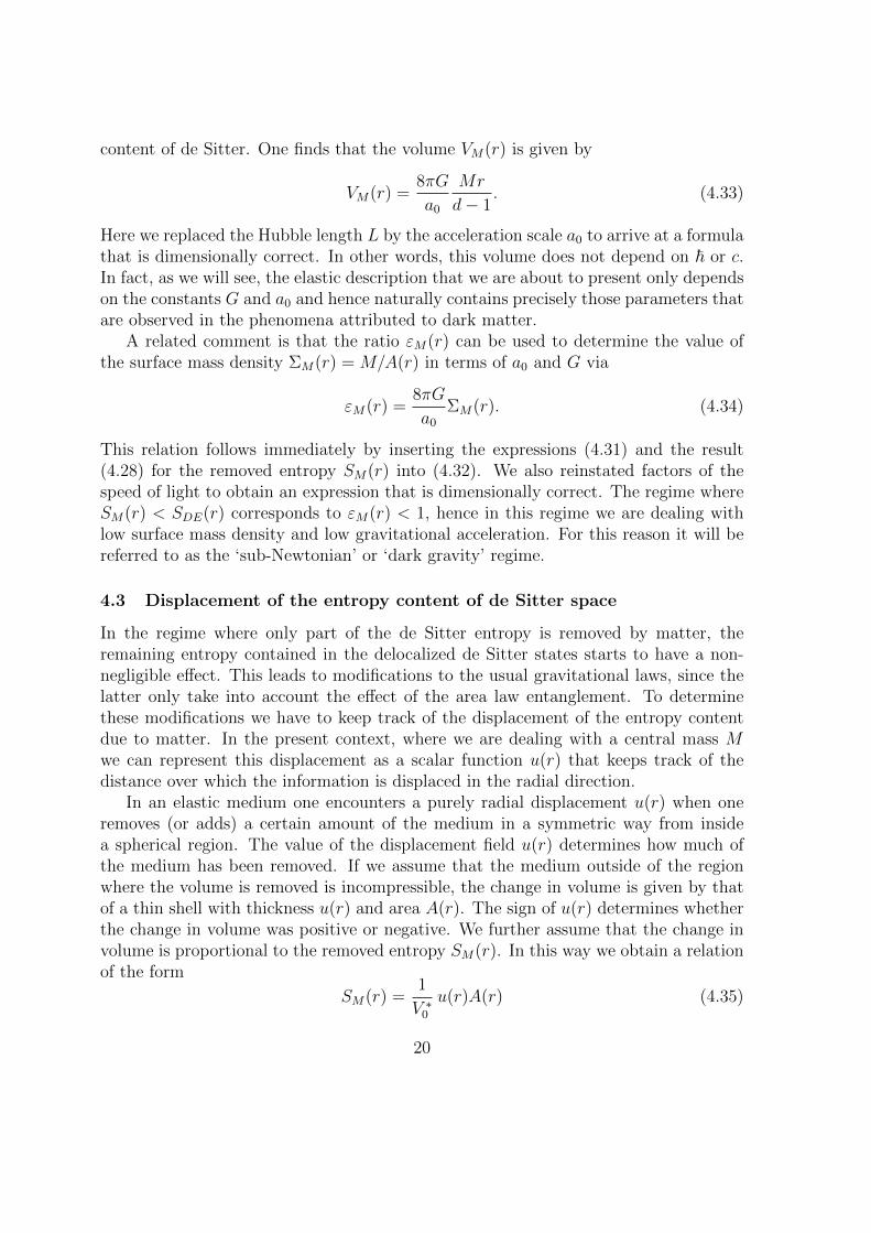
Figure 5: When a certain amount of volume V ∗0 is being removed from an incompressibleelastic medium it leads to a displacement u(r) = −V ∗0 /A(r).

where the volume V ∗0 is assumed to be of the same order as the volume V0 per unit ofentropy. To determine the value of V ∗0 we impose that at the horizon the displacementu(L) is identified with the shift of the position of the horizon: u(L) = Φ(L)/a0. Fromthe fact that the removed entropy SM(r) is linear in r we deduce that the displacementu(r) falls off like 1/rd−3 just like Newton’s potential Φ(r). This means that at anarbitrary radius r we can express u(r) in terms of Φ(r) as

u(r) = Φ(r)L. (4.36)

By combining the expressions (4.28) and (4.36) and inserting the explicit form of theNewtonian potential (4.23) one finds that the volume V ∗0 is slightly larger than V0

V ∗0 =4G~Ld− 2

henceV ∗0V0

=d− 1

d− 2. (4.37)

The total removed volume is therefore slightly larger than VM(r) by the same factor.We will denote the volume that has been removed from inside a spherial region B(r)by V ∗M(r). The displacement u(r) can thus be written as

u(r) = −V∗M(r)

A(r)where V ∗M(r) =

8πG

a0

Mr

d− 2. (4.38)

The relative factor between V ∗M(r) and VM(r) can be directly traced back to the factthat we are dealing with a transition from area law to volume law entanglement.

In a elastic medium a displacement field leads to an elastic strain and correspondingstress, which in general are described by tensor valued fields. For the present discussionwe are only interested in the normal components of the strain and the stress, hence to

21

simplify our notation we will suppress tensor indices and denote the normal strain andnormal stress simply by ε(r) and σ(r). Our proposed explanation of the gravitationalphenomena associated to ‘dark matter’ is that in the regime where only part of theentropy is removed, that is where εM(r)< 1, the remaining entropy associated to thedark energy behaves as an incompressible elastic medium. Specifically, we propose thatthe entropy SM(r) is only removed from a local inclusion region VM(r) with volumeVM(r). We represent the region VM(r) as the intersection of a fixed region VM(L) witha ball B(r) with radius r centered around the origin,

VM(r) = VM(L) ∩ B(r). (4.39)

The precise shape or topology of the region VM(L) will not be important for ourdiscussion.

To deal with the fact that the removed volume V ∗M(r) depends on the radius r, wemake use of the linearity of elasticity to decompose the region VM(r) in small ball-shaped regions Bi with volume NiV0. From each Bi a fixed volume NiV

∗0 has been

removed corresponding to Ni units of entropy. We first determine the displacement foreach region, and then compute the total displacement by adding the different contri-butions.

Let us consider the displacement field u(r) resulting from the removal of a vol-ume NV ∗0 from a single ball-shaped region B0 with volume NV0. For simplicity anddefiniteness, let us assume that B0 is centered at the origin of de Sitter space. Thedisplacement field outside of B0 is given by

u(r) = −NV∗0

A(r). (4.40)

The normal strain ε(r) corresponds to the r-r component of the strain tensor and isgiven by the radial derivative ε(r) = u′(r). Hence

ε(r) =NV0V (r)

. (4.41)

Here we absorbed a factor (d− 2)/(d− 1) by making the substitution V ∗0 → V0. Sincethe volume of B0 is equal to NV0, we find that the normal strain ε(r) at its boundaryis precisely equal to one. Note that to obtain this natural result we made use of thespecific ratio of V ∗0 and V0.

This same calculation can be performed for each small ball Bi and leads to a dis-placement field ui and strain εi identical to (4.40) and (4.41) where the radius is definedwith respect to the center of Bi and the number of units of removed entropy is equalto Ni. By adding all these different contributions we can in principle determine thetotal displacement and strain due to the removal of the entropy SM(r) from the regionVM . Here we have to distinguish two regimes. When VM(r) > V (r) we are inside the

22

region VM and ‘all the available volume’ has been removed. This means, the entropyreduction due to the mass is larger than the available thermal entropy. In this regionthe response to the entropy reduction due to the mass M is controlled by the area lawentanglement, which leads to the usual gravity laws. We are interested in the otherregime where VM(r) < V (r), since this is where the modifications due to the volumelaw will appear.

The total amount of entropy that is removed within a radius r is equal to SM(r).Hence, at first we may simply try to replace N by SM(r) so that the removed volumeNV ∗0 becomes equal to V ∗M(r), and NV0 to the volume VM(r) of the region VM(r).Indeed, if we make the substitutions

NV ∗0 −→ V ∗M(r) and NV0 −→ VM(r) (4.42)

the displacement u(r) becomes equal to (4.38) and the expression (4.41) for ε(r) be-comes identical to the quantity εM(r) introduced in (4.32). In other words, we findthat the apparent DM criterion can be interpreted as a condition on the normal elas-tic strain ε(r): the transition from standard Newtonian gravity to the apparent darkmatter regime occurs when the elastic strain drops in value below one.

The quantity ε(r), as we have now defined it, equals the normal strain in the regimewhere the removed volume is kept constant: in other words, where the medium istreated as incompressible. As we will explain in more detail in section 7, in this regimethe normal strain ε(r) determines the value of the apparent surface mass density Σ(r)precisely through the relation (4.34), which for convenience we repeat here in slightlydifferent form

Σ(r) =a0

8πGε(r). (4.43)

In the next subsection we will use this relation to determine the apparent surface massdensity in the regime ε(r) < 1. Here the volume VM(r) is smaller than the volumeV (r) of the sphere with radius r. Hence, it is not clear anymore that one can simplytake the relation (4.41) and make the substitution (4.42). A more precise derivationwould involve adding all these separate contributions of the small balls Bi that togethercompose the region VM(r). We will now show that this leads through the relation (4.43)to a surface mass density that includes the contribution of the apparent dark matter.

4.4 A heuristic derivation of the Tully-Fisher scaling relation

After having introduced all relevant quantities, we are now ready to present our pro-posed explanation of the observed phenomena attributed with dark matter. It is basedon the idea that the standard laws of Newton and general relativity describe the re-sponse of the area law entanglement to matter, while in the regime ε(r)<1 the gravi-tational force is dominated by the elastic response due to the volume law contribution.We will show that the Tully-Fisher scaling law for the surface mass densities of the

23

apparent dark matter and the baryonic matter is derived from a quantitive estimate ofthe strain and stress caused by the entropy SM(r) removed by matter.

Let us go back to the result (4.41) for the strain outside a small region B0 of sizeNV0, and let us compute the integral of the square ε2(r) over the region outside of B0with V (r) > NV0. We denote this region as the complement B0 of the ball B0. Theintegral is easy to perform and simply gives the volume of the region B0 from whichthe entropy was removed∫

B0ε2(r)A(r)dr =

∫ ∞NV0

(NV0V

)2

dV = NV0. (4.44)

This result is well known in the theory of ‘elastic inclusions’ [58]. In this contextequation (4.44) is used to estimate the elastic energy caused by the presence of theinclusion. This same method has also been applied to calculate memory effects inentangled polymer melts [60].

We can repeat this calculation for all the small balls Bi that together make up theregion VM(r) to show that the integral of ε2i over the region outside of Bi is given byNiV0. Since εi quickly falls off like 1/r(d−1) with the distance from the center, the maincontribution to the integral comes from the neighbourhood of Bi. We now assumethat, in the regime where VM(r) < V (r), all the small regions Bi are disjoint, and areseparated enough in distance so that the elastic strain εi for each ball Bi is primarilylocalized in its own neighbourhood. This means that the integral of the square of thetotal strain is equal to the sum of the contributions of the individual squares ε2i for allthe balls Bi. In other words, the cross terms between εi and εj can be ignored wheni 6= j. In section 7 we will show that this can be proven to hold exactly. The integral ofε2 over the ball B(r) with radius r thus decomposes into a sum of contributions comingfrom the neighbourhoods of each small region Bi∫

B(r)ε2dV ≈

∑i

∫Bi∩B(r)

ε2i dV ≈∑Bi⊂B(r)

∫Biε2i dV =

∑Bi⊂B(r)

NiV0 = VM(r). (4.45)

Each of these integrals is to a good approximation equal to the volume NiV0 of Bi,and since these together constitute the region VM , we find that the total sum gives thevolume VM(r). We will further make the simplifying assumption that in the sphericallysymmetric situation the resulting strain is just a function of the radius r. In this waywe find ∫ r

0

ε2(r′)A(r′)dr′ = VM(r). (4.46)

To arrive at the Tully-Fisher scaling relation between the surface mass density of theapparent dark matter and the baryonic dark matter we differentiate this expressionwith respect to the radius. If we assume that the mass distribution is well localised

24

near the origin, we can treat the mass M as a constant. In that case we obtain

ε2(r) =1

A(r)

dVM(r)

dr=

1

A(r)

8πG

a0

M

d− 1(4.47)

We now make the identification of the apparent surface mass density with ε(r). Weobtain a relationship for the square surface mass density of the apparent dark matterand surface mass density of the visible baryonic matter. To distinguish the apparentsurface mass density from the one defined in terms of the mass M we will denote thefirst as ΣD and the latter as ΣB. These quantities are defined as

ΣD(r) =a0

8πGε(r) and ΣB(r) =

M

A(r). (4.48)

With these definitions we precisely recover the relation

ΣD(r)2 =a0

8πG

ΣB(r)

d− 1. (4.49)

which was shown to be equivalent to the Tully-Fisher relation.In the remainder of this paper we will again go over the arguments that lead us

to the proposed elastic phase of emergent de Sitter gravity and further develop thecorrespondence between the familiar gravity laws and the tensorial description of theelastic phase. In particular, we will clarify the relation between the elastic strain andstress and the apparent surface mass density. We will also revisit the derivation ofthe Tully-Fisher scaling relations and present the details of the calculation at a lessheuristic level. This will clarify under what assumptions and conditions this relationis expected to hold.

5 The First Law of Horizons and the Definition of Mass

Our goal in this section is to understand the reduction of the de Sitter entropy due tomatter in more detail. For this purpose we will make use of Wald’s formalism [50] andmethods similar to those developed in [15, 16, 17] for the derivation of the (linearized)Einstein equations from the area law entanglement. We will generalise some of thesemethods to de Sitter space and discuss the modifications that occur in this context.Our presentation closely follows that of Jacobson [17].

5.1 Wald’s formalism in de Sitter space

In Wald’s formalism [50] the entropy associated to a Killing horizon is expressed as theNoether charge for the associated Killing symmetry. For Einstein gravity the explicit

25

expression is6

~2πS =

∫hor

Q[ξ] = − 1

16πG

∫hor

∇aξbεab. (5.1)

Here the normalization of the Killing vector ξa is chosen so that S precisely equalsA/4G~, where A is the area of the horizon. When there is no stress energy in the bulk,the variation δQ[ξ] of the integrand can be extended to a closed form by imposing the(linearized) Einstein equations for the (variation of) the background geometry. Forblack holes this fact is used to deform the integral over the horizon to the boundary atinfinity, which leads to the first law of black hole thermodynamics.

These same ideas can be applied to de Sitter space. Here the situation is ‘inverted’compared to the black hole case, since we are dealing with a cosmological horizon andthere is no asymptotic infinity. In fact, when there is no stress energy in the bulk thevariation of the horizon entropy vanishes, since there is no boundary term at infinity.The first law of horizon thermodynamics in this case reads [17, 22]

~2πδS + δHξ = 0 where δHξ =

∫CξaTab dΣb (5.2)

represents the variation of the Hamiltonian associated with the Killing symmetry. It isexpressed as an integral of the stress energy tensor over the Cauchy surface C for thestatic patch. We are interested in a situation where the stress is concentrated in a smallregion around the origin, with a radius r∞ that is much smaller than the Hubble scale.This means that the integrand of δHξ only has support in this region. Furthermore,the variation δQ[ξ] of integrand of the Noether charge can be extended to a closed formalmost everywhere in the bulk, except in the region with the stress energy. This meanswe can deform the surface integral over the horizon to an integral over a surface S∞well outside the region with the stress energy. Following Wald’s recipe we can writethis integral as

δHξ =

∫S∞

(δQ[ξ]− ξ · δB

)(5.3)

where we included an extra contribution ξ · δB which vanishes on the horizon.The Hamiltanian Hξ is proportional to the generator of time translations in the

static coordinates of de Sitter space, where the constant of proportionality given bythe surface gravity a0 on the cosmological horizon. Hence we have

ξa∂

∂xa=

1

a0

∂

∂twhich implies δHξ =

δM

a0, (5.4)

where δM denotes the change in the total mass or energy contained in de Sitter space.With this identification the first law takes an almost familiar form

TδS = −δM with T =~a02π

. (5.5)

6Here we use the notation of [15] by introducing the symbol εab = 1(d−2)!εabc1...cd−2

dxc1∧. . .∧dxcd−2 .

26

The negative sign can be understood as follows. In deforming the Noether integral(5.1) from the horizon to the surface S∞ we have to keep the same orientation of theintegration surface. However, in the definition of the mass the normal points outward,while the opposite direction is used in the definition of the entropy.

5.2 An approximate ADM definition of mass in de Sitter

We would like to integrate the second equation in (5.4) to obtain a definition of themass M similar to the ADM mass. Strictly speaking, the ADM mass can only bedefined at spatial infinity. However, suppose we choose the radius r∞ that definesthe integration surface S∞ to be (i) sufficiently large so that the gravitational fieldof the mass M is extremely weak, and (ii) small enough so that r∞ is still negligiblecompared to the Hubble scale L. In that situation it is reasonable to assume that toa good approximation one can use the standard ADM expression for the mass. Byfollowing the same steps as discussed in [50, 51] for the ADM mass, we obtain thefollowing surface integral expression for the mass M [52, 53]

M =

∫S∞

(Q[t]− t ·B) =1

16πG

∫S∞

(∇jhij −∇ihjj

)dAi. (5.6)

Here hij is defined in terms of the spatial metric.We assume now that we are in a Newtonian regime in which Newton’s potential Φ

is much smaller than one, and furthermore far away from the central mass distributionso that Φ depends only on the distance to the center of the mass distribution. In thisregime the metric takes the following form

ds2|x|=r∞

= −dt2 + dx2i − 2Φ(x)(dt2 +

(xidxi)2

|x|2). (5.7)

We will assume that the matter is localized well inside the region |x| < r∞ . This meansthat the Newtonian potential is in good approximation only a function of the radius.When we insert the spatial metric

hij = δij − 2Φ(x)ninj with nj ≡xj|x|

(5.8)

into the ADM integral (5.6) and choose a spherical surface with a fixed radius r∞ wefind the following expression for the mass

M = − 1

8πG

∫r∞

Φ(x)∇jnj dA (5.9)

where dA = nidAi. It is easy to check the validity of this expression using the explicitform of Φ(x) (4.23) and the fact that for a spherical surface

∇jnj =d− 2

|x|. (5.10)

27

6 The Elastic Phase of Emergent Gravity

We now return to the central idea of this paper. As we explained, the effect of matteris to displace the entropy content of de Sitter space. Our aim is to describe in detailhow the resulting elastic back reaction translates into an effective gravitational force.We will describe this response using the standard linear theory of elasticity.

6.1 Linear elasticity and the definition of mass

The basic variable in elasticity is the displacement field ui. The linear strain tensor isgiven in terms of ui by

εij =1

2(∇iuj +∇jui) . (6.1)

In the linear theory of elasticity the stress tensor σij obeys the tensorial version ofHooke’s law. For isotropic and homogeneous elastic media there are two independentelastic moduli conventionally denoted by λ and µ. These so-called Lame parametersappear in the stress tensor as follows

σij = λ εkkδij + 2µ εij. (6.2)

The combination K = λ+ 2µ/(d− 1) is called the bulk modulus. The shear modulusis equal to µ: it determines the velocity of shear waves, while the velocity of pressurewaves is determined by λ+ 2µ. Requiring that both velocities are real-valued leads tothe following inequalities on the Lame parameters

µ ≥ 0 and λ+ 2µ ≥ 0. (6.3)

Our aim is to relate all these elastic quantities to corresponding gravitational quantities.In particular, we will give a map from the displacement field, the strain and the stresstensors to the apparent Newton’s potential, gravitational acceleration and surface massdensity. In addition we will express the elastic moduli in terms of Newton’s constantG and the Hubble acceleration a0.

Since de Sitter space has no asymptotic infinity, the precise definition of mass issomewhat problematic. In general, the mass can only be precisely defined with the helpof a particular reference frame. In an asymptotically flat or AdS space, this referenceframe is provided by the asymptotic geometry. We propose that in de Sitter space therole of this auxiliary reference frame, and hence the definition of the mass, is providedby the elastic medium associated with the volume law contribution to the entanglemententropy. In other words, the reference frame with respect to which we define the massM has to be chosen at the location where the standard Newtonian gravity regime makesthe transition to the elastic phase. This implies that the definition of mass dependson the value of the displacement field and its corresponding strain and stress tensor inthe elastic medium.

28

We will now show that the ADM definition of mass can be naturally translated intoan expression for the elastic strain tensor or, alternatively, for the stress tensor. Insection 4, we found that the displacement field ui at the horizon is given by

ui =Φ

a0ni with ni =

xi|x|

(6.4)

and we argued that a similar identification holds in the interior of de Sitter space.Alternatively, we can introduce the displacement field ui in terms of the spatial metrichij via the Ansatz

hij = δij −a0c2

(uinj + niuj) . (6.5)

Eventually we take a non-relativistic limit in which we take L and c to infinity, whilekeeping a0 = c2/L fixed. Hence we will work almost exclusively in the Newtonianregime, and will not attempt to make a correspondence with the full relativistic gravi-tational equations.

It is an amusing calculation to show that the expression (5.9) for the mass M canbe rewritten in the following suggestive way in terms of the strain tensor εij for thedisplacement field ui defined in (6.4)

M =a0

8πG

∫S∞

(njεij − niεjj

)dAi . (6.6)

In this calculation we used the fact that the integration surface is far away from thematter distribution, so that Φ only depends on the distance |x| to the center of mass.This same result can be derived by inserting the expression (6.5) together with (6.4)into the standard ADM integral (5.6). It is interesting to note that the first termcorresponds to Q[t] while the second term is equal to −t ·B. We again point out thatthe prefactor a0/8πG in (6.6) is identical to the observed critical value for the surfacemass density.

When we multiply the expression (6.6) for M by the acceleration scale a0 we obtaina physical quantity with the dimension of a force. This motivates us to re-express theright hand side as

Ma0 =

∮S∞σijnj dAi (6.7)

where we identified the stress tensor σij with the following expression in terms of thestrain tensor

σij =a20

8πG

(εij − εkkδij

). (6.8)

By comparing with (6.2) we learn that the elastic moduli of the dark elastic mediumtake the following values

µ =a20

16πGand λ+ 2µ = 0. (6.9)

29

We thus find that the shear modulus has a positive value, but that the P-wave modulusvanishes. The shear modulus has the dimension of energy density, as it should, and isup to a factor (d− 1)(d− 2) equal to the cosmological energy density.

In the theory of elasticity the integrand of the right hand side of (6.7) representsthe outward traction force σijnj. The left hand side on the other hand is the outwardforce on a mass shell with total mass M when it experiences an outward accelerationequal to the surface acceleration a0 at the horizon. Hence, it is natural to interpret theequation (6.7) as expressing a balance of forces.

The precise value (6.9) of the shear modulus is dictated by the following calcula-tion. Let us consider the special situation in which the surface S∞ corresponds to anequipotential surface. In this case we can equate the gravitational self-energy enclosedby S∞ exactly with the elastic self energy

1

2MΦ =

1

2

∮S∞σijuj dAi . (6.10)

In the next subsection we further elaborate these correspondence rules between theelastic phase and the Newtonian regime of emergent gravity. Specifically, we will showthat the elastic equations naturally lead to an effective Newtonian description in termsof an apparent surface mass density.

6.2 The elasticity/gravity correspondence in the sub-Newtonian regime

First we start by rewriting the familiar laws of Newtonian gravity in terms of a surfacemass density vector. We introduce a vector field Σi defined in terms of the Newtonianpotential Φ via

Σi = −(d− 2

d− 3

)gi

8πGwhere gi = −∇iΦ (6.11)

is the standard gravitational acceleration. By working with Σi instead of gi we avoidsome annoying dimension dependent factors, and make the correspondence with theelastic quantities more straightforward. The normalization is chosen so that the grav-itational analogue of Gauss’ law simply reads

∇iΣi = ρ or

∮S

Σi dAi = M (6.12)

where M is the total mass inside the region enclosed by the surface S. We will refer toΣi as the surface mass density. The gravitational self-energy of a mass configurationcan be expressed in terms of the acceleration field gi and the surface mass densityvector field Σi as

Ugrav =1

2

∫dV giΣi. (6.13)

30

We are interested in the force on a small point mass m located at some point P .Its Newtonian potential Φ(m) and surface mass density Σ(m) are sourced by the massdensity ρ(m) = mδ(x−xP ). The force that acts on the point mass is derived from thegravitational potential, which obeys the representation formula

mΦ(P ) =

∮SdAi

(Φ(m)Σi − Φ Σ

(m)i

). (6.14)

Here the surface S is chosen so that it encloses the mass distribution that sources thefield Φ and Σi.

All these equations have direct analogues in the linear theory of elasticity. Thedisplacement field ui is analogous to the Newtonian potential Φ, the strain tensor εijplays a similar role as the gravitational acceleration gi, and the stress tensor σij is thedirect counterpart of the surface mass density Σi. For instance, our definition (6.11) ofthe surface mass density Σi is the direct analogue of the definition (6.2) of the stresstensor σij, with the obvious correspondence between the expressions for gi in terms ofΦ and εij in terms of ui. The counterparts of the Poisson equation and Gauss’ law read

∇iσij + bj = 0 and

∮Sσij dAj + Fi = 0 (6.15)

where the body force bj represents the force per unit of volume that acts on the mediumand Fj is the total force acting on the part of the medium enclosed by the surface S.Also the elastic energy is given, except for the sign, in a completely analogous way

Uelas =1

2

∫dV εijσij. (6.16)

The elastic equivalent of the point mass is a point force described by a delta-functionsupported body force b

(f)i = fi δ(x−xP ). It acts as a point source for the elastic

displacement field u(f)i and stress tensor σ

(f)ij . The elastic potential that determines the

elastic force acting on a point force satisfies an analogous representation formula as forthe gravitational case

− fiui(P ) =

∮SdAi

(u(f)j σji − ujσ(f)

ij

). (6.17)

Here the integration surface S has been chosen such that it contains the body forcesthat source ui and σij.

It is striking that the correspondence between gravitational and elastic quantitiesonly requires two dimensionful constants: Newton’s constant G and the Hubble accel-eration scale a0. All the other constants of nature, like the speed of light, Planck’sconstant or Boltzmann’s constant, do not play a role. We already announced thatthe elastic moduli take the values given in (6.9), but we have not yet justified why

31

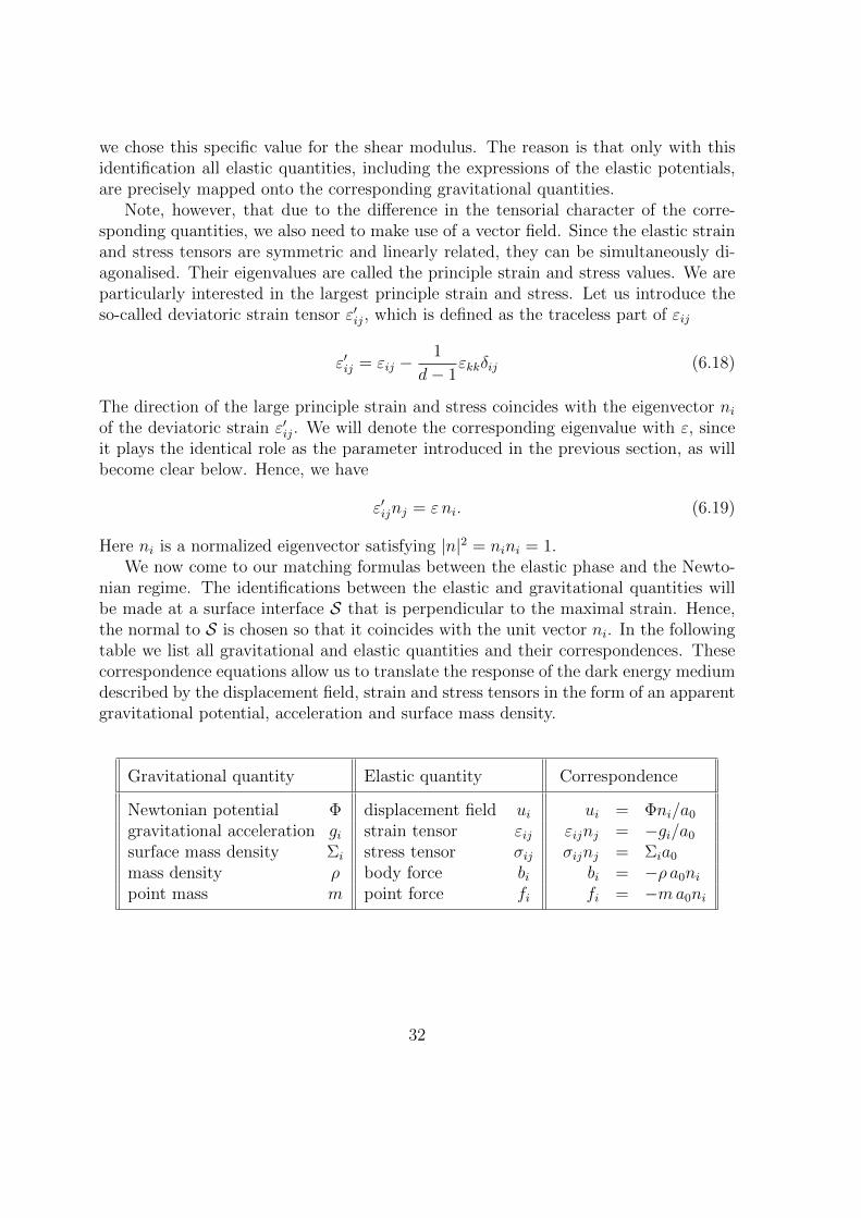
we chose this specific value for the shear modulus. The reason is that only with thisidentification all elastic quantities, including the expressions of the elastic potentials,are precisely mapped onto the corresponding gravitational quantities.

Note, however, that due to the difference in the tensorial character of the corre-sponding quantities, we also need to make use of a vector field. Since the elastic strainand stress tensors are symmetric and linearly related, they can be simultaneously di-agonalised. Their eigenvalues are called the principle strain and stress values. We areparticularly interested in the largest principle strain and stress. Let us introduce theso-called deviatoric strain tensor ε′ij, which is defined as the traceless part of εij

ε′ij = εij −1

d− 1εkkδij (6.18)

The direction of the large principle strain and stress coincides with the eigenvector niof the deviatoric strain ε′ij. We will denote the corresponding eigenvalue with ε, sinceit plays the identical role as the parameter introduced in the previous section, as willbecome clear below. Hence, we have

ε′ijnj = ε ni. (6.19)

Here ni is a normalized eigenvector satisfying |n|2 = nini = 1.We now come to our matching formulas between the elastic phase and the Newto-

nian regime. The identifications between the elastic and gravitational quantities willbe made at a surface interface S that is perpendicular to the maximal strain. Hence,the normal to S is chosen so that it coincides with the unit vector ni. In the followingtable we list all gravitational and elastic quantities and their correspondences. Thesecorrespondence equations allow us to translate the response of the dark energy mediumdescribed by the displacement field, strain and stress tensors in the form of an apparentgravitational potential, acceleration and surface mass density.

Gravitational quantity Elastic quantity Correspondence

Newtonian potential Φ displacement field ui ui = Φni/a0gravitational acceleration gi strain tensor εij εijnj = −gi/a0surface mass density Σi stress tensor σij σijnj = Σia0mass density ρ body force bi bi = −ρ a0nipoint mass m point force fi fi = −ma0ni

32

7 Apparent Dark Matter from Emergent Gravity

In this section we return to the derivation of the Tully-Fisher scaling relation for theapparent surface mass density. For this we will use the linear elastic description of theresponse of the dark energy medium due the presence of matter. The stress tensor andstrain tensor are related by Hooke’s law(6.8), which for convenience we repeat here

σij =a20

8πG

(εij − εkkδij

)(7.20)

We begin with a comment about this specific form of the stress tensor. As we remarked,it corresponds to a medium with vanishing P-wave modulus. This means that pressurewaves have zero velocity and thus exist as static configurations. The decomposition ofelastic waves in pressure and shear waves makes use of the fact that every vector fieldui can be written as a sum of a gradient ∇iχ and a curl part ∇jΛij with Λ(ij) = 0.Pressure waves obey ∇[iuj] = 0 and are of the first kind, while shear waves satisfy∇iui = 0 and hence are of the second kind. It follows from the fact that the P-wavemodulus vanishes that a displacement field which is a pure gradient automatically leadsto a conserved stress energy tensor. In other words,

ui = ∇iχ implies that ∇iσij = 0. (7.21)

In this paper we only consider quasi-static situations in which the elastic medium isin equilibrium. This means that without external body forces the stress tensor shouldbe conserved, which together with the above observation tells us that the displacementfield will take the form of a pure gradient. Note that the field ui = Φni indeedsatisfies this requirement in the case that ni points in the same direction as ∇iΦ. Theobservation that a displacement field ui of the form (7.21) automatically leads to aconserved stress tensor will become useful in our calculations below.

7.1 From an elastic memory effect to apparent dark matter

We now arrive at the derivation of our main result: the scaling relation between theapparent surface mass density ΣD and the actual surface mass density ΣB of the (bary-onic) matter. We will follow essentially the same steps as in our heuristic derivation,but along the way we will fill in some of the gaps that we left open in our initialreasoning.

The amount of de Sitter entropy inside a general connected subregion B is given bythe generalizations of (2.15) and (4.29)

SDE(B) =1

V0

∫BdV =

∮∂B

xiL

dAi4G~

. (7.22)

The first expression makes clear that the entropy content is proportional to the volume,while the second expression (which is equivalent through Stokes theorem) exhibits the

33

‘fractionalization’ of the quantum information. Each Planckian cell of the surface ∂Bcontributes a fraction determined by the ratio of the proper distances of a central point,say the origin, to this cell and the horizon.

A central assumption is that the matter has removed an amount of entropy SM(L)from a inclusion region VM(L) whose total volume VM(L) is proportional to the massM . Furthermore, we will also use the fact that the amount of entropy that is removedfrom a subregion grows linearly with its size. Let us choose such a large connectedsubregion B, which one may think of as a large ball of a given radius. The amount ofentropy that is removed from this region is given by

SM(B) = − 1

V0

∫B∩VM

dV =1

V ∗0

∫∂Bui dAi. (7.23)

Here and throughout this section we denote the entire inclusion region VM(L) simplyby VM . The last expression is the generalization of equation (4.35). Since the entropyis only removed from the region VM we can treat the medium as being incompressibleoutside of VM . This means that ∇iui vanishes everywhere except inside VM , where,as we will show below, it must be constant. By applying Stokes’ theorem to the lastexpression we then learn that inside the region B we have

∇iui =

−V ∗0 /V0 inside B ∩ VM

0 outside B ∩ VM(7.24)

We will assume that the dark elastic medium is in equilibrium and hence that the stresstensor σij is conserved. We can then make use of our observation (7.21) and representui as a pure gradient. Given the location of the region VM we thus find the followingsolution for the displacement field ui inside the region B

ui = ∇iχ with ∇2χ =

−d−1d−2 inside B ∩ VM0 outside B ∩ VM

(7.25)

Here we inserted the known value (4.37) for the ratio V ∗0 /V0. The full solution for ui isobtained by extending B to the entire space. The volume of the intersection of B withthe inclusion region VM will be denoted as

VM(B) ≡∫B∩VMdV (7.26)

and equals VM(r) given in (4.33) for the case that B represents a sphere of size r.We like to determine the apparent surface mass density ΣD in this region outside

of VM . According to the correspondence rules obtained in the subsection the surfacemass density ΣD can be expressed in terms of the largest principle stress σ as

ΣD =σ

a0where σijnj = σni. (7.27)

34

We now make use of the fact that the strain and stress tensor are purely deviatoricoutside of VM . This implies that the stress tensor is proportional to the deviatoricstrain tensor ε′ij, and hence that the largest principle stress σ is directly related to thelargest principle strain ε introduced in (6.19). Given the value of the shear modulus(6.9) we thus recover the same relation (4.43) as in our heuristic derivation

ΣD =a0

8πGε where ε′ijnj = εni. (7.28)

Our goal is to explain the baryonic Tully-Fisher relation for the surface mass densityΣD in terms of the surface mass density for the mass M . For this we will follow asimilar reasoning as in our heuristic derivation. In particular, we like to derive theanalogous relation to equation (4.46). It turns out, however, that we can only derivethe following inequality on the value of the largest principle strain ε∫

Bε2dV ≤ VM(B) (7.29)

where VM(B) is defined in (7.26). When we take B to be a spherical region with radiusr, and with the equality sign we recover equation (4.46) from which we derived theTully-Fisher relation. Our derivation of the inequality will make clear under whichconditions the equality sign is expected to hold.

The deviatoric strain ε′ij not only describes shear deformations, but also shapedeformations where for instance one direction is elongated (compressed) and the otherperpendicular directions are compressed (elongated) in such a way that the local volumeis preserved. One can derive an upper limit on the value of the largest principlestrain ε in terms of the matrix elements of the deviatoric strain ε′ij by asking thefollowing question: given the value of ε′ 2ij , what is the maximal possible value for thelargest principle strain ε? Clearly, ε is maximal when all the other principle strainsperpendicular to ni are equal in magnitude, and have the opposite sign to ε so thatthe sum of all principle strains vanishes. Hence, in this situation all the perpendicularprinciple strains are equal to −ε

d−2 . We thus obtain the following upper bound on ε

ε2 ≤(d− 2

d− 1

)ε′ij

2. (7.30)

The proof of the inequality (7.29) now becomes elementary and straightforward. Firstwe replace ε2 by the right hand side of (7.30) and express ε′ij in terms of χ by insertingthe solution (7.25) for ui. Next we extend the integration region from B to the entirespace, and perform a double partial integration to express the integrand entirely interms of ∇2χ by using ∫

(∇i∇jχ)2dV =

∫ (∇2χ

)2dV. (7.31)

35

Here it is important to verify that χ falls of rapidly enough so that there are noboundary terms. After these steps we are left with an integral whose support is entirelycontained in the intersection of B with VM . The dimension dependent numerical factorswork out precisely so that the integrand is equal to one in this intersection region. Inthis way one shows that the following relation holds exactly

a

(d− 2

d− 1

)∫ε′ij

2dV =

∫B∩VMdV. (7.32)

So the inequality sign in (7.29) will turn into an (approximate) equality sign if two as-sumptions are true: the first is that the largest principle strain ε is given to a good ap-proximation by its maximal possible value. This means that the perpendicular strainsare all approximately equal. The other assumption is that the contribution of the in-tegral (7.32) outside of B can be ignored. This is also reasonable, since the value of εfalls of as 1/ad−1 where a is the distance to the boundary of B ∩ VM .

We will now present a slightly different derivation of the same relation (7.32). Letus assume that the strain tensor εij is purely hydrostatic inside of B ∩ VM , whichmeans that the deviatoric strain ε′ij is only supported outside of the region B ∩ VM .This condition is equivalent to the assumption that the boundary of B ∩VM is normalto the direction of the largest principle strain and that the value of the normal strainε is equal to one. This can be shown for instance as follows. Consider the integral ofthe elastic energy density both inside as well as outside B ∩ VM . Conservation of thestress tensor gives us that these energies are equal in size but opposite in sign. Again,by partial integration one finds

1

2

∫B∩VM

εijσijdV = −1

2

∫B∩VM

εijσijdV =a20

16πG

∮∂(B∩VM )

uidAi. (7.33)

The first integral in (7.33) gives the contribution of the deviatoric strain and stress,while the middle integral represents the elastic energy due to the hydrostatic strainand stress inside the inclusion. Finally, the integral on the right hand side representsthe volume of the dark elastic medium that is removed by matter from the region B.

The hydrostatic part of the elastic energy is easily calculated using the fact thatthe strain and stress tensor are proportional to δij. In this way we learn from (7.33)that the deviatoric part of the elastic energy equals

1

2

∫Bε′ijσ

′ijdV =

a2016πG

(d− 1

d− 2

)∫B∩VM

dV =a20

16πG

∮∂BuidAi (7.34)

where we used the fact that the ∇iui = 0 outside of B ∩ VM to move the boundaryintegral from ∂(B ∩ VM) to ∂B. Note that the first equality is equivalent to (7.32). Tocomplete the derivation of the baryonic Tully-Fisher relation we now make use of ourassumption that the volume of the region B∩VM only depends on the mass distribution

36

of the actual matter that is present inside the region B. Indeed, we assume that theresult of the boundary integral in the last expression in (7.34) can be evaluated byreplacing the displacement field by the corresponding expression in terms of Newton’spotential ΦB of the ordinary ‘baryonic’ matter. Hence, we will make the identification∮

∂BuidAi =

∮∂B

ΦB

a0nidAi. (7.35)

Here we will make the assumption that the surface ∂B can be chosen so that itsnormal coincides with the direction ni. This is a natural assumption in the case that∂B coincides with an equipotential surface of ΦB.

We are finally in a position to combine all ingredients and obtain the main resultof our analysis. First we use (7.28) to express the largest principle strain ε in termsof ΣD. Next we assume that the conditions for the equality sign in (7.29) hold, andthe identification (7.35) can be made. Combined with (7.34) this leads to the followingintegral relation for the surface mass density ΣD for the apparent dark matter in termsof the Newtonian potential for the baryonic matter∫

B

(8πG

a0ΣD

)2

dV =

(d− 2

d− 1

)∮∂B

ΦB

a0nidAi. (7.36)

Since the integration region B can be chosen arbitrarily, we can also derive a localrelation by first converting the right hand side into a volume integral by applyingStokes’ theorem and then equating the integrands. In this way we obtain(

8πG

a0ΣD

)2

=

(d− 2

d− 1

)∇i

(ΦB

a0ni

). (7.37)

In the next subsection we will use this relation for a spherically symmetric situationto derive the mass density for the apparent dark matter from a given distribution ofbaryonic matter. For this situation we can take ni = xi/|x|, and easily evaluate theright hand side in terms of the mass distribution ρB of the baryonic matter.

7.2 A formula for apparent dark matter density in galaxies and clusters

To be able to compare our results with observations it will be useful to re-express ourresults directly as a relation between the densities ρB and ρD of the baryonic matterand apparent dark matter. It is not a straightforward task to do this for a general massdistribution, so we will specialize to the case that the baryonic matter is sphericallysymmetric. We will also put the number of spacetime dimensions equal to d = 4.

Let us begin by reminding ourselves of the relation (5.9) between the surface massdensity and Newton’s potential. For a spherically symmetric situation this relation canbe written as

Σ(r) = − 1

4πG

Φ(r)

r=M(r)

A(r)(7.38)

37

where

M(r) =

∫ r

0

ρ(r′)A(r′)dr′ (7.39)

is the total mass inside a radius r. With the help of these equations it is straigthforwardto re-express the integral relation (7.36) in terms of the apparent dark matter massMD(r) and baryonic mass MB(r). This leads to∫ r

0

GM2D(r′)

r′2dr′ =

MB(r)a0r

6. (7.40)

This is the main formula and central result of our paper, since it allows one to make adirect comparison with observations. It describes the amount of apparent dark matterMD(r) in terms of the amount of baryonic matter MB(r) for (approximately) spheri-cally symmetric and isolated astronomical systems in non-dynamical situations. Afterhaving determined MD(r) one can then compute the total acceleration

g(r) = gB(r) + gD(r) (7.41)

where the gravitational accelerations gB and gD are given by their usual Newtonianexpressions

gB(r) =GMB(r)

r2and gD(r) =

GMD(r)

r2. (7.42)

We will now discuss the consequences of equation (7.40) and present it in differentforms so that the comparison with observations becomes more straightforward.

First we note that the same relation (7.40) can also be obtained from the simpleheuristic derivation presented in section 4.4. By taking equation (4.46) and insertingall relevant definitions for the strain and the volume of the inclusion, one preciselyrecovers our main formula (7.40). In the special case that the baryonic mass MB isentirely centered in the origin it is easy to derive the well-known form of the baryonicTully-Fisher relation. In this case one can simply differentiate with respect to theradius while keeping the baryonic mass MB constant. It is easily verified that thisleads to the relation

gD(r) =√aMgB(r) with aM =

a06. (7.43)

The parameter aM is the famous acceleration scale introduced by Milgrom [32] in hisphenomenological fitting formula for galaxy rotation curves. We have thus given anexplanation for the phenomenological success of Milgrom’s fitting formula, in particularin reproducing the flattening of rotation curves. An alternative way to express (7.43)is as a result for the asymptotic velocity vf of the flattened galaxy rotation curve

v4f = aMGMB where gD(r) =v2fr. (7.44)

38

This is known as the baryonic Tully-Fisher relation and has been well tested by obser-vations [36, 37] of a very large number of spiral galaxies.

We like to emphasize that we have not derived the theory of modified Newtoniandynamics as proposed by Milgrom. In our description there is no modification of thelaw of inertia, nor is our result (7.43) to be interpreted as a modified gravitational fieldequation. It is derived from an estimate of an effect induced by the displacement of thefree energy of the underlying microscopic state of de Sitter space due to matter. Thiselastic response is then reformulated as an estimate of the gravitational self-energydue to the apparent dark matter in the form of the integral relation (7.40). Hence,although we derived the same relation as modified Newtonian dynamics, the physicsis very different. For this reason we referred to the relation (7.43) as a fitting formula,since it is important to make a clear separation between an empirical relation anda proposed law of nature. There is little dispute about the observed scaling relation(7.43), but the disagreement in the scientific community has mainly been about whetherit represents a new law of physics. In our description it does not.

The validity of (7.40) depends on a number of assumptions and holds only whencertain conditions are being satisfied. These conditions include that one is dealing witha centralized, spherically symmetric mass distribution, which has been in dynamicalequilibrium during its evolution. Dynamical situations as those that occur in theBullet cluster are not described by these same equations. The system should also besufficiently isolated so that it does not experience significant effects of nearby massdistributions. Finally, in the previous subsection we actually derived an inequality,which means that to get to equation (7.40) we have made an assumption about thelargest principle strain ε. While this assumption is presumably true in quite generalcircumstances, in particular sufficiently near the main mass distribution where theapparent dark matter first becomes noticable. But as one gets further out, or whenother mass distributions come into play, we are left only with an inequality.

It is known that the formula (7.43) fails to explain the observed gravitational ac-celeration in clusters, since it underestimates the amount of apparent dark matter. Toget the right amount one would need to multiply aM by about a factor of 3 accordingto [33, 35]. Equation (7.43) also can not account for the observed strong gravitationallensing due to dark matter in the central parts of the cluster, since the projected surfacemass densities required for strong lensing are larger than the expected value aM/πG byabout factor of 6 [61]. For these reasons proponents of modified newtonian dynamicsstill have to assume a form of particle dark matter at the cluster scale.

These discrepancies can be significantly reduced and perhaps completely explainedaway in our theoretical description. To go from (7.40) to (7.43) we assumed that thematter is entirely located in the origin, since in taking the derivative with respect tor we kept MB constant. In most galaxies this is indeed a good approximation, butthis assumption is not justified in clusters. Most of the baryonic mass in clusters iscontained in X-ray emitting gas, which extends all the way to the outer parts of the

39

cluster. In fact, even for galaxies a more precise treatment requires the use of the massdensity profile ρB(r) instead of a point mass approximation.

So let us go back to (7.40) and take its derivative while taking into account ther dependence of MB(r). We introduce the averaged mass densitities ρB(r) and ρD(r)inside a sphere of radius r by writing the integrated masses MB(r) and MD(r) as

MB(r) =4πr3

3ρB(r) and MD(r) =

4πr3

3ρD(r). (7.45)

We also introduce the slope parameters

βB(r) = −d log ρB(r)

d log rand βD(r) = −d log ρD(r)

d log r. (7.46)

When these slope parameters are approximately constant they give us the power lawbehavior of the averaged mass densitities. By differentiating (7.36) with respect to rand rewriting the result using (7.45) one finds that the average apparent dark matterdensity obeys

ρ2D(r) =(

4− βB(r)) a0

8πG

ρB(r)

r. (7.47)

For a central point mass MB the slope parameter βB is equal to 3, hence the prefactorwould be equal to one. The apparent dark matter has in that case a distribution witha slope βD = 2, which means that it falls off like 1/r2. A similar formula as (7.47)holds in modified Newtonian dynamics, except without the prefactor.

In the central parts of a cluster the slope parameter of the mass distribution isgenerally observed to be smaller than 1 or even close to 0, while in the outer parts theslope can still be significantly smaller than 3. We thus find that in our description wegain a factor in between 1.5 and 3.5 depending on the region of the cluster comparedto modified Newtonian dynamics. This means that the ‘missing mass problem’ inclusters is significantly reduced and given the uncertainty about the amount of baryons,possibly entirely removed. In fact, at this point it is good to mention that also othermatter particles, whatever they are, would in our description have to be counted inthe baryonic mass density. This means that they would also lead to an increase in theapparent dark matter component.

Given the averaged mass density ρD(r) one can find the actual mass density ρD(r)for the apparent dark matter via the relation

ρD(r) =(

1− 1

3βD(r)

)ρD(r). (7.48)

We now like to illustrate that these equations can, in contrast to modified Newtondynamics, lead to strong lensing phenomena in the cores of clusters in cases wherethere is a significant dark matter contribution. For this purpose let us consider an

40

idealized situation in which the dark matter and baryonic matter in the core regionr < r0 have exactly the same density profile with βB = βD = 1. This corresponds tothe case where the surface mass densities ΣB and ΣD are both equal to the maximalvalue a0/8πG corresponding to ε = 1. The total mass density profile inside the core isthen given by

ρB(r) = ρD(r) =a0

4πGrfor r < r0. (7.49)

One then finds that the projected surface mass density Σproj(< r0) of the entire coreregion, as astrophysicists would define it by integrating along the line of sight, is equalto cH0/πG, which should be sufficient to cause strong gravitational lensing, especiallyin the inner parts of the core region. This strong lensing effect would in this case beequally due to baryonic and dark matter.

As a final fun comment let us, just out of curiosity, take the formula (7.47) andapply it to the entire universe. By this we mean the following: we assume a constantbaryonic mass density, so we set βB = 0, and in addition we take the radius to be equalto the Hubble radius, i.e. we put r = L. Now we note that the critical mass density ofthe universe equals

ρcrit =3H2

0

8πG=

3a08πG

1

L. (7.50)

Hence, when we put r = L in the formula (7.47) we obtain a relation between thestandard cosmological density parameters ΩB = ρB/ρcrit and ΩD = ρD/ρcrit of thebaryonic and dark matter. We find

Ω2D =

4

3ΩB. (7.51)

This relation holds remarkably well for the values of ΩD and ΩB obtained by the WMAPand Planck collaborations. We ask the reader not to read too much in this striking andsomewhat surprising fact. Because it is far from clear that our derivation of the densityformula (7.47) would be applicable to the entire universe. For instance, an immediatequestion that comes to mind is whether this relation continues to hold throughout thecosmological evolution of the universe. We have worked exclusively in a static situationnear the center of the static patch of a dark energy dominated universe. Any questionsregarding the cosmological evolution of the universe are beyond the scope of this paper,and will hopefully be addressed in future work. This point will be reiterated in ourconclusion.

41

8 Discussion and Outlook

8.1 Particle dark matter versus emergent gravity

The observational evidence for the presence of dark matter appears to be overwhelming.The first known indications came from the observed velocity profiles in (clusters of)galaxies. Other strong evidence comes from strong and weak gravitational lensingdata, which show signs of what appears to be additional clumpy matter in clusters andaround (groups of) galaxies. Dark matter also plays a crucial role in the explanationof the spectrum of fluctuation in the cosmic microwave background and the theory ofstructure formation.

Since up to now there appeared to be no evidence that general relativity or New-tonian gravity could be wrong at the scales in question, the most generally acceptedpoint of view is that these observations indicate that our universe contains an enor-mous amount of a yet unknown form of dark matter particle. However, the discrepancybetween the observed gravitational force and the one caused by the visible baryonicmatter is so enormous that it is hard to claim that these observations provide evidencefor the validity of general relativity or Newtonian gravity in these situations. Purelybased on the observations it is more appropriate to say that these familiar gravitationaltheories can only be saved by assuming the presence of dark matter. Therefore, with-out further knowledge, the evidence in favour of dark matter is just as much evidencefor the possible breakdown of the currently known laws of gravity.

The real reason why most physicists believe in the existence of particle dark matteris not the observations, but because there was no theoretical evidence nor a conceptualargument for the breakdown of these laws at the scales where the new phenomenaare being observed. It has been the aim of this paper to provide a theoretical andconceptual basis for the claim that this situation changes when one regards gravity asan emergent phenomena. We have shown that the emergent laws of gravity, when onetakes into account the volume law contribution to the entropy, start to deviate fromthe familiar gravitational laws precisely in those situations where the observations tellus they do. We have only made use of the natural constants of nature, and providedreasonably straightforward arguments and calculations to derive the scales and thebehavior of the observed phenomena. Especially the natural appearance of the accel-eration scale a0 should in our view be seen as a particularly convincing aspect of ourapproach.

In our view this undercuts the common assumption that the laws of gravity shouldstay as they are, and hence it removes the rationale of the dark matter hypothesis. Oncethere is a conceptual reason for a new phase of the gravitational force, which is governedby different laws, and this is combined with a confirmation of its quantitative behavior,the weight of the evidence tips in the other direction. Admittedly, the observed scalingrelations have played a role in developing the theoretical description, and motivated ourhypothesis that the entropy of de Sitter space is distributed over de bulk of spacetime.

42

But the theoretical arguments that support this hypothesis together with the successfulderivation of the observed scaling relations are in our view sufficient proof of hypothesis.Our main conclusion therefore is:

The observed phenomena that are currently attributed to dark matter are theconesquence of the emergent nature of gravity and are caused by an elastic responsedue to the volume law contribution to the entanglement entropy in our universe.

In order to explain the observed phenomena we did not postulate the existence ofa dark matter particle, nor did we modify the gravitational laws in an ad hoc way.Instead we have to tried to understand their origin and their mutual relation by takingseriously the theoretical indications coming from string theory and black hole physicsthat spacetime and gravity are emergent. We believe this approach and the results weobtained tell us that the phenomena associated with dark matter are an unavoidableand logical consequence of the emergent nature of space time itself. The net effectshould be that in our conventional framework one has to add a dark component tothe stress energy tensor, which behaves very much like the cold dark matter neededto explain structure formation, but which in its true origin is an intrinsic propertyof spacetime rather than being caused by some unknown particle. Indeed, we haveargued that the observed dark matter phenomena are a remnant, a memory effect, ofthe emergence of spacetime together with the ordinary matter in it.

In particular, we have made clear why the apparent dark matter behaves exactly inthe right way to explain the phenomenological success of modified Newtonian dynamics,as well as its failures, without the introduction of any freely adjustable parameters. Wehave found that in many, but not all, aspects the apparent dark matter behaves similarto as one would expect from particle dark matter. In particular, the excess gravity andthe gravitational potential wells that play a role in these scenarios also appear in ourdescription.

Perhaps superficially our approach is similar in spirit to some earlier works [62, 63,64, 65, 66] on the relationship between dark matter and the thermodynamics of space-time. But the details of our derivations and especially the conceptual argumentationdiffers significantly from these papers. Our theoretical framework incorporates andhas been motivated by the recent developments on emergent gravity from quantuminformation, and is in our view a logical extension of this promising research direction.

8.2 Emergent gravity and apparent dark matter in cosmological scenarios

In this paper we have focussed on the explanation of the observed gravitational phe-nomena attributed to dark matter. By this we mean the excess in the gravitationalforce or the missing mass that is observed in spiral or elliptical galaxies and in galaxyclusters. Of course, dark matter plays a central role in many other aspects of the cur-rent cosmological paradigm, in particular in structure formation and the explanation

43

of the acoustic peaks in the cosmic microwave background. In none of these scenariosis it required that dark matter is a particle: all that is needed is that its cosmologi-cal evolution and dynamics is consistent with a pressureless fluid. In our descriptionwe eventually end up with an estimate of the apparent dark matter density that inmany respects behaves as required for structure formation and perhaps even for theexplanation of the CMB spectrum. Namely, effectively the apparent dark matter thatcomes out of our emergent gravity description also leads to a gravitational potentialthat attracts the baryonic matter as cold dark matter would do.

However, the arguments and calculations that we presented in this paper are not yetsufficient to answer the questions regarding the cosmological evolution of our equations.In particular, we made use of the value of the present-day Hubble parameter H0 inour equations, which immediately raises the question whether one should use anothervalue for the Hubble parameter at other cosmological times. In our calculations theparameter H0 was assumed to be constant, since we made the approximation that ouruniverse is entirely dominated by dark energy and that ordinary matter only leads toa small perturbation. This suggests that H0 or rather a0 should actually be definedin terms of the dark energy density, or the value of the cosmological constant. Thiswould imply that a0 is indeed constant, even though it takes a slightly different value.

A related issue is that in our analysis we assumed that dark energy is the dominantcontribution to the energy density of our universe. According to our standard cosmo-logical scenarios this is no longer true in the early times of our universe, in particularat the time of decoupling. This poses again the question whether a theory in which(apparent) dark matter is explained via emergent gravity would be able to reproducethe successful description of the CMB spectrum, the large scale structure and galaxyformation. These questions need to be understood before we can make any claim thatour description of dark matter phenomena is as successful as the ΛCDM paradigm indescribing the early universe and cosmology at large scales.

By changing the way we view gravity, namely as an emergent phenomenon in whichthe Einstein equations need be derived from the thermodynamics of quantum entan-glement, one also has to change the way we view the evolution of the universe. Inparticular, one should be able to derive the cosmological evolution equations fromemergent gravity. For this one needs to first properly understand the role of quantumentanglement and the evolution of the total entropy of our universe. So it is still anopen question if and how the standard cosmological picture is incorporated in a theoryof emergent gravity. How does one interpret the expansion of the universe from thisperspective? Or does inflation still play a role in an emergent cosmological scenario?

All these questions are beyond the scope of the present paper. So we will not makean attempt to answer all or even a part of these questions. This also means that beforethese questions are investigated it is too early to make a judgement on whether ouremergent gravity description of dark matter will also be able to replace the currentparticle dark matter paradigm in early cosmological scenarios.

44

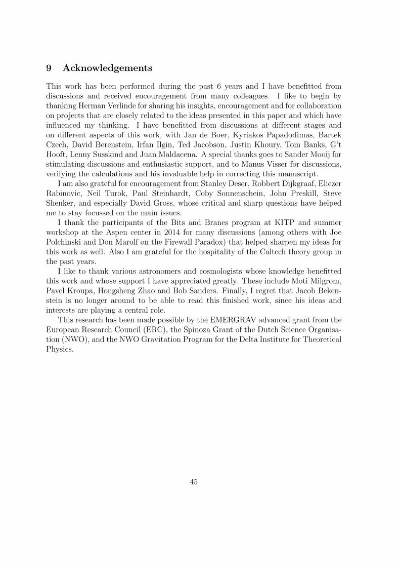
9 Acknowledgements

This work has been performed during the past 6 years and I have benefitted fromdiscussions and received encouragement from many colleagues. I like to begin bythanking Herman Verlinde for sharing his insights, encouragement and for collaborationon projects that are closely related to the ideas presented in this paper and which haveinfluenced my thinking. I have benefitted from discussions at different stages andon different aspects of this work, with Jan de Boer, Kyriakos Papadodimas, BartekCzech, David Berenstein, Irfan Ilgin, Ted Jacobson, Justin Khoury, Tom Banks, G’tHooft, Lenny Susskind and Juan Maldacena. A special thanks goes to Sander Mooij forstimulating discussions and enthusiastic support, and to Manus Visser for discussions,verifying the calculations and his invaluable help in correcting this manuscript.

I am also grateful for encouragement from Stanley Deser, Robbert Dijkgraaf, EliezerRabinovic, Neil Turok, Paul Steinhardt, Coby Sonnenschein, John Preskill, SteveShenker, and especially David Gross, whose critical and sharp questions have helpedme to stay focussed on the main issues.

I thank the participants of the Bits and Branes program at KITP and summerworkshop at the Aspen center in 2014 for many discussions (among others with JoePolchinski and Don Marolf on the Firewall Paradox) that helped sharpen my ideas forthis work as well. Also I am grateful for the hospitality of the Caltech theory group inthe past years.

I like to thank various astronomers and cosmologists whose knowledge benefittedthis work and whose support I have appreciated greatly. These include Moti Milgrom,Pavel Kroupa, Hongsheng Zhao and Bob Sanders. Finally, I regret that Jacob Beken-stein is no longer around to be able to read this finished work, since his ideas andinterests are playing a central role.

This research has been made possible by the EMERGRAV advanced grant from theEuropean Research Council (ERC), the Spinoza Grant of the Dutch Science Organisa-tion (NWO), and the NWO Gravitation Program for the Delta Institute for TheoreticalPhysics.

45

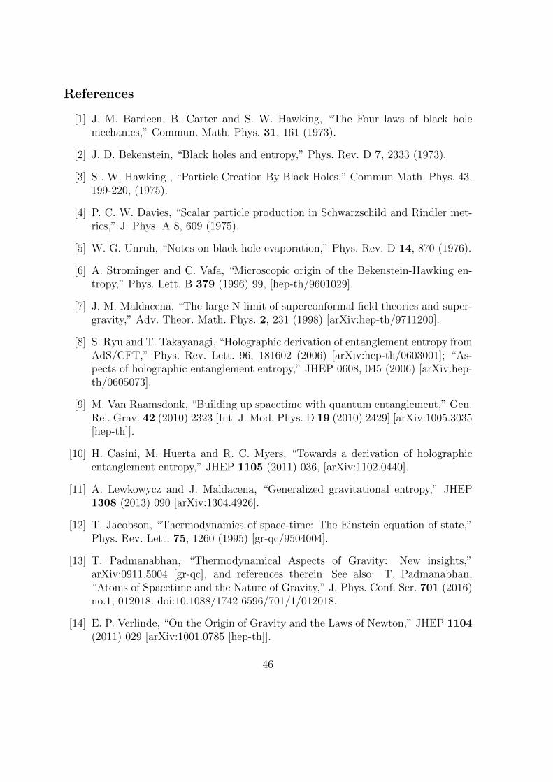
References

[1] J. M. Bardeen, B. Carter and S. W. Hawking, “The Four laws of black holemechanics,” Commun. Math. Phys. 31, 161 (1973).

[2] J. D. Bekenstein, “Black holes and entropy,” Phys. Rev. D 7, 2333 (1973).

[3] S . W. Hawking , “Particle Creation By Black Holes,” Commun Math. Phys. 43,199-220, (1975).

[4] P. C. W. Davies, “Scalar particle production in Schwarzschild and Rindler met-rics,” J. Phys. A 8, 609 (1975).

[5] W. G. Unruh, “Notes on black hole evaporation,” Phys. Rev. D 14, 870 (1976).

[6] A. Strominger and C. Vafa, “Microscopic origin of the Bekenstein-Hawking en-tropy,” Phys. Lett. B 379 (1996) 99, [hep-th/9601029].

[7] J. M. Maldacena, “The large N limit of superconformal field theories and super-gravity,” Adv. Theor. Math. Phys. 2, 231 (1998) [arXiv:hep-th/9711200].

[8] S. Ryu and T. Takayanagi, “Holographic derivation of entanglement entropy fromAdS/CFT,” Phys. Rev. Lett. 96, 181602 (2006) [arXiv:hep-th/0603001]; “As-pects of holographic entanglement entropy,” JHEP 0608, 045 (2006) [arXiv:hep-th/0605073].

[9] M. Van Raamsdonk, “Building up spacetime with quantum entanglement,” Gen.Rel. Grav. 42 (2010) 2323 [Int. J. Mod. Phys. D 19 (2010) 2429] [arXiv:1005.3035[hep-th]].

[10] H. Casini, M. Huerta and R. C. Myers, “Towards a derivation of holographicentanglement entropy,” JHEP 1105 (2011) 036, [arXiv:1102.0440].

[11] A. Lewkowycz and J. Maldacena, “Generalized gravitational entropy,” JHEP1308 (2013) 090 [arXiv:1304.4926].

[12] T. Jacobson, “Thermodynamics of space-time: The Einstein equation of state,”Phys. Rev. Lett. 75, 1260 (1995) [gr-qc/9504004].

[13] T. Padmanabhan, “Thermodynamical Aspects of Gravity: New insights,”arXiv:0911.5004 [gr-qc], and references therein. See also: T. Padmanabhan,“Atoms of Spacetime and the Nature of Gravity,” J. Phys. Conf. Ser. 701 (2016)no.1, 012018. doi:10.1088/1742-6596/701/1/012018.

[14] E. P. Verlinde, “On the Origin of Gravity and the Laws of Newton,” JHEP 1104(2011) 029 [arXiv:1001.0785 [hep-th]].

46

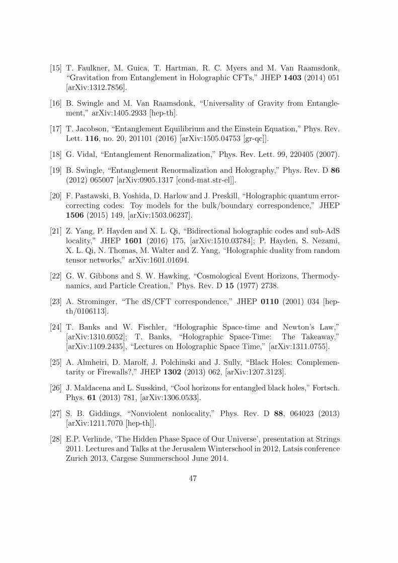
[15] T. Faulkner, M. Guica, T. Hartman, R. C. Myers and M. Van Raamsdonk,“Gravitation from Entanglement in Holographic CFTs,” JHEP 1403 (2014) 051[arXiv:1312.7856].

[16] B. Swingle and M. Van Raamsdonk, “Universality of Gravity from Entangle-ment,” arXiv:1405.2933 [hep-th].

[17] T. Jacobson, “Entanglement Equilibrium and the Einstein Equation,” Phys. Rev.Lett. 116, no. 20, 201101 (2016) [arXiv:1505.04753 [gr-qc]].

[18] G. Vidal, “Entanglement Renormalization,” Phys. Rev. Lett. 99, 220405 (2007).

[19] B. Swingle, “Entanglement Renormalization and Holography,” Phys. Rev. D 86(2012) 065007 [arXiv:0905.1317 [cond-mat.str-el]].

[20] F. Pastawski, B. Yoshida, D. Harlow and J. Preskill, “Holographic quantum error-correcting codes: Toy models for the bulk/boundary correspondence,” JHEP1506 (2015) 149, [arXiv:1503.06237].

[21] Z. Yang, P. Hayden and X. L. Qi, “Bidirectional holographic codes and sub-AdSlocality,” JHEP 1601 (2016) 175, [arXiv:1510.03784]; P. Hayden, S. Nezami,X. L. Qi, N. Thomas, M. Walter and Z. Yang, “Holographic duality from randomtensor networks,” arXiv:1601.01694.

[22] G. W. Gibbons and S. W. Hawking, “Cosmological Event Horizons, Thermody-namics, and Particle Creation,” Phys. Rev. D 15 (1977) 2738.

[23] A. Strominger, “The dS/CFT correspondence,” JHEP 0110 (2001) 034 [hep-th/0106113].

[24] T. Banks and W. Fischler, “Holographic Space-time and Newton’s Law,”[arXiv:1310.6052]; T. Banks, “Holographic Space-Time: The Takeaway,”[arXiv:1109.2435], “Lectures on Holographic Space Time,” [arXiv:1311.0755].

[25] A. Almheiri, D. Marolf, J. Polchinski and J. Sully, “Black Holes: Complemen-tarity or Firewalls?,” JHEP 1302 (2013) 062, [arXiv:1207.3123].

[26] J. Maldacena and L. Susskind, “Cool horizons for entangled black holes,” Fortsch.Phys. 61 (2013) 781, [arXiv:1306.0533].

[27] S. B. Giddings, “Nonviolent nonlocality,” Phys. Rev. D 88, 064023 (2013)[arXiv:1211.7070 [hep-th]].

[28] E.P. Verlinde, ‘The Hidden Phase Space of Our Universe’, presentation at Strings2011. Lectures and Talks at the Jerusalem Winterschool in 2012, Latsis conferenceZurich 2013, Cargese Summerschool June 2014.

47

[29] Y. Sekino and L. Susskind, “Fast Scramblers,” JHEP 0810 (2008)065 [arXiv:0808.2096]; L. Susskind, “Addendum to Fast Scramblers,”[arXiv:1101.6048].

[30] J.M. Deutsch, “Quantum statistical mechanics in a closed system,” PhysicalReview A 43 (4): 2046-2049.

[31] M. Srednicki, “Chaos and Quantum Thermalization,” Physical Review E 50 (2):888 [arXiv:cond-mat/9403051v2].

[32] M. Milgrom, “A Modification of the Newtonian dynamics as a possible alternativeto the hidden mass hypothesis,” Astrophys. J. 270 (1983) 365; M. Milgrom, “AModification of the Newtonian dynamics: Implications for galaxies,” Astrophys.J. 270 (1983) 371.

[33] J. Bekenstein and M. Milgrom, “Does the missing mass problem signal the break-down of Newtonian gravity?,” Astrophys. J. 286 (1984) 7.

[34] M. Milgrom, “MOND laws of galactic dynamics,” Mon. Not. Roy. Astron. Soc.437, no. 3, 2531 (2014) [arXiv:1212.2568]; M. Milgrom, “MOND theory,” Can.J. Phys. 93, no. 2, 107 (2015) [arXiv:1404.7661].

[35] R. H. Sanders, “A historical perspective on modified Newtonian dynamics,” Can.J. Phys. 93, no. 2, 126 (2015) [arXiv:1404.0531].

[36] W. J. G. de Blok, S.S. McGaugh, J.M. Schombert, G.D. Bothun, and W.J.G. deBlok, “The Baryonic Tully-Fisher Relation,” Astrophys.J. 533 (2000) L99-L102.

[37] S. McGaugh, F. Lelli, J. Schombert,“The Radial Acceleration Relation in Rota-tionally Supported Galaxies,” [arXiv:1609.05917].

[38] M. Milgrom, “The modified dynamics as a vacuum effect,” Phys. Lett. A 253,273 (1999), [astro-ph/9805346].

[39] A. Almheiri, X. Dong and D. Harlow, “Bulk Locality and Quantum Error Cor-rection in AdS/CFT,” JHEP 1504 (2015) 163 [arXiv:1411.7041].

[40] D. Gottesman, “Stabilizer codes and quantum error correction,” quant-ph/9705052.

[41] A. R. Brown, D. A. Roberts, L. Susskind, B. Swingle and Y. Zhao, “Complexity,action, and black holes,” Phys. Rev. D 93, no. 8, 086006 (2016) [arXiv:1512.04993[hep-th]].

[42] L. Susskind and E. Witten, “The Holographic bound in anti-de Sitter space,”hep-th/9805114.

48

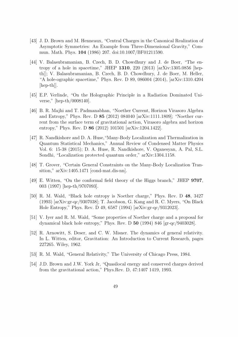
[43] J. D. Brown and M. Henneaux, “Central Charges in the Canonical Realization ofAsymptotic Symmetries: An Example from Three-Dimensional Gravity,” Com-mun. Math. Phys. 104 (1986) 207. doi:10.1007/BF01211590.

[44] V. Balasubramanian, B. Czech, B. D. Chowdhury and J. de Boer, “The en-tropy of a hole in spacetime,” JHEP 1310, 220 (2013) [arXiv:1305.0856 [hep-th]]; V. Balasubramanian, B. Czech, B. D. Chowdhury, J. de Boer, M. Heller,“A hole-ographic spacetime,” Phys. Rev. D 89, 086004 (2014), [arXiv:1310.4204[hep-th]].

[45] E.P. Verlinde, “On the Holographic Principle in a Radiation Dominated Uni-verse,” [hep-th/0008140].

[46] B. R. Majhi and T. Padmanabhan, “Noether Current, Horizon Virasoro Algebraand Entropy,” Phys. Rev. D 85 (2012) 084040 [arXiv:1111.1809]; “Noether cur-rent from the surface term of gravitational action, Virasoro algebra and horizonentropy,” Phys. Rev. D 86 (2012) 101501 [arXiv:1204.1422].

[47] R. Nandkishore and D. A. Huse,“Many-Body Localization and Thermalization inQuantum Statistical Mechanics,” Annual Review of Condensed Matter PhysicsVol. 6: 15-38 (2015); D. A. Huse, R. Nandkishore, V. Oganesyan, A. Pal, S.L.Sondhi, “Localization protected quantum order,” arXiv:1304.1158.

[48] T. Grover, “Certain General Constraints on the Many-Body Localization Tran-sition,” arXiv:1405.1471 [cond-mat.dis-nn].

[49] E. Witten, “On the conformal field theory of the Higgs branch,” JHEP 9707,003 (1997) [hep-th/9707093].

[50] R. M. Wald, “Black hole entropy is Noether charge,” Phys. Rev. D 48, 3427(1993) [arXiv:gr-qc/9307038]; T. Jacobson, G. Kang and R. C. Myers, “On BlackHole Entropy,” Phys. Rev. D 49, 6587 (1994) [arXiv:gr-qc/9312023].

[51] V. Iyer and R. M. Wald, “Some properties of Noether charge and a proposal fordynamical black hole entropy,” Phys. Rev. D 50 (1994) 846 [gr-qc/9403028].

[52] R. Arnowitt, S. Deser, and C. W. Misner. The dynamics of general relativity.In L. Witten, editor, Gravitation: An Introduction to Current Research, pages227265. Wiley, 1962.

[53] R. M. Wald, “General Relativity,” The University of Chicago Press, 1984.

[54] J.D. Brown and J.W. York Jr, “Quasilocal energy and conserved charges derivedfrom the gravitational action,” Phys.Rev. D, 47:1407 1419, 1993.

49

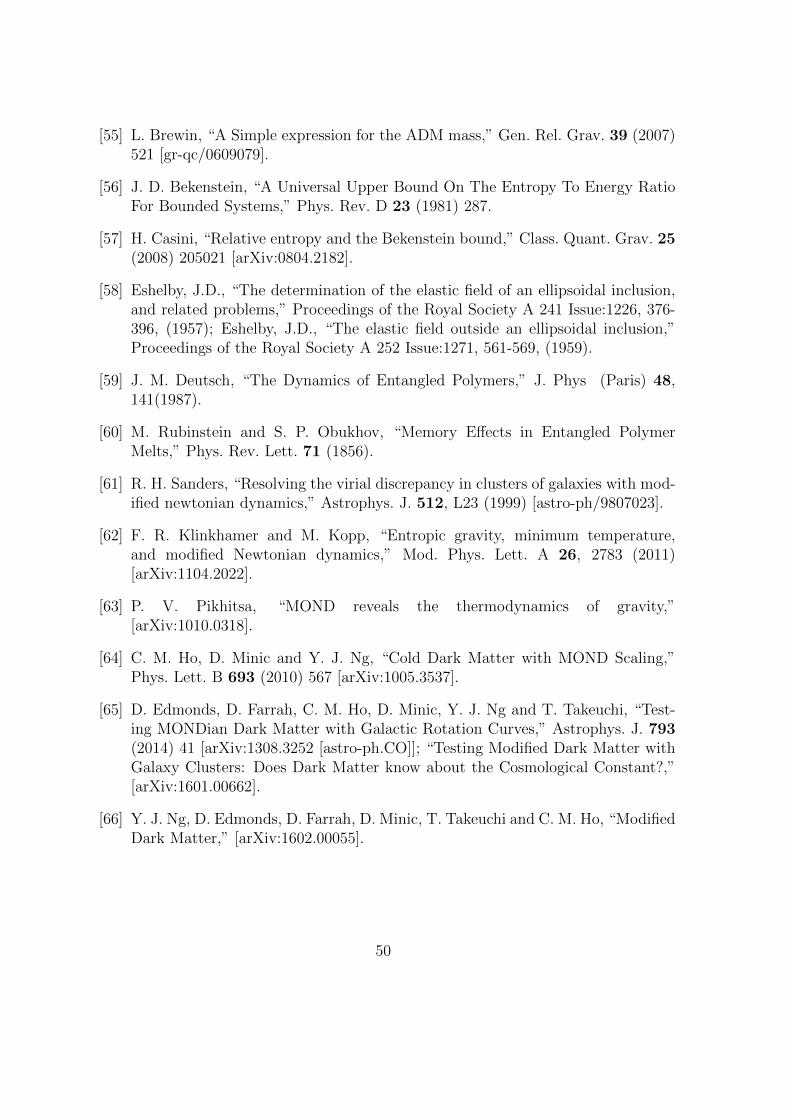
[55] L. Brewin, “A Simple expression for the ADM mass,” Gen. Rel. Grav. 39 (2007)521 [gr-qc/0609079].

[56] J. D. Bekenstein, “A Universal Upper Bound On The Entropy To Energy RatioFor Bounded Systems,” Phys. Rev. D 23 (1981) 287.

[57] H. Casini, “Relative entropy and the Bekenstein bound,” Class. Quant. Grav. 25(2008) 205021 [arXiv:0804.2182].

[58] Eshelby, J.D., “The determination of the elastic field of an ellipsoidal inclusion,and related problems,” Proceedings of the Royal Society A 241 Issue:1226, 376-396, (1957); Eshelby, J.D., “The elastic field outside an ellipsoidal inclusion,”Proceedings of the Royal Society A 252 Issue:1271, 561-569, (1959).

[59] J. M. Deutsch, “The Dynamics of Entangled Polymers,” J. Phys (Paris) 48,141(1987).

[60] M. Rubinstein and S. P. Obukhov, “Memory Effects in Entangled PolymerMelts,” Phys. Rev. Lett. 71 (1856).

[61] R. H. Sanders, “Resolving the virial discrepancy in clusters of galaxies with mod-ified newtonian dynamics,” Astrophys. J. 512, L23 (1999) [astro-ph/9807023].

[62] F. R. Klinkhamer and M. Kopp, “Entropic gravity, minimum temperature,and modified Newtonian dynamics,” Mod. Phys. Lett. A 26, 2783 (2011)[arXiv:1104.2022].

[63] P. V. Pikhitsa, “MOND reveals the thermodynamics of gravity,”[arXiv:1010.0318].

[64] C. M. Ho, D. Minic and Y. J. Ng, “Cold Dark Matter with MOND Scaling,”Phys. Lett. B 693 (2010) 567 [arXiv:1005.3537].

[65] D. Edmonds, D. Farrah, C. M. Ho, D. Minic, Y. J. Ng and T. Takeuchi, “Test-ing MONDian Dark Matter with Galactic Rotation Curves,” Astrophys. J. 793(2014) 41 [arXiv:1308.3252 [astro-ph.CO]]; “Testing Modified Dark Matter withGalaxy Clusters: Does Dark Matter know about the Cosmological Constant?,”[arXiv:1601.00662].

[66] Y. J. Ng, D. Edmonds, D. Farrah, D. Minic, T. Takeuchi and C. M. Ho, “ModifiedDark Matter,” [arXiv:1602.00055].

50