Embed Size (px)
Citation preview
Clemson UniversityTigerPrints
All Dissertations Dissertations
12-2006
Elevated Neutral-to-Earth Voltage in DistributionSystems Including HarmonicsJian JiangClemson University, [email protected]
Follow this and additional works at: https://tigerprints.clemson.edu/all_dissertations
Part of the Electrical and Computer Engineering Commons
This Dissertation is brought to you for free and open access by the Dissertations at TigerPrints. It has been accepted for inclusion in All Dissertations byan authorized administrator of TigerPrints. For more information, please contact [email protected].
Recommended CitationJiang, Jian, "Elevated Neutral-to-Earth Voltage in Distribution Systems Including Harmonics" (2006). All Dissertations. 42.https://tigerprints.clemson.edu/all_dissertations/42

ELEVATED NEUTRAL‐TO‐EARTH VOLTAGE IN DISTRIBUTION
SYSTEMS INCLUDING HARMONICS
A Dissertation Presented to
the Graduate School of Clemson University
In Partial Fulfillment of the Requirements for the Degree
Doctor of Philosophy Electrical Engineering
by Jian Jiang
December 2006
Accepted by: Dr. E. R. “Randy” Collins, Committee Chair
Dr. Michael A. Bridgwood Dr. John J. Komo Dr. Hyesuk K. Lee
ABSTRACT
The elevated neutral‐to‐earth voltage (NEV), and the related phenomenon
called stray voltage, is analyzed in multigrounded distribution systems. Elevated
NEV is typically caused by fundamental frequency currents returning to the
source via the neutral conductor and earth. However, harmonic distortion is also
found to contribute to elevated NEV. A multiphase harmonic load flow
algorithm is developed to examine the effects of various factors on the NEV,
including unsymmetrical system configuration, load unbalance and harmonic
injection. To fulfill this objective, the system modeling is adapted to include the
neutral conductor into the component equivalent circuit. The overhead
transmission line is remodeled in detail based on the Carson’s line theory. The
neutral and earth return paths are represented explicitly in the model.
Additionally, the harmonic analysis, embedded in the load flow algorithm, is
demonstrated using a single‐phase uncontrolled capacitor‐filtered rectifier model.
The algorithm and the associated models are tested on an IEEE example
system. The load flows are performed under different system and load
conditions, including both linear and non‐linear loads. The accuracy of the

iii
developed algorithm is verified by comparing the model predictions with field
measurements on real multigrounded distribution feeders.
Unbalanced loading and system asymmetry are observed to be the
important source of the elevated NEV. The magnitude is shown to be a function
of the earth resistivity, residual return current, feeder length and the neutral
conductor size. Additionally, the harmonic injection from nonlinear loads tends
to deteriorate the NEV by injecting additive triplen harmonic current into the
return path. Three‐phasing of single‐phase laterals, a common distribution
system upgrade method, is examined for its effectiveness to mitigate elevated
NEV when the system has harmonic loads. As expected, it is found that three‐
phasing is effective when the system has low distortion. However, three‐phasing
is less effective for alleviating NEV when the feeder is loaded with an
appreciable amount of single‐phase non‐linear devices.

DEDICATION
I dedicate this work to my family. This dissertation exists because of their
love and support.

ACKNOWLEDGEMENTS
I would like to thank my advisor, Dr. Randy Collins, for all of his
assistance and guidance. His high expectations and continuous support are
greatly appreciated. I am grateful to the other committee members: Dr. Michael
Bridgwood, Dr. John Komo and Dr. Hyesuk Lee. Additionally, I would like to
thank the Duke Energy Corporation for their support of the research that is the
topic of this dissertation.

TABLE OF CONTENTS
Page
TITLE PAGE ............................................................................................................ i
ABSTRACT .............................................................................................................. ii
DEDICATION ......................................................................................................... iv
ACKNOWLEDGEMENTS..................................................................................... v
LIST OF FIGURES................................................................................................... viii
LIST OF TABLES..................................................................................................... xii
CHAPTER
1. INTRODUCTION TO ELEVATED NEUTRAL‐TO‐EARTH VOLTAGE ................................................... 1
Voltage Potentials In the Earth ........................................................... 1 Definitions And Usage ......................................................................... 5 Concerns And Alleviation Methods................................................... 10
2. RESEARCH OBJECTIVES ....................................................................... 14
3. LITERATURE REVIEW............................................................................ 16
Power System Modeling ...................................................................... 16 Multiphase Load Flow ......................................................................... 19 Harmonic Analysis ............................................................................... 22
4. TRANSMISSION LINE MODELING FOR NEUTRAL‐TO‐EARTH VOLTAGE ANALYSIS......................................................................... 26
vii
Table of Contents (Continued)
Page
Carson’s Line ......................................................................................... 26 Practical Feeders With Non‐Zero Grounding Resistance ............... 34
5. MULTIPHASE LOADFLOW FOR NEV ANALYSIS .......................... 44
6. HARMONIC ANALYSIS FOR NEV STUDY........................................ 58
Modeling Of Single Phase Uncontrolled Capacitor‐Filtered Rectifier In Harmonic Load Flow ................................................. 58 Harmonic Multiphase Load Flow ...................................................... 63
7. NEV ANALYSIS USING THE MULTIPHASE HARMONIC LOAD FLOW ALGORITHM...................................... 67
IEEE Example System Tests ................................................................ 67 Comparison With Field Measurements............................................. 78 Evaluation Of Three‐Phasing Method In The Present Of Harmonic Distortion ................................................... 85
8. CONCLUSIONS AND FUTURE WORK............................................... 99
Conclusions............................................................................................ 99 Future Work........................................................................................... 101
APPENDICES.......................................................................................................... 103
I. Circuit Analysis Of Single Phase Uncontrolled Capacitor Filtered Rectifier.................................................................. 104 II. Multiphase Harmonic Load Flow Program Code................................ 126
REFERENCES.......................................................................................................... 170

LIST OF FIGURES
Figure Page
1. A three phase multigrounded power system............................................ 2
2. A three phase multigrounded transmission line with earth return....................................................................................... 3
3. Voltage potentials in the earth due to earth return current ........................................................................................... 4
4. Definition of stray voltage ............................................................................ 6
5. Measured neutral voltage waveform with harmonic distortion................................................................................. 13
6. Carson’s line for single phase feeder .......................................................... 27
7. Line geometrical spacing for two parallel conductors (a and b) with earth return ..................................................................... 28
8. Single phase feeder with neutral grounding ............................................. 35
9. Equivalent model for multigrounded feeder............................................. 39
10. A single phase multigrounded feeder ........................................................ 40
11. The Π equivalent circuit of a multigrounded feeder............................... 43
12. Topology plot of a radial network showing labeling hierarchy ..................................................................................... 46
13. The numbered distribution network .......................................................... 46
14. Residual current division between neutral and earth .............................. 51
15. Example system to demonstrate current division between neutral and earth....................................................................... 54

ix
List of Figures (Continued)
Page
16. Single‐phase bridge rectifier ........................................................................ 58
17. The characteristic waveform of a single phase bridge rectifier.......................................................................................... 60
18. Flow chart of the single phase rectifier modeling for harmonic load flow ............................................................................ 62
19. Single phase rectifier test using a distorted input voltage....................... 64
20. Multiphase harmonic load flow algorithm for distribution systems ........................................................................... 66
21. IEEE test system with underground cable omitted .................................. 68
22. Phase voltages with linear loads and m 10 ⋅Ω=ρ .................................... 70
23. Phase voltages with linear loads and m 100 ⋅Ω=ρ .................................. 70
24. Phase voltages with linear loads and m 1000 ⋅Ω=ρ ................................ 71
25. NEV with linear loads at different earth resistivities ............................... 71
26. Phase to neutral voltage with nonlinear loads .......................................... 74
27. Waveforms at the rectifier terminal for Case (i)........................................ 75
28. Neutral‐to‐Earth voltage spectrum with nonlinear loads at bus 3 ............................................................................................. 76
29. Neutral voltage with nonlinear loads ......................................................... 77
30. A three phase distribution feeder with single phase lateral.................... 79
31. Connection of the field measurement on the 7200 V phase conductor........................................................................................ 80
32. Measured phase voltage and phase current .............................................. 81
33. Measured phase voltage and neutral current............................................ 81

x
List of Figures (Continued)
Page
34. Synchronized waveforms aV (solid), aI (dot) and nI (dashed)......................................................................................... 82
35. Simulation setup for waveform verification.............................................. 83
36. Waveform comparison, measurement (solid) and calculation (dashed).......................................................................... 83
37. Single phase lateral current spectrum ....................................................... 86
38. Feeder NEV spectrum................................................................................... 87
39. Three phase feeder spacing data ................................................................. 88
40. Three phasing test on the original system.................................................. 88
41. Current spectrum after three phasing ........................................................ 89
42. Feeder NEV spectrum after three phasing................................................. 90
43. Rectifier terminal waveforms on the single phase lateral with projected load growth......................................................... 92
44. Current spectrum on the single phase lateral with projected load growth..................................................................... 93
45. Feeder NEV spectrum with projected load growth.................................. 94
46. Rectifier terminal waveforms after three phasing with projected load growth..................................................................... 95
47. Current spectrum after three phasing with projected load growth .................................................................. 95
48. Feeder NEV spectrum after three phasing with projected load growth................................................................ 96
A‐1. Single phase uncontrolled capacitor filtered rectifier............................... 104

xi
List of Figures (Continued)
Page
A‐2. The typical terminal waveform at a single phase rectifier terminal ....................................................................................... 105

LIST OF TABLES
Table Page
1. Estimated effects of 60 Hz AC Current ...................................................... 9
2. Simple grounding electrodes resistance..................................................... 45
3. Comparison of the two methods for current division.............................. 56
4. Spot linear loads on the IEEE test system .................................................. 69
5. Current harmonics at the bus with rectifier loads .................................... 75
6. Detailed results of harmonic components before and after three‐phasing using field measurement ...................................... 91
7. Detailed results of harmonic components before and after three‐phasing with projected load growth .................................. 98

CHAPTER I
INTRODUCTION TO ELEVATED
NEUTRAL‐TO‐EARTH
VOLTAGE
I. Voltage Potentials In The Earth
Elevated neutral‐to‐earth voltage (NEV) or so‐called “stray voltage” has
drawn increasing attention from the general public, regulatory organizations and
utilities, for both technical and legal reasons [1]. Considerable controversy
presently exists for the definition and usage of the term “stray voltage” when
approaching the problem from different perspectives. Another related
occurrence in power system is the ground potential rise (GPR). Hence, the
background about the voltage potential in the earth accompanying grounding
current is discussed briefly in order to clarify the concepts in this dissertation.
The nature of grounded power systems results in the fact that the neutral
conductors are not always at the zero potential with respect to the earth
underneath them. The concepts are easier to explain using the three–phase
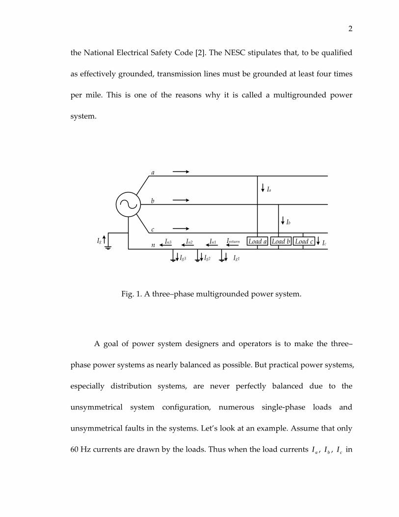
multigrounded power system in Fig. 1. The neutral conductor is grounded at
multiple points along the transmission line conforming to the requirement of
2
the National Electrical Safety Code [2]. The NESC stipulates that, to be qualified
as effectively grounded, transmission lines must be grounded at least four times
per mile. This is one of the reasons why it is called a multigrounded power
system.
Load a Load b Load c
a
b
c
n
Ia
Ib
IcIreturn
Ig1Ig2Ig3
In1In2In3Ig
Fig. 1. A three–phase multigrounded power system.
A goal of power system designers and operators is to make the three–
phase power systems as nearly balanced as possible. But practical power systems,
especially distribution systems, are never perfectly balanced due to the
unsymmetrical system configuration, numerous single‐phase loads and
unsymmetrical faults in the systems. Let’s look at an example. Assume that only
60 Hz currents are drawn by the loads. Thus when the load currents aI , bI , cI in
3
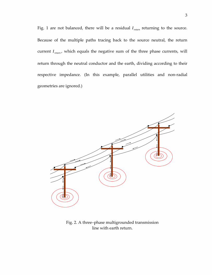
Fig. 1 are not balanced, there will be a residual returnI returning to the source.
Because of the multiple paths tracing back to the source neutral, the return
current returnI , which equals the negative sum of the three phase currents, will
return through the neutral conductor and the earth, dividing according to their
respective impedance. (In this example, parallel utilities and non‐radial
geometries are ignored.)
Fig. 2. A three–phase multigrounded transmission line with earth return.
4
Since the neutral conductors are not perfect in practical systems, the
return current is shared between the neutral and the earth. Some portion of the
return current is always driven into the earth every time the neutral is grounded.
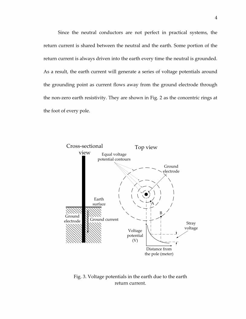
As a result, the earth current will generate a series of voltage potentials around
the grounding point as current flows away from the ground electrode through
the non‐zero earth resistivity. They are shown in Fig. 2 as the concentric rings at
the foot of every pole.
Ground current
Equal voltage potential contours
Voltage potential
(V)
Distance from the pole (meter)
Earth surface
Ground electrode
Ground electrode
Top viewCross‐sectional view
A
B
Stray voltage
Fig. 3. Voltage potentials in the earth due to the earth return current.

5
For simplicity, the earth is assumed to be a semi‐infinite media with
uniform resistivity. When the ground current enters the earth through the
ground electrode, voltage potentials are generated with their magnitude
determined by the ground electrode geometry, earth resistivity and the distance
from the measuring point to the ground electrode. The exact values of the
voltage potentials can be very complicated to compute due to the complexity of
the ground electrode and the earth electrical characteristics [3]. But the basic
trend is that the voltage potential decreases when moving away from the ground
electrode relative to the remote earth. For two points around the ground
electrode, e.g., A and B in Fig. 3, a voltage exists between these two points since
they are at different distances from the ground electrode.
II. Definitions And Usage
At the time this dissertation is written, there is no unanimous definition
on stray voltage. Since stray voltage was initially noticed in cow milking parlors,
it has been explored extensively by engineers and researchers for improving the
productivity in dairy farms [4]–[7]. Authorities in agriculture and public service
have provided guidelines on defining the stray voltage problems [8]–[10]. Since
they are all similar to each other, only the definition by U.S. Department of
6
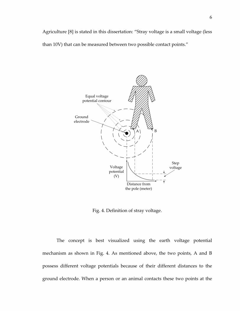
Agriculture [8] is stated in this dissertation: “Stray voltage is a small voltage (less
than 10V) that can be measured between two possible contact points.”
Equal voltage potential contour
Voltage potential
(V)
Distance from the pole (meter)
Ground electrode
A B
Step voltage
Fig. 4. Definition of stray voltage.
The concept is best visualized using the earth voltage potential
mechanism as shown in Fig. 4. As mentioned above, the two points, A and B
possess different voltage potentials because of their different distances to the
ground electrode. When a person or an animal contacts these two points at the

7
same time, the subjected voltage is the stray voltage. When the contact points are
between the person’s or the animal’s feet with a separation distance of 3 feet
(without any other contact to a grounded object), it is called “step voltage” [11]
as illustrated in Fig. 4. If the contact points are the hand on a grounded object
and the feet on the surface (with a separation distance of roughly 3 feet (1 meter),
it is called “touch voltage” [11]. (Both of these terms are normally used for
situations involving fault currents.)
The neutral‐to‐earth voltage is the voltage measured from the neutral
conductor to the remote earth. Since the neutral is solidly connected to the
ground electrode, the NEV is equal to the voltage potential difference from the
ground electrode to a point at infinity. The NEV is thus the maximum voltage
that can be measured in the earth. Considering the physical limit of a person or
an animal, the stray voltage will always be smaller than NEV. Also it is usually
the case that the voltage gradient is steeper close to the electrode, which causes
higher stray voltage when a person or an animal approaching the ground
electrode.
Although the NEV is not the stray voltage, the knowledge of NEV is
extremely important in solving stray voltage problems. By analyzing the NEV
profile of power system under different conditions, it is possible to locate the
source of stray voltage and develop means to mitigate the problems.

8
Another phenomenon in the power system related to the earth return
current is the ground potential rise. The GPR usually refers to the voltage
differential measured at the substations between the neutral to remote earth
when the ground fault current returns through the earth, creating high voltage
drop on the substation’s ground grid [12]. Thus GPR is a measure of neutral
voltage only when the system is undergoing a ground fault, while the relatively
small NEV/stray voltage is the term for steady state. This dissertation focus on
the steady‐state elevated NEV analysis; GPR is not in the scope of this research
project.
Because of the unbalance in a practical system, especially a multigrounded
distribution system, the question about NEV is not if the NEV exists, but what is
the safe level. As mentioned earlier in this section, there is no standard on stray
voltage. It is only recommend by U.S. Department of Agriculture in [8] that
actions should be taken to reduce neutral to earth voltage when the NEV at the
service entrance or between contact points is higher than the 2 to 4 volts range.
The stray voltage problem concerns dairy farm owners because that
current will flow through the cows’ body when they are subject to a portion of
the NEV. It is widely accepted to apply the recommendation in [8] to simulate
cow’s body resistance using a resistor of 500 Ω . Lefcourt performed extensive
investigation on the response of farm animals to different body currents [13]–[15].

9
He discovered that animals can perceive body currents below 0.1 mA at 60 Hz
under unusual circumstances. However, animals’ body currents below 0.3 mA
often have no change in their behavior while temporary behavior changes were
found with currents in the range of 0.3–0.6 mA at 60 Hz. Beside the academic
research on animals’ response, authorities also provide guidelines for stray
voltage monitoring and troubleshooting. For example, the “level of concern”, a
conservative and pre‐injury level is defined to be 2 mA by Public Service
Commission of Wisconsin in [16].
Table 1. Estimated effects of 60 Hz AC current.
1 mA Barely perceptible
16 mA Maximum current an average man can grasp and ʺlet goʺ
20 mA Paralysis of respiratory muscles
100 mA Ventricular fibrillation threshold
2 A Cardiac standstill and internal organ damage
15/20 A Common fuse or breaker opens circuit

10
The estimated effect of 60 Hz AC current on human is summarized in [17]
and shown in Table 1. Contact with currents of 20 mA can be lethal. The current
through the human body is dependent on the human body’s impedance.
However, the body impedance varies widely at different conditions. The body
impedance is especially affected by the applied voltage. Under dry conditions,
the resistance of the human body can be as high as 100,000 Ω . High‐voltage
electrical energy quickly breaks down human skin, reducing the human body
resistance to about 500 Ω . The definition for high or low voltage changes in
different scenarios. For example, a voltage of 1000 V is low voltage in power
transmission systems, but it is not commonplace in a typical home or workplace.
For the concern of electrical hazard to human, the “safe voltage” value found in
International Electrotechnical Commission (IEC) is 42.4 V (peak) for AC voltage
or 60 V for DC voltage [18].
III. Concerns And Alleviation Methods
Beside the interference with dairy farm animals, the unexpected touch
voltage can also be annoying to utility customers. The varying NEV in some
cases may affect the performance of sensitive electronic devices if they are using
the neutral voltage as reference. Buried metallic pipes can experience extra

11
corrosion when the high NEV is present in the proximity, especially if it has
become rectified.
Historically, the terms NEV and stray voltage are applied in the literatures
interchangeably. After years of exploration, engineers and researchers have
pinpointed the common origins for stray voltages at power frequency and
developed mitigation methods accordingly. The major sources and some of the
widely applied means for solving NEV/stray voltage problems are listed below.
Sources of NEV/stray voltage:
1. Power system grounding
2. Load unbalance
3. Transformer connections
4. Neutral conductor impedance
Mitigation methods for solving NEV/stray voltage:
1. Balancing the loads
2. Three–phasing single–phase laterals
3. Increasing the neutral conductor size
4. Improving grounding connection
5. Repairing bad neutral connections and splices
All of these methods are aimed at either reducing the unbalanced
returning current or increasing the return paths’ conductivity in the neutral

12
conductors. However, none of the work mentioned above considered the effect
of harmonic distortion. The proliferation of power electronic devices, especially
the single–phase nonlinear load on commercial/residential circuits, has raised
new concerns for the amplified NEV level related to harmonic distortion [19].
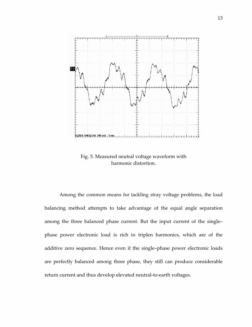
In Fig. 5, the neutral voltage with respect to the nearby ground is
measured on a distribution feeder using an oscilloscope. It is clear from the
neutral voltage waveform that a fair amount of 9th harmonic is riding on the crest
of the fundamental neutral voltage. This result cannot be seen if a standard RMS
multi‐meter is used. As the harmonic load currents increase with the utilization
of nonlinear devices in power systems, it is very important to identify the
additional NEV elevation due to harmonic distortion and assess its effect on the
NEV profile and stray voltage mitigation methods.
13
Fig. 5. Measured neutral voltage waveform with harmonic distortion.
Among the common means for tackling stray voltage problems, the load
balancing method attempts to take advantage of the equal angle separation
among the three balanced phase current. But the input current of the single–
phase power electronic load is rich in triplen harmonics, which are of the
additive zero sequence. Hence even if the single–phase power electronic loads
are perfectly balanced among three phase, they still can produce considerable
return current and thus develop elevated neutral‐to‐earth voltages.

CHAPTER II
RESEARCH OBJECTIVES
From the discussion presented in Chapter I, it is clear that conventional
techniques and tools need to be reevaluated in the presence of new sources of
NEV elevation and stray voltage problems. As the most frequently performed
analysis on power systems, load flow is the best technique for computing the
system’s voltage profile in steady state. Direct results of the systems’ NEV using
a load flow technique are highly desirable in predicting and developing
mitigation methods for stray voltage problems.
The first objective of this research project is to develop an appropriate
load flow algorithm and the associated power system modeling technique for
NEV profile calculation related to harmonic distortion. The new load flow
algorithm and modeling technique are then tested on an IEEE example system
for reliability evaluation. Also field measurements on real power systems are
compared with algorithm calculation to verify its accuracy.
Based on the test results, application of the load flow algorithm is
discussed for predicting and troubleshooting NEV elevation due to harmonic
15
distortion. The three–phasing method for distribution systems upgrading is
evaluated for NEV alleviation with nonlinear devices connected in the system.
This dissertation will proceed in the following steps. The modern
techniques in power system modeling, load flow and harmonic analysis are
reviewed in the next chapter. Then the transmission line is modeled in Chapter
IV using a new approach oriented to NEV analysis. A multiphase load flow is
developed in Chapter V. The single–phase rectifier is analyzed and the load flow
algorithm is expanded to include harmonic analysis in Chapter VI. After that, the
algorithm is tested on an IEEE example system and actual distribution feeders to
demonstrate its application in NEV analysis incorporating harmonic distortion.
Then conclusions are drawn and future research work is suggested.

CHAPTER III
LITERATURE REVIEW
I. Power System Modeling
Most of the component models in power systems do not have the explicit
neutral conductor. In their steady state models, the neutral variables are
absorbed into the phase branch equations. The neutral grounding can be simply
represented by a grounding resistance from the neutral to earth, if the neutral
point is provided in the actual device. Mature techniques are available for steady
state simulation in various literatures [20]–[22]. One exception is the transmission
line model due to magnetic mutual coupling among phase, neutral and earth.
More detailed examination of conventional modeling theories is required to
accurately represent the transmission line for NEV analysis.
The transmission line is one of the most important components in power
systems. Since the majority of power systems in North America are three–phase
multigrounded, the effect of earth return path has to be considered for accurate
transmission line modeling. The current distribution in the earth has been
examined extensively in the literature. Three well‐known modeling methods, i.e.,
Carson’s line, complex depth method and finite element method, are briefly

17
discussed below. In 1926, J.R. Carson (from Bell Laboratories) published a
monumental paper [23] describing the calculation of the transmission line
impedance incorporating the earth return effect. However, Carson’s formulas do
not give a closed form solution. Instead, the impedances are expressed in
improper integrations that need to be expanded into infinite series. Various
approximation methods have been proposed based on series truncation [20]–[21]
[24]. However, improper use of these approximation methods can cause
considerable error at high frequency.
An alternative approximation method was proposed by A. Deri [25] using
the concept of complex depth. In this method, the extensive earth is replaced by a
set of earth return conductors located underneath the overhead lines with the
depth of complex value. By assuming the complex depth for the earth return
conductor, the problem of adding terms in the truncation approximation is
eliminated when calculating high frequency impedance. The error of complex
depth method increases with the ratio of the horizontal distances between
conductors to their heights. Fortunately, this ratio in most realistic systems is too
small to cause any practical problems in the impedance calculation.
In both Carson’s line and the complex depth methods, the earth is
assumed to be a uniform semi‐infinite media with non‐ideal conductivity. The
finite element method [26] is applied in the detailed analysis of the earth return
18
current distribution in soil with irregular terrain. Also the frequency‐dependent
impedance of transmission line can be calculated using the finite element method.
This powerful method may not be preferable due to its high cost in
implementation and long calculation time.
All the methods above assume perfect ground connection from the neutral
conductors to the earth. Consequently, the variables related to neutral
conductors can be eliminated from the final equivalent circuit. The earth
impedance is first absorbed into the aerial conductors’ impedances according to
KCL. With all of the voltages referring to the remote earth, the neutral voltage is
always zero due to the ideal connection to earth. The neutral voltage equation is
then eliminated by the Kron reduction method.
However, the current and voltage relative to earth of the neutral
conductor is the goal of NEV analysis. The otherwise preferable elimination of
neutral conductor equation is not desirable in NEV analysis. Furthermore, the
non‐ideal conductive earth presents impedance to the current flowing from
neutral conductors to the earth. Recent works [27]–[28] have shown that
improper application of these transmission line models can lead to serious error
in transmission line impedance calculations.
Based on the above observations, a transmission line model needs to be
developed dedicated for NEV analysis. In the new transmission line model, the

19
neutral conductor is represented explicitly for direct determination of the
neutral‐to‐earth voltage. Since the Carson’s line is the standard method for
transmission line modeling among power engineers, it will be applied as the
foundation for the new model derivation.
II. Multiphase Load Flow
Load flow is the technique used in planning the future expansion of
power systems as well as in determining the best operation of existing systems in
steady state. The principle information obtained from a load flow study is the
magnitude and phase angle of the voltage at each bus and the real and reactive
power flowing in each line [22]. The first practical method for load flow
calculation was formulated by Ward and Hale [29] in 1956. Since then the load
flow techniques have been studied and documented extensively. For well‐
behaved systems like large scale transmission systems, the Newton‐Raphson and
fast decoupled load flow and their derivatives have been proven over years of
successful application to be the most efficient solution techniques.
However these load flow methods fail when they are applied to ill‐
conditioned power systems. The distribution networks fall in the category of ill‐
conditioned systems for the following features found in the typical distribution
system:
20
• Radial or near radial (weakly meshed) structure
• High R/X ratio
• Multiple phasing, unbalanced operation
• Unbalanced distributed loads
• High ratio of long‐to‐short line reactance of lines terminating on the same bus in rural areas
Special solution techniques dedicated for distribution systems load flow
calculation have been developed by exploiting the radial structure of the
distribution circuit. These different algorithms can be categorized into two basic
types: Backward/forward sweep method and busZ load flow method.
In the first category, the load flow algorithms are based on ladder network
theory [30]–[32]. These methods take advantage of the radial nature of
distribution system that the source reaches any node in the network via a unique
path. The methods consist of two basic steps, i.e., backward sweep and forward
sweep, which are repeated until convergence is achieved. The backward sweep is
primarily a summation of currents or power tapped along the distribution
feeders. The forward update is primarily a voltage drop calculation accompanied
by the nodal voltage update.
In 1967, Berg et al. [30] presented a ladder theory based load flow
algorithm which can be considered the start of the all of the backward/forward
21
sweep methods that followed. In this method, the driving point impedances are
calculated from the last bus to the source, and are applied to update the currents
and voltage forward from source to the last bus.
Among the variants developed over the years, the algorithm by
Shirmohammadi et al. [33] is more intuitive to understand and implement. This
method was initially proposed for single–phase load flow based on current
calculation and expanded to power calculation [34] and three–phase load flow
[35] later. The method starts with a flat voltage profile. Then the currents or
powers are collected backward from the last bus to the source. After that the
voltage drops are calculated forward from the source to the last bus, followed by
the new voltage update.
The load flow solutions in the second category are the so‐called busZ load
flow [36]–[37]. These methods use the sparse factorized busY and equivalent
current injections to perform the load flow calculations. The busZ method is based
on the principle of superposition applied to the system bus voltages: the voltage
of each bus is considered to arise from two contributions, the slack bus voltage
and the equivalent current injections. The loads, cogenerators, line charging
capacitors and any shunt elements are considered as current injections. The basic
solution is outlined in the following steps:
• Take an initial guess on network voltage profile
22
• Optimally order and factorize busY
• Compute equivalent current injections
• Compute voltage deviation due to current injections using the factorized busY
• Update bus voltage
• Repeat the process until convergence is achieved
• Calculate power flow, current flow and system loss
The load flow techniques in both categories are tailored specifically for
radial or weakly meshed systems. The experience of applying these techniques in
distribution networks has shown different performance in different networks
[38]. However, the neutral variables and earth return current are not available
directly in both methods. A load flow algorithm dedicated for NEV analysis is
required to analyze the neutral and grounding circuit. The backward/forward
sweep method is applied as the basis for the new algorithm for its ease on
implementation and efficiency in data storage.
III. Harmonic Analysis
Accompanying the increase of nonlinear devices in power system at
various voltage levels, considerable progress has been achieved over the last two
decades in harmonic analysis. Various methods have been developed to examine

23
the power system response to harmonic distortion, which can be classified in
three types.
The first step in harmonic analysis is to model the nonlinear devices by
computing their harmonic current spectrum as a function of the terminal voltage
and the nonlinear characteristics. Mature techniques are available to represent
the nonlinear devices for different requirement of details [39].
The simplest and most commonly used harmonic analysis technique is the
frequency scan [40]. It calculates the system response at a particular bus by
injecting harmonic current into the system at this bus and computing the voltage
response. Usually it is repeated within a range of frequencies. The voltage
responses are plotted vs. the corresponding frequencies to detect the possible
harmonic resonance at the buses of interest. It has been widely used in filter
design.
The second type harmonic analysis is the harmonic penetration study
which assume no harmonic interaction between the network and the nonlinear
devices [41]. The fundamental frequency load flow is performed by representing
the nonlinear devices as constant power loads. The fundamental bus voltages
obtained are used to determine harmonic currents from the nonlinear devices.
Finally, the harmonic bus voltages are calculated by injecting the harmonic
currents into the system.

24
Iterative harmonic load flow is the most comprehensive and accurate
harmonic analysis technique. The harmonic interaction is included in nonlinear
device models by expressing the harmonic current as a function of terminal
voltage at all harmonic frequency of interest. The load flow calculations at
harmonic frequencies are carried out similar to the fundamental frequency load
flow. Convergence is then checked for all frequencies.
The conventional Newton‐like load flow techniques [42] [43] have been
developed to solve the harmonic–distorted system by expanding the
fundamental frequency load flow calculation to harmonic frequencies. The same
problems mentioned in last section will occur when these methods are applied to
the ill‐conditioned distribution systems. Instead of changing the Newton load
flow techniques to suit the radial structure, a harmonic multiphase load flow
algorithm is developed to expand the backward/forward sweep to harmonic
frequencies.
IV. Summary
Various techniques have been developed for steady state modeling, load
flow calculation and harmonic analysis. But NEV in an unbalanced distribution
system with nonlinear devices is not directly available using the present analysis
methods. Thus a multiphase harmonic load flow algorithm is developed in this

25
dissertation for NEV analysis. A multigrounded distribution line model is
derived first in the next chapter.
CHAPTER IV
TRANSMISSION LINE MODELING
FOR NEUTRAL‐TO‐EARTH
VOLTAGE ANALYSIS
I. Carson’s Line
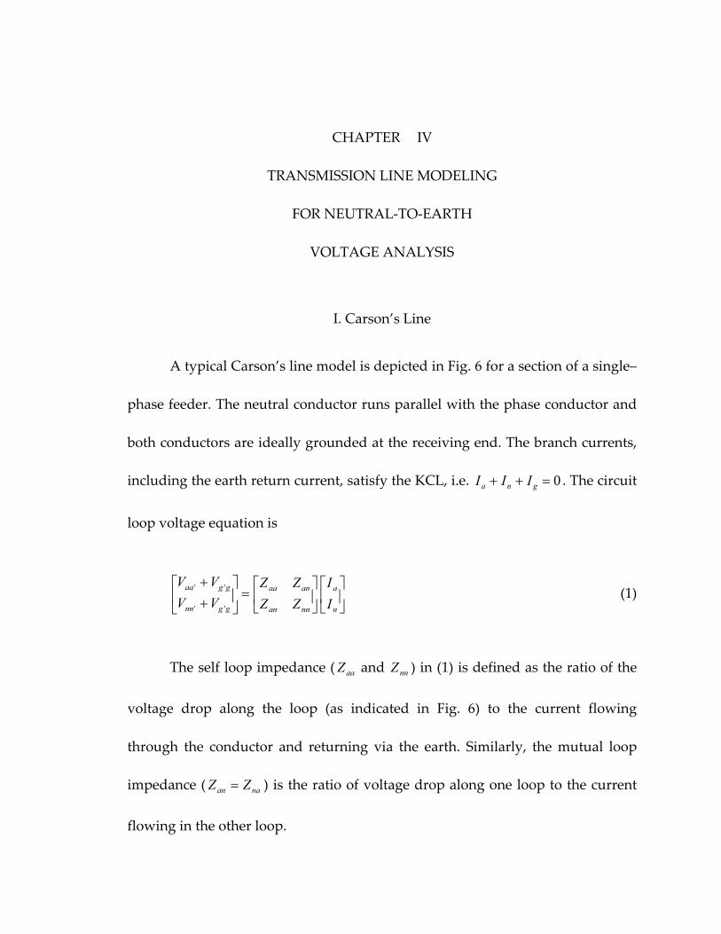
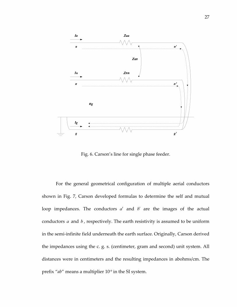
A typical Carson’s line model is depicted in Fig. 6 for a section of a single–
phase feeder. The neutral conductor runs parallel with the phase conductor and
both conductors are ideally grounded at the receiving end. The branch currents,
including the earth return current, satisfy the KCL, i.e. 0=++ gna III . The circuit
loop voltage equation is
⎥⎦
⎤⎢⎣
⎡⎥⎦
⎤⎢⎣
⎡=⎥
⎦
⎤⎢⎣
⎡++
n
a
nnan
anaa
ggnn
ggaa
II
ZZZZ
VVVV
''
'' (1)
The self loop impedance ( aaZ and nnZ ) in (1) is defined as the ratio of the
voltage drop along the loop (as indicated in Fig. 6) to the current flowing
through the conductor and returning via the earth. Similarly, the mutual loop
impedance ( naan ZZ = ) is the ratio of voltage drop along one loop to the current
flowing in the other loop.
27
Fig. 6. Carson’s line for single phase feeder.
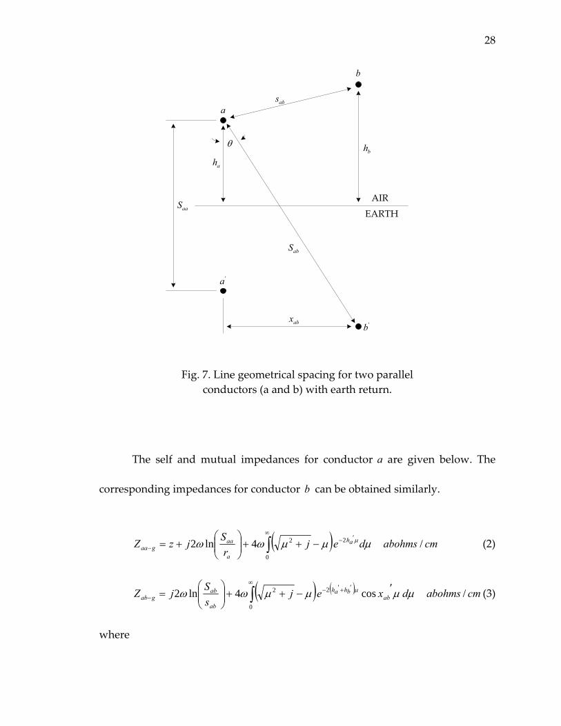
For the general geometrical configuration of multiple aerial conductors
shown in Fig. 7, Carson developed formulas to determine the self and mutual
loop impedances. The conductors a′ and b′ are the images of the actual
conductors a and b , respectively. The earth resistivity is assumed to be uniform
in the semi‐infinite field underneath the earth surface. Originally, Carson derived
the impedances using the c. g. s. (centimeter, gram and second) unit system. All
distances were in centimeters and the resulting impedances in abohms/cm. The
prefix “ab” means a multiplier 10‐9 in the SI system.
28
θ
absa
b
aaS
ahbh
EARTH
abS
abx
'a
'b
AIR
Fig. 7. Line geometrical spacing for two parallel conductors (a and b) with earth return.
The self and mutual impedances for conductor a are given below. The
corresponding impedances for conductor b can be obtained similarly.
( )∫∞
′−− −++⎟⎟
⎠
⎞⎜⎜⎝
⎛+=
0
22 4ln2 µµµωω µdejr
SjzZ ah
a
aagaa cmabohms / (2)
( ) ( )∫∞
′+′−−
′−++⎟⎟⎠
⎞⎜⎜⎝
⎛=
0
22 cos 4ln2 µµµµωω µ dxejsSjZ ab
bhah
ab
abgab cmabohms / (3)
where

29
z 2intωω jrLjr +=+ , conductor internal impedance in cmabohms /
r conductor intrinsic resistance in cmabohms /
ar conductor a radius in centimeters
S distance from conductors to image conductors in centimeters
s distance between conductors in centimeters
h height from conductor to earth surface in centimeters
x horizontal distance between conductors in centimeters
h′ αx , dimensionless
x′ αh , dimensionless
α πσωωµσ 4= in 2−cm for cmabhenriesmH / 4/ 104 7 ππµ =×= −
(µ in this case represents the earth permeability)
σ earth conductivity in cmabmho /
µ integration variable
In both the self and mutual impedance formulas (2) and (3), the terms
before the improper integrals represent the corresponding impedances when the
earth is a perfect conductor. The integrals account for the effect of non–ideal
earth conductivity on the self and mutual impedances, respectively.
For the self impedance, the first two terms can be combined together as
follows:
30
a
aa
a
aa
rSjjr
rSjz ln2
2 ln2 ωωω ++=+
⎟⎟⎠
⎞⎜⎜⎝
⎛++=
a
aa
rSjr ln
412 ω
′+=a
aa
r
Sjr ln2 ω cmabohms / (4)
where
41
'−
= err aa cm (5)
The relation in (5) is actually the definition of Geometric Mean Radius
(GMR) of solid cylinder conductors. The values for r and 'ar can be found in
manufacturers’ datasheets for standard conductors.
Next Carson solved the improper integrals in terms of infinite power
series. Because of the similarity between the two integrals in the self and mutual
impedances, a uniform solution was derived for the two integrals and the
corresponding value can be evaluated by changing the values for the following
two parameters accordingly.
( )( )⎩
⎨⎧
⋅⋅
=essdimensionledancemutual impin theS
essdimensionlanceself imped in theSkab
aa
αα (6)
⎩⎨⎧
=edancemutual imp in theθ
anceself imped in the
ab 0
θ )(radians (7)
31
The improper integrals can be evaluated as follows:
( ) ( )jQPdej ah +=−+∫∞ ′− 4 4
0
22 ωµµµω µ cmabohms / (8)
where
( ) θθπ 2cos2ln6728.016
cos23
18
2
⎟⎠⎞
⎜⎝⎛ ++−=
kkkP
1536
4cos2453cos 42 θπθ kk
−+ cmabhenries / (9)
2453cos
642cos
23cos2ln
210386.0
32 θθπθ kkkk
Q +−++−=
⎟⎠⎞
⎜⎝⎛ +−− 0895.12ln
3844cos
3844sin 44
kkk θθθ cmabhenries / (10)
Note that µ in (8) is an integration variable, not the permeability. Since
Carson solved the electromagnetic equations in terms of summation of infinite
power series, truncation is required for engineering applications. Additionally,
the unit system is cumbersome for power engineers, although it may be
convenient in physics research area. Clarke [20] presented a very good
approximation to the original solution including units transform for power
systems analysis. The geometric parameters for conductors’ spacing and size are
to be specified in feet conforming to the common practice among electrical

32
utilities in North America. Also, the calculated impedances need to be expressed
in ohms per mile.
The change on geometric specification (i.e., c.g.s. units to conventional
units) will not affect the terms before the improper integrals in (2) and (3), which
give the values of self and mutual impedances assuming perfect earth
conduction. As long as the units for spacing and conductor size are all the same,
the logarithm values will not change. And the conductor intrinsic resistance r is
usually provided by manufactures in ohms per mile.
However, the new units of geometric parameters will affect the values for
k , which consequently changes the earth return impedances in self and mutual
impedances. If the earth conductivity σ is replaced by ρ/10 11− with ρ equal the
earth resistivity in m⋅Ω , then value of k for self impedance equals
α××= 48.30aaSk
ρππ 11102448.30
−××××=
fSaa
ρfSaa
210713.1 3 ××= −
where
( ) ( ) 48.30 ×= feetSscentimeterS aaaa
33
The k in mutual impedance can be evaluated similarly by changing aaS to
abS . Since micmabohms / 106093.1/ 1 4 Ω×≅ − , the self and mutual impedance can
be expressed in ohms per mile by introducing the constant 4106093.1 −×=G as
follows
( ) GjQPr
SjrZa
aagaa ⎥
⎦
⎤⎢⎣
⎡++⎟⎟
⎠
⎞⎜⎜⎝
⎛+=− 4ln2 ' ωω
( )QGjPGGMR
SGjra
aa 4 4ln 2 ωωω ++⎟⎟⎠
⎞⎜⎜⎝
⎛+= mi/Ω (11)
( ) GjQPsSjZ
aa
aagab ⎥
⎦
⎤⎢⎣
⎡++⎟⎟
⎠
⎞⎜⎜⎝
⎛=− 4ln2 ωω
GQsSjPG
aa
aa ⎥⎦
⎤⎢⎣
⎡+⎟⎟
⎠
⎞⎜⎜⎝
⎛+= 4ln2 4 ωωω mi/Ω (12)
Note that names for P and Q are exactly the same for self and mutual
impedance, but their values are different since they are calculated separately
using corresponding k and θ parameters according to (6) and (7). The letter g in
the subscripts will be dropped in the following derivation for simplicity.
Clarke pointed out in [20] that the power series for P and Q evaluation
converge rapidly at the fundamental frequency and the order of four in series
truncation will be sufficient for accuracy in the self and mutual impedance
calculation. It is also shown in [44] that the truncation error with order of eight in

34
Carson’s model is only appreciable at frequency starting at 40 kHz, which is out
of the range for steady state harmonic analysis. Thus the fourth order truncation
suggested by Clarke is applied in this dissertation for transmission line modeling.
II. Practical Feeders with Non‐Zero Grounding Resistance
For the self impedance aaZ , the first two terms represent the line
impedance if the earth is a perfect conductor, while the last term results from the
non‐zero earth resistivity. As mentioned at the beginning of this section, the
Carson’s line model assumes that all the aerial conductors are perfectly
connected to earth. Consequently these terms can be added together because the
same current flowing through the aerial conductor returns through the earth.
Same principle also applies to the mutual impedance abZ .
This assumption works well in transmission system analysis since the load
currents in a transmission system are in most cases balanced and sinusoidal. The
effect of neutral current can be ignored without losing generality. However, in
distribution systems, the load currents can be quite unbalanced. Also the finite
earth conductivity introduces grounding resistance to the portion of the current
returning to the source through the ground electrode into the earth. A more
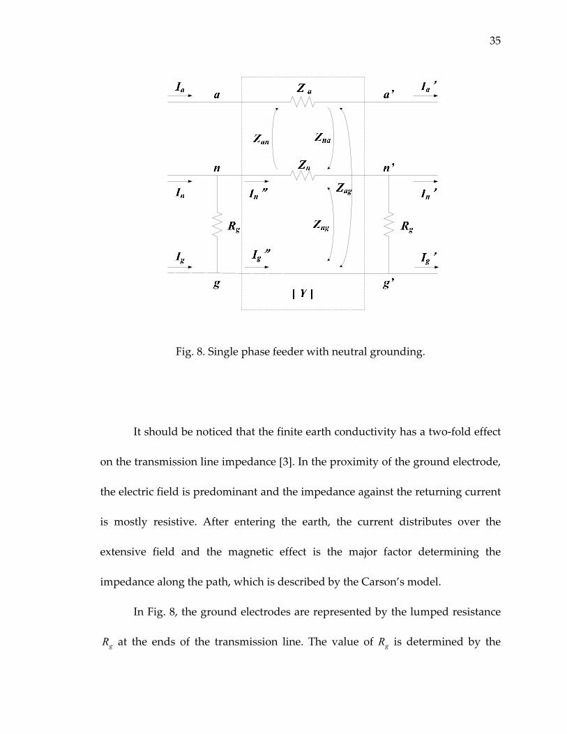
general configuration is shown in Fig. 8 for a section of single phase feeder.
35
Fig. 8. Single phase feeder with neutral grounding.
It should be noticed that the finite earth conductivity has a two‐fold effect
on the transmission line impedance [3]. In the proximity of the ground electrode,
the electric field is predominant and the impedance against the returning current
is mostly resistive. After entering the earth, the current distributes over the
extensive field and the magnetic effect is the major factor determining the
impedance along the path, which is described by the Carson’s model.
In Fig. 8, the ground electrodes are represented by the lumped resistance
gR at the ends of the transmission line. The value of gR is determined by the
36
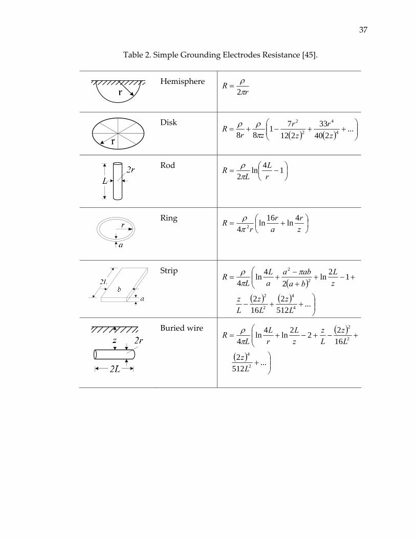
earth resistivity and the geometric configuration of grounding electrodes.
Various works have been published to examine the calculation of gR . Equations
for some simple configurations [45] are listed in Table 2.
The Carson’s line model cannot be applied in the equivalent circuit in Fig.
8 due to the shunt branches at the terminals. It would be intuitive to decompose
the loop equations into branch equations in order to add the shunt grounding
branches into the model. However there are various ways to disassemble the
loop impedances depending on the type of analysis. To avoid this uncertainty, an
alternative method is developed by taking advantage of the basic circuit
constraints while keeping the loop impedances in their entirety.
37
Table 2. Simple Grounding Electrodes Resistance [45].
Hemisphere r
Rπρ
2=
Disk ( ) ( ) ⎟⎟
⎠
⎞⎜⎜⎝
⎛++−+= ...
24033
21271
88 4
4
2
2
zr
zr
zrR
πρρ
Rod ⎟⎠⎞
⎜⎝⎛ −= 14ln
2 rL
LR
πρ
Ring ⎟⎠⎞
⎜⎝⎛ +=
zr
ar
rR 4ln16ln
4 2πρ
Strip ( )
( ) ( )⎟⎟⎠
⎞++−
⎜⎜⎝
⎛+−+
+−
+=
...512
2162
12ln2
4ln4
4
4
2
2
2
2
Lz
Lz
Lz
zL
baaba
aL
LR π
πρ
Buried wire ( )
( )⎟⎟⎠
⎞+
⎜⎜⎝
⎛+−+−+=
...512
2
16222ln4ln
4
2
4
2
2
Lz
Lz
Lz
zL
rL
LR
πρ

38
For the circuit in Fig. 6, the only assumption for the Carson’s model is that
the branch currents have to satisfy the KCL, i.e. 0=++ gna III . Also the loop
voltage drops can be rearranged as below
( ) '''''''' gaaggagaggaaggaa VVVVVVVVVVVV −=−−−=−+−=+ (13)
( ) '''''''' gnnggngnggnnggnn VVVVVVVVVVVV −=−−−=−+−=+ (14)
It is obvious that the loop voltage drop can interpreted as the voltage drop
across the corresponding aerial branch within the loop if all the terminal voltages
are referred to their own local earth.
The same interpretation also applies to the circuit in Fig. 8 after referring
the node voltages to their local earth. In addition, the KCL holds for the branch
currents within the dashed rectangle. Although the exact current division is yet
unknown, the sum of the currents in the neutral conductor and the earth has to
equal the negative phase current to complete the circuit.
Thus for the feeder shown in Fig. 8, all the basic constraints in the
Carson’s line model are satisfied for the circuit inside of dashed rectangle
independent of the terminal connection. Using the same voltage reference, the
ground electrode can be represented as a shunt branch with admittance.
39
[ ]⎥⎥
⎦
⎤
⎢⎢
⎣
⎡=−
gRR 10
001 (15)
Zse
R -1 R -1
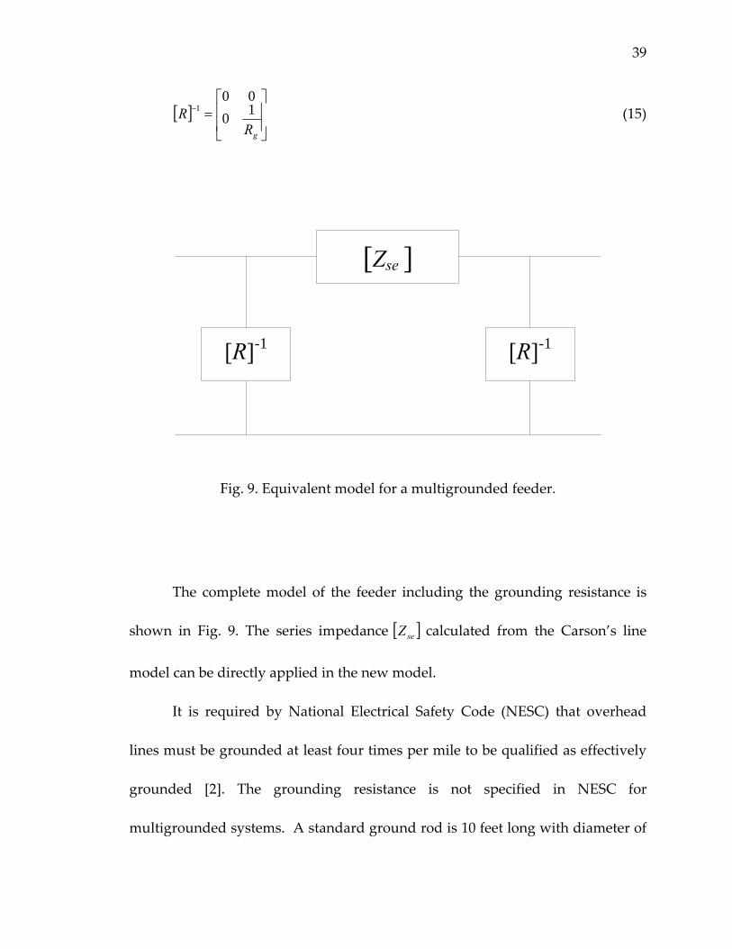
Fig. 9. Equivalent model for a multigrounded feeder.
The complete model of the feeder including the grounding resistance is
shown in Fig. 9. The series impedance [ ]seZ calculated from the Carson’s line
model can be directly applied in the new model.
It is required by National Electrical Safety Code (NESC) that overhead
lines must be grounded at least four times per mile to be qualified as effectively
grounded [2]. The grounding resistance is not specified in NESC for
multigrounded systems. A standard ground rod is 10 feet long with diameter of
40
5/8 inches. For a single ground rod driven vertically into the earth, the
grounding resistance according to Table 2 is about 25 Ω with earth resistivity of
100 m⋅Ω . This resistance value will be applied in this dissertation unless
otherwise specified.
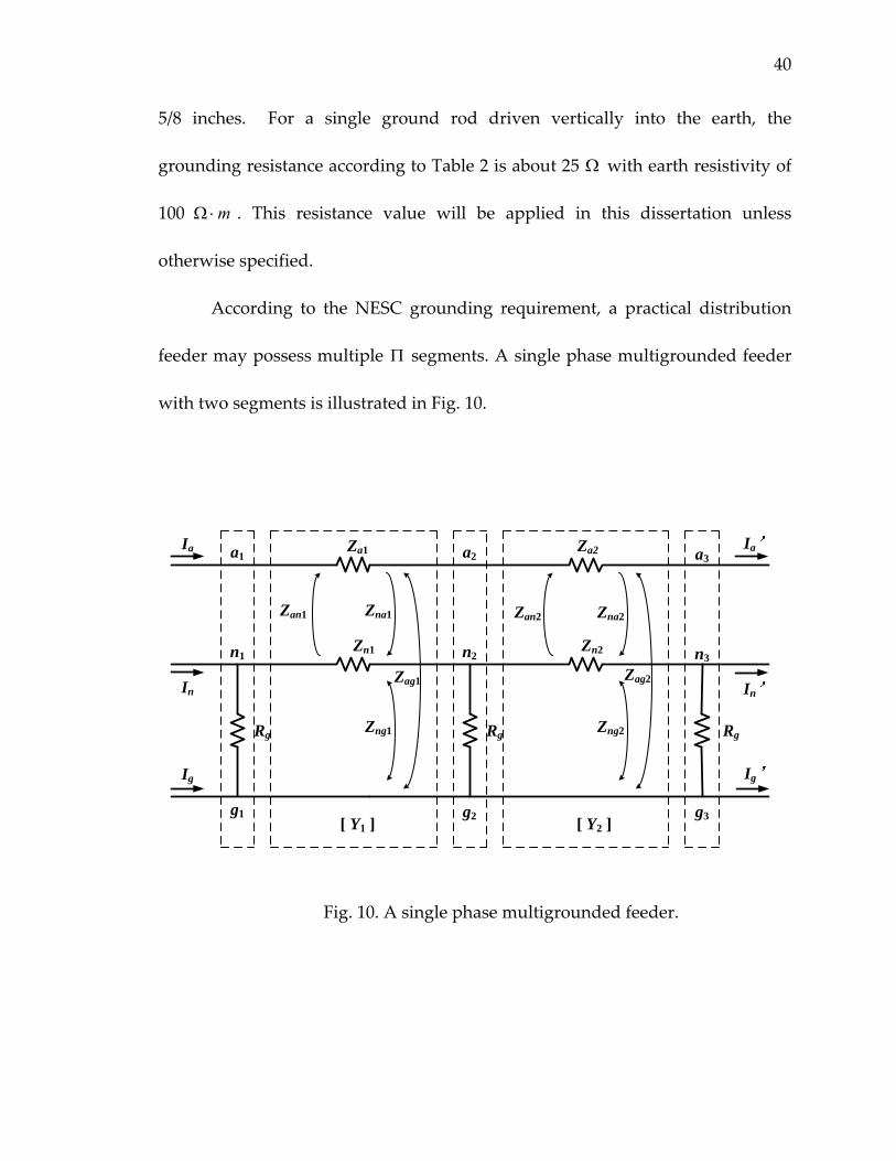
According to the NESC grounding requirement, a practical distribution
feeder may possess multiple Π segments. A single phase multigrounded feeder
with two segments is illustrated in Fig. 10.
a1
n1
g1
Za1
Zn1
Ia
In
Ig
Rg
a2
n2
g2
Za2
Zn2
a3
n3
g3
Ia
In
Ig
[ Y1 ] [ Y2 ]
Zan2 Zna2
Zng2
Zag2
Zan1 Zna1
Zng1
Zag1
Rg Rg
Fig. 10. A single phase multigrounded feeder.
41
The equivalent circuit in Fig. 10 represents two Π segments in series. The
series admittance matrix [ ]iY is calculated as the inverse the [ ]iseZ , for that
segment. In power system analysis, the distributed loads connected to the
transmission lines are usually aggregated at the nodes of interest. Thus for each
feeder, the nodes in the middle need to be eliminated from the final equivalent
circuit.
The Kron reduction method can be applied to simplify the above
equivalent circuit with multiple Π segments. The procedure is illustrated for the
feeder in Fig. 10. The admittance matrix [ ]busY , including the middle node 2, is
developed first using the admittance matrix assembling scheme [22]. For
simplicity, the resistance of each ground electrode is assumed to have the same
value. The resulting admittance matrix is given below.
[ ][ ] [ ] [ ]
[ ] [ ] [ ] [ ] [ ][ ] [ ] [ ] ⎥
⎥⎥
⎦
⎤
⎢⎢⎢
⎣
⎡
+−−++−
−+=
−
−
−
122
21
211
11
1
0
0
RYYYRYYY
YRYYbus (16)
Note that the dimension of the submatrixes, [ ]iY , [ ] 1−R is two by two. The 0 terms
represent a null matrix of the same dimension.
The nodal current injections are related to the node voltages as
42
[ ][ ][ ]
[ ][ ][ ]⎥
⎥⎥
⎦
⎤
⎢⎢⎢
⎣
⎡
⎥⎥⎥
⎦
⎤
⎢⎢⎢
⎣
⎡=
⎥⎥⎥
⎦
⎤
⎢⎢⎢
⎣
⎡
3
2
1
3
2
1
VVV
YIII
bus (17)
where
[ ] ⎥⎦
⎤⎢⎣
⎡=
ni
aii I
II external current injections
[ ] ⎥⎦
⎤⎢⎣
⎡=
ni
aii V
VV node voltages referred to local earth
As the loads are aggregated at the feeder terminals, the external current
injections at the middle node are zero. Kron reduction is applied to [ ]busY by
solving the second equation in (17) for [ ]2V and substitution in the first and the
third equations. The new admittance matrix takes form of
[ ] [ ] [ ][ ] [ ]⎥⎦
⎤⎢⎣
⎡=− AB
BAY newbus (18)
According to the admittance matrix assembling scheme, the off‐diagonal
terms equal the negative admittance connecting the corresponding nodes and the
diagonal terms equal the sum of all admittance originating from that node. The
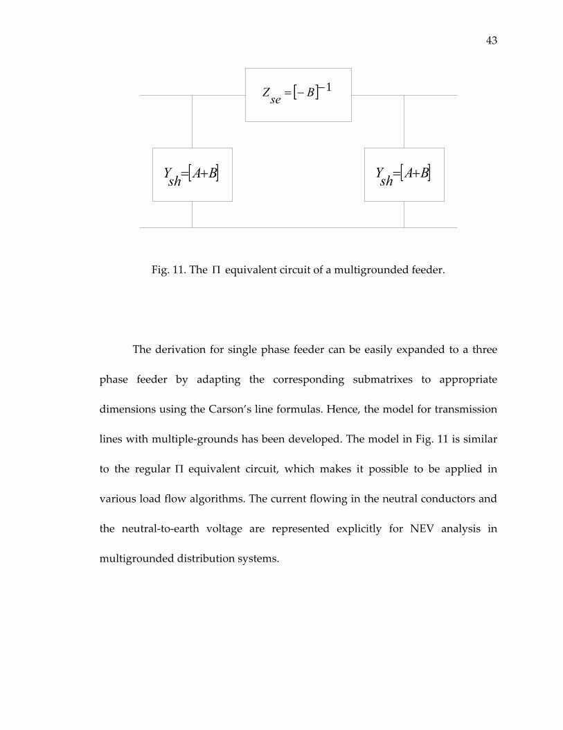
resulting equivalent circuit is shown in Fig. 11.
43
[ ] 1−−= BseZ
[ ]BAshY += [ ]BAshY +=
Fig. 11. The Π equivalent circuit of a multigrounded feeder.
The derivation for single phase feeder can be easily expanded to a three
phase feeder by adapting the corresponding submatrixes to appropriate
dimensions using the Carson’s line formulas. Hence, the model for transmission
lines with multiple‐grounds has been developed. The model in Fig. 11 is similar
to the regular Π equivalent circuit, which makes it possible to be applied in
various load flow algorithms. The current flowing in the neutral conductors and
the neutral‐to‐earth voltage are represented explicitly for NEV analysis in
multigrounded distribution systems.
CHAPTER V
MULTIPHASE LOAD FLOW FOR NEV ANALYSIS
The three phase load flow algorithm for distribution systems [35] is
revised in this dissertation to analyze the NEV in an unbalanced network with
various phasing configurations. Since the objective of this document is to
determine the neutral to earth voltage, some adjustments are required during the
application of the three phase load flow algorithm. The neutral conductor needs
to be included in the load flow formulation in order to directly obtain
information related to the network neutral conductors and the currents through
earth. Also, the current division between the neutral conductor and the earth
needs to be addressed for the stability of the load flow calculation. For simplicity,
only the radial distribution network is discussed in this dissertation. The
algorithm can be easily extended to a radial network with a few loops using the
compensation theory in [34].
Since the load flow method is branch oriented, there is no need to
construct either the nodal admittance matrix busY or the nodal impedance matrix
busZ . Using the models developed in the previous chapter, the parameters for

45
each branch, including the transformers, in a given distribution system are
calculated. The series primitive impedance matrixes are stored corresponding to
the branch and the shunt admittance matrices from neighboring branches are
aggregated at each node.
To proceed in a branch‐oriented load flow, the branches and nodes need
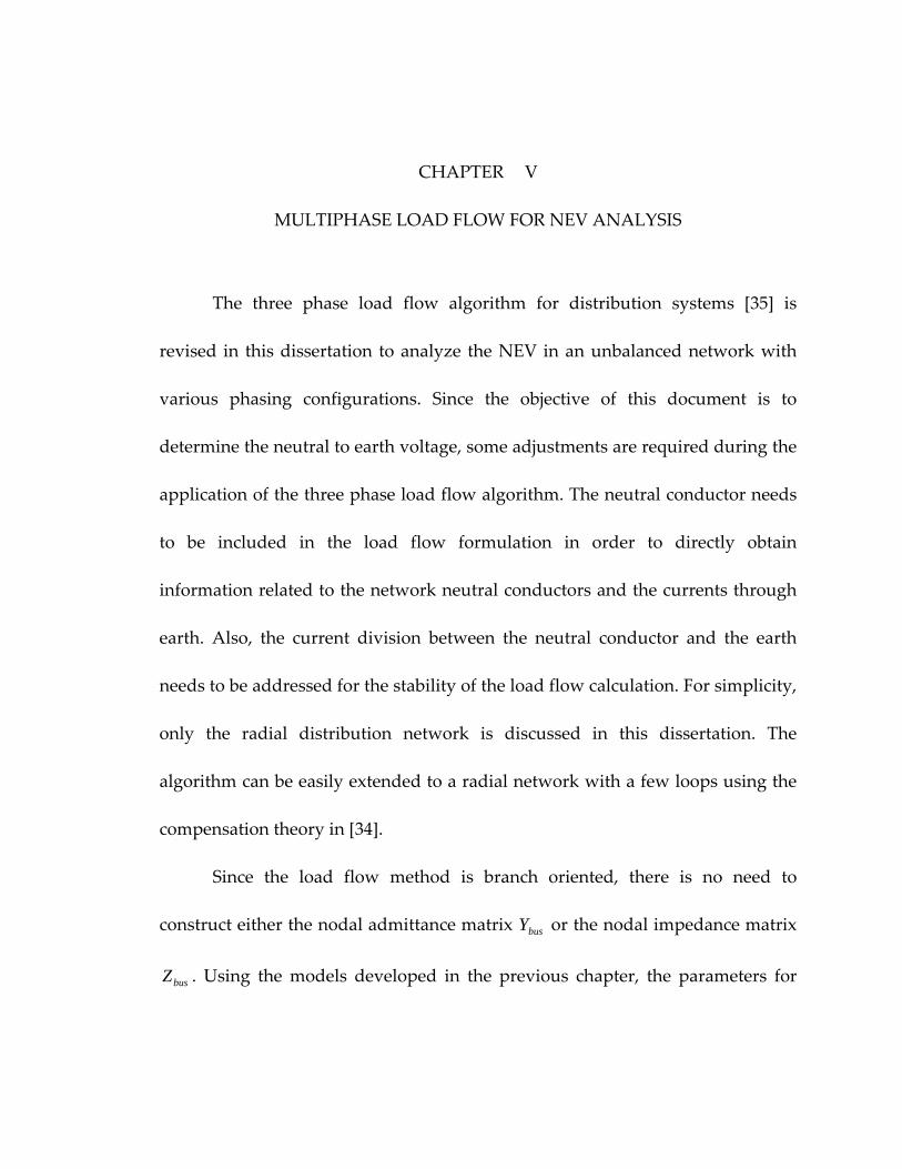
to be numbered to describe the radial topology of the distribution systems. The
procedure is better understood by using the following example network shown
in Fig. 12. The source, usually representing the substation, is denoted as the root
node, or node 0. The two nodes of each branch are labeled as 1L and 2L ,
respectively, where the node closer to the root node is 1L and the other node is
2L . The labeling procedure is shown in Fig. 12 for the several branches.
All of the branches within the network will be numbered in layers. The
first layer consists of the branches directly connected with the root node. The
branches in the first layer are numbered one by one. (Note 1L and 2L denote the
node names and should not be confused with the layer number.) In the
meantime, the 2L node of the corresponding branch is assigned with a node
number same as the branch number. Similarly, the next layer is composed of the
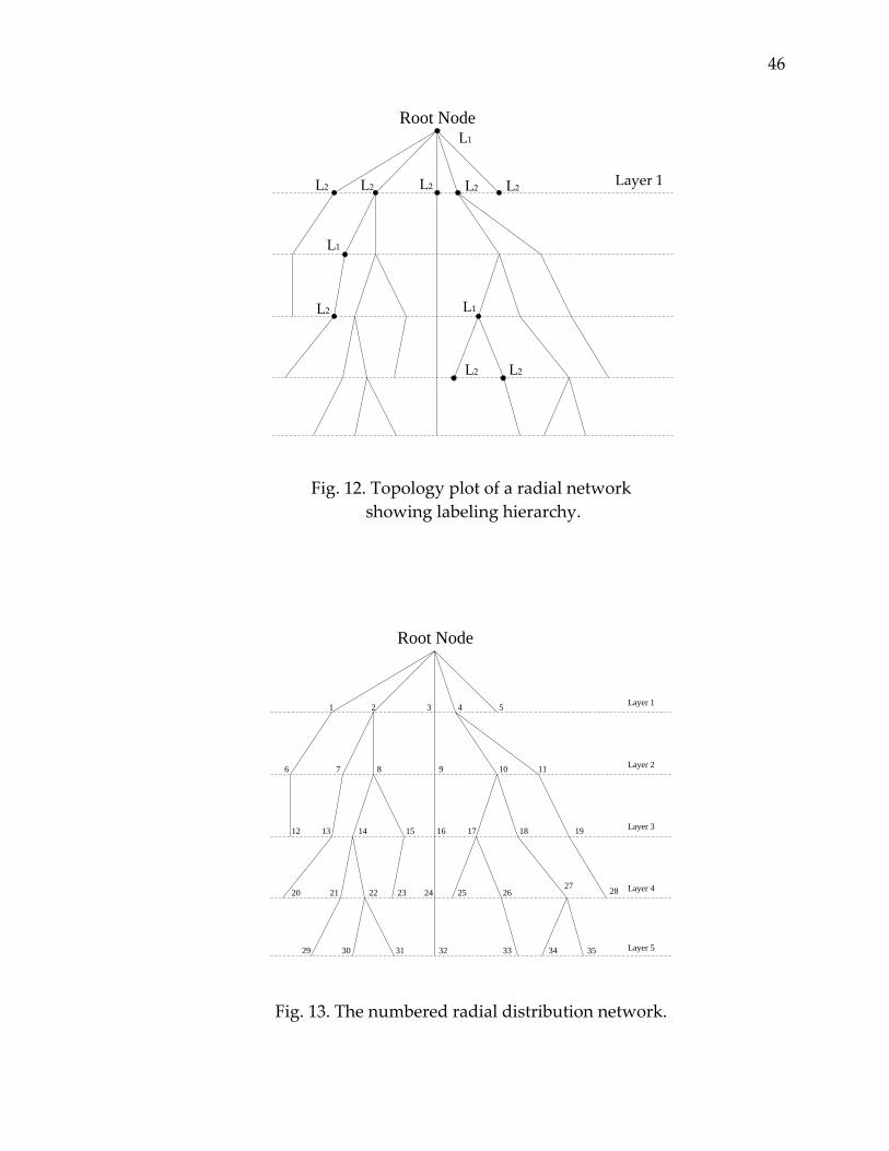
branches whose 1L node is connected to 2L node of any branch in the first layer.
The same procedure is carried out until all branches and nodes are numbered.
The final result is depicted in Fig. 13.
46
Root Node
L2
L1
L2 L2 L2 L2 Layer 1
L2
L2 L2
L1
L1
Fig. 12. Topology plot of a radial network showing labeling hierarchy.
Root Node
Layer 11 2 3 4 5
6 7 8 9 10 11
12 13 14 15 16 17 18 19
20 21 22 23 24 25 2627 28
29 30 31 32 33 34 35
Layer 2
Layer 5
Layer 4
Layer 3
Fig. 13. The numbered radial distribution network.
47
The initial guess of the network static state starts the load flow calculation.
The root node is chosen as the slack bus. If it happens to be the secondary
terminal of the substation transformer, the tap setting is assumed for the root
node phase voltages. Usually the voltages at the substation are well balanced and
the neutral to earth voltage at the substation can be ignored as a result of the low
grounding resistance there. For the rest of the nodes in the network, a flat voltage
profile is assumed as the initial guess with the initial NEVs set to zero.
Note that the dimension of voltage vector for each node is four by one,
even when none of the branches connected to the node is three‐phase, four‐wire.
In the practical programming, a voltage vector with uniform dimension is easier
to implement. A special indexing mechanism is required if using a vector with
exact correspondence to the node phasing. The voltage for the non‐existing phase
or neutral conductor will follow the voltage of the node directly connected it and
one layer higher. It will be shown that this arrangement does not affect the load
flow results.
The iterative load flow algorithm consists of three steps. In iteration k ,
1. Node current injection.
The node current injections are calculated as function of node voltages.
The loads at node i can be represented as constant power, constant current and
constant impedance. At node i ,

48
( ) ( )( )( ) ( )( )( ) ( )( )
( ) ( )
( ) ( )
( ) ( ) ⎥⎥⎥
⎦
⎤
⎢⎢⎢
⎣
⎡
−−−
⎥⎥⎥
⎦
⎤
⎢⎢⎢
⎣
⎡
−
∗
⎥⎥⎥⎥⎥⎥⎥
⎦
⎤
⎢⎢⎢⎢⎢⎢⎢
⎣
⎡
−
−
−
=⎥⎥⎥
⎦
⎤
⎢⎢⎢
⎣
⎡
−−
−−
−−
∗
∗
∗
−−
−−
−−
1,
1,
1,
1,
1,
1,
,
,
,
1,
1,
,
1,
1,
,
1,
1,
,
,
,
,
kni
kci
kni
kbi
kni
kai
ci
bi
ai
kni
kci
ci
kni
kbi
bi
kni
kai
ai
k
ci
bi
ai
VVVVVV
YY
Y
VVS
VVS
VVS
III
⎥⎥⎥
⎦
⎤
⎢⎢⎢
⎣
⎡+
loadci
loadbi
loadai
III
_,
_,
_,
(19)
where
aiI , , biI , , ciI , are the total phase current injections using the
generator convention,
aiS , , biS , , ciS , are the scheduled complex power injection
including the load demand and the power
delivery from the distributed generators,
aiV , , biV , , ciV , , niV , are the phase and/or neutral voltages referring
to the local earth,
aiY , , biY , , ciY , are the admittances of all shunt elements
including the shunt capacitor, constant load
impedance and any shunt branch in the branch
equivalent circuit,
loadaiI _, , loadbiI _, , loadciI _, are the scheduled constant current loads.

49
2. Backward collection to obtain the branch current.
Starting from the outmost branch, calculate the branch current by
summing the branch currents from lower layers if exist, plus the node current
injection at the 2L node of this branch. For branch L ,
k
Xx xc
xb
xa
k
ci
bi
ai
k
Lc
Lb
La
III
III
III
∑∈ ⎥
⎥⎥
⎦
⎤
⎢⎢⎢
⎣
⎡
+⎥⎥⎥
⎦
⎤
⎢⎢⎢
⎣
⎡−=
⎥⎥⎥
⎦
⎤
⎢⎢⎢
⎣
⎡
,
,
,
(20)
where
X the set of branches whose 1L nodes are directly connected to the 2L
of branch L .
The first term in (20) is the local injections determined by (19). The
negative sign results from the branch current reference directions where a
current flowing from source to load is assumed positive.
Due to the shunt grounding branch, a portion of the return injection
currents flow through shY . The detail of the current division will be discussed
later in this chapter. It can be just assumed that the neutral conductor current in
each branch has been collected and corrected to account for the current division
between neutral conductor and earth return path.

50
3. Forward node voltage update.
Starting from the layer right below the root node, the voltage drop across
each branch can be determined using the calculated branch currents. For branch
L , assume its 1L and 2L nodes equal j and i , respectively. Then the node i
voltages are updated as
( )
( )
( )
( )
( )
( )
( )
( )
( )k
Ln
Lc
Lb
La
Lnn
Lcn
Lcc
Lbn
Lbc
Lbb
Lan
Lac
Lab
Laa
knj
kcj
kbj
kaj
kni
kci
kbi
kai
IIII
ZZZZZZZZZZ
VVVV
VVVV
⎥⎥⎥⎥
⎦
⎤
⎢⎢⎢⎢
⎣
⎡
⎥⎥⎥⎥
⎦
⎤
⎢⎢⎢⎢
⎣
⎡
−
⎥⎥⎥⎥⎥
⎦
⎤
⎢⎢⎢⎢⎢
⎣
⎡
=
⎥⎥⎥⎥⎥
⎦
⎤
⎢⎢⎢⎢⎢
⎣
⎡
,
,
,
,
,
,
,
,
(21)
After the voltages are updated at all nodes, a convergence check is
performed. Since constant power is not the only type of load in the system, the
voltage error in (22) is checked instead of the usual power mismatch criterion.
The maximum error of 0.001 p.u. is applied in this dissertation as the
convergence criterion.
( )
( )
( )
( )
( )
( )
( )
( )
( )
( )
( )
( )⎥⎥⎥⎥⎥
⎦
⎤
⎢⎢⎢⎢⎢
⎣
⎡
−
⎥⎥⎥⎥⎥
⎦
⎤
⎢⎢⎢⎢⎢
⎣
⎡
=
⎥⎥⎥⎥⎥
⎦
⎤
⎢⎢⎢⎢⎢
⎣
⎡
∆∆∆∆
−
−
−
−
1,
1,
1,
1,
,
,
,
,
,
,
,
,
kni
kci
kbi
kai
kni
kci
kbi
kai
kni
kci
kbi
kai
VVVV
VVVV
VVVV
(22)
As mentioned in step 2, the current division between the neutral
conductor and the earth needs to be determined for correct neutral branch
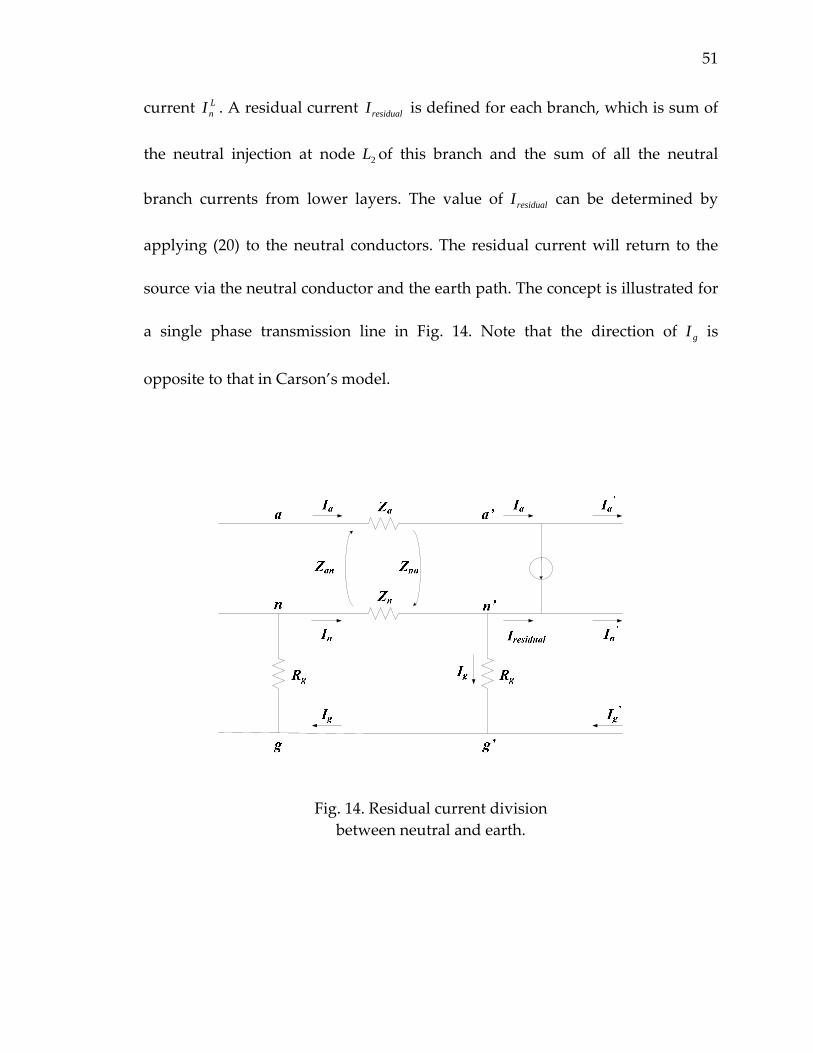
51
current LnI . A residual current residualI is defined for each branch, which is sum of
the neutral injection at node 2L of this branch and the sum of all the neutral
branch currents from lower layers. The value of residualI can be determined by
applying (20) to the neutral conductors. The residual current will return to the
source via the neutral conductor and the earth path. The concept is illustrated for
a single phase transmission line in Fig. 14. Note that the direction of gI is
opposite to that in Carson’s model.
Fig. 14. Residual current division between neutral and earth.
52
An intuitive method to determine the neutral branch current nI is to
exploit the constraint that the voltage drop of the shunt grounding branch ''gnV
results from the current flowing through it. With all voltage referred to local
earth,
g
ng R
VI '= (23)
gresidualn III += (24)
The current gI in each shunt branch is first calculated using (23) and the
neutral current nI is obtained by (24). This neutral current is then inserted into
step two of the iteration as a part of the results of the backward branch currents
collection. However, unlike the phase currents, the earth current is less
constrained by the network topology and load demand except for the calculated
neutral voltage. Thus 'nV can converge to an incorrect value or fail to converge at
all.
An improved means to ensure proper convergence is to take advantage of
branch voltage equation and the actual circuit connection. In Fig. 14, the voltage
drop across the neutral conductor is given as
nnnaannnnn IZIZVVV +=−= '' (25)
53
The neutral current is obtained by solving (24) and (25) for nI
simultaneously:
nng
residualgaannn ZR
IRIZVI
++−
= (26)
In the actual load flow calculation, nV is the source‐end neutral voltage
from the previous iteration, aI is the calculated phase current, and gR is replaced
by the shunt admittance from the transmission line model. The residual current
is forced to divide between neutral and earth according to the circuit
configuration using the assumed node voltage, thus expediting the convergence.
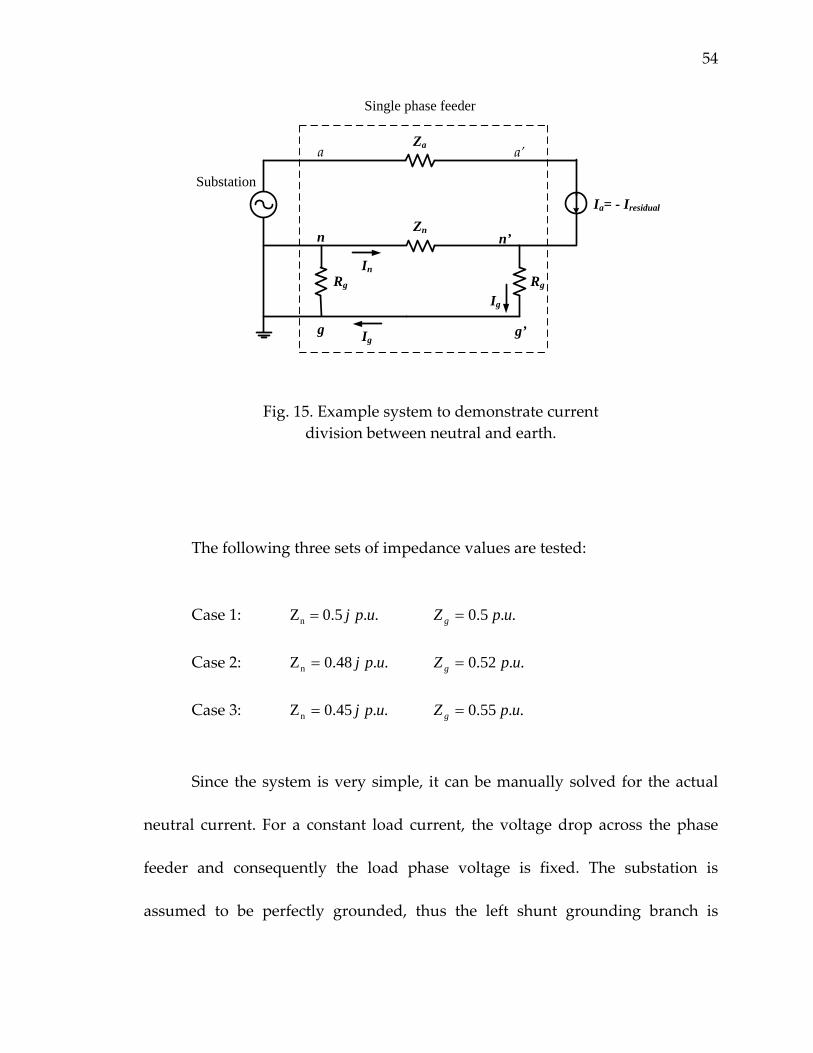
The effectiveness of these two current division methods is demonstrated
in the following simple example. In Fig. 15, a constant current load is fed by the
substation through a single phase feeder. The substation is represented as an
ideal voltage source. The feeder mutual impedance between the phase and
neutral conductor is ignored for simplicity. The feeder series resistance is also
neglected. The load current is assumed to be 0.1 p.u. The earth current gI in Fig.
15 is also assumed positive when it returns to the source.
54
n
g
Rg
n’
g’
In
Ig
Ig
Ia= - Iresidual
Rg
Zn
Za
Substation
Single phase feeder
a a’
Fig. 15. Example system to demonstrate current division between neutral and earth.
The following three sets of impedance values are tested:
Case 1: .. 5.0Zn upj= .. 5.0 upZg =
Case 2: .. 48.0Zn upj= .. 52.0 upZg =
Case 3: .. 45.0Zn upj= .. 55.0 upZg =
Since the system is very simple, it can be manually solved for the actual
neutral current. For a constant load current, the voltage drop across the phase
feeder and consequently the load phase voltage is fixed. The substation is
assumed to be perfectly grounded, thus the left shunt grounding branch is
55
shorted and nV is zero. Since there is only one load, the residual current residualI is
equal to the load current aI . The system can be solved after current division of
residualI is determined between nZ and shunt grounding branch gR on the right.
From the above analysis it is clear that nZ and gR on the right are in
parallel because of the shorted grounding branch on the left. residualI will simply
return through the parallel combination of nZ and gR and the neutral current is
determined as follows
agn
gresidual
gn
gn I
RZR
IRZ
RI
+=
+= (27)
The obtained neutral currents in three test cases are applied to compare
the performance of the two current division methods. Next, the system is solved
by the load flow algorithm with different current division methods. The neutral
voltage 'nV is initially assumed to be zero. The results using the two methods
above are compared with the actual values in Table 3. It is obvious from Table 3
that the second method utilizing forced current division is more accurate and
much faster. In case 1 when the magnitudes of nZ and gR are equal, the results
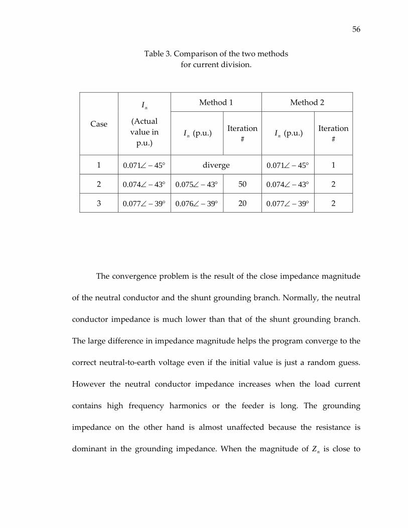
just bounce around two extreme values and never converge at all.
56
Table 3. Comparison of the two methods for current division.
Method 1 Method 2
Case
nI
(Actual value in p.u.)
nI (p.u.) Iteration # nI (p.u.) Iteration
#
1 °−∠ 45071.0 diverge °−∠ 45071.0 1
2 °−∠ 43074.0 °−∠ 43075.0 50 °−∠ 43074.0 2
3 °−∠ 39077.0 °−∠ 39076.0 20 °−∠ 39077.0 2
The convergence problem is the result of the close impedance magnitude
of the neutral conductor and the shunt grounding branch. Normally, the neutral
conductor impedance is much lower than that of the shunt grounding branch.
The large difference in impedance magnitude helps the program converge to the
correct neutral‐to‐earth voltage even if the initial value is just a random guess.
However the neutral conductor impedance increases when the load current
contains high frequency harmonics or the feeder is long. The grounding
impedance on the other hand is almost unaffected because the resistance is
dominant in the grounding impedance. When the magnitude of nZ is close to

57
that of gR , the first method cannot tell how much current should return through
the earth unless the neutral‐to‐earth voltage value is already correct.
The second method improves the convergence by calculating the correct
current division between neutral and earth every time the neutral‐to‐earth
voltage is available. Thus the answer will get closer to the correct value in each
iteration.
In the next chapter, this multiphase load flow algorithm is further
extended to include harmonic analysis. The effect of nonlinear loads upon NEV
in distribution systems can thus be analyzed using multiphase harmonic load
flow calculation.
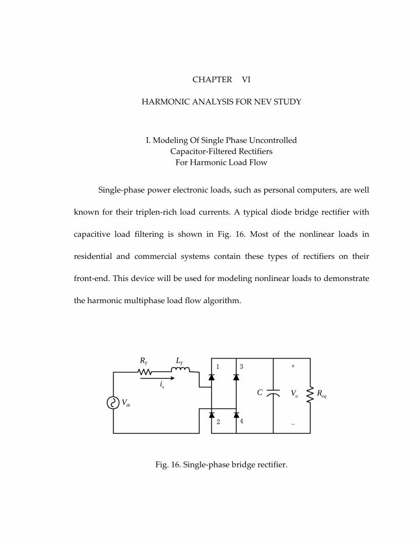
CHAPTER VI
HARMONIC ANALYSIS FOR NEV STUDY
I. Modeling Of Single Phase Uncontrolled Capacitor‐Filtered Rectifiers For Harmonic Load Flow
Single‐phase power electronic loads, such as personal computers, are well
known for their triplen‐rich load currents. A typical diode bridge rectifier with
capacitive load filtering is shown in Fig. 16. Most of the nonlinear loads in
residential and commercial systems contain these types of rectifiers on their
front‐end. This device will be used for modeling nonlinear loads to demonstrate
the harmonic multiphase load flow algorithm.
thV
TR TL
C eqRoVsi
+
-
1 3
2 4
Fig. 16. Single‐phase bridge rectifier.
59
A detailed model is proposed in [46], [47] to simulate this type of power
electronic circuit. The nonlinear load current is calculated as a function of the
distorted terminal voltage and device parameters. The general form of thV can be
expressed as follows
( )∑ +=h
hhth hVV φθcos2 (28)
The terminal voltage thV provided to the model is obtained either from the
initial guess or the intermediate result of the load flow calculation. A typical
waveform for rectifier operation is shown in Fig. 17.
The angles 1θ and 2θ are the conduction and extinction angles,
respectively. The detailed circuit analysis of the single phase rectifier is presented
in the appendix. If the angles 1θ and 2θ are known, the closed form solution of
the input current can be determined using the method in the appendix. The
general form of the input current si is given as follows
∑ +=h
hhs thIi )cos(2 φω (29)
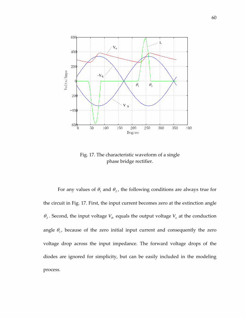
60
Volts/Amps
1θ 2θ
Fig. 17. The characteristic waveform of a single phase bridge rectifier.
For any values of 1θ and 2θ , the following conditions are always true for
the circuit in Fig. 17. First, the input current becomes zero at the extinction angle
2θ . Second, the input voltage thV equals the output voltage oV at the conduction
angle 1θ , because of the zero initial input current and consequently the zero
voltage drop across the input impedance. The forward voltage drops of the
diodes are ignored for simplicity, but can be easily included in the modeling
process.
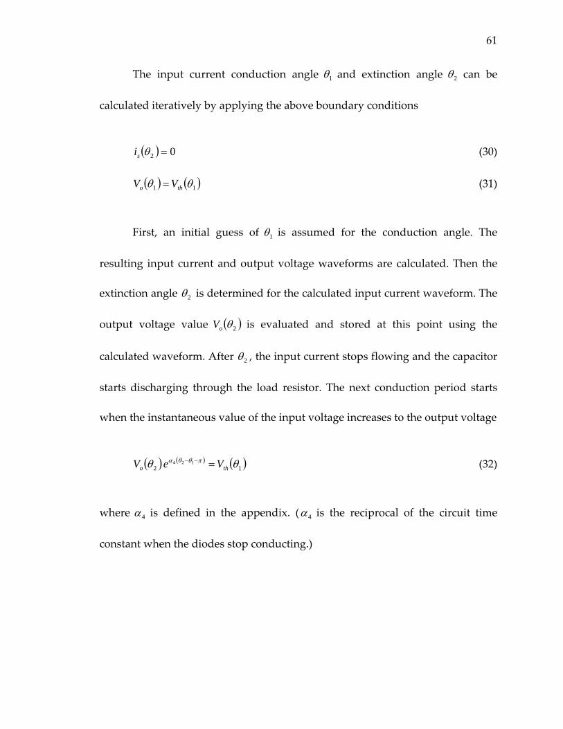
61
The input current conduction angle 1θ and extinction angle 2θ can be
calculated iteratively by applying the above boundary conditions
( ) 02 =θsi (30)
( ) ( )11 θθ tho VV = (31)
First, an initial guess of 1θ is assumed for the conduction angle. The
resulting input current and output voltage waveforms are calculated. Then the
extinction angle 2θ is determined for the calculated input current waveform. The
output voltage value ( )2θoV is evaluated and stored at this point using the
calculated waveform. After 2θ , the input current stops flowing and the capacitor
starts discharging through the load resistor. The next conduction period starts
when the instantaneous value of the input voltage increases to the output voltage
( ) ( ) ( )12124 θθ πθθα
tho VeV =−− (32)
where 4α is defined in the appendix. ( 4α is the reciprocal of the circuit time
constant when the diodes stop conducting.)
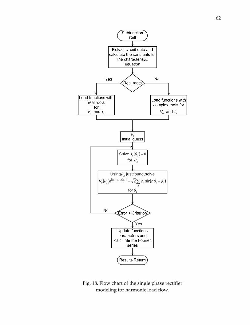
62
so iV and
1θ
so iV and
( )2 for
Solveθθ 02 =si
( ) ( )[ ] ( )
1
2
for
sin
solve found, just Using
θ
φθθ
θαπθθ ∑ +=−−
hhho hVeV 12 2412
Fig. 18. Flow chart of the single phase rectifier modeling for harmonic load flow.
63
The new value of 1θ is updated by solving (32) for 1θ . A convergence
check is performed at this point to determine if the process should be continued.
After the values of 1θ and 2θ settle down and converge, the Fourier series of the
input current is calculated and fed back to the load flow algorithm. The
procedure is illustrated by the flow chart in Fig. 18.
The single phase rectifier model is tested using a distorted input voltage.
Let Ω= 0085.0tR , mHLt 0513.0= , FC µ4200 = , Ω= 71.3eqR . The input voltage
harmonic content in RMS values are given as V 1002401 °∠=V , V 250153 °∠=V ,
V 10105 °∠=V , V 30107 °∠=V . The even harmonics are negligible, and they
usually do not exist in a properly designed power system with these types of
loads. The resulting waveforms are plotted in Fig. 19.
II. Harmonic Multiphase Load Flow
With the single phase rectifier model just described, the harmonic current
injection can be determined every time the nodal voltages are updated. Other
types of nonlinear loads can be provided to the algorithm to analyze the
interaction between the system distortion and the nonlinear load performance.
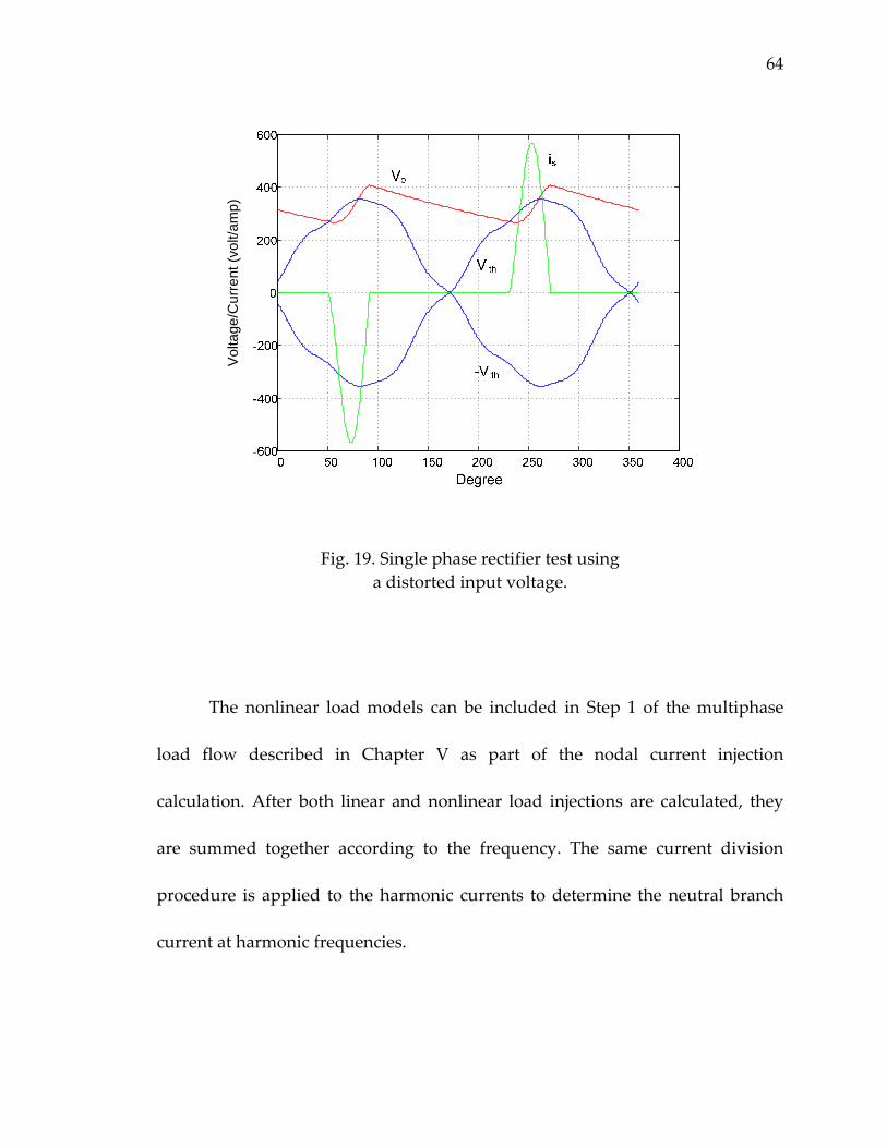
64
Vol
tage
/Cur
rent
(vol
t/am
p)
Fig. 19. Single phase rectifier test using a distorted input voltage.
The nonlinear load models can be included in Step 1 of the multiphase
load flow described in Chapter V as part of the nodal current injection
calculation. After both linear and nonlinear load injections are calculated, they
are summed together according to the frequency. The same current division
procedure is applied to the harmonic currents to determine the neutral branch
current at harmonic frequencies.

65
As the nonlinear loads are treated as the source of harmonic current, the
root node voltages at harmonic frequencies are assumed to be zeros. The nodal
voltages are updated at all frequencies of interest as in Step 3 of the multiphase
load flow in the previous chapter.
The input current is injected into the network to calculate the branch
harmonic currents and then the branch voltage drops. Following procedures
similar to those outlined above, the new distorted bus voltages are found and
compared to the criterion until they converge. A complete flow chart for the
multiphase harmonic load flow in a distribution system is shown in Fig. 20.
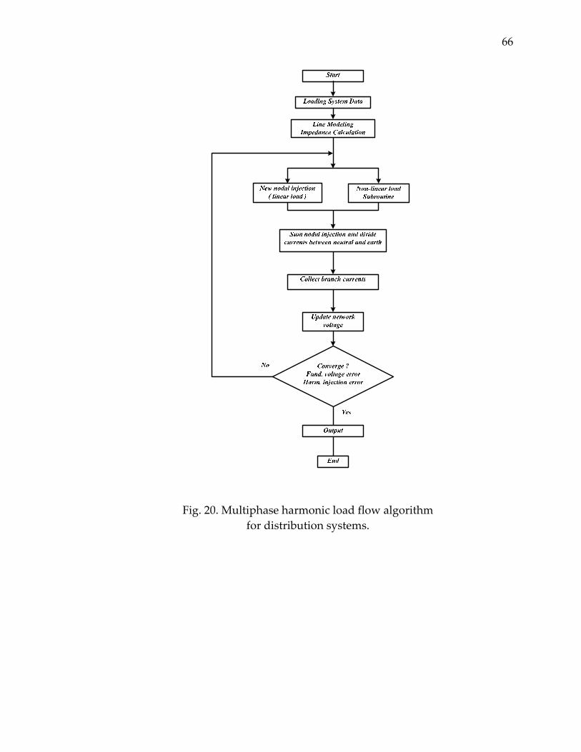
66
Fig. 20. Multiphase harmonic load flow algorithm for distribution systems.
CHAPTER VII
NEV ANALYSIS USING THE MULTIPHASE
HARMONIC LOAD FLOW ALGORITHM
I. IEEE Example System Tests
1. System description.
The IEEE 13 bus test distribution system [48] is widely applied to evaluate
load flow algorithms dedicated to unbalanced distribution systems. The
distribution feeder in this test system is highly loaded for its relatively short
length. It features various unbalanced line configurations, wye and delta load
connections, and voltage conditioning devices. This system is utilized in this
dissertation to examine the reliability of the multiphase harmonic load flow
algorithm developed in the previous chapters. Since this dissertation focuses on
NEV analysis, certain simplifications are assumed for the system modeling for
the scope of this dissertation:
1. All the underground cables are omitted since the emphasis for this research is on overhead (aerial) lines.
2. Line charging currents are negligible (all lines are short).
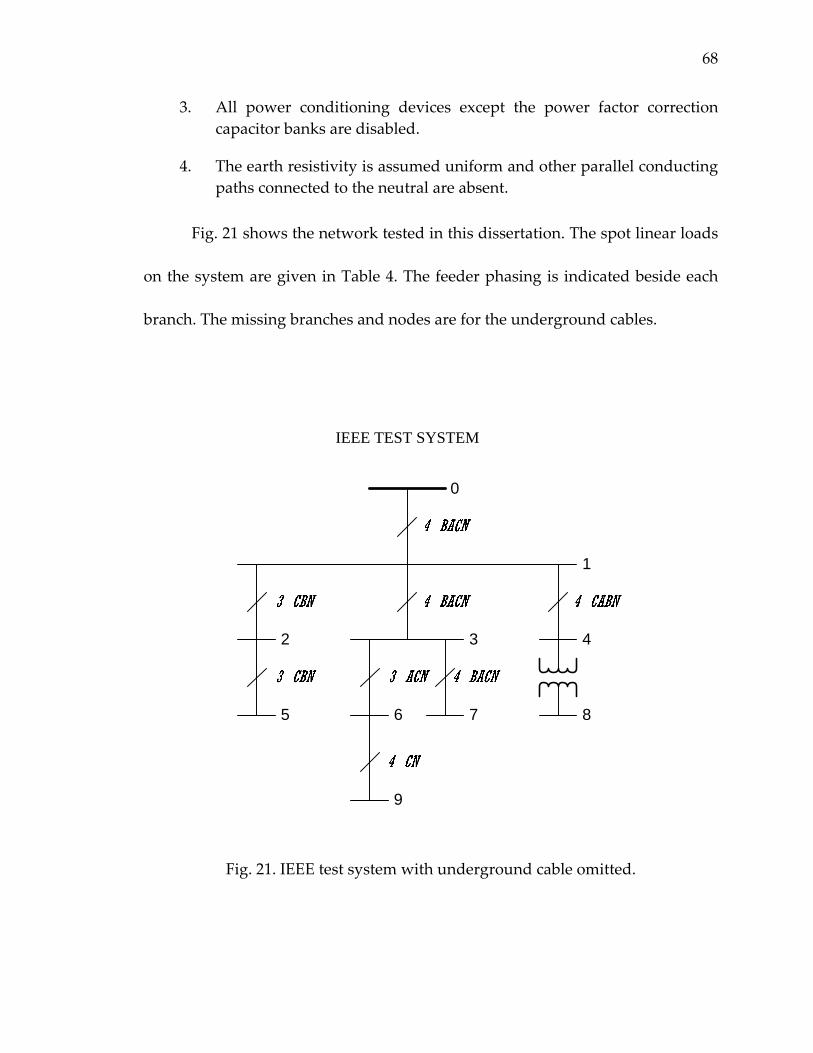
68
3. All power conditioning devices except the power factor correction capacitor banks are disabled.
4. The earth resistivity is assumed uniform and other parallel conducting paths connected to the neutral are absent.
Fig. 21 shows the network tested in this dissertation. The spot linear loads
on the system are given in Table 4. The feeder phasing is indicated beside each
branch. The missing branches and nodes are for the underground cables.
0
1
2 3 4
5 6 7 8
9
IEEE TEST SYSTEM
Fig. 21. IEEE test system with underground cable omitted.
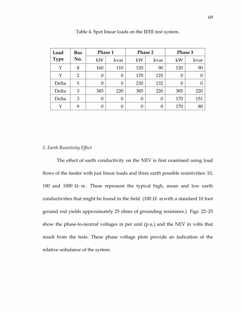
69
Table 4. Spot linear loads on the IEEE test system.
Phase 1 Phase 2 Phase 3 Load Type
Bus No. kW kvar kW kvar kW kvar
Y 8 160 110 120 90 120 90Y 2 0 0 170 125 0 0
Delta 5 0 0 230 132 0 0Delta 3 385 220 385 220 385 220Delta 3 0 0 0 0 170 151Y 9 0 0 0 0 170 80
2. Earth Resistivity Effect
The effect of earth conductivity on the NEV is first examined using load
flows of the feeder with just linear loads and three earth possible resistivities: 10,
100 and 1000 m⋅Ω . These represent the typical high, mean and low earth
conductivities that might be found in the field. (100 m⋅Ω with a standard 10 foot
ground rod yields approximately 25 ohms of grounding resistance.) Figs. 22–25
show the phase‐to‐neutral voltages in per unit (p.u.) and the NEV in volts that
result from the tests. These phase voltage plots provide an indication of the
relative unbalance of the system.
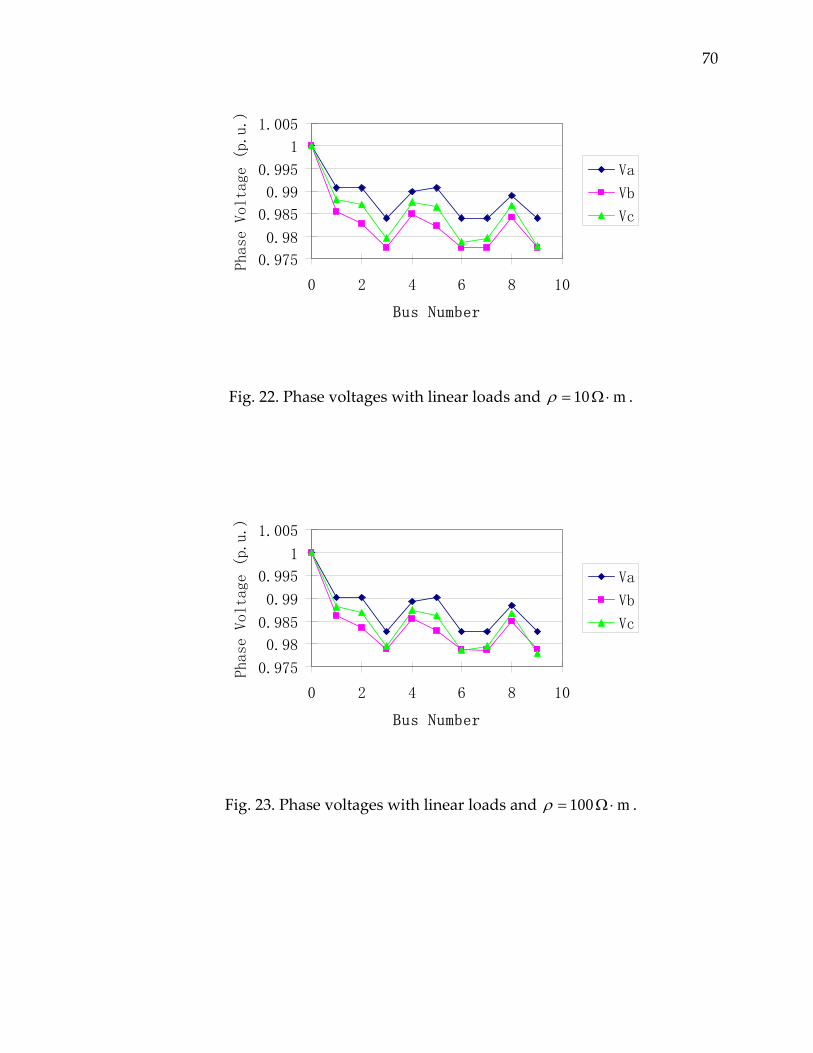
70
0.975
0.98
0.985
0.99
0.995
1
1.005
0 2 4 6 8 10
Bus Number
Phase Voltage (p.u.)
Va
Vb
Vc
Fig. 22. Phase voltages with linear loads and m 10 ⋅Ω=ρ .
0.975
0.98
0.985
0.99
0.995
1
1.005
0 2 4 6 8 10
Bus Number
Phase Voltage (p.u.)
Va
Vb
Vc
Fig. 23. Phase voltages with linear loads and m 100 ⋅Ω=ρ .
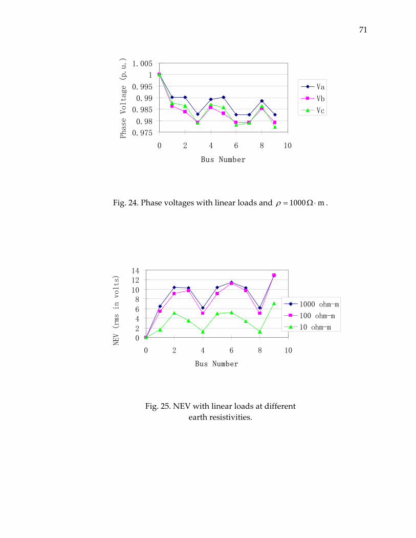
71
0.975
0.98
0.985
0.99
0.995
1
1.005
0 2 4 6 8 10
Bus Number
Phase Voltage (p.u.)
Va
Vb
Vc
Fig. 24. Phase voltages with linear loads and m 1000 ⋅Ω=ρ .
02
46
810
1214
0 2 4 6 8 10
Bus Number
NEV (rms in volts)
1000 ohm-m
100 ohm-m
10 ohm-m
Fig. 25. NEV with linear loads at different earth resistivities.

72
From the plots in Fig. 22–24, it can be seen that the change in the earth
conductivities has almost no effect on the phase voltages. The feeder’s series
impedance is not high enough to make any difference in phase voltage drop.
This result is reasonable considering the short length of the feeder. However,
NEV is much more sensitive to the change in earth resistivity. The higher earth
resistivity causes higher NEV, as is expected. It is shown Fig. 25 that NEV level is
doubled when the earth resistivity increases from 10 m⋅Ω to 100 m⋅Ω . It is
interesting to note that there is a significant difference between 10 m⋅Ω and 100
m⋅Ω , but above 100 m⋅Ω changes in the ground resistivity has little effect on
the NEV.
In these linear loads tests, the higher NEV is incidental to unbalanced bus
loads or single/two phase branches. Also the higher NEV on these buses can
affect other buses if the affected buses are on the backward trace of the buses that
cause NEV elevation, or they are at downstream of a bus with high NEV. For
example, the trace of bus 7 back to the source consists of three phase branches.
But unbalanced loads are connected at bus 3 upstream, and cause high NEV. So
even no load current is drawn at bus 7, its NEV is still higher than the NEV at
bus 8 where balanced loads are connected. These results show that besides the
earth resistivity, the network topology and the location of unbalanced loads and
branches are also important in an NEV investigation.

73
3. Effect of Nonlinear Loads
To examine the harmonic distortion effect on NEV, a 240V, 30kW single‐
phase rectifier with a 4200μF smoothing capacitor is applied to simulate the
lumped nonlinear loads connected on the feeder from phase–to‐neutral. The
original linear loads on the feeder are kept unchanged. The earth resistivity is
assumed to be 100 m⋅Ω in all of the following tests. Three scenarios are
considered in this paper for illustration:
(i) A single rectifier on a single‐phase line at bus 3
(ii) Three balanced rectifiers on a three‐phase line at bus 3
(iii) Two identical rectifiers on two phases of a three‐phase line at bus 3 to form an unbalanced load
Since the nonlinear loads are small compared with the linear loads in
Table 4, the phase voltage profiles for all cases are essentially the same as the
results in Figs. 22‐24. The voltage profile for the Case (i) is shown in Fig. 26.
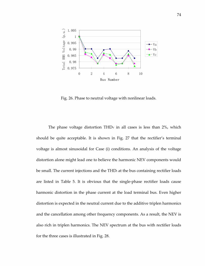
74
0.975
0.98
0.985
0.99
0.995
1
1.005
0 2 4 6 8 10
Bus Number
Total RMS Voltage (p.u.)
Va
Vb
Vc
Fig. 26. Phase to neutral voltage with nonlinear loads.
The phase voltage distortion THDV in all cases is less than 2%, which
should be quite acceptable. It is shown in Fig. 27 that the rectifier’s terminal
voltage is almost sinusoidal for Case (i) conditions. An analysis of the voltage
distortion alone might lead one to believe the harmonic NEV components would
be small. The current injections and the THDI at the bus containing rectifier loads
are listed in Table 5. It is obvious that the single‐phase rectifier loads cause
harmonic distortion in the phase current at the load terminal bus. Even higher
distortion is expected in the neutral current due to the additive triplen harmonics
and the cancellation among other frequency components. As a result, the NEV is
also rich in triplen harmonics. The NEV spectrum at the bus with rectifier loads
for the three cases is illustrated in Fig. 28.
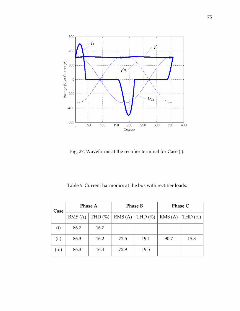
75
Fig. 27. Waveforms at the rectifier terminal for Case (i).
Table 5. Current harmonics at the bus with rectifier loads.
Phase A Phase B Phase C Case
RMS (A) THD (%) RMS (A) THD (%) RMS (A) THD (%)
(i) 86.7 16.7
(ii) 86.3 16.2 72.5 19.1 90.7 15.3
(iii) 86.3 16.4 72.9 19.5
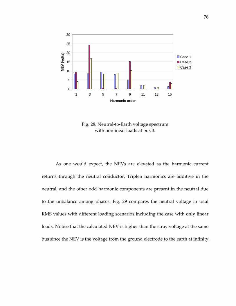
76
0
5
10
15
20
25
30
1 3 5 7 9 11 13 15
Harmonic order
NEV
(vol
ts)
Case 1Case 2Case 3
Fig. 28. Neutral‐to‐Earth voltage spectrum with nonlinear loads at bus 3.
As one would expect, the NEVs are elevated as the harmonic current
returns through the neutral conductor. Triplen harmonics are additive in the
neutral, and the other odd harmonic components are present in the neutral due
to the unbalance among phases. Fig. 29 compares the neutral voltage in total
RMS values with different loading scenarios including the case with only linear
loads. Notice that the calculated NEV is higher than the stray voltage at the same
bus since the NEV is the voltage from the ground electrode to the earth at infinity.
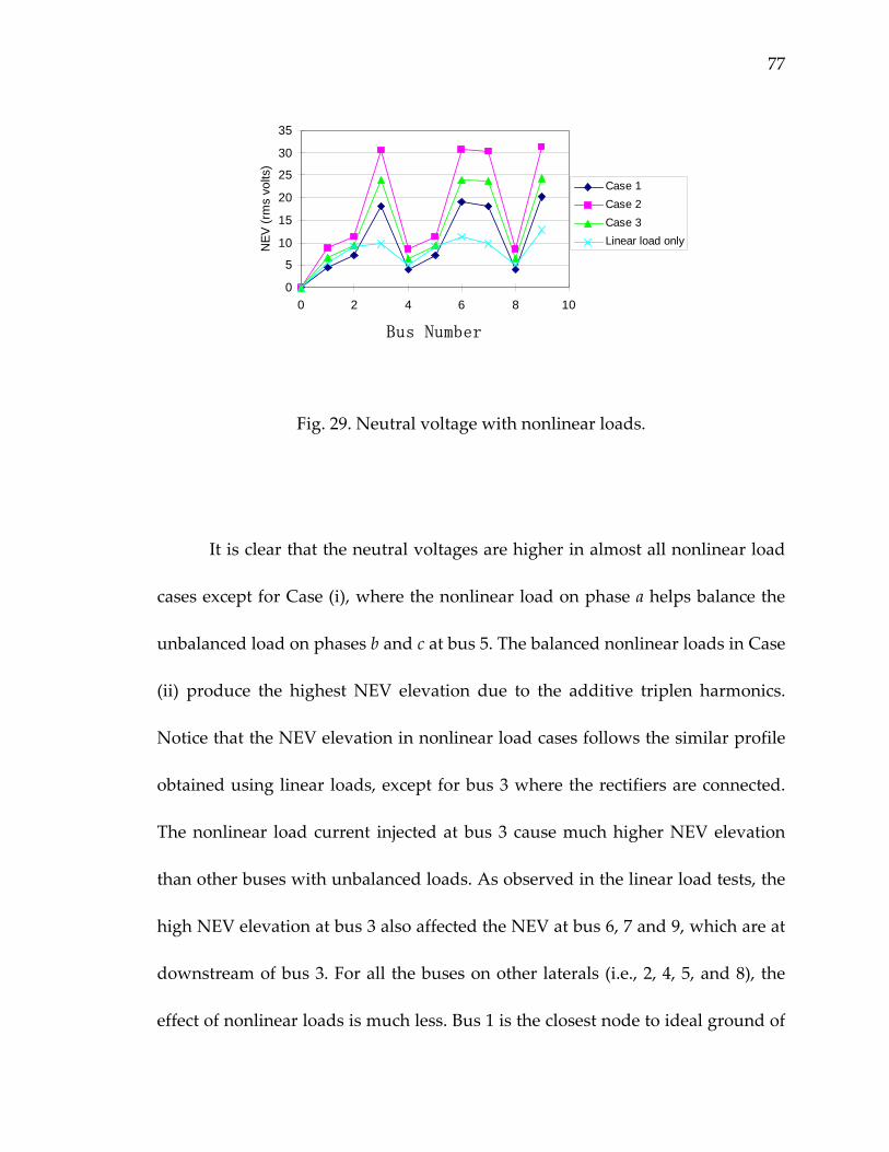
77
0
5
10
15
20
25
30
35
0 2 4 6 8 10
Bus Number
NEV
(rm
s vo
lts)
Case 1Case 2Case 3Linear load only
Fig. 29. Neutral voltage with nonlinear loads.
It is clear that the neutral voltages are higher in almost all nonlinear load
cases except for Case (i), where the nonlinear load on phase a helps balance the
unbalanced load on phases b and c at bus 5. The balanced nonlinear loads in Case
(ii) produce the highest NEV elevation due to the additive triplen harmonics.
Notice that the NEV elevation in nonlinear load cases follows the similar profile
obtained using linear loads, except for bus 3 where the rectifiers are connected.
The nonlinear load current injected at bus 3 cause much higher NEV elevation
than other buses with unbalanced loads. As observed in the linear load tests, the
high NEV elevation at bus 3 also affected the NEV at bus 6, 7 and 9, which are at
downstream of bus 3. For all the buses on other laterals (i.e., 2, 4, 5, and 8), the
effect of nonlinear loads is much less. Bus 1 is the closest node to ideal ground of

78
the source. And all load currents in the network flow through this bus, which
helps balance the phase currents. Consequently, the NEV at this bus is lowest
among all the nodes on the feeder.
II. Comparison With Field Measurements
The test on the IEEE example system shows that the developed
multiphase harmonic load flow algorithm developed in this dissertation is quite
reliable on handling various unbalanced system configuration. The nonlinear
model also works well for analyzing the effect of harmonic distortion on NEV
elevation. In this section, the algorithm’s accuracy is verified by comparing the
load flow calculations with field measurement.
A typical multigrounded three phase feeder with single phase lateral is
chosen and the line configuration is shown in Fig. 30. The three phase feeder is
fed through a 44/12.47 kV delta–wye grounded substation transformer. A typical
impedance of 7% is assumed for this investigation. The series resistance of the
transformer is ignored for simplicity. All conductors of the three phase primary
and the single phase lateral, including the neutral conductors, are ACSR 336,400.
The three phase primary and the single phase lateral are both 5 miles long.
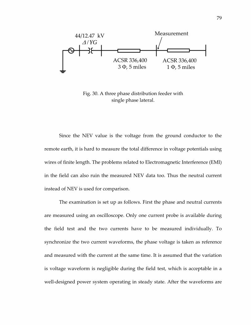
79
44/12.47 kVYG/∆
ACSR 336,400 3 Φ, 5 miles
ACSR 336,400 1 Φ, 5 miles
Measurement
Fig. 30. A three phase distribution feeder with single phase lateral.
Since the NEV value is the voltage from the ground conductor to the
remote earth, it is hard to measure the total difference in voltage potentials using
wires of finite length. The problems related to Electromagnetic Interference (EMI)
in the field can also ruin the measured NEV data too. Thus the neutral current
instead of NEV is used for comparison.
The examination is set up as follows. First the phase and neutral currents
are measured using an oscilloscope. Only one current probe is available during
the field test and the two currents have to be measured individually. To
synchronize the two current waveforms, the phase voltage is taken as reference
and measured with the current at the same time. It is assumed that the variation
is voltage waveform is negligible during the field test, which is acceptable in a
well‐designed power system operating in steady state. After the waveforms are
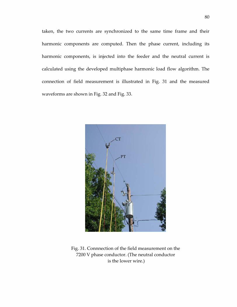
80
taken, the two currents are synchronized to the same time frame and their
harmonic components are computed. Then the phase current, including its
harmonic components, is injected into the feeder and the neutral current is
calculated using the developed multiphase harmonic load flow algorithm. The
connection of field measurement is illustrated in Fig. 31 and the measured
waveforms are shown in Fig. 32 and Fig. 33.
Fig. 31. Connnection of the field measurement on the 7200 V phase conductor. (The neutral conductor
is the lower wire.)
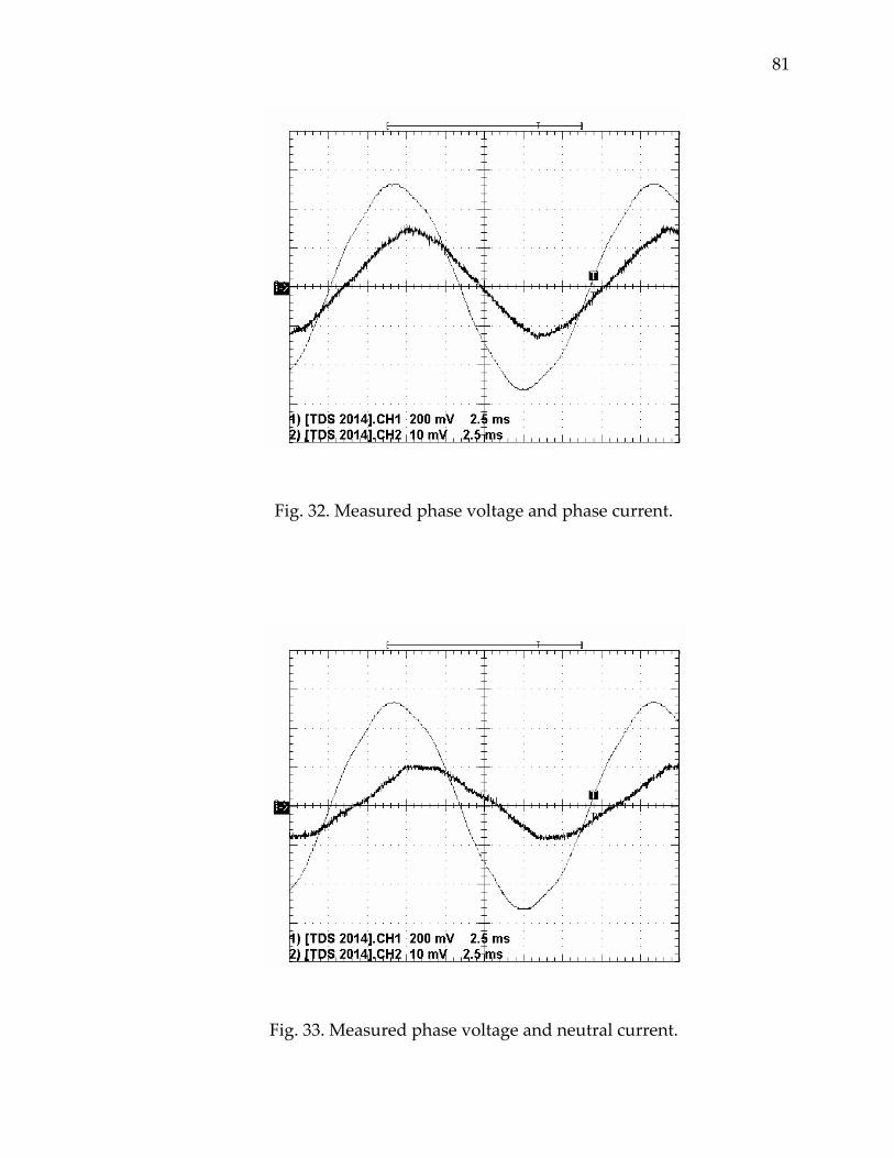
81
Fig. 32. Measured phase voltage and phase current.
Fig. 33. Measured phase voltage and neutral current.
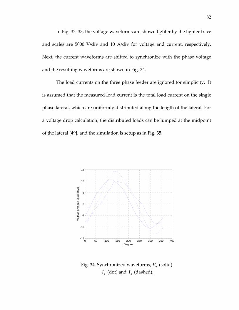
82
In Fig. 32–33, the voltage waveforms are shown lighter by the lighter trace
and scales are 5000 V/div and 10 A/div for voltage and current, respectively.
Next, the current waveforms are shifted to synchronize with the phase voltage
and the resulting waveforms are shown in Fig. 34.
The load currents on the three phase feeder are ignored for simplicity. It
is assumed that the measured load current is the total load current on the single
phase lateral, which are uniformly distributed along the length of the lateral. For
a voltage drop calculation, the distributed loads can be lumped at the midpoint
of the lateral [49], and the simulation is setup as in Fig. 35.
0 50 100 150 200 250 300 350 400-15
-10
-5
0
5
10
15
Degree
Vol
tage
(kV
) and
Cur
rent
(A)
Fig. 34. Synchronized waveforms, aV (solid) aI (dot) and nI (dashed).
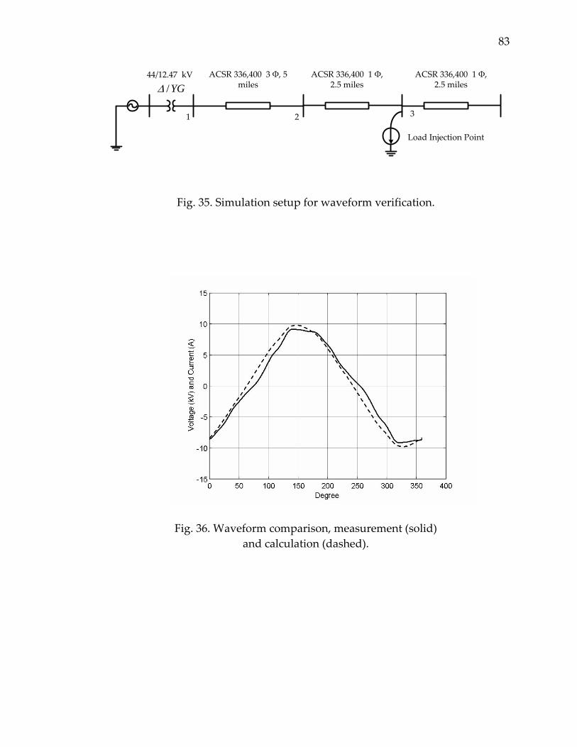
83
44/12.47 kV
YG/∆ACSR 336,400 3 Φ, 5
miles ACSR 336,400 1 Φ,
2.5 miles
1 2 3
Load Injection Point
ACSR 336,400 1 Φ, 2.5 miles
Fig. 35. Simulation setup for waveform verification.
Fig. 36. Waveform comparison, measurement (solid) and calculation (dashed).

84
The feeder is assumed to be grounded four times per mile using single
ground rod of 10 foot length with a diameter of 5/8 inches. The earth resistivity of
is assumed to be 100 m⋅Ω . The corresponding grounding resistance at each
grounding point is thus 25 Ω according to Table 2. The neutral current spectrum
is calculated with all the harmonic components. Then the waveform is generated
using the calculated results and the comparison with the measured waveform is
shown in Fig. 36. For the limited system information, the algorithm calculation is
very accurate and matches the measurement closely.
With satisfactory results on reliability and accuracy tests, it is possible to
apply the developed multiphase harmonic load flow algorithm in identifying the
origin of NEV elevation in actual distribution systems. The system configuration
data and load information are available to accurately model the distribution
feeders. The NEV profiles can be computed for various operation conditions.
After the power engineers take the field measurement, the discrepancy from the
load flow calculation may indicate the possible location of the bad neutral
connection or corroded splice on the feeder.

85
III. Evaluation Of Three‐Phasing Method In The Presence Of Harmonic Distortion
The three‐phasing method is commonly applied by electric utilities to
upgrade their distribution feeders to meet the demand growth. The original
single phase lateral is complemented by two other phase conductors running
parallel with it. Ideally, the loads are distributed among the three phases as
balanced as possible. The benefits of three‐phasing a single phase lateral include
reliability improvement, operational flexibility, lower line loss, voltage drop
decrease, etc. Among these benefits, the cancellation in return currents is directly
related to NEV mitigation. At the fundamental frequency (e.g. 60 Hz), the three
phase currents can cancel each other at the neutral point if they are balanced or
close to balanced. Consequently, almost no current needs to return the source
and the associated NEV is largely reduced.
However, the situation is different if nonlinear loads, especially single
phase electronic devices, are connected on the feeder. Most of these devices use
uncontrolled capacitor filtering rectifiers as their front‐end circuit. It is shown in
previous analysis that single phase rectifiers input currents are rich in triplen
harmonics and these triplen harmonic components are additive in neutral
conductors. Thus the three‐phasing method as an option for NEV alleviation
needs to evaluated in the present of harmonic distortion.
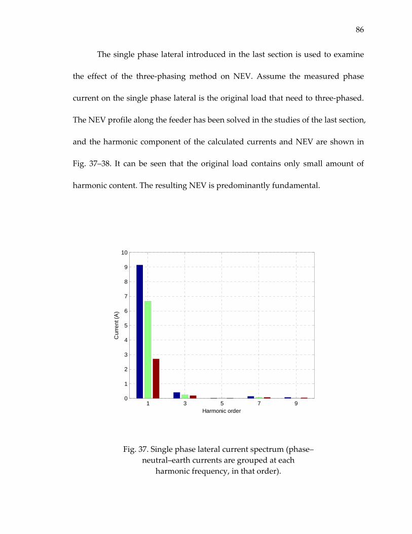
86
The single phase lateral introduced in the last section is used to examine
the effect of the three‐phasing method on NEV. Assume the measured phase
current on the single phase lateral is the original load that need to three‐phased.
The NEV profile along the feeder has been solved in the studies of the last section,
and the harmonic component of the calculated currents and NEV are shown in
Fig. 37–38. It can be seen that the original load contains only small amount of
harmonic content. The resulting NEV is predominantly fundamental.
1 3 5 7 90
1
2
3
4
5
6
7
8
9
10
Harmonic order
Cur
rent
(A)
Fig. 37. Single phase lateral current spectrum (phase– neutral–earth currents are grouped at each
harmonic frequency, in that order).
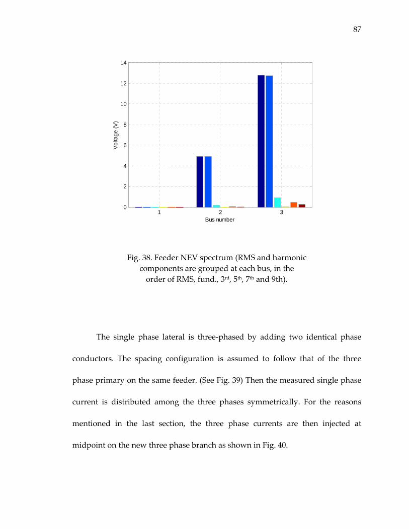
87
1 2 30
2
4
6
8
10
12
14
Bus number
Vol
tage
(V)
Fig. 38. Feeder NEV spectrum (RMS and harmonic components are grouped at each bus, in the order of RMS, fund., 3rd, 5th, 7th and 9th).
The single phase lateral is three‐phased by adding two identical phase
conductors. The spacing configuration is assumed to follow that of the three
phase primary on the same feeder. (See Fig. 39) Then the measured single phase
current is distributed among the three phases symmetrically. For the reasons
mentioned in the last section, the three phase currents are then injected at
midpoint on the new three phase branch as shown in Fig. 40.
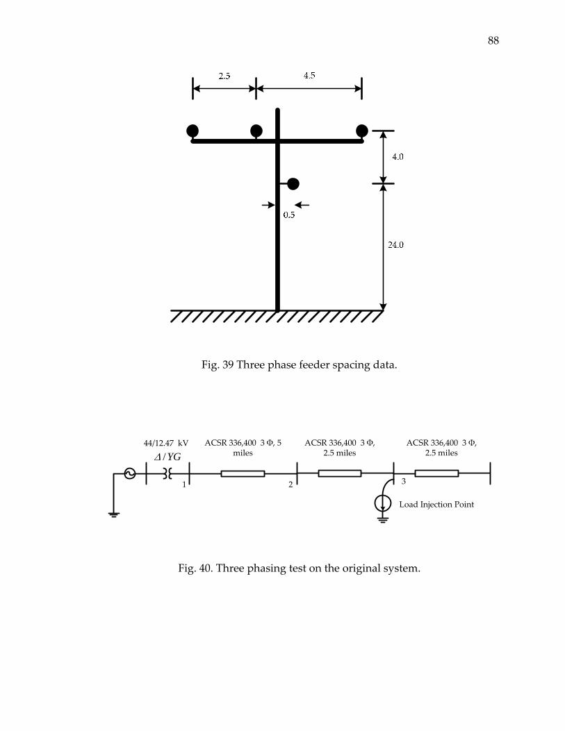
88
Fig. 39 Three phase feeder spacing data.
44/12.47 kV
YG/∆ACSR 336,400 3 Φ, 5
miles ACSR 336,400 3 Φ,
2.5 miles
1 2 3
Load Injection Point
ACSR 336,400 3 Φ, 2.5 miles
Fig. 40. Three phasing test on the original system.
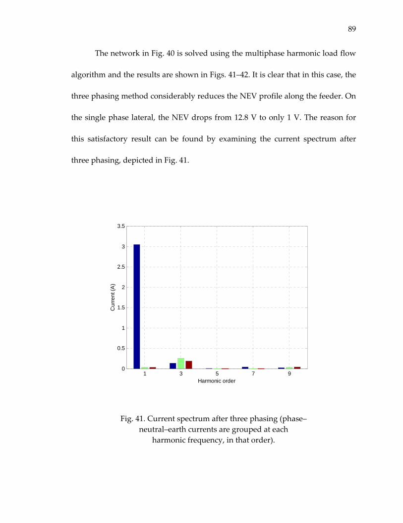
89
The network in Fig. 40 is solved using the multiphase harmonic load flow
algorithm and the results are shown in Figs. 41–42. It is clear that in this case, the
three phasing method considerably reduces the NEV profile along the feeder. On
the single phase lateral, the NEV drops from 12.8 V to only 1 V. The reason for
this satisfactory result can be found by examining the current spectrum after
three phasing, depicted in Fig. 41.
1 3 5 7 90
0.5
1
1.5
2
2.5
3
3.5
Harmonic order
Cur
rent
(A)
Fig. 41. Current spectrum after three phasing (phase– neutral–earth currents are grouped at each
harmonic frequency, in that order).
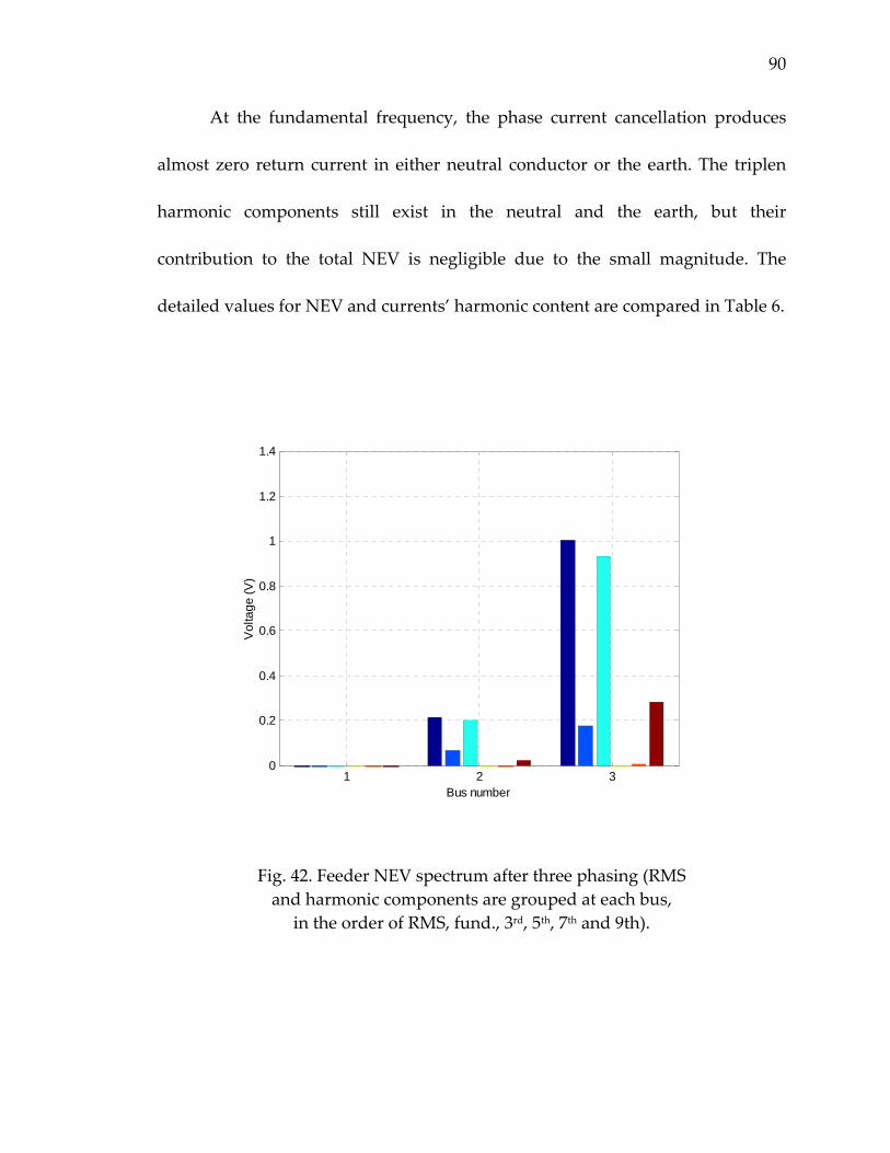
90
At the fundamental frequency, the phase current cancellation produces
almost zero return current in either neutral conductor or the earth. The triplen
harmonic components still exist in the neutral and the earth, but their
contribution to the total NEV is negligible due to the small magnitude. The
detailed values for NEV and currents’ harmonic content are compared in Table 6.
1 2 30
0.2
0.4
0.6
0.8
1
1.2
1.4
Bus number
Vol
tage
(V)
Fig. 42. Feeder NEV spectrum after three phasing (RMS and harmonic components are grouped at each bus,
in the order of RMS, fund., 3rd, 5th, 7th and 9th).
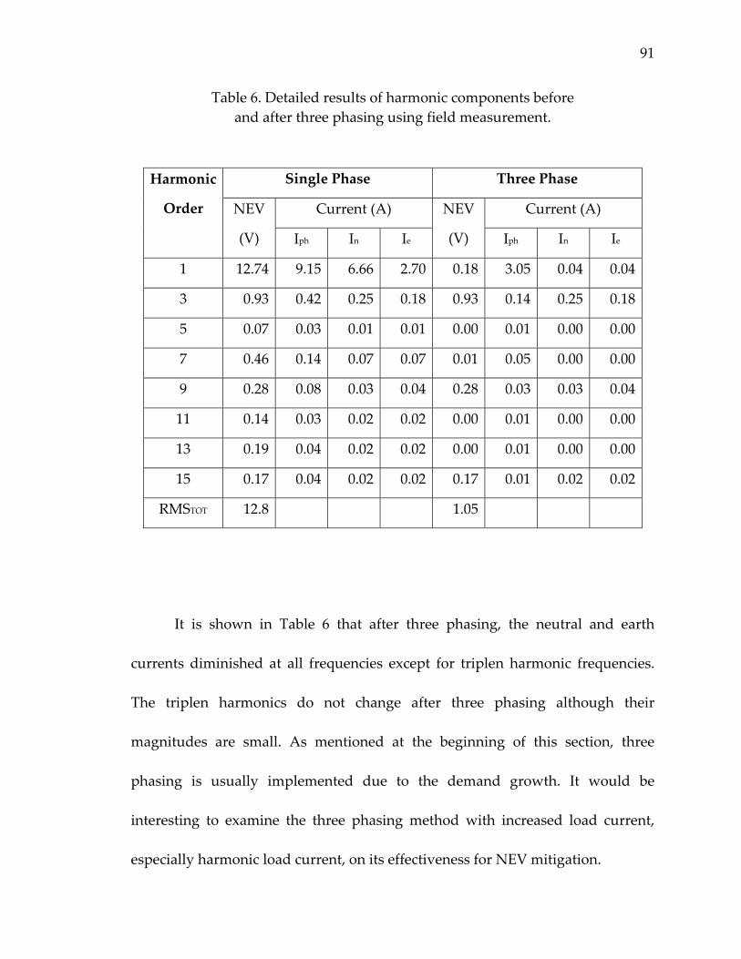
91
Table 6. Detailed results of harmonic components before and after three phasing using field measurement.
Single Phase Three Phase
Current (A) Current (A)
Harmonic
Order
NEV
(V) Iph In Ie
NEV
(V) Iph In Ie
1 12.74 9.15 6.66 2.70 0.18 3.05 0.04 0.04
3 0.93 0.42 0.25 0.18 0.93 0.14 0.25 0.18
5 0.07 0.03 0.01 0.01 0.00 0.01 0.00 0.00
7 0.46 0.14 0.07 0.07 0.01 0.05 0.00 0.00
9 0.28 0.08 0.03 0.04 0.28 0.03 0.03 0.04
11 0.14 0.03 0.02 0.02 0.00 0.01 0.00 0.00
13 0.19 0.04 0.02 0.02 0.00 0.01 0.00 0.00
15 0.17 0.04 0.02 0.02 0.17 0.01 0.02 0.02
RMSTOT 12.8 1.05
It is shown in Table 6 that after three phasing, the neutral and earth
currents diminished at all frequencies except for triplen harmonic frequencies.
The triplen harmonics do not change after three phasing although their
magnitudes are small. As mentioned at the beginning of this section, three
phasing is usually implemented due to the demand growth. It would be
interesting to examine the three phasing method with increased load current,
especially harmonic load current, on its effectiveness for NEV mitigation.
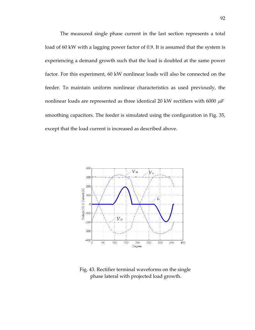
92
The measured single phase current in the last section represents a total
load of 60 kW with a lagging power factor of 0.9. It is assumed that the system is
experiencing a demand growth such that the load is doubled at the same power
factor. For this experiment, 60 kW nonlinear loads will also be connected on the
feeder. To maintain uniform nonlinear characteristics as used previously, the
nonlinear loads are represented as three identical 20 kW rectifiers with 6000 Fµ
smoothing capacitors. The feeder is simulated using the configuration in Fig. 35,
except that the load current is increased as described above.
Fig. 43. Rectifier terminal waveforms on the single phase lateral with projected load growth.
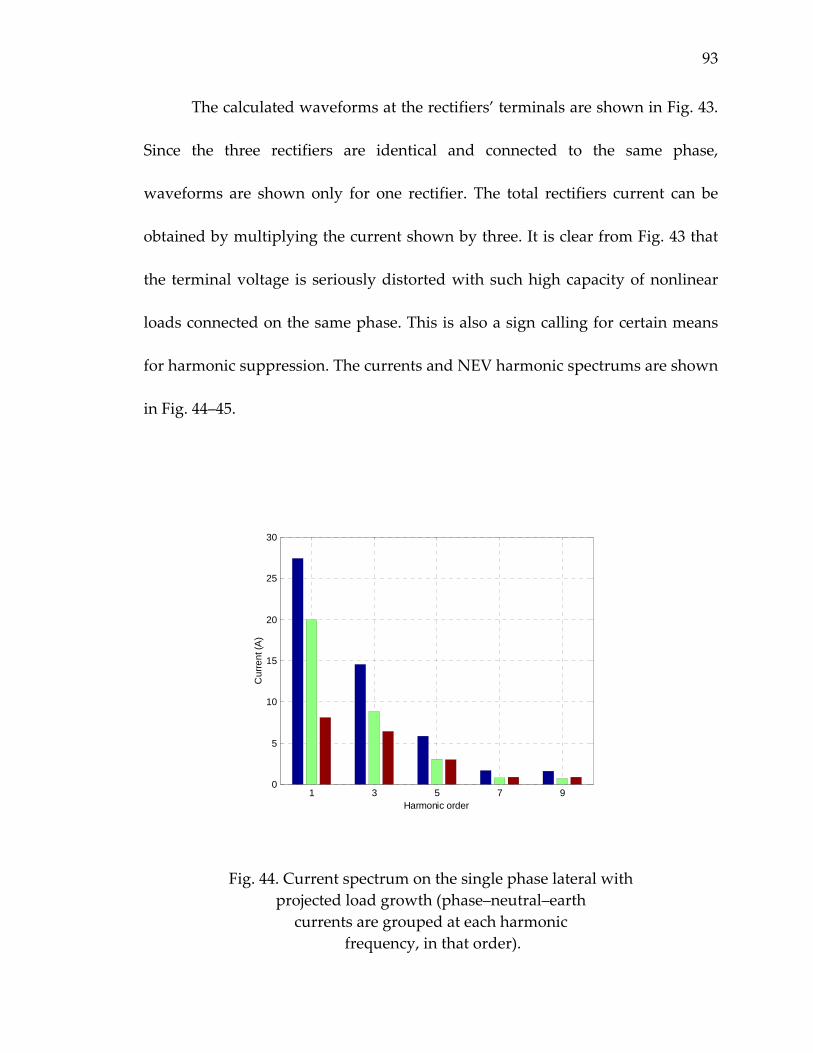
93
The calculated waveforms at the rectifiers’ terminals are shown in Fig. 43.
Since the three rectifiers are identical and connected to the same phase,
waveforms are shown only for one rectifier. The total rectifiers current can be
obtained by multiplying the current shown by three. It is clear from Fig. 43 that
the terminal voltage is seriously distorted with such high capacity of nonlinear
loads connected on the same phase. This is also a sign calling for certain means
for harmonic suppression. The currents and NEV harmonic spectrums are shown
in Fig. 44–45.
1 3 5 7 90
5
10
15
20
25
30
Harmonic order
Cur
rent
(A)
Fig. 44. Current spectrum on the single phase lateral with projected load growth (phase–neutral–earth
currents are grouped at each harmonic frequency, in that order).
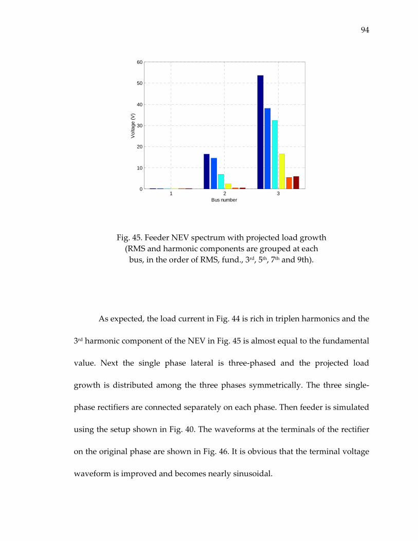
94
1 2 30
10
20
30
40
50
60
Bus number
Vol
tage
(V)
Fig. 45. Feeder NEV spectrum with projected load growth (RMS and harmonic components are grouped at each bus, in the order of RMS, fund., 3rd, 5th, 7th and 9th).
As expected, the load current in Fig. 44 is rich in triplen harmonics and the
3rd harmonic component of the NEV in Fig. 45 is almost equal to the fundamental
value. Next the single phase lateral is three‐phased and the projected load
growth is distributed among the three phases symmetrically. The three single‐
phase rectifiers are connected separately on each phase. Then feeder is simulated
using the setup shown in Fig. 40. The waveforms at the terminals of the rectifier
on the original phase are shown in Fig. 46. It is obvious that the terminal voltage
waveform is improved and becomes nearly sinusoidal.
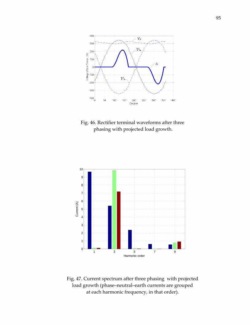
95
Fig. 46. Rectifier terminal waveforms after three phasing with projected load growth.
1 3 5 7 90
1
2
3
4
5
6
7
8
9
10
Harmonic order
Cur
rent
(A)
Fig. 47. Current spectrum after three phasing with projected load growth (phase–neutral–earth currents are grouped
at each harmonic frequency, in that order).
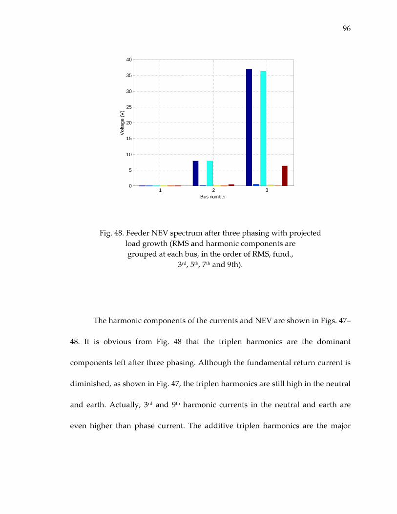
96
1 2 30
5
10
15
20
25
30
35
40
Bus number
Vol
tage
(V)
Fig. 48. Feeder NEV spectrum after three phasing with projected load growth (RMS and harmonic components are grouped at each bus, in the order of RMS, fund.,
3rd, 5th, 7th and 9th).
The harmonic components of the currents and NEV are shown in Figs. 47–
48. It is obvious from Fig. 48 that the triplen harmonics are the dominant
components left after three phasing. Although the fundamental return current is
diminished, as shown in Fig. 47, the triplen harmonics are still high in the neutral
and earth. Actually, 3rd and 9th harmonic currents in the neutral and earth are
even higher than phase current. The additive triplen harmonics are the major

97
factors that cause the NEV to only drop from 57 V to 37 V. The detailed values
for NEV and currents’ harmonic components are compared in Table 7.
This section has demonstrated that three‐phasing a feeder works well to
mitigate NEV in systems only containing mostly linear loads. Its effectiveness is
degraded in the presence of significant concentration of nonlinear loads in
distribution systems. As shown in test results, the voltage harmonic distortion
itself shows that harmonic suppression would be desirable. However, it is not
clear how filtering for triplen harmonics might impact the NEV. From the
perspective of NEV alleviation, diverting the phase harmonics into neutral
conductor is clearly not the correct means of filtering.
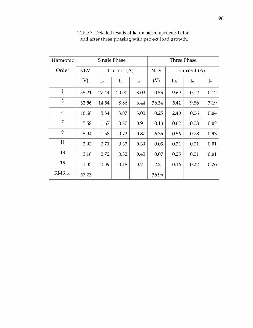
98
Table 7. Detailed results of harmonic components before and after three phasing with project load growth.
Single Phase Three Phase
Current (A) Current (A)
Harmonic
Order
NEV
(V) Iph In Ie
NEV
(V) Iph In Ie
1 38.21 27.44 20.00 8.09 0.55 9.69 0.12 0.12
3 32.56 14.54 8.86 6.44 36.34 5.42 9.86 7.19
5 16.68 5.84 3.07 3.00 0.25 2.40 0.06 0.04
7 5.58 1.67 0.80 0.91 0.13 0.62 0.03 0.02
9 5.94 1.58 0.72 0.87 6.35 0.56 0.78 0.93
11 2.93 0.71 0.32 0.39 0.05 0.31 0.01 0.01
13 3.18 0.72 0.32 0.40 0.07 0.25 0.01 0.01
15 1.83 0.39 0.18 0.21 2.24 0.16 0.22 0.26
RMSTOT 57.23 36.96
CHAPTER VIII
CONCLUSIONS AND FUTURE WORK
I. Conclusions
Neutral‐to‐earth voltage is caused, in part, because of the practice of
grounding the neutral of power system distribution feeders at multiple points
along their length for safety, fault clearing, and compliance with the codes. To
estimate problems associated with elevated NEV, especially in the presence of
harmonic distortion, several steps must be taken.
In this dissertation, multigrounded transmission lines are examined and a
model dedicated for NEV analysis is derived based on Carson’s line theory. The
neutral conductor is represented explicitly by considering the current
distribution between neutral and earth paths. A multiphase harmonic load flow
algorithm is developed to compute the NEV profile in radial distribution systems.
Since it is a branch‐oriented load flow technique, most of the distribution system
components can be included by adjusting the model’s voltage to the potential
from phase‐to‐local earth. The NEV profile throughout the system is available
directly from the solution. Harmonic interaction between nonlinear devices and

100
distribution systems parameters is included by incorporating the nonlinear
modeling into the multiphase load flow. A common single‐phase uncontrolled
rectifier is used to demonstrate the harmonic analysis.
The algorithm and the accompanying linear and nonlinear modeling
techniques are tested on an IEEE example system as well as an actual distribution
feeder model. Their reliability and accuracy are verified by satisfactory test
results. Three phasing of feeders, one of the conventional means for distribution
system upgrade, is evaluated using the developed algorithm from the
perspective of NEV elevation.
It is observed from the test results that the harmonic injections from
nonlinear devices, especially the single‐phase power electronic loads, can
considerably increase the NEV of the system. The location of nonlinear devices in
distribution systems is also an important factor on elevated NEV. The highest
elevation due to harmonic distortion is found on the bus where the nonlinear
loads are connected. However, this elevation can affect the downstream buses as
well as the buses on the path from the nonlinear load to source. The closer a bus
is to the source, the lower the effect of nonlinear loads on NEV elevation,
assuming the source has a nearly ideal grounding connection. The buses on other
laterals are less related to the harmonic injection, except for the already
connected linear loads.

101
The close match between field measurement and the load flow calculation
suggests that the developed algorithm can be applied to identify the origin of
NEV elevation in an actual distribution system. The evaluation of the three‐
phasing method shows that the method is not capable of reducing NEV profile
on a distribution feeder with large amount of single phase nonlinear loads,
although it works perfectly for a system with predominantly linear loads.
II. Future Work
Only one power electronic device, the uncontrolled capacitor filtered
rectifier, is modeled in this document. However, the technique is not limited to
the single‐phase rectifier; various power electronic devices can be represented
according to their nonlinear characteristics. Other non‐linear devices, such as the
saturated magnetic seen in single‐phase induction motors and lighting ballasts,
can be utilized with the load flow if modeled adequately.
Both linear and nonlinear loads are aggregated at the bus of interest in the
harmonic load flow formulation. A recent trend in harmonic analysis is to study
the distributed nonlinear loads throughout the system to account for the
harmonic attenuation and diversity [50]. The simple structure of the load flow
algorithm makes it feasible to improve the nonlinear load representation by
distributing it for better accuracy.

102
Future enhancements of this model would be to incorporate the influence
of the parallel utilities bonded to distribution system neutral, such as water pipes,
gas pipes, and telecommunication wires, to analyze this often‐encountered
complex situation. Additionally, the geometry of the feeder (i.e. not constructed
in straight line) and the use of non‐overhead conductors (such as semiconductor
jacketed underground cable) needs to be analyzed to produce a complete set of
tools for engineers to use.
Stray voltage, or elevated NEV, is a serious problem for many electric
utilities. This dissertation should provide a good first step in understanding the
problems, the impact of nonlinear loads, and possible mitigation strategies.

APPENDICES
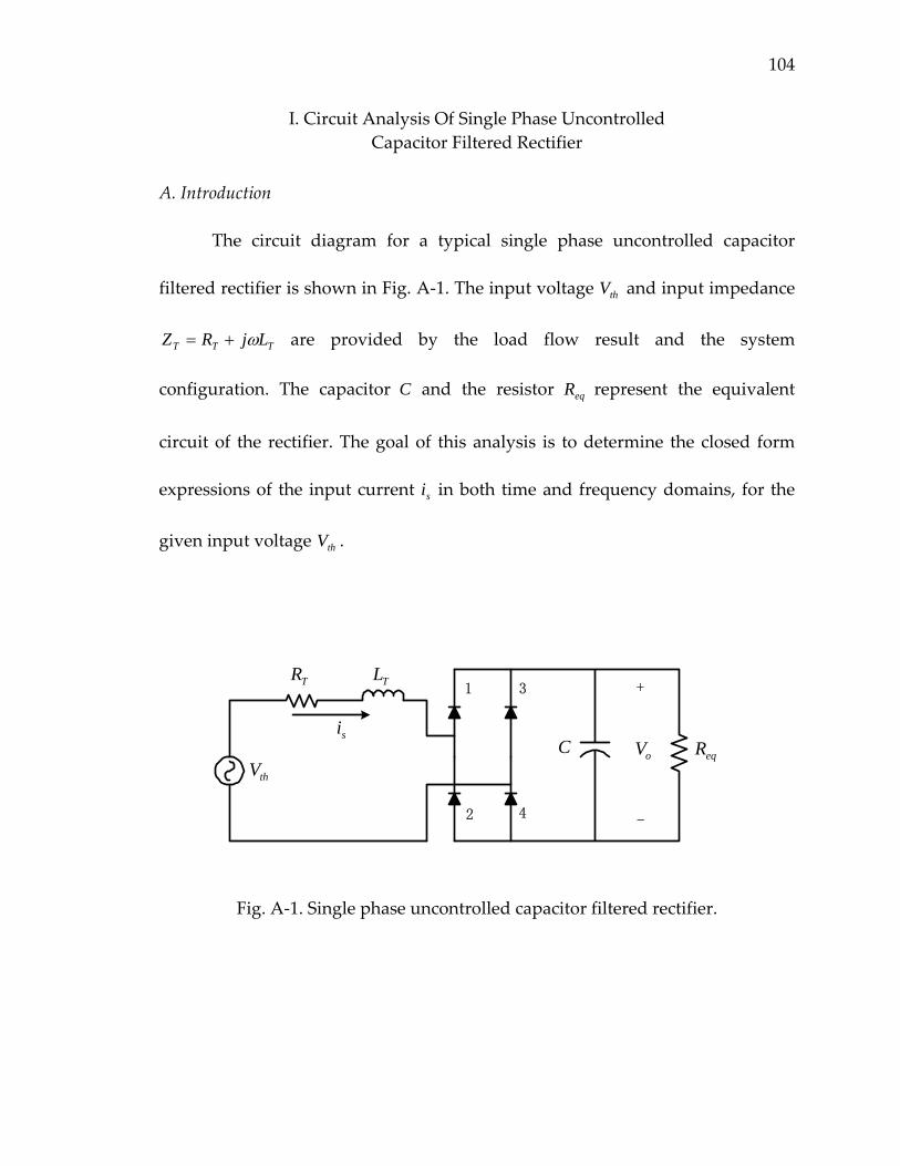
104
I. Circuit Analysis Of Single Phase Uncontrolled Capacitor Filtered Rectifier
A. Introduction
The circuit diagram for a typical single phase uncontrolled capacitor
filtered rectifier is shown in Fig. A‐1. The input voltage thV and input impedance
TTT LjRZ ω+= are provided by the load flow result and the system
configuration. The capacitor C and the resistor eqR represent the equivalent
circuit of the rectifier. The goal of this analysis is to determine the closed form
expressions of the input current si in both time and frequency domains, for the
given input voltage thV .
thV
TR TL
C eqRoVsi
+
-
1 3
2 4
Fig. A‐1. Single phase uncontrolled capacitor filtered rectifier.
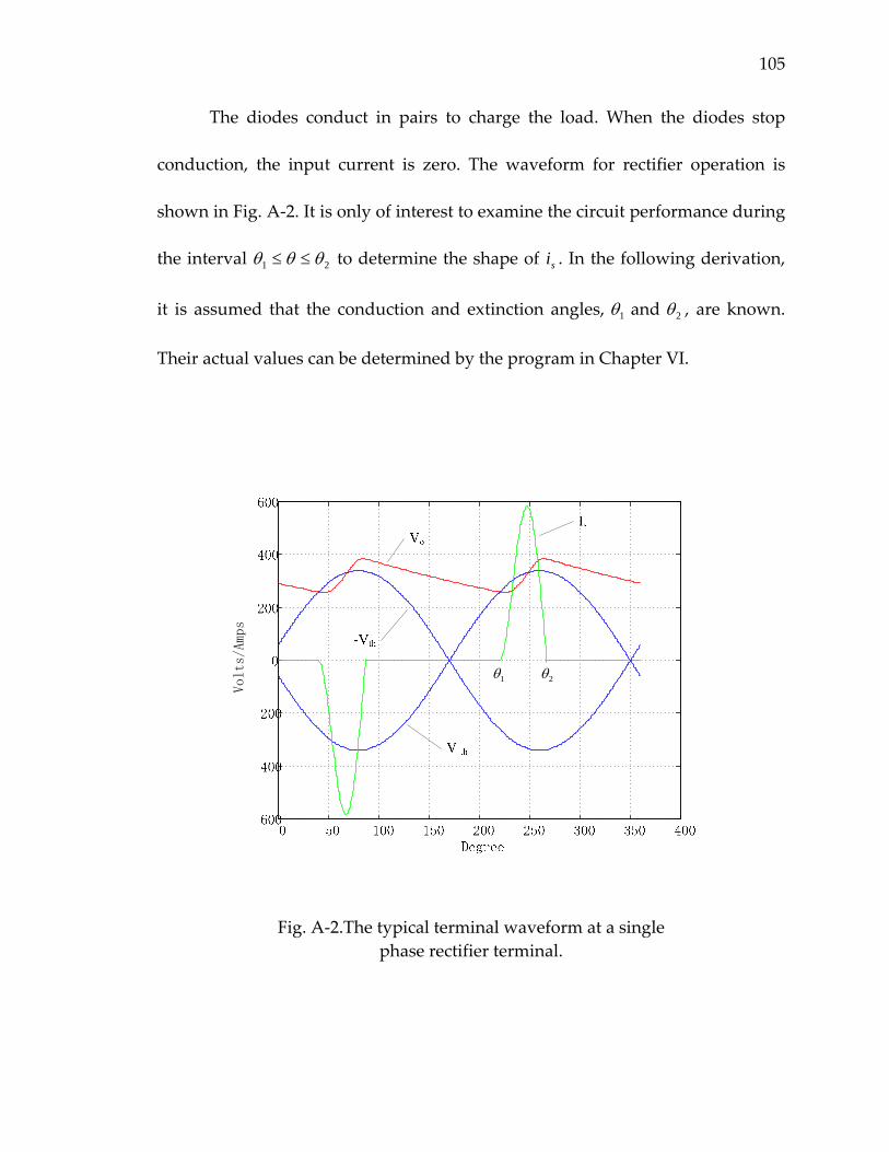
105
The diodes conduct in pairs to charge the load. When the diodes stop
conduction, the input current is zero. The waveform for rectifier operation is
shown in Fig. A‐2. It is only of interest to examine the circuit performance during
the interval 21 θθθ ≤≤ to determine the shape of si . In the following derivation,
it is assumed that the conduction and extinction angles, 1θ and 2θ , are known.
Their actual values can be determined by the program in Chapter VI.
Volts/Amps
1θ 2θ
Fig. A‐2.The typical terminal waveform at a single phase rectifier terminal.
106
For accurate modeling of rectifier response to harmonic distortion, the
input voltage thV is not restricted to fundamental sinusoidal. The general
expression for thV is given as ( )∑ +=h
hhth hVV φθsin2 . The subscript h
represents the harmonic order of interest. The highest harmonic frequency in a
typical harmonic analysis could reach up to the 25th harmonic.
To simplify the analysis, the axis can be shifted by 1θ where the input
current just starts flowing in the positive direction. The expression for thV is
rewritten as follows
( ) ( )∑∑ +=++=h
hhh
hhth hVhhVV δθθφθ sin2sin2 1 (A‐1)
At 1θ , the circuit can be described by the following equations
os
TsTth VddiLiRV ++=θ
ω (A‐2)
eq
oos R
VddVCi +=θ
ω (A‐3)
Solving (A‐2) (A‐3) simultaneously for oV , the differential equation for oV
is obtained as
107
thoeq
To
eq
TT
oT VV
RR
ddV
RLCR
dVdCL =⎟
⎟⎠
⎞⎜⎜⎝
⎛++⎟
⎟⎠
⎞⎜⎜⎝
⎛++ 12
22
θωω
θω (A‐4)
Let eqTT
T
CRCLLR
ωα
ωα
ωα
ωα 1 ,1 ,1 , 4321 ==== , then (4) becomes
( ) ( ) thooo VV
ddV
dVd
323241412
2
ααααααθ
ααθ
=++++ (A‐5)
Similarly, the equation for si can be obtained as flows
θω
θωω
θω
ddVC
RVi
RR
ddi
RLCR
didCL th
eq
ths
eq
Ts
eq
TT
sT +=⎟
⎟⎠
⎞⎜⎜⎝
⎛++⎟
⎟⎠
⎞⎜⎜⎝
⎛++ 12
22 (A‐6)
( ) ( )θ
αααααααθ
ααθ d
dVViddi
did th
thsss
2423241412
2
+=++++ (A‐7)
The differential equations (A‐5) (A‐7) for oV and si have the same
characteristic equation, which is what we expect. The only difference is the
driving force on the right side of the equations. The characteristic roots are
solved as follows
( )32
24141
2,1 42αααααα
−−
±+
−=±= bas (A‐8)
108
B. The particular solution of oV and si
The particular solutions of oV and si can be determined using the
undetermined coefficients method. Since the forcing functions on the right of (A‐
5) (A‐7) are summation of sinusoidal functions, the particular solutions should
take similar form. The particular solution of oV and its first and second
derivatives are written as follows
∑ +=h
hho hNhMV θθ sincos (A‐9)
∑ +−=h
hho hhNhhMV θθ cossin' (A‐10)
∑ −−=h
hho hhNhhMV θθ sincos 22'' (A‐11)
Substituting (A‐9), (A‐10) and (A‐11) in (A‐5), we have
( ) ( ) (
) ( ) ( )
( )hhhh
h
hh
hh
hh
hhh
hhV
hNhMhhN
hhMhhNhhM
δθδθαα
θθααααθ
θααθθ
sincoscossin2
sincoscos
sinsincos
32
3241
4122
+=
++++
−++−−
∑
∑
∑∑
(A‐12)
Collect similar terms for θhsin and θhcos , and compare both sides of (A‐
12) at each harmonic, we have

109
( )( ) ( ) hhhhh VNhMhN δαααααααα cos2 323241412 =++−++− (A‐13)
( )( ) ( ) hhhhh VMhNhM δαααααααα sin2 323241412 =++++− (A‐14)
Put (A‐13) and (A‐14) in a matrix form
( ) ( )( ) ( ) ⎥
⎦
⎤⎢⎣
⎡=⎥
⎦
⎤⎢⎣
⎡⎥⎦
⎤⎢⎣
⎡
+++−++−+−
h
hh
h
h VNM
hhhh
δδ
αααααααα
ααααααsincos
2 32413241
23241
241 (A‐15)
The determinant of the square matrix on the left is calculated as
( ) ( )[ ]2 3241
2241
2 αααααα ++−−+−=∆ hh (A‐16)
Let ( )4
241
32αααα −
−=B , ( )2222214
1Bahha
c h−−+
= , then hc1
1−=∆ . The
coefficients hM and hN can be calculated by inversing the coefficient matrix in
(A‐15)
( ) ( ) ( )( ) ( ) ⎥
⎦
⎤⎢⎣
⎡⎥⎦
⎤⎢⎣
⎡
+−+−+−+
−=⎥⎦
⎤⎢⎣
⎡
h
hh
h
h
hhhh
cVNM
δδ
αααααααααααα
ααsincos
2413241
23241
241
132 (A‐17)
Therefore
( )[ ][ ] hhhhhhh cVahBahcVM 5222
132 2cos2sin2 αδδαα −=−−−−= (A‐18)
110
( )[ ][ ] hh
hhhh
h ch
VhhBaahch
VN 72222
132 2cossin22 αδδαα =−++−= (A‐19)
where
( ) hhhh ahBahcc δδα cos2sin22135 −−−=
( ) hhhh hhBaahcc δδα cossin2 222137 −++−=
Thus the particular solution of oV becomes
∑ ⎟⎠⎞
⎜⎝⎛ +−=
h
hhho h
hchcVV θαθα sincos2 7
252 (A‐20)
Similar to oV , the particular solution of si is assumed to be as follows
∑ +=h
hhs hNhMi θθ sincos (A‐21)
Then its first and second order derivatives are calculated as
∑ +−=h
hhs hhNhhMi θθ cossin' (A‐22)
∑ −−=h
hhs hhNhhMi θθ sincos 22'' (A‐23)
Substituting (A‐21), (A‐22) and (A‐23) in (A‐7), we have
111
( ) ( ) (
) ( ) ( )
( ) ( )( )∑
∑
∑∑
++−=
++++
−++−−
hhhhhh
hh
hh
hh
hhh
hhhhV
hNhMhhN
hhMhhNhhM
δδαθδδαθα
θθααααθ
θααθθ
cossincossincossin2
sincoscos
sinsincos
442
3241
4122
(A‐24)
or in a matrix form
( ) ( )( ) ( )
⎥⎦
⎤⎢⎣
⎡+−
=
⎥⎦
⎤⎢⎣
⎡⎥⎦
⎤⎢⎣
⎡
+++−++−+−
hh
hhh
h
h
hh
V
NM
hhhh
δδαδδα
α
αααααααααααα
cossinsincos
24
42
4132412
32412
41
(A‐25)
Note that the matrix on the left in (A‐25) is the same as that in (A‐15).
Solve (A‐25) for hM and hN
( ) ( )[
( )( )]( )( )[[
( )]]hh
h
hhh
hh
hhhhh
cV
ahBah
hBaahcV
hBah
hahcVM
22
422
4222
12
422
412
2
2cos
2sin2
cossin
sincos22
α
αδ
αδα
δδα
δδαα
=
+−++
−++−=
+−−+
−−−=
(A‐26)
( ) ( )( )[( )]
( )( )[[( )( )]]
hcV
ahhBah
hBahach
Vhah
hBahcVN
hh
h
hhh
hh
hhhhh
42
24
22
222412
4
422
12
2
2cos
2sin2
cossin2 sincos2
α
αδ
αδα
δδαδδαα
=
−−++
−−+−=
++−−−−=
(A‐27)
112
where
( )[ ] ( ) 42222
42
12 2cos2sin αδαδ ahBahhBaahcc hhhh +−++−++−=
( ) ( ) 24
22222414 2cos2sin ahhBahhBahacc hhhh −−++−−+−= αδαδ
Thus the particular solution for si becomes
∑ ⎟⎠⎞
⎜⎝⎛ +=
h
hhhs h
hchcVi θαθα sincos2 4
222 (A‐28)
C. Complete solutions of oV and si
After the particular solutions of oV and si are determined, the next step is
to find the general solutions for the output voltage and the input current. The
characteristic roots in (A‐8) can be either real or complex depending on the
circuit parameters. Assume that the roots are real, then (A‐8) is repeated as
follows
( ) bas ±=−−
±+
−= 32
24141
2,1 42αααααα (A‐29)
Including the particular solution (A‐20), the complete solution of oV
becomes
113
∑ ⎟⎠⎞
⎜⎝⎛ +−++=
h
hhh
sso h
hchcVeAeAV θαθαθθ sincos2 7
2522121 (A‐30)
The parameters 1A and 2A in (A‐30) can be determined using the initial
conditions of the circuit. At 0=θ , the rectifier starts conduction and the input
voltage equals the output voltage, i.e.,
( ) ( )00 tho VV = (A‐31)
Substitute (A‐1) and (A‐30) in (A‐31) for 0=θ
( )∑∑ −++===h
hhh
hhtho cVAAVVV 5221 2sin2)0( αδ (A‐32)
Therefore
( )∑ +=+h
hhh cVAA 5221 sin2 αδ (A‐33)
By examining the circuit, we have
⎟⎟⎠
⎞⎜⎜⎝
⎛−==
eq
os
co R
ViCC
iVωω1' (A‐34)
At 0=θ , the input current has to be zero, i.e.,
114
( ) 00 =si (A‐35)
Take derivative of (A‐32) and evaluate at 0=θ ,
( ) ∑++=h
hho cVAsAsV 722211' 20 α (A‐36)
Substituting (A‐32), (A‐35) and (A‐36) in (A‐34), we
( ) ( )
∑
∑
++=
−=−=
hhh
hhh
eq
oo
cVAsAs
VCR
VV
722211
4'
2
sin200
α
δαω (A‐37)
therefore
( )∑ +−=+h
hhh cVAsAs 7242211 sin2 αδα (A‐38)
Solve (A‐33) and (A‐38) for 1A and 2A simultaneously. Then for each
harmonic, we have
( ) ( )[ ]hhhh
h ccssb
VA 6512111 sin2
2 +++= αδα
( ) ( )[ ]hhhh
h ccssb
VA 6522122 sin2
2 +−+−= αδα
where
115
( ) ( )[ ]hhhh hhBaBaacc δδα cos3sin2 222136 +−++=
Hence the output voltage is determined for real characteristic roots and its
complete solution is as follows
( ) ( ) ( )[
( ) ] ∑
∑
⎟⎠⎞
⎜⎝⎛ +−+++
+−+++=
h
hhh
shh
hs
hhhh
ho
hh
chcVeccs
seccssb
VV
θαθαα
δααδα
θ
θ
sincos2
sinsin2
2
72526522
12651211
2
1
(A‐39)
Similarly, si is solved for real characteristic roots as follows
[ ]
∑
∑
⎟⎠⎞
⎜⎝⎛ ++
−+++−−=
h
hhh
shhh
shhh
h
hs
hh
chcV
eccseccsb
Vi
θθα
δδα θθ
sincos2
sinsin2
2
422
322321221
(A‐40)
where
( )( )( ) ( )( ) h
hhh
BaahBah
ahBaBacc
δα
δα
cos23
sin2
2224
4222
13
+++−+
+−++=
If ( )32
241
4αααα
<− , the characteristic roots of both (A‐5) and (A‐7) are
complex, and the general solution of oV are as follows
( ) ∑ ⎟⎠⎞
⎜⎝⎛ +−++=
h
hhh
ao h
hchcVbAbAeV θαθαθθθ sincos2sincos 7
25221 (A‐41)
116
( ) ∑ ⎟⎠⎞
⎜⎝⎛ +++=
h
hhh
as h
hchcVbAbAei θθαθθθ sincos2 sincos 4
22'2
'1 (A‐42)
where
241 αα +
−=a , ( )4
241
32αααα −
−=b
Solve oV first. When 0=θ , (A‐41) becomes
( )∑
∑−+=
==
hhh
hhhtho
cVA
VVV
521 2
sin2)0(
α
δ
Therefore
( )∑ +=h
hhh cVA 521 sin2 αδ (A‐43)
Similar to the solution of oV with real characteristic roots, evaluate thV in
(1) and the first derivative of oV in (A‐41) at 0=θ , substitute the results and the
initial input current, i.e., ( ) 00 =si , into (A‐34). Then we have
( ) ( )
∑
∑
++=
−=−=
hhh
hhh
eq
oo
cVbAaA
VCR
VV
7221
4'
2
sin200
α
δαω
117
Solve for 2A
( ) ( )[ ]∑ +++=h
hhhh caca
bVA 65212 sin2 αδα
The final solution for the output voltage is then
( ) ( )[ ][
[ ] ]
∑
∑
⎟⎠⎞
⎜⎝⎛ +−+
+
+++=
h
hhh
ahh
hhhh
ho
hh
chcV
ebcb
bcacab
VV
θαθα
θαδ
θαδα
θ
sincos2
cossin
sinsin2
7252
52
6521
(A‐44)
Similarly
[ ]
∑
∑
⎟⎠⎞
⎜⎝⎛ ++
−+−−=
h
hhh
ahhhh
h
hs
hh
chcV
ebbcbcacb
Vi
θθα
θθδα θ
sincos2
cossinsin2
422
2322
(A‐45)
Thus finish the solutions for the differential equations describing the
circuit during positive conduction period. The equation for si will exactly the
same during the negative conduction period except that the phase angle is
shifted by π and the sign is negative. A simple summary of all solutions and the
parameters is listed below.
118
When ( )32
241
4αααα
>− ,
[ ]
∑
∑
⎟⎠⎞
⎜⎝⎛ ++
−+++−−=
h
hhh
shhh
shhh
h
hs
hh
chcV
eccseccsb
Vi
θθα
δδα θθ
sincos2
sinsin2
2
422
322321221
(A‐46)
( ) ( ) ( )[
( ) ] ∑
∑
⎟⎠⎞
⎜⎝⎛ +−+++
+−+++=
h
hhh
shh
hs
hhhh
ho
hh
chcVeccs
seccssb
VV
θαθαα
δααδα
θ
θ
sincos2
sinsin2
2
72526522
12651211
2
1
(A‐47)
where ( ) bas ±=−−
±+
−= 32
24141
2,1 42αααααα ;
When ( )32
241
4αααα
<− ,
[ ]
∑
∑
⎟⎠⎞
⎜⎝⎛ ++
−+−−=
h
hhh
ahhhh
h
hs
hh
chcV
ebbcbcacb
Vi
θθα
θθδα θ
sincos2
cossinsin2
422
2322
(A‐48)
( ) ( )[ ][
[ ] ]
∑
∑
⎟⎠⎞
⎜⎝⎛ +−+
+
+++=
h
hhh
ahh
hhhh
ho
hh
chcV
ebcb
bcacab
VV
θαθα
θαδ
θαδα
θ
sincos2
cossin
sinsin2
7252
52
6521
(A‐49)
where 2
41 αα +−=a , ( )
4
241
32αααα −
−=b .
119
In both case, the c parameters’ definition is the same. Let
( )4
241
32αααα −
−=B , then
( )2222214
1Bahha
c h−−+
=
( )[ ] ( ) 42222
42
12 2cos2sin αδαδ ahBahhBaahcc hhhh +−++−++−=
( )( )( ) ( )( ) h
hh
hhhh
BaahBah
ahBaBac
cacc
δα
δα
δ
cos23
sin2
2sin
2224
4222
1
423
+++−+
+−++=
−+=
( ) ( ) 24
22222414 2cos2sin ahhBahhBahacc hhhh −−++−−+−= αδαδ
( ) hhhh ahBahcc δδα cos2sin22135 −−−=
( ) ( )[ ]hhh
hhh
hhBaBaac
cacc
δδα cos3sin2
2
22213
756
+−++=
−−=
( ) hhhh hhBaahcc δδα cossin2 222137 −++−=
D. Frequency domain expressions si
With the closed form expressions of the input currents in time domain
determined, it is possible to derive the Fourier series at various harmonics.
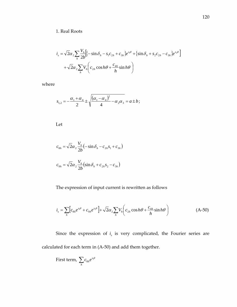
120
1. Real Roots
[ ]
∑
∑
⎟⎠⎞
⎜⎝⎛ ++
−+++−−=
h
hhh
shhh
shhh
h
hs
hh
chcV
eccseccsb
Vi
θθα
δδα θθ
sincos2
sinsin2
2
422
322321221
where
( ) bas ±=−−
±+
−= 32
24141
2,1 42αααααα ;
Let
( )hhhh
h cscb
Vc 31228 sin2
2 +−−= δα
( )hhhh
h cscb
Vc 32229 sin2
2 −+= δα
The expression of input current is rewritten as follows
[ ] ∑∑ ⎟⎠⎞
⎜⎝⎛ +++=
h
hhh
h
sh
shs h
hchcVececi θθαθθ sincos2 4
229821 (A‐50)
Since the expression of si is very complicated, the Fourier series are
calculated for each term in (A‐50) and add them together.
First term, ∑h
shec θ1
8
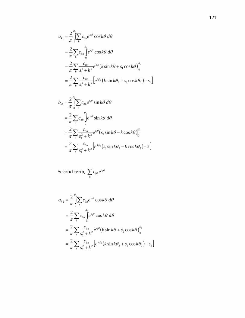
121
( )
( )[ ]∑
∑
∑ ∫
∫∑
−++
=
++
=
=
=
h
sh
s
h
h
h
sh
h
shk
skskkeks
c
kskkeks
c
dkec
dkeca
1212221
8
01221
8
08
081
cossin2
cossin2
cos2
cos2
21
21
2
1
2
1
θθπ
θθπ
θθπ
θθπ
θ
θθ
θθ
θθ
( )
( )[ ]∑
∑
∑ ∫
∫∑
+−+
=
−+
=
=
=
h
sh
s
h
h
h
sh
h
shk
kkkkseks
c
kkkseks
c
dkec
dkecb
221221
8
01221
8
08
081
cossin2
cossin2
sin2
sin2
21
21
2
1
2
1
θθπ
θθπ
θθπ
θθπ
θ
θθ
θθ
θθ
Second term, ∑h
shec θ2
9
( )
( )[ ]∑
∑
∑ ∫
∫∑
−++
=
++
=
=
=
h
sh
s
h
h
h
sh
h
shk
skskkeks
c
kskkeks
c
dkec
dkeca
2222222
9
02222
9
09
092
cossin2
cossin2
cos2
cos2
22
22
2
2
2
2
θθπ
θθπ
θθπ
θθπ
θ
θθ
θθ
θθ
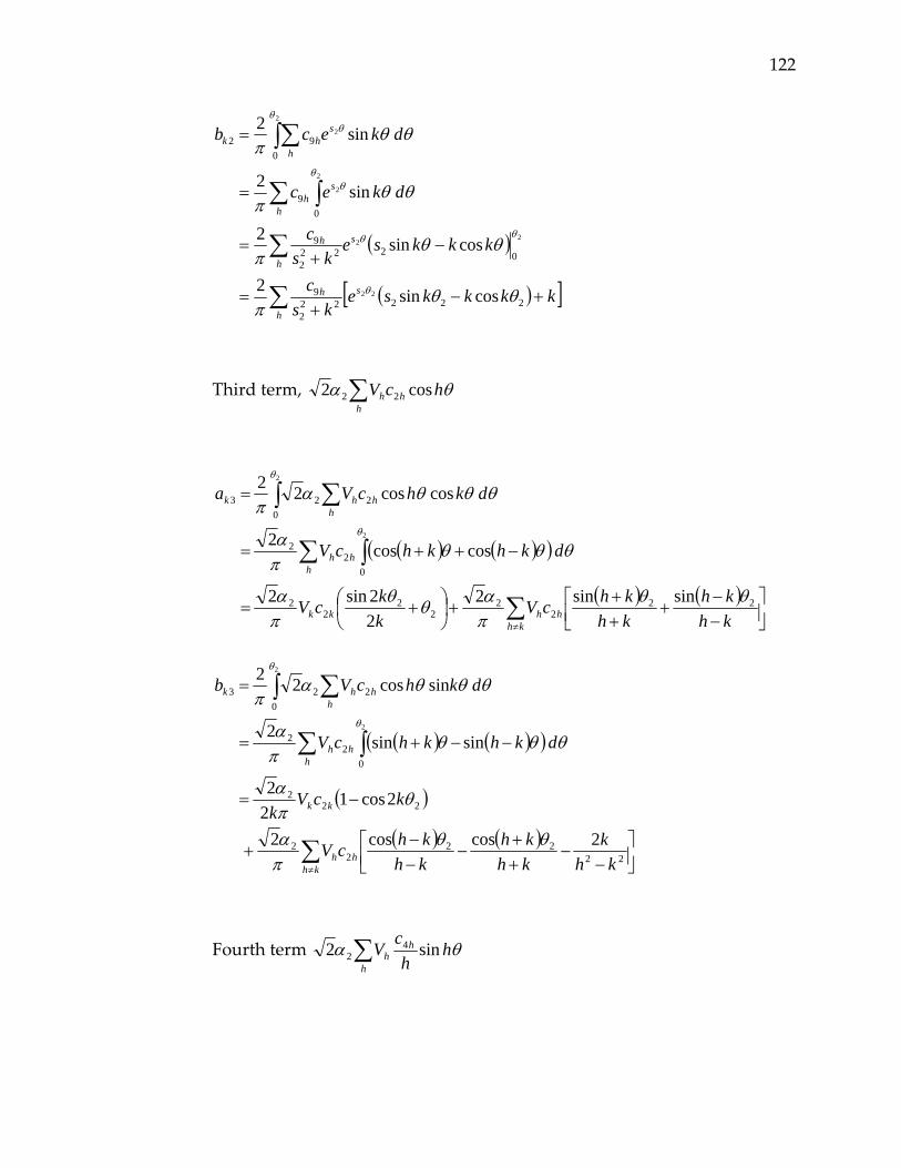
122
( )
( )[ ]∑
∑
∑ ∫
∫∑
+−+
=
−+
=
=
=
h
sh
s
h
h
h
sh
h
shk
kkkkseks
c
kkkseks
c
dkec
dkecb
222222
9
02222
9
09
092
cossin2
cossin2
sin2
sin2
22
22
2
2
2
2
θθπ
θθπ
θθπ
θθπ
θ
θθ
θθ
θθ
Third term, ∑h
hh hcV θα cos2 22
( ) ( )( )
( ) ( )∑
∑ ∫
∫ ∑
≠⎥⎦⎤
⎢⎣⎡
−−
+++
+⎟⎠⎞
⎜⎝⎛ +=
−++=
=
khhhkk
hhh
hhhk
khkh
khkhcV
kkcV
dkhkhcV
dkhcVa
222
22
22
2
02
2
0223
sinsin222sin2
coscos2
cos cos22
2
2
θθπαθθ
πα
θθθπα
θθθαπ
θ
θ
( ) ( )( )
( )
( ) ( )∑
∑ ∫
∫ ∑
≠⎥⎦⎤
⎢⎣⎡
−−
++
−−−
+
−=
−−+=
=
khhh
kk
hhh
hhhk
khk
khkh
khkhcV
kcVk
dkhkhcV
dkhcVb
2222
22
222
02
2
0223
2coscos2
2cos122
sinsin2
sin cos22
2
2
θθπα
θπα
θθθπα
θθθαπ
θ
θ
Fourth term ∑h
hh h
hcV θα sin2 4
2
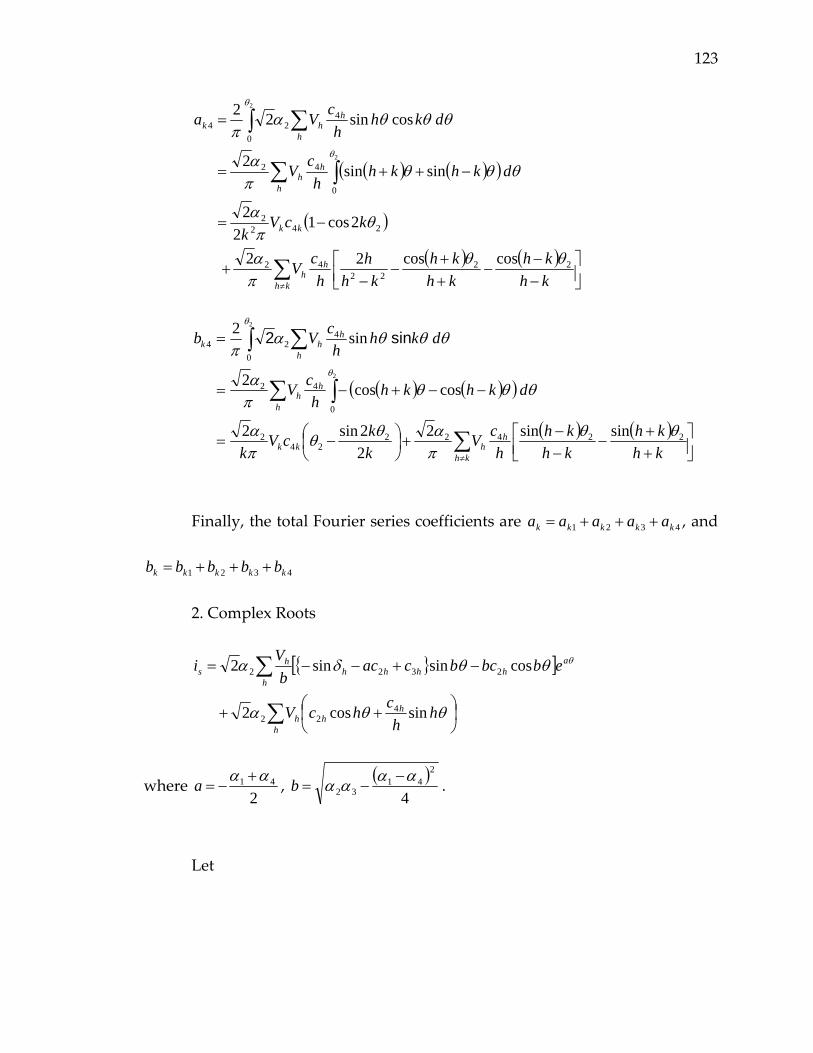
123
( ) ( )( )
( )
( ) ( )∑
∑ ∫
∫ ∑
≠⎥⎦⎤
⎢⎣⎡
−−
−++
−−
+
−=
−++=
=
kh
hh
kk
h
hh
h
hhk
khkh
khkh
khh
hcV
kcVk
dkhkhh
cV
dkhh
cVa
2222
42
2422
0
42
0
424
coscos22
2cos12
2
sinsin2
cos sin22
2
2
θθπα
θπα
θθθπα
θθθαπ
θ
θ
( ) ( )( )
( ) ( )∑
∑ ∫
∫ ∑
≠⎥⎦⎤
⎢⎣⎡
++
−−−
+⎟⎠⎞
⎜⎝⎛ −=
−−+−=
=
kh
hhkk
h
hh
h
hhk
khkh
khkh
hcV
kkcV
k
dkhkhh
cV
dkhh
cVb
2242224
2
0
42
0
424
sinsin222sin2
coscos2
sin2
2
2
θθπαθθ
πα
θθθπα
θθθαπ
θ
θ
sin 2
Finally, the total Fourier series coefficients are 4321 kkkkk aaaaa +++= , and
4321 kkkkk bbbbb +++=
2. Complex Roots
[ ]
∑
∑
⎟⎠⎞
⎜⎝⎛ ++
−+−−=
h
hhh
ahhhh
h
hs
hh
chcV
ebbcbcacb
Vi
θθα
θθδα θ
sincos2
cossinsin2
422
2322
where 2
41 αα +−=a , ( )
4
241
32αααα −
−=b .
Let
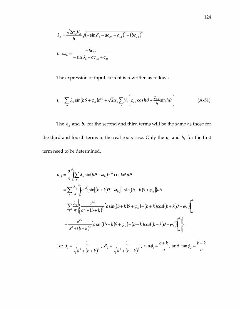
124
( ) ( )222
322 sin2
hhhhh
h bccacb
V++−−= δαλ
hhh
hh cac
bc
32
2
sintan
+−−−
=δ
ϕ
The expression of input current is rewritten as follows
( ) ∑∑ ⎟⎠⎞
⎜⎝⎛ +++=
h
hhh
h
ahhs h
hchcVebi θθαϕθλ θ sincos2sin 4
22 (A‐51)
The ka and kb for the second and third terms will be the same as those for
the third and fourth terms in the real roots case. Only the ka and kb for the first
term need to be determined.
( )
( )[ ] ( )[ ]
( )( )( ) ( ) ( )( )[ ]
( )( )( ) ( ) ( )( )[ ]
⎪⎭
⎪⎬⎫
+−−−+−−+
+
⎪⎩
⎪⎨⎧
+++−++++
=
+−+++=
+=
∑
∑ ∫
∫∑
2
2
2
2
022
022
0
01
cossin
cossin
sinsin
cossin2
θθ
θθ
θθ
θθ
ϕθϕθ
ϕθϕθπλ
θϕθϕθπλ
θθϕθλπ
hh
a
hhh
ah
hhh
ah
h
ahhk
kbkbkbakba
e
kbkbkbakba
e
dkbkbe
dkeba
Let ( )2211
kba ++=δ ,
( )2221
kba −+=δ ,
akb +
=1tanφ , and a
kb −=2tanφ
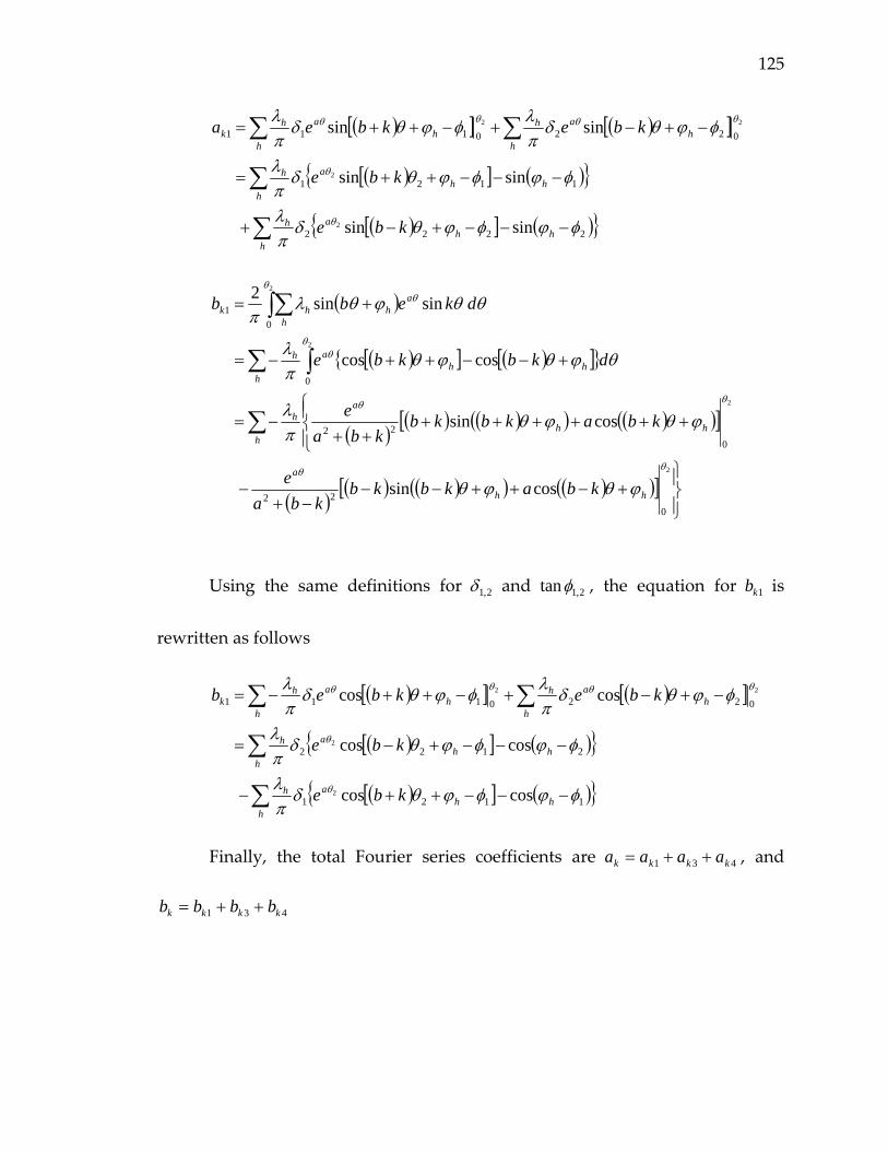
125
( )[ ] ( )[ ]
( )[ ] ( )
( )[ ] ( ) ∑
∑
∑∑
−−−+−+
−−−++=
−+−+−++=
hhh
ah
hhh
ah
hh
ah
hh
ahk
kbe
kbe
kbekbea
2222
1121
0220111
sinsin
sinsin
sinsin
2
2
22
φϕφϕθδπλ
φϕφϕθδπλ
φϕθδπλφϕθδ
πλ
θ
θ
θθθθ
( )
( )[ ] ( )[ ]
( )( ) ( )( ) ( )( )[ ]
( )( ) ( )( ) ( )( )[ ]
⎪⎭
⎪⎬⎫
+−++−−−+
−
⎪⎩
⎪⎨⎧
++++++++
−=
+−−++−=
+=
∑
∑ ∫
∫∑
2
2
2
2
022
022
0
01
cossin
cossin
coscos
sinsin2
θθ
θθ
θθ
θθ
ϕθϕθ
ϕθϕθπλ
θϕθϕθπλ
θθϕθλπ
hh
a
hhh
ah
hhh
ah
h
ahhk
kbakbkbkba
e
kbakbkbkba
e
dkbkbe
dkebb
Using the same definitions for 2,1δ and 2,1tanφ , the equation for 1kb is
rewritten as follows
( )[ ] ( )[ ]
( )[ ] ( )
( )[ ] ( ) ∑
∑
∑∑
−−−++−
−−−+−=
−+−+−++−=
hhh
ah
hhh
ah
hh
ah
hh
ahk
kbe
kbe
kbekbeb
1121
2122
0220111
coscos
coscos
coscos
2
2
22
φϕφϕθδπλ
φϕφϕθδπλ
φϕθδπλφϕθδ
πλ
θ
θ
θθθθ
Finally, the total Fourier series coefficients are 431 kkkk aaaa ++= , and
431 kkkk bbbb ++=
126
II. Multiphase Harmonic Load Flow Program Code
The multiphase harmonic load flow algorithm in this dissertation is
developed using MATLAB® 5.3 (R11) from The MathWorks, Inc. A complete list
of programs in this dissertation is presented below, followed by the detailed
code for each program.
A. Programs list
Line parameters calculation line_cal line impedance/admittance calculation: import
line configuration, call subprogram, store data for load flow
spacing line spacing parameters calculation pqfun P and Q constants in Carson’s line model config_601 series impedance per unit length for line
configuration type 601 config_602 series impedance per unit length for line
configuration type 602 config_603 series impedance per unit length for line
configuration type 603 config_604 series impedance per unit length for line
configuration type 604 config_605 series impedance per unit length for line
configuration type 605 config_702 series impedance for transformer type 702 assemble_config1_2 branch series impedance and shunt admittance
at the given line length for line configuration type 601 & 602
assemble_config3 branch series impedance and shunt admittance at the given line length for line configuration type 603
assemble_config4 branch series impedance and shunt admittance at the given line length for line configuration type 604
127
assemble_config5 branch series impedance and shunt admittance at the given line length for line configuration type 605
Single phase rectifier subroutine sphr single phase rectifier subprogram: import
rectifier parameters, calculate input current Fourier series for given terminal voltage
c_cal calculate the constants used in the single phase rectifier model
is_comp input current waveform generation for complex characteristic roots
is_real input current waveform generation for real characteristic roots
isf_comp input current Fourier series for complex characteristic roots
isf_real input current Fourier series for real characteristic roots
Vo_comp output voltage waveform generation for complex characteristic roots during conduction
Vo_real output voltage waveform generation for real characteristic roots during conduction
Vdecay output voltage discharge waveform generation
Load flow calculation main main program of load flow calculation load_curr_inj calculate linear load current injection sphr_curr combine the harmonic current from rectifier
with the other linear load injection by frequency
branch_curr_cal collect injections at the receiving end of each branch and calculate the current division between neutral and earth
busout screen print the load flow result after convergence
B. Program Codes
assemble_config1_2

128
% Function [Zse,Ysh]=assemble_config1_2(H,Z,leng,Rg) % % Function for incremental model assembling for configuration #601 & #602 at % all frequencies % The input: % Z series impedance Z for per unit length (mile) % leng feeder length in miles % Rg pole grounding resistance % The output: % Zse series admittance of the assembled model [4, 4, harm#] % Ysh shunt admittance of the assembled model [4, 4, harm#] % The function first calculates the total series impedance of the feeder % Then the impedance is divided into increment of 200 feet long. The number % of increments is rounded to the least value. The fractional length of the % feeder is divided in two and included in the first and the last spans. The % resulting spans are assembled using incidence matrix method. The nodes in % the middle are eliminated by Kron reduction to obtain an equivalent pi model. % The grounding resistances at the both ends are not included in this time. % Since the phases are full in these config, no need to consider the phasing. function [Zse,Ysh]=assemble_config1_2(H,Z,leng,Rg) % Total series impedance Ztot=Z*leng/5280; % Impedance division among spans span_num=ceil(leng/1320); if span_num > 2 for i=2:span_num‐1 span(i)=1320; end span(1)=(leng‐1320*(span_num‐2))/2; span(span_num)=span(1); Z_span=zeros(H*4,4,span_num); for l=1:span_num Z_span(:,:,l)=span(l)/leng*Ztot; end elseif span_num == 2 span(1)=leng/2; span(2)=span(1); Z_span=zeros(H*4,4,span_num); for l=1:span_num Z_span(:,:,l)=span(l)/leng*Ztot; end
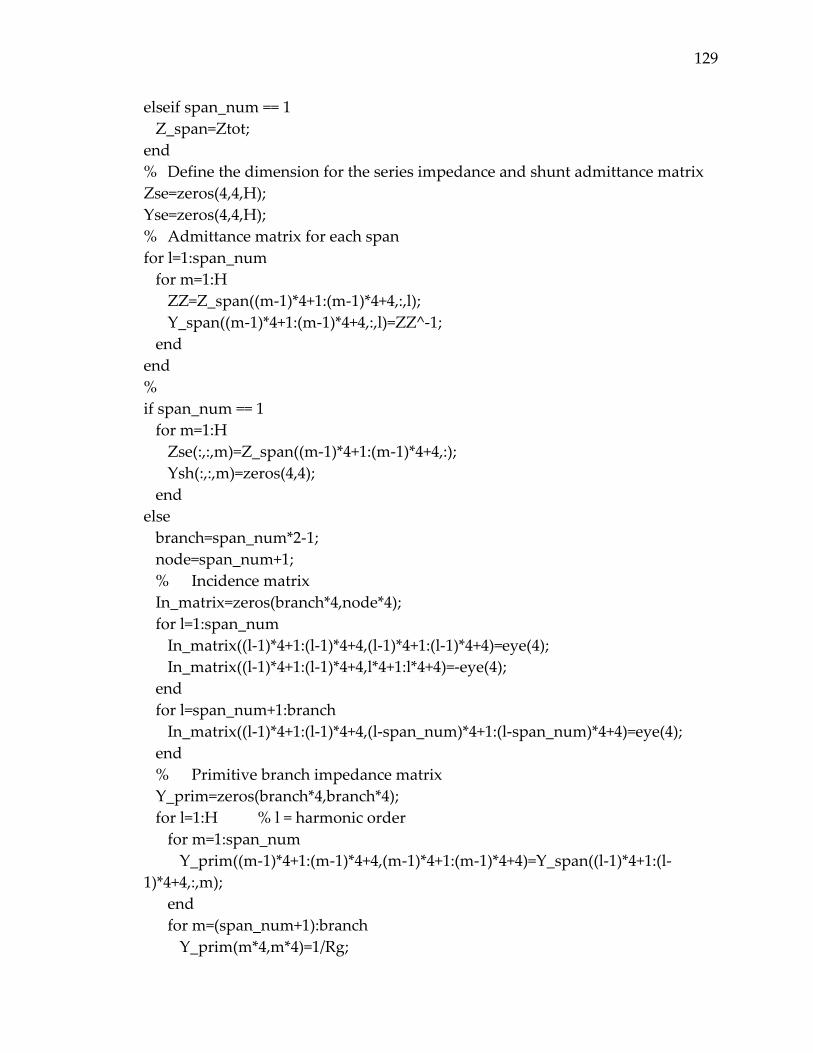
129
elseif span_num == 1 Z_span=Ztot; end % Define the dimension for the series impedance and shunt admittance matrix Zse=zeros(4,4,H); Yse=zeros(4,4,H); % Admittance matrix for each span for l=1:span_num for m=1:H ZZ=Z_span((m‐1)*4+1:(m‐1)*4+4,:,l); Y_span((m‐1)*4+1:(m‐1)*4+4,:,l)=ZZ^‐1; end end % if span_num == 1 for m=1:H Zse(:,:,m)=Z_span((m‐1)*4+1:(m‐1)*4+4,:); Ysh(:,:,m)=zeros(4,4); end else branch=span_num*2‐1; node=span_num+1; % Incidence matrix In_matrix=zeros(branch*4,node*4); for l=1:span_num In_matrix((l‐1)*4+1:(l‐1)*4+4,(l‐1)*4+1:(l‐1)*4+4)=eye(4); In_matrix((l‐1)*4+1:(l‐1)*4+4,l*4+1:l*4+4)=‐eye(4); end for l=span_num+1:branch In_matrix((l‐1)*4+1:(l‐1)*4+4,(l‐span_num)*4+1:(l‐span_num)*4+4)=eye(4); end % Primitive branch impedance matrix Y_prim=zeros(branch*4,branch*4); for l=1:H % l = harmonic order for m=1:span_num Y_prim((m‐1)*4+1:(m‐1)*4+4,(m‐1)*4+1:(m‐1)*4+4)=Y_span((l‐1)*4+1:(l‐1)*4+4,:,m); end for m=(span_num+1):branch Y_prim(m*4,m*4)=1/Rg;
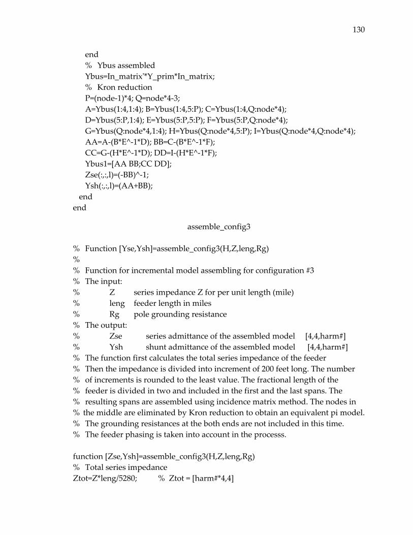
130
end % Ybus assembled Ybus=In_matrixʹ*Y_prim*In_matrix; % Kron reduction P=(node‐1)*4; Q=node*4‐3; A=Ybus(1:4,1:4); B=Ybus(1:4,5:P); C=Ybus(1:4,Q:node*4); D=Ybus(5:P,1:4); E=Ybus(5:P,5:P); F=Ybus(5:P,Q:node*4); G=Ybus(Q:node*4,1:4); H=Ybus(Q:node*4,5:P); I=Ybus(Q:node*4,Q:node*4); AA=A‐(B*E^‐1*D); BB=C‐(B*E^‐1*F); CC=G‐(H*E^‐1*D); DD=I‐(H*E^‐1*F); Ybus1=[AA BB;CC DD]; Zse(:,:,l)=(‐BB)^‐1; Ysh(:,:,l)=(AA+BB); end end
assemble_config3
% Function [Yse,Ysh]=assemble_config3(H,Z,leng,Rg) % % Function for incremental model assembling for configuration #3 % The input: % Z series impedance Z for per unit length (mile) % leng feeder length in miles % Rg pole grounding resistance % The output: % Zse series admittance of the assembled model [4,4,harm#] % Ysh shunt admittance of the assembled model [4,4,harm#] % The function first calculates the total series impedance of the feeder % Then the impedance is divided into increment of 200 feet long. The number % of increments is rounded to the least value. The fractional length of the % feeder is divided in two and included in the first and the last spans. The % resulting spans are assembled using incidence matrix method. The nodes in % the middle are eliminated by Kron reduction to obtain an equivalent pi model. % The grounding resistances at the both ends are not included in this time. % The feeder phasing is taken into account in the processs. function [Zse,Ysh]=assemble_config3(H,Z,leng,Rg) % Total series impedance Ztot=Z*leng/5280; % Ztot = [harm#*4,4]
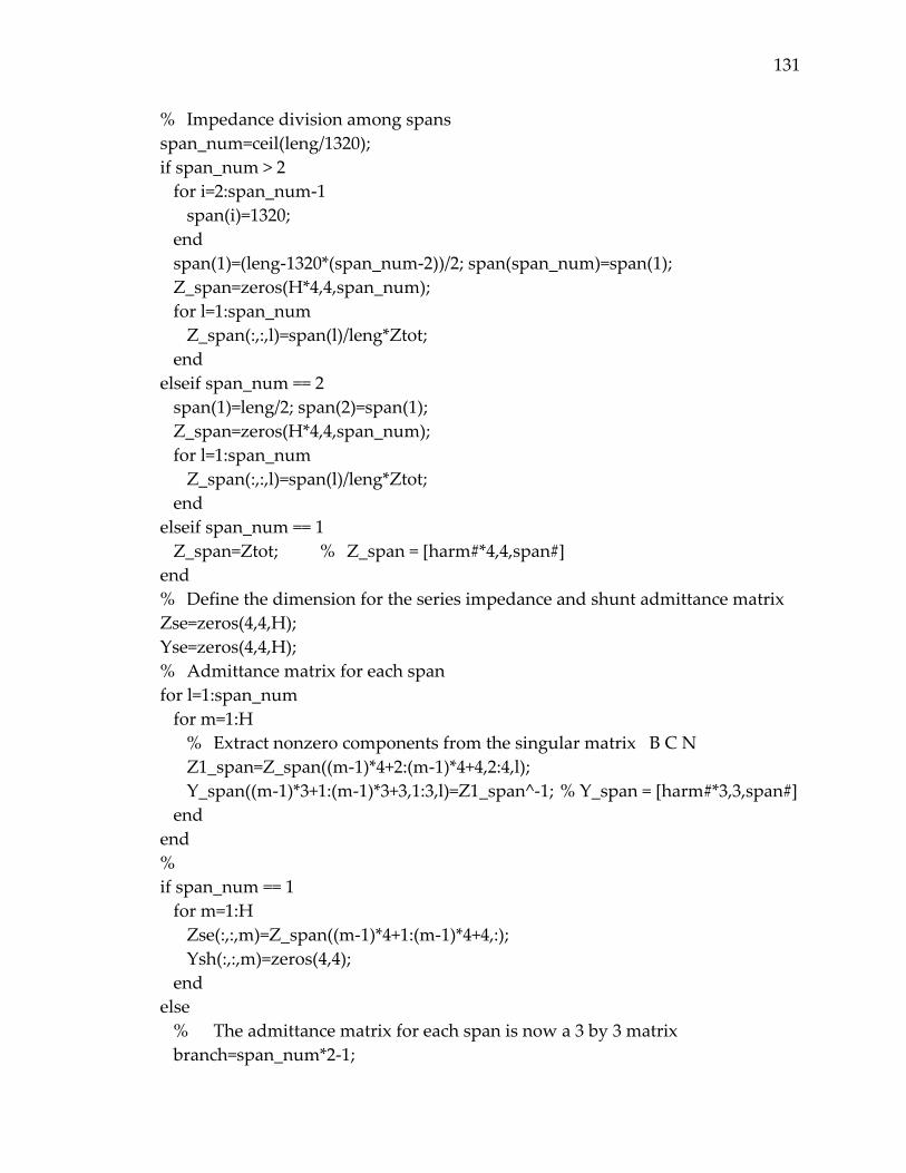
131
% Impedance division among spans span_num=ceil(leng/1320); if span_num > 2 for i=2:span_num‐1 span(i)=1320; end span(1)=(leng‐1320*(span_num‐2))/2; span(span_num)=span(1); Z_span=zeros(H*4,4,span_num); for l=1:span_num Z_span(:,:,l)=span(l)/leng*Ztot; end elseif span_num == 2 span(1)=leng/2; span(2)=span(1); Z_span=zeros(H*4,4,span_num); for l=1:span_num Z_span(:,:,l)=span(l)/leng*Ztot; end elseif span_num == 1 Z_span=Ztot; % Z_span = [harm#*4,4,span#] end % Define the dimension for the series impedance and shunt admittance matrix Zse=zeros(4,4,H); Yse=zeros(4,4,H); % Admittance matrix for each span for l=1:span_num for m=1:H % Extract nonzero components from the singular matrix B C N Z1_span=Z_span((m‐1)*4+2:(m‐1)*4+4,2:4,l); Y_span((m‐1)*3+1:(m‐1)*3+3,1:3,l)=Z1_span^‐1; % Y_span = [harm#*3,3,span#] end end % if span_num == 1 for m=1:H Zse(:,:,m)=Z_span((m‐1)*4+1:(m‐1)*4+4,:); Ysh(:,:,m)=zeros(4,4); end else % The admittance matrix for each span is now a 3 by 3 matrix branch=span_num*2‐1;
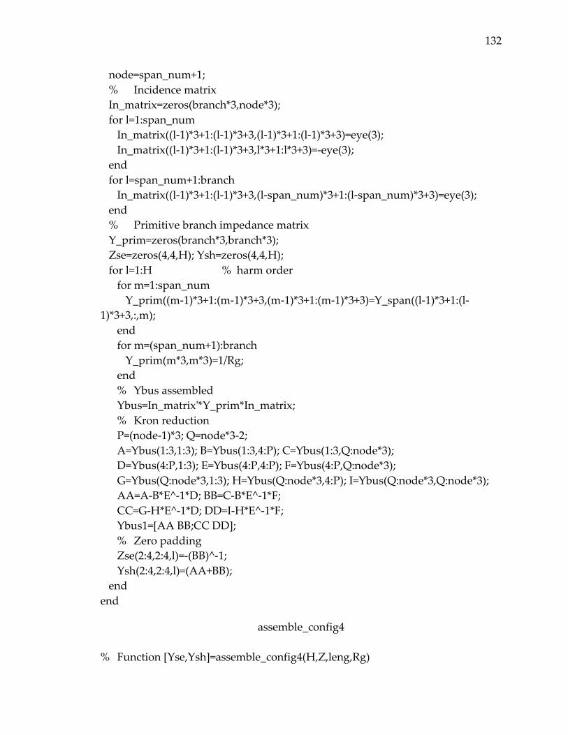
132
node=span_num+1; % Incidence matrix In_matrix=zeros(branch*3,node*3); for l=1:span_num In_matrix((l‐1)*3+1:(l‐1)*3+3,(l‐1)*3+1:(l‐1)*3+3)=eye(3); In_matrix((l‐1)*3+1:(l‐1)*3+3,l*3+1:l*3+3)=‐eye(3); end for l=span_num+1:branch In_matrix((l‐1)*3+1:(l‐1)*3+3,(l‐span_num)*3+1:(l‐span_num)*3+3)=eye(3); end % Primitive branch impedance matrix Y_prim=zeros(branch*3,branch*3); Zse=zeros(4,4,H); Ysh=zeros(4,4,H); for l=1:H % harm order for m=1:span_num Y_prim((m‐1)*3+1:(m‐1)*3+3,(m‐1)*3+1:(m‐1)*3+3)=Y_span((l‐1)*3+1:(l‐1)*3+3,:,m); end for m=(span_num+1):branch Y_prim(m*3,m*3)=1/Rg; end % Ybus assembled Ybus=In_matrixʹ*Y_prim*In_matrix; % Kron reduction P=(node‐1)*3; Q=node*3‐2; A=Ybus(1:3,1:3); B=Ybus(1:3,4:P); C=Ybus(1:3,Q:node*3); D=Ybus(4:P,1:3); E=Ybus(4:P,4:P); F=Ybus(4:P,Q:node*3); G=Ybus(Q:node*3,1:3); H=Ybus(Q:node*3,4:P); I=Ybus(Q:node*3,Q:node*3); AA=A‐B*E^‐1*D; BB=C‐B*E^‐1*F; CC=G‐H*E^‐1*D; DD=I‐H*E^‐1*F; Ybus1=[AA BB;CC DD]; % Zero padding Zse(2:4,2:4,l)=‐(BB)^‐1; Ysh(2:4,2:4,l)=(AA+BB); end end
assemble_config4
% Function [Yse,Ysh]=assemble_config4(H,Z,leng,Rg)
133
% % Function for incremental model assembling for configuration #3 % The input: % Z series impedance Z for per unit length (mile) % leng feeder length in miles % Rg pole grounding resistance % The output: % Zse series admittance of the assembled model [4, 4, harm#] % Ysh shunt admittance of the assembled model [4, 4, harm#] % The function first calculates the total series impedance of the feeder % Then the impedance is divided into increment of 200 feet long. The number % of increments is rounded to the least value. The fractional length of the % feeder is divided in two and included in the first and the last spans. The % resulting spans are assembled using incidence matrix method. The nodes in % the middle are eliminated by Kron reduction to obtain an equivalent pi model. % The grounding resistances at the both ends are not included in this time. % The feeder phasing is taken into account in the processs. function [Zse,Ysh]=assemble_config4(H,Z,leng,Rg) % Total series impedance Ztot=Z*leng/5280; % Ztot = [harm#*4, 4] % Impedance division among spans span_num=ceil(leng/1320); if span_num > 2 for i=2:span_num‐1 span(i)=1320; end span(1)=(leng‐1320*(span_num‐2))/2; span(span_num)=span(1); Z_span=zeros(H*4,4,span_num); for l=1:span_num Z_span(:,:,l)=span(l)/leng*Ztot; end elseif span_num == 2 span(1)=leng/2; span(2)=span(1); Z_span=zeros(H*4,4,span_num); for l=1:span_num Z_span(:,:,l)=span(l)/leng*Ztot; end elseif span_num == 1 Z_span=Ztot; % Z_span = [harm#*4,4,span#]
134
end % Define the dimension for the series impedance and shunt admittance matrix Zse=zeros(4,4,H); Yse=zeros(4,4,H); % Admittance matrix for each span for l=1:span_num for m=1:H % Extract nonzero components from the singular matrix A C N Z1_span(1,1)=Z_span((m‐1)*4+1,1,l); Z1_span(2:3,1)=Z_span((m‐1)*4+3:(m‐1)*4+4,1,l); Z1_span(1,2:3)=Z_span((m‐1)*4+1,3:4,l); Z1_span(2:3,2:3)=Z_span((m‐1)*4+3:(m‐1)*4+4,3:4,l); %Z1_span %pause Y_span((m‐1)*3+1:(m‐1)*3+3,1:3,l)=Z1_span^‐1; % Y_span = [harm#*3, 3, span#] end end % if span_num == 1 for m=1:H Zse(:,:,m)=Z_span((m‐1)*4+1:(m‐1)*4+4,:); Ysh(:,:,m)=zeros(4,4); end else branch=span_num*2‐1; node=span_num+1; % Incidence matrix In_matrix=zeros(branch*3,node*3); for l=1:span_num In_matrix((l‐1)*3+1:(l‐1)*3+3,(l‐1)*3+1:(l‐1)*3+3)=eye(3); In_matrix((l‐1)*3+1:(l‐1)*3+3,l*3+1:l*3+3)=‐eye(3); end for l=span_num+1:branch In_matrix((l‐1)*3+1:(l‐1)*3+3,(l‐span_num)*3+1:(l‐span_num)*3+3)=eye(3); end % Primitive branch impedance matrix Y_prim=zeros(branch*3,branch*3); for l=1:H % Harm order for m=1:span_num
135
Y_prim((m‐1)*3+1:(m‐1)*3+3,(m‐1)*3+1:(m‐1)*3+3)=Y_span((l‐1)*3+1:(l‐1)*3+3,:,m); end for m=(span_num+1):branch Y_prim(m*3,m*3)=1/Rg; end % Ybus assembled Ybus=In_matrixʹ*Y_prim*In_matrix; % Kron reduction P=(node‐1)*3; Q=node*3‐2; A=Ybus(1:3,1:3); B=Ybus(1:3,4:P); C=Ybus(1:3,Q:node*3); D=Ybus(4:P,1:3); E=Ybus(4:P,4:P); F=Ybus(4:P,Q:node*3); G=Ybus(Q:node*3,1:3); H=Ybus(Q:node*3,4:P); I=Ybus(Q:node*3,Q:node*3); AA=A‐B*E^‐1*D; BB=C‐B*E^‐1*F; CC=G‐H*E^‐1*D; DD=I‐H*E^‐1*F; Ybus1=[AA BB;CC DD]; % Zero padding Zse1=‐(BB)^‐1; Ysh1=(AA+BB); Zse(1,1,l)=Zse1(1,1); Ysh(1,1,l)=Ysh1(1,1); Zse(3:4,1,l)=Zse1(2:3,1); Ysh(3:4,1,l)=Ysh1(2:3,1); Zse(1,3:4,l)=Zse1(1,2:3); Ysh(1,3:4,l)=Ysh1(1,2:3); Zse(3:4,3:4,l)=Zse1(2:3,2:3); Ysh(3:4,3:4,l)=Ysh1(2:3,2:3); end end
assemble_config5
% Function [Yse,Ysh]=assemble_config5(H,Z,leng,Rg) % % Function for incremental model assembling for configuration #605 at % all frequencies % The input: % Z series impedance Z for per unit length (mile) % leng feeder length in miles % Rg pole grounding resistance % The output: % Zse series admittance of the assembled model [4, 4, harm#] % Ysh shunt admittance of the assembled model [4, 4, harm#] % The function first calculates the total series impedance of the feeder % Then the impedance is divided into increment of 200 feet long. The number
136
% of increments is rounded to the least value. The fractional length of the % feeder is divided in two and included in the first and the last spans. The % resulting spans are assembled using incidence matrix method. The nodes in % the middle are eliminated by Kron reduction to obtain an equivalent pi model. % The grounding resistances at the both ends are not included in this time. % The feeder phasing is taken into account in the processs. function [Zse,Ysh]=assemble_config5(H,Z,leng,Rg) % Total series impedance Ztot=Z*leng/5280; % Ztot = [harm#*4, 4] % Impedance division among spans span_num=ceil(leng/1320); if span_num > 2 for i=2:span_num‐1 span(i)=1320; end span(1)=(leng‐1320*(span_num‐2))/2; span(span_num)=span(1); Z_span=zeros(H*4,4,span_num); for l=1:span_num Z_span(:,:,l)=span(l)/leng*Ztot; end elseif span_num == 2 span(1)=leng/2; span(2)=span(1); Z_span=zeros(H*4,4,span_num); for l=1:span_num Z_span(:,:,l)=span(l)/leng*Ztot; end elseif span_num == 1 Z_span=Ztot; % Z_span = [harm#*4,4,span#] end % Define the dimension for the series impedance and shunt admittance matrix Zse=zeros(4,4,H); Yse=zeros(4,4,H); % Admittance matrix for each span for l=1:span_num for m=1:H % Extract nonzero components from the singular matrix Z1_span=Z_span((m‐1)*4+3:(m‐1)*4+4,3:4,l);%pause Y_span((m‐1)*2+1:(m‐1)*2+2,1:2,l)=Z1_span^‐1; % primitive admittance =[harm#*2, 2, span#]
137
end end % if span_num == 1 for m=1:H Zse(:,:,m)=Z_span((m‐1)*4+1:(m‐1)*4+4,:); Ysh(:,:,m)=zeros(4,4); end else branch=span_num*2‐1; node=span_num+1; % Incidence matrix In_matrix=zeros(branch*2,node*2); for l=1:span_num In_matrix((l‐1)*2+1:(l‐1)*2+2,(l‐1)*2+1:(l‐1)*2+2)=eye(2); In_matrix((l‐1)*2+1:(l‐1)*2+2,l*2+1:l*2+2)=‐eye(2); end for l=span_num+1:branch In_matrix((l‐1)*2+1:(l‐1)*2+2,(l‐span_num)*2+1:(l‐span_num)*2+2)=eye(2); end % Primitive branch impedance matrix Y_prim=zeros(branch*2,branch*2); for l=1:H % harm order for m=1:span_num Y_prim((m‐1)*2+1:(m‐1)*2+2,(m‐1)*2+1:(m‐1)*2+2)=Y_span((l‐1)*2+1:(l‐1)*2+2,:,m); end for m=(span_num+1):branch Y_prim(m*2,m*2)=1/Rg; end % Ybus assembled Ybus=In_matrixʹ*Y_prim*In_matrix; % Kron reduction P=(node‐1)*2; Q=node*2‐1; A=Ybus(1:2,1:2); B=Ybus(1:2,3:P); C=Ybus(1:2,Q:node*2); D=Ybus(3:P,1:2); E=Ybus(3:P,3:P); F=Ybus(3:P,Q:node*2); G=Ybus(Q:node*2,1:2); H=Ybus(Q:node*2,3:P); I=Ybus(Q:node*2,Q:node*2); AA=A‐(B*E^‐1*D); BB=C‐(B*E^‐1*F); CC=G‐(H*E^‐1*D); DD=I‐(H*E^‐1*F); Ybus1=[AA BB;CC DD];

138
% Zero padding Zse(3:4,3:4,l)=(‐BB)^‐1; % The zero value in Zse does not mean short circuit, just not be given Ysh(3:4,3:4,l)=(AA+BB); % any value, while the zero value in Ysh actually means zero end end
config_601
% Function config_601(H) Feeder Series Impedance Calculation for Config#601 % % Load the feeder spacing data, calculate the series impedance per unit length % then transmute the impedance matrix according the phasing specification. % The earth return path is accounted for by using the Carsonʹs line formula. % % Output: config_601_prim.wk1 = [real(H*4,4) | imag(H*4,4)] function config_601(H,p) % Generate Spacing Matrix (Spacing 500) Spacing=wk1read(ʹspacing.wk1ʹ); % S value S500=zeros(4,4); S500(1,1)=Spacing(1,1); S500(1,2)=Spacing(2,1); S500(2,1)=S500(1,2); S500(1,3)=Spacing(3,1); S500(3,1)=S500(1,3); S500(1,4)=Spacing(4,1); S500(4,1)=S500(1,4); S500(2,2)=Spacing(5,1); S500(2,3)=Spacing(6,1); S500(3,2)=S500(2,3); S500(2,4)=Spacing(7,1); S500(4,2)=S500(2,4); S500(3,3)=Spacing(8,1); S500(3,4)=Spacing(9,1); S500(4,3)=S500(3,4); S500(4,4)=Spacing(10,1); % D value D500=zeros(4,4); D500(1,2)=Spacing(11,1); D500(2,1)=D500(1,2); D500(1,3)=Spacing(12,1); D500(3,1)=D500(1,3); D500(1,4)=Spacing(13,1); D500(4,1)=D500(1,4);
139
D500(2,3)=Spacing(14,1); D500(3,2)=D500(2,3); D500(2,4)=Spacing(15,1); D500(4,2)=D500(2,4); D500(3,4)=Spacing(16,1); D500(4,3)=D500(3,4); % Value specified for this configuration type D500(1,1)=0.0244; D500(2,2)=0.0244; D500(3,3)=0.0244; D500(4,4)=0.0244; % theta value theta=zeros(4,4); theta(1,2)=Spacing(1,2); theta(2,1)=theta(1,2); theta(1,3)=Spacing(2,2); theta(3,1)=theta(1,3); theta(1,4)=Spacing(3,2); theta(4,1)=theta(1,4); theta(2,3)=Spacing(4,2); theta(3,2)=theta(2,3); theta(2,4)=Spacing(5,2); theta(4,2)=theta(2,4); theta(3,4)=Spacing(6,2); theta(4,3)=theta(3,4); % Primitive series impedances per unit length G=1.6095e‐4; % Specified conductor resistance per unit length R(1)=0.306; R(2)=R(1); R(3)=R(1); R(4)=0.306; % Transmutation matrix B=[0 1 0 0;1 0 0 0;0 0 1 0;0 0 0 1]; % transmute 1 and 2 % Harmonics 1 ~ 2*H‐1 for k=1:H w=2*pi*60*(2*k‐1); freq=(2*k‐1)*60; for i=1:4 [P,Q]=pqfun(S500(i,i),theta(i,i),freq,p); % earth conductivity is assumed to be 100 Z1(i,i)=R(i)+4*w*P*G+j*(2*w*log(S500(i,i)/D500(i,i))+4*w*Q)*G; end for l=1:4 for m=1:4 if l ~= m [P,Q]=pqfun(S500(l,m),theta(l,m),freq,p); Z1(l,m)=4*w*P*G+j*(2*w*log(S500(l,m)/D500(l,m))+4*w*Q)*G; end end end % Transmutation according to the phasing configuration Z1=B*Z1*B; % Assemble the sub‐matrix in an increasing order of freqs
140
for l=1:4 for m=1:4 Z((k‐1)*4+l,m)=Z1(l,m); end end end % Z_real=real(Z); Z_imag=imag(Z); ZZ=[Z_real Z_imag]; wk1write(ʹconfig_601_prim.wk1ʹ,ZZ);
config_602
% Function config_602(H) Feeder Series Impedance Calculation for Config#602 % % Load the feeder spacing data, calculate the series impedance per unit length % then transmute the impedance matrix according the phasing specification. % The earth return path is accounted for by using the Carsonʹs line formula. % % Output: config_602_prim.wk1 = [real (H*4,4) | imag (H*4,4)] function config_602(H,p) % Generate Spacing Matrix (Spacing 500) Spacing=wk1read(ʹspacing.wk1ʹ); % S value S500=zeros(4,4); S500(1,1)=Spacing(1,1); S500(1,2)=Spacing(2,1); S500(2,1)=S500(1,2); S500(1,3)=Spacing(3,1); S500(3,1)=S500(1,3); S500(1,4)=Spacing(4,1); S500(4,1)=S500(1,4); S500(2,2)=Spacing(5,1); S500(2,3)=Spacing(6,1); S500(3,2)=S500(2,3); S500(2,4)=Spacing(7,1); S500(4,2)=S500(2,4); S500(3,3)=Spacing(8,1); S500(3,4)=Spacing(9,1); S500(4,3)=S500(3,4); S500(4,4)=Spacing(10,1); % D value D500=zeros(4,4); D500(1,2)=Spacing(11,1); D500(2,1)=D500(1,2); D500(1,3)=Spacing(12,1); D500(3,1)=D500(1,3);
141
D500(1,4)=Spacing(13,1); D500(4,1)=D500(1,4); D500(2,3)=Spacing(14,1); D500(3,2)=D500(2,3); D500(2,4)=Spacing(15,1); D500(4,2)=D500(2,4); D500(3,4)=Spacing(16,1); D500(4,3)=D500(3,4); % Value specified for this configuration type D500_2=D500; D500_2(1,1)=0.00814; D500_2(2,2)=0.00814; D500_2(3,3)=0.00814; D500_2(4,4)=0.00814; % theta value theta=zeros(4,4); theta(1,2)=Spacing(1,2); theta(2,1)=theta(1,2); theta(1,3)=Spacing(2,2); theta(3,1)=theta(1,3); theta(1,4)=Spacing(3,2); theta(4,1)=theta(1,4); theta(2,3)=Spacing(4,2); theta(3,2)=theta(2,3); theta(2,4)=Spacing(5,2); theta(4,2)=theta(2,4); theta(3,4)=Spacing(6,2); theta(4,3)=theta(3,4); % Primitive series impedances per unit length G=1.6095e‐4; % Specified conductor resistance per unit length R(1)=0.592; R(2)=R(1); R(3)=R(1); R(4)=0.592; % Transmutation matrix B1=[1 0 0 0;0 0 1 0;0 1 0 0;0 0 0 1]; % transmute 2 and 3 B2=[0 1 0 0;1 0 0 0;0 0 1 0;0 0 0 1]; % transmute 1 and 2 % Harmonics 1 2*H‐1 for k=1:H w=2*pi*60*(2*k‐1); freq=(2*k‐1)*60; for i=1:4 [P,Q]=pqfun(S500(i,i),theta(i,i),freq*60,p); Z1(i,i)=R(i)+4*w*P*G+j*(2*w*log(S500(i,i)/D500_2(i,i))+4*w*Q)*G; end for l=1:4 for m=1:4 if l ~= m [P,Q]=pqfun(S500(l,m),theta(l,m),freq,p); Z1(l,m)=4*w*P*G+j*(2*w*log(S500(l,m)/D500_2(l,m))+4*w*Q)*G; end end end %Z1
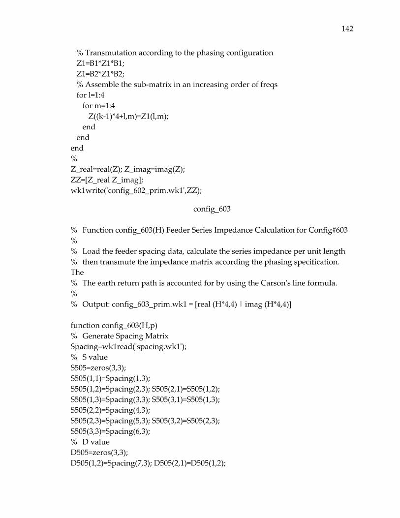
142
% Transmutation according to the phasing configuration Z1=B1*Z1*B1; Z1=B2*Z1*B2; % Assemble the sub‐matrix in an increasing order of freqs for l=1:4 for m=1:4 Z((k‐1)*4+l,m)=Z1(l,m); end end end % Z_real=real(Z); Z_imag=imag(Z); ZZ=[Z_real Z_imag]; wk1write(ʹconfig_602_prim.wk1ʹ,ZZ);
config_603
% Function config_603(H) Feeder Series Impedance Calculation for Config#603 % % Load the feeder spacing data, calculate the series impedance per unit length % then transmute the impedance matrix according the phasing specification. The % The earth return path is accounted for by using the Carsonʹs line formula. % % Output: config_603_prim.wk1 = [real (H*4,4) | imag (H*4,4)] function config_603(H,p) % Generate Spacing Matrix Spacing=wk1read(ʹspacing.wk1ʹ); % S value S505=zeros(3,3); S505(1,1)=Spacing(1,3); S505(1,2)=Spacing(2,3); S505(2,1)=S505(1,2); S505(1,3)=Spacing(3,3); S505(3,1)=S505(1,3); S505(2,2)=Spacing(4,3); S505(2,3)=Spacing(5,3); S505(3,2)=S505(2,3); S505(3,3)=Spacing(6,3); % D value D505=zeros(3,3); D505(1,2)=Spacing(7,3); D505(2,1)=D505(1,2);
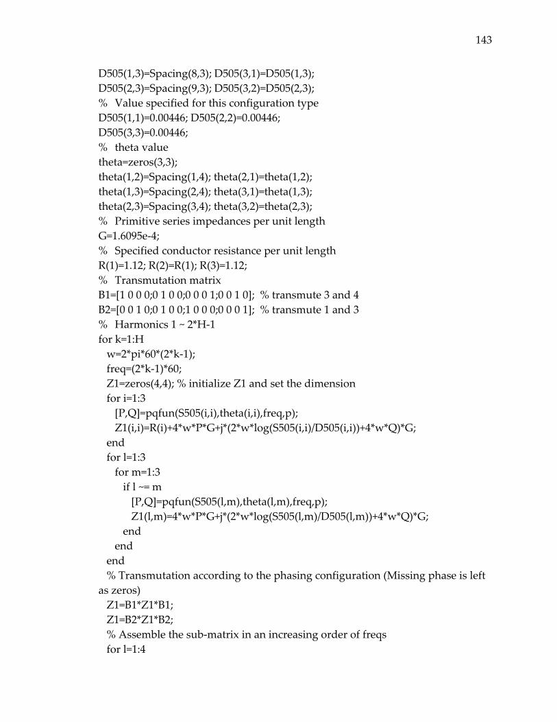
143
D505(1,3)=Spacing(8,3); D505(3,1)=D505(1,3); D505(2,3)=Spacing(9,3); D505(3,2)=D505(2,3); % Value specified for this configuration type D505(1,1)=0.00446; D505(2,2)=0.00446; D505(3,3)=0.00446; % theta value theta=zeros(3,3); theta(1,2)=Spacing(1,4); theta(2,1)=theta(1,2); theta(1,3)=Spacing(2,4); theta(3,1)=theta(1,3); theta(2,3)=Spacing(3,4); theta(3,2)=theta(2,3); % Primitive series impedances per unit length G=1.6095e‐4; % Specified conductor resistance per unit length R(1)=1.12; R(2)=R(1); R(3)=1.12; % Transmutation matrix B1=[1 0 0 0;0 1 0 0;0 0 0 1;0 0 1 0]; % transmute 3 and 4 B2=[0 0 1 0;0 1 0 0;1 0 0 0;0 0 0 1]; % transmute 1 and 3 % Harmonics 1 ~ 2*H‐1 for k=1:H w=2*pi*60*(2*k‐1); freq=(2*k‐1)*60; Z1=zeros(4,4); % initialize Z1 and set the dimension for i=1:3 [P,Q]=pqfun(S505(i,i),theta(i,i),freq,p); Z1(i,i)=R(i)+4*w*P*G+j*(2*w*log(S505(i,i)/D505(i,i))+4*w*Q)*G; end for l=1:3 for m=1:3 if l ~= m [P,Q]=pqfun(S505(l,m),theta(l,m),freq,p); Z1(l,m)=4*w*P*G+j*(2*w*log(S505(l,m)/D505(l,m))+4*w*Q)*G; end end end % Transmutation according to the phasing configuration (Missing phase is left as zeros) Z1=B1*Z1*B1; Z1=B2*Z1*B2; % Assemble the sub‐matrix in an increasing order of freqs for l=1:4
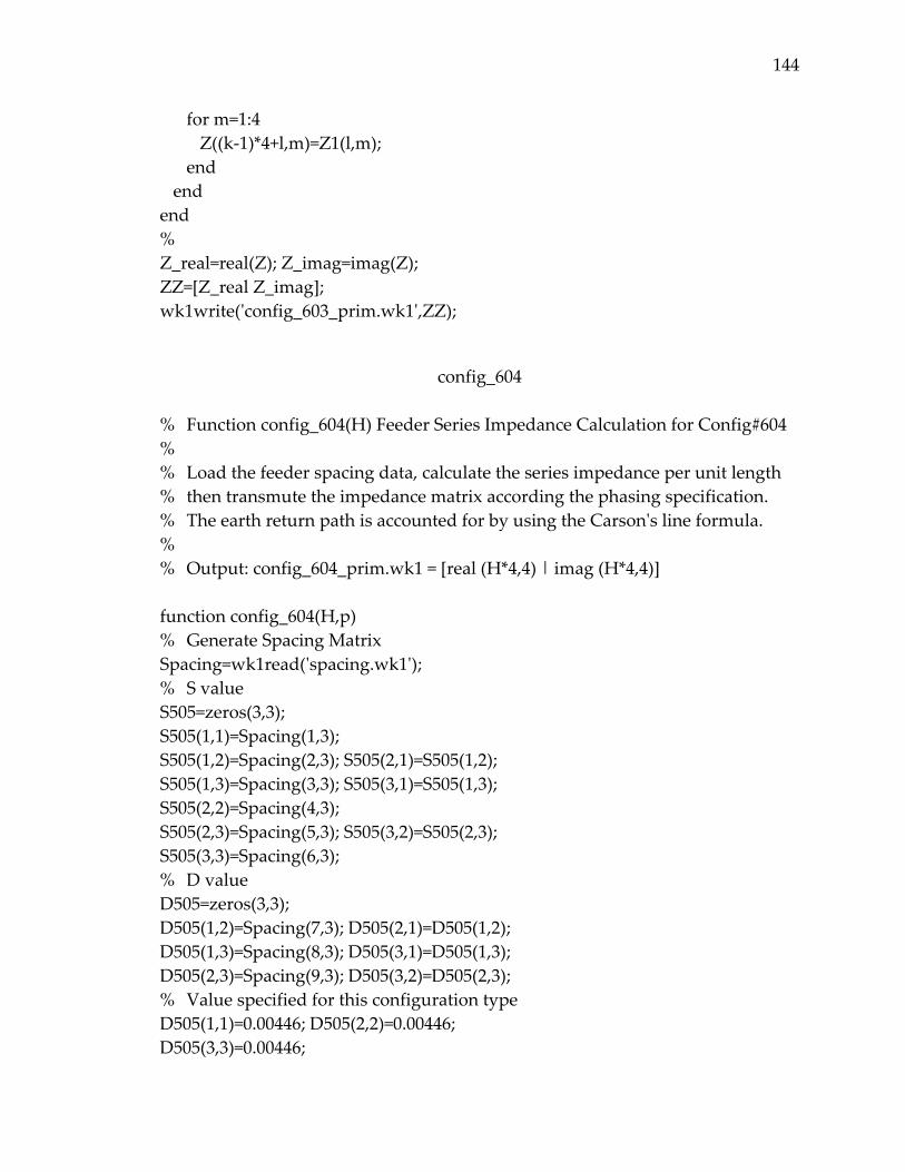
144
for m=1:4 Z((k‐1)*4+l,m)=Z1(l,m); end end end % Z_real=real(Z); Z_imag=imag(Z); ZZ=[Z_real Z_imag]; wk1write(ʹconfig_603_prim.wk1ʹ,ZZ);
config_604
% Function config_604(H) Feeder Series Impedance Calculation for Config#604 % % Load the feeder spacing data, calculate the series impedance per unit length % then transmute the impedance matrix according the phasing specification. % The earth return path is accounted for by using the Carsonʹs line formula. % % Output: config_604_prim.wk1 = [real (H*4,4) | imag (H*4,4)] function config_604(H,p) % Generate Spacing Matrix Spacing=wk1read(ʹspacing.wk1ʹ); % S value S505=zeros(3,3); S505(1,1)=Spacing(1,3); S505(1,2)=Spacing(2,3); S505(2,1)=S505(1,2); S505(1,3)=Spacing(3,3); S505(3,1)=S505(1,3); S505(2,2)=Spacing(4,3); S505(2,3)=Spacing(5,3); S505(3,2)=S505(2,3); S505(3,3)=Spacing(6,3); % D value D505=zeros(3,3); D505(1,2)=Spacing(7,3); D505(2,1)=D505(1,2); D505(1,3)=Spacing(8,3); D505(3,1)=D505(1,3); D505(2,3)=Spacing(9,3); D505(3,2)=D505(2,3); % Value specified for this configuration type D505(1,1)=0.00446; D505(2,2)=0.00446; D505(3,3)=0.00446;
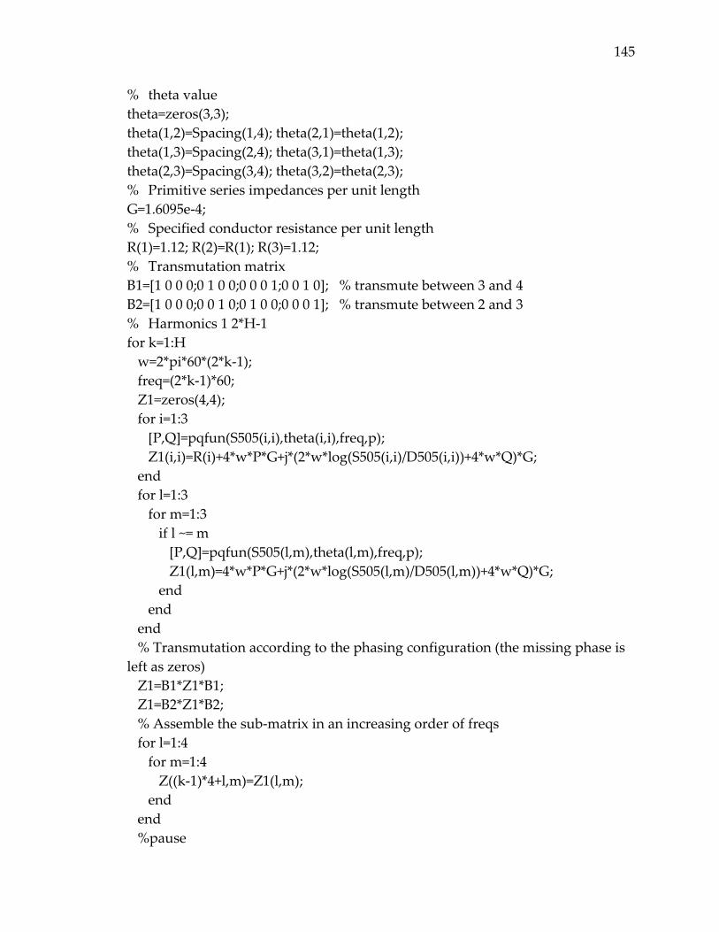
145
% theta value theta=zeros(3,3); theta(1,2)=Spacing(1,4); theta(2,1)=theta(1,2); theta(1,3)=Spacing(2,4); theta(3,1)=theta(1,3); theta(2,3)=Spacing(3,4); theta(3,2)=theta(2,3); % Primitive series impedances per unit length G=1.6095e‐4; % Specified conductor resistance per unit length R(1)=1.12; R(2)=R(1); R(3)=1.12; % Transmutation matrix B1=[1 0 0 0;0 1 0 0;0 0 0 1;0 0 1 0]; % transmute between 3 and 4 B2=[1 0 0 0;0 0 1 0;0 1 0 0;0 0 0 1]; % transmute between 2 and 3 % Harmonics 1 2*H‐1 for k=1:H w=2*pi*60*(2*k‐1); freq=(2*k‐1)*60; Z1=zeros(4,4); for i=1:3 [P,Q]=pqfun(S505(i,i),theta(i,i),freq,p); Z1(i,i)=R(i)+4*w*P*G+j*(2*w*log(S505(i,i)/D505(i,i))+4*w*Q)*G; end for l=1:3 for m=1:3 if l ~= m [P,Q]=pqfun(S505(l,m),theta(l,m),freq,p); Z1(l,m)=4*w*P*G+j*(2*w*log(S505(l,m)/D505(l,m))+4*w*Q)*G; end end end % Transmutation according to the phasing configuration (the missing phase is left as zeros) Z1=B1*Z1*B1; Z1=B2*Z1*B2; % Assemble the sub‐matrix in an increasing order of freqs for l=1:4 for m=1:4 Z((k‐1)*4+l,m)=Z1(l,m); end end %pause
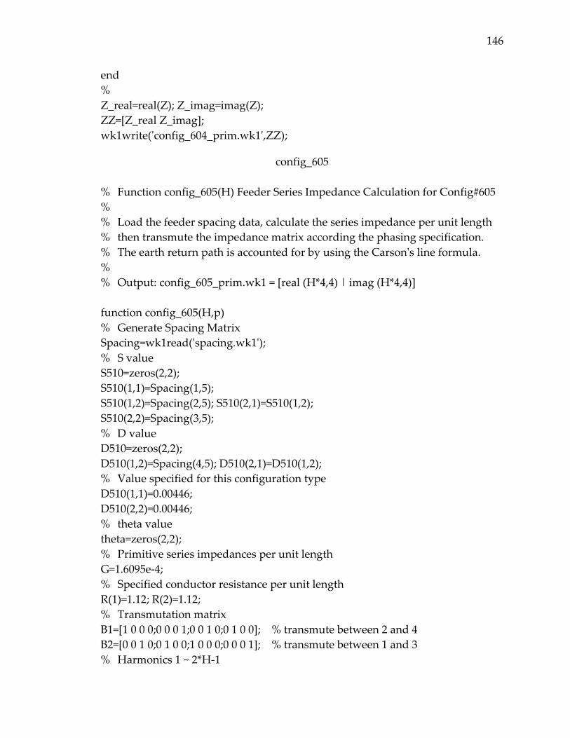
146
end % Z_real=real(Z); Z_imag=imag(Z); ZZ=[Z_real Z_imag]; wk1write(ʹconfig_604_prim.wk1ʹ,ZZ);
config_605
% Function config_605(H) Feeder Series Impedance Calculation for Config#605 % % Load the feeder spacing data, calculate the series impedance per unit length % then transmute the impedance matrix according the phasing specification. % The earth return path is accounted for by using the Carsonʹs line formula. % % Output: config_605_prim.wk1 = [real (H*4,4) | imag (H*4,4)] function config_605(H,p) % Generate Spacing Matrix Spacing=wk1read(ʹspacing.wk1ʹ); % S value S510=zeros(2,2); S510(1,1)=Spacing(1,5); S510(1,2)=Spacing(2,5); S510(2,1)=S510(1,2); S510(2,2)=Spacing(3,5); % D value D510=zeros(2,2); D510(1,2)=Spacing(4,5); D510(2,1)=D510(1,2); % Value specified for this configuration type D510(1,1)=0.00446; D510(2,2)=0.00446; % theta value theta=zeros(2,2); % Primitive series impedances per unit length G=1.6095e‐4; % Specified conductor resistance per unit length R(1)=1.12; R(2)=1.12; % Transmutation matrix B1=[1 0 0 0;0 0 0 1;0 0 1 0;0 1 0 0]; % transmute between 2 and 4 B2=[0 0 1 0;0 1 0 0;1 0 0 0;0 0 0 1]; % transmute between 1 and 3 % Harmonics 1 ~ 2*H‐1

147
for k=1:H w=2*pi*60*(2*k‐1); freq=(2*k‐1)*60; Z1=zeros(4,4); for i=1:2 [P,Q]=pqfun(S510(i,i),theta(i,i),freq,p); Z1(i,i)=R(i)+4*w*P*G+j*(2*w*log(S510(i,i)/D510(i,i))+4*w*Q)*G; end for l=1:2 for m=1:2 if l ~= m [P,Q]=pqfun(S510(l,m),theta(l,m),freq,p); Z1(l,m)=4*w*P*G+j*(2*w*log(S510(l,m)/D510(l,m))+4*w*Q)*G; end end end % Transmutation according to the phasing configuration (the missing phase is left as zeros) Z1=B1*Z1*B1; Z1=B2*Z1*B2; for l=1:4 for m=1:4 Z((k‐1)*4+l,m)=Z1(l,m); end end %pause end % Z_real=real(Z); Z_imag=imag(Z); ZZ=[Z_real Z_imag]; wk1write(ʹconfig_605_prim.wk1ʹ,ZZ);
config_702
% Function config_702 Distribution transformer impedance for config #702 % % Calculate the impedance for the transformer config #702 % Output: config_702_prim.wk1 = [real (4*4) | imag (4*4)]
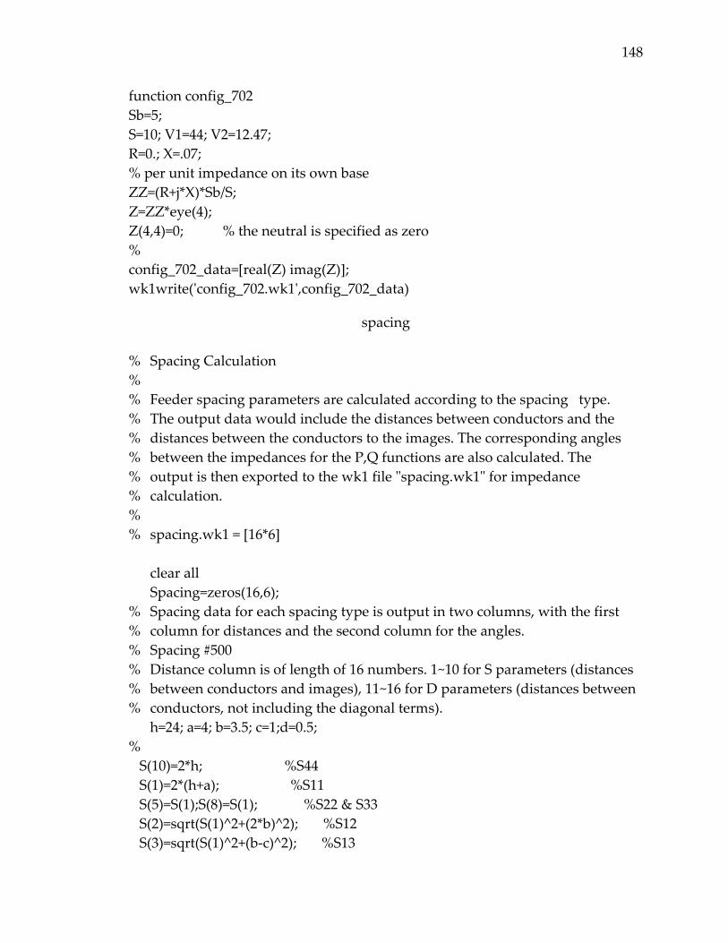
148
function config_702 Sb=5; S=10; V1=44; V2=12.47; R=0.; X=.07; % per unit impedance on its own base ZZ=(R+j*X)*Sb/S; Z=ZZ*eye(4); Z(4,4)=0; % the neutral is specified as zero % config_702_data=[real(Z) imag(Z)]; wk1write(ʹconfig_702.wk1ʹ,config_702_data)
spacing
% Spacing Calculation % % Feeder spacing parameters are calculated according to the spacing type. % The output data would include the distances between conductors and the % distances between the conductors to the images. The corresponding angles % between the impedances for the P,Q functions are also calculated. The % output is then exported to the wk1 file ʺspacing.wk1ʺ for impedance % calculation. % % spacing.wk1 = [16*6] clear all Spacing=zeros(16,6); % Spacing data for each spacing type is output in two columns, with the first % column for distances and the second column for the angles. % Spacing #500 % Distance column is of length of 16 numbers. 1~10 for S parameters (distances % between conductors and images), 11~16 for D parameters (distances between % conductors, not including the diagonal terms). h=24; a=4; b=3.5; c=1;d=0.5; % S(10)=2*h; %S44 S(1)=2*(h+a); %S11 S(5)=S(1);S(8)=S(1); %S22 & S33 S(2)=sqrt(S(1)^2+(2*b)^2); %S12 S(3)=sqrt(S(1)^2+(b‐c)^2); %S13
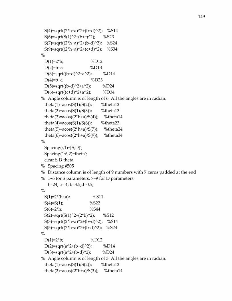
149
S(4)=sqrt((2*h+a)^2+(b+d)^2); %S14 S(6)=sqrt(S(1)^2+(b+c)^2); %S23 S(7)=sqrt((2*h+a)^2+(b‐d)^2); %S24 S(9)=sqrt((2*h+a)^2+(c+d)^2); %S34 % D(1)=2*b; %D12 D(2)=b‐c; %D13 D(3)=sqrt((b+d)^2+a^2); %D14 D(4)=b+c; %D23 D(5)=sqrt((b‐d)^2+a^2); %D24 D(6)=sqrt((c+d)^2+a^2); %D34 % Angle column is of length of 6. All the angles are in radian. theta(1)=acos(S(1)/S(2)); %theta12 theta(2)=acos(S(1)/S(3)); %theta13 theta(3)=acos((2*h+a)/S(4)); %theta14 theta(4)=acos(S(1)/S(6)); %theta23 theta(5)=acos((2*h+a)/S(7)); %theta24 theta(6)=acos((2*h+a)/S(9)); %theta34 % Spacing(:,1)=[S,D]ʹ; Spacing(1:6,2)=thetaʹ; clear S D theta % Spacing #505 % Distance column is of length of 9 numbers with 7 zeros padded at the end % 1~6 for S parameters, 7~9 for D parameters h=24; a= 4; b=3.5;d=0.5; % S(1)=2*(h+a); %S11 S(4)=S(1); %S22 S(6)=2*h; %S44 S(2)=sqrt(S(1)^2+(2*b)^2); %S12 S(3)=sqrt((2*h+a)^2+(b+d)^2); %S14 S(5)=sqrt((2*h+a)^2+(b‐d)^2); %S24 % D(1)=2*b; %D12 D(2)=sqrt(a^2+(b+d)^2); %D14 D(3)=sqrt(a^2+(b‐d)^2); %D24 % Angle column is of length of 3. All the angles are in radian. theta(1)=acos(S(1)/S(2)); %theta12 theta(2)=acos((2*h+a)/S(3)); %theta14

150
theta(3)=acos((2*h+a)/S(5)); %theta24 % Spacing(1:6,3)=Sʹ;Spacing(7:9,3)=Dʹ; Spacing(1:3,4)=thetaʹ; clear S D theta % % Spacing #510 % Distance column is of length of 4 numbers with 12 zeros padded at the end h=24; a=5;d=0.5; % S(1)=2*(h+a); %S11 S(2)=(2*h+a); %S14 S(3)=2*h; %S44 D=a; %D14 % Spacing(1:3,5)=Sʹ;Spacing(4,5)=D; % wk1write(ʹspacing.wk1ʹ,Spacing);
pqfun
% Function: P & Q Constants Evaluation % % [P,Q]=pqfun(S,theta,f,pp) calculate the P&Q constants according to the % Carsonʹs line formulas for both self and mutual impedances. % % f = frequency % pp = earth resistivity % % For self impedance, % Sii = twice the aerial conductor height % theta = 0 % % For mutual impedance, % Sij = distance between the aerial conductor to the image of the other conductor % theta = angle between Sii and Sij function [P,Q]=pqfun(S,theta,f,pp) K=8.565e‐4*S*sqrt(f/pp); P=pi/8‐1/(3*sqrt(2))*K*cos(theta)+K^2/16*cos(2*theta)*(0.6728+log(2/K));

151
Q=‐0.0386+1/2*log(2/K)+1/(3*sqrt(2))*K*cos(theta);
sphr
%Single Phase Rectifier Model function [Iamp,Iang,theta1,theta2,alpha,delta,a,b,c,B]=sphr1(Vth,theta,Rt,Lt,C,Req); H=length(Vth); w=2*pi*60; % Convert the input angle for cosine oriented to sine oriented for l=1:H theta(l)=theta(l)+90; end % Shift the waveform by angle of fund. voltage theta_shift=theta(1); for l=1:H theta_prim=theta(l)‐(2*l‐1)*theta_shift; theta(l)=theta_prim‐floor(theta_prim/360)*360; end %Calculate circuit parameters alpha(1)=Rt/(w*Lt);alpha(2)=1/(w*Lt);alpha(3)=1/(w*C);alpha(4)=1/(w*C*Req); a=‐(alpha(1)+alpha(4))/2; B=alpha(2)*alpha(3)‐(alpha(1)‐alpha(4))^2/4; %Determine real or complex routine if B < 0 Vo_fun=ʹVo_realʹ; is_fun=ʹis_realʹ; isf_fun=ʹisf_realʹ; b=sqrt(‐B); elseif B > 0 Vo_fun=ʹVo_compʹ; is_fun=ʹis_compʹ; isf_fun=ʹisf_compʹ; b=sqrt(B); end % Initial guess 80 degree after the positive going zero‐crossing for a sine wave theta1=70; % Initialize iteration related variables maxiter=100;iter=0; accuracy=0.01;error=100;

152
del=0.0001; options=optimset(ʹTolXʹ,del,ʹDisplayʹ,ʹoffʹ); sphr_err=0; % Iterations start while iter < maxiter & error > accuracy iter=iter+1; % c & delta parameters related to the theta1 for l=1:H h=2*l‐1; delta(l)=theta(l)+h*theta1; end c=c_cal(a,B,alpha,delta); % find the first positive point on the current waveform for i=1:20 is_test=feval(is_fun,i,Vth,delta,alpha,a,b,c); if is_test > 0 break end end % calculate the theta2 with axis shifted to theta1 err=0; while err ~=1 theta2=fzero(is_fun,i,options,Vth,delta,alpha,a,b,c);%theta1,theta2 if theta2 > i err=1; end i=i+1; end theta2=theta2‐floor(theta2/360)*360; % calculate the output voltage at the end of conduction using calculated theta2 Vo=feval(Vo_fun,theta2,Vth,delta,alpha,a,b,c); % shift it back to the source voltage reference theta2=theta2+theta1; % calculate the new theta1 theta1_new=fzero(ʹVdecayʹ,theta1,options,theta2,Vo,Vth,theta,alpha); theta1_new=theta1_new‐floor(theta1_new/360)*360; error=abs(theta1‐theta1_new); theta1=theta1_new; if iter == maxiter sphr_err=1;
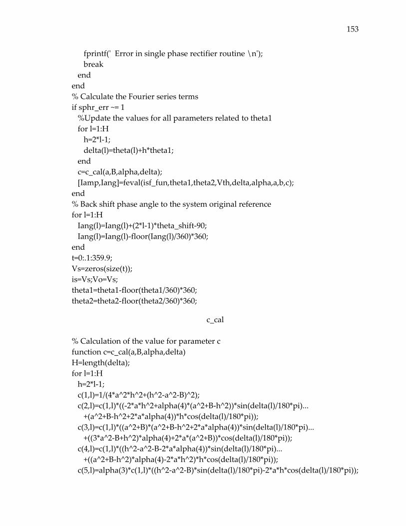
153
fprintf(ʹ Error in single phase rectifier routine \nʹ); break end end % Calculate the Fourier series terms if sphr_err ~= 1 %Update the values for all parameters related to theta1 for l=1:H h=2*l‐1; delta(l)=theta(l)+h*theta1; end c=c_cal(a,B,alpha,delta); [Iamp,Iang]=feval(isf_fun,theta1,theta2,Vth,delta,alpha,a,b,c); end % Back shift phase angle to the system original reference for l=1:H Iang(l)=Iang(l)+(2*l‐1)*theta_shift‐90; Iang(l)=Iang(l)‐floor(Iang(l)/360)*360; end t=0:.1:359.9; Vs=zeros(size(t)); is=Vs;Vo=Vs; theta1=theta1‐floor(theta1/360)*360; theta2=theta2‐floor(theta2/360)*360;
c_cal
% Calculation of the value for parameter c function c=c_cal(a,B,alpha,delta) H=length(delta); for l=1:H h=2*l‐1; c(1,l)=1/(4*a^2*h^2+(h^2‐a^2‐B)^2); c(2,l)=c(1,l)*((‐2*a*h^2+alpha(4)*(a^2+B‐h^2))*sin(delta(l)/180*pi)... +(a^2+B‐h^2+2*a*alpha(4))*h*cos(delta(l)/180*pi)); c(3,l)=c(1,l)*((a^2+B)*(a^2+B‐h^2+2*a*alpha(4))*sin(delta(l)/180*pi)... +((3*a^2‐B+h^2)*alpha(4)+2*a*(a^2+B))*cos(delta(l)/180*pi)); c(4,l)=c(1,l)*((h^2‐a^2‐B‐2*a*alpha(4))*sin(delta(l)/180*pi)... +((a^2+B‐h^2)*alpha(4)‐2*a*h^2)*h*cos(delta(l)/180*pi)); c(5,l)=alpha(3)*c(1,l)*((h^2‐a^2‐B)*sin(delta(l)/180*pi)‐2*a*h*cos(delta(l)/180*pi));
154
c(6,l)=alpha(3)*c(1,l)*(2*a*(a^2+B)*sin(delta(l)/180*pi)+(3*a^2+h^2‐B)*h*cos(delta(l)/180*pi)); c(7,l)=alpha(3)*c(1,l)*(‐2*a*h^2*sin(delta(l)/180*pi)+(a^2+B‐h^2)*h*cos(delta(l)/180*pi)); end
is_comp
% is function with real characteristic roots function is=is_comp(ang,V,delta,alpha,a,b,c); H=length(V); is=0; ang=ang/180*pi; A1=0;A2=0; for l=1:H h=2*l‐1; A1=‐sin(delta(l)/180*pi)‐a*c(2,l)+c(3,l); A2=‐b*c(2,l); isp=sqrt(2)*V(l)*alpha(2)*(c(2,l)*cos(h*ang)+c(4,l)/h*sin(h*ang)); is1=sqrt(2)*alpha(2)*V(l)/b*(A1*sin(b*ang)+A2*cos(b*ang))*exp(a*ang)+isp; is=is+is1; end
is_real
% is function with real characteristic roots function is=is_real(ang,V,delta,alpha,a,b,c); H=length(V); is=0; s1=a+b;s2=a‐b; ang=ang/180*pi; A1=0;A2=0; for l=1:H h=l*2‐1; A1=‐sin(delta(l)/180*pi)‐s1*c(2,l)+c(3,l); A2=sin(delta(l)/180*pi)+s2*c(2,l)‐c(3,l); isp=sqrt(2)*V(l)*alpha(2)*(c(2,l)*cos(h*ang)+c(4,l)/h*sin(h*ang)); is1=sqrt(2)*alpha(2)*V(l)/(2*b)*(A1*exp(s1*ang)+A2*exp(s2*ang))+isp; is=is+is1; end
155
isf_comp
%Fourier series closed‐form solution for real‐roots case function [Iamp,Iang,aa,bb]=isf_comp(theta1,theta2,V,delta,alpha,a,b,c); H=length(V); s1=a+b; s2=a‐b; theta=(theta2‐theta1)/180*pi; delta=delta/180*pi; for m=1:H k=2*m‐1; a1=0;b1=0; a3=a1;a4=a1; b3=b1;b4=b1; T1=1/sqrt(a^2+(b+k)^2);Tang1=angle(a+j*(b+k)); T2=1/sqrt(a^2+(b‐k)^2);Tang2=angle(a+j*(b‐k)); for n=1:H h=2*n‐1; lamida=sqrt(2)*alpha(2)*V(n)/b*sqrt((‐sin(delta(n))‐a*c(2,n)+c(3,n))^2+(b*c(2,n))^2); p=‐sin(delta(n))‐a*c(2,n)+c(3,n);q=‐b*c(2,n); phi=angle(p+j*q); a1=a1+lamida/pi*T1*(exp(a*theta)*sin((b+k)*theta+phi‐Tang1)‐sin(phi‐Tang1))... +lamida/pi*T2*(exp(a*theta)*sin((b‐k)*theta+phi‐Tang2)‐sin(phi‐Tang2)); b1=b1+lamida/pi*T2*(exp(a*theta)*cos((b‐k)*theta+phi‐Tang2)‐cos(phi‐Tang2))... ‐lamida/pi*T1*(exp(a*theta)*cos((b+k)*theta+phi‐Tang1)‐cos(phi‐Tang1)); if n ~= m a3=a3+sqrt(2)*alpha(2)/pi*V(n)*c(2,n)*(sin((h+k)*theta)/(h+k)+sin((h‐k)*theta)/(h‐k)); b3=b3+sqrt(2)*alpha(2)/pi*V(n)*c(2,n)*(cos((h‐k)*theta)/(h‐k)‐cos((h+k)*theta)/(h+k)‐2*k/(h^2‐k^2)); a4=a4+sqrt(2)*alpha(2)/pi*V(n)*c(4,n)/h*(2*h/(h^2‐k^2)‐cos((h+k)*theta)/(h+k)‐cos((h‐k)*theta)/(h‐k)); b4=b4+sqrt(2)*alpha(2)/pi*V(n)*c(4,n)/h*(sin((h‐k)*theta)/(h‐k)‐sin((h+k)*theta)/(h+k)); end end a3=a3+sqrt(2)*alpha(2)/pi*V(m)*c(2,m)*(sin(2*k*theta)/(2*k)+theta); b3=b3+sqrt(2)*alpha(2)/(2*k*pi)*V(m)*c(2,m)*(1‐cos(2*k*theta));
156
a4=a4+sqrt(2)*alpha(2)/(2*k^2*pi)*V(m)*c(4,m)*(1‐cos(2*k*theta)); b4=b4+sqrt(2)*alpha(2)/(k*pi)*V(m)*c(4,m)*(theta‐sin(2*k*theta)/(2*k)); aa(m)=a1+a3+a4; bb(m)=b1+b3+b4; Iamp(m)=abs(aa(m)+j*bb(m))/sqrt(2); ang=angle(bb(m)+j*aa(m))/pi*180‐theta1*k; Iang(m)=ang‐floor(ang/360)*360; if Iang(m) > 180 Iang(m)=Iang(m)‐360; end end
isf_real
%Fourier series closed‐form solution for real‐roots case function [Iamp,Iang,aa,bb]=isf_real(theta1,theta2,V,delta,alpha,a,b,c); H1=900; H=length(V); Vth=zeros(1,H1); delta1=Vth; cc=zeros(7,H1); for l=1:H Vth(l)=V(l); delta1(l)=delta(l); for m=1:7 cc(m,l)=c(m,l); end end V=Vth;delta=delta1;c=cc; s1=a+b; s2=a‐b; a1=0;b1=0; a2=a1;a3=a1;a4=a1; b2=b1;b3=b1;b4=b1; theta=(theta2‐theta1)/180*pi; delta=delta/180*pi; for m=1:H1 k=2*m‐1; a1=0;b1=0; a2=a1;a3=a1;a4=a1;
157
b2=b1;b3=b1;b4=b1; for l=1:H h=2*l‐1; c8=sqrt(2)*alpha(2)*V(l)/(2*b)*(‐sin(delta(l))‐c(2,l)*s1+c(3,l)); c9=sqrt(2)*alpha(2)*V(l)/(2*b)*(sin(delta(l))+c(2,l)*s2‐c(3,l)); a1=a1+2/pi*c8/(s1^2+k^2)*(exp(s1*theta)*(k*sin(k*theta)+s1*cos(k*theta))‐s1); b1=b1+2/pi*c8/(s1^2+k^2)*(exp(s1*theta)*(s1*sin(k*theta)‐k*cos(k*theta))+k); a2=a2+2/pi*c9/(s2^2+k^2)*(exp(s2*theta)*(k*sin(k*theta)+s2*cos(k*theta))‐s2); b2=b2+2/pi*c9/(s2^2+k^2)*(exp(s2*theta)*(s2*sin(k*theta)‐k*cos(k*theta))+k); if l ~= m a3=a3+sqrt(2)*alpha(2)/pi*V(l)*c(2,l)*(sin((h+k)*theta)/(h+k)+sin((h‐k)*theta)/(h‐k)); b3=b3+sqrt(2)*alpha(2)/pi*V(l)*c(2,l)*(cos((h‐k)*theta)/(h‐k)‐cos((h+k)*theta)/(h+k)‐2*k/(h^2‐k^2)); a4=a4+sqrt(2)*alpha(2)/pi*V(l)*c(4,l)/h*(2*h/(h^2‐k^2)‐cos((h+k)*theta)/(h+k)‐cos((h‐k)*theta)/(h‐k)); b4=b4+sqrt(2)*alpha(2)/pi*V(l)*c(4,l)/h*(sin((h‐k)*theta)/(h‐k)‐sin((h+k)*theta)/(h+k)); end end a3=a3+sqrt(2)*alpha(2)/pi*V(m)*c(2,m)*(sin(2*k*theta)/(2*k)+theta); b3=b3+sqrt(2)*alpha(2)/(2*k*pi)*V(m)*c(2,m)*(1‐cos(2*k*theta)); a4=a4+sqrt(2)*alpha(2)/(2*k^2*pi)*V(m)*c(4,m)*(1‐cos(2*k*theta)); b4=b4+sqrt(2)*alpha(2)/(k*pi)*V(m)*c(4,m)*(theta‐sin(2*k*theta)/(2*k)); aa(m)=a1+a2+a3+a4; bb(m)=b1+b2+b3+b4; Iamp(m)=abs(aa(m)+j*bb(m))/sqrt(2); ang=angle(bb(m)+j*aa(m))/pi*180‐theta1*k; Iang(m)=ang‐floor(ang/360)*360; if Iang(m) > 180 Iang(m)=Iang(m)‐360; end end
Vo_comp
% is function with real characteristic roots function Vo=Vo_comp(ang,V,delta,alpha,a,b,c); H=length(V); Vo=0;
158
ang=ang/180*pi; A1=0;A2=0; for l=1:H h=2*l‐1; A1=(a+alpha(1))*sin(delta(l)/180*pi)+alpha(2)*(a*c(5,l)+c(6,l)); A2=b*sin(delta(l)/180*pi)+b*alpha(2)*c(5,l); Vop=sqrt(2)*V(l)*alpha(2)*(‐c(5,l)*cos(h*ang)+c(7,l)/h*sin(h*ang)); V1=sqrt(2)*V(l)/b*(A1*sin(b*ang)+A2*cos(b*ang))*exp(a*ang)+Vop; Vo=Vo+V1; end
Vo_real
% is function with real characteristic roots function Vo=Vo_real(ang,V,delta,alpha,a,b,c); H=length(V); Vo=0; s1=a+b;s2=a‐b; ang=ang/180*pi; A1=0;A2=0; for l=1:H h=2*l‐1; A1=(s1+alpha(1))*sin(delta(l)/180*pi)+alpha(2)*(s1*c(5,l)+c(6,l)); A2=(s2+alpha(1))*sin(delta(l)/180*pi)+alpha(2)*(s2*c(5,l)+c(6,l)); Vop=sqrt(2)*V(l)*alpha(2)*(‐c(5,l)*cos(h*ang)+c(7,l)/h*sin(h*ang)); V1=sqrt(2)*V(l)/(2*b)*(A1*exp(s1*ang)‐A2*exp(s2*ang))+Vop; Vo=Vo+V1; end
Vdecay
% Voltage free‐decaying function function Y=Vdecay(theta1,theta2,Vo,Vth,theta,alpha) H=length(Vth); YY=Vo*exp(alpha(4)*((theta2‐theta1)/180*pi‐pi)); Y11=0; for l=1:H h=2*l‐1; Y1=‐sqrt(2)*Vth(l)*sin(h*theta1/180*pi+theta(l)/180*pi); Y11=Y11+Y1;

159
end Y=YY+Y11;
main
% Multiphase load flow program Main Program % % The load flow solution is obtained through the following iteration scheme. % The system voltages are assumed before the iteration started. In the iteration, % the nodal injection currents are first calculated using the assumed node % voltages and the given load data. Then the branch currents are calculated by % gathering the load injection from the lowest level nodes (branches) toward % the root node (substation). As the currents in the branches direct connected % the root node are obtained, the new node voltages are calculated using the % voltage drops due to the branch currents, from the higher level to lower level. % Thus finishes one iteration. The max power mismatch is calculated within % each iteration. The iteration stops when the mismatch is below the accuracy % requirement or the iteration number is larger than the specification, which % implicates divergence. clear all % System topology line_conf=csvread(ʹLine_data.csvʹ,3); % L1 and L2 are specified in ʹLine_data1.csvʹ, where the L2 node is the further end L1=line_conf(:,2); L2=line_conf(:,3); bus=max(L2); branch=line_conf(:,1); branch_num=max(branch); level=line_conf(:,8); level_num=max(level); bus_type=wk1read(ʹbus_type.wk1ʹ); In=wk1read(ʹIn.wk1ʹ); % Line impedance & Nodal admittance Line_se_data=wk1read(ʹLine_se.wk1ʹ); Node_sh_data=wk1read(ʹNode_sh.wk1ʹ); H=round(length(Line_se_data(:,1))/4); % Change layout of the line impedance and nodal admittance to one frequency per page for l=1:H inde=(l‐1)*4; Line_se(:,:,l)=Line_se_data((inde+1):(inde+4),1:branch_num*4)+j*Line_se_data((inde+1):(inde+4),branch_num*4+1:branch_num*8);

160
Node_sh(:,:,l)=Node_sh_data((inde+1):(inde+4),1:bus*4)+j*Node_sh_data((inde+1):(inde+4),bus*4+1:bus*8); end % Network Ybus ybus_load; % Load data load_data=csvread(ʹLoad_data.csvʹ,4,1); % load information of bus#, load type, number in the same type load_num=length(load_data(:,1)); % load number, may not equal bus number load_p_n=0; load_c_n=0; load_imp_n=0; load_conv_n=0; load_sphr_n=0; for l=1:load_num if load_data(l,3) == 1 | load_data(l,3) == 2 load_p_n=load_p_n+1; load_power=csvread(ʹLoad_power.csvʹ); elseif load_data(l,3) == 3 | load_data(l,3) == 4 load_c_n=load_c_n+1; load_curr=csvread(ʹLoad_curr.csvʹ); elseif load_data(l,3) == 5 | load_data(l,3) == 6 load_imp_n=load_imp_n+1; load_imp=csvread(ʹLoad_imp.csvʹ); elseif load_data(l,3) == 7 load_conv_n=load_conv_n+1; elseif load_data(l,3) == 8 load_sphr_n=load_sphr_n+1; end end % Base variables Sb=5000; % Base power in kVA Vb=4.16; % Base voltage in kV Ib=Sb/sqrt(3)/Vb; % Base current Zb=Vb^2/(Sb/1000); % Base impedance % Normalize load data if load_p_n >= 1 load_power=load_power/Sb; end if load_c_n >= 1 for l=1:load_c_n inde=(l‐1)*6; load_curr(:,inde+1)=load_curr(:,inde+1)/Ib; load_curr(:,inde+3)=load_curr(:,inde+3)/Ib;
161
load_curr(:,inde+5)=load_curr(:,inde+5)/Ib; end end if load_imp_n >= 1 load_imp=load_imp/Zb; end % Converter data if load_conv_n > 0 converter_data_load end % Single phase rectifier data if load_sphr_n > 0 sphr_data_load; end % The specified root node voltage Vroot=zeros(4,H); % Vroot(:,1)=[1.0; 1.0*exp(‐2*pi*j/3); 1.0*exp(2*pi*j/3); 0]; % RMS 1.05 p.u. % The initial assumption for the nodal voltage Vnode=zeros(4,bus,H); % Vnode(1,:,1)=1; Vnode(2,:,1)=exp(‐2*pi*j/3); Vnode(3,:,1)=exp(2*pi*j/3); % Contains unwanted voltage for missing phases % iteration control variables iter=0; maxiter=1000; fund_accuracy=0.001; harm_accuracy=1e‐6; converge=1; % iteration start while iter <= maxiter & converge == 1 iter=iter+1; %Collect load currents at the load terminal bus load_curr_inj; %Collect converter currents if exist if load_conv_n > 0 conv_curr; end %Collect sphr current if exist if load_sphr_n > 0 sphr_curr; end %Branch current calculation branch_curr_cal;

162
%Nodal voltage forward sweep Vnode1=Vnode; %first level for B=1:branch_num if level(B) == 1 for h=1:H Vnode(:,L2(B),h)=Vroot(:,h)‐Line_se(:,((B‐1)*4+1):((B‐1)*4+4))*branch_curr(:,B,h); end end end %higher level for l=2:level_num for B=1:branch_num if level(B) == l for h=1:H Vnode(:,L2(B),h)=Vnode(:,L1(B),h)‐Line_se(:,((B‐1)*4+1):((B‐1)*4+4),h)*branch_curr(:,B,h); end end end end %Convergence check dV=Vnode‐Vnode1; %fundamental err_fund=max(abs(dV(:,:,1))); maxerr_fund=max(err_fund); %harmonic err_harm=zeros(1,H‐1); for h=1:H‐1 err_harm_bus=max(abs(dV(:,:,h+1))); %max error among all phases at same freq. at same bus err_harm(h)=max(err_harm_bus); %max error among all buses at same freq. end maxerr_harm=max(err_harm); Node_vol_mag=abs(Vnode); Node_vol_ang=angle(Vnode)/pi*180; %busout,pause if iter == maxiter

163
if maxerr_fund > fund_accuracy | maxerr_harm > harm_accuracy fprintf(ʹ\nWARNING: Iterative solution did not converge after ʹ) fprintf(ʹ%gʹ, iter), fprintf(ʹ iterations.\n\nʹ) fprintf(ʹPress Enter to terminate the iterations and print the results \nʹ) converge = ‐1; pause, break end elseif iter < maxiter & maxerr_fund < fund_accuracy & maxerr_harm < harm_accuracy converge = 0; end if iter > 2 Vnode=Vnode1+.6*dV; end end if converge ~= 0 tech= (ʹ ITERATIVE SOLUTION DID NOT CONVERGEʹ); else tech=(ʹ Power Flow Solution For The IEEE 13‐Bus Test Systemʹ); end Node_vol_mag=abs(Vnode); Node_vol_ang=angle(Vnode)/pi*180; busout
load_curr_inj
% Subprogram: Regular load current injection % % Const. power, current and impedance load current injection are calculated and collected at each bus load_inj=zeros(4,bus,H); for b=1:bus for l=1:load_num if load_data(l,1) == b if load_data(l,3) == 1 | load_data(l,3) == 2 S1=load_power(load_data(l,4),1)+j*load_power(load_data(l,4),2); S2=load_power(load_data(l,4),3)+j*load_power(load_data(l,4),4); S3=load_power(load_data(l,4),5)+j*load_power(load_data(l,4),6); if load_data(l,3) == 1
164
load_inj(1,b,1)=load_inj(1,b,1)+conj(S1/(Vnode(1,b,1)‐Vnode(4,b,1))); load_inj(2,b,1)=load_inj(2,b,1)+conj(S2/(Vnode(2,b,1)‐Vnode(4,b,1))); load_inj(3,b,1)=load_inj(3,b,1)+conj(S3/(Vnode(3,b,1)‐Vnode(4,b,1))); load_inj(4,b,1)=load_inj(4,b,1)‐(load_inj(1,b,1)+load_inj(2,b,1)+load_inj(3,b,1)); elseif load_data(l,3) == 2 inj1=conj(S1/(Vnode(1,b,1)‐Vnode(2,b,1))); inj2=conj(S2/(Vnode(2,b,1)‐Vnode(3,b,1))); inj3=conj(S3/(Vnode(3,b,1)‐Vnode(1,b,1))); load_inj(1,b,1)=load_inj(1,b,1)+inj1‐inj3; load_inj(2,b,1)=load_inj(2,b,1)+inj2‐inj1; load_inj(3,b,1)=load_inj(3,b,1)+inj3‐inj2; end elseif load_data(l,3) == 3 inde=(load_data(l,4)‐1)*6; for h=1:H load_inj(1,b,h)=load_inj(1,b,h)+load_curr(h,inde+1)*exp(j*load_curr(h,inde+2)/180*pi); load_inj(2,b,h)=load_inj(2,b,h)+load_curr(h,inde+3)*exp(j*load_curr(h,inde+4)/180*pi); load_inj(3,b,h)=load_inj(3,b,h)+load_curr(h,inde+5)*exp(j*load_curr(h,inde+6)/180*pi); load_inj(4,b,h)=load_inj(4,b,h)‐(load_inj(1,b,h)+load_inj(2,b,h)+load_inj(3,b,h)); end elseif load_data(l,3) == 4 inde=(load_data(l,4)‐1)*6; for h=1:H inj1=load_curr(h,inde+1)*exp(j*load_curr(h,inde+2)/180*pi); inj2=load_curr(h,inde+3)*exp(j*load_curr(h,inde+4)/180*pi); inj3=load_curr(h,inde+5)*exp(j*load_curr(h,inde+6)/180*pi); load_inj(1,b,h)=load_inj(1,b,h)+inj1‐inj3; load_inj(2,b,h)=load_inj(2,b,h)+inj2‐inj1; load_inj(3,b,h)=load_inj(3,b,h)+inj3‐inj2; end elseif load_data(l,3) == 5 for h=1:H load_inj(1,b,h)=load_inj(1,b,h)+(Vnode(1,b,h)‐Vnode(4,b,h))/... (real(load_imp(l,1))+j*(2*h‐1)*imag(load_imp(l,1))); load_inj(2,b,h)=load_inj(2,b,h)+(Vnode(2,b,h)‐Vnode(4,b,h))/...
165
(real(load_imp(l,2))+j*(2*h‐1)*imag(load_imp(l,2))); load_inj(2,b,h)=load_inj(3,b,h)+(Vnode(3,b,h)‐Vnode(4,b,h))/... (real(load_imp(l,3))+j*(2*h‐1)*imag(load_imp(l,3))); load_inj(4,b,h)=load_inj(4,b,h)‐(load_inj(1,b,h)+load_inj(2,b,h)+load_inj(3,b,h)); end elseif load_data(l,3) == 6 for h=1:H inj1=(Vnode(1,b,h)‐Vnode(2,b,h))/(real(load_imp(l,1))+j*(2*h‐1)*imag(load_imp(l,1))); inj2=(Vnode(2,b,h)‐Vnode(3,b,h))/(real(load_imp(l,2))+j*(2*h‐1)*imag(load_imp(l,2))); inj1=(Vnode(3,b,h)‐Vnode(1,b,h))/(real(load_imp(l,3))+j*(2*h‐1)*imag(load_imp(l,3))); load_inj(1,b,h)=load_inj(1,b,h)+inj1‐inj3; load_inj(2,b,h)=load_inj(2,b,h)+inj2‐inj1; load_inj(3,b,h)=load_inj(3,b,h)+inj3‐inj2; end end end end end
sphr_curr
% Collect sphr load currents if called for l=1:load_sphr_n sphr_bus=sphr_data(l,1); if sphr_type(l,1) == 1 V1=Vnode(sphr_type(l,2),sphr_bus,:); V2=Vnode(4,sphr_bus,:); Vth=abs(V1‐V2)*240; theta=angle(V1‐V2)/pi*180; [Iamp,Iang,theta1,theta2,alpha,delta,a,b,c,B]=sphr1(Vth,theta,sphr_rth(l),sphr_Lth(l),sphr_cap(l),sphr_req(l)); Iamp=Iamp/Ib/10; for m=1:H load_inj(sphr_type(l,2),sphr_bus,m)=load_inj(sphr_type(l,2),sphr_bus,m)+Iamp(m)*exp(j*Iang(m)/180*pi); load_inj(4,sphr_bus,m)=load_inj(4,sphr_bus,m)‐Iamp(m)*exp(j*Iang(m)/180*pi); end

166
elseif sphr_type(l,1) == 2 V1=Vnode(sphr_type(l,2),sphr_bus,:); V2=Vnode(rem(sphr_type(l,2),3)+1,sphr_bus,:); Vth=abs(V1‐V2)*240; theta=angle(V1‐V2)/pi*180; [Iamp,Iang,theta1,theta2]=sphr1(Vth,theta,sphr_rth(l),sphr_Lth(l),sphr_cap(l),sphr_req(l)); Iamp=Iamp/Ib/10; for m=1:H load_inj(sphr_type(l,2),sphr_bus,m)=load_inj(sphr_type(l,2),sphr_bus,m)+Iamp(m)*exp(j*Iang(m)/180*pi); load_inj(rem(sphr_type(l,2),3)+1,sphr_bus,m)=load_inj(rem(sphr_type(l,2),3)+1,sphr_bus,m)... ‐Iamp(m)*exp(j*Iang(m)/180*pi); end end for m=1:H I_sphr(m,:,l)=[Iamp(m) Iang(m)]; end end
branch_curr_cal
% Subprogram: Calculated branch currents starting from the lowest level % % Total return currents are splitted between neutral and earth according to the voltage equation branch_curr=zeros(4,branch_num,H); curr_res=zeros(branch_num,H); % last level for B=1:branch_num if level(B) == level_num branch_curr(1:3,B,:)=load_inj(1:3,L2(B),:); if L1(B) == 0 V_up(:)=Vroot(4,:); else for h=1:H V_up(h)=Vnode(4,L1(B),h); end end for h=1:H

167
branch_curr(4,B,h)=(V_up(h)‐Line_se(4,(B‐1)*4+1:(B‐1)*4+3,h)*branch_curr(1:3,B,h)... +load_inj(4,L2(B),h)/Node_sh(4,L2(B)*4,h))/(Line_se(4,B*4,h)+1/Node_sh(4,L2(B)*4,h)); % earth current in the last level curr_res(B,h)=branch_curr(1,B,h)+branch_curr(2,B,h)+branch_curr(3,B,h)+branch_curr(4,B,h); end end end % higher level for l=1:level_num‐1 for B=1:branch_num if level(B) == (level_num‐l) return_curr=zeros(1,H); for n=1:branch_num if L1(n) == L2(B) branch_curr(1:3,B,:)=branch_curr(1:3,B,:)+branch_curr(1:3,n,:); for h=1:H return_curr(h)=return_curr(h)+branch_curr(4,n,h); end end end branch_curr(1:3,B,:)=branch_curr(1:3,B,:)+load_inj(1:3,L2(B),:); for h=1:H return_curr(h)=return_curr(h)+load_inj(4,L2(B),h); end if L1(B) == 0 V_up(:)=Vroot(4,:); else for h=1:H V_up(h)=Vnode(4,L1(B),h); end end for h=1:H branch_curr(4,B,h)=(V_up(h)‐Line_se(4,(B‐1)*4+1:(B‐1)*4+3,h)*branch_curr(1:3,B,h)... +return_curr(1,h)/Node_sh(4,L2(B)*4,h))/(Line_se(4,B*4,h)+1/Node_sh(4,L2(B)*4,h)); % earth current
168
curr_res(B,h)=branch_curr(1,B,h)+branch_curr(2,B,h)+branch_curr(3,B,h)+branch_curr(4,B,h); end end end end branch_curr_mag=abs(branch_curr); branch_curr_ang=angle(branch_curr)/pi*180;
busout
% This program prints the power flow solution in a tabulated form % on the screen. fprintf(ʹ\n\nʹ); %disp(tech) fprintf(ʹ Maximum Voltage Mismatch = %g \nʹ, maxerr_fund) fprintf(ʹ Maximum Harmonics Mismatch = %g \nʹ, maxerr_harm) fprintf(ʹ No. of Iterations = %g \n\nʹ, iter) head =[ʹ Bus Voltage THD Voltage THD Voltage THD Voltage THD ʹ ʹ No. TOT RMS % TOT RMS % TOT RMS % TOT RMS % ʹ ʹ A B C N ʹ ʹ ʹ]; disp(head) for n=1:bus fprintf(ʹ %5gʹ, n), [RMS(n,1),THD(n,1)]=harm(Node_vol_mag(1,n,:)); fprintf(ʹ %8.3fʹ, RMS(n,1)), fprintf(ʹ %9.3fʹ, THD(n,1)), [RMS(n,2),THD(n,2)]=harm(Node_vol_mag(2,n,:)); fprintf(ʹ %8.3fʹ, RMS(n,2)), fprintf(ʹ %9.3fʹ, THD(n,2)), [RMS(n,3),THD(n,3)]=harm(Node_vol_mag(3,n,:)); fprintf(ʹ %8.3fʹ, RMS(n,3)), fprintf(ʹ %9.3fʹ, THD(n,3)), [RMS(n,4),THD(n,4)]=harm(Node_vol_mag(4,n,:)); fprintf(ʹ %8.3fʹ, RMS(n,4)), fprintf(ʹ %9.3f\n\nʹ, THD(n,4)) end fprintf(ʹ\nʹ); wk1write(ʹNode_tot.wk1ʹ,RMSʹ) wk1write(ʹTHD.wk1ʹ,THDʹ); for l=1:H

169
loadnode(:,l)=Node_vol_mag(:,2,l); end wk1write(ʹloadfunvol.wk1ʹ,abs(Node_vol_mag(:,:,1)));

REFERENCES
1. Stray Voltage Panel Session, 2006 IEEE PES T&D Conference, Dallas, Texas, May, 2006.
2. IEEE, ANSI/IEEE C2‐2002, The National Electrical Safety Code®, Section 09, IEEE, Inc, 1995.
3. R. Rüdenberg, “Transient Performance of Electric Power Systems, Phenomena in Lumped Networks,” McGraw‐Hill Book Co. Inc., 1950.
4. T. C. Surbrook and N. D.Reese, “System and equipment grounding and their effects on stray voltage,” Proceedings of the National Stray Voltage Symposium., Syracuse, NY, USA, ASAE Publication, 1985, pp. 140‐146
5. L. D. Lillmars and T. C. Surbrook, “Procedures for investigating stray voltage problems on farms,” (Paper presented at ASAE Summer Meeting, Jun 15‐18 1980, San Antonio, TX), American Society of Agricultural Engineers, 1980, 16p
6. R. J., Gustafson, “Understanding and dealing with stray voltage in livestock facilities,” 1985 Rural Electric Power Conference., Springfield, IL, USA, Rural Electric Power Conference, 1985, 19p
7. R. A., Peterson, “Stray voltage research: past, present and future,” 1985 Winter Meeting ‐ American Society of Agricultural Engineers., Chicago, IL, USA, American Society of Agricultural Engineers, 1985, 3p
8. U.S. Department of Agriculture, “Effects of Electrical Voltage/Current on Farm Animals (How to Detect And Remedy Problems),” USDA Agriculture Handbook 696, 1991, December 1991.
9. Public Service Commission of Wisconsin, “Investigation on the Commissionʹs Own Motion Into the Practices, Policies and Procedures Concerning Stray Voltage for Electric Distribution Utilities in Wisconsin,” Docket 05‐EI‐106, January 1989.

171
10. The Science Advisors to the Minnesota Public Utilities Commission, “Proposed Research for Evaluating Possible Electrical Causes of Poor Health and Production in Dairy Cows,” Minnesota Public Utilities Commission, January 1996.
11. Institute of Electrical and Electronics Engineers, IEEE 100, “The authoritative dictionary of IEEE standards terms,” 7th Edition, New York: Standards Information Network, IEEE Press, 2000.
12. F. P. Zupa and J. F. Laidig, “A practical ground potential rise prediction technique for power stations,” IEEE Trans. Power Apparatus and Systems, vol. PAS‐99, no. 1, Jan/Feb, 1980, pp. 207‐216.
13. A. M. Lefcourt, “Behavioral responses of dairy cows subjected to controlled voltages,” Journal of Dairy Science, vol.65, no. 4, 1982, pp. 672‐674.
14. A. M. Lefcourt and R.M. Akers, “Endocrine responses of cows subjected to controlled voltages during milking,” Journal of Dairy Science, vol.65, no. 11, 1982, pp. 2125‐2130.
15. A. M. Lefcourt, R.M. Akers, R.H. Miller and B. Weinland. “Effects of intermittent electrical shock on responses related to milk ejection,” Journal of Dairy Science, vol. 68, no. 2, 1985, pp. 391‐401.
16. Public Service Commission of Wisconsin, “Findings of Fact, Conclusion of Law, And Order,” Docket 05‐EI‐115, January 1996.
17. National Institute for Occupational Safety and Health, “Worker Death by Electrocution, A Summery of NIOSH Surveillance and Investigative Findings,” U.S. Department of Health and Human Services, May, 1998.
18. International Electrotechnical Commission, “Information technology equipment‐Safety‐Part 1: General requirements,” IEC Standard 60950‐1, Ed. 2, 2005.
19. T. Q. Tran, Larry E. Conrad and Brian K. Stallman, “Electric shock and elevated EMF levels due to triplen harmonics,” IEEE Trans. Power Delivery, vol. 11, no. 2, April 1996, pp. 1041‐1049.
20. E. Clarke, “Circuit Analysis of A‐C Power Systems, Volume I: Symmetrical and Related Components,” McGraw‐Hill Book Company, Inc., 1933.
172
21. C. F. Wagner and R. D. Evans, “Symmetrical Components,” McGraw‐Hill Book Com. Inc., 1933.
22. W. D. Stevenson, Jr. and J. J. Grainger, “Power System Analysis,” McGraw‐Hill, Inc. 1994.
23. J. R. Carson, “Wave propagation in overhead wires with ground return,” Bell System Tech. Journal, vol. 5, 1926, pp. 539‐554.
24. P. M. Anderson, “Analysis of Faulted Power System,” Ames, Iowa: Iowa State University Press, 1973.
25. A. Deri, G. Tevan, A. Semlyen, A. Castanheira, “A simplified model for homogeneous and multi‐layer earth return,” IEEE Trans. Power Apparatus And Systems, vol. PAS‐100, no. 8, Aug. 1981, pp. 3686‐3693.
26. D. G. Triantafyllidis, G. K. Papagiannis, D. P. Labridis, “Calculation of overhead transmission line impedances: a finite element approach,” IEEE Trans. Power Delivery, vol. 14, no. 1, Jan. 1999, pp. 287‐293.
27. John M. Undrill and Roger E. Clayton, “Distribution line performance with imperfect grounding,” IEEE Trans. Industry Application, vol. 34, no. 5, Sep. 1988, pp. 805‐811.
28. R. E. McCotter, H. A. Smolleck, S. J. Ranade and W. H. Kersting, “An investigation of the fundamental‐frequency impedance of a single‐phase distribution lateral,” IEEE Trans. Power Delivery, vol. PWRD‐1, no. 1, Jan. 1986, pp. 232‐238.
29. J. B. Ward and H. W. Hale, “Digital computer solution of power‐flow problems,” AIEE Trans. Power Apparatus and Systems, vol. 75, June 1956, pp. 398‐404.
30. R. Berg, Jr., E. S. Hawkins and W. W. Pleines, “Mechanised calculation of unbalanced load flow for radial distribution circuits,” IEEE Trans. Power Apparatus and System, vol. PAS‐86, April 1967, pp. 415‐421.
31. W. H. Kersting and D. L. Mendive, “An application of ladder network theory to the solution of three phase radial load‐flow problems,” Proc. IEEE PES Winter Meeting, New York, 1976, IEEE Paper No. A76 044‐8.
173
32. D. I. H. Sun, S. Abe, R. R. Shoultz, M. S. Chen, P. Eichenberger and D. Farris, “Calculation of energy losses in a distribution system,” IEEE Trans. Power Apparatus and Systems, vol. PAS‐99, July/August 1980, pp. 1347‐1356.
33. D. Shirmohammadi, H. W. Hong, A. Semlyen and G. X. Luo, “A compensation‐based power flow method for weakly meshed distribution and transmission networks,” IEEE Trans. Power Systems, vol. 3, no. 2, May 1988, pp. 753‐762.
34. G. X. Luo and A. Semlyen, “Efficient load flow for large weakly meshed networks,” IEEE Trans. Power Systems, vol. 5, no. 4, Nov. 1990, pp. 1309‐1316.
35. C. S. Cheng and D. Shirmohammadi, “A three‐phase power flow method for real‐time distribution system analysis,” IEEE Trans. Power Systems, vol. 10, no. 2, May 1995, pp. 671‐679.
36. Tsai‐Hsiang Chen, Mo‐Shing Chen, Kab‐Ju Hwang, Paul Kotas and Elie A. Chebli, “ Distribution system power flow analysis – a rigid approach,” IEEE Trans. Power Delivery, vol. 6, no. 3, July 1991, pp. 1146‐1152.
37. Tsai‐Hsiang Chen, Mo‐Shing Chen, Toshio Inoue, Paul Kotas and Elie A. Chebli, “Three‐phase cogenerator and transformer models for distribution system analysis,” IEEE Trans. Power Delivery, vol. 6, no. 4, Oct. 1991, pp. 1671‐1678.
38. M. S. Srinivas, J. Nanda, M. L. Kothari, “On some aspects of distribution load flow,” Pro. IEEE TENCON 98, vol. II, pp. 510‐513.
39. W. Xu, “Component modeling issues for power quality assessment (invited paper for a power quality tutorial series),” IEEE Power Engineering Review, vol. 21, no. 11, Nov. 2001, pp. 12‐15+17.
40. IEEE Harmonics Modeling and Simulation Task Force, “Modeling and simulation of the propagation of harmonics in electric power networks: part I,” IEEE Trans. Power Delivery, vol. 11, no. 1, Jan. 1996, pp. 452‐465.
41. T. J. Densen, P. S. Bodger and J. Arrillaga, “Three–phase transmission system for harmonic penetration studies,” IEEE Trans. Power Apparatus and Systems, vol. PAS‐103, Feb. 1984, pp. 310‐317.
174
42. D. Xia and G. T. Heydt, “Harmonic power flow studies, Part I and II,” IEEE Trans. Power Apparatus and Systems, vol. PAS‐101, June 1982, pp. 1257‐1270.
43. W. Xu, J. R. Marti and H. W. Dommel, “A multiphase harmonic load flow solution technique,” IEEE Trans. Power Systems, vol. 6, Feb. 1991, pp. 174‐182.
44. Y. Wang and S. Liu, “A review of methods for calculation of frequency–dependent impedance of overhead power transmission lines,” Proc. Natl. Sci. Counc. Taiwan, vol. 25, no. 6, 2001, pp. 329–338.
45. IEEE, “IEEE Recommended Practice for Grounding of Industrial and Commercial Power Systems (Green Book),” IEEE Standard 142 – 1991.
46. A. Mansoor, W. M. Grady, A. H. Chowdhury and M. J. Samotyj, “An investigation of harmonics attenuation and diversity among distributed single‐phase power electronic loads,” IEEE Trans. Power Delivery, vol. 10, no. 1, Jan. 1995, pp. 467‐473.
47. A. Mansoor, W. M. Grady, R. S. Thallam, M. T. Doyle, S. D. Krein and M. J. Samotyj, “Effect of supply voltage harmonics on the input current of single‐phase diode bridge rectifier loads,” IEEE Trans. Power Delivery, vol. 10, no. 3, July 1995, pp. 1416‐1422.
48. W. Kersting, “Radial distribution test feeders,” Proceedings. IEEE PES T&D Conf., vol. 2, Winter Meeting, 2001, pp. 908‐912.
49. W. H. Kersting, “Distribution System Modeling and Analysis,” CRC Press, 2002
50. W. Xu, “Status and future directions of power system harmonic analysis,” Pro. IEEE Power Engineering Society General Meeting, vol. 1, 2004, pp. 756‐761.