Embed Size (px)
Citation preview
ECOLE NORMALE SUPERIEURE DE LYON
observingdescribing
representing
Elements of time-frequency analysis
Patrick Flandrin
CNRS & Ecole Normale Superieure de Lyon
Patrick Flandrin Elements of time-frequency analysis

observingdescribing
representingexamples
observing
Patrick Flandrin Elements of time-frequency analysis
observingdescribing
representingexamples
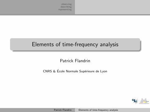
“chirps”
Waves and vibrations — Bird songs, bats , music(“glissando”), speech, “whistling atmospherics”, tidal waves,
gravitational waves , wide-band impulses propagating in a dispersivemedium, pendulum , diapason (string, pipe) with time-varyinglength, vibroseismics, radar, sonar, Doppler effect . . .
Biology and medicine — EEG (epilepsy), uterine EMG(contractions),. . .
Disorder and critical phenomena — Coherent structures inturbulence, accumulation of earthquake precursors,“speculative bubbless” prior a financial crash,. . .
Mathematical special functions — Weierstrass, Riemann . . .
Patrick Flandrin Elements of time-frequency analysis

observingdescribing
representing
chirpsinstantaneous descriptorsnoisetowards “time-frequency”
describing
Patrick Flandrin Elements of time-frequency analysis
observingdescribing
representing
chirpsinstantaneous descriptorsnoisetowards “time-frequency”
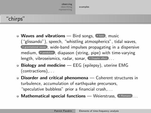
definition
Definition
A “chirp” is any complex-valued signal readingx(t) = a(t) exp{iϕ(t)}, where a(t) ≥ 0 is a low-pass amplitudewhose evolution is slow as compared to the phase oscillations ϕ(t).
Slow evolution? — Usual heuristic conditions assume that:
1 |a(t)/a(t)| � |ϕ(t)|: the amplitude is alomost constant atthe scale of a pseudo-period T (t) = 2π/|ϕ(t)|.
2 |ϕ(t)|/ϕ2(t) � 1: the pseudo-period T (t) is itself slowlyvarying from one oscillation to the enxt.
Patrick Flandrin Elements of time-frequency analysis
observingdescribing
representing
chirpsinstantaneous descriptorsnoisetowards “time-frequency”
modulations
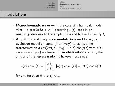
Monochromatic wave — In the case of a harmonic modelx(t) = a cos(2πf0t + ϕ0), observing x(t) leads in anunambiguous way to the amplitude a and to the frequency f0.
Amplitude and frequency modulations — Moving to anevolutive model amounts (intuitively) to achieve thetransformation a cos(2πf0t + ϕ0) → a(t) cos ϕ(t) with a(t)variable and ϕ(t) nonlinear. In an observation context, theunicity of the representation is however lost since
a(t) cos ϕ(t) =
[a(t)
b(t)
][b(t) cos ϕ(t)] =: a(t) cos ϕ(t)
for any function 0 < b(t) < 1.
Patrick Flandrin Elements of time-frequency analysis
observingdescribing
representing
chirpsinstantaneous descriptorsnoisetowards “time-frequency”
Fresnel
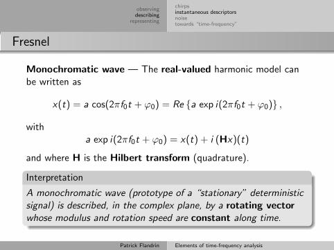
Monochromatic wave — The real-valued harmonic model canbe written as
x(t) = a cos(2πf0t + ϕ0) = Re {a exp i(2πf0t + ϕ0)} ,
witha exp i(2πf0t + ϕ0) = x(t) + i (Hx)(t)
and where H is the Hilbert transform (quadrature).
Interpretation
A monochromatic wave (prototype of a “stationary” deterministicsignal) is described, in the complex plane, by a rotating vectorwhose modulus and rotation speed are constant along time.
Patrick Flandrin Elements of time-frequency analysis
observingdescribing
representing
chirpsinstantaneous descriptorsnoisetowards “time-frequency”
instantaneous amplitude and frequency
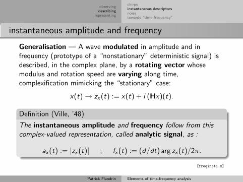
Generalisation — A wave modulated in amplitude and infrequency (prototype of a “nonstationary” deterministic signal) isdescribed, in the complex plane, by a rotating vector whosemodulus and rotation speed are varying along time,complexification mimicking the “stationary” case:
x(t) → zx(t) := x(t) + i (Hx)(t).
Definition (Ville, ’48)
The instantaneous amplitude and frequency follow from thiscomplex-valued representation, called analytic signal, as :
ax(t) := |zx(t)| ; fx(t) := (d/dt) arg zx(t)/2π.
[freqinst1.m]
Patrick Flandrin Elements of time-frequency analysis
observingdescribing
representing
chirpsinstantaneous descriptorsnoisetowards “time-frequency”
limitations
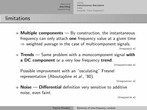
Multiple components — By construction, the instantaneousfrequency can only attach one frequency value at a given time⇒ weighted average in the case of multicomponent signals.
[freqinst2.m]
Trends — Same problem with a monocomponent signal witha DC component or a very low frequency trend.
[freqinsttrend.m]
Possible improvement with an “osculating” Fresnelrepresentation (Aboutajdine et al., ’80).
[freqinstosc.m]
Noise — Differential definition very sensitive to additivenoise, even faint.
[freqinst1b.m]
Patrick Flandrin Elements of time-frequency analysis

observingdescribing
representing
chirpsinstantaneous descriptorsnoisetowards “time-frequency”
stationarity
Definition
A process {x(t), t ∈ R} is said to be (second order) stationary ifits statistical properties (of orders 1 and 2) are independent ofsome absolute time.
Mean value — The expectation E{x(t)} is constant (→ 0)
Covariance — The covariance functionrx(t, t
′) := E{x(t) x(t ′)} is such that
rx(t, t′) =: γx(t − t ′).
Patrick Flandrin Elements of time-frequency analysis
observingdescribing
representing
chirpsinstantaneous descriptorsnoisetowards “time-frequency”
spectral representation
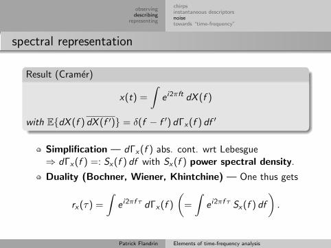
Result (Cramer)
x(t) =
∫e i2πft dX (f )
with E{dX (f ) dX (f ′)} = δ(f − f ′) dΓx(f ) df ′
Simplification — dΓx(f ) abs. cont. wrt Lebesgue⇒ dΓx(f ) =: Sx(f ) df with Sx(f ) power spectral density.
Duality (Bochner, Wiener, Khintchine) — One thus gets
rx(τ) =
∫e i2πf τ dΓx(f )
(=
∫e i2πf τ Sx(f ) df
).
Patrick Flandrin Elements of time-frequency analysis
observingdescribing
representing
chirpsinstantaneous descriptorsnoisetowards “time-frequency”
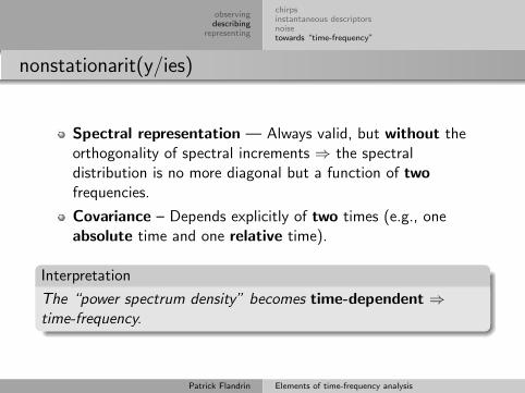
nonstationarit(y/ies)
Spectral representation — Always valid, but without theorthogonality of spectral increments ⇒ the spectraldistribution is no more diagonal but a function of twofrequencies.
Covariance – Depends explicitly of two times (e.g., oneabsolute time and one relative time).
Interpretation
The “power spectrum density” becomes time-dependent ⇒time-frequency.
Patrick Flandrin Elements of time-frequency analysis
observingdescribing
representing
chirpsinstantaneous descriptorsnoisetowards “time-frequency”
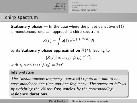
chirp spectrum
Stationary phase — In the case where the phase derivative ϕ(t)is monotonous, one can approach a chirp spectrum
X (f ) =
∫a(t) e i(ϕ(t)−2πft) dt
by its stationary phase approximation X (f ), leading to
|X (f )| ∝ a(ts) |ϕ(ts)|−1/2,
with ts such that ϕ(ts) = 2πf .
Interpretation
The “instantaneous frequency” curve ϕ(t) puts in a one-to-onecorrespondence one time and one frequency. The spectrum followsby weighting the visited frequencies by the correspondingresidence durations.
Patrick Flandrin Elements of time-frequency analysis
observingdescribing
representing
chirpsinstantaneous descriptorsnoisetowards “time-frequency”
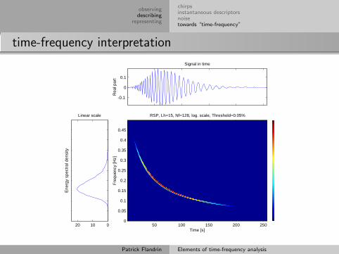
time-frequency interpretation
01020
Linear scale
Ene
rgy
spec
tral
den
sity
-0.1
0
0.1
Rea
l par
t
Signal in time
RSP, Lh=15, Nf=128, log. scale, Threshold=0.05%
Time [s]
Fre
quen
cy [H
z]
50 100 150 200 2500
0.05
0.1
0.15
0.2
0.25
0.3
0.35
0.4
0.45
Patrick Flandrin Elements of time-frequency analysis

observingdescribing
representing
time-frequency, from Fourier to Wignerbeyond Wignerthe stochastic caselocalizationtime-frequency decisions
representing
Patrick Flandrin Elements of time-frequency analysis
observingdescribing
representing
time-frequency, from Fourier to Wignerbeyond Wignerthe stochastic caselocalizationtime-frequency decisions
intuition
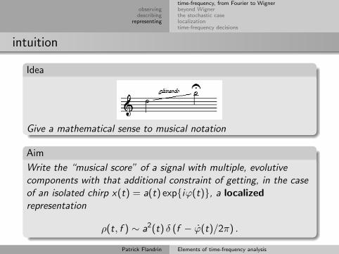
Idea
Give a mathematical sense to musical notation
Aim
Write the “musical score” of a signal with multiple, evolutivecomponents with that additional constraint of getting, in the caseof an isolated chirp x(t) = a(t) exp{iϕ(t)}, a localizedrepresentation
ρ(t, f ) ∼ a2(t) δ (f − ϕ(t)/2π) .
Patrick Flandrin Elements of time-frequency analysis
observingdescribing
representing
time-frequency, from Fourier to Wignerbeyond Wignerthe stochastic caselocalizationtime-frequency decisions
local methods and localization
The example of the short-time FT — One defines thelocal quantity
F(h)x (t, f ) =
∫x(s) h(s − t) e−i2πfs ds,
where h(t) is some short-time observation window.
Measurement — The representation results from aninteraction between the signal and a measurement device(the window h(t)).
Trade-off — A short window favors the “resolution” in timeat the expense of the “resolution” in frequency, and vice-versa.
[spectrodemo.m]
Patrick Flandrin Elements of time-frequency analysis

observingdescribing
representing
time-frequency, from Fourier to Wignerbeyond Wignerthe stochastic caselocalizationtime-frequency decisions
adaptation
Chirps — Adaptation to pulses if h(t) → δ(t) and to tonesif h(t) → 1 ⇒ adapting the analysis to arbitrary chirpssuggests to make h(t) (locally) depending on the signal.
Linear chirp — In the linear case fx(t) = f0 + αt, theequivalent frequency width δfS of the spectrogram
S(h)x (t, f ) := |F (h)
x (t, f )|2 behaves as:
δfS ≈√
1
δt2h
+ α2 δt2h
for a window h(t) with an equivalent time width δth ⇒minimum for δth ≈ 1/
√α (but α unknown. . . ).
Patrick Flandrin Elements of time-frequency analysis
observingdescribing
representing
time-frequency, from Fourier to Wignerbeyond Wignerthe stochastic caselocalizationtime-frequency decisions
self-adaptation and Wigner-Ville distribution
Matched filtering — If one takes for the window h(t) thetime-reversed signal x−(t) := x(−t), one readily gets that
F(x−)x (t, f ) = Wx(t/2, f /2)/2, where
Wx(t, f ) :=
∫x(t + τ/2) x(t − τ/2) e−i2πf τ dτ
is the Wigner-Ville Distribution (Wigner, ’32; Ville, ’48).
Linear chirps — The WVD perfectly localizes on straightlines of the plane:
x(t) = exp{i2π(f0t+αt2/2)} ⇒ Wx(t, f ) = δ (f − (f0 + αt)) .
Remark — Localization via self-adaptation leads to aquadratic transformation (energy distribution).
Patrick Flandrin Elements of time-frequency analysis
observingdescribing
representing
time-frequency, from Fourier to Wignerbeyond Wignerthe stochastic caselocalizationtime-frequency decisions
interpretation
Mirror symmetry — Indexing the analyzed signalwrt a localframe as xt(s) := x(s + t), one gets :
Wx(t, f ) :=
∫ [xt(+τ/2) xt(−τ/2)
]e−i2πf τ dτ,
[WVdemo.m]
Phase signal — If xt(s) = exp{iϕt(s)}, Wx(t, f ) is, as afunction of t, the FT od a phase signalΦt(τ) := ϕt(+τ/2)− ϕt(−τ/2), with “instantaneousfrequency”
fxt (τ) =1
2π
∂
∂τΦt(τ) =
1
2[fxt (+τ/2) + fxt (−τ/2)]
Localization — It follows that fxt (τ) = f0 if fxt (τ) = f0 + α τ ,for any modulation rate α.
[spectrovsWV.m]
Patrick Flandrin Elements of time-frequency analysis
observingdescribing
representing
time-frequency, from Fourier to Wignerbeyond Wignerthe stochastic caselocalizationtime-frequency decisions
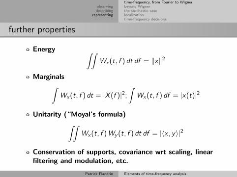
further properties
Energy ∫∫Wx(t, f ) dt df = ‖x‖2
Marginals∫Wx(t, f ) dt = |X (f )|2;
∫Wx(t, f ) df = |x(t)|2
Unitarity (“Moyal’s formula)∫∫Wx(t, f ) Wy (t, f ) dt df = |〈x , y〉|2
Conservation of supports, covariance wrt scaling, linearfiltering and modulation, etc.
Patrick Flandrin Elements of time-frequency analysis
observingdescribing
representing
time-frequency, from Fourier to Wignerbeyond Wignerthe stochastic caselocalizationtime-frequency decisions
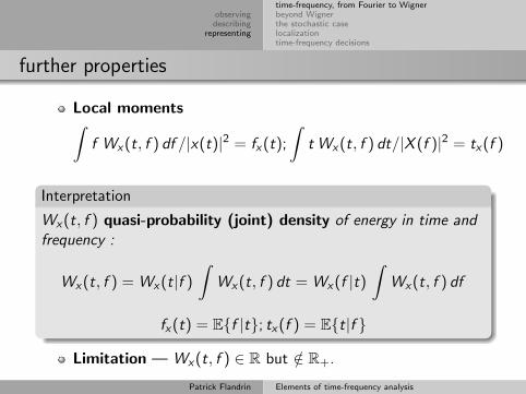
further properties
Local moments∫f Wx(t, f ) df /|x(t)|2 = fx(t);
∫t Wx(t, f ) dt/|X (f )|2 = tx(f )
Interpretation
Wx(t, f ) quasi-probability (joint) density of energy in time andfrequency :
Wx(t, f ) = Wx(t|f )
∫Wx(t, f ) dt = Wx(f |t)
∫Wx(t, f ) df
fx(t) = E{f |t}; tx(f ) = E{t|f }
Limitation — Wx(t, f ) ∈ R but /∈ R+.
Patrick Flandrin Elements of time-frequency analysis
observingdescribing
representing
time-frequency, from Fourier to Wignerbeyond Wignerthe stochastic caselocalizationtime-frequency decisions
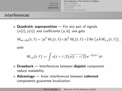
interferences
Quadratic superposition — For any pair of signals{x(t), y(t)} and coefficients (a, b), one gets
Wax+by (t, f ) = |a|2 Wx(t, f )+|b|2 Wy (t, f ) +2 Re{a b Wx ,y (t, f )
},
with
Wx ,y (t, f ) :=
∫x(t + τ/2) y(t − τ/2) e−i2πf τ dτ
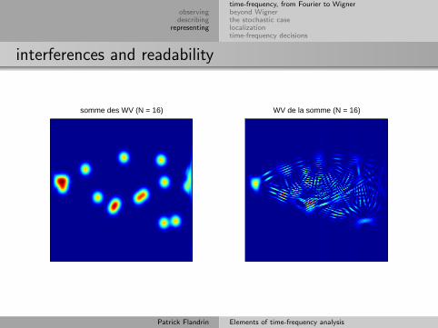
Drawback — Interferences between disjoint componentreduce readability.
Advantage — Inner interferences between coherentcomponents guarantee localization.
Patrick Flandrin Elements of time-frequency analysis

observingdescribing
representing
time-frequency, from Fourier to Wignerbeyond Wignerthe stochastic caselocalizationtime-frequency decisions
interferences
Janssen’s formula (Janssen, ’81) — It follows fromtheunitarity of Wx(t, f ) that:
|Wx(t, f )|2 =
∫∫Wx
(t +
τ
2, f +
ξ
2
)Wx
(t − τ
2, f − ξ
2
)dτ dξ
Geometry (Hlawatsch & F., ’85) — Contributions locatedin any two points of the plane plan interfere to create a thirdcontribution
1 midway of the segment joining the two components2 oscillating (positive and negativ values) in a direction
perpendicular to this segment3 with a “frequency” proportional to their “time-frequency
distance”.
[WV2trans.m, WVinterf.m]
Patrick Flandrin Elements of time-frequency analysis
observingdescribing
representing
time-frequency, from Fourier to Wignerbeyond Wignerthe stochastic caselocalizationtime-frequency decisions
interferences and readability
somme des WV (N = 16) WV de la somme (N = 16)
Patrick Flandrin Elements of time-frequency analysis

observingdescribing
representing
time-frequency, from Fourier to Wignerbeyond Wignerthe stochastic caselocalizationtime-frequency decisions
interferences and localization
sum(WV) (N = 16) WV(sum) (N = 16)
Patrick Flandrin Elements of time-frequency analysis
observingdescribing
representing
time-frequency, from Fourier to Wignerbeyond Wignerthe stochastic caselocalizationtime-frequency decisions
classes of quadratic distributions
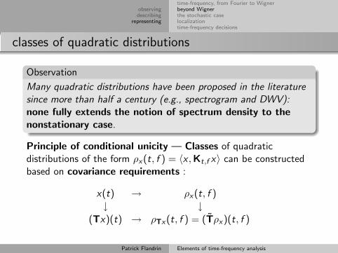
Observation
Many quadratic distributions have been proposed in the literaturesince more than half a century (e.g., spectrogram and DWV):none fully extends the notion of spectrum density to thenonstationary case.
Principle of conditional unicity — Classes of quadraticdistributions of the form ρx(t, f ) = 〈x ,Kt,f x〉 can be constructedbased on covariance requirements :
x(t) → ρx(t, f )↓ ↓
(Tx)(t) → ρTx(t, f ) = (Tρx)(t, f )
Patrick Flandrin Elements of time-frequency analysis
observingdescribing
representing
time-frequency, from Fourier to Wignerbeyond Wignerthe stochastic caselocalizationtime-frequency decisions
classes of quadratic distributions
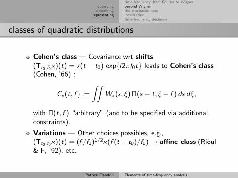
Cohen’s class — Covariance wrt shifts(Tt0,f0x)(t) = x(t − t0) exp{i2πf0t} leads to Cohen’s class(Cohen, ’66) :
Cx(t, f ) :=
∫∫Wx(s, ξ) Π(s − t, ξ − f ) ds dξ,
with Π(t, f ) “arbitrary” (and to be specified via additionalconstraints).
Variations — Other choices possibles, e.g.,(Tt0,f0x)(t) = (f /f0)
1/2x(f (t − t0)/f0) → affine class (Rioul& F, ’92), etc.
Patrick Flandrin Elements of time-frequency analysis
observingdescribing
representing
time-frequency, from Fourier to Wignerbeyond Wignerthe stochastic caselocalizationtime-frequency decisions
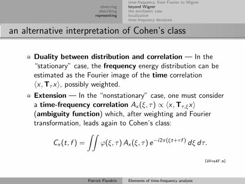
an alternative interpretation of Cohen’s class
Duality between distribution and correlation — In the“stationary” case, the frequency energy distribution can beestimated as the Fourier image of the time correlation〈x ,Tτx〉, possibly weighted.
Extension — In the “nonstationary” case, one must considera time-frequency correlation Ax(ξ, τ) ∝ 〈x ,Tτ,ξx〉(ambiguity function) which, after weighting and Fouriertransformation, leads again to Cohen’s class:
Cx(t, f ) =
∫∫ϕ(ξ, τ) Ax(ξ, τ) e−i2π(ξt+τ f ) dξ dτ.
[WVvsAF.m]
Patrick Flandrin Elements of time-frequency analysis
observingdescribing
representing
time-frequency, from Fourier to Wignerbeyond Wignerthe stochastic caselocalizationtime-frequency decisions
why “Cohen-type” classes?
Unification — Specifying a kernel (i.e., Π(t, f )) defines adistribution: unifying framework or most propositions of theliterature (Wigner-Ville, spectrogram, Page, Levin, Rihaczek,etc.).
Parameterization — Properties of a distribution are directlyconnected with admissibility conditions of the associatedkernel ⇒ simplified possibility of evaluation and design.
Patrick Flandrin Elements of time-frequency analysis

observingdescribing
representing
time-frequency, from Fourier to Wignerbeyond Wignerthe stochastic caselocalizationtime-frequency decisions
an example of definition
Spectrogram — If we consider the case of the spectrogram withwindow h(t), one can write:
S(h)x (t, f ) =
∣∣∣∫ x(s) h(s − t) e−i2πfs ds∣∣∣2
= |〈x ,Tt,f h〉|2=
∫∫Wx(s, ξ) WTt,f h(s, ξ) ds dξ
=∫∫
Wx(s, ξ) Wh(s − t, ξ − f ) ds dξ
⇒ a spectrogram is a member of Cohen’s class, with kernel
Π(t, f ) = Wh(t, f )
Patrick Flandrin Elements of time-frequency analysis
observingdescribing
representing
time-frequency, from Fourier to Wignerbeyond Wignerthe stochastic caselocalizationtime-frequency decisions
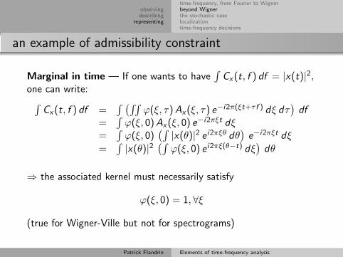
an example of admissibility constraint
Marginal in time — If one wants to have∫
Cx(t, f ) df = |x(t)|2,one can write:∫
Cx(t, f ) df =∫ (∫∫
ϕ(ξ, τ) Ax(ξ, τ) e−i2π(ξt+τ f ) dξ dτ)
df=
∫ϕ(ξ, 0) Ax(ξ, 0) e−i2πξt dξ
=∫
ϕ(ξ, 0)(∫|x(θ)|2 e i2πξθ dθ
)e−i2πξt dξ
=∫|x(θ)|2
(∫ϕ(ξ, 0) e i2πξ(θ−t) dξ
)dθ
⇒ the associated kernel must necessarily satisfy
ϕ(ξ, 0) = 1,∀ξ
(true for Wigner-Ville but not for spectrograms)
Patrick Flandrin Elements of time-frequency analysis
observingdescribing
representing
time-frequency, from Fourier to Wignerbeyond Wignerthe stochastic caselocalizationtime-frequency decisions
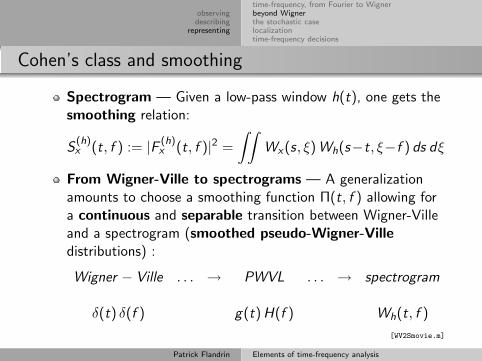
Cohen’s class and smoothing
Spectrogram — Given a low-pass window h(t), one gets thesmoothing relation:
S(h)x (t, f ) := |F (h)
x (t, f )|2 =
∫∫Wx(s, ξ) Wh(s−t, ξ−f ) ds dξ
From Wigner-Ville to spectrograms — A generalizationamounts to choose a smoothing function Π(t, f ) allowing fora continuous and separable transition between Wigner-Villeand a spectrogram (smoothed pseudo-Wigner-Villedistributions) :
Wigner − Ville . . . → PWVL . . . → spectrogram
δ(t) δ(f ) g(t) H(f ) Wh(t, f )
[WV2Smovie.m]
Patrick Flandrin Elements of time-frequency analysis
observingdescribing
representing
time-frequency, from Fourier to Wignerbeyond Wignerthe stochastic caselocalizationtime-frequency decisions
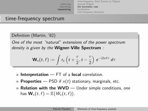
time-frequency spectrum
Definition (Martin, ’82)
One of the most “natural” extensions of the power spectrumdensity is given by the Wigner-Ville Spectrum :
Wx(t, f ) :=
∫rx
(t +
τ
2, t − τ
2
)e−i2πf τ dτ
Interpretation — FT of a local correlation.
Properties — PSD if x(t) stationary, marginals, etc.
Relation with the WVD — Under simple conditions, onehas Wx(t, f ) = E{Wx(t, f )}.
Patrick Flandrin Elements of time-frequency analysis
observingdescribing
representing
time-frequency, from Fourier to Wignerbeyond Wignerthe stochastic caselocalizationtime-frequency decisions
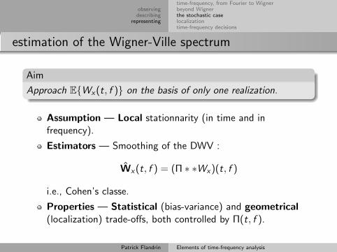
estimation of the Wigner-Ville spectrum
Aim
Approach E{Wx(t, f )} on the basis of only one realization.
Assumption — Local stationnarity (in time and infrequency).
Estimators — Smoothing of the DWV :
Wx(t, f ) = (Π ∗ ∗Wx)(t, f )
i.e., Cohen’s classe.
Properties — Statistical (bias-variance) and geometrical(localization) trade-offs, both controlled by Π(t, f ).
Patrick Flandrin Elements of time-frequency analysis
observingdescribing
representing
time-frequency, from Fourier to Wignerbeyond Wignerthe stochastic caselocalizationtime-frequency decisions
global vs. local
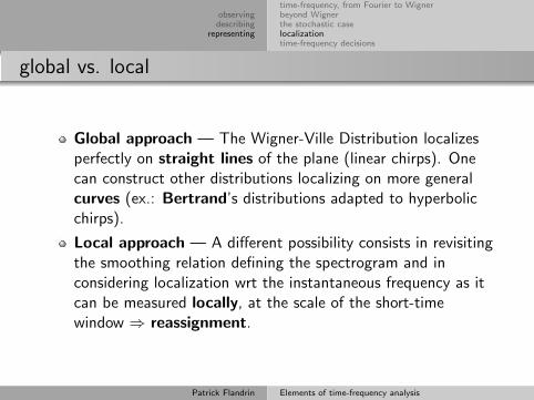
Global approach — The Wigner-Ville Distribution localizesperfectly on straight lines of the plane (linear chirps). Onecan construct other distributions localizing on more generalcurves (ex.: Bertrand’s distributions adapted to hyperbolicchirps).
Local approach — A different possibility consists in revisitingthe smoothing relation defining the spectrogram and inconsidering localization wrt the instantaneous frequency as itcan be measured locally, at the scale of the short-timewindow ⇒ reassignment.
Patrick Flandrin Elements of time-frequency analysis
observingdescribing
representing
time-frequency, from Fourier to Wignerbeyond Wignerthe stochastic caselocalizationtime-frequency decisions
reassignment
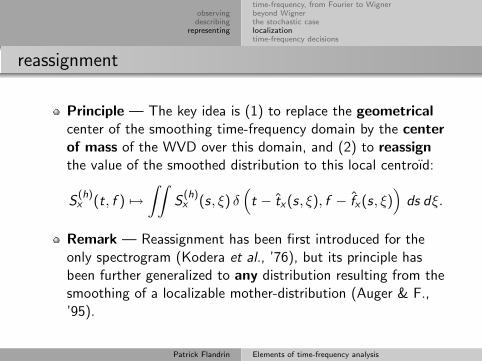
Principle — The key idea is (1) to replace the geometricalcenter of the smoothing time-frequency domain by the centerof mass of the WVD over this domain, and (2) to reassignthe value of the smoothed distribution to this local centroıd:
S(h)x (t, f ) 7→
∫∫S
(h)x (s, ξ) δ
(t − tx(s, ξ), f − fx(s, ξ)
)ds dξ.
Remark — Reassignment has been first introduced for theonly spectrogram (Kodera et al., ’76), but its principle hasbeen further generalized to any distribution resulting from thesmoothing of a localizable mother-distribution (Auger & F.,’95).
Patrick Flandrin Elements of time-frequency analysis
observingdescribing
representing
time-frequency, from Fourier to Wignerbeyond Wignerthe stochastic caselocalizationtime-frequency decisions
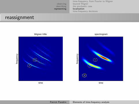
reassignment
Wigner-Ville
time
freq
uenc
y
spectrogram
time
freq
uenc
y
Patrick Flandrin Elements of time-frequency analysis

observingdescribing
representing
time-frequency, from Fourier to Wignerbeyond Wignerthe stochastic caselocalizationtime-frequency decisions
reassignment
Wigner-Ville
time
freq
uenc
y
reassigned spectrogram
time
freq
uenc
y
Patrick Flandrin Elements of time-frequency analysis

observingdescribing
representing
time-frequency, from Fourier to Wignerbeyond Wignerthe stochastic caselocalizationtime-frequency decisions
reassignment in action
Spectrogram — Implicit computation of the local centroıds(Auger & F., ’95) :
tx(t, f ) = t + Re
{F
(T h)x
F(h)x
}(t, f )
fx(t, f ) = f − Im
{F
(Dh)x
F(h)x
}(t, f ),
with (T h)(t) = t h(t) and (Dh)(t) = (dh/dt)(t)/2π.
Beyond spectrograms — Possible generalizations to othersmoothings (smoothed pseudo-Wigner-Ville, scalogram, etc.).
Patrick Flandrin Elements of time-frequency analysis
observingdescribing
representing
time-frequency, from Fourier to Wignerbeyond Wignerthe stochastic caselocalizationtime-frequency decisions
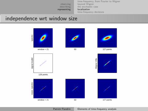
independence wrt window size
128 points
sign
al m
odel
Wig
ner-
Vill
e
window = 21
spec
tro
window = 21
reas
s. s
pect
ro
63
63
127 points
127 points
Patrick Flandrin Elements of time-frequency analysis
observingdescribing
representing
time-frequency, from Fourier to Wignerbeyond Wignerthe stochastic caselocalizationtime-frequency decisions
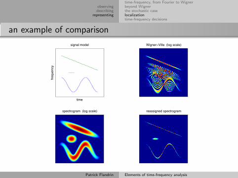
an example of comparison
time
freq
uenc
y
signal model Wigner−Ville (log scale)
spectrogram (log scale) reassigned spectrogram
Patrick Flandrin Elements of time-frequency analysis

observingdescribing
representing
time-frequency, from Fourier to Wignerbeyond Wignerthe stochastic caselocalizationtime-frequency decisions
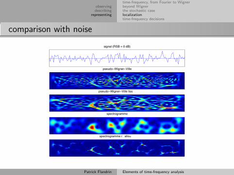
comparison with noise
signal (sans bruit)
pseudo−Wigner−Ville
pseudo−Wigner−Ville liss�
spectrogramme
spectrogramme r�allou�
Patrick Flandrin Elements of time-frequency analysis
observingdescribing
representing
time-frequency, from Fourier to Wignerbeyond Wignerthe stochastic caselocalizationtime-frequency decisions
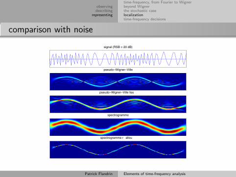
comparison with noise
signal (RSB = 20 dB)
pseudo−Wigner−Ville
pseudo−Wigner−Ville liss�
spectrogramme
spectrogramme r�allou�
Patrick Flandrin Elements of time-frequency analysis
observingdescribing
representing
time-frequency, from Fourier to Wignerbeyond Wignerthe stochastic caselocalizationtime-frequency decisions
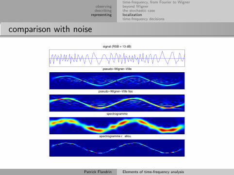
comparison with noise
signal (RSB = 13 dB)
pseudo−Wigner−Ville
pseudo−Wigner−Ville liss�
spectrogramme
spectrogramme r�allou�
Patrick Flandrin Elements of time-frequency analysis
observingdescribing
representing
time-frequency, from Fourier to Wignerbeyond Wignerthe stochastic caselocalizationtime-frequency decisions
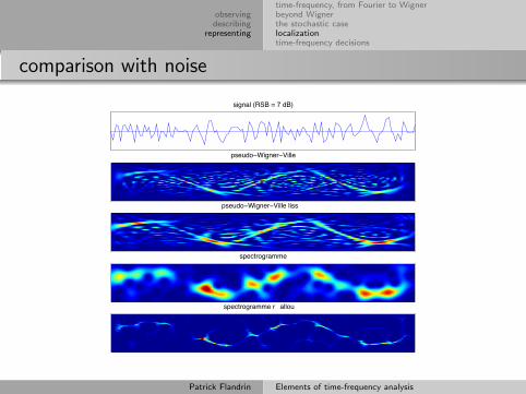
comparison with noise
signal (RSB = 7 dB)
pseudo−Wigner−Ville
pseudo−Wigner−Ville liss�
spectrogramme
spectrogramme r�allou�
Patrick Flandrin Elements of time-frequency analysis
observingdescribing
representing
time-frequency, from Fourier to Wignerbeyond Wignerthe stochastic caselocalizationtime-frequency decisions
comparison with noise
signal (RSB = 0 dB)
pseudo−Wigner−Ville
pseudo−Wigner−Ville liss�
spectrogramme
spectrogramme r�allou�
Patrick Flandrin Elements of time-frequency analysis
observingdescribing
representing
time-frequency, from Fourier to Wignerbeyond Wignerthe stochastic caselocalizationtime-frequency decisions
reassignment and estimation
Advantage — Very good properties of localization for chirps(> spectrogram).
Limitation — High sensitivity to noise (< spectrogram).
Aim
Reduce fluctuations while preserving localization.
Idea (Xiao & F., ’06)
Adopt a multiple windows approach.
Patrick Flandrin Elements of time-frequency analysis
observingdescribing
representing
time-frequency, from Fourier to Wignerbeyond Wignerthe stochastic caselocalizationtime-frequency decisions
back to spectrum estimation
Stationary processes — The power spectrum density canbe viewed as:
Sx(f ) = limT→∞
E
1
T
∣∣∣∣∣∫ +T/2
−T/2x(t) e−i2πft dt
∣∣∣∣∣2
In practice — Only one, finite duration, realization ⇒ crudeperiodogram (squared FT) = non consistent estimator withlarge variance
Patrick Flandrin Elements of time-frequency analysis
observingdescribing
representing
time-frequency, from Fourier to Wignerbeyond Wignerthe stochastic caselocalizationtime-frequency decisions
classical way out (Welch, ’67)
Principle — Method of averaged periodograms
S(W )x ,K (f ) =
1
K
K∑k=1
S(h)x (tk , f )
with tk+1 − tk of the order of the width of the window h(t).
Bias-variance trade-off — Given T (finite), increasing K ⇒reduces variance, but increases bias
Patrick Flandrin Elements of time-frequency analysis
observingdescribing
representing
time-frequency, from Fourier to Wignerbeyond Wignerthe stochastic caselocalizationtime-frequency decisions
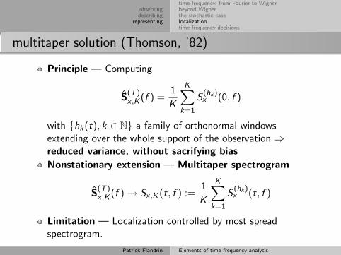
multitaper solution (Thomson, ’82)
Principle — Computing
S(T )x ,K (f ) =
1
K
K∑k=1
S(hk )x (0, f )
with {hk(t), k ∈ N} a family of orthonormal windowsextending over the whole support of the observation ⇒reduced variance, without sacrifying bias
Nonstationary extension — Multitaper spectrogram
S(T )x ,K (f ) → Sx ,K (t, f ) :=
1
K
K∑k=1
S(hk )x (t, f )
Limitation — Localization controlled by most spreadspectrogram.
Patrick Flandrin Elements of time-frequency analysis

observingdescribing
representing
time-frequency, from Fourier to Wignerbeyond Wignerthe stochastic caselocalizationtime-frequency decisions
Multitaper reassignment
Idea
Combining the advantages of reassignment (wrt localization) withthose of multitapering (wrt fluctuations) :
Sx ,K (t, f ) → RSx ,K (t, f ) :=1
K
K∑k=1
RS(hk )x (t, f )
1 coherent averaging of chirps (localization independent ofthe window)
2 incoherent averaging of noise (different TF distributions fordifferent windows)
Patrick Flandrin Elements of time-frequency analysis

observingdescribing
representing
time-frequency, from Fourier to Wignerbeyond Wignerthe stochastic caselocalizationtime-frequency decisions
in practice
Choice of windows — Hermite functions
hk(t) = (−1)ke−t2/2
√π1/22kk!
(Dkγ)(t); γ(t) = et2
rather than Prolate Spheroidal Wave functions
Two main reasons1 WVD with elliptic symmetry and maximum concentration
in the plane.2 recursive computation of hk(t), (T hk)(t) and (Dhk)(t) ⇒
better implementation in discrete-time. In particular:
(Dhk)(t) = (T hk)(t)−√
2(k + 1) hk+1(t)
Patrick Flandrin Elements of time-frequency analysis
observingdescribing
representing
time-frequency, from Fourier to Wignerbeyond Wignerthe stochastic caselocalizationtime-frequency decisions
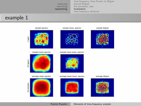
example 1
1 ta
per
sample spectro. sample reass. spectro. sample Wigner10
tape
rs
sample mean spectro. sample mean reass. spectro.
10 s
ampl
es
average mean spectro. average mean reass. spectro. average Wigner
Patrick Flandrin Elements of time-frequency analysis
observingdescribing
representing
time-frequency, from Fourier to Wignerbeyond Wignerthe stochastic caselocalizationtime-frequency decisions
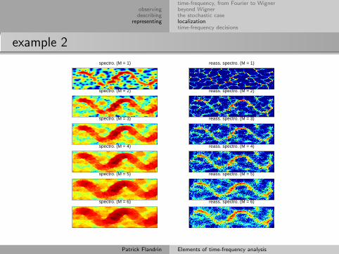
example 2
spectro. (M = 1)
reass. spectro. (M = 1)
spectro. (M = 2)
reass. spectro. (M = 2)
spectro. (M = 3)
reass. spectro. (M = 3)
spectro. (M = 4)
reass. spectro. (M = 4)
spectro. (M = 5)
reass. spectro. (M = 5)
spectro. (M = 6)
reass. spectro. (M = 6)
Patrick Flandrin Elements of time-frequency analysis
observingdescribing
representing
time-frequency, from Fourier to Wignerbeyond Wignerthe stochastic caselocalizationtime-frequency decisions
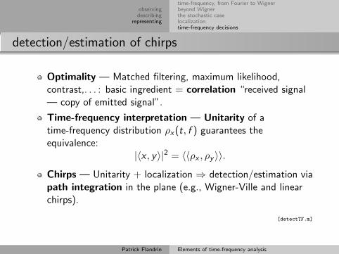
detection/estimation of chirps
Optimality — Matched filtering, maximum likelihood,contrast,. . . : basic ingredient = correlation “received signal— copy of emitted signal”.
Time-frequency interpretation — Unitarity of atime-frequency distribution ρx(t, f ) guarantees theequivalence:
|〈x , y〉|2 = 〈〈ρx , ρy 〉〉.
Chirps — Unitarity + localization ⇒ detection/estimation viapath integration in the plane (e.g., Wigner-Ville and linearchirps).
[detectTF.m]
Patrick Flandrin Elements of time-frequency analysis
observingdescribing
representing
time-frequency, from Fourier to Wignerbeyond Wignerthe stochastic caselocalizationtime-frequency decisions
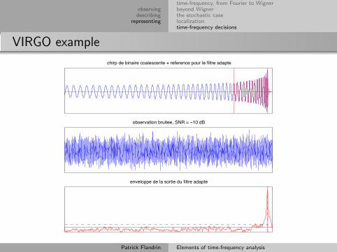
VIRGO example
chirp de binaire coalescente + reference pour le filtre adapte
observation bruitee, SNR = −10 dB
enveloppe de la sortie du filtre adapte
Patrick Flandrin Elements of time-frequency analysis

observingdescribing
representing
time-frequency, from Fourier to Wignerbeyond Wignerthe stochastic caselocalizationtime-frequency decisions
VIRGO example (Chassande-Mottin & F., ’98)
Patrick Flandrin Elements of time-frequency analysis

observingdescribing
representing
time-frequency, from Fourier to Wignerbeyond Wignerthe stochastic caselocalizationtime-frequency decisions
time-frequency detection ?
Language — The time-frequency viewpoint offers a naturallanguage for addressing detection/estimation problemsbeyond nominal situations.
Robustness — Incorporation of uncertainties in the chirpmodel by replacing the integration curve by a domain(example of post-newtonian approximations in the case ofgravitational waves).
time
freq
uenc
y
gravitational wave
?
Patrick Flandrin Elements of time-frequency analysis

observingdescribing
representing
time-frequency, from Fourier to Wignerbeyond Wignerthe stochastic caselocalizationtime-frequency decisions
interpretation example: Doppler-tolerance
Localization of a moving target — When estimating adelay by matched filtering with some unknown Doppler effect,estimations of delay and Doppler are coupled ⇒ bias andcontrast loss at the detector output.
Addressed problem — Suppress bias on delay and minimizecontrast loss.
Signal design — Specification of performance via ageometric interpretation of the time-frequency structure of achirp.
[dopptol.m, faTFdopp.m]
Patrick Flandrin Elements of time-frequency analysis
observingdescribing
representing
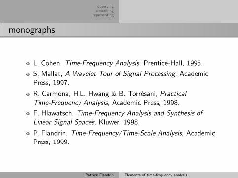
monographs
L. Cohen, Time-Frequency Analysis, Prentice-Hall, 1995.
S. Mallat, A Wavelet Tour of Signal Processing, AcademicPress, 1997.
R. Carmona, H.L. Hwang & B. Torresani, PracticalTime-Frequency Analysis, Academic Press, 1998.
F. Hlawatsch, Time-Frequency Analysis and Synthesis ofLinear Signal Spaces, Kluwer, 1998.
P. Flandrin, Time-Frequency/Time-Scale Analysis, AcademicPress, 1999.
Patrick Flandrin Elements of time-frequency analysis
observingdescribing
representing
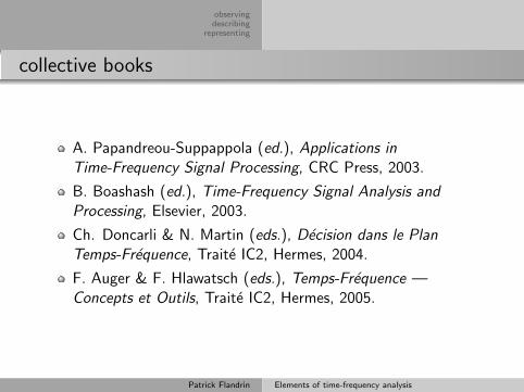
collective books
A. Papandreou-Suppappola (ed.), Applications inTime-Frequency Signal Processing, CRC Press, 2003.
B. Boashash (ed.), Time-Frequency Signal Analysis andProcessing, Elsevier, 2003.
Ch. Doncarli & N. Martin (eds.), Decision dans le PlanTemps-Frequence, Traite IC2, Hermes, 2004.
F. Auger & F. Hlawatsch (eds.), Temps-Frequence —Concepts et Outils, Traite IC2, Hermes, 2005.
Patrick Flandrin Elements of time-frequency analysis
observingdescribing
representing
preprints & Matlab codes
http://tftb.nongnu.org/
http://perso.ens-lyon.fr/patrick.flandrin/
Patrick Flandrin Elements of time-frequency analysis
observingdescribing
representing
contact
Patrick Flandrin Elements of time-frequency analysis
observingdescribing
representing
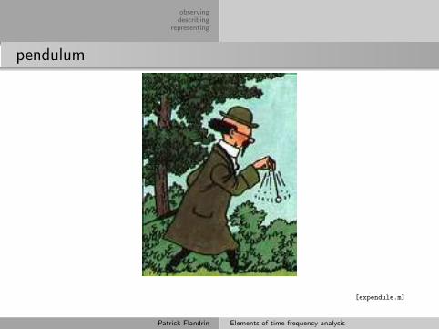
pendulum
[expendule.m]
Patrick Flandrin Elements of time-frequency analysis

observingdescribing
representing
pendulum
θ(t) + (g/L) θ(t) = 0
Constant length — L = L0 ⇒ small oscillations aresinusoidal, with constant period T0 = 2π
√L0/g .
“Slowly” varying length — L = L(t) ⇒ small oscillationsare quasi-sinusodal, with varying pseudo-periodT (t) ∼ 2π
√L(t)/g .
back
Patrick Flandrin Elements of time-frequency analysis

observingdescribing
representing
gravitational waves
[binaire.m]
Patrick Flandrin Elements of time-frequency analysis
observingdescribing
representing
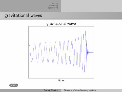
gravitational waves
time
gravitational wave
back
Patrick Flandrin Elements of time-frequency analysis
observingdescribing
representing
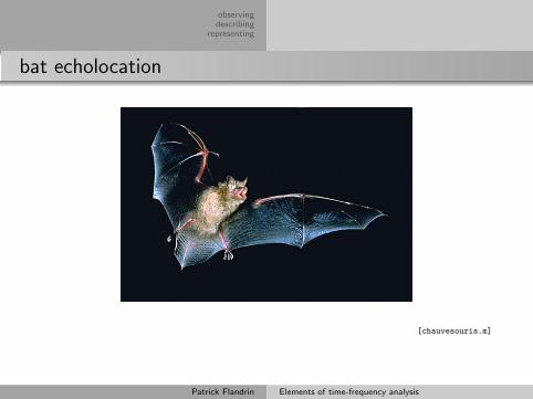
bat echolocation
[chauvesouris.m]
Patrick Flandrin Elements of time-frequency analysis
observingdescribing
representing
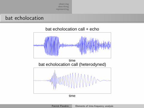
bat echolocation
time
bat echolocation call + echo
time
bat echolocation call (heterodyned)
Patrick Flandrin Elements of time-frequency analysis

observingdescribing
representing
bat echolocation
System —(Active) navigation system, natural sonar
Signals — Ultrasound acoustic waves, transient (a few ms)and “wideband” (some tens of kHz between 40 and 100kHz)
Performance — Close to optimality, with adaption of thewaveforms to multiple tasks (detection, estimation,recognition, interference rejection,. . . )
back
Patrick Flandrin Elements of time-frequency analysis

observingdescribing
representing
Doppler effect
[exdoppler.m]
Patrick Flandrin Elements of time-frequency analysis

observingdescribing
representing
Doppler effect
Moving monochromatic source — Differential perceptionof the emitted frequence.
f + ∆ f f - ∆ f "chirp"
back
Patrick Flandrin Elements of time-frequency analysis
observingdescribing
representing
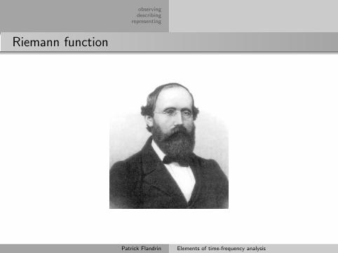
Riemann function
Patrick Flandrin Elements of time-frequency analysis
observingdescribing
representing
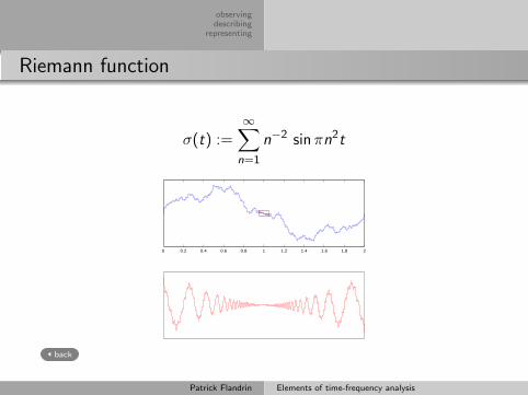
Riemann function
σ(t) :=∞∑
n=1
n−2 sin πn2t
0 0.2 0.4 0.6 0.8 1 1.2 1.4 1.6 1.8 2
back
Patrick Flandrin Elements of time-frequency analysis


![On the Influence of Sampling on the Empirical Mode ...perso.ens-lyon.fr/patrick.flandrin/ICASSP05_GRPF.pdf2.1. EMD algorithm Basically, Empirical Mode Decomposition (EMD) [1] considers](https://img.pdfslide.us/doc/110x75/5fed7db8896d555d3a31f923/on-the-influence-of-sampling-on-the-empirical-mode-persoens-lyonfr-21-emd.jpg)