Measuring time-frequency information content using the ...perso.ens-lyon.fr/patrick.flandrin/IEEE_IT2001.pdf · Measuring Time–Frequency Information Content Using the ... time–frequency

IEEE TRANSACTIONS ON INFORMATION THEORY, VOL. 47, NO. 4, MAY 2001 1391

Measuring Time–Frequency Information ContentUsing the Rényi Entropies

Richard G. Baraniuk, Senior Member, IEEE, Patrick Flandrin, Senior Member, IEEE,Augustus J. E. M. Janssen, Senior Member, IEEE, and Olivier J. J. Michel, Member, IEEE

Abstract—The generalized entropies of Rényi inspire newmeasures for estimating signal information and complexity inthe time–frequency plane. When applied to a time–frequencyrepresentation (TFR) from Cohen’s class or the affine class, theRényi entropies conform closely to the notion of complexity thatwe use when visually inspecting time–frequency images. Thesemeasures possess several additional interesting and useful proper-ties, such as accounting and cross-component and transformationinvariances, that make them natural for time–frequency analysis.This paper comprises a detailed study of the properties and severalpotential applications of the Rényi entropies, with emphasis onthe mathematical foundations for quadratic TFRs. In particular,for the Wigner distribution, we establish that there exist signalsfor which the measures are not well defined.

Index Terms—Complexity, Rényi entropy, time–frequency anal-ysis, Wigner distribution.

I. INTRODUCTION

T HE termcomponentis ubiquitous in the signal processingliterature. Intuitively, a component is a concentration of

energy in some domain, but this notion is difficult to trans-late into a quantitative concept [1]–[3]. In fact, the concept ofa signal component may never be clearly defined.

The use and abuse of this term is particularly severe in the lit-erature on time–frequency analysis. Time–frequency represen-tations (TFRs) generalize the concept of the time and frequencydomains to a joint time–frequency function that indi-cates how the frequency content of a signalchanges over time[4]–[6]. Common themes in the literature include the suppres-sion of TFR cross-components, the concentration and resolu-

Manuscript received September 29, 1998; revised October 10, 2000.This work was supported by the National Science Foundation under GrantsMIP-9457438 and CCR-997318, the Office of Naval Research under GrantsN00014-95-1-0849 and N00014-99-1-0813, the NATO Collaborative ResearchProgramme under Grant GRG-950202, and by URA 1325 CNRS. The materialin this paper was presented in part at the IEEE International Conference onAcoustics, Speech, and Signal Processing, Adelaide, Australia, May 1994, andat the IEEE International Symposium on Information Theory, Whistler, BC,Canada, September 1995.

R. G. Baraniuk is with the Department of Electrical and Computer En-gineering, Rice University, Houston, TX 77005-1892 USA (e-mail: [email protected]).

P. Flandrin is with the Laboratoire de Physique (UMR 5672 CNRS),Ecole Normale Supérieure de Lyon, 69364 Lyon Cedex 07, France (e-mail:[email protected]).

A. J. E. M. Janssen is with Philips Research Laboratories, 5656 AA Eind-hoven, The Netherlands (e-mail: [email protected]).

O. J. J. Michel is with the Laboratoire d’Astrophysique, 06108 Nice Cedex2, France (e-mail: [email protected]).

Communicated by J. A. O’Sullivan, Associate Editor for Detection and Esti-mation.

Publisher Item Identifier S 0018-9448(01)02844-9.

tion of autocomponents, and the property that the time-varyingspectral analysis of TFRs separates signal components, such asparallel chirps, that overlap in both time and frequency. More-over, the quality of particular TFRs is very often judged based onsubjective criteria related to the components of the signal beinganalyzed.

In this paper, rather than address the question “what is acomponent?” directly, we will investigate a class of quantitativemeasures of deterministic signalcomplexityand informationcontent.1 While they do not yield direct answers regardingthe locations and shapes of components, these measures areintimately related to the concept of a signal component, theconnection being the intuitively reasonable supposition thatsignals of high complexity (and therefore high informationcontent) must be constructed from large numbers of elementarycomponents.

Moment-based measures, such as the time–bandwidthproduct and its generalizations to second-order time–frequencymoments [4]–[6], [8], [9] have found wide application, but un-fortunately measure neither signal complexity nor informationcontent [1], [2]. To demonstrate, consider a signal comprisedof two components of compact support, and note that whilethe time–bandwidth product increases without bound withseparation, signal complexity clearly does not increase oncethe components become disjoint.

A more promising approach to complexity based onentropyfunctionals exploits the analogy between signal energy densitiesand probability densities [1]. Just as the instantaneous and spec-tral amplitudes and behave as unidimensionaldensities of signal energy in time and frequency, TFRs try veryhard to act as bidimensional energy densities in time–frequency.In particular, there exist TFRs whose marginal properties par-allel those of probability densities

(1)

(2)

The quadratic TFRs of the large and useful Cohen’s class canbe obtained as the convolution [4]–[6]

(3)

1Many alternative measures of complexity exist (such as Kolmogorov’s [7]).These measures lie beyond the scope of this paper, however, since they are typ-ically applied tosignals, whereas our analysis is based onTFRs, considered aspseudo probability densities.

0018–9448/01$10.00 © 2001 IEEE

1392 IEEE TRANSACTIONS ON INFORMATION THEORY, VOL. 47, NO. 4, MAY 2001

of a kernel function with the Wigner distribution of thesignal

(4)

The probabilistic analogy evoked by (1) and (2) suggests theclassical Shannon entropy [10] (given here for unit-energy sig-nals)

(5)

as a natural candidate for measuring the complexity of a signalthrough its TFR.2 The peaky TFRs of signals comprised ofsmall numbers of elementary components would yield smallentropy values, while the diffuse TFRs of more complicatedsignals would yield large entropy values. Unfortunately, how-ever, the negative values taken on by most TFRs (including allfixed-kernel Cohen’s class TFRs satisfying (1)) prohibit the ap-plication of the Shannon entropy due to the logarithm in (5).

In [1], Williams, Brown, and Hero sidestepped the negativityissue by employing the generalized entropies of Rényi [11](again for unit-energy signals)

(6)

Parameterized by , this class of information measuresis obtained simply by relaxing the mean value property of theShannon entropy from an arithmetic to an exponential mean.(Shannon entropy appears as .) In several empiricalstudies, Williams, Brown, and Hero found that in addition toappearing immune to the negative TFR values that invalidatethe Shannon approach, the third-order Rényi entropy seemedto measure signal complexity. Fig. 1 repeats the principal ex-periment of [1]. The third-order Rényi entropy of theWigner distribution of the sumof two Gaussian pulses is plotted versus the separation distance

. (At , the two pulses coincide and, therefore, be-cause of the assumed energy renormalization, have the sameinformation content as a solitary pulse.) The time–bandwidthproduct of is also plotted. It is clear from the figure that, un-like the time–bandwidth product, which grows without boundwith , the Rényi entropy saturates exactly one bit above thevalue .3 Similar results holdfor separated copies of ( bits information gain). Tosummarize, independent of the definition of signal component,the Rényi entropy indicates a “doubling of complexity” inasthe separation moves from to .

This paper comprises a detailed study of the properties andsome potential applications of the Rényi time–frequency infor-mation measures (6), with emphasis on the mathematical foun-dations for quadratic TFRs. In Section II, after reviewing thedevelopment of these measures, we examine their existence andshow that for each odd there exist signals for which (6)is not defined (due to ). This unprece-dented result surprises, for it indicates that the Rényi formalism

2Note that the complexity measure (Shannon entropy here) is applied not toa signal or process, but to a TFR that plays a rôle analogous to a probabilitydensity function.

3Readers should not be alarmed by negative Rényi entropy values. Even theShannon entropy takes on negative values for certain distributions in the contin-uous-variable case.

Fig. 1. Solid curve and axis on left. The third-order Rényi entropyH (W )of the Wigner distribution of the sums(t) := g(t ��t) + g(t +�t) of twoGaussian components plotted versus the displacement parameter�t (see (32)in Section III-B for the exact signal definition). (The asymptoticH (W ) levelsare� log � �0:208 and log 3 � 0:792 bits.) Dotted curve and axison right. Time–bandwidth product ofs.

is not universally applicable to time–frequency analysis. Coun-terexample signals are easily constructed for large odd; how-ever, our counterexamples are quite contrived. This isconsistent with the ample numerical evidence [1], [8], [9], [12],[13] indicating that the third-order entropy is defined for a broadclass of signals and TFRs, including even those distributionstaking locally negative values. When defined, these measureshave some striking properties that we investigate in Section III.

1) counts the “number of components” in a multi-component signal.

2) For odd orders , is asymptotically invariantto TFR cross-components and, therefore, does not countthem.

3) exhibits extreme sensitivity to phase differencesbetween closely spaced components. This sensitivity canbe reduced through smoothing in time–frequency. Weprovide analytical results for the sum of two Gaussiansignals.

4) The range of values is bounded from below. Forthe Wigner distribution, a single Gaussian pulse attainsthe lower bound.

5) The values of are invariant to time and frequencyshifts of the signal. Certain TFRs provide an additional in-variance to scale changes, while the Wigner distributionboasts complete invariance to symplectic transformationson the time–frequency plane. For more general invari-ances, the Rényi theory extends easily to encompass notonly the TFRs of the affine class [14] but also the gener-alized representations of the unitarily equivalent Cohen’sand affine classes [15]–[17].

In Section IV, we discuss the application of these measures asobjective functions in optimized time–frequency analysis andintroduce the notion of Rényi dimension. We close with a dis-cussion and conclusions. Proofs of the various results are con-tained in the appendixes.

BARANIUK et al.: MEASURING TIME-FREQUENCY INFORMATION CONTENT 1393

II. THE RÉNYI ENTROPIES

A. Rényi Entropy of a Probability Density

In [11] Rényi introduced an alternative axiomatic derivationof entropy based onincompleteprobability mass distributions

whose total probabilities sum to. He observed that the Shannon entropy

uniquely satisfies the axioms of symmetry, continuity, normal-ization, additivity, and, in addition, the mean value condition

(7)

Here and are any two incomplete densities such that, and signifies the composite density

.Extending the arithmetic mean in (7) to a generalized mean

yields generalized entropies closely resembling Shannon’s.Considering the generalized mean value condition

(8)

with a continuous monotone function, Rényi demonstratedthat just two types of functions are compatible with the otherfour axioms. The first, , yields the arithmeticmean (7) and the Shannon entropy. The second

(9)

yields the functional

(10)

now known as the Rényi entropy of order. The Shannonentropy can be recovered as . Extension of

to continuous-valued bivariate densities isstraightforward

(11)

We emphasize that since the passage from the Shannon entropyto the class of Rényi entropies involves only the relaxation ofthe mean value property from an arithmetic to an exponentialmean, behaves much like [11].

B. Rényi Entropy of a TFR

The central theme of this paper is the application of entropymeasures to TFRs to measure the complexity and informationcontent of nonstationary signals indirectly via the time–fre-quency plane. Our primary TFR tools of choice lie in Cohen’sclass [4]–[6], which can be expressed as in (3) as the convolu-tion between the Wigner distribution and a real-valued kernel

.4 The kernel and its inverse Fourier transformcompletely

4To avoid cumbersome machinations, we will restrict our attention to theWigner distribution and all TFRs obtained from (3) with� 2 L ( ). Sincewe will be interested in odd powers of TFRs (see (6)), we furthermore assumethat kernel is a real-valued function.

determine the properties of the corresponding TFR. For ex-ample, a fixed-kernel TFR possesses the energy preservationproperty (2) provided and the marginal properties(1) provided . Besides the Wignerdistribution, examples of Cohen’s class TFRs include thespectrogram ( ambiguity function of the time-reversedwindow function) and the smoothed pseudo-Wigner distribu-tions [4]–[6].

The analogy between TFRs and bidimensional probabilitydensities discussed in the Introduction breaks down at atleast two key points. First, because of the freedom of choiceof kernel function, the TFR of a given signal is nonunique,with many different distributions “explaining” the same data.Second, and more pertinent to the present discussion, mostCohen’s class TFRs are nonpositive and, therefore, cannot beinterpreted strictly as densities of signal energy.5 These locallynegative values will clearly play havoc with the logarithm inthe Shannon entropy (5).

While the Rényi entropies (6) appear intriguing and encour-aging for time–frequency application [1], [8], [9], [12], [13], ithas remained an open question whether, in general, these mea-sures can cope with the locally negative values of Cohen’s classTFRs. In order for (6) to be defined for a signal, we clearlyneed to be real and such that

(12)

Noninteger orders yield complex values and so ap-pear of limited utility. Integer orders that are even pose no suchhazards, since the integral of the positive function re-mains positive.

Unfortunately, odd integer orders are not so robust. For eachodd , there exist signals in and TFRs such that(12) fails, leaving (6) undefined. In Appendix I, we develop thefollowing counterexamples for the Wigner distribution .6

1) For sufficiently large odd , (12) fails for any smooth,rapidly decaying, odd signal.

2) For odd integers , (12) fails for the first-order Her-mite function.

3) For , (12) fails for a particular linear combination ofthe third- and nineth-order Hermite functions (see Fig. 2).

As noted in the Introduction, these surprising results suggest thatwe must proceed with caution when applying TFR-based Rényientropies.

Negative results aside, a preponderance of numerical evi-dence [1], [8], [9], [12] indicates that the third-order entropiesare well-defined for large classes of signals and TFRs (ourcounterexamples only apply to the Wigner distribution). InAppendix I, we spend a considerable effort to find a signal forwhich (12) fails for . Also, a small amount of Gaussiansmoothing of is generally enough for (12) to hold. Thisindicates that the examples for which (12) fails for arerather exceptional.

5While there do exist nonquadratic classes of positive TFRs that satisfy (2)and (1) [4], we will consider only quadratic TFRs in this paper.

6Clearly, these counterexamples invalidate the “proofs” of existence sketchedin [8], [9].


Fig. 2. Example of a signal for which the third-order Rényi entropyH (W ) of the Wigner distribution is not defined. (a) The signals consists of a specialcombination of two odd-order Hermite functions (see Appendix I-C). Its Wigner distribution (b) as an image and (c) in three dimensions (note the largenegativepeak).

Throughout the balance of this paper, we will assume thatall signals under consideration are such that the formula (6) iswell-defined.

We close this section with some important notes on normal-ization. In their experiments, Williams, Brown, and Hero actu-ally employed not from (11), but a prenormalized versionequivalent to normalizing the signal energybeforeraising theTFR to the power

(13)

The two measures are related by

(14)

and thus varies with the signal energy. Since an infor-mation measure should be invariant to the energy of the signalbeing analyzed, we will adhere strictly to the definition (13) forthe duration of this paper. Discretization of this measure (bysetting , with ) for use with com-puter-generated, discrete TFRs yields

(15)

The frequency step constant is computed as , givenuniform frequency samples spanning the frequency range ofhertz per sample. For both continuous and discrete TFRs,

operation in coordinates, with radial frequencyrad/s, introduces an offset

. Sang and Williams explore an alternative magnitudenormalization of the Rényi entropy in [13].

III. PROPERTIES OF THERÉNYI TIME–FREQUENCY

INFORMATION MEASURE

We now conduct a detailed analysis of the properties of theRényi entropy (when it exists) that make it a fascinating anduseful tool for studying the information content of time-varyingdeterministic signals.

A. Component Counting and Cross-Component Invariance

If TFRs were “quasi-linear”—such that each signal compo-nent contributed essentially separately to the overall TFR withno intervening cross-components—then the analogy betweenTFRs and probability density functions would predict an addi-tive or counting behavior from the Rényi entropy. This is rea-sonable, since a (nonoverlapping) combination of basic signalcomponents is more “complex” than the individual components.

To gain more intuition into this most fundamental propertyof , imagine applying this measure first to a compactly sup-ported signal using an ideal, quasi-linear TFR . Denotethe length of the supporting interval of by and assumethat for all and for all .

Form the two-component signal , whererepresents translation by time . Assuming that

, the distribution is given by

(16)

Since is compactly supported in the time direction, wecan appeal to the analogy between the right-hand side of (16)and the composite probability distribution in (8) to com-pute . In particular, substituting (14) into (8) with

and employing the factsand , some simple algebra yields

(17)

In words, the two-component signal contains exactlyone bit more information than the one-component signal.7 Thesaturation levels of the entropy curve in Fig. 1 display preciselythis behavior.

While this simple analysis provides considerable insight intothe counting behavior of , it does not take into account thenonideal, nonlinear behavior of the quadratic TFRs of Cohen’sclass. In particular, we have ignored the presence of cross-com-ponents in these distributions [4]–[6], which violate the linearityassumption underlying (16). We will broaden our analysis to en-compass actual TFRs in two stages.

7Note that the post-normalized entropyH from (11) exhibits the invarianceH (I ) = H (I ), since the energies ofs ands+ T s differ by a factorof two.


First, consider the Wigner distribution (4) of the compactlysupported, two-component signal

(18)

The term , called thecross-componentbetweenand , is derived from the cross-Wigner distribution [4]–[6],[18]

(19)

with the cross-Wigner distribution between signalsand de-fined by

(20)

In general, the Rényi entropy

(21)

involves a complicated polynomial in , , and .However, due to the compact support ofand thus [4]–[6],for separations , these terms lie disjoint in the time–fre-quency plane, and a tremendous simplification results

provided

(22)

While this is obviously not the case foreven, the oscillatorystructure of [4]–[6] cancels under integration with oddpowers for sufficiently large. We prove the following in Ap-pendix II-A as a special case of Theorem 2.

Proposition 1: Fix odd and let be a signal ofcompact support such that and obey (12). Denotingthe length of the supporting interval by, set .Then (22) holds and thus .

The linear growth of the separation conditionrecommends the first of the odd integers , namely,

, as the best order for information analysis with theWigner distribution. Problems with (12) and numerical consid-erations (stability in the face of quantization errors) also jus-tify small values. Using the symplectic transformation prop-erties of the Wigner distribution (see Appendix III-A and [5],[6], [19]), Proposition 1 can be easily extended from signalsof compact time support to signals whose Wigner distributions

are supported on a strip of arbitrary orientation in the time–fre-quency plane.

We can extend these counting results to include most Cohen’sclass TFRs and finite energy signals. For noncompactly sup-ported signals, the auto- and cross-components in the Cohen’sclass analog to (21) will always overlap to some degree, so weshould expect only asymptotic expressions. Define the time–fre-quency displacement operator

(23)

that translates signals by the distance

in the time–frequency plane (with 1 s and 1 Hz).The following is the key result of this section [8], [9].

Theorem 2 (Component Counting):Let be eitherthe Wigner distribution or a Cohen’s class TFR defined as in(3) with . Then, for any and oddsuch that and obey (12), we have

(24)

Theorem 2 implies also that the “information” in the cross-components of must decay to zero asymptotically.

Corollary 3 (Asymptotic Cross-Component Invariance):Letbe either the Wigner distribution or a Cohen’s class

TFR defined as in (3) with . Then, for anyand odd such that and obey (12), we

have

(25)

Proposition 1 extends to components and bits of in-formation gain, provided that the auto- and cross-componentsbecome sufficiently disjoint in the time–frequency plane. Thecounting property doesnothold generally when the signal cross-components overlap with the auto-components or other cross-components, however.

A simple example of such a signal is

where the cross-component lies upon theauto-component . For supported on and

, we compute

(26)

The first term on the right side arises from the auto-componentsof ; the second term arises from the (overlapping)auto-component of and cross-component betweenand (see (100)). Note that

(27)


for integer , which follows from the conditions on and. Now using arguments as in Appendix II-A and expanding

the second term on the right side of (26), we find that

(28)

Here denotes the coefficient of in . Thus,we have

(29)

For instance, yields rather than for thesecond term on the right side of (29).

As a second example, consider

with the support of and as above. Here, the cross-com-ponent overlaps the cross-component

. As above, we obtain

(30)

with the coefficient of in . For instance,yields rather than for the second term on

the right side of (30).These examples show that large intercomponent spacing

is not enough for correct component counting.Notice that the spacings between the signals in these examplesare regular; with signals of fixed supports and random spacingsthat tend to infinity, chances are much better that the componentcounting property will hold true.

B. Amplitude and Phase Sensitivity

The results of the experiment illustrated in Fig. 1 and ana-lyzed in the previous section are very appealing, but also incom-plete, because we introduced no amplitude or phase differencesbetween the two signal components.

First consider amplitude differences. Consider the signalconsisting of weighted components that are

time–frequency shifted versions of some basic component. Ifthe are pulled apart such that the asymptotic overlap of theauto- and cross-components of their TFR decays to zero, thenan analysis similar to that of Section III-A yields [20]

(31)

with a vector with entries

and the discrete Rényi entropy of (10). is a contin-uous function of the bounded by and and maximized withall equal. Thus, amplitude discrepancies alter the asymptoticsaturation levels of the Rényi entropy.

We will see that phase offsets induce strong oscillations be-tween the saturation levels. To shed further light on this matter,we will derive an analytic expression for the third-order entropyof the Wigner distribution of the sum of two Gaussian pulses

(32)

with the Gaussian

(33)

and , , . We consider

(34)

with

(35)

Using symplectic transformations, we show in AppendixIII-A that the complete can be computedfrom the values of

(36)

with

(37)

related to the time displacement, phase change, and ampli-tude disparity between the two components, respectively. InAppendix III-B we derive the following.

Proposition 4: For the signal (32) withreplaced by and with and

defined as in (34)–(37), we have

(38)

This expression is very convenient for studying the effects ofcomponent time, phase, and amplitude differences on the third-order Wigner entropy. For example, in Appendix III-C, we findthe bounds

(39)

From (38), we can compute the effect of component ampli-tude disparity on by fixing and varying the separa-tion distance via . For the asymptotic saturation level, we have

(40)

The obvious conclusion that equal amplitudes maxi-mize the complexity of signals composed of multiple identicalcomponents appears quite reasonable, for smaller componentsare dominated by larger ones and therefore carry less informa-tion.

In the region between saturation levels (where the TFR com-ponents overlap and the assumptions of Section III-A fail tohold), the relative phase between components controls the valueof the Rényi entropy. Fig. 3 extends the experiment of Fig. 1 byplotting the surface as a function of both inter-compo-nent displacement and phase . It is apparent from the curvesthat while phase changes do not affect the saturation levels of the


Fig. 3. The third-order Rényi entropyH (W ) of the Wigner distribution ofthe two-component Gaussian signal (32) plotted versus displacement parametera and phase' (in rads). We use (38) withv = 1. Comparison with Fig. 1(which coincides with the' = 0 slice of the surface) illustrates the sensitivityofH (W ) to relative phase. (The asymptotic levels here are the same as thosein Fig. 1; the (overestimation) peak value islog 27� 1 � 1.377 bits.)

information measure, they allow many possible trajectories be-tween the two levels, including even trajectories where an “over-estimation” [noted numerically in [1] and confirmed in (39)] ofinformation content occurs. Furthermore, if the phase of eachcomponent is fixed relative to the center of its envelope (so thatthe components do not change shape as they are shifted about),then the corresponding versus curve will be a sliceof the surface along an oblique trajectory in theplane. Curves of this form can be multimodal (see [8, Fig. 2],[9]).

The phase sensitivity of the measure for closelyspaced components is quite reasonable, given the sensitivity ofthe signals themselves to relative phase. For example, Fig. 4shows the composite signals and their respective Wignerdistributions for a fixed offset and relative phases and

. The difference in appearance is striking; clearly, thecomponents in the signal in Fig. 4 (b) are more separated thanthose in Fig. 4 (a). Accordingly, the entropies for thetwo signals differ widely: from 2.741 to 3.857 bits, respectively.

Since the interference pattern generated by cross-componentsencodes intercomponent phase information, signals with low in-formation content (“almost mono-component signals”) must ex-hibit mainly constructive interferencein the sense of [5], [6].Relative phase fades from importance after all components be-come disjoint.

C. Effects of Smoothing

TFRs based on low-pass kernels lead to more robust Rényiinformation estimates, since smoothing suppresses the Wignercross-components that carry the intercomponent phase informa-tion.

In Appendix III-D, we calculate for the two-compo-nent Gaussian signal (from (32) with ), with

the Wigner distribution smoothed by the Gaussian kernel

(41)

The choice results in the matched-window spectrogram8

as in Fig. 5, and we obtain from (174)

(42)

with and as in (37). For general , the upper satu-ration level is given by

(43)

To illustrate, we repeat in Fig. 5 the experiment of Fig. 3using a matched-window spectrogram TFR rather than theWigner distribution. While the spectrogram informationestimate remains somewhat phase-sensitive, it climbs moreswiftly to the saturation level and with a reduced overshootcompared to the Wigner distribution estimate. In general, theascent to saturation accelerates with increasing orderoncethe cross-components are smoothed to the same peak levelas the auto-components. (The opposite holds for the Wignerdistribution, because Wigner cross-components can tower overWigner auto-components by up to a factor of two.)

The price paid for the more robust information estimates de-rived from smoothed TFRs is a signal-dependent bias of en-tropy levels compared to those derived from the Wigner distri-bution, with the amount of bias increasing with the amount ofsmoothing. This bias is difficult to quantify, since the convolu-tion in (3) and the power and integral in (6) do not permute inany simple fashion. In the special case of the matched-windowspectrogram applied to a sum of Gaussian signal components,a direct computation finds a 1-bit bias in asymptotic informa-tion compared to that estimated using the Wigner distribution(compare Fig. 1 with Fig. 5). Despite the introduction of sys-tematic bias, smoothing is essential when measuring entropiesfor complicated multicomponent signals with overlapping auto-and cross-components.

Although it may be intuitively clear that smoothing attenuatesthe Wigner distribution’s negative values, it is by no means aneasy matter to get pertinent results on the existence offor odd . Even for the case of Hermite functions (as con-sidered in Appendix I) and Gaussian smoothing (see (41)), thisis a hard problem. It can be shown that the well-definedness of

for all and all requiresa Debbi–Gillis type result [21] in which thein the exponentialof (73) is replaced by . We can summarize our(partial) results on Hermite signals as follows.

: In this case, [22]and existence of is not an issue.

: It was kindly observed to us by Prof. R.Askey that a Debbi–Gillis result is easilyestablished for , which impliesthat is well-defined for thisrange of smoothing.

8A spectrogram computed using the time-reversed signal as the window.


Fig. 4. Signals and positive parts of the Wigner distributions from the experiment illustrated in Fig. 3 corresponding to a single fixed separationa and two differentphases'. (a) Signal (left) and Wigner distribution (right) for' = ; H (W ) = 2.741 bits. (b) Signal and Wigner distribution for' = ; H (W ) = 3.857bits.

Fig. 5. The third-order Rényi entropyH (C ) of the matched-windowspectrogram plotted versus displacement parameter�t and phase' (in rads)for the same signal utilized in Fig. 3 (see (42)). The reduced sensitivity ofthe spectrogram to relative phase results in swifter saturation with reducedovershoot. Furthermore, for small' and �t, H (C ) actually respondssooner thanH (W ) to small increases in�t. Note also the 1-bit bias in theasymptotic levels ofH (C ) versus those ofH (W ). (The asymptotic levelshere are log 3 � 0:792 and log 3 + 1 � 1:792.)

: We have been unable to prove results forthe case .

: This is the Debbi–Gillis result [21] thatshows that is well-defined.

D. Lower Bound on Signal Information Content

Simple to derive from Lieb’s inequality [23] (see AppendixIV-A), a lower bound on the Rényi entropy corresponds to the“peakiest” Cohen’s class TFR.

Theorem 5 (Lower Bound on Information Content forCohen’s Class):For any Cohen’s class TFR with

and , any , and any

(44)

For the Wigner distribution

(45)

with equality if and only if is a Gaussian. For the spectrogramwith Gaussian window

(46)

with equality if and only if is a Gaussian of the same form as.9

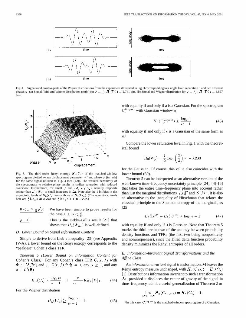
Compare the lower saturation level in Fig. 1 with the theoret-ical bound

for the Gaussian. Of course, this value also coincides with thelower bound (39).

Theorem 5 can be interpreted as an alternative version of thewell-known time–frequency uncertainty principle [24], [4]–[6]that takes the entire time–frequency plane into account ratherthan just the marginal distributions and . It is alsoan alternative to the inequality of Hirschman that relates theclassical principle to the Shannon entropy of the marginals, as[25]

(47)

with equality if and only if is Gaussian. Note that Theorem 5marks the third breakdown of the analogy between probabilitydensity functions and TFRs (the first two being nonpositivityand nonuniqueness), since the Dirac delta function probabilitydensity minimizes the Rényi entropies of all orders.

E. Information-Invariant Signal Transformations and theAffine Class

An information invariantsignal transformation leaves theRényi entropy measure unchanged, with[1]. Distributions information invariant to such a transformation

, provided it displaces the center of gravity of the signal intime–frequency, admit a useful generalization of Theorem 2 to

9In this case,C is the matched-window spectrogram of a Gaussian.


The transformations leaving the Rényi entropy invariant cor-respond to those that do not change the value of the integral in(13). For Cohen’s class TFRs, the invariance properties of threenested kernel classes are simple to quantify. All fixed-kernelTFRs are information-invariant to time and frequency shifts.Product-kernel TFRs, having kernels of the form

with a one-dimensional function, are in addition in-variant to scale changes of the form . TheWigner distribution is the lone fixed-kernel TFR fully informa-tion-invariant to time and frequency shifts, scale changes, andthe modulation and convolution by linear chirp functions thatrealize shears in the time–frequency plane (the symplectic trans-formations of (131), (132)). It is not coincidental that these samefive operations leave invariant the form of the (minimum-infor-mation) Gaussian signal [19].

The affine classprovides additional TFRs information-in-variant to time shifts and scale changes [5], [6], [14], [26].Affine class TFRs are obtained from the affine smoothing

(48)

of the Wigner distribution of the signal with a kernel function.10 Given proper normalization of the kernel, we have

Hence, the Rényi entropy of an affine class TFR can be definedexactly as in (13) (of course, with the requirement (12)). Theresulting time-scale information measure shares all ofthe properties discussed above in the context of Cohen’s class(counting, cross-component invariance, amplitude and phasesensitivity, bounds, etc.), except with time and frequency shiftsreplaced by time shifts and scale changes. In particular, wehave the following.

Theorem 6 (Lower Bound on Information Content for theAffine Class): Let be an affine class TFR with kernelsuch that and . Then, for allintegers and for all

(49)

For the proof, see Appendix IV-B. The conditionimplies for continuous kernels and en-

sures that the affine smoothing (48) is defined. Since the kernelgenerating the scalogram (the squared magnitude of the contin-uous wavelet transform) corresponds to the Wigner distribution

of the wavelet function , this condition also generalizesthe now classical “wavelet admissibility condition” [5], [6]. Inparticular, we have

(50)

10In order to emphasize the similarity of (48) to (3), we have reparameterizedthe original time-scale formulation of (48) from [14] in terms of time–frequencycoordinates by setting scalea = f =f , with f = 1 Hz.

For information invariances different from time and fre-quency shifts, scale changes, and chirp modulations andconvolutions, we must look beyond Cohen’s class and theaffine class. Fortunately, all the above results extend easilyto the recently developed unitarily equivalent Cohen’s andaffine classes [15]–[17]. The TFRs in these new classes areinformation-invariant to generalized time–frequency shifts andtime-scale changes.

IV. SELECTED APPLICATIONS

The foregoing properties of the Rényi entropies (when it isdefined) make these new information and complexity measuresparticularly appropriate for time–frequency analysis. In this sec-tion, we briefly discuss two areas of past and potential applica-tion.

A. Information-Based Performance Measures

The Rényi entropies make excellent measures of the infor-mation extraction performance of TFRs. By analogy to prob-ability density functions, minimizing the complexity or infor-mation in a particular TFR is equivalent to maximizing its con-centration, peakiness, and, therefore, resolution [27]. Optimiza-tion of a TFR (through its kernel) with respect to an informationmeasure yields a high-performance “information-optimal” TFRthat changes its form to best match the signal at hand [13], [28].

Many of the optimal-kernel TFRs in the literature have beenbased either implicitly or explicitly on information measures. Asnoted by Williams and Sang [13], [28], the performance indexcommon to the [29], radially Gaussian [30], and adaptiveoptimal kernel [31] optimization formulations can be rewrittenusing Parseval’s theorem as

(51)

Since the second-order Rényi entropy squares the TFR, it re-mains sensitive to cross-components and hence can be consid-ered as a measure of their information content [1]. Thus, max-imizing (51) over a class of low-pass smoothing kernelssi-multaneously minimizes the information in the cross-compo-nents of the optimal-kernel TFR. Maximizing theconcentration ratio of [32], [33] can also be viewed in informa-tion-theoretic terms, since this is equivalent to minimizing thedifferential entropy .

Differential performance measures formed with odd- andeven-order entropies also prove interesting [28]. For example,the differential measure

(52)

exploits the fact that odd- and even-order entropies decouple tosome degree the information content in the auto- and cross-com-ponents in a TFR. Minimizing this measure balances i) max-imizing the information in the auto-components (by keepingthem peaky through less smoothing) with ii) minimizing the in-formation in the cross-components (by flattening them throughmore smoothing). For positive TFRs, the special choice ,minimizing (52) is equivalent to maximizing the concentrationratio , making it an interesting alternative to the

measure used in [32], [33].


Fig. 6. The effect of time–frequency smoothing on (52) as a function of theparameter�. For a signal consisting of two well-separated Gaussian pulses(a > 2 in (37)), we form the TFRC = W � � , with � from (41). Theparameter� controls the degree of time–frequency smoothing:� = 0 generatesthe Wigner distribution;� = 1 generates the matched-window spectrogram.We plotH (C )� �H (C ) versus the smoothing parameter� for the elevenvalues� = 0; 0:1; . . . ; 1. (The upper curve corresponds to� = 0, while thelower curve corresponds to� = 1.) The minimum point of each curve, markedby a circle, corresponds to an “information-optimal TFR.” Data obtained bynumerical simulation; results from the analytical approximation (53) correspondclosely.

Fig. 6 explores the effect of time–frequency smoothing on(52) as a function of the parameter. Forming a signal fromtwo well-separated Gaussian pulses, we smooth the Wigner dis-tribution of with a Gaussian kernel (41) of increasing volume

to generate a series of smoothed TFRs. In the figure, thesmoothing parameter corresponds to the normalized degreeof smoothing, with leaving the Wigner distribution un-touched and generating the matched-window spectro-gram. We plot versus the smoothing param-eter for several values of ranging between and . From thefigure, it is clear that controls the tradeoff between measuringauto-component concentration and measuring cross-componentsuppression. Small favors auto-component concentration, and(52) is minimized by very little smoothing—no smoothing at allfor the extreme case. On the other hand, largefavorscross-component suppression, and (52) is minimized only afterconsiderable smoothing.

In Appendix III-D, we compute and forthis case analytically. Some additional approximations validfor large component separationlead us to the simple formula

(53)

The second term on the right side increases gently in ,while the third term decreases sharply inand is flat for largervalues of (but still decreasing). Among other things, it fol-lows that the minimum of (53) decreases whenincreases andthat the minimum point shifts very slowly toward as

approaches. For extremely close to , we have that (53)decreases in, whence for these . More compli-cated signals will exhibit local minima.

B. Rényi Dimensions

Based on the counting property of the Rényi entropy (Sec-tion III-A), we can define aRényi dimension of a signal

in terms of its TFR and a basic building block function[8], [9]

(54)

This dimension attempts to indicate—in terms of a highly over-complete set of building blocks obtained fromby all possibletranslations and modulations—the number of blocks requiredto “cover” the TFR of . For the Wigner TFR, a Gaussian isthe natural choice for the building block function, since it hasminimum intrinsic information (in the sense of Theorem 5) andleads to an always-positive dimension. A similar dimension canbe defined for affine class TFRs.

By permitting redundant time–frequency building blocks, theRényi time–frequency dimension generalizes the concepts ofthe number of “independent degrees of freedom” and number of“independent coherent states” that have proved useful in signalanalysis and quantum physics [34, p. 23]. Desirable invarianceproperties result from this redundancy: Cohen’s class Rényi di-mension estimates remain invariant under time and frequencyshifts in the signal, while affine class estimates remain invariantunder time and scale changes. Alternative dimensions that mea-sure signal complexity with respect to an orthonormal basis of(wavelet or Gabor) functions (see [35], for example) cannotshare these invariances without carrying out an optimizationover all “nice” bases [2].

For the simplest signals, composed of disjoint, equal-ampli-tude copies of one basic function, the Rényi dimension simplycounts the number of components. As the relative amplitudes ofthese components change, however, the dimension estimate willalso change, as some components begin to dominate others.

V. CONCLUSION

Taking off where Williams, Brown, and Hero left off in [1],this paper has studied a new class of signal analysis tools—theRényi entropies. Users must proceed with caution, for as wehave shown, the higher order entropies are not defined for largeclasses of signals. Counterexamples are much harder to findfor the third-order entropy, however, especially for suitablysmoothed TFRs (we have encountered none). This findingsupports the numerous numerical studies [1], [8], [9], [12] thathave indicated these measures’ general utility.

When well-defined, the accounting, and cross-componentand transformation invariance properties of the Rényi entropiesmake them natural for estimating the complexity of determin-istic signals through TFRs. Simple to apply, these measures alsoprovide new insights into the structure of the time–frequencyplane. For instance, a lower bound on the entropy of the Wignerdistribution yields a new time–frequency uncertainty principle(Theorems 5 and 6) based on the entire time–frequency planeas a whole rather than on the time and frequency domainsseparately.

The explorations of Section IV into TFR performance mea-sures and Rényi dimensions merely scratch the surface of po-tential applications of the Rényi entropies in time–frequency


analysis. Worthy of pursuit seems the extension of our resultsto TFRs outside the quadratic Cohen’s and affine classes. Thepositive TFRs of the Cohen–Posch class [4], for example, wouldallow the unrestricted use of the Shannon entropy. Moreover, anaxiomatic derivation of the “ideal” time–frequency complexitymeasure along the lines of Rényi’s work in probability theory[11] could yield other entropies meriting investigation.

In information theory, entropies form the basis for distanceand divergence measures between probability densities. Intime–frequency analysis, analogous measures between TFRswould find immediate application in detection and classifica-tion problems. Unfortunately, the Rényi entropy complicatesthe formation of distances, because it is neither a concave nor aconvex function for . Although the bulk of the work liesahead, some progress has been made in this direction. Consid-ering only positive TFRs (smoothed spectrograms in Cohen’sclass), we defined in [20] a distance measure between twoTFRs and that is reminiscent of the Jensen divergence

(55)

(Here, .) Currently, weare evaluating the potential of this measure for problems in non-parametric and blind transient detection.

APPENDIX ISIGNALS WITH UNDEFINED WIGNER DISTRIBUTION-BASED

RÉNYI ENTROPY

In this appendix, we display for any odd integer asignal such that

(56)

is negative. Hence, for such an, the -order Rényi entropyis not defined. All of our example signals are variations

on a theme: peaked, odd functions that create a large negativespike in the Wigner distribution.

First, some background on Hermite functions. Theth-orderHermite function [19, Ch. 1, Sec.7]

(57)

has a Wigner distribution that can be written in terms of a La-guerre polynomial. That is [19, p. 66],

(58)

with the th-order Laguerre polynomial

(59)

and with 1 s and 1 Hz (weassume this normalization ofand for the remainder of thepaper). As is well known, the Hermite functions have Wignerdistributions that are i) strongly peaked at the origin, with a neg-ative sign when the order is odd, ii) small but nonnegligible

away from the origin but inside a circle around the origin of ra-dius somewhat larger than , and iii) negligiblysmall outside that circle. Therefore, the odd-order Hermite func-tions are natural candidates for yielding negative values in (56).

A. Examples for Large Odd

Throughout this appendix, let be a smooth, rapidly de-caying,oddsignal of unit energy. Then is smooth andrapidly decaying as and

(60)

as one easily sees from the Cauchy–Schwarz inequality (the factthat causes the inequality to be strict). It thus followsthat the asymptotic behavior of (56) as , integer, is de-termined by the behavior of at . Since

(61)

(62)

at , we have

(63)

as . Therefore, we have explicitly

(64)

as , integer. Hence (56) is negative forany smooth,rapidly decaying, odd signaland large odd integer.

B. Example for

Let be the first-order Hermite function

(65)

with Wigner distribution

(66)

Using polar coordinates, we have for integer

(67)

For odd we have

(68)


The first integral on the right-hand side of (68) increases in, since the (nonnegative) integrand and integration range

increase in . The second integral can be evaluated as

(69)

and this decreases in . Hence the left-hand side of (68)increases in , odd integer. Since

(70)

and

(71)

we see that (67) is negative for all odd .

C. Example for

We will have to spend considerable effort to find anforwhich (56) is negative for . Also, a small amount ofGaussian smoothing of is generally enough to make (56)positive for our offending signal. This indicates that the exam-ples for which (56) fails to be positive for are rather ex-ceptional. Moreover, the results of Appendix III show that thethird-order Rényi entropy is well-defined for the sum of twoGaussians, irrespective of their mutual phases. See also the dis-cussion on Hermite functions above.

We shall show that (56) is negative for and

(72)

with suitably chosen and the th-order Hermitefunction.

Using polar coordinates, we obtain (see (58))

(73)

It is a quite nontrivial result from Debbi and Gillis [21] thatfor all . Hence, we cannot produce nega-

tive values in (56) with a single Hermite function.We now elaborate (56) for thein (72) and . We have

(74)

with the cross Wigner distribution11 between

(75)

11Formula (75) is due to Groenewold (see [36, eq. (5.16)]), except that Groe-newold has incorrectly a(�1) instead of(�1) and calls theL Legendre polynomials. Formula (75) can also be found in [19, p. 66, eq.(1.105)], except that there is a complex conjugate missing in the casen � m

(note thatW =W ; a similar error occurs in [19, p. 64, eq. (1.104)].

Here, , and the are the Laguerre polynomials

(76)

Now, expanding using (76), introducing polar coordi-nates in , and retaining only the tripleproducts of (cross) Wigner distributions that are independent of

(the others cancel upon integration), we obtain

(77)

where we also have used that . Inserting the explicitform (75) into the right-hand side of (77), we obtain

(78)

where we have set

(79)

Thus, we have

(80)

where

(81)

The computation of the can be done according to

(82)

For this we have used the explicit forms (59), (76) for the La-guerre polynomials and carried out the integration (see also [37,Sec. 2.a]). It follows that

(83)


The right-hand side of (80) is extremal for

(84)

Taking the sign in (84) so that , we obtain

(85)

This completes the construction of the example.

Fig. 2 illustrates the signal (72) and its Wigner distributionfor and .

APPENDIX IIPROOFS ONCOMPONENTCOUNTING

A. Proof of Proposition 1

Let be supported on the interval , and letbe supported on . We will show that

(22) holds

(86)

when . Here is the cross-componentbetween and (see (19) and (20)). We shall initially assumethat and are smooth, so that the manipulations below arejustified.

We have by binomial expansion that

(87)

with

(88)

We will show that each vanishes when .We first consider the case when . We have by defi-

nition

(89)

We write this as

(90)

Integrating over , a Dirac term appears. Usingthis to cancel the integration over , we obtain

(91)

Now suppose that we have a and

such that the integrand in (91) is not zero. Sinceis supportedon and is supported on , we have (92)at the bottom of the page. Adding the firstitems in (92) andsubtracting the last items, we obtain

(93)

(94)

Subtracting (94) from (93) yields

(95)

with

......

......

(92)


Since is odd, we have . Thus, we finally obtain

(96)

Hence, when , the integrand in (91) vanishesidentically, so , as required.

Next, consider the case . Here, the items with indexare absent from (92), but the above argument

still yields that whenever the integrand in(91) is nonzero for some , . A similarresult holds for the case .

We shall now remove the assumption thatand are smooth.To this end, we give the following Lemma, which will also beused in the proof of Theorem 2 below. We omit the (elementary)proof.

Lemma 7: Let , not necessarily com-pactly supported. Then, for all , we have

(97)

Also, and are in , and

(98)

Finally, ; that is, is continuous andbounded with as .

To complete the proof of Proposition 1, we take smooth,supported on , and smooth , supported on ,such that and are small. Then (97) and(98) show that is approximated by , both uniformlyand in sense. Hence, is approximated by in

sense, since . Now the result follows easilyfrom the fact that vanishes for smoothand when .

B. Proof of Theorem 2

For the proof we will need, in addition to Lemma 7, the Rie-mann–Lebesgue Lemma.

Lemma 8 (Riemann–Lebesgue):For and, we have

(99)

Furthermore, with (see (23)), we have the usefulformula [5, p. 240]

(100)

Wigner Distribution Case:We assume odd and ex-pand trinomially

(101)

where in the latter series we have collected the terms in the ex-pansion with and at least two of thepositive (the in the series on the right-hand sideare constants).

For the definition of , we should also say whatmeans in the case that ,

. Naturally, we define

(102)

for such cases. (When does belong to , the identity(102) also holds.) Then it follows that

(103)

when . Here we have used the lastitem in Lemma 7 and the fact that the inner product

with . Furthermore, we have by shift-invariancethat

(104)

these two numbers being supposed positive. Hence

(105)

when , provided we can show that

(106)

(107)

as for the relevant set of .As to (106), we write

(108)

where we note that , since is odd. Then, using (100)we obtain

(109)

The substitution , , which leavesthe form invariant, then yields integralsof the form

(110)

in the right-hand side series in (109). From Lemma 7 and ,it follows that , where by Lemma 8 we see thatthe integrals (110) tend to zero when and .


It follows then that the expression in (109) tends to zero when, since .

For the expressions in (107), we argue as follows. By (100),we have

(111)

Assume that , (the other cases go in a similarway). By Lemma 7, there is an such that

(112)where we have set

(113)By Lemma 7, we have that . Now let andtake smooth, compactly supported such that

(114)

Denote , so that is smooth and compactlysupported as well. Then we have for all by theCauchy–Schwarz inequality

(115)

This shows that can be approximated uniformly and arbi-trarily closely by functions of compact support.It follows that as . Hence, in(111) tends to zero as , and the proof for the Wignerdistribution case is complete.

Cohen’s Class TFR Case:Next we consider TFRs of theCohen type with and . Werequire Young’s Inequality.

Lemma 9 (Young):Let with. When and , we have

and

(116)

Moreover, when and , we have.

To prove Theorem 2 for the Cohen distributions, we replaceall and in the expansion (101) by and , therebynoting that the latter functions are in

since the same holds for and , and (see Lem-mata 7 and 9). As in (103), we have (solving the problem ofundefinedness of by the assumption

in the same way as was done in (102))

(117)

Also, the analog of (104) holds by shift-invariance. We must,therefore, show that

(118)

(119)

as for the set of relevant .For (118), we first note that , since

. Next we use (100) to obtain

(120)

where we have set

(121)

The identity between the last two lines of (120) is obtained bychange of variables according to ,followed by , . Evidently,

(122)

And also, by Lemma 8, for any

(123)

as . Since , we conclude from (122), (123), andLebesgue’s theorem on dominated convergence that

(124)

as . This settles (118).As to (119), we can literally repeat the argument used for the

Wigner distribution case (see just after Lemma 9). This provesTheorem 2 for the case of Cohen TFRs with ,

.

Finally, we note that the arguments to prove Theorem 2 re-main valid when is replaced by , where

are unrelated. In particular, for odd , wehave that

(125)

APPENDIX IIITHIRD-ORDER RÉNYI ENTROPY

FOR THESUM OF TWO GAUSSIANS

In this appendix, we consider the third-order Rényi entropyof the sum of two Gaussian pulses in (32), (33). The parameters


and/or in (33) will be suppressed in the case thatand/or ; that is,

(126)

A. Simplification via Symplectic Transformation

We first note that it is sufficient to consider the case

(127)

To see this, write as

(128)

where

(129)

(130)

The operators and in (128) are given by

(131)

and

(132)

when and

(133)

when . In (132), (133), the operator is givenapart from a sign that is irrelevant in the present context (justlike the number in (128)). The operators in (131)–(133) aremembers of themetaplectic group, [19, Ch. 4], and their actionon signals is reflected by certain symplectic linear transforms ofthe time–frequency plane. We have explicitly

(134)

(135)

(136)

(137)

showing that integrals of functions of over the entiretime–frequency plane are invariant under application toof anyof these operators. (See also [38, Secs. 27.3, 27.4.2, 27.12.2].)

Hence and the signal (see(128)) yield the same value for the right-hand side of (35). Thatis,

(138)

with and given in (130).

B. Proof of Proposition 4

In this case, the signal in (35) is given by

(139)

We first note that

(140)

(141)

Therefore,

(142)

(143)

with the obvious identifications for , , and . We thenobtain

(144)

with the definitions of and from Proposition 4. Expanding

(145)

we note that depends on only. Calculating

(146)

(147)

(148)

(149)

and using

(150)

leads us to

(151)


Therefore, from (144) and (151), we have

(152)

and (38) follows from the definition of in (37) and from (34).

C. Properties of

The form (38) is very convenient for finding the minimumand maximum of and for studying the behavior of as afunction of , , and .

We have, for instance, that decreases forfor fixed , . Hence the minimum of

equals the minimum of

(153)

over , . The right-hand side of (153) is in-creasing in when is fixed. Hence, the min-imum of equals the minimum of

(154)

over . Since

(155)

we see that decreases for , so that itsminimum value occurs at . Therefore,

(156)

for , , . Thus, the maximum value of

(see Fig. 3).The maximum of clearly equals and occurs at ,

. This bound and (156)combine to give (39). Thus, the minimum value of

(see Fig. 3).The behavior of at is somewhat irregular. We

have for that

(157)

Using (38) it is obvious that increases for whenand are fixed. However, from (38) and

(158)

it follows that decreases in near and increases innear when and are fixed (see Fig. 3).

Finally, decreases or increases infor andaccording to whether or .

Furthermore, we note that

(159)

is the limiting value of in (38) as .For the cases that , , we have the special results

(160)

(161)

where (see Proposition 4)

(162)

so that

(163)

This shows, for instance, that when increases from to, increases from to and

decreases from to .

D. Effects of Gaussian Smoothing

We next present formulas for the quantities

(164)

which are required in Sections III-C and IV-A. Here we take thesignal to be the sum of two Gaussians as in (32) with

and to be the two-dimensional Gaussian (41). Usingsymplectic transformations as in Appendix III-A and the radialsymmetry of both the Wigner distribution of and , itcan be shown that the quantities in (164) remain the same when

is replaced by the signal

(165)

with and .For the resulting signal (139) we compute

(166)

with

(167)


Next, with and as in (37) and

(168)

the same methods as those employed in Appendix III-B yield

(169)

(170)

(171)

(172)

A few additional simplifications lead to the forms

(173)

and

(174)

To obtain (42), we substitute , , and .Finally, we turn to (53) in Section IV-A. The definitions of

in (37) and of in (168) show that we can ignoreand in(173), (174) when is sufficiently large (in Fig. 6 we have, and this is sufficiently large). Hence, replacing the right-hand

sides of (173) and (174) by and , respectively,and using (167), we obtain, to a good approximation, (53).

APPENDIX IVENTROPY LOWER BOUNDS

A. Proof of Theorem 5

In addition to Young’s Inequality (Lemma 9 in Appendix IIabove), we will need a relatively recent result of Lieb [23].12

Recall that denotes the spectrogram of the signalcomputed using Gaussian window.

Lemma 10 (Lieb):Given and , then

(175)

with equality if and only if is a Gaussian. In addition,

(176)

with equality if and only if is a Gaussian of the same form as(see [23] for more details).

12Lieb sharpens Lemma 9 further in [23].

For unit-energy and a kernel such that ,we have . Using first Lemma 9 and then(175) from Lemma 10, we obtain

(177)Thus,

(178)

and (44) follows.The bound (45) for the Wigner distribution follows from the

same argument but omitting the kernel. While Gaussian sig-nals saturate the bound (45) for the Wigner distribution, themore general bound (44) may be unattainable for other Cohen’sclass TFRs.

The bound (46) for the Gaussian-windowed spectrogram fol-lows from the same argument as the Wigner distribution butusing (176) from Lemma 10.

B. Proof of Theorem 6

Since the classical Young’s theorem (Lemma 9) does notapply to the affine smoothing of (48), we begin by stating ananalog matched to the affine convolution

(179)

defined on the affine group. The following was obtained by spe-cializing the general results of [39, pp. 293–298] to the scalaraffine group having group operation “” defined by

, , and left Haar measure .All integrals and norms in the following can be interpreted to runover the upper half-plane to account for in

.

Lemma 11: Let with .When and , we have and

(180)

While the affine smoothing (48) is not a group convolutionproper, the condition for existence and integrability of an affineclass TFR follows immediately from this lemma. Substituting

into (48) immediately yields the form(179) and the conclusion that , ,provided and . A change of variableconverts the constraint on into a constraint on the originalkernel

(181)

Now, using first Lemma 11 and then Lemma 10, we have forunit-energy

(182)

Taking logarithms yields the result.


ACKNOWLEDGMENT

The authors wish to thank R. Askey, M. Basseville, P.Gonçalvès, A. Hero III, D. Jones, R. Orr, and W. Williams forstimulating discussions at various stages of this work. Thanksalso to the Isaac Newton Institute of Cambridge University,where the final version of the paper was completed.

REFERENCES

[1] W. J. Williams, M. L. Brown, and A. O. Hero, “Uncertainty, information,and time-frequency distributions,” inProc. SPIE Int. Soc. Opt. Eng., vol.1566, 1991, pp. 144–156.

[2] R. Orr, “Dimensionality of signal sets,” inProc. SPIE Int. Soc. Opt. Eng.,vol. 1565, 1991, pp. 435–446.

[3] L. Cohen, “What is a multicomponent signal?,” inProc. IEEE Int. Conf.Acoustics, Speech, and Signal Processing—ICASSP ’92, vol. V, 1992,pp. 113–116.

[4] , Time-Frequency Analysis. Englewood Cliffs, NJ: Prentice-Hall,1995.

[5] P. Flandrin,Temps-Fréquence, 2nd ed. Paris, France: Hermés, 1998.[6] P. Flandrin,Time-Frequency and Time-Scale Analysis. San Diego, CA:

Academic, 1999.[7] T. Cover and J. Thomas,Elements of Information Theory. New York:

Wiley, 1991.[8] R. G. Baraniuk, P. Flandrin, and O. Michel, “Information and complexity

on the time-frequency plane,” in14éme Coll. GRETSI, Juan Les Pins,France, 1993, pp. 359–362.

[9] P. Flandrin, R. G. Baraniuk, and O. Michel, “Time-frequency complexityand information,” inProc. IEEE Int. Conf. Acoustics, Speech, and SignalProcessing—ICASSP ’94, vol. III, 1994, pp. 329–332.

[10] C. E. Shannon, “A mathematical theory of communication—Part I,”BellSyst. Tech J., vol. 27, pp. 379–423, July 1948.

[11] A. Rényi, “On measures of entropy and information,” inProc. 4thBerkeley Symp. Mathematics of Statistics and Probability, vol. 1, 1961,pp. 547–561.

[12] W. J. Williams, “Reduced interference distributions: Biological appli-cations and interpretations,”Proc. IEEE, vol. 84, pp. 1264–1280, Sept.1996.

[13] T.-H. Sang and W. J. Williams, “Rényi information and signal-dependentoptimal kernel design,” inProc. IEEE Int. Conf. Acoustics, Speech, andSignal Processing—ICASSP ’95, vol. 2, 1995, pp. 997–1000.

[14] O. Rioul and P. Flandrin, “Time-scale energy distributions: A generalclass extending wavelet transforms,”IEEE Trans. Signal Processing,vol. 40, pp. 1746–1757, July 1992.

[15] A. Papandreou, F. Hlawatsch, and G. F. Boudreaux-Bartels, “The hy-perbolic class of quadratic time-frequency representations—Part I: Con-stant-Q warping, the hyperbolic paradigm, properties, and members,”IEEE Trans. Signal Processing, vol. 41, pp. 3425–3444, Dec. 1993.

[16] F. Hlawatsch, A. Papandreou-Suppappola, and G. F. Boudreaux-Bartels,“The power classes—Quadratic time-frequency representations withscale covariance and dispersive time-shift covariance,”IEEE Trans.Signal Processing, vol. 47, pp. 3067–3083, Nov. 1999.

[17] R. G. Baraniuk and D. L. Jones, “Unitary equivalence: A new twiston signal processing,”IEEE Trans. Signal Processing, vol. 43, pp.2269–2282, Oct. 1995.

[18] F. Hlawatsch and P. Flandrin, “The interference structure of the Wignerdistribution and related time-frequency signal representations,” inTheWigner Distribution—Theory and Applications in Signal Processing, W.Mecklenbräuker and F. Hlawatsch, Eds. Amsterdam, The Netherlands:Elsevier, 1997.

[19] G. B. Folland,Harmonic Analysis in Phase Space. Princeton, NJ:Princeton Univ. Press, 1989.

[20] O. Michel, R. G. Baraniuk, and P. Flandrin, “Time-frequency based dis-tance and divergence measures,” inProc. IEEE Int. Symp. Time-Fre-quency and Time-Scale Analysis, Oct. 1994, pp. 64–67.

[21] O. Debbi and J. Gillis, “An inequality relating to triple integrals of La-guerre functions,”Israel J. Math., vol. 18, pp. 45–52, 1974.

[22] A. J. E. M. Janssen, “Positivity properties of phase-plane distributionfunctions,”J. Math. Phys., vol. 25, pp. 2240–2252, July 1984.

[23] E. Lieb, “Integral bounds for radar ambiguity functions and the Wignerdistribution,”J. Math. Phys., vol. 31, pp. 594–599, Mar. 1990.

[24] D. Gabor, “Theory of communication,”J. Inst. Elec. Eng., vol. 93, pp.429–457, 1946.

[25] W. Beckner, “Inequalities in Fourier analysis,”Ann. Math., vol. 102, pp.159–182, 1975.

[26] J. Bertrand and P. Bertrand, “A class of affine Wigner functions withextended covariance properties,”J. Math. Phys., vol. 33, pp. 2515–2527,July 1992.

[27] D. L. Jones and T. W. Parks, “A resolution comparison of several time-frequency representations,”IEEE Trans. Signal Processing, vol. 40, pp.413–420, Feb. 1992.

[28] W. J. Williams and T. H. Sang, “Adaptive RID kernels which minimizetime-frequency uncertainty,” inProc. IEEE Int. Symp. Time-Frequencyand Time-Scale Analysis, Oct. 1994, pp. 96–99.

[29] R. G. Baraniuk and D. L. Jones, “A signal-dependent time-frequencyrepresentation: Optimal kernel design,”IEEE Trans. Signal Processing,vol. 41, pp. 1589–1602, Apr. 1993.

[30] , “A radially Gaussian, signal-dependent time-frequency represen-tation,” Signal Processing, vol. 32, pp. 263–284, June 1993.

[31] D. L. Jones and R. G. Baraniuk, “An adaptive optimal-kernel time-fre-quency representation,”IEEE Trans. Signal Processing, vol. 43, pp.2361–2371, Oct. 1995.

[32] D. L. Jones and T. W. Parks, “A high resolution data-adaptive time-frequency representation,”IEEE Trans. Acoust., Speech, Signal Pro-cessing, vol. 38, pp. 2127–2135, Dec. 1990.

[33] D. L. Jones and R. G. Baraniuk, “A simple scheme for adapting time-frequency representations,”IEEE Trans. Signal Processing, vol. 42, pp.3530–3535, Dec. 1994.

[34] I. Daubechies,Ten Lectures on Wavelets. New York: SIAM, 1992.[35] R. Coifman and V. Wickerhauser, “Entropy-based algorithms for best

basis selection,”IEEE Trans. Inform. Theory, vol. 38, pp. 713–718, Mar.1992.

[36] H. J. Groenewold, “On the principles of elementary quantum me-chanics,”Physica, vol. 21, pp. 405–460, 1946.

[37] J. Gillis and H. Shimshoni, “Triple product integrals of Laguerre func-tions,” Math. Comp., vol. 16, pp. 50–62, 1962.

[38] N. G. de Bruijn, “A theory of generalized functions with applicationsto Wigner distribution and Weyl correspondence,”Nieuw Archief voorWiskunde (3), vol. 21, pp. 205–280, 1973.

[39] E. Hewitt and K. A. Ross,Abstract Harmonic Analysis. New York:Academic, 1963, vol. I.

Documents

Measuring time-frequency information content using the ...perso.ens-lyon.fr/patrick.flandrin/IEEE_IT2001.pdf · Measuring Time–Frequency Information Content Using the ... time–frequency