Embed Size (px)
Citation preview
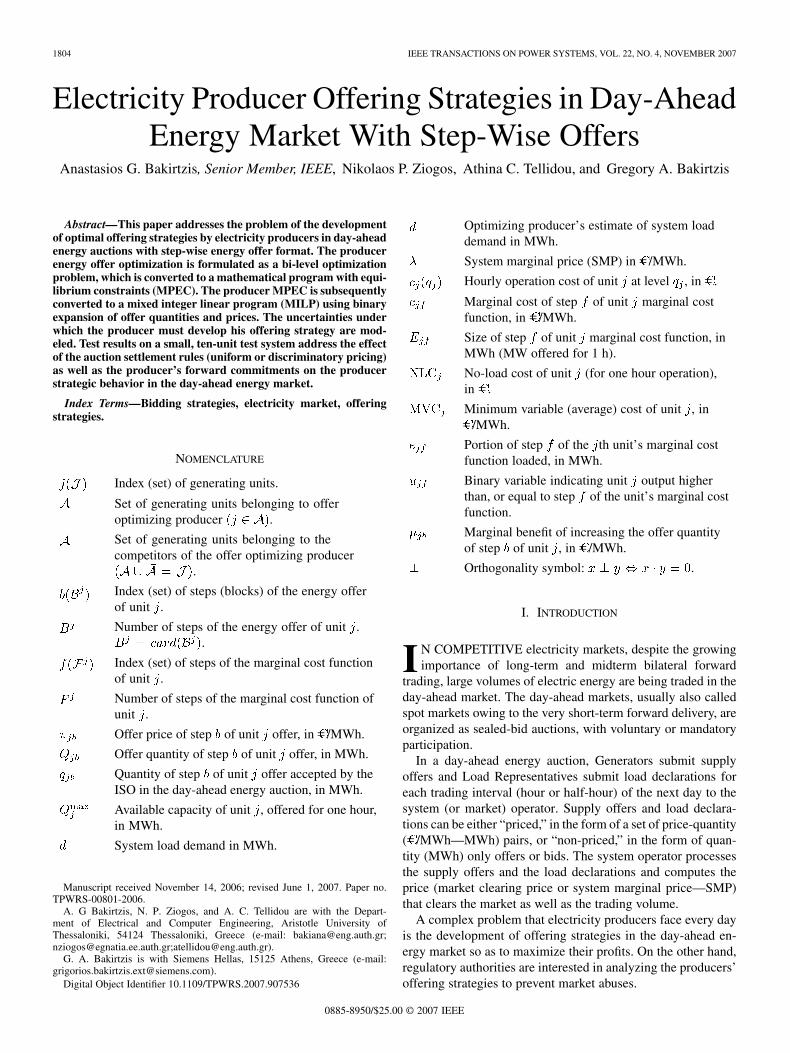
1804 IEEE TRANSACTIONS ON POWER SYSTEMS, VOL. 22, NO. 4, NOVEMBER 2007
Electricity Producer Offering Strategies in Day-AheadEnergy Market With Step-Wise Offers
Anastasios G. Bakirtzis, Senior Member, IEEE, Nikolaos P. Ziogos, Athina C. Tellidou, and Gregory A. Bakirtzis
Abstract—This paper addresses the problem of the developmentof optimal offering strategies by electricity producers in day-aheadenergy auctions with step-wise energy offer format. The producerenergy offer optimization is formulated as a bi-level optimizationproblem, which is converted to a mathematical program with equi-librium constraints (MPEC). The producer MPEC is subsequentlyconverted to a mixed integer linear program (MILP) using binaryexpansion of offer quantities and prices. The uncertainties underwhich the producer must develop his offering strategy are mod-eled. Test results on a small, ten-unit test system address the effectof the auction settlement rules (uniform or discriminatory pricing)as well as the producer’s forward commitments on the producerstrategic behavior in the day-ahead energy market.
Index Terms—Bidding strategies, electricity market, offeringstrategies.
NOMENCLATURE
Index (set) of generating units.
Set of generating units belonging to offeroptimizing producer .
Set of generating units belonging to thecompetitors of the offer optimizing producer
.
Index (set) of steps (blocks) of the energy offerof unit .
Number of steps of the energy offer of unit ..
Index (set) of steps of the marginal cost functionof unit .
Number of steps of the marginal cost function ofunit .
Offer price of step of unit offer, in /MWh.
Offer quantity of step of unit offer, in MWh.
Quantity of step of unit offer accepted by theISO in the day-ahead energy auction, in MWh.
Available capacity of unit , offered for one hour,in MWh.
System load demand in MWh.
Manuscript received November 14, 2006; revised June 1, 2007. Paper no.TPWRS-00801-2006.
A. G Bakirtzis, N. P. Ziogos, and A. C. Tellidou are with the Depart-ment of Electrical and Computer Engineering, Aristotle University ofThessaloniki, 54124 Thessaloniki, Greece (e-mail: [email protected];[email protected];[email protected]).
G. A. Bakirtzis is with Siemens Hellas, 15125 Athens, Greece (e-mail:[email protected]).
Digital Object Identifier 10.1109/TPWRS.2007.907536
Optimizing producer’s estimate of system loaddemand in MWh.
System marginal price (SMP) in /MWh.
Hourly operation cost of unit at level , in .
Marginal cost of step of unit marginal costfunction, in /MWh.
Size of step of unit marginal cost function, inMWh (MW offered for 1 h).
No-load cost of unit (for one hour operation),in .
Minimum variable (average) cost of unit , in/MWh.
Portion of step of the th unit’s marginal costfunction loaded, in MWh.
Binary variable indicating unit output higherthan, or equal to step of the unit’s marginal costfunction.
Marginal benefit of increasing the offer quantityof step of unit , in /MWh.
Orthogonality symbol: .
I. INTRODUCTION
I N COMPETITIVE electricity markets, despite the growingimportance of long-term and midterm bilateral forward
trading, large volumes of electric energy are being traded in theday-ahead market. The day-ahead markets, usually also calledspot markets owing to the very short-term forward delivery, areorganized as sealed-bid auctions, with voluntary or mandatoryparticipation.
In a day-ahead energy auction, Generators submit supplyoffers and Load Representatives submit load declarations foreach trading interval (hour or half-hour) of the next day to thesystem (or market) operator. Supply offers and load declara-tions can be either “priced,” in the form of a set of price-quantity( /MWh—MWh) pairs, or “non-priced,” in the form of quan-tity (MWh) only offers or bids. The system operator processesthe supply offers and the load declarations and computes theprice (market clearing price or system marginal price—SMP)that clears the market as well as the trading volume.
A complex problem that electricity producers face every dayis the development of offering strategies in the day-ahead en-ergy market so as to maximize their profits. On the other hand,regulatory authorities are interested in analyzing the producers’offering strategies to prevent market abuses.
0885-8950/$25.00 © 2007 IEEE
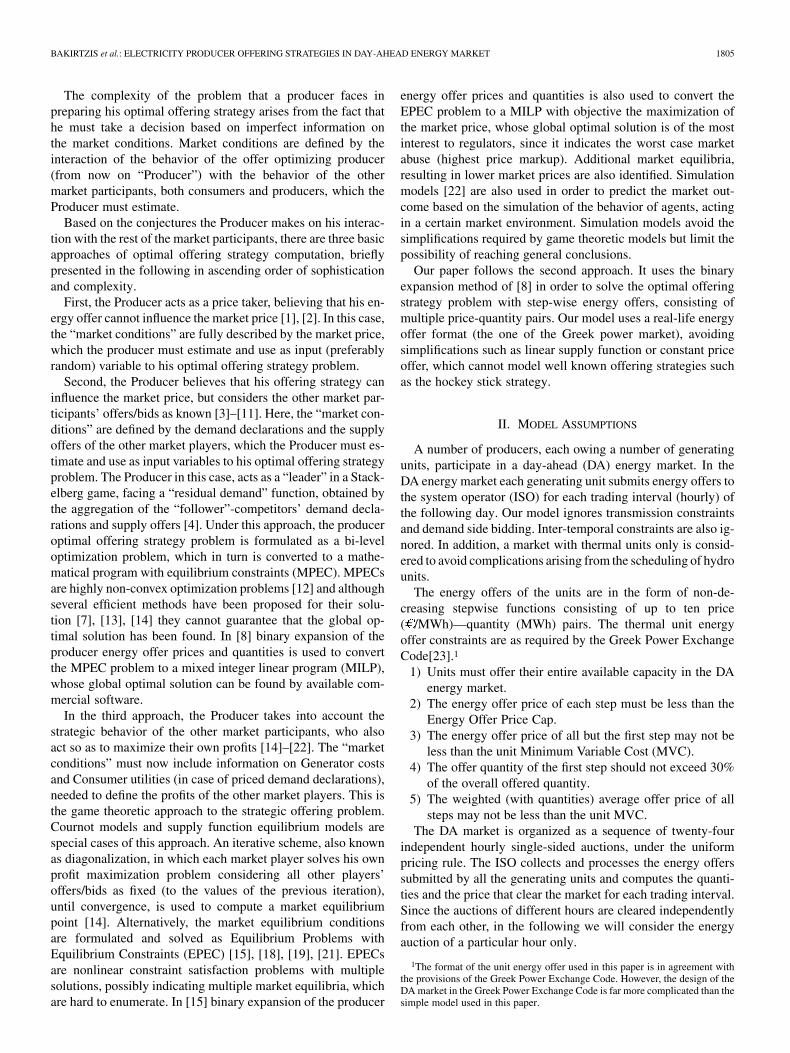
BAKIRTZIS et al.: ELECTRICITY PRODUCER OFFERING STRATEGIES IN DAY-AHEAD ENERGY MARKET 1805
The complexity of the problem that a producer faces inpreparing his optimal offering strategy arises from the fact thathe must take a decision based on imperfect information onthe market conditions. Market conditions are defined by theinteraction of the behavior of the offer optimizing producer(from now on “Producer”) with the behavior of the othermarket participants, both consumers and producers, which theProducer must estimate.
Based on the conjectures the Producer makes on his interac-tion with the rest of the market participants, there are three basicapproaches of optimal offering strategy computation, brieflypresented in the following in ascending order of sophisticationand complexity.
First, the Producer acts as a price taker, believing that his en-ergy offer cannot influence the market price [1], [2]. In this case,the “market conditions” are fully described by the market price,which the producer must estimate and use as input (preferablyrandom) variable to his optimal offering strategy problem.
Second, the Producer believes that his offering strategy caninfluence the market price, but considers the other market par-ticipants’ offers/bids as known [3]–[11]. Here, the “market con-ditions” are defined by the demand declarations and the supplyoffers of the other market players, which the Producer must es-timate and use as input variables to his optimal offering strategyproblem. The Producer in this case, acts as a “leader” in a Stack-elberg game, facing a “residual demand” function, obtained bythe aggregation of the “follower”-competitors’ demand decla-rations and supply offers [4]. Under this approach, the produceroptimal offering strategy problem is formulated as a bi-leveloptimization problem, which in turn is converted to a mathe-matical program with equilibrium constraints (MPEC). MPECsare highly non-convex optimization problems [12] and althoughseveral efficient methods have been proposed for their solu-tion [7], [13], [14] they cannot guarantee that the global op-timal solution has been found. In [8] binary expansion of theproducer energy offer prices and quantities is used to convertthe MPEC problem to a mixed integer linear program (MILP),whose global optimal solution can be found by available com-mercial software.
In the third approach, the Producer takes into account thestrategic behavior of the other market participants, who alsoact so as to maximize their own profits [14]–[22]. The “marketconditions” must now include information on Generator costsand Consumer utilities (in case of priced demand declarations),needed to define the profits of the other market players. This isthe game theoretic approach to the strategic offering problem.Cournot models and supply function equilibrium models arespecial cases of this approach. An iterative scheme, also knownas diagonalization, in which each market player solves his ownprofit maximization problem considering all other players’offers/bids as fixed (to the values of the previous iteration),until convergence, is used to compute a market equilibriumpoint [14]. Alternatively, the market equilibrium conditionsare formulated and solved as Equilibrium Problems withEquilibrium Constraints (EPEC) [15], [18], [19], [21]. EPECsare nonlinear constraint satisfaction problems with multiplesolutions, possibly indicating multiple market equilibria, whichare hard to enumerate. In [15] binary expansion of the producer
energy offer prices and quantities is also used to convert theEPEC problem to a MILP with objective the maximization ofthe market price, whose global optimal solution is of the mostinterest to regulators, since it indicates the worst case marketabuse (highest price markup). Additional market equilibria,resulting in lower market prices are also identified. Simulationmodels [22] are also used in order to predict the market out-come based on the simulation of the behavior of agents, actingin a certain market environment. Simulation models avoid thesimplifications required by game theoretic models but limit thepossibility of reaching general conclusions.
Our paper follows the second approach. It uses the binaryexpansion method of [8] in order to solve the optimal offeringstrategy problem with step-wise energy offers, consisting ofmultiple price-quantity pairs. Our model uses a real-life energyoffer format (the one of the Greek power market), avoidingsimplifications such as linear supply function or constant priceoffer, which cannot model well known offering strategies suchas the hockey stick strategy.
II. MODEL ASSUMPTIONS
A number of producers, each owing a number of generatingunits, participate in a day-ahead (DA) energy market. In theDA energy market each generating unit submits energy offers tothe system operator (ISO) for each trading interval (hourly) ofthe following day. Our model ignores transmission constraintsand demand side bidding. Inter-temporal constraints are also ig-nored. In addition, a market with thermal units only is consid-ered to avoid complications arising from the scheduling of hydrounits.
The energy offers of the units are in the form of non-de-creasing stepwise functions consisting of up to ten price( /MWh)—quantity (MWh) pairs. The thermal unit energyoffer constraints are as required by the Greek Power ExchangeCode[23].1
1) Units must offer their entire available capacity in the DAenergy market.
2) The energy offer price of each step must be less than theEnergy Offer Price Cap.
3) The energy offer price of all but the first step may not beless than the unit Minimum Variable Cost (MVC).
4) The offer quantity of the first step should not exceed 30%of the overall offered quantity.
5) The weighted (with quantities) average offer price of allsteps may not be less than the unit MVC.
The DA market is organized as a sequence of twenty-fourindependent hourly single-sided auctions, under the uniformpricing rule. The ISO collects and processes the energy offerssubmitted by all the generating units and computes the quanti-ties and the price that clear the market for each trading interval.Since the auctions of different hours are cleared independentlyfrom each other, in the following we will consider the energyauction of a particular hour only.
1The format of the unit energy offer used in this paper is in agreement withthe provisions of the Greek Power Exchange Code. However, the design of theDA market in the Greek Power Exchange Code is far more complicated than thesimple model used in this paper.
1806 IEEE TRANSACTIONS ON POWER SYSTEMS, VOL. 22, NO. 4, NOVEMBER 2007
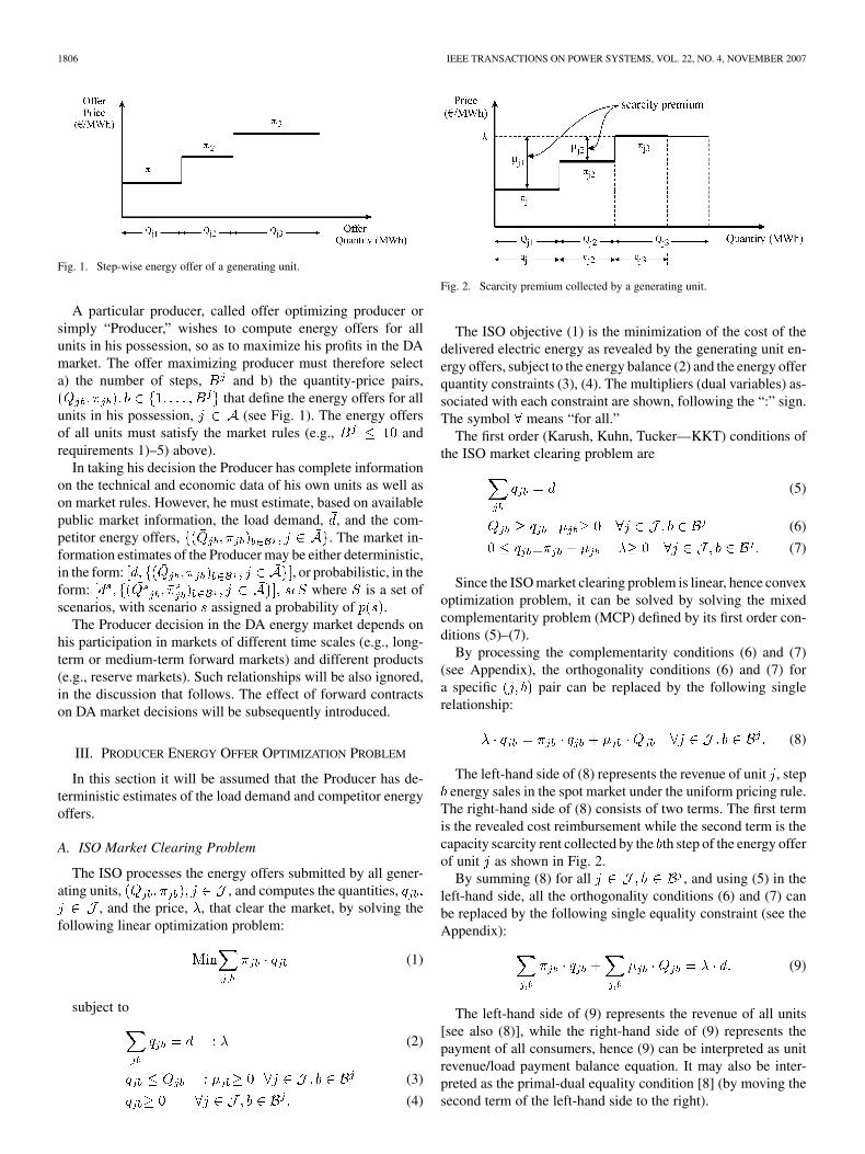
Fig. 1. Step-wise energy offer of a generating unit.
A particular producer, called offer optimizing producer orsimply “Producer,” wishes to compute energy offers for allunits in his possession, so as to maximize his profits in the DAmarket. The offer maximizing producer must therefore selecta) the number of steps, and b) the quantity-price pairs,
that define the energy offers for allunits in his possession, (see Fig. 1). The energy offersof all units must satisfy the market rules (e.g., andrequirements 1)–5) above).
In taking his decision the Producer has complete informationon the technical and economic data of his own units as well ason market rules. However, he must estimate, based on availablepublic market information, the load demand, , and the com-petitor energy offers, . The market in-formation estimates of the Producer may be either deterministic,in the form: , or probabilistic, in theform: where is a set ofscenarios, with scenario assigned a probability of .
The Producer decision in the DA energy market depends onhis participation in markets of different time scales (e.g., long-term or medium-term forward markets) and different products(e.g., reserve markets). Such relationships will be also ignored,in the discussion that follows. The effect of forward contractson DA market decisions will be subsequently introduced.
III. PRODUCER ENERGY OFFER OPTIMIZATION PROBLEM
In this section it will be assumed that the Producer has de-terministic estimates of the load demand and competitor energyoffers.
A. ISO Market Clearing Problem
The ISO processes the energy offers submitted by all gener-ating units, , and computes the quantities,
, and the price, , that clear the market, by solving thefollowing linear optimization problem:
(1)
subject to
(2)
(3)
(4)
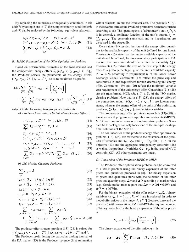
Fig. 2. Scarcity premium collected by a generating unit.
The ISO objective (1) is the minimization of the cost of thedelivered electric energy as revealed by the generating unit en-ergy offers, subject to the energy balance (2) and the energy offerquantity constraints (3), (4). The multipliers (dual variables) as-sociated with each constraint are shown, following the “:” sign.The symbol means “for all.”
The first order (Karush, Kuhn, Tucker—KKT) conditions ofthe ISO market clearing problem are
(5)
(6)
(7)
Since the ISO market clearing problem is linear, hence convexoptimization problem, it can be solved by solving the mixedcomplementarity problem (MCP) defined by its first order con-ditions (5)–(7).
By processing the complementarity conditions (6) and (7)(see Appendix), the orthogonality conditions (6) and (7) fora specific pair can be replaced by the following singlerelationship:
(8)
The left-hand side of (8) represents the revenue of unit , stepenergy sales in the spot market under the uniform pricing rule.
The right-hand side of (8) consists of two terms. The first termis the revealed cost reimbursement while the second term is thecapacity scarcity rent collected by the th step of the energy offerof unit as shown in Fig. 2.
By summing (8) for all , and using (5) in theleft-hand side, all the orthogonality conditions (6) and (7) canbe replaced by the following single equality constraint (see theAppendix):
(9)
The left-hand side of (9) represents the revenue of all units[see also (8)], while the right-hand side of (9) represents thepayment of all consumers, hence (9) can be interpreted as unitrevenue/load payment balance equation. It may also be inter-preted as the primal-dual equality condition [8] (by moving thesecond term of the left-hand side to the right).
BAKIRTZIS et al.: ELECTRICITY PRODUCER OFFERING STRATEGIES IN DAY-AHEAD ENERGY MARKET 1807
By replacing the numerous orthogonality conditions in (6)and (7) by a single one in (9) the complementarity conditions (6)and (7) can be replaced by the following, equivalent relations:
(10)
(11)
(12)
B. MPEC Formulation of the Offer Optimization Problem
Based on deterministic estimates of the load demand andthe competitors’ energy offers, ,the Producer selects the parameters of his energy offers,
, so as to maximize his profits
(13)
subject to the following two groups of constraints.a) Producer Constraints (Technical and Energy Offer):
(14)
(15)
(16)
(17)
(18)
(19)
(20)
b) ISO Market Clearing Problem:
(21)
(22)
(23)
(24)
(25)
(26)
(27)
(28)
The producer offer strategy problem (13)–(28) is solved forand .
The Producer profit during the particular trading interval ofthe DA market (13) is the Producer revenue (first summation
within brackets) minus the Producer cost. The productsin the revenue term of the Producer profit have been transformedaccording to (8). The operating cost of a Producer’s unit, ,is in general, a nonlinear function of the unit’s output,
. The generating unit cost and its linearization arediscussed in the Appendix.
Constraints (14) restrict the size of the energy offer quanti-ties to the available capacity of the unit (offered for one hour).Constraints (15) state that the entire available capacity of theunit should be offered; for non-mandatory participation in DAmarket, this constraint should be written as inequality .Constraints (16) restrict the size of the first step of the energyoffer to a given percentage, , of the unit’s available capacity( % according to requirement iv of the Greek PowerExchange Code). Constraints (17) reflect the price cap andconstraints (18) the requirement for non-decreasing unit energyoffer. Constraints (19) and (20) reflect the minimum variablecost requirement of the unit energy offer. Constraints (21)–(28)are the transformed MCP, (5), (10)–(12), of the ISO marketclearing problem. Note that in (13)–(28), the energy offers ofthe competitor units, , are known con-stants, whereas the energy offers of the units of the optimizingproducer, , are decision variables.
The producer energy offer optimization problem (13)–(28) isa mathematical program with equilibrium constraints (MPEC).MPECs are nonlinear, non-convex optimization problems. Stan-dard NLP packages can only locate one of the multiple local op-timal solutions of the MPEC.
The nonlinearities of the producer energy offer optimizationproblem, (13)–(28), are restricted to the existence of the prod-ucts of variables and and for , in theobjective (13) and the aggregate orthogonality constraint (28)as well as the product of variables in the second MVCconstraint (20). All other constraints are linear.
C. Conversion of the Producer MPEC to MILP
The Producer offer optimization problem can be convertedto a MILP problem using the binary expansion of the offerprices and quantities proposed in [8]. The binary expansionof prices and quantities starts with the selection of the offerprice and quantity steps, and according to market rules(e.g., Greek market rules require that /MWh and
MWh).For the binary expansion of the offer price , binary
variables are introduced. In order tomodel offer prices in the range (between zero and theprice cap) with a resolution of /MWh the required numberof binary variables for the binary expansion of the offer pricesis
(29)
The binary expansion of the offer price, , is
(30)

1808 IEEE TRANSACTIONS ON POWER SYSTEMS, VOL. 22, NO. 4, NOVEMBER 2007
The nonlinearity due to the product is resolved byintroducing new variables so that the productof variables is transformed to the following linear constraint:
(31)
The product of variables is transformed intothe following IF-THEN relation:
(32)
Relation (32) is then transformed into the following equiva-lent linear constraints [8]:
(33)
(34)
where is a large constant, so that constraints (33) and (34)are relaxed when and , respectively. Forexample, .
For the binary expansion of the offer quantity , bi-nary variables are introduced. Inorder to model offer quantities in the range with a res-olution of MW the required number of binary variables forthe binary expansion of the offer quantities of unit is
(35)
The binary expansion of the offer quantity, , is
(36)
The nonlinearity due to the product is resolved byintroducing new variables and following thesame procedure as with the product . The following setof linear constraints results:
(37)
(38)
(39)
where is a large constant, so that constraints (38) and (39)are relaxed when and , respectively. Forexample, .
The nonlinearity due to the product in (20) is simi-larly resolved by introducing new variables
so that the product of variables is transformed to the followinglinear constraint:
(40)
The product of variables is then trans-formed into the following two equivalent linear constraints:
(41)
(42)
that must be written .The producer offer strategy MPEC, (13)–(28), is converted
to MILP by the substitution of all stand-alone (not as productof variables terms) occurrences of the producer offer variables
with their corresponding binary expansions in (30) and(36), the substitution of the products of variables
, and , with their corresponding linear expressions,(31), (37), and (40), and the addition of the constraints resultingfrom the transformation of the products of variables, (33), (34),(38), (39), (41) and (42).
In the above MILP formulation, the number of the steps of theenergy offer of every unit belonging to the producer is consid-ered known and equal to the regulatory limit, , (e.g.,
). As stated in Section III, in preparinghis energy offer, the Producer must also determine the numberof steps, of the energy offer of every unit in his posses-sion. A reasonable and convenient selection would be the min-imum possible that would not jeopardize his profits. Thisis achieved by augmenting the Producer’s objective (13) by thefollowing term, penalizing the total number of steps offered bythe Producer:
(43)
The penalty weight, , is selected so that the absolute valueof the penalty term is always lower than a small monetary tol-erance, e.g., , so as not to intervene with the Pro-ducer’s profit maximization objective. Despite its small weight,the penalty term proved very effective in minimizing the numberof steps of the energy offers computed by the MILP model.
In practice, in the MILP formulation of the Producer offeringstrategy problem, , is selected equal to the regu-latory limit, , for all Producer units, , so that theMILP deals with fixed number of steps. Let , denote thenumber of the non-zero sized steps of the energy offer of the thunit. A zero-sized step of a unit’s energy offer has 0 MWh quan-tity assigned by the MILP model, , i.e., it wasdeemed “unnecessary” by the MILP model. New binary vari-ables, , are introduced in the MILP model,such that if step of unit’s energy offer is zero-sized

BAKIRTZIS et al.: ELECTRICITY PRODUCER OFFERING STRATEGIES IN DAY-AHEAD ENERGY MARKET 1809
and otherwise. The number of non-zero sized steps ofthe energy offer of the th unit, , needed to define the penaltyterm (43) can be expressed in terms of the binary variables, ,as .
The penalty term, (43) is expressed in terms of the new binaryvariables as
(44)
In addition, the following two sets of constraints must beadded to the MILP model, for the determination of the new bi-nary variables
(45)
(46)
With the introduction of the new binary variables,, the addition of the penalty term (44) in the Pro-
ducer’s objective and the addition of the new constraints (45)and (46) in the MILP model, the Producer profit maximizingenergy offer with the minimum possible number of steps is com-puted by the MILP model.
The application of the above complete MILP formulation tothe producer offer-strategy MPEC problem, in which both en-ergy offer prices and quantities are treated as decision variables,resulted in problematic MILP performance, even in the absenceof the second MVC constraint (20), which requires the additionof the numerous new variables, , for the resolution of theproduct . Although in our tests the MILP providedan optimal energy offer, the optimality of the solution could notbe guaranteed, since the optimality gap could not be reduced toan acceptable level.
A reduced MILP formulation of the producer offer-strategyMPEC problem was implemented with much better MILP per-formance. In the reduced formulation the number of steps,and the quantities, , of each unit’s energy offer are pre-defined by partitioning in advance the unit’s capacity so that(14), (15), and (16) are satisfied (and are no longer needed inthe optimization model), and only the energy offer prices, ,are treated as decision variables. In this case the MILP modelis formed by the substitution of all stand-alone occurrences ofthe producer offer prices , with their corresponding binaryexpansion in (30), the substitution of the product of variables
with the corresponding linear expressions, (31) andthe addition of the constraints resulting from the transformationof the product of variables, (33) and (34). The reduced MILPmodel is presented in the Appendix.
IV. MODEL EXTENSIONS
A. Uncertainty Modeling
In the previous section the Producer’s offering strategy isbased on the Producer’s deterministic knowledge of the systemdemand and the competitors’ energy offers. However, the Pro-ducer must estimate the demand and the competitors’ energy
offers based on available market information; both estimates en-tail some degree of uncertainty. Next day’s demand can be fore-casted based on historic demand records, which is public infor-mation, as well as weather historic records and forecasts, alsoavailable in public. The competitors’ energy offers can be esti-mated based on the Producer’s gathered information on his com-petitors (press releases, etc.) and on ISO released information onpast market outcomes; in some electricity markets the energyoffers of all participants become public information some timeafter the market clearing [6], [8]. In addition to uncertainties indemand forecasts and competitor offers the Producer may wishto incorporate uncertainties due to unforeseen events, such asunit outages. In fact, competitor unit outages can be modeledas changes to competitor energy offers (capacity withholding).The modeling of uncertainties is thus very important in the Pro-ducer’s decision process.
Uncertainties in demand and competitor energy offers aremodeled through the pre-definition of a number of scenarios ofdemand and competitor offers, and their associated probabilityof occurrence, , where
is a set of scenarios, and the probability assigned to sce-nario . The Producer’s objective is the maximization of his ex-pected profit
(47)
subject toa) Producer constraints (technical and energy offer):
(48)
(49)
(50)
(51)
(52)
(53)
(54)
b) ISO market clearing problem:
(55)
(56)
(57)
(58)
(59)
(60)
1810 IEEE TRANSACTIONS ON POWER SYSTEMS, VOL. 22, NO. 4, NOVEMBER 2007
(61)
(62)
The producer offer strategy problem (13)–(28) is solved for
and .Note that the number of binary variables required for the bi-
nary expansion of offer prices and quantities in the produceroffer strategy problem under uncertainty remains the same withthe ones in the deterministic case [8].
B. Forward Contract Modeling
If the producer has signed a forward contract to serveMWh at a contract price of /MWh, then the objective ofhis or her offer optimizing strategy must be changed from (13)to
(63)
The problem constraints remain the same.
C. Modeling of Pay-As-Bid Pricing
If the producer optimizes his energy offers under pay-as-bidpricing rule, then his objective (13) becomes
(64)
i.e., the capacity scarcity rent term, , is missing. Theconstraints remain the same.
D. Transmission Constraints and Multi-Period Decisions
The MILP model can be extended to incorporate transmis-sion constraints and Producer multi-period decisions, includinggenerating unit ramp-rates and commitment, as discussed in[8]. For example, when transmission constraints are includedin the ISO market-clearing problem, using locational marketprices, (8) still holds with denoting the nodal price of the nodeon which generating unit is connected. The payment balance(9) is also valid, with the addition of a transmission capacityscarcity rent (positive for all congested lines) to the left-handside and the interpretation of the right-hand side as the totalconsumer payment under locational marginal pricing. Owingto space limitations we will not elaborate further on transmis-sion constraints and multi-period decision modeling, which willbe the subject of our future work. However, it must be stated
TABLE IPRODUCER UNIT COST DATA (A) MARGINAL COST CURVE QUANTITY DATA
(B) MARGINAL COST AND NO LOAD COST (NLC) DATA
(C) MINIMUM VARIABLE COST (MVC) DATA
that for the equivalence of the Producer bi-level optimizationproblem with the related MPEC problem, it is required that theISO second-level problem be convex, so that it can be replacedby the corresponding KKT conditions. When a centralized unitcommitment is performed by the ISO, the ISO problem is nolonger convex and the proposed method cannot be applied.
V. TEST RESULTS
The developed method has been tested on a small, ten unittest system. The first four units belong to the Producer whilethe remaining six belong to his competitors. Table I providesthe Producer unit cost data (the marginal cost curve, the no-loadcost and the resulting minimum variable cost). Table II gives thecompetitor unit energy offer data.
All tests were performed on a 3 GHz Pentium IV with 1 GBof RAM. The models were implemented in GAMS using theCPLEX solver [24].
Two sets of tests are performed. In the first set the Producerenergy offers are computed based on deterministic estimates ofthe consumer demand, the competitor energy offers (as givenin Table II) and the competitor unit availability (all competitorunits are available). In the second set of tests uncertainty, re-garding the consumer demand and the competitor unit avail-ability, is introduced.
In each set of tests, three cases are examined, named and de-fined as follows.

BAKIRTZIS et al.: ELECTRICITY PRODUCER OFFERING STRATEGIES IN DAY-AHEAD ENERGY MARKET 1811
TABLE IICOMPETITOR UNIT ENERGY OFFER DATA (A) ENERGY OFFER QUANTITY DATA
(B) ENERGY OFFER PRICE DATA
UMP: Producer is paid under the Uniform Pricing rule.
PAB: Producer is paid under the Pay-As-Bid Pricingrule.
UMPc: Producer has signed a forward contract to deliver600 MWh at 60 /MWh during the current hour,and is paid according to the Uniform Pricing rule.
Unless otherwise specified, the Minimum Variable Cost(MVC) requirement is observed. The cases in which the MVCrequirement is relaxed are designated as “ .”
A. Reduced Model Results
As discussed in Section IV, in the reduced MILP model theenergy offer quantities are predefined and only the energy offerprices are treated as decision variables. Here it is assumed thatthe offer quantities coincide with the marginal cost curve quan-tity data of Table I, i.e., ,2 so that (78) is used.
In all cases considered, the energy price cap is 100 /MWh. Aprice resolution /MWh is used, thereforebinary variables are needed for the binary expansion of the offerprices of the units belonging to the Producer.
Tables III–V present the optimum energy offer prices of Unit1 of the Producer (the offer quantities are given in Table I), theresulting System Marginal Price (SMP) and the MILP executiontime for deterministically known load levels in the range
2Note that in Table I = 1=3 has been used to approximate the = 0:3requirement of the Greek Exchange Code modeled in (16) so that all offer quan-tities are multiples of 50 MW.
TABLE IIIUNIT 1 ENERGY OFFER PRICES, CASE UMP (UNIFORM PRICING)
TABLE IVUNIT 1 ENERGY OFFER PRICES, CASE PAB (PAY-AS-BID PRICING)
TABLE VUNIT 1 ENERGY OFFER PRICES, CASE UMP (CONTRACT)
[800–2000] MW, for each of the test cases defined above. Thehigh sensitivity of the MILP execution time to the load level is
1812 IEEE TRANSACTIONS ON POWER SYSTEMS, VOL. 22, NO. 4, NOVEMBER 2007
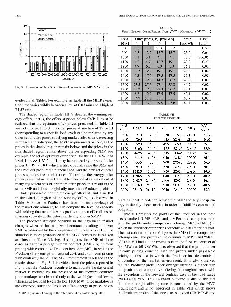
Fig. 3. Illustration of the effect of forward contracts on SMP (MVC = 0).
evident in all Tables. For example, in Table III the MILP execu-tion time varies wildly between a low of 0.03 min and a high of74.57 min.
The shaded region in Tables III–V denotes the winning en-ergy offers, that is, the offers at prices below SMP. It must berealized that the optimum offer prices presented in Table IIIare not unique. In fact, the offer prices at any line of Table III(corresponding to a specific load level) can be replaced by anyother set of offer prices satisfying market rules (non-decreasingsequence and satisfying the MVC requirement) as long as theprices in the shaded region remain below, and the prices in thenon-shaded region remain above, the corresponding SMP. Forexample, the set of optimum offer prices for the 1100 MW loadlevel, , may be replaced by the set of offerprices which is also optimal, since the SMP andthe Producer profit remain unchanged, and the new set of offerprices satisfies the market rules. Therefore, the energy offerprices presented in Table III must be interpreted as one set out ofmany equivalent sets of optimum offer prices that result in thesame SMP and the same globally maximum Producer profits.
Under pay-as-bid pricing the energy offers of Unit 1 are flatin the (shaded) region of the winning offers, as observed inTable IV: since the Producer has deterministic knowledge ofthe market environment, he can compute the level of capacitywithholding that maximizes his profits and then offer all his re-maining capacity at the deterministically known SMP.3
The producer strategic behavior in the day-ahead marketchanges when he has a forward contract, resulting at lowerSMP as observed by the comparison of Tables V and III. Thesituation is more pronounced if the MVC constraint is relaxedas shown in Table VI. Fig. 3 compares the SMP of threecases a) uniform pricing without contract (UMP), b) uniformpricing with competitive Producer behavior (MC), in which theProducer offers energy at marginal cost, and c) uniform pricingwith contract (UMPc). The MVC requirement is relaxed in theresults shown in Fig. 3. It is evident from the prices reported inFig. 3 that the Producer incentive to manipulate the day-aheadmarket is reduced by the presence of the forward contract:price markups are observed only at the two highest load levels,whereas at low load levels (below 1100 MW) price markdownsare observed, since the Producer offers energy at prices below
3SMP in pay-as-bid pricing is the offer price of the last winning offer.
TABLE VIUNIT 1 ENERGY OFFER PRICES, CASE UMP (CONTRACT), MVC = 0
TABLE VIIPRODUCER PROFIT (C)
marginal cost in order to reduce the SMP and buy cheap en-ergy in the day-ahead market in order to fulfill his contractualobligation.
Table VII presents the profits of the Producer in the threecases studied (UMP, PAB, and UMPc), and compares themwith the profits under competitive offering (MC and MCc) inwhich the Producer offer prices coincide with his marginal cost.The last column of Table VII gives the SMP of the competitiveoffering case. The profits of the columns “UMPc” and “MCc”of Table VII include the revenues from the forward contract of600 MWh at 60 /MWh. It is observed that the profits underuniform pricing coincide with the profits under pay-as-bidpricing in this test in which the Producer has deterministicknowledge of the market environment. It is also observedthat the Producer profit under strategic offering is higher thanhis profit under competitive offering (at marginal cost), withthe exception of the forward contract case in the load range[900–1400] MW. This awkward outcome is due to the factthat the strategic offering case is constrained by the MVCrequirement and is not observed in Table VIII which showsthe Producer profits of the three cases studied (UMP, PAB and
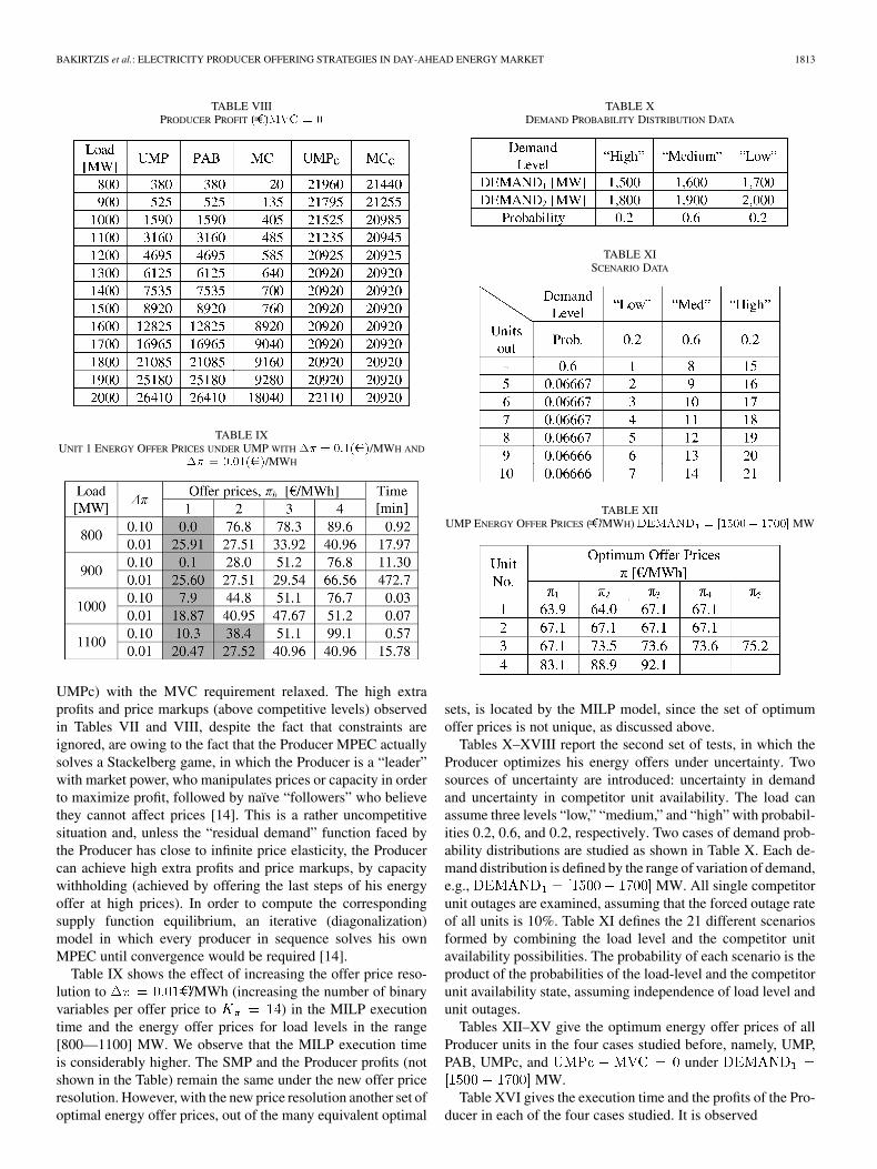
BAKIRTZIS et al.: ELECTRICITY PRODUCER OFFERING STRATEGIES IN DAY-AHEAD ENERGY MARKET 1813
TABLE VIIIPRODUCER PROFIT (C)MVC = 0
TABLE IXUNIT 1 ENERGY OFFER PRICES UNDER UMP WITH �� = 0:1(C=)/MWH AND
�� = 0:01(C=)/MWH
UMPc) with the MVC requirement relaxed. The high extraprofits and price markups (above competitive levels) observedin Tables VII and VIII, despite the fact that constraints areignored, are owing to the fact that the Producer MPEC actuallysolves a Stackelberg game, in which the Producer is a “leader”with market power, who manipulates prices or capacity in orderto maximize profit, followed by naïve “followers” who believethey cannot affect prices [14]. This is a rather uncompetitivesituation and, unless the “residual demand” function faced bythe Producer has close to infinite price elasticity, the Producercan achieve high extra profits and price markups, by capacitywithholding (achieved by offering the last steps of his energyoffer at high prices). In order to compute the correspondingsupply function equilibrium, an iterative (diagonalization)model in which every producer in sequence solves his ownMPEC until convergence would be required [14].
Table IX shows the effect of increasing the offer price reso-lution to /MWh (increasing the number of binaryvariables per offer price to ) in the MILP executiontime and the energy offer prices for load levels in the range[800—1100] MW. We observe that the MILP execution timeis considerably higher. The SMP and the Producer profits (notshown in the Table) remain the same under the new offer priceresolution. However, with the new price resolution another set ofoptimal energy offer prices, out of the many equivalent optimal
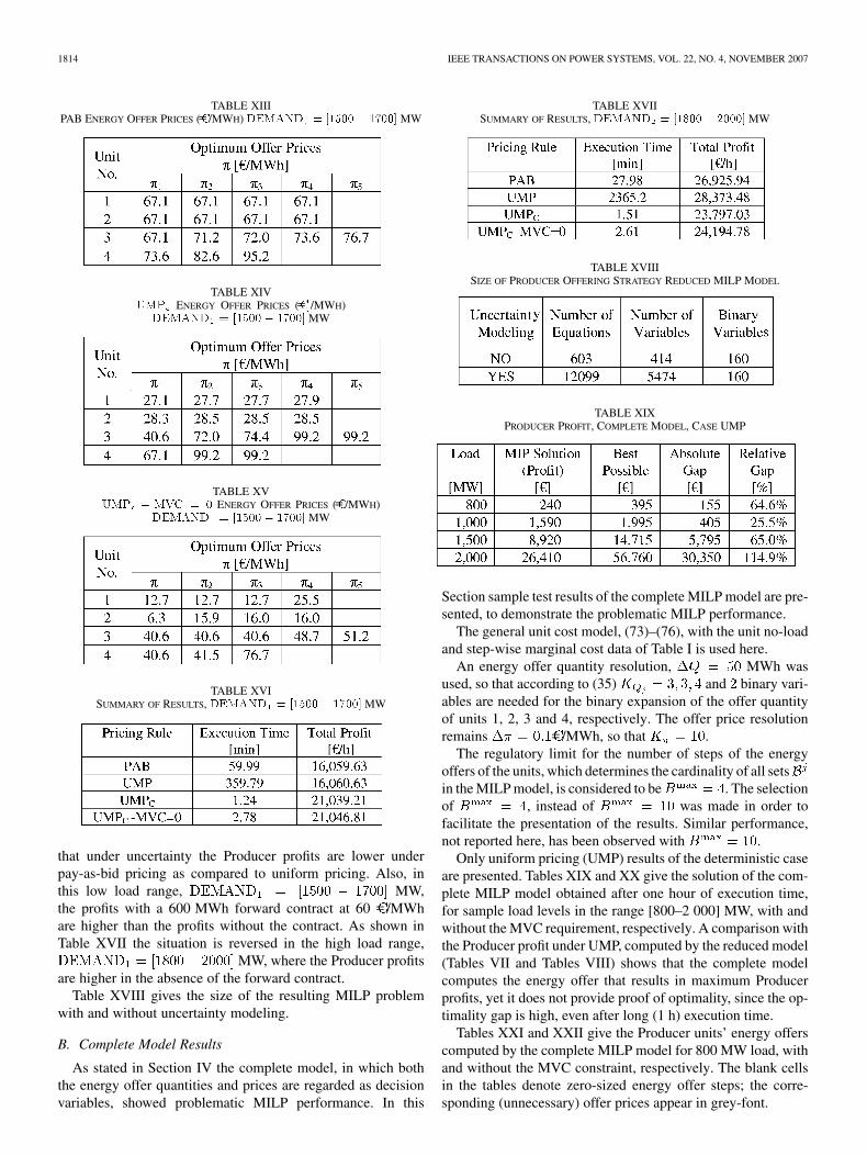
TABLE XDEMAND PROBABILITY DISTRIBUTION DATA
TABLE XISCENARIO DATA
TABLE XIIUMP ENERGY OFFER PRICES (C/MWH) DEMAND = [1500� 1700] MW
sets, is located by the MILP model, since the set of optimumoffer prices is not unique, as discussed above.
Tables X–XVIII report the second set of tests, in which theProducer optimizes his energy offers under uncertainty. Twosources of uncertainty are introduced: uncertainty in demandand uncertainty in competitor unit availability. The load canassume three levels “low,” “medium,” and “high” with probabil-ities 0.2, 0.6, and 0.2, respectively. Two cases of demand prob-ability distributions are studied as shown in Table X. Each de-mand distribution is defined by the range of variation of demand,e.g., MW. All single competitorunit outages are examined, assuming that the forced outage rateof all units is 10%. Table XI defines the 21 different scenariosformed by combining the load level and the competitor unitavailability possibilities. The probability of each scenario is theproduct of the probabilities of the load-level and the competitorunit availability state, assuming independence of load level andunit outages.
Tables XII–XV give the optimum energy offer prices of allProducer units in the four cases studied before, namely, UMP,PAB, UMPc, and under
MW.Table XVI gives the execution time and the profits of the Pro-
ducer in each of the four cases studied. It is observed
1814 IEEE TRANSACTIONS ON POWER SYSTEMS, VOL. 22, NO. 4, NOVEMBER 2007
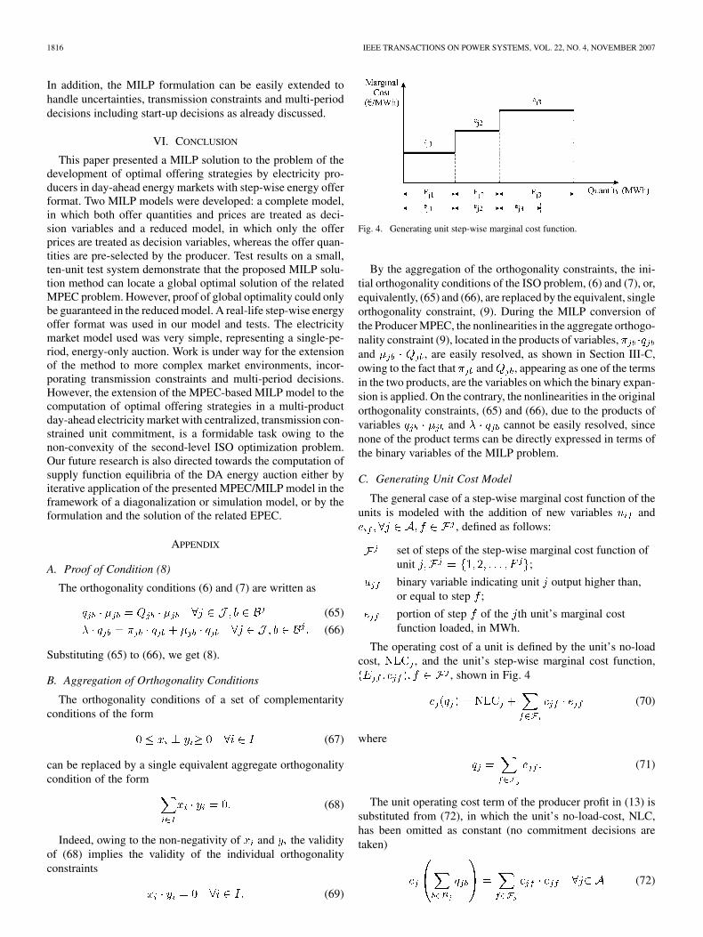
TABLE XIIIPAB ENERGY OFFER PRICES (C/MWH) DEMAND = [1500� 1700] MW
TABLE XIVUMP ENERGY OFFER PRICES (C]/MWH)
DEMAND = [1500� 1700] MW
TABLE XVUMP � MVC = 0 ENERGY OFFER PRICES (C/MWH)
DEMAND = [1500� 1700] MW
TABLE XVISUMMARY OF RESULTS, DEMAND = [1500� 1700] MW
that under uncertainty the Producer profits are lower underpay-as-bid pricing as compared to uniform pricing. Also, inthis low load range, MW,the profits with a 600 MWh forward contract at 60 /MWhare higher than the profits without the contract. As shown inTable XVII the situation is reversed in the high load range,
MW, where the Producer profitsare higher in the absence of the forward contract.
Table XVIII gives the size of the resulting MILP problemwith and without uncertainty modeling.
B. Complete Model Results
As stated in Section IV the complete model, in which boththe energy offer quantities and prices are regarded as decisionvariables, showed problematic MILP performance. In this
TABLE XVIISUMMARY OF RESULTS, DEMAND = [1800� 2000] MW
TABLE XVIIISIZE OF PRODUCER OFFERING STRATEGY REDUCED MILP MODEL
TABLE XIXPRODUCER PROFIT, COMPLETE MODEL, CASE UMP
Section sample test results of the complete MILP model are pre-sented, to demonstrate the problematic MILP performance.
The general unit cost model, (73)–(76), with the unit no-loadand step-wise marginal cost data of Table I is used here.
An energy offer quantity resolution, MWh wasused, so that according to (35) and binary vari-ables are needed for the binary expansion of the offer quantityof units 1, 2, 3 and 4, respectively. The offer price resolutionremains /MWh, so that .
The regulatory limit for the number of steps of the energyoffers of the units, which determines the cardinality of all setsin the MILP model, is considered to be . The selectionof , instead of was made in order tofacilitate the presentation of the results. Similar performance,not reported here, has been observed with .
Only uniform pricing (UMP) results of the deterministic caseare presented. Tables XIX and XX give the solution of the com-plete MILP model obtained after one hour of execution time,for sample load levels in the range [800–2 000] MW, with andwithout the MVC requirement, respectively. A comparison withthe Producer profit under UMP, computed by the reduced model(Tables VII and Tables VIII) shows that the complete modelcomputes the energy offer that results in maximum Producerprofits, yet it does not provide proof of optimality, since the op-timality gap is high, even after long (1 h) execution time.
Tables XXI and XXII give the Producer units’ energy offerscomputed by the complete MILP model for 800 MW load, withand without the MVC constraint, respectively. The blank cellsin the tables denote zero-sized energy offer steps; the corre-sponding (unnecessary) offer prices appear in grey-font.

BAKIRTZIS et al.: ELECTRICITY PRODUCER OFFERING STRATEGIES IN DAY-AHEAD ENERGY MARKET 1815
TABLE XXPRODUCER PROFIT, COMPLETE MODEL, CASE UMP, MVC = 0
TABLE XXICOMPLETE MODEL, UMP,Demand = 800MW ENERGY OFFERS (A) ENERGY
OFFER QUANTITIES AND (B) ENERGY OFFER PRICES
TABLE XXIICOMPLETE MODEL, UMP, MVC = 0;Demand = 800MW ENERGY OFFERS
(A) ENERGY OFFER QUANTITIES AND (B) ENERGY OFFER PRICES
The results shown in the tables demonstrate the effectivenessof the penalty term (44) in minimizing the number of thenon-zero sized steps of the energy offers. The results shown inTable XXII, also observed in all other load levels, demonstratethat if the Producer has deterministic market information andthe MVC requirement is relaxed, maximization of the Producerprofits can be achieved if every unit submits an energy offer
TABLE XXIIISIZE OF PRODUCER OFFERING STRATEGY COMPLETE MILP MODEL
TABLE XXIVPRODUCER PROFIT (C) COMPUTED BY MPEC SOLUTION
consisting of a single price—quantity pair [25]. When the MVCrequirement is enforced, some units may need to submit energyoffers consisting of two steps, to take advantage of the MVCrequirement relaxation in the first step, as shown in Table XXI(units 1 and 2).
Table XXIII gives the size of the complete MILP model withand without MVC modeling. The drastic increase in the numberof equations and (continuous) variables when MVC is modeledis due to the addition of the numerous variables and con-straints (40)–(42) for the modeling of the MVC requirement.Please note that, despite their binary nature, variables and
are declared as continuous variables, yet, owing to the re-lated constraints, they are assigned only binary values by theMILP model.
C. Comparison of MILP With Complementarity Solvers.
The Producer bi-level offer optimization problem was alsosolved as an MPEC problem (13)–(28), using NLPEC, theMPEC solver provided by GAMS [24]. The non-convex, non-linear MPEC problem, produced by NLPEC, was solved byBARON, a global NLP solver. The optimum Producer profitcomputed in four different cases (UMP and PAB with andwithout the MVC requirement) for load levels in the range[800–2 000] MW is shown in Table XXIV. The direct solutionof the Producer’s MPEC by NLPEC/BARON is very fast,compared to the MILP solution, requiring only a few secondsin all cases. However, it failed to provide the global optimalsolution in several cases. A star to the left of the Producerprofit figure in Table XXIV indicates a case in which the directMPEC solution provided inferior solution to MILP (comparewith MILP optimum Producer profits of Tables VII and VIII).
1816 IEEE TRANSACTIONS ON POWER SYSTEMS, VOL. 22, NO. 4, NOVEMBER 2007
In addition, the MILP formulation can be easily extended tohandle uncertainties, transmission constraints and multi-perioddecisions including start-up decisions as already discussed.
VI. CONCLUSION
This paper presented a MILP solution to the problem of thedevelopment of optimal offering strategies by electricity pro-ducers in day-ahead energy markets with step-wise energy offerformat. Two MILP models were developed: a complete model,in which both offer quantities and prices are treated as deci-sion variables and a reduced model, in which only the offerprices are treated as decision variables, whereas the offer quan-tities are pre-selected by the producer. Test results on a small,ten-unit test system demonstrate that the proposed MILP solu-tion method can locate a global optimal solution of the relatedMPEC problem. However, proof of global optimality could onlybe guaranteed in the reduced model. A real-life step-wise energyoffer format was used in our model and tests. The electricitymarket model used was very simple, representing a single-pe-riod, energy-only auction. Work is under way for the extensionof the method to more complex market environments, incor-porating transmission constraints and multi-period decisions.However, the extension of the MPEC-based MILP model to thecomputation of optimal offering strategies in a multi-productday-ahead electricity market with centralized, transmission con-strained unit commitment, is a formidable task owing to thenon-convexity of the second-level ISO optimization problem.Our future research is also directed towards the computation ofsupply function equilibria of the DA energy auction either byiterative application of the presented MPEC/MILP model in theframework of a diagonalization or simulation model, or by theformulation and the solution of the related EPEC.
APPENDIX
A. Proof of Condition (8)
The orthogonality conditions (6) and (7) are written as
(65)
(66)
Substituting (65) to (66), we get (8).
B. Aggregation of Orthogonality Conditions
The orthogonality conditions of a set of complementarityconditions of the form
(67)
can be replaced by a single equivalent aggregate orthogonalitycondition of the form
(68)
Indeed, owing to the non-negativity of and the validityof (68) implies the validity of the individual orthogonalityconstraints
(69)
Fig. 4. Generating unit step-wise marginal cost function.
By the aggregation of the orthogonality constraints, the ini-tial orthogonality conditions of the ISO problem, (6) and (7), or,equivalently, (65) and (66), are replaced by the equivalent, singleorthogonality constraint, (9). During the MILP conversion ofthe Producer MPEC, the nonlinearities in the aggregate orthogo-nality constraint (9), located in the products of variables,and , are easily resolved, as shown in Section III-C,owing to the fact that and , appearing as one of the termsin the two products, are the variables on which the binary expan-sion is applied. On the contrary, the nonlinearities in the originalorthogonality constraints, (65) and (66), due to the products ofvariables and cannot be easily resolved, sincenone of the product terms can be directly expressed in terms ofthe binary variables of the MILP problem.
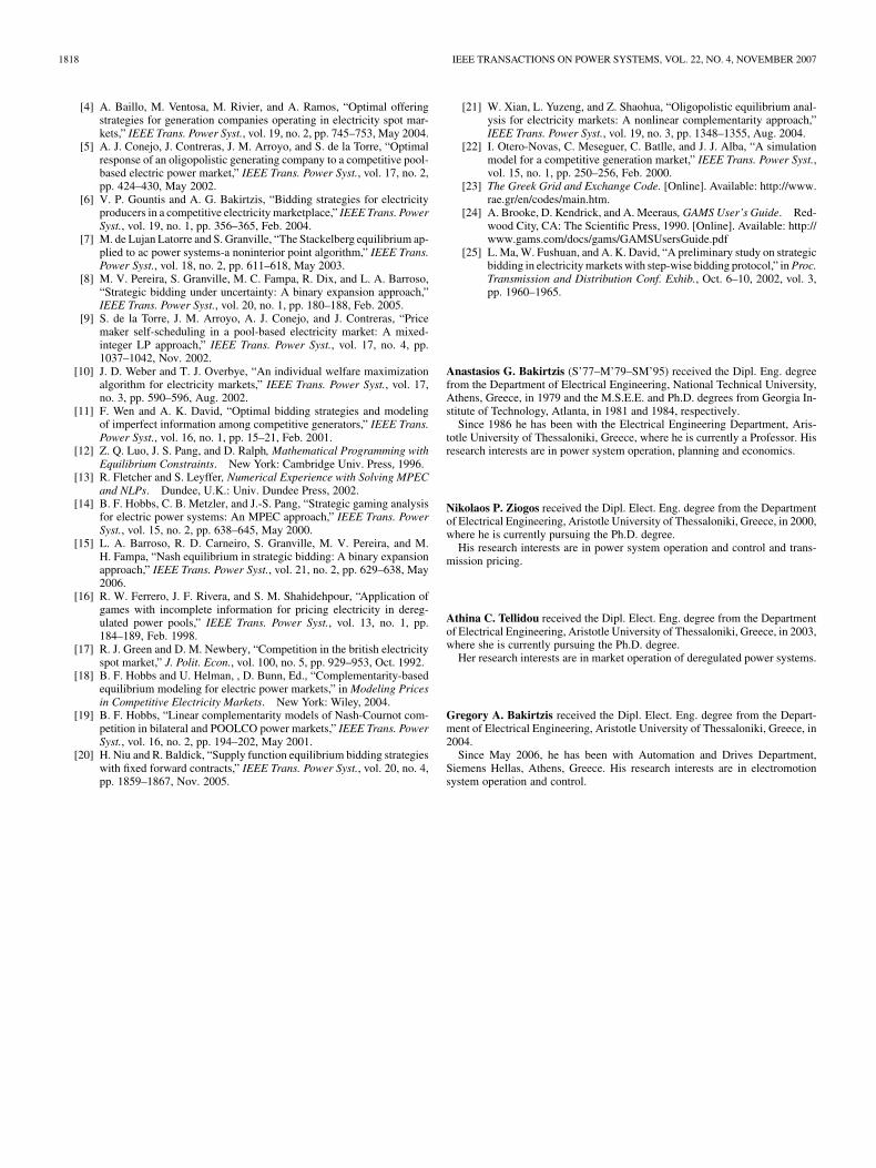
C. Generating Unit Cost Model
The general case of a step-wise marginal cost function of theunits is modeled with the addition of new variables and
, defined as follows:
set of steps of the step-wise marginal cost function ofunit ;
binary variable indicating unit output higher than,or equal to step ;
portion of step of the th unit’s marginal costfunction loaded, in MWh.
The operating cost of a unit is defined by the unit’s no-loadcost, , and the unit’s step-wise marginal cost function,
, shown in Fig. 4
(70)
where
(71)
The unit operating cost term of the producer profit in (13) issubstituted from (72), in which the unit’s no-load-cost, NLC,has been omitted as constant (no commitment decisions aretaken)
(72)

BAKIRTZIS et al.: ELECTRICITY PRODUCER OFFERING STRATEGIES IN DAY-AHEAD ENERGY MARKET 1817
so that the producer objective (13) becomes
(73)
In addition, the following constraints must be added to themodel
(74)
(75)
(76)
Two special cases of unit cost modeling avoid the use of thenew variables , and the introduction of the additionalconstraints (74)–(76).
If the unit’s marginal cost is constant, /MWh, over theunit’s full range of output, the producer objective (13) becomes
(77)
In the reduced MILP formulation of the producer offerstrategy MPEC problem, in which the offer quantities, , areknown in advance, the steps of the unit’s marginal cost curvemay be chosen to coincide with the steps of the unit’s energyoffer curve: . In this case theproducer objective (13) becomes
(78)
Given the unit’s no-load cost, , and the unit’s step-wisemarginal cost function, , the unit’s minimumvariable cost is computed from (79) and is measured at the unit’sbest efficiency point (close to the unit’s nominal power output)
(79)
D. Reduced MILP Model
The reduced MILP model, in which the Producer EnergyOffer quantities, , are pre-defined, is as follows:
(80)
subject toa) Producer Constraints (Technical and Energy Offer):
(81)
(82)
(83)
(84)
b) ISO Market Clearing Problem:
(85)
(86)
(87)
(88)
(89)
(90)
(91)
(92)
(93)
(94)
(95)
The producer offer strategy MILP (80)–(94) problem issolved for
and .Note that in forming the objective function (80) it was as-
sumed that , so that (78) was used. Also notethat offer quantity constraints (14)–(16) do not appear in the re-duced MILP model since they can be satisfied during the selec-tion of the energy offer quantities, , by the Producer.
REFERENCES
[1] A. J. Conejo, F. J. Nogales, and J. M. Arroyo, “Price-taker biddingstrategy under price uncertainty,” IEEE Trans. Power Syst., vol. 17, no.4, pp. 1081–1088, Nov. 2002.
[2] G. Gross and D. Finlay, “Generation supply bidding in perfectly com-petitive electricity markets,” Comput. Math. Org. Theor., vol. 6, pp.83–98, 2000.
[3] E. J. Anderson and A. B. Philpott, “Optimal offer construction in elec-tricity markets,” Math. Oper. Res., vol. 27, no. 1, pp. 82–100, Feb.2002.
1818 IEEE TRANSACTIONS ON POWER SYSTEMS, VOL. 22, NO. 4, NOVEMBER 2007
[4] A. Baillo, M. Ventosa, M. Rivier, and A. Ramos, “Optimal offeringstrategies for generation companies operating in electricity spot mar-kets,” IEEE Trans. Power Syst., vol. 19, no. 2, pp. 745–753, May 2004.
[5] A. J. Conejo, J. Contreras, J. M. Arroyo, and S. de la Torre, “Optimalresponse of an oligopolistic generating company to a competitive pool-based electric power market,” IEEE Trans. Power Syst., vol. 17, no. 2,pp. 424–430, May 2002.
[6] V. P. Gountis and A. G. Bakirtzis, “Bidding strategies for electricityproducers in a competitive electricity marketplace,” IEEE Trans. PowerSyst., vol. 19, no. 1, pp. 356–365, Feb. 2004.
[7] M. de Lujan Latorre and S. Granville, “The Stackelberg equilibrium ap-plied to ac power systems-a noninterior point algorithm,” IEEE Trans.Power Syst., vol. 18, no. 2, pp. 611–618, May 2003.
[8] M. V. Pereira, S. Granville, M. C. Fampa, R. Dix, and L. A. Barroso,“Strategic bidding under uncertainty: A binary expansion approach,”IEEE Trans. Power Syst., vol. 20, no. 1, pp. 180–188, Feb. 2005.
[9] S. de la Torre, J. M. Arroyo, A. J. Conejo, and J. Contreras, “Pricemaker self-scheduling in a pool-based electricity market: A mixed-integer LP approach,” IEEE Trans. Power Syst., vol. 17, no. 4, pp.1037–1042, Nov. 2002.
[10] J. D. Weber and T. J. Overbye, “An individual welfare maximizationalgorithm for electricity markets,” IEEE Trans. Power Syst., vol. 17,no. 3, pp. 590–596, Aug. 2002.
[11] F. Wen and A. K. David, “Optimal bidding strategies and modelingof imperfect information among competitive generators,” IEEE Trans.Power Syst., vol. 16, no. 1, pp. 15–21, Feb. 2001.
[12] Z. Q. Luo, J. S. Pang, and D. Ralph, Mathematical Programming withEquilibrium Constraints. New York: Cambridge Univ. Press, 1996.
[13] R. Fletcher and S. Leyffer, Numerical Experience with Solving MPECand NLPs. Dundee, U.K.: Univ. Dundee Press, 2002.
[14] B. F. Hobbs, C. B. Metzler, and J.-S. Pang, “Strategic gaming analysisfor electric power systems: An MPEC approach,” IEEE Trans. PowerSyst., vol. 15, no. 2, pp. 638–645, May 2000.
[15] L. A. Barroso, R. D. Carneiro, S. Granville, M. V. Pereira, and M.H. Fampa, “Nash equilibrium in strategic bidding: A binary expansionapproach,” IEEE Trans. Power Syst., vol. 21, no. 2, pp. 629–638, May2006.
[16] R. W. Ferrero, J. F. Rivera, and S. M. Shahidehpour, “Application ofgames with incomplete information for pricing electricity in dereg-ulated power pools,” IEEE Trans. Power Syst., vol. 13, no. 1, pp.184–189, Feb. 1998.
[17] R. J. Green and D. M. Newbery, “Competition in the british electricityspot market,” J. Polit. Econ., vol. 100, no. 5, pp. 929–953, Oct. 1992.
[18] B. F. Hobbs and U. Helman, , D. Bunn, Ed., “Complementarity-basedequilibrium modeling for electric power markets,” in Modeling Pricesin Competitive Electricity Markets. New York: Wiley, 2004.
[19] B. F. Hobbs, “Linear complementarity models of Nash-Cournot com-petition in bilateral and POOLCO power markets,” IEEE Trans. PowerSyst., vol. 16, no. 2, pp. 194–202, May 2001.
[20] H. Niu and R. Baldick, “Supply function equilibrium bidding strategieswith fixed forward contracts,” IEEE Trans. Power Syst., vol. 20, no. 4,pp. 1859–1867, Nov. 2005.
[21] W. Xian, L. Yuzeng, and Z. Shaohua, “Oligopolistic equilibrium anal-ysis for electricity markets: A nonlinear complementarity approach,”IEEE Trans. Power Syst., vol. 19, no. 3, pp. 1348–1355, Aug. 2004.
[22] I. Otero-Novas, C. Meseguer, C. Batlle, and J. J. Alba, “A simulationmodel for a competitive generation market,” IEEE Trans. Power Syst.,vol. 15, no. 1, pp. 250–256, Feb. 2000.
[23] The Greek Grid and Exchange Code. [Online]. Available: http://www.rae.gr/en/codes/main.htm.
[24] A. Brooke, D. Kendrick, and A. Meeraus, GAMS User’s Guide. Red-wood City, CA: The Scientific Press, 1990. [Online]. Available: http://www.gams.com/docs/gams/GAMSUsersGuide.pdf
[25] L. Ma, W. Fushuan, and A. K. David, “A preliminary study on strategicbidding in electricity markets with step-wise bidding protocol,” in Proc.Transmission and Distribution Conf. Exhib., Oct. 6–10, 2002, vol. 3,pp. 1960–1965.
Anastasios G. Bakirtzis (S’77–M’79–SM’95) received the Dipl. Eng. degreefrom the Department of Electrical Engineering, National Technical University,Athens, Greece, in 1979 and the M.S.E.E. and Ph.D. degrees from Georgia In-stitute of Technology, Atlanta, in 1981 and 1984, respectively.
Since 1986 he has been with the Electrical Engineering Department, Aris-totle University of Thessaloniki, Greece, where he is currently a Professor. Hisresearch interests are in power system operation, planning and economics.
Nikolaos P. Ziogos received the Dipl. Elect. Eng. degree from the Departmentof Electrical Engineering, Aristotle University of Thessaloniki, Greece, in 2000,where he is currently pursuing the Ph.D. degree.
His research interests are in power system operation and control and trans-mission pricing.
Athina C. Tellidou received the Dipl. Elect. Eng. degree from the Departmentof Electrical Engineering, Aristotle University of Thessaloniki, Greece, in 2003,where she is currently pursuing the Ph.D. degree.
Her research interests are in market operation of deregulated power systems.
Gregory A. Bakirtzis received the Dipl. Elect. Eng. degree from the Depart-ment of Electrical Engineering, Aristotle University of Thessaloniki, Greece, in2004.
Since May 2006, he has been with Automation and Drives Department,Siemens Hellas, Athens, Greece. His research interests are in electromotionsystem operation and control.