Purdue UniversityPurdue e-Pubs

CTRC Research Publications Cooling Technologies Research Center

2012

Electrical impedance-based void fractionmeasurement and flow regime identification inmicrochannel flows under adiabatic conditionsSidharth ParanjapePurdue University

Susan N. RitcheyPurdue University

S V. GarimellaPurdue University, sureshg@purdue.edu

Follow this and additional works at: http://docs.lib.purdue.edu/coolingpubs

This document has been made available through Purdue e-Pubs, a service of the Purdue University Libraries. Please contact epubs@purdue.edu foradditional information.

Paranjape, Sidharth; Ritchey, Susan N.; and Garimella, S V., "Electrical impedance-based void fraction measurement and flow regimeidentification in microchannel flows under adiabatic conditions" (2012). CTRC Research Publications. Paper 167.http://dx.doi.org/10.1016/j.ijmultiphaseflow.2012.02.010

ELECTRICAL IMPEDANCE-BASED VOID FRACTION

MEASUREMENT AND FLOW REGIME IDENTIFICATION IN

MICROCHANNEL FLOWS UNDER ADIABATIC CONDITIONS

Sidharth Paranjape, Susan N. Ritchey, and Suresh V. Garimella*

Cooling Technologies Research Center, an NSF I/UCRC

School of Mechanical Engineering

Purdue University

West Lafayette, IN 47907 USA

*Corresponding author: Tel: 1-765- 494-5621, Email: sureshg@purdue.edu

*ManuscriptClick here to view linked References

2

Abstract

Electrical impedance of a two-phase mixture is a function of void fraction and phase

distribution. The difference in the specific electrical conductance and permittivity of the two

phases is exploited to measure electrical impedance for obtaining void fraction and flow regime

characteristics. An electrical impedance meter is constructed for the measurement of void

fraction in microchannel two-phase flow. The experiments are conducted in air-water two-phase

flow under adiabatic conditions. A transparent acrylic test section of hydraulic diameter 780 µm

is used in the experimental investigation. The impedance void meter is calibrated against the void

fraction calculated using analysis of images obtained with a high-speed camera. Based on these

measurements, a methodology utilizing the statistical characteristics of the void fraction signals

is employed for identification of microchannel flow regimes. A self-organizing neural network is

used for classification of the flow regimes.

Keywords: Microchannel flow, two-phase flow, void fraction, impedance meter, flow regimes

3

1. Introduction

Microchannel heat sinks based on boiling and two-phase flow can meet the increasing

cooling needs for high-end electronics systems in applications ranging from high-performance

computers to avionics and spacecraft to electric vehicles. In order to design and build such heat

sinks, a unified model accounting for the prevalent flow regimes is needed to predict the boiling

heat transfer rates and pressure drops in microchannels. Flow regime-based correlations are

desired in two-phase flow analyses since a single heat transfer correlation does not apply in all

flow regimes (Hewitt, 1983). A number of studies in recent years have attempted to better

understand the flow patterns during boiling in microchannels using various working fluids as

reviewed in Sobhan and Garimella (2001), Garimella and Sobhan (2003) and Bertsch et al.

(2008). A systematic investigation into the effects of channel size, mass flux and heat flux on the

boiling flow patterns and heat transfer in microchannels was recently performed by Harirchian

and Garimella (2008, 2009). A generalized flow regime map for boiling in microchannels

covering a wide range of channel geometries, heat fluxes and mass fluxes was developed in

terms of three non-dimensional parameters – Boiling number, Reynolds number and Bond

number – by Harirchian and Garimella (2010).

In order to further develop predictive models for flow regime transitions, it is necessary to

measure void fraction in two-phase flow, since void fraction and its temporal variation is a

characteristic of the flow regime. Several studies in the past have relied on flow visualization for

the identification of flow regimes as well as for the measurement of void fraction (Serizawa et

al., 2002, Kawahara et al., 2006, Kawaji et al., 2006, and Kawahara et al., 2009). Though flow

regimes can be determined by observing high-speed movie camera recordings, the method is

subjective and cannot be used for conditions in which intermittent phenomena occur, as well as

4

when the aspect ratios of the observed field is such that the mechanisms are obscured from visual

observation. In order to overcome these shortcomings, a non-intrusive void fraction

measurement technique, which is based on the measurement of electrical impedance, is explored

in the present study. Electrical impedance-based void fraction measurements have been

successfully performed in the past several decades in macroscale two-phase flows. For cross-

sectional area-averaged or volume-averaged measurements, impedance void meters with

electrodes flush mounted to the channel walls were used by Asali et al. (1985), Andreussi et al.

(1988), Tsochatzidis et al. (1992), Fossa (1998) and Mi et al. (1998). A theoretical basis for this

design is given in Coney (1973). A similar geometry of the impedance meter is adapted to the

microscale channels considered in the present study. The practical implementation of the

electronic circuit measures the net electrical admittance, i.e., the inverse of electrical impedance,

of the two-phase mixture. The admittance is a function of the material properties (specific

conductance and electrical permittivity of the two phases), the void fraction and the flow regime.

The specific conductance determines the conductive reactance, while the permittivity determines

the capacitive reactance. For a given geometry of electrodes, an appropriately normalized

admittance is a function of void fraction and flow regime.

Two-phase flow regimes are typically described using qualitative categorization of flow

visualizations. This involves subjectivity in their identification. In order to overcome this

difficulty, Jones and Zuber (1975) first employed quantitative means for flow regime

determination. Using an X-ray source, they measured the temporal variation of the area-

averaged void fraction in a rectangular channel (10 cm × 1 cm) and plotted a probability density

function (PDF) of the void fraction. The significant differences in the PDF between various flow

regimes suggested their use for flow regime determination. Later studies by Tutu (1982) and

5

Matsui (1984) used void fraction distributions obtained with differential pressure transducers,

while non-intrusive impedance void meters were used by Mi et al. (1998) as flow regime

indicators. A comprehensive study by Costigan and Whalley (1997) on flow regimes in vertical

upflow used segmental impedance electrodes to determine void fraction, combined with the PDF

technique. Recently, bubble chord-length distributions obtained from conductivity probes were

used as flow regime indicators by Julia et al. (2008). The quantitative flow regime classification

proposed by Mi et al. (1998) is adapted in the present study to identify the flow regimes.

The present work aims to develop an impedance-based void fraction sensor for microchannel

two-phase flows. The experiments are conducted in air-water two-phase flow under adiabatic

conditions. Flow regimes are identified quantitatively using the statistics of the signals acquired

by the void fraction sensor.

2. Experimental method

2.1 Test section

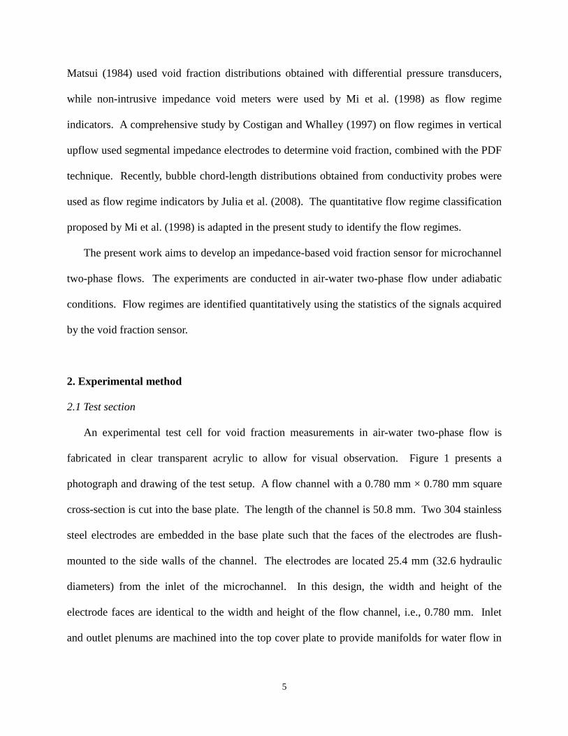
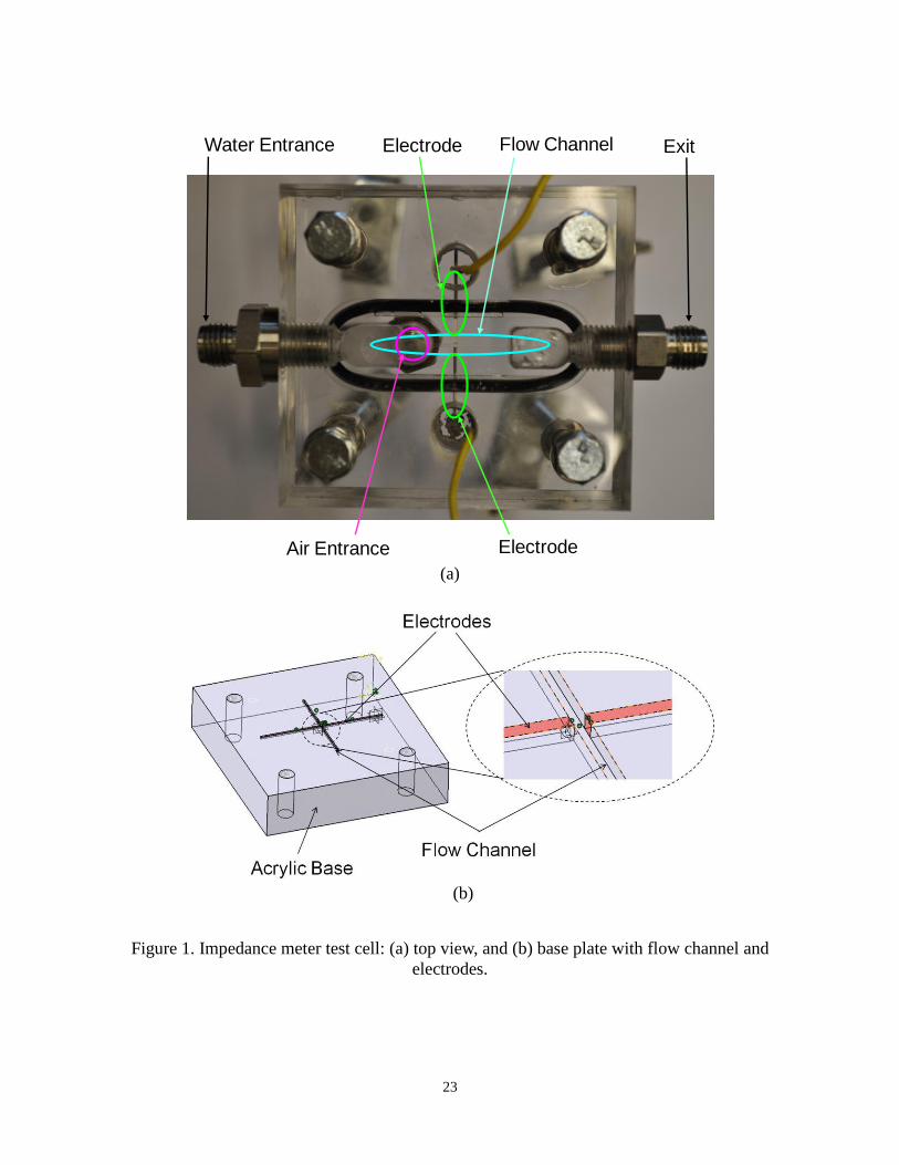
An experimental test cell for void fraction measurements in air-water two-phase flow is

fabricated in clear transparent acrylic to allow for visual observation. Figure 1 presents a

photograph and drawing of the test setup. A flow channel with a 0.780 mm × 0.780 mm square

cross-section is cut into the base plate. The length of the channel is 50.8 mm. Two 304 stainless

steel electrodes are embedded in the base plate such that the faces of the electrodes are flush-

mounted to the side walls of the channel. The electrodes are located 25.4 mm (32.6 hydraulic

diameters) from the inlet of the microchannel. In this design, the width and height of the

electrode faces are identical to the width and height of the flow channel, i.e., 0.780 mm. Inlet

and outlet plenums are machined into the top cover plate to provide manifolds for water flow in

6

the flow channel. The top cover plate is equipped with tube fittings to connect the test cell to the

flow loop. Single-phase water enters the flow channel from the inlet manifold. Air is directly

injected into the flow channel through a 0.3 mm diameter orifice at the bottom of the flow

channel. The air inlet orifice is located 10 mm downstream from the inlet of the flow channel.

The electrodes are connected to the electronic circuit via 14 gauge copper cables. Silver epoxy is

used to minimize the contact resistance between the electrodes and copper cables.

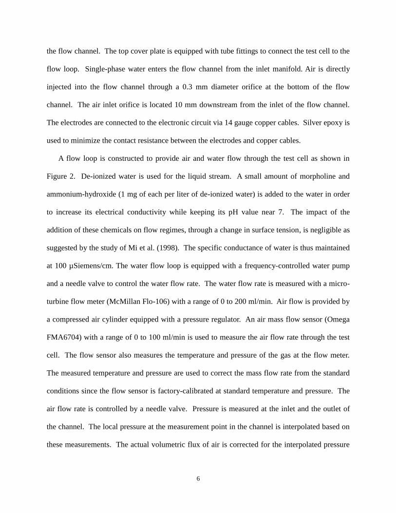
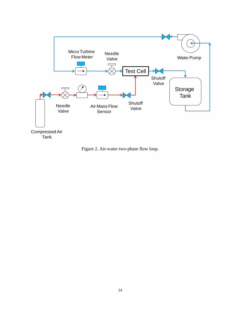
A flow loop is constructed to provide air and water flow through the test cell as shown in

Figure 2. De-ionized water is used for the liquid stream. A small amount of morpholine and

ammonium-hydroxide (1 mg of each per liter of de-ionized water) is added to the water in order

to increase its electrical conductivity while keeping its pH value near 7. The impact of the

addition of these chemicals on flow regimes, through a change in surface tension, is negligible as

suggested by the study of Mi et al. (1998). The specific conductance of water is thus maintained

at 100 µSiemens/cm. The water flow loop is equipped with a frequency-controlled water pump

and a needle valve to control the water flow rate. The water flow rate is measured with a micro-

turbine flow meter (McMillan Flo-106) with a range of 0 to 200 ml/min. Air flow is provided by

a compressed air cylinder equipped with a pressure regulator. An air mass flow sensor (Omega

FMA6704) with a range of 0 to 100 ml/min is used to measure the air flow rate through the test

cell. The flow sensor also measures the temperature and pressure of the gas at the flow meter.

The measured temperature and pressure are used to correct the mass flow rate from the standard

conditions since the flow sensor is factory-calibrated at standard temperature and pressure. The

air flow rate is controlled by a needle valve. Pressure is measured at the inlet and the outlet of

the channel. The local pressure at the measurement point in the channel is interpolated based on

these measurements. The actual volumetric flux of air is corrected for the interpolated pressure

7

at the measurement location. The storage tank is open to the atmosphere and also serves as an

air-water flow separator. Special care is taken to avoid flow instabilities from occurring due to

the accumulation of air in various tube fittings in the exit section of the flow loop. In order to

achieve this, flexible tygon tubing is used to connect the exit of the test section to the storage

tank, which is located at a higher elevation than the test section.

2.2 Impedance meter

An auto-balancing bridge method is implemented in a custom-built unit for measurement of

the electrical impedance of the two-phase mixture in the test cell. Details of auto-balancing

bridge methods are available in Tumanski (2006). The signal processing scheme is depicted in

Figure 3. The test cell is excited with an alternating sine wave voltage signal with a peak-to-

peak voltage difference of 3 V. The exciter signal is set at a frequency of 20 kHz. A current-to-

voltage amplifier is used for measurement of the resulting current. The voltage measured across

the reference resistor of the amplifier circuit serves as a measure of the current flowing through

the test cell. This signal is referred to as the modulated signal, while the exciter signal is taken as

the carrier wave. Both of these voltage signals are logged to a high-speed data acquisition

system (National Instruments NI 6259-USB) at a sampling rate of 500 kHz. The data acquisition

system has a 16-bit quantization for analog to digital conversion in the voltage range of -5 V to

+5 V. The signals are then processed numerically using a MATLAB program developed in-

house. The acquired signal is synchronously demodulated using the excitation signal and a 90º

phase-shifted excitation signal in order to calculate the real and imaginary parts of the

impedance. A low-pass Butterworth filter with cut-off frequency of 10 kHz is used to filter out

8

the excitation signal. The filtered signal is proportional to the electrical impedance of the two-

phase mixture between the electrodes.

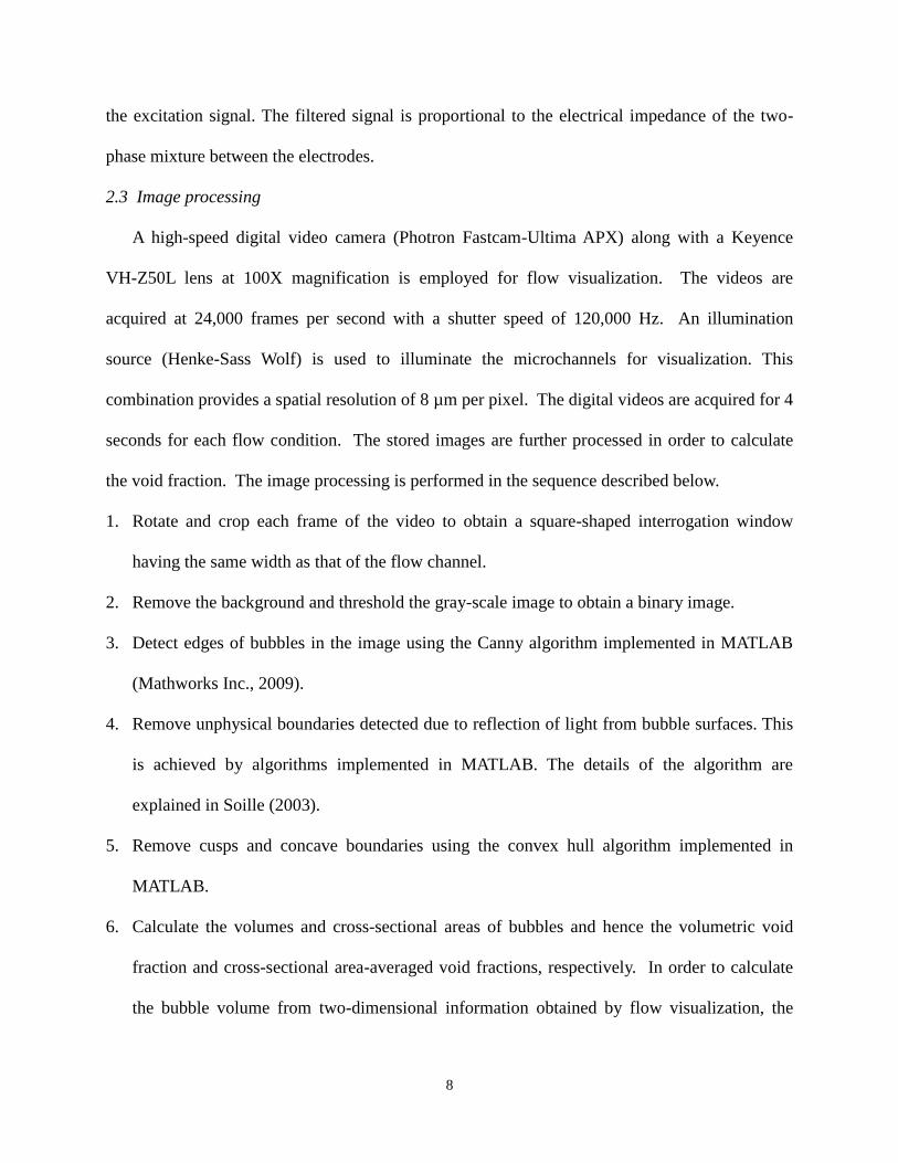
2.3 Image processing

A high-speed digital video camera (Photron Fastcam-Ultima APX) along with a Keyence

VH-Z50L lens at 100X magnification is employed for flow visualization. The videos are

acquired at 24,000 frames per second with a shutter speed of 120,000 Hz. An illumination

source (Henke-Sass Wolf) is used to illuminate the microchannels for visualization. This

combination provides a spatial resolution of 8 µm per pixel. The digital videos are acquired for 4

seconds for each flow condition. The stored images are further processed in order to calculate

the void fraction. The image processing is performed in the sequence described below.

1. Rotate and crop each frame of the video to obtain a square-shaped interrogation window

having the same width as that of the flow channel.

2. Remove the background and threshold the gray-scale image to obtain a binary image.

3. Detect edges of bubbles in the image using the Canny algorithm implemented in MATLAB

(Mathworks Inc., 2009).

4. Remove unphysical boundaries detected due to reflection of light from bubble surfaces. This

is achieved by algorithms implemented in MATLAB. The details of the algorithm are

explained in Soille (2003).

5. Remove cusps and concave boundaries using the convex hull algorithm implemented in

MATLAB.

6. Calculate the volumes and cross-sectional areas of bubbles and hence the volumetric void

fraction and cross-sectional area-averaged void fractions, respectively. In order to calculate

the bubble volume from two-dimensional information obtained by flow visualization, the

9

bubbles are assumed to be axisymmetric about their major axes. The uncertainties in the

volume measurement made under this assumption need careful quantification, which is the

focus of ongoing work. An approximate uncertainty analysis was performed for the

calculation of bubble volume for the simple geometries of spherical and cylindrical bubbles.

The maximum error was found to be 8% of the measured value.

7. Repeat Steps 1 through 6 for each frame in the movie to obtain a time series of the void

fraction. Further, calculate a time average of the volume- and area-averaged void fractions

for each flow condition.

Figure 4 illustrates the morphological operations performed in steps 1 through 5, which are

used to extract the boundaries of the bubbles from the original image. The time-averaged void

fractions calculated from the image processing of the videos are used as reference measurements

to calibrate the impedance void meter.

2.4 Uncertainty analysis

The uncertainties in the measurements of the steady-state values of gas and liquid flow rates

stem from a combination of uncertainty in the measurement by the flow meters and the inherent

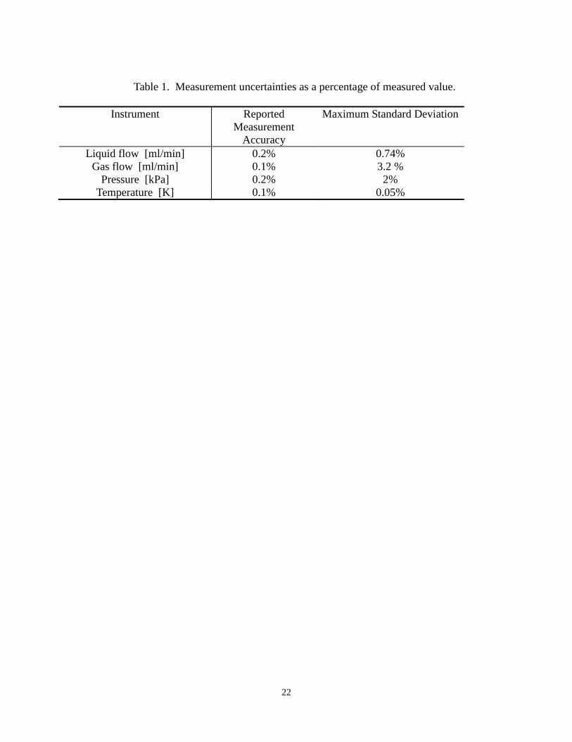
physical fluctuations in the flow conditions. Table 1 shows the measurement uncertainties for

the instruments used in the current experiments. The last column denotes the maximum standard

deviation as a percentage of the measured value observed in the current dataset of 71 flow

conditions.

For each flow condition, the quantities were acquired at 500 Hz for 10 s to obtain time-

averaged values after reaching a steady state. The resulting maximum uncertainties in the

measurement of gas and liquid flow rates are found to be 2.5% and 1% of the measured values,

respectively.

10

3. Results and discussion

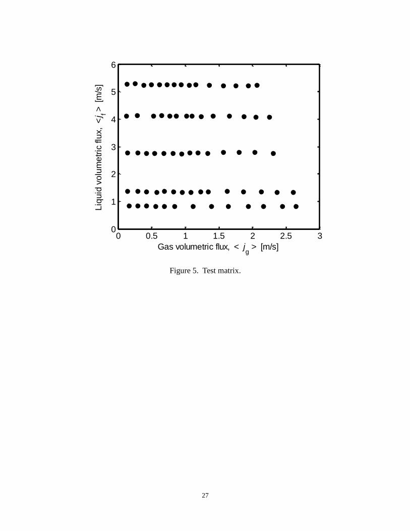
The void fraction measurements were performed under 71 different flow conditions. Each

flow condition was characterized by the velocity inlet boundary conditions, namely, volumetric

flux of gas gj

and volumetric flux of liquid fj . The range of flow conditions covered in this

study are 0.13m/s 2.65m/sgj and 0.8m/s 5.1m/sfj . The test matrix is presented using

coordinates of volumetric flux of gas and liquid flow as shown in Figure 5.

3.1 Flow visualization

The flow visualization study reveals the flow regimes observed under the current set of test

conditions. Figure 6 shows the images obtained using the high-speed video camera in various

flow regimes. The images presented are as acquired by the camera without any morphological

transformation. The void fraction reported in each panel is the time-averaged value of the

volume-averaged void fraction calculated using the image processing algorithm. The time series

of the volume-averaged void fractions corresponding to these flow conditions are presented in

Figure 7.

3.2 Calibration of impedance meter

The present measurement method determines the current passing through the test cell for a

given potential difference at a known excitation frequency. Thus, the measured current is

proportional to the admittance, i.e., the inverse of the impedance of the two-phase mixture in the

test cell. Further, in order to make the measurement independent of the material properties, the

measured admittance is normalized as: :

11

* 1

0 1

mG GG

G G

, (1)

where mG is the instantaneous two-phase mixture admittance, 0G is the admittance with zero

void fraction (i.e., for single-phase liquid) and 1G is the admittance when the void fraction is

unity (i.e., for single-phase gas). Finally, the liquid fraction is a monotonically increasing

function of normalized admittance, *G . Hence the void fraction is proportional to *1imp G .

For finely dispersed bubbly flow (void fraction < 10%), the functional relationship can be

obtained by the effective conductivity of a medium impregnated with uniformly distributed non-

conducting spheres. The expression for the effective conductivity given by Maxwell (1873) to a

first-order approximation is

* 31

2G

, (2)

where is the void fraction of the dispersed phase. This model is applicable to the bubbly flow

regime for void fractions less than 0.2. For void fractions above this limit, the sensor must be

calibrated due to the statistical nature of the distribution of voids, where no closed-form

analytical solution is available. The impedance meter is calibrated in a time-averaged sense.

That is, the time-averaged value of the impedance meter reading imp t is compared with the

time-averaged void fraction , ,V t im

obtained by flow visualization.

Figure 7 shows the calibration curve of the impedance meter against the void fraction

obtained by image processing for various flow regimes. The data show that the instrument has a

nearly linear response. The data are also compared with eq. (2) for bubbly flow conditions. It

can be observed that the data match the predicted values from this equation closely for void

12

fractions less than 0.15. A third-order polynomial curve is fit to the data to obtain a calibration

curve. The calibration curve is given by

3 21.18 1.57 0.61cal imp imp imp

. (3)

In order to assess the accuracy of the measurement, mean square deviation is calculated as

2

, ,1

1 N

RMS cal V t imi

EN

(4)

where, cal and , ,V t im

are void fractions obtained from the calibration curve and by image

processing, respectively. The mean square deviation is 0.023.

In order to validate the measurement of void fraction by the impedance meter, the void

fraction measured by the impedance meter is plotted against the ratio of gas volumetric flux to

total volumetric flux, , which is defined as,

g

g f

j

j j

. (5)

In the case of the homogeneous flow model, i.e. under the assumptions of uniform distribution

phases in flow cross-section and equal velocities, the void fraction is given by

. (6)

In view of the drift flux model, the relation between void fraction and volumetric fluxes is given

by Zuber and Findlay (1965),

0

g

g f gj

j

C j j v

. (7)

In eq. (7), 0C is the distribution parameter, while gjv is the void-weighted drift velocity.

These two parameters are specified by empirical correlations. The recommended value for the

13

distribution parameter is 1.2 as suggested by Armand (1946), Ali et al. (1993) and Mishima and

Hibiki (1996). For horizontal flow, the drift velocity is close to zero. Figure 8 shows a

comparison of the measured void fraction against the homogeneous flow and drift-flux models.

The agreement between the predictions from both models and the data is remarkable considering

the lack of established values for parameters in the drift flux model for the case of microchannel

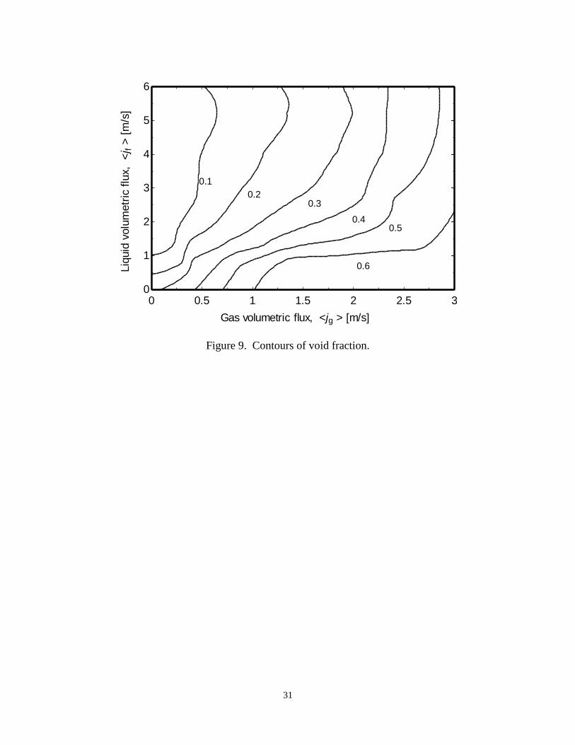
flow. Since the void fraction is a function of flow boundary conditions, i.e., volumetric fluxes of

gas and liquid, the measured void fraction contours are plotted on gas and liquid volumetric flux

coordinates in Figure 9. Such contour maps are helpful in developing void fraction correlations

for microchannel two-phase flows.

3.3 Flow regime identification

The approach originally developed by Jones and Zuber (1975), which utilizes the probability

density functions (PDF) of the void fraction fluctuations as flow regime indicators, is employed

for flow regime identification. Physically, the PDF denotes the contribution of different kinds of

bubbles to the time-averaged void fraction for a given flow condition. The normalized time series

signal obtained by the impedance meter, *( )G t , is used for this purpose. The PDF of *( )G t

denoted by *

*( )G

f G is calculated using the kernel smoothing density estimation method

described by Bowman and Azzalini (1997). A normal kernel is used as the smoothing function.

The PDF *

*( )G

f G is evaluated at 200 discrete points in the domain of * 0,1G . Thus, each

flow condition is represented by a 200-dimensional vector. The problem of identifying flow

regimes is equivalent to identifying clusters of vectors in 200-dimensional vector space. The

clusters of vectors are found by minimizing the distance between the vectors representing flow

conditions and the weight vectors corresponding to a flow regime. After minimization, the

weight vector positions align with the centroid of the clusters. Thus, the weight vectors that

14

denote the positions of the cluster centroids are characteristic of the flow regime. This

optimization problem is solved by the Kohonen Self-Organizing Map algorithm for pattern

recognition implemented in the Neural Network Toolbox of MATLAB based on the method

developed by Kohonen (1997). Physical interpretation of the recognized patterns is accomplished

by comparing them with the flow regimes observed using the high-speed camera.

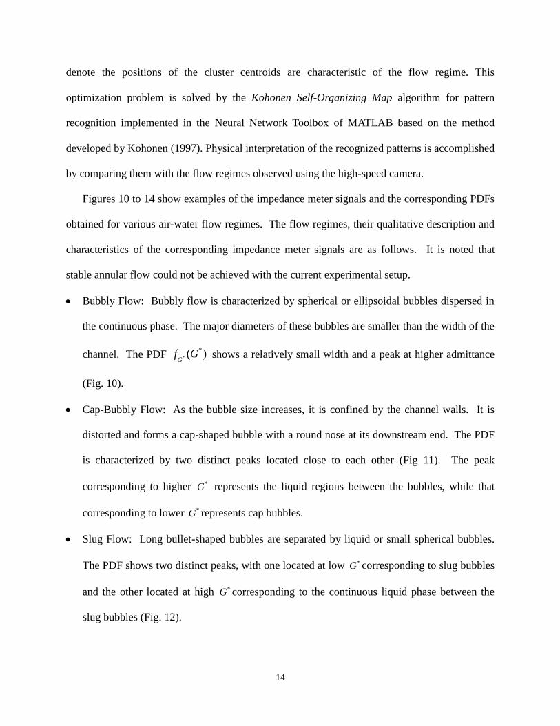
Figures 10 to 14 show examples of the impedance meter signals and the corresponding PDFs

obtained for various air-water flow regimes. The flow regimes, their qualitative description and

characteristics of the corresponding impedance meter signals are as follows. It is noted that

stable annular flow could not be achieved with the current experimental setup.

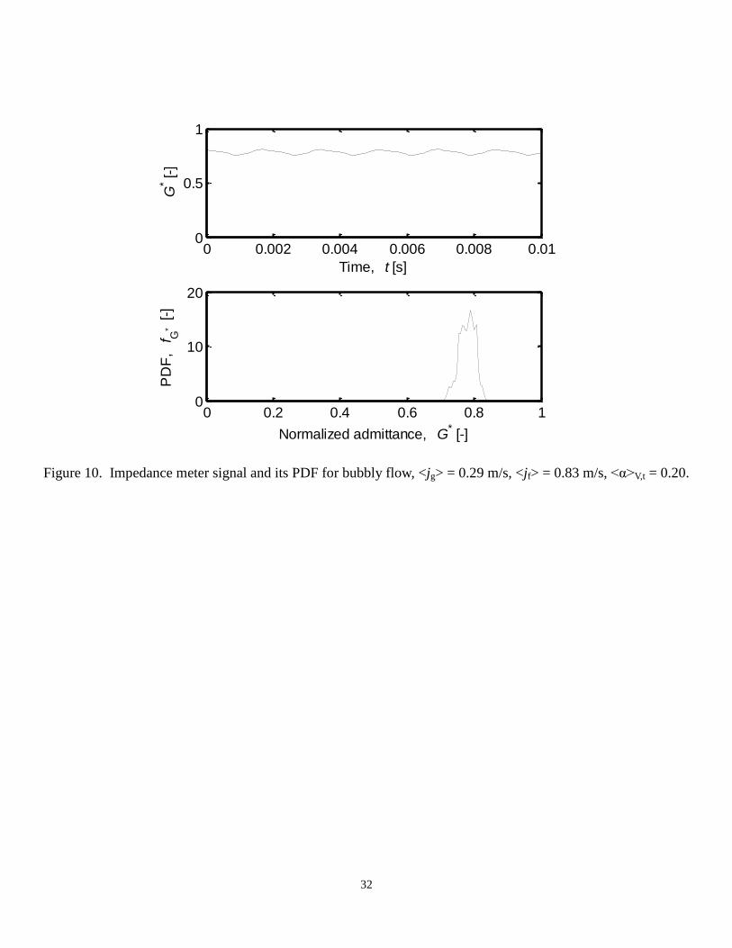
Bubbly Flow: Bubbly flow is characterized by spherical or ellipsoidal bubbles dispersed in

the continuous phase. The major diameters of these bubbles are smaller than the width of the

channel. The PDF *

*( )G

f G shows a relatively small width and a peak at higher admittance

(Fig. 10).

Cap-Bubbly Flow: As the bubble size increases, it is confined by the channel walls. It is

distorted and forms a cap-shaped bubble with a round nose at its downstream end. The PDF

is characterized by two distinct peaks located close to each other (Fig 11). The peak

corresponding to higher *G represents the liquid regions between the bubbles, while that

corresponding to lower *G represents cap bubbles.

Slug Flow: Long bullet-shaped bubbles are separated by liquid or small spherical bubbles.

The PDF shows two distinct peaks, with one located at low *G corresponding to slug bubbles

and the other located at high *G corresponding to the continuous liquid phase between the

slug bubbles (Fig. 12).

15

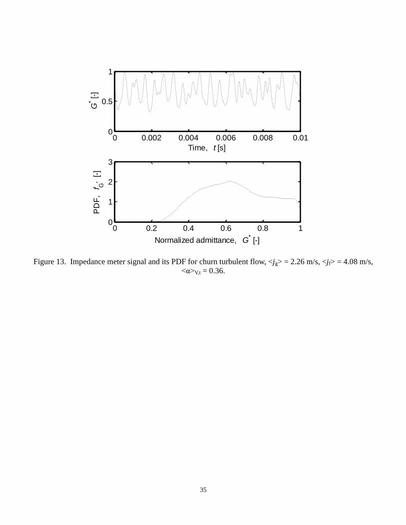
Churn-turbulent Flow: Due to turbulent agitation at the higher flow rates, churn-turbulent

flow exhibits interacting slug bubbles with distorted shape. This leads to a wider spread in

the PDF, where peaks corresponding to slug bubbles and liquid gaps between them are

merged. It should be noted here that the existence of a churn-turbulent regime does not

imply higher void fraction than that in the slug flow regime in a time-averaged sense (Fig.

13).

Long Slug Flow: This regime is characterized by the occurrence of long stable slugs such

that it appears to have a structure similar to annular flow in a local or short-time-averaged

sense. The PDF shows a high peak at low *G . Annular flow was not observed in the current

dataset (Fig. 14).

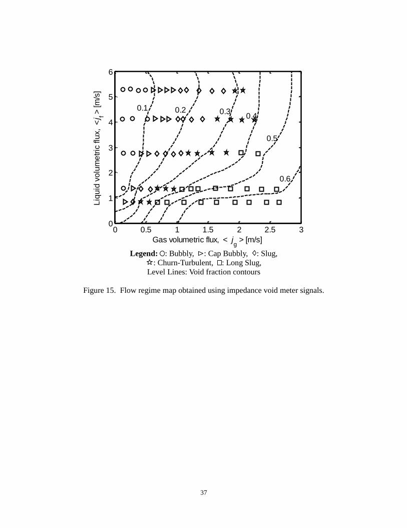
Using the quantitative method of flow regime classification described above, the dataset was

categorized into five regimes. The result of this classification is shown in Figure 15. The flow

conditions are presented on coordinates of volumetric flux of the gas and liquid phases. The

contours of time-averaged void fraction are superimposed on the flow regime map. This shows

the relationship between flow regime boundaries and the void fraction. This map could be used

for the development of theoretical flow regime transition criteria in microchannel two-phase

flow.

4. Summary and conclusions

Void fraction is measured in air-water two-phase flow in a microchannel of cross-section 780

µm X 780 µm using a custom-designed impedance void meter. The impedance void meter is

calibrated against the time-averaged void fraction determined from flow visualization using a

high-speed movie camera. The calculated time-averaged void fraction shows reasonable

16

agreement with those predicted by the homogeneous flow and drift flux models. However, a

conclusive statement in favor of a particular model cannot be made since the model parameters

(e.g., the distribution parameter and the drift velocity for the drift-flux model) are not available

for microchannel flows.

The probability density function (PDF) of the time series signal obtained by the impedance

meter is utilized for quantitative characterization of two-phase flow regimes. The flow regimes

are identified using a Kohonen Self-organizing map. The present study shows that the

impedance void meter designed in this work can be used for microchannel two-phase flows for

the measurement of void fraction and identification of flow regimes. The void fraction and flow

regime data obtained by the impedance void meter may be used for developing and

benchmarking theoretical flow regime transition criteria for microchannel two-phase flows.

Further studies are in progress for extending the flow regime map to include annular flow, in

addition to developing flow regime maps for additional flow channel geometries. The

measurement technique developed here can be used to study non-adiabatic and boiling flows

with similar geometry of electrodes along with the same electronic circuit, as long as the changes

in electrical properties of the fluid with temperature are taken into account.

Acknowledgments

This work was funded by the Office of Naval Research (Grant No. N000141010921). The

authors are grateful to Dr. Mark Spector for his support.

17

References

Ali, M.I., Sadatomi, M., Kawaji, M., 1993. Two-phase flow in narrow channels between flat

plates. Canadian Journal of Chemical Engineering 71, 657–666.

Andreussi, P., Di Donfrancesco, A., and Messia, M., 1988. An impedance method for the

measurement of liquid hold up in two-phase flow. Int. J. Multiphase Flow 14, 777-785.

Armand, A.A., 1946. The resistance during the movement of a two-phase system in horizontal

pipes. Izv. Vses. Teplotekh., Inst. 1, (AERE-Lib/Trans 828), 16–23.

Asali, J. C., Hanrtatty, T. J. and Andreussi, P., 1985. Interficial drag and film height in vertical

annular flow. AIChE J. 31, 895-902.

Bertsch, S.S., Groll, E.A. and Garimella, S.V., 2008. Review and comparative analysis of studies

on saturated flow boiling in small channels. Nanoscale MicroscaleThermophys. Eng. 12,

187–227.

Bowman, A. W., and A. Azzalini, Applied Smoothing Techniques for Data Analysis, New York:

Oxford University Press, 1997.

Coney, M.W.E., 1973. The theory and application of conductance probes for the measurement of

liquid film thickness in two-phase flow. Journal of Physics E (Scientific Instruments) 6, 903-

911.

Costigan, G. and Whalley, P. B., 1997. Slug flow regime identification from dynamic void

fraction measurements in vertical air-water flows. Int. J. Multiphase Flow 23, 263–282.

Fossa, M., 1998. Design and performance of a conductance probe for measuring the liquid

fraction in two-phase gas-liquid flows. J. Flow Meas. Instrum. 9, 103-109.

Garimella, S. V. and Sobhan, C. B., 2003. Transport in microchannles – a critical review. Annu.

Rev. Heat Transfer 13, 1-50.

Harirchian, T. and Garimella, S.V., 2008. Microchannel size effects on local flow boiling heat

transfer to a dielectric fluid. Int. J. Heat Mass Transfer 51, 3724–3735.

Harirchian, T., and Garimella, S.V., 2009. Effects of channel dimension, heat flux and mass flux

on flow boiling regimes in microchannels. Int. J. Multiphase Flow 35, 349-362.

Harirchian, T. and Garimella, S. V., 2010. A comprehensive flow regime map for microchannel

flow boiling with quantitative transition criteria. Int. J. Heat Mass Transfer 53, 2694-2702.

Hewitt, G. F., 1983. Two-Phase flow and its applications: past, present and future. Heat Transfer

Engineering 4, 67-79.

18

Jones Jr. O.C. and Zuber N., 1975. The interrelation between void fraction fluctuations and flow

patterns in two-phase flow. Int. J. Multiphase Flow 2, 273-306.

Julia, J. E., Liu, Y., Paranjape, S. and Ishii, M., 2008. Local flow regimes analysis in vertical

upward two-phase flow. Nucl. Eng. and Design 238, 156-169.

Kawahara, A., Sadatomi, M., Kumagae, K., 2006. Effects of gas–liquid inlet/mixing conditions

on two-phase flow in microchannels. Progress in Multiphase Flow Research 1, 197–203.

Kawahara, A., Sadatomi, M., Nei, K. and Matsuo, H., 2009. Experimental study on bubble

velocity, void fraction and pressure drop for gas–liquid two-phase flow in a circular

microchannel. International Journal of Heat and Fluid Flow 30, 831–841.

Kawaji, M., Kawahara, A., Mori, K., Sadatomi M., Kumagae, K., 2006. Gas–liquid twophase

flow in microchannels: the effects of gas–liquid injection methods. In: Proceedings of the

18th National and Seventh ISHMT–ASME Heat Transfer.

Kohonen, T., Self-Organizing Maps, Second Edition, Berlin: Springer-Verlag, 1997.

Matsui, G., 1984. Identification of flow regimes in vertical gas-liquid two-phase flow using

differential pressure fluctuations. Int. J. Multiphase Flow 10, 711-720.

Maxwell, J. C. 1873, A Treatise on Electricity and Magnetism,3rd

ed., Clarendon Press, Oxford,

England.

Mi, Y., Ishii, M. and Tsoukalas, L. H., 1998. Vertical two-phase flow identification using

advanced instrumentation and neural networks. Nucl. Eng. and Design 184, 409-420.

Mishima, K., Hibiki, T., 1996. Some characteristics of air–water two-phase flow in small

diameter vertical tubes. Int. J. Multiphase Flow 22, 703–712.

Serizawa, A., Feng, Z., Kawara, Z., 2002. Two-phase flow in microchannels. Experimental

Thermal and Fluid Science 26, 703–714.

Sobhan, C.B., and Garimella, S.V., 2001. A comparative analysis of studies on heat transfer and

fluid flow in microchannels. Microscale Thermophys. Eng. 5, 293–311.

Soille, P. 2003, Morphological Image Processing, 2nd

ed., Springer-Verlag, Germany.

The Mathworks Inc., 2009. MATLAB version 2009b

Tsochatzidis, N. A., Karapantios, T. D., Kostoglou, M. V., and Karabelas, A. J., 1992. A

conductance method for measuring liquid fraction in pipes and packed beds. Int. J.

Multiphase Flow 5, 653-667.

19

Tumanski, S. 2006, Principles of electrical measurement, CRC Press, Taylor & Francis, USA.

Tutu, N. K., 1982. Pressure fluctuations and flow pattern recognition in vertical two phase gas-

liquid flows. Int. J. Multiphase Flow 8, 443-447.

Zuber, N. and Findlay, J. A., 1965. Average volumetric concentration in two-phase flow systems.

J. Heat Transfer 87, 453-468.

20

List of Table and Figure Captions

Table 1. Measurement uncertainties as a percentage of measured value.

Fig 1. Impedance meter test cell. (a) Top view of test cell. (b) Base plate with flow

channel and electrodes.

Fig 2. Air-water two-phase flow loop.

Fig 3. Impedance meter circuit. (a) Signal processing scheme. (b) Basic electronic

circuit.

Fig 4. Image processing steps. (a) Original image, top view.. (b) Step 1, Rotated and

cropped image for interrogation window. (c) Step 2, Background subtracted

and threshold adjusted image. (d) Step 3, Edge detection. (e) Step 4, Remove

interior boundaries. (f) Step 5, Edges after finding convex hull, superimposed

on original image.

Fig 5. Test Matrix.

Fig. 6. Flow visualization and void fraction measured by image processing. Flow

direction is from left to right. (a) Bubbly, <jg> = 0.29 m/s, <jf> = 0.83 m/s,

<α>V,t = 0.20. (b) Cap Bubbly, <jg> = 0.56 m/s, <jf> = 0.83 m/s, <α>V,t =

0.37. (c) Slug, <jg> = 1.39 m/s, <jf> = 0.83 m/s, <α>V,t = 0.58. (d) Churn-

Turbulent <jg> = 2.26 m/s, <jf> = 4.08 m/s, <α>V,t = 0.36. (e) Long Slug,

<jg> = 2.65 m/s, <jf> = 0.82 m/s, <α>V,t = 0.65.

Fig. 7. Impedance meter calibration.

Fig. 8. Comparison of measured void fraction with homogeneous flow and drift-flux

21

models.

Fig. 9. Contours of void fraction.

Fig. 10. Impedance meter signal and its PDF for Bubbly flow, <jg> = 0.29 m/s, <jf>

= 0.83 m/s, <α>V,t = 0.20.

Fig. 11. Impedance meter signal and its PDF for Cap-Bubbly, <jg> = 0.56 m/s, <jf> =

0.83 m/s, <α>V,t = 0.37.

Fig. 12. Impedance meter signal and its PDF for Slug, <jg> = 1.39 m/s, <jf> = 0.83

m/s, <α>V,t = 0.58.

Fig. 13. Impedance meter signal and its PDF for Churn Turbulent flow, <jg> = 2.26

m/s, <jf> = 4.08 m/s, <α>V,t = 0.36.

Fig. 14. Impedance meter signal and its PDF for Long Slug, <jg> = 2.65 m/s, <jf> =

0.82 m/s, <α>V,t = 0.65.

Fig. 15. Flow regime map obtained using impedance void meter signals.

22

Table 1. Measurement uncertainties as a percentage of measured value.

Instrument Reported

Measurement

Accuracy

Maximum Standard Deviation

Liquid flow [ml/min] 0.2% 0.74%

Gas flow [ml/min] 0.1% 3.2 %

Pressure [kPa] 0.2% 2%

Temperature [K] 0.1% 0.05%

23

Electrode

Electrode

Flow Channel

Air Entrance

Water Entrance Exit

(a)

(b)

Figure 1. Impedance meter test cell: (a) top view, and (b) base plate with flow channel and

electrodes.

24

Test Cell

Storage

Tank

Compressed Air

Tank

Air Mass Flow

Sensor

Needle

Valve

Shutoff

Valve

Needle

Valve

Shutoff

Valve

Micro Turbine

Flow Meter Water Pump

Figure 2. Air-water two-phase flow loop.

25

Excitation Signal Test Cell

Synchronous

Demodulator

Low Pass Filter Output Signal

Numerically ComputedElectronic Circuit

(a)

Exciter Test Cell Reference Resistor

VCarrier Vmodulated

Buffer

Current-to Voltage

Op-Amp

+

-

(b)

Figure 3. Impedance meter circuit: (a) signal-processing scheme, and (b) basic electronic circuit.

26

(a)

(b) (c)

(d) (e)

(f)

Figure 4. Image processing steps: (a) original image, top view; (b) Step 1, rotated and cropped image for

interrogation window; (c) Step 2, background subtracted and threshold adjusted image; (d) Step 3, edge

detection; (e) Step 4, remove interior boundaries; and (f) Step 5, edges after finding convex hull, superimposed

on original image.

27

0 0.5 1 1.5 2 2.5 30

1

2

3

4

5

6

Gas volumetric flux, < jg > [m/s]

Liq

uid

vo

lum

etr

ic flu

x, <

jf >

[m

/s]

Figure 5. Test matrix.

28

0 0.002 0.004 0.006 0.008 0.010

0.5

1

Time, t [s]

<

>V [-]

(a)

0 0.002 0.004 0.006 0.008 0.010

0.5

1

Time, t [s]

<

>V [-]

(b)

0 0.002 0.004 0.006 0.008 0.010

0.5

1

Time, t [s]

<

>V [-]

(c)

0 0.002 0.004 0.006 0.008 0.010

0.5

1

Time, t [s]

<

>V [-]

(d)

0 0.002 0.004 0.006 0.008 0.010

0.5

1

Time, t [s]

<

>V [-]

(e)

Figure 6. Flow visualization and void fraction measured by image processing. Flow direction is from left to

right. (a) Bubbly, <jg> = 0.29 m/s, <jf> = 0.83 m/s, <α>V,t = 0.20. (b) Cap Bubbly, <jg> = 0.56 m/s, <jf> = 0.83

m/s, <α>V,t = 0.37. (c) Slug, <jg> = 1.39 m/s, <jf> = 0.83 m/s, <α>V,t = 0.58. (d) Churn-Turbulent <jg> = 2.26

m/s, <jf> = 4.08 m/s, <α>V,t = 0.36. (e) Long Slug, <jg> = 2.65 m/s, <jf> = 0.82 m/s, <α>V,t = 0.65.

29

0 0.2 0.4 0.6 0.8 10

0.1

0.2

0.3

0.4

0.5

0.6

0.7

0.8

0.9

1

Impedance meter measurement, imp

= (1-G*) [-]

Vo

id fra

ctio

n, <

>

V,t,im

[-]

Bubbly

Cap Bubbly

Slug

Churn-Turbulent

Long Slug

Polynomial fit

Linear

Maxwell (1873)

Figure 7. Impedance meter calibration.

30

0 0.2 0.4 0.6 0.8 10

0.2

0.4

0.6

0.8

1

[-]

Vo

id F

ractio

n,

[-

]

Data

Homogeneous Flow

Drift Flux

Figure 8. Comparison of measured void fraction with homogeneous flow and drift-flux models.

31

0 0.5 1 1.5 2 2.5 30

1

2

3

4

5

6

Gas volumetric flux, <jg > [m/s]

Liq

uid

volu

metr

ic f

lux,

<j f >

[m

/s]

0.1

0.20.3

0.40.5

0.6

Figure 9. Contours of void fraction.

32

0 0.002 0.004 0.006 0.008 0.010

0.5

1

Time, t [s]

G* [

-]

0 0.2 0.4 0.6 0.8 10

10

20

Normalized admittance, G* [-]

PD

F, f G

* [-]

Figure 10. Impedance meter signal and its PDF for bubbly flow, <jg> = 0.29 m/s, <jf> = 0.83 m/s, <α>V,t = 0.20.

33

0 0.002 0.004 0.006 0.008 0.010

0.5

1

Time, t [s]

G* [

-]

0 0.2 0.4 0.6 0.8 10

5

10

15

Normalized admittance, G* [-]

PD

F, f G

* [-]

Figure 11. Impedance meter signal and its PDF for cap-bubbly flow, <jg> = 0.56 m/s, <jf> = 0.83 m/s, <α>V,t =

0.37.

34

0 0.02 0.04 0.06 0.08 0.10

0.5

1

Time, t [s]

G* [

-]

0 0.2 0.4 0.6 0.8 10

1

2

3

Normalized admittance, G* [-]

PD

F, f G

* [-]

Figure 12. Impedance meter signal and its PDF for slug flow, <jg> = 1.39 m/s, <jf> = 0.83 m/s, <α>V,t = 0.58.

35

0 0.002 0.004 0.006 0.008 0.010

0.5

1

Time, t [s]

G* [

-]

0 0.2 0.4 0.6 0.8 10

1

2

3

Normalized admittance, G* [-]

PD

F, f G

* [-]

Figure 13. Impedance meter signal and its PDF for churn turbulent flow, <jg> = 2.26 m/s, <jf> = 4.08 m/s,

<α>V,t = 0.36.

36

0 0.02 0.04 0.06 0.08 0.10

0.5

1

Time, t [s]

G* [

-]

0 0.2 0.4 0.6 0.8 10

2

4

Normalized admittance, G* [-]

PD

F, f G

* [-]

Figure 14. Impedance meter signal and its PDF for long slug flow, <jg> = 2.65 m/s, <jf> = 0.82 m/s, <α>V,t =

0.65.

37

0 0.5 1 1.5 2 2.5 30

1

2

3

4

5

6

Gas volumetric flux, < jg > [m/s]

Liq

uid

vo

lum

etr

ic flu

x, <

jf >

[m

/s]

0.1 0.2 0.30.4

0.5

0.6

Legend: : Bubbly, : Cap Bubbly, : Slug,

: Churn-Turbulent, : Long Slug,

Level Lines: Void fraction contours

Figure 15. Flow regime map obtained using impedance void meter signals.