1 * Corresponding author: Phone: +34964728139, Fax: +34964728106, e-mail:

bolivar@emc.uji.es

On the use of area-averaged void fraction and

local bubble chord length entropies as two-

phase flow regime indicators

Leonor Hernández1, J. Enrique Juliá1,*, Sidharth Paranjape2, Takashi Hibiki2,

Mamoru Ishii2

1 Universitat Jaume I. Departamento de Ingeniería Mecánica y Construcción Campus de Riu Sec, Castellón, E-12071, Spain.

2 Purdue University. Nuclear Engineering Department West Lafayette, Indiana, USA

ABSTRACT

In this work, the use of the area-averaged void fraction and bubble chord length entropies

is introduced as flow regime indicators in two-phase flow systems. The entropy provides

quantitative information about the disorder in the area-averaged void fraction or bubble

chord length distributions. The CPDF (cumulative probability distribution function) of void

fractions and bubble chord lengths obtained by means of impedance meters and

conductivity probes are used to calculate both entropies. Entropy values for 242 flow

conditions in upward two-phase flows in 25.4 mm and 50.8 mm pipes have been

calculated. The measured conditions cover ranges from 0.13 m/s to 5 m/s in the

superficial liquid velocity jf and ranges from 0.01 m/s to 25 m/s in the superficial gas

velocity jg. The physical meaning of both entropies has been interpreted using the visual

flow regime map information. The area-averaged void fraction and bubble chord length

entropies capability as flow regime indicators have been checked with other statistical

parameters and also with different input signals durations. The area-averaged void

fraction and the bubble chord length entropies provide better or at least similar results

than those obtained with other indicators that include more than one parameter. The

entropy is capable to reduce the relevant information of the flow regimes in only one

significant and useful parameter. In addition, the entropy computation time is shorter than

the majority of the other indicators. The use of one parameter as input also represents

faster predictions.

Keywords: two-phase flow, flow regime identification, neural networks,

impedance meter, conductivity probe, two-phase flow entropy

2

1. INTRODUCTION

Gas-liquid two-phase flows are frequently encountered in important industrial

applications such as boilers, nuclear power plants, petroleum transportation and various

types of chemical reactors. The two phases can flow according to several topological

configurations called flow patterns or flow regimes, which are determined by the

interfacial structure between both phases. The existence of a particular flow regime

depends on a variety of parameters, which include the properties of the fluids, the flow

channel size, geometry and orientation, body force field and flow rates.

Vertical two-phase flows are usually classified into four or five basic flow regimes

(Taitel et al., 1980; Mishima & Ishii; 1984). A gradual increment in the gas flow rate

consecutively produces the transition between different flow patterns when an upward

two-phase flow in a vertical pipe with a constant liquid flow rate is considered. Therefore,

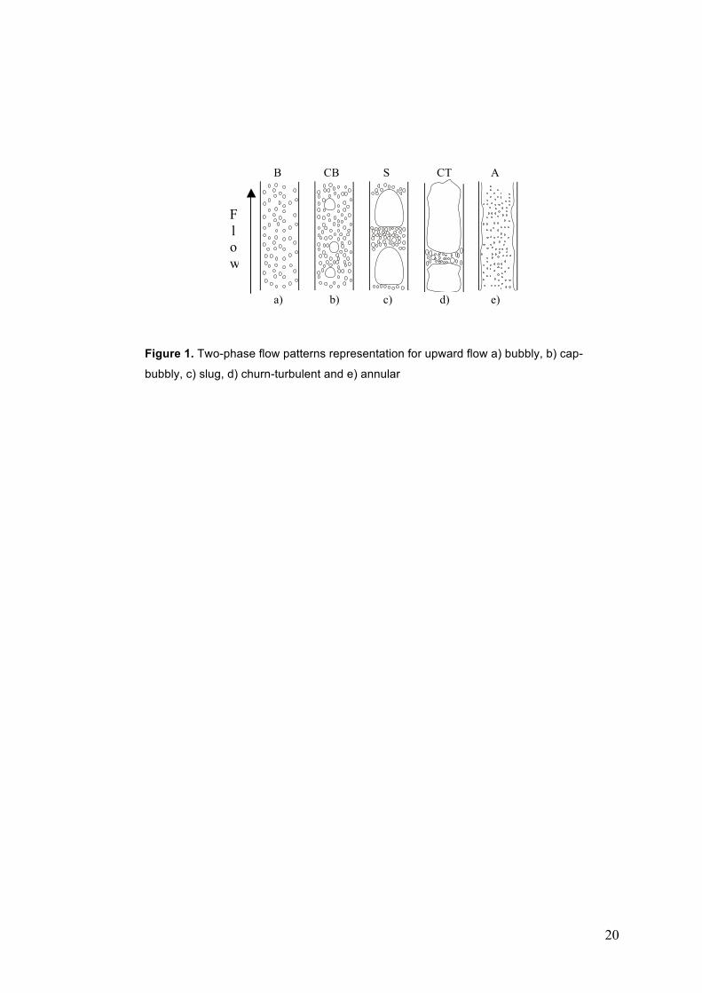
bubbly (B), cap-bubbly (CB), slug (S), churn-turbulent (CT) and annular (A) flow patterns

can be found (Figure 1).

The identification of the flow regimes and their transitions is important for industrial

application as well as from the theoretical analysis point of view. On one hand, almost all

constitutive relations in a two-fluid model (Ishii and Hibiki, 2007; Ishii & Mishima, 1984)

depend on the flow regime since physical mechanisms vary with flow regime transitions.

Additionally, industrial equipment offers durability and safety only when the installation

operates according to the flow regimes that it was designed for because important

parameters, such as heat and mass transfer rates, pressure drop, etc, are directly

connected with the flow regime.

Flow regime definitions are based on linguistic descriptions and graphical

illustrations like those in Figure 1, and therefore, their identification is strongly subjective.

Many researchers have been working on developing objective flow regime identification

methodologies. Most flow regime identification approaches have two steps in common:

the first step consists of developing an experimental methodology for measuring certain

parameters that are intrinsic to the flow and are also suitable flow regime indicators. In

the second step, a non-linear mapping is performed to obtain an objective identification of

the flow regimes in accordance with these indicators. There are two important parameters

to characterize the two-phase flow geometry, namely, void fraction and interfacial area

concentration. Consequently, the flow regime indicators have to be related with such

parameters. In this regard, void fraction distributions obtained with differential pressure

transducers (Jones and Zuber, 1975; Tutu 1982; Matsui 1984) or non-intrusive

impedance void metes (Mi et al., 1998; 2001a) have been widely used as flow regime

indicators in the last decades. In this case the flow regime is defined as a global, 3D or

2D, parameter (Global Flow Regime, GFR). Recently, Julia et al. (2008) used bubble

chord length distributions obtained from conductivity probes as flow regime indicators.

3

Bubble chord length represents the bubble size and is related with the interfacial area

concentration. Thus, the flow regimes are defined as time-averaged bubble chord length

patterns and they are considered as local parameters (Local Flow Regimes, LFR). The

main advantages of this approach over the conventional flow regime identification

methods are the stronger physical relevance of the bubble chord length distribution as

flow regime discriminator and, thus, the reduction in the temporal length of the signal

needed to obtain reliable results. In addition, the identification of LFR in different radial

locations provides 2D local flow regime maps that can be used to identify new GFR

configurations, not available with the conventional identification methods. Finally, the

experimental apparatus needed for the identification (conductivity probe) is simple,

affordable and commonly used in two-phase flow characterization.

In the first flow regime identification works the flow regime mapping were carried

out directly by the researcher. A significant advance in the objective flow regime mapping

was achieved by the use of artificial neural networks (ANN) (Cai et al., 1994; Mi et al.

1998; 2001a, 2001b). Using statistical parameters from the void fraction distribution and

Kohonen Self-Organizing Neural Networks (SONN) it was possible to identify the flow

regimes more objectively. Subsequently, some improvements in the methodology

developed by Mi et al. have been made. Lee et al. (2008a) used the Cumulative PDF

(CPDF) of the impedance void meter signals as the flow regime indicator. The CPDF is a

more stable parameter than the PDF because it is an integral parameter. Also, it has a

smaller input data requirement that makes faster flow regime identification possible.

Hernandez et al. (2006) developed different neural network strategies to improve the flow

regime identification results. Different types of neural networks, training strategies and

flow regime indicators based on the CPDF were tested in their work. In order to minimize

the effect of the fuzzy flow regime transition boundaries on the identification results, a

committee of neural networks was assembled. Then the identification result was obtained

by averaging the results provided by all the neural networks forming the committee. In

particular, the flow regime prediction capabilities of the Probabilistic Neural Networks

(PNN) were verified by Sharma et al. (2006) in round pipes. In their work, a large set of

experimental data obtained in round pipes was used for training a PNN using the

superficial velocities, pipe diameter and inclination angle as inputs. The results given by

the PNN showed good agreement even in the flow regime boundaries.

More sophisticated flow regime indicators are also available. Ruzicka et al. (1997)

used the Kolmogorov entropy from pressure signals in order to discriminate between flow

regimes in a bubble column. Furthermore, Zhang and Shi (1999) developed a

methodology that could be used to identify flow regimes in a two-phase flow loop using

the Shannon entropy of the PSD of pressure oscillation signals in a two-phase flow loop.

In addition, Elperin and Klochko (2002) used the wavelet transform in order to identify

two-phase flow regimes. In this case, the basis of the wavelet decomposition was the

entropy and the sparsity of differential pressure transducers signals. Finally, Lee et al.

(2008b) used the chaotic characteristics of time sequential impedance probe signals in

4

order to identify flow regimes in upward vertical two-phase flows

In this work, the use of the area-averaged void fraction and local bubble chord length

entropies as two-phase flow regime indicators is explored. The physical content of both

indicators and its dependence with superficial liquid and gas velocities is analyzed. In

addition, the capability of both entropies as flow regime indicators using different signal

durations has been compared with other statistical parameters used in previous works.

2. Experimental Facility and Methodology

2.1 Vertical two-phase flow loop

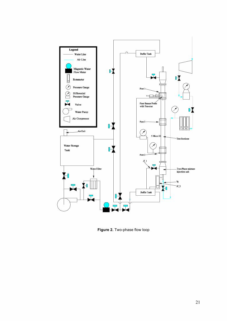
Figure 2 shows the schematic diagram of the two-phase flow loop. The experiments

have been performed in a vertical air-water flow facility at Thermal-hydraulics and

Reactor Safety Laboratory at Purdue University. The experimental facility is designed for

simulating adiabatic vertical air-water two-phase flows under both upward and downward

flow conditions. The test section consists of an acrylic round pipe with diameter (D) of

25.4mm or 50.8mm, and height (H) of 3.8 m. The acrylic pipe is transparent, which

provides a clear view of the flow for the entire length of the flow channel and helps to

identify the flow regimes by visual inspection. The liquid flow rate is adjusted by valves

and measured by an electro-magnetic flow meter with an accuracy of 3%. Air is supplied

by an air compressor with a maximum pressure of 60 bar. The air flow rate is adjusted by

valves and measured by rotameters with an accuracy of 8%. A sparger with a porous tip

with 10 micron pores is employed as a bubble generator. The present injection unit

produces almost uniform bubbles of approximately 1–2 mm in diameter at the test section

inlet. More technical details about this facility can be found in Goda et al. (2004).

2.2 Impedance meter

An impedance meter is used to perform area averaged void fraction measurements

with a sampling rate of 1 kHz and an acquisition time of 60 s. Two diagonal stainless steel

electrodes are flush-mounted at the insulated wall in the measuring axial position. The

electrodes are rectangle-shaped with round corners, a span- angle of 120º and a height

of 5 mm. Delrin, a good electrical insulator, was used as a liner. An alternating current is

supplied to the electrodes and the electrodes are connected to the electronic circuit,

which is specially designed so that the output voltage of the circuit is proportional to the

measured admittance, which is the inverse of impedance, between the electrodes. The

measured admittance is normalized by the following equation:

1

0 1

mnG GGG G

!=

! (1)

5

where, Gm is the instantaneous two-phase mixture admittance, G0 is the admittance when

void fraction is zero (i.e. single phase water) and G1 is the impedance when the void

fraction is unity (i.e. single phase air). Finally, the area averaged void fraction can be

obtained from the measured admittance. Cross-calibration made with gamma

densitometer shows that the void fraction is almost a linear function of the normalized

admittance (Mi et al., 2001b). In addition, to convert from the measured admittance to the

area-averaged void fraction value a calibration is made using differential pressure

measurements at low liquid velocities (Mi et al., 2001a). Thus, the void fraction

measured by the void meter is an instantaneous, area averaged void fraction. The

uncertainty of the impedance meter can be estimated as 3% and the least counts of 1%

(void fraction).

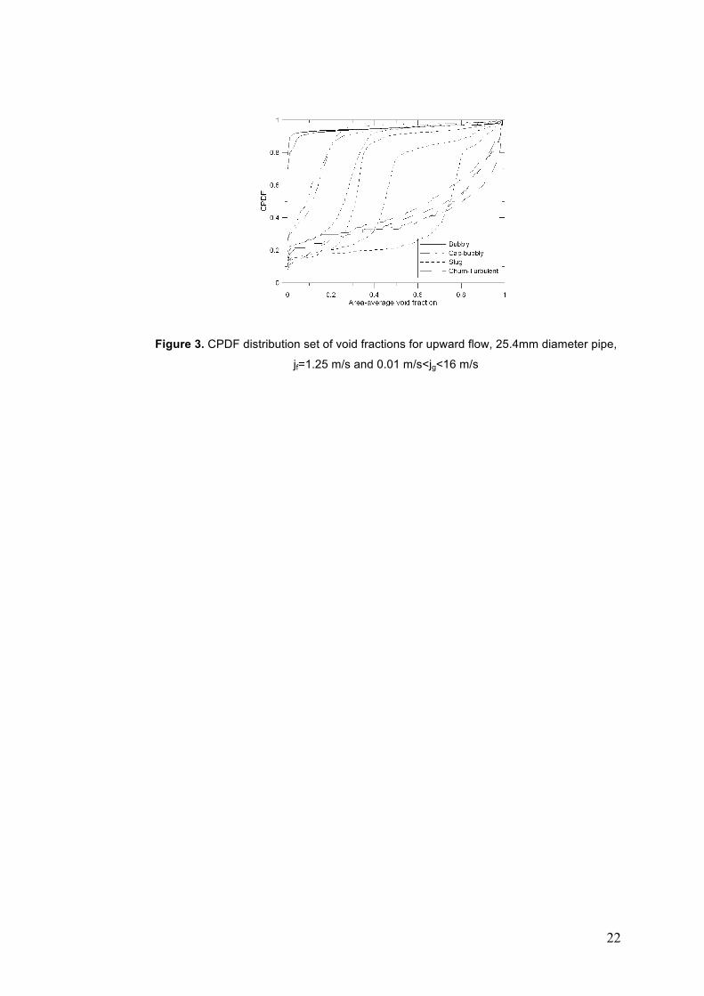
Once the signal from the impedance meter is converted into void fraction, the CPDF is

obtained by sorting and normalizing the void fraction information. Figure 3 shows an

example of set of CPDFs that corresponds to a constant liquid velocity and different gas

velocity values. The CPDFs are grouped in flow regimes following the visual information.

The shape of the CPDF depends on the interfacial distribution, i.e. flow regime, in the

measured flow channel section (Mi et al., 1998; 2001b).

2.3 Double sensor conductivity probes

Conductivity probes are often used to measure various two-phase flow parameters,

such as void fraction, interfacial velocity and interfacial area concentration (Kataoka et al.,

1986; Hibiki et al., 1998; Kim et al., 2000). A double-sensor conductivity probe is installed

at the center of the pipe and at the 3.4 m axial location after the test section inlet to

measure the bubble chord length distributions for each flow condition. The optimum

acquisition frequency and time length for obtaining the local bubble chord length entropy

depends on the flow conditions (Julia et al., 2008). In this work, data were acquired for

each flow condition with a frequency of 12 KHz for 60 seconds using a 12 bit A/D card.

Previous works assure a correct CPDF calculation using these two acquisition

parameters in the present flow conditions (Julia et al., 2008; Hernandez et al., 2006).

The first step in the CPDF calculation from conductivity probe signals consists of a

signal pre-processing, where the noise in the raw signals is removed using a median

filter. Then, the signals are normalized in relation to the maximum and minimum voltage

values in the raw signal and are converted into step-signals using a threshold technique.

Once the raw signals are pre-processed, the bubble residence time information is

obtained from the front sensor signal. The last step consists of calculating, sorting and

normalizing the bubble chord length. In order to transform the residence time information

into the bubble chord length distribution it is necessary to calculate the interfacial velocity

of each interface but, this is a time-consuming process. Instead, the interfacial velocity

obtained from the cross-correlation between the two sensors has been used for the

bubble chord length calculation. For the cross-correlation velocity calculation, the pre-

6

processed signals are converted into step-signals using a threshold technique and the

cross-correlation is computed. Since the distance between the sensors is known, it is

straightforward to calculate the cross-correlation interfacial velocity. Different researchers

have studied the accuracy of the cross-correlation interfacial velocity measured with

conductivity (Kendoush et al., 1980; Julia et al., 2008) or hot film anemometry sensors

(Gurau et al., 2004) in different flow regimes. These studies have shown that the cross-

correlation velocity can be used as a good estimator of the interfacial velocity. If a

constant superficial liquid velocity is considered and the superficial gas velocity is

increased from bubbly to churn-turbulent flow, the averaged difference between the

cross-correlation and averaged interfacial velocities is lower than 15%. The maximum

error is in slug flow and Group 2 bubbles. However, the maximum error in the entropy

calculation due to the use of the cross-correlation velocity is below 10% and does not

affect to the identification process. Additionally, the computation time of the cross-

correlation velocity is two orders of magnitude lower than the interfacial velocity. This fact

is especially important in fast identification process and justifies the use of the cross-

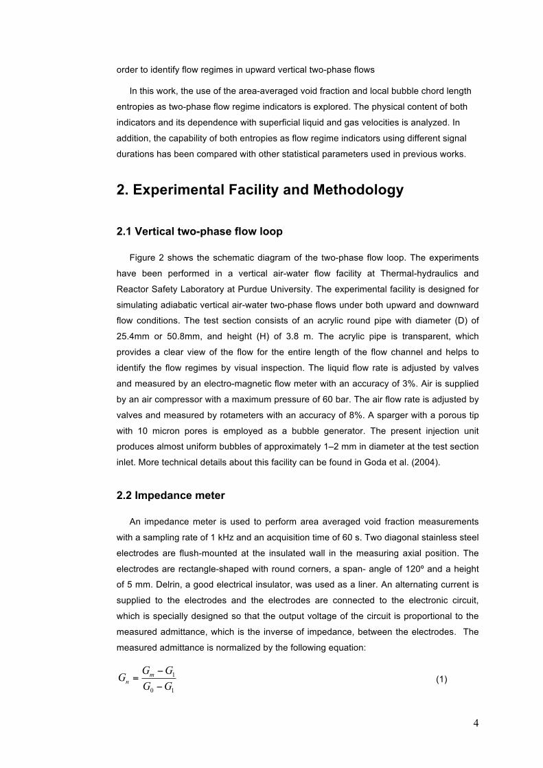
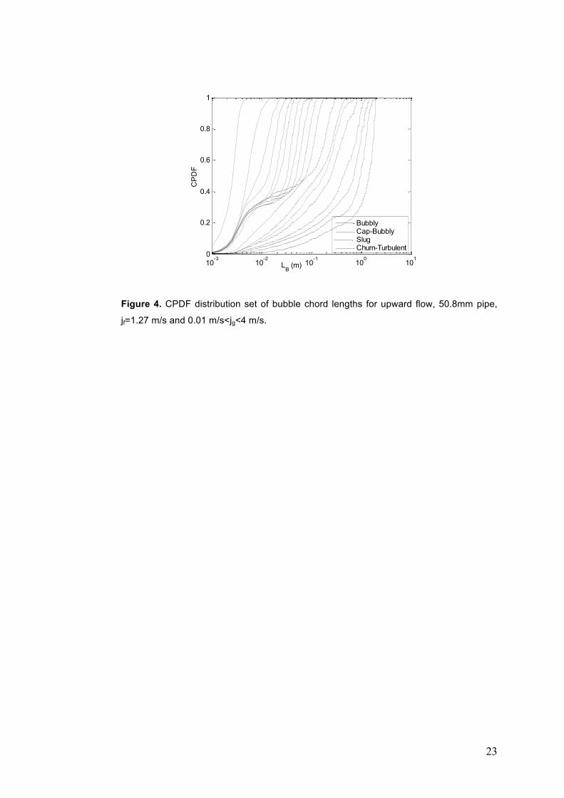
correlation velocity. Figure 4 shows an example of a set of bubble chord length CPDFs

taken in the center of a pipe. The CPDFs are grouped in flow regimes following the visual

information.

2.4 Probabilistic neural network

The human brain inspired the development of the ANN and their initial application to

practical problems started in the 1950s. Numerous ANN applications have been

developed, mainly solving problems where input and output values are known, but the

translation into a mathematical equation is difficult. A Probabilistic Neural Network (PNN)

is an ANN used for data classification tasks. In the current study, a PNN was chosen to

solve the problem of classifying the calculated flow regime indicators (inputs) into the five

different flow regimes (classes).

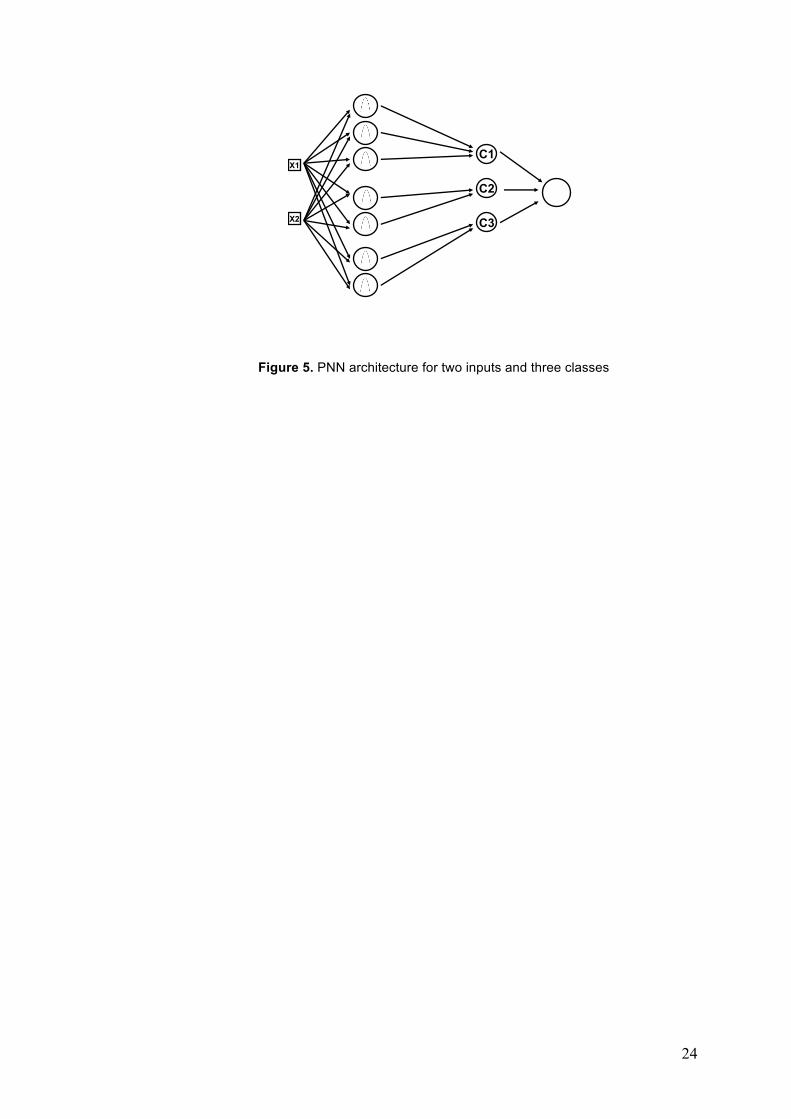
PNNs belong to the family of the radial basis ANN, feature a feed-forward architecture

and a fast supervised training algorithm, as is usually performed in a single pass. An

example of a PNN structure or architecture is shown in Figure 5. The PNN has four

layers. The input layer contains as many elements as parameters required to describe the

test cases to be classified. In this study, the number of parameters would range between

one and ten input components, and in Figure 5, two parameters are considered. The next

layer is the hidden layer, with as many elements as test cases in the training data set. In

the architecture shown in Figure 5, only seven test cases are depicted. The third layer is

the pattern or summation layer, which has as many elements are there are classes to be

recognized: three in the example of Figure 5 or five in the problem of flow regime

classification. The final layer is the decision or output layer, which assigns the final

classification of each pattern to the largest probability within the different classes.

The PNN model is first taught with a training data set, which in this study consists of

7

flow regime indicators along with their correct classification. PNN are based on the

combination of the Bayes decision strategy and Parzen’s method of PDF approximation

(Specht 1988; Specht 1990; Parzen 1962).The classification decision is made by means

of the PDF of each flow regime calculated using the training patterns. The goal of training

is to approximate the PDF of the underlying distribution of the training pattern. Finding the

PDF of the training patterns is based on its approximation by superposition of a certain

function, which in this study is the Gaussian function. When applying a PNN it is

important to ensure a proper selection of the width parameter in the curve, which controls

how spread the Gaussian curve is. The spread parameter ranges between 0 and 1 and

the smaller the spread value is, the more selective the corresponding neuron is and, in

turn, the more the ANN acts as a nearer neighbour classifier. A trial and error method

was used to find the optimum spread value. Once the training process is finished, the

PNN classifies the new test cases based on the PDF generated with the training data.

The neural networks were trained, using a random set of 90% of the available data

and predicting the remaining 10%. The process was repeated 50 times for each ANN

configuration, which resulted in 50 different ANNs. These 50 trained ANNs were

assembled in an ANN committee, in order to compensate for the differences in the

individual networks. The final classification results were obtained by averaging the

randomly resulting predictions provided by all the ANNs that integrate the ANN

committee. More technical information about the neural networks used in this work can be

found in Hernández et al. (2006).

2.5 Area-averaged void fraction and local bubble chord length entropies definition

The entropy computation is based on the CPDF distribution of the area-averaged void

fraction or local bubble chord length. The area-averaged void fraction entropy (S!) and the

bubble chord length entropy (SB) are defined as follows,

!"==

=#

Ni

0iiiBor )pln(p

N1

S (2)

where pi is the cumulative probability of finding a ith- area-averaged void fraction or

bubble chord length value in the CPDF and N is the number of samples.

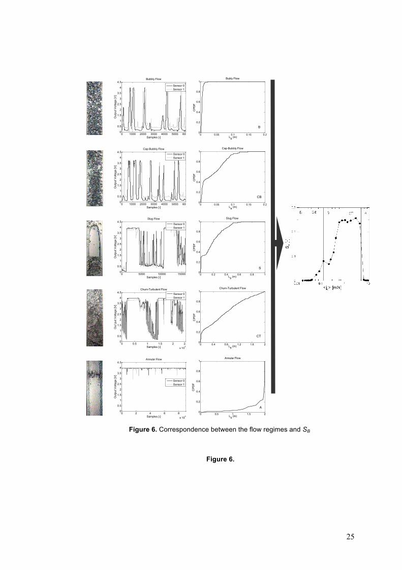
The relation between the flow regime, conductivity probe signals and SB value is

analyzed in Figure 6. This figure is interpreted from left to right. The first column provides

examples of images of the typical five flow regimes considered in this study (B, CB, CS,

CT and A). The second column of Figure 6 shows examples of typical conductivity probe

signals time series for every flow regime. The CPDF of the signals are also plotted in the

third column of the figure. The upper limit of the bubble chord length CPDF is 2 meters.

The CPDF for the bubbly flow extends to 1 cm with a constant slope. The SB value that

corresponds to bubbly flow (forth column of the figure) is low since most of the CPDF

8

values are equal to one.

In the case of the cap-bubbly, slug and churn-turbulent CPDFs it is possible to

distinguish two different regions, corresponding to the two different types of bubbles

found in these regimes. In the three cases, the regions corresponding to the small

bubbles are very similar to the CPDF of the bubbly flow, but the larger bubbles

contribution zone has different slopes. In the case of cap-bubbly flow, the contribution of

the small bubbles reaches to the 40% of the CPDF, and the cap bubbles contribution

extends to 10 cm. In the case of slug flow, the small bubbles contribution reaches to the

30% of the CPDF, and the Taylor bubbles contribution extends to 60 cm, with a gap

between 1 cm and 10 cm. In the case of churn-turbulent flow, the contribution of the

small bubbles reaches to the 20% of the CPDF, and the churn-turbulent bubbles

contribution extends to 2 m. The gap in the bubble chord lengths found in the slug flow

disappears due to the break-up of the Taylor bubbles. The SB values that correspond to

these flow regimes show a continuous increment due to the CPDF function enlargement

towards longer bubble chord lengths and its form.

In the case of annular flow, with extremely long Taylor bubbles, the CPDF should

be zero in all the range in the center of the flow channel. However, the figure shows a

slight increment for bubble chord lengths larger than 1 m. These measurements

correspond to intermittent liquid bridges that are present in the experimental loop, which

were identified as long churn-turbulent bubbles. The SB value drops to values closer to

those found in bubbly flow.

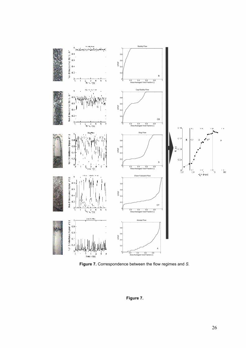
In a similar way, Figure 7 analyzes the relation between the flow regime,

impedance meter signal and S! value. The information provided by the S! value for the

bubbly, cap-bubbly, slug and churn-turbulent flow regimes is similar to the one provided

by SB. The main changes between S! and SB are found in the annular flow regime. The

S! value does not drop in this flow regime due to the fact that the ! values are area-

averaged. Then, the variations of thickness in the liquid film have a strong effect in the

impedance meter signal and the CPDF presents a similar shape to the one found for

churn-turbulent flow regime.

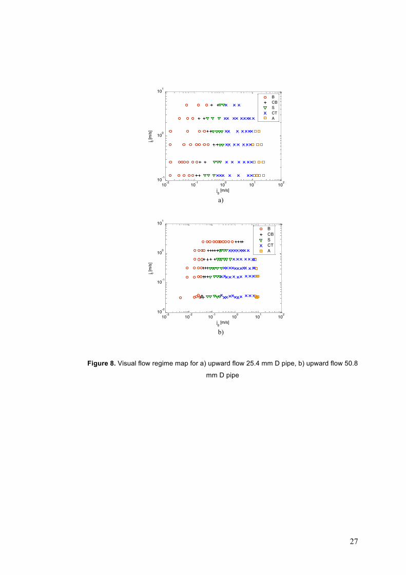
3. Results and Discussion

In this work, both area-averaged void fraction and bubble chord length entropies have

been calculated for 242 flow conditions in vertical upward two-phase flows in 25.4 mm

and 50.8 mm pipes. The superficial gas and liquid velocity conditions are 0.13 m/s<jf<5

m/s and 0.01 m/s<jg<25 m/s respectively. Figure 8 shows the flow regime maps by visual

observation for both configurations.

9

3.1 Area-averaged void fraction entropy

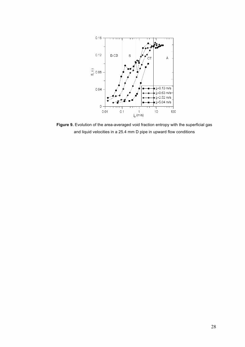
Figure 9 shows the evolution of the area-averaged void fraction entropy for upward

flow in a 25.4 mm diameter pipe at the axial location of z/D=144 and several superficial

liquid velocity values. The flow regime information has been obtained from the visual flow

regime map of Figure 8a) and they are shown only for indicative purposes and for low

superficial liquid velocities.

It is observed that the entropy provides quantitative information about the disorder in

the area-averaged void fraction distribution as analyzed in Figures 6 and 7. It has a low

value for bubbly flows. An increment in the gas flow rate increases the entropy as we find

a wider distribution of bubble types in the cap-bubbly, slug and churn-turbulent flow

regimes. The maximum occurs in the churn-turbulent flow regime and it is constant in

annular flow. The entropy values found for the annular flow regime does not drop

because S! is an area-averaged quantity and the entropy contribution of the two-phase

flow near the walls in this flow regime is quite important. In addition, the entropy values

show a monotonic increment with the superficial gas velocity and, for the same flow

regime, do not depend on the superficial liquid velocity. Some discontinuities in the

entropy values can be found in the flow regime transition zones. These discontinuities do

not affect the flow regime identification process. This fact can be related with the

experimental uncertainty in the CPDF calculation. However, more experimental data is

needed in order to analyze it in detail. This fact makes the mean S! a good flow regime

indicator aspirant in upward flow conditions. The evolution of the S! values with the

superficial gas and liquid velocities in a 50.8 mm D pipe is almost identical to the one

shown in Figure 9, confirming that the pipe diameter does not play an important role in

the flow regime transitions in upward flow conditions (Taitel et al., 1980; Mishima & Ishii;

1984)

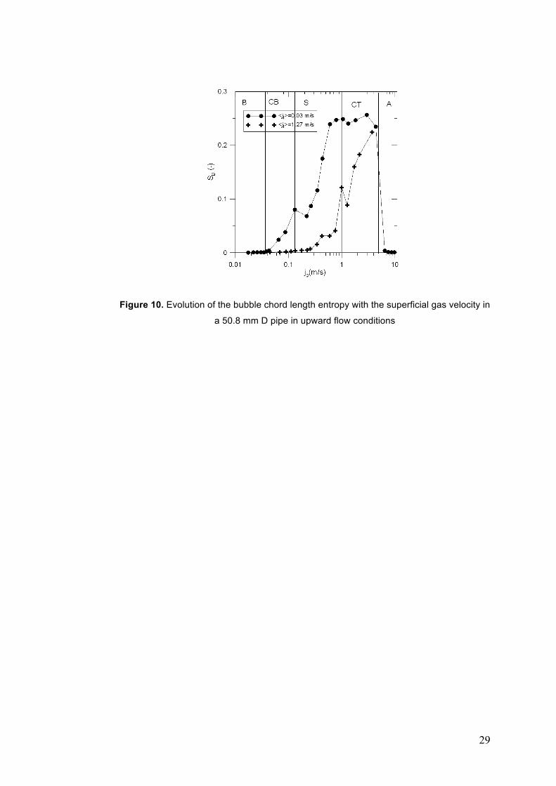
3.2 Local bubble chord length entropy

Figure 10 shows the SB calculated in the center of the pipe for two constant liquid

velocity conditions (jf=0.03m/s and jf=1.27 m/s), superficial gas velocities ranging from 0

to 10 m/s and at the location of z/D=65.

It is observed that the SB dependence with the superficial gas velocity in the center of

the pipe is quite similar to the one found for S!, except for the annular flow. In this way,

the SB values are very low for low gas velocity conditions (bubbly flow) and increase with

the gas velocity (cap-bubbly, and slug flow). When the gas velocity is between 1 m/s and

4 m/s the SB is almost constant (churn-turbulent flow). For gas velocity higher than 5 m/s

the SB drops (annular flow). This last fact is because the bubble chord length entropy is a

local measurement, so measurements in the gas core of the annular flow are possible

represented by very long chord lengths.

10

From the above, it is clear that the bubble chord length entropy presents better

characteristics than the area-averaged void fraction entropy as flow regime indicator. Its

main advantages are the higher dependency of the entropy value with the flow regime

(the ratio between the entropy values of CT and B flow regimes is much higher in the

case of SB), the drop of the entropy in the annular flow and the possibility of using several

entropy values in different radial locations since it is a local measurement (the later

advantage is not studied in the present work).

3.3 Flow regime identification results

In this section, the area-averaged void fraction and bubble chord length entropy

capabilities as flow regime indicators will be discussed. Thus, the flow regime

classification results obtained by both entropies have been compared to those obtained

by other statistical parameters using different durations of the input signals.

3.3.1 Area-averaged void fraction entropy

In this case, the S! values in a 25.4 mm D pipe in upward flow conditions have been

used as inputs of a PNN. The obtained results have been compared with those provided

by the same PNN, but using other statistical parameters of the void fraction CPDF

distribution. The statistical parameters used are as follows:

- Mean value and standard deviation of the PDF (Mean+std): this set of statistical

parameters is the most used in the flow regime identification works. The PDF is

calculated by differentiation of the CPDF and the mean and standard deviation are

calculated in the usual form (Mi et al. 1998; 2001b).

- Principal component analysis of the CPDF (PCA): it is a useful statistical

technique that compresses the data by reducing the number of dimensions without much

loss of information. This is done by transforming the data into orthogonal components, so

that a set of possible correlated variables are reduced into a smaller set of uncorrelated

variables. Components which contribute less than a specified fraction of the total variation

of the input data are eliminated, and only the reduced number of variables which best

explain the variance of the data are preserved. Following this methodology, the CPDF

vectors were reduced up to six components with a variance contribution higher than

0.1%. More details about this methodology can be found in Mohamad-Saleh and Hoyle

(2002) and Hernandez et al. (2006).

- Four indices of the CPDF (4IND): this is a simple and fast procedure to

characterize the CPDF vectors. In this case the four indices of the vectors where CPDF

values of 0.25, 0.5, 0.75 and 1 were reached are selected as being characteristic of the

CPDF shape. Afterwards, these four values are normalized so that they fall within the

range [-1,1]. More details about this methodology can be found in Hernandez et al.

(2006).

11

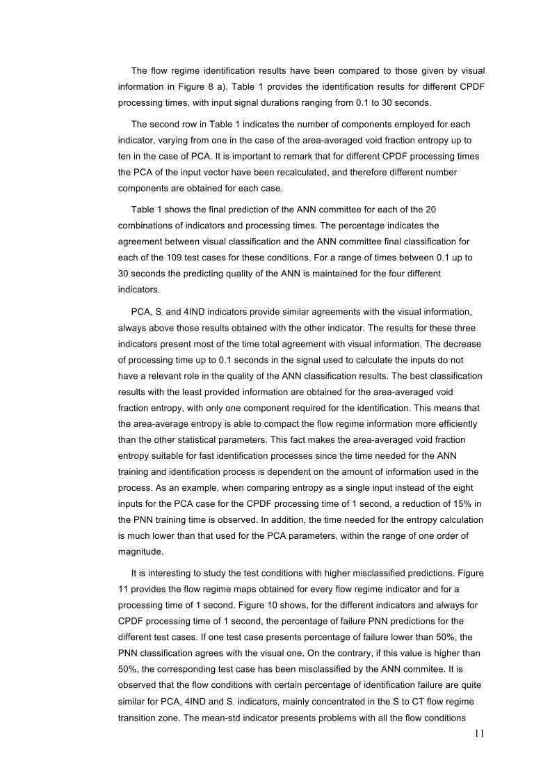
The flow regime identification results have been compared to those given by visual

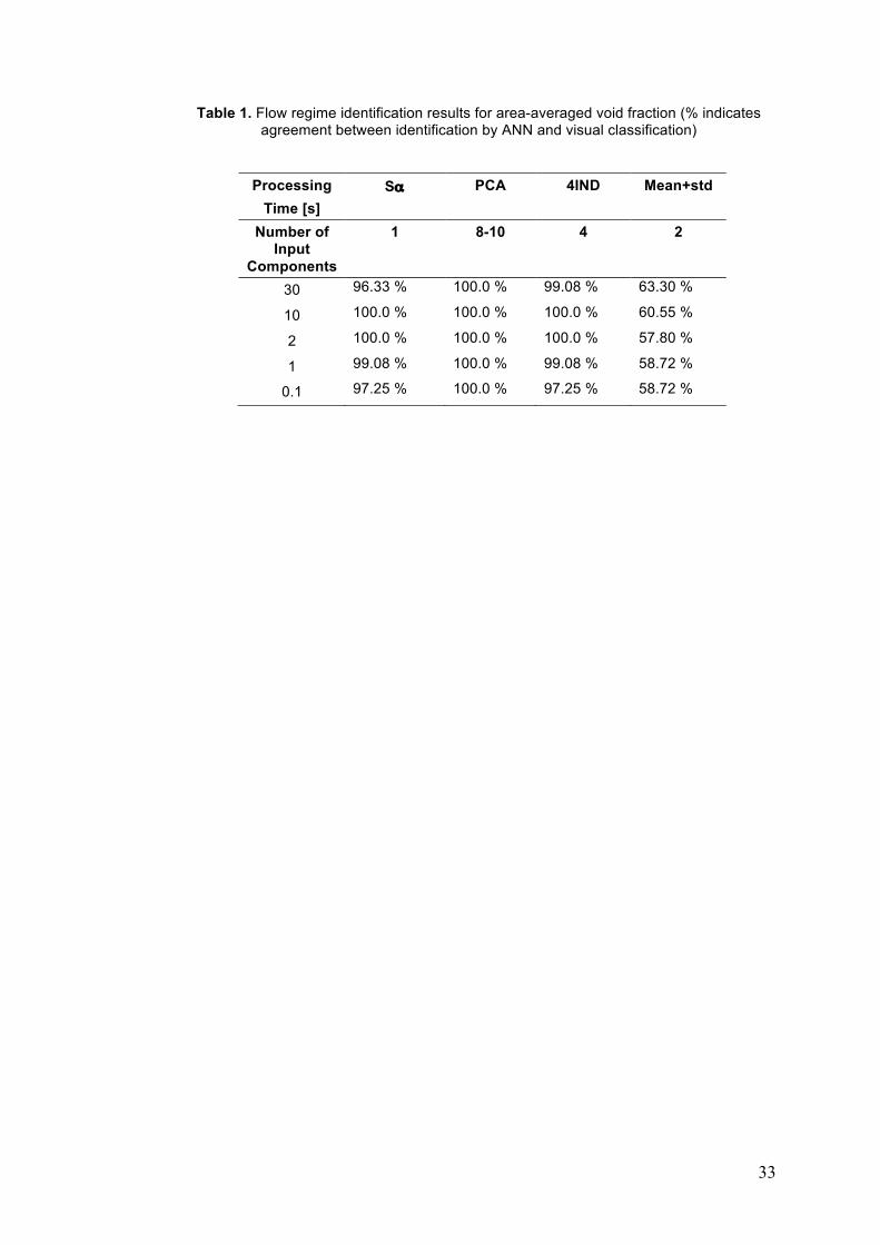
information in Figure 8 a). Table 1 provides the identification results for different CPDF

processing times, with input signal durations ranging from 0.1 to 30 seconds.

The second row in Table 1 indicates the number of components employed for each

indicator, varying from one in the case of the area-averaged void fraction entropy up to

ten in the case of PCA. It is important to remark that for different CPDF processing times

the PCA of the input vector have been recalculated, and therefore different number

components are obtained for each case.

Table 1 shows the final prediction of the ANN committee for each of the 20

combinations of indicators and processing times. The percentage indicates the

agreement between visual classification and the ANN committee final classification for

each of the 109 test cases for these conditions. For a range of times between 0.1 up to

30 seconds the predicting quality of the ANN is maintained for the four different

indicators.

PCA, S! and 4IND indicators provide similar agreements with the visual information,

always above those results obtained with the other indicator. The results for these three

indicators present most of the time total agreement with visual information. The decrease

of processing time up to 0.1 seconds in the signal used to calculate the inputs do not

have a relevant role in the quality of the ANN classification results. The best classification

results with the least provided information are obtained for the area-averaged void

fraction entropy, with only one component required for the identification. This means that

the area-average entropy is able to compact the flow regime information more efficiently

than the other statistical parameters. This fact makes the area-averaged void fraction

entropy suitable for fast identification processes since the time needed for the ANN

training and identification process is dependent on the amount of information used in the

process. As an example, when comparing entropy as a single input instead of the eight

inputs for the PCA case for the CPDF processing time of 1 second, a reduction of 15% in

the PNN training time is observed. In addition, the time needed for the entropy calculation

is much lower than that used for the PCA parameters, within the range of one order of

magnitude.

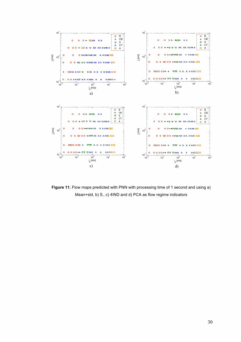
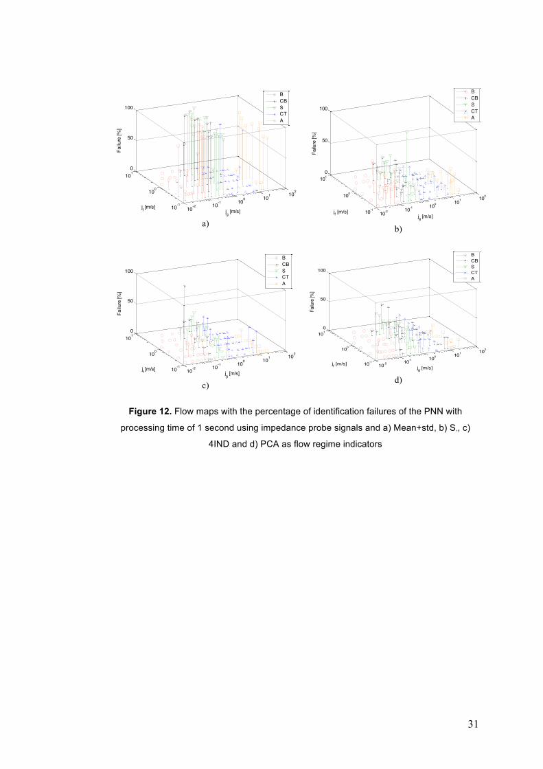
It is interesting to study the test conditions with higher misclassified predictions. Figure

11 provides the flow regime maps obtained for every flow regime indicator and for a

processing time of 1 second. Figure 10 shows, for the different indicators and always for

CPDF processing time of 1 second, the percentage of failure PNN predictions for the

different test cases. If one test case presents percentage of failure lower than 50%, the

PNN classification agrees with the visual one. On the contrary, if this value is higher than

50%, the corresponding test case has been misclassified by the ANN commitee. It is

observed that the flow conditions with certain percentage of identification failure are quite

similar for PCA, 4IND and S! indicators, mainly concentrated in the S to CT flow regime

transition zone. The mean-std indicator presents problems with all the flow conditions

12

except for the B and CT flow regimes.

If input signal durations lower than 0.1 seconds are processed, the ANN predictions

worsen for all the parameters. This duration agrees with the time scale given by the

bubble characteristic length (Laplace length) divided by the average bubble interfacial

velocity and modulated by the void fraction in bubbly flows.

3.3.2 Bubble chord length entropy

In this case, the SB values in a 50.8 mm D pipe in upward flow conditions have been

used as inputs for the ANN. The set of CPDF that correspond to the probe located at the

center of the pipe has been used.

The four flow regime indicators described in the previous section have been also used

and the flow regime identification results have been compared to those given by visual

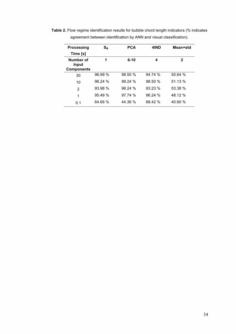
information in Figure 8b). Table 2 provides similar information as that Table 1 but now for

the case of bubble chord length indicators. As in Table 1, the prediction for SB, PCA and

4IND for processing times in the range of 1 to 30 seconds are quite similar among them.

Again, the mean+std indicator presents the lowest classification results. No much

influence of the CPDF processing time of the bubble chord length is neither observed for

this range. The best identification results with the lowest required components are

obtained for SB indicator, with PNN training time reductions similar as those presented for

the case of S!. However, ANN predictions worsen when processing time diminishes to 0.1

seconds, as the quality of the CPDF decreases and therefore the representativeness of

the indicators for the corresponding flow regime is lower. However, the results provided

by the impedance meter measurements based parameters where accurate for this input

signal duration. This last fact is easily explained since the conductivity probe and the

impedance meters are a local and an area-average measurement, respectively. Thus, the

probability of detecting a bubble with the conductivity probe is lower than with the

impedance meter if short measurement periods are considered.

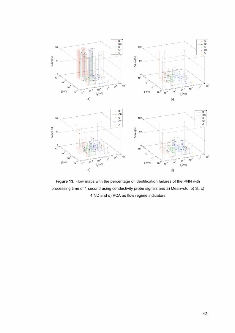
Figure 13 shows the same information as that in Figure 10, but using the conductivity

signal from the probe at the center of the pipe. The mean+std indicator presents

identification problems spread over all the flow regimes. For the other indicators, the

identification failures are concentrated in bubbly flow and churn-turbulent flow conditions.

Finally, it was shown in Sections 3.1 and 3.2 that the SB have better characteristics as

flow regime indicator than S!. However, the results provided by both entropies are quite

similar if input signals duration longer than 0.1 seconds are considered and the failures in

the flow regime identifications are located in the same flow regime map zones.

4. Conclusions

The area-averaged void fraction and bubble chord length entropies have been

13

introduced as flow regime indicators in two-phase flow systems. The entropy provides

quantitative information about the disorder in the area-averaged void fraction or bubble

chord length distributions. The area-averaged void fraction entropy is based on

impedance meter signals and the bubble chord length entropy in conductivity probe

signals. Both entropies have been calculated for 242 flow conditions in upward flow in

pipes.

The physical meaning of both parameters has been analysed using the visual flow

regime map information. In this way, it is possible to observe a clear dependence of the

entropy value with the flow regime in upward flows. Both area-averaged void fraction and

bubble chord length entropies present suitable characteristics as flow regime indicators.

The area-averaged void fraction and the bubble chord length entropies capability as

flow regime indicators has been checked with other statistical parameters of the void

fraction and bubble chord length CPDF distributions (Mean+std, 4IND and PCA).

Additionally, the variation of the indicators classification capability with different CPDF

processed with different input signals durations has been evaluated.

Classification efficiency using these entropy variables as inputs for the ANN commitee

are similar to those obtained by PCA or 4IND methods ("99% efficiency for area-

averaged entropy and "96% efficiency for bubble chord length entropy). However, the

entropy is capable to reduce the relevant information of the flow regimes in only one

significant and useful variable. In addition, the computation time for the entropy is much

lower than for the PCA. In terms of generating any empirical model to predict flow

regimes, reducing the independent variables to only one decreases the required

experimental data. Additionally for the case of using neural networks using one variable

as input represents less training time and faster predictions.

The time needed for obtaining good classification results depends on the type of

signal used. If area-averaged void fraction signals obtained from an impedance meter are

used a duration of 0.1 seconds is enough for obtaining accurate classifications (almost

100% agreement with visual information). If conductivity probe signals are used (bubble

chord length distributions) a temporal length of 1 second is necessary to accurate

classifications to be obtained (96% agreement with visual information). This difference in

the minimum temporal length requirement can be explained since conductivity probes

provide local measurements that are more dependent on the input temporal length.

Acknowledgements

This work was performed at Purdue University under the auspices of Mitsubishi Heavy

Industries Ltd. through the Institute of Thermal-hydraulics.

14

Nomenclature

Abbreviations

A annular flow regime

ANN

B

artificial neural network

bubbly flow regime

CB cap-bubbly flow regime

CT churn-turbulent flow regime

CPDF cumulative probability distribution function

GFR global flow regime

IND indices

LFR local flow regime

PCA principal components analysis

PDF probability distribution function

PNN probabilistic neural network

PSD power spectral density

S slug flow regime

SONN self-organizing neural network

z axial location (m)

Symbols

D pipe inner diameter (m)

G admittance (-)

H pipe height (m)

j superficial velocity (m/s)

L Chord length

N number of samples

p cumulative probability

S entropy (-)

z axial location (m)

15

Greek letters

! void fraction

Subscripts

0 zero void fraction

1 unity void fraction

! void fraction

g gas

f liquid

m mixture

n normalized

B bubble chord length

16

References

Cai, S., Toral, H., Qiu, J. and Archer J. S., (1994). Neural network based objective flow

regime identification in air-water two-phase flow. Can. J. Chem. Eng. 72, 440-445.

Elperin, T and Klochko, M. (2002). Flow regime identification in a two-phase flow using

wavelet transform. Exp. in Fluids 32, 674-682.

Goda, H., Hibiki, T., Kim, S., Ishii, M. and Uhle, J. (2004). Drift flux model for downward

two-phase flow. Int. J. Heat Mass Transfer 47, 4101-4118.

Gurau, B., Vasallo, P. and Keller, K. (2004). Measurement of gas and liquid velocities on

an air-water two-phase flow using cross-correlation of signals from a double sensor hot-

film probe. Exp. Thermal Fluid Science 28, 495-504.

Hernandez, L., Julia, J. E., Chiva, S., Paranjape, S., Ishii, M. (2006). Fast classification of

two-phase flow regimes based on conductivity signals and artificial neural networks.

Meas. Sci. Technol. 17, 1511-1521.

Hibiki, T., Hogsett, S., Ishii, M. (1998). Local measurement of interfacial area, interfacial

velocity and liquid turbulence in two-phase flow. Nuclear Eng. Des. 184, 287-304.

Ishii, M. and Mishima, K. (1984). Two-fluid model and hydrodynamic constitutive

relations. Nucl. Eng. Des. 82,107-126.

Ishii, M. and Hibiki, T. (2007). Thermo-fluid Dynamics of Two-Phase Flow. Springer.

Jones, O. C. and Zuber, N. (1975). The interrelation between void fraction fluctuations

and flow patterns in two-phase flow. Int. J. Multiphase Flow 3, 273-306.

Julia, J. E., Liu, Y., Paranjape, S. and Ishii, M. (2008). Local flow regimes analysis in

vertical upward two-phase flow. Nuclear Engineering Design 238, 156-169.

Kataoka, I., Ishii, M. and Serizawa, A. (1986). Local formulation and measurements of

interfacial area concentration in two-phase flow. Int. J. Multiphase Flow 12, 505-529.

Kendoush, A. A., Zaki, R. Y. and Shakir, B. M. (1980). Slip measurement in downward

two-phase bubbly flow using cross-correlation technique. Multiphase Transport:

Fundamentals, Reactor Safety, Applications Vol.5, T. Nejat Veziroglu Ed. Hemisphere

Publishing Corporation.

Kim, S., Fu, X. Y., Wang, X. and Ishii, M. (2000). Development of the miniaturized four-

sensor conductivity probe and the signal processing scheme. Int. J. Heat Mass Transfer

43, 4101-4118.

Lee, J. Y., Ishii, M. and Kim, N. S. (2008a). Instantaneous and objective flow regime

identification method for the vertical upward and downward co-current two-phase flow.

International Journal of Heat and Mass Transfer 51, 3442-3459.

17

Lee, J. Y., Kim, N. S., and Ishii, M. (2008b). Flow regime identification using chaotic

characteristics of two-phase flow. Nuclear Engineering and Design, 238, 945-957.

Matsui, G. (1984). Identification of flow regimes in vertical gas-liquid two-phase flow using

differential pressure fluctuations. Int. J. Multiphase Flow 10, 711-720.

Mi, Y., Ishii, M. and Tsoukalas, L. H. (1998). Vertical two-phase flow identification using

advanced instrumentation and neural networks. Nucl. Eng. Des. 184, 409-420.

Mi, Y., Ishii, M. and Tsoukalas, L. H. (2001a). Investigation of vertical slug flow with

advanced two-phase. Nucl. Eng. Des. 204, 69-85.

Mi, Y., Ishii, M. and Tsoukalas, L. H. (2001b). Flow regime identification methodology with

neural networks and two-phase flow models. Nucl. Eng. Des. 204, 87-100.

Mishima, K. and Ishii, M. (1984). Flow regime transition criteria for upward two-phase flow

in vertical tubes. Int. J. Heat Mass Transfer 27, 723-737.

Mohamad-Saleh, J. and Hoyle, B. S. (2002). Determination of multi-component flow

process parameters based on electrical capacitance tomography data using artificial

neural networks. Meas. Sci. Technol. 13, 1815-1821.

Parzen E. (1962). On estimation of a probability density function and mode Annals of

Mathematical Statisics 3, 1065-76.

Ruzicka, M. C., Drahos, J. Zahradnik, J. And Thomas, N. H. (1997). Intermittent transition

from bubbling to jetting regime in gas-liquid two-phase flow. Int. J. Multiphase Flow 23,

671-682.

Sharma, H., Das, G., Samanta, A.N., (2006). ANN-based prediction of two phase gas-

liquid flow patterns in a circular conduit. AIChE J. 52, 3018-3028.

Specht D F. (1988). Probabilistic neural networks for classification, mapping or

associative memory Proc. of IEEE Int. Conf. on Neural Networks 1 527-30

Specht D F (1990). Probabilistic neural networks Neural Netw. 3 109-18.

Taitel, T., Barnea, D. and Dukler, A. E. (1980). Modelling flow pattern transitions for

steady upward gas-liquid flow in vertical tubes. AIChE. J. 26, 345-354.

Tutu, N. K. (1982). Pressure fluctuations and flow pattern recognition in vertical two

phase gas-liquid flows. Int. J. Multiphase Flow 8, 443-447.

Zhang, Z. and Shi, L. (1999). Shannon entropy characteristics in two-phase flow systems.

J. Appl. Physics 85, 7544-7551.

18

Figure captions

Figure 1. Two-phase flow patterns representation for upward flow, a) bubbly, b) cap-

bubbly, c) slug, d) churn-turbulent and e) annular

Figure 2. Two-phase flow loop

Figure 3. CPDF distribution set of void fractions for upward flow, 25.4mm diameter pipe,

jf=1.25 m/s and 0.01 m/s<jg<16 m/s

Figure 4. CPDF distribution set of bubble chord lengths for upward flow, 50.8mm pipe,

jf=1.27 m/s and 0.01 m/s<jg<4 m/s

Figure 5. PNN architecture for two inputs and three classes

Figure 6. Correspondence between the flow regimes and SB

Figure 7. Correspondence between the flow regimes and S!

Figure 8. Visual flow regime map for upward flow a) upward flow 25.4 mm D pipe and b)

upward flow 50.8 mm D pipe

Figure 9. Evolution of the area-averaged void fraction entropy with the superficial gas and

liquid velocities in a 25.4 mm D pipe in upward flow conditions

Figure 10. Evolution of the bubble chord length entropy with the superficial gas velocity in

a 50.8 mm D pipe in upward flow conditions

Figure 11. Flow maps predicted with PNN with processing time of 1 second and using a)

Mean+std, b) S!, c) 4IND and d) PCA as flow regime indicators

Figure 12. Flow maps with the percentage of identification failures of the PNN with

processing time of 1 second using impedance probe signals and a) Mean+std, b) S!, c)

4IND and d) PCA as flow regime indicators

Figure 13. Flow maps with the percentage of identification failures of the PNN using

conductivity probe signals and a) Mean+std, b) S!, c) 4IND and d) PCA as flow regime

indicators

19

Table captions

Table 1. Flow regime identification results for area-averaged void fraction.

Table 2. Flow regime identification results for bubble chord length indicators.

20

B CB S CT A

a) b) c) d) e)

Figure 1. Two-phase flow patterns representation for upward flow a) bubbly, b) cap-

bubbly, c) slug, d) churn-turbulent and e) annular

Flow

21

Figure 2. Two-phase flow loop

22

Figure 3. CPDF distribution set of void fractions for upward flow, 25.4mm diameter pipe,

jf=1.25 m/s and 0.01 m/s<jg<16 m/s

23

10-3

10-2

10-1

100

101

0

0.2

0.4

0.6

0.8

1

LB (m)

CP

DF

Bubbly Cap-Bubbly Slug Churn-Turbulent

Figure 4. CPDF distribution set of bubble chord lengths for upward flow, 50.8mm pipe,

jf=1.27 m/s and 0.01 m/s<jg<4 m/s.

24

C1X1

X2

C2

C3

Figure 5. PNN architecture for two inputs and three classes

25

0 1000 2000 3000 4000 5000 60000

0.5

1

1.5

2

2.5

3

3.5

4

4.5Bubbly Flow

Samples [-]

Out

put V

olta

ge [V

]

Sensor 0Sensor 1

0 0.05 0.1 0.15 0.20

0.2

0.4

0.6

0.8

1Bubly Flow

LB (m)

CP

DF

B

0 1000 2000 3000 4000 5000 60000

0.5

1

1.5

2

2.5

3

3.5

4

4.5Cap-Bubbly Flow

Samples [-]

Out

put V

olta

ge [V

]

Sensor 0Sensor 1

0 0.05 0.1 0.15 0.20

0.2

0.4

0.6

0.8

1Cap-Bubbly Flow

LB (m)

CP

DF

CB

0 5000 10000 150000

0.5

1

1.5

2

2.5

3

3.5

4

4.5Slug Flow

Samples [-]

Out

put V

olta

ge [V

]

Sensor 0Sensor 1

0 0.2 0.4 0.6 0.8 10

0.2

0.4

0.6

0.8

1Slug Flow

LB (m)

CP

DF

S

0 0.5 1 1.5 2 2.5x 104

0

0.5

1

1.5

2

2.5

3

3.5

4

4.5Churn-Turbulent Flow

Samples [-]

Out

`put

Vol

tage

[V]

Sensor 0Sensor 1

0 0.4 0.8 1.2 1.6 20

0.2

0.4

0.6

0.8

1Churn-Turbulent Flow

LB (m)

CP

DF

CT

0 2 4 6 8x 104

0

0.5

1

1.5

2

2.5

3

3.5

4

4.5Annular Flow

Samples [-]

Out

put V

olta

ge [V

]

Sensor 0Sensor 1

0 0.5 1 1.5 20

0.2

0.4

0.6

0.8

1Annular Flow

LB (m)

CPD

F

A

Figure 6. Correspondence between the flow regimes and SB

Figure 6.

26

0 0.2 0.4 0.6 0.8 1

0

0.2

0.4

0.6

0.8

1Bubbly Flow

Area-Averaged Void Fraction [-]

CPD

F

B

0 0.2 0.4 0.6 0.8 10

0.2

0.4

0.6

0.8

1

Area-Averaged Void Faction [-]

CPD

F

Cap-Bubbly Flow

CB

0 0.2 0.4 0.6 0.8 10

0.2

0.4

0.6

0.8

1Slug Flow

Area-Averaged Void Fraction [-]

CPD

F

S

0 0.2 0.4 0.6 0.8 10

0.2

0.4

0.6

0.8

1

Area-Averaged Void Fraction [-]

CPD

F

Churn-Turbulent Flow

CT

0 0.2 0.4 0.6 0.8 1

0

0.2

0.4

0.6

0.8

1

Area-Averaged Void Fraction [-]

CPD

F

Annular Flow

A

Figure 7. Correspondence between the flow regimes and S!

Figure 7.

27

10-2

10-1

100

101

102

10-1

100

101

jg [m/s]

j f [m/s

]

BCBSCTA

a)

10-3

10-2

10-1

100

101

102

10-2

10-1

100

101

jg [m/s]

j f [m/s

]

BCBSCTA

b)

Figure 8. Visual flow regime map for a) upward flow 25.4 mm D pipe, b) upward flow 50.8

mm D pipe

28

Figure 9. Evolution of the area-averaged void fraction entropy with the superficial gas

and liquid velocities in a 25.4 mm D pipe in upward flow conditions

29

Figure 10. Evolution of the bubble chord length entropy with the superficial gas velocity in

a 50.8 mm D pipe in upward flow conditions

30

10-2

10-1

100

101

102

10-1

100

101

jg [m/s]

j f [m/s

]

BCBSCTA

a)

10-2

10-1

100

101

102

10-1

100

101

jg [m/s]

j f [m/s

]

BCBSCTA

b)

10-2

10-1

100

101

102

10-1

100

101

jg [m/s]

j f [m/s

]

BCBSCTA

c)

10-2

10-1

100

101

102

10-1

100

101

jg [m/s]

j f [m/s

]

BCBSCTA

d)

Figure 11. Flow maps predicted with PNN with processing time of 1 second and using a)

Mean+std, b) S!, c) 4IND and d) PCA as flow regime indicators

31

10-2 10

-1 100 10

1 102

10-1

100

1010

50

100

jg [m/s]jf [m/s]

Failu

re [%

]

BCBSCTA

a)

10-2 10-1 100 101 102

10-1

100

1010

50

100

jg [m/s]jf [m/s]

Failu

re [%

]

BCBSCTA

b)

10-2 10

-1 100 10

1 102

10-1

100

1010

50

100

jg [m/s]jf [m/s]

Failu

re [%

]

BCBSCTA

c)

10-2 10-1 100 101 102

10-1

100

1010

50

100

jg [m/s]jf [m/s]

Failu

re [%

]

BCBSCTA

d)

Figure 12. Flow maps with the percentage of identification failures of the PNN with

processing time of 1 second using impedance probe signals and a) Mean+std, b) S!, c)

4IND and d) PCA as flow regime indicators

32

10-3 10

-2 10-1 10

0 101 10

2

10-2

10-1

100

1010

50

100

jg [m/s]jf [m/s]

Failu

re [%

]

BCBSCTA

a)

10-3 10

-2 10-1 10

0 101 10

2

10-2

10-1

100

1010

50

100

jg [m/s]jf [m/s]

Failu

re [%

]

BCBSCTA

b)

10-3 10

-2 10-1 10

0 101 10

2

10-2

10-1

100

1010

50

100

jg [m/s]jf [m/s]

Failu

re [%

]

BCBSCTA

c)

10-3 10

-2 10-1 10

0 101 10

2

10-2

10-1

100

1010

50

100

jg [m/s]jf [m/s]

Failu

re [%

]

BCBSCTA

d)

Figure 13. Flow maps with the percentage of identification failures of the PNN with

processing time of 1 second using conductivity probe signals and a) Mean+std, b) S#, c)

4IND and d) PCA as flow regime indicators

33

Table 1. Flow regime identification results for area-averaged void fraction (% indicates agreement between identification by ANN and visual classification)

Processing Time [s]

S! PCA 4IND Mean+std

Number of Input

Components

1 8-10 4 2

30 96.33 % 100.0 % 99.08 % 63.30 %

10 100.0 % 100.0 % 100.0 % 60.55 %

2 100.0 % 100.0 % 100.0 % 57.80 %

1 99.08 % 100.0 % 99.08 % 58.72 %

0.1 97.25 % 100.0 % 97.25 % 58.72 %

34

Table 2. Flow regime identification results for bubble chord length indicators (% indicates

agreement between identification by ANN and visual classification).

Processing Time [s]

SB PCA 4IND Mean+std

Number of Input

Components

1 6-10 4 2

30 96.99 % 98.50 % 94.74 % 55.64 %

10 96.24 % 99.24 % 98.50 % 51.13 %

2 93.98 % 96.24 % 93.23 % 53.38 %

1 95.49 % 97.74 % 96.24 % 48.12 %

0.1 64.66 % 44.36 % 68.42 % 40.60 %