Electric Network Frequency (ENF) RecognitionAbdelrahman Gaber∗, Abdelrahman Zayed∗, Basem Ahmed∗, Eslam Elshiekh∗, Hesham Aly∗

Ibrahim Sherif∗, Khaled Elgammal∗, Omar Ahmadein∗, Omar Elzaafarany∗ and Taha Gamal∗∗Faculty of Engineering, Alexandria University, Egypt

Pursuit Of Processing TeamLeader’s email: Abdelrahman.M.Zayed@ieee.org

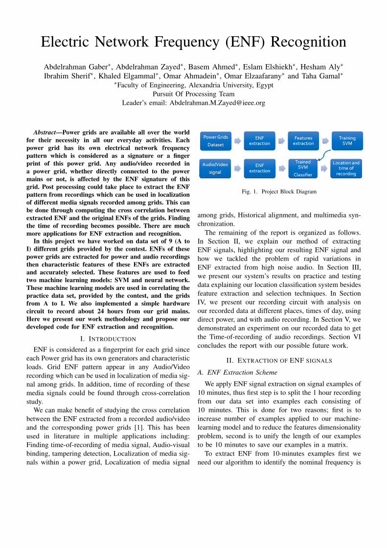
Abstract—Power grids are available all over the worldfor their necessity in all our everyday activities. Eachpower grid has its own electrical network frequencypattern which is considered as a signature or a fingerprint of this power grid. Any audio/video recorded ina power grid, whether directly connected to the powermains or not, is affected by the ENF signature of thisgrid. Post processing could take place to extract the ENFpattern from recordings which can be used in localizationof different media signals recorded among grids. This canbe done through computing the cross correlation betweenextracted ENF and the original ENFs of the grids. Findingthe time of recording becomes possible. There are muchmore applications for ENF extraction and recognition.

In this project we have worked on data set of 9 (A toI) different grids provided by the contest. ENFs of thesepower grids are extracted for power and audio recordingsthen characteristic features of these ENFs are extractedand accurately selected. These features are used to feedtwo machine learning models: SVM and neural network.These machine learning models are used in correlating thepractice data set, provided by the contest, and the gridsfrom A to I. We also implemented a simple hardwarecircuit to record about 24 hours from our grid mains.Here we present our work methodology and propose ourdeveloped code for ENF extraction and recognition.

I. INTRODUCTION

ENF is considered as a fingerprint for each grid sinceeach Power grid has its own generators and characteristicloads. Grid ENF pattern appear in any Audio/Videorecording which can be used in localization of media sig-nal among grids. In addition, time of recording of thesemedia signals could be found through cross-correlationstudy.

We can make benefit of studying the cross correlationbetween the ENF extracted from a recorded audio/videoand the corresponding power grids [1]. This has beenused in literature in multiple applications including:Finding time-of-recording of media signal, Audio-visualbinding, tampering detection, Localization of media sig-nals within a power grid, Localization of media signal

Fig. 1. Project Block Diagram

among grids, Historical alignment, and multimedia syn-chronization.

The remaining of the report is organized as follows.In Section II, we explain our method of extractingENF signals, highlighting our resulting ENF signal andhow we tackled the problem of rapid variations inENF extracted from high noise audio. In Section III,we present our system’s results on practice and testingdata explaining our location classification system besidesfeature extraction and selection techniques. In SectionIV, we present our recording circuit with analysis onour recorded data at different places, times of day, usingdirect power, and with audio recording. In Section V, wedemonstrated an experiment on our recorded data to getthe Time-of-recording of audio recordings. Section VIconcludes the report with our possible future work.

II. EXTRACTION OF ENF SIGNALS

A. ENF Extraction Scheme

We apply ENF signal extraction on signal examples of10 minutes, thus first step is to split the 1 hour recordingfrom our data set into examples each consisting of10 minutes. This is done for two reasons; first is toincrease number of examples applied to our machine-learning model and to reduce the features dimensionalityproblem, second is to unify the length of our examplesto be 10 minutes to save our examples in a matrix.

To extract ENF from 10-minutes examples first weneed our algorithm to identify the nominal frequency is

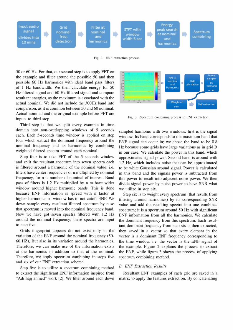
Fig. 2. ENF extraction process

50 or 60 Hz. For that, our second step is to apply FFT onthe example and filter around the possible 50 and thenpossible 60 Hz harmonics with ideal band pass filtersof 1 Hz bandwidth. We then calculate energy for 50Hz filtered signal and 60 Hz filtered signal and compareresultant energies, as the maximum is associated with theactual nominal. We did not include the 300Hz band intocomparison, as it is common between 50 and 60 nominal.Actual nominal and the original example before FFT areinputs to third step.

Third step is that we split every example in timedomain into non-overlapping windows of 5 secondseach. Each 5-seconds time window is applied on stepfour which extract the dominant frequency around thenominal frequency and its harmonics by combiningweighted filtered spectra around each nominal.

Step four is to take FFT of the 5 seconds windowand split the resultant spectrum into seven spectra eachis filtered around a harmonic of the nominal value; i.e.filters have center frequencies of n multiplied by nominalfrequency, for n is number of nominal of interest. Bandpass of filters is 1.2 Hz multiplied by n to have widerwindow around higher harmonic bands. This is donebecause ENF information is spread with n factor athigher harmonics so window has to not cutoff ENF. Wedown sample every resultant filtered spectrum by n sothat spectrum is moved into the nominal frequency band.Now we have got seven spectra filtered with 1.2 Hzaround the nominal frequency; these spectra are inputto step five.

Grids fingerprint appears do not exist only in thevariation of the ENF around the nominal frequency (50-60 HZ), But also in its variation around the harmonics.Therefore, we can make use of the information existsat the harmonics in addition to that at the nominal.Therefore, we apply spectrum combining in steps fiveand six of our ENF extraction scheme.

Step five is to utilize a spectrum combining methodto extract the significant ENF information inspired from”Adi hajj ahmed” work [2]. We filter around each down

Fig. 3. Spectrum combining process in ENF extraction

sampled harmonic with two windows; first is the signalwindow. Its band corresponds to the maximum band thatENF signal can occur in; we chose the band to be 0.8Hz because some grids have large variations as in grid Bin our case. We calculate the power in this band, whichapproximates signal power. Second band is around with1.2 Hz, which includes noise that can be approximatedto be white Gaussian around signal. Power is calculatedin this band and the signals power is subtracted fromthis power to result into adjacent noise power. We thendivide signal power by noise power to have SNR whatwe utilize in step six.

Step six is to weight every spectrum (that results fromfiltering around harmonics) by its corresponding SNRvalue and add the resulting spectra into one combinesspectrum; it is a spectrum around 50 Hz with significantENF information from all the harmonics. We calculatethe dominant frequency from this spectrum. Each resul-tant dominant frequency from step six is then extracted,then saved in a vector so that every element in thevector is a dominant ENF frequency corresponding tothe time window, i.e. the vector is the ENF signal ofthe example. Figure 2 explains the process to extractthe ENF, while figure 3 shows the process of applyingspectrum combining method.

B. ENF Extraction Results

Resultant ENF examples of each grid are saved in amatrix to apply the features extraction. By concatenating

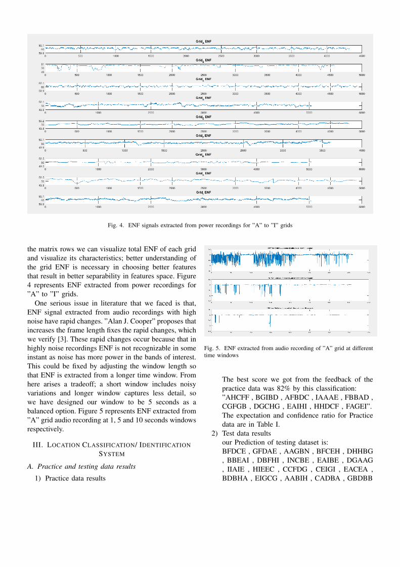
Fig. 4. ENF signals extracted from power recordings for ”A” to ”I” grids

the matrix rows we can visualize total ENF of each gridand visualize its characteristics; better understanding ofthe grid ENF is necessary in choosing better featuresthat result in better separability in features space. Figure4 represents ENF extracted from power recordings for”A” to ”I” grids.

One serious issue in literature that we faced is that,ENF signal extracted from audio recordings with highnoise have rapid changes. ”Alan J. Cooper” proposes thatincreases the frame length fixes the rapid changes, whichwe verify [3]. These rapid changes occur because that inhighly noise recordings ENF is not recognizable in someinstant as noise has more power in the bands of interest.This could be fixed by adjusting the window length sothat ENF is extracted from a longer time window. Fromhere arises a tradeoff; a short window includes noisyvariations and longer window captures less detail, sowe have designed our window to be 5 seconds as abalanced option. Figure 5 represents ENF extracted from”A” grid audio recording at 1, 5 and 10 seconds windowsrespectively.

III. LOCATION CLASSIFICATION/ IDENTIFICATION

SYSTEM

A. Practice and testing data results

1) Practice data results

Fig. 5. ENF extracted from audio recording of ”A” grid at differenttime windows

The best score we got from the feedback of thepractice data was 82% by this classification:”AHCFF , BGIBD , AFBDC , IAAAE , FBBAD ,CGFGB , DGCHG , EAIHI , HHDCF , FAGEI”.The expectation and confidence ratio for Practicedata are in Table I.

2) Test data resultsour Prediction of testing dataset is:BFDCE , GFDAE , AAGBN , BFCEH , DHHBG, BBEAI , DBFHI , INCBE , EAIBE , DGAAG, IIAIE , HIEEC , CCFDG , CEIGI , EACEA ,BDBHA , EIGCG , AABIH , CADBA , GBDBB

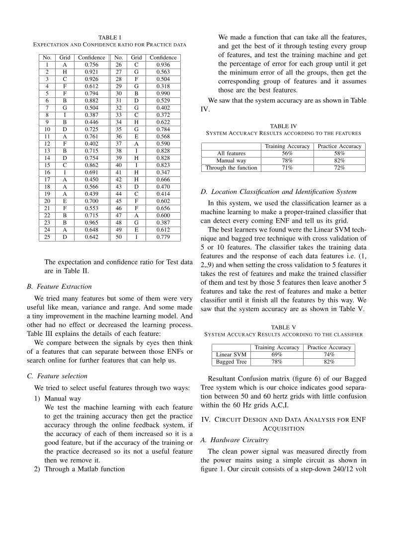
TABLE IEXPECTATION AND CONFIDENCE RATIO FOR PRACTICE DATA

No. Grid Confidence No. Grid Confidence1 A 0.756 26 C 0.9362 H 0.921 27 G 0.5633 C 0.926 28 F 0.5044 F 0.612 29 G 0.3185 F 0.794 30 B 0.9906 B 0.882 31 D 0.5297 G 0.504 32 G 0.4028 I 0.387 33 C 0.3729 B 0.446 34 H 0.62210 D 0.725 35 G 0.78411 A 0.761 36 E 0.56812 F 0.402 37 A 0.59013 B 0.715 38 I 0.82814 D 0.754 39 H 0.82815 C 0.862 40 I 0.82316 I 0.691 41 H 0.34717 A 0.450 42 H 0.66618 A 0.566 43 D 0.47019 A 0.439 44 C 0.41420 E 0.700 45 F 0.60221 F 0.553 46 F 0.65622 B 0.715 47 A 0.60023 B 0.965 48 G 0.38724 A 0.648 49 E 0.61225 D 0.642 50 I 0.779

The expectation and confidence ratio for Test dataare in Table II.

B. Feature Extraction

We tried many features but some of them were veryuseful like mean, variance and range. And some madea tiny improvement in the machine learning model. Andother had no effect or decreased the learning process.Table III explains the details of each feature:

We compare between the signals by eyes then thinkof a features that can separate between those ENFs orsearch online for further features that can help us.

C. Feature selection

We tried to select useful features through two ways:1) Manual way

We test the machine learning with each featureto get the training accuracy then get the practiceaccuracy through the online feedback system, ifthe accuracy of each of them increased so it is agood feature, but if the accuracy of the training orthe practice decreased so its not a useful featurethen we remove it.

2) Through a Matlab function

We made a function that can take all the features,and get the best of it through testing every groupof features, and test the training machine and getthe percentage of error for each group until it getthe minimum error of all the groups, then get thecorresponding group of features and it assumesthose are the best features.

We saw that the system accuracy are as shown in TableIV.

TABLE IVSYSTEM ACCURACY RESULTS ACCORDING TO THE FEATURES

Training Accuracy Practice AccuracyAll features 56% 58%Manual way 78% 82%

Through the function 71% 72%

D. Location Classification and Identification System

In this system, we used the classification learner as amachine learning to make a proper-trained classifier thatcan detect every coming ENF and tell us its grid.

The best learners we found were the Linear SVM tech-nique and bagged tree technique with cross validation of5 or 10 features. The classifier takes the training datafeatures and the response of each data features i.e. (1,2,,9) and when setting the cross validation to 5 features ittakes the rest of features and make the trained classifierof them and test by those 5 features then leave another 5features and take the rest of features and make a betterclassifier until it finish all the features by this way. Wesaw that the system accuracy are as shown in Table V.

TABLE VSYSTEM ACCURACY RESULTS ACCORDING TO THE CLASSIFIER

Training Accuracy Practice AccuracyLinear SVM 69% 74%Bagged Tree 78% 82%

Resultant Confusion matrix (figure 6) of our BaggedTree system which is our choice indicates good separa-tion between 50 and 60 hertz grids with little confusionwithin the 60 Hz grids A,C,I.

IV. CIRCUIT DESIGN AND DATA ANALYSIS FOR ENFACQUISITION

A. Hardware Circuitry

The clean power signal was measured directly fromthe power mains using a simple circuit as shown infigure 1. Our circuit consists of a step-down 240/12 volt

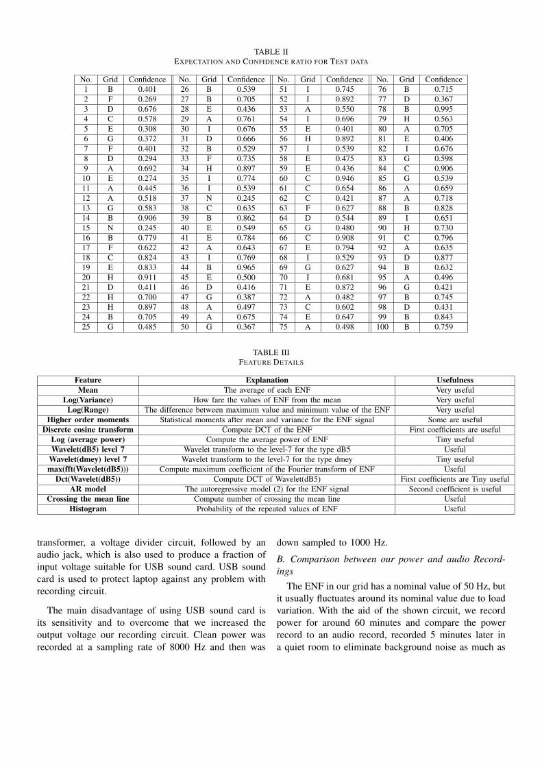
TABLE IIEXPECTATION AND CONFIDENCE RATIO FOR TEST DATA

No. Grid Confidence No. Grid Confidence No. Grid Confidence No. Grid Confidence1 B 0.401 26 B 0.539 51 I 0.745 76 B 0.7152 F 0.269 27 B 0.705 52 I 0.892 77 D 0.3673 D 0.676 28 E 0.436 53 A 0.550 78 B 0.9954 C 0.578 29 A 0.761 54 I 0.696 79 H 0.5635 E 0.308 30 I 0.676 55 E 0.401 80 A 0.7056 G 0.372 31 D 0.666 56 H 0.892 81 E 0.4067 F 0.401 32 B 0.529 57 I 0.539 82 I 0.6768 D 0.294 33 F 0.735 58 E 0.475 83 G 0.5989 A 0.692 34 H 0.897 59 E 0.436 84 C 0.90610 E 0.274 35 I 0.774 60 C 0.946 85 G 0.53911 A 0.445 36 I 0.539 61 C 0.654 86 A 0.65912 A 0.518 37 N 0.245 62 C 0.421 87 A 0.71813 G 0.583 38 C 0.635 63 F 0.627 88 B 0.82814 B 0.906 39 B 0.862 64 D 0.544 89 I 0.65115 N 0.245 40 E 0.549 65 G 0.480 90 H 0.73016 B 0.779 41 E 0.784 66 C 0.908 91 C 0.79617 F 0.622 42 A 0.643 67 E 0.794 92 A 0.63518 C 0.824 43 I 0.769 68 I 0.529 93 D 0.87719 E 0.833 44 B 0.965 69 G 0.627 94 B 0.63220 H 0.911 45 E 0.500 70 I 0.681 95 A 0.49621 D 0.411 46 D 0.416 71 E 0.872 96 G 0.42122 H 0.700 47 G 0.387 72 A 0.482 97 B 0.74523 H 0.897 48 A 0.497 73 C 0.602 98 D 0.43124 B 0.705 49 A 0.675 74 E 0.647 99 B 0.84325 G 0.485 50 G 0.367 75 A 0.498 100 B 0.759

TABLE IIIFEATURE DETAILS

Feature Explanation UsefulnessMean The average of each ENF Very useful

Log(Variance) How fare the values of ENF from the mean Very usefulLog(Range) The difference between maximum value and minimum value of the ENF Very useful

Higher order moments Statistical moments after mean and variance for the ENF signal Some are usefulDiscrete cosine transform Compute DCT of the ENF First coefficients are useful

Log (average power) Compute the average power of ENF Tiny usefulWavelet(dB5) level 7 Wavelet transform to the level-7 for the type dB5 Useful

Wavelet(dmey) level 7 Wavelet transform to the level-7 for the type dmey Tiny usefulmax(fft(Wavelet(dB5))) Compute maximum coefficient of the Fourier transform of ENF Useful

Dct(Wavelet(dB5)) Compute DCT of Wavelet(dB5) First coefficients are Tiny usefulAR model The autoregressive model (2) for the ENF signal Second coefficient is useful

Crossing the mean line Compute number of crossing the mean line UsefulHistogram Probability of the repeated values of ENF Useful

transformer, a voltage divider circuit, followed by anaudio jack, which is also used to produce a fraction ofinput voltage suitable for USB sound card. USB soundcard is used to protect laptop against any problem withrecording circuit.

The main disadvantage of using USB sound card isits sensitivity and to overcome that we increased theoutput voltage our recording circuit. Clean power wasrecorded at a sampling rate of 8000 Hz and then was

down sampled to 1000 Hz.

B. Comparison between our power and audio Record-ings

The ENF in our grid has a nominal value of 50 Hz, butit usually fluctuates around its nominal value due to loadvariation. With the aid of the shown circuit, we recordpower for around 60 minutes and compare the powerrecord to an audio record, recorded 5 minutes later ina quiet room to eliminate background noise as much as

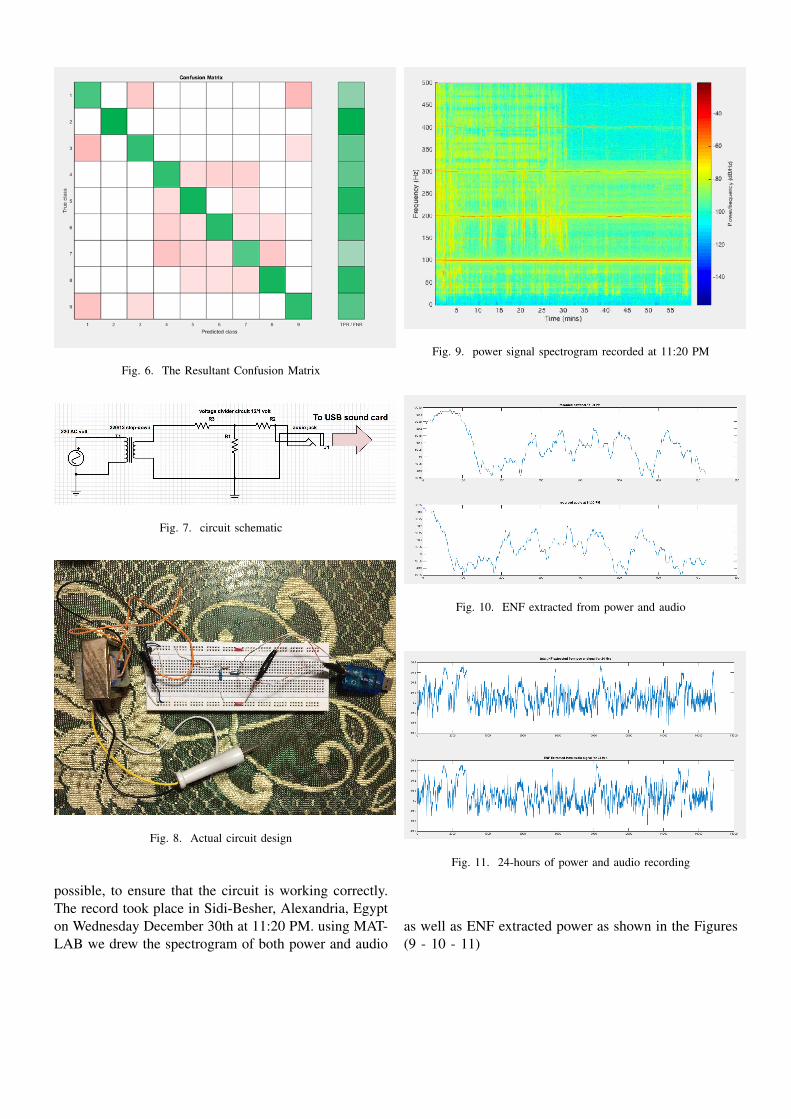
Fig. 6. The Resultant Confusion Matrix

Fig. 7. circuit schematic

Fig. 8. Actual circuit design

possible, to ensure that the circuit is working correctly.The record took place in Sidi-Besher, Alexandria, Egypton Wednesday December 30th at 11:20 PM. using MAT-LAB we drew the spectrogram of both power and audio

Fig. 9. power signal spectrogram recorded at 11:20 PM

Fig. 10. ENF extracted from power and audio

Fig. 11. 24-hours of power and audio recording

as well as ENF extracted power as shown in the Figures(9 - 10 - 11)

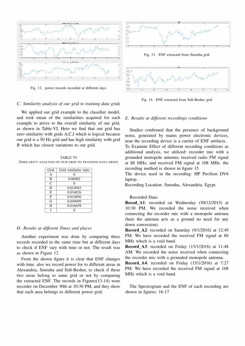
Fig. 12. power records recorded at different days

C. Similarity analysis of our grid to training data grids

We applied our grid example to the classifier model,and took mean of the similarities acquired for eachexample to arrive to the overall similarity of our grid,as shown in Table:VI. Here we find that our grid haszero similarity with grids A,C,I which is logical becauseour grid is a 50 Hz grid and has high similarity with gridB which has closest variations to our grid.

TABLE VISIMILARITY ANALYSIS OF OUR GRID TO TRAINING DATA GRIDS

Grid Grid similarity ratioA 0B 0.86902C 0D 0.014943E 0.034826F 0.014856G 0.049699H 0.016659I 0

D. Results at different Times and places

Another experiment was done by comparing threerecords recorded in the same time but at different daysto check if ENF vary with time or not. The result wasas shown in Figure 12

From the shown figure it is clear that ENF changeswith time. also we record power for to different areas inAlexandria, Smouha and Sidi-Besher, to check if thesetwo areas belong to same grid or not by comparingthe extracted ENF. The records in Figures(13-14) wererecorder on December 30th at 10:30 PM, and they showthat each area belongs to different power grid.

Fig. 13. ENF extracted from Smouha grid

Fig. 14. ENF extracted from Sidi-Besher grid

E. Results at different recordings conditions

Studies confirmed that the presence of backgroundnoise, generated by mains power electronic devices,near the recording device is a carrier of ENF artifacts.To Examine Effect of different recording conditions asadditional analysis, we utilized: recorder mic with agrounded monopole antenna; received radio FM signalat 88 MHz; and received FM signal at 108 MHz. therecording method is shown in figure 15The device used in the recording: HP Pavilion DV6laptop.Recording Location: Smouha, Alexandria, Egypt.

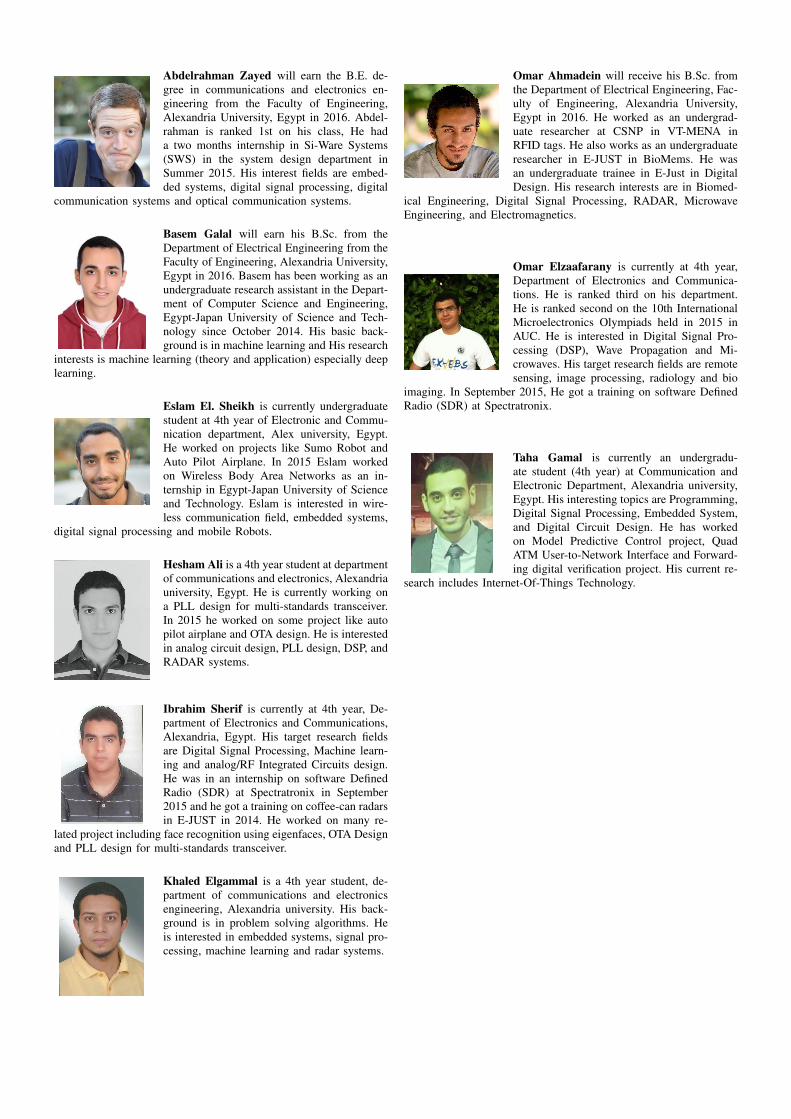
Recorded Data:Recod A1: recorded on Wednesday (30/12/2015) at10:30 PM. We recorded the noise received whenconnecting the recorder mic with a monopole antenna(here the antenna acts as a ground no need for anydown conversion).Record A2: recorded on Saturday (9/1/2016) at 12:49PM. We have recorded the received FM signal at 88MHz which is a void band.Record A3: recorded on Friday (15/1/2016) at 11:48AM. We recorded the noise received when connectingthe recorder mic with a grounded monopole antenna.Record A4: recorded on Friday (15/1/2016) at 7:27PM. We have recorded the received FM signal at 108MHz which is a void band.

The Spectrogram and the ENF of each recording areshown in figures: 16-17

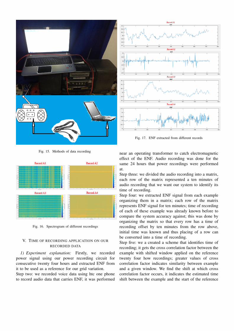
Fig. 15. Methods of data recording

Fig. 16. Spectrogram of different recordings

V. TIME OF RECORDING APPLICATION ON OUR

RECORDED DATA

1) Experiment explanation: Firstly, we recordedpower signal using our power recording circuit forconsecutive twenty four hours and extracted ENF fromit to be used as a reference for our grid variation.Step two: we recorded voice data using htc one phoneto record audio data that carries ENF, it was performed

Fig. 17. ENF extracted from different records

near an operating transformer to catch electromagneticeffect of the ENF. Audio recording was done for thesame 24 hours that power recordings were performedat.Step three: we divided the audio recording into a matrix,each row of the matrix represented a ten minutes ofaudio recording that we want our system to identify itstime of recording.Step four: we extracted ENF signal from each exampleorganizing them in a matrix; each row of the matrixrepresents ENF signal for ten minutes; time of recordingof each of these example was already known before tocompare the system accuracy against; this was done byorganizing the matrix so that every row has a time ofrecording offset by ten minutes from the row above,initial time was known and thus placing of a row canbe converted into a time of recording.Step five: we a created a scheme that identifies time ofrecording; it gets the cross correlation factor between theexample with shifted window applied on the referencetwenty four how recordings; greater values of crosscorrelation factor indicates similarity between exampleand a given window. We find the shift at which crosscorrelation factor occurs, it indicates the estimated timeshift between the example and the start of the reference

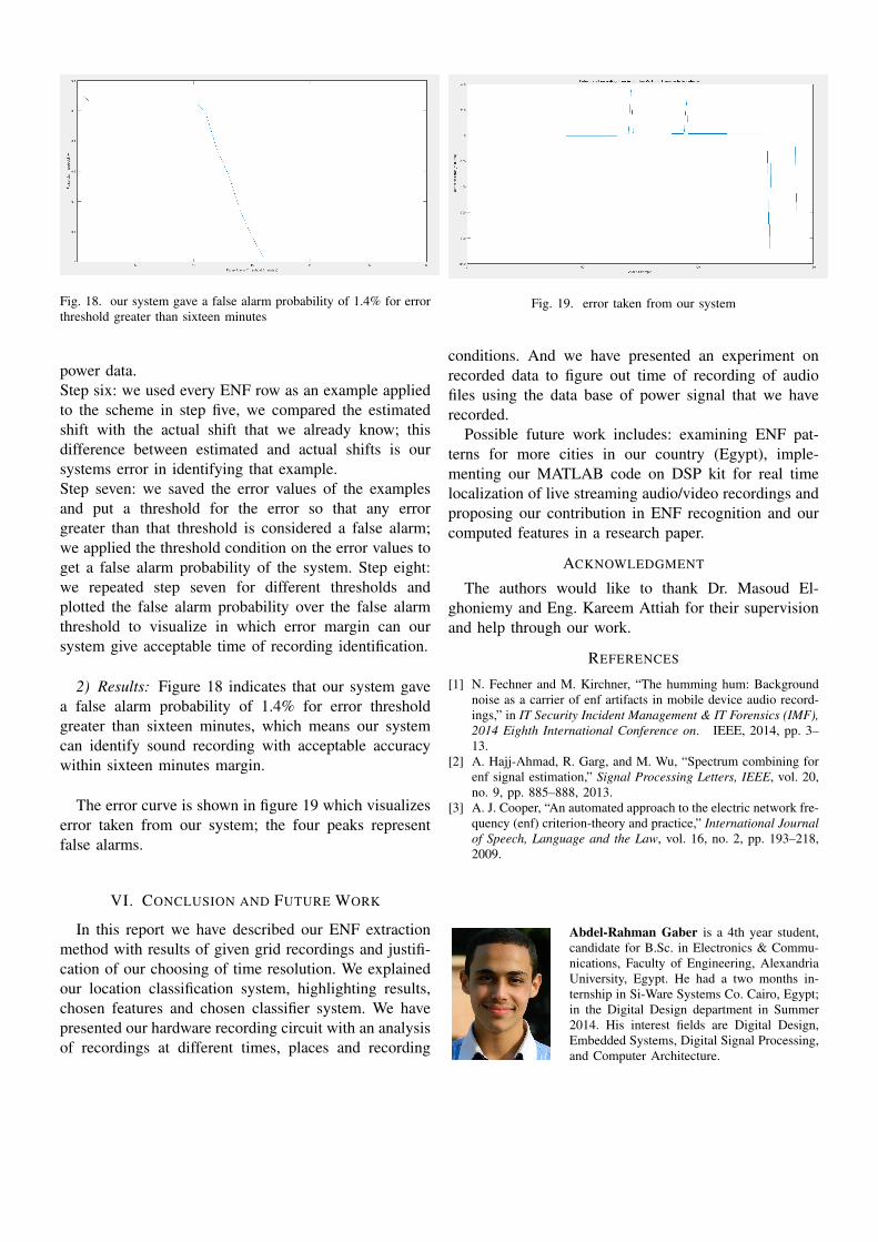
Fig. 18. our system gave a false alarm probability of 1.4% for errorthreshold greater than sixteen minutes

power data.Step six: we used every ENF row as an example appliedto the scheme in step five, we compared the estimatedshift with the actual shift that we already know; thisdifference between estimated and actual shifts is oursystems error in identifying that example.Step seven: we saved the error values of the examplesand put a threshold for the error so that any errorgreater than that threshold is considered a false alarm;we applied the threshold condition on the error values toget a false alarm probability of the system. Step eight:we repeated step seven for different thresholds andplotted the false alarm probability over the false alarmthreshold to visualize in which error margin can oursystem give acceptable time of recording identification.

2) Results: Figure 18 indicates that our system gavea false alarm probability of 1.4% for error thresholdgreater than sixteen minutes, which means our systemcan identify sound recording with acceptable accuracywithin sixteen minutes margin.

The error curve is shown in figure 19 which visualizeserror taken from our system; the four peaks representfalse alarms.

VI. CONCLUSION AND FUTURE WORK

In this report we have described our ENF extractionmethod with results of given grid recordings and justifi-cation of our choosing of time resolution. We explainedour location classification system, highlighting results,chosen features and chosen classifier system. We havepresented our hardware recording circuit with an analysisof recordings at different times, places and recording

Fig. 19. error taken from our system

conditions. And we have presented an experiment onrecorded data to figure out time of recording of audiofiles using the data base of power signal that we haverecorded.

Possible future work includes: examining ENF pat-terns for more cities in our country (Egypt), imple-menting our MATLAB code on DSP kit for real timelocalization of live streaming audio/video recordings andproposing our contribution in ENF recognition and ourcomputed features in a research paper.

ACKNOWLEDGMENT

The authors would like to thank Dr. Masoud El-ghoniemy and Eng. Kareem Attiah for their supervisionand help through our work.

REFERENCES

[1] N. Fechner and M. Kirchner, “The humming hum: Backgroundnoise as a carrier of enf artifacts in mobile device audio record-ings,” in IT Security Incident Management & IT Forensics (IMF),2014 Eighth International Conference on. IEEE, 2014, pp. 3–13.

[2] A. Hajj-Ahmad, R. Garg, and M. Wu, “Spectrum combining forenf signal estimation,” Signal Processing Letters, IEEE, vol. 20,no. 9, pp. 885–888, 2013.

[3] A. J. Cooper, “An automated approach to the electric network fre-quency (enf) criterion-theory and practice,” International Journalof Speech, Language and the Law, vol. 16, no. 2, pp. 193–218,2009.

Abdel-Rahman Gaber is a 4th year student,candidate for B.Sc. in Electronics & Commu-nications, Faculty of Engineering, AlexandriaUniversity, Egypt. He had a two months in-ternship in Si-Ware Systems Co. Cairo, Egypt;in the Digital Design department in Summer2014. His interest fields are Digital Design,Embedded Systems, Digital Signal Processing,and Computer Architecture.

Abdelrahman Zayed will earn the B.E. de-gree in communications and electronics en-gineering from the Faculty of Engineering,Alexandria University, Egypt in 2016. Abdel-rahman is ranked 1st on his class, He hada two months internship in Si-Ware Systems(SWS) in the system design department inSummer 2015. His interest fields are embed-ded systems, digital signal processing, digital

communication systems and optical communication systems.

Basem Galal will earn his B.Sc. from theDepartment of Electrical Engineering from theFaculty of Engineering, Alexandria University,Egypt in 2016. Basem has been working as anundergraduate research assistant in the Depart-ment of Computer Science and Engineering,Egypt-Japan University of Science and Tech-nology since October 2014. His basic back-ground is in machine learning and His research

interests is machine learning (theory and application) especially deeplearning.

Eslam El. Sheikh is currently undergraduatestudent at 4th year of Electronic and Commu-nication department, Alex university, Egypt.He worked on projects like Sumo Robot andAuto Pilot Airplane. In 2015 Eslam workedon Wireless Body Area Networks as an in-ternship in Egypt-Japan University of Scienceand Technology. Eslam is interested in wire-less communication field, embedded systems,

digital signal processing and mobile Robots.

Hesham Ali is a 4th year student at departmentof communications and electronics, Alexandriauniversity, Egypt. He is currently working ona PLL design for multi-standards transceiver.In 2015 he worked on some project like autopilot airplane and OTA design. He is interestedin analog circuit design, PLL design, DSP, andRADAR systems.

Ibrahim Sherif is currently at 4th year, De-partment of Electronics and Communications,Alexandria, Egypt. His target research fieldsare Digital Signal Processing, Machine learn-ing and analog/RF Integrated Circuits design.He was in an internship on software DefinedRadio (SDR) at Spectratronix in September2015 and he got a training on coffee-can radarsin E-JUST in 2014. He worked on many re-

lated project including face recognition using eigenfaces, OTA Designand PLL design for multi-standards transceiver.

Khaled Elgammal is a 4th year student, de-partment of communications and electronicsengineering, Alexandria university. His back-ground is in problem solving algorithms. Heis interested in embedded systems, signal pro-cessing, machine learning and radar systems.

Omar Ahmadein will receive his B.Sc. fromthe Department of Electrical Engineering, Fac-ulty of Engineering, Alexandria University,Egypt in 2016. He worked as an undergrad-uate researcher at CSNP in VT-MENA inRFID tags. He also works as an undergraduateresearcher in E-JUST in BioMems. He wasan undergraduate trainee in E-Just in DigitalDesign. His research interests are in Biomed-

ical Engineering, Digital Signal Processing, RADAR, MicrowaveEngineering, and Electromagnetics.

Omar Elzaafarany is currently at 4th year,Department of Electronics and Communica-tions. He is ranked third on his department.He is ranked second on the 10th InternationalMicroelectronics Olympiads held in 2015 inAUC. He is interested in Digital Signal Pro-cessing (DSP), Wave Propagation and Mi-crowaves. His target research fields are remotesensing, image processing, radiology and bio

imaging. In September 2015, He got a training on software DefinedRadio (SDR) at Spectratronix.

Taha Gamal is currently an undergradu-ate student (4th year) at Communication andElectronic Department, Alexandria university,Egypt. His interesting topics are Programming,Digital Signal Processing, Embedded System,and Digital Circuit Design. He has workedon Model Predictive Control project, QuadATM User-to-Network Interface and Forward-ing digital verification project. His current re-

search includes Internet-Of-Things Technology.