D. R. HamannMat-Sim Research LLC

Bell Laboratories, Lucent TechnologiesDepartment of Physics and Astronomy, Rutgers University

Elastic and Piezoelectric Elastic and Piezoelectric Properties in Properties in ABINITABINIT

Mat-SimResearch

HistoryHistory

• Bad old days (70’s)– Murnaghan function fit to energy vs. volume results– Bulk moduli from 2nd derivatives of fits– No piezoelectricity

• Moving forward (80’s +)– Analytic theories for stress (Nielsen & Martin) and polarization (Vanderbilt &

King-Smith)– Numerical 1st derivatives for elastic and piezoelectric constants

• The modern era (90’s +)– Density functional perturbation theory for analytic 2nd (& 3rd) derivatives– Phonons, Born effective charges, dielectric tensor

• Abinit in 2004 +– Strain in DFPT for analytic elastic and piezoelectric constants– Analytic treatment of atomic relaxation contributions

OverviewOverview

• Issues in the perturbation treatment of strain

• Reduced coordinates as the fundamental basis of an alternative approach

• Brief review of Density Functional Perturbation Theory

• Strain derivatives needed for DFPT – some special considerations

• Verifying DFPT results

• Incorporating atomic relaxation contributions

Periodicity in cases studied so farPeriodicity in cases studied so far

• Periodic atomic displacements– Derivatives wrt atomic coordinates including all periodic replicas

– Ground-state forces and response-function Q=0 phonons • Atomic displacements with a different period

– “Phase-shifted replica” technique permits treatment in terms of the original periodic lattice

– Second derivatives wrt one q and one –q perturbation give phonons.• Uniform electric fields

– Extended energy functional destroys periodicity– Berry-phase formulation restores the ability to treat this perturbation

in the original periodic framework– Derivatives give GS polarization, dielectric tensor, and Born effective

charges

i iRκτ +iκτ

HKSE E= − ⋅PE

i iRκτ + →i

i iR eκτ λ ⋅+ + q R

Strain tensor Strain tensor hhabab as a perturbationas a perturbation

• Uniform strain changes the positions of the atomic (pseudo)potentials proportionally to their distances from the origin,

cell cell

ext ext( ) ( ) ( ) [ ( ) ( ) ] .V V V V= → = ⋅ ⋅∑∑ ∑∑ητ τη

R τ R τr r - τ - R r r - 1+ η τ - 1+ η R

• This causes unique problems for perturbation expansions:– Viewed in terms of the infinite lattice, the strain perturbation can never be

small.– From the point of view of a single unit cell, strain changes the periodic

boundary conditions, so wave functions of the strained lattice cannot be expanded in terms of those of the unstrained lattice.

• The boundary-condition problem can be treated by a transformation introducing a fictitious self-consistent Hamiltonian.(1)

– However this changes structure of the DFPT calculation from that for “ordinary” perturbations, and has not been widely pursued.

(1) S. Baroni, P. Giannozzzi, and A. Testa, Phys. Rev. Lett. 59, 2662 (1987).

Reduced coordinate (~) formulationReduced coordinate (~) formulation

• Every lattice, unstrained or strained, is a unit cube in reduced coordinates.– Primitive real and reciprocal lattice vectors define the transformations:

– Cartesian indices and reduced indices

• Every term in the plane-wave DFT functional can be expressed in terms of dot products and the unit cell volume W

– Dot products and W in reduced coordinates are computed with metric tensors,

• This trick reduces strain to a “simple” parameter of a density functional whose wave functions have invariant boundary conditions.

– The only strain dependence is in the metric tensors.– Conveniently, Abinit already used reduced coordinates throughout its code.

P P P Pi , ( ) , 2i i i i j ij

i iX R X K k G G K R Gα α α α α α α α

απδ= ≡ + = =∑ ∑ ∑

1/ 2, , (det[ ]) ,ij iji j i jij ij

ijX X K KΞ ϒ Ω′ ′ ′ ′⋅ = ⋅ = = ⋅ ⋅Ξ∑ ∑X X K K K X =K X

, , 1,3α β = , , 1,3i j =

Reduced coordinate (~) formulation, continuedReduced coordinate (~) formulation, continued

• Strain derivatives of the metric tensors are straightforward,

• has uniquely simple derivatives for Cartesian Strains

P P P( ) ( )P P P P P,i j i j iij ij

i ij j ji jR R R R G G G Gα β β α α β β ααβ αβ

αβ αβ

η ηΞ ϒ

Ξ ϒ∂ ∂

≡ = + ≡ = − −∂ ∂

2

,αβ αβ γδαβ αβ γδ

δ δ δη η η∂ ∂= =∂ ∂ ∂Ω ΩΩ Ω

Ω

2P P P P P P( P P

P P P P P P P

)

P

( ) ( )

( ) ( ),

i j i j i j i j

i

ijij

j i j i j i j

R R R R R R R R

R R R R R R R R

αγ β δ δ β βγ α δ δ αγδ αβ

αδ β γ γ β βδ α γ

αβγ

α

δ

γ

δ δη η

δ δ

∂≡ = + + +∂

Ξ∂

+

Ξ

+ + +

• Key decision: strain will be Cartesian throughout the code– Existing perturbations will remain in reduced-coordinates

Stress and strain notationStress and strain notation

• Only the symmetric part of the strain tensor matters– Antisymmetric strains are simply rotations

• All these forms are used at various places internally and in the output

Cartesian xx yy zz yz xz xy

Cartesian 1 1 2 2 3 3 2 3 1 3 1 2

Voigt 1 2 3 4 5 6ipert, idir natom+3, 1 natom+3, 2 natom+3, 3 natom+4, 1 natom+4, 2 natom+4, 3

Density Functional Perturbation TheoryDensity Functional Perturbation Theory

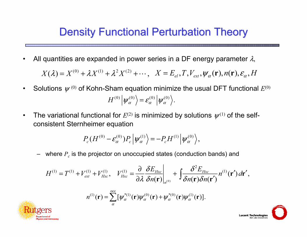
• All quantities are expanded in power series in a DF energy parameter l,

• Solutions y (0) of Kohn-Sham equation minimize the usual DFT functional E(0)

• The variational functional for E(2) is minimized by solutions y (1) of the self-consistent Sternheimer equation

– where Pc is the projector on unoccupied states (conduction bands) and

(0) (1) 2 (2)( ) ,X X X Xλ λ λ= + + + , , , ( ), ( ), ,el extX E T V n Hα αψ ε= r r

(0) (0) (0) (0) .H α α αψ ε ψ=

(0) (0) (1) (1) (0)( ) ,c c cP H P P Hα α αε ψ ψ− = −

(0)

2(1) (1) (1) (1) (1) (1), ( ) ,

( ) ( ) ( )Hxc Hxc

ext Hxc Hxcn

E EH T V V V n dn n n

δ δλ δ δ δ∂ ′ ′= + + = +

′∂ ∫ r rr r r

occ(1) *(1) (0) *(0) (1)( ) [ ( ) ( ) ( ) ( )].n α α α α

αψ ψ ψ ψ= +∑r r r r r

DFPT, continuedDFPT, continued

• Sternheimer equation for y (1) is solved using same techniques as ground-state Kohn-Sham equation– Residuals minimized by conjugate-gradient method– Solutions constrained to be orthogonal to occupied states– No normalization; inhomogeneous term determines amplitude

• First-order potential converged by conjugate-gradient or mixing methods

• Iterative steps for potential and wave functions alternate– Wave functions never “start from scratch”– Accurate wave-function convergence is never “wasted” on a poorly

converged potential• Variational 2nd-order energy decreases with y (1), V(1) convergence

(1)HxcV

(1) (0) (0) (

(1) (1) (1) (1) (1) (1) (0)

(0) (1)

(

(1) (1) (1) (1

(2)

0) (2) (2) (2)

) (1

(0 0) (0) (1))

(

(

)

1);

loc non loc Ha

loc non loc

Har loc n

r xc

loc non loc Har xc

on loc

occ

el

T V V V V

T V V

T VE

V V

T V V

Vα

α

α α

α

α α

α

α

α

ψ ψ

ψ ε ψ

ψ

ψ

ψ ψ

ψ

ψ

−

−

−

+ −

+ + + +

+ + + +

+ + −

+ +

=

+

+

+

∑

(0) (0)

0)

2 2 2

2 2 2

1 1 12 2 2

Har xc Ion Ion

n n

d E d E d Ed d dλ λ λ

−

+ + +

Variational Variational 2DTE expression for strain2DTE expression for strain

12 13 14

7 4 10 5 6

1 3 9 2

11 15 16, 17

• Numbered breakdown of components as in Abinit output

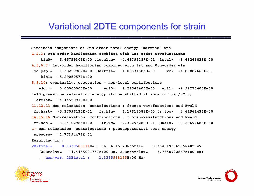
Variational Variational 2DTE components for strain2DTE components for strain

Seventeen components of 2nd-order total energy (hartree) are

1,2,3: 0th-order hamiltonian combined with 1st-order wavefunctions

kin0= 5.45759309E+00 eigvalue= -4.64795287E-01 local= -3.43266023E+00

4,5,6,7: 1st-order hamiltonian combined with 1st and 0th-order wfs

loc psp = 1.38229987E+00 Hartree= 1.08631683E+00 xc= -4.86887660E-01

kin1= -5.29050571E+00

8,9,10: eventually, occupation + non-local contributions

edocc= 0.00000000E+00 enl0= 2.22543400E+00 enl1= -4.92230408E+00

1-10 gives the relaxation energy (to be shifted if some occ is /=2.0)

erelax= -4.44550918E+00

11,12,13 Non-relaxation contributions : frozen-wavefunctions and Ewald

fr.hart= -5.37096135E-01 fr.kin= 4.17616081E+00 fr.loc= 2.61961436E+00

14,15,16 Non-relaxation contributions : frozen-wavefunctions and Ewald

fr.nonl= 3.24102985E+00 fr.xc= -2.30295282E-01 Ewald= -3.20692684E+00

17 Non-relaxation contributions : pseudopotential core energy

pspcore= -2.77394479E-01

Resulting in :

2DEtotal= 0.1339583111E+01 Ha. Also 2DEtotal= 0.364519096295E+02 eV

(2DErelax= -4.4455091757E+00 Ha. 2DEnonrelax= 5.7850922867E+00 Ha)

( non-var. 2DEtotal : 1.3395938195E+00 Ha)

Derivatives for elastic and piezoelectric tensorsDerivatives for elastic and piezoelectric tensors

• Calculating mixed 2nd derivatives of the energy wrt pairs of perturbations – By the “2n+1” theorem, these only require one set of 1st order wave functions,

– This expression is non-stationary (i.e., 1st-order in convergence errors)

• We need combinations of strain , electric field and atomic coordinate derivatives (some for atomic relaxation corrections).

– Clamped-atom elastic tensor ------------

– Internal strain tensor -----------------------

– Interatomic force constants (q=0) -------

– Clamped-atom piezoelectric tensor ----

– Born effective charges ---------------------

2

2

2

2

2

el

el j

el i j

el j

el i j

E

E

E

E

E

αβ γδ

αβ κ

κ κ

αβ

κ

η η

η τ

τ τ

η

τ

′

∂ ∂ ∂

∂ ∂ ∂

′∂ ∂ ∂

∂ ∂ ∂

∂ ∂ ∂

E

E

jEαβηiκτ

Non-self-consistent

1 2 2 1 1 1

1 21 2

(0)

occ( ) ( ) ( ) ( ) ( ) (0)

0

2occ( )( )(0) (0)

1 2

( )

1( ) ,2

el ext Hxc

Hxcext

n

E T V V

ET V

λ λ λ λ λ λα α

α

λ λλ λα α

α

ψ ψ

ψ ψλ λ

= + +

∂+ + +∂ ∂

∑

∑

Mixed derivative evaluationMixed derivative evaluation

• For strain – reduced atomic coordinate derivatives– Use 1st-order strain wave functions

– Use 1st-order reduced-atomic-coordinate Hamiltonian

– Calculate non-variational terms (explicit 2nd derivatives with and ) within the same framework as the strain-strain 2nd derivatives

– All terms enter (kinetic, local psp, nonlocal psp, hartree, xc, and ion-ion)

• For strain – electric field derivatives– Special, simpler non-stationary expression can be derived

– are 1st-order wave functions for the perturbation which enters. through the modern theory of polarization.(1)

– There are no explicit 2nd-derivative terms.

( )αβηαψ

( )iH κτ

(0)αψ (0)n

2 occ( ) ( )

3BZ

2 ,(2 )

jkelm m

mj

E i dαβη

αβ

ψ ψπη

∂ Ω=∂ ∂ ∑∫ k k kE

( )jkmψ k / k∂ ∂

(1) R. D. King-Smith and D. Vanderbilt, Phys. Rev. B 47,1651 (1993)

DFPT modifications for metalsDFPT modifications for metals

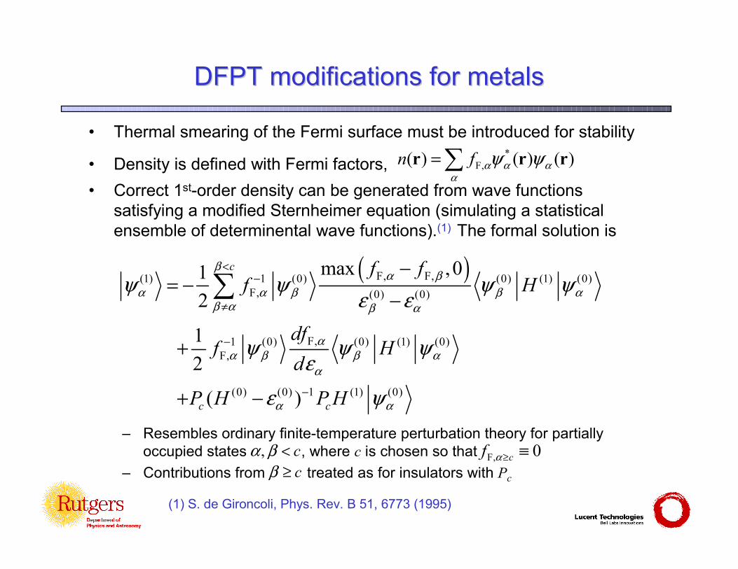
• Thermal smearing of the Fermi surface must be introduced for stability

• Density is defined with Fermi factors,• Correct 1st-order density can be generated from wave functions

satisfying a modified Sternheimer equation (simulating a statistical ensemble of determinental wave functions).(1) The formal solution is

– Resembles ordinary finite-temperature perturbation theory for partially occupied states , where c is chosen so that

– Contributions from treated as for insulators with Pc

(1) S. de Gironcoli, Phys. Rev. B 51, 6773 (1995)

*F,( ) ( ) ( )n f α α α

αψ ψ=∑r r r

( )F, F,(1) 1 (0) (0) (1) (0)F, (0) (0)

F,1 (0) (0) (1) (0)F,

(0) (0) 1 (1) (0)

max ,012

12

( )

c

c c

f ff H

dff H

d

P H P H

βα β

α α β β αβ α β α

αα β β α

α

α α

ψ ψ ψ ψε ε

ψ ψ ψε

ε ψ

<−

≠

−

−

−= −

−

+

+ −

∑

, cα β < F, 0cf α≥ ≡cβ ≥

Strain perturbation for metalsStrain perturbation for metals

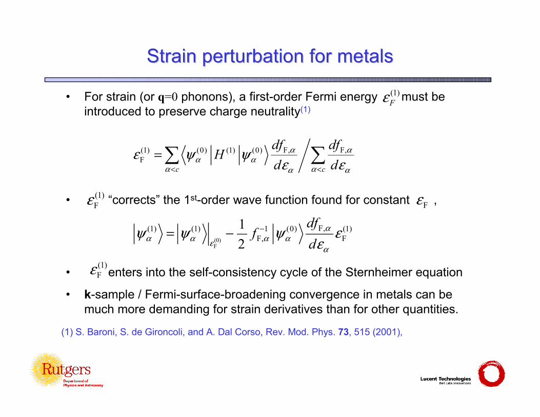
• For strain (or q=0 phonons), a first-order Fermi energy must be introduced to preserve charge neutrality(1)

• “corrects” the 1st-order wave function found for constant ,

• enters into the self-consistency cycle of the Sternheimer equation

• k-sample / Fermi-surface-broadening convergence in metals can be much more demanding for strain derivatives than for other quantities.

(1)Fε

(1) S. Baroni, S. de Gironcoli, and A. Dal Corso, Rev. Mod. Phys. 73, 515 (2001),

F, F,(1) (0) (1) (0)F

c c

df dfH

d dα α

α αα αα α

ε ψ ψε ε< <

=∑ ∑

(1)Fε Fε

(1)Fε

(0)F

F,(1) (1) 1 (0) (1)F, F

12

dff

dα

α α α αεα

ψ ψ ψ εε

−= −

Kinetic energy cutoff “smoothing”Kinetic energy cutoff “smoothing”

• Existing Abinit strategy to smooth energy dependence on lattice parameters in GS calculations

– Forces wave function coefficients smoothly to zero at cutoff sphere.

• RF strain derivative calculations do accurately reproduce GS numerical derivatives with non-zero ecutsm

• Divergence can produce large shifts in elastic tensor if calculation is not well converged with respect to ecut

– Remember, we take two derivatives

– Cutoff function was improved when strain was introduced

0 1 2 3 4 5 6 7 8

0

20

40

60

80

100

Without

With ecutsm

ecut = 25ecutsm = 5

Kin

etic

ene

rgy

(Har

tree)

K (aB-1)

∞

XC nonXC non--linear core correctionlinear core correction

• On the reduced real-space grid, electron charge depends only on

• Model core charge has a detailed dependence on– Resulting energy derivatives are rather complicated functions.

• Core charges must be extremely smooth functions to avoid convergence errors

– Reason: Strain and atomic position derivatives of the xc self-interaction of a single core don’t cancel point-by-point on the grid, but only in the integral

– 1st and 2nd derivatives of the core model enter these expressions

• Generalized gradient functionals have been implemented for strain as of release 4.4, and are probably even more demanding

1−Ω

ijΞ

Nonlocal pseudopotentialsNonlocal pseudopotentials in in AbinitAbinit

• Most mathematically complex objects for strain derivatives• Reduced-wave-vector matrix elements have the form

2

2

1| | ( )

( , , ) ( )

ij

ij ij i

iNL i j

ij

ii j i j i j i j

ij ij ij ijj ij

V e f K K

K K K K K K e f K K

κ

κ

πκ

κ

πκ

′⋅

− ⋅

′ ′ ′⟨ ⟩ = ×ϒΩ

ϒ ϒ ϒ ϒ′ ′ ′℘

∑ ∑

∑ ∑ ∑ ∑

K τ

K τ

K K

– modified Legendre polynomials, psp form factors, reduced atom coordinates

– All arguments are dot products expressed with metric tensors

• Psp’s act on wave functions by summing wave function coefficients times a set of tensor products of reduced components (~ ).

• Code for the 1st and 2nd strain derivatives was created using Mathematica. (If you can’t sleep, read cont*str*.F90, metstr.F90.)

• Despite this complexity, the computational cost of psp derivatives acting on wf’s is comparable to that of the psp’s themselves.

℘ fκ κτ

K mY

Response function code organizationResponse function code organizationabinitdriverrespfn

*.in*_WFK

eltfr*dyfr*

ipert1,idir1ipert2,idir2

loper3 ipert1,idir1

scfcv3 istep

vtorho3vtowfk3cgwf3

ikptiband

converged?

done?

*_1WF

d2sym3,gath3,dyout3 *_DDB

nstwf*, nselt3, nstdy3 ipert2, idir2

end

(2)0 0H

(1)1 0H′

(1) 0HKSternheimer Eq.,

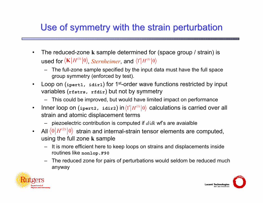
Use of symmetry with the strain perturbationUse of symmetry with the strain perturbation

• The reduced-zone k sample determined for (space group / strain) is used for , Sternheimer, and

– The full-zone sample specified by the input data must have the full spacegroup symmetry (enforced by test).

• Loop on (ipert1, idir1) for 1st-order wave functions restricted by input variables (rfstrs, rfdir) but not by symmetry

– This could be improved, but would have limited impact on performance• Inner loop on (ipert2, idir2) in calculations is carried over all

strain and atomic displacement terms– piezoelectric contribution is computed if d/dk wf’s are avaialble

• All strain and internal-strain tensor elements are computed, using the full zone k sample

– It is more efficient here to keep loops on strains and displacements inside routines like nonlop.F90

– The reduced zone for pairs of perturbations would seldom be reduced much anyway

(1) 0HK (1)1 0H′

(1)1 0H′

(2)0 0H

Verification using numerical derivatives Verification using numerical derivatives -- caveatscaveats

• RF 2nd strain derivatives do not correspond to strain derivatives of stress

– As of release 4.5, anaddb will calculate this correction to give the conventional elastic tensor in the presence of stress.

– DDB file from GS calculation must be merged with RF DDB file for this

• The strain derivatives of the polarization give the “improper” piezoelectric tensor. Abinit and anaddb (and correctly-performed experiments) give the “proper” tensor.(1)

2* *

, ,1 1, ,el elE EC C Cγδ

αβ γδ αβ γδ αβγδ αβ γδαβ γδ αβ αβ γδ

σδ σ

η η η η η∂∂ ∂∂≡ ≡ = = −

Ω ∂ ∂ ∂ ∂ Ω ∂

Proper,dPe e e P Pd

ααβγ αβγ αβγ βγ α αβ γ

βγ

δ δη

= = + −

(1) D. Vanderbilt, J. Phys. Chem. Solids 61, 147 (2000)

Comparisons with numerical derivativesComparisons with numerical derivatives

• Zinc-blende AlP with random distortions so all tensor elements are non-zero.– Ground state calculations of stress and polarization with clamped atomic coordinates– Finite-difference d/dk for best consistency with polarization calculations– 5-point numerical derivatives with strain increment 2X10-5

• RMS Errors 5.4X10-6 (ELT) and 2.0X10-8 (PZT)

Elastic Tensor (GPa)Numerical DFPT Diff

x xx 2.0211410 2.0211400 -8.7E-07y xx 5.2336140 5.2336120 -1.8E-06z xx 0.4003179 0.4003186 6.7E-07

x yy -8.2697310 -8.2697310 3.0E-08y yy 0.2471218 0.2471215 -3.3E-07z yy 0.7383708 0.7383704 -4.3E-07

x yz -69.2631000 -69.2631000 -3.6E-06y yz -0.1423518 -0.1423530 -1.2E-06z yz -1.3531730 -1.3531760 -2.9E-06

Numerical DFPT Diffxx xx 124.999900 124.999900 2.4E-05yy xx 66.990360 66.990360 -3.9E-06zz xx 68.396840 68.396840 -1.5E-06yz xx 0.088373 0.088374 1.1E-07xz xx -1.117333 -1.117333 -4.3E-07xy xx -0.418922 -0.418922 5.7E-08

xx yz 0.088374 0.088374 -6.6E-07yy yz 5.154470 5.154469 -1.0E-06zz yz -5.578270 -5.578270 -2.9E-07yz yz 90.315730 90.315730 4.5E-06xz yz -0.404749 -0.404749 5.0E-08xy yz 0.644728 0.644728 6.4E-08

Piezoelectric Tensor (C/m2 x 10-2)

αψ (1)'s

Incorporating atomic relaxationIncorporating atomic relaxation

• “Homogeneous strain” produced experimentally is only macroscopically homogeneous.

• For all but the simplest structures, strain will change the reduced atomic coordinates, not just the metric tensors.

– Diamond, for example, has relaxation corrections.

• Atomic relaxation makes modest changes the the elastic constants for “normal” solids, huge changes for special cases (eg., molecular solids)

• There are large relaxation changes in the piezoelectric constants for most piezoelectric materials.

• For all but very simple cases, accurate results by numerical differentiation incorporating GS relaxation are completely impractical.

– Atomic forces generated by incremental strains are too small.

Analytic treatment of atomic relaxationAnalytic treatment of atomic relaxation

• Introduce a model energy function quadratic in atomic displacements from a reference configuration, strain , and electric field

• Various terms, all “bare” or clamped-atom quantities with atom indices m,n and Cartesian components are as follows:

( )/ / / /

( , , ) //

T

T T

H ee

− Ω Ω − Ω − Ω = + − Ω − − − Ω

F K Λ Z uu η u η σ Λ C η

P Z χE E

E

αEαβηmu α

,

,

m

m n

m

F

PK

α

αβ

α

α γ

α γδ

σ

Λ

,

,

,

,

m

CZe

αβ γδ

α γ

α γδ

α γχ

, , ,α β γ

Atomic forces

Stress

Electric polarization

Interatomic force constants

“Force” internal strain tensor

Elastic tensor

Born effective charges

Piezoelectric tensor

Dielectric susceptibility

Atomic relaxation, continuedAtomic relaxation, continued

• The “relaxed atom” model energy function is defined as

– Additionally assume that in the reference configuration• Strain and electric field 2nd derivatives of then yield the

“dressed” or relaxed-atom elastic and piezoelectric tensors

– is the pseudo-inverse of the interatomic force constant matrix (zero eigenvalues suppressed).

natom 31 1

, , , , ,1 1

( )mi mi nj njmn ij

e e K Zαβ γ αβ γ αβ γ− −

= =

= +Ω Λ∑ ∑

0mF α =H

1K −

natom 31 1

, , , , ,1 1

( )mi mi nj njmn ij

C C Kαβ γδ αβ γδ αβ γδ− −

= =

= +Ω Λ Λ∑ ∑

( ) ( ), min , ,m

muH H u

ααβ α α αβ αη η=E E

Implementation of atomic relaxationImplementation of atomic relaxation

• Incorporated in anaddb program to be used as a post-processor of abinit results– All the needed second derivatives must be present in the DDB file

from the RF run (or merged from several runs).– Results are converted to conventional units rather than atomic or

reduced units.

• Various other tensors corresponding to differing boundary conditions such as fixed or zero polarization or stress, etc. can be calculated using the same approach.– See reference 3 in the bibliography.– See notes on the input variables elaflag, instrflag, and

piezoflag in the anaddb help file.– The dielectric tensor is also needed for some of these calculations.

Relaxed results compared to numerical derivativesRelaxed results compared to numerical derivatives

• Zinc-blende AlP with random distortions so all tensor elements are non-zero.– Ground state calculations of stress and polarization with exquisitely relaxed atomic

coordinates (but unrelaxed stress)– Sample of complete set of tensor elements

• RMS Errors 4.0X10-5 (ELT) and 1.7X10-6 (PZT)– 1-2 orders of magnitude larger than for clamped-atom quantities.

Elastic Tensor (GPa) Piezoelectric Tensor (C/m2 x 10-2)Numerical DFPT Diff

x xx 1.714769 1.714694 -7.5E-05y xx 5.107069 5.107080 1.1E-05z xx -0.883962 -0.883676 2.9E-04

x yy 0.828569 0.828454 -1.2E-04y yy 3.716843 3.716812 -3.2E-05z yy -0.810201 -0.810176 2.5E-05

x yz -3.871980 -3.872154 -1.7E-04y yz -1.245173 -1.245206 -3.3E-05z yz 1.902687 1.902693 5.6E-06

Numerical DFPT Diffxx xx 124.991500 124.991500 -1.1E-05yy xx 66.999750 66.999760 8.2E-06zz xx 68.359440 68.359440 7.0E-07yz xx 0.228447 0.228466 1.9E-05xz xx -1.139838 -1.139828 9.6E-06xy xx -0.015028 -0.015117 -9.0E-05

xx yz 0.228471 0.228466 -4.4E-06yy yz 1.940050 1.940054 3.7E-06zz yz -2.079264 -2.079275 -1.1E-05yz yz 66.593340 66.593390 5.2E-05xz yz 0.773972 0.773977 5.1E-06xy yz -0.568446 -0.568449 -3.2E-06

BibliographyBibliography

1. “Metric tensor formulation of strain in density-functional perturbation theory,” D. R. Hamann, X. Wu, K. M. Rabe, and D. Vanderbilt, Phys. Rev. B 71, 035117 (2005).

2. “Generalized-gradient-functional treatment of strain in density-functional perturbation theory,” D. R. Hamann, K. M. Rabe, and D. Vanderbilt, Phys. Rev. B 72, 033102 (2005).

3. “Systematic treatment of displacements, strains, and electric fields in density-functional perturbation theory,” X. Wu, D. Vanderbilt, and D. R. Hamann, Phys. Rev. B 72, 035105 (2005).

Mat-SimResearch