Embed Size (px)
Citation preview

EKC314: TRANSPORT PHENOMENACore Course for
B.Eng.(Chemical Engineering)Semester II (2008/2009)
Dr. Mohamad Hekarl [email protected]
School of Chemical Engineering
Engineering Campus, Universiti Sains Malaysia
Seri Ampangan, 14300 Nibong Tebal
Seberang Perai Selatan
Penang. EKC314-SCE – p. 1/54

Syllabus
1. Introduction and Concepts
2. Momentum Transport
Viscosity and and mechanism of momentumtransport
Newtonian and non-newtonian fluidsFlux and gradients
Velocity distribution in in laminar and turbulent flows
Boundary layer
Velocity distribution with more than oneindependent variables
EKC314-SCE – p. 2/54

Syllabus
3. Equation of changes in Isothermal Systems;
Interphase transport in isothermal system.
Macroscopic balances for isothermal systems.
EKC314-SCE – p. 3/54

Introduction and Concepts
What are Transport Phenomena?1. Fluid dynamics2. Heat transfer3. Mass transfer
They should be studied together since:1. they occur simultaneously2. basic equations that described the 3 transport
phenomena are closely related3. mathematical tools required are very similar4. molecular mechanisms underlying various transport
phenomena are very closely related
EKC314-SCE – p. 4/54

Introduction and Concepts
Macroscopic level
Microscopic level
Molecular level
Write down balance equation; macroscopic balances.
Equations should describe; mass, momentum, energy and angular momentum within the system.
No need to understand the details of the system.
Examination of the fluid mixture in a small region within the equipment.
Can write down the equation of change that describe mass, momentum, energy and angular momentum change within the small region
Aim is to get information about velocity, temperature, pressure and concentration profile within the system.
To seek a fundamental understanding of the mechanism of mass, momentum, energy and angular momentum in terms of molecular structure and intermolecular forces
Involve some theoretical physics and physical chemistry work EKC314-SCE – p. 5/54
Introduction and Concepts
Mixture of gases
Macroscopic
Microscopic
Molecular
Heat added to the system
EKC314-SCE – p. 6/54
Introduction and Concepts
The flow of fluid are studied in 3 different parts whichconsist of:
flow of pure fluids at constant temperature-withemphasis on viscous and convective momentumtransport
flow of pure fluids with varying temperature-withemphasis on conductive, convective and radiativeenergy transport
flow of fluid mixtures with varying composition-withemphasis on diffusive and convective mass transport
EKC314-SCE – p. 7/54
Introduction and Concepts
Conservation Laws (mass):
Consider two colliding diatomic molecules (N2 and O2).
The conservation of mass can be written as;
mN + mO = m′
N + m′
O
for a system with no chemical reaction;
mN = m′
N
andmO = m
′
O
EKC314-SCE – p. 8/54

Introduction and Concepts
Conservation Laws (momentum):
According to the law of conservation of momentum, thesum of the momenta of all atoms before collision mustequal that after the collision.
The conservation of momentum can be written as;
mN1rN1
+ mN2rN2
+ mO1rO1
+ mO2rO2
= m′
N1r′N1
+ m′
N2r′N2
+ m′
O1r′O1
+ m′
O2r′O2
EKC314-SCE – p. 9/54
Introduction and Concepts
Conservation Laws (momentum):
rN1is the position vector for atom 1 of molecule N and
rN1is its velocity.
It can be written as;
rN1= rN + RN1
rN1is the sum of the position vector for the centre of
mass and the position vector of the atom w.r.t thecentre of mass.
EKC314-SCE – p. 10/54

Introduction and Concepts
Conservation Laws (momentum):
Also RN2= −RN1
Then the conservation equation can be simplified as;
mN rN + mOrO = mN r′N + mOr′O
EKC314-SCE – p. 11/54
Introduction and Concepts
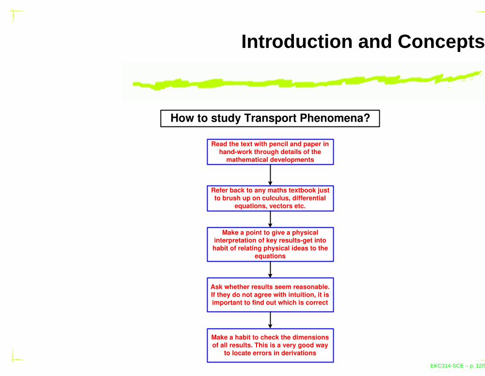
How to study Transport Phenomena?
Read the text with pencil and paper in hand-work through details of the
mathematical developments
Refer back to any maths textbook just to brush up on culculus, differential
equations, vectors etc.
Make a point to give a physical interpretation of key results-get into habit of relating physical ideas to the
equations
Ask whether results seem reasonable. If they do not agree with intuition, it is important to find out which is correct
Make a habit to check the dimensions of all results. This is a very good way
to locate errors in derivations
EKC314-SCE – p. 12/54

Introduction and Concepts
Recap: Vector Calculus
If given a vector of a form;
a = [a1, a2, a3] = a1i + a2j + a3k
consists of the real vector space R3 with vector
addition defined as;
[a1, a2, a3] + [b1, b2, b3] = [a1 + b1, a2 + b2, a3 + b3]
and scalar multiplication defined by;
c[a1, a2, a3] = [ca1, ca2, ca3]
EKC314-SCE – p. 13/54

Introduction and Concepts
The dot product of two vectors is defined by;
a · b = |a||b|cosγ = a1b1 + a2b2 + a3b3
where γ is the angle between a and b. This gives thenorm or length |a| of a with a formula;
|a| =√
a · a =√
a21 + a2
2 + a33
If a · b = 0 therefore a and b orthogonal.
EKC314-SCE – p. 14/54

Introduction and Concepts
Example of a dot product is given by;
W = p · d
which is work done by a force p in a displacement d.
EKC314-SCE – p. 15/54
Introduction and Concepts
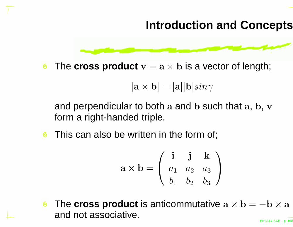
The cross product v = a × b is a vector of length;
|a × b| = |a||b|sinγ
and perpendicular to both a and b such that a, b, v
form a right-handed triple.
This can also be written in the form of;
a × b =
i j k
a1 a2 a3
b1 b2 b3
The cross product is anticommutative a× b = −b× a
and not associative.EKC314-SCE – p. 16/54

Introduction and Concepts
For a vector function given by
v(t) = [v1(t), v2(t), v3(t)] = v1(t)i + v2(t)j + v3(t)k
Then the derivative is;
v′ =dv
dt= lim
∆t→0
v(t + ∆t) − v(t)
∆t
therefore;
v′ = [v′
1, v′
2, v′
3] = v′
1i + v′
2j + v′
3k
EKC314-SCE – p. 17/54
Introduction and Concepts
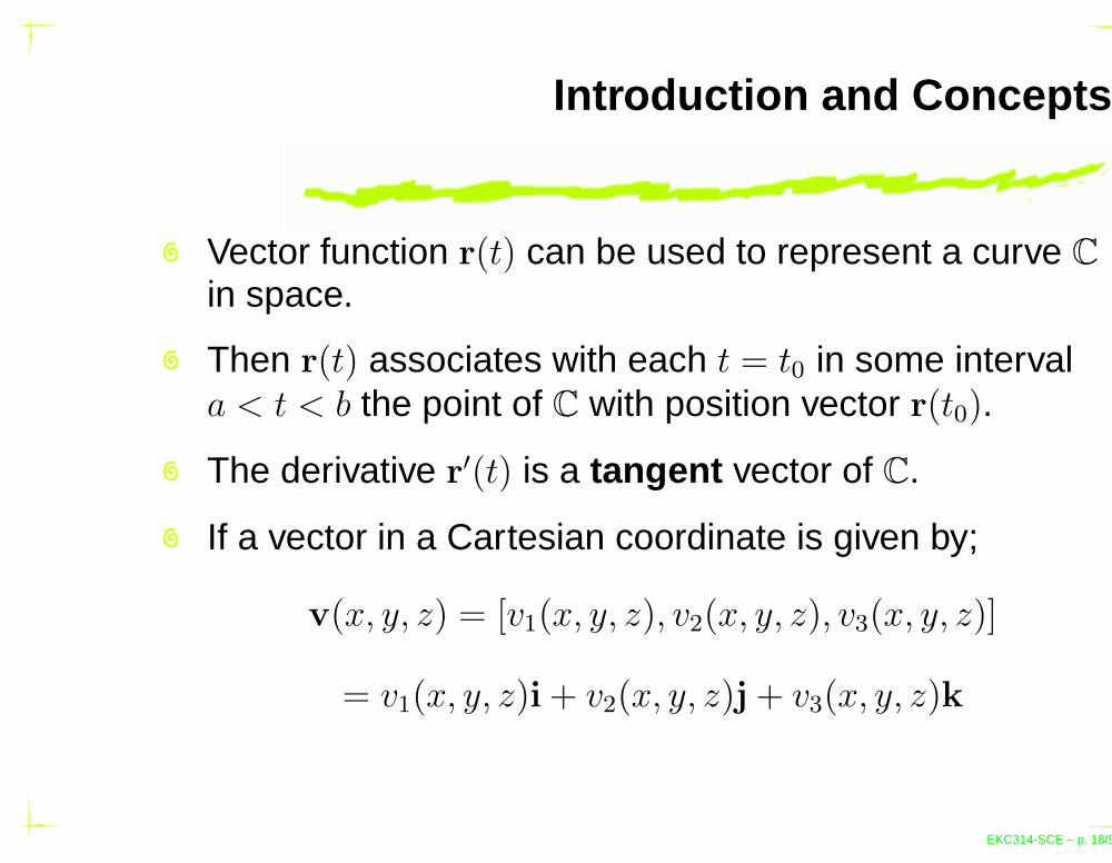
Vector function r(t) can be used to represent a curve C
in space.
Then r(t) associates with each t = t0 in some intervala < t < b the point of C with position vector r(t0).
The derivative r′(t) is a tangent vector of C.
If a vector in a Cartesian coordinate is given by;
v(x, y, z) = [v1(x, y, z), v2(x, y, z), v3(x, y, z)]
= v1(x, y, z)i + v2(x, y, z)j + v3(x, y, z)k
EKC314-SCE – p. 18/54
Introduction and Concepts
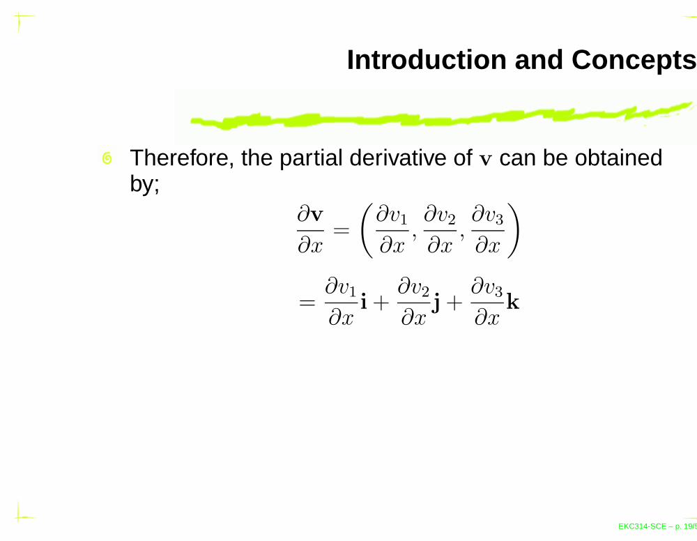
Therefore, the partial derivative of v can be obtainedby;
∂v
∂x=
(
∂v1
∂x,∂v2
∂x,∂v3
∂x
)
=∂v1
∂xi +
∂v2
∂xj +
∂v3
∂xk
EKC314-SCE – p. 19/54

Introduction and Concepts
Gradient of a function f can be written as;
grad f = ∇f =
[
∂f
∂x,∂f
∂y,∂f
∂z
]
Therefore, using the operation, the directionalderivative of f in a direction of a unit vector b can beobtained by;
Dbf =df
ds= b · ∇f
EKC314-SCE – p. 20/54

Introduction and Concepts
Divergence of a vector function v can be written as;
div v = ∇ · v =∂v1
∂x+
∂v2
∂y+
∂v3
∂z
And the curl of v is given as;
curl v = ∇× v =
i j k∂∂x
∂∂y
∂∂z
v1 v2 v3
EKC314-SCE – p. 21/54

Introduction and Concepts
Some basic formula for grad, div and curl;
Grad:∇(fg) = f∇g + g∇f
∇(f/g) = (1/g2)(g∇f − f∇g)
Div:div(fv) = fdiv v + v · ∇f
div(f∇g) = f∇2g + ∇f · ∇g
EKC314-SCE – p. 22/54
Introduction and Concepts
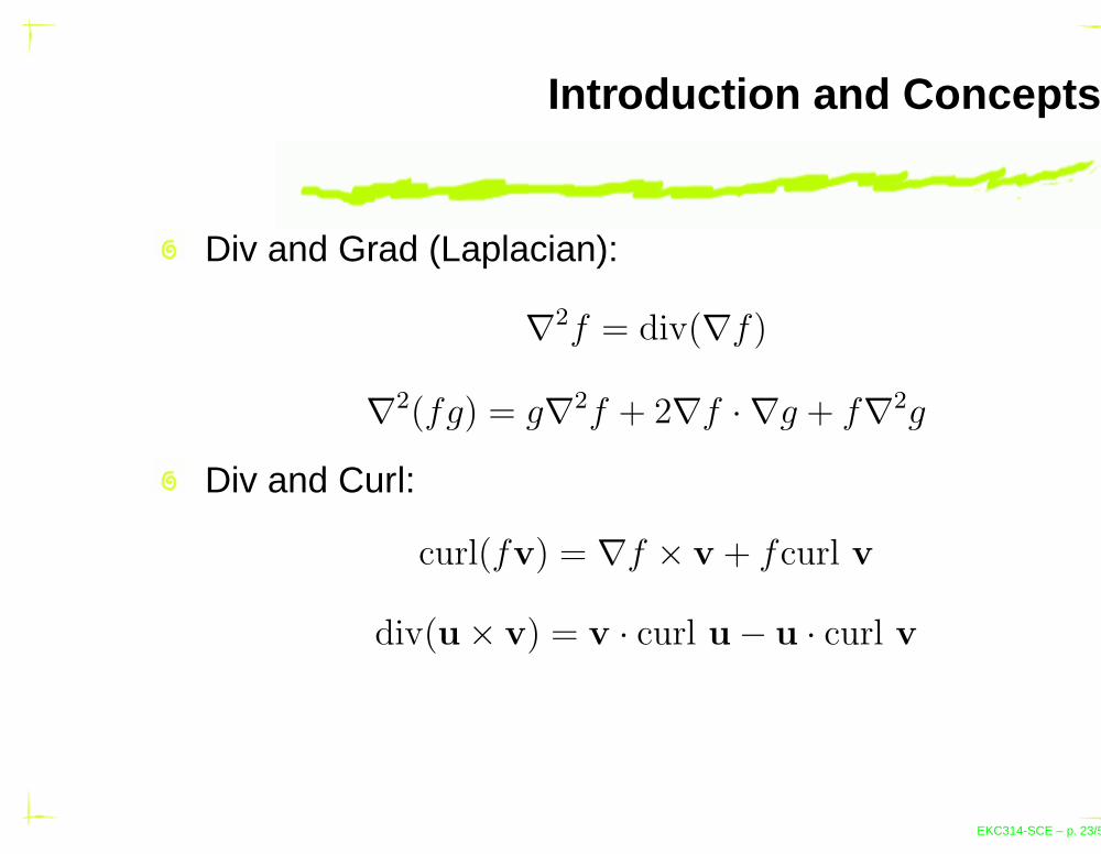
Div and Grad (Laplacian):
∇2f = div(∇f)
∇2(fg) = g∇2f + 2∇f · ∇g + f∇2g
Div and Curl:
curl(fv) = ∇f × v + fcurl v
div(u × v) = v · curl u − u · curl v
EKC314-SCE – p. 23/54

Introduction and Concepts
Extra:curl(∇f) = 0
div(curl v) = 0
EKC314-SCE – p. 24/54
Introduction and Concepts
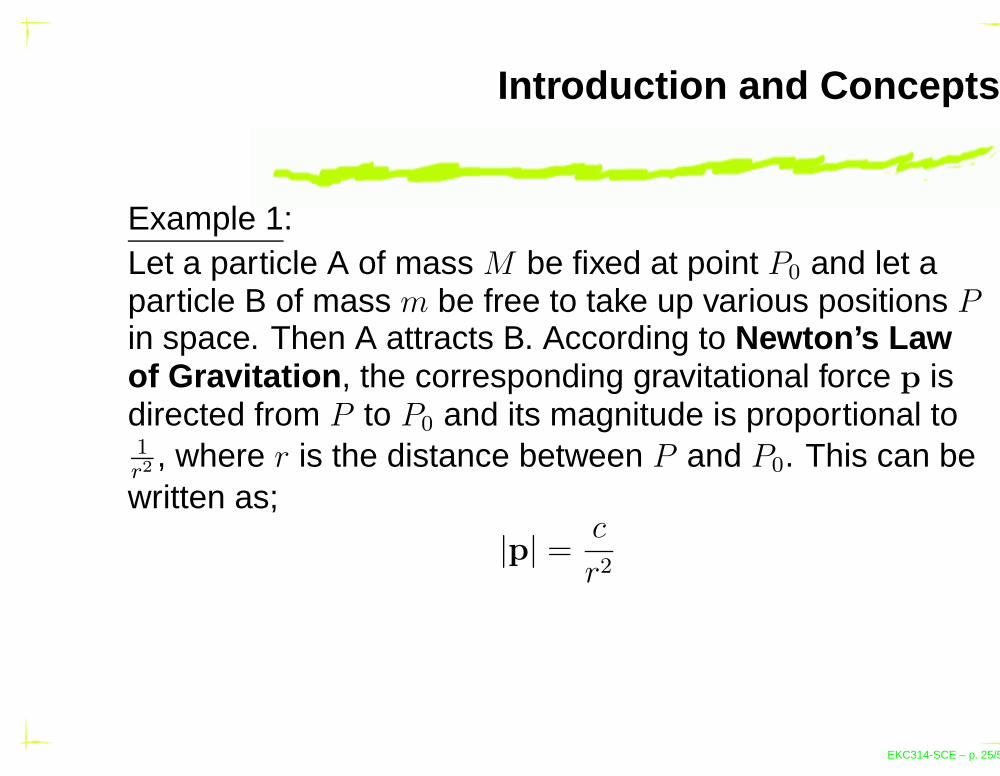
Example 1:Let a particle A of mass M be fixed at point P0 and let aparticle B of mass m be free to take up various positions Pin space. Then A attracts B. According to Newton’s Lawof Gravitation, the corresponding gravitational force p isdirected from P to P0 and its magnitude is proportional to1
r2 , where r is the distance between P and P0. This can bewritten as;
|p| =c
r2
EKC314-SCE – p. 25/54

Introduction and Concepts
Hence p defines a vector field in space. Using Cartesiancoordinates, such that P0(x0, y0, z0) and P (x, y, z), thereforethe distance r can be determined as;
r =√
(x − x0)2 + (y − y0)2 + (z − z0)2
For r > 0 in vector form;
r = [x − x0, y − y0, z − z0] = (x − x0)i + (y − y0)j + (z − z0)k
EKC314-SCE – p. 26/54

Introduction and Concepts
Therefore;|r| = r
and (−1/r)r is a unit vector in the direction of p. The minussign indicates that p is directed from P to P0. Thus,
p = |p|(
−1
rr
)
= − c
r3r = −c
x − x0
r3i − c
y − y0
r3j − c
z − z0
r3k
EKC314-SCE – p. 27/54
Introduction and Concepts
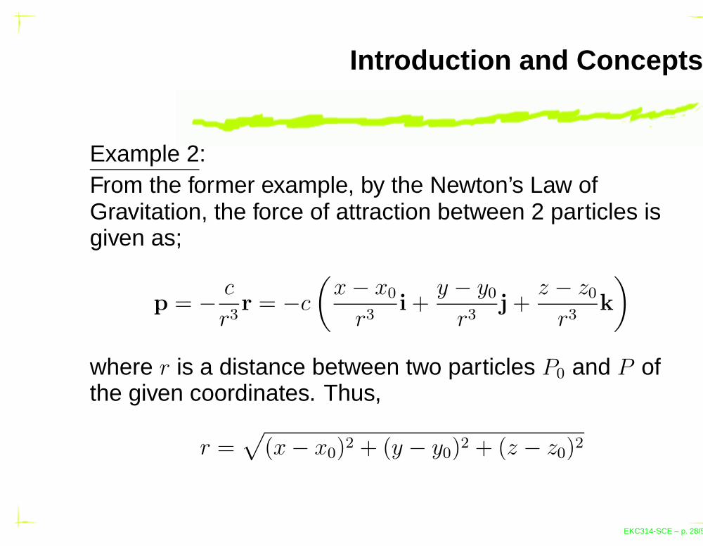
Example 2:From the former example, by the Newton’s Law ofGravitation, the force of attraction between 2 particles isgiven as;
p = − c
r3r = −c
(
x − x0
r3i +
y − y0
r3j +
z − z0
r3k
)
where r is a distance between two particles P0 and P ofthe given coordinates. Thus,
r =√
(x − x0)2 + (y − y0)2 + (z − z0)2
EKC314-SCE – p. 28/54
Introduction and Concepts
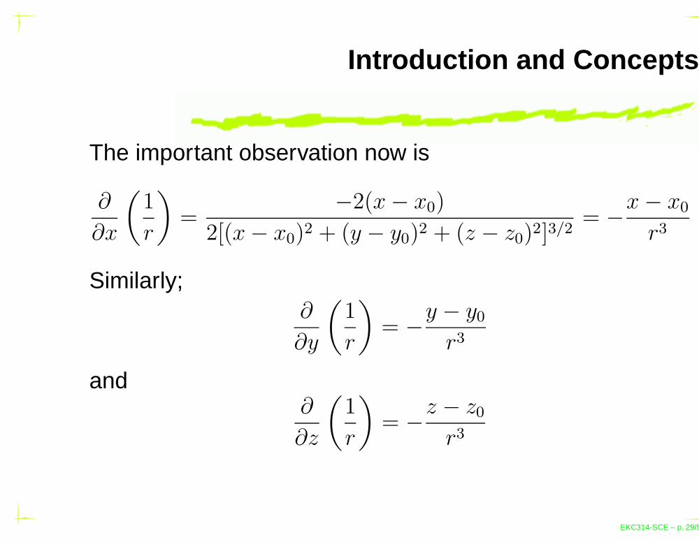
The important observation now is
∂
∂x
(
1
r
)
=−2(x − x0)
2[(x − x0)2 + (y − y0)2 + (z − z0)2]3/2= −x − x0
r3
Similarly;∂
∂y
(
1
r
)
= −y − y0
r3
and∂
∂z
(
1
r
)
= −z − z0
r3
EKC314-SCE – p. 29/54

Introduction and Concepts
From here, it is observed that p is the gradient of the scalarfunction;
f(x, y, z) =c
r
and f is a potential of that gravitational field. ApplyingLaplace Equation of the form;
∂2f
∂x2+
∂2f
∂y2+
∂2f
∂z2= 0
EKC314-SCE – p. 30/54
Introduction and Concepts
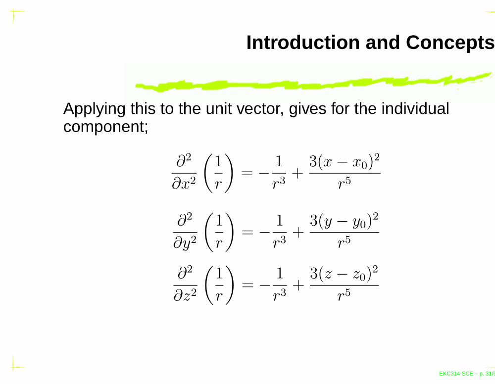
Applying this to the unit vector, gives for the individualcomponent;
∂2
∂x2
(
1
r
)
= − 1
r3+
3(x − x0)2
r5
∂2
∂y2
(
1
r
)
= − 1
r3+
3(y − y0)2
r5
∂2
∂z2
(
1
r
)
= − 1
r3+
3(z − z0)2
r5
EKC314-SCE – p. 31/54
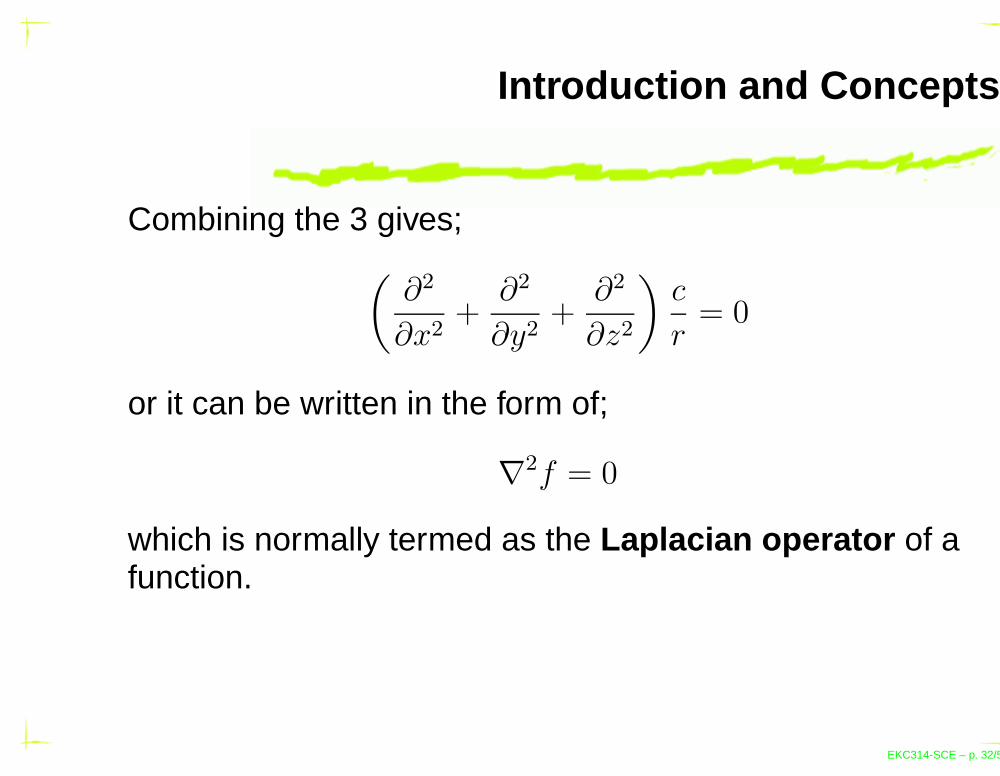
Introduction and Concepts
Combining the 3 gives;(
∂2
∂x2+
∂2
∂y2+
∂2
∂z2
)
c
r= 0
or it can be written in the form of;
∇2f = 0
which is normally termed as the Laplacian operator of afunction.
EKC314-SCE – p. 32/54
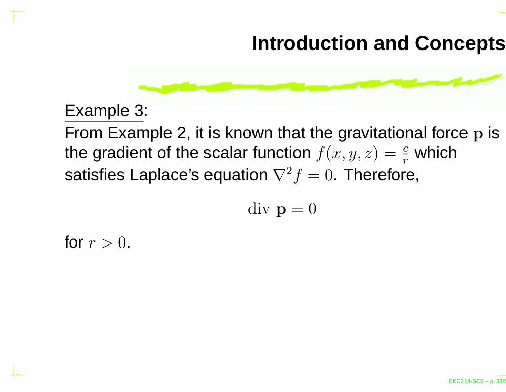
Introduction and Concepts
Example 3:From Example 2, it is known that the gravitational force p isthe gradient of the scalar function f(x, y, z) = c
rwhich
satisfies Laplace’s equation ∇2f = 0. Therefore,
div p = 0
for r > 0.
EKC314-SCE – p. 33/54

Introduction and Concepts
Example 4:Consider a motion of a fluid in a region R having nosources and sinks in R (no points at which the fluid isproduced or disappeared). Assuming that the fluid iscompressible and it flows through a small rectangular boxW of dimension ∆x, ∆y and ∆z with edges parallel to thecoordinate axes. W has a volume of ∆V = ∆x∆y∆z.Let v is the velocity vector of the form given by;
v = [v1, v2, v3] = v1i + v2j + v3k
EKC314-SCE – p. 34/54

Introduction and Concepts
Setting
u = ρv = [u1, u2, u3] = u1i + u2j + u3k
where ρ is the density of the fluid. Consider the flow of fluidout of the box W is through the left face whose area is∆x∆z and the components v1 and v3 are parallel to thatface and contribute nothing to that flow. Thus, the mass offluid entering through that face during a short time interval∆t is approx. given by;
(ρv2)y∆x∆z∆t = (u2)y∆x∆z∆t
EKC314-SCE – p. 35/54
Introduction and Concepts
And the mass of fluid leaving the opposite face of the boxW, during the same time interval is approx. given by;
(u2)y+∆y∆x∆z∆t
Therefore, the difference is in the form of;
∆u2∆x∆z∆t =∆u2
∆y∆V ∆t
where∆u2 = (u2)y+∆y − (u2)y
EKC314-SCE – p. 36/54
Introduction and Concepts
Two other pairs in x and z directions are taken andcombined in the form given by;
(
∆u1
∆x+
∆u2
∆y+
∆u3
∆z
)
∆V ∆t
The loss of mass in W is caused by the rate of change ofthe density and therefore equals to;
−∂ρ
∂t∆V ∆t
EKC314-SCE – p. 37/54

Introduction and Concepts
Equating both equations gives;(
∆u1
∆x+
∆u2
∆y+
∆u3
∆z
)
∆V ∆t = −∂ρ
∂t∆V ∆t
Diving the above equation by ∆V ∆t and let ∆x, ∆y, ∆zand ∆t approaching 0 leads to;
(
∂u1
∂x+
∂u2
∂y+
∂u3
∂z
)
= −∂ρ
∂t
EKC314-SCE – p. 38/54
Introduction and Concepts
Or in its simplified form;
div u = −∂ρ
∂t
or
div(ρv) = −∂ρ
∂t
which consequently becomes;
∂ρ
∂t+ div(ρv) = 0
which is the condition for the conservation of mass orthe continuity equation of a compressible fluid flow!
EKC314-SCE – p. 39/54
Introduction and Concepts
If the flow is steady, or it is independent of time, thus;
∂ρ
∂t= 0
and therefore the continuity equation reduces into
div(ρv) = 0
If the density ρ is constant, which means the fluid isincompressible, therefore the continuity equation becomes;
div v = 0
EKC314-SCE – p. 40/54
Viscosity and the Mechanisms ofMomentum Transport
Consider a parallel plates with area A separated bydistance Y with a type of fluid;
The system is initially at rest
At time t = 0, the lower plate is set in motion in thepositive x direction at a constant velocity V .
As time proceeds, the fluid gains momentum and thelinear steady-state velocity is established.
At steady motion, a constant force, F is required tomaintain the motion of the lower plate and this can beexpressed as;
F
A= µ
V
YEKC314-SCE – p. 41/54

Viscosity and the Mechanisms ofMomentum Transport
Y
V
x
y vx(y)
vx(y,t)
t < 0
t = 0
Small t
Large t
Fluid initially at rest
Lower plate set in motion
Velocity build up in unsteady flow
Final velocity distribution in steady flow
V
V
EKC314-SCE – p. 42/54
Viscosity and the Mechanisms ofMomentum Transport
Consider a parallel plates with area A separated bydistance Y with a type of fluid;
Force in the direction of x perpendicular to the ydirection given by F/A is replaced by τyx.
The term V/Y is replaced by −dvx/dy and thereforethe equation becomes;
τyx = −µdvx
dy
This means that the shearing force per unit area isproportional to the negative of the velocity gradient i.e.Newton’s Law of Viscosity.
EKC314-SCE – p. 43/54
Viscosity and the Mechanisms ofMomentum Transport
Similarly, let the angle between the fixed plate and themoving boundary δγ and the distance from the origin isδx.
Therefore,
tan δγ =δx
Y
for a very small angle,
δx
Y= δγ
EKC314-SCE – p. 44/54
Viscosity and the Mechanisms ofMomentum Transport
Butδx = V δt
thus,
δγ =V δt
Y
Taking limit on on the above terms;
limδt→0
δγ
δt=
V
Y=
dv
dy
EKC314-SCE – p. 45/54
Viscosity and the Mechanisms ofMomentum Transport
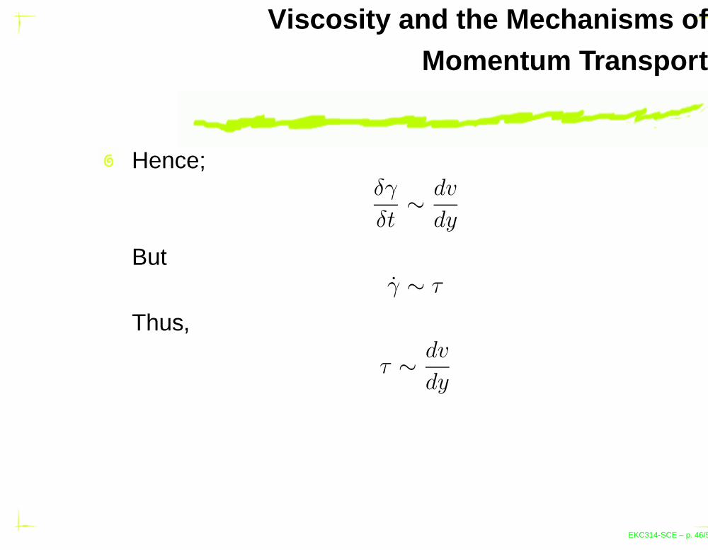
Hence;δγ
δt∼ dv
dy
Butγ ∼ τ
Thus,
τ ∼ dv
dy
EKC314-SCE – p. 46/54

Viscosity and the Mechanisms ofMomentum Transport
Which then becomes
τ = −µdv
dy
with µ as the proportionality constant.
The minus sign represents the force exerted by thefluid of the lesser Y on the fluid of greater Y.
EKC314-SCE – p. 47/54

Viscosity and the Mechanisms ofMomentum Transport
Shear thinning
Newtonian
Shear thickening
τ
dγ/dt
EKC314-SCE – p. 48/54

Viscosity and the Mechanisms ofMomentum Transport
Generalisation of Newton’s Law of Viscosity.
Consider a fluid moving in 3-dimensional space withrespect to time t.
Therefore, the velocity components are given asfollows;
vx = vx(x, y, z, t) vy = vy(x, y, z, t) vz = vz(x, y, z, t)
In the given situation, there will be 9 stresscomponents, τij.
EKC314-SCE – p. 49/54
Viscosity and the Mechanisms ofMomentum Transport
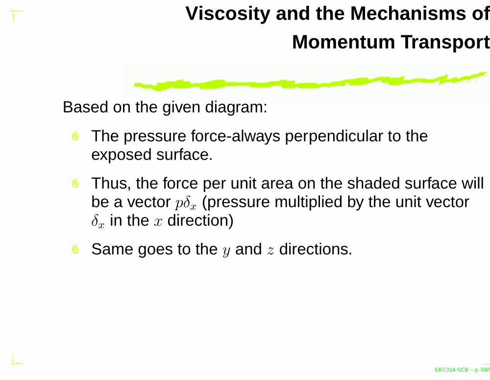
Based on the given diagram:
The pressure force-always perpendicular to theexposed surface.
Thus, the force per unit area on the shaded surface willbe a vector pδx (pressure multiplied by the unit vectorδx in the x direction)
Same goes to the y and z directions.
EKC314-SCE – p. 50/54

Viscosity and the Mechanisms ofMomentum Transport
The velocity gradients within the fluid are neitherperpendicular to the surface element nor parallel to it,but rather at some angle to the surface.
The force per unit area, τx exerted on the shaded areawith components (τxx, τxy and τxz).
This can be conveniently represented by standardsymbols which include both types of stresses(pressure and viscous stresses);
πij = pδij + τij
where i and j may be x, y or z.
EKC314-SCE – p. 51/54
Viscosity and the Mechanisms ofMomentum Transport
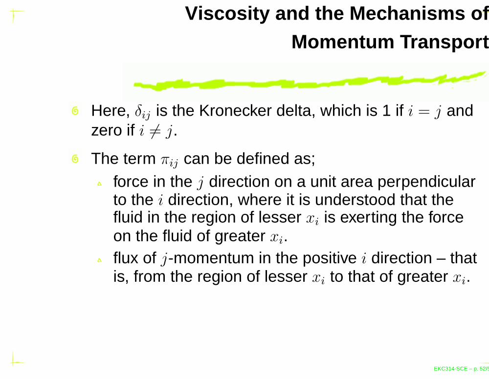
Here, δij is the Kronecker delta, which is 1 if i = j andzero if i 6= j.
The term πij can be defined as;force in the j direction on a unit area perpendicularto the i direction, where it is understood that thefluid in the region of lesser xi is exerting the forceon the fluid of greater xi.flux of j-momentum in the positive i direction – thatis, from the region of lesser xi to that of greater xi.
EKC314-SCE – p. 52/54
Viscosity and the Mechanisms ofMomentum Transport
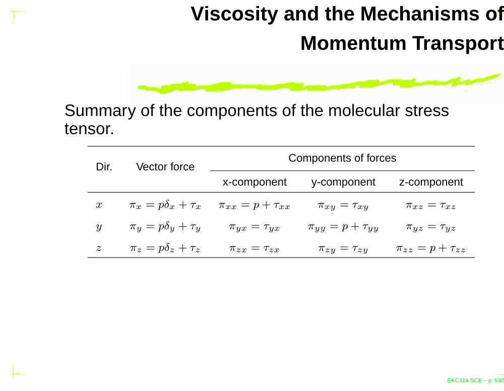
Summary of the components of the molecular stresstensor.
Dir. Vector forceComponents of forces
x-component y-component z-component
x πx = pδx + τx πxx = p + τxx πxy = τxy πxz = τxz
y πy = pδy + τy πyx = τyx πyy = p + τyy πyz = τyz
z πz = pδz + τz πzx = τzx πzy = τzy πzz = p + τzz
EKC314-SCE – p. 53/54