Eindhoven University of Technology MASTER … · two-phase flow in micro channels P.G.M. van Hoeij September 2006 Graduation report Graduate Coach: ... observing the different flow

Eindhoven University of Technology

MASTER

Hydrodynamics and pressure drop of two-phase flow in micro channels

van Hoeij, P.G.M.

Award date:2006

DisclaimerThis document contains a student thesis (bachelor's or master's), as authored by a student at Eindhoven University of Technology. Studenttheses are made available in the TU/e repository upon obtaining the required degree. The grade received is not published on the documentas presented in the repository. The required complexity or quality of research of student theses may vary by program, and the requiredminimum study period may vary in duration.

General rightsCopyright and moral rights for the publications made accessible in the public portal are retained by the authors and/or other copyright ownersand it is a condition of accessing publications that users recognise and abide by the legal requirements associated with these rights.

• Users may download and print one copy of any publication from the public portal for the purpose of private study or research. • You may not further distribute the material or use it for any profit-making activity or commercial gain

Take down policyIf you believe that this document breaches copyright please contact us providing details, and we will remove access to the work immediatelyand investigate your claim.

Download date: 12. Jul. 2018

Hydrodynamics and pressure drop of

two-phase flow in micro channels

P.G.M. van Hoeij

September 2006

Graduation report

Graduate Coach: Ir. M.J.F. Warnier

Project Supervisor: Dr. M.H.J.M. de Croon, Dr. E.V. Rebrov

Graduation professor: Prof.dr.ir. J.C. Schouten

Laboratory of Chemical Reactor Engineering

Department of Chemical Engineering and Chemistry

Eindhoven University of Technology

Summary

-S-

Summary

In this graduation work a hydrodynamic study of nitrogen-water flow in rectangular micro channels was

conducted. Three different channels with different cross sectional areas where used in the experiments, a

50x50 µm2 square channel, a rectangular 50x100 µm

2 channel and a rectangular 50x150 µm

2 channel.

There are no results from the 50x150 µm2 channel since the channel was contaminated.

The hydrodynamic study consisted of: making flow pattern maps, determining the gas hold-up of Taylor

flow and estimating the pressure drop of Taylor flow in the channel. The flow patterns were observed by

recording movies of the flow, using a microscope in combination with a high speed camera (10.000 fps).

Flow pattern maps were made for two different channels.

Movies of Taylor flow were made at different locations in the channel. The data obtained from these

movies were combined with a Taylor flow model based on a liquid mass balance. This combination made

it possible to calculate the gas hold-up. The gas hold-up was then used in combination with the bubble

velocity to determine the pressure in the channel.

The gas hold-up data can be described using Armand’s correlation, which implies that the dimensionless

bubble cross sectional area is constant along the channel. This indicates that the liquid film surrounding

the Taylor bubbles and liquid slugs is uniform along the channel.

The gas hold-up and the bubble velocity are both a function of the location of the channel, which implies

that expansion of the gas bubble occurs. The two pressure drop models specifically made for Taylor flow

that can be found in literature both assume a constant gas hold-up and can thus not be tested on our data.

Due to the limited time, no pressure drop correlation could be made. However, the pressure estimates were

checked by comparing the measured pressure drop with the pressure drop caused by the liquid slugs only.

Table of contents

-T-

Table of contents

Summary S

1. Introduction 1

1.1 Project objective 1

1.2 Outline 3

2. Theory – Hydrodynamics of two-phase flow 4 2.1 Taylor flow 4

2.2 Other flow patterns 4

2.3 Flow pattern maps 5

2.4 Gas hold-up 6

3. Theory – Taylor flow model 8

3.1 The Taylor flow model 8

3.2 Previous results of the Taylor flow model 9

4. Theory – Two-phase pressure drop 10 4.1 The homogeneous flow model 10

4.2 Lockhart-Martinelli models 11

4.3 The unit cell model 12

4.4 The Kreutzer model 13

5. Experimental set-up and procedures 15

5.1 Experimental set-up 15

5.2 Experimental procedure 16

6. Results and discussion 17 6.1 Flow pattern maps 17

6.2 Gas hold-up 18

6.3 Pressure estimation 20

7. Conclusions and recommendations 22 7.1 Conclusions 22

7.2 Recommendations 23

References 24

Nomenclature 26

Figure 1.1: Structures at different length scales.

Figure 1.2: Selective hydrogenation of hydrogenation of α,β-unsaturated aldehydes

microchannels macropores micropores clusters reactor plates

10-3 10-4 10-5 10-6 10-7 10-8 10-9 m

Hydrodynamics and mass transfer

Kinetics and catalyst development

R1 O

R2

R1 OH

R2

R1 O

R2

R1 OH

R2

Introduction

-1-

1. Introduction

Micro reactors are becoming an attractive alternative to conventional multiphase reactors like stirred

slurry reactors and slurry bubble columns for performing multiphase reactions. A few advantages of using

micro reactors instead of conventional reactors are low pressure drop, high surface to volume area, fast

mass transfer and fast heat transfer. The diameters of the channels in a micro reactor are in the order of 101

- 102 µm. The walls of the channels can be used as a catalyst support. Another advantage of micro reactors

is that scaling up is easier. Provided that the liquid and gas phases are distributed evenly over the

channels, a micro reactor can be scaled up by numbering up the micro channels.[1]

This graduation work is part of the Microstructured Reaction Architectures for Advanced Chemicals

Synthesis (MiRAACS) project. In this project a micro reactor, with a microporous catalytic coating on the

channel walls, will be developed for the production of fine chemicals. Being able to control the selectivity

of the reaction, by controlling the relevant processes at all length scales (see figure 1.1), is the goal of this

project. At the lower length scales (10-6

- 10-9

m), a catalyst coating consisting of a mesoporous silica

support with bimetallic clusters deposited on it, will be developed in the project. The chosen model

reaction is the selective hydrogenation of α,β-unsaturated aldehydes to their unsaturated alcohols. The

bimetallic catalyst must ensure that the C-O bond is hydrogenated instead of the thermodynamically

favorable C-C bond (figure 1.2).

At larger length scales (10-5

- 10-3

m), it is important to have an understanding of the gas-liquid flow

characteristics in micro channels. The information obtained from analyzing just one micro channel can be

used for the whole reactor, when the gas and liquid phase are distributed evenly over the reactor. Due to

the small size of the channels (101

- 102 µm), surface tension may play a important role and the

hydrodynamics may differ from the hydrodynamics of larger channels.

1.1 Project objective

The objective of this graduation work is to study the hydrodynamics and more specifically pressure drop

of Taylor flow in a horizontal micro channel with a square or rectangular cross sectional area. In order to

be able to compare measured data with data from literature, nitrogen-water was chosen as the gas-liquid

system. The hydrodynamic study consists of: observing the different flow patterns, creating flow pattern

maps, determining the gas hold-up of Taylor flow and estimating the pressure drop of Taylor flow in the

channel.

Flow patterns and flow pattern mapping

Five main flow patterns can be observed in a micro channel: churn flow, annular flow, bubbly flow,

Taylor flow and ring flow. Flow pattern maps can be used to find the gas and liquid velocity combination

at which a particular flow pattern will occur. In this graduation work flow pattern maps will be created for

three different micro channel diameters.

Of all flow patterns that can be observed, Taylor flow is found to be the most interesting pattern for

performing gas-liquid-solid reactions. It consists of a sequence of gas bubbles and liquid slugs. A thin

liquid film on the channel wall ensures a short diffusion path of the gas component from bubble to wall.

The liquid between the bubbles is trapped in slugs, which prevent coalescence of the bubbles. In doing so,

a circulation pattern develops in the liquid slug, which enhances mass transfer from the bubble through the

slug to the wall.

Introduction

-2-

Gas hold-up In previous work the gas hold-up of Taylor flow was determined at one location in the channel. The gas

hold-up as function of the gas volumetric fraction (gas quality) fits Armand’s equation, which indicates

that the liquid film surrounding the gas bubbles and liquid slugs is uniform. In this work the gas hold-up

will be determined at different locations in the channel and for different cross sectional areas.

Gas-liquid pressure drop There is a need for a pressure drop correlation specifically for Taylor flow. Many pressure drop

correlations found in literature are Lockhart-Martinelli type correlations, that correlate the measured

single-phase data to the measured two-phase data. These correlations have no physical background and are

used to describe the pressure drop of all flow patterns. There are only a few models available in literature,

that are specifically developed to describe the two-phase pressure drop for Taylor flow. Both the unit cell

model[2]

and the Kreutzer model[3,4]

are flow pattern dependent and have a physical background. These

models can therefore be compared with our measured pressure drop data.

As stated above, main objective of this graduation work is to obtain a pressure drop correlation for Taylor

flow, the correlation should be a function of measurable hydrodynamic parameters (i.e. liquid velocity,

slug length, bubble length, bubble velocity, bubble frequency, diameter of the channel).

Due to the small size of the micro channels, it is difficult to measure pressure drop with pressure sensors,

the membranes in these sensors are larger than the micro channel itself. The sensors are often placed in

measuring sections with larger hydraulic diameters (DH), due to this limitation in size. These diameter

adjustments can cause deviations in the measured data, due to the entrance and outlet effects of the

measuring sections on the pressure drop. Kohl et al.[5]

compare data of single-phase flow in micro

channels available in literature with the conventional theory valid for larger channels. Experimental

friction factor data obtained from literature for channels with diameters ranging from 25 < DH < 100 µm

were normalized with the theoretical values and plotted. The data were scattered both above and below the

theoretical friction factor values. They suggest that the offsets observed are the result of not accounting for

bias in the experimental set-ups and/or not accounting for increased pressure drop in the entrance and exit

regions of the channel. They avoided these problems by integrating pressure membranes in their micro

channel chips. Using these chips, they observed that the friction factor data for both incompressible as

compressible fluids can be described by conventional theories used for larger channels.

This article indicates that measuring pressure in small channels, even for single-phase flow, can be rather

difficult. If the single-phase pressure drop is difficult to measure, measuring the two-phase pressure drop

can be even more difficult. Therefore the pressure drop in this work is not measured by pressure sensors,

but estimated by visually studying the Taylor flow bubbles in the micro channel. A high speed camera in

combination with a microscope is used, to make video images of the flow. “Home made” Matlab scripts

made by Warnier[6,7]

are then used to obtain hydrodynamic parameters from the video images, like bubble

velocity, bubble length, bubble frequency and slug length. A Taylor flow model based on a liquid mass

balance was developed to calculate the gas hold-up using the parameters obtained from the video analysis.

The pressure at a certain location in the micro channel is calculated by determining the gas velocity at that

location (uG). Since gases are compressible, the gas velocity changes along the channel, due to the

pressure drop. In our set-up the gas velocity is only known at the mass flow controller (UG) at standard

conditions (i.e. 1 bar and 20°C). The gas hold-up determined with the Taylor flow model is used to

determine the gas velocity at a certain location in the channel. This gas velocity is a function of the gas

hold-up and the bubble velocity (uB):

G G Bu uε= ⋅ (1.1)

Introduction

-3-

The gas hold-up is determined using the Taylor flow model, the bubble velocity is obtained from the video

analysis. Now the local gas velocity and thus the local pressure can be estimated.

1.2 Outline

Chapter 2 discusses the different flow patterns that can be observed in micro channels, flow pattern maps

and the gas hold-up.

Chapter 3 is dedicated to the Taylor flow model, which is used to calculate the gas hold-up from

hydrodynamic parameters obtained from analysing video images of Taylor flow.

Chapter 4 is a literature review of two-phase pressure drop correlations.

Chapter 5 discusses the experimental set-up and the experimental procedures.

Chapter 6 gives an overview of all results.

Chapter 7 holds the conclusions and recommendations that can be made.

Figure 2.1: Circulation patterns in the liquid slugs

[4]

Figure 2.2: Three steps of gas-liquid mass transfer to the catalyst on the wall. Step 1 gas through the liquid film

layer to the wall. Step 2 gas to liquid through the bubble caps. Step 3 liquid to the wall through to film layer as

indicated by Kreutzer[4]

a) Bubbly flow b) Annular flow

c) Ring flow d) Churn flow

e) Taylor flow

Figure 2.3: Five flow patterns

observed for an air-water system

found in a 1mm round channel.

Images made by Triplett et al.[11]

Theory – Hydrodynamics of two-phase flow

-4-

2. Theory – Hydrodynamics of two-phase flow

In this chapter the different flow patterns that can be observed in a micro channel, are discussed. One of

the flow patterns observed is Taylor flow, which is considered to be the most suitable pattern for

performing multiphase reactions. Other flow patterns, besides Taylor flow, are discussed in the second

section of this chapter. Flow pattern maps indicate which flow pattern will occur, at which gas and liquid

velocity combination. Several flow pattern maps available in literature are discussed in this chapter.

A very important hydrodynamic parameter in gas-liquid reaction is the gas hold-up. There are different

correlations available in literature to describe the gas hold-up. There is also a lot of discussion on whether

these correlations for micro channels are very different than the correlations from larger channels.

2.1 Taylor flow

The Taylor flow pattern (figure 2.3e) is characterized as a sequence of gas bubbles and liquid slugs,

trapped between the bubbles. The bubbles almost fill the whole channel cross sectional area. A thin liquid

film separates the gas bubbles and the liquid slugs from the channel wall. The bubbles are elongated and

their length is several times the channel diameter. This pattern can be observed at relatively low gas and

low liquid velocities. The trapped liquid slugs prevent the gas bubbles to coalesce. At low capillary

numbers (Ca < 0.5) a circulation pattern occurs in the liquid slug.[8,9]

Figure 2.1 shows the circulation

patterns in the liquid slugs.

These characteristics of Taylor flow make this pattern the most suitable pattern for performing gas-liquid

reactions. The reactions performed in the micro channel are most likely to be gas-to-liquid mass transfer

limited. When a catalyst is deposited on the channel wall, the mass transfer from the gas bubble to the

catalyst can be described by three steps. The first step is the diffusion of gas through the thin liquid film to

the channel wall. In the second step gas is transferred through the caps at the nose and tail of the gas

bubble to the liquid slug. Due to the circulation in the liquid slugs, the gas-liquid interface at the caps is

renewed continuously. The last mass transfer step is the transfer of diluted gas from the slug through the

film layer to the channel wall, where the catalyst is deposited. A scheme representing these three steps can

be seen in figure 2.2. Both the constant refreshment of the gas-liquid interface and the short diffusion path

through the thin liquid film enhance mass transfer.[1,4,10]

2.2 Other two-phase flow patterns

Taylor flow is not the only flow pattern that can be observed in a microchannel. In this section other flow

patterns will be discussed. Triplett et al.[11]

describe five different flow patterns, which are often

mentioned in literature: Taylor flow, churn flow, annular flow, ring flow and bubbly flow. Images of these

flow patterns from Triplett et al. are shown in figure 2.3. For each flow pattern a short discussion is given

on the reason why Taylor flow is preferred to the pattern discussed.

Bubbly flow

At high liquid velocities and low gas velocities, gas bubbles are formed that do not fill the cross sectional

area of the channel (figure 2.3a). In previous work done in the MiRAACS project[6]

this flow pattern was

not observed in a 50x100 µm2 channel, due to limitations of the set-up. It was observed by Triplett et al.

[11]

for channels with a hydraulic diameter DH >1 mm and by Serizawa et al.[12]

for circular channels with

diameters of 20, 25 and 100 µm. This flow pattern could be suitable for performing reactions, due to its

large surface to volume ratio of the gas and the liquid. Nevertheless, the longer diffusion path from the gas

bubble to the catalyst deposited on the wall makes this pattern less suitable than Taylor flow for

performing gas-liquid reactions.

Figure 2.4: Hassan et al.’s universal flow pattern map for horizontal channels with DH < 1 mm.

[13]

Figure 2.5: Flow pattern maps for nitrogen-water in a) a square micro channel and b) a circular micro channel.

[14,15]

Figure 2.6: Serizawa’s

[12] flow pattern map for an air-water system in a 20 µm channel.

Slug-ring

Ring-slug Multiple

Semi-annular

Ring-slug Multiple

Semi-annular Slug-ring


-5-

Annular flow Annular flow (figure 2.3b) occurs, when the liquid velocity is low compared to the gas velocity. A

uniform and continuous gas core is present in the micro channel, which is surrounded by a thin liquid film.

The diameter of the gas core can be increased by either increasing the gas velocity or lowering the liquid

velocity. In annular flow there is a thin film present, through which the gas from the gas bubble can

diffuse to the catalyst. Annular flow does not have the benefit of the refreshment of the gas-liquid

interface Taylor flow has.

Ring flow

Ring flow (figure 2.3c) is very similar to annular flow. The gas core however is no longer uniform and

continuous. In waves a thickening of the liquid film layer occurs. This thickening is not sufficient to

separate the gas core in gas bubbles and create a liquid slug. Ring flow has the same disadvantages for

mass transfer as annular flow has.

Churn flow At large liquid and large gas velocities, churn flow (figure 2.3d) appears. Triplett et al.

[11] characterize

churn flow with two processes that occur. The first process is that of elongated bubbles in Taylor flow

becoming unstable, when they are near their trailing ends that causes disruptions. The other process is the

disrupting of annular flow by flooding type waves. Due to the disruptions small bubbles will appear in the

thin liquid film. Churn flow has the disadvantage of not having the circulation pattern in the liquid slugs,

that Taylor flow has. Perhaps the disruptions and the appearing small bubbles might improve mass

transfer, when compared to ring or annular flow.

Taylor-ring flow

This flow pattern is a combination of both Taylor flow and ring flow. Elongated Taylor bubbles remain

separated from each other at one moment, while at an other moment the Taylor bubbles will merge to ring

gas cores. It is not possible to distinguish this pattern in either Taylor or ring flow, since both patterns

occur alternately. This flow pattern was observed in previous work in this project for two types of mixer

designs (see figure 2.7).[6]

2.3 Flow pattern maps

Flow pattern maps are very useful to determine which flow pattern can be observed at which gas and

liquid velocity. Hassan et al.[13]

created a universal flow pattern map (figure 2.4) by comparing different

flow pattern transition boundaries found in literature for horizontal channels with a hydraulic diameter

ranging from 0.1 mm to 1 mm. Flow pattern maps in literature in this diameter range[2,11]

, indeed have

transition boundaries that are similar to the universal flow map of Hassan et al.

For channels with diameters smaller than 100 µm there are some deviations. Chung et al.[14]

made a flow

pattern map for a nitrogen-water system with a 96 µm square micro channel (figure 2.5a) and noticed a

similarity to the universal flow map, however in previous work by Kawahara et al.[15]

(figure 2.5b) for the

same system on a circular channel of 100 µm shows that the transition boundaries shift when the geometry

in the channel changes (see figure 2.5). Serizawa et al.[12]

made a flow pattern map for an air-water system

with a 20 µm circular channel (figure 2.6). The transition lines in the map represent the Mandhane et al.[16]

flow pattern map for larger channels. This flow pattern map is very similar to the universal map. The only

flow pattern map that differs significantly from the universal flow map is the flow pattern map for the 100

µm circular channel of Kawahara et al.[15]

No other flow maps are available for channels of similar

diameter.

Figure 2.7: The two different mixer geometries attached to a 50x100 µm

2 channel

[6].

10-1

100

101

102

103

10-2

10-1

100

101

Gas velocity [m/s]

Liq

uid

ve

loc

ity

[m

/s]

Annular

Churn

Ring

Taylor

Taylor Ring

Figure 2.8: Flow pattern map for nitrogen-water with a smooth mixer.

[6]

10-1

100

101

102

103

10-2

10-1

100

101

Gas velocity [m/s]

Liq

uid

ve

loc

ity

[m

/s]

Annular

Churn

Ring

Taylor

Taylor Annular

Taylor Ring

Figure 2.9: Flow pattern map for nitrogen-water with a cross shaped mixer.

[6]


-6-

In previous work in the MiRAACS project[6]

flow pattern maps were made for a nitrogen-water system.

The effect of mixer geometry on flow pattern maps was studied. The two different mixer geometries

(figure 2.7) were attached to a 50x100 µm2 micro channel. The flow patterns were visually determined at

the end of the channel, from recorded images (10,000 fps). The actual gas velocity in the channel is not

known, due to the pressure drop and the compressibility of the gas. The gas velocities represented are the

gas velocities in the channel at standard conditions (i.e. 1 bar and 20°C).

At low liquid velocities (UL < 0.08 m/s) the first transition boundary that can be found, when increasing

the gas velocity, is the transition from Taylor flow to annular flow (figure 2.8 and 2.9). At even larger gas

velocities ring flow occurs. At medium liquid velocities (0.08 < UL < 1 m/s), there is an area in the flow

pattern map where Taylor-ring flow occurs. This area is shaped differently in the two flow pattern maps

(figure 2.8 and 2.9). With increasing gas velocity the Taylor-ring flow pattern will change in either ring

flow at lower liquid velocities or in churn flow at higher liquid velocities. At high liquid velocities (UL > 1

m/s), there is no transition to Taylor-Ring flow from the Taylor flow pattern.

The difference in transition boundaries indicates that the geometry of the mixer has an influence on the

flow pattern map. In the low liquid velocity region surface tension forces are dominating and the flow

pattern maps do not differ much from each other. At higher gas velocities and particularly at higher liquid

velocities, inertia will become more and more important. The liquid velocity has more influence on the

flow pattern than the gas velocity, since it has a higher density and thus more momentum. The deviations

of the flow pattern maps in the region where surface tension is no longer dominating, are probably caused

by the different angle under which the two phases are mixed in the two mixer geometries.[6]

2.4 Gas hold-up

A very important hydrodynamic parameter for two-phase flow is the gas hold-up (εG), which is the

volume fraction of gas in the channel.

GG

V

Vε = (2.1)

Several correlations for the gas hold-up are proposed in literature, mostly for larger channels. The gas

hold-up is usually described as a function of the volumetric gas flow fraction, also referred to as the gas

flow quality (β).

G

G L

U

U Uβ =

+ (2.2)

The most simplistic correlation for the gas hold-up is the homogeneous flow model, herein it is assumed

that no slip occurs between the liquid phase and the gas phase. This indicates that the gas and liquid

velocities are assumed to be equal, which results in the gas hold-up being equal to the gas flow quality.

Triplett et al.[17]

fitted their measured gas hold-up data of their channels (1.09 < DH < 1.49 mm) with the

homogeneous flow model.

If slip does occur and the velocities of the gas and liquid differ, the gas hold-up cannot be equal to the gas

flow quality. In many models a fitting parameter C is multiplied with the gas flow quality.

GG

G L

UC

U Uε =

+ (2.3)

The fitting parameter mentioned in literature ranges between 0.8 < C < 1. Armand[18]

determined the

parameter to be 0.833 and Ali et al.[19]

use 0.8 for large channels. Seriwaza et al.[12]

fit Armand’s

correlation with their hold-up data for Taylor flow obtained from a 20 µm circular channel as can be seen

in figure 2.10. However, Kawahara et al.[20]

and Chung et al.[14]

find deviations from Armand’s

Figure 2.10: Gas hold-up data for a 20 µm circular channel

[12].

Figure 2.11: Gas hold-up data for a 100 µm circular channel.

[14,20]

Table 2.1: Fitting parameters for different channel geometries and sizes.

[14,20]

Channel specifics: C1 C2

100 µm circular channel 0.03 0.97

50 µm circular channel 0.02 0.98

96 µm square channel 0.03 0.97


-7-

correlation for their gas hold-up data of all their channels with DH < 100 µm. They determined the gas

hold-up for all the flow patterns observed. The plot for the 100 µm circular channel gas hold-up data is

shown in figure 2.11. They correlate the data with the following equation: 0.5

1

0.5

21G

C

C

βε

β=

− (2.4)

In table 2.1 different values of the two fitting parameters can be found for different channel sizes and

channel geometries. This correlation has not been verified by other studies. In previous work done on this

project the measured hold-up data of Taylor flow were fitted with the Armand correlation.[6]

The gas hold-

up data in this work are obtained from analyzing video images at the end of the channel. The gas hold-up

is obtained by using a Taylor flow model on the information obtained from video images. This model is

discussed in chapter 3. The two different mixer geometries mentioned before (figure 2.10) were used.

With both mixer geometries the Armand correlation seems to hold for gas flow qualities ranging between

0.50 < β < 0.95. These results can be found in the third chapter of this report.

Figure 3.1: Top view of the micro channel displaying a unit cell.

Figure 3.2: a) Non axisymmetrical regime Ca < 0.1 b) Axisymmetrical regime Ca > 0.1.

[9]

Figure 3.3: The changes of the bubble shape and circulation pattern as function of the capillary number.

[9]

Ca ≈ 0.15 Ca ≈ 0.3 Ca ≈ 0.6

Theory – Taylor flow model

-8-

3. Theory – Taylor flow model

In the first section of this chapter the Taylor flow model is explained. The results from previous work with

the Taylor flow model are discussed in the second section of this chapter.

3.1 The Taylor flow model

The Taylor flow model is based on a liquid mass balance, since the liquid phase is incompressible.

Furthermore the liquid velocity can be measured. Figure 3.1 represents the top view of the micro channel.

The micro channels used in this graduation work are either square or rectangular. The cross sectional area

of the bubble (AB), however, is unknown. It can have a variety of shapes, the extreme cases are shown in

figure 3.2. The cross sectional area of the bubble is considered to be non axisymmetrical, since Kolb and

Cerro[9]

indicate that for square channels the bubble flattens out against the wall at capillary numbers of

less than 0.1 (figure 3.2a). The relationship between the capillary number and the bubble shape, which

Kolb and Cerro suggest, is only valid for square channels and can thus not be used for the rectangular

channels used in this work.

The first important assumption in this model is that a uniform and stagnant film layer is surrounding the

Taylor gas bubbles and the liquid slugs. As mentioned in the previous chapter liquid circulation cells are

formed at Ca < 0.5.[8,9]

It is also known that at even lower capillary numbers (Ca < 0.15), the film layer

becomes stagnant[3,4,9,21]

in horizontal channels where gravity has no influence (figure 3.3). This means

that the liquid is only flowing in the liquid slugs.

The second assumption is that the gas remains in the bubble and that the gas from the bubble does not

dissolve in the liquid slug at a certain location in the channel. This assumption ensures that when

measuring at a certain location the volume of the gas bubbles passing that location does not vary.[6,7]

The

bubble volume only will change along the length of the micro channel, due to the pressure drop and the

compressibility of the gas.

The Taylor flow is a sequence of gas bubbles and liquid slugs, which can be divided in unit cells. A unit

cell consists of a Taylor bubble, a liquid slug and the surrounding liquid film. The gas hold-up can be

defined as the volume of a gas bubble divided by the volume of a unit cell. Therefore the bubble volume

has to be estimated. The volume of a gas bubble (VB) can be obtained by subtracting the volume of the

liquid (VL) entering the unit cell and the volume of the liquid film (VF) from the total volume of the unit

cell (VUC):

B UC L FV V V V= − − (3.1)

The volume of a unit cell can be described as:

( )UC S BV A L L= + (3.2)

Where A is the cross sectional area of the channel, LS and LB as mentioned in figure 3.1. The volume of the

liquid film is then:

( )( )F B B SV A A L L= − + (3.3)

Where AB is the unknown cross sectional bubble area. The volume of the liquid in a liquid slug (VL) is

equal to the volumetric liquid flow rate (UL⋅A) divided by the bubble frequency (FB) :

LL

B

U AV

F= (3.4)

LS

LS LB

LB

LUC

Figure 3.4: Accounting for the liquid surrounding the nose and tail of a bubble.

Figure 3.5: Results of the Taylor flow model using two different mixer geometries.

[6,7]

Figure 3.6: Gas hold-up results of the Taylor flow model using two different mixer geometries.

[6,7]

Cross mixer

A/AB = 1.22

δδδδ = 52 µµµµm

Smooth mixer

A/AB = 1.19

δδδδ = 47 µµµµm

Theory – Taylor flow model

-9-

Combining equations 3.1 - 3.4 gives the bubble volume:

( ) ( )( )LB S B B S B

B

AUV A L L A A L L

F= + − − − + (3.5)

As mentioned before the gas hold-up can be obtained by dividing the bubble volume (equation 3.5) by the

unit cell volume (equation 3.2):

( )

B B LG

UC B S B

V A U

V A F L Lε = = −

+ (3.6)

In order to be able to calculate the gas hold-up, the factor AB/A is needed. This factor can be obtained by

making a mass balance for the liquid in the unit cell. Before making this mass balance the amount of

liquid surrounding the nose and bubble is added to the liquid slug length as indicated in figure 3.4. This

additional liquid slug length is called δ. The total liquid volume entering the unit cell is the sum of the

volume of the liquid slug and the liquid surrounding the nose and tail of the bubble:

LB S B

B

AUA L A

Fδ= + (3.7)

Rearranging this equation gives a function of the measured slug length as a function of the superficial

liquid velocity and the bubble velocity:

LS

B B

A UL

A Fδ= − (3.8)

Plotting the slug length against UL/FB will give a linear relation if the ratio A/AB is constant. Both A/AB and

δ can then be obtained by curve fitting. Once this A/AB, is determined the gas-hold up can be determined

using equation 3.6. The gas velocity at that location can be calculated since the bubble velocity is known

from the analysis of the images (equation 1.1). This gas velocity can be used to calculate the gas flow

quality.

3.2 Previous results of the Taylor flow model

As mentioned in chapter 2, the Taylor flow model was used in previous work to calculate the gas hold-up

of nitrogen-water Taylor flow, in two different types of mixer geometries. Figure 3.5 gives the results of

those two mixer geometries at gas flow qualities ranging from 0.50 to 0.95. The values of A/AB and δ

obtained from the fit are mentioned in the figure as well. The data showed a linear relationship between

the liquid velocity divided by the bubble frequency and the slug length. This indicated that the bubble

velocity, obtained from the video analysis, has no influence on A/AB. The values of A/AB and δ for the two

mixer geometries deviate slightly from each other, which is probably caused by experimental errors.[6,7]

The gas hold-up was calculated using the fitted values of A/AB and equation 3.6. The gas flow quality was

determined with equation 1.1. Figure 3.6 shows the gas hold-up as a function of the gas quality for both

mixer geometries. The results show that Armand’s equation[18]

holds as already was indicated by Serizawa

et al.[12]

Table 4.1: Two phase homogeneous flow viscosity models.[15]

Owens (1961) H Lµ µ=

McAdams (1954)

1

1H

G L

x xµ

µ µ

− −

= +

Cicchitti et al. (1960) (1 )H G L

x xµ µ µ= + −

Dukler et al. (1963) (1 )H G L

µ βµ β µ= + −

Beattie and Whalley (1982) (1 )(1 2.5 )H L G

µ µ β β µ β= − + +

Lin et al. (1991) 1.4 ( )

L GH

G L Gx

µ µµ

µ µ µ=

+ −

Theory – Two-phase pressure drop

-10-

4. Theory - Two-phase pressure drop

Several correlations proposed in literature are used to predict the frictional two-phase pressure drop. These

correlations are discussed in this section. First the classical homogeneous flow approach is explained.

Then a variety of Lockhart-Martinelli models is discussed. Neither the homogeneous flow models nor the

Lockhart-Martinelli correlations are dependent of flow pattern. Furthermore these correlations have no

physical background to support the results obtained. There are only a few models available in literature

that specifically describe the two-phase pressure drop during Taylor flow: the unit cell model[2]

and the

Kreutzer model.[3,4]

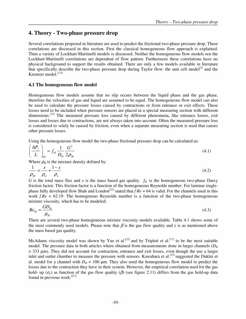
4.1 The homogeneous flow model

Homogeneous flow models assume that no slip occurs between the liquid phase and the gas phase,

therefore the velocities of gas and liquid are assumed to be equal. The homogeneous flow model can also

be used to calculate the pressure losses caused by contractions or from entrance or exit effects. These

losses need to be included when pressure sensors are placed in a special measuring section with different

dimensions.[15]

The measured pressure loss caused by different phenomena, like entrance losses, exit

losses and losses due to contractions, are not always taken into account. Often the measured pressure loss

is considered to solely be caused by friction, even when a separate measuring section is used that causes

other pressure losses.

Using the homogeneous flow model the two-phase frictional pressure drop can be calculated as: 21

2

f

H

H MTP

P Gf

L D ρ

∆ =

(4.1)

Where ρM is the mixture density defined by:

1 1

M G L

x x

ρ ρ ρ

−= + (4.2)

G is the total mass flux and x is the mass based gas quality. fH is the homogeneous two-phase Darcy

friction factor. This friction factor is a function of the homogeneous Reynolds number. For laminar single-

phase fully developed flow Shah and London[21]

stated that f⋅Re = 64 is valid. For the channels used in this

work f.Re = 62.19. The homogenous Reynolds number is a function of the two-phase homogeneous

mixture viscosity, which has to be modeled:

HH

H

GDRe

µ= (4.3)

There are several two-phase homogeneous mixture viscosity models available. Table 4.1 shows some of

the most commonly used models. Please note that β is the gas flow quality and x is as mentioned above

the mass based gas quality.

McAdams viscosity model was shown by Yue et al.[22]

and by Triplett et al.[17]

to be the most suitable

model. The pressure data in both articles where obtained from measurements done in larger channels (DH

> 333 µm). They did not account for contraction, entrance and exit losses, even though the use a larger

inlet and outlet chamber to measure the pressure with sensors. Kawahara et al.[15]

suggested the Dukler et

al. model for a channel with DH = 100 µm. They also used the homogeneous flow model to predict the

losses due to the contraction they have in their system. However, the empirical correlation used for the gas

hold- up (εG) as function of the gas flow quality (β) (see figure 2.11) differs from the gas hold-up data

found in previous work.[6,7]

Table 4.2: Variations on the Chisholm constant.

Author System DH (µm) C value

Kawahara et al.[15]

N2 - water 100 0.24

Chung et al.[14]

N2 - water 48, 100 0.12, 0.22

Mishima et al.[29]

Air - water 1000 - 4000 0.31921(1 exp )HD

C−= −

Yue et al.[22]

N2 - water 333, 528 0.0305 0.600428

00.411822L

C X Re−=

Lee and Lee[27]

Air - water 78, 191, 364, 667 0

0

2

q r s

L

HL

L

L

L H

L slug

C p Re

GDRe

D

u

λ ψ

µ

µλ

ρ σ

µψ

σ

=

=

=

=

Hwang and Kim[28]

Refrigerant 244, 430, 792 3

1 2

0 0

( )

C

L GC C

L

H

gC C Re X

D

σ

ρ ρ

− =


-11-

The homogeneous flow model is flow pattern independent. Furthermore it assumes no slip between the

two phases. During Taylor flow the liquid film layer in a horizontal micro channel during is stagnant at

low Capillary numbers (Ca < 0.15).[3,9,21]

Therefore, the gas travels through the micro channel at a higher

velocity than the liquid does. This indicates that even though this model may fit the measured data, the

physical background of the model is lacking.

4.2 Lockhart-Martinelli models

Lockhart and Martinelli (LM) type models[23]

are separated flow models that use a so called two-phase

multiplier (ΦL) to correlate the two-phase pressure drop as a function of the single liquid phase pressure

drop:

2

L

TP L

P P

L L

∆ ∆ = Φ

(4.4)

The two-phase multiplier can be correlated directly to the measured liquid single-phase pressure drop data,

like Ide and Fukano[24]

did for air-water flow in a channel with a DH of 0.99 mm. Sometimes the two-

phase multiplier is not based on the measured liquid pressure drop but based on a calculated liquid

pressure drop assuming that there is only liquid flowing in the channel as Friedel did.[25]

This multiplier is

given the symbol ΦL0.

In literature the two-phase multiplier is often correlated using the measured gas single-phase pressure drop

as well as the liquid single-phase pressure drop. The Chisholm and Laird correlation[26]

then is used:

2

2

11L

C

X XΦ = + + (4.5)

Where X is the Lockhart-Martinelli parameter given by:

2 ( / )

( / )

L

G

P LX

P L

∆=

∆ (4.6)

By measuring the liquid single-phase pressure drop, the gas single-phase pressure drop and the two-phase

pressure drop the two-phase multiplier is then correlated by varying the value of Chisholm (C) or

correlating this value. Chisholm suggested a C-value of 20 for large channels up to 5 for smaller channels.

For micro channels this value drops even more. In table 4.2 several values and correlations for the C-value

are given for channels with diameters ranging from 48 to 4000 µm. The value of C drops to approximately

0.20 and even approach zero, when the channel diameter is decreases.[2]

This corresponds with a

completely separated laminar flow of gas and liquid, without any momentum coupling between the two

phases.

Kawahara et al.[15]

and Chung et al.[14]

can also fit a C-value to their results by using the correlation of Lee

and Lee.[27]

Lee and Lee created a C-value correlation based on Taylor flow. It is dependent of the liquid

slug velocity (uslug). However they do not account for entrance and outlet losses of their pressure taps.

These losses are included in the experimentally obtained parameters. The equations can be found in table

4.2. ψ corresponds with the capillary number Ca and is a dimensionless group that represents the relative

importance of the viscous and surface tension effects. λ is a dimensionless group that corresponds with

Ca/Re is independent of the liquid slug velocity. The remaining four parameters were determined

experimentally by linear regression. Hwang and Kim[28]

integrated the surface tension effect in their

correlation. Furthermore they include the Reynolds number and four parameters that are determined by

fitting the model to the experimental data.

Separated flow correlations are empirical and flow pattern independent. The degree of separation between

the phases is not theoretically determined, they are determined by fitting measured data.

Figure 4.3: Scheme of a unit cell as described by Chung and Kawaji.

[2]

Table 4.3: Equations for calculating the liquid region pressure drop.

Chung and Kawaji[2]

Adjusted to fit Taylor model

G

LL

UU

ε−=

1

G

LL

UU

ε−=

1

L LL

L

U DRe

ρ

µ=

L L HL

L

U DRe

ρ

µ=

2

2

f L LL

L

P Uf

L D

ρ∆ =

2

2

f L LL

HL

P Uf

L D

ρ∆ =

64L

L

fRe

= 62.19

L

L

fRe

=


-12-

4.3 The unit cell model

Chung and Kawaji[2]

indicate that for channels with a DH of 100 µm or less homogeneous and separate

flow models do not fit their measured pressure data for Taylor flow. They instead propose a unit cell

model for Taylor flow in channels of DH < 100 µm, to avoid this problem. The unit cell model that

Garimella, Killion and Coleman[30]

proposed for Taylor flow of evaporating refrigerant was adjusted by

Chung and Kawaji to describe their nitrogen-water system.

The modified unit cell model is based on a unit cell consisting of two regions: a single liquid phase flow

region (the liquid slug) and a two-phase flow region (see figure 4.3). The bubble is assumed to be

axisymmetrical with cylindrical caps. The bubble is also considered to be surrounded by a moving

uniform liquid film. The moving film travels much slower through the channel, than the bubbles and the

liquid slugs due to viscous effects. The liquid slug contains no entrained bubbles. They assume that the

channel is smooth. The total pressure drop calculated is the sum of the frictional pressure drop of each

region:

f B L

B LUC UCTP

P L LP P

L L L L L

∆ ∆ ∆ = +

(4.7)

Here LUC is the unit cell length and LB and LL the bubble and slug length respectively.

The Darcy-Weisbach equation for fully developed flow is used to determine the pressure drop in the liquid

slug. For determining the liquid region friction factor for Re < 2100, they used fL⋅Re = 64. Since the film

layer is not considered to be stagnant, they use the gas hold-up to calculate the average liquid velocity ŪL.

Chung and Kawaji[2]

use the empirical gas hold-up correlation that they introduced, to calculate this

velocity.

To test this model on our data, some of the assumptions made for this model need to be adjusted to fit the

assumptions made in the Taylor flow model. First of all the gas hold-up is calculated by Chung and

Kawaji, using an empirical gas hold-up correlation, that could not be verified in previous work done in

this project.[6,7]

Secondly, they used circular channels, while rectangular channels were used in this work,

so the friction factor equation is different. In table 4.3 the original equations for the liquid region used by

Chung and Kawaji are shown next to the adjusted equations we use to test the model on our data.

To calculate the pressure drop in the two-phase region, Chung and Kawaji proposed six equations that can

be solved by iteration. One extra assumption was made to obtain the equations for the two-phase region.

They assume that 90% of the tube diameter is occupied by the bubble diameter. The model assumes that

the gas-liquid interfacial velocity is solely driven by the pressure drop. The gas-liquid interfacial velocity

ŪI is determined by iteration. The bubble velocity is also calculated using the empirical void fraction

model. All the equations Chung and Kawaji used for the iteration are mentioned in table 4.4. There are

two adjustments needed to fit assumptions of this model to the assumptions of the Taylor flow model.

First and foremost, with our method the bubble velocity (uB) is determined by visual analysis and does not

have to be estimated. Secondly, an adjustment is made for the approximation of the bubble diameter.

When using the Taylor flow model on the measured data, the ratio of the channel cross sectional area and

the bubble cross sectional area (A/AB) has be determined for each measurement location. An

approximation of the bubble diameter is needed and since the bubble is not axisymmetric, this is not an

easy task. Therefore the assumption is made, that the ratio of the hydraulic diameter and the bubble

diameter is equal to the ratio of the channel cross sectional area and the bubble cross sectional area as

obtained from the Taylor flow model. The adjustments to the unit cell model are also mentioned in table

4.4.

Table 4.4: Equations for calculating the two-phase region pressure drop.

Chung and Kawaji[2]

Adjusted to fit Taylor model

G

G

GB

UUU

ε== Bu

( )G B I BB

G

U U DRe

ρ

µ

−=

( )G B I BB

G

u U DRe

ρ

µ

−=

2( )

2

f G B IB

BB

P U Uf

L D

ρ∆ −=

2( )

2

f G B IB

BB

P u Uf

L D

ρ∆ −=

64B

B

fRe

= 62.19

B

B

fRe

=

2 2( )16

f

BI B

L

P

LU D D

µ

∆

= − 2 2( )

16

f

BI H B

L

P

LU D D

µ

∆

= −

DDB 90.0= H B

B

AD D

A≈

Figure 4.4: Schematic overview of the computational problem solved by Kreutzer.

[3]


-13-

Using both the calculated pressure drops for the two regions and the length of the two regions, the total

pressure drop can be calculated using equation 4.7. The slug length, bubble length and unit cell length can

all be obtained from the visual analysis in combination with the Taylor flow model.

Chung and Kawaji[2]

used a set-up with a mixer/measuring section with a larger diameter. Therefore the

entrance, outlet and contraction pressure losses are described using the homogeneous flow model. They

are subtracted from the total measured pressure drop, to obtain the frictional pressure drop. The model can

perhaps be used to describe our data if their assumptions are adjusted. Holt et al.[31]

use a similar model for

describing two-phase upwards flow. They designed models for four different flow patterns including

Taylor flow.

4.4 The Kreutzer model

Kreutzer et al.[3,4]

used a semi-numerical approach to be able to determine the slug length of Taylor flow

by measuring the frictional pressure drop. In the model the Reynolds number is limited to 900 to ensure

that the liquid flow is laminar. The basic idea of this model is that when the liquid slugs are infinitely

long, the pressure drop can be calculated with the single-phase pressure drop equation, using the Fanning

friction factor. When the slug length is decreased to less than 10 times the hydraulic diameter of the

channel, the two-phase Fanning friction factor increases drastically from the single-phase Fanning friction

factor value (f = 16/Re).[4]

This is caused by the difference in curvature between the front and back of the

bubble, which causes a Laplace pressure difference. The initial two-dimensional computational problem is

formulated as following: a region where a single axisymmetric bubble with hemispherical caps is traveling

between two slug regions at a velocity, which is the sum of both the liquid and the gas superficial velocity.

The problem was extended by changing the curvature of the nose and tail of the bubble. The liquid

properties are assumed to be constant in the micro channel. Far away from the bubble the liquid velocity

has developed into the parabolic Hagen-Poisseuille flow. Figure 4.3 gives a schematic overview of the

problem.

The numerical approach results in the following equation to calculate the two-phase pressure drop which

is a modification of the solution for single-phase fully developed Hagen-Poisseuille flow:

212

4f ( ( ) )S

S G L

S B H

LpU U

L L L Dρ

∆= +

+

(4.8)

The slug Fanning factor is given by:

16f 1 ( , , )H

S

S

DRe Ca

Re Lξ

= +

(4.9)

The ξ function is an excess pressure term that is introduced in the slug friction factor, to describe how the

pressure drop is affected by the presence of the bubbles. It is a function of Re, Ca and the dimensionless

slug length (LS/DH).

When inertia is negligible (i.e. at a low Weber numbers (We << 1)), Bretherton’s law for lubrication was

used to describe the slug friction factor:

2

37.16 (3 )16f 1

32

HS

S

D Ca

Re L Ca

= +

(4.10)


-13-

Figure 4.5: Effect of inertia on the bubble shape.

[3]


-14-

When inertia becomes more important (We > 1) a different correlation for ξ is suggested. With increasing

Re the nose of the bubble is elongated and the rear of the bubble is flattened (see figure 4.5) and

Bretherton’s law does not hold anymore. There is a need for a model for the friction factor when inertia

does play a role. The friction factor times the Reynolds number (f⋅Re) is found by experiments to be

independent of velocity, but does vary with the liquid properties. Therefore is suggested that the group

Ca/Re is used the describe the liquid properties. When the slugs are infinitely long the friction factor

needs to be equal to the single-phase friction factor f = 16/Re. This results in the following equation of the

ξ function with two parameters, which can be determined by non-linear regression.

b

H

S

D Rea

L Caξ

=

(4.11)

The experimental work done by Kreutzer resulted in the following expression for the slug friction factor:

0.3316

f 1 0.17 HS

S

D Re

Re L Ca

= +

(4.12)

Kreutzer uses the average velocity (UG+UL), to estimate the velocity at which the bubble travels. Since the

bubble velocity (uB) can be determined in using the video images, the bubble velocity should be used in

this model instead of the average velocity. Furthermore, Kreutzer says that the liquid hold-up (1-εG ) is

equal to the ratio of the slug length over the unit cell length (see equation 4.8). This is only correct is there

is no film layer. Therefore if this model is tested on our data the hold-up is used.

I-7I-8I-9

I-15

I-20

I-17

Figure 5.1: The P&ID of the flow system with a water reservoir pressurized with helium and a nitrogen supply

chain.

Table 5.1: Specifications of the controllers used in the flow system.

Controller: Type: Range:

Digital pressure controller Bronkhorst P-602C 0.8 – 40 barg

Digital liquid flow controller Bronkhorst L13V02 2 – 100 mg/min

Digital liquid flow controller Bronkhorst L23V02 60 – 30000 mg/min

Digital mass flow controller Bronkhorst F-200C 0.03 – 1.5 mln/min

Digital mass flow controller Bronkhorst F-201C 1 – 50 mln/min

8 mmLiquid

45 mm

20 mm

50/100/150 µm

50 µm

Gas

Glass chips

Figure 5.2: A glass chip with a micro channel etched in it. Three different micro channels are available with

different cross sectional areas.(50x50 µm2, 50x100 µm

2 and 50x150 µm

2).

Experimental set-up and procedures

-15-

5. Experimental set-up and procedures

In the first section of this chapter the experimental set-up is described in detail. In the second section of

this chapter the experimental procedures for making a flow pattern map and for estimating the pressure

drop along the micro channel are explained

5.1 Experimental set-up

The set-up can be divided into three segments: the flow system, the micro channel chips and the imaging

section.

The flow system

In this graduate work the gas-liquid system used was nitrogen-water. In previous work done in this

project, a HPLC pump was used to introduce the de-mineralized water to the micro channel. To avoid

pulses in the micro channel, a reservoir tank, pressurized with helium, is now used. Figure 5.1 gives a

complete overview of the flow system. The helium pressure in the water reservoir is regulated at 14 barg,

by a digital pressure controller. To regulate the liquid velocity in the micro channel, two liquid flow

controllers were used. The nitrogen flow is regulated by two mass flow controllers. The specifications of

all controllers used in the flow system are given in table 5.1.

Several filters are installed to ensure that no solid particles or other contaminations can enter the micro

channel. The outlet capillary is led to a liquid recovery beaker placed on a balance (Sartorius R 300S).

With this balance the mass flow and thus the liquid velocity, can be varified.

The micro channel chips The micro channels were etched in glass chips by Deep Reactive Ion Etching, the in- and outlet holes were

made by powder blasting. Three different chips, with three different cross sectional areas of the channels,

where used in this graduation work. Two rectangular channels with cross sectional areas of 50x100 µm2

and 50x150 µm2 where used, as well as a square channel of 50x50 µm

2 (see figure 5.2).

The liquid enters the chip and is then split into two streams, which recombine in the cross shaped mixer.

The gas enters the chip and is led to the mixer. The inlet chambers have the same cross sectional area as

the micro channel. The micro channel is 20 mm long.

In order to properly connect the chip to the in- and outlet capillaries, the glass chip is placed in a brass

holder. This holder (figure 5.3) has two inlet capillaries and one outlet capillary attached to it. It is placed

on the table of the microscope. A ruler is placed on the top side of the holder. This ruler is used to be able

to determine the location in the channel, when recording images.

The imaging section.

A Redlake MotionPro CCD camera was connected to a Zeiss Axiovert 200 MAT inverted microscope to

record images of the flow. The images were recorded at 10,000 fps. The movie has a resolution of 1280 x

48 pixels. For the 50x150 µm2 channel the frame rate needed to be lowered to 8,000 fps (1280x80 pixels)

to be able to capture the full channel height of 150 µm. A 100 W halogen lamp was used for illumination

of the micro channel by transmitted light. The lamp in combination with a shutter time of 12 µs was

sufficient to avoid any motion blurring of images.

Figure 5.3: Overview of the brass holder in which the glass chip is placed.

Figure 5.4a: Frame image before setting borders Figure 5.4b: Frame image with borders

Table 5.2: The location indication for the movies.

Letter Location

A 0 – 3.3 mm

B 3.3 – 6.3 mm

C 6.3 – 9.3 mm

D 9.3 – 12.3 mm

E 12.3 – 15.3 mm

F 15.3 – 18.3 mm

924 pixels

3.3 mm

840 pixels

3 mm

Border 1 Border 2

Beginning

of channel

Border 1 Border 2

Experimental set-up and procedures

-16-

5.2 Experimental procedure

There were two different experimental procedures used during this graduation work. The procedure for

determining the flow pattern map and the procedure for making movies for the pressure drop estimations

are discussed in this section.

Flow pattern mapping When a gas and liquid velocity combination is set, video images are made after waiting for 10 minutes, to

ensure stable flow. One movie is recorded at the beginning of the channel and one at the end of the

channel. Each movie is recorded at 10,000 fps and played back at a lower frame rate using Redlake

MiDAS software. The flow pattern type is determined. In case of the 50x50 µm2

channel the zoom

function of the MiDAS software is needed, to be able to distinguish ring flow from churn flow. The

disruptions and the deformation of the rings that occur during churn flow are only detectable when using

this function.

Pressure estimations

10 minutes after setting a gas and liquid velocity combination at which Taylor flow can be observed, the

flow pattern is stable. At the beginning of the channel a movie is made at 10,000 fps. 5,000 frames are

saved on the computer for further analysis, which corresponds with 0.5 s of measuring time. Each movie

is then analyzed, using a series of scripts made in Matlab. These “home-made” scripts[6,7]

enable the

determination of important hydrodynamic parameters, (like bubble length, slug length, bubble velocity,

bubble frequency etc), from the images.

Figure 5.4a shows one frame of a movie made of Taylor flow. The frame has dark edges at the beginning

and end, due to limited illumination of these edges. Therefore borders need to be set to at the beginning

and the end of the channel. The borders determine the measuring area of each frame of the movie. Only

bubbles within the measuring area are identified and tracked by the scripts. The borders are used to

determine the location in the channel.

In order to correctly determine the border a movie needs to be recorded at the beginning at the channel.

One frame of this movie is investigated in Matlab to determine the location of the borders. Figure 5.4a

shows one frame of a movie at a gas velocity UG of 1 m/s (at standard conditions) and a liquid velocity of

0.4 m/s. This picture of one frame is used to explain the location determination. First the beginning of the

channel is located in the frame. Border 1 is set 0.3 mm from the beginning of the channel to avoid

including the bubble formation in the measuring area of the frame. The accuracy of the ruler on the holder

of the micro channel is 1 mm, therefore the displacement of measuring location along the channel is

chosen to be 3 mm. The second border is thus set 3 mm further along the channel, which gives a sufficient

measuring to identify and track the bubbles (figure 5.6b). These borders are now valid for all movies made

along the channel. The channel is split into 6 sections of each 3 mm long. A movie is made of each

section. Each movie is given a letter, which corresponds with the location in the channel, see table 5.2.

The scripts are used to identify and track each bubble in a movie that was made at a particular location in

the channel. For each movie, each individual bubble is tracked and the length of the bubbles is averaged

over all bubbles over all frames in the movie where the bubble was identified. The average of all the

individual lengths is then the averaged bubble length (LB) of at that location in the channel. The average

slug length (Ls) is obtained in the same way. The number of tracked bubbles divided by the measured time

(0.5 s) gives the bubble frequency. The bubble velocity was determined by measuring the displacement of

the center point of the bubble between two frames. The bubble velocity first determined for one bubble

and then averaged over all bubbles in the movie, giving the averaged bubble velocity (uB) at that location

of the channel.[6,7]

Figure 6.1: Flow pattern map for a nitrogen-water system in a 50x50 µm

2 channel.

a) Annular flow UG = 20 m/s, UL = 0.05 m/s

b) Ring flow UG = 50 m/s, UL = 0.15 m/s

c) Churn flow UG = 20 m/s, UL = 0.3 m/s

d) Taylor flow UG = 3 m/s, UL = 0.5 m/s

e) Taylor-ring flow UG = 10 m/s, UL = 1.6 m/s

Figure 6.2: Top view of flow patterns observed in a 50x100 µm2 channel.

a) Bubbly flow UG = 10 m/s, UL = 2 m/s beginning of channel

b) Bubbly flow UG = 10 m/s, UL = 2 m/s end of channel

Figure 6.3: Effect of the pressure drop on bubbly flow in a 50x100 µm2 channel.

Figure 6.4: Taylor-annular UG = 0.4 m/s, UL = 0.05 m/s observed in the 50x100 µm

2 channel .

10-1

100

101

102

103

10-2

10-1

100

101

Gas velocity [m/s]

Liq

uid

ve

loc

ity

[m

/s]

Churn

Ring

Taylor

Taylor RIng

Results and discussion

-17-

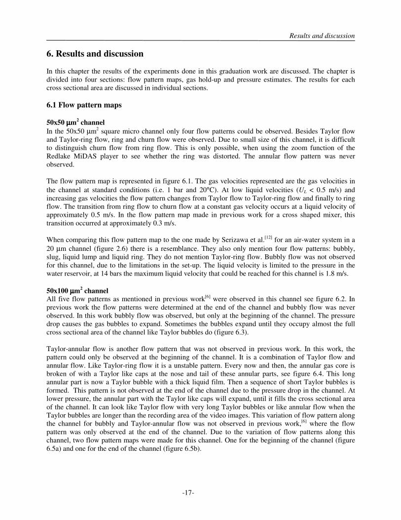
6. Results and discussion

In this chapter the results of the experiments done in this graduation work are discussed. The chapter is

divided into four sections: flow pattern maps, gas hold-up and pressure estimates. The results for each

cross sectional area are discussed in individual sections.

6.1 Flow pattern maps

50x50 µµµµm2 channel

In the 50x50 µm2 square micro channel only four flow patterns could be observed. Besides Taylor flow

and Taylor-ring flow, ring and churn flow were observed. Due to small size of this channel, it is difficult

to distinguish churn flow from ring flow. This is only possible, when using the zoom function of the

Redlake MiDAS player to see whether the ring was distorted. The annular flow pattern was never

observed.

The flow pattern map is represented in figure 6.1. The gas velocities represented are the gas velocities in

the channel at standard conditions (i.e. 1 bar and 20°C). At low liquid velocities (UL < 0.5 m/s) and

increasing gas velocities the flow pattern changes from Taylor flow to Taylor-ring flow and finally to ring

flow. The transition from ring flow to churn flow at a constant gas velocity occurs at a liquid velocity of

approximately 0.5 m/s. In the flow pattern map made in previous work for a cross shaped mixer, this

transition occurred at approximately 0.3 m/s.

When comparing this flow pattern map to the one made by Serizawa et al.[12]

for an air-water system in a

20 µm channel (figure 2.6) there is a resemblance. They also only mention four flow patterns: bubbly,

slug, liquid lump and liquid ring. They do not mention Taylor-ring flow. Bubbly flow was not observed

for this channel, due to the limitations in the set-up. The liquid velocity is limited to the pressure in the

water reservoir, at 14 bars the maximum liquid velocity that could be reached for this channel is 1.8 m/s.


All five flow patterns as mentioned in previous work[6]

were observed in this channel see figure 6.2. In

previous work the flow patterns were determined at the end of the channel and bubbly flow was never

observed. In this work bubbly flow was observed, but only at the beginning of the channel. The pressure

drop causes the gas bubbles to expand. Sometimes the bubbles expand until they occupy almost the full

cross sectional area of the channel like Taylor bubbles do (figure 6.3).

Taylor-annular flow is another flow pattern that was not observed in previous work. In this work, the

pattern could only be observed at the beginning of the channel. It is a combination of Taylor flow and

annular flow. Like Taylor-ring flow it is a unstable pattern. Every now and then, the annular gas core is

broken of with a Taylor like caps at the nose and tail of these annular parts, see figure 6.4. This long

annular part is now a Taylor bubble with a thick liquid film. Then a sequence of short Taylor bubbles is

formed. This pattern is not observed at the end of the channel due to the pressure drop in the channel. At

lower pressure, the annular part with the Taylor like caps will expand, until it fills the cross sectional area

of the channel. It can look like Taylor flow with very long Taylor bubbles or like annular flow when the

Taylor bubbles are longer than the recording area of the video images. This variation of flow pattern along

the channel for bubbly and Taylor-annular flow was not observed in previous work,[6]

where the flow

pattern was only observed at the end of the channel. Due to the variation of flow patterns along this

channel, two flow pattern maps were made for this channel. One for the beginning of the channel (figure

6.5a) and one for the end of the channel (figure 6.5b).

10-1

100

101

102

103

10-3

10-2

10-1

100

101

Gas velocity [m/s]

Liq

uid

ve

loc

ity

[m

/s]

Annular

Bubbly

Churn

Ring

Taylor

Taylor Annular

Taylor Ring

10-1

100

101

102

103

10-3

10-2

10-1

100

101

Gas velocity [m/s]

Liq

uid

ve

loc

ity

[m

/s]

Annular

Churn

Ring

Taylor

Taylor Ring

a) beginning of the channel b) end of the channel

Figure 6.5: Flow pattern map for nitrogen-water system at the beginning and the end of the 50x100 µm2 channel.

Figure 6.6: Effect of contaminations on the bubble shape.

Figure 6.7: The change of tail shape in the 50x150 µm

2 channel chips.

Figure 6.8: Air-water flow patterns in a hydrophobic channel.

[33]

Figure 6.9: Read-out of the 3000 mg/min liquid flow controller.


-18-

These flow pattern maps can be compared to the ones made in previous work.[6]

The flow pattern map for

the end of the channel was compared to flow pattern map of the cross shaped mixer connected to a

channel with the same cross sectional area of 50x100 µm2 (figure 2.9). The transition from ring flow to

churn flow at a constant gas velocity occurs at a liquid velocity of approximately 0.5 m/s. In the flow

pattern map made in previous work for a cross shaped mixer, this transition occurred at approximately 0.3

m/s. The area where Taylor-ring flow occurs has a similar shape. In both flow pattern maps, the transition

from Taylor-ring flow to churn flow occurs at a gas velocity of approximately 11 m/s and a liquid velocity

higher than 0.3 m/s.


Of each micro channel dimensions several chips were made. During the flow mapping with the first chip a

kind of oily substance appeared in the mixer that could not be removed. So a second chip was inserted into

the holder. During Taylor flow in this chip the bubble shape was altered by what looked like either surface

roughness or a solid particle, as shown in figure 6.6. Surface roughness and/or contaminations of the

surface can cause a change in contact angle.[32]

The surface seems hydrophobic as mentioned by Cabaud et

al.[33]

. Figure 6.7 shows the shape of the bubbles in a hydrophobic channel. This phenomena was observed

in both chip 2 and 3. No experiments could be done with these chips, due to these problems.

6.2 Gas hold-up

As mentioned before, gas hold-up measurements are done for Taylor flow. From the movie analysis the

slug length and the bubble frequency are determined. Then using the Taylor flow model the dimensionless

cross sectional bubble area at each location, can be determined using equation 3.8. Subsequently the gas

hold-up can be determined using equation 3.6. Finally the gas hold-up can be plotted against the gas

quality, which is calculated with the calculated local gas quality (uG).

Due to the too large range of the 3000 mg/min, most experiments were done at 2 – 20 % of the total range

of the flow controller. A log file was made of the measured read-out of the flow controller at a set-point of

3.33 % , see figure 6.9. The measured value oscillates between 0.25 m/s (set-point –17 %) and 0.37 m/s

(set-point +23 %). However most oscillations are within 10 % of the set-point. An oscillation has a time

span of approximately 1 second. Since the measuring time of a movie is 0.5 s, it is not possible to know

the exact liquid velocity. The oscillations can also be seen in the bubble velocity. When these oscillations

could be averaged the measurements where included. Two measurements for the 50x50 µm2 channel and

seven measurements of the 50x100 µm2 channel had to excluded due to this effect. A new liquid flow

controller should be used with a smaller range so that new measurements can be done at 50-70 % of the

range of the flow controller. However, due to the limited time left, these values are used in further

calculations.


For every location a curve fit was made for the dimensionless cross sectional bubble area (A/AB) and the

additional slug length (δ). In figure 6.10 the fit for the end of the channel (location F) is displayed. It is

clear that there is a linear relationship between the liquid velocity divided by the bubble frequency and the

slug length. This indicates that the cross sectional bubble area does not vary with the bubble velocity at

that location. Table 6.1 gives the A/AB ratio and the additional slug length for all the locations along the

channel.

0 0.05 0.1 0.15 0.2 0.25 0.3 0.350

0.05

0.1

0.15

0.2

0.25

0.3

0.35

Liquid velocity/Bubble frequency [mm]

Slu

g l

en

gth

[m

m]

Figure 6.10: Curve fit of location F for 50x50 µm

2 channel.

0 0.1 0.2 0.3 0.4 0.5 0.60

0.1

0.2

0.3

0.4

0.5

0.6

Liquid velocity/Bubble frequency [mm]

Slu

g l

en

gth

[m

m]

Figure 6.11: Curve fit of location F for 50x100 µm

2 channel .

0 0.1 0.2 0.3 0.4 0.5 0.6 0.7 0.8 0.9 10

0.1

0.2

0.3

0.4

0.5

0.6

0.7

0.8

0.9

1

ug/(ul+ug)

Ga

s h

old

up

Gas hold up data location F

Armand's equation

0 0.2 0.4 0.6 0.8 1

0

0.1

0.2

0.3

0.4

0.5

0.6

0.7

0.8

0.9

1

ug/(ul+ug)

Ga

s h

old

up

Gas hold-up data location F

Armand's equation

Figure 6.12: Gas hold-up 50x50 µm

2 channel. Figure 6.13: Gas hold-up 50x100 µm

2 channel.

Table 6.2: A/AB ratio and additional slug length

for all locations of the 50x100 µm2 channel

Location [mm] A/A B [m] δ [µm]

0 - 3.3 1.14 ±0.1 40

3.3 - 6.3 1.13 ±0.1 38

6.3 - 9.3 1.12 ±0.1 36

9.3 - 12.3 1.11 ±0.1 35

12.3 - 15.3 1.11 ±0.1 35

15.3 - 18.3 1.12 ±0.1 36

Table 6.1: A/AB ratio and additional slug length

for all locations of the 50x50 µm2 channel

Location [mm] A/A B [m] δ [µm]

0 - 3.3 1.29 ±0.1 36

3.3 - 6.3 1.25 ±0.1 33

6.3 - 9.3 1.22 ±0.1 31

9.3 - 12.3 1.20 ±0.1 30

12.3 - 15.3 1.18 ±0.1 27

15.3 - 18.3 1.16 ±0.1 26


-19-

The gas hold-up is calculated using equation 3.6. In figure 6.12 the gas hold-up plot of location F is

shown. There is a linear relationship between the gas quality and the gas hold-up as expected. The value

of AB/A is the slope, which corresponds with the Armand value of 0.833 ± 7% for all locations.


Similar to the 50x50 µm2 channel a curve fit was made for every measuring location for the dimensionless

cross sectional bubble area (A/AB) and the additional slug length (δ). In figure 6.11 the fit for the end of

the channel (location F) is displayed. Again there is linear relationship between the liquid velocity divided

by the bubble frequency and the slug length. Table 6.2 gives the A/AB ratio and the additional slug length

for all the locations along the channel.

In figure 6.13 gives the gas hold-up plot of location F. The value of AB/A is smaller that the Armand value

of 0.833. The maximum deviation was 0.833 +8 %.

Figure 6.14: Bubble velocity (left) and Gas hold-up (right) for the 50x50 µm2 channel at different locations in the

channel.

Figure 6.15: Bubble velocity (left) and Gas hold-up (right) for the 50x100 µm2 channel at different locations in the

channel.

Table 6.2: Results of equation 6.9 for the Table 6.3: Results of equation 6.9 for the

50x50 µm2 channel. 50x100 µm

2 channel.

Measurement From A to B From E to F

[bar.s/m] [bar.s/m]

N1.0 W0.3 9.70 2.16

N1.0 W0.4 3.61 2.24

N1.0 W0.9 2.05 0.85

N1.0 W1.0 0.54 0.42

N1.2 W0.6 4.92 1.41

N1.2 W0.8 1.10 1.06

N1.2 W1.0 1.24 0.69

N1.2 W1.2 1.51 0.80

N1.6 W0.4 2.66 1.41

N1.8 W0.6 0.98 0.94

N2.2 W0.3 1.72 1.72

N2.2 W0.4 1.81 1.11

N1.6 W0.3 2.09 1.61

N2.2 W0.5 1.62 1.14

Measurement From A to B From E to F

[bar.s/m] [bar.s/m]

N0.4 W0.5 0.40 0.23

N0.5 W1.0 0.23 0.26

N0.5 W1.2 0.31 0.25

N0.6 W0.4 0.87 0.73

N0.6 W0.5 0.43 0.26

N0.6 W0.6 1.22 0.65

N0.7 W1.3 0.28 0.25

N1.0 W0.4 1.19 0.54

N1.0 W0.5 0.51 0.32

N1.0 W1.3 0.52 0.24

N2.0 W0.6 0.58 0.37

N2.5 W0.4 0.72 0.51

N2.8 W0.6 0.31 0.53

N3.0 W0.4 1.02 0.53

N0.4W0.5

N0.5W1.0

N0.5W1.2

N0.6W0.4

N0.6W0.5

N0.6W0.6

N0.7W1.3

N1.0W0.4

N1.0W0.5

N1.0W1.3

N2.0W0.6

N2.5W0.4

N2.8W0.6

N3.0W0.40 2 4 6 8 10 12 14 16 18 20

0

0.1

0.2

0.3

0.4

0.5

0.6

0.7

0.8

0.9

1

Channel length [mm]

Ga

s h

old

-up

[-]

0 2 4 6 8 10 12 14 16 18 200

0.5

1

1.5

2

2.5

3

Channel length [mm]

Bu

bb

le v

elo

cit

y [

m/s

] N1.0W0.3

N1.0W0.4

N1.0W0.9

N1.0W1.0

N1.2W0.6

N1.2W0.8

N1.2W1.0

N1.2W1.2

N1.6W0.4

N1.8W0.6

N2.2W0.3

N2.2W0.4

N1.6W0.3

N2.2W0.50 2 4 6 8 10 12 14 16 18 200

0.1

0.2

0.3

0.4

0.5

0.6

0.7

0.8

0.9

1

Channel length [mm]

Ga

s h

old

-up

[-]

0 2 4 6 8 10 12 14 16 18 200

0.2

0.4

0.6

0.8

1

1.2

1.4

1.6

1.8

2

Channel length [mm]

Bu

bb

le v

elo

cit

y [

m/s

]


-20-

6.3 Pressure estimation

The gas velocity at a certain location in the channel is a function of the gas hold-up and the bubble

velocity (uB):

G G Bu uε= ⋅ (6.1)

The gas hold-up is determined using the Taylor flow model. The bubble velocity is obtained from the

video analysis. Since the gas velocity at the mass flow controller (UG) is known at standard conditions

(PMFC = 1 bar), the pressure at location (PL) can be estimated using the ideal gas law :

MFC G L GP U P u= (6.2)

Both the gas hold-up and the bubble velocity depend on the location in the channel, they both increase

along the channel length. Figure 6.14 shows the bubble velocity and gas hold-up as function of the

location in the channel for all measurements done in the 50x50 µm2 channel. Figure 6.15 shows the bubble

velocity and gas hold-up as function of the location in the channel for all measurements done in the

50x100 µm2 channel. “N” indicates the nitrogen superficial velocity at the mass flow controller, “W”

indicates the water superficial velocity set at the liquid flow controller.

The increase in gas hold-up and in bubble velocity along the channel indicates that gas phases expansion

occurs. Neither the Kreutzer model nor the unit cell model include expansion of the bubbles. They both

assume that the gas hold-up remains constant along the channel. Therefore applying their model on our

data is not that easy.

Due to the limited time no pressure drop correlation was made using the data obtained from the

measurements. However, an estimate can be made for the lower limit of the pressure drop data. The two-

phase pressure drop has to be higher than the single phase pressure drop of the liquid slugs, due the

influence of the gas bubble on the pressure drop. Factors of influence could be the difference in curvature

of the tail and nose of the gas bubbles, which creates a difference in Laplace pressure and/or a increase in

friction due to the recirculation patterns within the slugs.

The pressure drop caused by a unit cell consists out of the pressure drop caused by the liquid slug (∆PS)

and the gas bubble. The pressure drop caused by the gas bubble is negligible, since the density and the

viscosity of the gas phase is negligible compared to the density and viscosity of the liquid phase. The

pressure of the liquid slug can than be described by the pressure drop equation for fully developed single

phase Hagen- Poisseuille flow: 2

2

S L BS

S H

P uf

L D

ρ∆= (6.3)

For the friction factor (f) the solution for laminar flow as mentioned before in chapter 4 is used:

62.19S

S

fRe

= (6.4)

Where the Reynolds number is:

L B HS

L

u DRe

ρ

µ= (6.5)

Substituting equations 6.4 and 6.5 in 6.3 gives:

2

31.095S L B

S H

P u

L D

µ∆= (6.6)


-21-

The total pressure drop in between two measurement locations is the pressure drop over the unit cell times

the number of unit cells:

S

S B

LP P

L L∆ = ∆

+ (6.7)

The bubble velocity can be described as the bubble frequency (FB) times the length of a unit cell:

( )B B S Bu F L L= + (6.8)

Combining equations 6.6, 6.7 and 6.8 gives the following solution:

2

31.095 L

B S H

LP

F L D

µ∆= (6.9)

Where L is the channel length between two measurement locations. The right side of this equation is a

constant. For the 50x50 µm2 channel this value is 0.37 bar.s.m

-1. For the 50x100 µm

2 channel this value is

0.21 bar.s.m-1

.

For both the 50x50 µm2

channel and the 50x100 µm2 channel the left side of equation is calculated for the

pressure drop from location A to B and for the pressure drop from E to F to indicate that the two-phase

pressure drop is higher. The values of the bubble velocity, bubble frequency and the liquid slug length

between the two compared locations were averaged. The solutions of the 50x50 µm2

channel are shown in

table 6.3, the solutions of the calculations for the 50x100 µm2

channel are shown in table 6.4. None of the

values are lower than limit set by the pressure drop of the liquid slugs.

Conclusions and recommendations

-22-

7. Conclusions and recommendations

7.1 Conclusions

In this work a hydrodynamic study of nitrogen-water flow in micro channels was conducted. Three

different channels with different cross sectional areas were used in the experiments. There are only results

available for the 50x50 µm2 channel and the 50x100 µm

2 channel. The hydrodynamic study consisted of:

making flow pattern maps, determining the gas hold-up of Taylor flow and estimating the pressure drop of

Taylor flow in the channel. The conclusions are divided into these categories.

Flow pattern maps

In the 50x50 µm2 channel only four different flow patterns were observed: Taylor flow, ring flow, churn

flow and Taylor-ring flow. Six flow patterns were observed in the 50x100 µm2 channel, besides the four

mentioned above, annular flow and bubbly flow were observed. Flow patterns can change over the length

of the channel.

Flow pattern maps were made for both channels. The flow pattern map of the 50x100 µm2 channel

resembles the flow pattern map made in previous work for a similar channel with the same cross sectional

area but with different inlet channels. However, the transition from ring flow to churn flow occurs at a

different liquid velocity.

Gas hold-up The gas hold-up was determined at different measuring locations along the channel. It was determined

using the Taylor flow model described in chapter 3 and the data from the video analysis. The

dimensionless bubble cross sectional area, which in fact is a measure for the film thickness, seems to

remain constant over the channel length. The deviation from Armand’s equation is ±10 % for both

channels.

Some measurements showed oscillations of the bubble velocity, probably caused by the liquid mass flow

controller. When these oscillations could be averaged the measurements where included. The gas hold-up

is a function of the location in the channel as can be seen in figures 6.14 and 6.15. This has not been

reported in literature yet.

Pressure estimates

The pressure of Taylor flow along the channel length was determined using the gas velocity at a certain

location of the channel. The gas velocity at that certain location is a function of the bubble velocity and

the gas hold-up. Both are a function of the channel location and increase along the channel, which

indicates that expansion of the bubbles occurs. The two models that were considered to describe the

pressure drop specifically for Taylor flow, the unit cell model and the Kreutzer model, assume a constant

gas hold-up. Due to the limited time a pressure drop correlation could not be made. However, a simple

calculation was made to indicate that the measured two-phase pressure drop was higher that the pressure

drop if only the pressure drop of the liquid slugs was considered, which was expected.

Conclusions and recommendations

-23-

7.2 Recommendations

First and foremost, a new liquid flow controller (0-500 mg/min) should be connected to the set-up to

ensure that the measurements are done at 70-80 % of the range of the controller to limit the oscillations of

the liquid velocity. Furthermore, nitrogen can replace helium for pressurizing the water in the water

reservoir. In the beginning of the experimental work, the helium pressure on the water was kept constantly

at 14 barg. After four weeks of measuring, helium bubbles appeared in the liquid stream. This problem

was solved by replacing the water and only pressurizing the liquid during measurements. Nitrogen

however, is less soluble. New experiments should be done to verify the data from the experiments done in

this work. The use of a new liquid flow controller could produce a more stable liquid velocity.

The data produced in this work should be used to make a pressure drop model for Taylor flow that

accounts for the change in gas hold-up and bubble velocity along the channel. The slug length is constant

along the channel length and can be used as a parameter in this correlation. Experiments with other gas-

liquid combinations could be made to test how the pressure drop depends on the properties of the gas and

liquid.

References

-24-

References

[1] van Baten, J.M., Krishna, R., 2004. CFD simulations of mass transfer from Taylor bubble rising in

circular capillaries. Chemical Engineering Science 59, 2533-2545.

[2] Chung, P.M.Y., Kawaji, M., 2004. The effect of channel diameter on adiabatic two-phase flow

characteristics in microchannels. International Journal of Multiphase Flow 30, 735-761.

[3] Kreutzer, M.T., 2003. Hydrodynamics of Taylor flow in capillaries and monolith reactors.

Technical University Delft.

[4] Kreutzer, M.T., Kapteijn, F., Moulijn, J.A., 2005. Inertial and interfacial effects on pressure drop

of Taylor flow in capillaries. American Institute of Chemical Engineers 51, 2428-2440.

[5] Kohl, M.J, Abdel-Khalik, S.I., Jeter, S.M., Sadowski, D.L., 2005. An experimental investigation

of microchannel flow with internal pressure measurements. International Journal of Multiphase

Flow 48, 1518-1533.

[6] Schillemans, P., 2006. Gas-liquid hydrodynamics in rectangular glass microchannels. Graduation

report, Technical University of Eindhoven.

[7] Warnier, M.J.F, Rebrov, E.V., de Croon, M.H.J.M, Hessel, V., Schouten, J.C., 2006. Gas hold-up

in Taylor flow in rectangular micro channels. Submitted for the 9th International Conference on

Microreaction Technology.

[8] Thulasidas, T.C., Abraham, M.A., Cerro, R.L., 1997. Flow patterns in liquid slugs during bubble-

train flow inside capillaries. Chemical Engineering Science 52, 2947-2962.

[9] Kolb, W.B., Cerro, R.L., 1993. The motion of long bubbles in tubes of square cross section.

Physics of Fluids A: Fluid dynamics 7, 1549-1557.

[10] Heiszwolf, J.J., Engelvaart, L.B., van den Eijnden, M.G., Kreutzer, M.T., Kapeteijn, F., Moulijn,

J.A., 2001. Hydrodynamic aspects of the monolith loop reactor. Chemical Engineering Science

56, 805-812.

[11] Triplett, K.A., Ghiaansiaan, S.M., Abdel-Khalik, S.I., Sadowski, D.L., 1999. Gas-liquid two-

phase flow in microchannels Part I: two-phase flow patterns. International Journal of Multiphase

Flow 25, 377-394.

[12] Serizawa, A., Feng, Z., Kawahara, Z., 2002. Two-phase flow in microchannels. Experimental

Thermal and Fluid Science 26, 703-714.

[13] Hassan, I., Vaillancourt, M., Pehlivan, K., 2005. Two-phase flow regime transitions in

microchannel: A comparative experimental study. Microscale Thermophysical Engineering 9,

165-182.

[14] Chung, P.M.-Y., Kawaji, M., Kawahara, A., Shibata, Y., 2004. Two-phase flow through square

and circular microchannels – effects of channel geometry. Journal of Fluids Engineering:

Transactions of the ASME 126, 546-552.

[15] Kawahara, A., Chung, P.M.-Y., Kawaji, M., 2002. Investigation of two-phase flow pattern, void

fraction and pressure drop in a microchannel. International Journal of Multiphase Flow 28, 1411-

1435.

[16] Mandhane, J.M., Gregory G.A., Aziz, K., 1974. International Journal of Multiphase Flow 1, 537-

553.

[17] Triplett, K.A., Ghiaansiaan, S.M., Abdel-Khalik, S.I., LeMouel, A., McCord, B.N., 1999. Gas-

liquid two-phase flow in microchannels Part II: void fraction and pressure drop. International

Journal of Multiphase Flow 25, 395-410.

[18] Armand, A.A., 146. The resistance during the movement of a two-phase system in horizontal

pipes. Izv. Vses. Teplotekh. Inst., AERE-Lib/Trans 828 1, 16-23.

[19] Ali, M.I., Sadatomi, M., Kawaji, M., 1993. Two-phase flow in narrow channels between two flat

plates. Canadian Journal of Chemical Engineering 71, 657-666.

[20] Kawahara, A., Sadatomi, M., Okayama, K., Kawaji, M., Chung, P.M.-Y., 2005. Effects of channel

diameter and liquid properties on void fraction in adiabatic two-phase flow through

microchannels. Heat Transfer Engineering 26, 13-19.

References

-25-

[21] Shah, R.K., London, A.L., 1978. Laminar flow forced convection in ducts. Academic Press, New

York.

[22] Yue, J., Chen, G., Yuan, Q., 2004. Pressure drops of single and two-phase flows through T-type

microchannel mixers. Chemical Engineering Journal 102, 11-24.

[23] Celata, G.P., 2004. Heat transfer and fluid flow in microchannels. Series in Thermal & Fluid

Physics & Engineering, 91-118.

[24] Ide, H., Fukano, T., 2005. Experimental research on the correlations of holdup and frictional

pressure drop in air-water two-phase flow in a capillary rectangular channel. International Journal

of Multiphase flow 29, 833-841.

[25] Friedel, L. 1979. Improved friction pressure drop correlations for horizontal and vertical two

phase pipe flow. Rohreleitungstransport 18, 485-491.

[26] Chisholm, D., Laird, A.D.K., 1958. Two-phase flow in rough tubes. Pitman Press, Bath, England.

[27] Lee, H.J., Lee, Y.L., 2001. Pressure drop correlations for two-phase flow within horizontal

rectangular channels with small heights. International Journal of Multiphase Flow 27, 783-796.

[28] Hwang, Y.W., Kim, M.S., 2006. The pressure drop in microtubes and the correlation

development. International Journal of Heat and Mass Transfer 49. 1804-1812.

[29] Mishima, K., Hibiki, T., 1996. Some characteristics of air-water two-phase flow in small diameter

vertical tubes. International journal of multiphase flow 22. 703-712.

[30] Garimella, S., Killion, J.D., Coleman, J.W., 2002. An experimentally validated model for two-

phase pressure drop in the intermittent flow regime for circular microchannels. Journal of Fluids

Engineering 124, 205-214.

[31] Holt, A.J., Azzopardi, B.J., Biddulph, M.W., 1999. Calculation of two-phase pressure drop for

vertical upflow in narrow passages by means of a flow pattern specific model. Chemical

Engineering Research and Design 77, 7-15.

[32] Butt, H-J., Graf, K., Kappl, M., 2003. Physics and Chemistry of Interfaces. Whiley-VCH, 129-

133.

[33] Cabaud, T., Ulmanella, U., Ho, C-M., Two-phase flow in micro channels with surface

modifications. Plenary paper, 5th International Conference on Multiphase flow, Paper no. PL5.

Nomenclature

-26-

Nomenclature

a Fitting parameter [-]

A cross sectional area [m2]

b Fitting parameter [-]

C Chisholm value/fitting parameter [-]

D Diameter [m]

f Fanning friction factor [-]

g Gravitational constant [m2/s]

G Mass flux [kg m2/s]

L Length [m]

LM Lockhart-Martinelli

p Fitting parameter [-]

P Pressure [Pa]

q Fitting parameter [-]

r Fitting parameter [-]

s Fitting parameter [-]

u Superficial velocity at location [m/s]

U Superficial velocity measured at standard conditions [m/s]

Ū Average velocity [m/s]

V Volume [m3]

x Mass gas quality [-]

X Lockhart-Martinelli parameter [-]

Greek letters

β Volumetric gas quality [-]

ε Hold-up [-]

λ Dimensionless group Lee and Lee[27]

[-]

µ Viscosity [Pa s]

ξ Excess pressure term

ρ Density [kg/m3]

σ Surface tension [N/m]

Φ Two-phase multiplier [-]

ψ Dimensionless group Lee and Lee[27]

[-]

Dimensionless groups

Ca Capillary number [µ u/σ]

f Darcy friction factor

Re Reynolds number [ρ u DH/µ]

We Weber number [ρ u2 DH/σ]

λ Dimensionless group Lee and Lee[27]

[Ca/Re]

ψ Dimensionless group Lee and Lee[27]

[Ca]

Subscripts

B Bubble

exp Experimental

f Frictional

F Film

G Gas

H Hydraulic or homogeneous

Nomenclature

-27-

Subscripts continued

I Interface

L Liquid

M Mixture

MFC Mass flow controller

S Slug

th Theoretical

TP Two-phase

UC Unit cell

Documents

Eindhoven University of Technology MASTER … · two-phase flow in micro channels P.G.M. van Hoeij September 2006 Graduation report Graduate Coach: ... observing the different flow