Embed Size (px)
Citation preview
EIGENVECTOR-BASED CENTRALITY MEASURES FORTEMPORAL NETWORKS ∗
DANE TAYLOR† , SEAN A. MYERS‡ , AARON CLAUSET§ , MASON A. PORTER¶, AND
PETER J. MUCHA‖
Abstract. Numerous centrality measures have been developed to quantify the importances ofnodes in time-independent networks, and many of them can be expressed as the leading eigenvectorof some matrix. With the increasing availability of network data that changes in time, it is importantto extend such eigenvector-based centrality measures to time-dependent networks. In this paper, weintroduce a principled generalization of network centrality measures that is valid for any eigenvector-based centrality. We consider a temporal network with N nodes as a sequence of T layers thatdescribe the network during different time windows, and we couple centrality matrices for the layersinto a supra-centrality matrix of size NT × NT whose dominant eigenvector gives the centrality ofeach node i at each time t. We refer to this eigenvector and its components as a joint centrality, asit reflects the importances of both the node i and the time layer t. We also introduce the conceptsof marginal and conditional centralities, which facilitate the study of centrality trajectories overtime. We find that the strength of coupling between layers is important for determining multiscaleproperties of centrality, such as localization phenomena and the time scale of centrality changes.In the strong-coupling regime, we derive expressions for time-averaged centralities, which are givenby the zeroth-order terms of a singular perturbation expansion. We also study first-order terms toobtain first-order-mover scores, which concisely describe the magnitude of nodes’ centrality changesover time. As examples, we apply our method to three empirical temporal networks: the UnitedStates Ph.D. exchange in mathematics, costarring relationships among top-billed actors during theGolden Age of Hollywood, and citations of decisions from the United States Supreme Court.
Key words. Temporal networks, Eigenvector centrality, Hubs and authorities, Singular pertur-bation, Multilayer networks, Ranking systems
AMS subject classifications. 91D30, 05C81, 94C15, 05C82, 15A18
∗The first two authors contributed equally to this project. We are grateful to Mitch Kellerof the Mathematics Genealogy Project [101] for providing data. We thank Geoff Evans, MartinEverett, Bailey Fosdick, Echo Gao, Sam Howison, Florian Klimm, Flora Meng, Priya Narayan,Victor Preciado, Feng Shi, Gilbert Strang, Blair Sullivan, and Simi Wang for helpful discussionsand suggestions. We especially thank Elizabeth Leicht for many extensive discussions. DT and PJMwere supported partially by the Eunice Kennedy Shriver National Institute of Child Health & HumanDevelopment of the National Institutes of Health under Award Number R01HD075712. DT was alsofunded by the National Science Foundation (NSF) under Grant DMS-1127914 to the Statisticaland Applied Mathematical Sciences Institute. SAM and PJM were funded by the NSF (DMS-0645369). PJM was also funded by a James S. McDonnell Foundation 21st Century Science Initiative- Complex Systems Scholar Award (#220020315). MAP was supported by the FET-Proactive projectPLEXMATH (#317614) funded by the European Commission, a James S. McDonnell Foundation21st Century Science Initiative - Complex Systems Scholar Award (#220020177), and the EPSRC(EP/J001759/1). AC was funded by the NSF under Grant IIS-1452718. Any content is solely theresponsibility of the authors and do not necessarily reflect the views of any of the funding agencies.†Carolina Center for Interdisciplinary Applied Mathematics, Department of Mathematics, Univer-
sity of North Carolina, Chapel Hill, NC 27599-3250, USA; and Statistical and Applied MathematicalSciences Institute (SAMSI), Research Triangle Park, NC, 27709, USA‡Carolina Center for Interdisciplinary Applied Mathematics, Department of Mathematics, Uni-
versity of North Carolina, Chapel Hill, NC 27599-3250, USA (Current address: Department ofEconomics, Stanford University, Stanford, CA 94305-6072, USA)§Department of Computer Science, University of Colorado, Boulder, CO 80309, USA; Santa Fe
Institute, Santa Fe, NM 87501, USA; and BioFrontiers Institute, University of Colorado, Boulder,CO 80303, USA¶Mathematical Institute, University of Oxford, OX2 6GG, UK; CABDyN Complexity Centre,
University of Oxford, Oxford OX1 1HP, UK; and Department of Mathematics, University of Cali-fornia, Los Angeles, CA 90095, USA‖Carolina Center for Interdisciplinary Applied Mathematics, Department of Mathematics, Uni-
versity of North Carolina, Chapel Hill, NC 27599-3250, USA
1
arX
iv:1
507.
0126
6v3
[ph
ysic
s.so
c-ph
] 2
1 Se
p 20
16
2 D. TAYLOR et al.
1. Introduction. The study of centrality [94]—that is, determining the impor-tances of different nodes, edges and other structures in a network—has widespreadapplications in the identification and ranking of important agents (or interactions)in a network. These applications include ranking sports teams or individual ath-letes [14, 16, 110], the identification of influential people [70], critical infrastructuresthat are susceptible to congestion [53, 59], impactful United States Supreme Courtcases [41,42,79], genetic and protein targets [65], impactful scientific journals [7], andmuch more. An especially important type of centrality measure are ones that arise asa solution of an eigenvalue problem [46], with nodes’ importances given by the entriesof the dominant eigenvector of a so-called centrality matrix. Prominent examples in-clude eigenvector centrality [9], PageRank [12, 95] (which provides the mathematicalfoundation to the Web search engine Google [46,78]), hub and authority (i.e., HITS)scores [73], and Eigenfactor [7]. However, despite the fact that real-world networkschange with time [60–62], most methods for centrality (and node rankings that arederived from them) have been restricted to time-independent networks. Extendingsuch ideas to time-dependent networks (i.e., so-called temporal networks) has recentlybecome a very active research area [1,33,51,52,71,80,90,96,107,108,116,117,127,128].
In the present paper, we develop a generalization of eigenvector-based centrali-ties to ordered multilayer networks such as temporal networks. Akin to multilayermodularity [92], a critical underpinning of our approach is that we treat inter-layerand intra-layer connections as fundamentally different [26, 72]. For the purpose ofgeneralizing centrality, we implement this idea by coupling centrality matrices fortemporal layers in a supra-centrality matrix. For a temporal network with N nodesand T time layers, we obtain a supra-centrality matrix of size NT ×NT . To use thismatrix, we represent the temporal network as a sequence of network layers, which isappropriate for discrete-time temporal networks and continuous-time networks whoseedges have been binned to produce a discrete-time temporal network. Importantly,our methodology is independent of the particular choice of centrality matrix, so itcan be used, for example, with ordinary eigenvector centrality [9], hub and authorityscores [73], PageRank [95], or any other centralities that are given by components ofthe dominant eigenvector of a matrix.
The dominant eigenvector of a supra-centrality matrix characterizes the jointcentrality of each node-layer pair (i, t)—that is, the centrality of node i at time stept—and thus reflects the importances of both node i and layer t. We also introducethe concepts of marginal centrality and conditional centrality, which allow one to (1)study the decoupled centrality of just the nodes (or just the time layers) and (2)study a node’s centrality with respect to other nodes’ centralities at a particular timet (i.e., the centralities are conditional on a particular time layer). These notions makeit possible to develop a broad description for studying nodes’ centrality trajectoriesacross time. Although we develop this formalism for temporal networks, we notethat our approach is also applicable to multiplex and general multilayer networks,which are two additional scenarios in which the generalization of centrality measuresis important. (See, e.g., [54,112,113] for multiplex centralities and [30,114] for generalmultilayer centralities.)
Similar to the construction of supra-adjacency matrices [49, 72, 92] (see Sec. 2.2for definition), we couple nearest-neighbor temporal layers using inter-layer edges ofweight ω, which leads to a family of centrality measures that are parameterized byω. The parameter ω controls the coupling of each node’s eigenvector-based centralitythrough time and can be used to tune the extent to which a node’s centrality changes
Eigenvector-Based Centrality for Temporal Networks 3
Brescia
Tulsa
Dayton
Nova SE
Med Coll WI
Union
Nevada
DePaul
SCSU
Incarnate
FSU Southern Miss
Georgetown
UNLV
FIU
Claremont
Loyola
LA Tech
Wright St
GSU
Lousiville
Illinois StMTU
Memphis St
Marquette
MissSt
Fordham
Rush
Central Michigan
UM St Louis
Uniformed
Idaho St
TCU
Mississippi
N Colorado
Denver
Catholic
Maine
UTEP
Ohio Akron UAB
UT Houston
NMSMT
CaseIT
Baylor
Med U SC
Wichita St
MUST
NDSU
WVU
UAH
Rockefeller
FIT
Charlotte
Oakland
TX Southern
UCSF
AFAcad
Oregon HSU
American
VCU
Fairbanks
Polytechnic
CUHSCCSM
ODU
Idaho
Arkansas
WPI
BYU
Lafayette
Portland St
Adelphi
Union
USFUM KCUAT
FAU
UCF
S Illinois
W Michigan
Clark
Toledo
GMU
N Illinois
Auburn
UT Arlington
Vermont
PR
Utah St
Oregon IST
UT San Antonio
Oklahoma
Rutgers (Newark)
TX Tech
Wm & Mary
Memphis
Yeshiva
SLU
UNH
Wyoming
UC Denver
Howard
Montana
BGSU
UT Dallas
SMU
DrexelPolytechnic
Milwaukee
Kent St
Montana St
IIT
Wash St
Bryn Mawr
Claremont
URI
EmoryNJIT
Naval PS
GWU
Clemson
UMBC
Wayne St
Lowell
Clarkson
Kansas St
Delaware
S Carolina
Tennessee
Wesleyan
Missouri
NM State
BinghamtonStevens Tulane
Cincinnati
N Texas
Miami
Hawaii
Kansas
Oklahoma St
Nebraska
CSU
Tufts
Temple
Albany
Kentucky
Syracuse
Vanderbilt
Oregon
Florida St
ASU
Houston
Iowa
Riverside
LSU
NCSU
Buffalo
NM
Lehigh
UGA
Utah
IrvineCase Western
IowaSt
UCSC
Northeastern
Florida
VATech
Wash U
Virginia
UConn
Notre Dame
Dartmouth
UCSB
Rochester
MichSt
Oregon St
UIC
Indiana
Pitt
Brandeis
Rice
Texas A&M
Davis
Johns Hopkins
Arizona
CUNY
RPIBoulder
Duke
UNC
BUUSC
U Mass
Caltech
OhioSt
PennSt
Stony Brook
Penn
Northwestern
NYU
Yale
Columbia
Rutgers
Chicago
UCSD
Georgia Tech
Brown
Minnesota
Purdue
UT Austin
Wisconsin
MarylandCMU
UCLA
U Michigan
U Washington
Harvard
Cornell
UIUCPrinceton
Stanford
UC Berkeley
MIT
Time-Averaged Centrality0.60.30
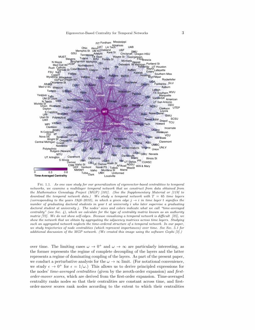
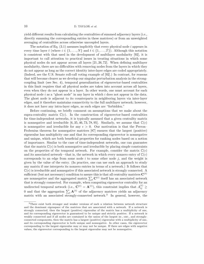
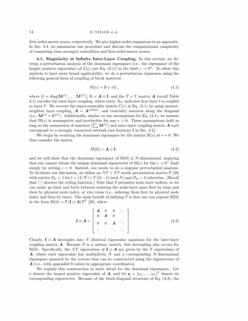
Fig. 1.1. As one case study for our generalization of eigenvector-based centralities to temporalnetworks, we examine a multilayer temporal network that we construct from data obtained fromthe Mathematics Genealogy Project (MGP) [101]. (See the Supplementary Material or [119] todownload the temporal network data.) We study a temporal network with T = 65 time layers(corresponding to the years 1946–2010), in which a given edge j → i in time layer t signifies thenumber of graduating doctoral students in year t at university i who later supervise a graduatingdoctoral student at university j. The nodes’ sizes and colors indicate what we call “time-averagedcentrality” (see Sec. 4), which we calculate for the type of centrality matrix known as an authoritymatrix [73]. We do not show self-edges. Because visualizing a temporal network is difficult [25], weshow the network that we obtain by aggregating the adjacency matrices across time layers. Studyingsuch an aggregated network neglects the time-ordered structure of a temporal network. In our paper,we study trajectories of node centralities (which represent importances) over time. See Sec. 5.1 foradditional discussion of the MGP network. (We created this image using the software Gephi [3].)
over time. The limiting cases ω → 0+ and ω → ∞ are particularly interesting, asthe former represents the regime of complete decoupling of the layers and the latterrepresents a regime of dominating coupling of the layers. As part of the present paper,we conduct a perturbative analysis for the ω →∞ limit. (For notational convenience,we study ε → 0+ for ε = 1/ω.) This allows us to derive principled expressions forthe nodes’ time-averaged centralities (given by the zeroth-order expansion) and first-order-mover scores, which are derived from the first-order expansion. Time-averagedcentrality ranks nodes so that their centralities are constant across time, and first-order-mover scores rank nodes according to the extent to which their centralities
4 D. TAYLOR et al.
change in time. The computation of both time-averaged centralities and first-order-mover scores can be very efficient, because they only require the numerical solutionof linear-algebraic problems of size N ×N , which is ordinarily much smaller than thefull supra-centrality matrix of size NT × NT . Moreover, our perturbative approachalso alleviates the need to demand a particular choice of intra-layer coupling weight ω.Note that our methodology is a retrospective analysis and complements alternativetemporal generalizations that take a causal approach.
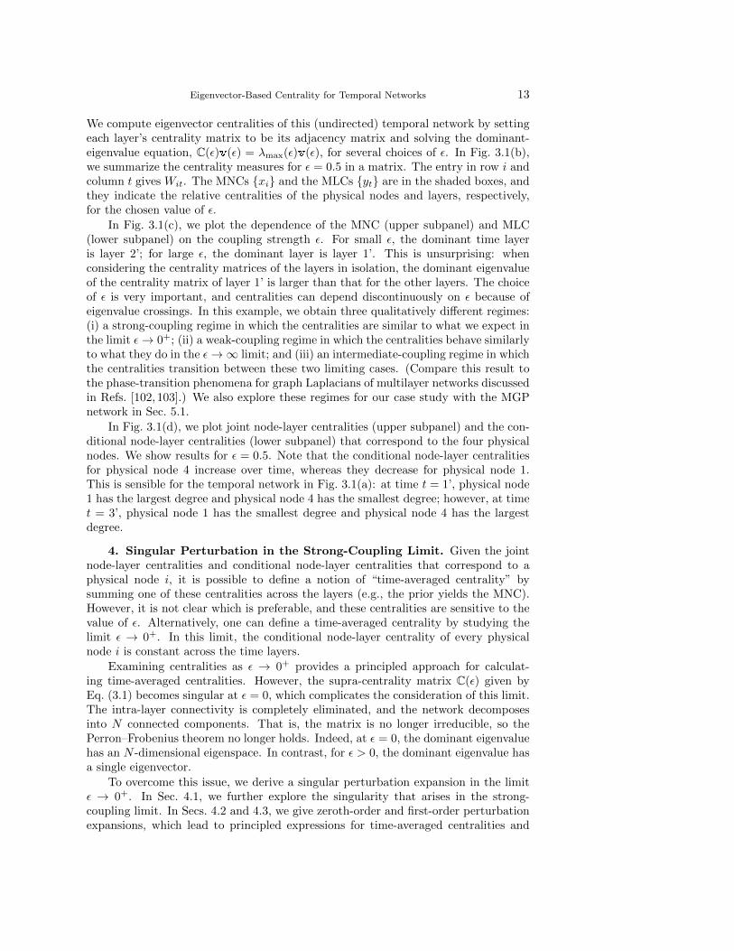
The remainder of our paper is organized as follows. In Sec. 2, we provide furtherbackground information. In Sec. 3, we present our generalization of eigenvector-basedcentralities for temporal networks. In Sec. 4, we derive principled expressions for time-averaged centralities and first-order-mover scores based on a singular perturbationexpansion. In Sec. 5, we illustrate our approach using three examples from empiricaldata: Ph.D. exchange using data from the Mathematics Genealogy Project [101](see Fig. 1.1), top billing in the Golden Age of Hollywood using the Internet MovieDatabase (IMDb) [63], and citations of United States Supreme Court decisions [40,64]. We conclude in Sec. 6 and provide further details of our perturbation expansionin the appendix.
2. Background Information and a Naive Approach. In Sec. 2.1, we pro-vide additional background information. In Sec. 2.2, we discuss a naive approachfor temporal eigenvector centrality that motivates our approach, and introduces ourmathematical notation and terminology.
2.1. Background Information. The analysis of large networks is ubiquitous inscience, engineering, medicine, and numerous other areas [94]. In the social sciences,for example, the abundance of data that describes the social behavior of individualsin academia [13, 15, 19, 93, 97, 101], show business [111], politics [8, 41, 42, 79, 100],and just about every other arena offers exciting avenues for the quantitative study ofsocial systems. For these and many other applications, it is important to develop (andimprove) mathematical techniques to extract concise and intuitive information fromlarge network data. From the interdisciplinary pursuit of what is now often callednetwork science, we know—from theory, computation, and data analysis—that manynetwork properties (e.g., degree heterogeneity, local clustering, community structure,and others [94]) have significant effects on dynamical processes on networks (e.g.,information dissemination and disease spreading) [20, 99, 125]. Although the vastmajority of research in network science has focused on time-independent networks,increased effort in recent years has aimed to generalize network analyses to “temporalnetworks” [4,60–62,69], in which network entities and/or interactions change in time.
In the study of time-independent networks, numerous centrality measures havebeen developed to try to quantify the relative importances of nodes [94, 125]. Thereare seemingly as many centrality measures as applications [6, 9, 10, 34, 43, 67], anddifferent types of centrality are appropriate for different situations. Importantly, onecan construct centrality measures not only from the direct consideration of networkstructure but also based on studying an appropriate dynamical process on a net-work [45,95,105]. In our paper, we focus on eigenvector-based centralities. Althougheigenvectors can obviously be used in different ways to introduce different notions ofcentrality, we reserve the term eigenvector-based centrality to refer only to centralitymeasures in which the nodes’ centralities are given by the entries of the dominanteigenvector of a matrix, which we call a centrality matrix. Centrality matrices in-clude a network’s adjacency matrix A (which indicates which nodes share a commonedge) and various functions of A [6, 35], such as the hub and authority matrices [73]
Eigenvector-Based Centrality for Temporal Networks 5
and PageRank matrices [46,78,95]. Eigenvector-based centralities reflect a network’sglobal structure and are often preferable to other types of centralities, because thereare a large number of computationally efficient algorithms for computing spectralproperties of matrices (e.g., the power method for computing the dominant eigenvec-tor [48]). An eigenvector-based centrality is also a key component to the function ofmajor Web search engines, including Google [46,73,95].
Although the study of centrality measures in time-independent networks has beeninsightful for numerous applications, most networks are time-dependent, and it isimportant to generalize centrality measures for temporal networks. This has been avery active area of research in recent years. Many approaches consider a temporalnetwork as a sequence of network layers, and initial studies examined centralitiesof such uncoupled individual network layers [11]. It was found, for example, thatin the absence of coupling between network layers, centrality scores can fluctuatesignificantly from one time step to the next due to stochasticity in the appearanceand disappearance of edges. Rankings can of course change over time (either slowly orrapidly). To give an example that is directly relevant to one of our case studies, it wasdemonstrated recently that uncoupled university rankings can fluctuate significantlyfrom year to year [115], which we consider to be a suboptimal description for thetemporal evolution of departmental prestige.
The most popular temporal extensions of centrality measures involve consider-ing notions of centrality based on paths in a time-independent network and gener-alizing them using time-respecting paths in a temporal network [74, 75]. We pointout temporal extensions to PageRank that have been introduced to counteract agebias [85, 124, 128], capture temporal changes for the external interests of nodes viadynamic teleportation [108], and study random walks taking place on temporal net-works [108]. We also highlight temporally extended versions of betweenness cen-trality [1, 71, 117, 127], closeness centrality [71, 96, 117, 127], Bonacich centrality [80],win/lose centrality [90], communicability [33,50,52], Katz centrality [51], and coveragecentrality [116]. These research efforts have extended centrality measures in differ-ent ways, which one can relate partly to the fact that one can define time-respectingpaths in different ways. A time-respecting path can allow one, several, or an unlim-ited number of edge traversals during a particular time step. Moreover, the lengthof a time-respecting path—which one can use to provide a notion of “distance” be-tween nodes—can also be measured in different ways [127]. For instance, the lengthof a time-respecting path can describe the number of edges that are traversed by thepath, latency between the initialization and termination times of the path, or a com-bination of such ideas. For temporal networks, even the notion of a “shortest path”lacks an unambiguous definition, which subsequently can also introduce ambiguityinto dynamical processes and network measures derived from them.
One common feature of existing generalizations of centralities for temporal net-works is that they illustrate the importance of studying an entire temporal network,as opposed to aggregating temporal layers into a single (time-independent) networkor analyzing the time layers in isolation from one another [60,61]. Specifically, study-ing a layer-aggregated network prevents one from studying centrality trajectories (i.e.,how centrality changes over time), and studying the time layers in isolation does notaccount for the temporal orderings of edges, which can be crucial for determiningcentralities in a temporal setting [33,38,50,51,84]. To provide additional context, wehighlight that dynamical processes can behave vastly differently on temporal versus
6 D. TAYLOR et al.
layer-aggregated networks.1 For example, a random walk—a process on which manyeigenvector-based centralities rely—on a temporal network is affected fundamentallyby the temporal ordering and time scale of the appearances and disappearances ofedges [57, 58, 60–62, 66]. Rankings, such as eigenvector-based centralities, that arederived from such dynamics are, in turn, affected fundamentally by the temporalstructure of the networks, and aggregation (as well as isolation) can lead to mislead-ing or even simply wrong results. Additionally, if one starts with a Markovian processon a temporal network and then aggregates the network, then in general one does notobtain a Markovian process [62], so fundamental (and often desirable) properties of adynamical process can be destroyed as a byproduct of neglecting a network’s inherenttemporal structure.
Finally, although extending centrality to temporal networks has become a veryactive research area, one should expect different generalizations of eigenvector-basedcentralities to be appropriate for different applications. Existing papers have notalways been clear about the modeling assumptions and tradeoffs of their approaches.
2.2. Naive Generalization of Eigenvector Centrality for Temporal Net-works. Before we present our primary approach in Sec. 3, it is instructive to considerone possible way to generalize eigenvector-based centralities. This example motivatesour approach and introduces mathematical notation and terminology. Importantly,it is naive in that it does not treat intra-layer edges and inter-layer edges as distincttypes of edges, which causes problems when the network layers are strongly coupled.
We use a multilayer representation of networks and seek to identify the mostcentral nodes of a temporal network with N distinct nodes (i.e., vertices or actors)across T time layers. We specify the network edges with a node-by-node-by-time
(N ×N × T ) adjacency tensor in which nonzero elements A(t)ij indicate the presence
and weight of the edge from node i to node j in time layer t. That is, the adjacencymatrix at time t is given by A(t). See Table 2.1 for a summary of our mathematicalnotation. We refer to node i in layer t as a node-layer pair (i, t) and node i (regardlessof layer) as a physical node. We are interested particularly in understanding thephysical nodes’ centrality trajectories through time.
It is tempting to reshape a network’s associated adjacency tensor into anNT×NT
1As discussed in, e.g., [26,72] and several references therein—and more recently in [27]—a similarissue arises more generally in multilayer networks, and one must also take into account the effects ofinter-layer edges (which are fundamentally different from intra-layer edges) when defining a dynamicalprocess on a multilayer network.
Table 2.1A summary of our mathematical notation.
Typeface Class Dimensionality
M matrix NT ×NTM matrix N ×NM matrix T × Tv vector NT × 1v vector N × 1v vector T × 1Mij scalar 1vi scalar 1
Eigenvector-Based Centrality for Temporal Networks 7
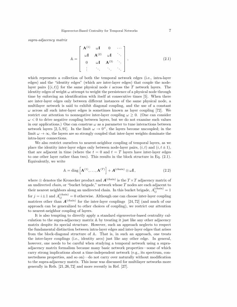
supra-adjacency matrix
A =
A(1) ωI 0 · · ·
ωI A(2) ωI. . .
0 ωI A(3) . . ....
. . .. . .
. . .
, (2.1)
which represents a collection of both the temporal network edges (i.e., intra-layeredges) and the “identity edges” (which are inter-layer edges) that couple the node-layer pairs {(i, t)} for the same physical node i across the T network layers. Theidentity edges of weight ω attempt to weight the persistence of a physical node throughtime by enforcing an identification with itself at consecutive times [5]. When thereare inter-layer edges only between different instances of the same physical node, amultilayer network is said to exhibit diagonal coupling, and the use of a constantω across all such inter-layer edges is sometimes known as layer coupling [72]. Werestrict our attention to nonnegative inter-layer coupling ω ≥ 0. (One can considerω < 0 to drive negative coupling between layers, but we do not examine such valuesin our applications.) One can construe ω as a parameter to tune interactions betweennetwork layers [2, 5, 91]. In the limit ω → 0+, the layers become uncoupled; in thelimit ω →∞, the layers are so strongly coupled that inter-layer weights dominate theintra-layer connections.
We also restrict ourselves to nearest-neighbor coupling of temporal layers, as weplace the identity inter-layer edges only between node-layer pairs, (i, t) and (i, t± 1),that are adjacent in time (where the t = 0 and t = T layers have inter-layer edgesto one other layer rather than two). This results in the block structure in Eq. (2.1).Equivalently, we write
A = diag[A(1), . . . ,A(T )
]+A(chain) ⊗ ωI , (2.2)
where ⊗ denotes the Kronecker product and A(chain) is the T ×T adjacency matrix ofan undirected chain, or “bucket brigade,” network whose T nodes are each adjacent to
their nearest neighbors along an undirected chain. In this bucket brigade, A(chain)ij = 1
for j = i±1 and A(chain)ij = 0 otherwise. Although one can choose inter-layer coupling
matrices other than A(chain) for the inter-layer couplings [24, 72] (and much of ourapproach can be generalized to other choices of coupling), we restrict our attentionto nearest-neighbor coupling of layers.
It is also tempting to directly apply a standard eigenvector-based centrality cal-culation to the supra-adjacency matrix A by treating it just like any other adjacencymatrix despite its special structure. However, such an approach neglects to respectthe fundamental distinction between intra-layer edges and inter-layer edges that arisesfrom the block-diagonal structure of A. That is, in such an approach, one treatsthe inter-layer couplings (i.e., identity arcs) just like any other edge. In general,however, one needs to be careful when studying a temporal network using a supra-adjacency matrix formalism because many basic network properties—some of whichcarry strong implications about a time-independent network (e.g., its spectrum, con-nectedness properties, and so on)—do not carry over naturally without modificationto the supra-adjacency matrix. This issue was discussed for multilayer networks moregenerally in Refs. [21, 26,72] and more recently in Ref. [27].
8 D. TAYLOR et al.
As a concrete example, let’s examine hub and authority centralities (i.e., HITS[73]) for a directed temporal network using the supra-adjacency matrix in Eq. (2.1) bysimply inserting it in place of a time-independent adjacency matrix in the standardformulas. In other words, we define the hub and authority matrices as AAT and ATA,respectively. At a glance, by noting that the inter-layer couplings are undirected butthat the intra-layer edges are directed, we already see that it is not clear whetherstandard interpretations of hub and authority rankings are still sensible. Nevertheless,one can try this approach for computing generalized hub and authority scores as thedominant eigenvectors of the symmetric matrices AAT and ATA. The simplicity ofthis approach makes it pleasing (and tempting), and the two symmetric matrices dohave a block structure. However, in contrast to A (whose blocks on and off of themain diagonal encode intra-layer and inter-layer edges, respectively), the blocks in thematrices AAT and ATA no longer separate neatly into describing only a single typeof edge (i.e., inter-layer versus intra-layer edges).
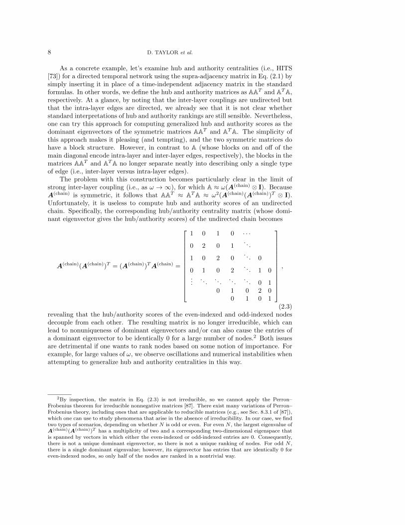
The problem with this construction becomes particularly clear in the limit ofstrong inter-layer coupling (i.e., as ω → ∞), for which A ≈ ω(A(chain) ⊗ I). BecauseA(chain) is symmetric, it follows that AAT ≈ ATA ≈ ω2(A(chain)(A(chain))T ⊗ I).Unfortunately, it is useless to compute hub and authority scores of an undirectedchain. Specifically, the corresponding hub/authority centrality matrix (whose domi-nant eigenvector gives the hub/authority scores) of the undirected chain becomes
A(chain)(A(chain))T = (A(chain))TA(chain) =
1 0 1 0 · · ·
0 2 0 1. . .
1 0 2 0. . . 0
0 1 0 2. . . 1 0
.... . .
. . .. . .
. . . 0 10 1 0 2 0
0 1 0 1
,
(2.3)revealing that the hub/authority scores of the even-indexed and odd-indexed nodesdecouple from each other. The resulting matrix is no longer irreducible, which canlead to nonuniqueness of dominant eigenvectors and/or can also cause the entries ofa dominant eigenvector to be identically 0 for a large number of nodes.2 Both issuesare detrimental if one wants to rank nodes based on some notion of importance. Forexample, for large values of ω, we observe oscillations and numerical instabilities whenattempting to generalize hub and authority centralities in this way.
2By inspection, the matrix in Eq. (2.3) is not irreducible, so we cannot apply the Perron–Frobenius theorem for irreducible nonnegative matrices [87]. There exist many variations of Perron–Frobenius theory, including ones that are applicable to reducible matrices (e.g., see Sec. 8.3.1 of [87]),which one can use to study phenomena that arise in the absence of irreducibility. In our case, we findtwo types of scenarios, depending on whether N is odd or even. For even N , the largest eigenvalue ofA(chain)(A(chain))T has a multiplicity of two and a corresponding two-dimensional eigenspace thatis spanned by vectors in which either the even-indexed or odd-indexed entries are 0. Consequently,there is not a unique dominant eigenvector, so there is not a unique ranking of nodes. For odd N ,there is a single dominant eigenvalue; however, its eigenvector has entries that are identically 0 foreven-indexed nodes, so only half of the nodes are ranked in a nontrivial way.
Eigenvector-Based Centrality for Temporal Networks 9
3. Temporal Coupling of Eigenvector-Based Centralities. In this section,we present a mathematical formalism for eigenvector-based centralities in temporalnetworks that treats inter-layer and intra-layer edges as distinct types of edges andensures appropriate behavior for all ω > 0. Similar to prior investigations using mul-tilayer representations of temporal networks [72, 92], we seek to develop an approachthat involves neither a heuristic averaging of centralities from individual layers norinvokes the centrality for a single network obtained from the aggregation of networklayers (e.g., summing the network edges across time).
The remainder of this section is organized as follows. In Sec. 3.1, we presentour methodology for temporal eigenvector-based centrality in terms of the dominanteigenvector of a supra-centrality matrix. In Sec. 3.2, we introduce the concepts of joint,marginal, and conditional centrality, and we use them to study decoupled centralitiesof nodes and layers based on the centralities of node-layer pairs. In Sec. 3.3, weillustrate these concepts for an example synthetic network.
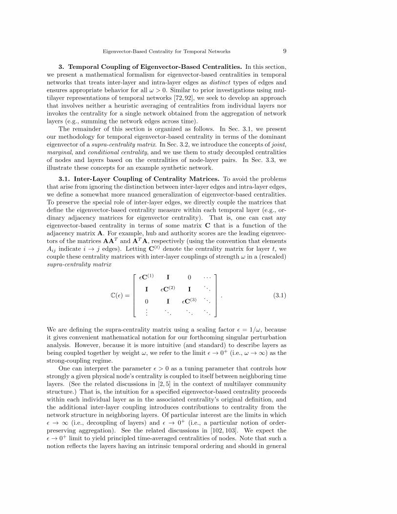
3.1. Inter-Layer Coupling of Centrality Matrices. To avoid the problemsthat arise from ignoring the distinction between inter-layer edges and intra-layer edges,we define a somewhat more nuanced generalization of eigenvector-based centralities.To preserve the special role of inter-layer edges, we directly couple the matrices thatdefine the eigenvector-based centrality measure within each temporal layer (e.g., or-dinary adjacency matrices for eigenvector centrality). That is, one can cast anyeigenvector-based centrality in terms of some matrix C that is a function of theadjacency matrix A. For example, hub and authority scores are the leading eigenvec-tors of the matrices AAT and ATA, respectively (using the convention that elementsAij indicate i → j edges). Letting C(t) denote the centrality matrix for layer t, wecouple these centrality matrices with inter-layer couplings of strength ω in a (rescaled)supra-centrality matrix
C(ε) =
εC(1) I 0 · · ·
I εC(2) I. . .
0 I εC(3) . . ....
. . .. . .
. . .
. (3.1)
We are defining the supra-centrality matrix using a scaling factor ε = 1/ω, becauseit gives convenient mathematical notation for our forthcoming singular perturbationanalysis. However, because it is more intuitive (and standard) to describe layers asbeing coupled together by weight ω, we refer to the limit ε→ 0+ (i.e., ω →∞) as thestrong-coupling regime.
One can interpret the parameter ε > 0 as a tuning parameter that controls howstrongly a given physical node’s centrality is coupled to itself between neighboring timelayers. (See the related discussions in [2, 5] in the context of multilayer communitystructure.) That is, the intuition for a specified eigenvector-based centrality proceedswithin each individual layer as in the associated centrality’s original definition, andthe additional inter-layer coupling introduces contributions to centrality from thenetwork structure in neighboring layers. Of particular interest are the limits in whichε → ∞ (i.e., decoupling of layers) and ε → 0+ (i.e., a particular notion of order-preserving aggregation). See the related discussions in [102, 103]. We expect theε→ 0+ limit to yield principled time-averaged centralities of nodes. Note that such anotion reflects the layers having an intrinsic temporal ordering and should in general
10 D. TAYLOR et al.
yield different results from calculating the centralities of summed adjacency layers (i.e.,directly summing the corresponding entries in these matrices) or from an unweightedaveraging of centralities across otherwise uncoupled layers.
The notation of Eq. (3.1) assumes implicitly that every physical node i appears inevery time layer t (where i ∈ {1, . . . , N} and t ∈ {1, . . . , T}). Although this notationis consistent with that used in the development of multilayer modularity [92], it isimportant to call attention to practical issues in treating situations in which somephysical nodes do not appear across all layers [21, 26, 72]. When defining multilayermodularity, there are no difficulties with removing nodes from the layers in which theydo not appear as long as the correct identity inter-layer edges are coded appropriately.(Indeed, see the U.S. Senate roll-call voting example of [92].) In contrast, for reasonsthat will become clearer as we develop our singular perturbation analysis in the strong-coupling limit (see Sec. 4), temporal generalization of eigenvector-based centralitiesin this limit requires that all physical nodes are taken into account across all layers,even when they do not appear in a layer. In other words, one must account for eachphysical node i as a “ghost node” in any layer in which i does not appear in the data.The ghost node is adjacent to its counterparts in neighboring layers via inter-layeredges, and it therefore maintains connectivity to the full multilayer network; however,it does not have any intra-layer edges, as such edges are “forbidden.”
Before continuing, we briefly comment on assumptions that we make about thesupra-centrality matrix C(ε). In the construction of eigenvector-based centralitiesfor time-independent networks, it is typically assumed that a given centrality matrixis nonnegative and irreducible [6, 35, 46, 73, 78, 95]. Similarly, we assume that C(ε)is nonnegative and irreducible for any ε > 0. Our motivation is that the Perron–Frobenius theorem for nonnegative matrices [87] ensures that the largest (positive)eigenvalue has multiplicity one and that its corresponding eigenvector is nonnegativeand unique, which are both beneficial properties for ranking nodes based on a notionof importance. Similar to the case of time-independent networks, one can guaranteethat the matrix C(ε) is both nonnegative and irreducible by placing simple constraintson the properties of the temporal network. For example, consider the matrix C(ε)and its associated network—that is, the network in which every nonzero entry of C(ε)corresponds to an edge from some node i to some other node j, and the weight isgiven by the value of the entry. (In practice, one can use such an approach to studyany matrix if one interprets its nonzero entries in terms of a network.) It follows thatC(ε) is irreducible and nonnegative if this associated network is strongly connected. Asufficient (but not necessary) condition to assure this is that all centrality matrices C(t)
are nonnegative and the aggregated matrix∑
t C(t) itself has an associated networkthat is strongly connected. For example, when computing eigenvector centrality for an
undirected temporal network (i.e., C(t) = A(t)), this constraint implies that A(t)ij ≥
0 and that the aggregation∑
t A(t) of the adjacency matrices yields an adjacencymatrix with an associated strongly-connected network.3 In general, however, the
3There exist both stronger and weaker versions of such a relation between network structureand the dominant eigenspace of the matrices that are associated with a network. If a network isstrongly connected, then the largest (positive) eigenvalue of the matrix has a multiplicity of one,and its corresponding eigenvector is guaranteed to be unique and strictly positive. If a network isweakly connected and if all nodes are contained in the union of the largest in-, out-, and strongly-connected components, then the matrix has a largest (positive) eigenvalue with a multiplicity of one,and its corresponding eigenvector is both unique and nonnegative. In other cases, the eigenvectorcorresponding to the largest eigenvalue may or may not be unique. If there are edges with negativevalues, the eigenvector corresponding to the largest eigenvalue may not be nonnegative.
Eigenvector-Based Centrality for Temporal Networks 11
irreducibility of C(ε) depends on that of the centrality matrices (i.e.,∑
t C(t)), ratherthan on the adjacency matrices.
Our assumption that C(ε) be irreducible places restrictions both on the set {C(t)}and on our choice for how to couple the layers. We choose to couple each timelayer t to both layers t + 1 and t − 1 (when present), so our temporal extension ofeigenvector centrality is non-causal; that is, the centralities are coupled both forwardand backward in time. In principle, one could choose other strategies for coupling thelayers. Note, however, that a causal strategy in the absence of other features (e.g.,one could examine different types of “teleportation” [46]) forces C(ε) to be reducible,because the centralities of past network layers cannot depend on future layers.
3.2. Joint, Marginal and Conditional Centrality for Multilayer Net-works. We study the dominant eigenvector v(ε) of C(ε), with corresponding (andlargest positive) eigenvalue λmax(ε) [i.e, C(ε)v(ε) = λmax(ε)v(ε)]. The entries of thedominant eigenvector give the centralities of each node-layer pair (i, t); this repre-sents the centrality of physical node i at time t. The dominant eigenvector v(ε) of asupra-centrality matrix in Eq. (3.1) gives the centrality of node-layer pairs. That is,the eigenvalue entry vN(t−1)+i(ε) indicates the centrality of node i at time t. Sucha joint centrality, whether given by v(ε) or any other centrality for node-layer pairs,reflects information about the importances of both the nodes and the layers. Wedevelop a simple formalism to decouple these centralities. For concreteness, we usev(ε), but this approach can be applied to any centrality measure of node-layer pairsin a multilayer (e.g., temporal) network including those not based on eigenvectors.
Our approach is inspired by multivariate statistics: we define “joint”, “marginal”,and “conditional” centralities. Joint centrality describes the importances of node-layerpairs, marginal centrality describes the uncoupled centrality of either nodes or layers,and conditional centrality describes the importance of a node-layer pair as comparedto, for example, other node-layer pairs in that same layer.
To proceed, it is convenient to map the vector v(ε), which has length NT , to anN × T matrix W, which we define entry-wise by
Wit = vN(t−1)+i(ε) . (3.2)
The scalar Wit gives the joint centrality of the node-layer pair (i, t); that is, it indicatesthe centrality of node i at time t. We define the marginal node centrality (MNC) xiand marginal layer centrality (MLC) yt by
xi =∑t
Wit , yt =∑i
Wit . (3.3)
The values {xi} and {yt} indicate the importances of nodes and layers, respectively,for a particular choice of ε. Although we use the summation to compute marginalnode and layer centralities, one can also consider other aggregation methods. Wedefine the conditional centrality of node-layer pair (i, t), conditioned on layer t, by
Zit = Wit/yt . (3.4)
The scalar Zit indicates the importance of physical node i relative to other physicalnodes in layer t. For some applications, it can be beneficial to similarly study theconditional centrality of layers conditional on a given node, but we do not explorethis notion in the present paper. For a given node i ∈ {1, . . . , N} and time t ∈{1, . . . , T}, the sets {Wit} and {Zit} of centrality values indicate trajectories for how
12 D. TAYLOR et al.
0.4
0.6
0.8
1
TA
ε
Centrality Dependence on �
10−1
100
101
0
1
2
LC
we ight (�)
1 2 3
1 2 3 4
1 1 1
2 2 2
3 3 3
4 4 4
1
2
3
1’ 2’ 3’
4
MLC
MNC
Time Layer
Time Layers
Node
Index
0.3570 0.3392 0.1679
0.2516 0.3298 0.2357
0.2471 0.3207 0.2312
0.2655 0.3579 0.2927
1.1213 1.3476 0.9275
0.8641
0.8171
0.7990
0.9162
3.3964
(a) (b)
(c)
0
0.2
0.4
joint
ǫ
Centrality Trajectorie s
1 2 30
0.2
0.4
conditional
t ime (t )
1 2 3 4
1 2 3 4
(d)
Centralities for e = 0.5Temporal Network
1’ 2’ 3’
MLC
MN
C
’ ’ ’
’ ’ ’
-1
-1
-1
-1
-1
-1
-1
-1
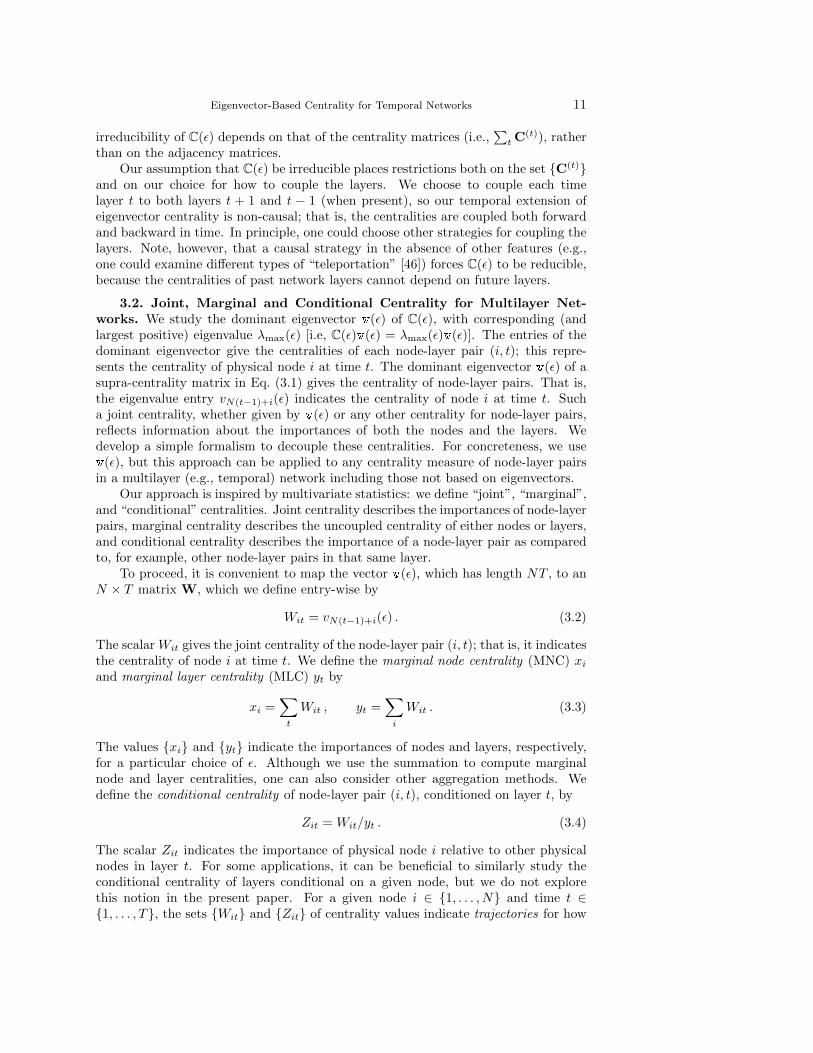
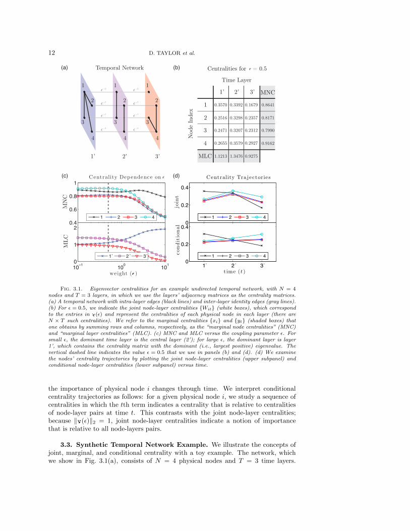
Fig. 3.1. Eigenvector centralities for an example undirected temporal network, with N = 4nodes and T = 3 layers, in which we use the layers’ adjacency matrices as the centrality matrices.(a) A temporal network with intra-layer edges (black lines) and inter-layer identity edges (gray lines).(b) For ε = 0.5, we indicate the joint node-layer centralities {Wit} (white boxes), which correspondto the entries in v(ε) and represent the centralities of each physical node in each layer (there areN × T such centralities). We refer to the marginal centralities {xi} and {yt} (shaded boxes) thatone obtains by summing rows and columns, respectively, as the “marginal node centralities” (MNC)and “marginal layer centralities” (MLC). (c) MNC and MLC versus the coupling parameter ε. Forsmall ε, the dominant time layer is the central layer (2’); for large ε, the dominant layer is layer1’, which contains the centrality matrix with the dominant (i.e., largest positive) eigenvalue. Thevertical dashed line indicates the value ε = 0.5 that we use in panels (b) and (d). (d) We examinethe nodes’ centrality trajectories by plotting the joint node-layer centralities (upper subpanel) andconditional node-layer centralities (lower subpanel) versus time.
the importance of physical node i changes through time. We interpret conditionalcentrality trajectories as follows: for a given physical node i, we study a sequence ofcentralities in which the tth term indicates a centrality that is relative to centralitiesof node-layer pairs at time t. This contrasts with the joint node-layer centralities;because ‖v(ε)‖2 = 1, joint node-layer centralities indicate a notion of importancethat is relative to all node-layers pairs.
3.3. Synthetic Temporal Network Example. We illustrate the concepts ofjoint, marginal, and conditional centrality with a toy example. The network, whichwe show in Fig. 3.1(a), consists of N = 4 physical nodes and T = 3 time layers.
Eigenvector-Based Centrality for Temporal Networks 13
We compute eigenvector centralities of this (undirected) temporal network by settingeach layer’s centrality matrix to be its adjacency matrix and solving the dominant-eigenvalue equation, C(ε)v(ε) = λmax(ε)v(ε), for several choices of ε. In Fig. 3.1(b),we summarize the centrality measures for ε = 0.5 in a matrix. The entry in row i andcolumn t gives Wit. The MNCs {xi} and the MLCs {yt} are in the shaded boxes, andthey indicate the relative centralities of the physical nodes and layers, respectively,for the chosen value of ε.
In Fig. 3.1(c), we plot the dependence of the MNC (upper subpanel) and MLC(lower subpanel) on the coupling strength ε. For small ε, the dominant time layeris layer 2’; for large ε, the dominant layer is layer 1’. This is unsurprising: whenconsidering the centrality matrices of the layers in isolation, the dominant eigenvalueof the centrality matrix of layer 1’ is larger than that for the other layers. The choiceof ε is very important, and centralities can depend discontinuously on ε because ofeigenvalue crossings. In this example, we obtain three qualitatively different regimes:(i) a strong-coupling regime in which the centralities are similar to what we expect inthe limit ε→ 0+; (ii) a weak-coupling regime in which the centralities behave similarlyto what they do in the ε→∞ limit; and (iii) an intermediate-coupling regime in whichthe centralities transition between these two limiting cases. (Compare this result tothe phase-transition phenomena for graph Laplacians of multilayer networks discussedin Refs. [102, 103].) We also explore these regimes for our case study with the MGPnetwork in Sec. 5.1.
In Fig. 3.1(d), we plot joint node-layer centralities (upper subpanel) and the con-ditional node-layer centralities (lower subpanel) that correspond to the four physicalnodes. We show results for ε = 0.5. Note that the conditional node-layer centralitiesfor physical node 4 increase over time, whereas they decrease for physical node 1.This is sensible for the temporal network in Fig. 3.1(a): at time t = 1’, physical node1 has the largest degree and physical node 4 has the smallest degree; however, at timet = 3’, physical node 1 has the smallest degree and physical node 4 has the largestdegree.
4. Singular Perturbation in the Strong-Coupling Limit. Given the jointnode-layer centralities and conditional node-layer centralities that correspond to aphysical node i, it is possible to define a notion of “time-averaged centrality” bysumming one of these centralities across the layers (e.g., the prior yields the MNC).However, it is not clear which is preferable, and these centralities are sensitive to thevalue of ε. Alternatively, one can define a time-averaged centrality by studying thelimit ε → 0+. In this limit, the conditional node-layer centrality of every physicalnode i is constant across the time layers.
Examining centralities as ε → 0+ provides a principled approach for calculat-ing time-averaged centralities. However, the supra-centrality matrix C(ε) given byEq. (3.1) becomes singular at ε = 0, which complicates the consideration of this limit.The intra-layer connectivity is completely eliminated, and the network decomposesinto N connected components. That is, the matrix is no longer irreducible, so thePerron–Frobenius theorem no longer holds. Indeed, at ε = 0, the dominant eigenvaluehas an N -dimensional eigenspace. In contrast, for ε > 0, the dominant eigenvalue hasa single eigenvector.
To overcome this issue, we derive a singular perturbation expansion in the limitε → 0+. In Sec. 4.1, we further explore the singularity that arises in the strong-coupling limit. In Secs. 4.2 and 4.3, we give zeroth-order and first-order perturbationexpansions, which lead to principled expressions for time-averaged centralities and
14 D. TAYLOR et al.
first-order-mover scores, respectively. We give higher-order expansions in an appendix.In Sec. 4.4, we summarize our procedure and discuss the computational complexityof computing time-averaged centralities and first-order-mover scores.
4.1. Singularity at Infinite Inter-Layer Coupling. In this section, we de-velop a perturbation analysis of the dominant eigenspace (i.e., the eigenspace of thelargest positive eigenvalue) of C(ε) [see Eq. (3.1)] in the limit ε → 0+. To allow thisanalysis to have more broad applicability, we do a perturbation expansion using thefollowing general form of coupling of block matrices:
M(ε) = B + εG , (4.1)
where G = diag[M(1), . . . ,M(T )], B = A ⊗ I, and the T × T matrix A (recall Table2.1) encodes the inter-layer coupling, where entry Att′ indicates how layer t is coupledto layer t′. We recover the supra-centrality matrix C(ε) in Eq. (3.1) by using nearest-neighbor layer coupling, A = A(chain), and centrality matrices along the diagonal(i.e., M(t) = C(t)). Additionally, similar to our assumptions for Eq. (3.1), we assumethat M(ε) is nonnegative and irreducible for any ε > 0. These assumptions hold aslong as the summation of matrices (
∑t M(t)) and inter-layer coupling matrix A each
correspond to a strongly connected network (see footnote 3 in Sec. 3.2).We begin by studying the dominant eigenspace for the matrix M(ε) at ε = 0. We
thus consider the matrix
M(0) = A⊗ I , (4.2)
and we will show that the dominant eigenspace of M(0) is N -dimensional, implyingthat one cannot obtain the unique dominant eigenvector of M(ε) for the ε→ 0+ limitsimply by setting ε = 0. Instead, one needs to do a singular perturbation analysis.To facilitate our discussion, we define an NT ×NT stride permutation matrix P [48]with entries Pkl = 1 for l = dk/Ne+T [(k−1) mod N ] and Pkl = 0 otherwise. (Recallthat d·e denotes the ceiling function.) Note that P permutes node-layer indices, so wecan easily go back and forth between ordering the node-layer pairs first by time andthen by physical node index, or vice versa (i.e., ordering them first by physical nodeindex and then by time). The main benefit of defining P is that one can express M(0)in the form M(0) = P (I⊗A)PT [28], where
I⊗A =
A 0 0 · · ·0 A 0
0 0 A. . .
.... . .
. . .
. (4.3)
Clearly, I ⊗ A decouples into N identical eigenvalue equations for the inter-layercoupling matrix A. Because P is a unitary matrix, this decoupling also occurs forM(0). Specifically, the NT eigenvalues of I ⊗ A are given by the T eigenvalues ofA, where each eigenvalue has multiplicity N and a corresponding N -dimensionaleigenspace spanned by the vectors that can be constructed using the eigenvectors ofA (i.e., with appended 0 values in appropriate coordinates).
We explain this construction in more detail for the dominant eigenspace. Letν denote the largest positive eigenvalue of A, and let u = [u1, . . . , uT ]T denote itscorresponding eigenvector. Because of the block-diagonal structure of Eq. (4.3), the
Eigenvector-Based Centrality for Temporal Networks 15
largest eigenvalue λ0 of I⊗A is λ0 = ν, and its corresponding eigenspace is spanned bythe N eigenvectors {ui}, where ui = [0T , . . . ,0T ,uT ,0T , . . . ,0T ]T . That is, the ithblock of ui is given by u, and all of the other blocks are vectors of zeros. Consequently,one can obtain the N dominant eigenvectors of M(0) = A⊗ I using the permutations{Pui}. That is, they have the general form
∑j αjPuj , where the constants {αi}
must satisfy∑
i α2i = 1 to ensure that the vector is normalized. Because there does
not exist a unique dominant eigenvector of M(0) since its dominant eigenspace is Ndimensional, we need to develop a singular perturbation analysis to obtain a uniquesolution for the dominant eigenvector of M(ε) in the ε→ 0+ limit.
When the network layers are coupled by an undirected chain network, the inter-layer coupling matrix is given by A = A(chain), which has N eigenvalues and eigen-vectors given by [82]
ν(chain) = 2 cos
(nπ
T + 1
), (4.4)
u(chain) =1√γn
[sin
(nπ
T + 1
), sin
(2nπ
T + 1
), . . . , sin
(Tnπ
T + 1
)]T, (4.5)
where n ∈ {1, ..., N} and the normalization constant is γn =∑T
t=1 sin2 [nπt/(T + 1)].Setting n = 1 gives the dominant eigenvalue and its corresponding eigenvector..
4.2. Zeroth-Order Expansion and Time-Averaged Centrality. In thissection, we study the zeroth-order expansion of the dominant eigenvector v(ε) inthe limit ε → 0+. As we now show, the conditional node-layer centralities {Zit}corresponding to a given physical node i become constant across time in this limit.(Recall our definitions of joint, marginal and conditional centralities in Sec. 3.2.) Foreach physical node, we refer to this limiting value as its time-averaged centrality. Byexamining the first-order expansion of v(ε) in the limit ε→ 0+, we show in Eq. (4.12)that one can obtain the time-averaged centralities as the eigenvector components cor-responding to the largest eigenvalue of a matrix of size N ×N .
We consider the dominant-eigenvalue equation
λmax(ε)v(ε) = M(ε)v(ε) = Bv(ε) + εGv(ε) . (4.6)
We expand λmax(ε) and v(ε) for small ε by writing λmax(ε) = λ0 + ελ1 + · · · and
v(ε) = v0 + εv1 + · · · to obtain kth-order approximations: λmax(ε) ≈∑k
j=0 εjλj and
v(ε) ≈∑k
j=0 εjvj . We use superscripts to indicate powers of ε in the terms in the
expansion, and we use subscripts for the terms that are multiplied by the power of ε.Note that λ0 and v0 respectively indicate the dominant eigenvalue and correspondingeigenvector in the limit ε→ 0+. Successive terms in these expansions represent higher-order derivatives of λmax(ε) and v(ε), and each term assumes appropriate smoothnessof these functions.
Our strategy is to develop consistent solutions to Eq. (4.6) for increasing valuesof k. Starting with the first-order approximation, we substitute λmax(ε) ≈ λ0 + ελ1and v(ε) ≈ v0 + εv1 into Eq. (4.6) and collect the zeroth-order and first-order termsin ε to obtain
(λ0I− B)v0 = 0 , (4.7)
(λ0I− B)v1 = (G− λ1I)v0 , (4.8)
16 D. TAYLOR et al.
where I is the NT ×NT identity matrix. Equation (4.7) is exactly the system that westudied in Sec. 4.1 [see Eq. (4.1) with ε = 0], where we found that the operator λ0I−Bis singular and has an N -dimensional null space. (This is the dominant eigenspace ofB.) We also found that Eq. (4.7) has a general solution of the form
λ0 = ν, v0 =∑j
αjPuj , (4.9)
where {αi} are constants that satisfy the constraint that v0 has magnitude 1 (i.e.,∑i α
2i = 1). We defined ui just below Eq. (4.3).
To find the set {αi} of unique constants that determine v0, we seek a solvabilitycondition in the first-order terms. Using the fact that the null space of λ0I − B isspan(Pu1, . . . ,PuN ) for any physical node i, it follows that (Pui)
T (λ0I− B)v1 = 0,and left-multiplying Eq. (4.8) by (Pui)
T leads to
uTi PTGv0 = λ1u
Ti PT
v0 . (4.10)
Using the solution of v0 in Eq. (4.9), we obtain∑j
αjuTi PTGPuj = λ1
∑j
αjuTi PTPuj = λ1αi , (4.11)
because PTP = PPT = I and uTi uj = δij , where δij is the Kronecker delta. Letting
α = [α1, . . . , αN ]T , Eq. (4.11) corresponds to an N -dimensional eigenvalue equation,
X(1)α = λ1α , (4.12)
where the matrix X(1) has elements
X(1)ij = u
Ti PTGPuj =
∑t
M(t)ij u
2t . (4.13)
Our assumption that M(ε) is nonnegative and irreducible for any ε > 0 ensures thatX(1) is also nonnegative and irreducible. By the Perron–Frobenius theorem for non-negative matrices [87], the largest positive eigenvalue λ1 of X(1) has a multiplicity ofone, and its eigenvector α is unique and has nonnegative entries. (See Sec. 3.1 andfootnote 3.) We normalize the solution α to Eq. (4.12) by
∑i α
2i = 1 and substitute
the normalized solution into Eq. (4.9) to obtain the zeroth-order term v0.When the layers are coupled by an undirected chain and the block matrices are
the layers’ centrality matrices (i.e., M(t) = C(t)), we obtain
X(1)ij = γ−11
∑t
C(t)ij sin2
(πt
T + 1
), (4.14)
where γ1 =∑T
t=1 sin2 (πt/(T + 1)) is the normalization constant for the dominanteigenvector u(chain) given by n = 1 in Eq. (4.5). In this case, recall that the vectorv0 is the dominant eigenvector of C(ε) in the limit ε → 0+ and gives the joint node-layer centralities in this limit. By inspection, we see that the elements of v0 areαi sin(πt/(T + 1)) for node-layer pair (i, t). Because these correspond to the limitingε→ 0+ entries of vector v(ε), they are independent of ε. At the same time, conditionalcentrality of node-layer pair (i, t) is αi (up to a normalization constant), independentof the layer t. That is, the conditional node centrality trajectories become constant
Eigenvector-Based Centrality for Temporal Networks 17
across time in the limit ε → 0+. These values of {αi} arise naturally from ourperturbative expansion in the supra-centrality framework, independently of the valueof ε. By contrast, recall that the marginal node centralities (MNCs) reflect averagingthe joint centralities across time layers for a specific choice of ε. Accordingly, wehereafter refer to the entry αi in the vector α as the time-averaged node centralityof physical node i. Because our approach can also be applied to multilayer networksthat are not necessarily temporal, we call αi the layer-averaged node centrality forthese situations.
4.3. First-Order Expansion and First-Order-Mover Scores. In this sec-tion, we show that the first-order expansion of Eq. (4.6) leads to a linear system [seeEq. (4.24)], which we solve to obtain a measurement of the variation over time of eachphysical node’s centrality trajectory [see Eq. (4.26)]. Specifically, as one increasesε above 0+, the first-order expansion, (which accounts for first derivatives with re-spect to ε), captures the dominant changes in centrality trajectories for small valuesof ε. (In the appendix, we derive expressions for higher-order terms that account forhigher-order derivatives with respect to ε.)
In Sec. 4.2, we derived closed-form expressions for λ0 and v0 and an eigenvalueequation satisfied by λ1. We now solve for v1 to complete our first-order approxi-mation. For notational convenience, we define L0 = λ0I − B and L1 = G − λ1I, soEq. (4.8) becomes L0v1 = L1v0. Letting L†0 denote the Moore–Penrose pseudoinverseof L0, we write
v1 = L†0L1v0 +∑j
βjPuj = L†0Gv0 +∑j
βjPuj . (4.15)
We simplify the first term in Eq. (4.15) using L1 = G− λ1I and v0 =∑
j αjPuj and
noting that each vector Puj lies in the null space of each of the matrices L0 and L†0.The second term in Eq. (4.15) accounts for the projection of v1 onto the null spaceof L0, where the constants βi = (Pui)
Tv1 indicate the projections onto the spanningvectors of the null space. To ensure numerical stability and computational efficiencyin practice, we calculate L†0 using the identity [28]
L†0 = (λ0I−A⊗ I)†
= (λ0I −A)† ⊗ I . (4.16)
Note that L†0 depends only on the inter-layer coupling matrix A (e.g., for nearest-neighbor-in-time coupling, A = A(chain)), which one can compute and save in memoryprior to analyzing network data.
Just as we examined first-order terms to solve for constants {αi}, we now seeka solvability condition in the second-order terms to determine {βi} in Eq. (4.15).Substituting λmax(ε) = λ0 + ελ1 + ε2λ2 and v(ε) = v0 + εv1 + ε2v2 into Eq. (4.6) andcollecting the second-order terms yields
L0v2 = L1v1 − λ2v0 . (4.17)
Similar to before, we left-multiply Eq. (4.17) by (Pui)T and require both sides to be
identically 0 to obtain
λ2uTi PT
v0 = uTi PTL1v1 = u
Ti PTGv1 − λ1uT
i PTv1. (4.18)
Using αi = uTi PTv0 and βi = uT
i PTv1, it then follows that
λ2αi + λ1βi = uTi PTGv1 . (4.19)
18 D. TAYLOR et al.
Substituting the expressions for v0 from Eq. (4.9) and v1 from Eq. (4.15) intoEq. (4.19) then yields
λ2αi + λ1βi =∑j
αjuTi PTGL†0GPuj +
∑j
βjuTi PTGPuj . (4.20)
After some rearranging, we obtain
(X(1) − λ1I)β = (λ2I−X(2))α , (4.21)
where the matrix X(1) was defined by Eq. (4.13), and the elements of the matrix X(2)
are
X(2)ij = u
Ti PTGL†0GPuj . (4.22)
Recalling that we determined α as the solution of X(1)α = λ1α such that∑
i α2i = 1,
we left-multiply Eq. (4.21) by αT to obtain
λ2 = αTX(2)α . (4.23)
We thereby obtain
β = (X(1) − λ1I)†(λ2I−X(2))α+ bα , (4.24)
where the constant b = αTβ describes the (possibly nonzero) projection of β ontothe null space of (X(1) − λ1I) [see Eq. (4.12)].
We now show that b = 0 in Eq. (4.24), by virtue of the requirement that theeigenvector obtained at first-order has a norm of 1. That is, we require that 1 =‖v0 + εv1‖2 = ‖v0‖2 + 2ε〈v0,v1〉 + O(ε2). However, ‖v0‖2 = 1, so 〈v0,v1〉 = 0,where we use the notation 〈·, ·〉 to denote the dot product between inputs. Using thedefinitions of v0 and v1, we see that
0 = 〈v0,v1〉 =
⟨∑j
αjPuj , L†0Gv0 +∑j
βjPuj
⟩=∑j
αjβj = b , (4.25)
because the vectors {Puj} are orthonormal and lie in the null space of L0. (In other
words, (Pui)TPuj = δij and (Pui)
TL†0 = 0.)
In practice, we solve Eq. (4.24) using a linear solver (see, e.g., [48]) rather thanthe pseudoinverse to avoid computing the inverse of (X(1)−λ1I). We then ensure thatthe solution is orthogonal to α by projecting it onto the subspace that is orthogonalto α.
One can substitute the solution β to Eq. (4.24) with b = 0 into Eq. (4.15) toobtain the first-order term v1 in the expansion for v(ε). This first-order term, whichyields the strongest temporal variation of the conditional centralities at small ε, is aconcise representation of temporal changes in centrality. There are multiple possibleways to use v1 to quantify the role of physical node i across the T layers. We define ameasure mi that equals the square root of the sum of the squares of the entries in v1
Eigenvector-Based Centrality for Temporal Networks 19
that correspond to physical node i. Specifically, we define the first-order-mover scoremi ≥ 0 of physical node i by
m2i = v
T1 PIiPT
v1
= β2i +
(L†0Gv0
)TPIiPTL†0Gv0
= β2i +
T∑t=1
([L†0Gv0]i+t(N−1)
)2, (4.26)
where [·]i denotes the ith entry in a vector and Ii = diag[0, . . . , 0, I, 0, . . . , 0] is amatrix of size NT × NT that contains all 0 entries except for the ith block, whichis an identity matrix I of size T × T . In other words, we measure the variationof v1 with respect to a physical node i by examining the 2-norm of the entries inv1 that correspond to the node-layer pairs (i, t) that are relevant to physical nodei (i.e., entries j such that j = N(t − 1) + i, with t = 1, . . . , T ). In principle, onecan also use a different vector norm or a heuristic method for aggregating centrality.Our choice has the virtue that it is mathematically consistent with our definition forthe time-averaged centralities {αi} [see Eq. (4.12)]. Specifically, α2
i = vT0 PIiPTv0.
Therefore, one can naturally extend our approach for quantifying the contributionof the first-order correction given by Eq. (4.26) to higher-order corrections. We alsonote that first-order-mover scores rank the nodes according to the magnitudes of theircorresponding entries in v1. Therefore, the associated centralities v(ε) can eitherincrease or decrease over time. One can easily check whether there is an increase ora decrease by examining the corresponding entries of v(ε).
4.4. Procedure for Computing Time-Averaged Centrality and First-Order-Mover Scores. We summarize our procedure for computing time-averagedcentrality and first-order-mover scores:
1. Construct the matrix X(1) using Eq. (4.14):
X(1)ij = γ−11
∑t
C(t)ij sin2
(πt
T + 1
).
When layers are coupled by a layer-adjacency matrix A (which is not nec-
essarily an undirected chain A(chain)), it follows that X(1)ij = uT
i PTGPuj ,
where G = diag[C(1), . . . ,C(T )] and P and ui are defined just before andafter, respectively, Eq. (4.3).
2. Solve for the time-averaged centralities {αi} using Eq. (4.12):
X(1)α = λ1α .
3. Construct the matrix X(2) using Eq. (4.22):
X(2)ij = u
Ti PTGL†0GPuj ,
where L†0 = (λ0I −A)† ⊗ I.
4. Solve for β in Eq. (4.21):
(X(1) − λ1I)β = (λ2I−X(2))α ,
where λ2 = αTX(2)α.
20 D. TAYLOR et al.
5. Solve for the first-order-mover scores {mi} using Eq. (4.26):
m2i = β2
i +
T∑t=1
([L†0Gv0]i+t(N−1)
)2,
where v0 =∑
j αjPuj .
We comment briefly on the computational costs of the above procedure. Thesupra-centrality matrix [see Eq. (3.1)], whose dominant eigenvector gives the jointnode-layer centralities, has size NT ×NT , and that can be problematic for large net-works with many time layers (i.e., when T � 1). The time-averaged node centralitiesare given by the solution to Eq. (4.12), which is a dominant eigenvalue problem for amatrix of size N ×N . To examine which physical nodes have centralities that changesignificantly over time, we examine the first-order-mover scores given by Eq. (4.26);this requires one to solve the N -dimensional linear system given by Eq. (4.24). Be-
cause L†0, G, and v0 are known prior to solving Eq. (4.24), one can directly computethe second term in Eq. (4.26). For sparse networks [i.e., those in which the numberof edges at a given time is O(N)], the matrices that we have discussed in this sectionare typically also sparse. One can thus solve Eqs. (4.12), (4.14), (4.21), (4.22), and(4.26) efficiently using data structures that are designed for sparse matrices, includ-ing direct methods [23], iterative methods [109], and methods designed for particularnetwork structures (e.g., nested dissection for planar networks [81]). In particular,the power method for computing a dominant eigenvalue and eigenvector of a sparsematrix reduces the per-iteration complexity from O(N2) to O(M), where M is thenumber of nonzero entries in the sparse matrix. However, the actual scaling can bemuch larger, because the number of iterations required for convergence depends onthe gap between the largest and second-largest eigenvalues.
5. Case Studies with Empirical Network Data. In this section, we examinetemporal centrality in case studies with three sets of empirical data: the MathematicsGenealogy Project (MGP; see Sec. 5.1) of Ph.D. receipt in the mathematical sciencesin U.S. universities, top billing in the Golden Age of Hollywood (GAH; see Sec. 5.2),and citations of U.S. Supreme Court decisions (SCD; see Sec. 5.3). We have postedMatlab software at [118] that implements our calculations and can be used to re-produce the results of this section.
Most of our calculations for these examples use a temporal generalization of huband authority scores [73], which are particularly appropriate for directed networks(such as our three examples). We also note that hub and authority scores havebeen used previously to examine time-independent faculty-hiring networks [39,93] andSupreme Court decisions [39, 41]. To illustrate a comparison with another choice ofcentrality, we also study a temporal generalization of PageRank for the MGP network.
We compute hub and authority scores independently using two supra-centralitymatrices, A(t)[A(t)]T and [A(t)]TA(t). For a single-layer network, it is possible tosimultaneously compute hub and authority scores by studying the single system[
0AT
A0
]. In general, however, a supra-centrality matrix that uses this alternative
formulation yields different time-dependent centralities from ones based on indepen-dent computations of hub and authority scores. For each centrality that we compute,we also examine the induced ranking of nodes in which the highest-ranked nodes (i.e.,those with ranks 1, 2, and so on) correspond to the largest centralities, whereas thelowest-ranked nodes correspond to the smallest centralities.
Eigenvector-Based Centrality for Temporal Networks 21
5.1. Doctoral Degree Exchange in the Mathematics Genealogy Project(MGP). Our first case study uses a network that encodes the exchange of mathemati-cians (and other mathematical scientists) who have obtained a Ph.D. (or equivalentdoctoral degree) between universities to study the academic prestige of those univer-sities. We study data provided by the Mathematics Genealogy Project (MGP) [101],which collects information for mathematicians (and members of related fields who arelisted in the MGP) with doctorates. For each mathematical scientist, the informa-tion includes graduation year, his/her official academic advisor(s), the degree-grantinguniversity, and a list of his/her students who have also obtained doctoral degrees. Asubset of the present authors previously utilized this data to approximate the flow ofdoctorates between universities—that is, a person graduates from one university andis then hired at a second university—and quantified the resulting hub and authorityscores for the total flow during a specified time period as a candidate measure of theseuniversities’ relative mathematical prestige [93]. Moreover, hub and authority scoreshave been used previously to study Ph.D. exchange networks in other disciplines [39].See [55] for a comparison of the hiring market for different academic disciplines, andsee [44, 83] for other analyses and visualization of data from the MGP. See [76] foran application of PageRank centrality to ranking world universities using data fromWikipedia.
It is well-documented that graduates typically obtain faculty positions at univer-sities that are either comparable to or less prestigious than the one from which theygraduate [13, 15, 19, 29, 39, 97], and we study university prestige as indicated by theexchange between universities of mathematicians with doctoral degrees. We general-ize a previous study of the MGP data in [93] by keeping the year that each facultymember graduated with his/her Ph.D. degree. We focus on the years 1946–2010,which includes all post-World War II information available in the data set.4 Thisyields T = 65 time layers, and we restrict our attention to a set of N = 227 U.S.universities that were connected during this period. To construct the network, wecreate directed intra-layer edges i→ j at time t to represent a doctoral degree in theMGP data awarded to a mathematical scientist from university j in year t who lateradvised at least one student at university i. Therefore, to contribute a directed edge,the mathematician must have at least one student in the MGP data. We weight edgesto indicate the number of doctorates from university j in year t awarded to facultywho later advise students at university i. Our construction aligns edge directions tobe opposite to that of the flow of people, so a node with large in-degree (i.e., withmany graduates who later advise students elsewhere) is considered both an academicauthority as well as an authority with respect to HITS centrality [73]. See Fig. 1.1 fora visualization of this network; due to the difficulty of visualizing temporal networks[25], we show a network corresponding to the aggregation
∑t A(t) of the adjacency
matrices. Although one could define the multilayer network in more intricate ways(e.g., by normalizing edge weights using the number of graduates) and examine howthe results vary for different choices, we wish to keep the present manuscript focusedon introducing and demonstrating our temporal generalization of eigenvector-basedcentralities. Therefore, we leave such detailed analyses for future work. We make theMGP temporal network available as a Supplementary Material and online at [119].
4The data set was provided to us in 2009, although it includes information up to 2010. The year2006 is the last year in which a Ph.D. degree was awarded to someone who was subsequently a Ph.D.advisor in the data, so it is also the last year in which intra-layers edges are present. Additionally,we decided to be optimistic and include Ph.D. degrees that were projected for the year 2010.
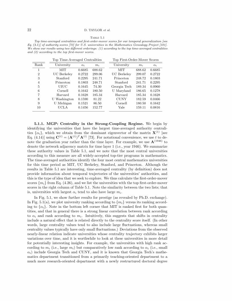
22 D. TAYLOR et al.
Table 5.1Top time-averaged centralities and first-order-mover scores for our temporal generalization [see
Eq. (3.1)] of authority scores [73] for U.S. universities in the Mathematics Genealogy Project [101].We show our results using two different orderings: (1) according to the top time-averaged centralitiesand (2) according to the top first-mover scores.
Top Time-Averaged Centralities Top First-Order-Mover Scores
Rank
12345678910
University αi mi
MIT 0.6685 688.62UC Berkeley 0.2722 299.06
Stanford 0.2295 241.71Princeton 0.1803 248.71
UIUC 0.1645 74.30Cornell 0.1642 180.50Harvard 0.1628 185.34
U Washington 0.1590 81.22U Michigan 0.1521 86.50
UCLA 0.1456 152.77
University mi αi
MIT 688.62 0.6685UC Berkeley 299.07 0.2722
Princeton 248.72 0.1803Stanford 241.71 0.2295
Georgia Tech 189.34 0.0960U Maryland 186.65 0.1278
Harvard 185.34 0.1628CUNY 182.59 0.0466Cornell 180.50 0.1642
Yale 159.11 0.0816
5.1.1. MGP: Centrality in the Strong-Coupling Regime. We begin byidentifying the universities that have the largest time-averaged authority centrali-ties {αi}, which we obtain from the dominant eigenvector of the matrix X(1) [seeEq. (4.14)] using C(t) = (A(t))TA(t) [73]. For notational convenience, we use t to de-note the graduation year rather than the time layer. For example, we use A(1946) todenote the network adjacency matrix for time layer 1 (i.e., year 1946). We summarizethese authority values in Table 5.1, and we note that the most central universitiesaccording to this measure are all widely-accepted top-tier programs in mathematics.The time-averaged authorities identify the four most central mathematics universitiesfor this time period as MIT, UC Berkeley, Stanford, and Princeton. Although theresults in Table 5.1 are interesting, time-averaged centrality (by definition) does notprovide information about temporal trajectories of the universities’ authorities, andthis is the type of idea that we seek to explore. We thus calculate the first-order-moverscores {mi} from Eq. (4.26), and we list the universities with the top first-order-moverscores in the right column of Table 5.1. Note the similarity between the two lists; thatis, universities with largest αi tend to also have large mi.
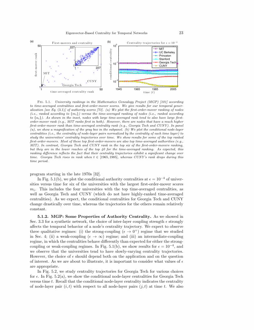
In Fig. 5.1, we show further results for prestige (as revealed by Ph.D. exchange).In Fig. 5.1(a), we plot university ranking according to {mi} versus its ranking accord-ing to {αi}. Note in the bottom left corner that MIT is ranked first for both quan-tities, and that in general there is a strong linear correlation between rank accordingto αi and rank according to mi. Intuitively, this suggests that shifts in centralityinclude a natural effect that is related directly to the centrality score itself. (In otherwords, large centrality values tend to also include large fluctuations, whereas smallcentrality values typically have only small fluctuations.) Deviations from the observednearly-linear relation indicate universities whose centrality trajectory exhibits largervariations over time, and it is worthwhile to look at these universities in more detailfor potentially interesting insights. For example, the universities with high rank ac-cording to mi (i.e., large mi) but comparatively low rank according to αi (i.e., smallαi) include Georgia Tech and CUNY, and it is known that Georgia Tech’s mathe-matics department transitioned from a primarily teaching-oriented department to amuch more research-oriented department with a newly restructured doctoral degree
Eigenvector-Based Centrality for Temporal Networks 23
1 501
50
t ime-averaged centrality rank
first-m
overrank
F irst-movers and centrality
1 2271
227
CUNY
(a)
MIT
Georgia Tech
1945 1965 1985 2005
10−2
10−1
100
t ime (t )
conditionalcentrality
C entrality tra jectorie s for ǫ = 10−4
MIT
UC Berkeley
Princeton
Stanford
Georgia Tech
CUNY
(b)
Fig. 5.1. University rankings in the Mathematics Genealogy Project (MGP) [101] accordingto time-averaged centralities and first-order-mover scores. We give results for our temporal gener-alization [see Eq. (3.1)] of authority scores [73]. (a) We plot the first-order-mover ranking of nodes(i.e., ranked according to {mi}) versus the time-averaged ranking of nodes (i.e., ranked accordingto {αi}). As shown in the inset, nodes with large time-averaged rank tend to also have large first-order-mover rank (e.g., MIT ranks first in both). However, there are nodes that have a much higherfirst-order-mover rank than time-averaged centrality rank (e.g., Georgia Tech and CUNY). In panel(a), we show a magnification of the gray box in the subpanel. (b) We plot the conditional node-layercentralities (i.e., the centrality of node-layer pairs normalized by the centrality of each time layer) tostudy the universities’ centrality trajectories over time. We show results for some of the top rankedfirst-order-movers. Most of these top first-order-movers are also top time-averaged authorities (e.g.,MIT). In contrast, Georgia Tech and CUNY rank in the top six of the first-order-movers ranking,but they are in the lower reaches of the top 40 for the time-averaged ranking. As expected, thisranking difference reflects the fact that their centrality trajectories exhibit a significant change overtime. Georgia Tech rises in rank when t ∈ [1965, 1985], whereas CUNY’s rank drops during thistime period.
program starting in the late 1970s [32].In Fig. 5.1(b), we plot the conditional authority centralities at ε = 10−4 of univer-
sities versus time for six of the universities with the largest first-order-mover scoresmi. This includes the four universities with the top time-averaged centralities, aswell as Georgia Tech and CUNY (which do not have highly-ranked time-averagedcentralities). As we expect, the conditional centralities for Georgia Tech and CUNYchange drastically over time, whereas the trajectories for the others remain relativelyconstant.
5.1.2. MGP: Some Properties of Authority Centrality. As we showed inSec. 3.3 for a synthetic network, the choice of inter-layer coupling strength ε stronglyaffects the temporal behavior of a node’s centrality trajectory. We expect to observethree qualitative regimes: (i) the strong-coupling (ε → 0+) regime that we studiedin Sec. 4; (ii) a weak-coupling (ε → ∞) regime; and (iii) an intermediate-couplingregime, in which the centralities behave differently than expected for either the strong-coupling or weak-coupling regimes. In Fig. 5.1(b), we show results for ε = 10−4, andwe observe that the universities tend to have slowly-varying centrality trajectories.However, the choice of ε should depend both on the application and on the questionof interest. As we are about to illustrate, it is important to consider what values of εare appropriate.
In Fig. 5.2, we study centrality trajectories for Georgia Tech for various choicesfor ε. In Fig. 5.2(a), we show the conditional node-layer centralities for Georgia Techversus time t. Recall that the conditional node-layer centrality indicates the centralityof node-layer pair (i, t) with respect to all node-layer pairs (j, t) at time t. We also
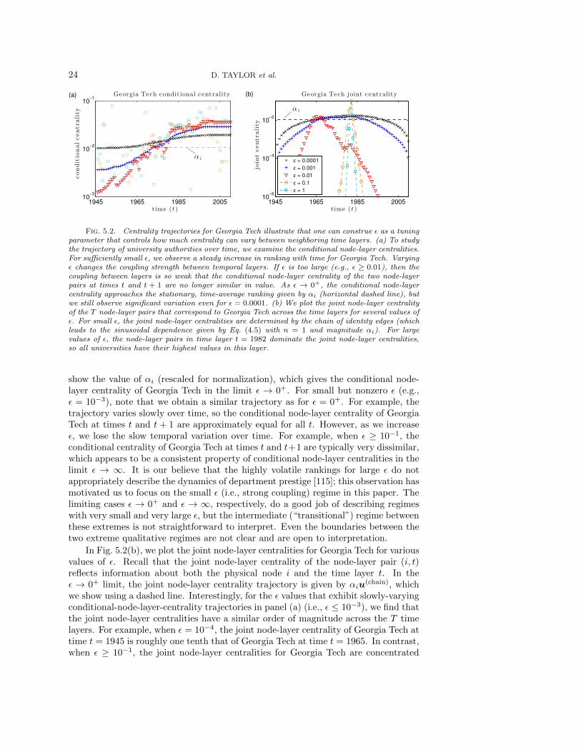
24 D. TAYLOR et al.
1945 1965 1985 200510
−3
10−2
10−1
Georgia Tech condit ional centrality
t ime (t )
conditionalcentrality
α i
(a)
1945 1965 1985 200510
−6
10−4
10−2
Georgia Tech joint centrality
t ime (t )
jointcentrality
ε = 0.0001
ε = 0.001
ε = 0.01
ε = 0.1
ε = 1
α i
(b)
Fig. 5.2. Centrality trajectories for Georgia Tech illustrate that one can construe ε as a tuningparameter that controls how much centrality can vary between neighboring time layers. (a) To studythe trajectory of university authorities over time, we examine the conditional node-layer centralities.For sufficiently small ε, we observe a steady increase in ranking with time for Georgia Tech. Varyingε changes the coupling strength between temporal layers. If ε is too large (e.g., ε ≥ 0.01), then thecoupling between layers is so weak that the conditional node-layer centrality of the two node-layerpairs at times t and t + 1 are no longer similar in value. As ε → 0+, the conditional node-layercentrality approaches the stationary, time-average ranking given by αi (horizontal dashed line), butwe still observe significant variation even for ε = 0.0001. (b) We plot the joint node-layer centralityof the T node-layer pairs that correspond to Georgia Tech across the time layers for several values ofε. For small ε, the joint node-layer centralities are determined by the chain of identity edges (whichleads to the sinusoidal dependence given by Eq. (4.5) with n = 1 and magnitude αi). For largevalues of ε, the node-layer pairs in time layer t = 1982 dominate the joint node-layer centralities,so all universities have their highest values in this layer.
show the value of αi (rescaled for normalization), which gives the conditional node-layer centrality of Georgia Tech in the limit ε → 0+. For small but nonzero ε (e.g.,ε = 10−3), note that we obtain a similar trajectory as for ε = 0+. For example, thetrajectory varies slowly over time, so the conditional node-layer centrality of GeorgiaTech at times t and t + 1 are approximately equal for all t. However, as we increaseε, we lose the slow temporal variation over time. For example, when ε ≥ 10−1, theconditional centrality of Georgia Tech at times t and t+1 are typically very dissimilar,which appears to be a consistent property of conditional node-layer centralities in thelimit ε → ∞. It is our believe that the highly volatile rankings for large ε do notappropriately describe the dynamics of department prestige [115]; this observation hasmotivated us to focus on the small ε (i.e., strong coupling) regime in this paper. Thelimiting cases ε → 0+ and ε → ∞, respectively, do a good job of describing regimeswith very small and very large ε, but the intermediate (“transitional”) regime betweenthese extremes is not straightforward to interpret. Even the boundaries between thetwo extreme qualitative regimes are not clear and are open to interpretation.
In Fig. 5.2(b), we plot the joint node-layer centralities for Georgia Tech for variousvalues of ε. Recall that the joint node-layer centrality of the node-layer pair (i, t)reflects information about both the physical node i and the time layer t. In theε → 0+ limit, the joint node-layer centrality trajectory is given by αiu
(chain), whichwe show using a dashed line. Interestingly, for the ε values that exhibit slowly-varyingconditional-node-layer-centrality trajectories in panel (a) (i.e., ε ≤ 10−3), we find thatthe joint node-layer centralities have a similar order of magnitude across the T timelayers. For example, when ε = 10−4, the joint node-layer centrality of Georgia Tech attime t = 1945 is roughly one tenth that of Georgia Tech at time t = 1965. In contrast,when ε ≥ 10−1, the joint node-layer centralities for Georgia Tech are concentrated
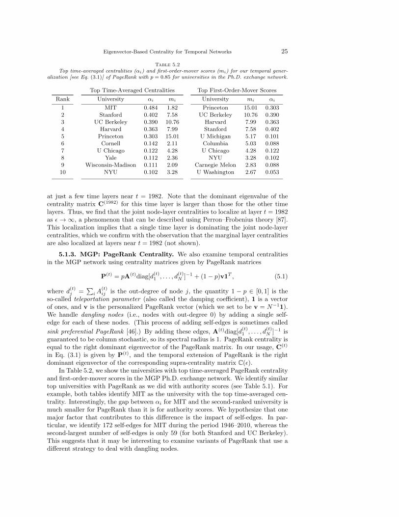
Eigenvector-Based Centrality for Temporal Networks 25
Table 5.2Top time-averaged centralities (αi) and first-order-mover scores (mi) for our temporal gener-
alization [see Eq. (3.1)] of PageRank with p = 0.85 for universities in the Ph.D. exchange network.
Top Time-Averaged Centralities Top First-Order-Mover Scores
Rank
12345678910
University αi mi
MIT 0.484 1.82Stanford 0.402 7.58
UC Berkeley 0.390 10.76Harvard 0.363 7.99
Princeton 0.303 15.01Cornell 0.142 2.11
U Chicago 0.122 4.28Yale 0.112 2.36
Wisconsin-Madison 0.111 2.09NYU 0.102 3.28
University mi αi
Princeton 15.01 0.303UC Berkeley 10.76 0.390
Harvard 7.99 0.363Stanford 7.58 0.402
U Michigan 5.17 0.101Columbia 5.03 0.088U Chicago 4.28 0.122
NYU 3.28 0.102Carnegie Melon 2.83 0.088U Washington 2.67 0.053
at just a few time layers near t = 1982. Note that the dominant eigenvalue of thecentrality matrix C(1982) for this time layer is larger than those for the other timelayers. Thus, we find that the joint node-layer centralities to localize at layer t = 1982as ε→∞, a phenomenon that can be described using Perron–Frobenius theory [87].This localization implies that a single time layer is dominating the joint node-layercentralities, which we confirm with the observation that the marginal layer centralitiesare also localized at layers near t = 1982 (not shown).
5.1.3. MGP: PageRank Centrality. We also examine temporal centralitiesin the MGP network using centrality matrices given by PageRank matrices
P(t) = pA(t)diag[d(t)1 , . . . , d
(t)N ]−1 + (1− p)v1T , (5.1)
where d(t)j =
∑iA
(t)ij is the out-degree of node j, the quantity 1 − p ∈ [0, 1] is the
so-called teleportation parameter (also called the damping coefficient), 1 is a vectorof ones, and v is the personalized PageRank vector (which we set to be v = N−11).We handle dangling nodes (i.e., nodes with out-degree 0) by adding a single self-edge for each of these nodes. (This process of adding self-edges is sometimes called
sink preferential PageRank [46].) By adding these edges, A(t)diag[d(t)1 , . . . , d
(t)N ]−1 is
guaranteed to be column stochastic, so its spectral radius is 1. PageRank centrality isequal to the right dominant eigenvector of the PageRank matrix. In our usage, C(t)
in Eq. (3.1) is given by P(t), and the temporal extension of PageRank is the rightdominant eigenvector of the corresponding supra-centrality matrix C(ε).
In Table 5.2, we show the universities with top time-averaged PageRank centralityand first-order-mover scores in the MGP Ph.D. exchange network. We identify similartop universities with PageRank as we did with authority scores (see Table 5.1). Forexample, both tables identify MIT as the university with the top time-averaged cen-trality. Interestingly, the gap between αi for MIT and the second-ranked university ismuch smaller for PageRank than it is for authority scores. We hypothesize that onemajor factor that contributes to this difference is the impact of self-edges. In par-ticular, we identify 172 self-edges for MIT during the period 1946–2010, whereas thesecond-largest number of self-edges is only 59 (for both Stanford and UC Berkeley).This suggests that it may be interesting to examine variants of PageRank that use adifferent strategy to deal with dangling nodes.
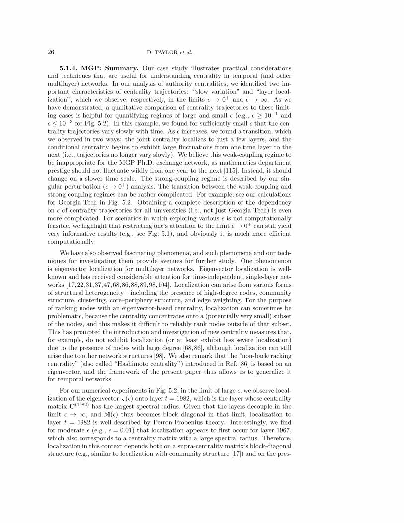
26 D. TAYLOR et al.
5.1.4. MGP: Summary. Our case study illustrates practical considerationsand techniques that are useful for understanding centrality in temporal (and othermultilayer) networks. In our analysis of authority centralities, we identified two im-portant characteristics of centrality trajectories: “slow variation” and “layer local-ization”, which we observe, respectively, in the limits ε → 0+ and ε → ∞. As wehave demonstrated, a qualitative comparison of centrality trajectories to these limit-ing cases is helpful for quantifying regimes of large and small ε (e.g., ε ≥ 10−1 andε ≤ 10−3 for Fig. 5.2). In this example, we found for sufficiently small ε that the cen-trality trajectories vary slowly with time. As ε increases, we found a transition, whichwe observed in two ways: the joint centrality localizes to just a few layers, and theconditional centrality begins to exhibit large fluctuations from one time layer to thenext (i.e., trajectories no longer vary slowly). We believe this weak-coupling regime tobe inappropriate for the MGP Ph.D. exchange network, as mathematics departmentprestige should not fluctuate wildly from one year to the next [115]. Instead, it shouldchange on a slower time scale. The strong-coupling regime is described by our sin-gular perturbation (ε→ 0+) analysis. The transition between the weak-coupling andstrong-coupling regimes can be rather complicated. For example, see our calculationsfor Georgia Tech in Fig. 5.2. Obtaining a complete description of the dependencyon ε of centrality trajectories for all universities (i.e., not just Georgia Tech) is evenmore complicated. For scenarios in which exploring various ε is not computationallyfeasible, we highlight that restricting one’s attention to the limit ε→ 0+ can still yieldvery informative results (e.g., see Fig. 5.1), and obviously it is much more efficientcomputationally.
We have also observed fascinating phenomena, and such phenomena and our tech-niques for investigating them provide avenues for further study. One phenomenonis eigenvector localization for multilayer networks. Eigenvector localization is well-known and has received considerable attention for time-independent, single-layer net-works [17,22,31,37,47,68,86,88,89,98,104]. Localization can arise from various formsof structural heterogeneity—including the presence of high-degree nodes, communitystructure, clustering, core–periphery structure, and edge weighting. For the purposeof ranking nodes with an eigenvector-based centrality, localization can sometimes beproblematic, because the centrality concentrates onto a (potentially very small) subsetof the nodes, and this makes it difficult to reliably rank nodes outside of that subset.This has prompted the introduction and investigation of new centrality measures that,for example, do not exhibit localization (or at least exhibit less severe localization)due to the presence of nodes with large degree [68,86], although localization can stillarise due to other network structures [98]. We also remark that the “non-backtrackingcentrality” (also called “Hashimoto centrality”) introduced in Ref. [86] is based on aneigenvector, and the framework of the present paper thus allows us to generalize itfor temporal networks.
For our numerical experiments in Fig. 5.2, in the limit of large ε, we observe local-ization of the eigenvector v(ε) onto layer t = 1982, which is the layer whose centralitymatrix C(1982) has the largest spectral radius. Given that the layers decouple in thelimit ε → ∞, and M(ε) thus becomes block diagonal in that limit, localization tolayer t = 1982 is well-described by Perron-Frobenius theory. Interestingly, we findfor moderate ε (e.g., ε = 0.01) that localization appears to first occur for layer 1967,which also corresponds to a centrality matrix with a large spectral radius. Therefore,localization in this context depends both on a supra-centrality matrix’s block-diagonalstructure (e.g., similar to localization with community structure [17]) and on the pres-
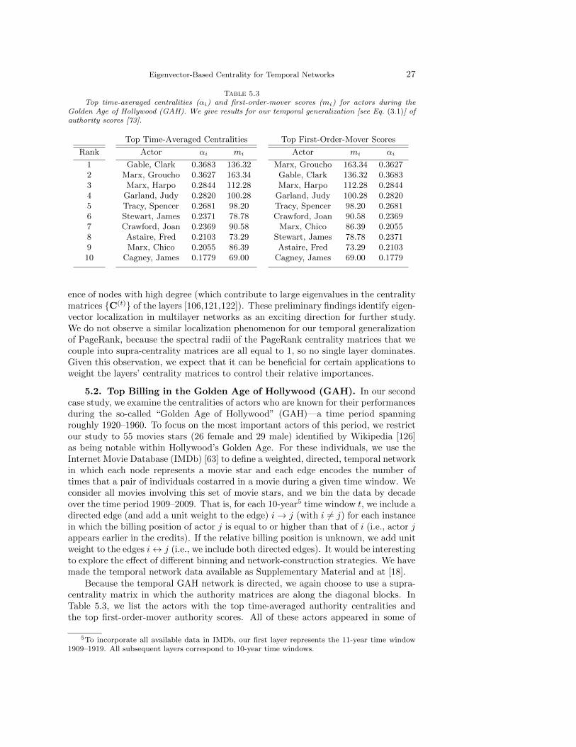
Eigenvector-Based Centrality for Temporal Networks 27
Table 5.3Top time-averaged centralities (αi) and first-order-mover scores (mi) for actors during the
Golden Age of Hollywood (GAH). We give results for our temporal generalization [see Eq. (3.1)] ofauthority scores [73].
Top Time-Averaged Centralities Top First-Order-Mover Scores
Rank
12345678910
Actor αi mi
Gable, Clark 0.3683 136.32Marx, Groucho 0.3627 163.34Marx, Harpo 0.2844 112.28
Garland, Judy 0.2820 100.28Tracy, Spencer 0.2681 98.20Stewart, James 0.2371 78.78Crawford, Joan 0.2369 90.58Astaire, Fred 0.2103 73.29Marx, Chico 0.2055 86.39
Cagney, James 0.1779 69.00
Actor mi αi
Marx, Groucho 163.34 0.3627Gable, Clark 136.32 0.3683Marx, Harpo 112.28 0.2844
Garland, Judy 100.28 0.2820Tracy, Spencer 98.20 0.2681Crawford, Joan 90.58 0.2369
Marx, Chico 86.39 0.2055Stewart, James 78.78 0.2371Astaire, Fred 73.29 0.2103
Cagney, James 69.00 0.1779
ence of nodes with high degree (which contribute to large eigenvalues in the centralitymatrices {C(t)} of the layers [106,121,122]). These preliminary findings identify eigen-vector localization in multilayer networks as an exciting direction for further study.We do not observe a similar localization phenomenon for our temporal generalizationof PageRank, because the spectral radii of the PageRank centrality matrices that wecouple into supra-centrality matrices are all equal to 1, so no single layer dominates.Given this observation, we expect that it can be beneficial for certain applications toweight the layers’ centrality matrices to control their relative importances.
5.2. Top Billing in the Golden Age of Hollywood (GAH). In our secondcase study, we examine the centralities of actors who are known for their performancesduring the so-called “Golden Age of Hollywood” (GAH)—a time period spanningroughly 1920–1960. To focus on the most important actors of this period, we restrictour study to 55 movies stars (26 female and 29 male) identified by Wikipedia [126]as being notable within Hollywood’s Golden Age. For these individuals, we use theInternet Movie Database (IMDb) [63] to define a weighted, directed, temporal networkin which each node represents a movie star and each edge encodes the number oftimes that a pair of individuals costarred in a movie during a given time window. Weconsider all movies involving this set of movie stars, and we bin the data by decadeover the time period 1909–2009. That is, for each 10-year5 time window t, we include adirected edge (and add a unit weight to the edge) i→ j (with i 6= j) for each instancein which the billing position of actor j is equal to or higher than that of i (i.e., actor jappears earlier in the credits). If the relative billing position is unknown, we add unitweight to the edges i↔ j (i.e., we include both directed edges). It would be interestingto explore the effect of different binning and network-construction strategies. We havemade the temporal network data available as Supplementary Material and at [18].
Because the temporal GAH network is directed, we again choose to use a supra-centrality matrix in which the authority matrices are along the diagonal blocks. InTable 5.3, we list the actors with the top time-averaged authority centralities andthe top first-order-mover authority scores. All of these actors appeared in some of
5To incorporate all available data in IMDb, our first layer represents the 11-year time window1909–1919. All subsequent layers correspond to 10-year time windows.
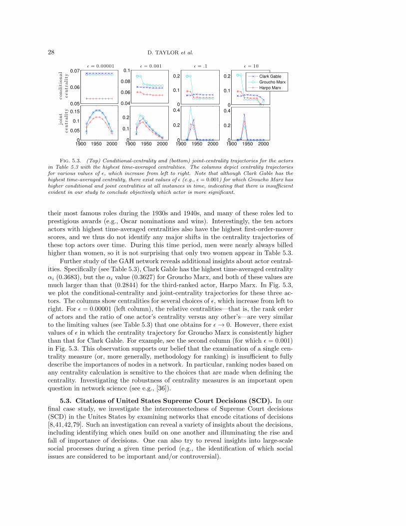
28 D. TAYLOR et al.
0.05
0.06
0.07
conditional
centrality
ǫ = 0.00001
1900 1950 20000
0.05
0.1
0.15
joint
centrality
0.04
0.06
0.08
0.1ǫ = 0.001
1900 1950 20000
0.1
0.2
0
0.1
0.2
ǫ = .1
1900 1950 20000
0.2
0.40
0.1
0.2
ǫ = 10
1900 1950 20000
0.2
0.4
Clark Gable
Groucho Marx
Harpo Marx
Fig. 5.3. (Top) Conditional-centrality and (bottom) joint-centrality trajectories for the actorsin Table 5.3 with the highest time-averaged centralities. The columns depict centrality trajectoriesfor various values of ε, which increase from left to right. Note that although Clark Gable has thehighest time-averaged centrality, there exist values of ε (e.g., ε = 0.001) for which Groucho Marx hashigher conditional and joint centralities at all instances in time, indicating that there is insufficientevident in our study to conclude objectively which actor is more significant.
their most famous roles during the 1930s and 1940s, and many of these roles led toprestigious awards (e.g., Oscar nominations and wins). Interestingly, the ten actorsactors with highest time-averaged centralities also have the highest first-order-moverscores, and we thus do not identify any major shifts in the centrality trajectories ofthese top actors over time. During this time period, men were nearly always billedhigher than women, so it is not surprising that only two women appear in Table 5.3.
Further study of the GAH network reveals additional insights about actor central-ities. Specifically (see Table 5.3), Clark Gable has the highest time-averaged centralityαi (0.3683), but the αi value (0.3627) for Groucho Marx, and both of these values aremuch larger than that (0.2844) for the third-ranked actor, Harpo Marx. In Fig. 5.3,we plot the conditional-centrality and joint-centrality trajectories for these three ac-tors. The columns show centralities for several choices of ε, which increase from left toright. For ε = 0.00001 (left column), the relative centralities—that is, the rank orderof actors and the ratio of one actor’s centrality versus any other’s—are very similarto the limiting values (see Table 5.3) that one obtains for ε→ 0. However, there existvalues of ε in which the centrality trajectory for Groucho Marx is consistently higherthan that for Clark Gable. For example, see the second column (for which ε = 0.001)in Fig. 5.3. This observation supports our belief that the examination of a single cen-trality measure (or, more generally, methodology for ranking) is insufficient to fullydescribe the importances of nodes in a network. In particular, ranking nodes based onany centrality calculation is sensitive to the choices that are made when defining thecentrality. Investigating the robustness of centrality measures is an important openquestion in network science (see e.g., [36]).
5.3. Citations of United States Supreme Court Decisions (SCD). In ourfinal case study, we investigate the interconnectedness of Supreme Court decisions(SCD) in the Unites States by examining networks that encode citations of decisions[8,41,42,79]. Such an investigation can reveal a variety of insights about the decisions,including identifying which ones build on one another and illuminating the rise andfall of importance of decisions. One can also try to reveal insights into large-scalesocial processes during a given time period (e.g., the identification of which socialissues are considered to be important and/or controversial).
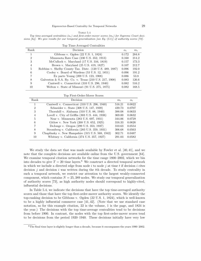
Eigenvector-Based Centrality for Temporal Networks 29
Table 5.4Top time-averaged centralities (αi) and first-order-mover scores (mi) for Supreme Court deci-
sions [64]. We give results for our temporal generalization [see Eq. (3.1)] of authority scores [73].
Top Time-Averaged Centralities
Rank Decision αi mi
1 Gibbons v. Ogden (22 U.S. 1, 1824) 0.172 284.82 Minnesota Rate Case (230 U.S. 352, 1913) 0.160 214.23 McCulloch v. Maryland (17 U.S. 316, 1819) 0.157 173.34 Brown v. Maryland (25 U.S. 419, 1827) 0.107 212.75 Robbins v. Shelby County Tax. Distr. (120 U.S. 489, 1887) 0.096 192.06 Cooley v. Board of Wardens (53 U.S. 12, 1851) 0.096 191.27 Ex parte Young (209 U.S. 123, 1908) 0.086 53.88 Galveston & S.A. Ry. Co. v. Texas (210 U.S. 217, 1908) 0.083 126.69 Cantwell v. Connecticut (310 U.S. 296, 1940) 0.082 516.210 Welton v. State of Missouri (91 U.S. 275, 1875) 0.082 168.5
Top First-Order-Mover Scores
Rank Decision mi αi
1 Cantwell v. Connecticut (310 U.S. 296, 1940) 516.21 0.08222 Schneider v. State (308 U.S. 147, 1939) 439.73 0.07073 Thornhill v. Alabama (310 U.S. 88, 1940) 388.08 0.06334 Lovell v. City of Griffin (303 U.S. 444, 1938) 369.00 0.06325 Near v. Minnesota (283 U.S. 697, 1931) 344.06 0.07296 Gitlow v. New York (268 U.S. 652, 1925) 316.33 0.06267 DeJonge v. Oregon (299 U.S. 353, 1937) 310.63 0.05548 Stromberg v. California (283 U.S. 359, 1931) 306.68 0.05639 Chaplinsky v. New Hampshire (315 U.S. 568, 1942) 302.71 0.048710 Whitney v. California (274 U.S. 357, 1927) 291.03 0.0582
We study the data set that was made available by Fowler et al. [40, 41], and wenote that the complete decisions are available online from the U.S. government [64].We examine temporal citation networks for the time range 1800–2002, which we bininto decades to give T = 20 time layers.6 We construct a directed temporal networkin which we include a directed edge from node i to node j at time t if decision i citesdecision j and decision i was written during the tth decade. To study centrality insuch a temporal network, we restrict our attention to the largest weakly-connectedcomponent, which contains N = 25, 389 nodes. We study our temporal generalizationof authority scores [73], as high authority nodes should correspond to highly-cited,influential decisions.
In Table 5.4, we indicate the decisions that have the top time-averaged authorityscores and those that have the top first-order-mover authority scores. We identify thetop-ranking decision to be Gibbons v. Ogden (22 U.S. 1, 1824), which is well-knownto be a highly influential commerce case [41, 42]. (Note that we use standard casenotation, so for this example citation, 22 is the volume, 1 is the page, and 1824 isthe year.) The decisions with the top time-average centralities tend to be decisionsfrom before 1900. In contrast, the nodes with the top first-order-mover scores tendto be decisions from the period 1920–1940. These decisions initially have very low
6The final time layer is slightly longer than a decade, because it encompasses the years 1990–2002.
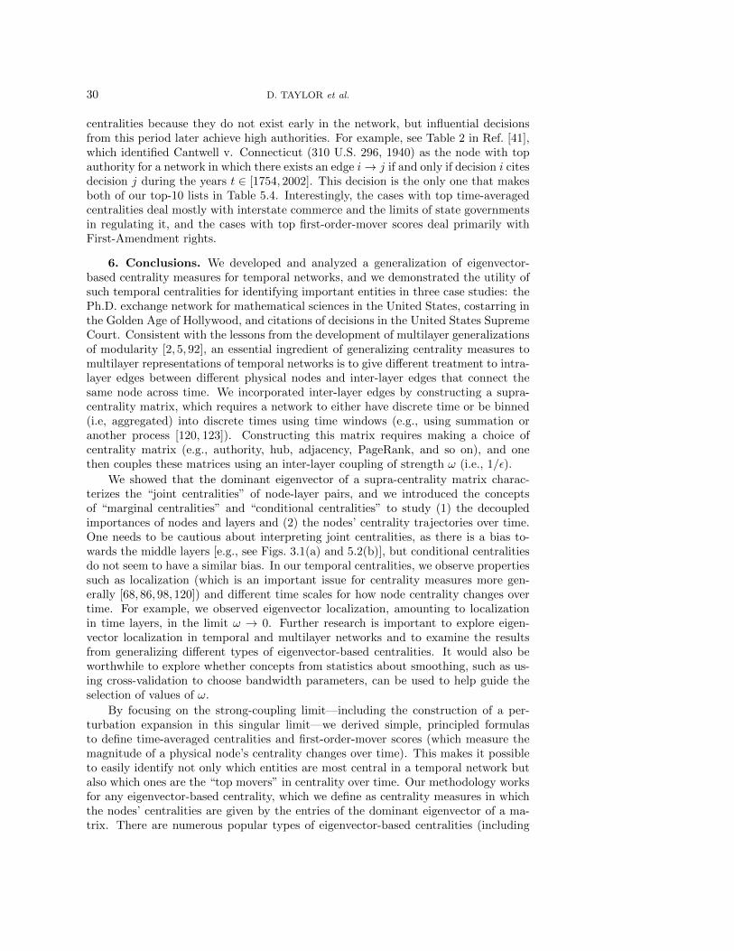
30 D. TAYLOR et al.
centralities because they do not exist early in the network, but influential decisionsfrom this period later achieve high authorities. For example, see Table 2 in Ref. [41],which identified Cantwell v. Connecticut (310 U.S. 296, 1940) as the node with topauthority for a network in which there exists an edge i→ j if and only if decision i citesdecision j during the years t ∈ [1754, 2002]. This decision is the only one that makesboth of our top-10 lists in Table 5.4. Interestingly, the cases with top time-averagedcentralities deal mostly with interstate commerce and the limits of state governmentsin regulating it, and the cases with top first-order-mover scores deal primarily withFirst-Amendment rights.
6. Conclusions. We developed and analyzed a generalization of eigenvector-based centrality measures for temporal networks, and we demonstrated the utility ofsuch temporal centralities for identifying important entities in three case studies: thePh.D. exchange network for mathematical sciences in the United States, costarring inthe Golden Age of Hollywood, and citations of decisions in the United States SupremeCourt. Consistent with the lessons from the development of multilayer generalizationsof modularity [2, 5, 92], an essential ingredient of generalizing centrality measures tomultilayer representations of temporal networks is to give different treatment to intra-layer edges between different physical nodes and inter-layer edges that connect thesame node across time. We incorporated inter-layer edges by constructing a supra-centrality matrix, which requires a network to either have discrete time or be binned(i.e, aggregated) into discrete times using time windows (e.g., using summation oranother process [120, 123]). Constructing this matrix requires making a choice ofcentrality matrix (e.g., authority, hub, adjacency, PageRank, and so on), and onethen couples these matrices using an inter-layer coupling of strength ω (i.e., 1/ε).
We showed that the dominant eigenvector of a supra-centrality matrix charac-terizes the “joint centralities” of node-layer pairs, and we introduced the conceptsof “marginal centralities” and “conditional centralities” to study (1) the decoupledimportances of nodes and layers and (2) the nodes’ centrality trajectories over time.One needs to be cautious about interpreting joint centralities, as there is a bias to-wards the middle layers [e.g., see Figs. 3.1(a) and 5.2(b)], but conditional centralitiesdo not seem to have a similar bias. In our temporal centralities, we observe propertiessuch as localization (which is an important issue for centrality measures more gen-erally [68, 86, 98, 120]) and different time scales for how node centrality changes overtime. For example, we observed eigenvector localization, amounting to localizationin time layers, in the limit ω → 0. Further research is important to explore eigen-vector localization in temporal and multilayer networks and to examine the resultsfrom generalizing different types of eigenvector-based centralities. It would also beworthwhile to explore whether concepts from statistics about smoothing, such as us-ing cross-validation to choose bandwidth parameters, can be used to help guide theselection of values of ω.
By focusing on the strong-coupling limit—including the construction of a per-turbation expansion in this singular limit—we derived simple, principled formulasto define time-averaged centralities and first-order-mover scores (which measure themagnitude of a physical node’s centrality changes over time). This makes it possibleto easily identify not only which entities are most central in a temporal network butalso which ones are the “top movers” in centrality over time. Our methodology worksfor any eigenvector-based centrality, which we define as centrality measures in whichthe nodes’ centralities are given by the entries of the dominant eigenvector of a ma-trix. There are numerous popular types of eigenvector-based centralities (including
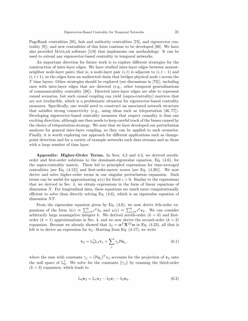
Eigenvector-Based Centrality for Temporal Networks 31
PageRank centralities [95], hub and authority centralities [73], and eigenvector cen-trality [9]), and new centralities of this form continue to be developed [86]. We havealso provided Matlab software [118] that implements our methodology. It can beused to extend any eigenvector-based centrality to temporal networks.
An important direction for future work is to explore different strategies for theconstruction of inter-layer edges. We have studied inter-layer edges between nearest-neighbor node-layer pairs; that is, a node-layer pair (i, t) is adjacent to (i, t− 1) and(i, t+1), so the edges form an undirected chain that bridges physical node i across theT time layers. Other strategies should be explored (see discussions in [72]), includingones with inter-layer edges that are directed (e.g., other temporal generalizationsof communicability centrality [38]). Directed inter-layer edges are able to representcausal scenarios, but such causal coupling can yield (supra-centrality) matrices thatare not irreducible, which is a problematic situation for eigenvector-based centralitymeasures. Specifically, one would need to construct an associated network structurethat satisfies strong connectivity (e.g., using ideas such as teleportation [46, 77]).Developing eigenvector-based centrality measures that respect causality is thus oneexciting direction, although one then needs to keep careful track of the biases caused bythe choice of teleportation strategy. We note that we have developed our perturbationanalyses for general inter-layer coupling, so they can be applied to such scenarios.Finally, it is worth exploring our approach for different applications such as change-point detection and for a variety of example networks such data streams and as thosewith a large number of time layer.
Appendix: Higher-Order Terms. In Secs. 4.2 and 4.3, we derived zeroth-order and first-order solutions to the dominant-eigenvalue equation, Eq. (4.6), forthe supra-centrality matrix. These led to principled expressions for time-averagedcentralities [see Eq. (4.12)] and first-order-mover scores [see Eq. (4.26)]. We nowderive and solve higher-order terms in our singular perturbation expansion. Suchterms can be useful for approximating v(ε) for fixed ε > 0. Similar to the expressionsthat we derived in Sec. 4, we obtain expressions in the form of linear equations ofdimension N . For longitudinal data, these equations are much more computationallyefficient to solve than directly solving Eq. (4.6), which is an eigenvalue equation ofdimension NT .
From the eigenvalue equation given by Eq. (4.6), we now derive kth-order ex-
pansions of the form λ(ε) ≈∑k
j=0 εkλk and v(ε) ≈
∑kj=0 ε
kvk. We can considerarbitrarily large nonnegative integers k. We derived zeroth-order (k = 0) and first-order (k = 1) approximations in Sec. 4, and we now derive the second-order (k = 2)expansion. Because we already showed that λ2 = αTX(2)α in Eq. (4.23), all that isleft is to derive an expression for v2. Starting from Eq. (4.17), we write
v2 = L†0L1v1 +∑j
γjPuj , (6.1)
where the sum with constants γj = (Puj)Tv2 accounts for the projection of v2 onto
the null space of L†0. We solve for the constants {γj} by examing the third-order(k = 3) expansion, which leads to
L0v3 = L1v2 − λ2v1 − λ3v0 . (6.2)
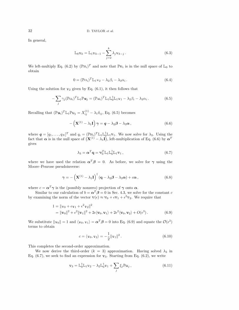
32 D. TAYLOR et al.
In general,
L0vk = L1vk−1 −k∑
j=2
λjvk−j . (6.3)
We left-multiply Eq. (6.2) by (Pui)T and note that Pui is in the null space of L0 to
obtain
0 = (Pui)TL1v2 − λ2βi − λ3αi . (6.4)
Using the solution for v2 given by Eq. (6.1), it then follows that
−∑j
γj(Pui)TL1Puj = (Pui)
TL1L†0L1v1 − λ2βi − λ3αi . (6.5)
Recalling that (Pui)TL1Puj = X
(1)ij − λ1δij , Eq. (6.5) becomes
−(X(1) − λ1I
)γ = q − λ2β − λ3α , (6.6)
where q = [q1, . . . , qN ]T and qi = (Pui)TL1L†0L1v1. We now solve for λ3. Using the
fact that α is in the null space of(X(1) − λ1I
), left-multiplication of Eq. (6.6) by αT
gives
λ3 = αTq = vT0 L1L†0L1v1 , (6.7)
where we have used the relation αTβ = 0. As before, we solve for γ using theMoore–Penrose pseudoinverse:
γ = −(X(1) − λ1I
)†(q− λ2β − λ3α) + cα , (6.8)
where c = αTγ is the (possibly nonzero) projection of γ onto α.Similar to our calculation of b = αTβ = 0 in Sec. 4.3, we solve for the constant c
by examining the norm of the vector v(ε) ≈ v0 + εv1 + ε2v2. We require that
1 = ‖v0 + εv1 + ε2v2‖2
= ‖v0‖2 + ε2‖v1‖2 + 2ε〈v0,v1〉+ 2ε2〈v0,v2〉+O(ε3) . (6.9)
We substitute ‖v0‖ = 1 and 〈v0,v1〉 = αTβ = 0 into Eq. (6.9) and equate the O(ε2)terms to obtain
c = 〈v0,v2〉 = −1
2‖v1‖2 . (6.10)
This completes the second-order approximation.We now derive the third-order (k = 3) approximation. Having solved λ3 in
Eq. (6.7), we seek to find an expression for v3. Starting from Eq. (6.2), we write
v3 = L†0L1v2 − λ2L†0v1 +∑j
ξjPuj , (6.11)
Eigenvector-Based Centrality for Temporal Networks 33
where the sum with constants ξj = (Puj)Tv3 accounts for the projection of v3 onto
the null space of L†0. Using the general form given by Eq. (6.3) for k = 4 yields
L0v4 = L1v3 − λ2v2 − λ3v1 − λ4v0 . (6.12)
We left-multiply Eq. (6.12) by (Pui)T to obtain
0 = (Pui)TL1v3 − λ2γi − λ3βi − λ4αi . (6.13)
We next substitute our solution for v3 given by Eq. (6.11) into Eq. (6.13) to obtain
−∑j
ξj(Pui)TL1Puj = (Pui)
TL1L†0 (L1v2 − λ2v1)− λ2γi − λ3βi − λ4αi , (6.14)
which in matrix notation is
(X(1) − λ1I)ξ = r− λ2γ − λ3β − λ4α , (6.15)
where we define r = [r1, . . . , rN ]T and ri = (Pui)TL1L†0 (L1v2 − λ2v1). As before, we
use the Moore–Penrose psuedoinverse to obtain
ξ = (X(1) − λ1I)†r− λ2(X(1) − λ1I)†γ − λ3(X(1) − λ1I)†β + dα , (6.16)
which uses the fact that α is in the null space of (X(1)−λ1I). The constant d = αT ξgives the projection of ξ onto α, and we calculate it by constraining the third-orderexpansion for v(ε) to have a norm of 1. This yields
1 = ‖v0 + εv1 + ε2v2 + ε3v3‖2
= ‖v0‖2 + ε2‖v1‖2 + 2ε〈v0,v1〉+ 2ε2〈v0,v2〉+ 2ε3〈v0,v3〉+ 2ε3〈v1,v2〉+O(ε4) . (6.17)
Recall that normalization of the zeroth-, first-, and second-order expansions, respec-tively, yields the relations ‖v0‖2 = 1, 〈v0,v1〉 = 0, and 〈v0,v2〉 = −(1/2)‖v1‖2.Equating the third-order terms in Eq. (6.17) then necessitates that
d = 〈v0,v3〉 = −〈v1,v2〉 . (6.18)
This completes the third-order approximation.In Figs. 6.1(a) and 6.1(b), we validate the above results using the MGP and GAH
networks, which we studied in Sec. 5.1 and Sec. 5.2, respectively. We plot the L2 errorfor the kth-order approximation ‖v(ε) −
∑kj=1 ε
jvk‖2 to the dominant eigenvector.We plot these approximations for several choices of k and several values of ε. Whenε is sufficiently small (i.e., ε / 3 × 10⁻⁴ for the MGP and ε / 10−3 for the GAH),we observe (as expected) that the error decreases with increasing k. We derived ourapproximate expressions in the limit ε→ 0+, so we only expect them to be accuratefor sufficiently small ε (although asymptotic expressions do have a long history ofoften being accurate even in many situations in which there are no guarantees forsuch success [56]). We also obtain the expected decay rates in the error as ε → 0+.We find linear decay for the zeroth-order approximation, quadratic decay for thefirst-order approximation, and so on.
REFERENCES
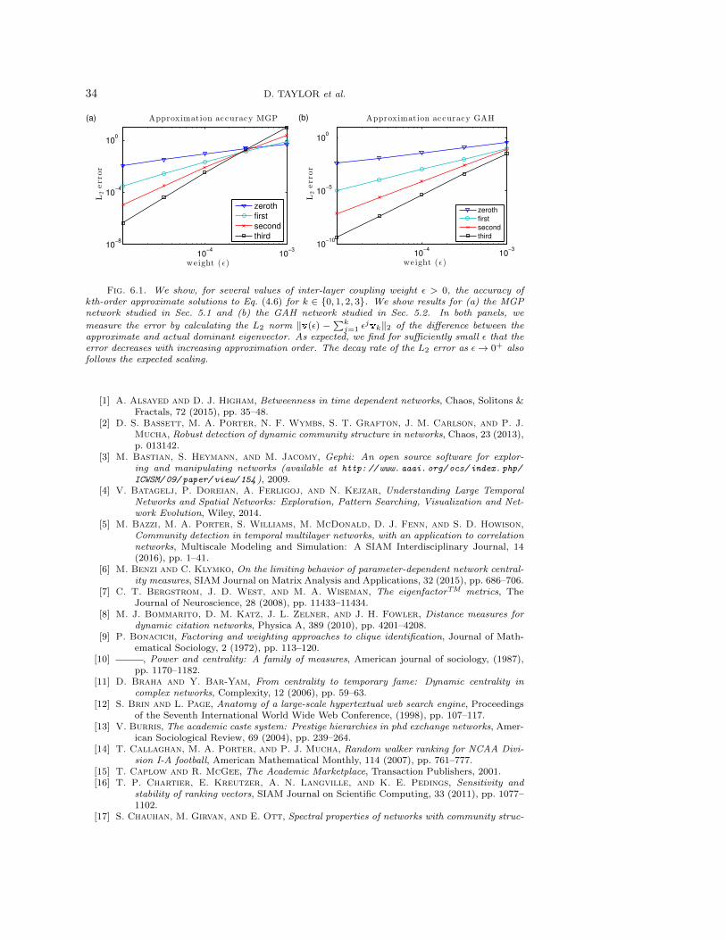
34 D. TAYLOR et al.
10−4
10−3
10−10
10−5
100
weight (ǫ)
L2error
Approximation accuracy GAH
zeroth
first
second
third
10−4
10−3
10−8
10−4
100
weight (ǫ)
L2error
Approximation accuracy MGP
zeroth
first
second
third
(a) (b)
Fig. 6.1. We show, for several values of inter-layer coupling weight ε > 0, the accuracy ofkth-order approximate solutions to Eq. (4.6) for k ∈ {0, 1, 2, 3}. We show results for (a) the MGPnetwork studied in Sec. 5.1 and (b) the GAH network studied in Sec. 5.2. In both panels, we
measure the error by calculating the L2 norm ‖v(ε) −∑k
j=1 εjvk‖2 of the difference between the
approximate and actual dominant eigenvector. As expected, we find for sufficiently small ε that theerror decreases with increasing approximation order. The decay rate of the L2 error as ε→ 0+ alsofollows the expected scaling.
[1] A. Alsayed and D. J. Higham, Betweenness in time dependent networks, Chaos, Solitons &Fractals, 72 (2015), pp. 35–48.
[2] D. S. Bassett, M. A. Porter, N. F. Wymbs, S. T. Grafton, J. M. Carlson, and P. J.Mucha, Robust detection of dynamic community structure in networks, Chaos, 23 (2013),p. 013142.
[3] M. Bastian, S. Heymann, and M. Jacomy, Gephi: An open source software for explor-ing and manipulating networks (available at http: // www. aaai. org/ ocs/ index. php/
ICWSM/ 09/ paper/ view/ 154 ), 2009.[4] V. Batagelj, P. Doreian, A. Ferligoj, and N. Kejzar, Understanding Large Temporal
Networks and Spatial Networks: Exploration, Pattern Searching, Visualization and Net-work Evolution, Wiley, 2014.
[5] M. Bazzi, M. A. Porter, S. Williams, M. McDonald, D. J. Fenn, and S. D. Howison,Community detection in temporal multilayer networks, with an application to correlationnetworks, Multiscale Modeling and Simulation: A SIAM Interdisciplinary Journal, 14(2016), pp. 1–41.
[6] M. Benzi and C. Klymko, On the limiting behavior of parameter-dependent network central-ity measures, SIAM Journal on Matrix Analysis and Applications, 32 (2015), pp. 686–706.
[7] C. T. Bergstrom, J. D. West, and M. A. Wiseman, The eigenfactorTM metrics, TheJournal of Neuroscience, 28 (2008), pp. 11433–11434.
[8] M. J. Bommarito, D. M. Katz, J. L. Zelner, and J. H. Fowler, Distance measures fordynamic citation networks, Physica A, 389 (2010), pp. 4201–4208.
[9] P. Bonacich, Factoring and weighting approaches to clique identification, Journal of Math-ematical Sociology, 2 (1972), pp. 113–120.
[10] , Power and centrality: A family of measures, American journal of sociology, (1987),pp. 1170–1182.
[11] D. Braha and Y. Bar-Yam, From centrality to temporary fame: Dynamic centrality incomplex networks, Complexity, 12 (2006), pp. 59–63.
[12] S. Brin and L. Page, Anatomy of a large-scale hypertextual web search engine, Proceedingsof the Seventh International World Wide Web Conference, (1998), pp. 107–117.
[13] V. Burris, The academic caste system: Prestige hierarchies in phd exchange networks, Amer-ican Sociological Review, 69 (2004), pp. 239–264.
[14] T. Callaghan, M. A. Porter, and P. J. Mucha, Random walker ranking for NCAA Divi-sion I-A football, American Mathematical Monthly, 114 (2007), pp. 761–777.
[15] T. Caplow and R. McGee, The Academic Marketplace, Transaction Publishers, 2001.[16] T. P. Chartier, E. Kreutzer, A. N. Langville, and K. E. Pedings, Sensitivity and
stability of ranking vectors, SIAM Journal on Scientific Computing, 33 (2011), pp. 1077–1102.
[17] S. Chauhan, M. Girvan, and E. Ott, Spectral properties of networks with community struc-
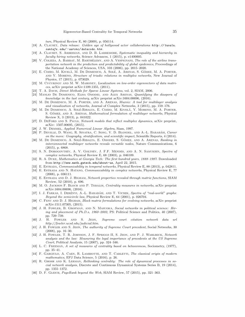
Eigenvector-Based Centrality for Temporal Networks 35
ture, Physical Review E, 80 (2009), p. 056114.[18] A. Clauset, Data release: Golden age of hollywood actor collaborations http: // tuvalu.
santafe. edu/ ~ aaronc/ datacode. htm .[19] A. Clauset, S. Arbesman, and D. B. Larremore, Systematic inequality and hierarchy in
faculty hiring networks, Science Advances, 1 (2015), p. e1400005.[20] V. Colizza, A. Barrat, M. Barthelemy, and A. Vespignani, The role of the airline trans-
portation network in the prediction and predictability of global epidemics, Proceedings ofthe National Academy of Sciences, USA, 103 (2006), pp. 2015–2020.
[21] E. Cozzo, M. Kivela, M. De Domenico, A. Sole, A. Arenas, S. Gomez, M. A. Porter,and Y. Moreno, Structure of triadic relations in multiplex networks, New Journal ofPhysics, 17 (2015), p. 073029.
[22] M. Cucuringu and M. W. Mahoney, Localization on low-order eigenvectors of data matri-ces, arXiv preprint arXiv:1109.1355, (2011).
[23] T. A. Davis, Direct Methods for Sparse Linear Systems, vol. 2, SIAM, 2006.[24] Manlio De Domenico, Elisa Omodei, and Alex Arenas, Quantifying the diaspora of
knowledge in the last century, arXiv preprint arXiv:1604.00696, (2016).[25] M. De Domenico, M. A. Porter, and A. Arenas, Muxviz: A tool for multilayer analysis
and visualization of networks, Journal of Complex Networks, 3 (2015), pp. 159–176.[26] M. De Domenico, A. Sole-Ribalta, E. Cozzo, M. Kivela, Y. Moreno, M. A. Porter,
S. Gomez, and A. Arenas, Mathematical formulation of multilayer networks, PhysicalReview X, 3 (2013), p. 041022.
[27] D. DeFord and S. Pauls, Network models that reflect multiplex dynamics, arXiv preprint,arXiv: 1507.00695, (2015).
[28] J. W. Demmel, Applied Numerical Linear Algebra, Siam, 1997.[29] P. Deville, D. Wang, R. Sinatra, C. Song, V. D. Blondel, and A.-L. Barabasi, Career
on the move: Geography, stratification, and scientific impact, Scientific Reports, 4 (2014).[30] M. De Domenico, A. Sole-Ribalta, E. Omodei, S. Gomez, and A. Arenas, Ranking in
interconnected multilayer networks reveals versatile nodes, Nature Communications, 6(2015), p. 6868.
[31] S. N. Dorogovtsev, A. V. Goltsev, J. F.F. Mendes, and A. N. Samukhin, Spectra ofcomplex networks, Physical Review E, 68 (2003), p. 046109.
[32] R. A. Duke, Mathematics at Georgia Tech: The first hundred years, 1888–1987. Downloadedfrom http://www.math.gatech.edu/about-us, April 22, 2015.
[33] E. Estrada, Communicability in temporal networks, Physical Review E, 88 (2013), p. 042811.[34] E. Estrada and N. Hatano, Communicability in complex networks, Physical Review E, 77
(2008), p. 036111.[35] E. Estrada and D. J. Higham, Network properties revealed through matrix functions, SIAM
Review, 52 (2010), p. 696.[36] M. O. Jackson F. Bloch and P. Tebaldi, Centrality measures in networks, arXiv preprint
arXiv:1604.00696, (2016).[37] I. J. Farkas, I. Derenyi, A.-L. Barabasi, and T. Vicsek, Spectra of “real-world” graphs:
Beyond the semicircle law, Physical Review E, 64 (2001), p. 026704.[38] C. Fenu and D. J. Higham, Block matrix formulations for evolving networks, arXiv preprint
arXiv:1511.07305, (2015).[39] J. H. Fowler, B. Grofman, and N. Masuoka, Social networks in political science: Hir-
ing and placement of Ph.D.s, 1960–2002, PS: Political Science and Politics, 40 (2007),pp. 729–739.
[40] J. H. Fowler and S. Jeon, Supreme court citation network data urlhttp://fowler.ucsd.edu/judicial.htm.
[41] J. H. Fowler and S. Jeon, The authority of Supreme Court precedent, Social Networks, 30(2008), pp. 16–30.
[42] J. H. Fowler, T. R. Johnson, J. F. Spriggs II, S. Jeon, and P. J. Wahlbeck, Networkanalysis and the law: Measuring the legal importance of precedents at the US SupremeCourt, Political Analysis, 15 (2007), pp. 324–346.
[43] L. C. Freeman, A set of measures of centrality based on betweenness, Sociometry, (1977),pp. 35–41.
[44] F. Gargiulo, A. Caen, R. Lambiotte, and T. Carletti, The classical origin of modernmathematics, EPJ Data Science, 5 (2016), p. 26.
[45] R. Ghosh and K. Lerman, Rethinking centrality: The role of dynamical processes in so-cial network analysis, Discrete and Continuous Dynamical Systems Series B, 19 (2014),pp. 1355–1372.
[46] D. F. Gleich, PageRank beyond the Web, SIAM Review, 57 (2015), pp. 321–363.
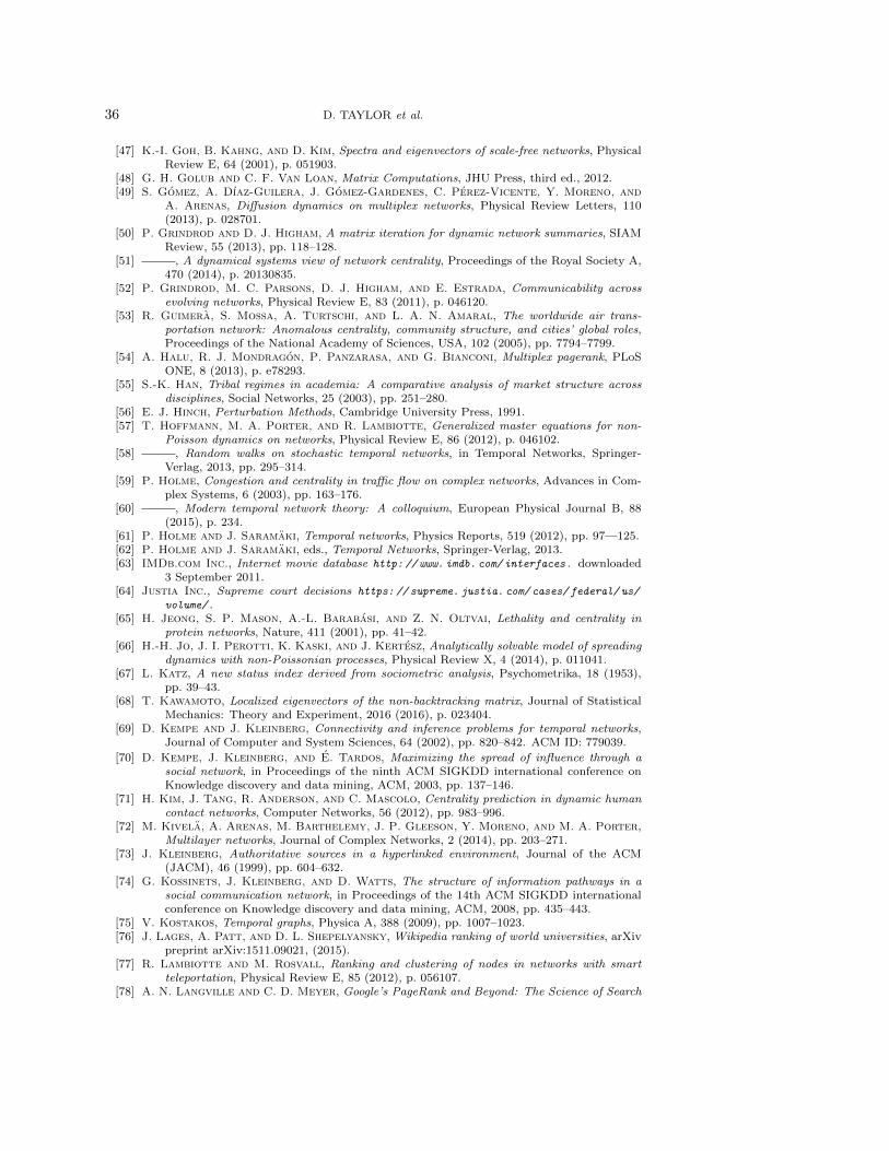
36 D. TAYLOR et al.
[47] K.-I. Goh, B. Kahng, and D. Kim, Spectra and eigenvectors of scale-free networks, PhysicalReview E, 64 (2001), p. 051903.
[48] G. H. Golub and C. F. Van Loan, Matrix Computations, JHU Press, third ed., 2012.[49] S. Gomez, A. Dıaz-Guilera, J. Gomez-Gardenes, C. Perez-Vicente, Y. Moreno, and
A. Arenas, Diffusion dynamics on multiplex networks, Physical Review Letters, 110(2013), p. 028701.
[50] P. Grindrod and D. J. Higham, A matrix iteration for dynamic network summaries, SIAMReview, 55 (2013), pp. 118–128.
[51] , A dynamical systems view of network centrality, Proceedings of the Royal Society A,470 (2014), p. 20130835.
[52] P. Grindrod, M. C. Parsons, D. J. Higham, and E. Estrada, Communicability acrossevolving networks, Physical Review E, 83 (2011), p. 046120.
[53] R. Guimera, S. Mossa, A. Turtschi, and L. A. N. Amaral, The worldwide air trans-portation network: Anomalous centrality, community structure, and cities’ global roles,Proceedings of the National Academy of Sciences, USA, 102 (2005), pp. 7794–7799.
[54] A. Halu, R. J. Mondragon, P. Panzarasa, and G. Bianconi, Multiplex pagerank, PLoSONE, 8 (2013), p. e78293.
[55] S.-K. Han, Tribal regimes in academia: A comparative analysis of market structure acrossdisciplines, Social Networks, 25 (2003), pp. 251–280.
[56] E. J. Hinch, Perturbation Methods, Cambridge University Press, 1991.[57] T. Hoffmann, M. A. Porter, and R. Lambiotte, Generalized master equations for non-
Poisson dynamics on networks, Physical Review E, 86 (2012), p. 046102.[58] , Random walks on stochastic temporal networks, in Temporal Networks, Springer-
Verlag, 2013, pp. 295–314.[59] P. Holme, Congestion and centrality in traffic flow on complex networks, Advances in Com-
plex Systems, 6 (2003), pp. 163–176.[60] , Modern temporal network theory: A colloquium, European Physical Journal B, 88
(2015), p. 234.[61] P. Holme and J. Saramaki, Temporal networks, Physics Reports, 519 (2012), pp. 97—125.[62] P. Holme and J. Saramaki, eds., Temporal Networks, Springer-Verlag, 2013.[63] IMDb.com Inc., Internet movie database http: // www. imdb. com/ interfaces . downloaded
3 September 2011.[64] Justia Inc., Supreme court decisions https: // supreme. justia. com/ cases/ federal/ us/
volume/ .[65] H. Jeong, S. P. Mason, A.-L. Barabasi, and Z. N. Oltvai, Lethality and centrality in
protein networks, Nature, 411 (2001), pp. 41–42.[66] H.-H. Jo, J. I. Perotti, K. Kaski, and J. Kertesz, Analytically solvable model of spreading
dynamics with non-Poissonian processes, Physical Review X, 4 (2014), p. 011041.[67] L. Katz, A new status index derived from sociometric analysis, Psychometrika, 18 (1953),
pp. 39–43.[68] T. Kawamoto, Localized eigenvectors of the non-backtracking matrix, Journal of Statistical
Mechanics: Theory and Experiment, 2016 (2016), p. 023404.[69] D. Kempe and J. Kleinberg, Connectivity and inference problems for temporal networks,
Journal of Computer and System Sciences, 64 (2002), pp. 820–842. ACM ID: 779039.
[70] D. Kempe, J. Kleinberg, and E. Tardos, Maximizing the spread of influence through asocial network, in Proceedings of the ninth ACM SIGKDD international conference onKnowledge discovery and data mining, ACM, 2003, pp. 137–146.
[71] H. Kim, J. Tang, R. Anderson, and C. Mascolo, Centrality prediction in dynamic humancontact networks, Computer Networks, 56 (2012), pp. 983–996.
[72] M. Kivela, A. Arenas, M. Barthelemy, J. P. Gleeson, Y. Moreno, and M. A. Porter,Multilayer networks, Journal of Complex Networks, 2 (2014), pp. 203–271.
[73] J. Kleinberg, Authoritative sources in a hyperlinked environment, Journal of the ACM(JACM), 46 (1999), pp. 604–632.
[74] G. Kossinets, J. Kleinberg, and D. Watts, The structure of information pathways in asocial communication network, in Proceedings of the 14th ACM SIGKDD internationalconference on Knowledge discovery and data mining, ACM, 2008, pp. 435–443.
[75] V. Kostakos, Temporal graphs, Physica A, 388 (2009), pp. 1007–1023.[76] J. Lages, A. Patt, and D. L. Shepelyansky, Wikipedia ranking of world universities, arXiv
preprint arXiv:1511.09021, (2015).[77] R. Lambiotte and M. Rosvall, Ranking and clustering of nodes in networks with smart
teleportation, Physical Review E, 85 (2012), p. 056107.[78] A. N. Langville and C. D. Meyer, Google’s PageRank and Beyond: The Science of Search
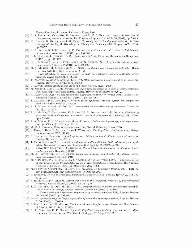
Eigenvector-Based Centrality for Temporal Networks 37
Engine Rankings, Princeton University Press, 2006.[79] E. A. Leicht, G. Clarkson, K. Shedden, and M. E. J. Newman, Large-scale structure of
time evolving citation networks, The European Physical Journal B, 59 (2007), pp. 75–83.[80] K. Lerman, R. Ghosh, and J. H. Kang, Centrality metric for dynamic networks, in Pro-
ceedings of the Eighth Workshop on Mining and Learning with Graphs, ACM, 2010,pp. 70–77.
[81] R. J. Lipton, D. J. Rose, and R. E. Tarjan, Generalized nested dissection, SIAM Journalon Numerical Analysis, 16 (1979), pp. 346–358.
[82] L. Lovasz and J. Pelikan, On the eigenvalues of trees, Periodica Mathematica Hungarica,3 (1973), pp. 175–182.
[83] R. D. Malmgren, J. M. Ottino, and L. A. N. Amaral, The role of mentorship in protegeperformance, Nature, 465 (2010), pp. 622–626.
[84] M. S. Mariani, M. Medo, and Y.-C. Zhang, Ranking nodes in growing networks: Whenpagerank fails, Scientific Reports, 5 (2015).
[85] , Identification of milestone papers through time-balanced network centrality, arXivpreprint, arXiv: 1608.08414, (2016).
[86] T. Martin, X. Zhang, and M. E. J. Newman, Localization and centrality in networks,Physical Review E, 90 (2014), p. 052808.
[87] C. Meyer, Matrix Analysis and Applied Linear Algebra, SIAM, 2000.[88] M. Mitrovic and B. Tadic, Spectral and dynamical properties in classes of sparse networks
with mesoscopic inhomogeneities, Physical Review E, 80 (2009), p. 026123.[89] R. Monasson, Diffusion, localization and dispersion relations on “small-world” lattices, The
European Physical Journal B, 12 (1999), pp. 555–567.[90] S. Motegi and N. Masuda, A network-based dynamical ranking system for competitive
sports, Scientific Reports, 2 (2012).[91] P. J. Mucha and M. A. Porter, Communities in multislice voting networks, Chaos, 20
(2010), p. 041108.[92] P. J. Mucha, T. Richardson, K. Macon, M. A. Porter, and J.-P. Onnela, Community
structure in time-dependent, multiscale, and multiplex networks, Science, 328 (2010),pp. 876–878.
[93] S. A. Myers, P. J. Mucha, and M. A. Porter, Mathematical genealogy and departmentprestige, Chaos, 21 (2011), p. 041104.
[94] M. E. J. Newman, Networks: An Introduction, Oxford University Press, 2010.[95] L. Page, S. Brin, R. Motwani, and T. Winograd, The PageRank citation ranking: Bring-
ing order to the Web, (1999).[96] R. Pan and J. Saramaki, Path lengths, correlations, and centrality in temporal networks,
Physical Review E, 84 (2011).[97] J. Panaretos and C. C. Malesios, Influential mathematicians: birth, education, and affil-
iation, Notices of the American Mathematical Society, 59 (2012), p. 274.[98] R. Pastor-Satorras and C. Castellano, Distinct types of eigenvector localization in net-
works, Scientific Reports, 6 (2016).[99] M. A. Porter and J. P. Gleeson, Dynamical systems on networks: A tutorial. arXiv
preprint, arXiv: 1403.7663, 2016.[100] M. A. Porter, P. J. Mucha, M. E. J. Newman, and C. M. Warmbrand, A network analysis
of committees in the United States House of Representatives, Proceedings of the NationalAcademy of Sciences, USA, 102 (2005), pp. 7057–7062.
[101] Mathematics Genealogy Project, The Mathematics Genealogy Project, 2009. http://
www.genealogy.ams.org, data provided 19 October 2009.[102] F. Radicchi, Driving interconnected networks to supercriticality, Physical Review X, 4 (2014),
p. 021014.[103] F. Radicchi and A. Arenas, Abrupt transition in the structural formation of interconnected
networks, Nature Physics, 9 (2013), pp. 717–720.[104] J. G. Restrepo, E. Ott, and B. R. Hunt, Desynchronization waves and localized instabili-
ties in oscillator arrays, Physical Review Letters, 93 (2004), p. 114101.[105] , Characterizing the dynamical importance of network nodes and links, Physical Review
Letters, 97 (2006), p. 094102.[106] , Approximating the largest eigenvalue of network adjacency matrices, Physical Review
E, 76 (2007), p. 056119.[107] L. E. C. Rocha and N. Masuda, Random walk centrality for temporal networks, New Journal
of Physics, 16 (2014), p. 063023.[108] R. A. Rossi and D. F. Gleich, Dynamic PageRank using evolving teleportation, in Algo-
rithms and Models for the Web Graph, Springer, 2012, pp. 126–137.
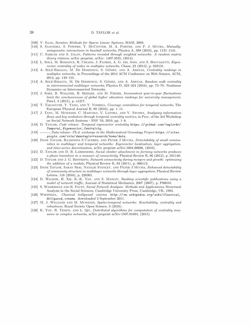
38 D. TAYLOR et al.
[109] Y. Saad, Iterative Methods for Sparse Linear Systems, SIAM, 2003.[110] S. Saavedra, S. Powers, T. McCotter, M. A. Porter, and P. J. Mucha, Mutually-
antagonistic interactions in baseball networks, Physica A, 389 (2010), pp. 1131–1141.[111] C. Sarkar and S. Jalan, Patterns revealed through weighted networks: A random matrix
theory relation, arXiv preprint, arXiv: 1407.3345, (2014).[112] L. Sola, M. Romance, R. Criado, J. Flores, A. G. del Amo, and S. Boccaletti, Eigen-
vector centrality of nodes in multiplex networks, Chaos, 23 (2013), p. 033131.[113] A. Sole-Ribalta, M. De Domenico, S. Gomez, and A. Arenas, Centrality rankings in
multiplex networks, in Proceedings of the 2014 ACM Conference on Web Science, ACM,2014, pp. 149–155.
[114] A. Sole-Ribalta, M. De Domenico, S. Gomez, and A. Arenas, Random walk centralityin interconnected multilayer networks, Physica D, 323–324 (2016), pp. 73–79. NonlinearDynamics on Interconnected Networks.
[115] J. Sorz, B. Wallner, H. Seidler, and M. Fieder, Inconsistent year-to-year fluctuationslimit the conclusiveness of global higher education rankings for university management,PeerJ, 3 (2015), p. e1217.
[116] T. Takaguchi, Y. Yano, and Y. Yoshida, Coverage centralities for temporal networks, TheEuropean Physical Journal B, 89 (2016), pp. 1–11.
[117] J. Tang, M. Musolesi, C. Mascolo, V. Latora, and V. Nicosia, Analysing informationflows and key mediators through temporal centrality metrics, in Proc. of the 3rd Workshopon Social Network Systems - SNS ’10, 2010, pp. 1–6.
[118] D. Taylor, Code release: Temporal eigenvector centrality https: // github. com/ taylordr/
Temporal_ Eigenvector_ Centrality .[119] , Data release: Ph.d. exchange in the Mathematical Genealogy Project https: // sites.
google. com/ site/ danetaylorresearch/ home/ data .[120] Dane Taylor, Rajmonda S Caceres, and Peter J Mucha, Detectability of small commu-
nities in multilayer and temporal networks: Eigenvector localization, layer aggregation,and time-series discretization, arXiv preprint arXiv:1604.00696, (2016).
[121] D. Taylor and D. B. Larremore, Social climber attachment in forming networks producesa phase transition in a measure of connectivity, Physical Review E, 86 (2012), p. 031140.
[122] D. Taylor and J. G. Restrepo, Network connectivity during mergers and growth: optimizingthe addition of a module, Physical Review E, 83 (2011), p. 066112.
[123] Dane Taylor, Saray Shai, Natalie Stanley, and Peter J Mucha, Enhanced detectabilityof community structure in multilayer networks through layer aggregation, Physical ReviewLetters, 116 (2016), p. 228301.
[124] D. Walker, H. Xie, K.-K. Yan, and S. Maslov, Ranking scientific publications using amodel of network traffic, Journal of Statistical Mechanics, 2007 (2007), p. P06010.
[125] S. Wasserman and K. Faust, Social Network Analysis: Methods and Applications, StructuralAnalysis in the Social Sciences, Cambridge University Press, Cambridge, UK, 1994.
[126] Wikipedia, Classical hollywood cinema http: // en. wikipedia. org/ wiki/ Classical_
Hollywood_ cinema . downloaded 3 September 2011.[127] M. J. Williams and M. Musolesi, Spatio-temporal networks: Reachability, centrality and
robustness, Royal Society Open Science, 3 (2016).[128] K. You, R. Tempo, and L. Qiu, Distributed algorithms for computation of centrality mea-
sures in complex networks, arXiv preprint arXiv:1507.01694, (2015).