Embed Size (px)
Citation preview

MULTISCALE MODEL. SIMUL. c© 2017 Society for Industrial and Applied MathematicsVol. 15, No. 1, pp. 537–574
EIGENVECTOR-BASED CENTRALITY MEASURES FORTEMPORAL NETWORKS∗
DANE TAYLOR† , SEAN A. MYERS‡ , AARON CLAUSET§ , MASON A. PORTER¶, AND
PETER J. MUCHA‖
Abstract. Numerous centrality measures have been developed to quantify the importances ofnodes in time-independent networks, and many of them can be expressed as the leading eigenvectorof some matrix. With the increasing availability of network data that changes in time, it is importantto extend such eigenvector-based centrality measures to time-dependent networks. In this paper, weintroduce a principled generalization of network centrality measures that is valid for any eigenvector-based centrality. We consider a temporal network with N nodes as a sequence of T layers thatdescribe the network during different time windows, and we couple centrality matrices for the layersinto a supracentrality matrix of size NT × NT whose dominant eigenvector gives the centrality ofeach node i at each time t. We refer to this eigenvector and its components as a joint centrality, asit reflects the importances of both the node i and the time layer t. We also introduce the conceptsof marginal and conditional centralities, which facilitate the study of centrality trajectories overtime. We find that the strength of coupling between layers is important for determining multiscaleproperties of centrality, such as localization phenomena and the time scale of centrality changes. Inthe strong-coupling regime, we derive expressions for time-averaged centralities, which are given bythe zeroth-order terms of a singular perturbation expansion. We also study first-order terms to obtainfirst-order-mover scores, which concisely describe the magnitude of the nodes’ centrality changes overtime. As examples, we apply our method to three empirical temporal networks: the United StatesPh.D. exchange in mathematics, costarring relationships among top-billed actors during the GoldenAge of Hollywood, and citations of decisions from the United States Supreme Court.
Key words. temporal networks, eigenvector centrality, hubs and authorities, singular pertur-bation, multilayer networks, ranking systems
AMS subject classifications. 91D30, 05C81, 94C15, 05C82, 15A18
DOI. 10.1137/16M1066142
∗Received by the editors March 16, 2016; accepted for publication (in revised form) December 14,2016; published electronically March 28, 2017.
http://www.siam.org/journals/mms/15-1/M106614.htmlFunding: The first and fifth authors were supported partially by the Eunice Kennedy Shriver
National Institute of Child Health and Human Development of the National Institutes of Health underAward R01HD075712. The first author was also funded by the National Science Foundation (NSF)under grant DMS-1127914 to the Statistical and Applied Mathematical Sciences Institute. The sec-ond and fifth authors were funded by the NSF (DMS-0645369). The fifth author was also funded bya James S. McDonnell Foundation 21st Century Science Initiative - Complex Systems Scholar Award(220020315). The fourth author was supported by the FET-Proactive project PLEXMATH (317614)funded by the European Commission, a James S. McDonnell Foundation 21st Century Science Ini-tiative - Complex Systems Scholar Award (220020177), and the EPSRC (EP/J001759/1). The thirdauthor was funded by the NSF under grant IIS-1452718. Any content is solely the responsibility ofthe authors and does not necessarily reflect the views of any of the funding agencies.†Carolina Center for Interdisciplinary Applied Mathematics, Department of Mathematics, Uni-
versity of North Carolina, Chapel Hill, NC 27599-3250, and Statistical and Applied MathematicalSciences Institute (SAMSI), Research Triangle Park, NC, 27709 ([email protected]).‡Carolina Center for Interdisciplinary Applied Mathematics, Department of Mathematics, Uni-
versity of North Carolina, Chapel Hill, NC 27599-3250 ([email protected]). Current address:Department of Economics, Stanford University, Stanford, CA 94305-6072.§Department of Computer Science, University of Colorado, Boulder, CO 80309 and Santa Fe
Institute, Santa Fe, NM 87501 and BioFrontiers Institute, University of Colorado, Boulder, CO80303 ([email protected]).¶Mathematical Institute, University of Oxford, OX2 6GG, UK and CABDyN Complexity Cen-
tre, University of Oxford, Oxford OX1 1HP, UK and Department of Mathematics, University ofCalifornia, Los Angeles, CA 90095 ([email protected]).‖Carolina Center for Interdisciplinary Applied Mathematics, Department of Mathematics, Uni-
versity of North Carolina, Chapel Hill, NC 27599-3250 ([email protected]).
537
538 TAYLOR, MYERS, CLAUSET, PORTER, AND MUCHA
1. Introduction. The study of centrality [94]—that is, determining the impor-tances of different nodes, edges, and other structures in a network—has widespreadapplications in the identification and ranking of important agents (or interactions)in a network. These applications include ranking sports teams or individual athletes[14, 16, 111], the identification of influential people [70], critical infrastructures thatare susceptible to congestion [53, 59], impactful United States Supreme Court cases[41, 42, 79], genetic and protein targets [65], impactful scientific journals [7], and muchmore. Especially important types of centrality measures are ones that arise as a solu-tion of an eigenvalue problem [46], with the nodes’ importances given by the entries ofthe dominant eigenvector of a so-called centrality matrix. Prominent examples includeeigenvector centrality [9], PageRank [12, 96] (which provides the mathematical foun-dation to the Web search engine Google [46, 78]), hub and authority (i.e., HITS) scores[73], and Eigenfactor [7]. However, despite the fact that real-world networks changewith time [60, 61, 62], most methods for centrality (and node rankings that are derivedfrom them) have been restricted to time-independent networks. Extending such ideasto time-dependent networks (i.e., so-called temporal networks) has recently become avery active research area [1, 33, 51, 52, 71, 80, 90, 95, 97, 108, 109, 117, 118, 128, 129].
In the present paper, we develop a generalization of eigenvector-based centrali-ties to ordered multilayer networks such as temporal networks. Akin to multilayermodularity [92], a critical underpinning of our approach is that we treat interlayerand intralayer connections as fundamentally different [26, 72]. For the purpose ofgeneralizing centrality, we implement this idea by coupling centrality matrices fortemporal layers in a supracentrality matrix. For a temporal network with N nodesand T time layers, we obtain a supracentrality matrix of size NT ×NT . To use thismatrix, we represent the temporal network as a sequence of network layers, which isappropriate for discrete-time temporal networks and continuous-time networks whoseedges have been binned to produce a discrete-time temporal etwork. Importantly,our methodology is independent of the particular choice of centrality matrix, so itcan be used, for example, with ordinary eigenvector centrality [9], hub and authorityscores [73], PageRank [96], or any other centralities that are given by components ofthe dominant eigenvector of a matrix.
The dominant eigenvector of a supracentrality matrix characterizes the joint cen-trality of each node-layer pair (i, t)—that is, the centrality of node i at time stept—and thus reflects the importances of both node i and layer t. We also introducethe concepts of marginal centrality and conditional centrality, which allow one to(1) study the decoupled centrality of just the nodes (or just the time layers) and (2)study a node’s centrality with respect to other nodes’ centralities at a particular timet (i.e., the centralities are conditional on a particular time layer). These notions makeit possible to develop a broad description for studying nodes’ centrality trajectoriesacross time. Although we develop this formalism for temporal networks, we note thatour approach is also applicable to multiplex and general multilayer networks, whichare two additional scenarios in which the generalization of centrality measures is im-portant. (See, e.g., [54, 113, 114] for multiplex centralities and [30, 115] for generalmultilayer centralities.)
Similarly to the construction of supra-adjacency matrices [49, 72, 92] (see sec-tion 2.2 for the definition), we couple nearest-neighbor temporal layers using interlayeredges of weight ω, which leads to a family of centrality measures that are parameter-ized by ω. The parameter ω controls the coupling of each node’s eigenvector-basedcentrality through time and can be used to tune the extent to which a node’s cen-trality changes over time. The limiting cases ω → 0+ and ω → ∞ are particularly

EIGENVECTOR-BASED CENTRALITY FOR TEMPORAL NETWORKS 539
interesting, as the former represents the regime of complete decoupling of the layersand the latter represents a regime of dominating coupling of the layers. As part of thepresent paper, we conduct a perturbative analysis for the ω → ∞ limit. (For nota-tional convenience, we study ε→ 0+ for ε = 1/ω.) This allows us to derive principledexpressions for the nodes’ time-averaged centralities (given by the zeroth-order expan-sion) and first-order-mover scores, which are derived from the first-order expansion.Time-averaged centrality ranks nodes so that their centralities are constant acrosstime, and first-order-mover scores rank nodes according to the extent to which theircentralities change in time. The computation of both time-averaged centralities andfirst-order-mover scores can be very efficient, because they only require the numericalsolution of linear-algebraic problems of size N ×N , which is ordinarily much smallerthan the full supracentrality matrix of size NT × NT . Moreover, our perturbativeapproach also alleviates the need to demand a particular choice of intralayer couplingweight ω. Note that our methodology is a retrospective analysis and complementsalternative temporal generalizations that take a causal approach.
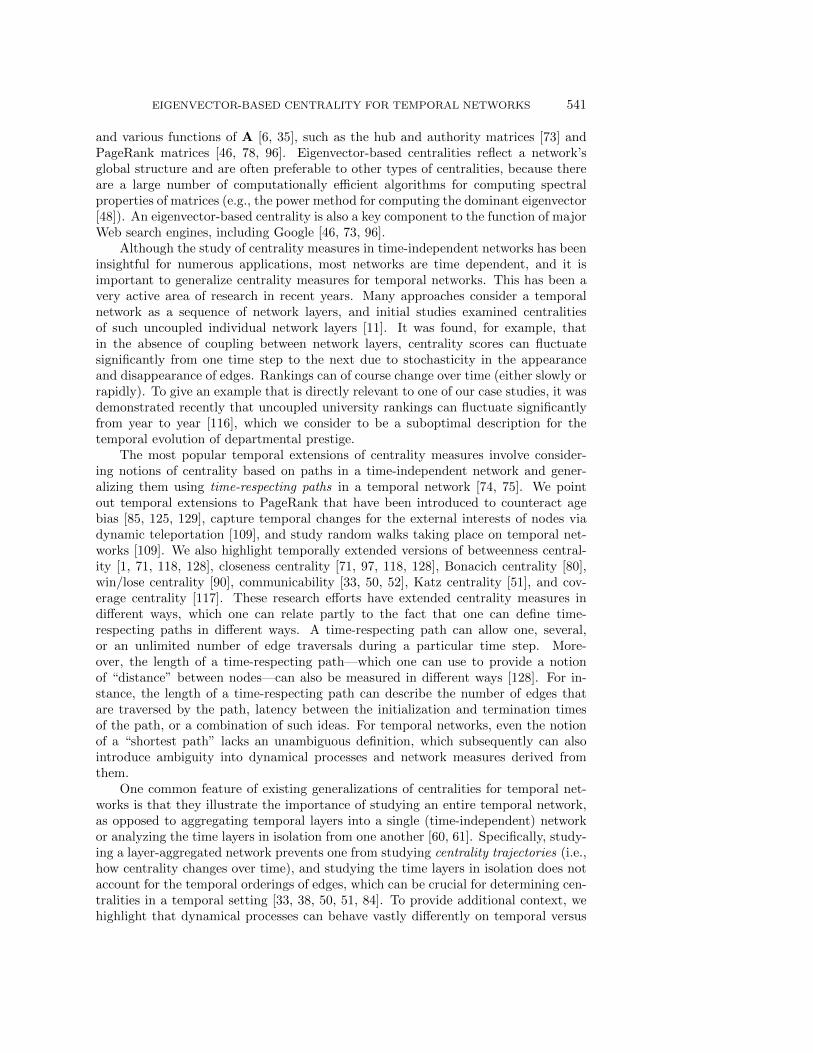
The remainder of our paper is organized as follows. In section 2, we provide furtherbackground information. In section 3, we present our generalization of eigenvector-based centralities for temporal networks. In section 4, we derive principled expres-sions for time-averaged centralities and first-order-mover scores based on a singularperturbation expansion. In section 5, we illustrate our approach using three examplesfrom empirical data: Ph.D. exchange using data from the Mathematics GenealogyProject [102] (see Figure 1), top billing in the Golden Age of Hollywood using theInternet Movie Database (IMDb) [63], and citations of United States Supreme Courtdecisions [40, 64]. We conclude in section 6 and provide further details of our per-turbation expansion in the appendix.
2. Background information and a naive approach. In section 2.1, we pro-vide additional background information. In section 2.2, we discuss a naive approachfor temporal eigenvector centrality that motivates our approach, and introduces ourmathematical notation and terminology.
2.1. Background information. The analysis of large networks is ubiquitous inscience, engineering, medicine, and numerous other areas [94]. In the social sciences,for example, the abundance of data that describe the social behavior of individualsin academia [13, 15, 19, 93, 98, 102], show business [112], politics [8, 41, 42, 79, 101],and just about every other arena offers exciting avenues for the quantitative study ofsocial systems. For these and many other applications, it is important to develop (andimprove) mathematical techniques to extract concise and intuitive information fromlarge network data. From the interdisciplinary pursuit of what is now often callednetwork science, we know—from theory, computation, and data analysis—that manynetwork properties (e.g., degree heterogeneity, local clustering, community structure,and others [94]) have significant effects on dynamical processes on networks (e.g.,information dissemination and disease spreading) [20, 100, 126]. Although the vastmajority of research in network science has focused on time-independent networks,increased effort in recent years has aimed to generalize network analyses to “temporalnetworks” [4, 60, 61, 62, 69], in which network entities and/or interactions change intime.
In the study of time-independent networks, numerous centrality measures havebeen developed to try to quantify the relative importances of nodes [94, 126]. Thereare seemingly as many centrality measures as applications [6, 9, 10, 34, 43, 67], anddifferent types of centrality are appropriate for different situations. Importantly, one
540 TAYLOR, MYERS, CLAUSET, PORTER, AND MUCHA
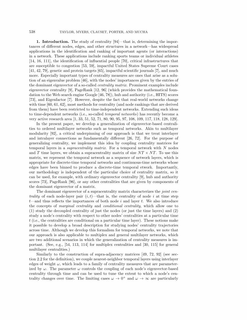
Fig. 1. As one case study for our generalization of eigenvector-based centralities to temporalnetworks, we examine a multilayer temporal network that we construct from data obtained from theMathematics Genealogy Project [102]. (See the supplementary material or [120] to download thetemporal network data.) We study a temporal network with T = 65 time layers (corresponding tothe years 1946–2010), in which a given edge j → i in time layer t signifies the number of graduatingdoctoral students in year t at university i who later supervise a graduating doctoral student atuniversity j. The nodes’ sizes and colors indicate what we call “time-averaged centrality” (seesection 4), which we calculate for the type of centrality matrix known as an authority matrix [73].We do not show self-edges. Because visualizing a temporal network is difficult [25], we show thenetwork that we obtain by aggregating the adjacency matrices across time layers. Studying suchan aggregated network neglects the time-ordered structure of a temporal network. In our paper, westudy trajectories of node centralities (which represent importances) over time. See section 5.1 foradditional discussion of this network. (We created this image using the software Gephi [3].)
can construct centrality measures not only from the direct consideration of networkstructure but also based on studying an appropriate dynamical process on a network[45, 96, 106]. In our paper, we focus on eigenvector-based centralities. Althougheigenvectors can obviously be used in different ways to introduce different notions ofcentrality, we reserve the term eigenvector-based centrality to refer only to centralitymeasures in which the nodes’ centralities are given by the entries of the dominanteigenvector of a matrix, which we call a centrality matrix. Centrality matrices includea network’s adjacency matrix A (which indicates which nodes share a common edge)
EIGENVECTOR-BASED CENTRALITY FOR TEMPORAL NETWORKS 541
and various functions of A [6, 35], such as the hub and authority matrices [73] andPageRank matrices [46, 78, 96]. Eigenvector-based centralities reflect a network’sglobal structure and are often preferable to other types of centralities, because thereare a large number of computationally efficient algorithms for computing spectralproperties of matrices (e.g., the power method for computing the dominant eigenvector[48]). An eigenvector-based centrality is also a key component to the function of majorWeb search engines, including Google [46, 73, 96].
Although the study of centrality measures in time-independent networks has beeninsightful for numerous applications, most networks are time dependent, and it isimportant to generalize centrality measures for temporal networks. This has been avery active area of research in recent years. Many approaches consider a temporalnetwork as a sequence of network layers, and initial studies examined centralitiesof such uncoupled individual network layers [11]. It was found, for example, thatin the absence of coupling between network layers, centrality scores can fluctuatesignificantly from one time step to the next due to stochasticity in the appearanceand disappearance of edges. Rankings can of course change over time (either slowly orrapidly). To give an example that is directly relevant to one of our case studies, it wasdemonstrated recently that uncoupled university rankings can fluctuate significantlyfrom year to year [116], which we consider to be a suboptimal description for thetemporal evolution of departmental prestige.
The most popular temporal extensions of centrality measures involve consider-ing notions of centrality based on paths in a time-independent network and gener-alizing them using time-respecting paths in a temporal network [74, 75]. We pointout temporal extensions to PageRank that have been introduced to counteract agebias [85, 125, 129], capture temporal changes for the external interests of nodes viadynamic teleportation [109], and study random walks taking place on temporal net-works [109]. We also highlight temporally extended versions of betweenness central-ity [1, 71, 118, 128], closeness centrality [71, 97, 118, 128], Bonacich centrality [80],win/lose centrality [90], communicability [33, 50, 52], Katz centrality [51], and cov-erage centrality [117]. These research efforts have extended centrality measures indifferent ways, which one can relate partly to the fact that one can define time-respecting paths in different ways. A time-respecting path can allow one, several,or an unlimited number of edge traversals during a particular time step. More-over, the length of a time-respecting path—which one can use to provide a notionof “distance” between nodes—can also be measured in different ways [128]. For in-stance, the length of a time-respecting path can describe the number of edges thatare traversed by the path, latency between the initialization and termination timesof the path, or a combination of such ideas. For temporal networks, even the notionof a “shortest path” lacks an unambiguous definition, which subsequently can alsointroduce ambiguity into dynamical processes and network measures derived fromthem.
One common feature of existing generalizations of centralities for temporal net-works is that they illustrate the importance of studying an entire temporal network,as opposed to aggregating temporal layers into a single (time-independent) networkor analyzing the time layers in isolation from one another [60, 61]. Specifically, study-ing a layer-aggregated network prevents one from studying centrality trajectories (i.e.,how centrality changes over time), and studying the time layers in isolation does notaccount for the temporal orderings of edges, which can be crucial for determining cen-tralities in a temporal setting [33, 38, 50, 51, 84]. To provide additional context, wehighlight that dynamical processes can behave vastly differently on temporal versus

542 TAYLOR, MYERS, CLAUSET, PORTER, AND MUCHA
Table 1A summary of our mathematical notation.
Typeface Class Dimensionality
M matrix NT ×NTM matrix N ×NM matrix T × Tv vector NT × 1v vector N × 1v vector T × 1Mij scalar 1vi scalar 1
layer-aggregated networks.1 For example, a random walk—a process on which manyeigenvector-based centralities rely—on a temporal network is affected fundamentallyby the temporal ordering and time scale of the appearances and disappearances ofedges [57, 58, 60, 61, 62, 66]. Rankings, such as eigenvector-based centralities, thatare derived from such dynamics are, in turn, affected fundamentally by the temporalstructure of the networks, and aggregation (as well as isolation) can lead to misleadingor even simply wrong results. Additionally, if one starts with a Markovian process ona temporal network and then aggregates the network, then, in general, one does notobtain a Markovian process [62], so fundamental (and often desirable) properties of adynamical process can be destroyed as a byproduct of neglecting a network’s inherenttemporal structure.
Finally, although extending centrality to temporal networks has become a veryactive research area, one should expect different generalizations of eigenvector-basedcentralities to be appropriate for different applications. Existing papers have notalways been clear about the modeling assumptions and tradeoffs of their approaches.
2.2. Naive generalization of eigenvector centrality for temporal net-works. Before we present our primary approach in section 3, it is instructive toconsider one possible way to generalize eigenvector-based centralities. This examplemotivates our approach and introduces mathematical notation and terminology. Im-portantly, it is naive in that it does not treat intralayer edges and interlayer edges asdistinct types of edges, which causes problems when the network layers are stronglycoupled.
We use a multilayer representation of networks and seek to identify the mostcentral nodes of a temporal network with N distinct nodes (i.e., vertices or actors)across T time layers. We specify the network edges with a node-by-node-by-time
(N ×N × T ) adjacency tensor in which nonzero elements A(t)ij indicate the presence
and weight of the edge from node i to node j in time layer t. That is, the adjacencymatrix at time t is given by A(t). See Table 1 for a summary of our mathematicalnotation. We refer to node i in layer t as a node-layer pair (i, t) and node i (regardlessof layer) as a physical node. We are interested particularly in understanding thephysical nodes’ centrality trajectories through time.
1As discussed in, e.g., [26, 72] and several references therein—and more recently in [27]—a similarissue arises more generally in multilayer networks, and one must also take into account the effects ofinterlayer edges (which are fundamentally different from intralayer edges) when defining a dynamicalprocess on a multilayer network.
EIGENVECTOR-BASED CENTRALITY FOR TEMPORAL NETWORKS 543
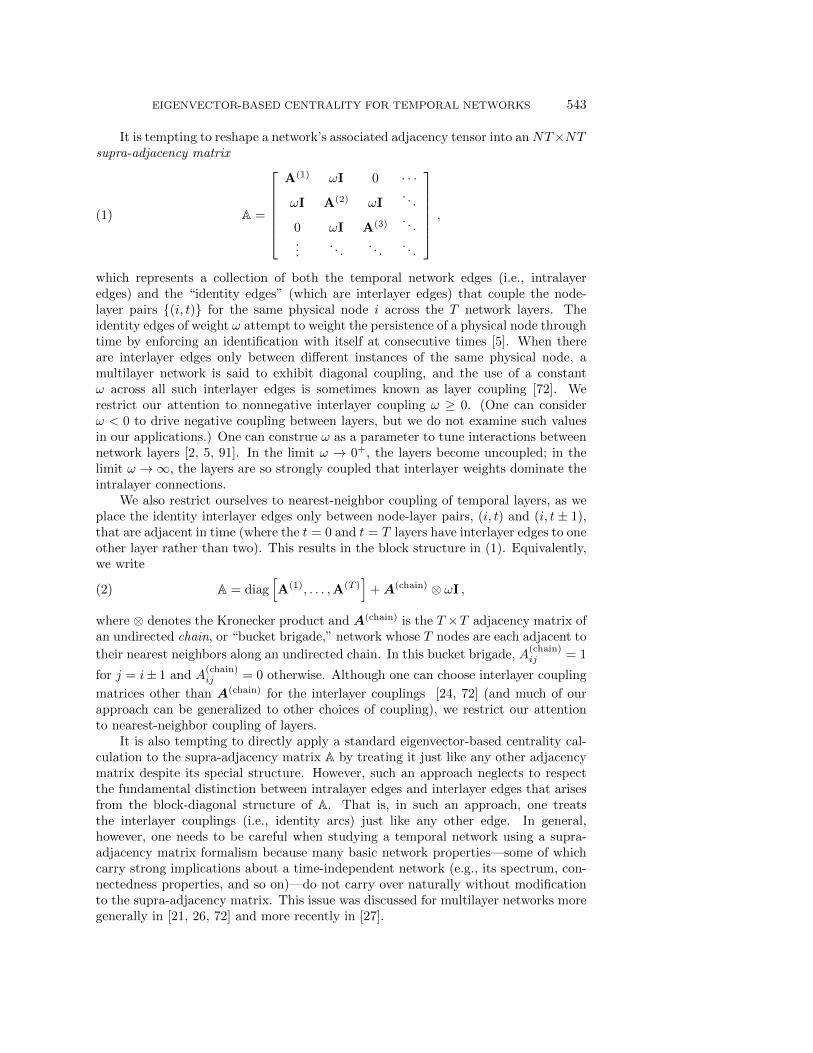
It is tempting to reshape a network’s associated adjacency tensor into anNT×NTsupra-adjacency matrix
(1) A =
A(1) ωI 0 · · ·
ωI A(2) ωI. . .
0 ωI A(3) . . ....
. . .. . .
. . .
,
which represents a collection of both the temporal network edges (i.e., intralayeredges) and the “identity edges” (which are interlayer edges) that couple the node-layer pairs {(i, t)} for the same physical node i across the T network layers. Theidentity edges of weight ω attempt to weight the persistence of a physical node throughtime by enforcing an identification with itself at consecutive times [5]. When thereare interlayer edges only between different instances of the same physical node, amultilayer network is said to exhibit diagonal coupling, and the use of a constantω across all such interlayer edges is sometimes known as layer coupling [72]. Werestrict our attention to nonnegative interlayer coupling ω ≥ 0. (One can considerω < 0 to drive negative coupling between layers, but we do not examine such valuesin our applications.) One can construe ω as a parameter to tune interactions betweennetwork layers [2, 5, 91]. In the limit ω → 0+, the layers become uncoupled; in thelimit ω →∞, the layers are so strongly coupled that interlayer weights dominate theintralayer connections.
We also restrict ourselves to nearest-neighbor coupling of temporal layers, as weplace the identity interlayer edges only between node-layer pairs, (i, t) and (i, t± 1),that are adjacent in time (where the t = 0 and t = T layers have interlayer edges to oneother layer rather than two). This results in the block structure in (1). Equivalently,we write
(2) A = diag[A(1), . . . ,A(T )
]+A(chain) ⊗ ωI ,
where ⊗ denotes the Kronecker product and A(chain) is the T ×T adjacency matrix ofan undirected chain, or “bucket brigade,” network whose T nodes are each adjacent to
their nearest neighbors along an undirected chain. In this bucket brigade, A(chain)ij = 1
for j = i± 1 and A(chain)ij = 0 otherwise. Although one can choose interlayer coupling
matrices other than A(chain) for the interlayer couplings [24, 72] (and much of ourapproach can be generalized to other choices of coupling), we restrict our attentionto nearest-neighbor coupling of layers.
It is also tempting to directly apply a standard eigenvector-based centrality cal-culation to the supra-adjacency matrix A by treating it just like any other adjacencymatrix despite its special structure. However, such an approach neglects to respectthe fundamental distinction between intralayer edges and interlayer edges that arisesfrom the block-diagonal structure of A. That is, in such an approach, one treatsthe interlayer couplings (i.e., identity arcs) just like any other edge. In general,however, one needs to be careful when studying a temporal network using a supra-adjacency matrix formalism because many basic network properties—some of whichcarry strong implications about a time-independent network (e.g., its spectrum, con-nectedness properties, and so on)—do not carry over naturally without modificationto the supra-adjacency matrix. This issue was discussed for multilayer networks moregenerally in [21, 26, 72] and more recently in [27].

544 TAYLOR, MYERS, CLAUSET, PORTER, AND MUCHA
As a concrete example, let’s examine hub and authority centralities (i.e., HITS[73]) for a directed temporal network using the supra-adjacency matrix in (1) bysimply inserting it in place of a time-independent adjacency matrix in the standardformulas. In other words, we define the hub and authority matrices as AAT andATA, respectively. At a glance, by noting that the interlayer couplings are undirectedbut that the intralayer edges are directed, we already see that it is not clear whetherstandard interpretations of hub and authority rankings are still sensible. Nevertheless,one can try this approach for computing generalized hub and authority scores as thedominant eigenvectors of the symmetric matrices AAT and ATA. The simplicity ofthis approach makes it pleasing (and tempting), and the two symmetric matrices dohave a block structure. However, in contrast to A (whose blocks on and off of themain diagonal encode intralayer and interlayer edges, respectively), the blocks in thematrices AAT and ATA no longer separate neatly into describing only a single typeof edge (i.e., interlayer versus intralayer edges).
The problem with this construction becomes particularly clear in the limit ofstrong interlayer coupling (i.e., as ω → ∞), for which A ≈ ω(A(chain) ⊗ I). BecauseA(chain) is symmetric, it follows that AAT ≈ ATA ≈ ω2(A(chain)(A(chain))T ⊗ I).Unfortunately, it is useless to compute hub and authority scores of an undirectedchain. Specifically, the corresponding hub/authority centrality matrix (whose domi-nant eigenvector gives the hub/authority scores) of the undirected chain becomes
(3) A(chain)(A(chain))T = (A(chain))TA(chain) =
1 0 1 0 · · ·
0 2 0 1. . .
1 0 2 0. . . 0
0 1 0 2. . . 1 0
.... . .
. . .. . .
. . . 0 10 1 0 2 0
0 1 0 1
,
revealing that the hub/authority scores of the even-indexed and odd-indexed nodesdecouple from each other. The resulting matrix is no longer irreducible, which canlead to nonuniqueness of dominant eigenvectors and/or can also cause the entries ofa dominant eigenvector to be identically 0 for a large number of nodes.2 Both issuesare detrimental if one wants to rank nodes based on some notion of importance. Forexample, for large values of ω, we observe oscillations and numerical instabilities whenattempting to generalize hub and authority centralities in this way.
3. Temporal coupling of eigenvector-based centralities. In this section,we present a mathematical formalism for eigenvector-based centralities in temporalnetworks that treats interlayer and intralayer edges as distinct types of edges and
2By inspection, the matrix in (3) is not irreducible, so we cannot apply the Perron–Frobeniustheorem for irreducible nonnegative matrices [87]. There exist many variations of Perron–Frobeniustheory, including ones that are applicable to reducible matrices (e.g., see [87, section 8.3.1]), whichone can use to study phenomena that arise in the absence of irreducibility. In our case, we find twotypes of scenarios, depending on whether N is odd or even. For even N , the largest eigenvalue ofA(chain)(A(chain))T has a multiplicity of two and a corresponding two-dimensional eigenspace thatis spanned by vectors in which either the even-indexed or odd-indexed entries are 0. Consequently,there is not a unique dominant eigenvector, so there is not a unique ranking of nodes. For odd N ,there is a single dominant eigenvalue; however, its eigenvector has entries that are identically 0 foreven-indexed nodes, so only half of the nodes are ranked in a nontrivial way.
EIGENVECTOR-BASED CENTRALITY FOR TEMPORAL NETWORKS 545
ensures appropriate behavior for all ω > 0. Similarly to prior investigations usingmultilayer representations of temporal networks [72, 92], we seek to develop an ap-proach that involves neither a heuristic averaging of centralities from individual layersnor invokes the centrality for a single network obtained from the aggregation of net-work layers (e.g., summing the network edges across time).
The remainder of this section is organized as follows. In section 3.1, we presentour methodology for temporal eigenvector-based centrality in terms of the dominanteigenvector of a supracentrality matrix. In section 3.2, we introduce the concepts ofjoint, marginal, and conditional centrality, and we use them to study decoupled cen-tralities of nodes and layers based on the centralities of node-layer pairs. In section 3.3,we illustrate these concepts for an example synthetic network.
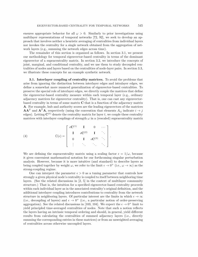
3.1. Interlayer coupling of centrality matrices. To avoid the problems thatarise from ignoring the distinction between interlayer edges and intralayer edges, wedefine a somewhat more nuanced generalization of eigenvector-based centralities. Topreserve the special role of interlayer edges, we directly couple the matrices that definethe eigenvector-based centrality measure within each temporal layer (e.g., ordinaryadjacency matrices for eigenvector centrality). That is, one can cast any eigenvector-based centrality in terms of some matrix C that is a function of the adjacency matrixA. For example, hub and authority scores are the leading eigenvectors of the matricesAAT and ATA, respectively (using the convention that elements Aij indicate i→ jedges). Letting C(t) denote the centrality matrix for layer t, we couple these centralitymatrices with interlayer couplings of strength ω in a (rescaled) supracentrality matrix
(4) C(ε) =
εC(1) I 0 · · ·
I εC(2) I. . .
0 I εC(3) . . ....
. . .. . .
. . .
.
We are defining the supracentrality matrix using a scaling factor ε = 1/ω, becauseit gives convenient mathematical notation for our forthcoming singular perturbationanalysis. However, because it is more intuitive (and standard) to describe layers asbeing coupled together by weight ω, we refer to the limit ε→ 0+ (i.e., ω →∞) as thestrong-coupling regime.
One can interpret the parameter ε > 0 as a tuning parameter that controls howstrongly a given physical node’s centrality is coupled to itself between neighboring timelayers. (See the related discussions in [2, 5] in the context of multilayer communitystructure.) That is, the intuition for a specified eigenvector-based centrality proceedswithin each individual layer as in the associated centrality’s original definition, and theadditional interlayer coupling introduces contributions to centrality from the networkstructure in neighboring layers. Of particular interest are the limits in which ε→∞(i.e., decoupling of layers) and ε → 0+ (i.e., a particular notion of order-preservingaggregation). See the related discussions in [103, 104]. We expect the ε→ 0+ limit toyield principled time-averaged centralities of nodes. Note that such a notion reflectsthe layers having an intrinsic temporal ordering and should, in general, yield differentresults from calculating the centralities of summed adjacency layers (i.e., directlysumming the corresponding entries in these matrices) or from an unweighted averagingof centralities across otherwise uncoupled layers.

546 TAYLOR, MYERS, CLAUSET, PORTER, AND MUCHA
The notation of (4) assumes implicitly that every physical node i appears inevery time layer t (where i ∈ {1, . . . , N} and t ∈ {1, . . . , T}). Although this notationis consistent with that used in the development of multilayer modularity [92], it isimportant to call attention to practical issues in treating situations in which somephysical nodes do not appear across all layers [21, 26, 72]. When defining multilayermodularity, there are no difficulties with removing nodes from the layers in which theydo not appear as long as the correct identity interlayer edges are coded appropriately.(Indeed, see the U.S. Senate roll-call voting example of [92].) In contrast, for reasonsthat will become clearer as we develop our singular perturbation analysis in the strong-coupling limit (see section 4), temporal generalization of eigenvector-based centralitiesin this limit requires that all physical nodes are taken into account across all layers,even when they do not appear in a layer. In other words, one must account for eachphysical node i as a “ghost node” in any layer in which i does not appear in the data.The ghost node is adjacent to its counterparts in neighboring layers via interlayeredges, and it therefore maintains connectivity to the full multilayer network; however,it does not have any intralayer edges, as such edges are “forbidden.”
Before continuing, we briefly comment on assumptions that we make about thesupracentrality matrix C(ε). In the construction of eigenvector-based centralities fortime-independent networks, it is typically assumed that a given centrality matrix isnonnegative and irreducible [6, 35, 46, 73, 78, 96]. Similarly, we assume that C(ε)is nonnegative and irreducible for any ε > 0. Our motivation is that the Perron–Frobenius theorem for nonnegative matrices [87] ensures that the largest (positive)eigenvalue has multiplicity one and that its corresponding eigenvector is nonnegativeand unique, which are both beneficial properties for ranking nodes based on a notionof importance. Similarly to the case of time-independent networks, one can guaranteethat the matrix C(ε) is both nonnegative and irreducible by placing simple constraintson the properties of the temporal network. For example, consider the matrix C(ε)and its associated network—that is, the network in which every nonzero entry of C(ε)corresponds to an edge from some node i to some other node j, and the weight isgiven by the value of the entry. (In practice, one can use such an approach to studyany matrix if one interprets its nonzero entries in terms of a network.) It follows thatC(ε) is irreducible and nonnegative if this associated network is strongly connected. Asufficient (but not necessary) condition to assure this is that all centrality matrices C(t)
are nonnegative and the aggregated matrix∑
t C(t) itself has an associated networkthat is strongly connected. For example, when computing eigenvector centrality for an
undirected temporal network (i.e., C(t) = A(t)), this constraint implies that A(t)ij ≥
0 and that the aggregation∑
t A(t) of the adjacency matrices yields an adjacencymatrix with an associated strongly connected network.3 In general, however, theirreducibility of C(ε) depends on that of the centrality matrices (i.e.,
∑t C(t)), rather
than on the adjacency matrices.
3There exist both stronger and weaker versions of such a relation between network structureand the dominant eigenspace of the matrices that are associated with a network. If a network isstrongly connected, then the largest (positive) eigenvalue of the matrix has a multiplicity of one,and its corresponding eigenvector is guaranteed to be unique and strictly positive. If a network isweakly connected and if all nodes are contained in the union of the largest in-, out-, and stronglyconnected components, then the matrix has a largest (positive) eigenvalue with a multiplicity of one,and its corresponding eigenvector is both unique and nonnegative. In other cases, the eigenvectorcorresponding to the largest eigenvalue may or may not be unique. If there are edges with negativevalues, the eigenvector corresponding to the largest eigenvalue may not be nonnegative.
EIGENVECTOR-BASED CENTRALITY FOR TEMPORAL NETWORKS 547
Our assumption that C(ε) be irreducible places restrictions both on the set {C(t)}and on our choice for how to couple the layers. We choose to couple each timelayer t to both layers t + 1 and t − 1 (when present), so our temporal extension ofeigenvector centrality is noncausal, that is, the centralities are coupled both forwardand backward in time. In principle, one could choose other strategies for coupling thelayers. Note, however, that a causal strategy in the absence of other features (e.g.,one could examine different types of “teleportation” [46]) forces C(ε) to be reducible,because the centralities of past network layers cannot depend on future layers.
3.2. Joint, marginal and conditional centrality for multilayer networks.We study the dominant eigenvector v(ε) of C(ε), with corresponding (and largest pos-itive) eigenvalue λmax(ε) [i.e, C(ε)v(ε) = λmax(ε)v(ε)]. The entries of the dominanteigenvector give the centralities of each node-layer pair (i, t); this represents the cen-trality of physical node i at time t. The dominant eigenvector v(ε) of a supracentralitymatrix in (4) gives the centrality of node-layer pairs. That is, the eigenvalue entryvN(t−1)+i(ε) indicates the centrality of node i at time t. Such a joint centrality,whether given by v(ε) or any other centrality for node-layer pairs, reflects informa-tion about the importances of both the nodes and the layers. We develop a simpleformalism to decouple these centralities. For concreteness, we use v(ε), but this ap-proach can be applied to any centrality measure of node-layer pairs in a multilayer(e.g., temporal) network including those not based on eigenvectors.
Our approach is inspired by multivariate statistics: we define “joint,” “marginal,”and “conditional” centralities. Joint centrality describes the importances of node-layerpairs, marginal centrality describes the uncoupled centrality of either nodes or layers,and conditional centrality describes the importance of a node-layer pair as comparedto, for example, other node-layer pairs in that same layer.
To proceed, it is convenient to map the vector v(ε), which has length NT , to anN × T matrix W, which we define entrywise by
(5) Wit = vN(t−1)+i(ε) .
The scalar Wit gives the joint centrality of the node-layer pair (i, t), that is, it indicatesthe centrality of node i at time t. We define the marginal node centrality (MNC) xiand marginal layer centrality (MLC) yt by
(6) xi =∑t
Wit , yt =∑i
Wit .
The values {xi} and {yt} indicate the importances of nodes and layers, respectively,for a particular choice of ε. Although we use the summation to compute marginalnode and layer centralities, one can also consider other aggregation methods. Wedefine the conditional centrality of node-layer pair (i, t), conditioned on layer t, by
(7) Zit = Wit/yt .
The scalar Zit indicates the importance of physical node i relative to other physicalnodes in layer t. For some applications, it can be beneficial to similarly study theconditional centrality of layers conditional on a given node, but we do not explorethis notion in the present paper. For a given node i ∈ {1, . . . , N} and time t ∈{1, . . . , T}, the sets {Wit} and {Zit} of centrality values indicate trajectories for howthe importance of physical node i changes through time. We interpret conditionalcentrality trajectories as follows: for a given physical node i, we study a sequence of
548 TAYLOR, MYERS, CLAUSET, PORTER, AND MUCHA
0.4
0.6
0.8
1
TA
ε
Centrality Dependence on �
10−1
100
101
0
1
2
LC
we ight (�)
1 2 3
1 2 3 4
1 1 1
2 2 2
3 3 3
4 4 4
1
2
3
1’ 2’ 3’
4
MLC
MNC
Time Layer
Time Layers
Node
Index
0.3570 0.3392 0.1679
0.2516 0.3298 0.2357
0.2471 0.3207 0.2312
0.2655 0.3579 0.2927
1.1213 1.3476 0.9275
0.8641
0.8171
0.7990
0.9162
3.3964
(a) (b)
(c)
0
0.2
0.4
joint
ǫ
Centrality Trajectorie s
1 2 30
0.2
0.4
conditional
t ime (t )
1 2 3 4
1 2 3 4
(d)
Centralities for e = 0.5Temporal Network
1’ 2’ 3’
MLC
MN
C
’ ’ ’
’ ’ ’
-1
-1
-1
-1
-1
-1
-1
-1
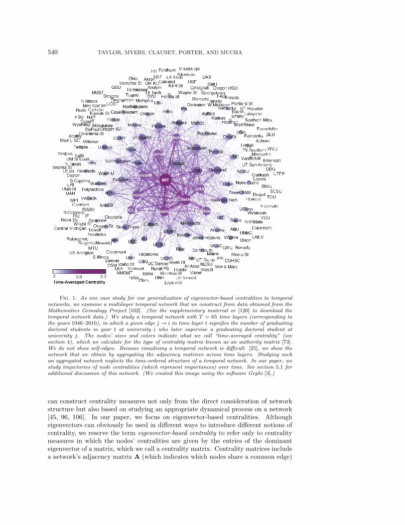
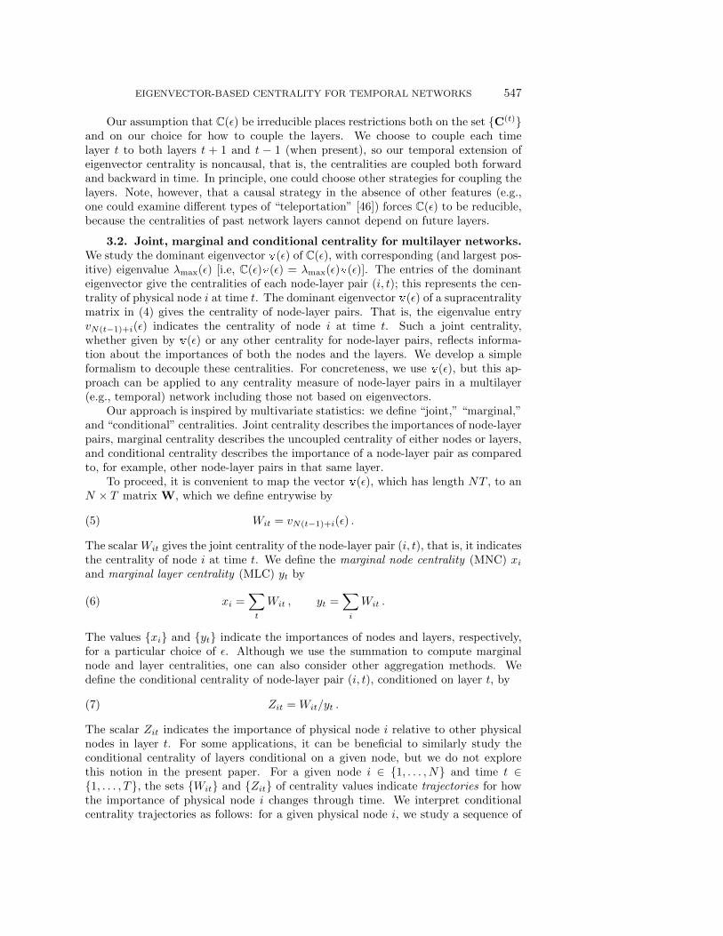
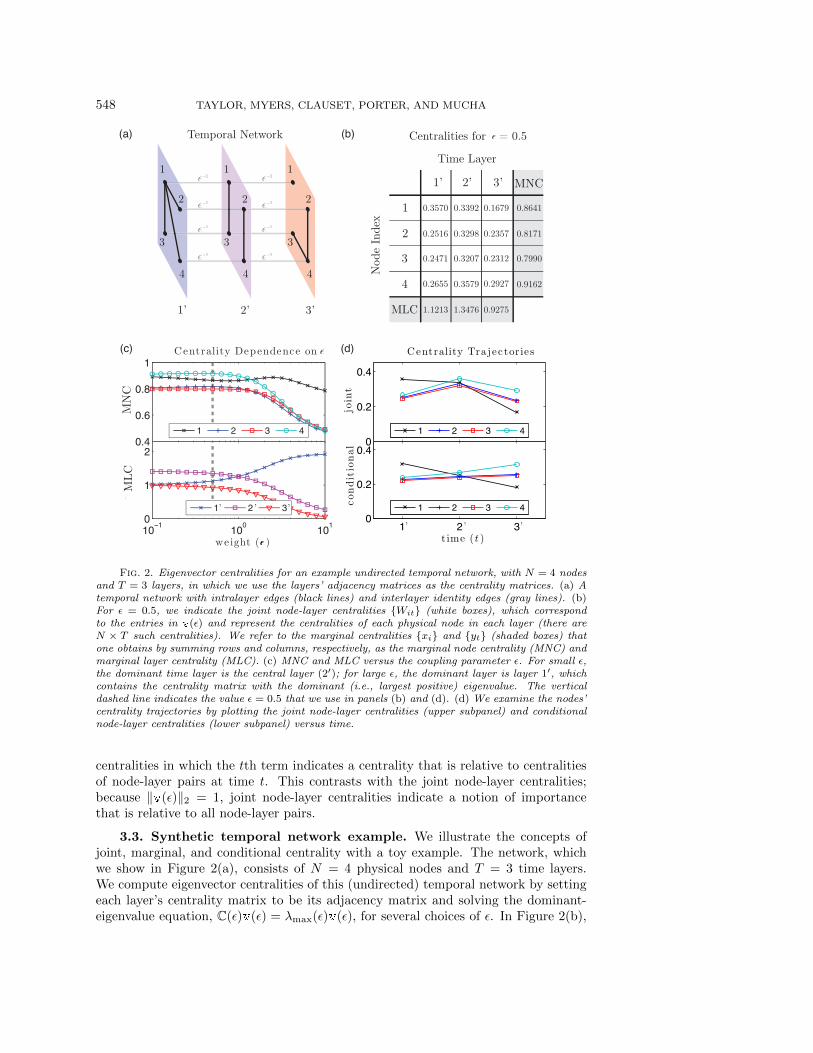
Fig. 2. Eigenvector centralities for an example undirected temporal network, with N = 4 nodesand T = 3 layers, in which we use the layers’ adjacency matrices as the centrality matrices. (a) Atemporal network with intralayer edges (black lines) and interlayer identity edges (gray lines). (b)For ε = 0.5, we indicate the joint node-layer centralities {Wit} (white boxes), which correspondto the entries in v(ε) and represent the centralities of each physical node in each layer (there areN × T such centralities). We refer to the marginal centralities {xi} and {yt} (shaded boxes) thatone obtains by summing rows and columns, respectively, as the marginal node centrality (MNC) andmarginal layer centrality (MLC). (c) MNC and MLC versus the coupling parameter ε. For small ε,the dominant time layer is the central layer (2′); for large ε, the dominant layer is layer 1′, whichcontains the centrality matrix with the dominant (i.e., largest positive) eigenvalue. The verticaldashed line indicates the value ε = 0.5 that we use in panels (b) and (d). (d) We examine the nodes’centrality trajectories by plotting the joint node-layer centralities (upper subpanel) and conditionalnode-layer centralities (lower subpanel) versus time.
centralities in which the tth term indicates a centrality that is relative to centralitiesof node-layer pairs at time t. This contrasts with the joint node-layer centralities;because ‖v(ε)‖2 = 1, joint node-layer centralities indicate a notion of importancethat is relative to all node-layer pairs.
3.3. Synthetic temporal network example. We illustrate the concepts ofjoint, marginal, and conditional centrality with a toy example. The network, whichwe show in Figure 2(a), consists of N = 4 physical nodes and T = 3 time layers.We compute eigenvector centralities of this (undirected) temporal network by settingeach layer’s centrality matrix to be its adjacency matrix and solving the dominant-eigenvalue equation, C(ε)v(ε) = λmax(ε)v(ε), for several choices of ε. In Figure 2(b),

EIGENVECTOR-BASED CENTRALITY FOR TEMPORAL NETWORKS 549
we summarize the centrality measures for ε = 0.5 in a matrix. The entry in row i andcolumn t gives Wit. The MNCs {xi} and the MLCs {yt} are in the shaded boxes, andthey indicate the relative centralities of the physical nodes and layers, respectively,for the chosen value of ε.
In Figure 2(c), we plot the dependence of the MNC (upper subpanel) and MLC(lower subpanel) on the coupling strength ε. For small ε, the dominant time layeris layer 2’; for large ε, the dominant layer is layer 1’. This is unsurprising: whenconsidering the centrality matrices of the layers in isolation, the dominant eigenvalueof the centrality matrix of layer 1’ is larger than that for the other layers. The choiceof ε is very important, and centralities can depend discontinuously on ε because ofeigenvalue crossings. In this example, we obtain three qualitatively different regimes:(i) a strong-coupling regime in which the centralities are similar to what we expect inthe limit ε→ 0+; (ii) a weak-coupling regime in which the centralities behave similarlyto what they do in the ε→∞ limit; and (iii) an intermediate-coupling regime in whichthe centralities transition between these two limiting cases. (Compare this result tothe phase-transition phenomena for graph Laplacians of multilayer networks discussedin [103, 104].) We also explore these regimes for our case study with the MGP networkin section 5.1.
In Figure 2(d), we plot joint node-layer centralities (upper subpanel) and the con-ditional node-layer centralities (lower subpanel) that correspond to the four physicalnodes. We show results for ε = 0.5. Note that the conditional node-layer centralitiesfor physical node 4 increase over time, whereas they decrease for physical node 1.This is sensible for the temporal network in Figure 2(a): at time t = 1’, physical node1 has the largest degree and physical node 4 has the smallest degree; however, at timet = 3’, physical node 1 has the smallest degree and physical node 4 has the largestdegree.
4. Singular perturbation in the strong-coupling limit. Given the jointnode-layer centralities and conditional node-layer centralities that correspond to aphysical node i, it is possible to define a notion of “time-averaged centrality” bysumming one of these centralities across the layers (e.g., the prior yields the MNC).However, it is not clear which is preferable, and these centralities are sensitive to thevalue of ε. Alternatively, one can define a time-averaged centrality by studying thelimit ε → 0+. In this limit, the conditional node-layer centrality of every physicalnode i is constant across the time layers.
Examining centralities as ε → 0+ provides a principled approach for calculatingtime-averaged centralities. However, the supracentrality matrix C(ε) given by (4)becomes singular at ε = 0, which complicates the consideration of this limit. Theintralayer connectivity is completely eliminated, and the network decomposes into Nconnected components. That is, the matrix is no longer irreducible, so the Perron–Frobenius theorem no longer holds. Indeed, at ε = 0, the dominant eigenvalue hasan N -dimensional eigenspace. In contrast, for ε > 0, the dominant eigenvalue has asingle eigenvector.
To overcome this issue, we derive a singular perturbation expansion in the limitε → 0+. In section 4.1, we further explore the singularity that arises in the strong-coupling limit. In sections 4.2 and 4.3, we give zeroth-order and first-order pertur-bation expansions, which lead to principled expressions for time-averaged centralitiesand first-order-mover scores, respectively. We give higher-order expansions in an ap-pendix. In section 4.4, we summarize our procedure and discuss the computationalcomplexity of computing time-averaged centralities and first-order-mover scores.

550 TAYLOR, MYERS, CLAUSET, PORTER, AND MUCHA
4.1. Singularity at infinite interlayer coupling. In this section, we developa perturbation analysis of the dominant eigenspace (i.e., the eigenspace of the largestpositive eigenvalue) of C(ε) (see (4)) in the limit ε → 0+. To allow this analysis tohave more broad applicability, we do a perturbation expansion using the followinggeneral form of coupling of block matrices:
(8) M(ε) = B + εG ,
where G = diag[M(1), . . . ,M(T )], B = A⊗ I, and the T ×T matrix A (recall Table 1)encodes the interlayer coupling, where entry Att′ indicates how layer t is coupled tolayer t′. We recover the supracentrality matrix C(ε) in (4) by using nearest-neighborlayer coupling, A = A(chain), and centrality matrices along the diagonal (i.e., M(t) =C(t)). Additionally, similarly to our assumptions for (4), we assume that M(ε) isnonnegative and irreducible for any ε > 0. These assumptions hold as long as thesummation of matrices (
∑t M(t)) and interlayer coupling matrix A each correspond
to a strongly connected network (see footnote 3 in section 3.2).We begin by studying the dominant eigenspace for the matrix M(ε) at ε = 0. We
thus consider the matrix
M(0) = A⊗ I ,(9)
and we will show that the dominant eigenspace of M(0) is N -dimensional, implyingthat one cannot obtain the unique dominant eigenvector of M(ε) for the ε→ 0+ limitsimply by setting ε = 0. Instead, one needs to do a singular perturbation analysis.To facilitate our discussion, we define an NT ×NT stride permutation matrix P [48]with entries Pkl = 1 for l = dk/Ne+T [(k−1) mod N ] and Pkl = 0 otherwise. (Recallthat d·e denotes the ceiling function.) Note that P permutes node-layer indices, so wecan easily go back and forth between ordering the node-layer pairs first by time andthen by physical node index, or vice versa (i.e., ordering them first by physical nodeindex and then by time). The main benefit of defining P is that one can express M(0)in the form M(0) = P (I⊗A)PT [28], where
(10) I⊗A =
A 0 0 · · ·0 A 0
0 0 A. . .
.... . .
. . .
.Clearly, I⊗A decouples into N identical eigenvalue equations for the interlayer cou-pling matrix A. Because P is a unitary matrix, this decoupling also occurs for M(0).Specifically, the NT eigenvalues of I⊗A are given by the T eigenvalues of A, whereeach eigenvalue has multiplicity N and a corresponding N -dimensional eigenspacespanned by the vectors that can be constructed using the eigenvectors of A (i.e., withappended 0 values in appropriate coordinates).
We explain this construction in more detail for the dominant eigenspace. Letν denote the largest positive eigenvalue of A, and let u = [u1, . . . , uT ]T denote itscorresponding eigenvector. Because of the block-diagonal structure of (10), the largesteigenvalue λ0 of I⊗A is λ0 = ν, and its corresponding eigenspace is spanned by the Neigenvectors {ui}, where ui = [0T , . . . ,0T ,uT ,0T , . . . ,0T ]T . That is, the ith block ofui is given by u, and all of the other blocks are vectors of zeros. Consequently, one canobtain the N dominant eigenvectors of M(0) = A⊗ I using the permutations {Pui}.
EIGENVECTOR-BASED CENTRALITY FOR TEMPORAL NETWORKS 551
That is, they have the general form∑
j αjPuj , where the constants {αi} must satisfy∑i α
2i = 1 to ensure that the vector is normalized. Because there does not exist a
unique dominant eigenvector of M(0) (as its dominant eigenspace is N -dimensional),we need to develop a singular perturbation analysis to obtain a unique solution forthe dominant eigenvector of M(ε) in the ε→ 0+ limit.
When the network layers are coupled by an undirected chain network, the inter-layer coupling matrix is given by A = A(chain), which has N eigenvalues and eigen-vectors given by [82]
ν(chain) = 2 cos
(nπ
T + 1
),(11)
u(chain) =1√γn
[sin
(nπ
T + 1
), sin
(2nπ
T + 1
), . . . , sin
(Tnπ
T + 1
)]T,(12)
where n ∈ {1, . . . , N} and the normalization constant is γn =∑T
t=1 sin2[nπt/(T + 1)].Setting n = 1 gives the dominant eigenvalue and its corresponding eigenvector.
4.2. Zeroth-order expansion and time-averaged centrality. In this sec-tion, we study the zeroth-order expansion of the dominant eigenvector v(ε) in thelimit ε → 0+. As we now show, the conditional node-layer centralities {Zit} corre-sponding to a given physical node i become constant across time in this limit. (Recallour definitions of joint, marginal, and conditional centralities in section 3.2.) For eachphysical node, we refer to this limiting value as its time-averaged centrality. By exam-ining the first-order expansion of v(ε) in the limit ε → 0+, we show in (19) that onecan obtain the time-averaged centralities as the eigenvector components correspondingto the largest eigenvalue of a matrix of size N ×N .
We consider the dominant-eigenvalue equation
(13) λmax(ε)v(ε) = M(ε)v(ε) = Bv(ε) + εGv(ε) .
We expand λmax(ε) and v(ε) for small ε by writing λmax(ε) = λ0 + ελ1 + · · · and
v(ε) = v0 + εv1 + · · · to obtain kth-order approximations: λmax(ε) ≈∑k
j=0 εjλj and
v(ε) ≈∑k
j=0 εjvj . We use superscripts to indicate powers of ε in the terms in the
expansion, and we use subscripts for the terms that are multiplied by the power of ε.Note that λ0 and v0, respectively, indicate the dominant eigenvalue and correspondingeigenvector in the limit ε→ 0+. Successive terms in these expansions represent higher-order derivatives of λmax(ε) and v(ε), and each term assumes appropriate smoothnessof these functions.
Our strategy is to develop consistent solutions to (13) for increasing values of k.Starting with the first-order approximation, we substitute λmax(ε) ≈ λ0 + ελ1 andv(ε) ≈ v0 + εv1 into (13) and collect the zeroth-order and first-order terms in ε toobtain
(λ0I− B)v0 = 0 ,(14)
(λ0I− B)v1 = (G− λ1I)v0 ,(15)
where I is the NT ×NT identity matrix. Equation (14) is exactly the system that westudied in section 4.1 (see (8) with ε = 0), where we found that the operator λ0I− Bis singular and has an N -dimensional null space. (This is the dominant eigenspace ofB.) We also found that (14) has a general solution of the form
(16) λ0 = ν, v0 =∑j
αjPuj ,
552 TAYLOR, MYERS, CLAUSET, PORTER, AND MUCHA
where {αi} are constants that satisfy the constraint that v0 has magnitude 1 (i.e.,∑i α
2i = 1). We defined ui just below (10).
To find the set {αi} of unique constants that determine v0, we seek a solvabilitycondition in the first-order terms. Using the fact that the null space of λ0I − B isspan(Pu1, . . . ,PuN ) for any physical node i, it follows that (Pui)
T (λ0I− B)v1 = 0,and left-multiplying (15) by (Pui)
T leads to
uTi PTGv0 = λ1u
Ti PT
v0 .(17)
Using the solution of v0 in (16), we obtain∑j
αjuTi PTGPuj = λ1
∑j
αjuTi PTPuj = λ1αi ,(18)
because PTP = PPT = I and uTi uj = δij , where δij is the Kronecker delta. Letting
α = [α1, . . . , αN ]T , (18) corresponds to an N -dimensional eigenvalue equation,
(19) X(1)α = λ1α ,
where the matrix X(1) has elements
(20) X(1)ij = u
Ti PTGPuj =
∑t
M(t)ij u
2t .
Our assumption that M(ε) is nonnegative and irreducible for any ε > 0 ensures thatX(1) is also nonnegative and irreducible. By the Perron–Frobenius theorem for non-negative matrices [87], the largest positive eigenvalue λ1 of X(1) has a multiplicity ofone, and its eigenvector α is unique and has nonnegative entries (see section 3.1 andfootnote 3). We normalize the solution α to (19) by
∑i α
2i = 1 and substitute the
normalized solution into (16) to obtain the zeroth-order term v0.When the layers are coupled by an undirected chain and the block matrices are
the layers’ centrality matrices (i.e., M(t) = C(t)), we obtain
(21) X(1)ij = γ−11
∑t
C(t)ij sin2
(πt
T + 1
),
where γ1 =∑T
t=1 sin2 (πt/(T + 1)) is the normalization constant for the dominanteigenvector u(chain) given by n = 1 in (12). In this case, recall that the vector v0
is the dominant eigenvector of C(ε) in the limit ε → 0+ and gives the joint node-layer centralities in this limit. By inspection, we see that the elements of v0 areαi sin(πt/(T + 1)) for node-layer pair (i, t). Because these correspond to the limitingε→ 0+ entries of vector v(ε), they are independent of ε. At the same time, conditionalcentrality of node-layer pair (i, t) is αi (up to a normalization constant), independentof the layer t. That is, the conditional node centrality trajectories become constantacross time in the limit ε → 0+. These values of {αi} arise naturally from ourperturbative expansion in the supracentrality framework, independently of the valueof ε. By contrast, recall that the MNCs reflect averaging the joint centralities acrosstime layers for a specific choice of ε. Accordingly, we hereafter refer to the entry αi
in the vector α as the time-averaged node centrality of physical node i. Because ourapproach can also be applied to multilayer networks that are not necessarily temporal,we call αi the layer-averaged node centrality for these situations.

EIGENVECTOR-BASED CENTRALITY FOR TEMPORAL NETWORKS 553
4.3. First-order expansion and first-order-mover scores. In this section,we show that the first-order expansion of (13) leads to a linear system (see (31)),which we solve to obtain a measurement of the variation over time of each physicalnode’s centrality trajectory (see equation (33)). Specifically, as one increases ε above0+, the first-order expansion, (which accounts for first derivatives with respect to ε),captures the dominant changes in centrality trajectories for small values of ε. (In theappendix, we derive expressions for higher-order terms that account for higher-orderderivatives with respect to ε.)
In section 4.2, we derived closed-form expressions for λ0 and v0 and an eigenvalueequation satisfied by λ1. We now solve for v1 to complete our first-order approxima-tion. For notational convenience, we define L0 = λ0I − B and L1 = G − λ1I, so (15)
becomes L0v1 = L1v0. Letting L†0 denote the Moore–Penrose pseudoinverse of L0,we write
(22) v1 = L†0L1v0 +∑j
βjPuj = L†0Gv0 +∑j
βjPuj .
We simplify the first term in (22) using L1 = G−λ1I and v0 =∑
j αjPuj and noting
that each vector Puj lies in the null space of each of the matrices L0 and L†0. Thesecond term in (22) accounts for the projection of v1 onto the null space of L0, wherethe constants βi = (Pui)
Tv1 indicate the projections onto the spanning vectors of thenull space. To ensure numerical stability and computational efficiency in practice, wecalculate L†0 using the identity [28]
(23) L†0 = (λ0I−A⊗ I)†
= (λ0I −A)† ⊗ I .
Note that L†0 depends only on the interlayer coupling matrix A (e.g., for nearest-neighbor-in-time coupling, A = A(chain)), which one can compute and save in memoryprior to analyzing network data.
Just as we examined first-order terms to solve for constants {αi}, we now seek asolvability condition in the second-order terms to determine {βi} in (22). Substitutingλmax(ε) = λ0 + ελ1 + ε2λ2 and v(ε) = v0 + εv1 + ε2v2 into (13) and collecting thesecond-order terms yields
(24) L0v2 = L1v1 − λ2v0 .
Similarly to before, we left-multiply (24) by (Pui)T and require both sides to be
identically 0 to obtain
(25) λ2uTi PT
v0 = uTi PTL1v1 = u
Ti PTGv1 − λ1uT
i PTv1.
Using αi = uTi PTv0 and βi = uT
i PTv1, it then follows that
(26) λ2αi + λ1βi = uTi PTGv1 .
Substituting the expressions for v0 from (16) and v1 from (22) into (26) then yields
(27) λ2αi + λ1βi =∑j
αjuTi PTGL†0GPuj +
∑j
βjuTi PTGPuj .
After some rearranging, we obtain
(X(1) − λ1I)β = (λ2I−X(2))α ,(28)
554 TAYLOR, MYERS, CLAUSET, PORTER, AND MUCHA
where the matrix X(1) was defined by (20), and the elements of the matrix X(2) are
(29) X(2)ij = u
Ti PTGL†0GPuj .
Recalling that we determined α as the solution of X(1)α = λ1α such that∑
i α2i = 1,
we left-multiply (28) by αT to obtain
(30) λ2 = αTX(2)α .
We thereby obtain
β = (X(1) − λ1I)†(λ2I−X(2))α+ bα ,(31)
where the constant b = αTβ describes the (possibly nonzero) projection of β ontothe null space of (X(1) − λ1I) (see (19)).
We now show that b = 0 in (31), by virtue of the requirement that the eigenvectorobtained at first order has a norm of 1. That is, we require that 1 = ‖v0 + εv1‖2 =‖v0‖2 + 2ε〈v0,v1〉 + O(ε2). However, ‖v0‖2 = 1, so 〈v0,v1〉 = 0, where we use thenotation 〈·, ·〉 to denote the dot product between inputs. Using the definitions of v0
and v1, we see that
0 = 〈v0,v1〉 =
⟨∑j
αjPuj , L†0Gv0 +∑j
βjPuj
⟩=∑j
αjβj = b ,(32)
because the vectors {Puj} are orthonormal and lie in the null space of L0. (In other
words, (Pui)TPuj = δij and (Pui)
TL†0 = 0.)In practice, we solve (31) using a linear solver (see, e.g., [48]) rather than the
pseudoinverse to avoid computing the inverse of (X(1) − λ1I). We then ensure thatthe solution is orthogonal to α by projecting it onto the subspace that is orthogonalto α.
One can substitute the solution β to (31) with b = 0 into (22) to obtain thefirst-order term v1 in the expansion for v(ε). This first-order term, which yields thestrongest temporal variation of the conditional centralities at small ε, is a conciserepresentation of temporal changes in centrality. There are multiple possible waysto use v1 to quantify the role of physical node i across the T layers. We define ameasure mi that equals the square root of the sum of the squares of the entries in v1
that correspond to physical node i. Specifically, we define the first-order-mover scoremi ≥ 0 of physical node i by
m2i = v
T1 PIiPT
v1
= β2i +
(L†0Gv0
)TPIiPTL†0Gv0
= β2i +
T∑t=1
([L†0Gv0]i+t(N−1)
)2,(33)
where [·]i denotes the ith entry in a vector and Ii = diag[0, . . . , 0, I, 0, . . . , 0] is a matrixof size NT×NT that contains all 0 entries except for the ith block, which is an identity

EIGENVECTOR-BASED CENTRALITY FOR TEMPORAL NETWORKS 555
matrix I of size T × T . In other words, we measure the variation of v1 with respectto a physical node i by examining the 2-norm of the entries in v1 that correspond tothe node-layer pairs (i, t) that are relevant to physical node i (i.e., entries j such thatj = N(t − 1) + i with t = 1, . . . , T ). In principle, one can also use a different vectornorm or a heuristic method for aggregating centrality. Our choice has the virtue thatit is mathematically consistent with our definition for the time-averaged centralities{αi} (see (19)). Specifically, α2
i = vT0 PIiPTv0. Therefore, one can naturally extend
our approach for quantifying the contribution of the first-order correction given by(33) to higher-order corrections. We also note that first-order-mover scores rank thenodes according to the magnitudes of their corresponding entries in v1. Therefore, theassociated centralities v(ε) can either increase or decrease over time. One can easilycheck whether there is an increase or a decrease by examining the correspondingentries of v(ε).
4.4. Procedure for computing time-averaged centrality and first-order-mover scores. We summarize our procedure for computing time-averaged centralityand first-order-mover scores:
1. Construct the matrix X(1) using (21):
X(1)ij = γ−11
∑t
C(t)ij sin2
(πt
T + 1
).
When layers are coupled by a layer-adjacency matrix A (which is not nec-
essarily an undirected chain A(chain)), it follows that X(1)ij = uT
i PTGPuj ,
where G = diag[C(1), . . . ,C(T )] and P and ui are defined just before andafter, respectively, (10).
2. Solve for the time-averaged centralities {αi} using (19):
X(1)α = λ1α .
3. Construct the matrix X(2) using (29):
X(2)ij = u
Ti PTGL†0GPuj ,
where L†0 = (λ0I −A)† ⊗ I.
4. Solve for β in (28):
(X(1) − λ1I)β = (λ2I−X(2))α ,
where λ2 = αTX(2)α.5. Solve for the first-order-mover scores {mi} using (33):
m2i = β2
i +
T∑t=1
([L†0Gv0]i+t(N−1)
)2,
where v0 =∑
j αjPuj .
We comment briefly on the computational costs of the above procedure. Thesupracentrality matrix (see (4)), whose dominant eigenvector gives the joint node-layercentralities, has size NT ×NT , and that can be problematic for large networks with

556 TAYLOR, MYERS, CLAUSET, PORTER, AND MUCHA
many time layers (i.e., when T � 1). The time-averaged node centralities are given bythe solution to (19), which is a dominant eigenvalue problem for a matrix of size N×N .To examine which physical nodes have centralities that change significantly over time,we examine the first-order-mover scores given by (33); this requires one to solve the
N -dimensional linear system given by (31). Because L†0, G, and v0 are known prior tosolving (31), one can directly compute the second term in (33). For sparse networks[i.e., those in which the number of edges at a given time is O(N)], the matrices thatwe have discussed in this section are typically also sparse. One can thus solve (19),(21), (28), (29), and (33) efficiently using data structures that are designed for sparsematrices, including direct methods [23], iterative methods [110], and methods designedfor particular network structures (e.g., nested dissection for planar networks [81]). Inparticular, the power method for computing a dominant eigenvalue and eigenvector ofa sparse matrix reduces the per-iteration complexity from O(N2) to O(M), where Mis the number of nonzero entries in the sparse matrix. However, the actual scaling canbe much larger, because the number of iterations required for convergence dependson the gap between the largest and second-largest eigenvalues.
5. Case studies with empirical network data. In this section, we examinetemporal centrality in case studies with three sets of empirical data: the MathematicsGenealogy Project of Ph.D. receipt in the mathematical sciences in U.S. universities(see section 5.1), top billing in the Golden Age of Hollywood (see section 5.2), andcitations of U.S. Supreme Court decisions (see section 5.3). We have posted MATLABsoftware at [119] that implements our calculations and can be used to reproduce theresults of this section.
Most of our calculations for these examples use a temporal generalization of huband authority scores [73], which are particularly appropriate for directed networks(such as our three examples). We also note that hub and authority scores have beenused previously to examine time-independent faculty-hiring networks [39, 93] andSupreme Court decisions [39, 41]. To illustrate a comparison with another choice ofcentrality, we also study a temporal generalization of PageRank for the MGP network.
We compute hub and authority scores independently using two supracentral-ity matrices, A(t)[A(t)]T and [A(t)]TA(t). For a single-layer network, it is possibleto simultaneously compute hub and authority scores by studying the single system[
0AT
A0
]. In general, however, a supracentrality matrix that uses this alternative for-
mulation yields different time-dependent centralities from ones based on independentcomputations of hub and authority scores. For each centrality that we compute, wealso examine the induced ranking of nodes in which the highest-ranked nodes (i.e.,those with ranks 1, 2, and so on) correspond to the largest centralities, whereas thelowest-ranked nodes correspond to the smallest centralities.
5.1. Doctoral exchange in the Mathematics Genealogy Project (MGP).Our first case study uses a network that encodes the exchange of mathematicians (andother mathematical scientists) who have obtained a Ph.D. (or equivalent doctoral de-gree) between universities to study the academic prestige of those universities. Westudy data provided by the MGP [102], which collects information for mathemati-cians (and members of related fields who are listed in the MGP) with doctorates. Foreach mathematical scientist, the information includes graduation year, his/her officialacademic advisor(s), the degree-granting university, and a list of his/her students whohave also obtained doctoral degrees. A subset of the present authors previously uti-lized these data to approximate the flow of doctorates between universities—that is,

EIGENVECTOR-BASED CENTRALITY FOR TEMPORAL NETWORKS 557
a person graduates from one university and is then hired at a second university—andquantified the resulting hub and authority scores for the total flow during a speci-fied time period as a candidate measure of these universities’ relative mathematicalprestige [93]. Moreover, hub and authority scores have been used previously to studyPh.D. exchange networks in other disciplines [39]. See [55] for a comparison of thehiring market for different academic disciplines, and see [44, 83] for other analysesand visualization of data from the MGP. See [76] for an application of PageRankcentrality to ranking world universities using data from Wikipedia.
It is well documented that graduates typically obtain faculty positions at univer-sities that are either comparable to or less prestigious than the one from which theygraduate [13, 15, 19, 29, 39, 98], and we study university prestige as indicated by theexchange between universities of mathematicians with doctoral degrees. We generalizea previous study of the MGP data in [93] by keeping the year that each faculty membergraduated with his/her Ph.D. degree. We focus on the years 1946–2010, which includeall post-World War II information available in the data set.4 This yields T = 65 timelayers, and we restrict our attention to a set of N = 227 U.S. universities that wereconnected during this period. To construct the network, we create directed intralayeredges i → j at time t to represent a doctoral degree in the MGP data awarded toa mathematical scientist from university j in year t who later advised at least onestudent at university i. Therefore, to contribute a directed edge, the mathematicianmust have at least one student in the MGP data. We weight edges to indicate thenumber of doctorates from university j in year t awarded to faculty who later advisestudents at university i. Our construction aligns edge directions to be opposite to thatof the flow of people, so a node with large in-degree (i.e., with many graduates wholater advise students elsewhere) is considered both an academic authority as well asan authority with respect to hub and authority centrality [73]. See Figure 1 for a vi-sualization of this network; due to the difficulty of visualizing temporal networks [25],we show a network corresponding to the aggregation
∑t A(t) of the adjacency matri-
ces. Although one could define the multilayer network in more intricate ways (e.g.,by normalizing edge weights using the number of graduates) and examine how theresults vary for different choices, we wish to keep the present manuscript focused onintroducing and demonstrating our temporal generalization of eigenvector-based cen-tralities. Therefore, we leave such detailed analyses for future work. We make theMGP temporal network available as supplementary material and online at [120].
5.1.1. MGP: Centrality in the strong-coupling regime. We begin by iden-tifying the universities that have the largest time-averaged authority centralities {αi},which we obtain from the dominant eigenvector of the matrix X(1) (see (21)) usingC(t) = (A(t))TA(t) [73]. For notational convenience, we use t to denote the grad-uation year rather than the time layer. For example, we use A(1946) to denote thenetwork adjacency matrix for time layer 1 (i.e., year 1946). We summarize theseauthority values in Table 2, and we note that the most central universities accord-ing to this measure are all widely accepted top-tier programs in mathematics. Thetime-averaged authorities identify the four most central mathematics universities forthis time period as MIT, UC Berkeley, Stanford, and Princeton. Although the resultsin Table 2 are interesting, time-averaged centrality (by definition) does not provide
4The data set was provided to us in 2009, although it includes information up to 2010. The year2006 is the last year in which a Ph.D. degree was awarded to someone who was subsequently a Ph.D.advisor in the data, so it is also the last year in which intralayers edges are present. Additionally,we decided to be optimistic and include Ph.D. degrees that were projected for the year 2010.
558 TAYLOR, MYERS, CLAUSET, PORTER, AND MUCHA
Table 2Top time-averaged centralities and first-order-mover scores for our temporal generalization (see
(4)) of authority scores [73] for U.S. universities in the MGP [102]. We show our results using twodifferent orderings: (1) according to the top time-averaged centralities and (2) according to the topfirst-mover scores.
Top time-averaged centralities Top first-order-mover scores
Rank
12345678910
University αi mi
MIT 0.6685 688.62UC Berkeley 0.2722 299.06
Stanford 0.2295 241.71Princeton 0.1803 248.71
UIUC 0.1645 74.30Cornell 0.1642 180.50Harvard 0.1628 185.34
U Washington 0.1590 81.22U Michigan 0.1521 86.50
UCLA 0.1456 152.77
University mi αi
MIT 688.62 0.6685UC Berkeley 299.07 0.2722
Princeton 248.72 0.1803Stanford 241.71 0.2295
Georgia Tech 189.34 0.0960U Maryland 186.65 0.1278
Harvard 185.34 0.1628CUNY 182.59 0.0466Cornell 180.50 0.1642
Yale 159.11 0.0816
1 501
50
t ime-averaged centrality rank
first-m
overrank
F irst-movers and centrality
1 2271
227
CUNY
(a)
MIT
Georgia Tech
1945 1965 1985 2005
10−2
10−1
100
t ime (t )
conditionalcentrality
C entrality tra jectorie s for ǫ = 10−4
MIT
UC Berkeley
Princeton
Stanford
Georgia Tech
CUNY
(b)
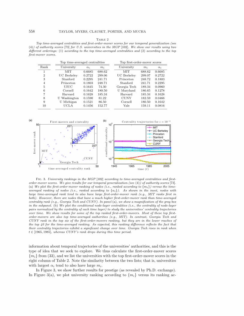
Fig. 3. University rankings in the MGP [102] according to time-averaged centralities and first-order-mover scores. We give results for our temporal generalization (see (4)) of authority scores [73].(a) We plot the first-order-mover ranking of nodes (i.e., ranked according to {mi}) versus the time-averaged ranking of nodes (i.e., ranked according to {αi}). As shown in the inset, nodes withlarge time-averaged rank tend to also have large first-order-mover rank (e.g., MIT ranks first inboth). However, there are nodes that have a much higher first-order-mover rank than time-averagedcentrality rank (e.g., Georgia Tech and CUNY). In panel (a), we show a magnification of the gray boxin the subpanel. (b) We plot the conditional node-layer centralities (i.e., the centrality of node-layerpairs normalized by the centrality of each time layer) to study the universities’ centrality trajectoriesover time. We show results for some of the top ranked first-order-movers. Most of these top first-order-movers are also top time-averaged authorities (e.g., MIT). In contrast, Georgia Tech andCUNY rank in the top six of the first-order-movers ranking, but they are in the lower reaches ofthe top 40 for the time-averaged ranking. As expected, this ranking difference reflects the fact thattheir centrality trajectories exhibit a significant change over time. Georgia Tech rises in rank whent ∈ [1965, 1985], whereas CUNY’s rank drops during this time period.
information about temporal trajectories of the universities’ authorities, and this is thetype of idea that we seek to explore. We thus calculate the first-order-mover scores{mi} from (33), and we list the universities with the top first-order-mover scores in theright column of Table 2. Note the similarity between the two lists; that is, universitieswith largest αi tend to also have large mi.
In Figure 3, we show further results for prestige (as revealed by Ph.D. exchange).In Figure 3(a), we plot university ranking according to {mi} versus its ranking ac-
EIGENVECTOR-BASED CENTRALITY FOR TEMPORAL NETWORKS 559
cording to {αi}. Note in the bottom left corner that MIT is ranked first for bothquantities, and that, in general, there is a strong linear correlation between rankaccording to αi and rank according to mi. Intuitively, this suggests that shifts incentrality include a natural effect that is related directly to the centrality score itself.(In other words, large centrality values tend to also include large fluctuations, whereassmall centrality values typically have only small fluctuations.) Deviations from theobserved nearly linear relation indicate universities whose centrality trajectory ex-hibits larger variations over time, and it is worthwhile to look at these universitiesin more detail for potentially interesting insights. For example, the universities withhigh rank according to mi (i.e., large mi) but comparatively low rank according toαi (i.e., small αi) include Georgia Tech and CUNY, and it is known that GeorgiaTech’s mathematics department transitioned from a primarily teaching-oriented de-partment to a much more research-oriented department with a newly restructureddoctoral degree program starting in the late 1970s [32].
In Figure 3(b), we plot the conditional authority centralities at ε = 10−4 ofuniversities versus time for six of the universities with the largest first-order-moverscores mi. This includes the four universities with the top time-averaged centralities,as well as Georgia Tech and CUNY (which do not have highly ranked time-averagedcentralities). As we expect, the conditional centralities for Georgia Tech and CUNYchange drastically over time, whereas the trajectories for the others remain relativelyconstant.
5.1.2. MGP: Some properties of authority centrality. As we showed insection 3.3 for a synthetic network, the choice of interlayer coupling strength ε stronglyaffects the temporal behavior of a node’s centrality trajectory. We expect to observethree qualitative regimes: (i) the strong-coupling (ε → 0+) regime that we studiedin section 4; (ii) a weak-coupling (ε→∞) regime; and (iii) an intermediate-couplingregime, in which the centralities behave differently than expected for either the strong-coupling or weak-coupling regimes. In Figure 3(b), we show results for ε = 10−4, andwe observe that the universities tend to have slowly varying centrality trajectories.However, the choice of ε should depend both on the application and on the questionof interest. As we are about to illustrate, it is important to consider what values of εare appropriate.
In Figure 4, we study centrality trajectories for Georgia Tech for various choicesfor ε. In Figure 4(a), we show the conditional node-layer centralities for Georgia Techversus time t. Recall that the conditional node-layer centrality indicates the centralityof node-layer pair (i, t) with respect to all node-layer pairs (j, t) at time t. We alsoshow the value of αi (rescaled for normalization), which gives the conditional node-layer centrality of Georgia Tech in the limit ε → 0+. For small but nonzero ε (e.g.,ε = 10−3), note that we obtain a similar trajectory as for ε = 0+. For example, thetrajectory varies slowly over time, so the conditional node-layer centrality of GeorgiaTech at times t and t + 1 are approximately equal for all t. However, as we increaseε, we lose the slow temporal variation over time. For example, when ε ≥ 10−1, theconditional centrality of Georgia Tech at times t and t+1 are typically very dissimilar,which appears to be a consistent property of conditional node-layer centralities in thelimit ε → ∞. It is our believe that the highly volatile rankings for large ε do notappropriately describe the dynamics of department prestige [116]; this observation hasmotivated us to focus on the small ε (i.e., strong-coupling) regime in this paper. Thelimiting cases ε → 0+ and ε → ∞, respectively, do a good job of describing regimeswith very small and very large ε, but the intermediate (“transitional”) regime between

560 TAYLOR, MYERS, CLAUSET, PORTER, AND MUCHA
1945 1965 1985 200510
−3
10−2
10−1
Georgia Tech condit ional centrality
t ime (t )
conditionalcentrality
α i
(a)
1945 1965 1985 200510
−6
10−4
10−2
Georgia Tech joint centrality
t ime (t )
jointcentrality
ε = 0.0001
ε = 0.001
ε = 0.01
ε = 0.1
ε = 1
α i
(b)
Fig. 4. Centrality trajectories for Georgia Tech illustrate that one can construe ε as a tuningparameter that controls how much centrality can vary between neighboring time layers. (a) To studythe trajectory of university authorities over time, we examine the conditional node-layer centralities.For sufficiently small ε, we observe a steady increase in ranking with time for Georgia Tech. Varyingε changes the coupling strength between temporal layers. If ε is too large (e.g., ε ≥ 0.01), then thecoupling between layers is so weak that the conditional node-layer centrality of the two node-layerpairs at times t and t + 1 are no longer similar in value. As ε → 0+, the conditional node-layercentrality approaches the stationary, time-average ranking given by αi (horizontal dashed line), butwe still observe significant variation even for ε = 0.0001. (b) We plot the joint node-layer centralityof the T node-layer pairs that correspond to Georgia Tech across the time layers for several values ofε. For small ε, the joint node-layer centralities are determined by the chain of identity edges (whichleads to the sinusoidal dependence given by (12) with n = 1 and magnitude αi). For large valuesof ε, the node-layer pairs in time layer t = 1982 dominate the joint node-layer centralities, so alluniversities have their highest values in this layer.
these extremes is not straightforward to interpret. Even the boundaries between thetwo extreme qualitative regimes are not clear and are open to interpretation.
In Figure 4(b), we plot the joint node-layer centralities for Georgia Tech forvarious values of ε. Recall that the joint node-layer centrality of the node-layer pair(i, t) reflects information about both the physical node i and the time layer t. In theε → 0+ limit, the joint node-layer centrality trajectory is given by αiu
(chain), whichwe show using a dashed line. Interestingly, for the ε values that exhibit slowly varyingconditional-node-layer-centrality trajectories in panel (a) (i.e., ε ≤ 10−3), we find thatthe joint node-layer centralities have a similar order of magnitude across the T timelayers. For example, when ε = 10−4, the joint node-layer centrality of Georgia Tech attime t = 1945 is roughly one tenth that of Georgia Tech at time t = 1965. In contrast,when ε ≥ 10−1, the joint node-layer centralities for Georgia Tech are concentratedat just a few time layers near t = 1982. Note that the dominant eigenvalue of thecentrality matrix C(1982) for this time layer is larger than those for the other timelayers. Thus, we find that the joint node-layer centralities to localize at layer t = 1982as ε→∞, a phenomenon that can be described using Perron–Frobenius theory [87].This localization implies that a single time layer is dominating the joint node-layercentralities, which we confirm with the observation that the MLCs are also localizedat layers near t = 1982 (not shown).
5.1.3. MGP: PageRank centrality. We also examine temporal centralities inthe MGP network using centrality matrices given by PageRank matrices
(34) P(t) = pA(t)diag[d(t)1 , . . . , d
(t)N ]−1 + (1− p)v1T ,
where d(t)j =
∑iA
(t)ij is the out-degree of node j, the quantity 1 − p ∈ [0, 1] is the
so-called teleportation parameter (also called the damping coefficient), 1 is a vector

EIGENVECTOR-BASED CENTRALITY FOR TEMPORAL NETWORKS 561
Table 3Top time-averaged centralities (αi) and first-order-mover scores (mi) for our temporal gener-
alization (see (4)) of PageRank with p = 0.85 for universities in the Ph.D. exchange network.
Top time-averaged centralities Top first-order-mover scores
Rank
12345678910
University αi mi
MIT 0.484 1.82Stanford 0.402 7.58
UC Berkeley 0.390 10.76Harvard 0.363 7.99
Princeton 0.303 15.01Cornell 0.142 2.11
U Chicago 0.122 4.28Yale 0.112 2.36
Wisconsin-Madison 0.111 2.09NYU 0.102 3.28
University mi αi
Princeton 15.01 0.303UC Berkeley 10.76 0.390
Harvard 7.99 0.363Stanford 7.58 0.402
U Michigan 5.17 0.101Columbia 5.03 0.088U Chicago 4.28 0.122
NYU 3.28 0.102Carnegie Melon 2.83 0.088U Washington 2.67 0.053
of ones, and v is the personalized PageRank vector (which we set to be v = N−11).We handle dangling nodes (i.e., nodes with out-degree 0) by adding a single self-edge for each of these nodes. (This process of adding self-edges is sometimes called
sink preferential PageRank [46].) By adding these edges, A(t)diag[d(t)1 , . . . , d
(t)N ]−1 is
guaranteed to be column stochastic, so its spectral radius is 1. PageRank centrality isequal to the right dominant eigenvector of the PageRank matrix. In our usage, C(t)
in (4) is given by P(t), and the temporal extension of PageRank is the right dominanteigenvector of the corresponding supracentrality matrix C(ε).
In Table 3, we show the universities with top time-averaged PageRank centralityand first-order-mover scores in the MGP Ph.D. exchange network. We identify similartop universities with PageRank as we did with authority scores (see Table 2). Forexample, both tables identify MIT as the university with the top time-averaged cen-trality. Interestingly, the gap between αi for MIT and the second-ranked university ismuch smaller for PageRank than it is for authority scores. We hypothesize that onemajor factor that contributes to this difference is the impact of self-edges. In par-ticular, we identify 172 self-edges for MIT during the period 1946–2010, whereas thesecond-largest number of self-edges is only 59 (for both Stanford and UC Berkeley).This suggests that it may be interesting to examine variants of PageRank that use adifferent strategy to deal with dangling nodes.
5.1.4. MGP: Summary. Our case study illustrates practical considerationsand techniques that are useful for understanding centrality in temporal (and othermultilayer) networks. In our analysis of authority centralities, we identified two im-portant characteristics of centrality trajectories: “slow variation” and “layer local-ization”, which we observe, respectively, in the limits ε → 0+ and ε → ∞. As wehave demonstrated, a qualitative comparison of centrality trajectories to these limit-ing cases is helpful for quantifying regimes of large and small ε (e.g., ε ≥ 10−1 andε ≤ 10−3 for Figure 4). In this example, we found for sufficiently small ε that the cen-trality trajectories vary slowly with time. As ε increases, we found a transition, whichwe observed in two ways: the joint centrality localizes to just a few layers, and theconditional centrality begins to exhibit large fluctuations from one time layer to thenext (i.e., trajectories no longer vary slowly). We believe this weak-coupling regime tobe inappropriate for the MGP Ph.D. exchange network, as mathematics departmentprestige should not fluctuate wildly from one year to the next [116]. Instead, it shouldchange on a slower time scale. The strong-coupling regime is described by our sin-

562 TAYLOR, MYERS, CLAUSET, PORTER, AND MUCHA
gular perturbation (ε→ 0+) analysis. The transition between the weak-coupling andstrong-coupling regimes can be rather complicated. For example, see our calculationsfor Georgia Tech in Figure 4. Obtaining a complete description of the dependencyon ε values of centrality trajectories for all universities (i.e., not just Georgia Tech) iseven more complicated. For scenarios in which exploring various ε’s is not computa-tionally feasible, we highlight that restricting one’s attention to the limit ε→ 0+ canstill yield very informative results (e.g., see Figure 3), and obviously it is much moreefficient computationally.
We have also observed fascinating phenomena, and such phenomena and our tech-niques for investigating them provide avenues for further study. One phenomenonis eigenvector localization for multilayer networks. Eigenvector localization is wellknown and has received considerable attention for time-independent, single-layer net-works [17, 22, 31, 37, 47, 68, 86, 88, 89, 99, 105]. Localization can arise from variousforms of structural heterogeneity—including the presence of high-degree nodes, com-munity structure, clustering, core–periphery structure, and edge weighting. For thepurpose of ranking nodes with an eigenvector-based centrality, localization can some-times be problematic, because the centrality concentrates onto a (potentially verysmall) subset of the nodes, and this makes it difficult to reliably rank nodes outside ofthat subset. This has prompted the introduction and investigation of new centralitymeasures that, for example, do not exhibit localization (or at least exhibit less severelocalization) due to the presence of nodes with large degree [68, 86], although local-ization can still arise due to other network structures [99]. We also remark that the“nonbacktracking centrality” (also called “Hashimoto centrality”) introduced in [86]is based on an eigenvector, and the framework of the present paper thus allows us togeneralize it for temporal networks.
For our numerical experiments in Figure 4, in the limit of large ε, we observelocalization of the eigenvector v(ε) onto layer t = 1982, which is the layer whose cen-trality matrix C(1982) has the largest spectral radius. Given that the layers decouplein the limit ε → ∞, and M(ε) thus becomes block diagonal in that limit, localiza-tion to layer t = 1982 is well described by Perron–Frobenius theory. Interestingly,we find for moderate ε (e.g., ε = 0.01) that localization appears to first occur forlayer 1967, which also corresponds to a centrality matrix with a large spectral radius.Therefore, localization in this context depends both on a supracentrality matrix’sblock-diagonal structure (e.g., similar to localization with community structure [17])and on the presence of nodes with high degree (which contribute to large eigenvaluesin the centrality matrices {C(t)} of the layers [107, 122, 123]). These preliminaryfindings identify eigenvector localization in multilayer networks as an exciting direc-tion for further study. We do not observe a similar localization phenomenon for ourtemporal generalization of PageRank, because the spectral radii of the PageRank cen-trality matrices that we couple into supracentrality matrices are all equal to 1, so nosingle layer dominates. Given this observation, we expect that it can be beneficial forcertain applications to weight the layers’ centrality matrices to control their relativeimportances.
5.2. Top billing in the Golden Age of Hollywood (GAH). In our secondcase study, we examine the centralities of actors who are known for their performancesduring the so-called GAH—a time period spanning roughly 1920–1960. To focus onthe most important actors of this period, we restrict our study to 55 movies stars (26female and 29 male) identified by Wikipedia [127] as being notable within Hollywood’sGolden Age. For these individuals, we use the Internet Movie Database (IMDb) [63] to
EIGENVECTOR-BASED CENTRALITY FOR TEMPORAL NETWORKS 563
Table 4Top time-averaged centralities (αi) and first-order-mover scores (mi) for actors during the
GAH. We give results for our temporal generalization (see (4)) of authority scores [73].
Top time-averaged centralities Top first-order-mover scores
Rank
12345678910
Actor αi mi
Gable, Clark 0.3683 136.32Marx, Groucho 0.3627 163.34Marx, Harpo 0.2844 112.28
Garland, Judy 0.2820 100.28Tracy, Spencer 0.2681 98.20Stewart, James 0.2371 78.78Crawford, Joan 0.2369 90.58Astaire, Fred 0.2103 73.29Marx, Chico 0.2055 86.39
Cagney, James 0.1779 69.00
Actor mi αi
Marx, Groucho 163.34 0.3627Gable, Clark 136.32 0.3683Marx, Harpo 112.28 0.2844
Garland, Judy 100.28 0.2820Tracy, Spencer 98.20 0.2681Crawford, Joan 90.58 0.2369
Marx, Chico 86.39 0.2055Stewart, James 78.78 0.2371Astaire, Fred 73.29 0.2103
Cagney, James 69.00 0.1779
define a weighted, directed, temporal network in which each node represents a moviestar and each edge encodes the number of times that a pair of individuals costarredin a movie during a given time window. We consider all movies involving this set ofmovie stars, and we bin the data by decade over the time period 1909–2009. That is,for each 10-year5 time window t, we include a directed edge (and add a unit weight tothe edge) i→ j (with i 6= j) for each instance in which the billing position of actor jis equal to or higher than that of i (i.e., actor j appears earlier in the credits). If therelative billing position is unknown, we add unit weight to the edges i ↔ j (i.e., weinclude both directed edges). It would be interesting to explore the effect of differentbinning and network-construction strategies. We have made the temporal networkdata available as supplementary material and at [18].
Because the temporal GAH network is directed, we again choose to use a supra-centrality matrix in which the authority matrices are along the diagonal blocks. InTable 4, we list the actors with the top time-averaged authority centralities and the topfirst-order-mover authority scores. All of these actors appeared in some of their mostfamous roles during the 1930s and 1940s, and many of these roles led to prestigiousawards (e.g., Oscar nominations and wins). Interestingly, the ten actors actors withhighest time-averaged centralities also have the highest first-order-mover scores, andwe thus do not identify any major shifts in the centrality trajectories of these topactors over time. During this time period, men were nearly always billed higher thanwomen, so it is not surprising that only two women appear in Table 4.
Further study of the GAH network reveals additional insights about actor central-ities. Specifically (see Table 4), Clark Gable has the highest time-averaged centralityαi (0.3683), the αi value (0.3627) for Groucho Marx is very close, and both of thesevalues are much larger than that (0.2844) for the third-ranked actor, Harpo Marx. InFigure 5, we plot the conditional-centrality and joint-centrality trajectories for thesethree actors. The columns show centralities for several choices of ε, which increasefrom left to right. For ε = 0.00001 (left column), the relative centralities—that is, therank order of actors and the ratio of one actor’s centrality versus any other’s—are verysimilar to the limiting values (see Table 4) that one obtains for ε→ 0. However, thereexist values of ε in which the centrality trajectory for Groucho Marx is consistentlyhigher than that for Clark Gable. For example, see the second column (for which
5To incorporate all available data in IMDb, our first layer represents the 11-year time window1909–1919. All subsequent layers correspond to 10-year time windows.
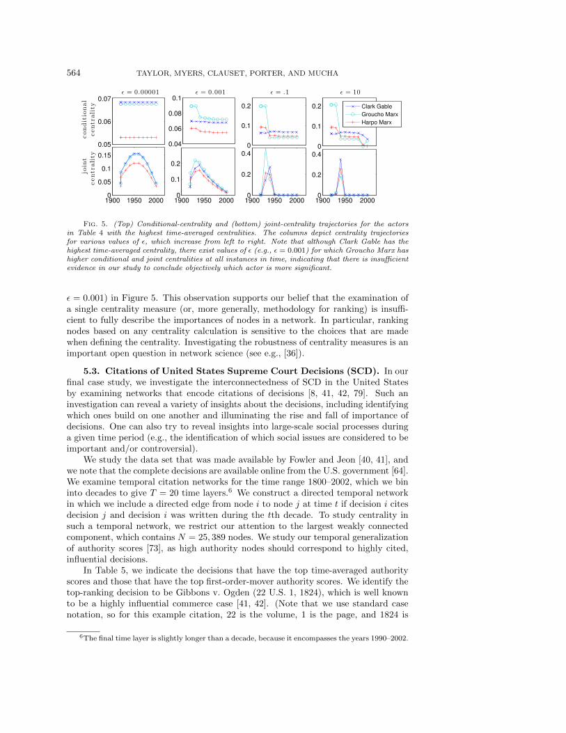
564 TAYLOR, MYERS, CLAUSET, PORTER, AND MUCHA
0.05
0.06
0.07
conditional
centrality
ǫ = 0.00001
1900 1950 20000
0.05
0.1
0.15
joint
centrality
0.04
0.06
0.08
0.1ǫ = 0.001
1900 1950 20000
0.1
0.2
0
0.1
0.2
ǫ = .1
1900 1950 20000
0.2
0.40
0.1
0.2
ǫ = 10
1900 1950 20000
0.2
0.4
Clark Gable
Groucho Marx
Harpo Marx
Fig. 5. (Top) Conditional-centrality and (bottom) joint-centrality trajectories for the actorsin Table 4 with the highest time-averaged centralities. The columns depict centrality trajectoriesfor various values of ε, which increase from left to right. Note that although Clark Gable has thehighest time-averaged centrality, there exist values of ε (e.g., ε = 0.001) for which Groucho Marx hashigher conditional and joint centralities at all instances in time, indicating that there is insufficientevidence in our study to conclude objectively which actor is more significant.
ε = 0.001) in Figure 5. This observation supports our belief that the examination ofa single centrality measure (or, more generally, methodology for ranking) is insuffi-cient to fully describe the importances of nodes in a network. In particular, rankingnodes based on any centrality calculation is sensitive to the choices that are madewhen defining the centrality. Investigating the robustness of centrality measures is animportant open question in network science (see e.g., [36]).
5.3. Citations of United States Supreme Court Decisions (SCD). In ourfinal case study, we investigate the interconnectedness of SCD in the United Statesby examining networks that encode citations of decisions [8, 41, 42, 79]. Such aninvestigation can reveal a variety of insights about the decisions, including identifyingwhich ones build on one another and illuminating the rise and fall of importance ofdecisions. One can also try to reveal insights into large-scale social processes duringa given time period (e.g., the identification of which social issues are considered to beimportant and/or controversial).
We study the data set that was made available by Fowler and Jeon [40, 41], andwe note that the complete decisions are available online from the U.S. government [64].We examine temporal citation networks for the time range 1800–2002, which we bininto decades to give T = 20 time layers.6 We construct a directed temporal networkin which we include a directed edge from node i to node j at time t if decision i citesdecision j and decision i was written during the tth decade. To study centrality insuch a temporal network, we restrict our attention to the largest weakly connectedcomponent, which contains N = 25, 389 nodes. We study our temporal generalizationof authority scores [73], as high authority nodes should correspond to highly cited,influential decisions.
In Table 5, we indicate the decisions that have the top time-averaged authorityscores and those that have the top first-order-mover authority scores. We identify thetop-ranking decision to be Gibbons v. Ogden (22 U.S. 1, 1824), which is well knownto be a highly influential commerce case [41, 42]. (Note that we use standard casenotation, so for this example citation, 22 is the volume, 1 is the page, and 1824 is
6The final time layer is slightly longer than a decade, because it encompasses the years 1990–2002.

EIGENVECTOR-BASED CENTRALITY FOR TEMPORAL NETWORKS 565
Table 5Top time-averaged centralities (αi) and first-order-mover scores (mi) for SCD [64]. We give
results for our temporal generalization (see (4)) of authority scores [73].
Top time-averaged centralities
Rank Decision αi mi
1 Gibbons v. Ogden (22 U.S. 1, 1824) 0.172 284.82 Minnesota Rate Case (230 U.S. 352, 1913) 0.160 214.23 McCulloch v. Maryland (17 U.S. 316, 1819) 0.157 173.34 Brown v. Maryland (25 U.S. 419, 1827) 0.107 212.75 Robbins v. Shelby County Tax. Distr. (120 U.S. 489, 1887) 0.096 192.06 Cooley v. Board of Wardens (53 U.S. 12, 1851) 0.096 191.27 Ex parte Young (209 U.S. 123, 1908) 0.086 53.88 Galveston & S.A. Ry. Co. v. Texas (210 U.S. 217, 1908) 0.083 126.69 Cantwell v. Connecticut (310 U.S. 296, 1940) 0.082 516.210 Welton v. State of Missouri (91 U.S. 275, 1875) 0.082 168.5
Top first-order-mover scores
Rank Decision mi αi
1 Cantwell v. Connecticut (310 U.S. 296, 1940) 516.21 0.08222 Schneider v. State (308 U.S. 147, 1939) 439.73 0.07073 Thornhill v. Alabama (310 U.S. 88, 1940) 388.08 0.06334 Lovell v. City of Griffin (303 U.S. 444, 1938) 369.00 0.06325 Near v. Minnesota (283 U.S. 697, 1931) 344.06 0.07296 Gitlow v. New York (268 U.S. 652, 1925) 316.33 0.06267 DeJonge v. Oregon (299 U.S. 353, 1937) 310.63 0.05548 Stromberg v. California (283 U.S. 359, 1931) 306.68 0.05639 Chaplinsky v. New Hampshire (315 U.S. 568, 1942) 302.71 0.048710 Whitney v. California (274 U.S. 357, 1927) 291.03 0.0582
the year.) The decisions with the top time-average centralities tend to be decisionsfrom before 1900. In contrast, the nodes with the top first-order-mover scores tendto be decisions from the period 1920–1940. These decisions initially have very lowcentralities because they do not exist early in the network, but influential decisionsfrom this period later achieve high authorities. For example, see Table 2 in [41],which identified Cantwell v. Connecticut (310 U.S. 296, 1940) as the node with topauthority for a network in which there exists an edge i→ j if and only if decision i citesdecision j during the years t ∈ [1754, 2002]. This decision is the only one that makesboth of our top-10 lists in Table 5. Interestingly, the cases with top time-averagedcentralities deal mostly with interstate commerce and the limits of state governmentsin regulating it, and the cases with top first-order-mover scores deal primarily withFirst Amendment rights.
6. Conclusions. We developed and analyzed a generalization of eigenvector-based centrality measures for temporal networks, and we demonstrated the utility ofsuch temporal centralities for identifying important entities in three case studies: thePh.D. exchange network for mathematical sciences in the United States, costarring inthe Golden Age of Hollywood, and citations of decisions in the United States SupremeCourt. Consistent with the lessons from the development of multilayer generalizationsof modularity [2, 5, 92], an essential ingredient of generalizing centrality measuresto multilayer representations of temporal networks is to give different treatment tointra-layer edges between different physical nodes and interlayer edges that connectthe same node across time. We incorporated interlayer edges by constructing a supra-centrality matrix, which requires a network to either have discrete time or be binned
566 TAYLOR, MYERS, CLAUSET, PORTER, AND MUCHA
(i.e, aggregated) into discrete times using time windows (e.g., using summation oranother process [121, 124]). Constructing this matrix requires making a choice ofcentrality matrix (e.g., authority, hub, adjacency, PageRank, and so on), and onethen couples these matrices using an interlayer coupling of strength ω (i.e., 1/ε).
We showed that the dominant eigenvector of a supracentrality matrix character-izes the “joint centralities” of node-layer pairs, and we introduced the concepts of“marginal centralities” and “conditional centralities” to study (1) the decoupled im-portances of nodes and layers and (2) the nodes’ centrality trajectories over time. Oneneeds to be cautious about interpreting joint centralities, as there is a bias towardsthe middle layers [e.g., see Figures 2(a) and 4(b)], but conditional centralities do notseem to have a similar bias. In our temporal centralities, we observe properties suchas localization (which is an important issue for centrality measures more generally[68, 86, 99, 121]) and different time scales for how node centrality changes over time.For example, we observed eigenvector localization, amounting to localization in timelayers, in the limit ω → 0. Further research is important to explore eigenvector local-ization in temporal and multilayer networks and to examine the results from generaliz-ing different types of eigenvector-based centralities. It would also be worthwhile to ex-plore whether concepts from statistics about smoothing, such as using cross validationto choose bandwidth parameters, can be used to help guide the selection of values of ω.
By focusing on the strong-coupling limit—including the construction of a per-turbation expansion in this singular limit—we derived simple, principled formulasto define time-averaged centralities and first-order-mover scores (which measure themagnitude of a physical node’s centrality changes over time). This makes it possibleto easily identify not only which entities are most central in a temporal network butalso which ones are the “top movers” in centrality over time. Our methodology worksfor any eigenvector-based centrality, which we define as centrality measures in whichthe nodes’ centralities are given by the entries of the dominant eigenvector of a ma-trix. There are numerous popular types of eigenvector-based centralities (includingPageRank centralities [96], hub and authority centralities [73], and eigenvector cen-trality [9]), and new centralities of this form continue to be developed [86]. We haveBrovided MATLAB software [119] that implements our methodology. It can be usedto extend any eigenvector-based centrality to temporal networks.
An important direction for future work is to explore different strategies for theconstruction of interlayer edges. We have studied interlayer edges between nearest-neighbor node-layer pairs, that is, a node-layer pair (i, t) is adjacent to (i, t− 1) and(i, t+1), so the edges form an undirected chain that bridges physical node i across theT time layers. Other strategies should be explored (see discussions in [72]), includ-ing ones with interlayer edges that are directed (e.g., other temporal generalizationsof communicability centrality [38]). Directed interlayer edges are able to representcausal scenarios, but such causal coupling can yield (supracentrality) matrices thatare not irreducible, which is a problematic situation for eigenvector-based centralitymeasures. Specifically, one would need to construct an associated network structurethat satisfies strong connectivity (e.g., using ideas such as teleportation [46, 77]).Developing eigenvector-based centrality measures that respect causality is thus oneexciting direction, although one then needs to keep careful track of the biases causedby the choice of teleportation strategy. We note that we have developed our perturba-tion analyses for general interlayer coupling, so they can be applied to such scenarios.Finally, it is worth exploring our approach for different applications such as change-point detection and for a variety of example networks such as data streams and thosewith a large number of time layers.

EIGENVECTOR-BASED CENTRALITY FOR TEMPORAL NETWORKS 567
Appendix: Higher-order terms. In sections 4.2 and 4.3, we derived zeroth-order and first-order solutions to the dominant-eigenvalue equation (13) for the supra-centrality matrix. These led to principled expressions for time-averaged centralities(see (19)) and first-order-mover scores (see (33)). We now derive and solve higher-order terms in our singular perturbation expansion. Such terms can be useful forapproximating v(ε) for fixed ε > 0. Similar to the expressions that we derived insection 4, we obtain expressions in the form of linear equations of dimension N . Forlongitudinal data, these equations are much more computationally efficient to solvethan directly solving (13), which is an eigenvalue equation of dimension NT .
From the eigenvalue equation given by (13), we now derive kth-order expansions
of the form λ(ε) ≈∑k
j=0 εkλk and v(ε) ≈
∑kj=0 ε
kvk. We can consider arbitrarilylarge nonnegative integers k. We derived zeroth-order (k = 0) and first-order (k = 1)approximations in section 4, and we now derive the second-order (k = 2) expansion.Because we already showed that λ2 = αTX(2)α in (30), all that is left is to derive anexpression for v2. Starting from (24), we write
(35) v2 = L†0L1v1 +∑j
γjPuj ,
where the sum with constants γj = (Puj)Tv2 accounts for the projection of v2 onto
the null space of L†0. We solve for the constants {γj} by examing the third-order(k = 3) expansion, which leads to
(36) L0v3 = L1v2 − λ2v1 − λ3v0 .
In general,
(37) L0vk = L1vk−1 −k∑
j=2
λjvk−j .
We left-multiply (36) by (Pui)T and note that Pui is in the null space of L0 to obtain
0 = (Pui)TL1v2 − λ2βi − λ3αi .(38)
Using the solution for v2 given by (35), it then follows that
−∑j
γj(Pui)TL1Puj = (Pui)
TL1L†0L1v1 − λ2βi − λ3αi .(39)
Recalling that (Pui)TL1Puj = X
(1)ij − λ1δij , (39) becomes
−(X(1) − λ1I
)γ = q − λ2β − λ3α ,(40)
where q = [q1, . . . , qN ]T and qi = (Pui)TL1L†0L1v1. We now solve for λ3. Using the
fact that α is in the null space of (X(1)−λ1I), left-multiplication of (40) by αT gives
λ3 = αTq = vT0 L1L†0L1v1 ,(41)
where we have used the relation αTβ = 0. As before, we solve for γ using theMoore–Penrose pseudoinverse
γ = −(X(1) − λ1I
)†(q− λ2β − λ3α) + cα ,(42)
where c = αTγ is the (possibly nonzero) projection of γ onto α.
568 TAYLOR, MYERS, CLAUSET, PORTER, AND MUCHA
Similarly to our calculation of b = αTβ = 0 in section 4.3, we solve for theconstant c by examining the norm of the vector v(ε) ≈ v0 + εv1 + ε2v2. We requirethat
1 = ‖v0 + εv1 + ε2v2‖2
= ‖v0‖2 + ε2‖v1‖2 + 2ε〈v0,v1〉+ 2ε2〈v0,v2〉+O(ε3) .(43)
We substitute ‖v0‖ = 1 and 〈v0,v1〉 = αTβ = 0 into (43) and equate the O(ε2)terms to obtain
c = 〈v0,v2〉 = −1
2‖v1‖2 .(44)
This completes the second-order approximation.We now derive the third-order (k = 3) approximation. Having solved λ3 in
equation (41), we seek to find an expression for v3. Starting from (36), we write
(45) v3 = L†0L1v2 − λ2L†0v1 +∑j
ξjPuj ,
where the sum with constants ξj = (Puj)Tv3 accounts for the projection of v3 onto
the null space of L†0. Using the general form given by (37) for k = 4 yields
(46) L0v4 = L1v3 − λ2v2 − λ3v1 − λ4v0 .
We left-multiply (46) by (Pui)T to obtain
(47) 0 = (Pui)TL1v3 − λ2γi − λ3βi − λ4αi .
We next substitute our solution for v3 given by (45) into (47) to obtain
(48) −∑j
ξj(Pui)TL1Puj = (Pui)
TL1L†0 (L1v2 − λ2v1)− λ2γi − λ3βi − λ4αi ,
which in matrix notation is
(49) (X(1) − λ1I)ξ = r− λ2γ − λ3β − λ4α ,
where we define r = [r1, . . . , rN ]T and ri = (Pui)TL1L†0 (L1v2 − λ2v1). As before, we
use the Moore–Penrose psuedoinverse to obtain
(50) ξ = (X(1) − λ1I)†r− λ2(X(1) − λ1I)†γ − λ3(X(1) − λ1I)†β + dα ,
which uses the fact that α is in the null space of (X(1)−λ1I). The constant d = αT ξ

EIGENVECTOR-BASED CENTRALITY FOR TEMPORAL NETWORKS 569
10−4
10−3
10−10
10−5
100
weight (ǫ)
L2error
Approximation accuracy GAH
zeroth
first
second
third
10−4
10−3
10−8
10−4
100
weight (ǫ)
L2error
Approximation accuracy MGP
zeroth
first
second
third
(a) (b)
Fig. 6. We show, for several values of interlayer coupling weight ε > 0, the accuracy of kth-order approximate solutions to (13) for k ∈ {0, 1, 2, 3}. We show results for (a) the MGP networkstudied in section 5.1 and (b) the GAH network studied in section 5.2. In both panels, we measure the
error by calculating the L2 norm ‖v(ε)−∑k
j=1 εjvk‖2 of the difference between the approximate and
actual dominant eigenvector. As expected, we find for sufficiently small ε that the error decreaseswith increasing approximation order. The decay rate of the L2 error as ε → 0+ also follows theexpected scaling.
gives the projection of ξ onto α, and we calculate it by constraining the third-orderexpansion for v(ε) to have a norm of 1. This yields
1 = ‖v0 + εv1 + ε2v2 + ε3v3‖2
= ‖v0‖2 + ε2‖v1‖2 + 2ε〈v0,v1〉+ 2ε2〈v0,v2〉+ 2ε3〈v0,v3〉+ 2ε3〈v1,v2〉+O(ε4) .(51)
Recall that normalization of the zeroth-, first-, and second-order expansions, respec-tively, yields the relations ‖v0‖2 = 1, 〈v0,v1〉 = 0, and 〈v0,v2〉 = −(1/2)‖v1‖2.Equating the third-order terms in (51) then necessitates that
d = 〈v0,v3〉 = −〈v1,v2〉 .(52)
This completes the third-order approximation.In Figures 6(a) and 6(b), we validate the above results using the MGP and GAH
networks, which we studied in sections 5.1 and 5.2, respectively. We plot the L2 errorfor the kth-order approximation ‖v(ε) −
∑kj=1 ε
jvk‖2 to the dominant eigenvector.We plot these approximations for several choices of k and several values of ε. Whenε is sufficiently small (i.e., ε / 3 × 10⁻⁴ for the MGP and ε / 10−3 for the GAH),we observe (as expected) that the error decreases with increasing k. We derived ourapproximate expressions in the limit ε→ 0+, so we only expect them to be accuratefor sufficiently small ε (although asymptotic expressions do have a long history ofoften being accurate even in many situations in which there are no guarantees forsuch success [56]). We also obtain the expected decay rates in the error as ε → 0+.We find linear decay for the zeroth-order approximation, quadratic decay for thefirst-order approximation, and so on.
Acknowledgments. The first two authors contributed equally to this project.We are grateful to Mitch Keller of the Mathematics Genealogy Project [102] for pro-viding data. We thank Geoff Evans, Martin Everett, Bailey Fosdick, Echo Gao, SamHowison, Florian Klimm, Flora Meng, Priya Narayan, Victor Preciado, Feng Shi,

570 TAYLOR, MYERS, CLAUSET, PORTER, AND MUCHA
Gilbert Strang, Blair Sullivan, and Simi Wang for helpful discussions and sugges-tions. We especially thank Elizabeth Leicht for many extensive discussions.
REFERENCES
[1] A. Alsayed and D. J. Higham, Betweenness in time dependent networks, Chaos SolitonsFractals, 72 (2015), pp. 35–48.
[2] D. S. Bassett, M. A. Porter, N. F. Wymbs, S. T. Grafton, J. M. Carlson, and P. J.Mucha, Robust detection of dynamic community structure in networks, Chaos, 23 (2013),013142.
[3] M. Bastian, S. Heymann, and M. Jacomy, Gephi: An open source software for exploringand manipulating networks, Third International AAAI Conference on Weblogs and SocialMedia, AAAI, Palo Alto, CA, 2009, pp. 361–362, http://www.aaai.org/ocs/index.php/ICWSM/09/paper/view/154).
[4] V. Batagelj, P. Doreian, A. Ferligoj, and N. Kejzar, Understanding Large TemporalNetworks and Spatial Networks: Exploration, Pattern Searching, Visualization and Net-work Evolution, Wiley, Chichester, England, 2014.
[5] M. Bazzi, M. A. Porter, S. Williams, M. McDonald, D. J. Fenn, and S. D. Howison,Community detection in temporal multilayer networks, with an application to correlationnetworks, Multiscale Model. Simul., 14 (2016), pp. 1–41.
[6] M. Benzi and C. Klymko, On the limiting behavior of parameter-dependent network cen-trality measures, SIAM J. Matrix Anal. Appl., 36 (2015), pp. 686–706.
[7] C. T. Bergstrom, J. D. West, and M. A. Wiseman, The EigenfactorTM metrics, J. Neu-rosci., 28 (2008), pp. 11433–11434.
[8] M. J. Bommarito, D. M. Katz, J. L. Zelner, and J. H. Fowler, Distance measures fordynamic citation networks, Phys. A, 389 (2010), pp. 4201–4208.
[9] P. Bonacich, Factoring and weighting approaches to clique identification, J. Math. Sociol.,2 (1972), pp. 113–120.
[10] P. Bonacich, Power and centrality: A family of measures, Amer. J. Sociol., 92 (1987),pp. 1170–1182.
[11] D. Braha and Y. Bar-Yam, From centrality to temporary fame: Dynamic centrality incomplex networks, Complexity, 12 (2006), pp. 59–63.
[12] S. Brin and L. Page, Anatomy of a large-scale hypertextual web search engine, in Proceedingsof the Seventh International World Wide Web Conference, Elsevier, Amsterdam, 1998,pp. 107–117.
[13] V. Burris, The academic caste system: Prestige hierarchies in PhD exchange networks,Amer. Sociol. Rev., 69 (2004), pp. 239–264.
[14] T. Callaghan, M. A. Porter, and P. J. Mucha, Random walker ranking for NCAA Divi-sion I-A football, Amer. Math. Monthly, 114 (2007), pp. 761–777.
[15] T. Caplow and R. McGee, The Academic Marketplace, Transaction Publishers, NewBrunswick, NJ, 2001.
[16] T. P. Chartier, E. Kreutzer, A. N. Langville, and K. E. Pedings, Sensitivity andstability of ranking vectors, SIAM J. Sci. Comput., 33 (2011), pp. 1077–1102.
[17] S. Chauhan, M. Girvan, and E. Ott, Spectral properties of networks with community struc-ture, Phys. Rev. E (3), 80 (2009), 056114.
[18] A. Clauset, Data Release: Golden Age of Hollywood Actor Collaborations, http://tuvalu.santafe.edu/∼aaronc/datacode.htm.
[19] A. Clauset, S. Arbesman, and D. B. Larremore, Systematic inequality and hierarchy infaculty hiring networks, Sci. Adv., 1 (2015), e1400005.
[20] V. Colizza, A. Barrat, M. Barthelemy, and A. Vespignani, The role of the airlinetransportation network in the prediction and predictability of global epidemics, Proc.Natl. Acad. Sci. USA, 103 (2006), pp. 2015–2020.
[21] E. Cozzo, M. Kivela, M. De Domenico, A. Sole, A. Arenas, S. Gomez, M. A. Porter,and Y. Moreno, Structure of triadic relations in multiplex networks, New J. Phys., 17(2015), 073029.
[22] M. Cucuringu and M. W. Mahoney, Localization on Low-Order Eigenvectors of Data Ma-trices, preprint, arXiv:1109.1355, 2011.
[23] T. A. Davis, Direct Methods for Sparse Linear Systems, Fundam. Algorithms 2, SIAM,Philadelphia, 2006.
[24] M. De Domenico, E. Omodei, and A. Arenas, Quantifying the diaspora of knowledge inthe last century, Appl. Netw. Sci., 1 (2016), 15.
EIGENVECTOR-BASED CENTRALITY FOR TEMPORAL NETWORKS 571
[25] M. De Domenico, M. A. Porter, and A. Arenas, Muxviz: A tool for multilayer analysisand visualization of networks, J. Complex Netw., 3 (2015), pp. 159–176.
[26] M. De Domenico, A. Sole-Ribalta, E. Cozzo, M. Kivela, Y. Moreno, M. A. Porter,S. Gomez, and A. Arenas, Mathematical formulation of multilayer networks, Phys. Rev.X, 3 (2013), 041022.
[27] D. DeFord and S. Pauls, Network Models that Reflect Multiplex Dynamics, preprint,arXiv:1507.00695, 2015.
[28] J. W. Demmel, Applied Numerical Linear Algebra, SIAM, Philadelpha, 1997.[29] P. Deville, D. Wang, R. Sinatra, C. Song, V. D. Blondel, and A.-L. Barabasi, Career
on the move: Geography, stratification, and scientific impact, Sci. Rep., 4 (2014), 4770.[30] M. De Domenico, A. Sole-Ribalta, E. Omodei, S. Gomez, and A. Arenas, Ranking in
interconnected multilayer networks reveals versatile nodes, Nature Commun., 6 (2015),6868.
[31] S. N. Dorogovtsev, A. V. Goltsev, J. F.F. Mendes, and A. N. Samukhin, Spectra ofcomplex networks, Phys. Rev. E (3), 68 (2003), 046109.
[32] R. A. Duke, Mathematics at Georgia Tech: The First Hundred Years, 1888–1987, http://www.math.gatech.edu/about (2015).
[33] E. Estrada, Communicability in temporal networks, Phys. Rev. E (3), 88 (2013), 042811.[34] E. Estrada and N. Hatano, Communicability in complex networks, Phys. Rev. E (3), 77
(2008), 036111.[35] E. Estrada and D. J. Higham, Network properties revealed through matrix functions, SIAM
Rev., 52 (2010), pp. 696–714.[36] M. O. Jackson F. Bloch and P. Tebaldi, Centrality Measures in Networks, preprint, https:
//doi.org/10.2139/ssrn.2749124.[37] I. J. Farkas, I. Derenyi, A.-L. Barabasi, and T. Vicsek, Spectra of “real-world” graphs:
Beyond the semicircle law, Phys. Rev. E (3), 64 (2001), 026704.[38] C. Fenu and D. J. Higham, Block Matrix Formulations for Evolving Networks, preprint
arXiv:1511.07305, 2015.[39] J. H. Fowler, B. Grofman, and N. Masuoka, Social networks in political science: Hiring
and placement of Ph.D.s, 1960–2002, PS Polit. Sci. Politics, 40 (2007), pp. 729–739.[40] J. H. Fowler and S. Jeon, Supreme Court Citation Network Data, http://fowler.ucsd.edu/
judicial.htm.[41] J. H. Fowler and S. Jeon, The authority of Supreme Court precedent, Soc. Netw., 30 (2008),
pp. 16–30.[42] J. H. Fowler, T. R. Johnson, J. F. Spriggs II, S. Jeon, and P. J. Wahlbeck, Network
analysis and the law: Measuring the legal importance of precedents at the US SupremeCourt, Polit. Anal., 15 (2007), pp. 324–346.
[43] L. C. Freeman, A set of measures of centrality based on betweenness, Sociometry, 40 (1977),pp. 35–41.
[44] F. Gargiulo, A. Caen, R. Lambiotte, and T. Carletti, The classical origin of modernmathematics, EPJ Data Science, 5 (2016), 26.
[45] R. Ghosh and K. Lerman, Rethinking centrality: The role of dynamical processes in socialnetwork analysis, Discrete Contin. Dyn. Syst. Ser. B, 19 (2014), pp. 1355–1372.
[46] D. F. Gleich, PageRank beyond the Web, SIAM Rev., 57 (2015), pp. 321–363.[47] K.-I. Goh, B. Kahng, and D. Kim, Spectra and eigenvectors of scale-free networks, Phys.
Rev. E (3), 64 (2001), 051903.[48] G. H. Golub and C. F. Van Loan, Matrix Computations, 3rd ed., JHU Press, 2012.[49] S. Gomez, A. Dıaz-Guilera, J. Gomez-Gardenes, C. Perez-Vicente, Y. Moreno, and
A. Arenas, Diffusion dynamics on multiplex networks, Phys. Rev. Lett., 110 (2013),028701.
[50] P. Grindrod and D. J. Higham, A matrix iteration for dynamic network summaries, SIAMRev., 55 (2013), pp. 118–128.
[51] P. Grindrod and D. J. Higham, A dynamical systems view of network centrality, Proc. R.Soc. A, 470 (2014), 20130835.
[52] P. Grindrod, M. C. Parsons, D. J. Higham, and E. Estrada, Communicability acrossevolving networks, Phys. Rev. E (3), 83 (2011), 046120.
[53] R. Guimera, S. Mossa, A. Turtschi, and L. A. N. Amaral, The worldwide air transporta-tion network: Anomalous centrality, community structure, and cities’ global roles, Proc.Natl. Acad. Sci. USA, 102 (2005), pp. 7794–7799.
[54] A. Halu, R. J. Mondragon, P. Panzarasa, and G. Bianconi, Multiplex pagerank, PLoSONE, 8 (2013), e78293.
572 TAYLOR, MYERS, CLAUSET, PORTER, AND MUCHA
[55] S.-K. Han, Tribal regimes in academia: A comparative analysis of market structure acrossdisciplines, Soc. Netw., 25 (2003), pp. 251–280.
[56] E. J. Hinch, Perturbation Methods, Cambridge University Press, Cambridge, 1991.[57] T. Hoffmann, M. A. Porter, and R. Lambiotte, Generalized master equations for non-
Poisson dynamics on networks, Phys. Rev. E (3), 86 (2012), 046102.[58] T. Hoffmann, M. A. Porter, and R. Lambiotte, Random walks on stochastic temporal
networks, in Temporal Networks, Springer, Berlin, 2013, pp. 295–314.[59] P. Holme, Congestion and centrality in traffic flow on complex networks, Adv. Complex
Syst., 6 (2003), pp. 163–176.[60] P. Holme, Modern temporal network theory: A colloquium, Eur. Phys. J. B, 88 (2015), 234.[61] P. Holme and J. Saramaki, Temporal networks, Phys. Rep., 519 (2012), pp. 97–125.[62] P. Holme and J. Saramaki, eds., Temporal Networks, Springer, Berlin, 2013.[63] IMDb.com, Internet Movie Database, http://www.imdb.com/interfaces (2011).[64] Justia, US Supreme Court, https://supreme.justia.com/cases/federal/us/volume/.[65] H. Jeong, S. P. Mason, A.-L. Barabasi, and Z. N. Oltvai, Lethality and centrality in
protein networks, Nature, 411 (2001), pp. 41–42.[66] H.-H. Jo, J. I. Perotti, K. Kaski, and J. Kertesz, Analytically solvable model of spreading
dynamics with non-Poissonian processes, Phys, Rev, X, 4 (2014), 011041.[67] L. Katz, A new status index derived from sociometric analysis, Psychometrika, 18 (1953),
pp. 39–43.[68] T. Kawamoto, Localized eigenvectors of the non-backtracking matrix, J. Stat. Mech. Theory
Exp., 2016 (2016), 23404.[69] D. Kempe and J. Kleinberg, Connectivity and inference problems for temporal networks, J.
Comput. System Sci., 64 (2002), pp. 820–842.
[70] D. Kempe, J. Kleinberg, and E. Tardos, Maximizing the spread of influence through asocial network, in Proceedings of the Ninth ACM SIGKDD International Conference onKnowledge Discovery and Data Mining, ACM, New York, 2003, pp. 137–146.
[71] H. Kim, J. Tang, R. Anderson, and C. Mascolo, Centrality prediction in dynamic humancontact networks, Comput. Netw., 56 (2012), pp. 983–996.
[72] M. Kivela, A. Arenas, M. Barthelemy, J. P. Gleeson, Y. Moreno, and M. A. Porter,Multilayer networks, J. Complex Netw., 2 (2014), pp. 203–271.
[73] J. Kleinberg, Authoritative sources in a hyperlinked environment, J. ACM, 46 (1999),pp. 604–632.
[74] G. Kossinets, J. Kleinberg, and D. Watts, The structure of information pathways in asocial communication network, in Proceedings of the 14th ACM SIGKDD InternationalConference on Knowledge Discovery and Data Mining, ACM, New York, 2008, pp. 435–443.
[75] V. Kostakos, Temporal graphs, Phys. A, 388 (2009), pp. 1007–1023.[76] J. Lages, A. Patt, and D. L. Shepelyansky, Wikipedia ranking of world universities, Eur.
Phys. J. B (3), 89 (2016), 69.[77] R. Lambiotte and M. Rosvall, Ranking and clustering of nodes in networks with smart
teleportation, Phys. Rev. E (3), 85 (2012), 056107.[78] A. N. Langville and C. D. Meyer, Google’s PageRank and Beyond: The Science of Search
Engine Rankings, Princeton University Press, Princeton, NJ, 2006.[79] E. A. Leicht, G. Clarkson, K. Shedden, and M. E. J. Newman, Large-scale structure of
time evolving citation networks, Eur. Phys. J. B, 59 (2007), pp. 75–83.[80] K. Lerman, R. Ghosh, and J. H. Kang, Centrality metric for dynamic networks, in Pro-
ceedings of the Eighth Workshop on Mining and Learning with Graphs, ACM, New York,2010, pp. 70–77.
[81] R. J. Lipton, D. J. Rose, and R. E. Tarjan, Generalized nested dissection, SIAM J. Numer.Anal., 16 (1979), pp. 346–358.
[82] L. Lovasz and J. Pelikan, On the eigenvalues of trees, Period. Math. Hungar., 3 (1973),pp. 175–182.
[83] R. D. Malmgren, J. M. Ottino, and L. A. N. Amaral, The role of mentorship in protegeperformance, Nature, 465 (2010), pp. 622–626.
[84] M. S. Mariani, M. Medo, and Y.-C. Zhang, Ranking nodes in growing networks: Whenpagerank fails, Sci. Rep., 5 (2015), 16181.
[85] M. S. Mariani, M. Medo, and Y.-C. Zhang, Identification of milestone papers throughtime-balanced network centrality, J. Informetr. (4), 10 (2016), pp. 1207–1223.
[86] T. Martin, X. Zhang, and M. E. J. Newman, Localization and centrality in networks, Phys.Rev. E (3), 90 (2014), 052808.
[87] C. D. Meyer, Matrix Analysis and Applied Linear Algebra, SIAM, Philadelphia 2000.

EIGENVECTOR-BASED CENTRALITY FOR TEMPORAL NETWORKS 573
[88] M. Mitrovic and B. Tadic, Spectral and dynamical properties in classes of sparse networkswith mesoscopic inhomogeneities, Phys. Rev. E (3), 80 (2009), 026123.
[89] R. Monasson, Diffusion, localization and dispersion relations on “small-world” lattices, Eur.Phys. J. B, 12 (1999), pp. 555–567.
[90] S. Motegi and N. Masuda, A network-based dynamical ranking system for competitivesports, Sci. Rep., 2 (2012), 904.
[91] P. J. Mucha and M. A. Porter, Communities in multislice voting networks, Chaos, 20(2010), 041108.
[92] P. J. Mucha, T. Richardson, K. Macon, M. A. Porter, and J.-P. Onnela, Communitystructure in time-dependent, multiscale, and multiplex networks, Science, 328 (2010),pp. 876–878.
[93] S. A. Myers, P. J. Mucha, and M. A. Porter, Mathematical genealogy and departmentprestige, Chaos, 21 (2011), 041104.
[94] M. E. J. Newman, Networks: An Introduction, Oxford University Press, Oxford, 2010.[95] M. Ogura and V. M. Preciado, Katz Centrality of Markovian Temporal Networks: Analysis
and Optimization, preprint, arXiv:1609.05962, 2016.[96] L. Page, S. Brin, R. Motwani, and T. Winograd, The PageRank Citation Ranking: Bring-
ing Order to the Web, Technical report, Stanford InfoLab, SIDL-WP-1999-0120, 1999.[97] R. Pan and J. Saramaki, Path lengths, correlations, and centrality in temporal networks,
Phys. Rev. E (3), 84 (2011), 016105.[98] J. Panaretos and C. C. Malesios, Influential mathematicians: Birth, education, and affil-
iation, Notices Amer. Math. Soc., 59 (2012), pp. 274–286.[99] R. Pastor-Satorras and C. Castellano, Distinct types of eigenvector localization in net-
works, Sci. Rep., 6 (2016), 18847.[100] M. A. Porter and J. P. Gleeson, Dynamical Systems on Networks: A Tutorial, Springer,
Cham, Switzerland, 2016.[101] M. A. Porter, P. J. Mucha, M. E. J. Newman, and C. M. Warmbrand, A network analysis
of committees in the United States House of Representatives, Proc. Natl. Acad. Sci. USA,102 (2005), pp. 7057–7062.
[102] Mathematics Genealogy Project, The Mathematics Genealogy Project, http://www.genealogy.ams.org (2009).
[103] F. Radicchi, Driving interconnected networks to supercriticality, Phys. Rev. X, 4 (2014),021014.
[104] F. Radicchi and A. Arenas, Abrupt transition in the structural formation of interconnectednetworks, Nature Phys., 9 (2013), pp. 717–720.
[105] J. G. Restrepo, E. Ott, and B. R. Hunt, Desynchronization waves and localized instabili-ties in oscillator arrays, Phys. Rev. Lett., 93 (2004), 114101.
[106] J. G. Restrepo, E. Ott, and B. R. Hunt, Characterizing the dynamical importance ofnetwork nodes and links, Phys. Rev. Lett., 97 (2006), 094102.
[107] J. G. Restrepo, E. Ott, and B. R. Hunt, Approximating the largest eigenvalue of networkadjacency matrices, Phys. Rev. E (3), 76 (2007), 056119.
[108] L. E. C. Rocha and N. Masuda, Random walk centrality for temporal networks, New J.Phys., 16 (2014), 063023.
[109] R. A. Rossi and D. F. Gleich, Dynamic PageRank using evolving teleportation, in Algo-rithms and Models for the Web Graph, Springer, New York, 2012, pp. 126–137.
[110] Y. Saad, Iterative Methods for Sparse Linear Systems, 2nd ed., SIAM, Philadelphia, 2003.[111] S. Saavedra, S. Powers, T. McCotter, M. A. Porter, and P. J. Mucha, Mutually-
antagonistic interactions in baseball networks, Phys. A, 389 (2010), pp. 1131–1141.[112] C. Sarkar and S. Jalan, Social patterns revealed through random matrix theory, EPL (4),
108 (2014), 48003.[113] L. Sola, M. Romance, R. Criado, J. Flores, A. G. del Amo, and S. Boccaletti, Eigen-
vector centrality of nodes in multiplex networks, Chaos, 23 (2013), 033131.[114] A. Sole-Ribalta, M. De Domenico, S. Gomez, and A. Arenas, Centrality rankings in
multiplex networks, in Proceedings of the 2014 ACM Conference on Web Science, ACM,New York, 2014, pp. 149–155.
[115] A. Sole-Ribalta, M. De Domenico, S. Gomez, and A. Arenas, Random walk centrality ininterconnected multilayer networks, Phys. D, 323–324 (2016), pp. 73–79.
[116] J. Sorz, B. Wallner, H. Seidler, and M. Fieder, Inconsistent year-to-year fluctuationslimit the conclusiveness of global higher education rankings for university management,PeerJ, 3 (2015), e1217.

574 TAYLOR, MYERS, CLAUSET, PORTER, AND MUCHA
[117] T. Takaguchi, Y. Yano, and Y. Yoshida, Coverage centralities for temporal networks, Eur.Phys. J. B, 89 (2016), pp. 1–11.
[118] J. Tang, M. Musolesi, C. Mascolo, V. Latora, and V. Nicosia, Analysing informationflows and key mediators through temporal centrality metrics, in Proceedings of the 3rdWorkshop on Social Network Systems - SNS ’10, ACM, New York, 2010, pp. 1–6.
[119] D. Taylor, Temporal Eigenvector Centrality, https://github.com/taylordr/TemporalEigenvector Centrality.
[120] D. Taylor, Data Release: PhD Exchange in the Mathematical Genealogy Project, https://sites.google.com/site/danetaylorresearch/home/data.
[121] D. Taylor, R. S. Caceres, and P. J. Mucha, Detectability of Small Communities in Mul-tilayer and Temporal Networks: Eigenvector Localization, Layer Aggregation, and Time-Series Discretization, preprint, arXiv:1604.00696, 2016.
[122] D. Taylor and D. B. Larremore, Social climber attachment in forming networks producesa phase transition in a measure of connectivity, Phys. Rev. E (3), 86 (2012), 031140.
[123] D. Taylor and J. G. Restrepo, Network connectivity during mergers and growth: Optimiz-ing the addition of a module, Phys. Rev. E (3), 83 (2011), 066112.
[124] D. Taylor, S. Shai, N. Stanley, and P. J. Mucha, Enhanced detectability of communitystructure in multilayer networks through layer aggregation, Phys. Rev. Lett., 116 (2016),228301.
[125] D. Walker, H. Xie, K.-K. Yan, and S. Maslov, Ranking scientific publications using amodel of network traffic, J. Stat. Mech. Theory Exp., 2007 (2007), P06010.
[126] S. Wasserman and K. Faust, Social Network Analysis: Methods and Applications, StructuralAnalysis in the Social Sciences, Cambridge University Press, Cambridge, UK, 1994.
[127] Wikipedia, Classical Hollywood Cinema, http://en.wikipedia.org/wiki/Classical Hollywoodcinema (2011).
[128] M. J. Williams and M. Musolesi, Spatio-temporal networks: Reachability, centrality androbustness, R. Soc. Open Sci., 3 (2016), 160196.
[129] K. You, R. Tempo, and L. Qiu, Distributed Algorithms for Computation of Central-ity Measures in Complex Networks, IEEE Trans. Automat. Control, to appear, https://doi.org/10.1109/TAC.2016.2604373.